
Sistemas de Lie y sus aplicaciones en Fısica y Teorıa de Control
300
arXiv:1106.3775v1 [math-ph] 19 Jun 2011 UNIVERSIDAD DE ZARAGOZA FACULTAD DE CIENCIAS DEPARTAMENTO DE F ´ ISICA TE ´ ORICA Sistemas de Lie y sus aplicaciones en F´ ısica y Teor´ ıa de Control TESIS DOCTORAL Arturo Ramos Guti´ errez Zaragoza, 2002
-
Upload
khangminh22 -
Category
Documents
-
view
1 -
download
0
Transcript of Sistemas de Lie y sus aplicaciones en Fısica y Teorıa de Control

arX
iv:1
106.
3775
v1 [
mat
h-ph
] 19
Jun
201
1
UNIVERSIDAD DE ZARAGOZAFACULTAD DE CIENCIAS
DEPARTAMENTO DE FISICA TEORICA
Sistemas de Lie y sus aplicacionesen Fısica y Teorıa de Control
TESIS DOCTORAL
Arturo Ramos Gutierrez
Zaragoza, 2002


UNIVERSIDAD DE ZARAGOZA
FACULTAD DE CIENCIASDEPARTAMENTO DE FISICA TEORICA
Sistemas de Lie y sus aplicacionesen Fısica y Teorıa de Control
Memoria de Tesis presentada porARTURO RAMOS GUTI ERREZ
para optar al grado de Doctor en Ciencias Fısicas
Dirigida porJOSE F. CARI NENA MARZO


Jose F. Carinena Marzo, Catedratico de Fısica Teoricade la Universidad de Zaragoza
CERTIFICA
que la presente memoria titulada
Sistemas de Lie y sus aplicaciones en Fısica y Teorıa de Control
ha sido realizada en el Departamento de Fısica Teorica de la Universidad de Zaragoza bajo sudireccion, por D. Arturo Ramos Gutierrez, y autoriza su presentacion para que sea calificadacomo Tesis Doctoral.
Zaragoza, 15 de marzo de 2002.


Dedicated to the memory of my father


Acknowledgments
The ‘little book’which the reader is holding in his/her hands now is the result of the work andcontributions of many people. I would like to express here mysincere thanks and appreciationto all of them.
First of all, I would like to thank my thesis advisor Prof. Jose F. Carinena, who gave methe opportunity to make this research under the auspices of aFPI Doctoral Grant associated tothe project PB96-0717 of the Spanish Education, Science andTechnology Ministries. Duringthese four years the experience of collaborating with him has been enormously enriching in allrespects.
I would like to give thanks as well to some people I have had theopportunity to work orinteract with. Profs. Willy Sarlet, Frans Cantrijn, Arjan van der Schaft, David J. Fernandez C.(and his family) and Andrew Lewis have very kindly accepted me as a research visitor in theirrespective institutions. I will never forget the warm hospitality received during my stay in Bel-gium, The Netherlands and Mexico. Unfortunately, local bureaucratic problems have preventedme from seeing the incomparable natural environment of Canada.
Likewise, other scientists have invited me for one-week visits to their institutions duringthese years, like Profs. Kurt Bernardo Wolf, Oscar Rosas-Ortiz and Francesco Fasso. I wouldlike to thank them for the warm hospitality as well as for giving me the opportunity of knowingthe beautiful cities of Cuernavaca, San Luis de Potosı and Padova.
I acknowledge moreover the pleasant scientific collaboration with Profs. Janusz Grabowski,Willy Sarlet and David J. Fernandez C., to whom I am indebtedfor several ideas and resultswhich are of key importance for this Thesis. In addition, thework presented here has benefittedin a not small measure from comments and suggestions from several people; specially, I wouldlike to thank Profs. Manuel Asorey, Luis J. Boya, Giuseppe Gaeta, Bogdan Mielnik and MiguelA. Rodrıguez for that.
I would like to thank also the Heads of the Department of Theoretical Physics of the Uni-versity of Zaragoza during these four years, namely Profs. Jose F. Carinena and Julio Abad, forproviding me with invaluable means for my research. Thanks are given as well to all the othermembers of the Department, for the formation received, for contributing to an incomparablework atmosphere, and for conforming an exceptional scientific centre.
Other young members of the Department have also contributedto the existence of this The-sis. It has been a pleasure for me to share the office with Eduardo Follana and Jaime Camacaroalong these years. Likewise, I have had the pleasure of sharing many good times with these andother research fellows of our Department. Some have finishedtheir Thesis already, some are inthe process, and some will do it in one or two years, but all of them are always ready to havea break and a relaxing conversation. Miguel Aguado, Jose M.Carmona, Susana Cebrian, Jesus
vii

viii Acknowledgments
Clemente-Gallardo, Igor Garcıa Irastorza, Vıctor Laliena, Justo Lopez, Ricardo Lopez, CarlosLopez Ullod and Alejandro Rivero need to be added to the listand I give thanks to all of themfor their friendship. Special thanks go to Jesus for havingbeen my precursor in many things andfor having shown me the basics of Linux, its installation andadministration, which has been ofgreat use and an interesting hobby.
The administrative staff of our Department, namely, Isabel, Rosa, Esther and Pedro havealways been excellent professionals and charming persons.A lot of bureaucratic matters wouldhave been much more difficult without them.
On the technical side I would like to thank the Linux-GNU community for providing avery appropriate, powerful and transparent operating system, as well as to the inventors anddevelopers of the TEX, LATEX and EMACS formatting page systems and text editor, respectively,for making the life of a scientist much easier. My appreciation also goes to the inventors anddevelopers of software for symbolic mathematical computation, for creating extremely usefultools in mathematical research. Without them, this Thesis would have taken much more time andeffort or maybe it would have been impossible to finish.
Finally, but not less importantly, my families have played an exceptional role along the de-velopment of this work. I would like to thank my parents for their continued love, encouragementand support, specially during the last months of the writingof this Thesis.
And a very special place corresponds to my wife and best friend Esther, whose uncondi-tional love and support is exactly what has allowed this workto exist. I am deeply indebted toher parents for having a so marvelous daughter, for loving and supporting us always and for hav-ing generously provided us, amongst many other things, witha home to give birth to this ‘littlebook’.
Arturo Ramos Guti errez9 March 2002

Preface
Meditationis est perscrutari occulta; contemplationis est admirari perspicua.... Admiratiogenerat quæstionem, quæstio investigationem, investigatio inventionem.
—Hugo de S. Victore.
This Thesis is the result of four years of research at the Department of Theoretical Physicsof the University of Zaragoza. It is devoted to study some aspects concerning a special classof systems of ordinary first order differential equations which have the remarkable property ofadmitting asuperposition rule. That is, that the general solution of such systems can be writ-ten in terms of a certain number of particular solutions and some constants related with initialconditions. We will call themLie systems, by reasons to be explained later. We will be mainlyconcerned with the general geometric structure of such systems, and as an illustration we willanalyze some problems from rather different branches of science, as they are one-dimensionalquantum mechanics and geometric control theory, from this new perspective. There will appearas well other related problems to which we will pay some attention.
These two fields of application are not the only possible ones, but just representative of howgeneral and powerful the theory is. Along this Thesis we willsuggest other possible applicationsor further developments of the ones treated, in the hope we would be able to study them in thefuture, but that have not been treated here for reasons of time and space.
We would like to introduce now the reader to the origins and some history of Lie systems.The first considerations go back to some works by Vessiot and Guldberg [151,327] in 1893, whowondered about whether it would be possible to characterizethe systems of ordinary differentialequations which have a “fundamental system of integrals”. In the same year, Lie solves thisproblem [231] by means of a theorem which we will refer to as Lie Theorem. Some years later,in 1899, Vessiot treats again the problem [328] in a review article that contains some of theproperties of this class of systems, which we will study later in this Thesis. Needless to say, theywere made precise to the extent allowed by the concepts and terminology known at that time.
In spite of being a quite popular problem by those years, it seems that the subject disap-peared from the literature until very recent years, or at least we have not been able to find areference in the subject after the mentioned work by Vessiotin 1899 until the last quarter of lastcentury. However, at the same time, it seems that some of the ideas concerning Lie systemshave been incorporated into the mathematical culture at some point in time. For example, inthe contributed article [60] it is explained some of the basic characteristics and properties of Liesystems, putting as an example the Riccati equation, but essentially, no references are given tothis respect. Likewise, in [157] it is suggested that the theory of systems obeying Lie Theoremare worth having a new look from the modern differential geometric perspective.
ix

x Preface
Indeed, it is not until the late seventies that Lie systems will attract the attention of theoret-ical and mathematical physics, and in a rather indirect way.In 1977 Crampin, Pirani and Robin-son [96] established certain relations between differential equations with solitonic solutions andthe theory of connections in principal fibre bundles, continuing this work in later articles [94,95].After, an article by Sasaki [292] developed the contents of the previous ones. All these worksattracted the attention of Anderson [11], who noticed the possible relation with the old results byLie et al.and therefore, the interesting applications that kind of systems might have in physics. Itis seen the need of classification of systems of Lie type and more specifically, of the correspond-ing superposition formulas. To this line of research incorporate several authors like Anderson,Winternitz, Harnad and collaborators, giving rise to a number of papers dealing with the men-tioned classification problem to our days [13, 34–36, 152, 153, 271,272, 277, 278,303, 304, 334–336].
Notwithstanding, in spite of these great efforts of classification of Lie systems and theirsuperposition rules, their actual applications in practice are not very numerous. However, someapplications are given in [282, 309], where certain superposition formula is used to solve nu-merically certain matrix Riccati equations arising in control theory. Moreover, the problem ofclassification of Lie systems and their superposition formulas deal with those systems which aresomehowindecomposableinto simpler ones. In addition, the common geometric properties toLie systems have scarcely been explored or used. Some exceptions are, for example, [72, 260],apart from certain specific situations which appear along the development of the mentioned clas-sification problem.
On the other hand, maybe it is worthwhile to say some words about our own interest in thesubject, how we got involved in it, and how we have developed it during these years.
From the previously mentioned works [72,260], which treated certain geometric aspects ofLie systems, and taking as an illustrating example the simplest nonlinear Lie system, i.e., theRiccati equation, it seemed to be a promising line of research the further study of the geometryof Lie systems. In this sense, these works are natural precursors of this Thesis, whose authorbegan his research work by that time.
Almost simultaneously, we came across a short article by Strelchenya [314], in which it wasclaimed that a new case of integrability of the Riccati equation was found. What we found mostinteresting in this paper was a rather surprising way of transforming a given Riccati equationinto another one by means of certain transformations on the coefficients of the original equation,constructed from the entries of an invertible2 × 2 matrix-valued curve. About two years laterwe found out that Calogero [61] had used similar transformations before also in connection withtransformations of the Riccati equation. We wondered aboutthe possible geometric structureand meaning of such transformations, if any, and decided to investigate them. This was anotherstarting point for all the work presented here.
We found that such transformations had a group theoretical origin, since they determinean affine action of the group ofGL(2, R)- (or SL(2, R)-) valued curves on the set of Riccatiequations. We interpreted the meaning of the results given in [314], and moreover, we wereable to interpret some well-known integrability conditions and properties of the Riccati equationfrom this new group theoretical viewpoint [75]. Motivated by these results, we wondered then,in collaboration with Grabowski, about the common general geometric structure of Lie systems,and in particular about the question of how and when a certainLie system can be reduced to asimpler one. The results of this research are given in [71].
We were also interested, from the beginning of this research, and motivated by a previ-

Preface xi
ous work [73], in certain problems of one-dimensional quantum mechanics where the Riccatiequation plays a fundamental role. The first is the factorization method initiated by Schrodinger[295–297] and others, and later developed by Infeld and Hull[168, 175, 176]. Other relatedsubjects are the technique of intertwined Hamiltonians, the Darboux transformation in super-symmetric quantum mechanics [93, 236] and the problems of shape invariance [139], the latterbeing exactly solvable problems by purely algebraic means.While studying the literature onthese subjects, we noticed that several aspects could be improved and generalized, some openproblems solved, and certain fundamental questions clarified. These are the subjects of [76–78].
Some time later, in collaboration with Fernandez, we realized that a previously introducedfinite-differenceformula [128] could be explained in terms of the affine actionon the set of Ric-cati equations developed in [75]. Moreover, we were able to explain the problem of intertwinedHamiltonians in one-dimensional quantum mechanics by thistechnique, and we could even gen-eralize the Darboux transformation theorem [104, 174] to a previously unknown situation. Theresults are given in [68].
Inspired by the results obtained so far, we wondered about whether it would be possible tounderstand Lie systems in terms of connections in (trivial)principal bundles and associated ones.This is in fact so, and a first step in this direction is given in[80]. The subject is further developedat the end of Chapter 2. In this way we recover the associationof the concepts guessed somehowby Anderson, but in a more general setting. However, the relations with nonlinear evolutionequations possessing solitonic solutions still remain to be clarified. As a further application ofthese ideas, we have shown in [80] how the solutions of certain Lie systems can be used to treateither the classical or the quantum version of time-dependent quadratic Hamiltonians. A furtherstep in this direction is taken in Chapter 6.
There exist as well other subjects in systems theory, specifically in control theory, where Liesystems appear in a natural way, but their properties are scarcely used or known. Moreover, it hasbecome clear in nonlinear control theory the great importance and usefulness of treating problemsby using concepts and methods of differential geometry. To this respect, control systems on Liegroups have been introduced, or other nonlinear control systems which turn out to be of Lietype, see, e.g., [55, 58, 59, 182–187, 190, 220, 255, 258, 268]. However, most of the times thesesystems appear as not related amongst themselves, and it seems that the researchers in that fieldsdo not know their relation with Lie systems. Then, this was the motivation for studying all theseproblems from our new perspective. Our first results to this respect have been reported in [79],and a further development of these ideas is the body of the third part of this Thesis.
In summary, this Thesis is aimed to give an unified perspective of these and other furtherproposed problems, with the basis of the Lie Theorem, by making use of the modern concepts ofdifferential geometry, like the theory of Lie groups and Liealgebras, homogeneous spaces, andconnections on principal and associated fibre bundles.
We have briefly sketched the (chrono)logical order in which we have worked out the ma-terial presented here. However, the order in the presentation may differ, mainly for the sake ofsimplicity in the exposition. The organization of the Thesis is as follows.
In the first part, we will develop the general geometric structure of Lie systems. We willstart with the introduction of the concept of Lie system and the Theorem characterizing them,given by Lie, along with some examples. It will follow a studyof the case of the Riccati equation,which is the simplest nonlinear ordinary differential equation admitting a superposition formulain the mentioned sense. This example will be a motivation forthe more general geometric studywhich is carried out next. It will be derived the general geometric structure, i.e., how all Lie

xii Preface
systems are associated in a canonical way to another ones formulated on certain Lie groups. Wedevelop then two ways to deal with the problem of solving Lie systems on Lie groups. One isa generalization of a method originally proposed by Wei and Norman [331, 332]. The secondis a reduction property of Lie systems into another ones whenparticular solutions of systemsassociated to the former ones are known. Afterwards, we givea formulation of Lie systemsin relation with the theory of connections on principal (trivial) fibre bundles overR and theassociated ones. This approach allows us to generalize the concept of Lie system to certainkind of partial differential equations, in relation to principal (trivial) fibre bundles over arbitrarymanifolds and their associated ones.
The second part deals with the applications we have developed in one-dimensional quantummechanics. The equivalence between the factorization method and shape invariant problems willbe described in detail, and then we review the classical factorization method, finding that theproperties of the Riccati equation as a Lie system allow us tounderstand better, and to generalizethe results previously known. Moreover, these results can be classified by means of criteriaof geometric origin. Afterwards, we will solve the problem of finding a whole class of shapeinvariant potentials, which was thought to be the best candidate to enlarge the class of potentialsof this type, but have not been found before. We analyze next the concept of partnership ofpotentials, and in this case the properties of the Riccati equation play also a fundamental role.
With the aid of the techniques developed in the first part of this Thesis, we study the abovementioned finite-difference formula and the associated algorithm, and this gives us the key to beable to generalize the classical Darboux transformation method [174] for homogeneous linearsecond-order differential equations of Schrodinger type, to a previously unknown situation. Atthe same time we give, for all these techniques, a group theoretical foundation. We are able tointerpret the problem of intertwined Hamiltonians in this setting, giving a new geometric insightinto the problem. Moreover, with the new techniques we obtain, sometimes new, potentials forwhich one eigenvalue and the corresponding eigenfunction are known exactly by construction.
After this, we study Hamiltonian systems, both in the classical and quantum framework,whose associated evolution law can be regarded as a Lie system. We specifically study the caseof having time-dependent quadratic Hamiltonians and some special subcases of them.
The third part is focused on the application of the theory of Lie systems in geometric controltheory. We will establish relations between previously unrelated systems, mainly in two ways.On the one hand, it will be shown that different control systems are closely related since theyhave the same underlying Lie algebra. On the other hand, it will be shown how some systemscan be reduced into another ones by the reduction procedure explained in the first part. Theexamples treated will illustrate the use of the theory in practical situations, showing the technicaldifficulties which could arise in specific examples.

Contents
Acknowledgments vii
Preface ix
Contents xiii
PART 1General theory of Lie systems 1
1 The concept of Lie system and study of the Riccati equation 31.1 Lie Theorem 41.2 Examples of Lie systems 51.3 Integrability of Riccati equations 71.4 Affine action on the set of Riccati equations 101.5 Properties of the Riccati equation from group theory 11
2 Geometric approach to Lie systems 172.1 Notation and basic definitions 172.2 Lie systems on Lie groups and on homogeneous spaces 202.3 Affine actions on Lie systems 232.4 The Wei–Norman method 252.5 Reduction of Lie systems 272.6 Connections and Lie systems 322.7 Lie systems of PDES 40
3 Examples of use of the theory of Lie systems 513.1 Inhomogeneous linear first order differential equation 513.2 Lie systems related toSL(2, R) 56
3.2.1 The reduction method for the Riccati equation 663.3 Lie systems related toSL(3, R) 703.4 An example of Lie system from physics 77
PART 2Lie systems in Physics 83

xiv Contents
4 Intertwined Hamiltonians, factorization method and shape invariance 854.1 Intertwined Hamiltonians 864.2 Dilation symmetry and reduction
of a linear second-order differential equation 884.3 Shape invariance and factorization method 904.4 Factorization method revisited 984.5 Shape invariance withn parameters transformed by translation 1034.6 Ambiguities in the definition of the partner potential 1134.7 Parameter invariance and shape invariance 117
4.7.1 Illustrative examples 118
5 Group theoretical approach to the intertwined Hamiltonians 1215.1 Introduction and the theorem of the finite-difference algorithm 1215.2 Group elements preserving Riccati equations of typew′ + w2 = V (x)− ǫ 1235.3 Group theory of intertwined Hamiltonians and finite difference algorithm 1285.4 Illustrative examples of the theorems of Section 5.2 132
5.4.1 Radial oscillator-like potentials 1335.4.2 Radial Coulomb-like potentials 135
5.5 Directions for further research 140
6 Classical and quantum Hamiltonian Lie systems 1436.1 Hamiltonian systems of Lie type 1436.2 Time-dependent quadratic Hamiltonians 1446.3 Classical and quantum time-dependent linear potential 1496.4 Quantum harmonic oscillator with a time-dependent perturbation
linear in the positions 1536.5 Comments and directions for further research 156
PART 3Lie systems in Control Theory 157
7 Lie systems and their reduction in control theory 1597.1 Introduction 1597.2 Brockett control system and related ones 161
7.2.1 Brockett control systems 1627.2.1.1 Hopping robot as a Lie system onH(3) 1677.2.1.2 Reduction of right-invariant control systems onH(3) 168
7.2.2 Planar rigid body with two oscillators 1727.2.2.1 Reduction of the planar rigid body with two oscillators 175
7.2.3 Some generalizations of Brockett’s system 1787.2.3.1 Generalization to second degree of Brockett system 1787.2.3.2 Generalization to third degree of Brockett system 184
7.2.4 Control systems non steerable by simple sinusoids 1887.3 Trailers and chained forms 192
7.3.1 Model of maneuvering an automobile or of a robot unicycle 1937.3.1.1 Reduction of right-invariant control systems onSE(2) 1977.3.1.2 Feedback nilpotentization of the robot unicycle 198

Contents xv
7.3.2 Front-wheel driven kinematic car 2017.3.2.1 Case of Martinet sphere as a Lie system 207
7.3.3 Front-wheel driven kinematic car pulling a trailer 2087.3.4 Chained and power forms of the kinematics of then trailer 214
7.4 Lie systems of the elastic problem of Euler 2197.4.1 Reduction of Lie systems onGǫ 2247.4.2 Kinematics inSO(3, R) as a Lie system 229
7.5 Lie control systems onSE(3) 2337.5.1 Reduction of Lie systems onSE(3) 236
7.6 Conclusions and directions for further work 240
PART 4Appendices 243
A Connections in fibre bundles 245A.1 Fibre bundles 245
A.1.1 Smooth fibre bundles 245A.1.2 Vector bundles 246A.1.3 Principal bundles 246A.1.4 Associated bundles 249
A.2 Connections in fibre bundles 250A.2.1 Preliminary concepts 250A.2.2 Principal connections 253A.2.3 Connections in associated bundles 258
PART 5Conclusions and Outlook 259
Conclusions and outlook 261
Bibliography 267


PART 1
GENERAL THEORY OF LIE SYSTEMS


Chapter 1
The concept of Lie system and study of the Riccatiequation
Time evolution of many physical systems is described by non-autonomous systems of differentialequations
dxi(t)
dt= X i(t, x) , i = 1, . . . , n , (1.1)
for instance, Hamilton equations, or Lagrange equations when transformed to the first order caseby doubling the number of degrees of freedom.
The Theorem of existence and uniqueness of solutions for such systems establishes that theinitial conditionx(0) determines the future evolution. It is also well-known thatfor the simplercase of a homogeneous linear system the general solution canbe written as a linear combinationof n independent particular solutions,x(1), . . . , x(n),
x = F (x(1), . . . , x(n), k1, . . . , kn) = k1 x(1) + · · ·+ kn x(n) , (1.2)
and for each set of initial conditions, the coefficients can be determined. For an inhomogeneouslinear system, the general solution can be written as an affine function ofn + 1 independentparticular solutions:
x = F (x(1), . . . , x(n+1), k1, . . . , kn)
= x(1) + k1(x(2) − x(1)) + . . .+ kn(x(n+1) − x(1)) . (1.3)
Under a non-linear change of coordinates both system becomenon-linear ones. However, thefact that the general solution is expressible in terms of a set of particular solutions is maintained,but the superposition function is no longer linear or affine,respectively.
The very existence of such examples of systems of differential equations admitting a super-position function suggests us an analysis of such systems. We are lead in this way to the problemof studying the systems of differential equations for whicha superposition function, allowing toexpress the general solution in terms ofm particular solutions, does exist.
The characterization of these systems admitting a (non-linear) superposition principle is dueto Lie in a very celebrated Theorem [231]. A particular example, the simplest non-linear one,is the Riccati equation. This equation plays a relevant role in many problems in physics andmany branches in mathematics, as well as other Lie systems do(see, e.g., [72,73], the excellentreview [335], and references therein).
3

4 Lie systems and Riccati equation Chap. 1
1.1 Lie Theorem
The characterization of non-autonomous systems (1.1) having the mentioned property that thegeneral solution can be written as a function ofm independent particular solutions and someconstants determining each specific solution is due to Lie. The statement of the theorem, whichcan be found in the book edited and revised by Scheffers [231], is as follows:
Theorem 1.1.1 (Lie Theorem). Given a non-autonomous system ofn first order dif-ferential equations like(1.1), a necessary and sufficient condition for the existence of a functionF : Rn(m+1) → Rn such that the general solution is
x = F (x(1), . . . , x(m); k1, . . . , kn) ,
with x(a) | a = 1, . . . ,m being any set of particular solutions of the system andk1, . . . , kn, narbitrary constants, is that the system can be written as
dxi
dt= Z1(t)ξ
1i(x) + · · ·+ Zr(t)ξri(x) , i = 1, . . . , n , (1.4)
whereZ1, . . . , Zr, are r functions depending only ont andξαi, α = 1, . . . , r, are functions ofx = (x1, . . . , xn), such that ther vector fields inRn given by
Y (α) ≡n∑
i=1
ξαi(x1, . . . , xn)∂
∂xi, α = 1, . . . , r, (1.5)
close on a real finite-dimensional Lie algebra, i.e., the vector fieldsY (α) are linearly independentand there existr3 real numbers,fαβ γ , such that
[Y (α), Y (β)] =
r∑
γ=1
fαβ γY(γ) . (1.6)
The numberr satisfiesr ≤ mn. In addition to the proof given by Lie, there exists a recentproof which makes use of the concepts of the modern differential geometry, see [69].
From the geometric viewpoint, the solutions of the system offirst order differential equa-tions (1.1) are the integral curves of thet-dependent vector field on ann-dimensional manifoldM
X =
n∑
i=1
X i(x, t)∂
∂xi,
in the same way as it happens for autonomous systems and true vector fields [67]. Thet-dependent vector fields satisfying the hypothesis of Theorem 1.1.1 are those which can be writtenas at-dependent linear combination of vector fields,
X(x, t) =
r∑
α=1
Zα(t)Y(α)(x) ,
where the vector fieldsY (α) close on a finite-dimensional real Lie algebra. They will be calledLie systems(or, sometimes, Lie–Scheffers systems). Lie systems have arelatively long historywhich dates back to the end of the XIX century; we refer the reader to the Preface for a briefaccount of it. We will be mainly interested in the common geometric structure of Lie systemsand how it can be used to obtain information of interest in applications.

Sec. 1.2 Examples of Lie systems 5
1.2 Examples of Lie systems
We have mentioned before that the general solution of homogeneous and inhomogeneous linearsystems of differential equations can be obtained in the wayexpressed in Theorem 1.1.1. Theyare, of course, examples of Lie systems: For the homogeneouslinear system
dxi
dt=
n∑
j=1
Ai j(t)xj , i = 1, . . . , n , (1.7)
we havem = n and the (linear) superposition function is given by (1.2), and for the inhomoge-neous linear system
dxi
dt=
n∑
j=1
Ai j(t)xj +Bi(t) , i = 1, . . . , n , (1.8)
we havem = n + 1 and the (affine) superposition function is (1.3). Let us identify the Liealgebras associated to these systems, according to Lie’s Theorem 1.1.1.
The solutions of the linear system (1.7) are the integral curves of thet-dependent vectorfield
X =
n∑
i,j=1
Ai j(t)xj ∂
∂xi, (1.9)
which is a linear combination witht-dependent coefficients,
X =
n∑
i,j=1
Ai j(t)Xij , (1.10)
of then2 vector fields
Xij = xj∂
∂xi, i, j = 1, . . . , n . (1.11)
Taking Lie brackets, we have
[Xij , Xkl] =
[xj
∂
∂xi, xl
∂
∂xk
]= δil xj
∂
∂xk− δkj xl
∂
∂xi,
i.e.,[Xij , Xkl] = δilXkj − δkj Xil . (1.12)
Thus, the vector fieldsXij , with i, j = 1, . . . , n, close on an2-dimensional Lie algebra anti-isomorphic to thegl(n,R) algebra, which is generated by the matricesEij with matrix elements(Eij)kl = δik δjl, satisfying the commutation rules
[Eij , Ekl] = δjk Eil − δil Ekj .
Therefore, in this homogeneous linear case,r = n2 andm = n, hence the inequalityr ≤ mn isactually an equality.

6 Lie systems and Riccati equation Chap. 1
For the case of the inhomogeneous system (1.8), thet-dependent vector field is
X =
n∑
i=1
n∑
j=1
Ai j(t)xj +Bi(t)
∂
∂xi, (1.13)
i.e., the linear combination witht-dependent coefficients
X =
n∑
i,j=1
Ai j(t)Xij +
n∑
i=1
Bi(t)Xi , (1.14)
of then2 vector fields (1.11) and then vector fields
Xi =∂
∂xi, i = 1, . . . , n . (1.15)
Now, these last vector fields commute amongst themselves
[Xi, Xk] = 0 , ∀ i, k = 1, . . . , n ,
and[Xij , Xk] = −δkj Xi , ∀ i, j, k = 1, . . . , n .
Therefore, the Lie algebra generated by the vector fieldsXij , Xk | i, j, k = 1, . . . , n is iso-morphic to the(n2 + n)-dimensional Lie algebra of the affine group inn dimensions. In thiscase,r = n2 + n andm = n+ 1, so the equalityr = mn also follows.
Another remarkable example is provided by the Riccati equation, which corresponds ton = 1. This equation has a big number of applications in physics (see, e.g., [335]), and someof them will be studied later on in this Thesis. The Riccati equation is the nonlinear first orderdifferential equation
dx
dt= a2(t)x
2 + a1(t)x+ a0(t) . (1.16)
In this case,r = 3 and
ξ1(x) = 1 , ξ2(x) = x , ξ3(x) = x2 ,
whileZ1(t) = a0(t) , Z2(t) = a1(t) , Z3(t) = a2(t) .
The equation (1.16) determines the integral curves of thet-dependent vector field
X = a2(t)Y(3) + a1(t)Y
(2) + a0(t)Y(1) ,
where the vector fieldsY (1), Y (2) andY (3) in the decomposition are given by
Y (1) =∂
∂x, Y (2) = x
∂
∂x, Y (3) = x2
∂
∂x. (1.17)
Taking Lie brackets, it is easy to check that they close on thefollowing three-dimensional realLie algebra,
[Y (1), Y (2)] = Y (1) , [Y (1), Y (3)] = 2 Y (2) , [Y (2), Y (3)] = Y (3) , (1.18)

Sec. 1.3 Integrability of Riccati equations 7
i.e., isomorphic to thesl(2,R) Lie algebra. The one-parameter subgroups of local transforma-tions ofR generated byY (1), Y (2) andY (3) are, respectively,
x 7→ x+ ǫ , x 7→ eǫx , x 7→ x
1− x ǫ.
Note thatY (3) is not a complete vector field onR. However, we can take the one-point com-pactification ofR, i.e.,R = R ∪ ∞, and thenY (1), Y (2) andY (3) can be considered as thefundamental vector fields corresponding to the actionΦ : SL(2,R)× R → R given by
Φ(A, x) =αx+ β
γx+ δ, if x 6= − δ
γ,
Φ(A,∞) =α
γ, Φ
(A,− δ
γ
)= ∞, (1.19)
when A =
(α βγ δ
)∈ SL(2,R).
It can be shown that for the Riccati equation,m = 3, and hence, asr = 3, the equalityr = mn holds. The superposition function comes from the relation
x− x1x− x2
:x3 − x1x3 − x2
= k , (1.20)
or, in other words (see, e.g., [72] and references therein),
x =x1(x3 − x2) + k x2(x1 − x3)
(x3 − x2) + k (x1 − x3), (1.21)
wherek is an arbitrary constant characterizing each particular solution. For example, the solu-tionsx1, x2 andx3 are obtained fork = 0, k → ∞ andk = 1, respectively.
Notice that the Theorem of uniqueness of solutions of differential equations shows that thedifference between two solutions of (1.16) has a constant sign. Therefore, the difference betweentwo different solutions never vanishes and the previous quotients are always well defined.
As a motivation for the study of Lie systems from a geometric viewpoint, we will study indetail the case of the mentioned Riccati equation. This study will provide us a number of thefeatures and properties which are likely to be generalizable for all Lie systems.
1.3 Integrability criteria for the Riccati equation
The Riccati equation is essentially the only differential equation, with one dependent variable,admitting a non-linear superposition principle in the sense of Lie’s Theorem. Moreover, it is thesimplest non-linear case of Lie system.
These facts show, on the one hand, that there exists an underlying group theoretical structurein the theory of Riccati equations which could be important for a proper understanding of theproperties of such equations. On the other hand, the Riccatiequation is expected to have themain features of Lie systems due to its nonlinearity, and is simple enough to make calculationsaffordable.

8 Lie systems and Riccati equation Chap. 1
In particular, we will try to explain from a geometric perspective the integrability conditionsof the Riccati equation, including those recently considered [314], and some other well-knownproperties. We give a brief account of these properties in what follows.
It is well-known that there is no way of writing the general solution of the Riccati equation(1.16), in a general case, by using a finite number of quadratures. However, there are someparticular cases for which one can write the general solution by such an expression. Of coursethe simplest case occurs whena2 = 0, i.e., when the equation is linear: Then, two quadraturesallow us to find the general solution, given explicitly by
x(t) = exp
∫ t
0
a1(s) ds
x0 +
∫ t
0
a0(t′) exp
[−∫ t′
0
a1(s) ds
]dt′.
It is also remarkable that under the change of variable
w = − 1
x(1.22)
the Riccati equation (1.16) becomes a new Riccati equation
dw
dt= a0(t)w
2 − a1(t)w + a2(t) . (1.23)
This shows that if in the original equationa0 = 0 (which is a Bernoulli equation with associatedexponent equal to 2), then the mentioned change of variable transforms the given differentialequation into a homogeneous linear one, and therefore the general solution can also be writtenby means of two quadratures.
We give next a short list of other integrability criteria of (1.16). The first two can be foundin [191], and the third one has been considered recently [314]:
a) The coefficients satisfya0 + a1 + a2 = 0.b) There exist constantsc1 andc2 such thatc21 a2 + c1 c2 a1 + c22 a0 = 0.c) There exist functionsα(t) andβ(t) such that
a2 + a1 + a0 =d
dtlog
α
β− α− β
αβ(α a2 − β a0) , (1.24)
which can also be rewritten as
α2 a2 + αβ a1 + β2 a0 = αβd
dtlog
α
β. (1.25)
We will see later that all these conditions are nothing but three particular cases of a well knownresult (see, e.g., [107]): If one particular solutionx1 of (1.16) is known, then the change ofvariable
x = x1 + x′ (1.26)
leads to a new Riccati equation for which the new coefficienta0 vanishes:
dx′
dt= (2 x1 a2 + a1)x
′ + a2 x′2, (1.27)

Sec. 1.4 Integrability of Riccati equations 9
that, as indicated above, can be reduced to a linear equationwith the changex′ = −1/u. Con-sequently, when one particular solution is known, the general solution can be found by means oftwo quadratures: It is given byx = x1 − 1/u, with
u(t) = exp
−∫ t
0
[2 x1(s) a2(s) + a1(s)] ds
×u0 +
∫ t
0
a2(t′) exp
∫ t′
0
[2 x1(s) a2(s) + a1(s)] ds
dt′. (1.28)
The criteria a) and b) correspond to the fact that either the constant functionx = 1, in case a), orx = c1/c2, in case b), are solutions of the given Riccati equation [254]. What is not so obviousis that, actually, the condition given in c) is equivalent tosay that the functionx = α/β is asolution of (1.16).
Moreover, it is also known (see, e.g., [107]) that when not only one but two particularsolutions of (1.16) are known,x1(t) andx2(t), the general solution can be found by means ofonly one quadrature. In fact, the change of variable
x =x− x1x− x2
(1.29)
transforms the original equation into a homogeneous lineardifferential equation in the new vari-ablex,
dx
dt= a2(t) (x1(t)− x2(t)) x ,
which has the general solution
x(t) = x(0) e∫
t0a2(s) (x1(s)−x2(s)) ds .
Another possibility is to consider the change
x′′ = (x1 − x2)x− x1x− x2
, (1.30)
and the original Riccati equation (1.16) becomes
dx′′
dt= (2 x1(t) a2(t) + a1(t))x
′′ ,
and therefore the general solution can be immediately found:
x′′ = x′′(0) e∫
t0(2x1(s) a2(s)+a1(s)) ds .
We will comment the relation between both changes of variable and find another possible onelater on.
When not only two but three particular solutionsx1(t), x2(t), x3(t) of (1.16) are known,we have that the general solution can be found by means of the non-linear superposition formula(1.21), without making use of any quadrature.
In the following section we will analyze the Riccati equation in a group theoretical frame-work, in order to give a geometric explanation of the previous properties. Moreover, thanks tothe new insight so obtained we will even obtain new properties.

10 Lie systems and Riccati equation Chap. 1
1.4 Affine action on the set of Riccati equations
From the observation of the equation (1.16), it is clear thatwhat distinguish one specific Riccatiequation from another one is just the choice of the coefficient functionsa2(t), a1(t) anda0(t).Thus, a Riccati equation can be considered as a curve inR3, or, in other words, as an element ofMap(I, R3), whereI ⊂ R is the domain of the coefficient functions.
On the other hand, we wonder whether it would be possible to generalize the action (1.19) inthe sense of taking curves inSL(2,R) to transform curves inR, rather than taking fixed elementsof SL(2,R) to transform elements ofR.
In particular, we could transform in this way solutions of Riccati equations of type (1.16)into solutions of, maybe different, Riccati equations. This idea has been considered before in [61,314], usingGL(2,R) instead ofSL(2,R), also in connection with transformations of the Riccatiequation. However, they provide no further information about the possible group theoreticalmeaning of such transformations.
More specifically, letx be an element ofMap(I ′, R), i.e., the set of curves inR with domainI ′ ⊂ R, andA an element of the group1 of smoothSL(2,R)-valued curvesMap(I ′, SL(2,R))with the same domain, to be denoted hereafter asG. Then, we define the left action
Θ : G ×Map(I ′, R) −→ Map(I ′, R)
(A, x) 7−→ Θ(A, x) , (1.31)
where the new curveΘ(A, x) is defined by
[Θ(A, x)](t) = Φ(A(t), x(t)) , ∀ t ∈ I ′ , (1.32)
andΦ : SL(2,R)× R → R is the left action defined in (1.19).Then, consider the case where the two intervals are equal,I = I ′. Take an elementA ∈ G
of the form
A(t) =
(α(t) β(t)γ(t) δ(t)
), ∀ t ∈ I . (1.33)
It is easy to check that ifx = x(t) is a solution of (1.16), then the new functionx′ = Θ(A, x),i.e.,x′(t) = Φ(A(t), x(t)) for all t ∈ I, is a solution of a Riccati equation of type (1.16), withthe same domain, and with coefficient functions given by
a′2 = δ2 a2 − δγ a1 + γ2 a0 + γδ − δγ , (1.34)
a′1 = − 2 βδ a2 + (αδ + βγ) a1 − 2αγ a0 + δα− αδ + βγ − γβ , (1.35)
a′0 = β2 a2 − αβ a1 + α2 a0 + αβ − βα , (1.36)
where the dot means derivative with respect tot. Some particular instances of transformations oftype (1.32) are those given by (1.22), (1.26), (1.29) and (1.30).
We show next that the previous expressions define an affine action of the groupG on theset of Riccati equations (with appropriate domain). In fact, the relation amongst new and old
1 The composition law inG is defined point-wise: IfA1, A2 ∈ G, then(A1 A2)(t) = A1(t)A2(t), for all t ∈ I′.The neutral element is the constant curveA(t) = Id, and the inverse ofA1 isA−1
1 defined by[A−11 ](t) = (A1(t))−1 ,
for all t ∈ I′.

Sec. 1.5 Properties of the Riccati equation from group theory 11
coefficients can be written in the matrix form
a′2a′1a′0
=
δ2 −δγ γ2
−2 βδ αδ + βγ −2αγβ2 −αβ α2
a2a1a0
+
γδ − δγ
δα− αδ + βγ − γβ
αβ − βα
. (1.37)
We recognize, in the first term of the right hand side, the adjoint representation ofSL(2, R)evaluated in the curveA, and the second term can be identified with the curve on the Liealgebrasl(2, R) given byAA−1. A detailed account of these facts, up to a slightly different notation,will be given in Section 3.2, see in particular Proposition 3.2.1 and the preceding paragraphstherein.
Let us denoteθ(A) = AA−1 for any matrixA of type (1.33). The important point now isthatθ(A) is a 1-cocycle for the adjoint action: IfA1,A2 are two elements ofG, we have
θ(A2A1) = (A2A1)˙(A2A1)−1 = (A2A1 +A2A1)A
−11 A−1
2
= A2A−12 +A2(A1A
−11 )A−1
2 ,
or in a different way,θ(A2A1) = θ(A2) + Ad(A2)(θ(A1)) ,
which is the 1-cocycle condition for the adjoint action, see, e.g., [230]. Consequently, the ex-pression (1.37) defines an affine action ofG on the set of Riccati equations.
In other words, ifTA denotes the transformation of type (1.37) associated withA ∈ G, thenit holds
TA2 TA1 = TA2A1 , ∀A1, A2 ∈ G , (1.38)
where means composition, as usual, andA2A1 is the product inG of A2 andA1.We will see in Chapter 2 how it is possible to generalize this affine action to more general
situations, when an arbitrary finite-dimensional Lie groupis involved, and, moreover, we willgive a geometric meaning to these transformations.
1.5 Properties of the Riccati equation from a group theoretical viewpoint
In this section, we will show that many of the properties of the Riccati equation can be understoodunder the light of the affine action ofG on the set of Riccati equations expressed by (1.37).
In particular, we will take advantage of some particular transformations of that kind inorder to reduce a given Riccati equation to a simpler one, thus explaining some of its well-knownintegrability conditions from a group theoretical perspective.
Consider again the Riccati equation (1.16). As a first example, the equation (1.35) showsthat if we chooseβ = γ = 0 andδ = α−1, i.e.,
(α 00 α−1
), (1.39)
12 Lie systems and Riccati equation Chap. 1
thena′1 = 0 if and only if the functionα is such that
a1 = −2α
α,
which has the particular solution
α(t) = exp
−1
2
∫a1(t)dt
,
i.e., the change isx′ = e−φx with φ =∫a1(t) dt, soa′2 = a2e
φ anda′0 = a0e−φ, which is the
property3-1-3.a.iof [254]. In fact, under the transformation (1.39)
a′2 = α−2a2 , a′1 = a1 + 2α
α, a′0 = α2a0 , (1.40)
and therefore with the above choice forα we see thata′1 = 0.If we use insteadα = δ = 1, γ = 0, the functionβ can be chosen in such a way thata′1 = 0
if and only if
β =a12a2
,
and then
a′0 = a0 + β − a214a2
, a′2 = a2 ,
which is the property3-1-3.a.iiof [254].As another instance, the original equation (1.16) can be reduced to one witha′0 = 0 if and
only if there exist functionsα(t) andβ(t) such that
β2a2 − αβa1 + α2a0 + αβ − βα = 0 .
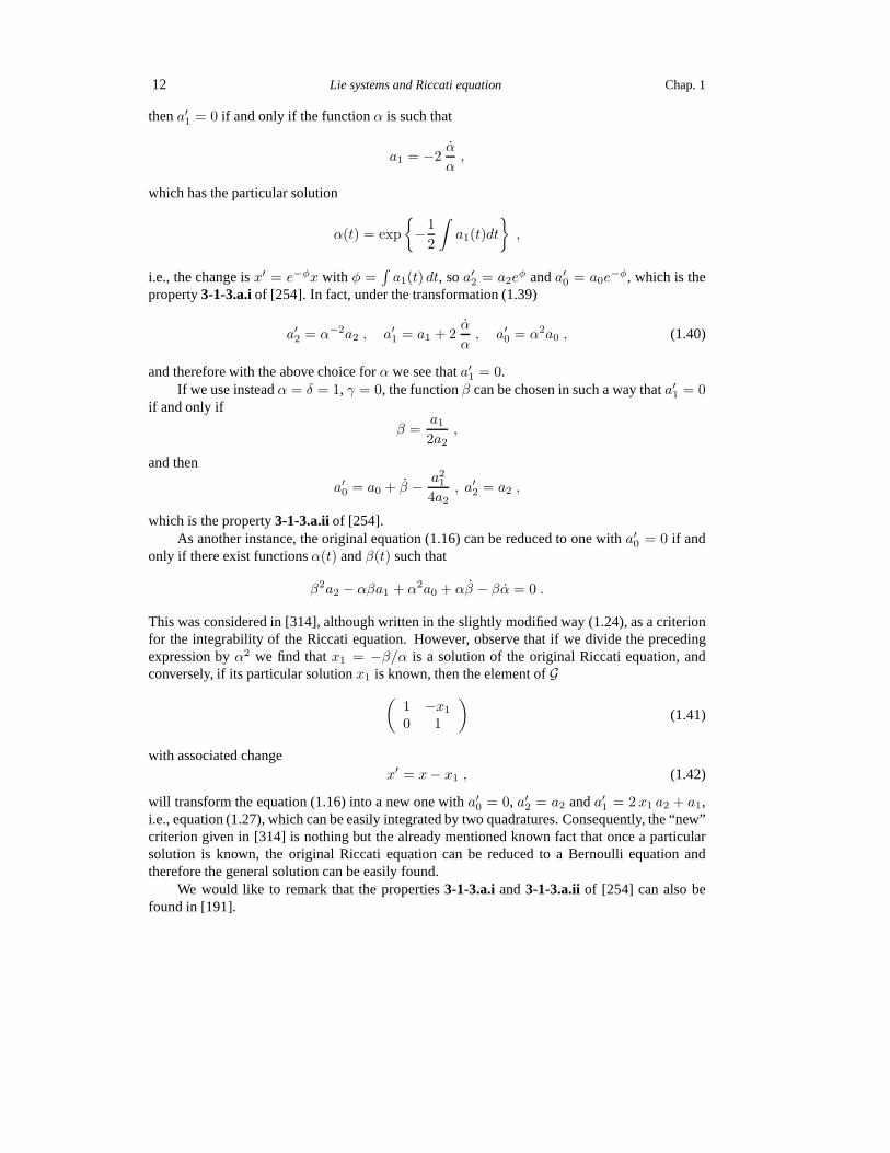
This was considered in [314], although written in the slightly modified way (1.24), as a criterionfor the integrability of the Riccati equation. However, observe that if we divide the precedingexpression byα2 we find thatx1 = −β/α is a solution of the original Riccati equation, andconversely, if its particular solutionx1 is known, then the element ofG
(1 −x10 1
)(1.41)
with associated changex′ = x− x1 , (1.42)
will transform the equation (1.16) into a new one witha′0 = 0, a′2 = a2 anda′1 = 2 x1 a2 + a1,i.e., equation (1.27), which can be easily integrated by twoquadratures. Consequently, the “new”criterion given in [314] is nothing but the already mentioned known fact that once a particularsolution is known, the original Riccati equation can be reduced to a Bernoulli equation andtherefore the general solution can be easily found.
We would like to remark that the properties3-1-3.a.iand3-1-3.a.ii of [254] can also befound in [191].

Sec. 1.5 Properties of the Riccati equation from group theory 13
Alternatively, we can follow a similar path by first reducingthe original equation (1.16) toa new one witha′2 = 0. Then, we should look for functionsγ(t) andδ(t) such that
a′2 = δ2a2 − δγa1 + γ2a0 + γδ − δγ = 0 .
This equation is similar to the one satisfied byα andβ in order to obtaina′0 = 0, with thereplacement ofβ by δ andα by γ, and therefore we should consider the transformation givenbythe element ofG (
1 0−x−1
1 1
), (1.43)
that is,x′ =
x1 x
x1 − x(1.44)
in order to obtain a new Riccati witha′2 = 0. More explicitly, the new coefficient functions are
a′2 = 0 , a′1 =2 a0x1
+ a1 , a′0 = a0 , (1.45)
i.e., the original Riccati equation (1.16) becomes
dx′
dt=
(2 a0x1
+ a1
)x′ + a0 . (1.46)
Therefore, the transformation (1.44) providesdirectly the linear equation (1.46). Such a changeseems to be absent in the literature previous to our work.
Let us suppose now that another solutionx2 of (1.16) is also known. If we make the change(1.42) the differencex2 − x1 will be a solution of the resulting equation (1.27) and therefore,after using the change given by (1.41), the element ofG
(1 0
(x1 − x2)−1 1
)(1.47)
will transform the Riccati equation (1.27) into a new one with a′′2 = a′′0 = 0 anda′′1 = a′1 =2 x1 a2 + a1, namely,
dx′′
dt= (2 x1 a2 + a1)x
′′ , (1.48)
which can be integrated with just one quadrature. This fact can be considered as a very ap-propriate group theoretical explanation of the introduction of the change of variable (1.30). Infact, we can check directly that if we use the transformationwith α = 1, β = 0, δ = 1 andγ = (x1 − x2)
−1 on the coefficients of (1.27), then we find that stilla′′0 = 0 and
a′′2 = a2 − (x1 − x2)−1a′1 + (x1 − x2)
−2(x1 − x2) ,
and asx1 andx2 are solutions of (1.16), we see that
x1 − x2 = a1(x1 − x2) + a2(x21 − x22) , (1.49)
hence
a′′2 = (x1 − x2)−2a2(x1 − x2)
2 + (x2 − x1)(a1 + 2x1a2)
+ a1(x1 − x2) + a2(x21 − x22) = 0 .

14 Lie systems and Riccati equation Chap. 1
The composition of both transformations (1.41) and (1.47) leads to the element ofG(
1 −x1(x1 − x2)
−1 −x2(x1 − x2)−1
)(1.50)
and therefore to the transformation (1.30). Now, we can compare the transformations (1.29) and(1.30). The first one corresponds to the element ofG (we assume thatx1(t) > x2(t), for all t)
1√x1 − x2
(1 −x11 −x2
), (1.51)
and therefore both matrices (1.50) and (1.51) are obtained one from the other by multiplicationby an element of type (1.39) withα = (x1 − x2)
−1/2, and then (1.40) relates the coefficientsa′′1anda1 arising after one or the other transformation. Taking into account (1.49), we have
a1 = a′′1 − a1 − a2(x1 + x2) = a2(x1 − x2) ,
as expected.On the other hand, if we use first the change of variable given by (1.44), the function
x′2 =x2 x1x1 − x2
will be a solution of (1.46). Then, a new transformation given by the element ofG(
1 − x2 x1
x1−x2
0 1
)(1.52)
will lead to a new equation in whicha′′0 = 0. More explicitly,
a′′2 = 0 , a′′1 = a′1 =2 a0x1
+ a1 , a′′0 = 0 . (1.53)
The composition of the two transformations is
(1 − x2 x1
x1−x2
0 1
)(1 0
− 1x1
1
)=
(x1
x1−x2− x2 x1
x1−x2
− 1x1
1
), (1.54)
which corresponds to the change of variable
x′′ =x21
(x2 − x1)
(x− x2)
(x− x1), (1.55)
leading to the homogeneous linear equation
˙x′′ =
(2 a0x1
+ a1
)x′′ , (1.56)
which can be integrated by means of just one quadrature.

Sec. 1.5 Properties of the Riccati equation from group theory 15
Now, we will see how the non-linear superposition formula for the Riccati equation can berecovered in this framework. Let us suppose that we know three particular solutionsx1, x2, x3of (1.16) and we can assume thatx1 > x2 > x3 for any value of the parametert. Following themethod described above, we can use the two first solutions forreducing the Riccati equation tothe simpler form of a linear equation, either to
x′′ = (2 x1 a2 + a1)x , (1.57)
or to˙x′′ =
(2 a0x1
+ a1
)x′′ . (1.58)
The sets of solutions of such differential equations are one-dimensional linear spaces, so it suf-fices to know a particular solution to find the general solution. As we know that
x′′3 = (x1 − x2)x3 − x1x3 − x2
(1.59)
is then a solution of equation (1.57), and
x′′3 =x21
(x2 − x1)
(x3 − x2)
(x3 − x1)(1.60)
is a solution of (1.58), we can take advantage of an appropriate diagonal element ofG of the form
(z−1/2 0
0 z1/2
),
with z being one of the two mentioned solutions, in order to reduce the equations either tox′′′ = 0 or ˙x′′′ = 0, respectively. These last equations have the general solutions
x′′′ = k ,
orx′′′ = k ,
which show the superposition formula (1.20). More explicitly, for the first case (1.57) the producttransformation will be given by
√(x2 − x3)
(x1 − x3)(x1 − x2)−x1
√(x2 − x3)
(x1 − x3)(x1 − x2)√
(x1 − x3)
(x2 − x3)(x1 − x2)−x2
√(x1 − x3)
(x2 − x3)(x1 − x2)
,
or, written in a different way,
−1√(x1 − x2)(x1 − x3)(x2 − x3)
(x2 − x3 −x1(x2 − x3)
x1 − x3 −x2(x1 − x3)
). (1.61)

16 Lie systems and Riccati equation Chap. 1
The transformation defined by this element ofG is
x′′′ =(x− x1)(x2 − x3)
(x− x2)(x1 − x3)(1.62)
and therefore we arrive in this way to the non-linear superposition function. That is, we obtainthe general solution of the Riccati equation (1.16) in termsof three particular solutions and aconstantk characterizing each particular solution:
(x− x1)(x2 − x3)
(x− x2)(x1 − x3)= k . (1.63)
The other case (1.58) can be treated in a similar way, leadingalso to the non-linear superpositionformula of the Riccati equation.

Chapter 2
Geometric approach to Lie systems
According to Theorem 1.1.1, Lie systems are systems of first order ordinary differential equationsof a special kind. Their solutions are integral curves of time-dependent vector fields which can bewritten as a time-dependent linear combination of certain vector fields closing on a Lie algebra.When these vector fields are complete, they can be regarded asfundamental vector fields withrespect to certain action of some Lie group.
After the insight gained from the study of the Riccati equation in the previous chapter, weare led now to the question of what are the structure and geometric properties of Lie systemsformulated on general differentiable manifolds, and in a more general situation in which thegroup playing a role is notSL(2,R) but a general Lie group. We will develop the subject afterthe introduction of some concepts and notation.
2.1 Notation and basic definitions
Let G be a Lie group. We will denote byLg andRg the left and right translations defined,respectively, byLg(g′) = gg′ andRg(g′) = g′g. Let us consider a left action ofG on a manifoldM , Φ : G×M → M . We will denotegx := Φg(x) := Φ(g, x) := Φx(g). By definition of leftaction the following properties hold:
ΦΦ(g,x) = Φx Rg , Φg Φx = Φx Lg , ∀x ∈M, g ∈ G . (2.1)
If a ∈ TeG, then the left-invariant vector field determined bya will be denotedXLa ,
(XLa )g = Lg∗e(a), and the right-invariant one byXR
a , (XRa )g = Rg∗e(a). In a similar way,
if ϑ ∈ T ∗eG, the left- and right-invariant 1-formsθLϑ andθRϑ in G determined byϑ are defined by
(θLϑ )g = (Lg−1)∗e(ϑ) , (θRϑ )g = (Rg−1 )∗e(ϑ) .
In particular, we have that(θLϑ )g(XLa )g = (θRϑ )g(X
Ra )g = ϑ(a), for all g ∈ G.
Denote byg the Lie algebra ofG, i.e., the set of left-invariant vector fields inG. Thecorrespondence between the sets of vectorsa ∈ TeG and of left-invariant vector fieldsXL
a isone-to-one, hence the Lie algebra structureg can be transported toTeG and we can consider theidentification of both setsTeG andg. The integral curve ofXL
a starting ate ∈ G is denotedexp(ta). Moreover, we recall that since the inner conjugationig can be written asig = Lg
17

18 Geometry of Lie systems Chap. 2
Rg−1 = Rg−1 Lg, andAd(g) = ig∗, right- and left-invariant vector fields are related point-wiseby (XL
a )g = Ad(g)(XRa )g.
Note that theΦg are diffeomorphisms and that(Φg)−1 = Φg−1 . It is clear that the differen-tial Φx∗e defines a mapΦx∗e : g ∼= TeG→ TxM . Then,X : TeG→ X(M), given bya 7→ Xa
such thatXa(x) = Φx∗e(−a), defines a mapping ofg into X(M). This is anactionof g onM , and we will callXa thefundamental vector field, or infinitesimal generator, associated to theelementa of g. It is easily seen that
(Xaf)(x) =d
dtf(exp(−ta)x)
∣∣∣t=0
, f ∈ C∞(M). (2.2)
Moreover, the minus sign has been introduced forX to be a Lie algebra homomorphism, i.e.,X[a,b] = [Xa, Xb]. Another important point is that for anya ∈ TeG, the correspondingXa ∈X(M) is complete, its flow being given byφ(t, x) = Φ(exp(−ta), x).
As an example, consider a Lie groupG acting on itself by left translations,Φg = Rg, andconsequently, for everya ∈ g the fundamental vector fieldXa is right invariant because
(Xa)g = Φg∗e(−a) = Rg∗e(−a) = −(XRa )g ,
whereXRa is the right-invariant vector field inG determined by its value at the neutral element
(XRa )e = a. In the preceding expressions the subindexg in Φg should be regarded as a point in
the manifoldG, and not as a group element.Given two actionsΦ1 andΦ2 of a Lie groupG on two differentiable manifoldsM1 andM2,
a mapF :M1 →M2 is said to be equivariant (sometimes, it is also said thatF is aG-morphism)if F Φ1g = Φ2g F , ∀ g ∈ G. The important property is that whenG is connected, the mapF : M1 → M2 is equivariant if and only if for eacha ∈ TeG the corresponding fundamentalvector fields inM1 andM2 areF -related. In fact, ifF is equivariant or aG-morphism, then theconditionF Φ1g = Φ2g F impliesF Φ1x = Φ2F (x), because of
(F Φ1x)(g) = F (Φ1(g, x)) = (F Φ1g)(x) = (Φ2g F )(x) = Φ2F (x)(g) .
Consequently, sinceX(1)a (x) = Φ1x∗e(−a), andX(2)
a (x′) = Φ2x′∗e(−a), we see thatX(1)a and
X(2)a areF -related:
F∗x(X(1)a (x)) = (F Φ1x)∗e(−a) = Φ2F (x)∗e(−a) = X(2)
a (F (x)) .
Conversely, if we assume that the corresponding fundamental vector fields areF -related, thenthe integral curve ofX(2)
a starting atF (x) ∈ M2 is the image underF of the integral curve of
X(1)a starting fromx ∈M1, and then
F Φ1 exp ta = Φ2 exp ta F ,
and thereforeF is aG-morphism, becauseG is connected and it is generated by the elementsexp ta with a ∈ g.
A particularly interesting case of the previous, to be used later, is the following: LetH be aLie subgroup of the Lie groupG and let us consider the homogeneous spaceG/H . The groupGacts on itself by left translations and on the homogeneous spaceG/H , byλ(g, g′H) = (gg′)H .The canonical projectionπL : G→ G/H , πL(g) = gH , is equivariant, because
(πL Lg)(g′) = gg′H , (λg πL)(g′) = gg′H , ∀ g′ ∈ G .

Sec. 2.1 Notation and basic definitions 19
Consequently, the fundamental vector fields onG corresponding to the left action ofG on itself,which are (minus) the right-invariant vector fields onG, areπL-related with the correspondingfundamental vector fields onG/H associated with the left actionλ of G onG/H . That is,
(XHa )gH = λgH ∗e(−a) = (πL Rg)∗e(−a) = −πL∗g(XR
a )g ,
where it has been used the relationλgH = πL Rg, which can be proved easily:
λgH(g′) = λ(g′, gH) = g′gH , (πL Rg)(g′) = πL(g′g) = g′gH , ∀ g′ ∈ G .
Now, let us choose a basisa1, . . . , ar for the tangent spaceTeG at the neutral elemente ∈ G and denoteXα = Xaα the corresponding fundamental vector fields for the actionΦ :G×M →M . The associated systems of differential equations admitting a superposition formulaare those giving the integral curves of the time-dependent vector field
X(x, t) =
r∑
α=1
bα(t)Xα(x) . (2.3)
In other words, we should determine the curvesx(t) such that
x(t) =
r∑
α=1
bα(t)Xα(x(t)) , (2.4)
satisfying some initial conditions.Alternatively we could start with a right action ofG on M , Ψ : M × G → M . The
reasoning is similar and we will only give the relevant expressions. Nowxg := Ψg(x) :=Ψ(x, g) := Ψx(g). The properties equivalent to (2.1) are now
ΨΨ(x, g) = Ψx Lg , Ψg Ψx = Ψx Rg , ∀x ∈M, g ∈ G . (2.5)
It is clear thatΨx∗e : g ∼= TeG → TxM . The mapY : g → X(M) given bya 7→ Ya such thatYa(x) = Ψx∗e(a) defines thefundamental vector fieldassociated to the elementa of g:
(Yaf)(x) =d
dtf(x exp(ta))
∣∣∣t=0
, f ∈ C∞(M).
The vector fieldYa is complete with flowφ(t, x) = Ψ(x, exp(ta)). Here, there is no needof introducing a minus sign forY to be a Lie algebra homomorphism, i.e., it already satisfiesY[a,b] = [Ya, Yb].
In the particular example of a Lie groupG acting on itself by right translations, for everya ∈ g the fundamental vector fieldYa is left-invariant because
(Ya)g = Ψg∗e(a) = Lg∗e(a) = (XLa )g .
If H is a Lie subgroup ofG, then the groupG acts on itself by right translations and on thehomogeneous spaceG\H , byµ(Hg′, g) = H(g′g). The canonical projectionπR : G→ G\H ,πR(g) = Hg, is equivariant: we haveπR Rg = µg πR for all g ∈ G. We have as well thatµHg = πR Lg.

20 Geometry of Lie systems Chap. 2
Therefore, the fundamental vector fields onG corresponding to the right action ofG on it-self, i.e., the left-invariant vector fields onG, areπR-related with the corresponding fundamentalvector fields onG\H associated with the right actionµ of G onG\H . That is,
(HXa)Hg = µHg ∗e(a) = (πR Lg)∗e(a) = πR∗g(XLa )g .
The analogous equation to (2.4) will be now
x(t) =
r∑
α=1
bα(t)Yα(x(t)) , (2.6)
which gives the integral curves of the time-dependent vector field
Y (x, t) =
r∑
α=1
bα(t)Yα(x) . (2.7)
2.2 Lie systems on Lie groups and on homogeneous spaces
In this section we will see how the general solution of (2.4) can be obtained if we are able tosolve the differential equation in the groupG
g(t) = −r∑
α=1
bα(t)XRα (g(t)) , (2.8)
with initial conditionsg(0) = e. Then, the particular solution of (2.4) determined by the initialconditionx0 will be x(t) = Φ(g(t), x0). Moreover, we will show the existing relation betweensystems of type (2.4) admitting a (non linear) superposition formula and Lie systems defined onG like (2.8), as well as with certain equations defined onTeG.
First of all, let us show that finding solutions of (2.4) is equivalent to determine the integralcurves inG of the right-invariant, time-dependent vector field inG
X(t) = −r∑
α=1
bα(t)XRα . (2.9)
Indeed, it is easy to see that the Lie groupG acts transitively on the integral curves of (2.9) byleft translations and, as indicated before, ifg(t) is the integral curve ofX with g(0) = e, thenx(t) = Φ(g(t), x0) is the integral curve of (2.3) starting atx0 ∈M :
x(t) =d
dtΦ(g(t), x0) =
d
dtΦx0(g(t)) = Φx0∗g(t)(g(t)) ,
and then, using (2.8),
x(t) = −Φx0∗g(t)
(r∑
α=1
bα(t)XRα (g(t))
)= −
r∑
α=1
bα(t)Φx0∗g(t)Rg(t)∗e(aα) .
Now, using the first property of (2.1), we see that
Φx0∗g(t) Rg(t)∗e = ΦΦ(g(t),x0)∗e ,

Sec. 2.2 Lie systems on Lie groups and on homogeneous spaces 21
and then
x(t) = −r∑
α=1
bα(t)ΦΦ(g(t),x0)∗e(aα) =r∑
α=1
bα(t)Xα(x(t)) .
Thus, the solution of (2.4) starting fromx0 will be x(t) = Φ(g(t), x0), whereg(t) is the solutionof (2.8) withg(0) = e. This is an important point: the knowledge of one particularsolution of(2.8) allows us to obtain the general solution of (2.4).
Even more, we show next that given a system of type (2.8), we can project it onto a homo-geneous space to give a Lie system of type (2.4) and conversely, Lie systems of type (2.4) arerealizations on homogeneous spaces of systems of type (2.8). Indeed, letH be a closed subgroupof G and consider the homogeneous spaceM = G/H . Then,G can be regarded as the totalspace of the principal bundle(G, πL, G/H) overG/H , whereπL denotes the canonical projec-tion. We have seen in the previous section thatπL is equivariant with respect to the left action ofG on itself by left translations and the actionλ onG/H , and consequently, the fundamental vec-tor fields corresponding to the two actions areπL-related. Therefore, the right-invariant vectorfieldsXR
α areπL-projectable and theπL-related vector fields inM are the fundamental vectorfieldsXH
α = XHaα corresponding to the natural left action ofG onM , (XH
α )gH = −πL∗g(XRα )g.
In this way we can project the time-dependent vector field (2.9) defining the Lie system inG(2.8) to the time-dependent vector field of type (2.3) defining a Lie system inG/H of type (2.4).
Conversely, assume we have a Lie system in a manifoldM defined by complete vector fieldsclosing on a Lie algebrag′, which is the Lie algebra of a connected Lie groupG′, defined up toa central discrete subgroup. Then, there exists at least oneLie groupG, and corresponding leftaction(s)Φ : G×M →M , such thatG′ is a subgroup ofG, andG′ ∼= G/Ker Φ, whereKer Φis the normal subgroupKer Φ = g ∈ G | Φ(g, x) = x, ∀x ∈ M. Usually, one would takethe smallest possible group, and takeG = G′. In particular, the corresponding actionΦ can bechosen to be effective. The restriction to an orbit will provide a homogeneous space of the typedescribed in the previous paragraph. The choice of a pointx0 in the orbit allows us to identifythis homogeneous space withG/H , whereH is the stability group ofx0. Different choices forx0 lead to conjugate subgroups.
Notice that when applyingRg(t)−1∗g(t) to both sides of the equation (2.8) we will obtain theequation onTeG
Rg(t)−1∗g(t)(g(t)) = −r∑
α=1
bα(t)aα . (2.10)
This equation is usually written with a slight abuse of notation as
(g g−1)(t) = −r∑
α=1
bα(t)aα ,
although only in the case of matrix groupsRg(t)−1∗g(t)g(t) becomes the productg(t) g(t)−1.When doing calculations in a general case, one should take this into account.
As far as Lie systems defined by right actions are concerned, the general solution of (2.6)will be obtained if we find the particular solution of the differential equation in the groupG
g(t) =
r∑
α=1
bα(t)XLα (g(t)) , (2.11)
22 Geometry of Lie systems Chap. 2
with initial conditionsg(0) = e, because then the particular solution determined by the initialconditionx0 will be x(t) = Ψ(x0, g(t)). Notice that when applyingLg(t)−1∗g(t) to both sides ofthe equation (2.11) we will obtain the equation onTeG
Lg(t)−1∗g(t)(g(t)) =r∑
α=1
bα(t)aα . (2.12)
As in the previous case is common to write this expression as
(g−1 g)(t) =
r∑
α=1
bα(t)aα ,
although only in the case of matrix groupsLg(t)−1∗g(t)g(t) = g(t)−1 g(t). The correspondencebetween systems of type (2.6), defined over a homogeneous space, and (2.11) (resp. of type(2.12)) is analogous to the one considered in the case of Lie systems associated to left actions.This correspondence is one-to-one if the actionΨ is effective.
It may seem that there is no advantage in considering insteadof the original equation (2.4),the equation (2.8), which in principle may be even more difficult to solve or treat. However, thepoint is that we have replaced the problem of finding the general solution of a system of type(2.4) for that of the particular solution of the system of type (2.8) which corresponds tog(0) = e.This follows from the fact that ifg(t) is such a solution, the one starting at a different pointg1is obtained by the right translationg′(t) = Rg1g(t) = g(t) g1. Moreover, for any Lie system oftype (2.4) associated to different actions ofG on the same or different manifolds, we obtain theirgeneral solution at once when we know the solution of (2.8) with g(0) = e.
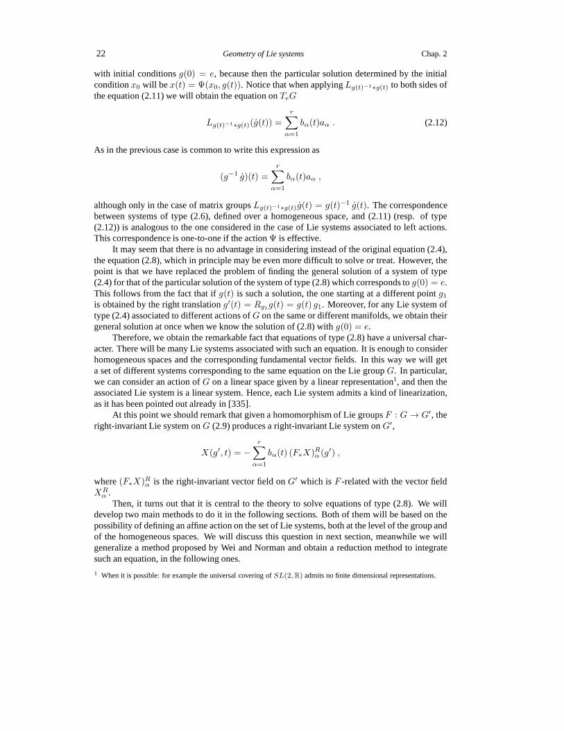
Therefore, we obtain the remarkable fact that equations of type (2.8) have a universal char-acter. There will be many Lie systems associated with such anequation. It is enough to considerhomogeneous spaces and the corresponding fundamental vector fields. In this way we will geta set of different systems corresponding to the same equation on the Lie groupG. In particular,we can consider an action ofG on a linear space given by a linear representation1, and then theassociated Lie system is a linear system. Hence, each Lie system admits a kind of linearization,as it has been pointed out already in [335].
At this point we should remark that given a homomorphism of Lie groupsF : G→ G′, theright-invariant Lie system onG (2.9) produces a right-invariant Lie system onG′,
X(g′, t) = −r∑
α=1
bα(t) (F∗X)Rα (g′) ,
where(F∗X)Rα is the right-invariant vector field onG′ which isF -related with the vector fieldXRα .
Then, it turns out that it is central to the theory to solve equations of type (2.8). We willdevelop two main methods to do it in the following sections. Both of them will be based on thepossibility of defining an affine action on the set of Lie systems, both at the level of the group andof the homogeneous spaces. We will discuss this question in next section, meanwhile we willgeneralize a method proposed by Wei and Norman and obtain a reduction method to integratesuch an equation, in the following ones.
1 When it is possible: for example the universal covering ofSL(2,R) admits no finite dimensional representations.

Sec. 2.3 Affine actions on Lie systems 23
2.3 Affine actions on Lie systems
We will generalize in this section the transformations considered in Section 1.4, where we haveused curves inSL(2, R) to transform solutions of a Riccati equation of type (1.16) into solutionsof an associated Riccati equation, and as a consequence we have obtained an affine action ofthe group ofSL(2, R)-valued curves on the set of Riccati equations. The procedure will begeneralized to any Lie system defined in a Lie groupG, and afterwards, in a homogeneousspace.
Let G be a connected Lie group. Let us consider the set of (smooth) curvesMap(R, G),which is endowed with the following group law, defined pointwise
(g1 ∗ g2)(t) = g1(t)g2(t), ∀ g1, g2 ∈ Map(R, G) . (2.13)
We show next that the left action of the groupMap(R, G) on itself induces an affine action of thisgroup on the set of differential equations of type (2.10) inTeG. As a consequence, we will beable to define an affine action on the set of equations of type (2.4) defined over a homogeneousspace. By this fact, we will be able to relate equations of that kind, being, for example, theintegrability of one of them (say, in the sense of being integrable by quadratures) equivalentto that of any other one in the same orbit. We will see also thatsimilar results appear whenconsidering the right action of the groupMap(R, G) on itself, but in that case (2.6) and (2.12)will be the relevant equations.
For that purpose, letg(t), g′(t) andg(t) be differentiable curves inG such that
g(t) = g′(t)g(t) , ∀ t ∈ R . (2.14)
We are interested now in how the three curves inTeG defined byg(t), g′(t) and g(t), i.e.,Rg(t)−1∗g(t)( ˙g(t)),Rg′(t)−1∗g′(t)(g
′(t)) andRg(t)−1∗g(t)(g(t)), respectively, are related amongstthemselves. Sinceg(t) = Lg′(t)g(t) = Rg(t)g
′(t), we have
Rg(t)−1∗g(t)( ˙g(t)) = Rg(t)−1g′(t)−1∗g′(t)g(t)Lg′(t)∗g(t)(g(t)) +Rg(t)∗g′(t)(g′(t))
= (Rg′(t)−1∗g′(t) Rg(t)−1∗g′(t)g(t))Lg′(t)∗g(t)(g(t)) +Rg(t)∗g′(t)(g′(t))
= (Rg′(t)−1∗g′(t) Lg′(t)∗e)Rg(t)−1∗g(t)(g(t))+Rg′(t)−1∗g′(t)(g′(t))
= Ad(g′(t))Rg(t)−1∗g(t)(g(t)) +Rg′(t)−1∗g′(t)(g′(t)) ,
where we have used, sucessively, the identitiesRgg′ = Rg′ Rg, Rg Lg′ = Lg′ Rg, andidG∗g = idTgG, valid for all g, g′ ∈ G, as well as the definition of the adjoint representation ofthe group. As a result, we finally obtain
Rg(t)−1∗g(t)( ˙g(t)) = Ad(g′(t))Rg(t)−1∗g(t)(g(t)) +Rg′(t)−1∗g′(t)(g′(t)) . (2.15)
Now, consider a left action ofG on the manifoldM , Φ : G ×M → M , as in the pre-vious section. If the curvex(t) is given byx(t) = Φ(g(t), x0), wherex0 ∈ M , we wonderabout how the tangent curvex(t) is defined in terms of the curve inTeG defined byg(t), i.e.,Rg(t)−1∗g(t)(g(t)). The relation is (see also [72])
x(t) = Φx(t)∗eRg(t)−1∗g(t)(g(t)) . (2.16)

24 Geometry of Lie systems Chap. 2
In fact, we have
x(t) =d
dtΦ(g(t), x0) = Φx0∗g(t)(g(t)) = ΦΦ(g(t)−1g(t), x0)∗g(t)(g(t))
= ΦΦ(g(t)−1, x(t))∗g(t)(g(t)) = Φx(t)∗eRg(t)−1∗g(t)(g(t)) ,
where the first property of (2.1) has been used. As a result, ifwe define the new curvey(t) asy(t) = Φ(g′(t), x(t)), we have thaty(t) = Φ(g′(t)g(t), x0). Takingg(t) = g′(t)g(t), it follows
y(t) = Φy(t)∗eRg(t)−1∗g(t)( ˙g(t))= Φy(t)∗eAd(g′(t))[Rg(t)−1∗g(t)(g(t))] +Rg′(t)−1∗g′(t)(g
′(t)) , (2.17)
by using the property (2.15). However, (2.17) can also be obtained directly. Indeed,
y(t) = Φx(t)∗g′(t)(g′(t)) + Φg′(t)∗x(t)(x(t))
= Φx(t)∗g′(t)(g′(t)) + (Φg′(t)∗x(t) Φx(t)∗e)Rg(t)−1∗g(t)(g(t))
= Φx(t)∗g′(t)g′(t) + Lg′(t)∗e(Rg(t)−1∗g(t)(g(t)))= ΦΦ(g′(t)−1, y(t))∗g′(t)g′(t) + Lg′(t)∗e(Rg(t)−1∗g(t)(g(t)))= Φy(t)∗eAd(g′(t))[Rg(t)−1∗g(t)(g(t))] +Rg′(t)−1∗g′(t)(g
′(t)) ,
where it has been used (2.16), the second property of (2.1), thatx(t) = Φ(g′(t)−1, y(t)) and thefirst property of (2.1), in this order.
The equation (2.15) tell us the following. The curvesg(t), g′(t) andg(t), as elements of thegroupMap(R, G), define the abovementioned curves inTeG. Therefore, they define differentdifferent equations of type (2.10).
Now, we define the map
θL : Map(R, G) −→ Map(R, TeG)
g(·) 7−→ θL(g(·)) = Rg(·)−1 ∗g(·)(g(·)) , (2.18)
and then the equation (2.15) expresses that, for the left action ofMap(R, G) on itself given by
g(·) 7−→ Lg′(·)g(·) = g′(·)g(·) ,
there exists an associated affine action (see, e.g., [230]) of Map(R, G) on Map(R, TeG) withlinear part given by the linear representationAd(·) of Map(R, G) and a 1-cocycle for the samerepresentation given by the mapθL itself. In fact, it can be rewritten (2.15) in terms ofθL as
θL(g′(·)g(·)) = Ad(g′(·))(θL(g(·))) + θL(g′(·)) . (2.19)
Clearly, we can immediately translate this property into Lie systems on every homogeneousspace ofG, by means of the properties (2.16) and (2.17). Therefore, wecan naturally definean affine action of the groupMap(R, G) on the set of differential equations of type (2.4). Theorbits of these actions are equivalence classes of systems of type (2.4), for which, for example,the integrability of one equation is a straightforward consequence of the integrability of anyother in the same orbit. This is a generalization to any Lie system of the properties discussed inSection 1.4.

Sec. 2.4 The Wei–Norman method 25
All these facts have an equivalent version in the case of right actions. We give only therelevant expressions in this case. Letg(t), g′(t) andg(t) be now differentiable curves inG suchthat
g(t) = g(t)g(t)′ , ∀ t ∈ R . (2.20)
Then, we can obtain the property similar to (2.15),
Lg(t)−1∗g(t)( ˙g(t)) = Ad(g′(t)−1)Lg(t)−1∗g(t)(g(t)) + Lg′(t)−1∗g′(t)(g′(t)) . (2.21)
If Ψ : M × G → M denotes now a right action ofG on the manifoldM , and the curvex(t) inM is given byx(t) = Ψ(x0, g(t)), wherex0 ∈M , we have the analogous property to (2.16),
x(t) = Ψx(t)∗eLg(t)−1∗g(t)(g(t)) . (2.22)
Moreover, if then we definey(t) = Ψ(x(t), g′(t)), we obtain
y(t) = Ψy(t)∗eAd(g′(t)−1)[Lg(t)−1∗g(t)(g(t))] + Lg′(t)−1∗g′(t)(g′(t)) , (2.23)
which is the property equivalent to (2.17). The map equivalent to (2.18) is
θR : Map(R, G) −→ Map(R, TeG)
g(·) 7−→ θR(g(·)) = Lg(·)−1 ∗g(·)(g(·)) , (2.24)
so if we consider now the right action ofMap(R, G) on itself given by
g(·) 7−→ Rg′(·)g(·) = g(·)g′(·) ,
we can rewrite (2.21) as
θR(g(·)g′(·)) = Ad(g′(·)−1)(θR(g(·))) + θR(g′(·)) , (2.25)
which is analogous to (2.19). That is, we also have an affine action of Map(R, G) over the setof curvesMap(R, TeG) and hence over the set of differential equations of type (2.6).
2.4 The Wei–Norman method
As we have already mentioned at the end of Section 2.2, it is essential to the theory of Lie systemsto have some method to solve, or at least to treat, the problemof obtaining the solution curveg(t) of a system of type (2.8), withg(0) = e, or equivalently, a system of type (2.10). We willdiscuss in this section that problem, developing a generalization of the method proposed by Weiand Norman [331, 332] in order to find the time evolution operator for a linear system of typedU(t)/dt = H(t)U(t), with U(0) = I andH(t) taking values in a matrix Lie algebra. We willgive a generalization in two senses: Firstly, the method will work for (almost) any Lie group, notonly for matrix Lie groups. Secondly, the generalized version only on the Lie algebra of interest,without making reference to any representation of it. In fact, the formulas only will depend on thestructure constants, with respect to the chosen basis, defining the Lie algebra of interest. The ideaof this generalization was initiated in [72], and we will develop here the complete expressions.We postpone to the next section the development of an alternative method to solve (2.10), basedon a reduction property.

26 Geometry of Lie systems Chap. 2
Let us consider, first of all, the generalization to several factors of the property (2.15), whichis as follows. Letg(t) be a curve inG which is given by the product of otherl curvesg(t) =
g1(t)g2(t) · · · gl(t) =∏li=1 gi(t). Then, denotinghs(t) =
∏li=s+1 gi(t), for s ∈ 1, . . . , l−1,
and applying (2.15) tog(t) = g1(t)h1(t) we have
Rg(t)−1 ∗g(t)(g(t)) = Ad(g1(t))Rh1(t)−1 ∗h1(t)(h1(t)) +Rg1(t)−1 ∗g1(t)(g1(t)) .
Simply iterating this procedure, and using the fact thatAd(gg′) = Ad(g)Ad(g′) for all g, g′ ∈G, we obtain
Rg(t)−1 ∗g(t)(g(t)) = Rg1(t)−1 ∗g1(t)(g1(t)) + Ad(g1(t))Rg2(t)−1 ∗g2(t)(g2(t))
+ · · ·+Ad
(l−1∏
i=1
gi(t)
)Rgl(t)−1 ∗gl(t)(gl(t))
=
l∑
i=1
Ad
∏
j<i
gj(t)
Rgi(t)−1 ∗gi(t)(gi(t))
=
l∑
i=1
∏
j<i
Ad(gj(t))
Rgi(t)−1 ∗gi(t)(gi(t))
, (2.26)
where it has been takeng0(t) = e for all t.The generalized Wei–Norman method consists of writing the desired solutiong(t) of an
equation of type (2.10) in terms of a set of canonical coordinates of the second kind with respectto a basisa1, . . . , ar of the Lie algebrag, for each value oft, i.e.,
g(t) =r∏
α=1
exp(−vα(t)aα) = exp(−v1(t)a1) · · · exp(−vr(t)ar) , (2.27)
and transforming the equation (2.10) into a system of differential equations for thevα(t), withinitial conditionsvα(0) = 0 for all α ∈ 1, . . . , r. The minus signs in the exponentials havebeen introduced for computational convenience. We should remark, however, that the expression(2.27) makes sense only in a neighbourhood of the identity elemente ∈ G.
Therefore, we use the result (2.26), in the particular case whenl = r = dimG andgα(t) =exp(−vα(t)aα) for all α ∈ 1, . . . , r. Now, sinceRgα(t)−1 ∗gα(t)(gα(t)) = −vα(t)aα, we seethat (2.26) reduces to
Rg(t)−1 ∗g(t)(g(t)) = −r∑
α=1
vα(t)
∏
β<α
Ad(exp(−vβ(t)aβ))
aα
= −r∑
α=1
vα(t)
∏
β<α
exp(−vβ(t) ad(aβ))
aα ,
where it has been used the identityAd(exp(a)) = exp(ad(a)), for all a ∈ g. Substituting inequation (2.10) we obtain the fundamental expression of thegeneralized Wei–Norman method
r∑
α=1
vα(t)
∏
β<α
exp(−vβ(t) ad(aβ))
aα =
r∑
α=1
bα(t)aα , (2.28)

Sec. 2.5 Reduction of Lie systems 27
with vα(0) = 0, α ∈ 1, . . . , r.If the Lie algebrag is solvable, and in particular, if it is nilpotent, the solution of the re-
sulting system of differential equations for the functionsvα(t) can be obtained by quadratures.If, instead, the Lie algebrag is semi-simple, then the integrability by quadratures is not as-sured [331,332].
We would like to remark that if we choose different basis of the Lie algebra of interest forcomputing (2.28), the systems of differential equations which appear are, in general, different.Even a reordering of the basis changes the result.
Apart from the examples given in Chapter 3, we will make extensive use of this method inPart 3 of this Thesis, where we will deal with systems from geometric control theory which turnout to be Lie systems.
2.5 The reduction method associated to a subgroup
We will develop in this section a method which allows us to reduce the problem of solvingan equation of type (2.10) to that of solving two related Lie systems, one defined in a suitablehomogeneous space, and other of the same form of (2.10) but defined in a subgroup. The ideafor obtaining this result is the following. Given an equation of the type (2.10),
Rg(t)−1∗g(t)(g(t)) = −r∑
α=1
bα(t)aα , (2.29)
with g(0) = e ∈ G, it may happen that the only non-vanishing coefficients are those correspond-ing to a subalgebrah of g. Then, according to the general theory developed in Section2.2, theequation would reduce in that case to a simpler equation on a subgroup, involving, for example,less coordinate functions in the Wei–Norman method explained in the preceding section.
On the other hand, we have developed in Section 2.3 a way of relating Lie systems bymeans of affine actions. The natural question arises: is it possible, given certain Lie system oftype (2.10), to reduce it to another one formulated in a Lie subgroup, by means of some suitabletransformation out of those provided by the corresponding affine action?.
More explicitly, given (2.29), let us choose a curveg′(t) in the groupG, and define thecurveg(t) by g(t) = g′(t)g(t), whereg(t) is the solution of (2.29). The new curve inG, g(t),determines a new Lie system by means of (2.15),
Rg(t)−1∗g(t)(g(t)) = Rg′ −1(t)∗g′(t)(g′(t)) −
r∑
α=1
bα(t)Ad(g′(t))aα , (2.30)
which is an equation similar to (2.29) but with different right hand side. Therefore, the aim isto choose the curveg′(t) appropriately, i.e., in such a way that the new equation be simpler. Forinstance, we can choose a Lie subgroupH ofG and look for a choice ofg′(t) such that the righthand side of (2.30) lies inTeH , and henceg(t) ∈ H for all t.
We will treat that question now. Let us suppose that we can choose a closed (and thereforea Lie) subgroupH of G, with associated Lie algebrah, which is a subalgebra ofg. For the sakeof simplicity, let us assume thath is spanned by the firsts elementsa1, . . . , as in the basis ofg, and then ther − s elementsas+1, . . . , ar span a supplementary space.

28 Geometry of Lie systems Chap. 2
When we restrict ourselves toH the equation we will obtain will be similar to (2.29), butwhere some parameters vanish, i.e.,
Rh(t)−1∗h(t)(h(t)) = −s∑
µ=1
dµ(t)aµ , (2.31)
or equivalently,
h(t) = −s∑
µ=1
dµ(t)XRµ (h(t)) . (2.32)
Let us show that the problem of finding the curveg(t) solution of (2.29), starting ate ∈ G,can be reduced to that of solving a similar equation in the subgroupH , provided thatonepartic-ular solutionx1(t) of a Lie system of type (2.4) for the left actionλ of G on the homogeneousspaceM = G/H is given.
The procedure is as follows. Take a liftg1(t) of the curvex1(t) from G/H to G. Thisis always possible, at least locally: For small enough valueof t, there are uniquely definedfunctions,u1(t), . . . , ur(t), such that
g1(t) = exp(ur(t)ar) · · · exp(u1(t)a1) ,
and therefore
x1(t) = πL(g1(t)) = g1(t)H = exp(ur(t)ar) · · · exp(us+1(t)as+1)H ,
whereπL denotes the canonical projectionπL : G → G/H . The functionsuα(t) are nothingbut the second class canonical coordinates of the elementg1(t) with respect to the chosen basis.We have seen in the preceding section how this type of coordinates is essential in the formulationof the Wei–Norman method.
Now, remember that the fundamental vector fieldsXHa corresponding to the left actionλ of
G onG/H are justXHa = −πL∗ (XR
a ). By hypothesis, we have that the curvex1(t) satisfies
x1(t) =
r∑
α=1
bα(t)XHα (x1(t)) ,
therefore,
x1(t) =d
dt[πL(g1(t))] = πL∗ g1(t)(g1(t)) =
r∑
α=1
bα(t)XHα (x1(t))
= −r∑
α=1
bα(t)πL∗ g1(t)(X
Rα (g1(t))) .
Hence,
πL∗ g1(t)g1(t) +r∑
α=1
bα(t)XRα (g1(t)) = 0 .

Sec. 2.5 Reduction of Lie systems 29
The kernel of the projectionπL∗ is spanned by the left-invariant vector fields onG generated byelements ofh, so that there are time-dependent coefficientscµ(t), for µ = 1, . . . , s, such that
g1(t) +
r∑
α=1
bα(t)XRα (g1(t)) =
s∑
µ=1
cµ(t)XLµ (g1(t))
=
s∑
µ=1
cµ(t)Ad(g1(t))XRµ (g1(t)) . (2.33)
If we write the solutiong(t) of (2.29) we are looking for in the form
g(t) = g1(t)h(t) ,
whereh(t) ∈ H for all t ∈ R, we have, using (2.15),
Rg(t)−1∗g(t)(g(t)) = Ad(g1(t))Rh(t)−1∗h(t)(h(t)) +Rg1(t)−1∗g1(t)(g1(t)) . (2.34)
We can applyRg1(t)−1∗g1(t) to (2.33) so that we obtain
Rg1(t)−1∗g1(t)(g1(t)) = −r∑
α=1
bα(t)aα +s∑
µ=1
cµ(t)Ad(g1(t))aµ (2.35)
and then, from (2.34), (2.35) and our hypothesis thatg(t) satisfies (2.29), we have
Ad(g1(t))Rh(t)−1∗h(t)(h(t)) = −s∑
µ=1
cµ(t)Ad(g1(t))aµ .
SinceAd(g1(t)) is an automorphism, we get
Rh(t)−1∗h(t)(h(t)) = −s∑
µ=1
cµ(t)aµ . (2.36)
The last equation is just of type (2.29) but for the subalgebrah ≡ TeH . We can summarize thepreceding results as follows:
Theorem 2.5.1. Every integral curve of the time-dependent vector field(2.9) on thegroupG can be written in the formg(t) = g1(t)h(t), whereg1(t) is a curve inG project-ing onto a solutionx1(t) of a Lie system of type(2.4), associated to the left actionλ on thehomogeneous spaceG/H , andh(t) is a solution of an equation of type(2.10)for the subgroupH , given explicitly by
Rh(t)−1∗h(t)(h(t)) = −Ad(g−11 (t))
(r∑
α=1
bα(t)aα +Rg1(t)−1∗g1(t)(g1(t))
)
= −Ad(g−11 (t))
(r∑
α=1
bα(t)aα
)− Lg1(t)−1∗g1(t)(g1(t)) . (2.37)

30 Geometry of Lie systems Chap. 2
We should remark that from the proof of this Theorem we see that, moreover, such a reduc-tion can be carried out if and only if we can find a particular solution on an associated homoge-neous space. It is interesting to note as well that we can takeany lift g1(t) toG of the solutionx1(t) on the homogeneous spaceG/H . With the choice of one or another lift, the final equationin TeH one has to solve only changes slightly. But this only means that we choose diferentrepresentatives of each class onG/H and has no real importance for our problem.
Note as well that if we want to find the integral curve of (2.9) starting from the identity, andwe take the solution of (2.37) withh(0) = e, then we must take a liftg1(t) such thatg1(0) = e.
The reduction can also be carried out using right actions andright cosets. Having found oneparticular solutionx1(t) for the problem inG\H , we select a liftg1(t), and then there will betime-dependent coefficientscν(t), for ν = 1, . . . , s, such that
g1(t)−r∑
α=1
bα(t)XLα (g1(t)) =
s∑
ν=1
cν(t)XRν (g1(t))
=
s∑
ν=1
cν(t)Ad(g1(t)−1)XL
ν (g1(t)) . (2.38)
Now, assuming that we have a solution of (2.29) of the formg(t) = h(t) g1(t), and following asimilar scheme to that of left actions we will arrive to the analogous formula to (2.36),
Lh(t)−1∗h(t)(h(t)) = −s∑
ν=1
cν(t)aν ,
i.e., the corresponding expression to that of Theorem 2.5.1is
Lh(t)−1∗h(t)(h(t)) = Ad(g1(t))
(r∑
α=1
bα(t)aα − Lg1(t)−1∗g1(t)(g1(t))
)
= Ad(g1(t))
(r∑
α=1
bα(t)aα
)−Rg1(t)−1∗g1(t)(g1(t)) ∈ TeH .
Let us discuss now some cases where the previously describedreduction can be applied ina direct way and in the general case.
Assume thatH is a normal subgroup inG of dimensions. Then, we haveexp(ta) gH =gH for any a ∈ h, so we see thatXH
a = 0, for anya ∈ h. Thus, the fundamental vectorfieldsXH
1 , . . . , XHs onG/H are just zero. Then, the equation of type (2.4) onG/H is just an
equation of type (2.8) for the factor groupG/H , so we can write
Rx1(t)−1 ∗x1(t)(x1(t)) = −r∑
α=s+1
bα(t)aα ,
whereas+1, . . . , ar is the basis of the factor Lie algebrag/h induced from that ofg. Notehowever that the liftg1(t) toG of x1(t) satisfies
Rg1(t)−1 ∗g1(t)(g1(t)) = −s∑
α=1
cα(t)aα −r∑
α=s+1
bα(t)aα ,

Sec. 2.5 Reduction of Lie systems 31
where thet-dependent coefficientscα(t) depend on the specific liftg1(t) we take. Therefore, theequation (2.37) becomes in this case
Rh(t)−1∗h(t)(h(t)) = −Ad(g−11 (t))
(r∑
α=1
bα(t)aα −s∑
α=1
cα(t)aα −r∑
α=s+1
bα(t)aα
)
= −s∑
α=1
(bα(t)− cα(t))Ad(g−11 (t))aα .
If the factor group in the reduction process is one-dimensional, one can solve equations oftype (2.8) or (2.10) easily, by means of one quadrature, because in appropriate coordinates it hasthe form
x(t) = a(t) ,
so the only problem is to solve the corresponding equation for H . In particular, if the groupG is solvable, then there is a chain of codimension one normal subgroups (i.e., each of thesesubgroups is normal in the smallest subgroup which containsit in the chain)
e ⊂ Gr−1 ⊂ · · · ⊂ G1 ⊂ G ,
and we can solve (2.8) or (2.10) in quadratures, by induction.We have seen how in the case that the subgroupH is normal inG, our reduction procedure
leads to solve equations of type (2.10) on two lower dimensional Lie groups:G/H andH . Ofcourse the simplest instance is when the groupG is a direct productG = G1 ⊗ G2 of twogroupsG1 andG2, and then the problem reduces to the corresponding problemsin each factor.Other well-known instances in which there appear normal subgroups are semidirect productsand (central) extensions of Lie groups. We recall briefly these notions, since the correspondingstructures appear in specific examples where we will apply the theory of reduction of Lie systems.
Let N , K be Lie groups, and letϕ : K → Aut(N) be a homomorphism ofK into thegroup of automorphisms ofN . Forn1, n2 ∈ N , k1, k2 ∈ K, define the composition
(n1, k1)(n2, k2) = (n1ϕ(k1)n2, k1k2) .
Let eN , eK be the respective identities ofN andK. It is easy to check that(n1, k1)(eN , eK) =(eN , eK)(n1, k1) = (n1, k1), and that(n1, k1)
−1 = (ϕ(k−11 )n−1
1 , k−11 ), these operations
being differentiable. Then, the previous composition law endows the setN × K with a Liegroup structure. We denote this group byN ⊙K, and call it thesemidirect productofN with K(relative toϕ). The setN × eK is a normal subgroup inN ⊙K, andeN ×K is a subgroup, with(N × eK) ∩ (eN ×K) = (eN , eK). Each element(n, k) ∈ N ⊙K can be written in a uniqueway as(n, k) = (n, eK)(eN , k), or (n, k) = (eN , k)(ϕ(k
−1)n, eK). In particular, ifϕ(k) isthe identity for allk ∈ K, the construction reduces to the usual direct product. Conversely, aLie groupG is a semidirect product of the Lie groupN with the Lie groupK if N is a normalsubgroup ofG, andK is a subgroup ofG, such that everyg ∈ G can be written in a unique wayasg = nk, wheren ∈ N andk ∈ K. In a similar way, we can consider the related constructionof semidirect sumof Lie algebras. We refer to, e.g., [324, p. 224] for the details.
A Lie groupE is acentral extensionof the Lie groupG by the Abelian Lie groupA if theexact sequence of group homomorphisms
1 −−−−→ Ai−−−−→ E
p−−−−→ G −−−−→ 1

32 Geometry of Lie systems Chap. 2
is such thatA is in the center ofE with the identification furnished by the injective mapi. Fromthe exactness of the sequence, we have thatG ∼= E/A. Similarly, the Lie algebrae is acentralextensionof the Lie algebrag by the Abelian Lie algebraa if the exact sequence of Lie algebras
0 −−−−→ ai−−−−→ e
η−−−−→ g −−−−→ 0
is such that the image ofa in e lies in its center. Again, exactness of the sequence means thatg ∼= e/a. See, e.g., [5].
Of course the whole procedure of reduction can be done in the opposite direction: If wehave a solution of an equation of type (2.4) on an orbit ofG in the manifoldM , then we canchooseH to be the isotropy subgroup of the initial condition of the known solution, and thenreduce the corresponding problem inG, to another inH .
Consider now the case of a general Lie algebrag, see, e.g., [173, 178, 324]. Letr be theradical, i.e., the maximal solvable ideal ing. Then, the Levi Theorem establishes that the factoralgebra,s = g/r, is a semi-simple Lie algebra, and therefore it can be written as a direct sumof simple Lie algebras,s = s1 ⊕ s2 ⊕ · · · ⊕ sk. Consequently, in the most general case anyLie system can be reduced to the corresponding one for a solvable subalgebra, its radical, whosesolution can be found by quadratures, and several Lie systems for simple Lie algebrassi, i =1, . . . , k.
To end this section, let us comment about some references which can be related to the the-ory of reduction of Lie systems. In [86], it is studied a reduction property of systems of a veryspecific type in matrix groups, which turn out to be Lie systems. Our theory generalizes thedecomposition method presented therein. Results of the theory of reduction of Lie systems arealso present in [60], from a slightly different approach. Likewise, some of the results found sofar in this section can be found in [328], of course expressedby means of the concepts and ter-minology known at that time. However, this reference also calls “Lie systems” to those systemscharacterized by Theorem 1.1.1.
The reference [38] considers Lie systems associated to matrix representations of the affineLie group. The authors wonder about when a change by a constant group element leads thesystem to a special system in a solvable subgroup.
The reference [306], following a different approach, dealswith a specific case of reductionfor the groupSL(2, R), and its generalization to matrix affine Lie systems. We willtreat thatcase of reduction forSL(2, R) later, see the last row in Table 3.2.
A formulation of the reduction property, only for the case ofan ideal in the Lie algebra(a normal subgroup in the Lie group), and for the case of direct sums of Lie algebras (directproducts of Lie groups) is given in [331]. Our theory works instead for any Lie subgroupH ofthe Lie groupG of interest.
Finally, there exist references about the classification ofLie groups and algebras, along withtheir subgroups and subalgebras, like [149, 276]. They can be helpful for choosing subalgebrasand the subgroups they generate, in order to perform the reduction in some specific cases of Liesystems.
2.6 Connections and Lie systems
We have seen in Section 2.3 how we can define certain affine actions on the set of Lie systems,based essentially on the properties (2.15) and (2.21), depending on whether we are working with

Sec. 2.6 Connections and Lie systems 33
left or right actions, respectively. The property (2.15) has been essential in the development oftwo ways of treating the problem of solving equations of type(2.10), namely, the generalizedWei–Norman method and the reduction method, explained in Sections 2.4 and 2.5, respectively.
However, the transformation law of objects of typeRg(t)−1∗g(t)( ˙g(t)) described by (2.15),which is induced from the left action ofMap(R, G) on itself, resembles the way in which thelocal components of a connection 1-form in a principal fibre bundle are related in the transitionopen sets provided by an open covering of the base manifold, see, e.g., [197, Chap. II] (orProposition A.2.9). We are led naturally to the question of whether our problem has a relationwith connections in principal bundles, and in an affirmativecase, we should identify and interpretthe meaning of the objects we are working with according to that formalism.
Moreover, there are other indications in the literature that Lie systems have a relation withconnections in (principal) fiber bundles. To start with, it has been noted in [1] a way of find-ing nonlinear partial differential equations (with only two independent variables), which admitsoliton solutions and are solvable by the inverse scattering method. Their method allows torecover previously known examples, as the Korteweg–de Vries, modified Korteweg–de Vries,sine-Gordon and nonlinear Schrodinger equations. After,a way of obtaining Backlund transfor-mations for the previous equations and further relations amongst them were proposed [85, 329].Then, it has been noted by several authors, see [88,94–96,109,110,156,157,280,292,335] andreferences therein, that the previous problems have a closerelation with the theory of connec-tions on principal bundles, mainly with structural groupSL(2, R) (or SO(2, 1)). On the otherhand, the work by Sasaki [292] attracted the attention of Anderson [11], who noted its relationwith a particular type of Lie systems, and then, a complete line of research on the classificationof Lie systems and their associated superposition rules wasstarted, continuing to our days, asit has been mentioned in the Preface. Moreover, it has been proposed very recently [270] anadaptation of the Theorem by Lie (Theorem 1.1.1) to partial differential equations, by makinguse of the theory of connections.
Therefore, we will try to relate the theory developed in previous sections with the theoryof connections in this and the following sections. We will follow the notations and treatmentof Appendix A. We refer the reader to this Appendix and references therein, which in turn ismainly based on the lecture notes [62], for a brief review of the theory of connections on fibrebundles. Other approaches to connections and their applications in mathematics and physicscan be found, for example, on [63, 82, 117–119, 133, 212–215,223, 232, 235, 262, 274, 293] andreferences therein.
We will develop in detail the example of a trivial principal bundle with baseI, which willdenote an open interval ofR, possibly the wholeR, or a connected open set defining a chart ofthe circleS1. In both cases we will parametrizeI such that it is a neighbourhood of 0. In thelast case, the arising Lie systems, at some stage, may need tosatisfy some periodic boundaryconditions, but we will not consider this class of systems further on this Thesis. Then, we willstudy the principal connections defined on the mentioned principal bundle. This will give ageometric meaning of systems of type (2.8) or (2.10). Considering associated bundles to thisprincipal bundle, and the corresponding induced connections, we will give a geometric meaningto equations of type (2.4).
LetG denote a connected Lie group, and letI be as described above. Consider the trivialprincipal bundle(I×G, πI , I, G), whereπI : I×G→ I, πI(t, g) = t is the natural projection,

34 Geometry of Lie systems Chap. 2
and the right action ofG on I ×G is given by
Ψ : (I ×G)×G −→ I ×G
((t, g′), g) 7−→ (t, g′g) .
Therefore, we haveΨg = idI ×Rg, for all g ∈ G. The defining properties of a principal bundle,cf. Definition A.1.6, are easily checked: Clearly, the rightaction is free and quotientingI × Gby the equivalence relation induced byG we obtainI. For every curve
gα : I −→ G
t 7−→ gα(t) ,
the bundle admits a principal coordinate representation, or trivialization, (I, ψα), whereψα isdefined by
ψα : I ×G −→ π−1I (I) = I ×G
(t, g) 7−→ ψα(t, g) = (t, gα(t)g) , (2.39)
and satisfies(πI ψα)(t, g) = t, as well asψα(t, gg′) = (t, gα(t)gg′) = Ψ(ψα(t, g), g
′), forall t ∈ I, g, g′ ∈ G. The orbit ofG through(t, g) is the fibre containing it,O(t, g) = (t, G) =
π−1I (t).
Since the considered bundle is trivial, admits global cross-sections, which are in one-to-onecorrespondence with the described principal coordinate representations. Indeed, associated to(I, ψα), defined above, we have the global cross-sectionσα defined by
σα : I −→ I ×G
t 7−→ ψα(t, e) = (t, gα(t)) . (2.40)
The converse result is immediate.Let us now consider the transition functions between two such principal coordinate repre-
sentations(I, ψα) and(I, ψβ). We have
σβ(t) = (t, gβ(t)) = Ψ(σα(t), γαβ(t)) = (t, gα(t)γαβ(t)) , ∀ t ∈ I
and therefore the transition functionγαβ(t) satisfies
gβ(t) = gα(t)γαβ(t) , ∀ t ∈ I .
The description of principal connections in our trivial principal bundle is our next task.Clearly, the vertical subspaceV(t, g)(I ×G) of T(t, g)(I ×G) is V(t, g)(I ×G) = kerπI∗(t, g) =Tg(G), for all (t, g). On the other hand, we know from Proposition A.2.2 that the vertical sub-space at(t, g) is spanned by the values of the fundamental vector fields withrespect to the rightactionΨ ofG onI×G at that point. In this case,Ψ(t, g)∗e = Lg∗e, so ifYa denotes the infinites-imal generator with respect toΨ associated toa ∈ TeG, we have(Ya)(t, g) = Ψ(t, g)∗e(a) =(XL
a )g. It is easy to check that these fundamental vector fieldsYa satisfy Proposition A.2.1, i.e.,Ψg∗(t, g′)(Ya)(t, g′) = (YAd(g−1)a)(t, g′g), for all (t, g′). Indeed,
Ψg∗(t, g′)(Ya)(t, g′) = (idTtI ×Rg∗g′)Lg′∗e(a) = (Rg Lg′)∗e(a) ,

Sec. 2.6 Connections and Lie systems 35
where it has been usedΨg∗(t, g′) = idTtI ×Rg∗g′ , consequence ofΨg = idI ×Rg, and on theother hand we have
(YAd(g−1)a)(t, g′g) = Lg′g∗e(Ad(g−1)a) = (Lg′∗gLg∗eLg−1∗gRg∗e)(a) = (RgLg′)∗e(a) .
Consider a basisa1, . . . , ar for the tangent spaceTeG at the neutral elemente ∈ G, anddenoteϑ1, . . . , ϑr the corresponding dual basis ofT ∗
eG, so thatϑα(aβ) = δαβ . We denotebyXL
α (resp.XRα ) the corresponding left- (resp. right-) invariant vector field onG determined
by aα, and byθLα (resp.θRα ) we mean the left- (resp. right-) invariant 1-form determined byϑα.Then, we have that
V(t, g)(I ×G) = 〈(XLα )g | α = 1, . . . , r〉 ,
where〈 〉 means linear span of the vectors inside.To define a principal connection in our trivial principal bundle, we must construct ahori-
zontaldistribution, complementary to the vertical subbundle inT (I × G), andG-stable underthe right action of the bundle, cf. Definition A.2.4. For each(t, g) ∈ I ×G, we will denote thehorizontallinear subspace ofT(t, g)(I×G) byH(t, g)(I×G). Note that the horizontal subspaceshave a dimension equal to the dimension of the base manifold,in this case equal to one.
It is easy to check that the horizontal subspaces defining a general horizontal distribution inthe trivial principal bundle(I ×G, πI , I, G) are of the form
H(t, g)(I ×G) =
⟨∂
∂t+Rg∗e(b
α(t)aα)
⟩, (t, g) ∈ I ×G , (2.41)
where sum in the repeated indexα is assumed. Indeed, the horizontal subspaces so defined satisfyH(t, g)(I×G)⊕V(t, g)(I×G) = T(t, g)(I×G) andΨg′∗(t, g)(H(t, g)(I×G)) = H(t, gg′)(I×G),for all (t, g) ∈ I ×G, g′ ∈ G.
For each different choice of the coefficient functionsbα(t) we obtain different horizontalsubbundles and hence different principal connections. In particular, the Maurer–Cartan connec-tion mentioned in Example A.2.1 corresponds to the choicebα(t) = 0 for all α andt.
Take one arbitrary but fixed connection of this type. In orderto find the correspondingconnection 1-form, let us consider the basis ofT ∗
(t, g)(I ×G), dual to the basis ofT(t, g)(I ×G)
given by(XLα )g, ∂/∂t+Rg∗e(b
α(t)aα), which is made up by 1-formsdt, (θLα)g+τα(t)dt,whereτα(t) are determined by the condition
((θLα )g + τα(t)dt)(∂/∂t+Rg∗e(bβ(t)aβ)) = 0 ,
for eachα ∈ 1, . . . , r. Simply operating, we obtain that
τα(t) = −(θLα)g(Rg∗e(bβ(t)aβ)) .
Therefore,dt, (θLα)g−(θLα)g(Rg∗e(bβ(t)aβ))dt is the desired dual basis ofT ∗
(t, g)(I×G). Thedefining properties of theg-valued connection 1-form corresponding to a principal connectionare given by Proposition A.2.7. In our current case, theg-valued connection 1-form given by
ω(t, g) =
r∑
α=1
(θLα)g − (θLα)g(Rg∗e(bβ(t)aβ))dt ⊗ aα ,

36 Geometry of Lie systems Chap. 2
satisfies such properties. In fact, by construction is a verticalg-valued 1-form, and we have that
ω(t, g)((Yaγ )(t, g)) =
r∑
α=1
(θLα)g − (θLα)g(Rg∗e(bβ(t)aβ))dt(XL
γ )g ⊗ aα
=
r∑
α=1
(θLα)g(XLγ )g ⊗ aα =
r∑
α=1
δαγaα = aγ ,
and
ω(t, g′g)(Ψg∗(t, g′)(Yaγ )(t, g′))
=
r∑
α=1
(θLα)g′g − (θLα)g′g(Rg′g∗e(bβ(t)aβ))dtRg∗g′ (XL
γ )g′ ⊗ aα
=r∑
α=1
(θLα)g′g Rg∗g′(XLγ )g′ ⊗ aα =
r∑
α=1
(R∗g)g′(θ
Lα )g′g(XL
γ )g′ ⊗ aα
= Ad(g−1)
r∑
α=1
(θLα )g′(XLγ )g′ ⊗ aα = Ad(g−1)ω(t, g′)((Yaγ )(t, g′)) ,
where it has been used thatθ, defined byθ =∑r
α=1 θLα ⊗ aα, is the left-invariant canonical
1-form overG, which satisfiesR∗g(θ) = Ad(g−1) θ for all g ∈ G.
Moreover, if we consider again two different trivializations(I, ψα) and(I, ψβ), and for theassociated cross-sectionsσα, σβ , we takeωα = σ∗
α(ω), ωβ = σ∗β(ω), it is easy to check that
(ωβ)t = Ad(γ−1αβ (t))(ωα)t + Lγ−1
αβ(t)∗γαβ(t)
γαβ∗t , ∀ t ∈ I . (2.42)
Indeed, applying (2.21) togβ(t) = gα(t)γαβ(t), we have
Lgβ(t)−1∗gβ(t) gb∗t = Ad(γαβ(t)−1) Lgα(t)−1∗gα(t) gα∗t + Lγαβ(t)−1∗γαβ(t) γαβ∗t .
Using the two properties proved in the preceding paragraph,it is easy to arrive to (2.42), cf.Proposition A.2.7 and the proof of Proposition A.2.9.
The vertical projector associated to the connection is given by
ver(t, g) =
r∑
α=1
(XLα )g ⊗ (θLα)g − (θLα)g(Rg∗e(b
β(t)aβ))dt = idTgG−Rg∗e(bβ(t)aβ)dt ,
where it has been used that∑rα=1(X
Lα )g ⊗ (θLα )g = idTgG and thatidTgG idTtI = 0. The
horizontal projector is
hor(t, g) = idTtI +Rg∗e(bβ(t)aβ)dt ,
sohor(t, g) +ver(t, g) = idT(t, g)(I×G).We are interested in the case when the horizontal distribution is integrable, in the sense of
the Frobenius Theorem (see, e.g., [177, 268]). In that case,we will characterize what are thehorizontal integral submanifolds.

Sec. 2.6 Connections and Lie systems 37
Now, since our horizontal distribution is one-dimensionaland therefore involutive, is auto-matically integrable. The equation to be satisfied by the integral sections, i.e., sections
σ : I −→ I ×G
t 7−→ (t, g(t))
with the property that every tangent vector to the image manifold σ(I) ⊂ I × G is horizontalwith respect to the connection, is just
verσ(t) σ∗t = 0 , ∀ t ∈ I . (2.43)
In other words, we require that the vertical part of vectors tangent toσ(I) vanish. Now, we havethatσ∗t = idTtI +g∗t. Evaluating the left hand side of (2.43) in∂/∂t, which spans the tangentspaceTtI, we have
(verσ(t) σ∗t)(∂
∂t
)= (idTg(t)G−Rg(t)∗e(bβ(t)aβ)dt)
(∂
∂t+ g∗t
(∂
∂t
))
= g∗t
(∂
∂t
)−Rg(t)∗e(b
β(t)aβ) ,
where we have used thatg∗t (∂/∂t) ∈ Tg(t)G. Thus, (2.43) is satisfied if and only if
g∗t
(∂
∂t
)−Rg(t)∗e(b
α(t)aα) = 0 , ∀ t ∈ I ,
that is,
g(t) =
r∑
α=1
bα(t)(XRα )g(t) , (2.44)
and applyingRg(t)−1∗g(t) to both sides, we have
Rg(t)−1∗g(t)(g(t)) =r∑
α=1
bα(t)aα . (2.45)
The horizontal integral submanifolds are those determinedby a sectionσ(t) = (t, g(t)), so-lution of (2.44) or (2.45), and its right translated ones by fixed elements ofG, Ψ(σ(t), g0) =(t, g(t)g0), for all g0 in G. In particular, we can consider the section solution of the previousequations such thatg(0) = e. Equations (2.44) and (2.45) are, respectively, the same as(2.8) and(2.10), with the identificationbα(t) = −bα(t), α ∈ 1, . . . , r.
Therefore, we have the important result that a Lie system formulated in the Lie groupG like(2.8) is just the equation giving the horizontal integral submanifolds with respect to a principalconnection on the trivial principal bundle(I × G, πI , I, G), whereI is the domain ofg(t),defined by the coefficient functionsbα(t) of (2.8). The right-invariance of equations (2.8) and(2.10) is just a consequence of the geometry of the mentionedconstruction.
The following natural question is whether a similar result holds in bundles associated toour trivial principal bundle. To this end, suppose thatΦ : G ×M → M is a fixed left actionof G on a manifoldM . We can construct the corresponding associated bundle, as indicated in

38 Geometry of Lie systems Chap. 2
Subsection A.1.4, in the following way. Consider the joint right action ofG on (I × G) ×Mgiven by
((t, g′), y)g = (Ψ((t, g′), g), Φ(g−1, y)) , ∀ (t, g′) ∈ I ×G, y ∈M, g ∈ G .
Now, denote byE the quotient set of(I ×G)×M byG, defining the equivalence classes as theorbits with respect to the joint action. The map
[ · ] : (I ×G)×M −→ E
((t, g′), y) 7−→ [(t, g′), y] ,
is the natural projection to the equivalence classes. Then,there is an associated fibre bundle(E, πE , I, M) where the projectionπE is such thatπE [(t, g′), y] = πI(t, g
′) = t. Sincethe principal bundle is trivial, the associated bundle is also trivial. If Φ is transitive, we canidentify E with I × M by setting[(t, e), y] = (t, y). Moreover, thenM can be identifiedwith a homogeneous spaceG/H , whereH is the isotropy subgroup of a fixed element inM .Choosing different elements inM leads to conjugated subgroups. IfΦ is not transitive, a similaridentification can be done but orbit-wise, so we can considerthe case of transitiveΦ without lossof generality. Then, the mapsφy defined in Subsection A.2.3 take the form
φy : I ×G −→ E
(t, g) 7−→ φy(t, g) = [(t, g), y] .
But from [(t, g), y] = [Ψ((t, e), g),Φ(g−1, Φ(g, y))] = [(t, e),Φ(g, y)] and the previous iden-tification ofE with I ×M , we can write
φy(t, g) = (t, Φ(g, y)) , ∀ (t, g) ∈ I ×G, y ∈M . (2.46)
Therefore, we haveφy∗(t, g) = idTtI ×Φy∗g.We construct now the connection on the associated bundle, induced from the principal
connection on the principal bundle, as described in Subsection A.2.3. The vertical subspaceV(t, y)(I ×M) of T(t, y)(I ×M) is V(t, y)(I ×M) = kerπE∗(t, y) = Ty(M). Taking into ac-count the identification ofE with I×M , we haveH(t,Φ(g, y))(I×M) = φy∗(t, g)(H(t, g)(I×G)),therefore,
H(t, y)(I ×M) = φΦ(g−1, y)∗(t, g)(H(t, g)(I ×G)) .
From (2.41), we have
φΦ(g−1, y)∗(t, g)
(∂
∂t+Rg∗e(b
α(t)aα)
)= (idTtI ×ΦΦ(g−1, y)∗g)
(∂
∂t+Rg∗e(b
α(t)aα)
)
=∂
∂t+ (ΦΦ(g−1, y)∗g Rg∗e)(bα(t)aα) =
∂
∂t+ΦΦ(g,Φ(g−1, y))∗e(b
α(t)aα)
=∂
∂t+Φy∗e(b
α(t)aα) =∂
∂t− bα(t)(Xα)y ,
where it has been used the first property of (2.1) and the definition of fundamental vector fieldswith respect to the left actionΦ. Then, we finally obtain
H(t, y)(I ×M) =
⟨∂
∂t− bα(t)(Xα)y
⟩, ∀ (t, y) ∈ I ×M . (2.47)

Sec. 2.6 Connections and Lie systems 39
The horizontal and vertical projectors in this case are analogous to that of the principal bundlecase:
hor(t, y) = idTtI −bα(t)(Xα)y dt , ver(t, y) = idTyM +bα(t)(Xα)y dt , (2.48)
thereforehor(t, y)+ver(t, y) = idT(t, y)(I×M).Now, the horizontal distribution defined by the horizontal subspaces (2.47) is integrable
since is one-dimensional. The integral submanifolds of thehorizontal distribution are sections
s : I −→ I ×M
t 7−→ (t, y(t))
such thatvers(t) s∗t = 0 , ∀ t ∈ I . (2.49)
In this case we haves∗t = idTtI +y∗t. Evaluating the left hand side (2.49) in∂/∂t, which spansthe tangent spaceTtI, and using (2.48), we obtain
(vers(t) s∗t)(∂
∂t
)= (idTy(t)M +bα(t)(Xα)y(t) dt)
(∂
∂t+ y∗t
(∂
∂t
))
= y∗t
(∂
∂t
)+ bα(t)(Xα)y(t) ,
where we have used thaty∗t (∂/∂t) ∈ Ty(t)M . Therefore, (2.49) holds if and only if
y∗t
(∂
∂t
)+ bα(t)(Xα)y(t) = 0 , ∀ t ∈ I ,
i.e.,
y(t) = −r∑
α=1
bα(t)(Xα)y(t) , (2.50)
which is nothing but an equation of type (2.4), identifying againbα(t) = −bα(t),α ∈ 1, . . . , r.In other words, a Lie system on a manifoldM like (2.4) is the equation giving the horizontal
integral submanifolds with respect to a induced connectionon an associated bundle, from aprincipal connection formulated on certain principal bundle.
Let us show how horizontal sections of the principal bundle are related with horizontal sec-tions of an associated bundle constructed by means of a left action Φ : G ×M → M . Thiscalculation is analogous to that carried out after Eq. (2.9), using now the formalism of connec-tions. Letσ(t) = (t, γ(t)) be a horizontal section of the principal bundle(I × G, πI , I, G),i.e., satisfying (2.43). In particular, we will haveγ(t) = g(t)g0, with g(0) = e andg0 = γ(0).Then,(t, z(t)) = φy0(t, γ(t)) is a horizontal section with respect to the induced connection onthe associated bundle, starting fromΦ(g0, y0). Indeed,
(t, z(t)) = φy0(t, γ(t)) = (t, Φ(γ(t), y0)) = (t, Φ(g(t), Φ(g0, y0))) ,
and then,z(0) = Φ(g0, y0). Moreover,
dz(t)
dt=dΦ(g(t), Φ(g0, y0))
dt= Φz(t)∗eRg(t)−1∗g(t)(g(t))
=
r∑
α=1
bα(t)Φz(t)∗e(aα) = −r∑
α=1
bα(t)(Xα)z(t) ,

40 Geometry of Lie systems Chap. 2
where it has been used the property (2.16), thatg(t) satisfies (2.45) and the definition of in-finitesimal generators with respect toΦ. Conversely, the horizontal curvey(t) starting fromy0,solution of (2.50), is obtained from the previousg(t) asy(t) = Φ(g(t), y0).
Using the theory of connections on principal bundles and associated ones, the propertiesfound on Section 2.3 admit a new interpretation as well. Let us show how sections of the principalbundle(I ×G, πI , I, G) transform under a change of trivialization. We have
gα(t)gα(t) = gβ(t)gβ(t) , ∀ t ∈ I ,
wheregα(t), gβ(t) are, respectively, “the component” of the same section withrespect to thetrivializationsgα(t) andgβ(t). Sincegβ(t) = gα(t)γαβ(t), it follows gβ(t) = γ−1
αβ (t)gα(t).Therefore, by the property (2.15) we have
Rgβ(t)−1∗gβ(t)( ˙gβ(t))
= Ad(γ−1αβ (t))Rgα(t)−1∗gα(t)( ˙gα(t)) +Rγαβ(t)∗γ−1
αβ(t)(γ
−1αβ (t)) . (2.51)
If gα(t) satisfies an equation of type (2.44), thengβ(t) will satisfy another equation of the sametype, determined by (2.51). The group of curvesg : I → G, which can now be identified as theset of sections of the principal bundle, is also the group of automorphisms of(I ×G, πI , I, G).This group of automorphisms acts on the set of principal connections in the described way, re-covering the affine action on the set of Lie systems on a Lie group described in Section 2.3. ForLie systems on manifolds, we have analogous results by simply considering associated bundlesto the previous principal bundle. In short, the affine actions described on Section 2.3 are bet-ter understood by thinking that they are the actions on the set of connections on principal andassociated bundles induced by the group of automorphisms ofthese bundles.
The theory developed in this section clarifies, in our opinion, the facts shown in Sections 2.2and 2.3, and moreover, they are given a geometric meaning in the context of principal and asso-ciated bundles. But these last constructions can be done in asimilar way in the case where thebase manifold is not only one-dimensional but a general manifoldB. We will treat this aspect inthe next section, and we will arrive, in a natural way, to systems of partial differential equations(PDES) rather than ordinary differential equations.
2.7 Lie systems of partial differential equations
The treatment of the previous section can be generalized easily, to the case in which the base isany manifoldB, although we will only present a local treatment, valid for an open neighbourhoodof B. However, all expressions remain valid globally if we replace the open neighbourhood ofB by an Euclidean space of the same dimension. Many facts are completely analogous but therewill appear as well important differences. Perhaps the mostrelevant ones are that we will obtainno longer a system of ordinary differential equations, but asystem of first order partial differentialequations, and that such a system will have solutions only ifa consistency condition is satisfied,which will be no other that the vanishing of the curvature of the connection involved. We willgive the analogous expressions and make some emphasis on thedifferences.
In particular, we will find analogs to the Wei–Norman method of Section 2.4 and the reduc-tion Theorem 2.5.1, applicable in this generalized situation. As far as we know, they are new inthe context of partial differential equations. However, wewill not develop further the subject of

Sec. 2.7 Lie systems of PDES 41
Lie systems of PDES, to be defined below, and their applications in this Thesis. We hope to treatthese questions in the future.
Let G denote a connected Lie group andB an l-dimensional manifold. We will denoteelements inB asx ∈ B. Take a chart(U, ϕ) of B, whereU is assumed to be homeomorphic toa connected open neigbourhood of the origin inRl, such that(U ×G, πU , U, G) be a principaltrivial bundle, whereπU : U × G → U , πU (x, g) = x is the natural projection, and the rightaction is given byΨ((x, g′), g) = (x, g′g), for all (x, g′) ∈ U×G, g ∈ G. Then, we haveΨg =idU ×Rg, for all g ∈ G. We will denote the coordinates ofx ∈ U by x1, . . . , xµ, . . . , xl.
The right actionΨ so defined is free, and clearly,(U ×G)/G = U , where we quotient bythe equivalence relation induced by the right action. This bundle admits the principal coordinaterepresentations, or trivializations, of the form(U, ψα), whereψα(x, g) = (x, gα(x)g) satisfies
(πU ψα)(x, g) = x ,
ψα(x, gg′) = (x, gα(x)gg
′) = Ψ(ψα(x, g), g′) , ∀x ∈ U, g, g′ ∈ G .
The orbit ofG through(x, g) is the fibre containing it,O(x, g) = (x, G) = π−1U (x). Associ-
ated to each trivialization we have a global cross-sectionσα defined byσα(x) = ψα(x, e) =(x, gα(x)). Conversely, each global cross-section defines a trivialization of the type described inthe natural way.
The transition functions are as follows. Consider two principal coordinate representations(U, ψα) and(U, ψβ). Then, we have
σβ(x) = (x, gβ(x)) = Ψ(σα(x), γαβ(x)) = (x, gα(x)γαβ(x)) , ∀x ∈ U ,
and thereforegβ(x) = gα(x)γαβ(x) , ∀x ∈ U .
Let us describe now principal connections in our locally trivial principal bundle. The ver-tical subspaceV(x, g)(U × G) of T(x, g)(U × G) is V(x, g)(U × G) = kerπU∗(x, g) = Tg(G),for all (x, g). We know from Proposition A.2.2 thatV(x, g)(U × G) is spanned by the infinites-imal generators of the right actionΨ at (x, g). SinceΨ(x, g)∗e = Lg∗e, we have(Ya)(x, g) =Ψ(x, g)∗e(a) = (XL
a )g. UsingΨg∗(x, g′) = idTxU ×Rg∗g′ , which is a consequence ofΨg =idU ×Rg, it is not difficult to check that Proposition A.2.1 holds, i.e., that
Ψg∗(x, g′)(Ya)(x, g′) = (YAd(g−1)a)(x, g′g) , ∀ (x, g′) ∈ U ×G, g ∈ G .
Consider again the basisa1, . . . , ar for the tangent spaceTeG, and denoteϑ1, . . . , ϑrthe corresponding dual basis ofT ∗
eG, so thatϑα(aβ) = δαβ . As before, we denote byXRα the
right-invariant vector field onG determined byaα, and byθLα we mean the left-invariant 1-formdetermined byϑα. The vertical subspaces are thus given by
V(x, g)(U ×G) = 〈(XLα )g | α = 1, . . . , r〉 .
A horizontal distribution, complementary to the vertical subbundle, andG-stable under theright actionΨ, is defined by means of the horizontal subspaces
H(x, g)(U×G) =⟨
∂
∂xµ+Rg∗e(b
αµ(x)aα)
∣∣ µ = 1, . . . , l
⟩, ∀ (x, g) ∈ U×G , (2.52)

42 Geometry of Lie systems Chap. 2
where sum in the repeated indexα is assumed. It is easy to check that the horizontal subspacesso defined satisfyH(x, g)(U ×G)⊕V(x, g)(U ×G) = T(x, g)(U ×G) andΨg′∗(x, g)(H(x, g)(U ×G)) = H(x, gg′)(U × G), for all (x, g) ∈ U × G, g′ ∈ G, cf. Definition A.2.4. We willwrite sometimes expressions with unpaired indices which are considered to run over all theirrange, e.g.,dxµ meansdxµlµ=1. Note that the given horizontal distribution has constantdimensionl. Different choices of the coefficient functionsbαµ(x) mean different horizontal sub-bundles and hence different principal connections. The Maurer–Cartan connection mentioned inExample A.2.1 corresponds to the choicebαµ(x) = 0 for all α, µ andx.
The connection 1-form corresponding to one of these principal connections, arbitrary butfixed, is constructed as follows. Consider the dual basis ofT ∗
(x, g)(U × G), dual to the basis
of T(x, g)(U × G) given by(XLα )g, ∂/∂x
µ + Rg∗e(bαµ(x)aα), which consists of the 1-formsdxµ, (θLα )g + ταµ(x)dx
µ, whereταµ(x) are determined by the condition
((θLα )g + ταµ(x)dxµ)(∂/∂xν +Rg∗e(b
βν (x)aβ)) = 0 ,
for eachα ∈ 1, . . . , r, andµ ∈ 1, . . . , l. After a short calculation, we obtain
ταµ(x) = −(θLα)g(Rg∗e(bβµ(x)aβ)) .
Hence,dxµ, (θLα)g − (θLα)g(Rg∗e(bβµ(x)aβ))dx
µ is the required basis ofT ∗(x, g)(U ×G). The
g-valued connection 1-form is given by
ω(x, g) =
r∑
α=1
(θLα)g − (θLα)g(Rg∗e(bβµ(x)aβ))dx
µ ⊗ aα .
Indeed, by construction is a verticalg-valued 1-form, and satisfies
ω(x, g)((Yaγ )(x, g)) =r∑
α=1
(θLα)g − (θLα )g(Rg∗e(bβµ(x)aβ))dx
µ(XLγ )g ⊗ aα
=
r∑
α=1
(θLα)g(XLγ )g ⊗ aα =
r∑
α=1
δαγaα = aγ ,
and
ω(x, g′g)(Ψg∗(x, g′)(Yaγ )(x, g′))
=
r∑
α=1
(θLα)g′g − (θLα)g′g(Rg′g∗e(bβµ(x)aβ))dx
µRg∗g′(XLγ )g′ ⊗ aα
=r∑
α=1
(θLα)g′g Rg∗g′(XLγ )g′ ⊗ aα =
r∑
α=1
(R∗g)g′(θ
Lα )g′g(XL
γ )g′ ⊗ aα
= Ad(g−1)
r∑
α=1
(θLα )g′(XLγ )g′ ⊗ aα = Ad(g−1)ω(x, g′)((Yaγ )(x, g′)) ,
where it has been used thatθ =∑r
α=1 θLα ⊗ aα is the left-invariant canonical 1-form overG,
with the propertyR∗g(θ) = Ad(g−1) θ for all g ∈ G. Thus, the defining properties given in
Proposition A.2.7 are satisfied.

Sec. 2.7 Lie systems of PDES 43
If we consider two different trivializations(I, ψα) and(I, ψβ), and for the associated cross-sectionsσα, σβ we takeωα = σ∗
α(ω), ωβ = σ∗β(ω), it is easy to check that the Proposition A.2.9
holds in this case, for it is based on the property
Lgβ(x)−1∗gβ(x) gb∗x= Ad(γαβ(x)
−1) Lgα(x)−1∗gα(x) gα∗x + Lγαβ(x)−1∗γαβ(x) γαβ∗x , (2.53)
and the properties proved in the previous paragraph. The property (2.53) is analogous to (2.21).The vertical projector associated to the connection is given in this case by
ver(x, g) =
r∑
α=1
(XLα )g ⊗ (θLα)g − (θLα)g(Rg∗e(b
βµ(x)aβ))dx
µ
= idTgG−Rg∗e(bβµ(x)aβ)dxµ ,
where it has been used that∑rα=1(X
Lα )g ⊗ (θLα)g = idTgG and thatidTgG idTxU = 0. The
horizontal projector is
hor(x, g) = idTxU +Rg∗e(bβµ(x)aβ)dx
µ ,
and thereforehor(x, g) +ver(x, g) = idT(x, g)(U×G).Now, we are interested in the search for integral horizontalsubmanifolds. We know from
Proposition A.2.11 that the horizontal distribution defining a principal connection is integrableif and only if the associated curvature 2-form vanishes. However, instead of calculating thecurvature 2-form, it is simpler to see when the horizontal distribution is involutive. Rememberthat it has a constant rank, equal tol.
We will take the Lie bracket of any two vectors out of the basisof H(x, g)(U × G) andrequire that the result be again a vector of this subspace. Wehave
[∂
∂xµ+Rg∗e(b
αµ(x)aα),
∂
∂xν+ Rg∗e(b
βν (x)aβ)
]
=
[∂
∂xµ+ bαµ(x)(X
Rα )g,
∂
∂xν+ bβν (x)(X
Rβ )g
]
=∂bβν (x)
∂xµ(XR
β )g −∂bαµ(x)
∂xν(XR
α )g − bαµ(x)bβν (x)c
γαβ(X
Rγ )g
=
∂bαν (x)
∂xµ−∂bαµ(x)
∂xν+ bγν (x)b
βµ(x)c
αγβ
(XR
α )g ,
where it has been used that the right-invariant vector fieldsinG close on the opposite Lie algebrato g, and the sum indexes have been reordered. The constantscγαβ are the structure constants ofthe Lie algebra with respect to the basis taken above, i.e.,[aα, aβ ] = cγαβaγ . Since the resultis a vertical vector, the previous bracket must be zero if we want it to be horizontal as well.Therefore, the integrability condition is that the connection coefficients satisfy
∂bαν (x)
∂xµ−∂bαµ(x)
∂xν+ bγν(x)b
βµ(x)c
αγβ = 0 , ∀α ∈ 1, . . . , r, µ, ν ∈ 1, . . . , l, x ∈ U .

44 Geometry of Lie systems Chap. 2
If we definebµ(x) =∑r
α=1 bαµ(x)aα, for all µ ∈ 1, . . . , l, the previous condition can be
written as
∂bν(x)
∂xµ− ∂bµ(x)
∂xν+ [bν(x), bµ(x)] = 0 , ∀ µ, ν ∈ 1, . . . , l, x ∈ U , (2.54)
where the bracket means here the Lie product defined onTeG. Therefore, the equation (2.54)is satisfied if and only if the curvature form associated withthe principal connection, defined bythe coefficient functionsbµ(x), vanish identically. In other words, (2.54) is the condition forhaving a flat principal connection.
When (2.54) is satisfied, the horizontal distribution is integrable. The equation to be satisfiedby the integral sections, i.e., sections
σ : U −→ U ×G
x 7−→ (x, g(x))
such that every tangent vector to the imageσ(U) ⊂ U ×G lies in the horizontal distribution, is
verσ(x) σ∗x = 0 , ∀x ∈ U . (2.55)
That is, we require that the vertical part of vectors tangentto σ(U) vanish. We have thatσ∗x =idTxU +g∗x. Take the basis∂/∂xµ of the tangent spaceTxU . Applying the left hand side of(2.55) to one of its elements, we have
(verσ(x) σ∗x)(
∂
∂xν
)= (idTg(x)G−Rg(x)∗e(bβµ(x)aβ)dxµ)
(∂
∂xν+ g∗x
(∂
∂xν
))
= g∗x
(∂
∂xν
)−Rg(x)∗e(b
βµ(x)aβ)δ
µν = g∗x
(∂
∂xν
)−Rg(x)∗e(b
βν (x)aβ) ,
where we have used thatg∗x (∂/∂xν) ∈ Tg(x)G. Therefore, (2.55) holds if and only if
g∗x
(∂
∂xµ
)−Rg(x)∗e(b
αµ(x)aα) = 0 , ∀µ ∈ 1, . . . , l ,
that is,∂g(x)
∂xµ=
r∑
α=1
bαµ(x)(XRα )g(x) , ∀µ ∈ 1, . . . , l , (2.56)
and applyingRg(x)−1∗g(x) to both sides, we have
Rg(x)−1∗g(x)
(∂g(x)
∂xµ
)=
r∑
α=1
bαµ(x)aα , ∀µ ∈ 1, . . . , l . (2.57)
The horizontal integral submanifolds are those determinedby a sectionσ(x) = (x, g(x)), so-lution of (2.56) or (2.57), and its right translated ones by fixed elements ofG, Ψ(σ(x), g0) =(x, g(x)g0), for all g0 in G. In particular, we can consider the section solution of the previousequations such thatg(0) = e.
In the case where the base manifold is one-dimensional we have interpreted the affine ac-tions on the set of Lie systems explained in Section 2.3 as theaction of the group of automor-phisms of the involved principal bundle on the the set of principal connections defined on it. In

Sec. 2.7 Lie systems of PDES 45
our current case, the group of automorphisms of the principal bundle(U ×G, πU , U, G) can beidentified again with the set of its sections, or equivalently, with the group of mapsg : U → G.In addition, a similar property to (2.15) and (2.51) holds: if g(x) = g′(x)g(x), for all x ∈ U ,taking the differential we have
g∗x = Lg′(x)∗g(x) g∗x +Rg(x)∗g′(x) g′∗x .
ApplyingRg(x)−1∗g(x) to both sides and following analogous steps as those for obtaining (2.15),we arrive to
Rg(x)−1∗g(x) g∗x = Ad(g′(x))Rg(x)−1∗g(x) g∗x+Rg′(x)−1∗g′(x) g′∗x , ∀x ∈ U . (2.58)
Therefore, we should be able to define an action of the group ofmapsg : U → G on the setof systems of type (2.56) or (2.57) in a similar way. Such an action will be well defined onlyif it preserves the set of integrable, i.e. flat, principal connections. But this is immediate sincethe property (2.58) can be regarded as coming from a change oftrivialization of the principalbundle(U × G, πU , U, G), and a geometric property like flatness of a principal connection isindependent of the choice of trivialization.
Another way to see it is the following. Assume that a principal connection on the principalbundle(U × G, πU , U, G) defined by the horizontal subspaces (2.52) is flat, i.e., (2.54) holds.Take a solutiong(x) of the corresponding equations (2.56) or (2.57). Take an arbitrary but fixed(smooth) mapg′ : U → G. This, and its right-translated maps, define by construction a flatprincipal connection, where the associated coefficient functionscαµ(x) are defined by
Rg′(x)−1∗g′(x)
g′∗x
(∂
∂xµ
)=
r∑
α=1
cαµ(x)aα , µ ∈ 1, . . . , l . (2.59)
Then, define a new mapg : U → G by saying thatg(x) = g′(x)g(x) for all x ∈ U . This definea new integrable horizontal distribution by the same reasonasg′(x) does. The new coefficientfunctionsbαµ(x), defined by
Rg(x)−1∗g(x)
g∗x
(∂
∂xµ
)=
r∑
α=1
bαµ(x)aα , µ ∈ 1, . . . , l , (2.60)
satisfy automatically (2.54). The relation between the three sets of coefficient functions is readilyobtained, just by applying (2.58) to∂/∂xµ and using the previous equations. In the boldfacenotation previously introduced, it reads
bµ(x) = Ad(g′(x))bµ(x) + cµ(x) , µ ∈ 1, . . . , l . (2.61)
As a byproduct, since the functionsbµ(x) satisfy the preceding equation as well as an equationanalogous to (2.54), we can find the interesting relation
(∂ Ad(g(x))
∂xµ
)a =
[Rg(x)−1∗g(x)
(∂g(x)
∂xµ
), Ad(g(x))a
], ∀x ∈ U , (2.62)
where the bracket is the Lie product onTeG, a ∈ g andg is any (smooth) mapg : U → G.This property can be checked easily by considering a faithful matrix representation ofG (when

46 Geometry of Lie systems Chap. 2
possible) and the corresponding matrix representation of the Lie algebrag, and by using theidentityg−1
∗x = −Lg(x)−1∗e Rg(x)−1∗g(x) g∗x.In analogy with the case of Lie systems in the groupG, which are those described by equa-
tions of type (2.8) and (2.10), we define a Lie system of partial differential equations formulatedin the Lie groupG as a system of partial differential equations of type (2.56)or (2.57), providedthat (2.54) holds. The solutions to these equations are the horizontal integral submanifolds withrespect to a principal connection on the trivial principal bundle(U×G, πU , U, G) defined by thecoefficient functionsbαµ(x), whereU is the domain ofg(x). The right-invariance of the systems(2.56) and (2.57) is again a consequence of the geometry of their underlying structure.
Now, as we did in the case of having an one-dimensional base, let us consider associatedbundles to our trivial principal bundle(U × G, πU , U, G) and the induced connections fromprincipal connections defined on it. Take an arbitrary but fixed transitive left actionΦ : G×M →M of G on a manifoldM . ThenM can be identified with a homogeneous spaceG/H , whereH is the isotropy subgroup with respect toΦ of a fixed element inM . If Φ is not transitive, thesame construction can be done orbit-wise. Then, the joint action ofG on (U ×G)×M is givenby
((x, g′), y)g = (Ψ((x, g′), g), Φ(g−1, y)) = ((x, g′g), Φ(g−1, y)) ,
where(x, g′) ∈ U × G, y ∈ M andg ∈ G. Denote byE the quotient set of(U ×G) ×M byG, defining the equivalence classes as the orbits with respectto the joint action. The map
[ · ] : (U ×G)×M −→ E
((x, g′), y) 7−→ [(x, g′), y] ,
is the natural projection onto the equivalence classes. Then, we obtain the associated fibre bundle(E, πE , U, M) whereπE is defined byπE [(x, g′), y] = πU (x, g
′) = x. Because the principalbundle is trivial, the associated bundle is also trivial. SinceΦ is transitive, we can identifyEwith U ×M by setting[(x, e), y] = (x, y). Then, the mapsφy defined in Subsection A.2.3 takethe form
φy : U ×G −→ E
(x, g) 7−→ φy(x, g) = [(x, g), y] .
But from [(x, g), y] = [Ψ((x, e), g),Φ(g−1, Φ(g, y))] = [(x, e),Φ(g, y)] and the previousidentification ofE with U ×M , we can write
φy(x, g) = (x, Φ(g, y)) , ∀ (x, g) ∈ U ×G, y ∈M . (2.63)
Therefore, we haveφy∗(x, g) = idTxU ×Φy∗g.The connection on the associated bundle, induced from a principal connection through the
mapsφy, is constructed as follows. The vertical subspaceV(x, y)(U ×M) of T(x, y)(U ×M)is V(x, y)(U ×M) = kerπE∗(x, y) = Ty(M). Taking into account the identification ofE withU ×M , we haveH(x,Φ(g, y))(U ×M) = φy∗(x, g)(H(x, g)(U ×G)), and as a consequence,
H(x, y)(U ×M) = φΦ(g−1, y)∗(x, g)(H(x, g)(U ×G)) .

Sec. 2.7 Lie systems of PDES 47
From (2.52), we have
φΦ(g−1, y)∗(x, g)
(∂
∂xµ+Rg∗e(b
αµ(x)aα)
)= (idTxU ×ΦΦ(g−1, y)∗g)
(∂
∂xµ+Rg∗e(b
αµ(x)aα)
)
=∂
∂xµ+ (ΦΦ(g−1, y)∗g Rg∗e)(bαµ(x)aα) =
∂
∂xµ+ΦΦ(g,Φ(g−1, y))∗e(b
αµ(x)aα)
=∂
∂xµ+Φy∗e(b
αµ(x)aα) =
∂
∂xµ− bαµ(x)(Xα)y ,
where use has been made of the first property of (2.1) and the definition of fundamental vectorfields with respect to the left actionΦ. Then, we finally obtain
H(x, y)(U ×M) =
⟨∂
∂xµ− bαµ(x)(Xα)y
∣∣ µ = 1, . . . , l
⟩, ∀ (x, y) ∈ U ×M . (2.64)
The horizontal distribution so defined isl-dimensional. Since[φy∗(x, g)(h1), φy∗(x, g)(h2)] =φy∗(x, g)([h1, h2]), and[h1, h2] = 0, for all h1, h2 ∈ H(x, g)(U ×G), the horizontal distributionso defined is involutive, and therefore integrable. Notwithstanding, this fact can be checkeddirectly. Taking the commutator of two vectors of the basis in (2.64), it will exactly vanish byvirtue of (2.54).
The horizontal and vertical projectors are given in this case by
hor(x, y) = idTxU −bαµ(x)(Xα)y dxµ , ver(x, y) = idTyM +bαµ(x)(Xα)y dx
µ , (2.65)
and they satisfyhor(x, y)+ver(x, y) = idT(x, y)(U×M).The integral submanifolds of the horizontal distribution are now sections
s : U −→ U ×M
x 7−→ (x, y(x))
such thatvers(x) s∗x = 0 , ∀x ∈ U . (2.66)
In this case we haves∗x = idTxU +y∗x. Thus, evaluating on elements of the above basis ofTxU ,we obtain that (2.66) holds if and only if
y∗x
(∂
∂xµ
)+ bαµ(x)(Xα)y(x) = 0 , ∀µ ∈ 1, . . . , l ,
that is,∂y(x)
∂xµ= −
r∑
α=1
bαµ(x)(Xα)y(x) , ∀µ ∈ 1, . . . , l . (2.67)
We will call Lie systems of partial differential equations on a manifoldM to systems of type(2.67), provided that (2.54) holds. The affine action on the set of Lie systems of PDES onGcan be translated to the set of Lie systems of PDES onM in an analogous way as we have donefor the case of Lie systems of ordinary differential equations, the integrability of the horizontaldistributions involved being preserved under such transformations.

48 Geometry of Lie systems Chap. 2
For completeness, let us show the way horizontal sections ofthe trivial principal bundle(U×G, πU , U, G) are related with horizontal sections of an associated bundle defined by meansof a left actionΦ : G ×M → M . Let σ(x) = (x, γ(x)) be a horizontal section with respectto the given connection, i.e., satisfying (2.55). In particular,γ(x) = g(x)g0, with g(0) = e andg0 = γ(0). Then,(x, z(x)) = φy0(x, γ(x)) defines a horizontal section with respect to theinduced connection on the associated bundle, starting fromΦ(g0, y0). In fact,
(x, z(x)) = φy0(x, γ(x)) = (x, Φ(γ(x), y0)) = (x, Φ(g(x), Φ(g0, y0))) ,
and then,z(0) = Φ(g0, y0). In addition,
∂z(x)
∂xµ=∂Φ(g(x), Φ(g0, y0))
∂xµ= Φz(x)∗e
Rg(x)−1∗g(x)
(∂g(x)
∂xµ
)
=
r∑
α=1
bαµ(x)Φz(x)∗e(aα) = −r∑
α=1
bαµ(x)(Xα)z(x) , ∀µ ∈ 1, . . . , l ,
where we have used thatg(x) satisfies (2.56), the definition of infinitesimal generatorswithrespect toΦ, and a similar property to (2.16):
y∗x = Φy(x)∗e Rg(x)−1∗g(x) g∗x , (2.68)
wherey : U →M andg : U → G are maps such thatg(0) = e andy(x) = Φ(g(x), y0), wherey0 ∈M . The proof is analogous as well. Conversely, the horizontalcurvey(x) starting fromy0,solution of (2.67), is obtained from the previousg(x) asy(x) = Φ(g(x), y0).
To end this section, we will generalize the Wei–Norman method of Section 2.4 and thereduction method of Section 2.5 to the problem of solving Liesystems of PDES of type (2.57),formulated on a Lie groupG, provided that the integrability condition (2.54) holds.
In order to find the corresponding generalized version of theWei–Norman method, weshould first generalize the property (2.58) to several factors. Consider a mapg : U → G givenby a product ofk other maps of the same type,g(x) = g1(x)g2(x) · · · gk(x) =
∏ki=1 gi(x), for
all x ∈ U . Therefore, following analogous steps to those in the derivation of (2.26), we obtain
Rg(x)−1 ∗g(x) g∗x =k∑
i=1
∏
j<i
Ad(gj(x))
Rgi(x)−1 ∗gi(x) gi∗x , (2.69)
where it has been takeng0(x) = e for all x. Then, as in the case studied in Section 2.4, theidea is to write the solutiong(x) of (2.57), withg(0) = e, in terms of its second kind canonicalcoordinates with respect to a basisa1, . . . , ar of the Lie algebrag. It is always possible to doit, at least in a neighbourhood of the neutral element ofG. Then, we will transform the system(2.57) into a system of first order partial differential equations for such canonical coordinates,which will be automatically integrable, being its integrability a consequence of (2.54).
More explicitly, we write (locally) the desired solutiong(x), with g(0) = e, as
g(x) =
r∏
α=1
exp(vα(x)aα) = exp(v1(x)a1) · · · exp(vr(x)ar) , (2.70)

Sec. 2.7 Lie systems of PDES 49
wherevα(0) = 0 for all α ∈ 1, . . . , r. We can use now (2.69), takingk = r = dimG andgα(x) = exp(vα(x)aα) for all α ∈ 1, . . . , r. Now, sinceRgα(x)−1 ∗gα(x) gα∗x = vα∗xaα,we obtain
Rg(x)−1 ∗g(x) g∗x =
r∑
α=1
vα∗x
∏
β<α
Ad(exp(vβ(x)aβ))
aα
=
r∑
α=1
vα∗x
∏
β<α
exp(vβ(x) ad(aβ))
aα ,
where it has been used the relationAd(exp(a)) = exp(ad(a)), valid for alla ∈ g. After the eval-uation of this expression on∂/∂xµ and upon substitution on (2.57), we obtain the fundamentalexpression of the generalized Wei–Norman method for solving systems of type (2.57),
r∑
α=1
∂vα(x)
∂xµ
∏
β<α
exp(vβ(x) ad(aβ))
aα =
r∑
α=1
bαµ(x)aα , µ = 1, . . . , l , (2.71)
with vα(0) = 0, α ∈ 1, . . . , r.By analogous reasons to that applicable in the case of only one independent variable, the
subsystem of (2.71) obtained for each fixedµ is integrable by quadratures if the Lie algebrag is solvable, and in particular, if it is nilpotent. However,if the Lie algebra is semi-simple,the integrability by quadratures is not assured [331, 332].By the compatibility of the completesystem, it is integrable by quadratures if the Lie algebra issolvable or at least nilpotent.
One can check, on the other hand, that the integrability of the system (2.71) is a consequenceof (2.54). In fact, using the former, the left hand side of thelatter becomes, after a long but notvery difficult calculation in which the property (2.62) mustbe used thoroughly,
∂bν(x)
∂xµ− ∂bµ(x)
∂xν+ [bν(x), bµ(x)]
=
r∑
α=1
(∂2vα(x)
∂xν∂xµ− ∂2vα(x)
∂xµ∂xν
)α−1∏
β=0
Ad(exp(vβ(x)aβ))
aα ,
as expected. Note that we have takenv0(x) = 0, for all x ∈ U .On the other hand, we have the following result, which is a natural generalization of Theo-
rem 2.5.1.
Theorem 2.7.1. Every solution of a system of type(2.57), where(2.54) is assumed tohold, can be written in the formg(x) = g1(x)h(x), whereg1(x) is a mapg1 : U → G projectingonto a solutiong1(x) of a system of type(2.67), associated to the left actionλ of G on thehomogeneous spaceG/H , andh(x) is a solution of a system of type(2.57)for the subgroupH ,given explicitly by
Rh(x)−1∗h(x)
(∂h(x)
∂xµ
)= Ad(g−1
1 (x))
r∑
α=1
bαµ(x)aα −Rg1(x)−1∗g1(x)
(∂g1(x)
∂xµ
)
= Ad(g−11 (x))
(r∑
α=1
bαµ(x)aα
)− Lg1(x)−1∗g1(x)
(∂g1(x)
∂xµ
), (2.72)

50 Geometry of Lie systems Chap. 2
whereµ ∈ 1, . . . , l.
Proof. Is analogous to the proof of Theorem 2.5.1, by using the theory developed in this
section.
Moreover, the reduction described by the previous result can be carried out if and only if wecan find a particular solution of the associated Lie system ofPDES on an homogeneous spaceforG. The choice of one or other liftg1(x) toG of the solutiong1(x) on the homogeneous spaceG/H only amounts to choosing diferent representatives of each class onG/H and therefore hasno real importance for the problem.
Finally, we remark that the nonlinear superposition principle for Lie systems of PDES hasbeen considered in [270], where some of the results of this section are also found, using a slightlydifferent approach to connections. In particular, we recover their result which interprets Lie sys-tems (of PDES) as the equations giving the cross-sections horizontal with respect to a connectionsatisfiying zero curvature conditions. Notwithstanding, we think that our general treatment givesa new perspective about the understanding and further development of the questions treated, e.g.,in [88,94–96,109,110,156,157,273,280,292,335] and references therein, and their relation withLie systems of PDES. However, we will not deal with these subjects further on this Thesis, butwe hope to do it in the future.

Chapter 3
Examples of use of the theory of Lie systems
In this chapter we will study some simple examples of Lie systems with regard to the applicationof the theory developed in previous chapters. We will illustrate in particular the use of the affineactions on Lie systems, described in Section 2.3, the Wei–Norman method, developed in Sec-tion 2.4, and the reduction procedure, explained in Section2.5. The examples chosen are simpleenough to make the calculations affordable, however they will show a number of features sharedby most of the examples which appear in practice.
3.1 Inhomogeneous linear first order differential equation
As it is the simplest non-trivial example, let us consider the inhomogeneous linear first orderdifferential equation
y = b2(t)y + b1(t) , (3.1)
wherey is the real dependent variable andt ∈ I is the independent one,I being some openinterval of the real line. This is the simplest case of systems of type (1.8), and accordingly, it hasan affine superposition formula for the general solution of type (1.3), namely
y = y1 + k(y2 − y1) ,
wherey1, y2 are two independent solutions of (3.1) andk is a constant. Note that it correspondsto the usual rule that “the general solution of (3.1) is a particular solution plus the general solutionof the associated homogeneous equation”.
Now, the solutions of the equation (3.1) are the integral curves of thet-dependent vectorfield
(b2(t)y + b1(t))∂
∂y= b2(t)y
∂
∂y+ b1(t)
∂
∂y,
and therefore, the vector fields required by Theorem 1.1.1 can be taken as
X1 =∂
∂y, X2 = y
∂
∂y,
which satisfy the commutation rule[X1, X2] = X1, and therefore they generate a Lie algebraisomorphic to the Lie algebra of the affine transformation groupA1 of the line. The Lie algebraa1 has a basisa1, a2 with the defining Lie product
[a1, a2] = a1 . (3.2)
51

52 Use of the theory of Lie systems Chap. 3
The flows of the previous vector fields are, respectively,
φX1(ǫ, y) = y + ǫ , φX2 (ǫ, y) = eǫy ,
so both of them are complete. Then, they can be regarded as thefundamental vector fields withrespect to the action of the affine groupA1 on the real lineR.
However, note that at this point we only know the defining relations of the Lie algebra of theLie group involved,A1. In order to perform the calculations, we need to find a parametrization ofthis group and the expression of the composition law with respect to it, as well as the expressionof the action with respect to which the original vector fieldsare infinitesimal generators, in thechosen coordinates for the group.
Therefore, instead of considering in first instance the natural parametrization of the affinegroup, which we will recover later anyway, we will follow another procedure which is of use inother cases where we do not know beforehand a representationof the Lie group or of the Liealgebra involved.
That is, we will compose the flows of the vector fieldsX1 andX2, which leads to theexpression of the desired action in terms of a set of second kind canonical coordinates, and thenthe composition law in these coordinates can be obtained by the defining properties of a groupaction. For more details, see Section 7.2.1, where we discuss this subject further.
The composition of the flowsφX1 (−a, φX2 (−b, y)) = e−by − a gives the expressionof the action ofA1 on R, when we take the canonical coordinates of second kind defined byg = exp(aa1) exp(ba2), with g ∈ A1:
Φ : A1 × R −→ R
((a, b), y) 7−→ e−by − a , (3.3)
which defines a transitive and effective action of the affine group in one dimensionA1 on R,such that a basis of infinitesimal generators isX1, X2.
In these coordinates, the group composition law forA1 reads
(a, b)(a′, b′) = (a+ a′e−b, b+ b′) ,
being(0, 0) the identity and(a, b)−1 = (−aeb, −b). If we denoteg = (a, b), g′ = (a′, b′), wehave
Lg(g′) = (a, b)(a′, b′) = (a+ a′e−b, b+ b′) , Rg(g
′) = (a′, b′)(a, b) = (a′ + ae−b′
, b+ b′) ,
and therefore
Lg∗g′ =
(e−b 00 1
), Rg∗g′ =
(1 −ae−b′0 1
), (3.4)
then
Lg∗e =
(e−b 00 1
), Rg∗e =
(1 −a0 1
).
It is easy to see that a basis of right-invariant vector fieldsin A1 is
XR1 =
∂
∂a, XR
2 = −a ∂∂a
+∂
∂b,

Sec. 3.1 Inhomogeneous linear first order differential equation 53
while the corresponding basis of left-invariant vector fields is
XL1 = e−b
∂
∂a, XL
2 =∂
∂b,
in the coordinates taken. In general, we haveAd(g) = Lg∗g−1 Rg−1∗e, so in this case
Ad(a, b) =
(e−b a0 1
).
We will illustrate now how the Wei–Norman method of Section 2.4 is useful for solving theoriginal equation (3.1). From (3.2), we have that
ad(a1) =
(0 10 0
), ad(a2) =
(−1 00 0
),
and therefore
exp(−v ad(a1)) =(
1 −v0 1
), exp(−v ad(a2)) =
(ev 00 1
),
for all v ∈ R. Then, if we express the solutiong(t), such thatg(0) = e, of the equation
Rg(t)−1∗g(t)(g(t)) = −b1(t)a1 − b2(t)a2 (3.5)
as the productg(t) = exp(−u1(t)a1) exp(−u2(t)a2), by applying (2.28) we obtain
u1 a1 + u2(a2 − u1 a1) = b1 a1 + b2 a2 ,
so it follows the systemu1 = b1 + b2 u1 , u2 = b2 , (3.6)
with the initial conditionsu1(0) = u2(0) = 0. Note that the first equation is essentially the sameas the original equation (3.1) but with initial conditionu1(0) = 0. The explicit solution can beobtained through two quadratures:
u1(t) = e∫
t0ds b2(s)
∫ t
0
ds b1(s) e−
∫
s0dr b2(r) , u2(t) =
∫ t
0
ds b2(s) . (3.7)
If we consider insteadg(t) = exp(−v2(t)a2) exp(−v1(t)a1), we will find the system
v1 = e−v2b1 , v2 = b2 , (3.8)
with the initial conditionsv1(0) = v2(0) = 0, whose solution by quadratures is
v1(t) =
∫ t
0
ds b1(s) e−
∫
s0dr b2(r) , v2(t) =
∫ t
0
ds b2(s) .
Now, our theory gives us the formula for the explicit generalsolution of (3.1). In fact, by usingthe first factorization forg(t), the solutiony(t) with initial conditiony(0) = y0 can be written as
y(t) = Φ(g(t), y0) = Φ(exp(−u1(t)a1) exp(−u2(t)a2), y0)= Φ(exp(−u1(t)a1), Φ(exp(−u2(t)a2), y0)) = eu2(t)y0 + u1(t) ,

54 Use of the theory of Lie systems Chap. 3
whereu1(t) andu2(t) are given by (3.7), namely
y(t) = e∫
t0ds b2(s)
y0 +
∫ t
0
ds b1(s) e−
∫
s0dr b2(r)
. (3.9)
Likewise, from the second factorization,
y(t) = Φ(exp(−v2(t)a2),Φ(exp(−v1(t)a1), y0)) = ev2(t)(y0 + v1(t)) , (3.10)
which clearly gives the same result.Let us consider how the affine transformation property explained in Sections 2.3 and 2.6
looks like in this example. We know that ifg(t) is a solution of (3.5), and we defineg(t) =g′(t)g(t), beingg′(t) another arbitrary but fixed curve, then (2.15) holds. If the new curveg(t)satisfies an equation of type (3.5), with coefficientsb1(t), b2(t), then it holds
(b1(t)b2(t)
)= Ad(g′(t))
(b1(t)b2(t)
)−Rg′(t)−1∗g′(t)(g
′(t)) , ∀ t ∈ I .
Let us denoteg′(t) = (a(t), b(t)). Then, using (3.4), we have
Rg′(t)−1∗g′(t)(g′(t)) =
(1 a(t)0 1
)(a(t)
b(t)
)=
(a(t) + a(t)b(t)
b(t)
),
and therefore,
(b1(t)b2(t)
)=
(e−b(t) a(t)0 1
)(b1(t)b2(t)
)−(a(t) + a(t)b(t)
b(t)
), ∀ t ∈ I . (3.11)
This equation expresses the mentioned affine action on Lie systems on the groupA1 of type (3.5),which induces a similar property for equations of type (3.1), by using (2.16) and (2.17) applied tothis case. In fact, ify(t) is a solution of (3.1) withy(0) = y0, theny(t) = Φ((a(t), b(t)), y(t))is a solution, withy(0) = Φ((a(0), b(0)), y0), of an equation of the same type but with newcoefficient functions given by (3.11). On the other hand, this fact can be checked directly.
We have seen how we can solve an equation like (3.1) by means ofa solution of the equa-tion (3.5) on the affine groupA1, which we have solved by the Wei–Norman method. We areinterested now in the way the reduction method of Section 2.5can be applied. Consider the twosubgroupsH1 andH2 of A1 generated, respectively, bya1 anda2. In our coordinates, we have
H1 = (a, 0) | a ∈ R , H2 = (0, b) | b ∈ R .
Note thatH1 is a normal subgroup inA1.Take first the subgroupH1 for performing the reduction. Note that if(a, b) = (0, b′)(a′, 0),
thenb′ = b anda′ = aeb, so the projectionπL : A1 → A1/H1 is given byπL(a, b) = b.Taking the coordinatez in the homogeneous space, the left action ofA1 onA1/H1 is given byλ((a, b), z) = πL((a, b)(a′, z)) = z + b. The fundamental vector fields with respect to thisaction are
XH11 = 0 , XH1
2 = − ∂
∂z,

Sec. 3.1 Inhomogeneous linear first order differential equation 55
which trivially satisfy[XH11 , XH1
2 ] = XH11 . Therefore, the equation on the homogeneous space
for which we need one particular solution isz = −b2(t). Assume we have a curveg1(t) onA1 such that its projectionπL(g1(t)) = z(t) satisfy the previous equation, for exampleg1(t) =(0, z(t)). Then, applying Theorem 2.5.1, we reduce the problem to one inH1, by means of theformula (2.37) adapted to our case,
Rh(t)−1∗h(t)(h(t)) = −Ad(g−11 (t))(b1(t)a1 + b2(t)a2)− Lg1(t)−1∗g1(t)(g1(t)) .
If we denote the desired curve inH1 as (a(t), 0), then the above expression givesa(t) =−ez(t)b1(t).
If we take instead the subgroupH2, following analogous steps we find thatπL : A1 →A1/H2 is nowπL(a, b) = a and taking againz as the coordinate on the homogeneous space, wehaveλ((a, b), z) = πL((a, b)(z, b′)) = e−bz + a. The corresponding infinitesimal generatorsare
XH21 = − ∂
∂z, XH2
2 = z∂
∂z,
which satisfy[XH21 , XH2
2 ] = XH21 . Therefore, we need a particular solution ofz = b2(t)z −
b1(t) in order to reduce the problem to one inH2; if we denoteg1(t) = (z(t), 0) andh(t) =(0, b(t)), wherez(t) satisfies the previous equation, we obtainb(t) = −b2(t).
The latter results become more familiar if we parametrize the Lie groupA1 in a different butmore natural and usual way. In fact, if we make the change of parametersα1 = −a, α2 = e−b,with inversea = −α1, b = − logα2, whenα2 > 0, the group law reads
(α1, α2)(α′1, α
′2) = (α1 + α2α
′1, α2α
′2) ,
and then, the action (3.3) is just the affine transformation group of the real line
Φ((α1, α2), y) = α2 y + α1 , α2 > 0 . (3.12)
Note that we can extend the range of the parameterα2 to α2 6= 0: The second kind canonicalcoordinates(a, b) used before only cover the open set withα2 > 0. In the new coordinates, theneutral element is(0, 1) and(α1, α2)
−1 = (−α−12 α1, α
−12 ). The above subgroups read now
H1 = (α1, 1) | α1 ∈ R , H2 = (0, α2) | α2 > 0 .
For the first reduction, we renamez(t) = − log u(t) anda(t) = −α1(t), so the equation on thehomogeneous spaceA1/H1 is u = b2(t)u. Once we know the particular solution withu(0) = 1,we have to solve the equation in the subgroupH1, α1 = b1(t)/u(t), with initial conditionα1(0) = 0. Then, the solution starting from the identity of the equation (3.5) is, in our currentcoordinates,(0, u(t))(α1(t), 1) = (u(t)α1(t), u(t)). The solution of (3.1) withy(0) = y0is thenΦ((u(t)α1(t), u(t)), y0) = u(t)(y0 + α1(t)). This gives a geometric interpretation toone usual rule for solving (3.1): Once we know a particular solution u(t) of the homogeneousequation, then the change of variabley = u ζ will simplify the original equation to the problemof finding thegeneralsolution ofζ = b1(t)/u(t).
For the second reduction, we renamez(t) = −u(t), b(t) = − logα2(t), so we have to findthe particular solution withu(0) = 0 of the equation onA1/H2, u = b2(t)u + b1(t), and thensolve the equation on the subgroupH2, α2 = b2(t)α2 with α2(0) = 1. The solution starting fromthe identity of the equation (3.5) reads now(u(t), 1)(0, α2(t)) = (u(t), α2(t)), and the solution

56 Use of the theory of Lie systems Chap. 3
of (3.1) withy(0) = y0 is thenΦ((u(t), α2(t)), y0) = α2(t)y0 + u(t). This corresponds againto another well-known change of variable for solving (3.1):When we know a particular solutionu(t), the change of variabley = u + ζ leads to find thegeneralsolution of the homogeneousequationζ = b2(t)ζ.
The two mentioned methods for solving the inhomogeneous linear differential equation areusually found in classical textbooks like [107, 174, 191, 254]. Now, we have seen that they arenothing but particular cases of a more general methodology,of geometric origin, for reductionof systems of differential equations to simpler ones.
In this way, the last method can be generalized when one considers an inhomogeneous linearsystem like (1.8), whose associated group is the corresponding affine group. Given a particularsolution, the problem is reduced to another one on its stabilizer, i.e. the groupGL(n,R), or, inother words, to a homogeneous linear system.
3.2 Lie systems related toSL(2, R)
This section is devoted to study several examples of Lie systems for which the associated Liealgebra issl(2, R), the Lie algebra of the Lie groupSL(2, R) of real invertible matrices2 × 2with determinant equal to one. As it is well-known, this Lie algebra can be identified in a naturalway with the set of the real matrices2× 2 with trace equal to zero, being the Lie product just thematrix commutator. We choose the basis
a1 =
(0 −10 0
), a2 =
1
2
(−1 00 1
), a3 =
(0 01 0
), (3.13)
such that the commutation rules read
[a1, a2] = a1 , [a1, a3] = 2a2 , [a2, a3] = a3 . (3.14)
Basically, we will consider three types of Lie systems associated to the three different Liealgebras of vector fields in two real variables, up to local diffeomorphisms, isomorphic to theLie algebrasl(2, R), see, e.g., [106, 143]. One of them corresponds to the simultaneous trans-formation of the components ofR2 by homographies, giving thus rise to a pair of equal Riccatiequations. The Riccati equation has been considered already in Chapter 1, and is fundamentalfor the applications in physics developed in the second partof this Thesis.
For each of these examples, we will identify the actions withrespect to which the corre-sponding vector fields are infinitesimal generators, and thesuperposition formula for the generalsolution. Afterwards, in a unified way, we will treat the following aspects: Integration of theseLie systems by the Wei–Norman method of Section 2.4, the definition of an affine action on theset of Lie systems of each type as an application of the theoryof Section 2.3, and the theory ofreduction of Section 2.5 applied to the problem of finding thecurve inSL(2, R) which providesthe general solution of the previous Lie systems. Finally, we will see how the reduction theorycan be useful to interpret some of the results of Section 1.5.
The first system of interest is the linear system
y =1
2b2(t)y + b1(t)z ,
z = − b3(t)y −1
2b2(t)z , (3.15)

Sec. 3.2 Lie systems related toSL(2, R) 57
which can be written also in matrix form as
d
dt
(yz
)=
(b2(t)/2 b1(t)−b3(t) −b2(t)/2
)(yz
). (3.16)
The second one is the already mentioned pair of Riccati equations,
y = b1(t) + b2(t)y + b3(t)y2 ,
z = b1(t) + b2(t)z + b3(t)z2 , (3.17)
and the third one is the nonlinear coupled system
y = b1(t) + b2(t)y + b3(t)(y2 − z2) ,
z = b2(t)z + 2b3(t)yz . (3.18)
In all of these three cases the coefficient functionsbi(t), i = 1, 2, 3, are assumed to be the same(smooth) arbitrary but fixed functions.
Each of these three systems is related with one of the three different actions of the groupSL(2, R) on a two-dimensional real manifold corresponding to certain canonical forms of theLie algebrasl(2, R), see [106]. The linear system (3.15) is related to the natural linear actionof SL(2, R) onR2. Considering simultaneous projective transformations oftype (1.19) on theCartesian product of two copies of the completed real lineR = R∪∞, gives the system of twoequal and uncoupled Riccati equations (3.17). Finally, thesystem (3.18) is related to the actionof SL(2, R) by projective transformations on the complex fieldC, which is identified withR2,as follows. Consider the projective actionSL(2, R) onC given by
u→ αu+ β
γu+ δ,
(α βγ δ
)∈ SL(2, R), u ∈ C .
The infinitesimal generators with respect to this action aresimply the vector fields in the complexvariableu,
∂
∂u, u
∂
∂u, u2
∂
∂u. (3.19)
The associated Lie system to this action is, according to thetheory of Chapter 2, the Riccatiequation with one complex dependent variable but with real coefficient functions
u = b1(t) + b2(t)u + b3(t)u2 . (3.20)
If we take now the usual identification ofC with R2 by takingu = y + iz, y = Reu, z = Imu,the previous equation becomes the system (3.18).
Now, the systems (3.15), (3.17) and (3.18) describe the integral curves of thet-dependentvector fieldb1(t)X1 + b2(t)X2 + b3(t)X3, whereX1,X2 andX3 are, respectively,
X1 = z∂
∂y, X2 =
y
2
∂
∂y− z
2
∂
∂z, X3 = −y ∂
∂z, (3.21)
X1 =∂
∂y+
∂
∂z, X2 = y
∂
∂y+ z
∂
∂z, X3 = y2
∂
∂y+ z2
∂
∂z, (3.22)
X1 =∂
∂y, X2 = y
∂
∂y+ z
∂
∂z, X3 = (y2 − z2)
∂
∂y+ 2yz
∂
∂z, (3.23)

58 Use of the theory of Lie systems Chap. 3
and for each of these instances, the commutation rules are
[X1, X2] = X1 , [X1, X3] = 2X2 , [X2, X3] = X3 , (3.24)
therefore they generate Lie algebras of vector fields isomorphic to the Lie algebrasl(2, R), seealso [106] and [143, Table 1].
The flows of these vector fields are the following. For (3.21) we have
φX1 (ǫ, (y, z)) = (y + ǫ z, z) , φX2 (ǫ, (y, z)) = (eǫ/2y, e−ǫ/2z) ,
φX3(ǫ, (y, z)) = (y, z − ǫ y) ;
for (3.22),
φX1(ǫ, (y, z)) = (y + ǫ, z + ǫ) , φX2(ǫ, (y, z)) = (eǫy, eǫz) ,
φX3 (ǫ, (y, z)) =
(y
1− ǫ y,
z
1− ǫ z
),
and for (3.23),
φX1 (ǫ, (y, z)) = (y + ǫ z, z) , φX2(ǫ, (y, z)) = (eǫy, eǫz) ,
φX3 (ǫ, (y, z)) =
(y − ǫ (y2 + z2)
1− 2ǫ y + ǫ2 (y2 + z2),
z
1− 2ǫ y + ǫ2 (y2 + z2)
).
We see that the vector fieldsX3 in (3.22) and (3.23) are not complete, so instead of consideringactions ofSL(2, R) onR× R andR2, we should take, in the first case, the productR× R, and
in the second case, the completed planeR2= R2 ∪ ∞ with the point at infinity.
Taking into account (3.13) and (2.2), we see that the vector fields (3.21), (3.22) and (3.23)are basis of infinitesimal generators, respectively, for the linear actionΦ1 : SL(2, R)×R2 → R2,defined by
Φ1(g, (y, z)) = (αy + βz, γy + δz) , (3.25)
the actionΦ2 : SL(2, R)× (R× R) → (R× R), defined by
Φ2(g, (y, z)) = (y, z) , where
y =αy + β
γy + δif y 6= − δ
γ, y = ∞ if y = − δ
γ, (3.26)
y =α
γif y = ∞ , and analogously forz ,
and the actionΦ3 : SL(2, R)× R2 → R
2, defined by
Φ3(g, (y, z)) =(αγ(y2 + z2) + y(αδ + βγ) + βδ, z)
γ2(y2 + z2) + 2yγδ + δ2, if (y, z) 6= (−δ/γ, 0) ,
Φ3(g, ∞) = (α/γ, 0) , Φ3 (g, (−δ/γ, 0)) = ∞ , (3.27)

Sec. 3.2 Lie systems related toSL(2, R) 59
where
g =
(α βγ δ
)∈ SL(2, R),
in the three cases.
We already know what are the superposition formulas for the Lie systems (3.15) and (3.17):The first of them is just a special instance of systems of type (1.7) with a superposition func-tion of type (1.2), that is,(y, z) = c1(y1, z1) + c2(y2, z2) wherec1, c2 are real constants and(yi, zi), i = 1, 2, are non-proportional particular solutions of (3.15). With respect to (3.17), itis enough to remember the superposition formula (1.21) for the Riccati equation, therefore thesuperposition formula for (3.17) reads
(y, z) =
(y1(y3 − y2) + ky y2(y1 − y3)
(y3 − y2) + ky (y1 − y3),z1(z3 − z2) + kz z2(z1 − z3)
(z3 − z2) + kz (z1 − z3)
), (3.28)
where(yi, zi), i = 1, 2, 3, are any three functionally independent particular solutions of (3.17)andky, kz are constants. The superposition rule for (3.18) is slightly more involved and can befound as follows.
Remember that (3.18) is the separation into real and imaginary part of the Riccati equationin one complex variable (3.20). For this last equation, a similar superposition rule to (3.28) holds,but with complex particular solutions and complex constant. Therefore, it suffices to separate thereal and imaginary part of such an expression, which is a simple but cumbersome calculation.If uj = yj + izj, yj = Reuj, zj = Imuj , j = 1, 2, 3, are three independent particularsolutions of (3.28), andk1, k2 are two arbitrary real constants, the following expressions give thesuperposition formula for the Lie system (3.18):
(y, z) =
(NyD,NzD
), (3.29)
where
Ny = y1(y2 − y3)2 + (z2 − z3)
2+ k1y22 y3 + (y3 − y2)y
21 + (z1 − z2)
2y3
− y2(y23 + (z1 − z3)
2)− y1((y2 − y3)2 + (z2 − z3)
2)+ k2y23(z2 − z1) + y22 (z1 − z3) + (z3 − z2)(y
21 + (z1 − z2)(z1 − z3))
+ (k21 + k22)y2(y1 − y3)2 + (z1 − z3)
2 ,

60 Use of the theory of Lie systems Chap. 3
Nz = z1(y2 − y3)2 + (z2 − z3)
2+ k1y22(z3 − z1)− y23(z1 + z2) + 2y2(y3z1 − y1z3)
+ 2y1y3z2 − (y21 + (z1 + z2)(z1 − z3))(z2 − z3)+ k2y21(y2 − y3) + y22 y3 + y3(z
22 − z21)
− y2(y23 + z23 − z21) + y1(y
23 − y22 + z23 − z22)
+ (k21 + k22)z2(y1 − y3)2 + (z1 − z3)
2 ,
D = (y2 − y3)2 + (z2 − z3)
2
− 2k1(y1 − y3)(y2 − y3) + (z1 − z3)(z2 − z3)+ 2k2y3(z2 − z1) + y2(z1 − z3) + y1(z3 − z2)+ (k21 + k22)(y1 − y3)
2 + (z1 − z3)2 .
For example, the particular solutions(y1, z1), (y2, z2) and(y3, z3) can be obtained by takingk1 = k2 = 0, the limit k1 → ∞ (or k2 → ∞), andk1 = 1, k2 = 0, respectively. In particular, ifwe restrict the system (3.18) to the real axis we recover, essentially, one of the Riccati equationsof (3.17); likewise, the previous superposition formula reduces to one of the components of(3.28) in such a particular case.
We turn our attention now to the common geometric structure of the previous Lie systems.When we have a matrix group, or a faithful matrix representation of the Lie group of interest ina specific case, and the corresponding matrix representation of its Lie algebra, the calculationof quantities like the the differentials of the right and left translations in the group is greatlysimplified. In fact, an expression likeRg(t)−1∗g(t)(g(t)) becomes the matrix productg(t)g(t)−1,and the adjoint representation of such a Lie group can be calculated by the ruleAd(g)a = gag−1,for all a in the Lie algebra. Otherwise, in order to perform explicit calculations we need to knowthe product group law in terms of some parametrization of theLie group, and in any case therelations of definition of the Lie algebra with respect to certain basis.
Now, the three Lie systems (3.15), (3.17) and (3.18) can be regarded as three differentrealizations on homogeneous spaces of the right-invariantLie system in the groupSL(2, R),
g(t)g(t)−1 = −b1(t)a1 − b2(t)a2 − b3(t)a3 , (3.30)
with initial condition, say,g(0) = id. Let us treat this problem by the Wei–Norman method.Taking into account (3.14), we have
ad(a1) =
0 1 00 0 20 0 0
, ad(a2) =
−1 0 00 0 00 0 1
, ad(a3) =
0 0 0−2 0 00 −1 0
,
therefore
exp(−v ad(a1)) =
1 −v v2
0 1 −2v0 0 1
, exp(−v ad(a2)) =
ev 0 00 1 00 0 e−v
,
exp(−v ad(a3)) =
1 0 02v 1 0v2 v 1
,

Sec.3.2
Lie
system
sre
late
dtoSL(2,R)
61
Table 3.1. Wei–Norman systems of differential equations for the solution of (3.30), wherea1, a2, a3 is the Lie algebra defined by (3.14). In allinstances, the initial conditions arev1(0) = v2(0) = v3(0) = 0. The first component of the general solution of the Lie system(3.17) and the generalsolution of (3.18) are shown for each case. The second component of the general solution of (3.17) is analogous to the firstone in all cases.
Factorization ofg(t) Wei–Norman system Φ2(g(t), (y0, z0)) Φ3(g(t), (y0, z0))
v1 = b1 + b2v1 + b3v21
exp(−v1a1) exp(−v2a2) exp(−v3a3) v2 = b2 + 2b3v1 v1 + ev2y01−v3y0
((v3y0−1)2v1+v23v1z
20−ev2 (y0(v3y0−1)+v3z
20), e
v2z0)
(v3y0−1)2+v23z
20
v3 = b3ev2
v1 = b1e−v2
exp(−v3a3) exp(−v2a2) exp(−v1a1) v2 = b2 − 2b1v3v1+y0
e−v2−v3(v1+y0)
ev2 (v1+y0−ev2v3((y0+v1)2+z20), z0)
1+e2v2 v23((v1+y0)2+z20)−2ev2v3(v1+y0)
v3 = b3 − b2v3 + b1v23
v1 = b1 + b2v1 + b3v21
exp(−v1a1) exp(−v3a3) exp(−v2a2) v2 = b2 + 2b3v1ev2 (v1v3−1)y0−v1
ev2v3y0−1
(v1−ev2 (2v1v3−1)y0+e2v2v3(v1v3−1)(y20+z20), e
v2z0)
1+e2v2v23(y
20+z20)−2ev2 v3y0
v3 = b3 − v3(b2 + 2b3v1)
v1 = b1 + v1(b2 − 2b1v3)
exp(−v3a3) exp(−v1a1) exp(−v2a2) v2 = b2 − 2b1v3v1+ev2y0
1−v1v3−ev2v3y0
(v1(v1v3−1)+ev2 (2v1v3−1)y0−e2v2v3(y20+z20), e
v2z0)
(v1v3−1)2+2(v1v3−1)ev2v3y0+e2v2v23(y
20+z20)
v3 = b3 − b2v3 + b1v23
v1 = b1e−v2
exp(−v2a2) exp(−v3a3) exp(−v1a1) v2 = b2 − 2b1e−v2v3ev2 (y0+v1)
1−v1v3−v3y0
ev2 (v1+y0−v3(v1+y0)2−v3z
20 , z0)
(v3(v1+y0)−1)2+v23z
20
v3 = b3ev2 − b1e−v2v23
v1 = b1e−v2 − b3ev2v21
exp(−v2a2) exp(−v1a1) exp(−v3a3) v2 = b2 + 2b3ev2v1 ev2v1 − ev2y0v3y0−1
ev2 (y0+v3(y20+z20)(v1v3−1)+v1(1−2v3y0), z0)
(v3y0−1)2+v23z
20
v3 = b3ev2
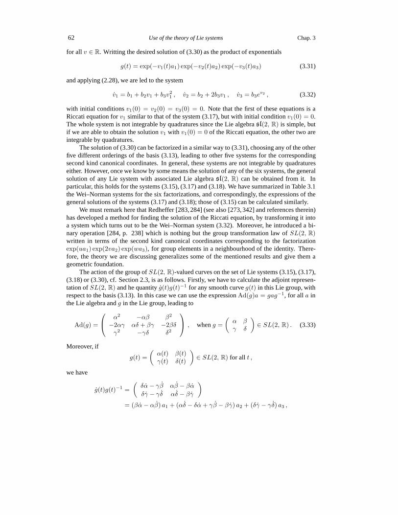
62 Use of the theory of Lie systems Chap. 3
for all v ∈ R. Writting the desired solution of (3.30) as the product of exponentials
g(t) = exp(−v1(t)a1) exp(−v2(t)a2) exp(−v3(t)a3) (3.31)
and applying (2.28), we are led to the system
v1 = b1 + b2v1 + b3v21 , v2 = b2 + 2b3v1 , v3 = b3e
v2 , (3.32)
with initial conditionsv1(0) = v2(0) = v3(0) = 0. Note that the first of these equations is aRiccati equation forv1 similar to that of the system (3.17), but with initial condition v1(0) = 0.The whole system is not integrable by quadratures since the Lie algebrasl(2, R) is simple, butif we are able to obtain the solutionv1 with v1(0) = 0 of the Riccati equation, the other two areintegrable by quadratures.
The solution of (3.30) can be factorized in a similar way to (3.31), choosing any of the otherfive different orderings of the basis (3.13), leading to other five systems for the correspondingsecond kind canonical coordinates. In general, these systems are not integrable by quadratureseither. However, once we know by some means the solution of any of the six systems, the generalsolution of any Lie system with associated Lie algebrasl(2, R) can be obtained from it. Inparticular, this holds for the systems (3.15), (3.17) and (3.18). We have summarized in Table 3.1the Wei–Norman systems for the six factorizations, and correspondingly, the expressions of thegeneral solutions of the systems (3.17) and (3.18); those of(3.15) can be calculated similarly.
We must remark here that Redheffer [283,284] (see also [273,342] and references therein)has developed a method for finding the solution of the Riccatiequation, by transforming it intoa system which turns out to be the Wei–Norman system (3.32). Moreover, he introduced a bi-nary operation [284, p. 238] which is nothing but the group transformation law ofSL(2, R)written in terms of the second kind canonical coordinates corresponding to the factorizationexp(ua1) exp(2va2) exp(wa3), for group elements in a neighbourhood of the identity. There-fore, the theory we are discussing generalizes some of the mentioned results and give them ageometric foundation.
The action of the group ofSL(2, R)-valued curves on the set of Lie systems (3.15), (3.17),(3.18) or (3.30), cf. Section 2.3, is as follows. Firstly, wehave to calculate the adjoint represen-tation ofSL(2, R) and he quantityg(t)g(t)−1 for any smooth curveg(t) in this Lie group, withrespect to the basis (3.13). In this case we can use the expressionAd(g)a = gag−1, for all a inthe Lie algebra andg in the Lie group, leading to
Ad(g) =
α2 −αβ β2
−2αγ αδ + βγ −2βδγ2 −γδ δ2
, wheng =
(α βγ δ
)∈ SL(2, R) . (3.33)
Moreover, if
g(t) =
(α(t) β(t)γ(t) δ(t)
)∈ SL(2, R) for all t ,
we have
g(t)g(t)−1 =
(δα− γβ αβ − βα
δγ − γδ αδ − βγ
)
= (βα− αβ) a1 + (αδ − δα+ γβ − βγ) a2 + (δγ − γδ) a3 ,

Sec. 3.2 Lie systems related toSL(2, R) 63
wherea1, a2, a3 is the basis ofsl(2, R) given by (3.13), and we have made use ofδα+αδ−γβ − βγ = 0, consequence ofαδ − βγ = 1. Therefore we can write, although with a slightabuse of notation,
g(t)g(t)−1 = −
αβ − βα
δα− αδ + βγ − γβ
γδ − δγ
.
By the theory of Sections 2.3 and 2.6 we have the following result.
Proposition 3.2.1. Let (y(t), z(t)), (y(t), z(t)), (y(t), z(t)), and g(t) be solutions,respectively, of the Lie systems(3.15), (3.17), (3.18)and(3.30), starting from(y0, z0), (y0, z0),(y0, z0) and the identity inSL(2, R). Let
g′(t) =
(α(t) β(t)γ(t) δ(t)
)
be a smooth curve inSL(2, R). Then, the new functionsΦi(g′(t), (y(t), z(t))), i = 1, 2, 3,andg′(t)g(t) are solutions, respectively, of Lie systems of type(3.15), (3.17), (3.18)and(3.30),starting fromΦi(g
′(0), (y0, z0)), i = 1, 2, 3, andg′(0), but with coefficient functions given by
b1b2b3
=
α2 −αβ β2
−2αγ αδ + βγ −2βδγ2 −γδ δ2
b1b2b3
+
αβ − βα
δα− αδ + βγ − γβ
γδ − δγ
.
Moreover, this transformation law for the coefficient functions defines an affine action of thegroup ofSL(2, R)-valued curves on Lie systems of type(3.15), (3.17), (3.18)and(3.30), respec-tively.
If we consider the particular case of Lie systems with associated Lie algebrasl(2, R), like(3.15), (3.17), (3.18) or (3.30), but with constant coefficientsb1, b2 andb3, and we transform themby using only constant matrices ofSL(2, R), the above affine action reduces, essentially, to theadjoint representation ofSL(2, R). Using the Killing–Cartan form onsl(2, R) we can establisha one-to-one correspondence of it with its dualsl(2, R)∗, and the action turns out to be thecoadjoint action. The orbits are then easily found: They aresymplectic manifolds characterizedby the values of the Casimir function corresponding to the natural Poisson structure defined onsl(2, R)∗, which in the basis taken readsb22 − 4b1b3. Thus, Lie systems with associated Liealgebrasl(2, R), for example of the types mentioned, and with constant coefficients, can beclassified according to the coadjoint orbits ofSL(2, R). A similar result holds for Lie systemswith associated semi-simple Lie algebras and with constantcoefficients.
We pay attention now to the question of applying the reduction method associated to sub-groups ofSL(2,R) in order to solve (3.30), cf. Section 2.5. To this end, we willtake Lie sub-groupsH of SL(2,R) determined by their Lie algebras, i.e., Lie subalgebras ofsl(2, R). Withrespect to the basis (3.13), we can easily distinguish some Lie subalgebras. Apart from the one-dimensional ones, generated by single elements ofsl(2, R), we see thata1, a2 anda2, a3generate Lie subalgebras isomorphic to the Lie algebra of the affine group in one dimension, see(3.14) and (3.2).

64
Use
ofth
eth
eory
ofL
iesyste
ms
Chap.3
Table 3.2. Some possibilities for solving (3.30) by the reduction method associated to a subgroup, cf. Section 2.5. We denoteG = SL(2, R), and takeLie subgroupsH whose Lie subalgebras of (3.14) are the ones selected. See explanation and remarks in text.
Lie subalgebra πL : G → G/H λ : G×G/H → G/H and fund. v.f. g1(t) and Lie system inG/H h(t) and Lie system inH
a2, a3 g 7→ β/δ (g, y) 7→ αy+βγ y+δ
(
1 y(t)0 1
) (
u(t) 0v(t) u−1(t)
)
XH1 = ∂y, XH
2 = y ∂y , y = b1 + b2 y + b3 y2, u = (b2/2 + b3 y)u, u(0) = 1
XH3 = y2 ∂y y(0) = 0 v = −(b2/2 + b3 y)v − b3 u, v(0) = 0
a1, a2 g 7→ α/γ (g, y) 7→ αy+βγ y+δ
(
1 0y−1(t) 1
) (
v−1(t) u(t)0 v(t)
)
XH1 = ∂y, XH
2 = y ∂y , y = b1 + b2 y + b3 y2, u = (b2/2 + b1/y)u + b1 v, u(0) = 0
XH3 = y2 ∂y y(0) = ∞ v = −(b2/2 + b1/y)v, v(0) = 1
a1 g 7→ (α, γ) (g, (y, z)) 7→ (α y + β z, γ y + δ z)
(
y(t) 0z(t) y−1(t)
) (
1 x(t)0 1
)
XH1 = z ∂y , XH
2 = (y ∂y − z ∂z)/2, y = b1 z + b2 y/2, y(0) = 1 x = b1/y2, x(0) = 0
XH3 = −y ∂y z = −b3 y − b2 z/2, z(0) = 0
a1 g 7→ (α/γ, 1/γ) (g, (y, z)) 7→(
α y+βγ y+δ
, zγ y+δ
)
(
y(t)z−1(t) 0z−1(t) z(t)y−1(t)
) (
1 x(t)0 1
)
XH1 = ∂y, XH
2 = y ∂y + z ∂z/2, y = b1 + b2 y + b3 y2, y(0) = ∞ x = b1z2/y2, x(0) = 0
XH3 = y2 ∂y + yz ∂z z = b2 z/2 + b3 yz, z(0) = ∞
a2 g 7→ (β/δ, γδ) (g, (y, z))
(
1 + y(t)z(t) y(t)z(t) 1
) (
x(t) 00 x−1(t)
)
7→(
α y+βγ y+δ
, (γ y + δ)(γ(1 + yz) + δz))
XH1 = ∂y, XH
2 = y ∂y − z ∂z , y = b1 + b2 y + b3 y2, y(0) = 0 x = (b2/2 + b3 y)x, x(0) = 1
XH3 = y2 ∂y − (2 yz + 1) ∂z z = −b2 z − b3(1 + 2 yz), z(0) = 0
whereg =(
α β
γ δ
)
∈ G and [XH1 , XH
2 ] = XH1 , [XH
1 , XH3 ] = XH
3 , [XH2 , XH
3 ] = 2XH2 in all cases

Sec. 3.2 Lie systems related toSL(2, R) 65
Consider for a start the 1-codimensional Lie subgroupH whose Lie subalgebra isa2, a3,that is,
H =
(u 0v u−1
) ∣∣∣∣ u 6= 0 , v ∈ R
, (3.34)
which is isomorphic to the affine group in one dimensionA1. Now, consider the open setU ofSL(2,R) given by
U =
(α βγ δ
)∈ SL(2, R)
∣∣∣∣ δ 6= 0
.
Then, any element inU can be factorized, in a unique way, as the product(α βγ δ
)=
(1 β/δ0 1
)(1/δ 0γ δ
),
where the second matrix factor belongs toH . Therefore, we can parametrize (locally) the homo-geneous spaceM = SL(2, R)/H by means of the coordinatey, defined in such a way that theprojection reads
πL : SL(2, R) −→ SL(2, R)/H(α βγ δ
)7−→ y = β/δ .
Then, the left action ofSL(2, R) onM is given by
λ : SL(2, R)×M −→M((α βγ δ
), y
)7−→ πL
((α βγ δ
)(1/δ′ + γ′y yδ′
γ′ δ′
))=αy + β
γy + δ,
whereγ′ andδ′ are real numbers parametrizing the lift ofy toSL(2, R). In this way we recover,essentially, one of the components of the action (3.26) previously considered as related with thesystem of equal and uncoupled Riccati equations (3.17). Needless to say, the subgroupH is theisotopy subgroup ofy = 0 with respect toλ andπL(H) = 0. The corresponding fundamentalvector fields can be calculated according to (2.2), and they are
XH1 =
∂
∂y, XH
2 = y∂
∂y, XH
3 = y2∂
∂y,
which satisfy[XH1 , X
H2 ] = XH
1 , [XH1 , X
H3 ] = XH
3 and[XH2 , X
H3 ] = 2XH
2 . If we factorizethe solution starting from the identity of (3.30) as the product
g1(t)h(t) =
(1 y(t)0 1
)(u(t) 0v(t) u−1(t)
),
whereg1(t) projects onto the solutionπL(g1(t)) = y(t), with y(0) = 0, of the Lie system onthe homogeneous spaceM , y = b1(t) + b2(t)y + b3(t)y
2, then we reduce the problem to a Liesystem in the subgroupH for h(t), with h(0) = id. The expression of this last system is givenby Theorem 2.5.1, i.e.,
h(t)h(t)−1 = −Ad(g−11 (t))(b1(t)a1 + b2(t)a2 + b3(t)a3)− g1(t)
−1g1(t) .

66 Use of the theory of Lie systems Chap. 3
Upon substitution, we finally obtain the system
u =
(b2(t)
2+ b3(t)y(t)
)u , u(0) = 1 ,
v = −(b2(t)
2+ b3(t)y(t)
)v − b3(t)u , v(0) = 0 , (3.35)
which is a Lie system forH ∼= A1. Since this group is solvable, the system can be integrated byquadratures.
Analogously, we can consider the reduction by other subgroups. For example, we haveconsidered as well the reduction by the subgroupH , isomorphic again toA1, whose Lie algebrais made up bya1, a2. The arising homogeneous spaceM = SL(2, R)/H can be identified asa neighbourhood of the point at infinity inR, the isotopy subgroup of the left action ofSL(2, R)onM beingH , andπL(H) = ∞, whereπL : SL(2, R) → M is the canonical projection.The results are similar and are summarized in the second row of Table 3.2. In the same tablewe have considered three other cases. The first two of them correspond to the reduction by thesubgroup generated bya1. The difference between them is that we choose different coordinatesfor the corresponding homogeneous space: If(y, z) are the coordinates ofSL(2, R)/H in thefirst case, and(y, z) are those of the second case, they are related byy = y/z and z = 1/z.The first parametrization yields the linear action (3.25) ofSL(2, R) on R2, with infinitesimalgenerators (3.21). These vector fields appear in [106] and [143, Table 1, I.5]. The second choiceof coordinates gives the fundamental vector fields shown in the fourth row of Table 3.2, whichare also those of Table 1, II.18,loc. cit. The last of the cases considered corresponds to thereduction by the subgroup generated bya2, with the simplest parametrization we can think offor the associated homogeneous space. The arising action and infinitesimal generators are shownin the last row of Table 3.2. The fourth and fifth cases of reduction considered yield other tworealizations of Lie systems with associated to the Lie algebrasl(2, R), namely
y = b1(t) + b2(t)y + b3(t)y2 , z =
1
2b2(t)z + b3(t)yz , (3.36)
andy = b1(t) + b2(t)y + b3(t)y
2 , z = −b2(t)z − b3(t)(1 + 2 yz) , (3.37)
which can be dealt with as well by the previous methods considered, i.e., the Wei–Normanmethod and reduction procedure. Likewise, the Proposition3.2.1 can be extended to cover thesesystems as well, taking into account the corresponding actions shown in Table 3.2. On the otherhand, note that the two systems (3.36) and (3.37) consist of aRiccati equation and a first orderdifferential equation, which becomes a linear differential equation once the Riccati equation issolved.
3.2.1 The reduction method for the Riccati equation
To end this section, let us show that the reduction method explains some of the results of Sec-tion 1.5, in relation to the reduction of Riccati equations to simpler ones when we know particularsolutions of the former.
Remember that according to the general theory, the solutionof the Riccati equation
y = b1(t) + b2(t)y + b3(t)y2 , (3.38)
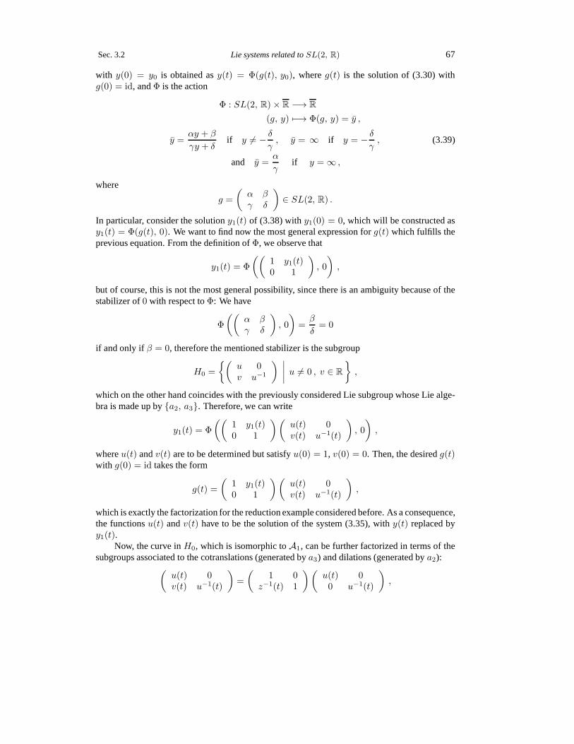
Sec. 3.2 Lie systems related toSL(2, R) 67
with y(0) = y0 is obtained asy(t) = Φ(g(t), y0), whereg(t) is the solution of (3.30) withg(0) = id, andΦ is the action
Φ : SL(2, R)× R −→ R
(g, y) 7−→ Φ(g, y) = y ,
y =αy + β
γy + δif y 6= − δ
γ, y = ∞ if y = − δ
γ, (3.39)
and y =α
γif y = ∞ ,
where
g =
(α βγ δ
)∈ SL(2, R) .
In particular, consider the solutiony1(t) of (3.38) withy1(0) = 0, which will be constructed asy1(t) = Φ(g(t), 0). We want to find now the most general expression forg(t) which fulfills theprevious equation. From the definition ofΦ, we observe that
y1(t) = Φ
((1 y1(t)0 1
), 0
),
but of course, this is not the most general possibility, since there is an ambiguity because of thestabilizer of0 with respect toΦ: We have
Φ
((α βγ δ
), 0
)=β
δ= 0
if and only if β = 0, therefore the mentioned stabilizer is the subgroup
H0 =
(u 0v u−1
) ∣∣∣∣ u 6= 0 , v ∈ R
,
which on the other hand coincides with the previously considered Lie subgroup whose Lie alge-bra is made up bya2, a3. Therefore, we can write
y1(t) = Φ
((1 y1(t)0 1
)(u(t) 0v(t) u−1(t)
), 0
),
whereu(t) andv(t) are to be determined but satisfyu(0) = 1, v(0) = 0. Then, the desiredg(t)with g(0) = id takes the form
g(t) =
(1 y1(t)0 1
)(u(t) 0v(t) u−1(t)
),
which is exactly the factorization for the reduction example considered before. As a consequence,the functionsu(t) andv(t) have to be the solution of the system (3.35), withy(t) replaced byy1(t).
Now, the curve inH0, which is isomorphic toA1, can be further factorized in terms of thesubgroups associated to the cotranslations (generated bya3) and dilations (generated bya2):
(u(t) 0v(t) u−1(t)
)=
(1 0
z−1(t) 1
)(u(t) 00 u−1(t)
),

68 Use of the theory of Lie systems Chap. 3
wherez(t) = u(t)/v(t) for all t. We have, using (3.35),
z =u
v− u
v2v =
(b22
+ b3y1
)u
v+
u
v2
(b22
+ b3y1
)v +
u
v2b3u
= (b2 + 2 b3y1)z + b3z2 ,
andz(0) = ∞. We can renameu(t) = w1/2(t) for all t, and thenw(t) satisfies
w = (b2 + 2 b3y1)w , w(0) = 1 .
In short, we have that the curve inSL(2, R), solution of (3.30), can be factorized as
g(t) =
(1 y1(t)0 1
)(1 0
z−1(t) 1
)(w1/2(t) 0
0 w−1/2(t)
),
wherey1(t), z(t), w(t) are, respectively, solutions of
y = b1(t) + b2(t)y + b3(t)y2 , y(0) = 0 , (3.40)
z = (b2(t) + 2 b3(t)y1(t))z + b3(t)z2 , z(0) = ∞ , (3.41)
w = (b2(t) + 2 b3(t)y1(t))w , w(0) = 1 . (3.42)
Then, going back to the solution of (3.38) withy(0) = y0, we can writey0 = Φ(g−1(t), y(t)),that is,
y0 = Φ
((w−1/2 0
0 w1/2
)(1 0
−z−1 1
)(1 −y10 1
), y
)
= Φ
((w−1/2 −w−1/2y1
−w1/2z−1 w1/2(z−1y1 + 1)
), y
)=
(y − y1)z
w(y1 − y + z). (3.43)
On the other hand, it is easy to check that the solutions of (3.41) and (3.42) we need can be con-structed from two other particular solutions of (3.38) in addition to y1(t), namely, the particularsolutionsy2(t), y3(t) with y2(0) = ∞ andy3(0) = 1. In fact, under these conditions,
z = Φ
((1 −y10 1
), y2
)= y2 − y1
is the desired solution of (3.41), and
w = Φ
((1 0
−z−1 1
), y3 − y1
)=
(y3 − y1)(y2 − y1)
y2 − y3
is the desired solution of (3.42). Substituting into (3.43), we have
y0 =(y − y1)(y2 − y1)
(y3−y1)(y2−y1)(y2−y3) (y1 − y + y2 − y1)
=(y − y1)(y2 − y3)
(y − y2)(y1 − y3). (3.44)
Since any set of independent initial conditions for three particular solutions of the Riccati equa-tion can be obtained from the set∞, 0, 1 by an element ofSL(2, R) underΦ (and theny0

Sec. 3.2 Lie systems related toSL(2, R) 69
may change as well), we recover the nonlinear superpositionprinciple for the Riccati equation,compare with (1.63).
Similar results can be obtained if we start from the particular solutiony1(t) of (3.38) withy1(0) = ∞. Then, the stability subgroup of∞ with respect toΦ is the subgroup
H∞ =
(v−1 u0 v
) ∣∣∣∣ v 6= 0 , u ∈ R
,
i.e., the Lie subgroup whose Lie algebra consists ofa1, a2, and therefore also isomorphic toA1. By the reduction method, see the second row of Table 3.2, we can arrive to the factorizationof the matrix curveg(t), solution of (3.30), as
g(t) =
(1 0
y−11 (t) 1
)(1 z(t)0 1
)(w1/2(t) 0
0 w−1/2(t)
),
wherey1(t), z(t), w(t) are now, respectively, solutions of
y = b1(t) + b2(t)y + b3(t)y2 , y(0) = ∞ , (3.45)
z =
(b2(t) + 2
b2(t)
y1(t)
)z + b1(t) , z(0) = 0 , (3.46)
w =
(b2(t) + 2
b2(t)
y1(t)
)w , w(0) = 1 . (3.47)
The solutions of these systems can be constructed as well from other solutions of the originalRiccati equation. If nowy2(t), y3(t) are the particular solutions of (3.38) withy2(0) = 0 andy3(0) = 1, then
z = Φ
((1 0
−y−11 1
), y2
)=
y2y1y1 − y2
solves (3.46), and
w = Φ
((1 −z0 1
),
y3y1y1 − y3
)=
y21(y3 − y2)
(y1 − y3)(y1 − y2)
solves (3.47). If we write againy0 = Φ(g−1(t), y(t)), we will obtain
y0 =y(y1 + z)− zy1w(y1 − y)
,
and upon substitution of the previous expressions,
y0 =(y − y2)(y1 − y3)
(y − y1)(y2 − y3),
which is exactly (3.44), taking into account thaty1 andy2 interchange their roles in both expres-sions.
We would like to remark that the two Lie subgroups we have worked with, which are iso-morphic toA1, are in addition conjugated each other:
(α−1 0−γ α
)=
(0 1−1 0
)(α γ0 α−1
)(0 −11 0
),

70 Use of the theory of Lie systems Chap. 3
therefore the two previous procedures transform into each other under such conjugation.We have seen, by means of the example of the Riccati equation,how the reduction method
can be used for obtaining the superposition formula of a Lie system on certain homogeneousspace. The knowledge of a particular solution reduce the problem to one in the isotopy subgroupof its initial condition with respect the relevant action. When not only one, but several particularsolutions of that Lie system are known, we reduce the problemto the subgroup made up by theintersection of the isotopy subgroups of all initial conditions. Taking the minimum number ofparticular solutions such that the intersection of the isotopy subgroups is just the identity, we canreconstruct the curve in the groupG in terms of these particular solutions, thus leading to thesuperposition formula, see also [13,14,60,335].
3.3 Lie systems related toSL(3, R)
We will consider in this section examples of Lie systems withassociated Lie algebrasl(3, R),the Lie algebra of the Lie groupSL(3, R) of real invertible matrices3 × 3 with determinantequal to one. As in the case ofsl(2, R), this Lie algebra is realized in a natural way by the setof real matrices3 × 3 with vanishing trace, and the Lie product is given again by the matrixcommutator. We recall that the groupSL(3,R) is the maximal symmetry group of the dynamicsof the free particle in the plane, see, e.g., [12,145]. The basis ofsl(3, R) we will work with is
a1 =
0 −1 00 0 00 0 0
, a2 =
1
2
−1 0 00 1 00 0 0
, a3 =
0 0 01 0 00 0 0
,
a4 =1
6
−1 0 00 −1 00 0 2
, a5 =
0 0 −10 0 00 0 0
, a6 =
0 0 00 0 −10 0 0
,
a7 =
0 0 00 0 01 0 0
, a8 =
0 0 00 0 00 1 0
, (3.48)
with the non-vanishing commutation rules
[a1, a2] = a1 , [a1, a3] = 2a2 , [a1, a6] = −a5 , [a1, a7] = a8 ,
[a2, a3] = a3 , [a2, a5] = −1
2a5 , [a2, a6] =
1
2a6 , [a2, a7] =
1
2a7 ,
[a2, a8] = −1
2a8 , [a3, a5] = a6 , [a3, a8] = −a7 , (3.49)
[a4, a5] = −1
2a5 , [a4, a6] = −1
2a6 , [a4, a7] =
1
2a7 , [a4, a8] =
1
2a8 ,
[a5, a7] = 3a4 + a2 , [a5, a8] = a1 , [a6, a7] = −a3 , [a6, a8] = 3a4 − a2 .
The first Lie system we will study has as solutions the integral curves of thet-dependentvector field
∑8i=1 bi(t)Xi, where the coefficient functionsbi(t), i = 1, . . . , 8 are (smooth)
arbitrary but fixed functions, andX1, . . . , X8 is a basis of vector fields in two real variables,with polynomial coefficients of at most second order, generating a Lie algebra isomorphic tosl(3, R). We would like to recover a Lie system of a previously studiedtype when restricting

Sec. 3.3 Lie systems related toSL(3, R) 71
ourselves, for example, to a subalgebrasl(2, R). Then, we choose for simplicity that the firstthree elementsX1,X2 andX3 of the previous basis be given by (3.21), and therefore, a basis ofvector fields with all the requirements is (see, e.g., [143,336] and references therein)
X1 = z∂
∂y, X2 =
y
2
∂
∂y− z
2
∂
∂z, X3 = −y ∂
∂z,
X4 =y
2
∂
∂y+z
2
∂
∂z, X5 =
∂
∂y, X6 =
∂
∂z, (3.50)
X7 = y2∂
∂y+ yz
∂
∂z, X8 = yz
∂
∂y+ z2
∂
∂z.
The non-vanishing commutation rules of these vector fields are analogous to those of (3.49),replacing theai’s by theXi’s, and the matrix commutator by the Lie bracket of vector fields.
Therefore, the system of interest is
y =1
2(b2(t) + b4(t))y + b1(t)z + b5(t) + b7(t)y
2 + b8(t)yz
z = − b3(t)y −1
2(b2(t)− b4(t))z + b6(t) + b7(t)yz + b8(t)z
2 , (3.51)
which can be written in matrix form as
dY
dt= T (t) +M(t)Y + Y Y TC(t) , (3.52)
where the superscriptT denotes matrix transpose,
M(t) =
(12 (b2(t) + b4(t)) b1(t)
−b3(t) 12 (b4(t)− b2(t))
),
and
Y =
(yz
), T (t) =
(b5(t)b6(t)
), C(t) =
(b7(t)b8(t)
).
The equation (3.52) is an example ofmatrix Riccatiequation, (see, e.g., [211,271,272,304,335]and references therein). Matrix Riccati equations play an important role in mathematical andphysical applications [287,335], as well as in control theory [41,217].
In particular, note that if we putT (t) = C(t) = 0 for all t, we obtain a linear homoge-neous system of differential equations, which is a linear Lie system with associated Lie algebragl(2, R), see [143, 336] for basis of vector fields generating that Liealgebra; if, further, we putb4(t) = 0 (and henceTrM(t) = 0) we recover the Lie system (3.16) forsl(2, R).
As it is well-known, the real projective spaceRPn−1 is the quotient ofRn \ 0 by theequivalence relation
y ∼ λy , ∀λ ∈ R \ 0,
wherey ∈ Rn \ 0. An atlas ofnonhomogeneous coordinatesfor RPn−1 is constructed asfollows. Take the atlas ofRn \ 0 given by then charts(Uk, id)nk=1, whereid is the identitymap and
Uk = (y1, . . . , yk, . . . , yn) ∈ Rn \ 0 | yk 6= 0 .

72 Use of the theory of Lie systems Chap. 3
Let fk be the maps defined by
fk : Uk −→ Rn−1
(y1, . . . , yk, . . . , yn) 7−→(y1yk, . . . ,
yk−1
yk,yk+1
yk, . . . ,
ynyk
),
for all k = 1, . . . , n. Let π : Rn \ 0 → RPn−1 be the natural projection, and letσk :π(Uk) → Uk be local sections ofπ, i.e., π σk = Idπ(Uk) for all k = 1, . . . , n. Then,(π(Uk), fk σk)nk=1 is an atlas of nonhomogeneous coordinates ofRPn−1.
By using (3.48) and (2.2), the eight vector fields (3.50) can be regarded as a basis of fun-damental vector fields with respect to the action of the groupSL(3, R) on the projective spaceRP 2 which reads, in a chart of nonhomogeneous coordinates(y, z) of RP 2, as [11,14]
Φ : SL(3, R)× RP 2 −→ RP 2
α β ǫγ δ ρν µ ω
, (y, z)
7−→
(αy + βz + ǫ
νy + µz + ω,γy + δz + ρ
νy + µz + ω
). (3.53)
Essentially, we have considered the analogous action of thegroup1 SL(2, R) onRP 1 = R
previously, see (1.19) and (3.39). The action (3.53) can be written in a more compact way usingthe matrix notation. If we denote
A =
(α βγ δ
), τ =
(ǫρ
), σ =
(νµ
),
then we have
Φ : SL(3, R)× RP 2 −→ RP 2
((A τσT ω
), Y
)7−→ AY + τ
σTY + ω. (3.54)
Now, inspired by what we have seen in Section 1.5 and specially, in Subsection 3.2.1, wewonder if certain changes of variable, based on the electionof subgroups ofSL(3, R) and bymeans of the action (3.54), can reduce the original Lie system (3.52) to simpler problems, pro-vided that some particular solutions of certain equations are known.
The scheme of reduction will be analogous to the first used in Subsection 3.2.1, that is, wewill consider first a particular solution of (3.52), construct a transformation by means of it, andthen the following reductions are made according to subgroups of the isotopy subgroup ofY = 0with respect to the actionΦ given above, which is made up by matrices of the form
(A 0σT ω
).
Thus, we start considering the Abelian subgroup generated by a5, a6. Take the newvariable
Y (1) = Φ
((id −Y10 1
), Y
)= Y − Y1 ,
1 Or PL(1, R) ∼= SL(2, R)/Z2 if we consider an effective action.

Sec. 3.3 Lie systems related toSL(3, R) 73
where
Y1 =
(y11y12
)(3.55)
will be determined by the requirement that the new equation of type (3.52) forY (1) should haveno independent term. The time derivative ofY (1) is
Y (1) = Y − Y1 = (M + Y T1 C + Y1CT )Y (1) + Y (1)Y (1)TC
+ T +MY1 + Y1YT1 C − Y1 ,
where it has been used (3.52) andY = Y (1)+Y1. Then,Y1 must be taken as a particular solutionof (3.52), and therefore, the new equation forY (1) is
Y (1) =M (1)Y (1) + Y (1)Y (1)TC , (3.56)
whereM (1) = M + Y T1 C + Y1CT . We transform nowY (1), using a suitably chosen curve on
the Abelian subgroup generated bya7, a8,
Y (2) = Φ
((id 0
−UT1 1
), Y (1)
)=
Y (1)
1− UT1 Y(1)
,
with inverse
Y (1) = Φ
((id 0UT1 1
), Y (2)
)=
Y (2)
1 + UT1 Y(2)
,
in order to reduce to an equation with no quadratic term. The time derivative ofY (2), using(3.56) and the previous expressions, reads, after some algebra,
Y (2) =M (1)Y (2) + Y (2)Y (2)T (C + U1 +M (1)TU1) .
Therefore,
U1 =
(u11u12
)(3.57)
has to be a particular solution of the equation
U1 = −C −M (1)TU1 , (3.58)
and then, the new equation forY (2) is
Y (2) =M (1)Y (2) . (3.59)
This equation can be further reduced to a linear Lie system oftype (3.16), by using a curve onthe subgroup generated bya4, that is,
Y (3) = Φ
((a−1/6 id 0
0 a1/3
), Y (2)
)= a−1/2Y (2) ,
with inverseY (2) = a1/2Y (3). Then, we have
Y (3) =
(M (1) − a
2aid
)Y (3) ,

74 Use of the theory of Lie systems Chap. 3
anda must be chosen such that the new matrix has zero trace, that is,
Tr
(M (1) − a
2aid
)= TrM (1) − a
a= 0 ,
hencea should be a particular solution of the linear homogeneous equationa = aTrM (1). Ifwe defineM (2) =M (1) − 1
2 TrM(1) id, the new equation forY (3) is
Y (3) =M (2)Y (3) , (3.60)
or more explicitly,
d
dt
(y(3)
z(3)
)=
(12 (b2 + b7y11 − b8y12) b1 + b8y11
−b3 + b7y12 − 12 (b2 + b7y11 − b8y12)
)(y(3)
z(3)
), (3.61)
which is a Lie system of type (3.51) or (3.52), with coefficient functions
b(2)1 = b1 + b8y11 , b
(2)2 = b2 + b7y11 − b8y12 , b
(2)3 = b3 − b7y12 ,
b(2)4 = · · · = b
(2)8 = 0 . (3.62)
Therefore, it can be regarded as well as a linear Lie system oftype (3.16), whose associated Liealgebra issl(2, R). The change of variable carrying the originalY into Y (3) can be obtainedeasily through the product of the three matrix transformations,
Y (3) = Φ
((a−1/6 id 0
0 a1/3
)(id 0
−UT1 1
)(id −Y10 1
), Y
)
= Φ
((a−1/6 id −a−1/6Y1−a1/3UT1 a1/3(1 + UT1 Y1)
), Y
)=
Y − Y1(1− UT1 (Y − Y1))a1/2
,
with inverse change
Y =(id+Y1U
T1 )Y (3) + Y1
(UT1 Y(3) + 1)a−1/2
.
We remark that these results can be generalized to the situation in which PL(n, R) ∼=SL(n+1, R)/Z2 acts onRPn by projective transformations, see [14]. However, we can formu-late an analogous property to Proposition 3.2.1 for all Lie systems with underlying Lie algebrasl(3, R), as a consequence of the general theory developed in Sections 2.3 and 2.6. If we takethe basis (3.48) of this Lie algebra, the expressions of the adjoint representation ofSL(3, R)and the curve in the Lie algebra− dg
dt g−1, whereg(t) is any (smooth) curve in that group, take
the form shown in Table 3.3. By using this property, the previous scheme of reduction, withthe same curves in the respective subgroups taken, is also useful for reducing other Lie systems,formulated in other homogeneous spaces ofSL(3, R).
Consider, for example, the linear action ofSL(3, R) onR3,
Φ2 : SL(3, R)× R3 −→ R
3
α β ǫγ δ ρν µ ω
,
y1y2y3
7−→
α β ǫγ δ ρν µ ω
y1y2y3
, (3.63)

Sec.3.3
Lie
system
sre
late
dtoSL(3,R)
75
Table 3.3.Matricial expressions of the adjoint representation ofSL(3, R) and− dgdtg−1 with respect to the basis (3.48) ofsl(3, R).
Ad(g) =
α(αω − ǫν) 12ǫ(αµ + βν)− αβω β(βω − ǫµ) 1
2ǫ(αµ − βν)
ν(γǫ + αρ)− 2αγω ω(αδ + βγ)− 12ǫ(γµ+ δν) − 1
2ρ(αµ + βν) µ(δǫ + βρ)− 2βδω 1
2ǫ(δν − γµ) + 1
2ρ(βν − αµ)
γ(γω − νρ) 12ρ(γµ + δν) − γδω δ(δω − µρ) 1
2ρ(γµ− δν)
3 ν(αρ − γǫ) 32ǫ(γµ+ δν) − 3
2ρ(αµ + βν) 3µ(βρ − δǫ) 1
2ǫ(δν − γµ) + 1
2ρ(αµ − βν) + ω(αδ − βγ)
α(γǫ − αρ) αβρ− 12ǫ(αδ + βγ) β(δǫ − βρ) 1
2ǫ(βγ − αδ)
γ(γǫ − αρ) 12ρ(αδ + βγ)− γδǫ δ(δǫ − βρ) 1
2ρ(βγ − αδ)
ν(γω − νρ) µνρ− 12ω(γµ + δν) µ(δω − µρ) 1
2ω(γµ − δν)
ν(ǫν − αω) 12ω(αµ + βν) − ǫµν µ(ǫµ− βω) 1
2ω(βν − αµ)
α(βν − αµ) β(βν − αµ) ǫ(βω − ǫµ) ǫ(ǫν − αω)
2αγµ− ν(βγ + αδ) µ(αδ + βγ)− 2βδν 2 ǫµρ− ω(δǫ + βρ) ω(αρ + γǫ)− 2 ǫνρ
γ(δν − γµ) δ(δν − γµ) ρ(δω − µρ) ρ(νρ− γω)
3 ν(βγ − αδ) 3 µ(βγ − αδ) 3ω(βρ − δǫ) 3ω(γǫ − αρ)
α(αδ − βγ) β(αδ − βγ) ǫ(δǫ− βρ) ǫ(αρ− γǫ)
γ(αδ − βγ) δ(αδ − βγ) ρ(δǫ − βρ) ρ(αρ − γǫ)
ν(δν − γµ) µ(δν − γµ) ω(δω − µρ) ω(νρ − γω)
ν(αµ− βν) µ(αµ − βν) ω(ǫµ − βω) ω(αω − ǫν)
− dgdt g
−1 =
(ǫµ− βω)α + (αω − ǫν)β + (βν − αµ)ǫ
2(βω − ǫµ)γ + 2(ǫν − αω)δ + 2(αµ − βν)ρ+ (αρ − γǫ)µ + (δǫ − βρ)ν + (βγ − αδ)ω
3((αρ − γǫ)µ + (δǫ − βρ)ν + (βγ − αδ)ω)
(βρ− δǫ)α+ (γǫ − αρ)β + (αδ − βγ)ǫ
(βρ− δǫ)γ + (γǫ − αρ)δ + (αδ − βγ)ρ
(γω − νρ)µ+ (µρ − δω)ν + (δν − γµ)ω
(ǫν − αω)µ + (βω − ǫµ)ν + (αµ − βν)ω
whereg =
α β ǫγ δ ρν µ ω
is a curve inSL(3, R)

76 Use of the theory of Lie systems Chap. 3
whose basis of infinitesimal generators, associated to the basis (3.48) ofsl(3, R), is made up bythe vector fields
X1 = y2∂
∂y1, X2 =
y12
∂
∂y1− y2
2
∂
∂y2, X3 = −y1
∂
∂y2,
X4 =y16
∂
∂y1+y26
∂
∂y2− y3
3
∂
∂y3, X5 = y3
∂
∂y1, X6 = y3
∂
∂y2, (3.64)
X7 = −y1∂
∂y3, X8 = −y2
∂
∂y3,
satisfying analogous commutation rules as those satisfied by the vector fields of (3.50). Thecorresponding Lie system, whose solutions are the integralcurves of thet-dependent vector field∑8
i=1 bi(t)Xi, can be written in matrix form as
d
dt
y1y2y3
=
16 (3b2(t) + b4(t)) b1(t) b5(t)
−b3(t) 16 (b4(t)− 3b2(t)) b6(t)
−b7(t) −b8(t) − 13b4(t)
y1y2y3
, (3.65)
where the functionsbi(t) are assumed to be the same as in (3.51).Take the same solutionsY1, U1 anda of the equations (3.52), (3.58) anda = aTrM (1), as
before. If we transform the variablesy1, y2, y3 by the linear change
y(3)1
y(3)2
y(3)3
=
a−1/6 0 0
0 a−1/6 00 0 a1/3
1 0 00 1 0
−u11 −u12 1
1 0 −y110 1 −y120 0 1
y1y2y3
=
a−1/6 0 −y11a−1/6
0 a−1/6 −y12a−1/6
−u11a1/3 −u12a1/3 (1 + y11u11 + y12u12)a1/3
y1y2y3
=
(y1 − y11y3)a−1/6
(y2 − y12y3)a−1/6
(1 + y11u11 + y12u12)y3 − u11y1 − u12y2a1/3
, (3.66)
then, we transform the original equation (3.65) into another one of the same type for the newvariablesy(3)1 , y
(3)2 , y
(3)3 , but with new coefficients given by (3.62), that is,
d
dt
y(3)1
y(3)2
y(3)3
=
12 (b2 + b7y11 − b8y12) b1 + b8y11 0
−b3 + b7y12 − 12 (b2 + b7y11 − b8y12) 0
0 0 0
y(3)1
y(3)2
y(3)3
.
This kind of Lie system can be regarded as that obtained by thelinear action onSL(2, R) on
planesy(3)3 = Const., wherey(3)1 , y(3)2 , y
(3)3 are coordinates inR3. Then, the previous system
is the analogous to (3.60) for the type of Lie systems (3.65),with the same scheme of reduction.Incidentally, note that the upper left2 × 2 block of the previous matrix coincides withM (2) of(3.60), see also (3.61).

Sec. 3.4 An example of Lie system from physics 77
The inverse change to (3.66) is just
y1y2y3
=
(1 + y11u11)a1/6 y11u12a
1/6 y11a−1/3
y12u11a1/6 (1 + y12u12)a
1/6 y12a−1/3
u11a1/6 u12a
1/6 a−1/3
y(3)1
y(3)2
y(3)3
=
(1 + y11u11)y(3)1 + y11u12y
(3)2 a1/6 + y11y
(3)3 a−1/3
y12u11y(3)1 + (1 + y12u12)y(3)2 a1/6 + y12y
(3)3 a−1/3
(u11y(3)1 + u12y
(3)2 )a1/6 + y
(3)3 a−1/3
. (3.67)
To end this section, we remark that it is also possible to follow other reduction schemes ofLie systems with Lie algebrasl(3, R), see [71] for another example.
3.4 An example of Lie system from physics
We present now an example of how a system of first order differential equations arising in prac-tical situations or physical problems can be identified as a Lie system. After that we can, or atleast try to, apply all the machinery at our disposal for thisclass of systems, in order to obtaintheir solutions or other information of interest, like the geometric structure of the system.
The system which interest us now, appears mainly in two problems of the mathematicalphysics, which in turn are closely related [176, 241]. The first is what is currently known asthe factorization method, which is a powerful method for computing eigenvalues and recurrencerelations for solutions of second order ordinary differential equations, like the Schrodinger equa-tions appearing in one-dimensional quantum mechanics. Thesecond is the representation theoryof certain Lie groups and of their associated Lie algebras and their relation with the theory ofspecial function theory, a problem to which the second of theprevious references is devoted.
The first of these problems will be treated with detail later in this Thesis, namely in Chap-ter 4, so let us summarize briefly where the system of interestenters into the second. Essentially,the problem is, following the notation of [241, p. 45], to represent a four dimensional Lie algebra,with basisJ+, J−, J3 , E and defining relations
[J3, J±] = ±J± , [J±, E] = [J3, E] = 0 , (3.68)
and2
[J+, J−] = 2 bE − 2 aJ3 , (3.69)
wherea andb are real constants, in terms of first order differential operators in two real variables.Miller proposes the representation [241]
J+ = ey(∂
∂x− k(x)
∂
∂y+ j(x)
), J3 =
∂
∂y,
J− = e−y(− ∂
∂x− k(x)
∂
∂y+ j(x)
), E = 1 , (3.70)
2 To be more precise, in [241] it is taken[J+, J−] = 2a2J3 − bE, but everything can be generalized to the case weconsider: Instead of taking only one sign fora in (3.69), we consider all of its possible real values. This generalizationis also discussed in Chapter 4, in relation with the factorization method.

78 Use of the theory of Lie systems Chap. 3
wherex andy are real variables and the functionsj(x) andk(x) are to be determined. Takingthe commutator of differential operators, it is easy to check that (3.70) satisfy (3.68), for allj(x)andk(x). However, we obtain
[J+, J−] = 2(j′ + jk)E − 2(k′ + k2)J3 ,
and therefore, comparing with (3.69), it follows thatj(x), k(x) have to be solutions of the system
k′ + k2 = a , j′ + jk = b .
In Chapter 4 we will see how a similar system arises from the development of the theory of thefactorization method, and related questions as the theory of shape invariance in one-dimensionalquantum mechanics.
Therefore, we will treat in this section the system of first order differential equations in thevariablesy andz
y′ + y2 = a , z′ + yz = b , (3.71)
where we denote the independent variable byx, a andb are real constants and the prime denotesderivative with respect tox. The first equation is a Riccati equation with constant coefficients,meanwhile the second is an inhomogeneous linear first order differential equation forz, once thesolution fory is known.
Since both equations are, separately, instances of Lie systems, we would like to identify thewhole system, if possible, as a Lie system as well. For doing this note that the solutions of thesystem are the integral curves of the vector field−y2∂y − yz∂z + a∂y + b∂z. Sincea andb cantake any real value, the two vector fields∂y and∂z should be two elements of the basis of vectorfields, closing on a finite dimensional Lie algebra, which we are trying to identify. Of course wehave[∂y, ∂z] = 0. We can try to find the minimal Lie algebra generated by∂y, ∂z and the term−y2∂y − yz∂z.
Then, denoting (the reason for the notation chosen will be clear afterwards)
X1 =∂
∂y, Y1 =
∂
∂z, X3 = y2
∂
∂y+ yz
∂
∂z,
and taking the Lie brackets
X2 =1
2[X1, X3] = y
∂
∂y+z
2
∂
∂z, Y2 = −[X3, Y1] = y
∂
∂z,
we see that the vector fieldsX1, X2, X3, Y1, Y2 close on the Lie algebra with non-vanishingcommutation relations
[X1, X2] = X1 , [X1, X3] = 2X2 , [X1, Y2] = Y1 , [X2, X3] = X3 ,
[X2, Y1] = −1
2Y1 , [X2, Y2] =
1
2Y2 , [X3, Y1] = −Y2 .
This Lie algebra is the member withn = 1 of the family of Lie algebras with Abelian ideals ofdimensionn+ 1, made up by the vector fields [335, (2.14)]:
X1 =∂
∂y, X2 = y
∂
∂y+n
2z∂
∂z, X3 = y2
∂
∂y+ n yz
∂
∂z,
Y1 =∂
∂z, Y2 = y
∂
∂z, . . . , Yn+1 = yn
∂
∂z, (3.72)

Sec. 3.4 An example of Lie system from physics 79
where the operatorsYi, i = 1, . . . , n + 1 form an Abelian ideal andn ∈ N. For eachn, theprevious vector fields provide a realization of the Lie algebraRn+1⋊sl(2, R) in terms of vectorfields in two real variables [143, Table 1.II.27], so our system of interest is a Lie system withassociated Lie algebraR2 ⋊ sl(2, R). Moreover, comparing with (3.50), it is not difficult to seethat the vector fieldsX1, X2, X3, Y1, Y2 close on a Lie subalgebra ofsl(3, R).
Then, the most general Lie system we can construct with our current Lie algebra is thosewhose solutions are the integral curves of the vector field
∑3i=1 bi(x)Xi + b4(x)Y1 + b5(x)Y2,
i.e.,
dy
dx= b1(x) + b2(x)y + b3(x)y
2 ,
dz
dx= b4(x) + b5(x)y +
1
2b2(x)z + b3(x)yz . (3.73)
The system of equations (3.71) is of this type, with constantcoefficient functionsb1(x) = a,b2(x) = 0, b3(x) = −1, b4(x) = b andb5(x) = 0, for all x.
Now, so as to find the (general) solution of the system (3.71),it is easier to solve first theRiccati equation and then the linear equation. Recall that the general solution of the inhomoge-neous linear first order differential equation forv(x)
dv
dx= a(x)v + b(x) , (3.74)
can be obtained by means of the formula
v(x) =
∫ xb(ξ) exp
−∫ ξa(η) dη
dξ + E
exp−∫ x
a(ξ) dξ , (3.75)
whereE is an integration constant. Then, the general solution of the second equation of (3.71)is easily obtained once we know the general solution of the first, i.e.,
z(x) =b∫ x
exp∫ ξ
y(η) dηdξ +D
exp∫ x
y(ξ) dξ , (3.76)
where we name the integration constant asD. So, let us first pay attention to the task of solvingthe constant coefficients Riccati equation of (3.71) in its full generality.
The general equation of this type is
dy
dx= a2y
2 + a1y + a0 , (3.77)
wherea2, a1 anda0 are now real constants,a2 6= 0. This equation, unlike the general Riccatiequation, is always integrable by quadratures, and the formof the solutions depends strongly onthe sign of the discriminant∆ = a21 − 4a0a2. This can be seen by separating the differentialequation (3.77) in the form
dy
a2y2 + a1y + a0=
dy
a2
((y + a1
2 a2
)2− ∆
4 a22
) = dx .

80 Use of the theory of Lie systems Chap. 3
After one quadrature, we obtain in this way non-constant solutions of (3.77).Looking for constant solutions of (3.77) amounts to solve analgebraic second order equa-
tion. So, if∆ > 0 there will be two different real constant solutions. If∆ = 0 there is only oneconstant real solution and if∆ < 0 we have no constant real solutions at all.
Table 3.4.General solutions of the systemy′+y2 = a, z′+yz = b. A,B andD are integration constants.The constantB selects the particular solution of the Riccati equation in each case.
Sign ofa y(x) z(x)
a = c2 > 0 c B sinh(c(x−A))−cosh(c(x−A))B cosh(c(x−A))−sinh(c(x−A))
bcB sinh(c(x−A))−cosh(c(x−A))+D
B cosh(c(x−A))−sinh(c(x−A))
a = 0 B1+B(x−A)
b(B2(x−A)2+x−A)+D
1+B(x−A)
a = −c2 < 0 −cB sin(c(x−A))+cos(c(x−A))B cos(c(x−A))−sin(c(x−A))
bcB sin(c(x−A))+cos(c(x−A))+D
B cos(c(x−A))−sin(c(x−A))
The value of the discriminant∆ for the Riccati equation of (3.71) is just4a. If a > 0 wecan writea = c2, wherec > 0 is a real number. The non-constant particular solution
y1(x) = c tanh(c(x −A)) , (3.78)
whereA is an arbitrary integration constant, is readily found by direct integration. In addition,there exist two different constant real solutions,
y2(x) = c , y3(x) = −c . (3.79)
Then, we can find out the general solution from these particular solutions using the non-linearsuperposition formula
y =y2(y3 − y1) k + y1(y2 − y3)
(y3 − y1) k + y2 − y3, (3.80)
which yields
y(x) = cB sinh(c(x−A)) − cosh(c(x−A))
B cosh(c(x −A))− sinh(c(x−A)), (3.81)
whereB = (2−k)/k, k being the arbitrary constant in (3.80). Substituting into (3.76) we obtainthe general solution forz(x),
z(x) =bcB sinh(c(x−A)) − cosh(c(x−A)) +D
B cosh(c(x−A))− sinh(c(x −A)), (3.82)
whereD is a new integration constant.Let us study now the case witha = 0. By direct integration we find the particular solution
y1(x) =1
x−A, (3.83)

Sec. 3.4 An example of Lie system from physics 81
whereA is an integration constant. It is clear that our Riccati equation admits now the identicallyvanishing solution, and the general solution has to reflect this fact. To find it, is particularlysimple the application of the change of variable
u =y y1y1 − y
, with inverse y =u y1u+ y1
, (3.84)
with y1 given by (3.83), which transforms the Riccati equation of (3.71) witha = 0 intodu/dx =0, which has the general solutionu(x) = B, B constant. Then, the desired general solution forthe casea = 0 is
y(x) =B
1 +B(x −A), (3.85)
withA andB being arbitrary integration constants. IfB = 0 we recover the identically vanishingsolution as expected. Substituting in (3.76) we obtain the general solution forz(x) in this case,
z(x) =b(B2 (x−A)2 + x−A) +D
1 +B(x−A), (3.86)
whereD is a new integration constant.The last case to be studied isa < 0. We write thena = −c2, wherec > 0 is a real number.
It is easy to find the non-constant particular solution
y1(x) = −c tan(c(x −A)) , (3.87)
whereA is an arbitrary integration constant, by direct integration. In order to find out the generalsolution, we make again the change of variable (3.84), withy1(x) given by (3.87). After somecalculations we obtain the general solution for the casea > 0,
y(x) = −c B sin(c(x −A)) + cos(c(x −A))
B cos(c(x −A))− sin(c(x −A)), (3.88)
whereB = cF , F an arbitrary constant. Substituting into (3.76) we obtain the correspondinggeneral solution forz(x),
z(x) =bcB sin(c(x−A)) + cos(c(x−A)) +D
B cos(c(x−A))− sin(c(x −A)), (3.89)
whereD is a new integration constant.These solutions can be written in many mathematically equivalent ways. We have tried
to give their simplest form and in such a way that the symmetrybetween the solutions for thecasesa > 0 anda < 0 were clearly recognized. Indeed, the former can be transformed into thelatter by means of the formal changesc → ic, B → iB and the identitiessinh(ix) = i sin(x),cosh(ix) = cos(x). The results are summarized in Table 3.4.


PART 2
LIE SYSTEMS IN PHYSICS


Chapter 4
Intertwined Hamiltonians, factorization methodand shape invariance
This chapter opens our treatment of the applications of Lie systems to problems from physics.The physical problems in which Lie systems appear are very numerous (see, e.g., [69, 260, 335]and references therein) and to try to deal with all of them is out of the scope of this Thesis.
Instead, we will study several problems from physics in which there is a Lie system in-volved, but either this fact is not recognized, or it is recognized but the associated properties areneither (completely) explored nor exploited. We will see that an appropriate use of the mathe-matical properties of Lie systems, having always in mind their associated geometric structure,developed in the preceding chapters, may be very useful in order to obtain a deep insight into theproblems treated.
Thus, we will study two types of problems in this and the next two chapters. The thirdone is devoted to the study of Lie systems which at the same time can be regarded as well asHamiltonian systems, both in the classical and the quantum frameworks. This and the next oneare devoted to problems in one-dimensional quantum mechanics in which the Riccati equationplays a key role in the relevant aspects of the corresponding theory.
These problems receive different names in the literature, and are closely related amongstthemselves, as intertwined operators, factorization method, supersymmetric (SUSY) quantummechanics, shape invariance, Darboux transformations, etc.
More explicitly, the factorization method was introduced by Schrodinger [295–297] andothers (see [176, p. 23]) and later developed by Infeld and Hull [168, 175, 176], and has beenshown to be very efficient in the search of exactly solvable potentials in quantum mechan-ics. It is closely related with the existence of intertwining operators [73, 124, 127, 128, 238],supersymmetric quantum mechanics [51, 53, 54, 93, 140, 263,337] and Darboux transforma-tions in this last context [24, 25, 104, 236]. Moreover, these techniques have important gen-eralizations: There exists extensions of these theories tohigher-dimensional spaces [15–17],to n-dimensional oriented Riemannian manifolds [142], using higher-order factorization oper-ators [18–20, 22, 24, 25, 125, 126, 130, 239, 289], and to the class of systems with partial al-gebraization of the spectrum [135, 136, 181, 301, 302, 323],amongst others. Actually, mostexactly solvable potentials can be obtained by making use ofan appropriate intertwining op-erator transformation, and other related problems can alsobe approached with similar tech-niques [131,134,137,180,298,326]
85

86 Intertwined Hamiltonians, factorization method and shapeinvariance Chap. 4
The theory of exactly solvable quantum mechanical potentials in one dimension was re-lated with SUSY quantum mechanics by Gendenshteın [139], who introduced the concept of adiscrete reparametrization invariance, usually called “shape invariance.” In particular, shape in-variant problems have been shown to be exactly solvable, andit was observed that a number ofknown exactly solvable potentials can be regarded as belonging to such a class. Moreover, shapeinvariance can be identified exactly with (a slight generalization of) the factorization method, aswe will show below. This relation has been pointed out also in[248,311].
We will treat the following aspects along this chapter. Firstly, we define the concept ofintertwined Hamiltonians in quantum mechanics and derive its first consequences. We establishthe relation between this concept, the problem of factorization of Hamiltonians and Darbouxtransformations through an application of the classical Lie theory of infinitesimal symmetries ofdifferential equations, when applied to time-independentSchrodinger equations. Then, we definethe concepts concerning shape invariance and the classicalfactorization method. We show thatthe former problem is essentially equivalent to a slight generalization of the latter, where we justinclude the necessary parameters.
After that, we review the classical factorization method, that is, shape invariant problemswith one parameter subject to translation and, thanks to theproperties of the Riccati equation, wefind the general solutions rather than the particular solutions which had been obtained before, andwe are able to classify the solutions so obtained according to a criterion based on the geometryof the problem.
Then, following similar techniques, we study the analogousproblem of shape invariantproblems with a finite number of parameters subject to translation, and we are able to find newfamilies of potentials of this type, therefore solving one of the open questions of the theory ofshape invariance.
We will analyze as well the important aspect of the proper definition of the partnershipof potentials in these problems. With respect to this question some properties of the Riccatiequation are essential. The same question is treated for thespecial subclass of shape invariantproblems: The interesting result is, roughly speaking, that shape invariance is incompatible withtaking different partners of a given potential.
Finally, we study the possibility of obtaining new factorizations of given problems whenthere exists an additional invariance of one potential under a parameter transformation. This canexplain the existence of certain alternative factorizations which appear in practice.
In the next chapter we will explain, using the affine action onthe set of Riccati equationsintroduced in Chapters 1 and 3, how the problem of intertwined Hamiltonians can be explainedfrom a group theoretical point of view, and how a generalization of the classical Darboux trans-formations can be easily obtained within this framework.
4.1 Hamiltonians related by first-order differential operators.
The simplest way of generating an exactly solvable Hamiltonian H from a known oneH isjust to consider an invertible bounded operatorB, with bounded inverse, and definingH =BHB−1. This transformed HamiltonianH has the same spectrum as the starting oneH . As ageneralization (see, e.g., [73]), we will say that two HamiltoniansH andH are intertwined orA-related whenAH = HA, whereAmay have no inverse. In this case, ifψ is an eigenvector ofH corresponding to the eigenvalueE andAψ 6= 0, at least formallyAψ is also an eigenvectorof H corresponding to the same eigenvalueE.

Sec. 4.2 Intertwined Hamiltonians 87
If A is a first order differential operator,
A =d
dx+W (x) , and A† = − d
dx+W (x) , (4.1)
then the relationAH = HA, with
H = − d2
dx2+ V (x) , H = − d2
dx2+ V (x) , (4.2)
leads toV = −2W ′ + V , W (V − V ) = −W ′′ − V ′ .
Taking into account the first equation, the second becomes2WW ′ =W ′′+V ′, which can easilybe integrated giving
V =W 2 −W ′ + ǫ , (4.3)
and then,V =W 2 +W ′ + ǫ , (4.4)
whereǫ is an integration constant. The important point here is thatH andH , given by (4.2),are related by a first order differential operatorA, given by (4.1), if and only if there exist aconstantǫ and a functionW such that the pair of Riccati equations (4.3) and (4.4) are satisfiedsimultaneously. Moreover, this means that both Hamiltonians can be factorized as
H = A†A+ ǫ , H = AA† + ǫ . (4.5)
Adding and subtracting equations (4.3) and (4.4) we obtain the equivalent pair which relatesV andV
V − ǫ = − (V − ǫ) + 2W 2 , (4.6)
V = V + 2W ′ . (4.7)
The functionW satisfying these equations is usually called thesuperpotential, the constantǫ isthe factorization energyor factorization constantandV andV (resp. H andH) are said to bepartnerpotentials (resp. Hamiltonians).
Notice that the initial solvable Hamiltonian can indistinctly be chosen asH or H . In bothcases the point will be to find a solutionW of the corresponding Riccati equation (4.3) or (4.4)for a specific factorization energyǫ. From this solution the expression for the (possibly) newpotential follows immediately from (4.7).
Note that these equations have an intimate relation with what it is currently known asDar-boux transformationsof linear second-order differential equations [104, 174],or in the contextof one-dimensional (or supersymmetric) quantum mechanics[236, pp. 7, 24]. In fact, it is easyto prove that the equation (4.3) can be transformed into a Schrodinger equation−φ′′ + (V (x)−ǫ)φ = 0 by means of the change−φ′/φ =W , and by means ofφ′/φ =W , (4.4) transforms into−φ′′ + (V (x) − ǫ)φ = 0. The relation betweenV andV is given by (4.7). Obviously,φφ = 1,up to a non-vanishing constant factor. It is also worth noting that these Schrodinger equationsexpress thatφ andφ are respective eigenfunctions of the Hamiltonians (4.2) for the eigenvalueǫ. These facts can be related in turn with the classical theoryof infinitesimal symmetries of dif-ferential equations; because of the interest of understanding better these relations, we devote thenext section to a further analysis of these aspects.

88 Intertwined Hamiltonians, factorization method and shapeinvariance Chap. 4
4.2 Dilation symmetry and reduction of a linear second-orderdifferential equation
In this section we recall briefly a well-known method of relating a homogeneous linear second-order differential equation to a Riccati equation, which can be regarded as an application of theclassical Lie theory of infinitesimal symmetries of differential equations. Its importance willbecome clear when applying the method to time-independent Schrodinger equations, and it willallow us to understand better the relations between the concept of intertwined Hamiltonians,Darboux transformations and factorization of Hamiltonians.
The homogeneous linear second-order differential equation
d2z
dx2+ b(x)
dz
dx+ c(x)z = 0 , (4.8)
admits as an infinitesimal symmetry the vector fieldX = z ∂/∂z generating dilations (see e.g.[72]) in the variablez, which is defined forz 6= 0. According to the Lie theory of infinitesimalsymmetries of differential equations, we should change thecoordinatez to a new one,u = ϕ(z),such that the vector fieldX = z ∂/∂z becomes a translation generatorX = ∂/∂u in the newvariable. This change is determined by the equationXu = 1, which leads tou = log |z|, i.e.,|z| = eu. In both cases of regions withz > 0 or z < 0 we have
dz
dx= z
du
dx, and
d2z
dx2= z
(du
dx
)2
+ zd2u
dx2,
so the equation (4.8) becomes
d2u
dx2+ b(x)
du
dx+
(du
dx
)2
+ c(x) = 0 .
As the unknown functionu does not appear in the preceding equation but just its derivative, wecan lower the order by introducing the new variablew = du/dx. We arrive to the followingRiccati equation forw
dw
dx= −w2 − b(x)w − c(x) . (4.9)
Notice that fromdz/dx = z du/dx and the definition ofw we have
w =1
z
dz
dx. (4.10)
The second order differential equation (4.8) is equivalentto the set of (4.9) and (4.10), becausegiven a functionw satisfying (4.9), the functionz defined (up to a factor) by (4.10), i.e.,z(x) =exp
(∫ xw(ζ) dζ
), satisfies (4.8). We could have followed a similar pattern straightening out
the vector field in the opposite sense, that is, by imposingXu = −1. This would have lead tou = − log |z|, or |z| = e−u. Now, in either case ofz > 0 or z < 0 we havedz/dx = −z du/dxandd2z/dx2 = z (du/dx)2 − z d2u/dx2, so we finally obtain the Riccati equation
dw
dx= w2 − b(x)w + c(x) , (4.11)

Sec. 4.2 Dilation symmetry and reduction of a linear second-order differential equation 89
where now
w =du
dx= −1
z
dz
dx. (4.12)
We will distinguish in what follows between these two alternatives of reduction of (4.8) bymeans of a subscript+ or − in the corresponding functions, respectively. We remark that bothare definedlocally, that is, in open intervals wherez has a constant sign.
Let us apply these ideas to the particular case of the one-dimensional time-independentSchrodinger equation
−d2φ
dx2+ (V (x) − ǫ)φ = 0 , (4.13)
whereV (x) is the potential andǫ is some specific energy eigenvalue. As explained before, wecan reduce (4.13) either to the pair
W ′+ = −W 2
+ + (V (x)− ǫ) , W+ =1
φ
dφ
dx, (4.14)
or, alternatively, to the pair
W ′− =W 2
− − (V (x)− ǫ) , W− = − 1
φ
dφ
dx. (4.15)
The Riccati equations appearing in these pairs resemble those appearing in Section 4.1, namelyequations (4.3) and (4.4), but in the systems (4.14) and (4.15) the unknown functionsW+ andW− are related byW+ = −W−, while in both (4.3) and (4.4) the unknownW is the samefunction.
However, the previous remark will be useful in the interpretation of equations (4.3) and(4.4). We can rewrite them as
W ′ =W 2 − (V (x)− ǫ) , (4.16)
W ′ = −W 2 + (V (x)− ǫ) . (4.17)
Then, we can regard equation (4.16) (resp. equation (4.17))as coming from a Schrodinger-typeequation like (4.13) (resp. like− d2φ/dx2 + (V (x) − ǫ)φ = 0) by means of, respectively, thechanges
W = − 1
φ
dφ
dx, or W =
1
φ
dφ
dx, (4.18)
so the two “eigenfunctions”φ andφ of the mentioned Schrodinger-type equations are related byφφ = Const. Of course, the changes (4.18) are locally defined, i.e., in common open intervals ofthe domains ofφ andφ determined by two consecutive zeros ofφ or φ, or maybe by a zero anda boundary of the domain of the problem. Note that there is no reason why they should providefunctionsφ, φ, defined in the same way in the entire domain ofW , but in general they will bedefined interval-wise. Moreover, if we choose the functionW of the two operatorsA andA†
defined in (4.1) as given by (4.18), it holdsAφ = 0 andA†φ = 0.We have seen that the Riccati equations (4.16) and (4.17) correspond, by means of the
changes (4.18), to two Schrodinger-type equations which in turn are equivalent to
Hφ = ǫ φ , Hφ = ǫ φ , (4.19)

90 Intertwined Hamiltonians, factorization method and shapeinvariance Chap. 4
whereH andH are given by (4.2). Then, it is equivalent to say thatH andH areA-related,with associated constantǫ, to say that the functionsφ and φ, which satisfyφφ = Const., arethe respective eigenfunctions with eigenvalueǫ of the HamiltoniansH andH. Each of thesefacts imply that both Hamiltonians can be factorized as in (4.5). If, in addition, we remember therelation (4.7) betweenV andV , we see the relation between the fact that two Hamiltonians areintertwinned with the existence of a Darboux transformation amongst them and their factoriza-tion. We finally insist again on the fact that these factorizations make sense only locally, i.e., incommon open intervals whereφ andφ are defined.
A special case where all becomes globally defined arises whenφ or φ is the ground statewave-function of its respective Hamiltonian, having then no zeros in the entire domain of theproblem. On the other hand, forǫ below the ground state energy ofH (resp.H) it is sometimespossible to find a non-normalizable eigenfunctionφ (resp. φ) of H (resp. H) without zeros,leading to physically interesting potentials [127,128].
4.3 Shape invariance and its equivalence with the factorization method
In this section, we define the concept of shape invariance of apair of partner potentials. Then,after considering a slight generalization of the factorization method, as appeared in [168, 175,176], we will show that both approaches are equivalent.
The idea ofshape invariancehas been introduced by Gendenshteın in [139], see also [140].He proved that the complete spectrum of quantum Hamiltoniants having this property can befound easily. Gendenshteın took equations (4.3) and (4.4)as a definition of the functionsV , Vin terms of the functionW and some constantǫ. After, he assumed thatW did depend on certainset of parametersa, i.e.,W = W (x, a), and as a consequenceV = V (x, a) andV = V (x, a)
as well. Then, the necessary condition forV (x, a) to be essentially of the same form asV (x, a),maybe for a different choice of the values of the parameters involved inV , is known as shapeinvariance. It amounts to assume the further relation betweenV (x, a) andV (x, a)
V (x, a) = V (x, f(a)) +R(f(a)) , (4.20)
wheref is an (invertible) transformation on the parameter spacea andR is some function.Let us remark that it is the choice of the parameter spacea and of the (invertible) transfor-
mationsf(a) what define the different types of shape invariant potentials. Note that in principle,different types of shape invariant potentials may have members in common. We will considersimple but important classes of shape invariant potentialsin Sections 4.4 and 4.5. Note as wellthat the functionf may be even the identity, i.e.,f(a) = a for all a [18].
Just writing thea-dependence the equations (4.3), (4.4) become
V (x, a) − ǫ =W 2 −W ′ , (4.21)
V (x, a) − ǫ =W 2 +W ′ . (4.22)
The simplest way of satisfying these equations is assuming thatV (x, a) andV (x, a) are obtainedfrom a superpotential functionW (x, a) by means of
V (x, a)− ǫ =W 2(x, a) −W ′(x, a) , (4.23)
V (x, a)− ǫ =W 2(x, a) +W ′(x, a) . (4.24)

Sec. 4.3 Shape invariance and factorization method 91
The shape invariance property requires the further condition (4.20) to be satisfied, which in theseterms reads
W 2(x, a)−W 2(x, f(a)) +W ′(x, f(a)) +W ′(x, a) = R(f(a)) . (4.25)
In practice, when searching shape invariant potentials with a given parameter spacea and thetransformation functionf , what it is done is to (try to) find solutions forW (x, a) andR(a)of (4.25), instead of solving the pair (4.23), (4.24) and then imposing (4.20). Apart from thepractical advantages of this procedure, we will see in Section 4.6 that there is a fundamentalreason for doing it.
We turn our attention now to the exposition of a slightly generalized version of the factoriza-tion method appeared in the celebrated paper [176, pp. 24–27], see also [168,175]. This methoddeals with the problem of factorizing the linear second-order ordinary differential equation
d2y
dx2+ r(x, a)y + λy = 0 , (4.26)
where the symbola denotes a parameter space as in the shape invariant problems, i.e., a set ofn independent real parametersa = (a1, . . . , an). Let us consider a transformation on suchparameter spacef(a) = (f1(a), . . . , fn(a)). We will denote byfk, wherek is a positiveinteger, the composition off with itself k times. For a negative integerk we will consider thecomposition off−1 with itself k times andf0 will be the identity. The admissible values of theparameters will bef l(a), wherel is an integer restricted to some subset to be precised later.Thenumberλ is, in principle, the eigenvalue to be determined.
In a way similar to that of [176], we will say that (4.26) can befactorized if it can be replacedby each of the two following equations:
Hf−1(a)+ H
f−1(a)− y(λ, a) = [λ− L(f−1(a))]y(λ, a) , (4.27)
Ha−H
a+y(λ, a) = [λ− L(a)]y(λ, a) , (4.28)
where
Ha+ =
d
dx+ k(x, a) , Ha
− = − d
dx+ k(x, a) . (4.29)
Here,k(x, a) is a function to be determined which depends on the set of parametersa, andL(a)is a real number for each value of then-tuplea. The fundamental idea of this generalization isexpressed in the following theorem:
Theorem 4.3.1. Let us suppose that our differential equation(4.26)can be factorized inthe previously defined sense. Ify(λ, a) is one of its solutions, then
y(λ, f−1(a)) = Hf−1(a)− y(λ, a) , (4.30)
y(λ, f(a)) = Ha+y(λ, a) , (4.31)
are also solutions corresponding to the sameλ but to different values of the parametern-tuplea, as it is suggested by the notations.

92 Intertwined Hamiltonians, factorization method and shapeinvariance Chap. 4
Proof. Multiplying (4.27) byHf−1(a)− and (4.28) byHa
+ we have
Hf−1(a)− H
f−1(a)+ H
f−1(a)− y(λ, a) = [λ− L(f−1(a))]H
f−1(a)− y(λ, a) ,
Ha+H
a−H
a+y(λ, a) = [λ− L(a)]Ha
+y(λ, a) .
Comparison of these equations with (4.27) and (4.28) shows thaty(λ, f−1(a)), defined by (4.30),is a solution of (4.26) witha replaced byf−1(a). Similarlyy(λ, f(a)), given by (4.31), is a solu-
tion with a replaced byf(a).
It is to be remarked that (4.30) or (4.31) may give rise to the zero function; actually, wewill see that this is necessary at some stage in order to obtain a sequence of square-integrablewave-functions.
Indeed we are only interested here in square-integrable solutionsy(λ, a). As we are dealingwith one-dimensional problems, these solutions can be taken as real functions. Under this domainthe following Theorem holds:
Theorem 4.3.2. The linear operatorsHa+ andHa
− are formally mutually adjoint. Thatis, if φψ vanishes at the ends of the intervalI,
∫
I
φ(Ha−ψ) dx =
∫
I
ψ(Ha+φ) dx . (4.32)
Proof. It is proved directly:∫
I
φ(Ha−ψ) dx = −
∫
I
φdψ
dxdx+
∫
I
φk(x, a)ψ dx
=
∫
I
ψdφ
dxdx+
∫
I
φk(x, a)ψ dx =
∫
I
ψ(Ha+φ) dx ,
where we have integrated the first term by parts and used thatψφ|∂I = 0.
Moreover, it is important to know when (4.30) and (4.31) produce new square-integrablefunctions.
Theorem 4.3.3. Lety(λ, a) be a non-vanishing, square-integrable solution of(4.27)and(4.28). The solutiony(λ, f−1(a)), defined by(4.30), is square-integrable if and only ifλ ≥L(f−1(a)). Similarly, the solutiony(λ, f(a)), defined by(4.31), is square-integrable if and onlyif λ ≥ L(a).
Proof. It is sufficient to compute∫
I
y(λ, f−1(a))2 dx =
∫
I
Hf−1(a)− y(λ, a)H
f−1(a)− y(λ, a) dx
=
∫
I
y(λ, a)(Hf−1(a)+ H
f−1(a)− y(λ, a)) dx = (λ− L(f−1(a)))
∫
I
y(λ, a)2 dx ,

Sec. 4.3 Shape invariance and factorization method 93
where Theorem 4.3.2 and (4.27) have been used. In a similar way,∫
I
y(λ, f(a))2 dx =
∫
I
Ha+y(λ, a)H
a+y(λ, a) dx
=
∫
I
y(λ, a)(Ha−H
a+y(λ, a)) dx = (λ− L(a))
∫
I
y(λ, a)2 dx ,
where use has been made of Theorem 4.3.2 and (4.28).
We will consider now the sequenceL(fk(a)) and analyze only the cases where it is eitheran increasing or a decreasing sequence. A more complicated behavior ofL(fk(a)) with respectto k (e.g., oscillatory) will not be treated here.
Theorem 4.3.4. Suppose thatL(fk(a)) is a decreasing sequence with no accumulationpoints. Then the necessary and sufficient condition for having square-integrable solutions of theequations(4.27)and(4.28)is that there exists a point of the parameter space,b = (b1, . . . , bn),such that
λ = L(b) , Hb−y(λ, f(b)) = 0 , (4.33)
provided that the functiony(L(b), f(b)) so obtained is square-integrable.
Proof. Let y(λ, a) be a non-vanishing, square-integrable solution of (4.27) and (4.28). Inorder to avoid a contradiction it is necessary, by Theorem 4.3.3, thatλ ≥ L(f−1(a)). If theequality does not hold, one can iterate the process to obtain
∫
I
y(λ, f−2(a))2 dx = (λ − L(f−2(a)))(λ− L(f−1(a)))
∫
I
y(λ, a)2 dx .
SinceL(fk(a)) is decreasing withk, we have that the differenceλ − L(f−2(a)) is positiveor vanishing and smaller thanλ − L(f−1(a)). If it still does not vanish, the process can becontinued until we arrive to a valuek0 such thatλ = L(f−k0(a)). It is then necessary that
y(λ, f−k0(a)) = Hf−k0 (a)− y(λ, f−k0+1(a)) = 0. It suffices to setb = f−k0(a) to obtain the re-
sult.
Theorem 4.3.5. If L(fk(a)) is an increasing sequence with no accumulation points, thenthe necessary and sufficient condition for having square-integrable solutions of the equations(4.27)and (4.28) is that there exists a specific point of the parameter space,b = (b1, . . . , bn),such that
λ = L(b) , Hb+y(λ, b) = 0 , (4.34)
provided that the functiony(L(b), b) so obtained is square-integrable.
Proof. Let y(λ, a) be a non-vanishing, square-integrable solution of (4.27) and (4.28). Inorder to avoid a contradiction it is necessary by Theorem 4.3.3 thatλ ≥ L(a). If the equalitydoes not hold, one can iterate the process to obtain
∫
I
y(λ, f2(a))2 dx = (λ− L(f(a)))(λ− L(a))
∫
I
y(λ, a)2 dx .

94 Intertwined Hamiltonians, factorization method and shapeinvariance Chap. 4
SinceL(fk(a)) is an increasing sequence,λ−L(f(a)) is positive or vanishing and smaller thanλ − L(a). If it still does not vanish, the process can be continued until we arrive tok0 such that
λ = L(fk0−1(a)). Then, it is necessary thaty(λ, fk0(a)) = Hfk0−1(a)+ y(λ, fk0−1(a)) = 0. It
suffices to setb = fk0−1(a).
WhenL(fk(a)) is a decreasing (resp. increasing) sequence, the functionsy defined byHb
−y(L(b), f(b)) = 0 (resp.Hb+y(L(b), b) = 0), provided that they are square-integrable, will
be those from where all the others will be constructed.We consider now what relation amongstr(x, a), k(x, a) andL(a) exists. Carrying out
explicitly the calculations involved in (4.27) and (4.28),and using (4.26), we find the equations
k2(x, f−1(a)) +dk(x, f−1(a))
dx= −r(x, a) − L(f−1(a)) , (4.35)
k2(x, a) − dk(x, a)
dx= −r(x, a) − L(a) . (4.36)
Eliminatingr(x, a) between these equations, we obtain
k2(x, f−1(a))− k2(x, a) +dk(x, f−1(a))
dx+dk(x, a)
dx= L(a)− L(f−1(a)) . (4.37)
Moreover, since (4.35) and (4.36) hold for eachfk(a), k in the range of integers correspondingto square-integrable solutions, we can rewrite them as
k2(x, a) +dk(x, a)
dx= − r(x, f(a)) − L(a) , (4.38)
k2(x, a)− dk(x, a)
dx= − r(x, a) − L(a) , (4.39)
and from them we can obtain the equivalent pair
r(x, a) + r(x, f(a)) + 2 k2(x, a) + 2L(a) = 0 , (4.40)
r(x, a) − r(x, f(a)) − 2dk(x, a)
dx= 0 . (4.41)
Both of the equations (4.35) and (4.36) are necessary conditions to be satisfied byk(x, a) andL(a), for a givenr(x, a). They are also sufficient since anyk(x, a) andL(a) satisfying theseequations lead unambiguously to a functionr(x, a) and so to a problem whose factorization isknown. It should be noted, however, that there exists the possibility that equations (4.35) and(4.36) did not have in general a unique solution fork(x, a) andL(a) for a givenr(x, a).
The equation (4.37) is what one uses in practice in order to obtain results by means of thefactorization method. We try to solve (4.37) instead of (4.35) and (4.36) since it is easier to findproblems which are factorizable by construction than seeing whether certain problem defined bysomer(x, a) is factorizable or not.
Conversely, a solutionk(x, a) of (4.37) gives rise to unique expressions for the differences−r(x, f(a))−L(a) and−r(x, a)−L(a) by means of equations (4.38) and (4.39), but it does notdetermine the quantitiesr(x, a) andL(a) in a unique way. In fact, the method does not determinethe functionL(a) unambiguously but only the differenceL(f(a)) − L(a). ThusL(a) is always

Sec. 4.3 Shape invariance and factorization method 95
defined up to a constant, and more ambiguity could arise in some situations, as it happens inthe case which we will study in Section 4.5. However, for the purposes of the application ofthis method to quantum mechanics the interesting quantity is L(f(a)) − L(a), as we will seebelow. The same way is underdeterminedr(x, a), with an ambiguity which cancels out exactlywith that ofL(a) since the differences−r(x, f(a))−L(a) and−r(x, a)−L(a) are completelydetermined from a given solutionk(x, a) of (4.37).
Going back to the problem of finding shape invariant which depend on the same set ofparametersa, we recall that the equations to be satisfied are (4.23) and (4.24), or the equivalentequations
V (x, a) − ǫ = − (V (x, a)− ǫ) + 2W 2(x, a) , (4.42)
V (x, a) = V (x, a) + 2W ′(x, a) , (4.43)
as well as the shape invariance condition (4.20).Remember that the potentialsV (x, a) andV (x, a) define a pair of Hamiltonians
H(a) = − d2
dx2+ V (x, a) , H(a) = − d2
dx2+ V (x, a) , (4.44)
which can be factorized as
H(a) = A(a)†A(a) + ǫ , H(a) = A(a)A(a)† + ǫ , (4.45)
whereǫ is a real number and
A(a) =d
dx+W (x, a) , A†(a) = − d
dx+W (x, a) . (4.46)
The shape invariance condition reads in terms of these Hamiltonians
H(a) = H(f(a)) +R(f(a)) . (4.47)
We establish next the identifications between the functionsand constants used in the gener-alized factorization method treated in this section and those used in the theory of shape invari-ance. We will see that the equations to be satisfied are exactly the same, and that both problemsessentially coincide when we consider square-integrable solutions. For that purpose is sufficientto identify
V (x, a)− ǫ = − r(x, f(a)) − L(a) , (4.48)
V (x, a)− ǫ = − r(x, a) − L(a) , (4.49)
W (x, a) = k(x, a) , (4.50)
R(f(a)) = L(f(a))− L(a) , (4.51)
and as an immediate consequence,
A(a) = Ha+ , A†(a) = Ha
− , (4.52)
for all allowed values ofa. Indeed, with these identifications it is immediate to see that equations(4.38) and (4.39) are equivalent to (4.24) and (4.23), respectively. Moreover
V (x, a)− V (x, f(a)) = − r(x, f(a)) − L(a) + r(x, f(a)) + L(f(a))
= L(f(a))− L(a) = R(f(a)) ,

96 Intertwined Hamiltonians, factorization method and shapeinvariance Chap. 4
which is nothing but equation (4.20); equations (4.40), (4.41) become
− (V (x, a)− ǫ)− L(a)− (V (x, a)− ǫ)− L(a) + 2W 2(x, a) + 2L(a)
= −(V (x, a)− ǫ)− (V (x, a)− ǫ) + 2W 2(x, a) = 0 ,
and
− (V (x, a) − ǫ)− L(a) + (V (x, a)− ǫ) + L(a)− 2W ′(x, a)
= −V (x, a) + V (x, a) − 2W ′(x, a) = 0 ,
i.e., equations (4.42) and (4.43), respectively.But the identification also applies to the respective eigenfunctions: Let us assume that The-
orem 4.3.4 is applicable. We shall see what it means in terms of the Hamiltonians (4.45). Tobegin with, we have a certain point of the parameter spaceb = (b1, . . . , bn) such thatλ = L(b)andA†(b)y(L(b), f(b)) = 0, where the functiony(L(b), f(b)) so defined is square-integrable.We will omit its first argument for brevity, writingy(f(b)). It is given by the expression
y(f(b)) = N exp
(∫ x
W (ξ, b) dξ
), (4.53)
whereN is a normalization constant. Note that this wave-function has no nodes. SinceL(fk(a))is a decreasing sequence, we have that the functionR(fk(b)) = L(fk(b)) − L(fk−1(b)) < 0for all of the acceptable values ofk.
Then, it is easy to check thaty(f(b)) is the ground state of the HamiltonianH(b), withenergyǫ. In fact,
H(b)y(f(b)) = (A(b)A(b)† + ǫ)y(f(b)) = ǫ y(f(b)) .
From equation (4.47) we haveH(b) = H(f−1(b))−R(b). The functiony(b) is the ground stateof H(b) with energyǫ−R(b):
H(b)y(b) = H(f−1(b))y(b)−R(b)y(b) = (ǫ −R(b))y(b) .
Now, the first excited state ofH(b) isA(b)y(b):
H(b)A(b)y(b) = A(b)H(b)y(b) = (ǫ −R(b))A(b)y(b) ,
where the propertyH(b)A(b) = A(b)H(b) has been used. In a similar way, it can be proved thatA(f−1(b))y(f−1(b)) is the first excited state ofH(b), with energyǫ−R(b)−R(f−1(b)). Onecan iterate the procedure in order to solve completely the eigenvalue problem of the HamiltoniansH(b) andH(b). The results are summarized in Table 4.1. Note thatǫ has the meaning of thereference energy chosen for the Hamiltonians, and is usually taken as zero.
A similar pattern can be followed when it is applicable the Theorem 4.3.5, that is, whenL(fk(a)) is an increasing sequence. The results are essentially the same as when the sequence isdecreasing but where now the Hamiltonian with a lower groundstate energy isH(b). The basicsquare-integrable eigenfunctiony(b) is defined now byA(b)y(b) = 0, that is,
y(b) =M exp
(−∫ x
W (ξ, b) dξ
), (4.54)

Sec. 4.3 Shape invariance and factorization method 97
Table 4.1. Eigenfunctions and eigenvalues ofH(b) andH(b) when Theorem 4.3.4 is applicable. Thefunctiony(f(b)) is defined by the relationA†(b)y(f(b)) = 0.
Eigenfunctions and energies H(b) H(b)
Ground state y(f(b)) y(b)
ǫ ǫ− R(b)
kth excited state A(b) · · ·A(f−k+1(b))y(f−k+1(b)) A(f−1(b)) · · ·A(f−k(b))y(f−k(b))
ǫ−∑k−1
r=0 R(f−r(b)) ǫ−∑k
r=0 R(f−r(b))
whereM is the normalization constant. Moreover, nowR(fk(b)) > 0 for all of the acceptablevalues ofk. The results are summarized in Table 4.2. Again,ǫ sets the energy reference level ofthe Hamiltonians.
In both cases the spectra of both Hamiltonians are exactly the same (with correspondingeigenfunctions shifted in one step) except for the ground state of one of them, which has thelowest possible energy. Only one of the eigenfunctions, either (4.53) or (4.54) may be square-integrable. It might happen, however, that neither of thesefunctions were square-integrable. Insuch a situation none of the schemes we have developed would be of use. The conditions on thefunctionW (x, b) such that one of the possible ground states exist are explained, e.g., in [140].Essentially it depends on the asymptotic behavior of
∫ xW (ξ, b) dξ asx→ ±∞.
Table 4.2. Eigenfunctions and eigenvalues ofH(b) and H(b) when is applicable Theorem 4.3.5. Thefunctiony(b) is defined by the relationA(b)y(b) = 0.
Eigenfunctions and energies H(b) H(b)
Ground state y(b) y(f(b))
ǫ ǫ+R(f(b))
kth excited state A†(b) · · ·A†(fk−1(b))y(fk(b)) A†(f(b)) · · ·A†(fk(b))y(fk+1(b))
ǫ+∑k
r=1 R(fr(b)) ǫ+∑k+1
r=1 R(fr(b))
In view of all of these identifications the following result is stated
Theorem 4.3.6. The problem of finding the square-integrable solutions of the factoriza-tion of(4.26), given by equations(4.27)and(4.28), is the same as to solve the discrete eigenvalueproblem of the shape invariant Hamiltonians(4.45)which depend on the same set of parameters.

98 Intertwined Hamiltonians, factorization method and shapeinvariance Chap. 4
We would like to remark that the equivalence between the factorization method and shapeinvariance has been first pointed out before, see, e.g., [248] and [310, 311]. However, we havenot seen so far a complete and clear identification in the general case where arbitrary set ofparametersa and transformation lawsf(a) are involved. This clarification is important becausethen we can identify factorizable and shape invariant problems in more general situations thanthose usually treated. An important example of this will be treated in Section 4.5, where we willfind shape invariant potentials where an arbitrary but finitenumber of parameters is subject totranslation.
In the next section, instead, we will analyze the case of onlyone parameter subject to trans-lation, i.e., the case originally studied by Infeld and Hull.
4.4 The Infeld–Hull factorization method revisited: Shapeinvariant po-tentials depending on one parameter transformed by translation
In this section we will consider the simplest but particularly important case of shape invariantpotentials having only one parameter whose transformationlaw is a translation. In other words,this case corresponds to the whole family of factorizable problems treated in [176], see also[168, 175]. Although we will follow their approach closely,at some stage we will see that theproperties of the Riccati equation will allow us to generalize their solutions, and classify themaccording to a geometric criterion.
Thus, we will consider problems where the parameter space isunidimensional, and thetransformation law is
f(a) = a− ǫ , or f(a) = a+ ǫ , (4.55)
whereǫ 6= 0. In both cases we can normalize the parameter in units ofǫ, introducing the newparameter
m =a
ǫ, or m = −a
ǫ, (4.56)
respectively. In each of these two possibilities the transformation law reads, with a slight abuseof the notationf ,
f(m) = m− 1 . (4.57)
Then, the relation amongst the relevant functions and constants between the two approaches,shape invariance and factorization method, becomes in thiscase
V (x,m)− ǫ = − r(x,m − 1)− L(m) , (4.58)
V (x,m)− ǫ = − r(x,m) − L(m) , (4.59)
W (x,m) = k(x,m) . (4.60)
R(m− 1) = L(m− 1)− L(m) , (4.61)
and the equations which should be solved in order to find potentials in this class are
V (x,m)− ǫ =W 2(x,m)−W ′(x,m) , (4.62)
V (x,m)− ǫ =W 2(x,m) +W ′(x,m) , (4.63)
or the equivalent equations
V (x,m)− ǫ = − (V (x,m) − ǫ) + 2W 2(x,m) , (4.64)
V (x,m) = V (x,m) + 2W ′(x,m) , (4.65)

Sec. 4.4 Factorization method revisited 99
as well as the shape invariance condition
V (x,m) = V (x,m− 1) +R(m− 1) . (4.66)
According to what we have said in Section 4.3, we will try to find solutions forW (x,m) =k(x,m) of this last equation, when written in the form
k2(x,m+ 1)− k2(x,m) +dk(x,m+ 1)
dx+dk(x,m)
dx= L(m)− L(m+ 1) , (4.67)
which is obtained from (4.66) after shiftingm in one unit, and using (4.60), (4.61), (4.62) and(4.63). The equation (4.67) is a differential-difference equation. The task of solving it in its fullgenerality seems to be very difficult, at least at first sight.Instead, it seems to be more appropriateto try to solve it with particular forms of the dependence ofk(x,m) onx andm. Then, we willfind out whether (4.67) is satisfied in each particular case.
First of all (see [176]), note that there exists a trivial solution of (4.67), namely
k(x,m) = f(m) , L(m) = −f2(m) ,
wheref(m) is any function ofm. This gives rise to the problem
d2y
dx2+ λy = 0 ,
which has been discussed by Schrodinger [296].We next try a solution with an affine dependence onm [176]
k(x,m) = k0(x) +mk1(x) , (4.68)
wherek0 andk1 are functions ofx only. Substituting into (4.67) and simplifying we obtain theequation
L(m)− L(m+ 1) = 2m(k21 + k′1) + k21 + k′1 + 2(k0k1 + k′0) . (4.69)
SinceL(m) is a function ofm alone, the coefficients of the powers ofm on the right hand sidemust be constant. Then, the equations to be satisfied are
k21 + k′1 = a , (4.70)
k1k0 + k′0 = b , (4.71)
wherea andb are, in principle, real arbitrary constants. When these equations are satisfied, (4.69)becomes
L(m)− L(m+ 1) = 2(ma+ b) + a .
Let us now look for the most general polynomialL(m) which solves this equation. It should beof degree two inm if a 6= 0 (degree one ifa = 0); otherwise we would find that the coefficients ofpowers greater or equal to three (resp. two) have to vanish. Then we putL(m) = rm2+ sm+ t,wherer, s, t are constants to be determined. Substituting into the previous equation we find therelations
r = −a, s = −2 b,

100 Intertwined Hamiltonians, factorization method and shapeinvariance Chap. 4
and as a result we have thatL(m) = −am2 − 2bm+ t , (4.72)
wheret is an arbitrary real constant. This expression is even validin the casea = 0, being thenL(m) = −2bm+ t.
In [176, Eqs. (3.1.5)] equations (4.70), (4.71) are writtenin the slightly more restricted way(we use Greek characters for the constants in order to avoid confusion)
k21 + k′1 = − α2 , (4.73)
k1k0 + k′0 = β , (4.74)
whereβ = −γα2 if α 6= 0. This means to consider only negative or zero values ofa in (4.70).Accordingly, the solutions of (4.70) fora > 0 are absent in [176, eqs. (3.1.7)]. But thesesolutions have their own physical importance, and they are somehow recovered in [176, pp. 27,30, 36, 46] after having made the formal changeα → −iα, when treating particular cases oftheir general factorization types(A), (B) and(E).
However, the important point from the point of view of Lie systems, is that even whendealing with their slightly restricted differential equation system (4.73) and (4.74), in [176] arenot considered the general solutions but particular ones: Only two particular solutions of theRiccati equation with constant coefficients (4.73) whenα 6= 0, and another two whenα = 0, areconsidered.
At this point, we would like to treat three main aspects. In the first place, we will studythe system of differential equations made up by (4.70) and (4.71) for all real values ofa andb. For each case of interest, we will find the general solution of the system by first consideringthe general solution of the Riccati equation (4.70). Secondly, we will prove that the solutionsincluded in [176] are particular cases of that general solutions. In addition, we will see that thereis no need of making formal complex changes of parameters forobtaining some of the relevantphysical solutions, since they already appear in the general ones. And thirdly, we will see thatrather than having four general basic types of factorizableproblems(A), (B), (C) and (D),where(B), (C) and(D) could be considered as limiting forms of(A) [176, p. 28], there existthree general basic types of factorizable problems which include the previously mentioned onesas particular cases, and they are classified by the simple distinction of what sign takesa in (4.70).The distinction by the sign ofa has a deep geometrical meaning: As we have seen in Section 3.2,see the paragraph after Proposition 3.2.1, Lie systems withassociated Lie algebrasl(2, R) (likethe Riccati equation) with constant coefficients, can be classified according to the coadjoint orbitsof SL(2, R), that is, by the values of the associated discriminant, which in the case of (4.70) is4a. It is well-known that the coadjoint orbits ofSL(2, R) are of three types (apart from theisolated zero orbit), distinguished by the sign of the Casimir. This kind of analysis could beuseful for a better understanding of other works based on thefactorization method as exposedin [176], like, e.g., [169–172].
Therefore, let us find the general solutions of (4.70) and (4.71). They are just the sameas that of the differential equation system (3.71), simply identifyingy(x) ask1(x) andz(x) ask0(x), with the same notation for the constants. The results are shown in Table 4.3. In the sametable we show how these solutions reduce to the ones contained in [176]: For the casea < 0,takingB → 0 we recover the factorization type(A) [176, eq. (3.1.7a)]. And takingB → i,with a slight generalization of the valuesB can take, we obtain their type(B) (see eq.(3.1.7b)).For practical cases of physical interest, they use these factorization types after making the formal

Sec. 4.4 Factorization method revisited 101
Table 4.3. General solutions of the equations (4.70) and (4.71), and some limiting cases.A andB areintegration constants. The constantB selects the particular solution of (4.70) in each case.D is not definedalways in the same way, but always represents an arbitrary constant.
Sign ofa k1(x) and limits k0(x) and limits Comments
a = c2 > 0 cB sinh(c(x−A))−cosh(c(x−A))B cosh(c(x−A))−sinh(c(x−A))
bcB sinh(c(x−A))−cosh(c(x−A))+D
B cosh(c(x−A))−sinh(c(x−A))
B→∞−−−−→ c tanh(c(x− A))
B→∞−−−−→ b
ctanh(c(x− A)) + D
cosh(c(x−A))See (3.78)
B→0−−−−→ c coth(c(x−A))
B→0−−−−→ b
ccoth(c(x− A)) + D
sinh(c(x−A))See text
B→∓1−−−−−→ ±c
B→∓1−−−−−→ ± b
c+D exp(∓c(x− A)) See (3.79)
a = 0 B1+B(x−A)
b(B2(x−A)2+x−A)+D
1+B(x−A)
B→∞−−−−→ 1
x−A
B→∞−−−−→ b
2(x− A) + D
x−AType(C)
B→0−−−−→ 0
B→0−−−−→ b(x− A) +D Type(D)
a = −c2 < 0 −cB sin(c(x−A))+cos(c(x−A))B cos(c(x−A))−sin(c(x−A))
bcB sin(c(x−A))+cos(c(x−A))+D
B cos(c(x−A))−sin(c(x−A))
B→∞−−−−→ −c tan(c(x−A))
B→∞−−−−→ b
ctan(c(x− A)) + D
cos(c(x−A))See (3.87)
B→0−−−−→ c cot(c(x−A))
B→0−−−−→ − b
ccot(c(x−A)) + D
sin(c(x−A))Type(A)
B→±i−−−−−→ ±ic
B→±i−−−−−→ ∓i b
c+D exp(∓ic(x− A)) Type(B)
changeα → −iα [176, pp. 27, 30, 36, 46]. The same results would be obtained if one considersthe limiting casesB → 0 orB → 1, respectively, whena > 0, so there is no need of making suchformal changes. For the casea = 0, takingB → ∞ or B → 0 we recover their factorizationtypes(C) and(D) (see their equations(3.1.7c) and(3.1.7d)), respectively. We show as wellsome limiting cases ofB which give us the particular solutions used in the construction of thegeneral ones.
We analyze now the generalization of (4.68) to higher powersof m. If we try
k(x,m) = k0(x) +mk1(x) +m2 k2(x) , (4.75)
substituting it into (4.67) we obtain
L(m)− L(m+ 1) = 4m3k22 + 2m2(3k1k2 + 3k22 + k′2)
+ 2m(k21 + 3k1k2 + 2k22 + 2k0k2 + k′1 + k′2) + . . . ,

102 Intertwined Hamiltonians, factorization method and shapeinvariance Chap. 4
where the dots stand for terms not involvingm. Since the coefficients of powers ofm mustbe constant, from the term inm3 we havek2 = Const. From the other terms, ifk2 6= 0 weobtain that both ofk1 andk0 have to be constant as well. That is, a case of the trivial solutionk(x,m) = f(m). The same procedure can be used to show that further generalizations to higherpowers ofm give no new solutions [176].
Table 4.4. New solutions of equations (4.70), (4.71) and (4.77).A is an arbitrary constant.B selects theparticular solution of (4.70) for each sign ofa.
Sign ofa k1(x) and limiting cases k0(x) k−1(x) Comments
a = c2 > 0 cB sinh(c(x−A))−cosh(c(x−A))B cosh(c(x−A))−sinh(c(x−A))
0 q ∈ R
B→0−−−−→ c coth(c(x− A)) 0 q ∈ R See text
a = 0 B1+B(x−A)
0 q ∈ R
B→∞−−−−→ 1
x−A0 q ∈ R Type(F )
a = −c2 < 0 −c B sin(c(x−A))+cos(c(x−A))B cos(c(x−A))−sin(c(x−A))
0 q ∈ R
B→0−−−−→ c cot(c(x−A)) 0 q ∈ R Type(E)
Let us try now the simplest generalization of (4.68) to inverse powers ofm. Assumingm 6= 0, we propose
k(x,m) =k−1(x)
m+ k0(x) +mk1(x) . (4.76)
Substituting into (4.67) we obtain
L(m)− L(m+ 1) =(2m+ 1)k2−1
m2(m+ 1)2− 2
k0 k−1
m(m+ 1)+
(2m+ 1)k′−1
m(m+ 1)+ . . . ,
where the dots denote now the right hand side of (4.69). Then,in addition to the equations (4.70)and (4.71) the following have to be satisfied
k2−1 = e , k0 k−1 = g , k′−1 = h , (4.77)
where the right hand side of these equations are constants. Is easy to prove that the only non-trivial new solutions appear whenk−1(x) = q, with q non-vanishing constant,k0(x) = 0 andk1(x) is not constant. We have to consider again the general solutions of (4.70) for each signof a, shown in Table 4.3. The new results are shown in Table 4.4. Inthis table, to obtain reallydifferent new non-trivial solutions,B should be different from±1 in the casea > 0, and differentfrom 0 in the casea = 0, otherwise we would obtain constant particular solutions of (4.70).
For the casea < 0, takingB → 0 we recover the factorization type(E) [176, eq.(3.1.7e)].Again, they use this factorization type for particular cases of physical interest after having made

Sec. 4.5 Shape invariance withn parameters transformed by translation 103
the formal changeα → iα [176, pp. 46, 47]. The same result is achieved by consideringthe limiting caseB → 0 in a > 0. For the casea = 0, takingB → ∞ we recover thefactorization type(F ) (see their equation(3.1.7f)). For all these solutions of (4.67) of type(4.76), the expression forL(m) isL(m) = −am2− q2/m2+ t, with t an arbitrary real constant.The expression is also valid for the casea = 0.
It can be checked that further generalizations of (4.76) to higher negative powers ofm leadto no new solutions apart from the trivial one and that of Tables 4.3 and 4.4.
Therefore, we have obtained all possible solutions of (4.67) for k(x,m) if it takes the formof a finite sum of terms involving functions of onlyx times powers ofm. As a consequence,we have found six different families of shape invariant potentials in the sense of [139] whichdepend on only one parameterm transformed by translation. These are calculated by means ofthe formulas (4.62), (4.63), (4.60) and (4.61). We show the final results in Tables 4.5, 4.6 and4.7. We would like to remark several relations that satisfy the functions defined in Table 4.5. Inthe casea = c2 we have
f ′+ = c(1− f2
+) = c(B2 − 1)h2+ , h′+ = −cf+h+ ,
in the casea = 0,
f ′0 = −B f2
0 , h′0 = −B f0h0 + 1 ,
and finally in the casea = −c2,
f ′− = c(1 + f2
−) = c(B2 + 1)h2− , h′− = cf−h− ,
where the prime means derivative respect tox and the arguments are the same as in the mentionedtable, but they have been dropped out for simplicity.
4.5 Shape invariant potentials depending on an arbitrary number ofparameters transformed by translation
In this section we will generalize the class of possible factorizations arising in the preceding sec-tion by considering superpotentials depending on an arbitrary but finite numbern of parameterswhich are transformed by translation. This will give, in turn, a class of shape invariant potentialswith respect ton parameters subject to translation, or in other words, a solution of a previouslyunsolved problem [92].
More explicitly, suppose that within the parameter space some of them transform accordingto
f(ai) = ai − ǫi , ∀ i ∈ Γ , (4.78)
and the remainder according to
f(aj) = aj + ǫj , ∀ j ∈ Γ′ , (4.79)
whereΓ ∪ Γ′ = 1, . . . , n, andǫi 6= 0 for all i. Using a reparametrization, one can normalizeeach parameter in units ofǫi, that is, we can introduce the new parameters
mi =aiǫi, ∀ i ∈ Γ , and mj = −aj
ǫj, ∀ j ∈ Γ′ , (4.80)

104 Intertwined Hamiltonians, factorization method and shapeinvariance Chap. 4
Table 4.5.General solutions for the two forms ofk(x,m) given by (4.68) and (4.76).A, B, D, q andt arearbitrary constants. The constantB selects the particular solution of (4.70) for each sign ofa. The constantb is that of (4.71).
Sign ofa k(x,m) = k0(x) +mk1(x), L(m) k(x,m) = q/m+ k1(x), L(m)
a = c2 > 0 b+mac
f+(x,A,B, c) +Dh+(x,A,B, c) qm
+mcf+(x, A,B, c)
−c2m2 − 2bm+ t −c2m2 − q2
m2 + t
a = 0 b h0(x, A,B) + (mB +D)f0(x,A,B) qm
+mBf0(x, A,B)
−2bm + t − q2
m2 + t
a = −c2 < 0 b+mac
f−(x, A,B, c) +Dh−(x,A,B, c) qm
−mcf−(x,A,B, c)
c2m2 − 2bm+ t c2m2 − q2
m2 + t
where
f+(x,A,B, c) =B sinh(c(x−A))−cosh(c(x−A))B cosh(c(x−A))−sinh(c(x−A))
h+(x,A,B, c) = 1B cosh(c(x−A))−sinh(c(x−A))
f0(x, A,B) = 11+B(x−A)
h0(x,A,B) =B2(x−A)2+x−A
1+B(x−A)
f−(x,A,B, c) = B sin(c(x−A))+cos(c(x−A))B cos(c(x−A))−sin(c(x−A))
h−(x, A,B, c) = 1B cos(c(x−A))−sin(c(x−A))
for which the transformation law reads, with a slight abuse of the notationf ,
f(mi) = mi − 1 , ∀ i = 1, . . . , n . (4.81)
Note that with these normalization, the initial values of each mi are defined by some valuein the interval(0, 1] (mod Z). We will use the notationm − 1 for the n-tuplem − 1 =(m1 − 1, m2 − 1, . . . , mn − 1). The transformation law for the parameters (4.81) is just aparticular case of the general transormations considered in Section 4.3.
In order to find solutions for the corresponding problems, weshould find solutions of theequation (4.37) adapted to this case, i.e., of the difference-differential equation
k2(x,m+ 1)− k2(x,m) +dk(x,m+ 1)
dx+dk(x,m)
dx= L(m)− L(m+ 1) , (4.82)
where nowm = (m1, m2, . . . , mn) denotes the set of parameters,m + 1 meansm + 1 =(m1 + 1, m2 + 1, . . . , mn + 1), andL(m) is some function to be determined, related toR(m)by R(m) = L(m) − L(m + 1). Recall that equation (4.82) is essentially equivalent to theshape invariance conditionV (x,m) = V (x,m− 1)+R(m− 1) for problems defined by (4.81).

Sec. 4.5 Shape invariance withn parameters transformed by translation 105
Table 4.6. Shape invariant potentials which depend on one parameterm transformed by traslation, whenk(x,m) is of the form (4.68).A, B, andD are arbitrary constants. The constantB selects the particularsolution of (4.70) for each sign ofa. The constantb is that of (4.71). The shape invariance conditionV (x,m) = V (x,m− 1) +R(m− 1) is satisfied in all cases.
Sign ofa V (x,m) − ǫ, V (x,m)− ǫ, R(m) whenk(x,m) = k0(x) +mk1(x)
a = c2 > 0 (b+ma)2
af2+ + D
c(2(b +ma) + a)f+h+ + (D2 − (B2 − 1)(b +ma))h2
+
(b+ma)2
af2+ + D
c(2(b +ma) − a)f+h+ + (D2 + (B2 − 1)(b +ma))h2
+
R(m) = L(m) − L(m + 1) = 2(b +ma) + a
a = 0 b2h20 + (D +mB)(D + (m+ 1)B)f2
0 + 2b(D + (m + 12)B)f0h0 − b
b2h20 + (D +mB)(D + (m− 1)B)f2
0 + 2b(D + (m − 12)B)f0h0 + b
R(m) = L(m) − L(m + 1) = 2b
a = −c2 < 0 −(b+ma)2
af2− + D
c(2(b +ma) + a)f−h− + (D2 − (B2 + 1)(b +ma))h2
−
− (b+ma)2
af2− + D
c(2(b +ma) − a)f−h− + (D2 + (B2 + 1)(b +ma))h2
−
R(m) = L(m) − L(m + 1) = 2(b +ma) + a
where f+ = f+(x, A,B, c), f0 = f0(x,A,B), f− = f−(x, A,B, c)
h+ = h+(x,A,B, c), h0 = h0(x, A,B), h− = h−(x, A,B, c) are defined as in Table 4.5
We would like to remark that (4.82) always has the trivial solution k(x,m) = h(m), for everyarbitrary functionh(m) of the parameters only.
Our first assumption for the dependence ofk(x,m) onx andm will be a generalization of(4.68) ton parameters, i.e.,
k(x,m) = g0(x) +
n∑
i=1
migi(x) . (4.83)
This form fork(x,m) is the same as the one proposed in [92, Eq. (6.24)], taking into account(4.80) and (4.81), and up to a slightly different notation. Substituting into (4.82) we obtain
L(m)− L(m+ 1)
= 2
n∑
j=1
mj
(g′j + gj
n∑
i=1
gi
)+
n∑
j=1
(g′j + gj
n∑
i=1
gi) + 2
(g′0 + g0
n∑
i=1
gi
). (4.84)

106 Intertwined Hamiltonians, factorization method and shapeinvariance Chap. 4
Table 4.7. Shape invariant potentials which depend on one parameterm transformed by traslation, whenk(x,m) is of the form (4.76).A, B, D andq are arbitrary constants. The constantB selects the particularsolution of (4.70) for each sign ofa. The constantb is that of (4.71). The shape invariance conditionV (x,m) = V (x,m− 1) +R(m− 1) is satisfied in all cases.
Sign ofa V (x,m)− ǫ, V (x,m)− ǫ, R(m) whenk(x,m) = q/m+mk1(x)
a = c2 > 0 q2
m2 +m2c2 + 2qcf+ −m(m + 1)c2(B2 − 1)h2+
q2
m2 +m2c2 + 2qcf+ −m(m − 1)c2(B2 − 1)h2+
R(m) = L(m) − L(m + 1) = q2
(m+1)2− q2
m2 + (2m + 1)c2
a = 0 q2
m2 + 2qBf0 +m(m + 1)B2f20
q2
m2 + 2qBf0 +m(m − 1)B2f20
R(m) = L(m) − L(m + 1) = q2
(m+1)2− q2
m2
a = −c2 < 0 q2
m2 −m2c2 − 2qcf− +m(m + 1)c2(B2 + 1)h2−
q2
m2 −m2c2 − 2qcf− +m(m − 1)c2(B2 + 1)h2−
R(m) = L(m) − L(m + 1) = q2
(m+1)2− q2
m2 − (2m + 1)c2
where f+ = f+(x, A,B, c), f0 = f0(x,A,B), f− = f−(x, A,B, c)
h+ = h+(x,A,B, c), h0 = h0(x, A,B), h− = h−(x, A,B, c) are defined as in Table 4.5
Since the coefficients of the powers of eachmi have to be constant, we obtain the followingsystem of first order differential equations:
g′j + gj
n∑
i=1
gi = cj , ∀ j ∈ 1, . . . , n , (4.85)
g′0 + g0
n∑
i=1
gi = c0 , (4.86)
whereci, i ∈ 0, 1, . . . , n are real constants.
An important point is that the solution of this system can be found by using barycentriccoordinates for thegi’s, that is, the functions which separate the unknownsgi’s in their mass-center coordinates and relative ones. Hence, we will make the following change of variables and

Sec. 4.5 Shape invariance withn parameters transformed by translation 107
use the notations
gcm(x) =1
n
n∑
i=1
gi(x) , (4.87)
vj(x) = gj(x) − gcm(x) =1
n
(ngj(x) −
n∑
i=1
gi(x)
), (4.88)
ccm =1
n
n∑
i=1
ci , (4.89)
wherej ∈ 1, . . . , n. Note that not all of the functionsvj are now linearly independent, butonlyn− 1 since
∑nj=1 vj = 0.
Table 4.8. General solutions for the differential equation system (4.90), (4.91) and (4.92).A, B, D0 andDj are arbitrary constants. The constantB selects the particular solution of (4.90) for each sign ofnccm.
Sign ofnccm ngcm(x) vj(x) for j ∈ 2, . . . , n andg0(x)
nccm = C2 > 0 Cf+(x,A,B, C)cj−ccm
Cf+(x, A,B, C) +Djh+(x, A,B, C)
c0Cf+(x,A,B, C) +D0h+(x,A,B, C)
nccm = 0 Bf0(x, A,B) (cj − ccm)h0(x, A,B) +Djf0(x, A,B)
c0h0(x, A,B) +D0f0(x, A,B)
nccm = −C2 < 0 −Cf−(x, A,B, C)cj−ccm
Cf−(x, A,B, C) +Djh−(x,A,B, C)
c0Cf−(x,A,B, C) +D0h−(x,A,B, C)
where
f+(x,A,B, C) =B sinh(C(x−A))−cosh(C(x−A))B cosh(C(x−A))−sinh(C(x−A))
h+(x,A,B, C) = 1B cosh(C(x−A))−sinh(C(x−A))
f0(x, A,B) = 11+B(x−A)
h0(x,A,B) =B2(x−A)2+x−A
1+B(x−A)
f−(x,A,B, C) = B sin(C(x−A))+cos(C(x−A))B cos(C(x−A))−sin(C(x−A))
h−(x, A,B, C) = 1B cos(C(x−A))−sin(C(x−A))
Taking the sum of equations (4.85) we obtain thatngcm satisfies the Riccati equation withconstant coefficients
ng′cm + (ngcm)2 = nccm .
On the other hand, we will consider the independent functions vj(x), j ∈ 2, . . . , n to com-

108 Intertwined Hamiltonians, factorization method and shapeinvariance Chap. 4
plete the system. Using equations (4.88) and (4.85) we find
v′j =1
n(ng′j −
n∑
i=1
g′i)
=1
n(g′j − g′1 + g′j − g′2 + · · ·+ g′j − g′j + · · ·+ g′j − g′n)
= − vjngcm + cj − ccm ,
and we will take the corresponding equations from2 to n. The system of equations (4.85) and(4.86) is written in the new coordinates as
ng′cm + (ngcm)2 = nccm , (4.90)
v′j + vjngcm = cj − ccm , ∀ j ∈ 2, . . . , n , (4.91)
g′0 + g0ngcm = c0 , (4.92)
and therefore the motion of the center of mass is decoupled from the other coordinates. But wealready know the general solutions of equation (4.90), which is nothing but the Riccati equationof (3.71) studied in Section 3.4 with the identification ofy anda with ngcm andnccm, respec-tively. Therefore, the possible solutions depend on the sign of nccm, that is, on the sign of thesum
∑ni=1 ci of all the constants appearing in equations (4.85). Moreover, all the remaining
equations (4.91) and (4.92) are linear differential equations like the linear equation of (3.71),identifyingz asvj or g0, and the constantb ascj − ccm or c0, respectively. The general solutionof these equations is readily found oncengcm is known, by means of the formula (3.76) adaptedto each case. As a result, the general solutions for the variablesngcm, vj andg0 are directlyfound by just looking at Table 3.4 and making the proper substitutions. The results are shown inTable 4.8.
Table 4.9. General solutions fork(x,m) of the form (4.83).A, B are arbitrary constants.D denotes thecombinationD0+
∑ni=2 Di(mi−m1), whereD0,Di are the same as in Table 4.8. The constantB selects
the particular solution of (4.90) for each sign ofnccm.
Sign ofnccm k(x,m) = g0(x) +∑n
i=1 mi gi(x)
nccm = C2 > 0 1C
(
c0 +∑n
i=1 mici)
f+(x, A,B, C) + Dh+(x,A,B,C)
nccm = 0(
c0 +∑n
i=1 mici)
h0(x,A,B) +(
D + B∑n
i=1 mi
n
)
f0(x, A,B)
nccm = −C2 < 0 1C
(
c0 +∑n
i=1 mici)
f−(x,A,B, C) + Dh−(x,A,B, C)
where f+ = f+(x, A,B, C), f0 = f0(x, A,B), f− = f−(x,A,B, C)
h+ = h+(x,A,B,C), h0 = h0(x,A,B), h− = h−(x,A,B, C) are defined as in Table 4.8
Once the solutions of equations (4.90), (4.91) and (4.92) are known it is easy to find theexpressions forgi(x) andg0(x) by reversing the change defined by (4.87) and (4.88). It is easy
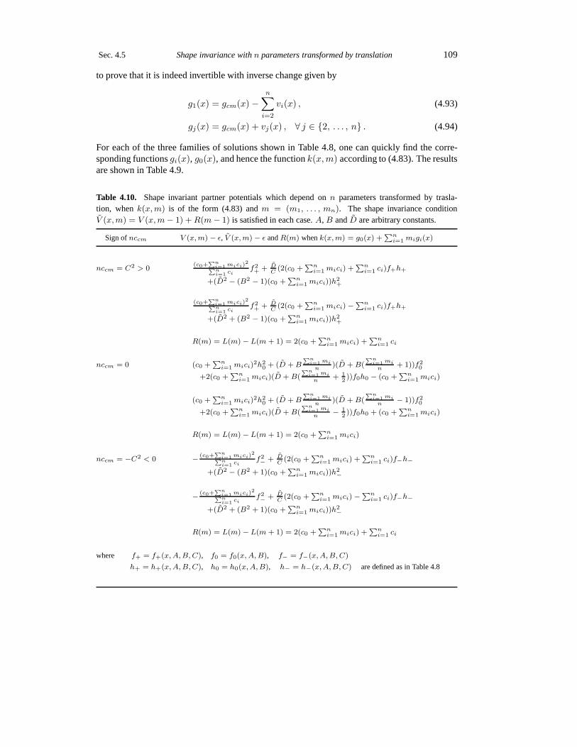
Sec. 4.5 Shape invariance withn parameters transformed by translation 109
to prove that it is indeed invertible with inverse change given by
g1(x) = gcm(x)−n∑
i=2
vi(x) , (4.93)
gj(x) = gcm(x) + vj(x) , ∀ j ∈ 2, . . . , n . (4.94)
For each of the three families of solutions shown in Table 4.8, one can quickly find the corre-sponding functionsgi(x), g0(x), and hence the functionk(x,m) according to (4.83). The resultsare shown in Table 4.9.
Table 4.10. Shape invariant partner potentials which depend onn parameters transformed by trasla-tion, whenk(x,m) is of the form (4.83) andm = (m1, . . . , mn). The shape invariance conditionV (x,m) = V (x,m− 1) +R(m− 1) is satisfied in each case.A, B andD are arbitrary constants.
Sign ofnccm V (x,m) − ǫ, V (x,m) − ǫ andR(m) whenk(x,m) = g0(x) +∑n
i=1 migi(x)
nccm = C2 > 0(c0+
∑ni=1 mici)
2∑
ni=1 ci
f2+ + D
C(2(c0 +
∑ni=1 mici) +
∑ni=1 ci)f+h+
+(D2 − (B2 − 1)(c0 +∑n
i=1 mici))h2+
(c0+∑n
i=1 mici)2
∑
ni=1 ci
f2+ + D
C(2(c0 +
∑ni=1 mici)−
∑ni=1 ci)f+h+
+(D2 + (B2 − 1)(c0 +∑n
i=1 mici))h2+
R(m) = L(m) − L(m + 1) = 2(c0 +∑n
i=1 mici) +∑n
i=1 ci
nccm = 0 (c0 +∑n
i=1 mici)2h2
0 + (D +B∑n
i=1 mi
n)(D + B(
∑ni=1 mi
n+ 1))f2
0
+2(c0 +∑n
i=1 mici)(D + B(∑n
i=1 mi
n+ 1
2))f0h0 − (c0 +
∑ni=1 mici)
(c0 +∑n
i=1 mici)2h20 + (D +B
∑ni=1 mi
n)(D + B(
∑ni=1 mi
n− 1))f2
0
+2(c0 +∑n
i=1 mici)(D + B(∑n
i=1 mi
n− 1
2))f0h0 + (c0 +
∑ni=1 mici)
R(m) = L(m) − L(m + 1) = 2(c0 +∑n
i=1 mici)
nccm = −C2 < 0 −(c0+
∑ni=1 mici)
2∑
ni=1 ci
f2− + D
C(2(c0 +
∑ni=1 mici) +
∑ni=1 ci)f−h−
+(D2 − (B2 + 1)(c0 +∑n
i=1 mici))h2−
−(c0+
∑ni=1 mici)
2∑
ni=1 ci
f2− + D
C(2(c0 +
∑ni=1 mici)−
∑ni=1 ci)f−h−
+(D2 + (B2 + 1)(c0 +∑n
i=1 mici))h2−
R(m) = L(m) − L(m + 1) = 2(c0 +∑n
i=1 mici) +∑n
i=1 ci
where f+ = f+(x, A,B, C), f0 = f0(x, A,B), f− = f−(x,A,B, C)
h+ = h+(x,A,B,C), h0 = h0(x,A,B), h− = h−(x,A,B, C) are defined as in Table 4.8

110 Intertwined Hamiltonians, factorization method and shapeinvariance Chap. 4
We can now calculate the corresponding shape invariant partner potentials by means ofthe formulas (4.23), (4.24), (4.50) and (4.51) adapted to this case. The results are shown inTable 4.10.
Let us comment on the solutions for the functionk(x,m) in Table 4.9 and for the shapeinvariant potentials in Table 4.10 we have just found. It is remarkable that the constantsci,c0, of equations (4.85), (4.86) appear always in the solutionsby means of the combinationc0 +∑n
i=1mici. On the other hand,D does not change under the transformationmi → mi−1 since itdepends only on differences of themi’s. AsD0, D2, . . . , Dn are arbitrary constants,D = D0+∑n
i=2Di(mi−m1) can be regarded as an arbitrary constant as well. It is very easy to check thatthe functionsk(x,m) satisfy indeed (4.82), just taking into account thatnccm =
∑ni=1 ci and
that whennccm = C2,∑ni=1 ci/C = C, meanwhile
∑ni=1 ci/C = −C whennccm = −C2.
Obviously, for the casenccm = 0 we have∑n
i=1 ci = 0. As we have mentioned already, (4.82)is essentially equivalent to the shape invariance condition V (x,m) = V (x,m− 1)+R(m− 1),but it can be checked directly. In order to do it, it may be useful to recall several relations thatthe functions defined in Table 4.8 satisfy. Whennccm = C2 we have
f ′+ = C(1 − f2
+) = C(B2 − 1)h2+ , h′+ = −Cf+h+ ,
whennccm = 0,
f ′0 = −B f2
0 , h′0 = −B f0h0 + 1 ,
and finally whennccm = −C2,
f ′− = C(1 + f2
−) = C(B2 + 1)h2− , h′− = Cf−h− ,
where the prime means derivative respect tox. The arguments of these functions are the sameas in the mentioned table and have been dropped out for simplicity. When we have only oneparameter, that is,n = 1, we recover the solutions fork(x,m) = k0(x) +mk1(x) shown in thefirst column of Table 4.5, and the corresponding shape invariant partner potentials of Table 4.6.
For all cases in Table 4.10, the formal expression ofR(m) is exactly the same, but either∑ni=1 ci = nccm have different sign or vanish. Although for the purposes of quantum mechanics
the relevant function isR(m), from which the energy spectrum is calculated, let us consider theproblem of how to determineL(m) fromR(m). Since
R(m) = L(m)− L(m+ 1) = 2
(c0 +
n∑
i=1
mici
)+
n∑
i=1
ci (4.95)
is a polynomial in then parametersmi, and we have considered only polynomial functions ofthese quantities so far,L(m) should be also a polynomial. It is of degree two, otherwise a simplecalculation would show that the coefficients of terms of degree 3 or higher must vanish. So,we proposeL(m) =
∑ni,j=1 rijmimj +
∑ni=1 simi + t, whererij is symmetric,rij = rji.
Therefore, there are12n(n + 1) + n + 1 constants to be determined. Then, making use of thesymmetry ofrij in its indices we obtain
L(m)− L(m+ 1) = − 2
n∑
i,j=1
rijmi −n∑
i,j=1
rij −n∑
i=1
si .

Sec. 4.5 Shape invariance withn parameters transformed by translation 111
Comparing with (4.95) we find the following conditions to be satisfied
−n∑
j=1
rij = ci , ∀ i ∈ 1, . . . , n , and −n∑
i=1
si = 2c0 .
The first of these equations expresses the problem of finding symmetric matrices of ordernwhose rows (or columns) sumn given numbers. That is, to solve a linear system ofn equationswith 1
2n(n + 1) unknowns. Forn > 1 the solutions determine an affine space of dimension12n(n + 1) − n = 1
2n(n − 1). Moreover, forn > 1 the second condition determines alwaysan affine space of dimensionn − 1. The well known case of ofn = 1, cf. Section 4.4, gives aunique solution to both conditions. However, the constantt always remains underdetermined.
We will try to find now other generalizations of shape invariant potentials which dependon n parameters transformed by means of a translation. We shouldtry a generalization usinginverse powers of the parametersmi; we know already that for the casen = 1 there appear atleast three new families of solutions, see Table 4.7. So, we will try a solution of the followingtype, provided thatmi 6= 0, for all i,
k(x,m) =n∑
i=1
fi(x)
mi+ g0(x) +
n∑
i=1
migi(x) . (4.96)
Here,fi(x), gi(x) andg0(x) are functions ofx to be determined. Substituting into (4.82) weobtain, after a little algebra,
L(m)− L(m+ 1) = −n∑
i,j=1
fifj(1 +mi +mj)
mi(mi + 1)mj(mj + 1)− 2g0
n∑
i=1
fimi(mi + 1)
− 2n∑
i,j=1
mjgjfimi(mi + 1)
+ 2n∑
i,j=1
gjfimi + 1
+n∑
i=1
2mi + 1
mi(mi + 1)
dfidx
+ . . . ,
where the dots represents the right hand side of (4.84). The coefficients of each of the differentdependences on the parametersmi have to be constant. The term
−n∑
i,j=1
fifj(1 +mi +mj)
mi(mi + 1)mj(mj + 1)
involves a symmetric expression under the interchange of the indicesi andj. As a consequencewe obtain thatfifj = Const. for alli, j. Sincei andj run independently the only possibilityis that eachfi = Const. for alli ∈ 1, . . . , n. We will assume that at least one of thefi isdifferent from zero, otherwise we would be in the already studied case. Then, the term
−2g0
n∑
i=1
fimi(mi + 1)
,
gives usg0 = Const. and the term which contains the derivatives of thefi’s vanishes. The sumof the terms
2
n∑
i,j=1
gjfimi + 1
− 2
n∑
i,j=1
mjgjfimi(mi + 1)

112 Intertwined Hamiltonians, factorization method and shapeinvariance Chap. 4
is only zero forn = 1. Then, forn > 1 the first of them provides us∑ni=1 gi = Const.
and the second one,gi = Const. for alli ∈ 1, . . . , n. This is just a particular case of thetrivial solution. Forn = 1, however, we obtain more solutions; is the case already discussed inSection 4.4. It should be noted that, in general,
2
n∑
i,j=1
gjfimi + 1
− 2
n∑
i,j=1
mjgjfimi(mi + 1)
6= 2
n∑
i,j=1
figjmi + 1
(1− mj
mi
).
Using this equation as being true will lead to incorrect results. As a conclusion we obtain thatthe trial solutionk(x,m) given by (4.76) admits no non-trivial generalization to solutions of thetype (4.96).
It can be shown that if we propose further generalizations tohigher degree inverse powersof the parametersmi, the only solution is also a trivial one. For example, if we try a solution oftype
k(x,m) =
n∑
i,j=1
hij(x)
mimj+
n∑
i=1
fi(x)
mi+ g0(x) +
n∑
i=1
migi(x) , (4.97)
wherehij(x) = hji(x), the only possibility we will obtain is that all involved functions ofxhave to be constant.
Now we try to generalize (4.83) to higher positive powers. That is, we will try now asolution of type
k(x,m) = g0(x) +n∑
i=1
migi(x) +n∑
i,j=1
mimjeij(x) . (4.98)
Substituting into (4.82) we obtain, after several calculations,
L(m)− L(m+ 1) = 4
n∑
i,j,k,l=1
mimjmkeijekl + 4
n∑
i,j,k,l=1
mieijmk(ekl + gk)
+ 2n∑
i,j=1
mimj
n∑
k,l=1
(ekl + gl)eij +deijdx
+ 4
n∑
i,j=1
mieij
n∑
k,l=1
(ekl + gl) + g0
+ 2
n∑
i=1
mi
gi
n∑
j,k=1
(ejk + gj) +d
dx
n∑
k=1
(eik + gi)
+
n∑
i,j=1
(eij + gi)
n∑
k,l=1
(elk + gl) + 2g0
+
d
dx
n∑
i,j=1
(eij + gi) + 2g0
. (4.99)
As in previous cases, the coefficients of each different typeof dependence on the parametersmi have to be constant. Let us analyze the term of highest degree, i.e., the first term on theright hand side of (4.99). Since it contains a completely symmetric sum in the parametersmi,

Sec. 4.6 Ambiguities in the definition of the partner potential 113
the dependence on the functionseij should also be completely symmetric in the correspondingindices. For that reason, we rewrite it as
4
n∑
i,j,k,l=1
mimjmkeijekl =4
3
n∑
i,j,k,l=1
mimjmk(eijekl + ejkeil + ekiejl) ,
from where it is found the necessary condition
n∑
l=1
(eijekl + ejkeil + ekiejl) = dijk , ∀ i, j, k ∈ 1, . . . , n ,
wheredijk are constants completely symmetric in their three indices.The number of independentequations of this type is just the number of independent components of a completely symmetrictensor in its three indices, each one running from 1 ton. This number is16n(n+ 1)(n+ 2). Thenumber of independent variableseij is 1
2n(n+ 1) from the symmetry on the two indices. Then,the number of unknowns minus the number of equations is
1
2n(n+ 1)− 1
6n(n+ 1)(n+ 2) = −1
6(n− 1)n(n+ 1) .
For n = 1 the system has the simple solutione11 = Const. Forn > 1 the system is not com-patible and has no solutions apart from the trivial oneeij = Const. for alli, j. In either of thesecases, it is very easy to deduce from the other terms in (4.99)that all of the remaining functionshave to be constant as well, provided that not all of the constantseij vanish. For higher positivepower dependence on the parametersmi’s a similar result holds. In fact, let us suppose thatthe highest order term in our trial solution is of degreeq,
∑ni1, ..., iq=1mi1mi2 · · ·miqTi1, ..., iq ,
whereTi1, ..., iq is a completely symmetric tensor in its indices. Then, is easy to prove that thehighest order term appearing after substitution in (4.82) is a sum whose general term is of degree2q − 1 in themi, being completely symmetric under the interchange of theseparameters. Thissum contains the product ofTi1, ..., iq by itself, but with one index summed. One then has tosymmetrize the expression for twoT ’s in order to obtain the number of independent equations tobe satisfied, which is equal to the number of independent components of a completely symmetrictensor in its2q − 1 indices. This number is(n + 2(q − 1))!/(2q − 1)!(n − 1)!. The number ofindependent unknowns is(n+ q− 1)!/q!(n− 1)!. Thus, the number of unknowns minus the oneof equations is
(n+ q − 1)!
q!(n− 1)!− (n+ 2(q − 1))!
(2q − 1)!(n− 1)!.
This number vanishes always forn = 1, which means that the problem is determined and weobtain thatT1, ..., 1 = Const., in agreement with [176, p. 28], see also Section 4.4.If n > 1,one can easily check that forq > 1 that number is negative and hence there cannot be othersolution apart from the trivial solutionTi1, ..., iq = Const. for alli1, . . . , iq ∈ 1, . . . , n. Fromthe terms of lower degree one should conclude that the only possibility is a particular case of thetrivial solution.
4.6 On the ambiguity in the definition of the partner potential
We will study in this section an important conceptual aspectconcerning the definition of a partnerpotential, in the sense of Section 4.1, when a specific potential is given. We will see that there

114 Intertwined Hamiltonians, factorization method and shapeinvariance Chap. 4
appear several ambiguities in such a definition, and part of them are due to the properties of theRiccati equation.
More explicitly, looking for a factorization of a given Hamiltonian amounts to find a con-stantǫ and a solution of a Riccati differential equation for the superpotential function. The firstambiguity is due to the choice of the factorization energyǫ, which is not unique in general. Afterthat, it arises the ambiguity in the choice of the solution ofthe corresponding Riccati equation.The choice of different solutions of the Riccati equation has been shown to be very useful inthe search of isospectral potentials, an idea due to Mielnik[238] and later developed in otherarticles, see, e.g., [108,111,124,263]. However, we feel that the mentioned underdeterminationsare worth having a new look in their own right because their understanding allows us to interpretcertain facts treated in the literature as consequences of this underdetermination.
Moreover, the ambiguity in the definition of the partner potential is inherited in the caseof shape invariance, so one may wonder to what extent it makessense the relation between apotential and its partner characterizing such a kind of problems.
Therefore, two main questions arise. Are there different solutions for the same Riccatiequation leading to the same partner?. On the other hand, if the shape invariance condition holdsfor a certain partner, is it also true for any other possible partner?.
Given one potential functionV , the equation (4.3) to be solved when searching for a su-perpotential functionW , onceǫ is fixed, is a Riccati equation. In general, its general solutioncannot be found by means of quadratures. However, now we onlyneed to compare solutions ofthe same equation when a particular solution is known, in which case its general solution can bewritten using two quadratures, cf. Sections 1.3 and 1.5. Thus, if Wp is a particular solution of(4.3) for some specific constantǫ, the change of variable
v =1
Wp −W, with inverse W =Wp −
1
v, (4.100)
transforms (4.3) into the inhomogeneous first order linear equation forv
dv
dx= −2Wp v + 1 , (4.101)
which has the general solution
v(x) =
∫ xexp
2∫ ξWp(η) dη
dξ + F
exp2∫ x
Wp(ξ) dξ , (4.102)
whereF is an integration constant. Therefore, the general solution of (4.3) reads as
Wg(x) =Wp(x)−exp
2∫ x
Wp(ξ) dξ
∫ xexp
2∫ ξWp(η) dη
dξ + F
. (4.103)
Then, “the partner”V of V is constructed by using (4.4), or equivalently, (4.7). But these for-mulas explicitly show thatV does depend upon the choice of the particular solution of (4.3)considered. Since the general solution of (4.3) can be written asWg = Wp − 1/v, wherev isgiven by (4.102), the general solution obtained forVg is, according to (4.7),
Vg = Vp − 2d
dx
(1
v
). (4.104)

Sec. 4.6 Ambiguities in the definition of the partner potential 115
This answers one of the questions above: all the partner potentials, obtained by using (4.104)are different, apart from the trivial case in whichWp andV are constant, because the differentialequation (4.101) only admits a constant solution whenWp is constant.
This implies that “the partner” ofonegiven potential is not a well defined concept and itseems better to say that an ordered pair(V, V ) is a (supersymmetric) pair of partner potentials ifthere exists a constantǫ and a functionW such that the latter is a common solution of the Riccatiequations (4.3) and (4.4) constructed with these potentials, respectively. Of course the precedingcomment shows that in such a case the superpotential functionW is essentially unique for eachǫ, which moreover makes the problem ofA-related Hamiltonians be well defined. Note as wellthat this reformulation of partnership comprehends the situation whereV is the potential we havestarted this section with,V is one of the functions obtained from (4.104) for aspecificvalue ofthe constantF , andW is obtained from (4.103) forthe samevalue ofF .
Now we will show what consequences have this underdetermination in the subclass of shapeinvariant potentials. For that, we should use instead of (4.3) and (4.4) the equations
V (x, a) − ǫ(a) =W 2(x, a)−W ′(x, a) , (4.105)
V (x, a) − ǫ(a) =W 2(x, a) +W ′(x, a) , (4.106)
where now the factorization constant depends on the parametera, changing slightly the conven-tion for the notations used so far. Consider a particular solutionWp(x, a) of equation (4.105)for some specific constantǫ(a), such that it is also a particular solution of (4.106),V (x, a) andV (x, a) being related by the further condition (4.20). As in the previous case, we can considerthe general solution of (4.105) starting fromWp(x, a), which is
Wg(x, a, F ) =Wp(x, a) + g(x, a, F ) , (4.107)
whereg(x, a, F ) is defined by
g(x, a, F ) = − exp2∫ x
Wp(ξ, a) dξ
∫ xexp
2∫ ξWp(η, a) dη
dξ + F
, (4.108)
andF is an integration constant. Note that the particular solutionWp(x, a) is obtained from(4.107) asF → ∞. Then, insertingWg(x, a, F ) into (4.106) we obtain the general family ofpartner potentials
V (x, a, F ) = V (x, a)− 2g′(x, a, F ) . (4.109)
The question now is whether the condition (4.20) is maintained when we consider the pairV (x, a, F ) andV (x, a) instead ofV (x, a) andV (x, a). Then, we ask for
V (x, a, F ) = V (x, f(a)) +R(f(a), F ) , (4.110)
for some suitableF , wheref is the same as in (4.20), andR(f(a), F ) is a number not dependingon x, maybe different from theR(f(a)) of (4.20). Taking into account (4.20) and (4.109), theequation (4.110) reads as
2g′(x, a, F ) = R(f(a), F )−R(f(a)) ,

116 Intertwined Hamiltonians, factorization method and shapeinvariance Chap. 4
that is,2g′(x, a, F ) should be a constant, which we name ask for brevity. Integrating respect tox we obtain2g(x, a, F ) = kx + l, wherel is another constant depending at most ona andF .On the other hand, sinceg(x, a, F ) is given by (4.108), it follows
∫ x
exp
2
∫ ξ
Wp(η, a) dη
dξ + F = −2 exp
2∫ x
Wp(ξ, a) dξ
kx+ l. (4.111)
Differentiating this last equation, and solving forWp(x, a), we obtain
Wp(x, k, l) =1
4
(2k
kx+ l− (kx+ l)
),
where we have made explicit that the parameter space should be a = k, l. Introducing thisexpression into (4.111) and performing the integrations, we obtain
−2 e−x(kx+2l)/4 + F = −2 e−x(kx+2l)/4
and henceF = 0. Now we have to check whether this particular case we have found, which isthe only candidate for fulfilling (4.110), satisfies our hypothesis (4.20). The partner potentialsdefined byWp(x, k, l) and equations (4.105), (4.106) are
V (x, k, l)− ǫ(k, l) =W 2p (x, k, l)−W ′
p(x, k, l) =(kx+ l)2
16+
3 k2
4 (kx+ l)2,
V (x, k, l)− ǫ(k, l) =W 2p (x, k, l) +W ′
p(x, k, l) =(kx+ l)2
16− k2
4 (kx+ l)2− k
2.
Now, we have to find out whether there are some transformationof the parametersk, l such thatthe condition (4.20) be satisfied. Denoting the transformedparameters ask1, l1 for simplicity,we have
V (x, k, l)− V (x, k1, l1) = d(k, l)− ǫ(k1, l1)−k
2− 1
4
(3 k21
(k1x+ l1)2+
k2
(kx+ l)2
)
+1
16((k − k1)x+ l − l1)((k + k1)x+ l + l1) .
The right hand side of this equation must be a constant and therefore, each of the differentdependences onx must vanish. The term((k − k1)x + l − l1)((k + k1)x + l + l1) vanish forthe combinationsk1 = −k, l1 = −l or k1 = k, l1 = l, apart form the casek1 = −k1 = k = 0,which will be studied separately. However, the term
3 k21(k1x+ l1)2
+k2
(kx+ l)2
is equal to4 k2/(kx+ l)2 for both combinations and does not vanish. Then, the shape invariancehypothesis is not satisfied. In the case ofk = 0 we have that the correspondingWp(x, a) isa constant and hence provides the trivial case where the corresponding partner potentials areconstant as well.
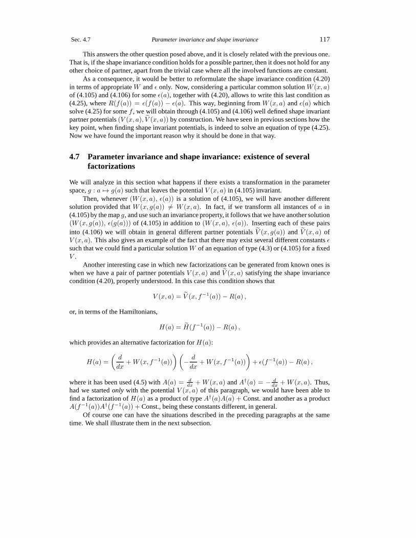
Sec. 4.7 Parameter invariance and shape invariance 117
This answers the other question posed above, and it is closely related with the previous one.That is, if the shape invariance condition holds for a possible partner, then it does not hold for anyother choice of partner, apart from the trivial case where all the involved functions are constant.
As a consequence, it would be better to reformulate the shapeinvariance condition (4.20)in terms of appropriateW andǫ only. Now, considering a particular common solutionW (x, a)of (4.105) and (4.106) for someǫ(a), together with (4.20), allows to write this last condition as(4.25), whereR(f(a)) = ǫ(f(a)) − ǫ(a). This way, beginning fromW (x, a) andǫ(a) whichsolve (4.25) for somef , we will obtain through (4.105) and (4.106) well defined shape invariantpartner potentials(V (x, a), V (x, a)) by construction. We have seen in previous sections how thekey point, when finding shape invariant potentials, is indeed to solve an equation of type (4.25).Now we have found the important reason why it should be done inthat way.
4.7 Parameter invariance and shape invariance: existence of severalfactorizations
We will analyze in this section what happens if there exists atransformation in the parameterspace,g : a 7→ g(a) such that leaves the potentialV (x, a) in (4.105) invariant.
Then, whenever(W (x, a), ǫ(a)) is a solution of (4.105), we will have another differentsolution provided thatW (x, g(a)) 6= W (x, a). In fact, if we transform all instances ofa in(4.105) by the mapg, and use such an invariance property, it follows that we haveanother solution(W (x, g(a)), ǫ(g(a))) of (4.105) in addition to(W (x, a), ǫ(a)). Inserting each of these pairsinto (4.106) we will obtain in general different partner potentials V (x, g(a)) and V (x, a) ofV (x, a). This also gives an example of the fact that there may exist several different constantsǫsuch that we could find a particular solutionW of an equation of type (4.3) or (4.105) for a fixedV .
Another interesting case in which new factorizations can begenerated from known ones iswhen we have a pair of partner potentialsV (x, a) andV (x, a) satisfying the shape invariancecondition (4.20), properly understood. In this case this condition shows that
V (x, a) = V (x, f−1(a))−R(a) ,
or, in terms of the Hamiltonians,
H(a) = H(f−1(a))−R(a) ,
which provides an alternative factorization forH(a):
H(a) =
(d
dx+W (x, f−1(a))
)(− d
dx+W (x, f−1(a))
)+ ǫ(f−1(a))−R(a) ,
where it has been used (4.5) withA(a) = ddx +W (x, a) andA†(a) = − d
dx +W (x, a). Thus,had we startedonly with the potentialV (x, a) of this paragraph, we would have been able tofind a factorization ofH(a) as a product of typeA†(a)A(a) + Const. and another as a productA(f−1(a))A†(f−1(a)) + Const., being these constants different, in general.
Of course one can have the situations described in the preceding paragraphs at the sametime. We shall illustrate them in the next subsection.

118 Intertwined Hamiltonians, factorization method and shapeinvariance Chap. 4
4.7.1 Illustrative examples
As a first example we will interpret the so-calledfour-way factorizationof the isotropic harmonicoscillator, introduced in [131, pp. 388–389]. In their notation, the potential and Hamiltonian ofinterest are
V (r, l) =l(l + 1)
r2+ r2 , H(l) = − d2
dr2+ V (r, l) ,
where the independent variable isr ∈ (0,∞) and the set of parameters is simplyl. Theirfactorization (6) is
H(l) =
(− d
dr+l
r+ r
)(d
dr+l
r+ r
)− (2l− 1) , (4.112)
from where it is suggested thatW (r, l) = lr + r. Substituting it intoV (r, l) = W 2(r, l) −
W (r, l)dr + ǫ(l) we obtainǫ(l) = −(2l − 1), so (4.112) is the appropriate version of (4.5) as
expected. Now, as the potentialV (r, l) is invariant under the mapg : l 7→ −l− 1, we will obtaina new solution(W (r, g(l)) , ǫ(g(l))) = (W (r,−l − 1) , ǫ(−l− 1)) of the equation
V (r, l) =W 2 − dW
dr+ ǫ .
ButW (r, g(l)) =W (r,−l− 1) = − l+1r + r andǫ(g(l)) = ǫ(−l− 1) = 2l+3, which is exactly
what corresponds to the factorization (4) of [131]. The factorizations (5) and (7)loc. cit. arerelated in a similar way; (7) is obtained from (5) by means of the changeg : l 7→ −l− 1 as well.
As far as the relation between their factorizations (6) and (5) loc. cit. is concerned, we havealready seen that, from their factorization (6), here reproduced as (4.112), it followsW (r, l) =lr + r, and thus, the correspondingV (r, l) through (4.106) is
V (r, l) =W 2(r, l) +dW (r, l)
dr+ ǫ(l) =
l(l− 1)
r2+ r2 + 2 .
Then it is very easy to check thatV (r, l) = V (r, f(l)) + R(f(l)), whereR(l) = 2 for all l, andf is defined either byf(l) = l− 1 or f(l) = −l. We obtain
H(l) = H(l + 1)−R(l) , V (r, l) = V (r, l + 1)−R(l) ,
andH(l) = H(−l)−R(l) , V (r, l) = V (r,−l)−R(l) ,
as well. In this way the factorization (5) of [131] is achieved.As a second example we will consider the modified Poschl–Teller potential, analyzed in an
interesting recent article [108]. The potential is now
V (x, α, λ) = −α2 λ(λ − 1)
cosh2 αx, (4.113)
wherex ∈ (−∞,∞) andα > 0, λ > 1 are two real parameters.Two different particular solutions(W (x, α, λ), ǫ(α, λ)) of the Riccati equation
W 2 −W ′ = V (x, α, λ) − ǫ ,

Sec. 4.7 Parameter invariance and shape invariance 119
have been found in [108], p. 8450, namely,
(W1(x, α, λ), ǫ1(α, λ)) = (−λα tanh2 αx,−λ2α2) ,
(W2(x, α, λ), ǫ2(α, λ)) = (−(1− λ)α tanh2 αx,−(1 − λ)2α2) .
It is clear that the second pair is obtained from the first by means of the parameter transformationg : (α, λ) 7→ (α, 1− λ). The reason is thatV (x, α, λ) is invariant underg, or more precisely, itsfactorλ(1− λ).
The associated partner potentialsV (x, α, λ) obtained using (4.106), are
V1(x, α, λ) =W 21 (x, α, λ) +W ′
1(x, α, λ) + ǫ1(α, λ) = −α2 λ(λ + 1)
cosh2 αx,
V2(x, α, λ) =W 22 (x, α, λ) +W ′
2(x, α, λ) + ǫ2(α, λ) = −α2 (λ− 1)(λ− 2)
cosh2 αx.
We see that both of the previous functions are just second degree monic polynomials inλ, withroots spaced one unit, times−α2/ cosh2 αx, like V (x, α, λ) itself. It is then obvious that atranslation of the typeλ 7→ λ−b orλ 7→ c−λ should transformV1(x, α, λ) andV2(x, α, λ) intoV (x, α, λ). This is in fact so, sinceV (x, α, λ) = V1(x, α, f
−1(λ)), wheref is defined either byf(λ) = λ− 1 or f(λ) = −λ, and similarlyV (x, α, λ) = V2(x, α, f
−1(λ)) whenf(λ) = λ− 1or f(λ) = 2− λ.
In this way one could propose other different factorizations for the potentialV (x, α, λ),being able, in principle, to perform a differential operator analysis for this potential similar towhat it is done in [131] for the first example of this subsection.


Chapter 5
Group theoretical approach to the intertwinedHamiltonians
5.1 Introduction and the theorem of the finite-difference algorithm
In this chapter we will study the problem of intertwined Hamiltonians from the group theoreticalpoint of view provided by the affine action on the set of Riccati equations introduced in Chap-ters 1 and 3. We will explain in these terms the above problem and, moreover, we will be able tofind the most general version, in some sense, of the classicalDarboux transformation by meansof the previous action. In addition, we will give to these transformations a group theoreticalfoundation.
Let us make some comments about how we have arrived to these problems and results.As we have mentioned in the preceding chapter, the factorization of Hamiltonian problems inquantum mechanics and other related techniques play an important role in the search of quantumsystems for which the energy spectrum is completely known. However, there has been recentlyan increasing interest in generating new exactly solvable Hamiltonians from known ones. To thisrespect, concerning iterations of the first order intertwining technique, it has been recently used afinite difference algorithmin [128], which provides in an algebraic fashion the solution of the keyRiccati equation at a given iteration step in terms of two solutions of the corresponding Riccatiequation at the previous step, associated to two different factorization energies. This procedurehas been successfully applied in order to obtain new exactlysolvable Hamiltonians departingfrom the harmonic oscillator and Coulomb potentials [127,128,289].
On the other hand, as we have shown in Sections 1.4 and 3.2, it is possible to define an affineaction on the set of Riccati equations. From the perspectiveof Lie systems (with associated Liealgebrasl(2, R)) as connections in principal and associated bundles, this affine action can beidentified as a kind ofgauge transformationsor, in other words, with how the given connectionchanges under the group of automorphisms of the involved bundle. We have used this affineaction in order to analyze the integrability properties of the Riccati equation in Section 1.5.
We wondered about whether this group theoretical approach could shed a new light on theabovementioned problem of intertwined orA-related Hamiltonians, and, in particular, a naturalquestion is whether there is a relation of this group action with the finite difference algorithm.The first result to this respect is immediate, since a direct proof of the theorem of the finitedifference algorithm can be obtained by means of the cited group action. From now on, we willfollow the definitions and notations of Sections 1.4 and 3.2,but we will denote the independent
121

122 Intertwined Hamiltonians Chap. 5
variable asx instead oft, and the dependent variable will bey instead ofx. Likewise, thederivatives with respect tot, denoted with a dot, become derivatives with respect tox, to bedenoted with a prime.
Theorem 5.1.1 (Finite difference Backlund algorithm [128,239]).Letwk(x),wl(x) betwo solutions of the Riccati equationsw′ +w2 = V (x)− ǫk andw′ +w2 = V (x)− ǫl, respec-tively, whereǫk < ǫl. Then, the functionwkl(x) defined by
wkl(x) = −wk(x)−ǫk − ǫl
wk(x) − wl(x), (5.1)
is a solution of the Riccati equationw′ + w2 = V (x)− 2w′k(x)− ǫl.
Proof. The functionwl(x) satisfies the Riccati equationw′+w2 = V (x)−ǫl by hypothesis.We transform it by means of the elementA0 of G given by
A0(x) =1√a
(h(x) −h2(x) + a−1 h(x)
), (5.2)
whereh(x) is a function with the same domain aswl(x) anda is a positive constant. Notice thatA0 ∈ G since its determinant is always one, for allx in the domain ofh(x). According to (1.32),we compute
Φ(A0(x), wl(x)) =h(x)wl(x) − h2(x) + a
h(x)− wl(x)= −h(x) + a
h(x)− wl(x).
This is a solution of the Riccati equation with coefficient functions given by (1.34), (1.35) and(1.36), with matrix elements
α(x) = δ(x) =h(x)√a, β(x) =
−h2(x) + a√a
, γ(x) = − 1√a,
and coefficients of the initial Riccati equation
a2(x) = −1 , a1(x) = 0 , a0(x) = V (x)− ǫl .
Simply performing the operations, we find
a2(x) =1
a−h2(x)− h′(x) + V (x)− ǫl + a − 1 ,
a1(x) =2 h(x)
a−h2(x)− h′(x) + V (x)− ǫl + a ,
a0(x) =h2(x)
a−h2(x)− h′(x) + V (x)− ǫl + a
+ h2(x) + h′(x)− 2 h′(x)− a .
Therefore, if the functionh(x) satisfies the Riccati equationw2+w′ = V (x)−ǫk, with ǫk = ǫl−a, and we rename it ash(x) = wk(x), the new coefficients reduce toa2(x) = −1, a1(x) = 0 and
a0(x) = V (x)− 2w′k(x)− ǫl.

Sec. 5.2 Group elements preserving Riccati equations of typew′ + w2 = V (x)− ǫ 123
Let us remark that in [128] the proof of Theorem 5.1.1 was justsketched. In addition, thereexists an alternative proof [239].
Thus, motivated by this result, we wondered about what are the group elements whichpreserve the subset of Riccati equations arising from the set of Schrodinger equations, afterapplying the reduction process outlined in Section 4.2, with respect to the affine action on theset of Riccati equations. This question is studied in Section 5.2. As a result of this analysis, wewill be able to find a new transformation relatingthreedifferent Schrodinger equations, whichrepresents a generalization of both the finite difference B¨acklund algorithm and the classicalDarboux transformation technique. As an application, we find in Section 5.3 that the problemof A-related Hamiltonians can be explained exactly in terms of the affine action on the set ofRiccati equations and the reduction procedure of Section 4.2. In Section 5.4 we illustrate theuse of the new theorems of Section 5.2 in the search of potentials for which one eigenstateand the corresponding eigenvalue will be exactly known. In particular, Examples 5.4.1, 5.4.3and 5.4.4 will provide potentials essentially different from the original ones. Since we know byconstruction an exact eigenvalue and eigenfunction of the new potential, this technique is a newalternative in order to find potentials for which only part ofthe eigenvalue prolem can be solvedexactly. Finally, we give in Section 5.5 some remarks and directions for further research.
5.2 Group elements preserving Riccati equations of typew′+w2 = V (x)−ǫ
We have seen how the affine action on the set of Riccati equations provides a direct proof ofTheorem 5.1.1. It relates one solutionwl(x) of theinitial Riccati equationw′ +w2 = V (x)− ǫlwith one solutionwkl(x) of thefinal Riccati equationw′ +w2 = V (x)− 2w′
k(x)− ǫl by usinga solutionwk(x) of theintermediateRiccati equationw′+w2 = V (x)− ǫk. These three Riccatiequations can be obtained from another three Schrodinger-like equations by means of one of thereduction possibilities explained in Section 4.2. Moreover, those associated with the initial andintermediate Riccati equations, namely−ψ′′+(V (x)− ǫl)ψ = 0 and−ψ′′+(V (x)− ǫk)ψ = 0,can be seen as the eigenvalue equations for the two energiesǫl, ǫk of the same potentialV (x),meanwhile the final Riccati equation can be associated to theeigenvalue equation for the potentialV (x)− 2w′
k(x), with eigenvalueǫl.
Then, we are naturally led to the question of which are the most general elements ofG suchthat, by means of the affine action on the set of Riccati equations, we transform an arbitrarybut fixed Riccati equation with coefficientsa2(x) = −1, a1(x) = 0 anda0(x) equal to somefunction, which we will write as an expression of the formV (x)− ǫ, into another equation of thesame type, i.e., with coefficientsa2(x) = −1, a1(x) = 0 anda0(x) = V (x)− ǫ.
The Riccati equation we will start from is
w′ = −w2 + V (x) − ǫ , (5.3)
which according to (1.16) has the coefficientsa2(x) = −1, a1(x) = 0 anda0(x) = V (x) − ǫ.
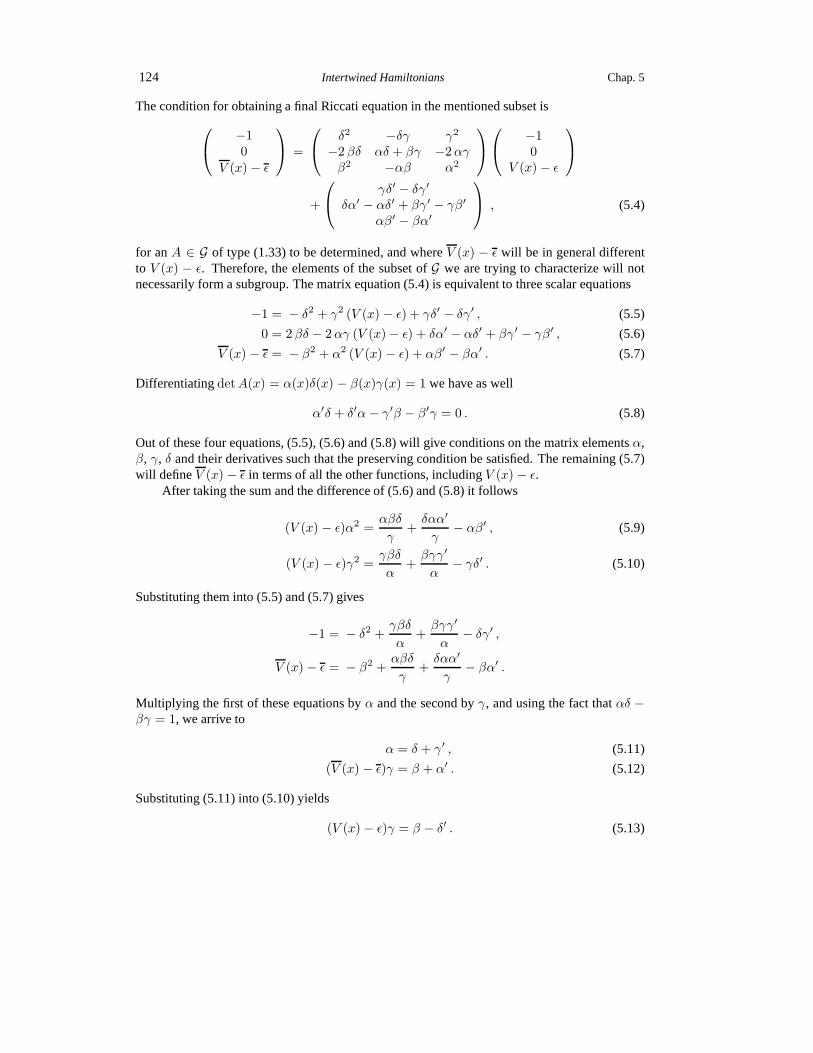
124 Intertwined Hamiltonians Chap. 5
The condition for obtaining a final Riccati equation in the mentioned subset is
−10
V (x)− ǫ
=
δ2 −δγ γ2
−2 βδ αδ + βγ −2αγβ2 −αβ α2
−10
V (x)− ǫ
+
γδ′ − δγ′
δα′ − αδ′ + βγ′ − γβ′
αβ′ − βα′
, (5.4)
for anA ∈ G of type (1.33) to be determined, and whereV (x) − ǫ will be in general differentto V (x) − ǫ. Therefore, the elements of the subset ofG we are trying to characterize will notnecessarily form a subgroup. The matrix equation (5.4) is equivalent to three scalar equations
−1 = − δ2 + γ2 (V (x) − ǫ) + γδ′ − δγ′ , (5.5)
0 = 2 βδ − 2αγ (V (x)− ǫ) + δα′ − αδ′ + βγ′ − γβ′ , (5.6)
V (x) − ǫ = − β2 + α2 (V (x) − ǫ) + αβ′ − βα′ . (5.7)
DifferentiatingdetA(x) = α(x)δ(x) − β(x)γ(x) = 1 we have as well
α′δ + δ′α− γ′β − β′γ = 0 . (5.8)
Out of these four equations, (5.5), (5.6) and (5.8) will giveconditions on the matrix elementsα,β, γ, δ and their derivatives such that the preserving condition besatisfied. The remaining (5.7)will defineV (x)− ǫ in terms of all the other functions, includingV (x) − ǫ.
After taking the sum and the difference of (5.6) and (5.8) it follows
(V (x) − ǫ)α2 =αβδ
γ+δαα′
γ− αβ′ , (5.9)
(V (x) − ǫ)γ2 =γβδ
α+βγγ′
α− γδ′ . (5.10)
Substituting them into (5.5) and (5.7) gives
−1 = − δ2 +γβδ
α+βγγ′
α− δγ′ ,
V (x)− ǫ = − β2 +αβδ
γ+δαα′
γ− βα′ .
Multiplying the first of these equations byα and the second byγ, and using the fact thatαδ −βγ = 1, we arrive to
α = δ + γ′ , (5.11)
(V (x) − ǫ)γ = β + α′ . (5.12)
Substituting (5.11) into (5.10) yields
(V (x)− ǫ)γ = β − δ′ . (5.13)

Sec. 5.2 Group elements preserving Riccati equations of typew′ + w2 = V (x)− ǫ 125
We have two relations amongst the functionsα, β, γ and δ, namely (5.11) and the determi-nant condition, so we can express these matrix elements in terms of only two of them and theirderivatives. Then we haveα = δ + γ′ andβ = (δ(δ + γ′)− 1)/γ. Using moreover the fact that
δ′
γ=
(δ
γ
)′+δγ′
γ2,
the equation (5.13) becomes(− δ
γ
)′+
(− δ
γ
)2
= V (x) +1
γ2− ǫ ,
so the new functionv defined asv = −δ/γ must satisfy the Riccati equation
v′ + v2 = V (x) +1
γ2− ǫ . (5.14)
Now, substituting in (5.12) the expressions ofβ andα′ in terms ofδ, γ and their derivatives, andusing the definition ofv and the equation (5.14) gives
V (x) − ǫ = V (x) − 2
(γ′
γv + v′
)+γ′′
γ− ǫ .
It only remains to find the expression of the function solution of the final Riccati equation, interms ofw andv. TheSL(2,R)-valued curve used for the transformation can be written as
C0 = γ
(−v + γ′
γ v2 − v γ′
γ − 1γ2
1 −v
), (5.15)
so the desired function is
w = Θ(C0, w) =−vw + wγ′/γ − 1/γ2 + v2 − vγ′/γ
w − v
= − v − 1/γ2
w − v+γ′
γ. (5.16)
In summary, we have just proved the following theorem:
Theorem 5.2.1. Letw(x) be a solution of the Riccati equation
w′ + w2 = V (x) − ǫ (5.17)
for some functionV (x) and some constantǫ, and letγ(x) be a never vanishing differentiablefunction defined on the domain ofV (x). If v(x) is a solution of the Riccati equation
v′ + v2 = V (x) +1
γ2(x)− ǫ , (5.18)
such that is defined in the same domain asw(x) andw(x) − v(x) does not vanish, then thefunctionw(x) defined by
w(x) = −v(x)− 1/γ2(x)
w(x) − v(x)+γ′(x)
γ(x)(5.19)

126 Intertwined Hamiltonians Chap. 5
is a solution of the Riccati equation
w′ + w2 = V (x)− 2
(γ′
γv + v′
)+γ′′
γ− ǫ . (5.20)
Needless to say, the coefficients of the final equation can be calculated directly by using(1.34), (1.35), (1.36) and taking into account (5.15), (5.17) and (5.18).
Corollary 5.2.1. The Theorem 5.1.1 is a particular case of Theorem 5.2.1.
Proof. It is sufficient to choose in Theorem 5.2.1w(x) = wl(x), v(x) = wk(x), ǫ = ǫl and
γ = 1/√ǫl − ǫk, with ǫk < ǫl.
Theorem 5.2.1 has a counterpart for linear second-order differential equations of Schrodin-ger type, which will be in turn of direct interest in physicalapplications. The key is to use in ainverse way the reduction procedure outlined in Section 4.2.
Consider the solutionw of the Riccati equation (5.17). We can define (locally and up to anon-vanishing multiplicative constant) the new functionφw as
φw(x) = exp
(∫ x
w(ξ) dξ
), (5.21)
which will satisfy−φ′′w + (V (x)− ǫ)φw = 0 ,
for the specific constantǫ. Analogously, by considering a solutionv of the Riccati equation(5.18) we can define (locally etc.)φv as
φv(x) = exp
(∫ x
v(ξ) dξ
), (5.22)
which will satisfy
−φ′′v +(V (x) +
1
γ2(x)− ǫ
)φv = 0 ,
for the same specific constantǫ. Then the functionw defined by (5.19) will satisfy the Riccatiequation (5.20). We could define as well (locally etc.) the new functionφw as
φw(x) = exp
(∫ x
w(ξ) dξ
), (5.23)
which in turn will satisfy
−φ′′w +
V (x)− 2
(γ′
γv + v′
)+γ′′
γ− ǫ
φw = 0 .
What has to be done now is to relate the functionφw with φw andφv, taking into account therelation amongstw, w andv.

Sec. 5.2 Group elements preserving Riccati equations of typew′ + w2 = V (x)− ǫ 127
Proposition 5.2.1. Letw, v, w be the functions for which the Theorem 5.2.1 holds, andφw, φv, φw the ones defined by (5.21), (5.22) and (5.23), respectively.Then we have
φ′wφw
= w ,φ′vφv
= v ,φ′wφw
= w , (5.24)
and it holds
φw = γ
(− d
dx+φ′vφv
)φw , (5.25)
up to a non-vanishing multiplicative constant.
Proof. The first assertion is immediate. As a consequence, we have
γ
(− d
dx+φ′vφv
)φw = γ(v − w)φw .
Taking the logarithmic derivative
(γ(v − w)φw)′
γ(v − w)φw=γ′
γ+v′ − w′
v − w+φ′wφw
=γ′
γ+w2 − v2
v − w+
1/γ2
v − w+ w =
γ′
γ− w − v +
1/γ2
v − w+ w
=γ′
γ− v +
1/γ2
v − w= w =
φ′wφw
,
where equations (5.17), (5.18) and (5.19) have been used.
With the previous results we have the following:
Theorem 5.2.2. Letφw(x) be a solution of the homogeneous linear second order differ-ential equation
−φ′′w + (V (x)− ǫ)φw = 0 , (5.26)
for some specific functionV (x) and constantǫ, and letγ(x) be a never vanishing differentiablefunction defined on the domain ofV (x). If the functionφv(x) 6= φw(x) is a solution of theequation
−φ′′v +(V (x) +
1
γ2(x)− ǫ
)φv = 0 , (5.27)
defined in the same domain asφw(x), then the functionφw(x) defined (up to a non-vanishingmultiplicative constant) by
φw = γ
(− d
dx+φ′vφv
)φw , (5.28)
satisfies the new equation
−φ′′w +
V (x)− 2
(γ′
γv + v′
)+γ′′
γ− ǫ
φw = 0 , (5.29)

128 Intertwined Hamiltonians Chap. 5
where the functionv(x) is defined (locally) asφ′v/φv = v.
Corollary 5.2.2 (Darboux theorem [104,174]). Letφw(x) be a solution of the homo-geneous linear second order differential equation
−φ′′w + (V (x)− ǫ)φw = 0 , (5.30)
for some specific functionV (x) and constantǫ, and letγ be a non-vanishing constant. If thefunctionφv(x) 6= φw(x) is a solution of the equation
−φ′′v +(V (x) +
1
γ2− ǫ
)φv = 0 , (5.31)
defined in the same domain asφw(x), then the functionφw(x) defined (up to a non-vanishingmultiplicative constant) by
φw =
(− d
dx+φ′vφv
)φw , (5.32)
satisfies the new equation
−φ′′w + (V (x) − 2 v′ − ǫ)φw = 0 , (5.33)
where the functionv(x) is defined (locally) asφ′v/φv = v.
Proof. It is sufficient to takeγ(x) equal to a non-vanishing constant in Theorem 5.2.2.
Note that Theorems 5.2.1, 5.2.2 are invariant under the change of sign ofγ. On the otherhand, to recover Darboux theorem completely would mean thatinstead of having1/γ2 in (5.31),we would need to have an arbitrary non-vanishing constant. We will see how to solve this appar-ent difficulty in the final section of this chapter.
5.3 Finite difference algorithm and intertwined Hamiltonians froma group theoretical viewpoint
We have already said that the finite difference algorithm, based on the Theorem 5.1.1, appearedin [128] when the authors wanted toiterate the standard first order intertwining technique. Thisidea has been kept also in subsequent works [127,289], and inall of these articles the algorithmhas been shown to be of use for obtaining new exactly solvableHamiltonians. Moreover, theproof of Theorem 5.1.1 given recently in [239, Sec. 2], alternative to that which has been givenhere, still relies on the idea of iteration of the intertwining technique.
On the other hand, we have given a direct proof of Theorem 5.1.1 by making use of theaffine action ofG on the set of Riccati equations, and we wonder whether it is possible to estab-lish a further relation between this transformation group and the (maybe iterated) intertwiningtechnique.

Sec. 5.3 Group theory of intertwined Hamiltonians and finite difference algorithm 129
The important result, which we show next, is the following. By using properly the finitedifference algorithm justonce, jointly with the reduction procedure described in Section4.2,it is possible to explain from a group theoretical viewpointthe usual problem ofA-related orintertwined Hamiltonians.
With this aim, let us consider two Hamiltonians
H0 = − d2
dx2+ V0(x) , H1 = − d2
dx2+ V1(x) , (5.34)
which by hypothesis areA1-related, i.e.,A1H1 = H0A1 andH1A†1 = A†
1H0, where
A1 =d
dx+ w1 , A†
1 = − d
dx+ w1 , (5.35)
andw1 is a function to be determined.Assume thatH0 is an exactly solvable Hamiltonian for which we know a complete set of
square-integrable eigenfunctionsψ(0)n with respective energiesEn, n = 0, 1, 2, . . . . We have
seen in Section 4.2 that, in particular,
V0(x)− E0 = w21(x,E0) + w′
1(x,E0) , (5.36)
V1(x)− E0 = w21(x,E0)− w′
1(x,E0) , (5.37)
or equivalently
V0(x) − E0 = − (V1(x) − E0) + 2w21(x,E0) , (5.38)
V1(x) = V0(x)− 2w′1(x,E0) . (5.39)
where we have chosenw1(x,E0) as
w1(x,E0) = ψ(0)′0 /ψ
(0)0 . (5.40)
Up to a non-vanishing multiplicative constant, we define thefunctionψ(1)0 asψ(1)
0 = 1/ψ(0)0 . We
have as wellw1(x,E0) = −ψ
(1)′0 /ψ
(1)0 . (5.41)
Then, both Hamiltonians factorize as
H0 = A1(E0)A†1(E0) + E0 , H1 = A†
1(E0)A1(E0) + E0 . (5.42)
We have made explicitE0 in the functionw1 and, as a consequence, in the operatorsA1
andA†1. However, it should be considered as a label reminding the factorization we are working
with rather than as a functional dependence. From (5.40) and(5.41) we haveA†1(E0)ψ
(0)0 = 0
andA1(E0)ψ(1)0 = 0; as a resultH1ψ
(1)0 = E0ψ
(1)0 andH0ψ
(0)0 = E0ψ
(0)0 . Asψ(0)
0 has no zerosin the domain ofV0(x), all the functions defined in this section will be globally defined providedthat such a domain is connected.
Equation (5.39) relates the new potentialV1(x) and the old oneV0(x). As it is well known,due to theA1(E0)-relationship of the HamiltoniansH0 andH1, the normalized eigenfunctions

130 Intertwined Hamiltonians Chap. 5
of H1 can be obtained transforming those ofH0 by means of the operatorA†1(E0) exceptψ(0)
0 ,
sinceA†1(E0)ψ
(0)0 = 0. In fact, a simple calculation shows that the functions
ψ(1)n =
A†1(E0)ψ
(0)n√
En − E0
, (5.43)
satisfyH1ψ
(1)n = Enψ
(1)n and (ψ(1)
n , ψ(1)m ) = δnm , (5.44)
for all n, m = 1, 2, 3, . . . , provided that the functionsψ(0)n are normalized.
Although the functionψ(1)0 satisfiesH1ψ
(1)0 = E0ψ
(1)0 , it does not correspond to a physical
state ofH1 since it is not normalizable, which means thatE0 does not belong to the spectrum ofH1. For this reason, the HamiltoniansH1 andH0 are said to bequasi-isospectral.
Let us formulate now these results in terms of the affine action on the set of Riccati equationsintroduced in Section 1.4. By hypothesis, we have
H0ψ(0)n = Enψ
(0)n , n = 0, 1, 2, . . . . (5.45)
AsH0 is given by (5.34), the set of spectral equations (5.45) can be written as
−ψ(0)′′n + (V0(x) − En)ψ
(0)n = 0 , n = 0, 1, 2, . . . . (5.46)
We introduce the new functions
w1(En) =ψ(0)′n
ψ(0)n
, n = 0, 1, 2, . . . , (5.47)
where the dependence onx has been omitted for brevity. As we know from Section 4.2, thesetransformations will be defined locally, i.e., for eachn the domain ofw1(En) will be the union
of the open intervals contained between two consecutive zeros ofψ(0)n or maybe a zero and one
boundary of the domain ofV0(x). In particular,w1(E0) is defined globally in the entire domain
of V0(x) becauseψ(0)0 has no zeros there. Therefore, the set of equations (5.46) reads in the new
variables as the set
w′1(En) + w2
1(En) = V0(x)− En , n = 0, 1, 2, . . . ,
that is, the functionsw1(En) are respective solutions of the Riccati equations
w′ + w2 = V0(x) − En , n = 0, 1, 2, . . . . (5.48)
Let us apply the Theorem 5.1.1 to this situation. We act on theset of all equations (5.48) butone by means of suitable group elements ofG. TheseSL(2,R)-valued curves are constructed bymeans of the solution of the equation of the set (5.48) which is to be set aside. In order to avoidsingularities, this solution should be the one withn = 0.
The mentioned elements ofG are analogous to the one used in the proof of Theorem 5.1.1.They turn out to be
Bn =1√
En − E0
(w1(E0) −w2
1(E0) + En − E0
−1 w1(E0)
), n = 1, 2, . . . . (5.49)

Sec. 5.3 Group theory of intertwined Hamiltonians and finite difference algorithm 131
We define the new functionsw1(En) by
w1(En) = Θ(Bn, w1(En)) =w1(E0)w1(En)− w2
1(E0) + En − E0
w1(E0)− w1(En)
= − w1(E0)−E0 − En
w1(E0)− w1(En), n = 1, 2, . . . . (5.50)
By Theorem 5.1.1 these functions satisfy, respectively, the new Riccati equations
w′ + w2 = V1(x) − En , n = 1, 2, . . . , (5.51)
whereV1(x) = V0(x)− 2w′
1(x,E0) .
We can define (locally etc.) the new set of functionsφ(1)n , for n = 1, 2, . . . , by
φ(1)n (x) = exp
(∫ x
w1(ξ, En) dξ
), n = 1, 2, . . . , (5.52)
which therefore satisfy, respectively, a linear second-order differential equation of the set
−φ′′ + (V1(x) − En)φ = 0 , n = 1, 2, . . . . (5.53)
Then, theφ(1)n are eigenfunctions of the HamiltonianH1 = − d2
dx2 +V1(x) with associated eigen-valuesEn, for n = 1, 2, . . . . As a consequence, they can be written as the linear combinationsφ(1)n (x) = ψ
(1)n (x) + λn ψ
(1)n (x)
∫ x dξ
ψ(1) 2n (ξ)
, for all n = 1, 2, . . . , up to non-vanishing constant
factors, whereλn are still unknown constants and the well-known Liouville formula has beenused for finding the second linearly independent solution ofeach equation of (5.53) starting fromψ(1)n .
Now, the important point is that each of the functionsφ(1)n turns out to be the same asψ(1)
n ,up to a non-vanishing constant factor, i.e., the previous constantsλn are all zero. In fact, thelogarithmic derivative ofψ(1)
n is
ψ(1)′n
ψ(1)n
=ddx(A
†1(E0)ψ
(0)n )
A†1(E0)ψ
(0)n
=
ddx
(−ψ(0)′
n +(ψ(0)′0 /ψ
(0)0
)ψ(0)n
)
−ψ(0)′n +
(ψ(0)′0 /ψ
(0)0
)ψ(0)n
=−ψ(0)′′
n +(ψ(0)′′0 /ψ
(0)0
)ψ(0)n −
(ψ(0)′0 /ψ
(0)0
)2ψ(0)n +
(ψ(0)′0 /ψ
(0)0
)ψ(0)′n
−ψ(0)′n +
(ψ(0)′0 /ψ
(0)0
)ψ(0)n
.
Taking common factorψ(0)n in both numerator and denominator, using the relations
ψ(0)′′n
ψ(0)n
= V0(x) − En , n = 0, 1, 2, . . . ,
and the definitions (5.47), we arrive to
ψ(1)′n
ψ(1)n
= −w1(E0)−E0 − En
w1(E0)− w1(En)= w1(En) =
φ(1)′n
φ(1)n
, (5.54)

132 Intertwined Hamiltonians Chap. 5
for n = 1, 2, . . . ; thereforeψ(1)n andφ(1)n must be proportional. It is also clear that these
equations hold interval-wise.
Now, as far asψ(0)0 is concerned, it is clear that Theorem 5.1.1 would make no sense for
wk(x) = wl(x) andǫk = ǫl. In a similar way, we cannot putEn = E0 in (5.49): the normalizingfactors1/
√En − E0, which were introduced in order to getSL(2,R)-valued curves, would
no longer make sense because these matrices, after droppingout such factors would have zerodeterminant. This means that one cannot use a transformation of type (5.50) withEn = E0 forthe functionw1(E0) itself. However, the function associated toψ(1)
0 at the Riccati level is justgiven by (5.41), i.e., the new functionw1(E0) = −w1(E0) satisfies an equation of type (5.51)
for n = 0, which is exactly (5.37). In summary, the equationA†1(E0)ψ
(0)0 = 0 is translated at
the Riccati level into the fact thatw1(E0) cannot be transformed in the sense mentioned above.Conversely, it is not possible to writew1(E0) = Θ(B0, w1(E0)) for B0 ∈ G.
We have just explained the problem of twoA1(E0)-related Hamiltonians by means of The-orem 5.1.1, which in turn is a particular case of Theorem 5.2.1. For the sake of completeness, letus show briefly how Theorem 5.2.2 applies to the same problem.Consider the set of equations(5.46), where we retain again the one withn = 0, which will play the role of equation (5.27).All the others will play the role of equation (5.26). For each n = 1, 2, . . . , the functionγ mustbe defined by
−E0 = −En +1
γ2.
Thus, we can chooseγ = 1/√En − E0. According to (5.28) and (5.29) the functions
ϕ(1)n =
1√En − E0
(− d
dx+ψ(0)′0
ψ(0)0
)ψ(0)n , n = 1, 2, . . . (5.55)
satisfy, respectively,
−ϕ′′ + (V0(x) − 2w′1(E0)− En)ϕ = 0 , n = 1, 2, . . . ,
where it has been usedw1(E0) = ψ(0)′0 /ψ
(0)0 . In this way we have recovered the normalized
eigenfunctions (5.43) associated to the new potentialV1(x) = V0(x) − 2w′1(x,E0). At the
same time, we see again that the classical Darboux transformations (see, e.g., [104, 174]) are aparticular case of Theorem 5.2.2, obtained when the function γ(x) is a constant.
5.4 Illustrative examples
In this section we will apply Theorem 5.2.2 to some cases where γ(x) is not a constant, whichprovides a more general situation than the usual intertwining and Darboux transformation tech-niques. However, note that with this method we will be able tofind potentials for whichoneeigenfunction and its corresponding eigenvalue are exactly known. We will use a slight gen-eralization of two well-known types of potentials, namely the radial oscillator and Coulombpotentials, which consists of taking the most general intervals of the appearing parameters suchthat it is possible to find square-integrable eigenfunctions.

Sec. 5.4 Illustrative examples of the theorems of Section 5.2 133
5.4.1 Radial oscillator-like potentials
Let us consider the family of potentials
Vl,b(x) =b2x2
4+l(l + 1)
x2, (5.56)
wherex ∈ (0,∞) andl, b are real parameters. Each member can be regarded as being part ofa pair of shape invariant partner potentials, with associated transformation lawl → l + 1 forthe parameterl, cf. Chapter 4. This fact allows to find the eigenvalues and the correspondingeigenfunctions, even normalized, in an algebraic way. The key is to find functions in the kernel ofthe first order differential operatord/dx− (l+1)/x+ bx/2 which be normalizable with respectto the norm induced by the standard scalar product defined inL2(0,∞). That will providethe ground state eigenfunction. The eigenfunctions of the excited states are obtained from theiterated action of−d/dx− (l+1)/x+ bx/2, with appropriatel at each step, times some suitablefactors, on the ground state eigenfunction. However, the point is that with this procedure, oneobtains the boundary conditions of the eigenfunctions as a consequence rather than beinga priorirequirements. The result for this family of potentials are the normalized eigenfunctions (up to amodulus one factor)
ζl,bk (x) =
√Γ(k + 1)
Γ(k + l+ 3/2)
(b2l+3
22l+1
)1/4
xl+1e−bx2/4L
l+1/2k
(bx2
2
), (5.57)
wherek = 0, 1, 2, . . . , for l > −3/2 and b > 0. The notationLan(u) means the Laguerrepolynomial of degreen and parametera in the variableu.
Note that in the intervall ∈ (−3/2,−1) these eigenfunctions go to infinity asx tends tozero, contrary to the usual requirement of going to zero, in spite of the fact of being square-integrable.
The problem of the quantum-mechanical motion of a particle in a potential on the halfline (0,∞) has been carefully studied in [285]. It has been shown there that the operatorH = − d2
dx2 +V (x), with domainC∞0 (0,∞) of differentiable functions with compact support in
(0,∞), V being a continuous real-valued function on(0,∞), is a symmetric operator and thatit is essentially self-adjoint if and only ifV (x) is in the limit point case in both zero and infin-ity [285, TheoremX.7]. In the case we have in hand, what happens is that the potentials of thefamily (5.56) lead to essentially self-adjoint Hamiltonians−d2/dx2+Vl,b(x) for the rangeb > 0andl > −3/2, with different self-adjoint extensions in each of the intervalsl ∈ (−3/2,−1) andl ∈ (−1,∞), the first including eigenfunctions which do not necessarily go to zero asx→ 0. Wewill see that one eigenfunction arising whenl ∈ (−3/2,−1) provides an interesting application,for the family of potentials (5.56), of our new method generalizing the first order intertwiningtechnique.
In both cases, the corresponding eigenvalues to the eigenfunctions (5.57) for the potentials(5.56) are
El,bk = b
(2k + l +
3
2
), k = 0, 1, 2, . . . . (5.58)
If b = 2 these eigenvalues reduce to those of [131]. Compare also with the eigenfunctions andeigenvalues given in [25, pp. 391–392].

134 Intertwined Hamiltonians Chap. 5
Example 5.4.1. Let us consider the following variant of the family of potentials (5.56)
Vl,b(x) =b2x2
4+l(l+ 1)
x2− b
(l +
3
2
), (5.59)
wherex ∈ (0,∞), l > −3/2 andb > 0. The normalized eigenfunctions are given again by(5.57), with the same peculiarities, but the correspondingeigenvalues are now
El,bk = 2bk , k = 0, 1, 2, . . . . (5.60)
We would like to apply Theorem 5.2.2, by using two potentialsof the family (5.59) fordifferent specificvalues ofl. The difference between them should be a positive function in(0,∞) in order to define appropriatelyγ(x) as required by the Theorem. We have
Vl,b(x) − Vl+r,b(x) = r
(b− 2l + 1 + r
x2
),
wherer is a positive integer. Sinceb > 0, the condition for the right hand side to be alwayspositive is that2l + 1 + r < 0. We can find a solution ifr = 1, since then it should happen2l + 2 < 0 or equivalentlyl < −1. For r = 2, 3, . . . , we would findl < −3/2, which isincompatible with the range ofl. Then, we have to chooser = 1, −3/2 < l < −1 and thereforean appropriate functionγ(x) is
γl,b(x) =
(b− 2l+ 2
x2
)−1/2
.
We will transform an eigenstate ofVl+1,b(x) by making use of the eigenstate ofVl,b(x) with thesame energy, i.e., with the samek. Consider the functions
vl,bk (x) =1
ζl,bk (x)
dζl,bk (x)
dx,
one of which will be used to find the final potential according to (5.29). Due to the presence ofthe Laguerre polynomials in (5.57),ζl,bk (x) hask zeros in(0,∞) and thereforevl,bk (x), as wellas the final potential, havek singularities in the same interval. In order to avoid them, we choosek = 0. Summarizing, we transform the eigenfunctionζl+1,b
0 (x) obeying
−d2ζl+1,b
0 (x)
dx2+ Vl+1,b(x)ζ
l+1,b0 (x) = 0 , (5.61)
by means of the solutionζl,b0 (x) of an equation similar to (5.61) but withl instead ofl+1. Sincel ∈ (−3/2,−1), both of the original eigenfunctionζl+1,b
0 (x) and the intermediate oneζl,b0 (x)are square-integrable, but this last goes to infinity whenx→ 0.
After some calculations, the final potential becomes
V finl,b (x) = Vl+1,b(x)− 2
(γ′l,bγl,b
vl,b0 +dvl,b0dx
)+γ′′l,bγl,b
=b2x2
4+
(l + 1)(l + 2)
x2− b
(l +
3
2
)+
6b(l+ 1)
(bx2 − 2(l + 1))2,

Sec. 5.4 Illustrative examples of the theorems of Section 5.2 135
for which we obtain the eigenstate with zero energy
ηl,b0 (x) = γl,b(x)
(− dζl+1,b
0 (x)
dx+ vl,b0 ζl+1,b
0 (x)
)
=
√bl+5/2
2l+3/2Γ(l + 5/2)
xl+2e−bx2/4
√bx2 − 2(l + 1)
,
as can be checked by direct calculation. Notice thatbx2 − 2(l + 1) > 0 always sincel < −1
andb > 0, and thereforeV finl,b (x) andηl,b0 (x) are defined in the whole interval(0,∞). Moreover,
ηl,b0 (x) has no zeros, and it tends to zero whenx goes to0 and to∞ fast enough to give asquare-integrable eigenfunction. In fact, it can be easilychecked that
(ηl,b0 , ηl,b0 ) =
∫ ∞
0
|ηl,b0 (x)|2 dx =e−l−1
2(−l − 1)l+3/2Γ
(− l− 3
2,−l− 1
),
whereΓ(α, x) denotes the incomplete Gamma function defined byΓ(α, x) =∫∞x e−ttα−1 dt.
The previous formula can be derived by means of the change of variablebx2 = 2t and using [146,Formula 8.353.3]:
Γ(α, x) =e−xxα
Γ(1− α)
∫ ∞
0
e−tt−α
t+ xdt , Reα < 1, x > 0 .
As we can see, the norm of the final eigenfunction depends onl, not onb, and it takes real valuesonly if l < −1, in agreement with the range of application forl previously derived.
5.4.2 Radial Coulomb-like potentials
Let us consider now the family of potentials
Vl,q(x) =2q
x+l(l+ 1)
x2, (5.62)
wherex ∈ (0,∞) andq 6= 0, l are real parameters. This family shares several characteristicswith that of (5.56). For a start, each member can be regarded as being part of a pair of shapeinvariant partner potentials, respect to the transformation lawl → l+1, cf. Chapter 4. Similarlyas before, one can obtain the normalized eigenfunctions (upto a modulus one factor)
ζl,qk (x) =
√Γ(k + 1)
Γ(2l + 2 + k)
2l+1|q|l+3/2
(k + l+ 1)l+2xl+1e
qxk+l+1L2l+1
k
( −2qx
k + l+ 1
). (5.63)
These eigenfunctions are square-integrable only in the following circumstances: for valuesl ∈(−3/2,−1) andq > 0, only the eigenfunction withk = 0. For l ∈ (−1,∞) andq < 0, thefunctions (5.63) are normalizable for allk = 0, 1, 2, . . . . The normalizable solution in the rangel ∈ (−3/2,−1), q > 0, goes to infinity asx tends to zero, meanwhile all the others go to zeroasx → 0. Again, the reason is the existence of different self-adjoint extensions on the different

136 Intertwined Hamiltonians Chap. 5
ranges, the HamiltoniansHl,q = − d2
dx2 + Vl,q(x) being essentially self-adjoint ifl > −3/2 andq/(l + 1) < 0.
The corresponding eigenvalues to the eigenfunctions (5.63) for the family (5.62) are
El,qk = − q2
(k + l + 1)2, k = 0, 1, 2, . . . (5.64)
If q = −1 and thusl > −1 we recover the spectrum given, for example, in [289]. Compare alsowith [25, p. 389].
Example 5.4.2. Let us use now Theorem 5.2.2 with two potentials of the family(5.62)with different values ofl. We ask that
Vl,q(x)− Vl−r,q(x) =(2l + 1− r)r
x2=
1
γ2l,r(x),
wherer > 0 is to be determined below, so we can chooseγl,r(x) = x/√r(2l + 1− r). We will
transform one eigenfunctionζl−r,qk (x) which satisfies
−d2ζl−r,qk (x)
dx2+
Vl−r,q(x) +
q2
(k + l − r + 1)2
ζl−r,qk (x) = 0 ,
for somek = 0, 1, 2, . . . , by using some suitable solution of the equation
−d2φvdx2
+
Vl,q(x) +
q2
(k + l − r + 1)2
φv = 0 .
A natural idea is to chooseφv(x) as one of the eigenfunctionsζl,qm (x) of Vl,q(x) for a certainintegerm defined by the condition
El,qm = − q2
(k + l − r + 1)2,
whose simplest solution ism = k − r. Sincem andk are non-negative integers, we havek ≥ rand thereforer must be a non-negative integer as well. As in Example 5.4.1, in order to avoidsingularities in the final potential, we have to takem = 0 and hencek = r. Then, we transformthe eigenfunction corresponding to the integerk > 0 of the potentialVl−k,q(x), with eigenvalue−q2/(l+1)2, by using the ground state of the potentialVl,q(x), with the same energy eigenvalue.The original eigenfunction has to be normalizable, so it must be l − k > −1 and henceq < 0,because in the rangel ∈ (−3/2,−1) there are only one normalizable eigenfunction andk > 0.Consequently,l > k− 1 ≥ 0, and both of the initial and intermediate eigenfunctions are square-integrable and go to zero asx → 0. If we denotevl,q0 (x) = (1/ζl,q0 (x))dζl,q0 (x)/dx, the imagepotential reads
Vl−k,q(x)− 2
(vl,q0x
+dvl,q0dx
)= Vl−k,q(x)−
2q
(l + 1)x= Vl−k,q l/(l+1)(x) .
Correspondingly we find, after some calculations, the final eigenfunction
ηl,qk (x) = γl,k(x)
(− dζl−k,qk (x)
dx+ vl,q0 ζl−k,qk (x)
)=
√l
l + 1ζl−k,q l/(l+1)k−1 (x) .

Sec. 5.4 Illustrative examples of the theorems of Section 5.2 137
In this way we recover the original potentialVl−k,q(x) but with the coupling constantq scaled bythe factorl/(l+1) > 0. This scaling is also reflected in the final eigenfunction, which moreoverhask − 1 instead ofk, and norm
√l/(l+ 1).
Example 5.4.3. We will consider now the following modified version of the potentials(5.62):
Vl,q(x) =2q
x+l(l+ 1)
x2+
q2
(l + 1)2, (5.65)
where againx ∈ (0,∞) andl, q are real parameters. The normalized eigenfunctions are givenalso by (5.63), and as before there exist only the normalizable eigenfunction fork = 0 if l ∈(−3/2,−1), q > 0, and in the rangel ∈ (−1,∞), q < 0, for all k = 0, 1, 2, . . . . However, thecorresponding eigenvalues for the potentials (5.65) are now
El,qk =q2
(l + 1)2− q2
(k + l + 1)2, k = 0, 1, 2, . . . (5.66)
As in previous examples, we use two members of the family (5.65) with different values ofl. Following Example 5.4.1, we think of usingVl+1,q(x) as the initial potential andVl,q(x) asthe intermediate one with−3/2 < l < −1. The eigenfunction of the initial potential has to besquare-integrable so we must setq < 0. This means that the intermediate potentialVl,q(x) willhavenosquare-integrable eigenfunctions.
One simple way to overcome this difficulty is just to change the sign ofq in the intermediatepotential, which is what we will do in this Example. The interesting point, however, is that it iseven possible to use a non normalizable eigenfunction ofVl,q(x) as the intermediate one, leadingto physically interesting results. We will see this in the next example. From the analysis of thesetwo examples it can be shown that the rangel ∈ (−3/2,−1) is indeed the only possibility if werestrictq to take the same absolute value in the initial and intermediate potentials.
Now, assuming thatq < 0, we calculate the difference
Vl,−q(x) − Vl+1,q(x) =q2
(l + 1)2− q2
(l + 2)2− 2(l+ 1)
x2− 4q
x.
The first two terms coincide withEl,q1 > 0. The third and fourth are always positive forx ∈(0,∞) if l < −1 andq < 0. An appropriateγ(x) is therefore
γl,q(x) =x√
(2l+3)q2x2
(l+1)2(l+2)2 − 4qx− 2(l + 1).
The spectra (5.66) of two members of the family (5.65) with values ofl differing by one coincideonly for the ground state energy. AsEl,q0 = 0 for all l, q, we will transform the ground stateof Vl+1,q(x) by using the ground state ofVl,−q(x), both of them with zero energy. The final

138 Intertwined Hamiltonians Chap. 5
potential is, after some calculations,
V finl,q (x) = Vl+1,q(x)− 2
(γ′l,qγl,q
vl,−q0 +dvl,−q0
dx
)+γ′′l,qγl,q
=2q
x+
(l + 1)(l + 2)
x2+
q2
(l + 2)2
+2(l + 1)q2(l+ 1)(l + 2)3 + (2l2 + 6l + 5)qx2(l + 1)2(l + 2)2(l + 1 + 2qx)x− (2l + 3)q2x3
+4(l + 1)2(l + 2)2(2l+ 3)q3x2
x2(l + 1)2(l + 2)2(l + 1 + 2qx)− (2l+ 3)q2x22
− 2(l + 1)3(l + 2)2q(2l3 + 10l2 + 10l− 1)qx+ 4(l + 1)2(l + 2)2x2(l + 1)2(l + 2)2(l + 1 + 2qx)− (2l + 3)q2x22 ,
wherevl,−q0 (x) = (1/ζl,−q0 (x))dζl,−q0 (x)/dx, as usual. The known eigenfunction, with zeroenergy, of the previous potential is
ηl,q0 (x) = γl,q(x)
(− dζl+1,q
0 (x)
dx+ vl,−q0 ζl+1,q
0 (x)
)
= − 2l+1|q|l+5/2eqxl+2xl+2(l+ 1)(l + 2) + (2l+ 3)qx
(l + 1)(l+ 2)l+4√Γ(2l+ 4)
√(2l+3)q2x2
(l+1)2(l+2)2 − 4qx− 2(l + 1).
Sincel ∈ (−3/2,−1) andq < 0, this function has neither zeros nor singularities in(0,∞).Moreover it is square-integrable, for the integral
(ηl,q0 , ηl,q0 ) =
∫ ∞
0
|ηl,q0 (x)|2 dx ,
becomes after the change of variablet = 2|q|x/(l + 2),
1
2(l + 2)Γ(2l+ 4)4(l+ 1)I1(l)− 4(l + 1)(2l+ 3)I2(l) + (2l + 3)2I3(l) ,
where
Ik(l) =
∫ ∞
0
e−tt2l+3+k
d(l, t)dt , k = 1, 2, 3,
and d(l, t) = (3 + 2l)t2 + 8(l + 2)(l + 1)2t − 8(l + 1)3. These integrals converge whenl ∈ (−3/2,−1). We have computed numerically the complete expression and checked that ittakes positive real values in the same interval. The result is a function strictly increasing withl, varying from approximately 0.4 to 1. Taking into account these properties, the eigenfunctionηl,q0 (x) should be the ground-state of the image potential.
Example 5.4.4. As our final example we will consider the previous one but using a nonsquare-integrable eigenfunction, but without zeros, of the intermediate potential. As sometimes

Sec. 5.4 Illustrative examples of the theorems of Section 5.2 139
happens for the standard intertwining technique, we will arrive to a physically meaningful imagepotential (see, for example, [127,128]).
Consider again the family of potentials (5.65). We chooseVl+1,q(x) as the original poten-tial, with l ∈ (−3/2,−1) andq < 0. The potentialVl,q(x) will be the intermediate one. Theirassociated spectra coincide just at zero energy, although the corresponding eigenfunction for theintermediate potential is not square-integrable. If we consider the difference
Vl,q(x)− Vl+1,q(x) =q2
(l + 1)2− q2
(l + 2)2− 2(l + 1)
x2,
we see again that the first two terms coincide withEl,q1 > 0 and that the third one is alwayspositive forx ∈ (0,∞) if l < −1, so we can define
γl,q(x) =x√
(2l+3)q2x2
(l+1)2(l+2)2 − 2(l + 1).
Now, we transform the ground state ofVl+1,q(x) by using the formal mathematical eigen-function ofVl,q(x) with zero eigenvalue, which is not normalizable and has no zeros. The finalpotential becomes now
V finl,q (x) = Vl+1,q(x) − 2
(γ′l,qγl,q
vl,q0 +dvl,q0dx
)+γ′′l,qγl,q
=q2
(l + 2)2
+2q
x+
(l + 1)(l + 2)
x2− 2(l+ 1)q2(l+ 1)(l + 2)2 + (2l+ 3)qx
2(l + 1)3(l + 2)2x− (2l + 3)q2x3
+6(l+ 1)3(l + 2)2(2l + 3)q2
2(l + 1)3(l + 2)2 − (2l + 3)q2x22 ,
wherevl,q0 (x) = (1/ζl,q0 (x)) dζl,q0 (x)/dx. The known eigenfunction with zero energy for theimage potential is of the form
ηl,q0 (x) = γl,q(x)
(− dζl+1,q
0 (x)
dx+ vl,q0 ζl+1,q
0 (x)
)
= − 2l+1|q|l+5/2eqxl+2xl+2(l + 1)(l + 2)− qx
(l + 1)(l + 2)l+4√Γ(2l + 4)
√(2l+3)q2x2
(l+1)2(l+2)2 − 2(l + 1).
As l ∈ (−3/2,−1) andq < 0, ηl,q0 (x) has no singularities forx ∈ (0,∞) but hasa zero at thevaluex0 = (l + 1)(l + 2)/q > 0. This function is square-integrable, since the integral
(ηl,q0 , ηl,q0 ) =
∫ ∞
0
|ηl,q0 (x)|2 dx
becomes after the change of variablet = 2|q|x/(l + 2)
1
2(l+ 2)Γ(2l + 4)4(l+ 1)2I1(l) + 4(l+ 1)I2(l) + I3(l) ,
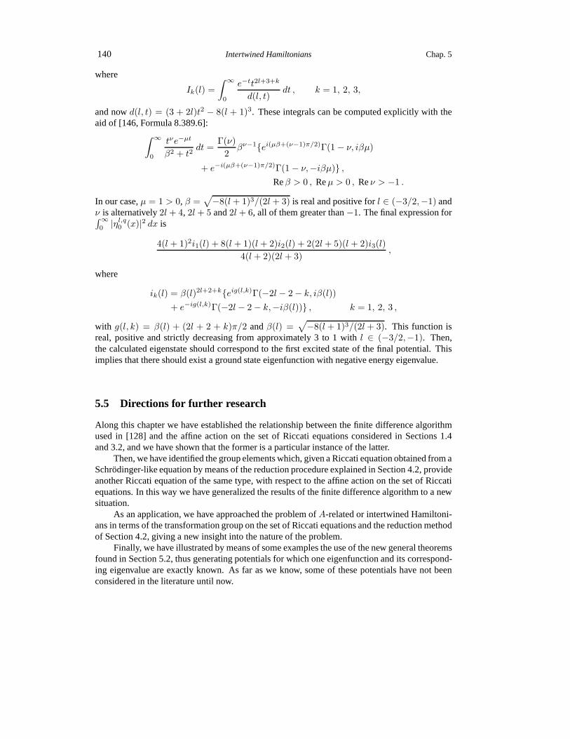
140 Intertwined Hamiltonians Chap. 5
where
Ik(l) =
∫ ∞
0
e−tt2l+3+k
d(l, t)dt , k = 1, 2, 3,
and nowd(l, t) = (3 + 2l)t2 − 8(l + 1)3. These integrals can be computed explicitly with theaid of [146, Formula 8.389.6]:
∫ ∞
0
tνe−µt
β2 + t2dt =
Γ(ν)
2βν−1ei(µβ+(ν−1)π/2)Γ(1− ν, iβµ)
+ e−i(µβ+(ν−1)π/2)Γ(1− ν,−iβµ) ,Reβ > 0 , Reµ > 0 , Reν > −1 .
In our case,µ = 1 > 0, β =√−8(l+ 1)3/(2l + 3) is real and positive forl ∈ (−3/2,−1) and
ν is alternatively2l+ 4, 2l+ 5 and2l+ 6, all of them greater than−1. The final expression for∫∞0 |ηl,q0 (x)|2 dx is
4(l + 1)2i1(l) + 8(l + 1)(l+ 2)i2(l) + 2(2l+ 5)(l + 2)i3(l)
4(l+ 2)(2l + 3),
where
ik(l) = β(l)2l+2+keig(l,k)Γ(−2l− 2− k, iβ(l))
+ e−ig(l,k)Γ(−2l− 2− k,−iβ(l)) , k = 1, 2, 3 ,
with g(l, k) = β(l) + (2l + 2 + k)π/2 andβ(l) =√−8(l+ 1)3/(2l+ 3). This function is
real, positive and strictly decreasing from approximately3 to 1 with l ∈ (−3/2,−1). Then,the calculated eigenstate should correspond to the first excited state of the final potential. Thisimplies that there should exist a ground state eigenfunction with negative energy eigenvalue.
5.5 Directions for further research
Along this chapter we have established the relationship between the finite difference algorithmused in [128] and the affine action on the set of Riccati equations considered in Sections 1.4and 3.2, and we have shown that the former is a particular instance of the latter.
Then, we have identified the group elements which, given a Riccati equation obtained from aSchrodinger-like equation by means of the reduction procedure explained in Section 4.2, provideanother Riccati equation of the same type, with respect to the affine action on the set of Riccatiequations. In this way we have generalized the results of thefinite difference algorithm to a newsituation.
As an application, we have approached the problem ofA-related or intertwined Hamiltoni-ans in terms of the transformation group on the set of Riccatiequations and the reduction methodof Section 4.2, giving a new insight into the nature of the problem.
Finally, we have illustrated by means of some examples the use of the new general theoremsfound in Section 5.2, thus generating potentials for which one eigenfunction and its correspond-ing eigenvalue are exactly known. As far as we know, some of these potentials have not beenconsidered in the literature until now.

Sec. 5.5 Directions for further research 141
Notwithstanding, there are some aspects which can be improved. The first is that it is possi-ble to explain the problem ofA-related or intertwinned Hamiltonians by using similar techniques,but using only Schrodinger-like equations, without need of passing everything to the Riccatilevel. The key is to consider the linear action ofGL(2, R) (rather thanSL(2, R)) on R2 andthe associated Lie systems. In addition, this allows to generalize the validity of Theorems 5.2.1and 5.2.2, and hence of Corollary 5.2.2, in the following sense:
Theorem 5.5.1. Letw(x) be a solution of the Riccati equation
w′ + w2 = V (x) − ǫ
for some specific functionV (x) and constantǫ. Let γ(x) be a never vanishing differentiablefunction defined on the domain ofV (x) and letc be a non-vanishing constant. Then, ifv(x) is asolution of the Riccati equation
v′ + v2 = V (x) +c
γ2(x)− ǫ ,
such that is defined in the same domain asw(x), andw(x) − v(x) does not vanish, the functionw(x) defined by
w(x) = −v(x)− c/γ2(x)
w(x) − v(x)+γ′(x)
γ(x)
is a solution of the Riccati equation
w′ + w2 = V (x)− 2
(γ′
γv + v′
)+γ′′
γ− ǫ .
This theorem has also a counterpart at the Schrodinger level:
Theorem 5.5.2. Letφw(x) be a solution of the homogeneous linear second order differ-ential equation
−φ′′w + (V (x)− ǫ)φw = 0 ,
for some specific functionV (x) and constantǫ. Let γ(x) be a never vanishing differentiablefunction defined on the domain ofV (x) and let c be a non-vanishing constant. Then, if thefunctionφv(x) 6= φw(x) is a solution of the equation
−φ′′v +(V (x) +
c
γ2(x)− ǫ
)φv = 0 ,
defined in the same domain asφw(x), then the functionφw(x) defined (up to a non-vanishingmultiplicative constant) by
φw = γ
(− d
dx+φ′vφv
)φw ,
satisfies the new equation
−φ′′w +
V (x)− 2
(γ′
γv + v′
)+γ′′
γ− ǫ
φw = 0 ,

142 Intertwined Hamiltonians Chap. 5
where the functionv(x) is defined (locally) asφ′v/φv = v.
As a consequence, we recover, in its full generality, the Darboux theorem:
Corollary 5.5.1 (Darboux theorem [104,174]). Letφw(x) be a solution of the homo-geneous linear second order differential equation
−φ′′w + (V (x)− ǫ)φw = 0 ,
for some specific functionV (x) and constantǫ. Let c be a non-vanishing constant. Then, if thefunctionφv(x) 6= φw(x) is a solution of the equation
−φ′′v + (V (x) + c− ǫ)φv = 0 ,
defined in the same domain asφw(x), then the functionφw(x) defined (up to a non-vanishingmultiplicative constant) by
φw =
(− d
dx+φ′vφv
)φw ,
satisfies the new equation
−φ′′w + (V (x) − 2 v′ − ǫ)φw = 0 ,
where the functionv(x) is defined (locally) asφ′v/φv = v.
On the other hand, these results can be checked by direct computation, and are derived indetail in a work in preparation.
The fact that the constantc can be any non-zero real number instead of 1 opens the possi-bility of finding more examples of application of Theorem 5.5.2 to other potentials than thosetreated in Section 5.4. To this respect, in principle, it seems that the potentials found in Chapter 4are good candidates, since the respective spectral problems are exactly solvable. We wonder aswell about whether it will be possible to consider explicitly other non square-integrable eigen-functions, without zeros, of the intermediate potential, even if they have no physical interpreta-tion. This means, in some sense, to adapt to our current method the idea introduced by Mielnikin [238], and developed later in [108,111,124,263], amongst other articles.
Finally, a finite difference formula has been used by Adler inorder to discuss the Backlundtransformations of the Painleve equations [3,4], also related with what are calleddressing chainsand the well-known Korteweg–de Vries equation, see [298, 326] and references therein. More-over, the Darboux transformation can be generalized by using more than one intermediate eigen-function of the original problem [104]. Likewise, there exist generalizations of the usual inter-twining technique to spaces with dimension greater than one[15–17], includingn-dimensionaloriented Riemannian manifolds [142]. The natural questionis whether there is some relationshipbetween these subjects and the affine action on the set of Riccati equations, or on other type ofLie systems.
We hope to develop some of these aspects in the future.

Chapter 6
Classical and quantum Hamiltonian Lie systems
We consider in this chapter other applications of the theoryof Lie systems in physics. Morespecifically, we will study the particular case where the Liesystems of interest are Hamiltoniansystems as well, both in the classical and quantum frameworks.
Time-dependent quantum Hamiltonians are not studied so often as their autonomous coun-terparts, because it is generally difficult to find their timeevolution. However, in the case thesystem could be treated as a Lie system in a certain Lie group,the calculation of the evolutionoperator is reduced to the problem of integrating such a Lie system.
After a brief description of the systems in classical and quantum mechanics which areHamiltonian as well as Lie systems, we will focus our attention on the particularly interestingexample of classical and quantum quadratic time-dependentHamiltonians. Particular examplesof this kind of systems, mainly in the quantum approach, and ocasionally in the classical one,have been studied by many authors. Some of them, incidentally, have used certain aspects ofthe theory of Lie systems but without knowing, most of the times, that such properties have ageometric origin, or the relations with other properties. Thus, some results of references in thisfield like [27, 81, 83, 87, 89, 129, 132, 150, 167, 179, 195, 196, 218, 224–227, 252, 253, 264–267,313, 331, 333, 338,340] and references therein, could be better understood under the light of thetheory of Lie systems.
However, instead of trying to give a detailed account of all these approaches in an uni-fied view provided by the mentioned theory, we will limit ourselves to develop some exampleswhere the usefulness of the theory of Lie systems can be clearly appreciated. In this sense, thesimple case of both the classical and quantum time-dependent linear potential will be explicitlysolved. We will solve as well a slightly generalized versionof the harmonic oscillator with atime-dependent driving term, linear in the position, solved in [81, 196] by means of the Magnusexpansion.
6.1 Hamiltonian systems of Lie type
Consider the usual mathematical framework for problems in classical mechanics, i.e., a sym-plectic manifold(M,Ω), with appropriately chosen Hamiltonian vector fields describing thedynamics of the system of interest. Thus, a Lie system in thisapproach can be constructed bymeans of a linear combination, witht-dependent coefficients, of Hamiltonian vector fieldsXα
closing on a real finite-dimensional Lie algebra.
143

144 Classical and quantum Hamiltonian Lie systems Chap. 6
These vector fields correspond to a symplectic action of a LiegroupG on the symplecticmanifold(M,Ω). However, note that the Hamiltonian functions of such vector fieldshXα
≡ hα,defined byi(Xα)Ω = −dhα, do not close in general the same Lie algebra when the Poissonbracket is considered, but we can only say that
d(hα, hβ − h[Xα,Xβ ]
)= 0 ,
and therefore they span a Lie algebra which is an extension ofthe original one.The situation in quantum mechanics is quite similar. It is well-known that a separable
complex Hilbert space of statesH can be seen as a real manifold admitting a global chart [52].The Abelian translation group allows us to identify the tangent spaceTφH at any pointφ ∈ Hwith H itself, where the isomorphism which associatesψ ∈ H with the vectorψ ∈ TφH is givenby
ψf(φ) :=
(d
dtf(φ+ tψ)
)
|t=0
,
for anyf ∈ C∞(H).The Hilbert spaceH is endowed with a symplectic 2-formΩ defined by
Ωφ(ψ, ψ′) = 2 Im〈ψ|ψ′〉 ,
where〈·|·〉 denotes the Hilbert inner product onH.By means of the identification ofH with TφH, a continuous vector field is just a continuous
mapA : H → H. Therefore, a linear operatorA onH is a special kind of vector field.Given a smooth functiona : H → R, its differentialdaφ atφ ∈ H is an element of the (real)
dual spaceH′ of H, given by
〈daφ , ψ〉 :=(d
dta(φ+ tψ)
)
|t=0
.
Now, as it has been pointed out in [52], the skew-self-adjoint linear operators inH defineHamiltonian vector fields, the Hamiltonian function of−i A for a self-adjoint operatorA beinga(φ) = 1
2 〈φ,Aφ〉. The Schrodinger equation plays then the role of Hamiltonequations becauseit determines the integral curves of the vector field−iH .
In particular, a Lie system occurs in this framework when we have at-dependent quan-tum Hamiltonian that can be written as a linear combination,with t-dependent coefficients, ofHamiltoniansHα closing on a finite-dimensional real Lie algebra under the commutator bracket.However, note that this Lie algebra does not necessarily coincide with that of the correspondingclassical problem, but it may be a Lie algebra extension of the latter.
6.2 Time-dependent quadratic Hamiltonians
For the illustration of the classical and quantum situations described in the previous section, weconsider now the important examples provided by the time-dependent classical and quantumquadratic Hamiltonians.
The first one is the mechanical system for which the configuration space is the real lineR,with coordinateq, and the corresponding phase spaceT ∗R, with coordinates(q, p), is endowed

Sec. 6.2 Time-dependent quadratic Hamiltonians 145
with the canonical symplectic structureω = dq ∧ dp. The dynamics is described by the time-dependent classical Hamiltonian
H = α(t)p2
2+ β(t)
q p
2+ γ(t)
q2
2+ δ(t) p+ ǫ(t) q . (6.1)
The dynamical vector fieldΓH , solution of the dynamical equation
i(ΓH)ω = dH ,
is given by
ΓH =
(α(t) p+
1
2β(t) q + δ(t)
)∂
∂q−(1
2β(t) p+ γ(t) q + ǫ(t)
)∂
∂p, (6.2)
which can be rewritten as
ΓH = α(t)X1 + β(t)X2 + γ(t)X3 − δ(t)X4 + ǫ(t)X5 ,
with
X1 = p∂
∂q, X2 =
1
2
(q∂
∂q− p
∂
∂p
), X3 = −q ∂
∂p, X4 = − ∂
∂q, X5 = − ∂
∂p,
being vector fields which satisfy the following commutationrelations:
[X1, X2] = X1 , [X1, X3] = 2X2 , [X1, X4] = 0 , [X1, X5] = −X4 ,
[X2, X3] = X3 , [X2, X4] = −1
2X4 , [X2, X5] =
1
2X5 ,
[X3, X4] = X5 , [X3, X5] = 0 , [X4, X5] = 0 ,
and therefore they close on a five-dimensional real Lie algebra. Consider the five-dimensionalLie algebrag for which the defining Lie products are
[a1, a2] = a1 , [a1, a3] = 2 a2 , [a1, a4] = 0 , [a1, a5] = −a4 ,
[a2, a3] = a3 , [a2, a4] = −1
2a4 , [a2, a5] =
1
2a5 ,
[a3, a4] = a5 , [a3, a5] = 0 , [a4, a5] = 0 ,
in a certain basisa1, a2, a3, a4, a5. Then, the Lie algebrag is a semi-direct sum of theAbelian two-dimensional Lie algebra generated bya4, a5 with thesl(2,R) Lie algebra gen-erated bya1, a2, a3, i.e., g = R2 ⋊ sl(2, R). The corresponding Lie group will be thesemi-direct productG = T2 ⊙ SL(2,R) relative to the linear action ofSL(2,R) on the two-dimensional translation algebra. When computing the flows of the previous vector fieldsXα, wesee that they correspond to the affine action ofG onR2, and therefore, the vector fieldsXα canbe regarded as fundamental fields with respect to that action, associated to the previous basis ofR2 ⋊ sl(2, R).
In order to find the time-evolution provided by the Hamiltonian (6.1), i.e., the integral curvesof the time-dependent vector field (6.2), we can solve first the corresponding equation in the Lie

146 Classical and quantum Hamiltonian Lie systems Chap. 6
groupG and then use the affine action ofG onR2. We focus on the first of these questions: Weshould find the curveg(t) in G such that
g g−1 = −5∑
α=1
bα(t) aα , g(0) = e ,
with b1(t) = α(t), b2(t) = β(t), b3(t) = γ(t), b4(t) = −δ(t), andb5(t) = ǫ(t). The explicitcalculation can be carried out by using the generalized Wei–Norman method, i.e., writingg(t) interms of a set of second class canonical coordinates, for instance,
g(t) = exp(−v4(t)a4) exp(−v5(t)a5) exp(−v1(t)a1) exp(−v2(t)a2) exp(−v3(t)a3) .
The adjoint representation ofR2 ⋊ sl(2, R) reads in the previous basis
ad(a1) =
0 1 0 0 00 0 2 0 00 0 0 0 00 0 0 0 −10 0 0 0 0
, ad(a2) =
−1 0 0 0 00 0 0 0 00 0 1 0 00 0 0 −1/2 00 0 0 0 1/2
,
ad(a3) =
0 0 0 0 0−2 0 0 0 00 −1 0 0 00 0 0 0 00 0 0 1 0
, ad(a4) =
0 0 0 0 00 0 0 0 00 0 0 0 00 1/2 0 0 00 0 −1 0 0
,
ad(a5) =
0 0 0 0 00 0 0 0 00 0 0 0 01 0 0 0 00 −1/2 0 0 0
,
and therefore
exp(−v1 ad(a1)) =
1 −v1 v21 0 00 1 −2v1 0 00 0 1 0 00 0 0 1 v10 0 0 0 1
, exp(−v3 ad(a3)) =
1 0 0 0 02v3 1 0 0 0v23 v3 1 0 00 0 0 1 00 0 0 −v3 1
,
exp(−v4 ad(a4)) =
1 0 0 0 00 1 0 0 00 0 0 0 00 −v4/2 0 1 00 0 v4 0 1
, exp(−v5 ad(a5)) =
1 0 0 0 00 1 0 0 00 0 1 0 0
−v5 0 0 1 00 v5/2 0 0 1
,
and exp(−v2 ad(a2)) =
ev2 0 0 0 00 1 0 0 00 0 e−v2 0 0
0 0 0 ev2/2 0
0 0 0 0 e−v2/2
.
Then, a straightforward application of (2.28) leads to the system
v1 = b1(t) + b2(t) v1 + b3(t) v21 , v2 = b2(t) + 2 b3(t) v1 , v3 = ev2 b3(t) ,
v4 = b4 +1
2b2(t) v4 + b1(t) v5 , v5 = b5(t)− b3(t) v4 −
1
2b2(t) v5 ,

Sec. 6.2 Time-dependent quadratic Hamiltonians 147
with initial conditionsv1(0) = · · · = v5(0) = 0.For some specific choices of the functionsα(t), . . . , ǫ(t), the problem becomes simpler
and it may be enough to consider a subgroup, instead of the whole Lie groupG, to deal with thearising system. For instance, consider the classical Hamiltonian
H =p2
2m+ f(t) q ,
which in the notation of (6.1) has the only non-vanishing coefficientsα(t) = 1/m andǫ(t) =f(t). Then, the problem is reduced to one in a three-dimensional subalgebra, generated byX1, X4, X5. The associated Lie group will be the subgroup ofG generated bya1, a4, a5.This example will be used later for illustrating the theory:Since such a subgroup is solvable, theproblem can be integrated by quadratures.
Another remarkable property is that the Hamiltonian functionshα corresponding to theHamiltonian vector fieldsX1, . . . , X5, defined byi(Xα)ω = −dhα, i.e.,
h1(q, p) = −p2
2, h2(q, p) = −1
2q p , h3(q, p) = −q
2
2, h4(q, p) = p , h5(q, p) = −q ,
have the Poisson bracket relations
h1, h2 = h1 , h1, h3 = 2 h2 , h1, h4 = 0 , h1, h5 = −h4 ,
h2, h3 = h3 , h2, h4 = −1
2h4 , h2, h5 =
1
2h5 ,
h3, h4 = h5 , h3, h5 = 0 , h4, h5 = 1 ,
which do not coincide with those of the vector fieldsXα, because ofh4, h5 = 1, but they closeon a Lie algebra which is a central extension ofR2 ⋊ sl(2, R) by a one-dimensional subalgebra.An analogous Lie algebra appears as well in the quantum formulation of the problem.
Let us now consider the quantum case, see, e.g., [339, 340], with applications in a numberof physical problems, as for instance, the quantum motion ofcharged particles subject to time-dependent electromagnetic fields (see, e.g., [129] and references therein), and connects with thetheory of exact invariants developed by Lewis and Riesenfeld [224–226]. Other related refer-ences have been cited above.
A generic time-dependent quadratic quantum Hamiltonian isgiven by
H = α(t)P 2
2+ β(t)
QP + P Q
4+ γ(t)
Q2
2+ δ(t)P + ǫ(t)Q+ φ(t)I . (6.3)
whereQ andP are the position and momentum operators satisfying the commutation relation
[Q,P ] = i I .
The previous Hamiltonian can be written as a sum witht-dependent coefficients
H = α(t)H1 + β(t)H2 + γ(t)H3 − δ(t)H4 + ǫ(t)H5 − φ(t)H6 ,
of the Hamiltonians
H1 =P 2
2, H2 =
1
4(QP + P Q) , H3 =
Q2
2, H4 = −P , H5 = Q , H6 = −I ,

148 Classical and quantum Hamiltonian Lie systems Chap. 6
which satisfy the commutation relations
[iH1, iH2] = iH1 , [iH1, iH3] = 2 iH2 , [iH1, iH4] = 0 , [iH1, iH5] = −iH4 ,
[iH2, iH3] = iH3 , [iH2, iH4] = − i
2H4 , [iH2, iH5] =
i
2H5 ,
[iH3, iH4] = iH5 , [iH3, iH5] = 0 , [iH4, iH5] = iH6 ,
and [iHα, iH6] = 0, α = 1, . . . , 5. That is, the skew-self-adjoint operatorsiHα generate asix-dimensional real Lie algebra which is a central extension of the Lie algebra arising in theclassical case,R2 ⋊ sl(2, R), by a one-dimensional Lie algebra. It can be identified as thesemi-direct sum of the Heisenberg–Weyl Lie algebrah(3), which is an ideal in the total Lie algebra,with the Lie subalgebrasl(2,R), i.e.,h(3) ⋊ sl(2, R). Sometimes this Lie algebra is referredto as the extended symplectic Lie algebrahsp(2,R) = h(3) ⋊ sp(2, R). The correspondingLie group is the semi-direct productH(3)⊙SL(2,R) of the Heisenberg–Weyl groupH(3) withSL(2,R), see also [340].
The time-evolution of a quantum system can be described in terms of the evolution operatorU(t) which satisfies the Schrodinger equation (see, e.g., [91])
i ~dU
dt= H(t)U , U(0) = Id , (6.4)
whereH(t) is the Hamiltonian of the system. In our current case, the Hamiltonian is given by(6.3), and therefore the time-evolution of the system is given by an equation of the type
g g−1 = −6∑
α=1
bα(t) aα , g(0) = e , (6.5)
where we take~ = 1, with the identification ofg(t) with U(t), e with Id, iHα with aα forα ∈ 1, . . . , 6 and the time-dependent coefficientsbα(t) are given by
b1(t) = α(t) , b2(t) = β(t) , b3(t) = γ(t) ,
b4(t) = −δ(t) , b5(t) = ǫ(t) , b6(t) = −φ(t) .
The calculation of the solution of (6.5) can be carried out aswell by using the generalizedWei–Norman method, i.e., writingg(t) in terms of a set of second class canonical coordinates.We take, for instance, the factorization
g(t) = exp(−v4(t)a4) exp(−v5(t)a5) exp(−v6(t)a6)× exp(−v1(t)a1) exp(−v2(t)a2) exp(−v3(t)a3) ,
and therefore, the equation (2.28) leads in this case to the system
v1 = b1(t) + b2(t) v1 + b3(t) v21 , v2 = b2(t) + 2 b3(t) v1 , v3 = ev2 b3(t) ,
v4 = b4(t) +1
2b2(t) v4 + b1(t) v5 , v5 = b5(t)− b3(t) v4 −
1
2b2(t) v5 ,
v6 = b6(t) + b5(t) v4 −1
2b3(t) v
24 +
1
2b1(t) v
25 ,
with initial conditionsv1(0) = · · · = v6(0) = 0.

Sec. 6.3 Classical and quantum time-dependent linear potential 149
Analogously to what happened in the classical case, specialchoices of the time-dependentcoefficient functionsα(t), . . . , φ(t) may lead to problems for which the associated Lie algebrais a subalgebra of that of the complete system, and similarlyfor the Lie groups involved. Forexample, we could consider as well the quantum Hamiltonian linear in the positions
H =P 2
2m+ f(t)Q ,
which in the notation of (6.3) has the only non-vanishing coefficientsα(t) = 1/m andǫ(t) =f(t). This problem can be regarded as a Lie system asociated to thefour-dimensional Lie alge-bra generated byiH1, iH4, iH5, iH6, which is also solvable, and hence the problem can besolved by quadratures.
Another simple case is the generalization of the harmonic oscillator with a time-dependentdriving term, linear in the position, solved in [81,196] by means of the Magnus expansion:
H =~ω(t)
2(P 2 +Q2) + f(t)Q ,
which in the notation of (6.3) has the only non-vanishing coefficientsα(t) = γ(t) = ~ω(t) andǫ(t) = f(t). The case studied in the cited references takesω(t) equal to the constantω0 for allt. This problem can be regarded as a Lie system asociated to thefour-dimensional Lie algebragenerated byi(H1 +H3), iH4, iH5, iH6, which is solvable as well, and hence the problemcan be solved again by quadratures.
The treatment of this system according to the theory of Lie systems, as well as of the abovementioned classical and quantum time-dependent Hamiltonians, linear in the positions, is thesubject of the next sections.
6.3 Classical and quantum time-dependent linear potential
Let us consider the classical system described by the classical Hamiltonian
Hc =p2
2m+ f(t) q , (6.6)
and the corresponding quantum Hamiltonian
Hq =P 2
2m+ f(t)Q , (6.7)
describing, for instance whenf(t) = q E0 + q E cosωt, the motion of a particle of electricchargeq and massm driven by a monochromatic electric field, whereE0 is the strength ofthe constant confining electrical field andE that of the time-dependent electric field that drivesthe system with a frequencyω/2π. These models have been considered recently due to theirnumerous applications in physics, see, e.g., [27,150] and references therein.
Now, instead of using the Lewis and Riesenfeld invariant method [224–226], as it has beendone, for example, in [150], we will study in parallel the classical and the quantum problems byreduction of both of them to similar equations, and solving them by the generalized Wei–Normanmethod. The only difference between the two cases is that theLie algebra arising in the quantumproblem is a central extension of that of the classical one.

150 Classical and quantum Hamiltonian Lie systems Chap. 6
The classical Hamilton equations of motion for the Hamiltonian (6.6) are
q =p
m, p = −f(t) , (6.8)
and therefore, the motion is given by
q(t) = q0 +p0 t
m− 1
m
∫ t
0
dt′∫ t′
0
f(t′′) dt′′ ,
p(t) = p0 −∫ t
0
f(t′) dt′ . (6.9)
Thet-dependent vector field describing the time evolution is
X =p
m
∂
∂q− f(t)
∂
∂p.
This vector field can be written as a linear combination
X =1
mX1 − f(t)X2 ,
with
X1 = p∂
∂q, X2 =
∂
∂p,
being vector fields closing on a 3-dimensional Lie algebra withX3 = ∂/∂q, isomorphic to theHeisenberg–Weyl algebra, namely,
[X1, X2] = −X3 , [X1, X3] = 0 , [X2, X3] = 0 .
The flow of these vector fields is given, respectively, by
φ1(t, (q0, p0)) = (q0 + p0 t, p0) ,
φ2(t, (q0, p0)) = (q0, p0 + t) ,
φ3(t, (q0, p0)) = (q0 + t, p0) .
In other words,X1, X2, X3 are fundamental vector fields with respect to the action of theHeisenberg–Weyl groupH(3), realized as the Lie group of upper triangular3 × 3 matrices, onR2, given by
qp1
=
1 a1 a30 1 a20 0 1
qp1
.
Note thatX1, X2 andX3 are Hamiltonian vector fields with respect to the usual symplec-tic structure,Ω = dq ∧ dp, meanwhile the corresponding Hamiltonian functionshα such thati(Xα)Ω = −dhα are
h1 = −p2
2, h2 = q , h3 = −p ,
thereforeh1, h2 = −h3 , h1, h3 = 0 , h2, h3 = −1 .

Sec. 6.3 Classical and quantum time-dependent linear potential 151
Then, the functionsh1, h2, h3 close on a four-dimensional Lie algebra withh4 = 1 under thePoisson bracket, which is a central extension of that generated byX1, X2, X3.
Let a1, a2, a3 be a basis of the Lie algebra with the only non-vanishing defining relation[a1, a2] = −a3. Then, the corresponding equation in the groupH(3) to the system (6.8) reads
g g−1 = − 1
ma1 + f(t) a2 .
Using the Wei–Norman formula (2.28) withg = exp(−u3 a3) exp(−u2 a2) exp(−u1 a1) wearrive to the system of differential equations
u1 =1
m, u2 = −f(t) , u3 =
u2m
,
together with the initial conditionsu1(0) = u2(0) = u3(0) = 0. The solution is
u1 =t
m, u2 = −
∫ t
0
f(t′) dt′ , u3 = − 1
m
∫ t
0
dt′∫ t′
0
f(t′′) dt′′ .
Therefore, the motion is given by
qp1
=
1 tm − 1
m
∫ t0dt′∫ t′0f(t′′) dt′′
0 1 −∫ t0f(t′) dt′
0 0 1
q0p01
,
in agreement with (6.9). Thus, we can identify the constant of the motion given in [150],
I1 = p(t) +
∫ t
0
f(t′) dt′ ,
together with the other one
I2 = q(t)− 1
m
(p(t) +
∫ t
0
f(t′) dt′)t+
1
m
∫ t
0
dt′∫ t′
0
f(t′′) dt′′ ,
as the initial conditions of the system, thanks to the identification of the system as a Lie system.As far as the quantum problem is concerned, also studied in [27], notice that the quantum
HamiltonianHq may be written as a sum
Hq =1
mH1 − f(t)H2 ,
with
H1 =P 2
2, H2 = −Q .
The skew-self-adjoint operators−iH1 and−iH2 close on a four-dimensional Lie algebrawith −iH3 = −i P , and−iH4 = i I, isomorphic to the above mentioned central extension ofthe Heisenberg–Weyl Lie algebra,
[−iH1,−iH2]=−iH3 , [−iH1,−iH3]=0 , [−iH2,−iH3]=−iH4 .

152 Classical and quantum Hamiltonian Lie systems Chap. 6
As we have seen in the preceding section, the time-evolutionof our current system is de-scribed by means of the evolution operatorU , which satisfies (we take~ = 1)
dU
dt= −iHqU , U(0) = Id .
This equation can be identified as that of a Lie system in a Lie group such that its Lie algebra isthe one mentioned above. Leta1, a2, a3, a4 be a basis of the Lie algebra with non-vanishingdefining relations[a1, a2] = a3 and[a2, a3] = a4. The equation in the Lie group to be consideredis now
g g−1 = − 1
ma1 + f(t) a2 .
Using g = exp(−u4 a4) exp(−u3 a3) exp(−u2 a2) exp(−u1 a1), the Wei–Norman formula(2.28) provides the following equations:
u1 =1
m, u2 = −f(t) ,
u3 = − 1
mu2 , u4 = f(t)u3 +
1
2mu22 ,
together with the initial conditionsu1(0) = · · · = u4(0) = 0, whose solution is
u1(t) =t
m, u2(t) = −
∫ t
0
f(t′) dt′ , u3(t) =1
m
∫ t
0
dt′∫ t′
0
f(t′′) dt′′ ,
and
u4(t) =1
m
∫ t
0
dt′f(t′)
∫ t′
0
dt′′∫ t′′
0
f(t′′′) dt′′′ +1
2m
∫ t
0
dt′(∫ t′
0
dt′′f(t′′)
)2
.
These functions provide the explicit form of the time-evolution operator:
U(t,0)=exp(−iu4(t))exp(iu3(t)P )exp(−iu2(t)Q)exp(iu1(t)P2/2) .
However, in order to find the time evolution of a wave-function in a simple way, it is advan-tageous to use instead the factorization
g = exp(−v4 a4) exp(−v2 a2) exp(−v3 a3) exp(−v1 a1) .
In such a case, the Wei–Norman formula (2.28) gives the system
v1 =1
m, v2 = −f(t) ,
v3 = − 1
mv2 , v4 = − 1
2mv22 ,
with initial conditionsv1(0) = · · · = v4(0) = 0. The solution is
v1(t) =t
m, v2(t) = −
∫ t
0
dt′ f(t′) ,

Sec. 6.4 Quantum harmonic oscillator with a time-dependent perturbationlinear in the positions 153
v3(t) =1
m
∫ t
0
dt′∫ t′
0
dt′′f(t′′) ,
v4(t) = − 1
2m
∫ t
0
dt′(∫ t′
0
dt′′f(t′′)
)2
.
Then, applying the evolution operator onto the initial wave-functionφ(p, 0), which is assumedto be written in momentum representation, we have
φ(p, t) = U(t, 0)φ(p, 0)
= exp(−iv4(t))exp(−iv2(t)Q)exp(iv3(t)P ) exp(iv1(t)P2/2)φ(p, 0)
= exp(−iv4(t)) exp(−iv2(t)Q)ei(v3(t)p+v1(t)p2/2)φ(p, 0)
= exp(−iv4(t))ei(v3(t)(p+v2(t))+v1(t)(p+v2(t))2/2)φ(p+ v2(t), 0) ,
where the functionsvi(t) are given by the preceding equations.
6.4 Quantum harmonic oscillator with a time-dependent perturbationlinear in the positions
Let us consider now the quantum system described by the Hamiltonian
Hq =~ω(t)
2(P 2 +Q2) + f(t)Q , (6.10)
which corresponds to a slight generalization of the quantumharmonic oscillator, with a time-dependent driving term linear in the position, solved in [81, 196] by means of the Magnus ex-pansion. In these references it has been takenω(t) = ω0 for all t. However, we will show thatthe theory of Lie systems gives the exact solution as well, and in the same way, for the case ofnon-constantω.
The Hamiltonian (6.10) may be written now as a sum
H = ~ω(t)H1 + f(t)H2 ,
with
H1 =1
2(P 2 +Q2) , H2 = Q .
The skew-self-adjoint operatorsiH1 and iH2 close on a four-dimensional Lie algebra withiH3 = i P , and iH4 = −i I, given by
[iH1, iH2] = iH3 , [iH1, iH3] = −iH2 , [iH2, iH3] = iH4 ,
and[iHα, iH4] = 0, α = 1, 2, 3. This Lie algebra can be regarded as a central extension of theLie algebra of the Euclidean group in the plane,se(2), by an onedimensional Lie algebra. Wewill consider Lie systems with associated Lie algebrase(2) when treating control systems, cf.Subsection 7.3.1.
As in preceding cases, the time-evolution of our current system is given by the equation(6.4). With the identification ofg(t) with the evolution operatorU(t), e with Id, iHα with aαfor α ∈ 1, . . . , 4, it takes the form
g g−1 = −b1(t)a1 − b2(t)a2 , g(0) = e , (6.11)

154 Classical and quantum Hamiltonian Lie systems Chap. 6
where the non-vanishing time-dependent coefficients areb1(t) = ω(t) andb2(t) = f(t)/~. Theelementsa1, a2, a3, a4 make up a basis of the Lie algebra with defining relations
[a1, a2] = a3 , [a1, a3] = −a2 , [a2, a3] = a4 ,
and[aα, a4] = 0, for α = 1, 2, 3. Note thata2, a3, a4 generate a Lie subalgebra isomorphicto the Heisenberg–Weyl Lie algebrah(3).
In order to solve the equation, we will apply the Wei–Norman method. We write the solutionof (6.11) as the product
g = exp(−v1 a1) exp(−v2 a2) exp(−v3 a3) exp(−v4 a4) . (6.12)
The adjoint representation of the Lie algebra reads now
ad(a1) =
0 0 0 00 0 −1 00 1 0 00 0 0 0
, ad(a2) =
0 0 0 00 0 0 0−1 0 0 00 0 1 0
,
ad(a3) =
0 0 0 01 0 0 00 0 0 00 −1 0 0
, ad(a4) = 0 ,
and therefore
exp(−v1 ad(a1)) =
1 0 0 00 cos v1 sin v1 00 − sin v1 cos v1 00 0 0 1
, exp(−v2 ad(a2)) =
1 0 0 00 1 0 0v2 0 1 0
−v22/2 0 −v2 1
,
exp(−v3 ad(a3)) =
1 0 0 0−v3 1 0 00 0 1 0
−v23/2 v3 0 1
, exp(−v4 ad(a4)) = Id .
The application of the Wei–Norman formula (2.28) yields thesystem of differential equations
v1 = b1(t) , v2 = b2(t) cos v1 , v3 = b2(t) sin v1 , v4 = b2(t) v2 sin v1 ,
with initial conditionsv1(0) = · · · = v4(0) = 0. If we denoteB1(t) =∫ t0b1(s) ds, the solution
of the system is
v1(t) = B1(t) , v2(t) =
∫ t
0
b2(s) cosB1(s) ds , v3(t) =
∫ t
0
b2(s) sinB1(s) ds ,
v4(t) =
∫ t
0
(∫ s
0
b2(r) cosB1(r) dr
)b2(s) sinB1(s) ds . (6.13)
Therefore, the evolution operator for the system describedby the Hamiltonian (6.10) is
U(t) = exp(−iv1(t)(P 2 +Q2)/2) exp(−iv2(t)Q) exp(−iv3(t)P ) exp(iv4(t)) ,

Sec. 6.4 Quantum harmonic oscillator with a time-dependent perturbationlinear in the positions 155
wherev1(t), v2(t), v3(t) andv4(t) are given by (6.13), andb1(t) = ω(t), b2(t) = f(t)/~.This solution is equivalent to that given in [81,196] when, in particular, we takeω(t) = ω0.
Notwithstanding, in order to see it, we have to write the expression in a slightly different form,which is what we do next.
Sincea2, a3, a4 generate a Lie subalgebra isomorphic to the Heisenberg–Weyl Lie alge-brah(3), with commutation relations
[a2, a3] = a4 , [a2, a4] = 0 , [a3, a4] = 0 ,
it is easy to check, for example by using the well-known Baker–Campbell–Hausdorff formulas[240,324], that
exp(aa2) exp(ba3) exp(ca4) = exp(aa2 + ba3 + (c+ ab/2)a4) ,
for all a, b, c ∈ R. We will see this with detail in Subsection 7.2.1.Thus, the solution (6.12) can be written as
g = exp(−v1 a1) exp(−v2 a2 − v3 a3 + (v2v3/2− v4)a4) ,
and therefore the evolution operator takes the form
U(t) = exp
(− i v1(t)
2(P 2 +Q2)
)exp
(−i[v2(t)Q + v3(t)P +
v2(t)v3(t)
2− v4(t)
]).
(6.14)We compute now the arguments of the exponentials in the particular case ofb1(t) = ω0 andb2(t) = f(t)/~. The solution (6.13) becomes
v1(t) = ω0t , v2(t) =1
~
∫ t
0
f(s) cos(ω0s) ds , v3(t) =1
~
∫ t
0
f(s) sin(ω0s) ds ,
v4(t) =1
~2
∫ t
0
(∫ s
0
f(r) cos(ω0r) dr
)f(s) sin(ω0s) ds .
Then, we have thatv2(t)Q + v3(t)P + 12v2(t)v3(t)− v4(t) is equal to
Q
~
∫ t
0f(s) cos(ω0s)ds+
P
~
∫ t
0f(s) sin(ω0s) ds+
1
2~2
(∫ t
0f(s) cos(ω0s) ds
)(∫ t
0f(s) sin(ω0s) ds
)
−1
~2
∫ t
0
(∫ s
0f(r) cos(ω0r) dr
)
f(s) sin(ω0s) ds ,
where the last two terms become
1
2~2
∫ t
0
∫ s
0
f(s)f(r) sin(ω0(r − s)) dr ds
by using the relation(∫ t
0f(s) cos(ω0s)ds
)(∫ t
0f(s) sin(ω0s) ds
)
=
∫ t
0
(∫ s
0f(r) sin(ω0r) dr
)
f(s) cos(ω0s) ds+
∫ t
0
(∫ s
0f(r) cos(ω0r) dr
)
f(s) sin(ω0s) ds ,

156 Classical and quantum Hamiltonian Lie systems Chap. 6
which is a consequence of the formula of integration by parts.
In summary, if we define the functionsφ(t) andψ(t) by
φ(t) =1
~
∫ t
0
f(s)eiω0s ds ,
ψ(t) =1
~2
∫ t
0
∫ s
0
f(s)f(r) sin(ω0(r − s)) dr ds ,
we see that the evolution operator (6.14) becomes
U(t) = exp
(− i ω0t
2(P 2 +Q2)
)exp
(−i(QReφ(t) + P Imφ(t)) − i
2ψ(t)
),
which is exactly the result given in [81,196].
6.5 Comments and directions for further research
As we have indicated at the beginning of this chapter, we havetried to illustrate how a specialkind of Hamiltonian systems can be dealt with by means of the theory of Lie systems, in theclassical and quantum approaches. The theory allows us to obtain known results as well as newones, and all of them are interpreted much more clearly in theunified geometric frameworkit provides. Very likely, the further application of the theory, including the reduction of Liesystems, to these and other related examples will give new results of interest. We intend to treatthese questions in the future.
On the other hand, thinking of quantum Hamiltonian systems,it is known that linear sys-tems, like the Schrodinger equation, can be thought of as defining horizontal curves of a con-nection [23]. The same property is suggested in [249], when the transformation properties of theevolution equation under certain gauge changes are considered. We know from Section 2.6 thatLie systems can be interpreted in terms of connections in principal and associated bundles. Thus,it seems to be interesting to develop these aspects further.
Finally, let us remark that other quantum Hamiltonian systems, where the Hilbert space isfinite-dimensional, can be dealt with the theory of Lie systems as well. Examples are then-levelsystems treated in [249], and the non-relativistic dynamics of a spin1/2 particle, when only thespinorial part is considered, see, e.g., [70] and references therein.

PART 3
LIE SYSTEMS IN CONTROL THEORY


Chapter 7
Lie systems and their reduction in control theory
7.1 Introduction
This chapter is devoted to the application of the theory of Lie systems in the subject of (geomet-ric) control theory. It turns out that certain specific examples of Lie systems (although they havenot been referred to with this name) and some of their features have been considered before inthis field, although without recognizing that a common geometric structure is shared by them. Inparticular, systems which can be related by means of the theory developed in previous chapters,specifically in Chapter 2, are sometimes considered only on their own, and not as related withother systems.
Notwithstanding, some previous work in control theory, which can be related with Lie sys-tems and the associated theory, are worth mentioning. Some works of Brockett [55, 56] areamongst the first considerations of control systems on matrix Lie groups, and then on homoge-neous spaces, with and without drift. Some important questions which can be related with thetheory of Lie systems are treated therein. Specifically, he considers there the minimal Lie alge-bra containing the input vector fields of the system of interest, tries to express the solution as aproduct of exponentials, inspired by the Wei–Norman method, and establishes the equivalenceof matrix Lie systems if the underlying Lie algebras are isomorphic. In addition, he studies theassociated controllability, observability, and optimal control problems.
Almost simultaneously, and closely related, other important works by Jurdjevic and Suss-mann about the controllability of control systems in (matrix) Lie groups and homogeneousspaces, with drift and drift-free, appeared [190, 321]. These two articles have had an importantinfluence in further research, see, e.g., [188,189,207].
In addition, the formulation of control systems on Lie groups and homogeneous spaceshas been shown to be appropriate in some other situations of practical interest. For example,Crouch shows that in the problem of “dynamical realizationsof finite Volterra series,” the statespace is naturally identified as a homogeneous space of certain nilpotent Lie groups [98]. Herealizes that the group theoretical point of view provides an unifying approach for the study ofthese systems. Moreover, as Krener showed in [204], affine control systems enter in the bilinearrealization as well as in the nonlinear realization of the so-called input-output maps. These affinecontrol systems are then formulated in matrix Lie groups. Inother words, it is considered, ina particular case, the idea of studying the system in the associated Lie group coming from thesystem formulated in a homogeneous space.
159
160 Lie systems in control theory Chap. 7
There has been since then an important line of research aboutaspects of control systems inLie groups. For example, Baillieul [26] considers systems,which turn out to be of Lie type, inmatrix Lie groups and affine in the controls, from the point ofview of optimal control and usingthe Pontryagin Maximum Principle [279]. The controllability, accesibility, and other questionsconcerning control systems formulated on Lie groups have been studied also in [49,50].
As an example, the control and controllability of spin and quantum systems can be seen asaffine or linear control systems defined on certain Lie groups, which describe the time evolutionof the system. These problems are of increasing interest, due to their potential technologicalapplications, see, e.g., [7,138,194]. The study of the evolution operators in quantum mechanicsis the subject of many studies in the physics literature, see, e.g., [240,260] and references therein.Mainly focused to control theory, similar studies of the evolution flows as the ordered temporalproduct of a product of exponentials or only one exponentialhas been carried out in [6], seealso [115,116,315].
Typically, Lie systems appear as the kinematic part of control systems formulated on Liegroups and homogeneous spaces, which are treated with the techniques of optimal control [47,120, 182–187, 250], variational calculus [42–44], or othercriteria, as in the case of the pathplanning problem [257–259].
Very related to this last problem, the path planning problemof (nonholonomic) systems(see, e.g., [123, 199] and references therein), there existtechniques of approximation of controlsystems, affine or linear in the controls, by systems with an underlying solvable Lie algebra[100, 165], or even nilpotent [164, 165, 204, 208–210, 320].In this last case there is a wholeline of research devoted to the nilpotentization of systemsby means of state space feedbacktransformations, see, e.g., [166, 255–258, 308] and references therein. In either case, the finalsystem can be considered as a Lie system with an associated solvable or nilpotent Lie algebra,respectively. As indicated in [216], the nonholonomic motion planning of nilpotent systems mayneed to make use of a further analysis of the involved geometry [141,325].
Another line of research, which relates control theory and extremal problems in singularRiemannian or sub-Riemannian geometry, initiated in [58],continued, e.g., in [59,220,247,315],and further developed in [251], has also a relation with the theory of Lie systems. Indeed, inthese problems, some of the systems under consideration canbe regarded, to some extent, as Liesystems, in particular the systems appearing in [58,59]. Thus, it seems that the application of thetheory of Lie systems could be helpful to relate the results of the corresponding optimal controlproblems.
Other field within control theory where the theory of Lie systems may play a role is in thestudy of the so-called “recursive estimators” and “conditional densities” [57], where there appeartwo related Lie systems with associated Lie algebras, respectively,R2⋊so(1, 1) and one centralextension of it byR. This is in turn closely related to the identification of a problem of Kalmanfiltering with the integration of a Lie system with Lie algebraR2 ⋊ so(1, 1) [246].
Needless to say, a complete account of the relation and applications of the theory of Liesystems with all these subjects would require much more workthan that what is presented here.However, it is our aim to illustrate how the theory of Lie systems can be applied in specific prob-lems which appear in the control theory literature, obtaining in this way some other interestingresults and relations, based on the geometric sructure of these systems.
For example, we will be able to relate (in principle) different systems with the same associ-ated Lie algebra, and to solve them once the associated right-invariant Lie system is solved, e.g.,by means of the generalized Wei–Norman method, cf. Section 2.4.

Sec. 7.2 Brockett control system and related ones 161
Other new relations between some of the systems treated are obtained through the theory ofreduction of Lie systems, cf. Section 2.5, in the sense that the solution of some of these systemscan be reduced to the problem of solving some other of them andcertain right-invariant Liesystem on a Lie group. The reduction theory also allows us to obtain other specific realizationsof a given control system of Lie type, by considering other homogeneous spaces of the Lie groupassociated to the given system.
This shows that taking into account the geometric structureof control systems which arealso of Lie type may be useful for a better understanding of them, an important advantage beingthat the main properties are given in an intrinsic way, i.e.,not depending of a particular choice ofcoordinates. Therefore, it is natural the idea of transferring known results for a specific realizationof a Lie system to others with the same underlying Lie algebra, or amongst those which areobtained by reduction from another ones with larger Lie algebras. Perhaps the most interestingproblem to this respect is how the associated optimal control problems are related, although wewill leave this question for future research.
The outline of this chapter is as follows. The first section isdevoted to the study of the well-known Brockett system introduced in [58] and some other systems taken form the literature,which can be related with the former by means of our theory. The second section deals with thestudy of the application of the theory of Lie systems to well-known systems as the unicycle, thefront wheel driven kinematic car (pulling a trailer) and a set of chained trailers. In particular,we will see how some of these systems are reduced into other ones, and eventually, they canbe even related to the above mentioned Brockett system. In addition, we interpret the so-calledchained and power form systems under the light of the generalized Wei–Norman method. The Liesystems appearing in the first and second sections have associated nilpotent Lie algebras exceptfor the unicycle, which is associated to the solvable Lie algebrase(2). In the third section wewill study the kinematic equations of a generalization, dueto Jurdjevic, of the known as elasticproblem of Euler, see, e.g., [185]. It turns out that they areright-invariant Lie systems withassociated simple Lie algebras (except for the case ofse(2)), and in one case the Lie algebra isthat of the rotation group in three dimensions,so(3). In all these cases we apply the Wei–Normanmethod and the reduction theory, obtaining the corresponding systems on certain homogeneousspaces. We particularize all the previous expressions for the case ofSO(3), which is of interestin many other problems formulated on this Lie group. The caseof kinematic control equationson the groupSE(3) is considered next. We show, in particular, that the problemcan be reducedto other Lie systems inSO(3) andR3, by means of the reduction theory of Lie systems. Finally,we discuss some questions for future research in the last section.
7.2 Brockett control system and some generalizations
When dealing with problems of optimal control and their relation with singular Riemanniangeometry, Brockett introduced some well-known type of control systems [58] which are currentlyconsidered as one of the prototypical examples relating control theory and extremal problemsin sub-Riemannian geometry. Indeed, his approach has directly inspired subsequent papers as[247], further applications as in [315], and many other investigations, see, e.g., [59,220].
The simplest of these systems is known to be related with the tridimensional HeisenberggroupH(3), which is the non Abelian nilpotent Lie group of lowest dimension. It is therefore arelevant control system we could try to study from the viewpoint of Lie systems. We will studythis question with detail. In particular, we will see how other realizations of Lie systems with

162 Lie systems in control theory Chap. 7
associated Lie groupH(3) are possible, and how their solutions are related.Moreover, this kind of systems can be generalized in different directions. For example,
in [59] some extensions are classified according to levels ofcomplementary families to basisof exact differentials in two variables, and then the corresponding optimal control problems aretreated, appearing in their solution elliptic functions.
Other variations of the Brockett control system come from physical models, as the optimalcontrol problem of rigid bodies with two oscillators [341].For the case of planar rigid body, thereappears a system similar to that of [58], with the only difference that one equation is quadraticin the coordinates instead of linear. This system shares with the extensions treated in [59] theproperty that its optimal solutions are solvable as well by means of elliptic functions.
Other kind of nilpotent control systems, could also be related with the previous type of sys-tems, as certain systems from [255,258], which do not admit steering by using simple sinusoids.
We will treat these systems under the perspective of the theory of Lie systems, and will findrelations amongst them not previously present in the literature.
7.2.1 Brockett control systems
We will consider firstly the system originally introduced byBrockett in [58], and studied afterby a number of authors, see, e.g., [42–45,59,221,258,269,315]. That is, we are interested in thecontrol system inR3 with coordinates(x, y, z)
x = b1(t) , y = b2(t) , z = b2(t)x − b1(t)y , (7.1)
whereb1(t) andb2(t) are the control functions. The solutions of this system are the integralcurves of the time-dependent vector fieldb1(t)X1 + b2(t)X2, with
X1 =∂
∂x− y
∂
∂z, X2 =
∂
∂y+ x
∂
∂z. (7.2)
The Lie bracketX3 = [X1, X2] = 2 ∂∂z is linearly independent fromX1, X2, and the set
X1, X2, X3 spansR3 everywhere, so that according to Chow’s theorem [90, 203, 312] thesystem is controllable and we can reach any point from any other point, by selecting, for exam-ple, appropriate piecewise constant controlsb1(t) andb2(t). Moreover, they close on the Liealgebra defined by
[X1, X2] = X3 , [X1, X3] = 0 , [X2, X3] = 0 , (7.3)
isomorphic to the Lie algebrah(3) of the Heisenberg groupH(3).We will treat this system with the theory of Lie systems, in order to find its general solu-
tion for arbitrary controlsb1(t) andb2(t). Eventually, we could select these controls as thoseminimizing the integral cost function
∫ 1
0
(b21(s) + b22(s)) ds (7.4)
when the system is required to join two prescribed points in one unit of time. However, thisbelongs to the domain of optimal control theory and will not be considered here, this questionbeing treated in the literature cited. Instead, we will showthe application of the Wei–Normanand reduction methods in this case.
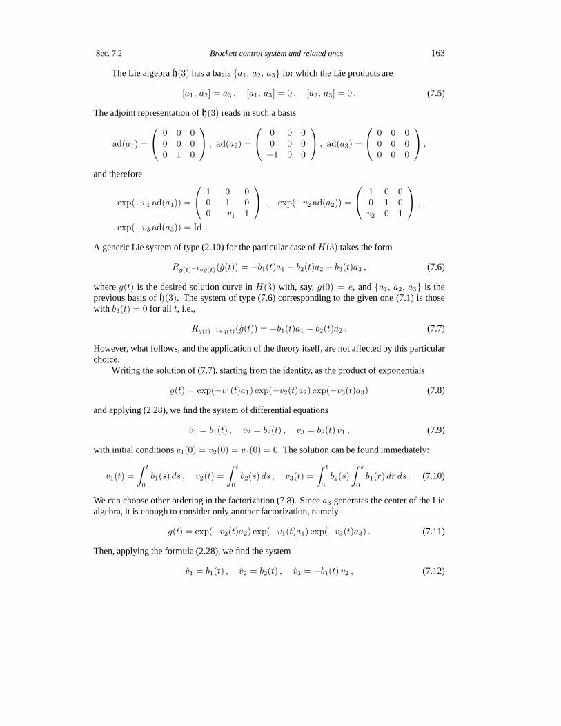
Sec. 7.2 Brockett control system and related ones 163
The Lie algebrah(3) has a basisa1, a2, a3 for which the Lie products are
[a1, a2] = a3 , [a1, a3] = 0 , [a2, a3] = 0 . (7.5)
The adjoint representation ofh(3) reads in such a basis
ad(a1) =
0 0 00 0 00 1 0
, ad(a2) =
0 0 00 0 0−1 0 0
, ad(a3) =
0 0 00 0 00 0 0
,
and therefore
exp(−v1 ad(a1)) =
1 0 00 1 00 −v1 1
, exp(−v2 ad(a2)) =
1 0 00 1 0v2 0 1
,
exp(−v3 ad(a3)) = Id .
A generic Lie system of type (2.10) for the particular case ofH(3) takes the form
Rg(t)−1∗g(t)(g(t)) = −b1(t)a1 − b2(t)a2 − b3(t)a3 , (7.6)
whereg(t) is the desired solution curve inH(3) with, say,g(0) = e, anda1, a2, a3 is theprevious basis ofh(3). The system of type (7.6) corresponding to the given one (7.1) is thosewith b3(t) = 0 for all t, i.e.,
Rg(t)−1∗g(t)(g(t)) = −b1(t)a1 − b2(t)a2 . (7.7)
However, what follows, and the application of the theory itself, are not affected by this particularchoice.
Writing the solution of (7.7), starting from the identity, as the product of exponentials
g(t) = exp(−v1(t)a1) exp(−v2(t)a2) exp(−v3(t)a3) (7.8)
and applying (2.28), we find the system of differential equations
v1 = b1(t) , v2 = b2(t) , v3 = b2(t) v1 , (7.9)
with initial conditionsv1(0) = v2(0) = v3(0) = 0. The solution can be found immediately:
v1(t) =
∫ t
0
b1(s) ds , v2(t) =
∫ t
0
b2(s) ds , v3(t) =
∫ t
0
b2(s)
∫ s
0
b1(r) dr ds . (7.10)
We can choose other ordering in the factorization (7.8). Sincea3 generates the center of the Liealgebra, it is enough to consider only another factorization, namely
g(t) = exp(−v2(t)a2) exp(−v1(t)a1) exp(−v3(t)a3) . (7.11)
Then, applying the formula (2.28), we find the system
v1 = b1(t) , v2 = b2(t) , v3 = −b1(t) v2 , (7.12)

164 Lie systems in control theory Chap. 7
with initial conditionsv1(0) = v2(0) = v3(0) = 0. The solution can be found immediately aswell:
v1(t) =
∫ t
0
b1(s) ds , v2(t) =
∫ t
0
b2(s) ds , v3(t) = −∫ t
0
b1(s)
∫ s
0
b2(r) dr ds . (7.13)
We would like to remark that this last system has been considered, following another lineof reasoning, in [320], compare (7.12) and (7.13) with theirequations (3.13) and (3.14).
Now, we want to use the solution of one of the systems (7.9) and(7.12) in order to find thegeneral solution of the given system (7.1). For doing that, we need to follow a general procedureapplicable also to other cases, which consists of obtainingbefore three other ingredients. Thefirst is to find a suitable parametrization of the Lie group involved, in this caseH(3), and theexpression of the composition law with respect to it. The second is to find the expression of thegroup action with respect to which the original vector fieldsare infinitesimal generators, in thechosen coordinates for the group. Thirdly, in case the chosen coordinates for the group are notthe second kind canonical coordinates with respect to whichthe associated Wei–Norman systemis written, we have to find the change of coordinates between them.
To this respect, if we have at hand a faithful linear representation of the Lie group involved,and a corresponding faithful linear representation of its Lie algebra, the work can be notablysimplified, and the differentials of right and left translations in the group become matrix products.However, this is not necessarily required by the theory and if we do not know it beforehand, tofind such a representation, can be a difficult or computationally involved problem.
When we have only the defining relations of the Lie algebra involved, a convenient set ofparameters of the group, may be the canonical coordinates ofthe first or second kind themselves.Then, we can try to find the composition law in these coordinates by using the well-knownBaker–Campbell–Hausdorff formula
exp(X) exp(Y ) = exp
(X + Y +
1
2[X, Y ] +
1
12([X, [X, Y ]] + [[X, Y ], Y ]) + · · ·
),
(7.14)which implies
exp(X) exp(Y ) = exp(Y ) exp(X) exp
([X, Y ] +
1
2[[X, Y ], X + Y ] + · · ·
), (7.15)
see, e.g., [240, 324]. The successive terms of the exponent in the right hand side of (7.14) canbe calculated in a recursive way, making use, for example, ofthe Lemma 2.15.3 of [324], andtherefore of the previous equation as well. However, when a number of terms is required, thecalculations can become extremely complicated, and in somecases it would be necessary to sumthe whole series (see, e.g., the expression in [240]). The terms involved would vanish, fromsome order on, for nilpotent Lie algebras, and therefore this method would be appropriate for Liesystems with associated non Abelian nilpotent Lie algebrasof moderately high dimension.
Another way of solving the problem, when possible, is just integrating the flow of a linearcombination with constant coefficients of the given vector fields, or composing the flows ofthese vector fields, which corresponds to the expression of the desired action written in terms ofcanonical coordinates of first and second kind, respectively. The second option is particularlywell suited to the problems we want to deal with. Then, the composition law in the respectivecoordinates can be obtained by the defining properties of a group action.

Sec. 7.2 Brockett control system and related ones 165
We will illustrate these last methods in our current particular case. Consider the linearcombination of the vector fieldsX1,X2 andX3 with constant coefficientsa, b, c,
Xabc = −aX1 − bX2 − cX3 = −a ∂∂x
− b∂
∂y− (ay − bx− 2c)
∂
∂z, (7.16)
whose flow is given by
φXabc(ǫ, (x, y, z)) = (x− ǫ a, y − ǫ b, z + (ay − bx− 2c)ǫ) .
Then, the action of the Heisenberg group onR3 with associated infinitesimal generatorsX1,X2
andX3 in terms of a set of canonical coordinates of the first kind(a, b, c) (that is, we parametrizeg ∈ H(3) asg = exp(aa1+ ba2+ ca3)) is obtained from the previous flow when we takeǫ = 1,sinceǫ can be regarded as being just a scaling factor. That is,
Φ : H(3)× R3 −→ R
3
((a, b, c), (x, y, z)) 7−→ (x− a, y − b, z + ay − bx− 2c) . (7.17)
It is clear that the coordinates of the neutral element should be(0, 0, 0), and from the requirementthat
Φ((a, b, c), Φ((a′, b′, c′), (x, y, z))) = Φ((a, b, c)(a′, b′, c′), (x, y, z)) , (7.18)
for all (x, y, z) ∈ R3, we obtain the group law ofH(3) written in terms of the previously definedcanonical coordinates of first kind,
(a, b, c)(a′, b′, c′) = (a+ a′, b+ b′, c+ c′ + (ab′ − ba′)/2) . (7.19)
Note that(a, b, c)−1 = (−a, −b, −c). This composition law can be verified by using (7.14)and the commutation relations of the Lie algebra in our current basis, and is essentially the sameas that used, e.g., in [39,247], see also [144].
Similarly, the action and the composition law can be writtenin terms of a set of canonicalcoordinates of second kind. To see this, consider the individual flows of the vector fieldsX1,X2,andX3,
φX1 (ǫ, (x, y, z)) = (x+ ǫ, y, z − yǫ) , φX2 (ǫ, (x, y, z)) = (x, y + ǫ, z + xǫ) ,
φX3(ǫ, (x, y, z)) = (x, y, z + 2ǫ) ,
then consider the composition of flows
φX1(−a, φX2(−b, φX3 (−c, (x, y, z)))) = (x − a, y − b, z + ay − bx− ab− 2c) , (7.20)
which provides the desired expression of the action in termsof the second kind canonical coor-dinates defined byg = exp(aa1) exp(ba2) exp(ca3), wheng ∈ H(3),
Φ : H(3)× R3 −→ R
3
((a, b, c), (x, y, z)) 7−→ (x − a, y − b, z + ay − bx− ab− 2c) . (7.21)
The neutral element is represented again by(0, 0, 0), as expected, and from the condition (7.18)we find the composition law ofH(3) in terms of the previously defined canonical coordinates ofsecond kind,
(a, b, c)(a′, b′, c′) = (a+ a′, b+ b′, c+ c′ − ba′) . (7.22)

166 Lie systems in control theory Chap. 7
In these coordinates,(a, b, c)−1 = (−a, −b, −c − ab). This composition law can be verifiedas well by using (7.15) and the commutation relations of the Lie algebra in our current basis.Moreover, it is easy to check that if we denote the canonical coordinates of first kind ofg ∈ H(3)as(a1, b1, c1), and of second kind as(a2, b2, c2), the relation amongst them is
a1 = a2 , b1 = b2 , c1 = c2 +1
2a2b2 . (7.23)
Remark 7.2. 1. Note that the introduction of the minus signs in (7.16) and inthe composi-tion of flows (7.20) is due to our convention for the definitionof infinitesimal generators of leftactions, recall (2.2) and comments therein.
We are now in a position to obtain the general solution of the original system (7.1) bymeans of the solution of the Wei–Norman system (7.9). It is just
Φ((−v1, −v2, −v3), (x0, y0, z0)) = (x0 + v1, y0 + v2, z0 + x0v2 − y0v1 − v1v2 + 2v3) ,
wherev1 = v1(t), v2 = v2(t), andv3 = v3(t) are given by (7.10), andΦ is given by (7.21). Thedirect integration of (7.1) gives the same result, upon application of the formula of integration byparts.
Other form of Brockett’s system in the literature [220] is the control system inR3 withcoordinates(x, y, z)
x = b1(t) , y = b2(t) , z = −b1(t)y , (7.24)
where the functionsb1(t) andb2(t) are again regarded as the controls. Note the close analogy ofthis system with the Wei–Norman system (7.12) but also the difference with (7.9). The solutionsof the system (7.24) are the integral curves of the time-dependent vector fieldb1(t)X1+b2(t)X2,where now
X1 =∂
∂x− y
∂
∂z, X2 =
∂
∂y, (7.25)
which is to be compared with (7.2). The Lie bracketX3 = [X1, X2] =∂∂z is linearly indepen-
dent fromX1, X2, and the setX1, X2, X3 spansR3 everywhere, so that according to Chow’stheorem the system is again controllable. Moreover, they satisfy as well the Lie brackets (7.3),and therefore, from the viewpoint of Lie systems, (7.24) is another Lie system corresponding tothe right-invariant system onH(3) given by (7.7).
Accordingly, we can follow the same steps as before. The vector fieldsX1, X2, X3can be regarded now as the infinitesimal generators of an action ofH(3) onR3 which reads asfollows, with respect to the canonical coordinates of first kind defined byg = exp(aa1 + ba2 +ca3) if g ∈ H(3):
Φ : H(3)× R3 −→ R
3
((a, b, c), (x, y, z)) 7−→ (x− a, y − b, z + ay − ab/2− c) , (7.26)
and with respect to the canonical coordinates of second kinddefined by the factorizationg =exp(aa1) exp(ba2) exp(ca3), it is
Φ : H(3)× R3 −→ R
3
((a, b, c), (x, y, z)) 7−→ (x− a, y − b, z + ay − ab− c) , (7.27)

Sec. 7.2 Brockett control system and related ones 167
to be compared with (7.17) and (7.21), respectively. Takingthe second form (7.27), we canexpress the general solution of the system (7.24) by using again the solution of the Wei–Normansystem (7.9), that is,
Φ((−v1, −v2, −v3), (x0, y0, z0)) = (x0 + v1, y0 + v2, z0 − y0v1 − v1v2 + v3) ,
wherev1 = v1(t), v2 = v2(t), andv3 = v3(t) are given by (7.10). The direct integration of(7.24) yields again the same result.
7.2.1.1 Hopping robot as a Lie system onH(3)
Next we consider an example which comes from a physical model. The system is a hoppingrobot in flight phase, which has been studied in [229, 255, 258]. It consists of a body with anactuated leg that can rotate and extend. The coordinates are(ψ, l, θ), which stand for the bodyangle, leg extension and leg angle of the robot. The constantml is the mass of the leg, and themass of the body is taken to be one. The interest is focused on the behaviour of the system forsmall elongation, that is, aboutl = 0. See [255,258] for a schematic picture of the system.
The system is subject to conservation of angular momentum, expressed as
θ +ml(l + 1)2(θ + ψ) = 0 , (7.28)
so that the control kinematic equations have to be compatible with it. The external controls ofthe system are the leg angle and extension. With these conditions, the control system of interestbecomes [255,258]
ψ = b1(t) , l = b2(t) , θ = − ml(l + 1)2
1 +ml(l + 1)2b1(t) , (7.29)
whose solutions are the integral curves of the time-dependent vector fieldb1(t)Y1 + b2(t)Y2,where now
Y1 =∂
∂ψ− ml(l + 1)2
1 +ml(l + 1)2∂
∂θ, Y2 =
∂
∂l. (7.30)
Taking the Lie bracket
Y3 = [Y1, Y2] =2ml(l + 1)
(1 +ml(l + 1)2)2∂
∂θ
we see thatY1, Y2, Y3 generate the full tangent space on points of the configuration spacewith l > −1, so the system is controllable in that region. However, it isnot a Lie system as it iscurrently written, since the iterated Lie brackets
[Y2, [Y2, . . . [Y2, Y1] · · · ]]
generate at each step vector fields linearly independent from those obtained at the previous stage.Notwithstanding, in order to steer the original system by sinusoids, it is proposed in [255, 258]to take the Taylor approximation, linear inl, of the system, that is,
ψ = b1(t) , l = b2(t) , θ = −(k1 + k2l)b1(t) , (7.31)

168 Lie systems in control theory Chap. 7
where the constantsk1, k2 are defined as
k1 =ml
1 +ml, k2 =
2ml
(1 +ml)2,
and then the vector fields become
X1 =∂
∂ψ− (k1 + k2l)
∂
∂θ, X2 =
∂
∂l. (7.32)
Now, the new vector field
X3 = [X1, X2] = k2∂
∂θ
closes, jointly withX1,X2, the Lie algebra (7.3), so that (7.31) can be regarded as a Liesystemwith associated Lie algebrah(3).
If we parametrize elementsg ∈ H(3) by second kind canonical coordinates(a, b, c) de-fined byg = exp(aa1) exp(ba2) exp(ca3), the corresponding (local) action to our Lie systemreads
Φ : H(3)×M −→M
((a, b, c), (ψ, l, θ)) 7−→ (ψ − a, l − b, θ + k2(al − c− ab) + ak1) , (7.33)
whereM is a suitable open set ofR3. Then, the general solution of the system (7.31) can bewritten, fort small enough, as
Φ((−v1, −v2, −v3), (ψ0, l0, θ0)) = (ψ0 + v1, l0 + v2, θ0 + k2(v3 − v1l0 − v1v2)− k1v1) ,
wherev1 = v1(t), v2 = v2(t), andv3 = v3(t) are given by (7.10). Again, this result can bechecked by direct integration.
7.2.1.2 Reduction of right-invariant control systems onH(3)
Other realizations of Brockett’s system, can be obtained bymeans of the reduction method asso-ciated to subgroups ofH(3), for solving the equation in the group (7.7). The interesting cases tothis respect, correspond to subgroups ofH(3) which are not normal, therefore with associatedLie subalgebras which are not ideals inh(3). Otherwise, the reduction procedure would split theoriginal problem into another two, corresponding to different Lie subgroups. Of course, this canbe useful for other purposes, cf. Section 2.5.
We will consider the reduction method choosing the subgroups generated bya1, a2 anda3, to illustrate these points. The first two examples will provide realizations of Lie systemswith associated groupH(3) on respective two-dimensional homogeneous spaces. The third willshow how the problem splits when the central (and hence normal) subgroup generated bya3 isconsidered.
Let us parametrize the group, for example, taking the canonical coordinates of first kinddefined byg = exp(aa1 + ba2 + ca3) wheng ∈ H(3). Then, the composition law reads as in(7.19). If we denoteg = (a, b, c), g′ = (a′, b′, c′), we have
Lg(g′) = (a, b, c)(a′, b′, c′) = (a+ a′, b+ b′, c+ c′ + (ab′ − ba′)/2) ,
Rg(g′) = (a′, b′, c′)(a, b, c) = (a+ a′, b + b′, c+ c′ − (ab′ − ba′)/2) ,

Sec. 7.2 Brockett control system and related ones 169
and therefore
Lg∗g′ =
1 0 00 1 0
−b/2 a/2 1
, Rg∗g′ =
1 0 00 1 0b/2 −a/2 1
, (7.34)
then
Lg∗e =
1 0 00 1 0
−b/2 a/2 1
, Rg∗e =
1 0 00 1 0b/2 −a/2 1
,
and sinceAd(g) = Lg∗g−1 Rg−1∗e, it follows
Ad(a, b, c) =
1 0 00 1 0−b a 1
. (7.35)
If now g(t) = (a(t), b(t), c(t)) is a curve in the groupH(3) expressed in the previous coordi-nates, we obtain
Lg−1∗g(g) =
1 0 00 1 0b/2 −a/2 1
a
bc
=
a
b
c+ (ba− ab)/2
,
(7.36)
Rg−1∗g(g) =
1 0 00 1 0
−b/2 a/2 1
a
bc
=
a
b
c− (ba− ab)/2
.
We consider now the subgroupH of H(3) whose Lie algebra is generated bya1, i.e.,
H = (a, 0, 0) | a ∈ R ,
in order to apply the reduction theory. It is easy to see that any element ofH(3), can be factorized,in a unique way, as the product
(a, b, c) = (0, b, c+ ab/2)(a, 0, 0) .
Therefore, we can describe the homogeneous spaceM = H(3)/H ∼= R2 by means of theprojection
πL : H(3) −→ H(3)/H
(a, b, c) 7−→ (b, c+ ab/2) ,
associated to the previous factorization. We take coordinates(y, z) in M . Then, the left actionof H(3) on such a homogeneous space reads
λ : H(3)×M −→M
((a, b, c), (y, z)) 7−→ πL((a, b, c)(a′, y, −a′y/2 + z)) = (y + b, z + ay + c+ ab/2) ,

17
0L
iesyste
ms
inco
ntro
ltheory
Chap.7
Table 7.1. Three possibilities for solving (7.7) by the reduction method associated to a subgroup, cf. Section 2.5. We denoteG = H(3), and take LiesubgroupsH whose Lie subalgebras of (7.5) are the ones shown. See explanation and remarks in text.
Lie subalgebra πL : G → G/H λ : G×G/H → G/H and fund. v.f. g1(t) and Lie system inG/H h(t) and Lie system inH
a1 (a, b, c) 7→ (b, c+ ab/2) ((a, b, c), (y, z))
7→ (y + b, z + ay + c+ ab/2) (0, y(t), z(t)) (a(t), 0, 0)
XH1 = −y ∂z , XH
2 = −∂y, y = −b2(t), y(0) = 0 a = −b1(t), a(0) = 0
XH3 = −∂z z = −b1(t)y, z(0) = 0
a2 (a, b, c) 7→ (a, c− ab/2) ((a, b, c), (y, z))
7→ (y + a, z − by + c− ab/2) (y(t), 0, z(t)) (0, b(t), 0)
XH1 = −∂y, XH
2 = y ∂z , y = −b1(t), y(0) = 0 b = −b2(t), b(0) = 0
XH3 = −∂z z = b2(t)y, z(0) = 0
a3 (a, b, c) 7→ (a, b) ((a, b, c), (y, z))
7→ (y + a, z + b) (y(t), z(t), 0) (0, 0, c(t))
XH1 = −∂y, XH
2 = −∂z , y = −b1(t), y(0) = 0 c = (b2(t)y − b1(t)z)/2,
XH3 = 0 z = −b2(t), z(0) = 0 c(0) = 0
where[XH1 , XH
2 ] = XH3 , [XH
1 , XH3 ] = 0, [XH
2 , XH3 ] = 0 in all cases

Sec. 7.2 Brockett control system and related ones 171
wherea′ is a real number parametrizing the lift of(y, z) toH(3). The corresponding fundamen-tal vector fields can be calculated according to (2.2), and they are
XH1 = −y ∂
∂z, XH
2 = − ∂
∂y, XH
3 = − ∂
∂z,
which span the tangent space at each point ofM , and in addition satisfy[XH1 , X
H2 ] = XH
3 ,[XH
1 , XH3 ] = 0 and[XH
2 , XH3 ] = 0.
Now, we factorize the desired solution of (7.7) as the product
g1(t)h(t) = (0, y(t), z(t))(a(t), 0, 0) ,
whereg1(t) projects onto the solutionπL(g1(t)) = (y(t), z(t)), with (y(0), z(0)) = (0, 0), ofthe Lie system on the homogeneous spaceM associated to (7.7),
y = −b2(t) , z = −b1(t)y . (7.37)
Then, we reduce the problem to a Lie system in the subgroupH for h(t) = (a(t), 0, 0), withh(0) = e, i.e.,a(0) = 0. The expression of this last system is given by Theorem 2.5.1, i.e.,
Rh(t)−1∗h(t)(h(t)) = −Ad(g−11 (t))(b1(t)a1 + b2(t)a2)− Lg1(t)−1∗g1(t)(g1(t)) .
Using (7.35), (7.36) and operating, we finally obtain the equation
a = −b1(t) ,
which is a Lie system forH ∼= R, solvable by one quadrature.The same procedure can be followed with other choices for thesubgroupH , for example the
already mentioned subgroups generated bya2 anda3. Then, we should take into account, respec-tively, the factorizations(a, b, c) = (a, 0, c− ab/2)(0, b, 0) and(a, b, c) = (a, b, 0)(0, 0, c).The results, including the previously considered case, aresummarized in Table 7.1. Needless tosay, the whole procedure can be done for the complete equation (7.6), following analogous steps.
Apart from a way of solving (7.7), these examples of application of the reduction theory pro-vide as a byproduct Lie systems formulated in two-dimensional homogeneous spaces ofH(3).In the three cases the associated vector fieldsXH
1 , XH2 andXH
3 = [XH1 , X
H2 ] span the tangent
space at each point ofM , therefore these systems are controllable. Most interesting are thoseobtained in the first and second cases studied in Table 7.1, since they truly haveH(3) as asso-ciated group. In principle, these two cases could be considered analogous systems to (7.1) onsuch spaces, with the same controls, and therefore it seems to be an interesting question to treatthe corresponding optimal control problem with respect to the same integral cost function (7.4).However, we will leave this question for future research.
In contrast, it is interesting to see that the third possibility of reduction in Table 7.1 showshow a Lie system onH(3) can be split into two other Lie systems on Lie groups; one in theAbelian groupR2 obtained by quotientingH(3) by its center, and another in the center itself,which can be identified with the additive groupR. However, the latter system is constructed withthe solution of the former.
We remark that this phenomenon always occurs in a general situation when we perform thereduction process by taking a normal subgroup of the original group, of course if there exists any.

172 Lie systems in control theory Chap. 7
To end this subsection, let us show the way the solution of theWei–Norman system (7.9)can be used to find the general solution of the Lie systems on homogeneous spaces ofH(3) ofTable 7.1, namely (7.37),
y = −b1(t) , z = b2(t)y , (7.38)
andy = −b1(t) , z = −b2(t) , (7.39)
for arbitrary initial conditions. In fact, just remembering the change of coordinates (7.23), thegeneral solution of each system reads
λ((−v1, −v2, −v3 + v1v2/2), (y0, z0))
wherev1 = v1(t), v2 = v2(t), andv3 = v3(t) are given by (7.10), andλ is the associated leftaction for each case, see Table 7.1. In other words, the general solution of (7.37) is
(y, z) = (y0 − v2, z0 − v1y0 − v3 + v1v2) ,
for (7.38) we have(y, z) = (y0 − v1, z0 + v2y0 − v3) ,
and for (7.39),(y, z) = (y0 − v1, z0 − v2) .
These results can be checked as well by direct integration.
7.2.2 Planar rigid body with two oscillators
The next example we will deal with comes from the consideration of the optimal control problemof a mechanical system consisting of a rigid body with two oscillators [341]. Specifically, wewill study the kinematic control system arising in the case of the planar rigid body with twooscillators, see p. 242,loc. cit.
Thus, the control system of interest turns out to be the system inR2 × S1, with coordinates(x1, x2, θ)
x1 = b1(t) , x2 = b2(t) , θ = x21b2(t)− x22b1(t) , (7.40)
whereb1(t) andb2(t) are the control functions. Note that (7.40) is similar to thesystem (7.1),but where the third equation is quadratic in the coordinatesinstead of linear, and the meaning ofthe third coordinate is now an angle.
Originally, the problem of optimal control is considered in[341], that is, how to find thecontrols which steer the system between two prescribed configurations in one unit of time, suchthat the cost function (7.4) is minimal. In contrast, we willfocus on the application of thetheory of Lie systems to this example, similarly to what we have done in Subsection 7.2.1 forthe system (7.1). However, the results could be useful, for example, for relating the associatedoptimal control problems, although we will not pursue that objective here. In fact, we will seehow the reduction theory of Section 2.5 allows us to relate the system (7.40) with a system oftype (7.1).
The solutions of the system (7.40) are the integral curves ofthe time-dependent vector fieldb1(t)X1 + b2(t)X2, with
X1 =∂
∂x1− x22
∂
∂θ, X2 =
∂
∂x2+ x21
∂
∂θ. (7.41)

Sec. 7.2 Brockett control system and related ones 173
The Lie brackets
X3 = [X1, X2] = 2(x1 + x2)∂
∂θ, X4 = [X1, X3] = 2
∂
∂θ,
jointly with X1, X2, make up a linearly independent set in points withx1 6= −x2, and the setX1, X2, X4 spans the tangent space at every point ofR2×S1. According to Chow’s theorem,every two such points can be joined by the choice of appropriate piecewise constant controlsb1(t)andb2(t), therefore the system is controllable. In addition, the setX1, X2, X3, X4 closes onthe nilpotent Lie algebra defined by
[X1, X2] = X3 , [X1, X3] = X4 , [X1, X4] = 0 ,
[X2, X3] = X4 , [X2, X4] = 0 , [X3, X4] = 0 , (7.42)
isomorphic to a nilpotent Lie algebra, denoted asg4, which can be regarded as a central extensionof the Heisenberg Lie algebrah(3) by R. In fact, if g4 has a basisa1, a2, a3, a4 for whichthe non-vanishing Lie products are
[a1, a2] = a3 , [a1, a3] = a4 , [a2, a3] = a4 , (7.43)
then the centerz of the algebra is generated bya4, and the factor Lie algebrag4/z is isomor-phic toh(3), see (7.5).
LetG4 be the connected and simply connected nilpotent Lie group such that its Lie algebrais the previousg4. A generic right-invariant Lie system of type (2.10) onG4 is of the form
Rg(t)−1∗g(t)(g(t)) = −b1(t)a1 − b2(t)a2 − b3(t)a3 − b4(t)a4 , (7.44)
whereg(t) is the solution curve inG4 starting, say, from the identity, anda1, a2, a3, a4 is theprevious basis ofg4. However, the system of type (7.44) corresponding to the control system(7.40) is that withb3(t) = b4(t) = 0 for all t, i.e.,
Rg(t)−1∗g(t)(g(t)) = −b1(t)a1 − b2(t)a2 . (7.45)
Let us solve (7.45) by the Wei–Norman method. The adjoint representation ofg4 reads inthe basisa1, a2, a3, a4
ad(a1) =
0 0 0 00 0 0 00 1 0 00 0 1 0
, ad(a2) =
0 0 0 00 0 0 0−1 0 0 00 0 1 0
,
ad(a3) =
0 0 0 00 0 0 00 0 0 0−1 −1 0 0
, ad(a4) = 0 ,

174 Lie systems in control theory Chap. 7
and therefore
exp(−v1 ad(a1)) =
1 0 0 00 1 0 00 −v1 1 0
0v212 −v1 1
, exp(−v2 ad(a2)) =
1 0 0 00 1 0 0v2 0 1 0
− v222 0 −v2 1
,
exp(−v3 ad(a3)) =
1 0 0 00 1 0 00 0 1 0v3 v3 0 1
, exp(−v4 ad(a4)) = Id .
Writing the solution of (7.45), starting from the identity,as the product of exponentials
g(t) = exp(−v1(t)a1) exp(−v2(t)a2) exp(−v3(t)a3) exp(−v4(t)a4) (7.46)
and applying (2.28), we find the system
v1 = b1(t) , v2 = b2(t) , v3 = b2(t) v1 , v4 = b2(t) v1(v1/2 + v2) , (7.47)
with initial conditionsv1(0) = v2(0) = v3(0) = v4(0) = 0. The solution is found by quadra-tures. If we denoteBi(t) =
∫ t0bi(s) ds, i = 1, 2, it is
v1(t) = B1(t) , v2(t) = B2(t) , v3(t) =
∫ t
0
b2(s)B1(s) ds .
v4(t) =
∫ t
0
b2(s)
(1
2B2
1(s) +B1(s)B2(s)
)ds . (7.48)
Of course, we can choose other orderings in the factorization (7.46). Asa4 generates the centerof the Lie algebra, we would have to consider other five possibilities, according to the differentrelative orderings ofa1, a2 anda3, but the results are similar and will not be shown here.
Now, following analogous steps to those of Subsection 7.2.1, we can find the expressionsof the actionΦ of G4 on the configuration manifoldR2 × S1 such thatXi be the infinitesimalgenerator associated toai for eachi ∈ 1, . . . , 4, and of the composition law ofG4. For doingthat, we will use canonical coordinates of the first and second kind inG4.
If we parametrize the elementsg ∈ G4 asg = exp(aa1 + ba2 + ca3 + da4), such an actionreadsΦ : G4 × (R2 × S1) → R2 × S1,
Φ((a, b, c, d), (x1, x2, θ)) = (x1 − a, x2 − b,
θ + ax22 − bx21 + ab(x1 − x2)− 2c(x1 + x2) + c(a+ b)− 2d− ab(a− b)/3) ,
meanwhile the composition law reads
(a, b, c, d)(a′, b′, c′, d′) = (a+ a′, b+ b′, c+ c′ + (ab′ − ba′)/2,
d+ d′ + (ac′ − ca′)/2 + (bc′ − cb′)/2 + (ab′ − ba′)(a− a′ + b− b′)/12) , (7.49)
the neutral element being represented by(0, 0, 0, 0).

Sec. 7.2 Brockett control system and related ones 175
If, instead, we parametrize the group elementsg ∈ G4 by the coordinates defined byg =exp(aa1) exp(ba2) exp(ca3) exp(da4), the action becomesΦ : G4 × (R2 × S1) → R2 × S1,
Φ((a, b, c, d), (x1, x2, θ)) = (x1 − a, x2 − b,
θ + ax22 − bx21 − 2(ab+ c)x2 − 2cx1 + ab2 − 2d) , (7.50)
and the composition law
(a, b, c, d)(a′, b′, c′, d′) = (a+ a′, b+ b′, c+ c′ − ba′,
d+ d′ − c(a′ + b′) + ba′(b + 2b′ + a′)/2) . (7.51)
The neutral element is represented as well by(0, 0, 0, 0) in these coordinates. If a specificg ∈ G4 has the first kind canonical coordinates(a1, b1, c1, d1) and the second kind canonicalcoordinates(a2, b2, c2, d2), the relation amongst them is
a1 = a2 , b1 = b2 , c1 = c2+1
2a2b2 , d1 = d2+
1
2(a2+b2)c2+
1
12a2b2(a2−b2) . (7.52)
The general solution of (7.40) can be calculated by means of the solution of the Wei–Norman system (7.47) as
Φ((−v1, −v2, −v3, −v4), (x10, x20, θ0)) = (x10 + v1, x20 + v2,
θ0 − v1x220 + v2x
210 − 2(v1v2 − v3)x20 + 2v3x10 − v1v
22 + 2v4) ,
wherev1 = v1(t), v2 = v2(t), v3 = v3(t) andv4 = v4(t) are given by (7.48),(x10, x20, θ0) ∈R2 × S1 are the initial conditions andΦ is given by (7.50).
7.2.2.1 Reduction applied to the planar rigid body with two oscillators
We will see now the way in which the reduction theory of Lie systems applies to the study ofthe control system (7.40). As in every instance of Lie system, if one studies and solves theassociated right-invariant Lie system in a suitable Lie group, not only one can solve the originalsystem but any other Lie system in any homogeneous space of such a group. In particular, theright-invariant Lie system associated to (7.40) is (7.45),which we have already solved by theWei–Norman method and hence (7.40) as well.
By means of the reduction theory, the problem of solving (7.45) can be reduced to firstsolving a Lie system on a homogeneous space, which could be different from (7.40), and thenanother right-invariant Lie system on the subgroup chosen to perform the reduction.
The aim of this subsection is to show several examples of Lie systems on homogeneousspaces, different from (7.40) but with the same associated Lie group, and how (7.40) can bereduced to a control system of Brockett type, i.e., of the form (7.1) via the system (7.45). Thislast case corresponds to the reduction by the center of the groupG4, yielding a Lie system inH(3) and another in the center, identified withR.
The calculations are completely analogous to that of Subsection 7.2.1.2. Using the canonicalcoordinates of first kind inG4 defined byg = exp(aa1+ ba2+ ca3+ da4), and the compositionlaw (7.49), we obtain the following results. The adjoint representation of the group is
Ad(a, b, c, d) =
1 0 0 00 1 0 0−b a 1 0
− b2 (a+ b)− c a
2 (a+ b)− c a+ b 1
. (7.53)

176 Lie systems in control theory Chap. 7
If g(t) = (a(t), b(t), c(t), d(t)) is a curve inG4 expressed in the previous coordinates, weobtain
Lg−1∗g(g) =
a
b
c+ 12 (ba− ab)
d− 16 (ab+ b2 − 3c)a+ 1
6 (a2 + ab+ 3c)b− 1
2 (a+ b)c
,
(7.54)
Rg−1∗g(g) =
a
b
c− 12 (ba− ab)
d− 16 (ab+ b2 + 3c)a+ 1
6 (a2 + ab− 3c)b+ 1
2 (a+ b)c
.
In order to perform the reduction we select the subgroups generated bya1, a2, a3anda4. The relevant factorizations of elements ofG4 are, respectively,
(a, b, c, d) = (0, b, c+ ab/2, d+ a(2ab+ b2 + 6c)/12)(a, 0, 0, 0) ,
(a, b, c, d) = (a, 0, c− ab/2, d− b(a2 + 2ab− 6c)/12)(0, b, 0, 0) ,
(a, b, c, d) = (a, b, 0, d− c(a+ b)/2)(0, 0, c, 0) ,
(a, b, c, d) = (a, b, c, 0)(0, 0, 0, d) ,
and accordingly, the projections on the respective homogeneous spaces, the left actions ofG4 oneach of them and the associated infinitesimal generators arecalculated. We have parametrizedthese homogeneous spaces by the coordinates(y1, y2, y3) in the four cases. Then, applying The-orem 2.5.1 we reduce the original problem of solving (7.45) to one in the respective subgroups,provided that a particular solution of the Lie system on the corresponding homogeneous space isgiven.
We recall that to take different initial conditions for a Liesystem on a homogeneous spaceof the Lie groupG is equivalent to take conjugate subgroupsH to identify such a homogeneousspace asG/H , cf. Section 2.2. Thus, we see that to change the initial condition for a Lie systemon a homogeneous space has no real importance from a geometric point of view.
Therefore, by means of the reduction theory of Section 2.5, we have just obtained Lie sys-tems which can be identified as control systems, with the samecontrols as (7.40), and essentially,with the same controllability properties: The fundamentalvector fieldsXH
1 , XH2 , X
H3 , X
H4
span the tangent space at each point of the three-dimensional homogeneous space in all instances,and they close the same commutation relations (7.42).
The first three cases truly have as associated Lie algebrag4, i.e., the same as (7.40), andtherefore, they should be considered as analogues of (7.40)on these homogeneous spaces.
The fourth case has instead an associated Lie algebrah(3), since the reduction has beenperformed by quotienting by the center of the Lie groupG4, therefore leading to a Lie systemon the Lie groupH(3). This system is of type (7.1) (indeed they are related by the simplechange of coordinatesx = −y1, y = −y2 andz = −2y3), and then we obtain two interestingresults. Firstly, that solving a system of type (7.40) can bereduced to solving first a system ofBrockett type (7.1) and then to solving a Lie system inR, which is immediate. Secondly, that thesystem (7.1) can be regarded as a Lie system onH(3) written, moreover, in terms of canonical

Sec.7.2
Bro
ckettco
ntro
lsystem
and
rela
ted
ones
17
7
Table 7.2. Four possibilities for solving (7.45) by the reduction method associated to a subgroup, cf. Section 2.5. The Lie groupG4 is that of Subsec-tion 7.2.2, and we take Lie subgroupsH whose Lie subalgebras of (7.43) are the ones shown. See explanation and remarks in text.
Lie subalgebra πL : G4 → G4/H λ : G4 ×G4/H → G4/H and fund. v.f. g1(t) and Lie system inG4/H h(t) and Lie system inH
a1 (a, b, c, d) ((a, b, c, d), (y1, y2, y3)) (0, y1(t), y2(t), y3(t)) (a(t), 0, 0, 0)
7→ (b, c+ ab/2, f1) 7→ (y1 + b, y2 + ay1 + c+ ab/2, g1) y1 = −b2, y1(0) = 0 a = −b1, a(0) = 0
XH1 = −y1 ∂y2 − y2 ∂y3 , XH
2 = −∂y1 − y22∂y3 , y2 = −b1y1, y2(0) = 0
XH3 = −∂y2 + y1
2∂y3 , XH
4 = −∂y3 y3 = −(b1 + b2/2)y2 , y3(0) = 0
a2 (a, b, c, d) ((a, b, c, d), (y1, y2, y3)) (y1(t), 0, y2(t), y3(t)) (0, b(t), 0, 0)
7→ (a, c− ab/2, f2) 7→ (y1 + a, y2 − by1 + c− ab/2, g2) y1 = −b1, y1(0) = 0 b = −b2, b(0) = 0
XH1 = −∂y1 − y2
2∂y3 , XH
2 = y1∂y2 − y2∂y3 , y2 = b2y1, y2(0) = 0
XH3 = −∂y2 + y1
2∂y3 , XH
4 = −∂y3 y3 = −(b2 + b1/2)y2 , y3(0) = 0
a3 (a, b, c, d) ((a, b, c, d), (y1, y2, y3)) (y1(t), y2(t), 0, y3(t)) (0, 0, c(t), 0)
7→ (a, b, f3) 7→ (y1 + a, y2 + b, g3) y1 = −b1, y1(0) = 0 c = (b2y1 − b1y2),
XH1 = −∂y1 + 1
3y2(y1 + y2) ∂y3 , y2 = −b2, y2(0) = 0 c(0) = 0,
XH2 = −∂y2 − 1
3y1(y1 + y2)∂y3 , y3 = (y1 + y2)(b1y2 − b2y1)/3,
XH3 = (y1 + y2)∂y3 , XH
4 = −∂y3 y3(0) = 0,
a4 (a, b, c, d) ((a, b, c, d), (y1, y2, y3)) (y1(t), y2(t), y3(t), 0) (0, 0, 0, d(t))
7→ (a, b, c) 7→(
y1 + a, y2 + b, y3 + c+ 12(ay2 − by1)
)
y1 = −b1, y1(0) = 0 d = 112
((y1 + y2)×
XH1 = −∂y1 − y2
2∂y3 , XH
2 = −∂y2 + y12∂y3 , y2 = −b2, y2(0) = 0 (b1y2 − b2y1)
XH3 = −∂y3 , XH
4 = 0 y3 = 12(b2y1 − b1y2), y3(0) = 0 −6y3(b1 + b2)), d(0) = 0
where f1 = d+ a12
(2ab + b2 + 6c), g1 = y3 + d+ y12(a(a + b/2) − c) + (a+ b/2)(y2 + ab/6) + ac
2
f2 = d− b12
(a2 + 2ab − 6c), g2 = y3 + d+ y12(b(b + a/2) − c) + (b+ a/2)(y2 − ab/6) + bc
2
f3 = d− 12c(a+ b), g3 = y3 + d+ 1
3(by21 − ay22) +
16(a+ b)(by1 − ay2)− c(y1 + y2 + (a+ b)/2) + 1
3(b − a)y1y2
and it holds [XH1 , XH
2 ] = XH3 , [XH
1 , XH3 ] = XH
4 , [XH2 , XH
3 ] = XH4 in all cases
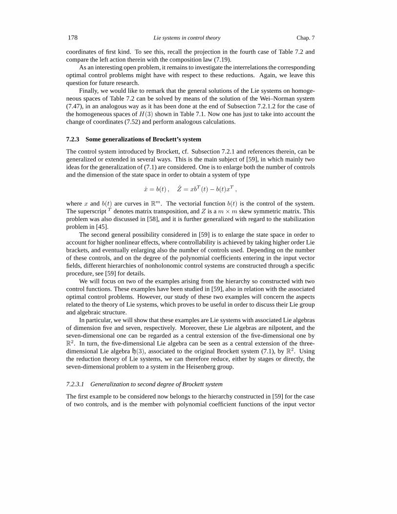
178 Lie systems in control theory Chap. 7
coordinates of first kind. To see this, recall the projectionin the fourth case of Table 7.2 andcompare the left action therein with the composition law (7.19).
As an interesting open problem, it remains to investigate the interrelations the correspondingoptimal control problems might have with respect to these reductions. Again, we leave thisquestion for future research.
Finally, we would like to remark that the general solutions of the Lie systems on homoge-neous spaces of Table 7.2 can be solved by means of the solution of the Wei–Norman system(7.47), in an analogous way as it has been done at the end of Subsection 7.2.1.2 for the case ofthe homogeneous spaces ofH(3) shown in Table 7.1. Now one has just to take into account thechange of coordinates (7.52) and perform analogous calculations.
7.2.3 Some generalizations of Brockett’s system
The control system introduced by Brockett, cf. Subsection 7.2.1 and references therein, can begeneralized or extended in several ways. This is the main subject of [59], in which mainly twoideas for the generalization of (7.1) are considered. One isto enlarge both the number of controlsand the dimension of the state space in order to obtain a system of type
x = b(t) , Z = xbT (t)− b(t)xT ,
wherex and b(t) are curves inRm. The vectorial functionb(t) is the control of the system.The superscriptT denotes matrix transposition, andZ is am×m skew symmetric matrix. Thisproblem was also discussed in [58], and it is further generalized with regard to the stabilizationproblem in [45].
The second general possibility considered in [59] is to enlarge the state space in order toaccount for higher nonlinear effects, where controllability is achieved by taking higher order Liebrackets, and eventually enlarging also the number of controls used. Depending on the numberof these controls, and on the degree of the polynomial coefficients entering in the input vectorfields, different hierarchies of nonholonomic control systems are constructed through a specificprocedure, see [59] for details.
We will focus on two of the examples arising from the hierarchy so constructed with twocontrol functions. These examples have been studied in [59], also in relation with the associatedoptimal control problems. However, our study of these two examples will concern the aspectsrelated to the theory of Lie systems, which proves to be useful in order to discuss their Lie groupand algebraic structure.
In particular, we will show that these examples are Lie systems with associated Lie algebrasof dimension five and seven, respectively. Moreover, these Lie algebras are nilpotent, and theseven-dimensional one can be regarded as a central extension of the five-dimensional one byR2. In turn, the five-dimensional Lie algebra can be seen as a central extension of the three-dimensional Lie algebrah(3), associated to the original Brockett system (7.1), byR2. Usingthe reduction theory of Lie systems, we can therefore reduce, either by stages or directly, theseven-dimensional problem to a system in the Heisenberg group.
7.2.3.1 Generalization to second degree of Brockett system
The first example to be considered now belongs to the hierarchy constructed in [59] for the caseof two controls, and is the member with polynomial coefficient functions of the input vector

Sec. 7.2 Brockett control system and related ones 179
fields of at most second degree. We will use a slightly different notation from the one used in thecited reference.
The system of interest is the control system inR5, with coordinates(x1, x2, x3, x4, x5)
x1 = b1(t) , x2 = b2(t) , x3 = b2(t)x1 − b1(t)x2 ,
x4 = b2(t)x21 , x5 = b1(t)x
22 , (7.55)
whereb1(t) andb2(t) are the control functions. This system appears as well as an approximationof the so-called plate-ball nonholonomic kinematic problem [59], which consists of a sphererolling without slipping between two horizontal, flat and parallel plates which are separated bya distance equal to the diameter of the sphere. It is assumed that one of the plates is fixed inspace and that the ball rolls because of the horizontal movement of the other plate. The geometryand the optimal control solutions of this problem have been considered in [182, 183], and afterin [200]. In particular, it has shown that the optimal control problem is integrable by ellipticfunctions, as it is the case for (7.55), see [59].
Now, for given control functionsb1(t) andb2(t), the solutions of the system (7.55) are theintegral curves of the time-dependent vector fieldb1(t)X1 + b2(t)X2, with
X1 =∂
∂x1− x2
∂
∂x3+ x22
∂
∂x5, X2 =
∂
∂x2+ x1
∂
∂x3+ x21
∂
∂x4. (7.56)
Taking the Lie brackets
X3 = [X1, X2] = 2∂
∂x3+ 2x1
∂
∂x4− 2x2
∂
∂x5,
X4 = [X1, X3] = 2∂
∂x4, X5 = [X2, X3] = −2
∂
∂x5,
we obtain a set of vector fields which span the tangent space ateach point ofR5, therefore thesystem (7.55) is controllable. Moreover, the setX1, X2, X3, X4, X5 closes on the nilpotentLie algebra defined by
[X1, X2] = X3 , [X1, X3] = X4 , [X2, X3] = X5 , (7.57)
all other Lie brackets being zero. Such a Lie algebra is isomorphic to a nilpotent Lie algebra,denoted asg5, which can be regarded as a central extension of the Lie algebra h(3) by R2.Indeed,g5 has a basisa1, a2, a3, a4, a5 with respect to which the non-vanishing Lie productsare
[a1, a2] = a3 , [a1, a3] = a4 , [a2, a3] = a5 , (7.58)
then the centerz of g5 is the Abelian subalgebra generated bya4, a5, and the factor Lie algebrag5/z is isomorphic toh(3), see (7.5).
Analogously to what we have done in previous subsections, wewill treat briefly the Wei–Norman problem associated to the system (7.55), and will give the expressions of the actions withrespect to which the vector fieldsX1, X2, X3, X4, X5 are infinitesimal generators. Then, wewill perform the reduction of the system (7.55) to another two: one of type (7.1), and one Liesystem inR2.

180 Lie systems in control theory Chap. 7
Let us denote byG5 the connected and simply connected nilpotent Lie group suchthat itsLie algebra isg5. A generic right-invariant Lie system of type (2.10) onG5 is of the form
Rg(t)−1∗g(t)(g(t)) = −b1(t)a1 − b2(t)a2 − b3(t)a3 − b4(t)a4 − b5(t)a5 , (7.59)
whereg(t) is the solution curve inG5 starting, for example, from the identity. The system of thistype corresponding to the system (7.55) is that withb3(t) = b4(t) = b5(t) = 0 for all t, i.e.,
Rg(t)−1∗g(t)(g(t)) = −b1(t)a1 − b2(t)a2 . (7.60)
To solve (7.60) by the Wei–Norman method, we need to compute the adjoint representationof the Lie algebrag5 with respect to the above basis. It reads
ad(a1) =
0 0 0 0 00 0 0 0 00 1 0 0 00 0 1 0 00 0 0 0 0
, ad(a2) =
0 0 0 0 00 0 0 0 0−1 0 0 0 00 0 0 0 00 0 1 0 0
,
ad(a3) =
0 0 0 0 00 0 0 0 00 0 0 0 0−1 0 0 0 00 −1 0 0 0
, ad(a4) = 0 , ad(a5) = 0 ,
and therefore
exp(−v1 ad(a1)) = Id−v1 ad(a1) +v212
ad(a1) ad(a1) ,
exp(−v2 ad(a2)) = Id−v2 ad(a2) +v222
ad(a2) ad(a2) ,exp(−v3 ad(a3)) = Id−v3 ad(a3) ,
exp(−v4 ad(a4)) = Id , exp(−v5 ad(a5)) = Id .
Writing the solution which starts from the identity, of (7.60), as the product
g(t) = exp(−v1(t)a1) exp(−v2(t)a2) exp(−v3(t)a3) exp(−v4(t)a4) exp(−v5(t)a5) (7.61)
and applying (2.28), we will find the system of differential equations
v1 = b1(t) , v2 = b2(t) , v3 = b2(t)v1 , v4 =1
2b2(t)v
21 , v5 = b2(t)v1v2 , (7.62)
with initial conditionsv1(0) = v2(0) = v3(0) = v4(0) = v5(0) = 0. The solution can be foundby quadratures; if we denoteBi(t) =
∫ t0bi(s) ds, i = 1, 2, the solution reads
v1(t) = B1(t) , v2(t) = B2(t) , v3(t) =
∫ t
0
b2(s)B1(s) ds ,
v4(t) =1
2
∫ t
0
b2(s)B21(s) ds , v5(t) =
∫ t
0
b2(s)B1(s)B2(s) ds . (7.63)

Sec. 7.2 Brockett control system and related ones 181
We would like to remark that the system (7.62) is closely related to the system appearing inExamples 8.1 of [209] and 6.1 of [210], following an approachdifferent to ours. Indeed, such asystem is essentially the Wei–Norman system correspondingto the equation (7.59) in the groupG5, whenb5(t) = 0, and to the factorization (7.61). This system can be found aswell by directapplication of (2.28).
Following steps analogous to those of Subsection 7.2.1, we find the following expressions.Parametrizing the elementsg ∈ G5 asg = exp(aa1 + ba2 + ca3 + da4 + ea5), the action ofG5
onR5 such thatXi be the infinitesimal generator associated toai for eachi ∈ 1, . . . , 5 reads
Φ : G5 × R5 −→ R
5
((a, b, c, d, e), (x1, x2, x3, x4, x5)) 7−→ (x1, x2, x3, x4, x5) ,
where
x1 = x1 − a , x2 = x2 − b , x3 = x3 + ax2 − bx1 − 2c ,
x4 = x4 − bx21 + (ab− 2c)x1 + ac− 2d− ba2/3 ,
x5 = x5 − ax22 + (ab + 2c)x2 − bc+ 2e− ab2/3 ,
meanwhile the composition law(a, b, c, d, e)(a′, b′, c′, d′, e′) = (a′′, b′′, c′′, d′′, e′′) is givenby
a′′ = a+ a′ , b′′ = b+ b′ , c′′ = c+ c′ + (ab′ − ba′)/2 ,
d′′ = d+ d′ + (ac′ − ca′)/2 + (a− a′)(ab′ − ba′)/12 , (7.64)
e′′ = e+ e′ + (bc′ − cb′)/2 + (b− b′)(ab′ − ba′)/12 ,
and the neutral element is represented by(0, 0, 0, 0, 0).If, instead, we parametrize the group elementsg ∈ G5 by the second kind canonical coor-
dinates defined byg = exp(aa1) exp(ba2) exp(ca3) exp(da4) exp(ea5), the action becomes
Φ : G5 × R5 −→ R
5
((a, b, c, d, e), (x1, x2, x3, x4, x5)) 7−→ (x1, x2, x3, x4, x5) ,
where
x1 = x1 − a , x2 = x2 − b , x3 = x3 + ax2 − bx1 − 2c− ab ,
x4 = x4 − bx21 − 2cx1 − 2d , (7.65)
x5 = x5 − ax22 + 2(ab+ c)x2 + 2e− ab2 ,
and the composition law(a, b, c, d, e)(a′, b′, c′, d′, e′) = (a′′, b′′, c′′, d′′, e′′) is given by
a′′ = a+ a′ , b′′ = b+ b′ , c′′ = c+ c′ − ba′ ,
d′′ = d+ d′ − ca′ + ba′ 2/2 , (7.66)
e′′ = e+ e′ − cb′ + ba′b′ + b2a′/2 ,
the neutral element being represented as well by(0, 0, 0, 0, 0) in these coordinates.

182 Lie systems in control theory Chap. 7
The relation between the first kind canonical coordinates(a1, b1, c1, d1, e1) and the secondkind canonical coordinates(a2, b2, c2, d2, e2) so defined of the same group elementg ∈ G5 is
a1 = a2 , b1 = b2 , c1 = c2 +1
2a2b2 ,
d1 = d2 +1
2a2c2 +
1
12a22b2 ,
e1 = e2 +1
2b2c2 −
1
12a2b
22 .
The general solution of (7.55) can be calculated by means of the solution of the Wei–Norman system (7.62) as
Φ((−v1, −v2, −v3, −v4, −v5), (x10, x20, x30, x40, x50)) = (x1, x2, x3, x4, x5)
whereΦ is that of (7.65), i.e.,
x1 = x10 + v1 , x2 = x20 + v2 , x3 = x30 − v1x20 + v2x10 + 2v3 − v1v2 ,
x4 = x40 + v2x210 + 2v3x10 + 2v4 ,
x5 = x50 + v1x220 + 2(v1v2 − v3)x20 − 2v5 + v1v
22 ,
the functionsv1 = v1(t), v2 = v2(t), v3 = v3(t), v4 = v4(t) andv5 = v5(t) are given by (7.63)and(x10, x20, x30, x40, x50) ∈ R5 are the initial conditions. It can be checked that the directintegration of (7.55) gives the same result.
Another control system exists in the literature with the same underlying Lie algebra as(7.55), see [269, Example 2]. With a slightly different notation, it is the control system inR5,with coordinates(x1, x2, x3, x4, x5)
x1 = b1(t) , x2 = b2(t) , x3 = b2(t)x1 ,
x4 = b2(t)x21 , x5 = 2 b2(t)x1x2 . (7.67)
This system is of the form (7.62), with the simple identification x1 = v1, x2 = v2, x3 = v3,x4 = 2v4 andx5 = 2v5. Analogous calculations to those above can be done for this case, withsimilar results.
Our next task is to show that the reduction theory of Lie systems, cf. Section 2.5, allowsto reduce the problem of solving (7.60), and hence of solving(7.55), to solving two other Liesystems: one of Brockett type (7.1), and another on the center of G5, which can be identifiedwith R2. The steps to follow are very similar to those of Subsections7.2.1.2 and 7.2.2.1: usingthe canonical coordinates of first kind inG5 defined byg = exp(aa1 + ba2 + ca3 + da4 + ea5),and the composition law (7.64), we obtain that the adjoint representation of the group reads
Ad(a, b, c, d, e) =
1 0 0 0 00 1 0 0 0−b a 1 0 0
−ab2 − c a2
2 a 1 0
− b2
2ab2 − c b 0 1
. (7.68)

Sec. 7.2 Brockett control system and related ones 183
If g(t) = (a(t), b(t), c(t), d(t), e(t)) is a curve inG5 expressed in the previous coordinates, weobtain
Lg−1∗g(g) =
a
b
c+ 12 (ba− ab)
d+ 16 (3c− ab)a+ 1
6a2b− 1
2ac
e− 16b
2a+ 16 (3c+ ab)b− 1
2bc
,
(7.69)
Rg−1∗g(g) =
a
b
c− 12 (ba− ab)
d− 16 (3c+ ab)a+ 1
6a2b+ 1
2ac
e− 16b
2a− 16 (3c− ab)b+ 1
2bc
.
To perform the reduction we select the subgroupH of G5 whose Lie algebra is the centerz of g5, which is generated bya4, a5. Then,g5/z
∼= h(3) andG5/H ∼= H(3). We use thefactorization
(a, b, c, d, e) = (a, b, c, 0, 0)(0, 0, 0, d, e) ,
therefore the projection reads
πL : G5 −→ G5/H
(a, b, c, d, e) 7−→ (a, b, c) .
We take coordinates(y1, y2, y3) in G5/H . The left action ofG5 onG5/H is then
λ : G5 ×G5/H −→ G5/H
((a, b, c, d, e), (y1, y2, y3)) 7−→ πL((a, b, c, d, e)(y1, y2, y3, d′, e′))
= (y1 + a, y2 + b, y3 + c+ (ay2 − by1)/2) ,
whered′ ande′ are real numbers parametrizing the lift of(y1, y2, y3) toG5. The correspondingfundamental vector fields can be calculated according to (2.2), and they are
XH1 = −∂y1 −
y22∂y3 , XH
2 = −∂y2 +y12∂y3 ,
XH3 = −∂y3 , XH
4 = 0 , XH5 = 0 ,
which span the tangent space at each point ofG5/H , and in addition satisfy[XH1 , X
H2 ] = XH
3 ,[XH
1 , XH3 ] = XH
4 and[XH2 , X
H3 ] = XH
5 , or, more precisely, the commutation relations of theHeisenberg Lie algebra (7.3).
Now, we factorize the solution starting from the identity of(7.60) as the product
g1(t)h(t) = (y1(t), y2(t), y3(t), 0, 0)(0, 0, 0, d(t), e(t)) ,
whereg1(t) projects onto the solutionπL(g1(t)) = (y1(t), y2(t), y3(t)), with initial conditions(y1(0), y2(0), y3(0)) = (0, 0, 0), of the Lie system onG5/H associated to (7.60),
y1 = −b1(t) , y2 = −b2(t) , y3 =1
2(b2(t)y1 − b1(t)y2) . (7.70)

184 Lie systems in control theory Chap. 7
Thus, we reduce the problem to a Lie system in the center ofG5 for h(t) = (0, 0, 0, d(t), e(t)),with h(0) = e, i.e.,d(0) = e(0) = 0. The expression of this last system is given by the formula(2.37) in Theorem 2.5.1. Using (7.68), and (7.69) we finally obtain the system
d =b1(t)
2
(1
6y1(t)y2(t)− y3(t)
)− 1
12b2(t)y
21(t) ,
e =1
12b1(t)y
22(t)−
b2(t)
2
(1
6y1(t)y2(t) + y3(t)
), (7.71)
which is a Lie system forH ∼= R2, solvable by two quadratures.If the solution of (7.60) is not required to start from the identity but from otherg0 ∈ G5,
the task of solving it reduces as well to solving first the system (7.70) with initial conditions(y1(0), y2(0), y3(0)) = πL(g0), and then the system (7.71), with initial conditionsh(0) =g−11 (0)g0. In this sense the original system (7.55) can be reduced to the system (7.70), which
becomes the Brockett system (7.1) under the simple change ofcoordinatesx = −y1, y = −y2andz = −2y3, and then a system in the center ofG5, identifiable withR2.
7.2.3.2 Generalization to third degree of Brockett system
We consider now the example from [59] which belongs to the hierarchy constructed therein withtwo controls, being the member with polynomial coefficient functions of the input vector fieldsof at most third degree.
Such a system is a Lie system defined onR8 with an associated seven-dimensional nilpo-tent Lie algebra, related to the one appearing in the exampleof the previous subsection. Moreprecisely, the former can be regarded as a central extensionby the Abelian Lie algebraR2 of thelatter. We already know that the Lie algebra of system (7.55)is a central extension of the Lie al-gebrah(3) byR2. It turns out that the Lie algebra to be considered below has afour-dimensionalAbelian ideali such that the factor algebra constructed with it is justh(3) again.
The system can be treated and solved by the same techniques that we have used to deal withsystem (7.55), namely, the Wei–Norman method, the integration of the system by consideringthe associated action, etc. This is just a matter of computation.
However, as we will show, the problem can be reduced again to another two: one in theHeisenberg group, of type (7.1), and another in the mentioned Abelian ideal of dimension four,which can be identified withR4. In this subsection we will focus on this reduction, since wefeelthat it is the most illuminating result. Of course one could perform instead the reduction withrespect to the center of the Lie group, giving rise to a Lie system with the same associated Liealgebra as that of (7.55), or by using other subgroups, yielding different realizations on lowerdimensional homogeneous spaces of the system below.
The system of interest is thus the control system inR8, with coordinates(x1, . . . , x8)(see [59])
x1 = b1(t) , x2 = b2(t) , x3 = b2(t)x1 − b1(t)x2 ,
x4 = b2(t)x21 , x5 = b1(t)x
22 , x6 = b2(t)x
31 , (7.72)
x7 = b1(t)x32 , x8 = b1(t)x
21x2 + b2(t)x1x
22 ,
whereb1(t) andb2(t) are the control functions. The solutions of this system are the integral

Sec. 7.2 Brockett control system and related ones 185
curves of the time-dependent vector fieldb1(t)X1 + b2(t)X2, with
X1 =∂
∂x1− x2
∂
∂x3+ x22
∂
∂x5+ x32
∂
∂x7+ x21x2
∂
∂x8,
X2 =∂
∂x2+ x1
∂
∂x3+ x21
∂
∂x4+ x31
∂
∂x6+ x1x
22
∂
∂x8.
Taking the Lie brackets
X3 = [X1, X2] = 2∂
∂x3+ 2x1
∂
∂x4− 2x2
∂
∂x5+ 3x21
∂
∂x6− 3x22
∂
∂x7+ (x22 − x21)
∂
∂x8,
X4 = [X1, X3] = 2∂
∂x4+ 6x1
∂
∂x6− 2x1
∂
∂x8,
X5 = [X2, X3] = −2∂
∂x5− 6x2
∂
∂x7+ 2x2
∂
∂x8,
X6 = [X1, X4] = 6∂
∂x6− 2
∂
∂x8, X7 = [X2, X5] = −6
∂
∂x7+ 2
∂
∂x8,
we obtain a set of linearly independent vector fieldsX1, . . . , X7 which closes on the nilpotentLie algebra defined by
[X1, X2] = X3 , [X1, X3] = X4 , [X1, X4] = X6 ,
[X2, X3] = X5 , [X2, X5] = X7 ,
all other Lie brackets being zero. This Lie algebra is isomorphic to a nilpotent Lie algebra,denoted asg7, which can be regarded as a central extension of the Lie algebra g5, defined inthe previous subsection, byR2. In fact,g7 has a basisa1, . . . , a7 with respect to which thenon-vanishing Lie products are
[a1, a2] = a3 , [a1, a3] = a4 , [a1, a4] = a6 ,
[a2, a3] = a5 , [a2, a5] = a7 ,
then the centerz of g7 is the Abelian subalgebra generated bya6, a7, and the factor Lie algebrag7/z is isomorphic tog5, see (7.58). Moreover,g7 contains an Abelian four-dimensional ideali generated bya4, a5, a6, a7, such that the factor Lie algebrag7/i is isomorphic toh(3),see (7.5). Finally, note that the maximal proper idealiM contained ing7, which is Abelian,is generated bya3, . . . , a7, the quotient beingg7/iM ∼= R2. We will denote byG7 theconnected and simply connected nilpotent Lie group such that its Lie algebra isg7.
As in previous cases, the set of vector fieldsX1, . . . , X7 can be regarded as the fun-damental vector fields with respect to an action ofG7 on R8. However, they do not span thefull tangent tangent space at each point ofR8, thus the system (7.72) is controllable orbit-wise:only configurations in the same orbit with respect to the previous action can be joined, e.g., byappropriately chosen piecewise constant controls.
We concentrate now on the task of reducing the system (7.72) into one of type (7.1) andother inR4. The right-invariant Lie system of type (2.10) onG7 corresponding to the system(7.72) is
Rg(t)−1∗g(t)(g(t)) = −b1(t)a1 − b2(t)a2 , (7.73)

186 Lie systems in control theory Chap. 7
wherea1, . . . , a7 is the basis ofg7 considered above.If we parametrize the elementsg ∈ G7 asg = exp(aa1 + ba2 + ca3 + da4 + ea5 + fa6 +
ka7), it can be checked that the composition law(a, b, c, d, e, f, k)(a′, b′, c′, d′, e′, f ′, k′) =(a′′, b′′, c′′, d′′, e′′, f ′′, k′′) reads in these coordinates
a′′ = a+ a′ , b′′ = b+ b′ , c′′ = c+ c′ + (ab′ − ba′)/2 ,
d′′ = d+ d′ + (ac′ − ca′)/2 + (a− a′)(ab′ − ba′)/12 ,
e′′ = e+ e′ + (bc′ − cb′)/2 + (b− b′)(ab′ − ba′)/12 , (7.74)
f ′′ = f + f ′ + (ad′ − da′)/2 + (a− a′)(ac′ − ca′)/12 + aa′(ba′ − ab′)/24 ,
k′′ = k + k′ + (be′ − eb′)/2 + (b− b′)(bc′ − cb′)/12 + bb′(ba′ − ab′)/24 ,
the neutral element being represented by(0, . . . , 0). The adjoint representation of the groupreads
Ad(a, b, c, d, e, f, k) =
1 0 0 0 0 0 00 1 0 0 0 0 0−b a 1 0 0 0 0
−ab2 − c a2
2 a 1 0 0 0
− b2
2ab2 − c b 0 1 0 0
−a2b6 − ac
2 − d a3
6a2
2 a 0 1 0
− b3
6ab2
6 − bc2 − e b2
2 0 b 0 1
. (7.75)
If g(t) = (a(t), b(t), c(t), d(t), e(t), f(t), k(t)) is a curve inG7 expressed in the previouscoordinates, we obtain
Lg−1∗g(g) =
a
b
c+ 12 (ba− ab)
d+ 16 (3c− ab)a+ 1
6a2b− 1
2ac
e− 16b
2a+ 16 (3c+ ab)b− 1
2bc
f + 124 (a
2b− 4ac+ 12d)a− 124a
3b+ 16a
2c− 12ad
k + 124b
3a− 124 (ab
2 + 4bc− 12e)b+ 16b
2c− 12be
,
(7.76)
Rg−1∗g(g) =
a
b
c− 12 (ba− ab)
d− 16 (3c+ ab)a+ 1
6a2b+ 1
2ac
e− 16b
2a− 16 (3c− ab)b+ 1
2bc
f − 124 (a
2b+ 4ac+ 12d)a+ 124a
3b+ 16a
2c+ 12ad
k − 124b
3a+ 124 (ab
2 − 4bc− 12e)b+ 16b
2c+ 12be
.
To perform the reduction we select the subgroupH ofG7 whose Lie algebra is the ideali ofg7 generated bya4, a5, a6, a7. Then,g7/i
∼= h(3) andG7/H ∼= H(3). Taking into account

Sec. 7.2 Brockett control system and related ones 187
the factorization
(a, b, c, d, e, f, k) = (a, b, c, 0, 0, 0, 0)(0, 0, 0, d, e, f, k) ,
the projection reads
πL : G7 −→ G7/H
(a, b, c, d, e, f, k) 7−→ (a, b, c) .
We take coordinates(y1, y2, y3) in G7/H so that the left action ofG7 onG7/H is
λ : G7 ×G7/H −→ G7/H
((a, b, c, d, e, f, k), (y1, y2, y3)) 7−→ πL((a, b, c, d, e, f, k)(y1, y2, y3, d′, e′, f ′, k′))
= (y1 + a, y2 + b, y3 + c+ (ay2 − by1)/2) ,
whered′, e′, f ′ andk′ are real numbers parametrizing the lift of(y1, y2, y3) toG7. The corre-sponding fundamental vector fields can be calculated according to (2.2), and they are
XH1 = −∂y1 −
y22∂y3 , XH
2 = −∂y2 +y12∂y3 , XH
3 = −∂y3 ,
XH4 = 0 , XH
5 = 0 , XH6 = 0 , XH
7 = 0 ,
which span the tangent space at each point ofG7/H ∼= H(3), and in addition satisfy the com-mutation relations of the Heisenberg Lie algebra, see (7.3).
Now, if we factorize the solution of (7.73) starting fromg0 ∈ G7 as the product
g1(t)h(t) = (y1(t), y2(t), y3(t), 0, 0, 0, 0)(0, 0, 0, d(t), e(t), f(t), k(t)) ,
whereg1(t) projects onto the solutionπL(g1(t)) = (y1(t), y2(t), y3(t)), with initial conditions(y1(0), y2(0), y3(0)) = πL(g0), of the Lie system onG7/H associated to (7.73), (which coin-cides with (7.70))
y1 = −b1(t) , y2 = −b2(t) , y3 =1
2(b2(t)y1 − b1(t)y2) . (7.77)
In this way we reduce to a Lie system inH ∼= R4 for h(t) = (0, 0, 0, d(t), e(t), f(t), k(t)),with h(0) = g−1
1 (0)g0, calculated according to the formulas (2.37), (7.75) and (7.76), i.e.,
d =b1(t)
2
(1
6y1(t)y2(t)− y3(t)
)− 1
12b2(t)y
21(t) ,
e =1
12b1(t)y
22(t)−
b2(t)
2
(1
6y1(t)y2(t) + y3(t)
), (7.78)
f = − 1
24y1(t)
(b1(t)(y1(t)y2(t)− 8y3(t))− b2(t)y
21(t)
),
k = − 1
24y2(t)
(b1(t)y
22(t)− b2(t)(y1(t)y2(t) + 8y3(t))
),
which is solvable by quadratures. Thus, we have reduced the solution of the system (7.73),and hence of (7.72), to solve first the system (7.77), which isthe same as (7.70) and becomes theBrockett system (7.1) under the simple change of coordinatesx = −y1, y = −y2 andz = −2y3.Once this has been solved, we simply have to integrate (7.78)in order to reconstruct the completesolution of (7.73).
We leave for future research the investigation of how these reductions can be interrelatedwith the associated optimal control problems for each case.

188 Lie systems in control theory Chap. 7
7.2.4 Control systems non steerable by simple sinusoids
We consider now two examples of control systems which, according to [255,258], are not possi-ble to be steered by using simple sinusoids, and share exactly the same behaviour to this respect.
Both of them are control systems withR8 as state space, with two controls, and it turns outthat both of them are Lie systems with the same associated Liealgebra, which is nilpotent andeight-dimensional.
The relation between these two systems can be further understood, moreover, under the lightof the theory of Lie systems. Indeed, one of the systems can beregarded as the Wei–Normansystem corresponding to the common underlying Lie algebra,and with certain ordering of thefactor exponentials.
Another interesting feature of these systems is that when wetake the quotient of their com-mon associated Lie algebra with respect to its center, whichis three-dimensional, we obtain theLie algebrag5, defined by the relations (7.58). We can therefore reduce theproblems below intoa Lie system with the same underlying algebra as (7.55), and another inR3. And more interest-ingly, by quotienting instead by a five-dimensional Abelianideal, we obtain againh(3) as thefactor Lie algebra, and therefore we can reduce again to a system of type (7.1) and then to a Liesystem inR5.
The first system of interest now is the control system inR8, with coordinates(x1, . . . , x8),of [255, p. 230],
x1 = b1(t) , x2 = b2(t) , x3 = b2(t)x1 , x4 = b1(t)x3 ,
x5 = b2(t)x3 , x6 = b1(t)x4 , x7 = b2(t)x4 , x8 = b2(t)x5 , (7.79)
whereb1(t) andb2(t) are the control functions. The solutions of this system are the integralcurves of the time-dependent vector fieldb1(t)X1 + b2(t)X2, with
X1 =∂
∂x1+ x3
∂
∂x4+ x4
∂
∂x6,
X2 =∂
∂x2+ x1
∂
∂x3+ x3
∂
∂x5+ x4
∂
∂x7+ x5
∂
∂x8.
Taking the Lie brackets
X3 = [X1, X2] =∂
∂x3− x1
∂
∂x4+ x3
∂
∂x7,
X4 = [X1, X3] = −2∂
∂x4+ x1
∂
∂x6, X5 = [X2, X3] = − ∂
∂x5+ 2x1
∂
∂x7,
X6 = [X1, X4] = 3∂
∂x6, X7 = [X1, X5] = 2
∂
∂x7, X8 = [X2, X5] =
∂
∂x8,
we obtain a set of linearly independent vector fieldsX1, . . . , X8 which span the tangent spaceat every point ofR8, and therefore (7.79) is a controllable system. In addition, these vector fieldsclose on the nilpotent Lie algebra defined by
[X1, X2] = X3 , [X1, X3] = X4 , [X1, X4] = X6 , [X1, X5] = X7 ,
[X2, X3] = X5 , [X2, X4] = X7 , [X2, X5] = X8 ,

Sec. 7.2 Brockett control system and related ones 189
where all other Lie brackets are zero. This Lie algebra is isomorphic to a nilpotent Lie algebra,denoted asg8, which can be regarded as a central extension of the Lie algebra g5, defined inSubsection 7.2.3.1, byR3. In fact,g8 has a basisa1, . . . , a8 for which the non-vanishing Lieproducts are
[a1, a2] = a3 , [a1, a3] = a4 , [a1, a4] = a6 , [a1, a5] = a7 ,
[a2, a3] = a5 , [a2, a4] = a7 , [a2, a5] = a8 .
The centerz of g8 is the Abelian subalgebra generated bya6, a7, a8, and the factor Lie algebrag8/z is isomorphic tog5, see (7.58). On the other hand,g8 contains an Abelian five-dimensionalideal i generated bya4, a5, a6, a7, a8, such that the factor Lie algebrag8/i is isomorphicto h(3), see (7.5). Finally, note that the maximal proper idealiM contained ing8, which isAbelian, is generated bya3, . . . , a8, and we have thatg8/iM ∼= R2. We will denote byG8
the connected and simply connected nilpotent Lie group suchthat its Lie algebra isg8.
The right-invariant Lie system of type (2.10) onG8 corresponding to the system (7.79) isof the form
Rg(t)−1∗g(t)(g(t)) = −b1(t)a1 − b2(t)a2 , (7.80)
wherea1, . . . , a8 is the previous basis ofg8. Let us apply the Wei–Norman method to solvethis system.
Firstly, we have to calculate the adjoint representation ofthe Lie algebrag8 with respect tothe above basis. It reads
ad(a1) =
0 0 0 0 0 0 0 00 0 0 0 0 0 0 00 1 0 0 0 0 0 00 0 1 0 0 0 0 00 0 0 0 0 0 0 00 0 0 1 0 0 0 00 0 0 0 1 0 0 00 0 0 0 0 0 0 0
, ad(a2) =
0 0 0 0 0 0 0 00 0 0 0 0 0 0 0−1 0 0 0 0 0 0 00 0 0 0 0 0 0 00 0 1 0 0 0 0 00 0 0 0 0 0 0 00 0 0 1 0 0 0 00 0 0 0 1 0 0 0
,
ad(a3) =
0 0 0 0 0 0 0 00 0 0 0 0 0 0 00 0 0 0 0 0 0 0−1 0 0 0 0 0 0 00 −1 0 0 0 0 0 00 0 0 0 0 0 0 00 0 0 0 0 0 0 00 0 0 0 0 0 0 0
, ad(a4) =
0 0 0 0 0 0 0 00 0 0 0 0 0 0 00 0 0 0 0 0 0 00 0 0 0 0 0 0 00 0 0 0 0 0 0 0−1 0 0 0 0 0 0 00 −1 0 0 0 0 0 00 0 0 0 0 0 0 0
,
ad(a5) =
0 0 0 0 0 0 0 00 0 0 0 0 0 0 00 0 0 0 0 0 0 00 0 0 0 0 0 0 00 0 0 0 0 0 0 00 0 0 0 0 0 0 0−1 0 0 0 0 0 0 00 −1 0 0 0 0 0 0
, ad(a6) = ad(a7) = ad(a8) = 0 ,

190 Lie systems in control theory Chap. 7
and therefore
exp(−v1 ad(a1)) = Id−v1 ad(a1) +v212
ad2(a1)−v316
ad3(a1) ,
exp(−v2 ad(a2)) = Id−v2 ad(a2) +v222
ad2(a2)−v326
ad3(a2) ,
exp(−v3 ad(a3)) = Id−v3 ad(a3) , exp(−v4 ad(a4)) = Id−v4 ad(a4) ,
exp(−v5 ad(a5)) = Id−v5 ad(a5) , exp(−v6 ad(a6)) = Id ,
exp(−v7 ad(a7)) = Id , exp(−v8 ad(a8)) = Id ,
where the notationadk(ai) means the composition ofad(ai) with itself k times.Writing the solution of (7.80), starting from the identity,as the product
g(t) =
8∏
i=1
exp(−vi(t)ai) , (7.81)
and applying (2.28), we find the system
v1 = b1(t) , v2 = b2(t) , v3 = b2(t)v1 , v4 =1
2b2(t)v
21 , v5 = b2(t)v1v2 ,
v6 =1
6b2(t)v
31 , v7 =
1
2b2(t)v
21v2 , v8 =
1
2b2(t)v1v
22 , (7.82)
with initial conditionsvi(0) = 0, i ∈ 1, . . . , 8. Its solution can be found immediately byquadratures.
We want to point out that the system (7.82), with maybe other initial conditions, and upto a slightly different notation, is the system in [258, p. 709]. This reference says that such asystem shares the same behaviour with respect to steering bysimple sinusoids as the first system(7.79). The system (7.82) is as well a Lie system, with the same associated Lie algebra as (7.79).However, the relation between both systems, in the terms we have stated, seems to have been notestablished before.
We treat now briefly the question of reducing the right-invariant system (7.80) to one of thetype (7.1) and other Lie system inR5. The calculations are similar to those in previous examples,and we restrict ourselves to give the essential points. Other possible reductions can be dealt within an analogous way.
We parametrize the elementsg ∈ G8 by the first kind canonical coordinates defined throughg = exp(aa1 + ba2 + ca3 + da4 + ea5 + fa6 + ka7 + la8). Then, the composition law
(a, b, c, d, e, f, k, l)(a′, b′, c′, d′, e′, f ′, k′, l′) = (a′′, b′′, c′′, d′′, e′′, f ′′, k′′, l′′)
is given by
a′′ = a+ a′ , b′′ = b+ b′ , c′′ = c+ c′ + (ab′ − ba′)/2 ,
d′′ = d+ d′ + (ac′ − ca′)/2 + (a− a′)(ab′ − ba′)/12 ,
e′′ = e+ e′ + (bc′ − cb′)/2 + (b− b′)(ab′ − ba′)/12 ,
f ′′ = f + f ′ + (ad′ − da′)/2 + (a− a′)(ac′ − ca′)/12 + aa′(ba′ − ab′)/24 , (7.83)
k′′ = k + k′ + (ae′ − ea′)/2 + (bd′ − db′)/2 + (abc′ + a′b′c)/6
− (c+ c′)(ab′ + ba′)/12 + (ab′ + ba′)(ba′ − ab′)/24 ,
l′′ = l + l′ + (be′ − eb′)/2 + (b − b′)(bc′ − cb′)/12 + bb′(ba′ − ab′)/24 ,

Sec. 7.2 Brockett control system and related ones 191
and the neutral element is represented by(0, . . . , 0). The calculation of the adjoint representa-tion of the group and the quantities of type (7.36) for this case is analogous to that of previousexamples, recall Subsection 7.2.1.2.
To perform the reduction we select the subgroupH of G8 whose Lie algebra is the idealiof g8 generated bya4, a5, a6, a7, a8. Then,g8/i ∼= h(3) andG8/H ∼= H(3). Taking intoaccount the factorization
(a, b, c, d, e, f, k, l) = (a, b, c, 0, 0, 0, 0, 0)(0, 0, 0, d, e, f, k, l) ,
the projection reads
πL : G8 −→ G8/H
(a, b, c, d, e, f, k, l) 7−→ (a, b, c) .
We take coordinates(y1, y2, y3) inG8/H so that the left actionλ : G8×G8/H → G8/H reads
λ((a, b, c, d, e, f, k, l), (y1, y2, y3))
= πL((a, b, c, d, e, f, k, l)(y1, y2, y3, d′, e′, f ′, k′, l′))
= (y1 + a, y2 + b, y3 + c+ (ay2 − by1)/2) ,
whered′, e′, f ′, k′ and l′ are real numbers parametrizing the lift of(y1, y2, y3) to G8. Theassociated infinitesimal generators can be calculated according to (2.2), and they are
XH1 = −∂y1 −
y22∂y3 , XH
2 = −∂y2 +y12∂y3 , XH
3 = −∂y3 ,
XH4 = 0 , XH
5 = 0 , XH6 = 0 , XH
7 = 0 , XH8 = 0 ,
which span the tangent space at each point ofG8/H ∼= H(3), and in addition satisfy the com-mutation relations of the Heisenberg Lie algebra, see (7.3). We factorize the solution of (7.80)starting fromg0 ∈ G8 as the productg1(t)h(t), where
g1(t) = (y1(t), y2(t), y3(t), 0, 0, 0, 0, 0)
projects onto the solutionπL(g1(t)) = (y1(t), y2(t), y3(t)) of the Lie system onG8/H asso-ciated to (7.80), (which is the same as (7.70) and (7.77)), with (y1(0), y2(0), y3(0)) = πL(g0).We have as well
h(t) = (0, 0, 0, d(t), e(t), f(t), k(t), l(t)) ,
and then, by Theorem 2.5.1, we reduce to a Lie system inH ∼= R5 for h(t), with initial conditionsh(0) = g−1
1 (0)g0, which takes the form
d =b1(t)
2
(1
6y1(t)y2(t)− y3(t)
)− 1
12b2(t)y
21(t) ,
e =1
12b1(t)y
22(t)−
b2(t)
2
(1
6y1(t)y2(t) + y3(t)
),
f = − 1
24y1(t)
(b1(t)(y1(t)y2(t)− 8y3(t)) + b2(t)y
21(t)
), (7.84)
k = − 1
12b1(t)y2(t) (y1(t)y2(t)− 4y3(t)) +
1
12b2(t)y1(t) (y1(t)y2(t) + 4y3(t)) ,
l = − 1
24y2(t)
(b1(t)y
22(t)− (y1(t)y2(t) + 8y3(t))
),

192 Lie systems in control theory Chap. 7
and is solvable by quadratures. As a consequence, we have reduced the solution of the system(7.80), and therefore of (7.79) (or (7.82)), to solve first the already familiar system (7.77) (or(7.70)), which is of type (7.1). Once this has been solved, wesimply have to integrate (7.84) toreconstruct the complete solution of (7.80).
7.3 Other nilpotentizable control systems: Trailers into chained systems
There exists in the control theory literature a whole familyof control systems, mainly within theframework of nonholonomic motion planning, which turns outto be closely related to the theoryof Lie systems.
These systems are typically drift-free and controllable. The corresponding input vectorfields, although span the tangent space at every point of the state space under bracket generation,do not necessarily close on a Lie algebra. However, in order to plan a desired motion for thesystem, very often it is convenient to deal with a more tractable version of it. Roughly speaking,three main approaches can be found in the literature to do so.
The first one is to approximate the original system by anotherin which a number of othervector fields generated by taking Lie brackets up to a certainorder are added, and then takingfurther commutators equal to zero. This leads to a nilpotentapproximation of the original system,i.e., the vector fields of the approximated system close on a nilpotent Lie algebra. Then, differentmethods are proposed to work with the approximated system, as the consideration of the so-called P. Hall basis (see, e.g., [288]) and certain formal equation in the associated Lie group,solved with a product of exponentials which in our language is just the Wei–Norman solution forthe approximated system. See [164,165,204,208–210,320] and [115,116,216] for an evolutionof these ideas. In particular, these approaches give exact results when the initial system is drift-free and nilpotent.
The second main idea is to establish a state space feedback law for the controls such thatthe resulting system becomes nilpotent. For an evolution ofthis idea see, e.g., [158–163] andspecifically [166], which introduces the problem of when a control system, affine in the controls,is feedback nilpotentizable. Of special interest is Theorem 2 therein, about nilpotentization ofcontrol systems with two input vector fields, see also [205].This line of research is continuedin [164, 165] and [209, 228]. In more recent years, further steps have been taken about thefeedback nilpotentization in articles like [255–258,308].
The third main approach to approximate certain control systems by other nilpotent onesconsists of taking a polynomial approximation in the state space variables of the given input vec-tor fields, up to a certain order. We have seen already an example for this, cf. Subsection 7.2.1.1.As another example, in [37] the systems of interest are written first in terms of certain privilegedcoordinates prior to the approximation by taking the Taylorexpansion up to certain order.
A strong motivation for considering nilpotent approximations of control systems is thatnilpotent systems are very appropriate systems with respect to the final objective of designinga specific control law for the motion planning problem. In particular, systems in chained form[255, 257, 258, 308] constitute a specially important classof nilpotent systems with regard tocontrol design, see also [269].
It is clear, therefore, the importance of nilpotent controlsystems not only by their own [97]but as the approximated version of other control systems. This has lead to investigations aboutthe structure of Lie algebras of nilpotent vector fields [147,166,192], see also [144].

Sec. 7.3 Trailers and chained forms 193
A slightly more general approach is to try to approximate a given control system by anothersystem whose input vector fields generate a solvable Lie algebra, although it seems that this lineof research is not so developed as the previous one. See, e.g., [100,165] and references therein.
Now, as far as the theory of Lie systems is concerned, what is essential is whether the inputvector fields of a control system close on a finite dimensionalLie algebra under Lie bracketing ornot. If they do, the theory of Lie systems is applicable always, regardless of whether such a Liealgebra is semisimple, solvable or nilpotent. However, thearising Lie system is exactly solvableby quadratures, in a general case, if its associated Lie algebra is solvable or at least nilpotent.
Along this section we will try to illustrate these aspects through the study of some examplesbelonging to the class of nonholonomic cars with trailers, which by one or another way arereducible to chained form, and some interrelations with thetheory of Lie systems, not noticedpreviously, will be pointed out.
We will begin by the simplest of these systems, the one known as robot unicycle, then amodel of a front wheel driven kinematic car, and afterwards,the previous one but with a pulledtrailer added. Finally the case of a trailer with a finite number of axles is analyzed, mainly fromthe point of view of the Wei–Norman method.
7.3.1 Model of maneuvering an automobile or of a robot unicycle
The example to be considered now is related to a very simplified model of maneuvering anautomobile [268, Examples 2.35, 3.5]. It is however one of the best known models in the fieldof nonholonomic motion planning, see, e.g., [123, 209, 210,220, 221], and it appears as wellas the kinematic equations of other problems. For example, as in [42–44, 46] or when findingoptimal paths for a car that can go both forwards and backwards and allowing cusps in thetrajectory [286], generalizing, in turn, a classical problem by Dubins [112,113], see also [8].
We will treat the following aspects of this system. Firstly,it can be viewed as a Lie sys-tem on the Euclidean group of the planeSE(2). This Lie group is already solvable, so exactsolutions can be given without need of further approximations. Then, by using the straightening-out Theorem for vector fields (which is illustrated as well in[268, Example 2.35] by means ofthis example), another realization of the system is found. We treat then the question of how theWei–Norman and reduction methods can be applied in this case.
Later, we will study, also from the perspective of Lie systems, a nilpotent version of the firstsystem, obtained by state space feedback transformation in[208–210]. This will lead to a newrealization of a Lie system with underlying Lie algebrah(3), cf. Subsection 7.2.1.
The configuration space of the system isR2 × S1, where we take coordinates(x1, x2, x3).The control system of interest can be written as
x1 = b2(t) sin x3 , x2 = b2(t) cos x3 , x3 = b1(t) , (7.85)
whereb1(t) andb2(t) are the control functions. The solutions of this system are the integralcurves of the time-dependent vector fieldb1(t)X1 + b2(t)X2, whereX1 andX2 are now
X1 =∂
∂x3, X2 = sinx3
∂
∂x1+ cosx3
∂
∂x2. (7.86)
The Lie bracket of both vector fields,
X3 = [X1, X2] = cosx3∂
∂x1− sinx3
∂
∂x2

194 Lie systems in control theory Chap. 7
is linearly independent fromX1, X2, and the setX1, X2, X3 spans the tangent space at eachpoint ofR2 × S1, therefore the system is controllable. In addition, we havethat
[X1, X2] = X3 , [X1, X3] = −X2 , [X2, X3] = 0 , (7.87)
so these vector fields close on a Lie algebra isomorphic to theLie algebrase(2) of the Euclideangroup in the planeSE(2). This Lie algebra has a basisa1, a2, a3 for which the Lie productsare
[a1, a2] = a3 , [a1, a3] = −a2 , [a2, a3] = 0 . (7.88)
Note thata2, a3 is a basis of the Abelian ideal inse(2) corresponding to the normal AbeliansubgroupR2, recall thatSE(2) = R2 ⊙ SO(2). Thus our first system (7.85) can be regarded asa Lie system withse(2) as associated Lie algebra.
On the other hand, the vector fieldsX2 andX3 commute, so there exist a chart with coor-dinates(y1, y2, y3) such thatX2 = ∂/∂y2 andX3 = ∂/∂y3, see [268, Example 2.35]. Then,y2will satisfy X2y2 = 1 andX3y2 = 0, and similarlyy3 is such thatX2y3 = 0 andX3y3 = 1.Particular solutions are
y2 = x1 sinx3 + x2 cosx3 , y3 = x1 cosx3 − x2 sinx3 ,
which can be completed withy1 = x3. In this new coordinatesX1 takes the form
X1 =∂
∂y1+ y3
∂
∂y2− y2
∂
∂y3.
These vector fields satisfy as well the Lie bracket relations(7.87), as can be checked immediately.The control system of interest, whose solutions are again the integral curves of the time-
dependent vector fieldb1(t)X1 + b2(t)X2, reads in the new coordinates as
y1 = b1(t) , y2 = b1(t)y3 + b2(t) , y3 = −b1(t)y2 , (7.89)
which can be regarded by itself as another realization of a Lie system withse(2) as associatedLie algebra.
A general right-invariant Lie system of type (2.10) onSE(2) takes the form
Rg(t)−1∗g(t)(g(t)) = −b1(t)a1 − b2(t)a2 − b3(t)a3 , (7.90)
whereg(t) is the solution curve inSE(2) starting, say, from the identity, anda1, a2, a3 is theprevious basis ofse(2). The system of this type corresponding to (7.85) and (7.89) is the onewith b3(t) = 0 for all t, i.e.,
Rg(t)−1∗g(t)(g(t)) = −b1(t)a1 − b2(t)a2 . (7.91)
Let us solve this system by the Wei–Norman method. The adjoint representation ofse(2) readsin the basisa1, a2, a3
ad(a1) =
0 0 00 0 −10 1 0
, ad(a2) =
0 0 00 0 0−1 0 0
, ad(a3) =
0 0 01 0 00 0 0
,

Sec. 7.3 Trailers and chained forms 195
and as a consequence
exp(−v1 ad(a1)) =
1 0 00 cos v1 sin v10 − sin v1 cos v1
,
exp(−v2 ad(a2)) =
1 0 00 1 0v2 0 1
, exp(−v3 ad(a3)) =
1 0 0−v3 1 00 0 1
.
Writing the solution which starts from the identity of (7.91) as the product of exponentials
g(t) = exp(−v1(t)a1) exp(−v2(t)a2) exp(−v3(t)a3) (7.92)
and applying (2.28), we obtain the system
v1 = b1(t) , v2 = b2(t) cos v1 , v3 = b2(t) sin v1 , (7.93)
with initial conditionsv1(0) = v2(0) = v3(0) = 0. DenotingB1(t) =∫ t0b1(s) ds, the solution
is found by quadratures,
v1(t) = B1(t) , v2(t) =
∫ t
0
b2(s) cosB1(s) ds , v3(t) =
∫ t
0
b2(s) sinB1(s) ds . (7.94)
We can choose other orderings in the product (7.92), leadingto other different systems for thecorresponding second kind canonical coordinates. Sincea2 anda3 commute, we have to consideronly three other possibilities. Let us comment briefly the complete results, which are summa-rized in Table 7.3. It can be checked that the Wei–Norman systems so obtained are as well Liesystems with associated Lie algebrase(2). In particular, those obtained from the first and secondfactorization in Table 7.3 are analogous to (7.85) and (7.89), respectively, with the identificationsv1 = x3, v2 = x2, v3 = x1 andv1 = y1, v2 = y2, v3 = y1. The other two possibilities leadthus to other two different realizations of Lie systems withLie algebrase(2). All of them areintegrable by quadratures.
Next, we will find the expressions of the actionΦ of SE(2) on the configuration manifoldR2 × S1 such that the previousXi be the fundamental vector field associated toai for i ∈1, 2, 3, in the coordinates(x1, x2, x3) and(y1, y2, y3).
In order to parametrize the groupSE(2), we could use its standard representation by matri-ces3× 3 of type
cos θ sin θ a− sin θ cos θ b
0 0 1
,
but we think it is more instructive to show that all calculations can be done by solely making useof the product law in certain coordinates. We choose a set of second kind canonical coordinates,which are relatively simple to work with, and are appropriate to use the solution of the Wei–Norman system (7.93) directly. The calculations can be donesimilarly by using a set of first kindcanonical coordinates, but the expressions and calculations become more complicated and addno substantial new insight into the problem.

196 Lie systems in control theory Chap. 7
Table 7.3.Wei–Norman systems of differential equations for the solution of (7.91), wherea1, a2, a3 isthe Lie algebra defined by (7.88). In all instances, the initial conditions arev1(0) = v2(0) = v3(0) = 0.
Factorization ofg(t) Wei–Norman system
exp(−v1a1) exp(−v2a2) exp(−v3a3) v1 = b1 , v2 = b2 cos v1 , v3 = b2 sin v1
exp(−v2a2) exp(−v3a3) exp(−v1a1) v1 = b1 , v2 = b2 + b1v3 , v3 = −b1v2
exp(−v3a3) exp(−v1a1) exp(−v2a2) v1 = b1 , v2 = (b2 + b1v3) sec v1 , v3 = (b2 + b1v2) tan v1
exp(−v2a2) exp(−v1a1) exp(−v3a3) v1 = b1 , v2 = b2 + b1v2 tan v1 , v3 = −b1v2 sec v1
Therefore, we parametrize the elementsg ∈ SE(2) with the three real parameters(θ, a, b)defined byg = exp(θa1) exp(aa2) exp(ba3). Following the methods explained in Subsec-tion 7.2.1, we obtain the following results. The composition law, in these coordinates, takesthe form
(θ, a, b)(θ′, a′, b′) = (θ + θ′, a′ + a cos θ′ + b sin θ′, b′ − a sin θ′ + b cos θ′) , (7.95)
and the neutral element is represented by(0, 0, 0). The actionΦ reads in terms of these coordi-nates for the group, and(x1, x2, x3) for R2 × S1 asΦ : SE(2)× (R2 × S1) → R2 × S1,
Φ((θ, a, b), (x1, x2, x3)) = (x1 − b cosx3 − a sinx3,
x2 + b sinx3 − a cosx3, x3 − θ) , (7.96)
and if we take the coordinates(y1, y2, y3) for R2 × S1, the expression is
Φ((θ, a, b), (y1, y2, y3)) = (y1 − θ, y2 cos θ − y3 sin θ − a cos θ + b sin θ,
y2 sin θ + y3 cos θ − a sin θ − b cos θ) . (7.97)
Then, the general solutions of (7.85) and (7.89) are
Φ((−v1, −v2, −v3), (x10, x20, x30))
andΦ((−v1, −v2, −v3), (y10, y20, y30))
whereΦ is given, respectively, by (7.96) and (7.97), and(x10, x20, x30), (y10, y20, y30) are,respectively, initial conditions inR2 × S1. In both cases,v1 = v1(t), v2 = v2(t) andv3 = v3(t)provide the solution (7.94) of the Wei–Norman system (7.93). The explicit expressions are
x1 = x10 + v3 cosx30 + v2 sinx30 ,
x2 = x20 + v2 cosx30 − v3 sinx30 , (7.98)
x3 = x30 + v1 ,

Sec. 7.3 Trailers and chained forms 197
and
y1 = y10 + v1 ,
y2 = y20 cos v1 + y30 sin v1 + v2 cos v1 + v3 sin v1 , (7.99)
y3 = y30 cos v1 − y20 sin v1 + v3 cos v1 − v2 sin v1 .
These results coincide with those from the integration of (7.85) and (7.89). However, the directintegration of (7.89) is, from the computational viewpoint, more involved than the integration of(7.93).
7.3.1.1 Reduction of right-invariant control systems onSE(2)
We will analyze now the application of the reduction theory of Lie systems associated to sub-groups ofSE(2), cf. Section 2.5, to solve the right-invariant control system (7.91) above. Inparticular, we will find realizations of control systems, analogous to (7.85) or (7.89), in statespace manifolds of dimension two.
To this end, we perform the reduction with respect to the unidimensional subgroups gener-ated, respectively, bya1, a2 anda3, and with respect to the two-dimensional subgroup generatedby a2, a3, wherea1, a2, a3 is the basis of the Lie algebrase(2) with commutation rela-tions (7.88). Recall thata2, a3 generates an Abelian ideal, and therefore the correspondingreduction will split the problem into two other Lie systems:one inS1 and then, another inR2.
In contrast with previous examples, e.g., that of Subsections 7.2.1.2 and 7.2.2.1, we para-metrize the group now with second kind canonical coordinates instead of first kind. This makesthe calculations simpler. Thus, we parametrize the elements g ∈ SE(2) with the three realparameters(θ, a, b) defined byg = exp(θa1) exp(aa2) exp(ba3), with respect to which thecomposition law is expressed by (7.95). If we denoteg = (θ, a, b) andg′ = (θ′, a′, b′), wehave
Lg(g′) = (θ, a, b)(θ′, a′, b′) = (θ + θ′, a′ + a cos θ′ + b sin θ′, b′ − a sin θ′ + b cos θ′) ,
Rg(g′) = (θ′, a′, b′)(θ, a, b) = (θ + θ′, a+ a′ cos θ + b′ sin θ, b− a′ sin θ + b′ cos θ) ,
and therefore
Lg∗g′ =
1 0 0b cos θ′ − a sin θ′ 1 0−a cos θ′ − b sin θ′ 0 1
, Rg∗g′ =
1 0 00 cos θ sin θ0 − sin θ cos θ
, (7.100)
then
Lg∗g−1 =
1 0 0b cos θ + a sin θ 1 0−a cos θ + b sin θ 0 1
, Rg∗e =
1 0 00 cos θ sin θ0 − sin θ cos θ
,
and sinceAd(g) = Lg∗g−1 Rg−1∗e, it follows
Ad(θ, a, b) =
1 0 0b cos θ + a sin θ cos θ − sin θ−a cos θ + b sin θ sin θ cos θ
. (7.101)

198 Lie systems in control theory Chap. 7
If now g(t) = (θ(t), a(t), b(t)) is a curve in the groupSE(2) expressed in the previous coordi-nates, we obtain
Lg−1∗g(g) =
1 0 0−b 1 0a 0 1
θa
b
=
θ
a− b θ
b + a θ
,
(7.102)
Rg−1∗g(g) =
1 0 00 cos θ − sin θ0 sin θ cos θ
θa
b
=
θ
a cos θ − b sin θ
a sin θ + b cos θ
.
The relevant factorizations of elements ofSE(2) for each case of reduction are, respectively,
(θ, a, b) = (0, a cos θ − b sin θ, b cos θ + a sin θ)(θ, 0, 0) ,
(θ, a, b) = (θ, 0, b)(0, a, 0) ,
(θ, a, b) = (θ, a, 0)(0, 0, b) ,
(θ, a, b) = (θ, 0, 0)(0, a, b) ,
and accordingly, the projections on the respective homogeneous spaces, the left actions ofSE(2)on each of them and the associated infinitesimal generators are calculated. We have parametrizedthe homogeneous spaces by the coordinates(z1, z2) in the first three cases; in the fourth we usethe coordinatez. Applying Theorem 2.5.1 for each case, we reduce the original problem ofsolving (7.91) to one in the respective subgroups, providedthat a particular solution of the Liesystem on the corresponding homogeneous space is known.
If we consider the Lie systems on the first three cases of homogeneous spaces so obtained,we obtain Lie systems which can be identified as control systems, with the same controls as(7.85) or (7.89) and with the same controllability properties: the fundamental vector fieldsXH
1 , XH2 , X
H3 span the tangent space at each point of the two-dimensional homogeneous
space, and they close on the same commutation relations (7.87). Therefore, they can be consid-ered the analogues of (7.85) or (7.89) on these homogeneous spaces.
The fourth case has instead an associated Lie algebraR, since this is the result of quotientingSE(2) by the Abelian normal subgroup generated bya2, a3. The integration is immediate,and then we have to solve a Lie system, constructed with the previous solution, on the mentionedsubgroup, which can be identified withR2.
Finally, we would like to remark that the general solutions of the Lie systems on homoge-neous spaces of Table 7.4 can be obtained by means of the solution of the Wei–Norman system(7.93), in an analogous way as it has been done at the end of Subsection 7.2.1.2 for the case ofthe homogeneous spaces ofH(3) shown in Table 7.1.
7.3.1.2 Feedback nilpotentization of the robot unicycle
We study now a nilpotentization of the robot unicycle system(7.85) by a state space feedbacktransformation, proposed by Lafferriere and Sussmann [208–210]. The final control system soobtained turns out to be a Lie system with associated Lie algebra h(3), but it is a differentrealization from these treated in Subsection 7.2.1.

Sec.7.3
Tra
ilers
and
chain
ed
form
s1
99
Table 7.4. Four possibilities for solving (7.91) by the reduction method associated to a subgroup, cf. Section 2.5. We denoteG = SE(2), and take LiesubgroupsH whose Lie subalgebras of (7.88) are the ones shown. See explanation and remarks in text.
Lie subalgebra πL : G → G/H λ : G×G/H → G/H and fund. v.f. g1(t) and Lie system inG/H h(t) and Lie system inH
a1 (θ, a, b) ((θ, a, b), (z1, z2)) (0, z1(t), z2(t)) (θ(t), 0, 0)
7→ (a cos θ − b sin θ, 7→ ((z1 + a) cos θ − (z2 + b) sin θ, z1 = −b2 + b1z2, z1(0) = 0 θ = −b1, θ(0) = 0
b cos θ + a sin θ) (z2 + b) cos θ + (z1 + a) sin θ) z2 = −b1z1, z2(0) = 0
XH1 = z2 ∂z1 − z1 ∂z2 , XH
2 = −∂z1 ,
XH3 = −∂z2
a2 (θ, a, b) 7→ (θ, b) ((θ, a, b), (z1, z2)) (z1(t), 0, z2(t)) (0, a(t), 0)
7→ (z1 + θ, z2 + b cos z1 − a sin z1) z1 = −b1, z1(0) = 0 a = −b2 cos z1,
XH1 = −∂z1 , XH
2 = sin z1∂z2 , z2 = b2 sin z1, z2(0) = 0 a(0) = 0
XH3 = − cos z1∂z2
a3 (θ, a, b) 7→ (θ, a) ((θ, a, b), (z1, z2)) (z1(t), z2(t), 0) (0, 0, b(t))
7→ (z1 + θ, z2 + a cos z1 + b sin z1) z1 = −b1, z1(0) = 0 b = b2 sin z1,
XH1 = −∂z1 , XH
2 = − cos z1∂z2 , z2 = −b2 cos z1, z2(0) = 0 b(0) = 0
XH3 = − sin z1∂z2
a2, a3 (θ, a, b) 7→ θ ((θ, a, b), z) = z + θ (z(t), 0, 0) (0, a(t), b(t))
XH1 = −∂z , XH
2 = 0, XH3 = 0 z = −b1, z(0) = 0 a = −b2 cos z, a(0) = 0
b = b2 sin z, b(0) = 0
where it holds [XH1 , XH
2 ] = XH3 , [XH
1 , XH3 ] = −XH
2 , [XH2 , XH
3 ] = 0 in all cases

200 Lie systems in control theory Chap. 7
To see it, recall the robot unicycle system (7.85),
x1 = b2(t) sin x3 , x2 = b2(t) cos x3 , x3 = b1(t) . (7.103)
In the cited references, it is proposed the state space feedback transformation (we use a slightlydifferent but equivalent notation)
b1(t) = c1(t) cos2 x3 , b2(t) =
c2(t)
cosx3, (7.104)
so that the system (7.103) becomes
x1 = c2(t) tanx3 , x2 = c2(t) , x3 = c1(t) cos2 x3 , (7.105)
where the functionsc1(t), c2(t) are regarded as the new controls. Maybe this feedback trans-formation could be understood better, in differential geometric terms, by saying that instead ofconsidering the input vector fieldsX1, X2 given by (7.86), we change to the new input vectorfields
Y1 = cos2(x3)X1 = cos2(x3)∂
∂x3, Y2 =
1
cos(x3)X2 = tanx3
∂
∂x1+
∂
∂x2, (7.106)
and then consider the system whose solutions are the integral curves of the time-dependent vectorfield c1(t)Y1 + c2(t)Y2, which is just (7.105). Note that the changes (7.106) and (7.105) aredefined in open intervals forx3 not containing solutions of the equationcosx3 = 0. We choosethe chart such thatx3 ∈ I = (−π/2, π/2). The Lie bracket
Y3 = [Y1, Y2] =
[cos2(x3)
∂
∂x3, tanx3
∂
∂x1+
∂
∂x2
]=
∂
∂x1
is linearly independent fromY1, Y2, andY1, Y2, Y3 span the tangent space at each point(x1, x2, x3) ∈ R2 × I, therefore the system (7.105) is controllable on this configuration mani-fold. Moreover, they satisfy the commutation relations (7.3), i.e.,
[Y1, Y2] = Y3 , [Y1, Y3] = 0 , [Y2, Y3] = 0 , (7.107)
therefore these vector fields close on a Lie algebra isomorphic toh(3) and (7.105) is a Lie systemassociated to that Lie algebra. The associated right-invariant Lie system onH(3) is again (7.7).
If we parametrize the elementsg of the Heisenberg groupH(3) by the second kind canon-ical coordinates defined byg = exp(aa1) exp(ba2) exp(ca3), wherea1, a2, a3 is the basisof h(3) with defining relations (7.5), the composition law is expressed by (7.22). By similarcalculations to those in Subsection 7.2.1, we find that the action ofH(3) onR2 × I with respectto which the vector fieldYi is the infinitesimal generator associated toai, i ∈ 1, 2, 3, reads inthe previous coordinates asΦ : H(3)× (R2 × I) → R2 × I,
Φ((a, b, c), (x1, x2, x3)) = (x1 − c− b tanx3, x2 − b, arctan(tan(x3)− a)) . (7.108)
Thus, the general solution of (7.105) can be calculated by using the solution of the Wei–Norman system (7.9), where we simply substituteb1(t) → c1(t), b2(t) → c2(t), and the previousaction. That is,
(x1, x2, x3) = Φ((−v1, −v2, −v3), (x10, x20, x30))= (x10 + v3 + v2 tanx30, x20 + v2, arctan(tan(x30) + v1)) ,

Sec. 7.3 Trailers and chained forms 201
wherev1 = v1(t), v2 = v2(t), andv3 = v3(t) are given by (7.10), with the mentioned sub-stitution for the controls, and(x10, x20, x30) ∈ R2 × I are the initial conditions. The directintegration of (7.105) gives again the same result, after some computations.
Therefore, this example illustrates how the state space feedback transformations change theLie algebraic structure of drift-free control systems. We will see more occurrences of this fact insubsequent examples.
Note that if in (7.103) we consider only “small angles”x3 ≈ 0, we could approximate it bythe system
x1 = b2(t)x3 , x2 = b2(t) , x3 = b1(t) , (7.109)
obtained by taking the zero order Taylor expansion for the trigonometric functions. It is easyto check that such a system is also a Lie system with associated Lie algebrah(3). It can bemoreover identified with the Wei–Norman system (7.9) (with other initial conditions if needed)by means ofx1 = v3, x2 = v2 andx3 = v1.
This way of approximating (7.103) has however a major drawback, which is that it is notdefined in an intrinsic way. In fact, taking other coordinates to formulate the original system(7.103), and approximating, say, to zero or first order in thecoordinates, do not necessarily leadto a Lie system with Lie algebrah(3). Take for example the realization of the system (7.89) tosee this. Its zero order approximation around the origin would give a Lie system with Lie algebraR2, and the first order one would leave it unchanged.
7.3.2 Front-wheel driven kinematic car
The example to be studied now can be considered as a better approximation of the modeling ofa car from the control theoretic point of view than the unicycle (7.85), since it not only modelsthe rear wheels of a car but a car with both front and rear wheels. It has been considered as wellby a number of authors, mainly with regard to the nonholonomic motion planning problem, andas such is made nilpotent by a state space feedback transformation [209,210,255,257,258], andalso from the optimal control viewpoint [123]. In [122,193]the system (a slight variation of it inthe case of [122], which includes the rolling angle of the front wheels) is treated from the pointof view of principal connections in principal bundles.
The system consists of a simple model of a car with front and rear wheels. The rear wheelsare aligned with the car and the front wheels, which keep parallel, are allowed to spin about theirvertical axes simultaneously. The system and the motion takes place on a plane. The distancebetween the rear and front axles isl, which we will take as 1 for simplicity.
The configuration of the car is determined by the Cartesian coordinates(x, y) of the rearwheels, the angle of the car bodyθ with respect to the horizontal coordinate axis, and the steeringfront wheel angleφ ∈ I = (−π/2, π/2) relative to the car body. The configuration space isthereforeR2×S1× I, with coordinates(x, y, θ, φ). The external controls of the system are thevelocity of the rear (or sometimes front) wheels and the turning speed of the front wheels. For aschematic picture of the system, see, e.g., [255,258]. We follow the notation therein.
The scheme of study will be the following. Firstly, we pose the control problem as statedin the literature. We check that it is not a Lie system at this stage, although is a controllablesystem. Then, we apply the state feedback transformation proposed in the literature to convertthe system into a nilpotent system in chained form. This willbe shown to be a Lie system withan associated nilpotent Lie algebra, which is a central extension of the Heisenberg Lie algebrah(3) by R. We integrate the system by the Wei–Norman method, and show how the system

202 Lie systems in control theory Chap. 7
can be reduced to one of Brockett type. Finally, we describe briefly another control system,which appears in the context of sub-Riemannian geometry when studying the known as case ofMartinet sphere, and turns out to have the same associated Lie algebra as the kinematic car afterthe feedback transformation is performed.
The control system for the front wheel driven car can be written, in the above coordinates,as [255,258] (compare with [209, Eq. (13.7)])
x = c1(t) , y = c1(t) tan θ , φ = c2(t) , θ = c1(t) tanφ sec θ . (7.110)
Note that this system is defined for anglesθ with cos θ 6= 0. We therefore restrictθ ∈ I as well.The solutions of (7.110) are the integral curves of the time-dependent vector fieldc1(t)Y1 +c2(t)Y2, where
Y1 =∂
∂x+ tan θ
∂
∂y+ tanφ sec θ
∂
∂θ, Y2 =
∂
∂φ. (7.111)
Taking the Lie brackets
Y3 = [Y1, Y2] = − sec θ sec2 φ∂
∂θ, Y4 = [Y1, Y3] = sec2 θ sec2 φ
∂
∂y,
we see thatY1, Y2, Y3, Y4 generate the full tangent space to points of the (restricted) config-uration spaceR2 × I × I, so that the system is controllable there. However, (7.110)is not a Liesystem, since the iterated Lie brackets
[Y2, [Y2, . . . [Y2, Y1] · · · ]] or [Y1, [Y1, . . . [Y1, Y2] · · · ]]
generate at each step vector fields linearly independent from those obtained at the previous stage,therefore they do not close a finite-dimensional Lie algebra.
Notwithstanding, it can be transformed into a nilpotent Liesystem as follows. Severalauthors [209, 255, 258] propose the following state space feedback transformation (however, itseems that in [255,258] there are some minor misprints, for their expressions do not do the work)
c1(t) = b1(t) c2(t) = −3 sin2 φ sec2 θ sin θ b1(t) + cos3 θ cos2 φ b2(t) , (7.112)
and then the change of coordinates
x1 = x , x2 = sec3 θ tanφ , x3 = tan θ , x4 = y , (7.113)
with inverse
x = x1 , y = x4 , θ = arctanx3 , φ = − arctan
(x2
(1 + x23)3/2
), (7.114)
which transforms (7.110) into the control system inR4 with coordinates(x1, x2, x3, x4) givenby
x1 = b1(t) , x2 = b2(t) , x3 = b1(t)x2 , x4 = b1(t)x3 , (7.115)
where the control functions are nowb1(t) andb2(t).We would like to remark that the approximation of the trigonometric functions appearing in
the system (7.110) to zero order around(0, 0) ∈ I × I gives a system of type (7.115), simply

Sec. 7.3 Trailers and chained forms 203
identifyingx1 = x, x2 = φ, x3 = θ, x4 = y, b1(t) = c1(t) andb2(t) = c2(t). However, withother choice of coordinates of the original system we might obtain other results, as it was thecase for the unicycle, cf. Subsection 7.3.1.2.
And as it happened as well in the example of the robot unicycle, the feedback transformation(7.112) can be understood as a point-wise change of the inputvector fields, fromY1 andY2 givenby (7.111), to the new input vector fields
X1 = Y1 − 3 sin2 φ sec2 θ sin θ Y2
=∂
∂x+ tan θ
∂
∂y+ sec θ tanφ
∂
∂θ− 3 sec θ tan θ sin2 φ
∂
∂φ(7.116)
X2 = cos3 θ cos2 φ Y2 = cos3 θ cos2 φ∂
∂φ,
and accordingly, one should consider the control system whose solutions are the integral curvesof the time-dependent vector fieldb1(t)X1 + b2(t)X2, b1(t) andb2(t) being the new controlfunctions. If we write it in the new coordinates(x1, x2, x3, x4), using (7.113) and (7.114), theresult is just the system (7.115).
The system (7.115) is usually said to be inchained form, see [255, 258]. Another exampleof such kind of systems is (7.109) or (7.9), and we will see other systems of this type along thissection.
Let us show that (7.115) is thus a Lie system. Its solutions are the integral curves, asindicated before, of the time-dependent vector fieldb1(t)X1 + b2(t)X2, where now
X1 =∂
∂x1+ x2
∂
∂x3+ x3
∂
∂x4, X2 =
∂
∂x2. (7.117)
The Lie brackets
X3 = [X1, X2] = − ∂
∂x3, X4 = [X1, X3] =
∂
∂x4,
are linearly independent fromX1 andX2, andX1, X2, X3, X4 generate the full tangentspace at every point of the configuration spaceR4, so the system is controllable. On the otherhand, the same set closes on the nilpotent Lie algebra definedby the Lie brackets
[X1, X2] = X3 , [X1, X3] = X4 , (7.118)
all other Lie brackets being zero. This Lie algebra is isomorphic to a four dimensional nilpotentLie algebra, denoted byg4, which can be viewed as a central extension of the Lie algebrah(3)byR. Indeed, ifg4 has a basisa1, a2, a3, a4 with non-vanishing defining relations
[a1, a2] = a3 , [a1, a3] = a4 , (7.119)
then the centerz of the algebra is generated bya4, and the factor Lie algebrag4/z is isomor-phic toh(3), see (7.5). However, this extension is not equivalent to theextension appearing inthe case of the planar rigid body with two oscillators, cf. Subsection 7.2.2 and compare (7.119)with (7.43).
Let G4 be the connected and simply connected nilpotent Lie group whose Lie algebra isg4.The right-invariant Lie system of type (2.10) onG4 corresponding to the control system (7.115)is
Rg(t)−1∗g(t)(g(t)) = −b1(t)a1 − b2(t)a2 . (7.120)

204 Lie systems in control theory Chap. 7
whereg(t) is the solution curve inG4 starting from the identity, anda1, a2, a3, a4 is theprevious basis ofg4. We will treat this equation by the Wei–Norman method. The adjointrepresentation of the Lie algebra takes the form
ad(a1) =
0 0 0 00 0 0 00 1 0 00 0 1 0
, ad(a2) =
0 0 0 00 0 0 0−1 0 0 00 0 0 0
,
ad(a3) =
0 0 0 00 0 0 00 0 0 0−1 0 0 0
, ad(a4) = 0 , (7.121)
and therefore
exp(−v1 ad(a1)) = Id−v1 ad(a1) +v212
ad(a1) ad(a1) ,exp(−v2 ad(a2)) = Id−v2 ad(a2) ,
exp(−v3 ad(a3)) = Id−v3 ad(a3) , exp(−v4 ad(a4)) = Id .
If we write the solution of (7.120) as the product
g(t) = exp(−v1(t)a1) exp(−v2(t)a2) exp(−v3(t)a3) exp(−v4(t)a4) , (7.122)
and applying (2.28), we obtain the system
v1 = b1(t) , v2 = b2(t) , v3 = b2(t)v1 , v4 = b2(t)v212, (7.123)
with initial conditionsv1(0) = v2(0) = v3(0) = v4(0) = 0, which is easily integrable byquadratures. DenotingBi(t) =
∫ t0bi(s) ds, i = 1, 2, the solution reads
v1(t) = B1(t) , v2(t) = B2(t) , v3(t) =
∫ t
0
b2(s)B1(s) ds ,
v4(t) =1
2
∫ t
0
b2(s)B21(s) ds . (7.124)
The results for other possible factorizations are similar.Now we follow analogous steps to those of Subsection 7.2.1 and of previous examples in
order to express the actionΦ of G4 onR4 corresponding to the infinitesimal generatorsXi,and the composition law ofG4, using canonical coordinates of the first and second kind forG4.
If we parametrize the elementsg ∈ G4 asg = exp(aa1+ba2+ca3+da4), the action reads
Φ : G4 × R4 −→ R
4
((a, b, c, d), (x1, x2, x3, x4)) 7−→ (x1, x2, x3, x4) ,
where
x1 = x1 − a , x2 = x2 − b ,
x3 = x3 − ax2 + ab/2 + c ,
x4 = x4 − ax3 + a2x2/2− a2b/6− ac/2− d ,

Sec. 7.3 Trailers and chained forms 205
and the composition law is
(a, b, c, d)(a′, b′, c′, d′) = (a+ a′, b+ b′, c+ c′ + (ab′ − ba′)/2,
d+ d′ + (ac′ − ca′)/2 + (ab′ − ba′)(a− a′)/12) , (7.125)
the neutral element being represented by(0, 0, 0, 0).If, instead, we parametrize the group elementsg ∈ G4 by the coordinates defined byg =
exp(aa1) exp(ba2) exp(ca3) exp(da4), the action becomes
Φ : G4 × R4 −→ R
4
((a, b, c, d), (x1, x2, x3, x4)) 7−→ (x1, x2, x3, x4) ,
where
x1 = x1 − a , x2 = x2 − b ,
x3 = x3 − ax2 + ab+ c , (7.126)
x4 = x4 − ax3 + a2x2/2− a2b/2− ac− d ,
and the composition law is
(a, b, c, d)(a′, b′, c′, d′) = (a+ a′, b+ b′, c+ c′ − ba′, d+ d′ − ca′ + ba′ 2/2) , (7.127)
the neutral element being represented by(0, 0, 0, 0) as well. If a concreteg ∈ G4 is representedby the first kind canonical coordinates(a1, b1, c1, d1) and the second kind canonical coordinates(a2, b2, c2, d2), the relation amongst them is
a1 = a2 , b1 = b2 , c1 = c2 +1
2a2b2 , d1 = d2 +
1
2a2c2 +
1
12a22b2 . (7.128)
The general solution of (7.115) is readily calculated by means of the solution of the Wei–Norman system (7.123) as
Φ((−v1, −v2, −v3, −v4), (x10, x20, x30, x40)) = (x10 + v1, x20 + v2,
x30 + v1x20 + v1v2 − v3, x40 + v1x30 + v21x20/2 + v21v2/2− v1v3 + v4) ,
wherev1 = v1(t), v2 = v2(t), v3 = v3(t) andv4 = v4(t) are given by (7.124), the initialconditions are(x10, x20, x30, x40) ∈ R4 andΦ is that of (7.126).
Due to the Lie algebra structure ofg4, we can reduce the solution of (7.120) (and hence of(7.115)) to two other problems: one, a Lie system inH(3) which is of Brockett type (7.1), andthen we have to integrate a Lie system inR. The procedure is analogous to those of previousexamples, and is specially close to that in Subsection 7.2.2.1. Using the canonical coordinates offirst kind defined above, we have the following results. The adjoint representation of the group is
Ad(a, b, c, d) =
1 0 0 00 1 0 0−b a 1 0
−ab2 − c a2
2 a 1
. (7.129)

206 Lie systems in control theory Chap. 7
If g(t) = (a(t), b(t), c(t), d(t)) is a curve inG4 expressed in the previous coordinates, weobtain
Lg−1∗g(g) =
a
b
c+ 12 (ba− ab)
d+ 16 (3c− ab)a+ 1
6a2b− 1
2ac
,
(7.130)
Rg−1∗g(g) =
a
b
c− 12 (ba− ab)
d− 16 (3c+ ab)a+ 1
6a2b+ 1
2ac
.
To perform the reduction we select the subgroupH of G4 whose Lie algebra is the centerz of g4 generated bya4. Then,g4/z
∼= h(3) andG4/H ∼= H(3). Taking into account thefactorization
(a, b, c, d) = (a, b, c, 0, )(0, 0, 0, d) ,
the projection reads
πL : G4 −→ G4/H
(a, b, c, d) 7−→ (a, b, c) .
We take coordinates(y1, y2, y3) in G4/H so that the left action ofG4 on G4/H reads
λ : G4 × G4/H −→ G4/H
((a, b, c, d), (y1, y2, y3)) 7−→ πL((a, b, c, d)(y1, y2, y3, d′))
= (y1 + a, y2 + b, y3 + c+ (ay2 − by1)/2) ,
whered′ is a real number parametrizing the lift of(y1, y2, y3) to G4. The associated infinitesimalgenerators can be calculated according to (2.2), and they are
XH1 = −∂y1 −
y22∂y3 , XH
2 = −∂y2 +y12∂y3 , XH
3 = −∂y3 , XH4 = 0 ,
which span the tangent space at each point ofG4/H ∼= H(3), and in addition satisfy the com-mutation relations of the Heisenberg Lie algebra, see (7.3). If we factorize the solution of (7.120)starting fromg0 ∈ G4 as the productg1(t)h(t), where
g1(t) = (y1(t), y2(t), y3(t), 0)
projects onto the solution of the Lie system onG4/H associated to (7.120) (which again coin-cides with (7.70) and (7.77)), that is,πL(g1(t)) = (y1(t), y2(t), y3(t)) with initial conditions(y1(0), y2(0), y3(0)) = πL(g0), and
h(t) = (0, 0, 0, d(t)) ,

Sec. 7.3 Trailers and chained forms 207
then, by Theorem 2.5.1, we reduce to a Lie system inH ∼= R for h(t), with initial conditionsh(0) = g−1
1 (0)g0, which takes the form
d =b1(t)
2
(1
6y1(t)y2(t)− y3(t)
)− 1
12b2(t)y
21(t) , (7.131)
and is solvable by one quadrature.
7.3.2.1 Case of Martinet sphere as a Lie system with Lie algebra g4
Within the context of sub-Riemannian geometry there existsa control system which can be re-garded as well as a Lie system, and its associated Lie algebraturns out to be isomorphic to the Liealgebrag4 defined above. It appears when studying the abnormal extremals, in the frameworkof optimal control, corresponding to the system known as Martinet sphere [48]. These authorsspecifically identify the problem as a right-invariant control system on a Lie group which theyterm as Engel group. They claim that the “Heisenberg case” and the “flat case” are contained inthis problem. It could be the case that the reduction theory of Lie systems can account for thesefacts: we have seen how to reduce any Lie problem with Lie algebrag4 to one inh(3), and thereduction to a problem inR2 is achieved in a similar way just quotienting by the maximal properideal ofg4.
We describe briefly the system and the way to integrate it by using the information above.The control system of interest is the system inR4, with coordinates(x, y, z, w) (we use aslightly different notation from that of [48, p. 242])
x = b2(t) , y = b1(t) , z = b2(t)y , w = b2(t)y2
2. (7.132)
Its solutions are the integral curves of the time-dependentvector fieldb1(t)X1+b2(t)X2, wherenow
X1 =∂
∂y, X2 =
∂
∂x+ y
∂
∂z+y2
2
∂
∂w. (7.133)
The Lie brackets
X3 = [X1, X2] =∂
∂z+ y
∂
∂w, X4 = [X1, X3] =
∂
∂w,
are linearly independent fromX1 andX2, andX1, X2, X3, X4 generate the full tangentspace at every point of the configuration spaceR4. Moreover, these vector fields close on the Liealgebra defined by the Lie brackets (7.118), and therefore (7.132) is a Lie system with associatedLie algebrag4, defined by (7.119). The corresponding right-invariant Liesystem inG4 is again(7.120). Note that in [48] it has been taken a4× 4 matrix representation of this group. Althoughit can be useful for calculations, it is not necessary.
Incidentally, note that the system (7.132) can be identifiedwith the Wei–Norman system(7.123), with other initial conditions if necessary, by thesimple changesx = v2, y = v1, z = v3andw = v4.
Using the second kind canonical coordinates defined by the factorization in exponentialsg = exp(aa1) exp(ba2) exp(ca3) exp(da4) for g ∈ G4, the action corresponding to the previousvector fields, seen as infinitesimal generators, isΦ : G4 × R4 → R4,
Φ((a, b, c, d), (x, y, z, w)) = (x− b, y − a, z − c− by, w − d− cy − b y2/2) . (7.134)

208 Lie systems in control theory Chap. 7
Therefore, the general solution of (7.132) is
Φ((−v1, −v2, −v3, −v4), (x0, y0, z0, w0))
= (x0 + v2, y0 + v1, z0 + v3 + v2y0, w0 + v4 + v3y0 + v2 y20/2) ,
wherev1 = v1(t), v2 = v2(t), v3 = v3(t) andv4 = v4(t) are given by (7.124) and the initialconditions are(x0, y0, z0, w0) ∈ R4.
7.3.3 Front-wheel driven kinematic car pulling a trailer
The case to be studied in this subsection is the system obtained by the addition of a pulled trailerto the front wheel driven car of the previous one. This systemis considered by a number ofauthors as well from the point of view of the nonholonomic motion planning, see, e.g., [37,209,210,216] and references therein. We will follow mainly the treatment and notation given in [209].
With regard to this system, we will treat the following questions. First, we will check thecontrollability properties and that it is not a Lie system asproposed therein. Then, after two statespace feedback transformations, it is obtained in [209] a control system which is a Lie systemwith an associated five-dimensional nilpotent Lie algebra,identifiable with a central extensionof the Lie algebrag4 of Subsection 7.3.2 byR. We will see that this Lie system has, however, apeculiarity, which is that the associated action cannot be expressed in a simple way. The Wei–Norman problem for this system is stated, and the reduction of systems with the same underlyingLie algebra as the Lie system obtained, to systems of Brockett type, is explained briefly.
We denote now by(x1, x2) the Cartesian coordinates of the rear wheels of the car,x3 ∈I = (−π/2, π/2) is the steering angle of the car’s front wheels, andx4, x5, are respectivelythe angles the main axes of the car and trailer make with thex1 axis. The distance between thefront and rear wheels of the car isl, and the distance between the rear wheels of the car and thewheels of the trailer isd. Thus, the configuration manifold isR2× I ×S1×S1 with coordinates(x1, x2, x3, x4, x5), and the control system reads [209]
x1 = c1(t) cosx3 cosx4 , x2 = c1(t) cosx3 sinx4 , x3 = c2(t) ,
x4 =c1(t)
lsinx3 , x5 =
c1(t)
dsin(x4 − x5) cosx3 , (7.135)
The solutions of this system are the integral curves of the time-dependent vector fieldc1(t)Y1 +c2(t)Y2, where now
Y1 = cosx3 cosx4∂
∂x1+ cosx3 sinx4
∂
∂x2+
1
lsinx3
∂
∂x4+
1
dsin(x4 − x5) cosx3
∂
∂x5,
Y2 =∂
∂x3, (7.136)

Sec. 7.3 Trailers and chained forms 209
andc1(t), c2(t) are the control functions. Taking the Lie brackets
Y3 = [Y1, Y2] = sinx3 cosx4∂
∂x1+ sinx3 sinx4
∂
∂x2
− 1
lcosx3
∂
∂x4+
1
dsin(x4 − x5) sinx3
∂
∂x5,
Y4 = [Y1, Y3] = −1
lsinx4
∂
∂x1+
1
lcosx4
∂
∂x2+
1
dlcos(x4 − x5)
∂
∂x5,
Y5 = [Y1, Y4] = − 1
l2sinx3 cosx4
∂
∂x1− 1
l2sinx3 sinx4
∂
∂x2
+1
d2l2(l cosx3 − d sinx3 sin(x4 − x5))
∂
∂x5,
we see thatY1, Y2, Y3, Y4, Y5 generate the full tangent space at points of the configurationspaceR2 × I × S1 × S1, so that the system is controllable. Nevertheless, (7.135)is not a Liesystem, since the iterated Lie brackets
[Y1, [Y1, . . . [Y1, Y2] · · · ]]
generate at each step vector fields linearly independent from those obtained at the previous stageand therefore they do not close a finite-dimensional Lie algebra.
Notwithstanding, it can be transformed into a nilpotent control system. That is achievedafter two consecutive state space feedback transformations and changes of variables, see [209]for the details. The final control system that is obtained there is the control system inR5, withcoordinates denoted again as(x1, x2, x3, x4, x5),
x1 = b1(t) , x2 = b2(t) , x3 = b1(t)x2 ,
x4 = b1(t)x3 , x5 = b1(t)
(x3
√1 + x24 + x4
), (7.137)
where the control functions are denoted byb1(t) andb2(t). We will focus now on the study ofthis system. Their solutions are the integral curves of the time-dependent vector fieldb1(t)X1 +b2(t)X2, with
X1 =∂
∂x1+ x2
∂
∂x3+ x3
∂
∂x4+
(x3
√1 + x24 + x4
)∂
∂x5, X2 =
∂
∂x2. (7.138)
Now we take the Lie brackets
X3 = [X1, X2] = − ∂
∂x3, X4 = [X1, X3] =
∂
∂x4+√1 + x24
∂
∂x5,
X5 = [X1, X4] = − ∂
∂x5,
in order to obtain a set of vector fields which span the tangentspace at each point ofR5, and asa consequence, (7.137) is controllable. Moreover, the setX1, X2, X3, X4, X5 closes on thenilpotent Lie algebra defined by the non-vanishing Lie brackets
[X1, X2] = X3 , [X1, X3] = X4 , [X1, X4] = X5 . (7.139)

210 Lie systems in control theory Chap. 7
This Lie algebra is isomorphic to a nilpotent Lie algebra, denoted asg5, which can be regardedas a central extension of the Lie algebrag4, defined in Subsection 7.3.2 through the relations(7.119), byR. In fact, g5 has a basisa1, a2, a3, a4, a5 with respect to which the non-vanishing Lie products are
[a1, a2] = a3 , [a1, a3] = a4 , [a1, a4] = a5 , (7.140)
then the centerz of g5 is generated bya5. The factor Lie algebrag5/z is isomorphic tog4,see (7.119).
Let us treat now the system (7.137) by the Wei–Norman method.We will denote byG5 theconnected and simply connected nilpotent Lie group whose Lie algebra isg5. The right-invariantLie system of type (2.10) onG5 corresponding to the control system (7.137) is
Rg(t)−1∗g(t)(g(t)) = −b1(t)a1 − b2(t)a2 . (7.141)
whereg(t) is the solution curve inG5 starting from the identity, anda1, a2, a3, a4, a5 is thebasis ofg5 defined above. We have
ad(a1) =
0 0 0 0 00 0 0 0 00 1 0 0 00 0 1 0 00 0 0 1 0
, ad(a2) =
0 0 0 0 00 0 0 0 0−1 0 0 0 00 0 0 0 00 0 0 0 0
,
ad(a3) =
0 0 0 0 00 0 0 0 00 0 0 0 0−1 0 0 0 00 0 0 0 0
, ad(a4) =
0 0 0 0 00 0 0 0 00 0 0 0 00 0 0 0 0−1 0 0 0 0
,
ad(a5) = 0 ,
and therefore
exp(−v1 ad(a1)) = Id−v1 ad(a1) +v212
ad2(a1)−v316
ad3(a1) ,
exp(−v2 ad(a2)) = Id−v2 ad(a2) , exp(−v3 ad(a3)) = Id−v3 ad(a3) ,
exp(−v4 ad(a4)) = Id−v4 ad(a4) , exp(−v5 ad(a5)) = Id ,
where the notationadk(ai) means the composition ofad(ai) with itself k times.Writing the solution starting from the identity, of (7.141), as the product
g(t) = exp(−v1(t)a1) exp(−v2(t)a2) exp(−v3(t)a3) exp(−v4(t)a4) exp(−v5(t)a5) (7.142)
and applying (2.28), we will find the system of differential equations
v1 = b1(t) , v2 = b2(t) , v3 = b2(t)v1 , v4 =1
2b2(t)v
21 , v5 =
1
6b2(t)v
31 , (7.143)

Sec. 7.3 Trailers and chained forms 211
with initial conditionsv1(0) = v2(0) = v3(0) = v4(0) = v5(0) = 0. The solution can be foundby quadratures; if we denoteBi(t) =
∫ t0bi(s) ds, i = 1, 2, the solution reads
v1(t) = B1(t) , v2(t) = B2(t) , v3(t) =
∫ t
0
b2(s)B1(s) ds ,
v4(t) =1
2
∫ t
0
b2(s)B21(s) ds , v5(t) =
1
6
∫ t
0
b2(s)B31(s) ds . (7.144)
Now, in order to use this solution of the Wei–Norman system (7.143) for solving the system(7.137), we should find the expression of the action ofG5 onR5 such thatXi be the infinitesimalgenerator associated toai for eachi ∈ 1, . . . , 5, and also the expression of the compositionlaw of G5.
The simplest option, in principle, could be to try to write such an action in terms of a setof second kind canonical coordinates forG5, by composing the flows of the vector fieldsXi, asexplained in Subsection 7.2.1. But there is a substantial difficulty to do this, for it is not easyto write the expression of the flow ofX1. In fact, takeX1 as given in (7.138). The differentialequations of the flow are
dx1dǫ
= 1 ,dx2dǫ
= 0 ,dx3dǫ
= x2 ,dx4dǫ
= x3 ,dx5dǫ
= x3
√1 + x24 + x4 ,
all of which can be integrated easily but the last one: we have
x1(ǫ) = x1(0) + ǫ , x2(ǫ) = x2(0) , x3(ǫ) = x2(0)ǫ+ x3(0) ,
x4(ǫ) =1
2x2(0)ǫ
2 + x3(0)ǫ+ x4(0) ,
and then, substituting into the last equation,
dx5dǫ
= (x2(0)ǫ+ x3(0))
√
1 +
(1
2x2(0)ǫ2 + x3(0)ǫ + x4(0)
)2
+1
2x2(0)ǫ
2 + x3(0)ǫ+ x4(0) .
The integration of this equation involves the evaluation ofintegrals of the type
∫ǫ√P (ǫ) dǫ , and
∫ √P (ǫ) dǫ ,
whereP (ǫ) is a fourth degree polynomial inǫ. According to [146, p. 904], every integral ofthese types can be reduced to a linear combination of integrals providing elementary functionsand elliptic integrals of first, second and third kind. It follows that the expression of the flow ofX1 cannot be given in a simple way, the expression being so complicated that it could not bevery useful for practical purposes. Remark that this difficulty comes solely from the realizationof the Lie system (7.137) and has nothing to do with the Lie algebra associated to it.
To see this, consider again the Wei–Norman system (7.143), with other initial conditions ifnecessary. It is as well a Lie system with associated Lie algebrag5, i.e., the same associated Lie

212 Lie systems in control theory Chap. 7
algebra as that of (7.137). In fact, the solutions of the system (7.143) are the integral curves ofthe time-dependent vector fieldb1(t)X1 + b2(t)X2, where now
X1 =∂
∂v1, X2 =
∂
∂v2+ v1
∂
∂v3+
1
2v21
∂
∂v4+
1
6v31
∂
∂v5. (7.145)
These vector fields, jointly with those appearing as the Lie brackets
X3 = [X1, X2] =∂
∂v3+ v1
∂
∂v4+
1
2v22
∂
∂v5, X4 = [X1, X3] =
∂
∂v4+ v1
∂
∂v5,
X5 = [X1, X4] =∂
∂v5,
generate the tangent space at each point of the configurationmanifold, identified with (an openset of)R5 and close on the Lie algebra defined by (7.139), as claimed. This time, however,the flows of these vector fields are easily integrable, and then the corresponding action in termsof the canonical coordinates of second kind defined by the product exponential representationg = exp(aa1) exp(ba2) exp(ca3) exp(da4) exp(ea5), if g ∈ G5, reads
Φ : G5 × R5 −→ R
5
((a, b, c, d, e), (v1, v2, v3, v4, v5)) 7−→ (v1, v2, v3, v4, v5) ,
where
v1 = v1 − a , v2 = v2 − b , v3 = v3 − bv1 − c ,
v4 = v4 − bv21/2− cv1 ,
v5 = v5 − bv31/6− cv21/2− dv1 − e ,
meanwhile the composition law(a, b, c, d, e)(a′, b′, c′, d′, e′) = (a′′, b′′, c′′, d′′, e′′) is givenby
a′′ = a+ a′ , b′′ = b+ b′ , c′′ = c+ c′ − ba′ ,
d′′ = d+ d′ − ca′ + ba′ 2/2 , (7.146)
e′′ = e+ e′ − da′ + ca′ 2/2− ba′ 3/6 ,
and the neutral element is represented by(0, 0, 0, 0, 0). With the expression forΦ given by(7.146), we have that the solution of (7.143), with initial conditions(0, 0, 0, 0, 0), is just
Φ((−v1, −v2, −v3, −v4, −v5), (0, 0, 0, 0, 0)) = (v1, v2, v3, v4, v5) ,
wherev1 = v1(t), v2 = v2(t), v3 = v3(t), v4 = v4(t) andv5 = v5(t) are given by (7.144), asexpected. Analogously it can be found the composition law interms of the first kind canonicalcoordinates defined byg = exp(aa1 + ba2 + ca3 + da4 + ea5), wheng ∈ G5, that is,
(a, b, c, d, e)(a′, b′, c′, d′, e′) = (a′′, b′′, c′′, d′′, e′′)
where
a′′ = a+ a′ , b′′ = b+ b′ , c′′ = c+ c′ + (ab′ − ba′)/2 ,
d′′ = d+ d′ + (ac′ − ca′)/2 + (a− a′)(ab′ − ba′)/12 , (7.147)
e′′ = e+ e′ + (ad′ − da′)/2 + (a− a′)(ac′ − ca′)/12− aa′(ab′ − ba′)/24 ,

Sec. 7.3 Trailers and chained forms 213
with the neutral element being represented by(0, 0, 0, 0, 0).This form of the composition law will be used to perform the reduction of the right-invariant
system (7.137) to one of Brockett’s type and another onR2. Other reduction possibilities canbe treated analogously. Amongst them, the reduction associated to the center of the Lie groupG5 will lead to a Lie system with associated Lie algebrag4. We will focus just on the firstlymentioned reduction possibility.
Using (7.147), we obtain the expression of the adjoint representation of the group
Ad(a, b, c, d, e) =
1 0 0 0 00 1 0 0 0−b a 1 0 0
−ab2 − c a2
2 a 1 0
−a2b6 − ac
2 − d a3
6a2
2 a 1
. (7.148)
If g(t) = (a(t), b(t), c(t), d(t), e(t)) is a curve inG5 expressed in the previous coordinates, weobtain
Lg−1∗g(g) =
a
b
c+ 12 (ba− ab)
d+ 16 (3c− ab)a+ 1
6a2b− 1
2ac
e+ 124 (a
2b − 4ac+ 12d)a− a3
24 b+a2
6 c− a2 d
,
(7.149)
Rg−1∗g(g) =
a
b
c− 12 (ba− ab)
d− 16 (3c+ ab)a+ 1
6a2b+ 1
2ac
e− 124 (a
2b+ 4ac+ 12d)a+ a3
24 b+a2
6 c+a2 d
.
Take now the subgroupH of G5 whose Lie algebra is the ideali of g5 generated bya4, a5. We have thatg5/i
∼= h(3) andG5/H ∼= H(3). Using the factorization
(a, b, c, d, e) = (a, b, c, 0, 0)(0, 0, 0, d, e) ,
the associated projection is
πL : G5 −→ G5/H
(a, b, c, d, e) 7−→ (a, b, c) .
We take coordinates(y1, y2, y3) in G5/H . The left action ofG5 on G5/H is then
λ : G5 × G5/H −→ G5/H
((a, b, c, d, e), (y1, y2, y3)) 7−→ πL((a, b, c, d, e)(y1, y2, y3, d′, e′))
= (y1 + a, y2 + b, y3 + c+ (ay2 − by1)/2) ,

214 Lie systems in control theory Chap. 7
whered′ ande′ are real numbers parametrizing the lift of(y1, y2, y3) to G5. The correspondingfundamental vector fields can be calculated again accordingto (2.2),
XH1 = −∂y1 −
y22∂y3 , XH
2 = −∂y2 +y12∂y3 ,
XH3 = −∂y3 , XH
4 = 0 , XH5 = 0 ,
which span the tangent space at each point ofG5/H , and in addition satisfy[XH1 , X
H2 ] = XH
3 ,[XH
1 , XH3 ] = XH
4 and [XH2 , X
H3 ] = XH
5 , that is, again the commutation relations of theHeisenberg Lie algebra (7.3).
If we factorize now the solution starting fromg0 of (7.137) as the product
g1(t)h(t) = (y1(t), y2(t), y3(t), 0, 0)(0, 0, 0, d(t), e(t)) ,
whereg1(t) projects onto the solution of the Lie system onG5/H associated to (7.137), namelythe system (7.70) or (7.77)), i.e.,πL(g1(t)) = (y1(t), y2(t), y3(t)), with initial conditions(y1(0), y2(0), y3(0)) = πL(g0), then, by Theorem 2.5.1 we reduce to a Lie system inH ∼= R2
for h(t), with initial conditionsh(0) = g−11 (0)g0. It takes the form
d =b1(t)
2
(1
6y1(t)y2(t)− y3(t)
)− 1
12b2(t)y
21(t) ,
e =1
24b1(t)y1(t)(8y3(t)− y1(t)y2(t)) +
1
24b2(t)y
31(t) , (7.150)
and is solvable by quadratures.
7.3.4 Chained and power forms of the kinematics of a trailer with a finite number of axles
We have treated the examples of a front-wheel kinematic car in Subsection 7.3.2 and the additionto this system of a trailer in Subsection 7.3.3. One can consider as well a nonholonomic controlsystem with more degrees of freedom consisting of a finite number of trailers, and treat to convertas well the arising kinematic problem into chained form, in order to apply control schemes forthis class of systems.
This has been one of the objectives of the theory of nilpotentization of systems with twoinput vector fields developed in [255, 257, 258]. However, itseems that Sørdalen [308] was thefirst to obtain a chained form of the kinematic control equations of the car with an arbitrarynumber of trailers through a state space feedback transformation. A very related approach istaken by Tilbury [322], who shows that the previous problem can be put into the so-called Goursatnormal form, and that the Goursat normal form is the dual version of the mentioned chained form.
This chained form has been related as well with other concepts. In [220] it is treated as aleft-invariant control system on a certain nilpotent matrix Lie group, and the version of the Wei–Norman method for matrix Lie groups is used, see also [281]. In [199,255] it is put into relationwith another system termed aspower form, and a global coordinate transformation relating bothsystems is suggested, the origin of the relation and the transformation being however not ex-plained. An example of a system related to such power form hasbeen used in [269, Example 4],with regard to the design of piecewise constant controls. Inaddition, the optimal control, stabilityand numerical integration problems for the chained form system have been treated in [281], andquestions of stabilization and tracking control in [255].

Sec. 7.3 Trailers and chained forms 215
In this subsection we will restrict our interest to the studyof the chained form correspondingto the kinematic control system of a concatenation of rolling axles, linked by their middle points.Each axle, by itself, is similar to the very simplified model for an automobile treated in [268,Examples 2.35, 3.5], cf. Subsection 7.3.1. The chained formfor this concatenation of axles hasbeen obtained by Sørdalen in [308], after certain appropriate coordinates for the system and aspecific state space feedback transformation had been used.We will focus on the system alreadywritten in chained form, and will analyze the following points.
It will be recovered the fact that the previous chained form is a Lie system with an associatednilpotent Lie algebra of certain kind. Then, we will study two Wei–Norman systems associatedto the chained form system, by choosing two different orderings of the elements of a certain basisof the mentioned Lie algebra. The resulting systems are the chained form system itself and thepower form system.
Therefore, the relation between the Wei–Norman method and the chained and power formsystems is made clear. Moreover, as a byproduct we can see that the change of coordinatesproposed in the literature for relating both kind of systemsis nothing but the change between thetwo associated sets of second kind canonical coordinates. As an example, we will identify thesystem presented in [269, Example 4] as a Lie system with the same Lie algebra structure, ofappropriate dimension, as that of the chained or power form systems.
We point out as well the algebraic structure of the Lie algebra involved, and a scheme ofreduction of Lie systems with the same Lie algebra as the chained form system is suggested.Eventually, and after a finite number of reductions, the chained and power form systems can berelated as well with a Lie system with the same associated Liealgebra as the Brockett system,i.e.,h(3), cf. Subsection 7.2.1.
We think that our analysis clarifies the distinction betweena Lie system, the associatedWei–Norman problems, and right-invariant Lie systems withthe same Lie algebra as that of thechained and power form systems.
The system in chained form of interest is the control system in Rn, where we take thecoordinates(x1, . . . , xn), given by (see, e.g., [255,258,281,308])
x1 = b1(t) , x2 = b2(t) , x3 = b1(t)x2 , . . . , xn = b1(t)xn−1 , (7.151)
whereb1(t) andb2(t) are the control functions. Its solutions are the integral curves of the time-dependent vector fieldb1(t)X1 + b2(t)X2, where
X1 =∂
∂x1+ x2
∂
∂x3+ · · ·+ xn−1
∂
∂xn, X2 =
∂
∂x2. (7.152)
Taking now the Lie brackets
X3 = [X1, X2] = − ∂
∂x3,
X4 = [X1, X3] =∂
∂x4,
· · ·Xn = [X1, Xn−1] = (−1)n
∂
∂xn,
we see thatX1, . . . , Xn generate the full tangent space at all points of the configurationspaceRn, and therefore the system is controllable. Moreover, thesevector fields close on an

216 Lie systems in control theory Chap. 7
n-dimensional nilpotent Lie algebra defined by the non-vanishing Lie brackets
[X1, X2] = X3 , [X1, X3] = X4 , . . . , [X1, Xn−1] = Xn . (7.153)
This Lie algebra is isomorphic to a nilpotent Lie algebra, which we will denote asgn, with thenon-vanishing defining Lie products
[a1, a2] = a3 , [a1, a3] = a4 , . . . , [a1, an−1] = an , (7.154)
with respect to a certain basisa1, . . . , an. Note thatg3 is just the Heisenberg Lie algebrah(3), used, e.g., in Subsection 7.2.1. Likewise, we have used already the casesg4 andg5 whenstudying the front-wheel driven car in Subsection 7.3.2, and the same system but pulling a trailerin Subsection 7.3.3, respectively. We defineg2 as the Lie algebraR2.
The structure of the nilpotent Lie algebragn is rather special: For a fixedn ≥ 3, the maxi-mal proper idealIn of gn is Abelian,(n− 2)-dimensional, and such thatgn/In is isomorphicto R2. The centerzn is one-dimensional, such thatgn/zn ∼= gn−1, and thereforegn can beregarded as a central extension ofgn−1 by the Lie algebraR. There exists as well (whenn > 3)a chain of nestedk-dimensional Abelian idealsin,k, for k ∈ 2, . . . , n− 3, such that
0 ⊂ zn ⊂ in,2 ⊂ in,3 ⊂ · · · ⊂ in,n−3 ⊂ In ⊂ gn , (7.155)
which is the form that the central descending sequence takesin this case. Moreover, we havethat gn/in,k ∼= gn−k for k ∈ 2, . . . , n − 3. In particular,gn/in,n−3
∼= g3 = h(3). In thenotation above, the center ofgn is generated byan, the maximal proper idealIn by the elementsa3, . . . , an, and the idealsin,k by an−k+1, an−k+2, . . . , an, whenk ∈ 2, . . . , n− 3.
We will treat now the system (7.151) by the Wei–Norman method. Let us denote byGn theconnected and simply connected nilpotent Lie group whose Lie algebra isgn. The right-invariantLie system of type (2.10) onGn corresponding to the control system (7.151) is
Rg(t)−1∗g(t)(g(t)) = −b1(t)a1 − b2(t)a2 , (7.156)
whereg(t) is the solution curve inGn starting from the identity, anda1, . . . , an is the basisof gn defined above. We will use the following notations:[A]ij denotes the entry in thei-th rowandj-th column of the matrixA, andδij is the Kronecker delta symbol, defined byδij = 1 wheni = j and zero otherwise.
The matrix elements of the adjoint representation of the Liealgebragn in the above basisare
[ad(a1)]jk = δj−1,k − δj−1,1δ1,k ,
[ad(ar)]jk = −δr+1,jδk,1 , 2 ≤ r ≤ n .
It can be easily checked that
[adl(a1)]jk = δj−l,k − δj−l,1δ1,k , n− 1 > l ≥ 1 ,
adn−1(a1) = 0 , (7.157)
ad2(ar) = 0 , 2 ≤ r ≤ n ,
where the notationadl(ai) means the composition ofad(ai) with itself l times, as usual. There-fore, we have that
exp(−vr(t) ad(ar)) = Id−vr(t) ad(ar) , 2 ≤ r ≤ n . (7.158)

Sec. 7.3 Trailers and chained forms 217
We write in first instance the solution of (7.156) starting from the identity, as the product
g(t) = exp(−vn(t)an) exp(−vn−1(t)an−1) · · · exp(−v1(t)a1) . (7.159)
Now the application of (2.28) requires some algebra. Let us carry out the calculation of its lefthand side on this case. We have
vnan + vn−1 exp(−vn ad(an))an−1 + vn−2 exp(−vn ad(an)) exp(−vn−1 ad(an−1))an−2
+ · · ·+ v1 exp(−vn ad(an)) · · · exp(−v2 ad(a2))a1= vnan + vn−1an−1 + · · ·+ v2a2
+ v1(Id−vn ad(an))(Id−vn−1 ad(an−1)) · · · (Id−v2 ad(a2))a1= vnan + vn−1an−1 + · · ·+ v2a2 + v1(a1 + v2a3 + · · ·+ vn−1an)
= v1a1 + v2a2 + (v1v2 + v3)a3 + · · ·+ (v1vn−1 + vn)an ,
where it has been used, successively, (7.158), thatad(ak)aj = [ak, aj ] = 0 if k, j 6= 1, and that
(Id−v2 ad(a2))a1 = a1 + v2a3 ,
(Id−v3 ad(a3))(a1 + v2a3) = a1 + v2a3 + v3a4 ,
· · ·(Id−vn ad(an))(a1 + v2a3 + · · ·+ vn−1an) = a1 + v2a3 + · · ·+ vn−1an .
Equating with the right hand side of (2.28) for this case, we obtain the system of differentialequations
v1 = b1(t) , v2 = b2(t) , v1v2 + v3 = 0 , . . . , v1vn−1 + vn = 0 ,
which in normal form is the Wei–Norman system
v1 = b1(t) , v2 = b2(t) , v3 = −b1(t)v2 , . . . , vn = −b1(t)vn−1 , (7.160)
with initial conditionsv1(0) = · · · = vn(0) = 0. The solution of this system can be found byquadratures.
Note, moreover, that the previous system can be identified, taking other initial conditionsif needed, with the original system in chained form (7.151),simply by changing the sign to allvariables and to the control functions in (7.160).
Therefore, we have obtained the result that the chained formsystem (7.151) is essentiallythe Wei–Norman system associated to the equation (7.156) inthe Lie groupGn, with Lie algebragn, when one takes the basisa1, . . . , an such that (7.154) holds, and the factorization (7.159)for expressing the solution of (7.156). Compare with [281, p. 148].
Now we take another factorization in order to write the solution of (7.156) starting from theidentity, i.e.,
g(t) = exp(−v1(t)a1) exp(−v2(t)a2) · · · exp(−vn(t)an) . (7.161)
Let us apply (2.28) in this case. Using again (7.158) andad(ak)aj = [ak, aj ] = 0 if k, j 6= 1, itreduces to
v1a1 +
n∑
α=2
vα exp(−v1 ad(a1))aα = b1(t)a1 + b2(t)a2 .

218 Lie systems in control theory Chap. 7
Multiplying both sides on the left byexp(v1 ad(a1)), we obtain
n∑
α=1
vαaα = b1(t)a1 + b2(t) exp(v1 ad(a1))a2 .
The calculation ofexp(v1 ad(a1))a2 is not difficult. We have
exp(v1 ad(a1))a2 =
∞∑
k=0
vk1k!
adk(a1)a2
=
(Id+v1 ad(a1) +
v212
ad2(a1) + · · ·+ vn−21
(n− 2)!adn−2(a1)
)a2
= a2 + v1a3 +v212a4 + · · ·+ vn−2
1
(n− 2)!an ,
due to the second equation of (7.157) and the commutation rules of the Lie algebra themselves.Therefore, we have
n∑
α=1
vαaα = b1(t)a1 + b2(t)
(a2 + v1a3 +
v212a4 + · · ·+ vn−2
1
(n− 2)!an
),
which leads to the system of differential equations
v1 = b1(t) , v2 = b2(t) , v3 = b2(t)v1 , . . . , vn = b2(t)vn−21
(n− 2)!, (7.162)
with initial conditionsv1(0) = · · · = vn(0) = 0. The solution of this system can be found byquadratures as well.
The system (7.162) is, taking other initial conditions if needed, thepower formsystemmentioned sometimes in the literature, see, e.g, [255, Example 7], [199] and references therein.Therefore, we have shown that the power form system is essentially the Wei–Norman systemassociated to (7.156), when we take the factorization (7.161) with respect to the basis ofgndefined above. This fact seems to have not been pointed out before.
In addition, the coordinate transformation given in [255, Eq. (16)], which relates thepower form and chained form systems, acquires the meaning ofthe change between two dif-ferent sets of second kind canonical coordinates of the Lie group with Lie algebragn involved,defined, respectively, by the factorizationsg = exp(vnan) exp(vn−1an−1) · · · exp(v1a1) andg = exp(−v1a1) exp(−v2a2) · · · exp(−vnan). Needless to say, the change between two sets ofsecond kind canonical coordinates for a general Lie group isdefined only in the intersection ofthe open neighbourhoods of the identity in which such coordinates are defined.
We remark that in previous examples we have obtained severalparticular cases of thechained and power forms. In Subsection 7.2.1, the factorization (7.8) leads to the power form(7.9), and the factorization (7.11) to the chained form (7.12), both withn = 3. In Subsec-tion 7.3.2, it is obtained the chained form (7.115) withn = 4 after a state space feedback trans-formation, and the factorization (7.122) leads to the powerform (7.123) withn = 4, which inturn can be identified with the sphere Martinet system (7.132). In Subsection 7.3.3 we havetreated the power form system (7.143) withn = 5 when taking the factorization (7.142).

Sec. 7.4 Lie systems of the elastic problem of Euler 219
As it has been mentioned before, there exists in the literature a control system which is arealization of a Lie system with the same underlying Lie algebra, of appropriate dimension, asthat of the chained or power form systems. Let us show this briefly. Using a slightly differentnotation, the Example 4 of [269] is the control system inR7, with coordinates(x1, . . . , x7),given by
x1 = b1(t) , x2 = b2(t) , x3 = b2(t)x41 , x4 = b2(t)x
51 ,
x5 = b2(t)x61 , x6 = b2(t)x
71 , x7 = b2(t)x
81 , (7.163)
where, as usual, the control functions areb1(t) andb2(t). Its solutions are the integral curves ofthet-dependent vector fieldb1(t)X1 + b2(t)X2, where
X1 =∂
∂x1, X2 =
∂
∂x2+ x41
∂
∂x3+ x51
∂
∂x4+ x61
∂
∂x5+ x71
∂
∂x6+ x81
∂
∂x7.
Note that the system (7.163) is, in certain sense, in power form, but not of the same kind as(7.162). Now, it is not difficult to prove that the new vector fields obtained by taking Lie brackets
X3 = [X1, X2] , X4 = [X1, X3] , . . . , X10 = [X1, X9] ,
span the full tangent space at each point ofR7, therefore the system is controllable, and close ona nilpotent Lie algebra isomorphic tog10. Thus (7.163) is a Lie system with that underlying Liealgebra. We can solve it, for example, by means of any of the associated Wei–Norman systems,e.g., the systems (7.160) and (7.162) withn = 10.
Finally, we point out some possible schemes of reduction of the right-invariant control sys-tem (7.156), and hence of the chained and power form systems,according to the theory of re-duction of Lie systems. Due to the structure of the Lie algebra gn, discussed above, we have anumber of possibilities to perform it. It is assumed thatn ≥ 3. We could follow, for example, apattern of successive reductions fromgn to gn−1, then togn−2 and so on, based on the propertygn/zn ∼= gn−1. At each step, we leave to be solved a Lie system in the Lie algebraR, whichis solved by one quadrature, and we can stop this procedure atany suitably chosen step. Forexample, we can always stop when we reach the Lie system with Lie algebrah(3).
Another possibility is to reduce directly by taking the Abelian subgroup generated by anyof the Abelian idealsin,k, whenk ∈ 2, . . . , n − 3: Then we would obtain a Lie system withassociated Lie algebragn/in,k ∼= gn−k and another within,k, which can be identified withRk.It is particularly interesting the casek = n − 3, which leads to a Lie system with Lie algebrah(3) and another inRn−3.
And of course, we could perform the reduction with respect tothe subgroup generated bythe maximal proper idealIn, obtaining then a Lie system with Lie algebragn/In ∼= R2 andanother inRn−2.
The explicit calculations for any of these reductions can becarried out in an analogousway to the cases treated so far; recall, in particular, the explanations in Subsection 7.2.1 and thepreviously treated examples.
7.4 Lie systems of the generalized elastic problem of Euler
In a recent series of articles [182–184,186,187], and in thebook [185], Jurdjevic has investigateda number of examples of control systems on Lie groups, tipically in semisimple and sometimes

220 Lie systems in control theory Chap. 7
solvable Lie groups. Generally, these problems consist of aset of kinematic equations, i.e.,a right-invariant control Lie system on the Lie group of interest, and a dynamic part, whichappears from the problem of minimizing the cost functional given by the integral of the sum ofthe squares of the control functions, according to the Pontryagin Maximum Principle [279], andthe associated Hamiltonian formalism. Similar techniqueshave been used, e.g., in [243–245]in order to generalize Dubin’s problem [112, 113] to non-Euclidean manifolds with constantcurvature.
Amongst these problems, we are interested now in the generalization of the so-called elasticproblem of Euler to homogeneous spaces of constant curvature embedded in a three-dimensionalEuclidean space [183–185, 187], and more specifically, on the kinematic part of such problem.This is described, as it has been mentioned, by a right-invariant control system, formulated onthe Lie group of symmetry of these homogeneous spaces.
The cases of interest are three: Apart from the original problem of Euler, formulated on theplane and therefore withSE(2) as associated Lie group, it is considered the case of the sphere,with associated Lie groupSO(3), and the case of either one-sheeted or two-sheeted hyperboloid,or the double cone, with associated Lie groupSO(2, 1). Thus, we are led to the study of right-invariant control systems on these Lie groups.
The case ofSE(2) has been studied already in Subsection 7.3.1, using a parametrizationof the group by second kind canonical coordinates. The studyof the case ofSO(3) will be ofuse in any (control) Lie system with this group as a configuration space, as the orientation ofa rigid body [55, 183], a model for DC to DC conversion [55], the Frenet equations in three-dimensional space [69, 242], spacecraft attitude control [26, 99, 206, 221, 268], models of self-propulsed bodies [299,300], and others.
However, as it has been pointed out in [184], the three cases can be dealt with at the sametime, by using a parameterǫ which takes the three values0 and±1 such that the Lie group ofinterest isGǫ, withG0 = SE(2),G1 = SO(3) andG−1 = SO(2, 1). Accordingly, the relevantLie algebra will begǫ, with g0 = se(2), g1 = so(3) andg−1 = so(2, 1). We will study in thisfashion the application of the Wei–Norman and reduction methods for these problems.
In these examples new features will appear. In contrast to some of the previous examples,the composition law ofGǫ, whenǫ = ±1, cannot be expressed in a simple way in terms of a setof second kind canonical coordinates. In addition, the change of coordinates between first andsecond kind canonical coordinates cannot be written in a simple way either, see, e.g., [10, 316].Notwithstanding, given a right-invariant Lie system, we can regard it as formulated in any Liegroup whose Lie algebra is the given one. Amongst these, there exists a unique connected andsimply connected Lie group which is the universal covering of all the others with the same Liealgebra. In the case of the Lie algebraso(3), such a group isSU(2), which coversSO(3)twice. It is known thatSU(2) is identifiable with the set of unit quaternions, and that it admits avery simple representation with respect to which the composition law is expressed easily. Thus,when dealing with the reduction, we will work inSU(2) rather than inSO(3). From our unifiedtreatment, we will take then the universal coveringGǫ of Gǫ in the three cases of interest.
We will start with a slightly more general system than that appearing in [183–185]; inparticular, the case posed therein is recovered taking (with our notation)b1(t) = 1, b2(t) = k(t)andb3(t) = 0 for all t. The system of interest is thus the control system with configuration spaceR3, and coordinates(x1, x2, x3), given by
x1 = b2(t)x3 − b1(t)x2 , x2 = b1(t)x1 − b3(t)x3 , x3 = ǫ(b3(t)x2 − b2(t)x1) , (7.164)

Sec. 7.4 Lie systems of the elastic problem of Euler 221
whereǫ = ±1, 0, andb1(t), b2(t) andb3(t) are the control functions. Note that this system canbe written as well in matrix form as
x1x2x3
=
0 −b1(t) b2(t)b1(t) 0 −b3(t)
−ǫ b2(t) ǫ b3(t) 0
x1x2x3
. (7.165)
The solutions of (7.164) or (7.165) are the integral curves of the time-dependent vector fieldb1(t)X1 + b2(t)X2 + b3(t)X3, where
X1 = x1∂
∂x2− x2
∂
∂x1, X2 = x3
∂
∂x1− ǫ x1
∂
∂x3, X3 = ǫ x2
∂
∂x3− x3
∂
∂x2. (7.166)
The Lie brackets of these vector fields are
[X1, X2] = X3 , [X1, X3] = −X2 , [X2, X3] = ǫX1 , (7.167)
and hence they generate a Lie algebra isomorphic togǫ, whereg0 = se(2), g1 = so(3) andg−1 = so(2, 1). This Lie algebra has a basisa1, a2, a3 with respect to which the definingLie products are
[a1, a2] = a3 , [a1, a3] = −a2 , [a2, a3] = ǫ a1 . (7.168)
(Compare the caseǫ = 0 with (7.88)).The right-invariant Lie system of type (2.10) corresponding to (7.164), on a Lie group with
Lie algebragǫ, takes the form
Rg(t)−1∗g(t)(g(t)) = −b1(t)a1 − b2(t)a2 − b3(t)a3 , (7.169)
whereg(t) is the solution curve starting, say, from the identity, anda1, a2, a3 is the previousbasis ofgǫ. In other words, this equation is, at least formally, the same if we take the Lie groupGǫ defined above, or for example its universal coveringGǫ. Let us study now the Wei–Normansystems which can be associated to the Lie system (7.169). The adjoint representation ofgǫreads in the basisa1, a2, a3
ad(a1) =
0 0 00 0 −10 1 0
, ad(a2) =
0 0 ǫ0 0 0−1 0 0
, ad(a3) =
0 −ǫ 01 0 00 0 0
.
In order to express in a compact way the exponentials of thesematrices, we define the signature-dependent trigonometric functions (see, e.g., [28])Cǫ(x), Sǫ(x) andTǫ(x) by
Cǫ(x) =
cosx ǫ = 11 ǫ = 0coshx ǫ = −1
Sǫ(x) =
sinx ǫ = 1x ǫ = 0sinhx ǫ = −1
Tǫ(x) =Sǫ(x)
Cǫ(x),
wherex ∈ R. These functions, amongst other properties, satisfy
Cǫ(x+ y) = Cǫ(x)Cǫ(y)− ǫ Sǫ(x)Sǫ(y) ,
Sǫ(x+ y) = Cǫ(x)Sǫ(y) + Sǫ(x)Cǫ(y) , (7.170)
C2ǫ (x) + ǫ S2
ǫ (x) = 1 ,

222 Lie systems in control theory Chap. 7
and
dCǫ(x)
dx= −ǫ Sǫ(x) ,
dSǫ(x)
dx= Cǫ(x) ,
dTǫ(x)
dx= 1 + ǫ T 2
ǫ (x) =1
C2ǫ (x)
. (7.171)
Then, we have
exp(−v1 ad(a1)) =
1 0 00 cos v1 sin v10 − sin v1 cos v1
,
exp(−v2 ad(a2)) =
Cǫ(v2) 0 −ǫ Sǫ(v2)0 1 0
Sǫ(v2) 0 Cǫ(v2)
,
exp(−v3 ad(a3)) =
Cǫ(v3) ǫ Sǫ(v3) 0−Sǫ(v3) Cǫ(v3) 0
0 0 1
.
Writing the solution which starts from the identity of (7.169) as the product of exponentials
g(t) = exp(−v1(t)a1) exp(−v2(t)a2) exp(−v3(t)a3) (7.172)
and using the Wei–Norman formula (2.28), we obtain the system of differential equations forv1(t), v2(t) andv3(t):
v1 = b1(t) + ǫ Tǫ(v2)(b3(t) cos v1 + b2(t) sin v1) ,
v2 = b2(t) cos v1 − b3(t) sin v1 , (7.173)
v3 =b3(t) cos v1 + b2(t) sin v1
Cǫ(v2),
with initial conditionsv1(0) = v2(0) = v3(0) = 0. We can choose other five orderings inthe product (7.172), leading to different systems of differential equations for the correspondingsecond kind canonical coordinates. The results are summarized in Table 7.5. It can be checkedthat all of these Wei–Norman systems can be regarded as well as Lie systems with associated Liealgebragǫ. For ǫ = ±1 the groupGǫ is not solvable and none of the Wei–Norman systems canbe integrated by quadratures in a general case. Note that thesystem (7.164) is linear, meanwhileall the systems in Table 7.5 are not. Note as well that if in these Wei–Norman systems we putǫ = 0 andb3(t) = 0, for all t, we recover the Wei–Norman systems forse(2) given in Table 7.3.
If one is able to solve, by some means, one of the Wei–Norman systems of Table 7.5, thenthe general solution of (7.164) can be obtained directly. For doing that, we need to obtain as wellthe expression of the action on the configuration manifold such that the infinitesimal generatorsassociated to the basisa1, a2, a3 be the given vector fieldsX1, X2, X3.
But it is not difficult to realize that the vector fieldsX1, X2, X3 can be regarded asfundamental vector fields with respect to the linear action of the groupGǫ, given byG0 =SE(2),G1 = SO(3) andG−1 = SO(2, 1), onR3 (in the case ofSE(2) the action is on planesx3 = Const.). Indeed, take the3× 3 matrix representation of the Lie algebragǫ given by
a1 =
0 1 0−1 0 00 0 0
, a2 =
0 0 −10 0 0ǫ 0 0
, a3 =
0 0 00 0 10 −ǫ 0
, (7.174)

Sec. 7.4 Lie systems of the elastic problem of Euler 223
Table 7.5.Wei–Norman systems of differential equations for the solution of (7.169), wherea1, a2, a3 isthe basis of the Lie algebragǫ defined by (7.168). The initial conditions arev1(0) = v2(0) = v3(0) = 0.
Factorization ofg(t) Wei–Norman system
v1 = b1(t) + ǫ (b3(t) cos v1 + b2(t) sin v1)Tǫ(v2)
exp(−v1a1) exp(−v2a2) exp(−v3a3) v2 = b2(t) cos v1 − b3(t) sin v1
v3 =b3(t) cos v1+b2(t) sin v1
Cǫ(v2)
v1 =b1(t)Cǫ(v2)+ǫ b3(t)Sǫ(v2)
Cǫ(v3)
exp(−v2a2) exp(−v3a3) exp(−v1a1) v2 = b2(t) + (b1(t)Cǫ(v2) + ǫ b3(t)Sǫ(v2)) Tǫ(v3)
v3 = b3(t)Cǫ(v2) − b1(t)Sǫ(v2)
v1 = b1(t)Cǫ(v3) − ǫ b2(t)Sǫ(v3)
exp(−v3a3) exp(−v1a1) exp(−v2a2) v2 = (b2(t)Cǫ(v3) + b1(t)Sǫ(v3)) sec v1
v3 = b3(t) + (b2(t)Cǫ(v3) + b1(t)Sǫ(v3)) tan v1
v1 = b1(t) + ǫ (b3(t) sin v1 − b2(t) cos v1)Tǫ(v3)
exp(−v1a1) exp(−v3a3) exp(−v2a2) v2 = b2(t) cos v1−b3(t) sin v1Cǫ(v3)
v3 = b3(t) cos v1 + b2(t) sin v1
v1 = b1(t)Cǫ(v2) + ǫ b3(t)Sǫ(v2)
exp(−v2a2) exp(−v1a1) exp(−v3a3) v2 = b2(t) + (b1(t)Sǫ(v2)− b3(t)Cǫ(v2)) tan v1
v3 = (b3(t)Cǫ(v2)− b1(t)Sǫ(v2)) sec v1
v1 = b1(t)Cǫ(v3)−ǫ b2(t)Sǫ(v3)Cǫ(v2)
exp(−v3a3) exp(−v2a2) exp(−v1a1) v2 = b2(t)Cǫ(v3) + b1(t)Sǫ(v3)
v3 = b3(t) + (ǫ b2(t) Sǫ(v3)− b1(t)Cǫ(v3))Tǫ(v2)
which satisfy the relations (7.168) under the commutator ofmatrices. Then, ifx denotes thecolumn vector
x =
x1x2x3
, (7.175)
it is easy to check, according to (2.2), that
d
dsf(exp(−s ai)x)
∣∣∣s=0
= (Xif)(x) , f ∈ C∞(R3) , i = 1, 2, 3 .
Therefore, the action can be written as
Φ : Gǫ × R3 −→ R
3
(g, x) 7−→ gx , (7.176)

224 Lie systems in control theory Chap. 7
whereg acts onx by matrix multiplication. Thus, ifg(t) is the solution starting from the identityof (7.169), which is assumed to be formulated onGǫ, then the general solution of (7.164) can beexpressed asx(t) = Φ(g(t), x0) = g(t)x0, wherex0 is a column vector of initial conditions inR3. For example, let us write the mentioned solution of (7.169)as the factorization (7.172). Theexplicit expression of
g(t) = exp(−v1a1) exp(−v2a2) exp(−v3a3) ,
with respect to the matrix representation of the Lie algebragǫ given by (7.174), is
Cǫ(v2) cos v1 ǫ Sǫ(v2)Sǫ(v3) cos v1 − Cǫ(v3) sin v1 Sǫ(v2)Cǫ(v3) cos v1 + Sǫ(v3) sin v1Cǫ(v2) sin v1 Cǫ(v3) cos v1 + ǫ Sǫ(v2)Sǫ(v3) sin v1 −Sǫ(v3) cos v1 + Sǫ(v2)Cǫ(v3) sin v1−ǫ Sǫ(v2) ǫ Cǫ(v2)Sǫ(v3) Cǫ(v2)Cǫ(v3)
,
wherevi = vi(t), i = 1, 2, 3. If x0 = (x10, x20, x30)T denotes the vector of initial conditions,
it is not difficult to check, although the computation is slightly cumbersome, thatx(t) = g(t)x0
indeed satisfies (7.164), provided that (7.173) holds. For the other factorizations we have similarresults.
7.4.1 Reduction of Lie systems onGǫ
We turn our attention now to the application of the theory of reduction of Lie systems to thekinematics described by the control system (7.164). More specifically, we will apply it to reducethe problem of solving the right-invariant system (7.169) to two other problems. If we are ableto solve them, the solution of (7.169) can be reconstructed,and then, the solution of (7.164) canbe calculated as indicated in the previous subsection.
A difficulty of topological origin appears when we try to solve (7.169) inGǫ: For the caseG1 = SO(3), it is known that it does not admit a global three-dimensional parametrizationwithout singular points [10,316]. Moreover, in order to perform the reduction in an explicit way,we need a suitable parametrization of the Lie group and the expression of the composition lawwith respect to it. The usual parametrization ofSO(3) by means of the Euler angles, or by meansof canonical coordinates of first or second kind, do not serveproperly for this aim.
In contrast, the universal covering ofSO(3), i.e., the Lie group of unitary matrices2×2withcomplex entriesSU(2), which can be identified in turn with the set of unit quaternions, admits asimple parametrization in terms of four real numbers (subject to the determinant condition). Thecomposition law in terms of these parameters is very simple to write. This representation seemsto be very appropriate as well in applications and in the numerical integration of the equationsof motion of a rigid body [55, 316]. Therefore, this suggestsus the possibility of posing theproblem (7.169) in the universal covering groupGǫ rather than inGǫ, and then apply the theoryof reduction.
However, with this way of proceeding, the solution so obtained cannot be used directly tosolve (7.164) by using the action (7.176), but a modificationshould be made on account of thefact thatSU(2) coversSO(3) twice.
Putting aside this last problem, we will concentrate on the application of the reductiontheory to solve (7.169), when formulated as a right-invariant Lie system on the universal coveringGǫ of Gǫ. Note thatG0 = SE(2), G1 = SU(2) andG−1 = SU(1, 1).
We proceed now to the parametrization of the groupGǫ. It is well-known that we can

Sec. 7.4 Lie systems of the elastic problem of Euler 225
identify the Lie groupSU(2) with the set of2× 2 matrices with complex entries of the form(
α β−β α
),
whereα, β ∈ C and the bar means complex conjugation. These matrices have determinant equalto one, i.e.,|α|2 + |β|2 = 1. The two complex numbersα andβ are known as Cayley–Kleinparameters.
Analogously, the Lie groupSU(1, 1) can be identified with the set of2 × 2 matrices withcomplex entries of the form (
α ββ α
),
whereα, β ∈ C, with determinant equal to one, i.e.,|α|2 − |β|2 = 1.Both cases can be studied at the same time by using the notation depending onǫ, that is, by
now we can identify
Gǫ =
(α β
−ǫ β α
) ∣∣∣∣ α, β ∈ C, |α|2 + ǫ |β|2 = 1
, ǫ = ±1 ,
with the matrix product as the composition. We prefer, however, to parametrize the group byusing real parameters, and express the composition law withrespect to them. If we writeα =a+ ib, β = c+ id, andα′ = a′+ ib′, β′ = c′+ id′, α′′ = a′′+ ib′′, β′′ = c′′+ id′′, we have that(
a+ ib c+ id−ǫ (c− id) a− ib
)(a′ + ib′ c′ + id′
−ǫ (c′ − id′) a′ − ib′
)=
(a′′ + ib′′ c′′ + id′′
−ǫ (c′′ − id′′) a′′ − ib′′
),
with
a′′ = aa′ − bb′ − ǫ (cc′ + dd′) , b′′ = ba′ + ab′ − ǫ (dc′ − cd′) ,
c′′ = ca′ + db′ + ac′ − bd′ , d′′ = da′ − cb′ + bc′ + ad′ . (7.177)
Therefore, we identifyGǫ, whenǫ = ±1, with the set of four real numbers(a, b, c, d) such thata2+b2+ǫ(c2+d2) = 1, and composition law(a, b, c, d)(a′, b′, c′, d′) = (a′′, b′′, c′′, d′′) givenby (7.177). Notwithstanding, if we putǫ = 0 in these expressions we will obtain a parametriza-tion of the Euclidean group in the plane, so the previous definitions can be extended to cover thiscase and we haveG0 = SE(2):
Gǫ =(a, b, c, d) | a2 + b2 + ǫ (c2 + d2) = 1
, ǫ = 0, ±1 ,
with the composition law given by (7.177). We can find very easily a 4× 4 matrix representationof this group. Ifg = (a, b, c, d) ∈ Gǫ, we can represent it by
g =
a −b −ǫ c −ǫ db a −ǫ d ǫ cc d a −bd −c b a
.
It is easy to check that the parameters of matrices of this kind compose according to (7.177)when taking the matrix product. Choosingǫ = 1 we recover the usual way of representing thegroup of unit quaternions, see, e.g., [10,316] and [55, p. 279].

226 Lie systems in control theory Chap. 7
We can distinguish easily three uniparametric subgroups ofGǫ, taking into account theproperties (7.170). They are made up, respectively, by matrices of the type
cos s − sin s 0 0sin s cos s 0 00 0 cos s − sin s0 0 sin s cos s
,
Cǫ(s) 0 −ǫ Sǫ(s) 00 Cǫ(s) 0 ǫ Sǫ(s)
Sǫ(s) 0 Cǫ(s) 00 −Sǫ(s) 0 Cǫ(s)
,
and
Cǫ(s) 0 0 −ǫ Sǫ(s)0 Cǫ(s) −ǫ Sǫ(s) 00 Sǫ(s) Cǫ(s) 0
Sǫ(s) 0 0 Cǫ(s)
,
wheres ∈ R in the three cases. Accordingly, we can find a4 × 4 matrix representation of theLie algebragǫ, with the basis
a1 =1
2
0 −1 0 01 0 0 00 0 0 −10 0 1 0
, a2 =
1
2
0 0 −ǫ 00 0 0 ǫ1 0 0 00 −1 0 0
,
a3 =1
2
0 0 0 −ǫ0 0 −ǫ 00 1 0 01 0 0 0
, (7.178)
satisfying the relations (7.168) under the commutator of matrices.We have to calculate now the adjoint representation of the Lie groupGǫ andg(t)g(t)−1 for
any smooth curveg(t) in this Lie group, with respect to the basis (7.178). We can use in this casethe expressionAd(g)a = gag−1, for all a in the Lie algebra andg in the Lie group, because ofthe matrix representations obtained above.
If we denoteg = (a, b, c, d) ∈ Gǫ, we obtain
Ad(g) =
a2 + b2 − ǫ (c2 + d2) 2ǫ (bc− ad) 2ǫ (ac+ bd)2 (bc+ ad) a2 − b2 + ǫ (c2 − d2) 2 (ǫ cd− ab)2 (bd− ac) 2 (ab+ ǫ cd) a2 − b2 − ǫ (c2 − d2)
.
(7.179)In the particular caseǫ = 1, we recover the expression of the adjoint representation ofSU(2)given in [316, p. 423]. On the other hand, if
g(t) =
a(t) −b(t) −ǫ c(t) −ǫ d(t)b(t) a(t) −ǫ d(t) ǫ c(t)c(t) d(t) a(t) −b(t)d(t) −c(t) b(t) a(t)
∈ Gǫ , for all t ,
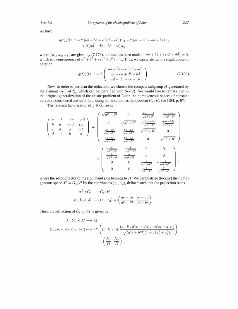
Sec. 7.4 Lie systems of the elastic problem of Euler 227
we have
g(t)g(t)−1 = 2 (ab− ba+ ǫ (cd− dc)) a1 + 2 (ac− ca+ db− bd) a2
+ 2 (ad− da+ bc− cb) a3 ,
wherea1, a2, a3 are given by (7.178), and use has been made ofaa + bb+ ǫ (cc+ dd) = 0,which is a consequence ofa2 + b2 + ǫ (c2 + d2) = 1. Thus, we can write, with a slight abuse ofnotation,
g(t)g(t)−1 = 2
ab− ba+ ǫ (cd− dc)
ac− ca+ db− bd
ad− da+ bc− cb
. (7.180)
Now, in order to perform the reduction, we choose the compactsubgroupH generated bythe elementa1 of gǫ, which can be identified withSO(2). We would like to remark that inthe original generalization of the elastic problem of Euler, the homogeneous spaces of constantcurvature considered are identified, using our notation, asthe quotientGǫ/H , see [184, p. 97].
The relevant factorization ofg ∈ Gǫ reads
a −b −ǫ c −ǫ db a −ǫ d ǫ cc d a −bd −c b a
=
√a2 + b2 0 ǫ(bd−ac)√
a2+b2− ǫ(ad+bc)√
a2+b2
0√a2 + b2 − ǫ(ad+bc)√
a2+b2ǫ(ac−bd)√a2+b2
ac−bd√a2+b2
bc+ad√a2+b2
√a2 + b2 0
ad+bc√a2+b2
bd−ac√a2+b2
0√a2 + b2
×
a√a2+b2
− b√a2+b2
0 0
b√a2+b2
a√a2+b2
0 0
0 0 a√a2+b2
− b√a2+b2
0 0 b√a2+b2
a√a2+b2
,
where the second factor of the right hand side belongs toH . We parametrize (locally) the homo-geneous spaceM = Gǫ/H by the coordinates(z1, z2), defined such that the projection reads
πL : Gǫ −→ Gǫ/H
(a, b, c, d) 7−→ (z1, z2) =
(ac− bd
a2 + b2,bc+ ad
a2 + b2
).
Then, the left action ofGǫ onM is given by
λ : Gǫ ×M −→M
((a, b, c, d), (z1, z2)) 7−→ πL
((a, b, c, d)
(a′, b′, a′z1 + b′z2, −b′z1 + a′z2)√(a′ 2 + b′ 2)(1 + ǫ (z21 + z22))
)
=
(N1
D,N2
D
),

228 Lie systems in control theory Chap. 7
where
N1 = (a2 − b2 − ǫ (c2 − d2))z1 − 2(ab+ ǫ cd)z2 + (ac− bd)(1 − ǫ (z21 + z22)) ,
N2 = 2(ab− ǫ cd)z1 + (a2 − b2 + ǫ (c2 − d2))z2 + (ad+ bc)(1− ǫ (z21 + z22)) ,
D = a2 + b2 − 2ǫ ((ac+ bd)z1 + (ad− bc)z2) + ǫ2(c2 + d2)(z21 + z22) ,
and the real numbersa′ and b′ parametrize the lift of(z1, z2) to Gǫ. Note that the isotopysubgroup of(0, 0) with respect toλ is H andπL(H) = (0, 0), as expected. The fundamentalvector fields with respect to this action, calculated according to (2.2), are
XH1 = z2
∂
∂z1− z1
∂
∂z2, XH
2 = −1
2(1 + ǫ (z21 − z22))
∂
∂z1− ǫ z1z2
∂
∂z2,
XH3 = −ǫ z1z2
∂
∂z1− 1
2(1− ǫ (z21 − z22))
∂
∂z2, (7.181)
which satisfy
[XH1 , X
H2 ] = XH
3 , [XH2 , X
H3 ] = ǫXH
1 , [XH1 , X
H3 ] = −XH
2 .
For the caseǫ = 1, the vector fields (7.181) are essentially the same as that of[143, Table 1, I.3],which provide a realization of the Lie algebraso(3) in terms of vector fields in the real plane.
Now, we factorize the solution which starts from the identity of (7.169) as the productg(t) = g1(t)h(t), where
g1(t) =1√
1 + ǫ (z21(t) + z22(t))
1 0 −ǫ z1(t) −ǫ z2(t)0 1 −ǫ z2(t) ǫ z1(t)
z1(t) z2(t) 1 0z2(t) −z1(t) 0 1
projects onto the solutionπL(g1(t)) = (z1(t), z2(t)), with (z1(0), z2(0)) = (0, 0), of the Liesystem associated to (7.169) on the homogeneous spaceM :
z1 = b1(t)z2 −1
2b2(t)(1 + ǫ (z21 − z22))− b3(t) ǫ z1z2 ,
z2 = −b1(t)z1 − b2(t) ǫ z1z2 −1
2b3(t)(1 − ǫ (z21 − z22)) , (7.182)
andh(t) is a curve inH , withh(0) = (1, 0, 0, 0). This curve satisfies, according to the reductionTheorem 2.5.1, the equation
h(t)h(t)−1 = −Ad(g−11 (t))(b1(t)a1 + b2(t)a2 + b3(t)a3 + g1(t)g1(t)
−1) .
Let us parametrize the curve inH ash(t) = exp(v(t)a1), i.e.,
h(t) =
cos( v(t)
2
)− sin
( v(t)2
)0 0
sin( v(t)
2
)cos( v(t)
2
)0 0
0 0 cos( v(t)
2
)− sin
( v(t)2
)
0 0 sin( v(t)
2
)cos( v(t)
2
)
.
Sec. 7.4 Lie systems of the elastic problem of Euler 229
Then the previous equation yields the differential equation for v
v = −b1(t) + ǫ (b3(t)z1(t)− b2(t)z2(t)) . (7.183)
Note that the infinitesimal generators (7.181), the equations in the homogeneous space (7.182)and the final equation in the subgroup (7.183) reduce, essentially, to those of the first case ofreduction forSE(2) in Table 7.4 whenǫ = 0.
7.4.2 Kinematics inSO(3, R) as a Lie system
We have treated in a unified fashion the kinematic equations of the generalized elastic problemof Euler from the perspective of the theory of Lie systems. Asa particular case, we obtain theanalysis of the kinematic equations on the Lie group of rotationsSO(3) (or onSU(2)) when inall formulas we chooseǫ = 1.
However, the kinematic control equations in the groupSO(3) appear in many applicationsof practical interest, so they deserve a special attention on their own. Equations of this kindappear, for example, as the rotational kinematic part of theplate-ball problem, already mentionedin Subsection 7.2.3.1, see [182, 183, 200], or the kinematiccontrol equations of a rigid bodymoving about one fixed point [55, 183], which appear mainly when considering the spacecraftattitude control problem [26, 97, 99, 206, 221, 268]. Equations of this type are also intimatelyrelated with the Frenet equations in three-dimensional space [69,242]. Even there exists modelsfor DC to DC conversion [55], or models of self-propulsed bodies at low Reynolds number[299,300] whose evolution equation is an equation of motionin SO(3) of the type mentioned.
Moreover, some of these problems, jointly with other motivations, have inspired subsequentdevelopments, as the generalization of some of the results of [99] to connected (or compactsemisimple) Lie groups of dimensionn, see [42, 47], or are related with other questions as theuniform generation of the rotation group inn dimensionsSO(n) [101], and the development ofthe dynamic interpolation problem and the De Casteljau algorithm on Lie groups and symmetricspaces [9,102,103,305].
Therefore, we will particularize the expressions of the previous subsection for the caseǫ = 1, in order to have a quick reference with regard to the kinematic control problem inSO(3)from the perspective of Lie systems. For more details on the derivation of the following formulaswe refer to the general case treated along this section.
We start with the control system with configuration spaceR3, and coordinates(x1, x2, x3),given by
x1 = b2(t)x3 − b1(t)x2 , x2 = b1(t)x1 − b3(t)x3 , x3 = b3(t)x2 − b2(t)x1 , (7.184)
whereb1(t), b2(t) andb3(t) are the control functions. The system can be written in matrix formas
x1x2x3
=
0 −b1(t) b2(t)b1(t) 0 −b3(t)−b2(t) b3(t) 0
x1x2x3
, (7.185)
and its solutions are the integral curves of the time-dependent vector fieldb1(t)X1 + b2(t)X2 +b3(t)X3, where now
X1 = x1∂
∂x2− x2
∂
∂x1, X2 = x3
∂
∂x1− x1
∂
∂x3, X3 = x2
∂
∂x3− x3
∂
∂x2. (7.186)

230 Lie systems in control theory Chap. 7
These vector fields satisfy the Lie brackets
[X1, X2] = X3 , [X1, X3] = −X2 , [X2, X3] = X1 , (7.187)
and hence they generate a Lie algebra isomorphic toso(3), which has a basisa1, a2, a3 withdefining Lie products
[a1, a2] = a3 , [a1, a3] = −a2 , [a2, a3] = a1 . (7.188)
The vector fieldsX1, X2, X3 are fundamental vector fields corresponding to the linear actionof SO(3) onR3: If x denotes a column vector as in (7.175), consider the action
Φ : SO(3)× R3 −→ R
3
(g, x) 7−→ gx , (7.189)
whereg acts onx by matrix multiplication. The Lie algebraso(3) is identified in a natural waywith the set of3× 3 antisymmetric matrices. A basis of this set is given by
a1 =
0 1 0−1 0 00 0 0
, a2 =
0 0 −10 0 01 0 0
, a3 =
0 0 00 0 10 −1 0
, (7.190)
which moreover satisfy the relations (7.188) under the commutator of matrices. Then, we have
d
dsf(exp(−s ai)x)
∣∣∣s=0
= (Xif)(x) , f ∈ C∞(R3) , i = 1, 2, 3 ,
and therefore, according to (2.2), the vector fields are as claimed.The right-invariant Lie system of type (2.10) corresponding to (7.184) or (7.185) on the Lie
groupSO(3) can be written, regarding it as a matrix Lie group, as
gg−1 = −b1(t)a1 − b2(t)a2 − b3(t)a3 , (7.191)
wherea1, a2, a3 is the basis ofso(3) given by (7.188).If we take the previous representation of the Lie algebra (7.190) then we can writegg−1 =
Ω(b(t)), org = Ω(b(t))g , (7.192)
where
Ω(b(t)) =
0 −b1(t) b2(t)b1(t) 0 −b3(t)−b2(t) b3(t) 0
.
The equation (7.192) is the usual way of writing the kinematic control equation on the Lie groupSO(3), which as we see is a right-invariant Lie system on that group.
Let us find now the Wei–Norman systems which can be associatedto the right-invariantsystem (7.191) or (7.192). Writing the solution of these equations which starts from the identityas the product of exponentials
g(t) = exp(−v1(t)a1) exp(−v2(t)a2) exp(−v3(t)a3) (7.193)

Sec. 7.4 Lie systems of the elastic problem of Euler 231
Table 7.6. Wei–Norman systems of differential equations for the solution of (7.191), wherea1, a2, a3 is the basis of the Lie algebraso(3) defined by (7.188). The initial conditions arev1(0) = v2(0) = v3(0) = 0.
Factorization ofg(t) Wei–Norman system
v1 = b1(t) + (b3(t) cos v1 + b2(t) sin v1) tan v2
exp(−v1a1) exp(−v2a2) exp(−v3a3) v2 = b2(t) cos v1 − b3(t) sin v1
v3 = (b3(t) cos v1 + b2(t) sin v1) sec v2
v1 = (b1(t) cos v2 + b3(t) sin v2) sec v3
exp(−v2a2) exp(−v3a3) exp(−v1a1) v2 = b2(t) + (b1(t) cos v2 + b3(t) sin v2) tan v3
v3 = b3(t) cos v2 − b1(t) sin v2
v1 = b1(t) cos v3 − b2(t) sin v3
exp(−v3a3) exp(−v1a1) exp(−v2a2) v2 = (b2(t) cos v3 + b1(t) sin v3) sec v1
v3 = b3(t) + (b2(t) cos v3 + b1(t) sin v3) tan v1
v1 = b1(t) + (b3(t) sin v1 − b2(t) cos v1) tan v3
exp(−v1a1) exp(−v3a3) exp(−v2a2) v2 = (b2(t) cos v1 − b3(t) sin v1) sec v3
v3 = b3(t) cos v1 + b2(t) sin v1
v1 = b1(t) cos v2 + b3(t) sin v2
exp(−v2a2) exp(−v1a1) exp(−v3a3) v2 = b2(t) + (b1(t) sin v2 − b3(t) cos v2) tan v1
v3 = (b3(t) cos v2 − b1(t) sin v2) sec v1
v1 = (b1(t) cos v3 − b2(t) sin v3) sec v2
exp(−v3a3) exp(−v2a2) exp(−v1a1) v2 = b2(t) cos v3 + b1(t) sin v3
v3 = b3(t) + (b2(t) sin v3 − b1(t) cos v3) tan v2
and using the Wei–Norman formula (2.28), we obtain the system of differential equations forv1(t), v2(t) andv3(t):
v1 = b1(t) + (b3(t) cos v1 + b2(t) sin v1) tan v2 ,
v2 = b2(t) cos v1 − b3(t) sin v1 , (7.194)
v3 = (b3(t) cos v1 + b2(t) sin v1) sec v2 ,
with initial conditionsv1(0) = v2(0) = v3(0) = 0. We can choose other five orderings in theproduct (7.193), yielding five different systems of differential equations for the associated secondkind canonical coordinates. The results are summarized in Table 7.6. It can be checked that all ofthese Wei–Norman systems can be regarded as well as Lie systems with associated Lie algebraso(3). This Lie algebra is simple and none of the Wei–Norman systems can be integrated byquadratures in a general case. We would like to remark that the system (7.194) is the same as thatof [99, Eq. (3)], obtained from a slightly different approach for the specific example ofSO(3).

232 Lie systems in control theory Chap. 7
Now, as far as the reduction theory of Lie systems is concerned, we will give the relevantexpressions. As explained in the preceding subsections, itis convenient to treat the reduction ofthe right-invariant Lie system (7.191) formulated onSU(2), rather than onSO(3). The formeris the universal covering of the latter, as it is well-known,and can be identified with the set ofunit quaternions. They admit a4× 4 matrix representation, with matrix elements [55]
a −b −c −db a −d cc d a −bd −c b a
,
such that the real numbersa, b, c andd satisfya2 + b2 + c2 + d2 = 1. The Lie algebraso(3) orsu(2) is represented by4× 4 matrices as well, a basis of it being given by
a1 =1
2
0 −1 0 01 0 0 00 0 0 −10 0 1 0
, a2 =
1
2
0 0 −1 00 0 0 11 0 0 00 −1 0 0
,
a3 =1
2
0 0 0 −10 0 −1 00 1 0 01 0 0 0
, (7.195)
which satisfy the defining relations (7.188) under the matrix commutator. Then, we can reducethe problem of solving (7.191) to that of solving a Lie systemon the subgroup generated bya1:If we factorize the solution of the first problem asg(t) = g1(t)h(t), where
g1(t) =1√
1 + z21(t) + z22(t)
1 0 −z1(t) −z2(t)0 1 −z2(t) z1(t)
z1(t) z2(t) 1 0z2(t) −z1(t) 0 1
is such that(z1(t), z2(t)) is a solution of the system of differential equations
z1 = b1(t)z2 −1
2b2(t)(1 + z21 − z22)− b3(t) z1z2 ,
z2 = −b1(t)z1 − b2(t) z1z2 −1
2b3(t)(1 − z21 + z22) , (7.196)
thenh(t), given by
h(t) = exp(v(t)a1) =
cos( v(t)
2
)− sin
( v(t)2
)0 0
sin( v(t)
2
)cos( v(t)
2
)0 0
0 0 cos( v(t)
2
)− sin
( v(t)2
)
0 0 sin( v(t)
2
)cos( v(t)
2
)
is such thatv(t) is a solution, with appropriate initial conditions, of the differential equation
v = −b1(t) + b3(t)z1(t)− b2(t)z2(t) . (7.197)

Sec. 7.5 Lie control systems onSE(3) 233
7.5 Lie control systems onSE(3)
There appear in the control literature some problems where the Lie groupSE(3) of rigid motionsin the Euclidean space play a relevant role. Usually, theseproblems correspond to the motioncontrol of a rigid body in such a space, as the motion of an autonomous underwater vehicle[220,221], the plate-ball problem [182,183,200], see alsoSubsection 7.2.3.1, and other problems.There exists, moreover, a recent interest in the generationof trajectories onSE(3), see [9, 102,103, 305] and references therein, which is also related to the previous problems. We will focuson the kinematic part of these systems, which as in previous examples, can be understood as aLie system on the Lie groupSE(3) itself or related ones.
Recall that the Lie groupSE(3) can be regarded as the semidirect productSE(3) = R3 ⊙SO(3) of the Abelian Lie group of translations in the spaceR3 with the rotation groupSO(3),relative to the natural action of the latter on the former. Thus, the Lie groupSE(3) admits anatural4× 4 matrix representation with elements
(A c
0 1
), (7.198)
whereA ∈ SO(3) andc is the real column vector
c =
c1c2c3
.
The composition law can be obtained easily through matrix multiplication:
(A c
0 1
)(A′
c′
0 1
)=
(AA′ Ac′ + c
0 1
).
For the sake of ease in the notation, we will denote sometimeselements of type (7.198) as pairs(c, A) with the composition law
(c, A)(c′, A′) = (c +Ac′, AA′) . (7.199)
It is clear that the identity element is(0, Id) and that(c, A)−1 = (−A−1c, A−1). Clearly,
the set of elements of type(0, A) make up a subgroup, identified withSO(3), and the set ofelements of type(c, Id), identified withR3, make up a normal subgroup:
(c, A)(c′, Id)(c, A)−1 = (c, A)(c′, Id)(−A−1c, A−1)
= (c +Ac′, A)(−A−1c, A−1) = (Ac′, Id) .
In addition, each element(c, A) ∈ SE(3) can be factorized in a unique way as(c, A) =(c, Id)(0, A) or (c, A) = (0, A)(A−1
c, Id). Compare with the definition of semidirect prod-ucts at the end of Section 2.5.
According to the representation of the Lie groupSE(3) above, we can easily find a4 × 4matrix representation of the Lie algebrase(3), using the matrix representation already found for

234 Lie systems in control theory Chap. 7
the Lie algebraso(3), see (7.190). Indeed, the six matrices
a1 =
0 1 0 0−1 0 0 00 0 0 00 0 0 0
, a2 =
0 0 −1 00 0 0 01 0 0 00 0 0 0
, a3 =
0 0 0 00 0 1 00 −1 0 00 0 0 0
,
(7.200)
a4 =
0 0 0 −10 0 0 00 0 0 00 0 0 0
, a5 =
0 0 0 00 0 0 −10 0 0 00 0 0 0
, a6 =
0 0 0 00 0 1 00 0 0 −10 0 0 0
,
generate the Lie algebrase(3) under the matrix commutator, with non-vanishing defining rela-tions
[a1, a2] = a3 , [a1, a3] = −a2 , [a1, a4] = −a5 ,[a1, a5] = a4 , [a2, a3] = a1 , [a2, a4] = a6 , (7.201)
[a2, a6] = −a4 , [a3, a5] = −a6 , [a3, a6] = a5 .
Note thata1, a2, a3 generate a Lie subalgebra isomorphic toso(3), (compare with (7.188))as expected. In addition,a4, a5, a6 generate an Abelian ideal.
In terms of the matrix representations ofSE(3) andse(3) described above, a general right-invariant Lie system of type (2.10) for this Lie group can be written as
gg−1 = −6∑
α=1
bα(t)aα , (7.202)
whereg(t) is the solution starting form the identity anda1, . . . , a6 are given by (7.200). Thefunctionsb1(t), . . . , b6(t), can be considered as the control functions.
In examples of practical interest, however, it is not alwayspossible to act directly on themotions generated by all the elements of the Lie algebra, so the corresponding controls are takenas zero, or the controls may be related amongst themselves. For example, in the case of the plate-ball problem one should take (in our notation)b3(t) = 0, b4(t) = ρ b2(t), b5(t) = −ρ b1(t) andb6(t) = 0 for all t, whereρ is the radius of the ball, cf. [182,183,200] and Subsection 7.2.3.1.
We will analyze now the right-invariant Lie system (7.202) by means of the generalizedWei–Norman method. The adjoint representation ofse(3) reads in terms of the basis (7.200) as
ad(a1) =
0 0 0 0 0 00 0 −1 0 0 00 1 0 0 0 00 0 0 0 1 00 0 0 −1 0 00 0 0 0 0 0
, ad(a2) =
0 0 1 0 0 00 0 0 0 0 0−1 0 0 0 0 00 0 0 0 0 −10 0 0 0 0 00 0 0 1 0 0
,

Sec. 7.5 Lie control systems onSE(3) 235
ad(a3) =
0 −1 0 0 0 01 0 0 0 0 00 0 0 0 0 00 0 0 0 0 00 0 0 0 0 10 0 0 0 −1 0
, ad(a4) =
0 0 0 0 0 00 0 0 0 0 00 0 0 0 0 00 0 0 0 0 01 0 0 0 0 00 −1 0 0 0 0
,
ad(a5) =
0 0 0 0 0 00 0 0 0 0 00 0 0 0 0 0−1 0 0 0 0 00 0 0 0 0 00 0 1 0 0 0
, ad(a6) =
0 0 0 0 0 00 0 0 0 0 00 0 0 0 0 00 1 0 0 0 00 0 −1 0 0 00 0 0 0 0 0
,
and as a consequence
exp(−v1 ad(a1)) =
1 0 0 0 0 00 cos v1 sin v1 0 0 00 − sin v1 cos v1 0 0 00 0 0 cos v1 − sin v1 00 0 0 sin v1 cos v1 00 0 0 0 0 1
,
exp(−v2 ad(a2)) =
cos v2 0 − sin v2 0 0 00 1 0 0 0 0
sin v2 0 cos v2 0 0 00 0 0 cos v2 0 sin v20 0 0 0 1 00 0 0 − sin v2 0 cos v2
,
exp(−v3 ad(a3)) =
cos v3 sin v3 0 0 0 0− sin v3 cos v3 0 0 0 0
0 0 1 0 0 00 0 0 1 0 00 0 0 0 cos v3 − sin v30 0 0 0 sin v3 cos v3
,
and
exp(−v4 ad(a4)) = Id−v4 ad(a4) , exp(−v5 ad(a4)) = Id−v5 ad(a5) ,exp(−v6 ad(a4)) = Id−v6 ad(a6) .
Writing the solution which starts from the identity of (7.202) as the product of exponentials
g(t) = exp(−v1(t)a1) exp(−v2(t)a2) exp(−v3(t)a3)× exp(−v4(t)a4) exp(−v5(t)a5) exp(−v6(t)a6) , (7.203)
and using the Wei–Norman formula (2.28), we obtain the system of differential equations for

236 Lie systems in control theory Chap. 7
v1(t), . . . , v6(t):
v1 = b1(t) + (b3(t) cos v1 + b2(t) sin v1) tan v2 ,
v2 = b2(t) cos v1 − b3(t) sin v1 ,
v3 = (b3(t) cos v1 + b2(t) sin v1) sec v2 ,
v4 = (b4(t) cos v2 + b5(t) sin v1) cos v2 − b6(t) sin v2 , (7.204)
v5 = (b5(t) cos v1 − b4(t) sin v1) cos v3 + b6(t) cos v2 sin v3
+ (b4(t) cos v1 + b5(t) sin v1) sin v2 sin v3 ,
v6 = (b4(t) sin v1 − b5(t) cos v1) sin v3 + b6(t) cos v2 cos v3
+ (b4(t) cos v1 + b5(t) sin v1) sin v2 cos v3 ,
with initial conditionsv1(0) = · · · = v6(0) = 0. Note that the subsystem made up by the firstthree equations is the same as (7.194), and once it has been solved, the three last equations aredirectly integrable by quadratures. If, for example, we take instead the factorization
g(t) = exp(−v6(t)a6) exp(−v5(t)a5) exp(−v4(t)a4)× exp(−v3(t)a3) exp(−v2(t)a2) exp(−v1(t)a1) , (7.205)
we will arrive to the system of differential equations forv1(t), . . . , v6(t):
v1 = (b1(t) cos v3 − b2(t) sin v3) sec v2 ,
v2 = b2(t) cos v3 + b1(t) sin v3 ,
v3 = b3(t) + (b2(t) sin v3 − b1(t) cos v3) tan v2 ,
v4 = b4(t) + b2(t)v6 − b1(t)v5 , (7.206)
v5 = b5(t) + b1(t)v4 − b3(t)v6 ,
v6 = b5(t) + b3(t)v5 − b2(t)v4 ,
with initial conditionsv1(0) = · · · = v6(0) = 0. Note as well that the subsystem which consistsof the first three of these equations is the same as that corresponding to the last factorization inTable 7.6, and that the subsystem made up by the last three equations can be written in matrixform as
v4v5v6
=
b4(t)b5(t)b6(t)
+
0 −b1(t) b2(t)b1(t) 0 −b3(t)−b2(t) b3(t) 0
v4v5v6
, (7.207)
which can be regarded as well as a Lie system with associated Lie algebrase(3) as we will showbelow. We remark that a similar system to (7.206) is obtainedin [220, Eq. (3.17)].
7.5.1 Reduction of Lie systems onSE(3)
We will apply in this subsection the theory of reduction of Lie systems to right-invariant Liesystems onSE(3) of type (7.202). Due to the structure of this Lie group as a semidirect productSE(3) = R3 ⊙ SO(3), it is natural to perform the reduction with respect to the subgroupsR3
andSO(3), in order to reduce the mentioned problems inSE(3) to others in these subgroups.

Sec. 7.5 Lie control systems onSE(3) 237
We start taking the normal subgroupH = R3 to carry out the reduction with respect to it.For more details about the procedure that we will follow, seethe end of Section 2.5. It is clearthatSE(3)/R3 ∼= SO(3), the projection being
πL : SE(3) −→ SO(3)
(c, A) 7−→ A .
Thus, the corresponding left action ofSE(3) onSO(3) is given by
λ : SE(3)× SO(3) −→ SO(3)
((c, A), B) 7−→ πL((c, A)(c′, B)) = AB ,
wherec′ parametrizes the lift ofB ∈ SO(3) to SE(3), and we have used the composition law(7.199). Now, letg1(t) be a lift toSE(3) of a curveA(t) in SO(3), solution of
AA−1 = −b1(t)a1 − b2(t)a2 − b3(t)a3 , (7.208)
wherea1, a2, a3 is the basis of the factor Lie algebrase(3)/R3 ∼= so(3) induced from the ba-sisa1, . . . , a6 with respect to which the equation (7.202) is written. In particular, the elementsof a1, a2, a3 satisfy the Lie products (7.188).
If we factorize the solutiong(t) of (7.202) as the productg(t) = g1(t)h(t), then, by Theo-rem 2.5.1, the curveh(t) ∈ R3 for all t, and satisfies
h h−1 = −Ad(g−11 (t))
(6∑
i=1
bi(t)ai + g1(t)g−11 (t)
).
The simplest choice for the mentioned liftg1(t) is just
g1(t) =
(A(t) 00 1
).
With this choice, we have
g1(t)g−11 (t) = −b1(t)a1 − b2(t)a2 − b3(t)a3 ,
and then, substituting into the previous equation forh(t), we obtain
h h−1 = −Ad(g−11 (t))
(6∑
i=4
bi(t)ai
). (7.209)
If now h(t) is of the form
h(t) =
(Id d(t)0 1
),
with
d(t) =
d1(t)d2(t)d3(t)
,

238 Lie systems in control theory Chap. 7
it is not difficult to prove that (7.209) becomes
di =
3∑
j=1
bj+3(t)[A(t)]ji , i = 1, 2, 3 ,
taking into account thatA(t) is an orthogonal matrix for allt and therefore its inverse is equal toits transpose matrix. This last system is clearly a Lie system with associated Lie algebraR3.
Take now the subgroupH = SO(3) to carry out the reduction procedure. In this case, wehave thatSE(3)/SO(3) ∼= R3, seen as a homogeneous space ofSE(3), the action being thenatural affine action on the three-dimensional Euclidean space. Indeed, the projection is just
πL : SE(3) −→ R3
(c, A) 7−→ c ,
and then, the corresponding left action is given by
λ : SE(3)× R3 −→ R
3
((c, A), d) 7−→ πL((c, A)(d, A′)) = c+Ad ,
whereA′ parametrizes the lift ofd ∈ R3 to SE(3), and we have used the composition law(7.199). Let us take coordinates(x1, x2, x3) in the homogeneous spaceR3. The fundamentalvector fields corresponding to the previous action can be calculated with the help of (2.2) andtaking into account the matrix representation (7.200) ofse(3). They turn out to be
XH1 = x1
∂
∂x2− x2
∂
∂x1, XH
2 = x3∂
∂x1− x1
∂
∂x3, XH
3 = x2∂
∂x3− x3
∂
∂x2,
XH4 =
∂
∂x1, XH
5 =∂
∂x2, XH
6 =∂
∂x3, (7.210)
for which we have the non-vanishing Lie brackets
[XH1 , X
H2 ] = XH
3 , [XH1 , X
H3 ] = −XH
2 , [XH1 , X
H4 ] = −XH
5 ,
[XH1 , X
H5 ] = XH
4 , [XH2 , X
H3 ] = XH
1 , [XH2 , X
H4 ] = XH
6 , (7.211)
[XH2 , X
H6 ] = −XH
4 , [XH3 , X
H5 ] = −XH
6 , [XH3 , X
H6 ] = XH
5 .
The Lie system in the homogeneous spaceR3 of SE(3) associated to the right-invariant sys-tem (7.202) is that whose solutions are the integral curves of the time-dependent vector field∑6
i=1 bi(t)XHi , that is,
x1 = b4(t) + b2(t)x3 − b1(t)x2 ,
x2 = b5(t) + b1(t)x1 − b3(t)x3 , (7.212)
x3 = b6(t) + b3(t)x2 − b2(t)x1 ,
or, written in matrix form,
x1x2x3
=
b4(t)b5(t)b6(t)
+
0 −b1(t) b2(t)b1(t) 0 −b3(t)−b2(t) b3(t) 0
x1x2x3
. (7.213)

Sec. 7.6 Lie control systems onSE(3) 239
Incidentally, recall that the system (7.207) is of this type. Now, let
x(t) =
x1(t)x2(t)x3(t)
be a particular solution of (7.212) or (7.213). Take a liftg1(t) of this curve toSE(3).If we factorize now the desired solutiong(t) of (7.202) as the productg(t) = g1(t)h(t),
then, by Theorem 2.5.1, the curveh(t) takes values in the subgroupSO(3) for all t, and satisfies
h h−1 = −Ad(g−11 (t))
(6∑
i=1
bi(t)ai + g1(t)g−11 (t)
).
For example, take the liftg1(t) given by
g1(t) =
(Id x(t)0 1
).
With this choice, we have
g1(t)g−11 (t) =
(0 x(t)0 0
)(Id −x(t)0 1
)=
(0 x(t)0 0
),
and as a result, in terms of the Lie algebra representation (7.200),
h h−1 = −Ad(g−11 (t))
0 b1(t) −b2(t) −b4(t) + x1
−b1(t) 0 b3(t) −b5(t) + x2
b2(t) −b3(t) 0 −b6(t) + x3
0 0 0 0
= −
1 0 0 −x1
0 1 0 −x2
0 0 1 −x3
0 0 0 1
0 b1(t) −b2(t) −b4(t) + x1
−b1(t) 0 b3(t) −b5(t) + x2
b2(t) −b3(t) 0 −b6(t) + x3
0 0 0 0
1 0 0 x1
0 1 0 x2
0 0 1 x3
0 0 0 1
= −
0 b1(t) −b2(t) −b4(t) + x1 + b1(t)x2 − b2(t)x3
−b1(t) 0 b3(t) −b5(t) + x2 + b3(t)x3 − b1(t)x1
b2(t) −b3(t) 0 −b6(t) + x3 + b2(t)x1 − b3(t)x2
0 0 0 0
=
0 −b1(t) b2(t) 0b1(t) 0 −b3(t) 0−b2(t) b3(t) 0 0
0 0 0 0
,
where we have used thatx(t) is a particular solution of (7.212). Ifh(t) is of the form
h(t) =
(A(t) 00 1
),
for all t, then the previous equation can be written as
AA−1 = −b1(t)a1 − b2(t)a2 − b3(t)a3 ,
that is, a right-invariant Lie system inSO(3) like (7.191) or (7.192).

240 Lie systems in control theory Chap. 7
7.6 Conclusions and directions for further work
We have illustrated with detail the use of the theory of Lie systems in specific examples of controltheory. In particular, we have shown how some of these systems can be studied in an unified way.Many of the arising results seem to be previously unknown.
Along the study of the examples, we have seen how some systemsof Lie type, which areoriginally considered in relation to optimal control problems, can be reduced to other problemsof Lie type which are the kinematic part of some other optimalcontrol problems but with thesame controls and the same integral functional to be minimized, see, e.g., the examples in Sub-sections 7.2.1, 7.2.2.1, 7.2.3 and subsequent examples in Section 7.3. Likewise, the examples ofSection 7.4 are considered originally in relation with optimal control problems, where the costfunctional to be minimized is the integral of the sum of the squares of the control functions. Wehave obtained the corresponding Lie systems on certain homogeneous spaces by means of ourreduction theory. In view of all this, it is natural to wonderabout the relation of the reductiontheory of Lie systems and the optimal control problems.
Another question which is highlighted by using the theory ofLie systems concerns the def-inition of kinematic nonholonomic control systems throughnonholonomic constraints, i.e., theinput vector fields appearing in the kinematic control system of interest belong to the kernel ofa set of non-exact constraint one-forms in phase space, which make up a non-integrable distri-bution, see, e.g., [42–44]. In addition, in some cases thesenon-integrable distributions can beregarded as those defining the horizontal distribution withrespect to a connection of differentkinds (principal, linear, Ereshman, etc.) [31–33,46,63–66,105,121,122,193,198,200–202,219,222,223,233,234,250,275,294,307].
As far as the theory of control systems is concerned, and morespecifically, with regard tothe theory of Lie systems, to start from the constraint distribution presents two problems. Thefirst is that if we start from the distribution, the input vector fields in the kernel are not uniquelydefined (if no extra information is provided), and the choiceof one or other set of input vectorfields may lead to very different systems from the algebraic point of view. We illustrate this pointby the following two examples.
In [256], it is considered the model of a vertical rolling coin, taking into account the rollingangle (we have studied this model, without such rolling angle, in Subsection 7.3.1). There aretwo constraint one-forms arising from the requirement thatthe coin roll in the direction it ispointing, with no slipping. Taking a certain chart inR4, with coordinates(x1, x2, x3, x4), theyread as
ω1 = cosx3 dx1 + sinx3 dx2 − dx4 , ω2 = sinx3 dx1 − cosx3 dx2 .
In order to consider the system as a control system, and following the mentioned reference, wecan choose the two input vector fields belonging to the kernelof these one-forms:
X1 = cosx3∂
∂x1+ sinx3
∂
∂x2+
∂
∂x4, X2 =
∂
∂x3.
Taking the Lie brackets
X3 = [X1, X2] = sinx3∂
∂x1− cosx3
∂
∂x2,
X4 = [X2, X3] = cosx3∂
∂x1+ sinx3
∂
∂x2,

Sec. 7.6 Conclusions and directions for further work 241
it is easy to check thatX1, X2, X3, X4 close on the solvable Lie algebra, with respect to theLie bracket, defined by
[X1, X2] = X3 , [X2, X3] = X4 , [X2, X4] = −X3 ,
all other Lie brackets being zero. The three vector fieldsX2, X3, X4 make up a Lie subalgebraisomorphic tose(2), compare with (7.88). Using the theory of Goursat normal forms, two newinput vector fields are taken in [256], in order to trasform the system into chained form. Indeed,the new vector fields
Y1 = X2 − (x2 cosx3 − x1 sinx3)X1 , Y2 = −X1 ,
close on the Lie algebra defined by the non-vanishing Lie brackets
[Y1, Y2] = Y3 , [Y1, Y3] = Y4 ,
where
Y3 = sinx3∂
∂x1− cosx3
∂
∂x2, Y4 = − ∂
∂x3.
That is, with this new choice of input vector fieldsY1, Y2 in the kernel of the above one-forms,we obtain a control system which can be regarded as a Lie system with associated nilpotent Liealgebrag4, in the notation of Subsection 7.3.4, see in particular (7.154). We note in passing thatthis Lie algebra also appears in the nilpotentized version of the front-wheel driven kinematic car,cf. Subsection 7.3.2.
Another example is given by the so-called Chaplygin skate, see for example [31]. Theconstraint one-form is defined in some open subset ofR3, with coordinates(x1, x2, x3), as
ω = sinx3 dx1 − cosx3 dx2 + dx3 .
We take first the simple choice of the vector fields in the kernel
X1 =∂
∂x1− sinx3
∂
∂x3, X2 =
∂
∂x2+ cosx3
∂
∂x3.
These vector fields close on the Lie algebra defined by the non-vanishing Lie brackets
[X1, X2] = X3 , [X1, X3] = X4 , [X1, X4] = X3 , [X2, X3] = X5 ,
[X2, X5] = X3 , [X3, X4] = −X5 , [X3, X5] = X4 , [X4, X5] = X3 ,
where
X3 =∂
∂x3, X4 = cosx3
∂
∂x3, X5 = sinx3
∂
∂x3.
The three vector fieldsX3, X4, X5 make up an ideal which is in turn isomorphic toso(2, 1),already used in Section 7.4, compare with (7.168) for the case ǫ = −1, establishing the corre-spondencesX3 → a1, X4 → −a2 andX5 → a3. If, instead, one takes the vector fields in thekernel
Y1 = cosx3∂
∂x1+ sinx3
∂
∂x2, Y2 = − sinx3
∂
∂x1+ cosx3
∂
∂x2+
∂
∂x3,

242 Lie systems in control theory Chap. 7
as it is suggested in [198], they close on a Lie algebra isomorphic to that of the Euclidean groupin the plane:
[Y1, Y2] = Y3 , [Y1, Y3] = 0 , [Y2, Y3] = Y1 ,
where
Y3 = sinx3∂
∂x1− cosx3
∂
∂x2.
Indeed, with the correspondencesY1 → a3, Y2 → a1, andY3 → a2, the above Lie bracketsbecome the commutation relations (7.88) considered in Subsection 7.3.1. The relation betweenboth pairs of input vector fields is
Y1 = cosx3X1 + sinx3X2 , Y2 = − sinx3X1 + cosx3X2 .
As we have seen in Subsections 7.3.1.2, 7.3.2 and the first of these two examples, the indeter-minacy of the input vector fields to be taken out of the kernel of a set of one-forms, is relatedwith the techniques of state space feedback transformations, for example to obtain a nilpotentsystem from another which is not. One might wonder, from our perspective, whether it wouldbe possible to develop other criteria in order to select other input vector fields such that the finalsystem would have other types of associated Lie algebras, for example solvable Lie algebras notnecessarily nilpotent, or other prescribed Lie algebra structures.
The second problem, in our opinion, is to make more precise towhat extent we are allowedto take Lie brackets of the input vector fields chosen out of the kernel of a set of one-formsdefining a non-integrable distribution. Since it is non-integrable, the Lie brackets will not belongin general to the mentioned kernel, so the vector fields so obtained are in some sense of differentnature of the chosen ones. However, to take Lie brackets of the input vector fields is important incontrol theory, for example to test controllability according to Chow’s theorem [90,203,312] andwith respect to the theory of Lie systems, where we have to findthe minimal finite-dimensionalLie algebra (if it exists) which contains the given input vector fields.
Another possible line for future research is related with the description of Lie systems asconnections in principal bundles and associated bundles, cf. Section 2.6. In some articles (see,e.g., [122, 193]), nonholonomic control systems are treated from the point of view of principalconnections in principal bundles, where the base manifold has to do with the configuration space.In addition, this principal connection approach is also applicable to systems which are not ofLie type. However, it would be an interesting problem to treat to relate both types of bundlestructures, in cases both exist.
We leave these and other problems for future research.

PART 4
APPENDICES


Appendix A
Connections in fibre bundles
We give in this appendix a brief review of the theory of connections in principal fibre bundlesand associated ones, which is the basis for the understanding of our development of the theory ofSections 2.6 and 2.7. The following material is adapted fromthe treatment given in [62], whichin turn is mainly based on standard textbooks as [40,148,197,330], and other references. We willrefer to any of them for the facts not explicitly proved here.We hope this Appendix will serve asa fast reference guide for the understanding of the relationbetween Lie systems and connectionsin principal and associated fibre bundles. We will assume basic knowledge of manifold theory,Lie group theory, and the theory of actions of Lie groups on manifolds, in what follows.
A.1 Fibre bundles
A.1.1 Smooth fibre bundles
Definition A.1.1. A smooth fibre bundleis a quadruple(E, π, B, F ), whereE, B, F , aremanifolds andπ is a smooth map ofE ontoB, such that there is an open coveringUα of Band a familyψα of diffeomorphisms
ψα : Uα × F −→ π−1(Uα)
(x, y) 7−→ ψα(x, y)
such that(π ψα)(x, y) = x, ∀x ∈ Uα, ∀y ∈ F . We call(Uα, ψα) a coordinate represen-tation for the bundle (it can be taken to be finite).E is thetotal spaceor bundle space, B is thebase spaceandF is thetypical fibre. Forx ∈ B, Fx = π−1(x) will be called thefibre overx.Clearly,E is the disjoint union of all the fibresFx, x ∈ B.
Note that we have diffeomorphisms
ψα, x : F −→ Fx
y 7−→ ψα(x, y) , x ∈ Uα .
Definition A.1.2. A (smooth) cross-sectionof a fibre bundle(E, π, B, F ) is a smoothmapσ : B −→ E such thatπ σ = idB .
245

246 Connections in fibre bundles Appendix A
Definition A.1.3. Let (E′, π′, B′, F ′) be another bundle. Then a smooth mapφ :E −→ E′ is fibre-preservingif π(z1) = π(z2) impliesπ′(φ(z1)) = π′(φ(z2)), for all z1, z2 inE. In that case,φ clearly determines a smooth mapφB : B −→ B′ by means ofπ′ φ = φB π.
The following result [148] is very important if we want to determine when we have a fibrebundle.
Proposition A.1.1. LetB, F be manifolds, andE a set. Suppose thatπ : E −→ B isonto, and
(1) There is an open coveringUα ofB and a familyψα of bijections
ψα : Uα × F −→ π−1(Uα) .
(2) For all x ∈ Uα, y ∈ F , (π ψα)(x, y) = x .(3) The mapsψβα : Uαβ × F −→ Uαβ × F defined byψβα(x, y) = (ψ−1
β ψα)(x, y) arediffeomorphisms, whereUαβ = Uα ∩ Uβ.
Then, there is exactly one manifold structure onE such that(E, π, B, F ) is a fibre bundle withcoordinate representation(Uα, ψα).
A.1.2 Vector bundles
Definition A.1.4. A vector bundleis a smooth fibre bundleξ = (E, π, B, F ) such that
(1) F and the fibresFx = π−1(x), x ∈ B, are vector spaces.(2) There exists a coordinate representation(Uα, ψα) such that the mapsψα, x : F −→ Fx
are linear isomorphisms (again this can be taken to be finite).
Therank of ξ is defined as dimF . A neighbourhoodU in B is a trivialising neighbourhoodforξ if there is a diffeomorphismψU : U × F −→ π−1(U) such that(π ψU )(x, y) = x, withx ∈ U , y ∈ F , and such that the induced mapsψU, x : F −→ Fx are linear isomorphisms. ThemapψU is called atrivialising map.
Definition A.1.5. Let ξ = (E, π, B, F ) andξ′ = (E′, π′, B′, F ′) be vector bundles.Then, abundle map(or morphism) φ : ξ −→ ξ′ is a smooth fibre-preserving map such that therestrictionsφx : Fx −→ F ′
φB(x), with x ∈ B, are linear. The mapφ is called anisomorphismif itis a diffeomorphism; we writeξ ∼= ξ′. The mapφ is called astrong bundle map(orB-morphism)if B = B′ andφB = idB. If, further, for anyx ∈ B, φx is injective, we will say thatξ is asubbundleof ξ′.
A.1.3 Principal bundles
Definition A.1.6. Let G be a Lie group. Aprincipal bundle with structure groupG is asmooth fibre bundleP = (P, π, B, G) with a right actionΨ : P × G −→ P satisfying thefollowing conditions:

A.1 Fibre bundles 247
(1) The right actionΨ is free.(2) The base manifoldB is the quotient space ofP by the equivalence relation induced byG,
B = P/G.(3) The fibre bundleP admits a coordinate representation(Uα, ψα) with diffeomorphisms
ψα : Uα ×G −→ π−1(Uα) satisfying
ψα(x, gg′) = Ψ(ψα(x, g), g
′) , ∀x ∈ Uα , ∀ g, g′ ∈ G .
Such a coordinate representation is calledprincipal.
The following properties are immediate consequences of thedefinition. Takeα arbitrarybut fixed. Then, the mapΨ, when restricted toπ−1(Uα), defines a right action as well. Indeed,since any elementp ∈ π−1(Uα) can be written asψα(x, g), wherex ∈ Uα, andg ∈ G, we have
Ψ(p, g′) = Ψ(ψα(x, g), g′) = ψα(x, gg
′) ∈ π−1(Uα) ,
and the defining properties of an action are inherited from the actionΨ ofG on the wholeP . Foreach diffeomorphismψα, consider the mapsψαx, with x ∈ Uα, defined by
ψαx : G −→ π−1(Uα)
g 7−→ ψαx(g) = ψα(x, g) .
Thus, we have thatψαx is equivariant with respect to the right actions ofG on itself, and theprevious right action ofG onπ−1(Uα), i.e.,
ψαx Rg = Ψg|π−1(Uα)
ψαx , ∀x ∈ Uα , ∀ g ∈ G .
Moreover, we have thatπ(Ψ(p, g)) = π(p), ∀ g ∈ G, p ∈ P . Indeed: anyp ∈ P belongsto π−1(Uα) for certainα. Asψα is a diffeomorphism, we havep = ψα(x, g
′), with g′ ∈ G andx = π(p) ∈ Uα. Then,
π(Ψ(p, g)) = π(Ψ(ψα(x, g′), g)) = π(ψα(x, g
′g)) = x = π(p) .
Finally, it is immediate to see that the orbitOp ofG throughp ∈ P is the fibre containingp.We writeGx for π−1(x). (No confusion should arise with the notation for isotropy subgroups,since the action is free).
Definition A.1.7. Let P = (P , π, B, G) be another principal bundle with actionΨ. Amorphism(resp.isomorphism) φ : P −→ P consists of a smooth mapφP : P −→ P and a ho-momorphism (resp. isomorphism)φG : G −→ G such thatφP (Ψ(p, g)) = Ψ(φP (p), φG(g)),for all p ∈ P , g ∈ G. Clearly,φP preserves fibres and so induces a mapφB : B −→ B. IfB = B andG = G with φB = idB, φG = idG, then we callφ a strong morphism(resp.strongisomorphism).
We show next simple examples of principal bundles.
Example A.1.1. Trivial or product bundles. Consider(B × G, π, B, G), whereBis a manifold,G a Lie group andπ the projection ofB × G ontoB. Consider the right action

248 Connections in fibre bundles Appendix A
Ψ((x, g), g′) = (x, gg′), where(x, g) ∈ B × G. Then we have a principal bundle, calledtrivial . If a principal bundleP is strongly isomorphic to a trivial bundle, is calledtrivialisable.
Example A.1.2. Homogeneous spaces. Let H be a closed subgroup ofG. Considerthe natural projectionπ : G −→ G/H given byπ(g) = gH . SinceH acts onG by righttranslations, we obtain a principal bundle(G, π, G/H, H).
We will discuss now the existence of cross-sections of principal bundles. The followingresult is of key importance.
Proposition A.1.2. Let P = (P, π, B, G) be a principal bundle and letU ⊂ B beopen. ThenP admits a local cross-sectionσ : U −→ P if, and only if,P|U is trivialisable.
Proof. Let σ : U −→ P be a section. Define the strong isomorphismφ : U × G −→π−1(U) by (x, g) 7−→ Ψ(σ(x), g). Conversely, givenφ : U × G −→ π−1(U) we define
σ : U −→ P by x 7−→ φ(x, e). Then,(π σ)(x) = x and thereforeσ ∈ Sec(P|U ).
Therefore, we have the result that, by the local triviality of P , many local cross-sectionsexist. However,P can have aglobalcross-section if and only ifP is trivialisable.
We will discuss now the local properties and transition functions of principal fibre bundles.Suppose(Uα, ψα) is a coordinate representation forP . By Proposition A.1.2, we have afamily of (local) cross-sectionsσα : Uα −→ P , x 7−→ ψα(x, e). Now, inUαβ = Uα ∩ Uβ, wehaveσβ(x) = Ψ(σα(x), γαβ(x)), whereγαβ : Uαβ −→ G. The functionsγαβ are called thetransition functionsfor P corresponding to the open coveringUα of B. Notice that
ψαβ(x, g) = (ψ−1α ψβ)(x, g) = ψ−1
α (Ψ(ψβ(x, e), g)) = ψ−1α (Ψ(σβ(x), g)) ,
but
ψα(x, γαβ(x)g) = Ψ(ψα(x, e), γαβ(x)g) = Ψ(σα(x), γαβ(x)g) = Ψ(σβ(x), g) ,
therefore, introducing the latter equation into the formerone, we have
ψαβ(x, g) = (x, γαβ(x)g) .
We could have used this last expression to define the transition functions. Notice as well thatψαβ ψβδ = ψαδ gives
γαβ(x)γβδ(x) = γαδ(x) , ∀x ∈ Uα ∩ Uβ ∩ Uδ . (A.1)
Corversely, we have the following result [197, Prop. 5.2]:
Proposition A.1.3. LetB be a manifold,Uα an open covering ofB, andG a Liegroup. Given mapsγαβ : Uαβ −→ G satisfying(A.1), we can construct a principal bundleP = (P, π, B, G) with transition functionsγαβ .

A.1 Fibre bundles 249
A.1.4 Associated bundles
In this subsectionP = (P, π, B, G) will denote a fixed principal bundle with actionΨ. SupposeΦ : G ×M −→ M is a fixed left action ofG on a manifoldM . Consider the right action ofGonP ×M given by
(p, y)g = (Ψ(p, g), Φ(g−1, y)) , ∀ p ∈ P, y ∈M, g ∈ G .
This is called thejoint actionof G. This action defines an equivalence relation, the equivalenceclasses being its orbits. LetE = P ×GM denote the set of orbits of the joint action, and let
[ · ] : P ×M −→ E
(p, y) 7−→ [p, y] ,
be the natural projection on the set of orbits of the joint action, where[p, y] denotes the equiva-lence class of(p, y). Then, this projection determines a mapπE : E −→ B via the commutativediagram
P ×M[ · ]−−−−→ E
pr1
yyπE
Pπ−−−−→ B
i.e.,πE([p, y]) = π(p), for all p ∈ P , y ∈ M . We will denoteMx = π−1E (x), for x ∈ B. We
have the following result.
Theorem A.1.1. There is a unique smooth structure onE such thatξ = (E, πE , B, M)is a smooth fibre bundle.
Proof. Let (Uα, ψα) be a coordinate representation ofP , with local cross-sectionsσα : Uα −→ P satisfyingσβ(x) = Ψ(σα(x), γαβ(x)), for anyx ∈ Uαβ . Define the maps
φα : Uα ×M −→ π−1E (Uα)
(x, y) 7−→ [σα(x), y] .
Then,πE(φα(x, y)) = πE([σα(x), y]) = π(σα(x)) = x ,
sinceσα is a local cross-section, the restrictions ofφα to the fibers,φα, x : M −→ π−1E (x), are
bijections. Now,φαβ(x, y) = φ−1
α (φβ(x, y)) = φ−1α ([σβ(x), y]) ,
for all x ∈ Uαβ , y ∈M . On the other hand,
φα(x, Φ(γαβ(x), y)) = [σα(x), Φ(γαβ(x), y)]
= [Ψ(σβ(x), γ−1αβ (x)), Φ(γαβ(x), y)] = [σβ(x), y] ,
by definition of[ · ]. Therefore, we obtain
φαβ(x, y) = (x, Φ(γαβ(x), y)) ,

250 Connections in fibre bundles Appendix A
and thenφαβ are diffeomorphisms. By Proposition A.1.1 there exists a unique manifold structure
onE = P ×GM such thatξ is a smooth bundle with coordinate representation(Uα, φα).
Definition A.1.8. The fibre bundleξ of the previous Theorem is called thefibre bundlewith fibreM and structure groupG associated withP .
Moreover, it can be proved as well that[ · ] : P ×M −→ E is a smooth fibre-preservingmap, restricting to diffeomorphisms[ · ]p : M −→ Mπ(p) on each fibre; that the quadruple(P ×M, [ · ], E, G) is a principal bundle with the joint action and thatpr1 is a morphism ofprincipal bundles [148,197].
Note that if the action ofG onM is trivial, thenξ = (E, πE , B, M) is trivial. Also, if Pis trivial, so isξ. And that ifG acts on itself by left translations, thenP ×G G is justP again.
Example A.1.3. Associated vector bundles. If M is a finite-dimensional vector space,andΦ defines a linear representation ofG in M , thenξ = (E, πE , B, M) is a vector bundle.In fact, if x ∈ B, p ∈ π−1(x), there is a unique vector space structure inMx such that themaps[ · ]p are linear isomorphisms;0x = [p, 0] ∈ Mx. Then, eachφα, x in the proof ofTheorem A.1.1 is a linear isomorphism.
A.2 Connections in fibre bundles
A.2.1 Preliminary concepts
Take a principal bundleP = (P, π, B, G), where dimB = n, dimG = r, and the right actionisΨ : P ×G −→ P . We will denote byg the Lie algebra ofG.
First of all, recall the mapΨp∗e : g ∼= TeG → TpP . The mapY : g → X(P ) given bya 7→ Ya(p) = Ψp∗e(a) defines thefundamental vector fieldassociated to the elementa of g, i.e.,
(Yaf)(p) =d
dtf(Ψ(p, exp(ta)))
∣∣∣t=0
, f ∈ C∞(P ) .
The vector fieldYa is complete with flowφ(t, p) = Ψ(p, exp(ta)). Moreover, the mapY is aLie algebra homomorphism,Y[a,b] = [Ya, Yb].
Definition A.2.1. A vector fieldX onP is invariant if Ψg∗p(Xp) = XΨ(p, g). We will
denote byXI(P ) the Lie subalgebra of invariant vector fields.
Proposition A.2.1. We have thatΨg∗(Ya) = YAd(g−1)a, for all g ∈ G, a ∈ g.
Proof. We must proveΨg∗p(Ya)p = (YAd(g−1)a)Ψ(p, g). This is immediate once one real-izes thatΨgΨp = ΨpRg = ΨΨ(p, g)ig, whereRg andig denote the right translation and con-
jugation byg onG, respectively.

A.2 Connections in fibre bundles 251
Now, fromπ : P −→ B, we have the bundle map
TPπ∗−−−−→ TB
τP
yyτB
Pπ−−−−→ B
Definition A.2.2. The spaceVp(P ) = Ker π∗p, p ∈ P , is called thevertical subspaceof TpP . Clearly, dimVp(P ) = dimG. We can think ofVp(P ) as the space of vectors tangent tothe fibre throughp.
We defineVP = ∪p∈PVp(P ), which is a subbundle ofτP : TP −→ P , i.e., the mapp 7−→ Vp(P ) is an r-dimensional distribution onP . VP is called thevertical subbundleofτP . We have dimVP = n + 2r. A vector fieldX ∈ X(P ) is vertical if Xp is vertical, i.e., ifπ∗p(Xp) = 0 for all p ∈ P . Clearly, the set of all vertical vector fields forms a Lie subalgebraXV (P ) of X(P ), sinceπ∗[X1, X2] = [π∗(X1), π∗(X2)] = 0 if X1,X2 are vertical.
Proposition A.2.2. The mapping
Ψp∗e : TeG −→ TpP
a 7−→ Ψp∗e = (Ya)p ,
is a linear isomorphism ofg ontoVp(P ).
Proof. Take an arbitrary but fixedp ∈ P . Since(π Ψp)(g) = π(p), for all g ∈ G,we haveπ∗p(Ya)p = (π∗p Ψp∗e)(a) = (π Ψp)∗e(a) = 0, soYa is vertical. SinceΨ is a
free action,Ya never vanishes onP if a 6= 0. Since dimVp(P ) = dimG, the result follows.
Corollary A.2.1. The map
P × g −→ VP
(p, a) 7−→ (Ya)p ,
is a strong bundle isomorphism.
Proposition A.2.3. If Z ∈ XI(P ), then there exist a unique vector fieldX ∈ X(B)
such thatπ∗p(Zp) = Xπ(p), ∀ p ∈ P . The mapπ∗, defined by
π∗ : XI(P ) −→ X(B)
Z 7−→ X
is a surjective Lie algebra homomorphism, withKer π∗ = XIV (P ).
Proof. If Z ∈ XI(P ), we have thatZΨ(p, g) = Ψg∗p(Zp), ∀ p ∈ P , g ∈ G. Then,
π∗Ψ(p, g)ZΨ(p, g) = (π∗Ψ(p, g) Ψg∗p)(Zp) = (π Ψg)∗p(Zp) = π∗p(Zp), sinceπ Ψg = π, for

252 Connections in fibre bundles Appendix A
all g ∈ G. If x ∈ B, there is a unique tangent vectorXx ∈ TxB such thatπ∗p(Zp) = Xx, p ∈π−1(x). The mapπ∗ is obviously a homomorphism, andπ∗Z = 0 if and only ifπ∗p(Zp) = 0 for
all p ∈ P , i.e.,Z is also vertical. Hence,Ker π∗ = XIV (P ). For the rest of the proof, see [148].
Proposition A.2.4. If Z ∈ XI(P ) andY ∈ XV (P ), then[Z, Y ] ∈ XV (P ).
Proof. π∗p[Z, Y ]p = [π∗p(Zp), π∗p(Yp)] = [π∗p(Zp), 0] = 0, for all p ∈ P .
We will denote the set of differential forms on a manifoldN byΛ(N).
Definition A.2.3. A differential formθ onP is called invariant ifΨ∗g(θ) = θ, ∀ g ∈ G.
The algebra of invariant forms is denoted byΛI(P ). A differential formθ such that it vanishwhen we saturate any of its entries with anyY ∈ XV (P ) is called horizontal. We will denotethe set of horizontal forms byΛH(P ).
Proposition A.2.5. The algebra homomorphismπ∗ : Λ(B) −→ Λ(P ) is injective andπ∗(Λ(B)) = ΛIH(P ).
Proof. π∗ is clearly injective. Ifθ ∈ Λ(B), π∗(θ) is horizontal and invariant:
i(Ya)π∗(θ) = π∗(θ)(Ya) = θ(π∗(Ya)) = 0 , ∀ a ∈ g ,
sinceYa ∈ XV (P ) for all a in g. As the map of Corollary A.2.1 is a strong bundle isomorphism,π∗(θ) is horizontal. Moreover,
Ψ∗g(π
∗(θ)) = (π Ψg)∗(θ) = π∗(θ) ,
sinceπ Ψg = π for all g ∈ G, soπ∗(θ) is invariant.
We will need as well the concept ofvector-valueddifferential forms. LetW be a finitedimensional vector space. Then, we denote by
Λ(P ;W ) = ⊕∞j=0 Λ
j(P ;W )
the space ofW -valued differential forms onP . So, ifΩ ∈ Λj(P ;W ), thenΩp : Tp(P )× · · · ×Tp(P ) −→ W , with p ∈ P , is a skew-symmetricj-linear map. Clearly, there is aC∞(P )-module isomorphism
Λ(P )⊗W −→ Λ(P ;W )
θ ⊗ w 7−→ Ω ,
given byΩx(X1, . . . , Xp) = θx(X1, . . . , Xp)w.Now, if W is a Lie algebrah, say, we can define the Lie bracket ofΩ1 ∈ Λj(P ;h) and
Ω2 ∈ Λk(P ;h) by[Ω1, Ω2] = (θ1 ∧ θ2)⊗ [w1, w2] ,

A.2 Connections in fibre bundles 253
whereΩi = θi ⊗ wi, i = 1, 2. In particular, ifΩ1, Ω2 ∈ Λ1(P ;h), andX, Y ∈ X(P ),
[Ω1, Ω2](X, Y ) = (θ1 ∧ θ2)(X, Y )⊗ [w1, w2]
= (θ1(X)θ2(Y )− θ1(Y )θ2(X))⊗ [w1, w2] = [Ω1(X), Ω2(Y )]− [Ω1(Y ), Ω2(X)] ,
where we have taken the convention[Ω1(X), Ω2(Y )] = θ1(X)θ2(Y ) ⊗ [w1, w2], whenΩi ∈Λ1(P ;h) are given byΩi = θi ⊗ wi, i = 1, 2.
If, further,Ω1 = Ω2 = Ω, we have12 [Ω, Ω](X, Y ) = [Ω(X), Ω(Y )].
A.2.2 Principal connections
Definition A.2.4. Let P = (P, π, B, G) be a principal bundle. Aprincipal connectioninP is ahorizontal subbundleHP of τP : TP −→ P , defined such that
TP = HP ⊕ VP ,
and which isG-stable in the sense that
Ψg∗p(Hp) = HΨ(p, g) , ∀ p ∈ P, g ∈ G ,
whereHp = Hp(P ) denotes the fibre ofHP at p ∈ P . These are calledhorizontal subspaces.Vectors inHp are calledhorizontal.
Remark that the vertical subbundleVP is alreadyG-stable by construction: IfYp ∈ Vp(P ),we haveΨg∗p(Yp) ∈ VΨ(p, g)(P ), since
π∗Ψ(p, g)(Ψg∗p(Yp)) = (π Ψg)∗p(Yp) = π∗p(Yp) = 0 ,
becauseπ Ψg = π for all g ∈ G. Since all vertical fibersVp(P ) have equal dimensionr, theG-stability follows.
Example A.2.1. If P is trivial, i.e.,P = (B × G, π, B, G), then the tangent bundleT (B ×G) is justTB ⊕ TG, since
T(x, g)(B ×G) ∼= Tx(B) ⊕ TgG , x ∈ B, g ∈ G .
Clearly, the vertical subbundle isB × TG. A (canonical) principal connection is given byHB×G = TB ×G. This is theMaurer–Cartan connectiononB ×G.
Definition A.2.5. We call a vector fieldX ∈ X(P ) horizontal if Xp ∈ Hp for allp ∈ P . We denote theC∞(P )-module of horizontal vector fields byXH(P ), which need not bea Lie subalgebra ofX(P ). Clearly,
X(P ) = XH(P )⊕XV (P ) ,
so we can write, uniquely,X ∈ X(P ) asX = hor(X) + ver(X), where
hor : X(P ) −→ XH(P ) ver : X(P ) −→ XV (P )

254 Connections in fibre bundles Appendix A
are defined through the maps
horp : Tp(P ) −→ Hp(P ) verp : Tp(P ) −→ Vp(P )
such thatΨg∗p horp = horΨ(p, g) Ψg∗p andΨg∗p verp = verΨ(p, g) Ψg∗p, for all p ∈ P andg ∈ G. We will call hor andver thehorizontalandvertical projectors, respectively.
In particular, if a vector fieldX ∈ X(P ) is invariant, thenhor(X) andver(X) are invariant:
Ψg∗p(horp(Xp)) = horΨ(g, p)(Ψg∗p(Xp)) = horΨ(g, p)(XΨ(g, p)) ,
andΨg∗p(verp(Xp)) = verΨ(g, p)(Ψg∗p(Xp)) = verΨ(g, p)(XΨ(g, p)) .
Hence,XI(P ) = X
IH(P )⊕X
IV (P ). Thus, the homomorphismπ∗ of Proposition A.2.3 restricts
to an isomorphismπ∗ : XIH(P ) −→ X(B), sinceKer π∗ = X
IV (P ).
Definition A.2.6. The inverse map : X(B) −→ XIH(P ) of π∗ : X
IH(P ) −→ X(B)
is called thehorizontal lifting isomorphism. If X ∈ X(B) we callX thehorizontal lift of X .
Proposition A.2.6. We havehor([X, Y ]) = [X, Y ], for all X, Y ∈ X(B).
Proof. Clearly,
π∗( [X, Y ]) = [X, Y ] = [π∗(X), π∗(Y )] = π∗([X, Y ]) ,
therefore,π∗([X, Y ] − [X, Y ]) = 0, hence[X, Y ]− [X, Y ] is vertical. Then,hor([X, Y ]) =[X, Y ] = hor([X, Y ]).
Definition A.2.7. LetHP be a principal connection inP . Theconnection form ofHP
is theg-valued 1-formω onP defined as follows: ForX ∈ X(P ), ωp(Xp) is the uniquea ∈ gsuch that(Ya)p = verp(Xp), whereYa is the fundamental vector field associated toa. Clearly,ω(X) = 0 if and only ifX ∈ XH(P ), i.e.,ω is avertical form.
Proposition A.2.7. The connection formω has the properties
(1) ω(Ya) = a, ∀ a ∈ g.(2) ω(Ψg∗(X)) = Ad(g−1)ω(X), ∀X ∈ X(P ), ∀ g ∈ G.
Conversely, ifω ∈ Λ1(P ;g) satisfies(1) and(2) then there is a unique principal connection inP whose connection form isω.

A.2 Connections in fibre bundles 255
Proof. (1) is immediate from the definition ofω. Let us prove (2). IfXp ∈ Hp, we havethatΨg∗p(Xp) ∈ HΨ(p, g), and thenωΨ(p, g)(Ψg∗p(Xp)) = 0, as well asωp(Xp) = 0, so theequality holds. IfXp ∈ Vp, we can chooseXp = (Ya)p for somea ∈ g. Then,
ωΨ(p, g)(Ψg∗p(Xp)) = ωΨ(p, g)(Ψg∗p((Ya)p)) = ωΨ(p, g)((YAd(g−1)a)Ψ(p, g))
= Ad(g−1)a = Ad(g−1)ωp((Ya)p) = Ad(g−1)ωp(Xp) ,
where it has been used Proposition A.2.1 and (1).For the converse, we define the horizontal subspaces to be
Hp = Xp ∈ Tp(P ) | ωp(Xp) = 0 .
For the rest of the proof see [197].
Because of this result, the connection form serves as an alternative description of a connec-tion. We shall often refer to it as “the connectionω.”
Proposition A.2.8. Any principal bundleP = (P, π, B, G), with B paracompact,admits a connection.
Proof. Let Uα be an open covering ofB such that(π−1(Uα), π, Uα, G) is trivial, andchoose Maurer–Cartan connectionsωα in eachπ−1(Uα). If pα is a partition of unity subor-dinate toUα (see, e.g., [330] for the definition and properties of this concept), then we putω =∑
α(pα π)∗ωα, which is a connection form inP .
We will consider now the local behaviour of connections in terms of the transition functionsdescribed in Subsection A.1.3. Suppose that(Uα, ψα) is a coordinate representation forP ,with corresponding family of transition functionsγαβ : Uαβ −→ G and local cross-sectionsσα : Uα −→ P .
Proposition A.2.9. Let ω be a connection form onP . For eachα, we define theg-valued 1-form onUα given byωα = σ∗
α(ω). Then, we have
(ωβ)x = Ad(γ−1αβ (x))(ωα)x + Lγ−1
αβ(x)∗γαβ(x)
γαβ∗x , ∀x ∈ Uα ∩ Uβ , (A.2)
whereLg denotes the left translation in the Lie groupG byg ∈ G. Conversely, for every familyof g-valued 1-formsωα each defined onUα and satisfying (A.2), there is a unique connectionformω onP which gives rise toωα in the described manner.
Proof. If Uαβ = Uα ∩ Uβ is non empty, we have
σβ(x) = Ψ(σα(x), γαβ(x)) , ∀x ∈ Uαβ .
Takex ∈ Uαβ andX ∈ Tx(Uαβ) arbitrary but fixed. Taking the differential on the previousequation, and evaluating onX we obtain
σβ∗x(X) = Ψγαβ(x)∗σα(x)(σα∗x(X)) + Ψσα(x)∗γαβ(x)(γαβ∗x(X)) .

256 Connections in fibre bundles Appendix A
Evaluatingω on this expression gives
ωσβ(x)(σβ∗x(X)) = ωσβ(x)(Ψγαβ(x)∗σα(x)(σα∗x(X))) + ωσβ(x)(Ψσα(x)∗γαβ(x)(γαβ∗x(X))) .
The left-hand side is equal to[(σ∗β)xωσβ(x)](X) = [σ∗
β(ω)]x(X) = (ωβ)x(X). Let us work outeach of the terms on the right-hand side separately. Consider the first term. We have
ωσβ(x)(Ψγαβ(x)∗σα(x)(σα∗x(X))) = Ad(γ−1αβ (x))(ωσα(x)(σα∗x(X)))
= Ad(γ−1αβ (x))[(σ
∗α)xωσα(x)](X) = Ad(γ−1
αβ (x))[σ∗α(ω)]x(X) ,
where it has been used (2) of Proposition A.2.7.For the second term, it is useful to recall thatσα(x) = Ψ(σβ(x), γ
−1αβ (x)) and that sinceΨ
is a right action, we haveΨΨ(p, g) = Ψp Lg for all p ∈ P andg ∈ G. Then, we have
ωσβ(x)(Ψσα(x)∗γαβ(x)(γαβ∗x(X))) = ωσβ(x)(ΨΨ(σβ(x), γ−1αβ
(x))∗γαβ(x)(γαβ∗x(X)))
= ωσβ(x)(Ψσβ(x)∗e(Lγ−1αβ
(x)∗γαβ(x)(γαβ∗x(X)))) .
Let us renamea = Lγ−1αβ
(x)∗γαβ(x)(γαβ∗x(X)) ∈ Te(G). It follows
ωσβ(x)(Ψσα(x)∗γαβ(x)(γαβ∗x(X))) = ωσβ(x)(Ψσβ(x)∗e(a))
= ωσβ(x)((Ya)σβ(x)) = a = Lγ−1αβ
(x)∗γαβ(x)(γαβ∗x(X)) ,
where it has been used the definition of fundamental vector fields for the right actionΨ and (1)of Proposition A.2.7. As a result, we obtain
(ωβ)x(X) = Ad(γ−1αβ (x))[σ
∗α(ω)]x(X) + Lγ−1
αβ(x)∗γαβ(x)
(γαβ∗x(X)) .
Since this holds for allX ∈ Tx(Uαβ), (A.2) follows.The converse property can be verified by following back the process of obtainingωα from
ω, see, e.g., [197].
By this result we see that a connection can also be defined by means of a family ofg-valued1-forms with the described features.
Definition A.2.8. The curvature formof the connection 1-formω is theg-valued2-formΩ defined by
Ω(X, Y ) = dω(hor(X), hor(Y )) , ∀X, Y ∈ X(P ) . (A.3)
Proposition A.2.10. The curvature formΩ has the properties
(1) Ω ∈ Λ2H(P ;g), i.e.,Ω is horizontal.
(2) Ψ∗gΩ = Ad(g−1)Ω, ∀ g ∈ G.

A.2 Connections in fibre bundles 257
Proof. To see (1), takeY ∈ XV (P ). Then, for allX ∈ X(P ), we have
(i(Y )Ω)(X) = Ω(Y, X) = dω(hor(Y ), hor(X)) = dω(0, hor(X)) = 0 .
We can prove (2) very easily as well:
Ψ∗gΩ = Ψ∗
g hor∗ dω = hor∗ Ψ∗g dω = hor∗ d(Ψ∗
gω)
= hor∗ d(Ad(g−1)ω) = Ad(g−1) hor∗ dω = Ad(g−1)Ω ,
where it has been used thatΨg∗ hor = hor Ψg∗ for all g ∈ G, that the exterior derivative com-
mutes with pull-backs and (2) of Proposition A.2.7.
Definition A.2.9. We will call a principal connectionflat if its curvature formΩvanishes identically. As a consequence, a principal connection is flat if and only ifdω(X, Y ) =0, for allX, Y ∈ XH(P ).
Proposition A.2.11. The principal connectionHP is an integrable distribution if andonly if it is flat.
Proof. By (1) of Proposition A.2.10, we have thatΩ(X, Y ) 6= 0 if and only if bothX andY belong toXH(P ). In such case,Ω(X, Y ) = dω(hor(X), hor(Y )) = dω(X, Y ). From theformuladθ(X1, X2) = X1(θ(X2)) −X2(θ(X1)) − θ([X1, X2]), valid for all θ ∈ Λ1(P ) andX1, X2 ∈ X(P ), we have
Ω(X, Y ) = X(ω(Y ))− Y (ω(X))− ω([X, Y ]) = −ω([X, Y ]) , ∀X, Y ∈ XH(P ) ,
becauseω vanishes on the horizontal vector fields. Then, the curvature vanishes identically,i.e., the connection is flat, if and only if the horizontal distribution HP is involutive, since
kerω = HP . According to Frobenius Theorem, (see, e.g., [177,268]), the claim follows.
Therefore, the curvature is a measure of the lack of integrability of the horizontal distributiondefining a principal connection.
Proposition A.2.12. Let P = (P, π, B, G) be a principal bundle where the baseBhas dimension 1. Then, every principal connection onP is flat.
Proof. We have that dimHp = 1 for all p ∈ P , soHp = RXp, say. Sincedω(Xp, Xp) =
0, the connection is flat.
Proposition A.2.13. LetP = (P, π, B, G) andP = (P , π, B, G) be principal bun-dles with the same structure groupG. Let φ : P −→ P be a morphism. Then a principalconnectionHP on P with connection formω and curvature formΩ induces a unique connectionHP onP such thatφ∗p : Hp −→ Hφ(p) for all p ∈ P , ω = φ∗(ω) andΩ = φ∗(Ω).
Proof. Defineω to beφ∗(ω). For the rest of the proof, see [197].

258 Connections in fibre bundles Appendix A
A.2.3 Connections in associated bundles
We will see in this Subsection how to define a connection in an associated bundle to a principalbundle. LetP = (P, π, B, G) be a principal bundle, andξ = (E, πE , B, M) be an associatedbundle toP .
We have avertical subspaceWz of Tz(E), z ∈ E = P ×G M , consisting of all vectorstangent to the fibre atx = πE(z). To construct ahorizontalsubspaceKz we proceed as follows.Fix p ∈ π−1(x). Then, there exists a uniquey ∈ M such that[p, y] = z. Therefore, for fixedy ∈M , we have a map
φy : P −→ E
p 7−→ φy(p) = [p, y] .
This map is well defined sinceφΦ(g−1, y) Ψg = φg, for all g ∈ G:
(φΦ(g−1, y) Ψg)(p) = [Ψ(p, g), Φ(g−1, y)] = [p, g] = φg(p) , ∀ p ∈ P .
Note as well thatπE φy = π, for all y ∈ M , and as a consequence,πE∗[p, y] φy∗p = π∗p forall p ∈ P . Therefore,φy∗p maps vectors of the vertical subspaceVp into vectors of the verticalsubspaceW[p, y]. The required horizontal subspaceK[p, y] in T[p, y](P ) isK[p, y] = φy∗p(Hp).

PART 5
CONCLUSIONS AND OUTLOOK

Conclusions and outlook
Along the previous chapters we have developed the geometrictheory of Lie systems describingthe common geometric structure they share. As a result of this unified geometric point of viewwe have been able to apply the theory in different fields, amongst what we have chosen someproblems of physics and control theory. We have thus obtained important new results: On the onehand we have obtained a geometric understanding of previously known results, but on the otherhand the same geometric theory has allowed us to generalize them and to obtain new, previouslyunsuspected ones.
We will give a summary of the main results obtained in the previous chapters, and then abrief account of the questions deserving further research,in which the theory of Lie systemscould have a fundamental role.
Conclusions
We describe briefly in this section the main contributions ofthis Thesis.In Chapter 1 we have formulated the Lie Theorem characterizing the systems of first or-
der differential equations which admit a superposition formula for their general solution. Aftershowing some examples, we have focused our attention on the case of the Riccati equation. Wehave found an affine action on the set of Riccati equations andwith means of it we have given agroup-theoretical foundation to the integrability properties of the Riccati equation.
Chapter 2 is a natural continuation of the preceding one. There, we develop the theory of Liesystems formulated on Lie groups and their homogeneous spaces, establishing the close relationexisting between them. We generalize the affine action we found in the case of the Riccatiequation to the case of an arbitrary Lie system. Using it, we generalize the Wei–Norman methodfor not necessarily linear systems, but for arbitrary (right-invariant) Lie systems. Moreover, wedevelop a reduction property of Lie systems to simpler ones,provided that a particular solutionof an associated Lie system on a homogeneous space is known. It turns out that the knowledgeof any solution of a Lie system may be useful for solving or reducing any other Lie system withthe same associated Lie algebra. We develop next the relation of Lie systems with connectionsin principal and associated fibre bundles. This relation allows us to generalize the concept of Liesystems to a class of systems of first order partial differential equations.
We illustrate in Chapter 3 the use of the geometric theory of Lie systems in some specificsituations. We analyze Lie systems with the following associated Lie algebras: The Lie algebraof the affine group in one dimensiona1, the Lie algebrassl(2, R) andsl(3, R), and anotherLie algebra which can be regarded as the semidirect sumR2 ⋊ sl(2, R). Interesting results are
261

262 Conclusions and outlook
the consideration of Lie systems in homogeneous spaces of the corresponding Lie groups, theirassociated affine action, and their reduction properties.
With Chapter 4 we begin our application of Lie systems to physics. We consider the prob-lems in one dimensional quantum mechanics known as intertwined operators, Darboux transfor-mations, supersymmetric quantum mechanics, shape invariance and factorization method. Weestablish the relation between the first three of them and thefactorization problem of Hamiltoni-ans. Then we formulate the concepts concerning shape invariance and (a slight generalization of)the factorization method, and we establish that they are equivalent. We review the results of theclassical factorization method, and thanks to the properties of the Riccati equation, we are ableto obtain more general solutions than those known before, and moreover, we can classify themaccording to a geometric criterion. We generalize afterwards these results to the class of shapeinvariant potentials with an arbitrary, but finite, number of parameters subject to translation, solv-ing therefore a main problem of the theory of shape invariance. The results are classified in thesame way as in the case of only one parameter. Afterwards, we propose a proper reformulationof the concept of partnership of potentials, using in an essential way properties of the Riccatiequation. For the subclass of shape invariant potentials this analysis shows that shape invarianceis essentially incompatible with taking different partners of a given potential. We analyze thenthe existence of alternative factorizations if there is a kind of parameter invariance of a givenpotential.
We establish in Chapter 5 a group theoretical explanation ofthe so-called finite-differencealgorithm and the problem of intertwined Hamiltonians, in an unified way, using the affine actionon the set of Riccati equations. In addition, using the same techniques, we are able to generalizethe classical Darboux transformation method for linear second order differential equations to acompletely new situation. Using the new theorems so obtained, we are able to find certain (non-trivial) potentials for which one eigenfunction and its associated eigenvalue is exactly known byconstruction.
Chapter 6 deals with Hamiltonian systems in the classical and quantum frameworks whichat the same time can be regarded as Lie systems. Specifically,we turn our attention to time-dependent quadratic Hamiltonians and some of its subcases:The classical and quantum time-dependent linear potential and the quantum harmonic oscillator with a time-dependent perturba-tion linear in the positions. Using the theory of Lie systemswe are able to solve them exactly,generating at the same time new results.
Finally, Chapter 7 conforms the application of the theory ofLie systems to (geometric)control theory. The application of the former to the latter has been shown to be very usefulfor relating previously unrelated systems, in two ways. Thefirst, is to identify the commongeometric structure of certain systems which can be regarded as Lie systems with the sameassociated Lie algebra. To this respect, we identify several well-known systems as Lie systemson a homogeneous space, and we relate them with a right-invariant control system defined ona properly chosen Lie group. The second is to relate, and obtain new, control systems via thereduction theory of Lie systems: The solution of some of themcan be reduced to solving otherrelated Lie system with the same Lie algebra (if the reduction is performed with respect to asubalgebra which is not an ideal) or an associated factor Liealgebra (if we reduce with respectto an ideal). In addition, the theory of Lie systems allow us to interpret the meaning of importantclasses of control systems, as for example the well-known chained and power form systems.

Conclusions and outlook 263
Directions for future research
The research presented in this Thesis suggests new possibilities for future research, some ofwhich we detail next.
We have seen in Chapter 2 the relation of Lie systems with the theory of connections inprincipal and associated fibre bundles. It would be interesting to develop this aspect further, andalso in relation with the generalization of the concept of Lie systems to systems of first orderpartial differential equations. The applications in this last field of the corresponding version ofthe Wei–Norman method and the reduction method seem to be very promising. In addition, therelation of Lie systems with nonlinear evolution equationspossessing solitonic solutions deservefurther investigation.
In Chapter 4 we have generalized the results of the classicalfactorization method and wehave found some previously unknown families of shape invariant potentials. Since all of themare exactly solvable in an algebraic way, it is natural to think about what are the exact eigenvaluesand corresponding (square-integrable) eigenfunctions ofthese problems.
In a similar way, it would be interesting to try to find new examples of application of thenew theorems found on Chapter 5 generalizing the classical Darboux transformation. For thispurpose, it could be of use the results of the previous paragraph. Likewise, the group elementswhich are used to perform the transformation could be constructed with non square-integrableeigenfunctions, but without zeros, of the intermediate potential. The relation of our group the-oretical approach with generalizations of the Darboux transformation to spaces with dimensiongreater than one and ton-dimensional oriented Riemannian manifolds is also worth studying.
The results of Chapter 6 suggest that a whole family of new results could be obtained in thefield of time-dependent classical and quantum (quadratic) Hamiltonians by means of the theoryof Lie systems, specially making use of their transformation and reduction properties.
As far as the application of Lie systems to control theory is concerned, the results obtainedsuggest new interesting questions. The most obvious one is what is the relation of the reductiontheory of Lie systems with the optimal control problems corresponding to the original and re-duced systems. A second interesting problem is to derive, possibly new, criteria such that upona state space feedback transformation (a new choice of the input vector fields) a given systemtransforms into another with a prescribed Lie algebra structure. A third aspect, related to theprevious one, is the further research of the criteria one should follow when choosing input vec-tor fields out of the kernel of a set of non-exact constraint one-forms in phase space defining anon-integrable distribution. Finally, the relation of theprincipal bundle structures arising in thegeometric formulation of Lie systems and those of certain approaches to nonholonomic (control)systems seem to be an interesting question.
We hope to give some answers to these and other problems in thefuture.

264 Conclusions and outlook
Conclusiones
En esta seccion describimos brevemente las principales contribuciones originales contenidas enla presente memoria de Tesis doctoral.
1. En el Capıtulo 1, tras la presentacion del Teorema de Lie, hemos demostrado la existenciade una accion afın del grupo de curvas con valores enSL(2, R) sobre el conjunto de ecua-ciones de Riccati, lo que nos ha permitido entender, desde unpunto de vista grupo-teorico,las condiciones de integrabilidad de dichas ecuaciones.
2. En el Capıtulo 2 hemos formulado la teorıa de sistemas deLie en grupos de Lie y espacioshomogeneos. Hemos generalizado la accion afın anterioral caso de un sistema de Liearbitrario. Por medio de la misma, hemos generalizado el metodo de Wei–Norman y hemosdesarrollado una tecnica de reduccion de sistemas de Lie aotros mas sencillos. Tambienhemos desarrollado la relacion de los sistemas de Lie con conexiones en fibrados principalesy asociados, generalizando el concepto de sistemas de Lie a sistemas de ecuaciones enderivadas parciales de primer orden.
3. En el Capıtulo 3 hemos estudiado, con esta teorıa geometrica, varios sistemas de Lie con lassiguientes algebras de Lie asociadas: la del grupo afın enuna dimension,sl(2, R), sl(3, R)y la suma semidirectaR2 ⋊ sl(2, R).
4. En el Capıtulo 4 hemos aplicado la teorıa de los sistemasde Lie a problemas de mecanicacuantica unidimensional. Hemos relacionado los conceptos de operadores entrelazados,transformaciones de Darboux y mecanica cuantica supersimetrica. Despues de formularla teorıa de invariancia de forma y del metodo de factorizacion, hemos probado que sonesencialmente equivalentes. Hemos obtenido soluciones m´as generales del metodo de fac-torizacion que las conocidas anteriormente, y las hemos clasificado de acuerdo a un criteriogeometrico. Hemos generalizado estos resultados para potenciales invariantes de forma conun numero arbitrario, aunque finito, de parametros transformados por traslacion. Hemosestablecido la adecuada formulacion del concepto de potenciales companeros, en especialpara la subclase de potenciales invariantes de forma. Hemosanalizado la existencia de fac-torizaciones alternativas si el potencial dado posee invariancia respecto a transformacionesde sus parametros.
5. En el Capıtulo 5 hemos usado la accion afın sobre el conjunto de ecuaciones de Riccatipara explicar, de una manera unificada, el algoritmo de diferencias finitas y el problemade los Hamiltonianos entrelazados. Hemos generalizado lastransformaciones de Darbouxde ecuaciones diferenciales lineales de segundo orden a unasituacion nueva, usando lasmismas tecnicas. Hemos encontrado ası potenciales no triviales con un autoestado y sucorrespondiente autovalor conocidos exactamente.
6. En el Capıtulo 6 hemos estudiado sistemas Hamiltonianos, que ademas pueden considerarsecomo sistemas de Lie, en los formalismos clasico y cuantico. Hemos desarrollado el casode Hamiltonianos cuadraticos dependientes del tiempo y algunos subcasos particulares: elpotencial lineal dependiente del tiempo y el oscilador arm´onico con una perturbacion de-pendiente del tiempo, lineal en las posiciones. Hemos resuelto exactamente estos sistemascon la teorıa de los sistemas de Lie, con ventaja frente a aproximaciones anteriores.

Conclusions and outlook 265
7. Finalmente, en el Capıtulo 7 hemos mostrado como la teorıa de los sistemas de Lie seaplica a la teorıa geometrica de control. Por medio de la primera hemos establecido nuevasrelaciones entre sistemas de control, identificando la estructura geometrica de sistemas decontrol con la misma algebra de Lie asociada y usando la tecnica de reduccion de sistemasde Lie. Hemos identificado los sistemas de control en forma encadenada o de potenciascomo sistemas obtenidos por aplicacion del metodo de Wei–Norman.


Bibliography
[1] Ablowitz M.J., Kaup D.J., Newell A.C. and Segur H.,Nonlinear-evolution equations of physi-cal importance, Phys. Rev. Lett.31, 125–127 (1973).
[2] Abraham P.B. and Moses H.E.,Changes in potentials due to changes in the point spectrum:Anharmonic oscillators with exact solutions, Phys. Rev.A 22, 1333–1340 (1980).
[3] Adler V.E., Recuttings of polygons, Funct. Anal. and Appl.27, 141–143 (1993).[4] Adler V.E., Nonlinear chains and Painleve equations, PhysicaD 73, 335–351 (1994).[5] Ado I.D.. The representation of Lie algebras by matrices, Amer. Math. Soc. Transl.1949, (2)
(1949).[6] Agracev A.A. and Gamkrelidze R.V.,The exponential representation of flows and the chrono-
logical calculus, Math. USSR Sbornik35, 727–785 (1979).[7] D’Alessandro D.,Small time controllability of systems on compact Lie groupsand spin angular
momentum, J. Math. Phys.42, 4488–4496 (2001).[8] Alexander J.C. and Maddocks J.H.,On the maneuvering of vehicles, SIAM J. Appl. Math.48,
38–51 (1988).[9] Altafini C., The de Casteljau algorithm onSE(3), in Nonlinear Control in the year 2000,
Isidori A., Lamnabhi-Lagarrigue F. and Respondek W. Eds., (Springer–Verlag, London,2001).
[10] Altmann S.L.,Rotations, quaternions, and double groups, (Clarendon Press, Oxford, 1986).[11] Anderson R.L.,A nonlinear superposition principle admitted by coupled Riccati equations of
the projective type, Lett. Math. Phys.4, 1–7 (1980).[12] Anderson R.L. and Davison S.M.,A generalization of Lie’s “counting” theorem for second-
order ordinary differential equations, J. Math. Anal. Appl.48, 301–315 (1974).[13] Anderson R.L., Harnad J. and Winternitz P.,Group theoretical approach to superposition rules
for systems of Riccati equations, Lett. Math. Phys.5, 143–148 (1981).[14] Anderson R.L., Harnad J. and Winternitz P.,Systems of ordinary differential equations with
nonlinear superposition principles, Physica4D, 164–182 (1982).[15] Andrianov A.A., Borisov N.V. and Ioffe M.V.,Factorization method and Darboux transforma-
tion for multidimensional Hamiltonians, Theor. Math. Phys.61, 1078–1088 (1984).[16] Andrianov A.A., Borisov N.V. and Ioffe M.V.,The factorization method and quantum systems
with equivalent energy spectra, Phys. Lett.A 105, 19–22 (1984).[17] Andrianov A.A., Borisov N.V., Ioffe M.V. andEides M.I.,Supersymmetric mechanics: A new
look at the equivalence of quantum systems, Theor. Math. Phys.61, 965–972 (1984).[18] Andrianov A.A., Cannata F., Ioffe M.V. and Nishnianidze D.,Systems with higher-order shape
invariance: Spectral and algebraic properties, Phys. Lett. A266, 341–349 (2000).[19] Andrianov A.A., Ioffe M.V., Cannata F. and Dedonder J.-P., Second order derivative super-
symmetry,q deformations and the scattering problem, Int. J. Mod. Phys. A10, 2683–2702(1995).
267

268 Bibliography
[20] Andrianov A.A., Ioffe M.V. and Nishnianidze D.N.,Polynomial SUSY in quantum mechanicsand second derivative Darboux transformations, Phys. Lett. A201, 103–110 (1995).
[21] Andrianov A.A., Ioffe M.V. and Nishnianidze D.N.,Polynomial supersymmetry and dynamicalsymmetries in quantum mechanics, Theor. Math. Phys.104, 1129–1140 (1995).
[22] Andrianov A.A., Ioffe M.V. and Spiridonov V.P,Higher-derivative supersymmetry and the Wit-ten index, Phys. Lett. A174, 273–279 (1993).
[23] Asorey M., Carinena J.F. and Paramio M.,Quantum evolution as a parallel transport, J. Math.Phys.23, 1451–1458 (1982).
[24] Bagrov V.G. and Samsonov B.F.,Darboux transformation, factorization, and supersymmetryin one-dimensional Quantum Mechanics, Theor. Math. Phys.104, 1051–1060 (1995).
[25] Bagrov V.G. and Samsonov B.F.,Darboux transformation of the Schrodinger equation, Phys.Part. Nucl.28, 374–397 (1997).
[26] Baillieul J.,Geometric methods for nonlinear optimal control problems, J. Optim. Theory Appl.25, 519–548 (1978).
[27] Balasubramanian S.,Time-development operator method in quantum mechanics, Am. J. Phys.69, 508–511 (2001).
[28] Ballesteros A., Herranz F.J., del Olmo M.A. and Santander M.,Quantum structure of the motiongroups of the two-dimensional Cayley–Klein geometries, J. Phys. A: Math. Gen.26, 5801–5823 (1993).
[29] Barclay D.T., Dutt R., Gangopadhyaya A., Khare A., Pagnamenta A. and Sukhatme U.,Newexactly solvable Hamiltonians: Shape invariance and self-similarity, Phys. Rev. A48, 2786–2797 (1993).
[30] Barclay D.T. and Maxwell C.J.,Shape invariance and the SWKB series, Phys. Lett. A157,357–360 (1991).
[31] Bates L.,Examples of singular nonholonomic reduction, Rep. Math. Phys.42, 231–247 (1998).[32] Bates L. andSniatycki J.,Nonholonomic reduction, Rep. Math. Phys.32, 99–115 (1992).[33] Bates L., Graumann H. and MacDonnell C.,Examples of gauge conservation laws in nonholo-
nomic systems, Rep. Math. Phys.37, 295–308 (1996).[34] Beckers J., Hussin V. and Winternitz P.,Complex parabolic subgroups ofG2 and nonlinear
differential equations, Lett. Math. Phys.11, 81–86 (1986).[35] Beckers J., Hussin V. and Winternitz P.,Nonlinear equations with superposition formulas and
the exceptional groupG2. I. Complex and real forms ofg2 and their maximal subalgebras,J. Math. Phys.27, 2217–2227 (1986).
[36] Beckers J., Gagnon L., Hussin V. and Winternitz P.,Superposition formulas for nonlinear su-perequations, J. Math. Phys.31, 2528–2534 (1990).
[37] Bellaıche A., Laumond J.-P. and Chyba M.,Canonical nilpotent approximation of control sys-tems: application to nonholonomic motion planning, Proc. 32nd IEEE Conf. Decision andControl, 2694–2699 (1993).
[38] Bernstein B. and Truesdell C.,The solution of linear differential systems by quadratures, J.Reine Angew. Math.197, 104–111 (1957).
[39] Birindelli I., Capuzzo Dolcetta I. and Cutrı A.,Liouville theorems for semilinear equations onthe Heisenberg group, Ann. Inst. H. Poincare Anal. Non Lineaire14, 295–308 (1997).
[40] Bishop R.L. and Crittenden R.J.,Geometry of manifolds, (Academic Press, New York, 1964).[41] The Riccati equation, Bittanti S., Laub A.J. and Willems J.C. Eds., Communications and Con-
trol Engineering Series, (Springer-Verlag, Berlin, 1991).[42] Bloch A.M. and Crouch P.E.,Nonholonomic and vakonomic control systems on Riemannian
manifolds, in Dynamics and control of mechanical systems, the falling catand related prob-lems, Enos M.J. Ed., Fields Institute Communications1, 25–52, (Amer. Math. Soc., Provi-dence, Rhode Island, 1993).
[43] Bloch A.M. and Crouch P.E.,Nonholonomic control systems on Riemannian manifolds, SIAM

Bibliography 269
J. Control Optim.33, 126–148 (1995).[44] Bloch A.M. and Crouch P.E.,Newton’s law and integrability of nonholonomic systems, SIAM
J. Control Optim.36, 2020–2039 (1998).[45] Bloch A.M., Drakunov S.V. and Kinyon M.K.,Stabilization of nonholonomic systems using
isospectral flows, SIAM J. Control Optim.38, 855–874 (2000).[46] Bloch A.M., Krishnaprasad P.S., Marsden J.E. and Murray R.M., Nonholonomic mechanical
systems with symmetry, Arch. Rational Mech. Anal.136, 21–99 (1996).[47] Bonnard B.,Controllabilite de systemes mecaniques sur les groupesde Lie, SIAM J. Control
Optim.22, 711–722 (1984).[48] Bonnard B. and Trelat E.,Stratification du secteur anormal dans la sphere de Martinet de
petit rayon, in Nonlinear control in the year 2000, Isidori A., Lamnabhi-Lagarrigue F. andRespondek W. Eds., (Springer–Verlag, London, 2001).
[49] Bonnard B., Jurdjevic V., Kupka I. and Sallet G.,Systemes de champs de vecteurs transitifssur les groupes de Lie semi-simples et leurs espaces homogenes, Asterisque75–76, 19–45(1980).
[50] Boothby W.,A transitivity problem from control theory, J. Diff. Equations17, 296–307 (1975).[51] Boya L.J.,Supersymmetric quantum mechanics: two simple examples, Eur. J. Phys.9, 139–144
(1988).[52] Boya L.J., Carinena J.F. and Gracia-Bondıa J.M.,Symplectic structure of the Aharonov–
Anandan geometric phase, Phys. Lett. A161, 30–44 (1991).[53] Boya L.J., Rosu H.C., Seguı-Santonja A.J. and Vila F.J., Strictly isospectral supersymmetry and
Schrodinger general zero modes, Nuov. Cim.113 B, 409–414 (1998).[54] Boya L.J., Wehrhahn R.F. and Rivero A.,Supersymmetry and geometric motion, J. Phys. A:
Math. Gen.26, 5825–5834 (1993).[55] Brockett R.W.,System theory on group manifolds and coset spaces, SIAM J. Contr.10, 265–
284 (1972).[56] Brockett R.W.,Lie theory and control systems defined on spheres, SIAM J. Appl. Math.25,
213–225 (1973).[57] Brockett R.W.,Some remarks on finite dimensional nonlinear estimation, Asterisque75–76,
47–55 (1980).[58] Brockett R.W.,Control theory and singular Riemannian geometry, in New directions in applied
mathematics, Hilton P.J. and Young G.S. Eds., (Springer-Verlag, New York, 1982).[59] Brockett R.W. and Dai L.,Nonholonomic kinematics and the role of elliptic functionsin con-
structive controllability, in Nonholonomic motion planning, Li Z.X. and Canny J.F. Eds.,(Kluwer, Norwell, 1993).
[60] Bryant R.L.,Lie groups and symplectic geometry, in Geometry and quantum field theory, FreedD.S. and Uhlenbeck K.K. Eds., IAS/Park City, Mathematics Series 1, (AMS/Institute forAdvanced Study, Providence, Rhode Island, 1995).
[61] Calogero F.,Note on the Riccati equation, J. Math. Phys.4, 427–430 (1963).[62] Cant A.,Lectures on fibre bundles in differential geometry, Lecture notes of a course at Depart-
ment of Theoretical Physics of University of St. Andrews, 1980-81. Unpublised.[63] Cantrijn F., Cortes J., de Leon M. and Martın de DiegoD., On the geometry of generalized
Chaplygin systems, Math. Proc. Cambridge Philos. Soc., to appear.[64] Cantrijn F., de Leon M., Marrero J.C. and Martın de Diego D., Reduction of nonholonomic
mechanical systems with symmetries, Rep. Math. Phys.42, 25–45 (1998).[65] Cantrijn F., de Leon M., Marrero J.C. and Martın de Diego D.,Reduction of constrained systems
with symmetry, J. Math. Phys.40, 795–820 (1999).[66] Cardin F. and Favretti M.,On nonholonomic and vakonomic dynamics of mechanical systems
with nonintegrable constraints, J. Geom. Phys.18, 295–325 (1996).[67] Carinena J.F.,Sections along maps in geometry and physics, Rend. Sem. Mat. Univ. Pol. Torino

270 Bibliography
54, 245–256 (1996).[68] Carinena J.F., Fernandez D.J. and Ramos A.,Group theoretical approach to the intertwined
Hamiltonians, Ann. Phys. (N.Y.)292, 42–66 (2001).[69] Carinena J.F., Grabowski J. and Marmo G.,Lie–Scheffers systems: a geometric approach,
(Bibliopolis, Napoli, 2000).[70] Carinena J.F., Grabowski J. and Marmo G.,Some applications in physics of differential equation
systems admitting a superposition rule, Rep. Math. Phys.48, 47–58 (2001).[71] Carinena J.F., Grabowski J. and Ramos A.,Reduction of time-dependent systems admitting a
superposition principle, Acta Appl. Math.66, 67–87 (2001).[72] Carinena J.F., Marmo G. and Nasarre J.,The nonlinear superposition principle and the Wei–
Norman method, Int. J. Mod. Phys. A13, 3601–3627 (1998).[73] Carinena J.F., Marmo G., Perelomov A.M. and Ranada M.F., Related operators and exact so-
lutions of Schrodinger equations, Int. J. Mod. Phys. A13, 4913–4929 (1998).[74] Carinena J.F. and Nasarre J.,Lie–Scheffers systems in opticsJ. Opt. B: Quantum Semiclass.
Opt.2, 94–99 (2000).[75] Carinena J.F. and Ramos A.,Integrability of the Riccati equation from a group theoretical
viewpoint, Int. J. Mod. Phys. A14, 1935–1951 (1999).[76] Carinena J.F. and Ramos A.,Riccati equation, factorization method and shape invariance, Rev.
Math. Phys.12, 1279–1304 (2000).[77] Carinena J.F. and Ramos A.,Shape invariant potentials depending onn parameters trans-
formed by translation, J. Phys. A: Math. Gen.33, 3467–3481 (2000).[78] Carinena J.F. and Ramos A.,The partnership of potentials in quantum mechanics ans shape
invariance, Mod. Phys. Lett. A15, 1079–1088 (2000).[79] Carinena J.F. and Ramos A.,Lie systems in control theory, in Contemporary trends in non-linear
geometric control theory and its applications, Anzaldo-Meneses A., Bonnard B., GauthierJ.P. and Monroy-Perez F. Eds., (World Scientific, Singapore, to appear).
[80] Carinena J.F. and Ramos A.,A new geometric approach to Lie systems and physical applica-tions, Acta Appl. Math.70, 43–69 (2002).
[81] Casas F., Oteo J.A. and Ros J.,Floquet theory: exponential perturbative treatment, J. Phys. A:Math. Gen.44, 3379–3388 (2001).
[82] Castellani L.,OnG/H geometry and its use inM -theory compactifications, Ann. Phys. (N.Y.)287, 1–13 (2001).
[83] Cervero J.M. and Lejarreta J.D.,The Floquet analysis and noninteger higher harmonics gener-ation, J. Math. Phys.40, 1738–1755 (1999).
[84] Chaturvedi S. and Raghunathan K.,Relation between the Gelfand–Levitan procedure and themethod of supersymmetric partners, J. Phys. A: Math. Gen.19, L775–L778 (1986).
[85] Chen H.-H.,General derivation of Backlund transformations from inverse scattering problems,Phys. Rev. Lett.33, 925–928 (1974).
[86] Chen K.-T.,Decomposition of differential equations, Math. Annalen146, 263–278 (1962).[87] Cheng C.M. and Fung P.C.W.,The evolution operator technique in solving the Schrodinger
equation, and its application to disentangling exponential operators and solving the problemof a mass-varying harmonic oscillator, J. Phys. A: Math. Gen.21, 4115–4131 (1988).
[88] Chinea F.J.,On the intrinsic geometry of certain nonlinear equations: The sine-Gordon equa-tion, J. Math. Phys.21, 1588–1592 (1980).
[89] Cho K.H. and Kim S.P.,Connection between classical and quantum harmonic oscillators, J.Phys. A: Math. Gen.27, 1387–1392 (1994).
[90] Chow W.-L., Uber Systeme von linearen partiellen Differential-gleichungen erster Ordnung,Math. Ann.117, 98–105 (1940/1941).
[91] Cohen-Tannoudji C., Diu B. and Laloe F.,Mecanique quantique, Vol. I, (Hermann, Paris, 1977).[92] Cooper F., Ginocchio J.N. and Khare A.,Relationship between supersymmetry and solvable

Bibliography 271
potentials, Phys. Rev. D36, 2458–2473 (1987).[93] Cooper F., Khare A. and Sukhatme U.P.Supersymmetry and quantum mechanics, Phys. Rep.
251, 267–385 (1995).[94] Crampin M.,Solitons andSL(2, R), Phys. Lett. A66, 170–172 (1978).[95] Crampin M. and McCarthy P.J.,On a geometrical property of the Backlund transformation of
the sine-Gordon equation, Lett. Math. Phys.2, 303–312 (1978).[96] Crampin M., Pirani F.A.E. and Robinson D.C.,The soliton connection, Lett. Math. Phys.2,
15–19 (1977).[97] Crouch P.E.,Geometric structures in systems theory, IEE Proc.128 D, 242–251 (1981).[98] Crouch P.E.,Dynamical realizations of finite Volterra series, SIAM J. Control Optim.19, 177–
202 (1981).[99] Crouch P.E.,Spacecraft attitude control and stabilization: Applications of geometric control
theory to rigid body models, IEEE Trans. Autom. Control29, 321–331 (1984).[100] Crouch P.E.,Solvable approximations to control systems, SIAM J. Control Optim.22, 40–54
(1984).[101] Crouch P.E. and Silva Leite F.,On the uniform finite generation ofSO(n,R), Syst. Control
Lett. 2, 341–347 (1983).[102] Crouch P.E. and Silva Leite F.,The dynamic interpolation problem: on Riemannian manifolds,
Lie groups, and symmetric spaces, J. Dynam. Control Systems1, 177–202 (1995).[103] Crouch P.E., Kun G. and Silva Leite F.,The de Casteljau algorithm on Lie groups and spheres,
J. Dynam. Control Systems5, 397–429 (1999).[104] Crum M.M.,Associated Sturm–Liouville systems, Quart. J. Math. Oxford6, 121–127 (1955).[105] Cushman R., Kemppainen D.,Sniatycki J. and Bates L.,Geometry of nonholonomic con-
straints, Rep. Math. Phys.36, 275–286 (1995).[106] Czichowski G.,Geometric aspects ofSL(2)-invariant second order ordinary differential equa-
tions, J. Lie Theory3, 231–236 (1993).[107] Davis H.T.,Introduction to nonlinear differential and integral equations, (Dover, New York,
1962).[108] Dıaz J.I., Negro J., Nieto L.M. and Rosas-Ortiz O.,The supersymmetric modified Poschl–Teller
and delta well potentials, J. Phys. A: Math. Gen.32, 8447–8460 (1999).[109] Ding Q.The NLS− equation and itsSL(2, R) structure, J. Phys. A: Math. Gen.33, L325–L329
(2000).[110] Dodd R.K. and Gibbon J.D.,The prolongation structures of a class of nonlinear evolution
equations, Proc. Roy. Soc. A359, 411–433 (1978).[111] Dongpei Z.,A new potential with the spectrum of an isotonic oscillator, J. Phys. A: Math. Gen.
20, 4331–4336 (1987).[112] Dubins L.E.,On curves of minimal length with a constraint on average curvature and with
prescribed initial and terminal position and tangents, Am. J. Math.79, 497–516 (1957).[113] Dubins L.E.,On plane curves with curvature, Pacific J. Math.11, 471–481 (1961).[114] Duistermaat J.J. and Grunbaum F.A.,Differential equations in the spectral parameter, Com-
mun. Math. Phys.103, 177–240 (1986).[115] Duleba I.,Locally optimal motion planning of nonholonomic systems, J. Robotic Systems14,
767–788 (1997).[116] Duleba I.,Algorithms of motion planning for nonholonomic robots, (Oficyna Wydawnicza Po-
litechniki Wrocławskiej, Wrocław, 1998).[117] Echeverrıa–Enrıquez A., Munoz–Lecanda M.C. and Roman–Roy N.,Non-standard connec-
tions in classical mechanics, J. Phys. A: Math. Gen.28, 5553–5567 (1995).[118] Echeverrıa–Enrıquez A., Munoz–Lecanda M.C. and Roman–Roy N.,Geometry of Lagrangian
first-order classical field theories, Fortschr. Phys.44, 235–280 (1996).[119] Eguchi T., Gilkey P.B. and Hanson A.J.,Gravitation, gauge theories and differential geometry,

272 Bibliography
Phys. Rep.66, 213–393 (1980).[120] Enos M.J.,On an optimal control problem onSO(3)×SO(3) and the falling cat, in Dynamics
and control of mechanical systems, the falling cat and related problems, Enos M.J. Ed.,Fields Institute Communications1, 193–218, (Amer. Math. Soc., Providence, Rhode Island,1993).
[121] Favretti M.,Equivalence of dynamics for nonholonomic systems with transverse constraints, J.Dynam. Differential Equations10, 511–536 (1998).
[122] Fecko M.,Gauge–potential approach to the kinematics of a moving car, Il Nuovo Cimento111B, 1315–1332 (1996).
[123] Fernandes C., Gurvits L. and Li Z.X.,Foundations of nonholonomic motion planning, in Non-holonomic motion planning, Li Z.X. and Canny J.F. Eds., (Kluwer, Norwell, 1993).
[124] Fernandez D.J.,New hydrogen-like potentials, Lett. Math. Phys.8, 337–343 (1984).[125] Fernandez D.J.,SUSUSY quantum mechanics, Int. J. Mod. Phys.A 12, 171–176 (1997).[126] Fernandez D.J., Glasser M.L. and Nieto L.M.,New isospectral oscillator potentials, Phys. Lett.
A 240, 15–20 (1998).[127] Fernandez D.J. and Hussin V.,Higher-order SUSY, linearized nonlinear Heisenberg algebras
and coherent states, J. Phys. A: Math. Gen.32, 3603–3619 (1999).[128] Fernandez D.J., Hussin V. and Mielnik B.,A simple generation of exactly solvable anharmonic
oscillators, Phys. Lett. A244, 309–316 (1998).[129] Fernandez D.J. and Mielnik B.,Controlling quantum motion, J. Math. Phys.35, 2083–2104
(1994).[130] Fernandez D.J., Negro J. and Nieto L.M.,Second-order supersymmetric periodic potentials,
Phys. Lett. A275, 338–349 (2000).[131] Fernandez D.J., Negro J. and del Olmo M.A.,Group approach to the factorization of the radial
oscillator equation, Ann. Phys. (N.Y.)252, 386–412 (1996).[132] Fernandez F.M.,Time-evolution operator and Lie algebras, Phys. Rev. A40, 41–44 (1989).[133] de Filippo S., Landi G., Marmo G. and Vilasi G.,An algebraic description of the electron-
monopole dynamics, Phys. Lett. B220, 576–580 (1989).[134] Finkel F., Gonzalez-Lopez A., Kamran N. and Rodrıguez M.A.,On form-preserving transfor-
mations for the time-dependent Schrodinger equation, J. Math. Phys.40, 3268–3274 (1999).[135] Finkel F., Gonzalez-Lopez A. and Rodrıguez M.A.,Quasi-exactly solvable spin1/2
Schrodinger operators, J. Math. Phys.38, 2795–2811 (1997).[136] Finkel F., Gonzalez-Lopez A. and Rodrıguez M.A.,Quasi-exactly solvable Lie superalgebras
of differential operators, J. Phys. A: Math. Gen.30, 6879–6892 (1997).[137] Finkel F., Gonzalez-Lopez A. and Rodrıguez M.A.,On the families of orthogonal polynomials
associated to the Razavy potential, J. Phys. A: Math. Gen.32, 6821–6835 (1999).[138] Fu H., Schirmer S.G. and Solomon A.I.,Complete controllability of finite-level quantum sys-
tems, J. Phys. A: Math. Gen.34, 1679–1690 (2001).[139] Gendenshteın L.E.,Derivation of exact spectra of the Schrodinger equation bymeans of super-
symmetry, JETP Lett.38, 356–359 (1983).[140] Gendenshteın L.E. and Krive I.V.,Supersymmetry in quantum mechanics, Soviet Phys. Usp.
28, 645–666 (1985).[141] Gershkovich V. and Vershik A.,Nonholonomic manifolds and nilpotent analysis, J. Geom.
Phys.5, 407–452 (1988).[142] Gonzalez-Lopez A. and Kamran N.,The multidimensional Darboux transformation, J. Geom.
Phys.26, 202–226 (1998).[143] Gonzalez-Lopez A., Kamran N. and Olver P.J.,Lie algebras of vector fields in the real plane,
Proc. London Math. Soc.64, 339–368 (1992).[144] Goodman R.W.,Nilpotent Lie groups: Structure and applications to analysis, Lecture Notes in
Mathematics562, (Springer-Verlag, Berlin, Heidelberg, 1976).

Bibliography 273
[145] Govinder K.S. and Leach P.G.L.,An elementary demonstration of the existence ofsl(3, R)symmetry for all second-order linear ordinary differential equations, SIAM Rev. 40, 945–946 (1998).
[146] Gradshteyn I.S. and Ryzhik I.M.,Table of integrals, series, and products, 4th ed., (AcademicPress, New York, 1965).
[147] Grayson M. and Grossman R.,Models for free nilpotent Lie algebras, J. Algebra135, 177–191(1990).
[148] Greub W., Halperin S. and Vanstone R.,Connections, curvature and cohomology, Vols. I andII, (Academic Press, New York, 1972, 1973).
[149] Grigore D.R. and Popp O.T.,On the classification of Lie subalgebras and Lie subgroups, J.Math. Phys.32, 33–39 (1991).
[150] Guedes I.,Solution of the Schrodinger equation from the time-dependent linear potential, Phys.Rev. A63, 034102 (2001).
[151] Guldberg A.,Sur les equations differentielles ordinaires qui possedent un systeme fondamentald’integrales, C.R. Acad. Sci. Paris116, 964–965 (1893).
[152] Harnad J., Winternitz P. and Anderson R.L.,Superposition principles for matrix Riccati equa-tions, J. Math. Phys.24, 1062–1072 (1983).
[153] Havlıcec M., Posta S. and Winternitz P.,Nonlinear superposition formulas based on imprimitivegroup action, J. Math. Phys.40, 3104–3122 (1999).
[154] Helgason S.,Differential geometry, Lie groups and symmetric spaces, (Academic Press, NewYork, 1978).
[155] Hermann R.,Lie groups for physicists, (W.A. Benjamin, New York and Amsterdam, 1966).[156] Hermann R.,Pseudopotentials of Estabrook and Wahlquist, the geometryof solitons, and the
theory of connections, Phys. Rev. Lett.36, 835–836 (1976).[157] Hermann R.,The geometry of non-linear differential equations, Backlund transformations,
and solitons. Part A, Interdisciplinary MathematicsXII , (Math Sci Press, Brookline, Mas-sachusetts, 1976).
[158] Hermes H.,On local and global controllability, SIAM J. Control12, 252–261 (1974).[159] Hermes H.,Local controllability and sufficient conditions in singular problems, J. Diff. Equa-
tions20, 213–232 (1976).[160] Hermes H.,Local controllability and sufficient conditions in singular problems. II., SIAM J.
Control Optim.14, 1049–1062 (1976).[161] Hermes H.,Lie algebras of vector fields and local approximation of attainable sets, SIAM J.
Control Optim.16, 715–727 (1978).[162] Hermes H.,On the synthesis of a stabilizing feedback control via Lie algebraic methods, SIAM
J. Control Optim.18, 352–361 (1980).[163] Hermes H.,Control systems which generate decomposable Lie algebras, J. Diff. Equations44,
166–187 (1982).[164] Hermes H.,Nilpotent approximations of control systems and distributions, SIAM J. Control
Optim.24, 731–736 (1986).[165] Hermes H.,Distributions and the Lie algebras their bases can generate, Proc. Amer. Math.
Soc.106, 555–565 (1989).[166] Hermes H., Lundell A. and Sullivan D.,Nilpotent bases for distributions and control systems,
J. Diff. Equations55, 385–400 (1984).[167] Hirayama M.,SO(2, 1) structure of the generalized harmonic oscillator, Prog. Theor. Phys.
86, 343–354 (1991).[168] Hull T.E. and Infeld L.,The factorization method, hydrogen intensities, and related problems,
Phys. Rev.74, 905–909 (1948).[169] Humi M.,Extension of the factorization method, J. Math. Phys.9, 1258–1265 (1968).[170] Humi M.,New types of factorizable equations, Proc. Camb. Phil. Soc.68, 439–446 (1970).

274 Bibliography
[171] Humi M.,Factorization of systems of differential equations, J. Math. Phys.27, 76–81 (1986).[172] Humi M., Novel types of factorisable systems of differential equations, J. Phys. A: Math. Gen.
20, 1323–1331 (1987).[173] Humphreys J.E.,Introduction to Lie algebras and representation theory, (Springer, New York,
1972).[174] Ince E.L.,Ordinary differential equations, (Dover publications, New York, 1956).[175] Infeld L.,On a new treatment of some eigenvalue problems, Phys. Rev.59, 737–747 (1941).[176] Infeld L. and Hull T.E.,The factorization method, Rev. Mod. Phys.23, 21–68 (1951).[177] Isidori A.,Nonlinear control systems, an introduction, Communications and Control Engineer-
ing Series72, (Springer-Verlag, Berlin, 1989).[178] Jacobson N.,Lie algebras, (Interscience Publishers, New York, 1961).[179] Ji J.-Y., Kim J.K. and Kim S.P.,Heisenberg-picture approach to the exact quantum motion ofa
time-dependent harmonic oscillator, Phys. Rev. A51, 4268–4271 (1995).[180] Junker G. and Roy P.,Construction of(1 + 1)-dimensional field models with exactly solvable
fluctuation equations about classical finite-energy configurations, Ann. Phys. (N.Y.)256,302–319 (1997).
[181] Junker G. and Roy P.,Conditionally exactly solvable potentials: a supersymmetric constructionmethod, Ann. Phys. (N.Y.)270, 155–177 (1998).
[182] Jurdjevic V.,The geometry of the plate-ball problem, Arch. Ration. Mech. Anal.124, 305–328(1993).
[183] Jurdjevic V.,Optimal control problems on Lie groups: crossroads betweengeometry and me-chanics, in Geometry of feedback and optimal control, Jakubczyk B. and Respondek W.Eds., (Marcel Dekker, New York, 1993).
[184] Jurdjevic V.,Non-Euclidean elastica, Am. J. Math.117, 93–124 (1995).[185] Jurdjevic V., Geometric control theory, Cambridge Studies in Advanced Mathematics52,
(Cambridge University Press, New York, 1997)[186] Jurdjevic V.,Integrable Hamiltonian systems on Lie groups: Kowalewski type, Ann. Math.150,
605–644 (1999).[187] Jurdjevic V.,Optimal control, geometry, and mechanics, in Mathematical control theory, Bail-
lieul J. and Willems J.C. Eds., (Springer-Verlag, New York,1999).[188] Jurdjevic V. and Kupka I.,Control systems subordinated to a group action: Accesibility, J. Diff.
Equations39, 186–211 (1981).[189] Jurdjevic V. and Kupka I.,Control systems on semisimple Lie groups and their homogeneous
spaces, Ann. Inst. Fourier, Grenoble31, 151–179 (1981).[190] Jurdjevic V. and Sussmann H.S.,Control systems on Lie groups, J. Differ. Equations12, 313–
329 (1972).[191] Kamke E.,Differentialgleichungen: Losungenmethoden und Losungen, (Akademische Verlags-
geselischaft, Leipzig, 1959).[192] Kawski M.,Nilpotent Lie algebras of vectorfields, J. Reine Angew. Math.388, 1–17 (1988).[193] Kelly S.D. and Murray R.M.,Geometric phases and robotic locomotion, J. Robotic Systems
12, 417–431 (1995).[194] Khaneja N., Brockett R. and Glaser S.J.,Time optimal control in spin systems, Phys. Rev. A63,
032308 (2001).[195] Kim S.P.,A class of exactly solved time-dependent quantum harmonic oscillators, J. Phys. A:
Math. Gen.27, 3927–3936 (1994).[196] Klarsfeld S. and Oteo J.A.,Analytic properties of the Magnus operator for two solvableHamil-
tonians, Phys. Lett. A142, 393–397 (1989).[197] Kobayashi S. and Nomizu K.,Foundations of differential geometry, Vol. I, (Wiley, New York,
1963).[198] Koiller J.,Reduction of some classical non-holonomic systems with symmetry, Arch. Rational

Bibliography 275
Mech. Anal.118, 113–148 (1992).[199] Kolmanovsky I. and McClamroch N.H.,Developments in nonholonomic control problems,
IEEE Control Systems Magazine15, 20–36 (1995).[200] Koon W.-S. and Marsden J.E.,Optimal control for holonomic and nonholonomic mechanical
systems with symmetry and Lagrangian reduction, SIAM J. Control Optim.35, 901–929(1997).
[201] Koon W.-S. and Marsden J.E.,The Hamiltonian and Lagrangian approaches to the dynamicsof nonholonomic systems, Rep. Math. Phys.40, 21–62 (1997).
[202] Koon W.-S. and Marsden J.E.,Poisson reduction for nonholonomic mechanical systems withsymmetry, Rep. Math. Phys.42, 101–134 (1998).
[203] Krener A.J.,A generalization of Chow’s theorem and the bang-bang theorem to nonlinear con-trol problems, SIAM J. Control12, 43–52 (1974).
[204] Krener A.J.,Bilinear and nonlinear realizations of input-output maps, SIAM J. Control13,827–834 (1975).
[205] Krener A.J.,Approximate linearization by state feedback and coordinate change, Syst. ControlLett. 5, 181–185 (1984).
[206] Krishnaprasad P.S.,Lie–Poisson structures, dual–spin spacecraft and asymptotic stability, Non-linear Anal.-Theor.9, 1011–1035 (1985).
[207] Kupka I.,Some problems in accessibility theory, Asterisque75–76, 167–176 (1980).[208] Lafferriere G.,A general strategy for computing steering controls of systems without drift, Proc.
IEEE Conf. Decison and Control, pp. 1115–1120. (IEEE Publications, New York, 1991).[209] Lafferriere G. and Sussmann H.J.,Motion planning for controllable systems without drift,
Proc. IEEE Conf. Robotics and Automation, pp. 1148–1153. (IEEE Publications, New York,1991).
[210] Lafferriere G. and Sussmann H.J.,A differential geometric approach to motion planning, inNonholonomic motion planning, Li Z.X. and Canny J.F. Eds., (Kluwer, Norwell, 1993).
[211] Lafortune S. and Winternitz P.,Superposition formulas for pseudounitary matrix Riccati equa-tions, J. Math. Phys.37, 1539–1550 (1996).
[212] Landi G. and Marmo G.,Graded Chern–Simons terms, Phys. Lett. B192, 81–88 (1987).[213] Landi G. and Marmo G.,Extensions of Lie superalgebras and supersymmetric Abelian gauge
fields, Phys. Lett. B193, 61–66 (1987).[214] Landi G. and Marmo G.,Lie algebra extensions and Abelian monopoles, Phys. Lett. B195,
429–434 (1987).[215] Landi G. and Marmo G.,Algebraic reduction of the ’t Hooft–Polyakov monopole to the Dirac
monopole, Phys. Lett. B201, 101–104 (1988).[216] Laumond J.P.,Singularities and topological aspects in nonholonomic motion planning, in Non-
holonomic motion planning, Li Z.X. and Canny J.F. Eds., (Kluwer, Norwell, 1993).[217] Lee E.B. and Markus L.,Foundations of optimal control theory, 2nd ed., (Krieger, Melbourne,
FL, 1986).[218] Lejarreta J.D.,The generalized harmonic oscillator and the infinite squarewell with a moving
boundary, J. Phys. A: Math. Gen.32, 4749–4759 (1999).[219] de Leon M. and Martın de Diego D.,On the geometry of non-holonomic Lagrangian systems,
J. Math. Phys.37, 3389–3414 (1996).[220] Leonard N.E.,Averaging and motion montrol of systems on Lie groups, Ph.D. Thesis, (Univer-
sity of Maryland, 1994).[221] Leonard N.E. and Krishnaprasad P.S.,Motion control of drift-free, left-invariant systems on Lie
groups, IEEE Trans. Autom. Control40, 1539–1554 (1995).[222] Lewis A.D.,Affine connections and distributions with applications to nonholonomic mechanics,
Rep. Math. Phys.42, 135–164 (1998).[223] Lewis A.D. and Murray R.M.,Configuration controllability of simple mechanical control sys-

276 Bibliography
tems, SIAM J Contr. Opt.35, 766–790 (1997).[224] Lewis H.R., Classical and quantum systems with time-dependent harmonic-oscillator-type
Hamiltonians, Phys. Rev. Lett.18, 510–512 (1967).[225] Lewis H.R.,Class of exact invariants for classical and quantum time-dependent harmonic os-
cillators J. Math. Phys.9, 1976–1986 (1968).[226] Lewis H.R. and Riesenfeld W.B.,An exact quantum theory of the time-dependent harmonic
oscillator and of a charged particle in a time-dependent electromagnetic field, J. Math. Phys.10, 1458–1473 (1969).
[227] Li F.-L., Wang S.J., Weiguny A. and Lin D.L.,Gauge transformation approach to the exactsolution of a generalized harmonic oscillator, J. Phys. A: Math. Gen.27, 985–992 (1994).
[228] Li Z.X. and Canny J.F.,Motion of two rigid bodies with rolling constraint, IEEE Trans. RoboticsAutom.6, 62–71 (1990).
[229] Li Z.X., Montgomery R. and Raibert M.,Dynamics and optimal control of a legged robot inflight phase, Proc. IEEE Int. Conf. Robot. Automation, pp. 1816–1821. (IEEE Publications,New York, 1989).
[230] Libermann P. and Marle Ch.-M.,Symplectic geometry and analytical mechanics, (Reidel, Dor-drecht, 1987).
[231] Lie S.,Vorlesungen uber continuierliche Gruppen mit Geometrischen und anderen Anwendun-gen, Edited and revised by G. Scheffers, (Teubner, Leipzig, 1893).
[232] Littlejohn R.G. and Reinsch M.,Gauge fields in the separation of rotations and internal motionsin then-body problem, Rev. Mod. Phys.69, 213–275 (1997).
[233] Marle Ch.-M.,Reduction of constrained mechanical systems and stabilityof relative equilibria,Commun. Math. Phys.174, 295–318 (1995).
[234] Marle Ch.-M.,Various approaches to conservative and nonconservative nonholonomic systems,Rep. Math. Phys.42, 211–229 (1998).
[235] Marsden J.E., Montgomery R. and Ratiu T.,Reduction, symmetry, and phases in mechanics,Mem. Amer. Math. Soc.88 (436), (1990).
[236] Matveev V.B. and Salle M.A.,Darboux transformations and solitons, Springer Series in Non-linear Dynamics5, (Springer-Verlag, Berlin Heidelberg, 1991).
[237] Messiah A.,Mecanique quantique, (Dunod, Paris, 1964).[238] Mielnik B., Factorization method and new potentials with the oscillator spectrum, J. Math.
Phys.25, 3387–3389 (1984).[239] Mielnik B., Nieto L.M. and Rosas-Ortiz O.,The finite difference algorithm for higher order
supersymmetry, Phys. Lett. A269, 70–78 (2000).[240] Mielnik B. and Plebanski J.,Combinatorial approach to Baker-Campbell-Hausdorff exponents,
Ann. Inst. Henri Poincare12, 215–254 (1970).[241] Miller Jr. W., Lie theory and special functions, Mathematics in Science and Engineering43,
(Academic Press, New York, 1968).[242] Miscenko A.S. and Fomenko A.T.,A course of differential geometry and topology, (MIR,
Moscow, 1988).[243] Mittenhuber D.,Dubins’ problem in hyperbolic space, in Geometric control and non-holonomic
mechanics (Mexico City, 1996), CMS Conf. Proc.25, (Amer. Math. Soc., Providence, RI,1998).
[244] Mittenhuber D.,Dubins’ problem in the hyperbolic plane using the open disc model, in Ge-ometric control and non-holonomic mechanics (Mexico City,1996), CMS Conf. Proc.25,(Amer. Math. Soc., Providence, RI, 1998).
[245] Mittenhuber D.,Dubin’s problem is intrinsically three-dimensional, ESAIM Control Optim.Calc. Var.3, 1–22 (1998).
[246] Mitter S.K.,Filtering theory and quantum fields, Asterisque75–76, 199–205 (1980).[247] Monroy-Perez F. and Anzaldo-Meneses A.,Optimal control on the Heisenberg group, J. Dy-

Bibliography 277
nam. Control Systems5, 473–499 (1999).[248] Montemayor R. and Salem L.D.,Supersymmetry, shape invariance and solubility in quantum
mechanics, Phys. Rev.A 40, 2170–2173 (1987).[249] Montesinos M. and Perez-Lorenzana A.,Exact solutions ofn-level systems and gauge theories,
Phys. Rev. A60, 2554–2557 (1999).[250] Montgomery R.,Gauge theory of the falling cat, in Dynamics and control of mechanical sys-
tems, the falling cat and related problems, Enos M.J. Ed., Fields Institute Communications1, 193–218, (Amer. Math. Soc., Providence, Rhode Island, 1993).
[251] Montgomery R.,Abnormal minimizers, SIAM J. Control Optim.32, 1605–1620 (1994).[252] Mostafazadeh A.,Time-dependent diffeomorphisms as quantum canonical transformations and
the time-dependent harmonic oscillator, J. Phys. A: Math. Gen.31, 6495–6503 (1998).[253] Mostafazadeh A.,Geometric phases, symmetries of dynamical invariants and exact solution of
the Schrodinger equation, J. Phys. A: Math. Gen.34, 6325–6338 (2001).[254] Murphy G.M.,Ordinary differential equations and their solutions, (Van Nostrand, New York,
1960).[255] Murray R.M.,Control of nonholonomic systems using chained form, in Dynamics and control
of mechanical systems, the falling cat and related problems, Enos M.J. Ed., Fields InstituteCommunications1, (Amer. Math. Soc., Providence, Rhode Island, 1993).
[256] Murray R.M.,Nilpotent bases for a class of non-integrable distributions with applications totrajectory generation for nonholonomic systems, Math. Control Signals Systems7, 58–75(1994).
[257] Murray R.M. and Sastry S.S.,Steering nonholonomic systems in chained form, Proc. IEEEConf. Decision and Control, pp. 1121–1126, (IEEE Publications, New York, 1991).
[258] Murray R.M. and Sastry S.S.,Nonholonomic motion planning: steering using sinusoids, IEEET. Automat. Contr.38, 700–716 (1993).
[259] Murray R.M., Li Z.X. and Sastry S.S.,A mathematical introduction to robotic manipulation,(CRC Press, Boca Raton, FL, 1994).
[260] Nasarre J.,Aplicacion de metodos algebraicos y geometricos al estudio de la evolucion desistemas dinamicos, Ph.D. Thesis, in Spanish, (Dpto. de Fısica Teorica. Universidad deZaragoza, 1999).
[261] Natanzon G.A.,General properties of potentials for which the Scrodingerequation can besolved by means of hypergeometric functions, Theor. Math. Phys.38, 146–153 (1979).
[262] Nakahara M.,Geometry, topology and physics, Graduate Student Series in Physics, (Instituteof Physics Publishing, Bristol, UK, 1990).
[263] Nieto M.M., Relation between supersymmetry and the inverse method in quantum mechanics,Phys. Lett.145B, 208–210 (1984).
[264] Nieto M.M. and Truax R.D.,Time-dependent Schrodinger equations having isomorphicsym-metry algebras. I. Classes of interrelated equations, J. Math. Phys.41, 2741–2752 (2000).
[265] Nieto M.M. and Truax R.D.,Time-dependent Schrodinger equations having isomorphicsym-metry algebras. II. Symmetry algebras, coherent and squeezed states, J. Math. Phys.41,2753–2767 (2000).
[266] Nieto M.M. and Truax R.D.,The Schrodinger systemH = − 12exp(Υ(t − t0)) ∂xx +
12ω2 exp(−Υ(t− t0))x
2, Ann. Phys. (N.Y.)292, 1–22 (2001).[267] Nieto M.M. and Truax R.D.,The Schrodinger systemH = − 1
2(t0/t)
a ∂xx + 12ω2 (t/t0)
b x2,Ann. Phys. (N.Y.)292, 23–41 (2001).
[268] Nijmeijer H. and van der Schaft A.J.,Nonlinear dynamical control systems, (Springer-Verlag,New York, 1990).
[269] Nikitin S., Control synthesis forCaplygin polynomial systems, Acta Appl. Math.60, 199–212(2000).
[270] Odzijewicz A. and Grundland A.M.,The superposition principle for the Lie type first-order

278 Bibliography
PDES, Rep. Math. Phys.45, 293–306 (2000).[271] del Olmo M.A., Rodrıguez M.A. and Winternitz P.,Simple subgroups of simple Lie groups
and nonlinear differential equations with superposition principles, J. Math. Phys.27, 14–23(1986).
[272] del Olmo M.A., Rodrıguez M.A. and Winternitz P.,Superposition formulas for rectangularmatrix Riccati equations, J. Math. Phys.28, 530–535 (1987).
[273] Onofri E.,An identity for T-ordered exponentials with applications to quantum mechanics, Ann.Phys. (N.Y.)102, 371–387 (1976).
[274] Ostrowski J.,The mechanics and control of undulatory robotic locomotion, Ph.D. Thesis, (Cal-ifornia Institute of Technology, 1992).
[275] Ostrowski J. and Burdick J.W.,The geometric mechanics of undulatory robotic locomotion, Int.J. Robot. Res.17, 683–702 (1998).
[276] Patera J. and Winternitz P.,Subalgebras of real three- and four-dimensional Lie algebras, J.Math. Phys.18, 1449–1455 (1977).
[277] Penskoi A.V.,Generalized matrix Riccati equations with superposition formulae, J. Phys. A:Math. Gen.34, 609–615 (2001).
[278] Penskoi A.V.,Ordinary differential equations with superposition formulae: II. Parabolic sub-groups of the symplectic group, J. Phys. A: Math. Gen.35, 425–434 (2002).
[279] Pontryagin L.S., Boltyanskii V., Gamkrelidze R. and Mishchenko E.,The mathematical theoryof optimal processes, (Interscience, New York, 1962).
[280] Prikarpatskiı A.K.,On an analogue of the Backlund transformation for Riccati ordinary differ-ential equations, Soviet Math. Dokl.22, 92–95 (1980).
[281] Puta M. and Pop C.,Control and stability in the kinematic model of an automobile withN − 3trailers, Rep. Math. Phys.45, 147–154 (2000).
[282] Rand D.W. and Winternitz P.,Nonlinear superposition principles: a new numerical method forsolving matrix Riccati equations, Comp. Phys. Commun.33, 305–328 (1984).
[283] Redheffer R.M.,On solutions in Riccati’s equation as functions of the initial values, J. RationalMech. Anal.5, 835–848 (1956).
[284] Redheffer R.M.,The Riccati equation. Initial values and inequalities, Math. Ann.133, 235–250(1957).
[285] Reed M. and Simon B.,Methods of modern mathematical physics II: Fourier analysis, self-adjointness, (Academic Press, New York, 1975).
[286] Reeds J.A. and Sheep L.A.,Optimal paths for a car that goes both forwards and backwards,Pacific J. Math.145, 367–393 (1990).
[287] Reid W.T.,Riccati differential equations, (Academic Press, New York, 1972).[288] Reutenauer C.,Free Lie algebras, London Mathematical Society Monographs, New Series7,
(The Clarendon Press, New York, 1993).[289] Rosas-Ortiz J.O.,Exactly solvable hydrogen-like potentials and the factorization method, J.
Phys. A: Math. Gen.31, 10163–10179 (1998).[290] Samsonov B.F.,New features in supersymmetry breakdown in quantum mechanics, Mod. Phys.
Lett. A 11, 1563–1567 (1996).[291] Samsonov B.F.,New possibilities for supersymmetric breakdown in quantummechanics and
second-order irreducible Darboux tranformations, Phys. Lett. A263, 274–280 (1999).[292] Sasaki R.,Soliton equations and pseudospherical surfaces, Nucl. Phys.B154, 343–357 (1979).[293] Saunders D.J.,The geometry of jet bundles, London Mathematical Society Lecture Notes Series
142, (Cambridge University Press, Cambridge, 1989).[294] van der Schaft A.J. and Maschke B.M.,On the Hamiltonian formulation of nonholonomic me-
chanical systems, Rep. Math. Phys.34, 225–233 (1994).[295] Schrodinger E.,A method of determining quantum-mechanical eigenvalues and eigenfunctions,
Proc. Roy. Irish Acad. AXLVI , 9–16 (1940).

Bibliography 279
[296] Schrodinger E.,Further studies on solving eigenvalue problems by factorization, Proc. Roy.Irish Acad. AXLVI , 183–206 (1941).
[297] Schrodinger E.,The factorization of the hypergeometric equation, Proc. Roy. Irish Acad. AXLVII , 53–54 (1941).
[298] Shabat A.B.,The infinite-dimensional dressing dynamical system, Inverse Problems8, 303–308(1992).
[299] Shapere A. and Wilczek F.,Geometry of self-propulsion at low Reynolds number, J. Fluid.Mech.198, 557–585 (1989).
[300] Shapere A. and Wilczek F.,Gauge kinematics of deformable bodies, Am. J. Phys.57, 514–518(1989).
[301] Shifman M.A.,New findings in quantum mechanics (partial algebraization of the spectral prob-lem), Int. J. Mod. Phys. A4, 2897–2952 (1989).
[302] Shifman M.A. and Turbiner A.V.,Quantal problems with partial algebraization of the spec-trum, Comm. Math. Phys.126, 347–365 (1989).
[303] Shnider S. and Winternitz P.,Nonlinear equations with superposition principles and thetheoryof transitive primitive Lie algebras, Lett. Math. Phys.8, 69–78 (1984).
[304] Shnider S. and Winternitz P.,Classification of systems of ordinary differential equations withsuperposition principles, J. Math. Phys.25, 3155–3165 (1984).
[305] Silva Leite F., Camarinha M. and Crouch P.E.,Elastic curves as solutions of Riemannian andsub-Riemannian control problems, Math. Control Signals Systems13, 140–155 (2000).
[306] Smith D.R.,Decoupling and order reduction via the Riccati transformation, SIAM Review29,91–113 (1987).
[307] Sniatycki J.,Almost Poisson spaces and nonholonomic singular reduction, Rep. Math. Phys.48, 235–248 (2001).
[308] Sørdalen O.J.,Conversion of the kinematics of a car withn trailers into chained form, Proc.IEEE Conf. Robotics and Automation, pp. 382–387, (IEEE Publications, New York, 1993).
[309] Sorine M. and Winternitz P.,Superposition laws for solutions of differential matrix Riccatiequations arising in Control Theory, IEEE Transactions on Automatic ControlAC-30, 266–272 (1985).
[310] Stahlhofen A.,The Riccati equation as a common basis for supersymmetric quantum mechanicsand the factorization method, Preprint Duke University (1988).
[311] Stahlhofen A.,Remarks on the equivalence between the shape-invariance condition and thefactorisation condition, J. Phys. A: Math. Gen.22, 1053–1058 (1989).
[312] Stefan P.,Accessible sets, orbits, and foliations with singularities, Proc. London Math. Soc.29,699–713 (1974).
[313] Steinberg S.,Applications of the Lie algebraic formulas of Baker, Campbell, Hausdorff andZassenhaus to the calculation of explicit solutions of partial differential equations, J. Diff.Equations26, 404–434 (1977).
[314] Strelchenya V.M.,A new case of integrability of the general Riccati equation and its applicationto relaxation problems, J. Phys. A: Math. Gen.24, 4965–4967 (1991).
[315] Strichartz R.S.,The Campbell–Baker–Hausdorff–Dynkin formula and solutions of differentialequations, J. Funct. Anal.72, 320–345 (1987).
[316] Stuelpnagel J.,On the parametrization of the three-dimensional rotation group, SIAM Review6, 422–430 (1964).
[317] Sukumar C.V.,Supersymmetry, factorisation of the Schrodinger equation and a Hamiltonianhierarchy, J. Phys. A: Math. Gen.18, L57–L61 (1985).
[318] Sukumar C.V.,Supersymmetric quantum mechanics of one-dimensional systems, J. Phys. A:Math. Gen.18, 2917–2936 (1985).
[319] Sukumar C.V.,Supersymmetric quantum mechanics and the inverse scattering method, J. Phys.A: Math. Gen.18, 2937–2955 (1985).

280 Bibliography
[320] Sussmann H.J.,New differential geometric methods in nonholonomic path finding, in Systems,models and feedback: Theory and applications, Isidori A. and Tarn T.J. Eds., (Birkhauser,Boston, 1992).
[321] Sussmann H.S. and Jurdjevic V.,Controllability of nonlinear systems, J. Differ. Equations12,95–116 (1972).
[322] Tilbury D., Exterior differential systems and nonholonomic motion planning, Ph.D. Thesis,(University of California, Berkeley, 1994).
[323] Turbiner A.V.,Quasi-exactly-solvable problems andsl(2) algebra, Comm. Math. Phys.118,467–474 (1988).
[324] Varadarajan V.S.,Lie groups, Lie algebras, and their representations, (Springer-Verlag, NewYork, 1984).
[325] Vershik A. and Gershkovich V.,Nonholonomic problems and the theory of distributions, ActaAppl. Math.12, 181–209 (1988).
[326] Veselov A.P. and Shabat A.B.,Dressing chains and the spectral theory of the Schrodingeroperator, Funct. Anal. Appl.27, 81–96 (1993).
[327] Vessiot M.E.,Sur une classe d’equations differentielles, Ann. Sci.Ecole Norm. Sup.10, 53–64(1893).
[328] Vessiot M.E.,Sur les systemes d’equations differentielles du premier ordre qui ont des systemesfondamentaux d’integrales, Ann. Fac. Sci. Toulouse1, 1–33 (1899).
[329] Wadati M., Sanuki H. and Konno K.,Relationships among inverse method, Backlund transfor-mation and an infinite number of conservation laws, Prog. Theor. Phys.53, 419–436 (1975).
[330] Warner F.W.,Foundations of differentiable manifolds and Lie groups, (Scott, Foresman andCo., Glenview, Illinois, 1971).
[331] Wei J. and Norman E.,Lie algebraic solution of linear differential equations, J. Math. Phys.4,575–581 (1963).
[332] Wei J. and Norman E.,On global representations of the solutions of linear differential equationsas a product of exponentials, Proc. Amer. Math. Soc.15, 327–334 (1964).
[333] Wei L.F., Wang S.J. and Lei X.L.,Gauge-covariant properties of a linear nonautonomousquantum system: time-dependent even and odd coherent states, J. Phys. A: Math. Gen.35,435–445 (2002).
[334] Winternitz P.,Nonlinear actions of Lie groups and superposition principles for nonlinear dif-ferential equations, PhysicaA 114, 105–113 (1982).
[335] Winternitz P.,Lie groups and solutions of nonlinear differential equations, in Nonlinear Phe-nomena, Wolf K.B. Ed., Lecture Notes in Physics189, (Springer-Verlag, New York, 1983).
[336] Winternitz P.,Comments on superposition rules for nonlinear coupled firstorder differentialequations, J. Math. Phys.25, 2149–2150 (1984).
[337] Witten E.,Dynamical breaking of supersymmetry, Nucl. Phys.B 188, 513–554 (1981).[338] Wolf F. and Korsch H.J.,Time-evolution operators for (coupled) time-dependent oscillators and
Lie algebraic structure theory, Phys. Rev. A37, 1934–1941 (1988).[339] Wolf K.B., Canonical transforms, separation of variables, and similarity solutions for a class
of parabolic differential equations, J. Math. Phys.17, 601–613 (1976).[340] Wolf K.B., On time-dependent quadratic quantum Hamiltonians, SIAM J. Appl. Math.40,
419–431 (1981).[341] Yang R., Krishnaprasad P.S. and Dayawansa W.,Optimal control of a rigid body with two
oscillators, in Mechanics day, Fields Institute Communications7, (Amer. Math. Soc., Prov-idence, Rhode Island, 1996).
[342] Zakhar-Itkin M.Kh.,The matrix Riccati differential equation and the semi-group of linear frac-tional transformations, Russ. Math. SurveysXXVIII , 89–131 (1973).
![n,...hi.i,iii,mi,s in lhe sircn.iii Id lie :;'-':^;- y'':;:]!' - Birmingham ...](https://static.fdokumen.com/doc/165x107/631d5c7a5c567f54b4038ca7/nhiiiiimis-in-lhe-sircniii-id-lie-y-birmingham-.jpg)