Programa de Doctorado en Economía y Empresa

TESIS DOCTORAL:

Aplicaciones del análisis de eficiencia y de redes complejas a

redes logísticas y de dominancia

Applications of efficiency and complex network analysis to logistics and

dominance networks

Laura Calzada Infante

Directores:

Sebastián Lozano Segura

Belarmino Adenso Díaz Fernández

Junio, 2018

I

ACKNOWLEDGEMENTS

First of all, I want to start the acknowledgements with the main people whose help has

been pivotal to the successful development of this Thesis, Sebastián Lozano and

Adenso Díaz. Their support, guidelines, patience and supervision have been critical to

keep focused and progress. The time they invested is invaluable, and I am very

thankful for it. Apart from that, thank you very much for the opportunity of starting

this Thesis. It has opened up a new world for me where I have learnt things that were

inconceivable to me at the beginning of this adventure, a process that will never end.

Also, I would like to thank Jalal Ashayeri for his knowledge and support during my

fellowship in the Netherlands. Our meetings were like fresh air, and I am very thankful

for all his time and advice.

I would like to thank also to Perry Rovers and his great team in Philips for all their

support during my fellowship in the Netherlands. I am very thankful for giving me the

opportunity to be in his team. Working with you has been a pleasure, I have felt as if I

was at home.

I am very thankful for all the help, advice and support from my colleagues in the

Department of Industrial Organization and Business Management of the University of

Seville and the Department of Business Administration of the University of Oviedo.

INTRODUCTION

II

I would like to thank all my friends who have supported me to achieve this goal and,

especially, my family for their unconditional support and my partner Fernando. Thank

for your encouragement, patience and help. Without you, it would not have been the

same.

III

PREFACE

This Thesis is presented as a compendium of five publications. The structure of the

document follows the recommendations stated in the University of Oviedo regulations

regarding the format of a Thesis to be presented at this institution.

The major purpose of this Thesis is to contribute to the knowledge of Data

Envelopment Analysis (DEA). Data Envelopment Analysis is a technique that aims to

evaluate the efficiency of homogeneous productive units and to determine

benchmarks to guide inefficient units to achieve the Efficient Frontier. Several

contributions to DEA are sought in this Thesis.

One of the main goals of this Thesis is to develop a new approach to analyse the

dominance relationships that appear between the assessed units in a DEA context. This

approach is a methodology based on Complex Network Analysis.

Complex Network Analysis (CNA) is a traditional technique to characterise the

relationships among the elements of a system. It has a powerful visualisation tool that

can be applied to a DEA context. The first methodological approach introduced here is

called Dominance Network Analysis (DNA). Since it is based on CNA, it is flexible

enough to represent the different relationships usually studied in DEA.

PREFACE

IV

In DEA there are many different models designed to evaluate the relative technical

efficiency, but also the economic efficiency. The proposed DNA metholodogy is

capable of evaluating both relationships at the same time, as described in three of the

papers included in this Thesis, using different datasets to show the potential of this

new approach.

Another main goal of this Thesis is to develop a new concept to determine

intermediate benchmarks that the inefficient units can achieve in the technology

seeking the Efficient Frontier. The new concept, called Gradient-based stepwise

benchmarking paths, is based on the Efficiency Field Potential (EFP). This approach

determines consecutive intermediate benchmarks, depending on the position of the

evaluated Decision Making Unit (DMU).

The last contribution of this Thesis is to explore the potential of DEA in a project team

assessment context. In teamwork, one of the most difficult problems is to measure the

contribution of each member to the team. However, if this contribution were known,

there should exist a relationship between the efficiency of the team members and the

efficiency of their developed projects. So, the efficiency of each team member could

be estimated based on the efficiency of their results.

This Thesis is divided into five Chapters. The first one, the Introduction, introduces the

issues studied in this Thesis and the basic literature, which was used to support the

research undertaken and developed. The second Chapter defines the objectives of the

Thesis, while the results are shown in the third Chapter, and the conclusions are

gathered in the fourth Chapter. Apart from that, there are three appendices

completing this documentation. In the first one the list of the five papers making up

this Thesis can be found. All these publications are included in the second appendix,

and the third one presents a report with the impact factors of the journals in which the

mentioned publications were published.

V

TABLE OF CONTENTS

ACKNOWLEDGEMENTS .................................................................................................................. I

PREFACE ....................................................................................................................................... III

TABLE OF CONTENTS ..................................................................................................................... V

LIST OF FIGURES .......................................................................................................................... VII

LIST OF TABLES ............................................................................................................................. IX

LIST OF ACRONYMS ...................................................................................................................... XI

1. INTRODUCTION ..................................................................................................................... 1

1.1 Data Envelopment Analysis ........................................................................................... 4

1.1.1 Relevant Additive Models in DEA .......................................................................... 5

1.1.2 Intermediate Target and Stratification ............................................................... 10

1.2 Complex Network Analysis .......................................................................................... 16

1.2.1 Kind of Networks and Basic Properties ............................................................... 16

1.2.2 Metrics................................................................................................................. 17

1.2.3 Classical Models .................................................................................................. 19

1.2.4 Applications of Complex Network Analysis ......................................................... 19

2. OBJECTIVES .......................................................................................................................... 21

3. RESULTS ............................................................................................................................... 27

3.1 Efficiency assessment using network analysis tools ................................................... 27

3.2 Analysing Olympic Games through dominance networks .......................................... 31

3.3 Dominance network analysis of economic efficiency ................................................. 36

3.4 Computing gradient-based stepwise benchmarking paths ........................................ 41

TABLE OF CONTENTS

VI

3.5 Assessing individual performance based on the efficiency of projects ...................... 43

4. CONCLUSIONS ..................................................................................................................... 47

4.1 Further Research ......................................................................................................... 49

LIST OF REFERENCES ................................................................................................................... 51

APPENDIX 1. LIST OF PAPERS PUBLISHED UNDER THE SCOPE OF THIS THESIS .......................... 55

APPENDIX 2. PAPERS ................................................................................................................... 57

APPENDIX 3. REPORT LISTING THE IMPACT FACTORS OF THE PAPERS .................................... 129

VII

LIST OF FIGURES

Figure 1: Visualisation of the Efficient Frontier and the direction of improvement for the

inefficient DMUs ........................................................................................................................... 5

Figure 2: Visualisation of a random generated network............................................................. 16

Figure 3: Dominance Network applied to the Lim et al. (2011) dataset ..................................... 28

Figure 4: The skeletonisation filtering of the Dominance Network applied to the Lim et al.

(2011) dataset ............................................................................................................................. 30

Figure 5: In-out strength difference versus per capita GDP (a=2) .............................................. 34

Figure 6: Geographical distribution of layer structure (a=2) ...................................................... 35

Figure 7: Example of TI and PI edges (discontinuous and continuous arrow, respectively) and AI

hyperedges (dotted arrow). ........................................................................................................ 37

Figure 8: Complete graph with technical inefficient relation of the small size dataset ............. 38

Figure 9: Skeleton filter over the graph with revenue inefficiency relationship of the small-size

dataset ......................................................................................................................................... 39

Figure 10: Spiral layout of the skeleton of the PI relationship of the bank branches’ dataset ... 40

Figure 11: Efficiency vector fields for three bidimensional cases. (The left figure shows a

dataset with one input and one output, the centre figure shows a dataset with two inputs and

one constant output, and the right figure shows a dataset with one constant input and two

outputs) ....................................................................................................................................... 42

LIST OF FIGURES

VIII

Figure 12: Boxplots of Pearson correlation between estimated relative performances and true

individual efficiencies for the different factors. .......................................................................... 45

IX

LIST OF TABLES

Table A3-1: Rank of Journal of the Operational Research Society ............................................ 129

Table A3-2: Rank of Physica A: Statistical Mechanics and its Applications ............................... 130

Table A3-3: Rank of Expert Systems with Applications ............................................................. 130

Table A3-4: Rank of Omega International Journal of Management Science ............................ 131

Table A3-5: Rank of Computers & Industrial Engineering......................................................... 131

XI

LIST OF ACRONYMS

(CNA) Complex Network Analysis

(CRS) Constant Return Scale

(DEA) Data Envelopment Analysis

(DMU) Decision Making Unit

(DNA) Dominance Network Analysis

(EES) Efficiency Equipotential Surface

(EFP) Efficiency Field Potential

(EFV) Efficiency Field Vector

(FDH) Free Disposal Hull

LIST OF ACRONYMS

XII

(GSS) Gradient Stepsize

(IBT) Intermediate Benchmarking Targets

(ID) Improvement Dimensions

(MILP) Mixed Integer Linear Programming

(MIP) Measure Inefficiency Proportions

(RAM) Russell Adjusted Measure

(SBI) Slack Based Inefficiency

(SEIP) Scale Efficiency Improvement Program

(SOM) Self-Organizing Map

(TEIP) Technical Efficiency Improvement Program

(UBT) Ultimate Benchmarking Targets

(VRS) Variable Return Scale

(WAM) Weighted Additive Model

1

1. INTRODUCTION

The successful results of a company in the market depend on achieving a competitive

advantage, its strategy in the market, and also the image that its customers have about

the firm, its products and its competitors. The technical process used by a company

has a direct effect on its strategy, and it could represent a competitive advantage over

its competitors. The importance of the efficiency of the technical process is based on

the limited resources needed by the firm to produce its outputs: the more valuable

and scarce they are, the more expensive it is to achieve them. As a consequence, the

management of resources and the efficiency of the process benchmarked against its

competitors is critical for the survival of the company.

There are several ways to make a difference in the market, the most common being

offering new products, improving their quality, or reducing the price of existing ones

by reducing costs. When a company wants to develop an efficient production process,

its ultimate goal is to achieve the largest amount of outputs possible using the

minimum quantity of resources. The cost of a productive factor depends mainly on its

accessibility and how it is managed. All these productive factors are ultimately

managed by the human factor, arguably the most valuable and critical asset of the

company. The performance of each company depends on its management capacity.

In the last 60 years, a considerable research effort has been undertaken to evaluate

the efficiency of the production units and how resources could be used to achieve

INTRODUCTION

2

better results. When a production process is assessed, it is important to do it not only

technically, but also from the management perspective. A production process is

technically more efficient than others if it requires fewer resources for the number of

finished goods, while retaining the same level of quality.

On the other hand, the projects that a company accomplish must be managed to

achieve a better position in the market against its competitors. From a project

management perspective, the good performance of the team affects the outcome of

the project and one of the main factors affecting the good performance of the team is

the individual contribution of each member. However, measuring the contribution and

efficiency of each member is a difficult task. Even so, the research by Wiest, Porter and

Ghiselli (1961) about the relationship between team performance and the individual

performance of each member of the team, states that a combination of the individual

scores is a good prediction of the team performance.

Data Envelopment Analysis (DEA) is a powerful methodology to evaluate the relative

efficiency of productive processes by comparing them with other homogeneous

productive processes. In the last 30 years, a huge variety of applications has been

developed. As reported by Liu et al. (2013), the main fields where this growth in

applications could be observed are banking, health care, transportation, education,

agriculture and farming. This technique allows the identification of the feasible

technological frontier regarding the information related to the resources and finished

goods.

DEA not only offers the possibility to evaluate the performance of each unit but also

the stepwise improvement path. The inefficient units could improve their performance

in multiple directions, either improving the reduction of inputs or increasing

production. Once the direction is defined, the potential improvement that it could

achieve depends on its resources and the available technology.

DEA can evaluate a huge amount of units and analyse multidimensional variables;

however, it focuses on computing individual efficiency scores and targets. It could be

interesting to assess the efficiency of the dataset as a whole by establishing a

dominance relationship between the assessed units to integrate the situation of each

INTRODUCTION

3

one compared to all the others. Therefore, another technique is needed that could

determine these kinds of relationships, visualise them and also analyse the structure of

all the relationships of the units as a whole.

Today there are multiple scientific areas studying systems as a whole. Any researched

process or system could be considered to be the result of multiple interactions

between different variables or items. For the sake of simplicity, following the

willingness to understand a process or system, there is a reduction in the number of

variables that could be taken into account. However, in different fields the current

tendency is to develop more integrationist models to justify non-linear phenomena

and understand dynamic processes. Several methodologies try to consolidate more

variables to provide an answer to how a system works, whether its behaviour is linked

to the structure of the network, which are the effect of that structure —Multi-agent

Systems and CNA can be listed among these methodologies. CNA has been

traditionally used to represent flows of information, material or relationships between

different agents. It is very well-known modelling in sociology, but in the last 25 years

there has been a spectacular growth in its application to other disciplines, such as

Linguistics, Engineering, Biology, Economics (as in da Fontoura Costa et al., 2011).

The main aim of CNA is to research the interaction of the system, then analyse and

characterise the resultant network. These analyses are used to model networks,

understand how they were created, reveal the hidden structures and predict the

future effects of the structure in the behaviour of the networks. The research on

complex networks determines, for instance, how diseases are spread, how information

could flow more quickly through a network, how vulnerable a network is to random or

target attack. Apart from these analyses, CNA provides a flexible and powerful

visualisation tool to represent the system.

The general aim of this Thesis is to contribute to further research on the field of

efficiency analysis and also provide a new tool to evaluate the situation of the assessed

units based on the dominance relationships between those units. These issues open a

fruitful field of research that could be applied to logistics and other different fields.

INTRODUCTION

4

In the rest of the Chapter, a review of the literature which was used to develop the

objectives of this Thesis is introduced.

1.1 Data Envelopment Analysis

DEA is a well-known non-parametric technique that can be used to gauge the relative

efficiency of homogeneous and comparable DMU. This technique assesses the

efficiency using the number of sources (inputs) which are used by each DMU and the

results that it achieves (outputs). The amount of the input � and the output � of the

unit � are defined by ��� and ��� respectively. One unit is more efficient than another

one if, when they are compared, the latter has potential input reductions while

maintaining the output levels, or potential output increases while maintaining the

input levels. The efficiency of a DMU is defined by an efficiency score based on the

potential improvements, the orientation of the used DEA model (i.e. if the aim is to

find input improvements, output improvements, or both), the metric (e.g. radial, non-

radial, additive, etc.), and the technology assumptions (Constant Return Scale (CRS),

Variable Return Scale (VRS), Free Disposal Hull (FDH), etc.).

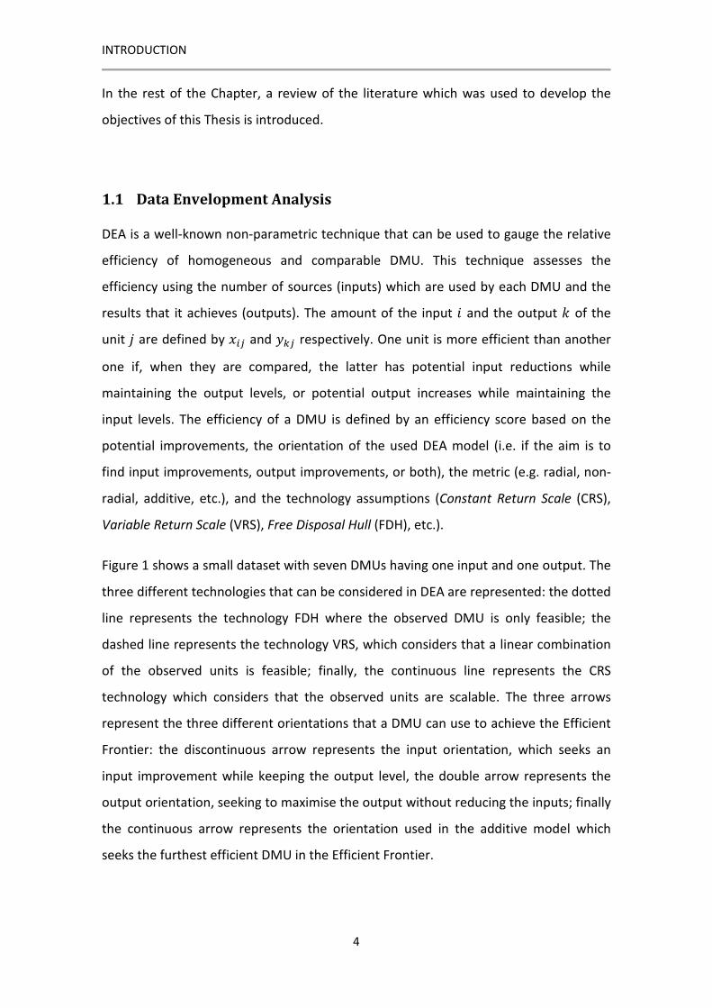
Figure 1 shows a small dataset with seven DMUs having one input and one output. The

three different technologies that can be considered in DEA are represented: the dotted

line represents the technology FDH where the observed DMU is only feasible; the

dashed line represents the technology VRS, which considers that a linear combination

of the observed units is feasible; finally, the continuous line represents the CRS

technology which considers that the observed units are scalable. The three arrows

represent the three different orientations that a DMU can use to achieve the Efficient

Frontier: the discontinuous arrow represents the input orientation, which seeks an

input improvement while keeping the output level, the double arrow represents the

output orientation, seeking to maximise the output without reducing the inputs; finally

the continuous arrow represents the orientation used in the additive model which

seeks the furthest efficient DMU in the Efficient Frontier.

INTRODUCTION

5

Figure 1: Visualisation of the Efficient Frontier and the direction of improvement for

the inefficient DMUs

1.1.1 Relevant Additive Models in DEA

DEA is used to evaluate the inefficiency of the DMUs belonging to the technology, thus

determining their distance to the Efficient Frontier. There are different ways to

measure this distance depending on the orientation of the model. There are three

main categories: it could be input oriented where the aim is to find input

improvement; output oriented if the aim is to seek output improvement; and additive

models if both variables are to be improved.

Apart from that, there are two different ways to evaluate the performance of a DMU,

i.e. it could be seen from a technical or economic point of view. The technical

perspective follows the criterion related to the efficiency of the production process.

However, a firm can change the input and output quantities to achieve a better

economic performance, depending on the input/output price units. As a consequence,

the economic performance could be assessed in relation to profit, cost or the revenue

of the firms.

INTRODUCTION

6

In this section, diverse models which were used to develop this Thesis are described,

including three well-known technical additive models from both a technical and

economic perspective. Based on these models, inefficiency or efficiency metrics are

developed to measure the inefficiency between two DMUs or between a DMU and the

Efficient Frontier.

In these models, n DMUs are assessed. Each DMU consumes inputs � =(� �, … , ���) and produces � outputs �� = (� �, … , ���). As described above, the

additive model seeks both input and output improvements, so the difference of each

variable from the Efficient Frontier is measured to determine the potential

improvement of each DMU. These differences are measured with input slacks (h��) and

output slacks (h��). So, all efficient DMUs which determine the Efficient Frontier are

identified with zero slacks. For these DMUs there is no possible improvement without

worsening any of these DMUs as defined by the “Pareto-Koopmans” definition.

The three models defined from the technical perspective are Measure Inefficiency

Proportions (MIP), Russell Adjusted Measure (RAM) and the Weighted Additive model.

MIP and RAM models are described in Cooper, Park and Pastor (1999). The MIP model

represents the potential improvement of each DMU with respect to its position. It is

described as [1]-[4] (DMU 0 being the assessed DMU). So, the inefficiency value is a

proportional improvement of the assessed DMU.

��� MIP = h�!�x�!#

�$ + h�!�

y�!'

�$ [1]

s.t.

x�! = ���(�)

�$ + h�!� � = 1, … , [2]

y�! = ���(�)

�$ − h�!� � = 1, … , � [3]

INTRODUCTION

7

0 ≤ (� , h�!� , h�!� ∀�, /, � [4]

On the other hand, RAM normalises the slacks of each DMU before maximising them.

In contrast to MIP, RAM is independent of the position of the assessed DMU. After

normalising, the value obtained in the model depends only on the distance of the

inefficient DMU to the Efficient Frontier (eqs. [5]-[8])

��� RAM = 1m + s 4 h�!�R��#

�$ + h�!�

R��'

�$ 5 [5]

s.t.

x�! = ���(�)

�$ + h�!� � = 1, … , [6]

y�! = ���(�)

�$ − h�!� � = 1, … , � [7]

0 ≤ (� , h�!� , h�!� ∀�, /, � [8]

The normalisation is done with the range of the variables [9]-[10]. These ranges

represent the maximum possible value of inefficiency and offer a fixed reference to

determine the inefficiency of the DMUs.

R�� = max7 {x�7} − min7 {x�7} [9]

R�� = max� {y�7} − min� {y�7} [10]

The previous models consider only the information related to the position of the

DMUs. However there are other models which take into account the relative

importance of each input and output. The following model [11]-[14] is described in

Cooper et al. (2011). It is a weighted additive model that measures the technical

inefficiency of a given DMU 0 (<=!). Each input and output has an associated weight,

INTRODUCTION

8

>� = (? �, … , ?��) for the inputs and >� = (? �, … , ?��) for the outputs. The

weights represent the relative importance of each variable.

<=! = ?���

�$ ℎ�!� + ?��ℎ�!�

�

�$ [11]

s.t.

���(�)

�$ + h�!� ≤ x�! � = 1, … , [12]

���(�)

�$ − h�!� ≥ y�! � = 1, … , � [13]

0 ≤ (� , h�!� , h�!� ∀�, /, � [14]

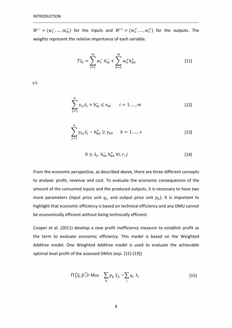
From the economic perspective, as described above, there are three different concepts

to analyse: profit, revenue and cost. To evaluate the economic consequences of the

amount of the consumed inputs and the produced outputs, it is necessary to have two

more parameters (input price unit B�, and output price unit C�). It is important to

highlight that economic efficiency is based on technical efficiency and any DMU cannot

be economically efficient without being technically efficient.

Cooper et al. (2011) develop a new profit inefficiency measure to establish profit as

the term to evaluate economic efficiency. This model is based on the Weighted

Additive model. One Weighted Additive model is used to evaluate the achievable

optimal level profit of the assessed DMUs (eqs. [15]-[19])

( ) k k i ik i

ˆ ˆq, p Max p y q xΠ = − [15]

INTRODUCTION

9

s.t.

j ij i

j

ˆx x iλ = ∀ [16]

j kj k

j

ˆy y kλ = ∀ [17]

j

j

1λ = [18]

{ }j 0,1 jλ ∈ ∀ [19]

So, the profit inefficiency, D=! of a DMU 0 is given by eq. [20], i.e., the normalised

difference between the optimal level of profit and the current profit of the assessed

DMU.

The main advantage of the proposed model is that it is homogeneous of degree zero

because it is normalised by the minimum ratio of market prices to its relative weights.

( ) k k0 i i0k i

0

s1 2 m 1 2

x x x y y y1 2 m s1 2

q, p p y q x

PI

pq q q p pmin , ,..., , , ,...,

w w w ww w

Π − −

=

[20]

Cooper et al. (2011) also prove that D=! ≥ <=!. Due to this fact, economic inefficiency

can be decomposed into technical inefficiency and allocative inefficiency (E=), the

latter being the difference between the economic inefficiency and the technical

inefficiency [21].

INTRODUCTION

10

D= = <= + E= [21]

Due to the PI and TI being based on slacks, the Pareto-Koopmans definition is applied,

so there is no risk that the projected DMUs on the production frontier belong to the

non-efficient frontier. All the efficient units are identified with slacks zero and belong

to the Efficient Frontier.

As mentioned above, revenue can be used to determine the economic efficiency. It is a

similar approach to Profit Inefficiency, but with an output orientation. Aparicio et al.

(2013) develop revenue inefficiency and also decompose it into technical inefficiency

and allocative inefficiency. However, a similar approach based on input orientation and

cost function evaluates the economic perspective from the cost term.

All the models are defined for CRS technology; however, they can be applied to other

technologies, such as VRS adding to the models ∑ (� = 1� , or in the case of considering

FDH technology, adding (� = {0,1}.

1.1.2 Intermediate Target and Stratification

In the same way that there are multiple assumptions to determine the feasible

technology or the orientation that an inefficient DMU can follow to achieve the

Efficient Frontier, multiple methodologies are developed to determine the stepwise

benchmarking path which guides the DMU to its desirable position in the Efficient

Frontier.

Two different kinds of benchmarks define the intermediate steps of an inefficient DMU

to its desirable position. Intermediate Benchmarking Targets (IBT) comprise the

benchmarks of the assessed DMU until the Efficient Frontier, while Ultimate

Benchmarking Targets (UBT) guide the DMU along the Efficient Frontier to its desirable

position.

The efficiency of a unit is assessed with respect to the DMUs that are used to assess its

performance. Based on this concept called Context-Dependent DEA, Seiford and Zhu

INTRODUCTION

11

(2003) define attractiveness and progress measures concerning DMUs of the

evaluation context and also a stratification process. The stratification process

categorises the DMU in layers depending on their efficiency and attractiveness. The

DMUs which belong to layers with lower values are more efficient, the DMUs of the

layer 0 being the efficient units of the technology. Layer 1 is built by analysing the

technology after removing the nodes of the previous layers, and so on for the

successive layers. All DMUs which belong to a layer have the same level of

attractiveness.

In the case that the efficient benchmark of an inefficient DMU is a distant target for

the inefficient units, several methodologies identify intermediate targets based on

similarity of DMUs. Other methodologies consider that the DMUs can only achieve

benchmarks which are below a certain distance, so determine a bounded stepwise

path.

Estrada et al. (2009) define a Proximity-Based Target Selection process. This process

uses a Self-Organizing Map (SOM) to cluster DMUs in neighbourhoods that consume

similar inputs in order to determine the potential intermediate benchmark of

inefficient DMUs. Moreover, the intermediate benchmarks that comprise the shortest

path to the Efficient Frontier are selected by the Reinforcement Learning algorithm.

This algorithm determines the intermediate benchmarking of an inefficient DMU

between its neighbours by limiting the efficiency score that a DMU can achieve.

Lozano and Villa (2010) propose two models in a VRS case to define successive

intermediate targets: one model, called the Technical Efficiency Improvement Program

(TEIP) for the inefficient units to achieve the Efficient Frontier, and another one called

the Scale Efficiency Improvement Program (SEIP) for efficient units to achieve the scale

efficiency. Both models determine the spaced intermediate targets by fixing an upper

bound.

In the same direction, Lim et al. (2011) define stepwise benchmarking paths for

inefficient units to achieve the Efficient Frontier, but selecting existing DMUs as

intermediate targets based on the concept of context-dependent. So, an intermediate

target would be an inefficient DMU but more attractive than the inefficient assessed

INTRODUCTION

12

DMU, taking into account the three criteria of attractiveness, progress and infeasibility,

after clustering DMUs into different layers.

Park, Bae and Lim (2011) propose a target selection method to take into account the

similarity using the k-means clustering algorithm. Instead of determining the size of

the stepwise benchmarking path depending on the number of stratified layers, the

target selection method selects the cluster which has the highest similarity with the

assessed DMU and determines the next benchmarking target of the DMU with the

highest efficiency in the selected cluster.

Another stepwise benchmarking method, which takes into account not only the

similarity between nodes, but also the efficiency gaps, is proposed by Ghahraman and

Prior (2016). This method reduces the risk of failure of achieving out-of-reach

efficiency targets. After measuring the efficiency scores with a DEA model, a directed

weighted network is created where all the inefficient units point to a better performer

and the weight of each link takes into account the input changes and the efficiency gap

covered. Dijkstra’s shortest path algorithm is used to calculate the optimal stepwise

benchmarking path for each inefficient unit.

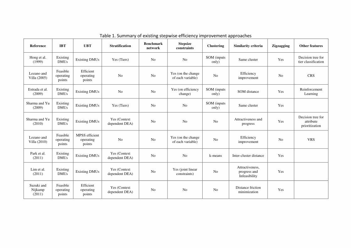
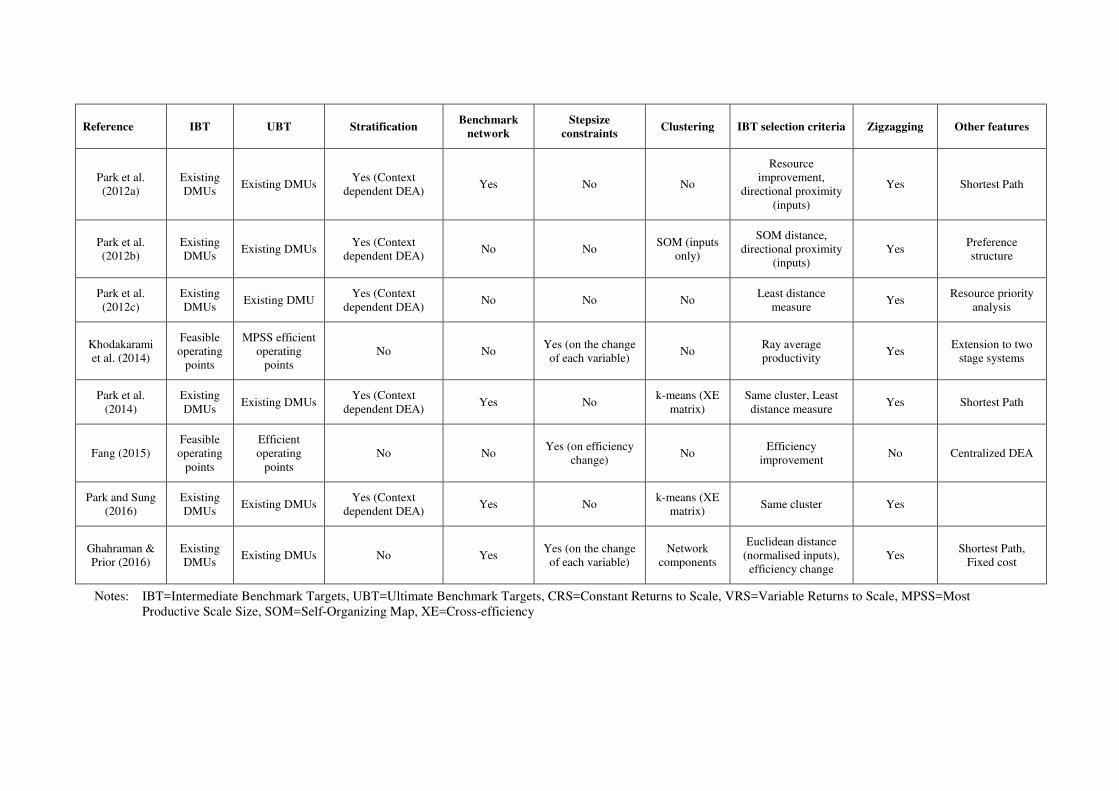
Table 1 shows a summary of the main characteristics of the different approaches. In

particular, for each approach the table shows the type of IBT, and UBT considered,

whether stratification is used, whether the benchmarking path is computed over a

benchmark network (whose nodes are the DMUs and whose edges indicate the

possible steps that can be taken to form the efficiency improvement path), whether

bounds on the stepsizes are considered, whether the DMUs are clustered, the

similarity criteria considered for selecting each IBT, and whether the method suffers

zigzagging (i.e. moving in inverse directions in successive steps). The final column

shows some specific features of the methods.

Among the specific features of some of the methods, it is remarkable that a preference

structure can be considered to select the UBT, the consideration of a fixed cost for

carrying out each benchmarking step, or computing a decision tree from the DMU

stratification to try to identify the differences in input and output ranges in two

INTRODUCTION

13

successive layers. The extension of stepwise benchmarking to centralized DEA and to

systems with two stages in series is also remarkable.

14

Table 1. Summary of existing stepwise efficiency improvement approaches

Reference IBT UBT Stratification Benchmark

network

Stepsize

constraints Clustering Similarity criteria Zigzagging Other features

Hong et al.

(1999)

Existing

DMUs Existing DMUs Yes (Tiers) No No

SOM (inputs

only) Same cluster Yes

Decision tree for

tier classification

Lozano and

Villa (2005)

Feasible

operating

points

Efficient

operating

points

No No Yes (on the change

of each variable) No

Efficiency

improvement No CRS

Estrada et al.

(2009)

Existing

DMUs Existing DMUs No No

Yes (on efficiency

change)

SOM (inputs

only) SOM distance Yes

Reinforcement

Learning

Sharma and Yu

(2009)

Existing

DMUs Existing DMUs Yes (Tiers) No No

SOM (inputs

only) Same cluster Yes

Sharma and Yu

(2010)

Existing

DMUs Existing DMUs

Yes (Context

dependent DEA) No No No

Attractiveness and

progress Yes

Decision tree for

attribute

prioritization

Lozano and

Villa (2010)

Feasible

operating

points

MPSS efficient

operating

points

No No Yes (on the change

of each variable) No

Efficiency

improvement No VRS

Park et al.

(2011)

Existing

DMUs Existing DMUs

Yes (Context

dependent DEA) No No k-means Inter-cluster distance Yes

Lim et al.

(2011)

Existing

DMUs Existing DMUs

Yes (Context

dependent DEA) No

Yes (joint linear

constraints) No

Attractiveness,

progress and

Infeasibility

Yes

Suzuki and

Nijkamp

(2011)

Feasible

operating

points

Efficient

operating

points

Yes (Context

dependent DEA) No No No

Distance friction

minimization Yes

Reference IBT UBT Stratification Benchmark

network

Stepsize

constraints Clustering IBT selection criteria Zigzagging Other features

Park et al.

(2012a)

Existing

DMUs Existing DMUs

Yes (Context

dependent DEA) Yes No No

Resource

improvement,

directional proximity

(inputs)

Yes Shortest Path

Park et al.

(2012b)

Existing

DMUs Existing DMUs

Yes (Context

dependent DEA) No No

SOM (inputs

only)

SOM distance,

directional proximity

(inputs)

Yes Preference

structure

Park et al.

(2012c)

Existing

DMUs Existing DMU

Yes (Context

dependent DEA) No No No

Least distance

measure Yes

Resource priority

analysis

Khodakarami

et al. (2014)

Feasible

operating

points

MPSS efficient

operating

points

No No Yes (on the change

of each variable) No

Ray average

productivity Yes

Extension to two

stage systems

Park et al.

(2014)

Existing

DMUs Existing DMUs

Yes (Context

dependent DEA) Yes No

k-means (XE

matrix)

Same cluster, Least

distance measure Yes Shortest Path

Fang (2015)

Feasible

operating

points

Efficient

operating

points

No No Yes (on efficiency

change) No

Efficiency

improvement No Centralized DEA

Park and Sung

(2016)

Existing

DMUs Existing DMUs

Yes (Context

dependent DEA) Yes No

k-means (XE

matrix) Same cluster Yes

Ghahraman &

Prior (2016)

Existing

DMUs Existing DMUs No Yes

Yes (on the change

of each variable)

Network

components

Euclidean distance

(normalised inputs),

efficiency change

Yes Shortest Path,

Fixed cost

Notes: IBT=Intermediate Benchmark Targets, UBT=Ultimate Benchmark Targets, CRS=Constant Returns to Scale, VRS=Variable Returns to Scale, MPSS=Most

Productive Scale Size, SOM=Self-Organizing Map, XE=Cross-efficiency

INTRODUCTION

16

1.2 Complex Network Analysis

As mentioned above, Complex Network methodology is used to represent systems.

Nodes and links compose each network, the nodes or vertices represent the entities of

the system, and the links or edges the relationships among them. A huge variety of

different fields, apart from sociology, have developed applications of CNA in their

areas to use an integrationist approach. One of the main purposes of this technique is

to visualise the relationship in the system and measure the defined properties in CNA

in order to understand the system as a whole, as communities and as individual units.

Figure 2: Visualisation of a random generated network

1.2.1 Kind of Networks and Basic Properties

There are different ways to establish a relationship between the nodes of the network.

The links can be directed or undirected; as a result, the network is a directed or

undirected graph respectively. Each link always has an associated weight, so the

network is a weighted graph, but in the case that all the links are equal to one, the

network is considered to be an unweighted graph.

INTRODUCTION

17

Therefore, a network can represent a system with different kinds of relationships, in

which case multiplex networks are used to evaluate each different relationship (type of

link). An edge is usually a connection between two nodes, but in the case that it

connects more than two vertices, these are called hyperedges. Moreover, the network

which contains them is called a hypergraph.

Another kind of network is the bipartite network, which has two types of nodes

connected by links and all the links connect nodes of a different type. So, there is no

link that connects two nodes of the same type. All these relationships among the

nodes are gathered in the adjacency matrix or the incidence matrix; both matrices

provide the same information although their structure is different.

The length between two nodes is the sum of the weights links that create the route to

connect them. There are different paths to achieve one node from another one;

however, the shortest one is called the geodesic path. There are multiple routes to

achieve a node from another node and each route could have a different length. If the

distance between two nodes independently on the considered route is the same, then

the network has the additivity property. Another highlighted property is the transitivity

property, if in all the situations where there is a link between nodes i and j and another

one between j and h, another link connects the nodes i and h.

1.2.2 Metrics

When measuring complex networks there are different metrics. Each one is classified

depending on from which level the network is being assessed. There are three kinds of

levels: one from a nodes perspective as the fundamental part of the network; another

one from a cluster of nodes; and another one from a network perspective.

One of the main metrics at the nodes level is the degree, which measures the number

of links that have their origin and destination in the same node, as well as the strength

whose value is the sum of the edges that are linked to the node. It is important to

highlight that for directed networks these metrics can consider the direction of the

edges if they have the origin or the destination of the node.

INTRODUCTION

18

Although the degree is a metric at the node level, the degree of the nodes can be

observed at the network level with the degree distribution or with the degree-degree

correlation. The degree distribution is the probability distribution of the degrees over

the whole network and the degree-degree correlation is used to establish a

relationship between the degree of a node and the average degree of its neighbour.

Apart from that, in the case that the purpose of the analysis is to study the position of

the node, clustering coefficient and centrality metrics can be used. The clustering

coefficient of a node determines if the neighbours of a node are connected between

them. Centrality metrics determine the importance of each node, but this can be

considered from different point of view. Specifically, betweenness centrality

determines the proportion of the number of geodesic paths that pass through it, while

eigenvector centrality analyses the importance of a node depending on the importance

of its neighbours. Apart from those, alpha-centrality is also a centrality metric with the

same interpretation as eigenvector centrality, but alpha-centrality being the

generalized formula.

Therefore, two nodes can be compared to study if they are equivalents, based on their

structure, meaning that they are linked to the same nodes. To study this equivalency

the Pearson correlation coefficient or Jaccard’s similarity coefficient can be used.

As a cluster of nodes, the nodes can be joined in communities or components. In

communities or clusters, a criterion is established to define which attribute must have

a group of nodes to be considered as a community. The criterion is usually based on

how they are connected, for example, if the network has more links than in a random

generated network or there are overlapping small connected structures.

Another way to gather nodes is with the component. A component is a subgraph of the

network whose nodes are connected so that each node can achieve any other node of

the subgraph. Depending on the direction of the links, whether it is considered or not,

the component is a strongly or weakly connected component respectively. Apart from

that, based on the structural similarity coefficient a hierarchical clustering algorithm

can be used to identify groups of nodes that have a given degree of structural

similarity among them.

INTRODUCTION

19

From the network perspective, some of the main metrics are diameter, geodesic path,

average path, network efficiency and density. The diameter represents the longest

geodesic path of the network, while the average path length calculates the average of

the geodesic path of the network. The network efficiency is the inverse harmonic

mean of the path lengths and the density, which determines how many links are in a

network by taking into account the maximum number of links that could exist. Apart

from that, if high connected nodes tend to be linked to other high connected nodes,

then it is considered that the network has an assortative property, or disassortative in

the case that they are connected to low connected nodes.

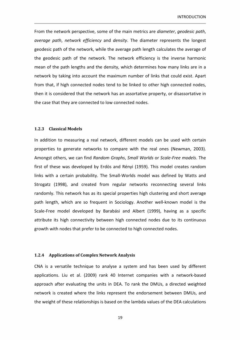
1.2.3 Classical Models

In addition to measuring a real network, different models can be used with certain

properties to generate networks to compare with the real ones (Newman, 2003).

Amongst others, we can find Random Graphs, Small Worlds or Scale-Free models. The

first of these was developed by Erdös and Rényi (1959). This model creates random

links with a certain probability. The Small-Worlds model was defined by Watts and

Strogatz (1998), and created from regular networks reconnecting several links

randomly. This network has as its special properties high clustering and short average

path length, which are so frequent in Sociology. Another well-known model is the

Scale-Free model developed by Barabási and Albert (1999), having as a specific

attribute its high connectivity between high connected nodes due to its continuous

growth with nodes that prefer to be connected to high connected nodes.

1.2.4 Applications of Complex Network Analysis

CNA is a versatile technique to analyse a system and has been used by different

applications. Liu et al. (2009) rank 40 Internet companies with a network-based

approach after evaluating the units in DEA. To rank the DMUs, a directed weighted

network is created where the links represent the endorsement between DMUs, and

the weight of these relationships is based on the lambda values of the DEA calculations

INTRODUCTION

20

after evaluating all the possible input/output combinations. The ranking is created with

a centrality measure called eigenvector centrality. A similar network approach is used

by Liu and Lu (2010) to evaluate and rank the research and development performance

of Taiwan’s government-supported research institutes, taking into account that the

performance is assessed in two-stages. One stage is for the technology development,

and the other for the technology diffusion. Ho et al. (2014) analyse the technology

transfer efficiencies in the US with a similar approach. Liu and Lu (2012) apply an

analogous network-based approach, but applying alpha centrality to each stage used

by DEA to evaluate a real-world problem of banks.

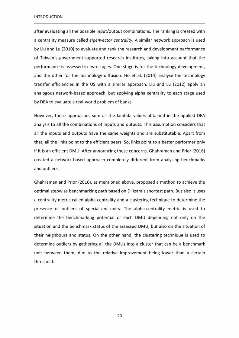
However, these approaches sum all the lambda values obtained in the applied DEA

analysis to all the combinations of inputs and outputs. This assumption considers that

all the inputs and outputs have the same weights and are substitutable. Apart from

that, all the links point to the efficient peers. So, links point to a better performer only

if it is an efficient DMU. After announcing these concerns, Ghahraman and Prior (2016)

created a network-based approach completely different from analysing benchmarks

and outliers.

Ghahraman and Prior (2016), as mentioned above, proposed a method to achieve the

optimal stepwise benchmarking path based on Dijkstra’s shortest path. But also it uses

a centrality metric called alpha-centrality and a clustering technique to determine the

presence of outliers of specialized units. The alpha-centrality metric is used to

determine the benchmarking potential of each DMU depending not only on the

situation and the benchmark status of the assessed DMU, but also on the situation of

their neighbours and status. On the other hand, the clustering technique is used to

determine outliers by gathering all the DMUs into a cluster that can be a benchmark

unit between them, due to the relative improvement being lower than a certain

threshold.

21

2. OBJECTIVES

As stated in the previous chapter, the goal of this Thesis is to contribute to further

research on the field of efficiency analysis, as well as providing a new tool to evaluate

the situation of the assessed units based on the dominance relationships between the

units.

Specially, the main objectives of this research are:

O1. To explore and formalise a tool to develop the concept of a dominance network

where dominance relationships between assessed units could be analysed and

visualised.

O2. To apply the developed tool to the concepts of profit and revenue efficiency.

O3. To introduce the concept of efficiency potential in DEA.

O4. To explore the use of DEA in project management contexts.

As mentioned above, in pursuing these objectives, five papers were published covering

those goals. The references of these papers ([A] to [E]) can be found in Appendix 1.

Each publication covers at least one of the goals stated above. In this chapter a general

overview of those objectives and papers is presented. A report on each one can be

found in Appendix 2.

OBJECTIVES

22

O1. To explore and formalise a tool to develop the concept of a dominance

network where dominance relationships between assessed units could be

analysed and visualised.

With the purpose of developing the concept of a dominance network, three research

papers were published ([A], [B] and [C]). All these papers introduce the methodology

called Dominance Network Analysis (DNA), which applies the techniques developed for

complex network to efficiency assessment.

DNA creates a network to manage the dominance relationships between the assessed

DMUs. As the dominance relationship is understood here, a link is created between

two nodes having its origin in the inefficient DMU and its destination in a more

efficient DMU. As a result a directed acyclic network called the Dominance Network is

defined. The weight of the links is the relative inefficiency of the connected DMUs.

Thanks to the transitivity and additivity property of the network, the minimum and

maximum distance of any inefficient DMU to the Efficient Frontier can easily be

measured.

DNA allows the classification of each node, depending on its dominance relationship

and position in the network. Apart from classification methods commonly used in DEA

such as stratification, others can be used based on CNA, such as gathering the nodes

into communities, components, or clusters based on the similarity of nodes. Both CNA

and DEA are useful to define different metrics to characterise the network at different

levels. These metrics vary, depending on the position of the DMUs and show the

relative position in the network, such as clustering coefficient, betweenness centrality,

etc. Others, such as degree-degree correlation shows to which kind of nodes the nodes

are linked. Degree-degree correlation is used to evaluate the relationships of the

nodes based on how they are linked to other nodes depending on their degree.

Assortativity is observed if high connected nodes are linked to other high connected

ones, or disassortativity when high connected nodes are linked to low connected ones.

Apart from the analysis and visualisation, Dominance Networks can be used to make

partial rankings using multi-criteria decision making. The computed ranking

OBJECTIVES

23

disaggregates the layers, and ranks of the nodes according to a defined preference

relation.

DNA offers a valuable integrated DEA CNA framework. DEA has different restrictions to

plot DMUs’ multidimensional input and output vectors; this handicap is solved by the

Dominance Network. The visualisation tools of CNA are really powerful due to the

filters linked to it.

O2. To apply the developed tool to the concepts of profit and revenue efficiency.

The proposed method in the previous objective is so flexible that it can stand different

kinds of relationships. DEA, as mentioned in the Introduction, considers that the DMUs

can be analysed from an economic perspective apart from the technical one.

An enhanced DNA is proposed to consider both kinds of relationships. Technical

efficiency considers the input consumption and the output production while economic

efficiency uses the cost of the inputs and the price of the outputs. Moreover, the

analysis of economic and technical inefficiency leads to the concept of Allocative

Inefficiency which measures the difference between both relative performances. As

mentioned in DEA, the economic perspective can be analysed using the concepts of

profit, cost or revenue. The utilization of each concept to analyse the DMUs from the

economic perspective depends on the availability of data and the criteria of the

analyst.

As a result of this enhanced approach, a multiplex directed weighted acyclic network is

created to represent technical and economic dominance relationships. The created

network has two Efficient Frontiers, one for the technical relationship and the other

for the economic relationship. The distance between them is measured by the concept

of allocative inefficiency, which will be represented by hyperedges.

The relationships between these two relationships and the properties of the created

network are studied, but due to the definition of the links, it is expected that the

economic relationship between two nodes only exists if there is a technical

OBJECTIVES

24

relationship between them. It is also expected that the existence of an economic

relationship is linked to the concept of scalar potential.

O3. To introduce the concept of efficiency potential in DEA.

The Introduction shows that there is an extensive literature about the stepwise

benchmarking paths. However, in this Thesis a new approach is introduced based on

the gradient of an EFP; the EFP is defined in such a way that the fewer inputs

consumed and the more outputs produced by DMUs, the lower its EFP value.

Each DMU, depending on its position, has a scalar EFP and a negative gradient which

defines the Efficiency Field Vector (EFV), and all the DMUs that have the same scalar

EFP are over the same Efficiency Equipotential Surface (EES). The EFVs are

perpendicular to the EES and define the direction of an inefficient DMU to achieve the

Efficient Frontier.

The EFP definition can be accommodated to dimensionless inputs and outputs, but it

has to keep the principles of strong monotonicity, efficiency achievement, and the

lower values being linked to the efficient DMUs.

Based on these concepts, two models are defined to determine the intermediate steps

that an inefficient DMU has to take to achieve the Efficient Frontier; also, another

model is developed to define the movement of the efficient DMU along the Efficient

Frontier to achieve the point of minimum potential.

O4. To explore the use of DEA in project management contexts.

A classical problem of the literature on project management is to determine the

contribution of the team members to the projects on which they have worked.

However, if the contribution of each member were known, theoretically there should

be a relationship between the efficiency of the team members and the efficiency of

the projects in which they were involved.

One of the objectives of this Thesis is to determine if DEA could be applied to

determine the performance of each of the team members. If there is a relationship

OBJECTIVES

25

between the performance of the team members and their results, the performance of

each member of the team could be assessed based on the performance of the projects

on which he/she has worked.

27

3. RESULTS

As stated in Chapter 2, there were four objectives to be developed in five research

papers. In this chapter, a summary of the achieved results in each of these research

papers are summarized. As mentioned before, all the publications are available in

Appendix 2.

3.1 Efficiency assessment using network analysis tools1

As mentioned in the previous chapter, this paper introduces in detail the Dominance

Network methodology to analyse and visualise multidimensional datasets. This

methodology, based on CNA and DEA, represents the dominance relationship and its

relative inefficiency performance among the assessed DMUs. The created network

represents all the possible benchmarking paths that any inefficient DMU has to take to

achieve the Efficient Frontier.

This paper presents multiple metrics that could be applied to dominance networks at

different levels, from the node level to the network level, and also defines different

filters that could be applied to the visualisation of the network.

1 Lozano, S. and Calzada-Infante, L., “Efficiency assessment using network analysis tools” Journal of the

Operational Research Society (2018) doi: https://doi.org/10.1080/01605682.2017.1409866

RESULTS

28

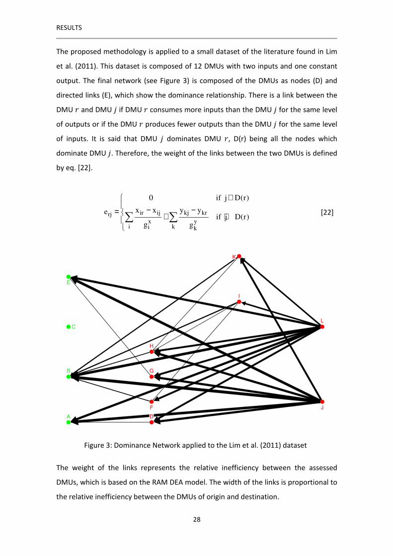
The proposed methodology is applied to a small dataset of the literature found in Lim

et al. (2011). This dataset is composed of 12 DMUs with two inputs and one constant

output. The final network (see Figure 3) is composed of the DMUs as nodes (D) and

directed links (E), which show the dominance relationship. There is a link between the

DMU / and DMU � if DMU / consumes more inputs than the DMU � for the same level

of outputs or if the DMU / produces fewer outputs than the DMU � for the same level

of inputs. It is said that DMU � dominates DMU /, D(r) being all the nodes which

dominate DMU �. Therefore, the weight of the links between the two DMUs is defined

by eq. [22].

ir ij kj krrjx y

i ki k

0 if j D(r)

x x y yeif j D(r)

g g

∉ − −= + ∈

[22]

Figure 3: Dominance Network applied to the Lim et al. (2011) dataset

The weight of the links represents the relative inefficiency between the assessed

DMUs, which is based on the RAM DEA model. The width of the links is proportional to

the relative inefficiency between the DMUs of origin and destination.

RESULTS

29

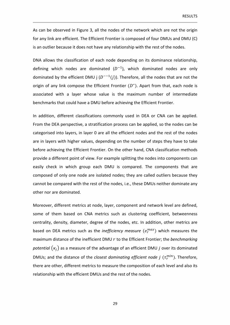
As can be observed in Figure 3, all the nodes of the network which are not the origin

for any link are efficient. The Efficient Frontier is composed of four DMUs and DMU (C)

is an outlier because it does not have any relationship with the rest of the nodes.

DNA allows the classification of each node depending on its dominance relationship,

defining which nodes are dominated (G� ), which dominated nodes are only

dominated by the efficient DMU j (G�� (�)). Therefore, all the nodes that are not the

origin of any link compose the Efficient Frontier (G∗). Apart from that, each node is

associated with a layer whose value is the maximum number of intermediate

benchmarks that could have a DMU before achieving the Efficient Frontier.

In addition, different classifications commonly used in DEA or CNA can be applied.

From the DEA perspective, a stratification process can be applied, so the nodes can be

categorised into layers, in layer 0 are all the efficient nodes and the rest of the nodes

are in layers with higher values, depending on the number of steps they have to take

before achieving the Efficient Frontier. On the other hand, CNA classification methods

provide a different point of view. For example splitting the nodes into components can

easily check in which group each DMU is compared. The components that are

composed of only one node are isolated nodes; they are called outliers because they

cannot be compared with the rest of the nodes, i.e., these DMUs neither dominate any

other nor are dominated.

Moreover, different metrics at node, layer, component and network level are defined,

some of them based on CNA metrics such as clustering coefficient, betweenness

centrality, density, diameter, degree of the nodes, etc. In addition, other metrics are

based on DEA metrics such as the inefficiency measure (IJ�KL) which measures the

maximum distance of the inefficient DMU / to the Efficient Frontier; the benchmarking

potential MN�O as a measure of the advantage of an efficient DMU � over its dominated

DMUs; and the distance of the closest dominating efficient node � (PJ��)). Therefore,

there are other, different metrics to measure the composition of each level and also its

relationship with the efficient DMUs and the rest of the nodes.

RESULTS

30

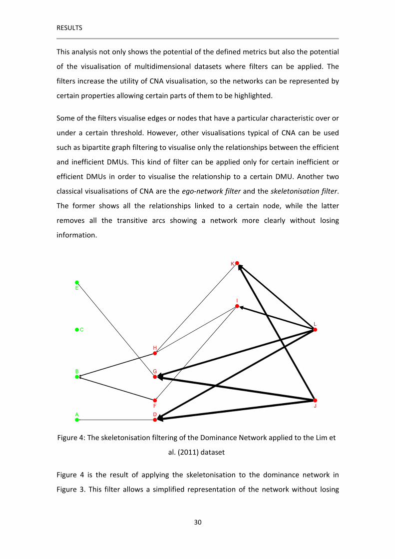
This analysis not only shows the potential of the defined metrics but also the potential

of the visualisation of multidimensional datasets where filters can be applied. The

filters increase the utility of CNA visualisation, so the networks can be represented by

certain properties allowing certain parts of them to be highlighted.

Some of the filters visualise edges or nodes that have a particular characteristic over or

under a certain threshold. However, other visualisations typical of CNA can be used

such as bipartite graph filtering to visualise only the relationships between the efficient

and inefficient DMUs. This kind of filter can be applied only for certain inefficient or

efficient DMUs in order to visualise the relationship to a certain DMU. Another two

classical visualisations of CNA are the ego-network filter and the skeletonisation filter.

The former shows all the relationships linked to a certain node, while the latter

removes all the transitive arcs showing a network more clearly without losing

information.

Figure 4: The skeletonisation filtering of the Dominance Network applied to the Lim et

al. (2011) dataset

Figure 4 is the result of applying the skeletonisation to the dominance network in

Figure 3. This filter allows a simplified representation of the network without losing

RESULTS

31

information due to the additivity and transitivity properties which are implied in the

network.

To test the robustness of the proposed approach, different direction vectors are

considered to calculate the normalisation. Four direction vectors are considered:

• ( )yxi k

g g ,g=

• ( )average aver averi kg x , y=

• ( )rangei k

ˆg R , R=

• ( )median median mediani kg x , y=

After creating and analysing the dominance network for each direction vector, the

obtained results show a high correlation between them. The absolute magnitude of

the applied metrics differs for different direction vectors, but their relative values are

totally consistent.

Apart from studying the impact of a change in the direction vector, the sensibility of

the network after introducing an additional efficient or inefficient DMU is also studied.

The network topology changes a little and affects the DMUs that are linked to the new

DMU. The position of the DMU can affect the number of geodesic paths, the layers

which are linked to the DMUs, etc., but by adding just a single DMU does not change

the network topology too much. However, the observed changes that appear in

Dominance Networks can also be observed in DEA, due to the efficiency score of the

DMUs, depending on their position.

3.2 Analysing Olympic Games through dominance networks2

The aim of this application paper is to assess and rank the performance of the

countries in the Olympic Games taking into account their capacity and the dominance

2 Calzada-Infante, L. and Lozano, S., “Analysing Olympic Games through dominance networks”, Physica

A, 462 (2016) pp:1215-1230

RESULTS

32

relationships within their performance. The advantage of this method over other

traditional simplified ranking methods, such as lexicographic order, is to consider the

capabilities of the countries. This point is considered in many DEA models that have

been applied to Olympic Games datasets. However, establishing a rank based on a DEA

model, such as the Integer-Valued DEA (IDEA) model defined in Wu et al. (2010), only

considers the distance to the Efficient Frontier, while the proposed approach considers

all the dominance relationships established by the position of all the DMUs in the

space.

In the proposed approach, two inputs (GDP and Populations (POP)) and one output

(number of medals) are used to evaluate the performance of the countries as is

traditionally done in DEA.

With these variables, a weighted directed network is created where the nodes are the

countries and the links are the dominance relationships between them. A directed link

from country / to country � exists if country � consumes fewer resources to produce

the same or higher level of outputs or if country � produces more outputs consuming

the same of inputs as country /. The weight of these links represents the weighted

difference of medals achieved between the linked countries (eq. [23]). In this analysis

the weighted coefficient used are 2B S Gv 1; v a; v a= = = .

( ) ( ) ( )rj G j r S j r B j r

G jr S jr B jr

w v Gold Gold v Silver Silver v Bronze Bronze

v Gold v Silver v Bronze

= ⋅ − + ⋅ − + ⋅ − =

= ⋅ ∆ + ⋅ ∆ + ⋅ ∆ [23]

After creating the network for three different values for the parameter a, minor

changes could be observed, so the value of a 2= is used to evaluate the performance

of the countries.

The network, which has a layered structure, has more than one component. Some of

them are outliers which cannot be benchmarked against other countries. Most of the

countries belong to the giant weakly connected component. All the efficient countries

are easily identified because they belong to layer 0. The layer is linked to the distance

RESULTS

33

of the performers to the Efficient Frontier and it is tied to the in- and out- strength.

Figure 6 shows to which layer each country belongs.

Some metrics based on CNA are used in this publication, such as strength, clustering or

betweenness centrality, among others. The value of these metrics varies, depending

on the position of the DMUs in the network, and shows the relative position of each

node. Other metrics such as the average length and the network diameter indicate the

overall magnitude of these performance differences.

Apart from that, after applying degree-degree correlation, assortativity is detected in

the case of the average in-degree of the average in-degree of in-nearest neighbours

and also for the average out-degree of the average out-degree of out-nearest

neighbours. This kind of assortativity means that nodes with high in-degree tend to

receive links from nodes with high in-degree and nodes with high out-degree tend to

connect to nodes with high out-degree. On the other hand, disassortativity is observed

in the average out-degree of in-nearest neighbours and the average in-degree of out-

nearest neighbours, which means that nodes with high in-degree tend to receive links

from nodes with low out-degree and nodes with high out-degree tend to connect to

nodes with low in-degree.

A hierarchical clustering algorithm is used to identity groups of nodes that have a given

degree of structural similarity among them based on Jaccard’s coefficient. To achieve

these clusters the Single Linkage Clustering Algorithm is applied. Three groups have

exactly the same structural similarity, which means they have the same incoming and

outgoing links, which in turn means that they dominate and are dominated by the

same countries. Bahrain (BH) and Trinidad & Tobago (TT) are structurally similar to

France (FR) and Italy (IT) and also to Tajikistan (TJ) and Kyrgyzstan (KG).

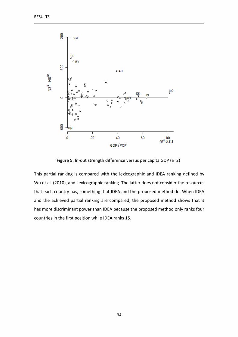
The differences between the in- and out- strength has been identified as useful to

gauge each country’s performance. Figure 5 shows this difference for each country and

its relationship to the ratio of their GDP to POP. So, a partial ranking of the countries

using an analogy between the in- and out- strength and the positive and negative

outranking flows is computed in Promethee I.

RESULTS

34

Figure 5: In-out strength difference versus per capita GDP (a=2)

This partial ranking is compared with the lexicographic and IDEA ranking defined by

Wu et al. (2010), and Lexicographic ranking. The latter does not consider the resources

that each country has, something that IDEA and the proposed method do. When IDEA

and the achieved partial ranking are compared, the proposed method shows that it

has more discriminant power than IDEA because the proposed method only ranks four

countries in the first position while IDEA ranks 15.

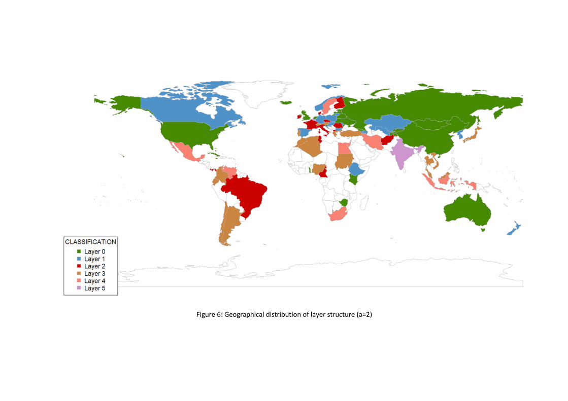
Figure 6: Geographical distribution of layer structure (a=2)

RESULTS

36

3.3 Dominance network analysis of economic efficiency3

The aim of this paper is to assess the technical, economic and allocative efficiency of a

set of DMUs using DNA. One DMU could be technically efficient, but not economically

efficient because of its input/output unit prices not being competitive.

In this research paper, a novel way of assessing the economic and technical

performance of DMUs using complex network tools is proposed. Technical efficiency

leads to technical dominance applied in the publications in §3.1 and §3.2; on the other

hand economic efficiency leads to economic dominance based on cost, revenue and

profit terms.

In this paper a multiplex directed weighted acyclic network integrates both technically

inefficient relationships and economically inefficient relationships. The nodes of the

network are linked by arcs, representing both the relationships along them. As

explained above, technical dominance relationship exists if two nodes are comparable

and one node is more efficient than the other. In this case, one link that represents the

dominance relationship in technical terms points to the better performer and the

length of this link measures the relative technical inefficiency between them. The same

is applicable for economically inefficient relationship.

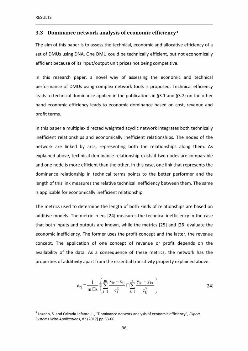
The metrics used to determine the length of both kinds of relationships are based on

additive models. The metric in eq. [24] measures the technical inefficiency in the case

that both inputs and outputs are known, while the metrics [25] and [26] evaluate the

economic inefficiency. The former uses the profit concept and the latter, the revenue

concept. The application of one concept of revenue or profit depends on the

availability of the data. As a consequence of these metrics, the network has the

properties of additivity apart from the essential transitivity property explained above.

m sir ij kj kr

rj x yi 1 k 1i k

x x y y1e

m s c c= =

− − = ⋅ + + [24]

3 Lozano, S. and Calzada-Infante, L., “Dominance network analysis of economic efficiency”, Expert

Systems With Applications, 82 (2017) pp:53-66

RESULTS

37

k kj i ij k kr i irk i k iPI

rj

s1 2 m 1 2

x x x y y y1 2 m s1 2

p y q x p y q x

e

pq q q p pmin , ,..., , , ,...,

w w w ww w

− − −

=

[25]

k kj k krRI k krj

s1 2

y y ys1 2

p y p y

e

pp pmin , ,...,

ww w

−=

[26]

As described in Chapter 1, the economic inefficiency between two DMUs is greater

than the technical inefficiency between them and the difference between these

inefficiencies is measured in DEA by allocative inefficiency. In DNA, Allocative

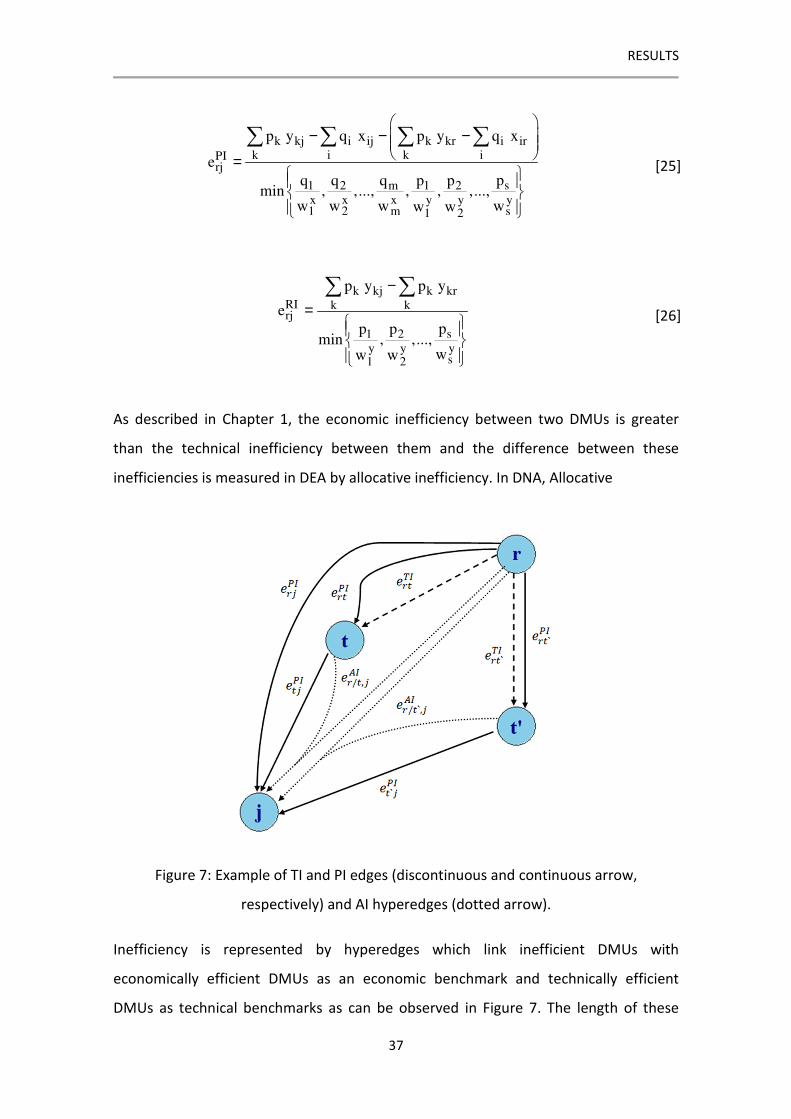
Figure 7: Example of TI and PI edges (discontinuous and continuous arrow,

respectively) and AI hyperedges (dotted arrow).

Inefficiency is represented by hyperedges which link inefficient DMUs with

economically efficient DMUs as an economic benchmark and technically efficient

DMUs as technical benchmarks as can be observed in Figure 7. The length of these

RESULTS

38

hyperedges determines the distance between the technically Efficient Frontier and the

economically Efficient Frontier through the connected technical benchmark.

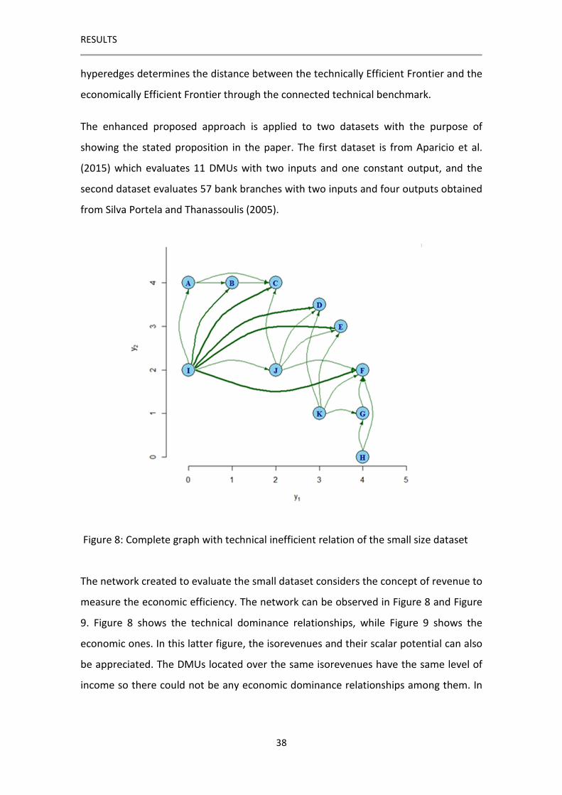
The enhanced proposed approach is applied to two datasets with the purpose of

showing the stated proposition in the paper. The first dataset is from Aparicio et al.

(2015) which evaluates 11 DMUs with two inputs and one constant output, and the

second dataset evaluates 57 bank branches with two inputs and four outputs obtained

from Silva Portela and Thanassoulis (2005).

Figure 8: Complete graph with technical inefficient relation of the small size dataset

The network created to evaluate the small dataset considers the concept of revenue to

measure the economic efficiency. The network can be observed in Figure 8 and Figure

9. Figure 8 shows the technical dominance relationships, while Figure 9 shows the

economic ones. In this latter figure, the isorevenues and their scalar potential can also

be appreciated. The DMUs located over the same isorevenues have the same level of

income so there could not be any economic dominance relationships among them. In

RESULTS

39

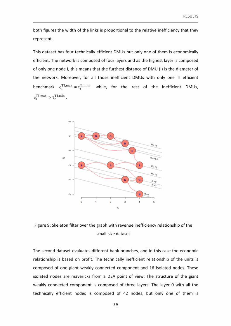
both figures the width of the links is proportional to the relative inefficiency that they

represent.

This dataset has four technically efficient DMUs but only one of them is economically

efficient. The network is composed of four layers and as the highest layer is composed

of only one node I, this means that the furthest distance of DMU (I) is the diameter of

the network. Moreover, for all those inefficient DMUs with only one TI efficient

benchmark TI,max TI,minr re = τ while, for the rest of the inefficient DMUs,

TI,max TI,minr re > τ .

The second dataset evaluates different bank branches, and in this case the economic

relationship is based on profit. The technically inefficient relationship of the units is

composed of one giant weakly connected component and 16 isolated nodes. These

isolated nodes are mavericks from a DEA point of view. The structure of the giant

weakly connected component is composed of three layers. The layer 0 with all the

technically efficient nodes is composed of 42 nodes, but only one of them is

Figure 9: Skeleton filter over the graph with revenue inefficiency relationship of the

small-size dataset

RESULTS

40

economically efficient. Looking at the economic relationships, it is observed there is no

more than one node per layer, due to all the DMUs having different levels of profit.

Observing the results of the applied metrics, it is easy to check how the in-strength is a

measure correlated with the good performance of the DMUs, and their higher values

are linked to a better performer. The skeleton of the profit inefficient relationship can

be observed in Figure 10, as the width of the links are proportional to the relative

inefficiency, the highest gap between each pair of nodes is between nodes B17 and

B53.

Figure 10: Spiral layout of the skeleton of the PI relationship of the bank branches’

dataset

In both datasets it can be observed that only when there is a technical relationship

between two DMUs, an economic relationship could exist between them. In addition,

the economic inefficiency is always greater than or equal to the technical inefficiency.

All the DMUs have an economic scalar potential linked to their position and based on

this scalar potential appears the economic relationships.

RESULTS

41

3.4 Computing gradient-based stepwise benchmarking paths4

In this research paper, a new stepwise benchmarking approach is designed based on

the gradient of an Efficiency Field Potential (EFP). The EFP is defined such that the

fewer inputs are consumed and the more outputs are produced by DMUs, the lower its

EFP value.

Each DMU, depending on its position, has a scalar EFP and a negative gradient which

defines the Efficiency Field Vector (EFV), and all the DMUs which have the same scalar

EFP are over the same Efficiency Equipotential Surface (EES). The EFV are

perpendicular to the EES and define the direction of an inefficient DMU to achieve the

Efficient Frontier. Figure 11 visualises these concepts in three bidimensional plots

where the arrows represent EFV and the dotted lines represents the EES.

Two models are proposed to determine the continuous stepwise path of the inefficient

DMUs: Improvement Dimensions (ID) and Gradient Stepsize (GSS). The ID model is

Mixed Integer Linear Programming (MILP) and determines which input/output

dimensions can be improved in step t if a minimum improvement could be achieved in

those dimensions. Using as an input the output of the ID model, the GSS model defines

the next position of the assessed DMU. This model is a Goal Programming model,

where the goal is the desired stepsize, which is limited by the maximum step that can

be achieved by that DMU.

Once the DMU has achieved the Efficient Frontier, the efficient DMU can be moved to

the area of minimum EFP, with the non-linear optimization model based on EFP

definition.

An extension of the proposed approach is also developed, in which it is described how

to apply a preference structure to the methodology and also how undesirable outputs

and non-discretional variables could be considered.

4 Lozano, S. and Calzada-Infante, L., “Computing gradient-based stepwise benchmarking paths”, Omega

(2017) doi: https://doi.org/10.1016/j.omega.2017.11.002

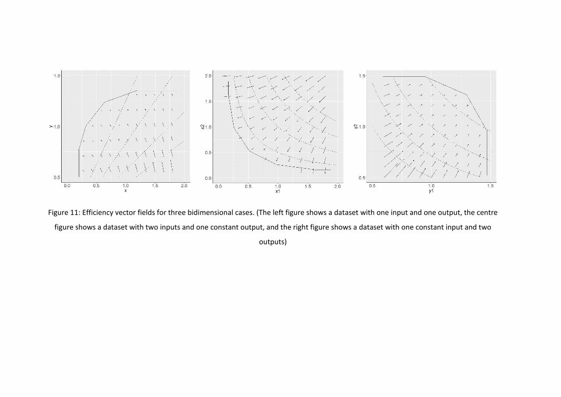
Figure 11: Efficiency vector fields for three bidimensional cases. (The left figure shows a dataset with one input and one output, the centre

figure shows a dataset with two inputs and one constant output, and the right figure shows a dataset with one constant input and two

outputs)

RESULTS

43

The new approach is applied to an organic farming dataset, which is composed of 26

DMUs, three inputs (Fuel consumption, Carbon input and Nitrogen input, where

Carbon input is non-discretional) and three outputs (Yield fresh matter, Net Primary

Production and CO2 emissions, the latter being undesirable).

The proposed approach offers good results regarding the relationship between the

Slack-Based Inefficiency (SBI) score and EFP values. There is a positive correlation

between both values and the DMUs having large SBI reductions are the ones that also

achieve the largest EFP reduction.

The proposed approach is flexible because it allows the stepsize to be changed, and

also a preference structure to be incorporated. Moreover, it is effective in avoiding

zigzagging, but it cannot handle either integer inputs or outputs, or operating points

with zero inputs or zero outputs. However, regarding the latter, it could be solved

using a linear definition of EFP.

3.5 Assessing individual performance based on the efficiency of

projects5

Assessing the performance of individual team members is a complex task. In this paper

a new approach based on DEA has been proposed to determine the individual

performance using as the start point the relative efficiency of the projects in which

they are involved, and considering that the contribution of each team member to the

project is known. A two-step approach is proposed to calculate the performance of the

team members.

The first step of the model is to evaluate the relative efficiency of the projects using an

input-oriented DEA model, taking into account the cost, duration and difficulty of the

projects as input and their revenue as output.

5 Adenso-Díaz, B., Lozano, S., Gutiérrez, E., Calzada, L. and García, S., “Assessing individual performance

based on the efficiency of projects” Computers & Industrial Engineering, 107 (2017) pp:280-288

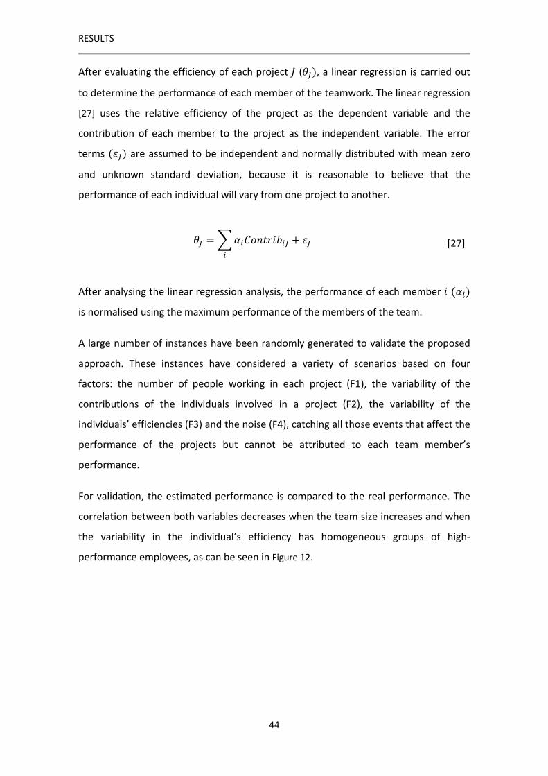
RESULTS

44

After evaluating the efficiency of each project R (ST), a linear regression is carried out

to determine the performance of each member of the teamwork. The linear regression

[27] uses the relative efficiency of the project as the dependent variable and the

contribution of each member to the project as the independent variable. The error

terms (UT) are assumed to be independent and normally distributed with mean zero

and unknown standard deviation, because it is reasonable to believe that the

performance of each individual will vary from one project to another.

ST = V�WXYZ/�[�T�

+ UT [27]

After analysing the linear regression analysis, the performance of each member � (V�)

is normalised using the maximum performance of the members of the team.

A large number of instances have been randomly generated to validate the proposed

approach. These instances have considered a variety of scenarios based on four

factors: the number of people working in each project (F1), the variability of the

contributions of the individuals involved in a project (F2), the variability of the

individuals’ efficiencies (F3) and the noise (F4), catching all those events that affect the

performance of the projects but cannot be attributed to each team member’s

performance.

For validation, the estimated performance is compared to the real performance. The

correlation between both variables decreases when the team size increases and when

the variability in the individual’s efficiency has homogeneous groups of high-

performance employees, as can be seen in Figure 12.

RESULTS

45

Figure 12: Boxplots of Pearson correlation between estimated relative performances

and true individual efficiencies for the different factors.

After testing the proposed approach, this paper evaluates in a real case the individual

performance of 10 programmers and analysts from a Spanish software engineering

company who have been involved in 46 projects.

After calculating the relative efficiencies of the projects and the multilinear regression

analysis, it can be observed that there is a good fit of the linear regression specification

with the R-squared value of 0.856. All the independent variables except one are

significant at the 0.1 level, which is not significant given the linear model specification

considered. All the employees had a significant and negative coefficient.

47

4. CONCLUSIONS

In this Thesis a new methodology called Dominance Network Analysis (DNA) was

defined. This methodology has been implemented to complement and enhance the

traditional numerical assessment of DEA, creating a DEA-CNA framework to analyse

the dataset at different levels, assessing the dataset as a whole considering an FDH

technology and an additive normalised-slacks efficiency measure. The filtering and

visualisation capabilities of these tools are very valuable for the large multidimensional

dataset. It is easy to identify for each inefficient unit all the possible stepwise paths,

i.e., the sequences of targets to achieve the Efficient Frontier, and how far they are

from it.

Therefore, it is also easy to determine the dominance relationships, who is dominated

by whom and the potential improvement of each step. The Dominance Network

visualisation features are very helpful to perceive and assess the relative performance

level of the different assessed units.

One application case was related to the performance of the countries that participated

in the Olympic Games in Beijing 2008. After applying this methodology, different global

and node-specific metrics provide a complete characterisation of the performance

differences between the assessed countries. Once the position of each country is

determined with respect to the rest of the DMU and has provided a complete

characterisation of the performance between the different countries, a partial ranking

CONCLUSIONS

48

has been computed using the analogy with Promethee I. This gives an assessment of

the relative performance of the different countries, which considers all the

relationships between the countries and makes use of all the information available.

The advantage of this method over other traditional, simplified ranking methods such

as lexicographic order is to consider the capabilities of the countries. This point is

considered in many DEA models, e.g. the Integer-Valued DEA model. However, DEA

models only consider the distance to the Efficient Frontier while the proposed

approach considers all the dominance relationships established by the position of all

the DMUs in the space.

Moreover, an enhanced approach of DNA was developed to evaluate the DMUs from

an economic perspective, apart from the technical perspective. This approach has

been applied to the bank field. A multiplex acyclic directed network is created. This

network is composed of two Efficient Frontiers, one per relationship. The distance

between both Efficient Frontiers is measured by Allocative Inefficiency hyperedges.

This new approach is applied to a bank dataset and has several interesting

relationships which were defined as propositions in the research paper.

Both approaches are interesting not only in assessing the efficiency of the individual

DMUs but also to capture the implicit dependencies between them through the

dominance relationships. This fact provides new insights that complement the

conventional DEA analysis.

Therefore the DNA methodology, which appears as an innovative approach to

determine the stepwise benchmarking paths based on efficiency gradient fields is

defined. New concepts are defined: Efficiency Field Potential, Efficiency Equipotential

Surfaces and Efficiency Field Vector. Each position of the DMUs is associated with an

EFP where the smaller the input consumption and the larger the output production,

the smaller the EFP. The negative EFP gradient defines the direction that the inefficient

DMUs have to follow to achieve the Efficient Frontier.

This benchmarking approach is comprised of three models to achieve the minimum

EFP. Two of them define a stepwise benchmarking path to achieve the Efficient

CONCLUSIONS

49

Frontier with a bounded stepsize along the negative EFP direction, and the third model

determines the minimum EFP to which the efficient DMU could aspire. The proposed

model can be used with preference structures, non-discretionary variables and

undesirable outputs.

This approach has been applied to two datasets, an illustrative example and an organic

farms dataset. The illustrative example shows the potential of the proposed approach,

while in the organic farms case it is proved that the new stepwise benchmarking

approach can be used for datasets with undesired outputs and non-discretional

variables.

The last contribution of this Thesis is a two-step approach to evaluate the performance

of team members in the context of project management, based on the performance of

the projects on which they have worked. The first step evaluates the relative efficiency

of the projects in order to calculate the relative performance of each member by using

a multilinear regression analysis. The normalised coefficient indicates the relative

performance of the individual and three cases are identified, depending on whether

the variable is significant, in which case the coefficient can be positive or negative; or

non-significant, which means that there is no contribution to the project. This

performance score allows the ranking of individuals. This methodology was

successfully applied to a software company involved in many development projects.

4.1 Further Research

Regarding the approach of DNA, it would be interesting to extend this approach to

other technologies studied in DEA, such as CRS and VRS. Moreover, other inefficiency

measures can be used in this approach. It could be interesting to determine how the

properties of the network, and also the sensibility of the resulting network based on

the considered metric, change despite the risk of losing additivity property.

In this Thesis, the efficiency of DMUs in a certain period as a fixed image has been

studied. However, in DEA the DMUs could be assessed in different periods of time and

CONCLUSIONS

50

their evolution over time could be controlled. It would be interesting to apply this

principle to the DNA and consider multi-period input-output data.

Regarding the gradient-based stepwise benchmarking path approach, it could be

interesting to define an additive EFP in order to be able to evaluate operating points

with zero inputs or zero outputs.

Finally, regarding the assessment of the individual performance, other DEA models

could be applied to evaluate the performance of the projects, avoiding the slacks of

the radial model used. Moreover, it could be interesting to evaluate the individual

performance of team members with other regression specifications, (sub-linear for

instance), althought the linear regression has given rather high goodness of fit indexes.

51

LIST OF REFERENCES

Aparicio, J., F. Borras, J. T. Pastor and F. Vidal, "Accounting for slacks to measure and

decompose revenue efficiency in the Spanish Designation of Origin wines

with DEA", European Journal of Operational Research, 231, 2 (2013) pp:443–

451.

Aparicio, J., F. Borras, J. T Pastor and F. Vidal, "Measuring and decomposing firm’s

revenue and cost efficiency: The Russell measures revisited", International

Journal of Production Economics, 165 (2015) pp:19–28.

Barabási, A.-L. and R. Albert, "Emergence of Scaling in Random Networks", Science, 286

(1999) pp:509–512.

Cooper, W. W., K. S. Park and J. T. Pastor, "RAM : A Range Adjusted Measure of

Inefficiency for Use with Additive Models, and Relations to Other Models

and Measures in DEA", Journal of Productivity Analysis, 11 (1999) pp:5–42.

Cooper, W. W., J. T. Pastor, J. Aparicio and F. Borras, "Decomposing profit inefficiency

in DEA through the weighted additive model", European Journal of

Operational Research, 212, 2 (2011) pp:411–416.

da Fontoura Costa, L., O. N. Oliveira Jr, G. Travieso, F. Aparecido Rodrigues, P. R. Villas

Boas, L. Antiqueira, M. Palhares Viana and L. E. Correa Rocha, "Analyzing and

LIST OF REFERENCES

52

modeling real-world phenomena with complex networks: a survey of

applications", Advances in Physics, 60, 3 (2011) pp:329–412.

Erdös, P. and A. Rényi, "On random graphs I.", Publicationes Mathematicae (Debrecen),

6 (1959) pp:290–297.

Estrada, S. A., H. S. Song, Y. A. Kim, S. H. Namn and S. C. Kang, "A method of stepwise

benchmarking for inefficient DMUs based on the proximity-based target

selection", Expert Systems with Applications, 36 (2009) pp:11595–11604.

Fang, L., “Centralized resource allocation based on efficiency analysis for step-by-step

improvement paths”, Omega, 51 (2015) 24-28.

Ghahraman, A. and D. Prior, "A learning ladder toward efficiency: Proposing network-

based stepwise benchmark selection", Omega, 63, 83–93 (2016) pp:1–11.

Ho, M. H.-C., J. S. Liu, W.-M. Lu and C.-C. Huang, "A new perspective to explore the

technology transfer efficiencies in US universities", Journal of Technology

Transfer, 39, 2 (2014) pp:247–275.

Hong, H. K., S. H. Ha, C. K. Shin, S. C. Park and S. H. Kim, “Evaluating the efficiency of

system integration projects using Data Envelopment Analysis (DEA) and

machine learning”, Expert Systems with Applications, 16, 3 (1999) 283-296.

Khodakarami, M., A. Shabani and R. F. Saen, “A new look at measuring sustainability of

industrial parks: A two-stage data envelopment analysis approach”, Clean

Technologies and Environmental Policy, 16, 8 (2014) 1577-1596.

Lim, S., H. Bae and L. H. Lee, "A study on the selection of benchmarking paths in DEA",

Expert Systems with Applications, 38, 6 (2011) pp:7665–7673.

Liu, J. S. and W.-M. Lu, "DEA and ranking with the network-based approach: A case of

R&D performance", Omega, 38 (2010) pp:453–464.

Liu, J. S. and W.-M. Lu, "Network-based method for ranking of efficient units in two-

stage DEA models", Journal of the Operational Research Society, 63 (2012)

LIST OF REFERENCES

53

pp:1153–1164.

Liu, J. S., L. Y. Y. Lu, W.-M. Lu and B. J. Y. Lin, "A survey of DEA applications", Omega, 41

(2013) pp:893–902.

Liu, J. S., W.-M. Lu, C. Yang and M. Chuang, "A network-based approach for increasing

discrimination in data envelopment analysis", The Journal of the Operational

Research Society, 60, 11 (2009) pp:1502–1510.

Lozano, S. and G. Villa, “Determining a sequence of targets in DEA”, Journal of the

Operational Research Society, 56, 12 (2005) 1439-1447.

Lozano, S. and G. Villa, "Gradual technical and scale efficiency improvement in DEA",

Annals of Operations Research, 173 (2010) pp:123–136.

Newman, M. E. J., "The structure and function of complex networks", SIAM Review, 45,

2 (2003) pp:167–256.

Park, J., H. Bae and S. Lim, "Method of Benchmarking Route Choice Based on the Input-

similarity Using DEA and SOM", Smart Innovation Systems and Technologies,

10 (2011) pp:519–528.

Park, J., H. Bae and S. Lim, “Stepwise Benchmarking Path Selection in DEA”, Smart

Innovation, Systems and Technologies, 16 (2012a) 477-484.

Park, J., H. Bae and S. Lim, “A DEA-Based Method of Stepwise Benchmark Target

Selection with Preference, Direction and Similarity Criteria”, International

Journal of Innovative Computing, Information and Control, 8, 8 (2012b)

5821-5834.

Park, J., S. Lim and H. Bae, “DEA-Based Port Efficiency Improvement and Stepwise

Benchmarking Target Selection”, Information, 15, 12C (2012c) 6155-6171.

Park, J., S. Lim and H. Bae, “An Optimization Approach to the Construction of a

Sequence of Benchmark Targets in DEA-Based Benchmarking”, Journal of the

Korean Institute of Industrial Engineers, 40, 6 (2014) 628-641.

LIST OF REFERENCES

54

Park, J. and S.-I. Sung, “Integrated Approach to Construction of Benchmarking Network

in DEA-Based Stepwise Benchmark Target Selection”, Sustainability, 8, 600

(2016).

Sharma, M. J. and S. J. Yu, “Performance based stratification and clustering for

benchmarking of container terminals”, Expert Systems with Applications, 36

(2009) 5016-5022.

Sharma, M. J. and S. J. Yu, “Benchmark optimization and attribute identification for

improvement of container terminals”, European Journal of Operational

Research, 201, 2 (2010) 568-580.

Seiford, L. M. and J. Zhu, "Context-dependent data envelopment analysis - Measuring

attractiveness and progress", Omega, 31 (2003) pp:397–408.

Silva Portela, M. C. A. and E. Thanassoulis, "Profitability of a sample of Portuguese

bank branches and its decomposition into technical and allocative

components", European Journal of Operational Research, 162, 4 (2005)

pp:850–866.

Suzuki, S. and P. Nijkamp, “A stepwise-projection data envelopment analysis for public

transport operations in Japan”, Letters in Spatial and Resources Sciences, 4

(2011) 139-156.

Watts, D. J. and S. H. Strogatz, "Collective dynamics of “small-world” networks",

Nature, 393, 6684 (1998) pp:440–442.

Wiest, W. M., L. W. Porter and E. E. Ghiselli, "Relationships between individual

proficiency and team performance and efficiency", Journal of Applied

Psychology, 45, 6 (1961) pp:435–440.

Wu, J., Z. Zhou and L. Liang, "Measuring the Performance of Nations at Beijing Summer

Olympics Using Integer-Valued DEA Model", Journal of Sports Economics, 11,

5 (2010) pp:549–566.

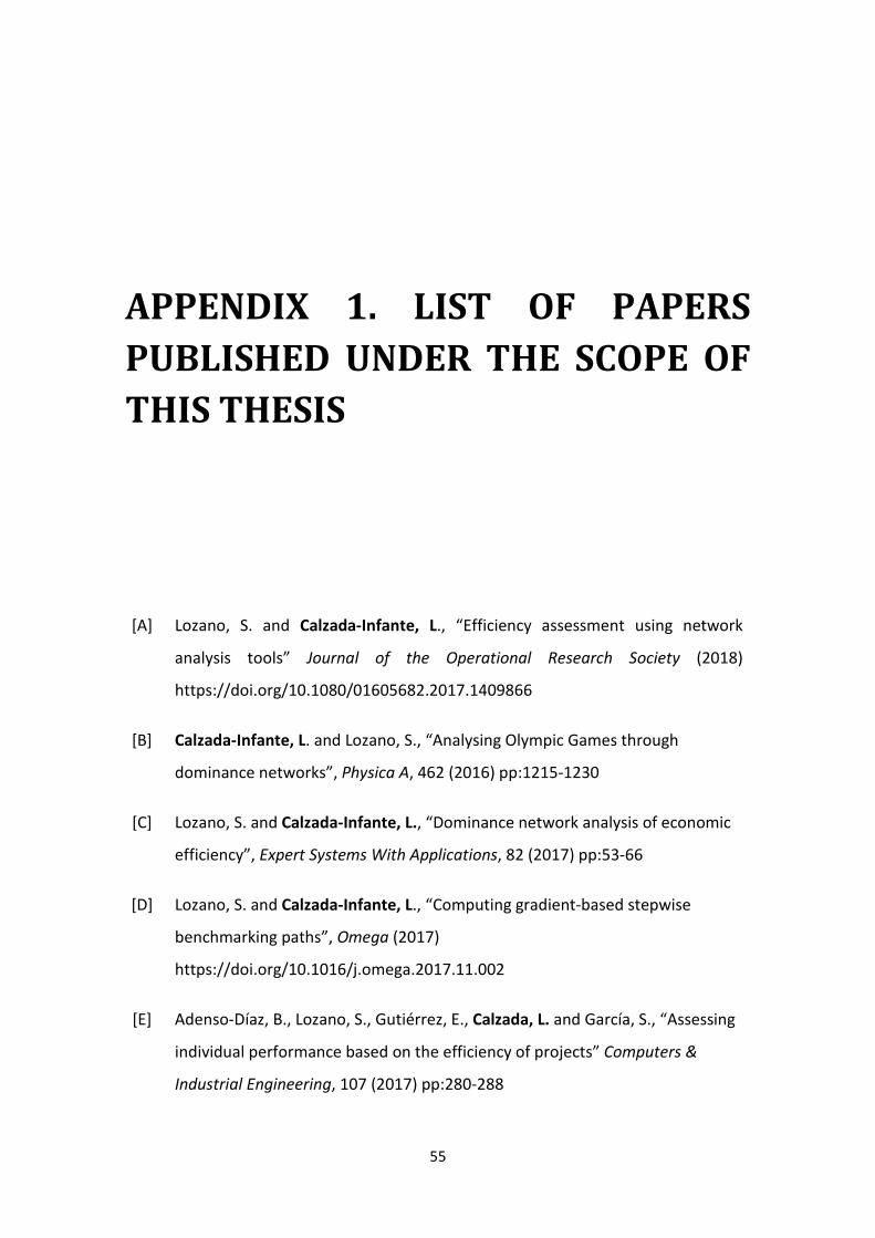
55

APPENDIX 1. LIST OF PAPERS

PUBLISHED UNDER THE SCOPE OF

THIS THESIS

[A] Lozano, S. and Calzada-Infante, L., “Efficiency assessment using network

analysis tools” Journal of the Operational Research Society (2018)

https://doi.org/10.1080/01605682.2017.1409866

[B] Calzada-Infante, L. and Lozano, S., “Analysing Olympic Games through

dominance networks”, Physica A, 462 (2016) pp:1215-1230

[C] Lozano, S. and Calzada-Infante, L., “Dominance network analysis of economic

efficiency”, Expert Systems With Applications, 82 (2017) pp:53-66

[D] Lozano, S. and Calzada-Infante, L., “Computing gradient-based stepwise

benchmarking paths”, Omega (2017)

https://doi.org/10.1016/j.omega.2017.11.002

[E] Adenso-Díaz, B., Lozano, S., Gutiérrez, E., Calzada, L. and García, S., “Assessing

individual performance based on the efficiency of projects” Computers &

Industrial Engineering, 107 (2017) pp:280-288

57

APPENDIX 2. PAPERS

JOURNAL OF THE OPERATIONAL RESEARCH SOCIETY, 2018

https://doi.org/10.1080/01605682.2017.1409866

KEYWORDS

Efficiency assessment; Data Envelopment Analysis (DEA); dominance network; Complex Networks Analysis

ARTICLE HISTORY

Received 4 October 2016 Accepted 21 November 2017

© Operational Research Society 2018

CONTACT Sebastián Lozano slozano@us.es

E�ciency assessment using network analysis tools

Sebastián Lozanoa and Laura Calzada-Infanteb

aDepartment of Industrial Management, University of Seville, Seville, Spain; bEngineering School, University of Oviedo, Gijón, Spain

ABSTRACT

In this paper, some of the network analysis techniques generally used for complex networks are applied to e!ciency assessment. The proposed approach is units invariant and allows the computation of many interesting indexes, such as node speci"city, benchmarking potential, clustering coe!cient, betweenness centrality, components and layers structure, in- and out-degree distributions, etc. It also allows the visualisation of the dominance relationships within the data-set as well as the potential benchmarks and the gradual improvement paths from ine!cient nodes. A number of useful "lters (bipartite subgraph, ego networks, threshold networks, skeletonisation, etc.) can be applied on the network in order to highlight and focus on speci"c subgraphs of interest. The proposed approach provides a new perspective on e!ciency analysis, one that allows not only to focus on the distance to the e!cient frontier and potential targets of individual units but also to study the data-set as a whole, with its component and layer structure, its overall dominance density, etc.

1. Introduction

Data Envelopment Analysis (DEA) is a well-known non-parametric technique that can be used to assess the relative e�ciency of homogeneous (i.e., comparable) Decision-Making Units (DMUs). Each DMU consumes certain amounts of inputs in order to produce certain amount of outputs. �e aim is to detect ine�ciencies, i.e., potential reductions of the inputs maintaining the output levels or potential output increases maintaining the input consumption levels. Based on these potential improvements an e�ciency score can be computed. �ere are di�erent DEA models, depending on the ori-entation (whether to seek mainly inputs improvements or output improvements or both), on the metric used for the improvements (e.g., radial, non-radial, additive, etc.) and the technology assumptions (Constant Returns to Scale, Variable Returns to Scales, Free Disposal Hull, etc.). With respect to DEA applications, they are numer-ous and span all sectors (see, e.g., Cooper, Seiford, & Zhu, 2004; Liu, Lu, Lu, & Lin, 2013a).

�e approach proposed in his paper is related to some research topics in DEA, such as DMU layers, interme-diate benchmarks, and closest targets. �us, Seiford and Zhu (2003) showed how to identify the successive layers of DMUs in a sample, a process that can also be called strati!cation. �us, the e�cient DMUs belong to layer 0 while layer 1 is formed by the DMUs that would be e�cient if those in the previous layer are removed, and

so on for the successive layers. Introducing the concept of context-dependent DEA, Seiford and Zhu (2003) also de!ned attractiveness and progress measures for each DMU with respect to the di�erent DMU layers.

Intermediate targets refer to the advantages of devel-oping gradual improvement paths to the e�cient fron-tier (e.g., Lozano & Villa, 2005, 2010). Lim, Bae, and Lee (2011) proposed a stepwise benchmarking path based on strati!cation and using a composite index of the attractiveness, progress, and feasibility of each e�-ciency improvement step. �e e�ciency measurements are based on the Range-Adjusted Measure (RAM) DEA model (Cooper, Park, & Pastor, 1999). Park, Bae, and Lim (2011) use, in addition to strati!cation, DMU clus-ters computed using k-means algorithm on the DMU input vectors. �e successive intermediate benchmarks are thus chosen among those DMUs in the cluster with highest similarity to that to which the current DMU belongs. Park, Bae, and Lim (2012a) also use strati!-cation but the benchmarking path selection uses two criteria, namely minimise resource improvement and maximise improvement direction proximity. Park, Bae, and Lim (2012b) uses the decision-maker’s preferences to select the ultimate target and, for the selection of the intermediate benchmarks, a weighted sum of a measure of direction improvement proximity and a measure of resource consumption proximity. �e latter is computed as the distance in the grid that results from quantising

2 S. LOZANO AND L. CALZADA-INFANTE

the input vectors using a Self-Organising Map (SOM). Estrada, Song, Kim, Namn, and Kang (2009) also uses SOM applied on input vectors but they propose comput-ing the optimal path to the frontier through a reinforced learning algorithm that uses e�ciency improvement as the reward of each step, thus e�ectively computing a shortest path to the e�cient frontier. More recently, Ghahraman and Prior (2016) have proposed a gradual improvement method that computes the optimal step-wise benchmarking paths from the ine�cient DMUs to the e�cient ones using Dijkstra’s shortest path on a benchmarking network whose edges have a length that depends on the input similarity and the e�ciency gap between the nodes linked. �e idea is to use as succes-sive intermediate targets operating points that are not very dissimilar in their input endowments and in their e�ciency level. �e method also considers maximum allowed change in inputs in each step.

�e issue of closest target and minimum distance to the e�cient frontier (EF) has been also the subject of much research. �us, González and Álvarez (2001) proposes to use an input-speci!c contraction measure that computes the sum of input contractions required to reach the EF. Silva Portela, Borges, and �anassoulis (2003) presents a procedure to compute closest targets using a non-oriented DEA model and studies the cases of convex and non-convex technologies, the latter a.k.a. Free Disposal Hull (FDH). Aparicio, Ruiz, and Sirvent (2007) proposes di�erent mathematical programming models for computing the closest target, depending on how closeness is measured. Baek and Lee (2009) pre-sents a method based on a Least-Distance Measure to obtain the shortest projection from a DMU to the EF. Aparicio and Pastor (2013, 2014a) propose an out-put Russell measure and an output-oriented strong Hölder distance function, respectively, both based on an extended facet production possibility set, that have the strong monotonicity property and that allow the computation of closest targets. López-Espín, Aparicio, Giménez, and Pastor (2014) introduce a new approach based on metaheuristics in order to determine least dis-tances. Aparicio, Mahlberg, Pastor, and Sahoo (2014) uses the Principle of Least Action and a minimisation version of the Measure of Ine�ciency Proportions (MIP) to compute the closest projection on the frontier and, hence, minimum total e�ort needed by to achieve tech-nical e�ciency. Aparicio and Pastor (2014b) proposes a model based on weighted Euclidean distance to obtain the closest targets. An, Pang, Chen, and Liang (2015) uses an enhanced Russell measure to compute closest targets in the presence of undesirable outputs. Last but not least, two recent papers deal with the minimum dis-tance to the EF in the case of FDH technology, namely Ebrahimnejad, Shahverdi, Balf, and Hate! (2013) and Fukuyama, Hougaard, Sekitani, and Shi (2016).

Consider now the also very fruitful !eld of Complex Networks Analysis (CNA), which has witnessed in the last decade a tremendous growth, both in terms of theory developments and of applications. �e basic concepts of these techniques are presented and explained in a num-ber of textbooks and survey papers (e.g., Jackson, 2010; Newman, 2003; Wasserman & Faust, 1994) while some interesting applications include transportation networks (e.g., Derrible & Kennedy, 2010; Lordan, Sallan, & Simo, 2014, Zanin & Lillo, 2013), power grid networks (Pagani & Aiello, 2013), !nancial markets (e.g., Nobi, Maeng, Ha, & Lee, 2014; Oh, 2014), etc.

Apart from the research carried out by Ghahraman and Prior (2016) mentioned above, CNA and DEA has been jointly used in Lee, Seo, Choe, and Kim (2012) to study collaboration network patterns and research per-formance of public research institutes and in Lin and Tan (2014) to study the relationship between the centrality and the performance of the individuals in an organisa-tion. �e bibliometric studies of DEA literature in Liu et al. (2013a), Liu, Lu, Lu, and Lin (2013b), Liu, Lu, and Lu (2016) and Lampe and Hilgers (2015) also use CNA and clustering techniques, applied, in this case, to cita-tion and co-citation networks. CNA tools have also been proposed to increase the discrimination power of DEA. �us, the network-based approach in Liu, Lu, Yang, and Chuang (2009) uses the intensity variables (the lambda values as they are generally termed in DEA) to build a weighted, directed network, computing eigenvector cen-trality measures to rank the e�cient DMUs. To populate the network arcs, di�erent input/output combinations are considered. Liu and Lu (2010, 2012) and Ho, Liu, Lu, and Huang (2014) extend the network-based approach to the case of two stage systems, building a separate network and computing a DMU ranking for each stage and computing the relative strength of each input/output factor for each e�cient DMU. Di�erent DEA models can be used to compute the corresponding lambda values for each stage. �is network-based approach has been applied in di�erent contexts, such as internet companies, banks, research institutes, and universities.

Recently, Calzada-Infante and Lozano (2016) pro-posed a CNA approach to assess the performance of countries in the Olympic Games in Beijing 2008, taking into account the number of medals won and the coun-tries’ population and GDP. �at paper introduced the concept of dominance network, whose usefulness for e�ciency assessment is further explored and formal-ised in this paper. Lozano and Calzada-Infante (2017) have applied dominance network analysis to pro!t and revenue e�ciency, i.e., to cases in which the input and output unit prices are known. In this paper, a method-ology for globally assessing the e�ciency of a sample of DMUs considering an FDH technology and using a CNA approach is proposed. Speci!cally, a dominance

JOURNAL OF THE OPERATIONAL RESEARCH SOCIETY 3

network is built using edges whose weight is equal to the relative e�ciency distance between the two DMUs, measured as the sum of the relative input reductions and output increases from the DMU origin of the link to the DMU destination of the link. �is weighted, directed network allows computing a number of interesting CNA indexes and measures for the individual nodes, for its connected components, for the di�erent layers and for the network as a whole. Also, the visualisation of the network, which can be enhanced through a series of selective !lters, provides additional information into the performance and benchmarking paths of the ine�-cient DMUs, about the benchmarking popularity of the e�cient DMUs, etc.

�e structure of the paper is the following. In Section 2, the network construction process is presented and some basic CNA sets and indexes are de!ned. In Section  3, additional CNA measures as well as a num-ber visualisation !lters are proposed. �e proposed methodology is illustrated in Section 4. Finally, Section 5 summarises and concludes.

2. Network construction and basic CNA sets

and indexes

2.1. Network construction and notation

Consider a production process that uses m inputs to produce s outputs. �ere is a set D of DMUs that corresponds to di�erent observed instances of this production process. �e number of DMUs is n, i.e., |D| = n. We are interested in assessing the perfor-mance of these DMUs in terms of their relative e�-ciency in carrying out the production process. Let

xj =(

x1j, x2j, … xmj

)

and yj =(

y1j, y2j, … ysj

)

denote

the input and output vectors, respectively, of DMU j. Let

D(r) ={

j ≠ r: xij ≤ xir ∀i, ykj ≥ ykr ∀k}

⊂ D be the

set of DMUs that weakly dominate DMU r.�e proposed dominance network (D, E) has D as the

set of nodes and E ={

(r, j):r ∈ D ∧ j ∈ D(r)}

as the corresponding set of edges. �e term dominance comes from the fact that the network has an arc between two DMUs r and j if and only if DMU j dominates DMU r. Let us de!ne the weight of an edge (r, j) as the relative e�ciency improvement obtained when moving from r to j, using a given normalisation vector g =

(

gxi , gy

k

)

, i.e.,

Note that this de!nition is units invariant. For the nor-malisation vectors, di�erent possibilities may be con-sidered. One option is to use g =

(

xaveri , yaverk

)

where

xaveri =1

n

∑

j∈D

xij ∀i and yaverk =1

n

∑

j∈D

ykj ∀k are the average

value of the di�erent inputs and outputs, respectively.

erj =

{

0 if j ∉ D(r)∑

i

xir−xij

gxi+∑

k

ykj−ykr

gy

k

if j ∈ D(r) .

Alternatively, the normalisation vector can use the range of the input and output variables Ri = xmax

i − xmin

i ∀i and Rk = ymax

k − ymin

k ∀k, respectively, i.e., g =(

Ri, Rk

)

. �is units-and-translation-invariant alternative is espe-cially interesting in case some of the data are negative. Note however that, as pointed out by one of the review-ers, using g =

(

xaveri , yaverk

)

or g =(

Ri, Rk

)

has the draw-back of making the e�ciency score dependent on the whole sample, including the ine�cient units, when it is clear that these units do not a�ect the e�cient frontier.

Note, before proceeding further, that the edges have the transitivity property, i.e., if there exist the arcs (r, p) and (p, j) then there exist also the arc (r, j). �is occurs because p    D(r)    j    D(p)    j    D(r). Moreover, the weight of this transitive arc is equal to the sum of the corresponding weights, i.e., erp + epj = erj ∀p, j ∈ D(r), j ∈ D(p). !is additivity property derives from the fact that the normalisation vector used to normalise the input and output changes in the de"nition of the edge weight is the same for all edges. Moreover, the additivity property implies that all the paths that connect two nodes r and j have the same weight, equal to that of the arc that directly links them. !is means that all the paths that connect two nodes are geodesics, i.e., shortest paths.

Using the notation

�

(

erj

)

=

{

1 erj > 0 ⇔ (r, j) ∈ E

0 otherwise to indicate

whether the arc (r, j) exists, we can de"ne the associated unweighted, undirected network (D, A) whose incidence matrix is

Given two nodes r and j, we will say that they are con-nected in the graph (D, E) if there is a path that connects them in the underlying undirected graph (D, A). !e graph (D, E) can have one or more maximally connected components. Each component c is formed by a set of nodes D

c   D such j and r are connected j, r   D

c and

r ∈ Dc ∧ j connected with r ⇒ j ∈ Dc. Note that a com-ponent c is actually formed by the nodes in D

c plus the arcs

that link them Ec ={(

r, j)

∈ E: r ∈ Dc ∧ j ∈ Dc

}

⊆ E. In other words, a component c is a subgraph (D

c, E

c).

Note, in passing, that Dc ∩ Dc′ = ∅ ∀c ≠ c′, ⋃

c

Dc = D and

∑

c

|

|

Dc|

|

= |D| = n.

Let D∗ ={

r:D(r) = ∅}

⊆ D be the set of e!cient

nodes and D∗(r) =

{

{r} if r ∈ D∗

D(r) ∩ D∗ if r ∉ D∗

}

⊆ D∗

the set of e!cient benchmarks of node r. "e set of e!cient nodes of component c is just D∗

c ={

j:j ∈ Dc ∩ D∗}

=⋃

r∈Dc

D∗(r) ⊆ D∗.

In order to compute the in-degree of a node, we will need to consider the set

arj = ajr =

{

1 if ∃ edge (r, j) or ∃ edge (j, r) ⇔ (r, j) ∈ E ∨ (j, r) ∈ E

0 otherwise.

4 S. LOZANO AND L. CALZADA-INFANTE

closer e!cient target than to a more distant one. "e di#erence is that �min

r is restricted to the e!cient nodes that dominate node r while the minimum distance to the e!cient frontier may sometimes identify as closest e!cient target an e!cient node that does not dominate node r. In other words, �min

r is no substitute for a proper measure of minimum distance to EF (like, e.g., the one proposed in Fukuyama et al., 2016), which requires a relatively complex calculation and that can, in any case, be computed to supplement the proposed CNA DEA approach.

In addition, for e!cient nodes j ∈ D∗ we may compute:

Benchmarking count: ||

D−1(j)||

= din

j

Benchmarking necessity: ||

D−−1(j)||

Benchmarking potential: �j =∑

r∈D−1(j)

erj

Inefficiency radius: �j = maxr∈D−1(j)

erj

Superefficiency index: 'j =|

|

|

{

r:D(r) ={

j}

∧ �(r) = 1}

|

|

|

At the layer level, we may compute:

Percentage of component c nodes that form layer q: �cq =|Lcq|

|Dc|

At the component level, we may compute:Size of component c (as number of nodes): |

|

Dc|

|

Size of component c (as % of nodes): �c =|Dc|

|D|

Size of component c (as number of edges): NEc =|

|

Ec|

|

Size of component (as % of edges): �c =NEc

NE

Average degree: daver

c =1

|Dc|

∑

r∈Dc

din

r =1

|Dc|

∑

r∈Dc

dout

r

Density: �c =

{

1 if ||

Dc|

|

= 1daver

c

|Dc|−1

otherwise

Average distance of component c to EF: �averc =1

|Dc|

∑

r∈Dc

emax

r

Diameter of component c: Δc = maxr, j∈Dc

erj

Efficient nodes percentage of component c: �c =|D∗

c |

|D∗|

=|D∗∩Dc|

|D∗|

Percentage of efficient nodes in component c: �c =|D∗

c |

|Dc|

=|D∗∩Dc|

|Dc|

At the network level, we may compute:

Total number of edges: NE =∑

r

|D(r)|

Number of components: NC

Network diameter:Δ = max(r, j)∈E

erj = maxr∈Dc

emax

r = maxj∈D∗

c

�j

Average distance to EF: �aver =∑

c

|Dc|⋅�

aver

c

|D|=

1

n

∑

r∈D

emax

r

Percentage of e!cient nodes: � =|D∗

|

|D|In order to get better acquainted with these de"ni-

tions, let us consider two extreme scenarios: one in which all DMUs are e!cient and another in which only one DMU is e!cient. If all DMUs are e!cient, then D∗ = D, D(r) = ∅ ∀r, din

r = dout

r = 0 ∀r. In that case there would be as many components as DMUs and their size would be minimal, i.e., NC = |D| = n and |

|

Dc|

|

= 1 ∀c. We also have that emax

r = 0 ∀r ⇒ Δc = 0 ∀c, i.e., the diame-ter of all the components, and therefore of the network, would be zero, as it would also be the density of the

D−1(r) ={

j ≠ r:xij ≥ xir ∀i ykj ≤ ykr ∀k}

⊂ D

which corresponds to the DMUs that are dominated by DMU r. Let E−1(j) =

{

(r, j):r ∈ D−1(j)}

be the set of edges that are incident to node j as. Also let D−1(j) =

{

r:r ∈ D−1(j) ∧ D(r) ∩ D∗ ={

j}}

⊆ D−1(j) be the set of nodes for which j is their only e!cient bench-mark. Let E(r) =

{

(r, j):j ∈ D(r)}

be the set of edges that go out of node r and E∗(r) =

{

(r, j):j ∈ D∗(r)}

⊆ E(r) the set of direct edges from node r to the EF.

Let NLc be the number of layers of component c. Let

c(r) denotes the component to which node r belongs and let

be the layer, within that component, to which node r belongs. Let Lcq =

{

r ∈ Dc: �(r) = q}

be set of nodes that belong to layer q of component c. In particular, Lc0 = D∗

c, i.e., the layer 0 of a component is formed by the e!cient nodes that belong to that component.

2.2. Basic CNA indexes

Once the necessary de"nitions and notations have been de"ned, we are ready to compute some basic CNA indexes. Since the meaning and interestingness of most of these indexes is clear and to keep the length of the paper within a reasonable limit, we will not comment them in detail. Some indexes are computed at the node level while others correspond to the layer, the compo-nent or the network level. #us, at the node level we may compute:

In-degree of node r: din

r = |

|

D−1(r)||

Out-degree of node r: dout

r = |D(r)|

Speci"city of node r: Hub index of node r: Number of

e!cient benchmarks of node r: |D∗(r)|

Maximum distance of node r to the EF: emax

r = maxj∈D∗(r)

erjDistance of node r to closest

dominating e!cient node: �min

r = minj∈D∗(r)

erjBefore proceeding further, and in order to avoid con-

fusion, let us make clear that the last indicator, �min

r , just computes the distance to the closest e!cient node that dominates node r. #is should not be confused with the minimum distance of node r to the e!cient frontier, a measure which can computed using speci"c DEA approaches (e.g. Fukuyama et al., 2016). #e purpose of computing �min

r is to complement the conventional inef-"ciency measure emax

r , which aims at improving inputs and outputs as much as possible and therefore looks for the most distant e!cient node that dominates node r. #e idea behind the minimum distance to the e!cient frontier (and also behind �min

r ) is that it should be easier (i.e., less demanding) for a node r to move towards a

�(r) =

{

0 if D(r) = ∅

1 + maxj∈D(r)

�(j) otherwise

�r = |D(r)| + |

|

D−1(r)||

= din

r + dout

r

r = |D(r)| ⋅ ||

D−1(r)||

= din

r ⋅ dout

r

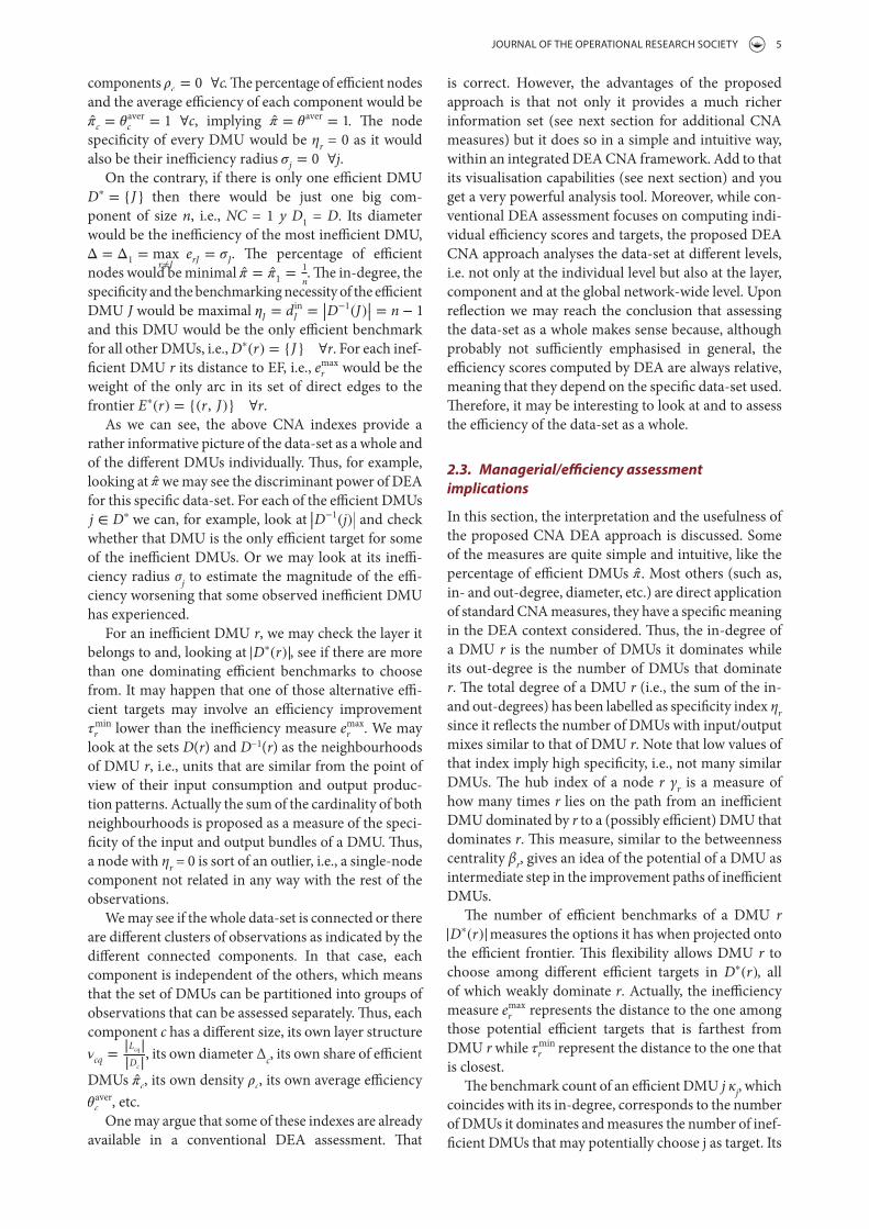
JOURNAL OF THE OPERATIONAL RESEARCH SOCIETY 5

is correct. However, the advantages of the proposed approach is that not only it provides a much richer information set (see next section for additional CNA measures) but it does so in a simple and intuitive way, within an integrated DEA CNA framework. Add to that its visualisation capabilities (see next section) and you get a very powerful analysis tool. Moreover, while con-ventional DEA assessment focuses on computing indi-vidual e�ciency scores and targets, the proposed DEA CNA approach analyses the data-set at di�erent levels, i.e. not only at the individual level but also at the layer, component and at the global network-wide level. Upon re�ection we may reach the conclusion that assessing the data-set as a whole makes sense because, although probably not su�ciently emphasised in general, the e�ciency scores computed by DEA are always relative, meaning that they depend on the speci�c data-set used. �erefore, it may be interesting to look at and to assess the e�ciency of the data-set as a whole.

2.3. Managerial/e�ciency assessment

implications

In this section, the interpretation and the usefulness of the proposed CNA DEA approach is discussed. Some of the measures are quite simple and intuitive, like the percentage of e�cient DMUs �. Most others (such as, in- and out-degree, diameter, etc.) are direct application of standard CNA measures, they have a speci�c meaning in the DEA context considered. �us, the in-degree of a DMU r is the number of DMUs it dominates while its out-degree is the number of DMUs that dominate r. �e total degree of a DMU r (i.e., the sum of the in- and out-degrees) has been labelled as speci�city index η

r

since it re�ects the number of DMUs with input/output mixes similar to that of DMU r. Note that low values of that index imply high speci�city, i.e., not many similar DMUs. �e hub index of a node r γ

r is a measure of

how many times r lies on the path from an ine�cient DMU dominated by r to a (possibly e�cient) DMU that dominates r. �is measure, similar to the betweenness centrality β

r, gives an idea of the potential of a DMU as

intermediate step in the improvement paths of ine�cient DMUs.

�e number of e�cient benchmarks of a DMU r |D∗(r)| measures the options it has when projected onto the e�cient frontier. �is �exibility allows DMU r to choose among di�erent e�cient targets in D∗(r), all of which weakly dominate r. Actually, the ine�ciency measure emax

r represents the distance to the one among those potential e�cient targets that is farthest from DMU r while �min

r represent the distance to the one that is closest.

�e benchmark count of an e�cient DMU j κj, which

coincides with its in-degree, corresponds to the number of DMUs it dominates and measures the number of inef-�cient DMUs that may potentially choose j as target. Its

components �c = 0 ∀c. �e percentage of e�cient nodes and the average e�ciency of each component would be �c = �

aver

c = 1 ∀c, implying � = �aver = 1. �e node

speci�city of every DMU would be ηr = 0 as it would

also be their ine�ciency radius �j = 0 ∀j.On the contrary, if there is only one e�cient DMU

D∗ = {J} then there would be just one big com-ponent of size n, i.e., NC  =  1 y D1  =  D. Its diameter would be the ine�ciency of the most ine�cient DMU, Δ = Δ

1= max

r≠JerJ = �J. �e percentage of e�cient

nodes would be minimal � = �1=

1

n. �e in-degree, the

speci�city and the benchmarking necessity of the e�cient DMU J would be maximal �J = din

J = |

|

D−1(J)||

= n − 1 and this DMU would be the only e�cient benchmark for all other DMUs, i.e., D∗(r) = {J} ∀r. For each inef-�cient DMU r its distance to EF, i.e., emax

r would be the weight of the only arc in its set of direct edges to the frontier E∗(r) = {(r, J)} ∀r.

As we can see, the above CNA indexes provide a rather informative picture of the data-set as a whole and of the di�erent DMUs individually. �us, for example, looking at � we may see the discriminant power of DEA for this speci�c data-set. For each of the e�cient DMUs j ∈ D∗ we can, for example, look at |

|

D−1(j)||

and check whether that DMU is the only e�cient target for some of the ine�cient DMUs. Or we may look at its ine�-ciency radius σ

j to estimate the magnitude of the e�-

ciency worsening that some observed ine�cient DMU has experienced.

For an ine�cient DMU r, we may check the layer it belongs to and, looking at |D∗(r)|, see if there are more than one dominating e�cient benchmarks to choose from. It may happen that one of those alternative e�-cient targets may involve an e�ciency improvement �min

r lower than the ine�ciency measure emax

r . We may look at the sets D(r) and D−1(r) as the neighbourhoods of DMU r, i.e., units that are similar from the point of view of their input consumption and output produc-tion patterns. Actually the sum of the cardinality of both neighbourhoods is proposed as a measure of the speci-�city of the input and output bundles of a DMU. �us, a node with η

r = 0 is sort of an outlier, i.e., a single-node

component not related in any way with the rest of the observations.

We may see if the whole data-set is connected or there are di�erent clusters of observations as indicated by the di�erent connected components. In that case, each component is independent of the others, which means that the set of DMUs can be partitioned into groups of observations that can be assessed separately. �us, each component c has a di�erent size, its own layer structure

�cq =|Lcq|

|Dc|

, its own diameter Δc, its own share of e�cient

DMUs �c, its own density �c, its own average e�ciency

�aver

c , etc.One may argue that some of these indexes are already

available in a conventional DEA assessment. �at

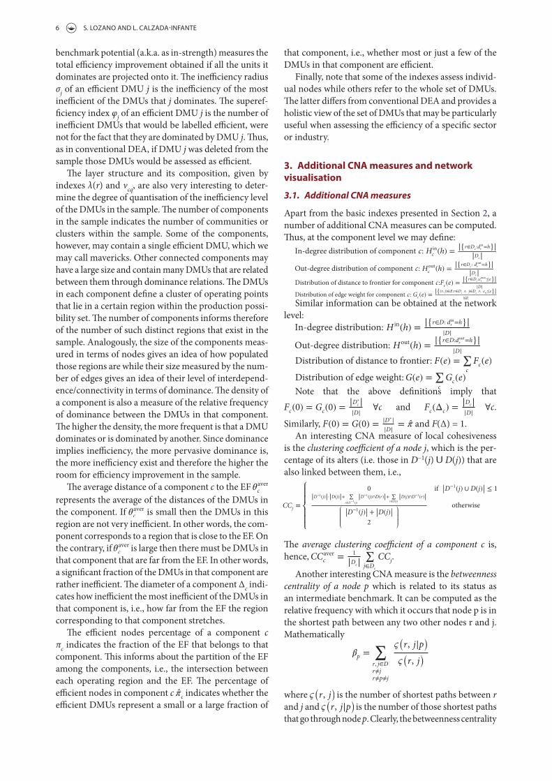
6 S. LOZANO AND L. CALZADA-INFANTE

that component, i.e., whether most or just a few of the DMUs in that component are e�cient.

Finally, note that some of the indexes assess individ-ual nodes while others refer to the whole set of DMUs. �e latter di�ers from conventional DEA and provides a holistic view of the set of DMUs that may be particularly useful when assessing the e�ciency of a speci�c sector or industry.

3. Additional CNA measures and network

visualisation

3.1. Additional CNA measures

Apart from the basic indexes presented in Section 2, a number of additional CNA measures can be computed. �us, at the component level we may de�ne:

In-degree distribution of component c: H in

c (h) =|{r∈Dc :d

in

r =h}|

|Dc|

Out-degree distribution of component c: Hout

c (h) =|{r∈Dc : d

out

r =h}|

|Dc|

Distribution of distance to frontier for component c:Fc(e) =|{r∈Dc :e

max

r ≤e}||D|

Distribution of edge weight for component c: Gc(e) =|{(r, j)∈E:r∈Dc ∧ j∈Dc ∧ erj≤e}|

NE

Similar information can be obtained at the network level:

In-degree distribution: H in(h) =|{r∈D: din

r =h}||D|

Out-degree distribution: Hout(h) =|{r∈D:dout

r =h}||D|

Distribution of distance to frontier: F(e) =∑

c

Fc(e)

Distribution of edge weight: G(e) =∑

c

Gc(e)

Note that the above de�nitions imply that

Fc(0) = Gc(0) =|D∗

c |

|D|∀c and Fc(Δc) =

|Dc|

|D|∀c.

Similarly, F(0) = G(0) = |D∗|

|D|= � and F(Δ) = 1.

An interesting CNA measure of local cohesiveness is the clustering coe&cient of a node j, which is the per-centage of its alters (i.e. those in D−1(j)   D(j)) that are also linked between them, i.e.,

!e average clustering coe!cient of a component c is, hence, CCaver

c =1

|Dc|

∑

j∈Dc

CCj.

Another interesting CNA measure is the betweenness

centrality of a node p which is related to its status as an intermediate benchmark. It can be computed as the relative frequency with which it occurs that node p is in the shortest path between any two other nodes r and j. Mathematically

where &(

r, j)

is the number of shortest paths between r and j and &

(

r, j|p)

is the number of those shortest paths that go through node p. Clearly, the betweenness centrality

CCj =

⎧

⎪

⎪

⎨

⎪

⎪

⎩

0 if |

|

D−1(j) ∪ D(j)||

≤ 1

|D−1(j)

|⋅|D(j)

|+

∑

r∈D−1

(j)

|D−1(j)∩D(r)

|+

∑

r∈D(j)|D(j)∩D−1(r)

|

⎛

⎜

⎜

⎜

⎝

|

|

D−1(j)||

+ |

|

D(j)||

2

⎞

⎟

⎟

⎟

⎠

otherwise

�p =∑

r, j∈Dr≠jr≠p≠j

&(

r, j|p)

&(

r, j)

benchmark potential (a.k.a. as in-strength) measures the total e"ciency improvement obtained if all the units it dominates are projected onto it. !e ine"ciency radius σ

j of an e"cient DMU j is the ine"ciency of the most

ine"cient of the DMUs that j dominates. !e superef-#ciency index φ

j of an e"cient DMU j is the number of

ine"cient DMUs that would be labelled e"cient, were not for the fact that they are dominated by DMU j. !us, as in conventional DEA, if DMU j was deleted from the sample those DMUs would be assessed as e"cient.

!e layer structure and its composition, given by indexes λ(r) and ν

cq, are also very interesting to deter-

mine the degree of quantisation of the ine"ciency level of the DMUs in the sample. !e number of components in the sample indicates the number of communities or clusters within the sample. Some of the components, however, may contain a single e"cient DMU, which we may call mavericks. Other connected components may have a large size and contain many DMUs that are related between them through dominance relations. !e DMUs in each component de#ne a cluster of operating points that lie in a certain region within the production possi-bility set. !e number of components informs therefore of the number of such distinct regions that exist in the sample. Analogously, the size of the components meas-ured in terms of nodes gives an idea of how populated those regions are while their size measured by the num-ber of edges gives an idea of their level of interdepend-ence/connectivity in terms of dominance. !e density of a component is also a measure of the relative frequency of dominance between the DMUs in that component. !e higher the density, the more frequent is that a DMU dominates or is dominated by another. Since dominance implies ine"ciency, the more pervasive dominance is, the more ine"ciency exist and therefore the higher the room for e"ciency improvement in the sample.

!e average distance of a component c to the EF �averc represents the average of the distances of the DMUs in the component. If �averc is small then the DMUs in this region are not very ine"cient. In other words, the com-ponent corresponds to a region that is close to the EF. On the contrary, if �averc is large then there must be DMUs in that component that are far from the EF. In other words, a signi#cant fraction of the DMUs in that component are rather ine"cient. !e diameter of a component Δ

c indi-

cates how ine"cient the most ine"cient of the DMUs in that component is, i.e., how far from the EF the region corresponding to that component stretches.

!e e"cient nodes percentage of a component c

πc indicates the fraction of the EF that belongs to that

component. !is informs about the partition of the EF among the components, i.e., the intersection between each operating region and the EF. !e percentage of e"cient nodes in component c �c indicates whether the e"cient DMUs represent a small or a large fraction of

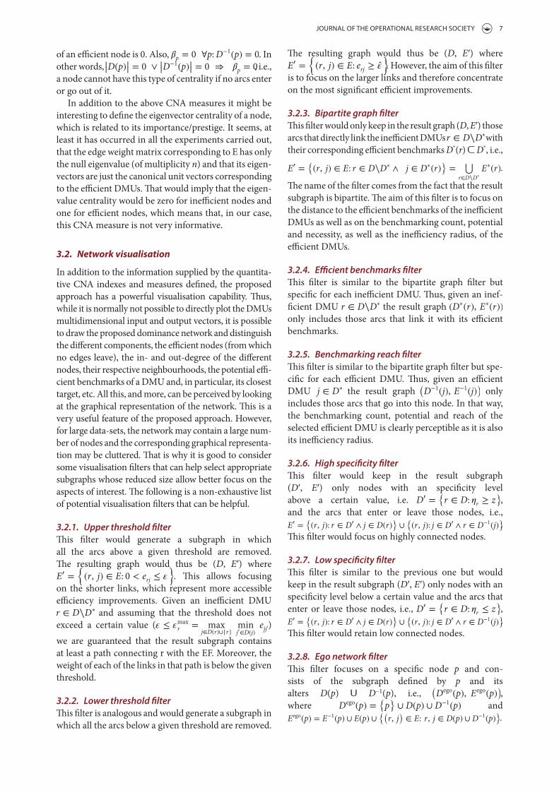
JOURNAL OF THE OPERATIONAL RESEARCH SOCIETY 7

!e resulting graph would thus be (D,  E ) where E′ =

{

(r, j) ∈ E: erj ≥ "

}

. However, the aim of this #lter is to focus on the larger links and therefore concentrate on the most signi#cant e"cient improvements.

3.2.3. Bipartite graph �lter

!is #lter would only keep in the result graph (D, E ) those arcs that directly link the ine"cient DMUs r ∈ D∖D∗ with their corresponding e"cient benchmarks D*(r)   D*, i.e.,

E′ ={

(r, j) ∈ E: r ∈ D∖D∗ ∧ j ∈ D∗(r)}

=⋃

r∈D∖D∗

E∗(r).

!e name of the "lter comes from the fact that the result subgraph is bipartite. !e aim of this "lter is to focus on the distance to the e#cient benchmarks of the ine#cient DMUs as well as on the benchmarking count, potential and necessity, as well as the ine#ciency radius, of the e#cient DMUs.

3.2.4. E�cient benchmarks �lter

!is "lter is similar to the bipartite graph "lter but speci"c for each ine#cient DMU. !us, given an inef-"cient DMU r ∈ D∖D∗ the result graph (D∗(r), E∗(r)) only includes those arcs that link it with its e#cient benchmarks.

3.2.5. Benchmarking reach �lter

!is "lter is similar to the bipartite graph "lter but spe-ci"c for each e#cient DMU. !us, given an e#cient DMU j ∈ D∗ the result graph

(

D−1(j), E−1(j))

only includes those arcs that go into this node. In that way, the benchmarking count, potential and reach of the selected e#cient DMU is clearly perceptible as it is also its ine#ciency radius.

3.2.6. High speci�city �lter

!is "lter would keep in the result subgraph (D ,  E ) only nodes with an speci"city level above a certain value, i.e. D′ =

{

r ∈ D: �r ≥ z}

, and the arcs that enter or leave those nodes, i.e., E′ =

{

(r, j): r ∈ D′ ∧ j ∈ D(r)}

∪{

(r, j): j ∈ D′ ∧ r ∈ D−1(j)}

. !is "lter would focus on highly connected nodes.

3.2.7. Low speci�city �lter

!is "lter is similar to the previous one but would keep in the result subgraph (D , E ) only nodes with an speci"city level below a certain value and the arcs that enter or leave those nodes, i.e., D′ =

{

r ∈ D: �r ≤ z}

, E′ =

{

(r, j): r ∈ D′ ∧ j ∈ D(r)}

∪{

(r, j): j ∈ D′ ∧ r ∈ D−1(j)}

. !is "lter would retain low connected nodes.

3.2.8. Ego network �lter

!is "lter focuses on a speci"c node p and con-sists of the subgraph de"ned by p and its alters D(p)    D−1(p), i.e.,

(

Dego(p), Eego(p))

, where Dego(p) =

{

p}

∪ D(p) ∪ D−1(p) and Eego(p) = E−1(p) ∪ E(p) ∪

{(

r, j)

∈ E: r, j ∈ D(p) ∪ D−1(p)}

.

of an e"cient node is 0. Also, �p = 0 ∀p:D−1(p) = 0. In other words, |

|

D(p)||

= 0 ∨ |

|

D−1(p)||

= 0 ⇒ �p = 0, i.e., a node cannot have this type of centrality if no arcs enter or go out of it.

In addition to the above CNA measures it might be interesting to de#ne the eigenvector centrality of a node, which is related to its importance/prestige. It seems, at least it has occurred in all the experiments carried out, that the edge weight matrix corresponding to E has only the null eigenvalue (of multiplicity n) and that its eigen-vectors are just the canonical unit vectors corresponding to the e"cient DMUs. $at would imply that the eigen-value centrality would be zero for ine"cient nodes and one for e"cient nodes, which means that, in our case, this CNA measure is not very informative.

3.2. Network visualisation

In addition to the information supplied by the quantita-tive CNA indexes and measures de#ned, the proposed approach has a powerful visualisation capability. $us, while it is normally not possible to directly plot the DMUs multidimensional input and output vectors, it is possible to draw the proposed dominance network and distinguish the di%erent components, the e"cient nodes (from which no edges leave), the in- and out-degree of the di%erent nodes, their respective neighbourhoods, the potential e"-cient benchmarks of a DMU and, in particular, its closest target, etc. All this, and more, can be perceived by looking at the graphical representation of the network. $is is a very useful feature of the proposed approach. However, for large data-sets, the network may contain a large num-ber of nodes and the corresponding graphical representa-tion may be cluttered. $at is why it is good to consider some visualisation #lters that can help select appropriate subgraphs whose reduced size allow better focus on the aspects of interest. $e following is a non-exhaustive list of potential visualisation #lters that can be helpful.

3.2.1. Upper threshold �lter

$is #lter would generate a subgraph in which all the arcs above a given threshold are removed. $e resulting graph would thus be (D,  E ) where E′ =

{

(r, j) ∈ E: 0 < erj ≤ "

}

. $is allows focusing on the shorter links, which represent more accessible e"ciency improvements. Given an ine"cient DMU r ∈ D∖D∗ and assuming that the threshold does not exceed a certain value (" ≤ "

max

r = maxj∈D(r)∪{r}

minj′∈D(j)

ejj′)

we are guaranteed that the result subgraph contains at least a path connecting r with the EF. Moreover, the weight of each of the links in that path is below the given threshold.

3.2.2. Lower threshold �lter

$is #lter is analogous and would generate a subgraph in which all the arcs below a given threshold are removed.

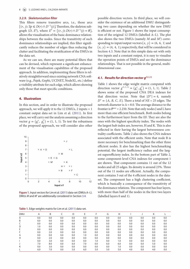
8 S. LOZANO AND L. CALZADA-INFANTE

possible direction vectors. In third place, we will con-sider the existence of an additional DMU distinguish-ing two cases depending on whether the new DMU is e"cient or not. Figure 1 shows the input consump-tion of the original 12 DMUs (labelled A–L). $e plot also shows the two DMUs (namely M and M ) corre-sponding to input/output vectors

(

x, y)

= (6, 6, 1) and (

x, y)

= (4, 4, 1), respectively, that will be considered in Section 4.3. Note that in this simple data-set with only two inputs and a constant output, it is easy to visualise the operation points of DMUs and see the dominance relationships. $at is not possible in the general, multi-dimensional case.

4.1. Results for direction vector g(1,1,1)

Table 1 shows the edge weight matrix computed with direction vector g (1, 1, 1) =

(

gxi , gy

k

)

= (1, 1, 1). Table  2 shows some of the proposed CNA DEA indexes for that direction vector. Note that |D∗

| = 4, namely D∗ = {A, B, C, E}. $ere a total of NE = 25 edges. $e network diameter is Δ = 8.0. $e average distance to the frontier is θaver = 2.250. Note that only nodes J and L have more than one e"cient benchmark. Both nodes belong to the furthermost layer from the EF. $ey are also the ones with the highest speci#city index. $e nodes with the largest hub index are, however, H and K. $is is also re'ected in their having the largest betweenness cen-trality coe"cients. Table 2 also shows the CNA indexes associated with the e"cient units. Note that node B is more necessary for benchmarking than the other three e"cient nodes. It also has the highest benchmarking potential, the largest ine"ciency radius and the larg-est supere"cieny index. In the bottom part of Table 2, some component-level CNA indexes for component 1 are shown. $at component contains 11 out of the 12 nodes and all 25 edges. Its density is around 23%. $ree out of the 11 nodes are e"cient. Actually, the compo-nent contains 3 out of the 4 e"cient nodes in the data-set. $e component has a high clustering coe"cient, which is basically a consequence of the transitivity of the dominance relations. $e component has four layers, with more than half of the nodes in the #rst two layers (labelled layers 0 and 1).

3.2.9. Skeletonisation �lter

$is #lters remove transitive arcs, i.e., those arcs {

(r, j):∃p ∈ D(r) ∩ D−1(j)}

. $erefore, the skeleton sub-graph (D, ES), where ES =

{

(r, j):D(r) ∩ D−1(j) = ∅}

, allows the visualisation of the basic dominance relation-ships between the nodes. Since the transitivity of such dominance relationships are implied, this #lter signi#-cantly reduces the number of edges thus reducing the clutter and facilitating the strati#cation of the DMUs in the data-set.

As we can see, there are many potential #lters that can be devised, which represent a signi#cant enhance-ment of the visualisation capabilities of the proposed approach. In addition, implementing these #lters is rel-atively straightforward since existing network CNA so+-ware (e.g., Pajek, Gephi, UCINET, NodeXL, etc.) de#ne a visibility attribute for each edge, which allows showing only those that meet speci#c conditions.

4. Illustration

In this section, and in order to illustrate the proposed approach, we will apply it to the 12 DMUs, 2 inputs + 1 constant output data-set in Lim et al. (2011). In #rst place, we will carry out the analysis assuming a direction vector g =

(

gxi , gy

k

)

= (1, 1, 1). To test the robustness of the proposed approach, we will consider also other

A

B

C

D

E

F

G

H I

J

K

L

M'

M

0

1

2

3

4

5

6

7

8

9

10

0 2 4 6 8 10 12

Inp

ut

x2

Input x1

Figure 1. Input vectors for Lim et al. (2011) data-set (DMUs A–L). DMUs M and M are additionally considered in Section 3.4.

Table 1. Edge weights matrix for Lim et al. (2011) data-set.

DMU A B C D E F G H I J K L

A 0.0 0.0 0.0 0.0 0.0 0.0 0.0 0.0 0.0 0.0 0.0 0.0B 0.0 0.0 0.0 0.0 0.0 0.0 0.0 0.0 0.0 0.0 0.0 0.0C 0.0 0.0 0.0 0.0 0.0 0.0 0.0 0.0 0.0 0.0 0.0 0.0D 1.0 0.0 0.0 0.0 0.0 0.0 0.0 0.0 0.0 0.0 0.0 0.0E 0.0 0.0 0.0 0.0 0.0 0.0 0.0 0.0 0.0 0.0 0.0 0.0F 0.0 2.0 0.0 0.0 0.0 0.0 0.0 0.0 0.0 0.0 0.0 0.0G 0.0 0.0 0.0 0.0 1.0 0.0 0.0 0.0 0.0 0.0 0.0 0.0H 0.0 2.0 0.0 0.0 0.0 0.0 0.0 0.0 0.0 0.0 0.0 0.0I 0.0 3.0 0.0 0.0 0.0 1.0 0.0 1.0 0.0 0.0 0.0 0.0J 7.0 8.0 0.0 6.0 7.0 0.0 6.0 6.0 0.0 0.0 5.0 0.0K 0.0 3.0 0.0 0.0 0.0 0.0 0.0 1.0 0.0 0.0 0.0 0.0L 6.0 7.0 0.0 5.0 6.0 5.0 5.0 5.0 4.0 0.0 4.0 0.0

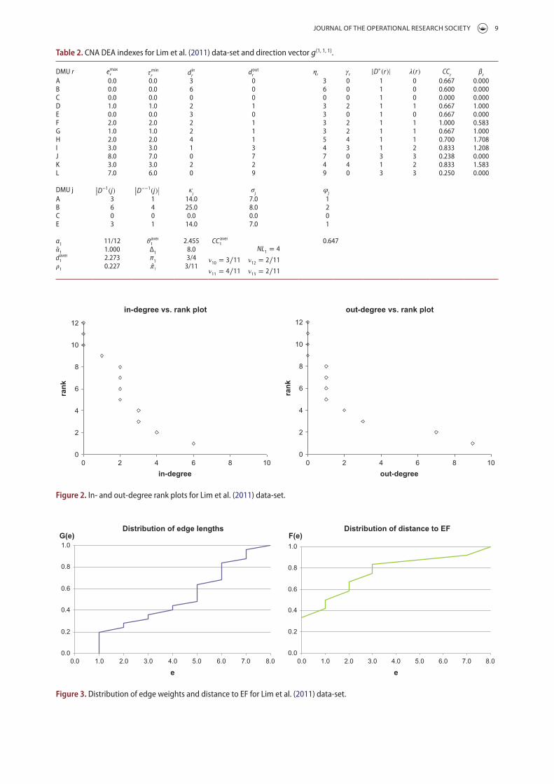
JOURNAL OF THE OPERATIONAL RESEARCH SOCIETY 9

Table 2. CNA DEA indexes for Lim et al. (2011) data-set and direction vector g(1, 1, 1).

DMU r emaxr �

minr

dinr

doutr

�r

r

|D∗(r)| �(r) CC

rβr

A 0.0 0.0 3 0 3 0 1 0 0.667 0.000B 0.0 0.0 6 0 6 0 1 0 0.600 0.000C 0.0 0.0 0 0 0 0 1 0 0.000 0.000D 1.0 1.0 2 1 3 2 1 1 0.667 1.000E 0.0 0.0 3 0 3 0 1 0 0.667 0.000F 2.0 2.0 2 1 3 2 1 1 1.000 0.583G 1.0 1.0 2 1 3 2 1 1 0.667 1.000H 2.0 2.0 4 1 5 4 1 1 0.700 1.708I 3.0 3.0 1 3 4 3 1 2 0.833 1.208J 8.0 7.0 0 7 7 0 3 3 0.238 0.000K 3.0 3.0 2 2 4 4 1 2 0.833 1.583L 7.0 6.0 0 9 9 0 3 3 0.250 0.000

DMU j |

|

D−1(j)||

|

|

D−−1

(j)||

�j

�j

'j

A 3 1 14.0 7.0 1B 6 4 25.0 8.0 2C 0 0 0.0 0.0 0E 3 1 14.0 7.0 1

α1

11/12 �aver1 2.455 CC

aver1 0.647

�1 1.000 Δ1

8.0 NL1 = 4

�10 = 3∕11 �12 = 2∕11

�11 = 4∕11 �13 = 2∕11

daver1 2.273 π

13/4

�1 0.227 �1 3/11

in-degree vs. rank plot

0

2

4

6

8

10

12

0 2 4 6 8 10

in-degree

ran

k

out-degree vs. rank plot

0

2

4

6

8

10

12

0 2 4 6 8 10

out-degree

ran

k

Figure 2. In- and out-degree rank plots for Lim et al. (2011) data-set.

Distribution of edge lengths

0.0

0.2

0.4

0.6

0.8

1.0

e

G(e)Distribution of distance to EF

0.0

0.2

0.4

0.6

0.8

1.0

0.0 1.0 2.0 3.0 4.0 5.0 6.0 7.0 8.0 0.0 1.0 2.0 3.0 4.0 5.0 6.0 7.0 8.0

e

F(e)

Figure 3. Distribution of edge weights and distance to EF for Lim et al. (2011) data-set.

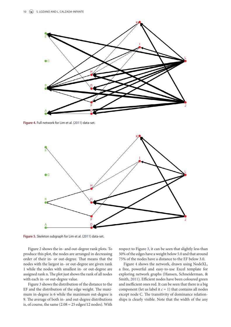
10 S. LOZANO AND L. CALZADA-INFANTE

respect to Figure 3, it can be seen that slightly less than 50% of the edges have a weight below 5.0 and that around 75% of the nodes have a distance to the EF below 3.0.

Figure 4 shows the network, drawn using NodeXL, a free, powerful and easy-to-use Excel template for exploring network graphs (Hansen, Schneiderman, & Smith, 2011). E!cient nodes have been coloured green and ine!cient ones red. It can be seen that there is a big component (let us label it c = 1) that contains all nodes except node C. #e transitivity of dominance relation-ships is clearly visible. Note that the width of the any

Figure 2 shows the in- and out-degree rank plots. To produce this plot, the nodes are arranged in decreasing order of their in- or out-degree. #at means that the nodes with the largest in- or out-degree are given rank 1 while the nodes with smallest in- or out-degree are assigned rank n. #e plot just shows the rank of all nodes with each in- or out-degree value.

Figure 3 shows the distribution of the distance to the EF and the distribution of the edge weight. #e maxi-mum in-degree is 6 while the maximum out-degree is 9. #e average of both in- and out-degree distributions is, of course, the same (2.08 = 25 edges/12 nodes). With

Figure 4. Full network for Lim et al. (2011) data-set.

Figure 5. Skeleton subgraph for Lim et al. (2011) data-set.

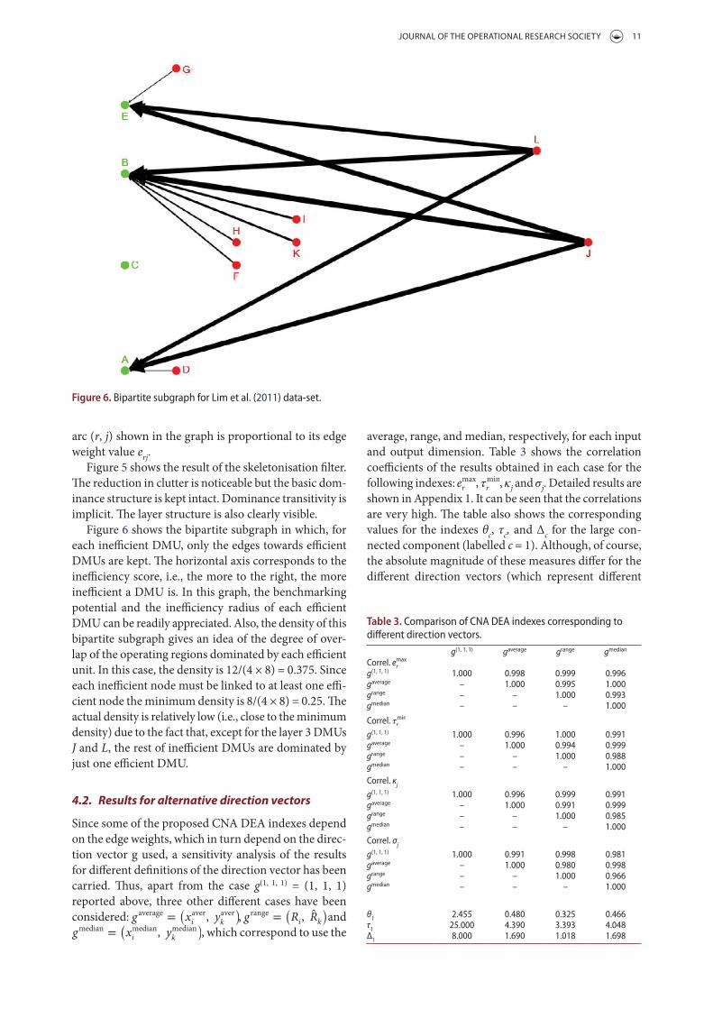
JOURNAL OF THE OPERATIONAL RESEARCH SOCIETY 11

average, range, and median, respectively, for each input and output dimension. Table 3 shows the correlation coe!cients of the results obtained in each case for the following indexes: emax

r , �min

r , �j and �j. Detailed results are shown in Appendix 1. It can be seen that the correlations are very high. #e table also shows the corresponding values for the indexes θ

c, τ

c, and Δ

c for the large con-

nected component (labelled c = 1). Although, of course, the absolute magnitude of these measures di'er for the di'erent direction vectors (which represent di'erent

arc (r, j) shown in the graph is proportional to its edge weight value e

rj.

Figure 5 shows the result of the skeletonisation *lter. #e reduction in clutter is noticeable but the basic dom-inance structure is kept intact. Dominance transitivity is implicit. #e layer structure is also clearly visible.

Figure 6 shows the bipartite subgraph in which, for each ine!cient DMU, only the edges towards e!cient DMUs are kept. #e horizontal axis corresponds to the ine!ciency score, i.e., the more to the right, the more ine!cient a DMU is. In this graph, the benchmarking potential and the ine!ciency radius of each e!cient DMU can be readily appreciated. Also, the density of this bipartite subgraph gives an idea of the degree of over-lap of the operating regions dominated by each e!cient unit. In this case, the density is 12/(4 × 8) = 0.375. Since each ine!cient node must be linked to at least one e!-cient node the minimum density is 8/(4 × 8) = 0.25. #e actual density is relatively low (i.e., close to the minimum density) due to the fact that, except for the layer 3 DMUs J and L, the rest of ine!cient DMUs are dominated by just one e!cient DMU.

4.2. Results for alternative direction vectors

Since some of the proposed CNA DEA indexes depend on the edge weights, which in turn depend on the direc-tion vector g used, a sensitivity analysis of the results for di'erent de*nitions of the direction vector has been carried. #us, apart from the case g(1,  1,  1)  =  (1,  1,  1) reported above, three other di'erent cases have been considered: g average =

(

xaveri , yaverk

)

, g range =(

Ri, Rk

)

and gmedian =

(

xmedian

i , ymedian

k

)

, which correspond to use the

Figure 6. Bipartite subgraph for Lim et al. (2011) data-set.

Table 3. Comparison of CNA DEA indexes corresponding to different direction vectors.

g(1, 1, 1) gaverage grange gmedian

Correl. emaxr

g(1, 1, 1) 1.000 0.998 0.999 0.996gaverage – 1.000 0.995 1.000grange – – 1.000 0.993gmedian – – – 1.000

Correl. �minr

g(1, 1, 1) 1.000 0.996 1.000 0.991gaverage – 1.000 0.994 0.999grange – – 1.000 0.988gmedian – – – 1.000

Correl. κj

g(1, 1, 1) 1.000 0.996 0.999 0.991gaverage – 1.000 0.991 0.999grange – – 1.000 0.985gmedian – – – 1.000

Correl. σj

g(1, 1, 1) 1.000 0.991 0.998 0.981gaverage – 1.000 0.980 0.998grange – – 1.000 0.966gmedian – – – 1.000

θ1

2.455 0.480 0.325 0.466τ

125.000 4.390 3.393 4.048

Δ1

8.000 1.690 1.018 1.698

12 S. LOZANO AND L. CALZADA-INFANTE

4.3. Impact of an additional DMU

In order to study the e'ects of considering an additional DMU using the proposed approach, in this section we will assume that the data-set includes the original 12 DMUs (A–L) plus a new one. We consider two cases. In one case, the new DMU (labelled M) has input/output vector (6,  6,  1) and therefore is not e!cient.

ways of normalising the input and output changes) their relative values are totally consistent. #ese results lead us to claim that it is not necessary to do the cal-culations with di'erent normalisation vectors because the e!ciency assessment carried out by the proposed CNA DEA approach will basically draw the same overall picture.

Figure 7. Skeleton for Lim et al. (2011) data-set plus new DMU M (panel a) and M (panel b).

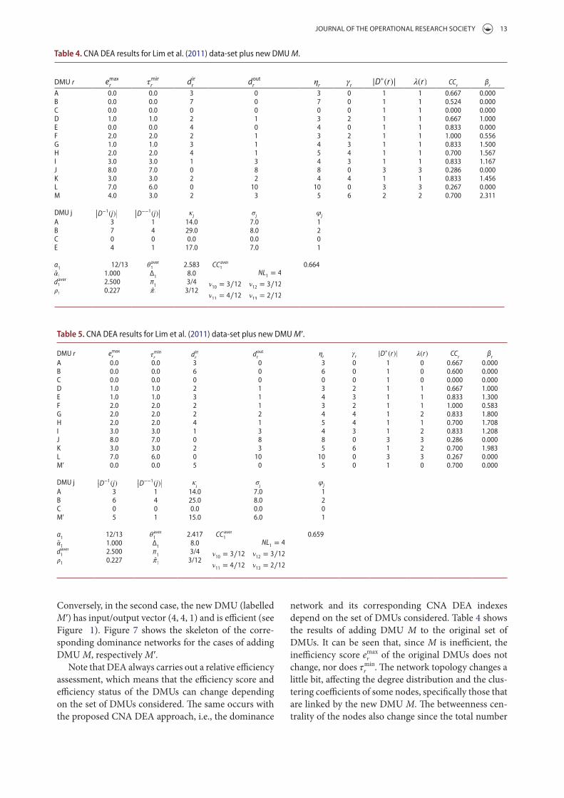
JOURNAL OF THE OPERATIONAL RESEARCH SOCIETY 13

network and its corresponding CNA DEA indexes depend on the set of DMUs considered. Table 4 shows the results of adding DMU M to the original set of DMUs. It can be seen that, since M is ine!cient, the ine!ciency score emax

r of the original DMUs does not change, nor does �min

r . #e network topology changes a little bit, a'ecting the degree distribution and the clus-tering coe!cients of some nodes, speci*cally those that are linked by the new DMU M. #e betweenness cen-trality of the nodes also change since the total number

Conversely, in the second case, the new DMU (labelled M ) has input/output vector (4, 4, 1) and is e!cient (see Figure   1). Figure 7 shows the skeleton of the corre-sponding dominance networks for the cases of adding DMU M, respectively M .

Note that DEA always carries out a relative e!ciency assessment, which means that the e!ciency score and e!ciency status of the DMUs can change depending on the set of DMUs considered. #e same occurs with the proposed CNA DEA approach, i.e., the dominance

Table 4. CNA DEA results for Lim et al. (2011) data-set plus new DMU M.

DMU r emaxr

�minr

dinr

doutr

�r

r

|D∗(r)| �(r) CC

rβr

A 0.0 0.0 3 0 3 0 1 1 0.667 0.000B 0.0 0.0 7 0 7 0 1 1 0.524 0.000C 0.0 0.0 0 0 0 0 1 1 0.000 0.000D 1.0 1.0 2 1 3 2 1 1 0.667 1.000E 0.0 0.0 4 0 4 0 1 1 0.833 0.000F 2.0 2.0 2 1 3 2 1 1 1.000 0.556G 1.0 1.0 3 1 4 3 1 1 0.833 1.500H 2.0 2.0 4 1 5 4 1 1 0.700 1.567I 3.0 3.0 1 3 4 3 1 1 0.833 1.167J 8.0 7.0 0 8 8 0 3 3 0.286 0.000K 3.0 3.0 2 2 4 4 1 1 0.833 1.456L 7.0 6.0 0 10 10 0 3 3 0.267 0.000M 4.0 3.0 2 3 5 6 2 2 0.700 2.311

DMU j |

|

D−1(j)||

|

|

D−−1

(j)||

�j

�j

'j

A 3 1 14.0 7.0 1B 7 4 29.0 8.0 2C 0 0 0.0 0.0 0E 4 1 17.0 7.0 1

α1

12/13 �aver1 2.583 CC

aver1 0.664

�1 1.000 Δ1

8.0 NL1 = 4

�10 = 3∕12 �12 = 3∕12

�11 = 4∕12 �13 = 2∕12

daver1 2.500 π

13/4

�1 0.227 �1 3/12

Table 5. CNA DEA results for Lim et al. (2011) data-set plus new DMU M .

DMU r emaxr �

minr

dinr

doutr

�r

r

|D∗(r)| �(r) CC

rβr

A 0.0 0.0 3 0 3 0 1 0 0.667 0.000B 0.0 0.0 6 0 6 0 1 0 0.600 0.000C 0.0 0.0 0 0 0 0 1 0 0.000 0.000D 1.0 1.0 2 1 3 2 1 1 0.667 1.000E 1.0 1.0 3 1 4 3 1 1 0.833 1.300F 2.0 2.0 2 1 3 2 1 1 1.000 0.583G 2.0 2.0 2 2 4 4 1 2 0.833 1.800H 2.0 2.0 4 1 5 4 1 1 0.700 1.708I 3.0 3.0 1 3 4 3 1 2 0.833 1.208J 8.0 7.0 0 8 8 0 3 3 0.286 0.000K 3.0 3.0 2 3 5 6 1 2 0.700 1.983L 7.0 6.0 0 10 10 0 3 3 0.267 0.000M’ 0.0 0.0 5 0 5 0 1 0 0.700 0.000

DMU j |

|

D−1(j)||

|

|

D−−1

(j)||

�j

�j

'j

A 3 1 14.0 7.0 1B 6 4 25.0 8.0 2C 0 0 0.0 0.0 0M’ 5 1 15.0 6.0 1

α1

12/13 �aver1 2.417 CC

aver1 0.659

�1 1.000 Δ1

8.0 NL1 = 4

�10 = 3∕12 �12 = 3∕12

�11 = 4∕12 �13 = 2∕12

daver1 2.500 π

13/4

�1 0.227 �1 3/12

14 S. LOZANO AND L. CALZADA-INFANTE

#e proposed CNA DEA approach allows the compu-tation of a number of interesting quantitative measures that together give a very complete picture of the perfor-mance of the individual DMUs and of the data-set as a whole, something which, for example, may be of interest in a centralised DEA context. #is distinctive feature of the approach, i.e., its use of a systemic perspective that is interested not only in assessing the e!ciency of the indi-vidual DMUs but also to capture the implicit (through the dominance relations) dependencies between them, provides new insights that complement the conventional DEA analysis. Take, for example, the existence of compo-nents that represent independent groups of DMUs, the characterisation of the layer structure of each compo-nent, the distribution of the distance to the frontier of the di'erent DMUs or of the weights of the di'erent edges, etc. In this respect, the proposed approach provides an integrated framework that allows processing and comparing the results of di'erent data-sets. Also very interesting is the possibility of analysing the dynamic features of the network when applied to multi-period input–output data. Similarly, metafrontier analysis can also be studied from this network perspective.

In spite of the many strengths of the proposed approach, there are some limitations as well as many issues that need further research. #e most important point is to try to extend the analysis to convex technol-ogies (CRS and VRS). #e case of multiple technolo-gies (e.g., Lozano, 2014) may also be considered. #e proposed CNA indexes can be computed for any domi-nance network, not being dependent on the assumption of an FDH technology. #e DEA technology assumed has an e'ect on the own dominance network de*ni-tion, that only considers the observed DMU. #us, in order to extend the approach to the CRS and VRS cases, additional nodes corresponding to the projections of the observed DMUs on those two frontiers may have to be introduced. In this way, the VRS and CRS frontiers can be sampled and included in the dominance network. In the case of FDH it is simpler, as the e!cient frontier is formed by a subset of the observed DMUs and it is therefore perfectly included in the proposed dominance network.

Extending the approach to other e!ciency meas-ures would also be interesting. In particular, it might be interesting to study the e'ect of computing edges weights using the MIP since in that case not all paths connecting two nodes would be geodesics. #ere are more venues of research that open up, like processing di'erent real-world data-sets (of which there are many in the DEA literature) and try to *nd regularities in their CNA measures (e.g., if the existence of one large com-ponent is the rule), using graph mining techniques to *nd clusters of DMUs, etc. What is clear is that the CNA

of shortest paths between the nodes in the network has increased. #e benchmarking potential of the two e!-cient DMUs that dominate M has increased, by 4.0 in the case of DMU B (which is farther from M) and by 3.0 in the case of DMU E (which is closer). #ese numbers correspond, respectively, to the distances emax

r and �min

r of DMU M. #e layer structure does not change much. All original nodes stay in their corresponding layers with the new DMU assigned to layer 2. Some aggregate indexes for component one (like the average degree daver

1 or the

average ine!ciency score �aver1

) also change. #e average clustering coe!cient of component 1 also increases a little bit.

Table 5 shows the results for adding DMU M to the original set of DMUs. It can be seen that in this case, since M is e!cient, the ine!ciency score emax

r of some of the original DMUs changes. In particular, DMU E, which originally was e!cient, is not any more. #e clustering and betweenness coe!cients of some of the original DMUs also change. Note how the CNA DEA indexes of the new DMU are completely di'erent to those that were observed for DMU M in the previous case. Actually, since M is e!cient, it has an associated benchmarking potential and ine!ciency radius. Also note that, as before, adding just a single DMU does not change the network topology much. Two of the original nodes though, namely, DMUs E and G, have moved to a deeper layer.

5. Conclusions

In this paper, a novel way of assessing the e�ciency of a set of DMUs using CNA tools has been presented. �e approach considers an FDH technology and an additive normalised-slacks e�ciency measure. �is new method-ology complements and enhances the traditional numer-ical assessment of DEA with, among other features, powerful �ltering and visualisation capabilities, which are very valuable, especially for large multidimensional data-sets. �us, for example, with this tool it is easy to identify a sequence of targets or stepwise path to the e�cient frontier. It is also rather easy to measure and visualise the potential of each e�cient DMU as a bench-mark for the ine�cient units. Similarly, from the point of view of the ine�cient DMUs, it is easy to assess the e�ort required to target the di�erent e�cient DMUs that dominate it. In addition, other indicators that have not been considered in DEA previously, such as betweenness centrality, clustering coe�cient or speci�city can now be computed. It is also possible to study the e�ects of the network growth (e.g., the impact of adding new DMUs to the data-set). In summary, the idea explored in this research is to build upon the strengths and versatility of both DEA and CNA.

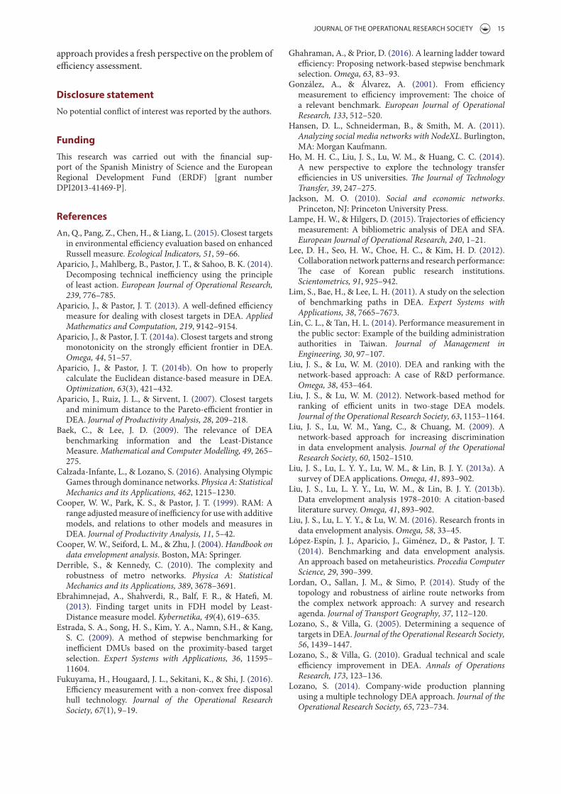
JOURNAL OF THE OPERATIONAL RESEARCH SOCIETY 15

Ghahraman, A., & Prior, D. (2016). A learning ladder toward e�ciency: Proposing network-based stepwise benchmark selection. Omega, 63, 83–93.

González, A., & Álvarez, A. (2001). From e�ciency measurement to e�ciency improvement: �e choice of a relevant benchmark. European Journal of Operational Research, 133, 512–520.

Hansen, D. L., Schneiderman, B., & Smith, M. A. (2011). Analyzing social media networks with NodeXL. Burlington, MA: Morgan Kaufmann.

Ho, M. H. C., Liu, J. S., Lu, W. M., & Huang, C. C. (2014). A new perspective to explore the technology transfer e�ciencies in US universities. !e Journal of Technology Transfer, 39, 247–275.

Jackson, M. O. (2010). Social and economic networks. Princeton, NJ: Princeton University Press.

Lampe, H. W., & Hilgers, D. (2015). Trajectories of e�ciency measurement: A bibliometric analysis of DEA and SFA. European Journal of Operational Research, 240, 1–21.

Lee, D. H., Seo, H. W., Choe, H. C., & Kim, H. D. (2012). Collaboration network patterns and research performance: �e case of Korean public research institutions. Scientometrics, 91, 925–942.

Lim, S., Bae, H., & Lee, L. H. (2011). A study on the selection of benchmarking paths in DEA. Expert Systems with Applications, 38, 7665–7673.

Lin, C. L., & Tan, H. L. (2014). Performance measurement in the public sector: Example of the building administration authorities in Taiwan. Journal of Management in Engineering, 30, 97–107.

Liu, J. S., & Lu, W. M. (2010). DEA and ranking with the network-based approach: A case of R&D performance. Omega, 38, 453–464.

Liu, J. S., & Lu, W. M. (2012). Network-based method for ranking of e�cient units in two-stage DEA models. Journal of the Operational Research Society, 63, 1153–1164.

Liu, J. S., Lu, W. M., Yang, C., & Chuang, M. (2009). A network-based approach for increasing discrimination in data envelopment analysis. Journal of the Operational Research Society, 60, 1502–1510.

Liu, J. S., Lu, L. Y. Y., Lu, W. M., & Lin, B. J. Y. (2013a). A survey of DEA applications. Omega, 41, 893–902.

Liu, J. S., Lu, L. Y. Y., Lu, W. M., & Lin, B. J. Y. (2013b). Data envelopment analysis 1978–2010: A citation-based literature survey. Omega, 41, 893–902.

Liu, J. S., Lu, L. Y. Y., & Lu, W. M. (2016). Research fronts in data envelopment analysis. Omega, 58, 33–45.

López-Espín, J. J., Aparicio, J., Giménez, D., & Pastor, J. T. (2014). Benchmarking and data envelopment analysis. An approach based on metaheuristics. Procedia Computer Science, 29, 390–399.

Lordan, O., Sallan, J. M., & Simo, P. (2014). Study of the topology and robustness of airline route networks from the complex network approach: A survey and research agenda. Journal of Transport Geography, 37, 112–120.

Lozano, S., & Villa, G. (2005). Determining a sequence of targets in DEA. Journal of the Operational Research Society, 56, 1439–1447.

Lozano, S., & Villa, G. (2010). Gradual technical and scale e�ciency improvement in DEA. Annals of Operations Research, 173, 123–136.

Lozano, S. (2014). Company-wide production planning using a multiple technology DEA approach. Journal of the Operational Research Society, 65, 723–734.

approach provides a fresh perspective on the problem of e�ciency assessment.

Disclosure statement

No potential con'ict of interest was reported by the authors.

Funding

�is research was carried out with the �nancial sup-port of the Spanish Ministry of Science and the European Regional Development Fund (ERDF) [grant number DPI2013-41469-P].

References

An, Q., Pang, Z., Chen, H., & Liang, L. (2015). Closest targets in environmental e�ciency evaluation based on enhanced Russell measure. Ecological Indicators, 51, 59–66.

Aparicio, J., Mahlberg, B., Pastor, J. T., & Sahoo, B. K. (2014). Decomposing technical ine�ciency using the principle of least action. European Journal of Operational Research, 239, 776–785.

Aparicio, J., & Pastor, J. T. (2013). A well-de�ned e�ciency measure for dealing with closest targets in DEA. Applied Mathematics and Computation, 219, 9142–9154.

Aparicio, J., & Pastor, J. T. (2014a). Closest targets and strong monotonicity on the strongly e�cient frontier in DEA. Omega, 44, 51–57.

Aparicio, J., & Pastor, J. T. (2014b). On how to properly calculate the Euclidean distance-based measure in DEA. Optimization, 63(3), 421–432.

Aparicio, J., Ruiz, J. L., & Sirvent, I. (2007). Closest targets and minimum distance to the Pareto-e�cient frontier in DEA. Journal of Productivity Analysis, 28, 209–218.

Baek, C., & Lee, J. D. (2009). �e relevance of DEA benchmarking information and the Least-Distance Measure. Mathematical and Computer Modelling, 49, 265–275.

Calzada-Infante, L., & Lozano, S. (2016). Analysing Olympic Games through dominance networks. Physica A: Statistical Mechanics and its Applications, 462, 1215–1230.

Cooper, W. W., Park, K. S., & Pastor, J. T. (1999). RAM: A range adjusted measure of ine�ciency for use with additive models, and relations to other models and measures in DEA. Journal of Productivity Analysis, 11, 5–42.

Cooper, W. W., Seiford, L. M., & Zhu, J. (2004). Handbook on data envelopment analysis. Boston, MA: Springer.

Derrible, S., & Kennedy, C. (2010). �e complexity and robustness of metro networks. Physica A: Statistical Mechanics and its Applications, 389, 3678–3691.

Ebrahimnejad, A., Shahverdi, R., Balf, F. R., & Hate�, M. (2013). Finding target units in FDH model by Least-Distance measure model. Kybernetika, 49(4), 619–635.

Estrada, S. A., Song, H. S., Kim, Y. A., Namn, S.H., & Kang, S. C. (2009). A method of stepwise benchmarking for ine�cient DMUs based on the proximity-based target selection. Expert Systems with Applications, 36, 11595–11604.

Fukuyama, H., Hougaard, J. L., Sekitani, K., & Shi, J. (2016). E�ciency measurement with a non-convex free disposal hull technology. Journal of the Operational Research Society, 67(1), 9–19.

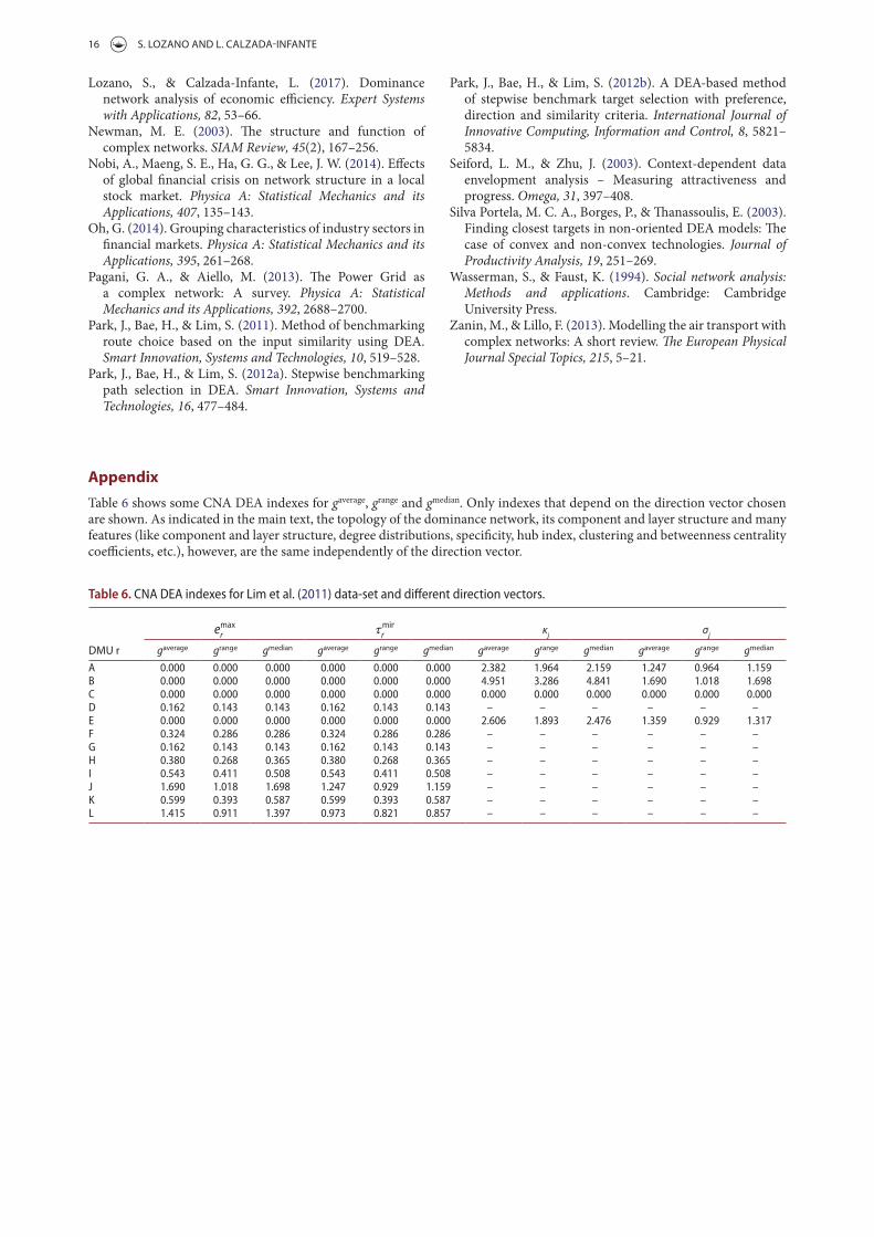
16 S. LOZANO AND L. CALZADA-INFANTE

Park, J., Bae, H., & Lim, S. (2012b). A DEA-based method of stepwise benchmark target selection with preference, direction and similarity criteria. International Journal of Innovative Computing, Information and Control, 8, 5821–5834.

Seiford, L. M., & Zhu, J. (2003). Context-dependent data envelopment analysis – Measuring attractiveness and progress. Omega, 31, 397–408.

Silva Portela, M. C. A., Borges, P., & �anassoulis, E. (2003). Finding closest targets in non-oriented DEA models: �e case of convex and non-convex technologies. Journal of Productivity Analysis, 19, 251–269.

Wasserman, S., & Faust, K. (1994). Social network analysis: Methods and applications. Cambridge: Cambridge University Press.

Zanin, M., & Lillo, F. (2013). Modelling the air transport with complex networks: A short review. !e European Physical Journal Special Topics, 215, 5–21.

Lozano, S., & Calzada-Infante, L. (2017). Dominance network analysis of economic e�ciency. Expert Systems with Applications, 82, 53–66.

Newman, M. E. (2003). �e structure and function of complex networks. SIAM Review, 45(2), 167–256.

Nobi, A., Maeng, S. E., Ha, G. G., & Lee, J. W. (2014). E�ects of global �nancial crisis on network structure in a local stock market. Physica A: Statistical Mechanics and its Applications, 407, 135–143.

Oh, G. (2014). Grouping characteristics of industry sectors in �nancial markets. Physica A: Statistical Mechanics and its Applications, 395, 261–268.

Pagani, G. A., & Aiello, M. (2013). �e Power Grid  as a complex network: A survey. Physica A: Statistical Mechanics and its Applications, 392, 2688–2700.

Park, J., Bae, H., & Lim, S. (2011). Method of benchmarking route choice based on the input similarity using DEA. Smart Innovation, Systems and Technologies, 10, 519–528.

Park, J., Bae, H., & Lim, S. (2012a). Stepwise benchmarking path selection in DEA. Smart Innovation, Systems and Technologies, 16, 477–484.

Table 6. CNA DEA indexes for Lim et al. (2011) data-set and different direction vectors.

DMU r

emaxr

�minr

κj

σj

gaverage grange gmedian gaverage grange gmedian gaverage grange gmedian gaverage grange gmedian

A 0.000 0.000 0.000 0.000 0.000 0.000 2.382 1.964 2.159 1.247 0.964 1.159B 0.000 0.000 0.000 0.000 0.000 0.000 4.951 3.286 4.841 1.690 1.018 1.698C 0.000 0.000 0.000 0.000 0.000 0.000 0.000 0.000 0.000 0.000 0.000 0.000D 0.162 0.143 0.143 0.162 0.143 0.143 – – – – – –E 0.000 0.000 0.000 0.000 0.000 0.000 2.606 1.893 2.476 1.359 0.929 1.317F 0.324 0.286 0.286 0.324 0.286 0.286 – – – – – –G 0.162 0.143 0.143 0.162 0.143 0.143 – – – – – –H 0.380 0.268 0.365 0.380 0.268 0.365 – – – – – –I 0.543 0.411 0.508 0.543 0.411 0.508 – – – – – –J 1.690 1.018 1.698 1.247 0.929 1.159 – – – – – –K 0.599 0.393 0.587 0.599 0.393 0.587 – – – – – –L 1.415 0.911 1.397 0.973 0.821 0.857 – – – – – –

Appendix

Table 6 shows some CNA DEA indexes for gaverage, grange and gmedian. Only indexes that depend on the direction vector chosen are shown. As indicated in the main text, the topology of the dominance network, its component and layer structure and many features (like component and layer structure, degree distributions, speci�city, hub index, clustering and betweenness centrality coe�cients, etc.), however, are the same independently of the direction vector.

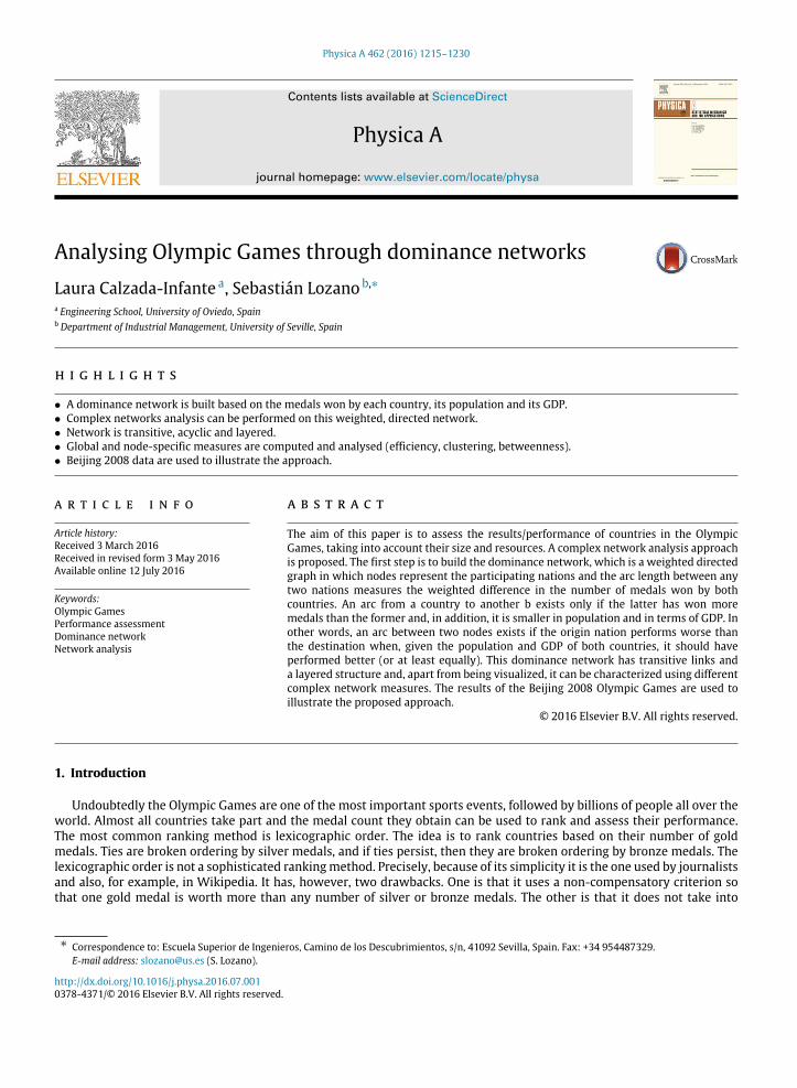
Physica A 462 (2016) 1215–1230

Contents lists available at ScienceDirect

Physica A

journal homepage: www.elsevier.com/locate/physa

Analysing Olympic Games through dominance networks

Laura Calzada-Infante a, Sebastián Lozano b,∗

a Engineering School, University of Oviedo, Spainb Department of Industrial Management, University of Seville, Spain

h i g h l i g h t s

• A dominance network is built based on the medals won by each country, its population and its GDP.• Complex networks analysis can be performed on this weighted, directed network.• Network is transitive, acyclic and layered.• Global and node-specific measures are computed and analysed (efficiency, clustering, betweenness).• Beijing 2008 data are used to illustrate the approach.

a r t i c l e i n f o

Article history:

Received 3 March 2016

Received in revised form 3 May 2016

Available online 12 July 2016

Keywords:

Olympic Games

Performance assessment

Dominance network

Network analysis

a b s t r a c t

The aim of this paper is to assess the results/performance of countries in the OlympicGames, taking into account their size and resources. A complex network analysis approachis proposed. The first step is to build the dominance network, which is a weighted directedgraph in which nodes represent the participating nations and the arc length between anytwo nations measures the weighted difference in the number of medals won by bothcountries. An arc from a country to another b exists only if the latter has won moremedals than the former and, in addition, it is smaller in population and in terms of GDP. Inother words, an arc between two nodes exists if the origin nation performs worse thanthe destination when, given the population and GDP of both countries, it should haveperformed better (or at least equally). This dominance network has transitive links anda layered structure and, apart from being visualized, it can be characterized using differentcomplex network measures. The results of the Beijing 2008 Olympic Games are used toillustrate the proposed approach.

© 2016 Elsevier B.V. All rights reserved.

1. Introduction

Undoubtedly the Olympic Games are one of the most important sports events, followed by billions of people all over theworld. Almost all countries take part and the medal count they obtain can be used to rank and assess their performance.The most common ranking method is lexicographic order. The idea is to rank countries based on their number of goldmedals. Ties are broken ordering by silver medals, and if ties persist, then they are broken ordering by bronze medals. Thelexicographic order is not a sophisticated rankingmethod. Precisely, because of its simplicity it is the one used by journalistsand also, for example, in Wikipedia. It has, however, two drawbacks. One is that it uses a non-compensatory criterion sothat one gold medal is worth more than any number of silver or bronze medals. The other is that it does not take into

∗ Correspondence to: Escuela Superior de Ingenieros, Camino de los Descubrimientos, s/n, 41092 Sevilla, Spain. Fax: +34 954487329.

E-mail address: slozano@us.es (S. Lozano).

http://dx.doi.org/10.1016/j.physa.2016.07.001

0378-4371/© 2016 Elsevier B.V. All rights reserved.

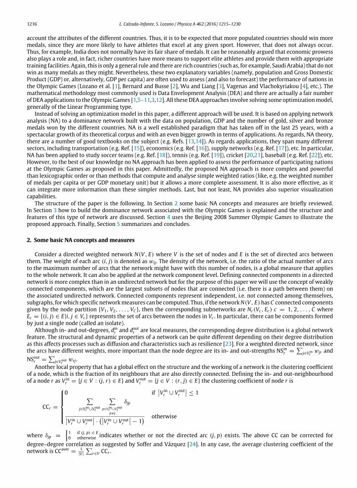
1216 L. Calzada-Infante, S. Lozano / Physica A 462 (2016) 1215–1230

account the attributes of the different countries. Thus, it is to be expected that more populated countries should win moremedals, since they are more likely to have athletes that excel at any given sport. However, that does not always occur.Thus, for example, India does not normally have its fair share of medals. It can be reasonably argued that economic prowessalso plays a role and, in fact, richer countries have more means to support elite athletes and provide themwith appropriatetraining facilities. Again, this is only a general rule and there are rich countries (such as, for example, Saudi Arabia) that do notwin as many medals as they might. Nevertheless, these two explanatory variables (namely, population and Gross DomesticProduct (GDP) or, alternatively, GDP per capita) are often used to assess (and also to forecast) the performance of nations inthe Olympic Games (Lozano et al. [1], Bernard and Busse [2], Wu and Liang [3], Vagenas and Vlachokyriakou [4], etc.). Themathematical methodology most commonly used is Data Envelopment Analysis (DEA) and there are actually a fair numberof DEA applications to theOlympic Games [1,5–11,3,12]. All theseDEA approaches involve solving some optimizationmodel,generally of the Linear Programming type.

Instead of solving an optimization model in this paper, a different approach will be used. It is based on applying networkanalysis (NA) to a dominance network built with the data on population, GDP and the number of gold, silver and bronzemedals won by the different countries. NA is a well established paradigm that has taken off in the last 25 years, with aspectacular growth of its theoretical corpus and with an even bigger growth in terms of applications. As regards, NA theory,there are a number of good textbooks on the subject (e.g. Refs. [13,14]). As regards applications, they span many differentsectors, including transportation (e.g. Ref. [15]), economics (e.g. Ref. [16]), supply networks (e.g. Ref. [17]), etc. In particular,NA has been applied to study soccer teams (e.g. Ref. [18]), tennis (e.g. Ref. [19]), cricket [20,21], baseball (e.g. Ref. [22]), etc.However, to the best of our knowledge no NA approach has been applied to assess the performance of participating nationsat the Olympic Games as proposed in this paper. Admittedly, the proposed NA approach is more complex and powerfulthan lexicographic order or than methods that compute and analyse simple weighted ratios (like, e.g. the weighted numberof medals per capita or per GDP monetary unit) but it allows a more complete assessment. It is also more effective, as itcan integrate more information than these simpler methods. Last, but not least, NA provides also superior visualizationcapabilities.

The structure of the paper is the following. In Section 2 some basic NA concepts and measures are briefly reviewed.In Section 3 how to build the dominance network associated with the Olympic Games is explained and the structure andfeatures of this type of network are discussed. Section 4 uses the Beijing 2008 Summer Olympic Games to illustrate theproposed approach. Finally, Section 5 summarizes and concludes.

2. Some basic NA concepts and measures

Consider a directed weighted network N(V , E) where V is the set of nodes and E is the set of directed arcs betweenthem. The weight of each arc (i, j) is denoted as wij. The density of the network, i.e. the ratio of the actual number of arcsto the maximum number of arcs that the network might have with this number of nodes, is a global measure that appliesto the whole network. It can also be applied at the network component level. Defining connected components in a directednetwork is more complex than in an undirected network but for the purpose of this paper wewill use the concept of weaklyconnected components, which are the largest subsets of nodes that are connected (i.e. there is a path between them) onthe associated undirected network. Connected components represent independent, i.e. not connected among themselves,subgraphs, forwhich specific networkmeasures can be computed. Thus, if the networkN(V , E)has C connected componentsgiven by the node partition {V1, V2, . . . , VC }, then the corresponding subnetworks are Nc(Vc, Ec) c = 1, 2, . . . , C whereEc = {(i, j) ∈ E|i, j ∈ Vc} represents the set of arcs between the nodes in Vc . In particular, there can be components formedby just a single node (called an isolate).

Although in- and out-degrees, dinr and doutr are local measures, the corresponding degree distribution is a global networkfeature. The structural and dynamic properties of a network can be quite different depending on their degree distributionas this affects processes such as diffusion and characteristics such as resilience [23]. For a weighted directed network, sincethe arcs have different weights, more important than the node degree are its in- and out-strengths NSinr =

j∈V inr

wjr and

NSoutr =

j∈Voutr

wrj.

Another local property that has a global effect on the structure and the working of a network is the clustering coefficientof a node, which is the fraction of its neighbours that are also directly connected. Defining the in- and out-neighbourhoodof a node r as V in

r = {j ∈ V : (j, r) ∈ E} and V outr = {j ∈ V : (r, j) ∈ E} the clustering coefficient of node r is

CCr =

0 if

V inr ∪ V out

r

≤ 1

j∈V inr ∪Vout

r

p∈V inr ∪Vout

rp=j

δjp

V inr ∪ V out

r

·

V inr ∪ V out

r

− 1 otherwise

where δjp =

1 if (j, p) ∈ E

0 otherwise indicates whether or not the directed arc (j, p) exists. The above CC can be corrected for

degree–degree correlation as suggested by Soffer and Vázquez [24]. In any case, the average clustering coefficient of thenetwork is CCaver = 1

|V |

r∈V CCr .

L. Calzada-Infante, S. Lozano / Physica A 462 (2016) 1215–1230 1217

Other interesting NA measures are the betweenness centrality of the nodes (which measure the frequency with whichthey lie in the shortest path between any two nodes in the network), the average path length (which is the average of thegeodesic distances between the nodes) the network diameter (which is the maximum geodesic distance between any twonodes), the closeness centrality of a node r (which is the inverse of the average geodesic distance of a node to the other nodes)or the network efficiency (whichmeasures the overall capability of the network to exchange information or transmit signalsalong the shortest paths).

Finally, many real-world networks show degree–degree correlations. Thus, plotting the degree-dependent average-nearest-neighbour degree versus the corresponding degree variable, positive correlations (a.k.a. assortativity) or negativecorrelations (a.k.a. disassortativity) can be found.

Also, there may be nodes in a network that are structurally similar, i.e. they have incoming links from more or less thesame nodes and have outgoing links to the same countries. The structural similarity between two nodes can be measuredusing, for example, Jaccard similarity coefficient. Based on this structural similarity coefficient a hierarchical clusteringalgorithm can be used to identify groups of nodes that have a given degree of structural similarity among them.

3. Proposed NA of Olympic Games

In order to apply NA to Olympic Games the first step is to build the corresponding dominance network. The set ofnodes V corresponds to the set of countries that won any medal. A directed arc between two countries r and j exists if ris dominated by j, which means that having j less population and less GDP than r it won, on a weighted basis, more medalsthan r . The weighted difference in the number of medals won by the two countries will be the weight associated with thatarc. Mathematically, the set of arcs corresponds to E =

(r, j) : Popj ≤ Popr ∧ GDPj ≤ GDPr ∧ wrj > 0

where the arcweights are computed as

wrj = vG ·

Goldj − Goldr

+ vS ·

Silverj − Silverr

+ vB ·

Bronzej − Bronzer

= vG · 1Goldjr + vS · 1Silverjr + vB · 1Bronzejr .

Theweighting coefficients vG, vS and vB above represent the relative value of gold, silver and bronzemedals, respectively.These relative values imply a compensation scheme so that, for example, one gold medal is worth

vGvS

silver medals orvGvB

bronze medals.

The dominance network N(V , E) defined above has two interesting characteristics. One is the transitivity of the arcs,i.e. (r, j) ∈ E ∧ (j, p) ∈ E ⇒ (r, p) ∈ E, which derives from the transitivity of the dominance relationship considered.Moreover, it is easy to see that

wrp = vG · 1Goldpr + vS · 1Silverpr + vB · 1Bronzepr

= vG ·

1Goldpj + 1Goldjr

+ vS ·

1Silverpj + 1Silverjr

+ vB ·

1Bronzepj + 1Bronzejr

= vG · 1Goldpj + vS · 1Silverpj + vB · 1Bronzepj + vG · 1Goldjr + vS · 1Silverjr + vB · 1Bronzejr

= wrj + wjp.

The above additive property means that the length of the shortest path between any two connected nodes is equal tothe sum of the weights of the arcs in the path and equal to the weight that directly connects the origin and the end of thepath. In other words, in this network all the paths between any two nodes have equal length and all of them are thereforegeodesics (i.e. shortest paths).

The network N(V , E) may have different weakly connected components. In particular, it may be possible that acomponent is formed by a single node, provided that it is not dominated by any other node and does not dominate anyother nodes. These isolates may be called outliers.

Another important property of this network is that each connected component c has a hierarchical, i.e. layered, structure.Thus, we can distinguish a subset of nodes that dominate some nodes but are not dominated by any other node. We can callthese nodes Dominating and denote this subset as VD

c ⊂ Vc . At the other extreme we can find a subset of nodes that aredominated by other nodes but do not dominate any other nodes. Let us call these nodes dominated and denote this subsetas V d

c ⊂ Vc . The rest of the nodes are such that they dominate some nodes and at the same time are dominated by other

nodes. Let us denote this subset as VDdc = Vc \

VDc ∪ V d

c

. We can assign each node to a layer depending on their position

in the chain of dominance relationships. Thus, the nodes in VDc have doutr = 0, i.e. they have no outgoing arcs, since they are

not dominated by any node. Let us assign them to layer 0. The layer of the rest of nodes of the component can be computedrecursively using

λ(r) =

0 if r ∈ VDc

1 + maxj:(r,j)∈Ec

λ(j) otherwise

i.e. each node belongs to the layer that follows the deepest layer to which those nodes that dominate it belong. The numberof layers in a component is thus λmax

c = 1 + maxr∈Vc λ(r).

1218 L. Calzada-Infante, S. Lozano / Physica A 462 (2016) 1215–1230

The average length within a component c represents the average weighted difference in the number of medals won bythe countries that belong to that component, i.e.αaver

c = 1|Vc |·(|Vc |−1)

·

(r,j)∈Ecwrj; analogously, the diameter, the component,

the maximum of those weighted differences, i.e. αmaxc = max(r,j)∈Ec wrj.

Since the proposed dominance network is not fully connected, we can compute the in- and out-closeness centrality of a

node r as κ inr =

V inr

j∈V inr

wjr=

V inr

NSinrand κout

r =|Vout

r |

j∈Voutr

wrj=

|Voutr |

NSoutr, respectively. They represent the average weighted medal

difference of country r with respect to those that it dominates (in-closeness) or that dominate it (out-closeness). Thus, thein- and out-closeness centrality of country r just corresponds to the inverse of the average in- and out-strengths NSinr andNSoutr , respectively, which indicate whether the weighted difference in the number of medals with respect to the countriesthat r dominates or that dominate r , respectively, is large or small. Good performing countries have high in-strength andlow out-strength, and correspondingly, low out-closeness centrality and high in-closeness centrality.

The network efficiency, η = 1|V |·(|V |−1)

(r,j)∈A1

wrj, represents in our case ameasure of the overall weighted differences in

the number of medals between the countries that form the network. A lower efficiencymeans that the weighted differencesin medals are large while the opposite occurs when the overall weighted medal differences are small.

As regards the nodes degrees, the in- and out-degree of a node r represent the number of nodes that r dominates andthat dominate r , respectively. Denoting as d(r) and D(r) respectively the corresponding sets, i.e. d(r) = {j : (j, r) ∈ E}and D(r) = {j : (r, j) ∈ E}, we have dinr = |d(r)| and doutr = |D(r)|. Note also that isolates have zero in- and out-degrees

dinr = doutr = 0. Similarly, the nodes in the layer 0 of a component c also have out-degree zero, i.e. doutr = 0 ∀r ∈ VDc(r).

That is because those nodes have, by definition, no nodes that dominate them, i.e. D(r) = ∅, i.e. there are no nodesthat dominate them. In our application, we can say that the countries with zero out-degree (and consequently, zero out-strength) are the best performing countries. They are the benchmarks, the role models, for all those countries that theydominate. Although outliers are also, in that sense, best performers, they do not have this benchmarking function, as thereare no countries dominated by them. It may be interesting to record which countries belong to these two categories.To that end, let us define the sets V outliers =

r ∈ V : dinr = doutr = 0

, V benchmarks =

r ∈ V : doutr = 0 ∧ dinr > 0

and

V best-performers = V outliers ∪ V benchmarks.The average degree of a component daverc represents, in our application, the number of countries that a country dominates

(or is dominated by) on average. The network density, in turn, indicates the probability that a country dominates or isdominated by another. The in- and out-degree distributions give an idea of how frequent and extended the dominancerelationships are. Thus, it may happen that the in-degree is centred around the average value or, alternatively, it may have alarge dispersion, with many countries dominating (or being dominated by) a few countries and a few countries dominating(or being dominated by) many.

As regards degree–degree correlations, since the dominance network N(V , E) is directed, the following average nearest-neighbour degrees can be computed for each node r:

• average in-degree of out-nearest neighbours (AIDONN)

AIDONNr =1

V outr

·

j∈Voutr

kinj

• average in-degree of in-nearest neighbours (AIDINN)

AIDINNr =1

V inr

·

j∈V inr

kinj

• average out-degree of out-nearest neighbours (AODONN)

AODONNr =1

V outr

·

j∈Voutr

koutj

• average out-degree of in-nearest neighbours (AODINN)

AODINNr =1

V inr

·

j∈V inr

koutj .

The corresponding degree-dependent averages correspond to averaging any of thesemeasures for all the nodes that havea given degree, i.e.

AIDONN(kout) =1

|V | · P (kout)·

r:koutr =kout

AIDONNr

AIDINN(kin) =1

|V | · P

kin ·

r:kinr =kin

AIDINNr

L. Calzada-Infante, S. Lozano / Physica A 462 (2016) 1215–1230 1219

AODONN(kout) =1

|V | · P (kout)·

r:koutr =kout

AODONNr

AODINN(kin) =1

|V | · P

kin ·

r:kinr =kin

AODINNr .

An important aspect of NA is the possibility of representing graphically the network and visualizing the relationships itcontains. Due to the arc transitivity property of the proposed Olympic Games dominance network, the clustering coefficientis relatively high due to the existence of many connections. Therefore, apart from drawing the whole network, with allits arcs, it may be interesting to draw two simplified but representative subnetworks. One is the network skeleton, whichis formed by removing from the network all transitive arcs, i.e. all the arcs in Etransitive = {(r, j) : ∃p ∈ D(r) ∩ d(j)}. Anequivalent form of expressing this is Eskeleton = E \ Etransitive = {(r, j) : ¬∃p ∈ V such that (r, p) ∈ E ∧ (p, j) ∈ E}. Notethat this skeletonization does not imply any loss of information since the transitive arcs are implicit and can be readilyrecovered.

The second subnetwork that may be interesting to draw is the bipartite graph that contains only the arcs between thenon-dominated nodes V best-performers and the dominated nodes V dominated = V \ V best-performers. The arcs in this subnetworkcorrespond to the maximum weighted differences in the number of medals between a country and those that dominate it.More precisely, this subgraph only retains, for each country, the arcs towards the best-performing countries that dominateit. The weights of those arcs represent, therefore, the corresponding medal difference, i.e. the effort that a country shouldhave to make in order to reach the same level as one of its benchmarks. The arcs from one country to other countries thatmay dominate but that are not best-performers do not appear in this subnetwork as they do not represent maximummedaldifferences, i.e. they do not represent maximum improvement potential.

Another type of subnetwork that may be of interest is the subgraph centred on a node, a.k.a. the ego network of thenode. This is formed by the node itself plus all the countries which it dominates and that dominate it. This subgraph allowsstudying the situation and performance of a specific country. Thus, it is not the same that a country has many incoming arcsand a few (or none) outgoing arcs as the opposite structure. Also, the weights of the corresponding incoming and outgoingarcs provide information about the separation (in terms of performance) between a country and those that it dominatesor that dominate it. Mathematically, the ego network on node r is N(V (r), E(r)) where V (r) = {r} ∪ D(r) ∪ d(r) andE(r) = {(r, j) : j ∈ D(r)} ∪ {(j, r) : j ∈ d(r)} ∪ {(j, k) : j ∈ d(r) k ∈ D(r)}.

4. NA of Beijing 2008 summer Olympic games

In this section the proposed approachwill be illustrated by the Olympic Games that took place in Beijing in 2008. The dataabout population, GDP and number of Gold, Silver and Bronze medals have been extracted from Ref. [11]. In order to weightthe differences inmedals between the countrieswe have consideredweight coefficients of the form vB = 1; vS = a; vG = a2

for some a ≥ 1. Table 1 shows some global information about the resulting dominance network for several values ofparameter a, which corresponds to varying the relative value between the different types ofmedals. Note that the dominancenetwork changes with the value of parameter a. Thus, the number of links, and consequently the network density, growsslightly as a increases. The average clustering (corrected by degree–degree correlation) is high, due to the transitivity ofthe links, and also increases with a. As can be expected, the average path length and diameter increase as a increases. Thenetwork efficiency, on the other hand, decreases as a increases.

It can be seen from Table 1 that although the values of all network measures depend on a, the changes are either minoror, in the case of the average path length, the diameter and the network efficiency, predictable and logical. That is why theresults that will be shown from now on correspond to a specific value of parameter a (namely a = 2). Thus, Table 2 shows,for a = 2, the joint distribution of the in- and out-degrees. The countries with the zero out-degree row are those that belongto the set of non-dominated nodes V best-performers. In particular, those in the cell zero in- and zero out-degree correspond tothe set of isolates V outliers. The countries with zero in-degree are those countries that do not dominate any other. In general, ahigh out-degree can be considered an indication of inferior performance. Note also that, although some countries dominatemany others and some countries are dominated by many others, it is not frequent that both situations coincide.

Fig. 1 shows the distribution of the in-, out- and total degree. The vertical axis represents the inverse cumulativeprobability Pr (≥k) = Pr (degree ≥ k). The in-, out- and total degree are distributed approximately linearly. Note that themaximum in-degree is around 50 while the maximum out-degree is somewhat smaller (around 40). Because nodes withlarge in-degree do not have large out-degrees (and vice versa) the maximum total degrees is also around 50.

Table 3 shows the layer distribution of the network. Since when a country dominates another, the latter must belong to ahigher numbered layer, the lower the layer the better the performance. In particular, by definition, the countries in layer 0 arethose that belong to the set of non-dominated nodesV best-performers. This includes the three isolates inV outliers = {CN, TG,US}.No countries are dominated by these outliers because for that to happen they would need to have a larger populationand larger GDP, something which, at least in the case of United States (US) and China (CN), is not feasible. They are alsonon-dominated since, at least in the case of CN and US, it is unlikely that smaller countries (with less population and lessGDP) win more medals. Other countries in layer 0 include Jamaica (JM), Cuba (CU), Australia (AU), Russia (RU), Great Britain(GB), among others. These countries are known for traditionally winning a relatively high number of medals, having, in

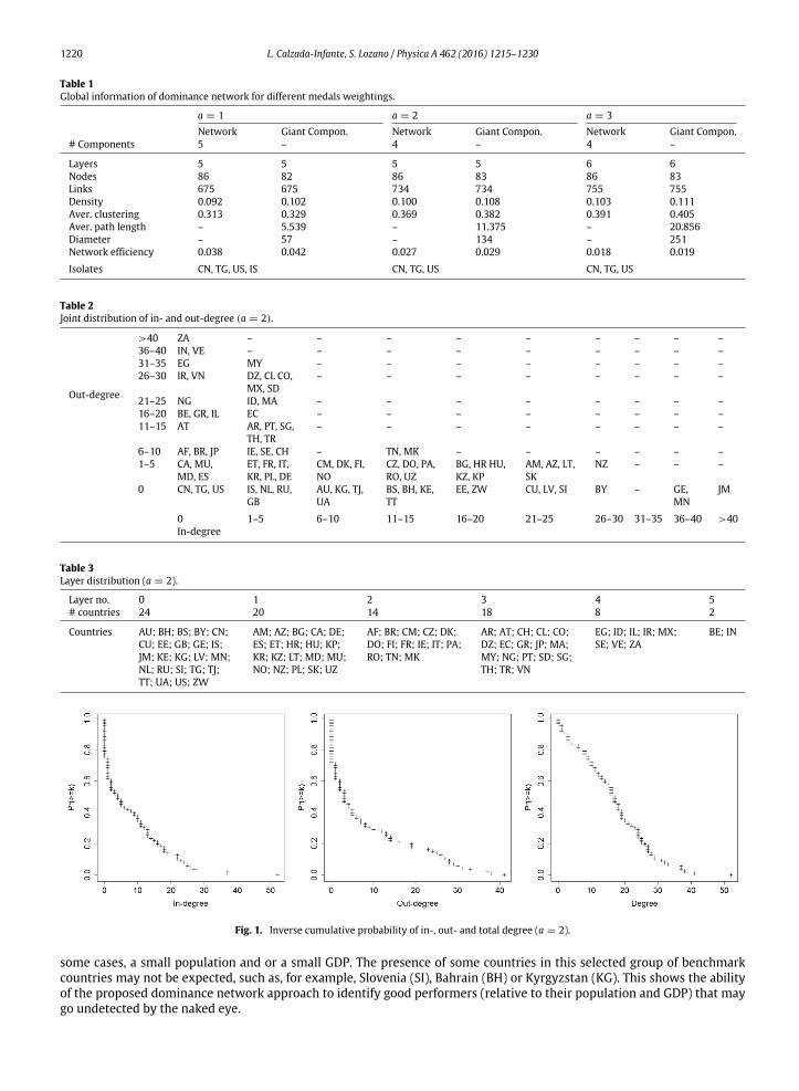
1220 L. Calzada-Infante, S. Lozano / Physica A 462 (2016) 1215–1230

Table 1

Global information of dominance network for different medals weightings.

a = 1 a = 2 a = 3

Network Giant Compon. Network Giant Compon. Network Giant Compon.

# Components 5 – 4 – 4 –

Layers 5 5 5 5 6 6

Nodes 86 82 86 83 86 83

Links 675 675 734 734 755 755

Density 0.092 0.102 0.100 0.108 0.103 0.111

Aver. clustering 0.313 0.329 0.369 0.382 0.391 0.405

Aver. path length – 5.539 – 11.375 – 20.856

Diameter – 57 – 134 – 251

Network efficiency 0.038 0.042 0.027 0.029 0.018 0.019

Isolates CN, TG, US, IS CN, TG, US CN, TG, US

Table 2

Joint distribution of in- and out-degree (a = 2).

Out-degree

>40 ZA – – – – – – – – –

36–40 IN, VE – – – – – – – – –

31–35 EG MY – – – – – – – –

26–30 IR, VN DZ, CL CO,

MX, SD

– – – – – – – –

21–25 NG ID, MA – – – – – – – –

16–20 BE, GR, IL EC – – – – – – – –

11–15 AT AR, PT, SG,

TH, TR

– – – – – – – –

6–10 AF, BR, JP IE, SE, CH – TN, MK – – – – – –

1–5 CA, MU,

MD, ES

ET, FR, IT,

KR, PL, DE

CM, DK, FI,

NO

CZ, DO, PA,

RO, UZ

BG, HR HU,

KZ, KP

AM, AZ, LT,

SK

NZ – – –

0 CN, TG, US IS, NL, RU,

GB

AU, KG, TJ,

UA

BS, BH, KE,

TT

EE, ZW CU, LV, SI BY – GE,

MN

JM

0 1–5 6–10 11–15 16–20 21–25 26–30 31–35 36–40 >40

In-degree

Table 3

Layer distribution (a = 2).

Layer no. 0 1 2 3 4 5

# countries 24 20 14 18 8 2

Countries AU; BH; BS; BY; CN;

CU; EE; GB; GE; IS;

JM; KE; KG; LV; MN;

NL; RU; SI; TG; TJ;

TT; UA; US; ZW

AM; AZ; BG; CA; DE;

ES; ET; HR; HU; KP;

KR; KZ; LT; MD; MU;

NO; NZ; PL; SK; UZ

AF; BR; CM; CZ; DK;

DO; FI; FR; IE; IT; PA;

RO; TN; MK

AR; AT; CH; CL; CO;

DZ; EC; GR; JP; MA;

MY; NG; PT; SD; SG;

TH; TR; VN

EG; ID; IL; IR; MX;

SE; VE; ZA

BE; IN

Fig. 1. Inverse cumulative probability of in-, out- and total degree (a = 2).

some cases, a small population and or a small GDP. The presence of some countries in this selected group of benchmarkcountries may not be expected, such as, for example, Slovenia (SI), Bahrain (BH) or Kyrgyzstan (KG). This shows the abilityof the proposed dominance network approach to identify good performers (relative to their population and GDP) that maygo undetected by the naked eye.

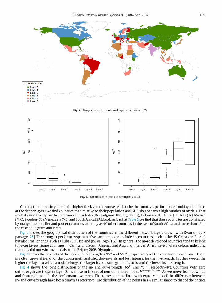
L. Calzada-Infante, S. Lozano / Physica A 462 (2016) 1215–1230 1221

Fig. 2. Geographical distribution of layer structure (a = 2).

Fig. 3. Boxplots of in- and out-strength (a = 2).

On the other hand, in general, the higher the layer, the worse tends to be the country’s performance. Looking, therefore,at the deeper layers we find countries that, relative to their population and GDP, do not earn a high number of medals. Thatis what seems to happen to countries such as India (IN), Belgium (BE), Egypt (EG), Indonesia (ID), Israel (IL), Iran (IR), Mexico(MX), Sweden (SE), Venezuela (VE) and South Africa (ZA). Looking back at Table 2we find that these countries are dominatedby many other smaller and poorer countries, as many as 40 other countries in the case of South Africa and more than 15 inthe case of Belgium and Israel.

Fig. 2 shows the geographical distribution of the countries in the different network layers drawn with Rworldmap Rpackage [25]. The strongest performers span the five continents and include big countries (such as the US, China and Russia)but also smaller ones (such as Cuba (CU), Iceland (IS) or Togo (TG)). In general, the more developed countries tend to belongto lower layers. Some countries in Central and South America and Asia and many in Africa have a white colour, indicatingthat they did not win any medals at the Beijing 2008 Olympics.

Fig. 3 shows the boxplots of the in- and out- strengths (NS in and NSout, respectively) of the countries in each layer. Thereis a clear upward trend for the out-strength and also, downwards and less intense, for the in-strength. In other words, thehigher the layer to which a node belongs, the larger its out-strength tends to be and the lower its in-strength.

Fig. 4 shows the joint distribution of the in- and out-strength (NS in and NSout, respectively). Countries with zeroout-strength are those in layer 0, i.e. those in the set of non-dominated nodes V best-performers. As we move from down upand from right to left, the performance worsens. The corresponding lines with equal values of the difference betweenin- and out-strength have been drawn as reference. The distribution of the points has a similar shape to that of the entries

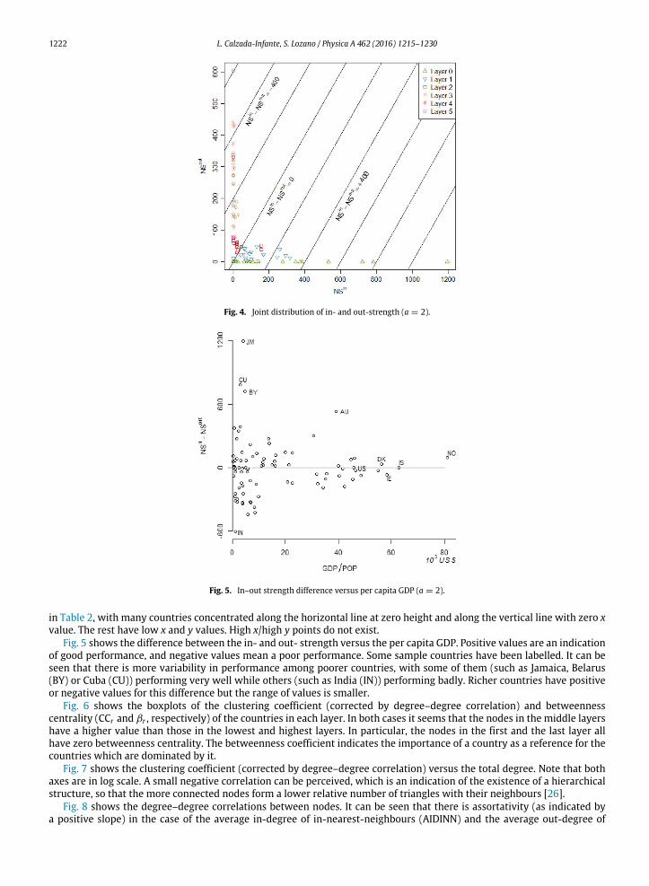
1222 L. Calzada-Infante, S. Lozano / Physica A 462 (2016) 1215–1230

Fig. 4. Joint distribution of in- and out-strength (a = 2).

Fig. 5. In–out strength difference versus per capita GDP (a = 2).

in Table 2, with many countries concentrated along the horizontal line at zero height and along the vertical line with zero x

value. The rest have low x and y values. High x/high y points do not exist.

Fig. 5 shows the difference between the in- and out- strength versus the per capita GDP. Positive values are an indicationof good performance, and negative values mean a poor performance. Some sample countries have been labelled. It can beseen that there is more variability in performance among poorer countries, with some of them (such as Jamaica, Belarus(BY) or Cuba (CU)) performing very well while others (such as India (IN)) performing badly. Richer countries have positiveor negative values for this difference but the range of values is smaller.

Fig. 6 shows the boxplots of the clustering coefficient (corrected by degree–degree correlation) and betweennesscentrality (CCr and βr , respectively) of the countries in each layer. In both cases it seems that the nodes in the middle layershave a higher value than those in the lowest and highest layers. In particular, the nodes in the first and the last layer allhave zero betweenness centrality. The betweenness coefficient indicates the importance of a country as a reference for thecountries which are dominated by it.

Fig. 7 shows the clustering coefficient (corrected by degree–degree correlation) versus the total degree. Note that bothaxes are in log scale. A small negative correlation can be perceived, which is an indication of the existence of a hierarchicalstructure, so that the more connected nodes form a lower relative number of triangles with their neighbours [26].

Fig. 8 shows the degree–degree correlations between nodes. It can be seen that there is assortativity (as indicated bya positive slope) in the case of the average in-degree of in-nearest-neighbours (AIDINN) and the average out-degree of

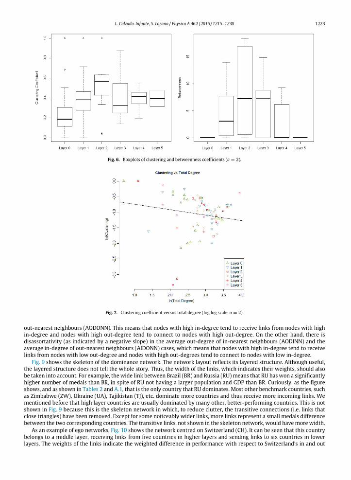
L. Calzada-Infante, S. Lozano / Physica A 462 (2016) 1215–1230 1223

Fig. 6. Boxplots of clustering and betweenness coefficients (a = 2).

Fig. 7. Clustering coefficient versus total degree (log log scale, a = 2).

out-nearest neighbours (AODONN). This means that nodes with high in-degree tend to receive links from nodes with highin-degree and nodes with high out-degree tend to connect to nodes with high out-degree. On the other hand, there isdisassortativity (as indicated by a negative slope) in the average out-degree of in-nearest neighbours (AODINN) and theaverage in-degree of out-nearest neighbours (AIDONN) cases, which means that nodes with high in-degree tend to receivelinks from nodes with low out-degree and nodes with high out-degrees tend to connect to nodes with low in-degree.

Fig. 9 shows the skeleton of the dominance network. The network layout reflects its layered structure. Although useful,the layered structure does not tell the whole story. Thus, the width of the links, which indicates their weights, should alsobe taken into account. For example, the wide link between Brazil (BR) and Russia (RU)means that RU has won a significantlyhigher number of medals than BR, in spite of RU not having a larger population and GDP than BR. Curiously, as the figureshows, and as shown in Tables 2 and A.1, that is the only country that RU dominates. Most other benchmark countries, suchas Zimbabwe (ZW), Ukraine (UA), Tajikistan (TJ), etc. dominate more countries and thus receive more incoming links. Wementioned before that high layer countries are usually dominated by many other, better-performing countries. This is notshown in Fig. 9 because this is the skeleton network in which, to reduce clutter, the transitive connections (i.e. links thatclose triangles) have been removed. Except for some noticeably wider links, more links represent a small medals differencebetween the two corresponding countries. The transitive links, not shown in the skeleton network, would havemore width.

As an example of ego networks, Fig. 10 shows the network centred on Switzerland (CH). It can be seen that this countrybelongs to a middle layer, receiving links from five countries in higher layers and sending links to six countries in lowerlayers. The weights of the links indicate the weighted difference in performance with respect to Switzerland’s in and out

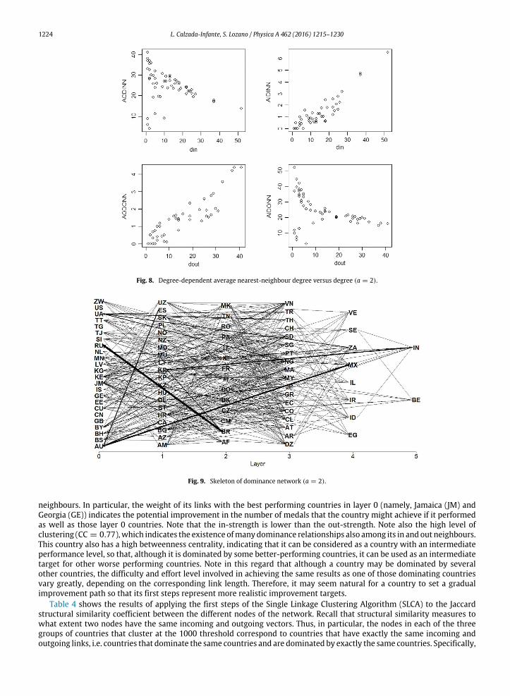
1224 L. Calzada-Infante, S. Lozano / Physica A 462 (2016) 1215–1230

Fig. 8. Degree-dependent average nearest-neighbour degree versus degree (a = 2).

Fig. 9. Skeleton of dominance network (a = 2).

neighbours. In particular, the weight of its links with the best performing countries in layer 0 (namely, Jamaica (JM) andGeorgia (GE)) indicates the potential improvement in the number of medals that the country might achieve if it performedas well as those layer 0 countries. Note that the in-strength is lower than the out-strength. Note also the high level ofclustering (CC = 0.77),which indicates the existence ofmanydominance relationships also among its in and out neighbours.This country also has a high betweenness centrality, indicating that it can be considered as a country with an intermediateperformance level, so that, although it is dominated by some better-performing countries, it can be used as an intermediatetarget for other worse performing countries. Note in this regard that although a country may be dominated by severalother countries, the difficulty and effort level involved in achieving the same results as one of those dominating countriesvary greatly, depending on the corresponding link length. Therefore, it may seem natural for a country to set a gradualimprovement path so that its first steps represent more realistic improvement targets.

Table 4 shows the results of applying the first steps of the Single Linkage Clustering Algorithm (SLCA) to the Jaccardstructural similarity coefficient between the different nodes of the network. Recall that structural similarity measures towhat extent two nodes have the same incoming and outgoing vectors. Thus, in particular, the nodes in each of the threegroups of countries that cluster at the 1000 threshold correspond to countries that have exactly the same incoming andoutgoing links, i.e. countries that dominate the same countries and are dominated by exactly the same countries. Specifically,

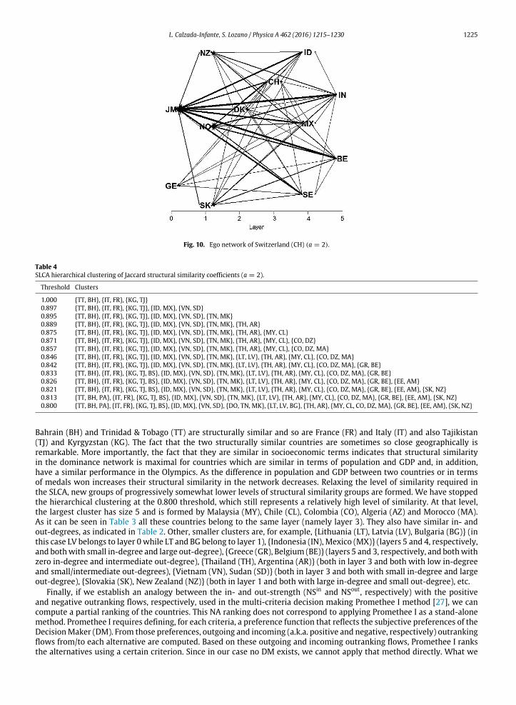
L. Calzada-Infante, S. Lozano / Physica A 462 (2016) 1215–1230 1225

Fig. 10. Ego network of Switzerland (CH) (a = 2).

Table 4

SLCA hierarchical clustering of Jaccard structural similarity coefficients (a = 2).

Threshold Clusters

1.000 {TT, BH}, {IT, FR}, {KG, TJ}

0.897 {TT, BH}, {IT, FR}, {KG, TJ}, {ID, MX}, {VN, SD}

0.895 {TT, BH}, {IT, FR}, {KG, TJ}, {ID, MX}, {VN, SD}, {TN, MK}

0.889 {TT, BH}, {IT, FR}, {KG, TJ}, {ID, MX}, {VN, SD}, {TN, MK}, {TH, AR}

0.875 {TT, BH}, {IT, FR}, {KG, TJ}, {ID, MX}, {VN, SD}, {TN, MK}, {TH, AR}, {MY, CL}

0.871 {TT, BH}, {IT, FR}, {KG, TJ}, {ID, MX}, {VN, SD}, {TN, MK}, {TH, AR}, {MY, CL}, {CO, DZ}

0.857 {TT, BH}, {IT, FR}, {KG, TJ}, {ID, MX}, {VN, SD}, {TN, MK}, {TH, AR}, {MY, CL}, {CO, DZ, MA}

0.846 {TT, BH}, {IT, FR}, {KG, TJ}, {ID, MX}, {VN, SD}, {TN, MK}, {LT, LV}, {TH, AR}, {MY, CL}, {CO, DZ, MA}

0.842 {TT, BH}, {IT, FR}, {KG, TJ}, {ID, MX}, {VN, SD}, {TN, MK}, {LT, LV}, {TH, AR}, {MY, CL}, {CO, DZ, MA}, {GR, BE}

0.833 {TT, BH}, {IT, FR}, {KG, TJ, BS}, {ID, MX}, {VN, SD}, {TN, MK}, {LT, LV}, {TH, AR}, {MY, CL}, {CO, DZ, MA}, {GR, BE}

0.826 {TT, BH}, {IT, FR}, {KG, TJ, BS}, {ID, MX}, {VN, SD}, {TN, MK}, {LT, LV}, {TH, AR}, {MY, CL}, {CO, DZ, MA}, {GR, BE}, {EE, AM}

0.821 {TT, BH}, {IT, FR}, {KG, TJ, BS}, {ID, MX}, {VN, SD}, {TN, MK}, {LT, LV}, {TH, AR}, {MY, CL}, {CO, DZ, MA}, {GR, BE}, {EE, AM}, {SK, NZ}

0.813 {TT, BH, PA}, {IT, FR}, {KG, TJ, BS}, {ID, MX}, {VN, SD}, {TN, MK}, {LT, LV}, {TH, AR}, {MY, CL}, {CO, DZ, MA}, {GR, BE}, {EE, AM}, {SK, NZ}

0.800 {TT, BH, PA}, {IT, FR}, {KG, TJ, BS}, {ID, MX}, {VN, SD}, {DO, TN, MK}, {LT, LV, BG}, {TH, AR}, {MY, CL, CO, DZ, MA}, {GR, BE}, {EE, AM}, {SK, NZ}

Bahrain (BH) and Trinidad & Tobago (TT) are structurally similar and so are France (FR) and Italy (IT) and also Tajikistan(TJ) and Kyrgyzstan (KG). The fact that the two structurally similar countries are sometimes so close geographically isremarkable. More importantly, the fact that they are similar in socioeconomic terms indicates that structural similarityin the dominance network is maximal for countries which are similar in terms of population and GDP and, in addition,have a similar performance in the Olympics. As the difference in population and GDP between two countries or in termsof medals won increases their structural similarity in the network decreases. Relaxing the level of similarity required inthe SLCA, new groups of progressively somewhat lower levels of structural similarity groups are formed. We have stoppedthe hierarchical clustering at the 0.800 threshold, which still represents a relatively high level of similarity. At that level,the largest cluster has size 5 and is formed by Malaysia (MY), Chile (CL), Colombia (CO), Algeria (AZ) and Morocco (MA).As it can be seen in Table 3 all these countries belong to the same layer (namely layer 3). They also have similar in- andout-degrees, as indicated in Table 2. Other, smaller clusters are, for example, {Lithuania (LT), Latvia (LV), Bulgaria (BG)} (inthis case LV belongs to layer 0while LT and BG belong to layer 1), {Indonesia (IN), Mexico (MX)} (layers 5 and 4, respectively,and bothwith small in-degree and large out-degree), {Greece (GR), Belgium (BE)} (layers 5 and 3, respectively, and bothwithzero in-degree and intermediate out-degree), {Thailand (TH), Argentina (AR)} (both in layer 3 and both with low in-degreeand small/intermediate out-degrees), {Vietnam (VN), Sudan (SD)} (both in layer 3 and both with small in-degree and largeout-degree), {Slovakia (SK), New Zealand (NZ)} (both in layer 1 and both with large in-degree and small out-degree), etc.

Finally, if we establish an analogy between the in- and out-strength (NSin and NSout, respectively) with the positiveand negative outranking flows, respectively, used in the multi-criteria decision making Promethee I method [27], we cancompute a partial ranking of the countries. This NA ranking does not correspond to applying Promethee I as a stand-alonemethod. Promethee I requires defining, for each criteria, a preference function that reflects the subjective preferences of theDecisionMaker (DM). From those preferences, outgoing and incoming (a.k.a. positive and negative, respectively) outrankingflows from/to each alternative are computed. Based on these outgoing and incoming outranking flows, Promethee I ranksthe alternatives using a certain criterion. Since in our case no DM exists, we cannot apply that method directly. What we

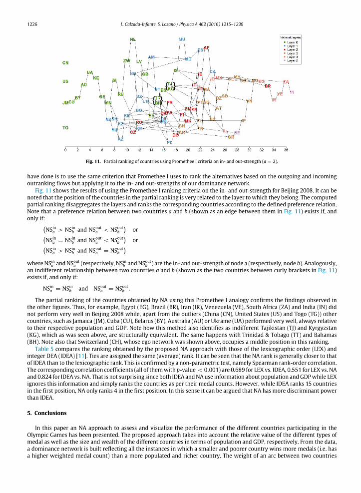
1226 L. Calzada-Infante, S. Lozano / Physica A 462 (2016) 1215–1230

Fig. 11. Partial ranking of countries using Promethee I criteria on in- and out-strength (a = 2).

have done is to use the same criterion that Promethee I uses to rank the alternatives based on the outgoing and incomingoutranking flows but applying it to the in- and out-strengths of our dominance network.

Fig. 11 shows the results of using the Promethee I ranking criteria on the in- and out-strength for Beijing 2008. It can benoted that the position of the countries in the partial ranking is very related to the layer to which they belong. The computedpartial ranking disaggregates the layers and ranks the corresponding countries according to the defined preference relation.Note that a preference relation between two countries a and b (shown as an edge between them in Fig. 11) exists if, andonly if:

NSina > NSinb and NSouta < NSoutb

or

NSina = NSinb and NSouta < NSoutb

or

NSina > NSinb and NSouta = NSoutb

whereNSina andNSouta (respectively, NSinb andNSoutb ) are the in- and out-strength of node a (respectively, node b). Analogously,an indifferent relationship between two countries a and b (shown as the two countries between curly brackets in Fig. 11)exists if, and only if:

NSina = NSinb and NSouta = NSoutb .

The partial ranking of the countries obtained by NA using this Promethee I analogy confirms the findings observed inthe other figures. Thus, for example, Egypt (EG), Brazil (BR), Iran (IR), Venezuela (VE), South Africa (ZA) and India (IN) didnot perform very well in Beijing 2008 while, apart from the outliers (China (CN), United States (US) and Togo (TG)) othercountries, such as Jamaica (JM), Cuba (CU), Belarus (BY), Australia (AU) or Ukraine (UA) performed very well, always relativeto their respective population and GDP. Note how this method also identifies as indifferent Tajikistan (TJ) and Kyrgyzstan(KG), which as was seen above, are structurally equivalent. The same happens with Trinidad & Tobago (TT) and Bahamas(BH). Note also that Switzerland (CH), whose ego network was shown above, occupies a middle position in this ranking.

Table 5 compares the ranking obtained by the proposed NA approach with those of the lexicographic order (LEX) andinteger DEA (IDEA) [11]. Ties are assigned the same (average) rank. It can be seen that the NA rank is generally closer to thatof IDEA than to the lexicographic rank. This is confirmed by a non-parametric test, namely Spearman rank-order correlation.The corresponding correlation coefficients (all of themwith p-value < 0.001) are 0.689 for LEX vs. IDEA, 0.551 for LEX vs. NAand 0.824 for IDEA vs. NA. That is not surprising since both IDEA andNAuse information about population andGDPwhile LEXignores this information and simply ranks the countries as per their medal counts. However, while IDEA ranks 15 countriesin the first position, NA only ranks 4 in the first position. In this sense it can be argued that NA has more discriminant powerthan IDEA.

5. Conclusions

In this paper an NA approach to assess and visualize the performance of the different countries participating in theOlympic Games has been presented. The proposed approach takes into account the relative value of the different types ofmedal as well as the size and wealth of the different countries in terms of population and GDP, respectively. From the data,a dominance network is built reflecting all the instances in which a smaller and poorer country wins more medals (i.e. hasa higher weighted medal count) than a more populated and richer country. The weight of an arc between two countries

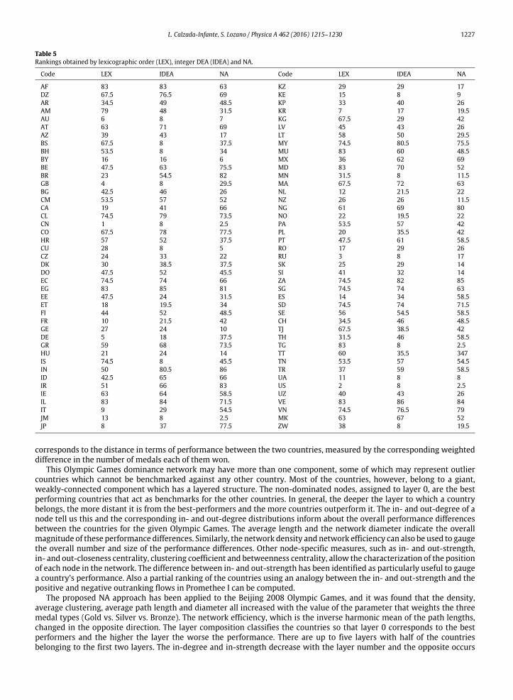
L. Calzada-Infante, S. Lozano / Physica A 462 (2016) 1215–1230 1227

Table 5

Rankings obtained by lexicographic order (LEX), integer DEA (IDEA) and NA.

Code LEX IDEA NA Code LEX IDEA NA

AF 83 83 63 KZ 29 29 17

DZ 67.5 76.5 69 KE 15 8 9

AR 34.5 49 48.5 KP 33 40 26

AM 79 48 31.5 KR 7 17 19.5

AU 6 8 7 KG 67.5 29 42

AT 63 71 69 LV 45 43 26

AZ 39 43 17 LT 58 50 29.5

BS 67.5 8 37.5 MY 74.5 80.5 75.5

BH 53.5 8 34 MU 83 60 48.5

BY 16 16 6 MX 36 62 69

BE 47.5 63 75.5 MD 83 70 52

BR 23 54.5 82 MN 31.5 8 11.5

GB 4 8 29.5 MA 67.5 72 63

BG 42.5 46 26 NL 12 21.5 22

CM 53.5 57 52 NZ 26 26 11.5

CA 19 41 66 NG 61 69 80

CL 74.5 79 73.5 NO 22 19.5 22

CN 1 8 2.5 PA 53.5 57 42

CO 67.5 78 77.5 PL 20 35.5 42

HR 57 52 37.5 PT 47.5 61 58.5

CU 28 8 5 RO 17 29 26

CZ 24 33 22 RU 3 8 17

DK 30 38.5 37.5 SK 25 29 14

DO 47.5 52 45.5 SI 41 32 14

EC 74.5 74 66 ZA 74.5 82 85

EG 83 85 81 SG 74.5 74 63

EE 47.5 24 31.5 ES 14 34 58.5

ET 18 19.5 34 SD 74.5 74 71.5

FI 44 52 48.5 SE 56 54.5 58.5

FR 10 21.5 42 CH 34.5 46 48.5

GE 27 24 10 TJ 67.5 38.5 42

DE 5 18 37.5 TH 31.5 46 58.5

GR 59 68 73.5 TG 83 8 2.5

HU 21 24 14 TT 60 35.5 347

IS 74.5 8 45.5 TN 53.5 57 54.5

IN 50 80.5 86 TR 37 59 58.5

ID 42.5 65 66 UA 11 8 8

IR 51 66 83 US 2 8 2.5

IE 63 64 58.5 UZ 40 43 26

IL 83 84 71.5 VE 83 86 84

IT 9 29 54.5 VN 74.5 76.5 79

JM 13 8 2.5 MK 63 67 52

JP 8 37 77.5 ZW 38 8 19.5

corresponds to the distance in terms of performance between the two countries, measured by the corresponding weighteddifference in the number of medals each of them won.

This Olympic Games dominance network may have more than one component, some of which may represent outliercountries which cannot be benchmarked against any other country. Most of the countries, however, belong to a giant,weakly-connected component which has a layered structure. The non-dominated nodes, assigned to layer 0, are the bestperforming countries that act as benchmarks for the other countries. In general, the deeper the layer to which a countrybelongs, the more distant it is from the best-performers and the more countries outperform it. The in- and out-degree of anode tell us this and the corresponding in- and out-degree distributions inform about the overall performance differencesbetween the countries for the given Olympic Games. The average length and the network diameter indicate the overallmagnitude of these performance differences. Similarly, the network density and network efficiency can also be used to gaugethe overall number and size of the performance differences. Other node-specific measures, such as in- and out-strength,in- and out-closeness centrality, clustering coefficient and betweenness centrality, allow the characterization of the positionof each node in the network. The difference between in- and out-strength has been identified as particularly useful to gaugea country’s performance. Also a partial ranking of the countries using an analogy between the in- and out-strength and thepositive and negative outranking flows in Promethee I can be computed.

The proposed NA approach has been applied to the Beijing 2008 Olympic Games, and it was found that the density,average clustering, average path length and diameter all increased with the value of the parameter that weights the threemedal types (Gold vs. Silver vs. Bronze). The network efficiency, which is the inverse harmonic mean of the path lengths,changed in the opposite direction. The layer composition classifies the countries so that layer 0 corresponds to the bestperformers and the higher the layer the worse the performance. There are up to five layers with half of the countriesbelonging to the first two layers. The in-degree and in-strength decrease with the layer number and the opposite occurs

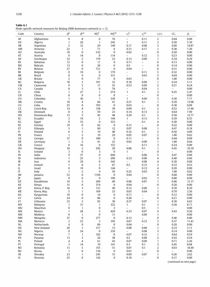
1228 L. Calzada-Infante, S. Lozano / Physica A 462 (2016) 1215–1230

Table A.1

Node-specific network measures for Beijing 2008 dominance network (a = 2).

Code Country dinr doutr NSinr NSoutr κ inr κout

r λ(r) CCr βr

AF Afghanistan 0 8 0 76 – 0.11 2 0.04 0.00

DZ Algeria 1 26 1 245 1 0.11 3 0.28 5.39

AR Argentina 5 12 29 149 0.17 0.08 3 0.60 14.87

AM Armenia 22 1 71 6 0.31 0.17 1 0.38 7.20

AU Australia 10 0 532 0 0.02 – 0 0.50 0.00

AT Austria 0 14 0 114 – 0.12 3 0.23 0.00

AZ Azerbaijan 22 2 170 23 0.13 0.09 1 0.34 9.29

BS Bahamas 12 0 17 0 0.71 – 0 0.13 0.00

BH Bahrain 13 0 26 0 0.5 – 0 0.14 0.00

BY Belarus 27 0 721 0 0.04 – 0 0.31 0.00

BE Belgium 0 19 0 179 – 0.11 5 0.32 0.00

BR Brazil 0 9 0 331 – 0.03 2 0.04 0.00

GB Britain 2 0 77 0 0.03 – 0 1.00 0.00

BG Bulgaria 18 3 101 32 0.18 0.09 1 0.34 5.11

CM Cameroon 9 5 17 55 0.53 0.09 2 0.57 8.24

CA Canada 0 3 0 78 – 0.04 1 – 0.00

CL Chile 1 27 1 274 1 0.1 3 0.25 5.47

CN China 0 0 0 0 – – 0 – 0.00

CO Colombia 1 30 1 330 1 0.09 3 0.30 7.17

HR Croatia 18 4 66 41 0.27 0.1 1 0.39 13.98

CU Cuba 25 0 783 0 0.03 – 0 0.30 0.00

CZ Czech Rep. 14 4 158 39 0.09 0.1 2 0.52 17.46

DK Denmark 8 3 59 23 0.14 0.13 2 0.64 7.99

DO Dominican Rep. 13 5 45 48 0.29 0.1 2 0.50 12.77

EC Ecuador 2 19 2 144 1 0.13 3 0.39 8.55

EG Egypt 0 33 0 323 – 0.1 4 0.38 0.00

EE Estonia 19 0 62 0 0.31 – 0 0.22 0.00

ET Ethiopia 5 1 69 12 0.07 0.08 1 0.47 0.18

FI Finland 6 5 19 48 0.32 0.1 2 0.56 4.09

FR France 1 2 19 29 0.05 0.07 2 1.00 0.62

GE Georgia 37 0 349 0 0.11 – 0 0.44 0.00

DE Germany 1 2 41 22 0.02 0.09 1 1.00 0.64

GR Greece 0 16 0 152 – 0.11 3 0.24 0.00

HU Hungary 18 2 292 20 0.06 0.1 1 0.45 10.10

IS Iceland 3 0 3 0 1 – 0 – 0.00

IN India 0 37 0 604 – 0.06 5 0.47 0.00

ID Indonesia 1 25 3 296 0.33 0.08 4 0.40 6.66

IR Iran 0 29 0 342 – 0.08 4 0.30 0.00

IE Ireland 1 8 2 67 0.5 0.12 2 0.33 0.52

IL Israel 0 19 0 144 – 0.13 4 0.20 0.00

IT Italy 1 2 4 59 0.25 0.03 2 1.00 0.62

JM Jamaica 52 0 1194 0 0.04 – 0 0.68 0.00

JP Japan 0 6 0 190 – 0.03 3 0.88 0.00

KZ Kazakhstan 16 3 260 40 0.06 0.07 1 0.46 12.17

KE Kenya 15 0 374 0 0.04 – 0 0.20 0.00

KP Korea, P. Rep. 16 3 131 49 0.12 0.06 1 0.39 8.29

KR Korea, Rep. 5 1 169 23 0.03 0.04 1 0.70 2.26

KG Kyrgyzstan 10 0 14 0 0.71 – 0 0.12 0.00

LV Latvia 24 0 86 0 0.28 – 0 0.21 0.00

LT Lithuania 22 2 82 30 0.27 0.07 1 0.30 6.62

MY Malaysia 1 31 1 322 1 0.1 3 0.28 8.71

MU Mauritius 0 1 0 2 – 0.5 1 – 0.00

MX Mexico 1 28 3 429 0.33 0.07 4 0.43 9.26

MD Moldova 0 1 0 11 – 0.09 1 – 0.00

MN Mongolia 37 0 277 0 0.13 – 0 0.46 0.00

MA Morocco 2 23 3 195 0.67 0.12 3 0.37 11.41

NL Netherlands 4 0 89 0 0.04 – 0 0.20 0.00

NZ New Zealand 26 1 317 13 0.08 0.08 1 0.33 5.11

NG Nigeria 0 24 0 310 – 0.08 3 0.14 0.00

NO Norway 7 1 102 8 0.07 0.12 1 0.64 0.59

PA Panama 13 3 26 38 0.5 0.08 2 0.43 6.54

PL Poland 4 4 61 43 0.07 0.09 1 0.71 2.26

PT Portugal 3 14 10 141 0.3 0.1 3 0.45 8.68

RO Romania 11 5 155 51 0.07 0.1 2 0.63 18.49

RU Russia 1 0 134 0 0.01 – 0 – 0.00

SK Slovakia 23 1 245 15 0.09 0.07 1 0.26 2.62

SI Slovenia 25 0 142 0 0.18 – 0 0.17 0.00

(continued on next page)

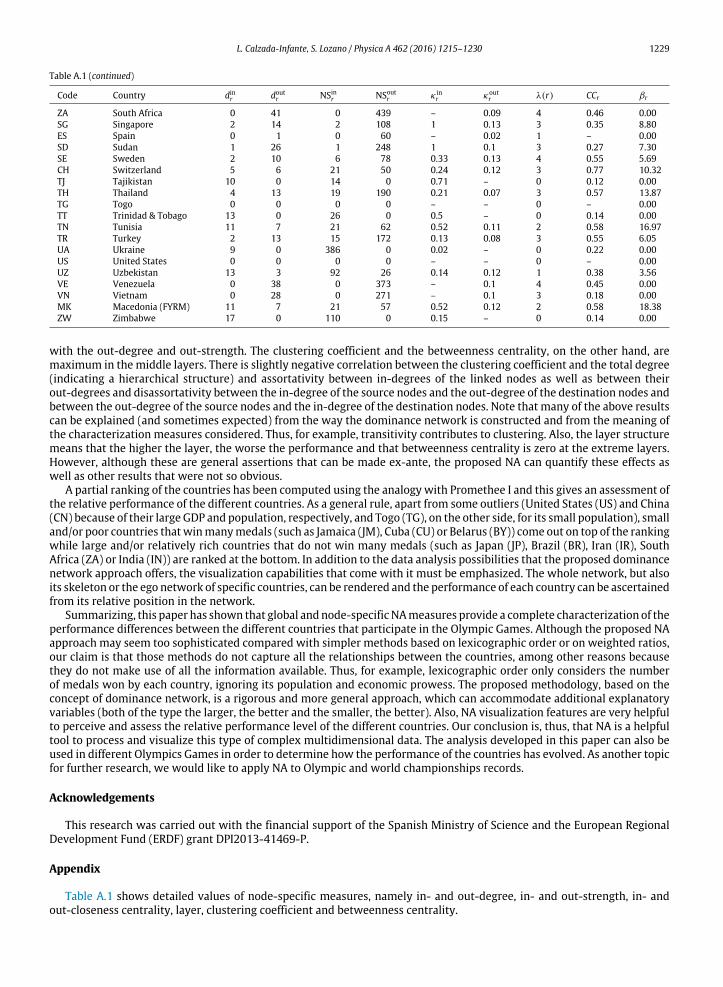
L. Calzada-Infante, S. Lozano / Physica A 462 (2016) 1215–1230 1229

Table A.1 (continued)

Code Country dinr doutr NSinr NSoutr κ inr κout

r λ(r) CCr βr

ZA South Africa 0 41 0 439 – 0.09 4 0.46 0.00

SG Singapore 2 14 2 108 1 0.13 3 0.35 8.80

ES Spain 0 1 0 60 – 0.02 1 – 0.00

SD Sudan 1 26 1 248 1 0.1 3 0.27 7.30

SE Sweden 2 10 6 78 0.33 0.13 4 0.55 5.69

CH Switzerland 5 6 21 50 0.24 0.12 3 0.77 10.32

TJ Tajikistan 10 0 14 0 0.71 – 0 0.12 0.00

TH Thailand 4 13 19 190 0.21 0.07 3 0.57 13.87

TG Togo 0 0 0 0 – – 0 – 0.00

TT Trinidad & Tobago 13 0 26 0 0.5 – 0 0.14 0.00

TN Tunisia 11 7 21 62 0.52 0.11 2 0.58 16.97

TR Turkey 2 13 15 172 0.13 0.08 3 0.55 6.05

UA Ukraine 9 0 386 0 0.02 – 0 0.22 0.00

US United States 0 0 0 0 – – 0 – 0.00

UZ Uzbekistan 13 3 92 26 0.14 0.12 1 0.38 3.56

VE Venezuela 0 38 0 373 – 0.1 4 0.45 0.00

VN Vietnam 0 28 0 271 – 0.1 3 0.18 0.00

MK Macedonia (FYRM) 11 7 21 57 0.52 0.12 2 0.58 18.38

ZW Zimbabwe 17 0 110 0 0.15 – 0 0.14 0.00

with the out-degree and out-strength. The clustering coefficient and the betweenness centrality, on the other hand, aremaximum in themiddle layers. There is slightly negative correlation between the clustering coefficient and the total degree(indicating a hierarchical structure) and assortativity between in-degrees of the linked nodes as well as between theirout-degrees and disassortativity between the in-degree of the source nodes and the out-degree of the destination nodes andbetween the out-degree of the source nodes and the in-degree of the destination nodes. Note that many of the above resultscan be explained (and sometimes expected) from the way the dominance network is constructed and from the meaning ofthe characterization measures considered. Thus, for example, transitivity contributes to clustering. Also, the layer structuremeans that the higher the layer, the worse the performance and that betweenness centrality is zero at the extreme layers.However, although these are general assertions that can be made ex-ante, the proposed NA can quantify these effects aswell as other results that were not so obvious.

A partial ranking of the countries has been computed using the analogy with Promethee I and this gives an assessment ofthe relative performance of the different countries. As a general rule, apart from some outliers (United States (US) and China(CN) because of their large GDP and population, respectively, and Togo (TG), on the other side, for its small population), smalland/or poor countries thatwinmanymedals (such as Jamaica (JM), Cuba (CU) or Belarus (BY)) come out on top of the rankingwhile large and/or relatively rich countries that do not win many medals (such as Japan (JP), Brazil (BR), Iran (IR), SouthAfrica (ZA) or India (IN)) are ranked at the bottom. In addition to the data analysis possibilities that the proposed dominancenetwork approach offers, the visualization capabilities that come with it must be emphasized. The whole network, but alsoits skeleton or the ego network of specific countries, can be rendered and the performance of each country can be ascertainedfrom its relative position in the network.

Summarizing, this paper has shown that global andnode-specific NAmeasures provide a complete characterization of theperformance differences between the different countries that participate in the Olympic Games. Although the proposed NAapproach may seem too sophisticated compared with simpler methods based on lexicographic order or on weighted ratios,our claim is that those methods do not capture all the relationships between the countries, among other reasons becausethey do not make use of all the information available. Thus, for example, lexicographic order only considers the numberof medals won by each country, ignoring its population and economic prowess. The proposed methodology, based on theconcept of dominance network, is a rigorous and more general approach, which can accommodate additional explanatoryvariables (both of the type the larger, the better and the smaller, the better). Also, NA visualization features are very helpfulto perceive and assess the relative performance level of the different countries. Our conclusion is, thus, that NA is a helpfultool to process and visualize this type of complex multidimensional data. The analysis developed in this paper can also beused in different Olympics Games in order to determine how the performance of the countries has evolved. As another topicfor further research, we would like to apply NA to Olympic and world championships records.

Acknowledgements

This research was carried out with the financial support of the Spanish Ministry of Science and the European RegionalDevelopment Fund (ERDF) grant DPI2013-41469-P.

Appendix

Table A.1 shows detailed values of node-specific measures, namely in- and out-degree, in- and out-strength, in- andout-closeness centrality, layer, clustering coefficient and betweenness centrality.

1230 L. Calzada-Infante, S. Lozano / Physica A 462 (2016) 1215–1230

References

[1] S. Lozano, G. Villa, F. Guerrero, P. Cortés, Measuring the performance of nations at the summer Olympics using data envelopment analysis, J. Oper.Res. Soc. 53 (2002) 501–511.

[2] A.B. Bernard, M.R. Busse, Who wins the Olympic Games: Economic resources and medal totals, Rev. Econ. Stat. 86 (2004) 414–417.[3] J. Wu, L. Liang, Cross-efficiency evaluation approach to Olympic ranking and benchmarking: the case of Beijing 2008, Internat. J. Appl. Manag. Sci. 2

(1) (2010) 76–92.[4] G. Vagenas, E. Vlachokyriakou, Olympic medals and demo-economic factors: Novel predictors, the ex-host effect, the exact role of team size, and the

‘‘population-GDP’’ model revisited, Sport Manag. Rev. 15 (2012) 211–217.[5] M.P. Estellita-Lins, E.G. Gomes, J.C.C.B. Soares de Mello, A.J.R. Soares de Mello, Olympic ranking based on a zero sum gains DEA model, European J.

Oper. Res. 148 (2) (2003) 312–322.[6] Y. Li, L. Liang, Y. Chen, H. Morita, Models for measuring and benchmarking Olympics achievements, Omega 36 (2008) 933–940.[7] Y. Li, X. Lei, Q. Dai, L. Liang, Performance evaluation of participating nations at the 2012 London summer Olympics by a two-stage data envelopment

analysis, European J. Oper. Res. 243 (2015) 964–973.[8] D. Zhang, X. Li, W. Meng, W. Liu, Measuring the performance of nations at the Olympic games using DEA models with different preferences, J. Oper.

Res. Soc. 60 (2009) 983–990.[9] J. Wu, L. Liang, Y. Chen, Achievement and benchmarking of countries at the summer Olympics using cross efficiency evaluation method, European J.

Oper. Res. 197 (2009) 722–730.[10] J. Wu, L. Liang, Y. Yang, DEA game cross-efficiency approach to Olympic rankings, Omega 37 (4) (2009) 909–918.[11] J. Wu, Z. Zhou, L. Liang, Measuring the performance of nations at Beijing summer Olympics using integer-valued DEA model, J. Sports Econom. 11

(2010) 549–566.[12] X. Lei, Y. Li, Q. Xie, L. Liang, Measuring Olympics achievements based on a parallel DEA approach, Ann. Oper. Res. 226 (1) (2015) 379–396.[13] S. Wasserman, K. Faust, Social Network Analysis: Methods and Applications, Cambridge University Press, Cambridge, UK, 1994.[14] M.O. Jackson, Social and Economic Networks, Princeton University Press, Princeton, USA, 2010.[15] O. Lordan, J.M. Sallan, P. Simo, D. González-Prieto, Robustness of the air transport network, Transp. Res. E 68 (2014) 155–163.[16] M.A. Serrano, M. Boguñá, Topology of the world trade web, Phys. Rev. E 68 (2003) 015101(R).[17] Y. Kim, Y.S. Chen, K. Linderman, Supply network disruption and resilience: A network structural perspective, J. Oper. Manage. 33–34 (2015) 43–59.[18] T. Narizuka, K. Yamamoto, Y. Yamazaki, Statistical properties of position-dependent ball-passing networks in football games, Physica A 412 (2014)

157–168.[19] F. Radicchi, Who is the best player ever? A complex network analysis of the history of professional tennis, PLoS One 6 (2) (2011) e17249.[20] S. Mukherjee, Identifying the greatest team and captain—a complex network approach to cricket matches, Physica A 391 (2012) 6066–6076.[21] S. Mukherjee, Quantifying individual performance in Cricket — a network analysis of batsmen and bowlers, Physica A 393 (2014) 624–637.[22] S. Saavedra, S. Powers, T. McCotter, M.A. Porter, P.J. Mucha, Mutually-antagonistic interactions in baseball networks, Physica A 389 (2010) 1131–1141.[23] R. Albert, H. Jeong, A.L. Barabási, Error and attack tolerance of complex networks, Nature 406 (2000) 378–382.[24] S. Soffer, A. Vázquez, Network clustering coefficient without degree-correlation biases, Phys. Rev. E 71 (5) (2005) 057101.[25] A. South, Rworldmap: A new r package for mapping global data, The R J. 3 (2011) 35–43.[26] E. Rabasz, A.L. Barabási, Hierarchical organization in complex networks, Phys. Rev. E 67 (2003) 026112.[27] J.P. Brans, B. Mareschal, PROMETHEE methods, in: J. Figueira, S. Greco, M. Ehrgott (Eds.), Multiple Criteria Decision Analysis: State of the Art Surveys,

Springer Verlag, 2005, pp. 163–196.

Expert Systems With Applications 82 (2017) 53–66

Contents lists available at ScienceDirect

Expert Systems With Applications

journal homepage: www.elsevier.com/locate/eswa

Dominance network analysis of economic efficiency

Sebastián Lozano a , ∗, Laura Calzada-Infante

b

a Department of Industrial Management, University of Seville, Spain b Engineering School, University of Oviedo, Spain

a r t i c l e i n f o

Article history:

Received 16 December 2016

Revised 13 March 2017

Accepted 2 April 2017

Available online 3 April 2017

Keywords:

Technical efficiency

Economic efficiency

Allocative efficiency

Dominance Network

Complex network analysis

a b s t r a c t

This paper proposes an enhanced Dominance Network (DN) to assess the technical, economic and al-

locative efficiency of a set of Decision Making Units (DMUs). In a DN, the nodes represent DMUs and

the arcs correspond to dominance relationships between them. Two types of dominance relationship are

considered: technical and economic. The length of a technical dominance arc between two nodes is a

weighted measure of the input and output differences between the two DMUs. The length of an eco-

nomic dominance arc between two nodes corresponds to the cost, revenue or profit difference between

them (depending on whether only unit input prices, unit output prices or both are known). The pro-

posed dominance network is a multiplex network with two relations; the structure of both relations is

similar. Thus, both of them are layered and their arcs have transitivity and additivity properties. How-

ever, since technical dominance implies economic dominance but not the reverse, economic dominance

is more common and has a deeper structure. It may also have an underlying potential field so that the

length of the arcs between any two nodes depends on the difference in their potentials and the direction

of the arcs depends on the sign of that difference. Allocative inefficiencies can also be gauged on this DN.

Complex network measures can be used to characterize and study this type of DN.

© 2017 Elsevier Ltd. All rights reserved.

1. Introduction

Non-parametric Frontier Analysis methods (of which Data En-

velopment Analysis, DEA, is probably the best known) assess the

relative efficiency of DMUs. These methods see the DMUs as pro-

duction processes that transform inputs into outputs. Moreover,

they are data-driven so that only the data on the input consump-

tion and output production of each DMU are required. DEA ap-

proaches have been extensively studied and applied as can be seen

in the existing textbooks on the subject (e.g. Cooper, Seiford, &

Zhu, 2004, 2006; Färe, Grosskopf, & Lovell, 1985, 1994 ).

Recently, Calzada-Infante and Lozano (2016) used DN to as-

sess the medal winning performance of nations at Olympic Games.

The corresponding DN is characterized using different complex

network measures, such as node strength, clustering coefficient,

betweenness centrality, degree-degree correlation, etc. This paper

proposes an enhanced DN analysis that includes not only techni-

cal efficiency but also economic (cost, revenue or profit) efficiency.

Technical efficiency (TE) basically measures the maximum input re-

duction and output increase that a given DMU may achieve. Eco-

∗ Corresponding author at: Escuela Superior de Ingenieros, Camino de los Des-

cubrimientos, s/n, 41092 Sevilla, Spain.

E-mail addresses: slozano@us.es (S. Lozano),

calzadalaura@uniovi.es (L. Calzada-Infante).

nomic efficiency, on the other hand, refers to the maximum cost

reduction or revenue or profit increase that a given DMU may

achieve. TE assessment only requires input and output data while

economic efficiency assessment also requires knowing the outputs

and inputs unit prices.

Since TE assessment does not use price information, the pro-

jection of a DMU is done considering only the operating points

that dominate it in technical terms, i.e. in terms of the input con-

sumption and output production. This leads to the technical domi-

nance criterion. Economic efficiency, on the other hand, makes use

of price information, allowing certain inputs to be increased or cer-

tain outputs to be decreased if that leads to an overall cost, rev-

enue or profit improvement, depending on whether we are con-

sidering cost, revenue or profit efficiency. In any case, economic

efficiency leads to an economic dominance criterion which is dif-

ferent from that of technical dominance and it is based on the

corresponding cost, revenue or profit. Hence, in the proposed ap-

proach we consider a DN with two different dominance relations,

one based on TE and the other based on economic efficiency.

The proposed enhanced DN approach is a novel way of assess-

ing the economic performance of DMUs using complex networks

tools. Some researchers have previously applied complex network

analysis in a DEA context but their approach was not based on

the DN concept. Thus, for example, complex network analysis has

been proposed to rank efficient DMUs ( Ho, Liu, Lu, & Huang, 2014 ;

http://dx.doi.org/10.1016/j.eswa.2017.04.004

0957-4174/© 2017 Elsevier Ltd. All rights reserved.

54 S. Lozano, L. Calzada-Infante / Expert Systems With Applications 82 (2017) 53–66

Leem & Chun, 2015 ; Liu & Lu, 2010 ; Liu, Lu, Yang, & Chuang, 2009,

2014 ). In these approaches, the network considered is weighted

and directed and it is constructed based on the optimal intensity

variables (commonly known as lambda parameters) computed us-

ing an envelopment DEA model, sometimes with different input-

output specifications. The nodes of this network are the DMUs and

the arc weights are the optimal values of the intensity variables. If

only one input-output specification is used, the resulting network

is bipartite, with the arcs going from each inefficient DMU to the

efficient DMUs in its peer group. Two different centrality measures

are proposed to rank the efficient DMUs.

Ghahraman and Prior (2015) use a different approach aimed at

selecting an optimal stepwise benchmark path from an inefficient

operating unit (OU) to the efficient frontier. Their network consid-

ers that the nodes are the DMUs but this time an arc between two

nodes r and j exists if, and only if, OU j has a higher efficiency

score than OU r . The corresponding arc weight is computed us-

ing a weighted measure that takes into account the input similari-

ties between the two DMUs, their efficiency gap (modified using

an exponential penalty function) and a fixed cost for each link.

They compute shortest paths on this network as well as clusters

of DMUs (based on the maximum input and output percentage

changes in a single step). They also use complex network analy-

sis to discriminate between efficient and intermediate DMUs, clus-

tering the DMUs and identifying possible outliers and specialized

units.

The DN approach first used in Calzada-Infante and

Lozano (2016) is different from those commented on above as it

constructs a DN based on the dominance relationships between

the DMUs. Thus, an arc between a node r and a node j exists if,

and only if, DMU j (weakly) dominates DMU r , i.e. if DMU j consumes

less (or at most the same amount of) inputs and produces more

(or at least an equal amount of) outputs than DMU r . Calzada-

Infante and Lozano (2016) use what can be called a Normalized

Additive Inefficiency (NAI) metric to compute the arc weights and

implicitly assumes a basic Free Disposal Hull (FDH) technology.

However, other DEA metrics and other DEA technologies can also

be considered.

In this paper, an enhanced DN is considered for the cases in

which, in addition to the input and output data, unit input prices,

unit output prices or both, are known. In those cases, in addition

to the technical dominance relationships, economic dominance re-

lationships can be defined. Thus, the relationships between the

DMUs are analysed from two different points of view: technical

and economic. The resulting DN integrates both relations and its

analysis, using complex network tools, provides an innovative ap-

proach to economic efficiency assessment. Thus, while in DEA the

TE score measures the distance to the frontier, i.e. the difference

between a DMU and its efficient benchmark, the DN approach

also considers the existence of links between any two inefficient

DMUs if one dominates the other in technical terms. The length of

the corresponding arc measures the relative inefficiency between

them, i.e. the difference in their respective TE. Similarly, while in

DEA the economic efficiency of a DMU refers to the maximum cost,

revenue or profit improvement for a given DMU, in the enhanced

DN approach the lengths of the arcs of the economic efficiency re-

lation correspond to the difference in cost, revenue or profit be-

tween the origin and the destination nodes. By following a directed

path along the DN, successive improvements in TE or in economic

efficiency (depending on the dominance relation considered) can

be obtained. Thus, the proposed approach allows a graphical and

quantitative representation of the TE and economic efficiency of

the DMUs in the sample and of the possible improvement paths

that can be followed.

This double graphical plus quantitative feature of the proposed

DN approach is useful because most DEA problems involve multi-

ple inputs and outputs observations whose direct visualization in

a multidimensional space is not possible. Particularly interesting is

the DN approach in those cases in which the DMUs belong to the

same organization (e.g. bank branches, retail stores, bus routes, etc)

because this analysis tool allows a global perspective of the prob-

lem, i.e. a systemic view of the dataset, at the same time that the

relative performance and relative position of each individual DMU

within the whole is ascertained. Another situation in which this

tool may be useful is in a competing DMU scenario (e.g. airlines,

mutual funds, etc) in which the visualization capability of DN al-

lows a sort of efficiency positioning map of the different DMUs so

that a strategic analysis of the technical and economic efficiency

status and relative position of each DMU may be assessed.

The structure of this paper is the following. In Section 2 a re-

view of the literature is carried out. In Section 3 the proposed ap-

proach is presented and discussed. Section 4 illustrates the pro-

posed approach on a simple dataset while Section 5 presents a real

world application in the banking sector. Section 6 summarizes and

concludes.

2. Literature review

In Section 2.1 the DN approach used in Calzada-Infante and

Lozano (2016) is reviewed while Section 2.2 reviews the relevant

profit efficiency decomposition literature.

2.1. DN analysis of Calzada-Infante and Lozano (2016)

Let

D = { 1 , 2 , ..., n } set of DMUs

j, r, p = 1 , 2 , . . . , n indexes on DMUs

i = 1 , 2 , . . . , m index on input dimensions

k = 1 , 2 , . . . , s index on output dimensions

x j = (

x 1 j , x 2 j , ..., x mj

)

input vector of DMU j

y j = (

y 1 j , y 2 j , ..., y s j )

output vector of DMU j

A dominance relationship exists between a DMU r and a

DMU j if the latter weakly dominates the former, i.e. x ij ≤

x ir for each i and y kj ≥ y kr for each k , with at least one of the in-

equalities being strict. Let D (r) = { j : j dominates r } , the set of DMUs that weakly dominate a DMU r . A DMU r is non-dominated,

hence efficient, if D (r) = ∅ . Let D ∗ = { r : D (r) = ∅ } , the set of non- dominated DMUs.

Calzada-Infante and Lozano (2016) build a DN (D,E) whose ver-

texes are the DMUs and whose directed edges correspond to the

dominance relationships, i.e. E = { ( r, j ) : j ∈ D (r) } . The length (i.e. the weight) of each edge can be computed using the following NAI

metric

e r j = 1

m + s ·

( m

∑

i =1

x ir − x i j

c x i

+

s ∑

k =1

y k j − y kr

c y k

)

(1)

where c x i and c y

k are slacks normalizing constants. These normaliz-

ing constants can be, for example, the range or the mean value.

Based on the DN thus defined, Calzada-Infante and

Lozano (2016) propose different measures to assess the effi-

ciency of each DMU and also of the whole sample. Thus, for

example, the out-degree of each node, d out r = | D (r) | , is the num-

ber of DMUs that dominate it. Defining D −1 (r) = { f : r ∈ D ( f ) } ,

S. Lozano, L. Calzada-Infante / Expert Systems With Applications 82 (2017) 53–66 55

the in-degree of a node, d in r = | D −1 (r) | , is the number of DMUs

that it dominates. The in- and out-strengths, s in r = ∑

f∈ D −1 (r) e f r

and s out r = ∑

j∈ D (r) e r j , measure the intensity of the dominance

relationships of a DMU. The efficient benchmarks of a DMU are

D ∗(r) = { { r} i f r ∈ D ∗

D (r) ∩ D ∗ i f r / ∈ D ∗} . An inefficiency score for each

DMU can be computed as the distance to its farthest efficient

benchmark e max r = max

j∈ D ∗(r) e r j . Also, the distance to the closest

efficient benchmark of a DMU can be computed, τmin r = min

j∈ D ∗(r) e r j .

DN are directed acyclic graphs and, therefore, have a layer

structure with the layer of each node determined recursively us-

ing λ(r) = { 0 i f D (r) = ∅

1 + max j∈ D (r)

λ( j) otherwise .

Another interesting property of the DN is that the arcs are

transitive, i.e. r ∈ D ( p ) ∧ j ∈ D ( r ) ⇒ j ∈ D ( p ). This transitivity al-

lows a simplified representation of the DN, called its skeleton, in

which all transitive edges have been removed and are implicit.

Also, for the NAI metric (1) the following additivity property holds:

r ∈ D (p) and j ∈ D (r) ⇒ e pj = e pr + e

r j .

In addition to the above local DN measures, some global DN

measures can also be defined:

Average degree (average number of DMUs that dominate a

given DMU = average number of DMUs that a given DMU domi-

nates): d a v er = 1

| D |

∑

r∈ D d in r =

1 | D |

∑

r∈ D d out r

Network density (number of arcs divided by maximum possible

number of arcs): ρ = d a v er

| D |−1

Network diameter (maximum distance between any two

nodes): � = max (r, j) ∈ E

e r j

Calzada-Infante and Lozano (2016) also compute other mea-

sures, such as clustering coefficient ( CC r ), betweenness centrality

( BC r ), etc. that are not going to be used in this paper. For the

meaning, mathematical expressions and algorithms for computing

these measures commonly used in complex network analysis, the

interested reader is referred to Fagiolo (2007) and Brandes (2008) .

2.2. Relevant profit efficiency decomposition approaches

There exist many DEA papers dealing with possible ways to de-

compose profit, revenue and cost efficiency (e.g. Aparicio, Borras,

Pastor, & Vidal, 2015; Färe, Fukuyama, Grosskopf, & Zelenyuk, 2015;

Silva Portela & Thanassoulis, 2005, 2007 ). The idea is to relate the

TE of a DMU with its economic efficiency. As we said before, TE is

restricted to look for operating points that consume less input and

produce more output while economic efficiency is not thus con-

strained. Hence economic efficiency is generally less than the TE

and can be decomposed into a TE component and an allocative ef-

ficiency (AE) component that captures the difference between the

two.

In what follows we will review those profit efficiency decom-

position approaches that are most relevant to this research, which

are Cooper, Pastor, Aparicio, and Borras (2011) and Aparicio, Borras,

Pastor, and Vidal (2013) , which use a weighted additive model to

measure TE. Let:

q i : unit price of input i

p k : unit price of output k

w x i : weight that represents the relative importance of input i

(from the decision maker’s point of view)

w y k : weight that represents the relative importance of output

k (from the decision maker point of view)

s −i : slack (i.e. potential improvement) of input i

s + k : slack (i.e. potential improvement) of output k

Cooper et al. (2011) use the following weighted additive model

to measure the technical inefficiency ( TI 0 ) of a given DMU 0

T I 0 = Max ∑

i

w x i s

−i +

∑

k

w y k s + k

(2)

s.t.

∑

j

λ j x i j = x i 0 − s −i ∀ i (3)

∑

j

λ j y k j = y k 0 + s + k

∀ k (4)

∑

j

λ j = 1 (5)

s −i ≥ 0 ∀ i s +

k ≥ 0 ∀ k (6)

λ j ≥ 0 ∀ j (7)

Note that (5) and (7) imply that the above model assumes Vari-

able Return Scale (VRS). For the FDH case assumed in this paper,

the only change to be made in the formulation is the substitution

of (7) by ( 7 ′ )

λ j ∈ { 0 , 1 } ∀ j (7 ′ )

To compute the profit inefficiency ( PI 0 ) of a given DMU 0,

Cooper et al. (2011) use

P I 0 = �( q , p ) −

(

∑

k p k y k 0 −∑

i q i x i 0

)

min {

q 1 w x

1 ,

q 2 w x

2 , ...,

q m w x m

, p 1 w y

1 ,

p 2 w y

2 , ...,

p s w y s

} (8)

where q = ( q 1 , ..., q m ) , p = ( p 1 , ..., p s ) and �( q , p ) represents the

optimal level of profit given by

�( q , p ) = Max ∑

k

p k ˆ y k −∑

i

q i ˆ x i

s.t.

∑

j

λ j x i j ≤ ˆ x i ∀ i

∑

j

λ j y k j ≥ ˆ y k ∀ k

∑

j

λ j = 1

λj ∈ { 0 , 1 } ∀ j

(9)

The Allocative Inefficiency ( AI 0 ) of DMU 0 is defined as the

residual component, i.e. A I 0 = P I 0 − T I 0 . Cooper et al. (2011) show

that PI 0 ≥ TI 0 and therefore AI 0 ≥ 0.

For revenue efficiency decomposition, Aparicio et al. (2013) use

a similar approach but considering an output orientation. Thus, for

example, the Revenue Inefficiency (RI) can be measured as

R I 0 = R ( x 0 , p ) −

∑

k p k y k 0

min {

p 1 w y 1

, p 2 w y 2

, ..., p s w y s

} (10)

where

56 S. Lozano, L. Calzada-Infante / Expert Systems With Applications 82 (2017) 53–66

R ( x 0 , p ) = Max ∑

k

p k ˆ y k

s.t.

∑

j

λ j x i j ≤ x i 0 ∀ i

∑

j

λ j y k j ≥ ˆ y k ∀ k

∑

j

λ j = 1

λj ∈ { 0 , 1 } ∀ j

(11)

Analogously, the output-oriented TI 0 can be computed by solv-

ing

T I 0 = Max ∑

k

w y k s + k

s.t.

∑

j

λ j x i j ≤ x i 0 ∀ i

∑

j

λ j y k j = y k 0 + s + k

∀ k

∑

j

λ j = 1

s + k

≥ 0 ∀ k λj ∈ { 0 , 1 } ∀ j

(12)

As before, the allocative efficiency can be computed as the dif-

ference A I 0 = R I 0 − T I 0 . Aparicio et al. (2013) show that RI 0 ≥ TI 0 and therefore AI 0 ≥ 0.

3. Enhanced DN for economic efficiency assessment

The DN analysis proposed in Calzada-Infante and

Lozano (2016) only considers technical efficiency dominance

relationships. Let us use the superscript TI (which stands for

Technical Inefficiency) to distinguish this type of dominance

relationship so that all the measures that refer to this TI re-

lation will be superscripted TI. Thus, for example, the arc

lengths defined in (1) will be labelled e T I r j , the set of DMUs

that dominate r in a technical efficiency sense are denoted

as D T I (r) = { j : x i j ≤ x ir ∀ i and y k j ≥ y kr ∀ k and j � = r } , the set

of TI arcs are E T I = { ( r, j ) : j ∈ D T I (r) } , the set of efficient (i.e.

non-dominated) DMUs are D TI ∗, the distance of a DMU to its

closest and farthest technical efficient benchmark are τ T I, min r

and e T I, max r , respectively, the in- and out-degrees of the TI rela-

tion are d T I,in r and d T I,out r , respectively, the average TI degree is

d T I,a v er = 1

| D |

∑

r∈ D d T I,in r =

1 | D |

∑

r∈ D d T I,out r , the network density of

the TI relation is ρT I = d TI,a v er

| D |−1 , the network diameter of the TI

relation is �T I = max (r, j) ∈ E

e T I r j , etc.

It is important to note that if we define the slacks normalizing

constant of the NAI metric so that w x i

= 1

(m + s ) ·c x i and w

y k

= 1

(m + s ) ·c y k ,

then (1) is consistent with the weighted additive TI measure (2) ,

leading to measuring the length of the TI arc from r to j ∈ D TI ( r ) as

e T I r j =

∑

i

w x i ·

(

x ir − x i j )

+

∑

k

w y k ·(

y k j − y kr )

(13)

Note also that, instead of NAI, other linear and non-linear ef-

ficiency metrics could be used to define the TI edge lengths. For

example:

Russell Graph Measure (RGM) ( Färe et al., 1985 )

e T I,RGM r j

= 1

m + s ·

( m

∑

i =1

x i j

x ir

+

s ∑

k =1

y kr y k j

)

(14)

Measure of Inefficiency Dominance (MID) ( Bardhan, Bowlin,

Cooper, & Sueyoshi, 1996 )

e T I ,MI D r j

= 1

m + s ·

( m

∑

i =1

x ir − x i j

x ir

+

s ∑

k =1

y k j − y kr

y k j

)

(15)

Measure of Inefficiency Proportions (MIP) ( Cooper & Tone, 1997 )

e T I ,MI P r j

= 1

m + s ·

( m

∑

i =1

x ir − x i j

x ir

+

s ∑

k =1

y k j − y kr

y kr

)

(16)

Enhanced Russell Graph Measure (ERM) ( Pastor, Ruiz, & Sirvent,

1999 ), a.k.a. Slacks-Based Measure of Efficiency (SBM) ( Tone, 2001 )

e T I,ERM r j

=

1 m ·

∑ m i =1

x i j x ir

1 s ·

∑ s k =1

y k j y kr

= 1 − 1

m ·∑ m

i =1 x ir −x i j x ir

1 + 1 s ·

∑ s k =1

y k j −y kr y kr

(17)

Geometric Distance Function (GDF) ( Silva Portela & Thanas-

soulis, 2005, 2007 )

e T I,GDF r j

=

(

∏

k y k j y kr

)1 /s

(

∏

i x i j x ir

)1 /m =

(

∏

k

y k j

y kr

) 1 /s (

∏

i

x ir x i j

) 1 /m

(18)

In the same way that NAI has the additivity property, MID

has the triangular inequality property r ∈ D (p) and j ∈ D (r) ⇒

e T I ,MI D pj

≤ e T I ,MI D pr + e T I ,MI D

r j and GDF has the multiplicative prop-

erty r ∈ D (p) and j ∈ D (r) ⇒ e T I,GDF pj

= e T I,GDF pr · e T I,GDF r j

. However,

although studying the different DN derived from using these

other TI metrics is an interesting research topic, it is outside the

scope of this paper since they do not lend themselves to the

revenue and profit decomposition of Cooper et al. (2011) and

Aparicio et al. (2013) that are applied in this paper. Actually that is

the main reason for choosing the NAI metric, apart from it being

simpler than other metrics.

In addition to the TI dominance relation, which is analogous

to the one used in Calzada-Infante and Lozano (2016) , this arti-

cle goes further and defines a PI dominance relation by directing

an arc from DMU r to DMU j if, and only if, ∑

k p k y kr −∑

i q i x ir < ∑

k p k y k j −∑

i q i x i j . From this we can define the sets D PI (r) =

{ j : j P I do min ates r } and the set of arcs of the PI dominance re-

lation E PI = { ( r, j ) : j ∈ D PI (r) } . Like TI dominance, PI dominance is

transitive.

To be consistent with (8) , the length of the PI arcs is computed

as

e PI r j =

∑

k p k y k j −∑

i q i x i j −(

∑

k p k y kr −∑

i q i x ir

)

min {

q 1 w x

1 ,

q 2 w x

2 , ...,

q m w x m

, p 1 w y

1 ,

p 2 w y

2 , ...,

p s w y s

} (19)

This means that, in the same way as the TI relation, the lengths

of the PI edges have the additivity property, i.e. r ∈ D PI (p) ∧ j ∈

D PI (r) ⇒ e PI pj = e PI pr + e PI

r j .

Therefore, the proposed enhanced DN consists of the nodes rep-

resenting the DMUs and among these nodes there exist two types

of arc: TI and PI. A TI arc between a DMU r and a DMU j indicates

that the origin of the arc is dominated in a TI sense, i.e. DMU j con-

sumes less (or at most equal) of each of the inputs and produces

more (or at least equal) of each of the outputs than DMU r does.

A PI arc between DMU r and DMU j simply means that the profit

of DMU j is greater than that of DMU r ; nothing is said about the

S. Lozano, L. Calzada-Infante / Expert Systems With Applications 82 (2017) 53–66 57

amounts of inputs consumed or the amounts of outputs produced

by each DMU.

Proposition 1. E TI ⊆E PI

Proof. (see Appendix)

Therefore, whenever there is a TI arc between two nodes then

there is also a PI arc between those two nodes. Moreover, as the

following proposition shows, the length of the PI arc is never

smaller than that of the TI arc.

Proposition 2. e PI r j ≥ e T I

r j ∀ (r, j) ∈ E T I

Proof. (see Appendix)

Analogous to the DN measures for the TI relation, DN measures

for the PI relation can be computed. However, some peculiarities

exist. Thus, for example, although the set of profit efficient (i.e.

PI non-dominated) DMUs D PI, ∗ = { r : D PI (r) = ∅ } may contain more

than one DMU, in that case, as the following proposition shows, all

of them must have the same profit.

Proposition 3. ∑

k p k y k j −∑

i q i x i j = �( q , p ) ∀ j ∈ D PI, ∗

Proof. (see Appendix)

Corollary 1. P I j = 0 ∀ j ∈ D PI, ∗

The following proposition shows that the distance from a DMU

to the PI efficient set is a unique value, i.e.

Proposition 4. e PI, max r = max

j∈ D PI, ∗(r) e PI r j = min

j∈ D PI, ∗(r) e PI r j = τ PI, min

r =

P I r ∀ r

Proof. (see Appendix)

The PI in-strength of a DMU r is s PI,in r = ∑

f∈ D PI, −1 (r) e PI f r , where

D PI, −1 (r) = { f : r ∈ D PI ( f ) } is the set of DMUs that it PI dominates.

This PI in-strength corresponds to the increase in profit that would

result if those DMUs it dominates raised their profit level to that

of DMU r . In particular, for any PI efficient DMU, this PI in-strength

would be equal to the overall increase in profit that results if all

DMUs become PI efficient, i.e.

Corollary 2. s PI,in r = ∑

p∈ D PI, −1 (r) e PI, max r =

∑

p∈ D P I r =

| D |·�( q , p ) −∑

p∈ D [ ∑

k p k y kp −∑

i q i x ip ]

min { q 1 w x 1

, q 2 w x 2

,..., q m w x m

, p 1 w y 1

, p 2 w y 2

,..., p s w y s

} ∀ r ∈ D PI, ∗

PI dominance is rather common. Actually there exist at least as

many PI arcs as TI arcs, i.e. | E PI | ≥ | E TI | as shown in Proposition 1 .

The overall network density is, in any case, the sum of those due

to the two relations, i.e. ρ = ρT I + ρPI .

Also the layers in the PI relation computed using λPI (r) =

{ 0 i f D PI (r) = ∅

1 + max j∈ D PI (r)

λPI ( j) otherwise represent a partial ordering

of the DMUs so that there are as many layers as different profit

values for the set of DMUs. This layer structure is, therefore, deeper

than in the case of the TI relation. Generally the layers of the

PI relation contain only one node. Two nodes j and j ′ belong

to the same layer if, and only if, ∑

k p k y k j −∑

i q i x i j = ∑

k p k y k j ′ −∑

i q i x i j ′ .

Another interesting feature of the PI relation is that it is based

on a scalar potential

P I ( q , p , x r , y r ) = �( q , p ) −

(

∑

k p k y kr −∑

i q i x ir

)

min {

q 1 w x 1

, q 2 w x 2

, ..., q m w x m

, p 1 w y 1

, p 2 w y 2

, ..., p s w y s

} (20)

= 1

α·

[

�( q , p ) −

(

∑

k

p k y kr −∑

i

q i x ir

) ]

(20)

Proposition 5. The PI relation results from the underlying scalar

potential P I( q , p , x , y ) . Moreover, the PI arc lengths equal the

potential differences among the nodes, i.e. e PI r j = P I( q , p , x r , y r ) −

P I( q , p , x j , y j ) = P I r − P I j

Proof. (see Appendix)

The above results allow us to picture the PI relation as em-

bedded in a potential field so that each operating point ( x , y ) PI-

dominates (and therefore has PI edges towards) every other op-

erating point with lower potential. The lowest potential nodes

are precisely those in the set D PI , ∗ and their PI potential, us-

ing Proposition 3 and (20) , is zero, i.e. P I( q , p , x j , y j ) = 0 ∀ j ∈

D PI, ∗. The corresponding gradient network (see Toroczkai, Kozma,

Bassler, Hengartner, & Korniss, 2008 ) would be formed by the arcs

linking each DMU with those in the set D PI , ∗, which is equivalent

to the result obtained with the bipartite graph filter applied to the

PI relation. This filter selects only the arcs between PI efficient and

PI inefficient DMUs.

The proposed enhanced DN considers two relations, TI

and PI. From them, and taking into account the PI de-

composition P I 0 = T I 0 + A I 0 , an AI hyper-relation can be de-

rived. The set of hyperedges of the AI hyper-relation is H AI =

{ (r/t, j) : r ∈ D ∧ t ∈ D T I, ∗(r) ∧ j ∈ D PI, ∗} . However, given any DMU

r ( r ∈ D ), let t be any of its TI efficient benchmarks (i.e. t ∈

D T I, ∗(r) = D T I (r) ∩ D T I, ∗) and j any of the PI efficient DMUs (i.e. j ∈

D PI , ∗). A directed AI hyperedge (r/t,j) can be defined whose length

is

e AI r/t, j = e PI r j − e T I rt (21)

Note that the existence of the RI arc (r,j) is guaranteed be-

cause the PI efficient DMUs in j ∈ D PI , ∗ PI-dominate all others.

Note also that for r ∈ D TI , ∗, we have D T I, ∗(r) = { r} and, therefore, the hyperedge (r/t,j) reduces to a normal edge (r/r,j) with length

e AI r/r, j = e PI

r j = P I r , i.e. the AI value of a TI efficient DMU is equal to

its PI value.

Interestingly, if a DMU r is inefficient and has more than one TI

efficient benchmark, its AI value depends not only on the TI inef-

ficient DMU r but also on the chosen TI efficient benchmark. Thus,

DMU r might be projected onto a closer (hence, easier to reach) TI

efficient benchmark, thus leading to a larger AI value or it might

be projected onto a further TI efficient benchmark, in which case

the TI reduction would be larger and the AI value lower.

This is illustrated in Fig. 1 , where DMU r is assumed to be

TI dominated by two TI efficient DMUs t and t’, with the latter

closer than the former, i.e. e T I rt ′

≤ e T I rt . Then, if r is projected onto

t , it would have to reduce its inputs and increase its outputs by

x ir − x it and y kt − y kr , respectively, which represents a weighted ef-

ficiency improvement effort of e T I rt . In that case, the remaining AI

would be e AI r/t, j = e PI

r j − e T I rt = P I r − e T I rt . If, however, t’ is chosen as the

TI efficient benchmark, then the reductions in inputs and outputs

would be x ir − x it ′ and y kt ′ − y kr , respectively, leading to a smaller

weighted efficiency improvement effort of e T I rt ′

but a higher AI value

e AI r/t ′ , j

= e PI r j − e T I

rt ′ = P I r − e T I

rt ′ .

Proposition 6. P I r − e T I, max r ≤ e AI

r/t, j ≤ P I r − τ T I, min r ∀ (r/t, j) ∈ H AI

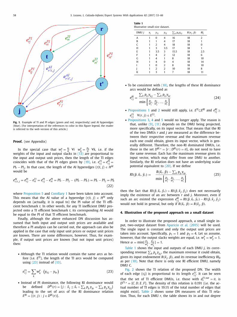
58 S. Lozano, L. Calzada-Infante / Expert Systems With Applications 82 (2017) 53–66

Fig. 1. Example of TI and PI edges (green and red, respectively) and AI hyperedges

(blue). (For interpretation of the references to color in this figure legend, the reader

is referred to the web version of this article.)

Proof. (see Appendix)

In the special case that w x i

= q i α ∀ i w

y k

= p k α ∀ k , i.e. if the

weights of the input and output slacks in (13) are proportional to

the input and output unit prices, then the length of the TI edges

coincides with that of the PI edges given by (19) , i.e. e T I r j = e PI

r j =

P I r − P I j . In that case, the length of the AI hyperedges ( r / t, j ) ∈ H AI

would be

e AI r/t, j = e PI r j − e T I rt = e PI r j − e PI rt = P I r − P I j − ( P I r − P I t ) = P I t − P I j = P I t

(22)

where Proposition 5 and Corollary 1 have been taken into account.

This means that the AI value of a hyperedge ( r / t, j ) ∈ H AI only

depends on (actually, it is equal to) the PI value of the TI effi-

cient benchmark t . In other words, for any TI inefficient DMU pro-

jected onto a TI efficient benchmark t , its corresponding AI would

be equal to the PI of that TI efficient benchmark.

Finally, although the above enhanced DN discussion has as-

sumed that both input and output unit prices are available and

therefore a PI analysis can be carried out, the approach can also be

applied in the case that only input unit prices or output unit prices

are known. There are some differences, however. Thus, for exam-

ple, if output unit prices are known (but not input unit prices)

then:

• Although the TI relation would contain the same arcs as be-

fore (i.e. E TI ), the length of the TI arcs would be computed

using (23) instead of (13) .

e T I r j =

∑

k

w y k ·(

y k j − y kr )

(23)

• Instead of PI dominance, the following RI dominance would

be defined D RI (r) = { j : x j ≤ x r ∧ ∑

k p k y kr < ∑

k p k y k j }

leading to the set of arcs of the RI dominance relation

E RI = { ( r, j ) : j ∈ D RI (r) } .

Table 1

Illustrative small-size dataset.

DMU j x j y 1 j y 2 j ∑

k p k y k j R ( x j , p ) RI j

A 1 0 4 16 18 2

B 1 1 4 17 18 1

C 1 2 4 18 18 0

D 1 3 3.5 17 18 1

E 1 3.5 3 15.5 18 2.5

F 1 4 2 12 18 6

G 1 4 1 8 18 10

H 1 4 0 4 18 14

I 1 0 2 8 18 10

J 1 2 2 10 18 8

K 1 3 1 7 18 11

• To be consistent with (10) , the lengths of these RI dominance

arcs would be defined as

e RI r j =

∑

k p k y k j −∑

k p k y kr

min {

p 1 w y 1

, p 2 w y 2

, ..., p s w y s

} (24)

• Propositions 1 and 2 would still apply, i.e. E TI ⊆E RI and e RI r j ≥

e T I r j ∀ (r, j) ∈ E T I .

• Propositions 3 , 4 and 5 would no longer apply. The reason is

that, unlike (9) , (11) depends on the DMU being projected,

more specifically, on its input vector. That means that the RI

of the two DMUs r and j are measured as the difference be-

tween their respective revenue and the maximum revenue

each one could obtain, given its input vector, which is gen-

erally different. Therefore, the non-RI dominated DMUs, i.e.

those in the set D RI, ∗ = { r : D RI (r) = ∅ } , do not need to have the same revenue. Each has the maximum revenue given its

input vector, which may differ from one DMU to another.

Similarly, the RI relation does not have an underlying scalar

potential equivalent to (20) . If we define

RI ( p , x r , y r ) = R ( x r , p ) −

∑

k p k y kr

min {

p 1 w y 1

, p 2 w y 2

, ..., p s w y s

} (25)

then the fact that RI( p , x r , y r ) > RI( p , x j , y j ) does not necessarily

imply the existence of an arc between r and j . Moreover, even if

such an arc existed the expression e RI r j = RI( p , x r , y r ) − RI( p , x j , y j )

would not hold in general, but only if R ( x r , p ) = R ( x j , p ) .

4. Illustration of the proposed approach on a small dataset

In order to illustrate the proposed approach, a small single in-

put, two-output dataset from Aparicio et al. (2015) will be used.

The single input is constant and only the output unit prices are

taken into account. Specifically, p 1 = 1 and p 2 = 4 . Let us assume,

however, that the output slacks weights are equal, i.e. w y 1 = w

y 2 = 1 .

Hence α = min { p 1 w y 1 ,

p 2 w y 2 } = 1 .

Table 1 shows the input and outputs of each DMU j , its corre-

sponding revenue ∑

k p k y k j , the maximum revenue it could obtain,

given its input endowment R ( x j , p ) , and its revenue inefficiency RI 0 as per (10) . Note that there is only one RI efficient DMU, namely

DMU C.

Fig. 2 shows the TI relation of the proposed DN. The width

of each edge (r,j) is proportional to its length e T I r j . It can be seen

that the set of TI efficient DMUs, i.e. those with d T I,out r = ∅ , is

D T I, ∗ = { C, D, E, F } . The density of this relation is 0.191 (i.e. the ac- tual number of TI edges is 19.1% of the total number of edges that

might exist). Table 2 shows some DN measures of this TI rela-

tion. Thus, for each DMU r , the table shows its in and out degree

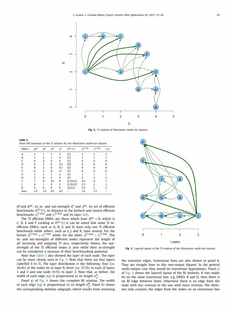
S. Lozano, L. Calzada-Infante / Expert Systems With Applications 82 (2017) 53–66 59

Fig. 2. TI relation of illustrative small-size dataset.

Table 2

Some DN measures of the TI relation for the illustrative small-size dataset.

DMU r d out r d in r s out r s in r D TI , ∗( r ) e TI, max r τ TI, min

r λ( r )

A 2 1 3 2 {C} 2 2 2

B 1 2 1 4 {C} 1 1 1

C 0 4 0 9 {C} 0 0 0

D 0 3 0 9.5 {D} 0 0 0

E 0 3 0 9.5 {E} 0 0 0

F 0 5 0 11 {F} 0 0 0

G 1 2 1 2 {F} 1 1 1

H 2 0 3 0 {F} 2 2 2

I 7 0 24 0 {C,D,E,F} 4.5 4 3

J 4 1 9 2 {C,D,E,F} 2.5 2 1

K 4 0 8 0 {D,E,F} 2.5 2 2

Aver. 1.9 1.9 4.5 4.5 – 1.4 1.3 –

d in r and d out r , its in- and out-strength s in r and s out r , its set of efficient

benchmarks D TI , ∗( r ), its distance to the farthest and closest efficient

benchmarks e T I, max r and τ T I, min

r and its layer λ( r ).

The TI efficient DMUs are those which have d out r = 0 , which is

C, D, E and F. Looking at D TI , ∗( r ) it can be noted that some TI in-

efficient DMUs, such as A, B, G and H, have only one TI efficient

benchmark while others, such as I, J and K, have several. For the

former e T I, max r = τ T I, min

r while, for the latter, e T I, max r > τ T I, min

r . The

in- and out-strengths of different nodes represent the length of

all incoming and outgoing TI arcs, respectively. Hence, the out-

strength of the TI efficient nodes is zero while their in-strength

can be considered a measure of their benchmarking potential.

Note that Table 2 also showed the layer of each node. The layer

can be more clearly seen in Fig. 3 . Note that there are four layers

(labelled 0 to 3). The layer distribution is the following: four (i.e.

36.4%) of the nodes lie in layer 0, three (i.e. 27.3%) in each of layers

1 and 3 and one node (9.1%) in layer 3. Note that, as before, the

width of each edge (r,j) is proportional to its length e T I r j .

Panel a) of Fig. 4 shows the complete RI relation. The width

of each edge (r,j) is proportional to its length e RI r j . Panel b) shows

the corresponding skeleton subgraph, which results from removing

Fig. 3. Layered layout of the TI relation of the illustrative small-size dataset.

the transitive edges. Isorevenue lines are also shown in panel b.

They are straight lines in this two-output dataset. In the general

multi-output case they would be isorevenue hyperplanes. Panel c)

of Fig. 4 shows the layered layout of the RI skeleton. If two nodes

lie on the same isorevenue line, e.g. DMUs B and D, then there is

no RI edge between them. Otherwise there is an edge from the

node with less revenue to the one with more revenue. The skele-

ton only contains the edges from the nodes on an isorevenue line

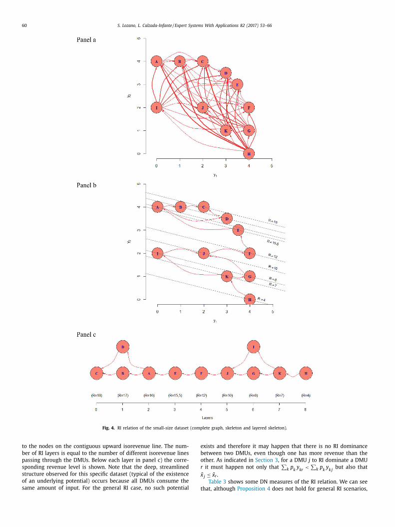
60 S. Lozano, L. Calzada-Infante / Expert Systems With Applications 82 (2017) 53–66

Fig. 4. RI relation of the small-size dataset (complete graph, skeleton and layered skeleton).

to the nodes on the contiguous upward isorevenue line. The num-

ber of RI layers is equal to the number of different isorevenue lines

passing through the DMUs. Below each layer in panel c) the corre-

sponding revenue level is shown. Note that the deep, streamlined

structure observed for this specific dataset (typical of the existence

of an underlying potential) occurs because all DMUs consume the

same amount of input. For the general RI case, no such potential

exists and therefore it may happen that there is no RI dominance

between two DMUs, even though one has more revenue than the

other. As indicated in Section 3 , for a DMU j to RI dominate a DMU

r it must happen not only that ∑

k p k y kr < ∑

k p k y k j but also that

x j ≤ x r .

Table 3 shows some DN measures of the RI relation. We can see

that, although Proposition 4 does not hold for general RI scenarios,

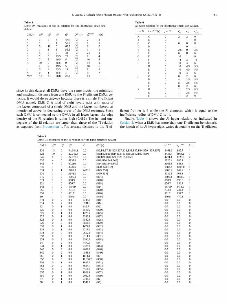
S. Lozano, L. Calzada-Infante / Expert Systems With Applications 82 (2017) 53–66 61

Table 3

Some DN measures of the RI relation for the illustrative small-size

dataset.

DMU r d out r d in r s out r s in r D RI , ∗( r ) e RI, max r λ( r )

A 3 7 4 47.5 {C} 2 2

B 1 8 1 55.5 {C} 1 1

C 0 10 0 65.5 {C} 0 0

D 1 8 1 55.5 {C} 1 1

E 4 6 6 44 {C} 2.5 3

F 5 5 23.5 23 {C} 6 4

G 7 2 49.5 5 {C} 10 6

H 10 0 88.5 0 {C} 14 8

I 7 2 49.5 5 {C} 10 6

J 6 4 35.5 13 {C} 8 5

K 9 1 58.5 3 {C} 11 7

Aver. 4.8 4.8 28.8 28.8 – 6.0 –

since in this dataset all DMUs have the same inputs, the minimum

and maximum distance from any DMU to the PI efficient DMUs co-

incide. It would do so anyway because there is a single PI-efficient

DMU, namely DMU C. A total of eight layers exist with most of

the layers composed of a single DMU and the layers numbered, as

mentioned above, in decreasing order of the DMU revenues. Since

each DMU is connected to the DMUs in all lower layers, the edge

density of the RI relation is rather high (0.482). The in- and out-

degrees of the RI relation are larger than those of the TI relation

as expected from Proposition 1 . The average distance to the PI ef-

Table 4

AI hyper-relation for the illustrative small-size dataset.

r ∈ D t ∈ D TI , ∗( r ) j ∈ D RI , ∗ e RI r j e TI rt e AI

r/t, j

A C C 2 2 0

B C C 1 1 0

C C C 0 0 0

D D C 1 0 1

E E C 2.5 0 2.5

F F C 6 0 6

G F C 10 1 9

H F C 14 2 12

I C C 10 4 6

D C 10 4.5 5.5

E C 10 4.5 5.5

F C 10 4 6

J C C 8 2 6

D C 8 2.5 5.5

E C 8 2.5 5.5

F C 8 2 6

K D C 11 2.5 8.5

E C 11 2.5 8.5

F C 11 2 9

ficient frontier is 6 while the RI diameter, which is equal to the

inefficiency radius of DMU C, is 14.

Finally, Table 4 shows the AI hyper-relation. As indicated in

Section 3 , when a DMU has more than one TI efficient benchmark,

the length of its AI hyperedges varies depending on the TI efficient

Table 5

Some DN measures of the TI relation for the bank branches dataset.

DMU r d out r d in r s out r s in r D TI , ∗( r ) e TI, max r τ TI, min

r λ( r )

B36 13 0 34,644.1 0.0 {B2;B4;B7;B8;B25;B27;B28;B33;B37;B44;B50; B55;B57} 4468.6 945.7 1

B22 10 0 20,042.4 0.0 {B5;B10;B20;B29;B32; B38;B50;B52;B53;B59} 3438.4 1014.3 1

B45 8 0 22,679.0 0.0 {B4;B20;B28;B29;B37; B50;B55} 4274.3 1723.8 2

B39 4 0 6237.9 0.0 {B10;B34;B46;B49} 2225.4 885.7 1

B42 4 0 6921.0 0.0 {B14;B38;B46;B49} 2363.5 848.5 1

B30 3 0 4227.6 0.0 {B20;B28;B37} 1582.2 1234.0 1

B18 2 1 2765.7 2473.6 {B29;B50} 1800.8 964.9 1

B26 2 0 2988.6 0.0 {B50;B53} 2225.8 762.8 1

B15 1 0 1806.3 0.0 {B34} 1806.3 1806.3 1

B19 1 0 890.9 0.0 {B20} 890.9 890.9 1

B21 1 0 656.7 0.0 {B38} 656.7 656.7 1

B48 1 0 1414.9 0.0 {B14} 1414.9 1414.9 1

B56 1 0 733.3 0.0 {B20} 733.3 733.3 1

B58 1 0 831.7 0.0 {B20} 831.7 831.7 1

B9 1 0 470.5 0.0 {B46} 470.5 470.5 1

B10 0 2 0.0 3746.3 {B10} 0.0 0.0 0

B14 0 2 0.0 3241.6 {B14} 0.0 0.0 0

B2 0 1 0.0 945.7 {B2} 0.0 0.0 0

B20 0 6 0.0 8590.2 {B20} 0.0 0.0 0

B25 0 1 0.0 1479.7 {B25} 0.0 0.0 0

B27 0 1 0.0 3343.1 {B27} 0.0 0.0 0

B28 0 3 0.0 7582.6 {B28} 0.0 0.0 0

B29 0 3 0.0 8886.4 {B29} 0.0 0.0 0

B32 0 1 0.0 1477.0 {B32} 0.0 0.0 0

B33 0 1 0.0 2717.2 {B33} 0.0 0.0 0

B34 0 2 0.0 2692.0 {B34} 0.0 0.0 0

B37 0 3 0.0 8114.9 {B37} 0.0 0.0 0

B38 0 3 0.0 3196.7 {B38} 0.0 0.0 0

B4 0 2 0.0 4477.6 {B4} 0.0 0.0 0

B44 0 1 0.0 2329.6 {B44} 0.0 0.0 0

B46 0 3 0.0 4096.9 {B46} 0.0 0.0 0

B49 0 2 0.0 4588.9 {B49} 0.0 0.0 0

B5 0 1 0.0 1014.3 {B5} 0.0 0.0 0

B50 0 5 0.0 11,610.2 {B50} 0.0 0.0 0

B52 0 1 0.0 1693.5 {B52} 0.0 0.0 0

B53 0 2 0.0 5664.3 {B53} 0.0 0.0 0

B55 0 2 0.0 5560.7 {B55} 0.0 0.0 0

B57 0 1 0.0 1668.9 {B57} 0.0 0.0 0

B59 0 1 0.0 2032.8 {B59} 0.0 0.0 0

B7 0 1 0.0 2738.0 {B7} 0.0 0.0 0

B8 0 1 0.0 1348.0 {B8} 0.0 0.0 0

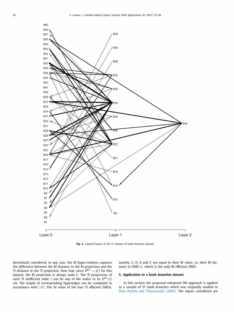
62 S. Lozano, L. Calzada-Infante / Expert Systems With Applications 82 (2017) 53–66

Fig. 5. Layered layout of the TI relation of bank branches dataset.

benchmark considered. In any case, the AI hyper-relation captures

the difference between the RI distance to the RI projection and the

TI distance to the TI projection. Note that, since D RI, ∗ = { C} for this dataset, the RI projection is always node C. The TI projections of

each TI inefficient node r can be any of the nodes in its D TI , ∗( r )

set. The length of corresponding hyperedges can be computed in

accordance with (18) . The AI value of the four TI efficient DMUs,

namely, C, D, E and F, are equal to their RI value, i.e. their RI dis-

tance to DMU C, which is the only RI efficient DMU.

5. Application to a bank branches dataset

In this section the proposed enhanced DN approach is applied

to a sample of 57 bank branches which was originally studied in

Silva Portela and Thanassoulis (2005) . The inputs considered are

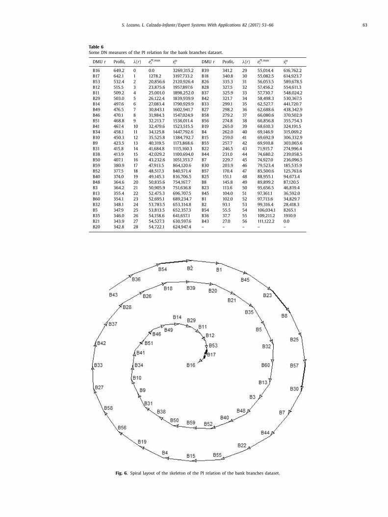
S. Lozano, L. Calzada-Infante / Expert Systems With Applications 82 (2017) 53–66 63

Table 6

Some DN measures of the PI relation for the bank branches dataset.

DMU r Profit r λ( r ) e PI, max r s in r DMU r Profit r λ( r ) e PI, max

r s in r

B16 649.2 0 0.0 3269,315.2 B39 341.2 29 55,014.4 616,762.2

B17 642.1 1 1278.2 3197,733.2 B18 340.8 30 55,082.5 614,923.7

B53 532.4 2 20,856.6 2120,926.4 B26 335.3 31 56,053.5 589,678.5

B12 515.5 3 23,875.6 1957,897.6 B28 327.5 32 57,456.2 554,611.3

B11 509.2 4 25,001.0 1898,252.0 B37 325.9 33 57,730.7 548,024.2

B29 503.0 5 26,122.4 1839,939.9 B42 321.7 34 58,498.3 530,367.5

B14 497.6 6 27,083.4 1790,929.9 B33 299.1 35 62,527.7 441,720.7

B49 476.5 7 30,843.1 1602,941.7 B27 298.2 36 62,688.6 438,342.9

B46 470.1 8 31,984.3 1547,024.9 B58 279.2 37 66,080.6 370,502.9

B51 468.8 9 32,213.7 1536,011.4 B56 274.8 38 66,856.8 355,754.3

B41 467.4 10 32,479.6 1523,515.5 B19 265.0 39 68,610.3 324,191.5

B34 458.1 11 34,125.8 1447,792.6 B4 262.0 40 69,146.9 315,069.2

B10 450.3 12 35,525.8 1384,792.7 B15 259.0 41 69,692.9 306,332.9

B9 423.5 13 40,319.5 1173,868.6 B55 257.7 42 69,910.8 303,065.6

B31 415.8 14 41,684.8 1115,160.3 B22 246.5 43 71,915.7 274,996.4

B38 413.9 15 42,029.2 1100,694.0 B44 231.0 44 74,680.2 239,058.5

B50 407.1 16 43,232.6 1051,353.7 B7 229.7 45 74,927.0 236,096.5

B59 380.9 17 47,913.5 864,120.6 B30 203.9 46 79,523.4 185,535.9

B52 377.5 18 48,517.3 840,571.4 B57 170.4 47 85,500.6 125,763.6

B40 374.0 19 49,145.3 816,706.5 B25 151.1 48 88,955.1 94,673.4

B48 364.6 20 50,835.6 754,167.7 B8 145.8 49 89,899.2 87,120.5

B3 364.2 21 50,905.9 751,636.8 B23 113.6 50 95,656.5 46,819.4

B13 355.4 22 52,475.3 696,707.5 B45 104.0 51 97,361.1 36,592.0

B60 354.1 23 52,695.1 689,234.7 B1 102.0 52 97,713.6 34,829.7

B32 348.1 24 53,783.5 653,314.8 B2 93.1 53 99,316.4 28,418.3

B5 347.9 25 53,813.5 652,357.3 B54 55.5 54 106,034.1 8265.1

B35 346.0 26 54,158.6 641,657.1 B36 37.7 55 109,211.2 1910.9

B21 343.9 27 54,527.3 630,597.6 B43 27.0 56 111,122.2 0.0

B20 342.8 28 54,722.1 624,947.4 – – – – –

Fig. 6. Spiral layout of the skeleton of the PI relation of the bank branches dataset.

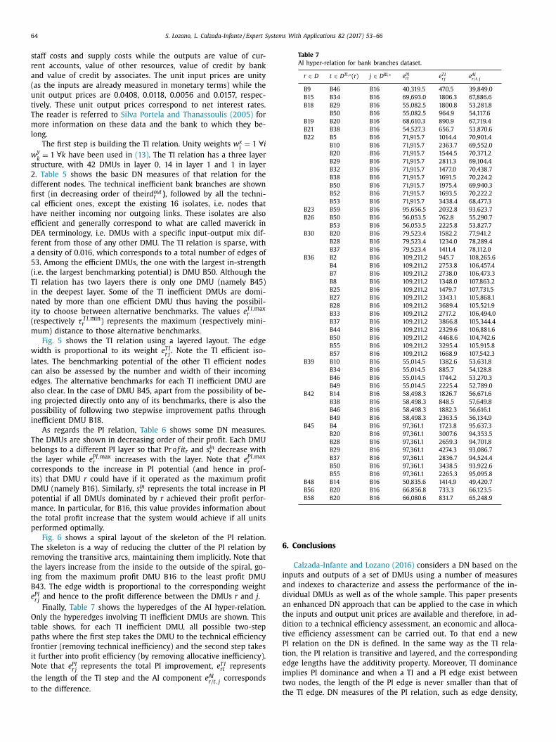
64 S. Lozano, L. Calzada-Infante / Expert Systems With Applications 82 (2017) 53–66

staff costs and supply costs while the outputs are value of cur-

rent accounts, value of other resources, value of credit by bank

and value of credit by associates. The unit input prices are unity

(as the inputs are already measured in monetary terms) while the

unit output prices are 0.0408, 0.0118, 0.0056 and 0.0157, respec-

tively. These unit output prices correspond to net interest rates.

The reader is referred to Silva Portela and Thanassoulis (2005) for

more information on these data and the bank to which they be-

long.

The first step is building the TI relation. Unity weights w x i

= 1 ∀ i

w y k

= 1 ∀ k have been used in (13) . The TI relation has a three layer

structure, with 42 DMUs in layer 0, 14 in layer 1 and 1 in layer

2. Table 5 shows the basic DN measures of that relation for the

different nodes. The technical inefficient bank branches are shown

first (in decreasing order of their d out r ) , followed by all the techni-

cal efficient ones, except the existing 16 isolates, i.e. nodes that

have neither incoming nor outgoing links. These isolates are also

efficient and generally correspond to what are called maverick in

DEA terminology, i.e. DMUs with a specific input-output mix dif-

ferent from those of any other DMU. The TI relation is sparse, with

a density of 0.016, which corresponds to a total number of edges of

53. Among the efficient DMUs, the one with the largest in-strength

(i.e. the largest benchmarking potential) is DMU B50. Although the

TI relation has two layers there is only one DMU (namely B45)

in the deepest layer. Some of the TI inefficient DMUs are domi-

nated by more than one efficient DMU thus having the possibil-

ity to choose between alternative benchmarks. The values e T I, max r

(respectively τ T I, min r ) represents the maximum (respectively mini-

mum) distance to those alternative benchmarks.

Fig. 5 shows the TI relation using a layered layout. The edge

width is proportional to its weight e T I r j . Note the TI efficient iso-

lates. The benchmarking potential of the other TI efficient nodes

can also be assessed by the number and width of their incoming

edges. The alternative benchmarks for each TI inefficient DMU are

also clear. In the case of DMU B45, apart from the possibility of be-

ing projected directly onto any of its benchmarks, there is also the

possibility of following two stepwise improvement paths through

inefficient DMU B18.

As regards the PI relation, Table 6 shows some DN measures.

The DMUs are shown in decreasing order of their profit. Each DMU

belongs to a different PI layer so that Pr of i t r and s in r decrease with

the layer while e PI, max r increases with the layer. Note that e PI, max

r

corresponds to the increase in PI potential (and hence in prof-

its) that DMU r could have if it operated as the maximum profit

DMU (namely B16). Similarly, s in r represents the total increase in PI

potential if all DMUs dominated by r achieved their profit perfor-

mance. In particular, for B16, this value provides information about

the total profit increase that the system would achieve if all units

performed optimally.

Fig. 6 shows a spiral layout of the skeleton of the PI relation.

The skeleton is a way of reducing the clutter of the PI relation by

removing the transitive arcs, maintaining them implicitly. Note that

the layers increase from the inside to the outside of the spiral, go-

ing from the maximum profit DMU B16 to the least profit DMU

B43. The edge width is proportional to the corresponding weight

e PI r j and hence to the profit difference between the DMUs r and j .

Finally, Table 7 shows the hyperedges of the AI hyper-relation.

Only the hyperedges involving TI inefficient DMUs are shown. This

table shows, for each TI inefficient DMU, all possible two-step

paths where the first step takes the DMU to the technical efficiency

frontier (removing technical inefficiency) and the second step takes

it further into profit efficiency (by removing allocative inefficiency).

Note that e PI r j represents the total PI improvement, e T I rt represents

the length of the TI step and the AI component e AI r/t, j corresponds

to the difference.

Table 7

AI hyper-relation for bank branches dataset.

r ∈ D t ∈ D TI , ∗( r ) j ∈ D RI , ∗ e PI rt e TI r j e AI

r/t, j

B9 B46 B16 40,319.5 470.5 39,849.0

B15 B34 B16 69,693.0 1806.3 67,886.6

B18 B29 B16 55,082.5 1800.8 53,281.8

B50 B16 55,082.5 964.9 54,117.6

B19 B20 B16 68,610.3 890.9 67,719.4

B21 B38 B16 54,527.3 656.7 53,870.6

B22 B5 B16 71,915.7 1014.4 70,901.4

B10 B16 71,915.7 2363.7 69,552.0

B20 B16 71,915.7 1544.5 70,371.2

B29 B16 71,915.7 2811.3 69,104.4

B32 B16 71,915.7 1477.0 70,438.7

B38 B16 71,915.7 1691.5 70,224.2

B50 B16 71,915.7 1975.4 69,940.3

B52 B16 71,915.7 1693.5 70,222.2

B53 B16 71,915.7 3438.4 68,477.3

B23 B59 B16 95,656.5 2032.8 93,623.7

B26 B50 B16 56,053.5 762.8 55,290.7

B53 B16 56,053.5 2225.8 53,827.7

B30 B20 B16 79,523.4 1582.2 77,941.2

B28 B16 79,523.4 1234.0 78,289.4

B37 B16 79,523.4 1411.4 78,112.0

B36 B2 B16 109,211.2 945.7 108,265.6

B4 B16 109,211.2 2753.8 106,457.4

B7 B16 109,211.2 2738.0 106,473.3

B8 B16 109,211.2 1348.0 107,863.2

B25 B16 109,211.2 1479.7 107,731.5

B27 B16 109,211.2 3343.1 105,868.1

B28 B16 109,211.2 3689.4 105,521.9

B33 B16 109,211.2 2717.2 106,494.0

B37 B16 109,211.2 3866.8 105,344.4

B44 B16 109,211.2 2329.6 106,881.6

B50 B16 109,211.2 4468.6 104,742.6

B55 B16 109,211.2 3295.4 105,915.8

B57 B16 109,211.2 1668.9 107,542.3

B39 B10 B16 55,014.5 1382.6 53,631.8

B34 B16 55,014.5 885.7 54,128.8

B46 B16 55,014.5 1744.2 53,270.3

B49 B16 55,014.5 2225.4 52,789.0

B42 B14 B16 58,498.3 1826.7 56,671.6

B38 B16 58,498.3 848.5 57,649.8

B46 B16 58,498.3 1882.3 56,616.1

B49 B16 58,498.3 2363.5 56,134.9

B45 B4 B16 97,361.1 1723.8 95,637.3

B20 B16 97,361.1 3007.6 94,353.5

B28 B16 97,361.1 2659.3 94,701.8

B29 B16 97,361.1 4274.3 93,086.7

B37 B16 97,361.1 2836.7 94,524.4

B50 B16 97,361.1 3438.5 93,922.6

B55 B16 97,361.1 2265.3 95,095.8

B48 B14 B16 50,835.6 1414.9 49,420.7

B56 B20 B16 66,856.8 733.3 66,123.5

B58 B20 B16 66,080.6 831.7 65,248.9

6. Conclusions

Calzada-Infante and Lozano (2016) considers a DN based on the

inputs and outputs of a set of DMUs using a number of measures

and indexes to characterize and assess the performance of the in-

dividual DMUs as well as of the whole sample. This paper presents

an enhanced DN approach that can be applied to the case in which

the inputs and output unit prices are available and therefore, in ad-

dition to a technical efficiency assessment, an economic and alloca-

tive efficiency assessment can be carried out. To that end a new

PI relation on the DN is defined. In the same way as the TI rela-

tion, the PI relation is transitive and layered, and the corresponding

edge lengths have the additivity property. Moreover, TI dominance

implies PI dominance and when a TI and a PI edge exist between

two nodes, the length of the PI edge is never smaller than that of

the TI edge. DN measures of the PI relation, such as edge density,

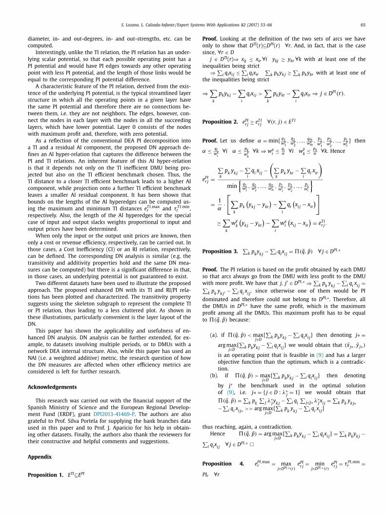
S. Lozano, L. Calzada-Infante / Expert Systems With Applications 82 (2017) 53–66 65

diameter, in- and out-degrees, in- and out-strengths, etc. can be

computed.

Interestingly, unlike the TI relation, the PI relation has an under-

lying scalar potential, so that each possible operating point has a

PI potential and would have PI edges towards any other operating

point with less PI potential, and the length of those links would be

equal to the corresponding PI potential difference.

A characteristic feature of the PI relation, derived from the exis-

tence of the underlying PI potential, is the typical streamlined layer

structure in which all the operating points in a given layer have

the same PI potential and therefore there are no connections be-

tween them, i.e. they are not neighbors. The edges, however, con-

nect the nodes in each layer with the nodes in all the succeeding

layers, which have lower potential. Layer 0 consists of the nodes

with maximum profit and, therefore, with zero potential.

As a reflection of the conventional DEA PI decomposition into

a TI and a residual AI component, the proposed DN approach de-

fines an AI hyper-relation that captures the difference between the

PI and TI relations. An inherent feature of this AI hyper-relation

is that it depends not only on the TI inefficient DMU being pro-

jected but also on the TI efficient benchmark chosen. Thus, the

TI distance to a closer TI efficient benchmark leads to a higher AI

component, while projection onto a further TI efficient benchmark

leaves a smaller AI residual component. It has been shown that

bounds on the lengths of the AI hyperedges can be computed us-

ing the maximum and minimum TI distances e T I, max r and τ T I, min

r ,

respectively. Also, the length of the AI hyperedges for the special

case of input and output slacks weights proportional to input and

output prices have been determined.

When only the input or the output unit prices are known, then

only a cost or revenue efficiency, respectively, can be carried out. In

those cases, a Cost Inefficiency (CI) or an RI relation, respectively,

can be defined. The corresponding DN analysis is similar (e.g. the

transitivity and additivity properties hold and the same DN mea-

sures can be computed) but there is a significant difference in that,

in those cases, an underlying potential is not guaranteed to exist.

Two different datasets have been used to illustrate the proposed

approach. The proposed enhanced DN with its TI and RI/PI rela-

tions has been plotted and characterized. The transitivity property

suggests using the skeleton subgraph to represent the complete TI

or PI relation, thus leading to a less cluttered plot. As shown in

these illustrations, particularly convenient is the layer layout of the

DN.

This paper has shown the applicability and usefulness of en-

hanced DN analysis. DN analysis can be further extended, for ex-

ample, to datasets involving multiple periods, or to DMUs with a

network DEA internal structure. Also, while this paper has used an

NAI (i.e. a weighted additive) metric, the research question of how

the DN measures are affected when other efficiency metrics are

considered is left for further research.

Acknowledgements

This research was carried out with the financial support of the

Spanish Ministry of Science and the European Regional Develop-

ment Fund (ERDF), grant DPI2013-41469-P . The authors are also

grateful to Prof. Silva Portela for supplying the bank branches data

used in this paper and to Prof. J. Aparicio for his help in obtain-

ing other datasets. Finally, the authors also thank the reviewers for

their constructive and helpful comments and suggestions.

Appendix

Proposition 1. E TI ⊆E PI

Proof. Looking at the definition of the two sets of arcs we have

only to show that D TI ( r ) ⊆D PI ( r ) ∀ r . And, in fact, that is the case

since, ∀ r ∈ D

j ∈ D TI ( r ) ⇒ x ij ≤ x ir ∀ i y kj ≥ y kr ∀ k with at least one of the

inequalities being strict

⇒ ∑

i q i x i j ≤∑

i q i x ir ∑

k p k y k j ≥∑

k p k y kr with at least one of

the inequalities being strict

⇒

∑

k

p k y k j −∑

i

q i x i j >

∑

k

p k y kr −∑

i

q i x ir ⇒ j ∈ D PI (r) .

Proposition 2. e PI r j ≥ e T I

r j ∀ (r, j) ∈ E T I

Proof. Let us define α = min { q 1 w x 1 ,

q 2 w x 2 , ...,

q m w x m

, p 1 w y 1 ,

p 2 w y 2 , ...,

p s w y s

} then

α ≤q i w x i

∀ i α ≤p k w y k

∀ k ⇒ w x i

≤q i α ∀ i w

y k

≤p k α ∀ k . Hence

e PI r j =

∑

k

p k y k j

−∑

i

q i x i j −

(

∑

k

p k y kr

−∑

i

q i x ir

)

min {

q 1 w x 1

, q 2 w x 2

, ..., q m w x m

, p 1 w y 1

, p 2 w y 2

, ..., p s w y s

}

= 1

α·

[

∑

k

p k (

y k j − y kr )

−∑

i

q i (

x i j − x ir )

]

≥∑

k

w y k

(

y k j − y kr )

−∑

i

w x i

(

x i j − x ir )

= e T I r j .

Proposition 3. ∑

k p k y k j −∑

i q i x i j = �( q , p ) ∀ j ∈ D PI, ∗

Proof. The PI relation is based on the profit obtained by each DMU

so that arcs always go from the DMU with less profit to the DMU

with more profit. We have that j, j ′ ∈ D PI, ∗ ⇒ ∑

k p k y k j −∑

i q i x i j = ∑

k p k y k j ′ −∑

i q i x i j ′ since otherwise one of them would be PI

dominated and therefore could not belong to D PI , ∗. Therefore, all

the DMUs in D PI , ∗ have the same profit, which is the maximum

profit among all the DMUs. This maximum profit has to be equal

to �( q , p ) because:

(a). if �( q , p ) < max j∈ D

{ ∑

k p k y k j −∑

i q i x i j } then denoting j∗ =

arg max j∈ D

{ ∑

k p k y k j −∑

i q i x i j } we would obtain that ( x j∗, y j∗)

is an operating point that is feasible in (9) and has a larger

objective function than the optimum, which is a contradic-

tion.

(b). if �( q , p ) > max j∈ D

{ ∑

k p k y k j −∑

i q i x i j } then denoting

by j ∗ the benchmark used in the optimal solution

of (9) , i.e. j∗ = { j ∈ D : λ∗j = 1 } we would obtain that

�( q , p ) = ∑

k p k ∑

j λ∗j y k j −

∑

i q i ∑

j∈ J∗ λ∗j x i j =

∑

k p k y k j∗−

∑

i q i x i j∗ >> arg max j∈ D

{ ∑

k p k y k j −∑

i q i x i j }

thus reaching, again, a contradiction.

Hence �( q , p ) = arg max j∈ D

{ ∑

k p k y k j −∑

i q i x i j } = ∑

k p k y k j −

∑

i q i x i j ∀ j ∈ D PI, ∗ �

Proposition 4. e PI, max r = max

j∈ D PI, ∗(r) e PI r j = min

j∈ D PI, ∗(r) e PI r j = τ PI, min

r =

P I r ∀ r

66 S. Lozano, L. Calzada-Infante / Expert Systems With Applications 82 (2017) 53–66

Proof. By (1) , Proposition 3 and (8) it follows that

e PI r j =

∑

k p k y k j −

∑

i q i x i j −

(

∑

k p k y kr −

∑

i q i x ir

)

min {

q 1 w x

1 ,

q 2 w x

2 , ...,

q m w x m

, p 1 w y

1 ,

p 2 w y

2 , ...,

p s w y s

}

=

�( q , p ) −

(

∑

k p k y kr −

∑

i q i x ir

)

min {

q 1 w x

1 ,

q 2 w x

2 , ...,

q m w x m

, p 1 w y 1

, p 2 w y 2

, ..., p s w y s

} = P I r ∀ j ∈ D PI, ∗

Hence, the PI distance from r to any PI efficient DMU (if there is

more than one) is exactly the same and coincides with its PI score.

�

Proposition 5. The PI relation results from an underlying scalar

potential P I( q , p , x , y ) . Moreover, the PI arc lengths are equal to the

potential differences between the nodes, i.e. e PI r j = P I( q , p , x r , y r ) −

P I( q , p , x j , y j ) = P I r − P I j

Proof. The existence of an underlying potential field means that

each node r has a potential P I( q , p , x r , y r ) so that there exist arcs

from nodes with higher potential to nodes with lower potential. In

our case the potential corresponds to the profit inefficiency (20) .

Hence

P I ( q , p , x r , y r ) − P I (

q , p , x j , y j )

= 1

α·

[

�( q , p ) −

(

∑

k

p k y kr −∑

i

q i x ir

) ]

−1

α·

[

�( q , p ) −

(

∑

k

p k y k j −∑

i

q i x i j

) ]

= 1

α·

[ (

∑

k

p k y k j −∑

i

q i x i j

)

−

(

∑

k

p k y kr −∑

i

q i x ir

) ]

= e PI r j

Proposition 6. P I r − e T I, max r ≤ e AI

r/t, j ≤ P I r − τ T I, min r ∀ (r/t, j) ∈ H AI

Proof. On the one hand, e T I rt is bounded by e T I, max r and τ T I, min

r

as τ T I, min r = min

t ′ ∈ D TI, ∗(r) e T I rt ′

≤ e T I rt ≤ max t ′ ∈ D TI, ∗(r)

e T I rt ′

= e T I, max r ∀ r ∈

D \ D T I, ∗ ∀ t ∈ D T I, ∗(r) .

On the other hand, from Proposition 5 and Corollary 1 , we

have that e PI r j = P I r − P I j = P I r ∀ j ∈ D PI, ∗. Hence, from (18) , the re-

sult follows. �

References

Aparicio, J. , Borras, F. , Pastor, J. T. , & Vidal, F. (2013). Accounting for slacks to mea- sure and decompose revenue efficiency in the Spanish Designation of Origin wines with DEA. European Journal of Operational Research, 231 , 443 −451 .

Aparicio, J. , Borras, F. , Pastor, J. T. , & Vidal, F. (2015). Measuring and decomposing firm’s revenue and cost efficiency: The Russell measures revisited. International Journal of Production Economics, 165 , 19 −28 .

Bardhan, I. , Bowlin, W. F. , Cooper, W. W. , & Sueyoshi, T. (1996). Models and mea- sures for efficiency dominance in DEA. Part I: Additive models and MED mea- sures. Journal of the Operations Research Society of Japan, 39 (3), 322 −332 .

Brandes, U. (2008). On variants of shortest-path betweenness centrality and their generic computation. Social Networks, 30 , 136–145 .

Calzada-Infante, L. , & Lozano, S. (2016). Analyzing Olympic games through domi- nance networks. Physica A, 462 , 1215 −230 .

Cooper, W. W. , & Tone, K. (1997). Measures of inefficiency in data envelopment anal- ysis and stochastic frontier estimation. European Journal of Operational Research, 99 , 82 −88 .

Cooper, W. W. , Pastor, J. T. , Aparicio, J. , & Borras, F. (2011). Decomposing profit effi- ciency in DEA through the weighted additive model. European Journal of Opera- tional Research, 212 , 411 −416 .

Cooper, W. W. , Seiford, L. M. , & Tone, K. (2006). Data envelopment analysis: a com-

prehensive text with models, applications, references and DEA-solver software (2nd ed.). New York: Springer .

Cooper, W. W. , Seiford, L. M. , & Zhu, J. (2004). Handbook on data envelopment anal- ysis . New York: Springer .

Fagiolo, G. (2007). Clustering in complex directed networks. Physical Review E, 76 , 026107 .

Färe, R. , Fukuyama, H. , Grosskopf, S. , & Zelenyuk, V. (2015). Decomposing profit ef- ficiency using a slacks-based directional distance function. European Journal of Operational Research, 247 , 335 −337 .

Färe, R. , Grosskopf, S. , & Lovell, C. A. K. (1985). The measurement of efficiency of pro- duction . Kluwer Academic Publishers .

Färe, R. , Grosskopf, S. , & Lovell, C. A. K. (1994). production frontiers . Cambridge Uni- versity Press .

Ghahraman, A. , & Prior, D. (2015). A learning ladder toward efficiency: Proposing network-based stepwise benchmark selection. Omega, 63 , 83 −93 (2016) .

Ho, M. H. C. , Liu, J. S. , Lu, W. M. , & Huang, C. C. (2014). A new perspective to ex- plore the technology transfer efficiencies in US universities. Journal of Technol- ogy Transfer, 39 (2), 247 −275 .

Leem, B.-H. , & Chun, H. (2015). Measuring the influence of efficient ports using so- cial network metrics. International Journal of Engineering Business Management, 7 (1), 1 .

Liu, J. S. , & Lu, W. M. (2010). DEA and ranking with the network-based approach: A case of R&D performance. Omega, 38 (6), 453 −464 .

Liu, J. S. , Lu, W. M. , & Ho, M. H. C. (2014). National characteristics: Innovation systems from the process efficiency perspective. R & D Management, 45 (4), 317 −338 .

Liu, J. S. , Lu, W. M. , Yang, C. , & Chuang, M. (2009). A network-based approach for in- creasing discrimination in data envelopment analysis. Journal of the Operational Research Society, 60 (11), 1502 −1510 .

Pastor, J. T. , Ruiz, J. L. , & Sirvent, I. (1999). An enhanced DEA Russell graph efficiency measure. European Journal of Operational Research, 115 , 596 −607 .

Silva Portela, M. C. A. , & Thanassoulis, E. (2005). Profitability of a sample of Por- tuguese bank branches and its decomposition into technical and allocative com- ponents. European Journal of Operational Research, 162 , 850 −866 .

Silva Portela, M. C. A. , & Thanassoulis, E. (2007). Developing a decomposable mea- sure of profit efficiency using DEA. Journal of the Operational Research Society, 58 (4), 4 81 −4 90 .

Tone, K. (2001). A slacks-based measure of efficiency in data envelopment analysis. European Journal of Operational Research, 130 , 498 −509 .

Toroczkai, Z. , Kozma, B. , Bassler, K. E. , Hengartner, N. W. , & Korniss, G. (2008). Gradi- ent networks. Journal of Physics A: Mathematical and Theoretical, 41 (15), 155103 .

ARTICLE IN PRESS JID: OME [m5G; November 22, 2017;12:3 ]

Omega 0 0 0 (2017) 1–13

Contents lists available at ScienceDirect

Omega

journal homepage: www.elsevier.com/locate/omega

Computing gradient-based stepwise benchmarking paths �

Sebastián Lozano a , ∗, Laura Calzada-Infante

b

a Department of Industrial Management, University of Seville, Spain b Engineering School, University of Oviedo, Spain

a r t i c l e i n f o

Article history:

Received 6 June 2017

Accepted 15 November 2017

Available online xxx

Keywords:

Data Envelopment Analysis (DEA)

Stepwise benchmarking

Efficiency field potential

Efficiency field vector

Organic farming

a b s t r a c t

In this paper, a new stepwise benchmarking approach is presented. It is based on the concept of effi-

ciency field potential given by a continuous and differentiable function that decreases monotonously as

the amount of inputs consumed is reduced and the amount of outputs produced is increased. A gradient-

based stepwise efficiency improvement method is proposed and the graphical interpretation of the con-

tinuous gradient-based trajectories is shown. A minimum potential DEA model is also formulated. The

proposed approach is units invariant and can take into account preference structure, non-discretionary

variables and undesirable outputs. The proposed method has been applied to an organic farming dataset.

© 2017 Elsevier Ltd. All rights reserved.

1. Introduction

Data Envelopment Analysis (DEA) is a well-known non-

parametric methodology for assessing the relative efficiency of a

set of Decision Making Units (DMUs). From the inputs consump-

tion and outputs production of the observed DMUs, and using a

few axioms such as convexity and free disposability, DEA infers

a Production Possibility Set (PPS) (a.k.a. DEA technology) which

contains all the feasible operating points. The corresponding non-

dominated subset is the Efficient Frontier (EF). Conventional DEA

models project the inefficient DMUs on the EF using an orientation

(input, output, directional distance, etc.) and a metric (radial, non-

radial, slacks-based, etc.) (see, e.g., [15,16,45] ). Note, however, that

some DEA models (like radial, directional distance, hyperbolic, etc)

do not necessarily exhaust all input and output slacks and hence

may compute targets that are only weakly efficient.

Since conventional DEA models aim at reducing inputs and/or

increasing outputs as much as possible, they tend to compute ef-

ficient targets that are as “far” from the observed DMU as possi-

ble. This makes those targets harder to achieve since the improve-

ments in terms of the corresponding input reductions and output

increases may be significant.

One way to alleviate this distant target problem is to compute

the closest efficient targets. There is an abundant literature on the

� This manuscript was processed by Associate Editor Sahoo. ∗ Corresponding author: University of Seville, Department of Industrial Manage-

ment, Escuela Superior de Ingenieros, Camino de los Descubrimientos, s/n, 41092

Sevilla, Spain.

E-mail address: slozano@us.es (S. Lozano).

subject, dating back to Frei and Harker [20] , which used the Eu-

clidean distance to the strongly efficient frontier. A weighted Eu-

clidean distance to the strongly efficient frontier has been used by

Baek and Lee [12] , Amirteimoori and Kordrostami [1] and Apari-

cio and Pastor [8] . Other authors have used other ways of mea-

surement the similarity/closeness between the DMU and the po-

tential efficient targets (e.g. [13,42] ). Other approaches include

Gonzalez and Alvarez [22] , which propose a modified version of

the input-oriented Russell efficiency measure, and Aparicio et al.

[11] , which use an Enhanced Russell Graph Measure (ERGM, a.k.a.

Slacks-Based Measure, SBM) together with a characterization of

the Pareto-efficient frontier based on the set of extreme efficient

DMUs. Additional papers dealing with least distance target compu-

tation are Pastor and Aparicio [38] , Ando et al. [2,3] , Aparicio and

Pastor [7,9] and Aparicio et al. [6] . The reader is referred to Apari-

cio [4] and Aparicio et al. [5,10] for recent developments in the

field as well as an up-to-date review of the literature on this topic.

Another line of research, which is the one followed in this pa-

per, is to compute a stepwise improvement path so that a num-

ber of Intermediate Benchmark targets (IBTs) are computed, lead-

ing to an Ultimate Benchmark target (UBT) on the EF. There are

two types of stepwise efficiency improvement method: those that

use the existing DMUs as IBT and UBT and those that compute IBT

and UBT belonging to the PPS and EF respectively, but not neces-

sarily coincident with any of the existing DMUs. The second group

is composed of just a few approaches, basically Lozano and Villa

[28,29] , Suzuki and Nijkamp [44] , Khodakarami et al. [25] and Fang

[19] . The first group is more numerous and, in most cases, uses the

stratification approach proposed in the Context-Dependent (CD)

DEA approach of Seiford and Zhu [39] which identifies successive

https://doi.org/10.1016/j.omega.2017.11.002

0305-0483/© 2017 Elsevier Ltd. All rights reserved.

Please cite this article as: S. Lozano, L. Calzada-Infante, Computing gradient-based stepwise benchmarking paths, Omega (2017),

https://doi.org/10.1016/j.omega.2017.11.002

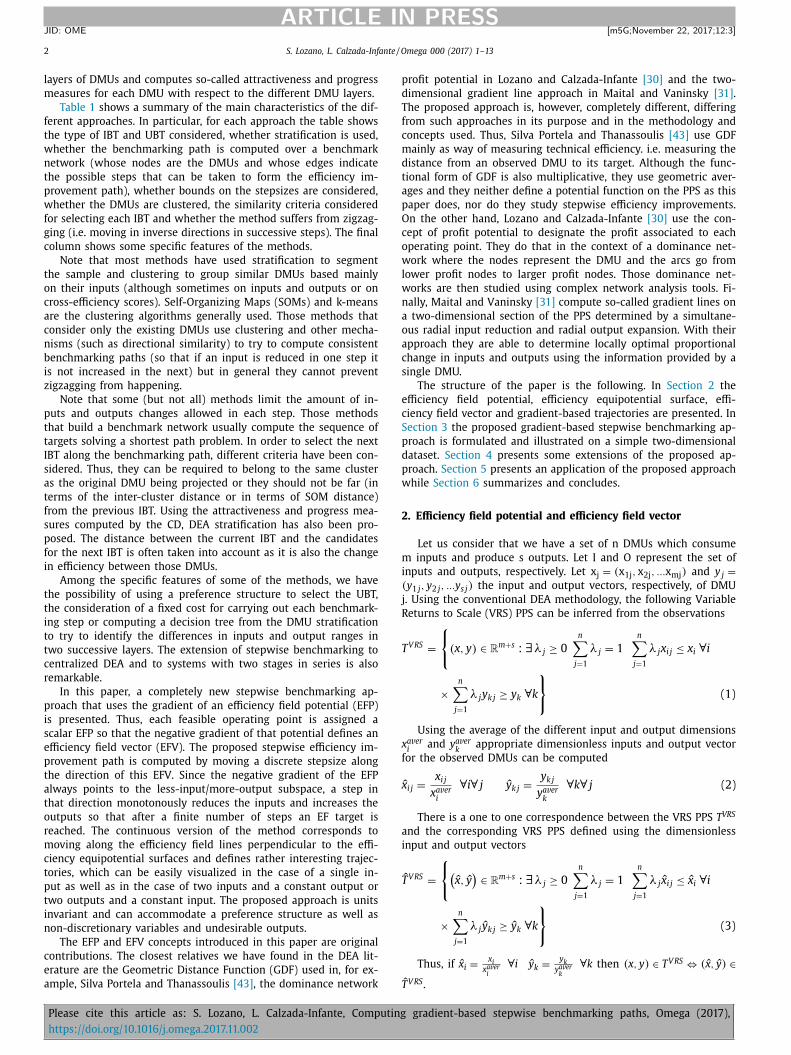
2 S. Lozano, L. Calzada-Infante / Omega 0 0 0 (2017) 1–13

ARTICLE IN PRESS JID: OME [m5G; November 22, 2017;12:3 ]

layers of DMUs and computes so-called attractiveness and progress

measures for each DMU with respect to the different DMU layers.

Table 1 shows a summary of the main characteristics of the dif-

ferent approaches. In particular, for each approach the table shows

the type of IBT and UBT considered, whether stratification is used,

whether the benchmarking path is computed over a benchmark

network (whose nodes are the DMUs and whose edges indicate

the possible steps that can be taken to form the efficiency im-

provement path), whether bounds on the stepsizes are considered,

whether the DMUs are clustered, the similarity criteria considered

for selecting each IBT and whether the method suffers from zigzag-

ging (i.e. moving in inverse directions in successive steps). The final

column shows some specific features of the methods.

Note that most methods have used stratification to segment

the sample and clustering to group similar DMUs based mainly

on their inputs (although sometimes on inputs and outputs or on

cross-efficiency scores). Self-Organizing Maps (SOMs) and k-means

are the clustering algorithms generally used. Those methods that

consider only the existing DMUs use clustering and other mecha-

nisms (such as directional similarity) to try to compute consistent

benchmarking paths (so that if an input is reduced in one step it

is not increased in the next) but in general they cannot prevent

zigzagging from happening.

Note that some (but not all) methods limit the amount of in-

puts and outputs changes allowed in each step. Those methods

that build a benchmark network usually compute the sequence of

targets solving a shortest path problem. In order to select the next

IBT along the benchmarking path, different criteria have been con-

sidered. Thus, they can be required to belong to the same cluster

as the original DMU being projected or they should not be far (in

terms of the inter-cluster distance or in terms of SOM distance)

from the previous IBT. Using the attractiveness and progress mea-

sures computed by the CD, DEA stratification has also been pro-

posed. The distance between the current IBT and the candidates

for the next IBT is often taken into account as it is also the change

in efficiency between those DMUs.

Among the specific features of some of the methods, we have

the possibility of using a preference structure to select the UBT,

the consideration of a fixed cost for carrying out each benchmark-

ing step or computing a decision tree from the DMU stratification

to try to identify the differences in inputs and output ranges in

two successive layers. The extension of stepwise benchmarking to

centralized DEA and to systems with two stages in series is also

remarkable.

In this paper, a completely new stepwise benchmarking ap-

proach that uses the gradient of an efficiency field potential (EFP)

is presented. Thus, each feasible operating point is assigned a

scalar EFP so that the negative gradient of that potential defines an

efficiency field vector (EFV). The proposed stepwise efficiency im-

provement path is computed by moving a discrete stepsize along

the direction of this EFV. Since the negative gradient of the EFP

always points to the less-input/more-output subspace, a step in

that direction monotonously reduces the inputs and increases the

outputs so that after a finite number of steps an EF target is

reached. The continuous version of the method corresponds to

moving along the efficiency field lines perpendicular to the effi-

ciency equipotential surfaces and defines rather interesting trajec-

tories, which can be easily visualized in the case of a single in-

put as well as in the case of two inputs and a constant output or

two outputs and a constant input. The proposed approach is units

invariant and can accommodate a preference structure as well as

non-discretionary variables and undesirable outputs.

The EFP and EFV concepts introduced in this paper are original

contributions. The closest relatives we have found in the DEA lit-

erature are the Geometric Distance Function (GDF) used in, for ex-

ample, Silva Portela and Thanassoulis [43] , the dominance network

profit potential in Lozano and Calzada-Infante [30] and the two-

dimensional gradient line approach in Maital and Vaninsky [31] .

The proposed approach is, however, completely different, differing

from such approaches in its purpose and in the methodology and

concepts used. Thus, Silva Portela and Thanassoulis [43] use GDF

mainly as way of measuring technical efficiency. i.e. measuring the

distance from an observed DMU to its target. Although the func-

tional form of GDF is also multiplicative, they use geometric aver-

ages and they neither define a potential function on the PPS as this

paper does, nor do they study stepwise efficiency improvements.

On the other hand, Lozano and Calzada-Infante [30] use the con-

cept of profit potential to designate the profit associated to each

operating point. They do that in the context of a dominance net-

work where the nodes represent the DMU and the arcs go from

lower profit nodes to larger profit nodes. Those dominance net-

works are then studied using complex network analysis tools. Fi-

nally, Maital and Vaninsky [31] compute so-called gradient lines on

a two-dimensional section of the PPS determined by a simultane-

ous radial input reduction and radial output expansion. With their

approach they are able to determine locally optimal proportional

change in inputs and outputs using the information provided by a

single DMU.

The structure of the paper is the following. In Section 2 the

efficiency field potential, efficiency equipotential surface, effi-

ciency field vector and gradient-based trajectories are presented. In

Section 3 the proposed gradient-based stepwise benchmarking ap-

proach is formulated and illustrated on a simple two-dimensional

dataset. Section 4 presents some extensions of the proposed ap-

proach. Section 5 presents an application of the proposed approach

while Section 6 summarizes and concludes.

2. Efficiency field potential and efficiency field vector

Let us consider that we have a set of n DMUs which consume

m inputs and produce s outputs. Let I and O represent the set of

inputs and outputs, respectively. Let x j = ( x 1j , x 2j , ... x mj ) and y j =

( y 1 j , y 2 j , ... y s j ) the input and output vectors, respectively, of DMU

j. Using the conventional DEA methodology, the following Variable

Returns to Scale (VRS) PPS can be inferred from the observations

T V RS =

{

( x, y ) ∈ R m + s : ∃ λ j ≥ 0

n ∑

j=1

λ j = 1 n

∑

j=1

λ j x i j ≤ x i ∀ i

×

n ∑

j=1

λ j y k j ≥ y k ∀ k

}

(1)

Using the average of the different input and output dimensions

x a v er i

and y a v er k

appropriate dimensionless inputs and output vector

for the observed DMUs can be computed

ˆ x i j = x i j

x a v er i

∀ i ∀ j ˆ y k j = y k j

y a v er k

∀ k ∀ j (2)

There is a one to one correspondence between the VRS PPS T VRS

and the corresponding VRS PPS defined using the dimensionless

input and output vectors

ˆ T V RS =

{

(

ˆ x , y )

∈ R m + s : ∃ λ j ≥ 0

n ∑

j=1

λ j = 1 n

∑

j=1

λ j x i j ≤ ˆ x i ∀ i

×

n ∑

j=1

λ j y k j ≥ ˆ y k ∀ k

}

(3)

Thus, if ˆ x i = x i

x a v er i

∀ i ˆ y k = y k

y a v er k

∀ k then ( x, y ) ∈ T V RS ⇔ ( x , y ) ∈

ˆ T V RS .

Please cite this article as: S. Lozano, L. Calzada-Infante, Computing gradient-based stepwise benchmarking paths, Omega (2017),

https://doi.org/10.1016/j.omega.2017.11.002

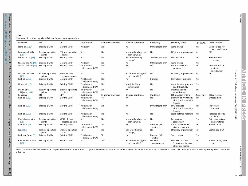
S. Lozano, L. C

alza

da-In

fante / O

mega 0 0 0 (2

017

) 1–13

3

ART

ICLE

IN P

RESS

JID

: OM

E

[m5G; N

ovem

ber 2

2, 2

017;1

2:3 ]

Table 1

Summary of existing stepwise efficiency improvement approaches.

Reference IBT UBT Stratification Benchmark network Stepsize constraints Clustering Similarity criteria Zigzagging Other features

Hong et al. [24] Existing DMUs Existing DMUs Yes (Tiers) No No SOM (inputs only) Same cluster Yes Decision tree for

tier classification

Lozano and Villa

[28]

Feasible operating

points

Efficient operating

points

No No Yes (on the change of

each variable)

No Efficiency improvement No CRS

Estrada et al. [18] Existing DMUs Existing DMUs No No Yes (on efficiency

change)

SOM (inputs only) SOM distance Yes Reinforcement

Learning

Sharma and Yu [40] Existing DMUs Existing DMUs Yes (Tiers) No No SOM (inputs only) Same cluster Yes

Sharma and Yu [41] Existing DMUs Existing DMUs Yes (Context

dependent DEA)

No No No Attractiveness and

progress

Yes Decision tree for

attribute

prioritization

Lozano and Villa

[29]

Feasible operating

points

MPSS efficient

operating points

No No Yes (on the change of

each variable)

No Efficiency improvement No VRS

Park et al. [32] Existing DMUs Existing DMUs Yes (Context

dependent DEA)

No No k-means Inter-cluster distance Yes

Lim et al. [27] Existing DMUs Existing DMUs Yes (Context

dependent DEA)

No Yes (joint linear

constraints)

No Attractiveness, progress

and Infeasibility

Yes

Suzuki and

Nijkamp [44]

Feasible operating

points

Efficient operating

points

Yes (Context

dependent DEA)

No No No Distance friction

minimization

Yes

Reference IBT UBT Stratification Benchmark network Stepsize constraints Clustering IBT selection criteria Zigzagging Other features

Park et al. [33] Existing DMUs Existing DMUs Yes (Context

dependent DEA)

Yes No No Resource improvement,

directional proximity

(inputs)

Yes Shortest Path

Park et al. [34] Existing DMUs Existing DMUs Yes (Context

dependent DEA)

No No SOM (inputs only) SOM distance,

directional proximity

(inputs)

Yes Preference

structure

Park et al. [35] Existing DMUs Existing DMU Yes (Context

dependent DEA)

No No No Least distance measure Yes Resource priority

analysis

Khodakarami et al.

[25]

Feasible operating

points

MPSS efficient

operating points

No No Yes (on the change of

each variable)

No Ray average

productivity

Yes Extension to two

stage systems

Park et al. [36] Existing DMUs Existing DMUs Yes (Context

dependent DEA)

Yes No k-means (XE

matrix)

Same cluster, Least

distance measure

Yes Shortest Path

Fang [19] Feasible operating

points

Efficient operating

points

No No Yes (on efficiency

change)

No Efficiency improvement No Centralized DEA

Park and Sung [37] Existing DMUs Existing DMUs Yes (Context

dependent DEA)

Yes No k-means (XE

matrix)

Same cluster Yes

Ghahraman & Prior

[21]

Existing DMUs Existing DMUs No Yes Yes (on the change of

each variable)

Network

components

Euclidean distance

(normalized inputs),

efficiency change

Yes Shortest Path, Fixed

cost

Notes: IBT = Intermediate Benchmark Targets, UBT = Ultimate Benchmark Targets, CRS = Constant Returns to Scale, VRS = Variable Returns to Scale, MPSS = Most Productive Scale Size, SOM = Self-Organizing Map, XE = Cross-

efficiency

Please

cite

this article

as:

S. Lo

zano, L.

Calza

da-In

fante, Computin

g gradient-b

ased ste

pwise

bench

marking paths,

Omega (2017

),

http

s://doi.o

rg/10.1016

/j.omega.2017.11.0

02

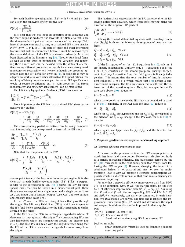
4 S. Lozano, L. Calzada-Infante / Omega 0 0 0 (2017) 1–13

ARTICLE IN PRESS JID: OME [m5G; November 22, 2017;12:3 ]

For each feasible operating point ( x , y ) with ˆ x > 0 and ˆ y > 0 we

can assign the following strictly positive EFP

P (

ˆ x , y )

=

∏ m i =1 ˆ x i

∏ s k =1 ˆ y k

(4)

It is clear that the less input an operating point consumes and

the more output it produces, the lower its EFP. Note also that, since

the dimensionless input and output vectors of the average DMU

have all components equal to one, its associated EFP is also one, i.e.

P ( x a v er , y a v er ) = P ( 1 , 1 ) = 1 . In spite of these and other interesting

features that will be commented below, it must be acknowledged

the above definition of the EFP is somewhat arbitrary. As it has

been discussed in the literature (e.g. [14,17] ) other functional forms

as well as other ways of normalizing the variables and remov-

ing their dimensions can be devised, with the different alterna-

tives having different properties as regards invariance, strong/weak

monotonicity, separability, etc. Hence, although the proposed ap-

proach uses the EFP definition given in (4) , in principle it may be

adapted to work also with other alternative EFP specifications. The

resulting efficiency improvement path for other EFP specifications

would of course be different, but its main properties (i.e. strong

monotonicity and efficiency achievement) can be maintained.

The Efficiency Equipotential Surfaces (EESs) correspond to ∏ m

i =1 ˆ x i ∏ s

k =1 ˆ y k = γ ⇔

s ∏

k =1

ˆ y k = γ −1 m ∏

i =1

ˆ x i (5)

More importantly, the EFP has an associated EFV given by the

negative EFP gradient

E (

ˆ x , y )

= −∇P (

ˆ x , y )

=

(

−∂P

∂ x 1 , −

∂P

∂ x 2 , ..., −

∂P

∂ x m , −

∂P

∂ y 1 , −

∂P

∂ y 2 , ..., −

∂P

∂ y s

)

(6)

The corresponding partial derivatives can be easily computed

and, interestingly, can be expressed in terms of the EFP since

∂P

∂ x i =

∏

i ′ � = i ˆ x i ′ ∏

k ˆ y k =

P (

ˆ x , y )

ˆ x i ∀ i

∂P

∂ y k = −

1

ˆ y 2 k

∏

i ˆ x i ∏

k ′ � = k ˆ y k ′ = −

P (

ˆ x , y )

ˆ y k ∀ k (7)

Note that the components of the EFV

E (

ˆ x , y )

=

(

−P (

ˆ x , y )

ˆ x 1 , −

P (

ˆ x , y )

ˆ x 2 , ..., −

P (

ˆ x , y )

ˆ x m , P (

ˆ x , y )

ˆ y 1 ,

P (

ˆ x , y )

ˆ y 2 , ...,

P (

ˆ x , y )

ˆ y s

)

(8)

always point towards the less input/more output region. It is also

clear that at each feasible operating point ( x , y ) , E( x , y ) is perpen-

dicular to the corresponding EES. Fig. 1 shows the EFV for three

special cases that can be shown in a bidimensional plot. These

three cases correspond to a single input and a single output (case

XY), two inputs and a constant output (case XX1) and two outputs

and constant input (case 1YY).

In the XY case, the EESs are straight lines that pass through

the origin. The Efficiency Field Lines (EFLs), which are tangent to

the EFV (and hence perpendicular to the EES), correspond to circles

centred at the origin.

In the XX1 case the EESs are rectangular hyperboles whose EP

decreases as they approach the origin. The corresponding EFLs are

also hyperboles which are symmetrical around the bisector line

ˆ x 1 = ˆ x 2 . The case 1YY is similar, with the only difference being that

the EFP of the EES decreases as the hyperboles move away from

the origin.

The mathematical expressions for the EFL correspond to the fol-

lowing differential equation, which represents moving along the

direction of the negative EFP gradient (

d x

dt , d y

dt

)

= −∇P (

ˆ x , y )

(9)

Solving this partial differential equation with boundary condi-

tion ( x 0 , y 0 ) leads to the following three groups of quadratic sur-

faces

ˆ x 2 i − ˆ x 2

i ′ = ˆ x 2 i 0 − ˆ x 2

i ′ 0 ∀ i � = i ′

ˆ y 2 k

− ˆ y 2 k ′

= ˆ y 2 k 0

− ˆ y 2 k ′ 0

∀ k � = k ′

ˆ x 2 i + ˆ y 2

k = ˆ x 2

i 0 + ˆ y 2 k 0

∀ i, k

(10)

Of the first group of m · (m − 1) / 2 equations in (10) , only m −1

are linearly independent. Similarly, only s −1 equations out of the

s · (s − 1) / 2 equations in the second group are linearly indepen-

dent. And only 1 equation from the third group is linearly inde-

pendent. This means that the total number of linearly indepen-

dent equations is m + s −1 which means that (10) defines a one-

dimensional subspace. The EFLs are curves that result from the in-

tersection of this equation system. Thus, for example, in the XY

case seen above, (10) reduces to

ˆ x 2 + ˆ y 2 = ˆ x 2 0 + ˆ y 2 0 (11)

which corresponds to the circular EFLs that can be noticed in panel

a) of Fig. 1 . Similarly, in the XX1 case the EFLs (10) reduce to

ˆ x 2 1 − ˆ x 2 2 = ˆ x 2 10 − ˆ x 2 20 (12)

which for ˆ x 10 � = ˆ x 20 are hyperboles and for ˆ x 10 = ˆ x 20 corresponds to

the bisector line ˆ x 1 = ˆ x 2 . Finally, in the 1YY case, the EFLs (10) re-

duce to

ˆ y 2 1 − ˆ y 2 2 = ˆ y 2 10 − ˆ y 2 20 (13)

which, again, are hyperboles for ˆ y 10 � = ˆ y 20 and the bisector line

ˆ y 1 = ˆ y 2 if ˆ y 10 = ˆ y 20 .

3. Proposed gradient-based stepwise benchmarking approach

3.1. Stepwise efficiency improvement path

As shown in the previous section, the EFV always points to-

wards less input and more output. Following such direction leads

to a strictly increasing efficiency. The trajectories defined by the

EFL (10) correspond to the continuous path that results from fol-

lowing the EFV as per (9) . However, changing the inputs in a

continuous fashion is not practical and may not even be imple-

mentable. That is why we propose a stepwise benchmarking ap-

proach which is a discrete version of that continuous efficiency im-

provement trajectory.

Assume that a stepwise efficiency improvement path from DMU

0 is to be computed. DMU 0 will the starting point, i.e. the step

t = 0, of efficiency improvement path ( x 0 , y 0 ) = ( x 0 , y 0 ) . Assuming

that ˆ x t > 0 and ˆ y t > 0 , the corresponding EFP and EFV P ( x t , y t )

and E( x t , y t ) , respectively, can easily be computed. In each itera-

tion two DEA models are solved. The first one is labelled the Im-

provement Dimensions (ID) DEA model and determines the input

and output dimensions that can be improved in that step. Let

Data

( x t , y t ) Current (i.e. step t) IBT

E( x t , y t ) EFV at current IBT

ɛ Small value stepsize along EFV from current IBT

Decision variables

λj linear combination variables used to compute a feasible

operating point

Please cite this article as: S. Lozano, L. Calzada-Infante, Computing gradient-based stepwise benchmarking paths, Omega (2017),

https://doi.org/10.1016/j.omega.2017.11.002

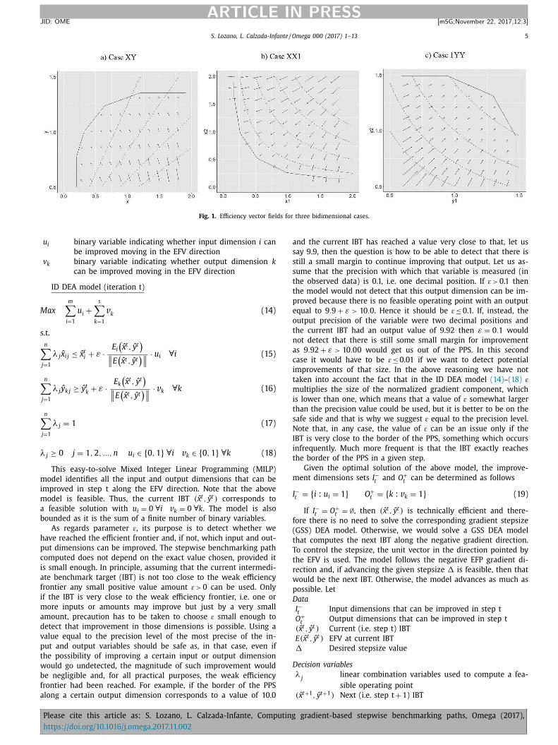
S. Lozano, L. Calzada-Infante / Omega 0 0 0 (2017) 1–13 5

ARTICLE IN PRESS JID: OME [m5G; November 22, 2017;12:3 ]

Fig. 1. Efficiency vector fields for three bidimensional cases.

u i binary variable indicating whether input dimension i can

be improved moving in the EFV direction

v k binary variable indicating whether output dimension k

can be improved moving in the EFV direction

ID DEA model (iteration t)

Max

m ∑

i =1

u i +

s ∑

k =1

v k (14)

s.t.

n ∑

j=1

λ j x i j ≤ ˆ x t i + ε ·E i (

ˆ x t , y t )

∥

∥E (

ˆ x t , y t )∥

∥

· u i ∀ i (15)

n ∑

j=1

λ j y k j ≥ ˆ y t k + ε ·E k

(

ˆ x t , y t )

∥

∥E (

ˆ x t , y t )∥

∥

· v k ∀ k (16)

n ∑

j=1

λ j = 1 (17)

λ j ≥ 0 j = 1 , 2 , ..., n u i ∈ { 0 , 1 } ∀ i v k ∈ { 0 , 1 } ∀ k (18)

This easy-to-solve Mixed Integer Linear Programming (MILP)

model identifies all the input and output dimensions that can be

improved in step t along the EFV direction. Note that the above

model is feasible. Thus, the current IBT ( x t , y t ) corresponds to

a feasible solution with u i = 0 ∀ i v k = 0 ∀ k . The model is also

bounded as it is the sum of a finite number of binary variables.

As regards parameter ɛ , its purpose is to detect whether we

have reached the efficient frontier and, if not, which input and out-

put dimensions can be improved. The stepwise benchmarking path

computed does not depend on the exact value chosen, provided it

is small enough. In principle, assuming that the current intermedi-

ate benchmark target (IBT) is not too close to the weak efficiency

frontier any small positive value amount ɛ > 0 can be used. Only

if the IBT is very close to the weak efficiency frontier, i.e. one or

more inputs or amounts may improve but just by a very small

amount, precaution has to be taken to choose ɛ small enough to

detect that improvement in those dimensions is possible. Using a

value equal to the precision level of the most precise of the in-

put and output variables should be safe as, in that case, even if

the possibility of improving a certain input or output dimension

would go undetected, the magnitude of such improvement would

be negligible and, for all practical purposes, the weak efficiency

frontier had been reached. For example, if the border of the PPS

along a certain output dimension corresponds to a value of 10.0

and the current IBT has reached a value very close to that, let us

say 9.9, then the question is how to be able to detect that there is

still a small margin to continue improving that output. Let us as-

sume that the precision with which that variable is measured (in

the observed data) is 0.1, i.e. one decimal position. If ɛ > 0.1 then

the model would not detect that this output dimension can be im-

proved because there is no feasible operating point with an output

equal to 9 . 9 + ε > 10 . 0 . Hence it should be ɛ ≤0.1. If, instead, the

output precision of the variable were two decimal positions and

the current IBT had an output value of 9.92 then ε = 0 . 1 would

not detect that there is still some small margin for improvement

as 9 . 92 + ε > 10 . 00 would get us out of the PPS. In this second

case it would have to be ɛ ≤0.01 if we want to detect potential

improvements of that size. In the above reasoning we have not

taken into account the fact that in the ID DEA model (14) –(18) ɛ

multiplies the size of the normalized gradient component, which

is lower than one, which means that a value of ɛ somewhat larger

than the precision value could be used, but it is better to be on the

safe side and that is why we suggest ɛ equal to the precision level.

Note that, in any case, the value of ɛ can be an issue only if the

IBT is very close to the border of the PPS, something which occurs

infrequently. Much more frequent is that the IBT exactly reaches

the border of the PPS in a given step.

Given the optimal solution of the above model, the improve-

ment dimensions sets I −t and O + t can be determined as follows

I −t = { i : u i = 1 } O + t = { k : v k = 1 } (19)

If I −t = O + t = ∅ , then ( x t , y t ) is technically efficient and there-

fore there is no need to solve the corresponding gradient stepsize

(GSS) DEA model. Otherwise, we would solve a GSS DEA model

that computes the next IBT along the negative gradient direction.

To control the stepsize, the unit vector in the direction pointed by

the EFV is used. The model follows the negative EFP gradient di-

rection and, if advancing the given stepsize � is feasible, then that

would be the next IBT. Otherwise, the model advances as much as

possible. Let

Data

I −t Input dimensions that can be improved in step t

O + t Output dimensions that can be improved in step t

( x t , y t ) Current (i.e. step t) IBT

E( x t , y t ) EFV at current IBT

� Desired stepsize value

Decision variables

λj linear combination variables used to compute a fea-

sible operating point

( x t+1 , y t+1 ) Next (i.e. step t + 1) IBT

Please cite this article as: S. Lozano, L. Calzada-Infante, Computing gradient-based stepwise benchmarking paths, Omega (2017),

https://doi.org/10.1016/j.omega.2017.11.002

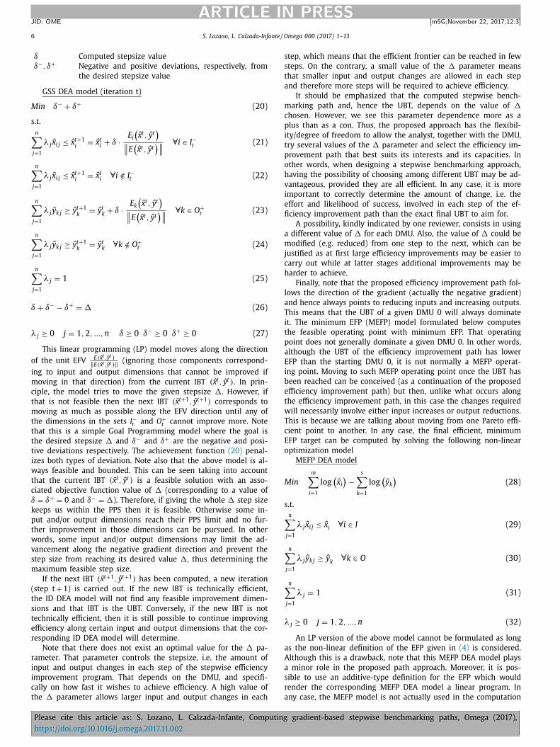
6 S. Lozano, L. Calzada-Infante / Omega 0 0 0 (2017) 1–13

ARTICLE IN PRESS JID: OME [m5G; November 22, 2017;12:3 ]

δ Computed stepsize value

δ−, δ+ Negative and positive deviations, respectively, from

the desired stepsize value

GSS DEA model (iteration t)

Min δ− + δ+ (20)

s.t.

n ∑

j=1

λ j x i j ≤ ˆ x t+1 i = ˆ x t i + δ ·

E i (

ˆ x t , y t )

∥

∥E (

ˆ x t , y t )∥

∥

∀ i ∈ I −t (21)

n ∑

j=1

λ j x i j ≤ ˆ x t+1 i = ˆ x t i ∀ i / ∈ I −t (22)

n ∑

j=1

λ j y k j ≥ ˆ y t+1 k

= ˆ y t k + δ ·E k

(

ˆ x t , y t )

∥

∥E (

ˆ x t , y t )∥

∥

∀ k ∈ O + t (23)

n ∑

j=1

λ j y k j ≥ ˆ y t+1 k

= ˆ y t k ∀ k / ∈ O + t (24)

n ∑

j=1

λ j = 1 (25)

δ + δ− − δ+ = � (26)

λ j ≥ 0 j = 1 , 2 , ..., n δ ≥ 0 δ− ≥ 0 δ+ ≥ 0 (27)

This linear programming (LP) model moves along the direction

of the unit EFV E( x t , y t )

‖ E( x t , y t ) ‖ (ignoring those components correspond-

ing to input and output dimensions that cannot be improved if

moving in that direction) from the current IBT ( x t , y t ) . In prin-

ciple, the model tries to move the given stepsize �. However, if

that is not feasible then the next IBT ( x t+1 , y t+1 ) corresponds to

moving as much as possible along the EFV direction until any of

the dimensions in the sets I −t and O + t cannot improve more. Note

that this is a simple Goal Programming model where the goal is

the desired stepsize � and δ− and δ+ are the negative and posi-

tive deviations respectively. The achievement function (20) penal-

izes both types of deviation. Note also that the above model is al-

ways feasible and bounded. This can be seen taking into account

that the current IBT ( x t , y t ) is a feasible solution with an asso-

ciated objective function value of � (corresponding to a value of

δ = δ+ = 0 and δ− = �). Therefore, if giving the whole � step size

keeps us within the PPS then it is feasible. Otherwise some in-

put and/or output dimensions reach their PPS limit and no fur-

ther improvement in those dimensions can be pursued. In other

words, some input and/or output dimensions may limit the ad-

vancement along the negative gradient direction and prevent the

step size from reaching its desired value �, thus determining the

maximum feasible step size.

If the next IBT ( x t+1 , y t+1 ) has been computed, a new iteration

(step t + 1) is carried out. If the new IBT is technically efficient,

the ID DEA model will not find any feasible improvement dimen-

sions and that IBT is the UBT. Conversely, if the new IBT is not

technically efficient, then it is still possible to continue improving

efficiency along certain input and output dimensions that the cor-

responding ID DEA model will determine.

Note that there does not exist an optimal value for the � pa-

rameter. That parameter controls the stepsize, i.e. the amount of

input and output changes in each step of the stepwise efficiency

improvement program. That depends on the DMU, and specifi-

cally on how fast it wishes to achieve efficiency. A high value of

the � parameter allows larger input and output changes in each

step, which means that the efficient frontier can be reached in few

steps. On the contrary, a small value of the � parameter means

that smaller input and output changes are allowed in each step

and therefore more steps will be required to achieve efficiency.

It should be emphasized that the computed stepwise bench-

marking path and, hence the UBT, depends on the value of �

chosen. However, we see this parameter dependence more as a

plus than as a con. Thus, the proposed approach has the flexibil-

ity/degree of freedom to allow the analyst, together with the DMU,

try several values of the � parameter and select the efficiency im-

provement path that best suits its interests and its capacities. In

other words, when designing a stepwise benchmarking approach,

having the possibility of choosing among different UBT may be ad-

vantageous, provided they are all efficient. In any case, it is more

important to correctly determine the amount of change, i.e. the

effort and likelihood of success, involved in each step of the ef-

ficiency improvement path than the exact final UBT to aim for.

A possibility, kindly indicated by one reviewer, consists in using

a different value of � for each DMU. Also, the value of � could be

modified (e.g. reduced) from one step to the next, which can be

justified as at first large efficiency improvements may be easier to

carry out while at latter stages additional improvements may be

harder to achieve.

Finally, note that the proposed efficiency improvement path fol-

lows the direction of the gradient (actually the negative gradient)

and hence always points to reducing inputs and increasing outputs.

This means that the UBT of a given DMU 0 will always dominate

it. The minimum EFP (MEFP) model formulated below computes

the feasible operating point with minimum EFP. That operating

point does not generally dominate a given DMU 0. In other words,

although the UBT of the efficiency improvement path has lower

EFP than the starting DMU 0, it is not normally a MEFP operat-

ing point. Moving to such MEFP operating point once the UBT has

been reached can be conceived (as a continuation of the proposed

efficiency improvement path) but then, unlike what occurs along

the efficiency improvement path, in this case the changes required

will necessarily involve either input increases or output reductions.

This is because we are talking about moving from one Pareto effi-

cient point to another. In any case, the final efficient, minimum

EFP target can be computed by solving the following non-linear

optimization model

MEFP DEA model

Min

m ∑

i =1

log (

ˆ x i )

−

s ∑

k =1

log (

ˆ y k )

(28)

s.t.

n ∑

j=1

λ j x i j ≤ ˆ x i ∀ i ∈ I (29)

n ∑

j=1

λ j y k j ≥ ˆ y k ∀ k ∈ O (30)

n ∑

j=1

λ j = 1 (31)

λ j ≥ 0 j = 1 , 2 , ..., n (32)

An LP version of the above model cannot be formulated as long

as the non-linear definition of the EFP given in (4) is considered.

Although this is a drawback, note that this MEFP DEA model plays

a minor role in the proposed path approach. Moreover, it is pos-

sible to use an additive-type definition for the EFP which would

render the corresponding MEFP DEA model a linear program. In

any case, the MEFP model is not actually used in the computation

Please cite this article as: S. Lozano, L. Calzada-Infante, Computing gradient-based stepwise benchmarking paths, Omega (2017),

https://doi.org/10.1016/j.omega.2017.11.002

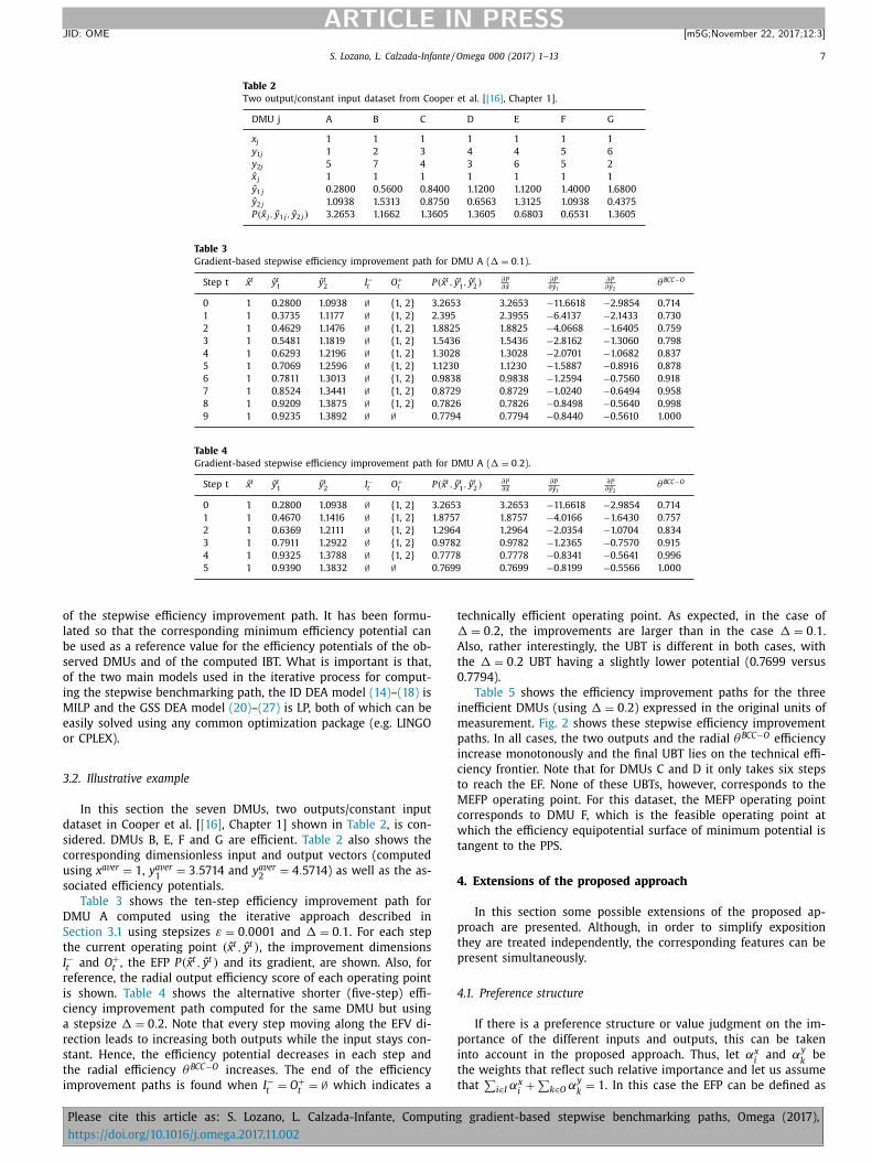
S. Lozano, L. Calzada-Infante / Omega 0 0 0 (2017) 1–13 7

ARTICLE IN PRESS JID: OME [m5G; November 22, 2017;12:3 ]

Table 2

Two output/constant input dataset from Cooper et al. [ [16] , Chapter 1].

DMU j A B C D E F G

x j 1 1 1 1 1 1 1

y 1 j 1 2 3 4 4 5 6

y 2 j 5 7 4 3 6 5 2

ˆ x j 1 1 1 1 1 1 1

ˆ y 1 j 0.2800 0.5600 0.8400 1.1200 1.1200 1.40 0 0 1.6800

ˆ y 2 j 1.0938 1.5313 0.8750 0.6563 1.3125 1.0938 0.4375

P( x j , y 1 j , y 2 j ) 3.2653 1.1662 1.3605 1.3605 0.6803 0.6531 1.3605

Table 3

Gradient-based stepwise efficiency improvement path for DMU A ( � = 0 . 1 ).

Step t ˆ x t ˆ y t 1 ˆ y t 2 I −t O + t P( x t , y t 1 , y t 2 )

∂P ∂ x

∂P ∂ y 1

∂P ∂ y 2

θBC C −O

0 1 0.2800 1.0938 ∅ {1, 2} 3.2653 3.2653 −11.6618 −2.9854 0.714

1 1 0.3735 1.1177 ∅ {1, 2} 2.395 2.3955 −6.4137 −2.1433 0.730

2 1 0.4629 1.1476 ∅ {1, 2} 1.8825 1.8825 −4.0668 −1.6405 0.759

3 1 0.5481 1.1819 ∅ {1, 2} 1.5436 1.5436 −2.8162 −1.3060 0.798

4 1 0.6293 1.2196 ∅ {1, 2} 1.3028 1.3028 −2.0701 −1.0682 0.837

5 1 0.7069 1.2596 ∅ {1, 2} 1.1230 1.1230 −1.5887 −0.8916 0.878

6 1 0.7811 1.3013 ∅ {1, 2} 0.9838 0.9838 −1.2594 −0.7560 0.918

7 1 0.8524 1.3441 ∅ {1, 2} 0.8729 0.8729 −1.0240 −0.6494 0.958

8 1 0.9209 1.3875 ∅ {1, 2} 0.7826 0.7826 −0.8498 −0.5640 0.998

9 1 0.9235 1.3892 ∅ ∅ 0.7794 0.7794 −0.8440 −0.5610 1.0 0 0

Table 4

Gradient-based stepwise efficiency improvement path for DMU A ( � = 0 . 2 ).

Step t ˆ x t ˆ y t 1 ˆ y t 2 I −t O + t P( x t , y t 1 , y t 2 )

∂P ∂ x

∂P ∂ y 1

∂P ∂ y 2

θBC C −O

0 1 0.2800 1.0938 ∅ {1, 2} 3.2653 3.2653 −11.6618 −2.9854 0.714

1 1 0.4670 1.1416 ∅ {1, 2} 1.8757 1.8757 −4.0166 −1.6430 0.757

2 1 0.6369 1.2111 ∅ {1, 2} 1.2964 1.2964 −2.0354 −1.0704 0.834

3 1 0.7911 1.2922 ∅ {1, 2} 0.9782 0.9782 −1.2365 −0.7570 0.915

4 1 0.9325 1.3788 ∅ {1, 2} 0.7778 0.7778 −0.8341 −0.5641 0.996

5 1 0.9390 1.3832 ∅ ∅ 0.7699 0.7699 −0.8199 −0.5566 1.0 0 0

of the stepwise efficiency improvement path. It has been formu-

lated so that the corresponding minimum efficiency potential can

be used as a reference value for the efficiency potentials of the ob-

served DMUs and of the computed IBT. What is important is that,

of the two main models used in the iterative process for comput-

ing the stepwise benchmarking path, the ID DEA model (14) –(18) is

MILP and the GSS DEA model (20) –(27) is LP, both of which can be

easily solved using any common optimization package (e.g. LINGO

or CPLEX).

3.2. Illustrative example

In this section the seven DMUs, two outputs/constant input

dataset in Cooper et al. [ [16] , Chapter 1] shown in Table 2 , is con-

sidered. DMUs B, E, F and G are efficient. Table 2 also shows the

corresponding dimensionless input and output vectors (computed

using x a v er = 1 , y a v er 1 = 3 . 5714 and y a v er 2 = 4 . 5714 ) as well as the as-

sociated efficiency potentials.

Table 3 shows the ten-step efficiency improvement path for

DMU A computed using the iterative approach described in

Section 3.1 using stepsizes ε = 0 . 0 0 01 and � = 0 . 1 . For each step

the current operating point ( x t , y t ) , the improvement dimensions

I −t and O + t , the EFP P ( x

t , y t ) and its gradient, are shown. Also, for

reference, the radial output efficiency score of each operating point

is shown. Table 4 shows the alternative shorter (five-step) effi-

ciency improvement path computed for the same DMU but using

a stepsize � = 0 . 2 . Note that every step moving along the EFV di-

rection leads to increasing both outputs while the input stays con-

stant. Hence, the efficiency potential decreases in each step and

the radial efficiency θBC C −O increases. The end of the efficiency

improvement paths is found when I −t = O + t = ∅ which indicates a

technically efficient operating point. As expected, in the case of

� = 0 . 2 , the improvements are larger than in the case � = 0 . 1 .

Also, rather interestingly, the UBT is different in both cases, with

the � = 0 . 2 UBT having a slightly lower potential (0.7699 versus

0.7794).

Table 5 shows the efficiency improvement paths for the three

inefficient DMUs (using � = 0 . 2 ) expressed in the original units of

measurement. Fig. 2 shows these stepwise efficiency improvement

paths. In all cases, the two outputs and the radial θBC C −O efficiency

increase monotonously and the final UBT lies on the technical effi-

ciency frontier. Note that for DMUs C and D it only takes six steps

to reach the EF. None of these UBTs, however, corresponds to the

MEFP operating point. For this dataset, the MEFP operating point

corresponds to DMU F, which is the feasible operating point at

which the efficiency equipotential surface of minimum potential is

tangent to the PPS.

4. Extensions of the proposed approach

In this section some possible extensions of the proposed ap-

proach are presented. Although, in order to simplify exposition

they are treated independently, the corresponding features can be

present simultaneously.

4.1. Preference structure

If there is a preference structure or value judgment on the im-

portance of the different inputs and outputs, this can be taken

into account in the proposed approach. Thus, let αx i

and αy k

be

the weights that reflect such relative importance and let us assume

that ∑

i ∈ I αx i

+ ∑

k ∈ O αy k

= 1 . In this case the EFP can be defined as

Please cite this article as: S. Lozano, L. Calzada-Infante, Computing gradient-based stepwise benchmarking paths, Omega (2017),

https://doi.org/10.1016/j.omega.2017.11.002

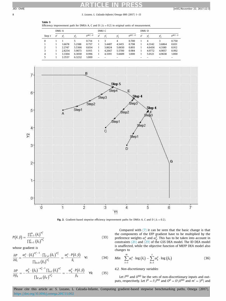
8 S. Lozano, L. Calzada-Infante / Omega 0 0 0 (2017) 1–13

ARTICLE IN PRESS JID: OME [m5G; November 22, 2017;12:3 ]

Table 5

Efficiency improvement path for DMUs A, C and D ( � = 0 . 2 ) in original units of measurement.

DMU A DMU C DMU D

Step t x t y t 1 y t 2 θBC C −O x t y t 1 y t 2 θBC C −O x t y t 1 y t 2 θBC C −O

0 1 1 5 0.714 1 3 4 0.700 1 4 3 0.750

1 1 1.6678 5.2188 0.757 1 3.4407 4.5415 0.798 1 4.3142 3.6864 0.831

2 1 2.2747 5.5366 0.834 1 3.8624 5.0650 0.893 1 4.6436 4.3180 0.912

3 1 2.8254 5.9073 0.915 1 4.2667 5.5700 0.984 1 4.9772 4.9057 0.992

4 1 3.3304 6.3030 0.996 1 4.3391 5.6609 1.0 0 0 1 5.0121 4.9638 1.0 0 0

5 1 3.3537 6.3232 1.0 0 0 – – – – – – – –

Fig. 2. Gradient-based stepwise efficiency improvement paths for DMUs A, C and D ( � = 0 . 2 ).

P (

ˆ x , y )

=

∏ m i =1

(

ˆ x i )αx

i

∏ s k =1

(

ˆ y k )αy

k (33)

whose gradient is

∂P

∂ x i =

αx i ·

(

ˆ x i )αx

i −1 ·∏

i ′ � = i

(

ˆ x i ′ )αx

i ′

∏

k ∈ O

(

ˆ y k )αy

k =

αx i · P

(

ˆ x , y )

ˆ x i ∀ i (34)

∂P

∂ y k = −

αy k

·(

ˆ y k )−αy

k −1 ∏

i ∈ I

(

ˆ x i )αx

i

∏

k ′ � = k

(

ˆ y k ′ )αy

k ′ = −

αy k

· P (

ˆ x , y )

ˆ y k ∀ k (35)

Compared with (7) it can be seen that the basic change is that

the components of the EFP gradient have to be multiplied by the

preference weights αx i and αy

k . This has to be taken into account in

constraints (21) and (23) of the GSS DEA model. The ID DEA model

is unaffected, while the objective function of MEFP DEA model also

changes to

Min

m ∑

i =1

αx i · log

(

ˆ x i )

−

s ∑

k =1

αy k

· log (

ˆ y k )

(36)

4.2. Non-discretionary variables

Let I ND and O ND be the sets of non-discretionary inputs and out-

puts, respectively. Let I D = I \ I ND and O D = O \ O ND and m ′ = | I D | and

Please cite this article as: S. Lozano, L. Calzada-Infante, Computing gradient-based stepwise benchmarking paths, Omega (2017),

https://doi.org/10.1016/j.omega.2017.11.002

S. Lozano, L. Calzada-Infante / Omega 0 0 0 (2017) 1–13 9

ARTICLE IN PRESS JID: OME [m5G; November 22, 2017;12:3 ]

s ′ = | O D | be the number of discretionary inputs and discretionary

outputs, respectively.

The ID DEA model changes slightly as the non-discretionary

dimensions are not considered as candidates for improvement.

Hence

Modified ID DEA model (iteration t)

Max ∑

i ∈ I D

u i +

∑

k ∈ O D

v k (37)

s.t.

n ∑

j=1

λ j x i j ≤ ˆ x t i + ε ·E i (

ˆ x t , y t )

∥

∥E (

ˆ x t , y t )∥

∥

· u i ∀ i ∈ I D (38)

n ∑

j=1

λ j x i j ≤ ˆ x t i ∀ i ∈ I ND (39)

n ∑

j=1

λ j y k j ≥ ˆ y t k + ε ·E k

(

ˆ x t , y t )

∥

∥E (

ˆ x t , y t )∥

∥

· v k ∀ k ∈ O D (40)

n ∑

j=1

λ j y k j ≥ ˆ y t k ∀ k ∈ O ND (41)

n ∑

j=1

λ j = 1 (42)

λ j ≥ 0 j = 1 , 2 , ..., n u i ∈ { 0 , 1 } ∀ i ∈ I D v k ∈ { 0 , 1 } ∀ k ∈ O D

(43)

The improvement dimensions sets are now defined as

I −t = {

i ∈ I D : u i = 1 }

O + t =

{

k ∈ O D : v k = 1

}

(44)

With respect to the GSS DEA model, there is no change in

the formulation. The MEFP DEA model also requires some minor

changes as shown below. In particular, since the MEFP operating

target of a DMU is constrained by the corresponding values of the

non-discretionary inputs and outputs, that MEFP depends on the

DMU being projected.

Modified MEFP DEA model

Min ∑

i ∈ I D

log (

ˆ x i )

−∑

k ∈ O D

log (

ˆ y k )

s.t. n

∑

j=1

λ j x i j ≤ ˆ x i ∀ i ∈ I D

n ∑

j=1

λ j x i j ≤ ˆ x i 0 ∀ i ∈ I ND

n ∑

j=1

λ j y k j ≥ ˆ y k ∀ k ∈ O D

n ∑

j=1

λ j y k j ≥ ˆ y k 0 ∀ k ∈ O ND

n ∑

j=1

λ j = 1

λ j ≥ 0 j = 1 , 2 , ..., n

(45)

4.3. Undesirable outputs

Let B be the set of undesirable outputs and p = | B | the number

of undesirable outputs. Let z bj be the amount of undesirable output

b produced by DMU j and ˆ z b j = z b j z a v er b

the corresponding dimension-

less value. The EFP can then be defined as

P (

ˆ x , y , z )

=

∏ m i =1 ˆ x i ·

∏ p b=1

z b ∏ s

k =1 ˆ y k (46)

which means that the components of the EFV are

E (

ˆ x , y , z )

= −∇P (

ˆ x , y , z )

=

(

−P (

ˆ x , y , z )

ˆ x 1 , ..., −

P (

ˆ x , y , z )

ˆ x m , P (

ˆ x , y , z )

ˆ y 1 , ...,

P (

ˆ x , y , z )

ˆ y s ,

−P (

ˆ x , y , z )

ˆ z 1 , ..., −

P (

ˆ x , y , z )

ˆ z p

)

(47)

Assuming weak disposability of the undesirable outputs and us-

ing the approach in Kuosmanen [26] , the corresponding modified

models are

Modified ID DEA model (iteration t)

Max

m ∑

i =1

u i +

s ∑

k =1

v k +

p ∑

b=1

w b

s.t.

n ∑

j=1

(

λ j + μ j

)

· ˆ x i j ≤ ˆ x t i + ε ·E i (

ˆ x t , y t , z t )

∥

∥E (

ˆ x t , y t , z t )∥

∥

· u i ∀ i

n ∑

j=1

λ j y k j ≥ ˆ y t k + ε ·E k

(

ˆ x t , y t , z t )

∥

∥E (

ˆ x t , y t , z t )∥

∥

· v k ∀ k

n ∑

j=1

λ jr z b j = ˆ z t b + ε ·E k

(

ˆ x t , y t , z t )

∥

∥E (

ˆ x t , y t , z t )∥

∥

· w b ∀ b

n ∑

j=1

(

λ j + μ j

)

= 1

λ j ≥ 0 μ j ≥ 0 ∀ j u i ∈ { 0 , 1 } ∀ i v k ∈ { 0 , 1 } ∀ k w b ∈ { 0 , 1 } ∀ b

(48)

I −t = { i : u i = 1 } O + t = { k : v k = 1 } B −t = { b : w b = 1 } (49)

Modified GSS DEA model (iteration t)

Min δ− + δ+

s.t. n

∑

j=1

(

λ j + μ j

)

· ˆ x i j ≤ ˆ x t+1 i = ˆ x t i + δ ·

E i (

ˆ x t , y t , z t )

∥

∥E (

ˆ x t , y t , z t )∥

∥

∀ i ∈ I −t

n ∑

j=1

(

λ j + μ j

)

· ˆ x i j ≤ ˆ x t+1 i = ˆ x t i ∀ i / ∈ I −t

n ∑

j=1

λ j y k j ≥ ˆ y t+1 k

= ˆ y t k + δ ·E k

(

ˆ x t , y t , z t )

∥

∥E (

ˆ x t , y t , z t )∥

∥

∀ k ∈ O + t

n ∑

j=1

λ j y k j ≥ ˆ y t+1 k

= ˆ y t k ∀ k / ∈ O + t

n ∑

j=1

λ j z b j = ˆ z t+1 b

= ˆ z t b + δ ·E b

(

ˆ x t , y t , z t )

∥

∥E (

ˆ x t , y t , z t )∥

∥

∀ b ∈ B −t

n ∑

j=1

λ j z b j = ˆ z t+1 b

= ˆ z t b ∀ b / ∈ B −t

n ∑

j=1

(

λ j + μ j

)

= 1

Please cite this article as: S. Lozano, L. Calzada-Infante, Computing gradient-based stepwise benchmarking paths, Omega (2017),

https://doi.org/10.1016/j.omega.2017.11.002

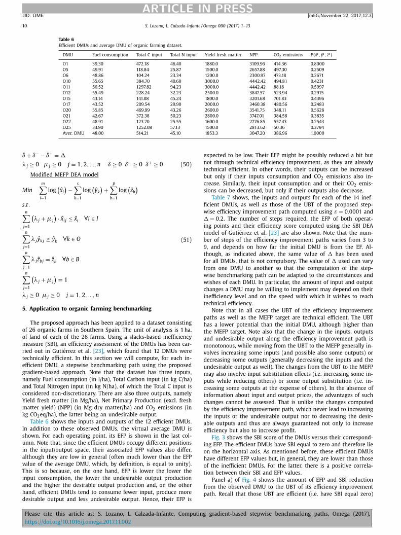
10 S. Lozano, L. Calzada-Infante / Omega 0 0 0 (2017) 1–13

ARTICLE IN PRESS JID: OME [m5G; November 22, 2017;12:3 ]

Table 6

Efficient DMUs and average DMU of organic farming dataset.

DMU Fuel consumption Total C input Total N input Yield fresh matter NPP CO 2 emissions P( x t , y t , z t )

O1 39.30 472.18 46.40 1880.0 3109.96 414.36 0.80 0 0

O5 49.91 118.84 25.87 1500.0 2657.88 497.30 0.2509

O6 48.86 104.24 23.34 1200.0 2300.97 473.18 0.2671

O10 55.65 384.70 40.60 30 0 0.0 4 4 42.42 494.81 0.4231

O11 56.52 1297.82 94.23 30 0 0.0 4 4 42.42 88.18 0.5997

O12 55.49 228.24 32.23 2500.0 3847.57 523.94 0.2915

O15 43.14 141.08 45.24 1800.0 3201.68 701.83 0.4396

O17 43.52 209.54 29.90 20 0 0.0 3460.38 480.56 0.2483

O20 55.85 469.99 43.26 2600.0 3541.75 348.11 0.5628

O21 42.67 372.38 50.23 2800.0 3747.01 384.58 0.3835

O22 48.91 123.70 25.55 1600.0 2776.85 557.43 0.2543

O25 33.90 1252.08 57.13 1500.0 2813.62 50.36 0.3794

Aver. DMU 48.00 514.21 45.10 1853.3 3047.20 386.96 1.0 0 0 0

δ + δ− − δ+ = �

λ j ≥ 0 μ j ≥ 0 j = 1 , 2 , ..., n δ ≥ 0 δ− ≥ 0 δ+ ≥ 0 (50)

Modified MEFP DEA model

Min

m ∑

i =1

log (

ˆ x i )

−

s ∑

k =1

log (

ˆ y k )

+

p ∑

b=1

log (

ˆ z b )

s.t. n

∑

j=1

(

λ j + μ j

)

· ˆ x i j ≤ ˆ x i ∀ i ∈ I

n ∑

j=1

λ j y k j ≥ ˆ y k ∀ k ∈ O

n ∑

j=1

λ j z b j = ˆ z b ∀ b ∈ B

n ∑

j=1

(

λ j + μ j

)

= 1

λ j ≥ 0 μ j ≥ 0 j = 1 , 2 , ..., n

(51)

5. Application to organic farming benchmarking

The proposed approach has been applied to a dataset consisting

of 26 organic farms in Southern Spain. The unit of analysis is 1 ha.

of land of each of the 26 farms. Using a slacks-based inefficiency

measure (SBI), an efficiency assessment of the DMUs has been car-

ried out in Gutiérrez et al. [23] , which found that 12 DMUs were

technically efficient. In this section we will compute, for each in-

efficient DMU, a stepwise benchmarking path using the proposed

gradient-based approach. Note that the dataset has three inputs,

namely Fuel consumption (in l/ha), Total Carbon input (in kg C/ha)

and Total Nitrogen input (in kg N/ha), of which the Total C input is

considered non-discretionary. There are also three outputs, namely

Yield fresh matter (in Mg/ha), Net Primary Production (excl. fresh

matter yield) (NPP) (in Mg dry matter/ha) and CO 2 emissions (in

kg CO 2 eq/ha), the latter being an undesirable output.

Table 6 shows the inputs and outputs of the 12 efficient DMUs.

In addition to these observed DMUs, the virtual average DMU is

shown. For each operating point, its EFP is shown in the last col-

umn. Note that, since the efficient DMUs occupy different positions

in the input/output space, their associated EFP values also differ,

although they are low in general (often much lower than the EFP

value of the average DMU, which, by definition, is equal to unity).

This is so because, on the one hand, EFP is lower the lower the

input consumption, the lower the undesirable output production

and the higher the desirable output production and, on the other

hand, efficient DMUs tend to consume fewer input, produce more

desirable output and less undesirable output. Hence, their EFP is

expected to be low. Their EFP might be possibly reduced a bit but

not through technical efficiency improvement, as they are already

technical efficient. In other words, their outputs can be increased

but only if their inputs consumption and CO 2 emissions also in-

crease. Similarly, their input consumption and or their CO 2 emis-

sions can be decreased, but only if their outputs also decrease.

Table 7 shows, the inputs and outputs for each of the 14 inef-

ficient DMUs, as well as those of the UBT of the proposed step-

wise efficiency improvement path computed using ε = 0 . 0 0 01 and

� = 0 . 2 . The number of steps required, the EFP of both operat-

ing points and their efficiency score computed using the SBI DEA

model of Gutiérrez et al. [23] are also shown. Note that the num-

ber of steps of the efficiency improvement paths varies from 3 to

9, and depends on how far the initial DMU is from the EF. Al-

though, as indicated above, the same value of � has been used

for all DMUs, that is not compulsory. The value of � used can vary

from one DMU to another so that the computation of the step-

wise benchmarking path can be adapted to the circumstances and

wishes of each DMU. In particular, the amount of input and output

changes a DMU may be willing to implement may depend on their

inefficiency level and on the speed with which it wishes to reach

technical efficiency.

Note that in all cases the UBT of the efficiency improvement

paths as well as the MEFP target are technical efficient. The UBT

has a lower potential than the initial DMU, although higher than

the MEFP target. Note also that the change in the inputs, outputs

and undesirable output along the efficiency improvement path is

monotonous, while moving from the UBT to the MEFP generally in-

volves increasing some inputs (and possible also some outputs) or

decreasing some outputs (generally decreasing the inputs and the

undesirable output as well). The changes from the UBT to the MEFP

may also involve input substitution effects (i.e. increasing some in-

puts while reducing others) or some output substitution (i.e. in-

creasing some outputs at the expense of others). In the absence of

information about input and output prices, the advantages of such

changes cannot be assessed. That is unlike the changes computed

by the efficiency improvement path, which never lead to increasing

the inputs or the undesirable output nor to decreasing the desir-

able outputs and thus are always guaranteed not only to increase

efficiency but also to increase profit.

Fig. 3 shows the SBI score of the DMUs versus their correspond-

ing EFP. The efficient DMUs have SBI equal to zero and therefore lie

on the horizontal axis. As mentioned before, these efficient DMUs

have different EFP values but, in general, they are lower than those

of the inefficient DMUs. For the latter, there is a positive correla-

tion between their SBI and EFP values.

Panel a) of Fig. 4 shows the amount of EFP and SBI reduction

from the observed DMU to the UBT of its efficiency improvement

path. Recall that those UBT are efficient (i.e. have SBI equal zero)

Please cite this article as: S. Lozano, L. Calzada-Infante, Computing gradient-based stepwise benchmarking paths, Omega (2017),

https://doi.org/10.1016/j.omega.2017.11.002

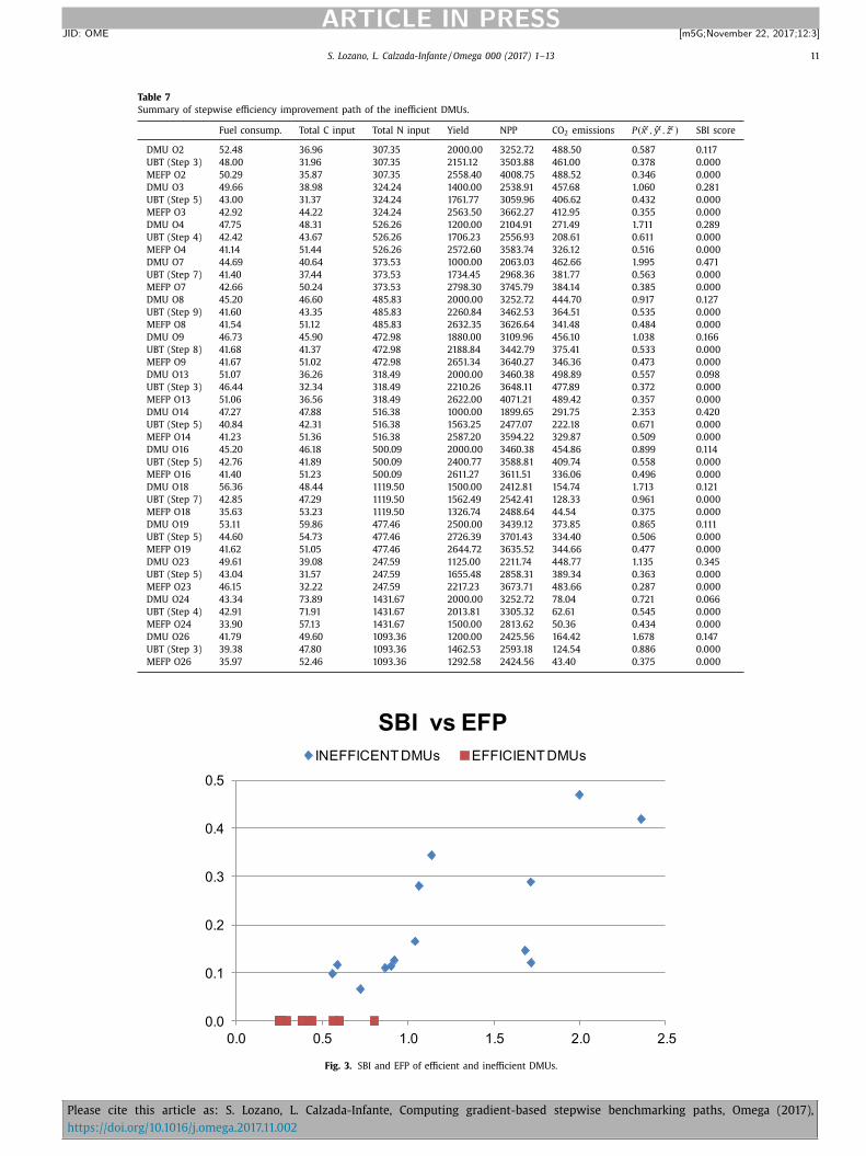
S. Lozano, L. Calzada-Infante / Omega 0 0 0 (2017) 1–13 11

ARTICLE IN PRESS JID: OME [m5G; November 22, 2017;12:3 ]

Table 7

Summary of stepwise efficiency improvement path of the inefficient DMUs.

Fuel consump. Total C input Total N input Yield NPP CO 2 emissions P( x t , y t , z t ) SBI score

DMU O2 52.48 36.96 307.35 20 0 0.0 0 3252.72 488.50 0.587 0.117

UBT (Step 3) 48.00 31.96 307.35 2151.12 3503.88 461.00 0.378 0.0 0 0

MEFP O2 50.29 35.87 307.35 2558.40 4008.75 488.52 0.346 0.0 0 0

DMU O3 49.66 38.98 324.24 140 0.0 0 2538.91 457.68 1.060 0.281

UBT (Step 5) 43.00 31.37 324.24 1761.77 3059.96 406.62 0.432 0.0 0 0

MEFP O3 42.92 44.22 324.24 2563.50 3662.27 412.95 0.355 0.0 0 0

DMU O4 47.75 48.31 526.26 120 0.0 0 2104.91 271.49 1.711 0.289

UBT (Step 4) 42.42 43.67 526.26 1706.23 2556.93 208.61 0.611 0.0 0 0

MEFP O4 41.14 51.44 526.26 2572.60 3583.74 326.12 0.516 0.0 0 0

DMU O7 44.69 40.64 373.53 10 0 0.0 0 2063.03 462.66 1.995 0.471

UBT (Step 7) 41.40 37.44 373.53 1734.45 2968.36 381.77 0.563 0.0 0 0

MEFP O7 42.66 50.24 373.53 2798.30 3745.79 384.14 0.385 0.0 0 0

DMU O8 45.20 46.60 485.83 20 0 0.0 0 3252.72 4 4 4.70 0.917 0.127

UBT (Step 9) 41.60 43.35 485.83 2260.84 3462.53 364.51 0.535 0.0 0 0

MEFP O8 41.54 51.12 485.83 2632.35 3626.64 341.48 0.484 0.0 0 0

DMU O9 46.73 45.90 472.98 1880.00 3109.96 456.10 1.038 0.166

UBT (Step 8) 41.68 41.37 472.98 2188.84 3442.79 375.41 0.533 0.0 0 0

MEFP O9 41.67 51.02 472.98 2651.34 3640.27 346.36 0.473 0.0 0 0

DMU O13 51.07 36.26 318.49 20 0 0.0 0 3460.38 498.89 0.557 0.098

UBT (Step 3) 46.44 32.34 318.49 2210.26 3648.11 477.89 0.372 0.0 0 0

MEFP O13 51.06 36.56 318.49 2622.00 4071.21 489.42 0.357 0.0 0 0

DMU O14 47.27 47.88 516.38 10 0 0.0 0 1899.65 291.75 2.353 0.420

UBT (Step 5) 40.84 42.31 516.38 1563.25 2477.07 222.18 0.671 0.0 0 0

MEFP O14 41.23 51.36 516.38 2587.20 3594.22 329.87 0.509 0.0 0 0

DMU O16 45.20 46.18 500.09 20 0 0.0 0 3460.38 454.86 0.899 0.114

UBT (Step 5) 42.76 41.89 500.09 2400.77 3588.81 409.74 0.558 0.0 0 0

MEFP O16 41.40 51.23 500.09 2611.27 3611.51 336.06 0.496 0.0 0 0

DMU O18 56.36 48.44 1119.50 150 0.0 0 2412.81 154.74 1.713 0.121

UBT (Step 7) 42.85 47.29 1119.50 1562.49 2542.41 128.33 0.961 0.0 0 0

MEFP O18 35.63 53.23 1119.50 1326.74 2488.64 44.54 0.375 0.0 0 0

DMU O19 53.11 59.86 477.46 250 0.0 0 3439.12 373.85 0.865 0.111

UBT (Step 5) 44.60 54.73 477.46 2726.39 3701.43 334.40 0.506 0.0 0 0

MEFP O19 41.62 51.05 477.46 2644.72 3635.52 344.66 0.477 0.0 0 0

DMU O23 49.61 39.08 247.59 1125.00 2211.74 448.77 1.135 0.345

UBT (Step 5) 43.04 31.57 247.59 1655.48 2858.31 389.34 0.363 0.0 0 0

MEFP O23 46.15 32.22 247.59 2217.23 3673.71 483.66 0.287 0.0 0 0

DMU O24 43.34 73.89 1431.67 20 0 0.0 0 3252.72 78.04 0.721 0.066

UBT (Step 4) 42.91 71.91 1431.67 2013.81 3305.32 62.61 0.545 0.0 0 0

MEFP O24 33.90 57.13 1431.67 150 0.0 0 2813.62 50.36 0.434 0.0 0 0

DMU O26 41.79 49.60 1093.36 120 0.0 0 2425.56 164.42 1.678 0.147

UBT (Step 3) 39.38 47.80 1093.36 1462.53 2593.18 124.54 0.886 0.0 0 0

MEFP O26 35.97 52.46 1093.36 1292.58 2424.56 43.40 0.375 0.0 0 0

0.0

0.1

0.2

0.3

0.4

0.5

0.0 0.5 1.0 1.5 2.0 2.5

SBI vs EFP

INEFFICENT DMUs EFFICIENT DMUs

Fig. 3. SBI and EFP of efficient and inefficient DMUs.

Please cite this article as: S. Lozano, L. Calzada-Infante, Computing gradient-based stepwise benchmarking paths, Omega (2017),

https://doi.org/10.1016/j.omega.2017.11.002

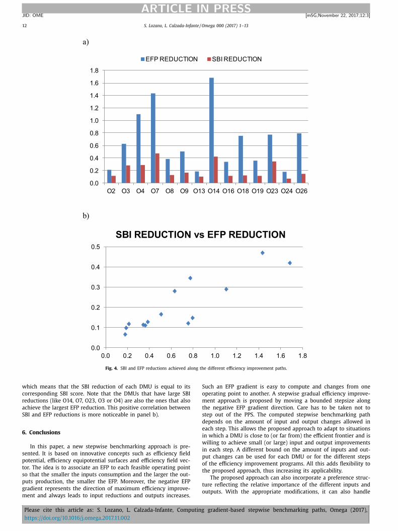
12 S. Lozano, L. Calzada-Infante / Omega 0 0 0 (2017) 1–13

ARTICLE IN PRESS JID: OME [m5G; November 22, 2017;12:3 ]

a)

0.0

0.2

0.4

0.6

0.8

1.0

1.2

1.4

1.6

1.8

O2 O3 O4 O7 O8 O9 O13 O14 O16 O18 O19 O23 O24 O26

EFP REDUCTION SBI REDUCTION

b)

0.0

0.1

0.2

0.3

0.4

0.5

0.0 0.2 0.4 0.6 0.8 1.0 1.2 1.4 1.6 1.8

SBI REDUCTION vs EFP REDUCTION

Fig. 4. SBI and EFP reductions achieved along the different efficiency improvement paths.

which means that the SBI reduction of each DMU is equal to its

corresponding SBI score. Note that the DMUs that have large SBI

reductions (like O14, O7, O23, O3 or O4) are also the ones that also

achieve the largest EFP reduction. This positive correlation between

SBI and EFP reductions is more noticeable in panel b).

6. Conclusions

In this paper, a new stepwise benchmarking approach is pre-

sented. It is based on innovative concepts such as efficiency field

potential, efficiency equipotential surfaces and efficiency field vec-

tor. The idea is to associate an EFP to each feasible operating point

so that the smaller the inputs consumption and the larger the out-

puts production, the smaller the EFP. Moreover, the negative EFP

gradient represents the direction of maximum efficiency improve-

ment and always leads to input reductions and outputs increases.

Such an EFP gradient is easy to compute and changes from one

operating point to another. A stepwise gradual efficiency improve-

ment approach is proposed by moving a bounded stepsize along

the negative EFP gradient direction. Care has to be taken not to

step out of the PPS. The computed stepwise benchmarking path

depends on the amount of input and output changes allowed in

each step. This allows the proposed approach to adapt to situations

in which a DMU is close to (or far from) the efficient frontier and is

willing to achieve small (or large) input and output improvements

in each step. A different bound on the amount of inputs and out-

put changes can be used for each DMU or for the different steps

of the efficiency improvement programs. All this adds flexibility to

the proposed approach, thus increasing its applicability.

The proposed approach can also incorporate a preference struc-

ture reflecting the relative importance of the different inputs and

outputs. With the appropriate modifications, it can also handle

Please cite this article as: S. Lozano, L. Calzada-Infante, Computing gradient-based stepwise benchmarking paths, Omega (2017),

https://doi.org/10.1016/j.omega.2017.11.002

S. Lozano, L. Calzada-Infante / Omega 0 0 0 (2017) 1–13 13

ARTICLE IN PRESS JID: OME [m5G; November 22, 2017;12:3 ]

non-discretionary variables and undesirable outputs. Actually, the

proposed approach has been applied to an organic farming dataset

with non-discretionary inputs and undesirable outputs. The use-

fulness of the proposed approach for computing bounded stepwise

efficiency improvements that end at an efficient operating point

has been shown. The length of the stepwise benchmarking paths

depends on the distance to the EF from which they start and on

the stepsize bound. Different stepsize bounds generally lead to dif-

ferent UBTs.

Although the proposed approach is rather intuitive and effec-

tive, it has some limitations. Thus, it cannot handle integer inputs

or outputs. Also, the EFP is undefined for those operating points

which have zero consumption of a certain input or zero production

of a certain output. Dealing with these zero data occurrences is a

topic for further research. One possible solution, kindly pointed out

by one of the reviewers, is to consider a linear (i.e. additive) defi-

nition of the EFP. That would lead to EES that are hyperplanes and

EFL that are straight lines (with negative slope for inputs and pos-

itive for outputs). In principle it seems possible, and it is a topic

for further research, to reformulate the proposed approach for this

type of additive EFP. Actually, an additive EFP would be very appro-

priate in case that the input and output prices were known since

then the EFP would be equivalent to the profit function. Such type

of profit potential was already considered in Lozano and Calzada-

Infante [30] in the context of dominance networks and using it

to compute profit improvement paths would be possible. Alterna-

tively, instead of the local information provided by the efficiency

potential gradient, the profit improvement direction proposed in

Zofio et al. [46] can be used to determine a stepwise profit im-

provement path.

Acknowledgment

This research was carried out with the financial support of the

Spanish Ministry of Science and the European Regional Develop-

ment Fund (ERDF), grant DPI2013-41469-P . The authors are thank-

ful to the reviewers for their helpful and insightful comments and

suggestions.

References

[1] Amirteimoori A , Kordrostami S . A Euclidean distance-based measure of effi- ciency in data envelopment analysis. Optimization 2010;59:985–96 .

[2] Ando K , Kai A , Maeda Y , Sekitani K . Least distance based inefficiency measures on the Pareto-efficient frontier in DEA. J Oper Res Soc Jpn 2012;55:73–91 .

[3] Ando K , Minamide M , Sekitani K . Monotonicity of minimum distance inefficiency measures for data envelopment analysis. Eur J Oper Res 2017;260(1):232–43 .

[4] Aparicio J . A survey on measuring efficiency through the determination of the least distance in data envelopment analysis. J Centrum Cathedra 2016;9(2):143–67 .

[5] Aparicio J , Cordero JM , Pastor JT . The determination of the least distance to the strongly efficient frontier in data envelopment analysis oriented models: modelling and computational aspects. Omega 2017;71:1–10 .

[6] Aparicio J , Mahlberg B , Pastor JT , Sahoo BK . Decomposing technical inefficiency using the principle of least action. Eur J Oper Res 2014;239:776–85 .

[7] Aparicio J , Pastor JT . A well-defined efficiency measure for dealing with closest targets in DEA. Appl Math Comput 2013;219:9142–54 .

[8] Aparicio J , Pastor JT . On how to properly calculate the Euclidean dis- tance-based measure in DEA. Optimization 2014;63(3):421–32 .

[9] Aparicio J , Pastor JT . Closest targets and strong monotonicity on the strongly efficient frontier in DEA. Omega 2014;44:51–7 .

[10] Aparicio J, Pastor JT, Sainz-Pardo JL, Vidal F. Estimating and decomposing overall inefficiency by determining the least distance to the strongly effi- cient frontier in data envelopment analysis. Oper Res Int J 2017. doi: 10.1007/ s12351- 017- 0339- 0 .

[11] Aparicio J , Ruíz JL , Sirvent I . Closest targets and minimum distance to the Pare- to-efficient frontier in DEA. J Productivity Anal 2007;28:209–18 .

[12] Baek C , Lee JD . The relevance of DEA benchmarking information and the least- -distance measure. Math Comput Modell 2009;49:265–75 .

[13] Cherchye L , Van Puyenbroeck T . A comment on multi-stage DEA methodology. Oper Res Lett 2001;28:93–8 .

[14] Cherchye L , Moesen W , Rogge N , Van Puyenbroeck T . An introduction to ‘ben- efit of the doubt’ composite indicators. Social Ind Res 2007;82(1):111–45 .

[15] Cooper WW , Seiford LM , Zhu J . Handbook on data envelopment analysis. Springer; 2004 .

[16] Cooper WW , Seiford LM , Tone K . Data envelopment analysis: a comprehensive text with models, applications, references and DEA-solver software. 2nd ed. New York: Springer; 2007 .

[17] Ebert U , Welsch H . Meaningful environmental indices: a social choice ap- proach. J Environ Econ Manage 2004;47(2):270–83 .

[18] Estrada SA , Song HS , Kim YA , Namn SH , Kang SC . A method of stepwise bench- marking for inefficient DMUs based on the proximity-based target selection. Expert Syst Appl 2009;36:11595–604 .

[19] Fang L . Centralized resource allocation based on efficiency analysis for step-by-step improvement paths. Omega 2015;51:24–8 .

[20] Frei FX , Harker PT . Projections onto efficient frontiers: theoretical and compu- tational extensions to DEA. J Productivity Anal 1999;11:275–300 .

[21] Ghahraman A , Prior D . A learning ladder toward efficiency: proposing net- work-based stepwise benchmark selection. Omega 2016;63:83–93 .

[22] González A , Álvarez A . From efficiency measurement to efficiency improve- ment: the choice of a relevant benchmark. Eur J Oper Res 2001;133:512–20 .

[23] Gutiérrez E , Aguilera E , Lozano S , Guzmán GI . A two-stage DEA approach for quantifying and analysing the inefficiency of conventional and organic rain-fed cereals in Spain. J Cleaner Prod 2017;149:335–48 .

[24] Hong HK , Ha SH , Shin CK , Park SC , Kim SH . Evaluating the efficiency of sys- tem integration projects using data envelopment analysis (DEA) and machine learning. Expert Syst Appl 1999;16(3):283–96 .

[25] Khodakarami M , Shabani A , Saen RF . A new look at measuring sustainability of industrial parks: a two-stage data envelopment analysis approach. Clean Tech- nol Environ Policy 2014;16:1577–96 .

[26] Kuosmanen T . Weak disposability in nonparametric production analysis with undesirable outputs. Am J Agri Econ 2005;87:1077–82 .

[27] Lim S , Bae H , Lee LH . A study on the selection of benchmarking paths in DEA. Expert Syst Appl 2011;38:7665–73 .

[28] Lozano S , Villa G . Determining a sequence of targets in DEA. J Oper Res Soc 2005;56:1439–47 .

[29] Lozano S , Villa G . Gradual technical and scale efficiency improvement in DEA. Ann Oper Res 2010;173:123–36 .

[30] Lozano S , Calzada-Infante L . Dominance network analysis of economic effi- ciency. Expert Syst Appl 2017;82:53–66 .

[31] Maital S , Vaninsky A . Data envelopment analysis with a single DMU: a graphic projected-gradient approach. Eur J Oper Res 1999;115:518–28 .

[32] Park J , Bae H , Lim S . Method of benchmarking route choice based on the input similarity using DEA. Smart Innov Syst Technol 2011;10:519–28 .

[33] Park J , Bae H , Lim S . Stepwise benchmarking path selection in DEA. Smart In- nov Syst Technol 2012;16:477–84 .

[34] Park J , Bae H , Lim S . A DEA-based method of stepwise benchmark target selec- tion with preference, direction and similarity criteria. Int J Innov Comput Inf Control 2012;8:5821–34 .

[35] Park J , Lim S , Bae H . DEA-based port efficiency improvement and stepwise benchmarking target selection. Information 2012;14(12C):6155–71 .

[36] Park J , Lim S , Bae H . An optimization approach to the construction of a se- quence of benchmark targets in DEA-based benchmarking. J Korean Inst Ind Eng 2014;40(6):628–41 .

[37] Park J , Sung SI . Integrated approach to construction of benchmarking network in DEA-based stepwise benchmark target selection. Sustainability 2016;8(600) .

[38] Pastor JT , Aparicio J . The relevance of DEA benchmarking information and the least-distance measure: comment. Math Comput Modell 2010;52:397–9 .

[39] Seiford LM , Zhu J . Context-dependent data envelopment analysis—measuring attractiveness and progress. Omega 2003;31:397–408 .

[40] Sharma MJ , Yu SJ . Performance based stratification and clustering for bench- marking of container terminals. Expert Syst Appl 2009;36:5016–22 .

[41] Sharma MJ , Yu SJ . Benchmark optimization and attribute identification for im- provement of container terminals. Eur J Oper Res 2010;201:568–80 .

[42] Silva Portela MCA , Castro Borges P , Thanassoulis E . Finding closest targets in non-oriented DEA models: the case of convex and non-convex technologies. J Productivity Anal 2003;19:251–69 .

[43] Silva Portela MCA , Thanassoulis E . Developing a decomposable measure of profit efficiency usng DEA. J Oper Res Soc 2007;58(4):481–90 .

[44] Suzuki S , Nijkamp P . A stepwise-projection data envelopment analysis for pub- lic transport operations in Japan. Lett Spatial Resour Sci 2011;4:139–56 .

[45] Zhu J . Quantitative models for performance evaluation and benchmarking: data envelopment analysis with spreadsheets and DEA excel solver. Boston: Kluwer Academic Publishers; 2002 .

[46] Zofio JL , Pastor JT , Aparicio J . The directional profit efficiency measure: on why profit inefficiency is either technical or allocative. J Productivity Anal 2013;40:257–66 .

Please cite this article as: S. Lozano, L. Calzada-Infante, Computing gradient-based stepwise benchmarking paths, Omega (2017),

https://doi.org/10.1016/j.omega.2017.11.002

Assessing individual performance based on the efficiency of projects

B. Adenso-Díaz a,⇑, S. Lozano b, E. Gutiérrez b, L. Calzada a, S. García a

a Engineering School, Campus de Gijon, University of Oviedo, 33204 Gijón, Spainb Engineering School, Department of Industrial Management, University of Seville, 41092 Seville, Spain

a r t i c l e i n f o

Article history:

Received 8 February 2016

Received in revised form 10 January 2017

Accepted 21 March 2017

Keywords:

Project efficiency

Teams

Individual performance

Data Envelopment Analysis

Regression analysis

a b s t r a c t

Assessing the performance of each of the team members in any project is a difficult task since in most

cases the outcomes mask the individual contributions. In this paper a two-step approach is proposed

to estimate the relative performance of the members of the organization who have participated in the

different projects carried out. Firstly, a DEA model evaluates the efficiency of the projects, whose results

are used later on in a regression model to assess the performance of each individual. The proposed

approach is validated using 480 instances identifying the factors that may affect the accuracy of the

results. The application to a case study involving a real-world dataset of 46 software development pro-

jects carried out by a ten-member team is also presented. The results show that the proposed approach

estimates, on average, the unknown true efficiency of the individuals rather well and is robust against

data noise.

� 2017 Published by Elsevier Ltd.

1. Introduction

Managing projects represents a big challenge from many

different aspects. Not only the technical difficulty of the tasks to

be performed is to be dealt with, trying to sort out all the problems

that may appear, but also the complexity of interacting groups of

people, from different backgrounds in many cases, adds further

issues to the project execution and success.

When different people are involved in the development of a

project, one of the problems that arise is how to measure the

performance of each team member with respect to the project

outcome. The nature of the contributions is usually different;

different people work in different stages of the projects, interacting

in complex ways, with different criticality in the tasks performed.

With all these factors in the scenario, on most occasions it is

impossible to measure accurately how much of the project out-

come could be credited to each participant, whether in order to

reward their work or simply to record their performance evolution.

Extensive research has been carried out dealing with team pro-

ject issues, such as team membership, diversity and performance

(Mathieu, Maynard, Rapp, & Gilson, 2008; Rubino, Avery, &

Volpone, 2014). However, the assessment of the performance of

each member to the global project outcome is a problem that has

not been sufficiently studied and with no clear solution so far.

In this paper we try to shine a light on the problem of evaluating

each member’s performance using the technical efficiency of the

projects in which they were involved. When an efficient team

member has been participating in different projects, it could be

expected that the performance of those projects would be higher

than if the team member had lower performance efficiency. Based

on that hypothesis, by using Data Envelopment Analysis (DEA) the

efficiency of the projects are evaluated, and then a regression

model taking into account the contribution of each member com-

putes an estimation of the individual contribution of each person.

The structure of the paper is the following: in the next section a

short review of the literature is presented, introducing in more

detail the problem to be tackled; Section 3 presents the modelling

details of the proposed approach, while Section 4 provides the

results of some computational experiments carried out to validate

and gauge the accuracy of the proposed approach. Section 5 com-

ments on the results of the application of the proposed approach to

a real case study, and Section 6 summarizes the main results of this

research.

2. Problem description

Most of the works dealing with team effectiveness (Kozlowski &

Ilgen, 2006) still consider the IPO (input-process-output) model,

where the input describes antecedents of team interaction (charac-

teristics, team-level factors, contextual and organization factors),

which interact to drive processes that transform the inputs into

outcomes (i.e., results and by-products valued by their perfor-

mance: quality, quantity, satisfaction, commitment. . .). Note that

there is not only one way to assess the individual quality of the

work done and different performance metrics can be used. For

http://dx.doi.org/10.1016/j.cie.2017.03.026

0360-8352/� 2017 Published by Elsevier Ltd.

⇑ Corresponding author.

E-mail address: adenso@uniovi.es (B. Adenso-Díaz).

Computers & Industrial Engineering 107 (2017) 280–288

Contents lists available at ScienceDirect

Computers & Industrial Engineering

journal homepage: www.elsevier .com/ locate/caie

instance, Gamble and Hale (2013) consider four facets when

assessing individual performance: the contribution (direct partici-

pation and involvement), the influence (how an individual directs

the team’s progress), impact (relationship between what they do

and their results) and impression (how well team members

acknowledge the efforts of the others).

Although the IPO model has been valuable in the study of effec-

tiveness, more recently it has been adapted and extended in differ-

ent ways. For instance, Tekleab, Quigley, and Tesluk (2009)

incorporate the length of time that the teams are interacting and

other mediator variables to better understand what is happening

in the process part of the model. However, the quantitative evalu-

ation of individuals when they are working in groups is quite dif-

ficult, in part due to the lack of information on the daily

evolution of the project, but also because in most cases the out-

comes mask individuals’ contributions.

Perhaps the most well-known case, in which huge interest has

been shown about this evaluation problem, is in higher education

when assessing the work developed by groups of students. In order

to expose students to real-world situations, it is quite usual for

them to be challenged to work in groups on relatively large pro-

jects (Coppit, 2006) that later are assessed and have an impact

on the individual marks of each member. However, to assign a

mark at the end of the project, the teacher will find it difficult to

determine the actual contribution of each team member in the

final work, given that most of the tasks are developed indepen-

dently, without the presence of the teacher.

In most cases, the easiest solution is to assign the same grade

to each member (Alden, 2011) as an emulation of the real world

where the success or failure of a project is the same for each par-

ticipant (for instance, in a sports competition all team members

receive identical medals). However, it is well known that this

procedure does not discourage the unproductive student who

benefits from the work of his/her peers. In fact, different typical

behaviours have been characterized (Coppit, 2006), by analyzing

how these group members interact, as follows: the hitchhiker

(who looks to maximize his mark while minimizing his work),

the underachiever (who minimizes his work and is happy with

a lower grade), the procrastinator (willing to work but delivering

his part just immediately prior to the deadline), the dilettante

(who is involved in many tasks but only superficially and never

delivers a result), among others. All these behaviours together

undermine the morale of the team and definitely affect the qual-

ity of the results as the system is not seen as fair by the more

efficient members.

There is also some literature analyzing ways to deal with this

problem in higher education, in many cases related to business

or engineering teaching (Gamble & Hale, 2013; Mathews, 1994;

Salama & Ahmed, 2011). The most usual way to look for a fairer

mark is to add a peer evaluation to the global assessment of the

outcome, given that those who really know what the individual

contribution of each member has been are the ones who have

worked on the inside. Different approaches have been used for rat-

ing the student’s contribution (Wang & Vollstedt, 2014) including

team journals (recording the effective distribution of effort among

the members) or computerized team evaluation using different

software. However many authors (Kennedy, 2005; Wang &

Vollstedt, 2014) have raised doubts about its accuracy, reporting

that when peer evaluation is used to obtain some extra points

(merit pay) teams frequently distribute the merit pay uniformly

– again making the evaluation system unfair.

In general, the management performance assessment of a pro-

ject has been widely studied in the literature (Qureshi, Warraich,

& Hijazi, 2009; Wateridge, 1995), considering new factors beyond

the traditional ‘‘iron triangle” of time, cost and quality.

Wateridge (1995) considers that the quality should be seen not

only from the clients’ point of view, but also from the perception

of all the stakeholders involved in the project.

If assessing team performance is a task that is not simple to

carry out, linking overall performance with individual proficiency

results is even harder. In the 60s, Wiest, Porter, and Ghiselli

(1961) identified three main points around this relationship: how

the team performance compares with the performance expected

on the basis of adding the members’ proficiency; how well the glo-

bal performance can be predicted from individuals’ performance;

and whether the group performance can be better explained by

the performance of the best and worst members.

Results show that regarding the first point, summation of indi-

vidual contributions exceeds the performance when working as a

group; in relation to the third point, it seems that depending on

the flexibility of the tasks that the members must carry out, there

is a higher correlation with the most proficient member or with the

least (in this latter case, when the tasks are more rigidly assigned).

Wiest et al. (1961) also found that when the proficiencies of the

members are similar, it is more likely that they form an efficient

team. Also Campion, Medsker, and Higgs (1993) studied the rela-

tionship between the group characteristics and their effectiveness,

finding that heterogeneity is not positively related to effectiveness,

which means that a variety of skills should be present in the group,

but all members must be similarly skilled. Other researchers have

studied how diversity affects group performance. For instance

Jackson and LePine (2003) observed that grouping low and high

performers could provoke a negative reaction from high perform-

ers if the low performance is attributed to low conscientiousness.

In relation to the number of projects in which an individual

should be involved, Chan (2014) studied the Multiple Team Mem-

bership problem, finding that as the number of projects in which a

person is simultaneously participating increases, his/her perfor-

mance improves due to an enrichment in his innovation process;

however, beyond a certain number of projects, performance starts

to decrease and this implies a fragmentation in his/her attention

due to continuous switches in the work.

In this paper we return to the second point raised byWiest et al.

(1961), but looking for the reverse equation: we are not concerned

with estimating the performance of a team, given the individual

performances, but the opposite: given the team performance, to

assess how good the performance of each single individual is. To

do this, first we need to assess the good performance of a project,

and DEA has been identified as an appropriate tool for the purpose.

DEA is a non-parametric methodology for assessing the relative

efficiency of a number of comparable entities, generally termed

Decision Making Units (DMUs). The methodology assumes that

DMUs consume inputs (i.e. resources) and produces outputs (e.g.

revenue). DEA identifies and uncovers sources of inefficiency by

seeing if it is possible for each DMU to attain their current output

level with a reduced amount of inputs. The larger the reduction of

inputs deemed feasible, the lower the efficiency. Those DMUs for

which no potential input reductions are feasible are labelled as

efficient. There is extensive literature on DEA, both in terms of the-

ory (e.g. Cooper, Seiford, & Tone, 2006) and application (e.g.

Cooper, Seiford, & Zhu, 2004). In particular, DEA has been used

for evaluating projects in project portfolio selection (e.g. Tavana,

Keramatpour, Santos-Arteaga, & Ghorbaniane, 2015), benchmark-

ing software development projects (e.g. Pai, Subramanian, &

Pendharkar, 2015; Sudhaman & Thangavel, 2015), contractor selec-

tion in procurement projects (e.g. Yang, Wang, Wang, & Ma, 2015),

appraising construction and engineering projects (Abbasian-

Hosseini, Hsiang, Leming, & Liu, 2014; Caulfield, Bailey, &

Mullarkey, 2013), and for managing new product development

projects (Donthu & Unal, 2014), etc. Moreover, regarding the eval-

uation of working teams, DEA (more specifically Network DEA) has

been used also to assess the performance of individuals in work-

B. Adenso-Díaz et al. / Computers & Industrial Engineering 107 (2017) 280–288 281

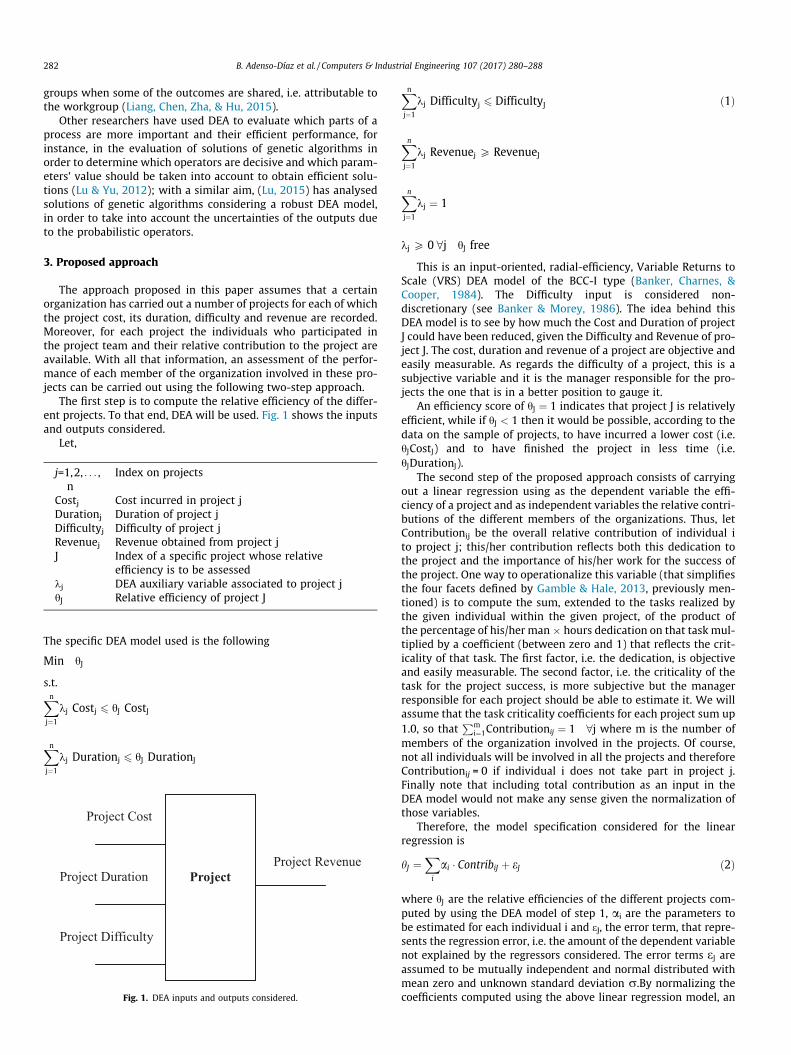
groups when some of the outcomes are shared, i.e. attributable to

the workgroup (Liang, Chen, Zha, & Hu, 2015).

Other researchers have used DEA to evaluate which parts of a

process are more important and their efficient performance, for

instance, in the evaluation of solutions of genetic algorithms in

order to determine which operators are decisive and which param-

eters’ value should be taken into account to obtain efficient solu-

tions (Lu & Yu, 2012); with a similar aim, (Lu, 2015) has analysed

solutions of genetic algorithms considering a robust DEA model,

in order to take into account the uncertainties of the outputs due

to the probabilistic operators.

3. Proposed approach

The approach proposed in this paper assumes that a certain

organization has carried out a number of projects for each of which

the project cost, its duration, difficulty and revenue are recorded.

Moreover, for each project the individuals who participated in

the project team and their relative contribution to the project are

available. With all that information, an assessment of the perfor-

mance of each member of the organization involved in these pro-

jects can be carried out using the following two-step approach.

The first step is to compute the relative efficiency of the differ-

ent projects. To that end, DEA will be used. Fig. 1 shows the inputs

and outputs considered.

Let,

j=1,2, . . . ,

n

Index on projects

Costj Cost incurred in project j

Durationj Duration of project j

Difficultyj Difficulty of project j

Revenuej Revenue obtained from project j

J Index of a specific project whose relative

efficiency is to be assessed

kj DEA auxiliary variable associated to project j

hJ Relative efficiency of project J

The specific DEA model used is the following

Min hJ

s.t.

Xn

j¼1

kj Costj 6 hJ CostJ

Xn

j¼1

kj Durationj 6 hJ DurationJ

Xn

j¼1

kj Difficultyj 6 DifficultyJ ð1Þ

Xn

j¼1

kj Revenuej P RevenueJ

Xn

j¼1

kj ¼ 1

kj P 0 8j hJ free

This is an input-oriented, radial-efficiency, Variable Returns to

Scale (VRS) DEA model of the BCC-I type (Banker, Charnes, &

Cooper, 1984). The Difficulty input is considered non-

discretionary (see Banker & Morey, 1986). The idea behind this

DEA model is to see by how much the Cost and Duration of project

J could have been reduced, given the Difficulty and Revenue of pro-

ject J. The cost, duration and revenue of a project are objective and

easily measurable. As regards the difficulty of a project, this is a

subjective variable and it is the manager responsible for the pro-

jects the one that is in a better position to gauge it.

An efficiency score of hJ ¼ 1 indicates that project J is relatively

efficient, while if hJ < 1 then it would be possible, according to the

data on the sample of projects, to have incurred a lower cost (i.e.

hJCostJ) and to have finished the project in less time (i.e.

hJDurationJ).

The second step of the proposed approach consists of carrying

out a linear regression using as the dependent variable the effi-

ciency of a project and as independent variables the relative contri-

butions of the different members of the organizations. Thus, let

Contributionij be the overall relative contribution of individual i

to project j; this/her contribution reflects both this dedication to

the project and the importance of his/her work for the success of

the project. One way to operationalize this variable (that simplifies

the four facets defined by Gamble & Hale, 2013, previously men-

tioned) is to compute the sum, extended to the tasks realized by

the given individual within the given project, of the product of

the percentage of his/her man � hours dedication on that task mul-

tiplied by a coefficient (between zero and 1) that reflects the crit-

icality of that task. The first factor, i.e. the dedication, is objective

and easily measurable. The second factor, i.e. the criticality of the

task for the project success, is more subjective but the manager

responsible for each project should be able to estimate it. We will

assume that the task criticality coefficients for each project sum up

1.0, so thatPm

i¼1Contributionij ¼ 1 8j where m is the number of

members of the organization involved in the projects. Of course,

not all individuals will be involved in all the projects and therefore

Contributionij = 0 if individual i does not take part in project j.

Finally note that including total contribution as an input in the

DEA model would not make any sense given the normalization of

those variables.

Therefore, the model specification considered for the linear

regression is

hJ ¼X

i

ai � ContribiJ þ eJ ð2Þ

where hJ are the relative efficiencies of the different projects com-

puted by using the DEA model of step 1, ai are the parameters to

be estimated for each individual i and eJ, the error term, that repre-

sents the regression error, i.e. the amount of the dependent variable

not explained by the regressors considered. The error terms eJ areassumed to be mutually independent and normal distributed with

mean zero and unknown standard deviation r.By normalizing the

coefficients computed using the above linear regression model, an

Project Cost

Project Duration

Project Difficulty

Project

Project Revenue

Fig. 1. DEA inputs and outputs considered.

282 B. Adenso-Díaz et al. / Computers & Industrial Engineering 107 (2017) 280–288

estimation of the relative performance of each individual in the

organization can be computed

Performancei ¼ai

maxkak

ð3Þ

The rationale behind the proposed approach is that if an indi-

vidual has a high participation in projects with high efficiency

scores then he/she should be credited and assigned a good relative

performance score. On the other hand, individuals who participate

in low efficiency projects receive a low relative performance score.

We can also see it the other way around, i.e. if an individual is a

good performer then the projects in which he/she participates

should tend to be efficient, especially if the other members of the

project team are also good performers. Bad performers, on the

other hand, tend to increase both cost and duration (and therefore

lower the efficiency) of the projects in which they participate. Note

that since the proposed approach computes a sort of average per-

formance of each individual in the different projects it participates,

it is reasonable to assume that the performance of the individuals

may vary from one project to another and that is why the regres-

sion specification includes an error term that captures those ran-

dom fluctuations.

A final remark about the proposed approach is that the regres-

sion analysis of step 2 identifies some of the regressors as signifi-

cant, while others may not be found significant at a given

significance level. For each non significant variable this means that

the null hypothesis cannot be rejected (at the given significance

level) and that its corresponding coefficient ai (and, therefore, Per-

formancei) is zero. For the significant variables the corresponding

coefficients ai are generally positive which means that the contri-

butions of those individuals to the projects in which they have par-

ticipated translate into an increase in efficiency of those projects.

But, in principle, it is also possible that a significant variable may

have an estimated coefficient ai < 0. This should be interpreted as

being that the contributions of the individual to the projects in

which he/she participates reduces the projects’ efficiency, i.e. he/

she subtracts more than adds to the projects’ efficiency. This is

an undesirable situation that does not occur frequently but that

the proposed approach can detect in case it happens. In any case,

the computed relative performance scores lead to a ranking of

the performance of the different individuals and this may be of

utmost importance for management.

4. Experimental framewok and results

In order to validate and test the accuracy of our model to eval-

uate individuals’ efficiency, a set of experiments have been carried

out. The idea is to generate a large number of instances (group of

projects) for which we know all the relevant data (contribution

of each team member, duration, cost and revenue of each project,

dependent on the – unknown for the model – performance level

of each individual).

Therefore the procedure consists of randomly generating ‘‘true”

performance levels (labelled individual efficiencies efi), randomly

assigning individuals to some projects j with randomly generated

contribution levels contij (so that Ri contij = 1 "j) and calculate

for each project its data partially based on these variables. Thus,

in our experiment,

� The difficulty of a project Difficultyj is a random variable in the

range [0.5, 1.5]

� The expected duration of a project edj is a random variable in

the range [4, 36] months multiplied by the difficulty of the pro-

ject Difficultyj. Thus, a project with a larger difficulty should

take longer than a project with a lower difficulty. The real

duration of a project, Durationj, is calculated as the expected

duration edj divided by an efficiency factor efj =Ri efi ⁄ contij + c,with c a random uniform variable in the interval [�b,b].

� The cost of a project Costj is calculated as the number of people

assigned to the project times the real duration of the project.

� The revenue of a project Revenuej is calculated as the number

of people assigned to the project, times edj, times a profit factor

(1.25, in our case).

Note that the way that the project data are generated involves

the efficiency of the projects and that these were linked to the effi-

ciency of the individuals. This was not done to produce favourable

results but because it is more reasonable than if we generate the

duration and cost of the projects without any regards to the sup-

posedly known efficiency of the individuals. The rationale of the

proposed approach is that efficient individuals perform efficiently

in the projects they participate. If the project data are generated

randomly then there would be no link between the project

efficiencies and the efficiencies of the individuals, i.e. inefficient

individuals might develop an efficient project and vice versa. Our

assumption is that is unlikely to happen.

In order to test the behaviour of our model in a variety of sce-

narios, we identified four factors that could affect its performance.

By introducing them into the procedure for the generation of the

instances, it will be possible to assess how relevant these factors

are for the accuracy of the obtained results. The factors considered

are the following:

� F1. Number of people working in each project. It may be expected

that bigger teams could be less exposed to the influence of indi-

vidual members. Therefore we considered a low level (F1.1)

with 30% of all the individuals in the department involved in

each project, and a high level (F1.2) with 60%. Assuming that

the number of individuals considered is ten, this means that

three or six people are involved in each project depending on

the level of this factor.

� F2. The variability of the contributions of the individuals involved

in a project. A low level of variability (F2.1), with (unnormal-

ized) contributions in the range [0.35,0.65] will capture the sit-

uation of quite homogeneous projects (with everybody involved

to a similar degree) while the high level (F2.2) will allow a dis-

persed degree of contributions in the project (in the range

[0.2,0.9]).

� F3. The variability of the individuals’ efficiencies. Homogenous

members could mean less individual influence on the project

results. Therefore, in our case a low level (F3.1) means a quite

homogeneous group of high-performance employees, everyone

in the range [0.75,1.0], while a high level (F3.2) means a larger

dispersion in the performance level of the personnel (in the

range [0.3,1.0]). We remark on how important it is in the liter-

ature dealing with team formation, i.e. the homogeneity of the

team members (Jackson & LePine, 2003). Note also that,

although the individual efficiencies are generated within the

given intervals, a certain number of individuals (one, two or

three, with equal probability) are assigned an individual effi-

ciency efi = 1.

� F4: Three levels of the amount of noise in the data

b 2 f0:2;0:5;0:8g have been considered. This noise represents

events that can affect the execution of the projects (their dura-

tion, cost, etc.) but cannot be attributed to the team members’

performance.

In our experiments, for each of the 23 � 3 factor level combina-

tions of the four factors considered, 20 instances were generated.

This gives a total of 8 � 20 � 3 = 480 instances. Each instance

was processed using the proposed approach. Thus, the relative effi-

B. Adenso-Díaz et al. / Computers & Industrial Engineering 107 (2017) 280–288 283

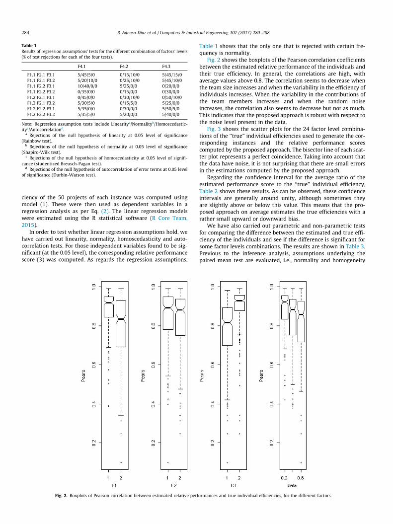
ciency of the 50 projects of each instance was computed using

model (1). These were then used as dependent variables in a

regression analysis as per Eq. (2). The linear regression models

were estimated using the R statistical software (R Core Team,

2015).

In order to test whether linear regression assumptions hold, we

have carried out linearity, normality, homoscedasticity and auto-

correlation tests. For those independent variables found to be sig-

nificant (at the 0.05 level), the corresponding relative performance

score (3) was computed. As regards the regression assumptions,

Table 1 shows that the only one that is rejected with certain fre-

quency is normality.

Fig. 2 shows the boxplots of the Pearson correlation coefficients

between the estimated relative performance of the individuals and

their true efficiency. In general, the correlations are high, with

average values above 0.8. The correlation seems to decrease when

the team size increases and when the variability in the efficiency of

individuals increases. When the variability in the contributions of

the team members increases and when the random noise

increases, the correlation also seems to decrease but not as much.

This indicates that the proposed approach is robust with respect to

the noise level present in the data.

Fig. 3 shows the scatter plots for the 24 factor level combina-

tions of the ‘‘true” individual efficiencies used to generate the cor-

responding instances and the relative performance scores

computed by the proposed approach. The bisector line of each scat-

ter plot represents a perfect coincidence. Taking into account that

the data have noise, it is not surprising that there are small errors

in the estimations computed by the proposed approach.

Regarding the confidence interval for the average ratio of the

estimated performance score to the ‘‘true” individual efficiency,

Table 2 shows these results. As can be observed, these confidence

intervals are generally around unity, although sometimes they

are slightly above or below this value. This means that the pro-

posed approach on average estimates the true efficiencies with a

rather small upward or downward bias.

We have also carried out parametric and non-parametric tests

for comparing the difference between the estimated and true effi-

ciency of the individuals and see if the difference is significant for

some factor levels combinations. The results are shown in Table 3.

Previous to the inference analysis, assumptions underlying the

paired mean test are evaluated, i.e., normality and homogeneity

Table 1

Results of regression assumptions’ tests for the different combination of factors’ levels

(% of test rejections for each of the four tests).

F4.1 F4.2 F4.3

F1.1 F2.1 F3.1 5/45/5/0 0/15/10/0 5/45/15/0

F1.1 F2.1 F3.2 5/20/10/0 0/25/10/0 5/45/10/0

F1.1 F2.2 F3.1 10/40/0/0 5/25/0/0 0/20/0/0

F1.1 F2.2 F3.2 0/35/0/0 0/15/0/0 0/30/0/0

F1.2 F2.1 F3.1 0/45/0/0 0/30/10/0 0/50/10/0

F1.2 F2.1 F3.2 5/30/5/0 0/15/5/0 5/25/0/0

F1.2 F2.2 F3.1 5/35/0/0 0/30/0/0 5/50/5/0

F1.2 F2.2 F3.2 5/35/5/0 5/20/0/0 5/40/0/0

Note: Regression assumption tests include Linearitya/Normalityb/Homoscedastic-

ityc/Autocorrelationd.a Rejections of the null hypothesis of linearity at 0.05 level of significance

(Rainbow test).b Rejections of the null hypothesis of normality at 0.05 level of significance

(Shapiro-Wilk test).c Rejections of the null hypothesis of homoscedasticity at 0.05 level of signifi-

cance (studentized Breusch-Pagan test).d Rejections of the null hypothesis of autocorrelation of error terms at 0.05 level

of significance (Durbin-Watson test).

Fig. 2. Boxplots of Pearson correlation between estimated relative performances and true individual efficiencies, for the different factors.

284 B. Adenso-Díaz et al. / Computers & Industrial Engineering 107 (2017) 280–288

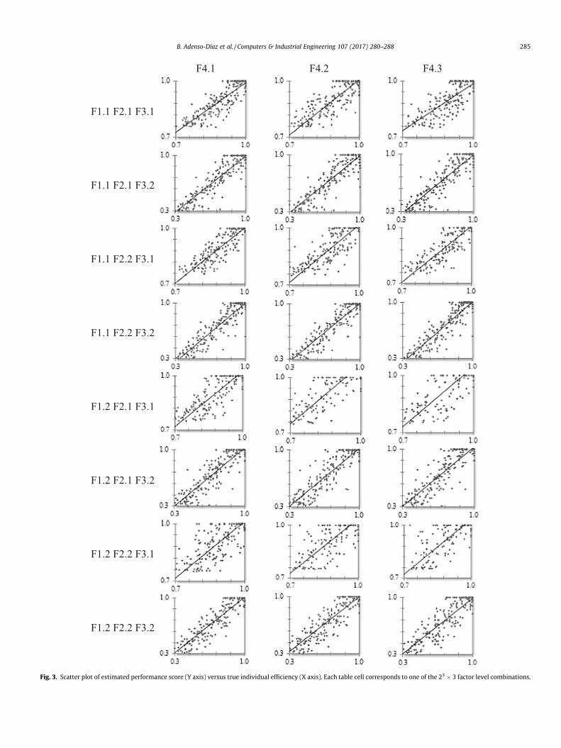
F4.1 F4.2 F4.3

F1.1 F2.1 F3.1

F1.1 F2.1 F3.2

F1.1 F2.2 F3.1

F1.1 F2.2 F3.2

F1.2 F2.1 F3.1

F1.2 F2.1 F3.2

F1.2 F2.2 F3.1

F1.2 F2.2 F3.2

Fig. 3. Scatter plot of estimated performance score (Y axis) versus true individual efficiency (X axis). Each table cell corresponds to one of the 23 � 3 factor level combinations.

B. Adenso-Díaz et al. / Computers & Industrial Engineering 107 (2017) 280–288 285

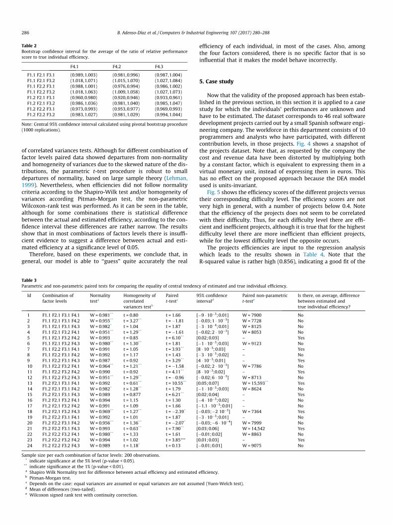
of correlated variances tests. Although for different combination of

factor levels paired data showed departures from non-normality

and homogeneity of variances due to the skewed nature of the dis-

tributions, the parametric t-test procedure is robust to small

departures of normality, based on large sample theory (Lehman,

1999). Nevertheless, when efficiencies did not follow normality

criteria according to the Shapiro-Wilk test and/or homogeneity of

variances according Pitman-Morgan test, the non-parametric

Wilcoxon-rank test was performed. As it can be seen in the table,

although for some combinations there is statistical difference

between the actual and estimated efficiency, according to the con-

fidence interval these differences are rather narrow. The results

show that in most combinations of factors levels there is insuffi-

cient evidence to suggest a difference between actual and esti-

mated efficiency at a significance level of 0.05.

Therefore, based on these experiments, we conclude that, in

general, our model is able to ‘‘guess” quite accurately the real

efficiency of each individual, in most of the cases. Also, among

the four factors considered, there is no specific factor that is so

influential that it makes the model behave incorrectly.

5. Case study

Now that the validity of the proposed approach has been estab-

lished in the previous section, in this section it is applied to a case

study for which the individuals’ performances are unknown and

have to be estimated. The dataset corresponds to 46 real software

development projects carried out by a small Spanish software engi-

neering company. The workforce in this department consists of 10

programmers and analysts who have participated, with different

contribution levels, in those projects. Fig. 4 shows a snapshot of

the projects dataset. Note that, as requested by the company the

cost and revenue data have been distorted by multiplying both

by a constant factor, which is equivalent to expressing them in a

virtual monetary unit, instead of expressing them in euros. This

has no effect on the proposed approach because the DEA model

used is units-invariant.

Fig. 5 shows the efficiency scores of the different projects versus

their corresponding difficulty level. The efficiency scores are not

very high in general, with a number of projects below 0.4. Note

that the efficiency of the projects does not seem to be correlated

with their difficulty. Thus, for each difficulty level there are effi-

cient and inefficient projects, although it is true that for the highest

difficulty level there are more inefficient than efficient projects,

while for the lowest difficulty level the opposite occurs.

The projects efficiencies are input to the regression analysis

which leads to the results shown in Table 4. Note that the

R-squared value is rather high (0.856), indicating a good fit of the

Table 2

Bootstrap confidence interval for the average of the ratio of relative performance

score to true individual efficiency.

F4.1 F4.2 F4.3

F1.1 F2.1 F3.1 (0.989,1.003) (0.981,0.996) (0.987,1.004)

F1.1 F2.1 F3.2 (1.018,1.071) (1.015,1.070) (1.027,1.084)

F1.1 F2.2 F3.1 (0.988,1.001) (0.976,0.994) (0.986,1.002)

F1.1 F2.2 F3.2 (1.018,1.063) (1.009,1.058) (1.027,1.073)

F1.2 F2.1 F3.1 (0.960,0.980) (0.920,0.946) (0.933,0.961)

F1.2 F2.1 F3.2 (0.986,1.036) (0.981,1.040) (0.985,1.047)

F1.2 F2.2 F3.1 (0.973,0.993) (0.953,0.977) (0.969,0.993)

F1.2 F2.2 F3.2 (0.983,1.027) (0.981,1.029) (0.994,1.044)

Note: Central 95% confidence interval calculated using pivotal bootstrap procedure

(1000 replications).

Table 3

Parametric and non-parametric paired tests for comparing the equality of central tendency of estimated and true individual efficiency.

Id Combination of

factor levels

Normality

testaHomogeneity of

correlated

variances testb

Paired

t-testc95% confidence

intervaldPaired non-parametric

t-testeIs there, on average, difference

between estimated and

true individual efficiency?

1 F1.1 F2.1 F3.1 F4.1 W = 0.981** t = 0.80 t = 1.66 [�9 � 10�3;0.01] W = 7900 No

2 F1.1 F2.1 F3.1 F4.2 W = 0.955** t = 3.27** t = �1.81 [�0.03;1 � 10�3] W = 7728 No

3 F1.1 F2.1 F3.1 F4.3 W = 0.982* t = 1.04 t = 1.87 [�3 � 10�4;0.01] W = 8125 No

4 F1.1 F2.1 F3.2 F4.1 W = 0.951** t = 1.29** t = �1.61 [�0.02;2 � 10�3] W = 8053 No

5 F1.1 F2.1 F3.2 F4.2 W = 0.993 t = 0.85 t = 6.10** [0.02;0.03] – Yes

6 F1.1 F2.1 F3.2 F4.3 W = 0.980** t = 1.30** t = 1.81 [�1 � 10�3;0.03] W = 9123 No

7 F1.1 F2.2 F3.1 F4.1 W = 0.991 t = 1.05 t = 3.93** [8 � 10�3;0.03] – Yes

8 F1.1 F2.2 F3.1 F4.2 W = 0.992 t = 1.17 t = 1.43 [�3 � 10�3;0.02] – No

9 F1.1 F2.2 F3.1 F4.3 W = 0.987 t = 0.92 t = 3.29** [4 � 10�3;0.01] – Yes

10 F1.1 F2.2 F3.2 F4.1 W = 0.964** t = 1.21** t = �1.58 [�0.02;2 � 10�3] W = 7786 No

11 F1.1 F2.2 F3.2 F4.2 W = 0.990 t = 0.92 t = 4.11** [8 � 10�3;0.02] – Yes

12 F1.1 F2.2 F3.2 F4.3 W = 0.951** t = 1.29** t = �0.96 [�0.02;6 � 10�3] W = 8713 No

13 F1.2 F2.1 F3.1 F4.1 W = 0.992 t = 0.61** t = 10.55** [0.05;0.07] W = 15,593** Yes

14 F1.2 F2.1 F3.1 F4.2 W = 0.982* t = 1.28** t = 1.79 [�1 � 10�3;0.03] W = 8624 No

15 F1.2 F2.1 F3.1 F4.3 W = 0.989 t = 0.877 t = 6.21** [0.02;0.04] – Yes

16 F1.2 F2.1 F3.2 F4.1 W = 0.994 t = 1.15 t = 1.30 [�4 � 10�3;0.02] – No

17 F1.2 F2.1 F3.2 F4.2 W = 0.991 t = 1.09 t = 1.66 [�1.1 � 10�3;0.01] – No

18 F1.2 F2.1 F3.2 F4.3 W = 0.969** t = 1.27** t = �2.39* [�0.03;�2 10�3] W = 7364 Yes

19 F1.2 F2.2 F3.1 F4.1 W = 0.992 t = 1.01 t = 1.87 [�3 � 10�3;0.01] – No

20 F1.2 F2.2 F3.1 F4.2 W = 0.956** t = 1.36** t = �2.07* [�0.03;�6 � 10�4] W = 7999 No

21 F1.2 F2.2 F3.1 F4.3 W = 0.993 t = 0.63** t = 7.90** [0.03;0.06] W = 14,542 Yes

22 F1.2 F2.2 F3.2 F4.1 W = 0.980** t = 1.33 t = 1.61 [�0.01;0.02] W = 8863 No

23 F1.2 F2.2 F3.2 F4.2 W = 0.994 t = 1.02 t = 3.85⁄⁄⁄ [0.01;0.03] – Yes

24 F1.2 F2.2 F3.2 F4.3 W = 0.989 t = 1.18* t = 0.13 [�0.01;0.01] W = 9075 No

Sample size per each combination of factor levels: 200 observations.* indicate significance at the 5% level (p-value < 0.05).

** indicate significance at the 1% (p-value < 0.01).a Shapiro Wilk Normality test for difference between actual efficiency and estimated efficiency.b Pitman-Morgan test.c Depends on the case: equal variances are assumed or equal variances are not assumed (Yuen-Welch test).d Mean of differences (two-tailed).e Wilcoxon signed rank test with continuity correction.

286 B. Adenso-Díaz et al. / Computers & Industrial Engineering 107 (2017) 280–288

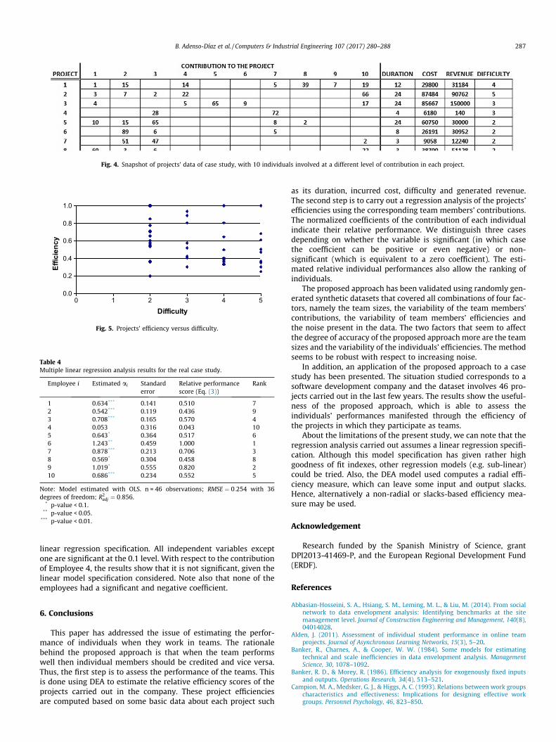
linear regression specification. All independent variables except

one are significant at the 0.1 level. With respect to the contribution

of Employee 4, the results show that it is not significant, given the

linear model specification considered. Note also that none of the

employees had a significant and negative coefficient.

6. Conclusions

This paper has addressed the issue of estimating the perfor-

mance of individuals when they work in teams. The rationale

behind the proposed approach is that when the team performs

well then individual members should be credited and vice versa.

Thus, the first step is to assess the performance of the teams. This

is done using DEA to estimate the relative efficiency scores of the

projects carried out in the company. These project efficiencies

are computed based on some basic data about each project such

as its duration, incurred cost, difficulty and generated revenue.

The second step is to carry out a regression analysis of the projects’

efficiencies using the corresponding team members’ contributions.

The normalized coefficients of the contribution of each individual

indicate their relative performance. We distinguish three cases

depending on whether the variable is significant (in which case

the coefficient can be positive or even negative) or non-

significant (which is equivalent to a zero coefficient). The esti-

mated relative individual performances also allow the ranking of

individuals.

The proposed approach has been validated using randomly gen-

erated synthetic datasets that covered all combinations of four fac-

tors, namely the team sizes, the variability of the team members’

contributions, the variability of team members’ efficiencies and

the noise present in the data. The two factors that seem to affect

the degree of accuracy of the proposed approach more are the team

sizes and the variability of the individuals’ efficiencies. The method

seems to be robust with respect to increasing noise.

In addition, an application of the proposed approach to a case

study has been presented. The situation studied corresponds to a

software development company and the dataset involves 46 pro-

jects carried out in the last few years. The results show the useful-

ness of the proposed approach, which is able to assess the

individuals’ performances manifested through the efficiency of

the projects in which they participate as teams.

About the limitations of the present study, we can note that the

regression analysis carried out assumes a linear regression specifi-

cation. Although this model specification has given rather high

goodness of fit indexes, other regression models (e.g. sub-linear)

could be tried. Also, the DEA model used computes a radial effi-

ciency measure, which can leave some input and output slacks.

Hence, alternatively a non-radial or slacks-based efficiency mea-

sure may be used.

Acknowledgement

Research funded by the Spanish Ministry of Science, grant

DPI2013-41469-P, and the European Regional Development Fund

(ERDF).

References

Abbasian-Hosseini, S. A., Hsiang, S. M., Leming, M. L., & Liu, M. (2014). From socialnetwork to data envelopment analysis: Identifying benchmarks at the sitemanagement level. Journal of Construction Engineering and Management, 140(8),04014028.

Alden, J. (2011). Assessment of individual student performance in online teamprojects. Journal of Asynchronous Learning Networks, 15(3), 5–20.

Banker, R., Charnes, A., & Cooper, W. W. (1984). Some models for estimatingtechnical and scale inefficiencies in data envelopment analysis. ManagementScience, 30, 1078–1092.

Banker, R. D., & Morey, R. (1986). Efficiency analysis for exogenously fixed inputsand outputs. Operations Research, 34(4), 513–521.

Campion, M. A., Medsker, G. J., & Higgs, A. C. (1993). Relations between work groupscharacteristics and effectiveness: Implications for designing effective workgroups. Personnel Psychology, 46, 823–850.

0.0

0.2

0.4

0.6

0.8

1.0

0 1 2 3 4 5

Difficulty

Efficiency

Fig. 5. Projects’ efficiency versus difficulty.

Table 4

Multiple linear regression analysis results for the real case study.

Employee i Estimated ai Standard

error

Relative performance

score (Eq. (3))

Rank

1 0.634*** 0.141 0.510 7

2 0.542*** 0.119 0.436 9

3 0.708*** 0.165 0.570 4

4 0.053 0.316 0.043 10

5 0.643* 0.364 0.517 6

6 1.243** 0.459 1.000 1

7 0.878*** 0.213 0.706 3

8 0.569* 0.304 0.458 8

9 1.019* 0.555 0.820 2

10 0.686*** 0.234 0.552 5

Note: Model estimated with OLS. n = 46 observations; RMSE ¼ 0:254 with 36

degrees of freedom; R2adj ¼ 0:856.

* p-value < 0.1.** p-value < 0.05.

*** p-value < 0.01.

Fig. 4. Snapshot of projects’ data of case study, with 10 individuals involved at a different level of contribution in each project.

B. Adenso-Díaz et al. / Computers & Industrial Engineering 107 (2017) 280–288 287

Caulfield, B., Bailey, D., & Mullarkey, S. (2013). Using data envelopment analysis as apublic transport project appraisal tool. Transport Policy, 29, 74–85.

Chan, K.-Y. (2014). Multiple project team membership and performance: Empiricalevidence from engineering project teams. South African Journal of Economic andManagement Sciences, 17(1), 76–90.

Cooper, W. W., Seiford, L. M., & Tone, K. (2006). Data envelopment analysis: Acomprehensive text with models, applications, references and DEA-solver software(2nd ed.). New York: Springer.

Cooper, W. W., Seiford, L. M., & Zhu, J. (2004). Handbook on data envelopmentanalysis. Springer.

Coppit, D. (2006). Implementing large projects in software engineering courses.Computer Science Education, 16(1), 53–73.

Donthu, N., & Unal, B. (2014). Identifying escalation of commitment in B2B newproduct development projects using data envelopment analysis. Journal ofBusiness & Industrial Marketing, 29(3), 209–214.

Gamble, R. F., & Hale, M. L. (2013). Assessing individual performance inagile undergraduate software engineering teams. In Proceedings of the 2013IEEE frontiers in education conference FIE 2013, Oklahoma city, USA(pp. 1678–1684).

Jackson, C. L., & LePine, J. A. (2003). Peer responses to a teams’s weakest link: A testand extension of LePine and Van Dyne’s model. Journal of Applied Psychology, 88,459–475.

Kennedy, G. J. (2005). Peer-assessment in group projects: Is it worth it? Proceedingsof the 7th Australasian Computing Education ACE Conference 2005, Newcastle,Australia (Vol. 42, pp. 59–65). .

Kozlowski, S. W. J., & Ilgen, D. R. (2006). Enhancing the effectiveness of work groupsand teams. Psychological Science in the Public Interest, 7, 77–124.

Lehman, E. L. (1999). Elements of large sample theory. Springer-Verlag New York Inc.Liang, M., Chen, Y., Zha, Y., & Hu, H. (2015). Performance evaluation of individuals in

workgroups with shared outcomes. INFOR, 53(2), 78–89.Lu, C.-C. (2015). Robust data envelopment analysis approaches for evaluating

algorithmic performance. Computers and Industrial Engineering, 81, 78–89.Lu, C.-C., & Yu, V. F. (2012). Data envelopment analysis for evaluating the efficiency

of genetic algorithms on solving the vehicle routing problem with soft timewindows. Computers & Industrial Engineering, 63(2), 520–529.

Mathews, B. P. (1994). Assessing individual contributions: experience of peerevaluation in major group projects. British Journal of Educational Technology, 25(1), 19–28.

Mathieu, J., Maynard, M. T., Rapp, T., & Gilson, L. (2008). Team effectiveness 1997–2007: A review of recent advancements and a glimpse into the future. Journal ofManagement, 34, 410–476.

Pai, D. R., Subramanian, G. H., & Pendharkar, P. C. (2015). Benchmarking softwaredevelopment productivity of CMMI level 5 projects. Information Technology andManagement, 16, 235–251.

Qureshi, T. M., Warraich, A. S., & Hijazi, S. T. (2009). Significance of projectmanagement performance assessment (PMPA) model. International Journal ofProject Management, 27, 378–388.

R Core Team (2015). R: A language and environment for statistical computing. Vienna,Austria: R Foundation for Statistical Computing <https://www.R-project.org/>.

Rubino, C., Avery, D. R., & Volpone, S. D. (2014). Does teaming obscure lowperformance? Exploring the temporal effects of team performance diversity.Human Performance, 27(5), 416–434.

Salama, G., & Ahmed, B. (2011). Using peer evaluation to assess individualperformance in team projects for freshman engineering students in theMiddle East. In Proceedings of 1st world engineering education flash weekWEE2011, Lisbon, Portugal (pp. 890–898).

Sudhaman, P., & Thangavel, C. (2015). Efficiency analysis of ERP projects—Softwarequality perspective. International Journal of Project Management, 33, 961–970.

Tavana, M., Keramatpour, M., Santos-Arteaga, F. J., & Ghorbaniane, E. (2015). A fuzzyhybrid project portfolio selection method using Data Envelopment Analysis,TOPSIS and Integer Programming. Expert Systems with Applications, 42(22),8432–8444.

Tekleab, A. G., Quigley, N. R., & Tesluk, P. E. (2009). A longitudinal study of teamconflict, conflict management, cohesion, and team effectiveness. Group &Organization Management, 34, 170–205.

Wang, E. L., & Vollstedt, A.-M. (2014). A method for adjusting group-based grades. InProceedings of the 2014 ASEE annual conference, indianapolis, USA. , pp. 24.66.1–24.66.10.

Wateridge, J. (1995). IT projects: A basis for success. International Journal of ProjectManagement, 13(3), 169–172.

Wiest, W. M., Porter, L. W., & Ghiselli, E. E. (1961). Relationships between individualproficiency and team performance and efficiency. Journal of Applied Psychology,45(6), 435–440.

Yang, J.-B., Wang, H.-H., Wang, W.-C., & Ma, S. M. (2015). Using data envelopmentanalysis to support best-value contractor selection. Journal of Civil Engineeringand Management. http://dx.doi.org/10.3846/13923730.2014.897984.

288 B. Adenso-Díaz et al. / Computers & Industrial Engineering 107 (2017) 280–288

�

;>C�

�

������7�-����������� �����8��

������������� �����8������� �

���������� ��� � �������!���� �� ������ ���������������������)�#������ ��� ���� �����

��������� "�������(� ��'�

/�0�1�2���������3�)��������������3��������

���!��?;@?D=@E>�

�24��3���+�85��.�.���*�����

�������5�� ���� ������������H�.������������ �����

�

6���

��������

�������

)������������3�7�$��������������

)��� =������ �

>?;@� ;'?AA� =@KEB� WB�

>?;=� ;'>>=� <;KE>� W>�

��!���BD;���������)�#������������� ���� ���������������� ��(�

++�*��9�B�

�

;B?�

�

/�0��3������5������������$�3������������������������

���!��?BAED<BA;�

�24��3�������5�������*���-5�

���������+�(� ����.#�� � �� � ���(�����+�(� ���

�

6���

��������

�������

�3���-�$2���������������

)��� =������ �

>?;@� >'><B� ;EKAC� W;�

>?;=� ;'AE=� >BKAC� W>�

��!���BD>���������+�(� ��������� �� ����.����� ������� ��� � ��� ����

�

/�0��8���������9��3�������������

���!5�?C=AD<;A<�

�24��3�5�+�8.�*D����5�������*�������

�������5� ��� #���� �� ������ �� � � ��� ������ �����I� ��� ���� ���� ������ ���� H�

�������� ������� ���� ������������H�.������������ �����

�

6���

�������

�������

����2��������-�

���������������������

�����������-�����������7�

����������

��)������������3�7�

$��������������

)��� =������ � )��� =������ � )��� =������ �

>?;@� B'C>E� ;EK;BB� W;� BAK>@>� W;� BKEB� W;�

>?;=� >'CE;� ;CK;B?� W;� >AK>=A� W;� @KE>� W;�

��!���BDB����������4 �����(������� ��� � ��� ����

� � � ++�*��9�B�

�

;B;�

�

/#0�)����:��������������1�2��������$��������������

���!5�?B?=D?<EB�

�24��3�5�+�8.�*D����5�������*�������

�������5�� ���� ������������H�.������������ ���������.����������

�

6���

��������

�������

)������������3�7�$��������������

)��� =������ �

>?;@� <'?>C� >KEB� W;�

>?;=� B'C@>� >KE>� W;�

��!���BD<����������������������� �����)�#��������.������������ �����

�

/�0�����2���7����2����������������

���!��;<=;,><?@�

�24��3���+�8.�*D����5�������*�������

�������5� ��� #���� �� ������ ������ �� � ���(� � ��� ���� ���� ��� ���� ����

���#��� ���

�

6���

�������

�������

����2��������-�

�������������������������������������-����2������

)��� =������ � )��� =������ �

>?;@� >'@>B� >EK;?=� W>� CK<<� W;�

>?;=� >'?E@� >AK;?<� W>� CK<<� W;�

��!���BD=������������ #�����H����#��� ������ ���� ���