Single-Pass PCA of Large High-Dimensional Data - IJCAI

Single-Pass PCA of Large High-Dimensional Data

Wenjian Yu, Yu Gu, Jian LiTNList,

Dept. Computer Science & Tech.,Tsinghua University, Beijing, China

[email protected]

Shenghua Liu ∗

Inst. Computing Technology,Chinese Academy of Sciences,

Beijing, [email protected]

Yaohang LiDept. Computer Science,Old Dominion University,Norfolk, VA 23529, USA

[email protected]

Abstract

Principal component analysis (PCA) is a funda-mental dimension reduction tool in statistics andmachine learning. For large and high-dimensionaldata, computing the PCA (i.e., the top singularvectors of the data matrix) becomes a challengingtask. In this work, a single-pass randomized algo-rithm is proposed to compute PCA with only onepass over the data. It is suitable for processing ex-tremely large and high-dimensional data stored inslow memory (hard disk) or the data generated in astreaming fashion. Experiments with synthetic andreal data validate the algorithm’s accuracy, whichhas orders of magnitude smaller error than an ex-isting single-pass algorithm. For a set of high-dimensional data stored as a 150 GB file, the al-gorithm is able to compute the first 50 principalcomponents in just 24 minutes on a typical 24-corecomputer, with less than 1 GB memory cost.

1 IntroductionMany existing machine learning models, no matter super-vised or unsupervised, rely on dimension reduction of inputdata. Even the applications of Deep Neural Networks on nat-ural language processing tasks, prefer to use an embeddingof each word in a sentence [Mikolov et al., 2013; Bahdanauet al., 2014], which essentially reduces the data dimension-ality. Principal component analysis (PCA) is an efficient andwell-structured dimension reduction technique [Halko et al.,2011a; Friedman et al., 2001]. However, how to calculatePCA of large-size (say terabyte) and high-dimensional densedata in a limited-memory computation node is still an openproblem. Plus some data are generated in stream, e.g., frominternet traffic, and signals from internet of things, we needa kind of pass-efficient algorithm, or even single-pass algo-rithm, to realize the dimension reduction of input data.

A single-pass algorithm has the benefit of requiring onlyone pass over the data, and is particularly useful and effi-cient for streaming data or data stored in slow memory [Halko

∗Also with CAS Key Laboratory of Network Data Science andTechnology.

et al., 2011b; Ye et al., 2016]. It also allows the computa-tion with small or fixed RAM size [De Stefani et al., 2016].Although there are provable single-pass truncated SVD al-gorithms for symmetric positive semi-definite (SPSD) ma-trices [Wang and Zhang, 2013; Gittens and Mahoney, 2016;Wang et al., 2016], the study for general matrices is not suf-ficient. [Halko et al., 2011b] proposed a single-pass algo-rithm for approximately calculating SVD for general matri-ces, but with a significant cost of accuracy. [Ordonez et al.,2014] developed a PCA algorithm for large-size data, but onlyapplicable to low-dimensional data (less than one thousandin dimension). Frequent-directions (FD) algorithm [Liberty,2013] was a single-pass and deterministic matrix sketchingscheme [Woodruff, 2014], which is useful for matrix multi-plication problem [Ye et al., 2016], but the PCA computation.

Randomized matrix computation has gained significant in-creases in popularity as the data sets are becoming largerand larger. It has been revealed that randomization can bea powerful computational resource for developing algorithmswith improved runtime and stability properties [Halko et al.,2011b; Drineas and Mahoney, 2016; Wang, 2015]. Com-pared with classic algorithms, the randomized algorithm in-volves the same or fewer floating-point operations (flops), andis more efficient for truely large high-dimensional data sets,by exploiting modern computing architectures. An idea ofrandomization is using random projection to identify the sub-space capturing the dominant actions of a matrix A. Withthe subspace’s orthonormal basis matrix Q, a so-called QBapproximation is obtained: A ≈ QB. This produces asmaller sketch matrix B, and facilitates the computation ofnear-optimal decompositions of A. A simple implementationof this idea and related techniques and theories have been pre-sented in [Halko et al., 2011b]. With the merit of requiring asmall constant number of passes over data, this algorithm hasbeen applied to compute PCA of data sets that are too large tobe stored in RAM [Halko et al., 2011a]. It has also been em-ployed to speed up the distributed PCA, without compromis-ing the quality of the solution [Liang et al., 2014]. However,this basic randQB algorithm still involves several passes in-stead of a single pass over data, which makes it not efficientenough or infeasible for some situations.

Progress has also been achieved based on the randomizedalgorithm for QB approximation. In [Mary et al., 2015], thebasic randQB algorithm [Halko et al., 2011b] was slightly

Proceedings of the Twenty-Sixth International Joint Conference on Artificial Intelligence (IJCAI-17)

3350

modified for computing the QR factorization. The main ef-forts were paid to investigate the algorithm’s performancescaling on shared-memory multi-core CPUs with multipleGPUs, and the comparison with the traditional QR factor-ization with column pivoting (QRCP). The results demon-strated that the randomized algorithm could be an excellentcomputational tool for many applications, with growing po-tential on the emerging parallel computers. In [Martinssonand Voronin, 2016], a randomized blocked algorithm wasproposed for computing rank-revealing factorizations in anincremental manner. Although it enables adaptive rank de-termination, the algorithm needs to access the matrix for anumber of times and is not efficient for large-size data.

Therefore, we reconstruct the randomized blocked algo-rithm [Martinsson and Voronin, 2016] and enforce numericalstability of the algorithm, which results in a single-pass PCAalgorithm owning the following advantages.• Single-pass: it involves only one pass over specified

large high-dimensional data.• Efficiency: it has O(mnk) or O(mn log(k)) time com-

plexity andO(k(m+ n)) space complexity for comput-ing k principal components of anm×nmatrix data, andwell adapts to parallel computing.• Accuracy: it has theoretical error bounds, and empiri-

cally shows much less error than the single-pass algo-rithm [Halko et al., 2011b], offering good PCA accuracyfor matrices with different singular value distributions.

We have examined the effectiveness of the proposed single-pass algorithm for performing PCA on large-size (∼150 GB)high dimensional data, which cannot be fit in RAM (32GB). The experimental results show that our single-pass al-gorithm outperforms the standard SVD and existing competi-tors, by largely reduced time and memory usage, and accu-racy guarantees. For reproducibility, we share the codes ofthe proposed algorithm and experimental data on https://github.com/WenjianYu/rSVD-single-pass.

2 PreliminariesAn orthonormal matrix denotes a matrix whose columns are aset of orthonormal vectors; I denotes the identity matrix. TheMatlab convention is obeyed to specify row/column indices.

2.1 Singular Value Decomposition and PCALet A denote an m× n matrix. The SVD of A is

A = UΣV>, (1)where U and V are m×min(m,n) and n×min(m,n) or-thonormal matrices respectively, and Σ is a diagonal matrix.The diagonal entries of Σ are the descending singular valuesof A: σ11 ≥ σ22 ≥ · · · ≥ 0. The columns of matrices U andV are the left and right singular vectors, respectively.

Taking the first k, k < min(m,n), columns of U and Vrespectively, and the first k singular values in Σ, we have thetruncated (partial) SVD of matrix A:

Ak = UkΣkV>k , (2)where Uk and Vk include the first k columns of U and V,respectively. Σk is the k × k up-left submatrix of Σ. Ak is

actually the optimal rank-k approximation of A, in terms ofl2-norm and Frobenius norm [Eckart and Young, 1936].

The approximation properties of the SVD explain theequivalence between SVD and PCA. Suppose each row ofmatrix A is an observed data. The matrix is assumed to becentered, i.e., the mean of each column is equal to zero. Then,the leading right singular vectors vi of A are the principalcomponents. Particularly, v1 is the first principal component.

2.2 The Basic Randomized Algorithm for PCAThe algorithm in [Halko et al., 2011a] is based on the ba-sic randQB algorithm for QB approximation, and describedas Algorithm 1. Ω is a Gaussian i.i.d. matrix. Replacing itwith a structured random matrix is also feasible, and can re-duces the computational cost for a dense A from O(mnl) toO(mn log(l)) flops [Halko et al., 2011b]. The over-samplingtechnique which uses Ω with more than k columns is em-ployed for better accuracy [Halko et al., 2011b]. Usually, theover-sampling parameter s is a small integer, like 5 or 10.“orth(X)” denotes the orthonormalization of the columns ofX. In practice, it is achieved efficiently by a call to a pack-aged QR factorization (e.g., qr(X, 0) in Matlab), whichimplements the QR factorization without pivoting.

Algorithm 1 Basic randomized scheme for truncated SVD

Require: A ∈ Rm×n, rank k, over-sampling parameter s.1: l = k + s;2: Ω = randn(n, l);3: Q = orth(AΩ);4: B = Q>A;5: [U,S,V] = svd(B);6: U = QU;7: U = U(:, 1 : k); V = V(:, 1 : k); S = S(1 : k, 1 : k);8: return U,S,V.

The first four steps in Algorithm 1 is the basic randQBscheme for building A’s QB approximation. This procedurecould not produce the optimal low-rank approximation. How-ever, in many applications the optimal approximation is notnecessary, and even impossible to obtain due to the high com-putational complexity of performing SVD. The existing workhas revealed that this randomized algorithm often producesa good enough solution. Compared with the classic rank-revealing QR factorization [Golub and Van Loan, 1996] forlow-rank approximation, it has less computational cost andcan obtain substantial speedup on a parallel computing plat-form [Martinsson and Voronin, 2016].

The error of the randomized QB approximation could belarge for the matrix whose singular values decay slowly[Halko et al., 2011b]. This can be eased by a technique calledpower scheme [Rokhlin et al., 2009]. It is based on the factthat matrix (AA>)PA has exactly the same singular vec-tors as A, but its j-th singular value is σ2P+1

jj . This largelyreduces the relative weight of the tail singular values. Thus,performing the randomized QB procedure on (AA>)PA canachieve more accurate approximation. More theoretical anal-ysis can be found in Sec. 10.4 of [Halko et al., 2011b]. On theother hand, the power scheme increases the number of passesover A from 2 to 2P+2 [Halko et al., 2011b].


3351

Notice that the output of the randomized approximation al-gorithms is a random variable However, the variation of thisrandom variable is small, which means the output is alwaysvery close to the variable’s expectation [Halko et al., 2011b].

2.3 An Existing Single-Pass Algorithm

Algorithm 1 involves two passes over matrix A. In [Halko etal., 2011b], a single-pass algorithm was proposed as a remedy(see Algorithm 2), where only Step 2 need access matrix A.

Algorithm 2 An existing single-pass algorithm

Require: A ∈ Rm×n, rank parameter k.1: Generate random n× k matrix Ω and m× k matrix Ω;2: Compute Y =AΩ and Y =A>Ω in a single pass over

A;3: Q = orth(Y); Q = orth(Y);4: Solve linear equation Ω>QB = Y>Q for B;5: [U,S, V] = svd(B);6: U = QU; V =QV;7: return U,S,V.

Step 3 of Algorithm 2 results in matrices Q and Q suchthat A ≈ QQ>AQQ>. Then, the left problem is how tocompute the small matrix B = Q>AQ. One can find out:

Q>Y = Q>A>Ω ≈ Q>A>QQ>Ω = B>Q>Ω. (3)So, B is approximately computed in Step 4. Due to theseapproximations, the accuracy of this algorithm or its variantsis not good. We will reveal this through experiments.

2.4 The Randomized Blocked Algorithm

The randomized blocked algorithm in [Martinsson andVoronin, 2016] is inspired by a greedy Gram-Schmidt proce-dure for the orthonormalization step of basic randQB, whichconstitutes an iterative updating of the QB approximation er-ror. Then, the algorithm is converted to a blocked version toattain high performance of linear algebraic computation (seeFig. 1). It is easy to prove that, if the algorithm is executedin exact arithmetic Q is orthonormal, B = Q>A, and afterStep (6) A becomes the approximation error: A−QB.

The algorithm is mathematically equivalent to the basicrandQB procedure (the first 4 steps of Algorithm 1), exceptfor the stopping criterion. The re-orthogonalization step (4)is for easing the accumulation of numerical round-off error.

Figure 1: The blocked randQB algorithm, from [Martinsson andVoronin, 2016].

3 Methodology3.1 A Pass-Efficient Blocked AlgorithmThe blocked randQB procedure in Fig. 1 facilitates adap-tive rank determination, but increases the number of passesover the data matrix. For many scenarios of using PCA, therank parameter k is a known value. Without the evaluationof approximation error, the block randQB procedure can bemodified to be a pass-efficient procedure. It is presented asAlgorithm 3, with the re-orthogonalization step ignored. Forsimplicity, we also assume that k is a multiple of b.

Algorithm 3 A pass-efficient blocked algorithm

Require: A ∈ Rm×n, rank parameter k, block size b.1: Q = [ ]; B = [ ];2: Ω = randn(n, k);3: G = AΩ;4: H = A>G;5: for i = 1, 2, · · · , k/b do6: Ωi = Ω(:, (i− 1)b+ 1 : ib);7: Yi = G(:, (i− 1)b+ 1 : ib)−Q(BΩi);8: [Qi, Ri] = qr(Yi);9: Bi = R−>i (H(:, (i− 1)b+ 1 : ib)> −Ω>i B>B);

10: Q = [Q, Qi]; B = [B>, B>i ]>;

11: end for

A major difference between Algorithm 3 and the algorithmin Fig. 1 is the multiplications with A moved out of the loop.With G = AΩ, Steps 7 and 8 in Algorithm 3 perform thesame function as Step (3) in the latter. Here, “qr” denotes astandard QR factorization, i.e., QiRi = Yi. During the firstiteration, Q and B are null matrices and therefore we shoulddrop off the last items in Step 7 and Step 9. The equivalenceof the both algorithms is guaranteed with Theorem 1.

Theorem 1. The Q and B obtained with Algorithm 3 satisfy:Q is orthonormal and B = Q>A.

Proof. We prove Theorem 1 via induction. For any variablev after the i-th iteration of the loop is executed, we use v(i)to denote its value. Moreover, we assume the random matrixΩ is of full column rank. In the base case, Q(1) = Q1 isorthonormal because of Step 8 in Algorithm 3. It also ensuresthat Qi is orthonormal, and QiRi = Yi. So,

B(1) = B1 = R−>1 Ω>1 A>A = (AΩ1R−11 )>A

= (Y1R−11 )>A =

(Q(1)

)>A .

(4)

Now, suppose the proposition holds for the i-th iteration.We need to prove Q(i+1) is orthonormal and B(i+1) =(Q(i+1)

)>A. We first check the orthogonality of Qi+1.

Q>i+1Q(i) =

((A−Q(i)B(i)

)Ωi+1R

−1i+1

)>Q(i)

=((

A−Q(i)(Q(i)

)>A)

Ωi+1R−1i+1

)>Q(i)

=((I−PQ(i))AΩi+1R

−1i+1

)>Q(i)

=(AΩi+1R

−1i+1

)>(Q(i) −PQ(i)Q(i)) = O.

(5)

The last two equalities of (5) is based on the properties of pro-jector matrix PQ(i) ≡ Q(i)

(Q(i)

)>. See the Appendix. Eq.


3352

(5) guarantees that Q(i+1) is an orthonormal matrix. Then,

Bi+1 = R−>i+1Ω>i+1

(A>A−B(i)>B(i)

)1= R−>i+1Ω

>i+1

(A−Q(i)B(i)

)> (A−Q(i)B(i)

)=(AΩi+1R

−1i+1 −Q(i)B(i)Ωi+1R

−1i+1

)> (A−Q(i)B(i)

)= Q>i+1

(A−Q(i)B(i)

) 2= Q>i+1A ,

where equality 1 holds due to Q(i) is orthonormal and B(i) =(Q(i)

)>A. Equality 2 just follows from (5).

Therefore, Q is orthonormal and B = Q>A, based on theinduction hypothesis and Step 10 in Algorithm 3.

As the blocked randQB algorithm is mathematically equiv-alent to the basic randQB, Algorithm 3 inherits the theoreti-cal error bound (if ignoring the round-off error):

E (‖A−QB‖F ) ≤(1 + k

s−1

)1/2 (∑min(m,n)j=k+1 σ2

jj

)1/2, (6)

where E denotes expectation. We see that the theoreticallyminimal error is only magnified by a factor of (1 + k

s−1 )1/2.

If measuring the error with l2-norm, we have a similar errorbound formula (see Theorem 10.6 of [Halko et al., 2011b]).

3.2 The Version with Re-OrthogonalizationDue to the accumulation of round-off errors, the orthonor-mality among the columns in Q1,Q2, · · · may lose. Thisaffects the correctness of some statements in Algorithm 3,and increases the error of its output. To fix this problem, weexplicitly reproject Qi away from the span of the previouslycomputed basis vectors, just as what is done in [Martinssonand Voronin, 2016]. Then, the formula for matrix Bi is re-vised to incorporate the modified Qi.

The re-orthogonalization step corresponds to:

QiRi = Qi −QQ>Qi, (7)

where Qi 6= Qi and Ri 6= I due to round-off error.And, Qi is better orthogonal to the previously generatedQ1,Q2, · · · ,Qi−1 than Qi. Since QiRi = Yi,

Qi =(I−QQ>

)YiR

−1i R−1i , (8)

Bi =Q>i A = (RiRi)−>Y>i

(I−QQ>

)A

=(RiRi)−> (H>i −Y>i QB−Ω>i B>B

),

(9)

where Hi denotes H(:, (i − 1)b + 1 : ib). The last equalityutilizes that B = Q>A, although this may not hold after alarge number of iterations due to numerical round-off error.

Based on (7) and (9), the version with re-orthogonalizationcan be obtained by replacing Step 9 with the following steps:

9: [Qi, Ri] = qr(Qi −Q(Q>Qi));9’: Ri = RiRi;9”: Bi=R−>i (H(:, (i−1)b+1 : ib)>−Y>i QB−Ω>i B>B);

Here, Qi and Bi are overwritten to stand for Qi and Bi.

3.3 The Single-Pass Algorithm for PCAAn important feature of Algorithm 3 is that Steps 3 and 4 canbe executed with only one pass over matrix A. Suppose ai

and gi denote the i-th rows of matrix A and G, respectively.

H = [a>1 ,a>2 , · · · ,a>m]

g1

g2

...gm

=m∑i=1

a>i gi. (10)

So, with the i-th row of A, we can calculate the i-th row ofG with Step 3, and then the i-th item in the summation forcalculating H as (10). Combined with the over-sampling, thesingle-pass algorithm for computing PCA is as Algorithm 4.

Algorithm 4 A single-pass algorithm for computing PCA

Require: A ∈ Rm×n, rank parameter k, block size b.1: Q = [ ]; B = [ ];2: Choose l = tb, which is slightly larger than k;3: Ω = randn(n, l); G = [ ]; Set H to an n× l zero matrix;4: while A is not completely read through do5: Read next few rows of A into RAM, denoted by a;6: g = aΩ; G = [G; g];7: H = H + a>g;8: end while9: for i = 1, 2, · · · , t do

10: Ωi = Ω(:, (i− 1)b+ 1 : ib);11: Yi = G(:, (i− 1)b+ 1 : ib)−Q(BΩi);12: [Qi, Ri] = qr(Yi);13: [Qi, Ri] = qr(Qi −Q(Q>Qi));14: Ri = RiRi;15: Bi=R−>i (H(:, (i−1)b+1 : ib)>−Y>i QB−Ω>i B>B);16: Q = [Q, Qi]; B = [B>, B>i ]

>;17: end for18: [U,S,V]= svd(B);19: U = QU;20: U = U(:, 1 : k); V = V(:, 1 : k); S = S(1 : k, 1 : k);21: return U,S,V.

In the algorithm, the while loop corresponds to Steps 3and 4 in Algorithm 3, but involves only one pass over A.In every step, small matrices in size m × l or n × l (notingl min(m,n) ) are used. So, the memory cost of this al-gorithm is small, which can be bounded by that for storing(m + 2n)l floating numbers. The computational cost of thisalgorithm is the same as Algorithm 3 and 1 [Halko et al.,2011a], i.e., O(mnk) or O(mn log(k)) flops. The theoret-ical error bounds of A−QB also apply to A−USV> inAlgorithm 4, as the latter hardly induces new error.

This single-pass algorithm requests that the data matrix Ais stored in a row-major format. Otherwise, we can applythe algorithm to A> instead. In case there is a request forhigher accuracy, the power scheme can be applied with likeP =1, which is equivalent to replacing A with AA>A in thealgorithm. It requests one additional pass over A, even the or-thonormalization is enforced [Martinsson and Voronin, 2016;Voronin and Martinsson, 2016]. Nevertheless, the single-passalgorithm works well in many applications.

4 ExperimentsAll experiments are carried out on a Linux server with two12-core Intel Xeon E5-2630 CPUs (2.30 GHz), and 32 GB


3353

RAM. The algorithms are implemented in C with OpenMPderivatives for multi-thread computing, and MKL libraries[Int, 2016]. QR factorization and other basic linear algebraoperations are realized through LAPACK routines which areautomatically executed in parallel on the multi-core CPUs.

We first validate the accuracy of the proposed single-passalgorithm. Then, large test cases stored on hard disk in IEEEsingle-precision float format are used to validate the algo-rithm’s efficiency. In all experiments, the block size b = 10.

4.1 Accuracy ValidationWe consider test matrices owning the following singular spec-trums with different decaying behavior, where σii denotes thei-th singular value (i.e., a diagonal element of matrix Σ).• Type 1:

σii =

10−4(i−1)/19, i = 1, 2, · · · , 20,10−4/(i− 20)1/10, i = 21, 22, · · · ,min(m,n).

• Type 2: σii = i−2, i = 1, 2, · · · .• Type 3: σii = i−3, i = 1, 2, · · · .• Type 4: σii = e−i/7, i = 1, 2, · · · .• Type 5: σii = 10−i/10, i = 1, 2, · · · .

Type 1 is from [Halko et al., 2011a], and Type 3 and Type 5are from [Mary et al., 2015]. These singular value distribu-tions are shown in Fig. 2. It reveals that the singular valuesof Type 1 and Type 2 matrices decay asymptotically slowly,although they attenuate fast at the start. The singular valuesof Type 4 and Type 5 matrices decay asymptotically faster.

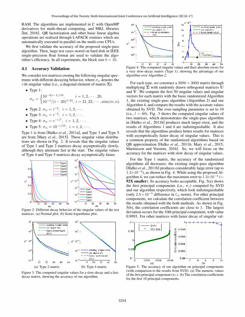
Figure 2: Different decay behavior of the singular values of the testmatrices. (a) Normal plot, (b) Semi-logarithmic plot.

(a) Type 2 matrix (b) Type 4 matrix

Figure 3: The computed singular values for a slow-decay and a fast-decay matrix, showing the accuracy of our algorithm.

Figure 4: The computed singular values and their absolute errors fora very slow-decay matrix (Type 1), showing the advantage of ouralgorithm over Algorithm 2.

For each type, we construct a 3000× 3000 matrix throughmultiplying Σ with randomly drawn orthogonal matrices Uand V. We compute the first 50 singular values and singularvectors for each matrix with the basic randomized Algorithm1, the existing single-pass algorithm (Algorithm 2) and ourAlgorithm 4, and compare the results with the accurate valuesobtained by SVD. The over-sampling parameter is set to 10(i.e., l = 60). Fig. 3 shows the computed singular values oftwo matrices, which demonstrates the single-pass algorithmin [Halko et al., 2011b] produces much larger error, and theresults of Algorithms 1 and 4 are indistinguishable. It alsoreveals that the algorithms produce better results for matriceswith asymptotically faster decay of singular values. This isa common property of the randomized algorithms based onQB approximation [Halko et al., 2011b; Mary et al., 2015;Martinsson and Voronin, 2016]. So, we will focus on theaccuracy for the matrices with slow decay of singular values.

For the Type 1 matrix, the accuracy of the randomizedalgorithms all decreases; the existing single-pass algorithm[Halko et al., 2011b] produces considerably large error (up to1.2×10−2), as shown in Fig. 4. While using the proposed Al-gorithm 4, we can reduce the maximum error to 1.3×10−4 (∼92X smaller). Its accuracy looks acceptable. Fig. 5(a) showsthe first principal components (i.e., v1) computed by SVDand our algorithm respectively, which look indistinguishable(only 2.8×10−5 difference in l∞-norm). For other principalcomponents, we calculate the correlation coefficient betweenthe results obtained with the both methods. As shown in Fig.5(b), the correlation coefficients are close to 1. The largestdeviation occurs for the 10th principal component, with value0.9993. For other matrices with faster decay of singular val-

Figure 5: The accuracy of our algorithm on principal components(with comparison to the results from SVD). (a) The numeric valuesof the first principal component (v1). (b) The correlation coefficientsfor the first 10 principal components.


3354

ues (Types 2∼5), the randomized algorithm exhibits betteraccuracy and outputs more accurate principal components.

4.2 Runtime ComparisonFollowing [Halko et al., 2011a], we construct several largedata using the unitary discrete cosine transform (command“dct” in Matlab). They are 200, 000×200, 000 matrices fol-lowing the singular value distributions given in last subsec-tion. Each matrix is stored as a 149 GB file on hard disk.We use fread function to read the file and run Algorithm 4for computing PCA. Each time we read l rows of matrix, toavoid extra memory cost. Once they are loaded into RAM,the data are converted to the IEEE double-precision format.Algorithm 1 and Algorithm 2 are also tested for comparison.

Some results for the matrices with slow-decay singular val-ues are listed in Table 1. l in Algorithm 4 is set to 20 or 30.tread and tPCA mean the total time (in seconds) for read-ing the data and the total runtime of the algorithm (includ-ing tread), respectively. “max err” is the maximum error ofthe computed singular values. From the table we see that thetime for reading data dominates the total runtime, and the pro-posed algorithm is about 2X faster than the basic randomizedalgorithm used in [Halko et al., 2011a] while keeping sameaccuracy. If comparing Algorithm 2 and ours, we see that theformer may be slightly faster but produces much larger error.

To improve the accuracy, the power scheme with P = 1could be applied, which corresponds to one more pass overthe data. For Algorithm 4, we just run the while loop onceagain with Ω replaced by H after “orth” operation. In our ex-periments, this two-pass algorithm has similar runtime as Al-gorithm 1, but dramatically reduces “max err” to 4.6× 10−7

and 3×10−6 for the Type 1 and Type 2 matrices, respectively.In the experiments, the memory cost of Algorithm 4 ranges

from 402 MB to 490 MB. In contrast, the standard SVD (in-cluding “svds” in Matlab for truncated SVD) requests muchlarger memory than the available physical RAM, and there-fore does not work. To have a taste of how fast the proposedrandomized algorithm runs, we test a 10,000×10,000 ma-trix. Performing a complete SVD and “svds” for the first50 principal components take 226 and 219 seconds, respec-tively, while the proposed algorithm costs only 0.69 seconds.

4.3 Real DataWe apply the single-pass algorithm with k=50 to the matrixrepresenting the images of faces from the FERET database[Phillips et al., 2000]. As in [Halko et al., 2011a], we addtwo duplicates for each image into the data. For each dupli-cate, the value of a random choice of 10% of the pixels isset to random numbers uniformly chosen from 0, 1, · · · , 255.Table 1: The results for several 200, 000× 200, 000 data, whichdemonstrate the efficiency of our Algorithm 4. (unit of time: second)

Matrix kAlgorithm 1 Algorithm 2 Algorithm 4

treadtPCAmax err treadtPCAmax err treadtPCAmax err

Type1 16 2390 2607 1.7e-3 1186 1404 2.2e-2 1206 1426 1.8e-3Type1 20 2420 2616 9e-4 1198 1380 1.6e-1 1217 1413 1.2e-3Type1 24 2401 2593 1e-3 1216 1400 1.5e-1 1216 1414 1.2e-3Type2 12 2553 2764 5e-4 1267 1477 3e-2 1276 1490 5e-4Type3 24 2587 2777 1e-5 1312 1500 1.7e-3 1310 1502 2e-5

(a) Computed singular values (b) Four eigenfaces

Figure 6: The computational results for the FERET matrix.

This forms a 102, 042× 393, 216 matrix, whose rows con-sist of images. Before processing, we normalize the matrixby subtracting from each row its mean, and then dividing itby its Euclidean norm. With the proposed algorithm, it takes1453 seconds (∼ 24 minutes) to process all 150 GB of thisdata stored on disk. The computed singular values are plottedin Fig. 6. We have also checked the computed “eigenfaces”,which well match those presented in [Halko et al., 2011a].

5 ConclusionsAn algorithm for single-pass PCA of large and high-dimensional data is proposed. It involves only one pass overthe data, and keeps the comparable accuracy to the existingrandomized algorithms. Experiments demonstrate the algo-rithm’s effectiveness for computing the principal componentsof large-size (∼150 GB) data with high dimension that cannotbe fit in memory, in terms of runtime and memory usage.

6 Appendix: Orthogonal Projector MatrixAn orthogonal projector matrix corresponds to a linear trans-formation which converts any vector to its orthogonal projec-tion on a subspace. It is uniquely determined by the subspace,e.g., range(X) corresponding to a projector matrix denotedby PX . Based on the theory of linear least squares, if X hasfull column rank [Golub and Van Loan, 1996],

PX = X(X>X)−1X> . (11)It is simplified to PX = XX>, if X is an orthonormal ma-trix. It is easy to see the following properties of a projector.

Lemma 1. For a real-valued matrix X with full column rank,• PX is a symmetric matrix, and P2

X = PX .• I − PX is the orthogonal projector determined by the

orthogonal complement of range(X).• PXX−X = O , where O is the zero matrix.

AcknowledgmentsThis work was supported by NSFC under grant No.61422402, and in part by Beijing NSF No. 4172059 and NSFNo. CCF-1066471.

Portions of the research in this paper use the FERETdatabase of facial images collected under the FERET pro-gram, sponsored by the DOD Counterdrug Technology De-velopment Program Office.


3355

References[Bahdanau et al., 2014] Dzmitry Bahdanau, Kyunghyun

Cho, and Yoshua Bengio. Neural machine translationby jointly learning to align and translate. arXiv preprintarXiv:1409.0473, 2014.

[De Stefani et al., 2016] Lorenzo De Stefani, AlessandroEpasto, Matteo Riondato, and Eli Upfal. TRIEST: Count-ing local and global triangles in fully-dynamic streamswith fixed memory size. In Proceedings of the 22nd ACMSIGKDD International Conference on Knowledge Discov-ery and Data Mining, 2016.

[Drineas and Mahoney, 2016] Petros Drineas andMichael W Mahoney. RandNLA: Randomized nu-merical linear algebra. Communications of the ACM,59(6):80–90, 2016.

[Eckart and Young, 1936] Carl Eckart and Gale Young. Theapproximation of one matrix by another of lower rank.Psychometrika, 1(3):211–218, 1936.

[Friedman et al., 2001] Jerome Friedman, Trevor Hastie,and Robert Tibshirani. The Elements of Statistical Learn-ing, volume 1. Springer series in statistics Springer, Berlin,2001.

[Gittens and Mahoney, 2016] Alex Gittens and Michael WMahoney. Revisiting the nystrom method for improvedlarge-scale machine learning. J. Mach. Learn. Res, 17:1–65, 2016.

[Golub and Van Loan, 1996] Gene H Golub and Charles FVan Loan. Matrix Computations. Johns Hopkins Univer-sity Press, 1996.

[Halko et al., 2011a] Nathan Halko, Per-Gunnar Martinsson,Yoel Shkolnisky, and Mark Tygert. An algorithm for theprincipal component analysis of large data sets. SIAMJournal on Scientific Computing, 33(5):2580–2594, 2011.

[Halko et al., 2011b] Nathan Halko, Per-Gunnar Martins-son, and Joel A Tropp. Finding structure with randomness:Probabilistic algorithms for constructing approximate ma-trix decompositions. SIAM review, 53(2):217–288, 2011.

[Int, 2016] Intel Parallel Studio XE Cluster Edition forLinux. https://software.intel.com/en-us/intel-parallel-studio-xe, 2016.

[Liang et al., 2014] Yingyu Liang, Maria-Florina F Balcan,Vandana Kanchanapally, and David Woodruff. Improveddistributed principal component analysis. In Advancesin Neural Information Processing Systems, pages 3113–3121, 2014.

[Liberty, 2013] Edo Liberty. Simple and deterministic matrixsketching. In Proceedings of the 19th ACM SIGKDD In-ternational Conference on Knowledge Discovery and DataMining, pages 581–588. ACM, 2013.

[Martinsson and Voronin, 2016] P.-G. Martinsson andS. Voronin. A randomized blocked algorithm for ef-ficiently computing rank-revealing factorizations ofmatrices. SIAM Journal on Scientific Computing,38(5):S485–S507, 2016.

[Mary et al., 2015] Theo Mary, Ichitaro Yamazaki, JakubKurzak, Piotr Luszczek, Stanimire Tomov, and Jack Don-garra. Performance of random sampling for computinglow-rank approximations of a dense matrix on GPUs. InProceedings of the International Conference for High Per-formance Computing, Networking, Storage and Analysis,SC ’15, pages 60:1–60:11, New York, NY, USA, 2015.ACM.

[Mikolov et al., 2013] Tomas Mikolov, Ilya Sutskever, KaiChen, Greg S Corrado, and Jeff Dean. Distributed rep-resentations of words and phrases and their composition-ality. In Advances in Neural Information Processing Sys-tems, pages 3111–3119, 2013.

[Ordonez et al., 2014] Carlos Ordonez, Naveen Mohanam,and Carlos Garcia-Alvarado. PCA for large data sets withparallel data summarization. Distrib. Parallel Databases,32(3):377–403, September 2014.

[Phillips et al., 2000] P Jonathon Phillips, Hyeonjoon Moon,Syed A Rizvi, and Patrick J Rauss. The FERET evalua-tion methodology for face-recognition algorithms. IEEETransactions on Pattern Analysis and Machine Intelli-gence, 22(10):1090–1104, 2000.

[Rokhlin et al., 2009] Vladimir Rokhlin, Arthur Szlam, andMark Tygert. A randomized algorithm for principal com-ponent analysis. SIAM Journal on Matrix Analysis andApplications, 31(3):1100–1124, 2009.

[Voronin and Martinsson, 2016] S. Voronin and P.-G. Mar-tinsson. RSVDPACK: Subroutines for computing partialsingular value decompositions via randomized samplingon single core, multi core, and GPU architectures. arXivpreprint, arXiv:1502.05366v3, 2016.

[Wang and Zhang, 2013] Shusen Wang and Zhihua Zhang.Improving cur matrix decomposition and the nystrom ap-proximation via adaptive sampling. Journal of MachineLearning Research, 14(1):2729–2769, 2013.

[Wang et al., 2016] Shusen Wang, Zhihua Zhang, and TongZhang. Towards more efficient spsd matrix approximationand cur matrix decomposition. Journal of Machine Learn-ing Research, 17(210):1–49, 2016.

[Wang, 2015] Shusen Wang. A practical guide to random-ized matrix computations with MATLAB implementa-tions. arXiv preprint arXiv:1505.07570, 2015.

[Woodruff, 2014] David P Woodruff. Sketching as a tool fornumerical linear algebra. Foundations and Trends R© inTheoretical Computer Science, 10(1–2):1–157, 2014.

[Ye et al., 2016] Qiaomin Ye, Luo Luo, and Zhihua Zhang.Frequent direction algorithms for approximate matrix mul-tiplication with applications in CCA. In Proceedings ofthe 25th International Joint Conference on Artificial Intel-ligence (IJCAI-16), pages 2301–2307, 2016.


3356

Single-Pass PCA of Large High-Dimensional Data - IJCAI

Documents

Transcript of Single-Pass PCA of Large High-Dimensional Data - IJCAI