TIP, DECEMBER 2014 1

Single-image super-resolution via linear mapping ofinterpolated self-examples

Marco Bevilacqua, Aline Roumy, Member, IEEE, Christine Guillemot, Fellow, IEEE,and Marie-Line Alberi Morel

Abstract—This paper presents a novel example-based single-image super-resolution (SR) procedure, that upscales to high-resolution (HR) a given low-resolution (LR) input image withoutrelying on an external dictionary of image examples. The dictio-nary instead is built from the LR input image itself, by generatinga “double pyramid” of recursively scaled, and subsequentlyinterpolated, images, from which self-examples are extracted.The upscaling procedure is multi-pass, i.e. the output imageis constructed by means of gradual increases, and consists inlearning special linear mapping functions on this double pyramid,as many as the number of patches in the current image toupscale. More precisely, for each LR patch, similar self-examplesare found, and, thanks to them, a linear function is learned todirectly map it into its HR version. Iterative back projection isalso employed to ensure consistency at each pass of the procedure.Extensive experiments and comparisons with other state-of-the-art methods, based both on external and internal dictionaries,show that our algorithm can produce visually pleasant upscalings,with sharp edges and well reconstructed details. Moreover, whenconsidering objective metrics like PSNR and SSIM, our methodturns out to give the best performance.

Index Terms—super resolution, example-based, regression,neighbor embedding

I. INTRODUCTION

SUPER-RESOLUTION (SR) refers to a family of tech-niques that aim at increasing the resolution of given

images. Nowadays, many applications, e.g. video surveillanceand remote sensing, require the display of images at a con-siderable resolution, that may not be easy to obtain giventhe limitations of physical imaging systems or environmentalconditions. Moreover, with the spread of digital technologies,there is a tremendous amount of user-produced images col-lected in the years, that are valuable but may be affected by apoor quality. Therefore, techniques to augment the resolutionof an image, i.e. the total number of pixels, and contextuallyimprove its visual quality, are particularly appealing.

SR methods are traditionally categorized according to thenumber of input images: when several low-resolution (LR)input images are available we speak about multi-frame SR

This work was supported by the joint research lab INRIA-Alcatel LucentBell Labs.

M. Bevilacqua is with IMT Institute for Advanced Studies Lucca, 55100Italy (e-mail: marco.bevilacqua@imtlucca.it). This work was performed whilehe was Ph.D. student at the SIROCCO research team in INRIA.

A. Roumy and C. Guillemot are with the SIROCCO research team inINRIA, Institut national de recherche en informatique et en automatique,Rennes, 35042 France (e-mail: firstname.lastname@inria.fr).

M-L. Alberi Morel is with Alcatel-Lucent Bell Labs France, Centre de Vil-larceaux, 91620 France (e-mail: marie line.alberi-morel@alcatel-lucent.com).

algorithm; vice versa, when the LR input image is unique,we have the single-image SR problem. In both cases, as anoutput, a unique high-resolution (HR) super-resolved image isproduced.

Multi-frame SR methods, of which a good overview is givenin [1], are the first ones that have been studied, since the SRproblem first appeared in the scientific community [2]. Here,the multiple LR input images are considered as different viewsof the same scene, taken with sub-pixel misalignment, i.e.each image is seen as a degraded version of an underlyingHR image to be estimated, where the degradation processescan include blurring, geometrical transformations, and down-sampling. Single-image SR, instead, aims at constructing theHR output image from as little as a single LR input image.The problem stated is an inherently ill-posed problem, asthere can be several HR images generating the same LRimage. Single-image SR is deeply connected with traditional“analytical” interpolation, since they share the same goal.Traditional interpolation methods, e.g. bicubic interpolation,by computing the missing pixels in the HR grid as averagesof known pixels, implicitly impose a “smoothness” prior.However, natural images often present strong discontinuities,such as edges and corners, and thus the smoothness priorresults in producing ringing and blurring artifacts in the outputimage. Single-image SR algorithms can be broadly classifiedinto two main approaches: interpolation-based methods [3]–[5], which, possibly in a nonparametric fashion, follow theinterpolation approach by posing more sophisticated statisticalpriors; and machine learning (ML) based methods.

In particular, the latter, by taking advantage of the powerful-ness of ML techniques, have shown to give very challengingresults, and many algorithms appeared in the literature inthe recent years. ML-based algorithms can consist in pixel-based procedures, where each value in the HR output imageis singularly inferred via statistical learning [6], [7], or patch-based procedures, where the HR estimation is performedthanks to a dictionary of correspondences of LR and HRpatches (i.e. squared blocks of image pixels). ML-based SRthat makes use of patches is also referred to as example-basedSR [8]. In the upscaling procedure the LR input image itselfis divided into patches, and for each LR input patch a singleHR output patch is reconstructed, by observing the “examples”contained in the dictionary.

Example-based methods mainly vary in two aspects: thepatch reconstruction method used and the typology of dictio-nary. As for the method to perform the single patch recon-structions, we have again two main categories: coding-basedreconstruction methods and direct mapping (DM). Neighbor

2

embedding (NE) belongs to coding-based methods. In NE-based SR [9]–[11], for each LR input patch we select Ksimilar LR examples in the dictionary by nearest neighborsearch (NNS), and a linear combination of these neighborsis computed to possibly approximate the input patch. Thecorresponding HR neighbors are then similarly combined, i.e.by using the same weights computed with the LR patches, togenerate the HR output patch. This approach relies on what in[12] is called “manifold assumption”: the linear combinationweights are meant to capture the local geometry of a manifoldon which the LR patches are supposed to lay; by applyingthe same weights to reconstruct the HR patches, we implicitlyassume that they too lay on a manifold with similar local struc-tures. In order to enforce the assumption of manifold similaritybetween the two distinct spaces represented by the LR and HRpatches, Gao et al. propose in [13] to compute the weights ina subspace common to the LR and HR patches. The methodtherefore assumes the existence of a common low-dimensionalspace that preserve some meaningful characteristics of thepatches.

Example-based SR via sparse representations [14], [15] alsofalls within the family of coding-based methods, and can beconsidered very close to NE-based SR: however, here, theweights are not computed on neighbors found by NNS, buttypical sparse coding algorithms are employed. The methodpresented in [16] bridges the two approaches (NE and sparserepresentations), by proposing a “sparse neighbor embedding”algorithm. In [17], instead, another sparse-representation-based SR algorithm is presented, which, in addition to asparse example-based term, uses several regularization termsto globally optimize the image generation process.

All the methods so far require manifold similarity betweenthe LR and HR spaces. A different patch reconstructionapproach that does not rely on this assumption is given insteadby direct mapping (DM). Example-based SR via DM [18]–[20] aims at finding, in fact, for each patch reconstruction,a function that directly map a given LR patch into its HRversion. The mapping function is commonly found with tra-ditional regression methods.

As for the second discriminating aspect of example-basedSR, the typology of the dictionary, we have mainly twochoices: an external dictionary, built from a set of externaltraining images, and an “internal” one, built without usingany other image than the LR input image itself. This lattercase exploits the so called “self-similarity” property, typicalof natural images, according to which image structures tendto repeat within and across different image scales: therefore,patch correspondences can be found in the input image itselfand possibly scaled versions of it. To learn these patch corre-spondences, that specifically take the name of self-examples,we can have one-step schemes [18], [21], [22] or schemesbased on a pyramid of recursively scaled images starting fromthe LR input image [23]–[25]. Clearly, the advantage of havingan external dictionary instead of an internal one lies in the factthat it is built in advance, while the internal one is generatedonline and updated at each run of the algorithm. However,external dictionaries have a considerable drawback: they arefixed and thus non-adapted to the input image. The study

conducted in [26] also confirms the benefit of using internalstatistics in patch-based image processing algorithms.

A. Main contributions

In this paper we present a novel example-based SR al-gorithm that makes use of an internal dictionary. The con-tributions are twofold. First, we build a “double pyramid”,where the traditional image pyramid of [23] is juxtaposed witha pyramid of interpolated images. Second, HR patches arereconstructed through DM, whereas in [23] the HR patches arereconstructed via NE. Therefore, in the proposed algorithm, alinear mapping is learned on the double pyramid from theLR interpolated patches to the HR patches, and then appliedto each interpolated LR input patch. As said before, unlikeNE, DM does not rely on any theoretical assumption (i.e. amanifold similarity between the LR and HR spaces), and istherefore preferable.

The rationale for the interpolation operation is to make thecomputation of the single mapping functions via regressionmore robust (LR and HR patches, in fact, turn out to havethe same sizes). Moreover, a Tikhonov regularization is addedto the problem to provide numerical stability in the compu-tation, since the linear mapping requires a matrix inversion.A double-pyramid-like scheme has also been introduced in[22]. However, our proposed algorithm differs from [22] intwo ways. First, the reconstruction in [22] is based on aneighbor embedding technique analyzed in [27] (NE with asum-to-one constraint). This NE technique was shown to havea performance highly dependent on the number of neighborschosen. More precisely, when this number is equal to the sizeof the LR input vectors, the performance of the algorithmsdramatically drops. As a second discriminating aspect, while[22] initializes the pyramid by down-scaling the LR inputimage only once, we instead initialize the pyramid with manysub-levels by recursively down-scaling the LR input image.We show that many sub levels are needed in order to betterreconstruct a HR image. More precisely, we have that at thefirst iteration of the algorithm around 35% of the selectedpatches come from the pyramid levels below the first one (seeFig. 3 for details). The patches initially selected play a crucialrole: in fact, since the whole algorithm is by nature recursive,it is very sensitive to its initialization.

All the listed contributions are possible at the cost of a slightincrease in the complexity of the algorithm (i.e. +10.7% fora scale factor of 3 and +8.1% for a scale factor of 4; seeSection IV-B for details), while having a beneficial effect onthe quality performance, both in terms of objective metrics(PSNR and SSIM) and visual results.

B. Organization of the paper

The rest of the paper is organized as follows. SectionII reviews the fundamentals of example-based SR using aninternal dictionary, by giving also a general introduction ofNE and DM methods. Then, in Section III, our algorithm isdescribed in detail, by explaining how the internal dictionary istrained and the whole upscaling procedure. Before drawing theconclusions, Section IV presents some extensive experiments

3

done: the different implementation choices are here validatedand the algorithm is compared with other state-of-the-artmethods, by showing visual and quantitative results.

II. EXAMPLE-BASED SR WITH SELF-EXAMPLES

A. Principles and notations

Single-image SR is the problem of estimating an underlyingHR image, given only one observed LR image. The generationprocess of the LR image from the original HR image, that weconsider, can be written as

IL = (IH ∗B) ↓s , (1)

where IL and IH are respectively the LR and HR image, B isa blur kernel the original image is convoluted with, which istypically modeled as a Gaussian blur [28], and the expression↓s denotes a downsampling operation by a scale factor of s.The LR image in then a blurred and down-sampled version ofthe original HR image.

Example-based single-image SR aims at reversing the imagegeneration model (1), by means of a dictionary of imageexamples that map locally the relation between an HR imageand its LR counterpart, the latter obtained with the model(1). For general upscaling purposes, the examples used aretypically in the form of patches, i.e. squared blocks of pixels(e.g. 3×3 or 5×5 blocks). The dictionary is then a collectionof patches, which, two by two, form pairs. A pair specificallyconsists of a LR patch and its HR version with enriched highfrequency details.

Example-based SR algorithms comprise two phases:1) A training phase, where the above-mentioned dictionary

of patches is built;2) The proper super-resolution phase, that uses the dictio-

nary created to upscale the input image.As for the training phase, in the next section we discuss how

to build an “internal” dictionary of patches, i.e. starting fromas little as the LR input image. As for the SR phase, instead, inexample-based algorithms the patch is also the reconstructionunit used in the upscaling procedure. In fact, the LR inputimage is partitioned into patches; for each single LR inputpatch, then, by using the LR-HR patch correspondences in thedictionary, a HR output patch is constructed. The HR outputimage is finally built by re-assembling all the reconstructedHR patches. In Section II-C we revise the two main patchreconstruction approaches: neighbor embedding and directmapping.

Hereinafter in this paper we will use the following notationto indicate the different kinds of patches. X l = {xl

i}Nxi=1 will

denote the set of LR patches into which the LR input imageis partitioned; similarly, X h = {xh

i }Nxi=1 will denote the set

of reconstructed HR patches, that will form the HR outputimage. Each patch is expressed in vector form, i.e. its pixelsare concatenated to form a unique vector. As for the dictionary,Y l = {yl

i}Ny

i=1 and Yh = {yhi }

Ny

i=1 will be respectively the setsof LR and HR example patches. In each patch reconstruction,then, the goal is to predict an HR output patch xh

i , giventhe related LR input patch xl

i, and the two coupled sets of

patches, Y l and Yh, that form the dictionary. Fig. 1 showsin a simple manner the operating diagram of an example-based SR algorithm, where the input image is partitionedinto LR patches, a dictionary of patch correspondences isexploited, and new HR patches are generated and subsequentlyre-assembled to create the super-resolved output image.

𝒀𝒍 𝒀𝒉

𝑿𝒉𝑿𝒍

LR input

image

HR output

image

Fig. 1. Operating diagram of the example-based SR procedure.

B. Searching for self-examples

In example-based SR, when performing the training phase,we speak about an internal learning when, instead of makinguse of external training images, we derive the patches directlyfrom the input image and processed versions of it. Local imagestructures, that can be captured in the form of patches, tendto recur across different scales of an image, especially forsmall scale factors. We can then use the input image itself,conveniently up-sampled or down-sampled into one or severaldifferently re-scaled versions, and use pairs of these imagesto learn correspondences of LR and HR patches, that willconstitute our internal dictionary. We call the patches learnedin this way self-examples. In this respect, there are two mainkinds of learning schemes described in the literature: one-stepschemes like in [18], [21], [22], and schemes involving theconstruction of a pyramid of recursively scaled images [23]–[25].

One-step schemes are meant to reduce as much as possiblethe size of the internal dictionary, i.e. the number of self-examples to be examined at each patch reconstruction, andthus the computational time of the SR algorithm. In fact,from the input image only one pair of training images isconstructed and thus taken into account for the construction ofthe dictionary. This approach is motivated by the fact that themost relevant patches correspondences can be found when therescale factor employed is rather small. Only one rescaling isthen sufficient to obtain a good amount of self-examples. LetD denote an image downscaling operator, s.t. D(I) = (I) ↓p,where p is a conveniently chosen small scale factor; and letU denote the dual upscaling operator, s.t. U(I) = (I) ↑p. Let

4

IL still indicate the LR input image. In [22], for example,JL = U(D(IL)), which represents a low-pass filtered versionof the LR input image IL, is used as source for the LR patches,whereas the HR example patches are directly sampled fromthe input image (JH = IL). Freedman and Fattal propose in[21] an equivalent approach, except that a high-pass versionof IL (JH = IL − JL) is used to get HR training patch. In[18], instead, we have JL = (IL ∗ B) and JH = U(IL): theLR examples patches are taken again from a low-pass filteredversion of IL, obtained by blurring the original image witha Gaussian blur kernel B, and the corresponding HR patchesare taken from an upscaled version of IL, which does not alterits frequency spectrum content.

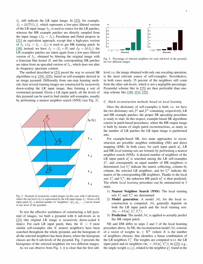
The method described in [23] paved the way to several SRalgorithms (e.g. [24], [25]), based on self-examples derived inan image pyramid. Differently from one-step learning meth-ods, here several training images are constructed by recursivelydown-scaling the LR input image, thus forming a sort ofoverturned pyramid. Given a LR input patch, all the levels ofthis pyramid can be used to find similar self-examples, usuallyby performing a nearest neighbor search (NNS) (see Fig. 2).

𝑰𝟎 (𝑰𝑳)

𝑰−𝟏

𝑰−𝟐

𝑰−𝟑

𝑰−𝟒

𝒙𝒊𝒍

𝒚𝟏𝒍

𝒚𝟐𝒍

Fig. 2. Pyramid of recursively scaled images (in this case with 4 sub-levels),where the top level (I0) is represented by the LR input image IL. Given a LRinput patch xl

i, a desired number of “neighbors” (yl1,y

l2, . . . ) can be found

at any level of the pyramid.

To test the effective usefulness of constructing a full pyra-mid of images, we built a pyramid with 6 sub-levels as in[23] (the original LR image is recursively down-scaled 6times). For each LR input patch, then, the K = 9 mostsimilar self-examples (the K nearest neighbors) have beensearched throughout the whole pyramid, and the histogram ofall the selected neighbors has been drawn, where the histogramclasses are the 6 sub-levels of the pyramid. Fig. 3 presents thehistograms of the selected neighbors for two different images.

As we can observe from Fig. 3, it is clear that the first sub-

Fig. 3. Percentage of selected neighbors for each sub-level of the pyramid,for two different images.

level, i.e. the image obtained with only one rescaling operation,is the most relevant source of self-examples. Nevertheless,in both cases nearly 35 percent of the neighbors still comefrom the other sub-levels, which is not a negligible percentage.Pyramidal scheme like in [23] are then preferable than one-step scheme like [18], [21], [22].

C. Patch reconstruction methods based on local learning

Once the dictionary of self-examples is built, i.e. we havethe two dictionary sets Y l and Yh containing, respectively, LRand HR example patches, the proper SR upscaling procedureis ready to start. In this respect, example-based SR algorithmsconsist in patch-based procedures, where the HR output imageis built by means of single patch reconstructions, as many asthe number of LR patches the LR input image is partitionedinto.

For example-based SR, two main approaches to recon-struction are possible: neighbor embedding (NE) and directmapping (DM). In both cases, for each input patch xl

i, LRand HR local training sets are formed, by performing a nearestneighbor search (NNS). A desired number of neighbors of theLR input patch xl

i is searched among the LR self-examplesY l, and consequently an equal number of HR neighbors isdetermined. Let Y l

i indicate the matrix collecting, column bycolumn, the selected LR neighbors, and let Y h

i indicate thematrix of the corresponding HR neighbors. Thanks to the localsets Y l

i and Y hi , the unknown HR patch xh

i is then predicted.The whole local learning procedure can be summarized in 3steps.

1) Nearest Neighbor Search (NNS): The local trainingsets Y l

i and Y hi are determined.

2) Model generation: A model Mi for the local re-construction is computed. Mi generally depends onboth the LR input patch and the local training sets:Mi =M(xl

i, Yli , Y

hi ).

3) Prediction: The modelMi is applied to actually predictthe HR output patch.

NE and DM differ in steps 2 and 3 of the local learningprocedure above. In NE, the reconstruction modelMi consistsof a vector of weights wi ∈ RK (where K is the numberof neighbors chosen), that identifies a linear combination ofthe LR neighbors Y l

i . The weights are computed w.r.t. the LRinput patch and its neighbors (wi =M(xl

i, Yli )). In [23], e.g.,

the single weight wi(j), related to the neighbor ylj found in the

5

pyramid, is an exponential function of the distance betweenthe latter and the LR input patch, according to the non-localmeans (NLM) model [29].

wi(j) =1

Ce−‖xl

i−yl

j‖22

t , (2)

where t is a parameter to control the decaying speed and Cis a normalizing constant to make the weights sum up to one.

In other NE methods, instead, the weights are meant todescribe a linear combination that approximates the LR inputpatch (i.e. xl

i ≈ Y li wi). In [9]–[11], e.g., the weights are

computed as the result of a least squares problem with a sum-to-one constraint:

wi = argminw

‖xli − Y l

i w‖2 s.t. wT1 = 1 . (3)

The formula (3) recalls the method used in Locally LinearEmbedding (LLE) [30] to describe a high-dimensional pointlying on a manifold through its neighbors. In [27], instead, thesum-to-one constraint is replaced by a nonnegative condition,thus leading to nonnegative weights.

wi = argminw

‖xli − Y l

i w‖2 s.t. w ≥ 0 . (4)

In [13], finally, the weight computation is performed inan appropriate subspace: the LR input patch and its HRneighbors are expressed as lower-dimensional vectors, thanksto convenient projection matrices. The weights are then foundby minimizing the error in the new subspace with no explicitconstraint:

wi = argminw

‖P lix

li − Ph

i Yhi w‖2 . (5)

Once the vector of weights wi is computed, the predictionstep (Step 3) of the NE learning procedure consists in gener-ating the HR output patch xh

i as a linear combination of theHR neighbors Y l

i , by using the same weights:

xhi ≈ Y h

i wi . (6)

Fig. 4a depicts the scheme of the patch reconstruction proce-dure in the NE case. The model, i.e. the weights, is totallylearned in the LR space, and then applied to the HR localtraining set to generate the HR output patch.

In direct mapping (DM) methods [18]–[20], instead, themodel is a regression function fi that directly maps theLR input patch into the HR output patch. The function islearned by taking into account the two local training sets(fi =M(Y l

i , Yhi )), by minimizing the empirical fitting error

between all the pairs of examples. An appropriate regulariza-tion term is placed to make the problem well-posed. We thenhave:

fi = argminf∈H

K∑j=1

‖yhj − f(yl

j)‖22 + λ‖f‖2H , (7)

where H is a desired Hilbert function space and λ ≥ 0 aregularization parameter. Examples similar to xl

i and theircorresponding HR versions are then used to learn a unique

mapping function, which is afterwards simply applied to xli to

predict the HR output patch (Step 3):

xhi = fi(x

li) (8)

Fig. 4b depicts the scheme of the patch reconstruction proce-dure also in the DM case.

𝑿𝒍 : LR test patches

𝒀𝒍 : LR training patches

𝑿𝒉 : HR test patches

𝒀𝒉 : HR training patches

1. NNS 2. Model

generation 3. Prediction

(a) Neighbor Embedding

𝑿𝒍 : LR test patches

𝒀𝒍 : LR training patches

𝑿𝒉 : HR test patches

𝒀𝒉 : HR training patches

1. NNS

2. Model

generation

3. Prediction

(b) Direct Mapping

Fig. 4. Operating schemes of the local learning based reconstruction pro-cedure, for the two approaches described (NE and DM). From the image itis clear how NE exploits the intra-space relationships, by learning a modelamong the LR patches and applying it on the HR patches. DM, instead,exploits the “horizontal” relationships, by attempting to learn the mappingbetween the two spaces.

An advantage of DM w.r.t. NE is that it can enable fastprocedures, while presenting only slightly degraded perfor-mance, as done in [31]. By allowing a mismatch in theneighborhood computation (neighborhood of the closest atomin the dictionary rather than neighborhood of the input patch),the mappings can be pre-computed and stored. Hence the fastimplementation.

III. PROPOSED ALGORITHM

In this section we present our novel SR algorithm, basedon an internal dictionary of self-examples. Starting fromthe image pyramid described in Section II-B, we proposea modified scheme with a “double pyramid”, presented inSection III-A. The self-examples found in this scheme areused to gradually upscale the LR input image up to the finalsuper-resolved image, according to the cross-level scale factor

6

chosen for the pyramid. The upscaling procedure employedfalls within the local learning based reconstruction methodsdescribed in Section II-C. In particular, it is a direct mappingmethod, where each LR patch is mapped into its HR versionby means of a specifically learned linear function. The wholeupscaling procedure and a summary of the whole algorithmare given in Section III-B.

A. Building the double pyramid

The goal of our SR algorithm is to retrieve the underlyingHR image IH from a degraded LR version of its IL, which issupposed to be originated according to the image generationmodel (1). We choose the blur kernel B to be a Gaussiankernel with a given variance σ2

B . The value s is instead aninteger scale factor (e.g. 3 or 4), which is the factor by whichwe want the LR input image IL to be magnified; i.e. if IL isof size N ×M , the final super-resolved image IH will havea size of sN × sM .

For complexity reason, the SR algorithm later describedis applied only on the luminance component Y of the inputimage IL (a colorspace transformation from the RGB to theY IQ model is then possibly performed at the beginning),whereas the color components I and Q are simply upsized byBicubic interpolation to the final desired size sN×sM . In fact,since humans are more sensitive to changes in the brightnessof the image rather than changes in color, it is a commonbelief that the SR procedure is worthy to be performed only onY , so reducing the complexity of the algorithm by one third.Hereafter, then, all the image matrices and patch vectors mustbe intended as collections of pixel luminance values.

As a starting point for our internal dictionary learningprocedure, we take the single pyramid depicted in Fig. 2.Here, the top-level is represented by the LR input image itself(I0 = IL). From it, a finite number of “sub-levels” is created,according the the following relation:

I−n = (IL ∗Bn) ↓pn , (9)

where p, the pyramid cross-level scale factor, is typically a“small” number (e.g. p = 1.25). The sub-level image I−n isthen a particular rescaled version of the original image IL(the total rescale factor amount to pn). As for the varianceof the Gaussian kernel Bn to which it is subjected, it canbe computed according to the following formula, which isexplained in [24]:

σ2Bn

= n · σ2B · log(p)/ log(s) . (10)

Once the single pyramid is created, we propose now tointerpolate each sub-level I−n by the factor p. The so obtainedinterpolated level U(I−n), where U is an upscaling operators.t. U(I) = (I) ↑p, is an image with the same size asthe original non-interpolated level located just above in thepyramid I−n+1 (except for possible 1-pixel differences, due tothe non-integer interpolation factors). We can then consider thepair constituted by U(I−n) and I−n+1 a pair of, respectively,LR and HR training images, from which derive a set ofself-examples. By using all the pairs {U(I−n), I−n+1} forn = 1, . . . NL, where NL is the chosen number of sub-levels,

and sampling at corresponding locations pairs of, respectively,LR and HR patches of equal size

√D×√D, we can then form

our LR and HR internal dictionary sets: Y l = {yli ∈ RD}Ny

i=1

and Yh = {yhi ∈ RD}Ny

i=1. Fig. 5 reports the schemedescribed, with the “double pyramid” formed by the traditionalimage cascade and, next to it, a side pyramid of interpolatedlevels.

B. Gradual upscalings

Once the LR and HR dictionary sets, Y l and Yh, are formed,by populating them with the correspondences of self-examplesfound in the double pyramid described in Section III-A, theproper SR reconstruction algorithm starts.

The algorithm consists in a multi-pass procedure, where theinput image is gradually magnified by an upscale factor equalto the cross-level scale factor p. Given s as the total scalefactor to be achieved, the number of necessary passes it then:

NP = dlogp se . (11)

If s is not a power of p, the image super-resolved afterNP passes will be over-sized w.r.t. to the targeted dimension(sM × sN ); which means that an extra resizing operation isneeded. I0 will be super-resolved into I1, I1 into I2, and sountil obtaining INP , which will be possibly resized to obtainthe SR estimated image IH with the desired dimension. Themulti-pass SR procedure is illustrated graphically in Fig. 6.

𝑰𝟑

𝑰𝟐

𝑰𝟏

𝑰𝑳

𝑰 𝑯

𝑰𝟒

𝒑𝟒

𝒑

𝒔

Fig. 6. Estimation of the HR image by gradual upscalings. The original imageIL, by 4 upscalings by a factor of p, is super-resolved into I4, that exceedsin dimension the desired scale factor s. IH is obtained by a finally resizingoperation.

When generally upscaling the image In, this is first interpo-lated into the image U(IN ) from which a set of overlappingpatches X l = {xl

i}Nxi=1 is formed, by scanning it with a

sliding window of dimension√D ×

√D. Each input patch

xli is processed singularly and, after the learning based patch

reconstruction procedure, a corresponding HR output patch xhi

is produced. By iterating for all patches, we have at the enda set of HR reconstructed patches X h = {xh

i }Nxi=1, which will

be finally re-assembled to form the upper-level image In+1. In

7

𝑰𝟎 (𝑰𝑳)

𝑰−𝟏

𝑰−𝟐

𝑰−𝟑

𝒙𝒊𝒍

𝒚𝟏𝒍

𝑰𝟏

U (𝑰𝟎)

U (𝑰−𝟏)

U (𝑰−𝟐)

U (𝑰−𝟑)

U

𝒙𝒊𝒍

𝒙𝒊𝒉

𝑴?

𝒚𝟐𝒍

𝒚𝟑𝒍

𝒚𝟏𝒍

𝒚𝟐𝒉

𝒚𝟑𝒉

𝒚𝟏𝒉

Fig. 5. Creation of the “double pyramid” and search of self-examples throughout it. The figure concerns the upscaling of I0 to I1. Given a reference patchin the interpolated version of the starting image U(I0), xl

i, 3 LR neighbors are found in the “side pyramid” of interpolated levels (yl1,y

l2,y

l3). Thanks to

these and the corresponding HR neighbors (yh1 ,y

h2 ,y

h3 ), a linear function M is meant to be learned to directly map xl

i into its corresponding HR outputpatch xh

i .

the following paragraph we describe the patch reconstructionmethod adopted.

1) Direct mapping of the self-examples via multi-linearregression: While most of the “pyramid-based” SR algorithmsin the literature [23]–[25] make use of a neighbor embedding(NE) based procedure to express each input and output patch interms of combinations of self-examples, we follow instead thedirect mapping (DM) approach. As explained in Section II-C,DM aims at learning, thanks to the LR and HR local trainingsets, a mapping to directly derive the single HR output patchas a function of the related LR input patch.

DM has been employed in SR example-based algorithmsusing external dictionaries [19], [20], by using in particularthe Kernel Ridge Regression (KRR) solution. In this case, thefunction spaceH is what is called a reproducing kernel Hilbertspace (RKHS), and the single regression function fi is seenas an expansion of kernel functions, where Gaussian kernelsare typically chosen.

For the sake of simplicity, we believe instead that, since inthe case of internal learning the dictionary patches are morepertinent training examples, a simple linear mapping “can dothe job”. With this goal, H is taken as a linear function space

H ={f(x) =Mx |M ∈ RD×D,x ∈ RD

}(12)

and the regularized empirical error (7) can be re-expressed asfollows:

Mi = argminM∈RD×D

K∑j=1

‖yhj −Myl

j‖22 + λ‖M‖2F

= argminM∈RD×D

‖Y hi −MY l

i ‖22 + λ‖M‖2F , (13)

where Y li and Y h

i are the usual, respectively LR and HR,local training sets related to the patch xl

i. In other words,we are looking for a linear transformation (i.e. the matrixMi) to be directly applied to the LR input patch. This linear

transformation is learned by observing the relations betweenthe LR and HR dictionary patches which are neighbors withxli, according to the machine learning pattern and a regression

model, where Y li is the matrix of the predictor variables or

regressors, and Y hi is the matrix of the response variables.

As the response variables are vectors and not scalars, weproperly speak about multi-variate regression (MLR) [32]. Thesolution to (13) is known, and can be written in a closed-formformula:

Mi = Y hi Y

li

T(Y li Y

li

T+ λI

)−1(14)

where I is the identity matrix. The equation (14) correspondsexactly to what we called “model generation” (Step 2 ofthe local learning procedure described in Section II-C). Theprediction of the HR unknown patch (Step 3) is the straightapplication of the linear mapping learned:

xhi =Mix

li . (15)

Fig. 5 gives a rough depiction of how the DM reconstructionmethod works in the double pyramid.

2) Patch aggregation and IBP: By learning for each inputpatch xl

i ∈ X l a linear function Mi with the equation (14), andby applying this function to generate the related output patch,we end up with a collection of HR patches X h = {xh

i }Nxi=1 that

need to be assembled to generate the current upscaling. Beforethe patch aggregation, the set of reconstructed HR patchesX h and the equivalent set of LR patches from which theyhave been originated, X l, are added to the dictionary as newcorrespondences of patches to be used in future upscalings: thepatches of the two sets, in fact, are equal in number, and a LR-HR relation stands. The update of the dictionary is performedby simple set union, i.e. Y l = Y l ∪ X l and Yh = Yh ∪ X h.

The patches of the input image, and consequently alsoin the equally-sized output image, are taken with a certainoverlap; that means that, when they are re-placed in the

8

original positions, at each pixel location we have a set ofdifferent candidate values. We can see the image at this stageas a 3-D image, where the multiple values per pixel arethe results of different local observations of the input image(i.e. different patches taken), and therefore contain differentpartial information about the unknown HR image. We obtaina single output image by convexly combining these candidatesat each pixel location: the convex combination is done bysimply taking uniform weights, i.e. each candidate is weightedby 1/Np, where Np is the number of overlapping patchescontributing to that particular position.

After the image of the new level is formed, by overlappingand averaging, before it is used as a starting image for thenext upscaling, it is further refined in an iterative fashion by theiterative back-projection (IBP) procedure. IBP is an additionaloperation adopted by several SR algorithms (e.g. [14], [23]),for which the output super-resolved image, once reconstructed,is “back-projected” to the LR dimension in order to assure itto be consistent with the LR input image, i.e. to assure it tobe a plausible estimation of the underlying HR image, andconveniently corrected if errors are observed.

At the iteration t of this refining procedure, the genericreconstructed n-th level Itn is first back-projected into anestimated LR image ItL:

ItL =(Itn ∗Bn

)↓pn (16)

where Bn is a Gaussian blur with variance as expressed in(10). The deviation between this LR image found by back-projection and the original LR image is then used to furthercorrect the HR estimated image:

It+1n = Itn +

((IL − ItL

)↑pn

)∗ b , (17)

where b is a back-projection filter that locally spreads thedifferential error.

In Listing 1, our proposed SR procedure is described in asimplified manner, by reporting the pseudocode for the twomain routines of the algorithm: “InternalLearning”, where thedouble pyramid is constructed and the dictionary sets of LRand HR patches are initially formed, and “SingleUpscale”, thatreports the procedure to upscale a generic level In to the upperlevel. To be noted, in particular, on line 15 the for loop, whichconsists of 3 instructions and implements the 3 steps of thelocal learning based patch reconstruction procedure describedin Section II-C: nearest neighbor search, model generation,and prediction.

IV. EXPERIMENTAL RESULTS

In this section we conduct some experiments on the pro-posed single-image SR algorithm. In particular, in SectionIV-A we evaluate the different contributions, in terms of imple-mentation choices, that led to its final formulation summarizedin Listing 1. Section IV-B provides some considerations aboutthe complexity, intended both as time and space complexity, ofthe proposed algorithm. In particular, we evaluate the amountof extra complexity possibly brought by the double pyramid.

Listing 1 Single-image SR via linear mapping of interpolatedself-examples

1: procedure INTERNALLEARNING(IL, NL, s, p, σ2B )

2: for n← 1, NL do . Create the pyramid levels3: σ2

Bn← n · σ2

B · log(p)/ log(s)4: I−n ← (IL ∗Bn) ↓pn

5: U(I−n)← (I−n) ↑p6: end for

7: for n← 1, NL do . Populate the internal dict.8: Sample patches from U(I−n) and add to Y l

9: Sample patches from I−n+1 and add to Yh

10: end for11: end procedure

12: procedure SINGLEUPSCALE(In, p, Y l, Yh)13: U(In)← (In) ↑p . Upscale the current level14: Extract LR patches from U(In) → X l = {xl

i}Nxi=1

15: for i← 1, Nx do . Single patch reconstructions16: Find the local train. sets of xl

i by NNS → Y li , Y

hi

17: Mi ← Y hi Y

liT(Y li Y

liT+ λI

)−118: xh

i ←Mixli

19: end for

20: Form In+1 with the constr. patches X h = {xhi }

Nxi=1

21: Refine In+1 by IBP22: Y l ← Y l ∪ X l . Update the LR dictionary23: Yh ← Yh ∪ X h . Update the HR dictionary24: end procedure

In Section IV-C, finally, we compare our algorithm with otherstate-of-the-art methods, by both showing visual comparisonson super-resolved images and reporting quantitative results,according to the PSNR and SSIM metrics. PSNR and SSIMvalues are obtained as measures of the distance between theHR original image, from which the LR input image, for testpurposes, has been originated, and the super-resolved image.The image generation model adopted is the one expressed inEquation (1), with the variance of the Gaussian blur σ2

B set to1 in all experiments. The interpolation method used is Bicubicinterpolation.

As for the various parameters of the algorithms, they havebeen “tuned” by empirically looking for their optimal values.Notably, the cross-level scale factor p is taken as p = 1.25; asfor the patch size, instead, 5×5 patches are sampled from theinternal images with a 4-pixel overlap. For each input patch,then, K = 12 are selected in the dictionary via NNS.

A. Evaluation of the different contributions

In this section we want to assess the different contributionsof our algorithm, which have been discussed in Section III.With respect to the well-known single-image SR algorithm in[23], two main contributions have been presented:

9

1) The employment of a DM reconstruction method (i.e.MLR), instead of NE;

2) The introduction of a different training and upscalingscheme, i.e. the “double” pyramid.

To singularly evaluate the two “ingredients” above, we testthree different procedures (summarized in Table I), whichall fall in the category of example-based single-image SRalgorithms employing an internal dictionary.

TABLE ISUMMARY OF THE INTERNAL-DICTIONARY PROCEDURES CONSIDERED TO

EVALUATE THE DIFFERENT CONTRIBUTIONS OF OUR ALGORITHM.

Rec. Method Double pyr.Algorithm 1 NE No

Algorithm 2 DM No

Proposed DM Yes

We first start with an algorithm, where a single pyramid isconstructed and NE with non-local means (NLM) weights (2)is used as patch reconstruction method (“Algorithm 1”). Thisalgorithm is very close in the spirit to the method in [23], andthus its implementation can be considered as a reference forthe mentioned method, except for possible slight differencesin the code configuration and the choice of the parameters.With respect to Algorithm 1, “Algorithm 2” uses a DM patchreconstruction method instead of NE, i.e. the MLR methoddescribed in Section III-B that linearly maps each LR patchinto the related HR patch. The finally proposed algorithmintroduces then the double pyramid scheme, featuring the sidepyramid of interpolated levels. Table II presents the PSNR andSSIM values for all the considered algorithms, when testedon seven input images and for two different scale factors(s = 3, 4).

TABLE IIPERFORMANCE RESULTS (PSNR AND SSIM VALUES) OF THE THREEDIFFERENT ALGORITHMS USING AN INTERNAL DICTIONARY, WHEN

SUPER-RESOLVING SEVERAL IMAGES FOR SCALE FACTORS OF 3 AND 4.

Algorithm 1 Algorithm 2 ProposedImage Scale PSNR SSIM PSNR SSIM PSNR SSIM

Bike 3 23.13 0.792 23.20 0.796 23.30 0.799Bird 3 33.71 0.884 34.06 0.890 34.13 0.890Butterfly 3 27.08 0.833 27.38 0.840 27.56 0.841Hat 3 29.95 0.651 30.11 0.655 30.11 0.655Head 3 32.43 0.633 32.47 0.667 32.43 0.668Lena 3 30.68 0.770 30.91 0.775 30.89 0.775Woman 3 30.33 0.862 30.41 0.866 30.52 0.867

Avg gain w.r.t. A1 - - 0.18 0.009 0.23 0.010

Bike 4 21.58 0.685 21.53 0.688 21.63 0.689Bird 4 30.61 0.810 30.89 0.824 31.01 0.826Butterfly 4 24.68 0.763 24.71 0.772 25.05 0.775Hat 4 28.54 0.553 28.60 0.556 28.53 0.555Head 4 31.17 0.556 31.28 0.591 31.23 0.590Lena 4 29.02 0.681 29.22 0.687 29.28 0.689Woman 4 27.60 0.778 27.90 0.793 27.96 0.793

Avg gain w.r.t. A1 - - 0.13 0.012 0.21 0.013

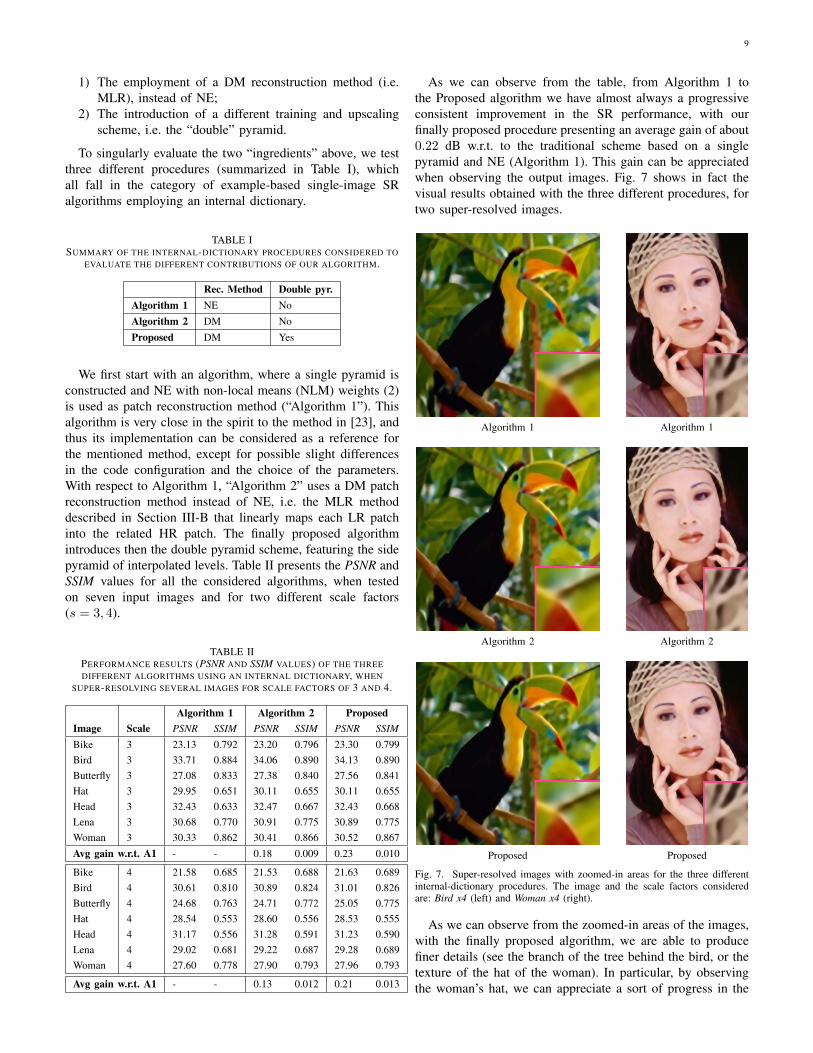
As we can observe from the table, from Algorithm 1 tothe Proposed algorithm we have almost always a progressiveconsistent improvement in the SR performance, with ourfinally proposed procedure presenting an average gain of about0.22 dB w.r.t. to the traditional scheme based on a singlepyramid and NE (Algorithm 1). This gain can be appreciatedwhen observing the output images. Fig. 7 shows in fact thevisual results obtained with the three different procedures, fortwo super-resolved images.

Algorithm 1 Algorithm 1

Algorithm 2 Algorithm 2

Proposed Proposed

Fig. 7. Super-resolved images with zoomed-in areas for the three differentinternal-dictionary procedures. The image and the scale factors consideredare: Bird x4 (left) and Woman x4 (right).

As we can observe from the zoomed-in areas of the images,with the finally proposed algorithm, we are able to producefiner details (see the branch of the tree behind the bird, or thetexture of the hat of the woman). In particular, by observingthe woman’s hat, we can appreciate a sort of progress in the

10

outcome of the three algorithms: Algorithm 1 gives a prettyblurred result; Algorithm 2, thanks to the use of DM in theplace of NE, shows instead more regular structures; the edgesand the shapes of these structures look even sharper withthe Proposed algorithm, where the DM functions have beencomputed on the interpolated patches of the double pyramid.

B. Considerations on the algorithm complexity

In order to evaluate the time complexity of the algorithm,we ran two versions of it, featuring the usual single pyramidand our double pyramid, for two different scale factors (3 and4). The single-pyramid implementation gives an idea of thecomplexity of several algorithms in the literature (e.g. [23]–[25]). The goal of this test is to evaluate the penalty broughtby the use of our double pyramid, in terms of increasedcomplexity. Table III summarizes the results of the tests made.

TABLE IIIAVERAGE RUNNING TIME OF THE ALGORITHM, FOR TWO SCALE FACTORS,

WITH SINGLE OR DOUBLE PYRAMID. TIME IS EXPRESSED IN SECONDS.

Scale LR size N. Passes Single Pyr. Double Pyr. ∆T

3 85× 85 5 75 83 +10.7%4 64× 64 7 111 120 +8.1%

As we can see from Table III, the double pyramid leads toan extra complexity in the order of about 10%. The increase inthe computational cost is mainly due to the fact that bigger LRvectors are processed (LR patches have the same size as HRpatches). Nevertheless, we believe that the complexity increaseis still within a tolerable extent.

To evaluate the space complexity, i.e. memory storagerequirement, we can instead compute an estimation of the sizeof the internal dictionary. Here, the only discriminating factorbetween the single and the double pyramid is the size of the LRpatches. In fact, in the case of double pyramid, both patcheshave the same size, whereas the LR patches are p2 smaller inthe case of single pyramid (where p is the small scale factorused at each pass). Given this, it is easy to compute the ratiobetween the two dictionary sizes:

R =2

1 + 1s2

. (18)

In our tests p was set to 1.25, which corresponds to a 22%increase of the storage requirement.

C. Comparison with state-of-the-art algorithms

In this section we perform a comparative assessment ofour method with other single-image SR algorithms in thestate-of-the art, by extending the comparison also to SRmethods based on external dictionaries. For this purpose, weconsider Bicubic interpolation as a reference for traditionalanalytical interpolation methods, and four other example-basedSR algorithms. The characteristic of the latter, as well as thoseones of our proposed method, are summarized in Table IV.

For the first three methods in the table, the original codeof the respective authors, possibly slightly modified to makethe comparison fair, has been used. For the “pyramid” method

TABLE IVSUMMARY OF OUR METHOD AND THE FOUR EXAMPLE-BASED SR

ALGORITHMS CONSIDERED FOR THE COMPARISON.

Method Reference Dictionary Rec. Method

LLE-basedNE

Chang et al. [9] External NE with LLEweights (3)

NonnegativeNE

Bevilacqua etal. [33]

External NE with NNweights (4)

Sparse SR Yang et al. [14] External Sparse coding

Pyramid Glasner et al.[23]

Internal, singlepyramid

NE with NLMweights (2)

Proposed This paper Internal, doublepyramid

DM via Multi-linear Regress.

of [23], instead, the third-party code of the authors of [24]has been adopted. Table V reports the performance results ofthe algorithms considered (PSNR and SSIM values), with theusual set of seven test images, and 3 and 4 as scale factors.

Table V shows clearly that our method outperforms theother algorithms in terms of objective quality of the super-resolved images, for all the images and the two scale factorsconsidered. The results are confirmed when observing thevisual comparisons (Fig. 8, Fig. 9, and Fig. 10).

From the visual results presented, we can see that methodsbased on external dictionaries (“LLE-based NE”, “NN NE”,and “Sparse SR”) often present blurring and ringing artifacts(see e.g. the Bike images in Fig. 9). Results for the twoalgorithms based on an internal dictionary (the “pyramid” al-gorithm of [23] and ours), instead, are certainly more pleasantat sight, presenting sharp edges and smooth artifact-free resultsin the regions with no texture. However, the algorithm of [23]in some cases shows results that look somehow “artificial”,with over-smoothed areas or unnatural edges (see Lena’s eyein Fig. 10e, whose shape is deformed). Our algorithm succeedsalso in avoiding these undesired effects.

V. CONCLUSION

In this paper we presented a novel single-image single-image (SR) method, which belongs to the family of example-based SR algorithms, using a dictionary of patches in theupscaling procedure. The algorithm originally makes use ofa “double pyramid” of images, built starting from the inputimage itself, to extract the dictionary patches (thus called“self-examples”), and employs a regression-based method todirectly map the low-resolution (LR) input patches into theirrelated high-resolution (HR) output patches. When comparedto other state-of-the-art algorithms, our proposed algorithmshows the best performance, both in terms of objective metricsand subjective visual results. As for the former, it presentsconsiderable gains in PSNR and SSIM values. When observingthe super-resolved images, also, it turns out to be the mostcapable in producing fine artifact-free HR details. The algo-rithm does not rely on extra information, since making use ofan internal dictionary automatically “self-adapted” to the inputimage content, and also the few parameters have proven to beeasy to tune. This makes it a particularly attractive method forSR upscaling purposes.

11

TABLE VPERFORMANCE COMPARISON (PSNR AND SSIM VALUES) WITH OTHER STATE-OF-THE-ART METHODS, WHEN SUPER-RESOLVING SEVERAL IMAGES FOR

SCALE FACTORS OF 3 AND 4.

Bicubic LLE-based NE NN NE Sparse SR Pyramid ProposedImage Scale PSNR SSIM PSNR SSIM PSNR SSIM PSNR SSIM PSNR SSIM PSNR SSIM

Bike 3 20.84 0.640 22.38 0.754 23.02 0.784 22.71 0.771 22.81 0.772 23.30 0.799Bird 3 29.88 0.820 32.11 0.834 33.37 0.864 32.90 0.858 32.18 0.862 34.13 0.890Butterfly 3 21.75 0.712 24.27 0.774 26.36 0.823 24.92 0.787 26.63 0.825 27.56 0.841Hat 3 27.27 0.536 29.24 0.619 29.65 0.632 29.21 0.602 29.66 0.626 30.11 0.655Head 3 31.02 0.583 32.05 0.626 32.28 0.638 32.23 0.653 31.69 0.629 32.43 0.668Lena 3 28.03 0.670 29.78 0.729 30.52 0.754 30.06 0.738 30.28 0.748 30.89 0.775Woman 3 26.17 0.778 28.27 0.806 29.35 0.840 29.02 0.815 29.89 0.857 30.52 0.867

Average 26.42 0.677 28.30 0.734 29.22 0.762 28.72 0.746 29.02 0.760 29.85 0.785

Bike 4 19.83 0.536 20.75 0.634 21.26 0.667 20.93 0.651 21.46 0.681 21.63 0.689Bird 4 28.09 0.738 29.25 0.741 30.41 0.786 30.00 0.787 30.10 0.803 31.01 0.826Butterfly 4 20.30 0.637 21.83 0.682 23.41 0.738 22.18 0.701 24.44 0.761 25.05 0.775Hat 4 26.30 0.462 27.48 0.505 27.85 0.530 27.31 0.506 28.41 0.544 28.53 0.555Head 4 30.07 0.516 30.71 0.537 30.92 0.556 30.85 0.573 30.86 0.575 31.23 0.590Lena 4 26.85 0.593 27.84 0.628 28.52 0.670 27.98 0.649 28.70 0.668 29.28 0.689Woman 4 24.61 0.697 25.84 0.696 26.76 0.752 26.18 0.732 27.20 0.777 27.96 0.793

Average 25.15 0.597 26.24 0.632 27.02 0.671 26.49 0.657 27.31 0.687 27.81 0.702

REFERENCES

[1] S. C. Park, M. K. Park, and M. G. Kang, “Super-Resolution ImageReconstruction: A Technical Overview,” IEEE Signal Process. Mag.,vol. 20, no. 3, pp. 21–36, 5 2003.

[2] T. S. Huang and R. Y. Tsai, “Multiframe image restoration and regis-tration,” Adv. Comput. Vis. Image Process., vol. 1, no. 7, pp. 317–339,1984.

[3] X. Li and M. T. Orchard, “New Edge-Directed Interpolation,” IEEETrans. Image Process., vol. 10, no. 10, pp. 1521–1527, Oct. 2001.

[4] M. F. Tappen, B. C. Russell, and W. T. Freeman, “Exploiting the SparseDerivative Prior for Super-Resolution and Image Demosaicing,” in Proc.IEEE Int. Work. Statist. Comput. Theories Vis., 2003.

[5] R. Fattal, “Image Upsampling via Imposed Edge Statistics,” ACM Trans.Graphics, vol. 26, no. 3, pp. 1–8, Jul. 2007.

[6] H. He and W.-C. Siu, “Single image super-resolution using Gaussianprocess regression,” in Proc. IEEE Conf. Comp. Vis. Pattern Recogn.(CVPR), 2011, pp. 449–456.

[7] K. Zhang, X. Gao, D. Tao, and X. Li, “Single Image Super-ResolutionWith Non-Local Means and Steering Kernel Regression,” IEEE Trans.Image Process., vol. 21, no. 11, pp. 4544–4556, 2012.

[8] W. T. Freeman, T. R. Jones, and E. C. Pasztor, “Example-Based Super-Resolution,” IEEE Comput. Graph. Appl., vol. 22, no. 2, pp. 56–65,2002.

[9] H. Chang, D.-Y. Yeung, and Y. Xiong, “Super-Resolution ThroughNeighbor Embedding,” in Proc. IEEE Conf. Comp. Vis. Pattern Recogn.(CVPR), vol. 1, 2004, pp. 275–282.

[10] W. Fan and D.-Y. Yeung, “Image Hallucination Using Neighbor Em-bedding over Visual Primitive Manifolds,” in Proc. IEEE Conf. Comp.Vis. Pattern Recogn. (CVPR), 7 2007, pp. 1–7.

[11] T.-M. Chan, J. Zhang, J. Pu, and H. Huang, “Neighbor embedding basedsuper-resolution algorithm through edge detection and feature selection,”Pattern Recogn. Lett., vol. 30, no. 5, pp. 494–502, 4 2009.

[12] B. Li, H. Chang, S. Shan, and X. Chen, “Locality preserving constraintsfor super-resolution with neighbor embedding,” in Proc. IEEE Int. Conf.Image Process. (ICIP), 11 2009, pp. 1189–1192.

[13] X. Gao, K. Zhang, D. Tao, and X. Li, “Joint learning for single-imagesuper-resolution via a coupled constraint,” IEEE Trans. Image Process.,vol. 21, no. 2, pp. 469–480, Feb. 2012.

[14] J. Yang, J. Wright, T. Huang, and Y. Ma, “Image Super-Resolution ViaSparse Representation,” IEEE Trans. Image Process., vol. 19, no. 11,pp. 2861 –2873, 11 2010.

[15] J. Wang, S. Zhu, and Y. Gong, “Resolution enhancement based onlearning the sparse association of image patches,” Pattern Recogn. Lett.,vol. 31, pp. 1–10, 1 2010.

[16] X. Gao, K. Zhang, D. Tao, and X. Li, “Image Super-Resolution WithSparse Neighbor Embedding,” IEEE Trans. Image Process., vol. 21,no. 7, pp. 3194–3205, 2012.

[17] K. Zhang, X. Gao, D. Tao, and X. Li, “Multi-scale dictionary for singleimage super-resolution,” in Proc. IEEE Conf. Comp. Vis. Pattern Recogn.(CVPR), Jun. 2012, pp. 1114–1121.

[18] J. Yang, Z. Lin, and S. Cohen, “Fast Image Super-Resolution Based onIn-Place Example Regression,” in Proc. IEEE Conf. Comp. Vis. PatternRecogn. (CVPR), Jun. 2013, pp. 1059–1066.

[19] Y. Tang, P. Yan, Y. Yuan, and X. Li, “Single-image super-resolution vialocal learning,” Int.J. Mach. Learning Cybern., vol. 2, pp. 15–23, 2011.

[20] K. I. Kim and Y. Kwon, “Single-Image Super-Resolution Using SparseRegression and Natural Image Prior,” IEEE Trans. Pattern Anal. Mach.Intell., vol. 32, no. 6, pp. 1127–1133, 2010.

[21] G. Freedman and R. Fattal, “Image and Video Upscaling from LocalSelf-Examples,” ACM Trans. Graphics, vol. 28, no. 3, pp. 1–10, 2010.

[22] K. Zhang, X. Gao, D. Tao, and X. Li, “Single image super-resolutionwith multiscale similarity learning,” IEEE Trans. Neural Netw. LearningSyst., vol. 24, no. 10, pp. 1648–1659, Oct. 2013.

[23] D. Glasner, S. Bagon, and M. Irani, “Super-Resolution from a SingleImage,” in Proc. IEEE Int. Conf. Comp. Vis. (ICCV), 10 2009, pp. 349–356.

[24] C.-Y. Yang, J.-B. Huang, and M.-H. Yang, “Exploiting Self-Similaritiesfor Single Frame Super-Resolution,” in Proc. Asian Conf. Comp. Vis.(ACCV), Nov. 2010.

[25] M.-C. Yang, C.-H. Wang, T.-Y. Hu, and Y.-C. F. Wang, “Learningcontext-aware sparse representation for single image super-resolution,”in Proc. IEEE Int. Conf. Image Process. (ICIP), Sep. 2011, pp. 1349–1352.

[26] M. Zontak and M. Irani, “Internal Statistics of a Single Natural Image,”in Proc. IEEE Conf. Comp. Vis. Pattern Recogn. (CVPR), 2011, pp.977–984.

[27] M. Bevilacqua, A. Roumy, C. Guillemot, and M.-L. A. Morel,“Low-Complexity Single-Image Super-Resolution based on NonnegativeNeighbor Embedding,” in Proc. British Mach. Vis. Conf. (BMVC).Guildford, UK: BMVA Press, Sep. 2012, pp. 135.1–135.10.

[28] S. Baker and T. Kanade, “Limits on Super-Resolution and How to BreakThem,” IEEE Trans. Pattern Anal. Mach. Intell., vol. 24, no. 9, pp. 1167–1183, 2002.

[29] A. Buades, B. Coll, and J.-M. Morel, “A Non-Local Algorithm for ImageDenoising,” in Proc. IEEE Conf. Comp. Vis. Pattern Recogn. (CVPR),vol. 2, Washington, DC, USA, 2005, pp. 60–65.

[30] S. T. Roweis and L. K. Saul, “Nonlinear Dimensionality Reduction byLocally Linear Embedding,” Science, vol. 290, no. 5500, pp. 2323–2326,12 2000.

12

(a) (b) (c)

(d) (e) (f)

Fig. 8. Comparative results with zoomed-in areas for Butterfly magnified by a factor of 3. The methods considered are: (a) Bicubic interpolation, (b) LLE-basedNE, (c) NN NE, (d) Sparse SR, (e) Pyramid, (f) Proposed.

(a) (b) (c)

(d) (e) (f)

Fig. 9. Comparative results with zoomed-in areas for Bike magnified by a factor of 3. The methods considered are: (a) Bicubic interpolation, (b) LLE-basedNE, (c) NN NE, (d) Sparse SR, (e) Pyramid, (f) Proposed.

13

(a) (b) (c)

(d) (e) (f)

Fig. 10. Comparative results with zoomed-in areas for Lena magnified by a factor of 3. The methods considered are: (a) Bicubic interpolation, (b) LLE-basedNE, (c) NN NE, (d) Sparse SR, (e) Pyramid, (f) Proposed.

[31] R. Timofte, V. D. Smet, and L. V. Gool, “Anchored neighborhoodregression for fast example-based super-resolution,” in Proc. IEEE Int.Conf. Comp. Vis. (ICCV), Dec. 2013.

[32] H. Hyotyniemi, “Multivariate regression - Techniques and tools,”Helsinki University of Technology, Control Engineering Laboratory,Helsinki, Finland, Tech. Rep. Report 125, 2001.

[33] M. Bevilacqua, A. Roumy, C. Guillemot, and M.-L. Alberi Morel,“Super-resolution using Neighbor Embedding of Back-projection resid-uals,” in Proc. Int. Conf. Digit. Signal Process. (DSP), Santorini, Greece,Jul. 2013.

Marco Bevilacqua Marco Bevilacqua is a Postdoc-toral Research Fellow at IMT Institute for AdvancedStudies Lucca, Italy. He received the Laurea (B.S.equivalent degree) and Laurea Specialistica (M.S.equivalent degree) from University of Florence,Italy, in 2006 and 2009 respectively. From February2010 to January 2011, he was a research fellow at theItalian National Research Council (C.N.R.). FromFebruary 2011 to March 2014, as a Ph.D. studentof University of Rennes 1 (France), he pursued hisPh.D. studies in Computer Science, by carrying out

a thesis project co-funded by INRIA (Institut National de Recherche enInformatique et en Automatique) and Alcatel-Lucent Bell Labs France. Hefinally received his Ph.D. degree in June 2014. His research interests liein signal processing, particularly for images, computer vision, and machinelearning techniques.

Aline Roumy Aline Roumy received the Engi-neering degree from Ecole Nationale Suprieure del’Electronique et de ses Applications (ENSEA),Cergy, France in 1996, the Master degree in June1997 and the Ph.D. degree in September 2000 fromthe University of Cergy-Pontoise, France. During2000-2001, she was a research associate at PrincetonUniversity, Princeton, NJ. On November 2001, shejoined INRIA, Rennes, France as a research scientist.She has held visiting positions at Eurecom andBerkeley University. Her current research and study

interests include the area of statistical signal and image processing, codingtheory and information theory. She has been a Technical Program Committeemember and session chair at several international conferences, including ISIT,ICASSP, Eusipco, WiOpt, Crowncom. She is currently serving as a memberof the French National University Council (CNU 61). She received the 2011“Francesco Carassa” best paper award.

Christine Guillemot Christine Guillemot, IEEEfellow, is “Director of Research” at INRIA, headof a research team dealing with image and videomodeling, processing, coding and communication.She holds a Ph.D. degree from ENST (Ecole Na-tionale Superieure des Telecommunications) Paris,and an “Habilitation for Research Direction” fromthe University of Rennes. From 1985 to Oct. 1997,she has been with FRANCE TELECOM, where shehas been involved in various projects in the areaof image and video coding for TV, HDTV and

multimedia. From Jan. 1990 to mid 1991, she has worked at Bellcore, NJ,USA, as a visiting scientist. She has (co)-authored 15 patents, 8 book chapters,50 journal papers and 140 conference papers. She has served as associatededitor (AE) for the IEEE Trans. on Image processing (2000-2003), for IEEETrans. on Circuits and Systems for Video Technology (2004-2006) and forIEEE Trans. On Signal Processing (2007-2009). She is currently AE for theEurasip journal on image communication and member of the editorial boardfor the IEEE Journal on selected topics in signal processing (2013-2015). Sheis a member of the IEEE IVMSP technical committees.

IEEE TRANSACTIONS ON IMAGE PROCESSING, VOL. XX, NO. X, MONTH 2014 14

Marie-Line Alberi Morel Dr. Marie-Line AlberiMorel is a researcher since 2001 at Alcatel-LucentBell Labs in Nozay, France. She received a M.S.degree in electronics and signal processing in 1995,and a Ph.D. degree in the signal processing field in2001 from University of Paris Sud Orsay, France.During her career at Alcatel-Lucent, she has con-tributed to various radio projects on deploymentand dimensioning studies for WLAN and small cellnetworks. She has conducted research on DVB-SHmobile broadcast network (“Television Mobile Sans

Limite” French project). Later, she worked on the design of optimizedsolutions of video services delivery over mobile wireless networks and overconverging 3GPP EMBMS and DVB NGH broadcasting networks (Adaptable,Robust, Streaming Solutions and Mobile Multi Media French projects).Currently, her research focuses on the video processing field, particularly onsuper resolution algorithms based on machine learning techniques and on thesource coding. She also serves as an associate professor at Marne-La-ValleeUniversity, France.