Simultaneous Estimation of Left Ventricular Motion and Material Propertieswith Maximum a Posteriori Strategy

Huafeng Liu and Pengcheng ShiDepartment of Electrical and Electronic EngineeringHong Kong University of Science and Technology

Clear Water Bay, Kowloon, Hong Kong

Abstract

In addition to its technical merits as a challenging non-rigidmotion and structural integrity analysis problem, quanti-tative estimation of cardiac regional functions and mate-rial characteristics has significant physiological and clin-ical values. We have earlier developed a stochastic finiteelement framework for the simultaneous estimation of my-ocardial motion and material parameters from medical im-age sequences with an extended Kalman filter approach.In this paper, we present a new computational strategy forthe framework based upon the maximum a posteriori es-timation principles, realized through the extended Kalmansmoother, that produce a sequence of kinematics state andmaterial parameter estimates from the entire sequence ofobservations. The system dynamics equations of the heartis constructed using a biomechanical model with stochasticparameters, and the tissue material and deformation pa-rameters are jointly estimated from the periodic imagingdata. Experiments with canine magnetic resonance imageshave been conducted with very promising results, as val-idated through comparison to the histological staining ofpost mortem myocardium.

1. Introduction

1.1 Cardiac Motion Analysis

Acute and chronic myocardial ischemia can be identi-fied and localized through the detection of morphologi-cal and kinematic abnormalities of the left ventricle (LV)[13]. Accordingly, there have been abundant efforts to an-alyze cardiac motion and deformation from medical im-age sequences [6]. Imaging-derived salient features ofthe LV have been used to establish correspondences be-tween cardiac image frames, including the implanted phys-ical markers [10], the crossings of magnetic resonance(MR) tagging images [20], and the geometrically signifi-cant shape landmarks [24]. In order to recover dense fieldmotion/deformation of the entire myocardium from thesesparsely matched points, assumptions must be made about

the myocardial behavior in order to constrain the ill-posedproblem for a unique solution. Popular strategies includethe uses of mathematically motivated regularization [20]and continuum mechanics based models [19, 23].

Because of the periodic nature of the heart motion, theimportance of multi-frame analysis is well recognized. As-suming elliptic trajectories of cardiac tissue elements, aKalman filter framework was constructed to estimate LVdeformation from MRI phase contrast velocity fields con-strained by segmented myocardial contours [15]. A globalgeometrical evolution analysis, followed by regional shapematching, was tested on simulated and real endocardial sur-faces [3]. And an adaptive filtering scheme with spatial-temporal smoothness and periodicity constraint was pro-posed to track myocardial contour motion [14].

Conjugate to biomechanics efforts, all image analysisworks are based on the premise that mechanical or otherconstraining models are known as prior information, andthe task is to use these models to help estimating kinemat-ics parameters in some optimal sense. The selection of anappropriate model with proper parameters thus largely de-termines the quality of the analysis results.

1.2 Myocardium Material Characterization

More fundamentally, it has been recognized that alterationsin myocardial fiber structure and material elasticity are re-lated to various cardiac pathologies [25], and there havebeen many works focusing on describing myocardial mate-rial characteristics from the biomechanics community [10]and from the medical imaging community [5, 16].

In biomechanics studies of cardiac mechanics and ma-terial properties, the kinematics of the heart tissues is as-sumed to be known from implanted markers or imagingmeans. The issue is then to use these kinematic obser-vations to estimate material parameters of the constitutivelaws. While most works deal with regional finite deforma-tions measured at isolated locations which are then used toarrive at suitable constitutive relationships [11, 12], MR tag-ging has been used more recently for the in vivo study of

1

the mechanics of the entire heart [5], where unknown ma-terial parameters are determined for an exponential strainenergy function that maximizes the agreement between theobserved (from MR tagging) and the predicted (from finiteelement modeling) regional wall strains. However, it is rec-ognized that the recovery of kinematics from MR tagging orother imaging techniques is not a solved problem yet, andconstraining models of mechanical nature may be neededfor the kinematics recovery in the first place [6].

More recently, magnetic resonance elastography (MRE)provides quantitative image of soft tissue material stiffnessby processing the displacements resulting from actuatingthe tissue and using MR imaging techniques to measure thetissue displacements [16]. The technology is still under de-velopment, and so far there have been only in vitro experi-ments on soft tissue elasticity measurement. No possibilityfor in vivo MRE of myocardium is at sight.

1.3 Joint Motion and Material Estimation

We have developed the first attempt of simultaneous jointestimation of myocardial kinematics functions and mate-rial model parameters based on a stochastic finite elementframework [22]. The biomechanical model parametersand the imaging data are treated as random variables withknown prior statistics in the dynamic system equations ofthe left ventricle, and the extended Kalman filter (EKF) pro-cedures are adopted to linearize the augmented state equa-tions and to provide the joint estimates in the least-mean-square sense. This framework is not restricted to any par-ticular imaging data, and experiments have been conductedwith MR tagging and MR phase contrast images.

In this paper, we present a new computational strategyfor our multi-frame joint estimation framework. The car-diac kinematics (displacement fields and strains) and mate-rial (parameters of constitutive laws) properties are recov-ered using the Bayesian estimation principles. We have em-ployed the extended Kalman smoother (EKS) as the maxi-mum a posteriori (MAP) state and parameter sequence es-timator. That is, we compute the most likely estimates thatbest describe the observed data as a whole. This way, weavoid the possible divergence problem of the EKF approachby employing forward and backward filtering to obtain im-proved averaged estimates.

We realize that several efforts in recursive structure andmotion estimation from images are of relevance to ourwork. An EKF strategy was used for recursive recoveryof motion, pointwise structure, and focal length from fea-ture correspondence tracked through an image sequence [1].A particle-filter like expectation maximization (EM) frame-work, based on the CONDENSATION algorithm, was de-veloped for non-Gaussian observations and multi-class dy-namics [18]. And EM/EKS is adopted to impose time-

continuity of estimated motion parameters in [21]. Ourwork differs from these in the sense that it is constrainedby biomechanically motivated system dynamics, and weare explicitly dealing with non-rigid object with much in-creased complexity.

2. LV System Dynamics

2.1 Biomechanical Model of the Myocardium

The biomechanical model of the myocardium implicitlyregularizes the dynamic behavior of the heart. In orderto construct a realistic yet computationally feasible analy-sis framework using imaging data and other available mea-surements, the structure, dynamics, and material of the leftventricle should be properly modeled. In general, the heartis a non-rigid object that deforms over time and has verycomplicated biomechanical properties in terms of the con-stitutive laws [10]. For computational simplicity, we adoptthe isotropic linear elastic model for the myocardium in ourcurrent implementation, where the stress σ and strain ε re-lationship obeys the Hooke’s law:

σ = Sε (1)

More realistic models, such as the transversely isotropicmaterial [10] which accounts for the preferential stiffness inthe myofiber directions (the fiber stiffness is about 1.5 to 3times greater than the cross-fiber stiffness in normal cases),can be easily adopted for the three-dimensional analysis ifthe myofiber structure is available from the myofiber model[17] or from diffusion tensor magnetic resonance images(DTMRI) [7]. However, since the presented framework isfor 2D case, we use the linear material model to illustratethe basic ideas and rationales of a novel joint estimationstrategy. Assuming the displacement along the x- and y-axis of a point to be u(x, y) and v(x, y) respectively, theinfinitesimal strain tensor ε of the point can be expressedas:

ε =

∂u∂x∂v∂y

∂u∂y + ∂v

∂x

(2)

and under plane strain condition, matrix S is:

S =E

(1 + ν)(1− 2ν)

1− ν ν 0

ν 1− ν 00 0 1−2ν

2

(3)

Here, E and ν, the Young’s modulus and the Poisson’s ra-tio, are two material-specific constants we want to estimate.Currently, the material parameter priors are derived fromliteratures on post mortem tissue testing [26], while theirdistributions over a large population are unknown.

2

2.2 Stochastic Finite Element Method

The stochastic finite element method (SFEM) is used for therepresentation of the LV structure and dynamics. SFEM hasbeen used for structural dynamics analysis in probabilisticframeworks [4], where structural material properties are de-scribed by random fields, possibly with known prior statis-tics, and the observations and loads are treated as noise-corrupted. This way, stochastic differential dynamics equa-tions are combined with the finite element method to studythe dynamic structures with uncertainty in their parametersand measurements.

In our 2D implementation, a Delaunay triangulated finiteelement mesh is formed (Fig. 3), bounded by endocardialand epicardial boundaries. An isoparametric formulationdefined in a natural coordinate system is used, where, fortri-nodal linear element, the basis functions are linear func-tions of the nodal coordinates [2]. We arrive at the followingsystem dynamics equation of the LV:

MU + CU +KU = R (4)

where M , C and K are the mass, damping and stiffnessmatrices, R the load vector, and U the displacement vector.Because the myocardium density is generally considered tobe uniform, M is a known function of the material densityand is temporally and spatially constant. K is a function ofthe material constitutive law, and is related to the material-specific Young’s modulus and Poisson’s ratio, which varytemporally and spatially. In our framework, these two lo-cal material parameters are treated as random variables withknown a priori statistics, and will be estimated along withthe motion functions. (Please note that currently we do notconsider the temporal dependency of the material parame-ters). C is frequency dependent, and we assume Rayleighdamping with C = αM + βK. In practice, it is difficultto determine the damping parameters because they are fre-quency dependent, and we assume Raleigh damping for thevery low damping heart tissue and fix the two weightingconstants to be 1%. These two parameters can actually beput into our augmented state vectors and be estimated fromour framework as well.

2.3 State Space Representation

Since we have employed the linear material model, Eqn.4 can be transformed into a state-space representation of acontinuous-time linear stochastic system:

x(t) = Ac(θ)x(t) +Bcw(t) (5)

where the material parameter vector θ, the state vector x,the system matricesAc andBc, and the control (input) term

w are:

θ =[Eν

], x(t) =

[U(t)U(t)

], w(t) =

[0R(t)

]

Ac =[

0 I−M−1K −M−1C

]

Bc =[

0 00 M−1

]

An associated measurement equation, which describes theobserved imaging data y(t), can be expressed in the form:

y(t) = Dx(t) + e(t) (6)

where D is a known measurement matrix, and e(t) is themeasurement noise.

In our framework, Eqns. 5 and 6 represent a continuous-time system with discrete-time measurements, or a so-called sampled data system. The input term, availablefrom pressure measurements or computed from the systemequation using the initial conditions, is piecewise constantover the sampling interval T . Implicitly assuming hiddenMarkov model for the state equations, we arrive at the dis-crete dynamics equation [9]:

x((k + 1)T ) = Ax(kT ) +Bw(kT ) (7)

with A = eAcT and B = A−1c (eAcT − I)Bc. For general

continuous-time system with discrete-time measurements,including the process noise v(t), we have the state equation:

x(t+ 1) = A(θ)x(t) +B(θ)w(t) + v(t) (8)

2.4 Augmented State Space Representation

The myocardial dynamics and observations are now repre-sented by Eqns. 6 and 8. This representation provides a nat-ural framework for the biomechanics study of myocardiummaterial constitutive laws with observations/measurementson the kinematics states, and for the physically-motivatedimage analysis of cardiac kinematics properties with as-sumed biomechanical constraining models. However, inpractice, neither the kinematics data nor the model parame-ters are precisely known. We have proposed a SFEM frame-work where the data and the model parameters are treatedas random variables, possibly with known or assumed priordistributions, to determine the best estimates of the spa-tial distributions of the material parameters and the spatial-temporal kinematics parameters simultaneously [22].

In order to perform the joint estimation, the unknownstate vector x is augmented by the unknown material pa-rameter vector θ to form the new state vector z = [x θ]T ,and we have the new pair of augmented state/measurementequations:

z(t+ 1) = f(z(t), w(t)) + vs(t) (9)

y(t) = h(z(t)) + eo(t) (10)

3

frame #1 frame #5 frame #9 frame #13

Figure 1: Canine cardiac MR images.

where

f(z(t), w(t)) =[A(θ)x(t) +B(θ)w(t)

θ

]

h(z(t)) =[D 0

] [x(t)θ(t)

]

vs(t) =[v(t)0

], eo(t) =

[e(t)0

]

The joint state and parameter estimation problem can beunderstood as a state estimation problem for this nonlinearsystem. Assuming known Gaussian augmented process andmeasurement noises:

vs(t) ∼ N(0, Qs), Qs =[Qv 00 0

]

eo(t) ∼ N(0, Ro), Ro =[Re

0

]

this form of formulation leads to a solution of the filter-ing problem using the extended Kalman filter (EKF) frame-work, which is based on linearization of the augmentedstate equations at each time step. A recursive procedurewith natural block structure is used to perform the jointstate (kinematics) and parameter (material) estimation [22].The Gaussian assumptions are convenient for the filteringframework, and their variances would determine the appli-cability of the framework to LV of different states of health.

3. The Maximum A Posteriori Estima-tion Strategy

We aim to estimate a dense displacement field and materialparameters distribution from the entire imaging/imagingderived data, which corresponds to maximize the poste-rior probability density function with the model parameterp(z|y). Here, we employ the EKS as the maximum a pos-teriori (MAP) state and parameter sequence estimator. Thisway, a Bayesian estimation framework allows us to com-bine the statistical likelihood in terms of probability density

Over-view Blown-up Over-view Blown-up

Endocardial Contour Epicardial Contour

Figure 2: Boundary displacement constraints throughoutthe cardiac cycle at selected endo- and epi-cardial points.

function (PDF) of the state and observation with a contin-uum biomechanics constraining model, using a state spacerepresentation of the system dynamics. It should be notedhere that we can incorporate any model parameters into theaugmented state z, such as the uncertain noise properties,without losing any generality of our approach.

3.1 Basic Concepts

With the Bayes’ rule, we have:

z = argmaxz

{p(z|y) = p(z, y)p(y)

} (11)

We note that p(y) is a constant once the measurements havebeen made and can therefore be ignored in the maximiza-tion process. Then maximizing the posterior PDF p(z|y) isequivalent to maximize the joint PDF p(z, y). This can beachieved by an EKS based estimation framework.

Assuming the prior distribution on the initial augmentedstate z(0) is Gaussian white with mean z0 and covarianceΣ0:

p(z(0)) =exp{− 1

2 [z(0)− z0]TQ−1s [z(0)− z0]}

2π|Σ0| 12(12)

We construct the PDF of z(t) given z(t− 1):

p(z(t)|z(t− 1)) = (13)

exp{− 12 [z(t)− f(t− 1)]TQ−1

s [z(t)− f(t− 1)]}2π|Qs| 12

and the conditional PDF of y(t) given z(t):

p(y(t)|z(t)) = (14)

exp{−12 [y(t)− h(z(t))]TR−1

o [y(t)− h(z(t))]}2π|Ro| 12

where f(t− 1) = f(z(t− 1), w(t− 1)), and |Qs| and |Ro|are the determinants of matrix Qs and Ro respectively.

4

frame #1 frame #5 frame #9 frame #13

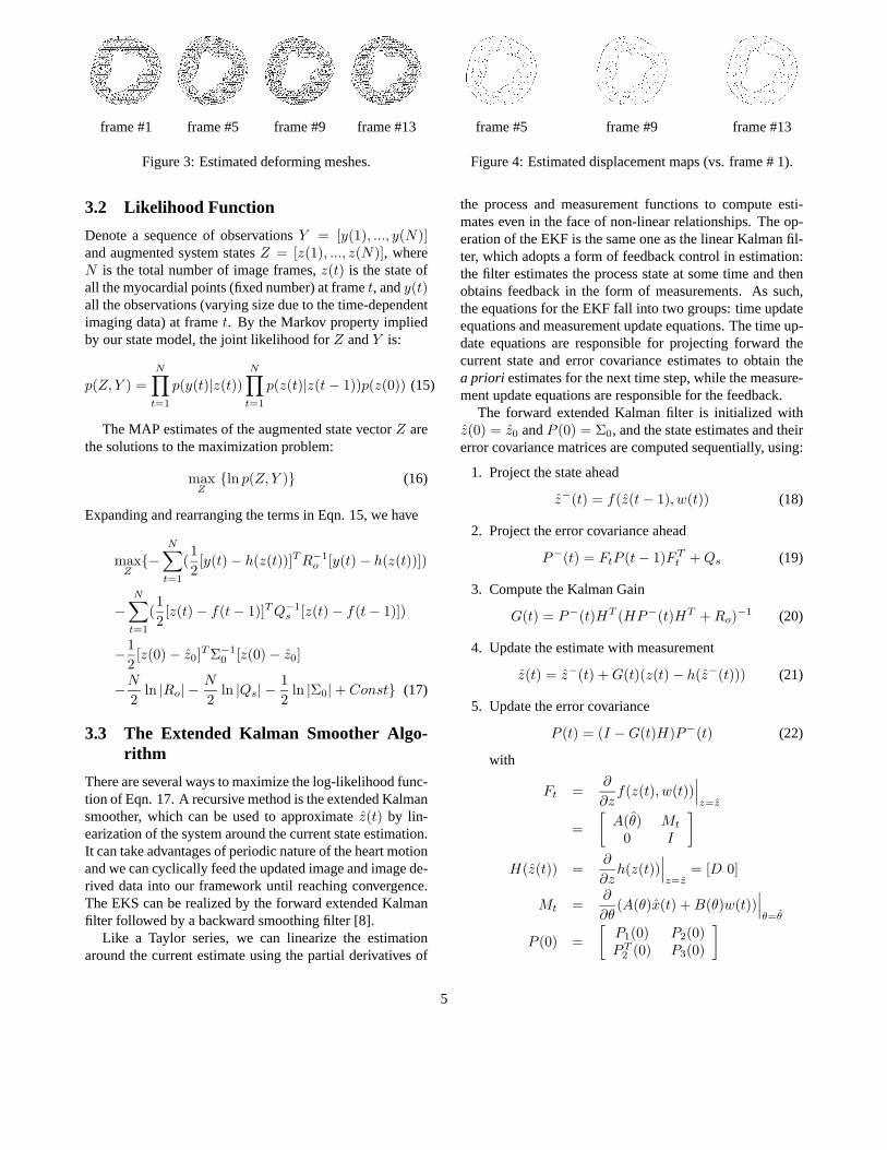
Figure 3: Estimated deforming meshes.

3.2 Likelihood Function

Denote a sequence of observations Y = [y(1), ..., y(N)]and augmented system states Z = [z(1), ..., z(N)], whereN is the total number of image frames, z(t) is the state ofall the myocardial points (fixed number) at frame t, and y(t)all the observations (varying size due to the time-dependentimaging data) at frame t. By the Markov property impliedby our state model, the joint likelihood for Z and Y is:

p(Z, Y ) =N∏

t=1

p(y(t)|z(t))N∏

t=1

p(z(t)|z(t− 1))p(z(0)) (15)

The MAP estimates of the augmented state vector Z arethe solutions to the maximization problem:

maxZ

{ln p(Z, Y )} (16)

Expanding and rearranging the terms in Eqn. 15, we have

maxZ

{−N∑

t=1

(12[y(t)− h(z(t))]TR−1

o [y(t)− h(z(t))])

−N∑

t=1

(12[z(t)− f(t− 1)]TQ−1

s [z(t)− f(t− 1)])

−12[z(0)− z0]TΣ−1

0 [z(0)− z0]

−N2ln |Ro| − N

2ln |Qs| − 1

2ln |Σ0|+ Const} (17)

3.3 The Extended Kalman Smoother Algo-rithm

There are several ways to maximize the log-likelihood func-tion of Eqn. 17. A recursive method is the extended Kalmansmoother, which can be used to approximate z(t) by lin-earization of the system around the current state estimation.It can take advantages of periodic nature of the heart motionand we can cyclically feed the updated image and image de-rived data into our framework until reaching convergence.The EKS can be realized by the forward extended Kalmanfilter followed by a backward smoothing filter [8].

Like a Taylor series, we can linearize the estimationaround the current estimate using the partial derivatives of

frame #5 frame #9 frame #13

Figure 4: Estimated displacement maps (vs. frame # 1).

the process and measurement functions to compute esti-mates even in the face of non-linear relationships. The op-eration of the EKF is the same one as the linear Kalman fil-ter, which adopts a form of feedback control in estimation:the filter estimates the process state at some time and thenobtains feedback in the form of measurements. As such,the equations for the EKF fall into two groups: time updateequations and measurement update equations. The time up-date equations are responsible for projecting forward thecurrent state and error covariance estimates to obtain thea priori estimates for the next time step, while the measure-ment update equations are responsible for the feedback.

The forward extended Kalman filter is initialized withz(0) = z0 and P (0) = Σ0, and the state estimates and theirerror covariance matrices are computed sequentially, using:

1. Project the state ahead

z−(t) = f(z(t− 1), w(t)) (18)

2. Project the error covariance ahead

P−(t) = FtP (t− 1)FTt +Qs (19)

3. Compute the Kalman Gain

G(t) = P−(t)HT (HP−(t)HT +Ro)−1 (20)

4. Update the estimate with measurement

z(t) = z−(t) +G(t)(z(t)− h(z−(t))) (21)

5. Update the error covariance

P (t) = (I −G(t)H)P−(t) (22)

with

Ft =∂

∂zf(z(t), w(t))

∣∣∣z=z

=[A(θ) Mt

0 I

]

H(z(t)) =∂

∂zh(z(t))

∣∣∣z=z

= [D 0]

Mt =∂

∂θ(A(θ)x(t) +B(θ)w(t))

∣∣∣θ=θ

P (0) =[P1(0) P2(0)PT

2 (0) P3(0)

]

5

Radial

Circumferential

frame #5 frame #9 frame #13R-C Shear

Strain Scale

Figure 5: Estimated radial, circumferential, and R-C shearstrain maps (vs. frame # 1).

Here, P1(0) is the kinematics state error covariance sub-matrix which is related to our confidence measure on theinput imaging data (see next section on the constructionof confidence measures for shape-based boundary displace-ments used in our experiments), P3(0) is the material pa-rameter covariance sub-matrix whose values are propor-tional to the possible knowledge of the myocardium understudy, and P2(0) is the kinematics-material correlation sub-matrix with zero entries.

The backward smoothing of the EKS is achieved throughthe well-known Rauch-Tung-Striebel smoother [8],:

Λ(t) = P (t)FTt P

−(t+ 1) (23)

z(t|T ) = z(t) + Λ(t)(z(t+ 1|T )− z−(t+ 1)) (24)

4. Experiments

4.1 Imaging Data

Canine experiment was conducted, where a hydraulic oc-cluder was used to produce a controlled, graded coronarystenosis in the central left anterior descending (LAD) coro-nary artery territory. Sixteen canine MR images are ac-quired over the heart cycle, with imaging parameters flip an-gle = 30o, TE = 34msec, TR = 34msec, FOV = 28cm,5mm skip 0, matrix 256x128, 4 nex, venc = 15cm/sec.

P1 Strain

P1 Direction

P2 Strain

frame #5 frame #9 frame #13P2 Direction

Principal Strain Scale

Figure 6: Estimated principal strain and associated directionmaps (vs. frame # 1).

The spatial resolution is 1.09mm/pixel, and the temporalresolution is 31.25msec/frame. Fig.1 shows the examplesof the images from the sequence and the detected endocar-dial and epicardial boundaries.

4.2 Inputs for the Framework

Boundary displacements between consecutive frames aredetected based on locating and matching geometric land-marks and a local coherent smoothness model [24]. Basedon the hypothesis that the LV boundary contours deform aslittle as possible between successive temporal frames, bend-ing energy measure is used as the matching criterion to ob-tain the point correspondences between contours:

minϕ∈C

ebend(φ, ϕ) = minϕ∈C

[κf (φ)− κs(ϕ)]2 (25)

where κf (φ) is the curvature for a point φ in the first con-tour, C the corresponding search region on the second con-tour, and κs(ϕ) the curvature of a candidate point ϕ withinthe search region. Among all the candidate points, the oneat ξ which yields the smallest bending energy is chosen as

6

the matched point, and the bending energy value indicatesthe goodnessmg(ξ) = ebend(φ, ξ) of the match.

Further, the bending energy measures for all other pointswithin the search region are recorded as the basis to measurethe uniqueness of the matching choice. Ideally, the bendingenergy value of the chosen point should be an outlier (muchsmaller value) compared to the values of the rest of the can-didate points. If we denote the mean value of the bendingenergy measures of all the points inside the search windowexcept the chosen point as ebend and the standard deviationas σbend, we define the uniqueness measure of the match as:

mu(ξ) = | ebend(φ, ξ)ebend − σbend

| (26)

Obviously for both goodness and unique measures, thesmaller the values the more reliable the match. Combiningthese two together, we arrive at a confidence measure for thematched second contour point ξ of the first contour point φ:

c(ξ) =1

k1,g + k2,gmg(ξ)1

k1,u + k2,umu(ξ)(27)

where k1,g, k2,g, k1,u, and k2,u are normalizing constantssuch that the confidence measures for all point matches be-tween contours are in the range of 0 to 1.

This process yields a set of shape-based, best-matcheddisplacement vectors for each pair of contours, and eachvector has an associated confidence measure. Elements ofthe kinematics error covariance sub-matrix P1(0) will beweighted by (1 − c(ξ)). Fig. 2 shows the displacementtrajectories for the endo- and epicardial points throughoutthe cardiac cycle, and these displacements and their associ-ated confidences are used as the initial kinematics states andthe initial covariance matrix entries. Appropriate covari-ance matrices play essential roles in determining the sen-sible/converged outputs, as it is well known that the majordisadvantage of any Kalman strategies is the required detailpriors on the noise statistics.

Based on biomechanics testing of canine myocardium[26], the initial Young’s modulus and Poisson ratio are set to75000 Pascal and 0.47, with initial variance 200 and 0.001,respectively. In order to handle large discontinuities of thematerial parameters, which if directly imposed may requireprior knowledge on the pathological conditions of the tissueelasticity, we have utilized a strategy by updating the mate-rial priors for the next iteration with the current estimatesand the original variances for the first a few loops of thecomputation. This enables the handling of a much widerrange of material variations.

4.3 Results

In the reported real image experiment, the LV slice consistsof 295 nodes and 500 elements. On a P4 1.8GHz PC and

Young’s Modulus Poisson’s Ratio TTC-staining

Young’s Modulus Scale

Poisson’s Ratio Scale

Figure 7: Estimated material parameter maps and the high-lighted TTC-stained post mortem myocardium.

under Matlab 6.0, it took ∼ 40 minutes for each loop and 10loops for the system to converge. Under C++ environment,the processing time is reduced to ∼ 40 minutes in total.

Fig. 3 shows the original LV mesh at end-diastole (ED)and the selected meshes (frames #5, #9, and #13) estimatedfrom the framework. The corresponding displacement mapsare shown in Fig. 4, the cardiac-specific radial (R), circum-ferential (C), and R-C shear strain maps are shown in Fig.5, and the principal strains and their associated principal di-rections are shown in Fig. 6.

The final converged estimates of the Young’s modu-lus and Poisson’s ratio distributions and mapping scalesare presented in Fig. 7, as well as the highlighted his-tological results of triphenyl tetrazolium chloride (TTC)stained post mortem myocardium, often considered thegold-standard. Spatially, the Young’s modulus varies from71500 to 77500Pascal, and the Poisson ratio varies from0.465 to 0.483. While meaningful interpretation of thesematerial parameter results is still underway, it is obviousthat the material parameters seem more sensitive than thekinematics results (displacement and strains) to differenti-ate the transmural properties, which are considered the keyindications for early detection of ischemic pathologies.

5. Summary and ConclusionsIn this paper, we have described an MAP based estima-tion framework for multi-frame joint estimation of cardiackinematics and material properties from medical image se-quence. Here, this approach adopts material models withrandom field parameters, and using EKS to estimate motion,deformation and material parameters simultaneously. Thisnon-invasive joint estimation strategy offers new possibili-

7

ties to study myocardial kinematics and material character-istic from a variety of imaging data, and early experimentshave shown that material parameters have better sensitivityfor transmural properties than motion parameters. Effortson adopting particle filter and H∞ filter are in progress,which can deal with global minimum issue and noise char-acteristics issue respectively.

Acknowledgments

Thanks to Dr. Albert Sinusas of Yale University for thecanine experiments and the imaging data. This work is sup-ported by HKRGC-CERG HKUST6057/00E.

References[1] A. Azarbayejani and A.P. Pentland. Recursive estimation

of motion, structure and focal length. IEEE Transactionson Pattern Analysis and Machine Intelligence, 17:562–575,1995.

[2] K. Bathe and E. Wilson. Numerical Methods in Finite Ele-ment Analysis. Prentice-Hall, New Jersey, 1976.

[3] P. Clarysse, D. Friboulet, and I.E. Magnin. Tracking geomet-rical descriptors on 3-D deformable surfaces - application tothe left-ventricular surface of the heart. IEEE Transactionson Medical Imaging, 16:392–404, 1997.

[4] H. Contreras. The stochastic finite element method. Com-puters and Structures, 12:341–348, 1980.

[5] L.L. Creswell, M.J. Moulton, S.G. Wyers, J.S. Pirolo, D.S.Fishman, W.H. Perman, K.W. Myers, R.L. Actis, M.W. Van-nier, B.A. Szabo, and M.K. Pasque. An experimental methodfor evaluating constitutive models of myocardium in in vivohearts. American Journal of Physiology, 267:H853–H863,1994.

[6] A.J. Frangi, W.J. Niessen, and M.A. Viergever. Three-dimensional modeling for functional analysis of cardiac im-ages: A review. IEEE Transactions on Medical Imaging,20(1):2–25, 2001.

[7] L. Geerts, P. Bovendeerd, K. Nicolay, and T. Arts. Charac-terization of the normal cardiac myofiber field in goat mea-sured with MR-diffusion tensor imaging. American Journalof Physiology, 283(1):H139–H145, 2002.

[8] A. Gelb. Applied Optimal Estimation. MIT Press, Cam-bridge, MA, 1974.

[9] T. Glad and L. Ljung. Control Theory. Taylor & Francis,London, 2000.

[10] L. Glass, P. Hunter, and A. McCulloch. Theory of Heart.Springer-Verlag, New York, 1991.

[11] J.M. Guccione, A.D. McCulloch, and L.K. Waldman. Pas-sive material properties of intact ventricular myocardium de-termined from a cylindrical model. Journal of Biomechani-cal Engineering, 113:42–55, 1991.

[12] P.J. Hunter and B.H. Smaill. The analysis of cardiac func-tion: a continuum approach. Progress in Biophysics andMolecular Biology, 52:101–164, 1989.

[13] M.J. Lipton, J. Bogaert, L.M. Boxt, and R.C. Reba. Imagingof ischemic heart disease. European Radiology, 12:1061–1080, 2002.

[14] J.C. McEachen, A. Nehorai, and J.S. Duncan. Multiframetemporal estimation of cardiac nonrigid motion. IEEE Trans-actions on Image Processing, 9:651–665, 2000.

[15] F.G. Meyer, R.T. Constable, A.J. Sinusas, and J.S. Dun-can. Tracking myocardial deformation using spatially con-strained velocities. IEEE Transactions on Medical Imaging,15(4):453–465, 1996.

[16] R. Muthupilla, D.J. Lomas, P.J. Rossman, J.F. Greenleaf,A. Manduca, and R.L. Ehman. Magnetic resonance elastog-raphy by direct visualization of propagating acoustic strainwaves. Science, 269(5232):1854–1857, 1995.

[17] P.M. Nielsen, I.J. LeGrice, B.H. Smaill, and P.J. Hunter.Mathematical model of geometry and fibrous structure ofthe heart. American Journal of Physiology, 260(4):H1365–H1378, 1991.

[18] B. North, A. Blake, M. Isard, and J. Rittscher. Learning andclassification of complex dynamics. IEEE Transactions onPattern Analysis and Machine Intelligence, 22:1016–1034,2000.

[19] X. Papademetris, A.J. Sinusas, D.P. Dione, R.T. Constable,and J.S. Duncan. Estimation of 3-D left ventricular de-formation from medical images using biomechanical mod-els. IEEE Transactions on Medical Imaging, 21(7):786–799,2002.

[20] J. Park, D.N. Metaxas, and L. Axel. Analysis of left ven-tricular wall motion based on volumetric deformable modelsand MRI-SPAMM. Medical Image Analysis, 1:53–71, 1996.

[21] Y.D. Seo and K.S. Hong. Structure and motion estima-tion with expectation maximization and extended kalmansmoother for continuous image sequences. In Computer Vi-sion and Pattern Recognition I, pages 1148–1154, 2001.

[22] P. Shi and H. Liu. Stochastic finite element framework forcardiac kinematics function and material property analysis.In Medical Image Computing and Computer Assisted Inter-vention, pages 634–641, 2002.

[23] P. Shi, A. Sinusas, R. T. Constable, and J. Duncan. Volumet-ric deformation analysis using mechanics-based data fusion:Applications in cardiac motion recovery. International Jour-nal of Computer Vision, 35(1):87–107, 1999.

[24] P. Shi, A. Sinusas, R. T. Constable, E. Ritman, and J. Dun-can. Point-tracked quantitative analysis of left ventricularmotion from 3D image sequences. IEEE Transactions onMedical Imaging, 19(1):36–50, 2000.

[25] S.A. Wickline, E.D. Verdonk, A.K. Wong, R.K. Shepard, andJ.G. Miller. Structural remodelling of human myocardial tis-sue after infarction: quantification with ultrasonic backscat-ter. Circulation, 85:269–268, 1992.

[26] H. Yamada. Strength of Biological Material. The Williamsand Wilkins Company, Baltimore, 1970.

8