Simulations for Modelling of Population Balance Equations of ...
105
S IMULATIONS FOR M ODELLING OF P OPULATION BALANCE E QUATIONS OF P ARTICULATE P ROCESSES USING D ISCRETE P ARTICLE M ODEL (DPM) NARNI NAGESWARA R AO Fakultät für Mathematik Otto-von-Guericke Universität Magdeburg
-
Upload
khangminh22 -
Category
Documents
-
view
1 -
download
0
Transcript of Simulations for Modelling of Population Balance Equations of ...

SIMULATIONS FOR MODELLING OF
POPULATION BALANCE EQUATIONS OF
PARTICULATE PROCESSES USING
DISCRETE PARTICLE MODEL (DPM)
NARNI NAGESWARA RAO
Fakultät für Mathematik
Otto-von-Guericke Universität Magdeburg


Simulations for Modelling of Population BalanceEquations of Particulate Processes using the
Discrete Particle Model (DPM)
Dissertationzur Erlangung des akademischen Grades
doctor rerum naturalium(Dr. rer. nat.)
genehmigt durch die Fakultät für Mathematikder Otto-von-Guericke-Universität Magdeburg
von Narni Nageswara Raogeb. am 01. July 1979 in Kappaladoddi, India
Gutachter:Prof. Dr. rer. nat. habil. Gerald WarneckeProf. Dr.-Ing. habil. Stefan Heinrich
Eingereicht am: 04. Februar 2009Verteidigung am: 24. März 2009


Nomenclature
Latin Symbol
a, b, c Constants —Ai Area of the particle i m2
Cd Drag coefficient —dα Diameter of the particle α m〈d〉 Average diameter me Coefficient of restitution —g Acceleration due to gravity m/sec2
G Growth rate 1/sech Height of the bed mI Unit tensor —Iα Moment of inertia of particle α Kgm2
J Impulse vector Kgm/seck Boltzmann constant 1.380× 10⁻¹⁶erg/K0
K(t, x, y) Aggregation kernel m3/secK(x, y) Collision frequency function m3/secK0(t) Aggregation efficiency function 1/secKi,j(t) Aggregation kernel among classes i and j m/sec2
Li Length of the particle i mM Average molecular weight of air Kg/molmα Mass of particle α Kgn Normal unit vector —n(t, x) Number density at time t of particle property x 1/m3
n0(x) Initial number density of the particle with property x 1/m3
ni Particle concentration of class i 1/m3
nj Particle concentration of class j 1/m3
Ni,j Number of collisions between class i and class j m3/secNi Number of particles of class i —Ni,sim Number of particles of class i from simulation —Ni,expt Number of particles of class i from experiment —Nj Number of particles of class j —Ncell Number of Eulerian grid cells —p Pressure of the gas dyne/m2(Pa)rα Radius of the particle α mR Gas constant 8.31× 10⁷erg/K0molReα Particle Reynolds number —〈Re〉 Average Reynolds number —

6
s Surface areas of the particle m2
St Stokes number —S∗
t Critical Stokes number —t Time sect Tangential unit vector —tsim Simulation time secT Temperature K0
Tα Torque Nmu Velocity of the gas m/secU Relative velocity m/secvα Velocity of the particle α m/secVα Volume of the particle α m3
Vbed Volume of the bed m3
Vcell Volume of Eulerian grid cell m3
Vfluid Volume of the fluid m3
Vparticles Volume of the particles m3
W Effective volume of the particle m3
W ∗ Critical volume of the particle m3
xα Position of the particle α mx, y Volume of the particle m3
z Random number —zα Height of the particle α m
Greek Symbol
β Interphase momentum transfer coefficient Kg/m3secβ0 Coefficient of tangential restitution —µ Gas phase shear viscosity Kg/msecµj The jth moment m3j ·m−3
δ Distance mδtflow Time step for gas phase secδ(x) Dirac-delta distribution —δi,j Kronecker delta —ε Void fraction —λ Gas phase bulk viscosity Kg/msecλ(t) Specific aggregation rate function 1/secΩ Discretized domain —ω Angular velocity 1/secρ Density of the gas Kg/m3
η Bed parameter (dimensionless)Γ Laminar shear velocity of gas m/secτ Gas phase stress tensor Kg/msec2
σ Standard deviation m

7
Subscripts
0 Initial conditionα Particle indexa Particle aab Between particle a and bb Particle bagg Aggregationbed Fluidized bedbreak Breakagecoll Collisioncell Cell sizeexpt Experimenti, j, k Indexn Normalstep Time stepsim Simulationt Tangential
Superscripts
− Mean or average values∧ Simulated valuen Value at nth level
Acronyms
CA Cell AverageDPM Discrete Particle ModelDEM Discrete Element MethodEKE Equi-partition Kineitc Energy kernelIPSD Initial Particle Size DistributionKTGF Kinetic Theory of Granular FlowPBE Population Balance EquationPSD Particle Size DistributionRE Relative ErrorSSE Sum of Square of Errors
Contents
1 General Introduction 11.1 Introduction . . . . . . . . . . . . . . . . . . . . . . . . . . . . . . . . . . . . . 11.2 Fluidized bed spray granulation . . . . . . . . . . . . . . . . . . . . . . . . . . . 21.3 Particle formation mechanisms . . . . . . . . . . . . . . . . . . . . . . . . . . . 3
1.3.1 Agglomeration . . . . . . . . . . . . . . . . . . . . . . . . . . . . . . . 41.3.2 Nucleation . . . . . . . . . . . . . . . . . . . . . . . . . . . . . . . . . 41.3.3 Growth . . . . . . . . . . . . . . . . . . . . . . . . . . . . . . . . . . . 4
1.4 Modelling of the spray granulation processes . . . . . . . . . . . . . . . . . . . 51.4.1 Multi scale modelling of fluidized beds . . . . . . . . . . . . . . . . . . 51.4.2 Micro-Macro modelling of the fluidized bed . . . . . . . . . . . . . . . . 7
1.5 Outline of the thesis . . . . . . . . . . . . . . . . . . . . . . . . . . . . . . . . . 8
2 Population Balance Equations 102.1 Introduction . . . . . . . . . . . . . . . . . . . . . . . . . . . . . . . . . . . . . 102.2 Aggregation equation . . . . . . . . . . . . . . . . . . . . . . . . . . . . . . . . 11
2.2.1 Continuous form of the aggregation equation . . . . . . . . . . . . . . . 122.3 Scaling of the equations . . . . . . . . . . . . . . . . . . . . . . . . . . . . . . . 13
2.3.1 Dimensional analysis for discrete equation . . . . . . . . . . . . . . . . 132.3.2 Dimensional analysis of the continuous equation . . . . . . . . . . . . . 142.3.3 Number density selection and dimensional analysis of the kernel in ap-
plications . . . . . . . . . . . . . . . . . . . . . . . . . . . . . . . . . . 142.4 Properties of agglomeration kernels . . . . . . . . . . . . . . . . . . . . . . . . 15
2.4.1 Theoretical kernels . . . . . . . . . . . . . . . . . . . . . . . . . . . . . 162.4.2 Empirical kernels . . . . . . . . . . . . . . . . . . . . . . . . . . . . . . 212.4.3 Experimental kernels . . . . . . . . . . . . . . . . . . . . . . . . . . . . 24
3 Discrete Particle Model 273.1 Introduction . . . . . . . . . . . . . . . . . . . . . . . . . . . . . . . . . . . . . 273.2 The discrete particles . . . . . . . . . . . . . . . . . . . . . . . . . . . . . . . . 283.3 The gas-phase . . . . . . . . . . . . . . . . . . . . . . . . . . . . . . . . . . . . 30
3.3.1 Initial and boundary conditions . . . . . . . . . . . . . . . . . . . . . . 313.4 Two-way coupling . . . . . . . . . . . . . . . . . . . . . . . . . . . . . . . . . 32
3.4.1 Hard sphere collision model . . . . . . . . . . . . . . . . . . . . . . . . 33
ix
x CONTENTS
3.5 Numerical calculations . . . . . . . . . . . . . . . . . . . . . . . . . . . . . . . 36
4 Modelling of collision frequency functions using DPM 434.1 Introduction . . . . . . . . . . . . . . . . . . . . . . . . . . . . . . . . . . . . . 434.2 Derivation of collision frequency functions . . . . . . . . . . . . . . . . . . . . 444.3 Correction to the aggregation equation . . . . . . . . . . . . . . . . . . . . . . . 464.4 Physical description of the flow pattern inside fluidized beds . . . . . . . . . . . 47
5 Simulation results 495.1 Initial parameters . . . . . . . . . . . . . . . . . . . . . . . . . . . . . . . . . . 49
5.1.1 Initial assumptions . . . . . . . . . . . . . . . . . . . . . . . . . . . . . 495.1.2 Initial particle size distributions . . . . . . . . . . . . . . . . . . . . . . 50
5.2 Evaluation of the bed parameter . . . . . . . . . . . . . . . . . . . . . . . . . . 535.3 Simulation results for a pseudo 3D bed . . . . . . . . . . . . . . . . . . . . . . . 55
5.3.1 Log-Normal distribution . . . . . . . . . . . . . . . . . . . . . . . . . . 625.4 Simulation results for 3D beds . . . . . . . . . . . . . . . . . . . . . . . . . . . 63
6 Evaluation of aggregation efficiency rate 666.1 Evaluation of the aggregation efficiency rate . . . . . . . . . . . . . . . . . . . . 666.2 Simulation results for the aggregation efficiency rate . . . . . . . . . . . . . . . 68
6.2.1 Aggregation in pseudo 3D fluidized bed . . . . . . . . . . . . . . . . . . 696.2.2 Aggregation in 3D fluidized beds . . . . . . . . . . . . . . . . . . . . . 716.2.3 Aggregation in pseudo 3D fluidized bed with log-normal distribution . . 74
6.3 Numerical methods for population balance equations . . . . . . . . . . . . . . . 746.4 Computation of the particle size distributions . . . . . . . . . . . . . . . . . . . 77
6.4.1 Computation of the particle size distribution for pseudo 3D fluidized bed 776.4.2 Computation of the particle size distribution for 3D fluidized bed . . . . 796.4.3 Computation of the particle size distribution for 3D fluidized bed with
log normal distribution . . . . . . . . . . . . . . . . . . . . . . . . . . . 79
7 General conclusions and outlook 81
A 83A.1 Analytical derivation of shear kernel for fluidized bed . . . . . . . . . . . . . . . 83A.2 Analytical solution for shear kernel for monodisperse initial conditions . . . . . . 85
B 87B.1 Physical and Numerical parameters of the simulations . . . . . . . . . . . . . . . 87B.2 Initial particle size distributions . . . . . . . . . . . . . . . . . . . . . . . . . . . 88
B.2.1 Particle size distribution for 5000 particles . . . . . . . . . . . . . . . . . 88B.2.2 Particle size distribution corresponding to 15000 particles . . . . . . . . 90

Chapter 1
General Introduction
1.1 Introduction
Mathematical modelling plays a vital role in all discliplines of science and engineering. Its aimis to describe the real world phenomena through mathematics. Due to enormous improvementsin computational speed and algorithms, simulating many real world phenomena is within reach.Using these simulation results modelers try to apply them to the realistic problems in differentfields such as industry, environment and weather prediction, life sciences, and sports in order tomake more efficient mathematical models. Further details of such improved models and applica-tions can be found in (42). The present thesis is concerned with such an application of modellingand simulations for fluidized bed granulation in process engineering.
Gas-fluidized beds are widely applied in the chemical process industry. Typical applicationscover a wide variety of physical and chemical processes such as fluidized bed combustion, cat-alytic cracking of oil and fluidized bed granulation (detergents, fertilizers, food industry) to namea few. They have several advantageous properties like isothermal conditions throughout the bed,excellent heat and mass transfer properties and possibility of continuous operation. Apart fromthe above advantages they have a special application of minimizing the industrial waste, whichresults to the reduction of the environmental pollution.
We have different mathematical models to describe the fluidized bed spray granulation. De-velopment of multiscale analysis techniques and algorithms to describe the exchange betweenmechanical, thermal, and chemical processes in heterogeneous spatial scales of the fluidizedbeds is still a challenging task to the researchers. A continuous heat and mass tranfer model forthe fluidized bed granulation was developed by Heinrich (50). Further, the model was extendedwith the inclusion of a drying mechanism by Peglow (39). An efficient numerical scheme forthese fluidized bed granulation models has been studied in Nagaiah (8). These models give onthe macro level physical insight into the fluidized bed granulation process and the results arecomparable to laboratory experiments.
1

2 CHAPTER 1. GENERAL INTRODUCTION
A main property required for the end product is the particle size. To understand the changes inthe particle size distribution, population balance equations are widely applied for the fluidizedbed. A detailed modelling and numerical aspects of these population balance equations for thefluidized bed are described in Peglow (39) and Kumar (30).
The final product is not only dependent on these macro properties but also on the micro proper-ties like particle movement, particle collisions, etc. and on the material properties like viscosity,density, etc. There exist no proper experimental techniques to understand these micro particleproperties in great detail. To analyse these micro properties, computer simulations based on thediscrete element methods (DEM) are widely used in the research.
In the present thesis we study a model which includes the micro and macro properties. Tostudy these micro-macro models, multi phase models are widely used in the research. In thiswork we used a two phase model which is known as Discrete Particle Model (DPM). In thismodel compressible Navier-Stokes equations are used to describe the gas flow (macro model)and Newtons equations to describe the particle movement (micro model) for a batch system. Areview of the use of the discrete particle models for understading the flow phenomena inside thefluidized beds is found in (11).
1.2 Fluidized bed spray granulationParticle size enlargement can be done by using different mechanisms. Granulation is one ofthe important techniques which are widely used in industry. Important granulation instruments,which are widely used in industry are pan, drum, and fluidized beds, etc. Major processes inthe granulation are agglomeration, nucleation, growth and breakage, etc. Some typical productsfrom granulation process are given in the Figures 1.1 and we can observe that the particle size isthe most important desired property.
Figure 1.1: Typical products of fluidized bed
A model for an industrial fluidized bed is given in the Figure 1.2. Important ingredients of the

1.3. PARTICLE FORMATION MECHANISMS 3
Air distributor plate
Binder
Feeding tube
Discharge tube
Hot dry fluidization gas
Nozzle
Figure 1.2: Schematic representation of a spray granulation process
granulation process are the liquid binder and solid particles. The particles are mixed by supplyingcontinuous hot dry gas flow from the bottom of the bed. The gas is distributed into the main bodyof the bed through air distributor. The liquid binder is sprayed from the top of the bed throughthe nozzle. The spraying in can occur from the top down, from the bottom up, or sideways.The liquid binder evaporates in the hot, unsaturated fluidizing gas and the liquid binder sticks tothe particles and grows in layers on the particle surface. This process is called granulation orlayered growth process.
The particles are fed through the feeding tube. The binder droplets are deposited on the particlesand distributed through spreading. After getting enough binder, the particles sticks together andforms bigger size particles. Once the desired particle size is achived, the particles are removedfrom the bed via a discharge tube inserted at the bottom of the bed. Typical particle formationmechanism are explained in the next section.
1.3 Particle formation mechanisms
Granulation is a complex process involving several physical and chemical phenomena. Combi-nation of all these phenomena ultimately leads to the formation of particles. We will divide thesephenomena into three groups of rate processes. In the following subsections we will explainthese particle formation mechanisms.
4 CHAPTER 1. GENERAL INTRODUCTION
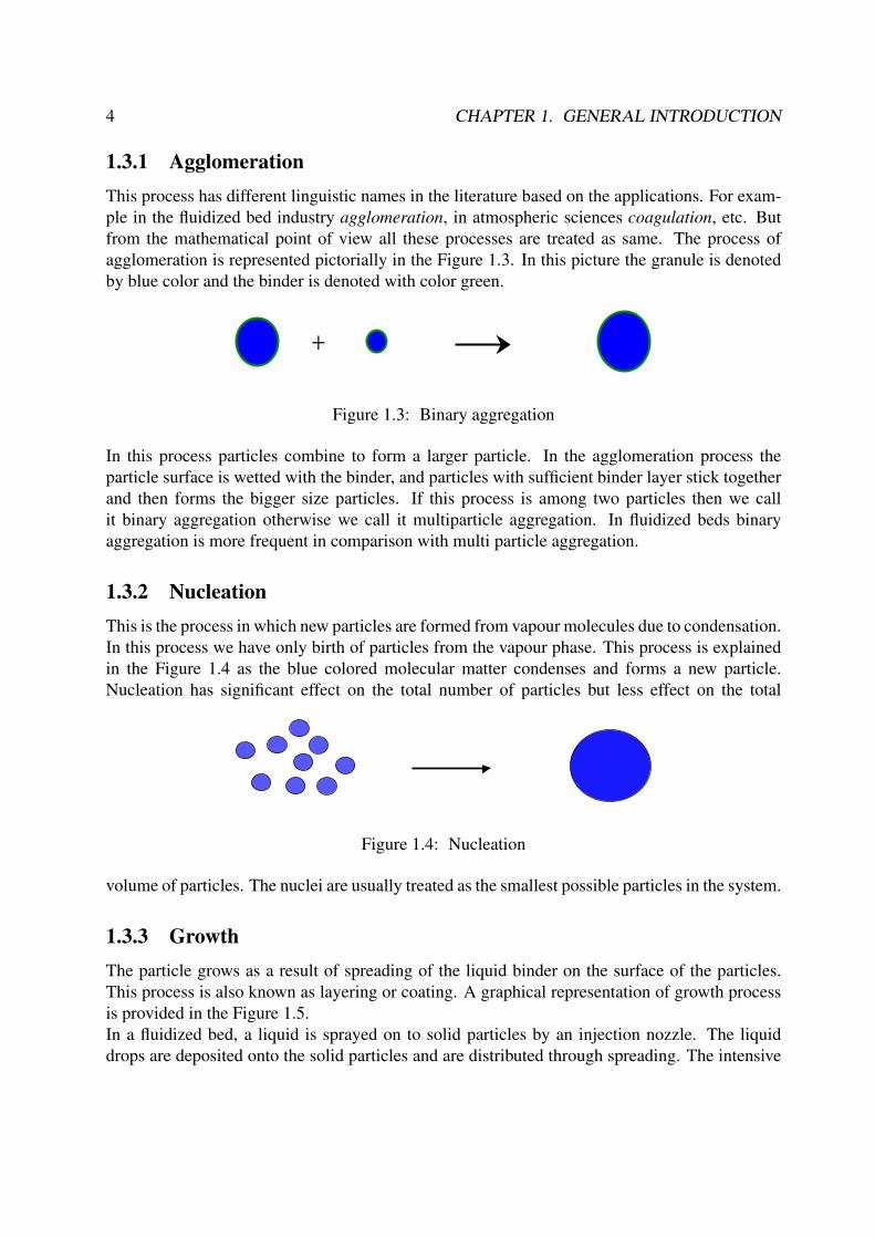
1.3.1 AgglomerationThis process has different linguistic names in the literature based on the applications. For exam-ple in the fluidized bed industry agglomeration, in atmospheric sciences coagulation, etc. Butfrom the mathematical point of view all these processes are treated as same. The process ofagglomeration is represented pictorially in the Figure 1.3. In this picture the granule is denotedby blue color and the binder is denoted with color green.
+
Figure 1.3: Binary aggregation
In this process particles combine to form a larger particle. In the agglomeration process theparticle surface is wetted with the binder, and particles with sufficient binder layer stick togetherand then forms the bigger size particles. If this process is among two particles then we callit binary aggregation otherwise we call it multiparticle aggregation. In fluidized beds binaryaggregation is more frequent in comparison with multi particle aggregation.
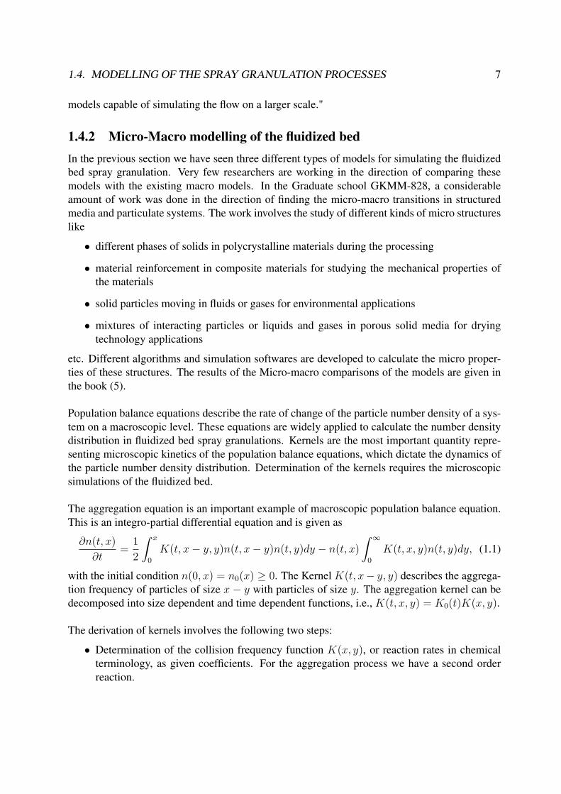
1.3.2 NucleationThis is the process in which new particles are formed from vapour molecules due to condensation.In this process we have only birth of particles from the vapour phase. This process is explainedin the Figure 1.4 as the blue colored molecular matter condenses and forms a new particle.Nucleation has significant effect on the total number of particles but less effect on the total
Figure 1.4: Nucleation
volume of particles. The nuclei are usually treated as the smallest possible particles in the system.
1.3.3 GrowthThe particle grows as a result of spreading of the liquid binder on the surface of the particles.This process is also known as layering or coating. A graphical representation of growth processis provided in the Figure 1.5.In a fluidized bed, a liquid is sprayed on to solid particles by an injection nozzle. The liquiddrops are deposited onto the solid particles and are distributed through spreading. The intensive

1.4. MODELLING OF THE SPRAY GRANULATION PROCESSES 5
+
Figure 1.5: Growth
heat and mass transfer, due to the supply of the hot gas, results in a rapid increase of hardness ofthe fluid film through drying. In this growth process the number of particles does not change butthe total volume of particles increases.
1.4 Modelling of the spray granulation processesParticle size distributions give one of the most important descriptions of the granulation process.Macroscopic models like Population Balance Models are widely used to evolve the particle sizedistribution in granulation processes. The use of population balance modelling was hamperedby the kinetic parameters like kernels have proven more difficult to predict PSD and are verysensitive to operating conditions and material properties. Therefore to model the effect of theseparameters a microscopic model involving the particle collision mechanism, material properties,etc. needs to be developed.
1.4.1 Multi scale modelling of fluidized beds
Chemical engineering uses mathematical models to simulate different processes like polymer-ization, granulation, etc. The development of granulation processes via drum, pan or fluidizedbed granulation is a multiscale operation, where the typical macro analysis of continuum mecha-nisms must be connected to micro operations. A review of systems modelling and applications ingranulation are explained in (7). Enormous increase in computer power and algorithm develop-ment, fundamental modelling of granulation process in a fluidized bed has come recently withinreach. In last decade a significant research efforts have been made to develop detailed microbalance models to study the complex hydrodynamics of gas-fluidized beds. Broadly speakingtwo different types of hydrodynamic models can be distinguished, Eulerian (continuum) modelsand Lagrangian (discrete element) models.Hoomans (20, p.14) states that, "In order to model a large (industrial) scale fluidized bed a contin-uum model, where the gas phase and the solids phase are regarded as interpenetrating continuousmedia, is the appropriate choice. This Eulerian-Eulerian type of model have been developed andsuccessfully applied over the last two decades . . . ." These models require closure relations forthe solids phase stress tensor and the fluid-particle drag relation. Improved empirical closurerelations for the solids phase stress tensor and fluid-particle drag coefficient can be obtained byusing kinetic theory of granular flow and lattice Boltzmann simulations (3) respectively.
"In discrete particle models the Newtonian equations of motion are solved for each individual

6 CHAPTER 1. GENERAL INTRODUCTION
Lattice Boltzmann models
Discrete particle models
Continuum modelsLarge (industrial) scale
simulations
Particle−particle interactions
Fluid particle interaction
Figure 1.6: Multi scale modelling of the spray granulation process
solid particle in the system. In this Eulerian-Lagrangian type of model a closure relation for thesolids phase rheology is no longer required since the motion of the individual particles is solveddirectly. However, the number of particles that can be taken into account in this technique islimited (< 10−6[sic]< 106). Therefore, it is not yet possible, even with modern day super com-puters, to simulate a large (industrial) scale system (20, p.14)." Despite this the discrete particlemodel is useful in understanding the influence of particle properties on the hydrodynamics ofgas-fluidized beds and particle-particle collisions in a microscopic level.
According to Hoomans (20, p.15), "When the gas flow is resolved on a length scale smaller thanthe particle size these closure relations for fluid-particle drag are no longer required. Instead theycan actually be obtained from the simulations. The Lattice Boltzmann technique seems to be bestsuited for such simulations because it is very flexible in dealing with complex flow geometries. . . . It is important to realise that these Lattice Boltzmann simulations are limited to systems con-sisting of a number of particles that is significantly smaller (< 10−3[sic]< 103) than the numberof particles that can be taken into account using discrete particle models (< 10−6[sic]< 106).
In short the multi-scale concept as presented in [Figure 1.6] consists of three classes of modelswhere more detail of the two-phase flow is resolved going from continuum models to discreteparticle models to Lattice Boltzmann models. This goes at the cost of increased computationalrequirements which necessitates a size reduction of the simulated system. The model capableof simulating a larger system is fed with a closure relation obtained from a more microscopicsimulation. In return the results of these simulations can be used to pass on information to
1.4. MODELLING OF THE SPRAY GRANULATION PROCESSES 7
models capable of simulating the flow on a larger scale."
1.4.2 Micro-Macro modelling of the fluidized bedIn the previous section we have seen three different types of models for simulating the fluidizedbed spray granulation. Very few researchers are working in the direction of comparing thesemodels with the existing macro models. In the Graduate school GKMM-828, a considerableamount of work was done in the direction of finding the micro-macro transitions in structuredmedia and particulate systems. The work involves the study of different kinds of micro structureslike
• different phases of solids in polycrystalline materials during the processing
• material reinforcement in composite materials for studying the mechanical properties ofthe materials
• solid particles moving in fluids or gases for environmental applications
• mixtures of interacting particles or liquids and gases in porous solid media for dryingtechnology applications
etc. Different algorithms and simulation softwares are developed to calculate the micro proper-ties of these structures. The results of the Micro-macro comparisons of the models are given inthe book (5).
Population balance equations describe the rate of change of the particle number density of a sys-tem on a macroscopic level. These equations are widely applied to calculate the number densitydistribution in fluidized bed spray granulations. Kernels are the most important quantity repre-senting microscopic kinetics of the population balance equations, which dictate the dynamics ofthe particle number density distribution. Determination of the kernels requires the microscopicsimulations of the fluidized bed.
The aggregation equation is an important example of macroscopic population balance equation.This is an integro-partial differential equation and is given as
∂n(t, x)
∂t=
1
2
∫ x
0
K(t, x− y, y)n(t, x− y)n(t, y)dy − n(t, x)
∫ ∞
0
K(t, x, y)n(t, y)dy, (1.1)
with the initial condition n(0, x) = n0(x) ≥ 0. The Kernel K(t, x− y, y) describes the aggrega-tion frequency of particles of size x − y with particles of size y. The aggregation kernel can bedecomposed into size dependent and time dependent functions, i.e., K(t, x, y) = K0(t)K(x, y).
The derivation of kernels involves the following two steps:
• Determination of the collision frequency function K(x, y), or reaction rates in chemicalterminology, as given coefficients. For the aggregation process we have a second orderreaction.
8 CHAPTER 1. GENERAL INTRODUCTION
• Make some physical assumptions on the interaction mechanism of the particles to calculatean explicit expression for the aggregation efficiency function K0(t).
The calculations of the kernels were evolved from two different approaches. 1. Calculationwith realistic experimental results. 2. Computer simulation of the experiements with simplemathematical models. For the last two decades few advances were made in the direction of de-termination of the kernels using computer simulations.
Recently Tan et al. (51) have made an attempt to build a population balance model for fluidizedbed melt granulation from the kinetic theory of granular flow (KTGF). They showed that thedistribution of particle velocities obtained from Discrete Particle Modelling (DPM) are same asthose obtained from the kinetic theory of granular flow. With this result he assumed that an EquiKinetic Energy (EKE) kernel will be a suitable choice. He compared the particle size distribu-tions obtained from the experiments and Discretized Population Balance (DPB) modelling withEKE kernel.A comparison of the experimental results and the simulated results of Discretized PopulationBalance (DPB) equations with EKE kernel are given in (51) for aggregation process.
1.5 Outline of the thesisThis thesis starts with an introduction to the population balance equations in Chapter 2. In Sec-tion 2.2 we explain the assumptions and properties of the discrete and continuous forms of theaggregation equation. Section 2.3 involves the dimensional analysis of these equations and theirimportance in the modelling of the the aggregation kernels and number density selection forvarious applications. Different aggregation kernels exist in the literature based on theoreticalderivation for the physical process, empirical the observations of the experiments and from theanalysis of the experimental data. Properties of the some of these kernels are explained in theSection 2.4.
Chapter 3 is concerned with the Discrete Particle Model (DPM), which is a two phase flowmodel. We give a short introduction to the model in Section 3.1. Section 3.2, 3.3 explain thegoverning equations describing solid particle phase and gas phase respectively. The closure lawscoupling these phases are described in Section 3.4 and Section 3.4.1 explains the hard spherecollision model for the solid particle interactions. We end this chapter with explanations of thenumerical calculations and the modifications made to the existing code for calculating the colli-sion frequency function.
Modeling of the kernels is explained in Chapter 4. The introductory Section 4.1 explains therecently existing literature for modeling of kernels. Section 4.2 explains the derivation of thecollision frequency functions. A correction to the aggregation equations and its effect on theaggregation equation is explained in Section 4.3. The last Section 4.4 is concerned with thephysical description of the flow pattern inside fluidized beds based on particle Reynolds number.

1.5. OUTLINE OF THE THESIS 9
The particle Reynolds number shows that the shear forces are dominating. This gives an indica-tion for use of the shear kernel.
Simulation results for modeling collision frequency functions are given in Chapter 5. Section5.1.1 explains the various initial parameters and assumptions for the computer simulations. Sec-tion 5.1.2 gives the various particle size distributions. In Section 5.2 we explain the evaluationof the bed parameter. Simulation results for a pseudo 3D bed are given in Section 5.3 and aspecial case of particle size distribution (normal distribution) results are given in Section 5.3.1.Simulation results for a 3D bed are given in Section 5.4. We end this chapter with the discussionof the results in Section 5.5.
Chapter 6 involves the crucial part of the thesis involving a micro-macro comparison. In Section6.1 we explain the assumptions on the simulations for the evaluation of the aggregation efficiency.In Section 6.2, we calculated the aggregation efficiency function from the discrete particle modelsimulations for pseudo 3d and 3d fluidized beds. Section 6.3 explains the numerical methods forsolving the population balance equations, in particular the cell average technique. Computationof the particle size distributions with the newly derived, simulation based kernels are given inSection 6.4.
Chapter 7 gives the general conclusions and outlook of the present thesis.
In Appendix A we explain the analytical derivation of the shear kernel based on geometry. Ap-pendix B explains the major simulation parameters of the Discrete Particle Model (DPM). Ap-pendix C gives the initial particle size distributions for different number of particles.

Chapter 2
Population Balance Equations
In this chapter we describe population balance equations for particulate systems. We describevarious forms of the aggregation equation and its mathematical properties. This chapter gives adeep insight into the modelling aspects of the aggregation kernel. We end up this chapter withthe some important properties of theoretical, phenomenalogical and experimental kernels whichare widely used in the applications.
2.1 IntroductionPopulation balance equations are used to determine the particle number density distribution ona macroscopic level. A general one particle property, e.g. particle volume, equation for a wellmixed system is given by the following
∂n(t, x)
∂t+
∂[G(t, x)n(t, x)]
∂x= F (t, x) (2.1)
where
F = Bnucleation(t, x) + Bagg(t, x) + Bbreak(t, x)−Dagg(t, x)−Dbreak(t, x). (2.2)
The above equation describes the change of particle size distribution n(t, x) with respect to timet ≥ 0 corresponding to the particle property, volume x ≥ 0. The second term on left hand sideof the Equation (2.1) represents the particle growth due to the addition of liquid binder to theparticles and G(t, x) = dx
dt. The first three terms on the right hand side of (2.2) represent the
birth of particles due to nucleation, aggregation and breakage. The last two terms on the righthand side of (2.2) represent the death of particles due to aggregation and breakage. The initialand boundary conditions required for (2.1) are generally stated as
n(0, x) = n0(x)
and
n(t, 0) = 0,
respectively. The latter condition indicates that there are no particles of zero size, which isphysically well justified.
10
2.2. AGGREGATION EQUATION 11
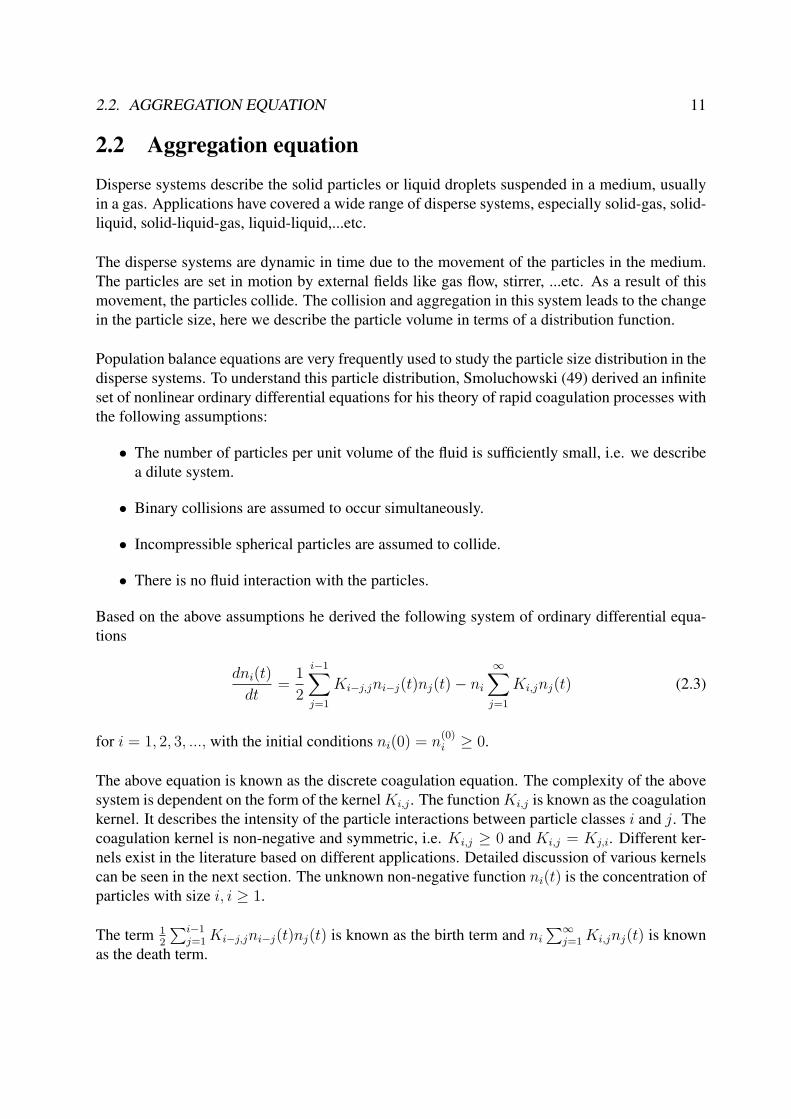
2.2 Aggregation equationDisperse systems describe the solid particles or liquid droplets suspended in a medium, usuallyin a gas. Applications have covered a wide range of disperse systems, especially solid-gas, solid-liquid, solid-liquid-gas, liquid-liquid,...etc.
The disperse systems are dynamic in time due to the movement of the particles in the medium.The particles are set in motion by external fields like gas flow, stirrer, ...etc. As a result of thismovement, the particles collide. The collision and aggregation in this system leads to the changein the particle size, here we describe the particle volume in terms of a distribution function.
Population balance equations are very frequently used to study the particle size distribution in thedisperse systems. To understand this particle distribution, Smoluchowski (49) derived an infiniteset of nonlinear ordinary differential equations for his theory of rapid coagulation processes withthe following assumptions:
• The number of particles per unit volume of the fluid is sufficiently small, i.e. we describea dilute system.
• Binary collisions are assumed to occur simultaneously.
• Incompressible spherical particles are assumed to collide.
• There is no fluid interaction with the particles.
Based on the above assumptions he derived the following system of ordinary differential equa-tions
dni(t)
dt=
1
2
i−1∑j=1
Ki−j,jni−j(t)nj(t)− ni
∞∑j=1
Ki,jnj(t) (2.3)
for i = 1, 2, 3, ..., with the initial conditions ni(0) = n(0)i ≥ 0.
The above equation is known as the discrete coagulation equation. The complexity of the abovesystem is dependent on the form of the kernel Ki,j . The function Ki,j is known as the coagulationkernel. It describes the intensity of the particle interactions between particle classes i and j. Thecoagulation kernel is non-negative and symmetric, i.e. Ki,j ≥ 0 and Ki,j = Kj,i. Different ker-nels exist in the literature based on different applications. Detailed discussion of various kernelscan be seen in the next section. The unknown non-negative function ni(t) is the concentration ofparticles with size i, i ≥ 1.
The term 12
∑i−1j=1 Ki−j,jni−j(t)nj(t) is known as the birth term and ni
∑∞j=1 Ki,jnj(t) is known
as the death term.
12 CHAPTER 2. POPULATION BALANCE EQUATIONS
2.2.1 Continuous form of the aggregation equation
Müller (36) derived the continuous form for the above equation as an integro partial differentialequation that is given as
∂n(t, x)
∂t=
1
2
∫ x
0
K(t, x− y, y)n(t, x− y)n(t, y)dy − n(t, x)
∫ ∞
0
K(t, x, y)n(t, y)dy, (2.4)
with the initial condition n(0, x) = n0(x) ≥ 0.The Kernel K(t, x − y, y) describes the coagulation of particles of size x − y with particles ofsize y. The first term on the right hand side of (2.4) describes birth of the particles. The secondterm on the right hand side of the equation (2.4) describes the death of the particles.
Mathematical classification
Mathematically the integral operators of (2.4) are classified as follows
• The birth term of the coagulation equation (2.4) is a nonlinear Volterra integral operator,
• The death term of the coagulation equation (2.4) is a quasilinear Fredholm integral opera-tor.
Remark 2.1 One should note that in the discrete as well as in the continuous case the time t isalways a continuous coordinate. The difference is in the property coordinate x (volume or mass)only.
Moments of the aggregation equation
The moments of the aggregation equation play a vital role in characterizing the properties of theparticle distribution. The jth moment of the particle size distribution n(t, x) of the aggregationequation (2.4) is defined as
µj =
∫ ∞
0
xjn(t, x)dx. (2.5)
The moments represent some important properties of the distribution. The zeroth (j = 0) andfirst (j = 1) moments are proportional to the total number and the total mass of particles respec-tively. In addition to the first two moments, the second moment of the distribution will be usedto compare numerical results, see (30). The second moment is proportional to the light scatteredby particles in the Rayleigh limit (18) and is used in atmospheric sciences for study of the raindrop coagulation process.

2.3. SCALING OF THE EQUATIONS 13
2.3 Scaling of the equationsFor analysis of a particle system one needs to evaluate the change in the population of particlesin the dispersed phase. It involves both, a local and a global environment. The local environmentinvolves the particle properties like diameter, volume, mass, ...etc. These are the state variables.The global environment consists of the space variables.
Usually for particulate systems one considers the influence of the local properties, and the effectof the global environment is neglected with the assumption of a homogenized medium. But whenwe do modelling one needs to consider the global environment, in order to understand whetherthe system is a homogenized or not. To understand the particle interactions, we need to considerthe physical description of the system. For this purpose we need to do dimensional analysis.
Dimensional analysis is applied in order to remove the influence of the arbitrary choice of phys-ical units for the systems. In the dimensionless form we can determine the influence of large andsmall terms in the system in order to simplify it.To discuss the concepts of dimensional analysis, we need the following definitions:
• We define the mass M of a representative particle by using the unit kg = kilogram.
• We define the volume for two physical quantities:
1. Volume of fluid as Vfluid and has the dimension length L3 for notational purpose wewrite it as Lfluid, which is an external parameter corresponding to the space coordi-nate with unit L = m.
2. Volume of particles as Vparticles and has the dimension length L3 for notational pur-pose we write it as Lparticles, which is an internal parameter corresponding to theparticle property with unit L = m.
• We define time as T with unit T = s.
Remark 2.2 Here we wish to give a note on particle number density n(t, x). The populationis described with the use of suitable external or internal or both the variables, usually numberof particles, sometimes with other variables such as mass (extensively used in crystalizationprocess), length (suitable to describe growth process) or volume of particles.
2.3.1 Dimensional analysis for discrete equation• Particle concentration ni(t) is defined as the number of particles per unit volume of the
fluid and has the dimension L−3fluid
• The coagulation kernel Ki,j is defined as the number of particle interactions in unit volumeof fluid per unit time and has the dimension L3
fluidT−1

14 CHAPTER 2. POPULATION BALANCE EQUATIONS
2.3.2 Dimensional analysis of the continuous equationCase 1:
• The particle concentration n(t, x) is defined as the number of particles per unit volume offluid per unit particle volume and has the dimension L−3
fluidL−3particle
• Dimension of the kernel K(t, x, y) is L3fluidT
−1
Case 2:
• Suppose that for the continuous equation we have dimension of n(t, x) as number of par-ticles per unit volume of particles. That is we are considering the number density as afunction of time and material volume with the dimension L−3
particle.
• Dimension of the kernel K(t, x, y) is T−1. This is usually called a collision frequencykernel in the literature.
2.3.3 Number density selection and dimensional analysis of the kernel inapplications
When we are trying to use this aggregation equation for a particulate process, the above dimen-sional analysis can be used as follows:
In the study of aerosol sciences the particle volume is not effective compared to the volume ofthe air. So in such models the discrete kernel is widely used by considering the number density asa function of fluid and time. In this case the discrete kernel K(t, x, y) has the dimension L3
airT−1.
In a fluidized bed the volume of the bed is not constant. Therefore the porosity of the bed changeswith the time. So in such situations it is necessary to consider both, the volume of fluid and vol-ume of the particles in the calculation of particle concentration. Since the porosity is not constantin our DPM, we consider the case 1 and the kernel has the dimension L3
fluidT−1.
As we stated earlier, the number density can be a function of any material coordinate. In certainapplications the mass of the particles is important compared to volume of the particles.
In crystalization processes, particles are formed as a result of change in the thermodynamics ofthe material. So in such processes the number density solely depends on the amount of materialpresent in the vessel. Therefore we can replace the number density as a function of material andtime, and having the dimension M−1L−3. In this case the aggregation kernel has the dimensionof ML3T−1. Here L3 represents the volume of the vessel.
In case of evaluating the numerical solution of the population balance equations with growth,breakage, aggregation and nucleation terms, the number density plays a vital role. One needs
2.4. PROPERTIES OF AGGLOMERATION KERNELS 15
to pay considerable attention to descritizing the equation satisfying the number and mass con-servation properties. A detailed discussion of numerical problems for various number densityrepresentations arising in crystallization modeling can be found in Costa et al. (9).
2.4 Properties of agglomeration kernelsPopulation balance equations are applied to determine the particle number density distribution ina macroscopic level. A binary agglomeration equation for a well mixed system is given as
∂n(t, x)
∂t=
1
2
∫ x
0
K(t, x− y, y)n(t, x− y)n(t, y)dy − n(t, x)
∫ ∞
0
K(t, x, y)n(t, y)dy, (2.6)
and n(0, x) = n0(x) ≥ 0, where K(t, x, y) is the agglomeration kernel. The equation (2.6)describes the number density distribution as a function of one particle property and time. Inorder to understand the agglomeration process, one needs to explore the physical significanceand mathematical nature of the agglomeration kernel. Up to now there is no proper kernel todescribe the particle size distribution for fluidized bed granulation. In the current section we areexploring the properties of different existing kernels and their usage.The agglomeration kernel K(t, x, y) represents the rate at which particles of volume x − y andy aggregating to form particle of volume x. The complexity of solving the equation depends onthe form of the kernel K(t, x, y) and it satisfies the following properties
• The kernel is symmeric i.e., K(t, x, y) = K(t, y, x)
• non-negative K(t, x, y) ≥ 0 for all x, y > 0
• The kernel is a continuous function on (0,∞)× (0,∞)
• Most kernels are homogeneous functions of non-negative degree
• By scaling time, we can eliminate a multiplicative constant from the kernel, e.g. K(x, y) =xy instead of K(x, y) = cxy for constant c
Sastry (46) proposed that the aggregation kernel is a product of two factors, and it is now commonpractice to view the aggregation kernel as the product of agglomeration efficiency K0(t) andcollision frequency K(x, y), i.e.
K(t, x, y) = K0(t)K(x, y). (2.7)
The discrete variant of the agglomeration kernel Ki,j among the classes i and j is defined asto the product of the collision frequency Ki,j of the particles and the agglomeration efficiencyK0(t) i.e.,
Ki,j(t) = K0(t)Ki,j.
16 CHAPTER 2. POPULATION BALANCE EQUATIONS
The first term, K0(t), is the efficiency rate constant, which is dependent on various processparamters like kinetic energies of particles, their trajectories and collision orientation, particlecharacteristics (e.g. mechanical properties and surface structure), viscous dissipation betweenapproaching particles and inter-particle forces, and binder properties, coalscence mechanism,...etc. Generally K0(t) is assumed to be remain constant throughout the experiment and is size-independent.
The collision frequecy K(x, y) or Ki,j is a function of particles size, gas velocity, system tem-perature,...etc. Most of the models assume that the collision frequency is a function of particlesize. Determination of collision frequency function is a complex task in most of the models andit is very difficult to determine from the experiments. In the present thesis we try to fix a sizedependent collision frequency function through the simulations.
As we have seen in the previous paragraphs that the agglomeration kernel can be resolved asproduct of time dependent and internal variable (length, volume, mass, ... etc) dependent com-ponents. The time dependent component is a function of the agglomeration process, where as theinternal variable dependent component is a function of transportation process. In the fluidizedbed the the transportant of particles is due to gas flow. Therefore this function is determined byflow of the gas inside the bed. Based on this flow mechanism of gas we have different kernels.In the next subsections we are giving a detailed account of various kernels used for fluidized bedgranulation.
We have different collision frequency functions for different kernels in the literature based ontheoritical, empirical and experimental calculations and observations. The Table 2.1 below givesan account of different collision frequency functions.
2.4.1 Theoretical kernels
We have very few kernels in the literature that are derived theoretically, and these kernels aredetermined based on the mechanism producing relative motion of the particles. In the followingsections we gives a brief discussion on the derivation of the theoritical kernels and their physicalsignificance.
Brownian kernel
Collisions among the particles of size larger than the mean free path of the gas are diffusionlimited. Smoluchowski derived an expression for the collisions of the spherical particles withvolume x
13 and y
13 suspended in an infinite medium (gas) in 1917 (49). During this derivation he
assumed that the particle motion is random, diffusive. The collision frequency function is givenas
K(x, y) = 4π(Dx + Dy)(x13 + y
13 ) (2.8)

2.4. PROPERTIES OF AGGLOMERATION KERNELS 17
Nam
eof
the
kern
elK
erne
lK(x
,y)
Com
men
tPh
ysic
alap
plic
atio
nSi
ze-i
ndep
ende
ntc
(26)
All
even
tseq
ually
prob
able
Dro
plet
coal
esce
nce
Bro
wni
anm
otio
nK
0(x
+y)(
x−
1+
y−
1)(
49)
Ran
dom
mov
emen
tofp
artic
les
Aer
osol
sPr
oduc
tK
0(x
y)
larg
e-la
rge,
smal
l-sm
all
Poly
mer
sG
ravi
tatio
nK
0(x
+y)2|x−
y|(4
)G
ravi
tatio
nalf
orce
isdo
min
ant
Aer
osol
sSh
ears
tres
sK
0(x
+y)3
(49)
Lar
ge-l
arge
even
tsfa
vore
dFl
uidi
zed
bed
Part
icle
iner
tiaK
0(x
+y)2|x
2−
y2|(2
6)In
ertia
lfor
ces
are
dom
inan
tA
eros
ols
EK
KK
0(x
+y)2
√ 1 x3
+1 y3(2
2)L
arge
-sm
alle
vent
sfa
vore
dG
ranu
latio
n
Kap
urK
0((x
+y)a
(xy)b
)(2
7)Ph
enom
enol
ogic
alG
ranu
latio
nSa
stry
K0(x
2/3y
2/3)(
1/x
+1/
y)(
46)
Phen
omen
olog
ical
Gra
nula
tion
Poly
mer
isat
ion
K0(x
1/3+
c)(y
1/3+
c)Po
lym
ers
Bra
nche
dpo
lym
ers
Ade
tayo
and
Enn
isk(c
onst
ant)
,if
W<
W∗
0,
ifW
>W
∗(1
)cu
toff
kern
elFl
uidi
zed
bed
Tabl
e2.
1:A
sum
mar
yof
prop
osed
kern
els
inth
elit
erat
ure
a whe
rea,
b,c,
K0
are
cons
tant
sb w
here
W∗
isth
ecr
itica
lvol
ume
ofth
epa
rtic
le

18 CHAPTER 2. POPULATION BALANCE EQUATIONS
where Dx, Dy are the diffusion constants for the particle classes of volumes x13 and y
13 . If the
Stokes-Einstein relation holds for the diffusion coefficient, then this expression becomes
K(x, y) =2kT
3µ(x
13 + y
13 )(x−
13 + y−
13 ) (2.9)
where k is the Boltzmann constant, T the absolute temperature, µ the viscosity of the medium.The Stokes-Einstein relation for the classes i and j is given as
DijRij = D1r1
(1
ri
+1
rj
)(ri + rj)
The collision surface among 10 classes of particles for the Brownian kernel is plotted in thefigure below. In this figure we can observe the large number of collisions among the large-smallsize classes and the lower number of collisions among large-large classes.
05
1015
2025
30
0
10
20
303.5
4
4.5
5
5.5
xi
Brownian kernel
xj
Ki,j
Remark 2.3 The Brownian kernel corresponds to disperse systems in an open domain, e.g., atypical aerosol: colloidal sol, liquid droplets, or air bubbles suspended in an agitated liquid.In a fluidized bed the particle motion is induced by the gas flow rather than random, diffusivemotion. Therefore the Brownian kernel will not be a suitable choice.
Remark 2.4 For monodisperse systems i.e., by setting x = y, the collision frequency is given by
K(x, x) =8kT
3µ= c, (2.10)
where c is a constant independent of particle size.

2.4. PROPERTIES OF AGGLOMERATION KERNELS 19
Shear kernel
Smoluchowski (49) derived the shear kernel while modelling the discrete aggregation equation.He derived the shear kernel in terms of geometrical property, volume with the following assump-tions
• Particles are spherical in shape
• Particles move in rectilinear paths
• There is no fluid interaction with the particles
• Particles move due to their shear motion
• Brownian motion does not exists in the system
The collision frequency function for shear motion is given as (49)
K(x, y) =4
3Γ(x
13 + y
13 )3, (2.11)
where Γ is the laminar shear velocity of the gas. The derivation of this kernel is explained inAppendix A.The collision surface among 10 classes of particles for the shear kernel is plotted in the figurebelow. In this figure we can observe that large number of collisions among the large-large sizeclasses and less number of collisions among small-small classes.
010
2030
0
10
20
300
100
200
300
xi
Shear kernel
xj
Ki,j
Remark 2.5 This kernel is widely used in fluidized beds and granulators to model the populationbalance equations. In the fluidized beds the particles move due to the gas flow. In the granulators,the particle mixing is due to impeller. These two mechanisms cause the laminar shear flow asopposed to the random fluctuations.
20 CHAPTER 2. POPULATION BALANCE EQUATIONS
Remark 2.6 This shear kernel is derived based on geometric approximations of particle paths.So this kernel is not exact, but it is an upper bound.
Equipartition of kinetic energy kernel
This kernel is based on the assumption that the kinetic theory of granular flow (KTGF) providesan acceptable description of granular flow in a high shear mixer. Hounslow (22) derived anagglomeration kernel based on the following assumptions:
• The kinetic theory of granular flow is an extension of the classical kinetic theory of densegases.
• The particles are assumed to be spherical, smooth and elastic.
• In a high shear mixer the granules adopt significant rotational velocities they also displaynoticeable deviations from the local average velocity.
• Each individual particle velocity v is decomposed into a local mean velocity u and a ran-dom fluctuating velocity V described by v = u + V .
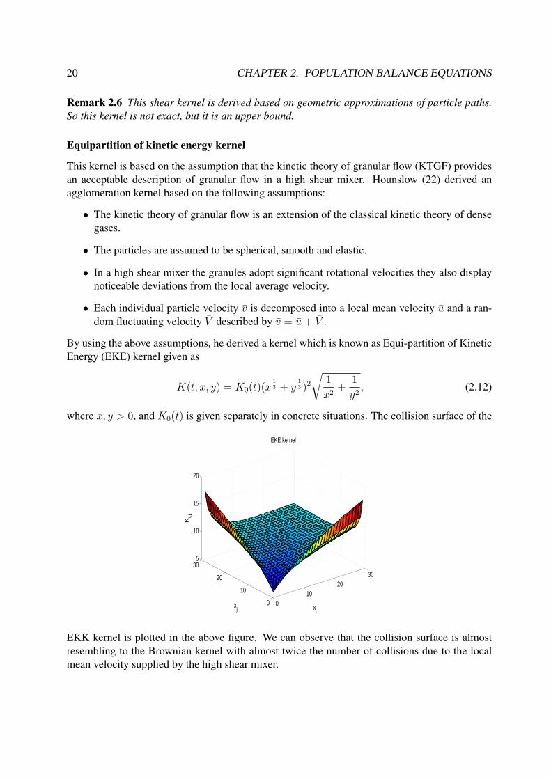
By using the above assumptions, he derived a kernel which is known as Equi-partition of KineticEnergy (EKE) kernel given as
K(t, x, y) = K0(t)(x13 + y
13 )2
√1
x2+
1
y2, (2.12)
where x, y > 0, and K0(t) is given separately in concrete situations. The collision surface of the
010
2030
0
10
20
305
10
15
20
xi
EKE kernel
xj
Ki,j
EKK kernel is plotted in the above figure. We can observe that the collision surface is almostresembling to the Brownian kernel with almost twice the number of collisions due to the localmean velocity supplied by the high shear mixer.

2.4. PROPERTIES OF AGGLOMERATION KERNELS 21
Remark 2.7 Kinetic theory assumes that all collisions are binary and instantaneous. In denseflows which are commonly found in high shear mixers, this assumption may not be valid.
Remark 2.8 This kernel is widely used in crystallization processes. Here the crystals are formedas a result of stirrer movement and thermodynamic forces which cause the random deviations tothe local velocity caused by the stirrer rotations.
2.4.2 Empirical kernelsBased on intuitive arguments, some of the requirements to be satisfied by the aggregation kernelscan be specified. Most of the empirical kernels are determined based on these arguments. Butmost of the time the validity of the kernels are questioned due to lack of their physical relevanceto the experimental results. Several empirical functional forms of the kernels were fitted to theexperimental data i.e., empirical kernels are not unique. In spite of all these difficulties, theywere widely used in the literature, because explicit solutions are available, and the mathematicalproperties of the aggregation equation are easily explored.
Size independent or constant kernel
This most simple kernel available in the literature was proposed by Kapur and Fuerstenau (26).In this kernel it is assumed that the particle interactions are random with no higher probabilityfor agglomeration between any two preferred sizes. That means the kernel is constant throughoutthe experiment, which is very far from the real fluidized bed granulation. But the simplicity ofthe kernel gives the advantage of having an exact solution to the aggregation equation and is usedas a test case in evaluating the efficiency and accuracy of the numerical schemes applied to thepopulation balance equations.
010
2030
0
10
20
301
1.5
2
2.5
3
Ki,j
Constant kernel
xi
xj
The collision frequency surface among the classes i and j can be seen in the above figure for theconstant kernel K(t, x, y) = 2.

22 CHAPTER 2. POPULATION BALANCE EQUATIONS
Remark 2.9 The continuous models with this kernel have the following limitations:
• It provides no information on the higher moments of the size distribution.
• The models tends to break down for powders of comparatively large specific surface area.
Kapur kernel
Kapur and Fuerstenau(28) proposed a population balance equation for nonrandom aggregationof discrete size granules. This equation differs from Smoluchowski’s well known aggregationequation, where the aggregation rate is proportional to the product of number concentrations ofthe two reacting species.
On the other hand, for a given size distribution the concentration of particles in a loosely packedgranulating bed is more or less fixed by the packing contraints. Indeed, to a first approximationthe packing characteristics (bed porosity and coordination number) are not expected to changeappreciably in course of granulation. In this situation, an agglomerate is most likely to encounteronly its nearest neighbours which form a cage around it. Consequently, the aggregation in granu-lation was stipulated in terms of the product of the number of species of one kind with the numberfraction of the second kind. This kind of aggregation process is also known as pseudo-first-orderrate process.
They proposed the following population balance equation for a batch, restricted-in-space, gran-ulation system as
dni(t)
dt= −λ(t)ni(t)
N(t)
∞∑j=1
nj(t) +λ(t)
2N(t)
i−1∑j=1
ni(t)ni−j(t) (2.13)
where ni(t) = Ni(t)Vbed
is the number of granules of size xi by volume Vbed at time t, N(t) =∑Ii=1 Ni is the total number of granules in the batch, and λ(t) is the specific aggregation rate
function. Here one should remember that λ(t) is not the same as K(t, x, y).
Kapur (27) proposed a phenomenological kernel based on an empirical rate function which, incontinuous sample space, is given by
λ(t) = β0(x + y)a
(xy)b(2.14)
where β0 is a function of water content, particle size distribution and surface area of the powder,nature of the balling device, etc. It does not depend on the granulate size. The other term reflectsthe non-random nature of the mechanism governing the process. The adjustable parameters aand b as well as β0 should provide sufficient flexibility for a realistic equivalent mathematicalrepresentation of the kinetics.

2.4. PROPERTIES OF AGGLOMERATION KERNELS 23
Remark 2.10 • Although the kernel (2.14) gives satisfactory results when compared withexperimental data, it is only an empirical one.
• This kernel did not give any physical insight into the granulation mechanism except for thenon-random nature.
Remark 2.11 Some of the moments of the similarity function may turn out to be physicallymeaningless as reported by Wang, and Kapur (27). This is due to the presence of the singularitiesat x = 0 and x = ∞.
Sastry kernel
Sastry (46) proposed an empirical kernel for nonrandom aggregation based on experimental ob-servations and intutive arguments. He considered that the driving force or potential for aggrega-tion is determined by the surfaces, and that resistance for further deformation is offered by thevolumes of the participating species. Thus, the larger the surface area of an agglomerate is, themore potential it has to grow, while at the same time it offers more resistance. Based on theseideas, the following functional form that satisfies most of the above described criteria is chosen:
K(t, s, s′, x, y) = K0(t)(s + s′)
(1
x+
1
y
)(2.15)
where s, s′ and x, y are the surface area and volume of the particles respectively. Given ρ, theapparent agglomerate density, the above equation becomes
K(t,m,m′) = K0(t)(36πρ)13 (m2/3 + m′2/3)
(1
m+
1
m′
). (2.16)
Therefore
K(m, m′) = (m2/3 + m′2/3)
(1
m+
1
m′
). (2.17)
The above kernel can be written interms of volume as
K(x, y) =(x
23 + y
23
) (1
x+
1
y
)(2.18)
Remark 2.12 The empirical kernel K(x, y) is a homogeneous function and has degree or order(−1/3). The order of the kernel has a major effect on the shape and evolution of particle sizedistribution. In general, the higher the kernel order, the broader the particle size distributionthat results.
24 CHAPTER 2. POPULATION BALANCE EQUATIONS
2.4.3 Experimental kernelsTwo approaches are widely used to extract the parameters of the agglomeration kernels from theexperimental data. Those two are the integral and differential approaches. In this section we aredescribing these two approaches for evaluating the parameters of the aggregation kernels.
In Chapter 2.4 we have neglected the time dependency of the kernels, but in a more generalapproach one can supply an additional time dependent factor K0(t) and write it as
K(t, x, y) = K0(t)K(x, y).
Therefore modeling of the agglomeration kernel involves these two functions. Frequently anintegral approach is used to determine aggregation rates, in which a kinetic model, containing anumber of adjustable parameters, is fitted to an integral form of the rate equations. For a givenvalues of the parameters the experimental data may be simulated by integrating a combinationof the rate and kinetic equations. The parameters are usually selected to optimize the fit of thesimulated results to those obtained experimentally.
There exists an empirical size-dependent kernel proposed by Kapur (27) for non-random aggre-gation process of the form
K(x, y) =(x + y)a
(xy)b,
where a and b are the empirical parameters to be evaluated. Peglow (39) used this empiricalkernel for modelling the fluidized bed spray agglomeration. He evaluated the values of the pa-rameters a and b by using a least squares fit to the experimental data. The values of a and b are0.7105 and 0.062. He calculated the time dependent parameter K0(t) for each experiment andobserved that the agglomeration rate K0(t) is independent of process parameters. For details ofthe process parameters and experimental results, we refer to Peglow (39).
Hounslow (23) developed a technique to determine nucleation, growth and aggregation ratesfrom steady-state experimental data. Having first determined the moments of the experimentalsize distribution, he determined the growth, aggregation and nucleation rates from these mo-ments. For details of the technique we refer (23).MMMfT-1.2.cgi.htmlBramley et al. (6) developed a differential technique to determine the growth and aggregationrates from experimental data. For size-independent aggregation in a batch system, he calculatedthe rate of change of zeroth and third moments, using length as the internal coordinate. They aregiven as
dµ0
dt= −1
2K0µ
20 (2.19)
dµ3
dt= 3Gµ2 (2.20)

2.4. PROPERTIES OF AGGLOMERATION KERNELS 25
where µ0, µ2 and µ3 are the zeroth, second and third moments. So if the rates of change of thezeroth and third moments are known, values of the aggregation rate K0 and growth rate G canbe calculated directly from the experimental data using the equations (2.19), (2.20).
The differential method outlined above is valid only for size-independent growth and aggrega-tion. For evaluating the rate constants of size dependent kernels, Bramley et al (6) modified theabove differential technique by including a source function. Details of the modified differentialtechnique can be see in (6). The differential technique is simple, but its main short coming is thatwe cannot estimate the errors of fitting.
He compared the simulated and experimental particle size distributions and their moments byusing sum of square of errors. The Sum of Squares of Errors (SSE) is defined as
SSE =∑
i
(Ni,sim −Ni,expt)2 (2.21)
where Ni,sim, Ni,expt are number of particles in the ith size interval from simulation and exper-iment. By using SSE it was shown that it is possible to distinguish between the kernels anddetermine which is appropriate for modeling the aggregation of calcium oxalate monohydrate. Itwas found that the size independent kernel is most appropriate.
Recently Adetayo et al. (1) proposed a two-stage sequential size independent kernel for the drumgranulation of the fertilizers. The shifting criteria is based on the critical effective size of thegranule. The kernel is given as
K(t, x, y) =
k, if W ≤ W ∗
0, if W > W ∗ (2.22)
where W is known as the effective volume and W ∗ is the critical limit of particle volume havingenough binder for possible agglomeration. This critical volume W ∗ is also referred to as cutoffsize and it varies with both binder and material properties, and can be determined by micro levelstudies of the agglomeration process.
The effective volume W is defined as
W =(xy)b
(x + y)a,
where a and b are empirical constants. These constants are measurable due to their close phys-ical relationship to the process of particle collision, deformation, and agglomeration process.Detailed characteristics of the cutoff kernel (2.22) with respect to the empirical constants a, band cutoff size W ∗ are explained in (1). Adetayo (1) used the coalescence mechanism basedon a physical theory developed by Norio et al. (37) to calculate the time dependent part of thecoagulation kernel K0(t).

26 CHAPTER 2. POPULATION BALANCE EQUATIONS
Population balance equations are widely applied in nano particle preparation and their characteri-zation. Hintz et al. (19) applied population balance equations involving aggregation and breakagein the preparation of titanium dioxide nanoparticles. They evaluated an equilibrium constant aswell as an agglomeration and a breakage constant were calculated for a real polydisperse systemon the basis of particle and aggregate size distributions.
Chapter 3
Discrete Particle Model
Fluidized beds are widely used in many industries, for example fertilizer industries, food in-dustries, etc. Population balance equations are widely applied to understand the quality of thefinal product. The most important parameter in these population balance equations is the kernel.Modelling of the kernel involves the understanding of the particle flow inside the fluidized bed.
Fluidized beds involve multiphase flows. Understanding the multiphase flow inside bed is verydifficult by using experimental techniques. Sometimes these experimental techniques may dis-turb the flow field. In recent times computer simulations are widely used to understand the flowinside the bed.
In the present chapter we explain the model which is used to understand the flow mechanisminside the fluidized bed. This is a two phase flow model consisting of solid particles in gas flow.This model is known as the Discrete Particle Model (DPM) and was developed by Anderson etal. (2). We treat the gas phase as a continuous phase, where as each solid particle is treated as asingle entity. The gas-solid phases are coupled through empirical relations and the solid particleinteractions are calculated through hard sphere collision model.
3.1 Introduction
In this model we considered a rectangular fludized bed within a Lagrangian frame work. Ini-tially the particles with positions xα ∈ R3
+ are placed inside the bed domain Ω and the gas issupplied from the bottom of the bed with a minimum fluidization velocity u under isothermalconditions. The collisions of the particles with the bed walls are considered as elastic reflections.The schematic representation of the bed can be seen in Figure 3.1.
27

28 CHAPTER 3. DISCRETE PARTICLE MODEL
Depth= 0.05m
Width = 0.1 m
Height = 0.3 m
Gas inlet
Gas outlet
Ω
Figure 3.1: Schematic representation of the fluidized bed
3.2 The discrete particlesThe motion of each individual particle α with mass mα and volume Vα is calculated from New-ton’s second law
mαdvα
dt= mα
d2xα
dt2= mαg +
Vαβ
(1− ε)(u− vα)− Vα∇p + Fcontact,α, (3.1)
where vα is the velocity and xα is the position vector of the particle α. The first three terms onthe right hand side of the equation are due to external forces acting on the particles, while thefourth term is due to particle collisions. The first term on the right hand side is due to gravity.The second term is due to the drag force where β represents an inter-phase momentum exchangecoefficient as it usually appears in two-fluid models. The third term is the pressure gradient andthe fourth term is due to contact forces, i.e. hard sphere collisions.
The angular momentum of the particles is computed with
Iαdωα
dt= Tα, (3.2)
3.2. THE DISCRETE PARTICLES 29
where Tα is the torque and Iα is the moment of inertia. The moment of inertia for the sphericalparticles with radius Rα is equal to Iα = 2
5mαR2
α.
The inter-phase momentum transfer coefficient β is frequently modelled by combining the Ergun(13) equation for dense regimes (ε < 0.8)
FErgun =βd2
α
µ= 150
(1− ε)2
ε+ 1.75(1− ε)Reα, (3.3)
and the correlation proposed by Wen and Yu (53) for more dilute regimes (ε > 0.8)
FWen,Y u =βd2
α
µ=
3
4CdReα(1− ε)ε−2.65. (3.4)
The drag coefficinet Cd is a function of the particle Reynolds number
Cd =
24
Reα(1 + 0.15(Reα)0.687) if Reα < 1000
0.44 if Reα ≥ 1000.
The particle Reynolds number in this case is defined as
Reα =ερ |u− vα| dα
µ,
where dα is the diameter of the particle α and µ is the viscosity of the gas.
Normally segregation occurs due to the difference in size or density of the particles. This phe-nomenon occurs due to difference in drag force and/or gravity. As a result of this difference,defluidization occurs in the fluidized beds. Small/low density particles will move to the top ofthe layers and large/high density particles moves to the bottom layers of the bed.
The present CFD models are not able to predict it accurately. The present coeffecients are notvalid for a wide range of particle diameters, densities, etc. Recently a new coefficient was pro-posed by Beetstra et al. (3), which is obtained based on lattice Boltzmann simulations. Thiscorrected coefficient gives better results for polydisperse particle systems, which accounts forthe effect of the drag coefficient for polydispersity. The new drag coefficient is given as
Fi(ε, 〈Re〉) =(εyi + (1− ε)y2
i + 0.064εy3i
)F (ε, 〈Re〉) (3.5)
where yi = di
〈d〉 , 〈Re〉 = ρu〈d〉µ
, 1〈d〉 =
∑i
ξi
di, with ξi is the mass fraction of the class i. In the
equation (3.5), F (ε, 〈Re〉) is the normalised drag force of a monodisperse system at the sameporosity and at Reynolds number 〈Re〉. This new F (ε, 〈Re〉) is given as
FBeetstra = 101− ε
ε2+ ε2
(1 + 1.5
√(1− ε)
)+
0.413Re
24ε2
(ε−1 + 3ε(1− ε) + 8.4Re−0.343
1 + 103φRe−0.5−2φ
),(3.6)
30 CHAPTER 3. DISCRETE PARTICLE MODEL
where φ = 1− ε, Re = ρU〈d〉µ
and U is the relative velocity between a particle and the fluid flow.
In the segregation process we have the formation of particle layers. As a result of this we expectmore collisions among the neighbour classes compared to far neighbour classes.
3.3 The gas-phaseThe gas-phase hydrodynamics are calculated from the volume-averaged Navier-Stokes equa-tions.Continuity equation of gas phase:
∂(ερ)
∂t+∇ · (ερu) = 0. (3.7)
Momentum equation of gas phase:
∂(ερu)
∂t+∇ · (ερu⊗ u) = −ε∇p−∇ · (ετ)− S + ερg. (3.8)
In the present work we considered an isothermal system, i.e. constant temperature. The three-dimensional motion which implies that four basic variables have to be specified. The four basicsvariables in this model are the pressure, p and the three velocity components of the gas-phase,ux, uy and uz. The void fraction ε, and the momentum exchange source term S are obtained fromsolid phase and will be explained in the Section 3.4.
The gas-phase density ρ is related to the pressure p and the gas temperature T by the ideal gaslaw
ρ =
(M
RT
)p, (3.9)
where R is the gas constant and M is the average molecular weight of air.
The viscous stress tensor τ is assumed to depend only on the gas motion. The general form for aNewtonian fluid has been implemented as
τ = −[(
λ− 2
3µ
)(∇ · u)I + µ
((∇u) + (∇u)T
)],
where the bulk viscosity λ can be set to zero for gases and µ is the gas phase shear viscosity. Theconstant I denotes the unit tensor.
Remark 3.1 Note that no turbulence modelling was taken into account. For bubbling beds thiscan be justified since the turbulence is damped out in the bed due to the very high solid fraction.

3.3. THE GAS-PHASE 31
outflow boundary∂Ω3
Wall surface∂Ω2
Bed particlesΩ
∂Ω2
Wall surface
∂Ω1
inflow boundary
Figure 3.2: Initial and boundary conditions
3.3.1 Initial and boundary conditions
Initial conditions for Newtons equations of motion:
xα(0) ∈ Ω and xα(0) ∈ R3.
Boundary conditions for Newtons equations of motion:
Elastic reflections of xα ∈ ∂Ω(= ∪3i=1∂Ωi).
Initial conditions for Navier-Stokes equations:
u(0, x) = u0(x) and p(0, x) = p0(x) are given functions.
Boundary conditions for Navier-Stokes equations:
u|∂Ω2 = 0, u|∂Ω1 is a given function.

32 CHAPTER 3. DISCRETE PARTICLE MODEL
3.4 Two-way couplingAn important issue in granular dynamics simulations of two-phase flow is the two-way coupling.The equations for the gas-phase are coupled with those of the particle phase through the calcu-lation of porosity and the inter-phase momentum exchange. All relevent quantities should beaveraged over a volume, which is large compared to the size of the particles, and in such a waythat they are independent of the Eulerian grid size. In the following paragraph it is explainedhow two-way coupling is achieved in the model used in this work.
The two-way coupling between the gas-phase and the particles is enforced via the sink term S inthe momentum equations of the gas-phase, which is computed from
S =1
Vcell
∫Vcell
Nα∑α=0
Vαβ
(1− ε)(u− vα)D(x− xα)dV, (3.10)
where Vcell is the volume of the Eulerian grid cell. The distribution function D ensures that thereaction force acts as a point force at the position of the particle in the system. In the numericalimplementation this force per volume term is distributed to the four nearest grid nodes using thearea weighted averaging technique described in Section 3.5.
A straightforward method for the calculation of the porosity was given by Hoomans (20). In hiswork, the porosity in an Eulerian cell is calculated as follows
εcell = 1− 1
Vcell
∑∀i∈cell
f icellV
iα, (3.11)
where f icell is the fractional volume of particle i residing in the cell under consideration. This
method works well when the size of the grid cells is much larger than that of the particles, i.e.Vcell >> Vα.
From a numerical point of view, sometimes it is desirable to obtain a grid-independent solution.To resolve this, it is required to use small computational cells in order to resolve all relevant de-tails of the gas flow field. Unfortunately, the method of Hoomans (20) generates problems onceVcell approaches Vα. That is, computational cells can be fully occupied by a particle, which leadsto numerical problems. The calculation of the porosity and the two-way coupling between thegas-phase and the particles through the fluid-particle interactions requires the ratio between thesize of the computational grid cells and the size of the particles to be large. To overcome thesecontradictory demands regarding the computational grid Link et al. (33) developed an alternativeinter-phase coupling method for the DPM.
In this method the porosity and the force exerted by the gas-phase on the particles are calculatedin a grid-independent manner, thus allowing a sufficiently fine solution of the gas flow field. Linket al. (33) represent the particles as porous cubes, where this geometry was selected becasue of
3.4. TWO-WAY COUPLING 33
its computational advantages.
The diameter of the cube depends on the particle diameter and a constant factor a. The constantfactor a is defined as the ratio between the cube and particle diameter.
a =dcube
dα
(3.12)
The volume of the cube should be larger than or equal to the volume of the particle, resulting in
a ≥(π
6
) 13 ≈ 0.8. (3.13)
In practice, a typically takes a value from 3 to 5. In the numerical implementation, we had thisa as a parameter of the window function. The porosity of a porous cube representing a particlecan be easily calculated as
εcube =Vα
Vcube
=π
6a3.
Finally, the porous cube representation can be used to calculate the gas fraction in a computa-tional cell in a manner analogous to the equation (3.11) as
εcell = 1− εcube
∑∀i∈cell
f icell, (3.14)
where f icell is the volume fraction of the cell under consideration that is occupied by the cube i.
The incorporation of the cube representation to the model eliminates some problems, but alsointroduces a new problem. Near the wall, the cube can overlap with the wall. The cube is notallowed to overlap with the wall because the particles do not interact with the wall except forcollisions.
The solution for this problem is to mirror the part of the cube back over the wall. The detailsand implementation issues of this mirroring procedure for various possible cases are explainedin (16).
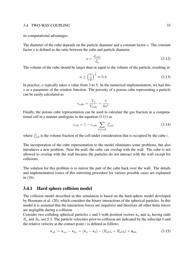
3.4.1 Hard sphere collision modelThe collision model described in this simulation is based on the hard-sphere model developedby Hoomans et al. (20), which considers the binary interactions of the spherical particles. In thismodel it is assumed that the interaction forces are impulsive and therefore all other finite forcesare negligible during a collision.Consider two colliding spherical particles a and b with position vectors xa and xb having radiiRa and Rb, see 5.3. The particle velocities prior-to-collision are indicated by the subscript 0 andthe relative velocity at the contact point c is defined as follows
vab := va,c − vb,c = (va − vb)− (Raωa + Raωb)× nab. (3.15)

34 CHAPTER 3. DISCRETE PARTICLE MODEL
|ra − rb|
vb
va
c
Rb
ωb
b
tab
a
ωa
nabRa
x
y
z
ba
rb ra
Figure 3.3: Hard sphere collision model
The normal and tangential unit vectors are respectively defined as
nab =xa − xb
|xb − xa|(3.16)
tab =vab,0 − nab · vab,0
|vab,0 − nab · vab,0|. (3.17)
As defined in Hoomans (20, p.33) "For a binary collision of these spheres, the following equa-tions can be derived by applying Newton’s second and third laws
ma(va − va,0) = −mb(vb − vb,0) = J, (3.18)
Ia
Ra
(ωa − ωa,0) = − Ib
Rb
(ωb − ωb,0) = −nab × J. (3.19)
The moment of inertia of a particle of mass m, radius R is given by
I =2
5mR2. (3.20)
The equations (3.18) and (3.19) can be rearranged to obtain
vab − vab,0 =7J− 5nab(J · nab)
2mab
, (3.21)

3.4. TWO-WAY COUPLING 35
where mab is the reduced mass given by
mab =
(1
ma
+1
mb
)−1
. (3.22)
In order to calculate the post-collision velocities, a closure model consisting of three parametersis used to describe the impulse vector J.
The first parameter is the coefficient of (normal) restitution (0 ≤ en ≤ 1),
vab · nab = −en(vab,0 · nab). (3.23)
The second parameter is the coefficient of (dynamic) friction (µ ≥ 0),
|nab × J| = −µ(nab · J). (3.24)
The third parameter is the coefficient of tangential restitution (0 ≤ β0 ≤ 1),
nab × vab = −β0(nab × vab,0). (3.25)
Following (20, p.36), "Combining equations (3.21) and (3.23) yields the following expressionfor the normal component of the impulse vector:
Jn = −(1 + en)mab(vab,0 · nab). (3.26)
For the tangential component, two types of collisions can be distinguished that are called stickingand sliding. If the tangential component of the relative velocity is sufficiently high in comparisonto the coefficients of friction and tangential restitution that gross sliding occurs throughout thewhole duration of the contact, the collision is of the sliding type. The non-sliding collisions areof the sticking type. When β0 is equal to zero the tangential component of the relative velocitybecomes zero during a sticking collision. When β0 is greater than zero in such a collision, reversalof the tangential component of the relative velocity will occur. The criterion to determine the typeof collision is as follows:
µJn ≥2
7(1 + β0)mab(vab,0 · tab) sticking,
µJn <2
7(1 + β0)mab(vab,0 · tab) sliding.
For collisions of the sticking type, the tangential impulse is given by:
Jt = −2
7(1 + β0)×mab(vab,0 · tab). (3.27)
For collisions of the sliding type, the tangential impulse is given by:
Jt = −µJn. (3.28)
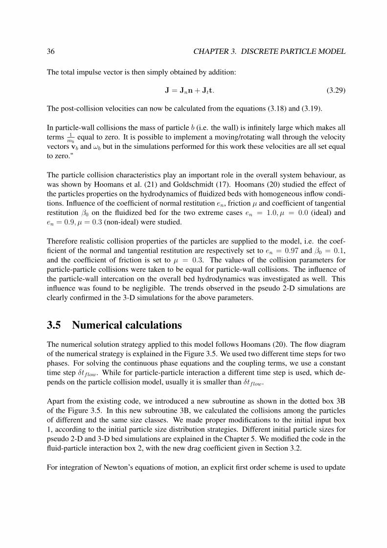
36 CHAPTER 3. DISCRETE PARTICLE MODEL
The total impulse vector is then simply obtained by addition:
J = Jnn + Jtt. (3.29)
The post-collision velocities can now be calculated from the equations (3.18) and (3.19).
In particle-wall collisions the mass of particle b (i.e. the wall) is infinitely large which makes allterms 1
mbequal to zero. It is possible to implement a moving/rotating wall through the velocity
vectors vb and ωb but in the simulations performed for this work these velocities are all set equalto zero."
The particle collision characteristics play an important role in the overall system behaviour, aswas shown by Hoomans et al. (21) and Goldschmidt (17). Hoomans (20) studied the effect ofthe particles properties on the hydrodynamics of fluidized beds with homogeneous inflow condi-tions. Influence of the coefficient of normal restitution en, friction µ and coefficient of tangentialrestitution β0 on the fluidized bed for the two extreme cases en = 1.0, µ = 0.0 (ideal) anden = 0.9, µ = 0.3 (non-ideal) were studied.
Therefore realistic collision properties of the particles are supplied to the model, i.e. the coef-ficient of the normal and tangential restitution are respectively set to en = 0.97 and β0 = 0.1,and the coefficient of friction is set to µ = 0.3. The values of the collision parameters forparticle-particle collisions were taken to be equal for particle-wall collisions. The influence ofthe particle-wall intercation on the overall bed hydrodynamics was investigated as well. Thisinfluence was found to be negligible. The trends observed in the pseudo 2-D simulations areclearly confirmed in the 3-D simulations for the above parameters.
3.5 Numerical calculationsThe numerical solution strategy applied to this model follows Hoomans (20). The flow diagramof the numerical strategy is explained in the Figure 3.5. We used two different time steps for twophases. For solving the continuous phase equations and the coupling terms, we use a constanttime step δtflow. While for particle-particle interaction a different time step is used, which de-pends on the particle collision model, usually it is smaller than δtflow.
Apart from the existing code, we introduced a new subroutine as shown in the dotted box 3Bof the Figure 3.5. In this new subroutine 3B, we calculated the collisions among the particlesof different and the same size classes. We made proper modifications to the initial input box1, according to the initial particle size distribution strategies. Different initial particle sizes forpseudo 2-D and 3-D bed simulations are explained in the Chapter 5. We modified the code in thefluid-particle interaction box 2, with the new drag coefficient given in Section 3.2.
For integration of Newton’s equations of motion, an explicit first order scheme is used to update

3.5. NUMERICAL CALCULATIONS 37
1
2
3A
4
5
6
7
8
3B
no
END
yes
BEGIN: Set up initial condition
Apply particle-particle interaction and
t = t + δt, n =⇒ n + 1
Solve Navier-Stokes equations
Apply fluid-particle interaction
move particles
In:rn, Out: εn (explicit)Determine porosity
In: vn−12un−1pn−1βn−1εn, Out: unpn
Calculate the
the particlesIn: vn+12rn, Out: vn+1rn+1 (explicit) collisions among
t < tend
In: vnunpnrn, Out: vn+12βn (explicit)
Figure 3.4: Flow diagram of the discrete particle model
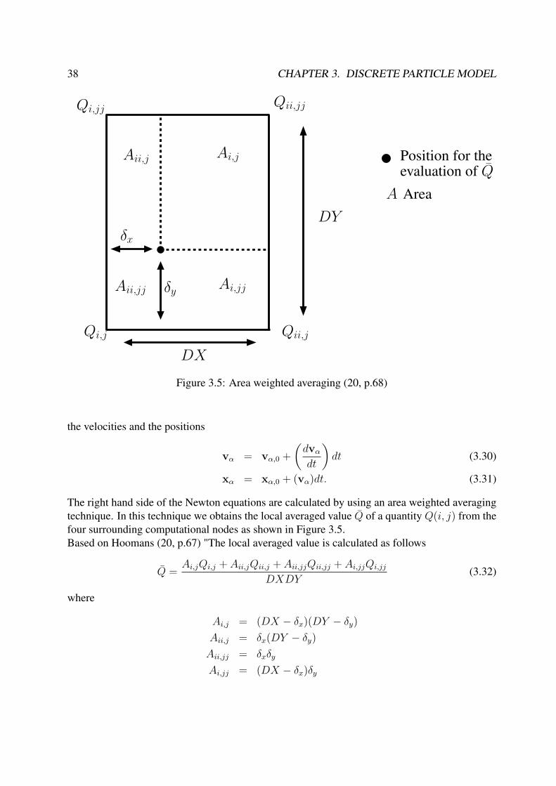
38 CHAPTER 3. DISCRETE PARTICLE MODEL
Qi,jjQii,jj
DY
Qii,jQi,j
Aii,j Ai,j
Ai,jjAii,jj δy
δx
Position for theevaluation of Q
Area
DX
A
Figure 3.5: Area weighted averaging (20, p.68)
the velocities and the positions
vα = vα,0 +
(dvα
dt
)dt (3.30)
xα = xα,0 + (vα)dt. (3.31)
The right hand side of the Newton equations are calculated by using an area weighted averagingtechnique. In this technique we obtains the local averaged value Q of a quantity Q(i, j) from thefour surrounding computational nodes as shown in Figure 3.5.Based on Hoomans (20, p.67) "The local averaged value is calculated as follows
Q =Ai,jQi,j + Aii,jQii,j + Aii,jjQii,jj + Ai,jjQi,jj
DXDY(3.32)
where
Ai,j = (DX − δx)(DY − δy)
Aii,j = δx(DY − δy)
Aii,jj = δxδy
Ai,jj = (DX − δx)δy
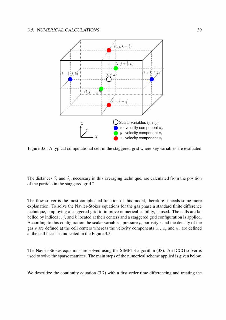
3.5. NUMERICAL CALCULATIONS 39
z - velocity component uz
y - velocity component uy
x - velocity component ux
Scalar variables (p, ε, ρ)
(i + 12, j, k)
(i, j, k − 12)
X
Y
Z
(i− 12, j, k)
(i, j, k + 12)
(i, j − 12, k)
(i, j, k)
(i, j + 12, k)
Figure 3.6: A typical computational cell in the staggered grid where key variables are evaluated
The distances δx and δy, necessary in this averaging technique, are calculated from the positionof the particle in the staggered grid."
The flow solver is the most complicated function of this model, therefore it needs some moreexplanation. To solve the Navier-Stokes equations for the gas phase a standard finite differencetechnique, employing a staggered grid to improve numerical stability, is used. The cells are la-belled by indices i, j, and k located at their centers and a staggered grid configuration is applied.According to this configuration the scalar variables, pressure p, porosity ε and the density of thegas ρ are defined at the cell centers whereas the velocity components ux, uy and uz are definedat the cell faces, as indicated in the Figure 3.5.
The Navier-Stokes equations are solved using the SIMPLE algorithm (38). An ICCG solver isused to solve the sparse matrices. The main steps of the numerical scheme applied is given below.
We descritize the continuity equation (3.7) with a first-order time differencing and treating the

40 CHAPTER 3. DISCRETE PARTICLE MODEL
convective fluxes implicitly as
(ερ)n+1i,j,k − (ερ)n
i,j,k +δt
δx
〈ερux〉n+1
i+ 12,j,k
− 〈ερux〉n+1i− 1
2,j,k
(3.33)
+δt
δy
〈ερuy〉n+1
i,j+ 12,k− 〈ερuy〉n+1
i,j− 12,k
+
δt
δz
〈ερuz〉n+1
i,j,k+ 12
− 〈ερuz〉n+1i,j,k− 1
2
= 0,
where n and n + 1 represents the old and new time level respectively.
The momentum equation (3.8) for the gas phase is descretized in the direction of x as
(ερux)n+1i+ 1
2,j,k
= Ani+ 1
2,j,k
+ εn+1i+ 1
2,j,k
δt
δx(pn+1
i,j,k − pn+1i+1,j,k)−∆tβn
i+ 12,j,k
uxn+1i+ 1
2,j,k
. (3.34)
The pressure and velocity terms are calculated implicitly, the stresses, gravity and a part of thedrag is taken into account explicitly,
Ani+ 1
2,j,k
= (ερux)ni+ 1
2,j,k
+δt
δx
〈ερuxux〉ni,j,k − 〈ερuxux〉ni+1,j,k
+
δt
δy
〈ερuyux〉ni+ 1
2,j− 1
2,k− 〈ερuyux〉ni+ 1
2,j+ 1
2,k
+
δt
δz
〈ερuzux〉ni+ 1
2,j,k− 1
2− 〈ερuzux〉ni+ 1
2,j,k+ 1
2
+δt
δx
(ε(λ− 2
3µ)
)n
i+1,j,k
((ux)n
i+32 ,j,k
−(ux)n
i+12 ,j,k
δx+
(uy)n
i+1,j+12 ,k
−(uy)n
i+1,j− 12 ,k
δy+
(uz)n
i+1,j,k+12
−(uz)n
i+1,j,k− 12
δz
)−
(ε(λ− 2
3µ)
)n
i,j,k
((ux)n
i+12 ,j,k
−(ux)n
i− 12 ,j,k
δx+
(uy)n
i,j+12 ,k
−(uy)n
i,j− 12 ,k
δy+
(uz)n
i,j,k+12
−(uz)n
i,j,k− 12
δz
)
+ 2δt
(δx)2
(εµ)n
i+1,j,k
((ux)
ni+ 3
2,j,k
− (ux)ni+ 1
2,j,k
)− (εµ)n
i,j,k
((ux)
ni+ 1
2,j,k
− (ux)ni− 1
2,j,k
)
+δt
δy
(εµ)n
i+ 12,j+ 1
2,k
((ux)n
i+12 ,j+1,k
−(ux)n
i+12 ,j,k
δy+
(uy)n
i+1,j+12 ,k
−(uy)n
i,j+12 ,k
δx
)−(εµ)n
i+ 12,j− 1
2,k
((ux)n
i+12 ,j,k
−(ux)n
i+12 ,j−1,k
δy+
(uy)n
i+1,j− 12 ,k
−(uy)n
i,j− 12 ,k
δx
)
+δt
δz
(εµ)n
i+ 12,j,k+ 1
2
((uz)n
i+1,j,k+12
−(uz)n
i,j,k+12
δx+
(ux)n
i+12 ,j,k+1
−(ux)n
i+12 ,j,k
δz
)−(εµ)n
i+ 12,j,k− 1
2
((uz)n
i+1,j,k− 12
−(uz)n
i,j,k− 12
δx+
(ux)n
i+12 ,j,k
−(ux)n
i+12 ,j,k−1
δz
)
+ δt · (ερ)ni+ 1
2,j,k
· gx + δtβni+ 1
2,j,k
(vx)n+1i+ 1
2,j,k
.
The value of εµ at a cell is calculated by averaging neighbour cell values as,
(εµ)ni+ 1
2,j+ 1
2,k
=(εµ)n
i,j,k + (εµ)ni+1,j,k + (εµ)n
i+1,j+1,k + (εµ)ni,j+1,k
4
(εµ)ni+ 1
2,j,k
=(εµ)n
i,j,k + (εµ)ni+1,j,k
2etc.

3.5. NUMERICAL CALCULATIONS 41
In a similar manner we can discretize the momentum equation in the y and z directions.
Solution of the finite difference equations
The numerical solution of the discretized equations evolves through a sequence of computationalcycles, or time steps. For each computational cycle the advanced (n + 1)-level values haveto be calculated through the entire computational domain using the old n-level values. Eachcomputational cycle consists of two distinct phases:
• Calculation of explicit terms An, Bn and Cn in the momentum equation for all interiorcells.
• Implicit computation of the pressure for the entire computational mesh with an iterativeprocedure. This implicit procedure consists of several steps.
The first step involves the calculation of mass residual Df from the continuity equation as
(Df )∗i,j,k = (ερ)∗i,j,k − (ερ)n
i,j,k +δt
δx
〈ερux〉∗i+ 1
2,j,k
− 〈ερux〉∗i− 12,j,k
(3.35)
+δt
δy
〈ερuy〉∗i,j+ 1
2,k− 〈ερuy〉∗i,j− 1
2,k
+
δt
δz
〈ερuz〉∗i,j,k+ 1
2− 〈ερuz〉∗i,j,k− 1
2
,
where the superscript (*) refers to the most recently obtained values. If the convergence criterion
(Df )∗i,j,k < eps · (ερ)∗i,j,k,
is not satisfied for all interior computational cells, then a whole field pressure correction is cal-culated as
Jni−1,j,kδp
newi−1,j,k + Jn
i+1,j,kδpnewi+1,j,k + Jn
i,j−1,kδpnewi,j−1,k + Jn
i,j+1,kδpnewi,j+1,k
+ Jni,j,k−1δp
newi,j,k−1 + Jn
i,j,k+1δpnewi,j,k+1 + Jn
i,j,kδpnewi,j,k = −(Df )
∗i,j,k (3.36)
with Jn the Jacobi matrix at the old time level n. The Jacobi matrix contains the derivativesof Df with respect to the pressure. An explicit expression can be obtained from the continuityequation in combination with the momentum equation.
Ji,j,k =∂(Df )
ni,j,k
∂pni,j,k
etc.
Applying (3.36) for all internal computational cells results in a set of linear equations that can beassembled in the matrix form as
Jn · δpnew = −D∗. (3.37)

42 CHAPTER 3. DISCRETE PARTICLE MODEL
To save computational effort the elements of the Jacobi matrix are evaluated at the old time level.The banded matrix problem corresponding to the equation (3.37) is solved using a standard ICCGsparse matrix technique. Once the pressure have been obtained, the corresponding new gas phasedensities are calculated.Df can be calculated from the continuity equation with these new values of density, pressure as
(Df )n+1i,j,k = (ερ)n+1
i,j,k − (ερ)ni,j,k +
δt
δx
〈ερux〉n+1
i+ 12,j,k
− 〈ερux〉n+1i− 1
2,j,k
(3.38)
+δt
δy
〈ερuy〉n+1
i,j+ 12,k− 〈ερuy〉n+1
i,j− 12,k
+
δt
δz
〈ερuz〉n+1
i,j,k+ 12
− 〈ερuz〉n+1i,j,k− 1
2
.
Provided that the corresponding estimates of the mass residual (3.35) do not meet the conver-gence criteria simultaneously for all interior computational cells, the pressure correction equa-tion (3.36) is again calculated using the updated velocity field to compute the mass residual Df
for all cells. This iterative process is repeated until the convergence criteria is satisfied or thespecified maximum allowable number of iterations reached.
For calculation of the convective mass and momentum fluxes, a second order accurate method isapplied to reduce numerical diffusion.

Chapter 4
Modelling of collision frequency functionsusing DPM
In this chapter we present an approach for the modelling of collision frequency functions ina fluidized bed. The aggregation kernel can be decomposed as the product of size dependentand size independent functions. The size dependent functions are known as collision frequencykernel and the size independent functions are known as aggregation efficiency functions. Inthis chapter we give a general expression for evaluating the size dependent collision frequencyfunction from computer simulation results.
4.1 Introduction
In recent times, due to the improvement of the computations, some authors (15; 51) have tried toextract the kernels from discrete element method (DEM) simulations. Tan et al. (51) investigatedan agglomeration kernel based on the priniciple of kinetic theory of granular flow to the fludizedbed melt granulation. Using the simulation results of the discrete particle model (DPM), theauthors showed that the velocity distribution of the particles inside the fluidized bed are in goodaggreement with those expected according to kinetic theory of granular flow (KTGF). Based onthis kinetic theory of granular flow they assumed that the collision rate function is analogous tothe existing equi-partition kinetic energy (EKE) kernel. This EKE kernel was originally derivedby Hounslow (22) and it was discussed in Chapter 2, Section 2.4.1. Tan et al. (51) tried to fitthe particle size distribution of the experimental results with the discritized population balancemodelling with EKE kernel.
Recently Gantt et al. (15) observed the shear kernel for high-shear granulation using discreteelement method simulations. For the discrete element method simulations, they assumed thatthe particles are spherical in shape and applied the soft sphere model as particle collision mech-anism. In these simulations, the authors used an aggregation kernel for deformable wet granulesderived by Liu et al. (35). A multi-scale shear kernel with four parameters for aggregationefficiency function is calculated using regression fit to the simulation data. Gantt et al. (15) con-
43

44 CHAPTER 4. MODELLING OF COLLISION FREQUENCY FUNCTIONS
sidered pore saturation, porosity, particle velocity and particle diameter as the parameters of theaggregation efficiency function and calculated these parameters for two different types of particlebinding mechanisms.
In the following sections we present the modelling of the aggregation frequency function usingthe Discrete Particle Model (DPM), which is a microscopic model developed by Hoomans et al.(20).
4.2 Derivation of collision frequency functionsAggregation processes lead to a reduction in the total number of particles and an increase in theaverage size. Therefore agglomeration leads a major change in the system as the time changes.As a result, the aggregation rate will be effected, which is a function of collision frequencyfunction and aggregation efficiency. Here we are deriving an expression for collision frequencyfunction.
Let Ni,j be the number of collsions occuring per unit time per unit volume between the twoclasses of particles of volumes vi and vj . All particles are assumed to be spherical in shape, andcollisions are treated as binary hard sphere collisions. The collision frequency function Ki,j canbe written in terms of concentrations of particles of volumes vi and vj as:
Ni,j = Ki,jninj, 1 ≤ i, j ≤ I
where ni, nj are the number concentrations of classes i, j. The number I denotes the total num-ber of classes. The parameter Ki,j is the frequency function among different classes i and j. Thecollision frequency function Ki,j is a function of flow properties, i.e. particle size, gas velocity,temperature, etc.
The number of collisions occuring during time tsim in the fluidized bed of volume Vbed is givenas
N toti,j = Ki,j
Ni
Vbed
Nj
Vbed
tsimVbed, (4.1)
where Ni, Nj are the number of particles of class i, j present in the fluidized bed of volume Vbed,i.e. ni = Ni
Vbed, nj =
Nj
Vbed.
Remark 4.1 In the experimental analysis of bed volume, it consists of the measurement of theheight of the fluidized layer. From the fluid flow point of view, the bed void fraction is important.The bed contains “bubbles”, called parvoids, that do not contain particles. Since the uppersurface of the bed remains neither perfectly plane nor motionless, due to particular parvoidmotion, the measurement of the mean level is not accurate. In order to overcome this difficulty
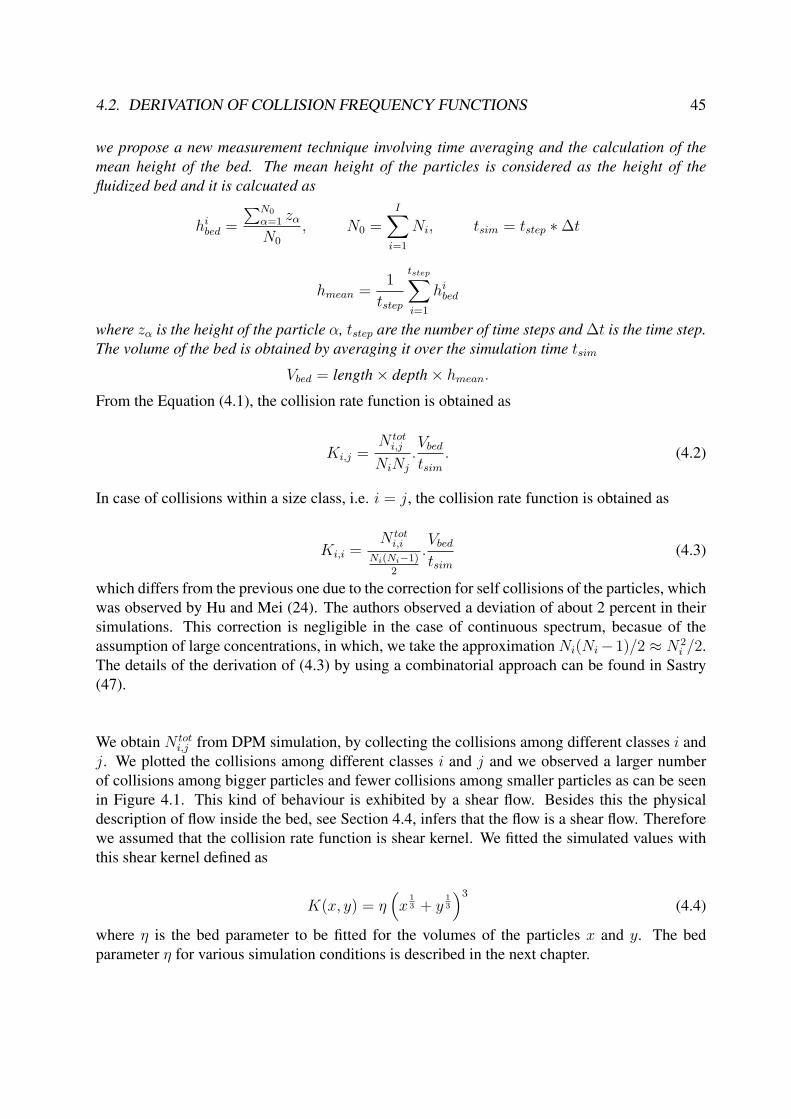
4.2. DERIVATION OF COLLISION FREQUENCY FUNCTIONS 45
we propose a new measurement technique involving time averaging and the calculation of themean height of the bed. The mean height of the particles is considered as the height of thefluidized bed and it is calcuated as
hibed =
∑N0
α=1 zα
N0
, N0 =I∑
i=1
Ni, tsim = tstep ∗∆t
hmean =1
tstep
tstep∑i=1
hibed
where zα is the height of the particle α, tstep are the number of time steps and ∆t is the time step.The volume of the bed is obtained by averaging it over the simulation time tsim
Vbed = length× depth× hmean.
From the Equation (4.1), the collision rate function is obtained as
Ki,j =N tot
i,j
NiNj
.Vbed
tsim. (4.2)
In case of collisions within a size class, i.e. i = j, the collision rate function is obtained as
Ki,i =N tot
i,i
Ni(Ni−1)2
.Vbed
tsim(4.3)
which differs from the previous one due to the correction for self collisions of the particles, whichwas observed by Hu and Mei (24). The authors observed a deviation of about 2 percent in theirsimulations. This correction is negligible in the case of continuous spectrum, becasue of theassumption of large concentrations, in which, we take the approximation Ni(Ni− 1)/2 ≈ N2
i /2.The details of the derivation of (4.3) by using a combinatorial approach can be found in Sastry(47).
We obtain N toti,j from DPM simulation, by collecting the collisions among different classes i and
j. We plotted the collisions among different classes i and j and we observed a larger numberof collisions among bigger particles and fewer collisions among smaller particles as can be seenin Figure 4.1. This kind of behaviour is exhibited by a shear flow. Besides this the physicaldescription of flow inside the bed, see Section 4.4, infers that the flow is a shear flow. Thereforewe assumed that the collision rate function is shear kernel. We fitted the simulated values withthis shear kernel defined as
K(x, y) = η(x
13 + y
13
)3
(4.4)
where η is the bed parameter to be fitted for the volumes of the particles x and y. The bedparameter η for various simulation conditions is described in the next chapter.

46 CHAPTER 4. MODELLING OF COLLISION FREQUENCY FUNCTIONS
Figure 4.1: Particle collisions among different classes
4.3 Correction to the aggregation equationLet us consider the combinatorial approach of the particle collisions among different classes andwithin the same class of particles. Here classes are based on the volume of the particle, i.e,V0, 2V0, 3V0, ... and V0 is the initial particle volume class.
The Figure 4.3 describes the number of possible collisions among two classes A and B whichcontain 2 and 3 particles respectively. The number of possible collisions between A and B are 6.The number of possible collisions among the particles of class B are 3.
We can generalize the above approach as follows. Suppose there are Ni particles of ith class andNj particles of jth class at a given instant. Then the number of possible collisions among ithclass and jth class are NiNj . When we have collisions among the particles of class i, then thenumber of possible collisions are Ni(Ni − 1)/2.
We can apply the above combinatorial approach to the fluidized bed as follows. Let Ki,j bethe collision frequency function of the fluidized bed. Then the number of collisions among theclasses i and j per unit time and per unit volume are Ni,j = Ki,jNiNj . In case of collisionsamong the particles in the ith class are Ni,j = Ki,jNi(Ni − 1)/2. The case of collisions amongthe same class are not considered during the derivation of the aggregation equation. So here weare showing the effect of this in modelling the aggregation kernel in Table 4.1. In this simulation
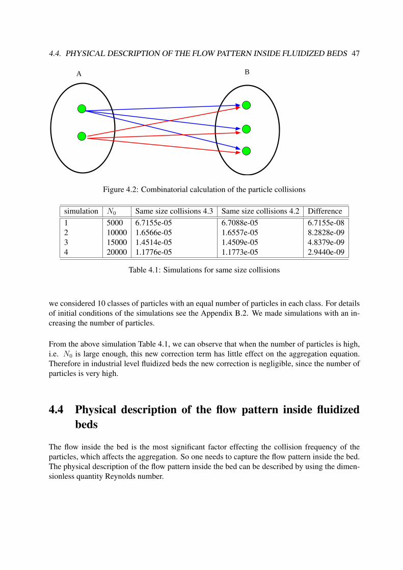
4.4. PHYSICAL DESCRIPTION OF THE FLOW PATTERN INSIDE FLUIDIZED BEDS 47
A B
Figure 4.2: Combinatorial calculation of the particle collisions
simulation N0 Same size collisions 4.3 Same size collisions 4.2 Difference1 5000 6.7155e-05 6.7088e-05 6.7155e-082 10000 1.6566e-05 1.6557e-05 8.2828e-093 15000 1.4514e-05 1.4509e-05 4.8379e-094 20000 1.1776e-05 1.1773e-05 2.9440e-09
Table 4.1: Simulations for same size collisions
we considered 10 classes of particles with an equal number of particles in each class. For detailsof initial conditions of the simulations see the Appendix B.2. We made simulations with an in-creasing the number of particles.
From the above simulation Table 4.1, we can observe that when the number of particles is high,i.e. N0 is large enough, this new correction term has little effect on the aggregation equation.Therefore in industrial level fluidized beds the new correction is negligible, since the number ofparticles is very high.
4.4 Physical description of the flow pattern inside fluidizedbeds
The flow inside the bed is the most significant factor effecting the collision frequency of theparticles, which affects the aggregation. So one needs to capture the flow pattern inside the bed.The physical description of the flow pattern inside the bed can be described by using the dimen-sionless quantity Reynolds number.
48 CHAPTER 4. MODELLING OF COLLISION FREQUENCY FUNCTIONS
The particle Reynolds number is given as (54)
Reα =ερgUαdα
µ, (4.5)
where Uα = |u − vα| is the relative velocity between a particle and the fluid flow. The particleReynolds number is a function of particle diameter, velocity, porosity, density and viscosity.
The particle Reynolds number characterizes the flow regime inside the bed. Frequently used flowregimes are
• The Stokes Regime: The flow regime is Stokes regime if Reα < 0.2. The Stokes lawregime is also known as creeping flow regime. In this regime, the viscosity of the fluid isdominating.
• The Intermediate Regime: The flow regime is known as intermediate regime if 0.2 <Reα < 500. In this regime the drag force is a function of the particle’s Reynolds number.
• The Newton’s Law Regime: If Reα > 500. In this regime inertia of the fluid is larger thanthe viscosity of the fluid.
Recently a new methodology for calculating the agglomeration kernels was proposed by Steven(10) for the Stokes regime. He assumed uncertainity in the Stokes regime and evaluated thecoefficients of uncertainity using a method proposed by Tatang (52). The newly postulated ag-glomeration kernel is given as
K(t, x, y) = K0
∫ S∗t
−∞f(t, φ)dφ
where f(t, φ) is the discrete probability density function for the Stokes number, and S∗t is the
critical stokes number. The constant K0 is determined from the experimental data.
In our DPM simulations the viscosity, density of the particles and gas velocity are constant withrespect to time, the only varying variables are particle velocity and diameter for different setsof simulations. We studied the particle Reynolds number for a wide range particle diameters inorder to understand the flow pattern inside the fluidized bed. It was observed that the particleReynolds number always lies below 500 and above 100. This shows that the flow inside the bedis dominated by shear forces. From this microscopic/macroscopic observation, we can expect ashear kernel.
Chapter 5
Simulation results for modelling ofaggregation kernels using DPM
In this chapter we describe the simulation results for modelling of aggregation kernels using theDiscrete Particle Model (DPM) which is explained in Chapter 3. Section 1 explains the essentialinitial parameters for the simulations. The second and third sections show the simulation resultsfor pseudo 3-D and 3-D fluidized beds. In these simulations we are trying to fit the simulationresults with the shear kernel. We calculated the fitting parameter η for each simulation andnamed it the bed parameter. The influence of this bed parameter for various initial particle sizedistributions is analysed.
5.1 Initial parametersInitial parameters play a significant role in the simulations of any model. All the major parame-ters used for our simulations are given in Appendix B.
5.1.1 Initial assumptions
In the present thesis we model the aggregation kernels with some assumptions and some simpli-fications of the discrete particle model for easy numerical calculations. Here in this section weexplains those assumptions. We have the following assumptions in our simulations:
1. Particle size characterizationThe particle size is characterized by one or more linear dimensions. In the present simula-tions we considered an ideal particle like a sphere characterized by its diameter.
2. Particle collisionsWe considered binary hard sphere collisions among the particles. The particles collideaccording to the hard sphere collision model as explained in the Chapter 3, Section 4. Theparameters of the collision model are given in the Appendix B.
49

50 CHAPTER 5. SIMULATION RESULTS
3. Basic particle size class: Volume based size class
+
+
6=
=V2
d2d1
V1
d3
V3
Figure 5.1: Schematic example for the choice of the volume based size class
It is necessary that population balance equation must be consistent with mass. This is satis-fied automatically if we consider volume as the intrinsic particle property as suggested byPouw et al. (40). Since volume is additive in a binary aggregation event, where as diameteris not. Figure 5.1 illustrates the obvious fact that the aggregation of particles of diameterd1 = 1 and d2 = 2 do not form a particle of diameter d3 = 1 + 2, but particles of volumesV1 = 1 and V2 = 2 produce an agglomerate particle of volume V3 = 1 + 2.
Therefore in the present simulations we considered volume based size classes with vol-umes V0, 2V0, 3V0, ..., where V0 is the volume of the smallest particle in the system.
4. No aggregationIn these simulations no aggregation, compaction or breakage takes place. Only particlecollisions due to gas flow are considered.
5.1.2 Initial particle size distributionsIn most of the practical cases fluidized beds are consisting of particles of different sizes, knownas polydisperse systems. Initial particle size distribution is very important in granulations pro-cess, since the final product is dependent on the initial size distribution. In this section we derivedifferent particle size distributions satisfying certain properties.
Let us consider N0 number of particles with Ni number of particles of classes i = 1, 2, ..., I withvolume V0, 2V0, 3V0, ..., IV0. Now we will determine different possible particle size distributions

5.1. INITIAL PARAMETERS 51
based on different criteria. The following gives the different possible criteria and the particle sizedistributions.
1. Equal zeroth moment
We consider the first criterion satisfying equal zeroth moment in each class, i.e. the numberof particles in each class i are equal and the total number of particles of all classes is N0,
N1 = N2 = ... = NI , (5.1)∑i
Ni = N0.
2. Equal length
Let L1, L2, ..., LI be the length of particles of classes 1, 2, ..., I . Consider the case satisfy-ing the equal length criterion, i.e. the total length of the particles in each class i is equaland the total number of particles of all classes is N0,
N1L1 = N2L2 = ... = NILI , (5.2)∑i
Ni = N0.
3. Equal surface area
Let A1, A2, ..., AI be the length of particles of classes 1, 2, ..., I . Consider the case satis-fying the equal surface area criterion, i.e. the total length of the particles in each class i isequal and the total number of particles of all classes is N0,
N1A1 = N2A2 = ... = NIAI , (5.3)∑i
Ni = N0.
4. Equal first moment (Equal volume)
Let V1, V2, ..., VI be the length of particles of classes 1, 2, ..., I . We consider simulationssatisfying the equal volume criteria, i.e. the total volume of the particles in each class i isequal and the total number of particles of all classes is N0.,
N1V1 = N2V2 = ... = NIVI , (5.4)∑i
Ni = N0.
5. Different number of particles
We calculate the particle size distribution satisfying the above four criteria 1-4 with differ-ent number of particles, i.e. N0 = 5000, 10000, 15000.

52 CHAPTER 5. SIMULATION RESULTS
6. Particles with three classes
The number of particles in each class Ni are determined with three number of classes, i.e.I = 5, 10, 15 for above four criteria 1-4.
7. Increasing volume of particles
We considered a particle size distributions satisfying the one of the above criteria 1-4 andthen we increased the volume V0. That is the first simulation is started with V0, 2V0, 3V0, ..., IV0,second simulation with 2V0, 3V0, ..., (I + 1)V0, and so on.
Simulation Criteria Number of particles1 1 2000, 2000, 2000, 2000, 20002 2 2701, 2144, 1873, 1702, 15803 3 3510, 2211, 1686, 1293, 12004 4 4380, 2190, 1460, 1095, 876
Table 5.1: Five classes
Simulation Criteria Number of particles5 1 1000, 1000, 1000, 1000, 1000, 1000, 1000, 1000, 1000, 10006 2 1608, 1276,1115, 1013, 940, 885, 840, 804, 773, 7467 3 2426, 1528, 1166, 963, 830, 735, 663, 606, 560, 5238 4 3414, 1707, 1138, 854, 683, 569, 488, 427, 379, 341
Table 5.2: Ten classes
Simulation Criteria Number of particles9 1 667, 667, 667, 667, 667, 667, 667, 667, 667, 667, 667, 667, 667, 667, 66710 2 1197, 950, 830, 754, 700, 659, 626, 599, 576, 556, 538, 523, 509, 497, 48011 3 1987, 1252, 955, 789, 679, 602, 543, 497, 459, 428, 402, 379, 359, 342, 32712 4 3014, 1507, 1004, 754, 603, 502, 430, 377, 335, 301, 274, 251, 232, 215, 201
Table 5.3: Fifteen classes
The Tables 5.1-5.3 show initial particle number for different sets of simulations. Table 5.1 givesthe number of particles in each class, having I = 5 classes, satisfying the criterias 1, 2, 3 and 4with N0 = 10000. Table 5.2 gives the number of particles in each class, having I = 10 classes,satisfying the criterias 1, 2, 3 and 4 with N0 = 10000. Table 5.3 gives the number of particles ineach class, having I = 15 classes, satisfying the criterias 1, 2, 3 and 4 with N0 = 10000.
Corresponding to the above tables, we plotted the figures for the number of particles versusclasses. The bar diagram Figure 5.2 represents the number of particles in each of the five classessatisfying the criteria 1-4 corresponding to the Table 5.1. The bar diagram Figure 5.3 represents

5.2. EVALUATION OF THE BED PARAMETER 53
Figure 5.2: Initial condition for the simulations
the number of particles in each of ten classes satisfying the criteria 1-4 corresponding to the Ta-ble 5.2. The bar diagram Figure 5.4 represents the number of particles in each of fifteen classessatisfying the criteria 1-4 corresponding to the Table 5.3.
In a similar manner we obtained the number of particles in each class satisfying the criterias 1-4with N0 = 5000 and N0 = 15000 for three classes I = 5, 10, 15. The values and the figurescorresponding to these criteria are given in Appendix B.
5.2 Evaluation of the bed parameter
We calculate the collision rate function using the formula (4.2), which is derived in Chapter 4,Section 2. From the physical description of flow inside the fluidized bed as shown in Chapter 4,Section 4, we expect a shear kernel. Therefore we try to fit the simulated data of the collisions tothe shear kernel by using a least squares fit. We introduced a new fitting parameter η. We call itthe bed parameter.
Define the predicted collision frequency as a set of collisions represented by K(vi, vj) and theobserved collisions of the fluidized bed simulations as the set of K ′(vi, vj), then by the leastsquare method
S =∑
i
∑j
(K ′(vi, vj)− ηK(vi, vj))2 (5.5)
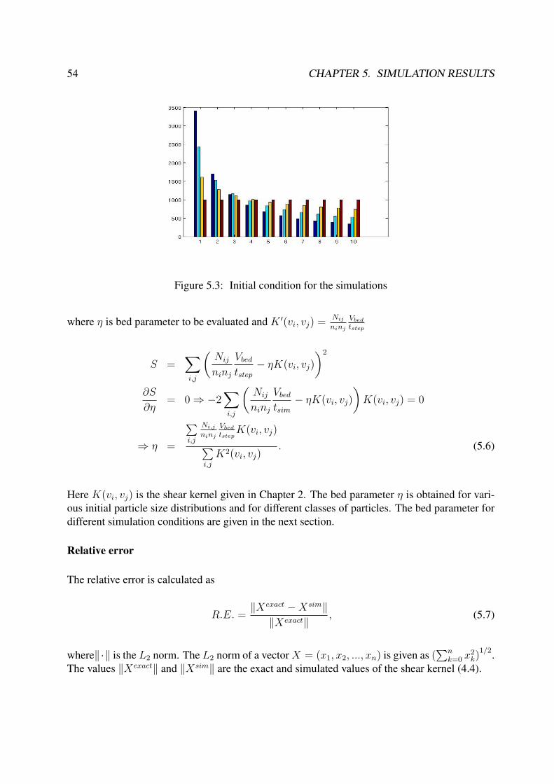
54 CHAPTER 5. SIMULATION RESULTS
Figure 5.3: Initial condition for the simulations
where η is bed parameter to be evaluated and K ′(vi, vj) =Nij
ninj
Vbed
tstep
S =∑i,j
(Nij
ninj
Vbed
tstep− ηK(vi, vj)
)2
∂S
∂η= 0 ⇒ −2
∑i,j
(Nij
ninj
Vbed
tsim− ηK(vi, vj)
)K(vi, vj) = 0
⇒ η =
∑i,j
Ni,j
ninj
Vbed
tstepK(vi, vj)∑
i,j
K2(vi, vj). (5.6)
Here K(vi, vj) is the shear kernel given in Chapter 2. The bed parameter η is obtained for vari-ous initial particle size distributions and for different classes of particles. The bed parameter fordifferent simulation conditions are given in the next section.
Relative error
The relative error is calculated as
R.E. =‖Xexact −Xsim‖
‖Xexact‖, (5.7)
where‖·‖ is the L2 norm. The L2 norm of a vector X = (x1, x2, ..., xn) is given as (∑n
k=0 x2k)
1/2.The values ‖Xexact‖ and ‖Xsim‖ are the exact and simulated values of the shear kernel (4.4).

5.3. SIMULATION RESULTS FOR A PSEUDO 3D BED 55
Figure 5.4: Initial condition for the simulations
5.3 Simulation results for a pseudo 3D bed
We consider the pseudo-3D bed for these simulations. Since gas phase hydrodynamics are re-solved in two dimensions and the particle movements are three dimensional, we can call it apseudo-3D bed. This can be justified since the simulated system is a flat fluidised bed with adepth of 1cm where the motion of the gas phase in the third dimension can be neglected, if wedisregard the boundary layer.
All the physical parameters like bed dimension, fluidization velocity, etc. are fixed and are thesame for all the pseudo 3D fluidized bed simulations. So the only changing parameter is particlenumber N0 and the number of classes I . The parameters of the simulation are shown in theAppendix B. We observe the collision rate function among different classes using the DPM atdifferent time intervals.
The Figures 5.5 shows the snapshots of the DPM simulations with bubbles. The colour of theparticles shows the position of the particles with respect to their depth from the front view of thefluidized bed. The simulation data are considered after t = 5 sec in order to get the spatiallyhomogeneous fludized bed. We run the simulation for t = 15 sec. We consider three differentsets of particle classes based on their volume, like particles with 5 classes, 10 classes and 15classes. In each simulation we collected the collisions amoung different classes of particles atdifferent time intervals.
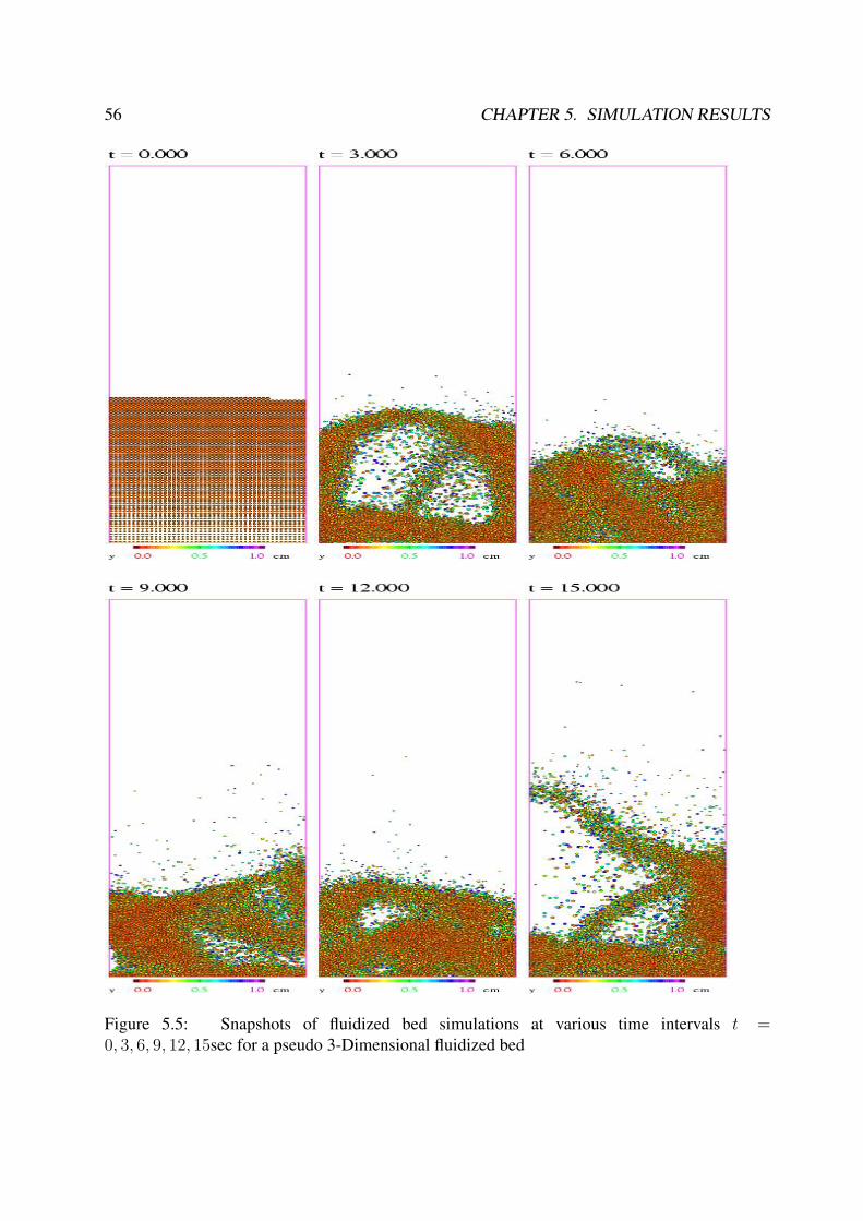
56 CHAPTER 5. SIMULATION RESULTS
Figure 5.5: Snapshots of fluidized bed simulations at various time intervals t =0, 3, 6, 9, 12, 15sec for a pseudo 3-Dimensional fluidized bed

5.3. SIMULATION RESULTS FOR A PSEUDO 3D BED 57
02
46
810
02
46
810
1
2
3
4
5
6
x 10−6
Class iClass j
Ki,j
02
46
810
02
46
810
0
2
4
6
8
x 10−6
Class iClass j
Ki,j
Figure 5.6: Simulated and Fitted collsion frequency functions during the time interval 5 to 10seconds of DPM simulation
02
46
810
02
46
810
1
2
3
4
5
6
x 10−6
Class iClass j
Ki,j
0
5
10
02
46
810
0
2
4
6
8
x 10−6
Class iClass j
Ki,j
Figure 5.7: Simulated and Fitted collsion frequency functions during the time interval 5 to 15seconds of DPM simulation
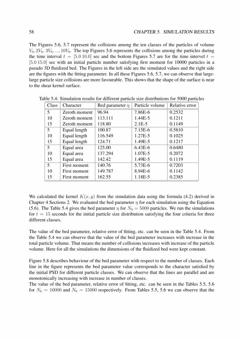
58 CHAPTER 5. SIMULATION RESULTS
The Figures 5.6, 5.7 represent the collisions among the ten classes of the particles of volumeV0, 2V0, 3V0, ..., 10V0. The top Figures 5.6 represents the collisions among the particles duringthe time interval t = [5.0 10.0] sec and the bottom Figures 5.7 are for the time intervel t =[5.0 15.0] sec with an initial particle number satisfying first moment for 10000 particles in apseudo 3D fluidized bed. The Figures in the left side are the simulated values and the right sideare the figures with the fitting parameter. In all these Figures 5.6, 5.7, we can observe that large-large particle size collisions are more favourable. This shows that the shape of the surface is nearto the shear kernel surface.
Table 5.4: Simulation results for different particle size distributions for 5000 particlesClass Character Bed parameter η Particle volume Relative error5 Zeroth moment 96.94 7.86E-6 0.253210 Zeroth moment 113.111 1.44E-5 0.121115 Zeroth moment 118.80 2.1E-5 0.11495 Equal length 100.87 7.15E-6 0.581010 Equal length 116.549 1.27E-5 0.102515 Equal length 124.71 1.49E-5 0.12175 Equal area 125.00 6.43E-6 0.648010 Equal area 137.294 1.07E-5 0.207215 Equal area 142.42 1.49E-5 0.11195 First moment 140.76 5.73E-6 0.720310 First moment 149.787 8.94E-6 0.114215 First moment 162.55 1.18E-5 0.2385
We calculated the kernel K(x, y) from the simulation data using the formula (4.2) derived inChapter 4 Sections 2. We evaluated the bed parameter η for each simulation using the Equation(5.6). The Table 5.4 gives the bed parameter η for N0 = 5000 particles. We run the simulationsfor t = 15 seconds for the initial particle size distribution satisfying the four criteria for threedifferent classes.
The value of the bed parameter, relative error of fitting, etc. can be seen in the Table 5.4. Fromthe Table 5.4 we can observe that the value of the bed parameter increases with increase in thetotal particle volume. That means the number of collisions increases with increase of the particlevolume. Here for all the simulations the dimensions of the fluidized bed were kept constant.
Figure 5.8 describes behaviour of the bed parameter with respect to the number of classes. Eachline in the figure represents the bed parameter value corresponds to the character satisfied bythe initial PSD for different particle classes. We can observe that the lines are parallel and aremonotonically increasing with increase in number of classes.The value of the bed parameter, relative error of fitting, etc. can be seen in the Tables 5.5, 5.6for N0 = 10000 and N0 = 15000 respectively. From Tables 5.5, 5.6 we can observe that the

5.3. SIMULATION RESULTS FOR A PSEUDO 3D BED 59
5 10 15 2090
100
110
120
130
140
150
160
170
Number of classes
Bed
para
met
er η
Equal number of particles
Equal length
Equal surface area
Equal volume
Figure 5.8: Bed parameter corresponding to various number of classes for 5000 particles
Table 5.5: Simulation results for different particle size distributions for 10000 particlesClass Character Bed parameter η Particle volume Relative error5 Zeroth moment 118.13 1.57E-5 0.102110 Zeroth moment 155.054 2.88E-5 0.107815 Zeroth moment 171.6367 4.19E-5 0.09365 Equal length 128.3580 1.43E-5 0.105710 Equal length 165.5839 2.53E-5 0.107415 Equal length 192.5386 3.62E-5 0.10215 Equal area 138.0706 1.28E-5 0.085910 Equal area 181.5455 2.15E-5 0.090415 Equal area 219.1333 2.98E-5 0.11185 First moment 151.6243 1.14E-5 0.072110 First moment 207.2792 1.78E-5 0.096615 First moment 246.8127 2.37E-5 0.0942

60 CHAPTER 5. SIMULATION RESULTS
Table 5.6: Simulation results for different particle size distributions of 15000 particlesClass Character Bed parameter η Particle volume Relative error5 Zeroth moment 188.6722 2.36E-5 0.111810 Zeroth moment 199.7154 4.32E-5 0.096515 Zeroth moment 225.3654 6.28E-5 0.07965 Equal length 199.8196 2.15E-5 0.089410 Equal length 256.2417 3.79E-5 0.097815 Equal length 284.7975 5.42E-5 0.09675 Equal area 222.9835 1.93E-5 0.081710 Equal area 281.4234 3.23E-5 0.105315 Equal area 325.0151 4.48E-5 0.10615 First moment 235.3659 1.72E-5 0.056510 First moment 303.3080 2.68E-5 0.111215 First moment 357.4970 3.55E-5 0.1204
5 10 15 20100
150
200
250
Number of classes
Bed p
ara
mete
r η
Equal number of particles
Equal length
Equal surface area
Equal volume
Figure 5.9: Bed parameter corresponding to various number of classes for 10000 particles
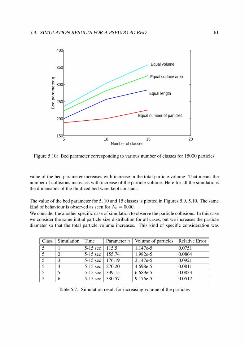
5.3. SIMULATION RESULTS FOR A PSEUDO 3D BED 61
5 10 15 20150
200
250
300
350
400
Number of classes
Bed p
ara
mete
r η
Equal number of particles
Equal length
Equal surface area
Equal volume
Figure 5.10: Bed parameter corresponding to various number of classes for 15000 particles
value of the bed parameter increases with increase in the total particle volume. That means thenumber of collisions increases with increase of the particle volume. Here for all the simulationsthe dimensions of the fluidized bed were kept constant.
The value of the bed parameter for 5, 10 and 15 classes is plotted in Figures 5.9, 5.10. The samekind of behaviour is observed as seen for N0 = 5000.We consider the another specific case of simulation to observe the particle collisions. In this casewe consider the same initial particle size distribution for all cases, but we increases the particlediameter so that the total particle volume increases. This kind of specific consideration was
Class Simulation Time Parameter η Volume of particles Relative Error5 1 5-15 sec 115.5 1.147e-5 0.07515 2 5-15 sec 155.74 1.982e-5 0.08645 3 5-15 sec 176.19 3.147e-5 0.09215 4 5-15 sec 270.20 4.698e-5 0.08115 5 5-15 sec 339.15 6.689e-5 0.08335 6 5-15 sec 380.57 9.176e-5 0.0512
Table 5.7: Simulation result for increasing volume of the particles
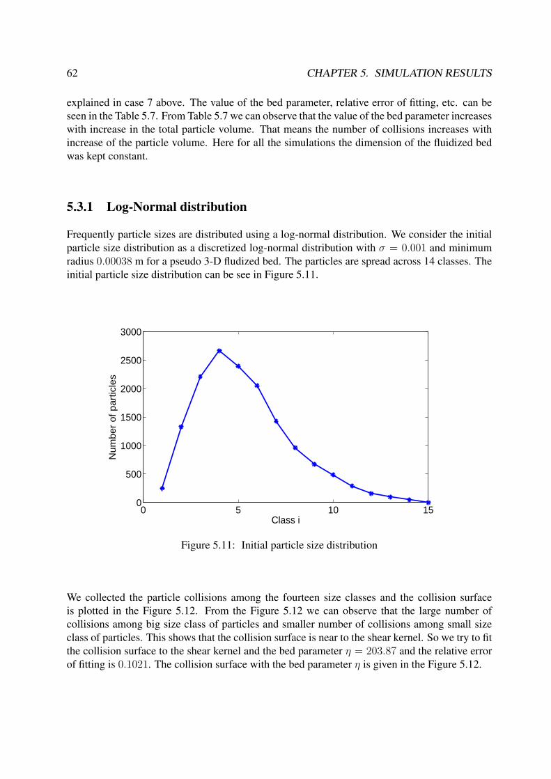
62 CHAPTER 5. SIMULATION RESULTS
explained in case 7 above. The value of the bed parameter, relative error of fitting, etc. can beseen in the Table 5.7. From Table 5.7 we can observe that the value of the bed parameter increaseswith increase in the total particle volume. That means the number of collisions increases withincrease of the particle volume. Here for all the simulations the dimension of the fluidized bedwas kept constant.
5.3.1 Log-Normal distribution
Frequently particle sizes are distributed using a log-normal distribution. We consider the initialparticle size distribution as a discretized log-normal distribution with σ = 0.001 and minimumradius 0.00038 m for a pseudo 3-D fludized bed. The particles are spread across 14 classes. Theinitial particle size distribution can be see in Figure 5.11.
0 5 10 150
500
1000
1500
2000
2500
3000
Class i
Num
ber
of p
artic
les
Figure 5.11: Initial particle size distribution
We collected the particle collisions among the fourteen size classes and the collision surfaceis plotted in the Figure 5.12. From the Figure 5.12 we can observe that the large number ofcollisions among big size class of particles and smaller number of collisions among small sizeclass of particles. This shows that the collision surface is near to the shear kernel. So we try to fitthe collision surface to the shear kernel and the bed parameter η = 203.87 and the relative errorof fitting is 0.1021. The collision surface with the bed parameter η is given in the Figure 5.12.

5.4. SIMULATION RESULTS FOR 3D BEDS 63
0
5
10
15
0
5
10
150
0.5
1
1.5
x 10−5
Class iClass j
Ki,j
0
5
10
15
0
5
10
150
0.2
0.4
0.6
0.8
1
1.2
x 10−5
Class iClass jK
i,j
Figure 5.12: Collision surfaces for log-normal distribution of particles from the simulated andthe corresponding fitted surfaces
5.4 Simulation results for 3D bedsWe started the simulation with 15000 polydisperse spherical glass particles with smallest diame-ter of 1 mm in a 3D bed of dimension 10×5×60 cm. The particle size classes are defined basedon volume (i.e. V0, 2V0, 3V0, ...) with 5, 10 and 15 classes. Here the particles are distributed intovarious size classes based on certain criteria satisfied by each size class as given in the Section5.1.2 cases 1-4. We used a hard sphere binary collision model for particle interactions and noaggregation process involved inside the bed.
For each particle size distribution we counted the collisions among different classes and plottedthe collision surface. Figure 5.13 represents collisions among different class of particles duringthe time interval 5 to 15 seconds with particle size distribution satisfying the zeroth momentcriteria i.e. equal number of particles in each size class i. We can observe that there are morecollisions among particles of large size and a smaller number of collisions among the particles ofsmaller size which is also observed in case of shear kernel. So we try to fit the simulated resultwith the shear kernel and evaluated the bed parameter for each simulation. Figure 5.13 representsthe collision surface with the bed parameter η = 6.6569.The value of the bed parameter, relative error of fitting, etc. can be seen in the Table 5.8. FromTable 5.8 we can observe that the value of the bed parameter increases with increase in the totalparticle volume. That means the number of collisions increases with increase of the particlevolume. Here for all the simulations the dimensions of the fluidized bed kept constant.
Figure 5.14 describes behaviour of the bed parameter with respect to the number of classes. Each

64 CHAPTER 5. SIMULATION RESULTS
02
46
810
02
46
810
0
1
2
3
4
5
x 10−6
Class iClass j
Ki,j
02
46
810
02
46
810
0
1
2
3
4
5
x 10−6
Class iClass jK
i,j
Figure 5.13: Collision surfaces for the zeroth moment criteria from the simulated (left) and thecorresponding fitted surface (right) with bed parameter η = 6.6569
line in the Figure 5.14 represents the bed parameter value corresponds to the character satisfiedby the initial PSD for different particle classes. We can observe that the lines are parallel andare monotonically increasing with increase in number of classes, due to the restricted size of thesimulation domain there is a limit to the number of particles that may be taken. Otherwise theycannot move and just stick together. This kind of same behaviour is also observed in case ofpseudo 3D fluidized bed simulations.
Remark 5.1 From the above simulation results one can observe the difference in the bed param-eter η for pseudo 3D and 3D fluidized bed simulations. This is due to difference in the numberof collisions. We have a higher number of collisions in a pseudo 3D fluidized bed compared to a3D fluidized bed.

5.4. SIMULATION RESULTS FOR 3D BEDS 65
Table 5.8: Simulation results for different particle size distributions for 15000 particlesClass Character Bed parameter η Particle volume Relative error5 Zeroth moment 5.8205 3.68E-4 0.536610 Zeroth moment 6.6569 6.75E-4 0.143315 Zeroth moment 6.8240 9.82E-4 0.12535 Equal length 6.9836 3.33E-4 0.533310 Equal length 7.4238 5.93E-4 0.156015 Equal length 8.1200 8.47E-4 0.12175 Equal area 7.6093 3.02E-4 0.641710 Equal area 7.7532 5.05E-4 0.213115 Equal area 8.6486 7.00E-4 0.13735 First moment 7.6816 2.68E-4 0.700210 First moment 8.9191 4.19E-4 0.368315 First moment 8.9645 5.55E-4 0.2181
10 15 205.5
6
6.5
7
7.5
8
8.5
9
Number of classes
Bed
para
met
er η
Equal number of particles
Equal length
Equal surface area
Equal volume
Figure 5.14: Bed parameter corresponding to various number of classes for 15000 particles
Chapter 6
Evaluation of aggregation efficiency rate
The present chapter contains the evaluation of the aggregation efficiency from the discrete par-ticle model simulations with aggregation. We evaluated the aggregation efficiency rate for arandom coalescence mechanism with the same initial conditions and parameters as used for theprevious simulations. Out of all simulations, we selected two simulations of a pseudo 3D fludizedbed, two simulations from 3D fluidized bed and one with an initial particle size distribution hav-ing discrete normal distribution.
We calculated the particle size distribution by solving the aggregation equations with the newlycalculated aggregation efficiency functions. A recently developed cell average technique is usedto solve the aggregation equation. We end up this chapter with the computation of the particlesize distributions from the macro model, population balance equations, for these new kernels.
6.1 Evaluation of the aggregation efficiency rateIn general, the aggregation kernel can be subdivided into two parts:
K(t, x, y) = K0(t)K(x, y). (6.1)
The collision frequency function K(x, y) was evaluated in the Chapter 5 using discrete particlemodel simulations for various possible criteria. The aggregation rate function K0(t), determinesthe rate at which collisions result in successful aggregation of the particles. Usually it dependson the operating conditions, such as bed agitation, and material properties such as wettabilityand binder viscosity. We have the following assumptions in our simulations:
• The classes are based on volume based size class: V0, 2V0, 3V0, ....
• The particles are spherical.
• The particles aggregate randomly.
• Only binary aggregation is considered.
66
6.1. EVALUATION OF THE AGGREGATION EFFICIENCY RATE 67
• A successful aggregation means that the two colliding particles appear in a larger volumeclass Vi + Vj = Vi+j .
• The granulation process is a batch process, so the total mass remains constant in time.
• The particle growth is due to aggregation process only. The effects of layering, breakage,etc. are neglected.
We made proper modifications to the Discrete Particle Model (DPM) code to incorporate theagglomeration process. When two particles aggregates, other particle has to be removed i.e., aghost particle was created. As a result of this aggregation a ghost particle was created and itsmass, volume and impulse are added to the new particle. The new particle is repositioned at thejoint mass centre of the ghost particle and the original particle. This is described by formulae as
• mass conservation: m′ = m1 + m2
• volume conservation: V ′ = V1 + V2
• momentum conservation: v′= m1v1+m2v2
m1+m2
• repositioning of the particle: x′= m1x1+m2x2
m1+m2
In these equations the subscripts 1 and 2 refer to the two aggregating particles and the primerefers to the newly formed particle.
The aggregation was done through the generation of a random number. We generate a randomnumber z corresponding to each particle collision and it lies between 0 and 1. We dictate theparticle aggregation or rebound based on the following criteria
if (z < 0.001)if we have enough space for a new particle then aggregationelserebound
We calculated the number of successful aggregations per second. It is observed that the numberof successful aggregations decreases with an increase of time. We fitted the obtained data f(ti)corresponding to the time ti with a two or three parameter polynomials f(c0, c1t, ..., cnt
n) basedon the nature of the aggregation. By using the least square method we evaluated the aggregationefficiency function K0(t) for the parameters c0, c1, ..., cn and is given by
I(c0, c1, ..., cn) = minc0,c1,...,cn
tend∑i=0
[f(ti)− f(c0, c1t, ..., cnt
n)]2
. (6.2)
The above process is incorporated into the DPM code by introducing new subroutines as shownin the dotted box 3B and 3C of the Figure 6.1. In the subroutine 3B we check for the availability
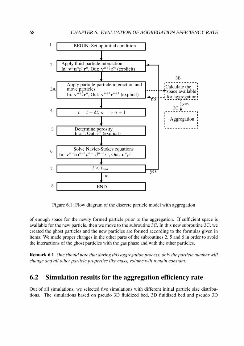
68 CHAPTER 6. EVALUATION OF AGGREGATION EFFICIENCY RATE
1
2
3A
4
5
6
7
8
3B
3C
no
END
yes
BEGIN: Set up initial condition
Apply particle-particle interaction and
t = t + δt, n =⇒ n + 1
Solve Navier-Stokes equations
Apply fluid-particle interaction
move particles
In:rn, Out: εn (explicit)Determine porosity
In: vn−12un−1pn−1βn−1εn, Out: unpn
Calculate the
In: vn+12rn, Out: vn+1rn+1 (explicit)
t < tend
In: vnunpnrn, Out: vn+12βn (explicit)
for aggregationyes
Aggregation
no
space available
Figure 6.1: Flow diagram of the discrete particle model with aggregation
of enough space for the newly formed particle prior to the aggregation. If sufficient space isavailable for the new particle, then we move to the subroutine 3C. In this new subroutine 3C, wecreated the ghost particles and the new particles are formed according to the formulas given initems. We made proper changes in the other parts of the subroutines 2, 5 and 6 in order to avoidthe interactions of the ghost particles with the gas phase and with the other particles.
Remark 6.1 One should note that during this aggregation process, only the particle number willchange and all other particle properties like mass, volume will remain constant.
6.2 Simulation results for the aggregation efficiency rateOut of all simulations, we selected five simulations with different initial particle size distribu-tions. The simulations based on pseudo 3D fluidized bed, 3D fluidized bed and pseudo 3D

6.2. SIMULATION RESULTS FOR THE AGGREGATION EFFICIENCY RATE 69
fluidized bed with discrete normal distribution as the initial particle size distribution.
6.2.1 Aggregation in pseudo 3D fluidized bedBased on the assumptions of the previous Section 6.1, we consider the discrete particle modelsimulations with N0 = 15000 with an initial particle size distribution of satisfying the zerothmoment criteria, i.e. equal number of particles in each size class for pseudo 3D fluidized bed.All the parameters are same as the previous Section 5.3 for pseudo 3D fluidized bed and aregiven in the Appendix A.
We started the aggregation process after 3 seconds of simulation in order to have a well mixedsystem and the simulation ran over a period of 30 seconds. We collected the number of success-ful aggregations in each step (1 second). We try to fit the obtained data with a two parameterpolynomials based on the nature of the aggregation. By using the least square method we evalu-ated the aggregation efficiency function K0(t) and relative error of fitting for each function. Theaggregation efficiency function K0(t) and its corresponding relative error of fitting are given inTable 6.1.
Table 6.1: Aggregation efficiency functions, case 1Aggregation efficiency K0(t) Relative error443.8462− 10.4335t 0.0541454.9983− 12.7408t + 0.0824t2 0.0527474.1814e−0.0361t 0.0551
From the above Table 6.1 we can observe that the relative error corresponding to the quadraticfunction is the smallest. Therefore suitable aggregation efficiency function for this simulationexperiment is given by
K0(t) = 454.9983− 12.7408t + 0.0824t2. (6.3)
The Figure 6.2 shows the aggregation efficiency curve with initial particle size satisfying zerothmoment. The line in the dotted blue color shows the fitted one where as the red color curvecorresponds to the simulated data. We found that the collision frequency function for theseparameters is a shear kernel and the results for these cases are presented in Section 5.3. Thereforethe complete agglomeration kernel is given as
K(t, x, y) = (454.9983− 12.7408t + 0.0824t2)(x13 + y
13 )3. (6.4)
We calculated the aggregation efficiency rate K0(t) with an initial particle size distribution sat-isfying the first moment criterion, i.e. equal total particle volume in each size class. We ran the
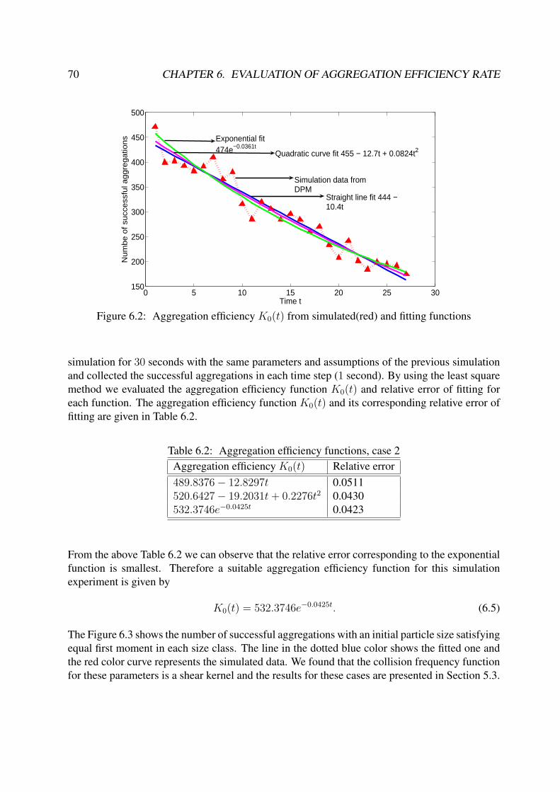
70 CHAPTER 6. EVALUATION OF AGGREGATION EFFICIENCY RATE
0 5 10 15 20 25 30150
200
250
300
350
400
450
500
Time t
Nu
mb
e o
f su
cce
ssfu
l ag
gre
ga
tion
s Exponential fit474e−0.0361t
Simulation data fromDPM
Quadratic curve fit 455 − 12.7t + 0.0824t2
Straight line fit 444 −10.4t
Figure 6.2: Aggregation efficiency K0(t) from simulated(red) and fitting functions
simulation for 30 seconds with the same parameters and assumptions of the previous simulationand collected the successful aggregations in each time step (1 second). By using the least squaremethod we evaluated the aggregation efficiency function K0(t) and relative error of fitting foreach function. The aggregation efficiency function K0(t) and its corresponding relative error offitting are given in Table 6.2.
Table 6.2: Aggregation efficiency functions, case 2Aggregation efficiency K0(t) Relative error489.8376− 12.8297t 0.0511520.6427− 19.2031t + 0.2276t2 0.0430532.3746e−0.0425t 0.0423
From the above Table 6.2 we can observe that the relative error corresponding to the exponentialfunction is smallest. Therefore a suitable aggregation efficiency function for this simulationexperiment is given by
K0(t) = 532.3746e−0.0425t. (6.5)
The Figure 6.3 shows the number of successful aggregations with an initial particle size satisfyingequal first moment in each size class. The line in the dotted blue color shows the fitted one andthe red color curve represents the simulated data. We found that the collision frequency functionfor these parameters is a shear kernel and the results for these cases are presented in Section 5.3.

6.2. SIMULATION RESULTS FOR THE AGGREGATION EFFICIENCY RATE 71
0 5 10 15 20 25 30 350
100
200
300
400
500
600
Time t
Nu
mb
er
of
succ
ess
ful a
gg
reg
atio
ns
Exponential fit 541e−0.0441t
Quadratic curve fit 519 − 18.6t + 0.205t2
Simulation data fromDPM
Straight line fit 475 −11.4917t
Figure 6.3: Aggregation efficiency K0(t) from simulated(red) and fitting functions
Therefore the complete agglomeration kernel is given as
K(t, x, y) = (532.3746e−0.0425t)(x13 + y
13 )3. (6.6)
6.2.2 Aggregation in 3D fluidized bedsIn this section we are presenting the simulation results for a 3D fluidized bed. Based on theassumptions of the Section 6.1, we consider the discrete particle model simulations with N0 =15000 with an initial particle size distribution of satisfying the zeroth moment criteria, i.e. equalnumber of particles in each size class for 3D fluidized bed. All the parameters are same as theprevious section 5.4 for 3D fluidized bed and are given in the Appendix B.
We started the aggregation process after 3 seconds of simulation in order to have a homogeneoussystem and the simulation ran over a period of 30 seconds. We collected the number of successfulaggregations in each step (1 second). We try to fit the obtained data with a two or three parameterpolynomials based on the nature of the aggregation. By using least square method we evaluatedthe aggregation efficiency function K0(t) and relative error of fitting for each function. Theaggregation efficiency function K0(t) and its corresponding relative error of fitting are given inTable 6.3.From the above Table 6.3 we can observe that the relative error corresponding to the exponentialfunction is the smallest. Therefore suitable aggregation efficiency function for this simulationexperiment is given by
K0(t) = 377.7213e−0.0333t. (6.7)

72 CHAPTER 6. EVALUATION OF AGGREGATION EFFICIENCY RATE
Table 6.3: Aggregation efficiency functionsAggregation efficiency K0(t) Relative error357.9373− 8.0220t 0.0550374.4991− 11.4486t + 0.1224t2 0.0528377.7213e−0.0333t 0.0526
The Figure 6.4 shows the aggregation efficiency curve with initial particle size satisfying zeroth
0 5 10 15 20 25 30100
150
200
250
300
350
400
Time t
Num
ber
of s
ucce
ssfu
l agg
rega
tions
Quadratic fit 374.5 − 11.45t + 0.1224t2
Exponential fit 377.7e−0.0333t
Simulation data from DPM
Straight line fit 358 − 8.022t
Figure 6.4: Aggregation efficiency K0(t) from simulated(red) and fitting functions
moment. The line in the dotted blue color shows the fitted one where as the red color curvecorresponds to the simulated data. We found that the collision frequency function for theseparameters is a shear kernel and the results for these cases are presented in Section 5.4. Thereforethe complete agglomeration kernel is given as
K(t, x, y) = (377.7213e−0.0333t)(x13 + y
13 )3. (6.8)
We calculated the aggregation efficiency rate K0(t) with an initial particle size distribution sat-isfying the first moment criteria, i.e. equal total particle volume in each size class. We ran thesimulation for 22 seconds with the same parameters and assumptions of the previous simulationand collected the successful aggregations in each time step (1 second). By using the least squaremethod we evaluated the aggregation efficiency function K0(t) and relative error of fitting foreach function. The aggregation efficiency function K0(t) and its corresponding relative error offitting are given in Table 6.4.
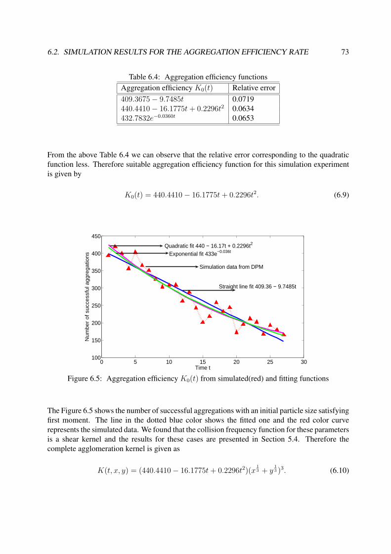
6.2. SIMULATION RESULTS FOR THE AGGREGATION EFFICIENCY RATE 73
Table 6.4: Aggregation efficiency functionsAggregation efficiency K0(t) Relative error409.3675− 9.7485t 0.0719440.4410− 16.1775t + 0.2296t2 0.0634432.7832e−0.0360t 0.0653
From the above Table 6.4 we can observe that the relative error corresponding to the quadraticfunction less. Therefore suitable aggregation efficiency function for this simulation experimentis given by
K0(t) = 440.4410− 16.1775t + 0.2296t2. (6.9)
0 5 10 15 20 25 30100
150
200
250
300
350
400
450
Time t
Nu
mb
er
of s
ucc
ess
ful a
gg
reg
atio
ns
Quadratic fit 440 − 16.17t + 0.2296t2
Simulation data from DPM
Exponential fit 433e−0.036t
Straight line fit 409.36 − 9.7485t
Figure 6.5: Aggregation efficiency K0(t) from simulated(red) and fitting functions
The Figure 6.5 shows the number of successful aggregations with an initial particle size satisfyingfirst moment. The line in the dotted blue color shows the fitted one and the red color curverepresents the simulated data. We found that the collision frequency function for these parametersis a shear kernel and the results for these cases are presented in Section 5.4. Therefore thecomplete agglomeration kernel is given as
K(t, x, y) = (440.4410− 16.1775t + 0.2296t2)(x13 + y
13 )3. (6.10)

74 CHAPTER 6. EVALUATION OF AGGREGATION EFFICIENCY RATE
6.2.3 Aggregation in pseudo 3D fluidized bed with log-normal distributionIn this section we consider a log-normal distribution as an initial particle size distribution. Basedon the assumptions of the Section 6.1, we consider the discrete particle model simulations withN0 = 15000 pseudo 3D fluidized bed. All the parameters are considered same as the Section5.3.1 for pseudo 3D fluidized bed and are given in the Appendix A.
We started the aggregation process after 3 seconds of simulation in order to have a homogeneoussystem and the simulation run over a period of 30 seconds. We collected the number of successfulaggregations in each step (1 second). We try to fit the obtained data with a multi parameterpolynomials based on the nature of the aggregation. By using least square method we evaluatedthe aggregation efficiency function K0(t) and relative error of fitting for each function. Theaggregation efficiency function K0(t) and its corresponding relative error of fitting are given inTable 6.5.
Table 6.5: Aggregation efficiency functionsAggregation efficiency K0(t) Relative error414.9345− 10.2705t 0.0671450.6718− 17.6644t + 0.2641t2 0.0499441.9886e−0.0382t 0.0523
From the above Table 6.5 we can observe that the relative error corresponding to the quadraticfunction to be the smallest. Therefore suitable aggregation efficiency function for this simulationexperiment is given by
K0(t) = 450.6718− 17.6644t + 0.2641t2 (6.11)
The Figure 6.6 shows the aggregation efficiency curve with initial particle size having log-normal distribution. The line in the dotted blue color shows the fitted one where as the red colorcurve corresponds to the simulated data. We found that the collision frequency function for theseparameters is a shear kernel and the results for this case are shown in Section 5.3.1. Thereforethe complete agglomeration kernel is given as
K(t, x, y) = (450.6718− 17.6644t + 0.2641t2)(x13 + y
13 )3. (6.12)
6.3 Numerical methods for population balance equationsAnalytical solutions for the population balance equations exists only for a few cases and for spe-cific kernels. So most of the times one needs to solve these equations using numerical methods.We have a number of methods in the literature. Among these methods the fixed pivot method is
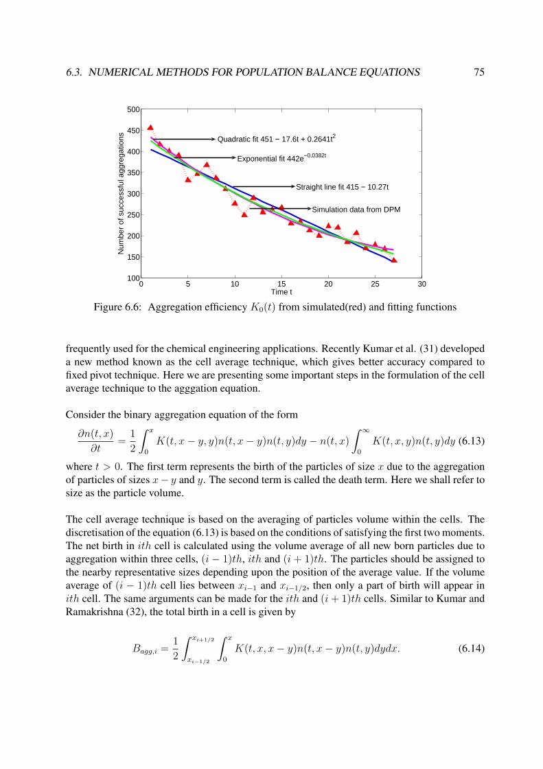
6.3. NUMERICAL METHODS FOR POPULATION BALANCE EQUATIONS 75
0 5 10 15 20 25 30100
150
200
250
300
350
400
450
500
Time t
Num
ber
of s
ucce
ssfu
l agg
rega
tions Quadratic fit 451 − 17.6t + 0.2641t2
Exponential fit 442e−0.0382t
Straight line fit 415 − 10.27t
Simulation data from DPM
Figure 6.6: Aggregation efficiency K0(t) from simulated(red) and fitting functions
frequently used for the chemical engineering applications. Recently Kumar et al. (31) developeda new method known as the cell average technique, which gives better accuracy compared tofixed pivot technique. Here we are presenting some important steps in the formulation of the cellaverage technique to the agggation equation.
Consider the binary aggregation equation of the form
∂n(t, x)
∂t=
1
2
∫ x
0
K(t, x− y, y)n(t, x− y)n(t, y)dy − n(t, x)
∫ ∞
0
K(t, x, y)n(t, y)dy (6.13)
where t > 0. The first term represents the birth of the particles of size x due to the aggregationof particles of sizes x− y and y. The second term is called the death term. Here we shall refer tosize as the particle volume.
The cell average technique is based on the averaging of particles volume within the cells. Thediscretisation of the equation (6.13) is based on the conditions of satisfying the first two moments.The net birth in ith cell is calculated using the volume average of all new born particles due toaggregation within three cells, (i − 1)th, ith and (i + 1)th. The particles should be assigned tothe nearby representative sizes depending upon the position of the average value. If the volumeaverage of (i − 1)th cell lies between xi−1 and xi−1/2, then only a part of birth will appear inith cell. The same arguments can be made for the ith and (i + 1)th cells. Similar to Kumar andRamakrishna (32), the total birth in a cell is given by
Bagg,i =1
2
∫ xi+1/2
xi−1/2
∫ x
0
K(t, x, x− y)n(t, x− y)n(t, y)dydx. (6.14)

76 CHAPTER 6. EVALUATION OF AGGREGATION EFFICIENCY RATE
Mathematically the number density function n(t, x) can be approximated in terms of Dirac-deltadistributions as
n(t, x) =I∑
i=1
Niδ(x− xi). (6.15)
We first discretize the birth to compute the total birth rate in each cell and then redistribute thetotal birth to the neighboring nodes to get the consistency with moments. Since particles areassumed to be concentrated at representative sizes xi, the number density n(t, x) can be replacedby its Dirac-delta representation (6.15). Substituting the Dirac-delta representation of n(t, x) inequation (6.14), for details of derivation see (30), we obtain
Bagg,i =
j≥k∑j,k
xi−1/2≤(xj+xk)<xi+1/2
(1− 1
2δj,k
)Kj,kNjNk. (6.16)
Thus, Bi is the net rate of addition of particles to cell i by aggregation of particles in lower cells.The net flux of volume Vi into cell i as a result of these aggregations is therefore given by
Vagg,i =
j≥k∑j,k
xi−1/2≤(xj+xk)<xi+1/2
(1− 1
2δj,k
)Kj,kNjNk(xj + xk). (6.17)
Consequently, the average volume of all newborn particles in the ith cell vi can be evaluated as
vagg,i =Vagg,i
Bagg,i
. (6.18)
Now we assume that the newborn particles Bi are assigned temporarily at vi. These particleshave to be divided depending upon the value of vi to neighboring nodes in such a way that theformulation is consistent with the total number and mass. The birth according to the cell averagetechnique is given as
BCAagg,i = Bagg,i−1λ
−i (vi−1)H(vi−1 − xi−1) + Bagg,iλ
−i (vi)H(xi − vi)
+Bagg,iλ+i (vi)H(vi − xi) + Bagg,i+1λ
+i (vi+1)H(xi+1 − vi+1). (6.19)
The function λ is defined as
λ±i (v) =v − vi±1
vi − vi±1
.
The Heaviside step function is a discountinuous function also known as unit step function and isdefined as
H(x) =
1, x > 012, x = 0
0, x < 0.(6.20)

6.4. COMPUTATION OF THE PARTICLE SIZE DISTRIBUTIONS 77
The death term is the same as it was in Kumar and Ramakrishna (32) and is given as
Dagg,i = Ni
I∑k=1
Ki,kNk. (6.21)
The final set of discrete equations can be written as
dNi(t)
dt= Bagg,i−1λ
−i (vi−1)H(vi−1 − xi−1) + Bagg,iλ
−i (vi)H(xi − vi)
+Bagg,iλ+i (vi)H(vi − xi) + Bagg,i+1λ
+i (vi+1)H(xi+1 − vi+1)
−Ni
I∑k=1
Ki,kNk. (6.22)
The set of ordinary differential equations (6.22) resulting from the discretized technique is solvedusing a Runge-Kutta fourth and fifth order method with adaptive step-size control based on theembedded Runge-Kutta formulas.
Higher order schemes are also developed by Sandu (45) based on Newton-Cotes quadratureapproach. He employed a semi-implicit Gauss-Seidel time integration method to the aggregationequation. This method gives fourth order accuracy. For the present comparison we uses ourinhouse code of cell average technique, whose accuracy is enough for our present application.
6.4 Computation of the particle size distributionsIn this section we calculated the particle size distribution by solving the aggregation equationswith the newly calculated shear kernels obtaind from the previous sections. A recently developedcell average technique is used to solve the aggregation equation and is explained in the Section6.3. We computed the particle size distributions for the new kernels obtained from the micromodel. The results of the new particle size distributions are presented in Section 6.4 for differentpossible cases.
6.4.1 Computation of the particle size distribution for pseudo 3D fluidizedbed
We considered two specific cases for the computation of the macro aggregation model. In thefirst case we considered the initial particle size distribution satisfying zeroth moment criteria,i.e. equal number of particles in each size class. For both the aggregation equation and discreteparticle simulations we have taken the same initial condition and can be seen in the Figure 6.7 asblue line.
The final particle size distribution at the end of 30 seconds is plotted in the Figure 6.7 as the redline. For this specific simulation we calculated the aggregation kernel (6.3) using least square

78 CHAPTER 6. EVALUATION OF AGGREGATION EFFICIENCY RATE
fit in the Section 6.2. We substituted the kernel (6.3) into the aggregation and then we solved itusing cell average technique developed by Kumar (30). We calculated the number of particles ineach class from the aggregation equation and the result can be seen in the Figure 6.7. In a similar
10−10
10−9
10−8
10−7
0
500
1000
1500
2000
2500
3000
cells
Num
ber
in e
ach
cell
Initial distributionfinal distribution
Figure 6.7: Aggregation starting with equal number (zero moment) criterion for pseudo 3D bed
manner we calculated the particle size distribution for the aggregation equation with the initialparticle size distribution satisfying first moment criteria. The aggregation kernel calculated fromthe discrete particle model simulations was given in (6.4).
10−10
10−9
10−8
10−7
0
1000
2000
3000
4000
5000
6000
7000
cells
Num
ber
in e
ach
cell
Initial distributionfinal distribution
Figure 6.8: Aggregation starting with equal volume (first moment) criterion for pseudo 3D bed

6.4. COMPUTATION OF THE PARTICLE SIZE DISTRIBUTIONS 79
6.4.2 Computation of the particle size distribution for 3D fluidized bed
We considered two specific cases for the computation of the particle size distribution using theaggregation equation. In the first case we considered the initial particle size distribution satis-fying zeroth moment criteria, i.e. equal number of particles in each size class. For both theaggregation equation and discrete particle simulations we have taken the same initial conditionand can be seen in the Figure 6.9 as blue line.
The final particle size distribution at the end of 30 seconds is plotted in the Figure 6.9 as the redline. For this specific simulation we calculated the aggregation kernel (6.5) using least squarefit in the Section 6.2. We substituted the kernel (6.5) into the aggregation and then we solved itusing cell average technique developed by Kumar (30). We calculated the number of particles ineach class from the aggregation equation and the result can be seen in the Figure 6.9.
10−10
10−9
10−8
10−7
0
500
1000
1500
2000
2500
3000
cells
Num
ber
in e
ach
cell
Initial distributionfinal distribution
Figure 6.9: Aggregation starting with equal number (zero moment) criterion for 3D bed
In a similar manner we calculated the particle size distribution for the aggregation equation withthe initial particle size distribution satisfying first moment criteria. We considered the same initialcondition for the simulations in the discrete particle model. The aggregation kernel calculatedfrom the discrete particle model simulations was given in (6.6).
6.4.3 Computation of the particle size distribution for 3D fluidized bedwith log normal distribution
We considered a specific case for the computation of the particle size distribution from the ag-gregation equation. In this case we considered the initial condition having a log normal particlesize distribution. For both the aggregation equation and discrete particle simulations we have
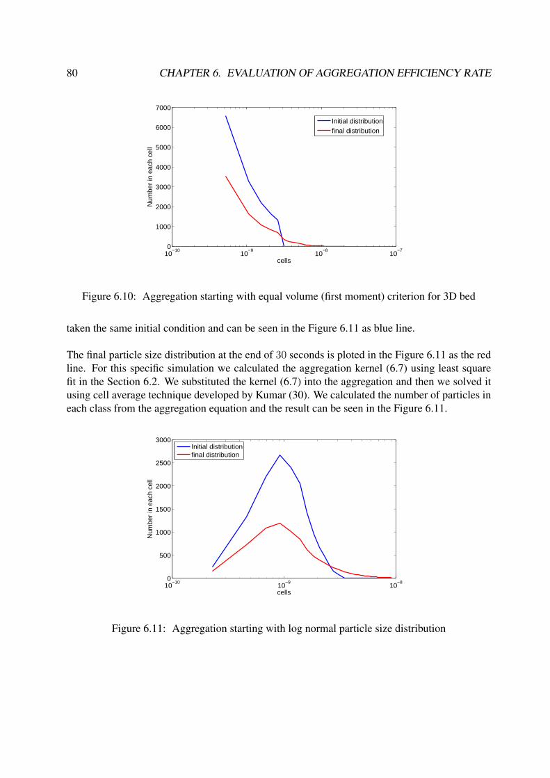
80 CHAPTER 6. EVALUATION OF AGGREGATION EFFICIENCY RATE
10−10
10−9
10−8
10−7
0
1000
2000
3000
4000
5000
6000
7000
cells
Num
ber
in e
ach
cell
Initial distributionfinal distribution
Figure 6.10: Aggregation starting with equal volume (first moment) criterion for 3D bed
taken the same initial condition and can be seen in the Figure 6.11 as blue line.
The final particle size distribution at the end of 30 seconds is ploted in the Figure 6.11 as the redline. For this specific simulation we calculated the aggregation kernel (6.7) using least squarefit in the Section 6.2. We substituted the kernel (6.7) into the aggregation and then we solved itusing cell average technique developed by Kumar (30). We calculated the number of particles ineach class from the aggregation equation and the result can be seen in the Figure 6.11.
10−10
10−9
10−8
0
500
1000
1500
2000
2500
3000
cells
Num
ber
in e
ach
cell
Initial distributionfinal distribution
Figure 6.11: Aggregation starting with log normal particle size distribution
Chapter 7
General conclusions and outlook
The main aim of the present thesis is to have a complete idea of micro-macro transisitions ofgranulation processes in the fluidized beds. We have different processes inside the fluidized bedslike aggregation, growth, nucleation, breakage, etc. To understand these processes in a macro-scopic level population balance equations are widely used in the literature. The present workinvolves the simulations for modelling the aggregation kernels of the Smoluchowski (49) equa-tion. This equation describes the coagulation of particles, when they come in contact with oneanother, on a macroscopic scale. As a result of this aggregation process the particle size dis-tribution will change in a given system due to various physical influences. The most importantquantity in this modeling is the aggregation kernel. In general, this aggregation kernel is a func-tion of time and particle diameter, volume, mass, etc and the physical and chemical processesinfluencing the aggregation. An elaborative discussion of the aggregation equation and variouskernels were presented in Chapter 2.
To model the aggregation kernels we used a micro model known as Discrete Particle Model(DPM) and it was developed by Prof. J. A. M. Kuipers group, University of Twente, The Nether-lands (29). The present Discrete Particle Model (DPM) involves both particle and gas phases.The particle phase is described by using Newton’s equation of motion for each particle as a singleentity. The continuous gas phase is described using volume averaged Navier-Stokes equationsunder isothermal conditions. The interaction between particles and gas phase is coupled throughtwo terms, porosity and momentum exchange source term. The porosity in each cell is calcu-lated by direct calculation of the volume of the particles present in a cell where as the momentumexchange source term is derived from lattice Boltzmann simulations. For solving the Newton’sequations we used a first order integration scheme. The gas phase equations are solved usingSIMPLE (Semi Implicit Method for Pressure Linked Equations) scheme. The particle interac-tions are resolved through binary hard sphere collision model. We used a smaller time step forthe calculation of the particle interactions compared to the gas phase equations.
A novel technique for calculating the particle collisions from the dynamic discrete particle sim-ulations of non-homogeneous granular flows of the particles was presented in Chapter 4. It wasobserved that the self collisions among the particles of the same size class were neglected in the
81
82 CHAPTER 7. GENERAL CONCLUSIONS AND OUTLOOK
Smoluchowski equation. The effect of this term was analyzed for discrete particle model simu-lations, we found that the effect of this term may be neglected for a large number of particles.We calculated the particle Reynolds number and it was observed that the shear forces are moredominent in the present fluidized bed simulations. Therefore a shear kernel is expected.
To calculate the collisions among the particles, we introduced new subroutines in the existingDiscrete Particle Model code. We introduced a new parameter known as the bed parameter inorder to understand macroscopic characters on the particle collisions. We considered differentinitial particle size distributions satisfying equal number of particles (zeroth moment), equallength, equal surface area, equal volume (first moment) criteria for each size class and a discretelog-normal particle size distribution. The effect of various initial particle size distributions onthe bed parameter were analyzed for pseudo three dimensional and three dimensional simulatedfluidized beds.
The evolution of the particle size distribution that results from the aggregation are presented inthe Chapter 6. We evaluated the particle aggregation efficiency for different initial particle sizedistributions. We incorporated a random aggregation mechanism for the aggregation of two par-ticles. As a result of this aggregation a new particle of larger size is formed and the other particledisappeared, we call this particle a ghost particle. This ghost particle has no physical significancein the simulation and proper modifications were made in order to avoid its presence for the rest ofthe simulation time. The number of ghost particles formed is equal to the number of successfulaggregations. We evaluated the aggregation efficiency rate for each simulation by collecting thenumber of successful aggregations and the resulting new particle size distribution. Therefore, weare able to model aggregation kernels from these micro simulations. We calculated the particlesize distribution from the macro model known as aggregation equation with these new kernels.The aggregation equation with these newly simulated kernels was solved by using the cell aver-age technique.
It was demonstrated in the thesis that the Discrete Particle Model (micro models) is an excellenttool to provide detailed information about the basic particle flow characteristics, which are (ex-tremely) difficult if not impossible to obtain from experiments. The present modelling approachcan be used to various types of fluidized beds like spouted fluidezed beds, circulating fluidizedbeds, risers, etc. In the future, we intend to incorporate the physically relevent aggregation mech-anism for the aggregation process by spraying the liquid binder on to particles. To model suchapplications one needs to extend the present model with the inclusion of a liquid droplet phaseand nozzle. A multi particle aggregation can be simulated by considering the particle interactionswith a soft sphere collision model, but the computational time will be expensive.
Comparing the present aggregation kernels with the experiments would be valuable for designingindustrial level fluidized beds.
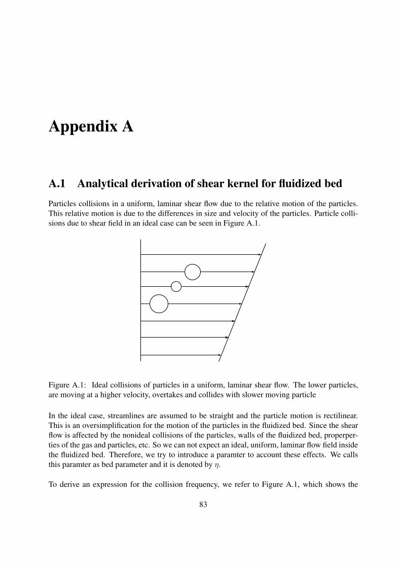
Appendix A
A.1 Analytical derivation of shear kernel for fluidized bed
Particles collisions in a uniform, laminar shear flow due to the relative motion of the particles.This relative motion is due to the differences in size and velocity of the particles. Particle colli-sions due to shear field in an ideal case can be seen in Figure A.1.
Figure A.1: Ideal collisions of particles in a uniform, laminar shear flow. The lower particles,are moving at a higher velocity, overtakes and collides with slower moving particle
In the ideal case, streamlines are assumed to be straight and the particle motion is rectilinear.This is an oversimplification for the motion of the particles in the fluidized bed. Since the shearflow is affected by the nonideal collisions of the particles, walls of the fluidized bed, properper-ties of the gas and particles, etc. So we can not expect an ideal, uniform, laminar flow field insidethe fluidized bed. Therefore, we try to introduce a paramter to account these effects. We callsthis paramter as bed parameter and it is denoted by η.
To derive an expression for the collision frequency, we refer to Figure A.1, which shows the
83

84 APPENDIX A.
particle interactions due to shear flow. As shown in figure 1 the particle of radius ai collides withthe particle of radius aj due to their relative difference in the velocity, as shown in Figure A.2.
X
ai + aj
θ
dx
Figure A.2: Geometry for coagulation in a laminar shear field
The velocity of the particle normal to the surface of the page, relative to the particle shown isxdu
dx. Hence flow of the particles into the shaded portion of the strip dx is given by
F = ηnjxdu
dx(ai + aj) sin θdx.
Here we introduced the parameter η to account for the distorted shear flow due to non-idealparticle collisions, effects of the boundary of the bed,...etc. Since x = (ai + aj) cos θ, the totalnumber of particles entering into the central sphere is given by
F = 2(2)ηnj
π2∫
0
(ai + aj)3du
dxsin2 θcosθdθ
where the first factor 2 takes into the account of particles entering from the upper hemispherefrom this side plus the particles entering from the bottom hemisphere from back side. The secondfactor 2 is necessary because the integration from 0 to π
2must be done twice. Carrying out the

A.2. ANALYTICAL SOLUTION FOR SHEAR KERNEL FOR MONODISPERSE INITIAL CONDITIONS85
integration the result is
F =4
3η(ai + aj)
3du
dxnj
⇒ Nij =4
3η(ai + aj)
3du
dxninj
⇒ Nij = ηβ(ai, aj)ninj
where β(ai, aj) = 43(ai + aj)
3 dudx
is the collision frequency function for the coagulation of theparticles by laminar shear flow. When we consider the volume of the particles, the collisionfrequency function for the laminar shear flow is given by
β(vi, vj) =4
3(v
13i + v
13j )3du
dx.
A.2 Analytical solution for shear kernel for monodisperse ini-tial conditions
The discrete coagulation equation for the laminar shear kernel is:
dnk
dt=
1
2
∑i+j=k
[4
3(ai + aj)
3du
dxninj]−
∞∑i=1
4
3(ai + aj)
3du
dxnink
If the system is composed of particles that are all of nearly the same size, ai ≈ a, then the aboveequation becomes
dnk
dt=
1
2
∑i+j=k
[32
3a3du
dxninj]−
∞∑i=1
32
3a3du
dxnink.
Summing over all k, the result is
dN∞
dt= −16
3
du
dxa3N2
∞.
But 43πa3N∞ = V = constant
dN∞
dt= −4V
π
du
dxN∞.
Here the decay is proportional to N∞, where as for the Brownian kernel it is proportional to N2∞
in the continuum range. Let N = N∞(0) be the initial number of particles at t = 0. Then solvingthe above equation subject to this initial condition gives:
dN∞
dt= −4V
π
du
dxN∞
N = N∞(0)

86 APPENDIX A.
N∞(t) = C1e− 4V
πdudx
t
∵ N∞(0) = C1e0
⇒ C1 = N∞(0)
∴ lnN∞(t)
N∞(0)=
4V
π
du
dxt

Appendix B
B.1 Physical and Numerical parameters of the simulations
Table B.1: The Parameters for the simulationParameter ValueTime step of calculation ∆t 1.00e-4 secSimulation time 15 secBed propertiesHeight 0.30 mWidth 0.10 mDepth 0.01 m (pseudo 3D bed),
0.10 m 3D bedParticle propertiesMaterial glass particlesNumber of primary particles 5000, 10000, 15000Diameter dα 1.0e-3 m pseudo 3D bed
1.8e-3 m 3D bedDensity ρ 2500 kg/m3
Gas propertiesFluidisation velocity u 2.4 m/secViscosity µ 1.82e-5 kg/msDensity ρg 1.21 kg/m3
Temperature T 298 KGas constant R 8.314 J/(mol K)Average molecular weight of air Mg 28.8e-3 kg/molParticle contact constantsSpring coefficient k 5.0e+5Restitution coefficient e 0.98Friction coefficient 0.09
87
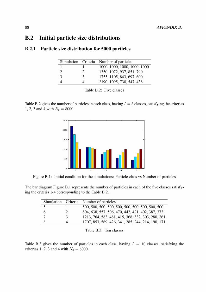
88 APPENDIX B.
B.2 Initial particle size distributions
B.2.1 Particle size distribution for 5000 particles
Simulation Criteria Number of particles1 1 1000, 1000, 1000, 1000, 10002 2 1350, 1072, 937, 851, 7903 3 1755, 1105, 843, 697, 6004 4 2190, 1095, 730, 547, 438
Table B.2: Five classes
Table B.2 gives the number of particles in each class, having I = 5 classes, satisfying the criterias1, 2, 3 and 4 with N0 = 5000.
Figure B.1: Initial condition for the simulations: Particle class vs Number of particles
The bar diagram Figure B.1 represents the number of particles in each of the five classes satisfy-ing the criteria 1-4 corresponding to the Table B.2.
Simulation Criteria Number of particles5 1 500, 500, 500, 500, 500, 500, 500, 500, 500, 5006 2 804, 638, 557, 506, 470, 442, 421, 402, 387, 3737 3 1213, 764, 583, 481, 415, 368, 332, 303, 280, 2618 4 1707, 853, 569, 426, 341, 285, 244, 214, 190, 171
Table B.3: Ten classes
Table B.3 gives the number of particles in each class, having I = 10 classes, satisfying thecriterias 1, 2, 3 and 4 with N0 = 5000.
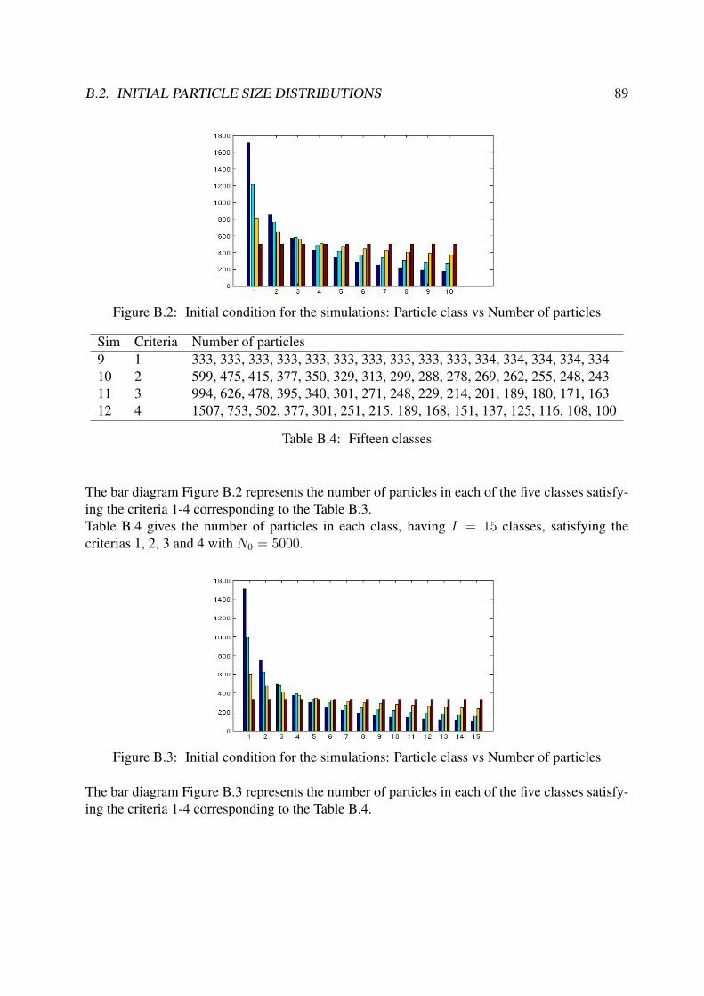
B.2. INITIAL PARTICLE SIZE DISTRIBUTIONS 89
Figure B.2: Initial condition for the simulations: Particle class vs Number of particles
Sim Criteria Number of particles9 1 333, 333, 333, 333, 333, 333, 333, 333, 333, 333, 334, 334, 334, 334, 33410 2 599, 475, 415, 377, 350, 329, 313, 299, 288, 278, 269, 262, 255, 248, 24311 3 994, 626, 478, 395, 340, 301, 271, 248, 229, 214, 201, 189, 180, 171, 16312 4 1507, 753, 502, 377, 301, 251, 215, 189, 168, 151, 137, 125, 116, 108, 100
Table B.4: Fifteen classes
The bar diagram Figure B.2 represents the number of particles in each of the five classes satisfy-ing the criteria 1-4 corresponding to the Table B.3.Table B.4 gives the number of particles in each class, having I = 15 classes, satisfying thecriterias 1, 2, 3 and 4 with N0 = 5000.
Figure B.3: Initial condition for the simulations: Particle class vs Number of particles
The bar diagram Figure B.3 represents the number of particles in each of the five classes satisfy-ing the criteria 1-4 corresponding to the Table B.4.
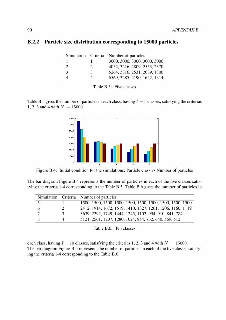
90 APPENDIX B.
B.2.2 Particle size distribution corresponding to 15000 particles
Simulation Criteria Number of particles1 1 3000, 3000, 3000, 3000, 30002 2 4052, 3216, 2809, 2553, 23703 3 5264, 3316, 2531, 2089, 18004 4 6569, 3285, 2190, 1642, 1314
Table B.5: Five classes
Table B.5 gives the number of particles in each class, having I = 5 classes, satisfying the criterias1, 2, 3 and 4 with N0 = 15000.
Figure B.4: Initial condition for the simulations: Particle class vs Number of particles
The bar diagram Figure B.4 represents the number of particles in each of the five classes satis-fying the criteria 1-4 corresponding to the Table B.5. Table B.6 gives the number of particles in
Simulation Criteria Number of particles5 1 1500, 1500, 1500, 1500, 1500, 1500, 1500, 1500, 1500, 15006 2 2412, 1914, 1672, 1519, 1410, 1327, 1261, 1206, 1160, 11197 3 3639, 2292, 1749, 1444, 1245, 1102, 994, 910, 841, 7848 4 5121, 2561, 1707, 1280, 1024, 854, 732, 640, 569, 512
Table B.6: Ten classes
each class, having I = 10 classes, satisfying the criterias 1, 2, 3 and 4 with N0 = 15000.The bar diagram Figure B.5 represents the number of particles in each of the five classes satisfy-ing the criteria 1-4 corresponding to the Table B.6.
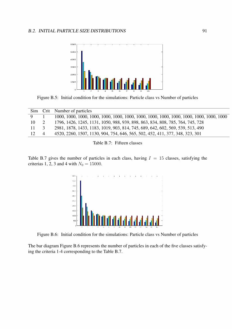
B.2. INITIAL PARTICLE SIZE DISTRIBUTIONS 91
Figure B.5: Initial condition for the simulations: Particle class vs Number of particles
Sim Crit Number of particles9 1 1000, 1000, 1000, 1000, 1000, 1000, 1000, 1000, 1000, 1000, 1000, 1000, 1000, 1000, 100010 2 1796, 1426, 1245, 1131, 1050, 988, 939, 898, 863, 834, 808, 785, 764, 745, 72811 3 2981, 1878, 1433, 1183, 1019, 903, 814, 745, 689, 642, 602, 569, 539, 513, 49012 4 4520, 2260, 1507, 1130, 904, 754, 646, 565, 502, 452, 411, 377, 348, 323, 301
Table B.7: Fifteen classes
Table B.7 gives the number of particles in each class, having I = 15 classes, satisfying thecriterias 1, 2, 3 and 4 with N0 = 15000.
Figure B.6: Initial condition for the simulations: Particle class vs Number of particles
The bar diagram Figure B.6 represents the number of particles in each of the five classes satisfy-ing the criteria 1-4 corresponding to the Table B.7.
Bibliography
[1] Adetayo, A. A., B. J. Ennis., 1997, ” Unifying approach to modelling granule coalescencemechanisms”, AIChE Journal, 43(4), 927-934.
[2] Anderson, T. B., R. Jackson., 1967, ” A fluid mechanical description of fluidized beds”, I& EC Fundamentals, 6(4), 527-539.
[3] Beetstra, R., M. A. van der Hoef., J. A. M. Kuipers., 2007, ”Numerical study of segregationusing a new drag force correlation for polydisperse systems derived from lattice-Boltzmannsimulations”, Chemical Engineering Science, 62, 246-255.
[4] Berry, E. X., 1967, ”Cloud droplet growth by collection”, Journal of Atmospheric Science,24, 688-701.
[5] Bertram. A., Jürgen Tomas, (Editors)., 2008, ”Micro-Macro-Interactions,”in StructuredMedia and Particle Systems, Springer-Verlag, Heidelberg.
[6] Bramley, A. S., M. J. Hounslow., R. L. Ryall., 1996, ” Aggregation during precipitationfrom solution: A method for extracting rates from experimental data”, Journal of Colloidand Interface Science, 183, 155-165.
[7] Cameron, I. T., F. W. Wang., C. D. Immanuel., F. Stepanek., 2005, ”Process systems mod-elling and applications in granulation: A review”, Chemical Engineering Sceince, 60, 3723-3750.
[8] Chamakuri, N., 2007, ” Adaptive numerical simulation of reaction-diffusion systems”, PhDthesis, Otto-von-Guericke University, Magdeburg.
[9] Costa, C. B.B., M. R. W. Maciel., R. Maciel Filho., 2006, ”Considerations on the crys-tallizating modelling: Populating balance solution”, Computers & Chemical Engineering,doi:10.1016/j.compchemeng.2006.06.005.
[10] Cryer, S. A., 1999, ”Modeling agglomeration processes in fluid-bed granulation”, AIChEJournal, 45(10), 2069-2078.
[11] Deen, N. G., M. Van Sint Annaland., M. A. Van der Hoef., J. A. M. Kuipers., 2006,”Review of discrete particle modeling of fluidized beds”, Chemical Engineering Sceince,doi:10.1016/j.ces.2006.08.014.
92
BIBLIOGRAPHY 93
[12] Drake, R. L., 1970, ”A General Mathematical Survey of the Coagulation Equation,”in Top-ics in Current Aerosol Research, (part 2), (G. M. Hidy and J. R. Brock, Eds.), p. 315,Pergamon Press, Newyork.
[13] Ergun, S., 1952, ”Fluid flow through packed columns”, Chemical Engineering Progress,48, 89-94.
[14] Friedlander, S. K., 1977, ”Smoke, Dust, and Haze: Fundamentals of Aerosol Dynamics”,Oxford University Press, NewYork.
[15] Gantt, J. A., I. T. Cameron., J. D. Litster., E. P. Gatzke., 2006, "Determination of coa-lescence kernels for high-shear granulation using DEM simulations", Powder Technology,170, 53-63.
[16] Godlieb, W., 2005, ”Simulating a granulator using the discrete particle model” Mastersthesis, University of Twente, The Netherlands.
[17] Goldsmith, M. J. V., 2001, ”Hydrodynamics modelling of fluidized bed spray granulation.”PhD thesis, University of Twente, The Netherlands.
[18] Handwerker, J., 2007, ”Vorlesung radarmeteorologie 2006/2007”, Institut für meteorologieund klimaforschung., Karlsruhe, 1-72.
[19] Hintz, W., Tzv. Nikolov., V. Jaordanova., J. Tomas., 2003, ”Preparation of titanium dioxidenanoparticles and their characterisation”, Nanoscience & Nanotechnology, 3, 73-76.
[20] Hoomans, B. P. B., 2000, ”Granular dynamics of Gas-Solid two-phase flow.” PhD thesis,University of Twente, The Netherlands.
[21] Hoomans, B. P. B., J. A. M. Kuipers., W. J. Briels., and W. P. M. van Swaaij., 1996,”Discrete particle simulation of the bubble and slug formation in a two-dimensional gas-fluidised bed, A hard sphere approach” Chemical Engineering Science, 51(1), 99-108.
[22] Hounslow, M. J., 1998, ”Some problems in particle technology: A statistical mechanicalformulation”, KONA., 19, 555.
[23] Hounslow, M. J., 1990, ”Nucleation, growth, and aggregation rates from steady-state ex-perimental data”, AIChE Journal., 36(11), 1748-1752.
[24] Hu, K. C., R. Mei., 1998, ”A note on particle collision rate in fluid flows”, Phys. Fluids,10, 1028-1030.
[25] Hulburt, H. M., S. Katz., 1964, ”Some problems in particle technology: A statistical me-chanical formulation”, Chem. Eng. Sci., 19, 555.
[26] Kapur, P. C., D. W. Fuerstenau., 1966, ” Size distributions and kinetic relationships in thenuclei region of wet pelletization”, I & EC Process design and development, 5(1), 5-10.
94 BIBLIOGRAPHY
[27] Kapur, P. C., 1972, ” Kinetics of granulation by non-random coalescence mechanism”,Chemical Engineering Science, 27, 1863-1869.
[28] Kapur, P. C., D. W. Fuerstenau., 1969, ”A coalescence model for granulation”, I & ECProcess Design and Development, 8(1), 56-62.
[29] Kuipers, J. A. M., Van Duin, K. J., Van Beckum, F. P. H., Van Swaaij, W. P. M., 1992, ”Anumerical model of gas-fluidized beds”, Chemical Engineering Science, 47(8), 1913-1924.
[30] Kumar, J., 2006, ”Numerical approximations of population balance equations in particulatesystems”,PhD thesis, Otto-von-Guericke University, Magdeburg. ISBN 3-93939665-13-4.
[31] Kumar, J., Peglow, M., Warnecke, G., Heinrich, S., Mörl, L., 2006, ”Improved accuracyand convergence of discretized population balance for aggregation: The cell average tech-nique”,Chemical Engineering Science, 61, 3327-3342.
[32] Kumar, S., Ramakrishna, D., 1996, ”On the solution of population balance equations bydiscretization -I. A fixed pivot technique.”, Chemical Engineering Science, 51, 1311-1332.
[33] Link, J. M., L.A., Cuypers, N. G. Deen and J. A. M. Kuipers. 2005, ”Flow regimes in aspout fluid bed: a combined experimental and simulation study.” Chemical EngineeringScience, 60, (13): 3425-3442.
[34] Litster, J., B. Ennis., L. Liu., 2004, ”The science and engineering of granulation process”,Kluwer Academic Publishers, The Netherlands.
[35] Liu, L. X., Litster, J. D., Iveson, S. M., Ennis, B. J., 2000, ”Coalescence of deformablegranules in wet granulation processes”, AIChE Journal, 46(3), 529-539.
[36] Müller, H., 1922, ”A calculation procedure for heat, mass and momentum transfer in three-dimensional parabolic flow.” Int. J. Heat and Mass Transfer, vol 15: 1787.
[37] Norio, O., Tatsuo, T., 1975, ” The probability of coalescence in granulation kinetics”, I &EC Process Design and Development, 14(3), 286-289.
[38] Patankar, S. V. and Spalding, D. B. 1972, ”A calculation procedure for heat, mass andmomentum transfer in three-dimensional parabolic flow.” Int. J. Heat and Mass Transfer,vol 15: 1787.
[39] Peglow, M., 2003, ” Population Balance Modelling”, PhD thesis, Otto-von-Guericke Uni-versity, Magdeburg.
[40] Pouw, A. G., Daan Verkoeijn., G. M. H. Meesters., B. Scarlett., 2002, ”Population balancesfor particulate processes-a volume apporach”, Chemical Engineering Science, 57 , 2287-2303.
[41] Pruppacher, H. R. and J. D. Klett., 1996, ”Microphysics of clouds and precipitation”,Kluwer Adademic Publishers, Dordecht, The Netherlands.
BIBLIOGRAPHY 95
[42] Quarteroni. A., 2009, ” Mathematical models in science and engineering”, Notices of AMS,56(1), 10-19.
[43] Ramakrishna, D., 2000, ”Population balances: Theory and Applications to Particulate Sys-tems in Engineering”, Academic Press, San Diego, CA.
[44] Rynhart, P. R., 2004, ”Mathematical modelling of granulation process”,PhD thesis, MasseyUniversity, New Zealand.
[45] Sandu, A., 2002, ”A Newton-Cotes quadrature approach for solving the aerosol coagulationequation”, Atmospheric Environment, 36, 583-589.
[46] Sastry, K. V. S., 1975, ”Similarity size disribution of agglomerates during their growth bycoalescence in granulation or green pelletization.” International Journal of Mineral Pro-cessing. 2, 187-203.
[47] Sastry, K. V. S., D. W. Fuerstenau., 1970, ”Size distribution of agglomerates in coalescingdispersed phase systems.” I & EC Fundamentals. 9(1), 145-149.
[48] Smoluchowski, M. V., 1916, ”Drei Vortrage uber Diffusion, Brownische Molekularbewe-gung und Koagulation von Kolloidteilchen”, Phys. Z., 17, 557.
[49] Smoluchowski, M. V., 1917, ”Mathematical theory of the kinetics of the coagulation ofcolloidal solutions”, Z. Phys. Chem., 92, 129-168.
[50] Stefan Heinrich., 2001, ”Modellierung des wärmeund stoffübergangs sowie der par-tikelpopulationen bei der wirbelschicht-sprühgranulation”, PhD thesis, Otto-von-GuerickeUniversity, Magdeburg. ISBN 3-18-367503-X.
[51] Tan, H. S., M. J. V. Goldschmidt., R. Boerefijn., M. J. Hounslow., A. D. Salman., J. A.M. Kuipers., 2004, ”Building population balance model for fluidized bed melt granulation:lessons from kinetic theory of granular flow”, Powder Technology, 142, 103-109.
[52] Tatang M. A., 1995, ”Direct incorporation of uncertainity in chemical and environmentalengineering systems”, PhD Thesis, MIT, Cambridge, MA.
[53] Wen, Y. C., Yu, Y. H., 1966, ”Mechanics of Fluidization. Chemical engineering progresssymposium series”, 62, 100-111.
[54] Yang, W. C., 2003, ”Handbook of fluidization and fluid-particle systems”, Dekker,NewYork.
[55] Zeilstra. C., A. Bokkers., 2005, ”3D-DPM manual”, Fundamental of Chemical and Reac-tion Group, University of Twente, The Netherlands.
Curriculum VitaePersonal DetailsName : Narni Nageswara RaoSex : MaleMartial status : SingleDate of birth : 01.07.1979Place of birth : Kappaladoddi, Krishna, A. P.Nationality : Indian
Education and Employment
1991-1994 High Schoolings, A. P. Residential School, Nimmakuru, India
1994-1996 Intermediate in Mathematics, Physics, ChemistryThe Hindu College, Machilipatnam, India
1996 - 1999 Bachelor of Science (B.Sc.) in Mathematics, Physics, ChemistryA. P. Residential Degree Collge, Nagarjuna Sagar, India
1999 - 2001 Master of Science (M.Sc.) in Applied MathematicsRegional Engineering College (REC) Warangal, India
2001 - 2002 Master of Philosophy (M.Phil.) in Applied MathematicsUniversity of Hyderabad, India
2002 - 2003 Temporary Assistant Lecturer in MathamticsNational Institute of Technology Karnataka (NITK), India
2003 - 2005 Master of Technology (M.Tech.) in Industrial Mathematics andScientific Computing,Indian Institute of Technology Madras, India
2005 - 2008 PhD graduation (DFG scholarship) within theGraduiertenkolleg, “GK 828”, Faculty of Mathematics,Otto-von-Guericke-University, Magdeburg, Germany.
Academic Honors
• Qualified National Eligibility Test (NET)-2002.
• DAAD-IIT Academic Exchange Fellowship, Germany (2004-2005).
• German Research Foundation (DFG) Graduiertenkolleg Scholarship (2005-2008).
96