SIMULATION RESULTS ON BUFFER ALLOCATION IN A CONTINUOUS FLOW TRANSFER LINE WITH THREE UNRELIABLE...

Advances in Production Engineering & Management 6 (2011) 1, 15-26 ISSN 1854-6250 Scientific paper

15

SIMULATION RESULTS ON BUFFER ALLOCATION IN A CONTINUOUS FLOW TRANSFER LINE WITH THREE

UNRELIABLE MACHINES

Sörensen, K.* & Janssens, G.K.**

*Faculty of Applied Economics, University of Antwerp

Prinsstraat 13, B–2000 Antwerp, Belgium

**Transportation Research Institute (IMOB), Hasselt University

Wetenschapspark 5, B-3590 Diepenbeek, Belgium

E-mail: [email protected], [email protected] Abstract: Engineers designing a continuous flow production line consisting of machines and buffers in series, have to determine the optimal sizes of the intermediate buffers. When the machines operating on the product are unreliable, this dimensioning decision becomes even more difficult. This paper aims to provide some insight into the optimal sizes of intermediate buffers in a continuous flow transfer line with three machines and two buffers.

To this end, an extensive series of simulation experiments are performed, and noted the performance (measured as the availability, i.e., the fraction of time that the system as a whole is producing output) under a large variety of different input conditions. The simulation model for this purpose is based on Petri-nets and has been extensively validated prior to this research.

Using these simulation results, we try to find rules to determine where to allocate which amount of buffer space in order to obtain a sufficiently high availability of the system. Different scenarios are simulated: all machines have equal reliability, one machine has significantly higher reliability and one machine has significantly lower reliability. For each scenario, a large number of settings is tested. A careful study of the availability of the system as a function of the sizes of the two buffers reveals some interesting results. We find that the optimal buffer sizes depend strongly on the (relative) reliability of the different machines and that–in general–the performance of the entire system can be considerably increased by correctly choosing the sizes of the two buffers. When all machines are equally reliable, both buffers should be equally large. When the first or the last machine is less reliable, the first respectively the second buffer should be used to dampen the impact of this unreliable machine. Another finding is that if the middle machine is considerably less reliable than the other two, the buffers have far less effect on the performance of the overall system.

The results reported in this paper can be used by practitioners in the field of design of continuous flow transfer line systems to gain insight into the optimal dimensioning of buffers in production systems. Future research in this area will consider simulation models of larger linear systems or more complex networks of machines and buffers. Also, the effects of relaxing one or more of the assumptions made in the simulation model (e.g., on the distribution of up- and down-times of the machines) should be investigated. Key Words: Production Systems, Simulation, Buffer Allocation, Unreliable Machines

1. INTRODUCTION Flow–line production systems are mostly associated with products which flow naturally. For example: in a petroleum refining process, the product and the raw material have a propensity to flow. Production systems that output discrete items–such as cars, domestic appliances, etc.–do not possess this natural characteristic unless the items are sufficiently small to be treated as a continuous flow. Wild [19] states that mass production using the flow principle is

Sörensen & Janssens: Simulation Results on Buffer Allocation in a Continuous Flow Transfer Line…

16

one of the most important achievements in manufacturing technology. But even today transfer lines remain the most effective solution for large volume, continuous production of limited variants. In the automotive industry they still are efficient for the production of cylinder heads, cylinder blocks, crank cases and crank shafts.

The problem of designing and improving flow line production systems has received a great deal of attention in the literature. These production systems consist of a number of stages (arranged in series) at which consecutive operations are performed. The machines or equipment are either perfectly reliable or subject to failure. Failure at any stage results in the failure of the entire production system and consequently the overall production rate is affected. The understanding of the machine failures is important in improving the reliability of a transfer line production system.

Algorithms have been developed to estimate performance characteristics of flow lines like throughput, average buffer contents, and blocking and starvation probabilities. A first modelling approach is the open queuing network approach, where each server has its own random processing time. While most approximation methods are quite accurate, they are often computationally complex, due to the number of states increasing with the buffer capacities. In another approach, the goods flow is continuous and the machines have production rates instead of service times. This approach is justified when cycle times are small compared to downtimes and uptimes [5].

In order to improve the availability of the system, two approaches exist. One option is the utilisation of stand-by machines, the other option is to allocate buffer storage between the production stages. Stand-by machines are put into operation in case one of the machines fails. Kubat and Sumita [9] present a dynamic programming model directed at designing a transfer line with standby machines and intermediate buffers of infinite capacity. It allocates the places for the stand-by machines and the buffers in order to maximize the line output rate. The use of redundant machines in an operation mode called ‗splitting‘ is considered by Elsayed and Hwang [7]. Each stage in the transfer line consists of two machines with the same operative performance, in regular operation, working at half production rates. When either of the machines fails, the remaining machine doubles its production rate instantaneously. The other option to install buffer storage between a pair of machines aims to avoid the failure of one machine to result in an immediate failure of the entire flow line. The decision how to allocate buffers to a production line is of great practical importance to many industrial systems like oil refining, canning, beverage production and many others.

The behaviour of a system with multiple machines and buffers is very complex. Industrial managers are interested in performance measures of such a system. Availability, i.e. the percentage of time that the line is producing output, is frequently used as an important performance measure. However, closed-form results exist only in very simple cases. In more complex cases either approximation models or simulation models are used.

In the literature on multi-stage lines with finite intermediate buffers, De Koster [6distinguishes four classes of models. A first class deals with systems in which the service times are random variables and the products are discrete. The machines are not susceptible to failure. A second class assumes deterministic processing times, but machines are unreliable and fail from time to time. Products are discrete. A third class deals with continuous flow models. Machine speeds are deterministic but machines may fail. This is the class of models this paper deals with. Some examples of these models can be found in articles by various authors [2, 3, 8, 10–13, 18, 20]. A fourth class deals with models with discrete products, failures of machines and random processing times.

Furthermore a distinction needs to be made into two types of machines failures: time-dependent and operation-dependent failures. In the former type, the failure only depends on the elapsed time, which means the machine can fail even if it is not working on products. The latter type of failure depends on the time a machine spends working on a product. In real-life manufacturing systems, both types of failures exist. According to Buzacott and Hanifin [2], operation-dependent failures are more common and represent more than 70 percent.

Obtaining analytical results for a system with many machines is considered to be an impossible task. Therefore, approximation or simulation models have to be used to


17

determine various performance measures. Repeated aggregation over production machines is a useful technique if the output of the aggregated production machine is close to the pattern of two buffered production machines. Aggregation over production machines and an intermediate buffer has been used already by Buzacott [1], who applied it to a fixed-cycle three stage line. Aggregation techniques require the evaluation of the output parameters for two-stage lines. This has been realized by assuming exponentially distributed uptimes and downtimes or by showing how more general two-stage lines can be approximated by this type of exponential lines [4].

The two-machine one-buffer system continuous flow line has been studied in an analytical way by Malathronas et al. [10]. Van Oudheusden and Janssens [17] formulate an approximative aggregation model, in which exponential uptimes and downtimes are assumed, which is useful for a line with three machines. This model is extended by Sörensen and Janssens [14] to include more machines and more buffers.

In Sörensen and Janssens [16], a simulation model based on Petri nets is developed. The advantages of using the Petri net formalism over other simulation models is that it offers some tools to study the properties of the system. Moreover, the computational requirements are not larger than those of other discrete-event simulation models. The Petri net simulation model has a place for each state of each machine and each buffer. The Petri net transitions describe the events that might occur during the simulation and their effect on the state of the system. By adding a time aspect to the Petri net model, it becomes a simulation model that can be used to determine performance measures of an (n-machine n-1 -buffer)- continuous flow line with unreliable machines. The model initiated in [16] is used to generate the results presented in this paper.

2. CONTINUOUS FLOW TRANSFER LINES WITH UNRELIABLE MACHINES 2.1 Assumptions

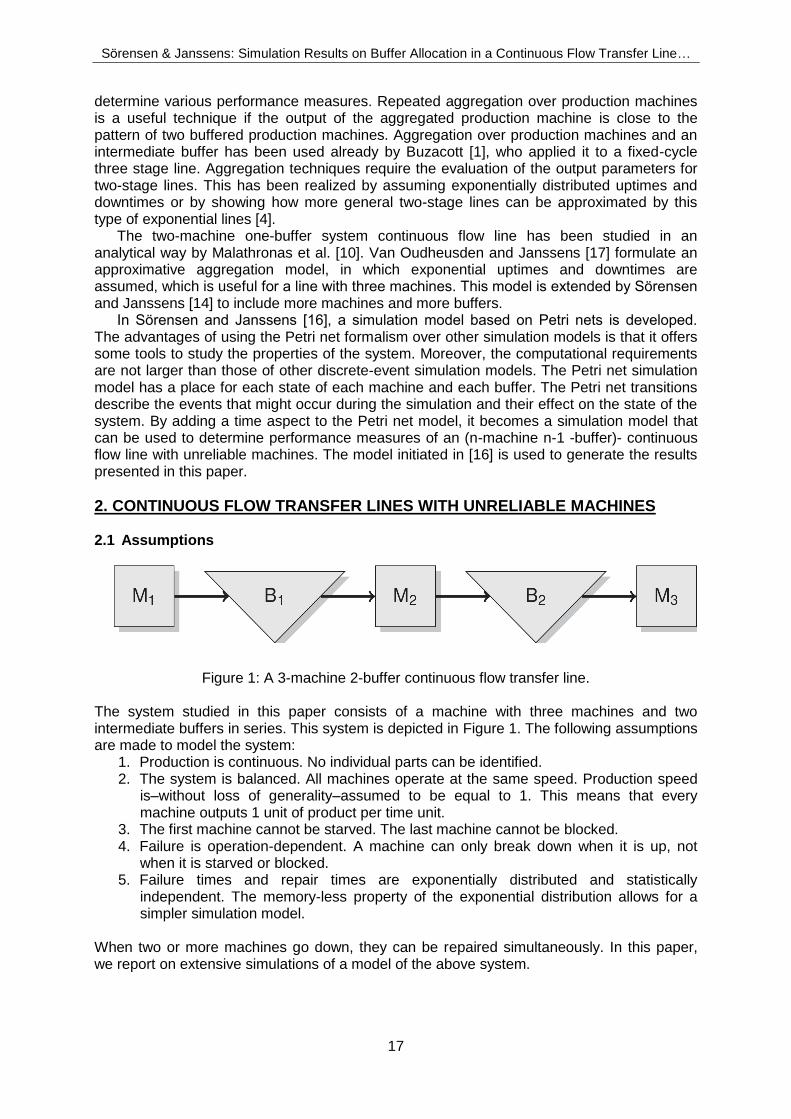
Figure 1: A 3-machine 2-buffer continuous flow transfer line. The system studied in this paper consists of a machine with three machines and two intermediate buffers in series. This system is depicted in Figure 1. The following assumptions are made to model the system:

1. Production is continuous. No individual parts can be identified. 2. The system is balanced. All machines operate at the same speed. Production speed

is–without loss of generality–assumed to be equal to 1. This means that every machine outputs 1 unit of product per time unit.

3. The first machine cannot be starved. The last machine cannot be blocked. 4. Failure is operation-dependent. A machine can only break down when it is up, not

when it is starved or blocked. 5. Failure times and repair times are exponentially distributed and statistically

independent. The memory-less property of the exponential distribution allows for a simpler simulation model.

When two or more machines go down, they can be repaired simultaneously. In this paper, we report on extensive simulations of a model of the above system.


18

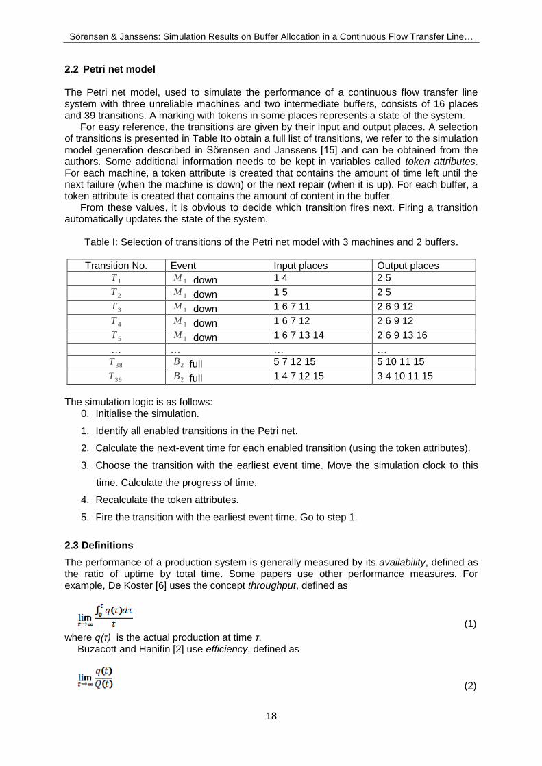
2.2 Petri net model The Petri net model, used to simulate the performance of a continuous flow transfer line system with three unreliable machines and two intermediate buffers, consists of 16 places and 39 transitions. A marking with tokens in some places represents a state of the system.

For easy reference, the transitions are given by their input and output places. A selection of transitions is presented in Table Ito obtain a full list of transitions, we refer to the simulation model generation described in Sörensen and Janssens [15] and can be obtained from the authors. Some additional information needs to be kept in variables called token attributes. For each machine, a token attribute is created that contains the amount of time left until the next failure (when the machine is down) or the next repair (when it is up). For each buffer, a token attribute is created that contains the amount of content in the buffer.

From these values, it is obvious to decide which transition fires next. Firing a transition automatically updates the state of the system.

Table I: Selection of transitions of the Petri net model with 3 machines and 2 buffers.

Transition No. Event Input places Output places T 1 M 1 down 1 4 2 5

T 2 M 1 down 1 5 2 5

T 3 M 1 down 1 6 7 11 2 6 9 12

T 4 M 1 down 1 6 7 12 2 6 9 12

T 5 M 1 down 1 6 7 13 14 2 6 9 13 16

… … … … T 38 B2 full 5 7 12 15 5 10 11 15

T 39 B2 full 1 4 7 12 15 3 4 10 11 15

The simulation logic is as follows:

0. Initialise the simulation.

1. Identify all enabled transitions in the Petri net.

2. Calculate the next-event time for each enabled transition (using the token attributes).

3. Choose the transition with the earliest event time. Move the simulation clock to this

time. Calculate the progress of time.

4. Recalculate the token attributes.

5. Fire the transition with the earliest event time. Go to step 1.

2.3 Definitions

The performance of a production system is generally measured by its availability, defined as the ratio of uptime by total time. Some papers use other performance measures. For example, De Koster [6] uses the concept throughput, defined as

(1)

where q(τ) is the actual production at time τ. Buzacott and Hanifin [2] use efficiency, defined as

(2)


19

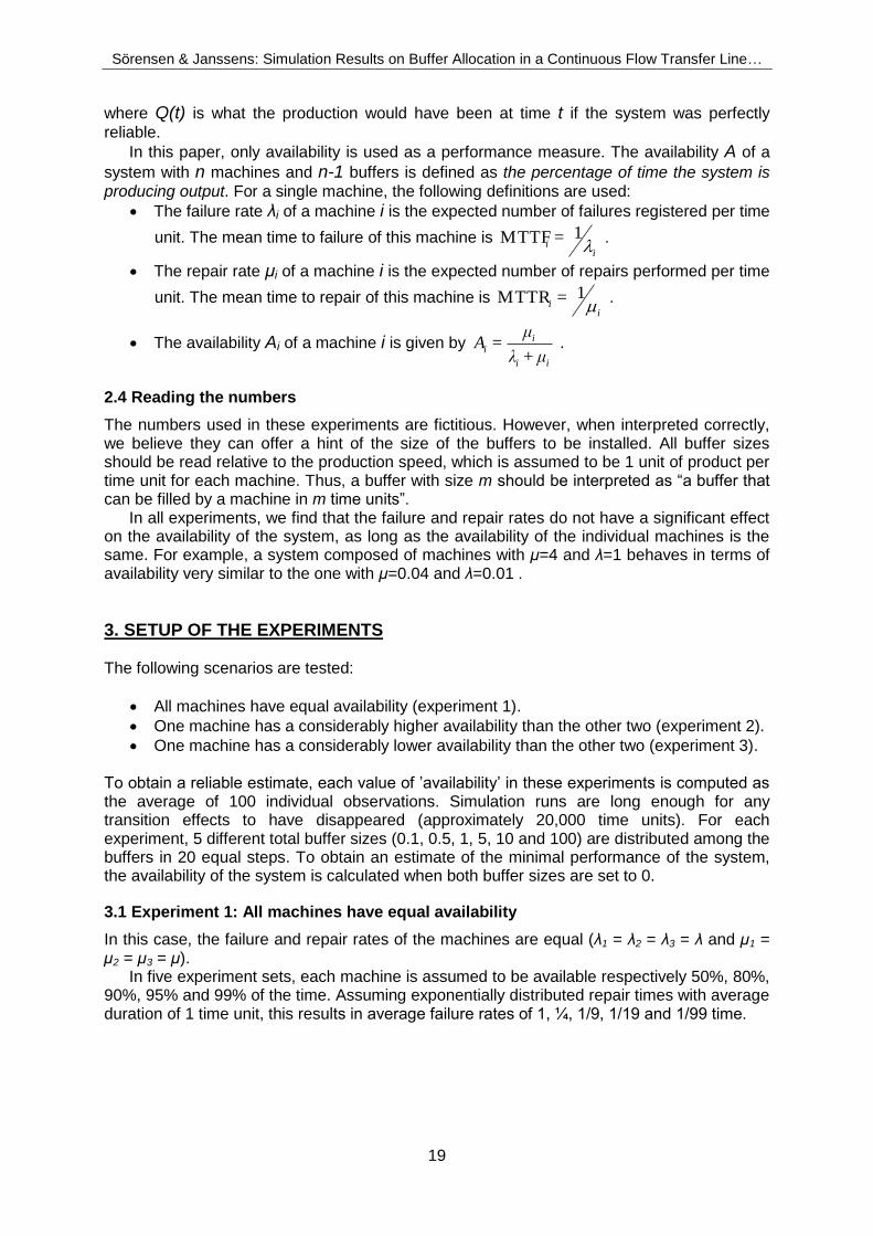
where Q(t) is what the production would have been at time t if the system was perfectly

reliable.

In this paper, only availability is used as a performance measure. The availability A of a

system with n machines and n-1 buffers is defined as the percentage of time the system is

producing output. For a single machine, the following definitions are used:

The failure rate λi of a machine i is the expected number of failures registered per time

unit. The mean time to failure of this machine is i

i =

1MTTF .

The repair rate μi of a machine i is the expected number of repairs performed per time

unit. The mean time to repair of this machine is i

i =

1MTTR .

The availability Ai of a machine i is given by ii

ii

μ+λ

μ=A .

2.4 Reading the numbers

The numbers used in these experiments are fictitious. However, when interpreted correctly, we believe they can offer a hint of the size of the buffers to be installed. All buffer sizes should be read relative to the production speed, which is assumed to be 1 unit of product per time unit for each machine. Thus, a buffer with size m should be interpreted as ―a buffer that can be filled by a machine in m time units‖.

In all experiments, we find that the failure and repair rates do not have a significant effect on the availability of the system, as long as the availability of the individual machines is the same. For example, a system composed of machines with µ=4 and λ=1 behaves in terms of availability very similar to the one with µ=0.04 and λ=0.01 .

3. SETUP OF THE EXPERIMENTS The following scenarios are tested:

All machines have equal availability (experiment 1).

One machine has a considerably higher availability than the other two (experiment 2).

One machine has a considerably lower availability than the other two (experiment 3). To obtain a reliable estimate, each value of ‘availability‘ in these experiments is computed as the average of 100 individual observations. Simulation runs are long enough for any transition effects to have disappeared (approximately 20,000 time units). For each experiment, 5 different total buffer sizes (0.1, 0.5, 1, 5, 10 and 100) are distributed among the buffers in 20 equal steps. To obtain an estimate of the minimal performance of the system, the availability of the system is calculated when both buffer sizes are set to 0.

3.1 Experiment 1: All machines have equal availability

In this case, the failure and repair rates of the machines are equal (λ1 = λ2 = λ3 = λ and µ1 = µ2 = µ3 = µ).

In five experiment sets, each machine is assumed to be available respectively 50%, 80%, 90%, 95% and 99% of the time. Assuming exponentially distributed repair times with average duration of 1 time unit, this results in average failure rates of 1, ¼, 1/9, 1/19 and 1/99 time.


20

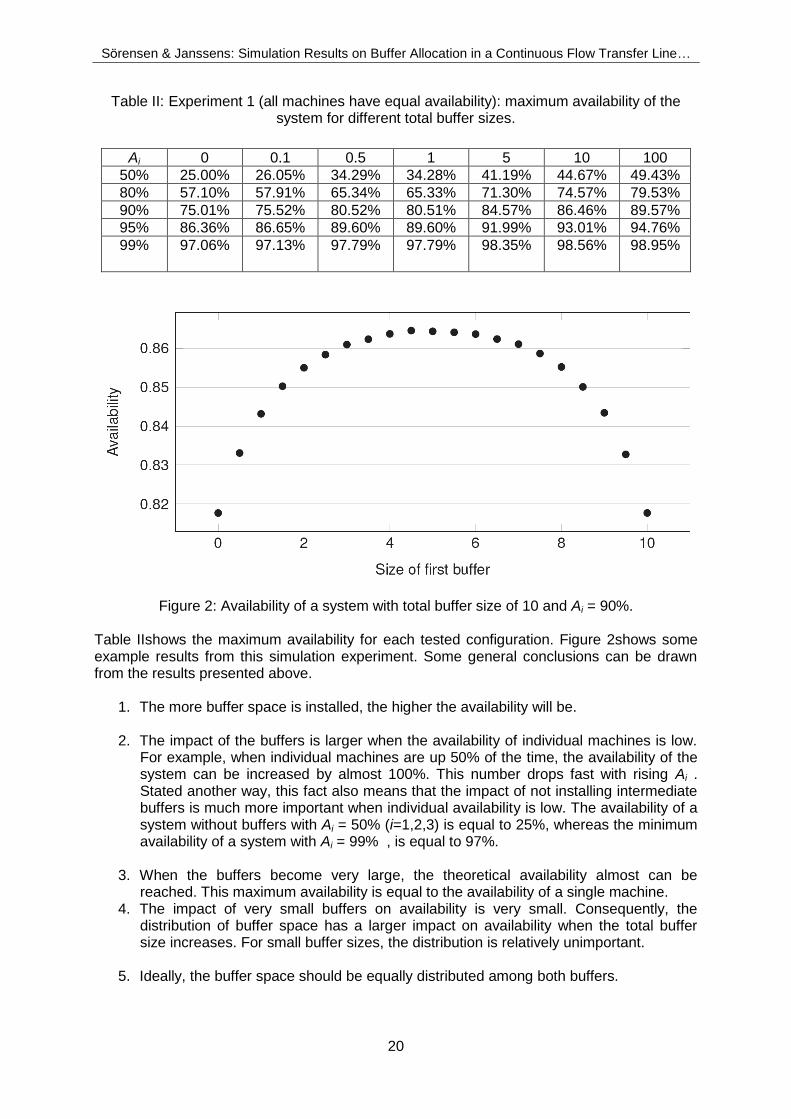
Table II: Experiment 1 (all machines have equal availability): maximum availability of the system for different total buffer sizes.

Ai 0 0.1 0.5 1 5 10 100 50% 25.00% 26.05% 34.29% 34.28% 41.19% 44.67% 49.43% 80% 57.10% 57.91% 65.34% 65.33% 71.30% 74.57% 79.53% 90% 75.01% 75.52% 80.52% 80.51% 84.57% 86.46% 89.57% 95% 86.36% 86.65% 89.60% 89.60% 91.99% 93.01% 94.76% 99% 97.06% 97.13% 97.79% 97.79% 98.35% 98.56% 98.95%

Figure 2: Availability of a system with total buffer size of 10 and Ai = 90%. Table IIshows the maximum availability for each tested configuration. Figure 2shows some example results from this simulation experiment. Some general conclusions can be drawn from the results presented above.

1. The more buffer space is installed, the higher the availability will be.

2. The impact of the buffers is larger when the availability of individual machines is low. For example, when individual machines are up 50% of the time, the availability of the system can be increased by almost 100%. This number drops fast with rising Ai . Stated another way, this fact also means that the impact of not installing intermediate buffers is much more important when individual availability is low. The availability of a system without buffers with Ai = 50% (i=1,2,3) is equal to 25%, whereas the minimum availability of a system with Ai = 99% , is equal to 97%.

3. When the buffers become very large, the theoretical availability almost can be

reached. This maximum availability is equal to the availability of a single machine. 4. The impact of very small buffers on availability is very small. Consequently, the

distribution of buffer space has a larger impact on availability when the total buffer size increases. For small buffer sizes, the distribution is relatively unimportant.

5. Ideally, the buffer space should be equally distributed among both buffers.


21

6. However, the availability of the system is quite robust with regard to the distribution of buffer space. Although the highest availability is reached when the buffer space is equally distributed among the two buffers, deviations from this ideal distribution do not have a large impact on availability, especially when the total buffer space is very large. In this case, there is ―more than enough‖ buffer space to allow for a high availability, even when the distribution of buffer space is not ideal.

The robustness of availability with regard to the ideal buffer space distribution is important. A manager wishing to minimise the total operating cost may wish to employ a smaller inventory level of high-cost products, as they may represent an important working capital investment. This robustness is highest when the total available buffer space is either very small or very large and arises for different reasons in both cases.

3.2 Experiment 2: One machine has the higher availability

In this experiment, we assume that two out of three machines are up 80% of the time. For these machines, we assume exponentially distributed repair times with average 1 time unit and exponentially distributed failure times with average 4 time units. In three different experiment sets, the better machine is placed first, second and third.

In three different experiments, one of the machines is up 90%, 95% and 99% of the time. If we assume exponentially distributed repair times with average of 1 time unit, failure rates are 1/9, 1/19 and 1/99 respectively. Depending on which of the three machines is the best, the results are quite different. The maximum attainable availability for each tested configuration is shown in Table III.

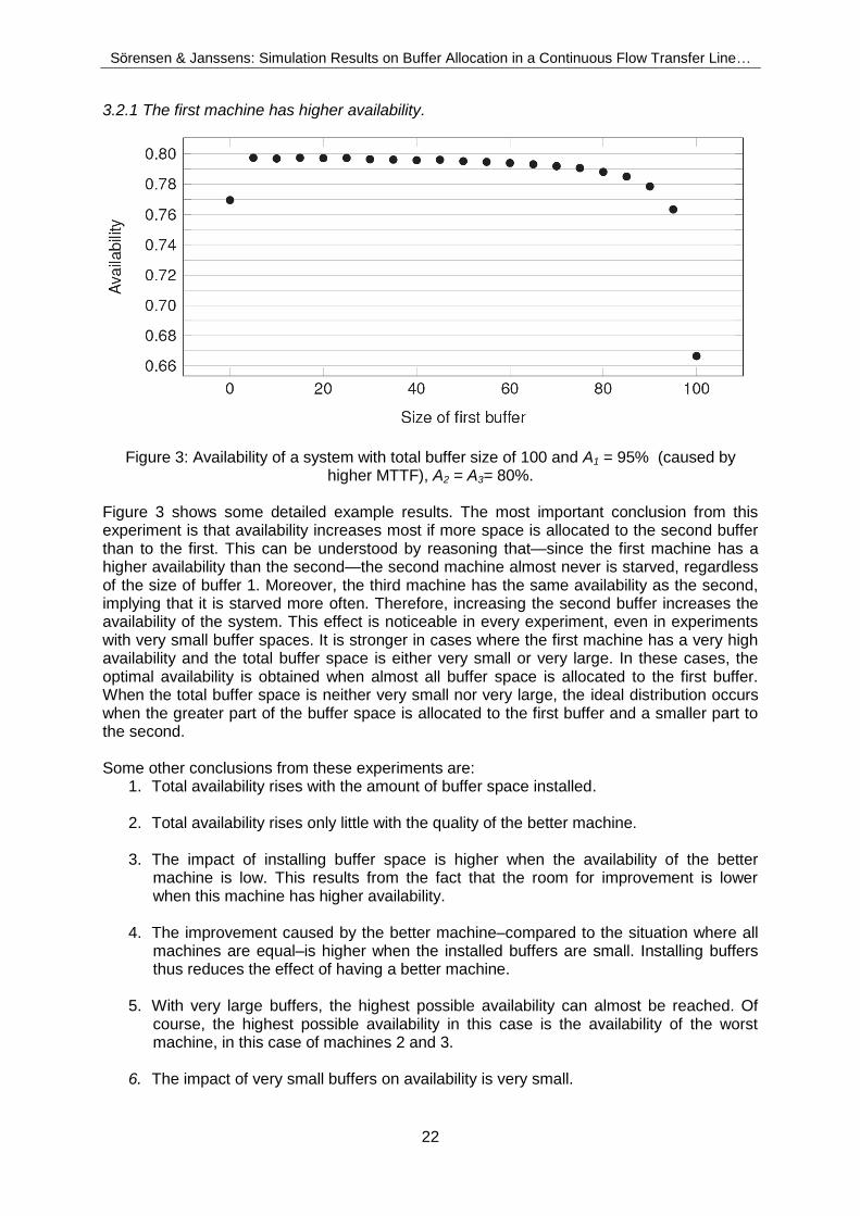
Table III: Experiment 2 (one machine has higher availability): maximum availability of the

system for different total buffer sizes.

A1 A2 A3 0 0.1 0.5 1 5 10 100

90% 80% 80% 62.08% 62.85% 67.43% 70.09% 73.95% 76.61% 79.73%

95% 80% 80% 64.43% 65.08% 67.93% 71.84% 74.91% 77.10% 79.73%

99% 80% 80% 66.27% 66.90% 68.99% 73.21% 75.94% 77.56% 79.77%

80% 90% 80% 62.03% 62.86% 70.22% 70.18% 74.70% 77.19% 79.81%

80% 95% 80% 64.40% 65.15% 72.20% 72.24% 75.71% 77.70% 79.81%

80% 99% 80% 66.23% 66.96% 73.56% 73.60% 76.22% 77.87% 79.81%

80% 80% 90% 62.08% 62.80% 70.05% 67.42% 73.97% 76.60% 79.76%

80% 80% 95% 64.34% 65.12% 71.89% 69.12% 74.94% 77.17% 79.78%

80% 80% 99% 64.40% 65.15% 67.44% 69.47% 75.71% 77.70% 79.81%


22

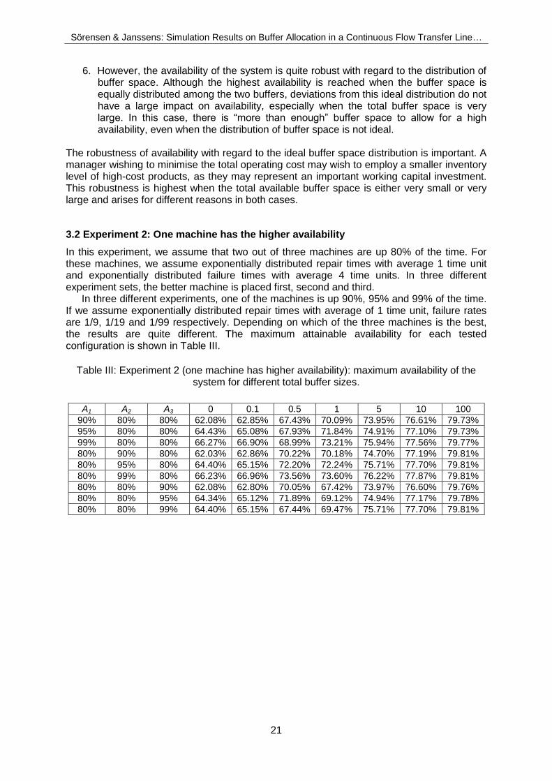
3.2.1 The first machine has higher availability.

Figure 3: Availability of a system with total buffer size of 100 and A1 = 95% (caused by higher MTTF), A2 = A3= 80%.

Figure 3 shows some detailed example results. The most important conclusion from this experiment is that availability increases most if more space is allocated to the second buffer than to the first. This can be understood by reasoning that—since the first machine has a higher availability than the second—the second machine almost never is starved, regardless of the size of buffer 1. Moreover, the third machine has the same availability as the second, implying that it is starved more often. Therefore, increasing the second buffer increases the availability of the system. This effect is noticeable in every experiment, even in experiments with very small buffer spaces. It is stronger in cases where the first machine has a very high availability and the total buffer space is either very small or very large. In these cases, the optimal availability is obtained when almost all buffer space is allocated to the first buffer. When the total buffer space is neither very small nor very large, the ideal distribution occurs when the greater part of the buffer space is allocated to the first buffer and a smaller part to the second. Some other conclusions from these experiments are:

1. Total availability rises with the amount of buffer space installed.

2. Total availability rises only little with the quality of the better machine.

3. The impact of installing buffer space is higher when the availability of the better machine is low. This results from the fact that the room for improvement is lower when this machine has higher availability.

4. The improvement caused by the better machine–compared to the situation where all machines are equal–is higher when the installed buffers are small. Installing buffers thus reduces the effect of having a better machine.

5. With very large buffers, the highest possible availability can almost be reached. Of course, the highest possible availability in this case is the availability of the worst machine, in this case of machines 2 and 3.

6. The impact of very small buffers on availability is very small.


23

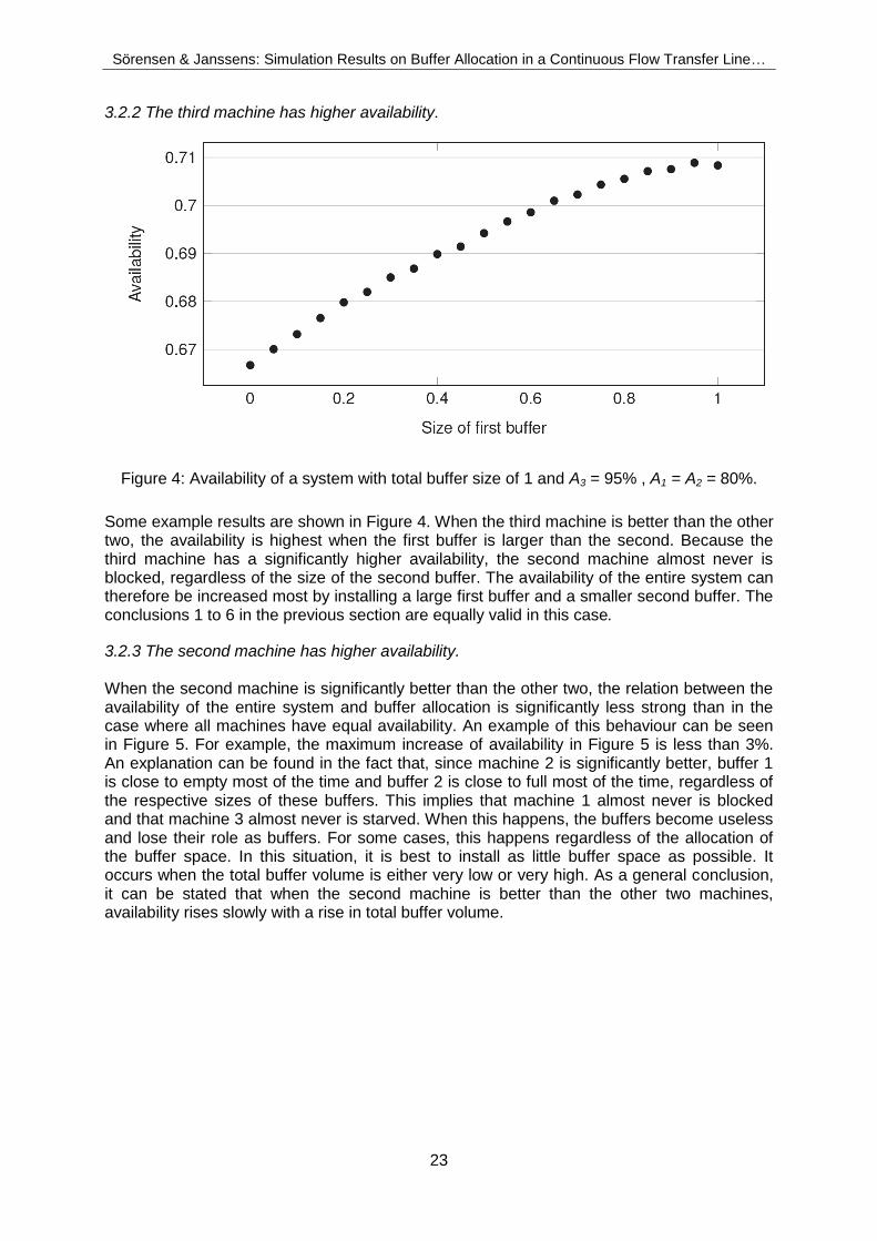
3.2.2 The third machine has higher availability.

Figure 4: Availability of a system with total buffer size of 1 and A3 = 95% , A1 = A2 = 80%.

Some example results are shown in Figure 4. When the third machine is better than the other two, the availability is highest when the first buffer is larger than the second. Because the third machine has a significantly higher availability, the second machine almost never is blocked, regardless of the size of the second buffer. The availability of the entire system can therefore be increased most by installing a large first buffer and a smaller second buffer. The conclusions 1 to 6 in the previous section are equally valid in this case.

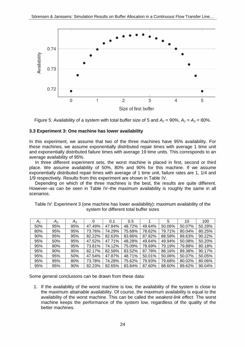
3.2.3 The second machine has higher availability. When the second machine is significantly better than the other two, the relation between the availability of the entire system and buffer allocation is significantly less strong than in the case where all machines have equal availability. An example of this behaviour can be seen in Figure 5. For example, the maximum increase of availability in Figure 5 is less than 3%. An explanation can be found in the fact that, since machine 2 is significantly better, buffer 1 is close to empty most of the time and buffer 2 is close to full most of the time, regardless of the respective sizes of these buffers. This implies that machine 1 almost never is blocked and that machine 3 almost never is starved. When this happens, the buffers become useless and lose their role as buffers. For some cases, this happens regardless of the allocation of the buffer space. In this situation, it is best to install as little buffer space as possible. It occurs when the total buffer volume is either very low or very high. As a general conclusion, it can be stated that when the second machine is better than the other two machines, availability rises slowly with a rise in total buffer volume.


24

Figure 5: Availability of a system with total buffer size of 5 and A2 = 90%, A1 = A3 = 80%. 3.3 Experiment 3: One machine has lower availability In this experiment, we assume that two of the three machines have 95% availability. For these machines, we assume exponentially distributed repair times with average 1 time unit and exponentially distributed failure times with average 19 time units. This corresponds to an average availability of 95%.

In three different experiment sets, the worst machine is placed in first, second or third place. We assume availability of 50%, 80% and 90% for this machine. If we assume exponentially distributed repair times with average of 1 time unit, failure rates are 1, 1/4 and 1/9 respectively. Results from this experiment are shown in Table IV.

Depending on which of the three machines is the best, the results are quite different. However–as can be seen in Table IV–the maximum availability is roughly the same in all scenarios.

Table IV: Experiment 3 (one machine has lower availability): maximum availability of the

system for different total buffer sizes

A1 A2 A3 0 0.1 0.5 1 5 10 100

50% 95% 95% 47.49% 47.84% 48.72% 49.64% 50.06% 50.07% 50.28%

80% 95% 95% 73.76% 74.29% 75.68% 78.62% 79.71% 80.04% 80.25%

90% 95% 95% 82.22% 82.63% 83.86% 87.82% 88.58% 89.63% 90.22%

95% 50% 95% 47.52% 47.71% 48.28% 49.64% 49.94% 50.08% 50.20%

95% 80% 95% 73.81% 74.12% 75.09% 78.69% 79.19% 79.88% 80.18%

95% 90% 95% 82.17% 82.58% 83.52% 87.78% 88.16% 89.38% 90.17%

95% 95% 50% 47.54% 47.87% 48.71% 50.01% 50.06% 50.07% 50.05%

95% 95% 80% 73.78% 74.28% 75.62% 79.93% 79.68% 80.02% 80.06%

95% 95% 90% 82.23% 82.65% 83.84% 87.60% 88.60% 89.62% 90.04%

Some general conclusions can be drawn from these data:

1. If the availability of the worst machine is low, the availability of the system is close to the maximum attainable availability. Of course, the maximum availability is equal to the availability of the worst machine. This can be called the weakest-link effect. The worst machine keeps the performance of the system low, regardless of the quality of the better machines.


25

2. The fact whether the worst machine is first, second or third does not have a large impact on the maximum availability of the system. Total availability is roughly the same in all three cases.

3. When the availability of the worst machine is rather large, the room for improvement grows. In these cases, the weakest-link effect is much less prominent and the provision of buffer space becomes more important.

3.3.1 The first machine has lower availability In this case, there is a slight preference for a larger first buffer. However, the relationship between buffer allocation and availability is weak.

3.3.2 The third machine has lower availability When the third machine is worse than the other two machines, slightly more buffer space should be allocated to the second buffer. Again, the relationship between buffer allocation and availability is weak.

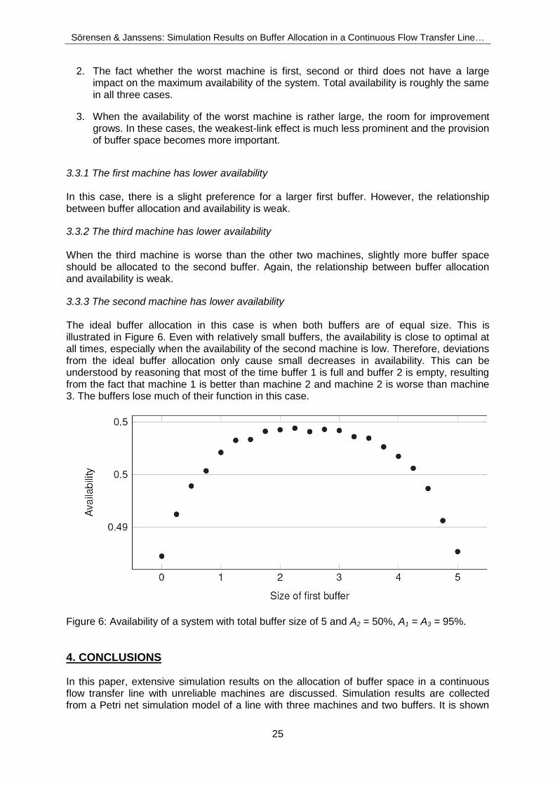
3.3.3 The second machine has lower availability The ideal buffer allocation in this case is when both buffers are of equal size. This is illustrated in Figure 6. Even with relatively small buffers, the availability is close to optimal at all times, especially when the availability of the second machine is low. Therefore, deviations from the ideal buffer allocation only cause small decreases in availability. This can be understood by reasoning that most of the time buffer 1 is full and buffer 2 is empty, resulting from the fact that machine 1 is better than machine 2 and machine 2 is worse than machine 3. The buffers lose much of their function in this case.

Figure 6: Availability of a system with total buffer size of 5 and A2 = 50%, A1 = A3 = 95%.

4. CONCLUSIONS In this paper, extensive simulation results on the allocation of buffer space in a continuous flow transfer line with unreliable machines are discussed. Simulation results are collected from a Petri net simulation model of a line with three machines and two buffers. It is shown


26

how these results can be used to find some generally applicable rules of thumb for the allocation of buffer space in a continuous flow-line.

REFERENCES [1] Buzacott, J.A. (1967). Automatic transfer lines with buffer stocks. International Journal of

Production Research, 5(3): 183–200 [2] Buzacott, J.A. and Hanifin, L.E. (1978). Model of automatic transfer lines with inventory banks:

a review and comparison. AIIE Transactions, 10(2): 197–207 [3] Coillard, P. and Proth, J.M.. Effet des stocks tampons dans une fabrication en ligne. JORBEL

(Belgian Journal of Operations Research, Statistics and Computer Science), 24(2):3–27, 1984 [4] De Koster, M.B.M. (1987). Estimation of line efficiency by aggregation. International Journal of

Production Research, 25(4): 615–626 [5] De Koster, M.B.M. (1988). An improved algorithm to approximate the behavior of flow lines.

International Journal of Production Research, 26(4): 691–700 [6] De Koster, M.B.M. (1989). Capacity oriented analysis and design of production systems. In

Lecture Notes in Economics and Mathematical Systems, volume 323, 245 pp., Springer-Verlag, Berlin

[7] Elsayed, E.A. and Hwang, C.C. (1986). Analysis of two-stage manufacturing systems with buffer storage and redundant machines. International Journal of Production Research, 24(1): 187–201

[8] Fox, R.A. and Zerbe, D.R. (1974). Some practical system availability calculations. AIIE Transactions, 6(3):228–235

[9] Kubat, P. and Sumita, U. (1985). Buffers and backup machines in automatic transfer lines. International Journal of Production Research, 23(6):1259–1270

[10] Malathronas, J. P.; Perkins, J.D. and Smith, R.L. (1983). The availability of a system of two unreliable machines connected by an intermediate storage tank. AIIE Transactions, 15(3): 195–201

[11] Mitra, D. (1988). Stochastic theory of a fluid model of producers and consumers coupled by a buffer. Advances in Applied Probability, 20: 646–676

[12] Murphy, R.A. (1975). The effect of surge on system availability. AIIE Transactions, 7(4): 439–443,

[13] Murphy, R.A. (1978). Estimating the output of a series production system. AIIE Transactions, 10(2): 139–148

[14] Sörensen, K. and Janssens, G.K.. Buffer allocation and required availability in a transfer line with unreliable machines. International Journal of Production Economics, 74: 163–173

[15] Sörensen, K. and Janssens, G.K. (2004). Automatic simulation model generation of a continuous flow transfer line with unreliable machines. Quality and Reliability Engineering International, 20(4): 343–362

[16] Sörensen, K. and Janssens, G.K. (2004). A Petri net model of a continuous flow transfer line with unreliable machines. European Journal of Operational Research, 152(1) :248–262

[17] Van Oudheusden, D.L. and Janssens, G.K. (1994). Availability of three-machine two-buffer systems. JORBEL (Belgian Journal of Operations Research, Statistics and Computer Science), 34(2): 17–37

[18] Wijngaard, J. (1979). The effect of interstage buffer storage on the output of two unreliable production units in series, with different production rates. AIIE Transactions, 11(1): 42–47

[19] Wild, R. (1972). Mass-Production Management: the Design and Operation of Production Flow-Line Systems. J. Wiley & Sons, London

[20] Yeralan, S.; Franck, W.E. and Quasem, M.A. (1986). A continuous materials flow production line with station breakdown. European Journal of Operational Research, 27:289–300

SIMULATION RESULTS ON BUFFER ALLOCATION IN A CONTINUOUS FLOW TRANSFER LINE WITH THREE UNRELIABLE...

Documents

Transcript of SIMULATION RESULTS ON BUFFER ALLOCATION IN A CONTINUOUS FLOW TRANSFER LINE WITH THREE UNRELIABLE...