Information Sciences 181 (2011) 519–535

Contents lists available at ScienceDirect

Information Sciences

journal homepage: www.elsevier .com/locate / ins

Simulation of the bird age-structured population growth based on aninterval type-2 fuzzy cellular structure

Cecilia Leal-Ramírez a, Oscar Castillo b,⇑, Patricia Melin a, Antonio Rodríguez-Díaz a

a Faculty of Chemical Sciences and Engineering, Autonomous University of Baja California, Tijuana Baja California, Mexicob Tijuana Institute of Technology, Tijuana Baja California, Mexico

a r t i c l e i n f o a b s t r a c t

Article history:Received 26 June 2009Received in revised form 11 September2010Accepted 7 October 2010

Keywords:Interval type-2 fuzzy logicCellular automataPopulation dynamics

0020-0255/$ - see front matter � 2010 Elsevier Incdoi:10.1016/j.ins.2010.10.011

⇑ Corresponding author.E-mail address: ocastillo@hafsamx.org (O. Castill

In this paper an age-structured population growth model, based on a fuzzy cellular struc-ture, is proposed. An age-structured population growth model enables a better descriptionof population dynamics. In this paper, the dynamics of a particular bird species is consid-ered. The dynamics is governed by the variation of natality, mortality and emigration rates,which in this work are evaluated using an interval type-2 fuzzy logic system. The use oftype-2 fuzzy logic enables handling the effects caused by environment heterogeneity onthe population. A set of fuzzy rules, about population growth, are derived from the inter-pretation of the ecological laws and the bird life cycle. The proposed model is formulatedusing discrete mathematics within the framework of a fuzzy cellular structure. The fuzzycellular structure allows us to visualize the evolution of the population’s spatial dynamics.The spatial distribution of the population has a deep effect on its dynamics. Moreover, themodel enables not only to estimate the percentage of occupation on the cellular spacewhen the species reaches its stable equilibrium level, but also to observe the occupationpatterns.

� 2010 Elsevier Inc. All rights reserved.

1. Introduction

Structured population models distinguish among individuals according to characteristics such as age or size to determinethe birth and death rates. The study of age-structured population growth has a long history in population biology. Age is oneof the most important characteristics in the modelling of populations (for example in Epidemiology [20]). Individuals withdifferent ages may have different reproduction and survival capacities. Therefore, it is often useful to divide a population intodifferent groups by age, for obtaining a better description of the population dynamics.

In this paper, we present a new age-structured population growth model to simulate the dynamics of a particular birdspecies. The life cycle of a species is composed by stages (of age or size) [34]. The stages are genetically determined statesthat all individuals of a species go through. The life cycle, in ecological time, is a ‘‘constant”, while the rate, at which indi-viduals go through it, is an environment specific variable in space and in time [31]. Bird species have a less complicated lifecycle than any other animal [28]. Therefore, some characteristics on their evolution are represented easier in the proposedmodel.

Mathematical models of populations incorporating spatial structure, age structure, or other structuring of individualswith continuously varying properties have been developed by many researchers [41]. Nevertheless, these models are math-ematically complex, and their scientific applicability depends on extensive parametric inputs. Furthermore, the mathemat-

. All rights reserved.

o).

520 C. Leal-Ramírez et al. / Information Sciences 181 (2011) 519–535

ical description of many biological processes requires very elaborate mathematical formulations based on differential equa-tions and integrals, and need an intensive scientific validation. To use a discrete number of age classes and a fuzzy cellularstructure in a population growth model is solely a matter of technical convenience to approach this model and obtain betterresults.

In this work, the proposed model is defined as a discrete mathematical population model within the framework of a fuzzycellular structure, which is composed by a cellular automata and an interval type-2 fuzzy logic system (IT2-FLS). Cellularautomata help the visualization of the evolution of the population’s spatial dynamics [30]. The IT2-FLS evaluates the effectscaused by the environment on the population, and determines how many individuals, of a given age class, die during eachtime interval, how many individuals will be moved into the next age class, and how many newborns will be created by themembers of reproductive age class. Our model provides a framework to predict the future bird population in each stage.

An IT2-FLS is a particular class of a type-2 fuzzy logic system (T2-FLS), where the fuzzy sets are represented as intervaltype-2 fuzzy sets. The concept of type-2 fuzzy set (T2-FS) was introduced initially in 1975 by Zadeh [42] as an extension ofthe concept of type-1 fuzzy set (T1-FS). The T2-FS can be used to work with circumstances with a high degree of uncertainty.John [14,15] and Karnik and Mendel [17] made the first applications of this concept. Recently, type-2 fuzzy logic systemshave been shown to manage uncertainty more effectively than type-1 fuzzy logic systems in several areas of application.For example, Coupland and John [9] reported an example application of type-2 fuzzy logic to mobile robot navigation, dem-onstrating the potential of type-2 fuzzy systems to outperform type-1 fuzzy systems in this area of application. Unfortu-nately, the T2-FS may require an undesirably large amount of computations since it involves numerous embedded T2-FSs. To reduce this complexity, interval type-2 fuzzy sets (IT2-FS) can be used instead of general T2-FS. This kind of set ischaracterized by two interval type-2 membership functions: lower and upper [24]. Turksen has worked extensively onthe inference process with interval type-2 fuzzy sets and if-then rules [35–39]. Furthermore, many applications on IT2-FShave emerged in different areas [16,10–13,26]. In ecology, the interval type-2 fuzzy sets have been used satisfactorily tomodel dynamic niches in [22] and to model the behavior of complex ecosystems in [21].

In Section 2, the definition and the more important characteristics of interval type-2 fuzzy sets are presented. In Section 3,the bird age-structured population growth model is described in detail. In Section 4, an interval type-2 fuzzy logic system isproposed. Simulations were made to examine the effects caused by environment and determine which information is impor-tant in order to avoid possible extinction of the species. In Section 5, the results and a comparison with the results obtainedin [19,34] are presented. In the last section, conclusions about the representativeness and applicability of this kind of modelare presented.

2. Interval type-2 fuzzy sets

Fuzzy set theory, which describes the ambiguity and uncertainty in mathematics, was adopted by ecologists such as in [4]for ecosystem analysis and in [32] for modelling an ecological process containing uncertain ecological data. It is introduced inthis paper to define the environmental concept into the proposed model.

Let A be a type-1 fuzzy set wherein the membership grade of x 2 X in A is lA(x), which is a crisp number in [0,1]. Themembership grade of a type-2 fuzzy set can be described as any fuzzy subset in [0,1] called the primary membership, unlikea type-1 set where the membership degree is a crisp value. Type-2 fuzzy sets are very useful in circumstances where it isdifficult to determine an exact membership function for a fuzzy set; hence, they are useful to incorporate uncertaintiesand propagate them, establishing their effects at the output of the fuzzy logic system [5,6].

A type-2 fuzzy set in X is eA and the membership grade of x 2 X in eA is leAðxÞ, which is a type-1 fuzzy set in [0,1]. A type-2fuzzy set eA can be described as:

eA ¼ fðx;leAðx;uÞÞj 8x 2 X; 8u 2 Jx # ½0;1�g ð1Þ

and the membership degree of any x 2 X in eA can be represented as:

leAðxÞ ¼Z

u2Jx

fxðuÞ=u u 2 Jx # ½0;1�; ð2Þ

where u 2 Jx indicates the primary memberships of x and fx(u) 2 [0,1] indicates the secondary memberships (degrees) of x.The integral sign indicates logical union such eA can also be described as:

eA ¼ Zx2X

Zu2Jx

leAðx;uÞ=u

!,x: ð3Þ

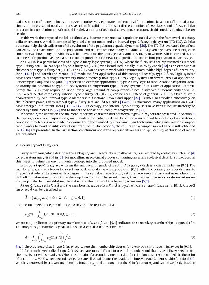
Fig. 1 shows a generalized type-2 fuzzy set, where the membership degree for every point is a type-1 fuzzy set in [0,1].Unfortunately, generalized type-2 fuzzy sets are more difficult to use and to understand than type-1 fuzzy sets; hence,

their use is not widespread yet. When the domain of a secondary membership function bounds a region (called the footprintof uncertainty, FOU) whose secondary degrees are all equal to one, the result is an interval type-2 membership function [24],which is expressed by a lower membership function leA and an upper membership function �leA and can be easily depicted in

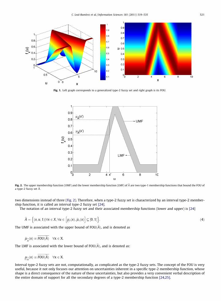
Fig. 1. Left graph corresponds to a generalized type-2 fuzzy set and right graph is its FOU.

Fig. 2. The upper membership function (UMF) and the lower membership function (LMF) of eA are two type-1 membership functions that bound the FOU ofa type-2 fuzzy set eA.

C. Leal-Ramírez et al. / Information Sciences 181 (2011) 519–535 521

two dimensions instead of three (Fig. 2). Therefore, when a type-2 fuzzy set is characterized by an interval type-2 member-ship function, it is called an interval type-2 fuzzy set [24].

The notation of an interval type-2 fuzzy set and their associated membership functions (lower and upper) is [24]

eA ¼ ðx;u;1Þj8x 2 X;8u 2 lkðxÞ; �lkðxÞh i

# ½0;1�n o

: ð4Þ

The UMF is associated with the upper bound of FOUðeAÞ, and is denoted as

�leAðxÞ � FOUðeAÞ 8x 2 X:

The LMF is associated with the lower bound of FOUðeAÞ, and is denoted as:

leAðxÞ � FOUðeAÞ 8x 2 X:

Interval type-2 fuzzy sets are not, computationally, as complicated as the type-2 fuzzy sets. The concept of the FOU is veryuseful, because it not only focuses our attention on uncertainties inherent in a specific type-2 membership function, whoseshape is a direct consequence of the nature of these uncertainties, but also provides a very convenient verbal description ofthe entire domain of support for all the secondary degrees of a type-2 membership function [24,25].

522 C. Leal-Ramírez et al. / Information Sciences 181 (2011) 519–535

3. The bird age-structured population growth model

The coexistence of a population is considerably linked to a phenomenon of self organized space, in which the connectionof the nonlinear dynamics and the dispersion of individuals forms structures defined by variable population densities [2].Therefore, the space concept is integrated in our age-structured population growth model using cellular automata, whichis composed by a rectangular region of M � N cells [27]. The union of all the cells defines the cellular space in which the evo-lution of each cell depends on its present state and the states of its immediate neighbouring cells. Let C be a single cell, thenC(i, j) is the cell centred at the coordinates (i, j), where 1 6 i 6M and 1 6 j 6 N. Each cell is a fundamental element for pop-ulation change at time t, reason why the contribution of all the cells determines the change of the total population density inthe system dynamics.

Let NC(i, j)(t + 1) be the local population density in the cell C(i, j) at time t + 1

NCði;jÞðt þ 1Þ ¼ bNCði;jÞðtÞ|fflfflfflfflfflffl{zfflfflfflfflfflffl}natality

� kNCði;jÞðtÞ|fflfflfflfflfflffl{zfflfflfflfflfflffl}mortality

�rNCði;jÞðtÞ|fflfflfflfflfflffl{zfflfflfflfflfflffl}emigration

þY

rNCðk;lÞðtÞ|fflfflfflfflfflfflfflfflffl{zfflfflfflfflfflfflfflfflffl}

immigration

; ð5Þ

where the constants b and k correspond to the natality and mortality rates respectively and r is the emigration rate, whichdetermines the population density that emigrates towards the neighbouring cells from a cell C(i, j) according to a local rule.The neighbourhood of the cell C(i, j) in terms of a radius r is represented by

Y

r

Cði; jÞ ¼ Cðk; lÞmaxfjk� 1j; jl� jjg 6 r

1 6 k 6 M; 1 6 l 6 N

���� ����� �; ð6Þ

where r is a positive integer number and (k, l) is the coordinate of another cell, where the magnitude of the difference be-tween (i,k) and (j, l) does not exceed the value of r. Then the population that immigrate from any neighboring cell C(k, l)to the cell C(i, j) is given by:

Y

r

NCðk;lÞðtÞ: ð7Þ

Assuming that the initial population N0 is distributed on the cellular space, we obtained that the total population at time t + 1is given by:

NTðt þ 1Þ ¼X

i

Xj

NCði;jÞðtÞ: ð8Þ

Demographic parameters of many populations vary with the individuals’ age. A bird age-structured population is consideredin the proposed model. Therefore, the total population, at time t + 1, is given by the population density of each age k class,localized in each cell C(i, j)

NTðt þ 1Þ ¼X

i

Xj

Xk

NkCði;jÞðtÞ; ð9Þ

where the limit of k is the chronological age of the considered species, of course, some finite number. To determine howmany individuals of a specific age class die, are born and survive during each time interval, how many individuals move intothe next age class, and how many individuals emigrate or immigrate towards the other cells, it is necessary to defineP

kNkCði;jÞðtÞ in terms of the bird life stages.

The bird population has three stages: chicks H, juveniles J and adults A. A chick is a young individual still being attendedby its parents. The period of being a chick varies considerably among different species. We consider a species where thechicks stay with their parents during one full season. When chicks are ready to leave their parents, they become juveniles.The juveniles are not ready to reproduce. Juveniles who survive a full season become adults. Adults are ready to lay eggs andto increase chicks. The above-mentioned bird life cycle can be expressed redefining Eq. (9) to model the population growthas an aggregation of age classes

NTðt þ 1Þ ¼X

i

Xj

HCði;jÞðtÞ|fflfflfflffl{zfflfflfflffl}chicks

þ JCði;jÞðtÞ|fflfflffl{zfflfflffl}juveniles

þACði;jÞðtÞ|fflfflfflffl{zfflfflfflffl}adults

: ð10Þ

The number of chicks next year will be the born chicks from the number of adults this year

HCði;jÞðt þ 1Þ ¼ bAACði;jÞðtÞ|fflfflfflfflfflffl{zfflfflfflfflfflffl}new chicks

; ð11Þ

where bA is the natality rate of the adult population. The survivor chicks from that year become the next year juveniles

JCði;jÞðt þ 1Þ ¼ HCði;jÞðtÞ � kHHCði;jÞðtÞ|fflfflfflfflfflfflfflfflfflfflfflfflfflfflfflfflfflffl{zfflfflfflfflfflfflfflfflfflfflfflfflfflfflfflfflfflffl}survivor chicks

; ð12Þ

where kH is the mortality rate of the chick population. Adult birds next year will be the sum adult birds that survive, plus thejuvenile birds that survive, minus the adult birds that emigrate, plus adult birds immigrated from any neighboring cell C(k, l)to the cell C(i, j), all from this year

C. Leal-Ramírez et al. / Information Sciences 181 (2011) 519–535 523

ACði;jÞðt þ 1Þ ¼ JCði;jÞðtÞ � kJ JCði;jÞðtÞ|fflfflfflfflfflfflfflfflfflfflfflfflfflfflffl{zfflfflfflfflfflfflfflfflfflfflfflfflfflfflffl}surv ivor juveniles

8><>:9>=>;þ ACði;jÞðtÞ � kAACði;jÞðtÞ|fflfflfflfflfflfflfflfflfflfflfflfflfflfflfflfflffl{zfflfflfflfflfflfflfflfflfflfflfflfflfflfflfflfflffl}

survivor adults

8><>:9>=>;� rAACði;jÞðtÞ|fflfflfflfflfflfflffl{zfflfflfflfflfflfflffl}

emigrated adults

8><>:9>=>;þ

YrNCðk;lÞðtÞ|fflfflfflfflfflfflfflfflffl{zfflfflfflfflfflfflfflfflffl}

immigrated adults

; ð13Þ

where the mortality rate of the juvenile population is kJ, kA and rA are the mortality and emigration rates of the adult pop-ulation respectively.

In an ecological system, the individuals of a population compete to occupy similar places into its habitat. Habitat is thespace wherein an individual lives, together with the biotic and non biotic resources that make possible its survival, such astemperature, humidity, altitude gradient, pH value, food, space–time and so on. The resources affect positively or negativelyto population density. Population does not maintain the same growth at every point of its ecological space [7]. In some pointsthe population shows an optimal growth, but in others it shows a suboptimal growth. By using the above mentioned facts,Eqs. (11)–(13) are modified to redefine the natality, mortality and emigration rates of each age class, in terms of a function oftwo parameters: resources R used by the population to survive and the carrying capacity K (number of individuals), bothlocalized in the cell C(i, j) at time t, let

HCði;jÞðt þ 1Þ ¼ bAðRCði;jÞðtÞ;KCði;jÞðtÞÞACði;jÞðtÞ|fflfflfflfflfflfflfflfflfflfflfflfflfflfflfflfflfflfflfflfflfflfflfflfflffl{zfflfflfflfflfflfflfflfflfflfflfflfflfflfflfflfflfflfflfflfflfflfflfflfflffl}new chicks

; ð14Þ

JCði;jÞðt þ 1Þ ¼ HCði;jÞðtÞ � kHðRCði;jÞðtÞ;KCði;jÞðtÞÞHCði;jÞðtÞ|fflfflfflfflfflfflfflfflfflfflfflfflfflfflfflfflfflfflfflfflfflfflfflfflfflfflfflfflfflfflfflfflfflfflfflfflffl{zfflfflfflfflfflfflfflfflfflfflfflfflfflfflfflfflfflfflfflfflfflfflfflfflfflfflfflfflfflfflfflfflfflfflfflfflffl}survivor chicks

; ð15Þ

Fig. 3. Interval type-2 fuzzy logic system.

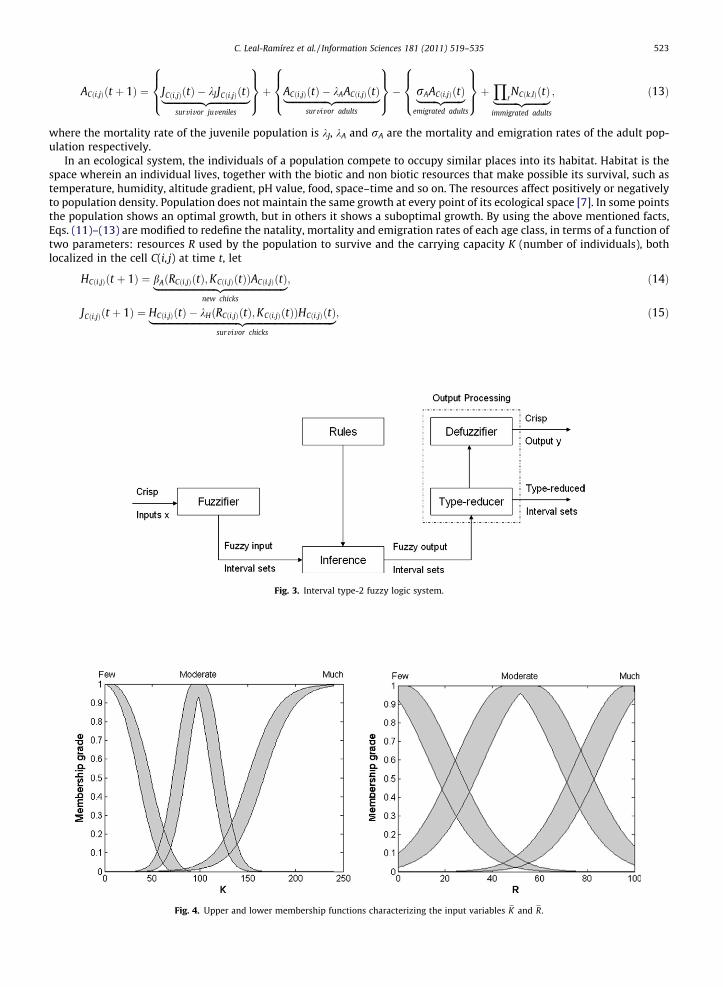
Fig. 4. Upper and lower membership functions characterizing the input variables eK and eR.

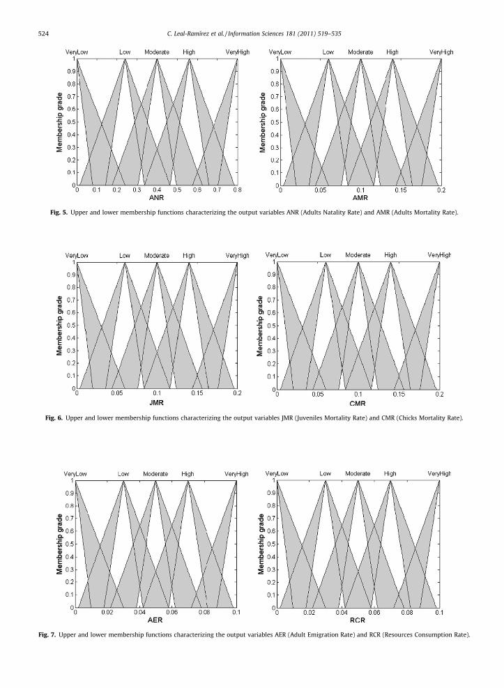
Fig. 5. Upper and lower membership functions characterizing the output variables ANR (Adults Natality Rate) and AMR (Adults Mortality Rate).

Fig. 6. Upper and lower membership functions characterizing the output variables JMR (Juveniles Mortality Rate) and CMR (Chicks Mortality Rate).

Fig. 7. Upper and lower membership functions characterizing the output variables AER (Adult Emigration Rate) and RCR (Resources Consumption Rate).

524 C. Leal-Ramírez et al. / Information Sciences 181 (2011) 519–535

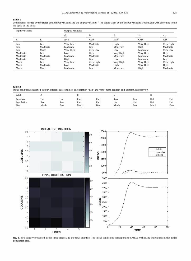
Table 1Combination formed by the states of the input variables and the output variables. * The states taken by the output variables are JMR and CMR according to thelife cycle of the birds.

Input variables Output variables

bA kA kJ kC rA

K R ANR AMR JMR* CMR* AER

Few Few Very Low Moderate High Very High Very HighFew Moderate Moderate Low Moderate High ModerateFew Much Very High Very Low Low Moderate Very LowModerate Few Low High Very High Very High HighModerate Moderate Moderate Moderate Moderate Moderate ModerateModerate Much High Low Low Moderate LowMuch Few Very Low Very High Very High Very High Very HighMuch Moderate Low Moderate High Very High HighMuch Much Moderate Low Moderate High Moderate

Table 2Initial conditions classified in four different cases studies. The notation ‘‘Ran” and ‘‘Uni” mean random and uniform, respectively.

CASE A B C D

Resource Uni Uni Ran Ran Ran Ran Uni UniPopulation Ran Ran Ran Ran Uni Uni Uni UniSize Much Few Much Few Much Few Much Few

Fig. 8. Bird density presented at the three stages and the total quantity. The initial conditions correspond to CASE A with many individuals in the initialpopulation size.

C. Leal-Ramírez et al. / Information Sciences 181 (2011) 519–535 525

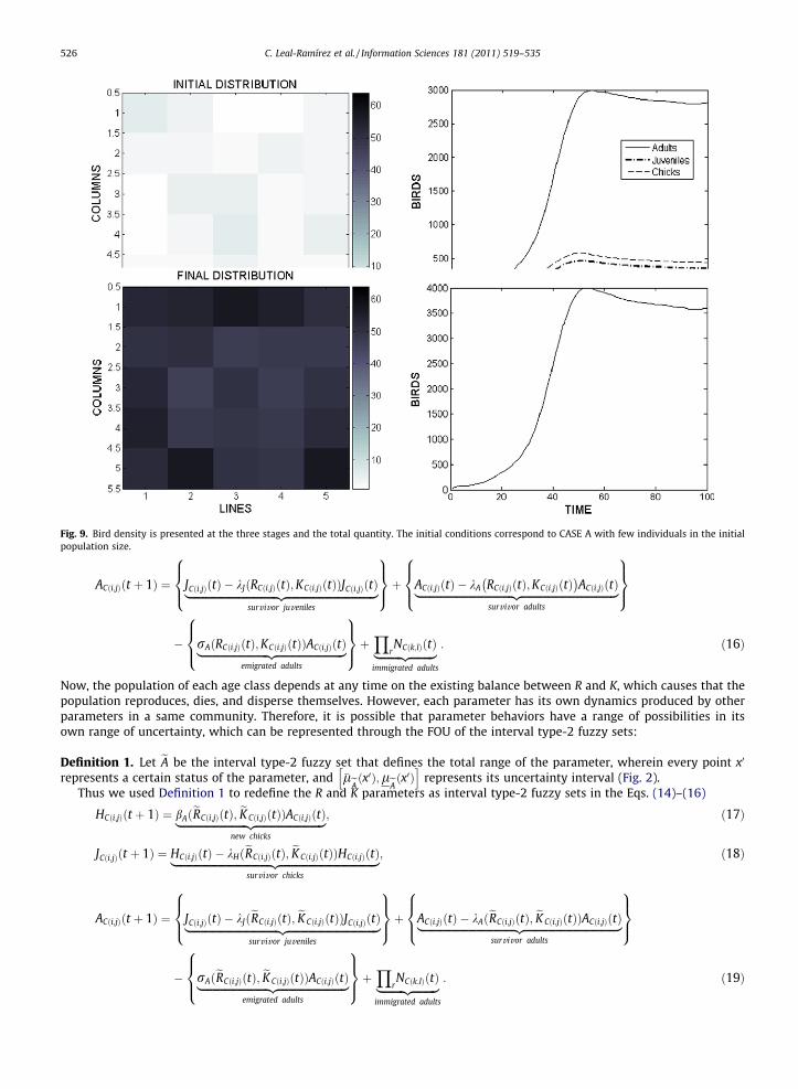
Fig. 9. Bird density is presented at the three stages and the total quantity. The initial conditions correspond to CASE A with few individuals in the initialpopulation size.

526 C. Leal-Ramírez et al. / Information Sciences 181 (2011) 519–535

ACði;jÞðt þ 1Þ ¼ JCði;jÞðtÞ � kJðRCði;jÞðtÞ;KCði;jÞðtÞÞJCði;jÞðtÞ|fflfflfflfflfflfflfflfflfflfflfflfflfflfflfflfflfflfflfflfflfflfflfflfflfflfflfflfflfflfflfflfflfflffl{zfflfflfflfflfflfflfflfflfflfflfflfflfflfflfflfflfflfflfflfflfflfflfflfflfflfflfflfflfflfflfflfflfflffl}survivor juveniles

8><>:9>=>;þ ACði;jÞðtÞ � kA RCði;jÞðtÞ;KCði;jÞðtÞ

� �ACði;jÞðtÞ|fflfflfflfflfflfflfflfflfflfflfflfflfflfflfflfflfflfflfflfflfflfflfflfflfflfflfflfflfflfflfflfflfflfflfflffl{zfflfflfflfflfflfflfflfflfflfflfflfflfflfflfflfflfflfflfflfflfflfflfflfflfflfflfflfflfflfflfflfflfflfflfflffl}

survivor adults

8><>:9>=>;

� rAðRCði;jÞðtÞ;KCði;jÞðtÞÞACði;jÞðtÞ|fflfflfflfflfflfflfflfflfflfflfflfflfflfflfflfflfflfflfflfflfflfflfflfflfflffl{zfflfflfflfflfflfflfflfflfflfflfflfflfflfflfflfflfflfflfflfflfflfflfflfflfflffl}emigrated adults

8><>:9>=>;þ

YrNCðk;lÞðtÞ|fflfflfflfflfflfflfflfflffl{zfflfflfflfflfflfflfflfflffl}

immigrated adults

: ð16Þ

Now, the population of each age class depends at any time on the existing balance between R and K, which causes that thepopulation reproduces, dies, and disperse themselves. However, each parameter has its own dynamics produced by otherparameters in a same community. Therefore, it is possible that parameter behaviors have a range of possibilities in itsown range of uncertainty, which can be represented through the FOU of the interval type-2 fuzzy sets:

Definition 1. Let eA be the interval type-2 fuzzy set that defines the total range of the parameter, wherein every point x0

represents a certain status of the parameter, and �leAðx0Þ;leAðx0Þh irepresents its uncertainty interval (Fig. 2).

Thus we used Definition 1 to redefine the R and K parameters as interval type-2 fuzzy sets in the Eqs. (14)–(16)

HCði;jÞðt þ 1Þ ¼ bAðeRCði;jÞðtÞ; eK Cði;jÞðtÞÞACði;jÞðtÞ|fflfflfflfflfflfflfflfflfflfflfflfflfflfflfflfflfflfflfflfflfflfflfflfflfflffl{zfflfflfflfflfflfflfflfflfflfflfflfflfflfflfflfflfflfflfflfflfflfflfflfflfflffl}new chicks

; ð17Þ

JCði;jÞðt þ 1Þ ¼ HCði;jÞðtÞ � kHðeRCði;jÞðtÞ; eK Cði;jÞðtÞÞHCði;jÞðtÞ|fflfflfflfflfflfflfflfflfflfflfflfflfflfflfflfflfflfflfflfflfflfflfflfflfflfflfflfflfflfflfflfflfflfflfflfflffl{zfflfflfflfflfflfflfflfflfflfflfflfflfflfflfflfflfflfflfflfflfflfflfflfflfflfflfflfflfflfflfflfflfflfflfflfflffl}survivor chicks

; ð18Þ

ACði;jÞðt þ 1Þ ¼ JCði;jÞðtÞ � kJðeRCði;jÞðtÞ; eK Cði;jÞðtÞÞJCði;jÞðtÞ|fflfflfflfflfflfflfflfflfflfflfflfflfflfflfflfflfflfflfflfflfflfflfflfflfflfflfflfflfflfflfflfflfflfflffl{zfflfflfflfflfflfflfflfflfflfflfflfflfflfflfflfflfflfflfflfflfflfflfflfflfflfflfflfflfflfflfflfflfflfflffl}survivor juveniles

8><>:9>=>;þ ACði;jÞðtÞ � kAðeRCði;jÞðtÞ; eK Cði;jÞðtÞÞACði;jÞðtÞ|fflfflfflfflfflfflfflfflfflfflfflfflfflfflfflfflfflfflfflfflfflfflfflfflfflfflfflfflfflfflfflfflfflfflfflffl{zfflfflfflfflfflfflfflfflfflfflfflfflfflfflfflfflfflfflfflfflfflfflfflfflfflfflfflfflfflfflfflfflfflfflfflffl}

survivor adults

8><>:9>=>;

� rAðeRCði;jÞðtÞ; eK Cði;jÞðtÞÞACði;jÞðtÞ|fflfflfflfflfflfflfflfflfflfflfflfflfflfflfflfflfflfflfflfflfflfflfflfflfflffl{zfflfflfflfflfflfflfflfflfflfflfflfflfflfflfflfflfflfflfflfflfflfflfflfflfflffl}emigrated adults

8><>:9>=>;þ

YrNCðk;lÞðtÞ|fflfflfflfflfflfflfflfflffl{zfflfflfflfflfflfflfflfflffl}

immigrated adults

: ð19Þ

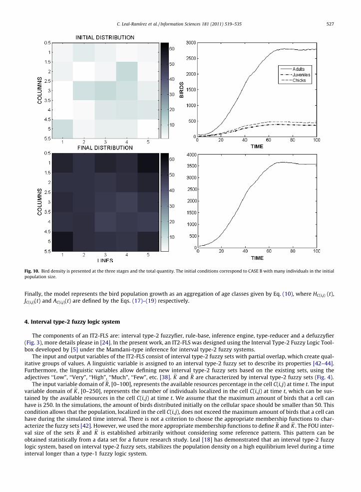
Fig. 10. Bird density is presented at the three stages and the total quantity. The initial conditions correspond to CASE B with many individuals in the initialpopulation size.

C. Leal-Ramírez et al. / Information Sciences 181 (2011) 519–535 527

Finally, the model represents the bird population growth as an aggregation of age classes given by Eq. (10), where HC(i,j) (t),JC(i,j)(t) and AC(i,j)(t) are defined by the Eqs. (17)–(19) respectively.

4. Interval type-2 fuzzy logic system

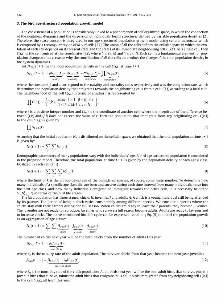
The components of an IT2-FLS are: interval type-2 fuzzyfier, rule-base, inference engine, type-reducer and a defuzzyfier(Fig. 3), more details please in [24]. In the present work, an IT2-FLS was designed using the Interval Type-2 Fuzzy Logic Tool-box developed by [5] under the Mamdani-type inference for interval type-2 fuzzy systems.

The input and output variables of the IT2-FLS consist of interval type-2 fuzzy sets with partial overlap, which create qual-itative groups of values. A linguistic variable is assigned to an interval type-2 fuzzy set to describe its properties [42–44].Furthermore, the linguistic variables allow defining new interval type-2 fuzzy sets based on the existing sets, using theadjectives ‘‘Low”, ‘‘Very”, ‘‘High”, ‘‘Much”, ‘‘Few”, etc. [38]. eK and eR are characterized by interval type-2 fuzzy sets (Fig. 4).

The input variable domain of eR, [0–100], represents the available resources percentage in the cell C(i, j) at time t. The inputvariable domain of eK , [0–250], represents the number of individuals localized in the cell C(i, j) at time t, which can be sus-tained by the available resources in the cell C(i, j) at time t. We assume that the maximum amount of birds that a cell canhave is 250. In the simulations, the amount of birds distributed initially on the cellular space should be smaller than 50. Thiscondition allows that the population, localized in the cell C(i, j), does not exceed the maximum amount of birds that a cell canhave during the simulated time interval. There is not a criterion to choose the appropriate membership functions to char-acterize the fuzzy sets [42]. However, we used the more appropriate membership functions to define eR and eK . The FOU inter-val size of the sets eR and eK is established arbitrarily without considering some reference pattern. This pattern can beobtained statistically from a data set for a future research study. Leal [18] has demonstrated that an interval type-2 fuzzylogic system, based on interval type-2 fuzzy sets, stabilizes the population density on a high equilibrium level during a timeinterval longer than a type-1 fuzzy logic system.

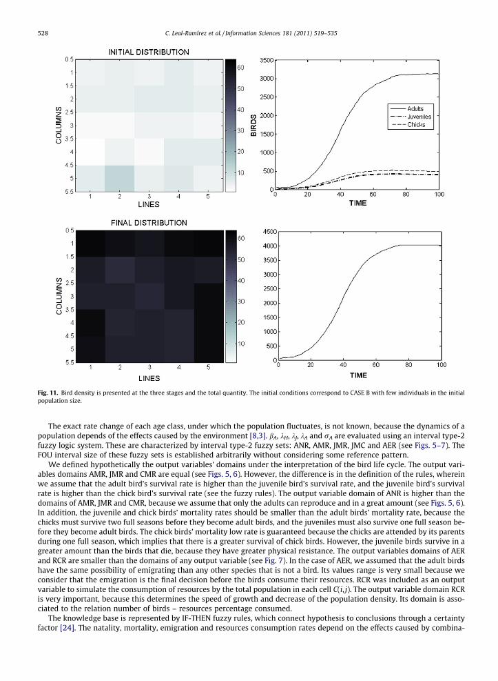
Fig. 11. Bird density is presented at the three stages and the total quantity. The initial conditions correspond to CASE B with few individuals in the initialpopulation size.

528 C. Leal-Ramírez et al. / Information Sciences 181 (2011) 519–535

The exact rate change of each age class, under which the population fluctuates, is not known, because the dynamics of apopulation depends of the effects caused by the environment [8,3]. bA, kH, kJ, kA and rA are evaluated using an interval type-2fuzzy logic system. These are characterized by interval type-2 fuzzy sets: ANR, AMR, JMR, JMC and AER (see Figs. 5–7). TheFOU interval size of these fuzzy sets is established arbitrarily without considering some reference pattern.

We defined hypothetically the output variables’ domains under the interpretation of the bird life cycle. The output vari-ables domains AMR, JMR and CMR are equal (see Figs. 5, 6). However, the difference is in the definition of the rules, whereinwe assume that the adult bird’s survival rate is higher than the juvenile bird’s survival rate, and the juvenile bird’s survivalrate is higher than the chick bird’s survival rate (see the fuzzy rules). The output variable domain of ANR is higher than thedomains of AMR, JMR and CMR, because we assume that only the adults can reproduce and in a great amount (see Figs. 5, 6).In addition, the juvenile and chick birds’ mortality rates should be smaller than the adult birds’ mortality rate, because thechicks must survive two full seasons before they become adult birds, and the juveniles must also survive one full season be-fore they become adult birds. The chick birds’ mortality low rate is guaranteed because the chicks are attended by its parentsduring one full season, which implies that there is a greater survival of chick birds. However, the juvenile birds survive in agreater amount than the birds that die, because they have greater physical resistance. The output variables domains of AERand RCR are smaller than the domains of any output variable (see Fig. 7). In the case of AER, we assumed that the adult birdshave the same possibility of emigrating than any other species that is not a bird. Its values range is very small because weconsider that the emigration is the final decision before the birds consume their resources. RCR was included as an outputvariable to simulate the consumption of resources by the total population in each cell C(i, j). The output variable domain RCRis very important, because this determines the speed of growth and decrease of the population density. Its domain is asso-ciated to the relation number of birds – resources percentage consumed.

The knowledge base is represented by IF-THEN fuzzy rules, which connect hypothesis to conclusions through a certaintyfactor [24]. The natality, mortality, emigration and resources consumption rates depend on the effects caused by combina-

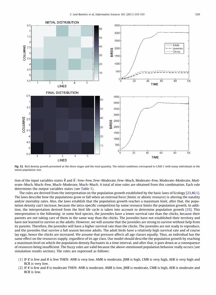
Fig. 12. Bird density growth presented at the three stages and the total quantity. The initial conditions correspond to CASE C with many individuals in theinitial population size.

C. Leal-Ramírez et al. / Information Sciences 181 (2011) 519–535 529

tion of the input variables states eR and eK : Few–Few, Few–Moderate, Few–Much, Moderate–Few, Moderate–Moderate, Mod-erate–Much, Much–Few, Much–Moderate, Much–Much. A total of nine rules are obtained from this combination. Each ruledetermines the output variables states (see Table 1).

The rules are derived from the interpretation on the population growth established by the basic laws of Ecology [23,40,1].The laws describe how the populations grow or fall when an external force (biotic or abiotic resource) is altering the natalityand/or mortality rates. Also, the laws establish that the population growth reaches a maximum limit, after that, the popu-lation density can’t increase, because the intra-specific competition by some resource limits the population growth. In addi-tion, the interpretation derived from the bird life cycle is taken into account to determine population growth [33]. Thisinterpretation is the following: in some bird species, the juveniles have a lower survival rate than the chicks, because theirparents are not taking care of them in the same way than the chicks. The juveniles have not established their territory andhave not learned to survive as the adults. However, we will assume that the juveniles are strong to survive without help fromits parents. Therefore, the juveniles will have a higher survival rate than the chicks. The juveniles are not ready to reproduce,and the juveniles that survive a full season become adults. The adult birds have a relatively high survival rate and of courselay eggs, hence the chicks are increased. We assume that pressure affects all age classes equally. Thus, an individual has thesame effect on the resources supply, regardless of its age class. Our model should describe the population growth by reachinga maximum level on which the population density fluctuates in a time interval, and after that, it goes down as a consequenceof resources being insufficient. The fuzzy rules are valid because the above-mentioned population behavior really occurs (seesimulation results section). The rules are expressed as follows:

(1) IF K is few and R is few THEN: ANR is very low, AMR is moderate, JMR is high, CMR is very high, AER is very high andRCR is very low.

(2) IF K is few and R is moderate THEN: ANR is moderate, AMR is low, JMR is moderate, CMR is high, AER is moderate andRCR is low.

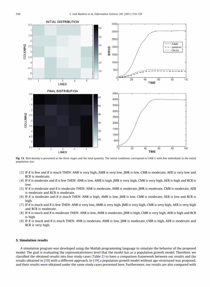
Fig. 13. Bird density is presented at the three stages and the total quantity. The initial conditions correspond to CASE C with few individuals in the initialpopulation size.

530 C. Leal-Ramírez et al. / Information Sciences 181 (2011) 519–535

(3) IF K is few and R is much THEN: ANR is very high, AMR is very low, JMR is low, CMR is moderate, AER is very low andRCR is moderate.

(4) IF K is moderate and R is few THEN: ANR is low, AMR is high, JMR is very high, CMR is very high, AER is high and RCR islow.

(5) IF K is moderate and R is moderate THEN: ANR is moderate, AMR is moderate, JMR is moderate, CMR is moderate, AERis moderate and RCR is moderate.

(6) IF K is moderate and R is much THEN: ANR is high, AMR is low, JMR is low, CMR is moderate, AER is low and RCR ishigh.

(7) IF K is much and R is few THEN: ANR is very low, AMR is very high, JMR is very high, CMR is very high, AER is very highand RCR is moderate.

(8) IF K is much and R is moderate THEN: ANR is low, AMR is moderate, JMR is high, CMR is very high, AER is high and RCRis high

(9) IF K is much and R is much THEN: ANR is moderate, AMR is low, JMR is moderate, CMR is high, AER is moderate andRCR is very high.

5. Simulation results

A simulation program was developed using the Matlab programming language to simulate the behavior of the proposedmodel. The goal is evaluating the representativeness level that the model has as a population growth model. Therefore, weclassified the obtained results into four study cases (Table 2) to have a comparison framework between our results and theresults obtained in [19] with a different approach. In [19] a population growth model without age-structured was proposed,and their results were obtained under the same study cases presented here. Furthermore, our results are also compared with

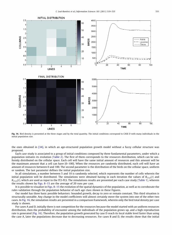
Fig. 14. Bird density is presented at the three stages and by the total quantity. The initial conditions correspond to CASE D with many individuals in theinitial population size.

C. Leal-Ramírez et al. / Information Sciences 181 (2011) 519–535 531

the ones obtained in [34], in which an age-structured population growth model without a fuzzy cellular structure wasproposed.

Each case study is associated to a group of initial conditions composed by three fundamental parameters, under which apopulation initiates its evolution (Table 2). The first of them corresponds to the resources distribution, which can be uni-formly distributed on the cellular space. Each cell will have the same initial amount of resources and this amount will bethe maximum amount that a cell can have [0–100]. When the resources are randomly distributed, each cell will have anamount of resources between 0 and 100. The second parameter is the distribution of the birds on the cellular space, uniformor random. The last parameter defines the initial population size.

In all simulations, a number between 5 and 10 is randomly selected, which represents the number of cells wherein theinitial population will be distributed. The simulations were obtained having in each iteration the values of RC(i,j)(t) andKC(i,j)(t), which are used as input to the IT2-FLS. The simulations results are presented per each case study (Table 1), whereinthe results shown by Figs. 8–15 are the average of 20 runs per case.

It is possible to visualize in Figs. 8–15 the evolution of the spatial dynamics of the population, as well as to corroborate therules validation through the population behavior of each age class shown in these Figures.

Our model has three basic possible behaviors: bounded growth, decay to zero or remain constant. This third situation isstructurally unstable. Any change in the model coefficients will almost certainly move the system into one of the other twocases. In Fig. 16, the simulation results are presented in a comparison framework, wherein only the bird total density per casestudy is shown.

For cases A and D, initially there is not competition for the resources because the model started with an uniform resourcesdistribution, then the probability of encounter among the individuals of the population grows up, and a high reproductionrate is generated (Fig. 16). Therefore, the population growth generated by case D reach its local stable level faster than usingthe case A, later the populations decrease due to decreasing resources. For cases B and D, the results show that the initial

Fig. 15. Bird density is presented at the three stages and the total quantity. The initial conditions correspond to CASE D with few individuals in the initialpopulation size.

532 C. Leal-Ramírez et al. / Information Sciences 181 (2011) 519–535

number of individuals determines the time that the population takes to reach its stable level before arriving to its extinction(Fig. 16). Nevertheless, a heterogeneous initial resources distribution (case B) determines that the population growth beslower than case C, because the individuals take time in looking for resources, and these probably are not near where theindividuals are. Therefore, this situation causes a low reproduction, high mortality and very high emigration. However, thisnot necessarily must be true, the heterogeneous resources distribution can determine another initial space configuration,where probably the population is nearer or farther from the resources. This situation causes different growth curves. Table3 shows time intervals wherein the population density is stable before going down.

Although it is difficult to understand why fluctuations in the population density happen, its study is very important be-cause these can have a deep effect on other species. We have previously proposed several methods to model populationgrowth [18,19]. Now, the model proposed in this work, was designed based on the life cycle of a bird species. The simulationsresults show that our model predicts the population growth better than any basic model, for example using the Verlhust’smodel [40]:

NðtÞ ¼ KN0ert

K � N0ðert � 1Þ : ð20Þ

Simulations were made using the Eq. (20) to show the population growth under different values for r (growth rate) and K(carrying capacity) (Fig. 17).

The population (Fig. 17) reaches the carrying capacity for any value of r, and even though the carrying capacity changes,the population also reaches its limits with any value of r, which means that there is not influence of the environment, this is,the environmental conditions always are optimal and the population only requires time to arrive at limit K. However, thiscannot be possible, because the environment can only support a limited number of individuals before the lack of resourceslimits the survival of these individuals.

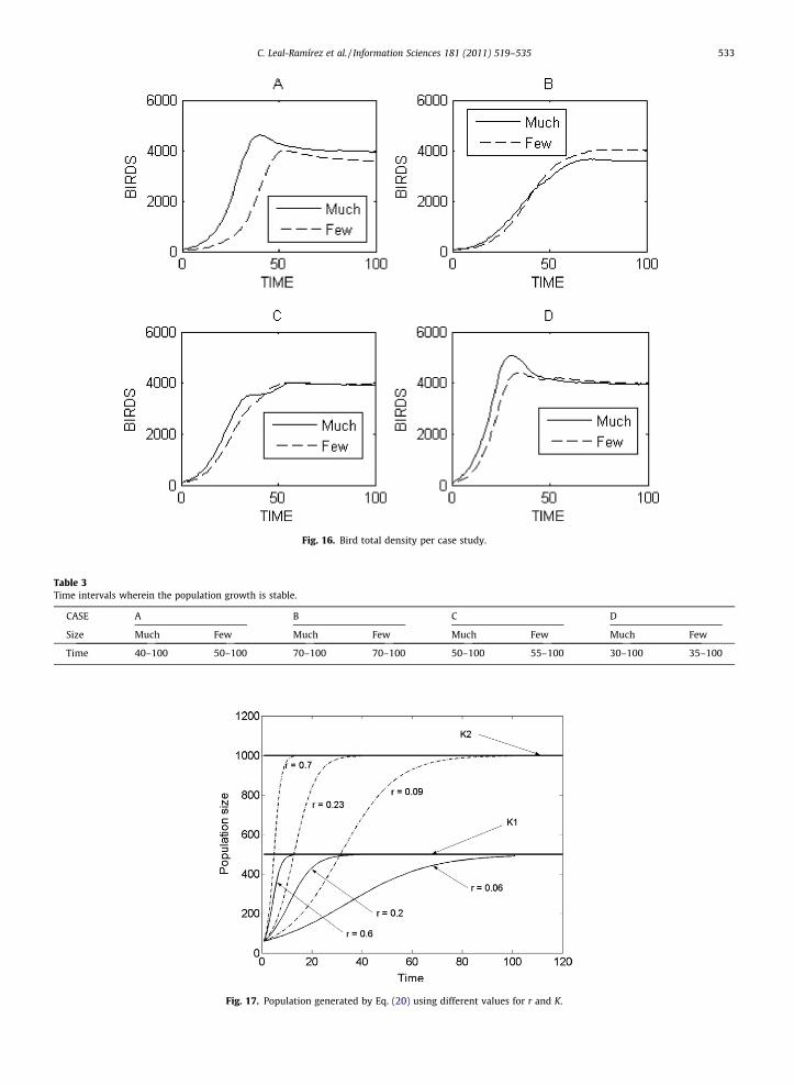
Fig. 16. Bird total density per case study.

Table 3Time intervals wherein the population growth is stable.

CASE A B C D

Size Much Few Much Few Much Few Much Few

Time 40–100 50–100 70–100 70–100 50–100 55–100 30–100 35–100

Fig. 17. Population generated by Eq. (20) using different values for r and K.

C. Leal-Ramírez et al. / Information Sciences 181 (2011) 519–535 533

534 C. Leal-Ramírez et al. / Information Sciences 181 (2011) 519–535

Stone [34] designed a simple linear age-structured population growth model. He looked at several possible nonlinear ef-fects and concluded that random effects could be considered. However, this model continues to work with constant coeffi-cients and without emigration. His results show curves of growth similar to the ones shown in Fig. 17.

6. Conclusion

All the living organisms show an important tolerance range towards environment resources that limit their development,for example: the light, the temperature, the salinity, the available water, the space, etc. Renshaw [29] concluded that virtu-ally all ecologically useful models will involve environmental variability. We have proposed several methods to model thepopulation growth: models presented in [15,16] and the model presented in this work. All these are examples that corrob-orate the statement by Renshaw [29]. The predictions made by our model are good when the interpretation derived fromecological laws and the bird life cycle is the correct one (Table 1). This sort of modeling can be used to predict how thechanges in the environment affect populations. In addition, these models are used for helping determine which informationis most critical and to know which things need to be changed. Of course, we can use the same techniques for different spe-cies. For that, it is necessary to understand the life cycle of the species considered. More complex models can be built, whichconsider more life stages and define the environment resources using several input variables in the fuzzy logic system.

References

[1] W.C. Alle, Animal Aggregations: A Study in General Sociology, University of Chicago Press, USA, 1932.[2] J. Bascompte, Ecological systems, in: R.A. Meyers (Ed.), Encyclopedia of Complexity and System Science, Springer, 2009.[3] A. Berryman, Principles of population dynamics and their application, Thornes, Cheltenham, 1999.[4] R.W. Bosserman, R.K. Ragade, Ecosystem analysis using fuzzy set theory, Ecological Modelling 16 (1982) 191–208.[5] J.R. Castro, O. Castillo, P. Melin, An interval type-2 fuzzy logic toolbox for control applications, FUZZ-IEEE (2007).[6] J.R. Castro, O. Castillo, P. Melin, A. Rodrı́guez-Dı́az, A hybrid learning algorithm for a class of interval type-2 fuzzy neural networks, Information

Sciences 179 (2009) 2175–2193.[7] F.B. Christiansen, T.M. Fenchel, Theories of Populations in Biological Communities, Springer, Berlin, 1977.[8] T. Coulson, S. Albon, F. Guinness, Population substructure, local density, and calf winter survival in red deer (Cervus elaphus), Ecology 78 (1997) 852–

863.[9] S. Coupland, R. John, Type-2 fuzzy logic and the modelling of uncertainty, in: H. Bustince, F. Herrera, J. Montero (Eds.), Fuzzy Sets and Their Extensions:

Representation, Aggregation and Models, Springer, 2008.[10] M.H. Fazel Zarandi, I.B. Turksen, O. Torabi-Kasbi, Type-2 fuzzy modelling for desulphurization of steel process, International Journal of Expert Systems

with Applications 32 (1) (2007) 157–171.[11] M.H. Fazel Zarandi, B. Rezaee, I.B. Turksen, E. Neshat, A type-2 fuzzy rule-based expert system model for stock price analysis, Journal of Expert Systems

with Applications 36 (1) (2009) 139–154.[12] S. Greenfield, F. Chiclana, S. Coupland, R. John, The collapsing method of defuzzification for discretised interval type-2 fuzzy sets, Information Sciences

179 (2009) 2055–2069.[13] D. Hidalgo, O. Castillo, P. Melin, Type-1 and type-2 fuzzy inference systems as integration methods in modular neural networks for multimodal

biometry and its optimization with genetic algorithms, Information Sciences 179 (2009) 2123–2145.[14] R.I. John, Type 2 fuzzy sets for community transport scheduling, in: Proceedings of the Fourth European Congress on Intelligent Techniques and Soft

Computing – EUFIT’96, vol. 2, 1996, pp. 1369–1372.[15] R.I. John, Type 2 Fuzzy Sets for Knowledge Representation and Inferencing, Research Monograph 10, School of Computing Sciences, De Montfort

University, 1998.[16] R. John, S. Coupland, Type-2 fuzzy logic: a historical view, IEEE Computational Intelligence Magazine (2007) 57–62.[17] N.N. Karnik, J.M. Mendel, Application of type-2 fuzzy logic system to forecasting of time-series, Information Sciences 120 (1999) 89–111.[18] C. Leal-Ramirez, O. Castillo, A. Rodriguez-Diaz, Fuzzy cellular model applied to the dynamics of a uni-specific population induced by environment

variations, in: Proceedings of Ninth Mexican International Conference on Computer Science, 2008, pp. 211–220.[19] C. Leal-Ramirez, O. Castillo, A. Rodriguez-Diaz, Interval type-2 fuzzy cellular model applied to the dynamic of the uni-specific population induced by

environment variations, International Journal of Computing and Information Technology 1 (2) (2009) 71–90.[20] J. Li, F. Brauer, Continuous-time age-structured models in population dynamics and Epidemiology, in: F. Brauer, P. van den Driessche, J. Wu (Eds.),

Mathematical Epidemiology, Springer, Berlin/ Heidelberg, 2008, pp. 205–227.[21] Y. Li, H. Jing, Type-2 fuzzy mathematical modeling and analysis of the dynamical behaviors of complex ecosystems, Simulation Modelling Practice and

Theory 16 (2008) 1379–1391.[22] Y. Li, S. Xihao, Modelling dynamic niche and community model by type-2 fuzzy set, Ecological Modelling 211 (2008) 375–382.[23] T.R. Malthus, An essay on the principle of population. J. Johnson, London, 1798.[24] J.M. Mendel, Uncertain Rule-Based Fuzzy Logic Systems: Introduction and New Directions, Prentice-Hall, Upper Saddleback River, NJ, 2001.[25] J.M. Mendel, Advances in type-2 fuzzy sets and systems, Information Sciences 177 (2006) 84–110.[26] O. Mendoza, P. Melin, G. Licea, A hybrid approach for image recognition combining type-2 fuzzy logic, modular neural networks and the Sugeno

integral, Information Sciences 179 (2009) 2078–2101.[27] J. Neumann, Theory of Self-Reproducing Automata, University of Illinois Press, Urbana, 1966.[28] B.R. Noon, J.R. Sauer, Population models for passerine birds: structure, parameterization, and analysis, in: D.R. McCullough, R.H. Barret, (Eds.), Wildlife

2001: Populations, Elsevier Applied Science, New York, 1992, pp. 441–464.[29] E. Renshaw, Modelling Biological Populations in Space and Time, Cambridge University Press, Cambridge, 1991.[30] D. Ruiz-Moreno, P. Federico, G.A. Canziani, Population dynamics models based on cellular automata that include habitat quality indices defined

through remote sensing, in: Buenos Aires 2002 – Proceedings of the 29th International Symposium on Remote Sensing of Environment (ISRSE).Information for Sustainability and Development CDR.

[31] S. Ruyong, Animal Ecological Principle, Beijing Normal University, 1983.[32] A. Salski, Fuzzy knowledge-based models in ecological research, Ecological Modelling 63 (1992) 103–112.[33] A.J. Schaefer, C. Wilson, The fuzzy structure of populations, Canadian Journal of Zoology 80 (2002) 2235–2241.[34] W.D. Stone, Age-structured population models, 1997.[35] I. Turksen, Interval valued fuzzy sets based on normal forms, Fuzzy Sets and Systems 20 (1986) 191–210.[36] I. Turksen, Four methods of approximate reasoning with interval-valued fuzzy sets, International Journal of Approximate Reasoning 3 (1989) 121–142.[37] I. Turksen, Interval valued fuzzy sets and fuzzy measures, in: Proceedings of the First International Joint Conference of NAFIPS, 1994, pp. 317–321.

C. Leal-Ramírez et al. / Information Sciences 181 (2011) 519–535 535

[38] I. Turksen, Type I and interval-valued type II fuzzy sets and logics, in: P. Wang (Ed.), Advances in Fuzzy Theory and Technology, 1995.[39] I. Turksen, Y. Tian, Interval-valued fuzzy sets representation on multiple antecedent fuzzy simplications and reasoning, Fuzzy Sets and Systems 52

(1992) 143–167.[40] P.F. Verhulst, Notice sur la loi que la population suit dans son accroissement, Corrective Mathematics and Physics 10 (1838) 113–121.[41] G.F. Webb, Population models structured by age, size, and spatial position, in: P. Magal, S. Ruan (Eds.), Structured population models in biology and

epidemiology, Lecture Notes in Mathematics Mathematical Biosciences Subseries, vol. 1936, Springer, 2008.[42] L.A. Zadeh, The concept of a linguistic variable and its application to approximate reasoning, Information Sciences 8 (1975) 199–249.[43] L.A. Zadeh, Toward a generalized theory of uncertainty (GTU) – an outline, Information Sciences 172 (2005) 1–40.[44] L.A. Zadeh, Is there a need for fuzzy logic?, Information Sciences 178 (2008) 2751–2779