Simulation and validation of in-cylinder combustion for a ...
82
Simulation and validation of in-cylinder combustion for a heavy-duty Otto gas engine using 3D-CFD technique Jacob Arimboor Chinnan A master thesis project carried out at SCANIA CV AB, Sweden Master of Science Thesis TRITA-ITM-EX 2018:673 KTH Industrial Engineering and Management Machine Design SE-100 44 STOCKHOLM
-
Upload
khangminh22 -
Category
Documents
-
view
2 -
download
0
Transcript of Simulation and validation of in-cylinder combustion for a ...
Simulation and validation of in-cylinder combustion for a heavy-duty Otto
gas engine using 3D-CFD technique
Jacob Arimboor Chinnan
A master thesis project carried out at SCANIA CV AB, Sweden
Master of Science Thesis TRITA-ITM-EX 2018:673
KTH Industrial Engineering and Management
Machine Design
SE-100 44 STOCKHOLM
1
Examensarbete TRITA-ITM-EX 2018:673
Simulation and validation of in-cylinder combustion for a heavy-duty Otto gas engine using 3D CFD technique
Jacob Arimboor Chinnan
Godkänt
2018-September-24
Examinator
Andreas Cronhjort
Handledare
Eric Furbo
Uppdragsgivare
Scania CV AB
Kontaktperson
Sammanfattning Utsläpp från bilar har spelat stor roll de senaste decennierna. Detta har lett till ökad användning av
Otto gasmotorer som använder naturgas som bränsle. Nya motordesigner behöver optimeras för
att förbättra motorens effektivitet. Ett effektivt sätt att göra detta på är genom användningen av
simuleringar för att minska ledtiden i motorutvecklingen. Verifiering och validering av
simuleringarna spelar stor roll för att bygga förtroende för och förutsägbarhet hos
simuleringsresultaten.
Syftet med detta examensarbete är att föreslå förbränningsmodellparametrarna efter utvärdering
av olika kombinationer av förbrännings- och tändmodeller för Otto förbränning, vad gäller
beräkningstid och noggrannhet. In-cylindertrycksspår från simulering och mätning jämförs för att
hitta den bästa kombinationen av förbrännings- och tändmodell. Inverkan av tändtid, antal
motorcykler och randvillkor för simuleringsresultatet studeras också.
Resultaten visar att ECFM-förbränningsmodellen förutsäger simuleringsresultaten mer exakt när
man jämför med mätningarna. Effekten av tändningstiden på olika kombinationer av förbrännings-
och tändningsmodell utvärderas också. Stabiliteten hos olika förbränningssimuleringsmodeller
diskuteras också under körning för fler motorcykler. Jämförelse av beräkningstid görs även för
olika kombinationer av förbrännings- och tändmodeller. Resultaten visar också att
flamspårningsmetoden med Euler är mer känslig för cellstorlek och kvalitet hos simuleringsnätet,
jämfört med övriga studerade modeller.
Rekommendationer och förslag ges om nät- och simulerings-inställningar för att prediktera
förbränningen på ett så bra sätt som möjligt. Några möjliga förbättringsområden ges som framtida
arbete för att förbättra noggrannheten i simuleringsresultaten.
Nyckelord: CFD, AVL FIRE, Otto Gasmotor, Förbränningsmodellering, ECFM-modell,
Flamspårningspartikelmodell, Flamspårningsmodell, G-ekvationsmodell, Tändningsmodeller.

2
3
Master of Science Thesis TRITA-ITM-EX 2018:673
Simulation and validation of in-cylinder combustion for a heavy-duty Otto gas engine using 3D CFD technique
Jacob Arimboor Chinnan
Approved
2018-September-24
Examiner
Andreas Cronhjort
Supervisor
Eric Furbo
Commissioner
Scania CV AB
Contact person
Abstract Emission from automobiles has been gaining importance for past few decades. This has gained a
lot of impetus in search for alternate fuels among the automotive manufacturers. This led to the
increase usage of Otto gas engine which uses natural gas as fuel. New engine designs have to be
optimized for improving the engine efficiency. This led to usage of virtual simulations for reducing
the lead time in the engine development. The verification and validation of actual phenomenon in
the virtual simulations with respect to the physical measurements was quite important.
The aim of this master thesis is to suggest the combustion model parameters after evaluating
various combination of combustion and ignition models in terms of computational time and
accuracy. In-cylinder pressure trace from the simulation is compared with the measurement in
order to find the nest suited combination of combustion and ignition models. The influence of
ignition timing, number of engine cycles and boundary conditions on the simulation results are
also studied.
Results showed that ECFM combustion model predicts the simulation results more accurately
when compare to the measurements. Impact of ignition timing on various combination of
combustion and ignition model is also assessed. Stability of various combustion simulation models
is also discussed while running for more engine cycles. Comparison of computational time is also
made for various combination of combustion and ignition models. Results also showed that the
flame tracking method using Euler is dependent on the mesh resolution and the mesh quality.
Recommendations and suggestions are given about the mesh and simulation settings for predicting
the combustion simulation accurately. Some possible areas of improvement are given as future
work for improving the accuracy of the simulation results.
Keywords: CFD, AVL FIRE, Otto Gas Engine, Combustion Modelling, ECFM Model, Flame
Tracking Particle Model, Flame Tracking Model, G-Equation Model, Ignition Models.

4
5
ACKNOWLEDGEMENTS
“Research is creating new knowledge - Neil Armstrong”
First of all, I am very thankful for having the opportunity of doing my master thesis at Scania CV
AB and working on this topic.
I would like to thank Eric Furbo who was my supervisor for this master thesis work for his support,
encouragement, valuable advices and constructive comments leading me towards accomplishing
this thesis.
I would like to thank Karl Pettersson who is manager of the Fluid and Combustion Simulation
(NMGD), for welcoming me in his group. I would like to thank everyone at NMGD Department
for helping me when needed and, for being all the time friendly with me. I was really happy to be
at NMGD department for this thesis work.
I would like to thank Martin Söder and Björn Waldheim for their input and critic in multiple areas
of this thesis. I would also like to thank Wolfgang Schwarz and Andreas Diemath both from AVL
for helping me with specific questions and problems about AVL FIRE. I would like to thank
Richard Adolfsson and Daniel Norling for generating the engine measurements which is used in
this thesis.
Additionally, I would like to thank KTH, Royal Institute of Technology which has supported my
education from the beginning of my master’s degree up to the end of my master thesis. I would
like to thank Assoc. Prof. Dr. Andreas Cronhjort who was my supervisor at KTH, Royal Institute
of Technology and who made everything simpler for me during this master thesis.
Finally, I am deeply thankful to my family for their patient, encouragement and motivation during
my studying in Sweden.
Jacob Arimboor Chinnan
Stockholm, September, 2018

6
7
NOMENCLATURE
This section describes the symbol and the abbreviations used in this research work.
Notations
Symbol Description
P Pressure (bar)
R Gas Constant
T Temperature (K)
ρ Density (kg/m3)
W Molecular Weight
τ Stress Tensor
g Acceleration due to gravity
I Internal Energy
Q Source Term
k Thermal conductivity
Abbreviations
EGR Exhaust Gas Recirculation
SI Spark Ignited
TWC Three Way Catalyst
CFD Computational Fluid Dynamics
BDC Bottom Dead Centre
TDC Top Dead Centre
IDI Indirect Injected engine
DI Direct Injected engine
0D Zero dimensional
1D One dimensional
3D Three dimensional
IVC Intake Valve Closing
EVO Exhaust Valve Opening
8
EBU Eddy Break Up Model
ECFM Extended Coherent Flame Model
FTPM Flame Tracking Particle Method
AKTIM Arc and Kernel Timing Ignition Model
ISSIM Imposed Stretched Spark Ignition Model
CADIM Curve Arc Diffusion Ignition Model
TFSC Turbulent Flame Speed Closure
CFM Coherent Flame Model
PDF Probability Density Function
CTM Characteristic Timescale Model
SCM Steady Combustion Model
FSD Flame Surface Density
ECFM-3Z Extended Coherent Flame-3 Zones model
ECFM-3Z+ Extended Coherent Flame-3 Zones plus model
PAH Polycyclic Aromatic Hydrocarbons
PSK Phenomenological Soot Kinetics
CORK CO Reduced Kinetics
FTM Flame Tracking Method
TKI Tabulated Kinetics of Ignition
2D Two dimensional
PDE Partial Differential Equations
URANS Unsteady Reynold’s Average Naiver Stokes
HACA Hydrogen Abstraction–C2H2 Addition
LES Large Eddy Simulation
DNS Direct Numerical Simulation
SIMPLE Semi-Implicit Method for Pressure-Linked Equation
AMG Algebraic Multi Grid Solver
GSTAB Gradient Stabilization Solver
ILU Incomplete LU preconditioner
FVM Finite Volume Method
FEP Fame Engine Plus
IVO Inlet Valve Opening
CAD Crank Angle in degrees
SF Stretch Factor
CP Combustion Parameter
9
TABLE OF CONTENTS
SAMMANFATTNING (SWEDISH) 1
ABSTRACT 3
FOREWORD 5
NOMENCLATURE 7
TABLE OF CONTENTS 9
LIST OF FIGURES 13
LIST OF TABLES 17
1 INTRODUCTION 19
1.1 Background 19
1.2 Otto Gas Engine 20
1.3 Research Objectives 21
1.4 Assumptions and Delimitations 21
1.5 Previous Research 22
1.6 Outline 23
2 MODELLING OF OTTO GAS ENGINE SIMULATION 25
2.1 Governing Equations 25
2.2 Combustion Models 26
2.2.1 Coherent Flame Model 27
2.2.2 Flame Tracking Particle Model 29
2.2.3 Flame Tracking Model 30
2.3 Ignition Models 30
2.3.1 Spherical Model 31
2.3.2 Spherical-Delay Model 31
2.3.3 Arc and Kernel Tracking Ignition Model (AKTIM) 31
2.3.4 Imposed Stretch Spark Ignition Model (ISSIM) 32
2.3.5 Flame Tracking Ignition Model 32
10
2.3.4 Curve Arc Diffusion Ignition Model (CADIM) 33
2.4 Emission Model 33
2.5 Turbulence Model 35
2.6 Simulation Control Settings 36
2.6.1 Solution Algorithms for Pressure-Velocity Coupling 36
2.6.2 Differencing Scheme 36
2.6.3 Linear Solver 36
2.6.4 Under-Relaxation Factors 37
3 SENSITIVITY ANALYSIS 39
3.1 Objectives 39
3.2 Computational Domain 39
3.3 Influence of Mesh 40
3.3.1 Simulation Cases 41
3.3.2 Results and Discussions 41
3.4 Influence of Initial Conditions 45
3.4.1 Simulation Cases 46
3.4.2 Results and Discussions 46
3.5 Key Parameters 50
4 COMBUSTION MODEL STUDY 51
4.1 Mesh 51
4.2 Simulation Cases 51
4.3 Available Experimental Data 52
4.4 Results and Discussions 53
4.4.1 Comparison of Simulation Models with Measurements at Second Operating
Condition 58
4.4.2 Influence of Ignition Timing on Combustion Models 61
4.4.3 Influence of Number of Cycles on Combustion Models 64
4.4.4 Influence of Boundary Conditions on Simulations Results 67
5 DISCUSSIONS AND CONCLUSIONS 71

11
5.1 Conclusions 71
5.2 Recommendations 71
5.3 Future Work 72
6 REFERENCES 73
APPENDIX A: SUPPLEMENTARY INFORMATION 77

12
13
LIST OF FIGURES
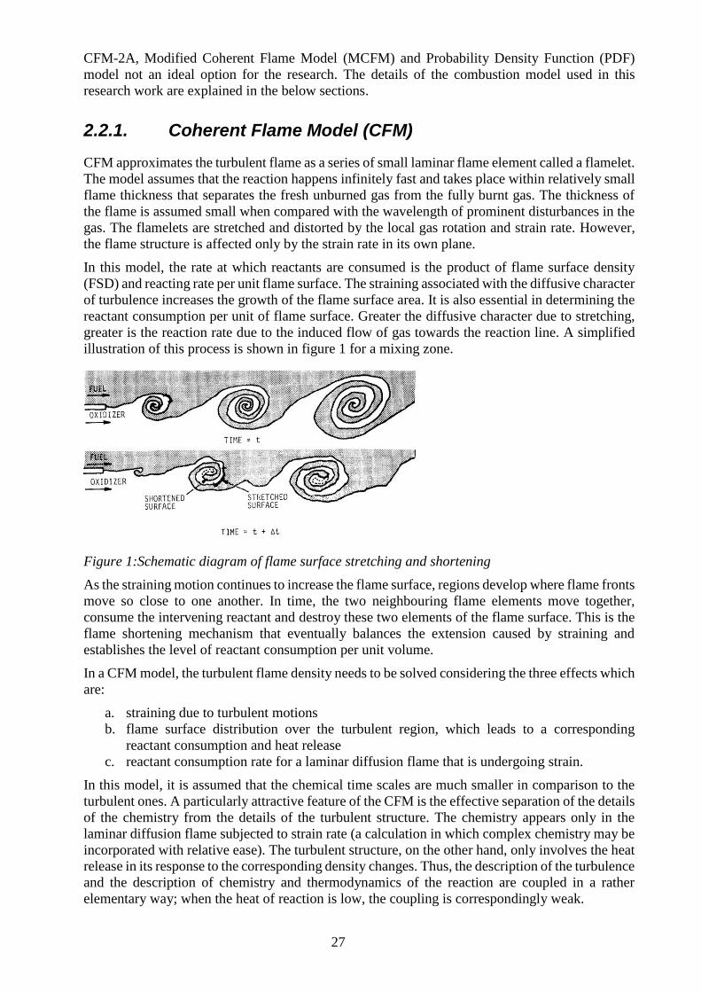
Figure 1:Schematic diagram of flame surface stretching and shortening ..................................... 27
Figure 2 Schematic diagram of spark channel .............................................................................. 33
Figure 3 Computational mesh domain at specific crank angle ..................................................... 40
Figure 4 Time varying computational domain of an engine ......................................................... 40
Figure 5 Heat release trace for in-cylinder cell size sensitivity .................................................... 42
Figure 6 In-cylinder pressure for in-cylinder cell size sensitivity ................................................. 42
Figure 7 Heat release trace for spark plug gap mesh sensitivty (in-cylinder cell size = 2mm) .... 43
Figure 8 In-cylinder pressure trace for spark plug gap mesh sensitivity (in-cylinder cell size =
2mm) ............................................................................................................................................. 43
Figure 9 Heat release trace for spark plug gap mesh sensitivity (in-cylinder cell size = 1.25mm)
....................................................................................................................................................... 44
Figure 10 In-cylinder pressure trace for spark plug gap mesh sensitivty (in-cylinder cell size =
1.25mm) ........................................................................................................................................ 44
Figure 11 In-cylinder temperature trace for the in-cylinder cell size sensitivity .......................... 45
Figure 12 In-cylinder pressure trace for in-cylinder cell size sensitivity ...................................... 46
Figure 13 In-cylinder pressure trace for number of engine cycles sensitivty ............................... 47
Figure 14 In-cylinder temperature trace for number of engine cycle sensitivity .......................... 47
Figure 15 Heat release trace for number of engine cycles sensitivity ........................................... 48
Figure 16 Species concentrations for number of engines cycles sensitivity ................................. 48
Figure 17 In-cylinder pressure trace for simulation start angle sensitivity ................................... 49
Figure 18 In-cylinder temperature for simulation start angle sensitivity ...................................... 49
Figure 19 In-cylinder pressure trace for understanding the influence of flame surface density (FSD)
and stretch factor (SF) in ECFM combustion model with spherical ignition model .................... 53
Figure 20 Zoomed in figure of In-cylinder pressure trace for understanding the influence of flame
surface density (FSD) and stretch factor (SF) in ECFM combustion model with spherical ignition
model ............................................................................................................................................. 54
Figure 21 In-cylinder pressure trace for understanding the influence of flame surface density (FSD)
and stretch factor (SF) in ECFM-3Z+ combustion model with spherical ignition model ............ 54
Figure 22 In-cylinder pressure trace for understanding the influence of flame surface density (FSD)
and stretch factor (SF) in ECFM combustion with spherical delay ignition model ...................... 55
Figure 23 Zoomed in figure of In-cylinder pressure trace for understanding the influence of flame
surface density (FSD) and stretch factor (SF) in ECFM combustion with spherical delay ignition
model ............................................................................................................................................. 56
14
Figure 24 In-cylinder pressure trace for understanding the influence of combustion parameter (CP)
for flame tracking particle method (FTPM) combustion model ................................................... 56
Figure 25 Zoomed in figure of In-cylinder pressure trace for understanding the influence of
combustion parameter (CP) for flame tracking particle method (FTPM) combustion model ...... 57
Figure 26 In-cylinder pressure trace to understand the influence of combustion parameter for flame
tracking method using Euler combustion model ........................................................................... 57
Figure 27 Zoomed in figure of In-cylinder pressure trace to understand the influence of
combustion parameter for flame tracking method using Euler combustion model ...................... 58
Figure 28 Comparison of in-cylinder pressure trace for various simulation models at engine speed
= 1000rpm ..................................................................................................................................... 59
Figure 29 Zoomed in figure of comparison of in-cylinder pressure trace for various simulation
models at engine speed = 1000rpm ............................................................................................... 59
Figure 30 Comparison of in-cylinder pressure for various simulation models at engine speed =
1400 rpm ....................................................................................................................................... 60
Figure 31 Zoomed in figure of comparison of in-cylinder pressure for various simulation models
at engine speed = 1400 rpm........................................................................................................... 60
Figure 32 Influence of ignition timing on in-cylinder pressure trace using ECFM combustion
model with spherical ignition model ............................................................................................. 61
Figure 33 Zoomed in figure of influence of ignition timing on in-cylinder pressure trace using
ECFM combustion model with spherical ignition model ............................................................. 62
Figure 34 Influence of ignition timing on in-cylinder pressure trace using ECFM combustion
model with spherical delay ignition model ................................................................................... 62
Figure 35 Zoomed in figure of influence of ignition timing on in-cylinder pressure trace using
ECFM combustion model with spherical delay ignition model .................................................... 63
Figure 36 Influence of ignition timing on in-cylinder pressure trace using flame tracking particle
method (FTPM) combustion model .............................................................................................. 63
Figure 37 Zoomed in figure of influence of ignition timing on in-cylinder pressure trace using
flame tracking particle method (FTPM) combustion model ......................................................... 64
Figure 38 Influence of number of cycles on in-cylinder pressure trace using ECFM combustion
model with spherical ignition model ............................................................................................. 64
Figure 39 Zoomed in figure of influence of number of cycles on in-cylinder pressure trace using
ECFM combustion model with spherical ignition model ............................................................. 65
Figure 40 Influence of number of cycles on in-cylinder pressure trace using ECFM combustion
model with spherical ignition model ............................................................................................. 65
15
Figure 41 Influence of number of cycles on in-cylinder pressure trace using flame tracking particle
method (FTPM) combustion model .............................................................................................. 66
Figure 42 Zoomed in figure of influence of number of cycles on in-cylinder pressure trace using
flame tracking particle method (FTPM) combustion model ......................................................... 67
Figure 43 Influence of Inlet pressure boundary conditions on in-cylinder pressure trace using flame
tracking particle method (FTPM) combustion model ................................................................... 68
Figure 44 Zoomed in figure of influence of Inlet pressure boundary conditions on in-cylinder
pressure trace using flame tracking particle method (FTPM) combustion model ........................ 68
Figure 45 Influence of wall temperature boundary conditions on in-cylinder pressure trace using
flame tracking particle method (FTPM) combustion model ......................................................... 69
Figure 46 Zoomed in figure of influence of wall temperature boundary conditions on in-cylinder
pressure trace using flame tracking particle method (FTPM) combustion model ........................ 70
Figure 47 Heat release trace for understanding the influence of flame surface density (FSD) and
stretch factor (SF) in ECFM combustion model with spherical ignition model ........................... 77
Figure 48 Heat release trace for understanding the influence of flame surface density (FSD) and
stretch factor (SF) in ECFM-3Z+ combustion model with spherical ignition model ................... 77
Figure 49 Heat release trace for understanding the influence of flame surface density (FSD) and
stretch factor (SF) in ECFM combustion model with spherical delay ignition model ................. 78
Figure 50 Heat release trace for understanding the influence of combustion parameter (CP) for
flame tracking particle method (FTPM) combustion model ......................................................... 78
Figure 51 Heat release trace to understand the influence of combustion parameter for flame
tracking method using Euler combustion model ........................................................................... 79
Figure 52 Comparison of heat release trace for various simulation models at engine speed =
1000rpm ........................................................................................................................................ 79
Figure 53 Comparison of heat release trace for various simulation models at engine speed =
1400rpm ........................................................................................................................................ 80
Figure 54 Influence of ignition timing on heat release trace using ECFM combustion model with
spherical ignition model ................................................................................................................ 80
Figure 55 Influence of ignition timing on heat release trace using ECFM combustion model with
spherical delay ignition model ...................................................................................................... 81
Figure 56 Influence of ignition timing on heat release trace using flame tracking particle method
(FTPM) combustion model ........................................................................................................... 81

16
17
LIST OF TABLES
Table 1 Various meshes considered for the in-cylinder cell size senistivity ................................ 40
Table 2 Various meshes considered for spark plug gap mesh sensitivty ...................................... 41
Table 3 Boundary conditions used in the mesh study and initial conditions simulations ............. 41
Table 4 Simulation model used in the mesh study and initial conditions simulations.................. 41
Table 5 Mesh considered for number of engine cycle and simulation start angle ........................ 46
Table 6 Mesh parameters used for combustion model studies ...................................................... 51
Table 7 Simulation cases for various combination of combustion and ignition model ................ 51
Table 8 Operating conditions ........................................................................................................ 52
Table 9 Specifications of engine used for measurements ............................................................. 52
Table 10 Recommended range of the tunning parameters suggested by AVL ............................. 53
Table 11 Comparison of exhaust gas temperature at domain outlet and simulation run time for
various simulation cases ................................................................................................................ 61
Table 12 Comparison of charge air mass flowrate from simulation and measurements for both
operating conditions ...................................................................................................................... 67

18
19
1 INTRODUCTION
This chapter begins with the detailing of the background and motivation of the research. It is then
followed by the previous research performed on the subject. Later, it is followed by the theory
which leads to the formulation of the research questions. Subsequently, the assumptions and
delimitations of the research are presented. Later, a brief overview of the previous research
performed on the subject is described.
1.1 Background
The pollution caused by automobile emissions has been the talking point for the past few decades.
The emission regulation was introduced by the government authorities around the world in order
to control this pollution. As the decades pass by, the emission norms became stricter and impact
of greenhouse gases became more important. This eventually, led the automobile manufacturers
to focus on higher efficiency engines and low engine emissions.
In the meantime, the computer technologies began to grow and foray into the automobile industry
for various virtual and real-time simulations. Now, an enormous amount of research is dedicated
to developing and improving the numerical simulation models for predicting and simulating real-
time problems. A rapid increase in computing power and relatively lower cost compared to the
physical experiments have made the numerical simulation models a vital part of improving the
efficiency and reducing the emissions of the engine.
The current requirements in the emission regulations have made the automobile manufacturers to
increase the use of various complex technologies such as high-pressure fuel injection, after
treatment devices, exhaust gas recirculation (EGR) and so on. Today’s global attention towards
increasing efficiency and reducing emissions including greenhouse gases and NOx has also
prompted the automobile manufacturers to look for alternative fuels. This has led to an increase in
the use of Otto gas engines which runs on alternative fuels such as methane, natural gas and biogas.
Natural gas has been recognized as one of the promising alternative fuels due to its significant
benefits compared to gasoline and diesel as fuel. Even though it is from fossil origin, natural gas
can theoretically provide 20% reduction of CO2 during vehicle operation compared to diesel or
gasoline due to its high H/C ratio [1][2]. Natural gas is generally considered a very safe fuel since
it is not poisonous and does not catch fire easily since its ignition temperature is higher than
convectional fuels such as gasoline and diesel.
Otto gas engine especially spark-ignited (SI) natural gas engines is commonly used as lean-burn
or stoichiometric combustion system based on the application. This leads to lower production of
soot for a homogeneous air-fuel mixture. The soot production can be further reduced with the help
of a three-way catalyst (TWC) emission technology to achieve the greatest emission potential. The
amount of NOx produced is also low when compared to diesel and gasoline engines since the
maximum temperature during combustion is lower. This also helps in reduction of thermal stress.
These reasons make natural gas a favourable fuel in heavy-duty engines using lean-burn
combustion system. The use of cooled EGR provides a further potential to increase the engine
output and, at the same time, decreases NOx emissions.
SI natural gas engine is usually operated at high compression ratio due to its wide flammability
limits. However, the valve timing needs to be modified in order to achieve the engine efficiency
requirements when compared to the existing gasoline or diesel engines [3]. Various computational
methods are used to predict the engine efficiency. However, the engine efficiency is also dependent
on the engine combustion process and its parameters which is a very complex phenomenon. This
led to the use of Computational Fluid Dynamics (CFD) which utilizes numerical methods and
20
high-fidelity algorithms to solve and analyze such complex fluid flows. The development of high-
speed computers provides the possibility to solve the complicated system of equations and use the
detailed chemical rate methods for combustion prediction.
Nowadays, a lot of commercial softwares are available which use CFD techniques to predict the
combustion process. In these softwares, the users can select various simulation models not only
to understand the physics involved in the complex combustion phenomenon but also to predict
various parameters of in-cylinder combustion which is the major focus of this research.
This research work has been carried out at the Fluid and Combustion Simulation group in Scania.
Scania is a world-leading provider of transport solutions, including trucks and buses for heavy
transport applications. It is also a leading provider of industrial and marine engines. It has around
49,300 employees in about 100 countries. Research and development activities are mainly
concentrated in Sweden, with branches in Brazil and India. The Fluid and Combustion Simulation
group is responsible for numerical simulation of fluid flow phenomena within the engine by using
CFD for investigating new and innovative concepts for future engine platforms.
1.2 Otto Gas Engine
Natural gas which comprises mostly of methane requires an ignition source for combustion due to
its high octane and low cetane number. Thus, it is usually operated on Otto cycle in indirect
injection (IDI) engine. It can also be operated on diesel cycle as direct ignition (DI) or dual fuel
natural gas engine. However, the usage of such engines is limited due to the emissions regulations
and cost.
Practically, the Otto cycle consists of four strokes which are intake stroke, compression stroke,
expansion stroke and exhaust stroke. It generates a power output once in every four strokes which
corresponds to two revolutions of the engine when the engine piston moves from bottom dead
centre (BDC) to top dead centre (TDC). Theoretically, the Otto cycle is a four-stroke
thermodynamic cycle in which each thermodynamic process corresponds to each stroke of the
engine. It includes constant pressure process in which the charge air (air-fuel mixture for an IDI
engine or air for a DI engine) is drawn into engine cylinder (intake stroke), adiabatic compression
process in which the charge air is compressed as the piston moves from BDC to TDC (which is
followed by constant pressure fuel addition in a DI engine) and a constant-volume heat addition
process from the spark plug to the charge air (both process combined in compression stroke),
adiabatic expansion process and a constant volume process in which the burnt gases expand in the
cylinder in which pushes the piston from TDC to BDC during and after the combustion (both
process combined in expansion stroke), and constant pressure process in which the burnt gases are
released to the atmosphere from the engine cylinder (exhaust stroke).
The combustion process in an SI engine can be divided into three areas: ignition and flame
development, flame propagation, and flame termination. The combustion process begins when the
air-fuel mixture is ignited with the help of a high voltage spark from the spark plug. This is usually
done 20-30 degrees before the TDC depending on the operating point. This spark generates a high
energy plasma for a short period of time and creates the flame kernel. Following the initial spark,
there is an ignition delay while the flame kernel created by the spark grows to a significant size to
form a flame front. Following that, the flame front spreads through the combustion chamber. The
rate of spread is determined by the burning velocity. This increase in the volume of the hot burned
gases behind the flame front presses the cooler unburned charge outward. Although the density of
unburned gases ahead of the flame is higher than the burned gases, the cylinder pressure increases,
raising the temperature of the unburned charge through compression heating. Finally, during late
combustion, the remaining elements of the unburned mixture burn out as the piston descends.
There are many simplifying assumptions that underlie the theoretical Otto cycle. These include
zero friction, air as the only working fluid, zero heat transfer, constant-volume heat addition and
21
constant-volume heat rejection. The efficiency of the Otto gas engine depends upon the air-fuel
mixture, compression ratio, high voltage spark and the maximum temperature attained during the
combustion.
1.3 Research Objectives
The commercial CFD softwares have various simulation models for modelling each phenomenon
in different orders of complexity. The prediction of various parameters during the in-cylinder
combustion is important to optimize the engine efficiency. However, it is noted that the results of
these simulation models should match the experimental values.
The accuracy (i.e, deviation between the measured value and simulated value) of the simulation
models determine the effectiveness of the simulation in optimizing the engine efficiency. Also,
increase in simulation runtime affects the engine efficiency optimization process which may cause
a delay in the product life cycle in an extremely sensitive and competitive market. Sometimes, this
can influence the outcome of the product. The above factors lead to a tradeoff between the accuracy
(closeness to the measured value) and runtime of the simulation models which in turn give rise to
the following questions.
1. Which combination of combustion and ignition simulation models predicts the results better
in accuracy (deviation<5%) when compared with the reference measurements (in-cylinder
pressure and heat release estimations)?
2. What is the impact of mesh size and solution initialization on the results, accuracy, and
runtime?
The main deliverables of this research to find the simulation and mesh parametric settings for the
best combination of combustion and ignition simulations models which can accurately predict the
simulation results when compared to the measurements. In this project, it is assumed that the
mathematical modelling of the algorithm for combustion phenomenon is correct. Therefore, the
correctness of these algorithm will not be checked in this research work. Only the implementation
of these combustion simulation models in an Otto gas engine is studied in this project.
1.4 Assumptions and Delimitations
The combustion process is a very complex process. A zero-dimensional (0D) or one-dimensional
(1D) simulation is not enough to predict the combustion phenomenon. In most of the high accuracy
combustion simulations, a three-dimensional (3D) simulation is required where the flame front
needs to be resolved in order to capture this complex phenomenon. The complexity of the
combustion phenomenon also depends upon the level of accuracy of the simulation models which
is used to predict the combustion phenomenon. So, choosing the right combustion, ignition and
emission simulation models are quite important to obtain realistic results in the Otto gas engine
simulation.
In this project, a 3D CFD software is used to simulate the combustion phenomenon. Even though
there are many commercially available CFD software to simulate combustion, AVL FIRE version
17.121 is selected to carry this research and MATLAB is used for post processing of the simulation
results. In AVL FIRE, a fast and stable grid formation process can be realized through automatic
grid technology based on the octree process. [4][5]. Using this software, the in-cylinder processes
can be simulated by a movable mesh model during the engine cycle process especially from Inlet
Valve Closing (IVC) time to Exhaust Valve Opening (EVO) time.
Some main assumptions used in the simulation are:
a. The engine used is a single-cylinder engine.
22
b. The simulation is carried out for two constant operating conditions.
c. The in-cylinder mixture is treated as an ideal gas.
d. Fuel is assumed as methane (CH4) which constitutes for ~93% of natural gas [6].
e. The numerical algorithm of the combustion models is correct.
f. Uniform mixing of air and fuel occurs in the inlet port.
Some of the delimitations of this research project are:
a. Engine blow-by is neglected.
b. Knocking phenomenon is not assessed or modelled.
c. Influence of the boundary layer mesh on the results is not assessed [7].
1.5 Previous Research
One of the earliest experiments with IC engines occurred when Abbe Hautefeuille, a Frenchman,
built a closed chamber in which he exploded gunpowder [8][9]. The resulting high pressure was
used to raise a water column that was in a connecting chamber. By 1680, a Dutch physicist named
Huyghens replaced the water column with a piston, which would move when the gunpowder was
exploded [9]. Such engines of the exploding type were not very efficient, primarily because the
gases in the combustion chamber were not compressed before ignition occurred.
More than 50 years later, in 1838, a scientist named Burnett pointed out the advantages of
compressing the gases in the combustion chamber before ignition [8][9]. Then, in 1862, Beau de
Rochas set forth his famous four principles of operation for an efficient IC engine [8][9]. In 1876,
Nikolaus Otto built on Beau de Rochas’ principles, patenting his famous Otto-cycle engine and
built a successful IC engine two years later [8][9]. Otto was the first to use the four-stroke cycle.
With the expiration of the Otto patent in 1890, there was a spurt in development and
commercialization of IC engines.
In the past decades, the emissions from IC engines have become a severe problem which has
resulted in strict emission regulations. In 2005, the Kyoto protocol was adopted which calls for a
reduction in greenhouse gas emissions [10]. Thereafter, the reduction of hazardous emissions and
greenhouse gases from engines has become a research focus. This lead to the research of the SI
engines which run on alternate fuels. One of these engines is Otto gas engine which emits very
low greenhouse emissions with the help of a TWC. Much effort was devoted to the improvement
of Otto gas engine performance in terms of engine efficiency and emissions. The use of cooled
EGR provides a further potential to increase the engine output and, at the same time, decreases
NOx emissions.
Rapid improvements in the computer power and increase in the knowledge of CFD have resulted
in more advanced and reliable commercial CFD softwares. In most of the commercial CFD
softwares, the end user has only limited knowledge about the CFD codes which is used behind the
simulation models. The measurements data of many practical flow experiments were used to verify
these CFD codes or algorithms. However, the ability to predict or solve flows including complex
process or phenomena using these CFD codes alone is still limited due to complexity of the flows.
Therefore, various approximations and simplifications are used in mathematical models to
describe the complex phenomena, which in turn affect the degree of accuracy of solutions obtained
using these codes.
The development of new engines involves the design of new combustion chamber design and
improved in-cylinder flow dynamics for better combustion. Among the available tools to
investigate and analyze engine combustion process, multidimensional simulation using CFD
techniques is increasingly being adopted to assist gas engine development and reduce the
development cost. In the early stages, these simulations were mainly used to better understand
23
experimental results and for predicting and analyzing the fluid flow motion inside the engine
cylinder towards revealing flow structures and turbulence conditions.
Initially, a simple combustion simulation model called Eddy Break Up (EBU) model was created
using simple approximations for prediction of combustion phenomenon [11]. The accuracy of
solution and replication of real-time phenomenon was still questionable for these models. Later,
more complex algorithms such as Extended Coherent Flame Model (ECFM) [12][13][14][15][16],
G-Equation model[17][18] and Flame Tracking Particle Model (FTPM)[19] were introduced to
predict the combustion phenomena. Some of these complex algorithms requires a detailed
chemical kinetics of the chemical reactions during the combustion phenomenon. The increase in
the capabilities of laboratories and the development of high-speed computers provide the
possibility to solve the complicated system of equations and use the detailed chemical rate methods
for combustion prediction. A lot of optimization of parameters were required to predict the
simulations solutions which are in line with the measurements. Subsequently, it was found that the
ignition simulation model plays a vital role in the accurate prediction of the combustion
phenomenon in SI engines.
A simple ignition model called spherical ignition model was used to replicate the spark ignition.
Later this model was extended to capture the effects of the flow on the spark ignition. However,
the accuracy of these models was found to be limited. A lot of research was carried out for
obtaining an accurate replication of the combustion and ignition phenomenon. More complex
ignition simulation model such as Arc and Kernel Tracking Ignition Model
(AKTIM)[20][21][22][23][24][25], Imposed Stretch Spark Ignition Model (ISSIM)[26][27] and
Curve Arc Diffusion Ignition Model (CADIM)[28] coupled with the combustion models predict
the combustion phenomenon more accurately [Reference].
In recent years, a lot of research has been carried out on combustion simulation with dual fuel and
alternate fuels such as methane, natural gas and biogas since the existing simulation models are
verified only for gasoline and diesel IC engines [Reference].
1.6 Project Outline
After introducing the research topic along with the detailing of the background motivation,
research objective assumptions, and delimitations of the research in chapter 1, chapter 2 gives
additional in-depth theoretical knowledge required to understand the research. It presents how the
Otto gas combustion simulation is modelled using the CFD techniques and how combustion,
ignition, and turbulence models are modelled in the AVL FIRE software. Chapter 3 presents the
sensitivity study of mesh and the initialization conditions. It presents the suggestions of mesh and
initialization conditions used in the research or thesis. Chapter 4 presents the main results of this
thesis where the results of the various combination of simulation models are compared with the
measurements for verifying the simulation results. Finally, the work done in this master thesis will
be summarized in Chapter 5. Some recommendations and suggestions for future work are also
listed in the same chapter.

24
25
2 MODELLING OF OTTO GAS ENGINE SIMULATION
This chapter presents the theoretical reference frame that is necessary to understand the
performed research. It begins with the governing equations used in the CFD simulations.
Subsequently, it describes various turbulence, combustion, ignition, emission models used in the
simulation. Later, it describes the various settings in the CFD software used for modeling it.
Finally, it describes the theory behind the various control settings used in the simulation.
2.1 Governing Equations
Nowadays, CFD simulations are used to predict, analyze and optimize the in-cylinder flow
dynamics and combustion in an engine. The main concept of CFD is the discretized solution of a
set of partial differential equations commonly known as the Navier-Stokes equations. The
governing equations for the CFD simulations are given by the physical laws governing the fluid
flow, heat transfer and chemical reaction. These are usually specified by the pressure, P,
temperature, T and velocity vector with three orthogonal components u,v,w, all of which are
functions of spatial coordinates x,y,z and time t. These are listed below.
1. Equation of State
The equation of state for a species m is given by
𝑃 = 𝑅𝑇∑(𝜌𝑚𝑊𝑚)
𝑚
(1)
where P, R, T, 𝜌𝑚 and 𝑊𝑚 is the pressure, gas constant, temperature, density and
molecular weight of the species m.
2. Conservation of Mass
The conservation of Mass for a species m is given by
𝜕𝜌𝑚𝜕𝑡
+ ∇. (𝜌𝑚𝑣) = ∇. [𝜌𝐷∇ (𝜌𝑚𝜌)] + 𝜌𝑚
�̇� (2)
where 𝜌 is the density of the fluid mixture, 𝜌𝑚 is the density of the species m and 𝜌𝑚�̇� is
the source term due to the combustion.
3. Conservation of Momentum
The conservation of Momentum for the fluid is given by
𝜕𝜌𝑣
𝜕𝑡+ ∇. (𝜌𝑣𝑣) = ∇. (𝑝𝐼 + 𝜏) + 𝜌𝑔 (3)
where 𝜌 is the density, 𝑝 is the pressure, 𝜏 is the stress tensor and g is the
acceleration due to gravity.
4. Conservation of Energy
The conservation of Energy in the fluid is given by
𝜕𝜌𝐼
𝜕𝑡+ ∇. (𝜌𝑣𝐼) = −𝑝∇. 𝑣 + 𝜏∇. 𝑣 + 𝑘∇2𝑇 + 𝑄�̇� (4)
where 𝜌 is the density, 𝑝 is the pressure, 𝑇 is the temperature,𝜏 is the stress tensor,
𝑄�̇� is the source term due to the chemical reaction, 𝑘 is the thermal conductivity and 𝐼 is the internal energy of the fluid respectively.
26
2.2 Combustion Models
Combustion is a complex phenomenon involving chemical reactions, heat transfer and mass
transfer as shown below.
Fuel + Oxidant → Products + Heat (5)
Even the simplest hydrocarbon methane on combustion can lead to higher hydrocarbons and soot.
The heterogeneity of real-world combustion leads to the complexity of the process and the wide
range of compounds. The concentrations of species like fuel, air, and combustion products in and
around the combustion zone vary by orders of magnitude over molecular scales. The temperature
also can change rapidly across a few millimetres of the flame front. In addition, flame fronts can
move quickly. Thus, the fuel can heat up rapidly, start to combust, and then cool due to quenching
the further reaction. Similarly, part of the flame can have excess oxygen while another part can
have excess fuel. All these happen in a small span of time which makes the entire combustion
phenomenon a complex one.
During combustion, the fate of organic fuel molecules is largely determined by the local conditions
(e.g. temperature, availability of oxygen, and time). If ample oxygen is present locally, i.e. directly
where the combustion is occurring, the fuel will tend to oxidize and break down into smaller
organic molecules until ultimately forming carbon monoxide (CO) and carbon dioxide (CO2). If
combustion in fuel-rich conditions is considered, the combustion mechanism becomes more
complex. Higher hydrocarbons will lead to the formation of many complex intermediates. The
emissions of air toxics from combustion can be reduced by raising the temperature of combustion,
increasing oxygen availability, and allowing a longer reaction time. However, these conditions are
difficult to meet as engines have a more limited residence time in the combustion region, cooler
reaction zones (particularly near the walls), and areas of reduced oxygen [30].
The kinetic equations are based on a combustion mechanism with a preliminary reaction series.
Increasing the number of chemical reactions and species will make the combustion model more
accurate. The transport equations for a reacting flow are the energy and species transport equations
with variable density. These equations can be solved using appropriate boundary conditions which
can be of Dirichlet or Neumann type. Modelling combustion requires modelling the reaction
kinetics and the flame propagation which requires the knowledge of the speeds of reactions,
product concentrations, temperature and other parameters. A fuel-air mixture will generally
combust if the reaction is fast enough to prevail until all the mixture is burned into products. If the
reaction is too slow, the flame will extinguish and if the reaction is too fast, explosion or even
detonation will occur.
The reaction rate of a typical combustion reaction is influenced mainly by the concentration of the
reactants, temperature, and pressure. Usually, it is found out through experiments with the help of
the Arrhenius equation. Usually, in a combustion-turbulence modelling, it has been anticipated
that the topology of the flame or its destruction in the turbulent field will be affected by the flow
turbulence.
Even though, there are many combustion models available in AVL FIRE, only a few were selected
for this research. The main reason for this decision is combustion modelling features, capability
of modelling the detailed ignition phenomenon, area of application (Otto gas SI engine), and also
from available previous research work. The dependence of the combusting modelling parameters
on engine operating conditions makes EBU combustion model (which is the simplest combustion
model) not an ideal option for the research. Similarly, the area of application makes Extended
Coherent Flame Model - 3Zone (ECFM-3Z), Characteristic Timescale Model (CTM) and Steady
Combustion Model (SCM) not an ideal option for the research. Similarly, the inability to model
the detailed ignition model makes Turbulent Flame Speed Closure (TFSC) combustion model,
27
CFM-2A, Modified Coherent Flame Model (MCFM) and Probability Density Function (PDF)
model not an ideal option for the research. The details of the combustion model used in this
research work are explained in the below sections.
2.2.1. Coherent Flame Model (CFM)
CFM approximates the turbulent flame as a series of small laminar flame element called a flamelet.
The model assumes that the reaction happens infinitely fast and takes place within relatively small
flame thickness that separates the fresh unburned gas from the fully burnt gas. The thickness of
the flame is assumed small when compared with the wavelength of prominent disturbances in the
gas. The flamelets are stretched and distorted by the local gas rotation and strain rate. However,
the flame structure is affected only by the strain rate in its own plane.
In this model, the rate at which reactants are consumed is the product of flame surface density
(FSD) and reacting rate per unit flame surface. The straining associated with the diffusive character
of turbulence increases the growth of the flame surface area. It is also essential in determining the
reactant consumption per unit of flame surface. Greater the diffusive character due to stretching,
greater is the reaction rate due to the induced flow of gas towards the reaction line. A simplified
illustration of this process is shown in figure 1 for a mixing zone.
Figure 1:Schematic diagram of flame surface stretching and shortening
As the straining motion continues to increase the flame surface, regions develop where flame fronts
move so close to one another. In time, the two neighbouring flame elements move together,
consume the intervening reactant and destroy these two elements of the flame surface. This is the
flame shortening mechanism that eventually balances the extension caused by straining and
establishes the level of reactant consumption per unit volume.
In a CFM model, the turbulent flame density needs to be solved considering the three effects which
are:
a. straining due to turbulent motions
b. flame surface distribution over the turbulent region, which leads to a corresponding
reactant consumption and heat release
c. reactant consumption rate for a laminar diffusion flame that is undergoing strain.
In this model, it is assumed that the chemical time scales are much smaller in comparison to the
turbulent ones. A particularly attractive feature of the CFM is the effective separation of the details
of the chemistry from the details of the turbulent structure. The chemistry appears only in the
laminar diffusion flame subjected to strain rate (a calculation in which complex chemistry may be
incorporated with relative ease). The turbulent structure, on the other hand, only involves the heat
release in its response to the corresponding density changes. Thus, the description of the turbulence
and the description of chemistry and thermodynamics of the reaction are coupled in a rather
elementary way; when the heat of reaction is low, the coupling is correspondingly weak.
28
2.2.1.1. ECFM Model (Extended CFM Model)
The ECFM model is dedicated specially to premixed combustion. In this model, it is assumed that
the total effect of all turbulent fluctuations can be deduced from the behaviour of turbulence length
scale and the chemical time scale. The production of FSD comes essentially from the turbulent net
flame stretch. The flame stretch can be written as the large-scale characteristic strain corrected by
a function which is a function of turbulence parameters and laminar flame characteristics. Hence,
the flame stretch is dependent upon the turbulence, turbulent to laminar flame velocity and length
ratios. It is corrected for the curvature and thermal expansion due to laminar combustion in
flamelets using the assumption of isotropy of the flame distribution.
The laminar flame speed depends upon the local pressure, the fresh gas temperature, the local
unburned fuel-air equivalence ratio using the Metghalchi and Keck correlation and the chemical
time arising due to the flame stretching [31]. The laminar flame thickness is calculated from the
temperature profile along the normal direction of the flame front and also from the chemical time.
The chemical time is calculated from the characteristic time of the laminar flame using Zeldovich
Number which depends on the activation temperature of the fuel oxidation. The isentropic
equations are used to calculate the properties of the fresh gases where the ratio of specific heat is
not a constant.
This model is also coupled with the spray model and enables to model stratified combustion with
EGR effects and NOx formation. So, the model needs to calculate burnt and unburnt gases (as
evaporated) using two transport equations and one energy equation for the unburnt gases. There
are usually five unburnt gases which are N2, CO2, O2, H2O and fuel while burnt gases have eleven
species which are O, O2, N, N2, NO, CO, CO2, H, H2, OH and H2O.
2.2.1.2. ECFM-3Z+ Model
The ECFM-3Z+ model is dedicated to both premixed and diffusion combustion and is identical to
ECFM-3Z model except the post-flame chemistry. However, the ECFM-3Z model is dedicated
only to diffusion combustion. In ECFM -3Z model relies on the ECFM combustion model,
previously described and implemented in three areas or zones of mixing (fuel, air, and air-fuel
mixture). However, the ECFM combustion model can be activated so that all the simulation can
be modelled by one model. In this model, the fuel can be prescribed as a mixture of several
components. The burnt and unburnt gases are divided into three areas or zones (fuel, air, and air-
fuel mixture). The amount of mixing of these three zones is computed with the help of the
characteristic time scale which is calculated based on k-zeta-f turbulence model [32].
In ECFM-3Z model, it is assumed that the unburnt gas composition of air and EGR is the same in
the mixed and unmixed zones. The burnt gas properties are calculated based on the values of the
reaction progress variable. An auto ignition model is included in this model to simulate the
diffusion combustion which calculates the auto ignition time delay using three methods (first using
a correlation, second using a table and third using two-step events in which the ignition time is
calculated as a function of chemical reaction time scale). In ECFM-3Z model, three new tracers
are modelled which change the post-flame chemistry.
The post-flame chemistry of ECFM-3Z+ is changed to include a new soot model when compared
to ECFM-3Z model. In comparison to the standard ECFM-3Z, new species such as C2H2, C2H4,
C25 (Polycyclic Aromatic Hydrocarbons -PAH) and C50 (Soot) are added. It is mainly used for
the soot model Phenomenological Soot Kinetics (PSK) [33] [34] in combination with the so-called
CO Reduced Kinetics (CORK) [33] [34] for the CO modelling. The ECFM-3Z+ combustion model
is by default coupled with the auto-ignition model Tabulated Kinetics of Ignition (TKI) [33] [34].
TKI includes auto ignition parameters such as cool flame heat release and auto ignition reaction
rates. The NO modelling in the post-flame phase is based on the extended Zeldovich approach
[33] [34].
29
2.2.2. Flame Tracking Particle Model (FTPM)
This model is used to simulate the kinetics of the premixed flame represented by a surface. The
method is based on a well-balanced combination of Lagrangian and Eulerian approach. In this
model, the detailed evolution of surface movement is based on flame speed and local flow velocity
from Lagrangian particles which is based on the Lagrangian approach and a smooth surface normal
vector field is computed from a set of Lagrangian particles which forms the Eulerian approach.
The essence of the model can be explained by the example of laminar flame propagation. In
laminar flame propagation, the front of the propagating flame surface at any instant is formed by
the envelope of spheres emitting from every point on the flame surface at the previous time instant
due to burning of the fresh mixture (normal to the flame surface) and also due to convective motion
of the mixture at local velocity. The local instantaneous velocity due to the burning of the fresh
mixture (laminar flame velocity) can be taken from the lookup tables. The local instantaneous
velocity due to convective motion can be calculated using a CFD code and high-order interpolation
technique. In two-dimensional (2D) flow approximation, the flame surface is represented by
straight line segments, whereas in 3D calculations, the flame surface is represented by a set of
notional points.
Similarly, the energy release rate in a computational cell is composed of two terms: energy release
due to frontal combustion and energy release due to volumetric reactions. The first term can be
calculated based on the estimated instantaneous flame surface area and the laminar flame velocity
since it is laminar flame propagation. The second term can be calculated using a particle method.
In a turbulent flame propagation, the local instantaneous velocity is a local turbulent flame velocity
which can be considered as the normal flame velocity which distorts the mean reactive (flame)
surface by wrinkling it due to pulsating velocity vector. In the theory of turbulent combustion,
there are many correlations between local turbulent flame velocity and laminar flame velocity.
One of the classical correlations is Damköhler and Shchelkin formula [31]. These correlations are
valid for laminar and turbulent combustion model which is an advantage. This feature will allow
using the same model to calculate the initial laminar flame kernel growth from the spark ignition
with the continuous transition to turbulent combustion.
Numerical methods for surface evolution are divided into two categories: front tracking methods
based on Lagrangian frame and front capturing methods based on Eulerian frame. The algorithm
used in FTPM method has an advantage of both Eulerian and Lagrangian approaches. The method
can compute stable geometrical properties and easily handle topological changes, but numerical
schemes suffer from numerical diffusion and oscillations along the surface movement. FTPM is
mainly based on the Lagrangian particle method to track characteristic information and it is well-
balanced with the Eulerian method to obtain a surface normal vector field and reduce numerical
instability caused by explicit particle movement.
The particle method allows continuous monitoring of pre-flame reactions. The pre-flame zone
exhibits the volumetric reactions of fuel oxidation and the formation of intermediate products. The
pre-flame reactions can result in the localized energy release. The direct (and computational time
consuming) way to calculate the volumetric reaction rates is to solve the equations of chemical
kinetics in the pre-flame zone in each computational cell with due regard to turbulence-chemistry
interaction. To shorten the computational time, one can introduce a certain number of trace
(notional) lagrangian particles which will move in the pre-flame zone according to the local
velocity vector. In each particle, the pre-flame reactions will proceed at the rates determined by its
instantaneous temperature and species concentrations. For determining the time and location of
pre-flame auto ignition, there will be a need for adopting a certain criterion which can be based on
the fixed rate of temperature rise in the particles.
The particle method is also applied to monitor the post-flame reactions after the combustion. When
the flame passes a computational cell, this cell is automatically filled with ‘n’ particles. For
30
stoichiometric and fuel-rich mixtures, the new particles are assigned with the temperature, as well
as fuel, N2, H2O, CO2 and O2 (for fuel-lean mixture) concentrations taken from the cell center or
are calculated from the stoichiometric relationship assuming complete combustion, whereas the
concentration of molecular oxygen, soot, CO and prompt NO are taken from look-up tables in the
flame tracking method. The mean values of pollutant mass fractions are then obtained by statistical
averaging over all particles currently located in a given cell. In general, the particle method implies
the existence of both pre-flame and post-flame particles, which differ by a single index denoting
their status. Depending on this index, a different set of kinetic equations are solved.
The FTPM is supplemented with the database of tabulated laminar flame velocities, prompt NOx,
flame soot and free oxygen, as well as flame CO for a given air-fuel mixture in the wide range of
initial temperature, pressure, exhaust gas recirculation, as well as the reaction kinetics of pre-flame
fuel oxidation. In combination with the flame velocity database, these kinetic databases constitute
a unique tool for advanced combustion simulation.
2.2.3. Flame Tracking Model (FTM)
This model is a combination of the classical G-equation model based on Ewald correlation closure
[17][18] and the chemical composition of the mixture computation from FTPM. A scalar field
named G (x, t) is used to represent a distance function from the average flame front position. The
main advantage of using the G-equation approach is to use a sophisticated, designed turbulent
burning velocity based on physics directly into a partial differential equation (PDE) and to
approximate the turbulent flame brush thickness from the G-variance equation. When compared
to FTPM, it has an advantage to naturally include the mean curvature effect of the flame surface.
The G-variance equation also has the same advection term in the G-equation. The same algorithm
is applied in G-equation to discretize the advection term. A mathematically correct formulation of
tangential diffusion term in G-variance field is provided for getting better performance when a
physically correct initialization is available on G-variance field.
2.3 Ignition Models
The ignition models are quite important for an Otto gas engine since the charge-air is spark ignited.
The ignition time and the early combustion process needs to be optimized to achieve maximum
efficiency. The ignition process can be divided into three phases: the breakdown, the arc and the
glow phases. In the first phase, the ignition voltage exceeds the voltage to ionize the gas to start
the breakdown process. As the gas is ionized, the spark channel is formed in the arc phase. In the
glow phase, the high temperature in the spark-channel leads to the steep temperature gradient and
increase the temperature of the mixture. The details of ignition models used in this research work
are described below.
2.3.1. Spherical Model
This model is the default model for all ECFM models. The spherical flame kernel is released using
spark position, ignition time, flame kernel radius and spark duration. The ignition energy can be
calculated from the flame kernel radius and the thermodynamic properties. The FSD is kept
constant in all ignition cells within the flame kernel radius over the spark duration. After the end
of ignition, the FSD must be self-sustaining for a propagating combustion.
31
2.3.2. Spherical-Delay Model
In the spherical-delay model, the time of flame initialization is assumed to be a function of the
chemical time and the mass fractions of reactive gases. Using this hypothesis, a criterion for flame
deposition is introduced with the help of flame time and the air density. The criterion is integrated
from the start of ignition. The deposition of the flame takes place if this criterion reaches a value
larger than unity. The flame deposition is made using a determined flame kernel radius which is
assumed to be the product of the thermal expansion rate and the laminar flame thickness. The
flame time is assumed to be the ratio of the laminar flame thickness to its speed using the prevailing
temperature, pressure and gas composition at the spark plug. The position of the flame kernel is
not fixed and fluctuates from one-time step to the other depending on the local turbulence
condition.
The FSD is calculated using the Gaussian function. For this ignition model, only the FSD is
initialized and the combustion which takes place between the start of ignition and FSD deposition
is neglected. The convection velocity at the spark plug has a strong influence on the flame
development. A simplified model for the convection at the spark plug is used where the convection
effect onto the flame kernel size for its deposition and quenching is calculated. The flow
convection effect on the flame development depends on the ignition duration. The approach uses
a local source term representing the FSD flux which is proportional to the mean flow velocities at
the spark. This flux starts after the deposition of the flame surface and continues during the electric
discharge.
2.3.3. Arc and Kernel Tracking Ignition Model (AKTIM)
AKTIM is based on three sub-models which are:
a. the secondary electrical circuit.
b. the spark which is represented by a set of Lagrangian particles.
c. the flame kernels
In this model, only secondary electrical circuit is modelled and only 60% of the primary electrical
circuit energy is available in the secondary electrical circuit. At ignition time, input parameters
such as initial electrical energy in the secondary circuit, secondary circuit resistance and secondary
circuit inductance are required to model the secondary electrical circuit. A spark is formed when
the voltage reaches the breakdown voltage which depends on the gas density around the spark plug
and the inter-electrode distance. Then, an amount of electrical energy is transmitted to the gas (to
the flame kernels). The main spark phase (glow phase) lasts for a few milliseconds. The available
energy and the intensity at the secondary electrical circuit decrease with time. The inter-electrode
voltage depends on the cathode voltage, anode voltage and the voltage in the gas column which
depends on the spark length and the gas pressure near the spark. The spark length depends on
distances between adjacent spark particles and can be many times larger than the inter-electrode
distance.
At instants of breakdown, a set of Lagrangian flame kernels are initiated along the spark. Each
flame kernel is initially a sphere of imposed radius of 5 microns containing the fresh gas mass that
will be burned during the combustion initiation phase. The flame kernels are then transported by
the mean gas flow and turbulent dispersion effect. When the critical energy is reached, flame kernel
ignition occurs, and a fraction of fresh gas mass is used to initialize the flame kernel burnt gas
mass. The critical energy depends on local gas pressure and local flame thickness. After the
ignition, evolution of each flame kernel is determined by the evolution of its excess of energy. The
flame kernel combustion is accompanied by a fuel consumption in the gas phase, in cells included
in the flame kernel volume. When combustion of a flame kernel ends, its surface is deposited as
FSD randomly in a cell contained in the flame kernel volume, thus initializing the ECFM model.
32
2.3.4. Imposed Stretch Spark Ignition Model (ISSIM)
This model is based on the electrical circuit model of AKTIM. At ignition timing, an initial burned
gas profile is created. The reaction rate is directly controlled by the FSD equation whose source
terms are modified to correctly represent flame surface growth during ignition. As long as a spark
exists, a spark source term is added to the ECFM combustion model in order to ensure the flame
holder effect at the spark. The usage of the FSD equation naturally allows a multi-spark
description. At breakdown, the spark length is equal to the spark gap. The spark is then stretched
by mean convection and turbulent motion of the flow.
The ISSIM model has a much simpler structure than the former Lagrangian AKTIM model and
presents some clear advantages that would improve the simulation of SI engines:
a. Both the early ignition and turbulent propagation phases are consistently modelled since
the FSD equation is transported from the very beginning of spark ignition.
b. The model provides the amount of burnt gas mass deposited near the spark due to the spark
source term in the ECFM equation and the corresponding fuel consumption rate.
c. During ignition, the flame growth is not controlled by a 0-D model, but directly by the
ECFM equation using local evaluations of the Eulerian fields. This has two advantages
over AKTIM model.
1. It appropriately accounts for the effect of mixture stratification near the spark which
is not the case with AKTIM.
2. It accounts for the aerodynamic effects resulting from the mean flow and turbulence
at the spark and the resulting spark and flame stretch.
d. It accounts for the flame holder effect and provides means to integrate a blow-off in the
case of excessive convection at the spark.
The ISSIM model can be applied with the ECFM-3Z combustion model only.
2.3.5. Flame Tracking Ignition Model
This model is based on differences in physics of flame propagation immediately after ignition and
at a finite time after ignition. At the ignition stage, the flame develops from a small-size discharge
channel through the phase of mixture ignition and flame formation. At this stage, combustion is
governed by local chemical reactions and small-scale turbulence. In a fully developed turbulent
flame, combustion is governed by large-scale turbulence.
At the initial stage of flame propagation including ignition stage, when the flame kernel is small,
the flame front can be wrinkled only by low-energy flow velocity pulsations with length scale less
than the characteristic size (diameter) of the flame kernel. The flame size in Unsteady Reynold’s
Averaged Naiver Stokes (URANS) simulations is of the order of grid spacing at the initial stage.
Thus, at the initial stage of flame propagation, the turbulent (eddy) viscosity should be estimated
based on the time-dependent unresolved pulsating velocity of scale lower than the instantaneous
equivalent flame kernel diameter. Physically, when the initial stage of turbulent flame propagation
comes to an end, the flame velocity should be determined by the correlation available in the flame
tracking method for regular stage of flame propagation. This transition takes place at the time when
turbulent flame velocity at the initial stage becomes larger than developed turbulent flame velocity.
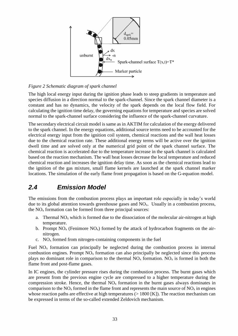
2.3.6. Curved Arc Diffusion Ignition Model (CADIM)
In this model, the spark-channel is tracked by Lagrangian marker particles to account for the
deflection of the spark-channel by local flow field. The geometry of the spark-channel is shown in
figure 2.
33
Figure 2 Schematic diagram of spark channel
The high local energy input during the ignition phase leads to steep gradients in temperature and
species diffusion in a direction normal to the spark-channel. Since the spark channel diameter is a
constant and has no dynamics, the velocity of the spark depends on the local flow field. For
calculating the ignition time delay, the governing equations for temperature and species are solved
normal to the spark-channel surface considering the influence of the spark-channel curvature.
The secondary electrical circuit model is same as in AKTIM for calculation of the energy delivered
to the spark channel. In the energy equations, additional source terms need to be accounted for the
electrical energy input from the ignition coil system, chemical reactions and the wall heat losses
due to the chemical reaction rate. These additional energy terms will be active over the ignition
dwell time and are solved only at the numerical grid point of the spark channel surface. The
chemical reaction is accelerated due to the temperature increase in the spark channel is calculated
based on the reaction mechanism. The wall heat losses decrease the local temperature and reduced
chemical reaction and increases the ignition delay time. As soon as the chemical reactions lead to
the ignition of the gas mixture, small flame kernels are launched at the spark channel marker
locations. The simulation of the early flame front propagation is based on the G-equation model.
2.4 Emission Model
The emissions from the combustion process plays an important role especially in today’s world
due to its global attention towards greenhouse gases and NOx. Usually in a combustion process,
the NOx formation can be formed from three principal sources:
a. Thermal NOx which is formed due to the dissociation of the molecular air-nitrogen at high
temperature.
b. Prompt NOx (Fenimore NOx) formed by the attack of hydrocarbon fragments on the air-
nitrogen.
c. NOx formed from nitrogen-containing components in the fuel
Fuel NOx formation can principally be neglected during the combustion process in internal
combustion engines. Prompt NOx formation can also principally be neglected since this process
plays no dominant role in comparison to the thermal NOx formation. NOx is formed in both the
flame front and post-flame gases.
In IC engines, the cylinder pressure rises during the combustion process. The burnt gases which
are present from the previous engine cycle are compressed to a higher temperature during the
compression stroke. Hence, the thermal NOx formation in the burnt gases always dominates in
comparison to the NOx formed in the flame front and represents the main source of NOx in engines
whose reaction paths are effective at high temperatures (> 1800 [K]). The reaction mechanism can
be expressed in terms of the so-called extended Zeldovich mechanism.
34
𝑁2 + 𝑂𝑘1 𝑘2⁄↔ 𝑁𝑂 + 𝑁
𝑂2 + 𝑁𝑘3 𝑘4⁄↔ 𝑁𝑂 + 𝑂
𝑁 + 𝑂𝐻𝑘5 𝑘6⁄↔ 𝑁𝑂 + 𝐻
Where k1, k2, k3, k4, k5 and k6 are the reaction rate constants. The first two reactions were originally
proposed by Zeldovich and extended later by including the third reaction. The first reaction
represents the rate-limiting step in comparison to the other reactions. A very high activation energy
(or temperature) is necessary to decompose the stable triple bond of the molecular air-nitrogen. It
was observed later that the nitrogen atoms released in the reaction are oxidized to NOx releasing
oxygen and hydrogen radicals at near stoichiometric conditions and in fuel-rich mixtures. This
reaction is significantly fast at high temperatures. The third reaction is usually negligible except
in fuel-rich flames. It considers the effect of oxygen, nitrogen and hydrogen radicals on NOx
formation. It is very important to point out that all three chemical reactions that represent the
Zeldovich mechanism exhibit strong temperature dependency.
In principle, it can be seen that the thermal NOx formation is mainly determined by only five
chemical species (O, H, OH, N and O2) but not directly by the fuel being used. To obtain the
required concentrations of the radicals, a complex reaction mechanism must be used in order to
determine NOx concentration. In this project, the extended Zeldovich NOx model is used which is
also the recommended emissions model for AVL FIRE software. Even though there are various
NOx formation models in the AVL FIRE software, the influence of these various NOx formation
models on the simulation results is not studied in this project.
Hydrocarbon fuels undergoing combustion also exhibit a strong tendency to form soot. The
formation of particulate matter and soot involves many different chemical and physical processes,
like the formation and growth of large aromatic hydrocarbons, their subsequent conversion to
particles, the coagulation of primary particles, and the growth of solid soot particles due to the
accumulation of gaseous components. The soot particle formation process is characterized by a
gaseous-solid conversion, where the solid phase does not exhibit a uniform chemical and physical
topology.
Due to the highly complex chemical process involving hundreds of reactions and as many
intermediate and radical species, a relatively small number of carbon atoms are converted into an
agglomerate comprising millions of carbon atoms leading to the formation of soot. Particle
oxidation mainly occurs due to the attack of atomic oxygen onto the carbonaceous particles under
high-temperature conditions. Despite the high complexity of the underlying processes, the
individual reactions contributing to the soot formation and oxidation rates can be related to known
flame parameters. The most important parameters during the soot formation are the local air/fuel
ratio (C/H ratio and C/O-ratio), temperature, pressure and residence time.
In this research project, the kinetic soot model is used since it replicates the soot formation based
on detailed chemical reaction. This is also the recommended soot formation model for AVL FIRE
software. Even though there are various soot formation models in the AVL FIRE software, the
influence of these various emission models on the simulation results is not studied in this project.
In this Sot formation model, it combines:
a. mechanisms of formation of PAH and polyynes,
b. two mechanisms of soot precursor formation due to condensation of PAH and polyyne
molecules,
c. soot particle growth by the reactions of Hydrogen Abstraction–C2H2 Addition (HACA)
mechanism and polyyne molecule addition,
d. mechanism of acetylene pyrolysis and pure carbon cluster formation, as well as the
reactions of hydrocarbon (n-heptane) oxidation.
35
The kinetic soot model can describe the behaviour of soot formation and oxidation for different
fuel classes. The reaction parameters for the main soot formation reaction change due to local
equivalence ratio. The soot is oxidized due to the presence of oxygen and water.
2.5 Turbulence Model
Turbulence plays an important role during the combustion phenomenon. Therefore, it is very
important to choose an appropriate model from the various turbulence models. However, in this
project, the influence of various turbulence models on the simulation results is not studied. The
turbulence model selected for the combustion simulation is k-zeta-f model which is also the
recommended turbulence model for AVL FIRE software.
The k-zeta-f model have been derived from Reynolds stress transport models and they can be seen
as simplified second moment closures model. The wall damping effect is incorporated by
modelling a three-equation model with elliptic relaxation equation. It also incorporates some near-
wall turbulence anisotropy as well as non-local pressure-strain effects. It is a general turbulence
model for low Reynolds-numbers.
Instead of turbulent kinetic energy k, this model uses a normalised wall-normal velocity scale for
the evaluation of the eddy viscosity. This normalised wall-normal velocity scale can be thought of
as the velocity fluctuation normal to the streamlines and can be regarded as the ratio of the two-
time scales: scalar (isotropic) and lateral (anisotropic). The anisotropic wall effects are modelled
through the elliptic relaxation function f, by solving a separate elliptic equation of the Helmholtz
type. This model overcomes the closure problem of the k-epsilon model and represents the
turbulent flows which indirectly affects combustion phenomenon at lower computational cost
when compared to Large Eddy Simulation (LES) and Direct Numerical Simulation (DNS).
2.6 Simulation Control Settings
There are various numerical methods used to solve the basic conservative equations used by the
various simulation models. These numerical methods determine the runtime of the simulation, and
the accuracy and consistency of the solution. Also, there are different settings to control these
numerical methods and these settings determine the following
a. how the pressure and velocity are calculated in the boundary,
b. how the low quality meshes affect the solution,
c. how the solution is computed by the solver, and
d. how a sudden change of variables affects the solution.
So, some detailed understanding is necessary to understand how these settings impact the solution.
2.6.1. Solution Algorithms for Pressure-Velocity Coupling
There are different numerical procedures to solve the Navier-Stokes equations and the
conservation of energy equation especially for calculating the pressure, velocity and temperature.
The method of solving the Navier-Stokes equations and conservation of energy equation determine
the runtime of the simulation because of the complexity arising due to nonlinearity in momentum
equations and the interdependence of pressure in all equations. In order to calculate the velocity
and temperature from the Navier-Stokes equations and conservation of energy equation, a
prediction and correction technique for the pressure calculation is used.
The discretized form of Navier-Stokes equations and conservation of energy equations are solved
for obtaining the values of velocity and temperature from the guessed pressure value using
predictor-corrector method. The most commonly used algorithm to solve the Navier-Stokes
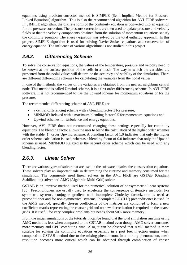
36
equations using predictor-corrector method is SIMPLE (Semi-Implicit Method for Pressure-
Linked Equations) algorithm. This is also the recommended algorithm for AVL FIRE software.
In SIMPLE algorithm, the discrete form of the continuity equation is converted into an equation
for the pressure correction. The pressure-corrections are then used to update pressure and velocity
fields so that the velocity components obtained from the solution of momentum equations satisfy
the continuity equation. The energy equation was solved by the total enthalpy approach. In this
project, SIMPLE algorithm is used for solving Navier-Stokes equations and conservation of
energy equation. The influence of various algorithms is not studied in this project.
2.6.2. Differencing Scheme
To solve the conservation equations, the values of the temperature, pressure and velocity need to
be known at the surface position of the cells in a mesh. The way in which the variables are
presented from the nodal values will determine the accuracy and stability of the simulation. There
are different differencing schemes for calculating the variables from the nodal values.
In one of the methods, the values of the variables are obtained from the nearest neighbour central
node. This method is called Upwind scheme. It is a first order differencing scheme. In AVL FIRE
software, it is not recommended to use the upwind scheme for momentum equations or for the
pressure.
The recommended differencing scheme of AVL FIRE are
• a central differencing scheme with a blending factor 1 for pressure,
• MINMOD Relaxed with a maximum blending factor 0.5 for momentum equations and
• Upwind schemes for turbulence and energy equations.
However, AVL FIRE does not recommend changing these settings especially for continuity
equations. The blending factor allows the user to blend the calculation of the higher order schemes
with the stable, 1st order Upwind scheme. A blending factor of 1.0 indicates that only the higher
order scheme calculation is used, whereas a blending factor of 0.0 indicates that only the Upwind
scheme is used. MINMOD Relaxed is the second order scheme which can be used with any
blending factor.
2.6.3. Linear Solver
There are various types of solver that are used in the software to solve the conservation equations.
These solvers play an important role in determining the runtime and memory consumed for the
simulation. The commonly used linear solvers in the AVL FIRE are GSTAB (Gradient
Stabilization) solver and AMG (Algebraic Multi Grid) solver.
GSTAB is an iterative method used for the numerical solution of nonsymmetric linear systems
[35]. Preconditioners are usually used to accelerate the convergence of iterative methods. For
symmetric systems, conjugate gradient with incomplete Cholesky factorization is used as
preconditioner and for non-symmetrical systems, Incomplete LU (ILU) preconditioner is used. In
the AMG method, specially chosen coefficients of the matrices are combined to form a new
coefficient matrix representing the coarser grid and no new discretization is required on the coarse
grids. It is useful for very complex problems but needs about 50% more memory.
From the initial simulations of the tutorials, it can be found that the total simulation run time using
AMG method is less when compared to the GSTAB method even though AMG solver consumes
more memory and CPU computing time. Also, it can be observed that AMG method is more
suitable for solving the continuity equations especially in a port fuel injection engine when
compared to GSTAB method due to the mixing phenomenon. In a mixing phenomenon, mesh
resolution becomes more critical which can be obtained through combination of chosen

37
coefficients of the matrix in the AMG method to obtain a finer or courser grid. Whereas in the
GSTAB method, it approximates the solution by the vector in a Krylov subspace with minimal
residual.
2.6.4. Under-Relaxation Factors
The under-relaxation factors provide a way to control how fast the flow equations can converge
within one outer iteration. As factor values approach 0, the solution stability increases, though this
may also increase the total processing time. As factor values approach 1, the solution stability
decreases but may lead to a faster solution. The objective is to match each simulation with a set of
under-relaxation factors that balance the solution stability and the convergence rate to minimize
the total processing time.

38
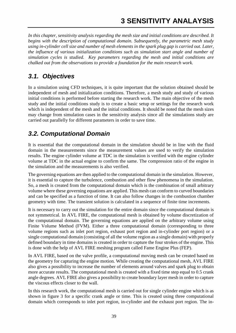
39
3 SENSITIVITY ANALAYSIS
In this chapter, sensitivity analysis regarding the mesh size and initial conditions are described. It
begins with the description of computational domain. Subsequently, the parametric mesh study
using in-cylinder cell size and number of mesh elements in the spark plug gap is carried out. Later,
the influence of various initialization conditions such as simulation start angle and number of
simulation cycles is studied. Key parameters regarding the mesh and initial conditions are
chalked out from the observations to provide a foundation for the main research work.
3.1. Objectives
In a simulation using CFD techniques, it is quite important that the solution obtained should be
independent of mesh and initialization conditions. Therefore, a mesh study and study of various
initial conditions is performed before starting the research work. The main objective of the mesh
study and the initial conditions study is to create a basic setup or settings for the research work
which is independent of the mesh and the initial conditions. It should be noted that the mesh sizes
may change from simulation cases in the sensitivity analysis since all the simulations study are
carried out parallelly for different parameters in order to save time.
3.2. Computational Domain
It is essential that the computational domain in the simulation should be in line with the fluid
domain in the measurements since the measurement values are used to verify the simulation
results. The engine cylinder volume at TDC in the simulation is verified with the engine cylinder
volume at TDC in the actual engine to confirm the same. The compression ratio of the engine in
the simulation and the measurements is also verified.
The governing equations are then applied to the computational domain in the simulation. However,
it is essential to capture the turbulence, combustion and other flow phenomena in the simulation.
So, a mesh is created from the computational domain which is the combination of small arbitrary
volume where these governing equations are applied. This mesh can conform to curved boundaries
and can be specified as a function of time. It can also follow changes in the combustion chamber
geometry with time. The transient solution is calculated in a sequence of finite time increments.
It is necessary to carry out the simulation for the entire domain since the computational domain is
not symmetrical. In AVL FIRE, the computational mesh is obtained by volume discretization of
the computational domain. The governing equations are applied on the arbitrary volume using
Finite Volume Method (FVM). Either a three computational domain (corresponding to three
volume regions such as inlet port region, exhaust port region and in-cylinder port region) or a
single computational domain (consisting of all the volume region as a single domain) with properly
defined boundary in time domains is created in order to capture the four strokes of the engine. This
is done with the help of AVL FIRE meshing program called Fame Engine Plus (FEP).
In AVL FIRE, based on the valve profile, a computational moving mesh can be created based on
the geometry for capturing the engine motion. While creating the computational mesh, AVL FIRE
also gives a possibility to increase the number of elements around valves and spark plug to obtain
more accurate results. The computational mesh is created with a fixed time step equal to 0.5 crank
angle degrees. AVL FIRE also gives a possibility to create boundary layer mesh in order to capture
the viscous effects closer to the wall.
In this research work, the computational mesh is carried out for single cylinder engine which is as
shown in figure 3 for a specific crank angle or time. This is created using three computational
domain which corresponds to inlet port region, in-cylinder and the exhaust port region. The in-
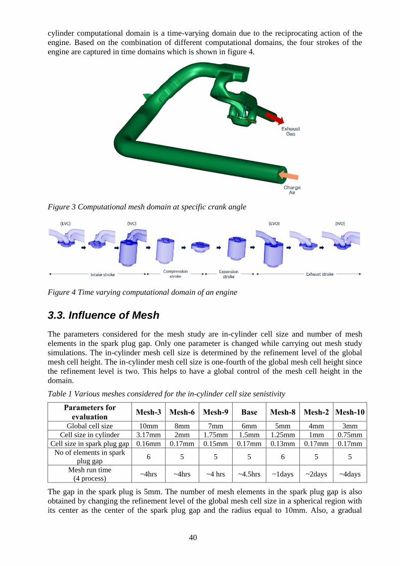
40
cylinder computational domain is a time-varying domain due to the reciprocating action of the
engine. Based on the combination of different computational domains, the four strokes of the
engine are captured in time domains which is shown in figure 4.
Figure 3 Computational mesh domain at specific crank angle
Figure 4 Time varying computational domain of an engine
3.3. Influence of Mesh
The parameters considered for the mesh study are in-cylinder cell size and number of mesh
elements in the spark plug gap. Only one parameter is changed while carrying out mesh study
simulations. The in-cylinder mesh cell size is determined by the refinement level of the global
mesh cell height. The in-cylinder mesh cell size is one-fourth of the global mesh cell height since
the refinement level is two. This helps to have a global control of the mesh cell height in the
domain.
Table 1 Various meshes considered for the in-cylinder cell size senistivity
Parameters for
evaluation Mesh-3 Mesh-6 Mesh-9 Base Mesh-8 Mesh-2 Mesh-10
Global cell size 10mm 8mm 7mm 6mm 5mm 4mm 3mm
Cell size in cylinder 3.17mm 2mm 1.75mm 1.5mm 1.25mm 1mm 0.75mm
Cell size in spark plug gap 0.16mm 0.17mm 0.15mm 0.17mm 0.13mm 0.17mm 0.17mm
No of elements in spark
plug gap 6 5 5 5 6 5 5
Mesh run time
(4 process) ~4hrs ~4hrs ~4 hrs ~4.5hrs ~1days ~2days ~4days
The gap in the spark plug is 5mm. The number of mesh elements in the spark plug gap is also
obtained by changing the refinement level of the global mesh cell size in a spherical region with
its center as the center of the spark plug gap and the radius equal to 10mm. Also, a gradual
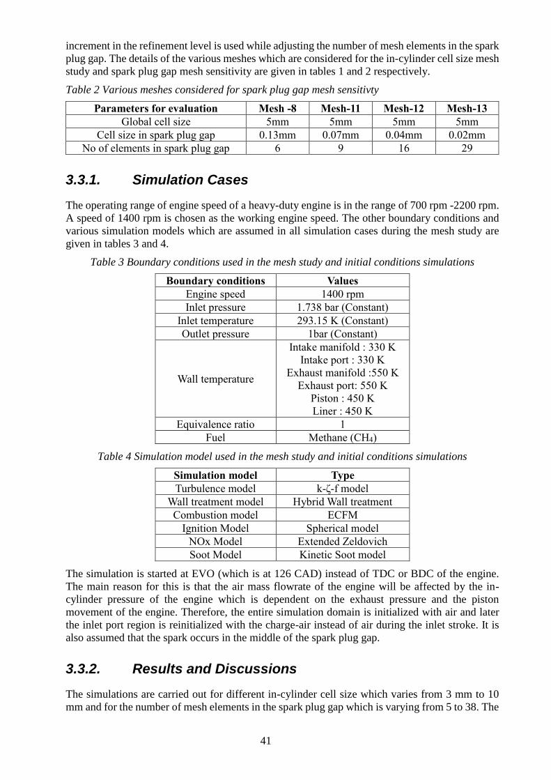
41
increment in the refinement level is used while adjusting the number of mesh elements in the spark
plug gap. The details of the various meshes which are considered for the in-cylinder cell size mesh
study and spark plug gap mesh sensitivity are given in tables 1 and 2 respectively.
Table 2 Various meshes considered for spark plug gap mesh sensitivty
Parameters for evaluation Mesh -8 Mesh-11 Mesh-12 Mesh-13
Global cell size 5mm 5mm 5mm 5mm
Cell size in spark plug gap 0.13mm 0.07mm 0.04mm 0.02mm
No of elements in spark plug gap 6 9 16 29
3.3.1. Simulation Cases
The operating range of engine speed of a heavy-duty engine is in the range of 700 rpm -2200 rpm.
A speed of 1400 rpm is chosen as the working engine speed. The other boundary conditions and
various simulation models which are assumed in all simulation cases during the mesh study are
given in tables 3 and 4.
Table 3 Boundary conditions used in the mesh study and initial conditions simulations
Boundary conditions Values
Engine speed 1400 rpm
Inlet pressure 1.738 bar (Constant)
Inlet temperature 293.15 K (Constant)
Outlet pressure 1bar (Constant)
Wall temperature
Intake manifold : 330 K
Intake port : 330 K
Exhaust manifold :550 K
Exhaust port: 550 K
Piston : 450 K
Liner : 450 K
Equivalence ratio 1
Fuel Methane (CH4)
Table 4 Simulation model used in the mesh study and initial conditions simulations
Simulation model Type
Turbulence model k-ζ-f model
Wall treatment model Hybrid Wall treatment
Combustion model ECFM
Ignition Model Spherical model
NOx Model Extended Zeldovich
Soot Model Kinetic Soot model
The simulation is started at EVO (which is at 126 CAD) instead of TDC or BDC of the engine.
The main reason for this is that the air mass flowrate of the engine will be affected by the in-
cylinder pressure of the engine which is dependent on the exhaust pressure and the piston
movement of the engine. Therefore, the entire simulation domain is initialized with air and later
the inlet port region is reinitialized with the charge-air instead of air during the inlet stroke. It is
also assumed that the spark occurs in the middle of the spark plug gap.
3.3.2. Results and Discussions
The simulations are carried out for different in-cylinder cell size which varies from 3 mm to 10
mm and for the number of mesh elements in the spark plug gap which is varying from 5 to 38. The
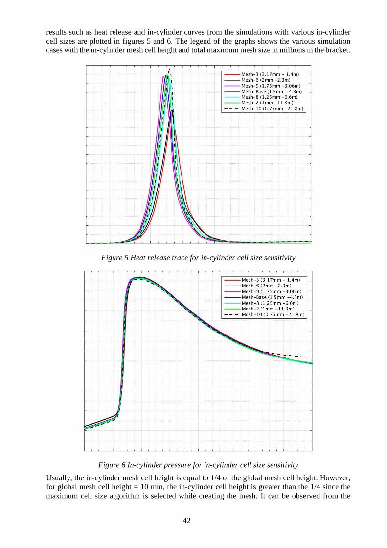
42
results such as heat release and in-cylinder curves from the simulations with various in-cylinder
cell sizes are plotted in figures 5 and 6. The legend of the graphs shows the various simulation
cases with the in-cylinder mesh cell height and total maximum mesh size in millions in the bracket.
Figure 5 Heat release trace for in-cylinder cell size sensitivity
Figure 6 In-cylinder pressure for in-cylinder cell size sensitivity
Usually, the in-cylinder mesh cell height is equal to 1/4 of the global mesh cell height. However,
for global mesh cell height = 10 mm, the in-cylinder cell height is greater than the 1/4 since the
maximum cell size algorithm is selected while creating the mesh. It can be observed from the
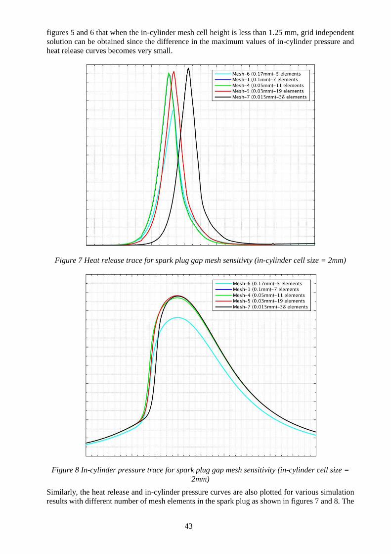
43
figures 5 and 6 that when the in-cylinder mesh cell height is less than 1.25 mm, grid independent
solution can be obtained since the difference in the maximum values of in-cylinder pressure and
heat release curves becomes very small.
Figure 7 Heat release trace for spark plug gap mesh sensitivty (in-cylinder cell size = 2mm)
Figure 8 In-cylinder pressure trace for spark plug gap mesh sensitivity (in-cylinder cell size =
2mm)
Similarly, the heat release and in-cylinder pressure curves are also plotted for various simulation
results with different number of mesh elements in the spark plug as shown in figures 7 and 8. The
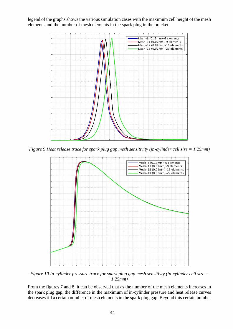
44
legend of the graphs shows the various simulation cases with the maximum cell height of the mesh
elements and the number of mesh elements in the spark plug in the bracket.
Figure 9 Heat release trace for spark plug gap mesh sensitivity (in-cylinder cell size = 1.25mm)
Figure 10 In-cylinder pressure trace for spark plug gap mesh sensitivty (in-cylinder cell size =
1.25mm)
From the figures 7 and 8, it can be observed that as the number of the mesh elements increases in
the spark plug gap, the difference in the maximum of in-cylinder pressure and heat release curves
decreases till a certain number of mesh elements in the spark plug gap. Beyond this certain number
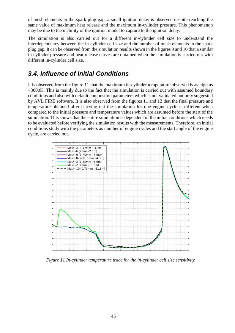
45
of mesh elements in the spark plug gap, a small ignition delay is observed despite reaching the
same value of maximum heat release and the maximum in-cylinder pressure. This phenomenon
may be due to the inability of the ignition model to capture to the ignition delay.
The simulation is also carried out for a different in-cylinder cell size to understand the
interdependency between the in-cylinder cell size and the number of mesh elements in the spark
plug gap. It can be observed from the simulation results shown in the figures 9 and 10 that a similar
in-cylinder pressure and heat release curves are obtained when the simulation is carried out with
different in-cylinder cell size.
3.4. Influence of Initial Conditions
It is observed from the figure 11 that the maximum in-cylinder temperature observed is as high as
~3000K. This is mainly due to the fact that the simulation is carried out with assumed boundary
conditions and also with default combustion parameters which is not validated but only suggested
by AVL FIRE software. It is also observed from the figures 11 and 12 that the final pressure and
temperature obtained after carrying out the simulation for one engine cycle is different when
compared to the initial pressure and temperature values which are assumed before the start of the
simulation. This shows that the entire simulation is dependent of the initial conditions which needs
to be evaluated before verifying the simulation results with the measurements. Therefore, an initial
conditions study with the parameters as number of engine cycles and the start angle of the engine
cycle, are carried out.
Figure 11 In-cylinder temperature trace for the in-cylinder cell size sensitivity
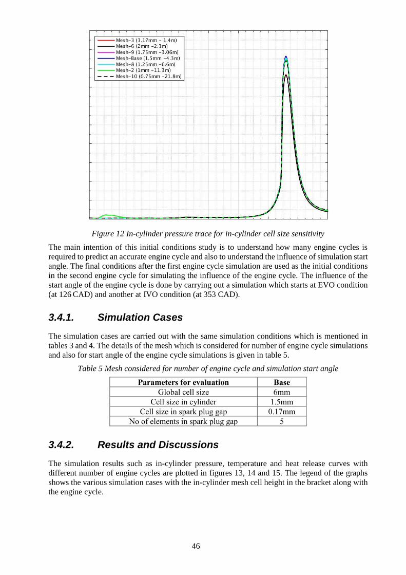
46
Figure 12 In-cylinder pressure trace for in-cylinder cell size sensitivity
The main intention of this initial conditions study is to understand how many engine cycles is
required to predict an accurate engine cycle and also to understand the influence of simulation start
angle. The final conditions after the first engine cycle simulation are used as the initial conditions
in the second engine cycle for simulating the influence of the engine cycle. The influence of the
start angle of the engine cycle is done by carrying out a simulation which starts at EVO condition
(at 126 CAD) and another at IVO condition (at 353 CAD).
3.4.1. Simulation Cases
The simulation cases are carried out with the same simulation conditions which is mentioned in
tables 3 and 4. The details of the mesh which is considered for number of engine cycle simulations
and also for start angle of the engine cycle simulations is given in table 5.
Table 5 Mesh considered for number of engine cycle and simulation start angle
Parameters for evaluation Base
Global cell size 6mm
Cell size in cylinder 1.5mm
Cell size in spark plug gap 0.17mm
No of elements in spark plug gap 5
3.4.2. Results and Discussions
The simulation results such as in-cylinder pressure, temperature and heat release curves with
different number of engine cycles are plotted in figures 13, 14 and 15. The legend of the graphs
shows the various simulation cases with the in-cylinder mesh cell height in the bracket along with
the engine cycle.
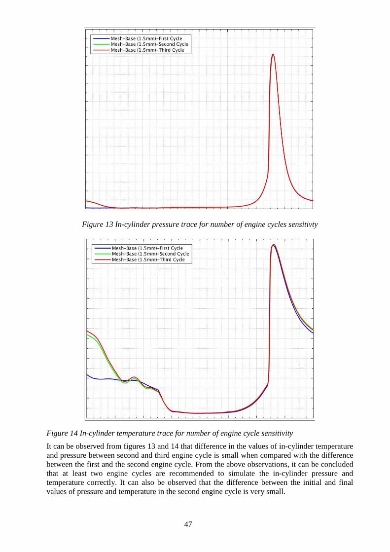
47
Figure 13 In-cylinder pressure trace for number of engine cycles sensitivty
Figure 14 In-cylinder temperature trace for number of engine cycle sensitivity
It can be observed from figures 13 and 14 that difference in the values of in-cylinder temperature
and pressure between second and third engine cycle is small when compared with the difference
between the first and the second engine cycle. From the above observations, it can be concluded
that at least two engine cycles are recommended to simulate the in-cylinder pressure and
temperature correctly. It can also be observed that the difference between the initial and final
values of pressure and temperature in the second engine cycle is very small.
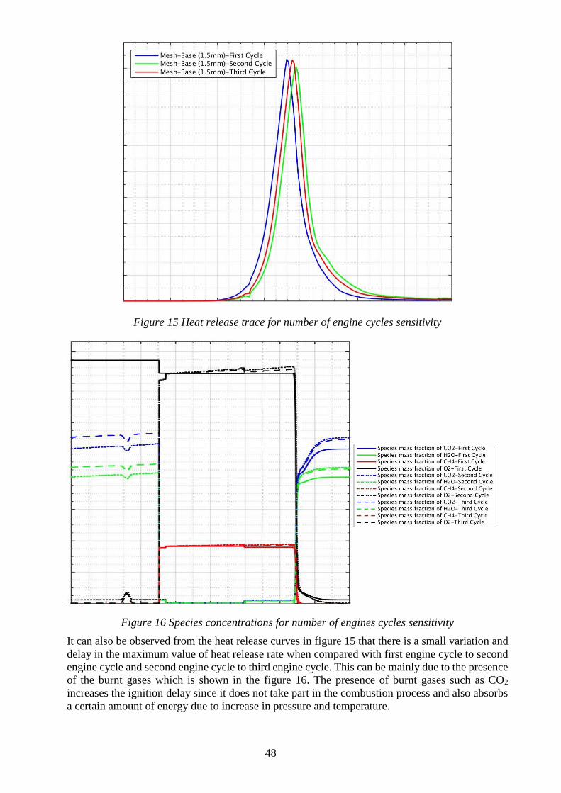
48
Figure 15 Heat release trace for number of engine cycles sensitivity
Figure 16 Species concentrations for number of engines cycles sensitivity
It can also be observed from the heat release curves in figure 15 that there is a small variation and
delay in the maximum value of heat release rate when compared with first engine cycle to second
engine cycle and second engine cycle to third engine cycle. This can be mainly due to the presence
of the burnt gases which is shown in the figure 16. The presence of burnt gases such as CO2
increases the ignition delay since it does not take part in the combustion process and also absorbs
a certain amount of energy due to increase in pressure and temperature.
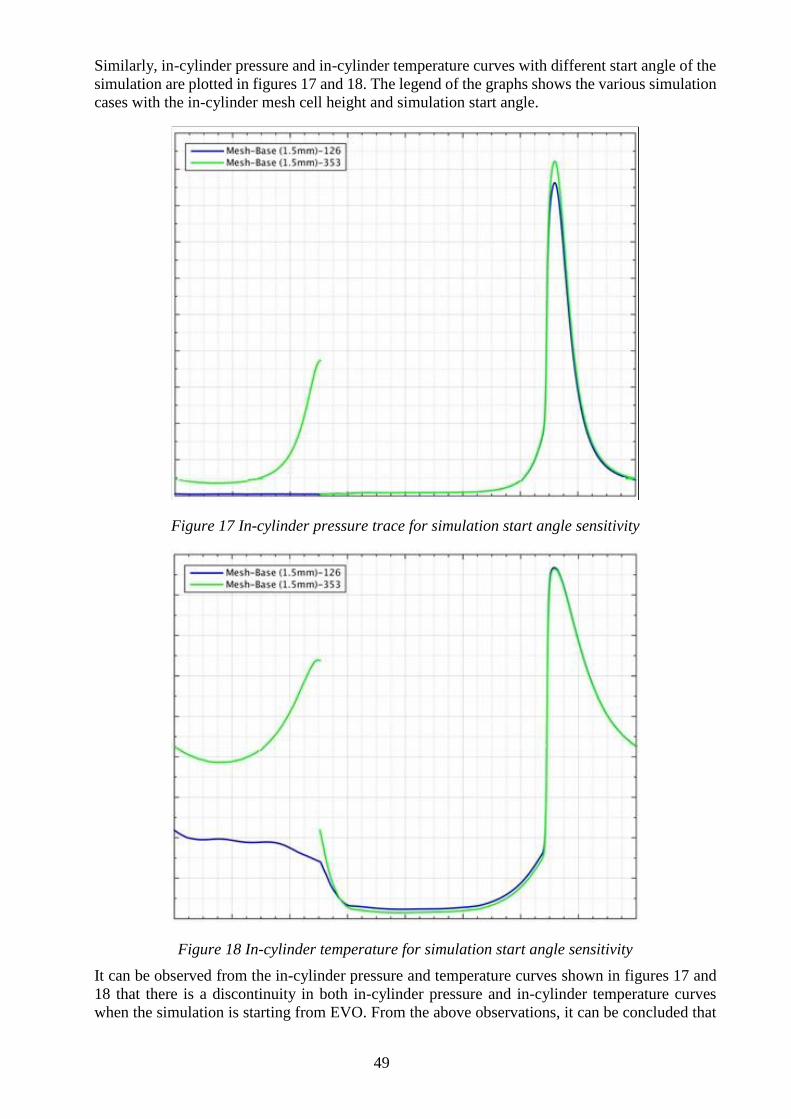
49
Similarly, in-cylinder pressure and in-cylinder temperature curves with different start angle of the
simulation are plotted in figures 17 and 18. The legend of the graphs shows the various simulation
cases with the in-cylinder mesh cell height and simulation start angle.
Figure 17 In-cylinder pressure trace for simulation start angle sensitivity
Figure 18 In-cylinder temperature for simulation start angle sensitivity
It can be observed from the in-cylinder pressure and temperature curves shown in figures 17 and
18 that there is a discontinuity in both in-cylinder pressure and in-cylinder temperature curves
when the simulation is starting from EVO. From the above observations, it can be concluded that
50
better simulation results can be achieved when the simulation is starting from EVO instead of IVO.
This is mainly due to the flow instabilities created in the exhaust port due to the relatively shorter
length of the exhaust port which cause an increase in the in-cylinder pressure and in-cylinder
temperature when the inlet valve is opened.
3.5. Key Parameters
Some key suggestions can be made for the research work regarding the simulation settings from
the observations of the sensitivity analysis. The simulation can be started from any crank angle.
However, from the observations of the sensitivity analysis, it is recommended to start the
simulation start angle at 126 CAD which corresponds to EVO instead of starting at 353 CAD
which corresponds to IVO.
It is suggested to carry out a minimum of 2 cycles or 4 engine revolutions to obtain a more accurate
solution. It is also suggested to limit the number of the mesh elements in the spark plug gap to a
range of 8 - 12 elements in order to reduce the simulation run time. Another suggestion is to limit
the in-cylinder mesh cell height to 1.25 mm for which the mesh convergence was observed from
the sensitivity analysis results.
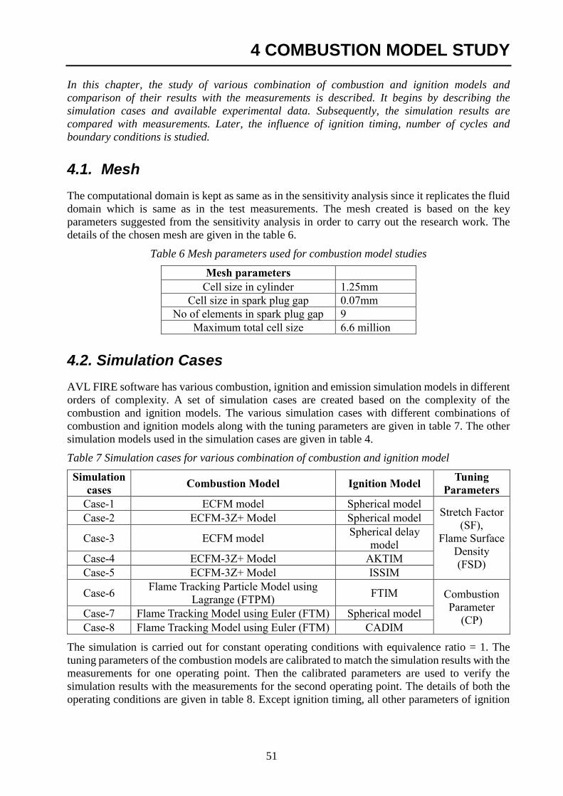
51
4 COMBUSTION MODEL STUDY
In this chapter, the study of various combination of combustion and ignition models and
comparison of their results with the measurements is described. It begins by describing the
simulation cases and available experimental data. Subsequently, the simulation results are
compared with measurements. Later, the influence of ignition timing, number of cycles and
boundary conditions is studied.
4.1. Mesh
The computational domain is kept as same as in the sensitivity analysis since it replicates the fluid
domain which is same as in the test measurements. The mesh created is based on the key
parameters suggested from the sensitivity analysis in order to carry out the research work. The
details of the chosen mesh are given in the table 6.
Table 6 Mesh parameters used for combustion model studies
Mesh parameters
Cell size in cylinder 1.25mm
Cell size in spark plug gap 0.07mm
No of elements in spark plug gap 9
Maximum total cell size 6.6 million
4.2. Simulation Cases
AVL FIRE software has various combustion, ignition and emission simulation models in different
orders of complexity. A set of simulation cases are created based on the complexity of the
combustion and ignition models. The various simulation cases with different combinations of
combustion and ignition models along with the tuning parameters are given in table 7. The other
simulation models used in the simulation cases are given in table 4.
Table 7 Simulation cases for various combination of combustion and ignition model
Simulation
cases Combustion Model Ignition Model
Tuning
Parameters
Case-1 ECFM model Spherical model Stretch Factor
(SF),
Flame Surface
Density
(FSD)
Case-2 ECFM-3Z+ Model Spherical model
Case-3 ECFM model Spherical delay
model
Case-4 ECFM-3Z+ Model AKTIM
Case-5 ECFM-3Z+ Model ISSIM
Case-6 Flame Tracking Particle Model using
Lagrange (FTPM) FTIM Combustion
Parameter
(CP) Case-7 Flame Tracking Model using Euler (FTM) Spherical model
Case-8 Flame Tracking Model using Euler (FTM) CADIM
The simulation is carried out for constant operating conditions with equivalence ratio = 1. The
tuning parameters of the combustion models are calibrated to match the simulation results with the
measurements for one operating point. Then the calibrated parameters are used to verify the
simulation results with the measurements for the second operating point. The details of both the
operating conditions are given in table 8. Except ignition timing, all other parameters of ignition
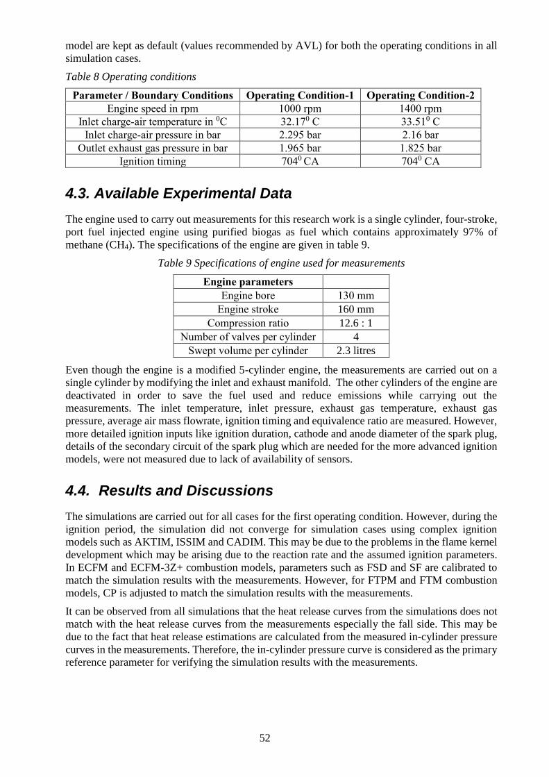
52
model are kept as default (values recommended by AVL) for both the operating conditions in all
simulation cases.
Table 8 Operating conditions
Parameter / Boundary Conditions Operating Condition-1 Operating Condition-2
Engine speed in rpm 1000 rpm 1400 rpm
Inlet charge-air temperature in 0C 32.170 C 33.510 C
Inlet charge-air pressure in bar 2.295 bar 2.16 bar
Outlet exhaust gas pressure in bar 1.965 bar 1.825 bar
Ignition timing 7040 CA 7040 CA
4.3. Available Experimental Data
The engine used to carry out measurements for this research work is a single cylinder, four-stroke,
port fuel injected engine using purified biogas as fuel which contains approximately 97% of
methane (CH4). The specifications of the engine are given in table 9.
Table 9 Specifications of engine used for measurements
Engine parameters
Engine bore 130 mm
Engine stroke 160 mm
Compression ratio 12.6 : 1
Number of valves per cylinder 4
Swept volume per cylinder 2.3 litres
Even though the engine is a modified 5-cylinder engine, the measurements are carried out on a
single cylinder by modifying the inlet and exhaust manifold. The other cylinders of the engine are
deactivated in order to save the fuel used and reduce emissions while carrying out the
measurements. The inlet temperature, inlet pressure, exhaust gas temperature, exhaust gas
pressure, average air mass flowrate, ignition timing and equivalence ratio are measured. However,
more detailed ignition inputs like ignition duration, cathode and anode diameter of the spark plug,
details of the secondary circuit of the spark plug which are needed for the more advanced ignition
models, were not measured due to lack of availability of sensors.
4.4. Results and Discussions
The simulations are carried out for all cases for the first operating condition. However, during the
ignition period, the simulation did not converge for simulation cases using complex ignition
models such as AKTIM, ISSIM and CADIM. This may be due to the problems in the flame kernel
development which may be arising due to the reaction rate and the assumed ignition parameters.
In ECFM and ECFM-3Z+ combustion models, parameters such as FSD and SF are calibrated to
match the simulation results with the measurements. However, for FTPM and FTM combustion
models, CP is adjusted to match the simulation results with the measurements.
It can be observed from all simulations that the heat release curves from the simulations does not
match with the heat release curves from the measurements especially the fall side. This may be
due to the fact that heat release estimations are calculated from the measured in-cylinder pressure
curves in the measurements. Therefore, the in-cylinder pressure curve is considered as the primary
reference parameter for verifying the simulation results with the measurements.
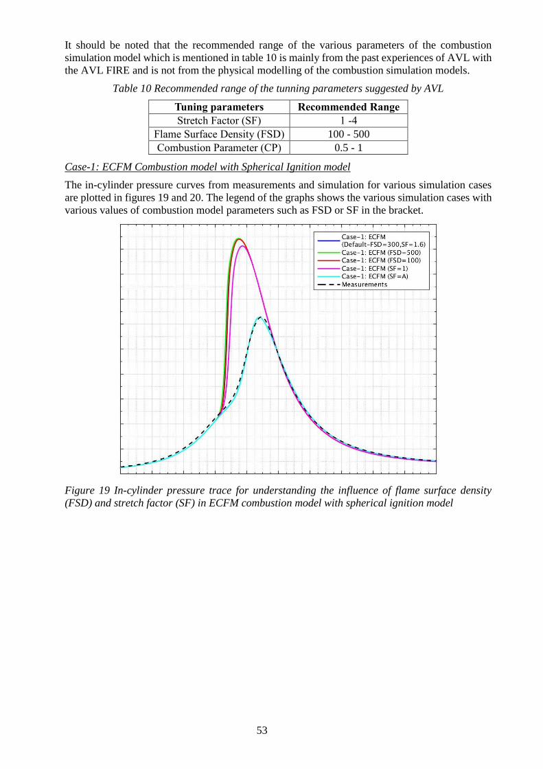
53
It should be noted that the recommended range of the various parameters of the combustion
simulation model which is mentioned in table 10 is mainly from the past experiences of AVL with
the AVL FIRE and is not from the physical modelling of the combustion simulation models.
Table 10 Recommended range of the tunning parameters suggested by AVL
Tuning parameters Recommended Range
Stretch Factor (SF) 1 -4
Flame Surface Density (FSD) 100 - 500
Combustion Parameter (CP) 0.5 - 1
Case-1: ECFM Combustion model with Spherical Ignition model
The in-cylinder pressure curves from measurements and simulation for various simulation cases
are plotted in figures 19 and 20. The legend of the graphs shows the various simulation cases with
various values of combustion model parameters such as FSD or SF in the bracket.
Figure 19 In-cylinder pressure trace for understanding the influence of flame surface density
(FSD) and stretch factor (SF) in ECFM combustion model with spherical ignition model
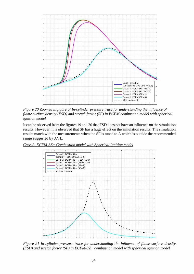
54
Figure 20 Zoomed in figure of In-cylinder pressure trace for understanding the influence of
flame surface density (FSD) and stretch factor (SF) in ECFM combustion model with spherical
ignition model
It can be observed from the figures 19 and 20 that FSD does not have an influence on the simulation
results. However, it is observed that SF has a huge effect on the simulation results. The simulation
results match with the measurements when the SF is tuned to A which is outside the recommended
range suggested by AVL.
Case-2: ECFM-3Z+ Combustion model with Spherical Ignition model
Figure 21 In-cylinder pressure trace for understanding the influence of flame surface density
(FSD) and stretch factor (SF) in ECFM-3Z+ combustion model with spherical ignition model
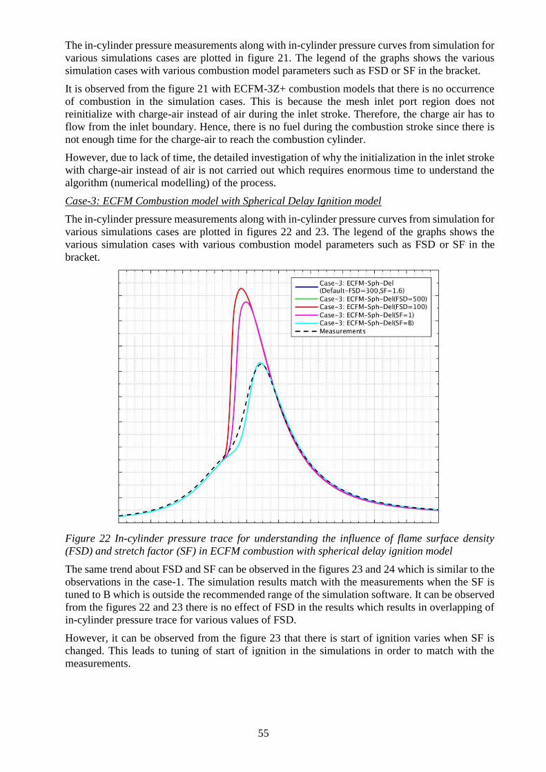
55
The in-cylinder pressure measurements along with in-cylinder pressure curves from simulation for
various simulations cases are plotted in figure 21. The legend of the graphs shows the various
simulation cases with various combustion model parameters such as FSD or SF in the bracket.
It is observed from the figure 21 with ECFM-3Z+ combustion models that there is no occurrence
of combustion in the simulation cases. This is because the mesh inlet port region does not
reinitialize with charge-air instead of air during the inlet stroke. Therefore, the charge air has to
flow from the inlet boundary. Hence, there is no fuel during the combustion stroke since there is
not enough time for the charge-air to reach the combustion cylinder.
However, due to lack of time, the detailed investigation of why the initialization in the inlet stroke
with charge-air instead of air is not carried out which requires enormous time to understand the
algorithm (numerical modelling) of the process.
Case-3: ECFM Combustion model with Spherical Delay Ignition model
The in-cylinder pressure measurements along with in-cylinder pressure curves from simulation for
various simulations cases are plotted in figures 22 and 23. The legend of the graphs shows the
various simulation cases with various combustion model parameters such as FSD or SF in the
bracket.
Figure 22 In-cylinder pressure trace for understanding the influence of flame surface density
(FSD) and stretch factor (SF) in ECFM combustion with spherical delay ignition model
The same trend about FSD and SF can be observed in the figures 23 and 24 which is similar to the
observations in the case-1. The simulation results match with the measurements when the SF is
tuned to B which is outside the recommended range of the simulation software. It can be observed
from the figures 22 and 23 there is no effect of FSD in the results which results in overlapping of
in-cylinder pressure trace for various values of FSD.
However, it can be observed from the figure 23 that there is start of ignition varies when SF is
changed. This leads to tuning of start of ignition in the simulations in order to match with the
measurements.
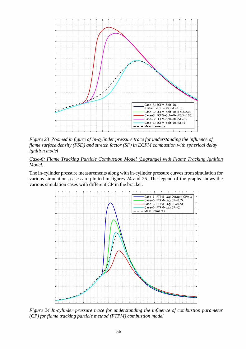
56
Figure 23 Zoomed in figure of In-cylinder pressure trace for understanding the influence of
flame surface density (FSD) and stretch factor (SF) in ECFM combustion with spherical delay
ignition model
Case-6: Flame Tracking Particle Combustion Model (Lagrange) with Flame Tracking Ignition
Model.
The in-cylinder pressure measurements along with in-cylinder pressure curves from simulation for
various simulations cases are plotted in figures 24 and 25. The legend of the graphs shows the
various simulation cases with different CP in the bracket.
Figure 24 In-cylinder pressure trace for understanding the influence of combustion parameter
(CP) for flame tracking particle method (FTPM) combustion model
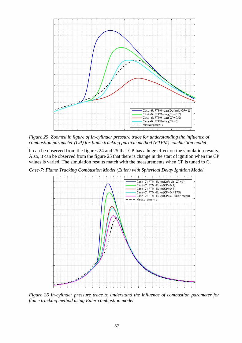
57
Figure 25 Zoomed in figure of In-cylinder pressure trace for understanding the influence of
combustion parameter (CP) for flame tracking particle method (FTPM) combustion model
It can be observed from the figures 24 and 25 that CP has a huge effect on the simulation results.
Also, it can be observed from the figure 25 that there is change in the start of ignition when the CP
values is varied. The simulation results match with the measurements when CP is tuned to C.
Case-7: Flame Tracking Combustion Model (Euler) with Spherical Delay Ignition Model
Figure 26 In-cylinder pressure trace to understand the influence of combustion parameter for
flame tracking method using Euler combustion model
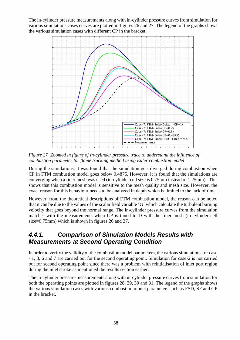
58
The in-cylinder pressure measurements along with in-cylinder pressure curves from simulation for
various simulations cases curves are plotted in figures 26 and 27. The legend of the graphs shows
the various simulation cases with different CP in the bracket.
Figure 27 Zoomed in figure of In-cylinder pressure trace to understand the influence of
combustion parameter for flame tracking method using Euler combustion model
During the simulations, it was found that the simulation gets diverged during combustion when
CP in FTM combustion model goes below 0.4875. However, it is found that the simulations are
converging when a finer mesh was used (in-cylinder cell size is 0.75mm instead of 1.25mm). This
shows that this combustion model is sensitive to the mesh quality and mesh size. However, the
exact reason for this behaviour needs to be analyzed in depth which is limited to the lack of time.
However, from the theoretical descriptions of FTM combustion model, the reason can be noted
that it can be due to the values of the scalar field variable ‘G’ which calculate the turbulent burning
velocity that goes beyond the normal range. The in-cylinder pressure curves from the simulation
matches with the measurements when CP is tuned to D with the finer mesh (in-cylinder cell
size=0.75mm) which is shown in figures 26 and 27.
4.4.1. Comparison of Simulation Models Results with Measurements at Second Operating Condition
In order to verify the validity of the combustion model parameters, the various simulations for case
- 1, 3, 6 and 7 are carried out for the second operating point. Simulation for case-2 is not carried
out for second operating point since there was a problem with reintialisation of inlet port region
during the inlet stroke as mentioned the results section earlier.
The in-cylinder pressure measurements along with in-cylinder pressure curves from simulation for
both the operating points are plotted in figures 28, 29, 30 and 31. The legend of the graphs shows
the various simulation cases with various combustion model parameters such as FSD, SF and CP
in the bracket.
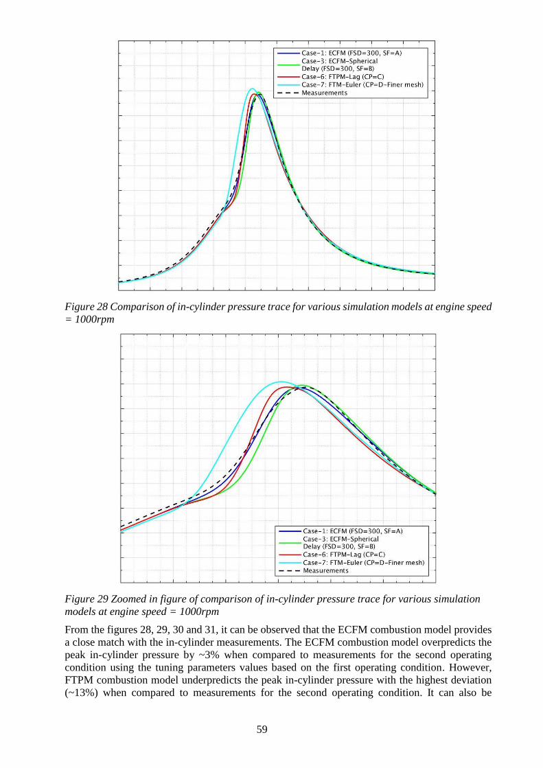
59
Figure 28 Comparison of in-cylinder pressure trace for various simulation models at engine speed
= 1000rpm
Figure 29 Zoomed in figure of comparison of in-cylinder pressure trace for various simulation
models at engine speed = 1000rpm
From the figures 28, 29, 30 and 31, it can be observed that the ECFM combustion model provides
a close match with the in-cylinder measurements. The ECFM combustion model overpredicts the
peak in-cylinder pressure by ~3% when compared to measurements for the second operating
condition using the tuning parameters values based on the first operating condition. However,
FTPM combustion model underpredicts the peak in-cylinder pressure with the highest deviation
(~13%) when compared to measurements for the second operating condition. It can also be
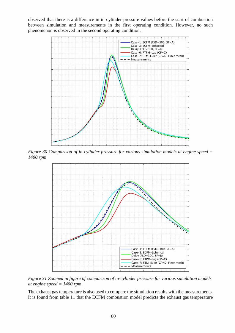
60
observed that there is a difference in in-cylinder pressure values before the start of combustion
between simulation and measurements in the first operating condition. However, no such
phenomenon is observed in the second operating condition.
Figure 30 Comparison of in-cylinder pressure for various simulation models at engine speed =
1400 rpm
Figure 31 Zoomed in figure of comparison of in-cylinder pressure for various simulation models
at engine speed = 1400 rpm
The exhaust gas temperature is also used to compare the simulation results with the measurements.
It is found from table 11 that the ECFM combustion model predicts the exhaust gas temperature
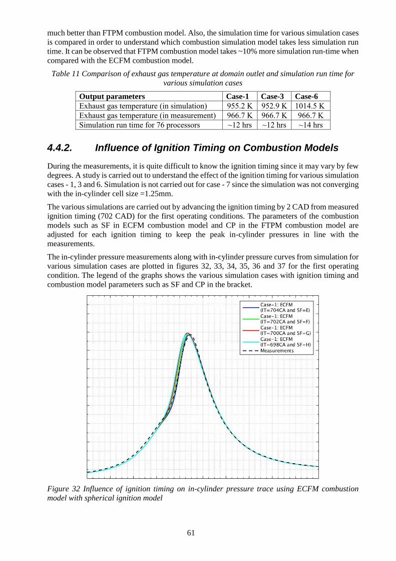
61
much better than FTPM combustion model. Also, the simulation time for various simulation cases
is compared in order to understand which combustion simulation model takes less simulation run
time. It can be observed that FTPM combustion model takes ~10% more simulation run-time when
compared with the ECFM combustion model.
Table 11 Comparison of exhaust gas temperature at domain outlet and simulation run time for
various simulation cases
Output parameters Case-1 Case-3 Case-6
Exhaust gas temperature (in simulation) 955.2 K 952.9 K 1014.5 K
Exhaust gas temperature (in measurement) 966.7 K 966.7 K 966.7 K
Simulation run time for 76 processors ~12 hrs ~12 hrs ~14 hrs
4.4.2. Influence of Ignition Timing on Combustion Models
During the measurements, it is quite difficult to know the ignition timing since it may vary by few
degrees. A study is carried out to understand the effect of the ignition timing for various simulation
cases - 1, 3 and 6. Simulation is not carried out for case - 7 since the simulation was not converging
with the in-cylinder cell size =1.25mm.
The various simulations are carried out by advancing the ignition timing by 2 CAD from measured
ignition timing (702 CAD) for the first operating conditions. The parameters of the combustion
models such as SF in ECFM combustion model and CP in the FTPM combustion model are
adjusted for each ignition timing to keep the peak in-cylinder pressures in line with the
measurements.
The in-cylinder pressure measurements along with in-cylinder pressure curves from simulation for
various simulation cases are plotted in figures 32, 33, 34, 35, 36 and 37 for the first operating
condition. The legend of the graphs shows the various simulation cases with ignition timing and
combustion model parameters such as SF and CP in the bracket.
Figure 32 Influence of ignition timing on in-cylinder pressure trace using ECFM combustion
model with spherical ignition model
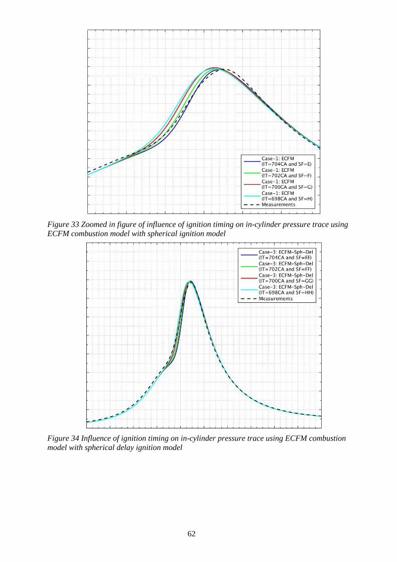
62
Figure 33 Zoomed in figure of influence of ignition timing on in-cylinder pressure trace using
ECFM combustion model with spherical ignition model
Figure 34 Influence of ignition timing on in-cylinder pressure trace using ECFM combustion
model with spherical delay ignition model
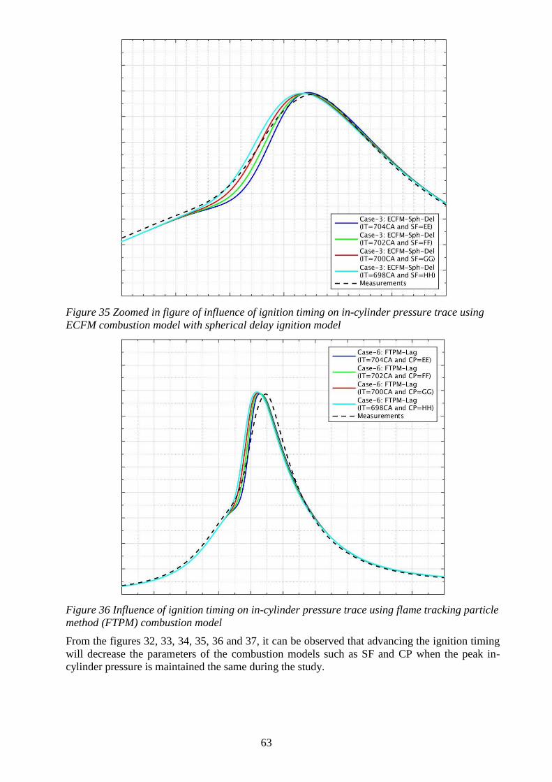
63
Figure 35 Zoomed in figure of influence of ignition timing on in-cylinder pressure trace using
ECFM combustion model with spherical delay ignition model
Figure 36 Influence of ignition timing on in-cylinder pressure trace using flame tracking particle
method (FTPM) combustion model
From the figures 32, 33, 34, 35, 36 and 37, it can be observed that advancing the ignition timing
will decrease the parameters of the combustion models such as SF and CP when the peak in-
cylinder pressure is maintained the same during the study.
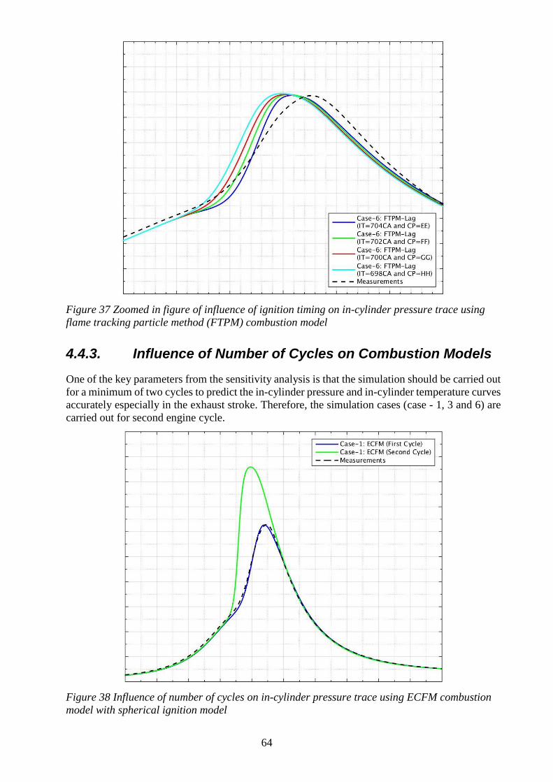
64
Figure 37 Zoomed in figure of influence of ignition timing on in-cylinder pressure trace using
flame tracking particle method (FTPM) combustion model
4.4.3. Influence of Number of Cycles on Combustion Models
One of the key parameters from the sensitivity analysis is that the simulation should be carried out
for a minimum of two cycles to predict the in-cylinder pressure and in-cylinder temperature curves
accurately especially in the exhaust stroke. Therefore, the simulation cases (case - 1, 3 and 6) are
carried out for second engine cycle.
Figure 38 Influence of number of cycles on in-cylinder pressure trace using ECFM combustion
model with spherical ignition model
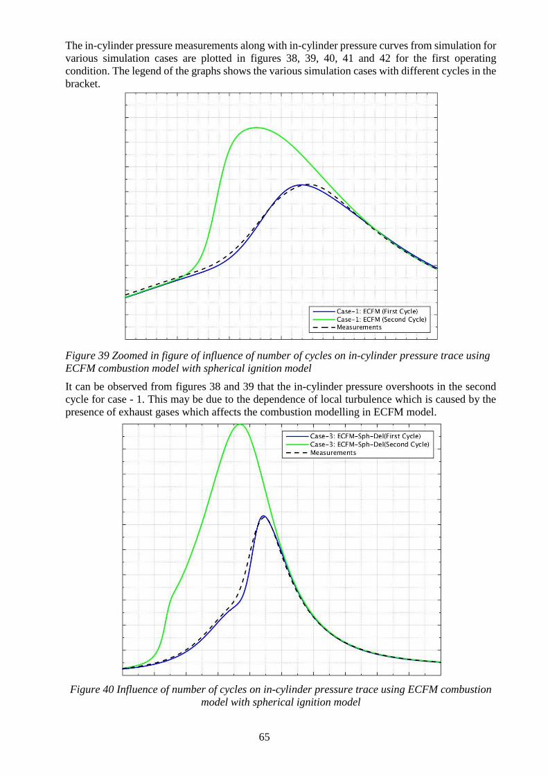
65
The in-cylinder pressure measurements along with in-cylinder pressure curves from simulation for
various simulation cases are plotted in figures 38, 39, 40, 41 and 42 for the first operating
condition. The legend of the graphs shows the various simulation cases with different cycles in the
bracket.
Figure 39 Zoomed in figure of influence of number of cycles on in-cylinder pressure trace using
ECFM combustion model with spherical ignition model
It can be observed from figures 38 and 39 that the in-cylinder pressure overshoots in the second
cycle for case - 1. This may be due to the dependence of local turbulence which is caused by the
presence of exhaust gases which affects the combustion modelling in ECFM model.
Figure 40 Influence of number of cycles on in-cylinder pressure trace using ECFM combustion
model with spherical ignition model
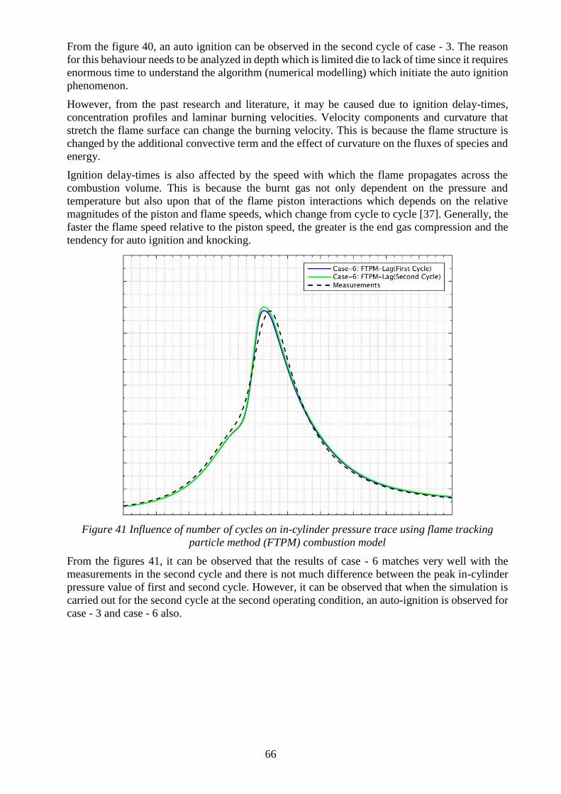
66
From the figure 40, an auto ignition can be observed in the second cycle of case - 3. The reason
for this behaviour needs to be analyzed in depth which is limited die to lack of time since it requires
enormous time to understand the algorithm (numerical modelling) which initiate the auto ignition
phenomenon.
However, from the past research and literature, it may be caused due to ignition delay-times,
concentration profiles and laminar burning velocities. Velocity components and curvature that
stretch the flame surface can change the burning velocity. This is because the flame structure is
changed by the additional convective term and the effect of curvature on the fluxes of species and
energy.
Ignition delay-times is also affected by the speed with which the flame propagates across the
combustion volume. This is because the burnt gas not only dependent on the pressure and
temperature but also upon that of the flame piston interactions which depends on the relative
magnitudes of the piston and flame speeds, which change from cycle to cycle [37]. Generally, the
faster the flame speed relative to the piston speed, the greater is the end gas compression and the
tendency for auto ignition and knocking.
Figure 41 Influence of number of cycles on in-cylinder pressure trace using flame tracking
particle method (FTPM) combustion model
From the figures 41, it can be observed that the results of case - 6 matches very well with the
measurements in the second cycle and there is not much difference between the peak in-cylinder
pressure value of first and second cycle. However, it can be observed that when the simulation is
carried out for the second cycle at the second operating condition, an auto-ignition is observed for
case - 3 and case - 6 also.
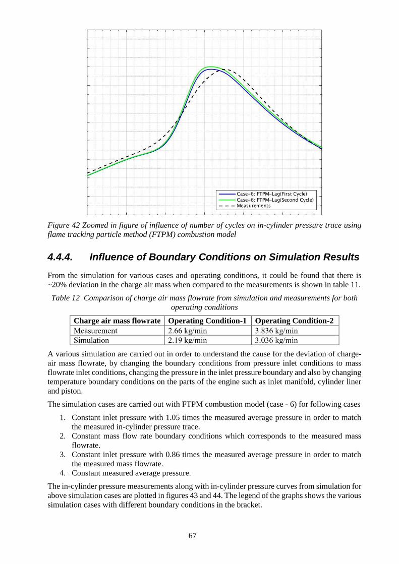
67
Figure 42 Zoomed in figure of influence of number of cycles on in-cylinder pressure trace using
flame tracking particle method (FTPM) combustion model
4.4.4. Influence of Boundary Conditions on Simulation Results
From the simulation for various cases and operating conditions, it could be found that there is
~20% deviation in the charge air mass when compared to the measurements is shown in table 11.
Table 12 Comparison of charge air mass flowrate from simulation and measurements for both
operating conditions
Charge air mass flowrate Operating Condition-1 Operating Condition-2
Measurement 2.66 kg/min 3.836 kg/min
Simulation 2.19 kg/min 3.036 kg/min
A various simulation are carried out in order to understand the cause for the deviation of charge-
air mass flowrate, by changing the boundary conditions from pressure inlet conditions to mass
flowrate inlet conditions, changing the pressure in the inlet pressure boundary and also by changing
temperature boundary conditions on the parts of the engine such as inlet manifold, cylinder liner
and piston.
The simulation cases are carried out with FTPM combustion model (case - 6) for following cases
1. Constant inlet pressure with 1.05 times the measured average pressure in order to match
the measured in-cylinder pressure trace.
2. Constant mass flow rate boundary conditions which corresponds to the measured mass
flowrate.
3. Constant inlet pressure with 0.86 times the measured average pressure in order to match
the measured mass flowrate.
4. Constant measured average pressure.
The in-cylinder pressure measurements along with in-cylinder pressure curves from simulation for
above simulation cases are plotted in figures 43 and 44. The legend of the graphs shows the various
simulation cases with different boundary conditions in the bracket.
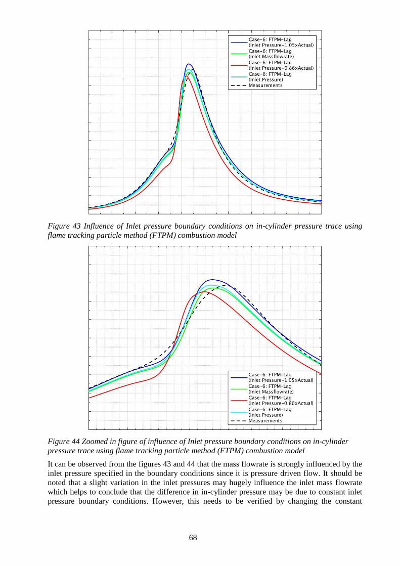
68
Figure 43 Influence of Inlet pressure boundary conditions on in-cylinder pressure trace using
flame tracking particle method (FTPM) combustion model
Figure 44 Zoomed in figure of influence of Inlet pressure boundary conditions on in-cylinder
pressure trace using flame tracking particle method (FTPM) combustion model
It can be observed from the figures 43 and 44 that the mass flowrate is strongly influenced by the
inlet pressure specified in the boundary conditions since it is pressure driven flow. It should be
noted that a slight variation in the inlet pressures may hugely influence the inlet mass flowrate
which helps to conclude that the difference in in-cylinder pressure may be due to constant inlet
pressure boundary conditions. However, this needs to be verified by changing the constant
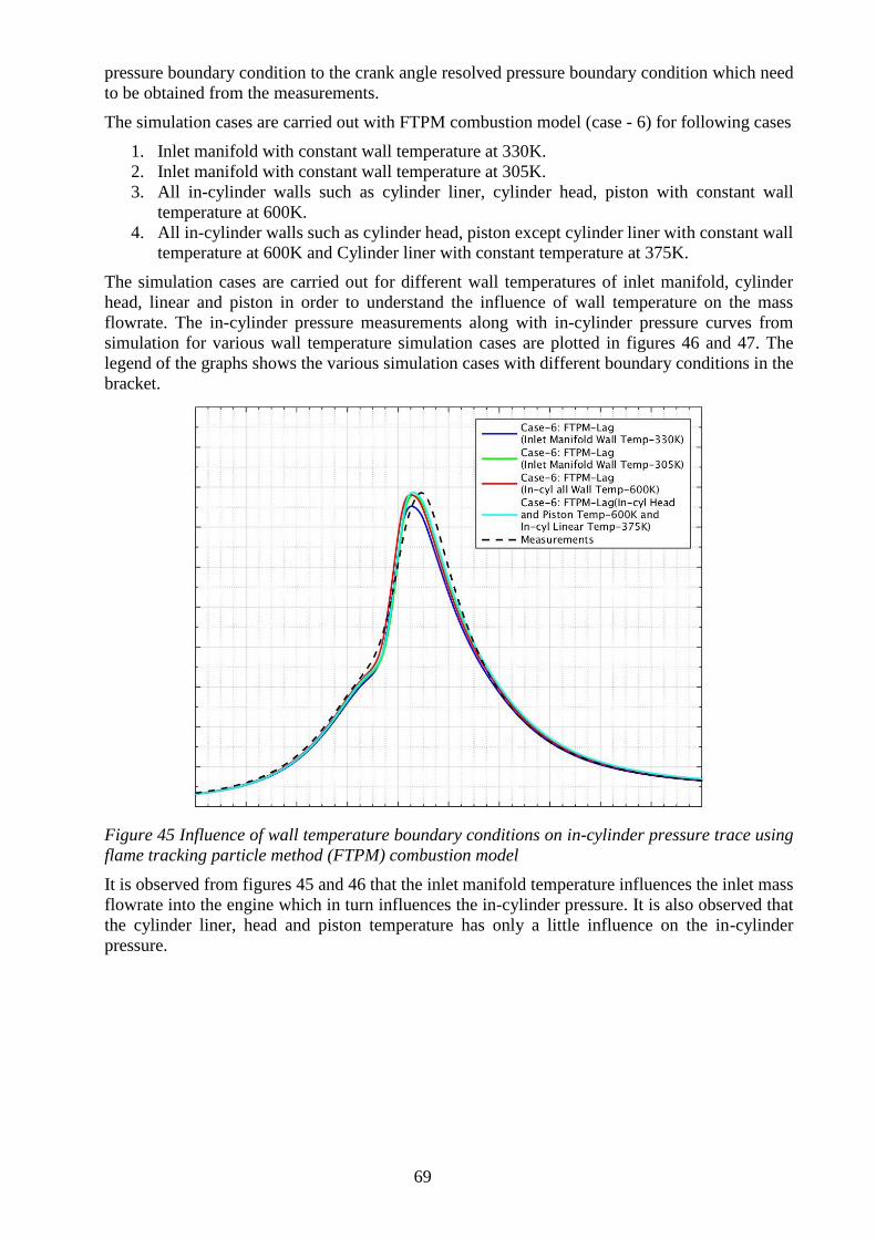
69
pressure boundary condition to the crank angle resolved pressure boundary condition which need
to be obtained from the measurements.
The simulation cases are carried out with FTPM combustion model (case - 6) for following cases
1. Inlet manifold with constant wall temperature at 330K.
2. Inlet manifold with constant wall temperature at 305K.
3. All in-cylinder walls such as cylinder liner, cylinder head, piston with constant wall
temperature at 600K.
4. All in-cylinder walls such as cylinder head, piston except cylinder liner with constant wall
temperature at 600K and Cylinder liner with constant temperature at 375K.
The simulation cases are carried out for different wall temperatures of inlet manifold, cylinder
head, linear and piston in order to understand the influence of wall temperature on the mass
flowrate. The in-cylinder pressure measurements along with in-cylinder pressure curves from
simulation for various wall temperature simulation cases are plotted in figures 46 and 47. The
legend of the graphs shows the various simulation cases with different boundary conditions in the
bracket.
Figure 45 Influence of wall temperature boundary conditions on in-cylinder pressure trace using
flame tracking particle method (FTPM) combustion model
It is observed from figures 45 and 46 that the inlet manifold temperature influences the inlet mass
flowrate into the engine which in turn influences the in-cylinder pressure. It is also observed that
the cylinder liner, head and piston temperature has only a little influence on the in-cylinder
pressure.
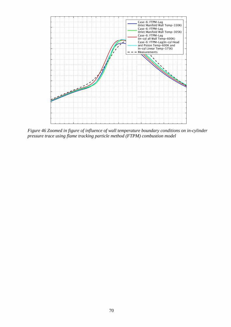
70
Figure 46 Zoomed in figure of influence of wall temperature boundary conditions on in-cylinder
pressure trace using flame tracking particle method (FTPM) combustion model
71
5 CONCLUSIONS AND FURTHER WORK
In this chapter, a discussion of the results and the conclusions are presented in this chapter. The
conclusions are based on the analysis with the intention to answer the formulation of questions
that are presented in Chapter 1. Recommendations on more detailed solutions and future work in
this project are presented.
5.1 Conclusions
The recommended range of the various parameters such as SF and CP of the combustion
simulation model is mentioned in table 10. These recommended range is purely from the past
experiences of AVL with the AVL FIRE and is not from the physical modelling of the combustion
simulation models. However, from the combustion model simulation study, it can be found that
the parametric settings of the combustion simulation models such as SF and CP, should be A, B,
C and D for case - 1, case - 3, case - 6 and case - 7 respectively. These values are outside the
recommended range except for case-6. This means that these parameters may cause some
numerical error when operating at different operating conditions due to the numerical modelling
of combustion model since there is no recommended range from the physical modelling of the
combustion models.
When comparing to measurements for the second operating point based on the tuning parameters
from the first operating point, it can also be concluded that ECFM combustion model (case - 1 and
case - 3) predicts the in-cylinder pressure more accurately than the other combination of simulation
model (case - 6 and case - 7). The deviation of the peak in-cylinder pressure is around 3% for the
ECFM combustion model (case - 1 and 3). Whereas, the deviation of the peak in-cylinder pressure
is around 10% and 13% for FTPM (case - 6) and FTM (case - 7) respectively when compared with
measurements.
Regarding the runtime of the simulation, it can be concluded that the simulation using FTPM
combustion model (case - 6) take around 10% more time when compared to the simulation using
ECFM combustion model (case - 1 and case - 3). No conclusion can be made for FTM combustion
model since the simulation did not converge for the same mesh size. However, it can be concluded
that the FTM combustion model requires fine mesh size to achieve a convergent solution which is
shown in figures 26 and 27. This means that the FTM combustion model depends on the mesh
quality and mesh size.
It can also be concluded that when the ignition timing of the simulation is advanced, the in-cylinder
pressure will increase which needs to be compensated by reducing the tuning parameters such as
stretch factor and combustion parameter. It can also be observed the possibility of the occurrence
of the auto ignition phenomenon is higher when running the simulation for second engine cycle.
While running for the second cycle, even though ECFM combustion model with spherical ignition
model overpredicts the in-cylinder pressure by 30%, it can also be concluded that ECFM
combustion model with spherical ignition model (case-1) is more stable when compared to other
combination of combustion and ignition models.
It can also be observed that the mass flowrate of the system is strongly influenced by the pressure
in the inlet boundary condition. However, it can also be observed that the wall temperature of the
system has only a little influence the mass flowrate of the system.
5.2 Recommendations
The following recommendations can be made based on the observations and the conclusions from
the simulation results of this project.
72
• It is better to start the simulation from EVO condition rather than the IVO condition.
• The number of mesh elements in the spark plug can be limited to the range of 9-11
elements.
• Out of the various combinations of combustion and ignition models that is used, it is also
better to use ECFM combustion model for modelling combustion phenomenon in the
simulation for stable results.
Even though FTM combustion model (which is commonly known as G-equation model) is the
most popular method due to the advancements and also from the past research, it should be noted
that it is quite sensitive to the mesh size and mesh quality. Therefore, it is advised to check the
convergence of the simulation while using the FTM combustion model for a specific mesh.
Also, it is advised to check the convergence of the simulation while using the advance ignition
model before starting any research project. It is also advised to check for the reinitialisation of
intake port region especially during the intake stroke while using ECFM-3Z+ combustion model.
5.3 Future Work
As mentioned earlier in the recommendations, one of the suggestions for the future work is to carry
out simulation for other cases after solving the problems in advance ignition model such as
AKTIM, ISSIM and CADIM and also the problems of auto-ignition at second cycle and at higher
engine speeds with the help of software supplier.
The problem of reinitialisation especially in the intake stroke was observed in ECFM-3Z+
combustion model simulations. However, on detailed analysis, it was found that this problem can
be solved by the simulations using a different meshing approach (single domain mesh). This single
domain mesh includes mesh domains of inlet port region, exhaust port region and combustion
cylinder region as a single domain where the different stroke of the engine is actuated by removing
the relevant mesh elements near the intake and exhaust valve region. A detailed analysis was not
able to be carried out in this thesis due to lack of time. Therefore, the evaluation of single domain
mesh can be one of the suggestions for future work.
It is also observed from the simulation results while using the single domain mesh that there is an
increase mass flowrate which reduces the difference in mass flowrate between the simulation and
the measurements. Therefore, another suggestion for future work is to study and analyze the effect
of computational domain (single domain with multi domain which is mentioned in section 3.2) on
computational time and simulation results which may be affected due to the change in the overall
domain mesh size and also in the effect of reinitialisation during the engine cycle.
It is also suggested from the research that it is better to understand the impact of the crank angle
resolved pressure boundary conditions and its effects on the difference in mass flowrate between
the simulation and the measurements. This can be one of the important future work since the mass
flowrate is strongly influence by the pressure in the inlet boundary conditions.
Also, it is assumed in the research that there is a uniform mixing of fuel and air in the inlet port
region. However, the measurements are carried out in a port fuel injection engine with the help of
natural gas injector which may not ensure uniform mixing of furl and air. So, one of the future
works can be carrying out the simulation with port fuel injection (without premixed combustion)
in order to understand whether the assumptions made in the research are correct or not and how
these assumptions can impact the results of the research.
It can be observed from the in-cylinder pressure measurements that both the operating conditions
are similar in nature. Therefore, it is suggested to carry out the simulation for more operating points
especially with different loads and different equivalence ratio in order to understand the robustness
of the simulation predictability.
73
6 REFERENCES
1. Kofod M. and Stephenson T., "Well-to Wheel Greenhouse Gas Emissions of LNG Used as
a Fuel for Long Haul Trucks in a European Scenario," SAE Technical Paper 2013-24-
0110, 2013, https://doi.org/10.4271/2013-24-0110.
2. Chehroudi B., 1993. "Use of Natural Gas in Internal Combustion Engines”. Proceedings
of the First International Non-Renewable Energy Sources Congress, University of Science
and Technology, Tehran, December 26-29. DOI: 10.13140/2.1.4630.4000
3. Boretti A., Lappas P., Zhang B., and Mazlan, S., "CNG Fueling Strategies for Commercial
Vehicles Engines-A Literature Review," SAE Technical Paper 2013-01-2812, 2013,
https://doi.org/10.4271/2013-01-2812.
4. Shuang He, Bao-Guo Du, Li-Yan Feng, Yao Fu, Jing-Chen Cui and Wu-Qiang Long; “A
Numerical Study on Combustion and Emission Characteristics of a Medium-Speed Diesel
Engine Using In-Cylinder Cleaning Technologies,” Energies 2015, 8, 4118-4137;
doi:10.3390/en8054118.
5. G.P. Merker et al. (eds.), Reinhard Tatschl, “Appendix- 3D-CFD Simulation of IC-Engine
Flow, Mixture Formation and Combustion with AVL FIRE, Combustion Engines
Development”, pp 601-627, DOI 10.1007/978-3-642-14094-5, # Springer-Verlag Berlin
Heidelberg 2012.
6. Gupta SB., Biruduganti M., Bihari B. and Sekar R., “Natural gas fired reciprocating
engines for power generation: concerns and recent advances”. Intech, pp 211–234, 2012;
DOI: 10.5772/45992
7. Luis Iñaki Martinez, “Investigation of CFD conjugate heat transfer simulation methods
for engine components at SCANIA CV AB”, Master Thesis, Linköpings Universitet,
Institutionen för ekonomisk och industriell utveckling, Examensarbete 2017.
8. From Wikipedia, “History of the internal combustion engine”,
https://en.wikipedia.org/wiki/History_of_the_internal_combustion_engine accessed on
2018 August 05.
9. Goering, Carroll E, Marvin L. Stone, Davos W. Smith, and Paul K. Turnquist,
“Thermodynamics and engine cycles, Chapter 4 in Off-Road Vehicle Engineering
Principles”, pp 57-74. ASAE. 2003.
10. From Wikipedia, “Kyoto Protocol”, https://en.wikipedia.org/wiki/Kyoto_Protocol
accessed on 2018 August 05.
11. G. Fontana, E. Galloni and R. Palmaccio, “Modeling of a Four-Valve S.I. Engine
Combustion: A Comparison of Two 3-D Computer Code”, SAE Technical paper no: 2001-
01-3235.
12. A. Trouv and T. Poinsot, “The evolution equation for the flame surface density in turbulent
premixed combustion”, Center for Turbulence Research Proceedings of the Summer
Program 1992.
13. C. Haworthy, “A probability density function/flamelet method for partially premixed
turbulent combustion”, Center for Turbulence Research Proceedings of the Summer
Program 2000.
14. Frank E. M and James E. B, “The coherent flame model for turbulent chemical reactions;
Project Squid Technical Report TRW-9-PU”, January 1977.
15. B. Jafari, D.D. Ganji and M. Mirsalim, “Experimental and Numerical Investigation of the
Effect of Exhaust Gas Recirculation on Performance and Emissions of a Dual Fuel
(Diesel–Gas) Engine”, Australian Journal of Basic and Applied Sciences, 7(7): 668-678,
2013, ISSN 1991-8178
16. O. Colin, A. Benkenida and C. Angelberger, “3D Modeling of Mixing, Ignition and
Combustion Phenomena in Highly Stratified Gasoline Engines”, pp. 47-62, Oil & Gas
Science and Technology - Rev. IFP, Vol. 58 (2003), No.1.
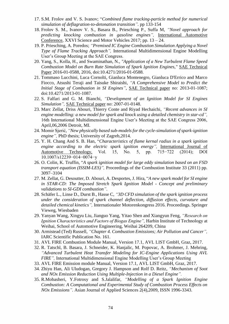
74
17. S.M. Frolov and V. S. Ivanov; “Combined flame tracking-particle method for numerical
simulation of deflagration-to-detonation transition”. pp 133-154
18. Frolov S. M., Ivanov V. S., Basara B., Priesching P., Suffa M, “Novel approach for
predicting knocking combustion in gasoline engines”, International Automotive
Conference, XXVI Science and Motor Vehicles 2017; pp. 13 – 24.
19. P. Priesching, A. Poredos; “Premixed IC Engine Combustion Simulation Applying a Novel
Type of Flame Tracking Approach”, International Multidimensional Engine Modelling
User’s Group Meeting at the SAE Congress.
20. Yang, S., Kolla, H., and Swaminathan, N., "Application of a New Turbulent Flame Speed
Combustion Model on Burn Rate Simulation of Spark Ignition Engines," SAE Technical
Paper 2016-01-0588, 2016, doi:10.4271/2016-01-0588.
21. Tommaso Lucchini, Luca Cornolti, Gianluca Montenegro, Gianluca D'Errico and Marco
Fiocco, Atsushi Teraji and Taisuke Shiraishi, “A Comprehensive Model to Predict the
Initial Stage of Combustion in SI Engines”, SAE Technical paper no: 2013-01-1087;
doi:10.4271/2013-01-1087.
22. S. Falfari and G. M. Bianchi, “Development of an Ignition Model for SI Engines
Simulation”, SAE Technical paper no: 2007-01-0148.
23. Marc Zellat, Driss Abouri, Thierry Conte and Riyad Hechaichi, “Recent advances in SI
engine modelling: a new model for spark and knock using a detailed chemistry in star-cd”,
16th International Multidimensional Engine User’s Meeting at the SAE Congress 2006,
April,06,2006 Detroit, MI.
24. Momir Sjerić, “New physically based sub-models for the cycle-simulation of spark-ignition
engine”, PhD thesis; University of Zagreb,2014.
25. Y. H. Chang And S. B. Han, “Characteristics of flame kernal radius in a spark ignition
engine according to the electric spark ignition energy”, International Journal of
Automotive Technology, Vol. 15, No. 5, pp. 715−722 (2014); DOI
10.1007/s12239−014−0074−y
26. O. Colin, K. Truffin, “A spark ignition model for large eddy simulation based on an FSD
transport equation (ISSIM-LES)”, Proceedings of the Combustion Institute 33 (2011) pp.
3097–3104
27. M. Zellat, G. Desoutter, D. Abouri, A. Desportes, J. Hira, “A new spark model for SI engine
in STAR-CD: The Imposed Stretch Spark Ignition Model - Concept and preliminary
validations to SI-GDI combustion”.
28. Schäfer L., Linse D., Durst B., Hasse C, “3D CFD simulation of the spark ignition process
under the consideration of spark channel deflection, diffusion effects, curvature and
detailed chemical kinetics”, Internationaler Motorenkongress 2016. Proceedings. Springer
Vieweg, Wiesbaden
29. Yanyan Wang, Xingyu Liu, Jianguo Yang, Yitao Shen and Xiangyun Feng, “Research on
Ignition Characteristics and Factors of Biogas Engine”, Harbin Institute of Technology at
Weihai, School of Automotive Engineering, Weihai 264209, China
30. Armistead (Ted) Russell, “Chapter 4. Combustion Emissions; Air Pollution and Cancer”,
IARC Scientific Publication No. 161.
31. AVL FIRE Combustion Module Manual, Version 17.1, AVL LIST GmbH, Graz, 2017.
32. R. Tatschl, B. Basara, J. Schneider, K. Hanjalic, M. Popovac, A. Brohmer, J. Mehring,
“Advanced Turbulent Heat Transfer Modeling for IC-Engine Applications Using AVL
FIRE”, International Multidimensional Engine Modelling User’s Group Meeting
33. AVL FIRE Emission module Manual, Version 17.1, AVL LIST GmbH, Graz, 2017.
34. Zhiyu Han, Ali Uludogan, Gregory J. Hampson and Rolf D. Reitz, “Mechanism of Soot
and NOx Emission Reduction Using Multiple-Injection in a Diesel Engine”.
35. R.Mobasheri, Y.Fotrosy and S.Jalalifar, “Modelling of a Spark Ignition Engine
Combustion: A Computational and Experimental Study of Combustion Process Effects on
NOx Emissions”. Asian Journal of Applied Sciences 2(4),2009, ISSN 1996-3343.
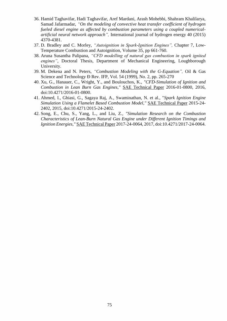
75
36. Hamid Taghavifar, Hadi Taghavifar, Aref Mardani, Arash Mohebbi, Shahram Khalilarya,
Samad Jafarmadar, “On the modeling of convective heat transfer coefficient of hydrogen
fueled diesel engine as affected by combustion parameters using a coupled numerical-
artificial neural network approach”, International journal of hydrogen energy 40 (2015)
4370-4381.
37. D. Bradley and C. Morley, “Autoignition in Spark-Ignition Engines”, Chapter 7, Low-
Temperature Combustion and Autoignition, Volume 35, pp 661-760.
38. Aruna Susantha Palipana, “CFD modelling of natural gas combustion in spark ignited
engines”, Doctoral Thesis, Department of Mechanical Engineering, Loughborough
University.
39. M. Dekena and N. Peters, “Combustion Modeling with the G-Equation”, Oil & Gas
Science and Technology Ð Rev. IFP, Vol. 54 (1999), No. 2, pp. 265-270
40. Xu, G., Hanauer, C., Wright, Y., and Boulouchos, K., "CFD-Simulation of Ignition and
Combustion in Lean Burn Gas Engines," SAE Technical Paper 2016-01-0800, 2016,
doi:10.4271/2016-01-0800.
41. Ahmed, I., Ghiasi, G., Sagaya Raj, A., Swaminathan, N. et al., "Spark Ignition Engine
Simulation Using a Flamelet Based Combustion Model," SAE Technical Paper 2015-24-
2402, 2015, doi:10.4271/2015-24-2402.
42. Song, E., Chu, S., Yang, L., and Liu, Z., "Simulation Research on the Combustion
Characteristics of Lean-Burn Natural Gas Engine under Different Ignition Timings and
Ignition Energies," SAE Technical Paper 2017-24-0064, 2017, doi:10.4271/2017-24-0064.

76
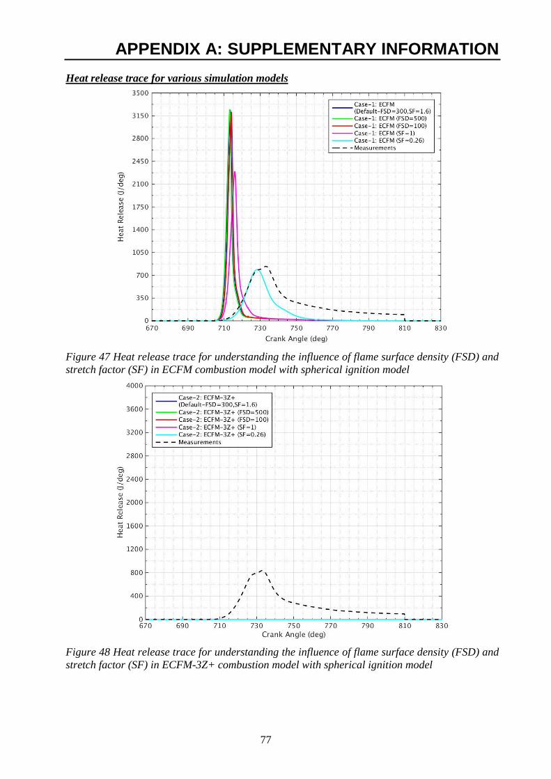
77
APPENDIX A: SUPPLEMENTARY INFORMATION
Heat release trace for various simulation models
Figure 47 Heat release trace for understanding the influence of flame surface density (FSD) and
stretch factor (SF) in ECFM combustion model with spherical ignition model
Figure 48 Heat release trace for understanding the influence of flame surface density (FSD) and
stretch factor (SF) in ECFM-3Z+ combustion model with spherical ignition model
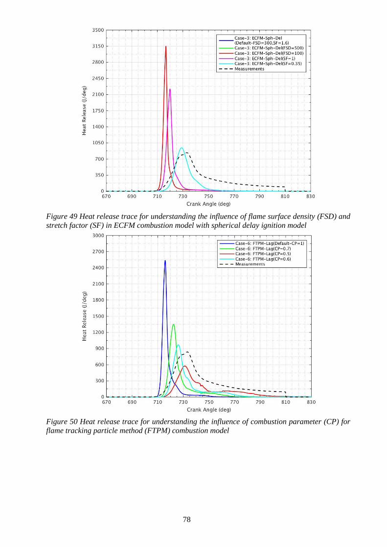
78
Figure 49 Heat release trace for understanding the influence of flame surface density (FSD) and
stretch factor (SF) in ECFM combustion model with spherical delay ignition model
Figure 50 Heat release trace for understanding the influence of combustion parameter (CP) for
flame tracking particle method (FTPM) combustion model
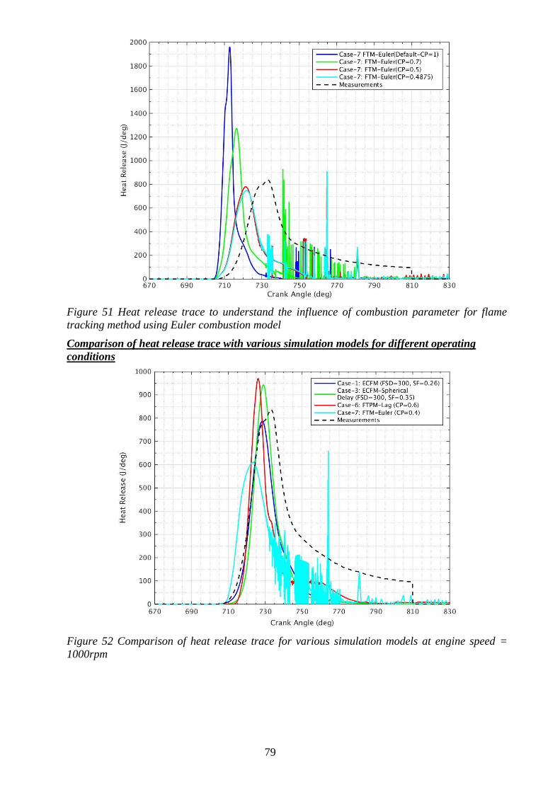
79
Figure 51 Heat release trace to understand the influence of combustion parameter for flame
tracking method using Euler combustion model
Comparison of heat release trace with various simulation models for different operating
conditions
Figure 52 Comparison of heat release trace for various simulation models at engine speed =
1000rpm
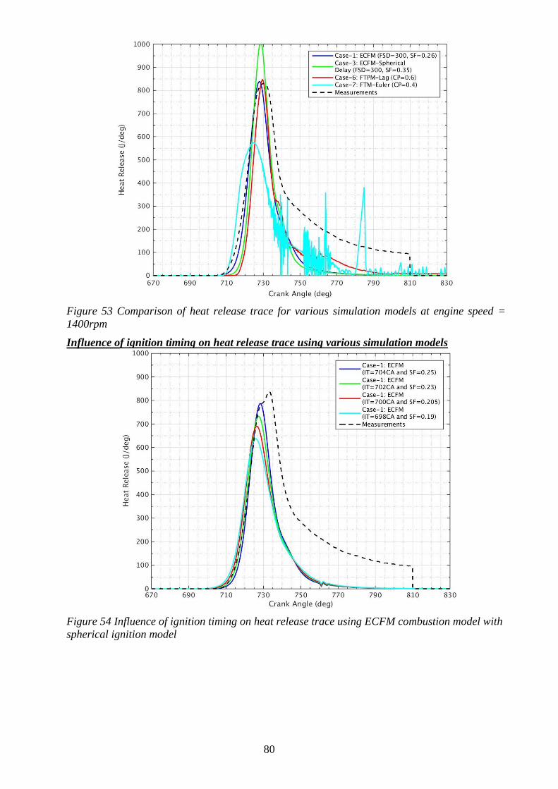
80
Figure 53 Comparison of heat release trace for various simulation models at engine speed =
1400rpm
Influence of ignition timing on heat release trace using various simulation models
Figure 54 Influence of ignition timing on heat release trace using ECFM combustion model with
spherical ignition model
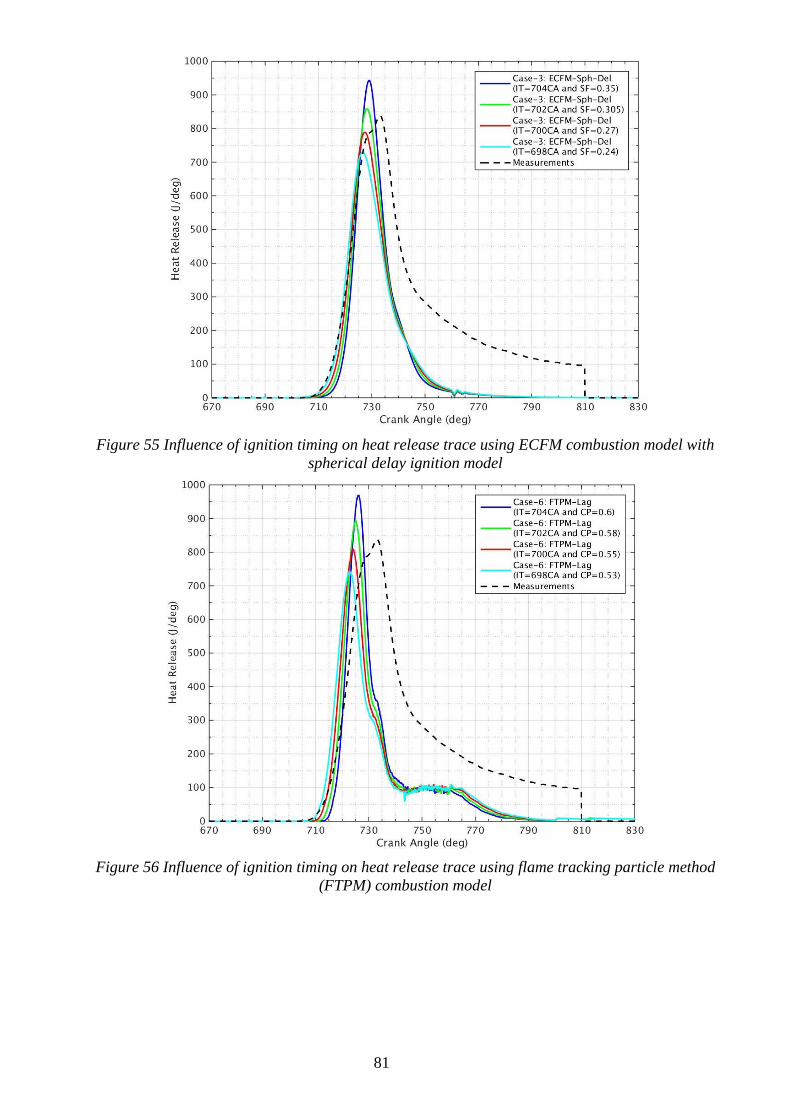
81
Figure 55 Influence of ignition timing on heat release trace using ECFM combustion model with
spherical delay ignition model
Figure 56 Influence of ignition timing on heat release trace using flame tracking particle method
(FTPM) combustion model