Simulating the impact of freshwater inputs and deep-draft icebergs formed during a MIS 6 Barents Ice...

Simulating the impact of freshwater inputs and deep‐draft icebergsformed during a MIS 6 Barents Ice Sheet collapse

Clare L. Green,1 J. A. Mattias Green,2 and Grant R. Bigg1

Received 23 November 2010; revised 17 February 2011; accepted 24 February 2011; published 11 May 2011.

[1] An intermediate complexity climate model is used to simulate the collapse of theBarents Ice Sheet during Marine Isotope Stage 6 (MIS 6; 140 ka B.P) with the purpose ofinvestigating whether a mass input of freshwater from the collapse could have affectedthe convection and deep water formation in the North Atlantic Ocean. Further experimentsused a coupled dynamic and thermodynamic iceberg model to determine the effects ofdeep‐draft icebergs, rather than freshwater alone, on the ocean circulation. The resultspredict that the collapse of the Barents Ice Sheet had a significant impact on the meridionaloverturning circulation in both the Atlantic and Pacific oceans. Freshwater fluxes havemore of an impact on the Atlantic overturning circulation during the actual release periodcompared to icebergs, but the bergs induce effects over longer time scales even afterthe pulse is removed. Freshwater fluxes of 0.15 sverdrup (Sv) and iceberg surges of 0.1 Svtrigger significant changes in the global patterns, particularly in the North Pacific wherethere is strengthening of the overturning circulation at the expense of that in the NorthAtlantic, and associated increases in Pacific sea surface temperatures. These resultshighlight the importance of simulating not only the correct flux but also the form of thefreshwater input from ice sheet collapses appropriately.

Citation: Green, C. L., J. A. M. Green, and G. R. Bigg (2011), Simulating the impact of freshwater inputs and deep‐drafticebergs formed during a MIS 6 Barents Ice Sheet collapse, Paleoceanography, 26, PA2211, doi:10.1029/2010PA002088.

1. Introduction

[2] The oceanic meridional overturning circulation(MOC) is the major global transporter of heat and thereforea key element in the global climate system (see Rahmstorf[2002] for a review). It is sustained by a continuous inputof mechanical energy which induces vertical mixing andthus balances the deep water formation at high latitudes[Wunsch and Ferrari, 2004], although large‐magnitudefreshwater fluxes from melting ice sheets may hamper theformation of deepwater [e.g., Broecker and Denton, 1990;Lenderink and Haarsma, 1994; Rahmstorf, 2002; Greenet al., 2009]. A sudden major input of freshwater from thecollapse of a large ice sheet in the northern part of theBarents Sea (hereafter the Barents Ice Sheet; see Figure 1)may therefore have had a significant effect on the oceanicand atmospheric circulation, hydrological balance, biologyand sedimentation in the Arctic Ocean at the end of MarineIsotope Stage 6 (MIS 6; the penultimate glaciation, ∼140 ka).There is evidence from plow marks and seafloor erosion forthe existence of very large icebergs in the Arctic duringMIS6, consistent with such a collapse [e.g., Dowdeswellet al., 1993; Syvitski et al., 2001; Kristoffersen et al.,

2004; Kuijpers and Werner, 2007; Metz et al., 2008]. Theimpact of icebergs from the Laurentide Ice Sheet on theocean and climate has been investigated previously[MacAyeal, 1993; Alley, 1998; Levine and Bigg, 2008], butstudies of the effect of freshwater inputs from the collapseof the Barents Ice Sheet during MIS 6 are lacking, despiteits potential consequences for the MOC and the possibilityto investigate abrupt climate change for another time periodthan the LGM.[3] Here the response of the Atlantic meridional over-

turning circulation (MOC) to freshwater fluxes added eitheras meltwater pulses or as deep‐draft icebergs calved fromthe ice edge of the glacial Barents Ice Sheet is investigated.The idea is that the MOC is less sensitive over longer per-iods to a meltwater pulse compared to icebergs, but that ameltwater pulse will have a larger initial impact on thecirculation than do icebergs during the actual discharge [seeGreen et al., 2009, 2010]. The impact of freshwater fluxesadded to the North Atlantic has been investigated in anumber of papers over the last few years [e.g., Zhang andDelworth, 2005; Stouffer et al., 2006; Levine and Bigg,2008]. Within the World Climate Research Program Cou-pled Model Intercomparison Project/Paleo‐Modeling Inter-comparison Project, the performance of a number of bothintermediate complexity models and fully coupled atmo-sphere‐ocean general circulation models was tested (seeStouffer et al. [2006] for a summary). The model consideredhere is somewhere in between these models as it is ofintermediate complexity but consisting of a full ocean model

1Department of Geography, University of Sheffield, Sheffield, UK.2School of Ocean Sciences, College of Natural Sciences, Bangor

University, Menai Bridge, UK.

Copyright 2011 by the American Geophysical Union.0883‐8305/11/2010PA002088

PALEOCEANOGRAPHY, VOL. 26, PA2211, doi:10.1029/2010PA002088, 2011

PA2211 1 of 16

http://dx.doi.org/10.1029/2010PA002088

coupled through wind‐ and heat‐flux feedbacks to a sim-plified atmospheric model.[4] Generally, the Atlantic MOC experiences a weaken-

ing, but not a shut down, in response to freshwater inputs of0.1 sverdrup (Sv) (1 Sv = 106 m3 s−1) in the North Atlantic[e.g., Zhang and Delworth, 2005; Swingedouw et al., 2009].A flux between 0.3 and 1 Sv is enough to shut down andeven reverse the Atlantic MOC, with the exact flux neededdepending on the model and release location [Stouffer et al.,2006; Bigg et al., 2010; Okumura et al., 2009]. A fresheningin the northern North Atlantic may thus lead to a switchin deepwater formation from the Atlantic the North Pacific[e.g., Seidov and Haupt, 2005]. This is because the globalsalinity conveyor is critically dependent on the salinitydifference between the Atlantic and Pacific Oceans, and areduced MOC can thus be associated with a reduced salinitydifference [Stouffer et al., 2007], but the exact quantitativeresponse depends on the mean background climate state[e.g., Swingedouw et al., 2009].[5] Due to the majority of the Barents Ice Sheet melting

over a short time period of about 500 years [e.g., Svendsenet al., 2004], the deglaciation can be described as a collapse.Studies of ice sheet collapse tend to focus on freshwatersurges; however, an important component of the deglacia-tion of the Eurasian ice sheets was the calving of icebergsalong the marine margins, as well as surface melting alongthe southern land‐based margins of the ice mass [Siegertand Dowdeswell, 2002; Green et al., 2010]. During calv-ing events the majority of freshwater does not enter theocean immediately but is instead released gradually as theicebergs melt. Such processes have been modeled for otherrelease points during the Last Glacial Maximum [Levine andBigg, 2008; Bigg et al., 2010], but not MIS 6. The signifi-cance of the Barents Ice Sheet for climate is that the coldtemperatures and subsequent slow melting could enablesome of the icebergs from its collapse to drift into the NorthAtlantic before melting [e.g., Green et al., 2010], providinga potential mechanism for transporting freshwater throughthe Fram Strait, directly into the Nordic Seas and toward thearea of deep water formation. Here we employ FRUGAL(the Fine ResolUtion Greenland sea And Labrador Seamodel), a global intermediate complexity coupled atmo-sphere ocean model, set up for the MIS 6, to simulate theimpact of meltwater and icebergs on the MOC [Bigg et al.,1998; Bigg and Wadley, 2001]. Forcing consisted of cou-pled heat and freshwater fluxes and climatological windfields, and the simulations included addition of a freshwaterpulse, either in the form of meltwater or as seeded icebergs,along the Barents Sea coastline to represent a collapsing icesheet. We begin by introducing the FRUGAL model and theiceberg trajectory model in section 2, where we also discussthe experiments, forcing, and freshwater fluxes. Section 3contains a discussion of the response in global transportsand upper‐ocean stratification to the experiments, section 4contains the discussion and summary, and section 5 containsthe conclusions.

2. The Model System

2.1. The Model System

[6] FRUGAL has a resolution of 1° × 1° and realisticrepresentation of processes in the central Arctic, yet does not

require inefficiently large computational power, despitebeing a global model. This is achieved by using a variable‐resolution orthogonal curvilinear coordinate system with thegrid North Pole located in Greenland (72.5°N, 40°W) and alower resolution (6° × 4°) in the Southern and Pacific Oceans(see Figure 1c). The ocean model in FRUGAL has 19 verticallayers with thicknesses between 30 and 500 m, a free surface,and is coupled to thermodynamic and dynamic atmosphere[Fanning and Weaver, 1996], sea ice [Parkinson andWashington, 1979], and iceberg models [Bigg et al., 1997].FRUGAL has been set up to employ a method for reducingtime step length at selected points within the grid [Wadley andBigg, 1999]. This variable time stepping method enablesincreasing numbers of shorter time steps to be taken inregions of higher resolution across the model domain,while maintaining a synchronous integration and achievingnumerical stability throughout the model. FRUGAL is com-bined with a reduced complexity atmosphere model, whichincludes parameterization of clouds, mountains, land ice andland hydrology, based on Fanning and Weaver [1996], but ithas been modified to include advection of water vapor andsimple wind feedback [Bigg and Wadley, 2001]. This cou-pling provides a grid point to grid point interactive exchangeof heat and freshwater between the atmosphere and ocean.FRUGAL has been used successfully to model present‐day[Bigg et al., 2005] and Last Glacial Maximum conditions[Bigg et al., 1998;Wadley andBigg, 2002;Green et al., 2009],although prior to this study it has only been employed tosimulate the MIS 6 by Green et al. [2010].[7] The thermodynamic and dynamic iceberg model is

described by Bigg et al. [1997] and includes drag forcingfrom the ocean, atmosphere and sea ice, in addition to theCoriolis force, pressure gradients and wave radiation. Ice-bergs are seeded individually at the ice edge and thenallowed to drift through the domain until they melt orbecome beached. To determine the forcing for each iceberg,the bergs are assumed to occupy a single point in space (avalid assumption with the current model resolution). Themain thermodynamical processes acting on the icebergs arebasal melting, buoyant convection, wave erosion, and to alesser extent sensible heating and sublimation at the ice‐airinterface. At each main ocean time step information aboutsea ice thickness, surface ocean velocities, wind velocities,sea surface temperature, sea surface salinity, and sea icevelocity are exchanged between the ocean and iceberg tra-jectory models. This information is used to determine ice-berg trajectories and melting rates, which are subsequentlypassed to the ocean model to provide information onfreshwater and heat fluxes in the ocean. Note that the ice-berg drift patterns have been shown to be satisfactory usingonly surface current (as they usually dominate the currentfield), so this approach is used here to keep the computa-tional cost down [Bigg et al., 1997; Gladstone et al., 2001].The impacts of the iceberg on atmospheric variables aresmall and thus there is no direct coupling between theatmosphere component of the ocean model and the icebergmodel. The iceberg model has been used previously withinFRUGAL by Levine and Bigg [2008] and Green et al.[2010], the latter of whom used it to study the drift pat-terns of icebergs released from the collapse of a MIS 6Barents Ice Sheet. For space reasons within the present

GREEN ET AL.: MIS 6 BARENTS ICE SHEET COLLAPSE PA2211PA2211

2 of 16

paper, readers are referred to Bigg et al. [1997], Levine andBigg [2008], and Green et al. [2010] for details.

2.2. Model Setup

[8] Most investigations into the timing and duration offreshwater pulses, either from ice streams or as meltwaterpulses, deal with the Last GlacialMaximum (LGM), 18–21 kaB.P. (see the summary by Bischof [2000]), and we havetherefore used some knowledge from MIS2 and applied it toMIS 6 whenever information is lacking.[9] The maximum extent of the Fennoscandian Ice Sheet

during MIS 6 is based on Svendsen et al. [2004] (Figure 1)as they significantly redefined the extent of the ice sheet.It was found to be smaller than implied by previousreconstructions [e.g., Grosswald and Hughes, 2002], butsedimentary sequences along the northern margin of Siberiashow no evidence of being overridden by an ice sheetand thus that these areas were ice free during MIS 6 (andthe more recent MIS 2) [Svendsen et al., 2004]. Thereconstructions indicate that the northern extent of the icesheet over Eurasia was essentially the same during both MIS2 and 6, with the ice front along the Barents Sea marginreaching the shelf break along the Norwegian Sea and ArcticOcean [Lubinski et al., 1996; Polyak et al., 1997, 2002;Mangerud et al., 1998]. The ice sheet extended furthernorthwestward toward Greenland during the MIS 6 glacia-tion than during the last glaciation, leading to a narrowerFram Strait. Also, during the earlier glaciation the ice sheetextended further east over the Kara Sea region to theSiberian Mountains and further south over the West SiberianLowlands [Spielhagen et al., 2004; Svendsen et al., 2004].The subsequent location of the Barents Ice Sheet as usedin FRUGAL is shown in Figure 1.[10] The ice sheet growth during MIS 6 resulted in a fall

in global sea level due to the transfer of water from theocean to the ice sheets. Few studies have been conductedwhich focus on a longer history of sea level [e.g., Mix andRuddiman, 1984], and the most recent estimates suggestthat sea level was 125–128 m below present‐day levelsduring MIS 6 [Rohling et al., 1998; Rabineau et al., 2006].Here we use the higher of these estimates, using the geo-graphical pattern provided by the LGM database fromPeltier [2004] and with sill depths adjusted from Thompson[1995] (note that the Bering Strait was closed during MIS6).Although this latter database may not be entirely correct forMIS 6, the sea level variations were roughly similar and it iscurrently the best available estimate.[11] The other variables which were altered in the setup

were related to the atmospheric CO2 concentration and var-iations in solar insolation due to variation in the Earth’s orbitand rotation. The latter consist of the precession, obliquityand eccentricity, and all are set to represent those appropriatefor MIS 6 (see Berger and Loutre [1992] for details andFanning and Weaver [1996] for the implementation).Theatmospheric CO2 concentration was set to 194 ppm basedon data from the Vostok Ice cores [Raynaud et al., 1993;Petit et al., 1999; Siegenthaler et al., 2005]. Note that duringMIS 2 the CO2 concentration was 181 ppm, the PD CO2

concentration is 350 ppm, and that the temporal accuracy ofthe MIS 6 estimate is ±15 kyr.

2.3. Experiments and Ice Sheet Collapse

[12] The model spin‐up was created by running themodel, using the described MIS 6 forcing and conditions,for 100 years in robust diagnostic mode from a state of rest.The relaxation was then suppressed and the integrationcontinued with surface forcing until the model’s naturalvariability showed no general trend and the Atlantic MOChad reached a quasi‐steady state. The time taken to reachthis state in the model simulations was less than 6000 years.Following this spin‐up, the control run was created bycontinuing the integrations for a further 3000 years. Notethat in the following MIS 6 conditions are being describedunless specifically noted. In the perturbation experiments, afreshwater pulse was added after the spin up (i.e., at year6000) to test the sensitivity of the MOC to amplitude andform of the prescribed freshwater pulses. The perturbationruns were then continued for 1500 years, as the model runshad mostly recovered or reached a new steady state at thistime. Note that in the following all time indications aregiven as time elapsed from the start of the perturbation (i.e.,year 6000; this holds for the control run as well). Two typesof perturbed freshwater experiments were performed: thefirst involved simulating the collapse as a freshwater surge(henceforth denoted FW), and the second involved model-ing implicit icebergs being calved from the circumference ofthe Barents Ice Sheet (ICE in the following).[13] The actual mechanism for collapse of the Barents Ice

Sheet during MIS 6 is unknown, but indications exist that theMIS2 ice sheets, especially the Laurentide, may have beensubject to intense tidally driven straining and erosion[Griffiths and Peltier, 2009]. Because the extents of the icesheets were roughly similar for both LGM and MIS 6 [e.g.,Svendsen et al., 2004] we use the estimates of ice volume andmelt rates from Bischof [2000] for MIS 2 and apply them tothis investigation. To account for uncertainties a number ofexperiments with different freshwater volume fluxes, both asmeltwater and icebergs, were done. In all simulations, thepulses began at 140,000 calendar year B.P (model year 6000;after the spin‐up using nonchanging MIS 6 conditions).[14] The majority of both FW and ICE simulations

involved a meltwater surge being added over the BarentsSea region for a period of 500 years, in compliance with theduration of extremely high deposition rates of IRD in theNorwegian Greenland Sea during the LGM [Bischof, 1994,2000]. Further model simulations were conducted in orderto investigate the sensitivity of the model to duration ofmeltwater additions, with FW pulses being simulated overtime periods within the range of 100–1000 years. The pulseswere applied equally at all ocean grid points covering theBarents Ice Sheet. A range of different magnitudes ofmeltwater pulses were applied, in accordance to estimatedfluxes required to melt the Barents Ice Sheet over 500 years,ranging from 0.01 to 0.3 Sv, although focus here is on the0.1, 0.15, and 0.3 Sv cases.[15] During iceberg seeding experiments similar volumes

of freshwater were added, but in the form of individualicebergs released at the seaward margin of the Barents IceSheet following the methodology used by Bigg et al. [2010]and Green et al. [2010]. Icebergs were seeded at the end ofthe spin‐up model runs for a typical period of 500 years,although again the perturbation periods ranged from 100 to


3 of 16

1000 years. A range of values for the flux of ice releasedfrom the Barents Ice Sheet was distributed between 10classes of initial sizes of icebergs proposed by Bigg et al.[1997]. The dimensions of the bergs are based on observa-tions of icebergs in the Southern Hemisphere by Morganand Budd [1978] and Scoresby Sund, East Greenland, byDowdeswell et al. [1992]. The observations suggested thaticebergs have a lognormal length distribution and there is asharp decline in the number of bergs above 1 km in length[Dowdeswell et al., 1992]. The icebergs here have a width‐length ratio of 1:1.5, and the draft equals the width up to300 m. A ratio of draft to freeboard of 6:1 is used. This isbased on 13% of the berg being freeboard, due to the densityof pure ice (here taken to be 917 kg m−3), but takes intoaccount observations of 18% of the berg being out of theseawater. Based on the findings of Orheim [1980] andDowdeswell et al. [1992], Bigg et al. [1997] proposed amaximum iceberg draft for large bergs of 300 m, but due tothe evidence that icebergs with drafts exceeding the 850 mexisted in the Arctic, the draft size in class 10 was altered toaccount for deep draft iceberg. These were presumed to havedimensions of draft and width of 900 m, allowing for somemelting and thus reduction in draft between release site andthe Lomonosov Ridge [see Green et al., 2010]. A freeboardthat is 16.7% of the total length of the berg gives an

equivalent freeboard of 190 m of a berg with draft 900 m,and a width:length ratio of 1:1.5 results in a length for class10 bergs of 1350 m. As a comparison, class 1 bergs have adraft of 67 m draft, class 5 have 300 m draft, and class 9have 300 m draft. The lengths increase from 100 m for class1 to 1350 m for class 10. Icebergs were released from eachclass size along the entire margin of the MIS 6 Barents IceSheet four times a year to account for seasonal effects ontrajectories. The equivalent volume flux of freshwater in theicebergs was distributed evenly between the seeding loca-tions and the flux was distributed among the 10 class sizesof icebergs so that the total number of bergs released at eachlocation satisfies the statistical distribution determined fromobservations (see Bigg et al. [1997] for details). The totalnumber of bergs released at each seeding occasion was1460, 15% of which belonged to class 1, 8% to class 5, and5% each to classes 9 and 10.

3. Results

3.1. Control Runs

[16] There are no major deviations from the expectedpicture in either global fields of sea surface salinity (SSS,Figure 2) or sea surface temperature (SST, Figure 3),except for a very high SSS in the upper part of the water

Figure 1. (a and b) Map of the central Arctic for the PD and MIS 6 bathymetries. The extent of the icesheets during MIS 6 is marked with dashed lines, whereas the Barents Ice Sheet we are investigating hereis highlighted with a solid line [see Svendsen et al., 2004]. (c) The model grid used with a superimposedlatitude‐longitude grid. Note the location of the Barents Ice Sheet in the model grid and that Bering Straitwould have been located around x grid 5, y grid 30.


4 of 16

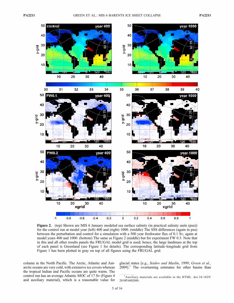
column in the North Pacific. The Arctic, Atlantic and Ant-arctic oceans are very cold, with extensive ice covers whereasthe tropical Indian and Pacific oceans are quite warm. Thecontrol run has an average Atlantic MOC of 17 Sv (Figure 4and auxiliary material), which is a reasonable value for

glacial states [e.g., Seidov and Maslin, 1999; Green et al.,2009].1 The overturning estimates for other basins than

Figure 2. (top) Shown are MIS 6 January modeled sea surface salinity (in practical salinity units (psu))for the control run at model year (left) 400 and (right) 1000. (middle) The SSS differences (again in psu)between the perturbation and control for a simulation with a 500 year freshwater flux of 0.1 Sv, again atmodel years 400 and 1000. (bottom) The same as Figure 2 (middle) but for experiment FW 0.3. Note thatin this and all other results panels the FRUGAL model grid is used; hence, the large landmass at the topof each panel is Greenland (see Figure 1 for details). The corresponding latitude‐longitude grid fromFigure 1 has been plotted in gray on top of all figures using the FRUGAL grid.

1Auxiliary materials are available in the HTML. doi:10.1029/2010PA002088.


5 of 16

the Atlantic are surprisingly energetic in the present controlrun. The Pacific MOC of 21 Sv exceeds that of the Atlantic(Figure 4), suggesting a state with a weakened Atlantic andan increased Pacific MOC. This is reflected in the surfacestream function (Figure 5), where we see a strong Pacificsubpolar gyre circulation but weak Atlantic gyres, andfurther highlighted in the transects of salinity and meridio-nal velocity (Figure 6).

[17] The MIS6 and LGM oceanic and states differ on afew significant points. Compared to the LGM, the NordicSeas are slightly fresher whereas the North Pacific is sig-nificantly saltier and slightly warmer during MIS 6, butthere are otherwise no major differences in SST [see, e.g.,Green et al., 2010]. The conveyor circulation is strongerduring MIS 6, including the Atlantic MOC [e.g., Seidov andMaslin, 1999; Green et al., 2009], but the latter is weakerthan the Present‐day circulation [Bigg et al., 1998; Green

Figure 3. (top) Shown are MIS 6 January modeled sea surface temperatures (in degrees Celsius) for thecontrol run at year (left) 400 and (right) 1000. (middle) The SST differences (in degrees Celsius), at years400 and 1000, between the perturbation and control for a simulation with a 500 year freshwater flux of0.1 Sv added. (bottom) The same as Figure 3 (middle) but for experiment FW 0.3.


6 of 16

Figure 4. (a) The modeled Atlantic Overturning (in sverdrups) during and after a 500 year freshwaterflux was added at the Barents Ice Sheet margin. Shown are results from both FW and ICE. Solid linesmark a flux of 0.3 Sv, whereas dotted lines denote results from the 0.1 Sv experiment. Note that the modelhas not reached equilibrium after 1500 years for all but FW 0.1 Sv (equilibrium reached after a further200 years). (b) As in Figure 4a but for the Pacific overturning. (c) The Atlantic overturning circulationduring the staggered pulse experiment where a freshwater pulse of 0.25 Sv applied over 500 years (darkgray line) is compared to the response when a freshwater pulse of 0.2 Sv is applied over 500 years andthen followed by one of 0.025 Sv being applied over 1500 years (lighter gray line). Note the different axisscales between Figures 4a, 4b, and 4c.


7 of 16

et al., 2009]. Furthermore, the strong Pacific MOC is notrecognized in investigations of previous time periods, andthe sum of the Atlantic and Pacific MOCs are nearly dou-bled compared to that simulated during the LGM [e.g.,Levine and Bigg, 2008]. These effects are present in theMIS 6 simulations despite the CO2 concentration, sea iceextent, sea level, and orbital configurations being onlymarginally altered. There are some (minor) differences inthe atmospheric variables between MIS 6 and the LGM (notshown), but a full climatic description of the MIS6, or acomparison of the MIS6‐LGM‐PD, is left for a future paper(C. L. Green et al., Comparison of the impacts of a BarentsIce Sheet collapse during MIS 6 and MIS 2, manuscript inpreparation, 2011). We can conclude, however, that the lackof major differences in SST or in the atmospheric forcingbetween the two periods and the previously mentionedNorth Pacific SSS maximum imply that the main reasonfor the response of the MOC in the perturbation experimentsare due to changes in the Pacific salinity transports [see also,e.g., Seidov and Haupt, 2005].

3.2. Freshwater Pulses

[18] Throughout the perturbation run there is a significantcooling and freshening in the equatorial Pacific, a cooling inthe Indian Ocean, and an increase in the Southern OceanSST, all of which persist long after the pulse has ended

(Figures 2 and 3). Figure 3 shows no cooling in the Arctic orNorth Atlantic because they are ice covered in Figure 3since we have chosen to show a winter situation to high-light the other changes which are most prominent duringboreal winter. During northern summers the previouslyreported North Atlantic cooling does take place [e.g., Stoufferet al., 2006], but is not shown here to save space (althoughthe main perturbations seen persist during summer as well).Note that the freshwater perturbation in the Arctic Oceanvisible during the pulse has vanished at year 1000, that is,within 500 years from the end of (Figure 2). In the 0.3 Svsimulation an initial weak reduction in SSS and SST ispresent in the northeast Pacific, but with an increase of bothSST and SSS postpulse (Figures 2 and 3; again we focus onNorthern Hemisphere winter conditions). The rest of theglobal ocean experiences long‐term decreases of SST in thisexperiment, but the salinity effects are mainly confined tothe northeast Pacific. The corresponding long‐term increasein temperature (Figure 3) is associated with an increase in airtemperature of more than 8°C in the atmosphere over thePacific and an even larger decrease in air temperature inthe North Atlantic (not shown).[19] The impact on the Atlantic MOC during the MIS 6

shows a reduction in strength during the freshwater surgesbut it recovers to almost original strength for the 0.1 Sv FWexperiment (Figure 4; note the difference between the

Figure 5. Surface stream functions at year (right) 400 and (left) 1000 for the (top) control, (middle) FW0.3, and (bottom) ICE 0.3. The streamline interval is 10 m2 s−1.


8 of 16

responses to FW and ICE (to be discussed in section 3.3)).In the 0.3 Sv FW experiment the MOC does not recoverat the end of the perturbation, and the change in the equa-torial Pacific upwelling seen in the 0.1 Sv case is not aspronounced. From the stream function (Figure 5) we cansee that the North Atlantic subpolar gyre has weakeneddramatically, whereas the subtropical North Atlantic isstrengthened compared to the control to accommodate theincreased volume flow due to the flushed freshwater (whichat this point is mixed into the ocean surface layer). ThePacific gyres are only slightly stronger than during thecontrol (approaching 100 m2 s−1), but their horizontalstructure is more regular.[20] The changes seen in the MOC for the 0.3 Sv case

correspond to the changes in the ocean SST, which in turn islinked to a switch in large‐scale conveyor from the NorthAtlantic to the North Pacific. However, whether the increasein SST (and air temperature and humidity) in the Pacific isinitially a cause or effect of the overturning switch isunclear. Other experiments show that the switch betweenwarming and cooling occurs just before fluxes of 0.15 Sv.Thus, freshwater surges of 0.15 Sv or greater, which arewithin the predicted estimates of fluxes from the Barents Ice

Sheet collapse, lead to a significant alteration in the globaloverturning circulation, with the overturning reducing in theNorth Atlantic Ocean and increasing in the North PacificOcean. This is not the case for the LGM [e.g., Green et al.,2009], which means the switch must be related to the MIS 6forcing; this is discussed further in section 4. The warmingof the upper ocean to the west of North America accom-panies a significant increase of nearly 10 Sv in the PacificOverturning during the simulation by year 1000 (Figure 4),and there are also increased volume transports in both thePacific subpolar and subtropical gyres (see auxiliarymaterial). The general overturning in the Southern Hemi-sphere increases whereas it decreases in the NorthernHemisphere (and the main formation site for the NorthernHemisphere is thus the North Pacific). This is a typicalbipolar seesaw effect, in which cooling in the NorthernHemisphere is balanced by warming in the SouthernHemisphere [e.g., Caillon et al., 2003; Dokken andNisancioglu, 2004]. The cause for the reduction in NorthAtlantic overturning in these MIS 6 FW experiments is thatthe freshwater from the Barents Ice Sheet collapse formsa cap over the North Atlantic (see the SSS in Figure 2),leading to a reduction in NADW formation, which is com-

Figure 6. (a) The salinity (in psu) and (b) meridional velocity (in centimeters per second) at year 400 ofthe control simulation for a meridional transect through the Atlantic (x grid row 25). (c and d) Salinity andvelocity but along x grid 7 (i.e., through the Pacific). See also Figures 10 and 11, and note that theFRUGAL grid is again used (thus, Greenland is on the very right of each panel). The x axis shows modely grid, with the corresponding latitudes plotted above the axis.


9 of 16

pensated for by the overturning in the Pacific Ocean. Thereare indications from both models and observations that theNorth Pacific MOC behave inversely to the North AtlanticMOC, with the latter increasing when conditions support amore globally distributed pattern of the conveyor circulation(see, e.g., Rahmstorf [2002], de Boer et al. [2008], andOkumura et al. [2009] for (LGM) modeling references orBrunelle et al. [2010] for MIS6 observational evidence).This is supported by cross sections of salinity and meridionalvelocity through the Atlantic (Figure 10) after 400 years ofa 0.3 Sv freshwater pulse. These show a significantly fresherupper ocean than for the control and the anomalous merid-ional surface velocity is stronger southward, with a strongernorthward component beneath it.[21] To identify the impact of having a more staggered

collapse of the Barents Ice Sheet a simulation was run with0.2 Sv of freshwater pulse being added at the location ofthe Barents Ice Sheet for 500 years, followed by a flux of0.025 Sv for a further 1000 years. The simulation was thencontinued for another 1000 years with no freshwater per-turbation. The results are compared to a 500 year flux of0.25 Sv (which has a response similar to that of the 0.3 Svcase and is thus not shown), since the same overall amountof freshwater is added during experiments. The longer,stepped simulation had less impact on the Atlantic over-turning strength between model years 0–1400 but thenshowed a higher than original overturning flux at the end of

the perturbation (Figure 4). Together with the reducedAtlantic overturning this implies a switch from a state wheredeepwater is formed in the Atlantic to one where the Pacificdominates. The long‐term impact is thus greater than the500 year pulse simulation and again stresses the importanceof knowing the duration of ice sheet collapse in order todetermine its impact on the ocean. During the second stage,the very weak flux being added is not enough to preventdeepwater formation but it does increase the circulatingvolume in the overturning system and it allows for com-pensation within the MOC to reach the prepulse equilib-rium. This is not seen in the 0.3 Sv experiment, which entersa new stable equilibrium state, nor in the reduced fluxexperiments (e.g., 0.1 Sv). In the latter case this is sobecause the overall perturbation induced is weaker in termsof stratification, although sufficient to hamper deepwaterformation (just as during the first part of the staggeredrelease experiment).

3.3. Iceberg Seeding

[22] An iceberg seeding surge equivalent to 0.1 or 0.3 Sv offreshwater results in a significantly reduced SSS in the sub-polar Atlantic during the 0.1 Sv flux experiments (Figure 7),which is different to the results from the FW experiment,where only changes of this magnitude were observed forfluxes equal to and greater than 0.15 Sv. The long‐termresponse of the ocean is thus more sensitive to iceberg

Figure 7. As in Figure 2 (but without the control run) but for experiments (top) ICE 0.1 and (bottom)ICE 0.3.


10 of 16

inputs than freshwater fluxes, whereas the freshwater pulsesgenerally have a larger immediate effect (see Green et al.[2010] for details, including a description of the iceberg tra-jectories). In the ICE experiments, increases in SST of up to5°C in the North Pacific occur by year 400 for both the 0.1 Svand 0.3 Sv additions (Figure 8). Again this is an impact of theincreased overturning in the Pacific Ocean which bringswarm waters to the region.[23] There is a reduction of 80% for ICE 0.1 and 75% for

ICE 0.3 of the Atlantic overturning strength (Figure 4).Similar changes in major transports and stream functions tothose from FW again reflect the changes in pattern of theglobal overturning circulation during the ICE experiments(Figure 5). In fact, the stream function for ICE 0.3 is verysimilar to that of FW 0.3. The increase in the Pacificoverturning observed during the iceberg trajectory experi-ment involving an iceberg flux of 0.3 Sv (Figure 4) is of asimilar scale to the equivalent freshwater surge experiment,although the long‐term increase in overturning strength is ofa lower magnitude. The strength of the Pacific overturningat year 1000 is 22 Sv for both runs, some 12 Sv higher thanin the control and 2 Sv higher than for the equivalent FWexperiments. Note that the overturning and gyres have notreached full equilibrium at year 1500, but a trial run showedthat this happens within 200 years and is not pursued fur-ther. The result indicates a significantly increased recoverytime in the ICE experiments [see Green et al., 2010].

[24] These effects are forced by the gradual melting of theicebergs and the subsequent release of the freshwater over alarger area than in the FW experiments (Figure 9) [Greenet al., 2010]. This leads to a more pronounced long‐termeffect in the ICE simulations. The lifetime of the largestbergs is about 20 years and some bergs have then traversedthe entire Arctic and will be close to Iceland. In practice,iceberg releases thus have a similar effect to what could beexpected from smaller freshwater releases from multiplelocations.[25] The transects exhibit somewhat reduced changes

compared to the equivalent FW (Figures 10c and 10d; seealso Figure 6), and in ICE 0.3 the salinity increase in thePacific is confined to the surface rather than extendingthroughout the deep water (Figures 11c and 11d). TheBeaufort Sea/Bering Strait area (y grid 35) is significantlyfresher in the FW run compared to the control, whereas theanomaly in ICE is almost negligible. This implies thatfreshwater accumulates in the area, but cannot exit to thePacific since the Bering Strait is closed. Icebergs, however,do not enter this part if seeded from the Barents Ice Sheet(see Figure 9) [Green et al., 2010] and instead exit throughthe Fram Strait into the northern North Atlantic as they driftwith the currents and only have a minor effect on thedynamics. A freshwater pulse, on the other hand, can alterthe upper ocean dynamics and may spread over the entirebasin.

Figure 8. The SST for the ICE experiments, with (top) ICE 0.1 and (bottom) ICE 0.3. Note that theextreme values are off‐scale (see text), but we have not distorted the scale shown so as to give the clearestview of the anomalies.


11 of 16

[26] The different freshwater content in the Arcticbetween the runs is also associated with an alteration of thesea surface height in the region (Figure 9, right). This showsthe expected result with a larger sea surface gradient fromthe Barents Ice Sheet toward the North Atlantic in the 0.3 Svcompared to the 0.1 Sv simulations. This is hardly surpris-ing, and more interesting is the larger sea surface elevationin the gyres in the Pacific during ICE 0.1 compared to ICE0.3. This response is the opposite of that in the Atlantic,where the elevation is proportional to the freshwater flux.This explains the modified gyre circulations in the runs, andit is very likely that the response of the Atlantic gyres is dueto them absorbing the freshwater volumes. This explains thefate of the freshwater: it is absorbed into the (wind‐driven)large‐scale upper ocean circulation or evaporating to theatmosphere (not shown, but there are significant changes inhumidity over the North Atlantic). The freshwater content inthe water column is on the order of tens of meters whichwhen mixed over the upper km or so will only provideminor changes in the SSS [see also Green and Bigg, 2011].

3.4. Summary

[27] The different methods for simulating the collapse ofthe ice sheet provide different results, with a freshwatersurge (experiments FW) producing a larger impact thanexplicit icebergs on the MOC. The lifespan of the largesticeberg is on the order of 20 years, and this gradual meltingand addition of freshwater over a larger area explains thedifferent responses. Ice sheet collapses are often simulatedas freshwater surges [e.g., Stouffer et al., 2007; Green et al.,

2009], which thus may overestimate the short‐term impactthat the collapses have on the MOC and the climate. Interms of the upper ocean circulation, the stream functionsare roughly similar between the two perturbation experi-ments but very different to the control (Figure 5). Further-more, even 500 years after the pulse has ended the patternsremain although with slightly different structures.

4. Discussion

[28] A mass input of freshwater from the collapse of theMIS 6 Barents Ice Sheet is modeled to have an immediateeffect of reducing the salinity of the surrounding surfacewaters. The freshwater spreads through the Arctic Oceanand some of the pulse moves through the Fram Strait intothe North Atlantic, where the northern arm of the meridionaloverturning circulation previously formed NADW. Thesubsequent reduction in salinity leads to increased stabilityof the upper layers, which prevents convection and deep-water formation. Even small volumes of added freshwater(0.05 Sv, not shown) at the Barents Ice Sheet cause a weakreduction in Atlantic Overturning, and larger freshwaterpulses of course have greater impacts. The reduced over-turning strength leads to reduced heat transport to the ArcticOcean and North Atlantic, resulting in a reduction in SSTand leading to reductions in atmospheric temperature andhumidity (not shown). This connection between reducedproduction of NADW and cold temperatures has beenobserved in planktonic foraminiferal assemblages [Oppoand Lehman, 1995]. However, the postpulse Atlantic

Figure 9. (left) Iceberg meltwater heights (in meters; note the log scale in color) and (right) sea surfaceelevation (in centimeters from the undisturbed level) at the end of year 500 during (top) ICE 0.1 and(bottom) ICE 0.3.


12 of 16

MOC partially recovers to control strength. This is not thecase for the simulations with freshwater surges of 0.15 Sv orgreater, which are within the predicted estimates of fluxesfrom a collapsing MIS 6 Barents Ice Sheet [Bischof, 2000],and lead to a significant alteration of the meridional over-turning circulation strengths. The reason for the differentresponses is that smaller fluxes can be flushed out of thesystem more rapidly, and do not cause a significant alter-ation in the hydrography at the location of deep water for-mation. However, fluxes of 0.15 Sv or greater form afreshwater cap over large parts of the Arctic and NorthAtlantic, which significantly retards the formation ofNADW. The differences between 0.2 and 0.3 Sv, and 0.3and 0.5 Sv (0.2 and 0.5 Sv results are not shown) are rel-atively small. Inputs of 0.5 Sv are approaching unrealisti-cally large fluxes, whereas at the other end of the spectra afreshwater input of 0.05 Sv shows only minor impacts.Furthermore, a total collapse of the Atlantic MOC occurs forfluxes over 0.5 Sv in the present model; see also Bigg et al.[2010] and Green et al. [2009] for further discussionsrelated to other time periods. The duration of freshwateraddition is also an important component of simulating icesheet collapse. Adding the same total volume of freshwater

over a longer period has a smaller effect on Atlantic MOCduring the pulse, although the long‐term ability to recover isnot clear and may need further investigation.[29] Similar responses are found when the freshwater is

added to the Arctic in the form of icebergs instead of afreshwater pulse, although the freshwater surge has a greaterimpact on the Atlantic Overturning than the iceberg experi-ments during the time of input [see also Stouffer et al.,2007; Green et al., 2010]. The addition of freshwater tothe ocean as the icebergs melt is more gradual than thefreshwater surges, and since the cold temperatures of theArctic allow the icebergs to travel significant distances andadd meltwater over a larger area, the ocean is more able toadjust to the freshwater additions. It is thus probable thatsimulating an ice sheet collapse as a freshwater surgeoverestimates the impact that the collapse has on ocean andclimate. This is an important finding as ice sheet collapsesare often simulated as freshwater surges, which may over-estimate the impact that the collapses have on the MOC andclimate. For fluxes of 0.1 Sv a similar impact is observed onthe strength of the Atlantic Overturning during both thefreshwater surge and iceberg calving experiments, but forlarger fluxes the same flux results in less of an impact

Figure 10. Cross sections through the center of the Atlantic Ocean at year 400 (x grid 25; see Figure 6 aswell) showing the difference in (a) salinity (psu) and (b) meridional velocity (centimeters per second)between the FW 0.3 Sv experiment and the control (Figures 10a and 10b). (c and d) The difference insalinity and meridional velocity, but this time for experiment ICE 0.3 Sv minus control.


13 of 16

during the iceberg seeding simulations. As with the fresh-water surges, icebergs affect the physical properties of theupper ocean, particularly temperature, salinity and density.Consequently, accurately simulating the Arctic and NorthAtlantic Ocean currents and including collapsing ice sheetsin the correct form is of importance in any (paleo)climateinvestigation.[30] The location of MIS 6 deep water formation for both

types of freshwater releases switches from the NorthAtlantic to the North Pacific Ocean. This is in agreementwith a few other investigations, albeit for the LGM [e.g.,Mikolajewicz et al., 1997; Seidov and Haupt, 2005; Okazakiet al., 2010], and has been explained previously by thedependence of the MOC on the Atlantic‐Pacific salinitydifference [Seidov and Haupt, 2005; Stouffer et al., 2007]. Ithas also been shown that the response of the Atlantic MOCto freshwater inputs is not linear and depends on the meanclimate state [e.g., Swingedouw et al., 2009] and we findsimilar results here (although other models do give differentresponses [see, e.g., Okumura et al., 2009]). This goessomeway to explain the different long‐term effects after the

pulse has been removed. In the present investigation weobtain a prolonged collapse after removal of the pulse – aresult not found using FRUGAL in investigations of the PDor MIS 2 [e.g., Green et al., 2009; Bigg et al., 2010].[31] This raises two significant questions: can we trust

the model results, and why is the (modeled) response of theocean during MIS 6 significantly different to the LGM? Theproxy evidence from the MIS 6 supports our model resultswith regard to the large‐scale pattern. However, since this is(to our knowledge) the first modeling attempt of this form ofMIS 6, we can only assume that the model gives reasonableresults because it does so when set up for PD conditions(compared to direct observations) and for LGM/MIS 2conditions (compared to proxies); see the discussions byBigg et al. [2005] and Levine and Bigg [2008] for details.There may be an issue with the resolution of the NorthAtlantic being finer than in the Southern and Pacific Oceans,which may affect the deepwater formation ratio between theNorth Atlantic and Southern Ocean. It is thus likely that theNorth Atlantic MOC is overestimated and the SouthernOcean and Pacific MOC are underestimated, and there are

Figure 11. As in Figure 10 but for a transect through the central Pacific (x grid point 7; see alsoFigure 6).


14 of 16

plans to run a high‐resolution version of model to quantifythe effect of the resolution (if any). Nevertheless, this hasnot been a major issue in past FRUGAL simulations of thePD or LGM. Hopefully, similar experiments with othermodels will soon follow and allow for model‐model com-parisons. While there is some evidence for a catastrophicBarents Ice Sheet collapse during MIS 6 such as thatassumed here [Kristoffersen et al., 2004; Green et al., 2010]it remains to be seen whether further observational evidencewill support the switch of deep convection locations.[32] The answer to the second questions (why is the MIS

6 responding differently than the LGM/MIS2?) is lessobvious. One explanation is that the mean climate state isslightly different to the PD and MIS2, and this is known toaffect the response of the MOC to perturbations, but part ofthe answer lies within the control simulation. The controlMIS 6 Pacific overturning strength is similar to that of theAtlantic (Figure 4), and the Pacific is relatively salty at thesurface (Figure 2), promoting deep water formation there[Seidov and Haupt, 2005]. There is evidence, based onseawater d18O values, of a larger Pacific‐Atlantic surfacesalinity gradient during MIS 6 compared to the LGM[McManus et al., 1999; Lea et al., 2000], as well as supportfor a shallow thermocline and significant upwelling inthe MIS 6 western Pacific [Li et al., 2010]. Both theseobservations are compatible with the North Pacific beingmore susceptible to convection during MIS 6, and so areconsistent with the MIS 6 model results presented here.[33] The response of the ocean to a combined collapse of

the Barents and Laurentide ice sheets would most likely leadto a catastrophic shut down of the Atlantic MOC, as thesystem can barely deal with one of these pulses on its own.That said, when the pulses have been flushed out theAtlantic MOC recovers somewhat, and a more detailedinvestigation is left for future studies. The same is true for adetailed comparison of MIS 2 and 6 with PD conditions.

5. Conclusions

[34] Focus here has been on freshwater perturbations inthe Arctic Ocean during MIS 6, whereas focus previouslyhave been on additions from the Laurentide and Fennos-candian ice sheets during the LGM, mainly in the form ofmeltwater additions. As shown by Bigg et al. [2010], there issignificant variance in the response of the MOC due tolocation of the pulse, with freshwater additions to the Arcticinducing larger reductions of the Atlantic MOC than pulsesfrom the other ice sheets. Here, it is also verified that sim-ulating the collapse as icebergs, which is the probablemechanism from the Barents Ice Sheet [Kristoffersen et al.,2004], gives a different response to simulations with melt-water pulses, which is probably most accurate for simulat-ing, for example, the Laurentide during the Younger Dryas.The Atlantic MOC in the MIS 6 state also seems to be lesssensitive to freshwater pulses (in the Arctic) than MIS 2 andthe reason for this is under investigation. These resultshighlight the importance of simulating not only the correctflux but also the form of the freshwater input from icesheet collapses appropriately, regardless of which area ortime period is under investigation. The model also producesresults supporting MIS 6 proxies with a more saline Pacific,which aids in setting up a dominating Pacific MOC. This

suggests that periods with a weakened Atlantic‐Pacificsalinity gradient may experience a different MOC pattern.

[35] Acknowledgments. Funding was provided by the British NaturalEnvironmental Research Council through grants NERC/S/R/2005/13953(e‐science studentship to C.L.G. through G.R.B.) and NE/F014821/1(Advanced Fellowship for J.A.M.G.). J.A.M.G. also acknowledges fundingfrom the Climate Change Consortium for Wales (C3W). The manuscriptwas greatly improved by comments from the editor (Rainer Zahn) andfrom three reviewers (Igor Polyakov and two anonymous reviewers).

ReferencesAlley, R. B. (1998), Icing the North Atlantic, Nature, 392, 335–337,doi:10.1038/32781.

Berger, A., and M. F. Loutre (1992), Astronomical solutions for paleocli-mate studies over the last 3 million years, Earth Planet. Sci. Lett., 111,369–382, doi:10.1016/0012-821X(92)90190-7.

Bigg, G. R., and M. R. Wadley (2001), Millennial‐scale variability in theoceans: An ocean modeling view, J. Quat. Sci., 16, 309–319,doi:10.1002/jqs.599.

Bigg, G. R., M. R. Wadley, D. P. Stevens, and J. A. Johnson (1997), Mod-eling the dynamics and thermodynamics of icebergs, Cold Reg. Sci.Technol., 26, 113–135, doi:10.1016/S0165-232X(97)00012-8.

Bigg, G. R., M. R. Wadley, D. P. Stevens, and J. A. Johnson (1998), Simu-lations of two last glacial maximum ocean states, Paleoceanography, 13,340–351, doi:10.1029/98PA00402.

Bigg, G. R., S. R. Dye, and M. R. Wadley (2005), Interannual variability inthe 1990s in the northern Atlantic and Nordic Seas, J. Atmos. Ocean Sci.,10, 123–143, doi:10.1080/17417530500282873.

Bigg, G. R., R. C. Levine, and C. L. Green (2010), Modeling abrupt glacialNorth Atlantic freshening: Rates of change and their implications forHeinrich events,Global Planet. Change, in press, doi:10.1016/j.gloplacha.2010.11.001.

Bischof, J. (1994), The decay of the Barents Ice Sheet as documented inNordic seas ice‐rafted debris, Mar. Geol., 117, 35–55, doi:10.1016/0025-3227(94)90005-1.

Bischof, J. (2000), Ice Drift, Ocean Circulation, and Climate Change,215 pp., Springer, Heidelberg, Germany.

Broecker, W. S., and G. H. Denton (1990), What drives glacial cycles, Sci.Am., 262, 48–56, doi:10.1038/scientificamerican0190-48.

Brunelle, B. G., D. M. Sigman, S. L. Jaccard, L. D. Keigwin, B. Plessen,G. Schettler, M. S. Cook, and G. H. Haug (2010), Glacial/interglacialchanges in nutrient supply and stratification in the western subarcticNorth Pacific since the penultimate glacial maximum, Quat. Sci. Rev.,29, 2579–2590, doi:10.1016/j.quascirev.2010.03.010.

Caillon, N., J. Jouzel, J. P. Severinghaus, J. Chappellaz, and T. Blunier(2003), A novel method to study the phase relationship between Antarc-tic and Greenland climate, Geophys. Res. Lett., 30(17), 1899,doi:10.1029/2003GL017838.

de Boer, A. M., J. R. Toggweiler, and D. M. Sigman (2008), Atlantic dom-inance of the meridional overturning circulation, J. Phys. Oceanogr., 38,435–450, doi:10.1175/2007JPO3731.1.

Dokken, T. M., and K. H. Nisancioglu (2004), Fresh angle on the polarseesaw, Nature, 430, 842–843, doi:10.1038/430842a.

Dowdeswell, J. A., R. J. Whittington, and R. Hodgkins (1992), The sizes,frequencies, and freeboards of East Greenland icebergs observed usingship radar and sextant, J. Geophys. Res., 97, 3515–3528, doi:10.1029/91JC02821.

Dowdeswell, J. A., H. Villinger, R. J. Whittington, and P. Marienfeld(1993), Iceberg scouring in Scoresby Sund and on the East Greenlandcontinental shelf, Mar. Geol., 111, 37–53, doi:10.1016/0025-3227(93)90187-Z.

Fanning, A. F., andA. J.Weaver (1996), An atmospheric energy‐moisture bal-ance model: Climatology, interpentadal climate change, and coupling to anocean general circulation model, J. Geophys. Res., 101, 15,111–15,128,doi:10.1029/96JD01017.

Gladstone, R. M., G. R. Bigg, and K. W. Nicholls (2001), Iceberg trajec-tory modeling and meltwater injection in the Southern Ocean, J. Geo-phys. Res., 106, 19,903–19,915, doi:10.1029/2000JC000347.

Green, J. A. M., and G. R. Bigg (2011), Impacts on the global ocean cir-culation from vertical mixing and a collapsing ice sheet, J. Mar. Res.,in press.

Green, J. A. M., C. L. Green, G. R. Bigg, T. P. Rippeth, J. D. Scourse, andK. Uehara (2009), Tidal mixing and the Meridional Overturning Circula-tion from the Last Glacial Maximum, Geophys. Res. Lett., 36, L15603,doi:10.1029/2009GL039309.


15 of 16

Green, C. L., G. R. Bigg, and J. A. M. Green (2010), Deep draft icebergsfrom the Barents Ice Sheet during MIS 6 are consistent with erosionalevidence from the Lomonosov Ridge, central Arctic, Geophys. Res. Lett.,37, L23606, doi:10.1029/2010GL045299.

Griffiths, S. D., and W. R. Peltier (2009), Modeling of global ocean tides atLast Glacial Maximum: Amplification, sensitivity, and climatologicalimplications, J. Clim., 22, 2905–2924, doi:10.1175/2008JCLI2540.1.

Grosswald, M. G., and T. J. Hughes (2002), The Russian component of anArctic Ice Sheet during the Last Glacial Maximum, Quat. Sci. Rev., 21,121–146, doi:10.1016/S0277-3791(01)00078-6.

Kristoffersen, Y., B. Coakley, W. Jokat, M. Edwards, H. Brekke, andJ. Gjengedal (2004), Seabed erosion on the Lomonosov Ridge, centralArctic Ocean: A tale of deep draft icebergs in the Eurasia Basin andthe influence of Atlantic water inflow on iceberg motion?, Paleoceano-graphy, 19, PA3006, doi:10.1029/2003PA000985.

Kuijpers, A., and F. Werner (2007), Extremely deep‐draft iceberg scouringin the glacial North Atlantic Ocean, Geo‐Mar. Lett., 27, 383–389,doi:10.1007/s00367-007-0059-1.

Lea, D. W., D. K. Pak, and H. J. Spero (2000), Climate impact of lateQuaternary Equatorial Pacific sea surface temperature, Science, 289,1719–1724, doi:10.1126/science.289.5485.1719.

Lenderink, G., and R. J. Haarsma (1994), Variability and multiple equilib-ria of the thermohaline circulation, associated with deep water formation,J. Phys. Oceanogr., 24, 1480–1493, doi:10.1175/1520-0485(1994)024<1480:VAMEOT>2.0.CO;2.

Levine, R. C., and G. R. Bigg (2008), Sensitivity of the glacial ocean toHeinrich events from different iceberg sources, as modeled by a coupleatmosphere‐iceberg‐ocean model, Paleoceanography, 23, PA4213,doi:10.1029/2008PA001613.

Li, T., J. Zhao, R. Sun, F. Chang, and H. Sun (2010), The variation ofupper ocean structure and paleoproductivity in the Kurioshio sourceregion during the last 200 kyr, Mar. Micropaleontol., 75, 50–61,doi:10.1016/j.marmicro.2010.02.005.

Lubinski, D. J., S. Korsun, L. Polyak, S. L. Forman, S. J. Lehman, F. A.Herlihy, and G. H. Miller (1996), The last deglaciation of the Franz Vic-toria Trough, northern Barents Sea, Boreas, 25, 89–100, doi:10.1111/j.1502-3885.1996.tb00838.x.

MacAyeal, D. R. (1993), Binge/purge oscillations of the Laurentide Ice‐sheet as a cause of the North‐Atlantics Heinrich events, Paleoceanogra-phy, 8, 775–784, doi:10.1029/93PA02200.

Mangerud, J., T. Dokken, D. Hebbeln, B. Heggen, O. Ingolfsson, J. Y.Landvik, V. Mejdahl, J. I. Svendsen, and T. O. Vorren (1998), Fluctua-tions of the Svalbard–Barents Sea ice sheet during the last 150 000 years,Quat. Sci. Rev., 17, 11–42, doi:10.1016/S0277-3791(97)00069-3.

McManus, J. F., D. W. Oppo, and J. L. Cullen (1999), A 0.5‐million‐yearrecord of millennial‐scale climate variability in the North Atlantic, Sci-ence, 283, 971–975, doi:10.1126/science.283.5404.971.

Metz, J. M., J. A. Dowdeswell, and C. M. T. Woodworth‐Lynas (2008),Sea‐floor scour at the mouth of Hudson Strait by deep‐keeled icebergsfrom the Laurentide Ice Sheet, Mar. Geol., 253, 149–159, doi:10.1016/j.margeo.2008.05.004.

Mikolajewicz, U., T. J. Crowley, A. Schiller, and R. Voss (1997), Model-ing teleconnections between the North Atlantic and North Pacific duringthe Younger Dryas, Nature, 387, 384–387, doi:10.1038/387384a0.

Mix, A., and W. F. Ruddiman (1984), Oxygen‐isotope analyses and Pleis-tocene ice volumes, Quat. Res., 21, 1–20, doi:10.1016/0033-5894(84)90085-1.

Morgan, V. I., and W. F. Budd (1978), The distribution, movement and meltrates of Antarctic icebergs, in Iceberg Utilization: Proceedings of the FirstInternational Conference and Workshops on Iceberg Utilization for FreshWater Production, Weather Modification, and Other Applications, editedby A. A. Husseiny, pp. 220–228, Iowa State Univ., Ames.

Okazaki, Y., A. Timmermann, L. Menviel, N. Harada, A. Abe‐Ouchi,M. O. Chikamoto, A. Mouchet, and H. Asahi (2010), Deepwater forma-tion in the North Pacific during the Last Glacial Termination, Science,329, 200–204, doi:10.1126/science.1190612.

Okumura, Y. M., C. Deser, A. Hu, A. Timmermann, and S.‐P. Xie (2009),North Pacific climate response to freshwater forcing in the subarcticNorth Atlantic: Oceanic and atmospheric pathways, J. Clim., 22,1424–1445, doi:10.1175/2008JCLI2511.1.

Oppo, D. W., and S. J. Lehman (1995), Suborbital timescale variability ofNorth Atlantic Deep Water during the past 200,000 years, Paleoceano-graphy, 10, 901–910, doi:10.1029/95PA02089.

Orheim, O. (1980), Icebergs in the Southern Ocean, Ann. Glaciol., 9,241–242.

Parkinson, C. L., and W. M. Washington (1979), A large‐scale numericalmodel of sea‐ice, J. Geophys. Res., 84, 311–337, doi:10.1029/JC084iC01p00311.

Peltier, W. (2004), Global glacial isostacy and the surface if the ice‐ageearth: The ICE‐5G (VM2) model and Grace, Annu. Rev. Earth Planet.Sci., 32, 111–149, doi:10.1146/annurev.earth.32.082503.144359.

Petit, J. R., et al. (1999), Climate and atmospheric history of the past 420,000years from the Vostok ice core, Antarctica, Nature, 399, 429–436,doi:10.1038/20859.

Polyak, L., S. L. Forman, F. A. Herlihy, G. Ivanov, and P. Krinitsky(1997), Late Weichselian deglaciation history of Svyataya (Saint) AnnaTrough, Northern Kara Sea, Arctic Russia, Mar. Geol., 143, 169–188,doi:10.1016/S0025-3227(97)00096-0.

Polyak, L., M. Levitan, T. Khusid, L. Merklin, and V. Mukhina (2002), Var-iations in the influence of riverine discharge on the Kara Sea during the lastdeglaciation and the Holocene, Global Planet. Change, 32, 291–309,doi:10.1016/S0921-8181(02)00072-3.

Rabineau, M., S. Berne, J. L. Olivet, D. Aslanian, F. Guillocheau, andP. Joseph (2006), Paleo sea levels reconsidered from direct observation ofpaleoshoreline position during Glacial Maxima (for the last 500,000 yr),Earth Planet. Sci. Lett., 252, 119–137, doi:10.1016/j.epsl.2006.09.033.

Rahmstorf, S. (2002), Ocean circulation and climate during the past120,000 years, Nature, 419, 207–214, doi:10.1038/nature01090.

Raynaud, D., J. Jouzel, J. M. Barnola, J. Chappellaz, R. J. Delmas, andC. Lorius (1993), The ice record of greenhouse gases, Science, 259, 926–934.

Rohling, E. J., M. Fenton, F. J. Jorissen, P. Bertrand, G. Ganssen, andJ. P. Caulet (1998), Magnitudes of sea‐level lowstands of the past500,000 years, Nature, 394, 162–165, doi:10.1038/28134.

Seidov, D., and B. J. Haupt (2005), How to run a minimalist’s global oceanconveyor, Geophys. Res. Lett., 32, L07610, doi:10.1029/2005GL022559.

Seidov, D., and M. Maslin (1999), North Atlantic deep water circulationcollapse during Heinrich events, Geology, 27, 23–26, doi:10.1130/0091-7613(1999)027<0023:NADWCC>2.3.CO;2.

Siegenthaler, U., et al. (2005), Stable carbon cycle‐climate relationshipduring the late Pleistocene, Science, 310, 1313–1317, doi:10.1126/science.1120130.

Siegert, M. J., and J. A. Dowdeswell (2002), Late Weichselian iceberg,surface‐melt and sediment production from the Eurasian Ice Sheet: Resultsfrom numerical ice‐sheet modeling, Mar. Geol., 188, 109–127, doi:10.1016/S0025-3227(02)00277-3.

Spielhagen, R., K.‐H. Baumann, H. Erlenkeuser, R. Nowaczyk,N. Nørgaard‐Pedersen, C. Vogt, and D. Weiel (2004), Arctic Oceandeep‐sea record of northern Eurasian ice sheet history, Quat. Sci. Rev.,23, 1455–1483, doi:10.1016/j.quascirev.2003.12.015.

Stouffer, R. J., et al. (2006), Investigating the causes of the response of thethermohaline circulation to past and future climate changes, J. Clim., 19,1365–1387, doi:10.1175/JCLI3689.1

Stouffer, R. J., D. Seidov, and B. J. Haupt (2007), Climate response toexternal sources of freshwater: North Atlantic versus the Southern Ocean,J. Clim., 20, 436–448, doi:10.1175/JCLI4015.1.

Svendsen, J. I., et al. (2004), Late Quaternary ice sheet history of northern Eur-asia,Quat. Sci. Rev., 23, 1229–1271, doi:10.1016/j.quascirev.2003.12.008.

Swingedouw, D., J. Mignot, P. Braconnot, E. Mosquet, M. Kageyama, andR. Alkama (2009), Impact of freshwater release in the North Atlantic underdifferent climate conditions in an OAGCM, J. Clim., 22, 6377–6403,doi:10.1175/2009JCLI3028.1.

Syvitski, J. P. M., A. B. Stein, and J. T. Andrews (2001), Icebergs and thesea floor of the East Greenland (Kangerlusuaq) continental margin, Arct.Antarct. Alp. Res., 33, 52–61, doi:10.2307/1552277.

Thompson, S. R. (1995), Sills of the global ocean: A compilation, OceanModell., 109, 7–9.

Wadley, M. R., and G. R. Bigg (1999), Implementation of variabletime stepping in an ocean general circulation model, Ocean Modell., 1,71–80, doi:10.1016/S1463-5003(99)00011-6.

Wadley, M. R., and G. R. Bigg (2002), Impact of flow through the Cana-dian Archipelago and Bering Strait on the North Atlantic and Arcticcirculation: An ocean modeling study, Q. J. R. Meteorol. Soc., 128,2187–2203, doi:10.1256/qj.00.35.

Wunsch, C., and R. Ferrari (2004), Vertical mixing, energy, and the generalcirculation of the oceans, Annu. Rev. Fluid Mech., 36, 281–314,doi:10.1146/annurev.fluid.36.050802.122121.

Zhang, R., and T. L. Delworth (2005), Simulated tropical response to a sub-stantial weakening of the Atlantic thermohaline circulation, J. Clim., 18,1853–1860, doi:10.1175/JCLI3460.1.

G. R. Bigg and C. L. Green, Department of Geography, University ofSheffield, Sheffield, S10 2TN, UK.J. A. M. Green, School of Ocean Sciences, College of Natural Sciences,

Bangor University,Menai Bridge, LL59 5AB, UK. ([email protected])


16 of 16

Simulating the impact of freshwater inputs and deep-draft icebergs formed during a MIS 6 Barents Ice...

Documents

Transcript of Simulating the impact of freshwater inputs and deep-draft icebergs formed during a MIS 6 Barents Ice...