Simulating reachability using first-order logic with applications to verification of linked data...
30
Logical Methods in Computer Science Vol. 5 (2:12) 2009, pp. 1–30 www.lmcs-online.org Submitted Apr. 2, 2006 Published May 28, 2009 SIMULATING REACHABILITY USING FIRST-ORDER LOGIC WITH APPLICATIONS TO VERIFICATION OF LINKED DATA STRUCTURES ∗ TAL LEV-AMI a , NEIL IMMERMAN b , THOMAS W. REPS c , MOOLY SAGIV d , SIDDHARTH SRIVASTAVA e , AND GRETA YORSH f a,d,f School of Computer Science, Tel Aviv University e-mail address: [email protected], {msagiv,gretay}@post.tau.ac.il b,e Department of Computer Science, University of Massachusetts, Amherst e-mail address: {immerman,siddharth}@cs.umass.edu c Computer Science Department, University of Wisconsin, Madison e-mail address: [email protected] ABSTRACT. This paper shows how to harness existing theorem provers for first-order logic to au- tomatically verify safety properties of imperative programs that perform dynamic storage allocation and destructive updating of pointer-valued structure fields. One of the main obstacles is specifying and proving the (absence) of reachability properties among dynamically allocated cells. The main technical contributions are methods for simulating reachability in a conservative way using first-order formulas—the formulas describe a superset of the set of program states that would be specified if one had a precise way to express reachability. These methods are employed for semi- automatic program verification (i.e., using programmer-supplied loop invariants) on programs such as mark-and-sweep garbage collection and destructive reversal of a singly linked list. (The mark-and- sweep example has been previously reported as being beyond the capabilities of ESC/Java.) 1. I NTRODUCTION This paper explores how to harness existing theorem provers for first-order logic to prove reach- ability properties of programs that manipulate dynamically allocated data structures. The approach that we use involves simulating reachability in a conservative way using first-order formulas—i.e., the formulas describe a superset of the set of program states that would be specified if one had an accurate way to express reachability. 1998 ACM Subject Classification: F.3.1, F.4.1, F.3.2. Key words and phrases: First Order Logic, Transitive Closure, Approximation, Program Verification, Program Analysis. ∗ A preliminary version of this paper appeared in Automated Deduction - CADE-20, 20th International Conference on Automated Deduction, Tallinn, Estonia, July 22-27, 2005. a This research was supported by an Adams Fellowship through the Israel Academy of Sciences and Humanities. b,e Supported by NSF grants CCF-0514621,0541018,0830174. c Supported by ONR under contracts N00014-01-1-{0796,0708}. f Partially supported by the Israeli Academy of Science. LOGICAL METHODS IN COMPUTER SCIENCE DOI:10.2168/LMCS-5 (2:12) 2009 c T. Lev-Ami, N. Immerman, T. Reps, M. Sagiv, S. Srivastava, and G. Yorsh CC Creative Commons
Transcript of Simulating reachability using first-order logic with applications to verification of linked data...

Logical Methods in Computer ScienceVol. 5 (2:12) 2009, pp. 1–30www.lmcs-online.org
Submitted Apr. 2, 2006Published May 28, 2009
SIMULATING REACHABILITY USING FIRST-ORDER LOGIC WITHAPPLICATIONS TO VERIFICATION OF LINKED DATA STRUCTURES ∗
TAL LEV-AMI a, NEIL IMMERMAN b, THOMAS W. REPSc, MOOLY SAGIV d, SIDDHARTH SRIVASTAVAe,AND GRETA YORSHf
a,d,f School of Computer Science, Tel Aviv Universitye-mail address: [email protected],{msagiv,gretay}@post.tau.ac.il
b,e Department of Computer Science, University of Massachusetts, Amherste-mail address: {immerman,siddharth}@cs.umass.edu
c Computer Science Department, University of Wisconsin, Madisone-mail address: [email protected]
ABSTRACT. This paper shows how to harness existing theorem provers for first-order logic to au-tomatically verify safety properties of imperative programs that perform dynamic storage allocationand destructive updating of pointer-valued structure fields. One of the main obstacles is specifyingand proving the (absence) of reachability properties amongdynamically allocated cells.
The main technical contributions are methods for simulating reachability in a conservative wayusing first-order formulas—the formulas describe a superset of the set of program states that wouldbe specified if one had a precise way to express reachability.These methods are employed for semi-automatic program verification (i.e., using programmer-supplied loop invariants) on programs suchas mark-and-sweep garbage collection and destructive reversal of a singly linked list. (The mark-and-sweep example has been previously reported as being beyond the capabilities of ESC/Java.)
1. INTRODUCTION
This paper explores how to harness existing theorem proversfor first-order logic to prove reach-ability properties of programs that manipulate dynamically allocated data structures. The approachthat we use involves simulating reachability in a conservative way using first-order formulas—i.e.,the formulas describe a superset of the set of program statesthat would be specified if one had anaccurate way to express reachability.
1998 ACM Subject Classification:F.3.1, F.4.1, F.3.2.Key words and phrases:First Order Logic, Transitive Closure, Approximation, Program Verification, Program
Analysis.∗ A preliminary version of this paper appeared in Automated Deduction - CADE-20, 20th International Conference on
Automated Deduction, Tallinn, Estonia, July 22-27, 2005.a This research was supported by an Adams Fellowship through the Israel Academy of Sciences and Humanities.
b,e Supported by NSF grants CCF-0514621,0541018,0830174.c Supported by ONR under contracts N00014-01-1-{0796,0708}.f Partially supported by the Israeli Academy of Science.
LOGICAL METHODSlIN COMPUTER SCIENCE DOI:10.2168/LMCS-5 (2:12) 2009c© T. Lev-Ami, N. Immerman, T. Reps, M. Sagiv, S. Srivastava, and G. YorshCC© Creative Commons

2 T. LEV-AMI, N. IMMERMAN, T. REPS, M. SAGIV, S. SRIVASTAVA, AND G. YORSH
Automatically establishing safety and liveness properties of sequential and concurrent pro-grams that permit dynamic storage allocation and low-levelpointer manipulations is challenging.Dynamic allocation causes the state space to be infinite; moreover, a program is permitted to mutatea data structure by destructively updating pointer-valuedfields of nodes. These features remain evenif a programming language has good capabilities for data abstraction. Abstract-datatype operationsare implemented using loops, procedure calls, and sequences of low-level pointer manipulations;consequently, it is hard to prove that a data-structure invariant is reestablished once a sequence ofoperations is finished [Hoa75]. In languages such as Java, concurrency poses yet another challenge:establishing the absence of deadlock requires establishing the absence of any cycle of threads thatare waiting for locks held by other threads.
Reachability is crucial for reasoning about linked data structures. For instance, to establishthat a memory configuration contains no garbage elements, wemust show that every element isreachable from some program variable. Other cases where reachability is a useful notion include
• Specifying acyclicity of data-structure fragments, i.e.,from every element reachable from noden, one cannot reachn• Specifying the effect of procedure calls when references are passed as arguments: only elements
that are reachable from a formal parameter can be modified• Specifying the absence of deadlocks• Specifying safety conditions that allow establishing thata data-structure traversal terminates, e.g.,
there is a path from a node to a sink-node of the data structure.
The verification of such properties presents a challenge. Even simple decidable fragments of first-order logic become undecidable when reachability is added [GME99, IRR+04a]. Moreover, theutility of monadic second-order logic on trees is rather limited because (i) many programs allow non-tree data structures, (ii) expressing the postcondition ofa procedure (which is essential for modularreasoning) usually requires referring to the pre-state that holds before the procedure executes, andthus cannot, in general, be expressed in monadic second-order logic on trees—even for proceduresthat manipulate only singly-linked lists, such as the in-situ list-reversal program shown in Fig. 6,and (iii) the complexity is prohibitive.
While our work was actually motivated by our experience using abstract interpretation – and,in particular, the TVLA system [LAS00, SRW02, RSW04] – to establish properties of programsthat manipulate heap-allocated data structures, in this paper, we consider the problem of verifyingdata-structure operations, assuming that we have user-supplied loop invariants. This is similar tothe approach taken in systems like ESC/Java [FLL+02], and Pale [MS01].
The contributions of the paper can be summarized as follows:
Handling FO(TC) formulas using FO theorem provers. We want to use first-order theoremprovers and we need to discuss the transitive closure of certain binary predicates,f . However,first-order theorem provers cannot handle transitive closure. We solve this conundrum by addinga new relation symbolftc for each suchf , together with first-order axioms that assure thatftc isinterpreted correctly. The theoretical details of how thisis done are presented in Section 3. Thefact that we are able to handle transitive closure effectively and reasonably automatically is quitesurprising.
As explained in Section 3, the axioms that we add to control the behavior of the added predi-cates,ftc, must be sound but not necessarily complete. One way to thinkabout this is that we aresimulating a formula,χ, in which transitive closure occurs, with a pure first-orderformulaχ′. If ouraxioms are not complete then we are allowingχ′ to denote more stores thanχ does. The study ofmethods that are sound but potentially incomplete is motivated by the fact thatabstraction[CC77]

SIMULATING REACHABILITY USING FIRST-ORDER LOGIC 3
can be an aid in the verification of many properties. In terms of logic, abstraction corresponds tousing formulas that describe a superset of the set of programstates that can actually arise. A definiteanswer about whether a property always holds can sometimes be obtained even when informationhas been lost because of abstraction.
If χ′ is proven valid in FO thenχ is also valid in FO(TC); however, if we fail to prove thatχ′ isvalid, it is still possible thatχ is valid: the failure would be due to the incompleteness of the axioms,or the lack of time or space for the theorem prover to completethe proof.
As we will see in Section 3, it is easy to write a sound axiom,T1[f ], that is “complete” in thevery limited sense that every finite, acyclic model satisfyingT1[f ] must interpretftc as the reflexive,transitive closure of its interpretation off . However, in practice this is not worth much because, asis well-known, finiteness is not expressible in first-order logic. Thus, the properties that we want toprove do not follow fromT1[f ]. We do prove thatT1[f ] is complete for positive transitive-closureproperties (Proposition 3.2). The real difficulty lies in proving properties involving the negation offtc, i.e., that a certainf -path does not exist.
Induction axiom scheme. To solve the above problem, we add an induction axiom scheme.Although in general, there is no complete, recursively-enumerable axiomatization of transitive clo-sure (Proposition 4.1), we have found, on the practical side, that on the examples we have tried,T1
plus induction allows us to automatically prove all of our desired properties. On the theoretical side,we prove that our axiomatization is complete for word models(Theorem 4.8).
We think of the axioms that we use as aides for the first-order theorem prover that we employ(SPASS[WGR96]) to prove the properties in question. Rather than giving SPASSmany instances ofthe induction scheme, our experience is that it finds the proof faster if we give it several axioms thatare simpler to use than induction. As already mentioned, thehard part is to show that certain pathsdo not exist.
Coloring axiom schemes.In particular, we use three axiom schemes, having to do with par-titioning memory into a small set of colors. We call instances of these schemes “coloring axioms”.Our coloring axioms are simple, and areeasily proved using SPASS (in under ten seconds) fromthe induction axioms. For example, the first coloring axiom scheme,NoExit[A, f ], says that if nof -edges leave color class,A, then nof -paths leaveA. It turns out that theNoExit axiom schemeimplies – and thus is equivalent to – the induction scheme. However, we have found in practicethat explicitly adding other coloring axioms (which are consequences ofNoExit) enables SPASStoprove properties that it otherwise fails at.
We first assume that the programmer provides the colors by means of first-order formulas withtransitive closure. Our initial experience indicates thatthe generated coloring axioms are useful toSPASS. In particular, it provides the ability to verify programs like the mark phase of a mark-and-sweep garbage collector. This example has been previously reported as being beyond the capabilitiesof ESC/Java. TVLA also succeeds on this example; however ournew approach provides verificationmethods that can in some instances be more precise than TVLA.
Prototype implementation. Perhaps most exciting, we have implemented the heuristics forselecting colors and their corresponding axioms in a prototype using SPASS. We have used thisto automatically choose useful color axioms and then verifya series of small heap-manipulatingprograms. We believe that the detailed examples presented here give convincing evidence of thepromise of our methodology. Of course much further study is needed.
Strengthening Nelson’s results.Greg Nelson considered a set of axiom schemes for reasoningabout reachability in function graphs, i.e., graphs in which there is at most onef -edge leaving anynode [Nel83]. He left open the question of whether his axiom schemes were complete for function

4 T. LEV-AMI, N. IMMERMAN, T. REPS, M. SAGIV, S. SRIVASTAVA, AND G. YORSH
graphs. We show that Nelson’s axioms are provable fromT1 plus our induction axioms. We alsoshow that Nelson’s axioms are not complete: in fact, they do not imply NoExit.
Outline. The remainder of the paper is organized as follows: Section 2explains our notationand the setting; Section 3 fills in our formal framework, introduces the induction axiom scheme,and presents the coloring axiom schemes; Section 4 providesmore detail about TC-completenessincluding a description of Nelson’s axioms, a proof that they are not TC-complete for the functionalcase, and a proof that our axiomatization is TC-complete forwords; Section 5 presents our heuris-tics including the details of their successful use on a variety of examples; Section 6 describes theapplicability of our methodology, relating it to the reasoning done in the TVLA system; Section 7describes some related work; and Section 8 describes some conclusions and future directions.
2. PRELIMINARIES
This section defines the basic notations used in this paper and the setting.
2.1. Notation. Syntax: A relationalvocabulary τ = {p1, p2, . . . , pk} is a set of relation symbols,each of fixed arity. We use the lettersu, v, andw (possibly with numeric subscript) for first-ordervariables. We write first-order formulas overτ with quantifiers∀ and∃, logical connectives∧,∨,→, ↔, and¬, where atomic formulas include: equality,pi(v1, v2, . . . vai
), andTC[f ](v1, v2),wherepi ∈ τ is of arityai andf ∈ τ is binary. HereTC[f ](v1, v2) denotes the existence of a finitepath of 0 or moref edges fromv1 to v2. A formula withoutTC is called afirst-order formula.
We use the following precedence of logical operators:¬ has highest precedence, followed by∧ and∨, followed by→ and↔, and∀ and∃ have lowest precedence.
Semantics: A model,A, of vocabularyτ , consists of a non-empty universe,|A|, and a relationpA over the universe interpreting each relation symbolp ∈ τ . We writeA |= ϕ to mean that theformulaϕ is true in the modelA. ForΣ a set of formulas, we writeΣ |= ϕ (Σ semantically impliesϕ) to mean that all models ofΣ satisfyϕ.
2.2. Setting. We are primarily interested in formulas that arise while proving the correctness ofprograms. We assume that the programmer specifies pre and post-conditions for procedures andloop invariants using first-order formulas with transitiveclosure on binary relations. The transformerfor a loop body can be produced automatically from the program code.
For instance, to establish the partial correctness with respect to a user-supplied specification ofa program that contains a single loop, we need to establish three properties: First, the loop invariantmust hold at the beginning of the first iteration; i.e., we must show that the loop invariant followsfrom the precondition and the code leading to the loop. Second, the loop invariant provided by theuser must be maintained; i.e., we must show that if the loop invariant holds at the beginning of aniteration and the loop condition also holds, the transformer causes the loop invariant to hold at theend of the iteration. Finally, the postcondition must follow from the loop invariant and the conditionfor exiting the loop.
In general, these formulas are of the form
ψ1[τ ] ∧ Tr[τ, τ′]→ ψ2[τ
′]

SIMULATING REACHABILITY USING FIRST-ORDER LOGIC 5
whereτ is the vocabulary of the before state,τ ′ is the vocabulary of the after state,1 andTr isthe transformer, which may use both the before and after predicates to describe the meaning of themodule to be executed. If symbolf denotes the value of a predicate before the operation, thenf ′
denotes the value of the same predicate after the operation.An interesting special case is the proof of the maintenance formula of a loop invariant. This
has the form:LC[τ ] ∧ LI[τ ] ∧ Tr[τ, τ ′]→ LI[τ ′]
HereLC is the condition for entering the loop andLI is the loop invariant.LI[τ ′] indicates that theloop invariant remains true after the body of the loop is executed.
The challenge is that the formulas of interest contain transitive closure; thus, the validity ofthese formulas cannot be directly proven using a theorem prover for first-order logic.
3. AXIOMATIZATION OF TRANSITIVE CLOSURE
The original formula that we want to prove,χ, contains transitive closure, which first-ordertheorem provers cannot handle. To address this problem, we replaceχ by a new formula,χ′, whereall appearances ofTC[f ] have been replaced by the new binary relation symbol,ftc.
We show in this paper that fromχ′, we can often automatically generate an appropriate first-order axiom,σ, with the following two properties:
(1) if σ → χ′ is valid in FO, thenχ is valid in FO(TC).(2) A theorem prover successfully proves thatσ → χ′ is valid in FO.
We now explain the theory behind this process. ATC model,A, is a model such that iff andftc are in the vocabulary ofA, then(ftc)
A = (fA)⋆; i.e.,A interpretsftc as the reflexive, transitiveclosure of its interpretation off .
A first-order formulaϕ is TC valid iff it is true in all TC models. We say that an axiomatization,Σ, is TC sound if every formula that follows fromΣ is TC valid. Since first-order reasoning issound,Σ is TC sound iff everyσ ∈ Σ is TC valid.
We say thatΣ is TC complete if for every TC-validϕ, Σ |= ϕ. If Σ is TC complete and TCsound, then for all first-orderϕ,
Σ |= ϕ ⇔ ϕ is TC valid
Thus a TC-complete set of axioms proves exactly the first-order formulas,χ′, such that thecorresponding FO(TC) formula,χ, is valid.
All the axioms that we consider are TC valid. There is no recursively enumerable TC-completeaxiom system (Proposition 4.1). However, the axiomatization that we give does allow SPASS toprove all the desired properties on the examples that we havetried. We do prove that our axiomati-zation is TC complete for word models (Theorem 4.8).
1In some cases it is useful for the postcondition formula to refer to the original vocabulary as well. This way thepostcondition can summarize some of the behavior of the transformer, e.g., summarize the behavior of an entire procedure.

6 T. LEV-AMI, N. IMMERMAN, T. REPS, M. SAGIV, S. SRIVASTAVA, AND G. YORSH
3.1. Some TC-Sound Axioms.We begin with our first TC axiom scheme. For any binary relationsymbol,f , let,
T1[f ] ≡ ∀u, v . ftc(u, v) ↔ (u = v) ∨ ∃w . f(u,w) ∧ ftc(w, v)
We first observe thatT1[f ] is “complete” in a very limited way for finite, acyclic graphs, i.e.,T1[f ] exactly characterizes the meaning offtc for all finite, acyclic graphs. The reason that we saythis is limited is that it does not give us a complete set of first-order axioms: as is well known, thereis no first-order axiomatization of “finite”.
Proposition 3.1. Any finite and acyclic model ofT1[f ] is a TC model.
Proof. LetA |= T1[f ] whereA is finite and acyclic. Leta0, b ∈ |A|. Assume that there is anf -pathfrom a0 to b. SinceA |= T1[f ], it is easy to see thatA |= ftc(a0, b). Conversely, suppose thatA |= ftc(a0, b). If a0 = b, then there is a path of length 0 froma0 to b. Otherwise, byT1[f ], thereexists ana1 ∈ |A| such thatA |= f(a0, a1) ∧ ftc(a1, b). Note thata1 6= a0 sinceA is acyclic. Ifa1 = b then there is anf -path of length 1 froma to b. Otherwise there must exist ana2 ∈ |A| suchthatA |= f(a1, a2) ∧ ftc(a2, b) and so on, generating a set{a1, a2, . . .}. None of theai can beequal toaj , for j < i, by acyclicity. Thus, by finiteness, someai = b. HenceA is a TC model.
Let T ′1[f ] be the← direction ofT1[f ]:
T ′1[f ] ≡ ∀u, v . ftc(u, v) ← (u = v) ∨ ∃w . f(u,w) ∧ ftc(w, v)
Proposition 3.2. Letftc occur only positively inϕ. If ϕ is TC valid, thenT ′1[f ] |= ϕ.
Proof. Suppose thatT ′1[f ] 6|= ϕ. Let A |= T ′1[f ] ∧ ¬ϕ. Note thatftc occurs only negatively in¬ϕ. Furthermore, sinceA |= T ′1[f ], it is easy to show by induction on the length of the path, thatif there is anf -path froma to b in A, thenA |= ftc(a, b). DefineA′ to be the model formed fromA by interpretingftc in A′ as(fA)⋆. ThusA′ is a TC model and it only differs fromA by the factthat we have removed zero or more pairs from(ftc)
A to form (ftc)A′
. BecauseA |= ¬ϕ andftc
occurs only negatively in¬ϕ, it follows thatA′ |= ¬ϕ, which contradicts the assumption thatϕ isTC valid.
Proposition 3.2 shows that proving positive facts of the form ftc(u, v) is easy; it is the task ofproving that paths do not exist that is more subtle.
Proposition 3.1 shows that what we are missing, at least in the acyclic case, is that there is nofirst-order axiomatization of finiteness. Traditionally, when reasoning about the natural numbers,this problem is mitigated by adding induction axioms. We next introduce an induction scheme that,together withT1, seems to be sufficient to prove any property we need concerning TC.
Notation: In general, we will useF to denote the set of all binary relation symbols,f , suchthat TC[f ] occurs in a formula we are considering. Ifϕ[f ] is a formula in whichf occurs, letϕ[F ] =
∧f∈F ϕ[f ]. Thus, for example,T1[F ] is the conjunction of the axiomT1[f ] for all binary
relation symbols,f , under consideration.
Definition 3.3. For any first-order formulasZ(u), P (u), and binary relation symbol,f , let theinduction principle , IND [Z,P, f ], be the following first-order formula:
(∀w .Z(w)→ P (w)) ∧ (∀u, v . P (u) ∧ f(u, v)→ P (v))
→ ∀u,w .Z(w) ∧ ftc(w, u)→ P (u)
In order to explain the meaning ofIND and other axioms it is important to remember that weare trying to write axioms,Σ, that are,

SIMULATING REACHABILITY USING FIRST-ORDER LOGIC 7
• TC valid , i.e., true in all TC models, and• useful, i.e., all models ofΣ are sufficiently like TC models that they satisfy the TC-valid proper-
ties we want to prove.
To make the meaning of our axioms intuitively clear, in this section we will say, for example, that“y is ftc-reachable fromx” to mean thatftc(x, y) holds. Later, we will assume that the reader hasthe idea and just say “reachable” instead of “ftc-reachable”.
The intuitive meaning of the induction principle is that if every zero point satisfiesP , andPis preserved when followingf -edges, then every pointftc-reachable from a zero point satisfiesP .Obviously this principle is TC valid, i.e., it is true for allstructures such thatftc = f⋆.
As an easy application of the induction principle, considerthe following cousin ofT1[f ],
T2[f ] ≡ ∀u, v . ftc(u, v) ↔ (u = v) ∨ ∃w . ftc(u,w) ∧ f(w, v)
The difference betweenT1 andT2 is thatT1 requires that each path represented byftc starts withan f edge andT2 requires the path to end with anf edge. It is easy to see that neither ofT1[f ],T2[f ] implies the other. However, in the presence of the inductionprinciple they do imply eachother. For example, it is easy to proveT2[f ] from T1[f ] usingIND [Z,P, f ] whereZ(v) ≡ v = u
andP (v) ≡ u = v ∨ ∃w . ftc(u,w) ∧ f(w, v). Here, for eachu we useIND [Z,P, f ] to prove byinduction that everyv reachable fromu satisfies the right-hand side ofT2[f ].
Another useful axiom scheme provable fromT1 plus IND is the transitivity of reachability:
Trans[f ] ≡ ∀u, v,w . ftc(u,w) ∧ ftc(w, v)→ ftc(u, v)
3.2. Coloring Axioms. We next describe three TC-sound axioms schemes that are not implied byT1[F ] ∧ T2[F ], and are provable from the induction principle. We will see in the sequel that thesecoloring axioms are very useful in proving that paths do not exist, permitting us to verify a varietyof algorithms. In Section 5, we will present some heuristicsfor automatically choosing particularinstances of the coloring axiom schemes that enable us to prove our goal formulas.
The first coloring axiom scheme is the NoExit axiom scheme:
(∀u, v .A(u) ∧ ¬A(v)→ ¬f(u, v)) → ∀u, v .A(u) ∧ ¬A(v)→ ¬ftc(u, v)
for any first-order formulaA(u), and binary relation symbol,f , NoExit[A, f ] says that if nof -edgeleaves color classA, then no point outside ofA is ftc-reachable fromA.
Observe that although it is very simple,NoExit[A, f ] does not follow fromT1[f ] ∧ T2[f ].Let G1 = (V, f, ftc, A) be a model consisting of two disjoint cycles:V = {1, 2, 3, 4}, f ={〈1, 2〉, 〈2, 1〉, 〈3, 4〉, 〈4, 3〉}, andA = {1, 2}. Let ftc have all 16 possible pairs. ThusG1 sat-isfiesT1[f ] ∧ T2[f ] but violatesNoExit[A, f ]. Even for acyclic models,NoExit[A, f ] does notfollow from T1[f ] ∧ T2[f ] because there are infinite models in which the implication does not hold(Proposition 4.7).
NoExit[A, f ] follows easily from the induction principle: if nof -edges leaveA, then inductiontells us that everythingftc-reachable from a point inA satisfiesA. Similarly, NoExit[A, f ] impliesthe induction axiom,IND [Z,A, f ], for any formulaZ.
The second coloring axiom scheme is the GoOut axiom: for any first-order formulasA(u), B(u),and binary relation symbol,f , GoOut[A,B, f ] says that if the onlyf -edges leaving color classAare toB, then anyftc-path from a point inA to a point not inA must pass throughB.
(∀u, v .A(u) ∧ ¬A(v) ∧ f(u, v)→ B(v)) →∀u, v .A(u) ∧ ¬A(v) ∧ ftc(u, v) → ∃w .B(w) ∧ ftc(u,w) ∧ ftc(w, v)

8 T. LEV-AMI, N. IMMERMAN, T. REPS, M. SAGIV, S. SRIVASTAVA, AND G. YORSH
To see thatGoOut[A,B, f ] follows from the induction principle, assume that the onlyf -edges outof A enterB. For any fixedu in A, we prove by induction that any pointv ftc-reachable fromu iseither inA or has a predecessor,b in B, that isftc-reachable fromu.
The third coloring axiom scheme is theNewStart axiom, which is useful in the context ofdynamically changing graphs: for any first-order formulaA(u), and binary relation symbolsf andg, think off as the previous edge relation andg as the current edge relation.NewStart[A, f, g] saysthat if there are no new edges betweenA nodes, then any new path, i.e.,gtc but notftc, fromAmustleaveA to make its change:
(∀u, v .A(u) ∧A(v) ∧ g(u, v) → f(u, v)) →∀u, v . gtc(u, v) ∧ ¬ftc(u, v) → ∃w .¬A(w) ∧ gtc(u,w) ∧ gtc(w, v)
NewStart[A, f, g] follows from the induction principle by a proof that is similar to the proof ofGoOut[A,B, f ].
3.2.1. Linked Lists.The spirit behind our consideration of the coloring axioms is similar to thatfound in a paper of Greg Nelson’s in which he introduced a set of reachability axioms for a func-tional predicate,f , i.e., there is at most onef edge leaving any point [Nel83]. Nelson asked whetherhis axiom schemes are complete for the functional setting. We remark that Nelson’s axiom schemesare provable fromT1 plus our induction principle. However, Nelson’s axiom schemes are not com-plete: we constructed a functional graph that satisfies Nelson’s axioms but violatesNoExit[A, f ](Proposition 4.7).
At least one of Nelson’s axiom schemes seems orthogonal to our coloring axioms and maybe useful in certain proofs. Nelson’s fifth axiom scheme states that the points reachable from agiven point are linearly ordered. The soundness of the axiomscheme is due to the fact thatf isfunctional. We make use of a simplified version of Nelson’s ordering axiom scheme: LetFunc[f ] ≡∀u, v,w . f(u, v) ∧ f(u,w)→ v = w; then,
Order [f ] ≡ Func[f ]→ ∀u, v,w . ftc(u, v) ∧ ftc(u,w) → ftc(v,w) ∨ ftc(w, v)
3.2.2. Trees. When working with programs manipulating trees, we have a fixed set of selectorsSeland transitive closure is performed on thedown relation, defined as
∀v1, v2 . down(v1, v2) ↔∨
s∈Sel
s(v1, v2)
Trees have no sharing (i.e., thedown relation is injective), thus a similar axiom toOrder [f ] is used:
∀u, v,w . downtc(v, u) ∧ downtc(w, u) → downtc(v,w) ∨ downtc(w, v)
Another important property of trees is that the subtrees below distinct children of a node are disjoint.We use the following axioms to capture this, wheres1 6= s2 ∈ Sel:
∀v, v1, v2, w .¬(s1(v, v1) ∧ s2(v, v2) ∧ downtc(v1, w) ∧ downtc(v2, w))

SIMULATING REACHABILITY USING FIRST-ORDER LOGIC 9
4. ON TC-COMPLETENESS
In this section we consider the concept of TC-Completeness in detail. The reader anxious tosee how we use our methodology is encouraged to skim or skip this section.
We first show that there is no recursively enumerable TC-complete set of axioms.
Proposition 4.1. LetΓ be an r.e. set of TC-valid first-order sentences. ThenΓ is not TC-complete.
Proof. By the proof of Corollary 9, page 11 of [IRR+04a], there is a recursive procedure that, givenany Turing machineMn as input, produces a first-order formulaϕn in a vocabularyτn such thatϕn is TC-valid iff Turing machine,Mn, on input0 never halts. The vocabularyτn consists of thetwo binary relation symbols,E,Etc, constant symbols,a, d, and some unary relation symbols. Itfollows that ifΓ were TC-complete, then it would prove all true instances ofϕn and thus the haltingproblem would be solvable.
Proposition 4.1 shows that even in the presence of only one binary relation symbol, there is nor.e. TC-complete axiomatization.
In [Avr03], Avron gives an elegant finite axiomatization of the natural numbers using transitiveclosure, a successor relation and the binary function symbol, “+”. Furthermore, he shows thatmultiplication is definable in this language. Since the unique TC-model for Avron’s axioms is thestandard natural numbers it follows that:
Corollary 4.2. Let Γ be an arithmetic set of TC-valid first-order sentences over avocabulary in-cluding a binary relation symbol and a binary function symbol (or a ternary relation symbol). ThenΓ is not TC-complete.
In Proposition 3.1 we showed that any finite and acyclic modelof T1[f ] is a TC model. Thiscan be strengthened to
Proposition 4.3. Any finite model ofT1 plus IND is a TC-model.
Proof. LetA be a finite model ofT1 plus IND . Let f be a binary relation symbol, and leta, b beelements of the universe ofA. SinceA |= T1, if there is anf path froma to b thenA |= ftc(a, b).
Conversely, suppose that there is nof path froma to b. LetRa be the set of elements of theuniverse ofA that are reachable froma. Let k = |Ra|. SinceA is finite we may use existentialquantification to name exactly all the elements ofRa : x1, . . . , xk. We can then define the colorclass:C(y) ≡ y = x1 ∨ · · · ∨ y = xk. Then we can prove usingIND , or equivalentlyNoExit, thatno vertex outside this color class is reachable froma, i.e.,A |= ¬ftc(a, b). Thus, as desired,A is aTC-model.
4.1. More About TC-Completeness. Even though there is no r.e. set of TC-complete axioms ingeneral, there are TC-complete axiomatizations for certain interesting cases. LetΣ be a set offormulas. We say thatψ is TC-valid wrtΣ iff every TC-model ofΣ satisfiesψ. Let Γ be TC-sound.We say thatΓ is TC-complete wrtΣ iff Γ ∪ Σ ⊢ ψ for everyψ that is TC-valid wrtΣ. We areinterested in whetherT1 plus IND is TC-complete with respect to interesting theories,Σ.
SinceTC[s](a, b) asserts the existence of a finites-path froma to b, we can express that astructure is finite by writing the formula:Φ ≡ Func[s] ∧ ∃x∀y . stc(x, y). Observe that every TC-model that satisfiesΦ is finite. Thus, if we are in a setting – as is frequent in logic –where we mayadd a new binary relation symbol,s, thenfiniteness is TC-expressible.

10 T. LEV-AMI, N. IMMERMAN, T. REPS, M. SAGIV, S. SRIVASTAVA,AND G. YORSH
Proposition 4.4. LetΣ be a finite set of formulas, andΓ an r.e., TC-complete axiomatization wrtΣin a language where finiteness is TC-expressible. Then finiteTC-validity forΣ is decidable.
Proof. Let Φ be a formula as above that TC-expresses finiteness. Letψ be any formula. Ifψ isnot finite TC-valid wrtΣ, then we can find a finite TC model ofΣ whereψ is false. Ifψ is finiteTC-valid, thenΓ ∪ Σ ⊢ Φ → ψ, and we can find this out by systematically generating all proofsfrom Γ.
From Proposition 4.4 we know that we must restrict our searchfor cases of TC-completenessto those where finite TC-validity is decidable. In particular, since the finite theory of two functionalrelations is undecidable, e.g., [IRR+04a], we know that,
Corollary 4.5. There are no r.e. TC-valid axioms for the functional case even if we restrict to atmost two binary relation symbols.
4.2. Nelson’s Axioms. Our idea of considering transitive-closure axioms is similar in spirit to theapproach that Nelson takes [Nel83]. To prove some program properties, he introduces a set ofreachability axiom schemes for a functional predicate,f . By “functional” we mean thatf is apartial function:Func[f ] ≡ ∀u, v,w . f(u, v) ∧ f(u,w)→ v = w.
We remark that Nelson’s axiom schemes are provable fromT1 plus our induction principle. Atleast two of his schemes may be useful for us to add in our approach. Nelson asked whether hisaxioms are complete for the functional setting. It follows from Corollary 4.5 that the answer is no.We prove below that Nelson’s axioms do not proveNoExit.
Nelson’s basic relation symbols are ternary. For example, he writes “u f→xv” to mean that there
is anf -path fromu to v that follows no edges out ofx. We encode this as,fxtc(u, v), where, foreach parameterx we add a new relation symbol,fx, together with the assertion:∀u, v . fx(u, v)↔f(u, v) ∧ (u 6= x). Nelson also includes a notation for modifying the partial functionf . He writes,
f(p)q for the partial function that agrees withf everywhere except on argumentp where it has valueq. Nelson’s eighth axiom scheme asserts a basic consistency property for this notation. In ourtranslation we simply assert thatf (p)
q (u, v) ↔ (u 6= p ∧ f(u, v)) ∨ (u = p ∧ v = q). When wetranslate Nelson’s eighth axiom scheme the result is tautological, so we can safely omit it.
Using our translation, Nelson’s axiom schemes are the following.
(N1) fxtc(u, v) ↔ (u = v) ∨ ∃z . (fx(u, z) ∧ fxtc(z, v))
(N2) fxtc(u, v) ∧ fxtc(v,w)→ fxtc(u,w)
(N3) fxtc(u, v)→ ftc(u, v)
(N4) fytc(u, x) ∧ fztc(u, y)→ f ztc(u, x)
(N5) ftc(u, x)→ fytc(u, x) ∨ f
xtc(u, y)
(N6) fytc(u, x) ∧ fztc(u, y)→ f ztc(x, y)
(N7) f(x, u) ∧ ftc(u, v)→ fxtc(u, v)
These axiom schemes can be proved using appropriate instances ofT1 and the induction prin-ciple. Just as we showed in Proposition 3.1 that any finite andacyclic model ofT1[f ] is a TC model,we have that,
Proposition 4.6. Any finite and functional model of Nelson’s axioms is a TC-model.

SIMULATING REACHABILITY USING FIRST-ORDER LOGIC 11
Proof. Consider any finite and function model,M. We claim that for eachf and x ∈ |M|,(fxtc)
M = ((fx)M)⋆. If there is anfx path fromu to v, then it follows from repeated uses of(N1) thatfxtc holds.
If there is nofx path fromu to v andu is not on anf -cycle, then using (N1) we can followf -edges fromu to the end and prove thatfxtc does not hold.
If there is nofx path fromu to v andu is on anf -cycle containingx, then using (N1) we canfollow f -edges fromu to x to prove thatfxtc(u, v) does not hold.
Finally, if there is nof path fromu to v andu is on anf -cycle, suppose for the sake of acontradiction thatftc(u, v) holds. Letx be the predecessor ofu on the cycle. By N7,fxtc(u, v) musthold. However, this contradicts the previous paragraph.
Axiom schemes (N5) and (N7) may be useful for us to assert whenf is functional. (N5) saysthat the points reachable fromu are totally ordered in the sense that ifx andy are both reachablefrom u, then in the path fromu eitherx comes first ory comes first. (N7) says that if there is anedge fromx to u and a path fromu to v, then there is a path fromu to v that does not go throughx. This implies the useful property that no vertex not on a cycle is reachable from a vertex on thecycle.
We conclude this section by proving the following,
Proposition 4.7. Nelson’s axioms do not implyNoExit.
Proof. Consider the structureG = (V, f, ftc, f0tc, f
1tc, f
2tc, . . . , f
∞tc , A) such thatV = N ∪ {∞}, the
set of natural numbers plus a point at infinity. LetA = N, i.e., the color classA is interpreted as allpoints except∞. Definef = {〈u, u + 1〉 |u ∈ N}, i.e., there is an edge from every natural numberto its successor, but∞ is isolated. However, letftc = {〈u, v〉 |u ≤ v}, i.e.,G believes that there isa path from each natural number to infinity. Similarly, for eachk ∈ V , fktc = {〈u, v〉|u ≤ v ∧ (k <u ∨ v ≤ k)}.
It is easy to check thatG satisfies all of Nelson’s axioms.The problem is thatG |= ¬NoExit[A, f ]. It follows that Nelson’s axioms do not entail
NoExit[A, f ]. This is another proof that they are not TC complete.
4.3. TC-Completeness for Words. In this subsection, we prove thatT1 plus IND is TC-completefor words.
For any alphabet,Σ, let the vocabulary of words overΣ bevocab(Σ) = 〈0,max; s2, s2tc, P1σ :
σ ∈ Σ〉 . The domain of a word model is an ordered set of positions, andthe unary relationPσ(x)expresses the presence of symbolσ at position x.s is the successor relation over positions, andstcis its transitive closure. The constants0 andmax represent the first and last positions in the word.A simple axiomatization of words isAΣw, the conjunction of the following four statements:
(A1) ∀x . (¬s(x, 0) ∧ ¬s(max, x) ∧ (x 6= 0→ ∃y . s(y, x)) ∧ (x 6= max→ ∃y . s(x, y)))
(A2) ∀xyz . ((s(x, y) ∧ s(x, z)) ∨ (s(y, x) ∧ s(z, x)))→ y = z
(A3) ∀x . stc(0, x) ∧ stc(x,max)
(A4) ∀x .∨
σ∈Σ
(Pσ(x) ∧∧
τ 6=σ
¬Pτ (x))
In particular, observe that a TC-model ofAΣw is exactly aΣ word. LetΓ = IND ∪ {T1}. Wewish to prove the following:
Theorem 4.8. Γ is TC-complete wrtAΣw.

12 T. LEV-AMI, N. IMMERMAN, T. REPS, M. SAGIV, S. SRIVASTAVA,AND G. YORSH
We first note thatΓ ∪ {AΣw} implies acyclicity:∀xy . s(x, y) → ¬stc(y, x). The proof usinginduction proceeds as follows: in the base case, there is no loop at0. Inductively, suppose there isno loop starting atx, s(x, y) holds, but there is a loop aty, i.e.,∃z . s(y, z) ∧ stc(z, y). Then byT1
andIND we know∃x′ . stc(z, x′)∧ s(x′, y), andstc(y, x′). (A2) asserts that the in-degree ofs is 1,which meansx′ = x and we have a contradiction:stc(y, x).
In order to prove Theorem 4.8, we need to show that ifϕ is true in all TC models ofΓ∪{AΣw},i.e., in all words, thenΓ ∪ {AΣw} ⊢ ϕ. By the completeness of first-order logic it suffices to showthatΓ∪{AΣw} |= ϕ. We prove the contrapositive of this in Lemma 4.10. In order to do so, we firstconstruct a DFADϕ that has some desirable properties.
Lemma 4.9. For anyϕ ∈ L(vocab(Σ)) we can build a DFADϕ = (Qϕ,Σ, δϕ, q1, Fϕ), satisfyingthe following properties:
(1) The statesq1, q2, . . . qn of Dϕ are first-order definable as formulasq11 , q12, . . . q
1n, where intu-
itively qi(x) will mean thatDϕ is in stateqi after reading symbols at word positions0, 1, . . . , x.(2) The transition functionδϕ ofDϕ is captured by the first-order definitions of the states. Thatis,
for all i ≤ n, Γ ∪AΣw semantically implies the following two formulas for every stateqi:(a) qi(0) ↔
∨
σ∈Σ,δϕ(q1,σ)=qi
Pσ(0).
(b) ∀u, v . s(u, v)→(qi(v) ↔
∨
σ∈Σ,δϕ(qj ,σ)=qi
(Pσ(v) ∧ qj(u)))
.
(3) Γ ∪ {AΣw} |= ϕ↔ F (max), whereF (u) ≡∨
qi∈Fϕ
qi(u).
Proof. We prove properties 1, 2, and 3 while constructingDϕ and the first-order definitions ofits states by induction on the length ofϕ. The reward is that we get a generalized form of theMcNaughton-Papert [MP71] construction that works on non-standard models.
Some subformulas ofϕ may have free variables, e.g.,x, y. In the inductive step consideringsuch subformulas, we expand the vocabulary of the automatonto Σ′ = {x, ǫ} × {y, ǫ} × Σ. Wewrite Pσ(u) ∧ (x = u) ∧ (y 6= u) to mean that at positionu, symbolσ occurs, as doesx, but noty.
Note: Since every structure gives a unique value to each variable,x, we are only interested instrings in whichx occurs at exactly one position.
For the following induction, letB be any model ofΓ ∪ {AΣw}. For the intermediate stages ofinduction where some variables may occur freely, we assume thatB interprets these free variables.We prove that the formulas of properties 2 and 3 must hold inB at each step of the induction.
Base cases: ϕ is eitherPσ(x), x = y, s(x, y), or stc(x, y).ϕ = Pσ(x): The automaton forPσ(x) and its state definitions are shown in Fig 1.
Figure 1:DPσ(x)
State predicate Definitionq1(v) ¬stc(x, v)q2(v) stc(x, v) ∧ Pσ(x)q3(v) stc(x, v) ∧ ¬Pσ(x)
Table 1:DPσ(x)

SIMULATING REACHABILITY USING FIRST-ORDER LOGIC 13
Properties 2 and 3 can be verified as follows:For property 2b, suppose thatB |= s(u, v). We must show thatB |= q2(v) iff one of two rules
leading to stateq2 holds. These two rules correspond to the edge fromq1 (if x = v), and the selfloop onq2 (if x 6= v). SupposeB |= q2(v) ∧ (v = x). Expanding the definition ofq2, we getB |= stc(x, v) ∧ Pσ(x) ∧ (v = x). But this meansB |= ¬stc(x, u) sinceB |= Γ ∪ {AΣw} andwe have acyclicity. Therefore, we haveB |= q1(u) by definition ofq1, and we get the desiredconclusion,B |= q1(u) ∧ Pσ(v).
The case corresponding tox 6= v is also easy, and relies on the fact thatB |= stc(x, v) ∧s(u, v) ∧ (x 6= v) → stc(x, u). In other words, ifq2(v) holds andx 6= v, thenq2 holds atv’spredecessor too.
This proves one direction of property 2b for stateq2. The other direction forq2, and the proofsfor other states proceed similarly. The proof for 2a is similar.
For property 3, we need to show thatB |= Pσ(x) ↔ q2(max). This can be verified easilyfrom the definition ofq2.
ϕ = (x = y) or s(x, y): The automata and their state definitions forϕ = (x = y) andϕ = s(x, y)are shown in Figs 2 and 3. Properties 2 and 3 can be verified easily for these definitions.
Figure 2:Dx=y
State predicate Definitionq1(v) ¬stc(x, v)q2(v) (x = y) ∧ stc(x, v)q3(v) (x 6= y) ∧ stc(x, v)
Table 2:Dx=y
Figure 3:Ds(x,y)
State predicate Definitionq1(v) ¬stc(x, v)q2(v) x = v
q3(v) s(x, y) ∧ stc(y, v)q4(v) stc(x, v) ∧ (x 6= v)∧
¬s(x, y)
Table 3:Ds(x,y)
ϕ = stc(x, y): The automaton forϕ = stc(x, y), and its state definitions are shown in Fig 4.We provide a sketch of the proof of property 2b for stateq3. Proofs for other states follow
using similar arguments. SupposeB |= q3(v) ∧ s(u, v). Expanding the definition ofq3(v), wegetB |= stc(x, y) ∧ stc(y, v) ∧ s(u, v).
There are two possibilities:v 6= y andv = y, corresponding to the loop on stateq3, and theincoming edges fromq2 or q1. Supposev = y. Now we have two further cases,x = y andx 6= y.

14 T. LEV-AMI, N. IMMERMAN, T. REPS, M. SAGIV, S. SRIVASTAVA,AND G. YORSH
Figure 4:Dstc(x,y)
State predicate Definitionq1(v) ¬stc(x, v)q2(v) stc(x, v)∧
¬(stc(x, y) ∧ stc(y, v))q3(v) stc(x, y) ∧ stc(y, v)
Table 4:Dstc(x,y)
If x = y = v, we getB |= ¬stc(x, u), or B |= q1(u) ∧ s(u, x) ∧ (x = y = v), denoting theappropriate transition from stateq1.
On the other hand, ifB |= (x 6= y), we need to show thatq3 was reached viaq2. Expanding thedefinition ofq3(v) we haveB |= stc(x, y)∧stc(y, v). Sincey = v, we getB |= stc(x, u)∧s(u, y).But by definition ofq2, this meansB |= q2(u). Thus, we haveB |= q2(u) ∧ s(u, v) ∧ v = y, theappropriate transition rule for moving from stateq2 to q3.
For this direction of property 2b, the only remaining case isy 6= v. In this case, it is easy toprove that we entered stateq3 at y, and looped thereafter using the appropriate transition for theloop.
For the reverse direction, we need to prove that if a transition rule is applicable at a positionthen the corresponding next state must hold at the next position. This is easily verified using thestate-definitions. Property 2 for other states follows by similar arguments. Property 3 can also beverified easily using the definition ofq3.
Inductive steps: ϕ is eitherϕ1 ∧ ϕ2, or¬ψ, or ∃x . ψ(x).ϕ = ϕ1∧ϕ2: Inductively we haveDϕ1
andDϕ2with final state definitionsqf1 andqf2 respectively.
To constructDϕ, we perform the product construction: letqi be state definitions ofDϕ1andq′i
those ofDϕ2. Then the state definitions ofDϕ areq〈i,j〉, and we haveq〈i,j〉(u) ≡ qi(u) ∧ q
′j(u).
The accepting states are
Fϕ1∧ϕ2(u) ≡
∨
f1∈F1∧f2∈F2
q〈f1,f2〉(u).
Property 1 holds because we are still in first-order. Property 2 follows because we are justperforming logical transliterations of the standard DFA conjunction operation. Property 3 followsfrom the fact that we already haveB |= F1(max)↔ ϕ1 andB |= F2(max)↔ ϕ2, and from thedefinition ofFϕ1∧ϕ2
.ϕ = ¬ψ: In this case, we take the complement ofDψ which is easy because our automata are
deterministic. Let the final state ofDψ beF ′. Dϕ has the same state definitions asψ, but its finalstate definition isF (u) ≡ ¬F ′(u). It is easy to see that properties 1, 2 and 3 hold in this case.
ϕ = ∃x . ψ(x):Inductively we haveDψ = ({q1, . . . , qn},Σ× {x, ǫ}, δψ , q1, Fψ).First we transformDψ to an NFANϕ = ({p1, . . . , pn, p
′1, . . . , p
′n},Σ, δ, p1, F ), whereF =
{p′i|qi ∈ Fψ} andδ(pi, σ) = {pj , p′k|δψ(qi, σ ∧ ¬x) = qj, δψ(qi, σ ∧ x) = qk}.
ThusNϕ no longer seesx’s. Instead, it guesses the one place thatx might occur, and that iswhere the transition frompi to p′i occurs. (See Fig. 5)
Let pi(u) ≡ ∃x .¬stc(x, u) ∧ qi(u); p′i(u) ≡ ∃x . stc(x, u) ∧ qi(u).

SIMULATING REACHABILITY USING FIRST-ORDER LOGIC 15
Figure 5:N∃x . Pσ(x)
DefineDϕ to be the DFA equivalent toNϕ using the subset construction. LetS0 = {pi0 , p′j|j ∈
J0}, S1 = {pi1 , p′j |j ∈ J1} be two states ofDϕ. (Note that each reachable state ofDϕ has exactly
one element of{p1, . . . , pn}.)Observe that in a “run” ofNϕ onB, we can be in statepi at positionu iff B |= pi(u) and we
can be in statep′i of u iff B |= p′i(u). Thus, the first-order formula capturing stateS0 is
S0(u) ≡ pi0 ∧∧
j∈J0
p′j(u) ∧∧
j /∈J0
¬p′j(u)
Conditions 2 and 3 forDϕ thus follow by these conditions forDψ, which hold by inductiveassumption.
For example, ifδϕ(S0, σ) = S1, thenδψ(pi0 , σ∧¬x) = pi1 , andj ∈ J1 iff δψ(qi0 , σ∧x) = qjor δψ(qj0, σ ∧ ¬x) = qj for somej0 ∈ J0.
Thus, we have inductively constructed theDϕ and proved that it satisfies properties 1, 2, and 3.
Lemma 4.9 tells us that for any modelB of Γ ∪ {AΣw}, B |= ϕ iff B |= Fϕ(max). In otherwords,B |= ϕ iff B “believes” that there is a path from the start state to someqf in Fϕ. As a part ofthe next lemma, we use induction to prove that this implies that there actually must be a path inDϕ
from the start state to someqf in Fϕ.
Lemma 4.10. SupposeB |= Γ ∪ {AΣw} ∪ {ϕ}. Then, there exists a word,w0, such that itscorresponding word model,B0, satisfiesϕ.
Proof. By Lemma 4.9, we can constructDϕ, and we haveB |= Fϕ(max). SoB “believes” thatthere is a path to someqf ∈ Fϕ. Suppose there is no such path inDϕ. LetC denote the disjunctionof all states that are truly reachable from the start state inDϕ. This situation can be expressed asfollows: ∀u, v .C(u) ∧ s(u, v) → C(v). But this is exactly the premise for the axiom schemeNoExit, which must hold sinceB |= Γ. Therefore, we haveB |= ∀u, v .C(v) ∧ stc(u, v) → C(v).This implies some accepting stateqf should be inC, becauseB |= ∀u . stc(u,max) ∧ Fϕ(max),and we get a contradiction.
Therefore, there has to be a real path from the start state to afinal stateqf in Dϕ. This impliesthat the DFADϕ accepts some standard word,w0. LetB0 be the word model corresponding tow0.ThusB0 |= Fϕ(max), and therefore by Lemma 4.9B0 |= ϕ as desired.

16 T. LEV-AMI, N. IMMERMAN, T. REPS, M. SAGIV, S. SRIVASTAVA,AND G. YORSH
Node reverse(Node x){[0] Node y = null;[1] while (x != null){[2] Node t = x.next;[3] x.next = y;[4] y = x;[5] x = t;[6] }[7] return y;
}
Figure 6: A simple Java-like implementation of the in-placereversal of a singly linked list.
5. HEURISTICS FORUSING THE COLORING AXIOMS
This section presents heuristics for using the coloring axioms. Toward that end, it answers thefollowing questions:
• How can the coloring axioms be used by a theorem prover to proveχ? (Section 5.2)• When should a specific instance of a coloring axiom be given tothe theorem prover while trying
to proveχ? (Section 5.4)• What part of the process can be automated? (Section 5.5)
We first present a running example (more examples are described in Section 5.6 and used in latersections to illustrate the heuristics). We then explain howthe coloring axioms are useful, describethe search space for useful axioms, give an algorithm for exploring this space, and conclude bydiscussing a prototype implementation we have developed that proves the example presented andothers.
5.1. Reverse Specification.The heuristics described in Sections 5.2–5.4 are illustrated on prob-lems that arise in the verification of partial correctness ofa list reversal procedure. Other examplesproven using this technique can be found in Section 5.6.
The procedure reverse, shown in Fig. 6, performs in-place reversal of a singly linked list, de-structively updating the list. The precondition requires that the input list be acyclic and unshared(i.e., each heap node is pointed to by at most one heap node). For simplicity, we assume that thereis no garbage. The postcondition ensures that the resultinglist is acyclic and unshared. Also, itensures that the nodes reachable from the formal parameter on entry to reverse are exactly the nodesreachable from the return value of reverse at the exit. Most importantly, it ensures that each edge inthe original list is reversed in the returned list.
The specification for reverse is shown in Fig. 7. We use unary predicates to represent programvariables and binary predicates to represent data-structure fields. Fig. 7(a) defines some shorthands.To specify that a unary predicatez can point to a single node at a time and that a binary predicatef of a node can point to at most one node (i.e.,f is a partial function), we useunique[z] andfunc[f ] . To specify that there are no cycles off -fields in the graph, we useacyclic[f ]. To specifythat the graph does not contain nodes shared byf -fields, (i.e., nodes with2 or more incomingf -fields), we useunshared[f ]. To specify that all nodes in the graph are reachable fromz1 or z2 byfollowing f -fields, we usetotal[z1, z2, f ]. Another helpful shorthand isrx,f (v) which specifies thatv is reachable from the node pointed to byx usingf -edges.

SIMULATING REACHABILITY USING FIRST-ORDER LOGIC 17
The precondition of the reverse procedure is shown in Fig. 7(b). We use the predicatesxeandne to record the values of the variablex and the next field at the beginning of the procedure.The precondition requires that the list pointed to byx be acyclic and unshared. It also requiresthatunique[z] andfunc[f ] hold for all unary predicatesz that represent program variables and allbinary predicatesf that represent fields, respectively. For simplicity, we assume that there is nogarbage, i.e., all nodes are reachable fromx.
The post-condition is shown in Fig. 7(c). It ensures that theresulting list is acyclic and un-shared. Also, it ensures that the nodes reachable from the formal parameterx on entry to theprocedure are exactly the nodes reachable from the return value y at the exit. Most importantly, wewish to show that each edge in the original list is reversed inthe returned list (see Eq. (5.9)).
A loop invariant is given in Fig. 7(d). It describes the stateof the program at the beginning ofeach loop iteration. Every node is in one of two disjoint lists pointed to byx andy (Eq. (5.10)). Thelists are acyclic and unshared. Every edge in the list pointed to byx is exactly an edge in the originallist (Eq. (5.12)). Every edge in the list pointed to byy is the reverse of an edge in the original list(Eq. (5.13)). The only original edge going out ofy is tox (Eq. (5.14)).
The transformer is given in Fig. 7(e), using the primed predicatesn′, x′, andy′ to describe thevalues of predicatesn, x, andy, respectively, at the end of the iteration.
5.2. Proving Formulas using the Coloring Axioms. All the coloring axioms have the formA ≡PA → CA, wherePA andCA are closed formulas. We callPA the axiom’s premise andCA theaxiom’s conclusion. For an axiom to be useful, the theorem prover will have to prove the premise(as a subgoal) and then use the conclusion in the proof of the goal formulaχ. For each of thecoloring axioms, we now explain when the premise can be proved, how its conclusion can help, andgive an example.
NoExit. The premisePNoExit [C, f ] states that there are nof -edges exiting color classC.WhenC is a unary predicate appearing in the program, the premise issometimes a direct result ofthe loop invariant. Another color that will be used heavily throughout this section is reachabilityfrom a unary predicate, i.e., unary reachability, formallydefined in Eq. (5.6). Let us examinetwo cases.PNoExit [rx,f , f ] is immediate from the definition ofrx,f and the transitivity offtc.PNoExit [rx,f , f
′] actually states that there is nof -path fromx to an edge for whichf ′ holds butfdoes not, i.e., a change inf ′ with respect tof . Thus, we use the absence off -paths to prove theabsence off ′-paths. In many cases, the change is an important part of the loop invariant, and pathsfrom and to it are part of the specification.
A sketch of the proof by refutation ofPNoExit [rx′,n, n′] that arises in the reverse example is
given in Fig. 8. The numbers in brackets are the stages of the proof.
(1) The negation of the premise expands to:
∃u1, u2, u3 . x′(u1) ∧ ntc(u1, u2) ∧ ¬ntc(u1, u3) ∧ n
′(u2, u3)
(2) Sinceu2 is reachable fromu1 andu3 is not, byT2, we have¬n(u2, u3).(3) By the definition ofn′ in the transformer, the only edge in whichn differs fromn′ is out ofx
(one of the clauses generated from Eq. (5.15) is∀v1, v2 .¬n′(v1, v2)∨n(v1, v2)∨x(v1)) . Thus,x(u2) holds.
(4) By the definition ofx′ it has an incomingn edge fromx. Thus,n(u2, u1) holds.The list pointed to byx must be acyclic, whereas we have a cycle betweenu1 andu2; i.e., we havea contradiction. Thus,PNoExit [rx′,n, n
′] must hold.CNoExit [C, f ] states there are nof paths (ftc edges) exitingC. This is useful because proving
the absence of paths is the difficult part of proving formulaswith TC.

18 T. LEV-AMI, N. IMMERMAN, T. REPS, M. SAGIV, S. SRIVASTAVA,AND G. YORSH
(a)
unique[z]def= ∀v1, v2.z(v1) ∧ z(v2)→ v1 = v2 (5.1)
func[f ]def= ∀v1, v2, v.f(v, v1) ∧ f(v, v2)→ v1 = v2 (5.2)
acyclic[f ]def= ∀v1, v2.¬f(v1, v2) ∨ ¬TC[f ](v2, v1) (5.3)
unshared[f ]def= ∀v1, v2, v.f(v1, v) ∧ f(v2, v)→ v1 = v2 (5.4)
total[z1, z2, f ]def= ∀v.∃w.(z1(w) ∨ z2(w)) ∧ TC[f ](w, v) (5.5)
rx,f (v)def= ∃w . x(w) ∧ TC[f ](w, v) (5.6)
rx,←−f(v)
def= ∃w . x(w) ∧ TC[f ](v,w) (5.7)
(b) predef= total[xe, xe, ne] ∧ acyclic[ne] ∧ unshared[ne] ∧ (5.8)
unique[xe] ∧ func[ne]
(c) postdef= total[y, y, n] ∧ acyclic[n] ∧ unshared[n] ∧ (5.9)
∀v1, v2.ne(v1, v2)↔ n(v2, v1)
(d)
LI[x, y, n]def= total[x, y, n] ∧ ∀v.(¬rx,n(v) ∨ ¬ry,n(v)) ∧ (5.10)
acyclic[n] ∧ unshared[n]
unique[x] ∧ unique[y] ∧ func[n] ∧ (5.11)
∀v1, v2.(rx,n(v1) → (ne(v1, v2)↔ n(v1, v2))) ∧ (5.12)
∀v1, v2.(ry,n(v2) ∧ ¬y(v1) → (ne(v1, v2)↔ n(v2, v1))) ∧ (5.13)
∀v1, v2, v.y(v1) → (x(v2)↔ ne(v1, v2)) (5.14)
(e)T
def= ∀v.(y′(v)↔ x(v)) ∧ ∀v.(x′(v)↔ ∃w.x(w) ∧ n(w, v)) ∧
∀v1, v2.n′(v1, v2) ↔
((n(v1, v2) ∧ ¬x(v1)) ∨ (x(v1) ∧ y(v2))) (5.15)
Figure 7: Example specification of reverse procedure: (a) shorthands, (b) preconditionpre, (c)postconditionpost, (d) loop invariantLI[x, y, n], (e) transformerT (effect of the loopbody).
x′[1] // GFED@ABCu1ntc[1]
//¬ntc[1]
%%KKKKKKKGFED@ABCu2
n[4]
{{
n′[1]
yysssssss
¬n[2]ii
x[3]oo
GFED@ABCu3
Figure 8: ProvingPNoExit [rx,n, n′].
GoOut. The premisePGoOut[A,B, f ] states that allf edges going out of color classA, go toB. WhenA andB are unary predicates that appear in the program, again the premise sometimesholds as a direct result of the loop invariant. An interesting special case is whenB is defined as

SIMULATING REACHABILITY USING FIRST-ORDER LOGIC 19
∃w .A(w) ∧ f(w, v). In this case the premise is immediate. Note that in this casethe conclu-sion is provable also fromT1. However, from experience, the axiom is very useful for improvingperformance (2 orders of magnitude when proving the acyclicpart of reverse’s postcondition).
CGoOut[A,B, f ] states that all paths out ofA must pass throughB. Thus, under the premisePGoOut[A,B, f ], if we know that there is a path fromA to somewhere outside ofA, we know thatthere is a path to there fromB. In case all nodes inB are reachable from all nodes inA, togetherwith the transitivity offtc this means that the nodes reachable fromB are exactly the nodes outsideof A that are reachable fromA.
For example,CGoOut[y′, y, n′] allows us to prove that only the original list pointed to byy is
reachable fromy′ (in addition toy′ itself).NewStart. The premisePNewStart[C, g, h] states that allg edges between nodes inC are also
h edges. This can mean the iteration has not added edges or has not removed edges according to theselection ofh andg. In some cases, the premise holds as a direct result of the definition of C andthe loop invariant.
CNewStart[C, g, h] means that everyg path that is not anh path must pass outside ofC. To-gether withCNoExit [C, g], it proves there are no new paths withinC.
For example, in reverse theNewStart scheme can be used as follows. No outgoing edges wereadded to nodes reachable fromy. There are non or n′ edges from nodes reachable fromy to nodesnot reachable fromy. Thus, no paths were added between nodes reachable fromy. Since the listpointed to byy is acyclic before the loop body, we can prove that it is acyclic at the end of the loopbody.
We can see thatNewStart allows the theorem prover to reason about paths within a color, andthe other axioms allow the theorem prover to reason about paths between colors. Together, givenenough colors, the theorem prover can often prove all the facts that it needs about paths and thusprove the formula of interest.
5.3. The Search Space of Possible Axioms.To answer the question of when we should use aspecific instance of a coloring axiom when attempting to prove the target formula, we first definethe search space in which we are looking for such instances. The axioms can be instantiated with thecolors defined by an arbitrary unary formula (one free variable) and one or two binary predicates.First, we limit ourselves to binary predicates for whichTC was used in the target formula. Now,since it is infeasible to consider all arbitrary unary formulas, we start limiting the set of colors weconsider.
The initial set of colors to consider are unary predicates that occur in the formula we want toprove. Interestingly enough, these colors are enough to prove that the postcondition of mark andsweep is implied by the loop invariant, because the only axiom we need isNoExit[marked, f ].
An immediate extension that is very effective is forward andbackward reachability from unarypredicates, as defined in Eq. (5.6) and Eq. (5.7), respectively. Instantiating all possible axioms fromthe unary predicates appearing in the formula and their unary forward reachability predicates, allowsus to prove reverse. For a list of the axioms needed to prove reverse, see Fig. 9. Other examples arepresented in Section 5.6. Finally, we consider Boolean combinations of the above colors. Thoughnot used in the examples shown in this paper, this is needed, for example, in the presence of sharingor when splicing two lists together.
All the colors above are based on the unary predicates that appear in the original formula. Toprove the reverse example, we neededx′ as part of the initial colors. Table 5 gives a heuristic forfinding the initial colors we need in cases when they cannot bededuced from the formula, and howit applies to reverse.

20 T. LEV-AMI, N. IMMERMAN, T. REPS, M. SAGIV, S. SRIVASTAVA,AND G. YORSH
NoExit[rx′,n, n′] GoOut[x, x′, n] NewStart[rx′,n, n, n′] NewStart[rx′,n, n′, n]NoExit[rx′,n′ , n] GoOut[x, y, n′] NewStart[rx′,n′ , n, n′] NewStart[rx′,n′ , n′, n]NoExit[ry,n, n′] NewStart[ry,n, n, n′] NewStart[ry,n, n′, n]NoExit[ry,n′ , n] NewStart[ry,n′ , n, n′] NewStart[ry,n′ , n′, n]
Figure 9: The instances of coloring axioms used in proving reverse.
Group CriteriaRoots[f] All changes are reachable from one of the colors usingftc
StartChange[f,g]All edges for whichf andg differ start from a node in these colorsEndChange[f,g] All edges for whichf andg differ end at a node in these colors
(a)
Group ColorsRoots[n] x(v), y(v)Roots[n′] x′(v), y′(v)StartChange[n, n′] x(v)EndChange[n, n′] y(v), x′(v)
(b)
Table 5: (a) Heuristic for choosing initial colors. (b) Results of applying the heuristic on reverse.
An interesting observation is that the initial colors we need can, in many cases, be deducedfrom the program code. As in the previous section, we have a good way for deducing paths betweencolors and within colors in which the edges have not changed.The program usually manipulatesfields using pointers, and can traverse an edge only in one direction. Thus, the unary predicates thatrepresent the program variables (including the temporary variables) are in many cases what we needas initial colors.
5.4. Exploring the Search Space.When trying to automate the process of choosing colors, theproblem is that the set of possible colors to choose from is doubly-exponential in the number ofinitial colors; giving all the axioms directly to the theorem prover is infeasible. In this section, wedefine a heuristic algorithm for exploring a limited number of axioms in a directed way. Pseudocodefor this algorithm is shown in Fig. 10. The operator⊢ is implemented as a call to a theorem prover.
Because the coloring axioms have the formA ≡ PA → CA, the theorem prover must provePAor the axiom is of no use. Therefore, the pseudocode works iteratively, trying to provePA from thecurrentψ ∧ Σ, and if successful it addsCA to Σ.
The algorithm tries colors in increasing levels of complexity. BC(i, C) gives all the Booleancombinations of the predicates inC up to sizei. After each iteration we try to prove the goalformula. Sometimes we need the conclusion of one axiom to prove the premise of another. TheNoExit axioms are particularly useful for provingPNewStart. Therefore, we need a way to orderinstantiations so that axioms useful for proving the premises of other axioms are acquired first.The ordering we chose is based on phases: First, try to instantiate axioms from the axiom schemeGoOut. Second, try to instantiate axioms from the axiom schemeNoExit. Finally, try to instantiateaxioms from the axiom schemeNewStart. For NewStart[c, f, g] to be useful, we need to be able

SIMULATING REACHABILITY USING FIRST-ORDER LOGIC 21
explore(Init, χ) {Let χ = ψ → ϕ
Σ := {Trans[f ],Order [f ] | f ∈ F}Σ := Σ ∪ {T1[f ], T2[f ] | f ∈ F}C := {rc,f (v) | c ∈ Init, f ∈ F}C := C ∪ Initi := 1forever {
C′ := BC(i, C)// Phase 1foreach f ∈ F, cs 6= ce ∈ C′
if Σ ∧ ψ ⊢ PGoOut[cs, ce, f ]Σ := Σ ∪ {CGoOut[cs, ce, f ]}
// Phase 2foreach f ∈ F, c ∈ C′
if Σ ∧ ψ ⊢ PNoExit [c, f ]Σ := Σ ∪ {CNoExit [c, f ]}
// Phase 3foreach CNoExit [c, f ] ∈ Σ, g 6= f ∈ Fif Σ ∧ ψ ⊢ PNewStart[c, f, g]
Σ := Σ ∪ {CNewStart[c, f, g]}if Σ ∧ ψ ⊢ ϕ
return SUCCESSi := i+ 1
}}
Figure 10: An iterative algorithm for instantiating the axiom schemes. Each iteration consists ofthree phases that augment the axiom setΣ
to show that there are either no incomingf -paths or no outgoingf -paths fromc. Thus, we only tryto instantiate such an axiom when eitherPNoExit [c, f ] or PNoExit [¬c, f ] has been proven.
5.5. Implementation. The algorithm presented here was implemented using aPerl script andthe SPASS theorem prover [WGR96] and used successfully to verify the example programs of Sec-tion 5.1 and Section 5.6.
The method described above can be optimized. For instance, if CA has already been added tothe axioms, we do not try to provePA again. These details are important in practice, but have beenomitted for brevity.
When trying to prove the different premises, SPASSmay fail to terminate if the formula that itis trying to prove is invalid. Thus, we limit the time that SPASScan spend proving each formula. Itis possible that we will fail to acquire useful axioms this way.
5.6. Further Examples. This section shows the code (Fig. 11) and the complete specification oftwo additional examples: appending two linked lists, and the mark phase of a simple mark andsweep garbage collector.

22 T. LEV-AMI, N. IMMERMAN, T. REPS, M. SAGIV, S. SRIVASTAVA,AND G. YORSH
Node append(Node x, Node y) {[0] Node last = x;[1] if (last == null)[2] return y;[3] while (last.next != null) {[4] last = last.next;[5] }[6] last.next = y;[7] return x;
}
(a)
void mark(NodeSet root, NodeSet marked) {[0] Node x;[1] if(!root.isEmpty()){[2] NodeSet pending = new NodeSet();[3] pending.addAll(root);[4] marked.clear();[5] while (!pending.isEmpty()) {[6] x = pending.selectAndRemove();[7] marked.add(x);[8] if (x.car != null &&[9] !marked.contains(x.car))[10] pending.add(x.car);[11] if (x.cdr != null &&[12] !marked.contains(x.cdr))[13] pending.add(x.cdr);
}}
}
(b)
Figure 11: A simple Java-like implementation of (a) the concatenation procedure for two singly-linked lists; (b) the mark phase of a mark-and-sweep garbagecollector.
5.6.1. Specification of append.The specification of append (see Fig. 11(a)) is given in Fig. 12. Thespecification includes procedure’s pre-condition, a transformer of the procedure’s body effect, andthe procedure’s post-condition. The pre-condition (Fig. 12(a)) states that the lists pointed to byx andy are acyclic, unshared and disjoint. It also states there is no garbage. The post condition(Fig. 12(b)) states that after the procedure’s execution, the list pointed to byx′ is exactly the unionof the lists pointed to byx andy. Also, the list is still acyclic and unshared. The transformer is givenin Fig. 12(c). The result of the loop in the procedure’s body is summarized as a formula definingthe last variable. The only change ton is the addition of an edge betweenlast andy.
The coloring axioms needed to prove append are given in Fig. 13.

SIMULATING REACHABILITY USING FIRST-ORDER LOGIC 23
(a)
predef= acyclic[n] ∧ unshared[n] ∧
unique[x] ∧ unique[y] ∧ func[n] ∧
(∀v.¬rx,n(v) ∨ ¬ry,n(v)) ∧ ∀v.rx,n(v) ∨ ry,n(v) (5.16)
(b)
postdef= acyclic[n′] ∧ unshared[n′] ∧
unique[x′] ∧ unique[last] ∧ func[n′] ∧
(∀v . rx′,n′(v) ↔ (rx,n(v) ∨ ry,n(v))) ∧
∀v1, v2 . n′(v1, v2)↔ n(v1, v2) ∨ (last(v1) ∧ y(v2)) (5.17)
(c)
T is the conjunction of the following formulas:
∀v.x′(v) ↔ x(v) (5.18)
∀v.last(v) ↔ rx,n(v) ∧ ∀u.¬n(v, u) (5.19)
∃v. last(v) (5.20)
∀v1, v2.n′(v1, v2) ↔ n(v1, v2) ∨ (last(v1) ∧ y(v2)) (5.21)
Figure 12: Example specification of append procedure: (a) preconditionpre, (b) postconditionpost, (c) transformerT (effect of the procedure body).
NoExit[ry,n, n′] GoOut[last, y, n′]NewStart[rx,n, n, n′] NewStart[rx,n, n′, n]NewStart[ry,n, n, n′] NewStart[ry,n, n′, n]
Figure 13: The instances of coloring axioms used in proving append.
5.6.2. Specification of the mark phase.Another example proven is the mark phase of a mark-and-sweep sequential garbage collector, shown in Fig. 11(b). The example goes beyond the reverseexample in that it manipulates a general graph and not just a linked list. Furthermore, as far aswe know, ESC/Java [FLL+02] was not able prove its correctness because it could not show thatunreachable elements were not marked. Note that the axiom needed to prove this property isNoExit,which we have shown to be beyond the power of Nelson’s axiomatization.
The loop invariant ofmark is given in Fig. 14(a). The first disjunct of the formula holdsonly inthe first iteration, when only the nodes in root are pending and nothing is marked. The second holdsfrom the second iteration on. Here, the nodes in root are marked or pending (they start as pending,and the only way to stop being pending is to become marked). Nonode is both marked and pending(because the procedure checks if the node is marked before adding it to pending). All nodes thatare marked or pending are reachable from the root set (we start with only the root nodes as pending,and after that only nodes that are neighbors of pending nodesbecame pending; furthermore, onlypending nodes may become marked). There are no edges betweenmarked nodes and nodes that areneither marked nor pending (because when we mark a node we addall its neighbors to pending,unless they are marked already). Our method succeeded in proving the loop invariant in Fig. 14(a)using only the positive axioms.
The post-condition ofmark is given in Fig. 14(b). To prove it, we had to use the fact thatthere are no edges between marked and unmarked nodes (i.e, there are no pending nodes at the end

24 T. LEV-AMI, N. IMMERMAN, T. REPS, M. SAGIV, S. SRIVASTAVA,AND G. YORSH
(a)
((∀v . root(v) ↔ pending(v)) ∧ (5.22)
(∀v . ¬ marked(v))) (5.23)
∨
((∀v . root(v) → marked(v) ∨ pending(v)) ∧ (5.24)
(∀v .¬pending(v) ∨ ¬marked(v)) ∧ (5.25)
(∀v . pending(v) ∨ marked(v)→ rroot,f (v)) ∧ (5.26)
(∀v1, v2 .marked(v1) ∧ ¬marked(v2) ∧ ¬pending(v2)
→ ¬f(v1, v2))) (5.27)
(b) ∀v .marked(v)↔ rroot,f (v) (5.28)
Figure 14: Example specification of mark procedure: (a) The loop invariant of mark, (b) The post-condition of mark.
of the loop). Thus, we instantiate the axiomNoExit[marked, f ], and this is enough to prove thepost-condition.
6. APPLICABILITY OF THE COLORING AXIOMS
The coloring axioms are applicable to a wide variety of verification problems. To demonstratethis, we describe the reasoning done by the TVLA system and how it can be simulated using thecoloring axioms. TVLA is based on the theory of abstract interpretation [CC79] and specifically oncanonical abstraction [SRW02]. TVLA has been successfullyused to analyze a large verity of smallbut intricate heap manipulating programs (see e.g., [LAS00, BLARS07]), including the verificationof several algorithms (see e.g., [LARSW00, LRS06]). Furthermore, the axioms described in thispaper have been used to integrate SPASS as the reasoning engine behind the TVLA system. Theintegrated system is used to perform backward analysis on heap manipulating programs as describedin [LASR07].
In [SRW02], logical structures are used to represent the concrete stores of the program, andFO(TC) is used to specify the concrete transformers. This provides great flexibility in what program-ming-language constructs the method can handle. For the purpose of this section, we assume that thevocabulary used is fixed and always contains equality. Furthermore, we assume that the transformercannot change the universe of the concrete store. Allocation and deallocation can be easily modeledby using a designated unary predicate that holds for the allocated heap cells. Similarly, we assumethat the universe of the concrete store is non-empty. Abstract stores are represented as finite3-valued logical structures. We shall explain the meaning of astructureS by describing the formulaγ(S) to which it corresponds.
The individuals of a3-valued logical structure are called abstract nodes. We usean auxiliaryunary predicate for each abstract node to capture the concrete nodes that are mapped to it. For anabstract structure with universe{node1, . . . , noden}, let {a1, . . . an} be the corresponding unarypredicates.
For eachk-ary predicatep in the vocabulary, eachk-tuple 〈node1, . . . , nodek〉 in the abstractstructure (called an abstract tuple) can have one of the following truth values{0, 1, 1
2} as follows:

SIMULATING REACHABILITY USING FIRST-ORDER LOGIC 25
• The truth value1 means that the predicatep universally holds for all of the concrete tuples mappedto this abstract tuple, i.e.,
∀v1, . . . , vk . a1(v1) ∧ . . . ∧ ak(vk)→ p(v1, . . . , vk) (6.1)
• The truth value0 means that the predicatep universally does not hold, for all of the concretetuples mapped to this abstract tuple, i.e.,
∀v1, . . . , vk . a1(v1) ∧ . . . ∧ ak(vk)→ ¬p(v1, . . . , vk) (6.2)
• The truth value12 means that we have no information about this abstract tuple,and thus the value
of the predicatep is not restricted.
We use a designated set of unary predicates calledabstraction predicatesto control the dis-tinctions among concrete nodes that can be made in an abstract element, which also places a boundon the size of abstract elements. For each abstract nodenodei, Ai denotes the set of abstractionpredicates for whichnodei has the truth value1, andAi denotes the set of abstraction predicatesfor which nodei has the truth value0. Every pairnodei, nodej of different abstract nodes eitherAi∩Aj 6= ∅ orAi∩Aj 6= ∅. In addition, we require that the abstract nodes in the structure representall the concrete nodes, i.e.,∀v .
∨i ai(v). Thus, the abstract nodes form a bounded partition of the
concrete nodes. Finally, each node must represent at least one concrete node, i.e.,∃v . ai(v).The vocabulary may contain additional predicates calledderived predicates, which are ex-
plicitly defined from other predicates using a formula in FO(TC). These derived predicates helpthe precision of the analysis by recording correlations notcaptured by the universal information.Some of the unary derived predicates may also be abstractionpredicates, and thus can induce finer-granularity abstract nodes.
We say thatS1 ⊑ S2 if there is a total mappingm between the abstract nodes ofS1 andthe abstract nodes ofS2 such thatS2 represents all of the concrete stores thatS1 represents whenconsidering each abstract node ofS2 as a union of the abstract nodes ofS1 mapped to it bym.Formally,γ(S1) ∧ ψm → γ(S2) where
ψm =∧
nodei ∈ S1
m(nodei) = node′j
∀v . ai(v)→ a′j(v)
The order is extended to sets using the induced Hoare order (i.e., XS1 ⊑ XS2 if for each elementS1 ∈ XS1 there exists an elementS2 ∈ XS2 such thatS1 ⊑ S2).
In the original TVLA implementation [LAS00] the abstract transformer is computed by a threestep process:
• First, a heuristic is used to perform case splits by refining the partition induced by the abstractionpredicates. This process is calledFocus.• Second, the formulas comprising the concrete transformer are used to conservatively approximate
the effect of the concrete transformer on all the represented memory states. Update formulas areeither handwritten or derived using finite differencing [RSL03].• Third, a constraint solver calledCoerceis used to improve the precision of the abstract element
by taking advantage of the inter-dependencies between the predicates dictated by the definingformulas of the derived predicates and constraints of the programming language semantics.
Most of the logical reasoning performed by TVLA is first orderin nature. The transitive-closurereasoning is comprised of three parts:
(1) The update formulas for derived predicates based on transitive closure use first-order formulasto update the transitive-closure relation, as explained inSection 6.1.

26 T. LEV-AMI, N. IMMERMAN, T. REPS, M. SAGIV, S. SRIVASTAVA,AND G. YORSH
(2) The Coerce procedure relates the definition of the edge relation with its transitive closure byperformingKleene evaluation(see below).
(3) Handwritten axioms are given to Coerce to allow additional transitive-closure reasoning. Theyare usually written once and for all per data-structure analyzed by the system.
To compare the transitive-closure reasoning of TVLA and thecoloring axioms presented inthis paper, we concentrate on programs that manipulate singly-linked lists and trees, although thebasic argument holds for other data-structures analyzed byTVLA as well. The handwritten axiomsused by TVLA for these cases are all covered by the axioms described in Section 3.2. The issueof update formulas is covered in detail in Section 6.1. A detailed description of Kleene evaluationis beyond the scope of this paper and can be found in [SRW02]. Kleene evaluation of transitiveclosure is equivalent to applying transitivity to infer theexistence of paths, and finding a subset ofthe partition that has no outgoing edges to infer the absenceof paths. The latter is equivalent toapplying theNoExit axiom on the formula that defines the appropriate partition.
6.1. Precise Update.Maintenance of transitive closure through updates in the underlying relationis required for the verification of heap-manipulating programs. In general, it is not possible toupdate transitive closure for arbitrary change using first-order-logic formulas. Instead, we limitthe discussion to unit changes (i.e., the addition or removal of a single edge). Work in descriptivedynamic complexity [PI97, Hes03] and database theory [DS95] gives first-order update formulas tounit changes in several classes of graphs, including functional graphs and acyclic graphs.
We demonstrate the applicability of the proposed axiom schemes by showing how they can beused to prove the precise update formula for unit changes in several classes of graphs.
6.1.1. Edge addition.We refer to the edge relation before the update bye and the edge relationafter the update bye′. Adding an edge froms to t can be formulated as
∀v1, v2 . e′(v1, v2) ↔ (e(v1, v2) ∨ (s(v1) ∧ t(v2))).
The precise update formula for this change is
∃vs, vt . s(vs) ∧ t(vt) ∧ ∀v1, v2 . e′tc(v1, v2) ↔ (etc(v1, v2) ∨ (etc(v1, vs) ∧ etc(vt, v2)))
We have used SPASS to prove the validity of this update formula using the color axioms de-scribed in this paper. The basic colors needed arert,e, i.e., forward reachability from the target ofthe new edge, andrs,←−e , i.e., backward reachability from the source of the new edge. The axiomsinstantiated in the proof are given in Table 6(a).
6.1.2. Edge removal.There is no known precise formula for updating the transitive closure of ageneral graph. For general acyclic graphs, Dong and Su [DS95] give a precise update formulathat is beyond the scope of this work. For functional graphs,Hesse [Hes03] gives precise updateformulas based on either an auxiliary binary relation, or byusing a ternary relation to describe pathsin the graph that pass through each node. Without these additions, it is not possible to give preciseupdate formulas in the presence of cyclicity.
When limiting the discussion to acyclic graphs in which between any two nodes there is at mostone path (such as acyclic functional graphs and trees) it is possible to give a simple precise updateformula. As before, lets be the source of the edge to be removed andt be the target of the edge.The formula for removing an edge is
∀v1, v2 . e′(v1, v2) ↔ (e(v1, v2) ∧ ¬(s(v1) ∧ t(v2))).
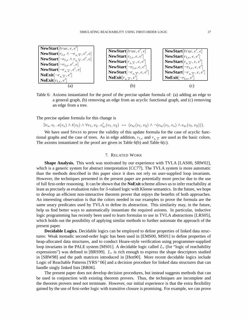
SIMULATING REACHABILITY USING FIRST-ORDER LOGIC 27
NewStart[true, e, e′]NewStart[rt,e ∧ ¬rs,←−e , e
′, e]NewStart[¬rt,e ∧ rs,←−e , e
′, e]NewStart[¬rt,e, e′, e]NewStart[¬rs,←−e , e
′, e]NoExit[¬rs,←−e , e
′]NoExit[rt,e, e′]
NewStart[true, e′, e]NewStart[rt,e, e, e′]NewStart[rs,←−e , e, e
′]NewStart[¬rt,e, e, e′]NewStart[¬rs,←−e , e, e
′]NoExit[rs,←−e , e
′]
NewStart[true, e′, e]NewStart[rt,e, e, e′]NewStart[rs,←−e , e, e
′]NewStart[¬rt,e, e, e′]NewStart[¬rs,←−e , e, e
′]NoExit[¬rt,e, e′]
(a) (b) (c)
Table 6: Axioms instantiated for the proof of the precise update formula of: (a) adding an edge toa general graph, (b) removing an edge from an acyclic functional graph, and (c) removingan edge from a tree.
The precise update formula for this change is
∃vs, vt . s(vs) ∧ t(vt) ∧ ∀v1, v2 . e′tc(v1, v2) ↔ (etc(v1, v2) ∧ ¬(etc(v1, vs) ∧ etc(vt, v2))).
We have used SPASS to prove the validity of this update formula for the case of acyclic func-tional graphs and the case of trees. As in edge addition,rt,e andrs,←−e are used as the basic colors.The axioms instantiated in the proof are given in Table 6(b) and Table 6(c).
7. RELATED WORK
Shape Analysis.This work was motivated by our experience with TVLA [LAS00, SRW02],which is a generic system for abstract interpretation [CC77]. The TVLA system is more automaticthan the methods described in this paper since it does not rely on user-supplied loop invariants.However, the techniques presented in the present paper are potentially more precise due to the useof full first-order reasoning. It can be shown that theNoExit scheme allows us to infer reachability atleast as precisely as evaluation rules for3-valued logic with Kleene semantics. In the future, we hopeto develop an efficient non-interactive theorem prover thatenjoys the benefits of both approaches.An interesting observation is that the colors needed in our examples to prove the formula are thesame unary predicates used by TVLA to define its abstraction.This similarity may, in the future,help us find better ways to automatically instantiate the required axioms. In particular, inductivelogic programming has recently been used to learn formulas to use in TVLA abstractions [LRS05],which holds out the possibility of applying similar methodsto further automate the approach of thepresent paper.
Decidable Logics.Decidable logics can be employed to define properties of linked data struc-tures: Weak monadic second-order logic has been used in [EMS00, MS01] to define properties ofheap-allocated data structures, and to conduct Hoare-style verification using programmer-suppliedloop invariants in the PALE system [MS01]. A decidable logiccalledLr (for “logic of reachabilityexpressions”) was defined in [BRS99].Lr is rich enough to express the shape descriptors studiedin [SRW98] and the path matrices introduced in [Hen90]. Morerecent decidable logics includeLogic of Reachable Patterns [YRS+06] and a decision procedure for linked data structures thatcanhandle singly linked lists [BR06].
The present paper does not develop decision procedures, butinstead suggests methods that canbe used in conjunction with existing theorem provers. Thus,the techniques are incomplete andthe theorem provers need not terminate. However, our initial experience is that the extra flexibilitygained by the use of first-order logic with transitive closure is promising. For example, we can prove

28 T. LEV-AMI, N. IMMERMAN, T. REPS, M. SAGIV, S. SRIVASTAVA,AND G. YORSH
the correctness of imperative destructive list-reversal specified in a natural way and the correctnessof mark and sweep garbage collectors, which are beyond the scope of Mona andLr.
Indeed, in [IRR+04b], we have tried to simulate existing data structures using decidable logicsand realized that this can be tricky because the programmer may need to prove a specific simulationinvariant for a given program. Giving an inaccurate simulation invariant causes the simulation to beunsound. One of the advantages of the technique described inthe present paper is that soundness isguaranteed no matter which axioms are instantiated. Moreover, the simulation requirements are notnecessarily expressible in the decidable logic.
Other First-Order Axiomatizations of Linked Data Structur es. The closest approach toours that we are aware of was taken by Nelson as we describe in Section 4. This also has somefollow-up work by Leino and Joshi [Lei98]. Our impression from their write-up is that Leino andJoshi’s work can be pushed forward by using our coloring axioms.
A more recent work by Lahiri and Qadeer [LQ06] uses first-order axiomatization. This workcan be seen as a specialization of ours to the case of (cyclic)singly linked lists.
Dynamic Maintenance of Transitive Closure.Another orthogonal but promising approach totransitive closure is to maintain reachability relations incrementally as we make unit changes in thedata structure. It is known that in many cases, reachabilitycan be maintained by first-order formulas[DS95, PI97] and even sometimes by quantifier-free formulas[Hes03]. Furthermore, in these cases,it is often possible to automatically derive the first-orderupdate formulas using finite differencing[RSL03].
8. CONCLUSION
This paper reports on our proposal of a new methodology for using off-the-shelf first-ordertheorem provers to reason about reachability in programs. We have explored many of the theoreticalissues as well as presenting examples that, while still preliminary, suggest that this is indeed a viableapproach.
As mentioned earlier, proving the absence of paths is the difficult part of proving formulaswith TC. The promise of our approach is that it is able to handle such formulas effectively andreasonably automatically, as shown by the fact that it can successfully handle the programs describedin Section 5 and the success of the TVLA system, which uses similar transitive-closure reasoning.Of course, much further work is needed including the following:• Exploring other heuristics for identifying color classes.• Exploring variations of the algorithm given in Fig. 10 for instantiating coloring axioms.• Exploring the use of additional axiom schemes, such as two ofthe schemes from [Nel83], which
are likely to be useful when dealing with predicates that arepartial functions. Such predicatesarise in programs that manipulate singly-linked or doubly-linked lists—or, more generally, datastructures that are acyclic in one or more “dimensions” [HHN92] (i.e., in which the iteratedapplication of a given field selector can never return to a previously visited node).• Additional work should be done on the theoretical power ofT1+IND and related axiomatizations
of transitive closure. We conjecture, for example, thatT1 + IND is TC-complete for trees.
Acknowledgements.Thanks to Aharon Abadi and Roman Manevich for interesting suggestions.Thanks to Viktor Kuncak for useful conversations includinghis observation and proof of Proposi-tion 4.4.

SIMULATING REACHABILITY USING FIRST-ORDER LOGIC 29
REFERENCES
[Avr03] A. Avron. Transitive closure and the mechanizationof mathematics. InThirty Five Years of AutomatingMathematics, pages 149–171. Kluwer Academic Publishers, 2003.
[BLARS07] I. Bogudlov, T. Lev-Ami, T. Reps, and M. Sagiv. Revamping tvla: Making parametric shape analysiscompetitive. InCAV, 2007.
[BR06] J. Bingham and Z. Rakamaric. A logic and decision procedure for predicate abstraction of heap-manipulating programs. InVMCAI, pages 207–221, 2006.
[BRS99] M. Benedikt, T. Reps, and M. Sagiv. A decidable logicfor describing linked data structures. InEuropeanSymp. On Programming, pages 2–19, March 1999.
[CC77] Patrick Cousot and Radhia Cousot. Abstract interpretation: a unified lattice model for static analysis of pro-grams by construction or approximation of fixpoints. InPOPL ’77: Proceedings of the 4th ACM SIGACT-SIGPLAN symposium on Principles of programming languages, pages 238–252. ACM Press, 1977.
[CC79] P. Cousot and R. Cousot. Systematic design of programanalysis frameworks. InSymp. on Princ. of Prog.Lang., pages 269–282, New York, NY, 1979. ACM Press.
[DS95] G. Dong and J. Su. Incremental and decremental evaluation of transitive closure by first-order queries.Inf.& Comput., 120:101–106, 1995.
[EMS00] J. Elgaard, A. Møller, and M.I. Schwartzbach. Compile-time debugging of C programs working on trees.In European Symp. On Programming, pages 119–134, 2000.
[FLL+02] C. Flanagan, K.R.M. Leino, M. Lillibridge, G. Nelson, J.B. Saxe, and R. Stata. Extended static checkingfor java. InSIGPLAN Conf. on Prog. Lang. Design and Impl., 2002.
[GME99] E. Gradel, M.Otto, and E.Rosen. Undecidability results on two-variable logics.Archive of Math. Logic,38:313–354, 1999.
[Hen90] L. Hendren.Parallelizing Programs with Recursive Data Structures. PhD thesis, Cornell Univ., Ithaca, NY,Jan 1990.
[Hes03] W. Hesse.Dynamic Computational Complexity. PhD thesis, Department of Computer Science, UMass,Amherst, July 2003.
[HHN92] L. Hendren, J. Hummel, and A. Nicolau. Abstractionsfor recursive pointer data structures: Improving theanalysis and the transformation of imperative programs. InSIGPLAN Conf. on Prog. Lang. Design andImpl., pages 249–260, New York, NY, June 1992. ACM Press.
[Hoa75] C.A.R. Hoare. Recursive data structures.Int. J. of Comp. and Inf. Sci., 4(2):105–132, 1975.[IRR+04a] N. Immerman, A. Rabinovich, T. Reps, M. Sagiv, and G. Yorsh. The boundary between decidability and
undecidability of transitive closure logics. InCSL’04, 2004.[IRR+04b] N. Immerman, A. Rabinovich, T. Reps, M. Sagiv, and G. Yorsh. Verification via structure simulation. In
Proc. Computer-Aided Verif., pages 281–294, 2004.[LARSW00] T. Lev-Ami, T. Reps, M. Sagiv, and R. Wilhelm. Putting static analysis to work for verification: A case
study. InISSTA 2000: Proc. of the Int. Symp. on Software Testing and Analysis, pages 26–38, 2000.[LAS00] T. Lev-Ami and M. Sagiv. TVLA: A system for implementing static analyses. InStatic Analysis Symp.,
pages 280–301, 2000.[LASR07] T. Lev-Ami, M. Sagiv, and T. Reps. Backward analysis for inferring quantified preconditions. Submitted
for publication, 2007.[Lei98] R. Leino. Recursive object types in a logic of object-oriented programs.Nordic J. of Computing, 5:330–360,
1998.[LQ06] S. K. Lahiri and S. Qadeer. Verifying properties of well-founded linked lists. InPOPL, pages 115–126,
2006.[LRS05] A. Loginov, T. Reps, and M. Sagiv. Abstraction refinement via inductive learning. InProc. Computer-Aided
Verif., 2005.[LRS06] A. Loginov, T. Reps, and M. Sagiv. Automatic verification of the Deutsch-Schorr-Waite tree-traversal al-
gorithm. InSAS, 2006.[MP71] R. McNaughton and S. Papert.Counter-Free Automata.MIT Press, 1971.[MS01] A. Møller and M.I. Schwartzbach. The pointer assertion logic engine. InSIGPLAN Conf. on Prog. Lang.
Design and Impl., pages 221–231, 2001.[Nel83] G. Nelson. Verifying reachability invariants of linked structures. InSymp. on Princ. of Prog. Lang., pages
38–47, 1983.[PI97] S. Patnaik and N. Immerman. Dyn-FO: A parallel, dynamic complexity class.Journal of Computer and
System Sciences, 55(2):199–209, October 1997.

30 T. LEV-AMI, N. IMMERMAN, T. REPS, M. SAGIV, S. SRIVASTAVA,AND G. YORSH
[RSL03] T. Reps, M. Sagiv, and A. Loginov. Finite differencing of logical formulas for static analysis. InEuropeanSymp. On Programming, pages 380–398, 2003.
[RSW04] T. Reps, M. Sagiv, and R. Wilhelm. Static program analysis via 3-valued logic. InCAV, pages 15–30, 2004.[SRW98] M. Sagiv, T. Reps, and R. Wilhelm. Solving shape-analysis problems in languages with destructive updat-
ing. Trans. on Prog. Lang. and Syst., 20(1):1–50, January 1998.[SRW02] M. Sagiv, T. Reps, and R. Wilhelm. Parametric shape analysis via 3-valued logic.Trans. on Prog. Lang.
and Syst., 2002.[WGR96] Christoph Weidenbach, Bernd Gaede, and Georg Rock.Spass & flotter version 0.42. InCADE-13: Pro-
ceedings of the 13th International Conference on AutomatedDeduction, pages 141–145. Springer-Verlag,1996.
[YRS+06] G. Yorsh, A. Rabinovich, M. Sagiv, A. Meyer, and A. Bouajjani. A logic of reachable patterns in linkeddata-structures. InFOSSACS, 2006.
This work is licensed under the Creative Commons Attribution-NoDerivs License. To viewa copy of this license, visit http://creativecommons.org/licenses/by-nd/2.0/ orsend a letter to Creative Commons, 171 Second St, Suite 300, San Francisco, CA 94105,USA, or Eisenacher Strasse 2, 10777 Berlin, Germany