supported by theEuropean Science Foundation

NEWSLETTER

ISSUE 1

March 2000

Editor: Donal Mac Kernan

Centre Europeen de Calcul Atomique et MoleculaireEcole Normale Superieure de Lyon,

46 Allee d’Italie, 69364 Lyon Cedex 07, France

Tel: 00-33-04-72728632 Fax: 00-33-04-72728636 email: dmack@cecam.fr

The SIMU programme aims at building cooperation across Europe in the field of computationl physics

and chemistry of condensed matter, with particular emphasis on the development of novel computa-

tional techniques to perform multiscale molecular simulations.

URL: http://simu.ulb.ac.be/

ii

Contents

I Preface 1

II SIMU in a nut shell 3

III The Computer, Machine of the Dreams of Theoretical Physics,Commentary by Giovanni Ciccotti 5

IV Industrial Aspects of Mesoscale Modeling,Letter by Hans Fraaije 13

V Hierarchical Modelling of Polymers, Review article by DorosN. Theodorou 19

VI Bridging the time-scale gap: Homogeneous nucleation,Reviewarticle by Pieter Rein ten Wolde and Daan Frenkel 41

VII Molecular Modeling and Simulation of a Photosynthetic ReactionCenter Protein, Review article by Matteo Ceccarelli, Marc Souailleand Massimo Marchi 59

VIII From Molecular Dynamics to Dissipative Particle Dynamics,Article by Peter V. Coveney, Gianni De Fabritiis, Eirik G.Flekkøyand James Christopher 73

IX The elements: A Beowulf class Computer,Technical note byStavros C. Farantos 95

X Did you see ? 101

XI Conferences, Schools, Workshops, Tutorials, andSIMUfellowships 105

XII Jobs, Grants and Fellowships 109

iii

iv

I

Preface

We are launching this, the first issue of theSIMU Newsletter, to contribute to the generalaim of theSIMUprogramme: namely, to provide support to the scientific community, whichrecognises itself via the goal of developing new simulationtechniques to meet the challengesof bridging scales in molecular simulations of condensed matter.

Why a newsletter? We feel that there is a need for more information to flow among us.Information on the very existence of the programme (some of you who endorsed the pro-posal submitted two years ago toESFmay have forgotten what it is all about!), informationon the activities which are being planned at this time (workshops, tutorials etc...), on theactivities which might be proposed in the future, information also on the different groupsthat participate: who they are, what they do, how they work, etc... We really would like thatthis newsletter to become a forum for discussion, so as to have in common a knowledge andunderstanding useful to others in their work.

We have asked someSIMU members to contribute to the newsletter in various ways.The main body consists of articles presenting research related to our ”bridging the gap”theme: dissipative particle dynamics, polymer modeling, homogeneous nucleation and elec-tron transfer in biological molecules. The articles we intend to present in future issues neednot be original, as the interest of collecting them here comes from the fact that we representa community with wide interests so that the results described may be unknown to many ofus. We will require your cooperation for future articles. The emphasis will rather be onpresenting state-of-the-art molecular modeling approaches in different fields to an audiencewhich may not be familiar with the precise physical context but share the concern about thetechniques to be used. We also know that writing papers and articles already takes much ofour time, and we would rather encourage you to provide us withreports that have alreadybeen written at other occasions, but whose distributions have been limited, or papers writtenfor specialised journals, but which may be of general interest.

We also would like to present here some material which is lesstraditional in the scientificliterature. We invited G. Ciccotti to present his thoughts on the importance of the changesthat have occurred in physics due to the possibilities offered by a heavy usage of numerics.Similar presentations of personal views are invited from theSIMUcommunity. We also wantto address some very practical questions, like how to choosea hardware configuration: wepresent the report of a group having acquired a cluster of PCs. We look forward to receiv-ing comments and reactions from you, possibly with different views and different choices,and we will be glad to relay those reactions in our next issue (we plan two issues a year).There are also sections dealing with conference announcements, interesting URLs on the

1

Web or job offers. Those sections might be very useful in the future, if you feed them withinformation you have or tricks, addresses etc...you know and wish to share.

This first issue of the newsletter is being sent to you by ordinary mail. Future issues willbe put on our web server (http://simu.ulb.ac.be/) from which it will be down-loadable anda notice will be sent to allSIMU members. Hard-copies will be sent on request only. Feelfree to contact us for positive or critical comments, ideas or suggestions: they will all bewelcome.

Michel Mareschal, Chairman of the SIMU steering committeeemail: michel.mareschal@cecam.fr

Donal Mac Kernan, Scientific Assistant to the SIMU programmeemail: dmack@cecam.fr

2

II

SIMU in a nut shell

WHAT is SIMU ?

SIMU is an acronym for a programme sponsored by the European Science Foundation (ESF)whose full title is :” Challenges in Molecular Simulations:Bridging the Length- and Time-scale Gap”. The proposal was submitted in 1998 toESFand has been approved for 5 years,starting in 1999 and ending in 2003. The text of the proposal as well as the list of teamsendorsing the programme can be found on our web site (http://simu.ulb.ac.be/).

What is the budget?

The ESFprogrammes are funded ”a la carte”, according to the numberof supportingESFmember organizations.SIMU is being funded by Belgium (FNRS) , Denmark, Finland,France (CEA andCNRS), Germany (MPG), the Netherlands, Italy (INFM andCNR), Nor-way, Portugal, Spain, Sweden, Switzerland and the United Kingdom. The total annual budgetis around one million French Francs and is meant to support networking activities like shortvisits, conferences, workshops and tutorials as it was planned in the proposal.

Who is in the steering committee?

The programme is managed through a steering committee: thiscommittee is composed ofone representative per country, plus the chairman and a few invited experts: D. Theodorou,D. Frenkel and G. Ciccotti. E. Crespeau,CECAMsecretary, is also in the steering committee.This committee met twice already: in March 99 and in November99. Its next meeting willtake place in November 2000 to decide the funding of activities for the year 2001.

Who is a member ofSIMU?

Funding is usually limited toSIMUmembers that are laboratories of funding countries whichhave endorsed the proposal. The steering committee has decided to have an open policyconcerning membership: laboratories whose research is directly concerned with the aim ofSIMU (development of techniques for bridging the gap) can apply to become members ofSIMU. They have to write to the committee chairman and to their national representative,presenting their lab and stating how they can contribute to the programme. Labs of countrieswhich are notSIMU funders (like Russia, Greece or the United States) can also be associated

3

to the programme. The committee also decided that workshop funding would be decidedon solely on scientific criteria, and not on nationality. Acceptance of a participant is theresponsibility of the organizer.

What are theSIMU activities?

In 1999, four workshops have been proposed within theSIMU programme and a similarnumber is being planned in 2000. Most of the workshops will take place atCECAM (inLyon), taking advantage of the cooperation offered. This ishowever not at all a mandatorylocation and workshops can be organized at any other place. Th typical budget is around50 000 FF, and covers staying expenses of between 20 and 30 participants for a few days.This yearSIMU is supporting two schools, one in Amsterdam and the other in Manchester.The Amsterdam school took place in January, the Manchester school will be organized atthe end of June at UMIST. TheSIMU support consists of grants for partial financial sup-port of staying and travel expenses. Tutorials are organized in collaboration withCECAMin Lyon. Three or four one-week tutorials will be organized this year: participants can ap-ply for grants to cover staying and travel expenses. Short visits can also be funded by theprogramme. Whereas in the case of workshops, tutorials and schools, support for year 2000was decided during the committee meeting last November, forshort visits, there is an emaildecision process taking place end of December, end of March and end of June, as well as theNovember session. Application forms for those funds can be found on our web site. Notethat the funding decision depends on a connection existing with the aims of the programme.Note also that such funding can cover meetings of groups who would like to organize TMRnetworks or similar projects. Finally, two major conferences will be organized during theprogramme’s duration. The first one, ”Bridging the time-scale gap”, will take place in Kon-stanz from September 11th till September 15th, 2000. More details on these activities are inthe newsletter and on the web site which is regularly updated.

Who can propose activities?

Members are encouraged to make proposals. Workshop proposals forms are available on theweb site and they should be sent to the programme chairman before September 30th this year.Proposals will be reviewed by two external experts and sent to the committee members. Thecommittee will then decide in November. Contact the programme chairman or your countryrepresentative to see how a proposal can fit within the general programme. Whom to contact?

Do not hesitate to contact directly the programme chairman,Michel Mareschal. You canalso contact Donal Mac Kernan, who is in charge of scientificassistance to the programme.

4

III

The Computer, Machine of the Dreams ofTheoretical Physics1

Giovanni CiccottiDipartimento di Fisica,

Universita di Roma “La Sapienza”,P. Aldo Moro 2, I-00185 Roma, Italy

email: Giovanni.Ciccotti@roma1.infn.it

The scope of theoretical physics

Modern science was born, at least in principle, the day when humanity decided to liber-ate itself from the Aristotelian idea of the limits which thecondition of being by Naturewould impose to our possible activities. For example, it is well known to the historian ofscience, the argument used by Aristotle to exclude the possibility of automatic machines (inhis words, “automata”): if such machines were to exist then slavery would be unnecessary,but slavery is ”by Nature” and therefore automata cannot exist. The methodological idea thatsomething unnecessary, or better still, even contradictory with something else cannot exist, isinteresting, and in other contexts, even useful. Here, however, it served to define somethingin principle impossible which was false, and was an ill-omenfor human development. Thefirst and most lucid herald of modern science was Francis Bacon, who, although contribut-ing nothing of during to modern knowledge, saw with great clarity what science could do forhumanity (making men masters of Nature) and under which condition: submitting mankindto Her own laws. The question obviously becomes a bit more entangled if we try to definewhat should be those laws, how they should be discovered/invented and what are their limitsof validity. There Bacon becomes totally useless, but we cango to Galileo for a few goodideas, or, more generally, to a formalized, or, even more explicitly, mathematical concept ofNature. Contrary to a widespread opinion, held also by physicists, the originality of Galileois not so much in his insistence on ”sensible experiences” (in the words of Galileo the ”sen-sate esperienze” are nothing else than what we call experiments), but in the idea that once themaximum number of ”sensible experiences” has been performed, it is necessary to formulatethe results mathematically, so that one can derive, by computing, the maximum number ofbehaviours from the fewest number of principles. The trust that we can place in mathematics

1Translated from Italian by Donal Mac Kernan.

5

guarantees us that, if a consequence is ill-predicted by ourmodel, there are not that manyculprits to look for; it is the model which is inadequate. Therefore we must change some-thing in the model, be that simply the change of parameters, or up to the higher level of thegeneral principles, but, in any case, through a relatively linear procedure remaining largelyunder our control. It is mathematics that plays here the roleof protagonist. It is worthwhileto try to understand, therefore, how this happens and why mathematics simplifies so muchthe search of the error, and, when applicable (we will come back to this shortly), providingso much surety. Yet again, it is Galileo that helps us with a truly amusing and cunning de-scription of the situation. God, Galileo says, knows all possible and imaginable mathematics,while we, poor men, know but a few scraps. Nevertheless, addsGalileo, those few scrapswe know as well as Him, for the simple reason that mathematicsis “truth” in its purest form,divine. In more modern and less theological terms, we could say that as mathematics is ourown creation, and not that of the external nature, it does nothave the margin of error thatbelong to anything which does not stem directly from us. Summing up, the essence of theproblem seems clear: if we succeed in representing a large family of phenomena with a fewequations, then all of those phenomena are totally under ourcontrol, and we may considerourselves, Bacon-like, to be their masters. That is we can use our knowledge to producesituations different from the ones naturally found, and moreover, to our own advantage. Sothe question changes, becoming: when is it possible to represent the largest number of phe-nomena knowable (i.e. the universe) with few equations? In the exact sciences three hundredyears have passed during which one has tried to say ALWAYS. Inthe human sciences, or inany case, as one gradually moves away from the exact sciences, the answer is NEVER, oralmost never, or at its most optimistic, a few times. Now the truth is less banal than that, andit is worth discussing in some detail.

Since the time of Newton, theoretical mechanics has earned the respect of “practical”mechanicians, and has given the impression that the Baconian ideal was at hand. Thanksto reductionism (atomic hypothesis and its derivatives: that the complexity of reality areonly manifestations of atoms and their movement) and to the generalization of mechanicsfrom the classical to the quantum (and relativistic), also chemistry has timidly followedthe same direction. However neither biology and even less still, the social sciences havefollowed this pattern. Why ? Is this an inevitable fact, linked to the inability of mankind todominate on a grand scale, or is it purely accidental, due to afew historical limitations in ourdevelopment ? Looked at closely the first hypothesis seems unnecessarily pessimistic, basedon an assumed incapacity of mankind, while the second, seemsmuch more convincing, atleast to the extent that one looks at chemistry and biology, where there are signs of profoundtransformations bringing these disciplines to resemble the best (theoretical) physics. While,in this field, no hypothesis can be completely proven, all recent developments add credibilityto the idea that, soon, chemical and biological procedures will be as controllable as thosemechanical. In other words, the dream of theoretical physics to reconstruct the world, whichuntil yesterday appeared inapplicable to the chemistry of materials or to biology, now seemsincreasingly credible. It seems best then to accept the optimistic hypothesis, and try tounderstand what primed this process, and what are the limitations of the theory that we arestarting to overcome. The idea I wish to demonstrate in the following pages, is that, in thelast three hundred years, the missing ingredient in the development of theoretical physics,in the sense of Bacon, has been simply calculating power. Equipped with an open theory(certainly much more refined that that of Newton, but fundamentally the same) and with agrowing computing power, we can hope to realize Bacon’s dream: to know nature so well as

6

to be able to think of submitting Her to homo sapiens.

Theoretical physics and computing

About three hundred years ago, thanks to the work culminating in the synthesis of Newton,the idea of science as power over the world was fully realizedin classical mechanics, whichthen was promoted, as the most accomplished model of complete knowledge. In ballistics,astronomy, or practical mechanics, the feeling that one hadin hand a theoretical instrumentcapable of going over every difficulty, was considered well founded. However, things werequite different if one left the domain of purely mechanical phenomena. So much so that, atthe beginning of the nineteenth century, Auguste Comte feltscience should not be classifiedin a unified way, but rather that each domain should define its own criteria and way of beingscientific: thermology and optics being presented as distinct from mechanics, similarly to,but with even greater justification, chemistry or life sciences. The interpretation of acoustic,electromagnetic, and optical phenomena in terms of mechanics (be it of particles or of thecontinuum, i.e., classical field theory) required about a century. But this was, in a sense, lessexhausting than unifying mechanics and thermodynamics. This accomplishment, of the endof the last century, required the conceptually new and remarkable use of the methods of statis-tics to understand the macroscopic behaviour of systems still fully mechanical. It was fromthis moment that the unifying ambition of physics ceased to be a chimera, reasonable butprovable only in very restricted domains, to become a concrete possibility, both theoreticallyand practically. It is true that to arrive so far, the laws of physics had to be revised (relativity,and above all quantum mechanics attest to this). However, the revisions were less profoundthan is often recounted, and did not so much affect the entireedifice of the scientific expla-nation of the universe, but only the internal consistency ofa few presuppositions. The trulyimportant addition to the mechanical ideas of Galileo and Newton was made by Boltzmann,who systematically used statistical methods in mechanics to obtain a unified explanation ofmacroscopic systems (that include the universe..) from mechanical microscopic ones ( theatoms...). To achieve that, a complete new mathematical discipline was created and formal-ized: the theory of probability, whose axiomatization was given by Kolmogorov in 1933,practically at the same time, as the completion of the construction of the new mechanics bySchroedinger, Pauli and Dirac, to mention a few of the betterknown names. At this point, theexplicative and predictive power of theoretical physics became extremely broad and, unlikewhat happened at the beginning of the nineteenth century, involved not only all of physics(mechanics, heat, electromagnetism etc), but also the simpler phenomena of chemistry and,at least as a potentiality, the basic phenomena of life. Although from a technical point ofview this happened at the beginning of the thirties, from a more general perspective, it wasalready expected by the great scientists of the end of the nineteenth century, foremost amongthem Henri Poincare. His writings on the future of physics, written at the beginning of thetwentieth century, are still astonishing for their lucidity, clarity and relevance today.

There is however, a but, and not a minor one, in all this gratification. To understand this,it is useful to make a distinction between the virtual and real predictive power of theoreticalphysics. The former is enormous, but obviously not very satisfying, while the latter is,everything considered, minimum. The difference is entirely due to the lack of capacity andpower to calculate, as I will try to show in what follows. And it is not a minor point, becauseto understand this is to appreciate a major epistemologicalchange. Scientific progress, in

7

these eyes, is no longer the addition of new scientific laws tothose already present, but ratherthe derivation of all of the consequences of the known laws, and only in the eventuality oftheir deficiency, the updating of the same. That is, the effort (and the value) of research is nomore concentrated on the creative activity of the legislator, but on the capacity to rationallyreconstruct a domain of phenomena by algorithmic derivation from simple and general laws.Here is the source of the importance acquired by the concept of the model (now sometimesconfused with theory) in modern research. A great theoretical physicist, Dirac, seems tohave completely missed the point when he maintained that theduty of theoretical physicsis to find the laws, the rest being chemistry, because in doingso he practically destroyedthe modern, Baconian, concept of science. But let us return to our theme, and try to showthe impact of the capacity and power to calculate on the development of science, and on theBaconian dream which corresponds to it.

I will proceed with two extreme examples to place what we are discussing exactly intocontext. The courageous book of Schroedinger on “What is life” and the comment of VonNeumann at the end of the forties on the problem of meteorological predictions. I will thentry to further illustrate the point by comparing the presentation of mechanics in an old, butstill excellent and often used book of mechanics, “The variational principles of mechanics”of Cornelius Lanczos, with that of any modern text.

In a book written at the beginning of the forties, and still very famous, Erwin Schroedinger,justly proud of the contribution of quantum mechanics to thedevelopment of knowledge, de-cided to face the question of the importance of the (new) physics for the understanding of thephenomena of life. The book is still today extremely interesting, and yet completely dated.Schrodinger’s wish in fact is not to explain in detail (or putmore precisely, to calculate) thephenomena of life, but rather to demonstrate that they are not incompatible with the knownlaws of physics, since, on the contrary, physics alone may even be sufficient to perceive afew biological regularities (laws in the sense of Comte...)without the need of anything else !In other words, a steady step backwards with respect to the the Newtonian realization of theBaconian programme.

The story of Von Neumann (one of the founding fathers not onlyof computationalphysics, but even of the modern computer) is completely different. Von Neumann had dis-covered and cured a few instabilities in the numerical solutions of partial differential equa-tions, and had decided to apply his algorithms to the equations governing weather prediction.The algorithms were for the epoch (and, to tell the truth, still are) computer intensive, so thecalculations could only be done by computer. All of the procedures checked, the calcula-tions took two days to make a two hour forecast. It was clear that either one found fasteralgorithms, or faster computers, or such “predictions” would remain of no practical interest.We all know how the situation evolved, so much so that today wecan produce in a couple ofhours a prediction valid for forty eight hours, and we continue to improve, Amen to Dirac’sridiculous comment.

I already said that the Von Neumann example is not a typical one, but an extreme caseif very important. The main significance in the power to calculate (in a computer intensiveway, not by hand!) lies in the possibility to study the so-called non linear equations, whosequalitative behaviours are totally unexpected since we have no analytical, exact, indicationon how they should behave. The first impact of the capacity to calculate introduced bycomputers into the theory was really here, in the possibility to study the behaviour of systemswhose evolution follows laws that we know how to write, but not how to compute, i.e., tosolve. This is the typical case in physics, and, even more striking, in mechanics as massive

8

calculations revealed, so creating an important divide between the situation before and afterthe advent of computers.

The easiest way to characterize the divide is to refer to the book of Lanczos, and to com-pare it with any modern book on mechanics. The former consists of an elegant, intelligentand profound presentation of the principles of classical mechanics as they have been elab-orated over the centuries. It is useful and complete and saysmuch on the various differentbut equivalent ways to formulate analytically a mechanicalproblem. However, Lanczos saysalmost nothing about how to solve a problem once it has been correctly formulated. For him,mechanics formulates, it does not solve. Solving is at the same time both banal, and toodifficult. In any event, it is the duty of mathematics, and, ifwe believe it, we can invoke theinfinitely able mathematician of Laplace, otherwise, we canlimit ourselves to the few, veryfew, problems having solutions that we know how to write. This is not only Lanczos, it isthe same for any book of mechanics of his generation. Today, instead, the scope of a bookon mechanics is to learn how to classify the solutions, including in depth discussions on thepossible behaviours of a system, its stability or instability, and according to which criteriaone can obtain clues on the behaviour of a given mechanical system. Here numerics plays anessential part, and any astute trick to help solve the problem is welcome. The idea can comefrom a qualitative study of the differential equations (that govern mechanical behaviour) orfrom having obtained a great deal of numerical evidence: it does not matter how, one is verytolerant about the methods, but the result must not be the FORMULATION of the problem,but its SOLUTION. Obviously, there are no solutions withoutexact formulations, but it isimportant to understand that the emphasis has moved and whatcounts now is not to find anew formulation that permits one to understand a particularproblem better, but to be ableto face it with brute force ( that is, as we say in the profession, by calculating massively)to extract all possible behaviours, and in the end, to predict concretely, and not virtually thebehaviour under given conditions.

We have come to the end of our general discussion of the present situation: the laws ofphysics until proven otherwise, are true and universally so. One applies and values them al-ways not virtually, but effectively. The world is made of space, time (i.e. motion) and matter(i.e. inertia to movement, or, equivalently, mass, and interactions). Its laws of evolution areknown to us, we solve them by calculation (or by finding the way, the algorithm that cando it). After which, if we already have the power to calculatesufficiently, the problem isno more a limit to our power, but a further occasion for the command of Nature, obtainedby submitting us to Her own laws (the famous Baconian formula). Otherwise one dealswith the problem from many sides, inventing new and more powerful calculating tools, newalgorithms and new approaches, further schematizations that could give a solution step bystep, and end in controlling Her. This is the most interesting part of the procedure that weare attempting to describe, and it is on it that we will concentrate in the final part of ourdiscussion.

Computer simulation, and the dream of infinite power of sci-ence

The success of the programme that I have tried to describe up to here is based on a char-acteristic of physics (but it would perhaps be better to say of the world, i.e. of the objectsthat we would like to know) that has simplified enormously thesolution of the reductionist

9

programme that we have posed: reconstruct mathematically the world from the ultimate andsimplest elements (before atomic theory I would have said the atoms, but with the philosoph-ical meaning of the term, instead our atoms are not ultimate in any sense, their place havingbeen taken by elementary particles). The point is that little by little, as a system becomesmore complex, its “atoms” become larger structures, so as toretain, at least for the problemat hand, the simple character that distinguishes the atoms.Let us try to explain a bit better.

Chemistry is constructed from atoms to form at first molecules, and then molecular com-plexes and materials as an aggregate state. Having discovered that the atom is not simplebut is made of electrons and nucleus, and that the latter is not in fact elementary, but can bebroken into fragments that cannot again be considered to be elementary, one finds that thesituation of chemistry has not changed greatly. In fact things are more or less the same as be-fore, in the sense that the essential of chemistry comes fromthe electromagnetic interactionbetween electrons and nuclei as stable entities, while their complexity, although true, needsonly be considered explicitly if one wishes to. Only in this case do the other fundamentalinteractions become important, for which there are all the conceptual tools of elementaryparticle physics (and this, when looked at closely, reducesto the same as one uses for elec-trons and nuclei, except for the simplifying low energy approximations, where the nuclei arestable, which are not valid at high energies, where nuclei can be broken). So we are permit-ted to solve one problem at a time, and never have to take into account simultaneously all ofthe possible levels of complexity. Thus, to give an example,to determine the stability andother properties of atoms it is necessary to consider electrons and nuclei. But, they may betreated as material points, with mass, charge, and magneticmoment, devoid of any internalstructure, even though we know that this is not true in all possible conditions. However, if weare able to split the nucleus, then the nuclei and the electrons will form not atoms, but ratheran anonymous, uninteresting mix of electrons and nuclei (ortheir fragments). Similarly, ifwe wish to construct a molecule, we not not need to consider all the nuclei and electronsindividually. It is enough to consider some heavy material points (constituted of the nucleiand the most tightly bound electrons), as being even fixed, and, as for the rest, light mate-rial points, consisting of the residual electrons. The ensuing objects may be considered aselementary for the problem that we wish to solve. Finally, ifone wishes to consider manymolecules together and predict the behaviour of such an aggregate (i.e. a piece of ordinarymatter), it is sufficient to treat the molecules as material points interacting according to givenlaws. Once the game is understood, it can be continued ad infinitum.

It is important to realize that the laws which reign over these “elementary particles” arealways the same (the famous apple falling on the head of Newton, made him understand uni-versal attraction, and thus the possibility of the moon falling on the earth), they are simplyshifted from one spatio-temporal scale to another. This wasnot unknown in the nineteenthirties, i.e. before it was possible to perform serious calculations, but could not bear fruiton a large scale until one knew how to perform intensive calculations on such scales. Beforethis, one had to invent simplistic mathematical models containing the essential informationof a few levels of complexity. Now, one can not only solve truly realistic models, but aboveall, systematically calculate the essential information relating adjacent levels of complex-ity, from the inferior level to the superior (e.g. compute the form of interaction betweenmolecules, using a very detailed model, and then depict molecules as a collection of materialpoints interacting with the computed laws to compute their collective behavior). Thus, oneno longer does what in the slang of physicists is called, and with some mild contempt, phe-nomenology, but true predictive theory or, as one says todayin appropriately noble Latin, ab

10

initio.An interesting cultural by-product of this situation, typical of our times, but one that I

do not wish to pursue here, is mathematical modeling runningwild for whatever type ofphenomenon, even in domains where it is not yet, or even not atall, possible to proceedmathematically (like in the social sciences or the explanation of history, those that someonehas called, with a well chosen metaphor, “ the formless doctrines”). The consequence is thatmathematical toys of little value are called scientific. Butlet us return to our principal theme.

The success of this programme, over the last fifty years, has been explosive, and hashad an effect not only in the ab-initio prediction of alreadyknown phenomena, but in thediscovery of new phenomena thanks to the more and more cunning management of contin-uously improving experimental equipment. Consider, for instance, that one can now ”see”experimentally spatial structures on atomic scales. As a result, we have now learned how topredict the molecular structure arising from not only a few atoms, but from thousands, andthe physical properties of natural and synthetic materialshaving the complexity of polymers.Little by little we are realizing that biology is of a complexity that we can already hope todeal with really and not only virtually, in our generation, that even life is constructible (notsimply understandable !) from matter and movement, that is,with the usual tools of physics.However this is not the physics of Comte but a physics gone beyond the discipline dealingonly with physical phenomena (as stated, with amusing logically vicious circles, in manyphysics textbooks), one that has permeated chemistry and biology, making it ever more dif-ficult to define a physicist as physics is going to be found everywhere, and, ultimately, willno more be characterisable as a separate discipline neighboring others. To content medicine,empirical practice par excellence, perennial nightmare ofphysicists! Whatever one maythink, bionics is less science-fiction, and more premonition for what is happening in front ofthe eyes of everyone.

11

12

IV

Industrial Aspects of Mesoscale Modeling

J.G.E.M. (Hans) FraaijeUniversity of Leiden, the Netherlandsemail: j.fraaije@chem.LeidenUniv.nl

Introduction

In the arena of applied soft-condensed matter physics, mesoscopic dynamics models are re-ceiving increased attention as they form a bridge between fast molecular kinetics and slowthermodynamic relaxations of macroscale properties. The topic is of considerable impor-tance for the understanding of many types of industrial complex liquids. Eventually coarse-grained models for the slow diffusive and hydrodynamic phenomena in phase-separationdynamics may serve as a new simulation tool for chemical engineers in industry... We haveall used introductions like this one, they sound nice. But, is there any reality to it? The orga-nizers of the SIMU newsletter asked me to write a paper about my industrial experiences andviews. I briefly discuss the background of the EU MesoDyn project we started a few yearsago, the current status and where to go in the future. The paper is not a scientific review, butrather a personal collection of views and ideas, and it does not necessarily reflect the opinionof the MesoDyn partners. For details and papers I refer to theMesoDyn pages athttp://www.fwn.rug.nl/mesodyn/index.html

MesoDyn project

The following is a citation from the abstract of the MesoDyn project description. ”In thisproject we aim to provide the chemical industry with generalpurpose software for mesoscalesoft-condensed matter simulations, based on a functional Langevin approach for HPCN-platforms. The prototype of the parallel MesoDyn simulation program produced in WorkPackage 5 of the CAESAR HPNC-demonstrator project (EP8328)is used as backgroundinformation” And from the introduction, ”In the last decademolecular modeling has grownto an essential part of research and development in the chemicals and pharmaceuticals in-dustries. For a longer time, chemical engineers have analyzed macroscale properties usinga variety of continuum mechanics models. Despite the considerable success of both molec-ular and macroscale modeling, in the past few years it has become more and more apparent

13

that in many materials mesoscale structures determine material properties to a very largeextent. Mesoscale structures are typically of the size of 10to 1000 nm. The emerging indus-trial relevance of mesoscale modeling is obvious, nevertheless the necessary general purposecomputational engineering tools are absent. The MesoDyn project bridges the gap betweenmicro- and macroscale modeling by the development of a new class of models and softwaremodules for the mesoscale chemical engineering of complex industrial polymer liquids. Theproject is part of the Information Technology Program (ESPRIT) of the European Commu-nities. The project started in January 1997.”

The partners of the project are: University of Groningen (mygroup, responsible for meth-ods development), IBM (Peter Altevogt, parallellisation), MSI (Dave Nicolaides, graphicalinterface and marketing), Shell (validation), Norsk Hydro(validation) and BASF (Olaf Ev-ers, software, validation and project management). The endof the project is spring 2000, sowe are wrapping things up right now.

In the core of the project is a general purpose library of fastnumerical routines, such asnon-linear equation solvers, stencil operators (these arespatial filters liker2

()) or convolu-tions

R

f(r r

0

)()dr

0), noise generators and several types of polymer path integral routines.The routines are written in MPI/C/C++, and can be accessed via a higher-level language(Tcl/Tk). The library runs on any machine which supports MPI, that is all parallel comput-ers, and most low-end workstations and PC’s.

In principle, the library lets a modeler compose his or her own model, by combiningvarious library calls. The set of routines as it is now is excellently suited for study of allkinds of non-linear partial equation systems which occur inpattern-formation models, suchas meteorological models, reaction-diffusion models or copolymer microphase separationmodels and even image analysis. In practice, the library hasbeen used mostly for simulationof polymer phase separation, and MSI’s graphical interfaceis also focused on these systems.Since fall 1997 the first version of MesoDyn software has beenavailable on the market. It isone of the packages in MSI’s Polymer Consortium 2000.

My group has been responsible for the theoretical background: both the numerical as-pects (stencils and solvers), as well as the modeling of the polymer phase separation. Thelatter is what we have referred to as the dynamic density functional method. The idea is verysimple: we imagine that for every real non-equilibrium system one can invent an equilibriumsystem, balanced by an external potential. The potential isconjugated to the order param-eter(s), which in the case of polymer phases are the concentrations of monomers, blocksor entire polymer molecules. The relation between order parameter and external potentialis the density functional. The gradient of the external potential is a thermodynamic force,which one can use to drive a dynamical process. As long as the dynamics is (very) slow -which is very often the case in condensed polymer systems - one can neglect elastic contribu-tions from incompletely relaxed polymer conformations. Sofar we have studied the classicalsingle-chain density functionals (Gaussian chains) in a mean-field environment. As a resultthe simulation produces the time-evolution of a 3D morphology of a certain (co)polymermixture on a coarse-grained scale. A typical set of equations to integrate is

t

= Mr

2

(U +

ÆF

Æ

MF

) (IV.1)

= DF (U) (IV.2)

where the first equation is the dynamic equation, and the second is the density functionalequation containing the polymer path integral. These are two equations with two unknowns

14

(the fieldsU and ). The set can be integrated by iteration ofU in time. The spirit ofthe method is very similar to the quantum molecular dynamicsmethods proposed by Carrand Parinello, and to the methods proposed by Hansen for colloid particle dynamics. Ofcourse, in the case of mesoscale chemical systems one has to take care of the proper mobilitycoefficients, the hydrodynamics and so on - this seems less ofa problem with quantummolecular dynamics.

In the course of the project we have studied a large number of theoretical and numericalaspects for the purpose of making the method more applicableto real industrial systems(papers can be found on the web site). Some problems turned out to be trivial, other turnedout to be very, very tough.

The trivial problems are those where one can adapt existing polymer self-consistent fieldtheories to the dynamical case, for example path integrals for branched polymers, path in-tegrals for worm-like polymers (rather than Gaussian models), models for polymers withdissimilar monomer size, mean-field models for Donnan equilibria, boundary methods forgeometry constraints and equation-of-state models for compressible systems. Even reactionsare relatively easy to model on this level. For a brief momentwe also contemplated adaptingdensity functional models for more strongly correlated polymer systems (such as PRISM),but we did not pursue the matter. It seems that the single-chain mean-field model worksreasonably well for a large class of problems, and, for practical applications perhaps moreimportant, Flory-Huggins parameters of sufficient accuracy are abundant or can easily bemeasured. The tough problems either have to do with the numerics or the dynamics; I willdiscuss these in more detail in the section Challenges.

For my colleagues from the academic community it may be interesting to comment onthe organizational aspects of the MesoDyn project. In industry one is accustomed to time-tables, deliverables and milestones. Since the MesoDyn project is in the heart an industrialproject, not an academic research project, this holds for the MesoDyn project as well. Forsomeone who believes in academic freedom, and the right of the unexpected, this can createstrange problems initially. When I hired people to work on the project, one of my (now) co-workers remarked that in the list of deliverables he could not find the date we were expectedto find the Higgs boson. And off he went, wearing a suit and a tie, instead of the usual T-shirt (he had to buy a tie). Another consequence was that I managed to hire some very goodpeople, precisely for the reason of the international industrial dimension. In these timeswhen students are scarce, this is rather important. Anotheraspect of the industrial setting isthe interdisciplinary setting. We have computer scientists, theoreticians, physical chemistsand mathematicians in one project. How difficult it still is to start a purely academic researchproject with such a broad range of expertise!

Challenges

Since the end of the MesoDyn project is near, it seems suited to list a number of toughtheoretical challenges for the future, inspired by the project. These are some of the problemswe are currently studying.

15

Numerics

The field equations are discretised on a simple cubic grid by finite differences. One canof course implement other grid-based methods, such as finiteelements, but whatever spatialdiscretisation scheme, the result will always be a large setof non-linear equations which haveto be solved each time step. There are as many equations as there are components nodes.For a full blown 3D-calculation this may involveO(106) equations. Because of the specialnature of the differential-algebraic system, we can prove mathematically that each time steponly one solution is possible. This does not mean however that the single solution is alwayseasy to find: the problem is ill-posed. We have studied various subspace iteration methodsbut so far we have not been able to find a satisfactory alternative above the steepest descentmethod which is now implemented. Yet I am convinced (believe) faster iteration methodscan be devised by making special use of the mathematical formof the density functionalrelation.

Alternatively, how about getting away from the grids? Can one develop an off-latticeintegration scheme? There is always some confusion here, since the word ’lattice’ seems tohave multiple meanings, depending on the particular scientific community one belongs to.In computational polymer physics one uses the word lattice to refer to those theories wherea polymer molecule is somehow constrained on fixed positionsin space. But in other areas,such as CFD or high energy physics, a lattice simply means that one uses fixed points in spaceto calculate the fields. In our case too, one must be careful indistinguishing between the 3Dcontinuum theory and the numerics. We use a grid for the fields, not for the molecules.This then, makes one wonder if particle based discretisation schemes can be invented forintegrating the same set of field-equations. The idea is not new (compare DPD methods),but...there is no universal approach and I do not have an answer.

Hydrodynamics from meso to macro.

The dynamical model we have studied the most is basically that of non-linear diffusion, suchas occurs at the onset of spinodal decomposition, sometimesaugmented by external shearfields (diffusion-convection), or simple Darcy hydrodynamics. Thereby we have neglectedmemory dependent and long-range hydrodynamic contributions. In other words, we havebeen unsuccessful in attaching to the vast literature on constitutive equations, ComputationalFluid Dynamics, or in general the rheology of (complex) polymer liquids. Still, there isa very large number of polymer systems for which internal hydrodynamic effects are notimportant, either because the system is sheared (in which case the flow field is almost com-pletely imposed from outside), or because the system is gel-like and/or the system has avery inhomogeneous viscosity on a mesoscale (in which case hydrodynamic interactions arecompletely screened). Yet it would be fascinating to develop a coherent model in which rel-evant hydrodynamics are reproduced correctly. The answer may be in a proper definition oflocal stress in an arbitrarily inhomogeneous system. If such an expression can be developed(which is not trivial) than perhaps one can attach to LatticeBoltzmann methods or CFD.

16

Molecules from micro to meso

On the other end of the spectrum is the mapping problem. How can one find a proper singlechain density functional to mimic the behavior of real polymer molecules? So, this is theproblem how to get the right chemistry, once the physics is OK. One novel approach wehad was to calculate the response functions from a single chain with full molecular detailby Monte Carlo. Once these response functions are known, onecan easily test and find theproper Gaussian chain which has the same response. If this isthe case, then one can showthat on a mesoscale the molecular-detailed polymer densityfunctional behaves in a sameway as the much simpler Gaussian chain density functional. In practice the approach hasdeficiencies, since the Monte Carlo calculations require anenormous amount of computerpower for a reasonably sized polymer molecule; and we have not been able to find a MonteCarlo method fast enough for our needs.

The virtual cell.

Suppose one wants to mimic the behavior of a living cell? On a mesoscale? Why not? In fact,although the idea sounds completely crazy, there are several groups now attempting to do justthis, with project names such as E-cell or virtual cell. Usually, the approach boils down tothe integration of coupled ordinary differential equations, in order to reproduce the complexbiochemical pathways. Also in this case, just as in our MesoDyn project, the molecular oratomic detail is integrated out. But now the integration results in a kind of logistics modelfor the entire cell, rather the spatial-temporal picture one normally associates with molecularor mesoscale models. We are currently trying to attach our knowledge of 3D morphologyformation to pathway modeling. Such a connection could result for example in insight inthe effect of confinement on the robustness and efficiency of biochemical pathways. Theprospects for mesoscale biochemical engineering are staggering, but unfortunately we lackgood theory.

Organization

Apart from the purely scientific challenges briefly discussed above, I believe there is alsoa challenge in the way we have organized the project. Can one do better? And did we re-ally have an impact in the industrial community? To start with the second question: yes Ithink we have. Since we started the project more than five years ago, a number of otherinitiatives have popped up around the world, for example the’seamless-zooming’ projectof Masao Doi in Japan, or Unilever’s mesoscale particle dynamics project. Masao’s project(http://www.stat.cse.nagoya-u.ac.jp/˜masao/ , the official name is quite long, in Japan every-one refers to it as Doi’s project) is truly spectacular. The ambitious goal is to connect microto meso and meso to macro, and provide one uniform simulationenvironment for all scales.In the US, in a recent assessment of US technology versus European and Japanese tech-nology (sponsored by the International Research Technology Institute), mesoscale modelingwas highlighted as one of the key technologies where the US was lagging behind (personalcommunication P. Westmoreland, see also the workshophttp://itri.loyola.edu/molmodel/amm99.html). In return, the MesoDyn project made it to the coverof Chemical&Engineering News (ACS journal), connected to afeature article describing the

17

bridge between molecular modeling and chemical engineering. I have mentioned before thatthe MesoDyn code is part of MSI’s commercial software, and isnow being sold worldwide.

Can we do better? In the MesoDyn project we have constructed ageneral purpose com-putational library which in principle can do much more than just polymer phase separation.Unfortunately, the library itself is locked into intellectual property rights, and cannot be madereadily accessible to the academic scientific community. Itis of course true that any companysponsoring such a project is entitled to an advantage edge, but I would welcome initiativesfrom the academic community to start construction of a general purpose simulation engine.The challenge here is that we must appreciate the interdisciplinary setting. Perhaps this issomething for SIMU to do.

Acknowledgments

The European Union is acknowledged for funding the CAESAR and MesoDyn projects.The following persons are gratefully acknowledged for ideas and suggestions: N.M. Mau-rits, B.A.C. van Vlimmeren, A.V. Zvelindovsky, G.J.A. Sevink, K.F.L. Michielsen, A.N.Morozov, B. Hess, D. Hekstra (all University of Groningen/Leiden) , O. Evers (BASF), Pe-ter Altevogt (IBM), Jose Brokken and Henk Huinink (Shell), G. Goldbeck-Wood (Universityof Cambridge), and D. Nicolaides and A. Bick (MSI).

18

V

Hierarchical Modelling of Polymers

Doros N. TheodorouDepartment of Chemical Engineering, University of Patras

and ICE/HT-FORTH, GR 26500 Patras, Greeceand Molecular Modelling of Materials Laboratory,

Institute of Physical Chemistry,National Research Centre for Physical Sciences “Demokritos”,

GR 15310 Ag. Paraskevi Attikis, Greeceemail:doros@sequoia.chemeng.upatras.gr

URL: http://tahoe.chemeng.upatras.gr

Polymer modelling and materials design

Polymeric materials are ubiquitous and becoming more important every day in contemporarylife, thanks to their processability and to the extremely broad range of properties they exhibit.To control these properties, one can manipulate a very largenumber of variables, which ulti-mately determine the molecular composition and morphologyof the material. Such variablesare the chemical constitution of monomers, the molecular architecture of homopolymer (lin-ear, short-branched, long-branched, tree, star, network)and copolymer (random, alternat-ing, block, graft) chains in the material, the molecular weight distribution, as well as theprocessing conditions (temperature-pressure history, flow field) and the relative amounts ofcomponents in the case of multicomponent materials such as blends and composites.

Materials design problems, as they appear in industrial practice, typically have to do withcomplex systems whose properties are affected by both synthesis and processing; they arevery targeted and have to be solved subject to strong financial and time constraints. For exam-ple, one may be seeking the optimal formulation of a pressure-sensitive adhesive, consistingof diblock copolymer, triblock copolymer and tackifier resin, to maximize the work expendedwhen two solid surfaces sticking together across a layer of the adhesive are detached underprescribed conditions of loading and strain rate. Or one maybe looking for chemical modi-fications that would reduce the permeability of a semicrystalline, oriented polymer to carbondioxide and thus increase the shelf-life of beverage bottles made of this polymer withoutaffecting their mechanical properties. Traditional approaches for solving such problems arebased on experimental “screening” of relatively large setsof homologous systems, aidedby phenomenological correlations between chemical constitution, morphology and proper-

19

ties. Such correlations have been systematized in convenient algebraic forms[1] and can bevaluable in the hands of experienced and inventive materials researchers.

In the mid-1980s the idea of using rigorous quantum and statistical mechanical theoryand simulation in addition to, or in place of, phenomenological correlations towards the de-sign of polymeric materials started gaining ground. Rigorous modelling approaches basedfirmly on the fundamental molecular sciences offer great advantages over phenomenologi-cal correlations: they are based on fundamental understanding, and can therefore be usedwith confidence to explore “what if” scenarios for which experimental data are scarce; theycan explain and predict the effects of subtle changes in tacticity and molecular architecture,which phenomenological correlations are simply too crude to capture; and they offer thepossibility of addressing a very wide range of properties using a minimal set of models andparameters. The Achilles’ heel of rigorous modelling is itsexcessive demand of computertime. The overly optimistic initial expectation that most polymer design problems would besolved by performing atomistic molecular dynamics (MD) simulations soon met with disap-pointment and considerable loss of interest in modelling onthe part of the industrial sector,as the CPU requirements of MD became apparent.

The challenge of multiple time and length scales

Polymers, perhaps more than any other category of materials, are characterized by a verywide spectrum of length scales in their structure and a very wide spectrum of time scalesin their molecular motion. Intramolecular correlations and local packing of chains in thebulk exhibit features on the length scale of bond lengths andatomic radii, i.e. a fewA. TheKuhn segment of a typical synthetic randomly coiled polymeris on the order of 10A andcan be considerably larger for very stiff polymers. The radius of gyration of entire chainsin the amorphous bulk scales asN1=2 with the chain lengthN and is on the order of 100A for typical molecular weights; the smallest dimension of microphases (lamellae, cylinders,spheres) in microphase-separated block copolymer systemsis on this order of magnitude,while crystallite sizes in semicrystalline polymers and domain sizes in immiscible polymerblends may well be on the order ofm.

Even broader is the range of time scales characterizing the dynamical properties of poly-mers. While localized vibrational modes of chains have periods on the order of 1014s, con-formational transitions of individual bonds over torsional energy barriers in the melt stateexhibit waiting times in excess of 1011s. Longer and longer sequences of segments alongthe backbone need longer and longer correlation times to rearrange. The longest relaxationtime, required for a chain to diffuse by a length commensurate to its size and thus “forget” itsprevious conformation, is critical to the viscoelastic response of polymer melts in flow. Thistime scales asN2 for low-molecular weight melts in the Rouse regime and asN

3:4 abovea critical molecular weight for entanglements, in the reptation regime; for a C

800

polyethy-lene melt at 450K this time is on the order of 3s, while it easily exceeds the millisecondtime scale for the molecular weights encountered in typicalprocessing operations. The timescales for morphology development through nucleation and growth or spinodal decomposi-tion processes typically exceed 1 s, while the characteristic times for volume and enthalpyrelaxation in a glassy polymer just 20ÆC below the glass temperatureT

g

are on the order ofyears. Atomistic MD, on the other hand, typically tracks theevolution of model systemsof length scale ca. 100A for times up to a few decades of ns. While the length scale can

20

be increased significantly by use of domain decomposition strategies on parallel computers,there is little one can do, even on the fastest machines available today, about the time scale,which falls dramatically short of the times one would wish toaddress in polymer systems.

There is no reason to despair, however. Recent years have witnessed a growing realiza-tion, within the materials modelling community, that theoretical and simulation approachesat different time and length scales can be connected together into hierarchical schemes[2]that are truly reliable and useful as design tools. A modelling hierarchy consists of sev-eral levels, each level utilizing a model whose parameters are derived from lower (morefundamental, smaller length- and time scale) levels and providing input to higher (morecoarse-grained, larger length- and time scale) levels. Ideally, the hierarchy could span all theway fromab initio electronic structure calculations of the geometry and energetics of smallstructural units of chains to, say, the stress-strain curve, permeability and index of refrac-tion of a finished product consisting of kilograms of polymeric material, the sole input beingthe monomers, synthesis and processing conditions used forits production. Such completehierarchical schemes are very rare, and perhaps even unnecessary, as modelling is alwaysaccompanied by experimental efforts, which it can use as sources of input as well as guideand interpret. Many partial hierarchies of modelling methods have emerged, however, whichprovide key connections for understanding structure-property relations and optimizing com-plex polymeric materials.

Main ingredients of contemporary hierarchical modelling approaches to polymer prop-erties are (a) efficient techniques for sampling polymer configurations and computing freeenergies; (b) systematic techniques for coarse-graining atomistic polymer models into mod-els involving fewer degrees of freedom; (c) analyses of the paths and rates of infrequentevent processes occurring in systems with rugged potentialenergy terrains, and of sequencesof such processes; (d) mesoscopic techniques for the simulation of transport phenomena andmorphology development under nonequilibrium conditions.Below we discuss recent devel-opments in each of these fields. The discussion is inevitablybrief and tainted by the researchinterests of the author. The reader is referred to relevant reviews, wherever possible.

Sampling polymer configurations

Although polymeric materials used in practice are most often not in thermodynamic equi-librium, they usually are close to equilibrium at some pointin their processing history, anddeviations from equilibrium play the role of driving forcesfor all changes they undergo. Fur-thermore, equilibrium thermodynamics remains useful as a framework for discussing manyproperties in configurationally arrested states, such as glasses. Thus, calculation of equilib-rium properties (e.g., equation of state and heat capacity,conditions for phase coexistenceand phase diagrams, sorption isotherms of small-molecularweight species in polymers, mi-crophase separation morphologies for copolymers, densityand conformation profiles formulticomponent polymer systems at interfaces) is a necessary starting point for predictingstructure-morphology-performance relations in polymers. Predicting equilibrium propertiesby simulation requires sampling a sufficiently large numberof uncorrelated microscopic con-figurations, weighted according to the prescription of an equilibrium ensemble. As alreadypointed out, this “equilibration” challenge cannot be met with MD, at least as regards thelong-length scale features of long-chain systems, which decorrelate with characteristic timesmany orders of magnitude longer than can be tracked by MD. Recent algorithmic develop-

21

ments, most notably time-reversible multiple time step methods based on Trotter factoriza-tion of the Liouville operator[3] have greatly enhanced thestability and efficiency of MDmethods, but not to the extent of being able to address these long polymeric time scales.On the other hand, spectacular advances in our ability to equilibrate polymer systems haveresulted from the development of novel Monte Carlo moves andmethods in recent years.These have been reviewed in connection with the problem of calculating phase transitions incomplex fluids[4].

By introducing bold changes in the configuration of dense, multichain systems, MonteCarlo moves can circumvent the bottlenecks limiting dynamical progress in real polymericsystems and in MD simulations, thereby accelerating equilibration by many orders of mag-nitude. The configurational bias (CB) move[5] cuts a terminal section of a chain and regrowsit in a bond-by-bond fashion, while avoiding excluded volume overlaps; the bias associatedwith the regrowth procedure is taken away in the acceptance criteria. It has been used inGibbs ensemble simulations for the prediction of vapour-liquid phase coexistence curves foralkanes[6] up to C

48

and for performing biased Widom insertions to estimate chemical poten-tials in mixed hydrocarbon phases[7]. It has also been adapted to networks[8] and branchedmolecules[9]. For long-chain systems the efficiency of CB decreases; Recoil-Growth CBMC[10], a modification using retractable “feelers” to explore available space around thegrowing chain, is likely to help in this respect.

The concerted rotation (CONROT) move brings about local conformational rearrange-ments which change the torsion angles of seven or eight consecutive bonds and the positionsof four or five atoms along the backbone[11]. It has been used very effectively, in com-bination with CB, to sample conformations of cyclic peptides[12]. The end-bridging (EB)move[13] was developed with the explicit purpose of equilibrating long-length scale features,such as the end-to-end distance, the radius of gyration and the distribution of chain centresof mass in dense phases of long chains. In EB the end of a chain “attacks” the backboneof a neighbouring chain, cutting it in two parts, one of whichis annexed to the attackingchain. Connectivity is thus drastically redistributed in the model system. The simulationis carried out in a semigrand ensemble, wherein the total number of chains and the totalnumber of monomer units are kept fixed and the molecular weight distribution is controlledby imposing chemical potentials for all chain species but two, which are taken as referencespecies. A variety of chain length distributions can be simulated by imposing appropriateprofiles of chemical potentials, the algorithm remaining efficient down to polydispersity in-dices of 1.02 or so. A remarkable attribute of the EB algorithm[14] is that, for fixed shapeand polydispersity of the molecular weight distribution, the CPU time required in order forchain centres of mass to move by a length equal to the root meansquare end-to-end distancescalesinverselywith the mean chain lengthN . Thus, the efficiency of the algorithm isen-hancedas the mean chain length increases. EB has been successful inequilibrating realisticunited-atom models of C

1000

at all length scales and is currently being tried on C6000

. Notonly long-length scale properties of chains, but also localdensity fluctuations are sampledmore efficiently by an algorithm based on EB, CONROT and reptation moves than with al-ternative algorithms[14]. When used with detailed models of the bonded geometry of chains,both CONROT and EB rest on determining all (up to 16) solutions to a geometric problem,that of bridging two dimers by a trimer such that the resulting heptamer has prescribed bondlengths and bond angles. An efficient scheme for solving thisproblem in Cartesian coordi-nates has been developed[14], and a more general scheme for bridging through a sequenceof rigid bodies connected by rotatable bonds has been implemented[12].

22

A number of new statistical mechanical ensembles have been used in Monte Carlo sim-ulations of polymeric systems in recent years. The motivation behind much of this workwas to alleviate the sampling problems associated with insertions of big molecules in densephases, required by the Widom test particle method for chemical potentials and by grandcanonical MC simulations, or with exchanges of big molecules between dense phases, re-quired by the Gibbs ensemble method for calculating phase equilibria. Semigrand MonteCarlo simulations[15], involving identity interchanges between molecules belonging to dif-ferent chemical species, have been used effectively in conjunction with coarse-grained mod-els to predict the mixing thermodynamics of symmetric polymer blends[16] and in con-junction with atomistic models to simulate polydisperse melts[13],[14] Sorption isothermsof a small-molecular weight species in a polymer matrix are readily calculated in a hybridisothermal-isobaric/grand canonical (N

1

f

2

PT ) ensemble, wherein the pressureP , the tem-peratureT , the number of (nonvolatile) polymer moleculesN

1

, and the fugacityf2

of thesmall penetrant are specified[17]; this ensemble is similarto the “osmotic” ensemble pro-posed for phase equilibria across semipermeable membranes[18]. For the determination ofhigh-pressure phase coexistence properties in binary mixtures of a light solvent and a heavyhydrocarbon, an atomistic simulation scheme involving twoboxes simulated in parallel intheN

1

f

2

PT ensemble at common values ofP; T , andf2

has proved useful[7]. The commonvalue off

2

is revised through a Newton-Raphson iterative scheme leading to equalizationof the fugacities of the heavy component in the two boxes. This scheme for simulatingphase equilibria of chain systems (SPECS) can be extended tomixtures containing an ar-bitrary number of light components. Truly polymeric heavy components can be treated bytaking advantage of the chain increment Ansatz, which states that the excess chemical po-tential of a chain inserted in a phase of given temperature, pressure and composition is alinear function of the chain length[19],[7]. SPECS can be considered as a “pseudoensem-ble” approach, the latter term denoting iterative schemes designed to converge to a desiredequilibrium state through successive updates of an intensive parameter, thus circumventingthe introduction of moves that would have very low probability of acceptance[4]. For tracinga phase coexistence line, given the properties of coexisting phases at one point of that line,the Gibbs-Duhem integration method has been proposed[20].

Sampling configurations of oriented melts, such as the ones resulting from impositionof a steady-state elongational flow during processing, was made possible by conducting EBMC simulations in the presence of a tensorial thermodynamicfield which couples to theend-to-end tensors of chains, inducing orientation[21].

Another way to alleviate problems associated with inserting/deleting large molecules indense phases for the calculation of phase equilibria is to employ an “expanded ensemble”scheme that inserts or deletes molecules in a gradual manner. In an expanded ensemble sim-

ulation configurations are sampled according to the partition functionM

P

y=1

Q

y

exp(w

y

) where

y is a parameter in the Hamiltonian of the system, allowed to range overM discrete val-ues;Q

y

is a conventional (e.g. canonical) partition function, evaluated at parameter valuey; and thew

y

are weighting factors modulating the probability of appearance of differentyvalues. The scheme allows calculation of free energy differences between thermodynamicstates corresponding to differenty and can thus be thought of as an application of the freeenergy perturbation method “on the fly”, within a single simulation[4]. It was originallyproposed[22] for the calculation of free energies of solvation at infinite dilution, the parame-tery corresponding to the strength of interaction between the solute and solvent molecules. It

23

has been implemented in the context of extended-ensemble MDsimulations to calculate thesorption thermodynamics of gases in glassy polymers[23]. It has also been adapted within aCB MC framework for the calculation of chemical potentials of polymers, withy controllingthe length of a “tagged” chain which is allowed to fluctuate insize[4].

The parallel tempering technique[24] has recently proven very promising for samplingsystems with rugged potential energy functions that tend tomake conventional simulationschemes nonergodic. Parallel tempering considers a large ensemble of n systems, eachsystem equilibrated at a different temperatureT

i

(i = 1; :::; n). The system of interest isthe system of lowest temperature; the systems of higher temperature usually have the sameHamiltonian as the system or interest and are added in order to aid in overcoming energy bar-riers and thereby aid in equilibration. The systems of different temperature are consideredas independent of each other, so the partition function sampled is actually the product of the

individual partition functions at the different temperatures, i.e. of the formM

Q

i=1

Q

i

(N; V; T

i

).

There are two types of moves: Regular “configuration” moves,performed at each tempera-ture, and “swapping moves”, which exchange configurations between two systemsi andj.A swapping move is accepted with probabilitymin [1; exp(

ij

V

ij

), with andVbeing the differences in reciprocal temperatures and energies between the two systems. Aprerequisite for the scheme to work is that the energy histograms of systems adjacent in thetemperature ladder should overlap. Parallel tempering hasbeen used with great advantagein sampling configurations of biological molecules[12] andpolymers[25]. In the latter case,an escalation in chemical potential, as well as in temperature, has been used to define thedifferent systems and the method has been coupled to an expanded ensemble scheme.

Histogram reweighting methods[26] analyze results from a limited number of simulationruns in order to extract information about the density of states, which is then used to deriveproperties at thermodynamic state points other than the ones simulated. These methods areparticularly useful for the study of phase transitions in the vicinity of critical points and havebeen applied to explore the critical properties of polymer solutions using lattice models[27].

Coarse-graining the molecular representation

Coarse-graining is an essential element of any hierarchical modelling approach. It entailsreplacing a detailed molecular model (e.g., an atomistic model with explicit representationof bond angle bending, torsion, intra- and intermolecular excluded volume, dispersive andCoulombic interactions depending on the positions of atomsand partial charges) with a sim-pler model, cast in terms of fewer variables, without loss ofsignificant information. Thesimpler (coarse-grained) model is desirable because it is more manageable computationallyin simulations and more amenable to theoretical treatment.The parameters of the coarse-grained model must be determinable from those of the detailed model through a rigorousmapping procedure. Inverse mapping (“fine-graining”), whereby well-equilibrated coarse-grained configurations are used to generate (sets of) detailed configurations is also importantfor the calculation of properties.

A rigorous framework for coarse-graining is offered by the projection operator formalismof statistical mechanics. For coarse-graining to be successful, the coarse-grained variablesmust evolve slowly relative to the detailed variables beingeliminated from the model de-scription. Interactions at the coarse-grained level are described in terms of the potential

24

of mean force (free energy), derivable by integrating the Boltzmann factor of the detailedmodel Hamiltonian over all detailed variables being eliminated at each coarse-grained con-figuration. The efficient sampling techniques discussed above are helpful in extracting suchpotentials of mean force and in equilibrating the coarse-grained models described thereby.The effects of eliminated detailed variables on the dynamics of the coarse-grained variablesare described in terms of stochastic and frictional forces.When there is complete time scaleseparation between the detailed variables being eliminated and the coarse-grained variablesbeing retained, the in general formidable problem of deriving memory functions for the de-scription of frictional forces is reduced to a calculation of a relatively small number of frictionfactors. These can be extracted from time correlation functions involving the coarse-grainedvariables, accumulated in the course of relatively short dynamic simulations of the detailedmodel.

In practice, rigorous projection operation formalisms areseldom adopted, and coarse-graining of detailed polymer models is performed in a more orless heuristic, neverthelessuseful, fashion. A procedure has been developed[28] for mapping polymers, such as poly-carbonates, onto the lattice-based bond fluctuation model.This procedure has subsequentlybeen extended to simulating the melt viscosity of polyethylene on the basis of bond fluc-tuation MC simulations. In an alternative approach, chainsrepresented in terms of a de-tailed rotational isomeric state model are mapped onto a second-nearest-neighbour diamondlattice[29]. This procedure has been used to look at a numberof polymers in the bulk meltand at interfaces. A continuous coarse-grained representation, cast in terms of hard-spheregroups connected by springs, has been employed for polycarbonates[30]. In this work, strate-gies for both mapping and reverse mapping between the detailed and coarse-grained modelsare proposed. Coarse-grained bond (spring) stretching andbond angle bending potentials aredetermined from histograms of the corresponding geometricquantities accumulated in thecourse of sampling atomistically detailed unperturbed single chains.

An interesting strategy for mapping to an even coarser level, wherein entire polymerchains are represented as soft ellipsoidal particles with dimensions, orientation, and interac-tions that are governed by their local environment, has beenproposed[31]. The ellipsoidalparticle shape and density distributions are derived from single-chain bead-spring calcula-tions, and interactions between different ellipsoids are expressed in terms of overlap integralsof their density distributions. The softness of interactions allows for very long effective timesteps in dynamic simulations of the coarse-grained model. The soft ellipsoid model has beenused to simulate phase separation by spinodal decomposition in a symmetric binary polymerblend.

A coarse-graining approach has been proposed for mapping detailed atomistic polymermelt models onto the dumbbell, Rouse chain and Doi-Edwards tube models invoked in meso-scopic simulations of viscoelastic flow. The free energy of an oriented melt is extracted asa potential of mean force with respect to the conformation tensor (reduced end-to-end ten-sor) and shown to be of purely entropic origin for long-chainmelts subjected to flow fieldsof low Deborah number[21]. In the case of linear polyethylene, which has been studied sofar, the dependence of this elastic free energy on the conformation tensor can be describedwell in terms of a finitely extensible nonlinear elastic (FENE) model with parameters ex-tracted directly from the unperturbed mean square end-to-end distance and contour lengthof atomistically detailed chains, while Hookean dumbbell models are less satisfactory. Therelation between anisotropy of stress and anisotropy of therefractive index predicted by thesimulations obeys the stress optical law with a coefficient very close to that measured exper-

25

imentally. The EBMC method was of critical importance in enabling these studies of meltorientation and elasticity. The friction factor invoked by the Rouse and reptation models isextracted from atomistic MD simulations initiated at well-equilibrated configurations sam-pled by EBMC. Friction factor values obtained from the self-diffusivity and from the auto-correlation functions of the two first modes of the chains areconsistent; they are chain-lengthdependent for short chains but assume a constant asymptoticvalue in the region C

80

- C150

.Zero-shear viscosities estimated from these values on the basis of the Rouse model arein excellent agreement with experimental values for unentangled polyethylene melts, as arethe self-diffusivities for all chain lengths[32]. The mapping of atomistic to coarse-grainedmodels of linear chain melts is completed by topological analysis of long-chain atomisticconfigurations equilibrated by EBMC, leading to the identification of entanglement pointsand the determination of the molecular weight between entanglements[33]. In this way, itbecomes possible to generate coarse-grained networks of entangled chains for the simulationof viscoelastic flow and mechanical failure of amorphous polymers out of detailed atomisticconfigurations.

Analysis of infrequent event processes

Many dynamical processes in polymers occur as successions of infrequent events, whereinthe system is led from one energetically favourable region of configuration space (state) intoanother, across a bottleneck (hyper)surface separating the states. Typically, a relatively smallnumber of system degrees of freedom are involved in such a transition. Whereas a “bruteforce” MD simulation would expend most of its time tracking the relatively uninterestingfast in-state motion of the system, dynamically corrected transition-state theory[34] (TST)focusses on the (free) energy barriers (saddle points) thathave to be overcome for a transitionto occur and calculates rate constants for the transition ata small computational cost. Thelong-time evolution of the system through a succession of uncorrelated transitions can betracked by kinetic Monte Carlo simulation (KMC), once the state equilibrium probabilitiesand interstate transition rates are known. A compilation ofrecent work on the analysis andsimulation of infrequent event processes can be found in Reference [35].

An example of TST-based calculations that has found widespread use is the evaluation ofdiffusivities of small penetrant molecules in low- temperature amorphous polymer matrices.Gas diffusivities in a polymer glass may be on the order of 108 to 109 cm2/s, and thereforenot accessible by MD simulation. A useful TST approach was introduced, which relies upondetermination of all minima of the polymer+penetrant free energy in the three-dimensionalspace of penetrant coordinates and all dividing surfaces for transitions between minima[36].In this approach, all atoms of the polymer matrix are envisioned as executing isotropic har-monic vibrations around their equilibrium positions. A more refined multidimensional TSTapproach, in which degrees of freedom of the polymer matrix are incorporated explicitly inthe transition path and rate constant calculation[37], starts with geometric analysis of ac-cessible volume in atomistic model configurations of the polymer matrix. This geometricanalysis yields initial guesses for the penetrant positionat the energy saddle points (bottle-necks), which have to be overcome for elementary jumps of thepenetrant between clusters ofaccessible volume to occur. The set of degrees of freedom with respect to which each saddlepoint is calculated is progressively augmented by including more and more polymer degreesof freedom, until the saddle point energy becomes asymptotic. The entire transition path for

26

the corresponding jump is mapped out in multidimensional configuration space through acouple of steepest descent constructions initiated at the saddle point. Rate constants for theelementary jumps are used within a KMC scheme to track the long-time diffusive progressof the penetrant.

Infrequent event analysis has also found widespread use in exploring the mechanisms andrates of side-group or main-chain local motions responsible for “Johari-Goldstein”-type localrelaxation processes in polymers. TST-based approaches ofvarying degrees of sophisticationhave been used to explore skeletal ring flips in glassy bisphenol A polycarbonate[38], sidegroup rotations in methyl acrylate/ethylene copolymers[39], and in PMMA[40], and phenylgroup rotations in glassy polystyrene[41]. Predictions are generally in good agreement withsolid-state NMR and dielectric spectroscopy measurements.

A challenge in analyzing dynamical processes in systems with rugged potential en-ergy landscapes is the identification of states and transition paths between the states. Insome problems, such as diffusion and side-group relaxational motion, this can be guidedby geometric arguments; in many other problems, however, itcannot. An elegant methodfor sampling all relevant transition paths between two given states, termed transition pathsampling[42], was proposed recently. For situations wherethe states are not even known,the recently proposed molecular hyperdynamics method[43]is very promising. This accel-erates the progress of molecular dynamics by “filling up” energy wells, using a bias potentialthat is calculated from local properties of the energy hypersurface. In this way, the system isencouraged to move over barriers, thereby “boosting” the simulation time by a known factor.Efficient numerical techniques for the identification of saddle points which do not requireexplicit calculation of the Hessian[44] are also likely to help in infrequent event analyses ofdynamical processes in polymers.

Mesoscopic simulation

Mesoscopic simulation techniques are designed to fill the gap between molecular simulationsand macroscopic analyses based on fluid mechanics and transport phenomena, continuummechanics and fracture mechanics, electromagnetic theory, and the continuum engineeringsciences in general. They focus on length scales of 100A to 1m and time scales of 0.1s to1s and are particularly needed for dealing with issues of complex morphology development,flow and deformation under highly nonequilibrium conditions.

Mesoscopic simulation approaches must necessarily employa coarse-grained model rep-resentation. The dynamic simulations employing a soft ellipsoid model for entire chains,discussed above[31] are an example of a mesoscopic approach. A mesoscopic approachthat has been used considerably to analyze viscoelastic flows in complex geometries isCONNFFESSIT[49] (Computation of Non-Newtonian Flows by Finite Elements and Stochas-tic Simulation Techniques). This employs stochastic simulations of coarse-grained molecu-lar models, such as dumbbells, to track the stress and velocity fields within the finite elementregions used to analyze a macroscopic flow, and thus obviatesthe need for closed- formanalytic constitutive equations.

Dissipative Particle Dynamics[45] (DPD) is a stochastic dynamic simulation techniquewhich tracks the evolution of large particles, each particle representing a “packet” of manyatomistic degrees of freedom (e.g. fluid molecules or polymer segments). As a result of thiscoarse-graining, interactions between the particles are very soft and numerical integration

27

can be performed using a long effective time step. An advantage of the method is that it hasbuilt-in hydrodynamic interactions. DPD has been used to simulate phase separation anddomain growth processes in systems containing low-molecular weight solvents, randomlycoiled polymers, rigid rod polymers and copolymers. Predicted phase transitions and mor-phologies are in qualitative agreement with experiment. Dealing with entangled polymersystems is a challenge, due to the softness of interactions,but recently algorithms have beendeveloped which incorporate uncrossability of interparticle bonds[46]. A more basic chal-lenge is how to extract the soft interparticle interactionsof DPD from atomistic interactionpotentials. Some promising steps in this direction have been taken for simple fluids[47].

Many mesoscopic techniques constitute numerical solutions of sets of integrodifferen-tial equations, which are derived from a general nonequilibrium thermodynamic formulationand cast in the coarse-grained variables. Although the problem of writing down a generalnonequilibrium thermodynamic formulation that can be usedto track the spatiotemporal evo-lution of mesoscopic variables such as mass, momentum, energy density and conformationfields is a very challenging one, recently there have been promising developments in this di-rection in the area of analyzing polymer flows. One such development is the Poisson bracketformulation[48], another is its generalization, the GENERIC formulation (General Equationfor Nonequilibrium Reversible-Irreversible Coupling)[50]. These formulations have beenused primarily to test rheological models proposed in the literature for thermodynamic con-sistency, to modify such models and to explore flow phenomenaat interfaces.

In recent years, considerable effort has been devoted to developing a dynamic mean-field density functional method, derived from generalized time-dependent Ginzburg-Landautheory[51]. The time derivative of the local concentrationof each species is expressed interms of gradients in the chemical potentials of all speciesmultiplied by nonlocal Onsagerkinetic coefficients, and of a random noise term obeying the requirements of the fluctuation-dissipation theorem. The chemical potential is typically expressed as an ideal part (corre-sponding to Gaussian single-chain statistics) and a nonideal part (mean field potential re-sulting from interchain interactions, involving Flory factors). The formulation is solvednumerically by discretizing space into an array of cubic elements. Applications have beenpresented for surfactant aggregation in solution and phaseseparation of quenched blockcopolymer melts under quiescent conditions and under shear. Predicted morphologies arein qualitative agreement with experimental observations.An independently developed den-sity functional theory approach has been used to track the effects of solid particles in aphase-separating polymer mixture[52].

A promising mesoscopic approach for the simulation of large-scale deformation and frac-ture in condensed polymer phases is entanglement network modelling. The polymer is rep-resented as a network of chains entangled pairwise at specific points in three-dimensionalspace. Positions of chain ends and entanglement points are the coarse-grained degrees offreedom with respect to which the simulation is performed. Deformation at a certain strainrate is introduced as a series of stepwise changes in the model “specimen” dimensions. Eachsuch change is followed by (free) energy minimization and KMC simulation of elementaryevents leading to topological changes in the network, such as slippage of a chain across anentanglement point or breakage of a strand between entanglements. This KMC simulation iscarried out according to specific rate expressions involving the local stress state around thenodal points for the time interval that elapses until the next deformation step. Applicationof such a scheme to polyethylene has allowed the observationof brittle fracture, necking,and homogeneous deformation with strain hardening phenomena as the molecular weight

28

of chains is increased, in good agreement with experimentalobservations[53]. A simplenetwork of random-walk chains was used for this purpose, although the actual polymer issemicrystalline. Efforts to incorporate crystallinity explicitly have also been undertaken[54].More recently, methods have been proposed for setting up entanglement networks to rep-resent polymer interfaces in a manner consistent with the composition and conformationprofiles yielded by a self-consistent field theory, and for expressing the free energy func-tion and rate coefficients involved in the KMC simulation in terms of interatomic potentialparameters and segmental friction factors[55]. These developments, along with techniquesfor identifying entanglement points through topological analysis of well- equilibrated atom-istic long-chain configurations[33], create the possibility of linking this type of entanglementnetwork modelling all the way down to the atomistic level.

Putting the pieces together

Having all the above methodological advances at our disposal, we can start thinking of hi-erarchical modelling schemes to address design problems such as the ones we mentioned inthe introduction. For example, in the case of the pressure-sensitive adhesive consisting of di-block and triblock copolymers and low-molecular weight resin, the material design variablesare the chemical constitutions and molecular weight distributions of the copolymer blocksand resin and the composition of the mixture (relative amounts of the three components). Thework expended in destroying an adhesive bond across the material under prescribed temper-ature and strain rate must be maximized as a function of thesevariables. One can envisiona hierarchical scheme which starts with efficient atomisticMC simulations at representa-tive compositions[14], with possible use of coarse-graining and fine-graining[30] to facili-tate equilibration, in order to determine equilibrium binary phase diagrams and enthalpiesof mixing, from which effective interaction parameters could be extracted. AnalogousMC simulations at free surfaces and next to the solid substrate of interest could yield equi-librium surface tensions and contact angles, while topological analyses of the well- equi-librated configurations could be used to extract spatial distributions of entanglements andentanglement spacings in the bulk and at interfaces. Atomistic MD simulations initiatedat well-equilibrated short-chain configurations generated by MC could be used to extractthe friction constant required in Rouse and reptation theory descriptions of the dynamics asa function of temperature and composition. From then on, onecould envision two stagesof mesoscopic modelling. The first would track morphology development under the con-ditions of formation and deposition of the adhesive, using an approach such as dynamicdensity functional theory[51] with coarse-grained chain elasticity parameters, factors, andOnsager coefficients based on the atomistic investigations. The second would take represen-tative morphologies from bulk and interfacial regions of the adhesive film, coarse-grain theminto networks of entanglement points[55] with the help of atomistic entanglement analyses,and simulate their deformation under a variety of strain states and rates to derive forms andparameters for a constitutive equation describing their rheological behaviour. The thermo-dynamic and rheological information extracted in this way could be used in a macroscopicanalysis of the debonding process, treating the adhesive film as a continuum with position-and deformation history-dependent properties, to simulate all stages of the debonding pro-cess (e.g. nucleation of cavities in the adhesive, elongation of cavities and formation offibrils, extension of fibrils and ultimate breakage or detachment of the fibrils from the solid

29

as the two solid surfaces are pulled apart with the adhesive in-between). In this way, the workrequired to destroy an adhesive bond would be determined. Validation against experimentcould be sought at the level of structure, mixing thermodynamics and equilibrium phasediagrams, chain conformation and linear viscoelastic properties, surface tensions and con-tact angles estimated from atomistic simulations; at the level of morphology predicted fromdynamic density functional theory; at the level of rheological behaviour predicted by the en-tanglement network modelling; and at the level of mechanismof debonding and stress-strainbehavior in actual and simulated adhesion tests.

For our second example problem, that of optimizing the barrier properties of a polymerconsisting of oriented glassy and crystalline domains, thechemical constitution of the chainsand the morphology are the main design variables. To assess the effect of chain chemicalconstitution under given morphology, one could envision a hierarchical scheme which firstcoarse-grains the atomistic representation into one wherein, e.g., rigid aromatic moieties arerepresented as soft ellipsoidal particles[30]. Simulations at this coarse-grained level in theabsence or presence of orienting fields, using an efficient MCalgorithm[14],[21], wouldthen yield well- equilibrated melt configurations corresponding to different degrees of ori-entation, which could be mapped back to the atomistic level.Collections of isotropic andoriented glassy configurations could be generated from the corresponding melt configura-tions through energy minimization and molecular dynamics.Henry’s law constants describ-ing the sorption equilibrium of the gaseous penetrant in each of these configurations couldbe obtained via Widom insertions, while entire sorption isotherms could be predicted usingN

1

f

2

PT MC simulations or expanded-ensemble molecular dynamics[23] atomistic simula-tions. On the other hand, diffusivity tensors for the penentrant in each (isotropic or oriented)glassy configuration could be obtained through multidimensional TST analysis and KMCsimulation[37]. Thus, given the spatial distribution, connectivity and orientation of amor-phous regions in the material (crystallites being impermeable) one would be in a position toknow the local solubility and the local diffusivity tensor at every point in the material. Amacroscopic simulation of the permeation process through aspecimen of given morphologyby finite difference, finite element or kinetic Monte Carlo methods, using this information asinput, would yield the permeability. Validation against experiment could be attempted at thelevel of structure (experimentally accessible through diffraction), volumetric properties andfree volume distribution (experimentally accessible through positron annihilation lifetimespectroscopy) of the atomistically simulated configurations, at the level of predicted sorptionisotherms and diffusivities in the amorphous material for various degrees of orientation, andat the level of the permeability of entire specimens of givenmorphology.

Challenges for the future

Realizing grand hierarchical modelling schemes, such as the ones outlined in the last section,entirely computationally sounds extremely complex and perhaps even unrealistic today; nev-ertheless, many of the techniques required are already in place. The biggest challenge is ininterfacing the different levels of modelling into a coherent hierarchy so as to minimize theloss of information in going from one level to the other, maximize predictive ability and ver-satility, and minimize computational cost. Global familiarity with efforts and advances at alllevels and willingness to work collaboratively towards thedevelopment of problem-orientedmultilevel approaches would certainly help the scientific community make computer-aided

30

polymeric materials design a reality.At each level of modelling, comparative studies of the performance of alternative meth-

ods on representative benchmark problems would be useful. For example, how do continuumand lattice-based strategies for deriving coarse-grainedatomistic models, equilibrating at thecoarse-grained level, and fine-graining back to the atomistic level, compare in terms of theircomputational requirements and in terms of the structural and thermodynamic propertiesthey ultimately predict? Which, among the several MC strategies that have been proposed inrecent years, can equilibrate melt models most efficiently,and how could different strategies(e.g. EB and parallel tempering) be combined to achieve evenbetter results? At the meso-scopic level, how do DPD and dynamic density functional theory compare in terms of themorphology predictions they give, e.g. for phase-separation of a binary blend under shearflow conditions, and in terms of their computational requirements?

There are problems for which it is still unclear how one couldbest proceed to formulatea hierarchical modelling approach, and significant methodological advances are necessary.One such problem is crystallization of polymers, especially under flow conditions. Techno-logically this is an extremely important problem, as the semicrystalline morphologies oneencounters in real-life polymers vary widely with thermal and processing history and haveprofound effects on properties. Crystallization is a problem in which different length- andtime scales seem to be inextricably interwoven, as evidenced by the complex hierarchicalstructure of a spherulite. Although significant advances have been made, for example inpredicting melting temperatures for long-chain alkanes[56], in calculating the dependenceof melting temperature on structural defects due to incorporation of comonomers along thechains[57], and in simulating lamellar growth through coarse-grained KMC simulations[58],we are still far from being able to predict semicrystalline morphology from chemical consti-tution and processing flow history.

Another outstanding problem is how to best model polymer glasses. It is frustrating thatgenerating a computer glass with a history that is both well-defined and realistic (comparableto what is used in applications) is impossible. One can certainly glassify liquid configurationsat a well-defined cooling rate of 1010 K/s or so with MD; this rate, however, is very farremoved from those of typical experiments (ca. 1 K/min). Many simulation studies focuson the region above the calorimetricT

g

and present comparisons against the predictionsof mode-coupling theory[59]. These simulations, althoughinstructive and leading to verysatisfactory agreement with theory, are still of limited utility for predictingT

g

or simulatinga real-life glass. Atomistic MD simulations of segmental motion aboveT

g

[60] yield stronglytemperature-dependent correlation times in good agreement with experimental relaxation(e.g. NMR, QENS) measurements. At low temperatures, the time correlation functions fromMD do not decay to zero over the simulation time, but their extrapolation using, e.g., astretched exponential (KWW) form which seems to be obeyed inthe region accessible byMD yields reasonable results. This makes one hope that atomistic MD simulations of low-temperature melts and accumulation of segmental correlation times as a function ofT , withappropriate extrapolation, may be a reliable way for estimatingT

g

through simulation; it doesnot solve the problem of generating realistic glassy configurations, however. Techniquesbased on energy minimization and MD, using some form of chaingrowth procedure basedon the rotational isomeric state model to generate initial guess configurations, have beendevised to build model polymer glass configurations. An early technique of this kind isthe “amorphous cell”[61] method, a more recent one that gives better predictions for chainconformation is “Polypack”[62]. These techniques have thedisadvantage that they do not

31

correspond to a well-defined glass formation history. Nevertheless, for some properties, suchas elastic constants, they have been shown to yield very satisfactory predictions, provided theglass density is correctly reproduced.

Predicting physical ageing and stress-induced relaxationphenomena in glasses intro-duces an additional level of difficulty. Although transition-state theory approaches have beenused to study local “Johari-Goldstein”-type motions, suchas methyl group rotations and aro-matic ring flips in polymer glasses, no clear methodology is available yet for connecting thesecalculations with the main-relaxation associated with the glass transition, with thevolumeand enthalpy changes observed over long times in the presence or absence of mechanicalload, and with the frequency-dependent dynamic mechanicalmoduli of polymeric glasses.

Polymer dynamics in confinement and how it affects glass trnsition and relaxation phe-nomena is another subject, of great importance to the properties of composite materials,where advances in simulation methodology are needed.

Research on these challenging problems is very active today. New, useful ideas are gen-erated every day and the realm of what is computationally possible is constantly expanding.Time is certainly on our side, as large-scale computing becomes ever more powerful and af-fordable, and bright young people are educated in multiscale modelling of materials. There isevery reason to believe that, besides being intellectuallyfascinating, hierarchical modellingof polymers will be increasingly important for future technological developments.

32

Four model representations for amorphous polypropylene

Top left: unperturbed single chain, used in Monte Carlo calculations of intramolecular cor-relations and chain dimensions in the melt. Top right: atomistic multichain configurationused in extractingPV T properties and segmental dynamics[60] and as a starting point forgas permeability calculations[37]. Bottom left: network of sorption sites, generated on thebasis of accessible volume and multidimensional TST analysis of configurations of type (a)and used for KMC simulations of diffusion of methane in glassy atactic polypropylene[37].Each node represents a site in which a methane penetrant molecule can reside and each linerepresents a transition path between two sites, to which a forward and a reverse rate con-stant are assigned. Bottom right: entanglement network model used in simulating interfacialfracture of polypropylene-polyamide interfaces[55]. Nodes are chain ends or entanglementpoints and lines represent chain strands of known contour length between the nodal points.

33

34

Bibliography

[1] D.W. van Krevelen,Properties of Polymers(3rd Edition; Elsevier: Amsterdam, 1990).J. Bicerano,Prediction of Polymer Properties(Marcel Dekker: New York, 1993).

[2] A. Uhlherr and D.N. Theodorou, Hierarchical simulationapproach to structure anddynamics of polymers. Curr. Opin. Solid State and Mat. Sci.3, 544-551 (1998).

[3] M.E. Tuckerman, G.J. Martyna, and B.J. Berne, Moleculardynamics algorithm forcondensed systems with multiple time scales. J. Chem. Phys.931287-1291 (1990). M.Tuckerman, B.J. Berne, G.J. Martyna, Reversible time scalemolecular dynamics. J.Chem. Phys.97, 1990-2001 (1992).

[4] J.J. de Pablo, Q. Yan, and F.A. Escobedo, Simulation of phase transitions in fluids. Ann.Rev. Phys. Chem.50, 377-411 (1999).

[5] J.I. Siepmann and D. Frenkel, D. Configurational bias Monte Carlo - A new samplingscheme for flexible chains. Mol. Phys.75, 59-70 (1992). J.J. de Pablo, M. Laso, andU.W. Suter, Simulation of polyethylene above and below the melting point. J. Chem.Phys.96, 2395-2403 (1992).

[6] B. Smit, S. Karaborni, and J.I. Siepmann, Computer simulations of vapor-liquid phaseequilibria of n-alkanes. J. Chem. Phys.102, 2126-2140 (1995); ibid.109, 352 (1995).

[7] T. Spyriouni, I.G. Economou, and D.N. Theodorou, Thermodynamics of chain flu-ids from atomistic simulation: a test of the chain incrementmethod for chemical po-tential. Macromolecules30, 4744-4755 (1997). T. Spyriouni, I.G. Economou, D.N.Theodorou, Phase equilibria of mixtures containing chain molecules through a novelsimulation scheme. Phys. Rev. Lett.80, 4466-4469 (1998).

[8] F.A. Escobedo and J.J. de Pablo, Phase behaviour of modelpolymeric networks andgels. Mol. Phys.90, 437-443 (1997).

[9] M.G. Martin and J.I. Siepmann, Novel configurational-bias Monte Carlo method forbranched molecules. Tranferable potentials for phase equilibria. 2. United-atom de-scription of branched alkanes. J. Phys. Chem. B103, 4508-4517 (1999). M.D. Mace-donia, and E.G. Maginn, A biased grand canonical Monte Carlomethod for simulatingadsorption using all-atom and branched united atom models.Mol. Phys.96, 1375-1390(1999).

[10] S. Consta, N.B. Wilding, D. Frenkel and Z. Alexandrowicz, Recoil-growth: an efficientsimulation method for multi-polymer systems. J. Chem. Phys. 110, 3220-3228 (1999).

35

[11] L.R. Dodd, T.D. Boone, and D.N. Theodorou, A concerted rotation algorithm for atom-istic Monte Carlo simulation of polymer melts and glasses. Mol. Phys.78, 961-996(1993).

[12] M.W. Deem and J.S. Bader, A configurational bias Monte Carlo method for linearand cyclic peptides. Mol. Phys.87, 1245-1260 (1996). M.G. Wu, and M.W. Deem,Analytical rebridging Monte Carlo: application to cis-trans isomerization in proline-containing, cyclic peptides. J. Chem. Phys.111, 6625-6632 (1999).

[13] P.V.K. Pant and D.N. Theodorou, Variable connectivitymethod for the atomisticMonte Carlo simulation of polydisperse polymer melts. Macromolecules28, 7224-7234 (1995).

[14] V.G. Mavrantzas, T.D. Boone, E. Zervopoulou, and D.N. Theodorou, End-BridgingMonte Carlo: a fast algorithm for atomistic simulation of condensed phases of longpolymer chains. Macromolecules32, 5072-5096 (1999).

[15] J.G. Briano and E.D. Glandt, E.D., Statistical Thermodynamics of polydisperse fluids.J. Chem. Phys.80, 3336 (1984). D.A. Kofke and E.D. Glandt, Monte Carlo simulationof multicomponent equilibria in a semigrand canonical ensemble. Mol. Phys.64, 1105-1131 (1988).

[16] H.P. Deutsch and K. Binder, Critical behavior and crossover scaling in symmetric poly-mer mixtures - A Monte Carlo investigation. Macromolecules25, 6214-6230 (1992).

[17] D.N. Theodorou, Simulations of sorption and diffusionin amorphous polymers, in P.Neogi, Ed.Diffusion in Polymers(Marcel Dekker: New York, 1996), pp 67-142.

[18] M. Mehta and D.A. Kofke, Coexistence diagrams of mixtures by molecular simulation.Chem. Eng. Sci.49, 2633-2645 (1994).

[19] S.K. Kumar, I. Szleifer, and A.Z. Panagiotopoulos, Determination of the chemical po-tentials of polymeric systems from Monte Carlo simulations. Phys. Rev. Lett.66, 2935-2938 (1991).

[20] D.A. Kofke, Direct evaluation of phase coexistence by molecular simulation via inte-gration along the saturation line. J. Chem. Phys.98, 4149-4162 (1993).

[21] V.G. Mavrantzas and D.N. Theodorou, Atomistic simulation of polymer melt elasticity:calculation of the free energy of an oriented polymer melt. Macromolecules31, 6310-6332 (1998).

[22] A.P. Lyubartsev, A.A. Martsinovski, S.V. Shevkunov, and P.N. Vorontsov- Velyaminov,New approach to Monte-Carlo calculation of the free energy -Method of expandedensembles. J. Chem. Phys.96, 1776-1783 (1992).

[23] N.F.A. van der Vegt and W.J. Briels, Efficient sampling of solvent free energies inpolymers. J. Chem. Phys.109, 7578-7582 (1998). N.F.A. van der Vegt, W.J. Briels,M. Wessling, and H. Strathmann, The sorption-induced glasstransition in amorphousglassy polymers. J. Chem. Phys.110, 11061-11069 (1999).

36

[24] C.J. Geyer,Computing Science and Statistics(American Statistical Association: NewYork, 1991), pp 156-163. E. Marinari, G. Parisi and J. Ruiz-Lorenzo, in A.P. Young,ed.Directions in Condensed Matter Physics(World Scientific: Singapore, 1998), vol12, pp 59-98.

[25] Prof. Juan J. de Pablo, personal communication.

[26] A.M. Ferrenberg and R.H. Swendsen, New Monte Carlo technique for studying phasetransitions. Phys. Rev. Lett.61, 2635-2638 (1988). Optimized Monte-Carlo data anal-ysis. Phys. Rev. Lett.63, 1195-1198 (1989).

[27] N.B. Wilding, Simulation studies of polymer critical behaviour. J. Phys. Condens. Mat-ter 9, 585-612 (1997). A.Z. Panagiotopoulos, V. Wong, M.A. Floriano, Phase equilib-ria of lattice polymers from histogram reweighting Monte Carlo simulations. Macro-molecules31, 912-918 (1998).

[28] W. Paul and N. Pistoor, A mapping of realistic onto abstract polymer models and anapplication to two bisphenol polycarbonates. Macromolecules 27, 1249-1255 (1994).V. Tries, W. Paul, J. Baschnagel, and K. Binder, Modeling polyethylene with the bondfluctuation model. J. Chem. Phys.106, 738-748 (1997).

[29] P. Doruker, R. Rapold, and W.L. Mattice, Rotational isomeric state models for poly-oxyethylene and polythiacetylene on a high coordination lattice. J. Chem. Phys.104,8742-8749 (1996).

[30] W. Tschop, K. Kremer, J. Batoulis, J. Burger, and O. Hahn, Simulation of poly-mer melts. I. Coarse-graining procedure for polycarbonates. Acta Polymer.49, 61-74(1998). W. Tschop, K. Kremer, O. Hahn, J. Batoulis, and T. B¨urger, Simulation of poly-mer melts. II. From coarse-grained models back to atomisticdescription. Acta Polymer.49, 75-79 (1998).

[31] M. Murat and K. Kremer, From many monomers to many polymers: soft ellipsoidmodel for polymer melts and mixtures. J. Chem. Phys.108, 4340-4348 (1998).

[32] V.A. Harmandaris, V.G. Mavrantzas, and D.N. Theodorou, Atomistic molecular dy-namics simulation of polydisperse linear polyethylene melts. Macromolecules31,7934-7943 (1998).

[33] G. Tsolou, V.G. Mavrantzas, and D.N. Theodorou, Work inprogress.

[34] S. Glasstone, K.J. Laidler, and H. Eyring,The Theory of Rate Processes; the Kinetics ofChemical Reactions, Diffusion, and Electrochemical Phenomena(McGraw-Hill: NewYork: New York, 1941). D. Chandler. Statistical Mechanics of isomerization dynamicsin liquids and the transition state approximation. J. Chem.Phys.68, 2959-2970 (1978).

[35] B.J. Berne, G. Ciccotti, and D.F. Coker (Eds.)Classical and Quantum Dynamics inCondensed-Phase Simulations(World Scientific: Singapore, 1998)

37

[36] A.A. Gusev and U.W. Suter, Dynamics of small molecules in dense polymers subject tothermal motion. J. Chem. Phys.99, 2228-2234 (1993). A.A. Gusev, F. Muller-Plathe,W.F. van Gunsteren, and U.W. Suter, Dynamics of small molecules in bulk polymers.Adv. Polym. Sci.116, 207-248 (1994).

[37] M.L. Greenfield and D.N. Theodorou, Molecular modelingof methane diffusionin glassy atactic polypropylene via multidimensional transition state theory. Macro-molecules31, 7068-7090 (1998).

[38] M. Hutnik, A.S. Argon, and U.W. Suter, Quasi-static modeling of chain dynamics inthe amorphous glassy polycarbonate of 4,4’-isopropylidene diphenol. Macromolecules24, 5970-5979 (1991).

[39] G.D. Smith and R.H. Boyd, A molecular model for the strength of the dielectric beta-relaxation in methyl acrylate and vinyl acetate polymers. Macromolecules24, 2731-2739 (1991).

[40] T.M. Nicholson and J.R. Davies, Modeling of methyl group rotations in PMMA.Macromolecules30, 5501-5505 (1997).

[41] R.F. Rapold, U.W. Suter, and D.N. Theodorou, Static atomistic modelling of the struc-ture and ring dynamics of bulk amorphous polystyrene. Macromol. Theory Simul.3,19-43 (1994). R. Khare and M.E. Paulaitis, A study of cooperative phenyl ring flipmotions in glassy polystyrene by molecular simulations.28, 4495-4504 (1995).

[42] C. Dellago, P.G. Bolhuis, F.S. Csajka, and D. Chandler,Transition path sampling andthe calculation of rate constants. J. Chem. Phys.108, 1964-1977 (1998). C. Dellago,P.G. Bolhuis, and D. Chandler, On the calculation of reaction rate constants in thetransition path ensemble. J. Chem. Phys.100, 6617-6625 (1999).

[43] A.F. Voter, Hyperdynamics, Hyperdynamics: accelerated molecular dynamics of infre-quent events. Phys. Rev. Lett.78, 3908-3911 (1997).

[44] G. Henkelman and H. Jonsson, A dimer method for finding saddle points on high di-mensional potential surfaces using only first derivatives.J. Chem. Phys.111, 7010-7022(1999).

[45] P.J. Hoogerbrugge and J.M.V.A. Koelman, Simulating microscopic hydrodynamic phe-nomena with dissipative particle dynamics. Europhys. Lett. 19, 155-160 (1992). I. Pag-onabarraga, M.H.J. Hagen, and D. Frenkel, Self-consistentdissipative particle dynam-ics algorithm. Europhys. Lett.42, 377-382 (1998). R.D. Groot and P.B. Warren, Dissi-pative particle dynamics: Bridging the gap between atomistic and mesoscopic simula-tion. J. Chem. Phys.107, 4423-4435 (1997).

[46] Professor W.J. Briels, Personal communication.

[47] E.G. Flekkoy and P.V. Coveney, From molecular dynamicsto dissipative particle dy-namics. Phys. Rev. Lett.30, 1775-1778 (1999).

[48] A.N. Beris and B.J. Edwards,Thermodynamics of Flowing Systems With Internal Mi-crostructure(Oxford University Press: Oxford, 1994)

38

[49] M. Laso and H.C.Ottinger, Calculation of viscoelastic flow using molecularmod-els - the CONNFFESSIT approach. J. Non-Newt. Fluid Mech.47, 1-20 (1993). H.C.Ottinger, B.H.A.A. van den Brule, and M. A. Hulsen, Brownianconfiguration fieldsand variance-reduced CONNFFESSIT. J. Non-Newt. Fluid Mech. 70, 255-261 (1997).

[50] M. Grmela and H.C.Ottinger, Dynamics and thermodynamics of complex fluids. I.Development of a general formalism. Phys. Rev. E566620-6632 (1997). H.C.Ottingerand M. Grmela, Dynamics and thermodynamics of complex fluidsII. Illustrations of ageneral formalism. Phys. Rev. E56, 6633-6655 (1997).

[51] J.G.E.M. Fraaije, Dynamic density functional theory for microphase separation kineticsof block copolymer melts. J. Chem. Phys.99, 9202-9212 (1993). N.M. Maurits andJ.G.E.M. Fraaije, Microscopic dynamics of copolymer melts: from density dynamicsto external potential dynamics using nonlocal kinetic coupling. J. Chem. Phys.107,5879-5889 (1997).

[52] V.V. Ginzburg, F. Qiu, M. Paniconi, G. Peng, D. Jasnow, and A.C. Balazs, Simulationof hard particles in a phase-separating polymer mixture. Phys. Rev. Lett.82, 4026-4029(1999). V.V. Ginzburg and A.C. Balazs, Calculating phase diagrams of polymer-plateletmixtures using density functional theory: Implications for polymer/clay composites.Macromolecules32, 5681-5688 (1999).

[53] Y. Termonia and P. Smith, Kinetic model for tensile deformation of polymers. 1. Effectof molecular weight. Macromolecules20, 835-838 (1987).

[54] J. Bicerano, N.K. Grant, J.E. Seitz, and P.V. K. Pant, Microstructural model for predic-tion of stress-strain curves of amorphous and semicrystalline elastomers. J. Polym. Sci.B: Polym. Phys.35, 2715-2739 (1997).

[55] A. Terzis, D.N. Theodorou and A. Stroeks, Entanglementnetwork of the polypropy-lene/polyamide interface. 1. Self-consistent field model;2. Network generation. Macro-molecules, in press (2000).

[56] J.M. Polson and D. Frenkel, Numerical prediction of themelting curve of n-octane. J.Chem. Phys.22, 1501-1510 (1999).

[57] J. Wendling, A.A. Gusev, and U.W. Suter, Predicting thecocrystallization behaviorof random copolymers via free energy calculations. Macromolecules31, 2509-2525(1998).

[58] J.P.K. Doye and D. Frenkel, Mechanism of thickness determination in polymer crystals.Phys. Rev. Lett.10, 2160-2163 (1998).

[59] A. van Zon and S. W. de Leeuw, Self-motion in glass-forming polymers: A moleculardynamics study. Phys. Rev. E60, 6942-6950 (1999).

[60] S.J. Antoniadis, C.T. Samara and D.N. Theodorou, Molecular dynamics of atacticpolypropylene melts. Macromolecules31, 7944-7952 (1998).

[61] D.N. Theodorou and U.W. Suter, Detailed molecular structure of a vinyl polymer glass.Macromolecules18, 1467-1478 (1985). Atomistic modeling of mechanical propertiesof polymeric glasses. Macromolecules19, 139-154 (1986).

39

[62] P. Robyr, M. Muller, and U.W. Suter, Atomistic simulations of glassy polystyrenes withrealistic chain conformations. Macromolecules32, 8681-8684 (1999).

40

VI

Bridging the time-scale gap:Homogeneous nucleation

Pieter Rein ten WoldePresent address: Department of Chemistry,

University of California at Berkeley, Berkeley, CA, USA,and Daan Frenkel

FOM Institute for Atomic and Molecular PhysicsAmsterdam, Netherlands.email: frenkel@amolf.nl

Abstract

Activated processes are a typical example of a physical phenomenon that spans a wide rangeof timescales. A specific example of such an activated process is homogeneous nucleation.Below we briefly describe some examples that show how computer simulation can now beused to study this elusive phenomenon.

Introduction

Gibbs [1] was the first to realize that the stability of a phaseis related to the work that has tobe done in order to create a critical nucleus of the new phase.However, the relevance of hiswork to nucleation remained largely unnoticed until the 1920’s and 1930’s when Volmer andWeber [2], and Becker and Doring [3] laid the foundations for what is now called classicalnucleation theory. In classical nucleation theory (CNT) itis assumed that the nuclei arecompact, spherical objects, that behave like small droplets of bulk phase. The free energy ofa spherical liquid droplet of radiusR in a vapor is then given by

G = 4R

2

+

4

3

R

3

; (VI.1)

where is the surface free energy, is the density of the bulk liquid, and is the differencein chemical potential between bulk liquid and bulk vapor. Clearly, the first term on the righthand side of Eq. VI.1 is the surface term, which is positive, and the second term is thevolume term, which is negative; the difference in chemical potential is the driving force for

41

the nucleation process. The height of the nucleation barrier can easily be obtained from theabove expression, yielding

G

=

16

3

3

2

2

: (VI.2)

This equation shows that the barrier height depends not onlyon the surface free energy (and the density), but also on the difference in chemical potential. The difference inchemical potential is related to the supersaturation. Hence, the height of the free-energybarrier that separates the stable from the metastable phasedepends on the degree of super-saturation. At coexistence, the difference in chemical potential is zero, and the height of thebarrier is infinite. Although the system is equally likely inthe liquid and vapor phase, oncethe system is one state or the other, the system will remain inthis state; it simply cannottransform into the other state.

Macroscopic thermodynamics dictates that the phase that isformed in a supersaturatedsystem is the one that has the lowest free energy. However, nucleation is an essentially dy-namic process, and therefore one cannot expecta priori that, on supersaturating the system,the thermodynamically most stable phase will be formed. In 1897, Ostwald [4] formulatedhis step rule, stating that the crystal phase that is nucleated from the melt need not be the onethat is thermodynamically most stable, but the one that is closest in free energy to the fluidphase. Stranski and Totomanow [5] reexamined this rule and argued that the nucleated phaseis the phase that has the lowest free-energy barrier of formation, rather than the phase thatis globally stable under the conditions prevailing. In experiments on rapidly cooled melt,nucleation of metastable phases is often found [6, 7, 8]. However, all these studies considerthe formation ofbulk phases. The simulation results discussed in this article suggest thateven on amicroscopicscale, something similar to Ostwald’s step rule seems to hold.

Homogeneous crystal nucleation from the melt

Alexander and McTague [9] have argued, on the basis of Landautheory, that at least for smallsupercooling, nucleation of the body-centered cubic (bcc)phase should uniquely be favoredin all simple fluids exhibiting a weak first order phase transition. Also a theoretical study byKlein and Levraz [10] suggests that a metastable bcc phase can easily be formed from theundercooled liquid. Experimentally, nucleation of a metastable bcc phase has been observedin rapidly cooled metal melts [6, 7, 8]. However, when attempts were made to investigate theformation of metastable bcc nuclei on a microscopic scale, using computer simulation [11,12, 13, 14, 1, 16, 17], the picture that emerged gave little support for the Alexander-McTaguescenario. For the Lennard-Jones system, which is known to have a stable face-centered cubic(fcc) structure up to the melting curve, the formation of a metastable bcc phase was observedin only one of the simulation studies reported [12], while all other studies [11, 13, 14, 1, 16,17] found evidence for the formation of fcc nuclei. Of particular interest is the simulation ofSwope and Andersen [17] on a system comprising one million Lennard-Jones particles. Thisstudy showed that, although both fcc and bcc nuclei are formed in the early stages of thenucleation, only the fcc nuclei grow into larger crystallites. It should be noted however, thatin all these simulation studies, large degrees of supercooling (down to 50% of the meltingtemperature, or lower) had to be imposed to see any crystal formation on the time-scale ofthe simulation. For such a large undercooling one should expect the free-energy barrier fornucleation into essentially all possible crystal phases tobe quite small. It is therefore not

42

obvious that crystal nucleation at large undercooling willproceed in the same way as closeto the freezing point.

We have studied homogeneous nucleation in a Lennard-Jones system closer to the freez-ing point, at 20% of below the melting point. As we show below,at this degree of super-cooling the barrier is significant and the “brute-force” approach, where we wait for nucleito form spontaneously, will not work. Instead, we have used the umbrella-sampling tech-nique [2] to compute the free-energy barrier to crystal nucleation. The umbrella samplingtechnique can be used even at small (i.e. realistic) undercooling where the straightforwardmolecular dynamics technique will fail, because the nucleation barrier diverges at coexis-tence. Moreover, the umbrella-sampling technique allows us to stabilize the critical nucleusand study its structure in detail.

The basic idea of the umbrella-sampling technique is that wecan sample states evennear the top of the barrier by biasing the sampling of configuration space and correcting forthe bias afterwards. We can bias the sampling of configuration space by adding a fictitiouspotential to the potential-energy function of our model system. In the present case, thebiasing potential was taken to be a function of the order parameterQ

6

, as introduced bySteinhardtet al. [19]. The value of this global order parameter is a measure for the long-range orientational order and hence for the degree of crystallinity in the system. On the otherhand,Q

6

is fairly insensitive to the differences between the possible crystalline structures.This implies that by using this order parameter as our reaction coordinate, we do not favorone crystalline structure over the other. Rather, the system is allowed to select its ‘own’specific reaction path from the liquid to the solid.

The Gibbs free energy,G, is a function of this order parameter

G(Q

6

) = constant ln[P (Q

6

); (VI.3)

where 1=k

B

T is the inverse temperature, withkB

Boltzmann’s constant andT the ab-solute temperature, andP (Q

6

) is the probability per unit interval to find the order parameteraround a given value ofQ

6

. We have computed the free-energy barrier by measuring theprobability distribution functionP (Q

6

) at two different pressures [20, 21]. Figure VI.1shows the free-energy barriers computed for these two pressures. Let us now considerthe structure of the nuclei. An analysis of the Voronoi signatures and the bond-order pa-rameters as introduced by Steinhardtet al. [19], indicated that the small crystallites in themetastable liquid are mainly bcc ordered, whereas the postcritical nuclei are predominantlyfcc-ordered1. In the metastable liquid we also found some small icosahedral clusters, butthese did not grow into larger crystallites. We therefore determined on the basis of the dis-tribution of the local bond-order parameter values, the fraction of particles that are in an fcc,bcc or liquid-like environment, denoted byf

f

, fb

andfliq

, respectively [21].Fig. VI.2 shows the structural “composition” of the largestcluster in the system, as a

function of the “reaction coordinate”,Q6

.The figure shows that the pre-critical nuclei are predominantly bcc- and liquid-like. How-

ever, near the top of the barrier, atQ6

= 0:025, there is a clear change in the nature of thesolid nuclei from bcc- and liquid-like to mainly fcc-like. The fact that the pre-critical nu-clei are rather liquid-like is not surprising as they are quite small and consist of nearly only

1An examination of the order parameterW4

revealed that mainly an fcc structure is formed, rather thananhcp structure, although the difference in free energies between the two structures is small. For a more detailedstudy of the competition of the formation of the fcc phase versus the hcp phase, we to refer to Ref. [22]

43

0.005 0.015 0.025 0.035 0.045Q6

−10.0

0.0

10.0

20.0

30.0

β∆G

(Q6)

P=5.68

P=0.67

Figure VI.1: The Gibbs free energy of a Lennard-Jones systemas a function of crystallinity(Q

6

) at 20% undercooling for two different pressures, i.e.P = 5:68 (T = 0:92) andP =

0:67 (T = 0:6). The temperatures and pressures are in units of the Lennard-Jones well depth and the Lennard-Jones diameter.

interface. The important point to note is that these nuclei have clearly more bcc than fcccharacter. This suggests that, at least for small crystallites, we find the behavior predicted byLandau theory [9]. Yet, as the critical and postcritical clusters are predominantly fcc-like,the present results are also compatible with the findings of Swope and Andersen [17], whoobserved that nucleation proceeded through fcc crystallites.

Still, we note that the critical and postcritical nuclei arenot fully fcc ordered. Theyhave both considerable liquid-like and bcc-like character. In fact, it is not surprising thatthe critical nucleus has some liquid-like character. Afterall, it consists only of some 642particles and has therefore a large surface-to-volume ratio. However, the bcc-like characteris more intriguing. We have therefore studied the local order of the critical nucleus in moredetail.

Visual inspection of the critical and postcritical nuclei showed that the nuclei at thismoderate degree of undercooling are fairly compact, more orless spherical objects. Giventhe spherical shape of the critical nucleus it is meaningfulto calculatef

liq

, fb

andff

ina spherical shell of radiusr around the center-of-mass of the cluster. Fig. VI.3 shows theradial profile of the local order of the critical nucleus. As expected, we find that the core ofthe nucleus is almost fully fcc-ordered and that far away from the center of the nucleus,f

f

decays to zero andfliq

approaches unity. More surprisingly however, is thatf

b

increases inthe interface and becomes even larger thanf

f

, before it decays to zero in the liquid. Hence,the present simulations suggest that the fcc-like core of the equilibrated nucleus is “wetted”by a shell which has more bcc character. This finding explainswhy Fig. VI.2 shows that evenfairly large nuclei do not have a pure fcc signature: there isalways a residual bcc signaturedue to the interface. It also explains the strong bcc character of the small clusters, suchas appear on the liquid side of the barrier: they are so small that their structure is stronglysurface-dominated.

44

0.005 0.015 0.025 0.035 0.045Q6

0.0

0.2

0.4

0.6

0.8

1.0

f, ∆2

f liq

fbcc

f fcc

∆2

Figure VI.2: Structural composition of the largest clusterin a Lennard-Jones sys-tem,indicated byf

liq

, fb

, ff

and

2, as a function ofQ6

(the reaction coordinate) at20% undercooling (P = 5:68 , T = 0:92). 2 is a measure for the fraction of particles, thestructure of which could not be identified as either being liquid-like, bcc-like, or fcc-like.

Coil-globule transition in condensation of polar fluids

The formation of a droplet of water from the vapor is probablythe best known example ofhomogeneous nucleation of a polar fluid. However, the nucleation behavior of polar flu-ids is still poorly understood. In fact, while classical nucleation theory gives a reasonableprediction of the nucleation rate of nonpolar substances, it seriously overestimates the rateof nucleation of highly polar compounds, such as acetonitrile, benzonitrile and nitroben-zene [23, 24].

In order to explain the discrepancy between theory and experiment, several nucleationtheories have been proposed. It has been suggested that in the critical nuclei the dipolesare arranged in an anti-parallel head-to-tail configuration [23, 24], giving the clusters a non-spherical, prolate shape, which increases the surface-to-volume ratio and thereby the heightof the nucleation barrier. In the oriented dipole model introduced by Abraham [25], it isassumed that the dipoles are perpendicular to the interface, yielding a size dependent sur-face tension due to the effect of curvature of the surface on the dipole-dipole interaction.However, in a density-functional study of a weakly polar Stockmayer fluid, it was foundthat on the liquid (core) side of the interface of critical nuclei, the dipoles are not orientedperpendicular to the surface, but parallel [26].

We have studied the structure and free energy of critical nuclei, as well as pre-and post-critical nuclei, of a highly polar Stockmayer fluid [27]. In the Stockmayer system, the parti-cles interact via a Lennard-Jones pair potential plus a dipole-dipole interaction potential

v(r

ij

;

i

;

j

) = 4

"

r

ij

12

r

ij

6

#

3(

i

r

ij

)(

j

r

ij

)=r

5

ij

+

i

j

=r

3

ij

: (VI.4)

Here is the Lennard-Jones well depth, is the Lennard-Jones diameter,i

denotes the

45

1.0 3.0 5.0 7.0 9.0r

0.0

0.2

0.4

0.6

0.8

1.0

f, ∆2

f liq

fbcc

f fcc

∆2

Figure VI.3: Structure of the critical nucleus, indicated by fliq

, fb

, ff

and2, as a functionof r, the distance to its center-of-mass, at 20% undercooling (P = 5:68, T = 0:92) in aLennard-Jones system.

dipole moment of particlei andrij

is the vector joining particlei andj. We have studied thenucleation behavior for = =

p

3

= 4, which is close to the value of water.We have computed [27] the excess free energy of a cluster of sizen in a volumeV ,

at chemical potential and at temperatureT , from the probability distribution functionPn

(n; ; V; T ) ln[P (n) = ln[N

n

=N : (VI.5)

Here is the reciprocal temperature;Nn

is the average number of clusters of sizen andN is the average total number of particles. As the density of clusters in the vapor is low,the interactions between them can be neglected. As a consequence, we can obtain the free-energy barrier at any desired chemical potential

0 from the nucleation barrier measured at agiven chemical potential via

(n;

0

; V; T ) = (n; ; V; T ) (

0

)n

+ ln [(

0

)=() ; (VI.6)

where = N=V is the total number density in the system.Fig. VI.4 shows the comparison between the simulation results and CNT for the height

of the barrier. Clearly, the theory underestimates the height of the nucleation barrier. Asthe nucleation rate is dominated by the height of the barrier, our results are in qualitativeagreement with the experiments on strongly polar fluids [23,24], in which it was found thatCNT overestimates the nucleation rate. But, unlike the experiments, the simulations allowus to investigate the microscopic origins of the breakdown of classical nucleation theory.

In classical nucleation theory it is assumed that already the smallest clusters are compact,more or less spherical objects. In a previous simulation study on a typical nonpolar fluid, theLennard-Jones fluid, we found that this is a reasonable assumption [28], even for nuclei assmall as ten particles. However, the interaction potentialof the Lennard-Jones system isisotropic, whereas the dipolar interaction potential is anisotropic. On the other hand, thebulk liquid of this polar fluid is isotropic.

46

0.0 10.0 20.01/(β∆µ)

2

0.0

10.0

20.0

30.0

40.0

β∆Ω

∗

(a)

Figure VI.4: Comparison of the barrier height between the simulation results (open cir-cles) and classical nucleation theory (straight solid line) for a Stockmayer fluid with reduceddipole moment = =

p

3

= 4 and reduced temperatureT

= k

B

T= = 3:5. The chemi-cal potential difference is the difference between the chemical potential of the liquid andthe vapor.

We find that the smallest clusters, that initiate the nucleation process, are not compact,spherical objects, but chains, in which the dipoles align head-to-tail. In fact, we find a wholevariety of differently shaped clusters in dynamical equilibrium: linear chains, branched-chains, and “ring-polymers”. Initially, when the cluster size is increased, the chains becomelonger. But, beyond a certain size, the clusters collapse toform a compact globule. Inorder to quantify this behaviour, we have determined the size dependence of the radius-of-gyration, as well as the three eigenvalues of the moment-of-inertia tensor. In Fig. VI.5 weshow the square of the radius of gyration, divided byn

2=3. For a compact, spherical objectR

2

g

scales withn2=3, whereas for chainsR2

g

scales withn, where1:2 < < 2, dependingon the stiffness of the chain. Hence, for chain-like clustersR2

g

=n

2=3 should increase withn,whereas for a globule it should approach a constant value.

Fig. VI.5 shows that initiallyR2

g

=n

2=3 increases with the size of the cluster. Moreover, oneeigenvalue of the moment-of-inertia tensor is much larger than the other two, indicating thetendency of clusters to form chains. However, at a cluster size ofn 30, R2

g

=n

2=3 starts todecrease and approaches a constant value atn 200. Analysis of the individual eigenvaluesshows that at that point the clusters have collapsed to compact objects that fluctuate arounda spherical shape. However, in the interface, traces of the tendency to form chains survive.

The Stockmayer fluid is a simple model system for polar fluids and the mechanism thatwe describe here might not be applicable for all fluids that have a strong dipole moment.The nucleation behavior of water, for instance, is probablymore dominated by hydrogenbonding [29]. Still, our simulations clearly show that the presence of a strong permanentdipole can drastically change the pathway for condensation.

47

0 100 200 300 400 500n

0.0

1.0

2.0

Rg2 /n

2/3

Rg

2/n

2/3

Rg1

2/n

2/3

Rg2

2/n

2/3

Rg3

2/n

2/3

Figure VI.5: Radius of gyrationRg

, and the three eigenvalues of the moment-of-inertia tensor, as a function of the sizen of a Stockmayer cluster, at supersaturationS = 1:26, temperatureT

= 3:5 and reduced dipole moment = 4. Initially,the clusters are chain-like (snapshot top left), but at a cluster size ofn 30 theycollapse to compact, spherical nuclei (snapshot top right

Protein crystallization

Proteins are notoriously difficult to crystallize. The experiments indicate that proteins onlycrystallize under very specific conditions [30, 31, 32]. Moreover, the conditions are often notknown beforehand. As a result, growing good protein crystals is a time-consuming business.

In 1994, George and Wilson [33] proposed that the success of protein crystallization iscorrelated with the value ofB

2

, the second osmotic virial coefficient. The second virial co-efficient describes the lowest order correction to the van ’tHoff law for the osmotic pressure:

k

B

T

= 1 +B

2

+ (terms of order2) (VI.7)

where is the number density of the dissolved molecules,k

B

is Boltzmann’s constant, andT is the absolute temperature. The value of the second virial coefficient depends on theeffective interaction between a pair of macromolecules in solution [34]:

B

2

= 2

Z

r

2

dr[1 exp[v(r) (VI.8)

where 1=k

B

T andv(r) is the interaction energy of a pair of molecules at distancer. Formacromolecules,B

2

can be determined from static light scattering experiments[35].

48

George and Wilson measuredB2

for a number of proteins in various solvents. They foundthat for those solvent conditions that are known to promote crystallization,B

2

was restrictedto a narrow range of small negative values. For large positive values ofB

2

crystallizationdid not occur at all, whereas for large negative values ofB

2

protein aggregation, rather thancrystallization, took place. This correlation has been extended to over 20 distinct proteinswith a wide variety of crystal structures and interaction potentials [36].

Subsequently, Rosenbaum, Zamora and Zukoski [36, 37] established a link between thework of George and Wilson and a computer-simulation study byHagen and Frenkel [38],who studied the phase behaviour of colloid-polymer mixtures. In these mixtures, the poly-mers induce an effective attraction between the colloids. The range of the attraction dependson the radius-of-gyration of the polymer. Thus, by regulating the effective size of the poly-mer, the interaction range between the colloids can be tuned. Since the theoretical work ofGast, Hall and Russel [39, 40], it is known that the range of attraction between sphericalcolloids has a drastic effect on the overall appearance of the phase diagram. If the rangeof attraction is long in comparison to the diameter of the colloids, the phase diagram of thecolloidal suspension resembles that of an atomic substance, such as argon: depending onthe temperature and density, the colloids can occur in threephases (Fig. VI.6A) – a dilutecolloidal fluid (analogous to the vapor phase), a dense colloidal fluid (analogous to the liquidphase), and a colloidal crystal phase.

49

1.0 1.5 2.0r/σ

0

2 v(r)/ε

1.0 1.5 2.0r/σ

0

2 v(r)/ε

0.0 0.5 1.0ρσ3

1.0

1.5

2.0

T/T

cB

0.0 0.5 1.0ρσ3

0.5

1.0

T/T

c

A

vapor−liquid

vapor−solidfluid−fluid

fluid−solid

fluid−solid

Figure VI.6: (A): Typical phase diagram of a molecular substance with a relatively long-ranged attractive interaction. The phase diagram shown here corresponds to the Lennard-Jones 6–12 potential (v(r) = 4[(=r)

12

(=r)

6

– solid curve in insert). The dashed lineindicates the triple point. (B): Typical phase diagram of colloids with short-ranged attrac-tion. The phase diagram was computed for the potential givenin Eq. VI.9 (solid curve ininsert), with = 50. In both figures, the temperature is expressed in units of thecritical tem-peratureT

, while the number density is given in units3, where, the effective diameterof the particles is defined in the expression forv(r). The diamonds indicate the fluid-fluidcritical points. In both figures, the solid lines indicate the equilibrium coexistence curves.The dashed curve in B indicates the metastable fluid-fluid coexistence. Crystal-nucleationbarriers were computed for the points denoted by open squares.

50

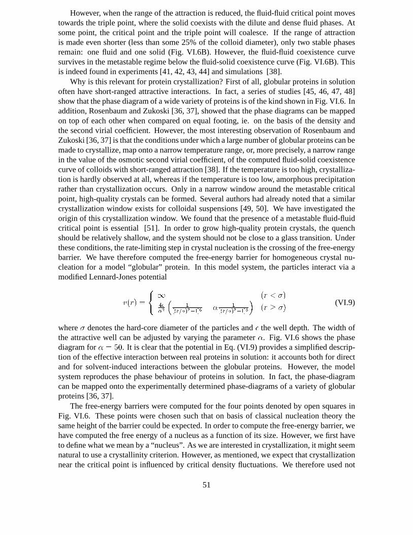
However, when the range of the attraction is reduced, the fluid-fluid critical point movestowards the triple point, where the solid coexists with the dilute and dense fluid phases. Atsome point, the critical point and the triple point will coalesce. If the range of attractionis made even shorter (less than some 25% of the colloid diameter), only two stable phasesremain: one fluid and one solid (Fig. VI.6B). However, the fluid-fluid coexistence curvesurvives in the metastable regime below the fluid-solid coexistence curve (Fig. VI.6B). Thisis indeed found in experiments [41, 42, 43, 44] and simulations [38].

Why is this relevant for protein crystallization? First of all, globular proteins in solutionoften have short-ranged attractive interactions. In fact,a series of studies [45, 46, 47, 48]show that the phase diagram of a wide variety of proteins is ofthe kind shown in Fig. VI.6. Inaddition, Rosenbaum and Zukoski [36, 37], showed that the phase diagrams can be mappedon top of each other when compared on equal footing, ie. on thebasis of the density andthe second virial coefficient. However, the most interesting observation of Rosenbaum andZukoski [36, 37] is that the conditions under which a large number of globular proteins can bemade to crystallize, map onto a narrow temperature range, or, more precisely, a narrow rangein the value of the osmotic second virial coefficient, of the computed fluid-solid coexistencecurve of colloids with short-ranged attraction [38]. If thetemperature is too high, crystalliza-tion is hardly observed at all, whereas if the temperature istoo low, amorphous precipitationrather than crystallization occurs. Only in a narrow windowaround the metastable criticalpoint, high-quality crystals can be formed. Several authors had already noted that a similarcrystallization window exists for colloidal suspensions [49, 50]. We have investigated theorigin of this crystallization window. We found that the presence of a metastable fluid-fluidcritical point is essential [51]. In order to grow high-quality protein crystals, the quenchshould be relatively shallow, and the system should not be close to a glass transition. Underthese conditions, the rate-limiting step in crystal nucleation is the crossing of the free-energybarrier. We have therefore computed the free-energy barrier for homogeneous crystal nu-cleation for a model “globular” protein. In this model system, the particles interact via amodified Lennard-Jones potential

v(r) =

(

1 (r < )

4

2

1

[(r=)

2

1

6

1

[(r=)

2

1

3

(r )

(VI.9)

where denotes the hard-core diameter of the particles and the well depth. The width ofthe attractive well can be adjusted by varying the parameter. Fig. VI.6 shows the phasediagram for = 50. It is clear that the potential in Eq. (VI.9) provides a simplified descrip-tion of the effective interaction between real proteins in solution: it accounts both for directand for solvent-induced interactions between the globularproteins. However, the modelsystem reproduces the phase behaviour of proteins in solution. In fact, the phase-diagramcan be mapped onto the experimentally determined phase-diagrams of a variety of globularproteins [36, 37].

The free-energy barriers were computed for the four points denoted by open squares inFig. VI.6. These points were chosen such that on basis of classical nucleation theory thesame height of the barrier could be expected. In order to compute the free-energy barrier, wehave computed the free energy of a nucleus as a function of itssize. However, we first haveto define what we mean by a “nucleus”. As we are interested in crystallization, it might seemnatural to use a crystallinity criterion. However, as mentioned, we expect that crystallizationnear the critical point is influenced by critical density fluctuations. We therefore used not

51

only a crystallinity criterion, but also a density criterion. We define the size of a high-densitycluster (be it solid- or liquid-like) as the number of connected particles,N

, that have asignificantly higher local density than the particles in theremainder of the system. Thenumber of these particles that is also in a crystalline environment, which is determined onthe basis of the local bond-order parameters [19], is denoted byN

rys

. In our simulations, wehave computed the free-energy “landscape” of a nucleus as a function of the two coordinatesN

andN rys

. Fig. VI.7 shows the free-energy landscape forT = 0:89T

andT = T

.

Figure VI.7: Contour plots of the free-energy landscape along the path from the metastablefluid to the critical crystal nucleus, for our system of spherical particles with short-rangedattraction. The curves of constant free energy are drawn as afunction ofN

andN rys

(seetext) and are separated by 5k

B

T . (A): The free energy landscape well below the criticaltemperature (T=T

= 0:89). The lowest free-energy path to the critical nucleus is indicatedby a dashed curve. This curve corresponds to the formation and growth of a highly crystallinecluster. (B): As (A), but forT = T

. In this case, the free-energy valley (dashed curve) firstruns parallel to theN

axis (formation of a liquid-like droplet), and then moves towards astructure with a higher crystallinity (crystallite embedded in a liquid-like droplet). The freeenergy barrier for this route is much lower than the one in (A).

The free-energy landscapes for the other two points are qualitatively similar to the one forT = 0:89T

and will not be shown here.We find that away fromT

(both above and below),the path of lowest free energy is one where the increase inN

is proportional to the increasein N

rys

(Fig. VI.7A). Such behavior is expected if the incipient nucleus is simply a smallcrystallite. However, aroundT

, critical density fluctuations lead to a striking change in thefree-energy landscape (Fig. VI.7B). First, the route to thecritical nucleus leads through aregion whereN

increases whileN rys

is still essentially zero. In other words: the first steptowards the critical nucleus is the formation of a liquid-like droplet. Then, beyond a certain

52

critical size, the increase inN

is proportional toN rys

, that is, a crystalline nucleus formsinside the liquid-like droplet.

Clearly, the presence of large density fluctuations close toa fluid-fluid critical point hasa pronounced effect on the route to crystal nucleation. But,more importantly, the nucleationbarrier close toT

is much lower than at either higher or lower temperatures (Fig. VI.8). Theobserved reduction inG nearT

by some30kB

T corresponds to an increase in nucle-ation rate by a factor1013. Finally, let us consider the implications of this reduction of the

0.8 1.0 1.2T/Tc

50

75

100

β∆G

*

Figure VI.8: Variation of the free-energy barrier for homogeneous crystal nucleation, as afunction ofT=T

, in the vicinity of the critical temperature. The solid curve is a guide to theeye. The nucleation barrier atT = 2:23T

is 128k

B

T and is not shown in this figure. Thesimulations show that the nucleation barrier goes through aminimum around the metastablecritical point (see text).

crystal nucleation barrier nearT

. An alternative way to lower the crystal nucleation barrierwould be to quench the solution deeper into the metastable region below the solid-liquidcoexistence curve. However, such deep quenches often result in the formation of amorphousaggregates [33, 36, 37, 42, 43, 44, 48]. Moreover, in a deep quench, the thermodynamic driv-ing force for crystallization (

liq

ryst

) is also enhanced. As a consequence, the crystallitesthat nucleate will grow rapidly and far from perfectly [31].Thus the nice feature of crystalnucleation in the vicinity of the metastable critical pointis, that crystals can be formed at arelatively small degree of undercooling. This should lead to protein crystals of high quality.It is clear that our model is simplified. However, our model system reproduces the phasebehavior of compact proteins in solution. Moreover, the mechanism that we describe here isgeneral, and does not depend on the details of the interaction potential. We expect that whena metastable fluid-fluid coexistence is present below the stable sublimation curve, criticaldensity fluctuations facilitates the formation of ordered structures.

Conclusions

Ostwald formulated his step rule more than a century ago [4] on the basis of macroscopicstudies of phase transitions. The simulations suggest thatalso on a microscopic level, a

53

“step rule” may apply and that metastable phases may play an important role in nucle-ation. We find that the structure of the pre-critical nuclei is that of a metastable phase(bcc/chains/liquid). As the nuclei grow, the structure in the core transforms into that ofthe stable phase (fcc/liquid/fcc-crystal). Interestingly, in the interface of the larger nucleitraces of the structure of the smaller nuclei are retained.

54

Bibliography

[1] J. W. Gibbs,The Scientific Papers of J. Willard Gibbs, Dover, New York (1961).

[2] M. Volmer and A. Weber, Z. Phys. Chem.119, 227 (1926).

[3] R. Becker and W. Doring, Ann. Phys.24, 719 (1935).

[4] W. Ostwald, Z. Phys. Chem.22, 289 (1897).

[5] I. N. Stranski and D. Totomanow, Z. Physikal. Chem.163, 399 (1933).

[6] R. E. Cech, J. Met.8, 585 (1956).

[7] H.-M. Lin, Y.-W. Kim, and T. F. Kelly, Acta Metall.36, 2537 (1988).

[8] W. Loser, T. Volkmann, and D. M. Herlach, Mat. Sci. Eng.A178, 163 (1994).

[9] S. Alexander and J. P. McTague, Phys. Rev. Lett.41, 702 (1978).

[10] W. Klein and F. Leyvraz, Phys. Rev. Lett.57, 2845 (1986).

[11] M. J. Mandell, J. P. McTague, and A. Rahman, J. Chem. Phys. 64, 3699 (1976).

[12] M. J. Mandell, J. P. McTague and A. Rahman, J. Chem. Phys.66, 3070 (1977).

[13] C. S. Hsu and A. Rahman, J. Chem. Phys.71, 4974 (1979).

[14] R. D. Mountain and A. C. Brown, J. Chem. Phys.80, 2730 (1984).

[15] S. Nose and F. Yonezawa, J. Chem. Phys.84, 1803 (1986).

[16] J. Yang, H. Gould, and W. Klein, Phys. Rev. Lett.60, 2665 (1988).

[17] W. C. Swope and H. C. Andersen, Phys. Rev. B41, 7042 (1990).

[18] G. M. Torrie and J. P. Valleau, Chem. Phys. Lett.28, 578 (1974).

[19] P. J. Steinhardt, D. R. Nelson, and M. Ronchetti, Phys. Rev. B 28, 784 (1983).

[20] P. R. ten Wolde, M. J. Ruiz-Montero, and D. Frenkel, Phys. Rev. Lett.75, 2714 (1995).

[21] P. R. ten Wolde, M. J. Ruiz-Montero, and D. Frenkel, J. Chem. Phys.104, 9932 (1996).

[22] S. Pronk and D. Frenkel, J. Chem. Phys.110, 4589 (1999).

55

[23] D. Wright, R. Caldwell, C. Moxeley, and M. S. El-Shall, J. Chem. Phys.98, 3356(1993).

[24] D. Wright and M. S. El-Shall, J. Chem. Phys.98, 3369 (1993).

[25] F. F. Abraham, Science168, 833 (1970).

[26] V. Talanquer and D. W. Oxtoby, J. Chem. Phys.99, 4670 (1993).

[27] P. R. ten Wolde, D. W. Oxtoby and D. Frenkel, Phys. Rev. Lett. 81, 3695 (1998).

[28] P. R. ten Wolde and D. Frenkel, J. Chem. Phys.109, 9901 (1998).

[29] I. Kusaka, Z.-G. Wang, and J. H. Seinfeld, J. Chem. Phys.108, 3446 (1998).

[30] A. McPherson,Preparation and analysis of protein crystals, Krieger Publishing, Mal-abar (1982).

[31] S. D. Durbin and G. Feher, Ann. Rev. Phys. Chem.47, 171 (1996).

[32] F. Rosenberger, J. Crystal Growth166, 40 (1996).

[33] A. George and W. W. Wilson, Acta Crytallogr. D50, 361 (1994).

[34] T. L. Hill, An Introduction to Statistical Thermodynamics, Dover, New York (1986).

[35] E. G. Richards,An Introduction to physical properties of large molecules in solution,Cambridge University Press, Cambridge (1980).

[36] D. Rosenbaum, P. C. Zamora, and C. F. Zukoski, Phys. Rev.Lett. 76, 150 (1996).

[37] D. Rosenbaum and C. F. Zukoski, J. Crystal Growth169, 752 (1996).

[38] M. H. J. Hagen and D. Frenkel, J. Chem. Phys.101, 4093 (1994).

[39] A. P. Gast, W. B. Russell, and C. K. Hall, J. Colloid Interface Sci.96, 251 (1983).

[40] A. P. Gast, W. B. Russell, and C. K. Hall, J. Colloid Interface Sci.109, 161 (1986).

[41] H. N. W. Lekkerkerker, W. C. K. Poon, P. N. Pusey, A. Stroobants, and P.B. Warren,Europhys. Lett.20, 559 (1992).

[42] S. M. Ilett, A. Orrock, W. C. K. Poon, and P. N. Pusey, Phys. Rev. E51, 1344 (1995).

[43] W. C. K. Poon, A. D. Pirie, and P. N. Pusey, Faraday Discuss. 101, 65 (1995).

[44] W. C. K. Poon, Phys. Rev. E55, 3762 (1997).

[45] C. R. Berland, G. M. Thurston, M. Kondo, M. L. Broide, J. Pande, O. O. Ogun, and G.B. Benedek, Proc. Natl. Acad. Sci. USA89, 1214 (1992).

[46] N. Asherie, A. Lomakin, and G. B. Benedek, Phys. Rev. Lett. 77, 4832 (1996).

[47] M. L. Broide, T. M. Tominc, and M. D. Saxowsky, Phys. Rev.E 53, 6325 (1996).

56

[48] M. Muschol and F. Rosenberger, J. Chem. Phys.107, 1953 (1997).

[49] A. Kose and S. Hachisu, J. Colloid Interface Sci.55, 487 (1976).

[50] C. Smits, J. S. van Duijneveldt, J. K. G. Dhont, H. N. W. Lekkerkerker, and W. J. Briels,Phase Transitions21, 157 (1990).

[51] P. R. ten Wolde and D. Frenkel, Science277, 1975 (1997).

57

58

VII

Molecular Modeling and Simulation of aPhotosynthetic Reaction Center

Matteo Ceccarelli1, Marc Souaille1;2, and Massimo Marchi3

1 Centre Europeen de Calcul Atomique et Moleculaire (CECAM), Ecole NormaleSuperieure de Lyon, 46 Allee d’Italie, F-69364 Lyon Cedex 07, France

2 Physical Chemistry Institute, University of Zurich, Winterthurerstrasse 190,CH-8057 Zurich, Switzerland

3 Section de Biophysique des Proteines et des Membranes, DBCM, CEA–Saclay,F-91191 Gif-sur-Yvette Cedex, France

Abstract

In this paper we give an account of our ongoing effort to understand bacterial photosynthe-sis at the atomic level. First, we describe earlier simulations which investigate the nuclearmotion coupled to the primary donor excitation in bacterialreaction centers (RC). Then, wediscuss the molecular modeling of the chromophores of the RCof rhodobacter sphaeroides.Finally, we report on our latest molecular dynamics simulation results concerning a RC in adetergent micelle.

Introduction

The bacterial photosynthetic reaction center (RC)[3, 4] isa membrane protein composed ofchromophores (bacteriochlorophylls, bacteriopheophytins and quinones) and three proteinsubunits named L, M and H (see Fig. VII.1). While proteins L and M form two branchesof the RC (almost the mirror images of each other) and providethe necessary scaffolding tohold in place bacteriochlorophylls and bacteriopheophytins, the H subunit is in contact withthe bacterial cytoplasm and binds the quinones in its interior. In the region of the RC nearthe pery-plasm is located a bacteriochlorophylls dimer, the so–called special pair (P). Thischromophore is at the junction point between the L and M branches and is involved directlyin the first photosynthetic electron transfer.

59

Figure VII.1: Pictorial views of the reaction center ofrb. sphaeroides(top) and its chro-mophores (bottom).

Photosynthesis in purple bacteria commences with the excitation of P, the energy for suchexcitation being transferred directly from surrounding light harvesting proteins. The excitedstate P then decays in a charge transfer state, P+ H

L

, where an electron has been exchangedwith the bacteriopheophytins on the L branch (H

L

), 17 A away. The electron transfer (ET),P H

L

! P+ H

L

, occurs with a quantum yield of 1 and is called primary chargeseparation.Experimentally no electron is detected arriving to the bacteriopheophytins on the M branch,HM

. Subsequently, the electron on HL

is first, transferred to the quinone (whose chemicalidentity changes with the type of RC) on the L side, or Q

A

, and second, passed to the quinoneon the M side, or Q

B

.

The primary ET in RC presents many aspects which are very challenging to understand.Despite the many efforts, as yet unresolved by either experiment or theory are the followingfeatures: (a) the remarkably fast rate (

1

3 ps) of this electron exchange between twochromophores separated by 17A; (b) the fact that the M branch acts as spectator in the re-action, despite structural similarities and quasi-C

2

symmetry between the L and M subunits;(c) the role of the accessory bacteriochlorophyll in Van derWaals contact with P and H

L

inthe mechanism of ET.

Since the first crystal structures of bacterial photosynthetic RC have been resolved[3],there have been a few investigations of the primary ET in the photosynthetic reaction cen-ter by MD simulations[3-6]. All of these investigations arebased on a reduced quantummechanical model whose relevant parameters are derived by running classical MD. This isthe so–called spin–boson model[9]. In the last 10 years or so, powerful techniques, de-rived mostly from this simple model, have been developed to handle linear and non–linear

60

spectroscopy[10]. This entails using the so–called spectral density formalism which re-lates spectroscopic properties to the fluctuation in the energy gap (i.e., energy difference)function between the ground and the excited states. ET theories derived from the Marcusapproach[11] and based on the same spectral density formalism have also been proposed inthe past[9]. In that case the energy gap is the energy difference between the neutral and thecharge transfer states.

This paper is an account of our continuing effort in the investigation of the primary chargeseparation in bacterial RC. In the next sections we will describe in some detail our advancesin the modeling and understanding of the RC photosynthetic proteins.

Nuclear coupling in the P! P transition

Due to limitations in computational power, the first simulations of RC proteins either ignored[6,7] or used mean field approximations[5, 8] of the environmentsurroundings these proteins.In both cases, however, only the atoms closer to the cofactors were actually simulated whilethe remaining atoms were kept fixed or harmonically restrained. In Ref. [12] we have im-proved on this model by simulating a RC ofrhodobacter (rb.) sphaeroidesin water. Inpractice, the simulation box of dimensionsa = 65:63 A , b = 58:0 A and = 65:0 A wascomposed of a RC protein having its quasi-symmetry axis parallel to thea-direction and of4104 water molecules which filled in the voids. All the simulation runs in Ref. [12] werecarried out by using our in-house molecular dynamics program ORAC[13, 14]. In this earlierwork, a spherical cutoff of 9A was applied to the non-bonded interactions thus neglectinglong range electrostatic effects. The potential parameters and the molecular topology of thesystem is fully described in Ref. [12]. Simulations of about100 ps each were carried out at300 K and 50 K. The latter calculation was done to compare withtime resolved data obtainedat low temperatures (' 10 K)[15].

Our investigation on a hydrated reaction center was focusedon the the dynamics of theP! P, transition which occurs before primary charge separation. In the past, time resolvedstimulated emission studies in the P! P region have been carried out on different RC[15,16]. A common feature obtained in all these studies is that low frequency (less than 200cm1) nuclear modes are coupled to this photoexcitation. Although it has been shown that theenvironment surrounding the special pair is responsible for the coherent oscillations foundin the spectra[15], no indication on the atomistic origin ofthese vibrations has been found.

The principal aim of our study was to gain insights in the coupling mechanism betweennuclear modes and electronic transition. To achieve this goal, we computed the time–resolved stimulated emission spectra in different regionsof the P ! P transition. Thisinvolved carrying out molecular dynamic simulations of thehydrated bacterial reaction cen-ter of rb. sphaeroidesin the ground and excited states of the special pair.

Modeling photoexcitation

The spin–boson model is well suited to handle theoreticallyphotoexcitation of a pigmentmolecule in contact with a dielectric from a ground to an excited state. In this model, thetwo electronic states of the chromophores are represented by a two–level system which islinearly coupled to a fluctuating dielectric described by harmonic fields. The interactionbetween dielectric and the photoexcitation is responsiblefor the broadening of the pigment

61

electronic bands in solution or within a protein. It is worthto point out that even for complexsystems the restriction on the harmonicity of the field is notso constraining as it might seem.Indeed, the binding requirement here is that only the nuclear modes coupled to photoexci-tation be harmonic[7]. This is in general compatible with very anharmonic systems such asthat discussed here.

Q0

Q

Ep U

Figure VII.2: Displaced oscillator manifold. Ep

is the free energy of obtained by integrationof the boson bath.

The underlying Hamiltonian of the spin–boson model is as follows:

H = jg iH

g

h gj+

e

H

e

ih

2

e

+

+ jg iH

ge

h ej+ je iH

eg

h gj

whereH

is the diabatic Hamiltonian of the state (ground or excited),Hge

andHeg

arethe interstate couplings. and is the inverse lifetime of the excited state. Only the diabaticHamiltonians are relevant to electron-nuclear coupling. If only a single harmonic mode of thebath is coupled the two–level system, the HamiltoniansH

g

andHe

correspond to a displacedharmonic oscillator system, i.e.

H

g

= H

B

+

1

2

m!

2

0

Q

2

H

e

= H

B

+

1

2

m!

2

0

(Q

2

+ 2Q

0

Q) + G (VII.1)

U = m!

2

0

Q

0

Q+G:

Here,G is the electronic energy difference between ground and excited states in the gasphase andH

B

is the Hamiltonian of those modes of the boson bath not coupled to the elec-tronic transition. Also,Q

0

is the displacement andU is the energy gap (see Fig. VII.2).In time resolved stimulated emissions experiment[15] the sample is at first pumped to the

excited state by a test beam of light of a given frequency!

1

. Then, at variable time delays,a white light continuum beam is shone on the photoexcited sample to probe its absorptionspectrum. In the end, the experiment measures the time resolved transmission induced bythe photoexciting beam of frequency!

1

on the absorption at a given frequency!2

. This

62

0.0 50.0 100.0 150.0 200.0 250.0ω/cm−1

−4.0

−2.0

0.0

2.0

I ω2(ω

)

Exp.Calc.

Figure VII.3: Comparison between the experimental and calculated reduced spectral densi-ties. The two spectra are normalized with respect to the intensities of their lowest frequencypeak.

transmission is then converted to absorption changes whichin turn are proportional to thestimulated emission coefficientS(!

1

; !

2

; t). Using a displaced harmonic oscillator model asin Eqs. VII.1, Mukamel[10] has shown that this emission coefficient can be readily computedfrom the knowledge of the energy gap dynamics. Thus, the major goal of our moleculardynamics investigation was to compute the energy gap for theP! P transition as a functionof time. Although empirical charge distribution was used inour study,ab initio data can,in principle, be obtained to model the charge distribution in the P and P states. As forthe pseudopotential model for the interaction between the special pair and the environment(proteins and water), we used a purely electrostatic model.

Results

After 130 ps of molecular dynamics equilibration and 100 ps of additional run time, thedeviation from the X–ray structure (X

rms

) of the three subunits increased to an average of3.1 A for the carbons. The subunit H had the largest deviations, while themembrane-spanning helices had a relatively low value of X

rms

. Of the 4101 water molecules solvatingthe RC, only 304 were trapped near the protein for more than 90% of the time. They werefound more often in the hydrophilic region of the subunits than near the membrane–spanninghelices of the L and M subunits.

During the 90 ps run at 50 K in the P state, the energy gap or energy difference betweenthe P excited and ground state were accumulated. The energy gap probability distributionderived from this simulation obeyed, to a good approximation, Gaussian statistics. Thisresult gives credibility to our approach in the calculationof the electronic spectra based on alinear response model.

Our calculation found that the oscillatory part ofS(!

1

; !

2

; t) at!1

( orH!

2

(t) ) behaveslike the experimental time evolution of the stimulated emission spectra. As shown in FromFig. VII.4, away from the bottom of the emission peak (!

2

= 968 nm),H!

2

(t) shows anoscillatory behavior, with a phase change of between!

2

=987 and 949 nm. Noticeably,at!

2

=968 nm, the maximum of the emission peak, the aspect ofH

!

2

(t) changes showing adecrease in the amplitude of the oscillations as well as the appearance of different oscillatingfeatures.

For all wavelength,H!

2

(t) shows coherent oscillations well beyond the 3 ps time mark.

63

0.0 2.0 4.0 6.0 8.0 10.0Time/ps

−0.50.00.5

Hω

2(t)

−0.50.00.5

Hω

2(t)

−0.50.00.5

Hω

2(t)

−0.50.00.5

Hω

2(t) 1003 nm

968 nm

987 nm

949 nm

a

b

c

d

Figure VII.4: Calculated time resolved stimulated emission intensity. From top to bottomthe four panels present results for probing frequency!

2

equal to respectively (a) 1003 , (b)968, (c) 987 and (d) 949 nm. For comparison, the autocorrelation function of the energy gaphas been added on the panel (a) (dotted line).

This contrasts with experimental results showing an exponential damping of the time corre-lation function within this time scale. Such a damping mightbe due to frictional damping orstatic disorder on the RCs.

The experimental and calculated reduced spectral densities obtained by Fourier transformof H

!

2

(t) are compared in Fig. VII.3. Although the calculation reproduces the first experi-mental peak at 10 cm1, the activities of the higher frequency modes is underestimated withrespect to experiment. This result and the finding in Ref. [12], that the higher frequencypeaks ( at 67 and 125 cm1) in the dimer energy gap spectral density are weakened consid-erably by solvent effects, may suggest the our simple electrostatic model underestimates thedimer-solvent energy gap with respect to the intra dimer counterpart.

Improving the reaction center model

Starting from the earlier simulation[12] described above,we have in the last few years,achieved major improvements on the modeling of the RC proteins and their environment.Indeed, MD simulations of membrane proteins are challenging for different reasons. First,although force fields for proteins have been steadily improving, ab initio based potentialmodels for chromophores such as bacteriochlorophylls and quinones have been lacking. Itis clear that in studies of ET realistic modeling of the prosthetic groups is essential. Second,because the coupling between electronic states and the solvent (the surrounding protein) isat the first order electrostatic, electrostatic forces mustbe computed accurately in MD sim-ulations. Because of the high cost this is not done in standard biomolecular simulations andwas not done in our earlier simulation. Third, the large sizeof the system: the RC protein ofrb. sphaeroidesby itself contains more than 15,000 atoms. The size of the system increasesconsiderably if its natural environment, solvent and phospholipid membrane, is included inrealistic simulations. Last but not least, the issue of electronic polarizability in modelingRC’s will need to be addressed because it is relevant to electron transfer.

64

Modeling the chromophores

Deriving a force field for chromophores entails calculations of the electronic structure ofthese large molecules. In recent times, the density functional theory (DFT)[17] approach hasbeen gaining popularity in the chemical community to investigate on the electronic groundstate structure of chemically relevant system. In the past,this technique has been applied byus and others to the study of bacteriochlorophylls molecules[18, 19] and quinones[20]. Allour DFT calculations on the chromophores were carried out inthe local density plus gradientcorrections approximation (LDA+GC), while the Kohn-Sham orbitals were expanded in abasis set of plane waves compatible with the periodic supercell containing the molecule.In this scheme only the valence electrons are included explicitly in the calculation. Theeffects due to atomic core electrons are taken into account by ab initio soft pseudopotentialsassociated with each atom[21].

In an earlier calculation[18] on a crystal of methyl bacteriopheophorbide (MeBPheo)a we have shown the viability of the DFT technique towards the computation of the elec-tronic structure and optimization of molecules important for photosynthesis. In a more re-cent investigation[19] we have carried out the first (to our knowledge) high quality DFTabinitio calculation of the vibrational structure of a bacteriochlorophyll derivative and assignedthe in plane frequencies detectable by resonant Raman spectroscopy. Theab-initio calcu-lations were performed on an isolated methyl bacteriochlorophyll a molecule. Our majorresult was the determination of a complete set of eigenvalues and eigenvectors which un-ambiguously identified the fundamental modes. The computedfrequencies are in very goodagreement with the available experimental data and show a small root mean square deviation(less than 20 cm1) from experimental modes. In addition, our calculation wasable to pinpoint a strong symmetric behavior of many in–plane vibration similar to results obtained forporphyrines. This is in contrast with results of earlier semiempirical calculations[22], whichpredicted more localized modes in (bacterio)pheophorbide-type macrocycles.

Based on DFT calculations on chlorophylls and, additionally, on ubiquinone and theRC main detergent, lauryl dimethylamine oxide or LDAO, we have then developed a forcefield for their classical modelization. Our approach to thisundertaking was straightforward.We initially use the DFT optimized structures and the vibrational analysis to determine thebonded part of the potential parameters described by the AMBER potential function. Then,atomicab initio partial charges on the chromophore are used to account for electrostaticeffects. At a later stage, experimental data from X-ray crystallography are used to check thestructural properties of the molecule in the condensed state and to refine the intermolecularLennard-Jones parameters.

A good starting point for parameter refinement of large molecules are values optimizedon small fragments. In the case of bacteriochlorophylls, westarted modeling their chemicalconstituents such as pyrrol, methyl acetate and methylic groups, for which DFT calculationswere also made. Subsequently, these parameters were transferred to the larger moleculesand refined as much as possible to reproduce the bacteriochlorophylls DFT results. Theexisting AMBER parameters were used, whenever possible, asa starting point for potentialof the fragments. Given the relative smaller size of the quinone and the hydrophilic head ofLDAO1, the force field refinement was done in this case directly on the molecules and notthe fragments.

1DFT optimization and vibrational analysis were performed on models of ubiquinone and LDAO obtainedby cutting and saturating their tails after the first 3 carbonatoms.

65

1594 1611 1620 1625

1571 1581 1614 1634

1665 1546 200 528

1648 1545 190 518

MM

DFT

MM

DFT DFT oop

Figure VII.5: Methyl bacteriochlorophylla normal modes. Frequencies are in cm1

In all our molecular modeling, special care was taken not only to reproduce the DFTfrequencies, but also the eigenvectors. Indeed, a great deal of spectroscopic experiments onphotosynthetic RC involve directly or indirectly the nuclear dynamics of the chromophores.In Fig. VII.5 we present some typical in–plane and out-of–plane normal modes computedfrom DFT and molecular mechanics (MM). Its visual inspection shows the good agreementbetween DFT and MM eigenvectors.

Methods for molecular dynamics

Due to the ever increasing power of computers, simulations of solvated proteins for lengthsup to hundreds of ps is nowadays becoming routine on desktop workstations. Howeverthe simulation of membrane proteins stabilized in membraneor detergent environments ismore challenging given the complexity and the large size of such systems. In addition, thedielectric properties of the aqueous solvent are of crucialimportance to electron and protontransfer reactions. Consequently, any theoretical investigation of such phenomena must dealwith the problem of how to simulate large systems and, at the same time, correctly handlelong-range electrostatic interactions.

In the past few years, we have developed new and fast multipletimestep MD algorithms[13,23, 24] which allow simulations of very large systems and include an accurate representationof the Coulombic interactions for infinite systems. The electrostatic series can be computedin principleexactlyusing the Ewald re-summation technique[25]. This method inits stan-dard implementation, is extremely CPU demanding and scaleslike N

2, with N being thenumber of charges with the unfortunate consequence that even moderately large size simu-

66

lations of inhomogeneous biological systems are not withinits reach. Notwithstanding, therigorous Ewald method, which suffers of none of the inconvenients experienced by the re-action field approach, has very recently regained the spotlight with the particle mesh Ewald(PME) technique[26]. PME, based on older ideas of Hockney’s[27], is essentially an inter-polation technique which involves charge smearing onto a regular grid and evaluation of thereciprocal lattice energy sums via fast Fourier Transform (FFT). The performance of thistechnique, both in accuracy and efficiency, is very good. Most importantly, the computa-tional cost scales likeNlogN for largeN , but it is essentiallylinear for practical applicationup to 20,000 particles.

The combination of the multiple time step algorithm and PME[28] makes the simula-tion of large size biomolecular systems such as membrane proteins extremely efficient andaffordable even for long time spans. Furthermore, it does not involve any uncontrolled ap-proximation and is entirely consistent with periodic boundary conditions.

Our most recent r-RESPA algorithm in combination with constraints and PME achievessubstantial computer savings (more than 10 times) with respect to standard Ewald tech-niques. In spite of this excellent performance, for a 40,000atom system 1 ns of simula-tion takes more than 12 days on a fast Compaq EV5 station. Further improvements canbe achieved running simulation on parallel machines. Indeed, a parallelized version ofORAC has been recently developed and each ns of simulation for thesame systems nowtakes 3 days on 8 processors of a Compaq ES232 cluster.

Simulation of a RC in a detergent micelle

To elucidate at the atomic level the asymmetry and the mechanism of the primary chargeseparation it is advantageous to construct a reliable modelof the RC protein and of its en-vironment. Given the latest technical developments in our computational tools[24], we have

0.0 1000.0 2000.0 3000.0Time/ps

0.0

0.5

1.0

1.5

2.0

XR

MS/A

Backbone Deviation from X-ray (T = 300 K P = 1 MPa)

Instantaneous

Dev. from avg.

Figure VII.6: Deviation from the crystallographic structure of the RC protein during 3.4 nsof simulation. The upper curve is the instantaneous deviation, while the lower curve is thedeviation of the averaged structure.

recently been able to simulate the RC ofrhodobacter sphaeroidesinglobed in a model mi-celle of detergent lauryl-dimethyl-amine-oxide (LDAO) and hydrated by water for more than3.4 ns. This hydrated micelle was constructed as follows. First, the isolated RC protein[29]

67

including 9 LDAO molecules and 160 crystallization waters were relaxed at 20 K for about5 ps to eliminate any accidental stress due to the force field.To this structure we then added150 LDAO molecules initially disposed around the protein hydrophobic helices in an all–trans conformation and with the polar head pointing away from the protein assembly. Fromthis conformation we ran equilibrations of the LDAO only (i.e. keeping fixed the proteincoordinates) for 30 and 230 ps at 250 K and 400 K, respectively. After this step the addedLDAO had relaxed to form an aggregate around the RC in which the aliphatic chains werein contact with the transmembrane helices and the polar heads pointed towards the exterior.

Finally, the system was placed in an orthorhombic box of dimension of 76x84x80A andhydrated by 6323 additional water molecules to fill the cell voids. A simulation run on ourfinal system, totaling 40,327 atoms, was then started at constant temperature and pressure atT=300 K and P=0.1 MPa.

28150 100 1501 200 250Residue

0

25

50

75

100400 450 500 550282 350 583

0

25

50

75

100

B-f

acto

r/A

2

SimulationCrystallographic

584 823650 700 750 8000

25

50

75

100Protein subunits: H-M-L (top to bottom)

Figure VII.7: Comparison between calculated and crystallographic Debey–Waller factors.

To achieve full relaxation the simulation box was entirely flexible for the first 300 ps andevolved to a hexagonal–like structure. For the remaining runs only isotropic changes of thebox were allowed. With the simulation algorithms in the NPT ensemble described in Ref.[30] and on 32 processors of a T3E parallel computer, 3.4 ns ofsimulation required 21 daysof simulation.

In this report we only provide a brief account of some preliminary results on the structureof the simulated RC. The full account of our results will be given in future publications.

Fig. VII.6 shows the overall deviation (or Xrms

) of the RC backbone atoms from theirX–ray coordinates. We first notice that with respect to our previous, and much shorter,simulations the X

rms

is twice as small. Moreover, the RC protein shows with time anoveralldrift towards higher X

rms

. With additional investigation, we find that this is due essentiallyto relative motion of subunit H with respect to L and M.

In addition to a low deviation from the crystallographic structure, the experimental Debey–Waller factors are also well reproduced within a constant offset, probably due to disorder (seeFig. VII.7).

In Fig. VII.8 we show a pictorial view of the RC protein surrounded by its detergent.

68

Figure VII.8: Instantaneous view of the RC ofrb. sphaeroidesduring the simulation (seetext for details).

The LDAO molecules are represented by their molecular surface and no water moleculesare displayed. This picture is evocative of the detergent micellar structure revealed by thelow resolution neutron scattering study of the RC crystal[31]. As in that investigation, ourdetergent has formed a distinct micelle around the protein.Its thickness along the quasi-C

2

symmetry axis is around 25-30A, similar to that observed experimentally. We point out thatin the simulation the micelle is a rather dynamics structurewith a lateral diffusion constantof 5.61010 m2 s1 which is about 30 times larger than that of the RC protein.

69

Conclusion and perspectives

Thanks to our ongoing efforts in molecular modeling of RC proteins, we have recently de-vised a reliable force field and a faithful model for photosynthetic RC proteins in detergentenvironment. Long simulations (3.4 ns) of a RC protein ofrb. sphaeroidesin its deter-gent environment have also been possible due our recent technical developments in the MDmethodology. The analysis of properties related to the primary ET and its asymmetry iscurrently underway. Our first task is to compute the average electrostatic field and its dy-namics on the bacteriochlorophyll chromophores of the L andM branches to investigate theorigin of the ET asymmetry. In this calculation we include both contributions from the fixedcharges of the RC and from induction computed from a distributed polarizable model[32].Investigation of effects from mutations is also underway.

70

Bibliography

[1] Nose, S.Mol. Phys.1986, 57, 187–191.

[2] Torrie, G.; Valleau, J.Chem. Phys. Lett.1974, 28, 578–581.

[3] Deisenhofer, J.; Epp, O.; Mike, K.; Huber, R.; Michel, H.J. Mol. Biol.1984, 180, 385.

[4] Deisenhofer, J.; Michel, H.Science1989, 245, 1463.

[5] Creighton, S.; Hwang, J. K.; Warshel, A.; Parson, W. W.; Norris, J.Biochemistry1988,27, 774.

[6] Treutlein, H.; Schulten, K.; Brunger, A.; Karplus, M.; Deisenhofer, J.; Michel, H.Proc.Natl. Acad. Sci. USA1992, 89, 75.

[7] Marchi, M.; Gehlen, J. N.; Chandler, D.; Newton, M.J. Am. Chem. Soc.1993, 115,4178.

[8] Parson, W. W.; Chu, Z. T.; Warshel, A.Photosynthesis Research1998, 55, 147.

[9] Chandler, D. InLiquids, Freezing and the glass transition,Leveque, D.; Hansen, J. P.,edts. North Holland, 1991, Page 193.

[10] Mukamel, S.Principles of Nonlinear Optical Spectroscopy. Oxford University Press,1995.

[11] Marcus, R. A.; Sutin, N.Biochim. Biophys. Acta1985, 811, 256.

[12] Souaille, M.; Marchi, M.J. Am. Chem. Soc.1996, 119, 3948.

[13] Procacci, P.; Darden, T.; Paci, E.; Marchi, M.J. Comp. Chem.1997, 18, 1848.

[14] Procacci, P.; Marchi, M. InAdvances in the Computer Simulations of Liquid Crys-tals, Zannoni, G.; Pasini, P.,edts, NATO ASI School (Kluwer Academic publishers,Dodrecht the Netherlands, 1999).

[15] Vos, M. H.; Rappaport, F.; Lambry, J.-C.; Breton, J.; Martin, J.-L. Nature1993, 363,320.

[16] Vos, M. H.; Jones, M. R.; Hunter, C. N.; Breton, J.; Lambry, J.-C.; Martin, J.-L.Bio-chemistry1994, 33, 6750.

[17] Parr, R. G.; Yang, W.Density Functional Theory of Atoms and Molecules. OxfordUniversity Press, Oxford1989.

71

[18] Marchi, M.; Hutter, J.; Parrinello, M.J. Am. Chem. Soc.1996, 118, 7847.

[19] Ceccarelli, M.; Lutz, M.; Marchi, M.J. Am. Chem. Soc.January (2000), . In press.

[20] Nonella, M.; Brandli, C.J. Phys. Chem.1996, 100, 14549.

[21] Troullier, N.; Martins, J. L.Phys. Rev. B1991, 43, 1993.

[22] Donohoe, R. J.; Frank, H. A.; Bocian, D. F.Photochem. Photobiol.1988, 48, 531.

[23] Procacci, P.; Darden, T.; Marchi, M.J. Phys. Chem.1996, 100, 10464.

[24] Procacci, P.; Marchi, M. InAdvances in the Computer Simulations of Liquid Crys-tals, Zannoni, G.; Pasini, P.,edts, NATO ASI School (Kluwer Academic publishers,Dodrecht the Netherlands, 1998).

[25] de Leeuw, S. W.; Perram, J. W.; Smith, E. R.Proc. R. Soc. Lond.1980, A 373, 27.

[26] Darden, T.; York, D.; Pedersen, L.J. Chem. Phys.1993, 98, 10089.

[27] Hockney, R. W.Computer Simulation Using Particles. McGraw-Hill, New York, 1989.

[28] Procacci, P.; Marchi, M.J. Chem. Phys.1996, 104, 3003–3012.

[29] Ermler, U.; Fritzsch, G.; Buchanan, S. K.; Michel, H.Structure1994, 2, 925.

[30] Marchi, M.; Procacci, P.J. Chem. Phys.1998, 109, 5194.

[31] Roth, M.; Lewit-Bentley, A.; Michel, H.; Deisenhofer,J.; Huber, R.; Oesterhelt, D.Nature1989, 340, 659.

[32] Thole, B. T.Chem. Phys.1981, 59, 341.

72

VIII

From Molecular Dynamics to DissipativeParticle Dynamics

Peter V. Coveney1, Gianni De Fabritiis1,Eirik G. Flekkøy2 and James Christopher1

1Centre for Computational Science, Queen Mary and Westfield College,University of London, London E1 4NS, United Kingdom

2Department of Physics, University of OsloP.O. Box 1048 Blindern, 0316 Oslo 3, Norway

Abstract

We describe a mesoscopic modeling and simulation techniquethat is very close to the tech-nique known as dissipative particle dynamics. The model is derived from molecular dynam-ics by means of a systematic coarse-graining procedure. Thus the rules governing this formof dissipative particle dynamics reflect the underlying molecular dynamics; in particular allthe underlying conservation laws carry over from the microscopic to the mesoscopic descrip-tions. Whereas previously the dissipative particles were spheres of fixed size and mass, nowthey are defined as cells on a Voronoi lattice with variable masses and sizes. This Voronoilattice arises naturally from the coarse-graining procedure which may be applied iterativelyand thus represents a form of renormalisation-group mapping. It enables us to select any de-sired local scale for the mesoscopic description of a given problem. Indeed, the method maybe used to deal with situations in which several different length scales are simultaneouslypresent. Simulations carried out with this scheme show goodagreement with theoreticalpredictions for the equilibrium behavior.

Introduction

The non-equilibrium behavior of fluids continues to presenta major challenge for both the-ory and numerical simulation. In recent times, there has been growing interest in the study ofso-called ‘mesoscale’ modeling and simulation methods, particularly for the description ofthe complex dynamical behavior of many kinds of soft condensed matter, whose propertieshave thwarted more conventional approaches. As an example,consider the case of complexfluids with many coexisting length and time scales, for whichhydrodynamic descriptions

73

are unknown and may not even exist. Such fluids include multi-phase flows, particulateand colloidal suspensions, polymers, and amphiphilic fluids, including emulsions and mi-croemulsions. Fluctuations and Brownian motion are often key features controlling theirbehavior.

From the standpoint of traditional fluid dynamics, a generalproblem in describing suchfluids is the lack of adequate continuum models. Such descriptions, which are usually basedon simple conservation laws, approach the physical description from the macroscopic side,that is in a ‘top down’ manner, and have certainly proved successful for simple Newto-nian fluids [1]. For complex fluids, however, equivalent phenomenological representationsare usually unavailable and instead it is necessary to base the modeling approach on a mi-croscopic (that is on a particulate) description of the system, thus working from the bot-tom upwards, along the general lines of the program for statistical mechanics pioneered byBoltzmann [2]. Molecular dynamics (MD) presents itself as the most accurate and funda-mental method [3] but it is far too computationally intensive to provide a practical option formost hydrodynamical problems involving complex fluids. Over the last decade several al-ternative ‘bottom up’ strategies have therefore been introduced. Hydrodynamic lattice gases[4], which model the fluid as a discrete set of particles, represent a computationally effi-cient spatial and temporal discretization of the more conventional molecular dynamics. Thelattice-Boltzmann method [5], originally derived from thelattice-gas paradigm by invokingBoltzmann’sStosszahlansatz, represents an intermediate (fluctuationless) approach betweenthe top-down (continuum) and ’bottom-up’ (particulate) strategies, insofar as the basic entityin such models is a single particle distribution function; but for interacting systems even theselattice-Boltzmann methods can be subdivided into bottom-up [6] and top-down models [7].

A recent contribution to the family of bottom-up approachesis the dissipative particledynamics (DPD) method introduced by Hoogerbrugge and Koelman in 1992 [8]. Althoughin the original formulation of DPD time was discrete and space continuous, a more recent re-interpretation asserts that this model is in fact a finite-difference approximation to the ‘true’DPD, which is defined by a set of continuous time Langevin equations with momentumconservation between the dissipative particles [9]. Successful applications of the techniquehave been made to colloidal suspensions [10], polymer solutions [11] and binary immisciblefluids [12]. For specific applications where comparison is possible, this algorithm is ordersof magnitude faster than MD [13]. The basic elements of the DPD scheme are particles thatrepresent rather ill-defined ‘mesoscopic’ quantities of the underlying molecular fluid. Thesedissipative particles are stipulated to evolve in the same way that MD particles do, but withdifferent inter-particle forces: since the DPD particles are pictured to have internal degreesof freedom, the forces between them have both a fluctuating and a dissipative componentin addition to the conservative forces that are present at the MD level. Newton’s third lawis still satisfied, however, and consequently momentum conservation together with massconservation produce hydrodynamic behavior at the macroscopic level.

Dissipative particle dynamics has been shown to produce thecorrect macroscopic (con-tinuum) theory; that is, for a one-component DPD fluid, the Navier-Stokes equations emergein the large scale limit, and the fluid viscosity can be computed [14, 15]. However, eventhough dissipative particles have generally been viewed asclusters of molecules, no attempthas been made to link DPD to the underlying microscopic dynamics, and DPD thus re-mains a foundationless algorithm, as is that of the hydrodynamic lattice gas anda fortiorithe lattice-Boltzmann method. It is the principal purpose of the present paper to provide anatomistic foundation for dissipative particle dynamics. Among the numerous benefits gained

74

by achieving this, we are then able to provide a precise definition of the term ‘mesoscale’, torelate the purely phenomenological parameters in the algorithm to the transport coefficientsof the fluid, and thereby to formulate DPD simulations forspecificphysicochemical systems,defined in terms of their molecular constituents. The DPD that we derive is a representationof the underlying MD. Consequently, to the extent that the approximations made are valid,the DPD and MD will have the same hydrodynamic descriptions,and no separate kinetictheory for, say, the DPD viscosity will be needed once it is known for the MD system. Sincethe MD degrees of freedom will be integrated out in our approach the MD viscosity willappear in the DPD model as a parameter that may be tuned freely.

In our approach, the ‘dissipative particles’ (DP) are defined in terms of appropriateweight functions that sample portions of the underlying conservative MD particles, and theforces between the dissipative particles are obtained fromthe hydrodynamic description ofthe MD system: the microscopic conservation laws carry overdirectly to the DPD, and thehydrodynamic behavior of MD is thus reproduced by the DPD, albeit at a coarser scale. Themesoscopic (coarse-grained) scale of the DPD can be precisely specified in terms of the MDinteractions. The size of the dissipative particles, as specified by the number of MD particleswithin them, furnishes the meaning of the term ‘mesoscopic’in the present context. Sincethis size is a freely tunable parameter of the model, the resulting DPD introduces a generalprocedure for simulating microscopic systems at any convenient scale of coarse graining,provided that the forces between the dissipative particlesare known. When a hydrodynamicdescription of the underlying particles can be found, theseforces follow directly; in caseswhere this is not possible, the forces between dissipative particles must be supplementedwith the additional components of the physical descriptionthat enter on the mesoscopiclevel.

The DPD model which we derive from molecular dynamics is formally similar to con-ventional, albeit foundationless, DPD [14]. The interactions are pairwise and conserve massand momentum, as well as energy [16, 17]. Just as the forces conventionally used to defineDPD have conservative, dissipative and fluctuating components, so too do the forces in thepresent case. In the present model, the role of the conservative force is played by the pres-sure forces. However, while conventional dissipative particles possess spherical symmetryand experience interactions mediated by purely central forces, our dissipative particles aredefined as space-filling cells on a Voronoi lattice whose forces have both central and tan-gential components. These features are shared with a model studied by Espanol [18]. Thismodel links DPD to smoothed particle hydrodynamics [19] anddefines the DPD forces byhydrodynamic considerations in a way analogous to earlier DPD models. Espanolet al. [20]have also carried out MD simulations with a superposed Voronoi mesh in order to measurethe coarse grained inter-DP forces.

While conventional DPD defines dissipative particle massesto be constant, this featureis not preserved in our new model. In our first publication on this theory [21], we statedthat, while the dissipative particle masses fluctuate due tothe motion of MD particles acrosstheir boundaries, the average masses should be constant. Infact, the DP-masses vary due todistortions of the Voronoi cells, and this feature is now properly incorporated in the model.

The magnitude of the thermal forces is given by a fluctuation-dissipation relation whichwe obtain by making use of a Fokker-Planck equation We show that the DPD system isdescribed in an approximate sense by the isothermal-isobaric ensemble. Simulations confirmthat, with the use of the fluctuating forces, the measured DP temperature is equal to the MDtemperature which is provided as input. This is an importantfinding in the present context

75

as the most significant approximations we have made underliethe derivation of the thermalforces.

Coarse-graining molecular dynamics: from micro to mesoscale

The essential idea motivating our definition of mesoscopic dissipative particles is to specifythem as clusters of MD particles in such a way that the MD particles themselves remainunaffected whileall being represented by the dissipative particles. The independence ofthe molecular dynamics from the superimposed coarse-grained dissipative particle dynamicsimplies that the MD particles are able to move between the dissipative particles. The stipula-tion that all MD particles must be fully represented by the DP’s implies that while the mass,momentum and energy of a single MD particle may be shared between DP’s, the sum of theshared components must always equal the mass and momentum ofthe MD particle.

Definitions

Full representation of all the MD particles can be achieved in a general way by introducing asampling functionf

k

(x) = s(x r

k

)=

P

l

s(x r

l

). Here the positionsrk

andrl

define theDP centers,x is an arbitrary position ands(x) is some localized function, which we chooseas a Gaussians(x) = exp (x

2

=a

2

). The mass, momentum and internal energyE of thekthDP are then defined as

M

k

=

X

i

f

k

(x

i

)m;

P

k

=

X

i

f

k

(x

i

)mv

i

;

1

2

M

k

U

2

k

+ E

k

=

X

i

f

k

(x

i

)

1

2

mv

2

i

+

1

2

X

j 6=i

V

MD

(r

ij

)

!

X

i

f

k

(x

i

)

i

; (VIII.1)

wherexi

, vi

and i

are respectively the position, velocity and total energy ofthe ith MDparticle, which are all assumed to have identical massesm, P

k

is the momentum of thekthDP andV

MD

(r

ij

) is the potential energy of the MD particle pairij, separated a distancerij

.The kinematic condition

_r

k

= U

k

P

k

=M

k

(VIII.2)

completes the definition of our dissipative particle dynamics.In the following sections, we shall use the notationr, M , P andE with the indices

k ; l ;m andn to denote DP’s while we shall usex, m, v and with the indicesi andj todenote MD particles.

Derivation of dissipative particle dynamics

We now need to draw on a hydrodynamic description of the underlying molecular dynamicsand construct a statistical mechanical description of our dissipative particle dynamics. For

76

concreteness we shall take the hydrodynamic description ofthe MD system in question to bethat of a simple Newtonian fluid [1]. This is known to be a good description for MD fluidsbased on Lennard-Jones or hard sphere potentials, particularly in three dimensions [3]. Herewe shall carry out the analysis for systems in two spatial dimensions; the generalization tothree dimensions is straight forward, the main difference being of a practical nature as theVoronoi construction becomes more involved.

We shall begin by specifying a scale separation between the dissipative particles and themolecular dynamics particles by assuming that

jx

i

x

j

j << jr

k

r

l

j ; (VIII.3)

wherexi

andxj

denote the positions of neighbouring MD particles. Such a scale sepa-ration is in general necessary in order for the coarse-graining procedure to be physicallymeaningful. Although for the most part in this paper we are thinking of the molecular inter-actions as being mediated by short-range forces such as those of Lennard-Jones type, a localdescription of the interactions will still be valid for the case of long-range Coulomb interac-tions in an electrostatically neutral system, provided that the screening length is shorter thanthe width of the overlap region between the dissipative particles. Indeed, as we shall showhere, the result of doing a local averaging is that the original Newtonian equations of motionfor the MD system become a set of Langevin equations for the dissipative particle dynam-ics. These Langevin equations admit an associated Fokker-Planck equation. An associatedfluctuation-dissipation relation relates the amplitude ofthe Langevin force to the temperatureand damping in the system.

With the mesoscopic variables now available, we need to define the correct average cor-responding to a dynamical state of the system. Many MD configurations are consistent witha given value of the setfr

k

;M

k

;U

k

; E

k

g, and averages are computed by means of an ensem-ble of systems with commoninstantaneousvalues of the setfr

k

;M

k

;U

k

; E

k

g. This meansthat only the time derivatives of the setfr

k

;M

k

;U

k

; E

k

g, i.e. the forces, have a fluctuat-ing part. In the end of our development approximate distributions for theU

k

’s andEk

’swill follow from the derived Fokker-Planck equations. These distributions refer to the largerequilibrium ensemble that contains all fluctuations infr

k

;M

k

;U

k

; E

k

g.It is necessary, to compute the average MD particle velocityhvi betweendissipative par-

ticle centers, givenfrk

;M

k

;U

k

; E

k

g. This velocity depends on all neighboring dissipativeparticle velocities. However, for simplicity we shall employ a “nearest neighbor” approx-imation, which consists in assuming thathvi interpolates linearly between the two nearestdissipative particles.

Equations of motion for the dissipative particles based on amicroscopicdescription

The fact that all the MD particles are represented at all instants in the coarse-grained schemeis guaranteed by the normalization condition

P

k

f

k

(x) = 1. This implies directly thatP

k

M

k

=

P

i

m,P

k

P

k

=

P

i

mv

i

andP

k

E

tot

k

=

P

i

i

, so that if mass, momentum andenergy are conserved at the MD level, they are also conservedat the DP level.

In order to obtain the equations of motion for the DPD we now take the time derivativesof Eqs. (VIII.1). The Gaussian form ofs makes it possible to write the time derivative_

f

k

(x

i

) = f

kl

(x

i

)(v

0

i

r

kl

+ x

0

i

U

kl

) where the overlap functionfkl

is defined asfkl

(x)

77

x

y

kleikl

Lkl

l k

Figure VIII.1: Two interacting Voronoi cells. The length ofthe intersection between DP’s kand l isl

kl

, the shift from the center of the intersection betweenr

kl

andlkl

is Lkl

(Lkl

= 0

whenrkl

intersectslkl

in the middle) and the unit vectorikl

is normal toekl

. The coordinatesystem x-y used for the integration has its origin on the intersection.

(2=a

2

)f

k

(x)f

l

(x) and we have rearranged terms so as to get them in terms of the centeredvariablesv0

i

= v

i

(U

k

+U

l

)=2, x0i

= x

i

(r

k

+ r

l

)=2,Ukl

= U

k

U

l

andrkl

= r

k

r

l

.After some algebra and averaging [22] the microscopic equations of motion then take theform

dMk

dt=

X

l

_

M

kl

X

li

f

kl

(x

i

)m (v

0

i

r

kl

+ x

0

i

U

kl

)

dPk

dt= M

k

g +

X

l

_

M

kl

U

k

+U

l

2

+

X

li

f

kl

(x

i

)h

0

i

i r

kl

(VIII.4)

+

X

li

f

kl

(x

i

)mv

0

i

x

0

i

U

kl

+

X

l

~

F

kl

dEk

dt=

X

l

_

M

kl

2

U

kl

2

2

+

X

li

f

kl

(x

i

)

hJ

0

i

i h

0

i

i

U

kl

2

r

kl

+

X

li

f

kl

(x

i

)

0

i

mv

0

i

U

kl

2

x

0

i

U

kl

+

X

~q

kl

(VIII.5)

where we have defined the general momentum-flux tensor

0

i

= mv

0

i

v

0

i

+(1=2)

P

j

F

ij

x

ij

and the microscopic energy flux vector

J

0

i

=

i

v

0

i

+ (1=4)

X

i 6=j

F

ij

(v

0

i

+ v

0

j

)x

ij

;

mg is the external force on an MD particle and~Fkl

; ~q

kl

are the fluctuating components ofthe momentum and energy. We note that Eq. (VIII.5) has been derived by sampling MDparticles over the Voronoi volume and considering the average and fluctuating componentsof mass, momentum and energy, without any other approximation.

All the interaction terms in the above transport equations are weighted by the overlapfunctionf

kl

(x). If only two DP’s, k and l say, are present it may be shown thatf

kl

(x) =

78

lfk

fkl

lk

k l

k)

)

r

1

rr

r

r

r

k/|r - r |2l

(r

(r

l

a

kl

Figure VIII.2: The overlap region between two Voronoi cellsis shown in grey. The samplingfunctionf

k

(r) is shown in the top graph and the overlap functionf

kl

(r) = f

k

(r)f

l

(r) in thebottom graph. The width of the overlap region isa2=jr

k

r

l

j and its length is denoted byl.

(1=(2a

2

)) osh

2

((x (r

k

+ r

l

)=2) (r

k

r

l

)=a

2

). This function is shown in Fig. VIII.2.Dissipative particle interactions only take place where the overlap function is non-zero. Thishappens along the dividing line which is equally far from thetwo particles. The contours ofnon-zerof

kl

thus define a Voronoi lattice with lattice segments of lengthl

kl

. This Voronoiconstruction is shown in Fig. VIII.3 in which MD particles inthe overlap region definedby f

kl

> 0:1, are shown, though presently not actually simulated as dynamic entities. Thevolume of the Voronoi cells will in general vary under the dynamics. However, even witharbitrary dissipative particle motion the cell volumes will approach zero only exceptionally,and even then the identities of the DP particles will be preserved so that they subsequentlyre-emerge.

When additional DP’s are present their contribution to the osh

2 result may be shown tobe negligible in the vicinity of the dividing line, except atthe corners, where dividing linesmeet. In the end the DPD equations of motion will bea-independent, and only the lengthl

kl

shown in Fig. VIII.3 will enter. At this point it suffices to construct the Voronoi lattice itself,and there is no need to evaluate the overlap functions.

Note that since the right hand side terms of Eq. (VIII.5) are all odd under the exchangel $ k the DP’s interact in a pairwise and explicitly conservativefashion.

Finally, we need to compute the average of the pressure tensor and the heat flux inEq. (VIII.5) over the overlap region using the corresponding constitutive equations. Wenote that all terms involvinghv0

i

i are zero since the linear assumption of the average MDvelocity implies this is equal to zero in the overlap region.It can be shown [22] that thisgives the final equations of motion as

_

M

k

=

X

l

(h

_

M

kl

i+

_

M

kl

) ; (VIII.6)

79

rk

Uk

Figure VIII.3: The Voronoi lattice defined by the dissipative particle positionsrk

. The greydots which represent the underlying MD particles are drawn only in the overlap region.

where

h

_

M

kl

i =

l

kl

2r

kl

L

kl

k

+

l

2

i

kl

U

kl

dPk

dt= M

k

g +

X

l

(h

_

P

kl

i+

X

l

~

F

kl

)

h

_

P

kl

i =

X

l

h

_

M

kl

i

U

k

+U

l

2

X

l

l

kl

p

kl

2

e

kl

+

r

kl

(U

kl

+ (U

kl

e

kl

) e

kl

)

(VIII.7)

and

_

E

k

=

X

l

l

lk

T

kl

r

kl

X

l

l

lk

p

k

+ p

l

2

e

kl

r

kl

(U

kl

+ (U

kl

e

kl

)e

kl

)

U

kl

2

+

X

l

1

2

h

_

M

kl

i

U

kl

2

2

+

l

kl

4r

kl

L

kl

i

kl

U

kl

E

k

V

k

+

E

l

V

l

X

l

~

F

kl

U

kl

2

+ ~q

kl

: (VIII.8)

The fluctuation of mass can be shown [22] to be of the order of1=N

k

whereNk

is the

80

number of MD particles in the regionk. Thus for largeNk

the mass fluctuations can beneglected.

Statistical mechanics of dissipative particle dynamics

In this section we discuss the statistical properties of theDP’s with the particular aim of ob-taining the magnitudes of~F

kl

and~qkl

. We follow the conventional Fokker-Planck descriptionof DPD[16].

It is not straightforward to obtain a general statistical mechanical description of the DP-system. The reason is that the DP’s, which exchange mass, momentum, energy and volume,are not captured by any standard statistical ensemble. For the grand canonical ensemble,the system in question is defined as the matter within a fixed volume, and in the case of theisobaric ensemble the particle number is fixed. Neither of these requirements hold for a DPin general.

A system which exchanges mass, momentum, energy and volume without any furtherrestrictions will generally be ill-defined as it will lose its identity in the course of time. TheDP’s of course remain well-defined by virtue of the coupling between the momentum andvolume variables: the DP volumes are defined by the positionsof the DP-centers and the DP-momenta govern the motion of the DP-centers. Hence the quantities that are exchanged withthe surroundings are not independent and the ensemble must be constructed accordingly.

However, for present purposes we shall leave aside the interesting challenge of designingthe statistical mechanical properties of such an ensemble,and derive the magnitude of~F

kl

and ~qkl

from the approximation of a Fokker-Planck description of the DP system. The ap-proximation is justifiable from the assumption that~

F

kl

and~qkl

have a negligible correlationtime. It follows that their properties may be obtained from the DP behavior on such shorttime scales that the DP-centers may be assumed fixed in space.As a result, we may takeeither the DP volume or the system of MD-particles fixed for the relevant duration of time.Hence for the purpose of getting~F

kl

and~qkl

we may use either the isobaric ensemble, appliedto the DP system, or the grand canonical ensemble, applied tothe MD system. We shall findthe same results from either route. The analysis of the DP system using the isobaric ensem-ble follows the standard procedure using the Fokker-Planckequation, and the result for theequilibrium distribution is only valid in the short time limit. This analysis is given below.We note that the analysis of the MD system corresponding to the grand canonical ensemblecould be conducted along similar lines.

We consider the system ofNk

1 MD particles inside a given DPk

at a given time. Atlater times it will be possible to associate a certain volumeper particle with these particles,and by definition the system they form will exchange volume and energy but not mass. Weconsider all the remaining DP’s as a thermodynamic bath withwhich DP

k

is in equilibrium.The system defined in this way will be described by the Gibbs free energy and the isobaricensemble. Due to the diffusive spreading of MD-particles, this system will only initiallycoincide with the DP; during this transient time interval, however, we may treat the DP’s assystems of fixed mass and describe them by the approximationh

_

M

kl

i = 0. The magnitudesof ~q and ~

F follow in the form of fluctuation-dissipation relations from the Fokker-Planckequivalent of our Langevin equations. The mathematics involved in obtaining fluctuation-dissipation relations is essentially well-known from the literature [9], and our analysis par-allels that of Avalos and Mackie [16]. However, the fact thatthe conservative part of the

81

conventional DP forces is here replaced by the pressure and that the present DP’s have avariable volume makes a separate treatment enlightening.

The probability(Vk

;P

k

; E

k

) of finding DPk

with a volumeVk

, momentumPk

andinternal energyE

k

is then proportional toexp(ST

=k

B

) whereST

is the entropy of all DP’sgiven that the values(V

k

;P

k

; E

k

) are known for DPk

[26]. Since there is nothing specialabout DP

k

it immediately follows that the the full equilibrium distribution has the form

eq= Z

1

(T

0

; p

0

) exp

0

X

k

P

2

k

2M

k

+G

k

!

; (VIII.9)

where0

= 1=(k

B

T

0

) and the Gibbs free energy has the standard formG

k

= E

k

+ p

0

V

k

T

0

S

k

. The temperatureTk

= (S

k

=E

k

)

1 and pressurepk

= T

k

(S

k

=V

k

) will fluctuatearound the equilibrium valuesT

0

andp0

. The above distribution is analyzed by Landau andLifshitz [27] who show that the fluctuations have the magnitude

hP

2

k

i =

k

B

T

0

V

k

S

; hT

2

k

i =

k

B

T

2

0

V

v

(VIII.10)

where the isentropic compressibilityS

= (1=V )(V=P )

S

and the specific heat capacity

v

are both intensive quantities. Comparing our expression with the distribution postulated byAvalos and Mackie, we have replaced the Helmholtz by the Gibbs free energy in Eq. (VIII.9).This is due to the fact that our DP’s exchange volume as well asenergy.

We write the fluctuating force as

~

F

kl

= !

klk

W

klk

+ !

kl?

W

kl?

(VIII.11)

where, for reasons soon to become apparent, we have chosen todecompose~Fkl

into compo-nents parallel and perpendicular toe

kl

. TheW ’s are defined as Gaussian random variableswith the correlation function

hW

kl

(t)W

nm

(t

0

)i = Æ

Æ(t t

0

)(Æ

kn

Æ

lm

+ Æ

km

Æ

ln

) (VIII.12)

where and denote either? or k. The product ofÆ factors ensures that only equal vectorialcomponents of the forces between a pair of DP’s are correlated, while Newton’s third lawguarantees that!

kl

= !

lk

. Likewise the fluctuating heat flux takes the form

~q

kl

=

kl

W

kl

(VIII.13)

whereWkl

satisfies Eq. (VIII.12) without theÆ

factor and energy conservation implies

kl

=

lk

.It is a standard result in non-equilibrium statistical mechanics that a Langevin description

of a dynamical variable has an equivalent probabilistic representation in terms of the Fokker-Planck equation. Using the above definitions andh

_

M

kl

i = 0 it is a standard matter [9]to obtain the Fokker-Planck equation and show that its steady-state solution is given byEq. (VIII.9). Following conventional procedures we can obtain the fluctuation-dissipationrelations for! and by insertingeq into the Fokker-Planck equation corresponding to theLangevin equations VIII.7-VIII.8and show that detailed balance [28] holds only to order1=N

k

: We may write down the sizes of the fluctuation in momentum and energy as

!

2

klk

= 2!

2

kl?

= 4k

B

kl

l

kl

r

kl

2

kl

= 2k

B

T

k

T

l

l

kl

r

kl

; (VIII.14)

82

0 100 200 300 400 500 600 700 800 900 10000

0.2

0.4

0.6

0.8

1

1.2

1.4

T

iter

Temperature

Figure VIII.4: The DPD temperature (energy units) averagedover 5000 dissipative particlesas a function of time (iteration number in the integration scheme), showing good convergenceto the underlying molecular dynamics temperature which wasset at one. This simulationprovides strong support for the approximations used to derive the fluctuation-dissipationrelations in our DPD model from molecular dynamics.

where1

kl

= (1=2)(T

1

k

+ T

1

l

).The fluctuation-dissipation relations Eqs. (VIII.14) complete our theoretical description

of dissipative particle dynamics, which has been derived bya coarse-graining of moleculardynamics. All the parameters and properties of this new version of DPD are related directlyto the underlying molecular dynamics, and properties such as the viscosity which are emer-gent from it.

Simulations

Relaxation towards equilibrium

We have carried out simulations to test the equilibrium behavior of the model in the case ofthe isothermal model. This is a crucial test as the derivation of the fluctuating forces relies onthe most significant approximations. The simulations are carried out using a periodic Voronoitesselation described in detail elsewhere [29]. Figure VIII.4 shows the relaxation processtowards equilibrium of an initially motionless system. TheDP temperature is measured ashP

2

k

=(2M

k

)i for a system of DPs with internal energy equal to unity. The simulations wererun for 1000 iterations of 5000 dissipative particles and a timestep dt = 0:0005 using aninitial molecular density = 5 for each DP. The molecular mass was taken to bem =

1, the viscosity was set at = 1, the expected mean free path is 0.79, and the Reynolds

83

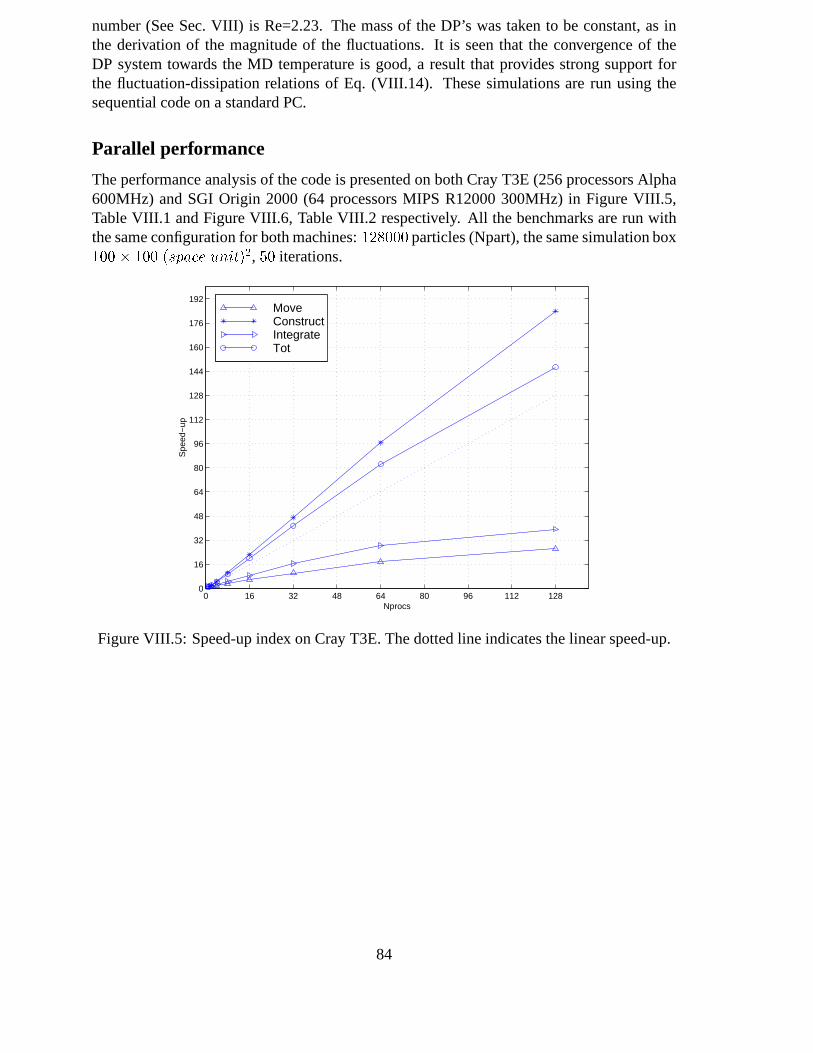
number (See Sec. VIII) is Re=2.23. The mass of the DP’s was taken to be constant, as inthe derivation of the magnitude of the fluctuations. It is seen that the convergence of theDP system towards the MD temperature is good, a result that provides strong support forthe fluctuation-dissipation relations of Eq. (VIII.14). These simulations are run using thesequential code on a standard PC.

Parallel performance

The performance analysis of the code is presented on both Cray T3E (256 processors Alpha600MHz) and SGI Origin 2000 (64 processors MIPS R12000 300MHz) in Figure VIII.5,Table VIII.1 and Figure VIII.6, Table VIII.2 respectively.All the benchmarks are run withthe same configuration for both machines:128000 particles (Npart), the same simulation box100 100 (spa e unit)

2, 50 iterations.

0 16 32 48 64 80 96 112 1280

16

32

48

64

80

96

112

128

144

160

176

192

Nprocs

Spe

ed−

up

Move ConstructIntegrateTot

Figure VIII.5: Speed-up index on Cray T3E. The dotted line indicates the linear speed-up.

84

Nprocs Npart/NProcs Move Construct Integration Comm Total1 128000 4.50 395.17 19.38 0 427.732 64000 5.45 180.96 16.54 1.49 206.994 32000 2.76 83.42 8.46 1.43 96.528 16000 1.48 38.48 4.43 1.02 45.3416 8000 0.78 17.70 2.24 0.67 21.2432 4000 0.44 8.40 1.16 0.44 10.3164 2000 0.25 4.09 0.68 0.38 5.18128 1000 0.17 2.14 0.49 0.47 2.91

Table VIII.1: Timings in seconds of the main routines on the Cray T3E. Comm measures thetotal time for communication, while the other timings are inclusive of the communicationtime. The number of iterations is 50.

0 4 8 12 16 20 24 28 320

4

8

12

16

20

24

28

32

36

40

44

48

Nprocs

Spe

ed−

up

Move ConstructIntegrateTot

Figure VIII.6: Speed-up index on SGI Origin 2000. The dottedline indicates the linearspeed-up.

Nprocs Npart/NProcs Move Construct Integration Comm Total1 128000 1.94 307.77 17.90 0 334.242 64000 3.15 124.44 13.16 0.56 143.534 32000 1.78 50.03 5.94 0.69 58.958 16000 0.90 22.89 3.44 1.89 27.8616 8000 0.59 11.20 1.77 1.25 13.8832 4000 0.71 6.66 1.75 2.73 9.51

Table VIII.2: Timings in seconds of the main routines on the SGI Origin 2000. Commmeasures the total time for communication, while the other timings are inclusive of the com-munication time. The number of iterations is 50.

85

The simulation is a relaxation towards equilibrium of the isothermal model starting froma random initial configuration. The timings have been taken measuring the CPU-clock timefor the routines:movethat updates the position and communicates the particle outside theboundary,constructthat constructs the tessellation,integrationthat integrates the Langevin’sequation and communicates the stochastic force,commthat is the total time of commu-nication without the time for buffering andtotal that measures the total time without Input-Output. All the times measured are inclusive of communication, which is reported separatelyfor comparison; the time for one processor is the time of the sequential version without anyoverhead due to buffering.

Looking at the speed-up index, it is worth noting that the super-linearity shown wasexpected because the algorithmic complexity of the construction is not linear, butNlog(N).The construction of the tessellation forN=2 takes less than half of the time spent forN

dissipative particles.

Applications

Dissipative particle dynamics has been successfully applied to many hydrodynamical prob-lems involving complex fluids. For example, Boeket al. [10] have successfully simulatedcolloidal suspensions at low to intermediate solids volumefractions, using the original DPDmodel developed by Hoogerbrugge and Koelman [8]. The colloidal particles are modelledby freezing together a spherical cluster of DP’s and considering the total mass and momen-tum of the cluster as an effective single object. In this way,the interactions are computedusing the standard DPD scheme for both the DP colloidal clusters and the DP fluid particles.Applications to polymeric fluids have been made by Schlijperet al. [11] who successfullyreproduced the essential physical phenomena of such systems. The polymer chains are intro-duced into the fluid as a linear chain of DPD particles connected by Fraenkel springs. Novikand Coveney [12] have reported simulations of binary immiscible fluids in agreement withexpectations. The fluids are modelled by assigning to different molecules a different ’color’.Individual molecules then attract similar and repel dissimilar coloured molecules. Laplace’slaw is shown to be satisfied in a series of bubble experiments,confirming the existence of asurface tension between the two phases. We now discuss some possible applications of ournew DPD model.

Multiscale phenomena

For most practical applications involving complex fluids, additional interactions and bound-ary conditions need to be specified. These too must be deducedfrom some suitable meso-description of the microscopic dynamics, just as we have done for the interparticle forces.This may be achieved by considering a particulate description of the boundary itself and in-cluding molecular interactions between the fluid MD particles and other objects, such as par-ticles or walls. Appropriate modifications can then be made on the basis of the momentum-flux tensor of Eq. (VIII.5), which is generally valid. Consider for example the case of acolloidal suspension, which is shown in Fig. VIII.7. Beginning with the hydrodynamicmomentum-flux tensor Eq. (VIII.5), it is evident that we alsoneed to define an interactionregion where the DP–colloid forces act: the DP–colloid interaction may be obtained in thesame form as the DP–DP interaction by making the replacementl

kl

! L

kI

, whereLkI

is the

86

k

L kI

U

Figure VIII.7: Multiscale modeling of colloidal fluids. As usual, the dissipative particlesare defined as cells in the Voronoi lattice. Note that there are four relevant length scalesin this problem: the scale of the large, gray colloid particles, the two distinct scales of thedissipative particles in between and away from the colloidsand finally the molecular scaleof the MD particles. These mediate the mesoscopic interactions and are shown as dots onthe boundaries between dissipative and colloidal particles.

87

length (or area in 3D) of the arc segment where the dissipative particle meets the colloid (seeFig. VIII.7) and the velocity gradientr1

kl

((U

kl

e

kl

)e

kl

+U

kl

) is that between the dissipativeparticle and the colloid surface. The latter may be computedusingU

k

and the velocity of thecolloid surface together with a no-slip boundary conditionon this surface. In Eq. (VIII.14)the replacementl

kl

! L

KI

must also be made.Although previous DPD simulations of colloidal fluids have proved rather successful [10]

at low to intermediate solids volume fractions, they break down for dense systems whosesolids volume fraction exceeds a value of about 40% because the existing method is un-able to handle multiple lengthscale phenomena. However, our new version of the algorithmprovides the freedom to define dissipative particle sizes according to the local resolutionrequirements as illustrated in Fig. VIII.7. In order to increase the spatial resolution wherecolloidal particles are within close proximity it is necessary and perfectly admissible to in-troduce a higher density of dissipative particles there; this ensures that fluid lubrication andhydrodynamic effects are properly maintained. After thesedissipative particles have movedit may be necessary to re-tile the DP system; this is easily achieved by distributing the massand momentum of the old dissipative particles on the new onesaccording to their area (orvolume in 3D). Considerations of space prevent us from discussing this problem further inthe present paper, but we plan to report in detail on such dense colloidal particle simulationsusing our method in future publications. We note in passing that a wide variety of other com-plex systems exist where modeling and simulation are challenged by the presence of severalsimultaneous length scales, for example in polymeric and amphiphilic fluids, particularly inconfined geometries such as porous media [30]. For instance,a simulation involving a poly-meric fluid could be set up with a large number of dissipative particles for the solvent andsets of 100-1000 dissipative particles for each polymer molecule. The polymer is modelledby different polymer-fluid and polymer-polymer interactions more the standard fluid-fluidinteraction. When a fluid dissipative particle is interacting with the polymer, the Delaunaytriangulation handles the individuation of the monomers (polymer particles) to interact with(see Figure VIII.8).

Figure VIII.8: Structure of a polymeric fluid according to the multiscale dissipative particledynamics method. The resolved length scale of the polymer ismuch finer than that of thefluid.

88

The low viscosity limit and high Reynolds numbers

In the kinetic theory derived by Marsh, Backx and Ernst [15] the viscosity is explicitly shownto have a kinetic contribution

K

= D=2 whereD is the DP self diffusion coefficient and the mass density. The kinetic contribution to the viscositywas measured by Masters andWarren [31] within the context of an improved theory. How then can the viscosity used inour model be decreased to zero while kinetic theory puts the lower limit

K

to it?To answer this question we must define a physical way of decreasing the MD viscos-

ity while keeping other quantities fixed, or, alternativelyrescale the system in a way thathas the equivalent effect. The latter method is preferable as it allows the underlying micro-scopic system to remain fixed. In order to do this we non-dimensionalize the DP momentumequation.

For this purpose we introduce the characteristic equilibrium velocity,U0

=

p

k

B

T=M ,the characteristic distancer

0

as the typical DP size. Then the characteristic timet

0

= r

0

=U

0

follows.Neglecting gravity for the time being, the DP momentum equation takes the form

dP0

k

dt0=

X

l

l

0

kl

p

0

kl

2

e

kl

+

1

Re(U

0

kl

+ (U

0

kl

e

kl

)e

kl

)

+

X

l

l

0

kl

L

0

kl

2r

0

kl

0

k

+

0

l

2

i

kl

U

0

kl

U

0

k

+U

0

l

2

+

X

l

~

F

0

kl

; (VIII.15)

whereP0

k

= P

k

=(MU

0

), p0kl

= p

kl

r

2

0

=(MU

2

0

), M = r

2

0

in 2d, the Reynolds number Re=U

0

r

0

= and ~

F

0

kl

= (r

0

=MU

2

0

)

~

F

kl

where ~Fkl

is given by Eqs. (VIII.11) and (VIII.14). Asmall calculations then shows that if~F0

kl

is related to!0

kl

andt0 like ~

F

kl

related to!kl

andt,then

!

0

2

kl

1

Rek

B

T

MU

2

0

1

Re(VIII.16)

where we have neglected dimensionless geometric prefactors like lkl

=r

kl

and used the factthat the ratio of the thermal to kinetic energy by definition of U

0

is one.The above results imply that when the DPD system is measured in non-dimensionalized

units everything is determined by the value of the mesoscopic Reynolds number Re. Thereis thus no observable difference in this system between increasingr

0

and decreasing.Returning to dimensional units again the DP diffusivity maybe obtained from the Stokes-

Einstein relation [32] as

D =

k

B

T

ar

0

(VIII.17)

wherea is some geometric factor (a = 6 for a sphere) and all quantities on the right handside exceptr

0

refer directly to the underlying MD. As we are keeping the MD system fixedand increasing Re by increasingr

0

, it is seen thatD and henceK

vanish in the process.We note in passing that ifD is written in terms of the mean free path: D =

p

k

B

T=(r

2

0

)

and this result is compared with Eq. (VIII.17) we get

0

= =r

0

1=r

0

in 2d, i.e. the meanfree path, measured in units of the particle size decreases as the inverse particle size. This isconsistent with the decay of

K

. The above argument shows that decreasing is equivalentto keeping the microscopic MD system fixed while increasing the DP size, in which case themean free path effects on viscosity is decreased to zero as the DP size is increased to infinity.It is in this limit that high Re values may be achieved.

89

Fokker-Planck equations

DPD2: Langevin equations

DPD1

Time symmetric coarsed grained equationsof motion

MD

ω= ω(η T, )

equilibrium statistical mechanics

constitutive relations and Markovian assumption

averaging over MD configurations

coarse graining

Fluctuation dissipation DPD complete

Fluctuating hydrodynamics

Figure VIII.9: Outline of the derivation of dissipative particle dynamics from moleculardynamics as presented in the present paper. The MD viscosityis denoted by and! is theamplitude of the fluctuating force~F as defined in Eq. (VIII.11)

Note that in this limit the thermal forces~Fkl

Re1=2 will vanish, and that we are ef-fectively left with a macroscopic, fluctuationless description. This is no problem when usingthe present Voronoi construction. However, the effectively spherical particles of conventionalDPD will freeze into a colloidal crystal, i.e. into a latticeconfiguration [8,9] in this limit.Also while conventional DPD has usually required calibration simulations to determine theviscosity, due to discrepancies between theory and measurements, the viscosity in this newform of DPD is simply an input parameter. However, there may still be discrepancies due tothe approximations made in going from MD to DPD. These approximations include the lin-earization of the inter-DP velocity fields, the Markovian assumption in the force correlationsand the neglect of a DP angular momentum variable.

None of the conclusions from the above arguments would change if we had worked inthree dimensions instead of two.

Conclusions

We have introduced a systematic procedure for deriving the mesoscopic modeling and sim-ulation method known as dissipative particle dynamics fromthe underlying description interms of molecular dynamics. Figure VIII.9 illustrates thestructure of the theoretical devel-opment of DPD equations from MD as presented in this paper. The initial coarse grainingleads to equations of essentially the same structure as the final DPD equations. However,they are still invariant under time-reversal. The development we have made which is shownin Fig.VIII.9 does not claim to derive the irreversible DPD equations from the reversible onesof molecular dynamics in a rigorous manner, although it doesillustrate where the transitiontakes place with the introduction of molecular averages. The kinetic equations of this new

90

DPD satisfy anH-theorem, guaranteeing an irreversible approach to the equilibrium state.This is the first time that any of the various existing mesoscale methods have been put

on a firm ‘bottom up’ theoretical foundation, a development which brings with it numerousnew insights as well as practical advantages. One of the mainvirtues of this procedure is thecapability it provides to choose one or more coarse-graining lengthscales to suit the particularmodeling problem at hand. The relative scale between molecular dynamics and the chosendissipative particle dynamics, which may be defined as the ratio of their number densitiesDPD=MD , is a free parameter within the theory. Indeed, this rescaling may be viewed asa renormalisation group procedure under which the fluid viscosity remains constant: sincethe conservation laws hold exactly at every level of coarse graining, the result of doing tworescalings, say from MD to DPD and from DPD to DPD, is the same as doing just onewith a larger ratio, i.e.DPD=MD = (DPD=DPD)(DPD=MD).

The present coarse graining scheme is not limited to hydrodynamics. It could in principlebe used to rescale the local description of any quantity of interest. However, only for locallyconserved quantities will the DP particle interactions take the form of surface terms as here,and so it is unlikely that the scheme will produce a useful description of non-conservedquantities.

In this context, we note that the bottom-up approach to fluid mechanics presented heremay throw new light on aspects of the problem of homogeneous and inhomogeneous turbu-lence. Top-down multiscale methods and, to a more limited extent, ideas taken from renor-malisation group theory have been applied quite widely in recent years to provide insightinto the nature of turbulence [33, 34]; one might expect an alternative perspective to emergefrom a fluid dynamical theory originating at the microscopiclevel, in which the central rela-tionship between conservative and dissipative processes is specified in a more fundamentalmanner. From a practical point of view it is noted that, sincethe DPD viscosity is the sameas the viscosity emergent from the underlying MD level, it may be treated as a free parameterin the DPD model, and thus high Reynolds numbers may be reached. In the ! 0 limit themodel thus represents a potential tool for hydrodynamic simulations of turbulence. However,we have not investigated the potential numerical complications of this limit.

The dissipative particle dynamics which we have derived is formally similar to the con-ventional version, incorporating as it does conservative,dissipative and fluctuating forces.The interactions are pairwise, and conserve mass and momentum as well as energy. However,now all these forces have been derived from the underlying molecular dynamics. The conser-vative and dissipative forces arise directly from the hydrodynamic description of the molec-ular dynamics and the properties of the fluctuating forces are determined via a fluctuation–dissipation relation.

The simple hydrodynamic description of the molecules chosen here is not a necessaryrequirement. Other choices for the average of the general momentum and energy flux tensorsmay be made and we hope these will be explored in future work. More significant is the factthat our analysis permits the introduction of specific physicochemical interactions at themesoscopic level, together with a well-defined scale for this mesoscopic description.

While the Gaussian basis we used for the sampling functions is an arbitrary albeit con-venient choice, the Voronoi geometry itself emerged naturally from the requirement that allthe MD particles be fully accounted for. Well defined procedures already exist in the litera-ture for the computation of Voronoi tesselations [35] and soalgorithms based on our modelare not computationally difficult to implement. Nevertheless, it should be appreciated thatthe Voronoi construction represents a significant computational overhead. This overhead is

91

of orderN logN , a factorlogN larger than the most efficient multipole methods in prin-ciple available for handling the particle interactions in molecular dynamics. However, theprefactors are likely to be much larger in the particle interaction case.

Finally we note the formal similarity of the present particulate description to existingcontinuum fluid dynamics methods incorporating adaptive meshes, which start out froma top-down or macroscopic description. These top-down approaches include in particularsmoothed particle hydrodynamics [19] and finite-element simulations. In these descriptionstoo the computational method is based on tracing the motion of elements of the fluid onthe basis of the forces acting between them [36]. However, while such top-down compu-tational strategies depend on a macroscopic and purely phenomenological fluid description,the present approach rests on amolecularbasis.

92

Bibliography

[1] L. D. Landau and E. M. Lifshitz,Fluid Mechanics(Pergamon Press, New York, 1959).

[2] L. Boltzmann.,Vorlesungenuber Gastheorie(Leipzig, 1872).

[3] J. Koplik and J. R. Banavar, Ann. Rev. Fluid Mech.27, 257 (1995).

[4] U. Frisch, B. Hasslacher, and Y. Pomeau, Phys. Rev. Lett.56, 1505 (1986).

[5] G. McNamara and G. Zanetti, Phys. Rev. Lett.61, 2332 (1988).

[6] X. W. Chan and H. Chen, Phys. Rev E49, 2941 (1993).

[7] M. R. Swift, W. R. Osborne, and J. Yeomans, Phys. Rev. Lett. 75, 830 (1995).

[8] P. J. Hoogerbrugge and J. M. V. A. Koelman, Europhys. Lett. 19, 155 (1992).

[9] P. Espanol and P. Warren, Europhys. Lett.30, 191 (1995).

[10] E. S. Boek, P. V. Coveney, H. N. W. Lekkerkerker, and P. van der Schoot, Phys. Rev. E54, 5143 (1997).

[11] A. G. Schlijper, P. J. Hoogerbrugge, and C. W. Manke, J. Rheol.39, 567 (1995).

[12] P. V. Coveney and K. E. Novik, Phys. Rev. E54, 5143 (1996).

[13] R. D. Groot and P. B. Warren., J. Chem. Phys.107, 4423 (1997).

[14] P. Espanol, Phys. Rev. E52, 1734 (1995).

[15] C. A. Marsh, G. Backx, and M. Ernst, Phys. Rev. E56, 1676 (1997).

[16] J. B. Avalos and A. D. Mackie, Europhys. Lett.40, 141 (1997).

[17] P. Espanol, Europhys. Lett40, 631 (1997).

[18] P. Espanol, Phys. Rev. E57, 2930 (1998).

[19] J. J. Monaghan, Ann. Rev. Astron. Astophys.30, 543 (1992).

[20] P. Espanol, M. Serrano, and I. Zuniga, Int. J. Mod. Phys. C8, 899 (1997).

[21] E. G. Flekkøy and P. V. Coveney, Phys. Rev. Lett.83, 1775 (1999).

[22] E. G. Flekkøy, P. V. Coveney, and G. De Fabritiis (submitted to Phys. Rev. E).

93

[23] P. V. Coveney and O. Penrose, J. Phys A: Math. Gen.25, 4947 (1992).

[24] O. Penrose and P. V. Coveney, Proc. R. Soc.447, 631 (1994).

[25] P. V. Coveney and R. Highfield,The Arrow of Time(W. H.Allen, London, 1990).

[26] F. Reif, Fundamentals of statistical and thermal physics(Mc Graw-Hill, Singapore,1965).

[27] L. D. Landau and E. M. Lifshitz,Statistical Physics(Pergamon Press, New York, 1959).

[28] C. W. Gardiner,Handbook of stochastic methods(Springer Verlag, Berlin Heidelberg,1985).

[29] G. De Fabritiis, P. V. Coveney, and E. G. Flekkøy, inProc. 5th European SGI/CrayMPP Workshop, Bologna, Italy 1999.

[30] P. V. Coveney, J. B. Maillet, J. L. Wilson, P. W. Fowler, O. Al-Mushadani and B. M.Boghosian, Int. J. Mod. Phys. C9, 1479 (1998).

[31] A. J. Masters and P. B. Warren,preprint cond-mat/9903293 (http://xxx.lanl.gov/) (un-published).

[32] A. Einstein, Ann. Phys.17, 549 (1905).

[33] U. Frisch,Turbulence(Cambridge University Press, Cambridge, 1995).

[34] A. Bensoussan, J. L. Lions, and G. Papanicolaou,Asymptotic Analysis for PeriodicStructures(North-Holland, Amsterdam, 1978).

[35] D. E. K. L. J. Guibas and M. Sharir, Algorithmica7, 381 (1992).

[36] B. M. Boghosian, Encyclopedia of Applied Physics23, 151 (1998).

94

IX

The elements: A Beowulf class Computer

Stavros C. FarantosInstitute of Electronic Structure and Lasers,

FORTH, Iraklion, Crete, 711 10, Greece, andDepartment of Chemistry, University of Crete, Iraklion,

Crete, 711 10, Greece

Abstract

The elements is a Beowulf-Type computer for supporting the project in Classical and Quan-tum Mechanical Molecular Dynamics of Theoretical and Computational Chemistry in Crete.This distributed parallel system is an effort to create large computational power by accumu-lating low cost CPUs, memory and hard discs for data storage using open software as faras possible. The current composition of Theelements is eight dual Pentium II systems withCPUs at 350 and 450 MHz, total memory 5GBytes, total hard discs 76 GBytes and all theseconnected with a fast Ethernet switch of 100 Mbits/s.

Introduction

The Beowulf-class era has dawned and this species of computers is rapidly multipling allover the world. The first book on how to build a Beowulf system [1] has been published andseveral documents have been written by those who have experienced the construction of aBeowulf computer(http://beowulf.gsfc.nasa.gov/). It is amazing that withtoday’s technology, low cost PCs andopen software, scientists in fields other than the computer science are capable of building aparallel system with memory and performance met in supercomputers just a few years ago.

Scientists from physics and chemistry are ravenous for CPU time and memory when try-ing to solve problems related to simulations of matter. There are several advantages with theBeowulf-class parallel computers [1]. However, the freedom of designing and constructinga system which is tailored to solving specific computationalproblems does not come easily.Decisions about how to split the budget among the number of CPUs, the memory or the sizeof hard discs, the kind and the speed of the connecting network in a parallel system dependon the applications one has in mind.

In our laboratory the main computational projects are in theareas:

95

1. Molecular Potential Energy Surfaces and Clusters [2,3].

2. Non-Linear Classical Mechanical Analysis of Molecular Systems: Periodic Orbit Mul-tiple Shooting Algorithms [4].

3. Molecular Quantum Dynamics: Periodic Orbit Assisted Grid Solutions of Time De-pendent Schrodinger Equation [5].

4. Molecular Electronic Structure Calculations (Quantum Chemistry) [6].

Parallelized codes are available for locating minima and transition states on multidimen-sional Potential Energy Surfaces and for solving the Time Dependant Schrodinger Equation.The latter is greatly facilitated by employing high order Finite Difference algorithms [5]. Forelectronic structure quantum chemistry type calculationsa parallelized packet, NWCHEM,1

is that from EMSL-PNNL. The above projects are memory and CPUtime intensive. There-fore, we have built the following Beowulf-class system.

Technical Characteristics

The system was built in two phases.PHASE 1 (JULY 1998)

Dual Nodes: / Fire / Water / Air / Earth /

CPUs: Eight Pentium II CPUs at 350 MHz - Cash Memory 512 KBytes

Motherboards: QDI Brilliant V, Chipset INTEL 440 BX 100MHz

Memory: 2.048 GBytes (4x512) (100 MHz SDRAM)

Discs: 21 GBytes (5x4.2) (WESTERN DIGITAL ULTRA WIDE SCSI)

Network: Bay 350T, 100 Mbits Switch, Backbone 1Gbits, 16 ports

PHASE 2 (APRIL 1999)Dual Nodes: / Hydrogen / Helium / Nitrogen[*] / Oxygen[*] /

CPUs: Eight Pentium II CPUs at 450 MHz - Cash Memory 512 KBytes

Motherboards: P2B-D, ASUS, Chipset INTEL 440 BX 100MHz

Memory: 3.072 GBytes (2x512+2x1024[*]) (100 MHz SDRAM)

Discs: 54.6 GBytes (6x9.1) (IBM, ULTRA WIDE2 SCSI)

In total the hardware consists of Sixteen Pentium II CPUs, 5 GBytes Memory and 76 GBytesHard Discs. Each system has 0.5 GBytes memory but two of 1 GByte. Special care was takenfor the cooling of the computers. Two more fans were added to each case which contains theCPUs.

1http://www.emsl.pnl.gov:2080/docs/nwchem/nwchem.html

96

Software

Operational System: Linux, Distributor Red Hat 6.1 (Cartman) (Kernel 2.2.13) (O)

Communication Programs: Message Passing Interface (MPI) Argonne MPI (O)

Batch Queuing Program: Generic NQS (Network Queuing System3.50.6) - SterlingSoftware Incorporated (O)

Compilers: /High Performance Fortran (HPF) / Fortran 90 / Fortran 77 / C / C++ /Portland Group 3.1 (C)

Libraries: Numerical Recipes (C) - PETSc (Portable, Extensible Toolkit for ScientificComputations) (O)

O = Open software, C = Commercial software, L = Local software.

Communication mode

The eight dual PCs connected by the fast Ethernet consist an isolated local area network(ILAN). The mode of accessing Theelements from the outside world is what is called“theGuarded Beowulf” [1]. In this scheme only one of the nodes has an IP address recognizablefrom machines outside Theelements. The“worldly-node” is Fire which has been upgradedto a 450 MHz dual Pentium II. Fire is protected by a firewall software. Each node has a localhard disc but a raid of 17 GBytes is supported my the server (Fire).

Cost and Performance

The cost of The Elements was: Phase 1: $25000, Phase 2: $17000. These prices of courseare relevant with the time of purchase of the systems mentioned above. The stability andreliability of the cluster is unquestionable. This has beentested by running two jobs in eachCPU simultaneously in the scientific fields mentioned above.Comparisons of the perfor-mance per CPU have been made with a HP-Exemplar system with eight CPUs and 1GBytememory. The speed is the expected for an INTEL processor at 350 MHz or 450 MHz (ap-proximately 2:1) for classical Molecular Dynamics calculations. However, the compilers ofPGgroup, especially of FORTRAN 90, are highly efficient for matrix-vector multiplication.Some tests as well as other information for our applicationsin The elements can be found inthe URL address:http://TCCC.iesl.forth.gr/AMSEPEAEK/theelements/theelementsprofile.html.

Discussion

Parallel systems of Beowulf-Type with a small number of CPUsare distinguished from themassively parallel systems, and should be compared with thesimilar size shared memoryparallel servers commercially available by SUN, SGI and HP.The latter have the advantageof having a common memory accessible by all CPUs simultaneously, something which sim-plifies the programming. In a Beowulf-class computer the memory is distributed among the

97

nodes and the programmer must take care to transfer data fromone computer to the other.This is achieved by using the Message Passing Interface (MPI) library which provides sub-routines in C or FORTRAN programming languages to facilitate the transfer of data. Thetask of writing the proper codes or as in most cases of modifying existing ones, is sometimesconsiderable and this is only compensated by the low cost of aBeowulf-Type computer. Theprices may differ even by an order of magnitude.

Using MPI itself is relatively simple and in most applications a small number of sub-routines are used. However, a serious planning is needed when we have to restructure thecode in order to parallelize our program. At present, we haveacquired limited experienceby parallelizing a code for solving the time-dependent Schrodinger equation which involvesmatrix-vector multiplications. Libraries with parallelized codes for numerical analysis appli-cations using MPI exist such as PETSc. To the best of our knowledge efficient open softwarefor converting a distributed memory system to a shared memory type is not yet available, butit is likely to appear in the future.

The amount of work for the administration of a parallel system depends, of course, on itssize. In our case we have adopted a master-slave scheme wherethe shared software is storedand maintained in the server. Software for batch queuing andstatistics of memory and CPUutilization by the running jobs is available, both commercial and public. The one that we use(Generic NQS) achieves a good balance in distributing the jobs among the CPUs. GenericNQS allows to define batch queues with different priorities and memory needs.

We have adopted two batch queues, thelarge with unlimited CPU time but maximummemory for each running job up to 250 MBytes, and themlarge with unlimited CPU timeand maximum memory of 500 MBytes, restricted only to those systems with one GBytememory. Also, the number of jobs running in each node is one per CPU, i.e. two jobs ineach dual system. The administrator can easily reconfigure Generic NQS to achieve the mostefficient use of memory and CPU time to a dynamically varying environment. Interactive useof the system is not encouraged, except for parallelized codes which utilize MPI.

The stability of the whole system has been tested under conditions where single jobs(mainly of quantum chemistry type) and parallel jobs using MPI are executed simultane-ously. The system can be run for several days without observing any error in the connectingnetwork. Up to now we have a positive experience from the performance of TheElenents,but the elaborate task of writing efficient parallel codes remains and this is the value to bepaid for having a low cost powerful distributed computer.

98

Bibliography

[1] T. L. Sterling, J. Salmon, D. J. Becker and D. F. Savarese.How to Build a Beowulf: A guide to the implementation and application of PC clusters.The MIT Press, Cambridge, Massachusetts, 1999.

[2] J. Papadakis, G. S. Fanourgakis, M. Founargiotakis and S. C. Farantos.Comparison of Line Search Minimization Algorithms for Exploring Topographyof Multidimensional Potential Energy Surfaces: Mg+Ar

n

case.J. Comput. Chem.,18:1011, 1997.

[3] S. Stamatiadis, R. Prosmiti and S. C. Farantos.AUTO DERIV: Tool for automatic differentiation of a FORTRAN code. Comp. Phys.Comm., in press, 2000.

[4] S. C. Farantos.POMULT: A Program for Computing Periodic Orbits in Hamiltonian Systems Basedon Multiple Shooting Algorithms.Comp. Phys. Comm., 108:240, 1998.

[5] R. Guantes and S. C. Farantos.High Order Finite Difference Algorithms for Solving the Schrodinger Equation inMolecular Dynamics.J. Chem. Phys., 111:10827, 1999.

[6] G. S. Fanourgakis, S. C. Farantos, M. Velegrakis and S. S.Xantheas.Photofragmentation Spectra and Structures of Sr+Ar

n

; n = 2 8 Clusters: Experimentand Theory.J. Chem. Phys., 109:108, 1998.

99

100

X

Did you see ?

We wish to have on the simu web site (http://simu.ulb.ac.be/) a list of books, newsletters,websites, programmes, in fact anything which coincides with the goals ofSIMU, providedthat each item is either striking, or very useful. We would like each of you, as a reader ofthis newsletter, to play the role of an expert filter, selecting and channeling information tothe site, so that it can be distributed to everyone. The following sections are only an attemptto “set the ball rolling” and are by no means complete.

Computer clusters and parallel computing

1. The Message Passing Interface (MPI) standard. Description of the MPI parallel library,manuals and exampleshttp://www-unix.mcs.anl.gov/mpi/index.html

2. The MPICH implementation of MPI. A public domain library.http://www-unix.mcs.anl.gov/mpi/mpich

3. The LAM-MPI implementation of MPI. A public domain libraryhttp://www.mpi.nd.edu/lam/

4. The Beowulf pages. Description of Linux clusters to do distributed computations:recommendations, software, documentation, etchttp://www.beowulf.org/

http://www.beowulf-underground.org/

5. Parallel Mac cluster description: technical details on building and running codes onthe cluster are available in Viktor K. Decyk, Dean E. Dauger,and Pieter R. Kokelaar,Appleseed: A Parallel Macintosh Cluster for Numerically Intensive Computinghttp://exodus.physics.ucla.edu/appleseed/appleseed.html

6. Other Macintosh cluster information is athttp://exodus.physics.ucla.edu/appleseed/appleseedsites.html

101

Physics

1. The XXX-LANL article depository. French mirrorhttp://xxx.lpthe.jussieu.fr/

2. The SISSA (Trieste) information web site for condensed matter, a treasure trovehttp://www.sissa.it/˜furio/cminfo.html

Chemistry

1. A URL for departments of chemistry ishttp://www.ch.cam.ac.uk/ChemSitesIndex.html

2. An article about Beowulf-Class Computers used by chemists, available athttp://TCCC.iesl.forth.gr/AMSEPEAEK/theelements/articles/ACSJan10.html

Scientific software

1. FFTW: An efficient FFT library for sequential and parallelcomputershttp://www.fftw.org/

2. Numerical Recipes on Line. PostScript and PDF files of the NR C/Fortran bookshttp://www.ulib.org/webRoot/Books/NumericalRecipes/

3. List of web references on numerical methods (benchmarks,fortran courses, books,sites etc...)http://tonic.physics.sunysb.edu/docs/nummeth.html

4. A general-purpose molecular dynamics simulation program called Moldy. It is suffi-ciently flexible that it ought to be useful for a wide range of simulation calculations ofatomic, ionic and molecular systems.http://www.earth.ox.ac.uk/˜keith/moldy.html

5. For a library of software on molecular dynamics, Monte Carlo, Lattice statistics andLattice dynamics containing the programmes of the book, seethe web site of the UKCCP5 group,http://www.daresbury.ac.uk/CCP/CCP5/librar.html

6. Quantum Simulations of Condensed Matter Systems, the NCSA Condensed MatterPhysics home page of David Ceperley containing lots of free software,http://www.ncsa.uiuc.edu/Apps/CMP/cmp-homepage.html

7. LASSP Tools: A great variety of scientific visualization programmeshttp://www.lassp.cornell.edu/LASSPTools/LASSPTools.html

102

Books and associated sites on molecular simulation

1. Understanding Molecular Simulation: From Algorithms toApplications Daan Frenkeland Berend Smit, Academic Press (1996). For new additions, exercises, programmesand associated courses seehttp://molsim.chem.uva.nl/frenkelsmit/

2. Computer Simulation of liquids, M.P. Allen and D.J. Tildesley, Oxford Science Pub-lications, 1997, one of the bibles of simulators. The programmes of the book, areavailable on the CCP5 group web site,http://www.daresbury.ac.uk/CCP/CCP5/librar.html

The web site of an associated summer school ishttp://molsim.ch.umist.ac.uk/CCP5SS/

3. Classical and Quantum Dynamics in Condensed Phase Systems, Editors: Bruce J.Berne, Giovanni Ciccotti and David F. Coker.For associated material, check out the web site of Giovanni Ciccottihttp://mefisto.phys.uniroma1.it/cgi-bin/wrap/ciccotti/Public/LERICI/

4. Monte Carlo and Molecular Dynamics of Condensed Matter Systems, Kurt Binder andGiovanni Ciccotti, Italian Physical Society, 1995

5. Monte Carlo Simulation in Statistical Physics, An Introduction, Kurt Binder and DieterW. Heermann, Springer, 1988

Newsletters and associated web sites

1. The k newsletter, Ab-initio (from electronic structure) calculation of complex pro-cesses in materials, which is supported by the European Science Foundation,http://psi-k.dl.ac.uk/

2. The webserver of the European Science Foundation, also our sponsor ishttp://www.esf.org/

3. The CCP3 Surface Science newsletter, seehttp://www.cse.clrc.ac.uk/Activity/CCP3

103

104

XI

Conferences, Schools, Workshops,Tutorials and SIMU fellowships

Upcoming activities supported completely or in part bySIMU

Detailed information on the following activities is available at the URL:http://simu.ulb.ac.be/activities/activities.html

ConferenceSIMU conference on Bridging the time scale gap, Konstanz, Germany, September 11-15,2001.

Workshops

1. Planning meeting on “Universal Statistics in CorrelatedSystems”, Lyon, France, March29-31, 2000Peter Holdsworth, Ecole Normale Superieure de Lyon, France;Jean Francois Pinton, Ecole Normale Superieure de Lyon, France;Steven T. Bramwell, University College London.

2. Characterizing and Studying Transition Mechanisms and States in High DimensionalSystems Lyon, France, May 4-6, 2000.Peter Bolhuis , Department of Chemistry, Cambridge University UK;Christoph Dellago , Department of Chemistry, University ofRochester, USA;David Chandler , Department of Chemistry, University of California, Berkeley, USA.

3. Multiscale Modeling of Macromolecular Systems , Max Planck-Institute for PolymerResearch, Mainz, Germany, September 4-6, 2000.Dr. Ralf Everaers, Dr. Burkhard Dunweg Max-Planck-Institut fur Polymerforschung,Mainz, Germany;Dr. Wolfgang Paul, Dr. Walter Kob Institut fur Physik, Johannes Gutenberg-Universitat,Mainz, Germany;

4. Statistical Mechanics of Materials with Extreme Nonequilibrium Constraints Lyon,France, August 28-31,2000.

105

Siegfried Hess, Techniche Universitat; Berlin, Germany;Malek Mansour Universite Libre de Bruxelles, Belgium.

5. Simulations of long time scale dynamics, molecular and continuum descriptions, Re-jkavik, Iceland, 26-30 July 2000.Hannes Jonsson, Chemistry Department, University of Washington Seattle, USA;Giovanni Ciccotti, Dipartimento di Fisica, Universita ”La Sapienza”, Rome, Italy.

6. Across the Length Scales II: Applications MML2000 , Oxford University, UK, 2000.Prof David G. Pettifor, Prof Adrian P. Sutton, Dr Robert E. Rudd, Dr Steven D. Kenny;Department of Materials, University of Oxford, UK.

SchoolsMethods in Molecular Simulation, summer 2000, to be held in UMIST, Manchester, UK.

Tutorials

1. SIMU-CECAMtutorial on Computational Stochastic Methods for Mesoscale Dynam-ics, Lyon, May 22-24, 2000.Alejandro L. Garcia Department of Physics, San Jose State University; Florence BarasCenter for Nonlinear Phenomena and Complex Systems, Universite Libre de Brux-elles.

2. SIMU-CECAMtutorial on Car-Parinello molecular dynamics, Lyon, 11-15September2000.Jurg Hutter University of Zurich, Switzeland;Michiel Sprik University of Cambridge, U.K.

3. SIMU-CECAMtutorial on Advanced Monte Carlo simulation techniques, Lyon, 16-20October 2000.Berend Smit and Thijs Vlugt, Universiteit van Amsterdam, Netherlands.

Short Visits and Fellowships

TheSIMU Programme supports individual short visits of up to one week(mainly for seniorresearchers) and fellowships for younger researchers to spend up to three months in a re-search group involved in theSIMU Programme in a different European country. Either theinstitute of origin or the receiving institute should be in acountryin which a funding agencycontributes to theSIMU Programme (currently Belgium, Denmark, Finland, France, Ger-many, Italy, The Netherlands, Norway, Portugal, Sweden, Switzerland, United Kingdom).All applications for support of a short visit or a fellowshipshould be made with the attachedlatex template. Grants for short visits and fellowships areawarded every three months, thedates for 2000 are March 31, June 30, November 15 and December31. Applications shouldbe sent to:Professor Michel Mareschalemail: Michel.Mareschal@cecam.frCECAM, ENS-Lyon46, allee d’Italie69364 Lyon cedex 7France.

106

Activities relevant to SIMU, organised by other organisa-tions/programmes.

1. Eilat Workshops on: Multiscale Computational Methods inChemistry, April 5-11,2000. Interdisciplinary forum of computational mathematicians, physicists and chemists,to study basic computational obstacles in chemistry and advanced multiscale approachesfor treating them. For scientific background, general information, current participantlist and registration forms, see:http://www.wisdom.weizmann.ac.il/ achi/conf00/index.html

2. ForCECAMandCECAM-k

Workhops, seehttp://www.cecam.fr/

3. ”Molecular Simulation IN THE 21st CENTURY”, the EPSRC CCP5 Annual Meeting,2nd-5th July 2000, University of Surrey Guildford, UK. For further information seehttp://www.dl.ac.uk/CCP/CCP5/meetings/ann2000.html

107

108

XII

Jobs, Grants and Fellowships

For more recent information please consult theSIMUnewsgroup on our web site where mostof these offers are available. Feel free to use our site to advertise offers as well.

Post-docs

In the Condensed Matter Theory Sector of the International School forAdvanced Studies in Trieste (Italy)

A postdoctoral position is available, starting immediately, for 1 year on a on a project en-titled: ”Density-functional theory-based molecular dynamics of biological systems.” Thework will involve applications of the Car-Parrinello to systems of pharmaceutical relevance,such as targets for anti-AIDS and anti-cancer therapy. Candidates should hold a Ph.D inPhysics or Chemistry or have equivalent research experience and have good computingand physical modeling skills. Further information can be obtained from Dr. Paolo Car-loni, International School for Advanced Studies, SISSA, via Beirut 4, 34014 Trieste, Italyhttp://www.sissa.it/cm/bc/

email: carloni@sissa.it Phone: +39-040-3787407, Fax:+39-040-3787528

PhD fellowships

Opportunities for research with the Atomistic Simulation Group at Queen’sUniversity, Belfast.

QUB expects to be offering studentships for research leading to a PhD starting in October.There may be funding for E.U. students as well as for U.K. students. For more informationvisit the web sitehttp://titus.phy.qub.ac.uk

or contact Professor Lynden-Bell or Professor Finnisr.lynden-bell@qub.ac.uk m.finnis@qub.ac.uk

109