arX

iv:c

ond-

mat

/061

1482

v1 [

cond

-mat

.mtr

l-sc

i] 1

7 N

ov 2

006

Simple implementation of complex functionals: scaled selfconsistency

Matheus P. Lima, Luana S. Pedroza, Antonio J. R. da Silva and A. FazzioInstituto de Fısica, Universidade de Sao Paulo, Sao Paulo, Brazil

Daniel Vieira, Henrique J. P. Freire and K. Capelle∗

Departamento de Fısica e Informatica, Instituto de Fısica de Sao Carlos,

Universidade de Sao Paulo, Caixa Postal 369, 13560-970 Sao Carlos, SP, Brazil

(Dated: February 6, 2008)

We explore and compare three approximate schemes allowing simple implementation of com-plex density functionals by making use of selfconsistent implementation of simpler functionals: (i)post-LDA evaluation of complex functionals at the LDA densities (or those of other simple func-tionals); (ii) application of a global scaling factor to the potential of the simple functional; and (iii)application of a local scaling factor to that potential. Option (i) is a common choice in density-functional calculations. Option (ii) was recently proposed by Cafiero and Gonzalez. We here puttheir proposal on a more rigorous basis, by deriving it, and explaining why it works, directly fromthe theorems of density-functional theory. Option (iii) is proposed here for the first time. Weprovide detailed comparisons of the three approaches among each other and with fully selfconsis-tent implementations for Hartree, local-density, generalized-gradient, self-interaction corrected, andmeta-generalized-gradient approximations, for atoms, ions, quantum wells and model Hamiltonians.Scaled approaches turn out to be, on average, better than post-approaches, and unlike these alsoprovide corrections to eigenvalues and orbitals. Scaled selfconsistency thus opens the possibility ofefficient and reliable implementation of density functionals of hitherto unprecedented complexity.

PACS numbers: 31.15.Ew, 31.25.Eb, 31.25.Jf, 71.15.Mb

I. INTRODUCTION

Density-functional theory1,2,3 is the driving force be-hind much of todays progress in electronic-structure cal-culations. Progress in density-functional theory (DFT)itself depends on the twin development of ever more pre-cise density functionals and of ever more efficient compu-tational implementations of these functionals. The firstline of development, functionals, has lead from the local-density approximation (LDA) to generalized-gradient ap-proximations (GGAs), hybrid functionals, and on tometa-GGAs and other fully nonlocal approximations,such as exact-exchange (EXX) and self-interaction cor-rections (SICs).4,5

As functionals get more and more complex, the secondtask, implementation, gets harder and harder. Indeed,very few truly selfconsistent implementations of beyond-GGA functionals exist, and even GGAs are still some-times implemented non-selfconsistently. At the heart ofthe problem is not so much the actual coding (althoughthat can also be a formidable task, considering the com-plexity of, e.g., meta-GGAs), but rather obtaining theexchange-correlation (xc) potential vxc(r) correspondingto a given approximation to the xc energy Exc[n]. Hy-brid functionals, meta-GGAs, EXX and SICs are all or-bital functionals, i.e., functionals of the general formEorb

xc [{ϕi[n]}], where our notation indicates an explicitdependence on the set of Kohn-Sham (KS) orbitals ϕi(r).This set may be restricted to the occupied orbitals, butmay also include unoccupied orbitals. Since by virtue ofthe Hohenberg-Kohn (HK) theorem these orbitals them-selves are density functionals, any explicit orbital func-

tional is an implicit density functional.The HK theorem itself, however, does not provide any

clue how to obtain the xc potentials, i.e., how to calculatethe functional derivative

vxc[n](r) =δEorb

xc [{ϕi}]

δn(r)(1)

of a functional whose density dependence is not knownexplicitly. Three different solutions to this dilemma havebeen advanced in the literature.

(i) The formally correct way to implement an implicitdensity functional in DFT is the optimized-effective po-tential (OEP) algorithm5 [also known as the optimizedpotential method (OPM)], which results in an integralequation for the KS potential corresponding to the or-bital functional. The first step of the derivation of theOEP is to write

vxc[n](r) =δEorb

xc [{ϕi}]

δn(r)(2)

=

∫

d3r′∑

i

[

δEorbxc [{ϕi}]

δϕi(r′)

δϕi(r′)

δn(r)+ c.c.

]

(3)

=

∫

d3r′d3r′′∑

i

[

δEorbxc [{ϕi}]

δϕi(r′)

δϕi(r′)

δvs(r′′)

δvs(r′′)

δn(r)+ c.c.

]

.(4)

Further evaluation of Eq. (4) gives rise to an integralequation that determines the vxc[n] belonging to thechosen orbital functional Eorb

xc [{ϕi[n]}]. This OEP in-tegral equation must be solved at every step of theselfconsistency cycle, which considerably increases de-mands on memory and computing time. Often (in

2

particular for systems that do not have spherical sym-metry) the integral equation is simplified by means ofthe Krieger-Li-Iafrate (KLI) approximation,6 but evenwithin this approximation, or other recently proposedsimplifications,7,8 an OEP calculation is computationallymore expensive than a traditional KS calculation. A sep-arate issue is the unexpected behaviour of the OEP in fi-nite basis sets, which was recently reported to cast doubton the reliability of the method.9 The OEP prescrip-tion moreover assumes in the first step that the orbital

derivative δEorbxc [{ϕi}]/δϕi(r

′) can be obtained, and eventhat is not a trivial task for complex orbital-dependentfunctionals such as meta-GGA and hyper-GGA. (For theFock term, on the other hand, this derivative is simple,and the implementation of the Fock term by means ofthe OEP is becoming popular under the name exact ex-change [EXX]).

(ii) Instead of taking the variation of Exc[{ϕi[n]}] withrespect to n(r), as in the OEP, one often makes Exc

stationary with respect to the orbitals. When appliedto the Fock term, this is simply the Hartree-Fock (HF)method, but similar procedures are commonly appliedwithin DFT to hybrid functionals, such as B3-LYP. Self-consistent implementations of meta-GGA reported untiltoday are also selfconsistent with respect to the orbitals,not the densities.10,11,12 For the Fock term, one finds em-pirically that the occupied orbitals obtained from orbitalselfconsistency are quite similar to those obtained fromdensity selfconsistency, but such empirical finding is noguarantee that the similarity will persist for all possiblefunctionals or systems — and in any case it does not ex-tend to the unoccupied orbitals. Computationally, theresulting nonlocal HF-like potential makes the solutionof the Kohn-Sham equation more complex than the localpotential resulting from the OEP (although the poten-tial itself is obtained in a simpler way). Moreover, asthe OEP, this prescription also requires that the orbitalderivative δEorb

xc [{ϕi}]/δϕi(r′) can be obtained, which

need not be simple for complex functionals.

(iii) Less demanding than density-selfconsistency ororbital-selfconsistency are post-selfconsistent implemen-tations, in which a selfconsistent KS calculation is per-formed with a simpler functional, and the resulting or-bitals and densities are once substituted in the more com-plex one. This strategy is sometimes used to implementGGAs in a post-LDA way, and has been applied also tometa-GGAs. It is much simpler than the other two pos-sibilities, but does not lead to KS potentials, orbitals,and single-particle energies associated with the complexfunctional. It simply yields the total energy the complexfunctional produces on the densities obtained from thesimpler functional.

As this brief summary shows, each of the three choiceshas its own distinct set of advantages and disadvantages.A method that is simple to implement, reliable, and pro-vides access to total energies as well as single-particlequantities would be a most useful addition to the arsenalof computational DFT.

A method we consider to have the desired character-istics was recently proposed by Cafiero and Gonzalez,13

and consists in the application of a scaling factor to thexc potential of a simple functional (which can be imple-mented fully selfconsistently), such that it approximatesthe potential expected to arise from a complex functional(which need not be implemented selfconsistently). Thisfourth possibility, which we call globally-scaled selfcon-

sistency (GSSC), is analysed in Sec. II of the presentpaper.

We believe the derivation presented by Cafiero andGonzalez to lack rigour at a crucial step, and thus ded-icate Sec. II A to an investigation of their procedure.Our investigation leads to an alternative derivation ofthe same approach, described in Sec. II B. Next, we pro-vide, in Sec. II C, an analysis of the validity of the scalingapproximation, arriving at the counterintuitive (but nu-merically confirmed and explainable) conclusion that thesuccess of this approximation is not due to the small-ness of the neglected term relative to the one kept. Wealso suggest a modification of the approach, which wecall locally-scaled selfconsistency (LSSC) and describe inSec. II D.

In Secs. III and IV we provide extensive numericaltests of GSSC and LSSC, and also of the more com-mon post-selfconsistent mode of implementation [heredenoted P-SC, option (iii) above]. Note that althoughP-SC is quite commonly used, it has not been systemat-ically tested in situations where the exact result or thefully selfconsistent result is known. All three schemesare applied to atoms and ions in Secs. III A and III B,to one-dimensional Hubbard chains, in Sec. IVA, and tosemiconductor quantum wells, in Sec. IVB. We compareHartree, LDA, GGA, MGGA and SIC calculations, im-plemented via P-SC, GSSC and LSSC, among each other,and, where possible, with results obtained from fully self-consistent implementations of the same functionals.

Our main conclusion is that scaled selfconsistencyworks surprisingly well, for all different combinations ofsystems and functionals we tried. Scaled selfconsistencyyields better energies than post-selfconsistent implemen-tations, and moreover provides access to orbitals andeigenvalues. This conclusion opens the possibility of effi-cient and reliable implementation of density functionalsof hitherto unprecedented complexity.

II. SCALED SELFCONSISTENCY

In this section we first briefly review the approach sug-gested by Cafiero and Gonzalez (CG),13 and point outwhere we believe their development to lack rigour. Nextwe present an alternative derivation and suggest a mod-ification.

3

A. The proposal of Cafiero and Gonzalez

CG consider a complex functional, EBxc[n] with poten-

tial vBxc(r), and a simple functional, EA

xc[n] with potentialvA

xc(r). They then define the energy ratio

Fxc[n] =EB

xc[n]

EAxc[n]

(5)

and differentiate EBxc[n] = Fxc[n]EA

xc[n] with respect tothe density n(r), obtaining, in their notation,

vBxc(r) = Fxc[n]vA

xc(r) + EAxc[n]

∂Fxc[n]

∂n(r). (6)

Next, CG argue that at the selfconsistent density, n∗,EB

xc[n∗] = EA

xc[n∗], so that Fxc[n

∗] → 1. According toCG, the last term in Eq. (6) is then equal to zero. Underthis ’constraint’13 they obtain

vBxc(r) = Fxc[n]vA

xc(r) (7)

which implies that an (approximate) selfconsistent im-plementation of the complicated functional EB

xc[n] canbe achieved by means of a selfconsistent implementationof the simple functional EA

xc[n], if at every step of theselfconsistency cycle the potential corresponding to func-tional A is multiplied by the ratio of the energies of B andA. This procedure completely avoids the need to ever cal-culate or implement the potential corresponding to B.CG go on to test their proposal for a few functionals andsystems, and claim very good numerical agreement be-tween approximate results obtained from (7) and fullyselfconsistent or post-selfconsistent implementations.

We were initially quite surprised by these good results,as the preceding argument lacks rigour at a key step.Apart from the use of partial derivatives instead of vari-ational ones (which is probably just a question of nota-tion), we do not see why at the selfconsistent density thesimple and the complex functional must approach thesame value, i.e., why F [n∗] should approach one. More-over, whatever value F approaches, this value should notbe used to simplify the equation for the xc potential be-cause the derivative must be carried out before substitut-ing numerical values in the energy functional, not after-wards.

B. An alternative derivation

In view of these troublesome features of the originalderivation we below present an alternative rationale forthe same approach. We start by writing the same identitythe CG approach is based on,

EB[n] =EB[n]

EA[n]EA[n] =: F [n]EA[n]. (8)

Note that we write this identity for an arbitrary energyfunctional, as the approach is, in principle, not limited to

xc functionals. Indeed, below we will show one applica-tion in which we deal with the entire interaction energy(Hartree + xc). Next, we take the functional derivativeof the product F [n]EA[n],

vB(r) ≡δEB[n]

δn(r)=

δF [n]

δn(r)EA[n] + F [n]

δEA[n]

δn(r)(9)

=δF [n]

δn(r)EA + F [n]vA(r). (10)

The functional derivative of the ratio F [n] is

δ

δn(r)

EB

EA=

EA[n]vB(r) − EB[n]vA(r)

EA[n]2. (11)

Substitution of this in the previous equation yields theidentity

vB(r) =EA[n]vB(r) − EB[n]vA(r)

EA[n]+ F [n]vA(r). (12)

Neglecting the first term leaves us with the simple ex-pression

vB(r) ≈ vGSSC(r) := F [n]vA(r) (13)

as an approximation to vB . In the following this approx-imation is called globally scaled selfconsistency (GSSC).Scaling here refers to the multiplication of the simplepotential vA(r) by the energy ratio F [n] in order to sim-ulate the more complex potential vB(r), and the specifierglobally is employed in anticipation of a local variant de-veloped in Sec. II D.

C. Validity of scaled selfconsistency

The form of Eq.(12) suggests a simple explanation ofwhy scaled selfconsistency can lead to results close tothose obtained from a fully selfconsistent implementationof functional B: Clearly, vGSSC(r) is a good approxima-tion to vB(r) if the first term in (12) can be neglectedcompared to the second. Globally scaled selfconsistencyis thus guaranteed to be valid if the validity criterium

C1(r) :=

∣

∣EA[n]vB(r) − EB[n]vA(r)∣

∣

|EB[n]vA(r)|<< 1 (14)

is satisfied at all points in space. Note that this is con-ceptually a very different requirement from F [n∗] → 1,although it leads to the same final result.

Interestingly, criterium (14) is a sufficient, but not atall a necessary, criterium for applicability of the GSSCapproach. In fact, in the applications reported belowwe have frequently encountered situations in which thefirst term on the right-hand side in Eq. (12) is not muchsmaller, but comparable to, or even larger than, the sec-ond term. The empirical success of scaled selfconsistency,

4

claimed in Ref. 13 and confirmed below for a wide vari-ety of functionals and systems, must thus have anotherexplanation, rooted in systematic error cancellation.

One source of error cancellation is the fact that Eq.(14) is a point-wise equation, which, in principle, mustbe satisfied for every value of r. For the calculation ofintegrated quantities (such as total energies) or quantitiesdetermined by the values of vB(r) at all points in space(such as KS eigenvalues) a violation of (14) at some pointin space can be compensated by that at some other point.We have numerically verified that this indeed happens:the sign of the term neglected in GSSC can be different indifferent regions of space, reducing the integrated error.

The extent to which errors at different points cancel inthe application of the scaling factor can be estimated byreplacing Eq. (14) by

C2 :=

∫

d3r EA[n]vB(r) − EB[n]vA(r)∫

d3rEB [n]vA(r)<< 1. (15)

Representative values of C2 are also reported below.In applications we have frequently obtained excellent

total energies even in situations in which this criteriumalso fails. A second source of error cancellation is theDFT total-energy expression

E0[n] =∑

i

ǫi−EH [n]−

∫

d3r n(r)vxc(r)+Exc[n], (16)

where, ideally, vxc is the functional derivative of Exc[n].Scaled selfconsistency is applied in situations in whichExc[n] is known, but vxc is hard to obtain or to imple-ment. Hence it replaces vxc by vGSSC

xc in the second-to-last term, but the last term is evaluated using theoriginal Exc. The entire expression is evaluated on theselfconsistent density arising from a Kohn-Sham calcu-lation with potential vGSSC

xc . In situations in which allterms in (16) can be obtained exactly, we have verifiednumerically that the errors arising from different termsin the GSSC total energy make contributions of similarsize but opposite sign to the total error. Representativeanalyses of this type are given below.

Numerical comparison of the exact equation (12) andits approximation (13) with results obtained from thelocal (14) or the integrated (15) validity criterium, andwith the errors of each term in the total-energy expression(16), permits us to identify the reason for the success ofGSSC. Anticipating results presented in detail in latersections, we find that the excellent approximations tototal energies obtained from the simple scaling approachare to a large extent due to the error cancellation betweendifferent terms of the total energy, and depend only veryweakly on the smallness of the neglected term relative tothe one kept.

We end this discussion of validity and errors by point-ing out that although frequently a violation of the criteria(14) or (15) still provides good energies, we have neverobserved the opposite situation, i.e., bad energies in sit-uations in which (14) or (15) are satisfied.

D. Locally-scaled selfconsistency

As a result of the previous section, we have the expres-sion

vB [n](r) ≈

vGSSC [n](r) =EB[n]

EA[n]vA[n](r) = F [n]vA[n](r) (17)

for globally-scaled selfconsistency. Note that the scalingfactor depends on the density, i.e., is updated in everyiteration of the selfconsistency cycle, but does not dependon the spatial coordinate r, i.e., is the same for all pointsin space.

Clearly, such a global scaling factor cannot properlyaccount for the fine point-by-point differences expectedbetween the potentials vA(r) and vB(r). In an attempt toaccount for these differences, we introduce a local scalingfactor, based on the observation that many functionals(in particular, LDA, GGA and MGGA) can be cast inthe form

E[n] =

∫

d3r e(n(r)), (18)

where the energy density e(n) is defined (up to a totaldivergence) by the above expression, and the dependenceof e(n) on n(r) may be both explicit (as in LDA) orimplicit (as in meta-GGA). The energy density allows usto introduce a local scaling factor f [n](r), according to

vB [n](r) ≈ vLSSC [n](r) = (19)

eB[n](r)

eA[n](r)vA[n](r) =: f [n](r)vA[n](r). (20)

In the applications below we refer to vGSSC [n] as theglobally scaled potential (with upper-case scaling factorF ), and to vLSSC as locally scaled potential (with lower-case scaling factor f(r)).

We also explored a variety of alternative scalingschemes, such as, e.g., application of scaling factors to thefull effective potential instead of just its xc contribution,or directly to the density. None of these consistently ledto better results than the GSSC and LSCC procedures,and we refrain from presenting detailed results from al-ternative schemes here.

III. TESTS AND APPLICATIONS TO ATOMS

AND IONS

In this section we compare post-selfconsistent imple-mentations and globally and locally scaled implementa-tions of different density functionals for total energies andKohn-Sham eigenvalues of atoms and ions. We providecomparisons of these modes of implementation amongeach other and, where possible, with fully selfconsistentapplications. We also provide representative evaluationsof the validity criteria discussed in Sec. II C.

5

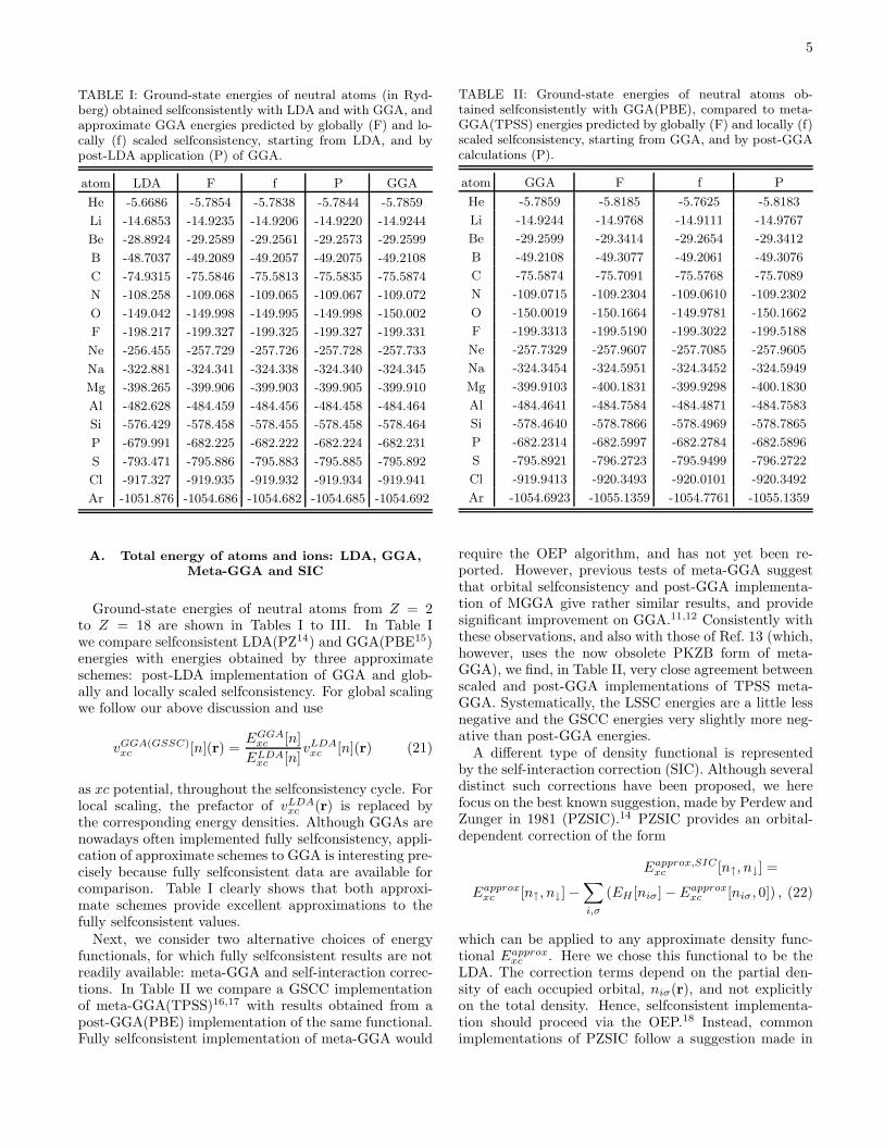
TABLE I: Ground-state energies of neutral atoms (in Ryd-berg) obtained selfconsistently with LDA and with GGA, andapproximate GGA energies predicted by globally (F) and lo-cally (f) scaled selfconsistency, starting from LDA, and bypost-LDA application (P) of GGA.

atom LDA F f P GGA

He -5.6686 -5.7854 -5.7838 -5.7844 -5.7859

Li -14.6853 -14.9235 -14.9206 -14.9220 -14.9244

Be -28.8924 -29.2589 -29.2561 -29.2573 -29.2599

B -48.7037 -49.2089 -49.2057 -49.2075 -49.2108

C -74.9315 -75.5846 -75.5813 -75.5835 -75.5874

N -108.258 -109.068 -109.065 -109.067 -109.072

O -149.042 -149.998 -149.995 -149.998 -150.002

F -198.217 -199.327 -199.325 -199.327 -199.331

Ne -256.455 -257.729 -257.726 -257.728 -257.733

Na -322.881 -324.341 -324.338 -324.340 -324.345

Mg -398.265 -399.906 -399.903 -399.905 -399.910

Al -482.628 -484.459 -484.456 -484.458 -484.464

Si -576.429 -578.458 -578.455 -578.458 -578.464

P -679.991 -682.225 -682.222 -682.224 -682.231

S -793.471 -795.886 -795.883 -795.885 -795.892

Cl -917.327 -919.935 -919.932 -919.934 -919.941

Ar -1051.876 -1054.686 -1054.682 -1054.685 -1054.692

A. Total energy of atoms and ions: LDA, GGA,

Meta-GGA and SIC

Ground-state energies of neutral atoms from Z = 2to Z = 18 are shown in Tables I to III. In Table Iwe compare selfconsistent LDA(PZ14) and GGA(PBE15)energies with energies obtained by three approximateschemes: post-LDA implementation of GGA and glob-ally and locally scaled selfconsistency. For global scalingwe follow our above discussion and use

vGGA(GSSC)xc [n](r) =

EGGAxc [n]

ELDAxc [n]

vLDAxc [n](r) (21)

as xc potential, throughout the selfconsistency cycle. Forlocal scaling, the prefactor of vLDA

xc (r) is replaced bythe corresponding energy densities. Although GGAs arenowadays often implemented fully selfconsistency, appli-cation of approximate schemes to GGA is interesting pre-cisely because fully selfconsistent data are available forcomparison. Table I clearly shows that both approxi-mate schemes provide excellent approximations to thefully selfconsistent values.

Next, we consider two alternative choices of energyfunctionals, for which fully selfconsistent results are notreadily available: meta-GGA and self-interaction correc-tions. In Table II we compare a GSCC implementationof meta-GGA(TPSS)16,17 with results obtained from apost-GGA(PBE) implementation of the same functional.Fully selfconsistent implementation of meta-GGA would

TABLE II: Ground-state energies of neutral atoms ob-tained selfconsistently with GGA(PBE), compared to meta-GGA(TPSS) energies predicted by globally (F) and locally (f)scaled selfconsistency, starting from GGA, and by post-GGAcalculations (P).

atom GGA F f P

He -5.7859 -5.8185 -5.7625 -5.8183

Li -14.9244 -14.9768 -14.9111 -14.9767

Be -29.2599 -29.3414 -29.2654 -29.3412

B -49.2108 -49.3077 -49.2061 -49.3076

C -75.5874 -75.7091 -75.5768 -75.7089

N -109.0715 -109.2304 -109.0610 -109.2302

O -150.0019 -150.1664 -149.9781 -150.1662

F -199.3313 -199.5190 -199.3022 -199.5188

Ne -257.7329 -257.9607 -257.7085 -257.9605

Na -324.3454 -324.5951 -324.3452 -324.5949

Mg -399.9103 -400.1831 -399.9298 -400.1830

Al -484.4641 -484.7584 -484.4871 -484.7583

Si -578.4640 -578.7866 -578.4969 -578.7865

P -682.2314 -682.5997 -682.2784 -682.5896

S -795.8921 -796.2723 -795.9499 -796.2722

Cl -919.9413 -920.3493 -920.0101 -920.3492

Ar -1054.6923 -1055.1359 -1054.7761 -1055.1359

require the OEP algorithm, and has not yet been re-ported. However, previous tests of meta-GGA suggestthat orbital selfconsistency and post-GGA implementa-tion of MGGA give rather similar results, and providesignificant improvement on GGA.11,12 Consistently withthese observations, and also with those of Ref. 13 (which,however, uses the now obsolete PKZB form of meta-GGA), we find, in Table II, very close agreement betweenscaled and post-GGA implementations of TPSS meta-GGA. Systematically, the LSSC energies are a little lessnegative and the GSCC energies very slightly more neg-ative than post-GGA energies.

A different type of density functional is representedby the self-interaction correction (SIC). Although severaldistinct such corrections have been proposed, we herefocus on the best known suggestion, made by Perdew andZunger in 1981 (PZSIC).14 PZSIC provides an orbital-dependent correction of the form

Eapprox,SICxc [n↑, n↓] =

Eapproxxc [n↑, n↓] −

∑

i,σ

(EH [niσ] − Eapproxxc [niσ, 0]) , (22)

which can be applied to any approximate density func-tional Eapprox

xc . Here we chose this functional to be theLDA. The correction terms depend on the partial den-sity of each occupied orbital, niσ(r), and not explicitlyon the total density. Hence, selfconsistent implementa-tion should proceed via the OEP.18 Instead, commonimplementations of PZSIC follow a suggestion made in

6

TABLE III: Ground-state energies of neutral atoms obtainedselfconsistently with LDA, and PZSIC energies predicted byglobally scaled selfconsistency, starting from LDA, and bypost-LDA implementation of PZSIC, all compared to ener-gies obtained from a standard (i.e., orbitally selfconsistent)implementation of LDA+PZSIC.

atom LDA F P LDA+PZSIC

He -5.6686 -5.8366 -5.8329 -5.8386

Li -14.6853 -15.0075 -15.0036 -15.0091

Be -28.8924 -29.3863 -29.3824 -29.3877

B -48.7037 -49.3992 -49.3946 -49.4007

C -74.9315 -75.8573 -75.8520 -75.8592

N -108.258 -109.442 -109.436 -109.445

O -149.042 -150.505 -150.497 -150.508

F -198.217 -199.987 -199.979 -199.991

Ne -256.455 -258.561 -258.551 -258.565

Na -322.881 -325.332 -325.324 -325.336

Mg -398.265 -401.060 -401.053 -401.064

Al -482.628 -485.769 -485.762 -485.773

Si -576.429 -579.922 -579.916 -579.926

P -679.991 -683.843 -683.836 -683.846

S -793.471 -797.689 -797.683 -797.692

Cl -917.327 -921.920 -921.914 -921.923

Ar -1051.876 -1056.850 -1056.850 -1056.854

the original reference,14 and vary the energy functionalwith respect to the orbitals. The resulting single-particleequation is not the usual Kohn-Sham equation, but fea-tures an effective potential that is different for each or-bital.

In Table III we compare energies obtained from so-lution of this equation with those obtained, in a muchsimpler way, from applying GSCC to LDA+PZSIC. Verygood agreement is achieved. This is even more remark-able as in usual implementations of PZSIC the potentialsare different for each orbital, and the resulting orbitalsare not orthogonal, whereas in the GSSC implementa-tion the local potential is the same for all orbitals, whichare automatically orthogonal. Formally, the GSSC im-plementation is thus more satisfying than the standardimplementation.

The analysis of total energies of neutral atoms is sum-marized in Figure 1, which displays the relative deviation

η =(Eref − EGSSC)

Eref

(23)

of GSCC from selfconsistent data (GGA), post-GGAdata (meta-GGA) and orbitally selfconsistent data(PZSIC).

Table IV presents a representative error analysis. Val-ues of C2, defined in Eq. (15), indicate that the term ne-glected in the GSSC approach is smaller than the termkept, but not by a sufficient margin to explain, on itsown, the very good approximation to total energies ob-

5 9 13 17

Z

-1.0

0

1.0

2.0

3.0

4.0

η (x

10-5

)

PZ-SICGGAMeta-GGA

FIG. 1: Relative deviation, as defined in Eq. (23), of GSSCGGA compared to selfconsistent GGA (full line), of GSSCmeta-GGA compared to post-GGA meta-GGA (dash-dottedline) and of GSCC LDA+PZSIC compared to orbitally self-consistent LDA+PZSIC. Note that only in the first case thisrelative deviation can be interpreted as a relative error ofGSSC relative to fully selfconsistent results, as in the othertwo cases different approximations are compared among eachother.

TABLE IV: Breakdown of errors of the different contribu-tions to the total energy in Eq. (16), comparing LDA-basedglobal-scaling predictions of GGA energies (GSSC GGA) withselfconsistent GGA energies. The column labeled C2 containsthe integrated validity criterium of global scaling, as definedin Eq. (15). Note that we have not defined an integratedvalidity criterium for local scaling.

atom C2 ∆EKS ∆EH ∆Vxc ∆Exc ∆E0

He 0.016 0.0974 0.0131 0.0766 -0.0081 -0.0004

C 0.115 0.2684 -0.1670 0.4504 0.0122 -0.0028

O 0.016 0.333 -0.318 0.679 0.024 -0.004

Na 0.353 0.464 -0.541 1.041 0.031 -0.004

Si 0.147 0.689 -0.691 1.416 0.030 -0.006

Ar 0.009 0.959 -0.948 1.950 0.036 -0.007

tained from global scaling. The breakdown of the errorof the total energy into the contributions arising fromeach term individually, shows that there is very substan-tial error cancellation, mostly between the sum of the KSeigenvalues and the potential energy in the xc potential.As a consequence of this error cancellation, which is ul-timately due to the variational principle, selfconsistenttotal energies are predicted by scaling approaches withmuch higher accuracy than the values of C2 suggest.

The performance of global and local scaling, as well asthat of post methods, for (positive) ions is essentially thesame obtained for neutral systems, as is illustrated forselected ions in Table V.

From the data in Tables I to V we conclude that globalscaling yields slightly better ground-state energies thanlocal scaling and post methods. In addition, for orbital-dependent functionals, such as PZ-SIC, it provides a com-

7

TABLE V: Ground-state energies of positive ions, obtainedfrom self-consistent LDA and GGA calculations, as well asfrom locally and globally scaled LDA calculations.

atom LDA F f P GGA

He+ -3.8838 -3.9873 -3.9853 -3.9864 -3.9875

Li+ -14.2831 -14.5130 -14.5105 -14.5116 -14.5135

Be+ -28.2278 -28.5977 -28.5945 -28.5960 -28.5986

B+ - 48.0742 -48.5858 -48.5827 -48.5840 -48.5869

C + -74.0698 -74.7273 -74.7238 -74.7258 -74.7292

N+ -107.159 -107.973 -107.969 -107.972 -107.976

O+ -148.014 -148.993 -148.990 -148.992 -148.997

F+ -196.886 -198.016 -198.013 -198.015 -198.020

Ne+ -254.823 -256.113 -256.110 -256.112 -256.117

Na+ -322.487 -323.947 -323.944 -323.946 -323.951

Mg+ -397.696 -399.346 -399.344 -399.346 -399.351

Al+ -482.188 -484.021 -484.018 -484.020 -484.026

Si+ -575.823 -577.851 -577.848 -577.850 -577.856

P+ -679.219 -681.450 -681.447 -681.449 -681.456

S+ -792.690 -795.133 -795.129 -795.132 -795.139

Cl+ -916.350 -918.975 -918.971 -918.974 -918.981

Ar+ -1050.703 -1053.524 -1053.520 -1053.523 -1053.530

mon local potential and orthogonal orbitals at no extracomputational cost.

B. Kohn-Sham eigenvalues of atoms and ions:

LDA, GGA, Meta-GGA and SIC

In principle, a further advantage of scaled approaches,as compared to post methods, is that the former alsoprovide corrections to the Kohn-Sham spectrum, whichcannot be obtained from the latter. Instead of consider-ing the entire spectrum, we focus on the highest occupiedeigenvalue, as it is physically most significant. Represen-tative data for this eigenvalue are collected in Tables VIto IX.

Unlike total energies, KS eigenvalues (single-particleenergies) are not protected by a variational principle,and simple approximations, such as global or local scal-ing, may work less well than for total energies. For thetransition from LDA to GGA, the data in Tables VI andVII show indeed that not applying any scaling factor atall, i.e., using the uncorrected LDA eigenvalues, producesbetter approximations to the GGA eigenvalues than ei-ther local or global scaling. For meta-GGA (Table VIII),no fully selfconsistent eigenvalues are available for com-parison (as explained in the introduction, this would re-quire the OEP algorithm to be implemented for meta-GGA). For PZ-SIC, on the other hand, Table IX showsthat substantial improvement on the LDA eigenvaluesis obtained by global scaling, although not by the samemargin observed for total energies.

TABLE VI: Highest occupied KS eigenvalues of neutralatoms, obtained selfconsistently from LDA and from GGA,and LDA-based predictions of the GGA energies by means ofglobal and local scaling.

atom LDA F f GGA

He -1.1404 -1.2073 -1.2187 -1.1585

Li -0.2326 -0.2558 -0.2548 -0.2372

Be -0.4120 -0.4455 -0.4328 -0.4122

B -0.2997 -0.3387 -0.3368 -0.2955

C -0.4517 -0.5008 -0.5013 -0.4482

N -0.6137 -0.6716 -0.6760 -0.6103

O -0.5502 -0.5951 -0.6082 -0.5287

F -0.7701 -0.8242 -0.8387 -0.7523

Ne -0.9955 -1.0576 -1.0757 -0.9810

Na -0.2263 -0.2427 -0.2515 -0.2234

Mg -0.3513 -0.3724 -0.3703 -0.3454

Al -0.2212 -0.2417 -0.2455 -0.2218

Si -0.3383 -0.3648 -0.3707 -0.3403

P -0.4602 -0.4922 -0.5007 -0.4626

S -0.4612 -0.4898 -0.4971 -0.4403

Cl -0.6113 -0.6454 -0.6519 -0.5978

Ar -0.7646 -0.8039 -0.8114 -0.7560

IV. TESTS AND APPLICATIONS TO MODELS

OF EXTENDED SYSTEMS

The calculations in the preceding sections were re-stricted to atoms and ions. Some results for moleculeswere already reported in Ref. 13. We therefore next turnto models for extended systems.

A. Hubbard model

First, we consider the Hubbard model, which is a muchstudied model Hamiltonian of condensed-matter physics,for which the basic theorems of density-functional theoryall hold.19,20,21 In the present context, this model consti-tutes a most interesting test case for scaled selfconsis-tency for three different reasons: (i) It is maximally dif-ferent from the atoms and ions considered in the previoussections, and thus provides tests in an entirely differentregion of functional space. (ii) For a small number oflattice sites the exact diagonalization of the Hamiltonianmatrix in a complete basis (consisting of one orbital persite) can be performed numerically, hence providing ex-act data against which all approximate functionals andimplementations can be checked. (iii) In the thermody-namic limit (infinite number of sites) with equal occupa-tion on each sites (homogeneous density distribution) theexact many-body solution of the one-dimensional Hub-bard model is known from the Bethe-Ansatz technique.22

This solution allows the construction of the exact local-density approximation,19,21 which circumvents the need

8

TABLE VII: Highest occupied KS eigenvalues of positive ions,obtained selfconsistently from LDA and from GGA, and LDA-based predictions of the GGA energies by means of global andlocal scaling.

atom LDA F f GGA

He+ -3.0211 -3.1623 -3.1610 -3.0898

Li+ -4.3793 -4.5188 -4.5348 -4.4400

Be+ -1.0509 -1.0969 -1.0954 -1.0637

B+ -1.4267 -1.4827 -1.4663 -1.4336

C+ -1.3072 -1.3724 -1.3702 -1.3031

N+ -1.6213 -1.6973 -1.6968 -1.6197

O+ -1.9384 -2.0233 -2.0269 -1.9381

F+ -1.9307 -1.9973 -2.0140 -1.9091

Ne+ -2.3093 -2.3860 -2.4043 -2.2926

Na+ -2.6857 -2.7709 -2.7932 -2.6734

Mg+ -0.8803 -0.9072 -0.9252 -0.8746

Al+ -1.0949 -1.1257 -1.1278 -1.0867

Si+ -0.8904 -0.9224 -0.9284 -0.8912

P+ -1.1005 -1.1387 -1.1461 -1.1046

S+ -1.3115 -1.3556 -1.3651 -1.3172

Cl+ -1.3592 -1.3983 -1.4075 -1.3376

Ar+ -1.5975 -1.6426 -1.6510 -1.5851

for analytical parametrizations of the underlying uni-form reference data, required for the conventional LDAof the ab initio Coulomb Hamiltonian. The simultaneousdisponibility of the exact solution and the exact LDAmakes this model an ideal test case for DFT approxima-tions.

The one-dimensional Hubbard model is specified bythe second-quantized Hamiltonian

H = −t

L∑

i,σ

(c†iσci+1,σ + H.c.) + U

L∑

i

c†i↑ci↑c†i↓ci↓ (24)

defined on a chain of L sites i, with one orbital per site.Here U parametrizes the on-site interaction and t thehopping between neighbouring sites. Below all energiesand values of U are given in multiples of t, as is commonpractice in studies of the model (24).

The availability of an exact many-body solution forsmall L, and of the exact LDA, permit us to eliminatemany of the uncertainties associated with more approxi-mate calculations. To test the ideas of scaled selfconsis-tency for the Hubbard model, we attempt to predict theenergies of a selfconsistent LDA calculation by startingwith a simple Hartree (mean-field) calculation. Equa-tion (13) cannot be directly applied to the xc potentialsbecause the xc potential of a pure Hartree calculationis zero, but we can apply it to the entire interaction-dependent contribution to the effective potential, i.e., tothe sum of Hartree and xc terms. We thus approximatethe entire interaction potential by its Hartree contribu-tion, and use scaled selfconsistency to predict the values

TABLE VIII: Highest occupied KS eigenvalues of neutralatoms, obtained from GGA and predicted for TPSS meta-GGA by global and local scaling.

atom GGA F f

He -1.1585 -1.1767 -0.7159

Li -0.2372 -0.2420 -0.1055

Be -0.4122 -0.4192 -0.2249

B -0.2955 -0.3023 -0.0968

C -0.4482 -0.4566 -0.1763

N -0.6103 -0.6208 -0.2656

O -0.5287 -0.5356 -0.2585

F -0.7523 -0.7606 -0.3881

Ne -0.9810 -0.9912 -0.5245

Na -0.2234 -0.2259 -0.1000

Mg -0.3454 -0.3486 -0.1841

Al -0.2218 -0.2249 -0.0731

Si -0.3403 -0.3443 -0.1364

P -0.4626 -0.4675 -0.2065

S -0.4403 -0.4444 -0.2202

Cl -0.5978 -0.6028 -0.3154

Ar -0.7560 -0.7618 -0.4140

of a Hartree+LDA calculation. In analogy to our previ-ous equations we write this as

vGSSC(H+LDA)int (i) =

EH+LDAint [ni]

EHint[ni]

vH(i). (25)

Results obtained from this approximation can be com-pared to a selfconsistent Hartree+LDA calculation, inwhich

vint(i) = vH(i) + vLDAxc (i). (26)

This comparison provides a severe test for the scaledselfconsistency concept, as the starting functional(Hartree) is quite different from the target functional(Hartree+LDA).

The effective potential vs(i) is, in principle, given byadding vint(i) to the external potential vext(i), but herewe chose vext(i) ≡ 0, so that the interaction-dependentcontribution becomes identical to vs(i). This makes thetest even tougher, as there is no large external potentialdominating the total energy and the eigenvalues, and po-tentially masking effects of vLDA

xc (i).The system becomes inhomogeneous because of the fi-

nite size of the chain. For L = 10 sites exact energies canstill be obtained, and are displayed, together with vari-ous approximations to them, in Table X. For L = 100sites obtaining exact energies is out of question, but allDFT procedures are still easily applicable. Correspond-ing results for total energies are also displayed in Table X.Eigenvalues are recorded in Table XI.

From Tables X and XI we conclude that: (i) Forground-state energies the LDA typically deviates by

9

TABLE IX: Highest occupied KS eigenvalues of neutralatoms, obtained selfconsistently from LDA and predicted forLDA+PZSIC by means of global scaling, compared to an or-bitally selfconsistent implementation of LDA+PZSIC.

atom LDA F LDA+PZSIC

He -1.1404 -1.2370 -1.8957

Li -0.2326 -0.2642 -0.3927

Be -0.4120 -0.4575 -0.6554

B -0.2997 -0.3538 -0.6125

C -0.4517 -0.5219 -0.8512

N -0.6137 -0.6990 -1.0960

O -0.5502 -0.6195 -1.0627

F -0.7701 -0.8570 -1.3732

Ne -0.9955 -1.0991 -1.6838

Na -0.2263 -0.2544 -0.3782

Mg -0.3513 -0.3875 -0.5502

Al -0.2212 -0.2571 -0.4081

Si -0.3383 -0.3844 -0.5717

P -0.4602 -0.5159 -0.7376

S -0.4612 -0.5116 -0.7696

Cl -0.6113 -0.6718 -0.9632

Ar -0.7646 -0.8348 -1.1586

TABLE X: Exact per-site ground-state energy (to six signifi-cant digits), selfconsistent LDA energy, selfconsistent Hartreeenergy, and Hartree-based simulations of the LDA energy viaglobal scaling, local scaling and post-Hartree implementation.All energies have been multiplied by −10/t. First set of threerows: L = 10 sites with N = 2 electrons. Second set of threerows: L = 10 sites with N = 8 electrons. Third set of threerows: L = 100 sites with N = 96 electrons. All calculationswere done for open boundary conditions with vext = 0.

N U exact Hartree F f P LDA

2 2 3.69905 3.58412 3.68371 3.68457 3.68456 3.68472

4 3.65957 3.35102 3.62921 3.63175 3.63014 3.63239

6 3.64244 3.12796 3.60332 3.60710 3.60117 3.60815

8 2 8.87176 8.24130 8.81004 8.81062 8.81064 8.81067

4 7.30440 5.02351 7.13510 7.13573 7.13529 7.13574

6 6.37228 1.81375 6.11910 6.11850 6.11520 6.11918

96 2 - 8.02648 8.71172 8.71174 8.71174 8.71174

4 - 3.41821 6.19811 6.19806 6.19791 6.19962

6 - -1.18994 4.74410 4.74411 4.74369 4.75018

about 1% from the exact values, while a Hartree calcula-tion is about 10% off. (ii) Taking the selfconsistent LDAdata as standard, we find that for ground-state energieslocally scaled selfconsistency comes closest, followed, inthis order, by post-Hartree data, globally scaled selfcon-sistency and the original Hartree calculation. (iii) Foreigenvalues the order changes: globally scaled selfcon-sistency does better than locally scaled selfconsistency,

TABLE XI: Highest occupied Kohn-Sham eigenvalue ob-tained from selfconsistent LDA calculations, selfconsistentHartree calculations, and Hartree-based simulations of theLDA energy via global scaling (F) and local scaling (f). Thesystems are the same as in Table X.

N U Hartree F f LDA

2 2 -1.67177 -1.76773 -1.76999 -1.74131

4 -1.44839 -1.71514 -1.72036 -1.66731

6 -1.23452 -1.69022 -1.69737 -1.63056

8 2 -0.02259 -0.16428 -0.16486 -0.09917

4 0.77959 0.25307 0.25211 0.39835

6 1.58054 0.50636 0.50562 0.68490

96 2 0.80452 0.66180 0.66175 0.74151

4 1.76435 1.18533 1.18531 1.25131

6 2.72424 1.48818 1.48819 1.47135

whereas post-calculations naturally do not provide anycorrection at all, and come a distant third.

We have performed similar comparisons also for othersystems (different number of sites L, different number ofelectrons N , different values of the on-site interaction pa-rameter U), but the general trend is the same, althoughin isolated cases the relative quality of F, f and P-typeimplementations can be different.

In Table XII we analyse the satisfaction of the va-lidity criteria of Sec. II C and the contribution of eachterm in the ground-state-energy expression to the totalerror. The values of C2 in Table XII show that the termneglected in global scaling is always smaller than theterm kept, but in unfavorable cases, such as low densityand strong interactions, can be a sizeable fraction of it.Hence, just as for atoms and ions, additional error can-cellation, arising from the separate contributions to theground-state energy, is taking place in these situations.

These contributions to the ground-state energy can bewritten as

E0 =∑

i

ǫi −

∫

d3r n(r)vint[n](r) + Eint[n] (27)

=: EKS − Vint + Eint, (28)

and their errors are recorded in Table XII.

The data in Table XII show that the total error ismuch less than that of each contribution individually.Global and local SSC thus benefit from systematic andextensive error compensation – mostly between the sumof the KS eigenvalues and the interaction potential en-ergy – which make it applicable even when the simplestfrom of the validity criterium, Eq. (14), or its integratedversion, Eq. (15), are violated. Clearly, locally scaledselfconsistence benefits even more than globally scaledselfconsistence.

10

TABLE XII: Validity criterium and error analysis for the sys-tem of Tables X and XI. C2 is defined in Eq. (15), and theother columns report, for each term of the total energy ex-pression (28), the difference between the fully selfconsistentresult and the result obtained by GSSC. The error in the to-tal energy is given by ∆E0 = ∆EKS − ∆Vint + ∆Eint, andalways significantly lower than each of the individual errors.First set of nine lines: global scaling. Second set of nine lines:local scaling. Recall that we have not defined an integratedvalidity criterium for local scaling.

N U C2 ∆EKS ∆Vint ∆Eint ∆E0

2 2 0.162 0.05285 0.04794 -0.00592 -0.00101

4 0.247 0.09565 0.08495 -0.01388 -0.00318

6 0.290 0.11933 0.10522 -0.01894 -0.00483

8 2 0.098 0.52085 0.51601 -0.00547 -0.00063

4 0.135 1.16243 1.15674 -0.00633 -0.00064

6 0.135 1.42893 1.42831 -0.00070 -0.00008

96 2 0.098 7.6541 7.6531 -0.0012 -0.0002

4 0.065 6.4775 6.4813 -0.0113 -0.0151

6 0.018 -0.7711 -0.7835 -0.0731 -0.0608

2 2 - 0.05737 0.05526 -0.00227 -0.00016

4 - 0.10610 0.10078 -0.00596 -0.00064

6 - 0.13363 0.12627 -0.00841 -0.00105

8 2 - 0.52543 0.52400 -0.00148 -0.00005

4 - 1.17013 1.17090 0.00075 -0.00002

6 - 1.43479 1.44124 0.00577 -0.00068

96 2 - 7.6551 7.6548 -0.0003 0.0000

4 - 6.4768 6.4811 -0.0114 -0.0156

6 - -0.7709 -0.7834 -0.0731 -0.0607

B. Quantum wells

Moving up from one dimension to three, we next con-sider semiconductor heterostructures. To illustrate themain features of scaled selfconsistency we consider a sim-ple quantum well, in which the electrons are free to movealong the x and y direction, but confined along the z di-rection. The modelling of such quantum wells by meansof the effective-mass approximation within DFT is de-scribed in Ref. 23 and the particular approach we use isthat of Ref. 24, whose treatment we follow closely, andto which we refer the reader for more details.

In Table XIII we display ground-state energies andhighest occupied KS eigenvalue obtained for represen-tative quantum wells by means of a selfconsistent LDAcalculation (using the PW9225 parametrization for theelectron-liquid correlation energy), a selfconsistent GGAcalculation (using the PBE15 form of the GGA), post-LDA GGA, and globally-scaled and locally-scaled simu-lations of PBE by means of LDA.

Total energy differences between all three approximateschemes are marginal, compared to the difference be-tween a pure LDA calculation and a GGA calculation: allthree LDA-based schemes closely approximate the results

TABLE XIII: Ground-state energies (in meV per particle)and highest-occupied KS eigenvalue (in meV ) of a quantumwell of depth 200meV , width 10nm, embedded in a back-ground semiconductor (charge reservoir) of width 50nm, arealdensity of nA = 1012cm−2, effective electron mass of 0.1m0

and relative dielectric constant ε = 10. These parameters aretypical of semiconductor heterostructures.26,27 For the secondset of two lines we have added a central barrier of width 3nmand hight 200meV , dividing the system in two weakly coupledhalves.

LDA(PW92) F f P GGA(PBE)

E 78.0197 77.7135 77.7194 77.7136 77.7122

ǫ 117.455 117.060 116.993 117.455 117.183

E 129.134 128.435 128.443 128.436 128.426

ǫ 163.322 162.420 162.375 163.322 162.706

of selfconsistent GGA calculations, with global scalingslightly better than the other two. Interestingly, this isthe opposite trend observed in the Hubbard chain, wherelocal scaling was best. For eigenvalues, post-calculationsdo not provide any improvement, whereas both globaland local scaling come close to the fully selfconsistentresults.

In Table XIV we show the values of C2, and the break-down of the error of the ground-state energy in its com-ponents, according to

E0[n] =∑

i

ǫi − EH [n] −

∫

d3r n(r)vxc(r) + Exc[n](29)

= EKS − EH [n] − Vxc + Exc[n].(30)

The GSSC validity criterium (15) is well satisfied. Val-ues of C2 are an order of magnitude smaller than for theHubbard chain. This reduction expresses the fact thatsimulating a GGA by starting from an LDA is a mucheasier task than simulating an LDA by starting from aHartree calculation. Also understandable are the slightlylarger values of C2 and of the errors in the energy foundfor the double well as compared to the single well, sincethis structure has more pronounced density gradients,enhancing the difference between LDA and GGA, andcomplicating the task the scaling factor has to accom-plish.

For the energy components, we observe the same typeof substantial error cancellation found also in the calcu-lations for atoms, ions and the Hubbard model, resultingin very good total energies. We note that this error can-cellation is taking place mainly between the sum of theKS eigenvalues and the potential energy in the xc po-tential, whose errors are subtracted in forming E0. Theerrors in the xc and the Hartree energies are orders ofmagnitude smaller. This is the same observation previ-ously made for the other systems, suggesting that thispattern of error cancellation is a general trend.

11

TABLE XIV: Error analysis for the heterostructures of Ta-ble XIII. First set of two lines: simple well. Second set oftwo lines: well with barrier. The total error is obtained as∆E0 = ∆EKS −∆EH −∆Vxc +∆Exc. Very substantial errorcancellation between the sum of the KS eigenvalues and thexc potential energy is taking place.

C2 ∆EKS ∆EH ∆Vxc ∆Exc ∆E0

GSSC 0.022 -0.1232 -0.0129 -0.1056 0.0061 0.0013

LSSC - -0.1904 -0.0953 -0.0703 0.0321 0.0072

GSSC 0.036 -0.237 0.036 -0.248 0.035 0.010

LSSC - -0.289 -0.032 -0.216 0.058 0.017

V. CONCLUSIONS

Three different possibilities for approximating theresults of selfconsistent calculations with a compli-cated functional by means of selfconsistent calculationswith a simpler functional have been compared: Post-selfconsistent implementation of the complicated func-tional (P), global scaling of the potential of the simplefunctional by the ratio of the energies (F), and local scal-ing of the potential of the simple functional by the ratioof the energy densities (f). While method P is a stan-dard procedure of DFT, method F was proposed onlyvery recently (and without a solid derivation or a valid-ity criterium, both of which we provide here). Method fis proposed here for the first time.

These three approaches were tested for atoms, ions,Hubbard chains and quantum wells, and applied toHartree, LDA, GGA, meta-GGA and SIC type densityfunctionals. Our conclusions are summarized as follows.

(i) All three prescriptions provide significant improve-ments on the total ground-state energies obtained fromthe simple functional (as measured by their proximity tothose obtained selfconsistently from the complex func-tional). For these energies, on average, globally scaledselfconsistency has a slight advantage compared to post-selfconsistent implementations and local scaling, but therelative performance of all three methods depends on finedetails of the system parameters, on the quantity cal-culated, and on the particular density functional used.In general, neither local scaling nor alternative scalingschemes (employing other scaling factors, or scaling othercontributions to the energy) provide consistent improve-

ments on global scaling, which for total energies is, onaverage, the best of all methods tested here.

(ii) An additional advantage of scaled selfconsistencyis that it also provides approximations to the eigenvalues,eigenfunctions and effective potentials of the complicatedfunctional, which is by construction impossible for post-methods. Indeed, for orbital-dependent potentials, suchas PZ-SIC, scaling provides a simple and effective wayto produce a common local potential and orthogonal or-bitals. For models of extended systems, scaling providessignificant improvement on eigenvalues obtained from thesimple functional, although by a smaller margin than forthe total energy. For finite systems, similar improvementwas found in applications of PZ-SIC, but not in teststrying to predict GGA eigenvalues from LDA.

(iii) The reason scaled selfconsistency works is due toan interplay of three distinct mechanisms. First, when-ever the term neglected in Eq. (12) is much smaller thanthe term kept, its neglect is obviously a good approx-imation. This is checked by the point-wise criterium(14). Second, even when the neglected term is not muchsmaller, quantities that depend on the potential at allpoints in space, such as the total energies or the eigen-values, benefit from error cancellation arising from dif-ferent points in space, as described by the integrated cri-terium (15). Total energies — but not eigenvalues — alsobenefit from an additional error cancellation between thedifferent contributions to the total energy expression ofDFT. Numerically, we found this third mechanism to bedominant. The fact that this additional error cancella-tion operates only for total energies explains why in allour tests these are consistently better described by scaledselfconsistency than eigenvalues.

Different scaling schemes from the two employed heremay be investigated, and certainly additional informa-tion from application to still other classes of systemsshould be useful, but it seems safe to conclude from thepresent analysis that scaled selfconsistency is a most use-ful concept for density-functional theory, allowing the ef-ficient and reliable implementation of density functionalsof hitherto unprecedented complexity, without ever re-quiring their variational derivative with respect to eitherorbitals or densities.

Acknowledgments This work was supported byFAPESP and CNPq.

∗ Electronic address: capelle@ifsc.usp.br1 W. Kohn, Rev. Mod. Phys. 71, 1253 (1999).2 R. M. Dreizler and E. K. U. Gross, Density Functional

Theory (Springer, Berlin, 1990).3 R. G. Parr and W. Yang, Density-Functional Theory of

Atoms and Molecules (Oxford University Press, Oxford,1989).

4 J. P. Perdew, A. Ruzsinszky, J. Tao, V. N. Staroverov, G.

E. Scuseria and G. I. Csonka, J. Chem. Phys. 123, 062201(2005). P. Ziesche, S. Kurth and J. P. Perdew, Comp. Mat.Sci. 11, 122 (1998).

5 T. Grabo, T. Kreibich, S. Kurth and E. K. U. Gross, inV. I. Anisimov (Ed.), Strong Coulomb Correlations in Elec-

tronic Structure Calculations: Beyond the Local Density

Approximation (Gordon & Breach, 1999). T. Grabo andE. K. U. Gross, Int. J. Quantum Chem. 64, 95 (1997).

12

T. Grabo and E. K. U. Gross, Chem. Phys. Lett. 240, 141(1995). E. Engel and S. H. Vosko, Phys. Rev. A 47, 2800(1993).

6 J. B. Krieger, Y. Li and G. J. Iafrate, Phys. Rev. A 45,101 (1992); ibid 46, 5453 (1992); ibid 47 165 (1993).

7 S. Kummel and J. P. Perdew, Phys. Rev. B 68, 035103(2003).

8 W. Yang and Q. Qu, Phys. Rev. Lett. 89, 143002 (2002).9 V. N. Staroverov, G. E. Scuseria and E. R. Davidson, J.

Chem. Phys. 124, 141103 (2006).10 R. Neumann, R. H. Nobes and N. C. Handy, Mol. Phys.

87, 1 (1996).11 V. N. Staroverov, G. E. Scuseria, J. Tao and J. P. Perdew,

J. Chem. Phys. 119, 12129 (2003).12 V. N. Staroverov, G. E. Scuseria, J. Tao and J. P. Perdew,

Phys. Rev. B 69, 075102 (2004).13 M. Cafiero and C. Gonzalez, Phys. Rev. A 71, 042505

(2005).14 J. P. Perdew and A. Zunger, Phys. Rev. B 23, 5048 (1981).15 J. P. Perdew, K. Burke and M. Ernzerhof, Phys. Rev.

Lett. 77, 3865 (1996). ibid 78, 1396(E) (1997). See alsoV. Staroverov et al., Phys. Rev. A 74, 044501 (2006).

16 J. Tao, J. P. Perdew, V. N. Staroverov and G. E. Scuseria,

Phys. Rev. Lett. 91, 146401 (2003).17 J. P. Perdew, J. Tao, V. N. Staroverov and G. E. Scuseria,

J. Chem. Phys. 120, 6898 (2004).18 M. R. Norman and D. D. Koelling, Phys. Rev. B 30, 5530

(1984).19 K. Schonhammer, O. Gunnarsson, and R. M. Noack, Phys.

Rev. B 52, 2504 (1995).20 N. A. Lima, M. F. Silva, L. N. Oliveira and K. Capelle,

Phys. Rev. Lett. 90, 146402 (2003).21 G. Xianlong, M. Polini, M. P. Tosi, V. L. Campo, Jr., K.

Capelle and M. Rigol, Phys. Rev. B 73, 165120 (2006).22 E. H. Lieb and F. Y. Wu, Phys. Rev. Lett. 20, 1445 (1968).23 T. Ando and S. Mori, J. Phys. Soc. Jpn. 47, 1518 (1976).24 H. J. P. Freire and J. C. Egues, Braz. J. Phys. 34, 614

(2004).25 J. P. Perdew and Y. Wang, Phys. Rev. B 45, 13244 (1992).26 Z. I. Alferov, Rev. Mod. Phys. 73, 767 (2001).27 Landolt-Bornstein: Numerical Data and Functional Re-

lationships in Science and Technology, New Series, Vol.17, Semiconductors, eds. O. Madelung, M. Schulz and H.Weiss. (Springer, Berlin 1982).