Consistency of the EKF-SLAM Algorithm

Tim Bailey, Juan Nieto, Jose Guivant and Eduardo Nebot

Australian Centre for Field Robotics, University of Sydney{tbailey,j.nieto,jguivant,nebot}@acfr.usyd.edu.au

Abstract. This paper presents a simulation-based analysis of the extended Kalmanfilter formulation of simultaneous localisation and mapping (EKF-SLAM). Weshow that the algorithm will always produce very inconsistent estimates once the“true” uncertainty in vehicle heading exceeds a limit. This failure is subtle andcannot, in general, be detected without ground-truth, although the inconsistent fil-ter may exhibit observable symptoms, such as “jumpy” vehicle path. Conventionalsolutions—adding stabilising noise, using iterated or unscented filters, etc—do notimprove the situation. However, if “small” heading uncertainty is maintained, EKF-SLAM behaves consistently and is insensitive to system noise and non-linearities.This result indicates the efficacy of submap methods for large-scale maps.

1 Introduction

The original stochastic solution to the SLAM problem by Smith et al. [13] isnow almost twenty years old, and the concept has reached a state of maturitysufficient to permit practical implementations in challenging environments.Important considerations that have been addressed are reliable data associa-tion in cluttered environments [12,1]; reduction of computational complexitythrough locally partitioned data-fusion [14,6] and conservative data-fusion[6,10,9]; and bounding accumulated non-linearity with submaps [1,3]. How-ever, in spite of its clear success in practical applications, the fundamentalconsistency of the SLAM algorithm has received little attention.

Non-linear SLAM is predominantly implemented as an extended Kalmanfilter (EKF), where system noise is presumed Gaussian and non-linear modelsare linearised to suit the Kalman filter algorithm.1 EKF-SLAM represents thestate uncertainty by an approximate mean and variance. This is a problemin two regards. First, these moments are approximate due to linearisationand may not accurately match the “true” first and second moments. Second,the true probability distribution may be non-Gaussian, so that even the truemean and variance may not be an adequate description. These factors affecthow the SLAM probability distribution is projected in time, over a sequence

1 A number of algorithms appearing in the recent literature, such as scan matching[7] and FastSLAM [11], are built on alternative foundations (e.g., data alignment,particle filters), but these have their own problems, both computational andstatistical, and are not considered further in this paper. Comparison of EKF-SLAM and FastSLAM will be made in the conference presentation.

2 T. Bailey et al.

of motions and measurements, and how approximation errors accumulate.Previous work on EKF-SLAM consistency [8,4] shows that eventual inconsis-tency of the algorithm is inevitable for large-scale maps, and the estimateduncertainty will become optimistic when compared to the true errors. Whilethis failure is clearly due to non-linearity, no previous work has examined theroot-cause of degeneracy.

In this paper, we show that the fundamental problem with EKF-SLAM isheading uncertainty. This is the single critical factor that causes the map es-timate to become inconsistent. All other modelling errors and non-linearitiescan be adequately compensated with stabilising noise. Inconsistency becomessignificant once heading uncertainty is “large enough” and, since heading un-certainty tends to accumulate as the vehicle moves away from the map origin,the problem is inevitable for large maps.

The next section describes the models used in the EKF-SLAM simulationexperiments, which are performed in the context of a robot with a range-bearing sensor in a 2-dimensional environment. Data association is assumedknown. Section 3 examines the symptoms that manifest once EKF-SLAMbecomes inconsistent, and shows that gross inconsistency is entirely due toheading uncertainty. Section 4 discusses the implications of these results andpossible solutions to minimise inconsistency, and the final section sums upwith concluding remarks.

2 Models for EKF-SLAM Experiments

We specify the SLAM state as the vehicle pose (position and heading) andthe locations of stationary landmarks observed in the environment. The stateat time k is represented by a joint state-vector xk.

xk = [xvk, yvk

, φvk, x1, y1, . . . , xN , yN ]T =

[xvk

m

](1)

Notice that the map parameters m = [x1, y1, . . . , xN , yN ]T do not have atime subscript as they are modelled as stationary.

To describe the vehicle motion, we use the kinematic model for the tra-jectory of the front wheel of a bicycle subject to rolling motion constraints(i.e., assuming zero wheel slip).

xvk= fv

(xvk−1 ,uk

)=

xvk−1 + Vk∆T cos(φvk−1 + γk)yvk−1 + Vk∆T sin(φvk−1 + γk)

φvk−1 + Vk∆TB sin(γk)

(2)

Here the time from k − 1 to k is denoted ∆T , and during this period thevelocity Vk and steering angle γk of the front wheel are assumed constant.Collectively, the velocity and steering values uk = [Vk, γk]T are termed the“controls”. The wheelbase between the front and rear axles is B. The process

Consistency of the EKF-SLAM Algorithm 3

model for the joint SLAM state is simply a concatenation of the vehiclemotion model and the stationary landmark model.

xk = f (xk−1,uk) =[fv

(xvk−1 ,uk

)m

](3)

For a range-bearing measurement from the vehicle to landmark mi =[xi, yi]T , the observation model is given by

zik= hi (xk) =

[√(xi − xvk

)2 + (yi − yvk)2

arctan yi−yvk

xi−xvk− φvk

](4)

The vehicle motion model, the observation model, and the measured val-ues of the control parameters uk, are not exact, but are subject to noise,which lead to uncertainty in the state estimate. For this reason, we require aprobabilistic filter to recursively estimate a distribution over the state givennoisy information.

3 Problems with EKF-SLAM

The work of Julier and Ulhmann [8] shows that EKF-SLAM inevitably be-comes inconsistent and that this problem is structural; it cannot be circum-vented by adding stabilising noise to the process and observation models.2

We use two measures for filter consistency. When the “true” statistics ofthe state are available, or can be well approximated, we can compare the truefirst and second moments (xk,Pk) with their EKF estimates (xk|k,Pk|k). Inparticular, it is possible to check whether the difference between the true andestimated covariances is positive semi-definite.

Pk −Pk|k ≥ 0 (5)

If it is negative, then the EKF is optimistic. When the true probability den-sity function is not available, but the true state xk is known, we use thenormalised estimation error squared (NEES) [2, page 234] to characterisethe filter performance.

εk = (xk − xk|k)T P−1k|k(xk − xk|k) (6)

The consistency of the filter can be found by examination of the averageNEES over N Monte Carlo runs of the filter.3 Under the hypothesis that the2 Compensation for inconsistency might be possible by inflating the landmark co-

variances after each update, but it is not clear how to quantify adequate inflation,and in any case this would nullify all of the SLAM convergence properties de-scribed in [5].

3 A commonly used test of filter consistency is to examine the sequence of nor-malised errors {ε0, . . . , εk} over a single run. This test is not adequate as theerror sequence is correlated and does not follow a χ2 distribution. Thus, even fora linear system, a single run of a consistent filter may appear inconsistent and asingle run of an inconsistent filter may appear consistent.

4 T. Bailey et al.

filter is consistent and approximately linear-Gaussian, εk is χ2 (chi-square)distributed with dim(xk) degrees of freedom. Then the average value of εk

tends towards the dimension of the state as N approaches infinity.

E[εk] = dim(xk) (7)

The validity of this hypothesis can be subjected to a χ2 acceptance test.The problem of inconsistency due to large heading uncertainty manifests

in two related symptoms. The first is excessive information gain (i.e., reduc-tion in uncertainty), such that the estimated covariance is less than the truecovariance. The second is peculiar update characteristics of the state mean,resulting in a jumpy vehicle path and linearly constrained locii of the land-mark estimates. The following sections describe these symptoms in detail andpresent simulation results of the filter consistency under various conditions.In these experiments, the process noise is (σV = 0.3m/s, σγ = 3◦) and the ob-servation noise is (σr = 0.1m, σθ = 1◦), unless otherwise stated. The controlsare updated every 0.025 seconds and observations occur every 0.2 seconds.

3.1 Symptom 1: Information Gain

To investigate the effect of heading uncertainty on information gain, we firstconsider a stationary vehicle so that we know throughout the true statistics,and subsequently examine information gain for a moving vehicle.

Stationary Vehicle Consider a stationary vehicle with an initial pose esti-mate

x0|0 = [0, 0, 0]T

P0|0 = diag(σ2x, σ2

y, σ2φ)

The vehicle subsequently observes a single landmark and adds it to theSLAM-map using the feature initialisation procedure described in [1, Sec-tion 2.2.4] and [8, Section 2]. Clearly, the true uncertainty of the landmarkcan never fall below the initial uncertainty of the vehicle pose. Similarly, thetrue uncertainty of the vehicle pose may never decrease, regardless of howmany times the landmark is observed.

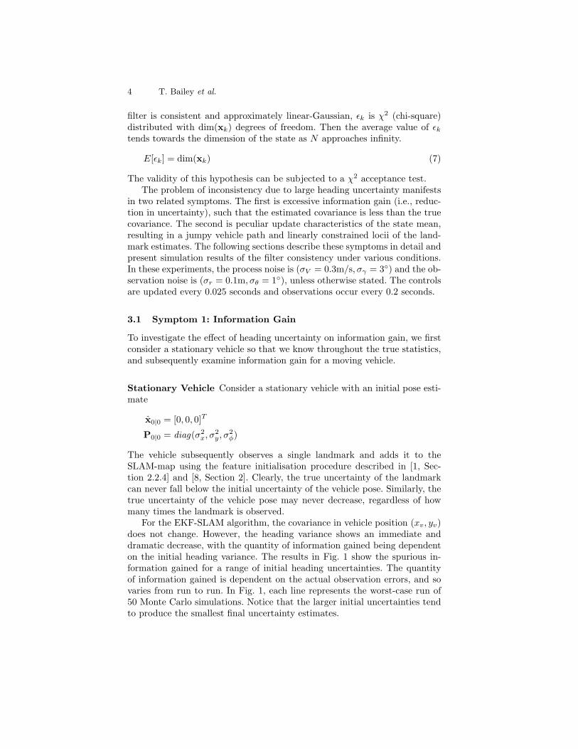
For the EKF-SLAM algorithm, the covariance in vehicle position (xv, yv)does not change. However, the heading variance shows an immediate anddramatic decrease, with the quantity of information gained being dependenton the initial heading variance. The results in Fig. 1 show the spurious in-formation gained for a range of initial heading uncertainties. The quantityof information gained is dependent on the actual observation errors, and sovaries from run to run. In Fig. 1, each line represents the worst-case run of50 Monte Carlo simulations. Notice that the larger initial uncertainties tendto produce the smallest final uncertainty estimates.

Consistency of the EKF-SLAM Algorithm 5

0 2 4 6 8 10 12 14 160

5

10

15

Observation number

Hea

ding

std

. dev

. (de

gree

s)

Fig. 1. Information gain in heading for a stationary vehicle. This figureshows estimated heading standard deviation σφ after each observation up-date.

The gain of information for a stationary vehicle is entirely due to thevariation in the observation Jacobian ∂h

∂xkover the observation sequence. If

the Jacobian were to remain fixed (e.g., linearised about the true state), therewould be no loss in uncertainty. For a normal EKF run, however, the amountof information gain tends to increase with observation uncertainty Rk and,more significantly, with the initial heading variance σ2

φ. (Note, informationgain is independent of vehicle position variance.)

Moving Vehicle To examine information gain for EKF-SLAM with a mov-ing vehicle, we compare the results from a nominal run with those obtainedusing Jacobians linearised about the true state throughout. Experiments in[8] indicate that using “ideal” Jacobians may not ensure true statistics, butour results show they do provide consistent estimates, and the difference be-tween ideal and EKF Jacobian results is a good indicator of nominal EKFperformance.

Fig. 2 shows the result of the two runs. Notice that the covariance esti-mates of the standard EKF are smaller than for the EKF with ideal Jaco-bians. This indicates a significant level of information gain in the standardalgorithm.4 The information gain in heading is shown in Fig. 3, where thetop line is the ideal Jacobian estimate and the lower line is the standard EKFestimate. This result corroborates with the findings of Castellanous et al. [4].The heading uncertainty for the ideal Jacobian solution grows while ever thevehicle travels further into unmapped territory but, for the standard EKFsolution, the heading uncertainty reaches a ceiling and levels off. Here, the

4 It is interesting to observe in Fig. 2 that the standard EKF estimate appears to bemore accurate than the ideal Jacobian estimate. This is purely coincidence, andthe standard algorithm is, in fact, inconsistent, but this becomes apparent only byrunning additional Monte Carlo simulations with the same noise characteristics.

6 T. Bailey et al.

information gain is negligible for heading standard deviation below about 1.7degrees, but rapidly becomes significant at around 2 degrees.

−100 −50 0 50 100−100

−80

−60

−40

−20

0

20

40

60

80

metres

met

res

−100 −50 0 50 100

−100

−80

−60

−40

−20

0

20

40

60

80

metres

met

res

Fig. 2. EKF-SLAM simulations showing the estimated vehicle trajectoryand 2-sigma ellipses of landmark locations. The true landmarks are shownas stars. The left-hand figure is normal EKF and the right-hand figure isEKF with Jacobians linearised about the true state.

0 50 100 150 200 250 300 350 400 4500

0.5

1

1.5

2

2.5

3

3.5

Time (s)

Hea

ding

std

. dev

. (de

gree

s)

Fig. 3. EKF-SLAM heading uncertainty. The vehicle performs two loopsof the trajectory shown in Fig. 2. The large decrease in uncertainty at 220seconds is when the vehicle first closes the loop.

If the standard EKF-SLAM algorithm is run with direct observation ofthe heading at regular intervals, so that the heading uncertainty is alwayssmall, the estimated covariance is virtually identical to the ideal Jacobianresult. That is, the information gain for EKF-SLAM with small heading un-certainty is negligible. This property is insensitive to the values of processand observation noise.

Consistency of the EKF-SLAM Algorithm 7

3.2 Symptom 2: Jumpy Path and Constrained Feature Locii

The inconsistency of the EKF-SLAM algorithm becomes visibly evident withthe appearance of discontinuities in the estimated vehicle trajectory. Oversuccessive observation updates, the mean estimate of the vehicle pose showsdramatic jumps, which tend to be disproportionately large when compared tothe size of the actual measurement error. A related symptom appears in thelocii of landmark location estimates. Rather than exhibiting motion in accordwith the sensor noise, the landmark mean updates seem to be constrainedto a line. Again, the size of the update tends to be much larger than theactual measurement error. These symptoms manifest once the vehicle headinguncertainty becomes “large”, but do not appear if the Jacobians are linearisedabout the true state (see Fig. 4).

560 570 580 590 600 610 620 630 640−10

0

10

20

30

40

50

60

metres

met

res

560 570 580 590 600 610 620 630 640−10

0

10

20

30

40

50

60

metres

met

res

Fig. 4. Jumpy path and linear feature locus. The left-hand figure shows asection of the estimated vehicle path and a landmark locus for EKF-SLAM.The right-hand figure shows the estimates given ideal Jacobians.

It is difficult to say precisely why these symptoms appear. The informationgain in heading induces over-strong correlations between the vehicle and thelandmarks. It would seem that these invalid cross-correlations constrain thefeature updates to follow linear paths. Measurements that attempt to shift alandmark estimate orthogonal to a certain line result in large updates alongthe line and large jumps in vehicle pose to compensate.

3.3 Monte Carlo Tests of Filter Consistency

Consistency of the EKF is evaluated by performing multiple Monte Carloruns and computing the average NEES. Given N runs, the average NEES iscomputed as

εk =1N

N∑

i=1

εik(8)

8 T. Bailey et al.

Given the hypothesis of a consistent linear-Gaussian filter, Nεk has a χ2

density with N dim(xk) degrees of freedom [2, pages 234–235]. Thus, for the3-dimensional vehicle pose, with N = 50, the 95% probability concentrationregion for εk is bounded by the interval [2.36, 3.72]. If εk rises significantlyhigher than the upper bound, the filter is optimistic, if it tends below thelower bound, the filter is conservative.

0 50 100 150 200 250 300 350 400 4500

5

10

15

20

25

30

35

40

Time (s)

Ave

rage

NE

ES

ove

r 50

run

s

0 50 100 150 200 250 300 350 400 4500

0.5

1

1.5

2

2.5

3

3.5

4

4.5

Time (s)

Ave

rage

NE

ES

ove

r 50

run

s

Fig. 5. Average NEES of the vehicle pose states over 50 Monte Carlo runs.The left-hand figure is nominal EKF-SLAM and the right-hand figure iswith ideal Jacobians.

Fig. 5 shows the average NEES of the vehicle pose states for nominalEKF-SLAM and for the ideal Jacobian case over two loops of the trajectoryshown in Fig. 2. The EKF is clearly inconsistent, rising above the upper boundmidway through the first loop (at about 120 seconds). There is a large spike atabout 220 seconds on closing the loop. The EKF with ideal Jacobians behavesconsistently throughout. This shows that the ideal Jacobian simulation, whilestill a linear filter, is a reasonable estimator of the true first and secondmoments of the state.

The failure of EKF-SLAM is unavoidable; no amount of added stabilisingnoise improves the result in Fig. 5. However, running the nominal EKF withregular observations of heading, so that the true heading uncertainty is alwayssmall, produces consistent results. This result is insensitive to the systemnoises. For example, we performed experiments with process noise (σV =1.0m/s, σγ = 5◦) and observation noise (σr = 1.0m, σθ = 10◦), and obtainedestimates within the upper/lower NEES bounds, similar to the second plot inFig. 5. Very long-term runs under these conditions continue to give consistentestimates; SLAM does not fail with time.

4 Discussion

Many of the arguments against the EKF-SLAM algorithm do not addressthe real problem. For example, two common arguments claim it is inadequate

Consistency of the EKF-SLAM Algorithm 9

because (i) it poorly linearises the process and observation models, and (ii) itcannot consistently “close the loop”. To investigate (i), we implemented twovariants of the EKF: the iterated EKF (IEKF) and the unscented Kalmanfilter (UKF). Both of these gave similar results to standard EKF-SLAM,indicating that improved local linearisation does not help.5 With regard to(ii), the failure to properly close large loops tends to occur only if the SLAMestimate is already inconsistent due to heading uncertainty. If the state isconsistent prior to closing the loop, then the EKF will usually produce aconsistent update even when the loop error is large.

Significant improvements in consistency are likely for EKF-SLAM vari-ants that minimise heading uncertainty and minimise variations in Jacobianlinearisation. The constrained local submap filter (CLSF) [14] is one suchmethod as it performs most updates in a local frame with small heading un-certainty. Batch update methods, such as fixed-interval smoothing betweentimesteps k and k + N , are also likely to help. For very large-scale maps,submap methods, such as network coupled feature maps (NCFM) [1] andATLAS [3], are currently the only solution that avoids data-fusion with largeheading variance. Submap methods confine all updates to small-scale mapsand use summation over a topology to compute consistent global estimateswithout information gain.

5 Conclusion

In this paper, we have shown that EKF-SLAM always fails once true headinguncertainty rises above a limit (typically about 1 to 2 degrees). Inflating theprocess and observation noise models does not help. Failure is subtle anddifficult to detect without ground-truth. The estimated uncertainty simplyplateaus while the “true” uncertain continues to grow. An observable symp-tom that may occur is a “jumpy” vehicle path, where the vehicle pose updateis significantly greater than would be expected from the actual measurementerror.

Inconsistency can be prevented if (i) the Jacobians are always linearisedabout the true state, or (ii) the vehicle heading uncertainty is always small.In either case, the filter is robust to process/observation noises and non-linearities, and minor modelling errors can be adequately compensated withstabilising noise, if necessary. SLAM is stable in the long-term under theseconditions.

The IEKF and UKF cannot prevent inconsistency. They offer no signifi-cant improvement over plain EKF-SLAM. Batch update methods are likely toextend the region over which EKF-SLAM can construct a consistent globalmap as they reduce local heading uncertainty and Jacobian variation. For

5 In fact, the IEKF tends to promote divergence as the SLAM state is not locallyobservable. The IEKF does, however, improve results when closing the loop.

10 T. Bailey et al.

large-scale maps, submaps confine EKF updates to the small-scale, and pre-vent any data fusion with large heading uncertainty. Submaps are currentlythe only way to implement large-scale EKF-SLAM without spurious infor-mation gain.

References

1. T. Bailey. Mobile Robot Localisation and Mapping in Extensive Outdoor En-vironments. PhD thesis, University of Sydney, Australian Centre for FieldRobotics, 2002.

2. Y. Bar-Shalom, X.R. Li, and T. Kirubarajan. Estimation with Applications toTracking and Navigation. John Wiley and Sons, 2001.

3. M. Bosse, P. Newman, J. Leonard, M. Soika, W. Feiten, and S. Teller. AnAtlas framework for scalable mapping. In IEEE International Conference onRobotics and Automation, pages 1899–1906, 2003.

4. J.A. Castellanos, J. Neira, and J.D. Tardos. Limits to the consistency of EKF-based SLAM. In IFAC Symposium on Intelligent Autonomous Vehicles, 2004.

5. M.W.M.G. Dissanayake, P. Newman, S. Clark, H.F. Durrant-Whyte, andM. Csorba. A solution to the simultaneous localization and map building(SLAM) problem. IEEE Transactions on Robotics and Automation, 17(3):229–241, 2001.

6. J. Guivant and E. Nebot. Improving computational and memory requirementsof simultaneous localization and map building algorithms. In IEEE Interna-tional Conference on Robotics and Automation, pages 2731–2736, 2002.

7. J.S. Gutmann and K. Konolige. Incremental mapping of large cyclic environ-ments. In IEEE International Symposium on Computational Intelligence inRobotics and Automation, pages 318–325, 1999.

8. S.J. Julier and J.K. Uhlmann. A counter example to the theory of simultaneouslocalization and map building. In IEEE International Conference on Roboticsand Automation, pages 4238–4243, 2001.

9. S.J. Julier and J.K. Uhlmann. Using multiple slam algorithms. In IEEE/RSJInternational Conference on Intelligent Robots and Systems, pages 200–205,2003.

10. J. Leonard and P. Newman. Consistent, convergent, and constant-time SLAM.Technical report, Massachusetts Institute of Technology, Department of OceanEngineering, 2003.

11. M. Montemerlo, S. Thrun, D. Koller, and B. Wegbreit. FastSLAM 2.0: Animproved particle filtering algorithm for simultaneous localization and map-ping that provably converges. In International Joint Conference on ArtificialIntelligence, pages 1151–1156, 2003.

12. J. Neira, J.D. Tardos, and J.A. Castellanos. Linear time vehicle relocation inSLAM. Technical report, University of Zaragoza, Department of ComputerScience and Systems Engineering, 2002.

13. R. Smith, M. Self, and P. Cheeseman. A stochastic map for uncertain spatialrelationships. In International Symposium of Robotics Research, pages 467–474,1987.

14. S.B. Williams. Efficient Solutions to Autonomous Mapping and NavigationProblems. PhD thesis, University of Sydney, Australian Centre for FieldRobotics, 2001.