Pablo Andrés Neumeyer, joint wih FernandoAlvarez and Patrick KehoeThe Time Consistency of the Friedman Rule

Federal Reserve Bank of MinneapolisResearch Department

The time consistencyof the Friedman Rule

Fernando Alvarez, Andy Neumeyer,and Patrick Kehoe¤

May 20, 2001Preliminary and Incomplete

ABSTRACT

We consider the problem of time consistency of the Ramsey monetary and &scal policies inan economy without capital. Following Lucas and Stokey (1983) we allow the government atdate t to leave its successor at t+ 1 a pro&le of real and nominal debt of all maturities, as away to in! uence its decisions. We show that the Ramsey policies are time consistent if andonly if the Friedman rule is the optimal Ramsey policy.

¤Alvarez, University of Chicago; Neumeyer, Universidad Torcuato Di Tella; Kehoe, Federal Reserve Bankof Minneapolis. We thank V.V. Chari, Juan Pablo Nicolini, and Pedero Teles for their suggestions andcomments. The views expressed herein are those of the authors and not necessarily those of the FederalReserve Bank of Minneapolis or the Federal Reserve System.

A classic issue in macroeconomics is the time consistency of optimal monetary and

&scal policy. In a seminal contribution, Calvo (1978) showed that the incentive for the

government to in! ate away its nominal liabilities leads to a time inconsistency problem. We

consider an in&nite horizon model with money in the utility function of the representative

consumer. The government has access to nominal and real debt of all maturities and must

&nance a given stream of government expenditures with a combination of consumption taxes

and seignorage. We show that with a su¢ciently rich maturity structure of real and nominal

debt, optimal policy is time consistent if and only if the Friedman rule holds, in the sense

that nominal interest rates are zero.

Our approach to the problem of time inconsistency follows that of Lucas and Stokey

(1983). We begin by solving for the Ramsey policies in which the government is presumed

to have a commitment technology that binds the actions of future government and hence

chooses policy once and for all. These Ramsey policies consist of sequences of consumption

taxes and money supplies. We then consider an environment without such a commitment

technology in which each government inherits a given maturity structure of nominal and real

debt. Each such government then decides on the current setting for the consumption tax

and the money supply as well as the maturity structure of nominal and real debt that its

successor will inherit. We ask whether it is possible to choose the maturity structure of real

and nominal debt so that each government carries out the Ramsey policies. If it is we call

the Ramsey policies time consistent.

Our model with both nominal and real bonds has two forces, nominal and real, that

lead to time inconsistency. These stem from the desire to minimize the need to raise revenues

with distortionary taxes. As in Calvo (1978), if the government has nominal liabilities it is

tempted to reduce the real value of these liabilities with a surprise in! ation or a change in the

term structure of nominal interest rates. Conversely, if the government has nominal assets

it is tempted to increase the real value of these assets with a surprise de! ation or a change

in the term structure of nominal interest rates. As in Lucas and Stokey (1983), when the

government has real liabilities or real assets it is tempted to reduce the value of its liabilities

or increase the value of its assets with an appropriate change in the real term structure of

interest rates. We ask, as do Lucas and Stokey (1983) and Persson, Persson and Svensson

(1987), if we can nullify these forces with a careful choice of the maturity structure of both

bonds and hence make the Ramsey policies time consistent.

We begin by showing that if the Friedman rule does not hold the Ramsey policies

cannot be made time consistent. Brie! y, when the Friedman rule does not hold the nominal

debt passed on to successor governments must be restricted greatly. These restrictions curtail

the ability of each government to in! uence the actions of its successor so much that they

cannot induce them to continue with the Ramsey policies. When the Friedman rule holds,

these restrictions are not binding and each government can induce its successor to continue

with the Ramsey policies.

More speci&cally, we proceed as follows. In Lemma 1 we derive the Ramsey problem

and in Proposition 1 we give su¢cient conditions for the Friedman rule to solve the Ramsey

problem. In this problem, the interesting initial conditions are those that lead the present

value of the initial nominal liabilities to be zero. Given such initial conditions, in Lemma 2

we show that in any period t in which the nominal interest rate is positive the value of the

nominal debt from date t on must be zero. If not the government could make the present

value of nominal liabilities from date 0 on negative by either raising or lowering the date

2

t interest rate, and then turn them into arbitrarily large real assets by making the initial

price level low enough. In Proposition 2 we show that when the Friedman rule does not

hold, the restrictions on nominal debt derived in Lemma 2 are so severe that the Ramsey

allocations cannot be made time consistent. In essence, the restrictions from Lemma 2 force

each government to rely mainly on real debt to in! uence it successors and this debt by itself

is not rich enough to control the two forces that lead to time inconsistency.

In Proposition 3 we show that if the Friedman rule holds in each period, the Ramsey

problems can be made time consistent. Brie! y, when the Friedman holds in each period

agents become satiated with money balances and marginal changes in interest rates have

no e¤ect on their behavior. In this sense, the e¤ect of money essentially disappears from

the economy. The real debt can then be set so as to nullify the forces from the real side

of the economy that lead to time inconsistency and the Ramsey policies can be made time

consistent. We show that there are multiple ways to set the nominal debt, including setting

it to zero in each period.

For most of the paper we follow the original approach to time inconsistency used by

Calvo (1978), Lucas and Stokey (1983), and Persson, Persson and Svensson (1987). We then

relate this de&nition to that of sustainable plans by Chari and Kehoe (1992) and credible

policies by Stokey (1991) which explicitly builds the lack of commitment of the government

into the environment with an equilibrium concept in which governments explicitly think

through how their choices of debt in! uence the choices of their successors. In Proposition 4,

we show that the Ramsey policies are time consistent if and only if they are supportable as

a Markov sustainable equilibrium.

We develop a useful analogy between our monetary model and a real economy of Lucas

3

and Stokey (1983). That real economy has leisure and two types of consumption goods as

well as two real bonds that payo¤ in units of the two consumption goods. Lucas and Stokey

show that if the maturity structure of both bonds are carefully chosen the Ramsey policies

can be made time consistent. Moreover, it is easy to show that if there is only one such

bond the Ramsey policies are time consistent if and only if it a uniform consumption tax is

optimal. Our monetary economy has leisure and two other goods, a consumption good and

real balances as well as a bond that pays o¤ in units of the consumption good and one that

pays o¤ in units of money. If we restrict the nominal bond to be one-period-lived there is

essentially only one real bond through which governments can in! uence the future. In such

a case, the Ramsey policies are time consistent if and only if the Friedman rule is optimal in

each period. The conditions for with the Friedman rule are optimal in the monetary economy

are the same as the conditions for uniform taxation to be optimal in the real economy.

Our paper is also closely related to that of Persson, Persson and Svensson (1987).

They argued that with a su¢ciently rich term structure of both nominal and real debt,

optimal policy can be made time consistent regardless of whether or not the Friedman rule is

satis&ed. Unfortunately, their result is not true. Calvo and Obstfeld (1990) argued that the

mistake made by Persson, Persson and Svensson (1987) was that their solution violated the

unchecked second order conditions. Our analysis shows that their mistake has nothing to do

with the second order conditions, rather it has to do with a lack of attention to subtle corners.

Moreover, in contrast to the conjectures by Calvo and Obstfeld (1990) the Persson, Persson

and Svensson (1987) conclusion can be rescued for environments in which the Friedman rule

is optimal.

4

1. The economy and the Ramsey problem

Consider a monetary economy with money, nominal debt and real debt. Time is

discrete. The economy is endowed with a linear technology described by

ct + gt = lt;(1)

where ct; gt; lt denote consumption, government spending and labor at t: Throughout the

sequence of government spending is exogenously given.

Consumers have preferences over sequences of consumption ct; (end-of-period) real

balances Mt=pt; and labor lt given by

1X

t=0¯tU (ct;Mt=pt; lt)(2)

with the discount factor 0 < ¯ < 1: Here Mt is nominal balances and pt is the nominal price

level and we let mt = Mt=pt denote real balances. We assume the period utility function

U(c;m; l) is concave, twice continuously di¤erentiable, increasing in c; weakly increasing in

m and increasing in l; where here and throughout the paper we denote partial derivatives

by Um; Umm and so on. We also assume that consumers are satiated at a &nite level of real

balances, so that for each value of c and l there is a &nite level of m such that Um(c;m; l) = 0:

In terms of assets, we assume there are both nominal and real bonds for each maturity

at each date. For the nominal bonds, for each t and s with t · s; we let Qt;s denote the

price of one dollar at time s in units of dollars at time t and let Bt;s denote the number

of such nominal claims. Likewise for the real bonds we let qt;s denote the price of one unit

of consumption at time s in units of consumption at time t and let bt;s denote the number

of such real bonds. We let Bt = (Bt;t+1; Bt;t+2; : : :) denote the sequence of nominal bonds

purchased at t which pay o¤ Bt;s at time s for all s ¸ t+ 1:We use similar notation for the

5

real bonds bt; the nominal and real debt prices Qt and qt: For later use it is worth noting that

arbitrage among these bonds implies that for all t · r · s their prices satisfy Qt;s = Qt;rQr;s,

qt;s = qt;rqr;s; Qt;s = qt;spt=ps: By convention, Qt;t = 1 and qt;t = 1.

The consumer s sequence budget constraint at date t can be written

pt(1+¿ t)ct+Mt+1X

s=t+1Qt;sBt;s+pt

1X

s=t+1qt;sbt;s = ptlt+Mt¡1+

1X

s=tQt;sBt¡1;s+pt

1X

s=tqt;sbt¡1;s(3)

Thus, at date t; the consumer has inherited nominal balances Mt¡1; the sequence of nominal

bonds Bt; and the sequence of real bonds bt and nominal wage income of ptlt. The consumer

purchases consumption ct, new money balances Mt; and new vectors of nominal bonds Bt

and real bonds bt. Purchases of consumption are taxed at rate ¿ t: At date 0 consumers have

initial money balances M¡1; together with initial sequences of nominal and real debt claims,

B¡1 and b¡1: We assume that the real value of both nominal and real debt is bounded by

some arbitrarily large constants.

It is convenient to work with the consumer s problem in its date 0 form. To that end,

note that the sequence of budget constraints can be collapsed to the date 0 budget constraint

1X

t=0q0;t [(1 + ¿t)ct + (1¡Qt;t+1)mt] =

1X

t=0q0;tlt +

M¡1p0

+1X

t=0Q0;tB¡1;tp0

+1X

t=0q0;tb¡1;t:(4)

The consumer s problem at date 0 is to choose sequences of consumption, real balances and

leisure to maximize (2) subject to the (4).

The government s sequence budget constraint at date t is

1X

s=t+1Qt;sBt;s+pt

1X

s=t+1qt;sbt;s =

1X

s=tQt;sBt¡1;s+pt

1X

s=tqt;sbt¡1;s +ptgt¡(Mt¡Mt¡1)¡pt¿ tct(5)

At date t; the government inherits the nominal liabilities Mt¡1 and Bt; and real liabilities bt:

To &nance government spending gt it collects consumption taxes ¿ tct and issues new money

6

supply Mt; new nominal liabilities Bt; and new real liabilities bt: Using the resource constraint

and the consumer s date 0 budget constraint we can collapse these sequence of constraints

into the government s date 0 budget constraint

1X

t=0q0;t [¿tct + (1¡Qt;t+1)mt] =

1X

t=0q0;tgt +

M¡1p0

+1X

t=0Q0;sB¡1;sp0

+1X

t=0q0;tb¡1;t(6)

We &nd it convenient to use the notation tc = (ct;ct+1; : : :) for consumption and other

variables as well. We then have, for given initial conditions M¡1; B¡1; and b¡1; a competitive

equilibrium is a collection of sequences of consumption, real balances and labor (0c; 0m; 0l)

together with sequences of prices (0p; Q0; q0) and taxes 0¿ that satisfy the resource constraint

and consumer maximization at date 0: The government budget constraint is then implied.

We show that the allocations in a competitive equilibrium are characterized by two

simple conditions: the resource constraint and the implementability constraint which is given

by

1X

t=0¯t[ctUct +mtUmt + ltUlt ] = ¡Ul0p0

[M¡1 +1X

t=0Q0;t B¡1;t] ¡

1X

t=0¯tUlt b¡1;t(7)

where Q0;t =Qt¡1s=0(1 + Ums=Uls): This implementability constraint should be thought of as

the date 0 budget constraint of either the consumer or the government where the consumer

&rst order conditions have been used to substitute out prices and policies.

Lemma 1. The consumption, real balances and labor allocations together with the

price p0 of a date 0 competitive equilibrium necessarily satisfy the resource constraint and the

implementability constraint. Furthermore, given such allocations and a price p0 that satisfy

these constraints, we can construct nominal money supplies, prices and real and nominal debt

prices such that these allocations and prices constitute a date 0 competitive equilibrium.

7

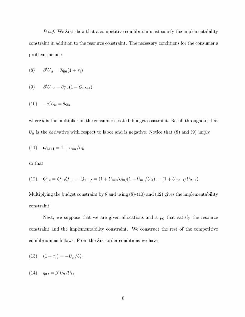
Proof. We &rst show that a competitive equilibrium must satisfy the implementability

constraint in addition to the resource constraint. The necessary conditions for the consumer s

problem include

¯tUct = µq0t(1 + ¿t)(8)

¯tUmt = µq0t(1¡Qt;t+1)(9)

¡¯tUlt = µq0t(10)

where µ is the multiplier on the consumer s date 0 budget constraint. Recall throughout that

Ult is the derivative with respect to labor and is negative. Notice that (8) and (9) imply

Qt;t+1 = 1+ Umt=Ult(11)

so that

Q0;t = Q0;1Q1;2 : : : Qt¡1;t = (1 + Um0=Ul0)(1 +Um1=Ul1) : : : (1 +Umt¡1=Ult¡1)(12)

Multiplying the budget constraint by µ and using (8)-(10) and (12) gives the implementability

constraint.

Next, we suppose that we are given allocations and a p0 that satisfy the resource

constraint and the implementability constraint. We construct the rest of the competitive

equilibrium as follows. From the &rst-order conditions we have

(1 + ¿t) = ¡Uct=Ult(13)

q0;t = ¯tUlt=Ul0(14)

8

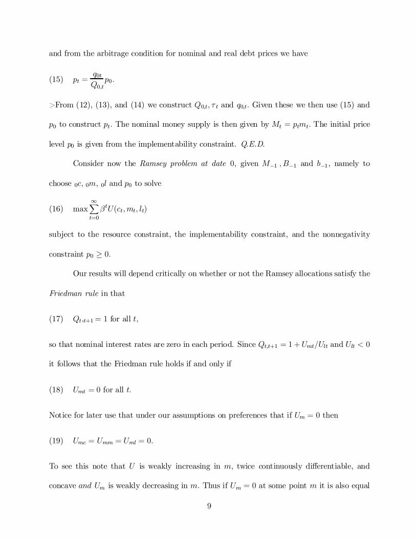
and from the arbitrage condition for nominal and real debt prices we have

pt =q0tQ0;tp0:(15)

>From (12), (13), and (14) we construct Q0;t; ¿ t and q0;t: Given these we then use (15) and

p0 to construct pt: The nominal money supply is then given by Mt = ptmt: The initial price

level p0 is given from the implementability constraint. Q.E.D.

Consider now the Ramsey problem at date 0, given M¡1 ; B¡1 and b¡1, namely to

choose 0c; 0m, 0l and p0 to solve

max1X

t=0¯tU(ct;mt; lt)(16)

subject to the resource constraint, the implementability constraint, and the nonnegativity

constraint p0 ¸ 0:

Our results will depend critically on whether or not the Ramsey allocations satisfy the

Friedman rule in that

Qt;t+1= 1 for all t;(17)

so that nominal interest rates are zero in each period. Since Qt;t+1 = 1+Umt=Ult and Ult < 0

it follows that the Friedman rule holds if and only if

Umt = 0 for all t:(18)

Notice for later use that under our assumptions on preferences that if Um = 0 then

Umc = Umm = Uml = 0:(19)

To see this note that U is weakly increasing in m; twice continuously di¤erentiable, and

concave and Um is weakly decreasing in m: Thus if Um = 0 at some point m it is also equal

9

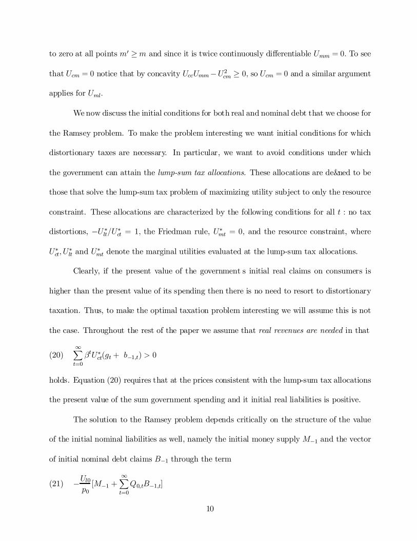
to zero at all points m0 ¸m and since it is twice continuously di¤erentiable Umm = 0: To see

that Ucm = 0 notice that by concavity UccUmm¡U2cm ¸ 0; so Ucm = 0 and a similar argument

applies for Uml:

We now discuss the initial conditions for both real and nominal debt that we choose for

the Ramsey problem. To make the problem interesting we want initial conditions for which

distortionary taxes are necessary. In particular, we want to avoid conditions under which

the government can attain the lump-sum tax allocations. These allocations are de&ned to be

those that solve the lump-sum tax problem of maximizing utility subject to only the resource

constraint. These allocations are characterized by the following conditions for all t : no tax

distortions, ¡U ¤lt=U¤ct = 1; the Friedman rule, U¤mt = 0; and the resource constraint, where

U¤ct; U¤lt and U¤mt denote the marginal utilities evaluated at the lump-sum tax allocations.

Clearly, if the present value of the government s initial real claims on consumers is

higher than the present value of its spending then there is no need to resort to distortionary

taxation. Thus, to make the optimal taxation problem interesting we will assume this is not

the case. Throughout the rest of the paper we assume that real revenues are needed in that

1X

t=0¯tU¤ct(gt + b¡1;t) > 0(20)

holds. Equation (20) requires that at the prices consistent with the lump-sum tax allocations

the present value of the sum government spending and it initial real liabilities is positive.

The solution to the Ramsey problem depends critically on the structure of the value

of the initial nominal liabilities as well, namely the initial money supply M¡1 and the vector

of initial nominal debt claims B¡1 through the term

¡Ul0p0

[M¡1 +1X

t=0Q0;tB¡1;t](21)

10

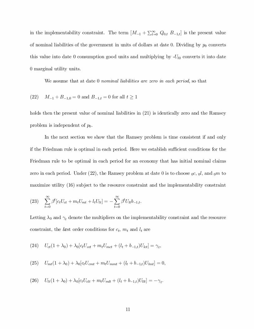
in the implementability constraint. The term [M¡1 +P1t=0 Q0;t B¡1;t] is the present value

of nominal liabilities of the government in units of dollars at date 0: Dividing by p0 converts

this value into date 0 consumption good units and multiplying by -Ul0 converts it into date

0 marginal utility units.

We assume that at date 0 nominal liabilities are zero in each period, so that

M¡1 +B¡1;0 = 0 and B¡1;t = 0 for all t ¸ 1(22)

holds then the present value of nominal liabilities in (21) is identically zero and the Ramsey

problem is independent of p0.

In the next section we show that the Ramsey problem is time consistent if and only

if the Friedman rule is optimal in each period. Here we establish su¢cient conditions for the

Friedman rule to be optimal in each period for an economy that has initial nominal claims

zero in each period. Under (22), the Ramsey problem at date 0 is to choose 0c; 0l; and 0m to

maximize utility (16) subject to the resource constraint and the implementability constraint

1X

t=0¯t[ctUct +mtUmt + ltUlt] = ¡

1X

t=0¯tUltb¡1;t:(23)

Letting ¸0 and °t denote the multipliers on the implementability constraint and the resource

constraint, the &rst order conditions for ct; mt and lt are

Uct(1 + ¸0) + ¸0[ctUcct +mtUmct + (lt + b¡1;t)Ulct] = °t;(24)

Umt(1 + ¸0) + ¸0[ctUcmt +mtUmmt + (lt + b¡1;t)Ulmt] = 0;(25)

Ult(1 + ¸0) + ¸0[ctUclt +mtUmlt + (lt + b¡1;t)Ullt] = ¡°t:(26)

11

We can use these &rst order conditions to establish circumstances under which the

Friedman rule is optimal. Consider an economy with preferences that are separable and

homothetic in that

U(c;m; l) = u(w(c;m)) + V (l)(27)

where w is homothetic in c and m and for which initial nominal claims are zero period by

period. Then we can adapt the logic of Chari, Christiano, and Kehoe (1996) to show the

following.

Proposition 1. If preferences are separable and homothetic so that (27) holds and the

initial nominal claims are zero in each period so that (22) holds then the Friedman rule is

optimal.

Proof. Using separability, we can arrange the &rst order conditions for real money

balances and consumption to be

Umtf(1 + ¸0) + ¸0· ctUcmt +mtUmmt

Umt

¸g = 0(28)

Uctf(1 + ¸) + ¸0·ctUcct +mtUcmt

Uct

¸g = °t(29)

Now in (28) either Umt = 0 or the expression in brackets is equal to 0:We claim that Umt = 0:

To see this note that since U (c;m) = u(w(c;m)) with w homothetic it follows that

Um(®c; ®m)Uc(®c; ®m)

=Um(c;m)Uc(c;m)

for a positive constant ®: Di¤erentiating this with respect to ® and evaluating it at ® = 1

gives that

ctUcmt +mtUmmtUmt

=ctUcct +mtUcmt

Uct:(30)

12

Hence the expression in brackets in (28) equals the expression in brackets in (29). But since

the multiplier on the resource constraint °t is strictly positive the term in brackets in both

(28) and (29) is strictly positive, so Umt = 0: Q:E:D:

It is worth pointing out that this lemma is related to but not covered by the result

in Chari, Christiano, and Kehoe (1996) which proved that the Friedman rule holds in an

environment with weakly separable preferences, labor income taxes and no initial government

debt. If we add to that environment long-lived initial real government debt then the Friedman

result typically does not hold. Here we have additively separable preferences, consumption

taxes and long-lived initial real government debt and the Friedman rule holds. (Brie! y, with

labor income taxes adding initial real debt introduces terms of the form Ucctb¡1;t and Ucmb¡1;t

that make the proof in Chari, Christiano and Kehoe not work. With labor income taxes

having real debt introduces terms of the form ¡Ulctb¡1;t and ¡Ulmtb¡1;t which disappear with

additive separability.)

2. Time consistency and the Friedman rule

In this section we give a version of Lucas and Stokey s de&nition of time consistency

and establish that, given certain conditions on initial nominal assets, the Ramsey problem is

time consistent if and only if the Friedman rule holds.

We begin with a de&nition of time consistency. It is convenient to de&ne the Ramsey

problem at date t; given inherited values for money balances Mt¡1; nominal debt Bt¡1 and

real debt bt¡1 to be the problem of choosing allocations from period t onward, namely tc; tl;

13

and tm; and the price level pt (by choosing Mt) to maximize

max1X

s=t¯sU(cs;ms; ls)

subject to the resource constraint for s ¸ t and the implementability constraint at t

1X

s=t¯s¡t[csUcs+msUms+ lsUls] = ¡Ult

pt[Mt¡1 +

1X

s=tQt;s Bt¡1;s] ¡

1X

s=t¯s¡tUls bt¡1;s]:(31)

where Qt;s =Qt¡1r=t(1 + Umt=Ult): The Ramsey problem at date t is said to be time consistent

for t+1 if there exist values for nominal money balances Mt; nominal debt Bt, and real debt

bt with Mt = ptmt such that taking these values as given, the continuation of the Ramsey

allocations at period t from t + 1 on, namely t+1c; t+1l; and t+1m together with the price

level pt+1 solve the Ramsey problem at t + 1 where the price level pt+1 is a function of the

allocations and the nominal money supply according to

pt+1 =Qt;t+1ptqt;t+1

= ¯Ult+1

Ultpt

(1 + Umt=Ult):

The Ramsey problem at date 0 is time consistent if the Ramsey problem at date t is time

consistent for t +1 for all t ¸ 0:

Given this de&nition, the way to establish that a Ramsey problem at say date 0 is time

consistent for date 1 is the show how the initial conditions for the date 1 problem, namely

M0; B0; and b0, can be chosen so as give incentives for the government at date 1 to continue

with the allocations chosen by the government at date 0:

Since the solution of the Ramsey problem at 0 entails an interior solution for p1 with

0 < p1 < 1 the &rst order conditions of the Ramsey problem at date 1 imply that for

the Ramsey plan at date 0 to be time consistent it is necessary that M0 and B0 satisfy the

14

condition

M0 +1X

t=1Q1;tB0;t = 0:(32)

This condition, however, is not su¢cient to eliminate the nominal forces that lead

to time inconsistency. Here we present an intermediate result which shows that restrictions

on the type of nominal debt sequences that can be part of the Ramsey policies when the

Friedman rule does not hold. This lemma will apply to the Ramsey problem at any date

t = 0; 1; : : : : For concreteness, consider the Ramsey problem at date 1 with inherited initial

conditions M0; B0; and b0. If at some date s; the Friedman rule does not hold so that

Qs;s+1 < 1;(33)

then the present value of debt from date s+1 on must be zero, so that

0 =1X

t=s+1Q1;t B¡1;t = Q1sQs;s+1

1X

t=sQs+1;t B¡1;t:(34)

We will assume there is some date, say r; in which strictly positive taxes are being levied

so that ¡Ucr=Ulr = (1 + ¿ r) > 1: We will assume that at this date r; the second derivatives

satis&es the conditions

Umm +Ulm < 0 if Um > 0; Ull+ Ulc ¸ 0; Umc +Uml ¸ 0:(35)

We show the following.

Lemma 2. If at the solution to the Ramsey problem at date 1; 0 < p1 < 1; there

is some date s at which the Friedman rule does not hold, there is some date r at which

consumption taxes are levied and the above conditions (35) on second derivatives hold then

the value of initial nominal debt from s+ 1 on is zero so that (34) holds.

15

Proof. We establish the result by showing that if the assumptions of the lemma hold

and (34) does not hold, then we can perturb the allocations and increase utility.

If (32) and (33) holds and (34) does not hold then we can make the present value of

the government s nominal liabilities negative by a small change in Qs;s+1. This change, which

may entail either raising or lowering Qs;s+1; is feasible since the Friedman rule does not hold

at s; rather (33) holds. We do so by changing cs;ms and ls in a way the satis&es the resource

constraint but changes Qs;s+1: Then by lowering the initial price level p1; we can generate

any level of real assets for the government net of the cost of government spending.

In the second part of the perturbation we simply change the allocation at that date

r in which we know positive taxes are being raised in a way that raises utility at that date

and holds &xed the Qr;r+1 so that we know the &rst part of the perturbation still works. To

that end note that positive taxes at date r implies that ¡Ulr < Ucr. Since Umr ¸ 0 we can

increase cr and mr and decrease lr in a way that keeps Qr;r+1 constant, satis&es the resource

constraint, and increases utility at date r: Clearly, by the implicit function theorem for a

&xed Qr;r+1 and gr there exist functions l(c) and m(c) such that c; l(c) and m(c) satisfy

Um(c;m(c); l(c)) + (1¡Qr;r+1)Ul(c;m(c); l(c)) = 0(36)

and c + gr = l(c): These functions satisfy l0(c) = 1 and if Um > 0 then

m0(c) = ¡"Umc + Uml + (1¡Qr;r+1)(Ull + Ulc)

Umm + (1¡Qr;r+1)Ulm

#(37)

which is nonnegative under our assumptions on second derivatives. (Note that since Umm · 0

then even if Ucm > 0 the denominator in (??) is nonnegative since Umm + Ulm < 0 and

1¡Qr;r+1 · 1:)

16

If Um > 0 then increasing c and thus l0(c) and m0(c) leads utility at r to change by

Uc +Ul +Umm0(c)

which is strictly positive since by assumption at r; ¡Ul < Uc; Um ¸ 0 and m0(c) ¸ 0:

If Um = 0 then by (19), Umc = Umm = Uml = 0 and thus many values of m solves

(36). For the resulting utility U (c;m(c); l(c)) it is irrelevant which value we choose. For

concreteness, we choose m to be the smallest value for which Um(c;m; l(c)) = 0: At such a

point increasing c and thus l0(c) leads utility at r to change by

Uc +Ul

which is also strictly positive at r: This establishes the contradiction. Q.E.D.

In the next proposition we consider utility functions which are additively separable in

leisure so that

U(c;m; l) = U(c;m) + V (l):(38)

We also assume that there is some date r at which the budget is not balanced in that

¿rcr + (1¡Qr;r+1)mt 6= gr + b¡1;r:(39)

where Qr;r+1 and ¿ r are given by (11) and (13). The left-side of (39) is the revenues raised

at r through direct tax levy and seignorage while the right-side are the &scal commitments

at r; namely government spending and initial commitments. We then have

Proposition 2. Suppose the initial nominal claims are zero in each period so that (22)

holds, the second order conditions (35) hold, and there is some date s at which the budget is

17

not balanced, so that (39) holds. Then the date 0 Ramsey problem is time consistent only if

the Friedman rule holds for each date.

Proof. We prove this by showing that if the Friedman rule does not hold at some

date s the Ramsey problem is not time consistent. By way of contradiction we suppose that

the Friedman rule does not hold at s but the Ramsey problem is time consistent. We show

that this implies that the Ramsey problem must have a balanced budget at each date which

contradicts (39).

Note that if the Friedman rule does not hold at s then Ums > 0: Letting ¸0 and ¸1

denote the multipliers on the implementability constraints for the Ramsey problems at date

0 and date 1; we &rst show that ¸0 = ¸1: To see this consider the &rst order conditions to

these problems for date s: From (22) we know that

0 =1X

t=sQ0;tB¡1;t(40)

Notice that when taking the &rst order conditions for ms the terms of the form,

Q0s@Qs;s+1

@ms

1X

t=sQs+1;t B¡1;t

equal zero in the date 0 Ramsey problem where Qs;s+1 = 1 + Ums=Uls and the &rst order

condition for ms has the form of (28). Since Ums > 0 it follows that

(1 + ¸0) + ¸0·csUcms +msUmms

Ums

¸= 0:(41)

For the date 1 Ramsey problem we know that

0 =1X

t=sQ1;tB0;t:

18

from Lemma 2 and the analogous terms are zero in the &rst order conditions for ms in this

problem. Thus, these &rst order conditions have the form of (28) also with ¸1 replacing ¸0

and thus can be written

(1 + ¸1) + ¸1·csUcms +msUmms

Ums

¸= 0:(42)

By assumption, the Ramsey problem is time consistent so that the allocations in brackets in

(41) and (42) are equal. Hence ¸0 = ¸1:

We next show that ¸0 = ¸1 implies that b¡1;t = b0;t: Consider taking the &rst order

conditions with respect to ct and lt in the date 1 Ramsey problem. We claim that at any

date t the terms of the form

Q0t@Qt;t+1

@ct

1X

v=t+1Qt+1;v B¡1;v = 0(43)

Suppose &rst that t is some date at which the Friedman rule holds. Then Umt = 0

and from (19) it follows that @Qt;t+1=@ct = (UmctUlt ¡ UlctUmt)=U2lt = 0 where we have used

Qt;t+1 = 1+Umt=Ult: A similar argument implies @Qt;t+1=@lt = 0 and hence the corresponding

terms are also zero when taking the &rst order conditions for lt: If t is a date, like date s; at

which the Friedman rule does not hold then (40) holds and these terms are zero as well.

Letting R(c;m; l) = cUc + mUm + lUl then using (43) in these &rst order conditions

and then combining them gives that

Uct +Ult + ¸0(Rct + Rlt) = ¡¸0(Uclt + Ullt)b¡1;t(44)

in the date 0 Ramsey problem and

Uct +Ult + ¸1(Rct + Rlt) = ¡¸1(Uclt + Ullt)b0;t(45)

19

in the date 1 Ramsey problem. Since ¸0 = ¸1; (44) and (45) imply that b¡1;t = b0;t for all t:

We now show that the budget must be balanced at each date so that (39) is contra-

dicted. Assuming that a solution to the Ramsey problem at date 1 exists, the &rst-order

condition for p1 implies that

¸1p1

[M0 +1X

t=1Q1;tB0;t] = 0(46)

Clearly, ¸1 6= 0 and hence the real value of initial nominal liabilities is zero. (If ¸1 = 0 then

the lump-sum allocations solve the Ramsey problem from date 1 on. But these allocations

can be the continuation of the date 0 Ramsey allocations only if ¸0 = 0 as well, so that the

lump-sum allocations solve the date 0 problem which they cannot given our assumption on

initial conditions.) Suppose then that the real value of initial nominal liabilities is zero and

evaluate the implementability constraint at this optimum. This gives

1X

t=1¯t¡1[ctUct +mtUmt + ltUlt] = ¡

1X

t=1¯t¡1Ultb0;t(47)

Subtracting ¯ times the date 1 implementability constraint from the date 0 implementability

constraint gives

Ucc0 +m0Um0 +Ul0l0 = ¡Ul0b¡1;0:(48)

Using the resource constraint and the consumer &rst order conditions, (48) implies that the

budget must be balanced at date 0

¿0c0 + (1¡Q0;1)m0 = g0 + b¡1;0:(49)

Repeating this argument for dates t and t + 1 gives that the budget must be balanced at

every date t: This contradicts (39). Q.E.D.

20

We next show that if the Friedman rule holds in each period then the Ramsey problem

is time consistent.

Proposition 3. Assume that the initial nominal claims are zero period by period so

that (22) holds. If the Friedman rule holds for each period the Ramsey problem at date 0 is

time consistent.

Proof. We begin by showing that the Ramsey problem for date 0 is time consistent

for date 1 by constructing the appropriate initial conditions for the date 1 Ramsey problem,

namely M0; 0B and 0b: For the nominal assets we set M0+ B0;0 = 0 and B0;t = 0 for t ¸ 1:

(The breakdown of M0 and B0;0 is irrelevant as long as M0 > 0:)

We construct the value for 0b in a manner similar to that used by Lucas and Stokey

(1983). Consider the &rst order conditions for mt in the two problems, namely

Umt + ¸sRmt = ¡¸sUlmtb¡1;t(50)

for s = 0; 1 where for the date 1 problem we have used our setting of the nominal claims and

separability in labor. Since Umt = 0 everywhere if follows from (19) that Rmt = Umt+ctUcmt+

mtUmmt + ltUmlt = 0. These &rst order conditions then trivially hold since the both sides

of (50) are identically zero regardless of the multiplier. To derive a formula for 0b consider

the combined &rst order conditions for ct and lt , as in (44) and (45). Under the separability

assumption these become

Uct +Ult + ¸0(Rct + Rlt) = ¡¸0(Ulct + Ullt)b¡1;t

in the date 0 Ramsey problem and

Uct +Ult + ¸1(Rct + Rlt) = ¡¸1(Ulct + Ullt)b0;t

21

in the date 1 Ramsey problem. Subtracting these from each other and rearranging gives the

formula for b0; namely

¸1b0;t = ¸0b¡1;t +(¸1 ¡ ¸0)(Rct + Rlt)

Ulct + Ullt:

Substituting this expression into the implementability constraint at t = 1 gives that ¸1 is

implicitly de&ned by

1X

t=1¯tRt = ¡

1X

t=1¯tUlt

ø0¸1b¡1;t ¡

(¸1 ¡ ¸0)(Rct + Rlt)¸1(Ulct +Ullt)

!:

With the M0; B0 and b0 set in this manner the continuation of the date 0 Ramsey allocations

solves the date 1 Ramsey problem and thus the Ramsey problem at date 0 is time consistent

for date 1: Repeating this same argument for any date t gives our result. Q.E.D.

In this proposition we have chosen to make the restructured nominal claims have value

zero period by period as in (22). It is worth pointing out that there are many other nominal

debt sequences that can be used to render the Ramsey problem time consistent. Consider

nominal debt sequences that satisfy the following

M0 +1X

t=0B0;t = 0(51)

so that at the Friedman rule the value of the initial nominal liabilities of the government of

date 1 are zero and the value of nominal liabilities for any date s¸ 1 are negative in that

1X

t=sB0;t · 0 :(52)

We refer to condition (52) as requiring negative tails of the nominal liabilities inherited at

date 1: We have

Lemma 3. If the Friedman rule is optimal in an economy in which initial nominal

claims are zero period by period so that (22) holds then it is also optimal in an economy in

22

which these claims have a present value of zero at the Friedman rule and have negative tails,

so that (51) and (52) hold.

Brie! y, if the Friedman rule holds then any deviation from it has to lower some Qt;t+1:

Under the negative tails condition such a deviation puts smaller weight on the negative tail

and hence raises the present value of initial nominal claims. This deviation does not improve

utility and the Friedman rule is optimal.

More formally, consider a relaxed Ramsey problem in which the implementability

constraint is written as an inequality and instead of having the bond prices connected to the

allocations through Q1;t =Qt¡1s=1(1 +Ums=Uls) we simply add the variables Qt;t+1 for all t as

new extra choice variables that must only satisfy 0 · Qt;t+1 · 1 and Q0;t = Q0;1 : : : Qt¡1;t:

It is clearly optimal to set Qt;t+1 to minimize the present value of nominal claims. Under

the negative tails assumption and (51), the lower bound for this present value is zero and is

attained at Qt;t+1 = 1: Substituting in this value for Qt;t+1 we see that the remaining problem

is the same as one for the economy with zero nominal claims in each period, in which the

Friedman rule is optimal. Thus, the solution to the relaxed problem is feasible for the original

unrelaxed problem and hence is the solution.

Thus, in order to ensure time consistency there is a unique restructuring of the real

debt but a whole variety of ways to restructure the nominal debt.

Combining Propositions 1 and 3 gives the following proposition.

Proposition 4. If the utility function is separable and homothetic so that (27) holds

and initial nominal claims are zero period by period so that (22) holds then Ramsey problem

at date 0 is time consistent.

Clearly, our results, especially Proposition 2, are at odds with the results in Persson,

23

Persson and Svensson (1987). In their analysis they constructed a nominal debt sequences to

be inherited by the date 1 government and supposed that taking this sequence as an initial

condition the date 1 government chose an interior point for p1; so that 0 < p1 < 1: As

Lemma 2 shows, unless the Friedman rule is satis&ed, the government will choose the lower

corner. Thus, there are restrictions on the nominal debt sequence they did not take into

account.

3. Sustainable plans

Here we relate the Lucas-Stokey notion of time consistency to the literature on sus-

tainable plans and credible policy. We show that if the Ramsey equilibrium is time consistent

then it is sustainable. More precisely, we show that the Ramsey allocations and policies are

sustainable outcomes generated by a Markov sustainable equilibrium. It is worth noting that

the converse is clearly not true, that is sustainable outcomes are not typically time consistent.

In the Lucas-Stokey de&nition the government at date 0 solves a problem under the

presumption that it has the ability to commit to all its future policies and that consumers

act under this presumption as well. What the government at date 0 actually gets to set,

however, are the date 0 policies including the new initial conditions for the government at

date 1: The problem at date 0 is time consistent for the problem at date 1 if there exists

initial conditions such that the government at date 1, under a similar presumptions about

commitment chooses to continue with the allocations and policies chosen by the government

at date 0: In this de&nition the government at date 0 does not explicitly think through

how altering the initial conditions for the government of date 1 a¤ects its choices, since the

government at date 0 simply presumes it can commit all the future policies.

24

The sustainable plan literature takes lack of commitment as given and explicitly builds

it into the de&nition of an equilibrium. In this de&nition the government at date 0 realizes

both that it cannot commit to all its future policies and that consumers realize that as well.

This government also explicitly thinks through how altering the initial conditions for the date

1 problem a¤ects the choices of the date 1 government.

In this literature, the lack of commitment is modeled by having the government choose

policy sequentially1. Consumer allocations, prices and government policy are speci&ed as

functions of the history of past policies of the government. These functions specify behavior

for any possible history, even for those in which the government deviates from prescribed

behavior. In contrast, the time consistent equilibrium simply speci&es a given sequence of

allocations, prices and policies and is thus not directly comparable to a sustainable equilib-

rium. Along the equilibrium path, however, a sustainable equilibrium generates a particular

sequence of allocations, prices and policies, called a sustainable outcome which is comparable

to the sequences speci&ed by a time consistent equilibrium.

For a version of the Lucas and Stokey (1983) economywithout money, Chari and Kehoe

(1993) show that the sustainable outcome generated by a Markov sustainable equilibrium

solves a simple programming problem. With a little work one can extend their results to our

economy and show that for some given initial conditions M¡1; b¡1; and B¡1; the allocations

(0c;0m;0 l) are sustainable Markov allocations if and only if they are part of the solution to

the following programming problem: choose allocations (0c;0m;0 l); nominal money supplies

M1, real and nominal debt b1 and B1 to solve the sustainable Markov problem

V0(M¡1; b¡1; B¡1) = max1X

t=0¯tU (ct;mt; lt)(53)

25

subject to the resource constraint for t ¸ 0; the implementability constraint for all t = 0

1X

t=0¯t[ctUct +mtUmt + ltUlt] = ¡Ul0

p0[M¡1 +

1X

t=0Q0;t B¡1;t] ¡

1X

t=0¯tUlt b¡1;t]:(54)

and t = 1 which is given by

1X

t=1¯t¡1[ctUct +mtUmt + ltUlt] = ¡Ul1

p1[M0 +

1X

t=1Q1;t B0;t] ¡

1X

t=1¯t¡1Ult b0;t]:(55)

and the sustainability constraint for all t > 0

1X

t=1¯t¡1U (ct;mt; lt) ¸ V1(M0; b0; B0)(56)

where Q0;t = Qt¡1s=0(1 + Ums=Uls) and p1 = M1=m1 and the functions Vt(Mt¡1; bt¡1; Bt¡1)

are de&ned recursively using (53). The sustainability constraint captures the restriction that

whatever sequence of allocations from date 0 to in&nity is contemplated by the government at

date 0, given the state variables (M0; b1; B1) that this government passes to the government

at date 1, the government at date 1 has an incentive to implement the continuation of these

allocations from date 1: The government at date 1 faces a similar constraint with respect

to the government at date 2 and so on for the government at all future dates. (One subtle

point is that here we are de&ning a equilibrium that is utility-Markov, in that the payo¤s

depend only on the state variables, rather than the more common strategy-Markov in that

the allocations and associated policies depend only on the state variables. We do so to avoid

the problems raised by Bernheim and Ray with respect to strategy-Markov equilibria. For

details see Chari and Kehoe (1993)).

Notice the sustainable Markov problem is essentially the Ramsey problem at date 0

with two extra constraints the implementability constraint at date 1 and the sustainability

constraint and extra choice variables (M0; b1; B1) and p1: The following is then immediate.

26

Proposition 5. If the utility function is separable and homothetic so that (27) holds and

initial nominal claims are zero period by period so that (22) holds then Ramsey allocations

are Markov sustainable allocations.

Our previous propositions contain the essence of the proof. Letting V R0 (M¡1; b¡1; B¡1)

denote the value of the Ramsey problem at date 0 with state variables (M¡1; b¡1; B¡1): Since

the Ramsey problem is a less constrained version of the sustainable Markov problem its value

is necessarily higher, so

V R0 (M¡1; b¡1; B¡1) ¸ V0(M¡1; b¡1; B¡1):

Thus, if the Ramsey allocations are feasible for the sustainable Markov problem they necessar-

ily solve it. Consider then the Ramsey allocations given the state variables (M¡1; b¡1; B¡1):

These allocations clearly satisfy the resource constraint and the implementability constraint

at date 0 in the sustainable Markov problem. Given the values for the new state variables

(M0; b0; B0) constructed in the proof of Proposition 3, these state variables plus the contin-

uation of the date 0 allocations clearly satisfy the remaining constraints of the sustainable

Markov problem, namely the implementability constraint at date 1 and the sustainability

constraint.

4. The analogy with a real economy

In this section we develop the connection between our results for a monetary econ-

omy and related results for a real economy. In our monetary economy we showed that the

incentive to in! ate away nominal debt severely restricted the government at any date from

using nominal debt to in! uence the behavior of its successors. In e¤ect the government was

endogenously forced to use only one type of debt, real debt to in! uence its successors.

27

Here we consider a real economy with two consumption goods and two consumption

taxes. We suppose that the government has access to only one real bond of all maturities. In

this environment the government at any date is exogenously forced to use only one type of

debt, a single real bond, to in! uence the behavior of it successors. We show that the Ramsey

policies are time consistent if and only if it is optimal taxes are uniform in the sense that it

is optimal to tax the two consumption goods at the same rate in all periods. We then show

that the su¢cient conditions for uniform consumption taxes in the real economy are similar

to those for the Friedman rule in the monetary economy.

The resource constraint for this economy is

c1t + c2t + gt = lt(57)

where c1t and c2t are the consumption goods, gt is government consumption and lt is labor.

The utility function is

1X

t=0¯tU(c1t; c2t; lt)(58)

and the date 0 budget constraint is

1X

t=0q0t[(1 + ¿ 1t)c1t + (1 + ¿2t)c2t ¡ lt] =

1X

t=0q0tb¡1t(59)

where b¡1 is the sequence of initial real debt of all maturities. The &rst order conditions are

¯tUit = µq0t(1 + ¿ it)(60)

¡¯tUlt = µq0t(61)

for i = 1; 2 and for all t; where Uit denotes the derivative with respect to cit: Notice that the

consumption taxes are uniform in the sense that ¿1t = ¿2t for all t if and only if

U1t = U2t(62)

28

for all t: The implementability constraint for this economy is

1X

t=0¯tR(c1t; c2t; lt) = ¡

1X

t=0¯tUltb¡1t(63)

where R(c1; c2; l) = c1U1 + c2U2 + lUl:

The Ramsey problem at date 0 is to maximize (58) subject to (57) and (63) given a

initial real debt b¡1: Time consistency is de&ned in the obvious fashion. We then have the

following proposition.

Proposition 5. Assume the utility function is additively separable in leisure and there

is some period for which the budget is not balanced under the Ramsey policies. Then the

Ramsey problem is time consistent if and only if consumption taxes are uniform.

Proof. Suppose &rst that the consumption taxes are uniform, we show that the Ramsey

problem is time consistent. The &rst order conditions for the Ramsey problem at date 0 are

Uit + ¸0Rit = °0t(64)

Ult + ¸0(Rlt + Ulltb¡1;t) = ¡°0t(65)

where ¸0 and ¯t°0t are the multipliers on the implementability constraint and the resource

constraint. Notice from (64) that U1t = U2t implies that

R1t = R2t(66)

Adding the &rst order conditions (64) to (65) gives

Uit +Ult + ¸0(Rit +Rlt + Ulltb¡1;t) = 0(67)

for i = 1; 2 and t ¸ 0: For the Ramsey problem at date 1, given some inherited debt b0; the

corresponding &rst order conditions are

Uit +Ult + ¸1(Rit +Rlt + Ulltb0;t) = 0(68)

29

for i = 1; 2 and t ¸ 1: Since taxes are uniform (62)) holds for all t and the two equations

in (67) are the same equations and likewise for the two equations in (68). Subtracting (68)

from (67) for t ¸ 1; gives

¸1Ulltb0t = ¸0Ulltb¡1t + (¸0 ¡ ¸1)(R1t +Rlt)(69)

Equation (69) gives the formula for the debt that the government at date 0 passes on to

the government at date 1. The multiplier ¸1 can be found by substituting (69) into the

implementability constraint. Given this debt b0 and the multiplier ¸1 the solution to the

Ramsey problem at date 1 is the continuation of the solution to the Ramsey problem at date

0.

Suppose next that the consumption taxes are not uniform, so that there is some date s

at which, say, U1s > U2s. We will show that if the Ramsey plan is time consistent the budget

must be balanced in each period. Subtracting the two equations in (67) from each other gives

U1t ¡ U2t + ¸0(R1t ¡R2t) = 0(70)

and doing the same for the two equations in (68) gives

U1t ¡ U2t + ¸1(R1t ¡R2t) = 0:(71)

Since U1s > U2s and ¸0 > 0 then (70) implies that R1s < R2s: Evaluating (70) and (71) at

t = s gives that ¸0 = ¸1: From (69) we note that b0t = b¡1t for t ¸ 0 and hence we can

write the implementability constraint at date 1 as Given this fact we can subtract ¯ times

the implementability constraint at date 1, namely,

1X

t=1¯t¡1R(c1t; c2t; lt) = ¡

1X

t=1¯t¡1Ultb¡1t:(72)

30

Subtracting ¯ times the implementability constraint at date 1 from the implementability

constraint at date 0 gives

R(c10; c20; l0) = Ul0b¡10

which, using the resource constraint (57) and the consumer &rst order conditions (60) and

(61) can be written

¿10c10 + ¿ 20c20 = g0 + b¡10

so that the government s budget is balanced at date 0: A similar argument shows that the

government s budget is balanced at each date t: Q:E:D:

It is easy to use the logic developed in Proposition 1 to show that if the utility function

U is additively separable and homothetic in that

U(c1;c2; l) = w(c1; c2) + V (l)(73)

withw homothetic, then uniform consumption taxes are optimal. Notice that this condition is

similar to the su¢cient condition for the Friedman rule in Proposition 1. It is also precisely the

obvious su¢cient condition for the Friedman rule to be optimal to the cash-credit monetary

economy that is analogous to the real economy considered here.

31

References

[1] Auernheimer, Leonardo (1974): The Honest Government s Guide to the Revenue from

the Creation of Money, Journal of Political Economy, 82, 598-606.

[2] Calvo, Guillermo A (1978): On the Time-Consistency of Optimal Policy in a Monetary

Economy, Econometrica, 46, 1411-1428.

[3] Calvo, Guillermo A., and Maurice Obstfeld (1990): Time Consistency of Fiscal and

Monetary Policy: A Comment, Econometrica, 58, 1245-1247.

[4] Chari, V. V., Lawrence J. Christiano, and Patrick J. Kehoe (1996): Optimality of the

Friedman Rule in Economies with Distorting Taxes, Journal of Monetary Economics,

37, 203-223.

[5] Correia, Isabel and Pedro M. Teles (1996), Is the Friedman Rule Optimal when Money

is an Intermediate Good? Journal of Monetary Economics, 38, 223-244.

[6] Correia, Isabel and Pedro M. Teles (1996), The Optimal In! ation Tax Review of

Economic Dynamics.

[7] Faig, Michael (1988): Characterization of the Optimal Tax on Money when it Functions

as a medium of Exchange, Journal of Monetary Economics, 22: 137-148.

[8] Guidotti, Pablo E., and Carlos A. Vegh, The Optimal In! ation Tax when Money Re-

duces Transaction Costs: A Reconsideration, Journal of Monetary Economics, 31, 189-

205.

32

[9] Kydland, Finn E., and Edward C. Prescott (1977), Rules Rather than Discretion: the

Inconsistency of Optimal Plans, Journal of Political Economy, 85, 473-492.

[10] Kimbrough, Kent P. (1986): The Optimum Quantity of Money Rule in the Theory of

Public Finance, Journal of Monetary Economics, 18, 277-284.

[11] Robert E. Lucas, Jr. and Nancy L. Stokey (1983): Optimal Fiscal and Monetary Policy

in an Economy without Capital, Journal of Monetary Economics, 12, 55-94.

[12] Persson, Mats, Torsten Persson, and Lars E. O. Svensson (1987): Time Consistency of

Fiscal and Monetary Policy, Econometrica, 55, 1419-1431.

[13] Persson, Mats, Torsten Persson, and Lars E. O. Svensson (1989): A Reply, Semi-

nar Paper No 427, Institute for International Economic Studies, Stockholm, Sweden,

January.

[14] Stokey, Nancy. 1991. Credible public policy. Journal of Economic Dynamics and Control,

627-656.

33