Radar SLAM: A Robust SLAM System for All Weather Conditions

Ziyang Hong, Yvan Petillot, Andrew Wallace and Sen Wang

Abstract— A Simultaneous Localization and Mapping(SLAM) system must be robust to support long-term mobilevehicle and robot applications. However, camera and LiDARbased SLAM systems can be fragile when facing challengingillumination or weather conditions which degrade their imageryand point cloud data. Radar, whose operating electromagneticspectrum is less affected by environmental changes, is promisingalthough its distinct sensing geometry and noise characteristicsbring open challenges when being exploited for SLAM. Thispaper studies the use of a Frequency Modulated ContinuousWave radar for SLAM in large-scale outdoor environments. Wepropose a full radar SLAM system, including a novel radarmotion tracking algorithm that leverages radar geometry forreliable feature tracking. It also optimally compensates motiondistortion and estimates pose by joint optimization. Its loopclosure component is designed to be simple yet efficient forradar imagery by capturing and exploiting structural infor-mation of the surrounding environment. Extensive experimentson three public radar datasets, ranging from city streets andresidential areas to countryside and highways, show competitiveaccuracy and reliability performance of the proposed radarSLAM system compared to the state-of-the-art LiDAR, visionand radar methods. The results show that our system is tech-nically viable in achieving reliable SLAM in extreme weatherconditions, e.g. heavy snow and dense fog, demonstrating thepromising potential of using radar for all-weather localizationand mapping.

Index Terms— adar Sensing, Simultaneous Localization andMapping (SLAM), All-Weather Perceptionadar Sensing, Si-multaneous Localization and Mapping (SLAM), All-WeatherPerceptionR

I. INTRODUCTION

Simultaneous Localization and Mapping (SLAM) has at-tracted substantial interest over recent decades, and extraor-dinary progress has been made in the last 10 years in boththe robotics and computer vision communities. In particular,camera and LiDAR based SLAM algorithms have been exten-sively investigated [1]–[4] and progressively applied to variousreal-world applications. Their robustness and accuracy arealso improved further by fusing with other sensing modalities,especially Inertial Measurement Unit (IMU) based motion as aprior [5]–[7].

Most existing camera and LiDAR sensors fundamentallyoperate within or near visible electromagnetic spectra, whichmeans that they are more susceptible to illumination changes,floating particles and water drops in environments. It is well-known that vision suffers from low illumination, causing imagedegradation with dramatically increased motion blur, pixelnoise and texture losses. The qualities of LiDAR point cloudsand camera images can also degenerate significantly, for in-stance, when facing a realistic density of fog particles, raindropsand snowflakes in misty, rainy and snowy weather. Given thefact that a motion prior is mainly effective in addressing short-period and temporary sensor degradation, even visual-inertial

The authors are with Edinburgh Centre for Robotics, Heriot-WattUniversity, Edinburgh, EH14 4AS, UK. {zh9, y.r.petillot,a.m.wallace, s.wang}@hw.ac.uk

or LiDAR-inertial SLAM systems are anticipated to fail in thesechallenging weather conditions. Therefore, how to construct arobust localization and mapping system operating in adverseweathers is still an open problem.

Radar is another type of active sensor, whose electromagneticspectrum usually lies in the much lower frequency (GHz) bandthan camera and LiDAR (from THz to PHz). Therefore, itcan operate more reliably in the majority of weather andlight conditions. It also offers extra values, e.g. further sensingrange, relative velocity estimates from the Doppler effectand absolute range measurement. Recently, radar has beengradually considered to be indispensable for safe autonomyand has been increasingly adopted in the automotive industryfor obstacle detection and Advanced Driver-Assistance Systems(ADAS). Meanwhile, recent advances in Frequency-ModulatedContinuous-Wave (FMCW) radar systems make radar sensingmore appealing since it is able to provide a relatively denserepresentation of the environment, instead of only returningsparse detections.

However, radar has a distinct sensing geometry and its datais formed very differently from vision and LiDAR. Therefore,there are new challenges for radar based SLAM comparedto vision and LiDAR based SLAM. For example, its noise andclutter characteristics are rather complex as a mixture of manysources, e.g., electromagnetic radiation in the atmosphere andmulti-path reflection, and its noise level tends to be much higher.This means that existing feature extraction and matchingalgorithms may not be well suited for radar images. Theusual lack of elevation information is also distinct from cameraand LiDAR sensors. Therefore, the potential of using recentlydeveloped FMCW radar sensors to achieve robust SLAM is yetto be explored.

In this paper, we propose such a novel SLAM systembased on an FMCW radar. It can operate robustly in variousoutdoor scenarios, e.g. busy city streets and highways, andweather conditions, e.g. heavy snowfall and dense fog. Our maincontributions are:• A robust data association and outlier rejection mechanism

for radar based feature tracking by leveraging radargeometry.

• A novel motion compensation model formulated to reducemotion distortion induced by a low scanning rate. Themotion compensation is jointly optimized with pose esti-mation in an optimization framework.

• A fast and effective loop closure detection scheme designedfor a FMCW radar with dense returns.

• Extensive experiments on three available public radardatasets, demonstrating and validating the feasibility ofa SLAM system operating in extreme weather conditions.

• Unique robustness and minimal parameter tuning, i.e.,the proposed radar SLAM system is the only competingmethod which can work properly on all data sequences,in particular using an identical set of parameters withoutmuch parameter tuning.

The rest of the paper is structured as follows. In Section II,we discuss related work. In Section III, we elaborate on thegeometry of radar sensing and the challenges of using radarfor SLAM. An overview of the proposed system is given in

arX

iv:2

104.

0534

7v1

[cs

.RO

] 1

2 A

pr 2

021

Radar DataCamera DataLiDAR DataSnow Sequence

Camera

Radar

Fig. 1: Map and trajectory estimated by our proposed radar SLAM system on a self-collected Snow Sequence. We canobserve random noisy LiDAR points around the vehicle due to reflection from snowflakes. The camera is completelycovered by frozen snow. The magnified areas are compared with satellite images showing reconstructed buildings and roads.Our proposed radar SLAM method can successfully handle this challenging sequence with heavy snowfall.

Section IV. The proposed motion compensation tracking modelis presented in Section V, followed by the loop closure detectionand pose graph optimization in Section VI. Experiments, resultsand system parameters are presented in Section VII. Finally,the conclusions and future work are discussed in Section VIII.

II. RELATED WORK

In this section, we discuss related work on localization andmapping in extreme weather conditions using optical sensormodalities, i.e. camera and LiDAR. We also review the past andcurrent state-of-the-art radar based localization and mappingmethods.

A. Vision and LiDAR based Localization and Mapping inAdverse Weathers

Typical adverse weather conditions include rain, fog andsnow which usually cause degradation on image quality orproduce undesired effects, e.g. due to rain streaks or ice.Therefore, significant efforts have been made to alleviate thisimpact by pre-processing image sequences to remove the effectsof rain [8], [9], for example using a model based on matrixdecomposition to remove the effects of both snow and rain inthe latter case. In contrast, [10] removes the effects of rainstreaks from a single image by learning the static and dynamicbackground using a Gaussian Mixture Model. A de-noisinggenerator that can remove noise and artefacts induced by thepresence of adherent rain droplets and streaks is trained in[11] using data from a stereo rig. A rain mask generated bytemporal content alignment of multiple images is also used forkeypoint detection [12], [13]. In spite of these pre-processingstrategies, existing visual SLAM and visual odometry (VO)methods tend to be susceptible to these image degradation

and there are hardly any visual SLAM/VO methods that aredesigned specifically to work robustly under such condition.

The quality of LiDAR scans can also be degraded whenfacing rain droplets, snowflakes and fog particles in extremeweather. A filtering based approach is proposed in [14] to de-noise 3D point cloud scans corrupted by snow before usingthem for localization and mapping. To mitigate the noisyeffects of LiDAR reflection from random rain droplets, [15]proposes ground-reflectivity and vertical features to build aprior tile map, which is used for localization in a rainyweather. In contrast to process 3D LiDAR scans, [16] suggeststhe use of 2D LiDAR images reconstructed and smoothed byPrincipal Component Analysis (PCA). An edge-profile matchingalgorithm is then used to match the run-time LiDAR imageswith a mapped set of LiDAR images for localization. However,these methods are not reliable when the rain, snow or fog ismoderate or heavy. The results of LIO-SAM [7], a LiDARbased odometry and mapping algorithm fused with IMU data,in light snow show that a LiDAR based approach can workto some degree in snow. However, as the snow increases, thereconstructed 3D point cloud map is corrupted to a high degreewith random points from the reflection of snowflakes, whichreduces the map’s quality and its re-usability for localization.

In summary, camera and LiDAR sensors are naturallysensitive to rain, fog and snow. Therefore, attempts to use thesesensors to perform localization and mapping tasks in adverseweather are limited.

B. Radar based Localization and MappingUsing millimeter wave (MMW) radar as a guidance sensor

for autonomous vehicle navigation can be traced back two orthree decades. An Extended Kalman Filter (EKF) based beaconlocalization system is proposed by [17] where the wheel encoder

Range Min Max

Target A

Azimuth beamwidth

Bird eye view Side view

Elevation

beamwidth

FMCW

Radar One azimuth scan S[a,:]

2𝜋

𝑁𝑠

S[a,:]

x

y

(a)

Cartesian image IPolar image S

Bilinear

Interpolation

ar

uv

(b)

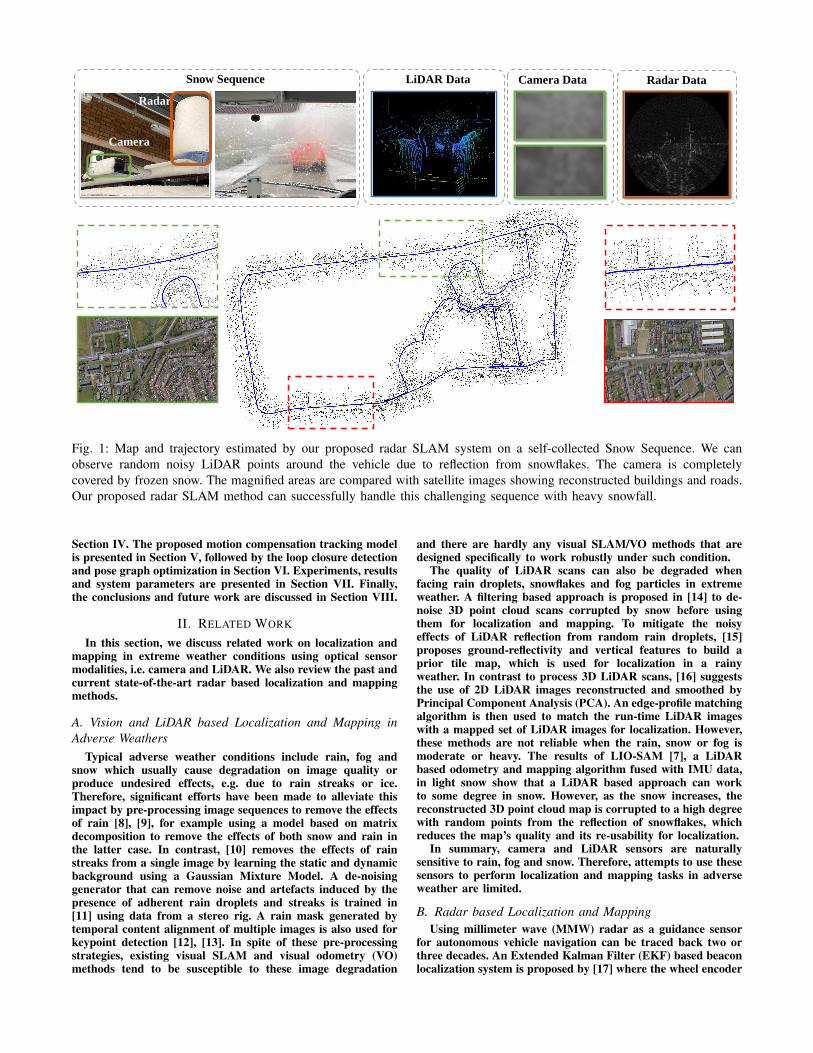
Fig. 2: Radar sensing and radar image formation. (a): A radar sends a beam with certain azimuth and elevation beamwidths,and the receiver waits for echoes from the target objects. Elevation information, like object height, is usually not retainedand collapsed to one point of S[a, :]. (b): Bilinear interpolation from a polar scan to a Cartesian image.

information is fused with range and bearing obtained by radar.One of the first substantial solutions for MMW radar basedSLAM is proposed in [18], detecting features and landmarksfrom radar to provide range and bearing information. [19]further extends the landmark description and formalizes anaugmented state vector containing rich absorption and local-ization information about targets. A prediction model is formedfor the augmented SLAM state. Instead of using the wholeradar measurement stream to perform scan matching, [20]suggests treating the measurement sequence as a continuoussignal and proposes a metric to access the quality of mapand estimate the motion by maximizing the map quality. Aconsistent map is built using a FMCW radar, an odometer anda gyroscope in [21]. Specifically, vehicle motion is correctedusing odometer and gyrometer while the map is updated byregistering radar scans. Instead of extracting and registeringfeature points, [22] uses Fourier-Mellin Transform (FMT) toestimate the relative transformation between two radar images.In [23], two approaches are evaluated for localization andmapping in a semi-natural environment using only a radar.The first one is the aforementioned FMT computing relativetransformation from whole images, while the second one usesa velocity prior to correct a distorted scan [24]. However, bothmethods are evaluated without any loop closure detection. Alandmark based pose graph radar SLAM system proves that itcan work in dynamic environments [25]. Radar is also utilizedin [26]–[30] for GPS-denied indoor mobile robot localizationand mapping.

Recently, FMCW radar sensors have been increasinglyadopted for vehicles and autonomous robots. [31] extractmeaningful landmarks for robust radar scan matching, demon-strating the potential of using radar to provide odometry infor-mation for mobile vehicles in dynamic city environments. Thiswork is extended with a graph based matching algorithm fordata association [32]. Radar odometry might fail in challengingenvironments, such as a road with hedgerows on both sides.Therefore, [33] train a classifier to detect failures in the radarodometry and fuse it with an IMU to improve its robustness.Recently, a direct radar odometry method is proposed toestimate relative pose using FMT, with local graph optimizationto further boost the performance ( [34]. In [35], they study thenecessity of motion compensation and Doppler effects on therecent emerging spinning radar for urban navigation.

Deep Learning based radar odometry and localization ap-proaches have been explored in [30], [36]–[41]. Specifically,in [37] the coherence of multiple measurements is learnt todecide which information should be kept in the reading. In[36], a mask is trained to filter out the noise from radar dataand Fast Fourier Transform (FFT) cross correlation is appliedon the masked images to compute the relative transformation.The experimental results show impressive accuracy of odometryusing radar. A self-supervised framework is also proposed forrobust keypoint detection on Cartesian radar images whichare further used for both motion estimation and loop closuredetection [38].

Full radar based SLAM systems are able to reduce driftand generate a more consistent map once a loop is closed.A real-time pose graph SLAM system is proposed in [42],which extracts keypoints and computes the GLARE descriptor[43] to identify loop closure. However, the system depends onother sensory information, e.g. rear wheel speed, yaw rates andsteering wheel angles.

1) Adverse Weather: Although radar is considered morerobust in adverse weather, the aforementioned methods donot directly demonstrate its operation in these conditions. [44]proposes a radar and GNSS/IMU fused localization system bymatching query radar images with mapped ones, and testsradar based localization in three different snow conditions:without snow, partially covered by snow and fully covered bysnow. It shows that the localization error grows as the volumeof snow increases. However they did not evaluate their systemduring snow but only afterwards. To explore the full potential ofFMCW radar in all weathers, our previous work [45] proposesa feature matching based radar SLAM system and performsexperiments in adverse weather conditions without the aidof other sensors. It demonstrates that radar based SLAM iscapable of operating even in heavy snow when LiDAR andcamera both fail. In another interesting recent work, groundpenetrating radar is used for localization in inclement weather[46] This takes a completely different perspective to addressthe problem. The ground penetrating radar (GPR) is utilizedfor extracting stable features beneath the ground. During thelocalization stage, the vehicle needs an IMU, a wheel encoderand GPR information to localize.

In this work, we extend our preliminary results presentedin [45] with a novel motion tracking algorithm optimally

compensating motion distortion and an improved loop closuredetection. Based on extensive experiments, we also demonstratea robust and accurate SLAM system operating in extremeweather conditions using radar perception.

III. RADAR SENSING

In this section, we describe the working principle of a FMCWradar and its sensing geometry. We also elaborate the challengesof employing a FMCW radar for localization and mapping.

A. NotationThroughout this paper, a reference frame j is denoted as Fj

and a homogeneous coordinate of a 2D point Pj in frame Fjis defined as pj = [xj , yj , 1]>. A homogeneous transformationTi,j ∈ SE(2) which transforms a point from the coordinateframe Fj to Fi is denoted by a transformation matrix:

Ti,j =

[Ri,j ti,j0 1

](1)

where Ri,j ∈ SO(2) is the rotation matrix and ti,j ∈ R2 is thetranslation vector. Perturbation ω ∈ R3 around the pose Ti,j

uses a minimal representation and its Lie algebra representationis expressed as ω∧ ∈ se(2). We use the left multiplicationconvention to define its increment on Ti,j with an operator⊕, i.e.,

ω ⊕Ti,j = exp(ω∧ ·Ti,j (2)

A polar radar image and its bilinear interpolated Cartesiancounterpart are denoted as S and I, respectively. A point inthe Cartesian image I is represented by its pixel coordinatesP = [u, v]>.

B. Geometry of a Rotating FMCW RadarThere are two types of continuous-wave radar: unmodulated

and frequency-modulated radars. Unmodulated continuous-wave radar can only measure the relative velocity of targetedobjects using the Doppler effect, while a FMCW radar isalso able to measure distances by detecting time shifts and/orfrequency shifts between the transmitted and received signals.Some recently developed FMCW radars make use of multipleconsecutive observations to calculate targets’ speeds so thatDoppler processing is strictly required. This improves theprocessing performance and accuracy of target range measure-ments.

Assume a radar sensor rotates 360 degrees clockwise in afull cycle with a total of Ns azimuth angles as shown in Fig.2a, i.e., the step size of the azimuth angle is 2π/Ns. For eachazimuth angle, the radar emits a beam and collapses the returnsignal to the point where a target is sensed along a rangewithout considering elevation. Therefore, a radar image is ableto provide absolute metric information of distance, differentfrom a camera image which lacks depth by nature. As shownin Fig. 2b, given a point (a, r) in a polar image S where a andr denote its azimuth and range, its homogeneous coordinatesp can be computed by

p =

µp · r · cos θµp · r · sin θ

1

(3)

where θ = −a · 2π/Ns is the ranging angle in Cartesiancoordinates, and µp (m/pixel) is the scaling factor between theimage space and the world metric space. This point on the polarimage can also be related to a point on the Cartesian image Iwith a pixel coordinate P by

u = w2− µp

µc· r · sin θ

v = h2− µp

µc· r · cos θ

(4)

where w and h are the width and height of the Cartesian image,and µc (m/pixel) is the scale factor between the pixel space andthe world metric space used in the Cartesian image. Therefore,the raw polar scan S can be transformed into a Cartesian space,represented by a grey-scale Cartesian image I through bilinearinterpolation, as shown in Fig. 2b.

C. Challenges of Radar Sensing for SLAMDespite the increasingly widespread adoption of radar sys-

tems for perception in autonomous robots and in AdvancedDriver-Assistance Systems (ADAS), there are still significantchallenges for an effective radar SLAM system.

1) Coupled Noise Sources.: As a radio active sensor, radarsuffers from multiple sources of noise and clutter, e.g. specklenoise, receiver saturation and multi-path reflection, as shownin Fig. 3a. Speckle noise is the product of interaction betweendifferent radar waves which introduces light and dark randomnoisy pixels on the image. Meanwhile, multi-path reflection maycreate “ghost” objects, presenting repetitive similar patternson the image. The interaction of these multiple sources addsanother dimension of complexity and difficulty when applyingtraditional vision based SLAM techniques to radar sensing.

2) Discontinuities of Detection.: Radar operates at alonger wavelength than LiDAR, offering the advantage ofperceiving beyond the closest object on a line of sight. However,this could become problematic for some key tasks in poseestimation, e.g. frame-to-frame feature matching and tracking,since objects or clutter detected (not detected) in the currentradar frame might suddenly disappear (appear) in next frame.As shown in Fig. 3b, this can happen even during a smallpositional change. This discontinuity of detection can introduceambiguities and challenges for SLAM, reducing robustness andaccuracy of motion tracking and loop closure.

3) Motion Distortion.: In contrast to camera and LiDAR,current mechanical scanning radar operates at a relatively lowframe rate (4Hz for our radar sensor). Within a full 360-degreeradar scan, a high-speed vehicle can travel several meters anddegrees, causing serious motion distortion and discontinuities onradar images, in particular between scans at 0 and 360 degrees.An example in Fig. 3c shows this issue on the Cartesian imageon the left, i.e. skewed radar detections due to motion distortion.By contrast, there are no skewed detections when it is static.Therefore, directly using these distorted Cartesian images forgeometry estimation and mapping can introduce errors.

In the next sections, we propose an optimization based motiontracking algorithm and a graph SLAM system to handle thesechallenges.

IV. SYSTEM OVERVIEW

The proposed system includes radar motion tracking, loopclosure detection and pose graph optimization. The system,shown in Fig. 4, is divided into two threads. The main threadis the tracking thread which takes the Cartesian images asinput, tracks the radar motion and creates new points andkeyframes for mapping. The other parallel thread takes thepolar images as input and is responsible for generation ofthe dense point cloud and computation of descriptors for loopclosure detection. Finally, once a loop is detected, it performspose graph optimization to correct the drift induced by trackingbefore updating the map.

V. RADAR MOTION TRACKING

This section describes the proposed radar motion trackingalgorithm, which includes feature detection and tracking, graphbased outlier rejection and radar pose tracking with optimalmotion distortion compensation.

𝑎Raw Polar Scan Cartesian Representation

Speckle

noise

Receiver

Saturation

Multipath

Reflection𝑟

(Azimuth)

(Range)

2𝜋

𝑁𝑠

(a) Major types of radar image degradation include speckle noise,receiver saturation and multipath reflection.

(b) Discontinuity between two consecutive radar frames: two in-consistent detections are highlighted.

Caused by motion

Scan

starting

position

Scan

ending

positionScan

starting

position

Scan

ending

position

(c) Motion distortion shown on a Cartesian radar image. Left image:the right half of the radar where the azimuth scan starts does notmatch the left half which belongs to the end of the azimuth scandue to a high speed. Right image: No distortion between the startand end scans while the radar is static.

Fig. 3: Three major types of challenges for radar SLAM.

A. Feature Detection and Tracking

For each radar Cartesian image Ij , we first detect keypointspurely using a blob detector based on a Hessian matrix.Keypoints with Hessian responses larger than a threshold areselected as candidate points. The candidate points are then se-lected based on the adaptive non-maximal suppression (ANMS)algorithm [47], which selects points that are homogeneouslyspatially distributed. Instead of using a descriptor to matchkeypoints as in [45], we track them between frames Ij−1 andIj using the KLT tracker [48].

B. Graph based Outlier RejectionIt is inevitable that some keypoints are detected and tracked

on dynamic objects, e.g., cars, cyclist and pedestrians, and onradar noise, e.g., multi-path reflection. We leverage the absolutemetrics that radar images directly provide to form geometricconstraints used for detecting and removing these outliers.

We apply a graph based outlier rejection algorithm describedin [49]. We impose a pairwise geometric consistency constrainton the tracked keypoint pair based on the fact that they shouldfollow a similar motion tendency. The assumption is that mostof the tracked points are from static scene data. Therefore, forany two pairs of keypoint matches between the current Ij andthe last Ij−1 radar frames, they should satisfy the followingpairwise constraint:∣∣‖Pm

j−1 −Pnj−1‖2 − ‖Pm

j −Pnj ‖2∣∣ < δc (5)

where |·| is the absolute operation, ‖·‖2 is the Euclideandistance, δc is a small distance threshold, and Pm

j−1, Pnj−1,

Pmj and Pn

j are the pixel coordinates of two pairs of trackedpoints between Ij−1 and Ij . Hence, Pm

j−1 and Pmj denote

a pair of associated points while Pnj−1 and Pn

j is anotherpair, see Fig. 5 for an intuitive example. A consistency matrixG is then used to represent all the associations that satisfythis pairwise consistency. If a pair of associations satisfies thisconstraint, the corresponding entry in G is set as 1 shownin Fig. 5. Finding the maximum inlier set of all matches thatare mutually consistent is equivalent to deriving the maximumclique of a graph represented by G, which can be solvedefficiently using [50]. Once the maximum inlier set is obtained,it is used to compute the relative transformation Tj−1,j , whichtransforms a point from local frame j to local frame j − 1using Singular Value Decomposition (SVD) [51]. Given Tj−1,j

and the fixed radar frame rate, an initial guess of currentvelocity vj = [vx, vy, vθ]

> ∈ R3 can be computed for the motioncompensation tracking model.

C. Motion Distortion ModellingAfter the tracked points are associated, they can be used to

estimate the motion. However, since the radar scanning rateis slow, they tend to suffer from serious motion distortion asdiscussed in Section III-C. This can dramatically degrade theaccuracy of motion estimation, which is different from most ofthe vision and LiDAR based methods. Therefore, we explicitlymodel and compensate for motion distortion in radar posetracking using an optimization approach.

Assume a full polar radar scan Sj takes ∆t seconds tofinish. Denote Tw,j as the pose of radar scan Sj in the worldcoordinate frame Fw and Tj,jt as the pose of the radar scanin the local frame Fj while capturing its azimuth beam at timet ∈ [−∆t/2,∆t/2]. Without losing generality, we compensatethe motion distortion relative to the central azimuth beam att = 0, i.e., Fj0 defines the local coordinate frame Fj of Sj .The motion distortion model is designed to correct detectionson each beam of a radar scan, i.e. optimally estimating thedetections on an undistorted radar image as shown in Fig. 6.

The radar pose in the world coordinate frame while captur-ing an azimuth scan at time t can be obtained by

Tw,jt = Tw,jTj,jt . (6)

Consider a constant velocity model in a full scan, we cancompute the relative transformation Tj,jt given the velocityvj , i.e

Tj,jt = exp((vjt)

∧) =

cos(vθt) − sin(vθt) vxtsin(vθt) cos(vθt) vyt

0 0 1

(7)

Raw Polar

Images

Cartesian Images Radar Motion Tracking

Point Cloud

Generation

M2DP

Descriptor

Extraction

Loop Closure

DetectionCurrent Descriptor

Candidate Loop

Descriptors

…

Pose Graph

Optimization

New Points

and

Keyframes

Update Map

: Keyframes: Map Points

Map

Loop

Optimize

Tracking

Thread

Loop

Closure

Thread

Fig. 4: System diagram.

Ij-1 Ij

P𝑗−11

P𝑗−12

P𝑗2

P𝑗1P𝑗−1

3

P𝑗−14

P𝑗3

P𝑗4

1 1 1 01 1 1 11 1 1 00 1 0 0

G =

P1 P2 P3 P4: Edge in maximum clique: Edge outside maximum clique

Fig. 5: Pairwise constraint: the pairwise constraint is checkedby comparing the edge length difference between the points.The maximum clique is found through the consistency matrixG. Points that are not within the maximum clique areconsidered as outliers, e.g., P4.

where exp() is the matrix exponential map and ∧ is theoperation to transform a vector to a matrix. If the ith keypointpiw in the world frame Fw is observed as pijt in the azimuthscan at time t, its motion compensated location is then

pij0 = Tj,jtpijt . (8)

In other words, pij0 is the compensated location of piw in thelocal frame Fj0 . Therefore, the feature residual between thelocally observed and estimated (after motion compensation)locations of this ith keypoint can be computed as:

eip = ρc(T−1w,jp

iw − pij0 (9)

where ρc is the Cauchy robust cost function used to accountfor perspective changes described in III-C.2.

D. Optimal Motion Compensated Radar Pose Tracking

Radar pose tracking aims to find the optimal radar poseTw,j and the current velocity vj while considering the motiondistortion. In order to ensure smooth motion dynamics, avelocity error ev is also introduced as a velocity prior term:

ev = vj − vj,prior (10)

Distorted Undistorted

x

y

x

y

x

y

ℱ𝑗𝑡=∆𝑡/2

x

y

Direct Measurement

Pseudo Measurement

r

∆𝑡/2−∆𝑡/2 0

Azimuth (t)

Features Undistorted

ℱ𝑗𝑡=0

ℱ𝑗𝑡=−∆𝑡/2

ℱ𝑗𝑡=0 ℱ𝑗𝑡=0

Fig. 6: Motion modelling to remove distortion. (Left): Foreach azimuth angle in a single scan, a radar detection isobserved within frame Fjt while moving. (Middle): All thedetections are projected onto frame Fj0 using the optimizedmotion model, compensating for motion distortion. (Right):Corresponding azimuth scans of the detections shown on apolar image and the positional changes of detections with-out distortion in a Cartesian image. All these compensateddetections are within frame Fj0 .

where vj,prior is a prior on the current velocity which isparameterized as

vj,prior =log((Tw,j−1)−1 T∨w,j

∆t(11)

Here, ∨ is the operation to convert a matrix to a vector. Thisvelocity prior term establishes a constraint on velocity changesby considering the previous pose Tw,j−1. This prior is crucialto stabilize the optimization. The results with and without thisprior are compared in Fig. 7. Therefore, the pose trackingoptimizes the velocity vj and the current radar pose Tw,j byminimizing the cost function including the feature residuals of

-200 0 200 400 600 800 1000 1200 1400 1600

x [m]

-1500

-1000

-500

0

500

1000y [

m]

groundtruth

odometry

(a) Without ev

-200 0 200 400 600 800 1000 1200 1400

x [m]

-800

-600

-400

-200

0

200

400

600

y [

m]

groundtruth

odometry

(b) With ev

Fig. 7: Odometry trajectories without and with the residualterm ev in the optimization. Without the residual term evto correlate pose with velocity, we might obtain an arbitrarysolution for pose and velocity. To stabilize the optimization,ev is needed.

: Optimizable variable : Constant

𝐓𝑤,𝑗−𝟏 𝐯𝑗 𝐓𝒘,𝑗 p𝑤1 p𝑤

2 p𝑤3

e𝑣 e𝑝1 e𝑝

2 e𝑝3

: Contribute to error

p𝑤𝑁

e𝑝N

…

…

Fig. 8: Factor graph for the motion compensation model.

all the N keypoints tracked in Sj and the velocity prior, i.e.,

v∗j ,T∗w,j = argmin

vj ,Tw,j

N∑i=1

eipTΛipeip + eTv Λvev (12)

where Λip and Λv are the information matrices of the keypoint

i and the velocity.By formulating a state variable Θ containing all the variables

to be optimized, i.e. the velocity vj and the current radar poseTw,j , and denoting e(Θ) as a generic residual block of eithereip or ev , Θ can be solved in an optimization whose factor graphrepresentation is shown in Fig. 8. The optimization problem isthen framed as finding the minimum of the weighted Sum ofSquared Errors cost function:

F(Θ) =∑i

eTi (Θ)Wiei(Θ) (13)

Θ∗ = argminΘ

F(Θ) (14)

where Wi is a symmetric positive definite weighting matrix.The total cost in 13 is minimized using the Leven-

berg–Marquardt algorithm. With the initial guess Θ, theresidual ei(∆Θ � Θ) is approximated by its first order Taylorexpansion around the current guess Θ:

ei(∆Θ � Θ) ' Ji∆Θ � ei (15)

where Ji is the Jacobian of ei evaluated with the currentparameters Θ. � represents an addition operator for thevelocity variable vj and a ⊕ operation for the pose Tw,j , asdefined in Eq. 2. Ji can be decomposed into two parts withrespect to the velocity and the pose:

Ji = [Jv,Jp] (16)

i.e., the Jacobian part with respect to the velocity as

Jv =∂ei(Θ)

∂(vjt)

∂(vjt)

∂vj(17)

and the Jacobian with respect to the pose as

Jp =∂ei(Θ)

∂(Tw,j(18)

which is equivalent to computing the Jacobian with respect tozero perturbation ∆Θp around the pose [52], i.e.

∂ei(Θ)

∂(Tw,j=∂ei(∆Θ � Θ)

∂∆Θp(19)

The Levenberg–Marquardt algorithm computes a solution ∆Θat each iteration such that it minimizes the residual functionei(∆Θ�Θ). We refer the reader to [53] for further details onthe optimization process.

E. New Point Generation

After tracking the current radar scan Sj , the total number ofsuccessfully tracked keypoints is checked to decide whether newkeypoints should be generated. If it is below a certain threshold,new keypoints are extracted and added for tracking if they arelocated in image grids whose total numbers of keypoints arelow. Once a new keypoint pijt is associated with the currentframe Sj , its global position pw can be derived from

pw = T∗w,j exp((v∗j t)

∧)pijt (20)

using its direct observation of pijt (with distortion). T∗w,j andv∗j are the optimal radar pose and velocity derived in Eq. 12.

F. New Keyframe Generation

To scale the system in a large-scale environment, we use apose-graph representation for the map with each node parame-terized by a keyframe. Each keyframe which contains a velocityand a pose is connected with its neighbouring keyframes usingits odometry derived from the motion tracking. The keyframegeneration criterion is similar to that introduced in [54], i.e., thecurrent frame is created as a new keyframe if its distance withrespect to the last keyframe is larger than a certain thresholdor its relative yaw angle is larger than a certain threshold. Anew keyframe is also generated if the number of tracked pointsis less than a certain number.

VI. LOOP CLOSURE AND POSE GRAPH OPTIMIZATION

Robust loop closure detection is critical to reduce driftin a SLAM system. Although the Bag-of-Words model hasproved efficient for visual SLAM algorithms, it is not adequatefor radar based loop closure detection due to three mainreasons: first, radar images have less distinctive pixel-wisecharacteristics compared to optical images, which means similarfeature descriptors can repeat widely across radar imagescausing a large number of incorrect feature matches; second,the multi-path reflection problem in radar can introduce furtherambiguity for feature description and matching; third, a smallrotation of the radar sensor may produce tremendous scenechanges, significantly distorting the histogram distribution ofthe descriptors. On the other hand, radar imagery encapsulatesvaluable absolute metric information, which is inherently miss-ing for an optical image. Therefore, we propose a loop closuretechnique which captures the geometric scene structure andexploits the spatial signature of reflection density from radarpoint clouds.

Algorithm 1: Radar Polar Scan to Point CloudConversion

Input: Radar polar scan S ∈ Rm×n;Output: Point Cloud C ∈ Rz×2;Parameters: Minimum peak prominence δp and

minimum peak distance δd;Initialize empty point cloud set C;for i← 1 to m do

Qk×1 ← findPeaks(S[i, :], δp, δd);(µ, σ) ← meanAndStandardDeviation(Qk×1);for each peak q in Q do

if q ≥ (µ+ σ) thenp ← transformPeakToPoint(q, i);Add the point p to C;

endend

end

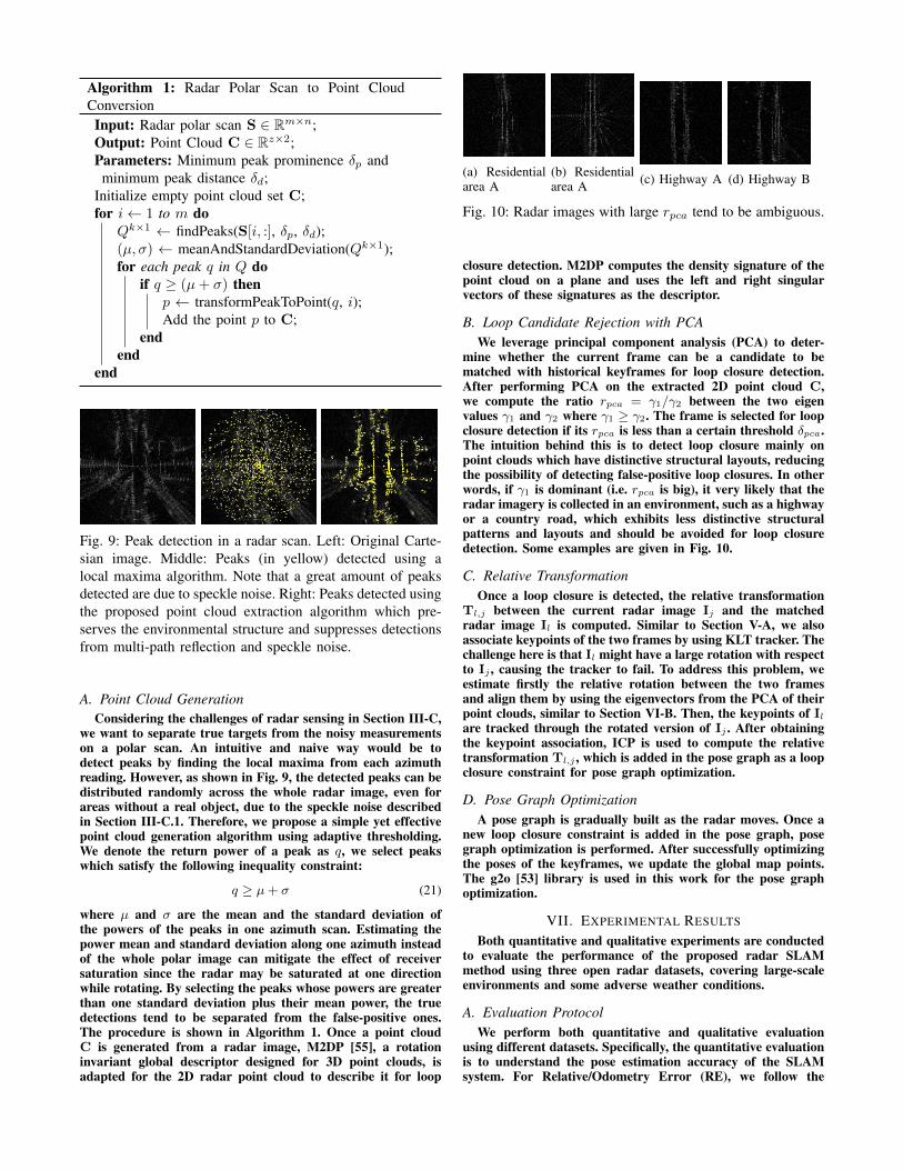
Fig. 9: Peak detection in a radar scan. Left: Original Carte-sian image. Middle: Peaks (in yellow) detected using alocal maxima algorithm. Note that a great amount of peaksdetected are due to speckle noise. Right: Peaks detected usingthe proposed point cloud extraction algorithm which pre-serves the environmental structure and suppresses detectionsfrom multi-path reflection and speckle noise.

A. Point Cloud GenerationConsidering the challenges of radar sensing in Section III-C,

we want to separate true targets from the noisy measurementson a polar scan. An intuitive and naive way would be todetect peaks by finding the local maxima from each azimuthreading. However, as shown in Fig. 9, the detected peaks can bedistributed randomly across the whole radar image, even forareas without a real object, due to the speckle noise describedin Section III-C.1. Therefore, we propose a simple yet effectivepoint cloud generation algorithm using adaptive thresholding.We denote the return power of a peak as q, we select peakswhich satisfy the following inequality constraint:

q ≥ µ+ σ (21)

where µ and σ are the mean and the standard deviation ofthe powers of the peaks in one azimuth scan. Estimating thepower mean and standard deviation along one azimuth insteadof the whole polar image can mitigate the effect of receiversaturation since the radar may be saturated at one directionwhile rotating. By selecting the peaks whose powers are greaterthan one standard deviation plus their mean power, the truedetections tend to be separated from the false-positive ones.The procedure is shown in Algorithm 1. Once a point cloudC is generated from a radar image, M2DP [55], a rotationinvariant global descriptor designed for 3D point clouds, isadapted for the 2D radar point cloud to describe it for loop

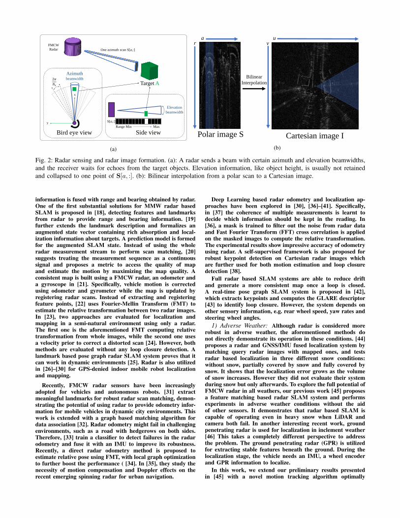
(a) Residentialarea A

(b) Residentialarea A (c) Highway A (d) Highway B

Fig. 10: Radar images with large rpca tend to be ambiguous.

closure detection. M2DP computes the density signature of thepoint cloud on a plane and uses the left and right singularvectors of these signatures as the descriptor.

B. Loop Candidate Rejection with PCAWe leverage principal component analysis (PCA) to deter-

mine whether the current frame can be a candidate to bematched with historical keyframes for loop closure detection.After performing PCA on the extracted 2D point cloud C,we compute the ratio rpca = γ1/γ2 between the two eigenvalues γ1 and γ2 where γ1 ≥ γ2. The frame is selected for loopclosure detection if its rpca is less than a certain threshold δpca.The intuition behind this is to detect loop closure mainly onpoint clouds which have distinctive structural layouts, reducingthe possibility of detecting false-positive loop closures. In otherwords, if γ1 is dominant (i.e. rpca is big), it very likely that theradar imagery is collected in an environment, such as a highwayor a country road, which exhibits less distinctive structuralpatterns and layouts and should be avoided for loop closuredetection. Some examples are given in Fig. 10.

C. Relative TransformationOnce a loop closure is detected, the relative transformation

Tl,j between the current radar image Ij and the matchedradar image Il is computed. Similar to Section V-A, we alsoassociate keypoints of the two frames by using KLT tracker. Thechallenge here is that Il might have a large rotation with respectto Ij , causing the tracker to fail. To address this problem, weestimate firstly the relative rotation between the two framesand align them by using the eigenvectors from the PCA of theirpoint clouds, similar to Section VI-B. Then, the keypoints of Ilare tracked through the rotated version of Ij . After obtainingthe keypoint association, ICP is used to compute the relativetransformation Tl,j , which is added in the pose graph as a loopclosure constraint for pose graph optimization.

D. Pose Graph OptimizationA pose graph is gradually built as the radar moves. Once a

new loop closure constraint is added in the pose graph, posegraph optimization is performed. After successfully optimizingthe poses of the keyframes, we update the global map points.The g2o [53] library is used in this work for the pose graphoptimization.

VII. EXPERIMENTAL RESULTS

Both quantitative and qualitative experiments are conductedto evaluate the performance of the proposed radar SLAMmethod using three open radar datasets, covering large-scaleenvironments and some adverse weather conditions.

A. Evaluation ProtocolWe perform both quantitative and qualitative evaluation

using different datasets. Specifically, the quantitative evaluationis to understand the pose estimation accuracy of the SLAMsystem. For Relative/Odometry Error (RE), we follow the

Left RightRadar

LiDAR

Fig. 11: Synchronized radar, stereo, and LiDAR data fromthe Oxford Radar RobotCar Dataset [57].

TABLE I: Lengths of Collected Sequences in RADIATEDataset.

Sequence Fog 1 Fog 2 Rain Normal Snow 1 Snow 2 NightLength (km) 4.7 4.8 3.3 3.3 8.7 3.3 5.6

popular KITTI odometry evaluation criteria, i.e., computingthe mean translation and rotation errors from length 100 to 800meters with a 100 meters increment. Absolute Trajectory Error(ATE) is also adopted to evaluate the localization accuracy offull SLAM, in particular after loop closure and global graphoptimization. The trajectories of all methods (see full list inSection VII-C are aligned with the ground truth trajectoriesusing a 6 Degree-of-Freedom (DoF) transformation providedby the evaluation tool in [56] for ATE evaluation. On the otherhand, the qualitative evaluation focuses on how some challeng-ing scenarios, e.g. in adverse weather conditions, influence theperformance of various vision, LiDAR and radar based SLAMsystems.

B. DatasetsSo far there exist three public datasets that provide long-

range radar data with dense returns: the Oxford RobotCarRadar Dataset [57], [58], the MulRan Dataset [59] and theRADIATE Dataset [60]. We choose the Oxford RobotCar andMulRan datasets for detailed quantitative benchmarking andour RADIATE dataset mainly for qualitative evaluation in ourexperiments.

1) Oxford RobotCar Radar Dataset.: The Oxford Robot-Car Radar Dataset [57], [58] provides data from a NavtechCTS350-X Millimetre-Wave W radar for about 280 km ofdriving in Oxford, UK, traversing the same route 32 times. Italso provides stereo images from a Point Grey Bumblebee XB3camera and LiDAR data from two Velodyne HDL-32E sensorswith ground truth pose locations. The radar is configured toprovide 4.38 cm and 0.9 degree resolutions in range and azimuthrespectively, with a range up to 163 meters. The radar scanningfrequency is 4 Hz. See Fig. 11 for some examples of data.

2) MulRun Dataset.: The MulRan Dataset [59] providesradar and LiDAR range data, covering multiple cities atdifferent times in a variety of city environments (e.g., bridge,tunnel and overpass). A Navtech CIR204-H Millimetre-WaveFMCW radar is used to obtain radar images with 6 cm rangeand 0.9 degree rotation resolutions with a maximum range of200 m. The radar scanning frequency is also 4Hz. It also hasan Ouster 64-channel LiDAR sensor operating at 10Hz witha maximum range of 120 m. Different routes are selected forour experiments, including Dajeon Convention Center (DCC),

DCC KAIST Riverside

Fig. 12: Radar and LiDAR data from the MulRan Dataset.In Riverside, we can see the repetitive structures of treesand bushes, which makes it challenging for LiDAR basedodometry and mapping algorithms [59].

Snow Fog/Rain Night

Fig. 13: Images collected in Snow (left), Fog/Rain (middle),and Night (right). The image quality degrades in theseconditions, making it extremely challenging for vision basedodometry and SLAM algorithms. Note that for the snowsequence, the camera is completely covered by snow.

KAIST and Riverside. Specifically, DCC presents diverse struc-tures while KAIST is collected while moving within a campus.Riverside is captured along a river and two bridges withrepetitive features. Each route contains 3 traverses on differentdays. Some LiDAR and radar data examples are given in Fig.12.

3) RADIATE Dataset.: The RADIATE dataset is our re-cently released dataset which includes radar, LiDAR, stereocamera and GPS/IMU [60]. One of its unique features is that itprovides data in extreme weather conditions, such as rain andsnow, as shown Fig. 13. A Navtech CIR104-X radar is usedwith 0.175 m range resolution and maximum range of 100 mat 4 Hz operation frequency. A 32-channel Velodyne HDL-32ELiDAR and a ZED stereo camera are set at 10Hz and 15 Hz,respectively. The 7 sequences used in this work include 2 fog,1 rain, 1 normal, 2 snow and 1 night recorded in the City ofEdinburgh, UK. Their sequence lengths are given in Table I.Note that only the rain, normal, snow and night sequences haveloop closures and the GPS signal is occasionally lost in the snowsequence.

TABLE II: Relative error on Oxford Radar RobotCar Dataset

SequenceMethod 10-11-

46-2110-12-32-52

16-11-53-11

16-13-09-37

17-13-26-39

18-14-14-42

18-14-46-59

18-15-20-12

Mean

ORB-SLAM2 6.11/1.7 6.09/1.6 6.16/1.7 6.23/1.7 6.41/1.7 7.05/1.8 7.17/1.9 11.5/3.3 7.09/3.1SuMa 1.1/0.3∗12% 1.1/0.3∗20% 0.9/0.3∗27% 1.2/0.4∗29% 1.1/0.3∗23% 0.9/0.1∗10% 1.0/0.1∗10% 1.0/0.2∗20% 1.03/0.3Cen Odometry N/A N/A N/A N/A N/A N/A N/A N/A 3.71/0.95Barnes Odometry N/A N/A N/A N/A N/A N/A N/A N/A 2.7848/0.85Baseline Odometry 3.26/0.9 2.98/0.8 3.28/0.9 3.12/0.9 2.92/0.8 3.18/0.9 3.33/1.0 2.85/0.9 3.11/0.9Baseline SLAM 2.27/0.9 2.16/0.6 2.24/0.6 1.83/0.6 2.45/0.8 2.21/0.7 2.34/0.7 2.24/0.8 2.21/0.7Our Odometry 2.16/0.6 2.32/0.7 2.49/0.7 2.62/0.7 2.27/0.6 2.29/0.7 2.12/0.6 2.25/0.7 2.32/0.7Our SLAM 1.96/0.7 1.98/0.6 1.81/0.6 1.48/0.5 1.71/0.5 2.22/0.7 1.68/0.5 1.77/0.6 1.83/0.6

Results are given as translation error / rotation error. Translation error is in %, and rotation error is in degrees per 100 meters (deg/100m). For the Cenand Barnes odometry methods, only their mean errors are shown since individual sequence errors are not reported in their papers. ∗xx% indicates that

the algorithm cannot finish the full sequence, and its result is reported up to the point (xx% of the full sequence) where it fails.

TABLE III: Absolute trajectory error for position (RMSE) on Oxford Radar RobotCar Dataset

SequenceMethod 10-11-

46-2110-12-32-52

16-11-53-11

16-13-09-37

17-13-26-39

18-14-14-42

18-14-46-59

18-15-20-12

ORB-SLAM2 7.301 7.961 3.539 7.590 7.609 24.632 9.715 12.174SuMa N/A N/A N/A N/A N/A N/A N/A N/ABaseline SLAM 58.138 14.598 12.933 12.829 10.898 49.599 23.270 56.422Our SLAM 13.784 9.593 7.136 11.182 5.835 21.206 6.011 7.740

The absolute trajectory error of position is in meters. N/A: SuMa fails to finish all eight sequences, no absolute trajectory error is applicable here.

100 200 300 400 500 600 700 800

Path Length (m)

0

1

2

3

4

5

6

7

8

9

10

Tra

nsla

tion E

rror

(%)

Baseline Odometry

ORB-SLAM2

Our Odometry

Our SLAM

SuMa

(a) Translation against pathlength.

100 200 300 400 500 600 700 800

Path Length (m)

0

0.01

0.02

0.03

0.04

0.05

0.06

Rota

tion E

rror

(deg/m

)

Baseline Odometry

ORB-SLAM2

Our Odometry

Our SLAM

SuMa

(b) Rotation against path length.

0 5 10 15 20 25 30 35 40 45

Speed (km/h)

0

2

4

6

8

10

12

14

16

18

Tra

nsla

tion E

rror

(%)

Baseline Odometry

ORB-SLAM2

Our Odometry

Our SLAM

SuMa

(c) Translation against speed.

0 5 10 15 20 25 30 35 40 45

Speed (km/h)

0

0.01

0.02

0.03

0.04

0.05

0.06

0.07

Rota

tion E

rror

(deg/m

)

Baseline Odometry

ORB-SLAM2

Our Odometry

Our SLAM

SuMa

(d) Rotation against speed.

Fig. 14: Average error against different path lengths and speeds on Oxford Radar RobotCar Dataset. Note that SuMa’s resultsare computed up to the point where it fails matching the xx% percentages in Table II.

100 200 300 400 500 600 700 800

Path Length (m)

0

2

4

6

8

10

12

Tra

nsla

tion E

rror

(%)

Baseline Odometry

ORB-SLAM2

Our Odometry

Our SLAM

SuMa

(a) Low, median and high translation errors against path length.

100 200 300 400 500 600 700 800

Path Length (m)

0

0.01

0.02

0.03

0.04

0.05

0.06

0.07

Rota

tion E

rror

(deg/m

)

Baseline Odometry

ORB-SLAM2

Our Odometry

Our SLAM

SuMa

(b) Low, median and high rotation errors against path length.

Fig. 15: Bar charts for translation and rotation errors against path length on Oxford Radar RobotCar Dataset.

C. Competing Methods and Their Settings

In order to validate the performance of our proposedradar SLAM system, state-of-the-art odometry and SLAMmethods for large-scale environments using different sensormodalities (camera, LiDAR, radar) are chosen. These includeORB-SLAM2 [54], SuMa [61] and our previous version ofRadarSLAM [45], as baseline algorithms for vision, LiDAR andradar based approaches, respectively. For the Oxford Radar

RobotCar Dataset, the results reported in [31], [36] are alsoincluded as a radar based method due to the unavailability oftheir implementations.

We would like to highlight that we use an identical setof parameters for our radar odometry and SLAM algorithmacross all the experiments and datasets, without any parametertuning. We believe this is worthwhile to tackle the challengethat most existing odometry or SLAM algorithms require some

levels of parameter tuning in order to reduce or avoid resultdegradation.

1) Stereo Vision based ORB-SLAM2.: OBR-SLAM2 [54]is a sparse feature based visual SLAM system which relies onORB features. It also possesses loop closure and pose graphoptimization capabilities. Local Bundle Adjustment is usedto refine the map point position which boosts the odometryaccuracy. Based on its official open-source implementation, weuse its stereo setting in all experiments and loop closure isenabled.

2) LiDAR based SuMa.: SuMa [61] is one of the state-of-the-art LiDAR based odometry and mapping algorithms forlarge-scale outdoor environments, especially for mobile vehicles.It constructs and uses a surfel-based map to perform robustdata association for loop closure detection and verification. Weemploy its open-source implementation and keep the originalparameter setting used for KITTI dataset in our experiments.

3) Radar based RadarSLAM.: Our old version ofRadarSLAM [45] extracts SURF features from Cartesian radarimages and matches the keypoints based on their descriptorsfor pose estimation, which is different from the feature trackingtechnique in this work. It does not consider motion distortionalthough it includes loop closure detection and pose graphoptimization to reduce drift and improve the map consistency.

4) Cen’s Radar Odometry.: Cen’s method [31] is one ofthe first attempts using the Navtech FMCW radar sensor toestimate ego-motion of a mobile vehicle. Landmarks are ex-tracted from polar scans before performing data association bymaximizing the overall compatibility with pairwise constraints.Given the associated pairs, SVD is used to find the relativetransformation.

5) Barnes’ Radar Odometry.: Barnes’ method [36] lever-ages deep learning to generate distraction-free feature mapsand uses FFT cross correlation to find relative poses onconsecutive feature maps. After being trained end-to-end, thesystem is able to mask out multipath reflection, speckle noiseand dynamic objects. This facilitates the cross correlation stageand produces accurate odometry. The spatial cross-validationresults in appendix of [36] are chosen for fair comparison.

D. Experiments on RobotCar DatasetResults of eight sequences of RobotCar Dataset are reported

here for evaluation, i.e., 10-12-32-52, 16-13-09-37, 17-13-26-39, 18-15-20-12, 10-11-46-21, 16-11-53-11 and 18-14-46-59. Thewide baseline stereo images are used for the stereo ORB-SLAM2 and the left Velodyne HDL-32E sensor is used forSuMa.

1) Quantitative Comparison: The RE and ATE results ofeach sequence are given in Tables II and III respectively. Sincethe groundtruth poses provided by the Oxford Radar RobotCarDataset are 3-DoF, only the x, y and yaw of the estimated6-DoF poses of ORB-SLAM2 and SuMa are evaluated. Notethat SuMa fails on all eight sequences at 10 − 30% of the fulllengths and all its results are reported until the point whereit fails, and ATE is not applicable due to the lack of fullyestimated trajectories. Specifically, the stereo version of ORB-SLAM2 is able to complete all eight sequences, successfullyclose the loops and achieve superior localization accuracy.SuMa also performs accurately when it works although it isless robust using this dataset. This may be due to the largenumber of dynamic objects, e.g. surrounding moving cars andbuses. Regarding radar based approaches, we can see that ourproposed radar odometry/SLAM achieves less RE comparedto the baseline radar odometry/SLAM and Cen’s method anda similar mean AE to the learning based Barnes’ method.It can also be seen that our proposed radar odometry andSLAM methods achieve better or comparable RE and ATEperformance to ORB-SLAM2 and SuMa. Fig. 14 describes the

0 100 200 300 400 500

-20

0

20

m/s

Optimized velocity compared to groundtruth

Velocity X groundtruth

Velocity X optimized

0 100 200 300 400 500-10

0

10

m/s

Velocity Y groundtruth

Velocity Y optimized

0 100 200 300 400 500

Frame

-20

0

20

De

gre

e/s

Velocity Yaw groundtruth

Velocity Yaw optimized

Fig. 16: Optimized x, y and yaw velocities on RobotCar.

REs of ORB-SLAM2, SuMa, baseline radar odometry and ourradar odometry/SLAM algorithms using different path lengthsand speeds, following the popular KITTI odometry evaluationprotocol. SuMa has the lowest error on both translation androtation against path lengths and speed until it fails, while ourradar SLAM and odometry methods are the second and thirdlowest respectively. The low, median and high translation androtation errors are presented in Figs. 15a and 15b. It can beseen that our SLAM and odometry achieve low values for bothtranslation and rotation errors for different path lengths.

The optimized velocities of x, y and yaw are given in Fig 16compared to the ground truth. The optimized velocities havevery high accuracy, which verifies the superior performance ofour proposed radar motion tracking algorithm.

2) Qualitative Comparison: We show the estimated tra-jectories of 6 sequences in Fig. 17 for qualitative evaluation.For most of the sequences, our SLAM results are closest tothe ground truth although the trajectories of baseline SLAMand ORB-SLAM2 are also accurate except for sequence 18-14-14-42. Fig. 18 elaborate on the trajectory of each method onsequence 17-13-26-39 for qualitative performance.

We further compare the proposed radar odometry withthe baseline radar odometry [45]. Estimated trajectories of3 sequences are presented in Fig. 19. It is clear that ourradar odometry drifts much slower than the baseline radarodometry method, validating the superior performance of themotion tracking algorithm with feature tracking and motioncompensation. Therefore, our SLAM system also benefits fromthis improved accuracy.

E. Experiments on MulRun DatasetThe RE and ATE of SuMa, baseline radar odometry/SLAM

and our radar SLAM are shown in Table IV and Table V.ORB-SLAM2 is not applicable here since MulRan only containsradar and LiDAR data. Similar to the RobotCat dataset, weagain transform its provided 6-DoF ground truth poses into3-DoF for evaluation. Both RE and ATE are evaluated on9 sequences: DCC01, DCC02, DCC03, KAIST01, KAIST02,KAIST03, Riverside01, Riverside02 and Riverside03. In termsof RE, both our odometry and SLAM system achieve compa-rable or better performance on all sequences.

Our odometry method reduces both translation error androtation errors significantly compared to the baseline. OurSLAM system, to a great extent, outperforms both baselineSLAM and SuMa on ATE. More importantly, only our SLAMreliably works on all 9 sequences which cover diverse urbanenvironments. Specifically, the baseline SLAM detects wrong

−200 0 200 400 600 800 1000 1200

x [m]

−1000

−800

−600

−400

−200

0

200

400

600

y[m

]

Baseline SLAM

ORB-SLAM2

Our SLAM

SuMa

Groundtruth

(a) 10-11-46-21

−200 0 200 400 600 800 1000 1200

x [m]

−1000

−800

−600

−400

−200

0

200

400

600

y[m

]

Baseline SLAM

ORB-SLAM2

Our SLAM

SuMa

Groundtruth

(b) 10-12-32-52

−200 0 200 400 600 800 1000 1200

x [m]

−1000

−800

−600

−400

−200

0

200

400

600

y[m

]

Baseline SLAM

ORB-SLAM2

Our SLAM

SuMa

Groundtruth

(c) 16-11-53-11

−200 0 200 400 600 800 1000 1200

x [m]

−1000

−800

−600

−400

−200

0

200

400

600

y[m

]

Baseline SLAM

ORB-SLAM2

Our SLAM

SuMa

Groundtruth

(d) 16-13-09-37

−200 0 200 400 600 800 1000 1200

x [m]

−1000

−800

−600

−400

−200

0

200

400

600

y[m

]

Baseline SLAM

ORB-SLAM2

Our SLAM

SuMa

Groundtruth

(e) 17-13-26-39

−200 0 200 400 600 800 1000 1200

x [m]

−1000

−800

−600

−400

−200

0

200

400

600

y[m

]

Baseline SLAM

ORB-SLAM2

Our SLAM

SuMa

Groundtruth

(f) 18-14-14-42

Fig. 17: 6 sequences trajectories results of different SLAM algorithms on Oxford Radar RobotCar Dataset.

−200 0 200 400 600 800 1000 1200

x [m]

−800

−600

−400

−200

0

200

400

600

y[m

]

Baseline SLAM

Groundtruth

(a) Baseline Radar SLAM

−200 0 200 400 600 800 1000 1200

x [m]

−800

−600

−400

−200

0

200

400

600

y[m

]

ORB-SLAM2

Groundtruth

(b) ORB-SLAM2 Stereo

−200 0 200 400 600 800 1000 1200

x [m]

−800

−600

−400

−200

0

200

400

600

y[m

]

Our SLAM

Groundtruth

(c) Our Radar SLAM

−200 0 200 400 600 800 1000 1200

x [m]

−800

−600

−400

−200

0

200

400

600

y[m

]

SuMa

Groundtruth

(d) SuMa

Fig. 18: Trajectories results of different SLAM algorithms on sequence 17-13-26-39 of Oxford Radar RobotCar Dataset.

TABLE IV: Relative error on MulRan Dataset

SequenceMethod DCC01 DCC02 DCC03 KAIST01 KAIST02 KAIST03 Riverside01 Riverside02 Riverside03 MeanSuMa 2.71/0.4 4.07/0.9 2.14/0.6 2.9/0.8 2.64/0.6 2.17/0.6 1.66/0.6∗30%1.49/0.5∗23%1.65/0.4∗5% 2.38/0.5Baseline Odometry 3.35/0.9 2.12/0.6 1.74/0.6 2.32/0.8 2.69/1.0 2.62/0.8 2.70/0.7 3.09/1.1 2.71/0.7 2.59/0.8Baseline SLAM 3.81/0.9 2.04/0.5 1.90/5.5 2.34/0.7 1.95/0.6 20.1/5.1 3.56/0.9 3.05/6.8 152/0.175 21.1/2.3Our Odometry 2.70/0.5 1.90/0.4 1.64/0.4 2.13/0.7 2.07/0.6 1.99/0.5 2.04/0.5 1.51/0.5 1.71/0.5 1.97/0.5Our SLAM 2.39/0.4 1.90/0.4 1.56/0.2 1.75/0.5 1.76/0.4 1.72/0.4 3.40/0.9 1.79/0.3 1.95/0.5 2.02/0.4

Results are given as translation error / rotation error. Translation error is in %, and rotation error is in degrees per 100 meters (deg/100m). ∗ indicatesthe algorithm fails at the xx% of the sequence and its result is reported up to that point.

loop closures on sequence KAIST03, Riverside02 and River- side03 and fails to detect a loop in DCC03, which causes its

−200 0 200 400 600 800 1000 1200 1400

x [m]

−1000

−800

−600

−400

−200

0

200

400

600

y[m

]

Baseline Odometry

Our Odometry

Groundtruth

(a) 10-12-32-52

−200 0 200 400 600 800 1000 1200 1400

x [m]

−1000

−800

−600

−400

−200

0

200

400

600

y[m

]

Baseline Odometry

Our Odometry

Groundtruth

(b) 17-13-26-39

−200 0 200 400 600 800 1000 1200 1400

x [m]

−1000

−800

−600

−400

−200

0

200

400

600

y[m

]

Baseline Odometry

Our Odometry

Groundtruth

(c) 18-14-46-59

Fig. 19: Trajectories of radar odometry results of different algorithms on Oxford Radar RobotCar Dataset.

TABLE V: Absolute trajectory error for position (RMSE) on MulRan Dataset

SequenceMethod DCC01 DCC02 DCC03 KAIST01 KAIST02 KAIST03 Riverside01 Riverside02 Riverside03SuMa 13.509 17.834 29.574 38.693 31.864 45.970 N/A N/A N/ABaseline SLAM 17.458 24.962 76.138 4.931 3.918 50.809 10.531 95.247 1091.605Our SLAM 12.886 9.878 3.917 6.873 6.028 4.109 9.029 7.049 10.741

The absolute trajectory error of position is in meters. N/A: SuMa fails to finish Riverside01, 02 and 03 sequences.

−100 0 100 200 300 400 500 600 700

x [m]

−600

−500

−400

−300

−200

−100

0

100

200

y[m

]

Baseline SLAM

Our SLAM

SuMa

Groundtruth

(a) DCC01

−100 0 100 200 300 400 500 600 700

x [m]

−600

−500

−400

−300

−200

−100

0

100

200

y[m

]

Baseline SLAM

Our SLAM

SuMa

Groundtruth

(b) DCC02

−100 0 100 200 300 400 500 600 700

x [m]

−600

−500

−400

−300

−200

−100

0

100

200

y[m

]

Baseline SLAM

Our SLAM

SuMa

Groundtruth

(c) DCC03

−400 −200 0 200 400 600

x [m]

−800

−600

−400

−200

0

200

y[m

]

Baseline SLAM

Our SLAM

SuMa

Groundtruth

(d) KAIST01

−400 −200 0 200 400 600

x [m]

−800

−600

−400

−200

0

200

y[m

]

Baseline SLAM

Our SLAM

SuMa

Groundtruth

(e) KAIST02

−400 −200 0 200 400 600

x [m]

−800

−600

−400

−200

0

200

y[m

]

Baseline SLAM

Our SLAM

SuMa

Groundtruth

(f) KAIST03

Fig. 20: 6 sequences trajectories results of different SLAM algorithms on MulRan Dataset.

large ATEs for these sequences. SuMa, on the other hand, failsto finish the sequences Riverside01, 02 and 03, likely due to thechallenges of less distinctive structures along the rather openand long road as shown in Fig. 22. It can be very challenging

to register LiDAR scans accurately in this kind of environment.

The estimated trajectories on sequences DCC01, DCC02,DCC03, KAIST01, KAIST02, KAIST03 are shown in Figure20. These qualitative results of the algorithms provide similar

0 500 1000 1500 2000

x [m]

−800

−600

−400

−200

0

200

400

600y

[m]

Baseline SLAM

Our SLAM

SuMa

Groundtruth

(a) Comparision

0 500 1000 1500 2000

x [m]

−800

−600

−400

−200

0

200

400

600

y[m

]

Baseline SLAM

Groundtruth

(b) Baseline Radar SLAM

0 500 1000 1500 2000

x [m]

−800

−600

−400

−200

0

200

400

600

y[m

]

Our SLAM

Groundtruth

(c) Our Radar SLAM

0 500 1000 1500 2000

x [m]

−800

−600

−400

−200

0

200

400

600

y[m

]

SuMa

Groundtruth

(d) SuMa

Fig. 21: Trajectories results of different SLAM algorithms on sequence Riverside01 of MulRan.

Fig. 22: Riverside scenery of MulRan from Google StreetView: repetitive structures are challenging to LiDAR basedmethods moving on high way.

(a) Place 1 snow (b) Place 1 normal

(c) Place 2 snow (d) Place 2 normal

Fig. 23: Two types of LiDAR degeneration. (a)-(b): Place1 with less reflection from the scene. (c)-(d): Place 2 withmany noisy detections from snowflakes around.

observations to the RE and ATE. For clarity, Figure 21 presentstrajectories of the SLAM algorithms on Riverside01 in separatefigures.

F. Experiments on the RADIATE DatasetTo further verify the superiority of radar against LiDAR and

camera in adverse weathers and degraded visual environments,we perform qualitative evaluation by comparing the estimatedtrajectories with a high-precision Inertial Navigation System(inertial system fused with GPS) using our RADIATE dataset.

Since ORB-SLAM2 fails to produce meaningful results due tothe visual degradation caused by water drops, blurry effects inlow-light conditions and occlusion from snow (see Fig. 13 forexample images), its results are not reported in this section.

1) Experiments in Adverse Weather: Estimated trajectoriesof SuMa, baseline and our odometry for Fog 1 and Fog 2 areshown in Figs. 24a and 24b respectively. We can see that ourSLAM drifts less than SuMa and the baseline radar SLAMalthough they all suffer from drift without loop closure. SuMaalso loses tracking for sequence Fog 2, which is likely due tothe impact of fog on LiDAR sensing.

The impact of snowflakes on LiDAR reflection is moreobvious. Fig. 23 shows the LiDAR point clouds of two of thesame places in snowy and normal conditions. Depending on thesnow density, we can see two types of degeneration of LiDARin snow. It is clear that both the number of correct LiDARreflections and point intensity dramatically drop in snow forplace 1, while there are a lot of noisy detections around theorigin for place 2. Both cases can be challenging for LiDARbased odometry/SLAM methods. This matches the results ofthe Snow sequence in Fig. 25. Specifically, when the snowwas initially light, SuMa was operating well. However, whenthe snow gradually became heavier, the LiDAR data degradedand eventually SuMa lost track. The three examples of LiDARscans at the point when SuMa fails are shown in Fig. 25. Thevery limited surrounding structures sensed by LiDAR makesit extremely challenging for LiDAR odometry/SLAM methodslike SuMa. In contrast, our radar SLAM method is still able tooperate accurately in heavy snow, estimating a more accuratetrajectory than the baseline SLAM.

2) Experiments on the Same Route in Different Weathers:To compare different algorithms’ performance on the sameroute but in different weather conditions, we also provide resultshere in normal weather, rain and snow conditions respectively.The estimated trajectories of SuMa, baseline SLAM and ourSLAM result in normal weather are shown in Fig. 26a whilefor the Rain sequence these are shown in Fig. 26b. In theRain sequence, there is moderate rain. LiDAR based SuMa isslightly affected, and as we can see at the beginning of thesequence, SuMa estimates a shorter length. Our radar SLAMalso performs better than the baseline SLAM. In the Snow 2sequence, there is moderate snow, and the results are shownin Fig. 26c. The Snow 2 sequence was taken while movingquickly. Therefore, without motion compensation, the baselineSLAM drifts heavily and cannot close the loop while our SLAMconsistently performs well. Hence, the results in Fig. 26 onceagain confirm the our proposed SLAM system is robust in allweather conditions.

3) Experiments at Night: The estimated trajectories ofSuMa, baseline SLAM and our SLAM on the Night sequenceare shown in Fig. 24c. LiDAR based SuMa is almost unaffectedby the dark night although it does not detect the loops.Both baseline and our SLAM perform well in the nightsequence, producing more accurate trajectories after detectingloop closures.

SuMaGPS Baseline SLAM Our SLAM

(a) Fog 1

SuMaGPS Baseline SLAM Our SLAM

(b) Fog 2

SuMaGPS Baseline SLAM Our SLAM

(c) Night.

Fig. 24: Estimated trajectories and groundtruth of sequence Fog 1, Fog 2 and Night.

LiDAR scans where

SuMa loses track

Radar scans where

SuMa loses track

SuMaGPS Baseline SLAM Our SLAM

Fig. 25: Results on the Snow sequence of the RADIATE dataset. Left: LiDAR scans when SuMa loses track. Note the noisyLiDAR reflection of snowflakes. Middle: GPS and estimated trajectories on Google Map. Right: Radar images when SuMaloses track.

G. Average Completion PercentageWe calculate the average completion percentage for each

competing algorithm on each dataset, to evaluate the robustnessof each algorithm representing a different sensor modality.The number of frames that a method completed before losingtracking is denoted as Kcompleted while the total number offrames is denoted as Ktotal. The metric is computed as:

Percentage = Kcompleted/Ktotal ∗ 100% (22)

The MulRan dataset does not include camera data so it isshown as N/A for ORB-SLAM2. In the RADIATE dataset, thecamera is either blocked by snow or blurred in the night soORB-SLAM2 fails to initialize and it is also shown as N/A. InTable VII we can see that only the radar based methods are

reliable and completed in all cases. Neither vision based norLiDAR based methods manage to finish on all three datasets.

TABLE VI: Completion Percentage %

DatasetMethod Oxford MulRan RADIATESuMa 20 72 63

Baseline SLAM 100 100 100ORB-SLAM2 100 N/A N/AOur SLAM 100 100 100Completion Percentage on Different Datasets

SuMa

GPS

Baseline SLAM

Our SLAM

(a) Normal weather sequence (b) Rain sequence (c) Snow 2 sequence (d) Images

Fig. 26: (a)-(c): Estimated trajectories and ground truth on multi-session traversals in normal, rain and snow conditions.(d)Top: image data in normal weather captured by our stereo camera, centre: image data in rain captured by our stereocamera, bottom: image data in snow captured by our phone for reference.

H. Parameters UsedThe same set of parameters provided in Table VII is

employed in all the experiments, covering different cities, radarresolutions and ranges, weather conditions, road scenarios, etc.

TABLE VII: Parameters for Radar SLAM

Parameter Value NoteMax polar distance 87.5 Maximum selected distance in

radar reading in meters in our ex-periments

Min Hessian 700 Minimum Hessian value a point tobe considered as keypoint

δc 3 Pixel value for maximal clique ingraph outlier rejection in Eq. 5

Max tracked points 60 Maximum number of points intracking

Keyframe distance 2.0 Distance between keyframes in me-ters

Keyframe rotation 0.2 Rotation between keyframes in ra-dians

rpca 3 PCA ratio to reject loop candidatein VI-B

I. RuntimeThe system is implemented in C++ without a GPU. The

computation time of a tracking thread is shown in Fig. 27showing that our proposed system runs at 8Hz, which is twiceas fast as the 4 Hz radar frame rate, on a laptop with an Inteli7 2.60GHz CPU and 16 GB RAM. The loop closure and posegraph optimization are performed with an independent threadwhich does not affect our real-time performance.

0 500 1000 1500 2000

Frame

20

40

60

80

100

120

140

Mill

iseco

nds

Tracking thread computation time

Fig. 27: Computation time of tracking on the Rain sequence.

VIII. CONCLUSION

In this paper we have presented a FMCW radar based SLAMsystem that includes pose tracking, loop closure and pose graphoptimization. To address the motion distortion problem in radarsensing, we formulate the pose tracking as an optimizationproblem that explicitly compensates for the motion without theaid of other sensors. A robust loop closure detection scheme isspecifically designed for the FMCW radar. The proposed systemis agnostic to the radar resolutions, radar range, environmentand weather conditions. The same set of system parametersis used for the evaluation of three different datasets coveringdifferent cities and weather conditions.

Extensive experiments show that the proposed FMCW radarSLAM algorithm achieves comparable localization accuracy innormal weather compared to the state-of-the-art LiDAR andvision based SLAM algorithms. More importantly, it is the onlyone that is resilient to adverse weather conditions, e.g. snow andfog, demonstrating the superiority and promising potential ofusing FMCW radar as the primary sensor for long-term mobilerobot localization and navigation tasks.

For future work, we seek to use the map built by ourSLAM system and perform long-term localization on it acrossall weather conditions.

ACKNOWLEDGEMENTS

We thank Joshua Roe, Ted Ding, Saptarshi Mukherjee, Dr.Marcel Sheeny and Dr. Yun Wu for the help of our datacollection. This work was supported by EPSRC Robotics andArtificial Intelligence ORCA Hub (grant No. EP/R026173/1)and EU H2020 Programme under EUMarineRobots project(grant ID 731103).

REFERENCES

[1] J. Engel, T. Schops, and D. Cremers, “Lsd-slam: Large-scale directmonocular slam,” in European Conference on Computer Vision(ECCV). Springer, 2014, pp. 834–849.

[2] R. Mur-Artal, J. M. M. Montiel, and J. D. Tardos, “Orb-slam: a versatile and accurate monocular SLAM system,” IEEETransactions on Robotics, vol. 31, no. 5, pp. 1147–1163, 2015.

[3] J. Zhang and S. Singh, “Loam: Lidar odometry and mapping inreal-time,” in Robotics: Science and Systems (RSS), vol. 2, no. 9,2014.

[4] T. Shan and B. Englot, “Lego-loam: Lightweight and ground-optimized lidar odometry and mapping on variable terrain,”in IEEE/RSJ International Conference on Intelligent Robots andSystems (IROS). IEEE, 2018, pp. 4758–4765.

[5] T. Qin, P. Li, and S. Shen, “Vins-mono: A robust and versatilemonocular visual-inertial state estimator,” IEEE Transactions onRobotics, vol. 34, no. 4, pp. 1004–1020, 2018.

[6] C. Campos, R. Elvira, J. J. G. Rodrıguez, J. M. Montiel, andJ. D. Tardos, “ORB-SLAM3: An accurate open-source libraryfor visual, visual-inertial and multi-map slam,” arXiv preprintarXiv:2007.11898, 2020.

[7] T. Shan, B. Englot, D. Meyers, W. Wang, C. Ratti, and R. Daniela,“Lio-sam: Tightly-coupled lidar inertial odometry via smoothingand mapping,” in IEEE/RSJ International Conference on Intelli-gent Robots and Systems (IROS). IEEE, 2020, pp. 5135–5142.

[8] K. Garg and S. K. Nayar, “Detection and removal of rain fromvideos,” in IEEE Conference on Computer Vision and PatternRecognition (CVPR), vol. 1. IEEE, 2004, pp. I–I.

[9] W. Ren, J. Tian, Z. Han, A. Chan, and Y. Tang, “Video desnowingand deraining based on matrix decomposition,” in IEEE Confer-ence on Computer Vision and Pattern Recognition (CVPR), 2017,pp. 4210–4219.

[10] Y. Li, R. T. Tan, X. Guo, J. Lu, and M. S. Brown, “Rain streakremoval using layer priors,” in IEEE Conference on ComputerVision and Pattern Recognition (CVPR), 2016, pp. 2736–2744.

[11] H. Porav, T. Bruls, and P. Newman, “I can see clearly now: Imagerestoration via de-raining,” in IEEE International Conference onRobotics and Automation (ICRA). IEEE, 2019, pp. 7087–7093.

[12] H. Huang, Y. Sun, and M. Liu, “Reliable monocular ego-motionestimation system in rainy urban environments,” in IEEE Intelli-gent Transportation Systems Conference (ITSC). IEEE, 2019, pp.1290–1297.

[13] M. Yamada, T. Sato, H. Chishiro, and S. Kato, “Vision-basedlocalization using a monocular camera in the rain,” in IEEEIntelligent Transportation Systems Conference (ITSC). IEEE, 2019,pp. 293–298.

[14] N. Charron, S. Phillips, and S. L. Waslander, “De-noising of lidarpoint clouds corrupted by snowfall,” in Conference on Computerand Robot Vision (CRV). IEEE, 2018, pp. 254–261.

[15] C. Zhang, M. H. Ang, and D. Rus, “Robust lidar localizationfor autonomous driving in rain,” in IEEE/RSJ InternationalConference on Intelligent Robots and Systems (IROS). IEEE, 2018,pp. 3409–3415.

[16] M. Aldibaja, N. Suganuma, and K. Yoneda, “Improving localiza-tion accuracy for autonomous driving in snow-rain environments,”in IEEE/SICE International Symposium on System Integration(SII). IEEE, 2016, pp. 212–217.

[17] S. Clark and H. Durrant-Whyte, “Autonomous land vehiclenavigation using millimeter wave radar,” in IEEE InternationalConference on Robotics and Automation (ICRA), vol. 4. IEEE,1998, pp. 3697–3702.

[18] M. G. Dissanayake, P. Newman, S. Clark, H. F. Durrant-Whyte,and M. Csorba, “A solution to the simultaneous localization andmap building (slam) problem,” IEEE Transactions on Robotics andAutomation, vol. 17, no. 3, pp. 229–241, 2001.

[19] E. Jose and M. D. Adams, “An augmented state slam formulationfor multiple line-of-sight features with millimetre wave radar,”in IEEE/RSJ International Conference on Intelligent Robots andSystems (IROS). IEEE, 2005, pp. 3087–3092.

[20] M. Chandran and P. Newman, “Motion estimation from mapquality with millimeter wave radar,” in IEEE/RSJ InternationalConference on Intelligent Robots and Systems (IROS). IEEE, 2006,pp. 808–813.

[21] R. Rouveure, M. Monod, and P. Faure, “High resolution mappingof the environment with a ground-based radar imager,” in Interna-tional Radar Conference Surveillance for a Safer World (RADAR).IEEE, 2009, pp. 1–6.

[22] P. Checchin, F. Gerossier, C. Blanc, R. Chapuis, andL. Trassoudaine, “Radar scan matching slam using the fourier-mellin transform,” in Field and Service Robotics. Springer, 2010,pp. 151–161.

[23] D. Vivet, F. Gerossier, P. Checchin, L. Trassoudaine, and R. Cha-puis, “Mobile ground-based radar sensor for localization andmapping: An evaluation of two approaches,” International Journalof Advanced Robotic Systems, vol. 10, no. 8, p. 307, 2013.

[24] D. Vivet, P. Checchin, and R. Chapuis, “Radar-only localizationand mapping for ground vehicle at high speed and for riversideboat,” in IEEE International Conference on Robotics and Automa-tion (ICRA). IEEE, 2012, pp. 2618–2624.

[25] F. Schuster, C. G. Keller, M. Rapp, M. Haueis, and C. Curio,“Landmark based radar slam using graph optimization,” in IEEE

International Conference on Intelligent Transportation Systems(ITSC). IEEE, 2016, pp. 2559–2564.

[26] J. W. Marck, A. Mohamoud, E. vd Houwen, and R. van Heijster,“Indoor radar slam a radar application for vision and gps deniedenvironments,” in European Radar Conference. IEEE, 2013, pp.471–474.

[27] M. Mercuri, P. J. Soh, D. Schreurs, and P. Leroux, “A practicaldistance measurement improvement technique for a sfcw-basedhealth monitoring radar,” in ARFTG Microwave MeasurementConference. IEEE, 2013, pp. 1–4.

[28] Y. S. Park, J. Kim, and A. Kim, “Radar localization and mappingfor indoor disaster environments via multi-modal registrationto prior lidar map,” in IEEE/RSJ International Conference onIntelligent Robots and Systems (IROS). IEEE, 2019, pp. 1307–1314.

[29] Y. Almalioglu, M. Turan, C. X. Lu, N. Trigoni, and A. Markham,“Milli-rio: Ego-motion estimation with low-cost millimetre-waveradar,” IEEE Sensors Journal, vol. 21, no. 3, pp. 3314–3323, 2021.

[30] M. Gadd, D. De Martini, and P. Newman, “Look around you:Sequence-based radar place recognition with learned rotationalinvariance,” in IEEE/ION Position, Location and Navigation Sym-posium (PLANS). IEEE, 2020, pp. 270–276.

[31] S. H. Cen and P. Newman, “Precise ego-motion estimation withmillimeter-wave radar under diverse and challenging conditions,”in IEEE International Conference on Robotics and Automation(ICRA). IEEE, 2018, pp. 1–8.

[32] ——, “Radar-only ego-motion estimation in difficult settings viagraph matching,” in IEEE International Conference on Roboticsand Automation (ICRA). IEEE, 2019, pp. 298–304.

[33] R. Aldera, D. De Martini, M. Gadd, and P. Newman, “Whatcould go wrong? introspective radar odometry in challenging envi-ronments,” in IEEE Intelligent Transportation Systems Conference(ITSC). IEEE, 2019, pp. 2835–2842.

[34] Y. S. Park, Y.-S. Shin, and A. Kim, “Pharao: Direct radar odom-etry using phase correlation,” in IEEE International Conferenceon Robotics and Automation (ICRA). IEEE, 2020, pp. 2617–2623.

[35] K. Burnett, A. P. Schoellig, and T. D. Barfoot, “Do we need tocompensate for motion distortion and doppler effects in spinningradar navigation?” IEEE Robotics and Automation Letters, vol. 6,no. 2, pp. 771–778, 2021.

[36] D. Barnes, R. Weston, and I. Posner, “Masking by moving:Learning distraction-free radar odometry from pose information,”in Conference on Robot Learning. PMLR, 2020, pp. 303–316.

[37] R. Aldera, D. De Martini, M. Gadd, and P. Newman, “Fastradar motion estimation with a learnt focus of attention usingweak supervision,” in International Conference on Robotics andAutomation (ICRA). IEEE, 2019, pp. 1190–1196.

[38] D. Barnes and I. Posner, “Under the radar: Learning to predictrobust keypoints for odometry estimation and metric localisationin radar,” in Proceedings of the IEEE International Conference onRobotics and Automation (ICRA). Paris: IEEE, 2020, pp. 9484–9490.

[39] T. Y. Tang, D. De Martini, D. Barnes, and P. Newman, “Rsl-net:Localising in satellite images from a radar on the ground,” IEEERobotics and Automation Letters, vol. 5, no. 2, pp. 1087–1094, 2020.

[40] T. Y. Tang, D. De Martini, S. Wu, and P. Newman, “Self-supervisedlocalisation between range sensors and overhead imagery,” inRobotics: Science and Systems (RSS), 2020.

[41] S. Saftescu, M. Gadd, D. De Martini, D. Barnes, and P. New-man, “Kidnapped radar: Topological radar localisation usingrotationally-invariant metric learning,” in IEEE InternationalConference on Robotics and Automation (ICRA). IEEE, 2020,pp. 4358–4364.

[42] M. Holder, S. Hellwig, and H. Winner, “Real-time pose graphslam based on radar,” in IEEE Intelligent Vehicles Symposium(IV). IEEE, 2019, pp. 1145–1151.

[43] M. Himstedt, J. Frost, S. Hellbach, H.-J. Bohme, and E. Maehle,“Large scale place recognition in 2d lidar scans using geometricallandmark relations,” in IEEE/RSJ International Conference onIntelligent Robots and Systems. IEEE, 2014, pp. 5030–5035.

[44] K. Yoneda, N. Hashimoto, R. Yanase, M. Aldibaja, andN. Suganuma, “Vehicle localization using 76ghz omnidirectionalmillimeter-wave radar for winter automated driving,” in IEEEIntelligent Vehicles Symposium (IV). IEEE, 2018, pp. 971–977.

[45] Z. Hong, Y. Petillot, and S. Wang, “Radarslam: Radar based large-scale slam in all weathers,” in IEEE/RSJ International Conferenceon Intelligent Robots and Systems (IROS), 2020, pp. 5164–5170.

[46] T. Ort, I. Gilitschenski, and D. Rus, “Autonomous navigationin inclement weather based on a localizing ground penetratingradar,” IEEE Robotics and Automation Letters, vol. 5, no. 2, pp.3267–3274, 2020.

[47] O. Bailo, F. Rameau, K. Joo, J. Park, O. Bogdan, and I. S.Kweon, “Efficient adaptive non-maximal suppression algorithmsfor homogeneous spatial keypoint distribution,” vol. 106. Elsevier,2018, pp. 53–60.

[48] B. D. Lucas and T. Kanade, “An iterative image registrationtechnique with an application to stereo vision,” in InternationalJoint Conference on Artificial Intelligence (IJCAI), 1981.

[49] A. Howard, “Real-time stereo visual odometry for autonomousground vehicles,” in IEEE/RSJ International Conference on Intel-ligent Robots and Systems (IROS). IEEE, 2008, pp. 3946–3952.

[50] J. Konc and D. Janezic, “An improved branch and boundalgorithm for the maximum clique problem,” Proteins, vol. 4, no. 5,2007.

[51] J. H. Challis, “A procedure for determining rigid body transfor-mation parameters,” Journal of Biomechanics, vol. 28, no. 6, pp.733–737, 1995.

[52] J. Sola, J. Deray, and D. Atchuthan, “A micro lie theory forstate estimation in robotics,” CoRR, vol. abs/1812.01537, 2018.[Online]. Available: http://arxiv.org/abs/1812.01537

[53] R. Kummerle, G. Grisetti, H. Strasdat, K. Konolige, and W. Bur-gard, “g2o: A general framework for graph optimization,” in IEEEInternational Conference on Robotics and Automation. IEEE, 2011,pp. 3607–3613.

[54] R. Mur-Artal and J. D. Tardos, “ORB-SLAM2: an open-sourceSLAM system for monocular, stereo and RGB-D cameras,” IEEETransactions on Robotics, vol. 33, no. 5, pp. 1255–1262, 2017.

[55] L. He, X. Wang, and H. Zhang, “M2dp: A novel 3d pointcloud descriptor and its application in loop closure detection,”in IEEE/RSJ International Conference on Intelligent Robots andSystems (IROS). IEEE, 2016, pp. 231–237.

[56] Z. Zhang and D. Scaramuzza, “A tutorial on quantitative tra-jectory evaluation for visual(-inertial) odometry,” in IEEE/RSJInternational Conference on Intelligent Robots and Systems (IROS).IEEE, 2018, pp. 7244–7251.

[57] D. Barnes, M. Gadd, P. Murcutt, P. Newman, and I. Posner, “Theoxford radar robotcar dataset: A radar extension to the oxfordrobotcar dataset,” in IEEE International Conference on Roboticsand Automation (ICRA). Paris: IEEE, 2020, pp. 6433–6438.

[58] W. Maddern, G. Pascoe, C. Linegar, and P. Newman, “1 Year,1000km: The Oxford RobotCar Dataset,” The International Jour-nal of Robotics Research (IJRR), vol. 36, no. 1, pp. 3–15, 2017.

[59] G. Kim, Y. S. Park, Y. Cho, J. Jeong, and A. Kim, “Mulran:Multimodal range dataset for urban place recognition,” in IEEEInternational Conference on Robotics and Automation (ICRA).IEEE, 2020, pp. 6246–6253.

[60] M. Sheeny, E. D. Pellegrin, S. Mukherjee, A. Ahrabian, S. Wang,and A. Wallace, “Radiate: A radar dataset for automotiveperception,” in IEEE International Conference on Robotics andAutomation (ICRA). IEEE, 2021, p. accepted.

[61] J. Behley and C. Stachniss, “Efficient surfel-based slam using 3dlaser range data in urban environments,” in Robotics: Science andSystems (RSS), 2018.