Deflection Control of High Rise Symmetrical Building Using ...
Similarity Symmetrical Equivalencies
between ‘Demand’ – ‘Supply’ aspects in an interindustry system: Transformations, Weighted Multiplier Decomposition & Distributions.
XI International Conference on Input-Output Techniques New Delhi, India 27 November - 1 December 1995
Nikolaos K. Adamou Sage Graduate School, Albany NY, USA
ABSTRACT
This paper demonstrates the similarity symmetrical equivalencies between the demand driven production model and the supply driven allocation model in a balanced interindustry accounting system. Both models, based on the same data and the methodological assumption of linearity, provide the same solution for gross output. Each model provides different descriptive and some structural information. Both models contain similar matrices and therefore have the same determinants and eigenvalues. Eigenvectors are the same for all matrices in each one of the respective system. The descriptive and structural information of each modeling aspect is transformed among modelling aspects. The properly weighted gross output multiplier is the same in both aspects, and if decomposed appropriately, provides differently viewed diversified influences. A variety of descriptive and structural distributions extend the practical application of interindustry analysis.
1 INTRODUCTION
2 INTERINDUSTRY ACCOUNTING: THE COMMON BASE FOR THE DEMAND & SUPPLY ASPECTS IN INTERINDUSTRY MODELLING
3 DESCRIPTIVE COEFFICIENTS IN INTERINDUSTRY MODELLING 3.1 Column Distributions matrices
3.2 Row Distributions matrices 3.3 Two-dimensional Distribution Matrices of Intermediate Transactions, Final Demand and Primary Inputs 3.4 Two-dimensional Total Gross Output Distribution Matrices
4 INTERINDUSTRY ‘DEMAND’ & ‘SUPPLY’ MODELS AND EQUIVALENCE TRANSFORMATIONS 4.1 Same Solution from ‘Demand’ and ‘Supply’ Models
4.2 Quasi-Inverses 4.3 Multiplier Overestimation & Decomposition 4.4 Involved Determinants & Equivalent Similarity Transformations 4.5 Fundamental Interindustry Identity 4.6 Eigenvalues & Eigenvectors in the ‘Demand’ - ‘Supply’ Modelling
LIST OF TABLES & FIGURES
BIBLIOGRAPHY
Similarity Symmetrical Equivalencies between ‘Demand’ - ‘Supply’ aspects in an interindustry system 2
1 Introduction
The idea of sectoral interdependence among various economic activities was explicitly formulated first by Quesnay in his “Tableau Economique.” The Tableau was a chart showing the flow of production between social classes.1 Later, Marx used similar concepts in his reproduction process.2 One can also observe the concept of sectoral interdependence in Warlas.3 Leontief developed the interindustry model4 tractable for empirical research. The interdependence of the productive sectors provides the structure of the economy. Leontief’s model is based on the fact that production is the most important economic activity, and the other activities are related to and based upon the production process. Von Neuamann’s model of an expanding economy is an extension of Leontief’s model.5
Ghosh6 suggested that the same methodology might be used in allocation decisions. Yamada7 analyzed clearly the meaning of production and allocation interindustry modelling aspects, however this did not have any significant influence on western audiences. Augustinovics8 interpreted the structural information of both modelling aspects and provided proofs of their equivalence. Bulmer-Thomas9 discussed the differences between purchases and absorptions indicating that the fundamental assumption of input-output refers to the stability of the relationship between absorptions (not purchases) and gross output. Oosterhaven10 discussed the supply model in an interregional framework. Several authors11 have utilized 1 Maital S. (1972) “The Tableau economique as a simple Leontief Model: an amendment”. Quarterly Journal of Economics, 86 (3), pp. 504-507. 2 Morishima M. & F. Seton (1961) “Aggregation in Leontief matrices and the labour theory of value” Econometrica. 3 Morishima M. (1959) “A Reconsideration of the Warlas-Cassel-Leontief Model of General Equilibrium” in Arrow K. J., Karlin S. & Supposes
(ed.) Mathematical Methods in the Social Sciences. 4 Leontief W. (1936) “Quantitative Input and Output Relations in the Economic System of the United States” Review of Economics and Statistics,
XVIII. Leontief W. (1937) “Interrelation of Prices, Output, Savings, and Investment”, Review of Economics and Statistics, XIX. Leontief W. (1941) The Structure of American Economy, 1919-1929. Harvard University Press. 5 Gale (1960)The theory of linear models, chapter 9.3, pp. 310-316. McGraw Hill. 6 Ghosh, A. (1958) “Input-Output Approach in an Allocation System.” Economica 25, pp. 58-64. 7 Yamada I. (1961) Theory and Applications of Interindustry Analysis, Kinokunika Bookstore, Tokyo, Japan. 8 Augustinovics, Maria (1970) “Methods of international and intertemporal comparison of structure.” In Carter & Bródy (ed.) Contributions to
Input-Output Analysis, North Holland, Vol. I, Chapter 13, pp. 249-269. 9 Bulmer-Thomas, V. (1982) Input-Output Analysis in Developing Countries. p. 172, New York, Wiley. 10 Oosterhaven, J. (1981) Interregional Input-Output Analysis and Dutch Regional Policy Problems, pp. 138-155, Aldershot, England: Gover. 11 Marthur, P. N. (1970) “Introduction” Carter & Bródy (ed.) Contributions to Input-Output Analysis, North Holland. - Conway R. S. Jr., (1975) “A note on the stability of regional interindustry models” Journal of Regional Science, Vol. 15, pp. 67-72. - Gray, S. Lee, etc. (1979) “Measurement of Growth equalized employment multiplier effects: an empirical example.” Annals of Regional Science,
13 (3), pp. 68-75. - Clapp J. M. (1977) “The relationships among regional input-output intersectoral flows and rows-only analysis” International Regional Science
Review 2 pp. 79-89. - Giarratani F. (1976) “Application of an interindustry supply model to energy issues” Environment and Planning A, 8, pp. 447-454. - Giarratani F. (1980) “The scientific basis fir explanation in regional analysis” Papers of Regional Science Association 45, pp. 185-196. - Giarratani F. (1981) “A supply constrained interindustry model: Forecasting performance and an evaluation.” In W. Buhr and P. Friedrich (eds.)
Regional Development under Stagnation. Baden-Baden: Nomos Verlagsgesellshaft. - Socher C. F. (1981) “A Comparison of Input-Output Structure and Multipliers.” Environment and Planning A, Apr. 13 (4), pp. 497-509. - Bon, Ranko (1984) “Comparative Stability Analysis of Multiregional Input-Output Models: Column, Row, and Leontief-Strout Gravity
Coefficient Models.” Quarterly Journal of Economics, Nov., 99 (4), pp. 791-815. - Davis, H. C., and E. L. Salkin (1984) “Alternative Approaches to the estimation of economic impacts resulting from supply constraints.” Annals of
Regional Science, 18, pp. 25-34. - Cronin J. (1984) “Analytical assumptions and causal ordering in interindustry modeling” Southern Economic Journal 51, pp. 521-529. - Deman S. (1985) “Political economy of regional development: a review of theories” Indian Journal of Regional Science Vol. 24 pp. 192-200. - Primero, Elidoro P. (1985) “Effects of changing industrial structures and changes levels and composition of the final demand bill on the input
factor requirements of the economy: An application of input-output analysis.” The Philippine Economic Journal, XXIV (2&3), pp. 200-221. - Bon, Ranko (1986) “Comparative Stability Analysis of Demand-side and Supply-Side Input-Output Models.” International Journal of
Forecasting, 2, pp. 231-235. - Chen C. Y. (1986) “The optimal Adjustment of mineral supply disruptions” Journal of Policy Modeling, 8, pp. 199-221. - Chen C. Y., and A. Rose (1986) “The joint stability of input-output production and allocation coefficients.” Modelling and Simulation 17, pp.
251-255.
XI International Conference on Input-Output Techniques, New Delhi, India, 1995 3
the allocation technique in various applications. The use of the supply driven approach has generated lengthy discussion on its plausibility. The main problems are three: 1) the difficulty in interpreting fixed output12 coefficients the way fixed input coefficients are accepted, 2) the interpretation of the multiplier matrix (Ghoshian inverse) and 3) the problem of stability.
This paper attempts to clarify methodological aspects interrelating supply to the demand driven input-output model. An equivalence proof of both modelling approaches is provided. Transformations of all descriptive and structural information between both approaches are furnished. Detailed discussions on the weighted multiplier and its decomposition, as well as other distributions are examined for policy initiative exploration and simulation.
2 Interindustry Accounting: The Common Base for the Demand & Supply Aspects in Interindustry Modelling
Interindustry transaction flows is the starting point in interindustry modelling. Transaction flows provide information about sales and purchases of the industrial sectors indicating both production and allocation structure. Gross production is absorbed by industrial and final demand. The square matrix X:=[xij], i,j=1,2,...,n of interindustry transactions indicates the amount (x) produced by industry (i) and purchased by the industry (j) being an output for industry (i) and simultaneously an input for industry (j). The amount (xii) is produced and used within industry (i). The output xi could then be an intermediate or final
- Cella Guido (1988) “The Supply Side Approaches to Input-Output Analysis: An Assessment.” Ricerche Economiche, XLII, (3), pp. 433-451. - Deman, S. (1988) “Stability of Supply coefficients and consistency of supply-driven and demand-driven input-output models.” Environment and
Planning A, 20, pp. 811-816. - Bon, Ranko (1988) “Supply-Side Multiregional Input-Output Models.” Journal of Regional Science, 28 (1), pp. 41-50. - Penson, John B. Jr. & Hovav Talpaz (1988) “Endogenization of final demand and primary input supply in input-output analysis.” Applied
Economics, 20, pp. 739-752. - Oosterhaven, J. (1988) “On the plausibility of the supply-driven input-output model.” Journal of Regional Science, 28, pp. 203-217. - Adamou, N. (1988) Structural Analysis and Analysis of Structural Change in an Extended Input-Output Framework, Ph.D. Dissertation,
Department of Managerial Economics, Rensselaer Polytechnic Institute. - Dietzenbacher E. (1989) “On the relationship between the supply-driven and the demand driven input-output model.” Environment and Planning
A, Vol. 21 (11) pp. 1133-1539. - Gruver G. (1989) “On the plausibility of the supply-driven input-output model: a theoretical basis for input-coefficient change” Journal of Regional
Science Vol. 29, pp. 441-450. - Miller, R. E. (1989) “Stability of Supply coefficients and consistency of supply-driven and demand-driven input-output models: a comment.”
Environment and Planning A, 21, pp. 1113-1120. - Gruver Gene W (1989) “On the Plausibility of the Supply-Driven Input-Output Model: A Theoretical Basis for Input-Output Coefficient Change”
Journal of Regional Science, 29(3) pp. 441-450. - Rose, A. and T. Allison (1989) “On the plausibility of supply-driven input-output model: Empirical evidence on joint stability.” Journal of
Regional Science 29, pp. 451-458. - Oosterhaven J. (1989) “The Supply-Driven Input-Output Model: A New Interpretation but Still Implausible” Journal of Regional Science, 29(3)
pp. 459-465. - Beaumont P. M. (1990) “Supply and Demand Interaction in Integrated Econometric and Input-Output Models” International Regional Science
Review, 13(1&2) pp. 167-181. - McGilvray, James (1989) “Supply-Driven Input-Output Models” 9th International I-O Conference, Keszthely, Hungary. - Lorenzen, G. (1989) “Input-Output multipliers when data are incomplete or unreliable” Environment and Planning A, Vol. 21, pp. 1075-1092. - Adamou N. and J. M. Gowdy (1990) “Inner, final, and feedback structures in an extended input-output system.” Environment and Planning A, Vol.
22, pp. 1621-1636. - Dewhurst J. H. L. (1990) “Intensive income in demo-economic input-output models” Environment and Planning A, Vol. 22, pp. 119-128. - Miller R. E. & G Shao (1990) “Spatial & sectoral aggregation in the commodity-industry multiregional input-output model” Environment and
Planning A, Vol. 22, pp. 1637-1656. - Chen, C. Y. and A. Rose (1991) “The Absolute and relative Joint Stability of Input-Output Production and Allocation Coefficients.” in W.
Peterson (eds.) Advances in Input-Output Analysis: Technology, Planning, & Development, Oxford Univ. Press, pp. 25-36. - Deman S. (1991) “Stability of Supply coefficients and consistency of supply-driven and demand driven input-output models: a reply” Environment
and Planning A, Vol. 23, pp. 1811-1817 - Gowdy J. (1991) “Structural Change in the USA and Japan: an extended input-output analysis.” Economic System Research, 3, pp. 413-423. - Lekakis J. N. (1991) “Employment effects of environmental policies in Greece” Environment and Planning A, Vol. 23, pp. 1627-1637. - Campisi D., A Natasi & A. La Bella (1992) “Balanced growth and stability of the Leontief dynamic Model: an analysis of an Italian Economy”
Environment and Planning A, Vol. 24, pp. 591-600. - Lieu S. & G. I. Treyz (1992) “Estimating the economic and demographic effects of an air quality management plan. The case of Southern
California” Environment and Planning A, Vol. 24, pp. 1799-1811. - Szyrmer J. M. (1992) “Input-output coefficients and multipliers from a total flow perspective” Environment & Planning A Vol. 24, pp. 921-937. 12 Miller R. E. and P. D. Blair (1985) Input-output Analysis: Foundations and Extensions, Prentice Hall, p.319.
Similarity Symmetrical Equivalencies between ‘Demand’ - ‘Supply’ aspects in an interindustry system 4
product.13 Final products are demanded by private consumers (yC), government (y
G), business for
investment processes (yI), and foreign consumers (y
X) (exports). These items constitute the demand of
domestically produced commodities. Total demand (net output) also includes the demand for foreign commodities (y
M) (imports).14 Primary inputs are not produced within the interindustry structure, such as
that of labor. Primary inputs may be decomposed as salaries and wages indicated by (wj), indirect taxes by (tj), and other value added by (vj). The most detailed decomposition of final demand and primary inputs is desirable. Interindustry flows can be represented in physical or in value flows, both ways being equivalent with different problems associated with each one of them.15 What is required for a balanced table is that the value of total production is equal to the value of the total demand. The column stocks in the final demand balances the value of total demand with the value of total production. Final demand is decomposed into domestic demand of both domestic and foreign products Y
D=[ y
C + yG + y
I - yM ] and yX
foreign demand of domestic products.
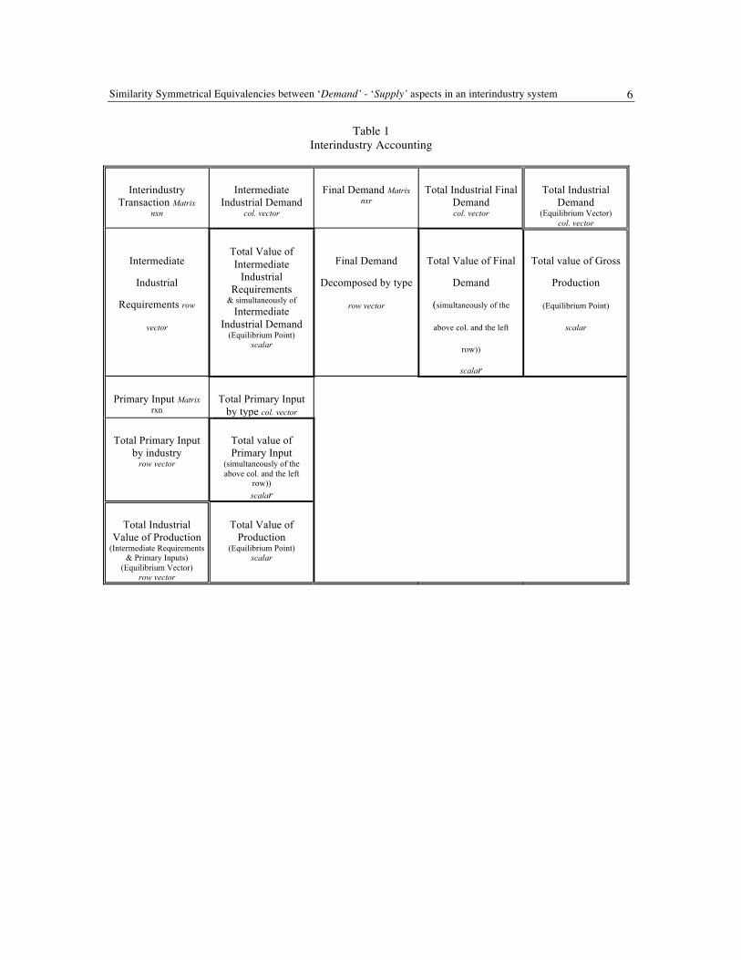
The concepts of interindustry accounting are presented in Table 1.1, their mathematical formulation in Table 1.3, and a numerical example16 in Table 1.2. The value of industrial demand is the summation of the row elements of the transaction matrix xio and the cost of the intermediate inputs of an industry is x
ojT.
The cost of the intermediate inputs is not equal to the value of the intermediate demand, i.e. xio ≠ xoj
T. The summation of all elements of the transaction matrix x
oo indicates the total value of intermediate input being
equal to the total value of intermediate output, the equilibrium of the aggregate intermediate demand to the aggregate intermediate supply. The Yi,j=1,...,r := [ y
C yG yI yS yX yM ] final demand (net output) is where the sum of row elements yields to total sectoral final demand yi. and the summation of the column
elements y.r := iTY the aggregate decomposition of the GNP as C+G+I+X+M. The total value of aggregate demand can be decomposed in terms of industrial (rows) and origin (columns). The primary input matrix Hi=1,..s, j provides the value of primary input per industry h.j
T and hs. the value of the decomposed output. The sum of all elements is the total value of the supply factors h.. . A column vector i
indicates a vector of 1's as i = [1, 1, ... , 1]T.
Theoretically, we may define another area of the interindustry flows representing the connection between final demand and primary input outside of the interindustry purchases.17 I do not use that alternative for the sake of simplicity, although, I believe it is preferable because it is complete conceptually permitting
13 It is clearly that interindustry analysis is a production oriented approach as Christ presented, and not just a technical distinction between
endogenous and exogenous sectors, as Sigel proposed, and Copeland M. A. in his comparative comment emphasized. See NBER (1955) Input-Output Analysis, An appraisal. Studies in Income and Wealth., Vol. 18, Princeton University Press, p. 286. The term endogenous sector is equivalent to processing sector, and the term exogenous sector is equivalent to final demand or primary input sector.
14 Imports may be used as inputs in the production process, and then their proper position is not in the final demand since are not final products but intermediate products. If they are not able to be produced domestically but required in the production process they should be placed below the processing sectors as a row of the primary input. A model with positive import row in primary input matrix or a negative column in final demand matrix provides the same algebraic results, but certainly, the interpretation is different. An import matrix that could allocate imports to their proper destination could provide an explicit information of the affect of imports in the economic structure. Although this would be my preference, I keep imports as part of the final demand following the conventional data.
15 Yan (1969) Introduction to Input-Output Economics, Chapter 1, Holt and Winston, New York for the equivalence between the physical and value approach.
16 As a numerical example I use the one provided by Miller & Blair (1985) pp. 15-18 and 321. The only difference from the above example is that here primary input and final demand are decomposed matrices instead of an aggregate row and column vector as in Miller and Blair.
17 Such date are published by the Planning Bureau of The Netherlands Gecumuleerde Productiestruc-tururmatrices (GPS-matrices) 1969-1985 Centraal Planbureau, Interne Notice, 17 Februari 1989.
XI International Conference on Input-Output Techniques, New Delhi, India, 1995 5
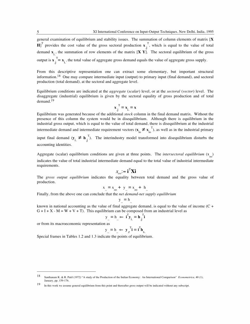
general examination of equilibrium and stability issues. The summation of column elements of matrix [X H]T provides the cost value of the gross sectoral production x.j
T, which is equal to the value of total demand xi., the summation of row elements of the matrix [X Y]. The sectoral equilibrium of the gross
output is x.jT= xi., the total value of aggregate gross demand equals the value of aggregate gross supply.
From this descriptive representation one can extract some elementary, but important structural information.18 One may compare intermediate input (output) to primary input (final demand), and sectoral production (total demand), at the sectoral and aggregate level.
Equilibrium conditions are indicated at the aggregate (scalar) level, or at the sectoral (vector) level. The disaggregate (industrial) equilibrium is given by the sectoral equality of gross production and of total demand.19
x.jT = xi. = x
Equilibrium was generated because of the additional stock column in the final demand matrix. Without the presence of this column the system would be in disequilibrium. Although there is equilibrium in the industrial gross output, which is equal to the value of total demand, there is disequilibrium at the industrial intermediate demand and intermediate requirement vectors (xio ≠ xio
T), as well as in the industrial primary
input final demand (yi. ≠ h.jT). The interindustry model transformed into disequilibrium disturbs the
accounting identities.
Aggregate (scalar) equilibrium conditions are given at three points. The intersectoral equilibrium (xoo
) indicates the value of total industrial intermediate demand equal to the total value of industrial intermediate requirements.
The gross output equilibrium indicates the equality between total demand and the gross value of production.
x.. = xoo
+ y.. = xoo
+ h.. Finally, from the above one can conclude that the net demand-net supply equilibrium
y.. = h.. known in national accounting as the value of final aggregate demand, is equal to the value of income (C + G + I + X - M = W + V + T). This equilibrium can be composed from an industrial level as
y.. = h.. ⇐ iTyi. = h.jTi
or from its macroeconomic representation as y.. = h.. ⇐ y.r
Ti = iThs. Special frames in Tables 1.2 and 1.3 indicate the points of equilibrium.
18 Santhanam K. & R. Patil (1972) “A study of the Production of the Indian Economy: An International Comparison” Econometrica, 40 (1),
January, pp. 159-176. 19 In this work we assume general equilibrium from this point and thereafter gross output will be indicated without any subscript.
xoo:= iΤXi
Similarity Symmetrical Equivalencies between ‘Demand’ - ‘Supply’ aspects in an interindustry system 6
Table 1 Interindustry Accounting
Interindustry Transaction Matrix
nxn Intermediate
Industrial Demand col. vector
Final Demand Matrix nxr
Total Industrial Final Demand col. vector
Total Industrial Demand
(Equilibrium Vector) col. vector
Intermediate
Industrial
Requirements row
vector
Total Value of Intermediate
Industrial Requirements
& simultaneously of Intermediate
Industrial Demand (Equilibrium Point)
scalar
Final Demand
Decomposed by type
row vector
Total Value of Final
Demand
(simultaneously of the
above col. and the left
row))
scalar
Total value of Gross
Production
(Equilibrium Point)
scalar
Primary Input Matrix rxn
Total Primary Input by type col. vector
Total Primary Input by industry
row vector Total value of Primary Input
(simultaneously of the above col. and the left
row)) scalar
Total Industrial Value of Production
(Intermediate Requirements & Primary Inputs)
(Equilibrium Vector) row vector
Total Value of Production
(Equilibrium Point) scalar
XI International Conference on Input-Output Techniques, New Delhi, India, 1995 7
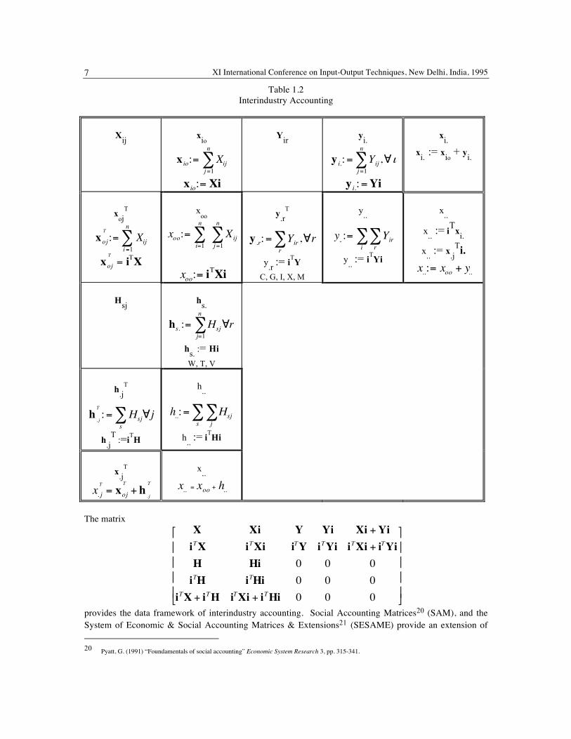
Table 1.2 Interindustry Accounting
Xij xio
Yir yi.
xi. xi. := xio + yi.
xoj
T
xoo
y.rT
y.r := iTY C, G, I, X, M
y..
y.. := iTYi
x.. x.. := iTxi.
x.. := x.jTi.
Hsj
hs.
hs. := Hi W, T, V
h.jT
h.jT :=iTH
h..
h.. := iTHi
x.jT
x..
The matrix
provides the data framework of interindustry accounting. Social Accounting Matrices20 (SAM), and the System of Economic & Social Accounting Matrices & Extensions21 (SESAME) provide an extension of 20 Pyatt, G. (1991) “Foundamentals of social accounting” Economic System Research 3, pp. 315-341.
x io:= Xijj=1
n
∑xio:= Xi
y i.:= Yijj=1
n
∑ ,∀ι
y i.:=Yi
x ojT
:= Xiji=1
n
∑xoj
T
= iΤX
xoo:=i=1
n
∑ Xijj=1
n
∑
xoo:= iΤXi
y .r:= Yirr∑ ,∀r y.. := Yir
r∑
i∑
x..:= xoo + y..
hs. := Hsjj=1
n
∑ ∀r
h. j
T
:= Hsjs∑ ∀j h..:= Hsj
j∑
s∑
x. jT= xoj
T
+ h. j
T x.. = xoo + h..
X Xi Y Yi Xi +YiiTX iTXi iTY iTYi iTXi + iTYiH Hi 0 0 0iTH iTHi 0 0 0
iTX + iTH iTXi + iTHi 0 0 0
⎡
⎣
⎢ ⎢ ⎢ ⎢
⎤
⎦
⎥ ⎥ ⎥ ⎥
Similarity Symmetrical Equivalencies between ‘Demand’ - ‘Supply’ aspects in an interindustry system 8
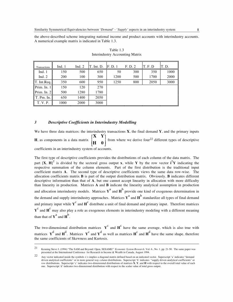
the above-described scheme integrating national income and product accounts with interindustry accounts. A numerical example matrix is indicated in Table 1.3.
Table 1.3 Interindustry Accounting Matrix
Transactions Ind. 1 Ind. 2 T. Int. D. F. D. 1 F. D. 2 T. F. D T. D. Ind. 1 150 500 650 50 300 350 1000 Ind. 2 200 100 300 1200 500 1700 2000
T. Int.Req. 350 600 950 1250 800 2050 3000 Prim. In. 1 150 120 270 Prim. In. 2 500 1280 1780 T. Pm. In. 650 1400 2050 T. V. P. 1000 2000 3000
3 Descriptive Coefficients in Interindustry Modelling
We have three data matrices: the interindustry transactions X, the final demand Y, and the primary inputs
H, as components in a data matrix from where we derive four22 different types of descriptive
coefficients in an interindustry system of accounts.
The first type of descriptive coefficients provides the distributions of each column of the data matrix. The part [X, H]T is divided by the sectoral gross output x, while Y by the row vector iTY indicating the respective summation of the column elements. Part of the first distribution is the traditional input coefficient matrix A. The second type of descriptive coefficients views the same data row-wise. The allocation coefficients matrix B is part of the output distribution matrix. Obviously, B indicates different descriptive information than that of A, but one cannot accept linearity in allocation with more difficulty than linearity in production. Matrices A and B indicate the linearity analytical assumption in production and allocation interindustry models. Matrices Ya and Hb provide one kind of exogenous determination in
the demand and supply interindustry approaches. Matrices Ya and Hb standardize all types of final demand and primary input while Yc and Hc distribute a unit of final demand and primary input. Therefore matrices Yc and Hc may also play a role as exogenous elements in interindustry modeling with a different meaning
than that of Ya and Hb.
The two-dimensional distribution matrices Yc and Hc have the same average, which is also true with matrices Yd and Hd. Matrices Yc and Yd as well as matrices Hc and Hd have the same shape, therefore the same coefficients of Skewness and Kurtosis. 21 Keuning Steve J. (1994) “The SAM and Beyond: Open, SESAME!” Economic System Research, Vol. 6., No. 1, pp. 21-50. The same paper was
presented at the International Conference for Research in Income & Wealth in Canada, August 1994. 22 Any vector indicated inside the symbols < > implies a diagonal matrix defined based on an indicated vector. Superscript ‘a’ indicates “demand
driven analytical coefficients” or in more general way column distributions. Superscript ‘b’ indicates “supply driven analytical coefficients” or row distributions. Superscript ‘c’ indicates two-dimensional distributions of matrices X, Y, and H with respect to the overall total value of each one. Superscript ‘d’ indicates two-dimensional distribution with respect to the scalar value of total gross output.
X YH 0⎡
⎣ ⎢ ⎤
⎦ ⎥
XI International Conference on Input-Output Techniques, New Delhi, India, 1995 9
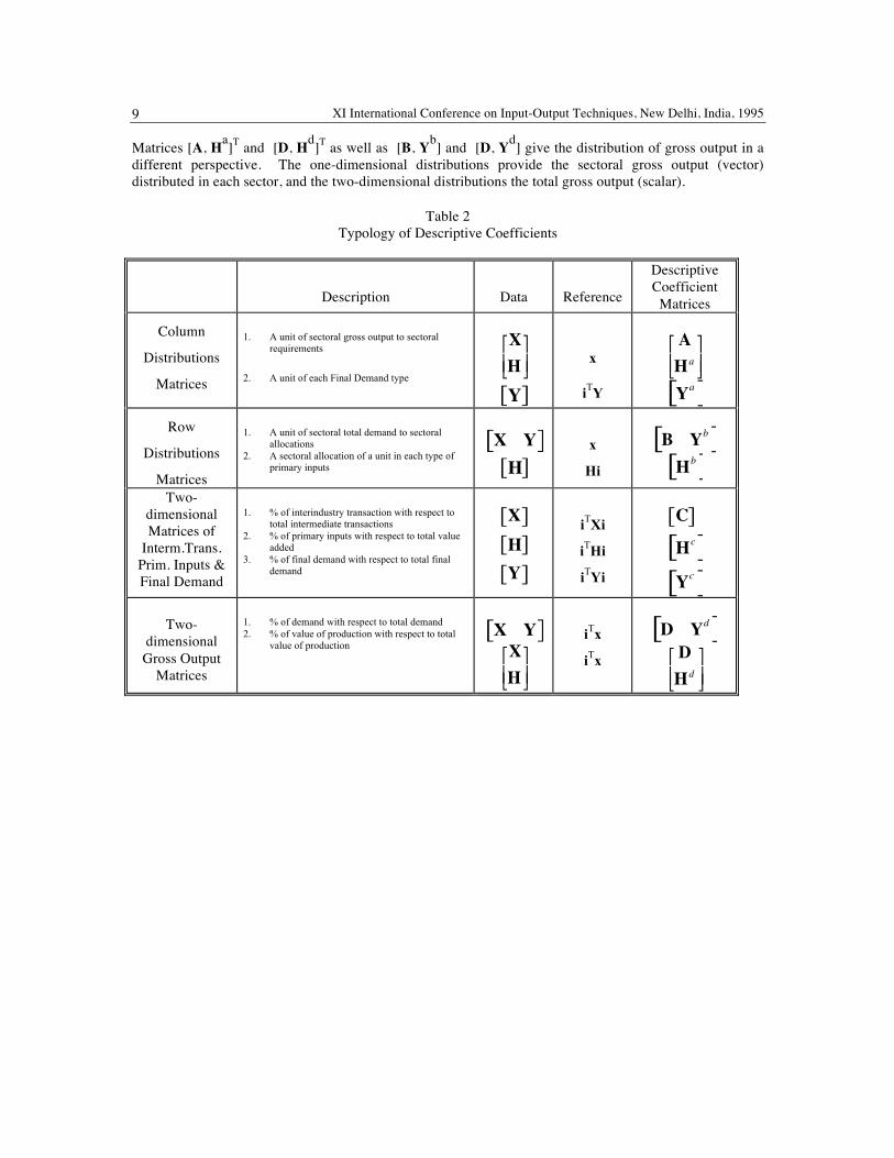
Matrices [A, Ha]T and [D, Hd]T as well as [B, Yb] and [D, Yd] give the distribution of gross output in a different perspective. The one-dimensional distributions provide the sectoral gross output (vector) distributed in each sector, and the two-dimensional distributions the total gross output (scalar).
Table 2 Typology of Descriptive Coefficients
Description Data Reference
Descriptive Coefficient
Matrices
Column
Distributions
Matrices
1. A unit of sectoral gross output to sectoral requirements
2. A unit of each Final Demand type
x
iTY
Row
Distributions
Matrices
1. A unit of sectoral total demand to sectoral allocations
2. A sectoral allocation of a unit in each type of primary inputs
x
Hi
Two-dimensional Matrices of
Interm.Trans. Prim. Inputs & Final Demand
1. % of interindustry transaction with respect to total intermediate transactions
2. % of primary inputs with respect to total value added
3. % of final demand with respect to total final demand
iTXi
iTHi
iTYi
Two-dimensional Gross Output
Matrices
1. % of demand with respect to total demand 2. % of value of production with respect to total
value of production
iTx
iTx
XH⎡
⎣ ⎢ ⎤
⎦ ⎥
Y[ ]
AHa⎡
⎣ ⎢ ⎤
⎦ ⎥
Ya[ ]
X Y[ ]H[ ]
B Yb[ ]Hb[ ]
X[ ]H[ ]Y[ ]
C[ ]
Hc[ ]Yc[ ]
X Y[ ]XH⎡
⎣ ⎢ ⎤
⎦ ⎥
D Yd[ ]DHd⎡
⎣ ⎢ ⎤
⎦ ⎥

Similarity Symmetrical Equivalencies between ‘Demand’ - ‘Supply’ aspects in an interindustry system 10
3.1 Column distributions matrices
Column distributions23 show the requirements of total sectoral production unit and the sectoral
distributions in final demand [Ya]. The traditional input coefficient matrix A indicates linearity in the production model. Explicit knowledge of A and x implies knowledge of primary inputs.
The matrix Ha reveals the share of primary input to total production. The summation of column elements of the input coefficients and the share of primary input to total value of production equals to one.24
The summation of the column elements of matrix Ya yields one.25
Descriptive coefficients of the traditional demand driven model are derived whenever we post multiply the interindustry accounting matrix by the inverse diagonal of the value of total production and final demand.
In a more general form we have the following matrix:26
23
24 iT[A, Ha ] = iTX<x>-1 + iT H<x>-1 = (iT X + iT H)<x>-1 =
= (xT I)<x>-1 = <xT ><x>-1 = I
25 iTYa = iTY<iTy>-1= I 26 The second & fourth column of the general matrix is NOT the summation of the rows of the first & third columns. Their numerical results are
calculated from the original data.
AHa⎡
⎣ ⎢ ⎤
⎦ ⎥
Aiji∑ + Hsj
a
s∑ = 1∀j
Yira
i∑ = 1∀r
X YH 0⎡
⎣ ⎢ ⎤
⎦ ⎥ < x >−1 00 < iTy> −1
⎡
⎣ ⎢ ⎤
⎦ ⎥ =A Y a
Ha 0⎡
⎣ ⎢ ⎤
⎦ ⎥
A =
X11
x1LX1n
xnM O MXn1
x1L
Xnn
xn
⎡
⎣
⎢ ⎢ ⎢ ⎢ ⎢ ⎢ ⎢ ⎢
⎤
⎦
⎥ ⎥ ⎥ ⎥ ⎥ ⎥ ⎥ ⎥
Ha =H < x > −1=
T1x1
L Tnxn
W1
x1L Wn
xnV1x1
L Vn
xn
⎡
⎣
⎢ ⎢ ⎢ ⎢
⎤
⎦
⎥ ⎥ ⎥ ⎥
Y a = Y < iTy >−1=
Yc1YcMYcnYc
Yg1Yg
L Ym1
YmM O MYgnYg
L YmnYm
⎡
⎣
⎢ ⎢ ⎢ ⎢
⎤
⎦
⎥ ⎥ ⎥ ⎥
XI International Conference on Input-Output Techniques, New Delhi, India, 1995 11
.
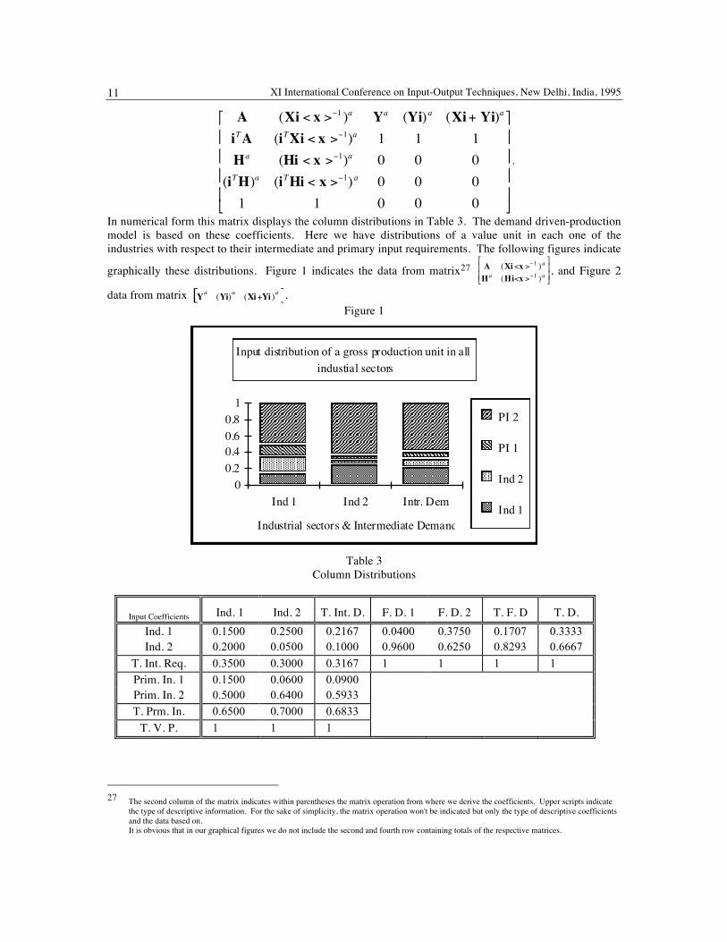
In numerical form this matrix displays the column distributions in Table 3. The demand driven-production model is based on these coefficients. Here we have distributions of a value unit in each one of the industries with respect to their intermediate and primary input requirements. The following figures indicate
graphically these distributions. Figure 1 indicates the data from matrix27 , and Figure 2
data from matrix . Figure 1
Table 3
Column Distributions
Input Coefficients Ind. 1 Ind. 2 T. Int. D. F. D. 1 F. D. 2 T. F. D T. D. Ind. 1 0.1500 0.2500 0.2167 0.0400 0.3750 0.1707 0.3333 Ind. 2 0.2000 0.0500 0.1000 0.9600 0.6250 0.8293 0.6667
T. Int. Req. 0.3500 0.3000 0.3167 1 1 1 1 Prim. In. 1 0.1500 0.0600 0.0900 Prim. In. 2 0.5000 0.6400 0.5933 T. Prm. In. 0.6500 0.7000 0.6833
T. V. P. 1 1 1
27 The second column of the matrix indicates within parentheses the matrix operation from where we derive the coefficients. Upper scripts indicate
the type of descriptive information. For the sake of simplicity, the matrix operation won't be indicated but only the type of descriptive coefficients and the data based on. It is obvious that in our graphical figures we do not include the second and fourth row containing totals of the respective matrices.
A (Xi < x >−1 )a Ya (Yi)a (Xi+ Yi)a
iTA (iTXi < x >−1)a 1 1 1Ha (Hi < x >−1)a 0 0 0
(iTH)a (iTHi < x >−1)a 0 0 01 1 0 0 0
⎡
⎣
⎢ ⎢ ⎢ ⎢
⎤
⎦
⎥ ⎥ ⎥ ⎥
A (Xi<x >−1 )a
Ha (Hi<x >−1 )a
⎡
⎣
⎢ ⎢
⎤
⎦
⎥ ⎥
Ya (Yi)a (Xi+Yi )a[ ]
Input distribution of a gross production unit in allindustial sectors
Industrial sectors & Intermediate Demand
Inpu
t Disr
ibut
ion
00.20.40.60.8
1
Ind 1 Ind 2 Intr. Dem
PI 2
PI 1
Ind 2
Ind 1
Similarity Symmetrical Equivalencies between ‘Demand’ - ‘Supply’ aspects in an interindustry system 12
Figure 1 illustrates the requirement distributions in each industry in terms of a produced value unit. All industries are standardized in terms of their production value.
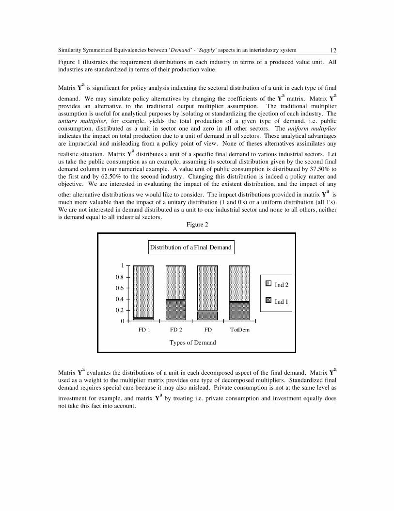
Matrix Ya is significant for policy analysis indicating the sectoral distribution of a unit in each type of final
demand. We may simulate policy alternatives by changing the coefficients of the Ya matrix. Matrix Ya provides an alternative to the traditional output multiplier assumption. The traditional multiplier assumption is useful for analytical purposes by isolating or standardizing the ejection of each industry. The unitary multiplier, for example, yields the total production of a given type of demand, i.e. public consumption, distributed as a unit in sector one and zero in all other sectors. The uniform multiplier indicates the impact on total production due to a unit of demand in all sectors. These analytical advantages are impractical and misleading from a policy point of view. None of theses alternatives assimilates any realistic situation. Matrix Ya distributes a unit of a specific final demand to various industrial sectors. Let us take the public consumption as an example, assuming its sectoral distribution given by the second final demand column in our numerical example. A value unit of public consumption is distributed by 37.50% to the first and by 62.50% to the second industry. Changing this distribution is indeed a policy matter and objective. We are interested in evaluating the impact of the existent distribution, and the impact of any other alternative distributions we would like to consider. The impact distributions provided in matrix Ya is much more valuable than the impact of a unitary distribution (1 and 0's) or a uniform distribution (all 1's). We are not interested in demand distributed as a unit to one industrial sector and none to all others, neither is demand equal to all industrial sectors.
Figure 2
Matrix Ya evaluates the distributions of a unit in each decomposed aspect of the final demand. Matrix Ya used as a weight to the multiplier matrix provides one type of decomposed multipliers. Standardized final demand requires special care because it may also mislead. Private consumption is not at the same level as investment for example, and matrix Ya by treating i.e. private consumption and investment equally does not take this fact into account.
Distribution of a Final Demand
Types of Demand
Fina
l Dem
and
Dist
ribut
ion
0
0.2
0.4
0.6
0.8
1
FD 1 FD 2 FD TotDem
Ind 2
Ind 1
XI International Conference on Input-Output Techniques, New Delhi, India, 1995 13
3.2 Row distributions matrices28
Row distributions matrices provide descriptive information of a sectoral total demand unit for industries by
matrix [B, Yb] and by matrix Hb the industrial distributions of a unit in each type of primary input. The analytical assumption of the allocation model (linearity in allocation) is given by matrix B. The matrix of the final demand share to total demand is given by Yb. The matrix of sectoral distributions in primary
inputs, given by Hb is useful for policy evaluations in an analogous way to matrix Ya, since its coefficients reflect the sectoral composition of a unit in a specific type of primary inputs.
The summation of the row elements in matrix [B, Yb] equals one for all i rows.29
The summation of the row elements in matrix Hb is one for all s rows.30
The same data matrix premultiplied by the diagonal inverse matrix of the row summations
provides the allocation coefficients.
Transactions are presented either as required input for all interdependent processing sectors and primary input rows, or as an allocated output between the processing sectors and final demand. Table 4, the respective matrix and Figures 3 & 4 give numerical, mathematical and graphical information of the allocation descriptive coefficients. The distribution of a unit of total demand to intermediate and final demand given in Figure 3 is the analytical assumption of the allocation model. It is obvious that the main
28
29 [B, Yb ]i = Bi + Ybi = <x>-1Xi +<x>-1Yi = <x>-1(Xi + Yi) = <x>-1I<x> =
= <x>-1<x> = I
30 Hbi = <Hi>-1Hi= I.
Bijj∑ + Yir
b
r∑ = 1∀i
Hsjb
j∑ = 1∀s
X YH 0⎡
⎣ ⎢ ⎤
⎦ ⎥
< x >−1 00 < hi >−1
⎡
⎣ ⎢ ⎤
⎦ ⎥ X YH 0⎡
⎣ ⎢ ⎤
⎦ ⎥ =B Yb
Hb 0⎡
⎣ ⎢ ⎤
⎦ ⎥
B =
X11
x1LX1n
x1M O MXn1
xnLXnn
xn
⎡
⎣
⎢ ⎢ ⎢ ⎢ ⎢ ⎢ ⎢ ⎢
⎤
⎦
⎥ ⎥ ⎥ ⎥ ⎥ ⎥ ⎥ ⎥
Yb =< x >−1 Y =
Yc1x1MYcnxn
Yg1x1
L Ym1x1
M O MYgn
xnL Ymn
xn
⎡
⎣
⎢ ⎢ ⎢
⎤
⎦
⎥ ⎥ ⎥
Hb =<Hi >−1 H =
T1T j
L TnT j
W1
Wj
L Wn
WjV1V j
L Vn
V j
⎡
⎣
⎢ ⎢ ⎢ ⎢ ⎢
⎤
⎦
⎥ ⎥ ⎥ ⎥ ⎥
Similarity Symmetrical Equivalencies between ‘Demand’ - ‘Supply’ aspects in an interindustry system 14
diagonal elements in both matrices A and B are the same. Deman shows that for every non-main diagonal
element of the matrices A and B the relationship exist.31 These two points yield to the fact
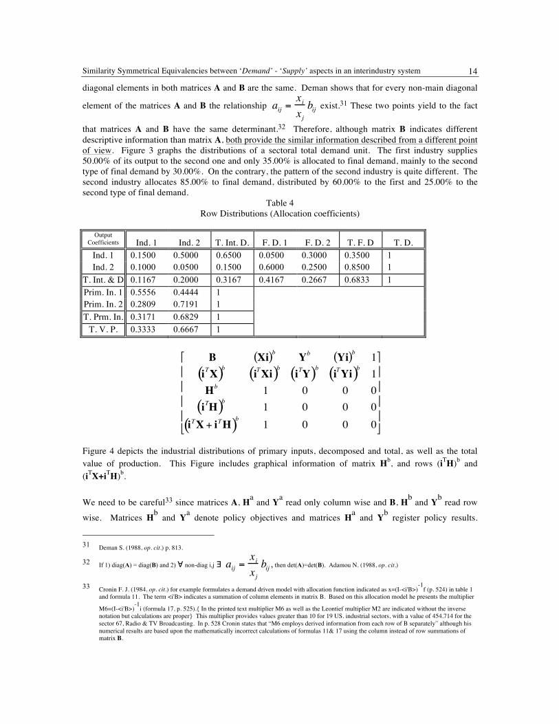
that matrices A and B have the same determinant.32 Therefore, although matrix B indicates different descriptive information than matrix A, both provide the similar information described from a different point of view. Figure 3 graphs the distributions of a sectoral total demand unit. The first industry supplies 50.00% of its output to the second one and only 35.00% is allocated to final demand, mainly to the second type of final demand by 30.00%. On the contrary, the pattern of the second industry is quite different. The second industry allocates 85.00% to final demand, distributed by 60.00% to the first and 25.00% to the second type of final demand.
Table 4 Row Distributions (Allocation coefficients)
Output
Coefficients Ind. 1 Ind. 2 T. Int. D. F. D. 1 F. D. 2 T. F. D T. D. Ind. 1 0.1500 0.5000 0.6500 0.0500 0.3000 0.3500 1 Ind. 2 0.1000 0.0500 0.1500 0.6000 0.2500 0.8500 1
T. Int. & D 0.1167 0.2000 0.3167 0.4167 0.2667 0.6833 1 Prim. In. 1 0.5556 0.4444 1 Prim. In. 2 0.2809 0.7191 1 T. Prm. In. 0.3171 0.6829 1
T. V. P. 0.3333 0.6667 1
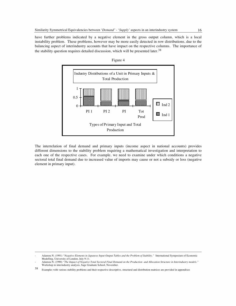
Figure 4 depicts the industrial distributions of primary inputs, decomposed and total, as well as the total value of production. This Figure includes graphical information of matrix Hb, and rows (iTH)b and (iTX+iTH)b.
We need to be careful33 since matrices A, Ha and Ya read only column wise and B, Hb and Yb read row
wise. Matrices Hb and Ya denote policy objectives and matrices Ha and Yb register policy results.
31 Deman S. (1988, op. cit.) p. 813.
32 If 1) diag(A) = diag(B) and 2) ∀ non-diag i,j ∃ , then det(A)=det(B). Adamou N. (1988, op. cit.)
33 Cronin F. J. (1984, op. cit.) for example formulates a demand driven model with allocation function indicated as x=(I-<i'B>)-1
f (p. 524) in table 1 and formula 11. The term <i'B> indicates a summation of column elements in matrix B. Based on this allocation model he presents the multiplier
M6=(I-<i'B>)-1
i (formula 17, p. 525).{ In the printed text multiplier M6 as well as the Leontief multiplier M2 are indicated without the inverse notation but calculations are proper} This multiplier provides values greater than 10 for 19 US. industrial sectors, with a value of 454.714 for the sector 67, Radio & TV Broadcasting. In p. 528 Cronin states that “M6 employs derived information from each row of B separately” although his numerical results are based upon the mathematically incorrect calculations of formulas 11& 17 using the column instead of row summations of matrix B.
aij =xixjbij
B Xi( )b Yb Yi( )b 1iTX( )b iTXi( )b iTY( )b iTYi( )b 1Hb 1 0 0 0iTH( )b 1 0 0 0
iTX + iTH( )b 1 0 0 0
⎡
⎣
⎢ ⎢ ⎢ ⎢
⎤
⎦
⎥ ⎥ ⎥ ⎥
aij =xixjbij

XI International Conference on Input-Output Techniques, New Delhi, India, 1995 15
Matrices Ya and Hb provide the distributions causing production. Matrices, or specific columns and rows respectively of Ya and Hb can be used in policy simulations. Given sectoral distributions in public expenditures and taxes, one can evaluate the sectoral gross output multiplier of a balanced budget.34 Having the sectoral distribution in investment and wages one can explore their feedback.35 One can examine the different impact of imports and exports on gross output.36
Figure 3
The negative column of imports effects the row summation of the final demand matrix and the sectoral value of gross output. It is not unusual to observe negative total final demand due to larger demand for imports than the domestic demand of domestic products in a given industry. A negative element of total final demand indicates a local stability problem.37 If imports are greater than domestic production then we
- Oosterhaven (1988, op. cit.,) in his footnote 3 (p. 208) presents correctly the demand-constrained Ghoshian model as x=(I-<Bi>)
-1v, and
criticizing the nature (diagonal matrix does not provide interrelations) of the demand constrained Ghoshian model properly concludes that this models as well as the supply-constrained Leontief model are not too useful.
- Adamou N. (1991) “Clarifying Analytical Assumptions in Inter-industry Modelling” Workshop in interindustry economics, Sage Graduate School, Troy, NY, August.
34 Adamou N. (1992) “Inter-Industry Structure in New York State and its implication for fiscal policy, with a particular emphasis on taxes.” New York State Tax Study Legislative Commission, April.
- Adamou, N. (1991) “Fiscal Policy , Foreign Trade and Industrial Structure in Japan: 1960-1985.” Ways & Means Committee of the New York State Assembly, December.
- Adamou N. (1989) “Interindustry Analysis and Budgeting Process .” Ways & Means Committee of the New York State Assembly, November. 35 Adamou N. (1990) “Capital and Labor Feedback Structures in an Extended Input-Output System: A Comparison of the United States and Japan.”
International Symposium on Economic Modelling, University of Urbino, Italy, July 23-25. 36 Adamou, N. (1991) “Industrial Impact of Imports and Exports in Japan: 1960-1985.” International Conference of the International Trade &
Finance Association, May 31-June 2, Marseilles, France. 37 Stability in terms of aij and bij requires the coefficients to be less than one and positive. This implies that the vectors of total final demand and
total primary input are positive or non negative. - Takayama, A. (1987) Mathematical Economics, 2nd ed., Cambridge U. Press, p. 360 ( - the existence problem ) assumes positive final demand. If
there is a negative element in the total final demand vector due to a great value of imports, then the respective sum of bij row is greater than one. Cronin (1984, op. cit., p. 524, footnote 3) comments that the demand driven output multiplier is negative ( ∂xi/∂fi<0 ). Cronin also assesses that in the case the industrial output is allocated completely into processing sectors and not at all to the final demand, i.e. the sum of bij coefficient of the respective row is one, then the demand driven output multiplier( ∂xi/∂fi ) is undefined. We may also face the opposite case, an industrial sector allocating all its output to final demand (shoes). In this case the sum of the respective interindustry allocation coefficient row is zero, and the matrix does not have full rank. Very rarely a negative element may appear in a transaction table as those reported for the 1960, 1965 & 1970 Japanese I-O tables. See:
- Uno, K. (1989) Measurement of Services in an Input-Output Framework, Amsterdam, North-Holland. Such cases were examined by
Distribution of a unit of Total Demand
Industries
Dis
tribu
tion
0
0.20.4
0.60.8
1
Ind 1 Ind 2 T_Dem
FD 2
FD 1
Ind 2
Ind 1
Similarity Symmetrical Equivalencies between ‘Demand’ - ‘Supply’ aspects in an interindustry system 16
have further problems indicated by a negative element in the gross output column, which is a local instability problem. These problems, however may be more easily detected in row distributions, due to the balancing aspect of interindustry accounts that have impact on the respective columns. The importance of the stability question requires detailed discussion, which will be presented later.38
Figure 4
The interrelation of final demand and primary inputs (income aspect in national accounts) provides different dimensions to the stability problem requiring a mathematical investigation and interpretation to each one of the respective cases. For example, we need to examine under which conditions a negative sectoral total final demand due to increased value of imports may cause or not a subsidy or loss (negative element in primary input).
- Adamou N. (1991) “Negative Elements in Japanese Input-Output Tables and the Problem of Stability.” International Symposium of Economic
Modelling, University of London, July 9-11. - Adamou N. (1990) “The Impact of Negative Total Sectoral Final Demand on the Production and Allocation Structure in Interindustry models.”
Workshop in interindustry analysis, Sage Graduate School, November. 38 Examples with various stability problems and their respective descriptive, structural and distribution matrices are provided in appendixes
Industry Distributions of a Unit in Primary Inputs &Total Production
Types of Primary Input and TotalProduction
Dis
tribu
tion
0
0.5
1
PI 1 PI 2 PI TotProd
Ind 2
Ind 1
XI International Conference on Input-Output Techniques, New Delhi, India, 1995 17
3.3 Two-dimension distribution matrices of Intermediate Transactions, Final Demand and Primary Inputs
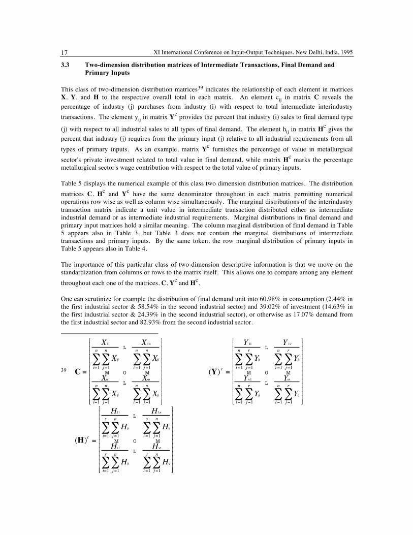
This class of two-dimension distribution matrices39 indicates the relationship of each element in matrices X, Y, and H to the respective overall total in each matrix. An element cij in matrix C reveals the percentage of industry (j) purchases from industry (i) with respect to total intermediate interindustry transactions. The element yij in matrix Yc provides the percent that industry (i) sales to final demand type
(j) with respect to all industrial sales to all types of final demand. The element hij in matrix Hc gives the percent that industry (j) requires from the primary input (j) relative to all industrial requirements from all types of primary inputs. As an example, matrix Yc furnishes the percentage of value in metallurgical sector's private investment related to total value in final demand, while matrix Hc marks the percentage metallurgical sector's wage contribution with respect to the total value of primary inputs.
Table 5 displays the numerical example of this class two dimension distribution matrices. The distribution matrices C, Hc and Yc have the same denominator throughout in each matrix permitting numerical operations row wise as well as column wise simultaneously. The marginal distributions of the interindustry transaction matrix indicate a unit value in intermediate transaction distributed either as intermediate industrial demand or as intermediate industrial requirements. Marginal distributions in final demand and primary input matrices hold a similar meaning. The column marginal distribution of final demand in Table 5 appears also in Table 3, but Table 3 does not contain the marginal distributions of intermediate transactions and primary inputs. By the same token, the row marginal distribution of primary inputs in Table 5 appears also in Table 4.
The importance of this particular class of two-dimension descriptive information is that we move on the standardization from columns or rows to the matrix itself. This allows one to compare among any element throughout each one of the matrices, C, Yc and Hc.
One can scrutinize for example the distribution of final demand unit into 60.98% in consumption (2.44% in the first industrial sector & 58.54% in the second industrial sector) and 39.02% of investment (14.63% in the first industrial sector & 24.39% in the second industrial sector), or otherwise as 17.07% demand from the first industrial sector and 82.93% from the second industrial sector.
39
C =
X11
Xij
j=1
n
∑i=1
n
∑L
X1n
Xij
j=1
n
∑i=1
n
∑M O MXn1
Xij
j=1
n
∑i=1
n
∑L
Xnn
Xij
j=1
n
∑i=1
n
∑
⎡
⎣
⎢ ⎢ ⎢ ⎢ ⎢ ⎢ ⎢ ⎢ ⎢ ⎢ ⎢ ⎢ ⎢ ⎢ ⎢
⎤
⎦
⎥ ⎥ ⎥ ⎥ ⎥ ⎥ ⎥ ⎥ ⎥ ⎥ ⎥ ⎥ ⎥ ⎥ ⎥
(Y) c =
Y 11
Yij
j=1
r
∑i=1
n
∑L
Y 1r
Yij
j=1
r
∑i=1
n
∑M O MYn1
Yij
j=1
r
∑i=1
n
∑L
Ynr
Yij
j=1
r
∑i=1
n
∑
⎡
⎣
⎢ ⎢ ⎢ ⎢ ⎢ ⎢ ⎢ ⎢ ⎢ ⎢ ⎢ ⎢ ⎢ ⎢ ⎢
⎤
⎦
⎥ ⎥ ⎥ ⎥ ⎥ ⎥ ⎥ ⎥ ⎥ ⎥ ⎥ ⎥ ⎥ ⎥ ⎥
(H)c =
H11
Hij
j=1
n
∑i=1
s
∑L
H1n
Hij
j=1
n
∑i=1
s
∑M O MHs1
Hij
j=1
n
∑i=1
s
∑L
Hsn
Hij
j=1
n
∑i=1
s
∑
⎡
⎣
⎢ ⎢ ⎢ ⎢ ⎢ ⎢ ⎢ ⎢ ⎢ ⎢ ⎢ ⎢ ⎢ ⎢ ⎢
⎤
⎦
⎥ ⎥ ⎥ ⎥ ⎥ ⎥ ⎥ ⎥ ⎥ ⎥ ⎥ ⎥ ⎥ ⎥ ⎥
Similarity Symmetrical Equivalencies between ‘Demand’ - ‘Supply’ aspects in an interindustry system 18
Similarly, one can categorize the distribution of a unit in primary inputs as 13.17% paid wages (7.32% in the first industrial sector & 5.85% in the second industrial sector) and 86.98% as other value added (24.39% in the first industrial sector & 62.44% in the second industrial sector), that is 31.71% of primary input unit are allocated to the first industrial sector and 68.29% to the second industrial sector.
Table 5 Two-Dimensional Distributions of Intermediate Transactions, Final Demand and Primary Inputs
Ind. 1 Ind. 2 T. F. D. 1 F. D. 2 T. F. D
Ind. 1 0.1579 0.5263 0.6842 0.0244 0.1463 0.1707 Ind. 2 0.2105 0.1053 0.3158 0.5854 0.2439 0.8293
T. 0.3684 0.6316 1 0.6098 0.3902 1 Prim. In. 1 0.0732 0.0585 0.1317 Prim. In. 2 0.2439 0.6244 0.8683
T. 0.3171 0.6829 1
The Table 5 given as a matrix
provides three two-dimensional distribution matrices and the resulting marginal distributions. The matrix
composition of the two-dimensional matrices is . Each one of these matrices is
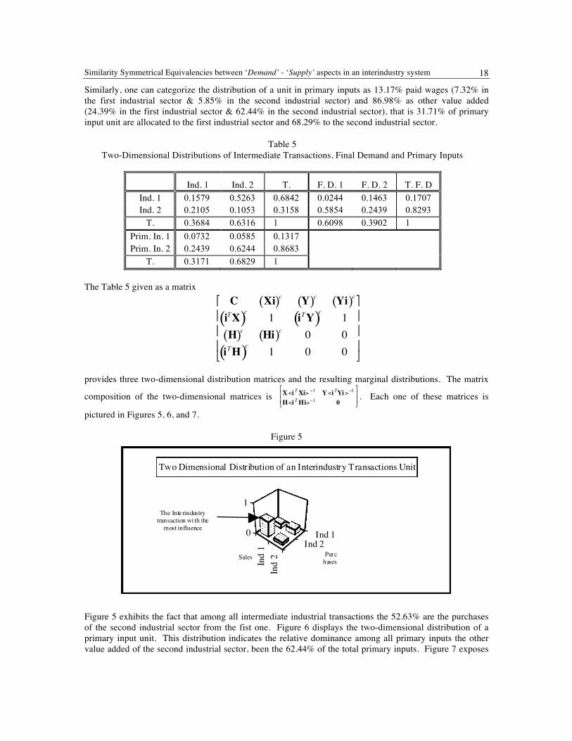
pictured in Figures 5, 6, and 7.
Figure 5
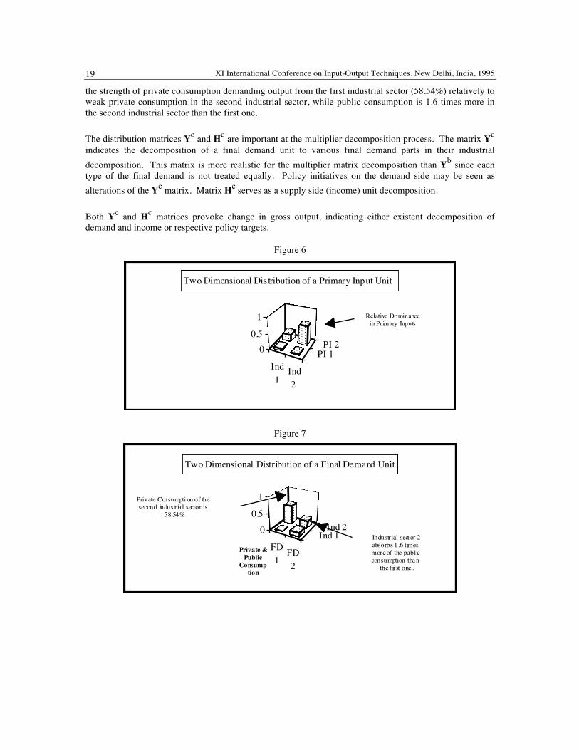
Figure 5 exhibits the fact that among all intermediate industrial transactions the 52.63% are the purchases of the second industrial sector from the fist one. Figure 6 displays the two-dimensional distribution of a primary input unit. This distribution indicates the relative dominance among all primary inputs the other value added of the second industrial sector, been the 62.44% of the total primary inputs. Figure 7 exposes
C Xi( )c Y( )c Yi( )c
iTX( )c 1 iTY( )c 1H( )c Hi( )c 0 0iTH( )c 1 0 0
⎡
⎣
⎢ ⎢ ⎢
⎤
⎦
⎥ ⎥ ⎥
X<i TXi> −1 Y<i TYi> −1
H<i THi>−1 0
⎡
⎣
⎢ ⎢
⎤
⎦
⎥ ⎥
Ind 1Ind 2
PurchasesIn
d 1
Ind
2Sales
0
1
Two Dimensional Distribution of an Interindustry Transactions Unit
The Inte rindustrytransaction wi th the
most influence
XI International Conference on Input-Output Techniques, New Delhi, India, 1995 19
the strength of private consumption demanding output from the first industrial sector (58.54%) relatively to weak private consumption in the second industrial sector, while public consumption is 1.6 times more in the second industrial sector than the first one.
The distribution matrices Yc and Hc are important at the multiplier decomposition process. The matrix Yc indicates the decomposition of a final demand unit to various final demand parts in their industrial decomposition. This matrix is more realistic for the multiplier matrix decomposition than Yb since each type of the final demand is not treated equally. Policy initiatives on the demand side may be seen as alterations of the Yc matrix. Matrix Hc serves as a supply side (income) unit decomposition.
Both Yc and Hc matrices provoke change in gross output, indicating either existent decomposition of demand and income or respective policy targets.
Figure 6
Figure 7
Ind1
Ind2
PI 1PI 20
0.5
1
Two Dimensional Dis tribution of a Primary Input Unit
Relative Dominancein Primary Inputs
FD1
FD2
Private &Public
Consumption
Ind 1Ind 20
0.5
1
Two Dimensional Distribution of a Final Demand Unit
Private Consumpti on of thesecond industria l sector is
58.54%
Industrial sect or 2absorbs 1.6 timesmore of the publicconsumption than
the first one .

Similarity Symmetrical Equivalencies between ‘Demand’ - ‘Supply’ aspects in an interindustry system 20
3.4 Two-dimensional Total Gross Output Distribution Matrices
Two-dimensional total gross output distribution matrices measure all elements of the interindustry accounting as a percentage of the total gross output. Two two-dimensional distribution matrices view the gross output unit as requirement and as demand. Interindustry transactions are a common area to both. Table 6 provides this information.
Table 6 Two-Dimensional Distribution of the Gross Output
Ind. 1 Ind. 2 T. F. D. 1 F. D. 2 T. F. D T. D.
Ind. 1 0.0500 0.1667 0.2167 0.0167 0.1000 0.1167 0.3333 Ind. 2 0.0667 0.0333 0.1000 0.4000 0.1667 0.5667 0.6667
T. Int. Req. 0.1167 0.2000 0.3167 0.4167 0.2667 0.6833 1 Prim. In. 1 0.0500 0.0400 0.0900 Prim. In. 2 0.1667 0.4267 0.5933 T. Prm. In. 0.2167 0.4667 0.6833
T. V. P. 0.3333 0.6667 1
This indicates40 the distribution matrix of the demand side of the gross output [D Yd] and the requirement side of the gross output matrix [D Hd]T. From interpretation point of view matrices D Yd and Hd relate the
40
D =
X11
Xij +j=1
n
∑ Yij
j=1
r
∑i=1
n
∑i=1
n
∑L
X1n
Xij +j=1
n
∑ Yij
j=1
r
∑i=1
n
∑i=1
n
∑M O MXn1
Xij +j=1
n
∑ Yij
j=1
r
∑i=1
n
∑i=1
n
∑L
Xnn
Xij +j=1
n
∑ Yij
j=1
r
∑i=1
n
∑i=1
n
∑
⎡
⎣
⎢ ⎢ ⎢ ⎢ ⎢ ⎢ ⎢ ⎢ ⎢ ⎢ ⎢ ⎢ ⎢ ⎢ ⎢
⎤
⎦
⎥ ⎥ ⎥ ⎥ ⎥ ⎥ ⎥ ⎥ ⎥ ⎥ ⎥ ⎥ ⎥ ⎥ ⎥
(Y)d =
Y11
Xij +j=1
n
∑ Yij
j=1
r
∑i=1
n
∑i=1
n
∑L
Y 1r
Xij +j=1
n
∑ Yij
j=1
r
∑i=1
n
∑i=1
n
∑M O MYn1
Xij +j=1
n
∑ Yij
j=1
r
∑i=1
n
∑i=1
n
∑L
Ynr
Xij +j=1
n
∑ Yij
j=1
r
∑i=1
n
∑i=1
n
∑
⎡
⎣
⎢ ⎢ ⎢ ⎢ ⎢ ⎢ ⎢ ⎢ ⎢ ⎢ ⎢ ⎢ ⎢ ⎢ ⎢
⎤
⎦
⎥ ⎥ ⎥ ⎥ ⎥ ⎥ ⎥ ⎥ ⎥ ⎥ ⎥ ⎥ ⎥ ⎥ ⎥
(H)c =
H 11
Xij +j=1
n
∑i=1
n
∑ Hij
j=1
n
∑i=1
s
∑L
H 1n
Xij +j=1
n
∑i=1
n
∑ Hij
j=1
n
∑i=1
s
∑M O MHs 1
Xij +j=1
n
∑i=1
n
∑ Hij
j=1
n
∑i=1
s
∑L
Hsn
Xij +j=1
n
∑i=1
n
∑ Hij
j=1
n
∑i=1
s
∑
⎡
⎣
⎢ ⎢ ⎢ ⎢ ⎢ ⎢ ⎢ ⎢ ⎢ ⎢ ⎢ ⎢ ⎢ ⎢ ⎢
⎤
⎦
⎥ ⎥ ⎥ ⎥ ⎥ ⎥ ⎥ ⎥ ⎥ ⎥ ⎥ ⎥ ⎥ ⎥ ⎥
XI International Conference on Input-Output Techniques, New Delhi, India, 1995 21
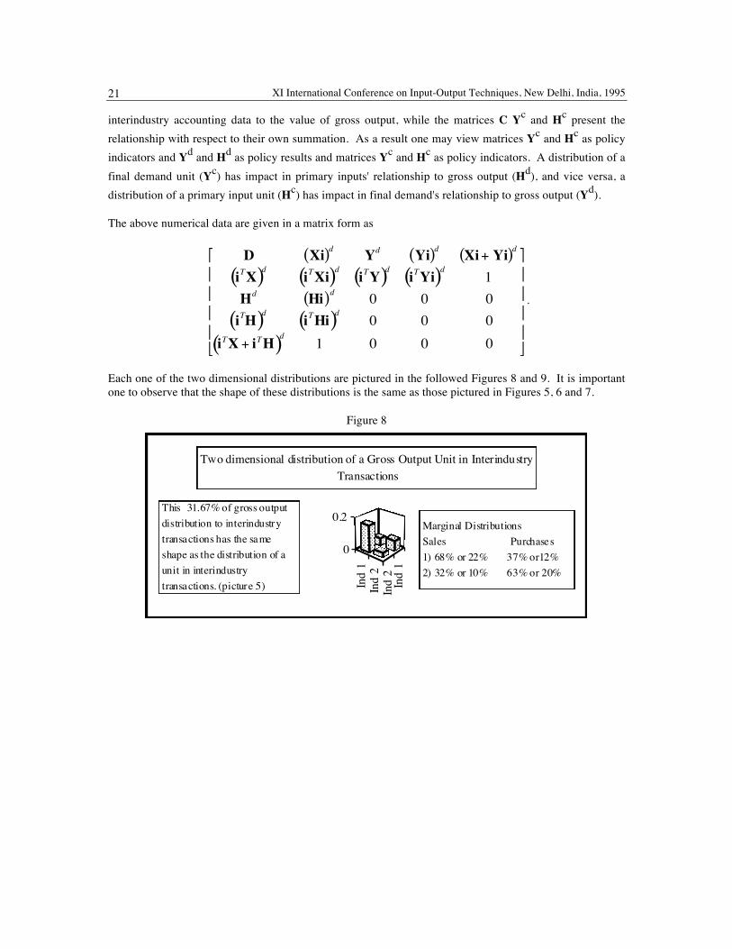
interindustry accounting data to the value of gross output, while the matrices C Yc and Hc present the relationship with respect to their own summation. As a result one may view matrices Yc and Hc as policy indicators and Yd and Hd as policy results and matrices Yc and Hc as policy indicators. A distribution of a final demand unit (Yc) has impact in primary inputs' relationship to gross output (Hd), and vice versa, a distribution of a primary input unit (Hc) has impact in final demand's relationship to gross output (Yd).
The above numerical data are given in a matrix form as
.
Each one of the two dimensional distributions are pictured in the followed Figures 8 and 9. It is important one to observe that the shape of these distributions is the same as those pictured in Figures 5, 6 and 7.
Figure 8
D Xi( )d Yd Yi( )d Xi+ Yi( )d
iTX( )d iTXi( )d iTY( )d iTYi( )d 1Hd Hi( )d 0 0 0iTH( )d iTHi( )d 0 0 0
iTX + iTH( )d 1 0 0 0
⎡
⎣
⎢ ⎢ ⎢ ⎢
⎤
⎦
⎥ ⎥ ⎥ ⎥
Ind
1In
d 2
Ind
1In
d 2
0
0.2
Two dimensional distribution of a Gross Output Unit in InterindustryTransactions
This 31.67% of gross outputdistribution to interindustrytransactions has the sameshape as the distribution of aunit in interindustrytransactions. (picture 5)
Marginal Distributions Sales Purchases 1) 68% or 22% 37% or12% 2) 32% or 10% 63% or 20%
Similarity Symmetrical Equivalencies between ‘Demand’ - ‘Supply’ aspects in an interindustry system 22
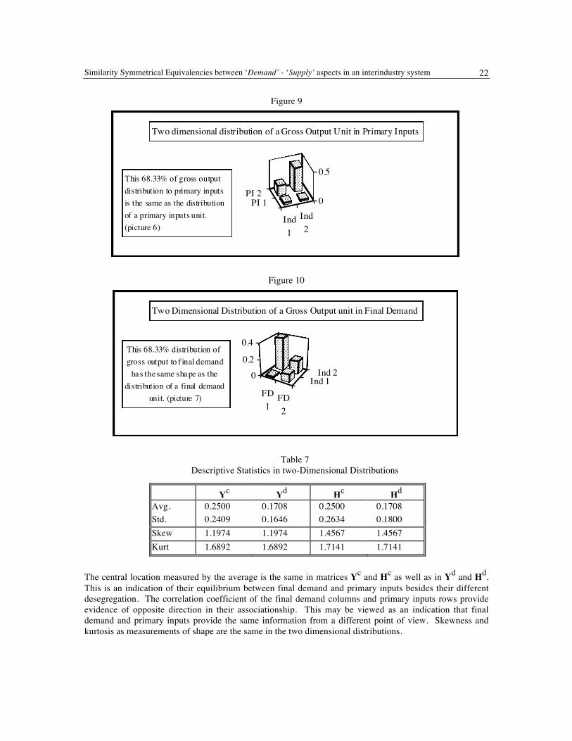
Figure 9
Figure 10
Table 7 Descriptive Statistics in two-Dimensional Distributions
Yc Yd Hc Hd Avg. 0.2500 0.1708 0.2500 0.1708 Std. 0.2409 0.1646 0.2634 0.1800 Skew 1.1974 1.1974 1.4567 1.4567 Kurt 1.6892 1.6892 1.7141 1.7141
The central location measured by the average is the same in matrices Yc and Hc as well as in Yd and Hd. This is an indication of their equilibrium between final demand and primary inputs besides their different desegregation. The correlation coefficient of the final demand columns and primary inputs rows provide evidence of opposite direction in their associationship. This may be viewed as an indication that final demand and primary inputs provide the same information from a different point of view. Skewness and kurtosis as measurements of shape are the same in the two dimensional distributions.
Ind1
Ind2
PI 1PI 2
0
0.5
Two dimensional distribution of a Gross Output Unit in Primary Inputs
This 68.33% of gross outputdistribution to primary inputsis the same as the distributionof a primary inputs unit.(picture 6)
FD1
FD2
Ind 1Ind 20
0.2
0.4
Two Dimensional Distribution of a Gross Output unit in Final Demand
This 68.33% distribution ofgross output to f inal demand
has the same shape as thedistribution of a final demand
unit. (picture 7)
XI International Conference on Input-Output Techniques, New Delhi, India, 1995 23
4 Interindustry Demand & Supply Models and Equivalence transformations
4.1 Same Solution from ‘Demand’ and ‘Supply’ Models
Given demand and production structures the Leontief model provides gross output. The matrix of interindustry transactions X, the vector of final demand y, and a linearity assumption are utilized.41 Linearity is a harsh assumption not easily acceptable even in production, and criticized by Leontief.42
The Leontief system is represented by a) the accounting identity of a sectoral distribution in total demand; b) the analytical assumption of linearity in production, i.e. the value of total demand of an industry is proportional to its production requirements; and c) the model specified by the Leontief inverse matrix. The model means that for a given level and composition of final demand, and with the given technology, we can determine the appropriate level and mix of industrial production. This determination is evaluated by the Leontief inverse, providing explicitly the interrelations among industrial sectors.
x ≡ Xi + Yi A = X<x>-1
x = [I-A]-1Yi = ZYi
The same value of industrial production is determined also by the Ghoshian system.43 Accounting identities present equalities between value of total industrial production and value of total demand in each industrial sector. The accounting identity in a final demand driven44 Leontief model provides the allocation of demanded gross output. The linearity assumption in the input requirements of the same model is linked to the allocation of the total demand. A different point of view presents the primary inputs driven model. The accounting identity in the Ghoshian model presents the production requirements linked to the linearity assumption of interindustry output allocation proportional to gross output. This reveals a clear and obvious symmetry between the two systems. As the Leontief model relates the allocation of final demand
41 Samuelson, Paul, A. (1952) “A Theorem Concerning Substitutability in Open Leontief Models” and
Georgescu-Roegen, Nicholas (1952) “Some Properties of a Generalized Leontief Model” , both in Activity Analysis of Production and Allocation. 42 Leontief W. (1943) “Exports, Imports, Domestic Output and Employment”, The Quarterly Journal of Economics, February.
Leontief W., (1946) “Wages, Profits and Prices”, The Quarterly Journal of Economics, November. 43 Solutions to Leontief and Ghoshian models are provided in matrix form. The solution of the demand driven model is:
x ≡ Xi + Yi ⇒ x = A<x>i + Yi ⇒ x = Ax + Yi ⇒ Ix - Ax = Yi ⇒
⇒ [I-A]x = Yi ⇒ x = [I-A] -1Yi The solution of the supply driven models is:
xT ≡ iTX + iTH ⇒ x ≡ XTi + HTi
xT = iT<x>B + iT H ⇒ x = (<x>B)T i + HT i = BT<x>i + HT i xT = xTB + iTH ⇒ x = BTx + HTi xTI− xTB = iTH ⇒ Ix − BTx = HTi xT [I-B] = iTH ⇒ [I-BT] x= HTi xT = iTH [I-B] -1 ⇒ x=[I-BT] -1 HTi The two linear systems of equations provide the same solution.
44 The exogenous driving elements in the Leontief model is the vector or matrix of final demand and in the Ghoshian model the vector or matrix of primary inputs. It is not a demand or a supply function as an interrelationship of quantities to prices. None of the models assumes anything about price elasticities. For this reason the names final demand and primary inputs driven systems will be used instead of the traditionally accepted demand and supply driven systems.
Similarity Symmetrical Equivalencies between ‘Demand’ - ‘Supply’ aspects in an interindustry system 24
to production requirements the Ghoshian model relates primary input requirements to interindustry (intermediate) output allocation.
In the Leontief system the accounting identity decomposes the total demand while in the Ghoshian system the accounting identity decomposes the total value of production. The Leontief system is based on a production activity and the Ghoshian on an allocation activity. Production and allocation are dual activities. The Ghoshian system does not ‘take the demand for granted’ as it has been criticized45 the same way the Leontief system does not take primary inputs for granted. Final demand is in equilibrium with primary inputs. When speaking about final demand in reality we are speaking about the ‘use’ as Augustinovics46 correctly states. Interindustry accounting does not suppose anything about elasticities.47 There is no demand or supply function in the interindustry accounting identities but value of final demand and primary inputs.
The analytical assumption of linearity in the Ghoshian model underlines the proportionality of industrial gross production of an industry to its own output allocation. Linearity is applied to dual activities, production and allocation. The primary inputs driven model provides a level and composition of industrial output given the level and composition of primary inputs and output allocation coefficients. The Ghoshian inverse is different than the Leontief inverse in all elements but the main diagonal.
xT ≡ iTX + iTH B = <x>-1X
x = [I-BT]-1HTi = UTHTi = [HU]Ti.
The differences in the causal relations, the underlying analytical assumptions and the multiplier matrices Z = [I-A]-1 and U = [I-B]-1 require further investigation of the two approaches.
Accounting identities provide the equality of gross output as a summation of total interindustry transactions and total final demand, or as total interindustry transactions and primary inputs. This implies value of total final demand equal to the value of primary inputs. Their decomposition is different. The difference in their decomposition does not disturb their equilibrium at a scalar aggregate level.
The final demand driven model is based on the input direct requirement coefficients A structure where the primary inputs driven model is based on the output direct allocation coefficients structure B. A production structure defines an allocation structure and vice versa. If linearity is applicable, it is applicable in both, production and allocation. The difficulty is accepting linearity itself. As we accept linearity in production automatically it is accepted in allocation. Assumption about production is not abandoned in a Ghoshian model48 because we base the analysis on its dual allocation activity of a linear system.
45 Oosterhaven (1988, op. cit., p. 207) 46 Ibid. 47 ibid. 48 ibid.
XI International Conference on Input-Output Techniques, New Delhi, India, 1995 25
Table 8 Comparisons of Modelling Aspects
Leontief Ghoshian
Data Allocation of Total Demand Requirements of Total Production
Assumption Proportional Requirements Proportional Allocation
Solution Gross Output Gross Output
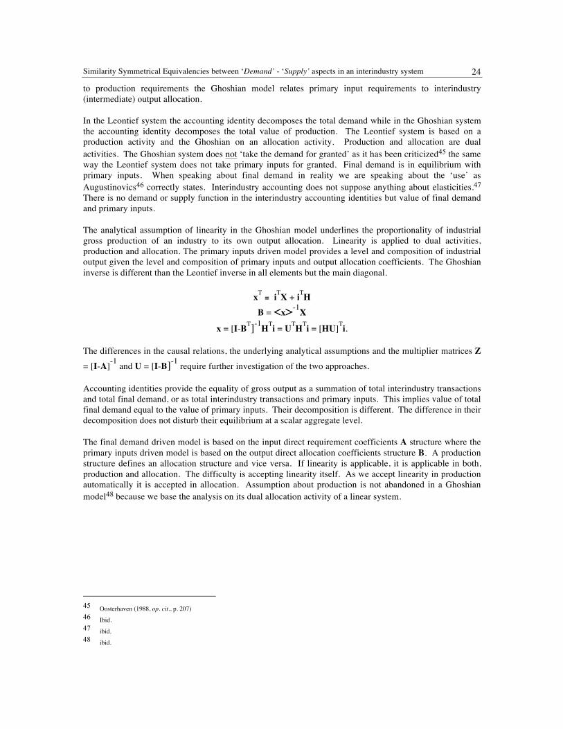
The data used and (linearity) assumption is the same in both approaches. The two models provide the same solution for gross output . [ ZY] i = x, and [ HU] T i = [ U] T[ H] Ti = x.
One needs to examine more carefully the differences in matrices Z and U. Matrix Z measures the total production of sector (i) necessary to deliver a unit of final demand of sector (j). It relates total production to final demand that is to a unit of product leaving the interindustry system at the end of the production process. Matrix U measures the total value of production that comes about in sector (j) per unit of primary input in sector (i), and therefore relates total production to primary inputs entering the interindustry system at the beginning of the production process.
Matrices Z and U have the same main diagonal. As multiplier matrices then provide unitary and uniform multipliers in the summation of their columns and rows respectively. These multipliers are different in both approaches as one may see in the numerical example. The traditional unitary and uniform multipliers are given as the summation of row and column elements in the inverse matrices respectively. The total result (sum) of unitary and uniform multipliers is the same in each activity but different in both activities as well as in its multiplier decomposition.
The above differences brought about the conclusion that production and allocation models provide different results. The difference in the above results is due to the fact that both models have similar types of causal element injection applied to a different inverse structure. These results are admissible whenever one evaluates the impact due to same cause of different matrix multipliers. The differences in the traditional multipliers and as well as the differences in the off main diagonal elements of Leontief and Ghoshian inverses is not admissible evidence that Leontief and Ghoshian models provide different results. At the same time the fact that both models provide the same solution for gross output is admissible evidence that provides the same result in a different approach.
1.2541 0.33000.2640 1.1221⎡
⎣ ⎢ ⎤
⎦ ⎥ 50 3001200 500⎡
⎣ ⎢ ⎤
⎦ ⎥ 11⎡
⎣ ⎢ ⎤
⎦ ⎥ =10002000⎡
⎣ ⎢ ⎤
⎦ ⎥
1.2541 0.13200.6601 1.1221⎡
⎣ ⎢ ⎤
⎦ ⎥ 150 500120 1280⎡
⎣ ⎢ ⎤
⎦ ⎥ 11⎡
⎣ ⎢ ⎤
⎦ ⎥ =10002000⎡
⎣ ⎢ ⎤
⎦ ⎥
Similarity Symmetrical Equivalencies between ‘Demand’ - ‘Supply’ aspects in an interindustry system 26
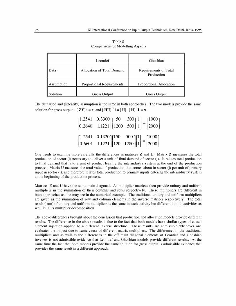
Table 9 Production Interconnected Structure
Leontief Inverse Industry 1 Industry 2 Unitary
Multipliers Industry 1 1.2541 0.3300 1.5841 Industry 2 0.2640 1.1221 1.3861 Uniform Multipliers 1.5181 1.4521 2.9702
Table 10 Allocation Interconnected Structure
Ghoshian Inverse Industry 1 Industry 2 Unitary
Multipliers Industry 1 1.2541 0.6600 1.9141 Industry 2 0.1320 1.1221 1.2541 Uniform Multipliers 1.3861 1.7821 3.1682
4.2 Quasi-Inverses
Leontief and Ghoshian inverses provide the total interrelations among industrial sectors. The Taylor expansion provides the convergence of the geometric sequence of input coefficients in ‘round effects’ of the initial I, direct A, and indirect input requirements due to a final demand vector.49
I + A + A2 + A3 + ... + An = [I-A]-1 for n approaching ∞
The similar expansion of the initial I, direct allocation coefficient matrix B, and indirect allocation coefficients approach the Ghoshian inverse.
I + B + B2 + B3 + ... + Bn = [I-B]-1 for n approaching ∞
Whenever the requirement round effect matrices are postmultiplied to a vector of final demand vector then yield the intermediate demand required in order to satisfy the final and total demand y and x.
Ay + A2y + A3y + ... + Any = Xi
A similar expansion of the Ghoshian model has a similar meaning with economic interpretations50 given. The injection vectors y and h have the same total value iTy = iTh but different element decomposition. Matrices A and B may be transformed to each other given gross output.51 Therefore any round of one
49 Takayama (1985, ibid., p. 362) and Miller and Blair (1985, op. cit., pp. 22-24) 50 Miller and Blair (1985, op. cit., pp. 358-359) 51 Augustinovics (1970, op. cit. p. 256) and Miller and Blair (1985, op. cit., p. 360)
XI International Conference on Input-Output Techniques, New Delhi, India, 1995 27
approach may be transformed into the other. Each round effect of the output coefficient matrix premultiplied to the row of primary inputs yields the row of intermediate input requirements necessary to comply with primary inputs h and satisfy gross production x.
hTB + hTB2 + hTB3 + ... + hTBn = iTX
The following parallel presentation in every round indicates the same total effect but different sectoral decomposition.
A final demand column of [350, 1700] requires total intermediate demand of [650, 300] given the input coefficients. Similarly, a primary input row of [650, 1400] necessitates a value of [350, 600] in interindustry requirements given the allocation coefficients. Taylor's expansion is not ‘extremely implausible’52 case limited to uneven sector growth in the allocation model. It is a clear indication of the symmetry between the two approaches. Knowing A one could evaluate intermediate demand Xi and having B determine intermediate input iTX.
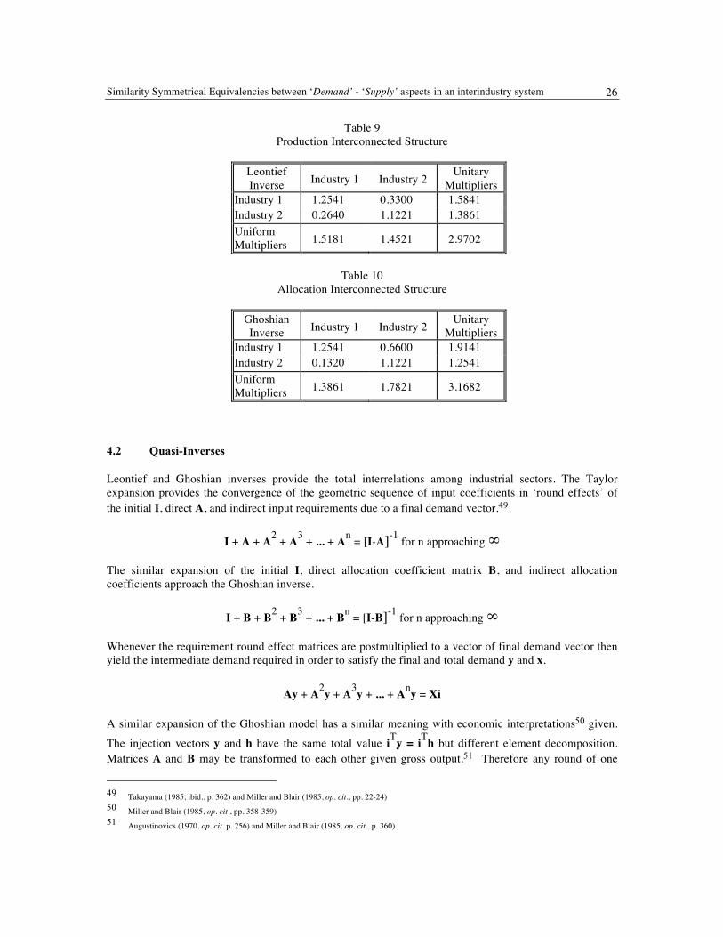
Table 11 Sectoral Decomposition of Round Effects
Total Ind. 1 Ind. 2
Intermediate Demand - ‘Demand‘ Side 950 650 300
Interindustry Requirements - ’Supply‘ Side 950 350 600
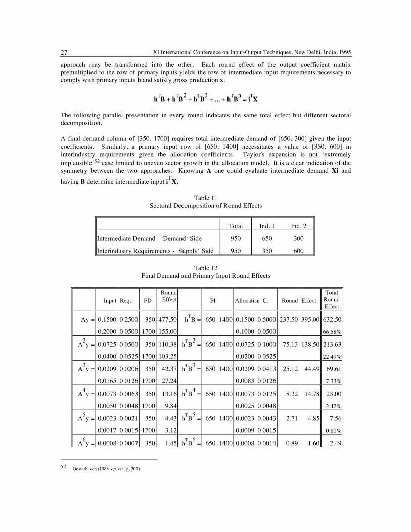
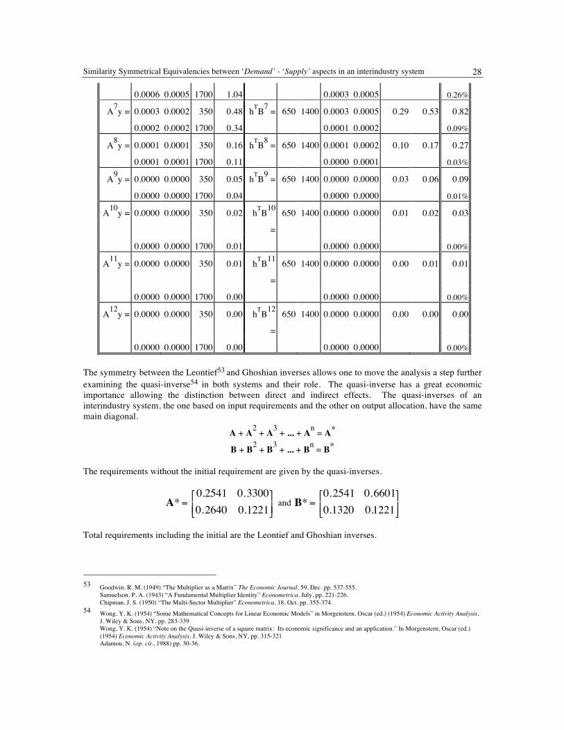
Table 12 Final Demand and Primary Input Round Effects
Input Req. FD Round Effect PI Allocati on C. Round Effect
Total Round Effect
Ay = 0.1500 0.2500 350 477.50 hTB = 650 1400 0.1500 0.5000 237.50 395.00 632.50
0.2000 0.0500 1700 155.00 0.1000 0.0500 66.58%
A2y = 0.0725 0.0500 350 110.38 hTB2 = 650 1400 0.0725 0.1000 75.13 138.50 213.63
0.0400 0.0525 1700 103.25 0.0200 0.0525 22.49%
A3y = 0.0209 0.0206 350 42.37 hTB3 = 650 1400 0.0209 0.0413 25.12 44.49 69.61
0.0165 0.0126 1700 27.24 0.0083 0.0126 7.33%
A4y = 0.0073 0.0063 350 13.16 hTB4 = 650 1400 0.0073 0.0125 8.22 14.78 23.00
0.0050 0.0048 1700 9.84 0.0025 0.0048 2.42%
A5y = 0.0023 0.0021 350 4.43 hTB5 = 650 1400 0.0023 0.0043 2.71 4.85 7.56
0.0017 0.0015 1700 3.12 0.0009 0.0015 0.80%
A6y = 0.0008 0.0007 350 1.45 hTB6 = 650 1400 0.0008 0.0014 0.89 1.60 2.49
52 Oosterhaven (1988, op. cit., p. 207)
Similarity Symmetrical Equivalencies between ‘Demand’ - ‘Supply’ aspects in an interindustry system 28
0.0006 0.0005 1700 1.04 0.0003 0.0005 0.26%
A7y = 0.0003 0.0002 350 0.48 hTB7 = 650 1400 0.0003 0.0005 0.29 0.53 0.82
0.0002 0.0002 1700 0.34 0.0001 0.0002 0.09%
A8y = 0.0001 0.0001 350 0.16 hTB8 = 650 1400 0.0001 0.0002 0.10 0.17 0.27
0.0001 0.0001 1700 0.11 0.0000 0.0001 0.03%
A9y = 0.0000 0.0000 350 0.05 hTB9 = 650 1400 0.0000 0.0000 0.03 0.06 0.09
0.0000 0.0000 1700 0.04 0.0000 0.0000 0.01%
A10y = 0.0000 0.0000 350 0.02 hTB10
=
650 1400 0.0000 0.0000 0.01 0.02 0.03
0.0000 0.0000 1700 0.01 0.0000 0.0000 0.00%
A11y = 0.0000 0.0000 350 0.01 hTB11
=
650 1400 0.0000 0.0000 0.00 0.01 0.01
0.0000 0.0000 1700 0.00 0.0000 0.0000 0.00%
A12y = 0.0000 0.0000 350 0.00 hTB12
=
650 1400 0.0000 0.0000 0.00 0.00 0.00
0.0000 0.0000 1700 0.00 0.0000 0.0000 0.00%
The symmetry between the Leontief53 and Ghoshian inverses allows one to move the analysis a step further examining the quasi-inverse54 in both systems and their role. The quasi-inverse has a great economic importance allowing the distinction between direct and indirect effects. The quasi-inverses of an interindustry system, the one based on input requirements and the other on output allocation, have the same main diagonal.
A + A2 + A3 + ... + An = A* B + B2 + B3 + ... + Bn = B*
The requirements without the initial requirement are given by the quasi-inverses.
and
Total requirements including the initial are the Leontief and Ghoshian inverses.
53 Goodwin, R. M. (1949) “The Multiplier as a Matrix” The Economic Journal, 59, Dec. pp. 537-555.
Samuelson, P. A. (1943) “A Fundamental Multiplier Identity” Econometrica, July, pp. 221-226. Chipman, J. S. (1950) “The Multi-Sector Multiplier” Econometrica, 18, Oct. pp. 355-374.
54 Wong, Y. K. (1954) “Some Mathematical Concepts for Linear Economic Models” in Morgenstern, Oscar (ed.) (1954) Economic Activity Analysis, J. Wiley & Sons, NY, pp. 283-339 Wong, Y. K. (1954) “Note on the Quasi-inverse of a square matrix: Its economic significance and an application.” In Morgenstern, Oscar (ed.) (1954) Economic Activity Analysis, J. Wiley & Sons, NY, pp. 315-321 Adamou, N. (op. cit., 1988) pp. 30-36.
A*=0.2541 0.33000.2640 0.1221⎡
⎣ ⎢ ⎤
⎦ ⎥ B*=
0.2541 0.66010.1320 0.1221⎡
⎣ ⎢ ⎤
⎦ ⎥
XI International Conference on Input-Output Techniques, New Delhi, India, 1995 29
and
Weighting the initial ejection to final demand plus the intermediate demand in term of a Taylor expansion yields total demand.
Iy + Ay + A2y + A3y + ... + Any = x Weighting the initial ejection to primary inputs plus the intermediate input in terms of a Taylor expansion provides total production.
hTI + hTB + hTB2 + hTB3 + ... + hTBn = xT Input requirements premultiplied to gross output provide intermediate demand.
Ax = Xi
Output coefficients postmultiplied to gross output give intermediate requirements.
xTB = iTX = XTi
Since A is the matrix of direct requirements, A* is the matrix of total requirements, indirect requirement transactions are given by the matrix of their difference. Indirect requirement is the operation (matrix multiplication) of total requirement A* on direct requirement A.
A* - A = A* A
Indirect requirement transactions are given as a matrix difference or as a matrix product. The same holds for indirect allocations. Requirements are satisfied by sales in an equilibrium system.
B* - B = B* B
Indirect requirement transactions are defined as (A*-A) and the indirect allocation transactions are given as (B*-B). The left hand side of the equation illuminates the concept of the indirect transaction as a requirement or allocation. On the right hand side of the equation the interrelation of indirect to direct transactions are given in terms of the matrix multiplying operation. This is an operation of the total requirement row on the direct requirement column valid in production and allocation activities.
Intermediate demand Xi may be expressed either in terms of input coefficients related to gross output Ax or as the difference between gross and net demand x-Yi. Similarly, intermediate inputs iTX are given in terms of output coefficients xTB as well as a difference between total production and total primary inputs xT-iTH.
The input coefficient matrix is the operator on the vector of gross demand to intermediate demand.
Ax = x - Yi = [650, 300]T
The output coefficient matrix is the operator on the vector of gross production to intermediate input requirements.
I +A* =1.2541 0.33000.2640 1.1221⎡
⎣ ⎢ ⎤
⎦ ⎥ I +B* =
1.2541 0.66010.1320 1.1221⎡
⎣ ⎢ ⎤
⎦ ⎥
Similarity Symmetrical Equivalencies between ‘Demand’ - ‘Supply’ aspects in an interindustry system 30
xTB = xT-iTH = [350, 600]
Since [I+A*][I-A] = I, and x=[I+A*]y, as well as [I+B*][I-B] = I, and xT=hT[I+B*], then A*y=x-y and hTB*=xT-hT. This implies that A* operates on the final demand vector in the same way that A operates on the vector of gross output.
A*y = Ax = [650, 300]T
Similarly, B* operates in the vector of primary inputs in the same way that B operates on the vector of total production.
hTB* = xTB = [350, 600]
The above result may be expanded decomposing final demand from a vector y to a matrix Y, and primary inputs from h to H. This would decompose intermediate demand and intermediate inputs to their respective indirect requirements.
A*Y = and HB* =
The summation of row elements of the A*Y matrix provides the intermediate demand [650, 300]T and the summation of column elements of HB* intermediate inputs [350, 600].
In a similar way one may allocate gross output to demand or requirement dimensions as:
(I+A*)Y = and H(I+B*) =
The summation of row elements of the (I+A*)Y matrix provides the total demand [1000, 2000]T and the summation of column elements of H(I+B*) total production [1000, 2000]. The differences of the above two groups of matrices provide the final demand and primary input matrices as:
[(I+A*)Y - A*Y] = and [H(I+B*) - HB*] =
Due to the above, Wong indicated that the essential matrix is not the Leontief inverse but the indirect requirement matrix (A*-A). One may extend the symmetry to (B*-B). For the indirect requirement matrices we have the following properties:
A*-A = A*A = AA* and B*-B = B*B = BB*.
The difference between total input requirements (A*) and direct input requirements (A) is the indirect input requirements matrix (A*-A). The matrix of the indirect requirements is given also as the operation of the
408.75 241.25159.74 140.26⎡
⎣ ⎢ ⎤
⎦ ⎥ 53.96 113.66296.04 486.34⎡
⎣ ⎢ ⎤
⎦ ⎥
458.75 541.251359.74 640.26⎡
⎣ ⎢ ⎤
⎦ ⎥ 203.96 233.66796.04 1766.34⎡
⎣ ⎢ ⎤
⎦ ⎥
50 3001200 500⎡
⎣ ⎢ ⎤
⎦ ⎥ 150 120500 1280⎡
⎣ ⎢ ⎤
⎦ ⎥
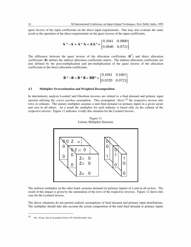
XI International Conference on Input-Output Techniques, New Delhi, India, 1995 31
quasi inverse of the input coefficients on the direct input requirements. One may also evaluate the same result as the operation of the direct requirements on the quasi inverse of the input coefficients.
The difference between the quasi inverse of the allocation coefficients (B*) and direct allocation coefficients (B) defines the indirect allocation coefficients matrix. The indirect allocation coefficients are also defined by the post-multiplication and pre-multiplication of the quasi inverse of the allocation coefficients to the direct allocation coefficients.
4.3 Multiplier Overestimation and Weighted Decomposition
In interindustry analysis Leontief and Ghoshian inverses are related to a final demand and primary input ejection utilizing the ceteris paribus assumption. This assumption ‘slices’55 the respective inverse into rows or columns. The unitary multiplier assumes a unit final demand (or primary input) in a given sector and zero to all others. As a result the multiplier for each industry is based only on the column of the respective inverse. Figure 11 indicates vividly this situation for the Leontief inverse.
Figure 11 Unitary Multiplier Structure
The uniform multiplier on the other hand, assumes demand (or primary inputs) of a unit in all sectors. The result of this impact is given by the summation of the rows of the respective inverses. Figure 12 shows this case for the Leontief inverse.
The above situations do not present realistic assumptions of final demand and primary input distributions. The multiplier should take into account the actual composition of the total final demand or primary inputs
55 The ‘slicing’ idea in its graphical form is Dr. Panethymitakis' idea.
A *−A = A*A =AA*=0.1041 0.08000.0640 0.0721⎡
⎣ ⎢ ⎤
⎦ ⎥
B *−B =B *B= BB*=0.1041 0.16010.0320 0.0721⎡
⎣ ⎢ ⎤
⎦ ⎥
Z11 0 Z21 0 Zn1 0
0 0 Z 1n 0 0
0 Z 12 0 0 0
1 0 0
0 1 0
0 0 1
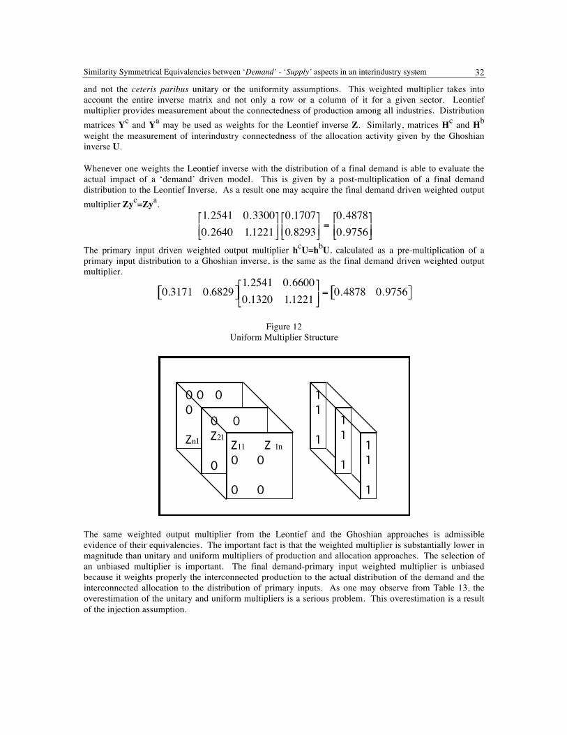
Similarity Symmetrical Equivalencies between ‘Demand’ - ‘Supply’ aspects in an interindustry system 32
and not the ceteris paribus unitary or the uniformity assumptions. This weighted multiplier takes into account the entire inverse matrix and not only a row or a column of it for a given sector. Leontief multiplier provides measurement about the connectedness of production among all industries. Distribution matrices Yc and Ya may be used as weights for the Leontief inverse Z. Similarly, matrices Hc and Hb weight the measurement of interindustry connectedness of the allocation activity given by the Ghoshian inverse U.
Whenever one weights the Leontief inverse with the distribution of a final demand is able to evaluate the actual impact of a ‘demand’ driven model. This is given by a post-multiplication of a final demand distribution to the Leontief Inverse. As a result one may acquire the final demand driven weighted output multiplier Zyc=Zya.
The primary input driven weighted output multiplier hcU=hbU, calculated as a pre-multiplication of a primary input distribution to a Ghoshian inverse, is the same as the final demand driven weighted output multiplier.
Figure 12
Uniform Multiplier Structure
The same weighted output multiplier from the Leontief and the Ghoshian approaches is admissible evidence of their equivalencies. The important fact is that the weighted multiplier is substantially lower in magnitude than unitary and uniform multipliers of production and allocation approaches. The selection of an unbiased multiplier is important. The final demand-primary input weighted multiplier is unbiased because it weights properly the interconnected production to the actual distribution of the demand and the interconnected allocation to the distribution of primary inputs. As one may observe from Table 13, the overestimation of the unitary and uniform multipliers is a serious problem. This overestimation is a result of the injection assumption.
1.2541 0.33000.2640 1.1221⎡
⎣ ⎢ ⎤
⎦ ⎥ 0.17070.8293⎡
⎣ ⎢ ⎤
⎦ ⎥ =0.48780.9756⎡
⎣ ⎢ ⎤
⎦ ⎥
0.3171 0.6829[ ]1.2541 0.66000.1320 1.1221⎡
⎣ ⎢ ⎤
⎦ ⎥ = 0.4878 0.9756[ ]
Z11 Z 1n 0 0 0 0
0 0 0 0 Zn1 1
1 1
1 1 1
1 1 1
0 0 Z21
0

XI International Conference on Input-Output Techniques, New Delhi, India, 1995 33
Multiplier decomposition is the second issue that has significant practical implications. One may derive decomposed multiplier premultiplying matrices Yc and Hc to respective Leontief and Ghoshian inverses. Tables 14 and 15 provide relative numerical examples.
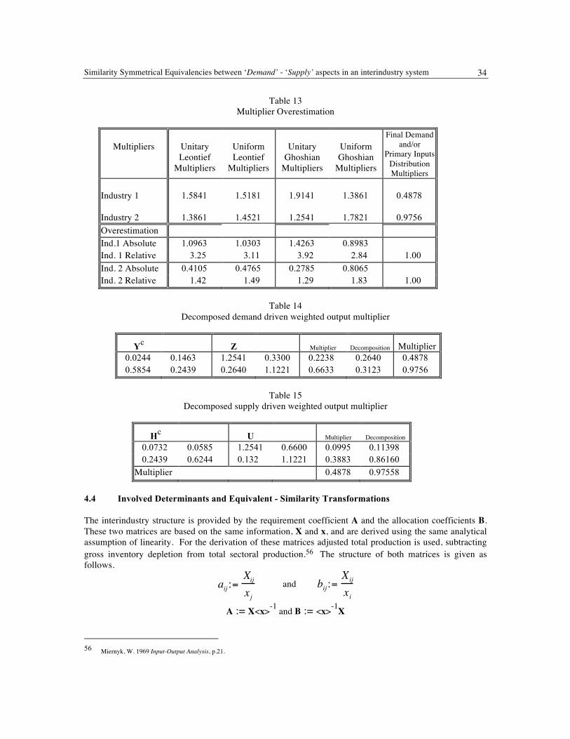
Similarity Symmetrical Equivalencies between ‘Demand’ - ‘Supply’ aspects in an interindustry system 34
Table 13 Multiplier Overestimation
Multipliers Unitary Leontief
Multipliers
Uniform Leontief
Multipliers
Unitary Ghoshian
Multipliers
Uniform Ghoshian
Multipliers
Final Demand and/or
Primary Inputs Distribution Multipliers
Industry 1 1.5841 1.5181 1.9141 1.3861 0.4878
Industry 2 1.3861 1.4521 1.2541 1.7821 0.9756 Overestimation Ind.1 Absolute 1.0963 1.0303 1.4263 0.8983 Ind. 1 Relative 3.25 3.11 3.92 2.84 1.00 Ind. 2 Absolute 0.4105 0.4765 0.2785 0.8065 Ind. 2 Relative 1.42 1.49 1.29 1.83 1.00
Table 14 Decomposed demand driven weighted output multiplier
Yc Z Multiplier Decomposition Multiplier 0.0244 0.1463 1.2541 0.3300 0.2238 0.2640 0.4878 0.5854 0.2439 0.2640 1.1221 0.6633 0.3123 0.9756
Table 15 Decomposed supply driven weighted output multiplier
Hc U Multiplier Decomposition 0.0732 0.0585 1.2541 0.6600 0.0995 0.11398 0.2439 0.6244 0.132 1.1221 0.3883 0.86160
Multiplier 0.4878 0.97558
4.4 Involved Determinants and Equivalent - Similarity Transformations
The interindustry structure is provided by the requirement coefficient A and the allocation coefficients B. These two matrices are based on the same information, X and x, and are derived using the same analytical assumption of linearity. For the derivation of these matrices adjusted total production is used, subtracting gross inventory depletion from total sectoral production.56 The structure of both matrices is given as follows.
and
A := X<x>-1 and B := <x>-1X
56 Miernyk, W. 1969 Input-Output Analysis, p.21.
aij :=Xijxj
bij :=Xij
xi
XI International Conference on Input-Output Techniques, New Delhi, India, 1995 35
This indicates that interindustry transactions take the form either of the technological coefficients of production or the allocation coefficients.
X = A<x> = <x>B Matrices A and B are equivalent, related by a similarity transformation.57
A = <x> B <x>-1
B = <x>-1A <x> Matrices [I-A] and [I-B] have a distinct economic interpretation. Matrix [I-A] provides the structure of production and [I-B] the structure of allocation. Reading across the columns, an element of matrix [I-A] indicates the amount of commodity xj necessary to produce a unit of commodity xj. A negative element for
i≠j implies required input, a positive element indicates produced output. Reading across the row of matrix [I-B], a negative element indicates the distribution of output to other sectors, and the positive element (1-bii) = (1-aii) , located at the main diagonal, the produced output.
The rank of matrices A and B may be different, but not the rank of matrices [I-B] and [I-A] is the same. The rank of a matrix is the minimum number of dimensions in space required to depict the row or columns of a matrix as vectors. A matrix of a full rank implies that its rows or columns are linearly interdependent, and its determinant is not vanishing. A determinant is vanished if a row or a column is zero. It is not unusual to have a row or a column of zeros in matrices A or B. If the product of an industrial sector is final, for example shoes, its total production is allocated only to the final demand and not between industrial and final demand. Then, the relative row of B has only zero elements, but the relative column of A has nonnegative elements since inputs are required from another sector in order to produce shoes. Public services could be another example. In these cases, the diagonal element of production and allocation matrices are equal. A solution to the system exists if and only if production and allocation matrices are of full rank.
Similarity transformation interrelates production and allocation matrices. Using elementary operations we have
[I-A] = <x>[I-B]<x>-1 or
[I-B] = <x>-1[I-A]<x>
When we have two matrices of the same order, the determinant of their product is the product of their determinants. The production and allocation matrices have the same determinant,58 as
det(I-A) = det(I-B).
and
57 Equivalent transformations are defined by the expression
A=PBQ where P and Q are non-singular matrices of a proper dimensionality. Similarity transformations as well as congruence and orthogonal
transformations are used in interindustry modeling. For the definitions of the above and their use in interindustry modeling see: Stone, Richard, 1961, Input-Output and National Accounts, OEEC, pp. 87-88.
58 det (I-A) = (1-a11)(1-a22)-(a21a12) = (1-b11)(1-b22)-((x21/x1)(x12/x2)) =(1-b11)(1-b22)-((x21x2)(x12/x1)= (1-b11)(1-b22)-(b21 b12) = det (I-B).
det(I −A) =0.85 −0.25−0.20 0.95 = 0.7575 det(I −B) =
0.85 −0.50−0.10 0.95 = 0.7575
Similarity Symmetrical Equivalencies between ‘Demand’ - ‘Supply’ aspects in an interindustry system 36
The meaning of the determinant is the value of net production as final demand or as the value of primary inputs payments.59 A similar relation exists also among the determinants of A and B,60 although the economic meaning of these determinants is not as clear as the det(I-A) and det(I-B).
det(A) = det(B)
and
A graphical interpretation of the equivalence of determinants (I-A) and (I-B) is presented later on in this section.
Production and allocation inverse matrices are similar.61
[I - A]-1 = <x>[I - B]-1<x>-1
[I - B]-1 = <x>-1[I - A]-1<x>
Total production is a function of primary inputs from an allocation of output point of view. Similarly, total production is a function of final demand from the production of output point of view. Primary inputs and final demand are major policy targets.
det(I-A)-1 = det(I-B)-1
and
Production and allocation determinants, det(I-A) & det(I-B), may be presented graphically in the net output space62 and in the gross output space.63 Net output may be seen either as net demand (final) or as net inputs (primary). Figures 13 and 14 present det(I-A) & det(I-B) respectively.
In Figure 13 we have each one of the vectors of the [I-A] production matrix.
Vectors (oa1) = and (oa2)= define the parallelogram
21yyyΟ , the determinant of the matrix [I-A]. The magnitude of this determinant specifies the final demand necessary for a gross output unit decomposed to its different types. Similarly, we have the graphical
59 For more detailed discussion of the structure of the linear demand driven models see:
Wong, Y. K., 1954, “Some Mathematical Concepts for Linear Economic Models”, in Oscar Morgenstern (ed.) Economic Activity, J. Wiley and Sons, N.Y., pp. 283-339.
60 det (A) = (a11)(a22)-(a21a12) = (X11/x1)(X22/x2)-((X21/x2)(X12/x1)) = (b11 b22)-((X21/x1)(x12/x2) = (b11)(b22)-(b21 b12) = det (B)
61 [I-A]-1 = {<x>[I-B]<x>-1}-1 = <x>-1)-1[I-B]-1<x>-1
62 Wong (op. cit.) 63 Dorfman, Solow & Samuelson (op. cit.)
det(A)=0.15 0.250.20 0.05 = −0.0425 det(B)=
0.15 0.500.10 0.05 = −0.0425
det(Z)=12541 0.33000.2640 1.1221 =1.32013 det(U) =
12541 0.66010.1320 1.1221 = 1.32013
1 − a11−a 21
⎛
⎝ ⎜ ⎞
⎠ =
0.85−0.20⎛
⎝ ⎜ ⎞
⎠
−a121 − a22⎛
⎝ ⎜ ⎞
⎠ =
−0.250.95
⎛
⎝ ⎜ ⎞
⎠
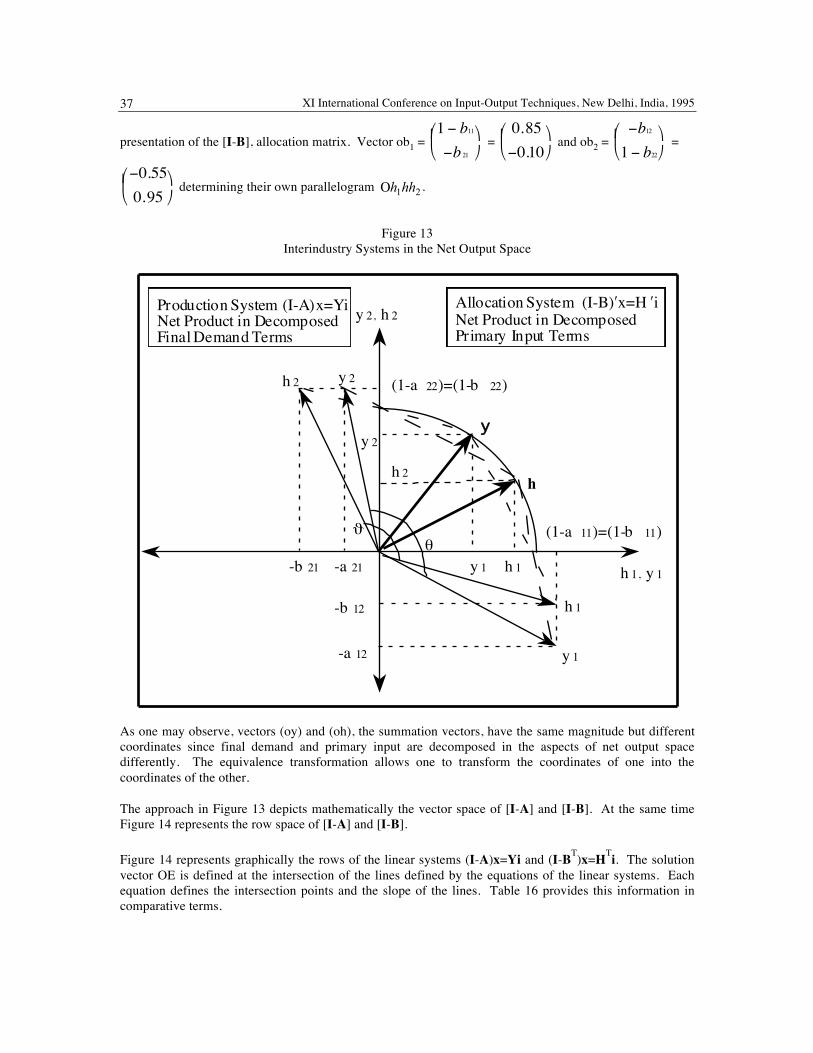
XI International Conference on Input-Output Techniques, New Delhi, India, 1995 37
presentation of the [I-B], allocation matrix. Vector ob1 = = and ob2 = =
determining their own parallelogram 21hhhΟ .
Figure 13 Interindustry Systems in the Net Output Space
As one may observe, vectors (oy) and (oh), the summation vectors, have the same magnitude but different coordinates since final demand and primary input are decomposed in the aspects of net output space differently. The equivalence transformation allows one to transform the coordinates of one into the coordinates of the other.
The approach in Figure 13 depicts mathematically the vector space of [I-A] and [I-B]. At the same time Figure 14 represents the row space of [I-A] and [I-B].
Figure 14 represents graphically the rows of the linear systems (I-A)x=Yi and (I-BT)x=HTi. The solution vector OE is defined at the intersection of the lines defined by the equations of the linear systems. Each equation defines the intersection points and the slope of the lines. Table 16 provides this information in comparative terms.
1 − b11−b 21
⎛
⎝ ⎜ ⎞
⎠
0.85−0.10⎛
⎝ ⎜ ⎞
⎠
−b121− b22⎛
⎝ ⎜ ⎞
⎠ −0.550.95
⎛
⎝ ⎜ ⎞
⎠
Production System (I-A)x=Yi Net Product in Decomposed Final Demand Terms
Allocation System (I-B)ʹ′x=H ʹ′i Net Product in Decomposed Primary Input Terms
y 2, h 2
h
y
h 1, y 1
(1-a 11)=(1-b 11)
-a 21-b 21
(1-a 22)=(1-b 22)
-b 12
-a 12
y 2
y 1 h 1
h 2
ϑθ
h 2
h 1
y 1
y 2

Similarity Symmetrical Equivalencies between ‘Demand’ - ‘Supply’ aspects in an interindustry system 38
One clearly may observe that distances OA, OB and OA v& OB vare defined as having the same denominators, the elements of the main diagonal of the respective matrices, while numerators are the respective values of sectoral final demand yj or primary input hi. The distances OC and OC vand OD and
OD v are defined having differences in both numerator and denominator. It is noticeable that as the symmetric position of their respective denominators. Likewise is the case of the numerators in the comparison of the slopes.
Figure 14 Gross Output Space
in the Production [(I-A)x=Yi] and Allocation [(I-BT)x=HTi] Systems
A
A ʹ′
B
Bʹ′
C Cʹ′
D
Dʹ′
ψ ψʹ′ φʹ′
φ
Production System (I-A)x=Yi Lines 1 (AD) & 2 (CB)
Allocation System (I-B)ʹ′x=H ʹ′i Lines 3 (Aʹ′Dʹ′)& 4 (Cʹ′Βʹ′)
Line 2
Line 1
Line 4
Line 3
x1
x2
xOA = y 1 /(1-a 11) OB = y 2 /(1-a 22) OC = -(y 2 /a 21) OD = -(y 1 /a 12) = a 12 /(1-a 11) = a 21 /(1-a 22)
OAʹ′ = h 1 /(1-b 11) OBʹ′ = h 2 /(1-b 22) OCʹ′ = -(h 2 /b 21) ODʹ′ = -(h 1 /b 12) ʹ′ = b 12 /(1-b 11) ʹ′ = b 21 /(1-b 22)
x =
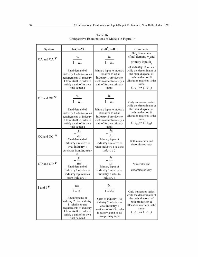
XI International Conference on Input-Output Techniques, New Delhi, India, 1995 39
Table 16 Comparative Examinations of Models in Figure 14
System (I-A)x=Yi (I-BT)x=HTi Comments
OA and OA v
Final demand of
industry 1 relative to net requirements of industry 1 from itself in order to satisfy a unit of its own
final demand
Primary input to industry 1 relative to what
industry 1 provides to itself in order to satisfy a unit of its own primary
input
Only Numerator (final demand y
1and
primary input h1
of industry 1) varies, while the denominator of
the main diagonal of both production &
allocation matrices is the same
(1-a11) = (1-b11)
OB and OB v
Final demand of
industry 2 relative to net requirements of industry 2 from itself in order to satisfy a unit of its own
final demand
Primary input to industry 2 relative to what
industry 2 provides to itself in order to satisfy a unit of its own primary
input
Only numerator varies while the denominator of
the main diagonal of both production &
allocation matrices is the same
(1-a22) = (1-b22)
OC and OC v
Final demand of industry 2 relative to
what industry 1 purchases from industry
2.
Primary input of industry 2 relative to
what industry 1 sales to industry 2.
Both numerator and denominator vary
OD and OD v
Final demand of industry 1 relative to industry 2 purchases
from industry 1.
Primary input of industry 1 relative to industry 2 sales to
industry 1.
Numerator and
denominator vary
f and f v .
Requirements of
industry 2 from industry 1, relative to net
requirements of industry 1 from itself in order to satisfy a unit of its own
final demand
Sales of industry 1 to industry 2, relative to
what industry 1 provides to itself in order
to satisfy a unit of its own primary input
Only numerator varies while the denominator of
the main diagonal of both production &
allocation matrices is the same
(1-a11) = (1-b11)
y11− a11
h11− b11
y21− a 22
h 2
1− b22
−y2a21
−h2b12
−y1a12
−h1b21
a121− a11
b211− b11
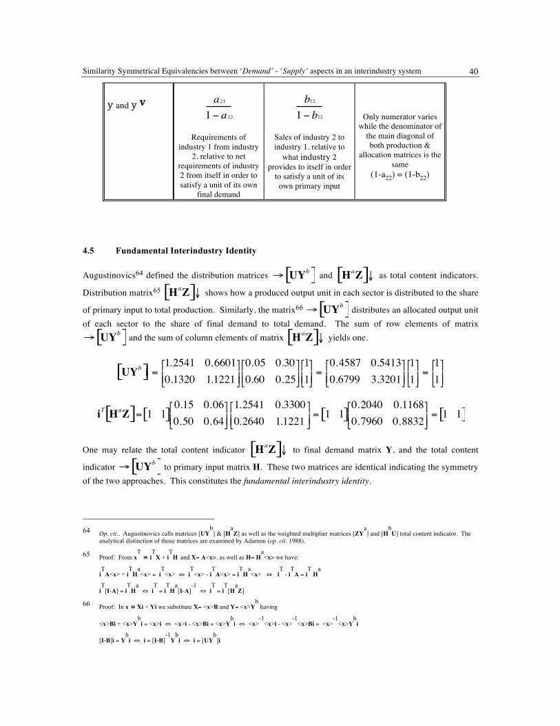
Similarity Symmetrical Equivalencies between ‘Demand’ - ‘Supply’ aspects in an interindustry system 40
y and y v
Requirements of
industry 1 from industry 2, relative to net
requirements of industry 2 from itself in order to satisfy a unit of its own
final demand
Sales of industry 2 to industry 1, relative to
what industry 2 provides to itself in order
to satisfy a unit of its own primary input
Only numerator varies while the denominator of
the main diagonal of both production &
allocation matrices is the same
(1-a22) = (1-b22)
4.5 Fundamental Interindustry Identity
Augustinovics64 defined the distribution matrices and as total content indicators.
Distribution matrix65 shows how a produced output unit in each sector is distributed to the share
of primary input to total production. Similarly, the matrix66 distributes an allocated output unit of each sector to the share of final demand to total demand. The sum of row elements of matrix
and the sum of column elements of matrix yields one.
One may relate the total content indicator to final demand matrix Y, and the total content
indicator to primary input matrix H. These two matrices are identical indicating the symmetry of the two approaches. This constitutes the fundamental interindustry identity.
64 Op. cit.. Augustinovics calls matrices [UY
b] & [H
aZ] as well as the weighted multiplier matrices [ZY
a] and [H
bU] total content indicator. The
analytical distinction of those matrices are examined by Adamou (op. cit. 1988).
65 Proof: From xT ≡ i
TX + i
TH and X= A<x>, as well as H= H
a<x> we have:
iT
A<x> + iT
Ha<x> = i
T<x> ⇔ i
T<x> - i
TA<x> = i
TH
a<x> ⇔ i
T - i
TA = i
T H
a
iT
[I-A] = iT
Ha ⇔ i
T = i
TH
a[I-A]
-1 ⇔ i
T = i
T[H
aZ]
66 Proof: In x ≡ Xi + Yi we substitute X= <x>B and Y= <x>Yb
having
<x>Bi + <x>Yb
i = <x>i ⇔ <x>i - <x>Bi = <x>Yb
i ⇔ <x>-1
<x>i - <x>-1
<x>Bi = <x>-1
<x>Yb
i
[I-B]i = Yb
i ⇔ i = [I-B]-1
Yb
i ⇔ i = [UYb
]i
a 21
1− a 22
b121− b22
→ UYb[ ] HaZ[ ]↓HaZ[ ]↓
→ UYb[ ]
→ UYb[ ] HaZ[ ]↓
UYb[ ]i =1.2541 0.66010.1320 1.1221⎡
⎣ ⎢ ⎤
⎦ ⎥ 0.05 0.300.60 0.25⎡
⎣ ⎢ ⎤
⎦ ⎥ 11⎡
⎣ ⎢ ⎤
⎦ ⎥ =0.4587 0.54130.6799 3.3201⎡
⎣ ⎢ ⎤
⎦ ⎥ 11⎡
⎣ ⎢ ⎤
⎦ ⎥ =11⎡
⎣ ⎢ ⎤
⎦ ⎥
iT HaZ[ ]= 1 1[ ]0.15 0.060.50 0.64⎡
⎣ ⎢ ⎤
⎦ ⎥ 1.2541 0.33000.2640 1.1221⎡
⎣ ⎢ ⎤
⎦ ⎥ = 1 1[ ]
0.2040 0.11680.7960 0.8832⎡
⎣ ⎢ ⎤
⎦ ⎥ = 1 1[ ]
HaZ[ ]↓→ UYb[ ]
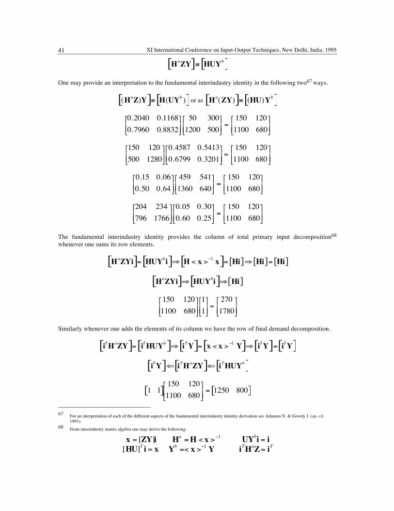
XI International Conference on Input-Output Techniques, New Delhi, India, 1995 41
One may provide an interpretation to the fundamental interindustry identity in the following two67 ways.
or as
The fundamental interindustry identity provides the column of total primary input decomposition68 whenever one sums its row elements.
Similarly whenever one adds the elements of its column we have the row of final demand decomposition.
67 For an interpretation of each of the different aspects of the fundamental interindustry identity derivation see Adamou N. & Gowdy J. (op. cit.
1991). 68 From interindustry matrix algebra one may derive the following:
HaZY[ ]≡ HUYb[ ]
(HaZ)Y[ ]≡ H(UYb )[ ] Ha(ZY)[ ]≡ (HU)Yb[ ]0.2040 0.11680.7960 0.8832⎡
⎣ ⎢ ⎤
⎦ ⎥ 50 3001200 500⎡
⎣ ⎢ ⎤
⎦ ⎥ =150 1201100 680⎡
⎣ ⎢ ⎤
⎦ ⎥
150 120500 1280⎡
⎣ ⎢ ⎤
⎦ ⎥ 0.4587 0.54130.6799 0.3201⎡
⎣ ⎢ ⎤
⎦ ⎥ =150 1201100 680⎡
⎣ ⎢ ⎤
⎦ ⎥
0.15 0.060.50 0.64⎡
⎣ ⎢ ⎤
⎦ ⎥ 459 5411360 640⎡
⎣ ⎢ ⎤
⎦ ⎥ =150 1201100 680⎡
⎣ ⎢ ⎤
⎦ ⎥
204 234796 1766⎡
⎣ ⎢ ⎤
⎦ ⎥ 0.05 0.300.60 0.25⎡
⎣ ⎢ ⎤
⎦ ⎥ =150 1201100 680⎡
⎣ ⎢ ⎤
⎦ ⎥
HaZYi[ ]= HUYbi[ ]⇒ H < x >−1 x[ ]= Hi[ ]⇒ Hi[ ]= Hi[ ]
HaZYi[ ]⇒ HUYbi[ ]⇒ Hi[ ]
150 1201100 680⎡
⎣ ⎢ ⎤
⎦ ⎥ 11⎡
⎣ ⎢ ⎤
⎦ ⎥ =2701780⎡
⎣ ⎢ ⎤
⎦ ⎥
iTHaZY[ ]= iTHUYb[ ]⇒ iTY[ ]= x < x > −1 Y[ ]⇒ iTY[ ]= iTY[ ]
iTY[ ]⇐ iTHaZY[ ]⇐ iTHUYb[ ]
1 1[ ]150 1201100 680⎡
⎣ ⎢ ⎤
⎦ ⎥ = 1250 800[ ]
x = [ZY]i Ha =H < x >−1 UYbi = i[HU]T i = x Yb =< x >−1 Y iTHaZ= iT
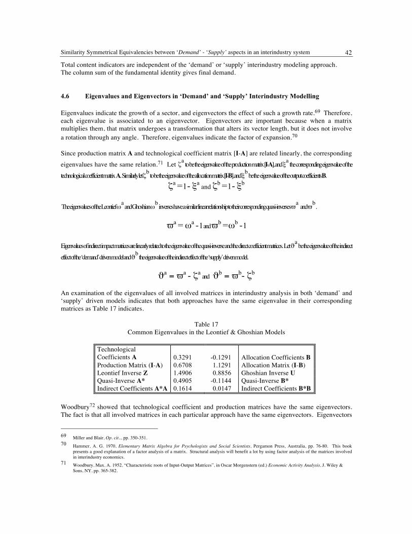
Similarity Symmetrical Equivalencies between ‘Demand’ - ‘Supply’ aspects in an interindustry system 42
Total content indicators are independent of the ‘demand’ or ‘supply’ interindustry modeling approach. The column sum of the fundamental identity gives final demand.
4.6 Eigenvalues and Eigenvectors in ‘Demand’ and ‘Supply’ Interindustry Modelling
Eigenvalues indicate the growth of a sector, and eigenvectors the effect of such a growth rate.69 Therefore, each eigenvalue is associated to an eigenvector. Eigenvectors are important because when a matrix multiplies them, that matrix undergoes a transformation that alters its vector length, but it does not involve a rotation through any angle. Therefore, eigenvalues indicate the factor of expansion.70
Since production matrix A and technological coefficient matrix [I-A] are related linearly, the corresponding eigenvalues have the same relation.71 Let ζa to be the eigenvalue of the production matrix [I-A], and ξa the corresponding eigenvalue of the technological coefficient matrix A. Similarly let ζb to be the eigenvalue of the allocation matrix [I-B], and ξb be the eigenvalue of the output coefficients B.
ζa = 1 - ξa and ζb = 1 - ξb
The eigenvalues of the Leontief ωa and Ghoshian ωb inverses have a similar linear relationship to their corresponding quasi-inverses ϖa and ϖb.
ϖa = ωa - 1 and ϖb = ωb - 1
Eigenvalues of indirect impact matrices are linearly related to the eigenvalue of the quasi-inverse and the direct coefficient matrices. Let ϑa be the eigenvalue of the indirect
effect of the ‘demand’ driven model and ϑb the eigenvalue of the indirect effect of the ‘supply’ driven model.
ϑa = ϖa - ζa and ϑb = ϖb- ζb
An examination of the eigenvalues of all involved matrices in interindustry analysis in both ‘demand’ and ‘supply’ driven models indicates that both approaches have the same eigenvalue in their corresponding matrices as Table 17 indicates.
Table 17 Common Eigenvalues in the Leontief & Ghoshian Models
Technological Coefficients A 0.3291 -0.1291 Allocation Coefficients B Production Matrix (I-A) 0.6708 1.1291 Allocation Matrix (I-B) Leontief Inverse Z 1.4906 0.8856 Ghoshian Inverse U Quasi-Inverse A* 0.4905 -0.1144 Quasi-Inverse B* Indirect Coefficients A*A 0.1614 0.0147 Indirect Coefficients B*B
Woodbury72 showed that technological coefficient and production matrices have the same eigenvectors. The fact is that all involved matrices in each particular approach have the same eigenvectors. Eigenvectors
69 Miller and Blair, Op. cit.., pp. 350-351. 70 Hammer, A. G. 1970, Elementary Matrix Algebra for Psychologists and Social Scientists, Pergamon Press, Australia, pp. 76-80. This book
presents a good explanation of a factor analysis of a matrix. Structural analysis will benefit a lot by using factor analysis of the matrices involved in interindustry economics.
71 Woodbury, Max, A. 1952, “Characteristic roots of Input-Output Matrices”, in Oscar Morgenstern (ed.) Economic Activity Analysis, J. Wiley & Sons, NY, pp. 365-382.
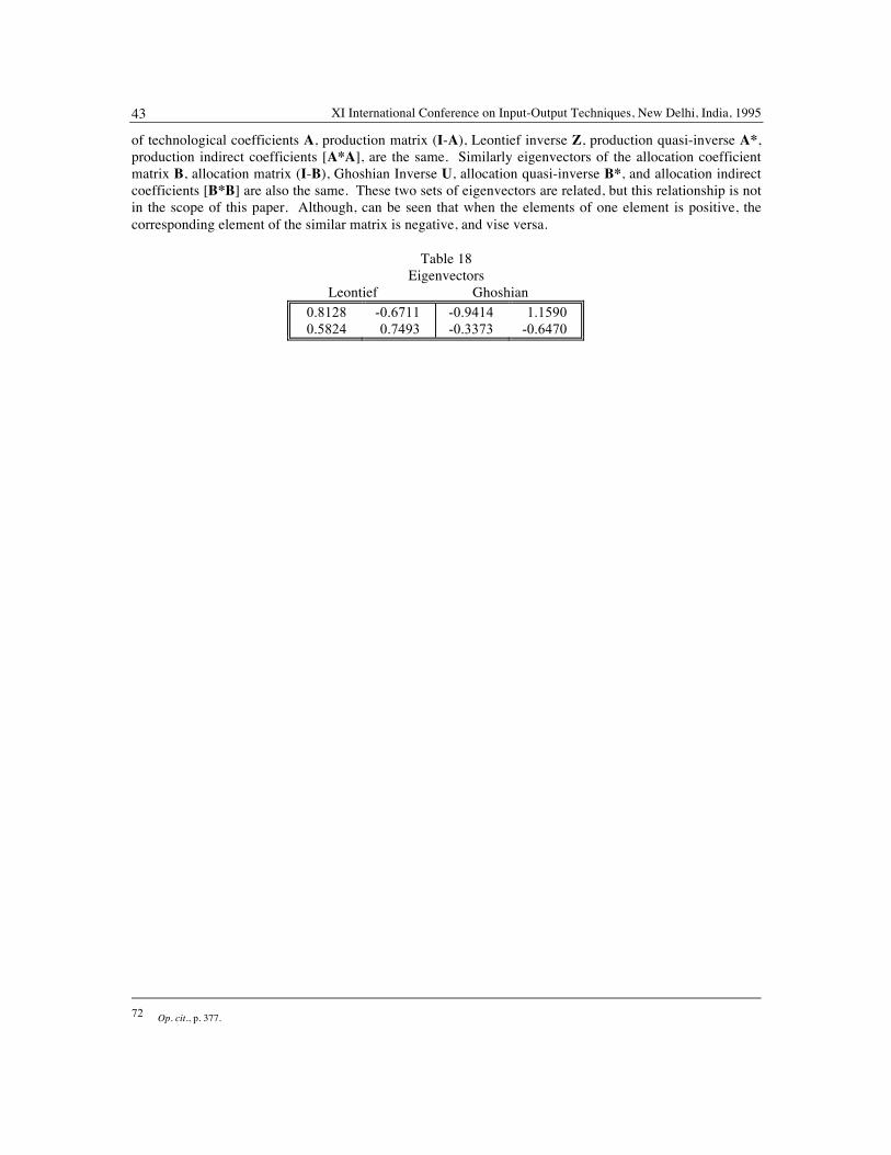
XI International Conference on Input-Output Techniques, New Delhi, India, 1995 43
of technological coefficients A, production matrix (I-A), Leontief inverse Z, production quasi-inverse A*, production indirect coefficients [A*A], are the same. Similarly eigenvectors of the allocation coefficient matrix B, allocation matrix (I-B), Ghoshian Inverse U, allocation quasi-inverse B*, and allocation indirect coefficients [B*B] are also the same. These two sets of eigenvectors are related, but this relationship is not in the scope of this paper. Although, can be seen that when the elements of one element is positive, the corresponding element of the similar matrix is negative, and vise versa.
Table 18 Eigenvectors
Leontief Ghoshian 0.8128 -0.6711 -0.9414 1.1590 0.5824 0.7493 -0.3373 -0.6470
72 Op. cit., p. 377.
Similarity Symmetrical Equivalencies between ‘Demand’ - ‘Supply’ aspects in an interindustry system 44
List of Tables & Figures
Table 1 Interindustry Accounting (Concept Presentation) Table 1.2 Interindustry Accounting Matrix (Mathematical Formulations) Table 1.3 Interindustry Accounting (Numerical Example) Table 2 Typology of Descriptive Coefficients Table 3 Column Distributions (Input Coefficients) Figure 1 Input Distribution of a Sectoral Unit of Gross Production Figure 2 Distribution of different types of Final Demand units. Table 4 Row Distributions (Allocation coefficients) Figure 3 Distribution of a unit of Total Demand Figure 4 Industry Distributions of a unit in Primary Inputs & Total Production Table 5 Two-Dimensional Distributions of Intermediate Transactions, Final Demand and
Primary Inputs Figure 5 Two-dimensional interindustry distribution of an intermediate demand unit Figure 6 Two-dimensional industry-primary inputs distribution of a total primary input
unit Figure 7 Two-dimensional industry-final demand distribution of a total final demand unit Table 6 Two-dimensional distribution of the Gross Output Figure 8 Two-dimensional distribution of gross output to processing sectors Figure 9 Two-dimensional distribution of gross output to primary inputs Figure 10 Two-dimensional distribution of gross output to final demand Table 7 Descriptive Statistics in two-Dimensional Distributions Table 8 Comparison of Modelling Aspects Table 9 Production Interconnected Structure Table 10 Allocation Interconnected Structure Table 11 Sectoral Decomposition of Round Effects Table 12 Final Demand and Primary Input Round Effects Figure 11 Unitary Multiplier Structure Figure 12 Uniform Multiplier Structure Table 13 Multiplier Overestimation Table 14 Decomposed demand driven weighted output multiplier Table 15 Decomposed supply driven weighted output multiplier Figure 13 Determinants (I-A) and (I-B) in the Net Output Space Figure 14 Systems (I-A)x=Yi and (I-BT)x=HTi in the Gross Output Space Table 16 Comparative Examination of Figures 13 and 14 Table 17 Common Eigenvalues in the Leontief & Ghoshian Models Table 18 Leontief & Ghoshian Eigenvectors
XI International Conference on Input-Output Techniques, New Delhi, India, 1995 45
BIBLIOGRAPHY
Adamou, N. (1987) Structural Analysis with Input-Output methodology: The case of Greece. Eastern Economic Association Conference, Washington, DC., March 5-7
Adamou N. (1989) “Interindustry Analysis and Budgeting Process” Ways & Means Committee of the New York State Assembly, November
Adamou N. (1990) “Capital and Labor Feedback Structures in an Extended Input-Output System: A Comparison of the United States and Japan.” International Symposium on Economic Modelling, University of Urbino, Italy, July 23-25
Adamou N. (1990) “The Impact of Negative Total Sectoral Final Demand on the Production and Allocation Structure in Interindustry models.” Workshop in interindustry analysis, Sage Graduate School, November
Adamou N. (1990) The Equivalence of the Demand to Supply Driven Input-Output Models and their integration to National Income and Product Accounts. Interindustry Analysis Workshop, Sage College, October and Economics Department Workshop, Rensselaer Polytechnic Institute, November
Adamou N. (1991) “Clarifying Analytical Assumptions in Inter-industry Modelling” Workshop in interindustry economics, Sage Graduate School, Troy, NY, October
Adamou N. (1991) “Negative Elements in Japanese Input-Output Tables and the Problem of Stability.” International Symposium of Economic Modelling, University of London, July 9-11
Adamou N. (1991) Decomposing Weighted Output Multipliers in a Multisectoral Demand and Supply Driven System. The Japanese experience, 1960-1985. Interindustry Analysis Workshop, Sage Graduate School, Troy, NY, September
Adamou N. (1992) “Inter-Industry Structure in New York State and its implication for fiscal policy, with a particular emphasis on taxes.” New York State Tax Study Legislative Commission, April
Adamou N. (1992) Technological Change in Production and Structural Change in Allocation: A Multivariate Statistical Approach. New York State Tax Study Legislative Commission, June
Adamou N. and J. M. Gowdy (1990) “Inner, final, and feedback structures in an extended input-output system.” Environment and Planning A, Vol. 22, pp. 1621-1636
Adamou, N. (1988) Structural Analysis and Analysis of Structural Change in an Extended Input-Output Framework, Ph.D. Dissertation, Department of Managerial Economics, Rensselaer Polytechnic Institute
Adamou, N. (1991) “Fiscal Policy , Foreign Trade and Industrial Structure in Japan: 1960-1985.” Ways & Means Committee of the New York State Assembly, December
Adamou, N. (1991) “Industrial Impact of Imports and Exports in Japan: 1960-1985.” International Conference of the International Trade & Finance Association, May 31-June 2, Marseilles, France
Adamou, N. (1995) Economic Interpretation of Several Linear Systems Solutions to Interindustry Modelling, 3rd Balkan Conference of Operational Research, Forthcoming Proceedings, October
Adamou, N. (1995) Ejection Biasedness in the ‘Demand’ Driven Interindustry Multiplier and Weighted Decomposition: Greek Empirical Evidence Center of Planning and Economic Research, Athens, Greece, July 4
Adamou, N. (1995) Supply and Demand Industry Multipliers in Greece, 3rd Balkan Conference of Operational Research, Forthcoming Proceedings, October
Aidenoff A. (1970) “Input-Output Data in the United Nations System of National Accounts” in Carter & Bródy (ed.) (1970) Contributions to Input-Output Analysis, North Holland Vol. II, pp. 349-368. Reprinted in Sohn I. (1986) Readings in Input-Output Analysis, pp. 130-150
Ara K. (1959) “The Aggregation Problems in Input-Output Analysis” Econometrica April, pp. 257-62 Ara K. (1986) “Conditions for the Aggregation of Industrial Sectors into the Capital-Goods Sectors and the
Consumption-Goods Sector” Hitotsubashi Journal of Economics, December pp. 99-109 Arrow K. J., Karlin S. & Suppes (ed.) (1960) Mathematical Methods in the Social Sciences, Stanfort
University Press
Similarity Symmetrical Equivalencies between ‘Demand’ - ‘Supply’ aspects in an interindustry system 46
Augustinovics, Maria (1968) “Methods of international and intertemporal comparison of structure” In Carter & Bródy (ed.) (1970) Contributions to Input-Output Analysis, North Holland, Vol. I, Chapter 13, pp. 249-269
Beaumont P. M. (1990) “Supply and Demand Interaction in Integrated Econometric and Input-Output Models” International Regional Science Review, 13(1&2) pp. 167-181
Berman A., Plemmons R. J. (1979) Nonnegative Matrices in the Mathematical Sciences, Academic Press, New York
Bickley W. C. and R. S. G. (1964) Matrices: Their Meaning and Manipulation, D. Van Norstrand Co. Inc., Princeton, New Jersey
Bon, Ranko (1984) “Comparative Stability Analysis of Multiregional Input-Output Models: Column, Row, and Leontief-Strout Gravity Coefficient Models.” Quarterly Journal of Economics, Nov., 99 (4), pp. 791-815
Bon, Ranko (1986) “Comparative Stability Analysis of Demand-side and Supply-Side Input-Output Models.” International Journal of Forecasting, 2, pp. 231-235
Bon, Ranko (1988) “Supply-Side Multiregional Input-Output Models.” Journal of Regional Science, 28 (1), pp. 41-50
Brauer A. (1946) “Limits for the Characteristic Roots of a Matrix” Duke Mathematical Journal 13, September
Bruno M. (1972) “Optimal patterns of Trade and Development” in Chenery H. B. (ed.) Studies in Development Planning Harvard University Press
Buhr W. and P. Friedrich (eds.) (1981) Regional Development under Stagnation, Baden-Baden: Nomos Verlagsgesellshaft
Bulmer-Thomas, V. (1982) “Application of Input-Output Analysis for Less Developed Countries” in Reiner Stäglin (ed.) (1982) International Use of Input-Output Analysis pp. 199-230. Reprinted in Sohn I. (1986) Readings in Input-Output Analysis, pp. 108-129
Bulmer-Thomas, V. (1982) Input-Output Analysis in Developing Countries., New York, Wiley Campisi D., A Natasi & A. La Bella (1992) “Balanced growth and stability of the Leontief dynamic Model:
an analysis of an Italian Economy” Environment and Planning A, Vol. 24, pp. 591-600 Carter & Bródy (ed.) (1970) Contributions to Input-Output Analysis, North Holland, Vol. I & II Cella Guido (1988) “The Supply Side Approaches to Input-Output Analysis: An Assessment.” Ricerche
Economiche, XLII, (3), pp. 433-451 Chander P. (1983) “Nonlinear Input-Output Model” Journal of Economic Theory 30, pp. 219-229 Chen C. Y. (1986) “The optimal Adjustment of mineral supply disruptions” Journal of Policy Modeling, 8,
pp. 199-221 Chen C. Y., and A. Rose (1986) “The joint stability of input-output production and allocation
coefficients.” Modelling and Simulation 17, pp. 251-255 Chen, C. Y. and A. Rose (1991) “The Absolute and relative Joint Stability of Input-Output Production and
Allocation Coefficients.” in W. Peterson (eds.) Advances in Input-Output Analysis: Technology, Planning, & Development, Oxford Univ. Press, pp. 25-36
Chenery H. B. (ed.) (1972) Studies in Development Planning, Harvard University Press Chenery H. B. and Clark, P. G., (1959) Interindustry Economics, Wiley Chenery H. B. and T. Watanabe (1958) “Interindustry Comparisons of the Structure of Production”
Econometrica, 26(4), pp. 487-521 Chien M. J. and L. Chan (1979) “Nonlinear Input-Output Model with Piecewise Affine Coefficients”
Journal of Economic Theory 21, pp. 389-410 Chipman J. S. (1951) The Theory of Inter-Sectoral Money Flows and Income Formation, Baltimore, Md.,
Johns Hopkins University Press Chipman, J. S. (1950) “The Multi-Sector Multiplier” Econometrica, 18, Oct. pp. 355-374 Ciaschini M. (ed.) (1988) Input-Output Analysis: Current Developments, Chapman and Hall Clapp J. M. (1977) “The relationships among regional input-output intersectoral flows and rows-only
analysis” International Regional Science Review, pp. 79-89
XI International Conference on Input-Output Techniques, New Delhi, India, 1995 47
Conway R. S. Jr., (1975) “A note on the stability of regional interindustry models” Journal of Regional Science, Vol. 15, pp. 67-72
Cronin J. (1984) “Analytical assumptions and causal ordering in interindustry modeling” Southern Economic Journal 51, pp. 521-529
Cullen C. G. (1966) Matrices and Linear Transformations, Addison-Wesley, Reading Massachusetts. Curry,. B. (1963) Foundations of Mathematical Logic, McGraw-Hill Davis, H. C., and E. L. Salkin (1984) “Alternative Approaches to the estimation of economic impacts
resulting from supply constraints.” Annals of Regional Science, 18, pp. 25-34 Debreu G. and I. N. Herstein (1953) “Nonnegative Square Matrices” Econometrica 21 October Deman S. (1985) “Political economy of regional development: a review of theories” Indian Journal of
Regional Science Vol. 24 pp. 192-200 Deman S. (1988) “Stability of Supply coefficients and consistency of supply-driven and demand-driven
input-output models.” Environment and Planning A, 20, pp. 811-816 Deman S. (1991) “Stability of Supply coefficients and consistency of supply-driven and demand driven
input-output models: a reply” Environment and Planning A, Vol. 23, pp. 1811-1817 Dewhurst J. H. L. (1990) “Intensive income in demo-economic input-output models” Environment and
Planning A, Vol. 22, pp. 119-128 Dietzenbacher E. (1989) “On the relationship between the supply-driven and the demand driven input-
output model.” Environment and Planning A, Vol. 21 (11) pp. 1533-1539 Dorfman, Samuelson & Solow (1958) Linear Programming and Economic Analysis, McGraw-Hill. Evans W. D. (1954) “The Effect of Structural Matrix Errors on Interindustry Relations Estimates”
Econometrica 22, pp. 461-480 Fisher W. D. (1962) “An Alternative Proof and Extension of Solow's Theorem on Nonnegative Square
Matrices” Econometrica 30 April Fisher W. D. (1965) “Choice of Units, Column Sums, and Stability in Linear Dynamic Systems with
Nonnegative Square Matrices” Econometrica 33, April Fisher W. D. (1969) Clustering and Aggregation in Economics John Hopkins University Press Freeman C. (1982) The Economics of Industrial Innovation, Pinter, London Fujimoto T. (1986) “Non-Linear Leontief Models in Abstract Spaces” Journal of Mathematical Economics
15, pp. 151-156 Gale (1960)The theory of linear models, McGraw Hill Gantmacher F. R. (1959) The Theory of Matrices, Vol. II, New York, Chalsea Publishing Co., (tr. from
Russian) Gardini A. (1985) “Structural Form, Interdependence and Statistical Estimation in the Input-Output Model”
Ricerche Economiche, 39, pp. 29-39 Georgescu-Roegen, Nicholas (1951) “Some Properties of a Generalized Leontief Model”, in Koopmans, T.
C., (ed.) Activity Analysis of Production and Allocation, Wiley Gerking S. D. (1976) “Input-Output as a Simple Econometric Model” Review of Economics and Statistics,
58, pp. 274-282 Gerking S. D. (1976) Estimation of Stochastic Input-Output Models, Martinus Njihoff, Leiden Ghosh, A. (1958) “Input-Output Approach in an Allocation System.” Economica 25, pp. 58-64. Giarratani F. (1976) “Application of an interindustry supply model to energy issues” Environment and
Planning A, 8, pp. 447-454 Giarratani F. (1980) “The scientific basis fir explanation in regional analysis” Papers of Regional Science
Association 45, pp. 185-196 Giarratani F. (1981) “A supply constrained interindustry model: Forecasting performance and an
evaluation.” In W. Buhr and P. Friedrich (eds.) Regional Development under Stagnation, Baden-Baden: Nomos Verlagsgesellshaft
Goodwin, R. M. (1949) “The Multiplier as a Matrix” The Economic Journal, 59, Dec. pp. 537-555 Goodwin, R. M. (1950) “Does the Matrix Multiplier Oscillate?” Economic Journal, LX, December Gowdy J. (1991) “Structural Change in the USA and Japan: an extended input-output analysis.” Economic
System Research, 3, pp. 413-423
Similarity Symmetrical Equivalencies between ‘Demand’ - ‘Supply’ aspects in an interindustry system 48
Gray, S. Lee, etc. (1979) “Measurement of Growth equalized employment multiplier effects: an empirical example.” Annals of Regional Science, 13 (3), pp. 68-75
Gruver G. (1989) “On the plausibility of the supply-driven input-output model: a theoretical basis for input-coefficient change” Journal of Regional Science Vol. 29, pp. 441-450
Gruver Gene W (1989) “On the Plausibility of the Supply-Driven Input-Output Model: A Theoretical Basis for Input-Output Coefficient Change” Journal of Regional Science, 29(3) pp. 441-450
Hammer, A. G. 1970, Elementary Matrix Algebra for Psychologists and Social Scientists, Pergamon Press, Australia
Hawkins D. (1948) “Some Conditions of Macro-economic Stability” Econometrica 16 October Hawkins D. and Simon H. A. (1949) “Note: Some Conditions on Macroeconomic Stability” Econometrica
July-October Helmstädter E., Richtering J., (1982) “Input coefficients versus output coefficients types of models and
empirical findings”, in Proceedings of the Third Hungarian Conference on Input-Output Techniques, Statistical Publishing House, Budapest, pp. 213-224
Herstein I. N. (1952) “Comments on Solow's Structure of Linear Models” Econometrica 20 October Hirshman (1958) The Strategy of Economic Development Yale University Press, New Haven, Conn. Horn R. & Johnson C. R. (1985) Matrix Analysis, Cambridge University Press Hurosh A. (1972) Higher Algebra tr. from the Russian by George Yankovsky (1980) Mir Publishers.
Moscow Hurowicz L. (1955) “Input-Output Analysis and Economic Structure: A Review Article” American
Economic Review 45, pp. 468-470 Ilyin V. A. and E. G. Poznyak (1984) Linear Algebra tr. from the Russian by Irene Aleksanova (1986), Mir
Publishes Moscow Jones L. P. (1976) “The Measurement of Hirshmanian Linkages” The Quarterly Journal of Economics
90(2) pp. 323-333 Karlin S. (1959) Mathematical Methods and Theory of Games, Programming and Economics Vol. I.
Addison-Wesley. Keuning Steve J. (1994) “The SAM and Beyond: Open, SESAME!” Economic System Research, Vol. 6.,
No. 1, pp. 21-50. The same paper was presented at the International Conference for Research in Income & Wealth in Canada, August 1994
Koopmans T. (1949) “Identification Problems in Economic Model Construction” Econometrica 17(2) April, p. 127
Kuboniwa M. (1989) Quantitative Economics of Socialism: Input-Output Approaches, Kinokuniya-Oxford University Press
Lahiri S. (1976) “Input-Output analysis with Scale-Dependent Coefficients” Econometrica 44(5) pp. 947-961
Lahiri S. (1985) “Nonlinear Generalizations of the Hawkins-Simon conditions: Some Comparisons” Math. Soc. Sci. 9, pp. 293-97
Lahiri S. and G Pyatt (1980) “On the Solution of Scale-Dependent Input-Output Models” Econometrica 48(7) pp. 1827-30
Lekakis J. N. (1991) “Employment effects of environmental policies in Greece” Environment and Planning A, Vol. 23, pp. 1627-1637
Lemke, C. E. (1965) “Bimatrix equilibrium points and mathematical programming” Management Science, 11, pp. 681-689
Leontief W. (1936) “Quantitative Input and Output Relations in the Economic System of the United States” Review of Economics and Statistics, XVIII
Leontief W. (1937) “Interrelation of Prices, Output, Savings, and Investment”, Review of Economics and Statistics, XIX
Leontief W. (1941) The Structure of American Economy, 1919-1929. Harvard University Press Leontief W. (1943) “Exports, Imports, Domestic Output and Employment”, The Quarterly Journal of
Economics, February Leontief W. (1951) The Structure of American Economy, 1919-1959. Oxford University Press
XI International Conference on Input-Output Techniques, New Delhi, India, 1995 49
Leontief W., (1946) “Wages, Profits and Prices”, The Quarterly Journal of Economics, November Liebling H. I. “Interindustry Economics and National Income Theory” in NBER (1955) Input-Output
Analysis, An appraisal. Studies in Income and Wealth., Vol. 18, Princeton University Press, pp. 291-320
Lieu S. & G. I. Treyz (1992) “Estimating the economic and demographic effects of an air quality management plan. The case of Southern California” Environment and Planning A, Vol. 24, pp. 1799-1811
Lorenzen, G. (1989) “Input-Output multipliers when data are incomplete or unreliable” Environment and Planning A, Vol. 21, pp. 1075-1092
Maital S. (1972) “The Tableau economique as a simple Leontief Model: an amendment”. Quarterly Journal of Economics, 86 (3), pp. 504-507
Marthur, P. N. (1970) “Introduction” Carter & Bródy (ed.) Contributions to Input-Output Analysis, North Holland
McGilvray, James (1989) “Supply-Driven Input-Output Models” 9th International I-O Conference, Keszthely, Hungary
McKenzie, L. W. (1957) “An Elementary Analysis of the Leontief System” Econometrica 25 July McKenzie, L. W. (1959) “Matrices with Dominant Diagonals and Economic Theory,” in Arrow K. J.,
Karlin S. & Suppes (ed.) (1960)Mathematical Methods in the Social Sciences Stanfort University Press Metzler L. A. (1945) “Stability of Multiple Markets: The Hicks Conditions” Econometrica 13 October. Metzler L. A. (1950) “A Multiple Region Theory of Income and Trade” Econometrica 18 October Miernyk, W. (1965) Input-Output Analysis, Random House Miller R. E. & G Shao (1990) “Spatial & sectoral aggregation in the commodity-industry multiregional
input-output model” Environment and Planning A, Vol. 22, pp. 1637-1656 Miller R. E. and P. D. Blair (1985) Input-output Analysis: Foundations and Extensions, Prentice Hall Miller R. E., K. R. Polenske and A. Z. Roze (ed.) (1989) Frontiers of Input-Output Analysis, Oxford
University Press Miller, R. E. (1989) “Stability of Supply coefficients and consistency of supply-driven and demand-driven
input-output models: a comment.” Environment and Planning A, 21, pp. 1113-1120 Miyazawa K. (1966) “Internal and External Matrix Multipliers in the Input-Output Model” Hitotsubashi
Journal of Economics June, pp. 38-55 Miyazawa K. (1968) “Input-Output Analysis and Inter-relational Income Multipliers as a Matrix”
Hitotsubashi Journal of Economics February, pp. 39-58 Miyazawa K. (1971) “An Analysis of the Interdependence between service and Goods-Producing Sectors”
Hitotsubashi Journal of Economics June, pp. 10-21 Miyazawa K. (1976) Interindustry Analysis and the Structure of Income Distribution, Lecture Notes in
Economics and mathematical Systems, Vol. 116, Springer-Verlag Morgenstern, Oscar (ed.) (1954) Economic Activity Analysis, J. Wiley & Sons, NY, pp. 283-339 Morimoto Y. (1971) “A Note on Weighted Aggregation in Input-Output Analysis” International Economic
Review 12(1) February pp. 138-143 Morishima M. & F. Seton (1961) “Aggregation in Leontief matrices and the labour theory of value”
Econometrica Morishima M. (1959) “A Reconsideration of the Warlas-Cassel-Leontief Model of General Equilibrium” in
Arrow K. J., Karlin S. & Supposes (ed.) Mathematical Methods in the Social Sciences Morishima M. (1976) The Economic Theory of Modern Society, Cambridge University Press NBER (1955) Input-Output Analysis, An appraisal: Studies in Income and Wealth., Vol. 18, Princeton
University Press Nikaido, H., (1968) Convex Structures and Economic Theory, Academic Press Nikaido, H., (1970) Introduction to Sets and Mappings in Modern Economics, tr. by Sato, North-Holland Nuget J. (1970) “Linear Programming Models for National Planning: Demonstration of a Testing
Procedure” Econometrica, November, pp. 831-855 Okuguchi K. and F. Szidarovszky (1987) “On a Nonlinear Input-Output System: Note” Math. Soc. Sci.
13(3), pp. 277-81
Similarity Symmetrical Equivalencies between ‘Demand’ - ‘Supply’ aspects in an interindustry system 50
Oosterhaven J. (1989) “The Supply-Driven Input-Output Model: A New Interpretation but Still Implausible” Journal of Regional Science, 29(3) pp. 459-465
Oosterhaven, J. (1981) Interregional Input-Output Analysis and Dutch Regional Policy Problems, pp. 138-155, Aldershot, England: Gover
Oosterhaven, J. (1988) “On the plausibility of the supply-driven input-output model.” Journal of Regional Science, 28, pp. 203-217
Penson, John B. Jr. & Hovav Talpaz (1988) “Endogenization of final demand and primary input supply in input-output analysis.” Applied Economics, 20, pp. 739-752
Peterson W. (eds.) (1991) Advances in Input-Output Analysis: Technology, Planning, & Development, Oxford Univ. Press, pp. 25-36
Pettofrezzo A. J. (1966) Matrices and Transformations, Prentice-Hall Planning Bureau of The Netherlands Gecumuleerde Productiestruc-tururmatrices (GPS-matrices) 1969-
1985 Centraal Planbureau, Interne Notice, 17 Februari 1989. Polenske K. R. (1980) The U.S. Multiregional Input-Output Accounts and Model, Lexington Books Preston, R. S. (1975) “The Warton Long Term Model: Input-Output within the Context of a Macro
Forecasting Model” International Economic Review, 16(1), February Price G. G. (1951) “Bounds for Determinants with Dominant Principal Diagonals” Proceedings of the
American Mathematical Society 2 Primero, Elidoro P. (1985) “Effects of changing industrial structures and changes levels and composition
of the final demand bill on the input factor requirements of the economy: An application of input-output analysis.” The Philippine Economic Journal, XXIV (2&3), pp. 200-221
Pyatt, G. (1991) “Foundamentals of Social Accounting” Economic System Research 3, pp. 315-341. Quandt R. E. (1958) “Probabilistic Errors in the Leontief System” Naval Research Logistics Quarterly 5(2)
pp. 155-170 Quandt R. E. (1959) “On the Solution of Probabilistic Leontief Systems” Naval Research Logistics
Quarterly 6(4) pp. 295-305 Raa T. and R. van der Ploeg (1989) “A Statistical Approach to the Problem of Negatives in Input-Output
Analysis” Economic Modelling 6(1), pp. 2-19 Rose, A. and T. Allison (1989) “On the plausibility of supply-driven input-output model: Empirical
evidence on joint stability.” Journal of Regional Science 29, pp. 451-458 Samuelson, P. A. (1943) “A Fundamental Multiplier Identity” Econometrica, July, pp. 221-226 Samuelson, P. A. (1951) “A Theorem Concerning Substitutability in Open Leontief Models,” in
Koopmans, T. C., (ed.) Activity Analysis of Production and Allocation, Wiley Sandberg I. W. (1973) “A Nonlinear Input-Output Model of a Multisector Economy” Econometrica 41(6),
Nov. pp. 1167-82 Santhanam K. & R. Patil (1972) “A study of the Production of the Indian Economy: An International
Comparison” Econometrica, 40 (1), January, pp. 159-176 Schneider H., Baker G. P. (1968) Matrices and Linear Algebra, Hold, Rinehart and Winston, Inc. Senn L. and C. Miglierina (1987) “Empirical Test of the Stochastic Estimation of Technical Coefficients”
Ricerche Economiche 41(1) Jan.-Mar. pp. 62-81 Sigel S. I. (1955) “A Comparison of the Structure of Three Social Accounting Systems” in NBER (1955)
Input-Output Analysis, An appraisal. Studies in Income and Wealth., Vol. 18, Princeton University Press, pp. 253-289
Silva J. A. (1986) “Equivalent Conditions on Solvability for Non-Linear Leontief Models” Metroeconomica, 38(2) June, pp. 167-69
Simpson D. and J. Tsukui (1965) “The Fundamental Structure of Input-Output Tables: An International Comparison” Review of Economics and Statistics 47, pp. 434-446
Socher C. F. (1981) “A Comparison of Input-Output Structure and Multipliers.” Environment and Planning A, Apr. 13 (4), pp. 497-509
Sohn I. (ed.) (1986) Readings in Input-Output Analysis, Oxford University press, New York and Oxford. Solow R. (1952) “On the Structure of Linear Models” Econometrica 20, pp. 29-46

XI International Conference on Input-Output Techniques, New Delhi, India, 1995 51
Sonh B. N. (1977) “The Production Structure of the Korean Economy: International Comparisons” Econometrica, 45(1), pp. 147-162.
Stäglin R. (ed.) (1982) International Use of Input-Output Analysis, Vandenhoeck and Ruprecht, Göttingen. Stern E. M. (1963) Mathematics for Management, Prentice-Hall. Stone, Richard, 1961, Input-Output and National Accounts, OEEC, pp. 87-88. Szyrmer J. M. (1992) “Input-output coefficients and multipliers from a total flow perspective” Environment
& Planning A Vol. 24, pp. 921-937 Takayama, A. (1987) Mathematical Economics, 2nd ed., Cambridge U. Press, p. 360 Uno, K. (1989) Measurement of Services in an Input-Output Framework, Amsterdam, North-Holland Van Arkadie B. & Frank C. (1966) Economic Accounting and Development Planning, Oxford University
Press. West G. R. (1986) “A Stochastic Analysis of an Input-Output Model” Econometrica, 54(2), pp. 163-374 Wong, Y. K. (1954) “Note on the Quasi-inverse of a square matrix: Its economic significance and an
application.” in Morgenstern, Oscar (ed.) (1954) Economic Activity Analysis, J. Wiley & Sons, NY, pp. 315-321
Wong, Y. K. (1954) “Some Mathematical Concepts for Linear Economic Models” in Morgenstern, Oscar (ed.) (1954) Economic Activity Analysis, J. Wiley & Sons, NY, pp. 283-339
Woodbury, Max, A. 1952, “Characteristic roots of Input-Output Matrices”, in Oscar Morgenstern (ed.) Economic Activity Analysis, J. Wiley & Sons, NY, pp. 365-382
Yale, P. B. (1968) Geometry and Symmetry Halden-Day, San Francisco Yamada I. (1961) Theory and Applications of Interindustry Analysis, Kinokunika Bookstore, Tokyo, Japan Yan (1969) Introduction to Input-Output Economics, Holt and Winston, New York
Copyright © 2022 FDOKUMEN