1. The Concept and Representation of Periodic Sampling of a CT Signal

2. Analysis of Sampling in the Frequency Domain3. The Sampling Theorem — the Nyquist Rate4. In the Time Domain: Interpolation5. Undersampling and Aliasing

Signals and SystemsFall 2003

Lecture #1321 October 2003

We live in a continuous-time world: most of the signals we encounter are CT signals, e.g. x(t). How do we convert them into DT signals x[n]?

SAMPLING

How do we perform sampling?

— Sampling, taking snap shots of x(t) every T seconds.

T – sampling periodx[n] ≡ x(nT), n = ..., -1, 0, 1, 2, ... — regularly spaced samples

Applications and Examples— Digital Processing of Signals— Strobe— Images in Newspapers— Sampling Oscilloscope— …

Why/When Would a Set of Samples Be Adequate?

• Observation: Lots of signals have the same samples

• By sampling we throw out lots of information – all values of x(t) between sampling points are lost.

• Key Question for Sampling:Under what conditions can we reconstruct the original CT signal x(t) from its samples?

Impulse Sampling — Multiplying x(t) by the sampling function

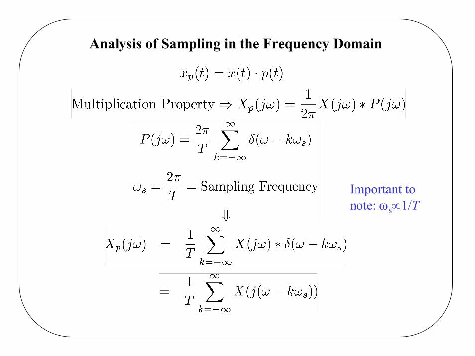
Analysis of Sampling in the Frequency Domain

Important tonote: ωs∝1/T

Illustration of sampling in the frequency-domain for a band-limited (X(jω)=0 for |ω|> ωM) signal

No overlap between shifted spectra

Reconstruction of x(t) from sampled signals

If there is no overlap between shifted spectra, a LPF can reproduce x(t) from xp(t)

The Sampling Theorem

Suppose x(t) is bandlimited, so that

Then x(t) is uniquely determined by its samples {x(nT)} if

Observations on Sampling

(1) In practice, we obviously don’t sample with impulses or implement ideal lowpass filters.— One practical example:

The Zero-Order Hold

Observations (Continued)

(2) Sampling is fundamentally a time-varying operation, since we multiply x(t) with a time-varying function p(t). However,

is the identity system (which is TI) for bandlimited x(t) satisfying the sampling theorem (ωs > 2ωM).

(3) What if ωs ≤ 2ωM? Something different: more later.

Time-Domain Interpretation of Reconstruction of Sampled Signals — Band-Limited Interpolation

The lowpass filter interpolates the samples assuming x(t) containsno energy at frequencies ≥ ωc

T

h(t)

Graphic Illustration of Time-Domain Interpolation

Original CT signal

After sampling

After passing the LPF

Interpolation Methods

• Bandlimited Interpolation• Zero-Order Hold • First-Order Hold — Linear interpolation

Undersampling and Aliasing

When ωs ≤ 2 ωM ⇒ Undersampling

Undersampling and Aliasing (continued)

— Higher frequencies of x(t) are “folded back” and take on the “aliases” of lower frequencies

— Note that at the sample times, xr(nT) = x(nT)

Xr(jω)≠ X(jω) Distortion because of aliasing

Demo: Sampling and reconstruction of cosωot

A Simple Example

Picture would be Modified…