SI 335, Unit 6: Completeness and Complexity

Daniel S. Roche (roche@usna.edu)

Spring 2016

1 Introduction

So far in this class we’ve concentrated on how to compare different algorithms for the same problem. Welooked at a bunch of algorithms for sorting, for integer multiplication, for all-pairs shortest paths, etc.

Now we want to get all “meta” and actually compare different problems to each other. This is an ambitiousendeavor, but one that is really important to understand the inherent difficulty of problems. One reason thatyou should care about this is cryptography. For example, if integer factorization is inherently difficult, thenwe can be more confident in the security of the RSA cryptosystem.

1.1 Computational Complexity

The field of computational complexity, which is what we’ll be getting into in this unit, is the study andclassification of different problems according to their inherent difficulty. For example we would like to makestatements like “sorting has roughly the same difficulty as integer multiplication” or “integer factorization ismore difficult than computing shortest paths in a graph”.

The first step to comparing problems is to define what the difficulty of a problem actually is:

Definition

The difficulty of a problem is the best worst-case cost among all possible algorithms thatcorrectly solve that problem.

In other words, I take all the possible algorithms for that problem (including ones that haven’t been inventedyet!), figure out the worst-case cost (maybe running time or space, whatever we’re measuring) of each of thosealgorithms, and then take the least of all those worst-case costs. That’s the inherent difficulty of the problem.

If this seems crazy, that’s because it is! This is the first indication that getting complete answers to ourquestions regarding computational complexity is going to be kind of rare. What this really means is thatwe will be making a lot of simplifications, and even then that there will be some fundamental questions leftunanswered.

However, we actually have seen a few instances where the computational complexity is completely nailed, suchas sorting in the comparison model. We know the inherent difficulty of that problem is Θ(n log n) becausethere are algorithms with this worst-case cost, and there is a lower bound on the problem to say that theworst-case cost of any algorithm must be at least this much.

1.2 Comparing problems (overview)

Short of getting an exact measure of their computational complexity (which is hard to do in general), how canwe compare two completely different problems? We’ll spend a lot of time making this precise, but let’s startwith a dead-simple example: finding the minimum element in a list versus sorting the list. In complexity, we

1

like to give problems upper-case names to make it easier to talk about them, so I’ll call these two problemsMIN and SORT.

Now you are already thinking in your head of the algorithms you know to solve MIN and SORT - but that’snot what we’re talking about here! We’re not talking about MergeSort or InsertionSort or any particular wayof solving these problems; we’re talking about the problems themselves. How can we compare the inherentdifficulty of MIN and SORT?

One way to compare these problems directly, without having to talk about any particular algorithm for eitherproblem, is to figure out how to solve one problem with an algorithm for the other. For this example, MINcan obviously be solved by running any SORT algorithm once, and then you return the first thing in thesorted array. What this means is that any brilliant sorting algorithm immediately gives you an algorithm forMIN, with exactly the same cost. We say the inherent difficulty of MIN is less than or equal to that of SORT.

How about the other direction? We have to think of how to solve SORT using MIN. As you know, there arelots and lots of ways to SORT, but in order to compare these two problems we just want to think about howto use MIN to do it. Well, you can SORT using n calls to MIN, by finding the MIN, then changing thatnumber to infinity, finding the MIN again (which is the second-smallest number now), changing that numberto infinity, and so on until you’ve computed the whole sorted order.

(This is exactly what the SelectionSort algorithm does, but in a stupider way here because here we don’tbother to reduce the size of the array for subsequent MINs. Notice that we are allowed - even encouraged -to do a lot of “stupid” things in the context of complexity!)

What this means is that any brilliant MIN algorithm would right away give you a SORT algorithm whoserunning time is n times more than the MIN algorithm’s running time. We say that the inherent difficulty ofSORT is less than or equal to n times that of MIN.

Putting these two together, and being a little more formal, we could write

MIN ≤ SORT ≤ n ∗ MIN

This general process of figuring out how to solve one problem using an algorithm for another one is calleda reduction, and it will be our main tool in actually comparing algorithms. What we just showed was areduction from MIN to SORT, and a reduction from SORT to n MINs. We’ll have to get more specific aboutthe “rules” of this game of doing reductions, but this is the basic idea, and the basic tool we will use tocompare problems. The important thing to recognize is that we didn’t rely on any particular algorithm foreither problem, or on any lower bound, in order to make this comparison.

1.3 Tractable vs intractable

The ultimate goal of our brief study of complexity is to decide what problems are tractable and what problemsare intractable. So we have to define what these words mean!

Luckily, we already have a pretty good definition of what kind of problem should be solved in a reasonableamount of time (tractable). The Cobham-Edmonds thesis that we talked about back in Unit 3 declares thatan algorithm is tractable only if it runs in polynomial-time in the size of the input.

The key task ahead of us in this unit is to try and show that some problems are actually hard, or intractable.Let’s consider the realm of what intractable problems could look like:

• Undecidable problems. You learned in Theory class that the Halting Problem (“Does this programalways terminate?”) is undecidable, meaning that no computer program can always solve it in a finiteamount of time. Then we definitely won’t be getting any polynomial-time algorithms!

• Problems with big output. For example, consider the problem of computing every path between twovertices. Since a path is really just an ordering (or permutation) of the vertex names, there are something

2

like n! possible paths in the worst case, which means output size exponentially larger than the inputsize. So this is another kind of problem that is definitely not going to have a polynomial-time solution.

• Problems that seem infinitely hard. For example, consider the problem of determining whether two givenregular expressions (with the Kleene star and a squaring operator) represent the same language. Thereare actually ways to solve this problem, but none that require less than exponential space. Problemsthis hard are also definitely not going to yield any polynomial-time algorithms.

These are all ridiculously hard, intractable problems. But the problems we’re thinking about as being “hard”are not this hard. For example, consider integer factorization, where we are given a number and asked to findits least prime factor. It’s certainly decidable. The output isn’t too large either, since the factor can’t belarger than the input operator. And it doesn’t require an exponential amount of space; we can solve it byjust checking each possible factor from 2 up to the (square root of) the input number until we find one. Andyet we think factorization is a hard problem!

This is actually the class of “hard” problems that we are going to be most interested in. In a way, they’re theeasiest kind of hard problems. And what characterizes problems like integer factorization and minimal vertexcover is that, while computing the answer might be difficult, checking the answer is easy. Given a factor, wecan see that it actually divides the input. Given a vertex cover, we can confirm that it actually covers all theedges in a graph.

So the problems we’re going to focus on are essentially those that can be solved by a “guess-and-check”or “trial-and-error” strategy: repeatedly guess the answer, then check it, and return your best guess. Andactually almost all the problems we’ve seen in this class can be categorized this way. Yet some of them(like finding the shortest path in a graph) are tractable, and some others (like finding a minimum vertexcover) seem intractable. The most important (and difficult) question we will ask in this class is whether anyproblems are so hard that they can only be solved by a brute-force trial-and-error approach. We just need alittle more background in order to be able to ask that question in a precise way.

2 Complexity Basics

Any time we try to say something about how difficult a problem is, it requires us to be very precise abouthow the problem is defined, what kinds of operations allowed, and how the difficulty and performance willbe measured. This is sort of like laying out the rules of a very precise game. We have to define the rulescarefully so that the comparisons made between algorithms will be fair, consistent, and meaningful.

2.1 Machine models

The first thing to define is what kinds of operations are allowed by the algorithms we consider. This is likewhen we proved the lower bound on the sorting problem earlier, and said that only comparisons betweenarray elements were allowed. Except now, since we are talking about all different kinds of problems, we can’tbe so restrictive. We want to come up with a general model of computation that is well-defined (so we canreason about it) but which also corresponds closely to the power of actual computers.

Traditionally, the preferred model of computation for theoretical work is a Turing machine, like you learnedabout in Theory. In this class, we’ve been using a model of “primitive operations”, which we defined sort ofloosely as anything which would take a fixed number of operations on any real computer. We could also getmore specific, like counting the number of MIPS assembly instructions, or use another abstract computermodel.

The good news is, it doesn’t actually matter for us! Why? Well, our only goal in this brief foray intocomputational complexity is to understand what problems are tractable and which ones are intractable. Whilethe models listed above are certainly not identical, they could be mapped to each other in polynomial-time.That is, given any program in one model that runs in time Θ(nk), we could construct a program in any ofthe other models that runs in time Θ(n`), where k and ` are both constants.

3

(I’ll spare you the proof of that last claim.)

2.2 Input Size

What definitely will matter for is is the size of the input. In order to have fair and consistent analysis,we must measure the size of the input the same for all problems. The following list of previously-statedcomplexities demonstrates that we have definitely not been doing this so far:

• Least Prime Factor: Θ(√

n)• Karatsuba multiplication: O(n1.59)• Strassen multiplication: O(n2.81)• Dijkstra’s (using adjacency lists): Θ((n + m) log n)

The key problem here is that each of these analyses is measuring the size of its input in a different way. Wealready know that Θ(

√n) isn’t really the cost of factorization in terms of the size of the input, because n in

this equation is the number itself, whereas the number of digits in that number is more like s = lg n.

But even between Karatsuba’s and Strassesn’s algorithms, there’s a discrepancy. The n in the cost ofKaratsuba’s is giving the number of digits in the input numbers, but in Strassen’s it’s the dimension of oneside of a square matrix. So the actual size of the input to Strassen’s is more like s = n2. Using this definitionof size, Strassen’s algorithm actually looks faster than Karatsuba’s; it’s O(n1.41). Dijkstra’s is even moreconfusing because it introduces this second parameter m into the cost.

The issue at hand is that we need a way of comparing all different kinds of problems to each other. Measuringthe difficulty in slightly different ways is fine if you’re just comparing a bunch of algorithms for the sameproblem (for example, computing shortest paths). But when we start talking about different problemstogether, we need a consistent and universal definition of input size.

Bit size is the answer to this problem. Since everything is stored in a computer, every input takes up acertain number of bits. So we’ll count the total number of bits as the size of the input for every problemfrom now on, and we’ll always call this n. So in terms of bit size, the above algorithms actually cost

• Least Prime Factor: Θ(2n/2)• Karatsuba multiplication: O(n1.59)• Strassen multiplication: O(n1.41)• Dijkstra’s (using adjacency lists): Θ(n log n)

(The last one is a little tricky. The reason it becomes Θ(n log n) is that the original input size is n = |V |+ |E|.Notice that having a larger input size actually makes algorithms look faster, which seems a bit counter-intuitiveat first!)

2.3 Decision problems

So we’ve nailed down the input size — well what about the output size? Clearly the size of the outputmakes a difference (potentially) for the difficulty of the problem. So are we going to have to have a secondparameter in the measure of difficulty of a problem?

To avoid this, we will only study a very restricted class of problems called decision problems that only answeryes-or-no questions. So the output will always be a single bit: YES or NO, TRUE or FALSE, ON or OFF,etc.

In fact, these are the only kind of problems that can be handled by the basic models of computation that youstudied in Theory. Formally, a Turning machine can only output ACCEPT or REJECT. So we must restrictthe discussion to decision problems in order to include such machines in the discussion.

4

Let’s look at an example: factorization. The normal factorization problem (as solved by the LeastPrimeFactoralgorithm) is, given a number N, to compute the smallest prime factor of N. How could we make this into adecision problem?

The first decision problem version we might try is, “Does N have any prime factors?” This indeed followsalong the lines of the original problem, and clearly by solving the original problem of factorization we couldanswer this question. But the question has gotten too much easier, it would seem: while we suspect theoriginal factorization problem is intractable, we know that this decision problem (primality testing) can besolved in polynomial-time. Since the whole point of this unit is to figure out which problems are tractableand intractable, this is a simplification gone too far!

So let’s try a different decision problem version of factorization. In this version, we’ll try to mirror the actualcomputation, and add a second parameter K, which is the candidate factor. So the decision problem becomes,“Does N have a factor equal to K?” This seems good because it mirrors the actual computation and doesn’tjust ask about primality, but we’ve fallen into the same trap! Our new decision problem is actually an eveneasier one: testing divisibility! Once again, the decision problem is clearly tractable, although we suspect theoriginal problem is not.

OK, third time’s a charm. Instead of asking for exact divisibility, we’ll turn the question into an inequality:“Does N have any factor less than or equal to K?” This way, we concentrate on the factorization problem(not just primality), but we’re also asking about a whole bunch of factors, not just one.

As it turns out, this problem is almost the same difficulty as the original factorization problem. How do Iknow? A reduction of course! If we wanted to factor a number N, and had access to an algorithm that solvedthe third decision problem version above, then this we could find the factor by using something like a gallopsearch, calling the decision-factorization problem Θ(log N) times. And since the size of the input in this caseis n = Θ(log N + log K), the cost of the reduction is just Θ(n) times the cost of the decision problem. Butmore on this kind of reduction later.

Here are a few more problems, stated carefully as decision problems, for us to think about and discuss.

FACT(N,K)

Input: Integers N and k

Output: Does N have a prime factor less than k?

SHORTPATH(G,u,v,k)

Input: Graph G = (V, E), vertices u and v, integer k

Output: Does G have a path from u to v of length at most k?

LONGPATH(G,u,v,k)

Input: Graph G = (V, E), vertices u and v, integer k

Output: Does G have a path from u to v of length at least k?

VC(G,k)

Input: Graph G = (V, E), integer k

Output: Does G have a vertex cover with at most k vertices?

One thing to take note of is the difference between “at least” and “at most”. It makes a big difference, everytime! For example, the SHORTPATH problem can be solved quickly by Dijkstra’s algorithm: just computethe shortest path, then compare its length to k. But we don’t know any way of solving LONGPATH quickly.Same with vertex cover: the VC problem above seems difficult — the best thing we know how to do isapproximate it using a maximal matching. But if we changed the “at most” to “at least k vertices”, then itwould be really easy, since we know that the set of all vertices always forms a vertex cover. This one-sidednessof problems turns out to be really important for the kinds of hard problems we’re going to be thinking about.

5

2.4 Definition of P

Remember that the study of complexity theory is all about classifying problems based on their inherentdifficulty. Formally, what this means is defining sets of problems (called complexity classes) whose membershave some kind of common level of difficulty.

It’s important to recognize that actual complexity theory consists of a ton of different complexity classes, somany in fact that there’s a whole website to help researchers keep track of them. It’s called the complexityzoo and currently claims to have 495 different complexity classes on display.

Fortunately, we’re only going to worry about TWO different complexity classes, which will roughly correspondto our notions of “tractable” and “intractable”. And the first one is what you should already be familiar with:polynomial-time:

The complexity class P consists of all decision problems whose inherent difficulty is O(nk) primitiveoperations, for some constant k, and where n is the bit-length of the input instance.

Remember that “inherent difficulty” means “the worst-case cost of the best possible algorithm for thisproblem”. So this definition, although it corresponds to the very simple and intuitive notion of tractableproblems, actually requires all our previous careful definitions.

Of the four problems just presented, only SHORTPATH is known to be in P. And actually most problemsthat we’ve talked about (if they can be stated as a decision problem) are in this class as well.

What exactly would it require to show a problem is in P? All we need to know that the “best worst case”is at most O(nk) is to have an example of a single algorithm that is polynomial-time. So for example,SHORTPATH can be solved by running Dijkstra’s algorithm in O(n log n) time (remember that n is the sizeof the input!), and since n log n ∈ O(n2), and obviously 2 is a constant, this means that the SHORTPATHproblem is in P.

Something important to keep in mind as we go forward is that this notion of polynomial-time allows us tobe really lazy in our analysis. For example, consider the problem of sorting. The idea of something likeselection sort is not particularly brilliant: find the smallest thing, put that first, then repeat. The worst-caserunning time of selection sort is Θ(n2). More sophisticated algorithms like HeapSort and RadixSort havebetter worst-case running times (maybe), but they’re also more difficult to reason about. The point hereis that, as far as polynomial-time is concerned, these algorithms are all basically the same! Any one ofthese sorting algorithms we’ve talked about is good enough to show that the sorting problem is solvable inpolynomial-time.

The lesson here is that a lot of the low-level tricks we’ve learned to move the running time from say Θ(n2)to Θ(n log n), while extremely important in developing efficient algorithms for these problems, are notparticularly useful in this unit, where we’re trying to compare problems in the broad sense of polynomial-time.Some particular properties of polynomial-time that might be useful are:

• Closed under addition. If the running times of two algorithms are O(nk) and O(nell), respectively,then the worst-case cost of calling one after the other is O(nk + nell) = O(nmax(k,`)).

In other words, two polynomial-time algorithms performed in sequence is still polynomial-time.

• Closed under multiplication. If we call a O(n`)-time algorithm inside a loop that runs O(nk) times,the total cost is O(nk+`) — still polynomial-time!

This means that repeating any polynomial-time algorithm, a polynomial number of times, is stillpolynomial-time.

• Closed under composition. If we all an O(nk)-time algorithm on an input whose bit-length is O(n`),the total cost is O(n`k) — still polynomial-time!

This allows polynomial-time algorithms to be effectively composed, like piping the output of one to theinput of another, and still be polynomial-time.

6

3 Certificates and NP

At this point we know what polynomial-time is, but that’s really nothing new. The challenge is going tobe how we can classify problems such as minimum vertex cover, longest path, and factorization. The keyproperty that unites these kinds of problems is that, while it’s hard to come up with the answer, it’s easyto check the validity of an answer once we have it. This kind of reasoning seems fine for talking aboutcomputational problems like finding a minimum vertex cover or the least prime factor of an integer. But whatabout the decision problem versions? How can we check a “yes” answer? That’s where certificates come in.

3.1 Certificates

A certificate is like a digital “proof” that the answer to a decision problem is YES. For example, if you askedme, “Does this graph have a vertex cover with at most 10 nodes?” and I said “yes”, then you probablywouldn’t be very satisfied. To really convince you the answer is “yes”, I would need to demonstrate that thereis such a vertex cover, by producing the vertex cover itself! Then you could check that it’s an actual vertexcover, and it has less than or equal to 10 nodes, and you would be sure that the answer I gave is correct.

So even though the original decision problem may have just a yes/no answer, the justification that the answeris “yes” — what we call a certificate — can be anything. But usually, the certificate is prettyobvious; it’s the output of whatever the computational version of the question would ask for.

Can you think of what the certificate would be for the four decision problems mentioned above?

3.2 Verifiers and NP

Since I said a certificate “can be anything”, what does it actually mean? In the context of what we’re talkingabout, it should mean that there’s some easy way of actually using the certificate to check the correctness ofthe “yes” answer. For example, if you asked for proof that the longest path in some graph has length at least20, and I just pointed to the graph and said, “Look, it’s right there”, that wouldn’t be very helpful (or nice)of me. I would need to show you the actual path, so you could check that it is indeed a path and its length isindeed at least 20.

So the definition of a certificate is actually connected to some algorithm, which we will call a verifier, thatuses the certificate to check the answer. The verifier algorithm for the LONGPATH problem is basically:“Check the nodes in the given path (the certificate). If they form a valid path, then compute the path length.If it is at least k, then accept the certificate as valid proof.”

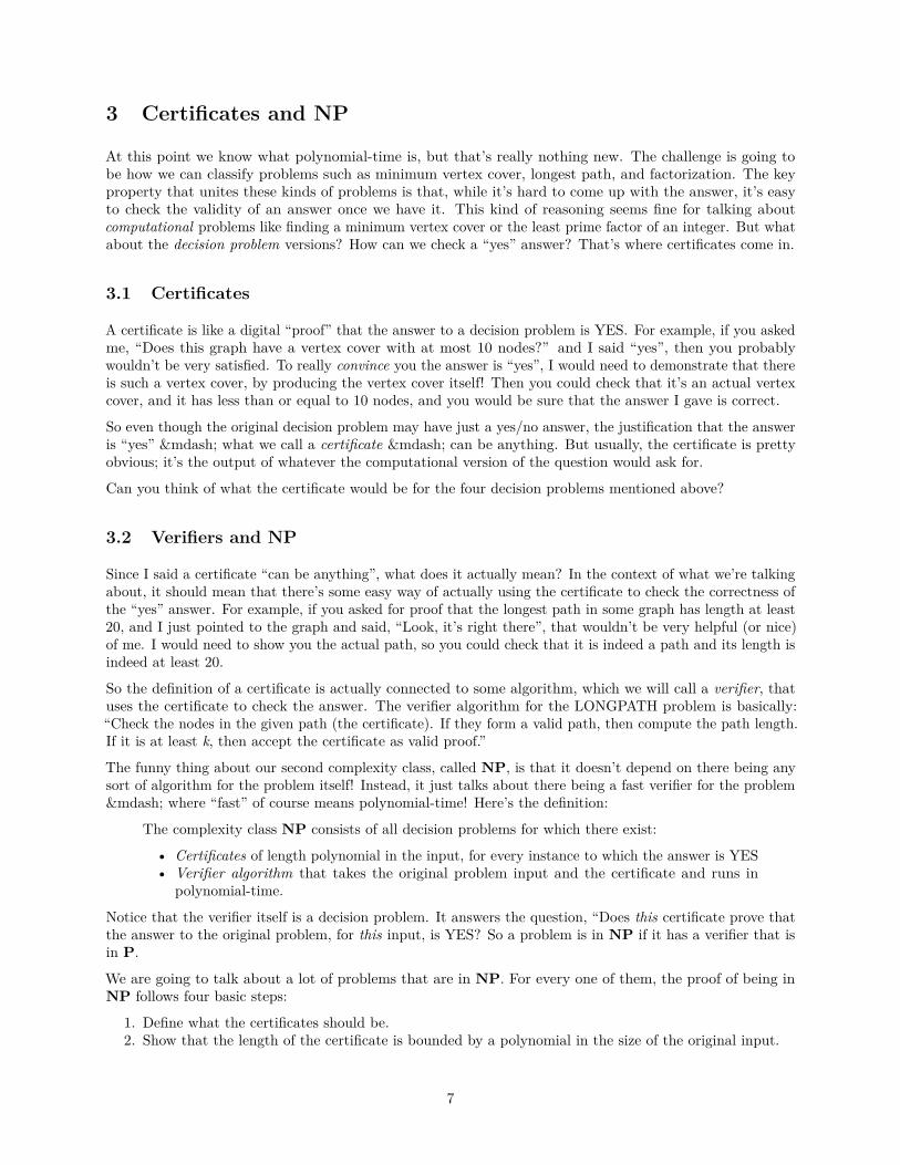
The funny thing about our second complexity class, called NP, is that it doesn’t depend on there being anysort of algorithm for the problem itself! Instead, it just talks about there being a fast verifier for the problem— where “fast” of course means polynomial-time! Here’s the definition:

The complexity class NP consists of all decision problems for which there exist:

• Certificates of length polynomial in the input, for every instance to which the answer is YES• Verifier algorithm that takes the original problem input and the certificate and runs in

polynomial-time.

Notice that the verifier itself is a decision problem. It answers the question, “Does this certificate prove thatthe answer to the original problem, for this input, is YES? So a problem is in NP if it has a verifier that isin P.

We are going to talk about a lot of problems that are in NP. For every one of them, the proof of being inNP follows four basic steps:

1. Define what the certificates should be.2. Show that the length of the certificate is bounded by a polynomial in the size of the original input.

7

3. Present the verifier algorithm based on what the certificates are.4. Analyze the verifier algorithm and show that it is polynomial-time.

For example, here is a proof that the minimum vertex cover problem is in NP.

Theorem: The problem VC(G,k) is in NP.

Proof : First we have to define the certificates. The certificate that the answer is YES will be avertex cover of size at most k. This will be stored as a list of node names, for the nodes that arein the vertex cover.

The vertex cover contains at most |V | nodes, since that’s how many nodes are in the originalgraph. So the size of the certificate is never more than the size of the original input graph G.Therefore the size is O(n) (remember n means the bit-length of the original input), which is apolynomial in n.

The verifier algorithm works as follows: For every edge in the graph G, go through every node inthe vertex cover (the certificate), and check that one of the endpoints of the graph is in the vertexcover. If not, then return NO. If every edge of the graph is covered in this way, then check thesize of the vertex cover. If the size is more than k, then return NO. Otherwise return YES.

The input graph is an adjacency list, so it takes O(|V |2) = O(n) time to go through every edge inthe graph. For each edge, we have to compare its endpoints to every vertex in the cover, whichcan have size at most |V |. This gives a total cost of O(|V |3), which is O(n1.5). The final loop tocheck the size of the cover is O(n) as well, so the whole verifier algorithm is polynomial-time.

See how the four steps are followed? The only thing that’s a little odd is that I described the verifier algorithmin words instead of writing out pseudocode. This is fine for such a simple one, but for more complicated NPproofs, you probably want to right out the verifier algorithm in pseudocode, to make sure everything is clear.

By the way, how does this compare to the class P? Well let’s say I have a problem that’s in P, likeSHORTPATH(G,u,v,k). This means that there’s some algorithm to solve this problem that runs in polynomial-time. But can we verify a YES answer in polynomial-time? The answer is, of course! The certificate canactually be empty, and the verifier is the original algorithm that solves the problem. Since we can alreadyanswer the problem in polynomial-time, we don’t need any “help” (in the form of a certificate) to show thatthe problem is in NP. This is a bit like my “unhelpful” answer above of “just look at the graph”. Whenthe problem is in P, we can “verify” an answer in polynomial-time by just computing it. This proves that,mathematically, P is a subset of NP.

The big question is whether P is actually equal to NP or not. And by “big question”, I mean “the biggest,baddest, most important question in the history of computer science”. This is not just my opinion, and it’snot an exaggeration. In fact, if you can answer this question, the Clay Institute will give you a million dollars.Seriously. The reasons why this question is so important will become clearer as we move along.

3.3 Alternate definition of NP

You know that P stands for “polynomial-time”, but what does NP stand for? A common — andTOTALLY INCORRECT — misconception is that it stands for “not polynomial”.

Actually what it stands for is “nondeterministic polynomial-time”. This is an alternate definition of the class.Now you should recognize the term nondeterministic from Theory class. The difference between a DFA andan NDFA is that the NDFA can sort of take multiple computational paths in processing any given string,and as long as at least one of those paths ends up in an accepting state, the string is accepted.

Nondeterministic computing is like that, except applied to more powerful machines than DFAs. The originaldefinition corresponds to a nondeterministic Turning machine, which is like a regular Turning machine, exceptthere can be many transitions out of every state. Again as long as one computational path ends up in anaccepting state, the string is accepted.

8

In more general computing the way we usually think of it, a “nondeterministic machine” can make yes/no“guesses” at any point and branch based on that guess, like an “if” statement whose conditional is just anarbitrary guess. The true answer is YES as long as there is at least one sequence of “guesses” that makes theprogram output YES.

And now hopefully you see the connection to our definition of NP using certificates: the certificate can bethought of as the series of guesses, or the sequence of Turing-machine transitions, that ends in a YES outputor an accepting state. The verifier is just the non-deterministic algorithm, executed deterministically usingthe certificate’s information.

So what the famous “P vs NP” problem really boils down to is whether having a nondeterministic machinethat could magically make correct guesses all the time actually makes some problems easier to solve or not.Since such a machine doesn’t actually exist, it’s easy to think that the answer is “of course it makes someproblems easier”. In fact this is what most computer scientists suspect, that P is actually not equal to NP.But none of us can prove it yet, unfortunately!

4 Reductions

Great, so we know what P and NP are. And we know that everyone suspects there are some problems inNP that are not in P, but they can’t prove it yet. So what can we say about these classes? Remember thatreductions are a tool that allowed us to compare problems without having any particular algorithm for theproblem. With some really clever reductions, we’ll be able to say quite a bit about P versus NP. But firstwe need to be a little more precise about what a reduction is and how to analyze it.

A reduction from problem A to problem B is an algorithm that solves problem A by using anyalgorithm for problem B as a subroutine.

The terminology is confusing, even to me after seeing it for a number of years. But I’ve been told that otherpeople don’t get confused by the reduction terminology, so maybe it will seem more natural to you. Thepoint is, always remember:

• What you’re reducing from because this is the problem you’re actually solving — you take theinput for that problem and produce the output for that problem.

• What you’re reducing to is the problem that you use as a subroutine. You will be creating input(s) forthis problem, and using output(s) from it.

Also keep in mind the core meaning of a reduction: it’s comparing the difficulty of the two problems. Areduction from problem A to problem B shows that (in some sense) problem B is at least as difficult asproblem A.

4.1 Example: Matrix Multiplication

Let’s look at a concrete example: matrix multiplication versus squaring. The matrix multiplication problem,MMUL(A,B) is, given two square matrices, compute their matrix product AB. The matrix squaring problem,MSQR(A) is, given a single square matrix, compute its square A2.

We want to reduce these problems to each other. That means solving each problem with the other one. Here’show that is done:

• MSQR reduces to MMUL.

Usually one direction of a reduction will be fairly easy or straightforward. For these two problems, thisis the straightforward direction, reducing squaring to multiplication.

Remember that a reduction is an algorithm to solve one problem using the other. So we want analgorithm for the MSQR(A) problem that will use MMUL as a subroutine.

9

This algorithm just has a single step: compute MMUL(A,A) and return the result. This result will beA ·A = A2, so the reduction is correct.

• MMUL reduces to MSQR.

This one is a little trickier, and maybe not obvious. How can we do matrix multiplication, just bysquaring matrices? One way to think about this that I find to be useful is, how can I “trick” analgorithm for one problem to solve the other? That is, imagine I have a stubborn assistant who willonly square matrices for me, but I want to multiply two different matrices. How can I trick my assistantinto doing my job?

The way to “trick” the assistant is to somehow embed one problem in the other one. This is usuallywhere some ingenuity comes into play. For this particular problem, the reduction works in three steps.Remember that this is an algorithm to solve MMUL(A,B), so the input is the two matrices A and B,and the output should be their product.

1. Compute matrix C as follows:

C =[

0 AB 0

]2. Compute matrix D as the result of SQR(C)

3. Return the top-left quarter of D.

The reason this works is because of the following mathematical equation:

[0 AB 0

]·[

0 AB 0

]=

[AB 00 BA

]Now the details of the math are I think really fascinating, but not particularly important to understand.The main point is that we managed to embed the multiplication problem into an input to the squaringalgorithm, so that any algorithm for squaring could be used to solve multiplication.

Now the question is, so what? What have we actually shown? What this demonstrates is that, if we had analgorithm to solve MMUL in say f(n) time, then we would have an algorithm to solve MSQR in O(f(n))time as well. And if we had an algorithm to solve MSQR in say g(n) time, then the second reduction wouldproduce an algorithm for MMUL that uses O(g(n)) time. In other words, these two problems are equivalentup to a constant factor; the inherent difficulty of both problems is essentially the same.

Of course, this is a very restricted kind of equivalence, where any algorithm for one problem gives an algorithmfor the other with exactly the same asymptotic cost. This kind of equivalence between completely differentproblems is actually quite rare. What kind of a definition of equivalence would make sense to answer ourbig tractable-versus-intractable questions? To answer this, we have to look a little more carefully at thereductions themselves.

4.2 Analyzing Reductions

Now we have a pretty good idea of what a reduction is, but can you see how the loose definitions so far can beabused? What about an algorithm that say, reduces integer factorization to integer division, by trying everypossible factor and testing divisibility? This is a plausible reduction, but certainly we wouldn’t conclude thatfactorization is easier than integer division. If it were, the RSA algorithm would be in a lot of trouble!

The issue here is how to analyze the efficiency of a reduction. There are three places we have to look at forthis. Supposing that we are reducing problem A to problem B, we must examine:

• The number of times an algorithm for problem B is called• The size of each input created for problem B

10

• The amount of extra work besides calling the problem B algorithm

If each one of these three parts is bounded by O(nk) for some constant k, and where n is the input size of theoriginal input to problem A, then this is called a polynomial-time reduction. If there is such a reductionfrom A to B, then we write A ≤P B.

Now observe what this means for our big classification of problems as tractable or intractable:

Theorem: If A reduces to B in polynomial-time, and B is in P, then A is in P as well.

Proof : What does it mean for A to reduce to B in polynomial-time? From the definition above,it means that there are three constants k1, k2, k3 such that A calls the algorithm for B O(nk1)times, each on inputs whose size is O(nk2), and does O(nk3) amount of extra work.

And if B is in P, this means B can be solved in O(n`) time for some other constant `. And noticethat this is NOT the same n as above! This n is the size of the input to B.

So what to we get when we put this together? The cost of the reduction, using the O(n`) algorithmfor B, is in total

O(nk1(nk2)` + nk3)

What an ugly formula! But what can we say about it? It’s just the multiplication, addition, andcomposition of some polynomials. Therefore it’s another polynomial! And thus A is also in P.

Actually the contra-positive of the above theorem is even more useful in many situations:

Corollary: If A ≤P B, and A is not in P, then B is not in P either.

So you see, polynomial-time reductions are exactly the tool we need to compare programs in terms of tractableversus intractable.

4.3 A polynomial-time reduction

Ready for an example? First we need to add a couple more problems to our repertoire:

Minimum hitting set: HITSET(L,k)

Input: List L of sets S1, S2, . . . , Sm, and an integer k

Output: Is there a set H with size at most k such that every Si ∩H is not empty?

This is like asking for a list of representatives to cover every group in a list. For example, maybe each of thesets Si represents a certain muscle group, and the elements in each set represent some different exercises thatworks that muscle group. Then the question asks whether we can construct a complete workout (to workevery muscle group) using only k different exercises.

Hamiltonian Cycle: HAMCYCLE(G)

Input: Graph G = (V, E)

Output: Does G have a cycle that goes through every vertex exactly once?

A cycle that goes around the entire graph, traveling through every vertex exactly once, is called a Hamiltoniancycle or sometimes a Rudrata cycle. This decision problem is just asking whether such a cycle exists in agiven graph.

Now for our first “real” polynomial-time reduction, from HAMCYCLE to LONGPATH. The key thing toobserve here is that we don’t have any good algorithms to solve either problem. This is the first reductionbetween two problems that both seem to be difficult in general.

11

Theorem: HAMCYCLE(G) ≤P LONGPATH(G,u,v,k)

Proof : To do this reduction, we need to consider any input to the HAMCYCLE problem, andshow how to solve HAMCYCLE by using some algorithm for LONGPATH. Here’s the algorithmto do that, given a graph G:

def HAMCYCLE(G) :n = G. nfor (u , v ) in G. edges ( ) :

newE = l i s t (G. edges ( ) )newE . remove ( ( u , v ) )H = ALGraph(G.V, newE)# H = G with (u , v ) removedi f LONGPATH(H, v , u , n−1) == "YES" :

return "YES"return "NO"

The first thing we need to show is that this reduction is correct. First, if the reduction algorithmoutputs YES, then there really is a Hamiltonian cycle in the graph. The reason is that, since thecall to LONGPATH returned YES, then there must be a path with |V | − 1 edges that goes fromv to u and doesn’t include edge (u, v). So now if I add that edge from u to v that was removed,I have a path from u to v and then back to u — that is, a cycle! And this cycle musthit every vertex exactly once, since its length is |V |. Therefore it’s a Hamiltonian cycle, and thereduction works correctly in this case.

But it’s still possible that the reduction doesn’t “catch” every Hamiltonian cycle. To see whyit does, say there is a Hamiltonian cycle in the graph G. Then this cycle contains many edges;say one of those edges is (u, v). This edge will be examined in the for loop, and when it is, wewill discover there is indeed a LONGPATH from v back to u, which is just the Hamiltonian cycleminus that one edge. Therefore the reduction gives the correct output in every case.

We now know that this is a correct reduction, but is it polynomial-time? Recall that there arethree parts to examine for this:

• The number of time LONGPATH is called is exactly the number of edges in G, which is |E|and is less than the size of the input.

• The size of each input created for the call to LONGPATH is the same as the original inputG, with one edge removed. So this is also less than the size of the original input.

• The amount of extra work besides calling the LONGPATH algorithm. The only real “work”performed by the reduction is in removing each edge from the original graph G. This couldbe accomplished by just copying the whole adjacency matrix and setting that one edge toinfinity. The cost would be O(|V |2) for every step, for a total cost of O(|E| · |V |2). Thereare probably more clever ways to do this, but this is certainly polynomial-time in the size ofthe input, so that’s good enough!

All in all, we have shown the reduction algorithm, shown why it’s correct, and why it’s polynomial-time. Therefore the statement of the theorem is proved. QED.

Now remember what this means: any fast algorithm for LONGPATH would immediately give us a fastalgorithm for HAMCYCLE. But we don’t have any algorithm for either one, so what good is this? Well whatif we knew that the HAMCYCLE problem was difficult? Then the LONGPATH problem must be difficulttoo! Take a moment to wrap your head around this idea.

12

5 NP-Completeness

Imagine the Fairy Godmother of Algorithms visits you. She will give you a fast algorithm for any problemthat you like; you get to pick the problem. So what problem would you pick?

You might like to have an algorithm for integer factorization, so you could crack everyone’s encrypted messages.But then there are other crypto schemes that are based on other hard problems. And of course there arehard problems we want to solve that have nothing to do with security as well!

Well how about a problem that could solve every other problem? This is a little like wishing for more wishes.Well. . .

5.1 Halting problem

Recall from Theory that the Halting Problem is, given a program P and an input I for that program, determinewhether P halts on input I in any finite amount of time.

I claim that an algorithm to solve the halting problem can solve any other problem that’s in NP. How couldI prove such a thing? With a reduction of course! But this will be a special kind of reduction — onethat takes ANY problem in NP and reduces it to the halting problem.

Say we have some problem, call it PROB, that’s in NP. We want to reduce it to the halting problem. Theonly thing we really know about PROB is that it is in NP, so we have to use the definition of NP in orderto start the reduction.

This definition tells us two things about PROB: for every instance that should produce a “YES” answer,there is a polynomial-size certificate, and there is also a polynomial-time verifier that checks the validity of agiven certificate for a given input.

Knowing only this information about PROB, how could you solve it? Well, for some input instance I forPROB, we know that the answer to PROB(I) is “YES” if and only if there is some certificate C such thatthe verifier returns YES when you give it both I and C. This gives a basic sort of approach to solving PROB:

for every p o s s i b l e c e r t i f i c a t e C:i f v e r i f i e r ( I ,C) == "YES" :

return "YES"return "NO"

Now it seems odd to say that we could generate every possible certificate C, when we don’t know if thecertificates should be vertices, or integers, or paths, or something completely different, since we don’t reallyknow what PROB is all about. But remember that everything is just bits, so every certificate is just somestring of bits. Therefore the for loop above can be implemented by simply trying every possible sequence ofbits in some order: maybe something like 0, 1, 00, 01, 10, 11, 000, 001, 010, . . . you get the idea.

This is basically the guess-and-check strategy that we have said categorizes all NP problems: try everypossible answer (certificate), and check each one until you get a “hit”. If the answer to PROB(I) is “YES”,then this will eventually be returned by the algorithm. But what happens otherwise? An infinite loop! If theanswer to PROB(I) is “NO”, then the verifier will just keep returning NO for longer and longer certificates.

In summary: we have an algorithm that eventually returns “YES” if the real answer is “YES”, and otherwiseruns forever, and we want to figure out which is the case for some particular input. Hopefully a light bulb isgoing off in your head right now: This is exactly what the Halting problem can do for us!

Formally, then, the reduction from PROB to the Halting problem works by using the verifier for PROB(which must exist since PROB is in NP), and plugging the verifier into the algorithm above to make aprogram. Then we give this program to the Halting problem, with the given input, and say “Does this halt?”If so, then the answer is “YES”, and otherwise the answer is “NO”.

13

In other words, given any input to any problem that is in NP, we can use an algorithm for the Haltingproblem to answer the problem for that input. This means that VC ≤P HALTING, LONGPATH ≤P HALTING,SHORTPATH ≤P HALTING, we could go on and on.

5.2 Nomenclature

Since a reduction from A to B means that B is at least as hard as problem A, the result above showed thatthe Halting problem is at least as hard as EVERY problem in NP. There’s actually a name for this sort ofthing:

A problem B is NP-hard if every problem in NP is polynomial-time reducible to B.

Therefore, from the previous subsection:

Theorem: The Halting problem is NP-hard.

The awesomeness of the previous subsection notwithstanding, this isn’t actually too surprising when it comesto the Halting problem. You know from theory that HALTING is actually *undecidable‘, meaning it can’tbe solved by any computer in any finite amount of time. So it should come as no surprise that it’s at least asdifficult as problems like minimum vertex cover and integer factorization which, while seemingly difficult, cancertainly be solved if given enough time.

What would be really awesome if some problem that is in the class NP were also NP-hard. Then we couldsay that this is really the “hardest problem” in the class NP. Well there’s a name for this too:

A problem B is NP-complete if B is in NP and B is NP-hard.

So, any guesses on an NP-complete problem, the hardest problem in the land of NP?

5.3 CIRCUIT-SAT

Time to define a new problem:

Circuit Satisfiability Problem: CIRCUIT−SAT(C)

Input: Boolean logic circuit C with multiple inputs, one output, and any number of AND, OR,and NOT gates, connected with wires.

Output: Is there any setting of the inputs that will make the output “true”?

We want to figure out how hard this problem is. First thing we might ask: can you think of any polynomial-timealgorithm to solve it?

Hmm, I can’t. But what we can do is pretty exciting: we can prove this problem is NP-complete. This isquite a long and complicated proof, but you should be able to follow each part. The proof will proceed as aseries of “claims”, and then an informal proof of each claim.

First claim: CIRCUIT-SAT is in NP. A certificate for a “YES” answer will just be a setting of each ofthe inputs to true or false. The size of this certificate is just the number of inputs, which is certainly less thanthe size of the whole circuit. Then the verifier just has to simulate the circuit and check whether the outputis true. This means simulating the logic of every gate in sequence until we get to the output. Constant-timefor every gate means polynomial-time in the total number of gates, which is the size of the input. ThereforeCIRCUIT−SAT is in NP.

OK, nothing new so far. But what we want to do now is prove that CIRCUIT−SAT is NP-hard, like weproved for the Halting problem above. The basic approach is going to be to turn the verifier for any problemin NP into a polynomial-size boolean circuit, then run CIRCUIT−SAT on that verifier circuit to see if there’sany certificate that verifies the given input, thereby telling us if the real answer to the problem is “YES” or“NO”.

14

Second claim: Polynomial-time programs use polynomial-space. Suppose some program runs inpolynomial-time O(nk). In the worst case, this program might do nothing at all but just access memory.Since it can only access a fixed number of memory locations for every primitive operation it performs, thetotal space usage of the program is also at most O(nk).

Third claim: Any YES/NO program can be modeled by a boolean circuit. Think back to yourArchitecture class. You learned that the CPU in every computer you have ever used is essentially the samething: a big sequential logic circuit. It’s built from a bunch of pieces that look like this:

Figure 1: Sequential circuit

The combinational circuitry here is everything in the CPU that gets executed at each step: MUXes, ALUs,adders, shifters, and control logic. All these things are constructed out of simple AND, OR, and NOT gates.At each step of the program, the boolean values for the current state are run through this combinationalcircuit to produce the boolean values for the next state.

Each “state” consists of all the storage that is used to control the program: registers, program counter, andmain memory. We can represent all these things with wires that are true or false. The initial state will bethe initial settings of things like the program counter, plus the input to the program. The final state willcontain a single boolean value that contains the YES/NO output of the program.

Now for a particular input, the program will proceed through some finite number of steps. So we could writeout a single circuit (with no feedback loops) for the ENTIRE program just by pasting together a bunch ofcopies of the combinational circuit, corresponding to the total number of steps in the program. This circuitwill be pretty big, yes, but its behavior will correspond exactly to the original program.

Fourth claim: Any polynomial-time YES/NO program can be modeled by a polynomial-sizeboolean circuit. We have to use the previous two claims. From the second claim, the total storage spaceused by any polynomial-time program is polynomial-time. Therefore the size of the “state” in each part ofthe circuit is polynomial in the size n of the actual input to the program.

Now since the combinational part of each piece of the circuit has polynomial-size in the size of the state, andsince polynomials are closed under composition, the size of each combinatorial part is also a polynomial inthe size of the original input.

Finally, the total number of parts in the circuit corresponds to the number of steps in the program, which ispolynomial-time. Since polynomials are closed under multiplication, the total size of this circuit is STILL a(very big) polynomial in the size of the input to the program itself.

Fifth claim: CIRCUIT-SAT is NP-hard. Take any problem PROB in NP. It must have a polynomial-time verifier algorithm, which takes as input the original problem instance and a polynomial-size certificate,and answers “YES” if the certificate is a valid proof that the original problem’s answer is “YES” on thatinput. From the last claim, we can take this verifier algorithm, and any input I for PROB, and construct apolynomial-size boolean circuit that will check any certificate against the input I.

Now if we hard-wire I into this circuit, and make the only “inputs” of the circuit the bits of the certificate,then we have a circuit that is satisfiable if and only if there is some polynomial-size certificate which verifiesa “YES” answer for PROB(I). Now give this big (but still polynomial-size!) circuit to any algorithm thatsolves the CIRCUIT−SAT problem. If the circuit is satisfiable, then there is a certificate for I and PROB(I)is “YES”; otherwise PROB(I) is “NO”.

Since this reduction is polynomial-time, CIRCUIT−SAT can be used to solve any problem that is in NP.

Theorem: CIRCUIT−SAT is NP-Complete.

15

Proof : The first and last claims give us all that we need: CIRCUIT−SAT is in NP, and it isalso NP-hard.

5.4 Implications of NP-Completeness

Something truly amazing has happened here. What we have shown is that the CIRCUIT−SAT problem is,in a very precise sense, the hardest problem in NP. Unfortunately this doesn’t resolve the P vs NP question— we aren’t millionaires yet. But it does give us two really important implications:

• If P 6= NP, then CIRCUIT−SAT is not in P. Since CIRCUIT−SAT is the hardest problem in NP, ifthere’s any problem in NP that can’t be solved in polynomial-time, CIRCUIT-SAT must be it.

• If CIRCUIT−SAT is in P, then P = NP. This is just the contrapositive of the statement above.

In other words, the whole grand question of P vs NP boils down to a simple question: can you solveCIRCUIT−SAT in polynomial-time? If you come up with an answer, in either direction, you get a millionbucks (and everlasting fame, and groupies, and job offers, etc.).

6 More NP-Complete Problems

The best part about our awesome and impressive NP-hard proof for CIRCUIT SAT is. . . we’ll never haveto do it again! To prove a new problem is NP-hard, I can just give a reduction from CIRCUIT−SAT, ratherthan having to have a reduction from every problem in NP. Since CIRCUIT−SAT is NP-complete, anyother problem is NP-hard if and only if it can be used to solve CIRCUIT−SAT!

As we move on, we’ll be proving more and more problems are NP-complete. So the basic task in provingsome new problem is NP-hard is just to give a reduction from any known NP-complete problem. As we findmore and more NP-complete problems, the task gets easier and easier.

6.1 3-SAT

The 3−SAT problem is all about boolean formulas — those that can be written with variables (Trueor False) and the operators AND (∧), OR (∨), and NOT (¬).

And 3−SAT isn’t about just any boolean formula, it’s about those that can be written as a “conjunctionof disjunctions”, a.k.a. “product of sums”, a.k.a. “conjunctive normal form (CNF)”. Let’s break this down.Don’t worry, it’s not too complicated.

A variable in a boolean formula is just like any other variable, except that it can only stand for True or False.We’ll write variables as lowercase letters like x or y.

A literal is either a single variable, or the negation of a single variable. So x and ¬x and y and ¬y are allliterals.

A clause is a “disjunction of literals”, i.e., a whole bunch of literals OR’ed with each other. So (x∨ y ∨¬x) isan example of a clause with 3 literals.

FINALLY, a CNF formula is a “conjunction of clauses”, i.e., a whole bunch of clauses AND’ed with eachother. For example, here is a CNF boolean formula:

(¬x ∨ y ∨ z) ∧ (x ∨ y ∨ ¬x) ∧ (¬y ∨ y ∨ ¬z)

This formula is also special because every clause has at most 3 literals in it. This is exactly the kind offormula that 3−SAT is about:

16

Boolean Satisfiability Problem: 3−SAT(F)

Input: CNF boolean formula F with at most three literals in every clause

Output: Does F have a “satisfying assignment”, i.e., a setting of every variable to True or Falsethat makes the whole formula True?

For the example CNF formula above, one satisfying assignment is x=True, y=False, and z=True. You canconfirm that each clause evaluates to True with these settings, which makes the whole formula True.

Now how could we prove 3−SAT is NP-complete? As always, there are two steps.

First we must prove that 3−SAT is in NP. This also involves two parts: polynomial-size certificates, anda polynomial-time verifier. Both of these should feel pretty obvious to you at this point: the certificate isa single “satisfying assignment” of the variables, and the verifier plugs in the assignment specified by thecertificate, and computes the value of the entire formula, confirming that it is True.

Now the tricky part of proving 3−SAT is NP-complete will be to prove that it is NP-hard. We will dothis by showing a reduction from CIRCUIT−SAT, our only known NP-complete problem at this point. Ina nutshell, this means taking any input to the CIRCUIT−SAT problem (a boolean circuit), and solvingCIRCUIT−SAT for that input by using 3−SAT as a subroutine.

The reduction will work by transforming any given boolean circuit into a CNF formula (with at most threeliterals per clause), such that the original circuit is satisfiable if and only if the formula has a satisfyingassignment.

The first step to doing this is: every wire in the circuit becomes a variable in the formula. By “wire”I mean: the original inputs to the circuit, and the outputs of every gate in the circuit. We can just numberall these wires 1, 2, 3, . . . , and then call the variables x1, x2, x3, . . .. We saw an example in class of how thislooks on an example circuit.

Now the original circuit satisfiability question is just asking whether there is an assignment of True/False toall these variables such that:

• All the gates work correctly. (Output wire from each gate is correctly set according to the input wiresto that gate.)

• The output wire of the whole circuit is set to “True”.

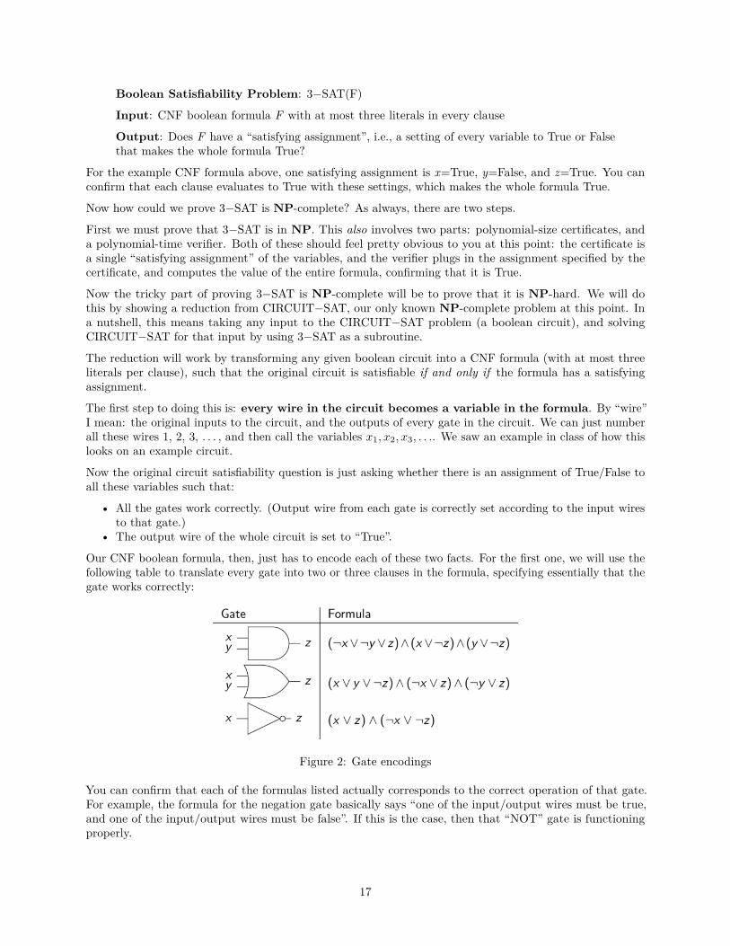
Our CNF boolean formula, then, just has to encode each of these two facts. For the first one, we will use thefollowing table to translate every gate into two or three clauses in the formula, specifying essentially that thegate works correctly:

Figure 2: Gate encodings

You can confirm that each of the formulas listed actually corresponds to the correct operation of that gate.For example, the formula for the negation gate basically says “one of the input/output wires must be true,and one of the input/output wires must be false”. If this is the case, then that “NOT” gate is functioningproperly.

17

We use these formula translations for every gate in the original circuit, then combine them all together withAND’s to get one big CNF formula. But notice that every clause only has at most three literals, and the totalnumber of clauses is at most 3 times the number of gates in the circuit. So the formula has polynomial-size inthe size of the original input circuit. That’s important!

The only missing piece of the formula now is the second point above: we have to ensure that the output wirefrom the entire circuit is set to “True”. This is easy to do: just add one more clause that looks like (x), wherex is the name of the wire for the output from the circuit. Then the whole formula is satisfiable if and only if(1) all the gates are functioning properly, and (2) the output from the circuit is True. Therefore this CNFformula has a satisfying assignment if and only if the original circuit is satisfiable. That’s the reduction!

Here’s an summary of the reduction that we just did:

1. Take any circuit C on which we want to solve CIRCUIT−SAT2. Number all the “wires” in C, and make variables for them3. Convert C into an equivalent CNF formula F using the rules in the table above, plus one more clause

for the output wire4. Feed F into any algorithm that solves 3−SAT5. Return the answer to 3−SAT(F) — it’s the same as the answer to CIRCUIT−SAT(C).

Since this reduction works in polynomial-time, we conclude that

Lemma: CIRCUIT−SAT ≤P 3−SAT

Now, since we already know CIRCUIT−SAT can be used to solve any problem in NP, and 3−SAT can beused to solve any CIRCUIT−SAT problem, 3−SAT can also be used in a round-about way to solve anyproblem in NP! Since we also proved that 3−SAT is in NP, this means that

Theorem: 3−SAT is NP-complete.

Awesome! Hopefully you agree that this was much easier than the last reduction, from any NP problem toCIRCUIT−SAT. And now that we know two NP-complete problems, we can use either one as the basis forour next NP-hard proof!

6.2 Vertex Cover

Time for a really surprising reduction. We want to prove that VC is hard, but all we know about so farare these two problems about the satisfiability of circuits and boolean formulas. As it turns out, there is aconnection from the seemingly unrelated problem of 3−SAT to VC. Here is the reduction:

3−SAT−to−VC(F)

Input: Boolean formula F in CNF form with three literals per clause (input to a 3−SAT problem).

Output: Is there a satisfying assignment for the variables in F?

1. Create an empty graph G.2. For each variable xi that appears in F, create two nodes labeled xi and ¬xi, with an edge

between them, and add the two nodes and one edge to G3. For each clause (L1 ∨ L2 ∨ L3) in F, create a “triangle” of three nodes L1, L2, and L3, with

three edges connecting them. (Remember that each “literal” Li is either a variable xi or thenegation of a variable ¬x1.) Add the three nodes and three edges to G.

4. Add additional edges between every node in each triangle to the node with the same label inthe original pairings, to G.

5. Return VC(G, v + 2c), where v is the number of variables and c is the number of clauses in G.

Here’s why this works. Each of the edges in the original pairings must have at least one endpoint vertex in thecover: these v vertices correspond to the satisfying assignment of the variables. Each triangle must have atleast two of its vertices in the cover: these 2c vertices correspond to the 2 literals in each clause that could befalse. The third literal in each clause — the one that must be true — corresponds to the vertex

18

in the triangle that is not in the cover. Its edge to the vertex in the matching must be covered by that vertexin matching. This corresponds to saying that literal is true because of that variable’s setting in the satisfyingassignment. So a satisfying assignment exists if and only if there is a vertex cover of size v + 2c. Awesome!

I acknowledge that this is a difficult reduction. Reviewing the pictures we drew on the board in class wouldbe helpful. But the important point to remember is that we can have reductions between seemingly unrelatedproblems. And the payoff is sweet: now we know that VC is NP-hard! Since we already proved it was inNP, we actually know that it is NP-complete. Another “hardest problem in NP”!

6.3 More NP-Complete Problems

This process can, and has, continued to show a whole bunch of problems are NP-complete. In fact, Wikipediaclaims that there are thousands of them — all of them of course being the “hardest problem in NP”.

And this is actually a good thing! It means that, to show a new problem is NP-hard, all we have to do iscome up with a reduction from some known NP-complete problem to the new problem. This is a mucheasier task than the very first NP-hard proof for CIRCUIT−SAT, and as we learn about more and moreNP-complete problems, the chances that any new problem we see is related to one of them should increase.

The NP-complete problems we have looked at so far are:

• LONGPATH• VC• HITSET• HAMCYCLE• CIRCUIT−SAT• 3−SAT• SPLIT−EVENLY

Notice something missing? It’s FACT, the integer factorization problem that was one of our originalmotivations for studying the inherent difficulty of problems. The basic issue with FACT is that, unlike allthe examples above, it’s easy to verify both “YES” and “NO” answers to FACT. The certificate for eitherone would just be a list of the prime factors of the input integer N. This means FACT is not only in NP butalso in another complexity class called coNP, and the fact that FACT is in both of these makes it extremelyunlikely to be NP-complete. In any case, most researchers still don’t believe the problem is solvable inpolynomial-time, but it is classified as an “NP-intermediate” problem, somewhere in the ether between Pand NP.

7 Hardness of TSP

Remember the Traveling Salesman problem from before?

Traveling Salesman Problem: TSP(G)

Input: Weighted graph G

Output: Least-weight cycle in G that goes through every vertex exactly once.

We came up with some approaches to tackle this in the last unit, but none of the algorithms there were bothoptimal and polynomial-time. Now we have a good guess as to why - TSP is NP-Hard! Here’s a proof.

Theorem: TSP is NP-Hard

Proof.

This is a “specific-to-general” reduction, where we show a reduction from a specific case to amore general problem. Hopefully the problem we will reduce from is fairly obvious: HAMCYCLE.Here is an algorithm to solve HAMCYCLE using TSP:

19

1. Take the input graph to HAMCYCLE, and make it weighted by setting every edge to weight1.

2. Run TSP on the weighted graph. The TSP returns a Hamiltonian cycle, if there is one.

Therefore HAMCYCLE ≤P TSP. Since HAMCYCLE is a known NP-complete problem, thenTSP must be NP-hard.

The important take-away here is that there are ways to deal with NP-hard problems, as we saw in the lastunit. Many of the approaches we saw for TSP and for VC (greedy algorithms, constant-factor approximation,branch and bound, etc.) can be applied to many NP-hard problems to find solutions that are pretty good, orto usually find the optimal solution quickly.

There are excellent software packages available not only to solve TSP but also other NP-Hard problems,including SAT solving. Proving a problem is NP-Hard doesn’t mean it’s time to give up, it just means that afast, always-correct solution is out of reach, so you better start compromising somehow!

20