Complexity-effective superscalar embedded processors using ...
Upload
khangminh22Category
view
0download
0
The Complexity of Digraph Homomorphisms:Local Tournaments, Injective Homomorphisms and
Polymorphisms
by
Jacobus S. SwartsBEng, Rand Afrikaans University, 1995MEng, Rand Afrikaans University, 1999BSc, Rand Afrikaans University, 2000MSc, Rand Afrikaans University, 2001
A Dissertation Submitted in Partial Fulfillment of theRequirements for the Degree of
Doctor of Philosophy
in the Department of Mathematics and Statistics
c© Jacobus S. Swarts, 2008
University of Victoria
All rights reserved. This dissertation may not be reproduced in whole or in part byphotocopy or other means, without the permission of the author.

ii
The Complexity of Digraph Homomorphisms:Local Tournaments, Injective Homomorphisms and
Polymorphisms
by
Jacobus S. SwartsBEng, Rand Afrikaans University, 1995MEng, Rand Afrikaans University, 1999BSc, Rand Afrikaans University, 2000MSc, Rand Afrikaans University, 2001
Supervisory Committee
Dr. G. MacGillivray, Supervisor (Department of Mathematics and Statistics)
Dr. C. M. Mynhardt, Member (Department of Mathematics and Statistics)
Dr. U. Stege, Outside Member (Department of Computer Science)

iii
Supervisory Committee
Dr. G. MacGillivray, Supervisor (Department of Mathematics and Statistics)
Dr. C. M. Mynhardt, Member (Department of Mathematics and Statistics)
Dr. U. Stege, Outside Member (Department of Computer Science)
Abstract
In this thesis we examine the computational complexity of certain digraph homo-morphism problems. A homomorphism between digraphs, denoted by f : G → H ,is a mapping from the vertices of G to the vertices of H such that the arcs of G arepreserved. The problem of deciding whether a homomorphism to a fixed digraph Hexists is known as the H-colouring problem.
We prove a generalization of a theorem due to Bang-Jensen, Hell and MacGillivray.Their theorem shows that for every semicomplete digraph H , H-colouring exhibitsa dichotomy: H-colouring is either polynomial time solvable or it is NP-complete.We show that the class of local tournaments also exhibit a dichotomy. The NP-completeness results are found using direct NP-completeness reductions, indicatorand vertex (and arc) sub-indicator constructions. The polynomial cases are handledby appealing to a result of Gutjhar, Woeginger and Welzl: the X-graft extension.We also provide a new proof of their result that follows directly from the consistencycheck. An unexpected result is the existence of unicyclic local tournaments withNP-complete homomorphism problems.
During the last decade a new approach to studying the complexity of digraphhomomorphism problems has emerged. This approach focuses attention on so-calledpolymorphisms as a measure of the complexity of a digraph homomorphism problem.For a digraph H , a polymorphism of arity k is a homomorphism f : Hk → H .
Certain special polymorphisms are conjectured to be the key to understandingH-colouring problems. These polymorphisms are known as weak near unanimityfunctions (WNUFs). A WNUF of arity k is a polymorphism f : Hk → H such thatf is idempotent and f(y, x, x, . . . , x) = f(x, y, x, . . . , x) = f(x, x, y, . . . , x) = · · · =f(x, x, x, . . . , y). We prove that a large class of polynomial time H-colouring problemsall have a WNUF. Furthermore we also prove some non-existence results for WNUFson certain digraphs. In proving these results, we develop a vertex (and arc) sub-indicator construction as well as an indicator construction in analogy with the onesdeveloped by Hell and Nesetril. This is then used to show that all tournaments withat least two cycles do not admit a WNUFk for k > 1. This furnishes a new proof (inthe case of tournaments) of the result by Bang-Jensen, Hell and MacGillivray referred

iv
to at the start. These results lend some support to the conjecture that WNUFs arethe “right” functions for measuring the complexity of H-colouring problems.
We also study a related notion, namely that of an injective homomorphism. Ahomomorphism f : G → H is injective if the restriction of f to the in-neighboursof every vertex in G is an injective mapping. In order to classify the complexityof these problems we develop an indicator construction that is suited to injectivehomomorphism problems.
For this type of digraph homomorphism problem we consider two cases: reflexiveand irreflexive targets. In the case of reflexive targets we are able to classify all in-jective homomorphism problems as either belonging to the class of polynomial timesolvable problems or as being NP-complete. Irreflexive targets pose more of a prob-lem. The problem lies with targets of maximum in-degree equal to two. Targets withmaximum in-degree one are polynomial, while targets with in-degree at least threeare NP-complete. There is a transformation from (ordinary) graph homomorphismproblems to injective, in-degree two, homomorphism problems (a reverse transforma-tion also exists). This transformation provides some explanation as to the difficultyof the in-degree two case. We nonetheless classify all injective homomorphisms toirreflexive tournaments as either being a problem in P or a problem in the class ofNP-complete problems. We also discuss some upper bounds on the injective orientedirreflexive (reflexive) chromatic number.

v
Table of Contents
Supervisory Committee ii
Abstract iii
Table of Contents v
List of Tables viii
List of Figures ix
List of Decision Problems xii
List of Algorithms xiii
Acknowledgements xiv
1 Introduction 1
1.1 A dichotomy for graph homomorphisms . . . . . . . . . . . . . . . . . 2
1.2 A sample of previous results . . . . . . . . . . . . . . . . . . . . . . . 4
1.3 A connection to constraint satisfaction problems . . . . . . . . . . . . 7
1.4 Indicator and Sub-indicator Constructions . . . . . . . . . . . . . . . 9

vi
1.5 Direct NP-completeness Reductions . . . . . . . . . . . . . . . . . . . 14
1.6 Polymorphisms . . . . . . . . . . . . . . . . . . . . . . . . . . . . . . 26
1.7 Injective Homomorphisms . . . . . . . . . . . . . . . . . . . . . . . . 30
2 The Complexity of Colouring by Local Tournaments 34
2.1 Introduction . . . . . . . . . . . . . . . . . . . . . . . . . . . . . . . . 34
2.2 Some Tools . . . . . . . . . . . . . . . . . . . . . . . . . . . . . . . . 35
2.3 Local Tournaments . . . . . . . . . . . . . . . . . . . . . . . . . . . . 41
2.4 Connected vs. Disconnected Local Tournaments . . . . . . . . . . . . 47
2.5 Road map . . . . . . . . . . . . . . . . . . . . . . . . . . . . . . . . . 48
2.6 Unicyclic Local Tournaments . . . . . . . . . . . . . . . . . . . . . . 50
2.7 Round Local Tournaments . . . . . . . . . . . . . . . . . . . . . . . . 61
2.8 Round Decomposable Local Tournaments . . . . . . . . . . . . . . . . 80
2.9 Non-Round Decomposable Local Tournaments . . . . . . . . . . . . . 89
2.10 The Dichotomy for Connected Local Tournaments . . . . . . . . . . . 93
3 Weak Near-Unanimity Functions 95
3.1 Introduction . . . . . . . . . . . . . . . . . . . . . . . . . . . . . . . . 95
3.2 Boosting the Arity . . . . . . . . . . . . . . . . . . . . . . . . . . . . 96
3.3 Polynomial Problems With WNUFs . . . . . . . . . . . . . . . . . . . 98
3.4 Some Non-existence Results for WNUFs . . . . . . . . . . . . . . . . 104
3.5 Indicators and Sub-indicators . . . . . . . . . . . . . . . . . . . . . . 109
3.6 Tournaments and WNUFs . . . . . . . . . . . . . . . . . . . . . . . . 113
4 Injective Homomorphisms 125
4.1 Introduction . . . . . . . . . . . . . . . . . . . . . . . . . . . . . . . . 125
4.2 Injective Indicator Construction . . . . . . . . . . . . . . . . . . . . . 126
4.3 Reflexive Targets . . . . . . . . . . . . . . . . . . . . . . . . . . . . . 127
4.4 Irreflexive Targets . . . . . . . . . . . . . . . . . . . . . . . . . . . . . 133

vii
4.5 Bounds on the Injective Oriented Chromatic Number . . . . . . . . . 145
4.6 Obstructions to Injective Oriented Reflexive Colouring . . . . . . . . 149
4.7 Injective Oriented Colourings on Trees . . . . . . . . . . . . . . . . . 151
5 Conclusions and Future Work 156
5.1 Local Tournaments . . . . . . . . . . . . . . . . . . . . . . . . . . . . 156
5.2 Complexity with Acyclic Inputs . . . . . . . . . . . . . . . . . . . . . 157
5.3 Weak Near Unanimity Functions . . . . . . . . . . . . . . . . . . . . 157
5.4 Injective Homomorphisms . . . . . . . . . . . . . . . . . . . . . . . . 158
References 159

viii
List of Tables
1.1 The kth out-neighbourhood of each vertex of H for 1 ≤ k ≤ 7. . . . . 12
1.2 Homomorphisms of the gadget G to H . . . . . . . . . . . . . . . . . . 20
2.1 Homomorphisms from K to T . . . . . . . . . . . . . . . . . . . . . . . 55
4.1 Some injective homomorphisms from I to the first three vertices of Pn. 129
4.2 Injective homomorphisms from P4 = abcde to T4. . . . . . . . . . . . 139

ix
List of Figures
1.1 A local tournament H for which the H-colouring problem is NP-
complete. . . . . . . . . . . . . . . . . . . . . . . . . . . . . . . . . . 11
1.2 The result, H∗, of applying the indicator I = P7 to the local tourna-
ment H . . . . . . . . . . . . . . . . . . . . . . . . . . . . . . . . . . . 11
1.3 An example of a round decomposable local tournament D. . . . . . . 14
1.4 The sequence of digraphs obtained in the proof of Proposition 1.4.5. . 15
1.5 The target H . . . . . . . . . . . . . . . . . . . . . . . . . . . . . . . . 19
1.6 The gadget F . . . . . . . . . . . . . . . . . . . . . . . . . . . . . . . . 19
1.7 The gadget G. . . . . . . . . . . . . . . . . . . . . . . . . . . . . . . . 20
1.8 The digraph D. . . . . . . . . . . . . . . . . . . . . . . . . . . . . . . 21
1.9 The graphs used in proving that OCN4 is NP-complete. . . . . . . . . 23
1.10 The oriented, acyclic graph D. . . . . . . . . . . . . . . . . . . . . . . 24
2.1 The structure of a strong locally semi-complete digraph that is not
semi-complete and not round decomposable. . . . . . . . . . . . . . . 44
2.2 The structure of a unicyclic local tournament that’s not a directed cycle. 51
2.3 The special unicyclic local tournament, LT5, on five vertices. . . . . . 53
2.4 The gadget K for unicyclic local tournaments. . . . . . . . . . . . . . 54

x
2.5 The first gadget G1 for the last unicyclic case. . . . . . . . . . . . . . 57
2.6 The second gadget G2 for the last unicyclic case. . . . . . . . . . . . . 57
2.7 The third gadget G3 for the last unicyclic case. . . . . . . . . . . . . 58
2.8 A typical clause in the instance D for the last unicyclic case. . . . . . 60
2.9 The first case where D has a unique cycle of shortest length . . . . . 62
2.10 The sub-indicator for the first case. . . . . . . . . . . . . . . . . . . . 63
2.11 The second case where D has a unique cycle of shortest length . . . . 65
2.12 The gadget Z . . . . . . . . . . . . . . . . . . . . . . . . . . . . . . . 65
2.13 The gadget K . . . . . . . . . . . . . . . . . . . . . . . . . . . . . . . 66
2.14 The gadget F . . . . . . . . . . . . . . . . . . . . . . . . . . . . . . . 66
2.15 The instance H . . . . . . . . . . . . . . . . . . . . . . . . . . . . . . 68
2.16 The arc-subindicator. . . . . . . . . . . . . . . . . . . . . . . . . . . . 70
2.17 The sub-indicator. . . . . . . . . . . . . . . . . . . . . . . . . . . . . 71
2.18 The new sub-indicator. . . . . . . . . . . . . . . . . . . . . . . . . . . 73
2.19 The sub-indicator for the first round decomposable case. . . . . . . . 81
2.20 The indicator for the second round decomposable case. . . . . . . . . 82
2.21 The two indicators for the third round decomposable case. The one
on the left is used when ℓ− 1 6≡ 0 (mod 3), the one on the right when
ℓ− 1 ≡ 0 (mod 3). . . . . . . . . . . . . . . . . . . . . . . . . . . . . 83
2.22 The first base case for the fourth round decomposable case. . . . . . . 84
2.23 Applying the indicator I to D yields D∗. . . . . . . . . . . . . . . . . 85
2.24 An illustration of the first sub-indicator construction in the fifth round
decomposable case. . . . . . . . . . . . . . . . . . . . . . . . . . . . . 87
2.25 An illustration of the second sub-indicator construction in the fifth
round decomposable case. . . . . . . . . . . . . . . . . . . . . . . . . 89
2.26 Proving that no vertex in S can have both in-and out-neighbours in D′
2. 90
2.27 The case ss′ ∈ A(D). . . . . . . . . . . . . . . . . . . . . . . . . . . . 92

xi
2.28 The case s′s ∈ A(D). . . . . . . . . . . . . . . . . . . . . . . . . . . . 93
3.1 The strong tournament on four vertices T4. . . . . . . . . . . . . . . . 115
3.2 The family of subgraphs Gt of T k4 . . . . . . . . . . . . . . . . . . . . . 116
3.3 The family of 4-cycles Hj in T k4 . . . . . . . . . . . . . . . . . . . . . . 117
3.4 The exceptional tournaments. . . . . . . . . . . . . . . . . . . . . . . 119
3.5 The exceptional tournaments, A–D, and their sub-indicators. . . . . . 124
4.1 The indicator I for directed, reflexive paths. . . . . . . . . . . . . . . 128
4.2 The indicator for directed, reflexive cycles. . . . . . . . . . . . . . . . 129
4.3 A reduction from injective Ct-colouring. . . . . . . . . . . . . . . . . 132
4.4 The replacement operation. . . . . . . . . . . . . . . . . . . . . . . . 134
4.5 The second replacement operation. . . . . . . . . . . . . . . . . . . . 136
4.6 The quadratic residue tournament on 5 vertices. . . . . . . . . . . . . 138
4.7 The strong tournament on four vertices T4. . . . . . . . . . . . . . . . 138
4.8 The variable gadget, Gx, for variable x. . . . . . . . . . . . . . . . . . 139
4.9 The clause gadget, Kℓ1,ℓ2,ℓ3, corresponding to the clause {ℓ1, ℓ2, ℓ3}. . 140
4.10 The digraph T0. . . . . . . . . . . . . . . . . . . . . . . . . . . . . . . 141
4.11 The digraph H . . . . . . . . . . . . . . . . . . . . . . . . . . . . . . . 142

xii
List of Decision Problems
1.1 HOMH . . . . . . . . . . . . . . . . . . . . . . . . . . . . . . . . . . . 3
1.2 CSP(T ) . . . . . . . . . . . . . . . . . . . . . . . . . . . . . . . . . . 8
1.3 ℓ-SAT . . . . . . . . . . . . . . . . . . . . . . . . . . . . . . . . . . . 16
1.4 MONOTONE NOT-ALL-EQUAL ℓ-SAT . . . . . . . . . . . . . . . . 17
1.5 MONOTONE ONE-IN-ℓ ℓ-SAT . . . . . . . . . . . . . . . . . . . . . 18
1.6 OCNk . . . . . . . . . . . . . . . . . . . . . . . . . . . . . . . . . . . 22
1.7 ICNk . . . . . . . . . . . . . . . . . . . . . . . . . . . . . . . . . . . . 31
1.8 INJ-LIST-HOMH . . . . . . . . . . . . . . . . . . . . . . . . . . . . . 32
2.1 LIST-HOMH . . . . . . . . . . . . . . . . . . . . . . . . . . . . . . . 37

xiii
List of Algorithms
2.1 The Consistency Check . . . . . . . . . . . . . . . . . . . . . . . . . . 36
4.1 Irreflexive Injective Hom Tinj−→ H . . . . . . . . . . . . . . . . . . . . 153

xiv
Acknowledgements
I would like to thank the following people for making this thesis possible.
❒ My supervisor, Gary MacGillivray. If any one person played a larger role ingetting me through this, he is the one. His infinite patience with my blankstares and dumb questions, his steady stream of good advice and ideas, and hisencouragement in general, turned this from an impossible task into somethingthat I could do. Not to mention the fact that he did all this while being chair.I can only hope that our theorem-to-coffee ratio is close to one.
❒ The other members of my committee: Kieka Mynhardt, who as a fellow SouthAfrican, made my move here possible as well as enjoyable, not to mention herrole as graduate advisor. Dr. Ulrike Stege and Dr. Richard Nowakowski fortheir willingness to act as outside member and external member, respectively.
❒ Jørgen Bang-Jensen of the University of Southern Denmark for suggesting thelocal tournament problem, getting us off to a good start with it and eventuallyreading the chapter on local tournaments.
❒ Ernie Cockayne with whom I spent an enjoyable few months working on graphdomination problems — I hope retirement is treating you well.
❒ The math department at UVic as a whole. From the office staff and the fac-ulty, right through to my fellow graduate students. Everyone made the ridesomewhat less traumatic.
❒ My parents, brother and sister-in-law for the non-stop interest, encouragementand support on many levels through what must have seemed like a never endinglife as a student. Julle alleen weet hoe lank dit my geneem het om hier uit tekom en julle het nooit getwyfel dat ek dit kon doen nie. Baie dankie daarvoor.
❒ My wife, Dana, whose love and support made this bearable. You always be-lieved in me and got me to see the brighter side of things. Finally, it’s over andI am looking forward to our life together without “the thesis” hanging over ourheads.
I never thought this day would come. We have a saying in Afrikaans: Die agteroskom ook in die kraal. Roughly translated it means that the ox at the back of thepack will also make it into the pen. This is one ox that’s happy to be in the kraal.

xv
Combinatorics, the finite case, is where the genuine, deep insight is. Generalizing,making it infinite is sometimes intricate and sometimes difficult, and I might evenbe willing to say that it’s sometimes deep, but it is nowhere near as fundamental asseeing the finite structure.
Paul Halmos
1916 – 2006
The infinite we shall do right away.The finite may take a little longer.
Stanislaw Ulam
1909 – 1984
As soon as an Analytical Engine exists, it will necessarily guide the future course ofthe science. Whenever any result is sought by its aid, the question will then arise —By what course of calculation can these results be arrived at by the machine in theshortest time?
Charles Babbage
1791 – 1871

1
Introduction
Structure-preserving maps play a central and unifying role in modern mathematics.
Eilenberg and MacLane felt so strongly about this, they studied them for their own
sake:
Frequently in modern mathematics there occur phenomena of “naturality”:
a “natural” isomorphism between two groups or between two complexes, a
“natural” homeomorphism of two spaces and the like. We here propose a
precise definition of the “naturality” of such correspondences, as a basis
for an appropriate general theory.
Eilenberg and MacLane [16].
Graph theory is no different. Here we have the concept of a graph homomorphism as
a mapping between two graphs that preserves the structure of the first — its edges
(or arcs in the case of a digraph).
1.1. A dichotomy for graph homomorphisms 2
More precisely, given two graphs (or digraphs) G and H , a homomorphism from
G to H is a mapping f : V (G)→ V (H) such that uv ∈ E(G) implies that f(u)f(v) ∈
E(H).
The simplicity of the concept belies the great wealth of interesting and deep results
that have been obtained in the (almost) fifty year history of the subject [32, 33, 37]. A
search on MathSciNet for “homomorphism” with 05C (graph theory) as its primary
subject results in about 450 matches. With 05C as primary or secondary subject,
there are about 600 matches.
Our focus in this thesis is on the computational aspects of graph homomorphisms:
given two graphs (or digraphs) G and H , is there an efficient procedure for deciding
the existence of a homomorphism from G to H?
It is not too surprising that the answer to the question varies depending on the
graphs G and H involved. More surprising is the fact that in the case of (undirected)
graphs the question has been settled completely by Hell and Nesetril [36]. In the
case of digraphs the search for a complete classification has not met with as much
success. Accordingly we focus on the digraph problem for certain restricted classes of
digraphs. We will also consider a variation of the basic homomorphism idea, namely
that of an injective homomorphism.
For graph theory terms not defined here, the reader may consult [9]. A general ref-
erence for directed graphs is [3]. For graph homomorphisms see [37]. For complexity
theory see [26].
1.1 A dichotomy for graph homomorphisms
We begin this section by briefly discussing Hell and Nesetril’s result cited above. The
existence of a homomorphism from G to H is often abbreviated as G → H . In this
case we will also say that G is H-colourable. This terminology stems from the fact
that graph colourings may be viewed as homomorphisms to complete graphs. H is

1.1. A dichotomy for graph homomorphisms 3
also known as the target of the homomorphism problem. The H-colouring problem
is defined in Problem 1.1.
Problem 1.1 HOMH
Instance: A graph or digraph G.
Question: Does there exist a homomorphism f : G→ H?
Theorem 1.1.1 (Hell and Nesetril [36, 37]). Let H be a graph with loops allowed.
❒ If H is bipartite or contains a loop, then the H-colouring problem has a poly-
nomial time algorithm.
❒ Otherwise the H-colouring problem is NP-complete.
Another way of viewing this result is that among graph homomorphism problems,
there are no problems of intermediate nature. That is, problems that are neither in P
nor NP-complete. A result of Ladner’s [41] states that the existence of such problems
is a real possibility if we assume that P 6= NP (as is widely believed). So for graph
homomorphism problems there is a dichotomy : every H-colouring problem is either
in P or it is NP-complete.
For the past twenty years or so the goal has been to try and extend Hell and
Nesetril’s result to digraphs. This seems to be a much harder problem. Various
classes of digraphs have been shown to exhibit a dichotomy. That is if H is a member
of some well defined family of digraphs (say tournaments), then H-colouring is either
in P or it is NP-complete.
A complete classification seems to be out of reach. As an example of this we note
a sequence of six (unicyclic) digraphs in [7] where each digraph is obtained from its
predecessor by adding a single arc and yet the complexity oscillates between being
polynomial and being NP-complete. In addition to this there are also oriented trees

1.2. A sample of previous results 4
T such that the T -colouring problem is NP-complete [29, 34]. More than that even,
the trees in [34] only have one vertex of degree three and ∆ ≤ 3 (in the underlying
undirected tree). The frustration of the homomorphism research community was
summarized quite well by Gutjahr, Woeginger and Welzl when they said “Did we
really want trees to be NP-complete?” [29].
1.2 A sample of previous results
Undirected graphs may be viewed as directed graphs where each undirected edge
corresponds to a pair of symmetric arcs. From now on we will state all of our results
and definitions for digraphs only, with the understanding that they also apply to
undirected graphs using the above correspondence.
1.2.1 The core of a digraph
From a complexity theoretic viewpoint one would like to consider homomorphism
problems that are in some way irreducible. The core of a digraph plays exactly that
role.
Two digraphs G and H that are homomorphic to each other are said to be ho-
momorphically equivalent.
If H ′ is a subgraph of H , then a retraction of H to H ′ is a homomorphism
ρ : H → H ′ such that ρ(x) = x for every x ∈ V (H ′). In this case we say that H
retracts to H ′ or that H ′ is a retract of H . In this case H and H ′ are homomorphically
equivalent.
A digraph H is said to be a core if H does not retract to a proper subgraph.
It turns out that a digraph is a core if and only if it is not homomorphic to a
proper subgraph and that every digraph H has a unique retract that is also a core
[37]. This retract is called the core of H .
The importance of the core of a digraph H lies in the fact that if H ′ is the core

1.2. A sample of previous results 5
of H , then H and H ′ have equivalent homomorphism problems: G→ H if and only
if G → H ′. Thus when considering the complexity of the H-colouring problem, we
only need to consider digraphs H that are themselves cores.
1.2.2 Complexity results
The dichotomy conjecture stated below has stimulated a great deal of work in the
complexity of digraph homomorphisms [37]
Conjecture 1.2.1. For each digraph H, the H-colouring problem is polynomial time
solvable or NP-complete.
For relatively simple families of digraphs such as directed paths and directed
cycles, polynomial-time algorithms are known [37, 46].
Oriented paths took somewhat longer to settle, but ultimately they were shown
to be polynomial-time solvable as well [29].
Oriented cycles are more subtle. The net length of an oriented cycle is the number
of forward arcs minus the number of backward arcs with respect to some fixed traver-
sal of the cycle. An oriented cycle is balanced if its net length is zero and unbalanced
otherwise.
Theorem 1.2.2 (Hell and Zhu [39], Gutjahr [28]). If C is an unbalanced oriented
cycle, then C-colouring is in P. On the other hand there exist balanced oriented cycles
C for which C-colouring is NP-complete.
It was shown later by Feder [19] that the family of all oriented cycles does exhibit
a dichotomy.
As stated before there exist oriented trees for which the corresponding homomor-
phism problem is NP-complete. The first example was constructed in [29] and had
287 vertices. A few years later smaller examples were constructed in [34], the small-

1.2. A sample of previous results 6
est of which has 45 vertices, ∆ ≤ 3, and exactly one vertex of degree three (in the
underlying undirected tree).
One of the first dichotomy results for a “natural” family of digraphs was the result
by Bang-Jensen, Hell and MacGillivray [5]. Their result deals with so-called semi-
complete digraphs. A semi-complete digraph has the property that between every
pair of vertices there is at least one arc. Parallel arcs and loops are not allowed, but
symmetric arcs may occur. It should be pointed out that the family of semi-complete
digraphs contains both undirected complete graphs (every pair of vertices has a pair of
symmetric arcs) as well as tournaments (orientations of undirected complete graphs).
Theorem 1.2.3 (Bang-Jensen, Hell and MacGillivray [5]). Let H be a semi-complete
digraph.
❒ If H contains at most one directed cycle, then H-colouring is polynomial time
solvable.
❒ Otherwise H-colouring is NP-complete.
Chapter 2 deals with a generalization of this theorem from tournaments to local
tournaments. In a local tournament every vertex v has the property that both N+(v)
as well as N−(v) induce tournaments.
The existence of two cycles in a digraph is often enough for NP-completeness to
hold. This was investigated in [4] and [6] and lead to the following conjecture on
so-called smooth digraphs. A digraph H is said to be smooth if it does not contain
any sources or sinks.
Conjecture 1.2.4 (Bang-Jensen and Hell [4]). Let H be a smooth digraph. If the
core of H is a directed cycle, then H-colouring is in P. Otherwise H-colouring is
NP-complete.
This conjecture was only verified recently using techniques from universal algebra
[8].

1.3. A connection to constraint satisfaction problems 7
1.3 A connection to constraint satisfaction problems
Large classes of problems in discrete mathematics (and other areas) may be viewed
as constraint satisfaction problems. As evidence of this we quote from the appendix
to [20].
In this paper, we have proposed constraint satisfaction as a unifying frame-
work for problems that can be solved with Datalog, such as Horn clauses
and 2-satisfiability; for NP-complete problems, such as 3-coloring and
one-in-three satisfiability; for problems from group theory, such as sys-
tems of linear equations and labeled graph isomorphism; for linear pro-
gramming, graph matching, and a family of matroid parity problems; and
for network stability and stable matching.
Feder and Vardi [20] also show that there is a direct connection between constraint
satisfaction problems and so called link systems. These systems unify problems in
Markov processes and quantum mechanics and also provide an interpretation for
relativity and for relational databases.
The importance of constraint satisfaction problems are therefore undeniable.
We now define the constraint satisfaction problem [37]. A general relational sys-
tem S consists of:
❒ A finite set V = V (S), the vertices of S.
❒ A finite set of relations Ri(S), i ∈ I (I being the index set). Denote the arity
of Ri(S) by ki.
❒ The finite set I and the integers ki form the pattern (or type) of S.
A homomorphism between two general relational systems S and T with the same
pattern is a mapping f : V (S) → V (T ) such that (v1, v2, . . . , vki) ∈ Ri(S) implies

1.3. A connection to constraint satisfaction problems 8
that (f(v1), f(v2), . . . , f(vki)) ∈ Ri(T ). The existence of such a homomorphism is
denoted by S → T .
A constraint satisfaction problem (CSP) is the problem of finding a homomor-
phism between two general relational systems S and T (with the same pattern). The
vertices in S may be thought of as the variables of the problem and the vertices of T
as possible values for the variables. A homomorphism S → T is then an assignment
of values to variables satisfying the constraints captured by the relations.
A digraph is a relational system with one binary relation. If one were to consider
arcs of different colours, this would correspond to a relational system with several
binary relations (one for each colour). So in a sense a relational system is a directed
hypergraph with arcs of different colours and a homomorphism between such systems
preserves each hyperarc as well as its colour.
If T is a fixed relational system, then T defines a constraint satisfaction problem
with respect to T , CSP(T ).
Problem 1.2 CSP(T )
Instance: A relational system S with the same pattern as T .
Question: Does there exist a homomorphism f : S → T ?
As stated before, Ladner’s result [41] guarantees that if P 6= NP, then there are
NP-problems that are neither in P nor NP-complete. Feder and Vardi’s work was
motivated by the question “what is the most general subclass of NP that we can
define that may not contain such in-between problems?” [20]. Their work led them
to the following conjecture.
Conjecture 1.3.1 (Feder and Vardi [20]). For each general relational system T , the
constraint satisfaction problem CSP(T ) is polynomial time solvable or NP-complete.

1.4. Indicator and Sub-indicator Constructions 9
The importance of CSPs for us follows from the following result of Feder and
Vardi [20].
Theorem 1.3.2 (Feder and Vardi [20]). For every constraint satisfaction problem,
CSP(T ), there is a corresponding digraph H, such that CSP(T ) is polynomially equiv-
alent to H-colouring.
This result would imply that if the H-colouring problem has a dichotomy, then
so will CSP(T ). That is, Conjecture 1.2.1 implies Conjecture 1.3.1.
1.4 Indicator and Sub-indicator Constructions
Hell and Nesetril [36] introduced a number of powerful tools for proving that a given
digraph has an NP-complete homomorphism problem. The aim of this section is to
introduce these tools and to provide some examples illustrating their use.
1.4.1 The Indicator Construction
Let I be a fixed digraph with two specified vertices i and j. The indicator construction
(with respect to the indicator I, i, j) transforms a digraph H to the digraph H∗ as
follows. The vertex set of H∗ is the same as that of H . Arcs are defined by the
following rule: xy is an arc of H∗ if and only if there exists a homomorphism from I
to H mapping i to x and j to y. We then have the following result.
Lemma 1.4.1 (Hell and Nesetril [36, 37]). If the H∗-colouring problem is NP-
complete, then the H-colouring problem is also NP-complete.
1.4.2 The (Vertex) Sub-indicator Construction
Let J be a fixed digraph with specified vertices k1, k2, . . . , kt and j. The sub-indicator
construction (with respect to the sub-indicator J, k1, k2, . . . , kt, j) transforms a di-
graph H with specified vertices x1, x2, . . . , xt to an induced subgraph H+ defined as

1.4. Indicator and Sub-indicator Constructions 10
follows. Let W be the digraph obtained from a copy H and a copy of J by identifying
each ki with the corresponding xi for i = 1, 2, . . . , t. Then H+ is the subgraph of H
induced by those vertices u for which some retraction of W to H maps j to u.
Lemma 1.4.2 (Hell and Nesetril [36, 37]). Let H be a digraph that is a core. If
the H+-colouring problem is NP-complete, then the H-colouring problem is also NP-
complete.
Often, when using the sub-indicator construction, we take the vertices k1, k2,. . . , kt
above to be a set of isolated vertices in J . This has the effect that the digraph W
above is H ∪ (J −{k1, k2, . . . , kt}). In considering retractions of W to H , we see that
we are actually considering homomorphisms of J − {k1, k2, . . . , kt} to H .
1.4.3 The Arc-sub-indicator Construction
Let J be a fixed graph with a specified arc jj′ and t specified vertices k1, k2, . . . , kt.
The arc-sub-indicator construction (with respect to the arc-sub-indicator J, k1, k2, . . . ,
kt, jj′) transforms a digraph H with t specified vertices x1, x2, . . . , xt into its subgraph
H− determined by the images of the arc jj′ under retractions of W (defined as above)
to H . This construction is therefore an arc version of the (vertex) sub-indicator out-
lined above.
Lemma 1.4.3 (Hell and Nesetril [36]). Let H be a core. If the H−-colouring problem
is NP-complete, then so is the H-colouring problem.
1.4.4 Examples
We now illustrate the use of these tools.
Example 1
Consider the local tournament H shown in Figure 1.1. This is in fact a round local
tournament (see Chapter 2).

1.4. Indicator and Sub-indicator Constructions 11
v0 v1
v2
v3v4
v5
Figure 1.1: A local tournament H for which the H-colouring problem is NP-complete.
Proposition 1.4.4. The H-colouring problem is NP-complete.
Proof. To show that this digraph defines an NP-complete problem, we use the indi-
cator construction. Our indicator, I, is a directed path of length seven with i equal
to the initial vertex of the path and j equal to the terminal vertex of the path. The
images of i and j under homomorphisms from I to H can be found by constructing
a table as shown below.
This table shows the kth out-neighbourhood of each vertex in H . Therefore if,
for instance, i mapped to v0, then j can map to any of {v1, v2, v3, v4, v5}. The result
of the indicator, H∗ is shown in Figure 1.2. Undirected edges (a pair of symmetric
arcs) is shown as an edge without any arrows.
v0 v1
v2
v3v4
v5
Figure 1.2: The result, H∗, of applying the indicator I = P7 to the local tournament H.

1.4
.In
dica
tor
and
Sub-in
dica
tor
Constru
ctions
12
Table 1.1: The kth out-neighbourhood of each vertex of H for 1 ≤ k ≤ 7.
v N+(v) N+2(v) N+3(v) N+4(v) N+5(v) N+6(v) N+7(v)
v0 v1, v2, v3 v2, v3, v4 v3, v4, v5 v0, v4, v5 v0, v1, v2, v3, v5 v0, v1, v2, v3, v4 v1, v2, v3, v4, v5
v1 v2, v3 v3, v4 v4, v5 v0, v5 v0, v1, v2, v3 v1, v2, v3, v4 v2, v3, v4, v5
v2 v3, v4 v4, v5 v0, v5 v0, v1, v2, v3 v1, v2, v3, v4 v2, v3, v4, v5 v0, v3, v4, v5
v3 v4 v5 v0 v1, v2, v3 v2, v3, v4 v3, v4, v5 v0, v4, v5
v4 v5 v0 v1, v2, v3 v2, v3, v4 v3, v4, v5 v0, v4, v5 v0, v1, v2, v3, v5
v5 v0 v1, v2, v3 v2, v3, v4 v3, v4, v5 v0, v4, v5 v0, v1, v2, v3, v5 v0, v1, v2, v3, v4

1.4. Indicator and Sub-indicator Constructions 13
In order to show that H-colouring is NP-complete, we have to examine the new
digraph H∗. Here we have two options:
❒ H∗ is a semi-complete digraph with at least two cycles, so therefore by The-
orem 1.2.3, H∗-colouring is NP-complete. This means that by Lemma 1.4.1,
H-colouring is NP-complete.
❒ Observe that the “undirected portion” of H∗ is not bipartite. In order to
extract the undirected portion of H∗, we apply, as an arc-sub-indicator, the
digraph J with two vertices j and j′ and arcs jj′ and j′j. That is, J is an
undirected edge. When J → H∗, j and j′ can only map to vertices that have an
undirected edge between them. The result, (H∗)−, is therefore the undirected
portion of H∗. Since (H∗)− is not bipartite, Theorem 1.1.1 implies that the
(H∗)−-colouring problem is NP-complete. Lemma 1.4.3 then implies that H∗-
colouring is NP-complete (since H∗ is a core). Now Lemma 1.4.1 finally implies
that H-colouring is NP-complete.
Example 2
Our next example is the local tournament D shown in Figure 1.3. This is an example
of a round decomposable local tournament with strong components D0, D1, D2 and
D3 (see Chapter 2).
Proposition 1.4.5. The D-colouring problem is NP-complete.
Proof. Here we first apply an indicator equal to a directed path of length 2, where
the vertices i and j of the indicator are taken to be the initial vertex of the path and
the terminal vertex of the path, respectively. This produces the result, D∗, shown in
Figure 1.4. Note that the orientation of the C3 changed, and that there are symmetric

1.5. Direct NP-completeness Reductions 14
D1 = v1D3 = v3
D0 = C3
D2 = v2
Figure 1.3: An example of a round decomposable local tournament D.
arcs between v2 and the triangle and between v1 and v3. These symmetric arcs are
drawn as undirected edges. D∗ is also a core.
At this point we apply a sub-indicator, J , that is also equal to a directed path of
length 2. We let j be the terminal vertex of the path and k1 the initial vertex of the
path. We also take x1 = v2. That is we identify k1 in J with v2 in D∗ and consider
all retractions to D∗, keeping track of the possible images of j. The result, D∗+, is
equal to D∗ − v3, the core of which is a wheel with three spokes (or a semi-complete
digraph on four vertices with at least two cycles). This sequence of digraphs is shown
in Figure 1.4.
Since the wheel-colouring problem is NP-complete (see Section 1.5.1), we find
that D∗-colouring is NP-complete, and that ultimately, D-colouring is NP-complete.
1.5 Direct NP-completeness Reductions
Another technique for proving that a given problem P is NP-complete, is to show
that there is a polynomial time transformation from some other known NP-complete
problem P ′. This entails taking an instance I ′ of P ′, transforming it (in polynomial
time) into an instance I of P and showing that I ′ is a yes instance of P ′ if and only

1.5. Direct NP-completeness Reductions 15
v3
v2
v1
D∗ D∗+ The core of D∗+
Figure 1.4: The sequence of digraphs obtained in the proof of Proposition 1.4.5.
if I is a yes instance of P .
The known NP-complete problems that we will use are all variations of Boolean
satisfiability. These problems all have a formulation as a Boolean constraint satisfac-
tion problem. Schaefer [49] proved the following dichotomy theorem (this formulation
is from [35]).
Theorem 1.5.1. Suppose H is a relational system with V (H) = {0, 1} and relations
R1, R2, . . . , Rp. Then CSP(H) is NP-complete, except in the following polynomial
time solvable cases:
1. each Ri contains the tuple (0, 0, . . . , 0),
2. each Ri contains the tuple (1, 1, . . . , 1),
3. each Ri is closed under the OR operation,
4. each Ri is closed under the AND operation,
5. each Ri is closed under the MAJORITY operation, or
6. each Ri is closed under the XOR operation.

1.5. Direct NP-completeness Reductions 16
The OR operation on two tuples (a1, a2, . . . , as) and (b1, b2, . . . , bs) is the tuple
(z1, z2, . . . , zs) with zi = ai ∨ bi. The AND operation on two tuples (a1, a2, . . . , as)
and (b1, b2, . . . , bs) is the tuple (z1, z2, . . . , zs) with zi = ai ∧ bi. The MAJORITY op-
eration on three tuples (a1, a2, . . . , as), (b1, b2, . . . , bs) and (c1, c2, . . . , cs) is the tuple
(z1, z2, . . . , zs) with zi the majority of ai, bi, ci. The XOR (or MINORITY) oper-
ation on three tuples (a1, a2, . . . , as), (b1, b2, . . . , bs) and (c1, c2, . . . , cs) is the tuple
(z1, z2, . . . , zs) with zi the exclusive-or (or minority) of ai, bi, ci.
The three satisfiability problems that we will need are: ℓ-satisfiability (Problem
1.3), monotone not-all-equal ℓ-satisfiability (Problem 1.4) and monotone one-in-ℓ ℓ-
satisfiability (Problem 1.5).
Problem 1.3 ℓ-SAT
Instance: A set U of Boolean variables and a collection C of clauses over U
such that each clause has size ℓ.
Question: Is there a truth assignment for U such that each clause in C has
at least one true literal?
In the case of ℓ-SAT, V (H) = {0, 1} (“False” and “True”) and there are 2ℓ
relations
R00···0 = {(r1, r2, . . . , rℓ) | (r1, r2, . . . , rℓ) 6= (0, 0, . . . , 0)},
R00···1 = {(r1, r2, . . . , rℓ) | (r1, r2, . . . , rℓ) 6= (0, 0, . . . , 1)},
...
R11···1 = {(r1, r2, . . . , rℓ) | (r1, r2, . . . , rℓ) 6= (1, 1, . . . , 1)},
where each ri = 0, 1. An instance of ℓ-SAT has V (U) = {u1, u2, . . . , uk} (the vari-

1.5. Direct NP-completeness Reductions 17
ables) and 2ℓ relations
Q00···0 = {(ui1, ui2, . . . , uiℓ) | if ui1 ∨ ui2 ∨ · · · ∨ uiℓ is a clause},
Q00···1 = {(ui1, ui2, . . . , uiℓ) | if ui1 ∨ ui2 ∨ · · · ∨ uiℓ is a clause},
...
Q11···1 = {(ui1, ui2, . . . , uiℓ) | if ui1 ∨ ui2 ∨ · · · ∨ uiℓ is a clause}.
When ℓ = 2, we have case 5 above. This is the well-known 2-SAT problem that
is polynomial time solvable.
Therefore let ℓ ≥ 3.
It is clear that cases 1 and 2 of Theorem 1.5.1 do not hold. Case 3 does not
hold since (0, 1, 1, . . . , 1) and (1, 0, 1, . . . , 1) are both in R11···1 whilst their OR, which
is equal to (1, 1, 1, . . . , 1), is not. For case 4, consider the tuples (1, 0, 0, . . . , 0) and
(0, 1, 0, . . . , 0). They are in R00···0 but their AND is not. For case 5, consider the tuples
(1, 0, 0, . . . , 0), (0, 1, 0, . . . , 0) and (0, 0, 1, . . . , 0). These tuples are in R00···0 but the
MAJORITY is not. For case 6, consider the tuples (0, 1, 1, . . . , 0), (1, 0, 1, . . . , 1) and
(1, 1, 0, . . . , 1). These tuples are in R00···0 but their XOR (or MINORITY) is not.
Therefore ℓ-SAT is NP-complete by Theorem 1.5.1.
Problem 1.4 MONOTONE NOT-ALL-EQUAL ℓ-SAT
Instance: A set U of Boolean variables, and a collection C of clauses over U
such that each clause has size ℓ and contains only un-negated
variables.
Question: Is there a truth assignment for U such that each clause in C
has at least one true literal and at least one false literal?
For monotone not-all-equal ℓ-SAT we have V (H) = {0, 1} with one relation of
1.5. Direct NP-completeness Reductions 18
arity ℓ
R = {(r1, r2, . . . , rℓ) | ri = 0, 1} − {(0, 0, . . . , 0), (1, 1, . . . , 1)}.
An instance of monotone not-all-equal ℓ-SAT has V (U) = {u1, u2, . . . , uk} (the vari-
ables) with one relation of arity ℓ, the clauses themselves. As with ℓ-SAT, Theorem
1.5.1 shows that monotone not-all-equal ℓ-SAT is NP-complete (using the same tuples
as before).
Problem 1.5 MONOTONE ONE-IN-ℓ ℓ-SAT
Instance: A set U of Boolean variables, and a collection C of clauses over U
such that each clause has size ℓ.
Question: Is there a truth assignment for U such that each clause in C has
exactly one true literal?
Monotone one-in-ℓ ℓ-SAT has V (H) = {0, 1} and one relation of arity ℓ
R = {(1, 0, 0, . . . , 0), (0, 1, 0, . . . , 0), (0, 0, 1, . . . , 0), . . . , (0, 0, 0, . . . , 1)}.
An instance is handled in the same way as with monotone not-all-equal ℓ-SAT and
again by Theorem 1.5.1, monotone one-in-ℓ ℓ-SAT is NP-complete.
1.5.1 Colouring by Wheels is NP-complete
Let H be the wheel-graph shown below in Figure 1.5. H has vertices {0, 1, 2, . . . , n}
and arcs 0i, i0 for i = 1, 2, . . . , n, j(j + 1) for j = 1, 2, . . . , n− 1 and n1.
Theorem 1.5.2. H-colouring is NP-complete, even for acyclic inputs.
Proof. The proof is via a reduction from not-all-equal 3-SAT without negated vari-
ables.

1.5. Direct NP-completeness Reductions 19
1 2
3
4n− 1
n
0
Figure 1.5: The target H.
Throughout let k ∈ {1, 2, . . . , n} and define
k+ =
k + 1 if 1 ≤ k < n,
1 if k = n,
and
k− =
k − 1 if 1 < k ≤ n,
n if k = 1.
We have the following transitive triples in H : 0kk+, k0k+ and kk+0. Let F be the
digraph shown below in Figure 1.6
a
b
cd
e
Figure 1.6: The gadget F .
If F → H , then c 67→ 0: if c 7→ 0, then b 7→ k and a 7→ k+. This implies that
d 7→ k and e 7→ k+. Therefore the arc eb is mapped to k+k which is not an arc of H .
On the other hand there is a homomorphism f : F → H in which f(c) = k, where

1.5. Direct NP-completeness Reductions 20
k ∈ {1, 2, . . . , n}. This homomorphism is given by: f(a) = 0, f(b) = k+, f(c) = k,
f(d) = k− and f(e) = 0.
Let G be the digraph shown in Figure 1.7.
u v w
x y z
Figure 1.7: The gadget G.
If G → H , then (x, y, z) 6= (0, 0, 0) as this would force a, b and c to all map
to nonzero vertices and no transitive triple on nonzero vertices alone exists. Also if
G→ H , then (x, y, z) 6= (k, k, k). If this was the case then a, b and c are forced to map
to {0, k+} and no such transitive triple exists. On the other hand homomorphisms
from G to H are shown in Table 1.2 where x, y and z have been pre-coloured with
{0, k} using a majority of 0’s or a majority of k’s.
Table 1.2: Homomorphisms of the gadget G to H.
u v w k k+ 0 k 0 k+ 0 k k+
x y z 0 0 k 0 k 0 k 0 0
u v w k+ 0 k++ 0 k k+ k 0 k+
x y z k k 0 k 0 k 0 k k
We are now ready to exhibit the reduction.
Let an instance of not-all-equal 3-SAT without negated variables be given:
X = {x1, x2, . . . , xℓ} — the variables,
C1, C2, . . . , Cm — the clauses.
Each clause Ci = {xi1 , xi2 , xi3} with xi1 , xi2 , xi3 ∈ X and i = 1, 2, . . . , m.

1.5. Direct NP-completeness Reductions 21
Construct a digraph D as follows: Take a copy of F and add vertices x1, x2, . . . , xm
to F as well as the arcs cxi i = 1, 2, . . . , m. For each clause Ci = {xi1 , xi2 , xi3} take
a copy of G and identify x, y, z in G with the corresponding xi1 , xi2 , xi3 . This is
illustrated in Figure 1.8.
xi1
c
. . . . . .xi3xi2 xℓx1
Figure 1.8: The digraph D.
If D → H , then c 7→ k ∈ {1, 2, . . . , n} which in turn implies that x1, x2, . . . , xℓ →
{0, k+}. The clause gadget G prevents all of the x’s in the same clause from being
mapped to the same vertex. This allows one to read off a satisfying truth assignment:
0 =“False” and k+ =“True.”
If there exists a satisfying truth assignment we identify “True” with the vertex
1 in H and “False” with the vertex 0 in H . This produces a pre-colouring on the
vertices x1, x2, . . . , xℓ in D which can be extended to a homomorphism D → H .
Therefore there exists a satisfying truth assignment for not-all-equal 3-SAT with-
out negated variables if and only if D → H . Thus H-colouring is NP-complete (even
for acyclic inputs).

1.5. Direct NP-completeness Reductions 22
1.5.2 The Complexity of Oriented Colouring
An oriented graph is a digraph without 2-cycles.
An oriented colouring of an oriented graph D is an assignment of colours to the
vertices of D such that adjacent vertices receive different colours and that between any
two colour classes the arcs are all oriented in the same direction [50]. Alternatively,
one may view an oriented colouring of D as a homomorphism to some oriented graph
H . The smallest number of colours for which D has an oriented colouring is the
oriented chromatic number of D, χo(D). Minimizing the number of colours used,
is the same as minimizing the order of H in the homomorphism D → H . Since
the addition of arcs to H will not affect the existence of a homomorphism D →
H , one may assume that the targets in the oriented chromatic problem are always
tournaments. The oriented chromatic problem with k colours, OCNk, is Problem 1.6.
Problem 1.6 OCNk
Instance: An oriented graph D and a positive integer k.
Question: Does D have an oriented k-colouring ?
Our aim here is to show that the oriented chromatic number problem is NP-
complete for every k ≥ 4, even for acyclic inputs to the problem.
We focus first on the case k = 4 and make use of the graphs in Figure 1.9.
The proof that OCN4 is NP-complete is via a reduction from monotone not-all-
equal 3-SAT.
Before proceeding with the proof that OCN4 is NP-complete, we observe the
following facts.
Fact 1.5.3. G1 has a unique homomorphism to T4: a 7→ 2, b 7→ 1, c 7→ 0, d 7→ 3,
e 7→ 2, f 7→ 1.
1.5. Direct NP-completeness Reductions 23
TT4
4 5 6 7
9
11
108 Tin Tout
13
15
12 14
G2
yi
ui
xj
uj
yj
xk
uk
yk
xi
G1
a
b
c
e
d
f
2
0
1
3
T4
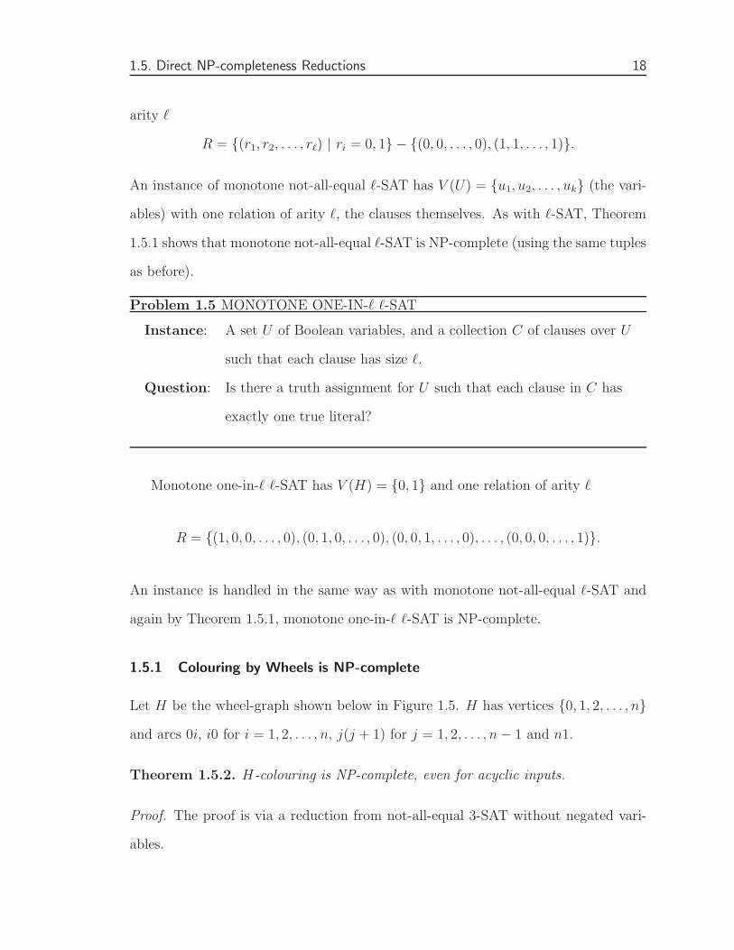
Figure 1.9: The graphs used in proving that OCN4 is NP-complete.
Proof. Observe that T4 has only two transitive tournaments on three vertices namely:
0, 1, 2 and 1, 2, 3. The two transitive tournaments a, b, c and d, e, f in G1 have to map
to transitive tournaments in T4. The arcs (a, d) and (c, f) in G1 force the mapping
as shown above.
Fact 1.5.4. Any pre-colouring of xi, xj , xk in G2 with the colours {0, 1} such that at
least one 0 and at least 1 is used can be extended to a homomorphism from G2 to
T4. On the other hand if all of xi, xj, xk are coloured the same (with 0 or 1), it does
not extend to a homomorphism to T4.
Fact 1.5.5. G1 6→ Tin, G1 6→ Tout, G2 6→ TT4.
Proof. The only way that G1 → Tin is if both vertices a and d map to vertex 11,
since they’re adjacent that is not allowed. Similarly, the only way that G1 → Tout is if

1.5. Direct NP-completeness Reductions 24
both vertices c and f map to vertex 15, again this is not allowed. Finally G2 9 TT4
since it has a path of length 4: xi, ui, yi, yj, yk.
We now describe the reduction to monotone not-all-equal 3-SAT.
Given an instance of monotone not-all-equal 3-SAT: U = {x1, x2, . . . , xn} and
C = {c1, c2, . . . , cm}, we construct an acyclic, oriented graph D as follows. Take a
copy of G1 and for each variable xi ∈ U add a vertex labeled xi to G1 and join vertex xi
to vertex a of G1 by an arc directed in this direction. For each clause {yi, yj, yk} ⊆ U ,
construct the corresponding graph G2 and then identify the vertices xi, xj , xk from
this G2 with the vertices labeled xi, xj, xk from before. Once this has been done for
all clauses in C, we have the acyclic, oriented graph D. The construction of D can
be carried out in polynomial time. The graph D is shown in Figure 1.10.
abc
def
x1
xi
xj
xk
xm
ui
uj
uk
yi
yj
yk
...
...
...
...
Figure 1.10: The oriented, acyclic graph D.
Lemma 1.5.6. D has an oriented 4-colouring if and only if there exists a satisfying
truth assignment for monotone not-all-equal 3-SAT.
Proof. ⇒:
Assume D is 4-colourable. That implies that D has a homomorphism to one of the

1.5. Direct NP-completeness Reductions 25
four tournaments on four vertices: TT4, Tin, Tout or T4. Since D has both G1 and
G2 as subgraphs, these prevent D from having a homomorphism to TT4, Tin or Tout.
Thus D → T4. From the facts presented above we know that vertex a will map
to vertex 2 of T4. Therefore the only possible images of the vertices xi are {0, 1}.
Furthermore they cannot all map to 0 or all map to 1 (by the facts above). The
images of the vertices xi form a satisfying truth assignment for monotone not-all-
equal 3-SAT (FALSE = 0 and TRUE = 1).
⇐:
Assume that there exists a satisfying truth assignment for monotone not-all-equal 3-
SAT. Use this assignment to colour the vertices xi in D (FALSE= 0 and TRUE= 1).
This pre-colouring can be extended to the whole D to give a homomorphism to T4
(by the facts above). Therefore D is 4-colourable.
Proposition 1.5.7. OCN4 is NP-complete, even when restricted to acyclic, oriented
graphs.
Proof. Since it is easy to check whether a given colouring of an acyclic, oriented
graph D is in fact a 4-colouring, OCN4 is in NP. By the lemma above and since it
is known that monotone not-all-equal 3-SAT is NP-complete, we know that OCN4 is
NP-complete. Note that the graph D constructed above is acyclic.
Proposition 1.5.8. OCNk is NP-complete for any k ∈ Z+, k ≥ 4, even when
restricted to acyclic, oriented graphs.
Proof. The case k = 4 is the theorem above. For any k ≥ 5, we construct an oriented
acyclic graph D′ from D by adding k − 4 new vertices to D (one at a time) and
letting them dominate all the previous vertices. This new graph D′ is k-colourable if
and only if D is 4-colourable. Therefore k-colourability of D′ is equivalent to solving
monotone not-all-equal 3-SAT, and so is NP-complete.
1.6. Polymorphisms 26
1.6 Polymorphisms
An algebraic approach to studying the complexity of the CSP(T ) problem (and there-
fore that of the H-colouring problem) was proposed by Jeavons in [40]. In this
framework we associate an algebra to T , and the properties of this algebra will then,
hopefully, provide us with useful information on the complexity of CSP(T ).
An algebra is a pair A = (A, F ) consisting of a set A (the universe of A), and a
set F of operations on A (the basic operations of A). An operation of rank (or arity)
k (for some natural number k) is a function f : Ak → A.
Let T be a relational system with vertex set V = V (T ), index set I and relations
Ri(T ) = Ri (of arity ri), i ∈ I. We define the direct product T k (for k ≥ 1) by
V (T k) = V k and relations R′
i (of arity ri), i ∈ I by
((x1
1, x12, . . . , x
1k), (x
21, x
22, . . . , x
2k), . . . , (x
ri
1 , xri
2 , . . . , xri
k ))∈ R′
i if and only if
(x11, x
21, . . . , x
ri
1 ), (x12, x
22, . . . , x
ri
2 ), . . . , (x1k, x
2k, . . . , x
ri
k ) are all in Ri.
For a digraph H = (V, A) (which is a relational system with one binary relation, A),
this definition amounts to: V (Hk) = V k and arcs (x11, x
12, . . . , x
1k) → (x2
1, x22, . . . , x
2k)
if and only if x1i → x2
i is an arc of H for 1 ≤ i ≤ k.
Given a constraint satisfaction problem CSP(T ), a polymorphism of T is a homo-
morphism f : T k → T . That is if
((x1
1, x12, . . . , x
1k), (x
21, x
22, . . . , x
2k), . . . , (x
ri
1 , xri
2 , . . . , xri
k ))∈ R′
i,
then(f(x1
1, x12, . . . , x
1k), f(x2
1, x22, . . . , x
2k), . . . , f(xri
1 , xri
2 , . . . , xri
k ))∈ Ri.
For a digraph H this means that f : Hk → H is a polymorphism if (x11, x
12, . . . , x
1k)→

1.6. Polymorphisms 27
(x21, x
22, . . . , x
2k) implies that f(x1
1, x12, . . . , x
1k)→ f(x2
1, x22, . . . , x
2k).
Denote the set of polymorphisms of T by Pol(T ). Associate with the constraint
satisfaction problem CSP(T ), the algebra (V (T ),Pol(T )).
Jeavons [40] showed that for each constraint satisfaction problem, Pol(T ) could
be classified into one of six categories depending on the polymorphisms present in
Pol(T ). The polymorphisms present in Pol(T ) ultimately determine the complexity
of CSP(T ).
In [13], Bulatov, Jeavons and Krokhin show that we only need to consider idem-
potent polymorphisms to determine the complexity of CSP(T ). An idempotent poly-
morphism f : T k → T has the property that f(x, x, . . . , x) = x for every x ∈ V (T ).
They also show that one only has to consider relational systems, T , that are cores:
each homomorphism T → T is an automorphism. This is analogous to the digraph
situation.
An operation f : Ak → A is called essentially unary if there exists a (nonconstant)
unary operation g : A→ A and an index i ∈ {1, 2, . . . , k} such that f(x1, x2, . . . xk) =
g(xi) for all choices of x1, x2, . . . , xk. If g is the identity operation, then f is called a
projection.
The set of polymorphisms Pol(T ), for a given constraint satisfaction problem
CSP(T ), always contains the projections. The question then is whether there are
other polymorphisms and whether they are of any use. The following theorem shows
what happens if one is restricted to essentially unary polymorphisms.
Theorem 1.6.1 (Bulatov, Jeavons and Krokhin [13]). If for a given constraint sat-
isfaction problem CSP(T ), Pol(T ) contains only essentially unary polymorphisms,
then CSP(T ) is NP-complete.
For an undirected complete graph Kn, with n ≥ 3, the only idempotent polymor-
phisms are projections [42]. Therefore Theorem 1.6.1 furnishes a different proof of
the result that (undirected) graph k-colouring is NP-complete for k ≥ 3.

1.6. Polymorphisms 28
It was conjectured in [13] that the essentially unary polymorphisms are exactly
the dividing line between NP-complete CSP problems and CSP problems that are
polynomial time solvable.
There is an equivalent formulation of Theorem 1.6.1 due to Larose and Zadori
[43]. The equivalence follows from results in Universal Algebra, see [14, 44] for more
on this.
An idempotent polymorphism f : T k → T is said to be a Taylor polymorphism if
it satisfies k identities of the form
f(xi1, xi2, . . . , xik) = f(yi1, yi2, . . . , yik), i = 1, 2, . . . , k,
where xij , yij ∈ {x, y} for all i, j and xii 6= yii for i = 1, 2, . . . , k. Note that a
projection is not a Taylor polymorphism.
Theorem 1.6.2 (Larose and Zadori [43]). Let CSP(T ) be given. If Pol(T ) does not
contain any Taylor polymorphisms, then CSP(T ) is NP-complete.
The conjecture of Bulatov, Jeavons and Krokhin [13] is the following (here we use
the alternative formulation from [43]).
Conjecture 1.6.3. If T admits a Taylor polymorphism, then CSP(T ) is polynomial
time solvable. Otherwise CSP(T ) is NP-complete.
Thus it is conjectured that the Taylor polymorphisms differ from projections in
just the right way to be of use in proving CSP(T ) polynomial.
A recent result of Maroti and McKenzie [45] shows (again through Universal
Algebra) that the existence of a Taylor polymorphism is equivalent to the existence
of a weak near unanimity function of arity k > 1. A weak near unanimity function

1.6. Polymorphisms 29
of arity k (WNUFk) is an idempotent polymorphism f : T k → T such that
f(y, x, x, . . . , x, x) = f(x, y, x, . . . , x, x) = f(x, x, y, . . . , x, x) = · · ·
= f(x, x, x, . . . , x, y),
for all x, y ∈ V (T ).
The two theorems above (Theorems 1.6.1 and 1.6.2) can now be formulated as
follows.
Theorem 1.6.4. If T does not admit a WNUFk of arity k > 1, then CSP(T ) is
NP-complete.
Conjecture 1.6.3 now becomes the following.
Conjecture 1.6.5 ([14]). If T admits a WNUF, then CSP(T ) is polynomial time
solvable. Otherwise CSP(T ) is NP-complete.
In Chapter 3 we study weak near unanimity functions in the context of the digraph
homomorphism problem. We prove that a wide range of H-colouring problems with
known polynomial time algorithms have a WNUF. On the other hand, we prove some
non-existence results for WNUFs (including some known NP-complete digraphs).
This lends some support to the conjecture above. We also show that there is a
close resemblance between traditional NP-completeness proofs and the ones using
WNUFs. This is accomplished by proving a version of the vertex (and arc) sub-
indicator construction and the indicator construction for WNUFs and then using
this result to prove that all tournaments with at least two cycles do not admit a
WNUF (using virtually the same proof as in [5]).

1.7. Injective Homomorphisms 30
1.7 Injective Homomorphisms
Let G and H be digraphs. The homomorphism f : G → H is said to be injective if
f |N−(v) is an injective mapping from V (G) to V (H) for every v ∈ V (G). Therefore,
the in-neighbours of every vertex v ∈ V (G) have to be mapped to distinct vertices
in H while preserving the arcs of G.
One can of course also define a homomorphism f : G → H to be injective if it
is injective on the out-neighbours of the vertices in G. This would be the same as
requiring the homomorphism to be injective on the in-neighbours of the converse of
G (where of course we are now also mapping to the converse of H).
It is also possible to insist that the homomorphism be injective on N+(v)∪N−(v)
for every v ∈ V (G). This is exactly what happens in the undirected case. If G and
H are undirected graphs, then the homomorphism f : G→ H is said to be injective
if f is injective on the neighbourhood of every vertex in G.
Injective homomorphisms of undirected graphs are studied in [22, 23, 24, 25, 31].
In some cases they are referred to as partial covers, in contrast to full covers which may
be viewed as bijective homomorphisms (the mapping is bijective on neighbourhoods).
If the target in the homomorphism problem is a complete undirected graph, one
obtains the injective chromatic number [31]. This is the smallest n such that a given
graph G has an injective homomorphism to Kn.
Hahn, Kratochvıl, Siran and Sotteau [31] were particularly interested in deter-
mining the injective chromatic number of the hypercube because of its connections
to coding theory. It has to be noted here that in their definition of the injective
chromatic number, they allow the possibility that adjacent vertices may receive the
same colour. A colouring in their sense may therefore not be a homomorphism to an
undirected complete graph, unless we include a loop at every vertex of the complete
graph. Since we are mostly interested in complexity results, this will be the only type

1.7. Injective Homomorphisms 31
of result from [31] that we will list here. The injective chromatic number problem
(ICNk) may be stated formally as follows.
Problem 1.7 ICNk
Instance: A graph G and a natural number k.
Question: Is there an injective k-colouring of G?
Theorem 1.7.1 (Hahn, Kratochvıl, Siran and Sotteau [31]). The problem ICNk is
NP-complete for every fixed k ≥ 3.
Fiala and Kratochvıl [22, 23, 24] and Fiala, Kratochvıl and Por [25] consider the
more general problem of injective homomorphisms where the target is not a com-
plete graph. In all of these papers it is pointed out that the injective homomorphism
problem is connected to so-called L(2, 1) labellings of graphs: adjacent vertices must
receive labels that differ by at least two, while vertices at distance two must receive
labels that differ by at least one. This has applications in radio frequency assign-
ment. Radio towers (for example cell phone towers) that are close together (where
interference is quite possible) need frequencies that are far apart. Towers that are
not as close to each other may only need frequencies that differ by a smaller amount.
The complexity results in these papers are mostly centered around a family of
graphs which we describe next. Denote by Θ(a1, a2, . . . , an) the (multi)graph that is
formed by joining two vertices by n internally disjoint paths of lengths a1, a2, . . . , an.
An abbreviated version of this notation is as follows: Θ(ak1
1 , ak2
2 , . . . , aknn ) is taken to
mean that there are ki paths of length ai joining the two vertices.
The authors show that the family of graphs defined above exhibit both problems
that are polynomial and problems that are NP-complete:
❒ Θ(an) is polynomial for every fixed a.
❒ Θ(ai, bj) is polynomial for every odd a, b.

1.7. Injective Homomorphisms 32
❒ Θ(ai, bj) is NP-complete for every a and b of different parity.
❒ Θ(a, b, c) is NP-complete if c is divisible by a + b.
❒ Θ(1, 2, c) is NP-complete for every c.
❒ Θ(ai, bj) is polynomial when a and b are divisible by the same power of 2 or if
i + j ≤ 2. It is is NP-complete otherwise.
❒ Θ(1, 2, a) and Θ(1, 3, b) are NP-complete for all positive integers a > 2 and
b > 3.
❒ For any three distinct odd positive integers a, b and c, Θ(a, b, c) is NP-complete.
As with ordinary homomorphisms, the hope is that the injective problems will exhibit
a dichotomy. Towards this end Fiala and Kratochvıl [24] considered the list version
of the injective homomorphism problem.
The list version of the injective homomorphism problem with target H , is the
following problem (INJ-LIST-HOMH).
Problem 1.8 INJ-LIST-HOMH
Instance: A graph G and lists L(v) ⊆ V (H).
Question: Does there exist an injective homomorphism f : G→ H such
that f(v) ∈ L(v) for every v ∈ V (G)?
The lists L(v) are to be thought of as admissible images for the vertex v ∈ V (G).
Fiala and Kratochvıl [24] were able to show that for this problem there is a dichotomy.
Theorem 1.7.2 (Fiala and Kratochvıl [24]). The list, injective, homomorphism prob-
lem with target H is solvable in linear time if the graph H contains at most one cycle
in each component. It is NP-complete otherwise.

1.7. Injective Homomorphisms 33
It is also interesting to note that injective graph homomorphisms are being applied
to problems in mathematical biology [11, 17, 18, 21]. Here the interactions between
proteins in a given species are modelled as an undirected graph. The problem then is
to consider the protein networks of two different species and to determine whether a
subgraph of one maps under an injective homomorphism to the network of the other.
If it does, it may indicate that the two species share a sub-network that may have
been passed along by a common ancestor.
As before, our focus will be on directed graphs. We will consider two versions of
the injective homomorphism problem: (i) reflexive targets, where each vertex in the
target has a loop and (ii) irreflexive targets, where no vertex in the target has a loop.
A dichotomy was found for the reflexive version, while the irreflexive version proved
to be much harder to deal with. We show that a polynomial time transformation
exists between all digraph homomorphism problems and certain irreflexive injective
digraph homomorphism problems. To some degree this explains the difficulty of the
irreflexive case.

34
2
The Complexity of Colouring by Local Tournaments
2.1 Introduction
In this chapter we consider a generalization of the theorem by Bang-Jensen, Hell and
MacGillivray [5] on the complexity of colouring by semi-complete digraphs. Recall
that a semi-complete digraph has the property that between every pair of vertices
there is at least one arc; parallel arcs and loops are not allowed, but a pair of sym-
metric arcs is allowed.
Theorem 2.1.1 (Bang-Jensen, Hell and MacGillivray [5]). Let H be a semi-complete
digraph.
❒ If H contains at most one directed cycle, then H-colouring is polynomial time
solvable.
❒ Otherwise H-colouring is NP-complete.
There is the related notion of a locally semi-complete digraph. A digraph H , is
said to be locally semi-complete if for every vertex v of H , both N+(v) and N−(v)

2.2. Some Tools 35
induce semi-complete digraphs. A special case of this is that of a local tournament.
A local tournament, H , is a digraph such that between every pair of vertices there
is at most one arc and that for every vertex v of H both N+(v) and N−(v) induce
tournaments.
Bang-Jensen introduced the notion of locally semi-complete digraphs in [1] where
it was shown that many of the known results on tournaments generalize to this family
of digraphs.
It is, of course, the case that Theorem 2.1.1 applies to tournaments since they are
a special case of semi-complete digraphs. In this chapter, we aim to generalize this
special case of Theorem 2.1.1 to the class of local tournaments.
We will see that Theorem 2.1.1 doesn’t generalize in the way one would expect. In
particular there are unicyclic local tournaments such that the corresponding colouring
problem is NP-complete. This is in contrast with unicyclic tournaments that all define
polynomial colouring problems.
Since a classification of the complexity of smooth digraphs has already been ob-
tained (Conjecture 1.2.4 was proved in [8]), this would imply that the complexity of
some local tournaments are already known. The result in [8] was obtained by using
results from universal algebra though. We give here a completely graph theoretic
proof of the complexity of colouring by local tournaments. This is hopefully more
appealing to graph theorists. In fact, the graph theoretic proof actually does more
than just this. It showcases all of the techniques that have been built up over the
last two decades in the study of the complexity of graph homomorphisms.
2.2 Some Tools
In addition to the indicator and sub-indicators mentioned in Chapter 1, we also need
a few other tools to fully discuss the complexity of colouring by local tournaments.

2.2. Some Tools 36
2.2.1 The Consistency Check
Suppose that H is a fixed digraph that will act as the target in a homomorphism
problem. As input to the problem we have a digraph G. In trying to find a homo-
morphism G→ H , we may start the process by assigning a list L(v) = V (H) to each
vertex v of G. These lists record possible images for the vertices of G and initially
every vertex of H is a possible image for any given vertex of G. The algorithm we
describe in this section processes each list L(v), v ∈ V (G), by removing any vertices
from L(v) that cannot possibly be images of v.
The lists attached to each vertex of G are said to be consistent if for any arc uv
of G the following two properties hold:
❒ for any x ∈ L(u), there exists y ∈ L(v) such that xy is an arc of H and
❒ for any b ∈ L(v), there exists a ∈ L(u) such that ab is an arc of H .
The goal of the consistency check (Algorithm 2.1) is to reduce the initial lists to
ones that are consistent. Our presentation here follows [37].
Algorithm 2.1 The Consistency Check
Input: A digraph G with lists L(v) = V (H), v ∈ V (G).
Task: Reduce the lists to L∗(v) ⊆ V (H), v ∈ V (G), that are consistent.
Action: Initially set all lists L∗(v) = L(v), and then, as long as changes occur,
process each arc uv of G repeatedly as follows: remove from L∗(u)
any x for which no element y ∈ L(v) has xy an arc in H , and
remove from L∗(v) any b for which no a ∈ L∗(u) has ab an arc in H .
The consistency check is often used as a building block in designing polynomial
time algorithms for the digraph homomorphism problem [37]. It is also known as the
arc-consistency check since it checks for consistency across arcs of G. Higher order
consistency checks are also possible [37].

2.2. Some Tools 37
2.2.2 The X-enumeration and the Graft Extension
An enumeration {h1, h2, . . . , hn} of the vertices of a digraph H is called an X-
enumeration if the following property holds: if hihj and hkhl are arcs of H , then
min(hi, hk) min(hj , hl) is also an arc of H , where the minimum is taken with respect
to the X-enumeration.
Theorem 2.2.1 (Gutjahr, Woeginger and Welzl [29]). Let H be a digraph such that
H admits an X-enumeration. Then the H-colouring problem is solvable in polynomial
time.
This result follows by running the consistency check on the input digraph (this is
not the original algorithm presented in [29]). If a list becomes empty at any point
during the consistency check, then there is no homomorphism to the target. If, on
the other hand, the resulting lists are nonempty the minimum element (with respect
to the X-enumeration) in each list defines a homomorphism to the target [37].
There is one more result from [29] that we need, the so-called graft extension.
We will consider a slightly more general problem than the one presented in [29].
Gutjahr, Woeginger and Welzl [29] only considered the H-colouring problem in their
paper, HOMH . We will show here that their result actually applies to a more general
problem, namely that of list homomorphisms.
The list homomorphism problem with target H is the following decision problem
(LIST-HOMH).
Problem 2.1 LIST-HOMH
Instance: (G,L): A digraph G with lists L(v) ⊆ V (H), v ∈ V (G).
Question: Does there exist a homomorphism f : G→ H
such that f(v) ∈ L(v) for every v ∈ V (G)?
Let H1 be a loop-free digraph that has an X-enumeration, say {h1, h2, . . . , hn}.

2.2. Some Tools 38
Let H2 be a digraph such that H2-colouring is polynomial. We form a new digraph H
by deleting the vertex hn from H1 and replacing it by the digraph H2: every vertex
hi ∈ V (H1) that is adjacent to (from) hn is now adjacent to (from) every vertex in
H2. The digraph H is called the X-graft(H1,H2).
Theorem 2.2.2. Let H=X-graft(H1,H2) such that LIST-HOMH2is polynomial.
Then LIST-HOMH is polynomial.
Proof. Let (G,L) be an instance of LIST-HOMH . Modify H1 by adding a loop at
hn. Clearly, the existence of a homomorphism of G to H1 is a necessary condition
for the existence of a homomorphism of G to H .
First, alter the lists by replacing any vertices of H2 by hn in any list where they
occur. Now, apply the arc-consistency check. If it fails, then G is a NO-instance.
Hence assume the consistency check succeeds. By the discussion earlier, the mapping
f(x) = min L(x), where the minimum is with respect to the X-enumeration, is a
list-homomorphism G→ H1.
Since the minimum element in each list is chosen, the vertices that map to hn in
this list-homomorphism of G to H1 map to vertices of H2 in any list-homomorphism
of G to H . By the construction of H and the consistency check, there is now a list-
homomorphism of G to H if and only if the subgraph of G induced by f−1(hn) admits
a list-homomorphism to H2, where the lists are the intersections of the initially given
lists with V (H2). As LIST-HOMH2is polynomial, the result follows.
Corollary 2.2.3 (Gutjahr, Woeginger and Welzl [29]). Let H=X-graft(H1,H2) such
that HOMH2is polynomial. Then HOMH is polynomial.
This result follows since HOMH is a special case of LIST-HOMH where each list
L(v) = V (H) for each v ∈ V (G).

2.2. Some Tools 39
2.2.3 The Frobenius-Schur Index
The result discussed in this section is a purely number theoretic result. It will help
in choosing the correct lengths for directed paths that are to act as indicators and
sub-indicators.
Given a set of relatively prime positive integers B = {a1, a2, . . . , an}, a linear
combination of these integers is an expression of the form
x1a1 + x2a2 + · · ·+ xnan, (2.1)
where each xi ∈ {0, 1, 2, . . .}. A natural question to ask is for the smallest integer φ
such that each every integer t ≥ φ can be represented in the form of equation 2.1.
The existence of such an integer φ is guaranteed by a result of Schur (see [12]).
Lemma 2.2.4. Let S be a nonempty set of positive integers which is closed under
addition. Let d be the greatest common divisor of the integers in S. Then there exists
a positive integer N such that td is in S for every integer t ≥ N .
Since the set of all linear combinations of elements in B is closed under addition,
Schur’s result guarantees a threshold above which every integer is of the form 2.1.
Frobenius (according to [10]) then posed the problem of finding the smallest inte-
ger φ = φ(a1, a2, . . . , an) such that every integer t ≥ φ is of the form 2.1 (or at least
good bounds this number). The integer φ is known as the Frobenius-Schur index of
the set B [12] or as the conductor of the set B [51]. Equivalently, one may ask for the
largest integer not representable as 2.1. In general, this is a very hard problem with
a rich literature [48]. The problem sometimes also goes by the name of the money
changing problem. Given a fixed set of coins (the set B) what is the largest amount
of money that cannot be changed using the coins in B? See [30] or [51] for more on
this.

2.2. Some Tools 40
We are typically interested in finding the Frobenius-Schur index of the cycle
lengths of a strong round local tournament D. By Lemma 2.3.6 we know that the
cycle lengths of D is an interval of integers, {ℓ, ℓ + 1, . . . , n}, where ℓ is the girth of
D and n = |V (D)|. Fortunately, in this case, the Frobenius-Schur index is known
exactly.
Lemma 2.2.5 (Brauer [10]). Let ℓ be a positive integer. Then
φ(ℓ, ℓ + 1, . . . , n) =
⌊n− 2
n− ℓ
⌋ℓ.
We would like to give a short justification of this result as this may aid the reader
later on when we apply this result to local tournaments.
Consider the following table. Row k of the table contains numbers that can be
written as a linear combination using k numbers from {ℓ, ℓ + 1, . . . , n}.
ℓ, ℓ + 1, ℓ + 2, . . . , n = ℓ + (n− ℓ).
2ℓ, 2ℓ + 1, 2ℓ + 2, . . . 2n = 2ℓ + 2(n− ℓ).
3ℓ, 3ℓ + 1, 3ℓ + 2, . . . , 3n = 3ℓ + 3(n− ℓ).
...
kℓ, kℓ + 1, kℓ + 2, . . . , kn = kℓ + k(n− ℓ).
(k + 1)ℓ, (k + 1)ℓ + 1, (k + 1)ℓ + 2, . . . , (k + 1)n = (k + 1)ℓ + (k + 1)(n− ℓ).
...
Note that each row is a list of consecutive integers. Therefore each number that
cannot be written as a linear combination has to occur somewhere between the rows
of the table. Between the last entry of a row and the first entry of the next row there
is a “gap” of integers that cannot be written as a linear combination. The size of
the gap also decreases as one moves down the table so that it is inevitable that it
eventually closes.

2.3. Local Tournaments 41
We now ask what is the largest integer that occurs somewhere between the rows
of the table. This integer has to occur in a gap of size at least two (a gap of size one
corresponds to two consecutive integers). So what is the largest integer k such that
between rows k and (k + 1) there is still a gap of size at least two. That is
(k + 1)ℓ− kn = (k + 1)ℓ− k(ℓ + n− ℓ) = ℓ− k(n− ℓ) ≥ 2,
implying
k =
⌊ℓ− 2
n− ℓ
⌋.
So as soon as we move beyond this row, every integer can be written as a linear
combination. Therefore the smallest integer φ defined above occurs at (k+1)ℓ. That
is
φ(ℓ, ℓ + 1, ℓ + 2, . . . , n) =
(⌊ℓ− 2
n− ℓ
⌋+ 1
)ℓ =
⌊n− 2
n− ℓ
⌋ℓ.
2.3 Local Tournaments
Since we aim to give a graph theoretic proof of the complexity of HOMH where H is
a local tournament, it comes as no surprise that the structure of local tournaments
plays a central role in this proof. In this section we state the results on the structure
of locally semi-complete digraphs (since local tournaments are a special case of these)
that we need. Bang-Jensen and Gutin [3] is a standard reference on these matters.
A digraph D is said to be strong or strongly connected if for every pair of vertices
x and y in D, there is directed path joining x to y and a directed path joining y to x.
A strong component of a digraph D is a maximal induced sub-digraph of D that
is strong.
The strong components of a digraph D are disjoint and can be labeled as D1,
D2, . . .Dt such that there is no arc from Di to Dj unless i < j. We call such an

2.3. Local Tournaments 42
ordering an acyclic ordering of the strong components of D.
Theorem 2.3.1 (Guo and Volkmann [3, 27]). Let D be a connected locally semi-
complete digraph that is not strong and let D1, D2, . . . , Dp be the acyclic ordering of
the strong components of D. Then D can be decomposed into r ≥ 2 induced subgraphs
D′
1, D′
2, . . . , D′
r as follows:
D′
1 = Dp, λ1 = p,
λi+1 = min{j | N+(Dj) ∩ V (D′
i) 6= ∅},
and D′
i+1 = D〈V (Dλi+1) ∪ V (D(λi+1)+1) ∪ · · · ∪ V (Dλi−1)〉.
The sub-digraphs D′
1, D′
2, . . . , D′
r satisfy the properties below:
(a) D′
i consists of some strong components of D and is semi-complete for i =
1, 2, . . . , r.
(b) D′
i+1 dominates the initial component of D′
i and there exists no arc from D′
i to
D′
i+1 for i = 1, 2, . . . , r − 1.
(c) If r ≥ 3, then there is no arc between D′
i and D′
j for i, j satisfying |j − i| ≥ 2.
If D is a connected locally semi-complete digraph that is not strong, then the
unique sequence D′
1, D′
2, . . . , D′
r defined in Theorem 2.3.1 is called the semi-complete
decomposition of D.
A digraph on n vertices is said to be round if we can label its vertices v1, v2, . . . , vn
so that for each i, N+(vi) = {vi+1, . . . , vi+d+(vi)} and N−(vi) = {vi−d−(vi), . . . , vi−1},
where all subscripts are taken modulo n.
Let D be a digraph with vertex set {v1, v2, . . . , vn} and let G1, G2, . . . , Gn be
digraphs which are pairwise vertex disjoint. The composition D[G1, G2, . . . , Gn] is

2.3. Local Tournaments 43
the digraph H with vertex set V (G1) ∪ V (G2) ∪ . . .∪ V (Gn) and arcs (∪ni=1A(Gi)) ∪
{gigj | gi ∈ V (Gi), gj ∈ V (Gj), vivj ∈ A(D)}.
A locally semi-complete digraph D is round decomposable if there exists a round
local tournament R on r ≥ 2 vertices such that D = R[S1, . . . , Sr], where each Si is
a strong semi-complete digraph.
For a strong digraph D a set S ⊆ V (D) is a separator or separating set if D − S
is not strong.
Lemma 2.3.2 (Bang-Jensen, Guo, Gutin and Volkmann [2, 3]). Let D be a strong
locally semi-complete digraph which is not semi-complete. Then D is not round de-
composable if and only if the following conditions are satisfied:
(a) There is a minimal separating set S such that D− S is not semi-complete and
for each such S, D〈S〉 is semi-complete and the semi-complete decomposition
of D − S has exactly three components D′
1, D′
2, D′
3;
(b) There are integers α, β, µ, ν with λ2 ≤ α ≤ β ≤ p−1 and p+1 ≤ µ ≤ ν ≤ p+ q
such that
N−(Dα) ∩ V (Dµ) 6= ∅ and N+(Dα) ∩ V (Dν) 6= ∅,
or N−(Dµ) ∩ V (Dα) 6= ∅ and N+(Dµ) ∩ V (Dβ) 6= ∅,
where D1, D2, . . . , Dp and Dp+1, . . . , Dp+q are the acyclic orderings of the strong
components of D− S and D〈S〉, respectively, and Dλ2is the initial component
of D′
2.
The structure described in Lemma 2.3.2 is illustrated in Figure 2.1.

2.3. Local Tournaments 44
Dα
Dβ
Dp−1
Dλ2
Dp+1
Dµ
Dν
Dp+q
D1 Dp
D′
1
D′
2
D′
3
S
Dλ2−1
...
...
...
...
...
...
...
Figure 2.1: The structure of a strong locally semi-complete digraph that is not semi-complete and not round decomposable.

2.3. Local Tournaments 45
Theorem 2.3.3 (Bang-Jensen, Guo, Gutin and Volkmann [2, 3]). Let D be a con-
nected locally semi-complete digraph. Then exactly one of the following possibilities
holds.
(a) D is round decomposable with a unique round decomposition given by
D = R[D1, D2, . . . , Dα],
where R is a round local tournament on α ≥ 2 vertices and Di is a strong
semi-complete digraph for i = 1, 2, . . . , α;
(b) D is not round decomposable and not semi-complete and it has the structure
described in Lemma 2.3.2;
(c) D is a semi-complete digraph which is not round decomposable.
Proposition 2.3.4 (Bang-Jensen, Guo, Gutin and Volkmann [2, 3]). Let D be a
strong non-round decomposable locally semi-complete digraph and let S be a minimal
separating set of D such that D − S is not semi-complete. Let D1, D2, . . . , Dp be
the acyclic ordering of the strong components of D − S and Dp+1, Dp+2, . . . , Dp+q be
the acyclic ordering of the strong components of D〈S〉. Suppose that there is an arc
s→ v from S to D′
2 with s ∈ V (Di) and v ∈ V (Dj), then
Di ∪Di+1 ∪ · · · ∪Dp+q 7→ D′
3 7→ Dλ2∪ · · · ∪Dj.
Here, A 7→ B, means that A dominates B and there are no arcs from B to A.
Lemma 2.3.5 (Bang-Jensen and Gutin [3]). Let R be a strong round local tournament
and let C be a shortest cycle of R and suppose C has k ≥ 3 vertices. Then for
every round labeling v0, v1, . . . , vn−1 of R such that v0 ∈ V (C) there exist indices
0 < a1 < a2 < . . . ak−1 < n so that C = v0va1va2· · · vak−1
v0.

2.3. Local Tournaments 46
Lemma 2.3.6 (Bang-Jensen and Gutin [3]). A strong round local tournament R on
r vertices has cycles of length k, k + 1, . . . , r, where k is the girth of R.
Lemma 2.3.7 (Bang-Jensen and Gutin [3]). If a strong round local tournament with
r vertices has a cycle of length k through a vertex v, then it has cycles of all lengths
k, k + 1, . . . , r through v.
Strictly speaking a round digraph is also round decomposable (all |Di| = 1). We
prefer to distinguish between round and round decomposable digraphs. So when
a local tournament is said to be round decomposable then at least one |Di| ≥ 3.
Furthermore, since a connected locally semi-complete digraph that is not strongly
connected is round decomposable (an acyclic ordering of its strong components), a
round local tournament (in our sense) is strongly connected and therefore Hamilto-
nian (by Lemma 2.3.6).
In proving some of our results, we will use the sub-indicator construction (both
the vertex and arc versions). A glance at Lemmas 1.4.2 and 1.4.3 confirms the fact
that in order to apply a sub-indicator to a digraph H , one has to know that H is a
core. We show next that a connected local tournament is indeed a core. The following
lemma will be useful in this regard.
Lemma 2.3.8 (Bang-Jensen [1, 3]). A locally semi-complete digraph has a hamilton
path if and only if its underlying graph is connected.
Proposition 2.3.9. A connected locally semi-complete digraph D is a core.
Proof. By Lemma 2.3.8, D has a hamilton path, say v1, v2, . . . , vn.
Let f : D → D′ be a retraction of D where D′ is a subgraph of D. Let v be a
vertex in D′. By the enumeration above v = vi for some i ∈ {1, 2, . . . , n} and by the
retraction f(vi) = vi.
Consider the vertices vi−1 and vi+1 (at least one of these exists), say vi−1. Let
f(vi−1) = vj , j ∈ {1, 2, . . . , n}. Clearly j 6= i. Since vi−1vi ∈ A(D), f(vi−1)f(vi) =

2.4. Connected vs. Disconnected Local Tournaments 47
vjvi ∈ A(D). That is vi−1, vj ∈ N−(vi). Therefore by the locally semi-complete
property of D, vi−1 and vj are adjacent. If i− 1 6= j, the arc(s) between vi−1 and vj
are not preserved by f . So the image of vi−1 is exactly vi−1 under the retraction. If
vi+1 exists, the same reasoning shows that f(vi+1) = vi+1.
Repeating the argument along the hamilton path eventually shows that every
vertex has to map to itself. Therefore D is a core.
2.4 Connected vs. Disconnected Local Tournaments
When H is a disconnected local tournament such that each component of H (all of
which are local tournaments themselves) is polynomial time solvable, then HOMH
is also polynomial time solvable. NP-completeness results for disconnected local
tournaments are much harder to obtain.
The NP-completeness results that follow are all for connected local tournaments
since we only give polynomial time transformations from NP-complete problems to
HOMH when H is connected. A natural conjecture would be: if a disconnected local
tournament H contains at least one component that is NP-complete, then HOMH
is NP-complete. The difficulty in proving this lies with constructing a polynomial
transformation from some NP-complete problem. In general, it is hard to set up the
transformation without forcing certain vertices of the transformed instance to map to
a specific component of H . This may have the unintended consequence of restricting
the images of one or more vertices of the transformed instance too severely.
On the other hand one can easily obtain a polynomial time Turing reduction.
Here, an instance of some NP-complete problem Q is transformed into many dif-
ferent instances of HOMH . The transformation has to run in polynomial time and
furthermore an instance I of Q is a yes instance if and only if at least one the trans-
formed instances is a yes instance of HOMH . This shows that for a disconnected
local tournament with at least one NP-complete component, HOMH is polynomial

2.5. Road map 48
time solvable if and only if P=NP. Therefore solving HOMH in polynomial time for
a disconnected local tournament H with at least one NP-complete component, is
highly unlikely.
Let H be a disconnected local tournament that is also a core and let H ′ be a
component of H such that HOMH′ is NP-complete. The polynomial time Turing
reduction is from HOMH′ to HOMH . Let G be an instance of HOMH′ . We now
form |V (H ′)| instances of HOMH as follows: take |V (H ′)| copies each of G and H ′,
let v ∈ V (G) and V (H ′) = {h1, h2, . . . , hn}. Denote by Fi the graph obtained by
identifying the vertex v in G with the vertex hi in H ′, 1 ≤ i ≤ n.
It is now easy to see that G → H ′ if and only if there exists at least one i ∈
{1, 2, . . . , n} such that Fi → H .
From now on we assume that all local tournaments are connected.
2.5 Road map
As an aid to reading our proof that local tournaments exhibit a dichotomy, we provide
the following road map.
At its highest level the proof is divided into five cases, as shown below.
1. Acyclic local tournaments: Acyclic local tournaments were shown to define
polynomial problems by Hell, Zhou and Zhu [38]. Therefore Case 1 has already
been dealt with.
2. Unicyclic local tournaments: The unicyclic case is treated in Section 2.6
and relies on the graft extension as well as some direct NP-completeness reduc-
tions. Unicyclic local tournaments have both problems that are polynomial and
problems that are NP-complete. The remaining cases all define NP-complete
problems.

2.5. Road map 49
3. Round local tournaments: Round local tournaments with at least two di-
rected cycles are discussed in Section 2.7. The first lemma we prove deals with
the case of a round local tournament with at least two cycles and a unique
cycle of shortest length. Such a round local tournament is shown to define
an NP-complete problem via an NP-completeness reduction. The rest of the
section examines a smallest counterexample (minimum number of vertices and
minimum number of arcs). Therefore we assume that there is a round local tour-
nament, T , with at least two cycles, such that T -colouring is not NP-complete.
We then derive some structural information about this counterexample showing
that it doesn’t exist. The structural information is derived using the indica-
tor, vertex sub-indicator and arc sub-indicator constructions. This allows us
to conclude that a round local tournament with at least two cycles defines an
NP-complete problem.
4. Round decomposable local tournaments: The round decomposable case
is dealt with in Section 2.8. Here we rely exclusively on the indicator and vertex
sub-indicator constructions to show that round decomposable local tournaments
with at least two cycles all define NP-complete problems.
5. Non-round decomposable local tournaments: In Section 2.9 non-round
decomposable local tournaments are shown to define NP-complete problems.
Here we again examine a smallest counterexample, derive structural information
about it using the indicator and vertex sub-indicator constructions, and finally
conclude that it doesn’t exist.
This covers all local tournaments and may we therefore conclude that they do
indeed exhibit a dichotomy.

2.6. Unicyclic Local Tournaments 50
2.6 Unicyclic Local Tournaments
Let T be a unicyclic local tournament. Then the cycle, C, in T is an induced cycle. If
C has length at least four and T is connected, then V (T ) = V (C). Otherwise there is
a vertex not on the cycle adjacent to/from a vertex on the cycle and since T is a local
tournament, this vertex is adjacent to/from every vertex on the cycle. Hence T is not
a local tournament (since C is induced). In this case T -colouring is polynomial. We
may therefore assume that the cycle has length 3 and T = A[D1, D2, . . . , Dl]. Here
A is an acyclic local tournament and furthermore there exists a j ∈ {1, 2, . . . , l} such
that |Di| = 1 for 1 ≤ i ≤ j − 1, Dj = C3, and |Di| = 1 for j + 1 ≤ i ≤ l.
The unicyclic local tournament T may also be viewed as follows. Let S be the
set of neighbours (in-and out-neighbours) of the 3-cycle in T . Then V (T ) \ S is
the union of two disjoint sets of vertices: those that come before S in the ordering
shown above, call these A, and those that come after S in the ordering above, call
these B. Define the following three induced sub-digraphs: T1 = T [A], T2 = T [S] and
T3 = T [B]. Each Ti is local tournament and T1 and T3 are acyclic as well. Note that
T1 or T3 may be empty. This general structure is illustrated in Figure 2.2 where we
have written Dt = {yt} for t ∈ {1, 2 . . . , l} \ {j}. Note that the arc yj−1yj+1 may or
may not be present depending on whether T2 is or isn’t a tournament. Furthermore,
since T is a local tournament, yj−1 dominates the cycle and yj+1 is dominated by the
cycle.

2.6. Unicyclic Local Tournaments 51
yi
y1
...
Dj
yj+1
...
yj−1
yi+1
...
...
yk
yk+1
T2
yl
T1
T3
Figure 2.2: The structure of a unicyclic local tournament that’s not a directed cycle.

2.6. Unicyclic Local Tournaments 52
In discussing the complexity of colouring by a unicyclic local tournament where
T1 = ∅ and T3 6= ∅, or where T1 6= ∅ and T3 = ∅, we only need to consider one of
these situations since the digraphs are converses of one another.
Lemma 2.6.1. If T is a unicyclic local tournament in which T2 is a unicyclic tour-
nament and T1 6= ∅ and T3 = ∅, then T -colouring is polynomial.
Proof. We show that T is an instance of the graft extension.
Let V (T1) = {y1, y2, . . . , yi} and V (T2) = {yi+1, yi+2, . . . , yj−1, 0, 1, 2, yj+1, . . . yk}
(the 3-cycle’s vertices are labeled 0, 1 and 2). Define T ′ to be the acyclic local tour-
nament obtained by contracting the vertices {0, 1, 2, yj+1, . . . , yk} to a single vertex
(in T ) and deleting the resulting loop. Let T ′′ be the unicyclic tournament induced
by the vertices {0, 1, 2, yj+1, . . . , yk}. Since T ′ is an acyclic local tournament, it has
an X-enumeration. Also, T ′′ is a unicyclic tournament and so T ′′-colouring is poly-
nomial. It can now be seen that T =X-graft(T ′, T ′′).
It is worth noting at this point that if T2 is a unicyclic tournament and both T1
and T2 are empty, then T -colouring is polynomial.
In determining the complexity of colouring by a unicyclic local tournament, the
local tournament LT5 shown below in Figure 2.3 plays a special role.
Lemma 2.6.2. Let T be a unicyclic local tournament. If T contains LT5 as an
induced subgraph, then T -colouring is NP-complete.
Proof. The proof of NP-completeness is via a reduction from monotone one-in-three
3-SAT (i.e. no negations).
Let T = A[D1, D2, . . . , Dl], with Dj = C3, j ∈ {1, 2, . . . , l} and |Di| = 1 for
i ∈ {1, 2, . . . , l}, i 6= j. Label the vertices in Di with 1 ≤ i ≤ j − 1 as t1, t2, . . . tj−1,
the vertices in Di with j + 1 ≤ i ≤ l as b1, b2, . . . , bl−j and the vertices on the C3
as 0, 1, 2. Let c = min{i | ti dominates the C3}. Since T is a local tournament and

2.6. Unicyclic Local Tournaments 53
0
12
t
b
Figure 2.3: The special unicyclic local tournament, LT5, on five vertices.
LT5 is an induced subgraph, tc is not adjacent to any bi, 1 ≤ i ≤ l − j. Let d
be equal to the maximum i such that ti dominates the C3 and ti is not adjacent
to any bs, 1 ≤ s ≤ l − j. Denote the vertices {tc, tc+1, . . . , td} by F , the vertices
{td+1, td+2, . . . , tj−1} by M , the vertices {0, 1, 2} by C, and the length of the path
tctc+1 . . . tj−1 by k. In a similar way we are able to find an index e, such that the set
B = {b1, b2, . . . , be} is the set of vertices being dominated by the 3-cycle.
The set F will be associated with “False” and M ∪ C with “True.”
Consider the digraph K shown below in Figure 2.4.
In any homomorphism from K to T , the vertices ℓi and ℓ′i, for i = 1, 2, 3, must
map into F ∪M ∪ C. The reason for this is that each ℓi (ℓ′i) dominates a vertex on
a 3-cycle, and a 3-cycle in K has to map to the 3-cycle in T .
The vertices v1, v4 and v6 have to map in such a way that they are being dominated
by the 3-cycle in T . Therefore each of v1, v4 and v6 map into C ∪B. If ℓ1 maps into
F , then v6 has to map into C. The same is true for ℓ2 and v1 and for ℓ3 and v4.
Therefore if ℓ1, ℓ2 and ℓ3 all map into F , then the oriented 7-cycle on v0, v1, . . . , v6 has
to map into the C3 in T . This is not possible since this oriented cycle has net-length

2.6. Unicyclic Local Tournaments 54
ℓi ℓ′i
ℓ1
ℓ′1
ℓ2
ℓ′2
ℓ3ℓ′3
=ℓi ℓ′i︸ ︷︷ ︸
Pk
v0
u0 u1
u2
v2
v3
v5
v6 v1
v4
Figure 2.4: The gadget K for unicyclic local tournaments.
one. Thus at most two of ℓ1, ℓ2 and ℓ3 can map into F .
If ℓi, 1 ≤ i ≤ 3, maps into M , then ℓ′i has to map into C: ℓ′i has to map into
M ∪C in this case and ℓ′i cannot map into M since the images of ℓi and ℓ′i are joined
by a directed walk of length k (the image of the Pk joining them) in T , the distance
between two vertices in M is less than k and the subgraph induced by M is acyclic.
On the other hand when ℓi, 1 ≤ i ≤ 3 maps into C, then again ℓ′i maps into C.
Therefore if ℓi 7→ M ∪ C, then ℓ′i 7→ C for i = 1, 2, 3. Furthermore if any two of
{ℓ′1, ℓ′
2, ℓ′
3} are mapped into C, then in fact these two vertices are mapped to the
same vertex in C. The reason for this is that each pair of vertices from {ℓ′1, ℓ′
2, ℓ′
3}
have a common out-neighbour that is on a C3 in K. If for instance ℓ′1 and ℓ′2 both
mapped to vertex y ∈ C, then vertices u0 and u1 both have to map to vertex y+, the
successor of y on the C3 in T . This is clearly not a homomorphism. The other two
pairs from {ℓ′1, ℓ′
2, ℓ′
3} follow in a similar way. Therefore in a homomorphism from K

2.6. Unicyclic Local Tournaments 55
to T , at most one of {ℓ′1, ℓ′
2, ℓ′
3} can map into C. This implies that at most one of
{ℓ1, ℓ2, ℓ3} can map into M ∪ C.
From before we know that at most two of ℓ1, ℓ2 and ℓ3 can map into F . Therefore
exactly one of ℓ1, ℓ2 and ℓ3 must map into M ∪ C and exactly two of ℓ1, ℓ2 and ℓ3
must map into F .
If there is a homomorphism f : K → T such that f(ℓi) ∈M ∪C, f(ℓi+1) ∈ F and
f(ℓi+3) ∈ F (subscripts taken mod 3), then f(ℓ′i) ∈ C, so that f(ℓ′i+1), f(ℓ′i+2) 6∈ C.
This implies that f(ℓi+1) = f(ℓi+2) = tc and that f(ℓ′i+1) = f(ℓ′i+2) = tj−1.
We now show that as long as exactly one of {ℓ1, ℓ2, ℓ3} map to M ∪C, then there
exists a homomorphism from K to T . We denote by y a vertex in M ∪C and by z a
vertex in C. These homomorphisms are shown in Table 2.1.
Table 2.1: Homomorphisms from K to T .
ℓ1 ℓ2 ℓ3 ℓ′1 ℓ′2 ℓ′3 v0 v1 v2 v3 v4 v5 v6 u0 u1 u2
y tc tc z tj−1 tj−1 z z+ z z++ z z++ b1 z+ z++ z
tc y tc tj−1 z tj−1 z b1 z+ z z+ z z+ z z+ z++
tc tc y tj−1 tj−1 z z+ z++ z+ z b1 z+ z++ z++ z z+
Given an instance of one-in-three 3-SAT with variables x1, x2, . . . , xs and clauses
C1, C2, . . . , Ct, we construct a digraph D as follows. For each variable xi there a
corresponding vertex xi and for each clause {ℓ1, ℓ2, ℓ3}, we use a copy of K. Identify
each vertex xi with the corresponding vertex in each of the clauses in which it appears.
This forms the digraph D.
If there is a homomorphism from D to T , then by what was shown above we see
that in a clause {ℓ1, ℓ2, ℓ3}, exactly one of the ℓis map to M ∪ C, the others have to
map to F . We can recover a truth assignment by declaring that a variable is “True”
if its corresponding vertex xi maps to M ∪C declaring it to be “False” if it maps to
F .
On the other hand if there is a satisfying truth assignment, then in a clause

2.6. Unicyclic Local Tournaments 56
{ℓ1, ℓ2, ℓ3}, at most one ℓi is “True.” We can set up a homomorphism from K to T
by mapping a vertex xi to vertex 0 in T if the corresponding variable is “True” and
mapping it to tc if the variable is “False.” As was shown above these pre-colourings
extend to all of D.
Therefore D → T if and only if there is a satisfying truth assignment. This implies
that T -colouring is NP-complete.
Lemma 2.6.2 covers the case where T2 is not a tournament since the local tour-
nament in Figure 2.3 must be an induced subgraph in this case. Lemma 2.6.1 covers
the case where T2 is a tournament, T1 6= ∅ and T3 = ∅ (or T1 = ∅ and T3 6= ∅). All
that remains therefore is the case where T2 is a tournament and both T1 and T2 are
not empty.
Lemma 2.6.3. Let T be a unicyclic local tournament with T1, T2 and T3 defined as
above. If both T1 and T3 are non-empty and T2 is a tournament, then T -colouring is
NP-complete.
Proof. The proof of NP-completeness is by a reduction from not-all-equal 3-SAT
without negated variables. We label the vertices of T as in Figure 2.2 (note that the
arc yj−1yj+1 is present in T since T2 is a tournament). The vertices on the 3-cycle
are labeled as 0, 1 and 2.
In describing the reduction we use a number of gadgets. The first of which, G1,
is shown in Figure 2.5.
The property of G1 of interest to us is that in any homomorphism G1 → T , the
vertex labeled v cannot map to any vertex of the three cycle in T . If this happens,
the oriented 5-cycle in G1 is forced to map to the 3-cycle in T which is not possible
since the oriented 5-cycle has net-length one.
Consider the directed path yi+1yi+2 · · · yj−10 in T . Suppose that this path has
length t. The next gadget, G2, is constructed from a directed path of length t and

2.6. Unicyclic Local Tournaments 57
v
Figure 2.5: The first gadget G1 for the last unicyclic case.
t copies of G1. Form G2 by identifying each vertex on the directed path, except the
last vertex, with the vertex v in one copy of G1. This is shown in Figure 2.6.
...
w
ℓ
Figure 2.6: The second gadget G2 for the last unicyclic case.
The third gadget, G3, is shown in Figure 2.7. It is constructed from three copies of
G2 in which the three respective terminal vertices of the directed paths of length t are
identified with particular vertices on an oriented 7-cycle. This oriented 7-cycle has
net-length one, and some of its vertices are on 3-cycles. These vertices have to map
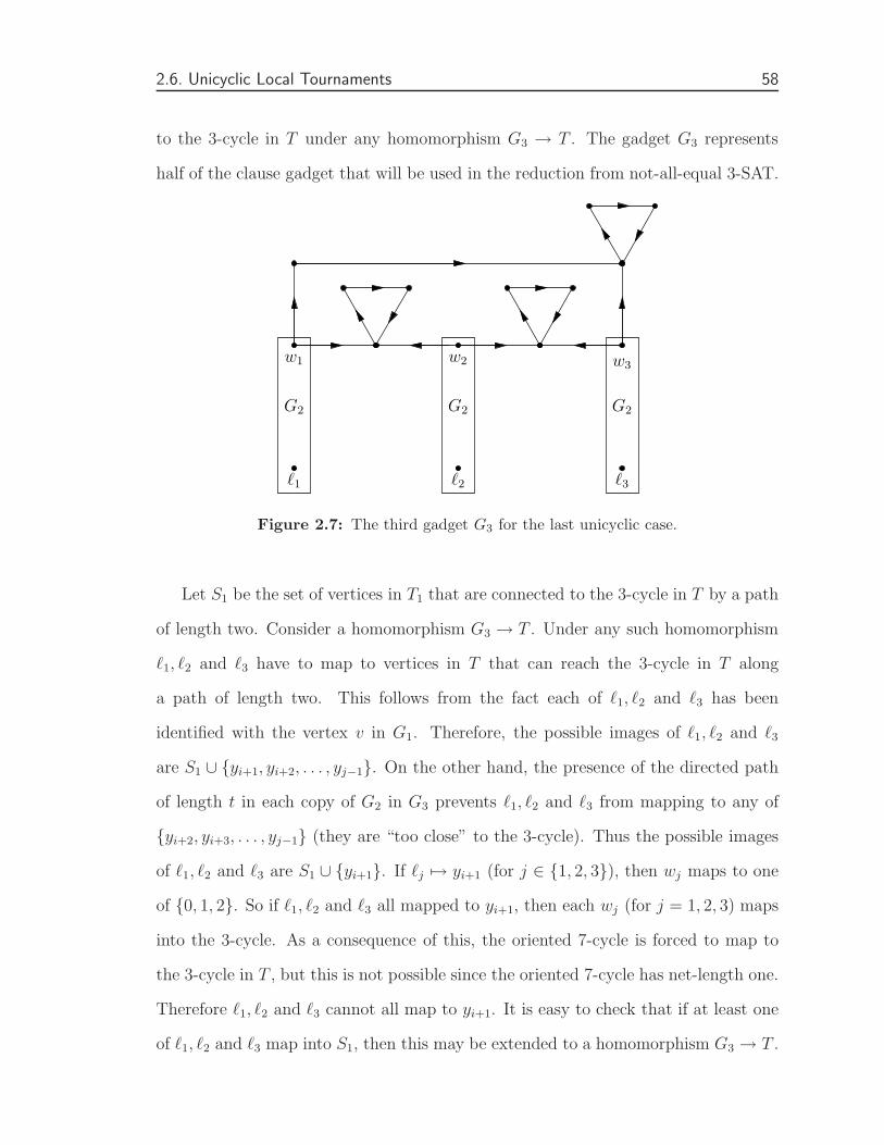
2.6. Unicyclic Local Tournaments 58
to the 3-cycle in T under any homomorphism G3 → T . The gadget G3 represents
half of the clause gadget that will be used in the reduction from not-all-equal 3-SAT.
G2 G2 G2
w1 w2 w3
ℓ1 ℓ2 ℓ3
Figure 2.7: The third gadget G3 for the last unicyclic case.
Let S1 be the set of vertices in T1 that are connected to the 3-cycle in T by a path
of length two. Consider a homomorphism G3 → T . Under any such homomorphism
ℓ1, ℓ2 and ℓ3 have to map to vertices in T that can reach the 3-cycle in T along
a path of length two. This follows from the fact each of ℓ1, ℓ2 and ℓ3 has been
identified with the vertex v in G1. Therefore, the possible images of ℓ1, ℓ2 and ℓ3
are S1 ∪ {yi+1, yi+2, . . . , yj−1}. On the other hand, the presence of the directed path
of length t in each copy of G2 in G3 prevents ℓ1, ℓ2 and ℓ3 from mapping to any of
{yi+2, yi+3, . . . , yj−1} (they are “too close” to the 3-cycle). Thus the possible images
of ℓ1, ℓ2 and ℓ3 are S1 ∪ {yi+1}. If ℓj 7→ yi+1 (for j ∈ {1, 2, 3}), then wj maps to one
of {0, 1, 2}. So if ℓ1, ℓ2 and ℓ3 all mapped to yi+1, then each wj (for j = 1, 2, 3) maps
into the 3-cycle. As a consequence of this, the oriented 7-cycle is forced to map to
the 3-cycle in T , but this is not possible since the oriented 7-cycle has net-length one.
Therefore ℓ1, ℓ2 and ℓ3 cannot all map to yi+1. It is easy to check that if at least one
of ℓ1, ℓ2 and ℓ3 map into S1, then this may be extended to a homomorphism G3 → T .

2.6. Unicyclic Local Tournaments 59
Let the length of the path 0yj+1yj+2 . . . yk (Figure 2.2) be t′. The other half of the
clause gadget, G4, is formed by taking the converse of G3, changing the lengths of the
paths in G2 to t′, and re-labeling the vertices ℓ1, ℓ2 and ℓ3 as ℓ′1, ℓ′
2 and ℓ′3 respectively.
Define S3 to be the vertices in T3 that are reachable by a path of length two from
the 3-cycle in T . It now follows in a similar manner as before that ℓ′1, ℓ′
2 and ℓ′3 have
to map into the set S3 ∪ {yk} under any homomorphism G4 → T . As before at least
one of ℓ′1, ℓ′
2 and ℓ′3 has to map to S3.
The clause gadget, K, can now (finally) be constructed. K is the disjoint union
of G3 and G4. The idea behind the clause gadget is that “True” and “False” are to
be encoded based on how each pair (ℓj, ℓ′
j), j = 1, 2, 3, is mapped.
We are now ready to give the reduction. Given an instance of not all equal 3-
SAT (without negations) with variables x1, x2, . . . , xs and clauses C1, C2, . . . , Ct we
construct a digraph D as follows. For each variable xi, we have a directed path of
length two, P i, with initial vertex (also) labeled xi and terminal vertex labeled x′
i.
For every clause {ℓ1, ℓ2, ℓ3} take a copy of K. Each time a variable xi appears in a
clause {ℓ1, ℓ2, ℓ3} (say xi = ℓ2), identify the vertex xi in P i with the vertex ℓ2 and
the vertex x′
i in P i with ℓ′2 in the corresponding clause gadget. This is illustrated in
Figure 2.8.
Let D → T be a homomorphism. Based on the discussion before the possible
images for the pair (ℓj , ℓ′
j), j = 1, 2, 3, is the set [S1 ∪ {yi+1}]× [S3 ∪ {yk}]. Since no
vertex in S1 is joined to a vertex in S3 by a path of length two, we are able to refine
the images somewhat. We define two subsets of the set [S1 ∪ {yi+1}] × [S3 ∪ {yk}]:
T = {(yi+1, yk) ∪ [{yi+1} × S3] and F = S1 × {yk}. It can now be seen that the
images of each pair (ℓj , ℓ′
j), j = 1, 2, 3, is the set T ∪F . A pair is not allowed to map
only to T (as this forces each ℓj to map to yi+1 which is not possible). Also, no pair
maps to F (as this forces all ℓ′js to map to yk which is not possible). Thus each pair
(representing a variable) maps in such a way that there is at least one image in T

2.6. Unicyclic Local Tournaments 60
ℓ′1 ℓ′2 ℓ′3
G4
ℓ1 ℓ2 ℓ3
G3
Figure 2.8: A typical clause in the instance D for the last unicyclic case.
and at least one image in F . A satisfying truth assignment can now be recovered by
examining the images of the end-vertices of the path P i, representing the variable xi:
into T corresponds to “True” and into F corresponds to “False.”
Given a satisfying truth assignment to not-all-equal 3-SAT (without negations)
we construct a homomorphism as follows. Let y ∈ S1. If the variable xi is assigned
the value “True,” map the end-vertices of the path P i to the pair (yi+1, yk). If the
variable xi is assigned the value “False,” map the ends of P i to the pair (y, yk). This
pre-colouring can be extended to a homomorphism on each clause gadget.
Therefore there is a homomorphism D → T if and only if there is a satisfying
truth assignment to not-all-equal 3-SAT without negations.
For unicyclic local tournaments, we have the following dichotomy.
Theorem 2.6.4. Let T be a unicyclic local tournament. If T is a directed cycle or T
has the structure shown in Figure 2.2 with T2 a tournament and at least one of T1 and
T3 is empty, then T -colouring is polynomial. Otherwise T -colouring is NP-complete.

2.7. Round Local Tournaments 61
We close this section by pointing out that if the 3-cycle in all of the above ar-
guments is replaced by a directed 2-cycle, then all of the results carry over. In the
polynomial cases, we are still dealing with a graft extension. For the NP-complete
cases, we relied on oriented cycles of net-length one not mapping to the 3-cycle. These
same oriented cycles do not map to a directed 2-cycle either.
2.7 Round Local Tournaments
Let D be a round local tournament containing at least two cycles and let ℓ denote
the length of a shortest cycle in D. Proving NP-completeness is done in the following
way:
❒ If D has a unique cycle of length ℓ, D-colouring is NP-complete.
❒ A smallest counterexample, D, (both in the number of vertices and the number
of arcs)
• has all vertices on a shortest cycle,
• does not have δ+ ≥ ℓ,
• does not have ∆+ ≥ ℓ,
• does not have φ ≥ 2ℓ, where φ is the Frobenius-Schur index of the cycle
lengths of D.
• This forces φ = ℓ and ∆+ < ℓ which leads to a contradiction. Therefore
the counterexample does not exist and D-colouring is NP-complete.
Lemma 2.7.1. Let D be a round local tournament containing at least two cycles. If
D has a unique cycle of shortest length, then D-colouring is NP-complete.
Proof. Let v0, v1, . . . , vn−1 be a round labeling of V (D), C be a shortest cycle in D
and ℓ be the length of C. Since D is strongly connected, by Lemma 2.3.5 there exist
indices 0 < a1 < a2 < . . . ak−1 < n so that C = v0va1va2· · · vak−1
v0.

2.7. Round Local Tournaments 62
Since D has at least two cycles, there must be vertices of D not on C.
The proof is divided into two cases. Firstly, we consider the situation where there
are three indices i, i+1 and i+2 (mod ℓ) such that ai+2−ai+1 ≥ 2 and ai+1−ai ≥ 2.
Therefore there are vertices of D, not on C, between ai and ai+1 and between ai+1
and ai+2. Once this has been dealt with, what then remains is the case where these
vertices do not exist. This will imply the existence of four indices i, i + 1, i + 2 and
i + 3 (mod ℓ) such that ai+3− ai+2 = 1, ai+2− ai+1 ≥ 2 and that ai+1− ai = 1. That
is, vai+3and vai+2
are consecutive, as are vai+1and vai
, and there exists a vertex of D
not on C between vai+1and vai+2
.
Case 1: ai+2 − ai+1 ≥ 2 and ai+1 − ai ≥ 2.
Let u be any vertex between ai and ai+1 and let w be the successor of ai+1 on the
outer n-cycle (w is between ai+2 and ai+1). This is illustrated in Figure 2.9.
D
vai
vai+1
vai+2
u
w
Figure 2.9: The first case where D has a unique cycle of shortest length
We handle this case by assuming the lemma is false and examining a minimum
counterexample. That is assume that there exists a round local tournament D with
at least two cycles and a unique cycle of shortest length that is of the form shown
in Figure 2.9. In addition to this we assume that D has the minimum number of
vertices possible. Also, D-colouring is not NP-complete.
We apply the sub-indicator J shown in Figure 2.10 to D. Note that the vertex
on the left is identified with vertex ai+1 in D and that the vertex j of J is the vertex
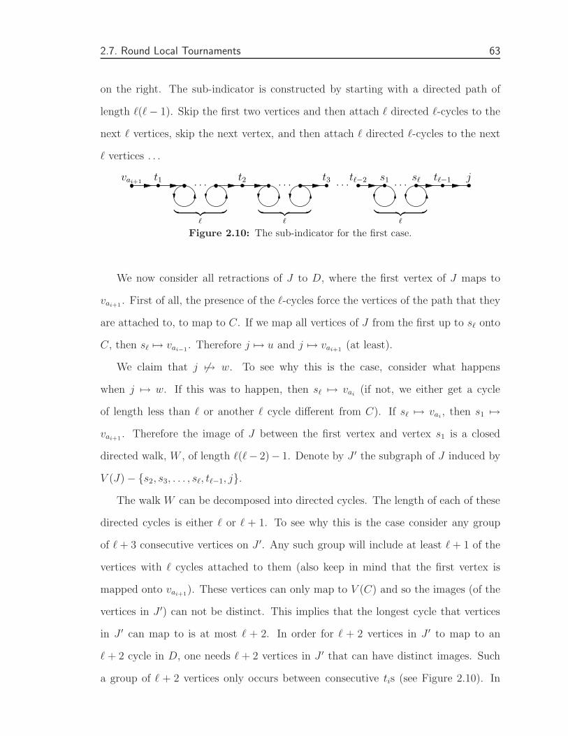
2.7. Round Local Tournaments 63
on the right. The sub-indicator is constructed by starting with a directed path of
length ℓ(ℓ− 1). Skip the first two vertices and then attach ℓ directed ℓ-cycles to the
next ℓ vertices, skip the next vertex, and then attach ℓ directed ℓ-cycles to the next
ℓ vertices . . .
t1vai+1 . . . t2 . . . t3 . . .tℓ−2 s1 sℓ tℓ−1 j. . .
︸ ︷︷ ︸ℓ
︸ ︷︷ ︸ℓ
︸ ︷︷ ︸ℓ
Figure 2.10: The sub-indicator for the first case.
We now consider all retractions of J to D, where the first vertex of J maps to
vai+1. First of all, the presence of the ℓ-cycles force the vertices of the path that they
are attached to, to map to C. If we map all vertices of J from the first up to sℓ onto
C, then sℓ 7→ vai−1. Therefore j 7→ u and j 7→ vai+1
(at least).
We claim that j 67→ w. To see why this is the case, consider what happens
when j 7→ w. If this was to happen, then sℓ 7→ vai(if not, we either get a cycle
of length less than ℓ or another ℓ cycle different from C). If sℓ 7→ vai, then s1 7→
vai+1. Therefore the image of J between the first vertex and vertex s1 is a closed
directed walk, W , of length ℓ(ℓ− 2)− 1. Denote by J ′ the subgraph of J induced by
V (J)− {s2, s3, . . . , sℓ, tℓ−1, j}.
The walk W can be decomposed into directed cycles. The length of each of these
directed cycles is either ℓ or ℓ + 1. To see why this is the case consider any group
of ℓ + 3 consecutive vertices on J ′. Any such group will include at least ℓ + 1 of the
vertices with ℓ cycles attached to them (also keep in mind that the first vertex is
mapped onto vai+1). These vertices can only map to V (C) and so the images (of the
vertices in J ′) can not be distinct. This implies that the longest cycle that vertices
in J ′ can map to is at most ℓ + 2. In order for ℓ + 2 vertices in J ′ to map to an
ℓ + 2 cycle in D, one needs ℓ + 2 vertices in J ′ that can have distinct images. Such
a group of ℓ + 2 vertices only occurs between consecutive tis (see Figure 2.10). In

2.7. Round Local Tournaments 64
order for the group to map to an (ℓ + 2)-cycle ti and the vertex following ti+1 must
have the same image. That means that ti is mapped to a vertex on V (C) and so the
ℓ + 2 vertices do not have distinct images. This shows that the directed cycles in the
decomposition of W can only be of length ℓ and ℓ + 1.
Since W can be decomposed into ℓ and ℓ + 1 cycles, we have that ℓ(ℓ− 2)− 1 =
k1ℓ + k2(ℓ + 1) = (k1 + k2)ℓ + k2 where k1 is the number ℓ-cycles and k2 the number
of (ℓ + 1)-cycles in such a decomposition. Note that 0 ≤ k1, k2 ≤ ℓ− 2. This means
that ℓ(ℓ−1) = (k1 +k2)ℓ+(k2 +1) or that ℓ divides (k2 +1), but 1 ≤ (k2 +1) ≤ ℓ−1,
so we have a contradiction. Therefore if the first vertex of J maps to vai+1, then j
cannot map to w.
We now also claim that j maps to every vertex of C. From before we already
know that j 7→ vai+1. If we map t1 to w and then all other vertices of J to C, we
find that j 7→ vai: if t1 7→ w, the vertex preceding t2 maps to vai+1
and the length
of the path that remains in J is ℓ(ℓ − 2) − 1 — a multiple of ℓ minus 1. In general
by mapping t1, t2, . . . , tk to w and all other vertices (from the first up to the vertex
preceding tk+1) to C, we find that the vertex preceding tk maps to vai+1. The length
of the path remaining in J is ℓ(ℓ − 1) − (kℓ + k) = ℓ(ℓ − 1 − k) − k (we have used
kℓ + k + 1 vertices or kℓ + k arcs up to this point). If we now map all the remaining
vertices to C we see that j 7→ vai+1−k.
The result of this sub-indicator, D+, contains (at least) the subgraph induced
by C ∪ {u}, but not the vertex w. Therefore D+ contains at least two cycles and
also has a unique shortest cycle of length ℓ. Since D has the minimum number of
vertices for a counterexample, D+-colouring is NP-complete, implying D-colouring is
NP-complete — a contradiction.
Case 2: ai+3 − ai+2 = 1, ai+2 − ai+1 ≥ 2 and that ai+1 − ai = 1.
This case is illustrated in Figure 2.11.
The proof in this case is via a reduction from not all equal ℓ-SAT without nega-

2.7. Round Local Tournaments 65
D
vai+2
vai+3
vai
vai+1
Figure 2.11: The second case where D has a unique cycle of shortest length
tions.
In carrying out the proof we need to construct the gadget Z shown in Figure 2.12.
The gadget Z is constructed from a copy of D and two directed paths of length two,
say a′ua and z′vz. Identify a′ and z′, attach directed ℓ-cycles to vertices z′, v and z
and finally identify a with vai+1.
vai+2
Cℓ CℓCℓ
D
vai+3
vai
vai+1
z′ z
Figure 2.12: The gadget Z
In a retraction of Z to D, the vertex z′ can only map to vai+1or vai
. This forces
the pair of vertices (z′, z) to map to the pair (vai, vai+2
) or the pair (vai+1, vai+3
).
We also need the gadget K shown in Figure 2.13 (it is the same as the sub-
indicator used in the first case).
Let f : K → D be a homorphism from K to D. If f(r) = vai, then f(s) 6= vai+1
. If
f(s) = vai+1, then f(tℓ−1) = vai
. This means that the image of K under f corresponds
to a closed walk from vaito vai
of length ℓ(ℓ − 1)− 1. Through a similar technique

2.7. Round Local Tournaments 66
t1r . . . t2 . . . t3 . . .tℓ−2 s1 sℓ tℓ−1 s. . .
︸ ︷︷ ︸ℓ
︸ ︷︷ ︸ℓ
︸ ︷︷ ︸ℓ
Figure 2.13: The gadget K
as in the previous case, one can show that this is impossible: the walk of length
ℓ(ℓ−1)−1 can only be decomposed into ℓ and ℓ+1 cycles (because of the placement
of the ℓ-cycles) and this is impossible. As in case one, it is possible to show that
if f(r) = vai, then s maps to every vertex of C except vai+1
. This accomplished by
mapping the tis of K “into” the gap between vai+1and vai+2
. On the other hand if
f(r) = vai+1, then s can map to any vertex of C (again the tis are mapped into the gap
between vai+1and vai+2
). In a similar way it is possible to show that if f(s) = vai+3,
then f(r) can map to any vertex of C except vai+2and that if f(s) = vai+2
, then r
can map to any vertex of C.
Next, we construct a new gadget F from two copies of K, say with end-vertices
r1, s1 and r2, s2 respectively. To construct F identify vertex s1 with vertex r2 and
call this vertex c. This is shown in Figure 2.14.
s1 = r2 = c
s2r1
Figure 2.14: The gadget F
The gadget F has the property that if the pair (r1, s2) maps to the pair (vai, vai+2
),
under a homomorphism from F to D, then the vertex c can map to any vertex on C,
except vai+1. If the pair (r1, s2) maps to (vai+1
, vai+3), then c can map to any vertex

2.7. Round Local Tournaments 67
on C except vai+2.
As mentioned earlier, the proof is via a reduction from not all equal ℓ-SAT without
negated variables. So let an instance of not all equal ℓ-SAT without negated variables
be given:
Z = {z1, z2, . . . , za} — the variables ,
K1, K2, . . . , Kb — the clauses ,
Kj = {zj1, zj2 , . . . , zjℓ} for each j ∈ {1, 2, . . . , b}.
We now construct an instance of D-colouring. For each variable zj take a copy of
the gadget Z. Identify all copies of D. Label the z and z′-vertices in the copies of Z
as z1, z2, . . . , za, z′
1, z′
2, . . . , z′
a. These vertices correspond to variables in the instance
of not all equal ℓ-SAT without negated variables. This produces the variable gadget.
For each clause Kj = {zj0 , zj1, . . . , zjℓ−1} take ℓ copies of the gadget F , say
Fj1, Fj2 , . . . , Fjℓwith end-vertices (rj11 , sj21), (rj12 , sj22), . . . , (rj1ℓ
, sj2ℓ) and top-vertices
cj1, cj2, . . . , cjℓ, respectively. Now identify rj1i
with z′jiand sj2i
with zjiand form an
ℓ-cycle through cj1, cj2, . . . , cjℓ. This produces the instance H of D-colouring shown
in Figure 2.15.
We now show that H → D if and only if there exists a satisfying truth assignment
for the instance of not all equal ℓ-SAT without negated variables. Define the pair
(vai, vai+2
) (in D) to be T and the pair (vai+1, vai+3
) to be F .
If H → D, then each pair (z′i, zi) maps to T or to F . Furthermore for a given
clause Kj = {zj1, zj2 , . . . , zjℓ} it is not the case that all pairs (z′ji
, zji), 1 ≤ i ≤ ℓ,
map to T . If this was the case, none of the cjis are allowed to map to vai+1
and since
there is a unique ℓ-cycle in D, we won’t be able to complete the ℓ-cycle through the
cjis. In a similar way it is possible to show that the pairs (z′ji
, zji), 1 ≤ i ≤ ℓ can not
all map to F (here we would be missing the vertex vai+2on the ℓ-cycle). Therefore

2.7. Round Local Tournaments 68
D
vai
vai+1
cj1
cji
cjℓ
z′1
z′j1
z′ji
z′jℓ
z1
zj1
zji
zjℓ
...
...
...
...
z′a
za
vai+3
va
i+2
Figure 2.15: The instance H
in every clause there is at least one pair that maps to T and at least one pair that
maps to F . A satisfying truth assignment can now be recovered by assigning “True”
(“False”) to variable zi if (z′i, zi) maps to T (F ).
Conversely, let a satisfying truth assignment be given. Pre-colour the pair (z′i, zi)
by T (F ) if zi is assigned the value “True” (“False”). For the clause gadget corre-
sponding to clause Kj = {zj1, zj2 , . . . , zjℓ} we extend the colouring as follows: locate
two consecutive vertices cjkand cjk+1
such that (z′jk, zjk
) maps to F and (z′jk+1, zjk+1
)
maps to T (all subscripts are taken modulo ℓ). Map the corresponding Fjkin such
a way that cjkmaps to vai+1
and map Fjk+1in such a way that cjk+1
maps to vai+2.
Now map Fjk+2such that cjk+2
maps to vai+3, Fjk+3
such that cjk+3maps to vai+4
, . . . ,
Fjk−1such that cjk−1
maps to vai. By the properties of F and K discussed earlier,
this is always possible. The remaining vertices of H map in an obvious way to D.

2.7. Round Local Tournaments 69
Therefore H → D.
To complete the proof that colouring by a round local tournament is NP-complete,
we assume that the result is false and examine a smallest counterexample (minimum
number of vertices and minimum number of arcs). Being a counterexample, the
corresponding colouring problem is not NP-complete. We derive additional properties
of the counterexample to see that it cannot exist and in doing so we can then conclude
that the colouring problem is in fact NP-complete.
The first property of this counterexample follows from Lemma 2.7.1.
Lemma 2.7.2. Every vertex of a smallest counterexample is on a shortest cycle.
Proof. If D is a smallest counterexample then D-colouring is not NP-complete. This
being the case, by Lemma 2.7.1 it must have at least two cycles of shortest length.
Let ℓ denote the length of a shortest cycle in D. If, in addition, D has vertices that
are not on these shortest cycles, we apply a sub-indicator Cℓ to D. The result of
this, say D′, will be the digraph induced by the vertices of D that are on a shortest
cycle. Since there are at least two shortest cycles, D′ contains at least two cycles
and furthermore it has fewer vertices that D. In addition to this it is also a round
local tournament because it is an induced subgraph of D. Since it has fewer vertices
than D (and D is a smallest counterexample), D′-colouring has to be NP-complete
(otherwise it would be smaller than a smallest counterexample). This implies that
D-colouring is also NP-complete, a contradiction.
The next property deals with the minimum out-degree of the smallest counterex-
ample.
Lemma 2.7.3. Let D be a smallest counterexample and denote by δ+ the minimum
out-degree of D. Then δ+ < ℓ, where ℓ is the length of a shortest cycle in D.

2.7. Round Local Tournaments 70
Proof. Assume that D has δ+ ≥ ℓ ≥ 3. To prove the lemma we apply the arc-
subindicator shown in Figure 2.16 (a transitive tournament on δ+ + 1 vertices with
the two arcs spanning end-to-end as shown), with respect to the dashed arc, to D.
Since every vertex in D has degree at least δ+, the result of this arc-subindicator is a
0 1 2 3 δ+. . .
. . .
Figure 2.16: The arc-subindicator.
digraph D′ in which every vertex has out-degree at least 2 (the two vertices following
the given vertex in the round enumeration). Every vertex also loses its outneighbour
furthest away from it in the round enumeration. This implies that D′ has at least
two cycles and is a round local tournament. Furthermore D′ has at least one vertex
with out-degree less than ℓ (these are the vertices in D that have out-degree exactly
δ+) and so has fewer arcs than D. Since D has the minimum number of arcs possible
for a counterexample, D′ cannot be a counterexample and so D′-colouring is NP-
complete. By the arc-subindicator construction this implies that D-colouring is also
NP-complete, a contradiction.
Next, we prove that a similar result holds for ∆+.
Lemma 2.7.4. Let D be a smallest counterexample and denote by ∆+ the maximum
out-degree of D. Then ∆+ < ℓ, where ℓ is the length of a shortest cycle in D.
Proof. Assume that D has ∆+ ≥ ℓ. By the previous result this implies that there
exist two vertices x and y in D such that d+(x) < ℓ and d+(y) ≥ ℓ.
Let V (D) = v0, v1, . . . , vn−1 be a round enumeration of the vertices of D. We
claim that there exists an i ∈ {0, 1, . . . , n− 1} such that d+(vi−1) < l and d+(vi) ≥ ℓ.

2.7. Round Local Tournaments 71
To see this, take any vertex u with d+(u) ≥ ℓ; if the predecessor of u (in the round
enumeration) has out-degree less than ℓ we are done. Otherwise, the predecessor has
out-degree greater than or equal to ℓ. We then repeat the process of considering the
predecessor. Since there is a vertex of out-degree less than ℓ, this process terminates.
By shifting the labels of D (mod n) we can assume that d+(vn−1) < ℓ and that
d+(v0) ≥ ℓ.
Let’s say that d+(v0) = m ≥ ℓ and d+(vn−1) = a < ℓ. We then use the sub-
indicator formed by taking a copy of D and attaching a path of length ℓ to vertex
v0 and letting j be the final vertex on the path of length ℓ. This is shown below in
Figure 2.17.
jv0
v1
va−1
va
vn−1. . .
vm = u1u2
u3
u+k
vt
uk
Pℓ︷ ︸︸ ︷
Figure 2.17: The sub-indicator.
Every vertex is on a shortest cycle (an ℓ-cycle). In particular, v0 is on one and
moreover there is a shortest cycle containing v0 that uses the arc v0vm. To see this
consider any shortest cycle through v0, if it is not using v0vm then there is at most
one vertex of this cycle between v0 and vm (otherwise we can find a shorter cycle).
Call this vertex u. The vertex u is adjacent to some vi with i > m, otherwise there is
a shorter cycle. This also means that vm is adjacent to vi. By replacing the arc v0u
with v0vm and then following the rest of the ℓ-cycle, we now have a shortest cycle
that uses v0vm. Let C be such a shortest cycle through v0. Label the vertices on C
(starting with v0) as v0 = u0, vm = u1, . . . , uℓ−1.

2.7. Round Local Tournaments 72
It is easy to see that vertex j maps to vℓ, vℓ+1, . . . , vm by using the outer n-cycle
together with the arcs vℓ−1vi where i ∈ {ℓ, ℓ + 1, . . . , m}. Furthermore, j maps to
any vt with m < t ≤ n− 1: for a given vt, let s = max{x | x < t and vx ∈ C}. Since
vs ∈ C, vs = uk for some 1 ≤ k ≤ ℓ− 1. The idea is that uk is the first vertex on C,
not including vt, that is encountered when moving backwards along C. The successor
uk on C, u+k = vi, with i ≥ t. This implies that ukvt is an arc of D. In order to
obtain a walk of length ℓ from v0 = u0 to vt we first proceed along the n-cycle from
v0 to vℓ−(k+1) (0 ≤ ℓ − (k + 1) < m). Next, we use the arc vℓ−(k+1)vm = vℓ−(k+1)u1,
then proceed along C to uk and finally use the arc ukvt.
By using C, it is clear that j maps to v0. The resulting digraph derived from
using this sub-indicator, contains C. It therefore has at least one cycle.
We now show that vertex j does not map to va. Here we have that N−(va) ⊆
{v0, v1, . . . , va−1}. In order to obtain a contradiction assume that W = x0x1 · · ·xℓ−1
is walk of length ℓ from v0 to va. That is x0 = v0, x1 = vj1, x2 = vj2, . . . , xℓ−2 =
vjℓ−2, xℓ−1 = va. Let k = max{0, j1, j2, . . . , jℓ−2, a}. Note that k > a, otherwise
ji ≤ a and W is a walk of length ℓ inside the transitive tournament D[v0, v1, . . . , va].
Furthermore vkva is not an arc of D, for if it was then d+(vn−1) ≥ ℓ. Therefore
d(vk, va) ≥ 2 and so the length of the sub-walk of W from v0 to vk is at most ℓ− 2.
In order to complete W , vkvi ∈ A(D) for some i ∈ {0, 1, . . . , a − 1}. This implies
that vkv0 ∈ A(D) which means that there is a closed walk from v0 to itself of length
at most ℓ− 1. This is clearly not possible and so j cannot map to va.
Now, if d+(v0) > l, then the result, say D′, of this sub-indicator has at least two
cycles, but does not contain va. Since it is smaller than D it is not a counterexam-
ple and so D′-colouring is NP-complete. Therefore D-colouring is NP-complete, a
contradiction. Thus d+(v0) = l.
On the other hand, if there is a vertex vi ∈ {vm = vℓ, vℓ+1, . . . , vn−2} with d+(vi) ≥
2, then the result of the sub-indicator will again have at least two cycles and as

2.7. Round Local Tournaments 73
above this leads to D-colouring being NP-complete, a contradiction. This shows that
D[vm = vℓ, vℓ+1, . . . , vn−1] is an induced path. Note that, in this case, vn−1 is the
predecessor of v0 on the ℓ-cycle C above.
If we now have that d+(vn−1) ≥ 2, j will map to v1 by using C. Therefore, the
sub-indicator results in a digraph with at least two cycles and fewer vertices than D (j
still does not map to va). Once again, we conclude that D-colouring is NP-complete,
a contradiction. Hence, d+(vn−1) = 1.
We now apply the sub-indicator shown below in Figure 2.18. This is formed using
a copy of D and attaching an oriented path as shown to v0.
v0
v1
vn−1
vm = vℓ
Pℓ−1︷ ︸︸ ︷jx
. . .
Figure 2.18: The new sub-indicator.
No vertex between v0 and vℓ is adjacent to a vertex vi with i > ℓ + 1, otherwise
vℓ has out-degree at least two. Therefore any vertex between v0 and vℓ is adjacent
to vℓ+1 so that it can be on a cycle of length ℓ. Also note that the vertex x shown
above can map to any of {v0, v1, . . . , vℓ−1}.
The distance between vℓ and v0 is exactly ℓ− 1, because of the ℓ-cycle C through
v0. This allows j to map to v0: first map x to vi ∈ {v1, . . . , vℓ−1}, then use vivℓ+1
together with the path of length ℓ− 2 from vℓ+1 to v0. It is also possible to map j to
vi ∈ {vℓ−1, vℓ, . . . , vn−1}: first map x to vi−(ℓ−1) (0 ≤ i− (ℓ− 1) ≤ n− 1− (ℓ− 1) =
n− ℓ = ℓ− 1), then follow the outer n-cycle from vi−(ℓ−1) to vi.
This sub-indicator therefore guarantees that we have at least the ℓ-cycle C through

2.7. Round Local Tournaments 74
v0 and the vertex vℓ−1. Thus the result has at least two cycles.
We now note that j does not map to v1, otherwise there exists a directed walk
of length ℓ − 1 from vi ∈ {v0, v1, . . . , vℓ−1} (since x can only map to vi) to v1 and
such a walk does not exist. Therefore the result has at least one fewer vertex and
so its colouring problem is NP-complete, forcing D-colouring to be NP-complete, a
contradiction.
The next two results deal with the Frobenius-Schur index of the cycle lengths of
a minimum counterexample. The first one may seem somewhat artificial, but it is
needed to establish the second.
Lemma 2.7.5. Let D be a round local tournament on the vertex set {0, 1, . . . , n−1}
with n = 2ℓ − 2, where ℓ is the length of a shortest cycle in D. If for every v ∈
{ℓ − 2, ℓ − 1, . . . , n − 1}, N+(v) = v + 1 (mod n), then D cannot be a minimum
counterexample to the D-colouring problem.
Proof. Let φ(ℓ, ℓ+1, . . . , n) = φ be the Frobenius-Schur index of the cycle lengths of
D. Recall that φ is the smallest integer such that every integer x ≥ φ can be written
as a linear combination of ℓ, ℓ + 1, . . . , n. By the minimality of φ, φ − 1 cannot be
written as such a linear combination. Therefore D does not possess a closed walk of
length φ − 1: If it did, this closed walk can be decomposed into arc disjoint cycles
with lengths in the set {ℓ, ℓ+1, . . . , n}. This is equivalent to writing φ−1 as a linear
combination of ℓ, ℓ + 1, . . . , n which is not possible.
We assume that D is a minimum counterexample and derive a contradiction.
Since n = 2ℓ− 2,
φ =
⌊n− 2
n− ℓ
⌋ℓ = 2ℓ.
Therefore φ−1 = 2ℓ−1 = n+1. Also, since 0 has to be on an ℓ-cycle, 0(ℓ−1) ∈ A(D)
and by the local tournament property 0a ∈ A(D) where a ∈ {1, 2, . . . , ℓ − 1}. To
derive the contradiction, we use a sub-indicator construction. This sub-indicator is

2.7. Round Local Tournaments 75
constructed from a copy of D and by attaching a path of length φ − 1 to vertex 0
and taking the end of this path to be the vertex j. Some of the possible images of
j are: 1, 2, . . . ℓ − 1. This is accomplished by going around the n-cycle once back
to 0 and then using the arc 0a, a ∈ {1, 2, . . . , ℓ − 1}. To map j to vertex x, where
ℓ ≤ x ≤ n− 1, we proceed as follows: use an (n− (x− ℓ + 1))-cycle to go from 0 to 0
(ℓ ≤ n−(x−ℓ+1) ≤ n−1). Then use the remaining φ−1−(n−(x−ℓ+1)) = x−ℓ+2
arcs (2 ≤ x−ℓ+2 ≤ n−ℓ+1) first to go from 0 to ℓ−1 and then from ℓ−1 to x along
the n-cycle. Its impossible for j to map to 0 since this would correspond to a closed
walk from 0 to 0 of length φ− 1. Therefore the result of applying this sub-indicator
is D − {0}. Furthermore, since ℓ − 2 is not adjacent to ℓ, 1 is not adjacent to ℓ.
In order for 1 to be on an ℓ-cycle, (n − 1) is adjacent to 1. Therefore D − {0} has
at least two cycles. Since D is a minimum counterexample, (D − {0})-colouring is
NP-complete, and so D-colouring is NP-complete, a contradiction.
Lemma 2.7.6. If D is a minimum counterexample, then the Frobenius-Schur index,
φ, of the cycle lengths of D satisfies φ = ℓ, where ℓ is the length of a shortest cycle
in D.
Proof. Label the vertices of D as {0, 1, . . . n− 1}. By Lemma 2.2.5,
φ = kl where k =
⌊n− 2
n− ℓ
⌋.
We assume now that φ ≥ 2ℓ, and derive a contradiction.
If φ ≥ 2ℓ, then
k =
⌊n− 2
n− ℓ
⌋≥ 2,
and this happens if and only if (n− 2)/(n− ℓ) ≥ 2 which is equivalent to 2ℓ ≥ n + 2.
To obtain the sought after contradiction we employ as an indicator a directed path
of length φ− 1. This indicator has the property that its result will not contain loops
by the fact that D has no closed walks of length φ− 1.
2.7. Round Local Tournaments 76
Note that φ−1 = (k−1)ℓ+(ℓ−1). This implies that in applying the indicator to
D, we obtain an arc from 0 to ℓ−1 (use (k−1) ℓ-cycles to get from 0 to 0, and then use
the remaining (ℓ−1) arcs to get from 0 to ℓ−1). Also, φ−1 = (k−2)ℓ+(ℓ+1)+(ℓ−2).
This produces an arc from 0 to ℓ− 2 when applying the indicator.
We now show that it is also possible to have arcs from ℓ− 1 to 0 and from ℓ− 2
to 0. The number of arcs on the outer n-cycle from ℓ− 1 to 0 is n− ℓ + 1. Consider
now φ− 1− (n− ℓ + 1) = φ− (n− ℓ + 2). If it is possible to write φ− (n− ℓ + 2) as
a linear combination of cycle lengths, then there will a closed walk from any vertex
back to itself of this length. In particular, there will be a walk of this length from
ℓ − 1 to ℓ − 1. A further n − ℓ + 1 arcs will then carry the walk from ℓ − 1 to 0
along the outer n-cycle. Therefore, applying the indicator above will produce an arc
from ℓ − 1 to 0 provided that φ − (n − ℓ + 2) is a sum of cycle lengths. This is
indeed the case: We know that all x ≥ φ = kℓ is a sum of cycle lengths. Furthermore
(k− 1)ℓ, (k− 1)ℓ + 1, . . . , (k− 1)n are also linear combinations (of k− 1) of the cycle
lengths. Let t = kℓ − (k − 1)n, this represents the length of a “gap” of integers
that cannot be written as a linear combination of the cycle lengths. We see that
k(ℓ− n) = t− n so that
k =t− n
ℓ− n=
n− t
n− ℓ=
n− 2
n− ℓ−
t− 2
n− ℓ.
Since
k =
⌊n− 2
n− ℓ
⌋,
we get that (t − 2)/(n − ℓ) < 1. Therefore t < n − ℓ + 2 or t ≤ n − ℓ + 1. Further
from 2ℓ ≥ n + 2 it follows that n − ℓ + 2 ≤ ℓ. Thus φ − (n − ℓ + 2) ∈ {(k − 1)ℓ =
φ − ℓ, (k − 1)ℓ + 1, . . . , (k − 1)n = φ − t} and so φ − (n − ℓ + 2) is a sum of cycle
lengths. To obtain an arc from ℓ− 2 to 0, we are searching for a walk of length φ− 1
from ℓ− 2 to 0. The number of arcs on the outer n-cycle from ℓ− 2 to 0 is n− ℓ + 2.

2.7. Round Local Tournaments 77
Here φ− 1− (n− ℓ + 2) = φ− (n− ℓ + 3). Also φ− (n− ℓ + 3) > φ− (n− ℓ + 2) > t
and φ− (n− ℓ + 3) ≤ ℓ + 1. If φ− (n− ℓ + 3) ≤ ℓ, then φ− (n− ℓ + 3) ∈ {(k− 1)ℓ =
φ− ℓ, (k − 1)ℓ + 1, . . . , (k − 1)n = φ− t}. This enables a closed walk from ℓ− 2 to
ℓ − 2 of length φ − (n − ℓ + 3) to be formed. The remaining n − ℓ + 2 arcs on the
walk of length φ − 1 then goes from ℓ − 2 to 0. What remains at this point is the
case n− ℓ + 3 = ℓ + 1, or n− ℓ + 2 = ℓ. This implies that the number of arcs on the
n-cycle from ℓ− 2 to 0 is ℓ. If there exists a vertex in {ℓ− 2, ℓ− 1, . . . , n− 2} with
out-degree at least two, then there exists a path of length ℓ− 1 from ℓ− 2 to 0. This
path together with a closed walk of length φ− (n− ℓ + 2) provides us with a walk of
length φ−1 from ℓ−2 to 0. If there does not exist a vertex in {ℓ−2, ℓ−1, . . . , n−2}
with out-degree at least two, then D[ℓ − 2, ℓ − 1, . . . , n − 1, 0] is an induced path.
This is not possible by Lemma 2.7.5.
We now see that using a path of length φ− 1 as an indicator, produces the arcs
0(ℓ − 1), (ℓ − 1)0, (ℓ − 2)0 and 0(ℓ − 2). The same, of course, applies to any other
vertex in D: Starting at vertex a, we have symmetric arcs between a and a + (ℓ− 1)
as well as between a and a + (ℓ − 2), where addition is done modulo n. Again, if
it is not possible to obtain a path of length ℓ − 1 from a + (ℓ − 2) to a, then we
are in the case dealt with by Lemma 2.7.5. If we now apply as arc-subindicator the
digraph with vertices {i, j} and arcs ij and ji, with respect to the arc ij, the end
result will be only the symmetric arcs or in other words the undirected part of the
indicator construction. This undirected part contains the circulant on the vertices
{0, 1, . . . , n− 1} and the edges a(a + (ℓ− 1)) and a(a + (ℓ− 2)). Such a circulant is
not bipartite and so colouring by the undirected portion of the indicator construction
(that was obtained through the sub-indicator construction) is NP-complete, and so
colouring by the whole result of the indicator construction is NP-complete. This
implies that D-colouring is NP-complete, which is a contradiction.

2.7. Round Local Tournaments 78
The final contradiction is now obtained by noting that if D is a minimum coun-
terexample to the D-colouring problem, then D has ∆+ < ℓ and φ = ℓ. Here ℓ is
the length of a shortest cycle in D and φ is the Frobenius-Schur index of the cycle
lengths of D. We show next that these two conditions on D are incompatible, and
so D does not exist.
Lemma 2.7.7. Let D be a round local tournament with the Frobenius-Schur index of
its cycle lengths φ(ℓ, ℓ + 1, . . . , n) = φ = ℓ and ∆+(D) < ℓ, where ℓ is the length of a
shortest cycle in D. Then D cannot be a minimum counterexample to the D-colouring
problem.
Proof. We assume that D is a minimum counterexample and then derive a contra-
diction.
Label the vertices of D as {0, 1, . . . , n− 1}. Since
φ =
⌊n− 2
n− ℓ
⌋= ℓ,
(n− 2)/(n− ℓ) < 2, that is 2ℓ ≤ n + 1 or n− ℓ + 1 ≥ ℓ. Also ∆+ < ℓ and so every
vertex has out-degree at most ℓ− 1.
To obtain the contradiction we use an indicator that is equal to a path of length
ℓ−1 with the two end-vertices of the path as the distinguished vertices of the indicator.
We see that the result of this indicator, D∗, has an arc from 0 to ℓ − 1 (using the
n-cycle from 0 to ℓ− 1). Also, there is an arc from 0 to ℓ in D∗: If there is at least
one vertex in {0, 1, . . . , ℓ−2} with out-degree at least two, then there exists a path of
length ℓ− 1 from 0 to ℓ. We show that such a vertex exists. Assume that all vertices
in {0, 1, . . . , ℓ − 2} have out-degree one. Then D[0, 1, . . . , ℓ − 1] is an induced path
of length ℓ − 1. In order for 0 to be on a cycle of length ℓ, (ℓ − 1)0 ∈ A(D). This
implies that d+(ℓ − 1) = n − (ℓ− 1) ≥ ℓ, which contradicts ∆+ < ℓ. Therefore, the
required vertex exists and there is a path of length ℓ− 1 from 0 to ℓ.

2.7. Round Local Tournaments 79
Next, we show that there are also arcs from ℓ− 1 to 0 and from ℓ to 0.
The length of the path on the n-cycle from ℓ−1 to 0 is n− (ℓ−1) = n−ℓ+1 ≥ ℓ.
Since ∆+ < ℓ, N−(ℓ− 1) ⊆ {0, 1, . . . , ℓ− 2}. Using the ℓ-cycle through vertex ℓ− 1,
we get a path of length ℓ−1 from vertex ℓ−1 to its predecessor on this ℓ-cycle. Note
that this predecessor is in the set {0, 1, . . . , ℓ− 2}. Let P = ℓ− 1 = x0, x1, . . . , xℓ−1
be this path of length ℓ− 1. Set k = max{x0, x1, . . . , xℓ−1}. Then P ′ = x0, x1, . . . , xk
has length at most ℓ − 2 and xk+1, xk+2, . . . , xℓ−1 ∈ {0, 1, . . . , ℓ − 2}. By the local
tournament property P ′′ = ℓ−1 = x0, x1, . . . , xk, 0 is a path from ℓ−1 to 0 of length
at most ℓ− 1. Therefore, we have two paths from ℓ− 1 to 0: P1 of length at least ℓ
that uses the n-cycle, and P2 of length at most ℓ− 1 described above. Let t be equal
to the difference in the lengths of P1 and P2, t = ℓ(P1)− ℓ(P2) ≥ 1. Then there exist
vertices y1, y2, . . . , yt on P1 but not on P2. If ℓ(P2) = ℓ − 1 − s and s = 0, we have
path from vertex ℓ− 1 to 0 of length ℓ− 1. If s 6= 0 we show how to use y1, y2, . . . , yt
to augment P2 to obtain a path of length ℓ − 1 from vertex ℓ − 1 to 0. First note
that t = ℓ(P1)− ℓ(P2) = ℓ(P1)− ℓ + 1 + s ≥ ℓ− ℓ + 1 + s = 1 + s. Therefore we have
enough vertices with which to augment. We use the vertices y1, y2, . . . , ys along with
P2 as follows: Each yi ∈ {y1, y2, . . . , ys} has the property that there exists vertices vi
and vi+1 on P2 such that vi < yi < vi+1. By the local tournament property we then
also have the arcs viyi and yivi+1. These arcs allow us to incorporate the yis into P2
to form a path of length ℓ− 1 from vertex ℓ− 1 to vertex 0.
To see that we will obtain an arc from vertex ℓ to vertex 0 we proceed in a similar
way as before. Here N−(ℓ) ⊆ {1, 2, . . . , ℓ − 1}. The length of the path from vertex
ℓ to vertex 0 on the n-cycle is n − ℓ ≥ ℓ − 1. If n − ℓ = ℓ − 1, we already have a
path of length ℓ− 1 from vertex ℓ− 1 to vertex 0. So we may assume that n− ℓ ≥ ℓ.
As before this gives us a path from vertex ℓ to vertex 0 of length at least ℓ. What
remains is to see that there is also a path of length at most ℓ− 1. If ℓ0 ∈ A(D), this
path is a single arc. If ℓ0 /∈ A(D), then N+(ℓ) ⊆ {ℓ+1, ℓ+2, . . . , n−1}. In this case

2.8. Round Decomposable Local Tournaments 80
we may proceed as above using the ℓ-cycle through vertex ℓ to ultimately construct
a path from vertex ℓ to vertex 0 of length at most ℓ− 1.
The above, of course, also applies to any vertex a: we obtain symmetric arcs
between a and a+(ℓ−1) and between a and a+ ℓ, where addition is done modulo n.
This implies that the result of the indicator construction, D∗, contains the undirected
circulant with edges a(a + ℓ− 1) and a(a + ℓ). This circulant is not bipartite. If we
now apply the arc sub-indicator with vertices {i, j} and arcs ij and ji to D∗, this
sub-indicator results in the undirected portion, say D∗∗, of D∗ (which contains the
circulant). D∗∗-colouring is NP-complete, therefore D∗-colouring is NP-complete.
Thus D-colouring is NP-complete, a contradiction.
Theorem 2.7.8. If D is a round local tournament, containing at least two cycles,
then D-colouring is NP-complete.
Proof. Since a minimum counterexample was shown not to exist, we conclude that
the theorem is indeed true.
2.8 Round Decomposable Local Tournaments
Let D = R[D0, D1, . . . , Dn−1] be a round decomposable local tournament with at
least two directed cycles. Here R is a round local tournament on n ≥ 2 vertices and
each Di is a strongly connected tournament. The proof of NP-completeness in this
case will proceed as follows:
❒ D-colouring is NP-complete if there exists at least one Di with |Di| ≥ 4.
❒ Now |Di| = 1, 3. If R is acyclic, D-colouring is NP-complete.
❒ If R contains a cycle and |Di| = 1, 3
• D-colouring is NP-complete if |Di| = 3 for at least two Dis.

2.8. Round Decomposable Local Tournaments 81
• Now |Di| = 3 for exactly one i.
– D-colouring is NP-complete if R =−→C n.
– D-colouring is NP-complete if R 6=−→C n.
Lemma 2.8.1. Let D = R[D0, D1, . . . , Dn−1] be a round decomposable local tour-
nament with |Di| ≥ 4 for at least one i ∈ {0, 1, . . . , n − 1}. Then the D-colouring
problem is NP-complete.
Proof. To prove this result we use the sub-indicator shown below in Figure 2.19. This
is constructed using a copy of Di−1 and Di+1, provided that both Di−1 and Di+1 exist.
If only one of Di−1 and Di+1 exists (at least one exists), use only the one that exists.
Add to this a vertex j such that V (Di−1) dominates j and j dominates V (Di+1). We
take the vertices k1, k2, . . . , kt of J to be exactly V (Di−1) ∪ V (Di+1).
Di−1 Di+1
k1, . . . , ks ks+1, . . . , ktj
Figure 2.19: The sub-indicator for the first round decomposable case.
Furthermore we take the vertices x1, x2, . . . , xt of D (required for the sub-indicator
construction) also to be V (Di−1) ∪ V (Di+1). In this way when we perform the sub-
indicator construction we force the copy of Di−1 (Di+1) in J to map to Di−1 (Di+1) in
D. Since j retracts to every vertex of Di, the result of the sub-indicator construction,
D+, is exactly Di. Since Di is a strong tournament on at least 4 vertices, Di-colouring
is NP-complete. Therefore D-colouring is NP-complete.
We have now reduced the problem to that of considering round decomposable
local tournaments D = R[D0, D1, . . . , Dn−1] (with at least two directed cycles) where
each |Di| = 1, 3.

2.8. Round Decomposable Local Tournaments 82
Lemma 2.8.2. Let D = R[D0, D1, . . . , Dn−1] be a round decomposable local tour-
nament containing at least two directed cycles, and with each |Di| = 1, 3. If R is
acyclic, then D-colouring is NP-complete.
Proof. Since D contains at least two directed cycles and R is acyclic, there are at
least two Dis with |Di| = 3 (each such Di is a directed triangle). For a given Di, let
vi be the corresponding vertex in R. Let d = max{d(vi, vj) | |Di| = |Dj | = 3} and
define
k =
d if d 6≡ 0 (mod 3),
d + 1 if d ≡ 0 (mod 3).
We use as a sub-indicator two directed C3s with a path of length k joining the two
C3s. Take as vertex i the first vertex of the path and as vertex j the last vertex of
the path. This is shown in Figure 2.20.
i j. . .︸ ︷︷ ︸
Pk
Figure 2.20: The indicator for the second round decomposable case.
Both vertex i and vertex j map to C3s in D. Furthermore by the choice of k any
vertex in a Di with |Di| = 3 is within a distance k of any other vertex in a Dj with
|Dj| = 3 where j ≥ i. Also, i and j cannot map to the same vertex. Each C3 in D
results in a C3 in D∗, either the C3 is preserved or its direction is reversed, depending
on whether k is congruent to 1 or 2 (mod 3), respectively. Therefore, if D contains
t ≥ 2 C3s, D∗ = Tt[C3, C3, . . . , C3], where Tt is a transitive tournament on t vertices.
Hence D∗-colouring is NP-complete, and so D-colouring is NP-complete.
We now consider the case where D = R[D0, D1, . . . , Dn−1] is a round decompos-
able local tournament where each |Di| = 1, 3 and R contains at least one cycle. The
proof is much the same as the case where R is acyclic except that more care is needed

2.8. Round Decomposable Local Tournaments 83
to ensure that one does not introduce loops when using the indicator construction.
Lemma 2.8.3. Let D = R[D0, D1, . . . , Dn−1] be a round decomposable local tour-
nament such that R contains at least one cycle and |Di| = |Dj| = 3 for i 6= j and
i, j ∈ {0, 1, . . . , n− 1}. Then D-colouring is NP-complete.
Proof. Let ℓ be the length of a shortest cycle in R. Then for any u, v ∈ V (R), u
and v are within a distance ⌊ℓ/2⌋ + 1 of each other. This is accomplished by using
the arcs of a shortest cycle as well as the local tournament property. Note also that
ℓ − 1 ≥ ⌊ℓ/2⌋ + 1. Here we use one of the two indicators shown in Figure 2.21,
depending on whether ℓ− 1 6≡ 0 (mod 3) or ℓ− 1 ≡ 0 (mod 3).
i j. . .︸ ︷︷ ︸
Pℓ−1
i . . .︸ ︷︷ ︸
Pℓ−1
j
Figure 2.21: The two indicators for the third round decomposable case. The one on theleft is used when ℓ− 1 6≡ 0 (mod 3), the one on the right when ℓ− 1 ≡ 0 (mod 3).
The two vertices i and j, in either case, map to a 3-cycle in D. Also, i and j
never map to the same vertex: If the whole indicator maps to the same C3 in D, then
clearly i and j have different images (in both cases). Therefore, in order for i and j
to possibly map to the same vertex in D, the image of the indicator has to involve
vertices in D that are not all restricted to the same C3. This would imply though
that there exists a closed walk in R of length ℓ− 1, which is not possible.
By mapping the whole indicator (in either case) to the same C3 in D, we either
preserve the C3, or reverse its orientation. Furthermore any two vertices on two
distinct C3s in D are within distance ⌊ℓ/2⌋+1 of each other. Since ℓ−1 ≥ ⌊ℓ/2⌋+1,
the result of applying the appropriate indicator, D∗, will be a semi-complete digraph
with at least two C3s. This means that D∗-colouring is NP-complete, and so D-
colouring is NP-complete.

2.8. Round Decomposable Local Tournaments 84
At this point we are left with a round decomposable local tournament D =
R[D0, D1, . . . , Dn−1], where exactly one |Di| = 3. This is dealt with in two ways:
first when R is a directed n-cycle, and secondly when R is not a directed n-cycle.
Lemma 2.8.4. Let D = R[D0, D1, . . . , Dn−1] be a round decomposable local tourna-
ment with exactly one |Di| = 3 and R = Cn. Then D-colouring is NP-complete.
Proof. The proof is by induction on n. Without loss of generality we may assume
that |D0| = 3. That is, D0 = C3 and Dj = K1 for j ∈ {1, 2, . . . , n − 1}. Also,
label the vertices of R = Cn as v0, v1, . . . , vn−1, so that vi corresponds to Di for
i = 0, 1, . . . , n− 1. The first base case (n = 3) is actually a tournament and is shown
below in Figure 2.22. Therefore in this case D-colouring is NP-complete.
D1 = v1D2 = v2
D0 = C3
Figure 2.22: The first base case for the fourth round decomposable case.
The second base case (n = 4) was dealt with in Proposition 1.4.5.
This completes the two base cases. The rest of the proof proceeds in exactly the
same way as the second base case (please refer to Proposition 1.4.5 and its proof).
The only exception is that the end-result is not a wheel, but a smaller instance of
the same problem.
Let D = Cn[C3, K1, . . . , K1] and n ≥ 5. Assume that D′-colouring is NP-complete
for every D′ = Cm[C3, K1, . . . , K1] with m < n. As with the second base case, we
first apply an indicator, I, equal to a path of length 2, with i and j equal to the initial
and terminal vertices of the path, respectively. The result, D∗, is shown in Figure

2.8. Round Decomposable Local Tournaments 85
2.23. Note that, as before, the orientation of the C3 (shown in the figure as the small
triangle) changes. We also have the arcs v0v1, v0v2, vn−2v0, vn−1v0 and vn−1v1. In
addition to these we also have the arcs vivi+2 for i = 1, 2, . . . , n− 3.
D
vn−1
vn−2
v1
v2
v3
v4vn−4
vn−3
v0
D∗
vn−1
vn−2
v1
v2
v3
v4vn−4
vn−3
v0
Figure 2.23: Applying the indicator I to D yields D∗.
We now apply the sub-indicator, J , that is equal to a path of length n− 2, with
the terminal vertex equal to j and the initial vertex equal to k1. We also take x1 = v2
in D∗. Therefore we identify k1 and v2 and consider all retractions to D∗, recording
the images of j in the process. We now complete the proof based on the parity of n.
❒ Let n be even. Then v0 and v2 are on an (n/2)-cycle in D∗: v0v2v4 · · · vn−4vn−2.
This means that there exists a path of length n/2−1 from v2 to v0. Since n ≥ 5,
n − 2 > n/2 − 1, and so j maps to every vertex on the C3 (by varying where
we enter the C3 and then wrapping around it). Furthermore, v0 is on an (n/2)-
cycle with all the vis where i is even and on an (n/2+1)-cycle with all the vjs, j
odd. Using the first n/2− 1 arcs of the Pn−2 sub-indicator, we move from v2 to
v0, this means that the remaining (n−2)−(n/2−1) = n/2−1 arcs can be used
to go from v0 to every vi, (i even) and from v0 to every vj (j odd) except vn−1.
This is done by wrapping around the C3 first, if needed. To see that j cannot
map to vn−1, note that the directed distance from v2 to vn−1 is n− 1. The core

2.8. Round Decomposable Local Tournaments 86
of this can be found by wrapping the path v0v1v3v5 · · · vn−3 around the C3. The
result of this sub-indicator, D∗+, has a core equal to Cn/2[C3, K1, . . . , K1]. By
the induction hypothesis, D∗+-colouring is NP-complete, so that D∗-colouring
is NP-complete, implying that D-colouring is NP-complete in this case.
❒ Let n be odd. Then v0 and v2 are on an ((n + 1)/2)-cycle in D∗ given by
v0v2v4 · · · vn−3vn−1. Therefore we have a path of length (n+1)/2−1 = (n−1)/2
from v2 to v0. As before j maps to every vertex on the C3. Now v0 is on an
((n + 1)/2)-cycle with the vis (i even). Also, v0 is on an ((n + 1)/2)-cycle with
the vjs (j odd). Here we can use the first (n−1)/2 arcs of the Pn−2 sub-indicator
to go from v2 to v0. Then use the remaining (n−2)−(n−1)/2 = (n−3)/2 arcs
to map j to v1, v2, . . . , vn−3 (again one may have to wrap the path around the
C3 first). It is also possible to map j to vn−2, first go from v2 to vn−1 using the
(n+1)/2−2 = (n−3)/2 arcs on the cycle through the vis with i even. Now use
the remaining (n−2)− (n−3)/2 = (n−1)/2 arcs on the Pn−2 for the following
walk: vn−1v1v3v5 · · · vn−2. It is not possible to map j to vn−1, first note that the
shortest cycle through vn−1 has length (n+1)/2 (vn−1v0v2v4 · · · vn−3). Secondly,
starting at v2, one is forced to use the arcs v2iv2i+2 for i = 1, 2, . . . , (n − 3)/2
(a total of (n − 3)/2 arcs). This takes us to vn−1. At this point, if j is going
to map to vn−1, the remaining (n − 2) − (n − 3)/2 = (n − 1)/2 arcs will have
to form a closed walk from vn−1 back to itself, which is not possible. Thus
the result of this sub-indicator, D∗+, is D∗ − vn−1. The core of this may be
obtained by wrapping the path v0v2v4 · · · vn−3 around the C3. This core is
equal to C(n+1)/2[C3, K1, . . . , K1]. Therefore by the induction hypothesis, D∗+-
colouring is NP-complete, implying that D∗-colouring is NP-complete. It now
follows that D-colouring is NP-complete in this case.
This completes the proof.

2.8. Round Decomposable Local Tournaments 87
We have now reached the final case for the round decomposable local tournaments.
Lemma 2.8.5. Let D = R[D0, D1, . . . , Dn−1] be a round decomposable local tourna-
ment with exactly one |Di| = 3 and R 6= Cn, but R contains at least one cycle. Then
D-colouring is NP-complete.
Proof. Label the vertices of R as v0, v1, . . . , vn−1. Then to each vertex vi of R there
corresponds a component Di of the round decomposition. As in the previous proof,
we assume that D0 = C3 and that Di = K1 = vi for i = 1, 2, . . . , n− 1.
Let P be the set of predecessors of v0 on the shortest cycles through v0 and define
j = max{k | vk ∈ P}. Then vj is the “closest” predecessor of v0 on all the shortest
cycles through v0. Denote the length of a shortest cycle through v0 by ℓ.
If there exists a vertex vi with 0 ≤ i ≤ j − 1 such that d+(vi) ≥ 2 (in R), we use
the following sub-indicator: a path of length ℓ− 1 with the terminal vertex equal to
j and the initial vertex equal to k1. Also, let any vertex of D0 = C3 be x1. Therefore
we identify k1 with x1 and consider all retractions of the path to D. The possible
images of j are: exactly one vertex of D0 (by wrapping around the 3-cycle in D0)
and all vertices vt with t = 1, 2, . . . , j (by wrapping around D0, if necessary, and
then using one of the shortest cycles through v0). This sub-indicator is illustrated in
Figure 2.24.
v0 ≡ D0 = C3. . . j
︸ ︷︷ ︸Pℓ−1
vi
vj
Figure 2.24: An illustration of the first sub-indicator construction in the fifth rounddecomposable case.
If 0 ≤ i ≤ j−2, then since j 7→ vi, the result of this sub-indicator, D+, is a round

2.8. Round Decomposable Local Tournaments 88
local tournament with at least two cycles. If i = j − 1 (that is no vertex vt with
0 ≤ t ≤ j − 2 has d+(vt) ≥ 2 and d+(vj−1) ≥ 2), then vj−1 is the predecessor of vj
on a shortest cycle through v0 and vj. This implies that there exists a walk of length
ℓ−2 from v0 to vj−1. Also, vj−1 is not adjacent to v0 as this would result in a shorter
cycle through v0. Therefore vj−1 has an outneighbour (say v′) between vj and v0. By
following the walk of length ℓ− 2 by the arc vj−1v′, we see that j 7→ v′. This again
implies that the result of this sub-indicator, D+, is a round local tournament with at
least two cycles. Therefore D+-colouring is NP-complete, implying that D-colouring
is NP-complete.
We are now left with the case where there does not exist a vertex vi with 0 ≤ i ≤
j − 1 such that d+(vi) ≥ 2 (in R). This would imply that v0v1 . . . vj is an induced
path (in R).
❒ If vj = vn−1, then d+(vj) = d+(vn−1) ≥ 2 since R 6= Cn. Here we apply the
same sub-indicator as above and the result is again a round local tournament
with at least two cycles.
❒ If vj 6= vn−1, then vj+1 6= v0. Denote the length of a shortest cycle through
vj+1 by s. Use as a sub-indicator a path of length s − 1, with the terminal
vertex equal to j and the initial vertex equal to k1. Let x1 be equal to vj+1, so
that we attach the path of length s−1 to vj+1 and consider all retractions to D.
Note that N−(vj+1) = {vj} and since vjv0 ∈ A(R), we also have vj+1v0 ∈ A(R).
Therefore the possible images of j are: every vertex in D0 as well as each vt
with t = 1, 2, . . . , vj. This sub-indicator is illustrated in Figure 2.25.
So the result of this sub-indicator, D+ = Cj+1[C3, K1, K1, . . . , K1]. We know
that D+-colouring is NP-complete, therefore D-colouring is NP-complete.

2.9. Non-Round Decomposable Local Tournaments 89
v0 ≡ D0 = C3...
vj+1
vj
j
Ps−1
Figure 2.25: An illustration of the second sub-indicator construction in the fifth rounddecomposable case.
2.9 Non-Round Decomposable Local Tournaments
In discussing the complexity of non-round decomposable local tournaments, its not
too surprising that the structural result in Lemma 2.3.2 plays a central role. Note
that a non-round decomposable local tournament has at least two directed cycles,
since a local tournament with at most one directed cycle is round decomposable. The
proof that colouring by a non-round decomposable local tournament is NP-complete
proceeds along a familiar line. We assume that the result is false and examine a
smallest counterexample (one that has the minimum number of vertices). Such a
counterexample is then shown not to exist, and the result follows.
The counterexample will have the structure described in Lemma 2.3.2, since it
is non-round decomposable. Let S, D′
1, D′
2 and D′
3 be the subsets of vertices of
D defined in Lemma 2.3.2. The first lemma deals with the possibilities for in-and
out-neighbours of the vertices in S.
Lemma 2.9.1. Let D be a non-round decomposable local tournament that is also a
minimum counterexample to the D-colouring problem. Then every vertex in S can
only have in-neighbours or out-neighbours in D′
2, but not both.
Proof. Since D is a counterexample, D-colouring is not NP-complete.

2.9. Non-Round Decomposable Local Tournaments 90
D is not round decomposable so it has the structure described in Lemma 2.3.2.
S, D′
1, D′
2 and D′
3 are the subsets of vertices of D defined in Lemma 2.3.2.
Let s ∈ S and a, a′ ∈ D′
2 such that as, sa′ ∈ A(D). D does not have symmetric
arcs, so a 6= a′. By Lemma 2.3.2 there is a vertex y ∈ D′
1 with ay, a′y, ys ∈ A(D).
Lemma 2.3.2 and Proposition 2.3.4 imply that there is a vertex x ∈ D′
3 such that
sx, xa′ ∈ A(D). This is illustrated in Figure 2.26.
a
a′
s
D′
1
D′
2
D′
3
x y
S
Figure 2.26: Proving that no vertex in S can have both in-and out-neighbours in D′
2.
By Theorem 2.3.1 D′
2 is a tournament. Therefore a and a′ are adjacent.
❒ If aa′ ∈ A(D), we use a sub-indicator equal to a directed path of length 2,
where the terminal vertex is equal to j and the initial vertex is identified with
vertex a in D. That is we consider all retractions of this path of length 2 to
D keeping track of the images of j and identifying its initial vertex with vertex
a in D. The vertex j maps to (at least) the following vertices: s, a′, x, y but
not the vertex a. The result of this sub-indicator, D+, will have fewer vertices,
but will still contain at least two cycles (sxa′y and sa′y). Since D+ is smaller
than D it cannot be a counterexample, and so D+-colouring is NP-complete,
but this would imply that D-colouring is NP-complete — a contradiction.

2.9. Non-Round Decomposable Local Tournaments 91
❒ If a′a ∈ A(D), we apply an indicator equal to a directed path of length 2
to D. This will produce the following symmetric arcs: a′s (a′ys and sxa′), sa
(sa′a and ays), ax (asx and xa′a), xy (xa′y and ysx) and ya′ (ysa′ and a′ay).
Therefore the result of the indicator, D∗, contains an undirected 5-cycle, a′saxy,
and so it is not bipartite. The undirected portion of D∗ may be extracted
using an arc sub-indicator equal to a pair of symmetric arcs. This produces an
undirected, non-bipartite graph D∗+. D∗+-colouring is NP-complete, implying
that D∗-colouring is NP-complete, which in turn implies that D-colouring is
NP-complete — a contradiction.
Theorem 2.9.2. Let D be a non-round decomposable local tournament, then D-
colouring is NP-complete.
Proof. Assume that the theorem is false. Among all counterexamples to the theorem,
let D be one with the minimum number of vertices.
Therefore D is a non-round decomposable local tournament such that D-colouring
is not NP-complete. Furthermore, D has the minimum number of vertices possible.
Hence D has the structure described in Lemma 2.3.2. As before we let S, D′
1, D′
2
and D′
3 be the subsets of vertices of D defined in Lemma 2.3.2.
By Lemma 2.3.2 there are arcs between S and D′
2, oriented in opposite directions
and with their vertices in specific locations with respect to one another. That is there
are vertices s, s′ ∈ S and a, a′ ∈ D′
2 such that sa, a′s′ ∈ A(D). By the previous lemma
s 6= s′, but a may be equal to a′. Furthermore, Lemma 2.3.2 implies the existence
of a vertex y ∈ D′
1 such that ay, a′y, ys, ys′ ∈ A(D). Also, by Lemma 2.3.2 and
Proposition 2.3.4, there exists a vertex x ∈ D′
3 together with the arcs sx, s′x, xa, xa′.
We now distinguish two cases: ss′ ∈ A(D) and s′s ∈ A(D) (by Lemma 2.3.2 S is
semi-complete).

2.9. Non-Round Decomposable Local Tournaments 92
❒ Let ss′ ∈ A(D). Then s′, a ∈ N+(s) and since D is a local tournament, s′
and a have to be adjacent. The previous lemma forbids the arc s′a and so
as′ ∈ A(D). This is illustrated in Figure 2.27.
x ya
s
D′
1D′
3
D′
2
s′
a′
S
Figure 2.27: The case ss′ ∈ A(D).
Apply a sub-indicator equal to a directed path of length 2, where the terminal
vertex is equal to j and the initial vertex is identified with the vertex s in D. We
retract the path to D and determine the images of j. The images of j include
the following vertices: s′, x, y, a but not s. The result of this sub-indicator, D+,
has fewer vertices than D, but still contains at least two cycles (s′xay and s′xa).
Since its smaller, D+-colouring is NP-complete, implying that D-colouring is
NP-complete — a contradiction.
❒ Let s′s ∈ A(D). This is shown in Figure 2.28.
Here we apply an indicator equal to a directed path of length 2. This produces
the following symmetric arcs: s′x (s′sx and xa′s′), xy (xay and ysx), ys (ys′s
and say), sa (sxa and ays) and as′ (ays′ and s′xa). The result of this indicator,
D∗, will therefore contain an undirected 5-cycle, s′xysa. Thus the undirected

2.10. The Dichotomy for Connected Local Tournaments 93
x ya
s
D′
1D′
3
D′
2
s′
a′
S
Figure 2.28: The case s′s ∈ A(D).
portion of D∗ is not bipartite. As before, we may extract the undirected portion
with an arc sub-indicator equal to a pair of symmetric arcs. All of this implies
that D∗-colouring is NP-complete which in turn says that D-colouring is NP-
complete — a contradiction.
This shows that the counterexample does not exists. Therefore the theorem is
true.
2.10 The Dichotomy for Connected Local Tournaments
Summarising the results of the previous sections, we obtain the following dichotomy
for connected local tournaments.
Theorem 2.10.1. Let T be a connected local tournament.
❒ If T is acyclic, then T -colouring is polynomial.
❒ If T is unicyclic and T is a directed cycle or T has the structure shown in
Figure 2.2 with T2 a tournament and at least one of T1 and T3 is empty, then
T -colouring is polynomial. Otherwise T -colouring is NP-complete.

2.10. The Dichotomy for Connected Local Tournaments 94
❒ If T contains at least two cycles, then T -colouring is NP-complete.
We also have the following theorem.
Theorem 2.10.2. The dichotomy for list homomorphisms to connected local tourna-
ments is exactly the same as the dichotomy for homomorphisms to local tournaments.
Proof. Let T be a connected local tournament. If HOMT is NP-c, then LIST-HOMT
will also be NP-complete (set all lists of the input equal to V (T )).
On the other hand if HOMT is polynomial, then LIST-HOMT is also polynomial
since our algorithm in the polynomial case is a list processing algorithm.

95
3
Weak Near-Unanimity Functions
3.1 Introduction
In this chapter we study the algebraic approach to the CSP(T ) problem as outlined
in Chapter 1. In particular T is a digraph so that we study the H-colouring problem
by examining the polymorphisms of H .
Let H be a digraph. A homomorphism f : Hk → H is called a polymorphism of
arity k, where Hk is the k-fold categorical product of H defined as follows.
V (Hk) = V (H)× V (H)× · · · × V (H)︸ ︷︷ ︸k
,
(x1, x2, . . . , xk)→ (y1, y2, . . . , yk) is an arc of Hk if and only if
xi → yi is an arc of H, 1 ≤ i ≤ k.
A polymorphism of arity k is called weak near-unanimity function of arity k
(WNUFk) if it satisfies the following two properties:

3.2. Boosting the Arity 96
❒ f(x, x, x, . . . , x) = x (idempotent); and,
❒ f(y, x, x, . . . , x) = f(x, y, x, . . . , x) = f(x, x, y, . . . , x) = · · · = f(x, x, x, . . . , y)
(weakly nearly-unanimous), where x and y are vertices of H .
The collection of all weak near-unanimity functions of arity k on H will be denoted
by WNUFk(H).
If f ∈ WNUFk(H) and f(x1, x2, . . . , xk) ∈ {x1, x2, . . . , xk}, then f is termed a
conservative WNUFk.
If the WNUFk f : Hk → H satisfies f(y, x, x, . . . , x) = f(x, y, x, . . . , x) =
f(x, x, y, . . . , x) = · · · = f(x, x, x, . . . , y) = x, for all x, y ∈ V (H), then it is called a
near unanimity function of arity k (NUFk).
Recall that if H does not have a WNUFk of any arity k > 1, then H-colouring is
NP-complete (Theorem 1.6.4). It is conjectured that the existence of a WNUFk of
arity k > 1 implies that H-colouring is polynomial time solvable (Conjecture 1.6.5).
In this chapter, we prove that a number of digraphs do not possess a WNUFk
with k > 1. Included among these will be all tournaments with at least two cycles.
This gives an independent proof of the result in [5]. We also develop WNUF analogs
of the vertex (and arc) sub-indicator construction and the indicator construction.
On the other hand, we will show that a number of known polynomial H-colouring
problems all have a WNUF3. This lends support to the conjecture that WNUFs are
the right measure for the complexity of H-colouring.
3.2 Boosting the Arity
Often when showing the nonexistence of a WNUFk we will only consider arities k ≥ 3.
The results in this section show that we don’t have to consider an arity of k = 2 as
this would imply a WNUF4.

3.2. Boosting the Arity 97
Proposition 3.2.1. Let f ∈WNUFk(H) and g ∈WNUFl(H). Then there exists an
h ∈WNUFkl(H).
Proof. Let f : Hk → H and g : H l → H be weak near-unanimity functions on H of
arities k and l respectively. Define h : Hkl → H as follows
h(x1, x2, x3, . . . , xkl) =
f(g(x1, x2, . . . , xl), g(xl+1, xl+2, . . . , x2l), . . . , g(xkl−l+1, xkl−l+2, . . . , xkl)).
If (x1, x2, . . . , xkl) is adjacent to (y1, y2, . . . , ykl), then (xi, xi+1, . . . , xi+l−1) is ad-
jacent to (yi, yi+1, . . . , yi+l−1) for i = 1, l + 1, 2l + 1, . . . , kl − l + 1. Therefore
g(xi, xi+1, . . . , xi+l−1) is adjacent to g(yi, yi+1, . . . , yi+l−1) for i = 1, l+1, 2l+1, . . . , kl−
l + 1. Finally f(g(x1, x2, . . . , xl), g(xl+1, xl+2, . . . , x2l), . . . , g(xkl−l+1, xkl−l+2, . . . , xkl))
is adjacent to f(g(y1, y2, . . . , yl), g(yl+1, yl+2, . . . , y2l), . . . , g(ykl−l+1, ykl−l+2, . . . , ykl)).
This shows that h is a homomorphism.
It is clear that h is idempotent.
Consider the kl-tuples
(y, x, x, . . . , x), (x, y, x, . . . , x), (x, x, y, . . . , x), . . . , (x, x, x, . . . , y),
where x and y are vertices of H . We also have that
g(y, x, x, . . . , x) = g(x, y, x, . . . , x) = g(x, x, y, . . . , x) = · · · = g(x, x, x, . . . , y)
= a (say).
Note that g is defined on l-tuples. When applying h to the kl-tuples shown above,
the result is one of the following
f(a, x, x, . . . , x), f(x, a, x, . . . , x), f(x, x, a, . . . , x), . . . , f(x, x, x, . . . , a),

3.3. Polynomial Problems With WNUFs 98
depending on which block of length l y finds itself. Since f is a weak near unanimity
function, these are all equal. This shows that h is also weakly nearly unanimous.
Corollary 3.2.2. Let f ∈WNUFk(H). Then there exists a g ∈WNUFk2(H).
Proof. Take g = f in the proof of Lemma 3.2.1.
3.3 Polynomial Problems With WNUFs
In section we show that a number of polynomial problems that were treated by
Gutjahr, Woeginger and Welzl [29] have WNUFs.
We encountered these concepts in Chapter 2. We repeat the necessary definitions
and results here.
Recall that an enumeration {h1, h2, . . . , hn} of the vertices of a digraph H is called
an X-enumeration if the following property holds: if hihj and hkhl are arcs of H ,
then min(hi, hk) min(hj , hl) is also an arc of H , where the minimum is taken with
respect to the X-enumeration.
Theorem 3.3.1 (Gutjahr, Woeginger and Welzl [29]). Let H be a digraph such that
H admits an X-enumeration. Then the H-colouring problem is solvable in polynomial
time.
Theorem 3.3.2. If a digraph H has an X-enumeration, then H has a conservative
WNUFk, k > 1.
Proof. Define a WNUFk f : Hk → H as follows
f(x1, x2, . . . , xk) = min{x1, x2, . . . , xk},
where the minimum is with respect to the X-enumeration. Its easy to see that f is
idempotent and weakly nearly unanimous. We show that f is a homomorphism. Con-
sider the arc (x1, x2, . . . , xk)(y1, y2, . . . , yk) in Hk. Let’s say that min{x1, x2, . . . , xk} =

3.3. Polynomial Problems With WNUFs 99
xi and min{y1, y2, . . . , yk} = yj with i, j ∈ {1, 2, . . . , k}. Then xiyi and xjyj are arcs
in H . By the X-enumeration, min{xi, xj}min{yi, yj} = xiyj is an arc of H . Therefore
f is a homomorphism.
Theorem 3.3.3. Let Ck be a directed cycle of length k. Then Ck has a conservative
NUFt, t ≥ 3.
Proof. Each vertex of Ck has a unique in-neighbour and a unique out-neighbour.
Therefore, if (x1, x2, . . . , xt) ∈ Ctk, then (x1, x2, . . . , xt) has a unique in-neighbour and
unique out-neighbour as in Ctk as well. Define a conservative NUFt f : Ct
k → Ck as
follows: if (x1, x2, . . . , xt) is unanimous or nearly unanimous map the 3-tuple accord-
ingly; If (x1, x2, . . . , xt) is not unanimous nor nearly unanimous, let f(x1, x2, . . . , xt) =
x1. Let (x1, x2, . . . , xt)(y1, y2, . . . , yt) be an arc in Ctk. Due to the uniqueness of in
and out neighbours in Ctk, the degree of unanimity (or lack thereof) in (x1, x2, . . . , xt)
is reflected in (y1, y2, . . . , yt). Thus f preserves all arcs.
An extension of the X-enumeration was also discussed by Gutjahr, Woeginger and
Welzl [29]. A digraph H is said to have the Ck-extended X property if the following
holds.
❒ There exists a homomorphism f : H → Ck. Label the vertices of Ck as
{0, 1, . . . , k − 1}. Let Vi = {v ∈ V (H) | f(v) = i}. Therefore for each arc
xy of H there exists a unique integer i ∈ {0, 1, . . . , k− 1} such that x ∈ Vi and
y ∈ Vi+1, where the subscripts are handled modulo k.
❒ There is an enumeration of the vertices of H such that each subgraph of H
induced by Vi ∪ Vi+1, 0 ≤ i ≤ k − 1, has the X property with respect to this
enumeration.
Theorem 3.3.4 (Gutjahr, Woeginger and Welzl [29]). If a digraph H has the Ck-
extended X property, then H-colouring is polynomial time solvable.

3.3. Polynomial Problems With WNUFs 100
Theorem 3.3.5. Let H be a digraph that has the Ck-extended X property. Then H
has a conservative WNUFt, t ≥ 3.
Proof. By the definition of the Ck-extended X property, H has a homomorphism
to Ck. Denote this homomorphism by f : H → Ck. Also Ck has a conservative
NUFt, say g : Ctk → Ck. Define a WNUFt on h : H t → H as follows: given
a t-tuple (x1, x2, . . . , xt) ∈ H t, apply f coordinate-wise to the t-tuple to produce
(f(x1), f(x2), . . . , f(xt)). Now apply g to this new t-tuple, the result will be f(xi),
i ∈ {1, 2, . . . , t} since g is conservative. Next, form the intersection f−1(f(xi)) ∩
{x1, x2, . . . , xt}, this intersection is non-empty since it contains at least xi. Finally
take the minimum with respect to the X-enumeration of this set. This is well defined
since the Ck-extended X-enumeration is defined over arcs of Ck and in particular
there is a minimum on each set of the form f−1(u), where u ∈ V (Ck). The mapping
therefore is
(x1, x2, . . . , xt) ; (f(x1), f(x2), . . . , f(xt)) ;
g(f(x1), f(x2), . . . , f(xt)) = f(xi) ; min{f−1(f(xi)) ∩ {x1, x2, . . . , xt}}.
It’s not too difficult to see that h is idempotent, weakly nearly-unanimous and
conservative. What remains to be shown is that h is a homomorphism.
Let (x1, x2, . . . , xt)(y1, y2, . . . , yt) be an arc of H t. Therefore
(f(x1), f(x2), . . . , f(xt))(f(y1), f(y2), . . . , f(yt))
is an arc of Ctk. Let g(f(x1), f(x2), . . . , f(xt)) = a and g(f(y1), f(y2), . . . , f(yt)) = b.
Since g is a homomorphism, ab is an arc of Ck and, by the extended X-enumeration,
there is an X-enumeration on the subgraph of H induced by f−1(a)∪f−1(b). We have
h(x1, x2, . . . , xt) = min{f−1(a) ∩ {x1, x2, . . . , xt}} = xi (say) and h(y1, y2, . . . , yt) =

3.3. Polynomial Problems With WNUFs 101
min{f−1(b) ∩ {y1, y2, . . . , yt}} = yj (say), where i, j ∈ {1, 2, . . . , j}. Consider the
arcs xiyi and xjyj in H . By the homomorphism f : H → Ck, yi ∈ f−1(b) and
that xj ∈ f−1(a). Therefore there is an X-enumeration on xi, yi, xj, yj and so
min{xi, xj}min{yi, yj} = xiyj is an arc in H . Note that min{xi, xj} = xi since
both xi and xj are in f−1(a); the same applies to yi and yj.
Of course Theorem 3.3.2 is really a corollary of Theorem 3.3.5 since we may take
Ck to be a loop in the case of Proposition 3.3.2.
Our next result deals with the X-graft extension that we encountered in Chapter
2. We repeat the definitions here, albeit in a slightly different (but equivalent) form.
Suppose that h1, h2, . . . , hn is an X-enumeration of the vertices of a digraph H1,
where there is a loop at hn but not at any other vertex. Let H2 be another digraph.
Form a new digraph H by replacing hn by H2 and, whenever hihn (respectively hnhi)
is an arc of H1 (with i < n), add arcs joining hi to (respectively from) all vertices of
H2. The digraph H is called X-graft(H1,H2).
Theorem 3.3.6 (Gutjahr, Woeginger and Welzl [29]). Let H=X-graft(H1,H2) such
that HOMH2is polynomial. Then HOMH is polynomial.
We will show that if H=X-graft(H1,H2), where H2 has a (conservative) WNUF,
then H has a (conservative) WNUF. In fact, we will prove a slightly stronger result
that does not depend directly on the existence of an X-enumeration for H1. Instead,
we will replace this by a condition on a WNUFk from Hk1 to H1.
Theorem 3.3.7. Let H1 be a digraph with exactly one loop, say at the vertex v.
Furthermore let f1 : Hk1 → H1 be a WNUFk such that f−1
1 (v) = {(v, v, . . . , v)}. Let
H2 be a digraph with a WNUFk f2 : Hk2 → H2. Form a new digraph H by replacing
v by H2 and, whenever hv (respectively vh) is an arc of H1 (with v 6= h), add arcs
joining h to (respectively from) all vertices of H2. Then H has a WNUFk. If both f1
and f2 have a conservative WNUFk, then H has a conservative WNUFk.

3.3. Polynomial Problems With WNUFs 102
Proof. Let H1, H2, f1, f2 and H be given as in the statement of the theorem. Define
a WNUFk h : Hk → H by
h(x1, x2, . . . , xk) =
f1(x1, x2, . . . , xk) if x1, x2, . . . , xk ∈ H1 − {v},
f2(x1, x2, . . . , xk) if x1, x2, . . . , xk ∈ H2,
f1(y1, y2, . . . , yk) with yi = xi if xi ∈ H1 − {v} and
yi = v if xi ∈ H2.
Note that in the third case above there is at least one xi ∈ H1−{v} and at least one
xj ∈ H2. This means that (y1, y2, . . . , yk) is never equal to (v, v, . . . , v). Furthermore,
by the assumption on the inverse image of v, h never maps to v.
We show that h is a homomorphism. Let (a1, a2, . . . , ak) → (b1, b2, . . . , bk) be an
arc of Hk. There are nine possibilities to consider because of the three cases present
in the definition of h that apply to each k-tuple vertex in the pair forming the arc
(throughout keep in mind that vv is a loop in H1).
❒ If both ends are in Hk1 or in Hk
2 , h preserves the arc since the same homo-
morphism is applied to both (f1 or f2).
❒ If one end (either one) is in Hk1 and the other is such that it contains a vertex
from H1 − {v} and a vertex from H2, then h preserves the arc. The reason
for this is that ultimately (after certain vertices have been replaced by vs) we
apply the same homomorphism to the k-tuples (namely f1).
❒ If both k-tuples have a vertex in H1 − {v} and a vertex in H2, then again
after the necessary vertices have been replaced by vs we map them under them
same homomorphism (f1), so h preserves the arc.
❒ Consider now the case where each ai ∈ H1 − {v} and each bj ∈ H2. The
image of (b1, b2, . . . , bk) under h is in H2. Also (a1, a2, . . . , ak) → (v, v, . . . , v)

3.3. Polynomial Problems With WNUFs 103
and this implies that h(a1, a2, . . . , ak) = f1(a1, a2, . . . , ak) ∈ N−(v). By the
definition of H the arc is preserved. The reverse situation, each ai ∈ H2 and
each bj ∈ H1 − {v} is handled in a similar way.
❒ Finally, consider the case where each ai ∈ H2, some bs ∈ H1 − {v} and
some bt ∈ H2. Note that h(a1, a2, . . . , ak) = f2(a1, a2, . . . , ak) ∈ H2. On the
other hand h(b1, b2, . . . , bk) = f1(z1, z2, . . . , zk) where zi = bi if bi ∈ H1 − {v}
and zi = v if bi ∈ H2. Since (v, v, . . . , v) → (z1, z2, . . . , zk) this implies that
f1(z1, z2, . . . , zk) ∈ N+(v). Therefore h preserves the arc. The reverse, some
as ∈ H1 − {v}, some at ∈ H2 and each bi ∈ H2 is handled in a similar way.
The mapping h is idempotent since these are covered by the first two cases in the
definition of h. Near unanimity follows easily when x1, x2, . . . , xk are all in H1 − {v}
or when they are all in H2 (cases one and two in the definition of h, respectively).
The other two nearly unanimous cases involve two distinct vertices, say a ∈ H1−{v}
and b ∈ H2 (so that we are dealing with case three in the definition of h). There is
either exactly one a and k−1 bs or k−1 as and exactly one b among {x1, x2, . . . , xk}.
In either case the corresponding tuple of ys that is formed is nearly unanimous so
that when f1 is applied to it, the result is always the same. Therefore h is nearly
unanimous.
This shows that h is indeed a WNUFk.
Corollary 3.3.8. Let H1 be a digraph with an X-enumeration {h1, h2, . . . , hn} (i.e.
there is a loop at hn). If H2 has a (conservative) WNUFk, then H=graft(H1,H2) has
a (conservative) WNUFk.
Proof. By Theorem 3.3.2, H1 has a conservative WNUFk, say f1, such that f−11 (hn) =
{(hn, hn, . . . , hn)}. Therefore by Theorem 3.3.7, if H2 has a (conservative) WNUFk,
then H has a (conservative) WNUFk.

3.4. Some Non-existence Results for WNUFs 104
3.4 Some Non-existence Results for WNUFs
In this section we take a different approach to WNUFs and exhibit a number of
digraphs that do not possess a WNUFk of any arity k > 1. This immediately implies
that the corresponding H-colouring problem is NP-complete.
Let D be a digraph with the following properties:
❒ There is a homomorphism f : P2 → D, where P2 is a directed path of length
two: V (P2) = {a, b, c} and E(P2) = {ab, bc}. As a convenience we will write
f(a) = 0, f(b) = 1 and f(c) = 2.
❒ N+(0) = {1}, N+(1) = {2}, N−(1) = {0}, N−(2) = {1}, N−({1, 2}) = ∅ and
N+({0, 1}) = ∅.
❒ The oriented cycles, 3.1 and 3.2, (of net-length one) defined below do not have
homomorphisms to D.
Add two vertices t and b to D as well as all arcs tv, v ∈ V (D), ub, u ∈ V (D) and
lastly either the arc from b to t or no arc between t and b to form a new digraph Dtb.
We now define oriented cycles in (Dtb)
k for some integer k ≥ 2:
(111 . . . 11t)→ (222 . . . 221)← (111 . . . 1t0)→ (222 . . . 211)←
(111 . . . t00)→ · · · ← (11t . . . 000)→ (221 . . . 111)← (1t0 . . . 000)→
(211 . . . 111)← (t00 . . . 000)→ (111 . . . 111)→ (222 . . . 222)← (111 . . . 11t),
(3.1)

3.4. Some Non-existence Results for WNUFs 105
(111 . . .11b)← (000 . . . 001)→ (111 . . . 1b2)← (000 . . . 011)→
(111 . . . b22)← · · · → (11b . . . 222)← (001 . . . 111)→ (1b2 . . . 222)←
(011 . . .111)→ (b22 . . . 222)← (111 . . . 111)← (000 . . . 000)→ (111 . . . 11b).
(3.2)
Both cycles have 2k + 1 vertices and net-length one. Furthermore note that the
vertices on the cycles are of the form
(x1x2x3 . . . xk−2xk−1xk),
(x1x2x3 . . . xitxi+1 . . . xk−2xk−1xk) or
(x1x2x3 . . . xibxi+1 . . . xk−2xk−1xk),
where each xj ∈ {0, 1, 2}.
Theorem 3.4.1. The digraph Dtb defined above does not have a WNUFk for any
k ≥ 2.
Proof. We assume that f : (Dtb)
k → Dtb is a WNUFk and derive a contradiction.
Throughout this proof let xi ∈ {0, 1, 2} (defined above).
Since f(ttt . . . t) = t and (ttt . . . t) is adjacent to (x1x2x3 . . . xk), f(x1x2x3 . . . xk) ∈
V (D). Also, (x1x2x3 . . . xitxi+1 . . . xk−2xk−1xk) is adjacent to both (bbb . . . b1b . . . bbb)
and (bbb . . . b2b . . . bbb).
Also (000 . . . 000 . . . 000) is adjacent to (bbb . . . b1b . . . bbb), (111 . . . 111 . . . 111) is
adjacent to (bbb . . . b2b . . . bbb), f(000 . . .000 . . . 000) = 0 and f(111 . . . 111 . . . 111) =
1, it follows that f(bbb . . . b1b . . . bbb) ∈ {1, b} and f(bbb . . . b2b . . . bbb) ∈ {2, b}.
If either one of (bbb . . . b1b . . . bbb) or (bbb . . . b2b . . . bbb) is mapped to b, then
(x1x2x3 . . . xitxi+1 . . . xk−2xk−1xk) must be mapped into V (D) (for any choice of the
xjs). This would force the first oriented cycle, 3.1, shown above to be mapped into

3.4. Some Non-existence Results for WNUFs 106
V (D) which is not possible. Therefore
f(bbb . . . b1b . . . bbb) = 1 and f(bbb . . . b2b . . . bbb) = 2.
The vertex (x1x2x3 . . . xitxi+1 . . . xk−2xk−1xk) is an in-neighbour of the vertices
(bbb . . . b1b . . . bbb) and (bbb . . . b2b . . . bbb), and so f(x1x2x3 . . . xitxi+1 . . . xk−2xk−1xk)
is a common in-neighbour of vertices 1 and 2. Therefore
f(x1x2x3 . . . xitxi+1 . . . xk−2xk−1xk) = t.
It is also the case that (x1x2x3 . . . xibxi+1 . . . xk−2xk−1xk) is adjacent from both
(ttt . . . t0t . . . ttt) and (ttt . . . t1t . . . ttt). Furthermore since (111 . . . 111 . . . 111) is ad-
jacent from (ttt . . . t0t . . . ttt), (222 . . . 222 . . . 222) is adjacent from (ttt . . . t1t . . . ttt),
f(111 . . . 111 . . . 111) = 1 and f(222 . . . 222 . . . 222) = 2, it follows that
f(ttt . . . t0t . . . ttt) ∈ {t, 0} and f(ttt . . . t1t . . . ttt) ∈ {t, 1}.
Again if either one of (ttt . . . t0t . . . ttt) or (ttt . . . t2t . . . ttt) is mapped to t, then
(x1x2x3 . . . xibxi+1 . . . xk−2xk−1xk) must be mapped into V (D). This would force the
second oriented cycle, 3.2, shown above to be mapped into V (D) which is not possible.
Therefore, f(ttt . . . t0t . . . ttt) = 0 and f(ttt . . . t1t . . . ttt) = 1.
The vertex (x1x2x3 . . . xibxi+1 . . . xk−2xk−1xk) is an out-neighbour of the vertices
(ttt . . . t0t . . . ttt) and (ttt . . . t1t . . . ttt), and so f(x1x2x3 . . . xibxi+1 . . . xk−2xk−1xk) is
a common out-neighbour of vertices 0 and 1. Therefore
f(x1x2x3 . . . xibxi+1 . . . xk−2xk−1xk) = b.
We now observe that the vertex (t00 . . . 0) is adjacent to the vertex (1b1 . . . 1). Also

3.4. Some Non-existence Results for WNUFs 107
f(t00 . . . 0) = t and f(1b1 . . . 1) = b, but t and b are not adjacent or the adjacency is
from b to t. Therefore f is not a homomorphism.
Corollary 3.4.2. If D is a directed cycle or a directed path of length at least two,
then Dtb does not have a WNUFk for any k ≥ 2.
The following Corollary was actually the starting point for many of the WNUF
results in this chapter.
Corollary 3.4.3. The local tournament shown in Figure 2.3 does not have a WNUFk
for any k ≥ 2.
It is interesting to note that D may be a directed cycle of length two, in which
case 0 = 2 in all of the above.
Let D1 and D2 be two digraphs with the following properties:
❒ There exist homomorphisms f : P3 → D1 and g : P2 → D2, where P3 = wxyz
is a directed path of length three and P2 = tuv is a directed path of length two.
Let f(w) = 0, f(x) = 1, f(y) = 2, f(z) = 3, g(t) = a, g(u) = b and g(v) = c.
❒ N+(a) = {b}, N−(b) = {a} and N−({a, b}) = ∅ (that is a and b do not have a
common in-neighbour).
❒ The oriented cycle, 3.3, defined below does not have a homomorphism to D1.
Form a new digraph D1 ⇀ D2 by taking a copy of D1, a copy of D2 and adding the
following arcs: 0a, 1a, 0b, 1b, 2b, 1c, 2c, 3c.
Consider the following oriented cycle in (D1 ⇀ D2)k for some integer k ≥ 2:
(111 . . . 11a)← (000 . . . 001)→ (111 . . . 1a2)← (000 . . . 011)→
(111 . . . a22)← · · · → (11a . . . 222)← (001 . . . 111)→ (1a2 . . . 222)←
(011 . . . 111)→ (a22 . . . 222)← (111 . . . 111)← (000 . . . 000)→ (111 . . . 11a).
(3.3)

3.4. Some Non-existence Results for WNUFs 108
The vertices on the oriented cycle are of the form
(111 . . . 1a2 . . . 222),
(000 . . . 011 . . . 111),
(000 . . . 000), or
(111 . . . 111).
The cycle has 2k + 1 vertices and net-length one.
Theorem 3.4.4. The digraph D1 ⇀ D2 does not have a WNUFk for any k ≥ 2.
Proof. We assume that f : (D1 ⇀ D2)k → (D1 ⇀ D2) is a WNUFk and derive a
contradiction.
The vertices (000 . . . 011 . . . 111), (000 . . . 000) and (111 . . . 111) are in-neighbours
of the vertices (aaa . . . aaa) and (bbb . . . bbb).
Since f(aaa . . . aaa) = a and f(bbb . . . bbb) = b, we see that (000 . . . 011 . . . 111),
(000 . . . 000) and (111 . . . 111) all map into V (D1) under f .
Furthermore (111 . . . 1a2 . . . 222) is adjacent to (bbb . . . bbb). Therefore
f(111 . . . 1a2 . . . 222) ∈ {a} ∪ V (D1).
If f(111 . . . 1a2 . . . 222) = a, then since (222 . . . 2b3 . . . 333) and (ccc . . . cbc . . . ccc)
are both out-neighbours of (111 . . . 1a2 . . . 222), we see that f(222 . . . 2b3 . . . 333) =
b and f(ccc . . . cbc . . . ccc) = b. There is also an arc from (222 . . . 2b3 . . . 333) to
(bcc . . . ccc . . . ccc). By near-unanimity the last arc also has to map to b, which is not
possible. This shows that f(111 . . . 1a2 . . . 222) ∈ V (D1).
All of the above now implies that the oriented cycle, 3.3, maps to D1 which is not
possible.

3.5. Indicators and Sub-indicators 109
Corollary 3.4.5. Let Ck be a directed cycle of length k and Pl be a directed path of
length l. The following digraphs do not have a WNUFk for any k ≥ 2.
❒ (Ck1⇀ Ck2
),
❒ (Ck ⇀ Pl) as long as l ≥ 2,
❒ (Pl1 ⇀ Pl2) as long as l1 ≥ 3 and l2 ≥ 2,
❒ (Pl ⇀ Ck) as long as l ≥ 3.
It is worth noting that more arcs may be added between the digraphs D1 and D2
above. The list of arcs between D1 and D2, given above, represents a minimum that
is needed to prove the non-existence of a WNUF.
3.5 Indicators and Sub-indicators
In this section we develop the WNUF analogs to the indicator construction (Lemma
1.4.1) and the vertex (and arc) sub-indicator construction (Lemmas 1.4.2 and 1.4.3).
These results have a very interesting implication. Suppose that HOMH is shown
to be NP-complete for a family of digraphs H . If the proof of this follows from
direct NP-completeness reductions for the bases cases B1, B2, . . . , Bt and by treating
the remaining cases through a combination of the indicator and vertex (arc) sub-
indicators, then there exists a proof that the family of digraphs H do not admit a
WNUFk for any k > 1, provided that one can show the base cases B1, B2, . . . , Bt do
not admit a WNUFk for any k > 1. In fact, the two proofs will look exactly the same
once the bases cases have been dealt with. The reason for this is the correspondence
between the constructions in both cases: “NP-complete” can be replaced by “no
WNUF.”
3.5. Indicators and Sub-indicators 110
3.5.1 Indicator Construction
Let I be a fixed digraph with two specified vertices i and j. The indicator construction
(with respect to the indicator I, i, j) transforms a digraph H into the digraph H∗
defined as follows. V (H∗) = V (H) and arcs xy if there exists a homomorphism
f : I → H such that f(i) = x and f(j) = y.
Lemma 3.5.1. If H∗ does not admit a WNUFk of any arity k > 1, then H does not
admit a WNUF of any arity greater than one.
Proof. Let I, H and H∗ be defined as above. We will assume that H has a WNUF
and derive a contradiction.
Assume that f : Hk → H is a WNUFk. Since H and H∗ have the same vertex
set, f is also a mapping of the vertices of (H∗)k to the vertices of H∗. In fact, we
will show that f is also a WNUFk of H∗. To do this all we have to show is that f is
a homomorphism from (H∗)k to H∗ since all other WNUF properties are inherited
from f : Hk → H .
Let (x1, x2, . . . , xk) → (y1, y2, . . . , xk) be an arc of (H∗)k. Then by the definition
of H∗ there exist k homomorphisms gt : I → H such that gt(i) = xt and gt(j) = yt,
1 ≤ t ≤ k. Define H ′ = g1(I)× g2(I)× · · · × gk(I) ⊆ Hk.
Define a homomorphism h : I → H ′ by h(w) = (g1(w), g2(w), . . . , gk(w)). The
composition f ◦ h : I → H is a homomorphism from I to H . We now note that
f(x1, x2, . . . , xk) = f ◦ h(i) and that f(y1, y2, . . . , yk) = f ◦ h(j). By the definition of
the arcs of H∗, f(x1, x2, . . . , xk)→ f(y1, y2, . . . , yk) is an arc of H∗.
3.5.2 Vertex Sub-indicator
Let J be a digraph with distinguished vertices u and j. The sub-indicator con-
struction with respect to J , u, and j transforms a digraph H with a distinguished
vertex v into the induced subgraph H+ of H defined as follows: V (H+) = {x ∈

3.5. Indicators and Sub-indicators 111
V (H) | there exists f : J → H with f(u) = v and f(j) = x}.
Lemma 3.5.2. Let H be a digraph. If H+ does not have a WNUFk for k > 1, then
H does not have a WNUF of arity greater than one.
Proof. The proof is by contradiction. Assume that g : Hk → H is a WNUFk and
that H+ does not have a WNUF. We show that g|H+ = g′ : (H+)k → H+ is in fact
a WNUF — a contradiction.
Let (x1, x2, . . . , xk) ∈ (V (H+))k. Then, there exist homomorphisms fi : J → H
such that fi(u) = v and fi(j) = xi for 1 ≤ i ≤ k. Set H ′ = f1(J)×f2(J)×· · ·×fk(J).
Define h : V (J) → V (H ′) by h(w) = (f1(w), f2(w), . . . , fk(w)) for each w ∈ V (J).
Then it is easy to see that h is a homomorphism J → H ′. That is, H ′ contains a
homomorphic image of J .
Now g′(x1, x2, . . . , xk) = g′(f1(j), f2(j), . . . , fk(j)) = g′ ◦ h(j) and g′ ◦ h(u) =
g′(f1(u), f2(u), . . . , fk(u)) = g′(v, v, . . . , v) = v. Therefore, (x1, x2, . . . , xk) is the
homomorphic image of vertex j under the homomorphism g′ ◦ h : J → H where
g′ ◦ h(u) = v. By the definition of H+, g′(x1, x2, . . . , xk) ∈ V (H+). That is, g′ maps
into H+.
Since g′ inherits all of g’s WNUF properties, g′ is a WNUFk on H+.
3.5.3 Arc Sub-indicator
Let J be a fixed digraph with a distinguished arc jj′ and with a distinguished vertex
u. The arc-subindicator construction transforms a given digraph H with a distin-
guished vertex v into its subgraph H− induced by the images of the arc jj′ under
homomorphisms f : J → H , where f(u) = v.
Lemma 3.5.3. If H− does not admit a WNUFk of arity k > 1, then H does not
admit a WNUF of any arity greater than one.

3.5. Indicators and Sub-indicators 112
Proof. Let H, H− and J be given as above. We assume that H has a WNUF, and
then show that this implies that H− also has a WNUFk — a contradiction.
Assume that f : Hk → H is a WNUFk. We will show that the restriction of f to
(H−) (suitably modified) defines a WNUFk on (H−). The first concern is that some
vertices of (H−)k may be isolated. Choose a vertex of H−, say z, and use z as the
image of all isolated k-tuples in (H−)k. This partial mapping is a homomorphism from
(H−)k to H− (since no arcs are involved yet). If an isolated tuple is nearly unanimous,
any tuple formed by rearranging its individual vertices will also be isolated, and so
they will all be mapped in the same way (to z). No unanimous tuple (x, x, . . . , x) in
(H−)k is isolated since no x in (H−) is an isolated vertex (by the definition of H−).
We now extend the partial homomorphism to all of (H−)k. By the above we may
assume that (H−)k does not have isolated vertices. Let (x1, x2, . . . , xk) ∈ (H−)k.
Since (x1, x2, . . . , xk) is not isolated we assume without loss of generality that there is
another k-tuple (y1, y2, . . . , yk) ∈ (H−)k such that (x1, x2, . . . , xk)→ (y1, y2, . . . , yk) is
an arc of (H−)k. For these non-isolated vertices we restrict the WNUFk f : Hk → H
to (H−)k. We only have to show that f |(H−)k actually maps into H−, the other
WNUF properties are inherited from f .
Since (x1, x2, . . . , xk)→ (y1, y2, . . . , yk) is an arc of (H−)k, xi → yi is an arc of H−,
1 ≤ i ≤ k. Furthermore, there exist homomorphisms gi : J → H such that gi(j) = xi,
gi(j′) = yi and gi(u) = v, 1 ≤ i ≤ k. Let H ′ = g1(J) × g2(J) × · · · × gk(J) ⊆
Hk. Define a homomorphism h : J → H ′ by h(w) = (g1(w), g2(w), . . . , gk(w)).
Then f(x1, x2, . . . , xk) = f ◦ h(j), f(y1, y2, . . . , yk) = f ◦ h(j′) and f ◦ h(u) =
f(g1(u), g2(u), . . . , gk(u)) = f(v, v, . . . , v) = v. Therefore the arc (x1, x2, . . . , xk) →
(y1, y2, . . . , yk) is the image of the arc jj′ under the homomorphism f ◦ h : J → H
such that f ◦ h(u) = v. By the definition of H−, (x1, x2, . . . , xk) is mapped into
H−.

3.6. Tournaments and WNUFs 113
3.6 Tournaments and WNUFs
The goal of this section is to prove that WNUFs follow the dichotomy laid out for
tournaments by Bang-Jensen, Hell and MacGillivray in [5] exactly. Recall that the
dichotomy says that tournaments with at most one cycle define a polynomial problem,
while tournaments with at least two cycles define an NP-complete problem. We will
show that tournaments with at most one cycle all have a conservative WNUF3. No
tournament with at least two cycles admits a WNUFk, k > 1.
Furthermore this section is an illustration of the correspondence between NP-
completeness proofs and no WNUF proofs alluded to at the start of Section 3.5. All
of the results here are derived without assuming P 6= NP.
3.6.1 Acyclic Tournaments and WNUFs
Since acyclic tournaments have an X-enumeration (the acyclic order of its vertices
{v1, v2, . . . , vn} where vi is adjacent to vj if and only if i < j) it has a conservative
WNUF3 by Proposition 3.3.2.
3.6.2 Unicyclic Tournaments and WNUFs
We start by showing that most unicyclic tournaments do not have a NUFk for any
k ≥ 3 even although the corresponding homomorphism problem is polynomial time
solvable. On the other hand they all have a conservative WNUF3. This is further
evidence that WNUFs are “the right way to go.”
Let T be a unicyclic tournament. Then the cycle in T has length three. It is
well known that T may be constructed by starting with a 3-cycle and then adding
sources/sinks recursively.
Theorem 3.6.1. Let T be a unicyclic tournament in which there are at least two
vertices that dominate the cycle or in which there are at least two vertices dominated

3.6. Tournaments and WNUFs 114
by the cycle. Then T does not have a NUFk for any k ≥ 3.
Proof. We only focus on the first case: there are at least two vertices dominating the
cycle. The second case is the converse of the first.
Label the vertices on the cycle with {0, 1, 2}. If there are vertices dominating
the cycle, let t and t′ be the first two source vertices that were added in forming T .
Therefore they both dominate the cycle, t′ is adjacent to t and there are no other
vertices “between” t and t′ and the cycle. Assume that f : T k → T is a NUFk.
Then f(ttt . . . t) = t and f(ttt . . . tt′t . . . t) = t. Furthermore (ttt . . . t) is adjacent
to (x1x2x3 . . . xk) where xj ∈ {0, 1, 2}. Therefore f(x1x2x3 . . . xk) ∈ N+(t). If there
are no vertices dominated by the cycle, this would imply that f(x1x2x3 . . . xk) ∈
{0, 1, 2}. If, on the other hand, there is a vertex dominated by the cycle, let b be the
first sink vertex that was added in forming T . Then f(bbb . . . b) = b and (x1x2x3 . . . xk)
is adjacent to (bbb . . . b). Therefore f(x1x2x3 . . . xk) has to be an out-neighbour of t
and an in-neighbour of b implying that again f(x1x2x3 . . . xk) ∈ {0, 1, 2}.
In the same way, it may be shown that f(x1x2x3 . . . xitxi+1 . . . xk) ∈ {0, 1, 2} since
(ttt . . . tt′t . . . t) is adjacent to (x1x2x3 . . . xitxi+1 . . . xk) which in turn is adjacent to
(bbb . . . b) (if b exists).
The above implies that the oriented cycle, 3.1 (which also exists in T k), maps to
the 3-cycle in T . This is not possible since the oriented cycle has net-length one.
Corollary 3.6.2. Let T be a unicyclic tournament. Then T has a conservative
WNUF3.
Proof. Let T be a unicyclic tournament on n vertices in which its unique 3-cycle is
being dominated by all other vertices in T . Then there exists a transitive tournament,
H1, on n−2 vertices and a directed 3-cycle, H2, such that T=graft(H1,H2). Therefore
T has a conservative WNUF3, say f , by Corollary 3.3.8.
If T ′ is a unicyclic tournament in which its unique 3-cycle is dominating all other
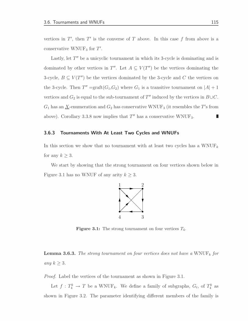
3.6. Tournaments and WNUFs 115
vertices in T ′, then T ′ is the converse of T above. In this case f from above is a
conservative WNUF3 for T ′.
Lastly, let T ′′ be a unicyclic tournament in which its 3-cycle is dominating and is
dominated by other vertices in T ′′. Let A ⊆ V (T ′′) be the vertices dominating the
3-cycle, B ⊆ V (T ′′) be the vertices dominated by the 3-cycle and C the vertices on
the 3-cycle. Then T ′′ =graft(G1,G2) where G1 is a transitive tournament on |A|+ 1
vertices and G2 is equal to the sub-tournament of T ′′ induced by the vertices in B∪C.
G1 has an X-enumeration and G2 has conservative WNUF3 (it resembles the T ′s from
above). Corollary 3.3.8 now implies that T ′′ has a conservative WNUF3.
3.6.3 Tournaments With At Least Two Cycles and WNUFs
In this section we show that no tournament with at least two cycles has a WNUFk
for any k ≥ 3.
We start by showing that the strong tournament on four vertices shown below in
Figure 3.1 has no WNUF of any arity k ≥ 3.
1 2
4 3
Figure 3.1: The strong tournament on four vertices T4.
Lemma 3.6.3. The strong tournament on four vertices does not have a WNUFk for
any k ≥ 3.
Proof. Label the vertices of the tournament as shown in Figure 3.1.
Let f : T k4 → T be a WNUFk. We define a family of subgraphs, Gt, of T k
4 as
shown in Figure 3.2. The parameter identifying different members of the family is

3.6. Tournaments and WNUFs 116
the number, t, of 2s in the tuple (44 . . . 422 . . . 2)
(44 . . . 41 3 . . . 3︸ ︷︷ ︸t−1
)
(22 . . . 22 4 . . . 4︸ ︷︷ ︸t−1
)(22 . . . 24 2 . . .2︸ ︷︷ ︸t−1
)
(11 . . . 13 4 . . .4︸ ︷︷ ︸t−1
)
(44 . . . 4 22 . . . 2︸ ︷︷ ︸t
)(33 . . . 34 1 . . .1︸ ︷︷ ︸t−1
)
Figure 3.2: The family of subgraphs Gt of T k4 .
Consider the subgraph G2 of T k4 . The vertices on the 3-cycle map to one of the
three cycles in T4. Furthermore since f is a WNUF, (22 . . . 242) and (22 . . . 224) map
to the same vertex in T4. Among the two 3-cycles in T4 (234 and 134) only one
of these is such that two consecutive vertices on it have a common out-neighbour,
namely 134.
This implies that
f(11 . . . 134) = 1, f(44 . . . 413) = 4,
f(33 . . . 341) = 3, f(22 . . . 242) = 2,
f(22 . . . 224) = 2, f(44 . . . 422) = 4. (3.4)
Since f is a WNUF, any tuple with k − 1 2s and exactly one 4 has to map to 2. In
particular f(22 . . . 24 2 . . .2︸ ︷︷ ︸t−1
) = 2
Next consider the family of 4-cycles, Hj , in T k4 shown in Figure 3.3. This family
is parametrized by the number, j, of 2s in the tuple (44 . . . 422 . . . 2).
By (3.4), f(44 . . . 422) = 4. If we apply this to H2 and note that the 4-cycle maps
to the 4-cycle in T4, it follows that f(22 . . . 244) = 2. Using this on G3, together with
the fact that (as before) there is only one 3-cycle in T4 such that two consecutive

3.6. Tournaments and WNUFs 117
(33 . . . 3 1 . . . 11︸ ︷︷ ︸j
) (22 . . . 2 4 . . . 44︸ ︷︷ ︸j
)
(11 . . . 1 3 . . . 33︸ ︷︷ ︸j
)(44 . . . 4 2 . . . 22︸ ︷︷ ︸j
)
Figure 3.3: The family of 4-cycles Hj in T k4 .
vertices have a common out-neighbour, we see that f(44 . . .4222) = 4. This can
now be used on H3 to find that f(22 . . . 2444) = 2, which in G4 will imply that
f(44 . . . 42222) = 4. Alternating in this way between Hi and Gi+1 we conclude (when
we reach Gk−1) that f(422 . . .22) = 4. This contradicts f(22 . . . 224) = 2 from (3.4),
since f is weakly nearly unanimous.
Therefore f does not exist.
By Corollary 3.4.5 and the remark following it, the six-vertex tournament defined
as two 3-cycles, with one cycle completely dominating the other, does not have a
WNUF.
We are now ready to show that every tournament with at least two directed cycles
does not possess a WNUFk for any k ≥ 3. The proof is carried out be examining a
minimal counterexample and showing that it cannot exist. Our proof follows (almost
exactly) the proof for tournaments in [5].
Theorem 3.6.4. If T is a tournament with at least two cycles, then T does not
possess a WNUFk for any k ≥ 3.
Proof. Assume that the theorem is false. That is, there exists a tournament with
at least two cycles that has a WNUF. Among all such tournaments, let T be one
with the minimum number of vertices and let f : T k → T be a WNUFk. No proper
induced sub-tournament of T , with at least two cycles, has a WNUFt for any t ≥ 3.
By Lemma 3.6.3, we may assume that T has at least five vertices.

3.6. Tournaments and WNUFs 118
1. For every vertex v in T , N+(v), N+2(v), N−(v) and N−2(v) induce sub-
tournaments with at most one cycle.
Proof. If N+(v) (N+2(v), N−(v), N−2(v)) contains at least two cycles, we could
apply the sub-indicator from Lemma 3.5.2 with J equal to the path u → j
(u → a → j, u ← j, u ← a ← j). The proper sub-tournament (none of these
paths ever reach v), T+, would then contain at least two cycles, and T+ would
not possess a WNUF forcing T not have a WNUF — a contradiction.
2. Consider the case where T is not strong. Let T1, T2, . . . , Tk, k ≥ 2 be the
acyclic ordering of the strong components of T . By point number 1, |Ti| ≤ 3
for 1 ≤ i ≤ k, since a strong tournament is pancyclic. By Corollary 3.4.5 (and
the remark following it), k ≥ 3. Point number 1 now implies that |Ti| = 1 for
2 ≤ i ≤ k − 1. Therefore T1 and Tk are 3-cycles and none of the intermediate
vertices lies on a cycle. (At this point our proof differs slightly from that in
[5].) Denote by T ′ the proper sub-tournament induced by T1∪T2. Let g = f |T ′.
We claim that g is in fact a WNUFk on T ′, which is impossible since T ′ is a
proper sub-tournament. All that we have to show is that g maps into T ′, all
other properties are inherited from f . Let (x1, x2, . . . , xk) ∈ V (T ′). Then
(x1, x2, . . . , xk)→ (x+1 , x+
2 , . . . , x+k )→ (x++
1 , x++2 , . . . , x++
k )→ (x1, x2, . . . , xk),
is a 3-cycle in (T ′)k. Since T1 and Tk are exactly the 3-cycles of T , g maps
(x1, x2, . . . , xk) into T ′.
This completes the case where T is not strong. We may therefore assume that
T is strong.
3. We now show that T is one of the exceptional tournaments shown in Figure
3.4.

3.6. Tournaments and WNUFs 119
A B C
D E
Figure 3.4: The exceptional tournaments.
❒ Consider first the case where T is not two-connected. Let x be a vertex
such that T − x is not strongly connected and let T1, T2, . . . , Tk, k ≥ 2, be
the acyclic ordering of the strong components of T−x. As in point number
2, |Ti| ≤ 3 for i = 1, 2, . . . , k. The strong connectivity of T implies that x
is dominated by some vertex in Tk and that x dominates some vertex in
T1.
• Suppose now that |Ti| = |Tj| = 3 for some i < j. By the same
method as in point 2, we find that |T1| = |Tk| = 3 and |Ti| = 1 for
2 ≤ i ≤ k − 1. Denote the vertices of T1 (in their cyclic order) as
a, b, c and the vertices of Tk (in their cyclic order) as u, v, w. Without
of loss of generality, u → x → a. Hence {x, u, v, w} ⊆ N+2(a). Point
number 1 now implies that v, w → x and that x → b, c. Hence
{x, a, b, c, w} ⊆ N+2(u). These vertices induce more than one directed

3.6. Tournaments and WNUFs 120
cycle, contradicting point 1.
Therefore at most one of the strong components of T − x is a 3-cycle.
• Suppose that T1 is a 3-cycle, abc, and let Tk = {y}. As before, x →
a, b, c since {x, a, b, c} ⊆ N−2(y). If |T | = 5, then T is E in Figure 3.4.
Therefore we may assume that |T | ≥ 6, so that k ≥ 3. Let T2 = {u}.
Then {c, x, y, u} ⊆ N+2(a) and these vertices induce more than one
cycle, contradicting point 1. The case where |Tk| = 3 and |T1| = 1 is
similar and also leads to E in Figure 3.4.
• Suppose that Ti is a 3-cycle, abc, for some 2 ≤ i ≤ k−1. Let T1 = {u}
and Tk = {y}. By the strong connectivity of T , y → x → u. Since
{x, a, b, c} ⊆ N−2(y), either x → a, b, c or a, b, c → x. In the first
instance, {a, x, y, u} ⊆ N−2(c) and these vertices induce two directed
cycles. In the second instance {c, x, y, u} ⊆ N+2(a) and these vertices
also induce two directed cycles. Neither of these cases is possible by
point number 1.
Therefore T−x is acyclic. Let Ti = {vi}, 1 ≤ i ≤ k, as before vk → x→ v1
since T is strong.
• Suppose |T | ≥ 6. If v2 → x, then {v1, vk−1, vk, x} ⊆ N+2(v2) and
these vertices would induce two directed cycles. Therefore x→ v2. If
v3 → x, then {v1, v2, vk, x} ⊆ N+2(v3) and these vertices would induce
two directed cycles. So, x → v3. Now, {v3, v4, . . . , vk, x} ⊆ N+2(v1).
These vertices induce at least two directed cycles.
Therefore |T | = 5. If x→ v2, v3, then T is A in Figure 3.4, where x is the
top vertex of A. If v2, v3 → x, then T is also A in Figure 3.4, with x the
bottom vertex of A. If v3 → x → v2, then T is B in Figure 3.4, where x
is the bottom vertex of B. It is impossible for v2 → x → v3, otherwise

3.6. Tournaments and WNUFs 121
{x, v1, v3, v4} ⊆ N+2(v2) and these vertices induce two cycles.
❒ We now consider the case where T is 2-connected. If |T | = 5, then T is
C in the list as C is the only 2-connected tournament on five vertices.
Therefore we may assume that |T | ≥ 6. Let v be a vertex of maximum
out-degree in T and write O = N+(v) and I = N−(v). By examining the
average out-degree of T , we see that |O| ≥ 3. Also, I ⊆ N+2(v) since v is
a king. Since T is 2-connected, every vertex has at least two in-neighbours
and at least two out-neighbours. Therefore |I| ≥ 2. Let O1, O2, . . . , Oq
and I1, I2, . . . , Ik be the acyclic ordering of the strong components of T [O]
and T [I] respectively.
• If |O1| ≥ 3. Then N+2(v) = T − v which is strongly connected and so
has at least two cycles.
Therefore |O1| = 1. Let O1 = {o1}.
• Suppose that there exists a vertex u ∈ I1 and a vertex r ∈ Oq such
that u → r. (Here our proof also differs from that in [5].) Then
I ⊆ N−2(r). Furthermore since v is a king, u has an in-neighbour
from O, say x. Therefore x ∈ N−2(r). Also, v → o1 → r since o1 and
r cannot be in the same strong component of O. If |I1| ≥ 3 choose w
to be in N+(u)∩ I1. Otherwise |I1| = 1 and u dominates all of I − u;
in this case choose w to be any vertex in I different from u. Therefore,
{u, w, x, v} ⊆ N−2(r) and these vertices induce two directed cycles.
Thus Oq completely dominates I1. Let r ∈ Oq and u ∈ I1. Note that
N+2(v) = T − {v, o1} (use o1 to get every vertex in O − o1 and use that
fact that v is a king). Therefore T−{v, o1} cannot be a strong tournament
as this would force at least two directed cycles since |T−{v, o1}| ≥ 4. This
in turn implies that O2 completely dominates Ik, otherwise we can find a

3.6. Tournaments and WNUFs 122
Hamilton cycle in T − {v, o1}.
• Suppose that o1 → z for some z ∈ I. Then {r, u, v} ∪ Ik ⊆ N+2(o1).
Since o1 and r are not in the same strong component, o1 → r → u,
o1 → z → v and O2 dominates Ik (as well as |I| ≥ 2), respectively.
These vertices induce at least two directed cycles.
Therefore I completely dominates o1.
• Suppose |O| ≥ 4. We claim that there exists a vertex x in O2 such
that x is joined to r by a directed path of length two. If q = 2, then
r ∈ O2 and |O2| ≥ 3. Since O2 is strong, its easy to find the vertex x
by using a Hamilton cycle. Otherwise q ≥ 3. If q > 3, there exists a
strong component between O2 and Oq and x can then be any vertex in
O2. Hence q = 3. Since |O| ≥ 4, there either are at least two vertices
in O2 and so an arc in O2 and x is easy to find, or at least two vertices
in Oq. Oq is strong and so r has an in-neighbour in Oq and x is any
vertex in O2.
– If x does not have a directed path of length two to u, then x and
r are both in O2, r → x and u → f where x → f → r is an
(x, r)-path from above. In this case {x, f, r, u} ⊆ N+2(v) (use o1
to get x, f, r and v → r → u to get u). These vertices induce two
cycles.
Therefore there is a directed path of length two from x to u. Now since
x ∈ O2 dominates Ik, and I dominates o1, there is a path of length
two to r from above. We also have one to u, and x dominates Ik which
are all in-neighbours of v. Thus {o1, r, u, v} ⊆ N+2(x). These vertices
induce two cycles.
Therefore |O| = 3.

3.6. Tournaments and WNUFs 123
• If |I| ≥ 4, there exists a vertex a in I with at least two out-neighbours
in I. This vertex also has o1 and v as out-neighbours. Hence a has
at least four out-neighbours, which is impossible since v is a vertex of
maximum out-degree and we have now determined that v has degree
three.
Thus |I| ≤ 3. Also, since O is not strong (because of O1) we have that
T [O] is a transitive triple. Write Oi = {oi} for i = 1, 2, 3. Hence |Ik| = 1,
otherwise the out-degree of o2 is too big (since it dominates Ik). This
implies that I is also transitive. Write Ij = {ij} for 1 ≤ j ≤ k.
• If k = 3, then {i1, v, o1, o3} ⊆ N−2(i3) (i1 → i2 → i3, v → o2 → i3,
o1 → o2 → i3, o3 → i1 → i3) and these vertices have two directed
cycles.
Therefore k = 2, as k 6= 1 since |T | ≥ 6. Then o3 → i2, so that d+(o3) ≥ 2,
by the 2-connectivity of T . Also, o2 → i1, as i1 does not have any other out-
neighbours because of a maximum out-degree of three. This now means
that T is in fact D in Figure 3.4.
The tournament E does not have a WNUF by Corollary 3.4.2. Tournaments A
through D can be handled by an appropriate sub-indicator; see Figure 3.5.
For tournaments B, C and D, let J = P3 (a directed path of length 3) with u the
initial vertex and j the terminal vertex of the path. Map u to the white vertices in
Figure 3.5. In the case of tournament A use J = P5 (directed path of length 5) with u
the initial vertex and j the terminal vertex. The images of j in all cases are indicated
by the check marks (✓) in Figure 3.5. In each case the resulting tournament T+
is the strong tournament on four vertices. Hence T does not have a WNUF — a
contradiction.

3.6. Tournaments and WNUFs 124
B
D
A
C
✓
✓
✓
✓
✓
✓
✓
✓
✓✓
✓
✓
✓
✓ ✓
✓
Figure 3.5: The exceptional tournaments, A–D, and their sub-indicators.

125
4
Injective Homomorphisms
4.1 Introduction
A homomorphism f : G→ H is injective if the restriction of f to N−(v) is an injective
mapping, for each v ∈ V (G). Alternatively one may think of each vertex in N−(v)
as receiving a different “colour” in H . The existence of an injective homomorphism
between G and H is denoted by Ginj−→ H .
The complexity results in this chapter are derived through the repeated applica-
tion of an indicator construction. This construction is similar in spirit to the one in
Lemma 1.4.1, except that it is tailored to injective homomorphism problems.
We classify all reflexive injective homomorphism problems (where the target graph
H is reflexive — H has a loop at every vertex). Irreflexive targets (no loops) pose
more of a problem. The difficulty lies with targets where the maximum in-degree is
equal to two. All targets with in-degree at least three are NP-complete and those
with in-degree one are polynomial. The in-degree two case exhibits both polynomial
problems and NP-complete problems. We also describe two transformations, the one

4.2. Injective Indicator Construction 126
transforming any (ordinary) H-colouring problem into an injective, in-degree two
problem and the other performing a reverse transformation of the above (unfortu-
nately they are not inverses).
Finally we discuss some upper bounds on related colouring problems.
4.2 Injective Indicator Construction
H is a digraph and is used as the target in the injective H-colouring problem. H
may be reflexive or irreflexive.
Let I be a digraph with two distinguished vertices i and j such that N−(i) =
N−(j) = ∅, N+(i) 6= ∅ and N+(j) 6= ∅.
We define a new digraph H∗ with the same vertex set as H and with arcs given
by xy ∈ A(H∗) if and only of there exists an injective homomorphism f : Iinj
−→ H
such that f(i) = x and f(j) = y.
Lemma 4.2.1. H∗-colouring polynomially reduces to injective H-colouring.
Proof. Let G be an instance of the H∗-colouring problem. Form a new digraph ∗G
by replacing each arc xy in G by a copy of I, identifying x with i and y with j.
Then G→ H∗ if and only if ∗Ginj−→ H :
⇒:
Let f : G → H∗ be a homomorphism. If xy ∈ A(G), then f(x)f(y) ∈ A(H∗).
Therefore there exists and injective homomorphism fxy : Iinj
−→ H such that fxy(x) =
f(x) and fxy(y) = f(y). In this way f may be extended to an injective homomorphism
∗Ginj−→ H . This is possible since the vertices of G in ∗G only have out-neighbours.
⇐:
Let g :∗Ginj−→ H be an injective homomorphism. If xy ∈ A(G), let Ixy be the copy
of I that was used to replace xy in forming ∗G. Then g|Ixy: Ixy
inj
−→ H is an injective
4.3. Reflexive Targets 127
homomorphism from Ixy to H . Therefore g|Ixy(x)g|Ixy
(y) ∈ A(H∗) by the definition
of H∗. We can therefore find a homomorphism G→ H∗ by restricting g to V (G).
Note that if I is chosen such that f : Iinj
−→ H is an injective homomorphism with
f(i) = x and f(j) = y implies that there also exists an injective homomorphism
g : Iinj−→ H with g(i) = y and g(j) = x, for all x, y ∈ V (H), then H∗ above may be
viewed as an undirected graph. Furthermore if the input to the H∗-colouring problem
contains an undirected edge, it is sufficient to replace this edge with one copy of I
using any orientation of I (i.e., i can be identified with x or y and j with y or x,
respectively).
4.3 Reflexive Targets
Lemma 4.3.1. If H is a reflexive digraph and δ−(H) ≥ 3 (H has a vertex with
at least two distinct in-neighbours, other than itself), then injective H-colouring is
NP-complete.
Proof. Let H be a reflexive digraph with δ−(H) ≥ 3 and let a be a vertex of H with
at least two distinct in-neighbours, say b and c. For this digraph we use the indicator
I with vertices {i, x, j} and arcs ix and jx. If uv is an arc of H , then the following
mappings are injective homomorphisms from I to H : i 7→ u, x 7→ v, j 7→ v and i 7→ v,
x 7→ v, j 7→ u. This produces the undirected edge uv in H∗. In particular, ab and
ac are undirected edges. Furthermore the edge bc is in H∗ since i 7→ b, x 7→ a, j 7→ c
and i 7→ c, x 7→ a, j 7→ b are injective homomorphisms from I to H . Therefore, H∗
contains the triangle abc and so is not bipartite. Since H∗-colouring is NP-complete,
injective H-colouring is NP-complete.
Lemma 4.3.2. If Pn is a directed, reflexive path of length n ≥ 2, then injective
Pn-colouring is NP-complete.

4.3. Reflexive Targets 128
b ci j
a
d e
f
Figure 4.1: The indicator I for directed, reflexive paths.
Proof. To prove this result we use the indicator I shown below in Figure 4.1.
Note that I has an automorphism that exchanges i and j. Hence the digraph
obtained by applying I to Pn has undirected edges.
Let Pn be a directed, reflexive path of length n ≥ 2. Let f : Iinj−→ Pn be an
injective homomorphism. Note that f(b) 6= f(c), f(d) 6= f(i) and f(e) 6= f(j). Also,
|f(d)− f(e)| = 0, 1. If x is a vertex of Pn we denote by x− and x+ the predecessor
and successor (respectively) of x, when they exist. We now observe that we cannot
have f(i) = f(j) = x, if this was the case then d 7→ x−, x+ and e 7→ x−, x+. Since
|f(d)− f(e)| = 0, 1 we must have f(d) = f(e) = x+ or f(d) = f(e) = x−. This forces
f(b) = f(c) = x+ or f(b) = f(c) = x (respectively) which is not possible. Therefore
there are no loops when we apply this indicator.
As an example we have the injective homomorphisms from I to the first three
vertices of Pn (labeled 0, 1 and 2 respectively) shown in Table 4.1.
Keeping in mind that we obtain undirected edges in P ∗
n , we see that P ∗
n contains
an undirected triangle on the vertices 0, 1, and 2 and so is not bipartite. Therefore
P ∗
n -colouring is NP-complete implying that injective Pn-colouring is NP-complete.
Lemma 4.3.3. If C is a reflexive, directed cycle of length at least three, then injective
C-colouring is NP-complete.
Proof. Let C be a directed, reflexive n-cycle and x ∈ V (C). Denote by x− and x+

4.3. Reflexive Targets 129
Table 4.1: Some injective homomorphisms from I to the first three vertices of Pn.
a 2 2i b c j 0 1 2 2 0 1 2 1
d e 1 1 1 2f 1 1
a 2 2i b c j 1 1 2 2 1 1 2 1
d e 0 1 0 2f 0 ∄
the predecessor and successor (respectively) of x on C. Here we use the indicator I
shown below in Figure 4.2.
x x+ x+ x x−
x+ x+ x
i j. . .
︸ ︷︷ ︸Pn−1
Figure 4.2: The indicator for directed, reflexive cycles.
Also shown in the figure is a partial injective homomorphism where the vertex i
(of I) has been mapped to the vertex x in C. Note that vertex j can be mapped
to any vertex on C except the vertex x. This is accomplished by using the loops
and the directed path from x− to x+ on C. It is impossible to map j to x since the
length of the path in I from j to the vertex mapped to x− is only n− 1. The result
of this indicator, C∗, is a complete graph on n vertices and so the NP-completeness
of injective C-colouring follows from the NP-completeness of C∗-colouring.
Lemma 4.3.4. If H is a reflexive, directed cycle of length two or H is a reflexive,
directed path of length one, then injective H-colouring is polynomial.
Proof. Let be a H reflexive, directed cycle of length two: V (H) = {0, 1} and A(H) =
{00, 11, 01, 10}. We show that injective H-colouring is polynomial by reducing the
problem to an instance of 2-SAT.

4.3. Reflexive Targets 130
Let G be the input digraph to the injective H-colouring problem. If ∆−(G) ≥ 3,
then G does not map injectively to H . We therefore restrict our attention to inputs
with ∆−(G) ≤ 2.
For each vertex v of G there are two variables: v0 and v1 (v0 is true iff v 7→ 0
and v1 is true iff v 7→ 1). Since v may only map to exactly one of 0 and 1, we form
the clause v0 ⊻ v1 = (v0 ∨ v1) ∧ (v0 ∨ v1) for each vertex v ∈ V (G). For each vertex
x ∈ V (G) with N−(x) = {u, v}, u 6= v add the clauses: u0 ⊻ v0 and u1 ⊻ v1. It is now
a simple matter to check that Ginj−→ H if and only if there exists a satisfying truth
assignment.
We now deal with the case where H is a reflexive directed path of length one,
with V (H) = {0, 1} and A(H) = {00, 11, 01}. This is handled in exactly the same
way as the reflexive 2-cycle except that we add one more set of clauses: for each arc
uv in the input digraph G we form the clause u1 → v1. Again it’s easy to check that
Ginj−→ H if and only if there exists a satisfying truth assignment.
Theorem 4.3.5. If H is a loop, a reflexive arc or a reflexive 2-cycle, then injective
H-colouring is polynomial. Otherwise injective H-colouring is NP-complete.
Proof. The cases where H is a reflexive arc or a reflexive 2-cycle are covered by
Lemma 4.3.4. If H is a loop, then the input to the problem has in-degree at most
one in order to have an injective homomorphism to H . In this case, all vertices can
be coloured with the same colour.
Let H be a reflexive digraph that is not a loop, a reflexive arc or a reflexive 2-cycle.
In addition, we may assume that H is a core with respect to injective homomorphisms.
The proof that injective H-colouring is NP-complete in this case proceeds according
to the maximum in-degree of H . Note that ∆−(H) 6= 1 as this would imply that H
is a single loop.
❒ ∆−(H) ≥ 3. This case is covered by Lemma 4.3.1.

4.3. Reflexive Targets 131
❒ ∆−(H) = 2.
• We first assume that H is acyclic (there are no directed cycles of length
greater than one; loops are not considered to be cycles). Then there exists
a vertex v in H with no in-neighbours other than v itself. The vertex v
has to have an out-neighbour other than v itself, otherwise the component
containing v is just a single loop and since ∆−(H) = 2, H will not be a
core. If v has more than one out-neighbour different from v, then H is
a reflexive, oriented tree rooted at v with all arcs directed away from v.
In this case, H is not a core. Therefore v has exactly one out-neighbour,
say N+[v] = {v, w}. The same idea may be applied to w to conclude
that w has exactly one out-neighbour. Continuing in this way find that
the component containing v is a reflexive, directed path. In fact, if H
has more than one component, then each component of H is a reflexive,
directed path. In this case though, H is not a core. Therefore, H has
exactly one component and this component is a reflexive, directed path of
length at least two. By Lemma 4.3.2, H-colouring is NP-complete.
• If H contains a cycle (of length at least two), this cycle is an induced cycle
since ∆−(H) = 2. Furthermore, every component of H contains a cycle,
because an acyclic component is a reflexive, directed path which can easily
be mapped injectively to a directed cycle in H , implying that H is not a
core. Consider any component of H and let v be a vertex on a cycle in
this component. The vertex v only has it predecessor on the cycle as an
in-neighbour (different from itself). As for out-neighbours of v (different
from v), v obviously has its successor on the cycle as an out-neighbour. If
it had more than one out-neighbour different from v, these out-neighbours
are not on the cycle. As in the acyclic case above we can form an oriented
tree rooted at v with all arcs directed away from v. This tree is equivalent

4.3. Reflexive Targets 132
to a reflexive, directed path that can be mapped injectively to the cycle
in the component under consideration. This would show that H is not
a core. Therefore each component of H is a reflexive, directed cycle and
these cycles have relatively prime lengths (in order for H to be a core).
Let ℓ be the length of a longest cycle in H .
If ℓ = 2, then H is a reflexive, directed 2-cycle. Therefore ℓ ≥ 3. Let t be
the length of a shortest cycle, not equal to two, in H . We now show that
there is a polynomial reduction from injective Ct-colouring to injective H-
colouring. Since injective Ct-colouring is NP-complete for t ≥ 3 by Lemma
4.3.3, we will have that injective H-colouring is NP-complete.
Let G be an instance of injective Ct-colouring. We form an instance G′ of
injective H-colouring as shown Figure 4.3 below.
GCt
x
x
x+
x−−
x−
Figure 4.3: A reduction from injective Ct-colouring.
If t is even, then H does not contain a 2-cycle. This follows from the fact
that an even cycle would map injectively to a two cycle showing that H
is not a core. If Ginj−→ Ct, then its easy to see that G′
inj−→ H as shown in
Figure 4.3. Conversely if G′inj−→ H , then the copy of Ct in G′ can only map
to the copy of Ct in H : the Ct in G′ has to map onto one of the cycles in
H because the ends of each arc are also common in-neighbours of a vertex
of in-degree two. Furthermore this Ct cannot map to a smaller cycle in H
(if t is even there is no 2-cycle to map to and if t is odd it cannot map to

4.4. Irreflexive Targets 133
a 2-cycle if one is present in H). This forces the copy of G in G′ to map
injectively to Ct as well.
In the special case of reflexive, injective, oriented colourings, the target is always
a reflexive tournament. By Lemma 4.3.4 it is possible to decide in polynomial time
whether the reflexive, injective oriented chromatic number of an input digraph is at
most two.
Corollary 4.3.6. It is an NP-complete problem to decide whether the reflexive, in-
jective oriented chromatic number of an input digraph is at most k for k ≥ 3.
Proof. Let T be a reflexive tournament on n ≥ 3 vertices. If n = 3, then T is either
a reflexive, directed cycle or T is a reflexive, transitive tournament. By Lemmas
4.3.3 and 4.3.1 respectively, injective T -colouring is NP-complete. Therefore we may
assume that n ≥ 4. The sum of the in-degrees of T is equal to the number of arcs
which is n(n − 1)/2 plus n (for the loops). Therefore the average in-degree of T is
(n− 1)/2 + 1 = (n + 1)/2 ≥ 5/2. Since T has a vertex with in-degree greater than or
equal to its average in-degree, T has a vertex of in-degree at least 3. So, by Lemma
4.3.1 injective T -colouring is NP-complete.
4.4 Irreflexive Targets
Lemma 4.4.1. If the irreflexive digraph H has ∆−(H) ≥ 3, then injective H-
colouring is NP-complete.
Proof. This follows in almost exactly the same way as for the reflexive case. Let a be
a vertex with at least three distinct in-neighbours b, c, d. By applying the indicator I
with vertices {i, x, j} and arcs ix and jx to H we obtain an undirected 3-cycle: bcd.

4.4. Irreflexive Targets 134
Since the undirected portion of H∗ is not bipartite, H∗-colouring is NP-complete,
implying that injective H-colouring is NP-complete.
We note at this point that if the irreflexive digraph H has ∆−(H) = 1, then H is a
union of paths and cycles. The core of H (under injective homomorphisms) is either
a union of directed cycles (of relative prime lengths) or a directed path. In each of
these cases the input has a maximum in-degree of at most 1 in order for it to map to
H . In fact an injective homomorphism is exactly an ordinary homomorphism in this
case. Therefore the injective H-colouring problem is polynomial when ∆−(H) = 1.
Let D be the set of all irreflexive digraphs. We now define a new set of irreflexive
digraphs with maximum in-degree two, denoted by I . If H ∈ D , define H ∈ I as
follows: replace each arc uv of H with an oriented path on four vertices Puv given by
V (Puv) = {u, xuv, yuv, v} and arcs uxuv, xuvyuv, vyuv. This replacement operation is
shown in Figure 4.4.
u v u xuv yuv v
Figure 4.4: The replacement operation.
Lemma 4.4.2. If H ∈ D, then H-colouring polynomially transforms to injective
H-colouring.
Proof. We need to prove the following. If G, H ∈ D , then G → H if and only if
Ginj−→ H.
Let f : G→ H be a homomorphism. If uv is an arc of G, then f(u)f(v) is an arc
of H . There exists an oriented path on the vertices u, xuv, yuv, v together with the arcs
uxuv, xuvyuv and vyuv in G. Similarly, in H there is an oriented path on the vertices
f(u), xf(u)f(v), yf(u)f(v), f(v) together with the arcs f(u)xf(u)f(v), xf(u)f(v)yf(u)f(v) and

4.4. Irreflexive Targets 135
f(v)yf(u)f(v). We define an injective homomorphism f : Ginj
−→ H as follows:
f(u) = f(u),
f(v) = f(v),
f(xuv) = xf(u)f(v),
f(yuv) = yf(u)f(v).
Conversely, let f : Ginj−→ H be an injective homomorphism. Note that V (G) ⊂
V (G). We define a homomorphism f : G → H by setting f(u) = f(u) for all
u ∈ V (G). Let uv be an arc of G and Puv the corresponding oriented path in
G. Puv is a core under injective homomorphisms and so Puv maps onto a similar
oriented path in H under f , say Pf(u)f(v). The existence of Pf(u)f(v) in H implies that
f(u)f(v) = f(u)f(v) is an arc of H .
Corollary 4.4.3. If H ∈ D and H-colouring is NP-complete, then injective H-
colouring is NP-complete. On the other hand if injective H-colouring is polynomial,
then H-colouring is polynomial.
This corollary in particular implies that there are oriented trees with in-degree
two for which the corresponding injective colouring problem is NP-complete. The
problems in I therefore display a richness comparable to that of the problems in D .
We now show that there is also a polynomial-time reduction from injective colour-
ing problems in I to colouring problems in D . In order to describe this reduction
we perform the following replacement on a digraph H ∈ I : for each x ∈ V (H) let
x1x2x3 be a 3-cycle on three new vertices, identify x with x1. Next, if y is a vertex
of in-degree two in H and N−(y) = {x, z}, add two new vertices uy and vy as well as
the arcs xuy, uyz, zvy and vyx. This replacement is shown in Figure 4.5.
If H ∈ I we denote the result of this replacement by H◦ ∈ D . Note that
V (H) ⊆ V (H◦) and that each of the original vertices of H is now on a 3-cycle in H◦.

4.4. Irreflexive Targets 136
x y z
uy
vy
x y = y1 z
x2
x3 z3
z2
x1 z1
y2y3
Figure 4.5: The second replacement operation.
Let G be an instance of injective H-colouring, where H ∈ I . If G contains a
directed cycle, or a directed path of length at least three or a vertex of indegree
at least three, then G is a NO instance of injective H-colouring. The reason for
this is that H is acyclic, the length of a longest path in H is at most two and that
∆−(H) = 2. Furthermore if x, z ∈ N−(y), then x and z are not adjacent, since H
does not contain any transitive triples.
We may therefore assume that G is acyclic, that the length of a longest path in
G is at most two, that ∆−(G) ≤ 2 and that any common in-neighbours of a vertex
are independent.
The transformed instance G◦ of H◦-colouring is obtained in the same way as H◦:
attach 3-cycles to each vertex of G and if y is a vertex of in-degree two in G and
N−(y) = {x, z}, add two new vertices uy and vy as well as the arcs xuy, uyz, zvy and
vyx.
Lemma 4.4.4. If H ∈ I , then injective H-colouring polynomially transforms to
H◦-colouring.
Proof. Let f : Ginj
−→ H be an injective homomorphism. We now extend f to a
homomorphism g : G◦ → H◦. Note that V (G) ⊆ V (G◦). If y is a vertex of indegree

4.4. Irreflexive Targets 137
two in G, then f(y) is a vertex of indegree two in H , by injectivity.
g(x) =
f(x) if x ∈ V (G),
vf(y) if x = vy for some y ∈ V (G),
uf(y) if x = uy for some y ∈ V (G),
f(z)i if x = zi for some z ∈ V (G) and i = 2, 3.
It is easy to check that g is a homomorphism from G◦ to H◦.
Suppose that f : G◦ → H◦ is a homomorphism. We show that g = f |V (G) is an
injective homomorphism, g : Ginj−→ H . Let x, y ∈ V (G) ⊆ V (G◦). Then x and y are
both on 3-cycles. The homomorphism, f , maps x and y in such a way that f(x) and
f(y) are also on 3-cycles. The only 3-cycles in H◦ are the ones incident with vertices
of H (recall that H itself is acyclic). Therefore g maps into V (H). If xy is an arc of
G, then xy is also an arc of G◦, therefore f(x)f(y) is an arc of H . Let y be a vertex
of indegree two in G, with N−(y) = {x, z}. Then x and z are on the 4-cycle xuyzvy.
Since there are no 2-cycles in H◦, f must map x and z to distinct vertices. Therefore
g is an injective homomorphism from G to H .
Corollary 4.4.5. If H ∈ I and injective H-colouring is NP-complete, then H◦-
colouring is NP-complete. On the other hand if H◦-colouring is polynomial, then
injective H-colouring is polynomial.
4.4.1 The Complexity of Injective Homomorphisms to Irreflexive Tournaments
Lemma 4.4.6. If T is a tournament on at least 5 vertices, then injective T -colouring
is NP-complete.
Proof. The average in-degree of a tournament on n vertices is (n − 1)/2. If T is a
tournament on n ≥ 6 vertices, the average in-degree is at least 5/2. This implies
that T has a vertex of in-degree at least 3. We now apply the indicator with vertices

4.4. Irreflexive Targets 138
i, x, j and arcs ix and jx to T . The result, T ∗, will contain an undirected 3-cycle.
Therefore T ∗-colouring is NP-complete and so injective T -colouring is NP-complete.
If T is a tournament on 5 vertices then T has a vertex of in-degree at least 3,
except in one case: the quadratic residue tournament on 5 vertices, shown below in
Figure 4.6.
Figure 4.6: The quadratic residue tournament on 5 vertices.
On the other hand this tournament has the property that every vertex has in-
degree equal to 2. If we apply the same indicator as above, the result is an undirected
5-cycle. Again, this leads to injective T -colouring being NP-complete.
We now examine the remaining tournaments individually.
The strong tournament on four vertices, T4, is shown below in Figure 4.7.
0 1
23
Figure 4.7: The strong tournament on four vertices T4.
Lemma 4.4.7. Injective T4-colouring is NP-complete.
Proof. The proof is via a reduction from 3-SAT.

4.4. Irreflexive Targets 139
There are two 3-cycles in T4: 123 and 023. There are two transitive triples in T4:
301 and 012.
Consider the digraph G shown in Figure 4.8.
x x
2
3
10 2
Figure 4.8: The variable gadget, Gx, for variable x.
In an injective homomorphism from G to T4, the vertices map as shown. In
addition to this, either x 7→ 0 and x 7→ 1, or x 7→ 1 and x 7→ 0. Consider also a
directed path of length 4, abcde. If we pre-colour vertex e with the vertices 0, 1, 2, 3
of T4, we find the injective homomorphisms from the path to T4 shown in Table 4.2
Table 4.2: Injective homomorphisms from P4 = abcde to T4.
e d c b a
0 3 2 0, 1 0, 3
1 0, 3 2, 3 0, 1, 2 0, 1, 3
2 0, 1 0, 3 2, 3 0, 1, 2
3 2 0, 1 0, 3 2, 3
Next, consider the digraph K shown below in Figure 4.9. It consists of a directed
3-cycle, with paths of length 4 attached to each vertex of the 3-cycle and directed
away from the 3-cycle. To this we add three copies of the oriented path with vertices
x, y, z and arcs xy zy, each attached to a path of length 4.
Note if ℓ1, ℓ2 and ℓ3 are all pre-coloured 1, this does not extend to an injective
homomorphism to T4: pre-colouring in this way forces one to use a 0 on the terminal
vertices of each P4, which in turn forces one to use only 0 and 3 on the 3-cycle. On

4.4. Irreflexive Targets 140
P4
ℓ1 ℓ2 ℓ3
z
y
x
Figure 4.9: The clause gadget, Kℓ1,ℓ2,ℓ3, corresponding to the clause {ℓ1, ℓ2, ℓ3}.
the other hand using only {0, 1} on ℓ1, ℓ2 and ℓ3 with the requirement that there be
at least one 0, extends to an injective homomorphism to T4.
Given an instance of 3-SAT we construct the following digraph D: for each vari-
able x, there is a corresponding variable gadget Gx. For each clause {ℓ1, ℓ2, ℓ3} (where
each literal ℓi is either equal to a variable x or its negation x) there is a corresponding
clause gadget Kℓ1,ℓ2,ℓ3. D is formed by identifying each variable vertex x (or x) with
the corresponding variable vertex in each clause gadget in which it occurs.
If there is a satisfying truth assignment, we can form an injective homomorphism
from D to T4: whenever a variable is assigned the value “True”, map the correspond-
ing vertex to vertex 0 of T4, if its assigned the value “False” map the corresponding
vertex to vertex 1 of T4. This pre-colouring extends to an injective homomorphism,
as shown above.
On the other hand if there is an injective homomorphism from D to T4, we can
form a satisfying truth assignment. The vertices x and x can only map to 0 and 1
respectively (or 1 and 0 respectively). As shown above the clause gadget ensures that
at least one literal vertex per clause has to map to 0. Now by assigning the value
“True” to x whenever the variable vertex x has been mapped to 0 and “False” when
it maps to 1, we have a satisfying truth assignment.

4.4. Irreflexive Targets 141
Lemma 4.4.8. If T is a transitive tournament on 4 vertices or T is equal to a 3-cycle
with a sink vertex, then injective T -colouring is NP-complete.
Proof. In each case there is a vertex of in-degree 3. We can therefore proceed as
above.
The only remaining four-vertex case is a 3-cycle that is dominated by a source
vertex. We will prove that this problem is polynomial by proving a slightly stronger
result. First we prove the following lemma.
Lemma 4.4.9. Let T0 be the digraph with vertices t and c, and arcs tc and cc, then
injective T0-colouring is polynomial.
Proof. The digraph T0 is shown below.
t
c
Figure 4.10: The digraph T0.
We prove that injective T0-colouring is polynomial by showing how the problem
may be reduced to 2-SAT.
Let D be an instance of T0-colouring. With each vertex of D we associate a
variable vt. The interpretation of vt is that vt is “True” if and only if there is an
injective homomorphism from D to T0 that maps v to t. For each arc xy in D we
have the following clauses:
yt = yt ∨ yt,
xt → yt = xt ∨ yt,
xt → yt = xt ∨ yt.

4.4. Irreflexive Targets 142
If u is a vertex of in-degree at least two in D, then for each {x, y} ⊆ N−(u) we have
the following clause: xt ⊻ yt = (xt ∨ yt)∧ (xt ∨ yt). It is now easy to see that Dinj
−→ T0
if and only if there is a satisfying truth assignment.
Lemma 4.4.10. Let H be the digraph formed by taking a copy of an n-cycle, Cn,
and adding to this a new vertex, t, as well as all arcs from t to the n-cycle. Then
injective H-colouring is polynomial.
Proof. The digraph H is shown below.
Cn
t
Figure 4.11: The digraph H.
Let D be an instance of injective H-colouring. Note first of all that if Dinj−→ H ,
then Dinj−→ T0. We therefore start by testing whether D has an injective homomor-
phism to T0 and if the result of this is negative, we may declare that D does not have
an injective homomorphism to H either.
Assume now that f : Dinj
−→ To is an injective homomorphism. Let Dc = {v ∈
V (D) | f(v) = c}, D′ = D〈Dc〉 and Dt = {v ∈ V (D) | f(v) = t}. We now test
whether D′ → Cn. We only need to consider ordinary homomorphisms here since
∆−(D′) ≤ 1. In fact Dinj
−→ H if and only if D′ → Cn: let g : D′ → Cn be a
homomorphism. Then the map h given by h(v) = g(v) if v ∈ Dc and h(v) = t if
v ∈ Dt is an injective homomorphism. Conversely, assume that Dinj−→ H , but that
D′ 6→ Cn. Then there exists a closed walk in D′ of net-length not congruent to zero
(mod n). Since ∆−(D′) = 1 this closed walk is in fact a directed cycle. Thus D does
not have an injective homomorphism to H , contrary to the assumption.

4.4. Irreflexive Targets 143
Therefore, once the test D′ → Cn has been performed, we may declare that Dinj
−→
H if the test succeeds or declare that D does not have an injective homomorphism
to H if it fails.
Corollary 4.4.11. If T is the four-vertex tournament consisting of a 3-cycle domi-
nated by a source, then injective T -colouring is polynomial.
There are only two three-vertex tournaments: the transitive triple and the 3-cycle.
Lemma 4.4.12. If T is a three-vertex tournament, then injective T -colouring is
polynomial.
Proof. Let T be a directed 3-cycle and D an instance of injective T -colouring. We
start by checking the maximum in-degree of D. If it exceeds one we may declare that
D does not have an injective homomorphism to T . If ∆−(D) ≤ 1, the sought after
injective homomorphism is in fact an ordinary homomorphism and we may proceed
by testing whether D → C3.
Let T be the transitive triple, V (T ) = {0, 1, 2} and A(D) = {01, 12, 02}, and D an
instance of injective T -colouring. We show that injective T -colouring is polynomial
by providing a reduction to 2-SAT.
To each u ∈ V (D) we associate three variables: u0, u1 and u2. We interpret these
to mean that ui is “True” if and only if there exists an injective homomorphism from
D to T in which u maps to i for i = 0, 1, 2. For each arc xy ∈ A(D) we form the
following clauses:
x2 = x2 ∨ x2,
y0 = y0 ∨ y0,
x1 → y2 = x1 ∨ y2,
y1 ⊻ y2 = (y1 ∨ y2) ∧ (y1 ∨ y2),
x0 ⊻ x1 = (x0 ∨ x1) ∧ (x0 ∨ x1).

4.4. Irreflexive Targets 144
For each u ∈ V (D) with d−(u) ≥ 2 and for every {x, y} ⊆ N−(u) we form the
following clauses:
u2 = u2 ∨ u2,
x0 ⊻ y0 = (x0 ∨ y0) ∧ (x0 ∨ y0).
If there exists an injective homomorphism Dinj−→ H , then it is clear that there
exists a satisfying truth assignment. Conversely if there is a satisfying truth assign-
ment, we note first of all that for each u ∈ V (D) exactly one of u0, u1 and u2 is
“True:” if u has an out-neighbour, then u2 is “False” and the clause u0 ⊻ u1 ensures
that exactly one of u0 and u1 is “True.” Similarly if u has an in-neighbour, u0 is
“False” and the clause u1 ⊻ u2 ensures that exactly one of u1 and u2 is “True.” If
u has both an in-neighbour and an out-neighbour, then u2 and u0 are both “False”
and the clauses (u0 ⊻ u1) ∧ (u1 ⊻ u2) ensure that u1 is “True.” Therefore we may
define a mapping f : V (D)→ V (T ) by f(v) = i ∈ {0, 1, 2} if vi is “True.” It is now
easy to see that f is in fact an injective homomorphism by the way the clauses were
defined.
The case where T is a one or two-vertex tournament is handled in a similar way to
the 3-cycle case above: first check the in-degree of the input, then proceed by testing
for the existence of an ordinary homomorphism.
In summary, we have the following result.
Theorem 4.4.13. Let T be a tournament. Then the injective T -colouring problem
is NP-complete, except when T is a tournament on at most three vertices or when T
consists of 3-cycle dominated by a source.

4.5. Bounds on the Injective Oriented Chromatic Number 145
4.5 Bounds on the Injective Oriented Chromatic Number
Let D be an oriented graph, that is D does not have any 2-cycles. The reflexive
(irreflexive) injective oriented chromatic number of D, χrio(D) (χi
io(D)), is defined
to be the least k such that D has an injective homomorphism to some reflexive
(irreflexive) tournament on k vertices. One may also think of the reflexive (irreflexive)
injective oriented chromatic number as the least amount of colours that can be used in
an improper (proper) injective oriented colouring of the vertices of D. In an oriented
colouring of D, the arcs between two colour classes must all be oriented in the same
direction. In an improper (proper) injective oriented colouring of D one adds the
restriction that the colouring be injective on the in-neighbourhood of every vertex
with the possibility that the same colour may (may not) appear on the ends of an
arc.
Since injective colourings are defined in terms of in-neighbourhoods, one may
suspect that there may be a Brooks-type theorem giving upper bounds on χrio(D)
and χiio(D) in terms of ∆−(D). This turns out to be false, as the next proposition
shows. Note that ∆−(D) (∆−(D) + 1) is always a lower bound for χrio(D) (χi
io(D)).
Proposition 4.5.1. It is impossible find an upper bound on χrio(D) and χi
io(D) in
terms of ∆−(D).
Proof. To show that it is impossible to bound χrio(D) and χi
io(D) in terms of ∆−(D),
we have to show that there exist oriented graphs D with a fixed ∆−(D), but with
arbitrarily high χrio(D) and χi
io(D).
Let ∆− be given and let k ≥ ∆− be a fixed positive integer.
Define two sets of vertices L = {v1, v2, . . . , vk} and R = {u1, u2, . . . , ut} where
t =
(k
∆−
).

4.5. Bounds on the Injective Oriented Chromatic Number 146
For every ∆−-subset of L there is one vertex in R. For a fixed set of ∆− elements of
L, say Lj = {vj1, vj2, . . . , vj∆−} join every member of Lj to its corresponding vertex
uj in R.
Every vertex in R has in-degree ∆− and any two vertices in L are in-neighbours
of some vertex in R. In colouring this oriented graph injectively, every vertex in L
has to receive a different colour. Therefore we need at least k colours to colour this
graph injectively (whether proper or improper).
It turns out that one is able to bound the injective oriented chromatic number if
one takes into account the maximum in-degree, maximum out-degree and the max-
imum degree of the underlying undirected graph. In general though, the bound has
to be exponential as the following example shows.
Fix a positive integer ∆. We construct a digraph D as follows: take the disjoint
union of all tournaments on ∆ vertices, say T1∪T2∪· · ·∪Tm. Now add m new vertices,
say x1, x2, . . . , xm and let Ti dominate xi. At this point we have to find a tournament
T so that Dinj−→ T . Since the vertices of every Ti are the in-neighbours of xi, we
see that each Ti has to map injectively to T (whether T is reflexive or irreflexive).
Therefore T has to contain each tournament on ∆ vertices as a subgraph. Such a
tournament is known as a ∆-universal tournament and lower bounds on its size are
known [47]: |V (T )| ≥ 2(∆−1)/2. This shows that χrio(D), χi
io(D) ≥ 2(∆−1)/2.
Next, we present an upper bound on χrio(D) and χi
io(D). We treat the irreflexive
case (different colours have to appear on the ends of an arc) first and then show how
this can be modified to handle the reflexive case. The bound is derived by constructing
a suitable undirected graph, colouring this undirected graph, using Brooks’ Theorem
to bound the chromatic number of this graph and then converting the (undirected)
colouring into an irreflexive injective oriented colouring.

4.5. Bounds on the Injective Oriented Chromatic Number 147
Theorem 4.5.2. If D is an oriented graph, then
χiio(D) ≤ 2(∆+(∆−
−1)∆++(∆+)2+1) − 1,
where ∆ is the maximum degree of the underlying graph of D, ∆− is the maximum
in-degree of D and ∆+ is the maximum out-degree of D.
Proof. Given an oriented graph D, we define an undirected graph, D•, that will cap-
ture the properties of an irreflexive injective oriented colouring that we are interested
in:
❒ If x, y ∈ V (D) and d(x, y) = 2, then x and y must receive different colours.
This follows from the fact that our target is an irreflexive tournament and so
does not contain any 2-cycles.
❒ If x, y ∈ N−(v) for some vertex v of D, then x and y must receive different
colours.
❒ If x and y are adjacent in D, they must receive different colours.
The graph D• is defined as follows: V (D•) = V (D), E(D•) = A∗(D) ∪ {xy | x, y ∈
V (D) and d(x, y) = 2} ∪ {xy | x, y ∈ N−(v) for some v ∈ V (D)}, where A∗(D)
denotes the edges of of the underlying graph of D.
Each vertex in D• has at most ∆ neighbours from the underlying graph of D, at
most (∆− − 1)∆+ neighbours that are derived from joining common in-neighbours
by an edge and at most (∆+)2 vertices that are at a distance two from it. Therefore
the maximum degree of D• is at most ∆ + (∆− − 1)∆+ + (∆+)2. We now colour D•
and by Brooks’ Theorem we need at most ∆ + (∆− − 1)∆+ + (∆+)2 + 1 colours.
Let the colour classes of this colouring be C1, C2, . . . , Ck where k = ∆ + (∆− −
1)∆+ + (∆+)2 + 1 and colour every vertex of D with the same colour it received
in D•. This colouring of D is certainly irreflexive (because of A∗(D)) and it is also

4.5. Bounds on the Injective Oriented Chromatic Number 148
injective because common in-neighbours were joined by an edge. At this point it may
not be an oriented colouring. We now recolour the vertices of D in order to ensure
an oriented colouring.
Let the colour of v ∈ V (D) be j. For any colour i 6= j, v has at most one in-
neighbour in colour class i (the in-neighbours of v are adjacent in D• and so receive
different colours). Furthermore, v does not have both an in-neighbour and an out-
neighbour in colour class i (vertices at distance two received different colours since
they are adjacent). Therefore v either has exactly one in-neighbour in colour class i or
only out-neighbours in colour class i. Define the signature of v to be a k-tuple where
the jth entry is a “·” and the ith entry is either “+” or “−” depending on whether
v has out-neighbours or in-neighbours respectively in colour class i, 1 ≤ i ≤ k, i 6= j.
We now use the information encoded in the signatures of each vertex to decide
how to recolour it so that we have an oriented colouring. Since the vertices in C1
are independent, we assign them all the same colour. Next, consider the possible
arcs between C1 and C2: every vertex in C2 either has an out-neighbour in C1 (so its
signature starts with (+ · . . .)) or an in-neighbour in C1 (their signatures start with
(− · . . .)). These vertices have to receive different colours in an oriented colouring.
If we now consider the arcs between C3 and Ci, i = 1, 2, we see that the signatures
start in one of four ways: (− − · . . .), (− + · . . .), (+ − · . . .) or (+ + · . . .). The
vertices in C3 with different signatures on the first two coordinates need different
colours in an oriented colouring. In general, the vertices in colour class i can be
partitioned into 2i−1 sets depending on their signatures on the first i−1 coordinates.
As before, vertices in Ci in different blocks of the partition need different colours in
an oriented colouring. In total we therefore need 1 + 2 + 22 + · · · + 2k−1 = 2k − 1
colours to recolour the vertices of D.
4.6. Obstructions to Injective Oriented Reflexive Colouring 149
Theorem 4.5.3. If D is an oriented graph, then
χrio(D) ≤ 2((∆−
−1)∆++(∆+)2+1) − 1,
where ∆− is the maximum in-degree of D and ∆+ is the maximum out-degree of D.
Proof. The proof here is exactly the same as above except for E(D•) = {xy | x, y ∈
V (D) and d(x, y) = 2} ∪ {xy | x, y ∈ N−(v) for some v ∈ V (D)}. Here we don’t
need the edges of the underlying graph of D since the same colours may appear on
the ends of an arc.
4.6 Obstructions to Injective Oriented Reflexive Colouring
In the case of injective oriented reflexive colourings, there are three polynomial cases:
a target digraph that is a loop, a reflexive arc or a reflexive 2-cycle. These correspond
to χrio ≤ 2.
In this section we are interested in studying obstructions to a digraph D having
χrio(D) ≤ 2. An obstruction is a digraph F such that χr
io(D) 6= k if and only if
Finj−→ D, for k = 1 or 2. Note that if a digraph D has an injective homomorphism
to the reflexive arc, then it has an injective homomorphism to the reflexive 2-cycle.
So, for the purposes of studying injective oriented reflexive two-colourings, we may
assume that the target (in this case) is the reflexive 2-cycle.
Let J1 be the digraph with vertices {a, b, c} and arcs ab and cb. J1 is the obstruc-
tion to a digraph D having χrio(D) = 1.
Theorem 4.6.1. A digraph D has χrio(D) 6= 1 if and only if J1
inj
−→ D.
Proof. If ∆−(D) ≤ 1, all vertices can be coloured with one colour. So if χrio(D) 6= 1,
then D must have a vertex of in-degree at least two, and so J1inj−→ D.

4.6. Obstructions to Injective Oriented Reflexive Colouring 150
On the other hand if J1inj
−→ D, the image of J1 in D needs at least two colours.
So χrio(D) 6= 1.
If a digraph D has ∆−(D) ≥ 3, then χrio(D) 6= 2. In this case the digraph J2 with
V (J2) = {a, b, c, d} and A(D) = {ba, ca, da} is an obstruction. It is possible for a
digraph D to have ∆−(D) = 2, but χrio(D) 6= 2. We now define a family obstructions
for this case. Let C be the family of all odd undirected cycles and define C to be the
family of digraphs obtained from a graph in C be replacing each edge with a copy of
J1.
Theorem 4.6.2. A digraph D has χrio(D) > 2 if and only if either J2
inj
−→ D or there
exists a digraph C ∈ C such that Cinj
−→ D.
Proof. Since χrio(J2) = 3 and since every C ∈ C has χr
io(C) = 3 it follows immediately
that if either J2inj−→ D or C
inj−→ D, then χr
io(D) > 2.
Conversely let χrio(D) > 2. If ∆−(D) ≥ 3, then J2
inj−→ D. Therefore we may
assume that ∆−(D) ≤ 2. Define an auxiliary (undirected) graph D• by
V (D•) = V (D), E(D•) = {uv | u, v ∈ N−(x) for some x ∈ V (D)}.
We now claim that D• is 2-colourable (bipartite) if and only if Dinj
−→ T , where T
is the reflexive 2-cycle: V (T ) = {0, 1}, A(T ) = {00, 01, 10, 11}. A 2-colouring of D•
(with the colours 0 and 1) is immediately an injective homomorphism Dinj−→ T and
conversely if Dinj−→ T , we have a 2-colouring of D•.
Since χrio(D) > 2, it must be the case that D• is non-bipartite and so D• contains
an odd cycle. From the definition of D• it is now clear that some member of C maps
injectively to D.
The 2-colouring of the auxiliary graph above provides another way, apart from
the 2-SAT formulations for the reflexive arc and the reflexive 2-cycle, of showing that

4.7. Injective Oriented Colourings on Trees 151
injective oriented reflexive 2-colouring is polynomial time solvable. If the input has
∆−(D) > 2, then D is a NO instance. Otherwise, form D• and test for (undirected)
2-colourability. If it succeeds, we have an oriented reflexive 2-colouring, if it fails
χrio(D) > 2. Of course, here we are assuming that the target is the reflexive 2-cycle.
4.7 Injective Oriented Colourings on Trees
Let T be an oriented tree. In this section we give an algorithm that tests for a fixed
irreflexive (reflexive) digraph H , whether Tinj
−→ H and finds an injective irreflexive
(reflexive) homomorphism if one exists.
If T is an oriented tree rooted at a vertex x, we may arrange the vertices of T
into its level sets based on the distance from x (in the underlying undirected tree T ′):
Vi = {v | dT ′(v, x) = i}, 0 ≤ i ≤ ℓ, where ℓ is the eccentricity of x. Vℓ is considered
to be the bottom of the tree and V0 the top of the tree.
The algorithm first assigns lists, L(v) ⊆ V (H), v ∈ V (T ), to the vertices of T .
These lists are to be thought of as possible images (or colours) for the vertices of T .
The assignment is based on the fact that if f : Tinj
−→ H is an injective homomorphism,
then d−
H(f(v)) ≥ d−
T (v) since the image of v has to accommodate the in-neighbours of
v in H . The lists are then processed from the bottom-up and the eventual colouring
is from the top-down.
Since the colouring will be from the top-down, the processing of the lists has to
ensure that once a possible image for a vertex has been decided upon (i.e. we’ve made
a choice from L(v)), this choice can be extended downwards. “Extending downwards”
means that we can make choices for vertices lower down in the tree (from their lists)
that will preserve arcs as well as respect injectivity on in-neighbours.
To preserve arcs we essentially do a one-sided consistency check. That is if u ∈ Vi
and v ∈ Vi+1 such that uv (vu) is an arc of T , we remove a ∈ L(u) if there does not
exist a b ∈ L(v) such that ab (ba) is an arc of H . This is done for all u ∈ Vi, for i

4.7. Injective Oriented Colourings on Trees 152
from ℓ − 1 to 0. In this way if we reach the root, x, and L(x) 6= ∅, we can make a
choice for the image of x and extend all the way down preserving arcs in the process.
Let A = {v ∈ V (T ) | |N−(v)| ≥ 2}. If u ∈ A, with N−(u) = {u1, u2, . . . , uk} and
y ∈ L(u), then there exists an injective mapping of N−(u) with u 7→ y, if and only if
there exists a system of distinct representatives (SDR) for the sets
L(u1) ∩N−(y), L(u2) ∩N−(y), . . . , L(uk) ∩N−(y).
Therefore to process L(u) we remove y from L(u) if there does not exist an SDR
as shown above. Note that the lists have to be intersected with N−(y) in order to
“localize” them around y in H .
If u ∈ A∩Vi, for some 0 ≤ i ≤ ℓ−1, is such that N−(u) ⊆ Vi+1, then the processing
above is sufficient since a top-down colouring will colour u first (make a choice from
L(u)) and if the SDR checks succeeded we will then be able to extend downwards
(injectively). On the other hand it could happen that N−(v) ∩ Vi−1 6= ∅ for some
v ∈ A∩Vi. In this case |N−(v)∩Vi−1| = 1. Let u be the vertex in |N−(v)∩Vi−1|. Here
u will be coloured (in a top down colouring) before any of {v} ∪ (N−(v)−{u}) have
been coloured. For such a vertex u we have to ensure that a choice a ∈ L(u) can be
extended downwards. Of course, u may be an in-neighbour of more than one vertex
in Vi. Let A∗ = {v ∈ V (T ) | v ∈ Vi and N+(v) ∩ Vi+1 6= ∅, 0 ≤ i ≤ ℓ− 1}. Suppose
that u ∈ A∗ ∩ Vi. That is, u is an in-neighbour of some vertices v1, v2, . . . , vk ∈ Vi+1.
We remove a ∈ L(u) if there exists vj ∈ {v1, v2, . . . , vk} ∩ A, such that for every
z ∈ L(vj) there does not exist an SDR for the sets
{a} ∩N−(z), L(uj1) ∩N−(z), L(uj2) ∩N−(z), . . . , L(ujk) ∩N−(z),
where (N−(vj)−{u}) = {uj1, uj2, . . . , ujk}. In essence, we are checking here whether
u 7→ a can be extended to an injective mapping on all the in-neighbourhoods of

4.7. Injective Oriented Colourings on Trees 153
vertices in {v1, v2, . . . , vk} ∩ A — we only need to consider vertices with more than
one in-neighbour, hence the intersection with A.
The algorithm is shown below (Algorithm 4.1). The algorithm is for irreflexive,
injective homomorphisms Tinj−→ H . To obtain the corresponding algorithm for the
reflexive problem, we change all intersections of the form L(uj) ∩ N−(y) to L(uj) ∩
N−[y] since we are now allowed to re-use the colour (y) of the “centre” vertex on the
in-neighbours.
Algorithm 4.1 Irreflexive Injective Hom Tinj
−→ H
Input: An oriented tree T rooted at a vertex x.
Level sets V0 = {x}, V1, . . . , Vℓ.
The sets A and A∗ as defined as above.
A target digraph H .
Task: Find an injective homomorphism Tinj−→ H if one exists.
Action: Assign lists to V (T ) as follows: L(v) = {y ∈ V (H) | d−
H(y) ≥ d−
T (v)}.
For i = ℓ− 1 to 0 perform the following for all u ∈ Vi.
For each arc uv (vu) with v ∈ Vi+1, remove a ∈ L(u) if there does
not exist a b ∈ L(v) with ab (ba) an arc of H .
If u ∈ A, remove y ∈ L(u) if there does not exist an SDR for the
sets: L(u1) ∩N−(y), L(u2) ∩N−(y), . . . , L(uk) ∩N−(y), where
N−(u) = {u1, u2, . . . , uk}.
If u ∈ A∗ and N+(u) ∩ Vi+1 = {v1, v2, . . . , vk}, remove a ∈ L(u) if
there exists a vj ∈ {v1, v2, . . . , vk} ∩ A, such that for every
z ∈ L(vj) there does not exist an SDR for the sets: {a} ∩N−(z),
L(uj1) ∩N−(z), L(uj2) ∩N−(z), . . . , L(ujk) ∩N−(z), where
(N−(vj)− {u}) = {uj1, uj2, . . . , ujk}.
Let T be an oriented tree rooted at a vertex x together with the corresponding

4.7. Injective Oriented Colourings on Trees 154
level sets V0 = {x}, V1, . . . , Vℓ. For v ∈ Vi, consider the forest induced by V (T )−(V0∪
V1 ∪ · · · ∪ Vi−1). Let Tv be the sub-tree of T that contains v in the aforementioned
forest. This is the sub-tree of T rooted at v, relative to x. The height of Tv is at
most ℓ− i.
Theorem 4.7.1. Let H be a digraph and T an oriented tree rooted at a vertex x.
If Algorithm 4.1 terminates with L(x) 6= ∅, then for every v ∈ V (T ) and for every
a ∈ L(v), there exists an injective homomorphism f : Tvinj
−→ H such that f(v) = a.
Proof. If L(x) 6= ∅, then L(v) 6= ∅ for every v ∈ V (T ) (an empty list in Vi would lead
to empty lists in Vj, j ≤ i, in particular V0 = {x} would have an empty list).
Let v ∈ Vi. The proof is by induction on the height of Tv: h = ℓ− i, 0 ≤ i ≤ ℓ.
When h = 0, i = ℓ, v is a leaf and Tv = {v}. Therefore any element in L(v)
defines an injective homomorphism f : Tvinj
−→ H .
Assume that the statement is true for all 0 ≤ h < k ≤ ℓ. That is, the statement
is true for all v ∈ Vj with ℓ − k + 1 ≤ j ≤ ℓ. Let v ∈ Vℓ−k so that Tv has height
h = k. Since L(v) 6= ∅, there exists an a ∈ L(v) such that we can define an injective
homomorphism f : T [(N(v)∩Vℓ−k+1)∪{v}]inj
−→ H with f(v) = a (we might have to re-
compute some of the SDRs to do this). Let u ∈ N(v)∩Vℓ−k+1, with f(u) = b ∈ L(u).
The height of (Tv)u is k− 1 and by the induction hypothesis there exists an injective
homomorphism fu : (Tv)uinj−→ H such that fu(u) = f(u) = b. Since this applies to
every u ∈ N(v) ∩ Vk−1 we can extend f to all of Tv.
Corollary 4.7.2. Let H be a digraph and T an oriented tree rooted at a vertex x.
Then there exists an injective homomorphism f : Tinj
−→ H if and only if Algorithm
4.1 terminates with L(x) 6= ∅.
Proof. If f : Tinj−→ H is an injective homomorphism, then d−
H(f(v)) ≥ d−
T (v) and so
f(v) ∈ L(v). Furthermore, f(v) is never removed from L(v) during the execution of
the algorithm. In particular f(x) ∈ L(x), and so L(x) 6= ∅.

4.7. Injective Oriented Colourings on Trees 155
The converse follows from Theorem 4.7.1.
We mention in closing that the algorithm has a running time that is proportional
to the number of vertices in T . This follows from the fact that each vertex of T
is processed only once and the processing (one-sided consistency check and SDR
computation) at each vertex is a function of |V (H)|, which is fixed.

156
5
Conclusions and Future Work
In this chapter we look back at some of the results in this thesis, and we also look
forward to possible future work.
5.1 Local Tournaments
By proving the dichotomy theorem for local tournaments, we have extended the
class of digraphs for which a dichotomy is known. The most surprising result is the
existence of unicyclic tournaments that define NP-complete problems. This together
with the result on smooth digraphs by Barto, Kozik and Niven [8] highlights the fact
that sources and sinks pose a significant problem to determining the complexity of
digraph homomorphisms.
Possible future work in this area may include trying to extend the theorem to
all locally semicomplete digraphs. New ideas may be needed here since our sub-
indicators (for local tournaments) were often paths of length two. The presence of
2-cycles in locally semicomplete digraphs may negate the usefulness of these sub-

5.2. Complexity with Acyclic Inputs 157
indicators.
5.2 Complexity with Acyclic Inputs
The results in Section 1.5.2 on the complexity of oriented colourings with acyclic
inputs can possibly be extended to tournaments (or even semicomplete digraphs) in
general. That is, one would like to prove that colouring by a tournament (or maybe
even a semicomplete digraph) with at least two cycles, is still NP-complete even if
the input is an acyclic digraph. All tournaments with at most six vertices have been
examined and this result holds for these tournaments.
5.3 Weak Near Unanimity Functions
We know of at least one homomorphism problem that has a polynomial time algo-
rithm and has a NUF: directed Ck-colouring. Most unicyclic tournaments do not
have a NUF, but they do have a WNUF; they are also polynomial problems.
❒ What is the difference (if any) between polynomial problems with a NUF and
those with no NUF, but a WNUF?
❒ Is it possible to find more parallels between polynomial problems and WNUFs?
❒ Is there a polynomial digraph homomorphism problem that does not have a
WNUF3, but has one of higher arity?
❒ Extend the no-WNUF result for tournaments to semi-complete (local tourna-
ments?) digraphs. A result like this will be embedded in the smooth digraph
result of Barto, Kozik and Niven [8]. It may nonetheless be instructive to find
an alternative proof using sub-indicators.
❒ Let G be an undirected, non-bipartite graph. Bulatov [15] has shown that
all polymorphisms of G are essentially unary (re-proving Hell and Nesetril’s

5.4. Injective Homomorphisms 158
result [36] using polymorphisms). Through the universal algebraic equivalences
outlined in Chapter 1, this must mean that G does not have a WNUF. Give a
direct proof of this.
❒ What can be said about oriented cycles and and their WNUFs?
5.4 Injective Homomorphisms
As far as irreflexive injective homomorphisms are concerned, our results have shown
that targets with in-degree two exhibit a richness in complexity comparable to that
of ordinary digraph homomorphisms. It would be beneficial to try and identify more
polynomial cases of in-degree two.
❒ In particular, what can be said about oriented paths? Are they always poly-
nomial, NP-complete, or do they exhibit a dichotomy (for injective homomor-
phisms)?
❒ Is it possible to extend results that hold for ordinary homomorphisms to injec-
tive homomorphisms?
❒ Is there a product of digraphs that’s relevant to injective homomorphisms?
❒ Can the injective homomorphism problem be recast as a constraint satisfaction
problem? When this is achieved, the corresponding polymorphisms may be
interesting.

159
References
[1] Jørgen Bang-Jensen, Locally semicomplete digraphs: a generalization of tourna-
ments, J. Graph Theory 14 (1990), no. 3, 371–390. MR MR1060865 (91g:05055)
[2] Jørgen Bang-Jensen, Yubao Guo, Gregory Gutin, and Lutz Volkmann, A classi-
fication of locally semicomplete digraphs, Discrete Math. 167/168 (1997), 101–
114, 15th British Combinatorial Conference (Stirling, 1995). MR MR1446736
(98a:05121)
[3] Jørgen Bang-Jensen and Gregory Gutin, Digraphs: Theory, Algorithms and Ap-
plications, Springer Monographs in Mathematics, Springer-Verlag London Ltd.,
London, 2001. MR MR1798170 (2002e:05002)
[4] Jørgen Bang-Jensen and Pavol Hell, The effect of two cycles on the complexity
of colourings by directed graphs, Discrete Appl. Math. 26 (1990), no. 1, 1–23.
MR MR1028872 (91c:05072)
[5] Jørgen Bang-Jensen, Pavol Hell, and Gary MacGillivray, The complexity of
colouring by semicomplete digraphs, SIAM J. Discrete Math. 1 (1988), no. 3,
281–298. MR MR955645 (89e:05095)

REFERENCES 160
[6] Jørgen Bang-Jensen and Gary MacGillivray, Further effects of two directed cycles
on the complexity of H-colouring, J. Combin. Math. Combin. Comput. 10 (1991),
33–50. MR MR1137820 (93a:05116)
[7] , On the complexity of colouring by digraphs with at most one directed
cycle, Ars Combin. 35 (1993), no. A, 175–186. MR MR1275235 (94m:05075)
[8] Libor Barto, Marcin Kozik, and Todd Niven, The CSP dichotomy holds for
digraphs with no sources and no sinks (a positive answer to a conjecture of
Bang-Jensen and Hell), To appear in SIAM J. Computing.
[9] J. A. Bondy and U. S. R. Murty, Graph theory, Graduate Texts in Mathematics,
vol. 244, Springer, New York, 2008. MR MR2368647
[10] Alfred Brauer, On a problem of partitions, Amer. J. Math. 64 (1942), 299–312.
MR MR0006196 (3,270d)
[11] Gaelle Brevier, Romeo Rizzi, and Stephane Vialette, Pattern matching in
protein-protein interaction graphs, Fundamentals of Computation Theory, Lec-
ture Notes in Comput. Sci., vol. 4639, Springer, Berlin, 2007, pp. 137–148.
[12] Richard A. Brualdi and Herbert J. Ryser, Combinatorial matrix theory, Encyclo-
pedia of Mathematics and its Applications, vol. 39, Cambridge University Press,
Cambridge, 1991. MR MR1130611 (93a:05087)
[13] Andrei Bulatov, Peter Jeavons, and Andrei Krokhin, Classifying the complexity
of constraints using finite algebras, SIAM J. Comput. 34 (2005), no. 3, 720–742
(electronic). MR MR2137072 (2005k:68181)
[14] Andrei Bulatov and Matthew Valeriote, Recent results on the algebraic approach
to the CSP, Submitted. Available at
http://www.cs.sfu.ca/˜abulatov/jpapers.html .
REFERENCES 161
[15] Andrei A. Bulatov, H-coloring dichotomy revisited, Theoret. Comput. Sci. 349
(2005), no. 1, 31–39. MR MR2183466 (2006i:05057)
[16] Samuel Eilenberg and Saunders MacLane, Natural isomorphisms in group theory,
Proc. Nat. Acad. Sci. U. S. A. 28 (1942), 537–543. MR MR0007421 (4,134d)
[17] Isabelle Fagnot, Gaelle Lelandais, and Stephane Vialette, Bounded list injective
homomorphism for comparative analysis of protein-protein interaction graphs,
CompBioNets 2004: Algorithms & computational methods for biochemical and
evolutionary networks, Texts Algorithmics, vol. 3, King’s Coll. Publ., London,
2004, pp. 45–70. MR MR2209695 (2006j:92036)
[18] , Bounded list injective homomorphism for comparative analysis of
protein-protein interaction graphs, J. Discrete Algorithms 6 (2008), no. 2, 178–
191. MR MR2418976
[19] Tomas Feder, Classification of homomorphisms to oriented cycles and of k-
partite satisfiability, SIAM J. Discrete Math. 14 (2001), no. 4, 471–480 (elec-
tronic). MR MR1861785 (2002j:05063)
[20] Tomas Feder and Moshe Y. Vardi, The computational structure of monotone
monadic SNP and constraint satisfaction: a study through Datalog and group
theory, SIAM J. Comput. 28 (1999), no. 1, 57–104 (electronic). MR MR1630445
(2000e:68063)
[21] Guillaume Fertin, Romeo Rizzi, and Stephane Vialette, Finding exact and max-
imum occurrences of protein complexes in protein-protein interaction graphs,
Mathematical foundations of computer science 2005, Lecture Notes in Com-
put. Sci., vol. 3618, Springer, Berlin, 2005, pp. 328–339. MR MR2237379
(2007b:92025)

REFERENCES 162
[22] Jirı Fiala and Jan Kratochvıl, Complexity of partial covers of graphs, Algorithms
and computation (Christchurch, 2001), Lecture Notes in Comput. Sci., vol. 2223,
Springer, Berlin, 2001, pp. 537–549. MR MR1917771 (2003e:68108)
[23] , Partial covers of graphs, Discuss. Math. Graph Theory 22 (2002),
no. 1, 89–99, Conference on Graph Theory (Elgersburg, 2000). MR MR1936227
(2003i:05125)
[24] , Locally injective graph homomorphism: lists guarantee dichotomy,
Graph-theoretic concepts in computer science, Lecture Notes in Comput. Sci.,
vol. 4271, Springer, Berlin, 2006, pp. 15–26. MR MR2290714 (2007i:05063)
[25] Jirı Fiala, Jan Kratochvıl, and Attila Por, On the computational complexity of
partial covers of theta graphs, Discrete Appl. Math. 156 (2008), no. 7, 1143–1149.
MR MR2404227
[26] Michael R. Garey and David S. Johnson, Computers and intractability, W. H.
Freeman and Co., San Francisco, Calif., 1979, A guide to the theory of NP-
completeness, A Series of Books in the Mathematical Sciences. MR MR519066
(80g:68056)
[27] Yubao Guo and Lutz Volkmann, On complementary cycles in locally semicom-
plete digraphs, Discrete Math. 135 (1994), no. 1-3, 121–127. MR MR1310875
(96e:05094)
[28] Wolfgang Gutjahr, Graph colourings, Ph.D. thesis, Freie Universitat Berlin,
1991.
[29] Wolfgang Gutjahr, Emo Welzl, and Gerhard Woeginger, Polynomial graph-
colorings, Discrete Appl. Math. 35 (1992), no. 1, 29–45. MR MR1138082
(92m:05081)

REFERENCES 163
[30] Richard K. Guy, Unsolved problems in number theory, third ed., Problem
Books in Mathematics, Springer-Verlag, New York, 2004. MR MR2076335
(2005h:11003)
[31] Gena Hahn, Jan Kratochvıl, Jozef Siran, and Dominique Sotteau, On the injec-
tive chromatic number of graphs, Discrete Math. 256 (2002), no. 1-2, 179–192.
MR MR1927065 (2003h:05081)
[32] Gena Hahn and Gary MacGillivray, Graph homomorphisms: computational as-
pects and infinite graphs, Unpublished document.
http://www.math.uvic.ca/faculty/gmacgill/homomorphi sms/ .
[33] Gena Hahn and Claude Tardif, Graph homomorphisms: structure and symmetry,
Graph symmetry (Montreal, PQ, 1996), NATO Adv. Sci. Inst. Ser. C Math.
Phys. Sci., vol. 497, Kluwer Acad. Publ., Dordrecht, 1997, pp. 107–166. MR
MR1468789 (99c:05091)
[34] P. Hell, J. Nesetril, and X. Zhu, Complexity of tree homomorphisms, Discrete
Appl. Math. 70 (1996), no. 1, 23–36. MR MR1402736 (97e:68049)
[35] Pavol Hell, From graph colouring to constraint satisfaction: there and back again,
Topics in discrete mathematics, Algorithms Combin., vol. 26, Springer, Berlin,
2006, pp. 407–432. MR MR2249279 (2007f:68081)
[36] Pavol Hell and Jaroslav Nesetril, On the complexity of H-coloring, J. Combin.
Theory Ser. B 48 (1990), no. 1, 92–110. MR MR1047555 (91m:68082)
[37] , Graphs and homomorphisms, Oxford Lecture Series in Mathematics and
its Applications, vol. 28, Oxford University Press, Oxford, 2004. MR MR2089014
(2005k:05002)

REFERENCES 164
[38] Pavol Hell, Hui Shan Zhou, and Xu Ding Zhu, On homomorphisms to acyclic
local tournaments, J. Graph Theory 20 (1995), no. 4, 467–471. MR MR1358537
(96f:05085)
[39] Pavol Hell and Xu Ding Zhu, The existence of homomorphisms to oriented cycles,
SIAM J. Discrete Math. 8 (1995), no. 2, 208–222. MR MR1329507 (96i:05096)
[40] Peter Jeavons, On the algebraic structure of combinatorial problems, Theoret.
Comput. Sci. 200 (1998), no. 1-2, 185–204. MR MR1625523 (99d:68085)
[41] Richard E. Ladner, On the structure of polynomial time reducibility, J. Assoc.
Comput. Mach. 22 (1975), 155–171. MR MR0464698 (57 #4623)
[42] Benoit Larose and Claude Tardif, Projectivity and independent sets in pow-
ers of graphs, J. Graph Theory 40 (2002), no. 3, 162–171. MR MR1905132
(2003d:05159)
[43] Benoit Larose and Laszlo Zadori, The complexity of the extendibility problem for
finite posets, SIAM J. Discrete Math. 17 (2003), no. 1, 114–121 (electronic). MR
MR2033309 (2004h:06007)
[44] , Taylor terms, constraint satisfaction and the complexity of polynomial
equations over finite algebras, Internat. J. Algebra Comput. 16 (2006), no. 3,
563–581. MR MR2241624 (2007i:08004)
[45] Miklos Maroti and Ralph McKenzie, Existence theorems for weakly symmetric
operations, To appear in Algebra Universalis.
http://www.math.u-szeged.hu/˜mmaroti/publications.h tml .
[46] H. A Maurer, J. H. Sudborough, and E. Welzl, On the complexity of the general
coloring problem, Inform. and Control 51 (1981), no. 2, 128–145. MR MR686834
(84i:68073)

REFERENCES 165
[47] John W. Moon, Topics on tournaments, Holt, Rinehart and Winston, New York,
1968. MR MR0256919 (41 #1574)
[48] J. L. Ramırez Alfonsın, The Diophantine Frobenius problem, Oxford Lecture
Series in Mathematics and its Applications, vol. 30, Oxford University Press,
Oxford, 2005. MR MR2260521 (2007i:11052)
[49] Thomas J. Schaefer, The complexity of satisfiability problems, Conference Record
of the Tenth Annual ACM Symposium on Theory of Computing (San Diego,
Calif., 1978), ACM, New York, 1978, pp. 216–226. MR MR521057 (80d:68058)
[50] Eric Sopena, Oriented graph coloring, Discrete Math. 229 (2001), no. 1-3, 359–
369, Combinatorics, graph theory, algorithms and applications. MR MR1815613
(2002g:05088)
[51] Herbert S. Wilf, generatingfunctionology, second ed., Academic Press Inc.,
Boston, MA, 1994. MR MR1277813 (95a:05002)
Copyright © 2022 FDOKUMEN