UNIVERSITY OF TAMPERE

School of Management

SHORT-TERM SALES FORECASTING

Case Nokian Tyres plc in the US

Marketing

Master’s thesis

November 2016

Supervisor: Pekka Tuominen

Olli Mononen

ABSTRACT

University of Tampere

Author:

Title:

Master’s thesis:

Date:

Keywords:

School of Management, marketing

Mononen, Olli

SHORT-TERM SALES FORECASTING – Case Nokian

Tyres plc in the US

105 pages, 7 appendix pages

November 2016

Quantitative and qualitative sales forecasting, time series

aggregation, exponential smoothing

Sales forecasting is an important process for every business to master regardless of the

company size or industry. Accurate forecasts allow the company to answer customer

demand better and hence, the company to increase its sales and decrease its costs. The

ability to forecast sales more accurately than competitors may also work as a valuable

competitive advantage as the company is better at exploiting positive market

opportunities while avoiding those that destroy value. Some argue that sales forecasting

is impossible, however, this thesis refutes the thought. In fact, with some simple methods,

a company can increase its sales forecasting accuracy considerably.

The purpose of the thesis is to explore how an accurate short-term sales forecast can be

provided and to exploit these findings when forecasting the short-term replacement tire

sales of Nokian Tyres in the US. In the first, theoretical part of the thesis, the short-term

sales forecasting process is explored by answering questions such as from which

components a sales time series is composed and whether a qualitative or quantitative

forecasting method should be preferred. From the main findings, a theoretical framework

is built, which is then tested in practice. This forms the second, empirical part of the thesis.

According to the theoretical framework, actions such as aggregating homogenous time

series, estimating seasonality components, and using quantitative exponential smoothing

methods, either alone or in combination, should increase the short-term sales forecasting

accuracy considerably. These and other findings were tested on 17 tire product family

sales of Nokian Tyres in the US replacement tire market, which is the biggest in the world.

In total, the research concluded the study of five market area segmentations, five seasonal

indices, 11 forecasting methods, and three method combinations. The results are

astonishing. The forecasting accuracy was increased 500 percent compared with the

current practices–a finding that, if well exploited, can theoretically provide a yearly

economic gain of hundreds of thousands of euros for the company.

In addition to the economic importance of sales forecasting for businesses, the current

research topic is also important for the academic community. This is especially because

sales forecasting is closely linked to quantifying marketing actions, which the Marketing

Science Institute has set as a tier one research subject. Hence, as the interests of

practitioners and academicians clearly meet in this thesis, this work can also be seen to

decrease the gap between the interests of practitioners and academics that currently

prevail in the marketing discipline.

TIIVISTELMÄ

Tampereen yliopisto

Tekijä:

Tutkielman nimi:

Pro gradu -tutkielma:

Aika:

Avainsanat:

Johtamiskorkeakoulu, markkinointi

Mononen, Olli

SHORT-TERM SALES FORECASTING – Case Nokian

Tyres plc in the US

105 sivua, 7 liitesivua

Marraskuu 2016

Kvantitatiivinen ja kvalitatiivinen myynnin ennustaminen,

aikasarjojen yhdistäminen, silottavat eksponenttiennustusmallit

Myynnin ennustaminen on yksi yhtiön avainprosesseista sen koosta ja toimialasta

riippumatta. Tarkempi myynnin ennustaminen muun muassa auttaa yhtiötä paremmin

vastaamaan asiakkaiden kysyntään, joka taas mahdollistaa yhtiön sekä kasvattaa myyntiä

että laskea kustannuksia. Kilpailijoita parempi kyky ennustaa voi toimia myös yhtiön

kilpailuetuna, sillä tällöin yhtiö pystyy muita paremmin valitsemaan kannattavat ja

välttämään arvoa tuhoavat hankkeet. Jotkut ajattelevat myynnin ennustamisen olevan

mahdotonta, mutta tämä työ kuitenkin selvästi osoittaa tämän ajattelun olevan väärin.

Todellisuudessa jopa suhteellisen yksinkertaisilla menetelmillä myynnin

ennustetarkkuutta voidaan kasvattaa huomattavasti.

Tämän työn tarkoituksen on tutkia, miten tarkka lyhyenajan myyntiennuste tehdään ja

hyödyntää näitä löytöjä ennustettaessa Nokian Renkaiden rengasmyyntiä Yhdysvalloissa.

Tutkielman ensimmäinen osa koostuu teoreettisesta osasta, jossa myynnin ennustamista

tutkitaan muun muassa vastaamalla kysymyksiin mistä komponenteista myynnin

aikasarja muodostuu, miten nämä komponentit tulisi ottaa huomioon ennustettaessa ja

tulisiko myyntiä ennustaa joko kvalitatiivisilla vai kvantitatiivisilla menetelmillä.

Lopuksi teoriaosuuden tärkeimmistä löydöistä rakennetaan teoreettinen viitekehys.

Teoreettisen viitekehyksen mukaan toimet, kuten myynnin aikasarjojen yhdistäminen,

kausaalikomponenttien estimointi ja silottavien eksponenttiennustusmallien käyttäminen

parantavat lyhyenajan myynnin ennustetarkkuutta. Näiden ja myös muiden teoriaosassa

tehtyjen löytöjen toimivuutta tutkitaan ennustamalla Nokian Renkaiden 17

rengastuoteperheen myyntiä maailman suurimmilla rengasmarkkinoilla Yhdysvalloissa.

Tämä tutkimus muodostaa työn toisen osan. Yhteensä empiriaosuudessa tutkitaan viiden

markkina-aluejaon, viiden kausaali-indeksin, 11 ennustusmallin ja kolmen

ennustusmalliyhdistelmän vaikutusta ennustetarkkuuteen. Tutkimuksen löydöt ovat

merkittävät. Suhteellisen yksinkertaisilla menetelmillä ennustetarkkuus parani yli

kuusinkertaiseksi verrattuna nykyisiin ennustusmenetelmiin. Hyvin hyödynnettyinä

nämä löydöt voivat teoriassa mahdollistaa yhtiön kasvattaa myyntiä ja laskea

kustannuksia vuositasolla jopa satojen tuhansien eurojen edestä.

Sen lisäksi, että myynnin ennustaminen on merkittävä prosessi yhtiöille, tämä on myös

tärkeä tutkimusaihe markkinoinnin akateemikoille. Tämä erityisesti sen takia, että

myynnin ennustaminen on läheisesti sidoksissa markkinoinnin vaikutuksien rahalliseen

mittaamiseen, jonka Marketing Science Institute on asettanut yhdeksi tärkeimmistä

tämänhetkisistä markkinoinnin tutkimusaiheista. Koska tässä työssä selvästi liike-elämän

ja markkinoinnin akateemikoiden intressit kohtaavat, tämän työn voidaan nähdä myös

kaventavan näiden sidosryhmien välillä vallitsevaa intressikuilua.

CONTENTS

1 INTRODUCTION ................................................................................................... 7 1.1 Importance and relevance of sales forecasting research ............................................. 7 1.2 Realities of sales forecasting ...................................................................................... 8 1.3 Purpose of the thesis ................................................................................................... 9

2 SHORT-TERM SALES FORECASTING PROCESS ...................................... 11

2.1 Generally cited sales forecasting processes .............................................................. 11 2.2 Sales forecasting process and its five phases ........................................................... 12

2.2.1 Defining the forecasting problem ..................................................................... 12 2.2.2 Gathering information ....................................................................................... 13

2.2.2.1 Assessing the data quality ......................................................................... 14 2.2.2.2 Commonly used data in sales forecasting ................................................. 14 2.2.2.3 Required amount of data ........................................................................... 17

2.2.3 Preliminary analysis .......................................................................................... 18 2.2.3.1 Visualizing and adjusting data .................................................................. 18

2.2.3.2 Decomposing time series .......................................................................... 19 2.2.3.3 Aggregating and segmenting data ............................................................. 24

2.2.4 Choosing a forecasting method ......................................................................... 24

2.2.4.1 Qualitative forecasting .............................................................................. 25

2.2.4.2 Forecasting with quantitative methods...................................................... 29 2.2.4.3 Qualitative versus quantitative forecasting ............................................... 31

2.2.5 Using and evaluating a forecasting method ...................................................... 32

2.2.5.1 Communicating forecasts .......................................................................... 33 2.2.5.2 Measuring forecasting accuracy ................................................................ 33

2.2.5.3 Becoming an expert sales forecaster ......................................................... 34 2.3 Theoretical framework and its comparison with the current sales forecasting

practices .......................................................................................................................... 35

3 CONDUCTING THE RESEARCH .................................................................... 38

3.1 Case-study as a research approach ........................................................................... 38

3.2 Replicability and importance instead of significance tests ....................................... 39 3.2.1 Disclosing an effect size to measure the strength of a relationship .................. 40 3.2.2 Importance of replicability ................................................................................ 41

4 FORECASTING THE SALES OF NOKIAN TYRES IN THE US ................. 42 4.1 Nokian Tyres and the replacement tire market of the US ........................................ 42

4.1.1 Nokian Tyres plc ............................................................................................... 42 4.1.2 Nokian Tyres in North America ....................................................................... 43

4.1.3 Main drivers of tire sales in the US .................................................................. 46 4.1.4 Current forecasting process .............................................................................. 47 4.1.5 Analysis of the current forecasting process ...................................................... 49

4.2 Problem definition and gathering information ......................................................... 51

4.3 Preliminary analysis ................................................................................................. 52 4.3.1 Analyzing and combining sales between products and product families ......... 52

4.3.2 Segmenting the US tire market geographically ................................................ 55 4.3.2.1 Current market segmentation .................................................................... 55 4.3.2.2 Proposed market areas for further analysis ............................................... 58

4.4 Chosen forecasting methods ..................................................................................... 59

4.4.1 Naïve 1, 2, and classical decomposition methods ............................................ 60 4.4.2 Forming seasonal indices .................................................................................. 61 4.4.3 Exponential smoothing methods ....................................................................... 62 4.4.4 Initializing and analyzing the forecasting methods .......................................... 65

4.5 Results of the study .................................................................................................. 66

4.5.1 Naïve 1 and the optimal market segmentation .................................................. 66 4.5.2 Naïve 2 and the effect of seasonality analysis on the forecasting accuracy ..... 68 4.5.3 Forecasting accuracy of various exponential smoothing methods ................... 71

4.5.3.1 Exponential smoothing methods compared with the Naïve 1 method ...... 71 4.5.3.2 Exponential smoothing methods compared with the current forecasting

practices................................................................................................................. 74 4.6 Using the forecasts and developing the forecasting process .................................... 77

5 CONCLUSIONS AND DISCUSSION ................................................................ 79 5.1 Summary of the research .......................................................................................... 79 5.2 Theoretical contribution of the research and recommendations for future research 80

5.3 Managerial implications ........................................................................................... 82 5.4 Quality of the research .............................................................................................. 83

REFERENCES ............................................................................................................. 86

APPENDIX 1: LIST OF PERSONS INTERVIEWED ........................................... 105 APPENDIX 2: TIME SERIES OF PRODUCT FAMILIES .................................. 106

APPENDIX 3: MARKETING MATERIAL OF NOKIAN TYRES IN THE US 109

List of figures

Figure 1. Forecasting process and the structure of the thesis ......................................... 11

Figure 2. Optimal sales forecast horizon ........................................................................ 13 Figure 3. Bullwhip effect ................................................................................................ 15 Figure 4. Fitted versus true model .................................................................................. 17 Figure 5. Four pattern regimes in a time series .............................................................. 19 Figure 6. Upward linear trend in yearly sales of Kone plc ............................................. 20

Figure 7. Sales growth of European companies in 1992–2011 ...................................... 21 Figure 8. Seasonal sales pattern in quarterly winter tire sales of Nokian Tyres plc ....... 22

Figure 9. 100-point series made from randomly signed values –1, 0, and 1 .................. 23

Figure 10. Theoretical framework .................................................................................. 36 Figure 11. Current market segmentation ........................................................................ 47 Figure 12. Current sales forecasting process of Nokian Tyres in the US ....................... 48 Figure 13. Sales of passenger winter tire product families in one of the US states ....... 54 Figure 14. Aggregate winter tire sales in three of the NE states .................................... 56

Figure 15. Aggregate winter tire sales, and the sales of all-weather and all-season

product families in the OT and NE areas ....................................................................... 57 Figure 16. Current NE area, the proposed new market areas, and the US climate ........ 59

List of tables

Table 1. Common biases and fallacies in forecasting .................................................... 27

Table 2. Sales of Nokian Tyres and its key competitors in North America ................... 44

Table 3. Replacement tire market in the US ................................................................... 45

Table 4. Formed product families................................................................................... 53

Table 5. MAE of the Naïve 1 method in various market area segmentations ................ 67

Table 6. MAE of the Naïve 2 method with various seasonal indices ............................. 69

Table 7. MAE of exponential smoothing methods and method combinations .............. 72

Table 8. MAE of the Chosen exponential methods compared with the current

forecasting practices ....................................................................................................... 75

7

1 INTRODUCTION

1.1 Importance and relevance of sales forecasting research

Inability to forecast sales accurately may cost you your job: “Two key executives leave

Walgreen due to a $1 billion forecasting error” (Forbes 2014). In fact, this finding is

universal as there is a correlation between poor forecasting accuracy and the probability

of a CEO getting fired (Lee, Matsunaga & Park 2012). Forecasting ability, is extremely

important for businesses because more accurate forecasts enable companies to enhance

their customer service, lower costs, and exploit market opportunities better (Morlidge &

Player 2010, 28–31). Inaccurate forecasts indeed may be expensive as, for example,

Microsoft was forced to write-off $900 million because of their inaccurate forecast of

demand for their Microsoft Surface tablets in 2013 (Covert 2013). It does not come as a

surprise then that a predictive insight is seen as one of the key qualities of outperforming

companies but also why CFOs around the world have ranked sales forecasting as their

fourth most critical task (IBM Institute for Business Value 2014, 2–5).

Sales forecasting is a process where the future is systematically and rationally assessed

to give a predictive insight to a company (Morlidge & Player 2010, 9). This thesis studies

from which steps the sales forecasting process is made up of and what different aspects

should be taken into consideration so that an accurate forecast can be achieved. After

reading this thesis, the reader should be able to provide a relatively accurate sales forecast.

The literature used in the thesis consists of highly influential forecasting books and a few

hundred articles from marketing, statistics, psychology, and forecasting disciplines.

In the second part of the thesis, some of the most important findings made in the

theoretical part are tested empirically. Here the replacement tire sales of Nokian Tyres

plc are forecasted in the US, which is the world’s largest tire market. The sales are

forecasted in a step-by-step basis so that the study can be replicated. As it will be seen,

with simple methods the forecasting accuracy can be increased considerably and can have

an enormous economic impact on the company. In the current case study, the forecasting

8

accuracy was increased over 500 percent which can theoretically provide a yearly

economic gain of hundreds of thousands of euros for the company.

This thesis is highly valuable for both the academic community and practitioners. The

academic community benefits from more accurate forecasting practices, for example,

because then the effects of promotions can be studied better. In fact, the problem of

quantifying the effect of different marketing activities is a tier 1 level research topic set

by Marketing Science Institute for the years 2014–2016 (Marketing Science Institute

2014). As it will be later shown, the current forecasting practices of companies are

generally far from optimal (McCarthy, Davis, Golicic & Mentzer 2006). This thesis has

therefore also a high practical value and decreases the gap between the interests of

practitioners and academics that currently prevail in the marketing science (Reibstein,

Day & Wind 2009).

1.2 Realities of sales forecasting

The first step to predicting the future is admitting you can’t.

–Stephen Dubner, journalist.

Forecasting should not be confused with prophecy. While forecasting is in its best

assessing the possible different future outcomes rationally or with quantitative methods,

it is not usually possible to state precisely what will happen. (Morlidge & Player 2010, 9)

In some rare real world situations, we can predict some outcomes precisely. For instance,

we can calculate the probability to hit heads or tails when flipping a coin. This, however,

is not possible in more complex, nonlinear, and dynamic situations such as in the business

environment. In these environments, predicting is impossible because the future is a result

of complex and chaotic interactions between different parties such as customers,

businesses, and governments where even little changes in the initial conditions may lead

to an absolutely different outcome. Yet, even in environments like these, short-term sales

forecasting is possible where the sales are forecasted for a few years or less. (Levy 1994)

Indeed, stating that short-term forecasting is impossible is strictly speaking just naïve.

Forecasting sales is possible because human purchasing behavior is predictable to some

extent. For example, past purchasing behavior predicts sales especially because satisfied

customers are usually reluctant to switch to a different brand, known as the inertia effect.

9

Thus, they tend to be loyal and repurchase the brand also in the future. This is actually a

rational thing to do because this reduces daily purchasing comparisons and therefore,

customers may gain the same level of satisfaction with less cognitive effort. (Vogel,

Evanschitzky & Ramaseshan 2008, 100–101; Corstjens & Lal 2000, 283–284)

The predictive power of past sales increases when customers repeat their purchasing

behavior often enough so that the behavior becomes a habit. Habits are human behaviors

that are produced automatically and are cognitively effortless. In fact, to act differently

than habitually, requires effort. Because humans are reluctant to use cognitive effort and

habits make alternative actions cognitively less accessible, they limit the power of

intentions, attitudes, and decisions towards alternative purchasing behaviors. (Duhigg

2012, 17–18; Wood & Neal 2009, 580–582; Ajzen 2001; Neal, Wood & Quinn 2006,

199) This results in that past habitual purchasing behavior predicts future human

behavior, for example, better than customers’ intentions (Vogel, et al. 2008, 100–101).

Yet, even though sales forecasting is possible to some extent, the forecasts include

uncertainty, which neither can be assessed precisely (Makridakis & Taleb 2009a, 717–

718). The problem, however, is not that the future cannot be forecasted with certainty but

instead that people think it can. This misconception can lead to huge disasters such as the

dot-com bubble and recent subprime mortgage crisis. Instead of trying to predict the

future precisely, the limits of forecasting should be accepted. Sales forecasts will always

involve unknown uncertainties and nothing is certain. Thus, the best that can be done is

to be prepared for the unexpected. Companies should maintain protective and proactive

strategies. They should be concentrating on uncertainty and be ready to act. This applies

both to negative and positive surprises from market crises to new market opportunities.

(Makridakis & Taleb 2009b, 841–843; Makridakis, Hogarth & Gaba 2009)

1.3 Purpose of the thesis

The purpose of the thesis is to explore how an accurate short-term sales forecast can be

provided and to exploit these findings when forecasting the short-term replacement tire

sales of Nokian Tyres in the US. In the first, theoretical part of the thesis, the short-term

10

sales forecasting process is explored by answering questions such as from which

components a sales time series is composed and whether a qualitative or quantitative

forecasting method should be preferred. From the main findings, a theoretical framework

is built, which is then tested in practice. This study forms the second, empirical part of

the thesis, where the 17 tire product family sales of Nokian Tyres will be forecasted in

the US (Heinonen 2016).

Nokian Tyres is a Finnish public tire manufacturing company, which was the 19th biggest

and the most profitable tire manufacturing company in the world in 2015 (Nokian Tyres

2016a; Colwell 2015; Davis 2015b). The company is especially known for its high quality

tires which, for example, can be seen in its continuous success in tire tests and winning

the highly respected technology of the year award in 2016 (Tire Technology International

2016). In 2015, Nokian Tyres employed 4,400 personnel and had a revenue of 1,360

million euros from which the US contributed approximately 6 percent. The US is the

biggest single tire market in the world where over 230 million tires are sold annually.

(Nokian Tyres 2016a; Heinonen 2016; Modern Tire Dealer 2016)

The focus of the thesis is not only to study the different sales forecasting methods

available but rather the process in its entirety, from gathering information to measuring

the sales forecasting accuracy. The effectiveness of various actions studied in this thesis

are evaluated based on how they affect the forecasting accuracy. Forecasting accuracy

has been chosen as the benchmark because it is ranked as the most important sales forecast

criterion (Yokum & Armstrong 1995). After reading this thesis, the reader should be able

to understand the most critical factors in the sales forecasting process and to produce an

accurate short-term sales forecast.

This thesis will not study a) nowcasting, which is forecasting the present value of a certain

unknown, external figure such as the current value of GDP or b) how to forecast them

with models such as bridge models. In addition, this will not either study c) predictive

analytics, which is predicting the behavior of individuals, d) how to forecast the sales of

new products or inventions, or e) how the company should manage their sales forecasting

processes. Even though the findings of the study can be to some extent generalized to

making long-term sales forecasts and forecasts in other disciplines, this should be done

with caution. This is, for example, because long-term sales are affected by different

factors than short-term sales are (Makridakis, Wheelwright & Hyndman 1998, 558).

11

2 SHORT-TERM SALES FORECASTING PROCESS

2.1 Generally cited sales forecasting processes

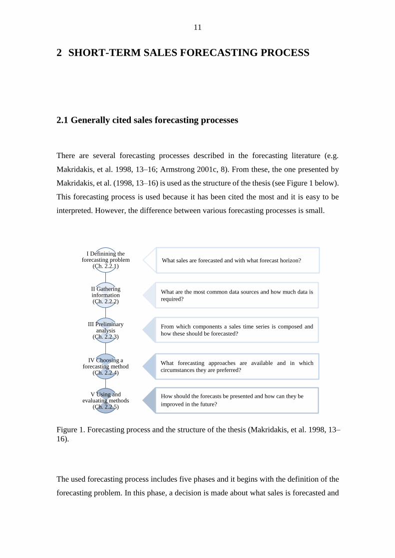
There are several forecasting processes described in the forecasting literature (e.g.

Makridakis, et al. 1998, 13–16; Armstrong 2001c, 8). From these, the one presented by

Makridakis, et al. (1998, 13–16) is used as the structure of the thesis (see Figure 1 below).

This forecasting process is used because it has been cited the most and it is easy to be

interpreted. However, the difference between various forecasting processes is small.

The used forecasting process includes five phases and it begins with the definition of the

forecasting problem. In this phase, a decision is made about what sales is forecasted and

I Definining the forecasting problem

(Ch. 2.2.1)

II Gathering information(Ch. 2.2.2)

III Preliminary analysis

(Ch. 2.2.3)

IV Choosing a forecasting method

(Ch. 2.2.4)

V Using and evaluating methods

(Ch. 2.2.5)

What sales are forecasted and with what forecast horizon?

What are the most common data sources and how much data is

required?

From which components a sales time series is composed and

how these should be forecasted?

What forecasting approaches are available and in which

circumstances they are preferred?

How should the forecasts be presented and how can they be

improved in the future?

Figure 1. Forecasting process and the structure of the thesis (Makridakis, et al. 1998, 13–

16).

12

what is the chosen timeframe, forecast horizon. The second step of the sales forecasting

process is to gather relevant information that concerns both the past and future. In this

chapter, it will be studied from what characteristics are common to good quality data and

how the data can be analyzed, segmented, and decomposed. Then, the choice between

qualitative and quantitative forecasting methods is made. Finally, the chosen method is

used, reported, recorded, and evaluated. (Makridakis, et al. 1998, 13–16)

2.2 Sales forecasting process and its five phases

2.2.1 Defining the forecasting problem

Roughly speaking, sales forecasts are used in an effort to change the future for the better

or to achieve the anticipated positive results (Morlidge & Player 2010, 39–40). Thus, they

are not the end in itself but instead used as a tool in a wide range of decisions concerning

activities such as marketing, production, and finance (Makridakis & Wheelwright 1977,

24). As there are many uses for sales forecasts, the first step in the forecasting process is

to define the purpose of the forecast. The purpose should then outline what 1) products

are forecasted, in which 2) markets, and what is the 3) forecast horizon. In general, the

more strategic the purpose of the forecast, the more aggregate the forecasts and the longer

the forecast horizons are. (Zotteri & Kalchschmidt 2007, 74–75)

The minimum length of the forecast horizon is set by the required planning, decision

making, and lead times, which measure the duration of a certain process such as

production time (see Figure 2 below). Because a shorter forecast horizon increases

predictability the company can usually increase the forecasting accuracy by shortening

lead times. Indeed, this should be a general goal for companies as relatively short lead

times can also serve as a competitive advantage. (Tokatli 2007; Pan & Yang 2002; Stalk

& Hout 1990, 62; Clements & Hendry 2001, 552)

13

Figure 2. Optimal sales forecast horizon. Analysis by the author.

In general, forecasts with longer forecast horizons include more knowledge but they also

tend to be more inaccurate, which leads to a trade-off between these two. How quickly

the predictability reaches the level of chance when lengthening the forecast horizon

depends on the complexity of the forecasting environment. (Levy 1994; Mauboussin

2012) The value of the additional information gained from this procedure again depends

on the forecasting problem. Hence, because the business environment is relatively

complex, as it requires forecasting human behavior, the forecast horizon should be set

according to the forecasting problem. (Makridakis et al. 1998, 558; Yaniv & Foster 1995;

Morlidge & Player 2010, 58–62; Stalk & Hout 1990, 62)

2.2.2 Gathering information

The second phase in the forecasting process is to gather relevant data. As the quality of

the sales forecast can only be as good as the data used, the common characteristics of a

good quality data are described first (Yates, Price, Lee & Ramirez 1996, 42). Then the

most common data sources with their advantages and disadvantages will be presented in

addition to how much data is needed to conduct a quantitative or qualitative sales forecast.

This helps the reader to understand some of the limits of forecasting methods presented

in the subsequent chapters.

14

2.2.2.1 Assessing the data quality

The data quality assessment is an important step in the forecasting process as poor data

leads to poor forecasts and therefore, less effective decision making. For instance, a

suspicion of the quality data quality may lead to a suspended decision altogether.

(Redman 1998) The quality assessment is, however, hard. This is especially the case when

analyzing the quality of external data such as the knowledge of others and economic

indicators. (Tayi & Ballou 1998; Makridakis et al. 1998, 558) Regardless of the data

source, the quality of the data can be assessed by studying the following characteristics

(Wang & Strong 1996, 18–21):

1) Intrinsic, is the data accurate and objective?

2) Contextual, is the data relevant, timely, and complete?

3) Representational, is the data consistent and easy to understand?

4) Accessibility, is the data accessible?

In general, the data should be accurate, timely, consistent, and easily accessible (Wang &

Strong 1996, 6). Timeliness is indeed an important characteristic because the most recent

data is the most valuable data especially when making short-term sales forecasts (Green

& Armstrong 2015, 1679–1681). In addition, if the data provider provides both non-

adjusted and adjusted data, the former is preferred as adjustments may lead to information

loss especially when they are made inefficiently (Bell & Hillmer 2002, 109). The risk of

using inaccurate and dubious data can be reduced by using unbiased, reliable, and diverse

sources (Armstrong 2001e, 683–684).

2.2.2.2 Commonly used data in sales forecasting

Depending on the forecasting design, various data sources are used. Sales forecasts can

be made either with a top-down or bottom-up design. In the top-down design the total

size of the market, industry, or economy is forecasted first from which the sales of the

company and its products will be derived. Whereas in the bottom-up design the product

sales are forecasted directly. (Koller, Goedhart, & Wessels 2010, 193–194)

15

Commonly used data when using the bottom-up forecasting design

The most commonly used data in sales forecasting is past sales. This is reasonable as the

data has forecasting power, it is objective, easily gathered, timely, and the quality of the

data is controllable. (e.g. Makridakis et al. 1998) If the sales data is not the point-of-sales

(POS) data, that is sales to end customers, but sales to other stakeholders that are higher

in the supply chain, the sales variability is usually amplified decreasing the forecasting

accuracy (Figure 3 below). This effect is known as the bullwhip effect and it arises, for

example, because retailers use safety stock and optimize orders. (Lee, Padmanabhan &

Whang 1997) Hence, one way for manufacturing companies to increase forecasting

accuracy is to pursue to negotiate to have the POS data from retailers (Dong, Dresner &

Yao 2014).

Figure 3. Bullwhip effect (Lee, et al. 1997, 94).

Another commonly used data source when forecasting sales directly are customer

intentions, which are the customers’ subjective estimations of their future purchasing

behavior (Morwitz 2001, 33). Customer intentions are argued to be useful especially

when they concern near-term behavior, existing, durable products, and the purchasing

behavior is not habitual. What favors the use of customer intentions is that the data has

forecasting power, it is easily understood, and is inexpensive to gather. (Morwitz, Steckel

& Gupta 2007, 357–358; Vogel, et al. 2008; Armstrong, Morwitz & Kumar 2000)

Gathering the intentions data, however, may be time consuming and the results may be

inaccurate. This may be because of external factors such as job loss, but also because the

measurement process makes the purchasing behavior cognitively more accessible

therefore overstating the purchasing behavior of the respondents who have positive

Ord

er q

uan

tity

Ord

er q

uan

tity

Consumer sales

Time Time

Retailer’s orders to manufacturer

16

images of the product and vice versa. For example, in a study participants who told they

were certain to buy an automobile only 53% of them actually bought one. (Armstrong, et

al. 2000; Morwitz 2001; Morrison 1979; Chandon, Morwitz & Reinartz 2005)

Commonly used data when forecasting sales indirectly

Even though sales are forecasted directly, it is usually recommended to also analyze and

forecast the development of the industry and economy as they may set limits to the

forecasted sales. For instance, if it is anticipated that the competitors are going to reduce

their prices or the consumption if the economy would decrease, the sales of the company

would most likely decrease as well. Hence it is important to answer questions such as

how the aggregate consumption in the economy is most likely to develop and are there

new competitors, products, or innovations pending. (Palepu, Healy & Peek 2013, 241)

When forecasting the aggregate consumption of an economy, the attention should be

firstly paid to the fiscal and monetary policies of the government. If, for example, the

government intended to increase personal taxes, it would lead to a decrease in consumers’

disposable income and hence, consumption. (Blanchard & Johnson 2013) Indeed,

consumer wealth, which is the present value of consumer’s future income and owned

assets, affects consumption as the level of consumption is proportional to it (Zeldes 1989,

278–280). Therefore, data on asset prices and leading indicators such as consumer

confidence, unemployment rates, and the sales of durable goods, are important because

they indicate the development of consumer wealth in the economy (Constable & Wright

2011; Bram & Ludvigson 1998, 61–69).

Indicators of consumer wealth are reasonable to be used when forecasting the sales

because they are free and have forecasting power (e.g. Carrol, Fuhrer & Wilcox 1994;

Dees & Brinca 2013; Mian, Rao & Sufi 2013). However, caution should be exercised.

First, leading indicators are usually set up quickly which is why they may include errors

and are therefore revised later. Second, asset indices and leading indicators include

considerable amount of randomness, which is why attention should mainly be paid to the

usual trends and large changes rather than to daily fluctuations. (Constable & Wright

2011; Dees & Brinca 2013, 9–12) Third, how much the increase in wealth increases

17

consumption depends on whose wealth increases and consumers’ marginal propensity to

consume (MPC), which measures how much of the increased disposable income is

consumed (Carroll & Kimball 1996, 982). For instance, the MPC of poor consumers is

higher than that of the rich meaning that the same absolute increase in the consumer

wealth of the poor increases consumption more than vice versa. Finally, how much the

increase in consumption increases product sales depends on the industry, for example, the

sales of durables increase more than that of non-durables. (Mian, et al. 2013)

2.2.2.3 Required amount of data

When sales are forecasted with a quantitative forecasting method, the common minimum

amount of data required is the number of parameters in the model. Even though adding

more data is not required it is recommendable as it usually increases the forecasting

accuracy. This is especially the case when the historical data is highly variable and

includes considerable amount of randomness (see Figure 4 below). In fact, all the past

data should be used as long as there have not been any considerable structural changes

that have made the data irrelevant. This is because quantitative models should be built so

that they can forecast similar changes that have happened before. (Hyndman & Kostenko

2007; Armstrong, Green & Graefe 2015, 1719; Armstrong 2001e, 687)

Figure 4. Fitted (dashed line) versus true (solid line) model. The regression in the left is

closer to the true model because the sample variation is smaller. (Hyndman & Kostenko

2007, 13)

18

Qualitative forecasts again can be made without any data–people can guess. Yet as the

forecaster’s knowledge increases, the guess becomes a rational assessment. Hence, by

gathering more information, the forecasting accuracy can be increased. This, however, is

only possible to some extent because usually after ten different variables, the accuracy

actually begins to decrease. Making things worse, even though the forecasts begin to be

less accurate, the forecaster’s confidence in its accuracy continues to increase, easily

leading to overconfidence. (Green & Armstrong 2015, 1681; Levitin 2014, 310; Tsai,

Klayman, & Hastie 2008, 100–102; Dane 2010; Fisher & Keil 2015)

2.2.3 Preliminary analysis

After the data has been gathered, it is analyzed and possibly adjusted. To determine

whether the data should be adjusted, the forecaster should get an insight of the overall

development of the data. If there are, for example, discontinuities in the data, the data

should be adjusted so it would be as representative as possible. This may increase the

forecasting accuracy considerably. (Armstrong 2001e, 687–690) In addition, forecasting

accuracy can also be increased by segmenting, aggregating, and decomposing the data.

2.2.3.1 Visualizing and adjusting data

In general, the historical data can be analyzed by statistical techniques or visually. From

these, visualization is preferred, especially in cases where only a little is known about the

data and the data is noisy, which means that the data includes a considerable amount of

randomness. Visualization is indeed efficient as humans are quick to scan, recognize, and

detect changes in shapes and movements. (Shneiderman 1996, 337; Keim 2002, 100)

However, because of the common human desire to gain a feeling of control and

understanding, there is a tendency for judges to seek patterns and cause-and-effect

relations excessively. This easily leads to finding patterns that really do not exist and

therefore decreasing forecasting accuracy. (Whitson & Galinsky 2008, 115)

19

Visualization is preferred to rather be done in a graphical than a tabular form (Harvey &

Bolger 1996, 127). There are numerous graphical frameworks that can be used such as

spirals and flocking boids, however, the most common is the line chart (see Figure 5

below). In this framework, time is generally progressing from left to right and the time-

varying values are set according to the vertical axis. Even though there are more

sophisticated visualization frameworks, this usually outperforms them because they are

easy to learn and interpret. (Heer, Kong & Agrawala 2009, 1303–1304; Aigner, Miksch,

Müller, Schumann & Tominski 2007, 402–405)

Figure 5. Four pattern regimes in a time series (Duncan, Gorr & Szczypula 2001, 198).

By overviewing the time series, some deviant subsequences can be spotted for further

analysis (Shneiderman 1996, 337). For instance, more data should be gathered to analyze

the reasons behind a step jump and outlier, which is an observation that differs

considerably from others. If their occurrence can be determined to be discontinuing, their

values may have to be adjusted. As an example, a step jump resulting from a sales

promotion should be adjusted downwards or else the forecasts will overestimate sales.

(Blattberg & Neslin 1989, 83; Armstrong, Adya & Collopy 2001, 260; Armstrong 2001b)

2.2.3.2 Decomposing time series

To get further insights of the time series data, the data can be decomposed to three

components which are 1) trend, 2) seasonality, and 3) randomness. A commonly

Time

Dep

end

ent

var

iab

le

Outlier

Step jump

Turning point

Slope change

20

distinguished component is also cyclicality, however, in short-term forecasting this can

be seen to be formed from short-term trends and hence, it is not studied further here

(White & Granger 2011, 30). When forecasting sales, the time series should, however, be

decomposed only when this enables the forecaster to use more information in the forecasts

(MacGregor 2001, 110–112). This is important because, for instance, estimating the trend

component poorly may result in worse forecasting accuracy than not taking the trend

component into consideration at all (Chen & Boylan 2008, 531).

Trending time series

Even though trends have been analyzed for nearly a century, there is no precise definition

for a trend. It can be understood as a formation of consecutive observations that have a

1) direction and 2) the formation is quite smooth (see Figure 6 below). The trend in itself

can be stochastic, which means unpredictable, or it can be a deterministic trend such as a

linear or an exponential trend, where the trend accelerates or decelerates as time passes.

In addition, the trend can be either long- or short-term, known as a local trend, that can

also exist simultaneously. (White & Granger 2011)

Figure 6. Upward linear trend in yearly sales of Kone plc (Kone 2016). Analysis by the

author.

When a time series seems to have a trend, possible reasons for its occurrence should be

analyzed. Generally, trends are the consequence of other economic and non-economic

trends, for example, an increasing trend in job growth leads to growth in income,

consumption, and hence, sales. (Phillips 2005, 403; White & Granger 2011, 14–15) In

21

addition, sales trends may also be the result of a competitive advantage or its lack. A long-

term competitive advantage is usually achieved by acquiring and exploiting unique, non-

imitative assets. (Barney 1991; Eisenhardt & Martin 2000; Wiggins & Ruefli 2002, 99–

100; Jacobson 1992)

By understanding the fundamentals behind the trend, it is possible to better forecast its

endurance. In general, abnormally high or low trends tend to regress to the mean (see

Figure 7 below). (Palepu, et al. 2013) In other words, rapidly growing sales tend to slow

down in the future and in fact, this is happening in an increasing pace as technologies

develop faster and the product lives gets shorter (Mauboussin 2012, 106). This, however,

does not mean that every company in the same industry encounter the same sales growth

rate. Rather, industries should be seen as a formation of different clusters or strategic

groups that include companies with similar strategies and hence, growth opportunities.

(Porter 1979, 215; Palepu, et al. 2013)

Figure 7. Sales growth of European companies in 1992–2011 (Palepu, et al. 2013, 243).

Because trends do not last forever, their magnitude is usually reduced, damped, or ignored

altogether when forecasting sales (Gardner & McKenzie 1985; Gardner 2006; 2015). This

should especially be done when the trend is unstable, uncertain, or the short- and long-

term trends contradict each other (Armstrong, et al. 2015; Armstrong 2001b).

Seasonally varying time series

When the time series features a similar sales variance around a certain period of time, for

example, daily, weekly, or monthly, the time series is said to include seasonality (see

Figure 8 below). Seasonality occurs because of different seasonal factors from which an

22

example is the weather. (Makridakis, et al. 1998, 25) Even though the impact of weather

on sales would be easily assessed, forecasting is still extremely hard because the seasonal

component in this case is actually stochastic; the strength, duration, and timing of the

weather cannot be forecasted accurately when the forecast horizon is longer than a few

months. Seasonality analysis is nevertheless important as it usually provides one of the

largest improvements to forecasting accuracy. (Makridakis, Chatfield, Hibon, Lawrence,

Mills, Ord & Simmons 1993, 15; Dekker, Donselaar, Ouwehand 2004)

Figure 8. Seasonal sales pattern in quarterly winter tire sales of Nokian Tyres plc (Nokian

Tyres 2016a). Analysis by the author.

Seasonality can be taken into consideration either by 1) adjusting the time series from the

effects of seasonality, forecasting the deseasonalized time series, and then adding the

seasonality back, or by 2) including the seasonality component in the quantitative

forecasting model directly. (Bell & Hillmer 2002, 99–110) The seasonal component can

be estimated either from the time series under investigation or from a group of

homogenous time series. The latter has been argued to lead to more accurate estimation

as aggregation increases the amount of data to be used and decreases the overall level of

randomness as well (Chen & Boylan 2007; Boylan, Chen, Mohammadipour & Syntetos

2014, 232–234). Finally, as it was with the trend component, if the seasonal component

is uncertain or it varies considerably from period to period, the component is usually

damped (Armstrong, et al. 2015, 1724–1725).

23

Randomness in a time series

The final time series component is randomness, which is usually determined as the value

left, residual value, after the two former components have been estimated. Usually, the

more variable the series is, the more randomness it contains. (Chen & Boylan 2007, 1662)

Randomness, however, cannot be precisely extracted from a time series making the

decomposition process insufficient. This result in that some of the formations in the time

series may actually exist solely because of chance (see Figure 9 below). The probability

of chance playing a role, however, decreases as the amount of observations increases.

(Henderson, Raynor & Ahmed 2012)

Figure 9. 100-point series made from randomly signed values –1, 0, and 1. The analysis

is made with the random numbers formula in Excel. Analysis by the author.

In fact, the probability that a time series, which is made up of many observations, does

not produce any short-term patterns due to chance is negligible. This attribute is hard for

forecasters to comprehend as the usual tendency is to try to understand the world by

organizing it to cause-and-effect relationships. (Eggleton 1982, 90; Kahneman & Tversky

1982, 33–37; Bar-Hillel & Wagenaar 1991, 438–444). This again leads to over analysis

and decreased forecasting accuracy. It is therefore reasonable to make forecasts that are

more conservative when the amount of observations decreases. (Armstrong, et al. 2015,

1726; Mauboussin 2012; Harvey, Ewart & West 1997, 119–120)

24

2.2.3.3 Aggregating and segmenting data

In addition to decomposing the time series, a time series can also be segmented to

subseries or aggregated with other homogenous series. Time series can be aggregated, for

example, on product level, periodically, and geographically. (Kahn 1998, 15–16) If the

forecasting problem allows aggregation, this is usually a reasonable thing to do because

the aggregate time series is generally smoother and hence, increases the forecasting

accuracy. The time series tend to become smoother because the random errors of

observations from different time series tend to cancel each other out, a phenomenon

known as compensating errors. (Lapide 2006; Zotteri & Kalchschmidt 2007, 81)

How well an aggregation works depends on the correlation between the time series where

a negative correlation brings the biggest gain (Schwarzkopf, Tersine & Morris 1988).

Aggregation does not always provide better results, for example, it should be avoided

when the variation of the time series is low and the scale difference between the combined

time series is large (Zotteri & Kalchschmidt 2007, 79). Finally, as it was with

decomposition, a time series should be segmented if this enables the forecaster to use

more information and the value from this is more than the value gained from forecasting

the smoother, aggregate time series (MacGregor 2001, 113; Armstrong, et al. 2015).

2.2.4 Choosing a forecasting method

Basically, forecasting methods can be split into qualitative and quantitative methods.

Qualitative methods that are based on human judgment are argued to be quick and easily

implemented while the latter ones have the advantage of being objective and having

unlimited processing capacity. In which circumstances should these methods be used, is

the key topic of this chapter. After reading this chapter, the reader should be able to

understand the common characteristics of both of these methods and to choose a method

fitting the forecasting problem at hand.

25

2.2.4.1 Qualitative forecasting

The general advantages of qualitative forecasts are easiness, quickness, no data

requirements, and they can be implemented in any economic condition and time series

(Makridakis, et al. 1998, 9–12). The forecasting procedure is straightforward. The process

begins with gathering relevant data, which the forecaster then interprets, weights, and

aggregates in a normative manner. The procedure seems simple however to end up with

an accurate forecast, forecasters are required to possess the true view of the world and

unlimited cognitive capabilities. (Stewart & Lusk 1994, 584; Simon 1955; 1986)

Unfortunately, this is far from the truth.

In reality, the qualitative forecasting accuracy is limited mostly because humans are bad

at gathering and processing information. Humans tend to search, remember, and weight

the information more, which is consistent with the prevailing preference. In addition,

judgment is also affected by information, which is known to be incorrect. (Grove & Meehl

1996, 315–316; Koriat, Lichtenstein & Fischhoff 1980, 115; Klayman & Ha 1987; Griffin

& Tversky 1992; Ross, Lepper & Hubbard 1975) Qualitative forecasts are inconsistent as

changing the order in which the information is processed, usually results in different

forecasts (Hogarth & Einhorn 1992; Kahneman & Klein 2009, 517). Therefore, a

generally accepted concept is bounded rationality, which refers to humans to operate

within the limits of cognitive capacity and environment (Simon 1955; 1986).

Limits of cognitive capacity: Bounded rationality

The human mind can be seen to be formed from two information processing “systems”

that drive human decisions and behavior. The System 1 is automatic, quick, and

unconscious, while the System 2 is controlled, rule-based, and analytical. (Stanovich &

West 2002, 658–659) Both of these systems are always active, however, System 1 usually

makes most of the work. It perceives the world continuously and if nothing alarming is

perceived, humans behave solely on it, which can be called acting intuitively. However,

if profounder reasoning is required or the System 2 questions the reasoning of System 1

reasoning, System 2 takes effect leading to human judgment. (Kahneman 2011, 24–25)

26

The split between these two reasoning styles is a demonstration of how advanced the

human mind is. This operating framework reduces the cognitive effort required to operate

as the System 1 reasoning is mostly based on rules of thumbs, heuristics. (Kahneman

2011) For instance, the System 1 may lean on 1) availability heuristic, where a forecaster

perceives the probability of an event according to how easily and how many instances are

remembered, 2) representativeness heuristic, where the probability of an event is

achieved by comparing its resemblance with its parent population or generating process,

and finally, 3) affect heuristic, where judgments are based on the forecaster’s feelings and

stimuli (Kahneman 2011; Schwarz, Bless, Strack, Klumpp, Rittenauer-Schatka & Simons

1991; Kahneman & Tversky 1982; Slovic, Finucane, Peters, MacGregor 2002, 329–333).

Most of the time System 1 provides relatively accurate forecasts, decisions, and behavior,

however, there are times when leaning solely on it may lead forecasters astray. This is

mostly due to the numerous, predictable cognitive biases and fallacies attached to the

heuristics that the System 1 uses. For instance, if the judge relies on availability heuristic,

the probability of salient and extreme events such as terrorist attacks, are usually

overestimated. Affect heuristic may again lead to inaccurate forecasts as desirable

outcomes are generally perceived as less risky because forecasters unknowingly tend to

disregard disconfirming information and to process confirming information less critically.

(Kahneman 2011, 129; Schwarz, et al. 1991; Finucane, Alhakami, Slovic & Johnson

2000, 13; Slovic, et al. 2002; Ditto & Lopez 1992, 576). The list of different cognitive

biases in qualitative forecasting is, in fact, long (some of them listed in Table 1).

Table 1 also includes proactive methods to mitigate the effect of the listed biases. The use

of these methods is indeed justified as the System 2 is not always able to discover and

correct the inaccurate forecasts made by the System 1. In fact, how well the System 2 is

able to do this depends on forecaster’s motivation, energy, feelings, emotions, moods,

and the efficiency of the system (Soll, Milkman & Payne 2016; Schwarz 2011). For

instance, the System 2 works less efficiently under sleep deprivation, hunger, depletion,

happiness, anger, time pressure, stress, and depression (Harrison & Horne 2000;

Danziger, Levav & Avnaim-Pesso 2011; Schwarz & Clore 2007; Tiedens & Linton 2001;

Maule, Hockey & Bdzola 2000; Starcke & Brand 2012). Which makes bias correction

afterwards also problematic is the fact that humans tend to be blind to their own biases,

known as the bias blind spot. (Pronin, Lin & Ross 2002; Goodwin & Lawton 2003; Lord,

Lepper & Preston 1984; Fischhoff 1977)

27

Table 1. Common biases and fallacies in forecasting. Analysis by the author.

Bias or fallacy Description of the bias or fallacy Methods to reduce the effect of the bias or fallacy

Adding noise to

time series

Forecasters tend to add noise to a time series so it would seem more representative, i.e. random. This reduces

forecasting accuracy, as the optimal way would be to ignore noise entirely. (Harvey 1995)

The bias can be reduced by learning statistical reasoning or making the

most distant forecast first (Harvey 1995; Theocharis & Harvey 2016).

Anchor and

adjustment bias

Anchoring is a bias where a possibly irrelevant number acts as an anchor, a starting point, for a forecast.

First, the plausibleness of the anchor is analyzed and then it is adjusted accordingly. These adjustments,

however, tend to be insufficient leading to the final forecast to be too close to the anchor. (Tversky &

Kahneman 1974, 1128; Epley & Gilovich 2006)

By motivating the forecaster to adjust more, or by using relevant

anchors such as base-rates, or by analyzing the plausibleness of other

figures, the effect of anchoring bias may be reduced (Epley & Gilovich

2006, 316; Hoch & Schkade 1996, 55; Kahneman 2011, 127).

Base-rate

fallacy

Forecasters incorrectly underweight statistical base-rates in favor of the case specific information, for

example, because they think the current situation is unique and therefore, assess the base-rates to be

irrelevant (Bar-Hillel 1980; Kahneman 2011; Bazerman & Moore 2012).

Base-rate fallacy can be mitigated by learning correct reasoning

methods (e.g. Bayes’ rule) or by increasing the perceived relevance of

the base-rate (Kahneman 2011, 154; Bar-Hillel 1980, 228).

Confirmation

bias

Judges tend to search only confirming evidence and weighting it more than disconfirming information

(Wason 1960; Koriat, et al. 1980, 116). This bias may also lead to overconfidence (Tsai, et al. 2008).

By introducing skepticism and increasing the motivation to disconfirm,

can confirmation bias be reduced (Dawson, Gilovich & Regan 2002).

Conjunction

and disjunction

fallacy

In the conjunction fallacy, the probability of a conjunction of events is estimated to be more probable than

one of its constituents alone, while in the disjunction fallacy, a disjunction of two events is estimated to be

less probable than one of the events alone (Tversky & Kahneman 1983; Bar-Hillel & Neter 1993).

Decomposition of the task and more experience with probability

calculus can reduce the effect of the conjunction and disjunction

fallacies (Tversky & Kahneman, 1983).

Curse of

knowledge

Curse of knowledge is the expert’s inability to disregard the additional information they possess (Camerer,

Loewenstein & Weber 1989). For instance, marketing experts do not forecast consumer interests well as

they fail to acknowledge they know more about the product than customers do (Hoch 1988).

By concentrating on the differences between the self and others, a

forecaster can adopt the perspective of others better and hence, reduce

the curse of knowledge (Todd, Hanko, Galinsky & Mussweiler 2011).

Hindsight bias The hindsight bias is made up of (Blank, Nestler, Collani & Fischer 2008):

1) Memory distortions: judges overestimate how much they knew beforehand,

2) Impressions of necessity: after judges knowing the fact, they give higher probability for its occurrence,

3) Impressions of foreseeability: judges overestimate how well they would have forecasted the outcome

beforehand, as they knew it all along (Fischhoff 1975, 290; 1977).

From these, especially the last two causes myopia, which is the failure to locate the correct explanations of

an event, while the last component may lead to overconfidence (Roese & Vohs 2012; Fischhoff 1977).

The hindsight bias can be reduced by using counterfactual thinking,

where plausible alternative outcomes are thought and listed (Slovic &

Fischhoff 1977, 548; Arkes, Faust, Guilmette & Hart 1988, 307). Only

a few of these, however, should be listed as listing many of them can

make the task difficult and hence, the outcome to be perceived as

inevitable. Therefore, increasing rather than decreasing the hindsight

bias. (Sanna & Schwarz 2003, 293)

Overconfidence Humans tend to be overconfident about their abilities and knowledge. For example, when judges estimate

that they are 90 percent sure, they are usually right half of the time. (McKenzie, Liersch & Yaniv 2008)

Overconfidence may appear in three different ways (Moore & Healy 2008):

1) Overestimation: humans overestimate their i) abilities in hard tasks, ii) chances to succeed, iii) control

over outcomes, and iv) task execution times (Langer 1975; Buehler, Griffin & Ross 1994),

2) Overplacement: humans tend to believe to be better in easy tasks and are more likely to face common

desirable events than others (Cain, Moore & Haran 2015; Chambers, Windschitl & Suls 2003),

3) Overprecision: judges are overconfident of their abilities which is why they a) avoid others’ advice, b)

fail to search for alternative solutions, and c) use too narrow forecast ranges (Bazerman & Moore 2012).

Overconfidence can be reduced by performing a premortem in which a

judge thinks it is the future and the forecast made was inaccurate. For

this occurrence, the judge then lists plausible reasons. (Klein 2007) The

bias can also be reduced by motivating judges to analyze contradictory

information, to concentrate on failures, by increasing their

accountability, and knowledge about the forecasting environment, what

is actually known and what is not. (Russo & Schoemaker 1992; Tetlock

& Boettger 1989; Thompson 1999; Chambers, et al. 2003; Griffin &

Tversky 1992; Cain, et al. 2015).

Trend damping Forecasters tend to damp a positive and anti-damp a negative trend too much, leading to too conservative

forecasts especially in noisy series (Harvey & Reimers 2013; Eggleton 1982; O’Connor, Remus & Griggs

1997; Bolger & Harvey 1993; Lawrence & Makridakis 1989).

Trend damping can be reduced by providing data in a graphical form

and by studying analogous series to increase knowledge about how

trends behave (Harvey & Bolger, 1996, 129; Harvey & Reimers 2013).

28

By studying the causes of biases, a suitable proactive method can be found. For instance,

if a bias is a result of loss of motivation, it can be limited by using incentives or increasing

forecaster’s accountability. (Shah & Oppenheimer 2008, 207; Stanovich 2009; Soll, et al.

2016; Shu, Mazar, Gino, Ariely & Bazerman 2012). If they again arise from ignorance,

these can be overcome by teaching or providing more information, and finally, by using

neutral forecasters, biases arising from the valence attached to the forecast can be avoided

(Stanovich 2009; Russo & Schoemaker 1992; Stanovich & West 2002; Soll, et al. 2016;

Einhorn & Hogarth 1978; Hoch & Schkade 1996; Windschitl, Scherer, Smith & Rose

2013; Kunda 1990; Eil & Rao 2011, 133).

Combining judgmental forecasts

Another way to combat against biases is to combine forecasts made by various

forecasters. This usually increases the forecasting accuracy because unsystematic biases

tend to cancel each other out, as was the case with randomness in time series earlier.

Combining forecasts may also increase forecasting accuracy because forecasters may

correct the others incorrect assumptions, but also because a group’s level of knowledge

is larger than that of individual’s. Forecasting accuracy to increase, however, requires that

the forecasters are competent and the group performs well. The latter again depends

among of other things on the group size, diversity, the efficiency of information sharing,

and the distribution of the individual forecasts. (Larrick & Soll 2006; Armstrong 2006;

Soll & Mannes 2011, 84–85; Kerr & Tindale 2011)

Group forecasts do not always increase the forecasting accuracy. This may happen, for

example, because the group does not use more knowledge as group members tend mostly

to discuss information, which is already shared by the group members and consistent with

the prevailing group preference. (Stasser, Vaughan & Stewart 2000; Stasser & Titus

1985) In addition, even though groups formed from more heterogenous individuals have

a wider knowledge base, some group diversion such as diversion based on race and job

tenure actually tend to decrease the group performance (Gruenfeld, Mannix, Williams &

Nealer 1996; Mannix & Neale 2005). To overcome some of these limitations, structured

group forecasting methods such as the Delphi method, are designed. In this method, for

example, face-to-face meetings are avoided and individual estimates are presented in an

29

anonymous manner reducing the effects of group pressure. These structured forecasting

methods usually increase the forecasting accuracy, which is why they are generally

preferred over unstructured ones. (Graefe & Armstrong 2011, 186; Armstrong 2001d)

In general, the biggest gain in the forecasting accuracy is gained when estimates from two

forecasters are aggregated. Yet the accuracy tends to increase as more forecasts are added

but in a diminishing manner. A substantial increase can be gained already with six

forecasters. (Ashton & Ashton 1985; Ariely, Au, Bender, Budescu, Dietz, Gu, Wallsten

& Zauberman 2000)

2.2.4.2 Forecasting with quantitative methods

Non-causal and extrapolative methods

As learned before a quantitative forecasting method can be used if there is enough data to

be used. Quantitative methods are indeed universally used as they are unbiased and they

can process limitless amount of data. (Blattberg & Hoch 1990, 888–890) Generally, a

quantitative method is understood as a combination of a model, which is a forecasting

equation, and the estimation procedure (Meade 2000, 516). Quantitative methods can be

split into two categories, to causal and extrapolative methods. Extrapolative methods are

built only on the historical sales data, whereas causal methods different independent

variables such as economic indicators to forecast sales. (Smith 1997, 558)

Causal methods are favorable for decision making as the forecaster has the power to

choose and manipulate the chosen independent variables (Armstrong & Brodie 1999).

The selection of the independent variables, however, may be difficult as the amount of

independent variables is immense and the strength of the relations between variables tend

to change as time goes by; the relations are said to be nonstationary. Finally, the causal

relations may also exist solely when forecasting aggregate quantities such as industry

sales, limiting the use of causal methods when forecasting product sales. (Allen & Fildes

30

2001; Lieberson 1991, 309–310; Brighton & Gigerenzer 2015, 1781; Chapman &

Chapman 1969; Einhorn & Hogarth 1982; Fildes, Wei & Ismail 2011)

Indeed, one of the strongest advantages of extrapolative methods is that they do not

require other information than past sales. In addition, the most accurate methods in

different forecasting competitions have usually been simple exponential smoothing

methods (Makridakis & Hibon 2000; Makridakis, et al. 1993). The two most common

extrapolative methods are moving averages and exponential smoothing methods which

only differ in how they weight the past sales. As the name implies, in moving averages

the past sales are equally weighted whereas in exponential smoothing methods the

weighting increases towards the latest observation. This is reasonable as the latest

observation usually includes the most amount of information about the future.

(Makridakis, et al. 1998, 136–144) This also increases the robustness of the forecasting

method as extrapolative methods are also based on the assumption of time series being

stationary (Armstrong 2001b; Clemen 2001, 549; Clements & Hendry 2001, 551; Fildes

& Makridakis 1995).

Choosing a quantitative method

According to a universalistic perspective, there is one forecasting method, which is the

best in every situation and environment. For practitioners, this would be ideal but,

unfortunately, this does not seem to be the case. In fact, forecasting methods have been

shown to work better in some situations than in others, for example, depending on from

which components a time series is formed. (Kalchschmidt 2012) Therefore, forecasters

should test various methods on different time series to find the best one. If this is not

possible, averaging several quantitative methods is usually the best choice. (Soll &

Mannes 2011)

Indeed, as was the case with combining forecasters, combining different quantitative

methods, may lead to increased knowledge used in the forecasting process and hence,

increase forecasting accuracy (Clemen 1989). A forecasting method combination may

even work better than the included methods alone. However on average, they are not more

accurate than the known best forecasting method but if the best method is unknown, the

31

combination tends to be more accurate than the chosen method because combinations

work rarely poorly as individual methods may do. (Makridakis & Hibon 2000; Armstrong

2006, 585; Hibon & Evgeniou 2005)

Combining is the most effective when the forecasting errors, the difference between the

forecast and actual sales, between the methods are negatively correlated and the forecasts

bracket the actual outcome, meaning that some of the models under- and others

overforecast (Larrick & Soll 2006). Usually, the best combinations involve combining

less than seven models as combining more tend to begin to decrease the forecasting

accuracy (Hibon & Evgeniou 2005, 20). Finally, when the methods are relatively good,

equally weighting is usually close to the optimal weighting. In some rare cases, the

forecasting accuracy may be increased by using dissimilar weights, but their

determination ex-ante is difficult. Therefore, even in these circumstances equal weighting

is usually the most reasonable way. (Aiolfi, Capistrán & Timmermann 2011, 356; Ashton

& Ashton 1985; Genre, Kenny, Meyler & Timmermann 2013)

2.2.4.3 Qualitative versus quantitative forecasting

So how do qualitative and quantitative methods compete against each other? As argued

earlier the advantages of the former ones was their easiness and quickness, yet their

inconsistencies and biases made them usually relatively unreliable and inaccurate. It has

been therefore argued that quantitative methods are more accurate as they are objective

and process information more efficiently. This argument is, however, far from new.

Already in the 50’s, Paul Meehl provided strong evidence that simple quantitative

methods are in various circumstances almost always superior to human judgment; a

finding, which has been proven to be correct numerous times ever since. (Meehl 1957;

1996; Grove, Zald, Lebow, Snitz & Nelson 2000)

In forecasting discipline, the quality of qualitative forecasts has also been under scrutiny

several times. According to one study only four companies out of 13, judgmentally

forecasted the sales of the next month significantly more accurate than a naïve

quantitative method (Lawrence, O'Connor & Edmudson 2000). In a forecasting

32

competition again, the participating five forecasters were approximately 26 percent less

accurate than the mean of three simple quantitative methods. By equally combining their

forecasts, they were over 23 percent more accurate on average, however, still they fell

short almost 9 percent in the former comparison. (Makridakis, et al. 1993, 9) Hence, the

result is the same in forecasting discipline as it is in other disciplines of social sciences–

if there is a usable quantitative method, judgment should seldom be used (Meehl 1957,

273; 1996; Yaniv & Hogarth 1993).

One of the disadvantages of quantitative methods, however, is that they do not work well

in highly nonstationary environments. Therefore, by analyzing in what extent the past

resembles the future, a forecaster may add valuable information to the forecasting

process. (Fildes & Makridakis 1995) Qualitative and quantitative methods can be

combined by adjusting a quantitative forecast judgmentally or by combining their

forecasts together. Generally, if the judge possesses enough information to produce an

adequate qualitative forecast, then a combination is preferred. (Bunn & Wright 1991, 513;

Sanders & Ritzman 2001, 411) This is especially because of the risk of double counting

where the information included in the adjustment is already incorporated in the

quantitative method (Goodwin 2002, 129).

Adjustments have in fact been studied to often decrease the forecasting accuracy. They

are usually too often made and overoptimistic; the most damaging adjustments are

generally the large positive ones. (Goodwin & Fildes 1999; Franses & Legerstee 2009;

Goodwin 2000; Fildes & Goodwin 2007; Fildes, Goodwin, Lawrence & Nikolopoulos

2009; Trapero, Pedregal & Kourentzes 2013) Combinations between qualitative and

quantitative methods again have lead to increased forecasting accuracy in numerous

studies (e.g. Bunn & Wright 1991, 893–894). For instance, in one study almost 90 percent

of the 444 combined forecasts lead to higher forecasting accuracy while the optimal

weighting of the methods was close to 50 percent (Franses & Legerstee 2011, 2367).

2.2.5 Using and evaluating a forecasting method

The final step in the forecasting process is to communicate the forecasts and measure their

accuracy in order to enable learning and process development. These are studied in the

33

current chapter and after, a theoretical framework is presented, which is also compared

with the current forecasting practices.

2.2.5.1 Communicating forecasts

Finally, the forecasts made are given to decision makers. This should be done in a clear

and precise manner where estimations are separated from facts. The forecasts should be

represented in a numerical form and the use of ambiguous words such as “likely” should

be avoided. This is because judges interpret ambiguous words differently. For example,

in one study judges’ interpretations of “serious possibility” ranged from 20 to 80 percent.

(Tetlock & Gardner 2015, 59; Kent 1964, 49–53). Secondly, the presented forecasts

should be objective assessments of the future. This may sound obvious but unfortunately,

forecasts are commonly revised for political reasons. For instance, in one study 45 percent

of the forecasters replied that the senior management often asked them to adjust the sales

forecasts upwards. (Galbraith & Merrill 1996)

As it was argued at the beginning of the thesis, forecasts involve uncertainty. Therefore,

the forecasts made are usually presented together with confidence intervals or prediction

intervals, which set upper and lower bounds for the forecasts. Usually, a 95 percent

confidence interval is used, which means that 95 of 100 times the forecast will be included

within these boundaries. The more certain the outcome and the smaller the used

confidence, the narrower the confidence intervals will be. By using confidence intervals,

the forecaster can communicate the uncertainty included in the forecast efficiently.

However, their accuracy should also be studied because in general, the provided

boundaries are too narrow. (Chatfield 2001; Field 2013, 54–57)

2.2.5.2 Measuring forecasting accuracy

The sales forecasting process does not however end when the forecasts are made and

given to the decision makers. Rather the forecasting process should be seen as a circling

34

process where the forecasting accuracy if measured continuously and these results are

used to improve the forecasting process. The forecasting accuracy should be measured

from the out-of-sample observations that are left out from the modeling process. Some

authors measure the “accuracy” from the in-sample observations that are used in the

modeling process. This, however, does not tell how well the method actually forecasts

but rather describes how well the method explains the past. In fact, if the method explains

the history perfectly, there is a risk that it has been overfitted to the data, and therefore its

use leads to poor forecasts. (Green & Armstrong 2015; Brighton & Gigerenzer 2015,

1775; Fildes & Makridakis 1995)

The forecasting accuracy can be measured with four designs (Hyndman & Koehler 2006):

1) Scale-dependent measures (e.g. mean absolute error, MAE),

2) Percentage-error measures (e.g. mean absolute percent error, MAPE),

3) Relative-error measures (e.g. mean relative absolute error, MRAE),

4) Scale-free error measures (e.g. mean absolute scaled error, MASE).

From these, MASE has the advantage to be the only accuracy measure, which is both

scale independent and can be used with intermittent data. This, for instance, makes it

possible to compare the results between different series. Both the percentage-error and

relative-error measures again have the disadvantage of not being able to be used with

intermittent data as it would require dividing with a zero. (Hyndman & Koehler 2006)

2.2.5.3 Becoming an expert sales forecaster

Measuring, registering, and analyzing forecasting accuracy is indeed important as it

enables learning (Davis & Mentzer 2007, 491). Studies have shown that by only analyzing

the forecasting accuracy results per se does not improve forecasting performance.

Therefore more analysis is required, especially the analysis of the forecasting

environment such as how noisy the time series is, have shown to improve the forecasting

accuracy. (Balzer, Sulsky, Hammer & Sumner 1992; Remus, O'Connor & Griggs 1996)

Yet even though correct feedback is given, the efficiency of learning, however, may be

reduced because of the judge’s biased cognitive processing. For instance, judges

35

generally tend to address positive outcomes to internal and negative to external factors.

They may also argue that their inaccurate forecasts were almost right and hence, there is

not much to learn. (Hoch 1985, 727; Tetlock 1998)

Yet is it even possible to become an expert in sales forecasting? Expertise requires judges

to possess sufficient 1) domain knowledge, 2) psychological traits, 3) cognitive skills, and

4) decision strategy skills; all of these have been shown in this thesis to be developable if

the forecaster has the right mindset. The fifth required component to gain expertise,

however, is the limiting factor in the domain of sales forecasting. That is, to become an

expert, an environment is also required, which allows learning. This requirement however

is not met in sales forecasting because the environment is dynamic and overly

complicated. (Shanteau 1992; Dweck 2006) Therefore, expertise in sales forecasting can

be gained to some extent, however, the ceiling is achieved relatively quickly. This is also

one of the reasons, why forecasters do not learn to outperform simple quantitative

methods. (Armstrong 1980)

2.3 Theoretical framework and its comparison with the current sales

forecasting practices

In the final chapter of the thesis, a theoretical framework is presented and compared with

the current sales forecasting practices (see Figure 10 below). One of the key findings

made earlier, was that quantitative methods in general are preferred over qualitative ones.

This is because they have been shown to better in different business environments,

industries, companies, products, and periods. (Sanders & Manrodt 2003) Yet even though

this finding is far from new, still the most common sales forecasting method in large US

companies is a qualitative one, followed by exponential smoothing methods (McCarthy,

et al. 2006). The same conclusion was made in a more recent study with large Austrian

companies (Hofer, Eisl & Mayr 2015). Some of the reasons for the prevalence of

qualitative forecasts may be that judges think they have valuable information, adding

judgment creates a sense of ownership, and there may be a view that sales forecasting is

not possible, which is why investing in it is regarded as unnecessary (Sanders & Manrodt

1994).

36

I Definining the forecasting problem

II Gathering information

III Preliminary analysis

IV Choosing a forecasting method

V Using and evaluating methods

Lea

rnin

g a

nd

dev

elo

pin

g t

he

fore

cast

ing

pro

cess

Ha

s th

e fo

reca

stin

g e

nvi

ron

men

t

cha

ng

ed? S

hou

ld t

he

fore

cast

ing

met

ho

ds

be

re-m

od

eled

?

Ha

ve t

he

fore

cast

ing

pro

ble

m o

r

lea

d t

imes

cha

ng

ed?

The best decisions can be made when the sales forecast is tailored for the decision making problem.

Usually, the forecasting accuracy can be increased by shortening the forecast horizon.

Forecasts can be as good as the data behind them. When using quantitative methods, all of the past data should be used as long as it is representative. This again, may not

necessarily be the case when making qualitative forecasts. This especially the case after the cognitive capacity has been

exceeded because then increasing the amount of information tends to begin to decrease the forecasting accuracy.

The forecasting accuracy of quantitative methods can be increased by adjusting data from outliers and discontinuing events. The aggregation of homogenous time series reduces the aggregate amount of randomness and hence, increases the

forecasting accuracy.

Time series can be decomposed or segmented if it allows more knowledge to be used in the forecasts. The accuracy of a seasonal component estimate can be made more accurate by estimating it from a combination of

homogenous time series.

By combining forecasters and using proactive methods against cognitive biases, the forecasting accuracy of qualitative

methods can be increased. Quantitative sales forecasting methods tend to outperform qualitative methods. If the best performing quantitative method is unknown, a method combination leads to the best forecasts on average. In nonstationary environments, the forecasting accuracy can be increased by combining quantitative and qualitative

methods.

Decision making can be enhanced by providing confidence intervals with the presented sales forecasts. Sales forecasts are best understood in a numerical form where facts are separated from estimations. Measuring forecasting accuracy from out-of-sample observations provides information about how well the method actually

forecasts. By recording forecasts and analyzing their accuracies and the forecasting environment in general, the forecaster can learn

and improve the forecasting process.

Figure 10. Theoretical framework

37

Sadly, by studying the trend of the sales forecasting practices, it seems that the use of

quantitative methods has not increased in decades. This finding is indeed alarming

because during this time, the forecasting discipline has developed considerably and

quantitative methods are easier to be used as computers have become more common. In

fact, the situation may be even more alarming as it seems that the familiarity of all of the

forecasting methods has been decreasing. For instance, a finding, which signals of the

alarming situation, is that only 38 percent of the large US companies were familiar with

a decomposition method even though their use usually leads to one of the biggest

increases in the forecasting accuracy. (McCarthy, et al. 2006; Makridakis, et al. 1993)

Another key finding made earlier was that if the environment is nonstationary, the

quantitative and qualitative methods should be combined rather than judgmentally

adjusting them. According to one study, 25.1 and 24.8 percent of the responding

forecasters used only qualitative or quantitative methods respectively, while 16.7 percent

combined these methods, and 33.7 percent judgmentally adjusted the forecast of the

quantitative method (Fildes & Goodwin 2007, 572). Therefore again against suggested

practices, combining these forecasts seems to be less common than adjusting the

quantitative forecasts. One reason for this finding may be the common misbelief that

averaging methods only leads to average results (Larrick & Soll 2006). Making matters

worse, adjustments are not made rarely but rather continuously as according to one study

they are made to 90 percent of the forecasts (Franses & Legerstee 2009). The adjustments

are also usually made because of wrong intentions, as the majority of the respondents said

to under or overforecast purposefully therefore reducing the objectiveness of the forecasts

(Fildes & Goodwin 2007; Sanders & Manrodt 1994).

In summary, this chapter showed that there seems to be a wide gap between theory and

practice in the forecasting discipline. Various top academicians in the field have made

this same conclusion (e.g. Armstrong & Fildes 2006). For this reason, the empirical part

of the thesis has a high contribution value for the forecasting discipline as it shows how

sales forecasting can be implemented in practice. As it will be soon seen, the economic

results for the case company are astonishing.

38

3 CONDUCTING THE RESEARCH

3.1 Case-study as a research approach

The empirical part of the thesis consists of a case study where the theories presented in

the theoretical part are tested in practice. These theories are tested by developing the

short-term sales forecasting process of Nokian Tyres plc in the US replacement tire

market. The aim of the research is to achieve more accurate sales forecasts compared with

the sales forecasts provided currently. The sales forecasted here include the 17 product

family sales of winter, all-weather, and all-season passenger and sport utility vehicle

(SUV) tires. From these, all-weather tires can be used around the year, while all-season

tires are meant to be used in three of the four seasons met in the Northern, snowing

countries: spring, summer, and fall. (Trauss 2016)

By increasing the forecasting accuracy, the company has the ability to meet the customer

demand better and hence, to increase its sales and decrease its costs by being able to meet

the customer demand better. This indeed would be beneficial for the company as there

seems to be room for improvement. For example, one distributor commented in a

customer satisfaction survey (n=112): “… You don’t have the tires in stock, when can you

get them? Typical answer: I don’t know, they are in the boat, maybe next month, maybe

next year. That’s unacceptable.” In total, 16 percent of the respondents thought the

availability of the products is worse than that of rivalry companies. (Nokian Tyres 2015b)

Even though case study research is usually regarded as a qualitative research method, it

can also be used in quantitative studies. However, in these circumstances, it is better

understood as a research approach than a method. Because the number of case companies

is one, the case research in question is regarded as an intensive research design. This

provides an opportunity to describe the company and the forecasting environment in

detail so that the reader is able to understand, evaluate, and possibly improve the

processes and methods used. The goal of this research is therefore not to produce

generalizations, but rather to test several theories in this company and forecasting

39

environment. In fact, testing several methods simultaneously is highly recommended as

it helps the forecasting discipline to develop considerably. By describing the process in

detail, the results of this study may be used in a meta-analysis, which can be used to

generalize findings. (Armstrong 2001a; Eriksson & Kovalainen 2008, 116–118)

3.2 Replicability and importance instead of significance tests

Because of the questionable reputation and relevance of significance tests, they will not

be used in the following research. Psychologist Paul Meehl (1978, 817) has stated “I

believe that the almost universal reliance on merely refuting the null hypothesis… is…

one of the worst things that ever happened in the history of psychology.” Even though

significance tests have been argued to be for instance, a good way to study if a finding is

real or due to chance, the method has considerable flaws. For example, significance tests

are dependent on the sample size and they do not tell how strong or meaningful the finding

is. (Schmidt 1992; 1996)

One of the biggest drawbacks of significance tests however is that they are commonly

misinterpreted. If the static is not significant, the wrong conclusion is that there is no

relation or effect at all, or it is so small that it can be safely rejected. This is not always

the case because the significance test includes two kinds of errors: Type I (alpha) and

Type II (beta) errors. A Type I error originates when a relation or effect is detected when

there actually is none and when the test cannot find an actual relation or effect it is called

a Type II error. Because both of these errors cannot be controlled, studies usually choose

to limit the probability of a Type I error to a probability level of 5 percent. This procedure

however, may increase the probability of a Type II error to as high as 50–80 percent.

Therefore, the sole use of significance tests easily leads to that actual effects are being

missed, debilitating the development of cumulative knowledge. (Schmidt 1992)

For these and other reasons, some journals require disclosing the effect sizes but also

encouraging researchers to use confidence intervals and enable replications (Hubbard &

Ryan 2000). In accordance with these recommendations, this thesis will calculate effect

sizes with confidence intervals when assessing the findings of the study and make

40

replications possible by describing the forecasting process in detail. The used confidence

intervals are 95 percent and they are calculated from the t value (Field 2013).

3.2.1 Disclosing an effect size to measure the strength of a relationship

It has been recommended that effect sizes should be used when comparing forecasting

accuracies but also in marketing papers in general. An effect size describes the magnitude

of an effect or relation between variables where the higher the effect size, the stronger the

effect. It therefore determines the economic significance of the effect and hence, tackles

one of the limitations of significance tests. (Sawyer & Ball 1981; Armstrong 2007, 322)

Another advantage of using effect sizes is their independency on the sample size although

one has to remember that by increasing the sample size the probability of the risk that the

sample does not represent the population decreases (Field 2013, 79–81).

This thesis uses Cohen’s d to measure the effect size of the forecasting accuracy

differences between forecasting methods. This method is chosen because it is

standardized, commonly used, and scale-independent. Cohen’s d is calculated as follows

(Field 2013, 79–81):

(1) d ̂= X̅1 – X̅2

s

Where ^ describes that it is an estimate of the effect size of the population, X̅1, 2 are the

means of two samples, and s is the standard deviation of a sample. If the standard

deviations of the samples differ, as is the case in this thesis, the standard deviation can be

taken from a control group. Here it is the standard deviation of the forecasted sales. (Field

2013, 79–81; Makridakis, et al. 1998, 46) Cohen has suggested that the effect size is small

when the result is over 0.2, medium if over 0.5, and large if it is over 0.8 (Cohen 1992,

157).

41

3.2.2 Importance of replicability

According to King (1995, 444) “[T]he only way to understand and evaluate an empirical

analysis fully is to know the exact process by which the data were generated and the

analysis produced.” Therefore, to ensure the contribution value of the study, the research

process is described in detail enabling the research to be replicated. In short, reproduction

means that independent researchers with the same data are able to come up with the same

numerical result presented in a study, whereas replication means that the same qualitative

result can be obtained with the same method but different data. (Boylan, Goodwin,

Mohammadipour & Syntetos 2015 79–80; King 1995, 444–445)

In the present study, because the sales figures of Nokian Tyres are classified, they will

not be disclosed. This unfortunately prevents the possibility from reproducing the study.

However, by describing the different steps involved in the research process in detail, the

reader should be able to understand, evaluate, and replicate the forecasting process.

(Boylan, et al. 2015; King 1995)

42

4 FORECASTING THE SALES OF NOKIAN TYRES IN

THE US

This chapter studies different ways how the sales forecasting accuracy of Nokian Tires in

the US can be increased. The chapter begins by describing the company and the current

forecasting environment. This enables the reader to better understand the analysis made

ahead. Then different actions and methods are used in the view of increasing the

forecasting accuracy. After reading the empirical part of the thesis, the reader should be

able to assess which of the processes led to an increase in the forecasting accuracy and

implement these methods also in other companies and market areas.

4.1 Nokian Tyres and the replacement tire market of the US

4.1.1 Nokian Tyres plc

Nokian Tyres is a Finnish public tire manufacturing company founded in 1988, yet its

roots go back to 1898, when the Finnish Rubber Works was founded. In the early 20th

century, the company produced products such as rubber galoshes while the production of

car tires began in 1932. Two years later, the company presented the world’s first winter

tire that eventually led to the birth of the famous winter tire trademark, Hakkapeliitta, in

1936. In 2015, Nokian Tyres was the 19th biggest tire manufacturing company in the

world. (Nokian Tyres 2016a; Nokian Footwear 2016; Colwell 2015). The company is

especially known for its high quality tires which, for example, can be seen in its

continuous success in tire tests and winning the highly respected technology of the year

award in 2016 (Tire Technology International 2016).

The tire industry is made up of two markets: original equipment (OE) and the replacement

tire market. OE consists of the sales of tires that are initially installed in new cars while

43

the replacement market consists of tire sales to old cars. From these markets, the sales

margins in the OE market are significantly lower than in the replacement market.

However, because past consumer experience is an important purchasing criterion for

customers, OE market generates valuable customer loyalty opportunities for the tire

manufacturing companies. (Rajan, Volpin & Zingales 2000, 58; Google 2012, 4)

Nevertheless, as Nokian Tyres has made the strategic decision of concentrating solely on

the replacement market in the US, the following discussion is only about the replacement

market (Heinonen 2016).

As in other consumer markets, tires can be split into segments relative to their price and

quality. The segment A consists of premium, B of economy, and C of budget tires. From

these, Nokian Tyres focuses on the first two segments. The company sells premium tires

under trademarks such as Hakkapeliitta, eNTYRE, zLINE, Rotiiva, and WR, while

Nordman tires are sold under the B segment. The company does not sell any C segment

tires. (Heinonen 2016) This strategic focus on the higher price segments has made it

possible for Nokian Tyres to be the most profitable tire company in the world with a five-

year average operating profit margin of 24 percent (Davis 2015b; Nokian Tyres 2016a).

This characteristic reflects the ability of the company to ask for a high premium on its

tires, which again is a sign of high brand value and thus, a competitive advantage

(McGrath, Tsai, Venkataraman & MacMillan 1996, 393).

In 2015, Nokian Tyres employed 4,400 personnel and had a revenue of 1,360 million

euros from which the passenger car tire sales composed nearly 70 percent. The sales in

North America (NA) was approximately 12 percent of the revenue and it is seen as an

important area for the company. This is especially because the 1) replacement tire market

in NA is the biggest in the world, 2) current sales there is relatively low, and 3) the climate

supports the current product offerings. (Heinonen 2016) This importance of the market

area also increases the economic value of the study.

4.1.2 Nokian Tyres in North America

In 2015, the sales of the company in NA was 159.7 million euros, which contributed

approximately 12 percent of the revenue of Nokian Tyres (see Table 2 below). As can be

44

seen from Table 2, the revenue of the company has decreased for several consecutive

years. This is mainly because of the challenging situation in Russia where the GDP,

consumer income, and value of the currency, ruble, have decreased. (Nokian Tyres 2016a;

Heinonen 2016) At the same time, however, the sales in NA have increased with a five-

year average annual growth rate of over 11 percent. In 2015, the sales in NA was split

quite evenly between US and Canada while there were no sales in Mexico.

Table 2. Sales of Nokian Tyres and its key competitors in North America (Nokian Tyres

2016a; Bridgestone 2016; Goodyear 2016; Michelin 2016; Modern Tire Dealer 2016).

MEUR 2011 2012 2013 2014 2015 avg.

Nokian Tyres 1,457 1,612 1,521 1,389 1,360 Sales in NA 102 114.6 108.5 130.5 159.7 Sales growth in NA 7% 12% –5% 20% 22% 11%

Bridgestone1 27,256 29,659 27,519 26,185 28,220 Sales in US 9,180 10,313 10,049 9,957 11,434 Sales growth in US 10% 12% –3% –1% 15% 7%

Goodyear2 16,356 16,339 14,713 13,652 14,820 Sales in NA 7,083 7,523 6,539 6,086 7,007 Sales growth in NA 14% 6% –13% –7% 15% 3%

Michelin 20,719 21,474 20,247 19,553 21,199 Sales in NA 6,942 7,745 7,032 6,883 8,084 Sales growth in NA 13% 12% –9% –2% 17% 6% Avg. EUR/USD 1.392 1.2848 1.3281 1.3285 1.1095

Avg. EUR/JPY 110.96 102.49 129.66 140.31 134.31 1Converted from yens to euros with the average exchange rate of the reporting year (Bank of Finland 2016). 2Converted from US dollars to euros with the average exchange rate of the reporting year (Bank of Finland 2016).

The three main competitors of Nokian Tyres are Goodyear, Michelin, and Bridgestone

(Heinonen 2016). Compared with them the sales of Nokian Tyres in NA have grown the

fastest in percentage terms. However, the absolute difference between sales is still

striking–the level of sales is 50 to 100 times smaller than compared with any of the three

companies. Caution, however, should be exercised when analyzing these figures. This is

because the market areas and product offerings between companies differ, but also

because sales growth rates are affected by the development of the USD/EUR and

JPY/EUR exchange rates. For instance, the large sales growth rates seen in revenues in

2015 are largely because of the depreciation of EUR relative to JPY and USD. To

illustrate, the sales of Goodyear in 2015 in euros increased over 15 percent, however, the

45

sales actually decreased almost 4 percent in terms of their reporting currency, USD

(Goodyear 2016).

From the NA replacement tire market, the US contributes approximately 90 percent,

making it the biggest single market in the world. The size of the passenger and SUV

replacement tire market was estimated to be over 230 million tires, or 26 billion euros in

2015 (see Table 3 below). From the tires sold, over 12 percent were SUV tires, which

relatively high market share is a unique aspect of the growing US tire market. (Heinonen

2016; Modern Tire Dealer 2016) A growing market is indeed a positive characteristic as

it enables companies to increase sales without necessarily the need to compete with other

companies (Palepu, et al. 2013).

Table 3. Replacement tire market in the US (Modern Tire Dealer 2016, 46).

Millions of tires (BN EUR) 2011 2012 2013 2014 2015 avg.

Replacement tire market of

passenger and SUV tires in US*

225

(21.6)

220

(23.2)

230

(22.5)

235

(22.4)

234

(26.3)

Passenger tires 197 192 202 207 205

SUV tires 29 28 28 29 29

Market growth of sold tires –1% –2% 4% 2% –1% 1% *Converted to euros with the average exchange rate of the reporting year (Bank of Finland 2016).

From the US replacement tire market, all-season tires contribute approximately 70

percent of the sales, while the market size of winter tires is only five percent. The share

of premium tires is approximately 20 percent but it is expected to increase because

consumers are willing to spend more money on tires when the economy strengthens.

(Niemi 2016) Nokian Tyres sells their tires via its equity owned tire chain, Vianor, or

over thousand external distributors in 46 of the 50 US states. In general, the winter and

all-weather tires of the company position against those of competitors well, while the all-

season tires are good but not the best in the market. The total market share of Nokian

Tyres in the US is approximately half a percent while the market shares of winter and

premium winter tires were eight and 30 percent respectively. (Heinonen 2016)

46

4.1.3 Main drivers of tire sales in the US

One of the reasons for the relatively small US market share of Nokian Tyres, is the intense

level of competition; there are over 100 tire brands for the customer to choose from.

Making matters worse, the large size of the country makes investing in brand awareness

expensive. These are some of the reasons why the brand awareness of Nokian Tyres in

the US is relatively weak. This conclusion can be made from the results of a customer

satisfaction survey (n=1,026), which was made in the US North-East for winter tire

customers. According to the survey, every tenth winter tire customer were familiar with

Nokian Tyres when over 80 percent of them were familiar with Goodyear and Michelin.

(Modern Tire Dealer 2016, 52; Nokian Tyres 2015a) In addition, according to the head

of North America the brand awareness in other geographical areas and product groups is

even weaker (Heinonen 2016). A comforting finding is, however, that brand awareness

was ranked only as the ninth most important factor for the tire customer in the US (Google

2012, 4). In fact, according to the “70–30 rule”, 70 percent of the US tire customers do

not have any brand preferences, but rather buy tires recommended by the tire sellers

(Modern Tire Dealer 2015, 38).

In fact, the most important factors that drive replacement tire sales in the US are the

weather, mileage, and price (Heinonen 2016; Google 2012, 4). Tire prices in the US are

mostly driven by raw material prices especially that of rubber, and tire imports, which

contributed 75 percent of the sold tires in 2014. The surging imports have pushed the

prices down, which again have led to increased political concerns. In fact, tariffs against

Chinese tires, which contributed third of the imports in 2014, was set first in 2009 and

again in 2015. (Lacroix 2014, 2; Modern Tire Dealer 2015, 30–36; Davis 2015a; Moore

2015) The latter cut the tire imports from China in half in 2015 but did not increase the

prices as they are in their all-time low in 2016. The current price level has also lowered

the profit margin of Nokian Tyres but it has not affected the sales volume. (Modern Tire

Dealer 2016, 48; Heinonen 2016)

47

4.1.4 Current forecasting process

Currently, the US sales are forecasted at a quarter level in a monthly basis. First, the sales

that come from distributors who forecast customer demand themselves and orders tires

accordingly, are excluded. The remaining sales are then aggregated at a product level

within two geographical areas, the US North-East (NE) and the US Other (OT) (see

Figure 11 below). The aggregated sales are then forecasted with a combination of both

qualitative and quantitative forecasting methods (see Figure 12 in the next page).

(Tarasova 2016)

Figure 11. Current market segmentation. Orange represents the US Other (OT) and blue

the US North East (NE) market area. Analysis by the author.

Starting from the bottom left of Figure 12, the supply chain planning director provides a

bottom-up sales forecast. First, the sales are forecasted with the Naïve 1 method where

the sales of the quarter are forecasted to be the same as they were last year. This is then

adjusted by using intuition, the company targets, preorder data, and the forecasts made

by the sales force from one of which is the head of North America. (Larose 2016) At the

same time, the head of NA makes his own forecast by using a qualitative, top-down

design. The information such as market growth estimates and economy outlooks are used

in the forecasts. (Heinonen 2016) These two forecasts are then combined, where the final

forecast is usually closer to the sales forecast made by the head of NA (Larose 2016).

48

Supply chain

planning director

Sales forecast

Economy &

regulation

Competitor

analysis

Aggregate

sales data

Industry

analysis

Customer

preferences

Demand planner

Sales forecast

for production

planning

Head of North

America

Check-upCombining forecasts Approval

or adjustment

Qualitative forecast

Qualitative and quantitative forecast

Product level

sales data

TO

P-D

OW

N D

ES

IGN

BO

TT

OM

-UP

DE

SIG

N

RecordingFollow-up &

analysis

Discussion, analysis, and improvement

Discussion, analysis,and improvementDiscussion

Figure 12. Current sales forecasting process of Nokian Tyres in the US (Heinonen 2016; Larose 2016; Tarasova 2016). Analysis by the author.

49

The combined forecast is then sent to the demand planner in Finland who checks the

forecast for possible errors and biases. The forecast is then discussed with the supply

chain planning director and if the forecast does not seem reasonable, it will be adjusted.

This is the final forecast sent to the production planning team including positive and

negative scenario estimates. Finally, the forecasts made are recorded so they can be

analyzed and discussed in the future. The forecasting accuracy measure currently used is

the weighted mean absolute percentage error (WMAPE) where the forecasting error is

divided with sales and aggregated according to their weights. (Tarasova 2016)

4.1.5 Analysis of the current forecasting process

The current forecasting process includes several shortcomings that if fixed should

increase the forecasting accuracy considerably. First, by forecasting at a month rather

than quarter level, the informativeness but possibly also the forecasting accuracy can

increase because the seasonal component may be more accurate to estimate (Yaniv &

Foster 1995, 424–425; Makridakis, et al. 1993, 15). Second, the primitiveness of the used

quantitative method most likely result in considerably less accurate forecasts than can be

achieved with methods that are more sophisticated. The biggest disadvantage of the

current method is that it uses only one observation. Hence, the model neglects the trend

component, considers seasonality only indirectly, and may lead to relatively high

inaccuracies when the observation is not representative. (Armstrong 2001e, 687–690;

White & Granger 2011)

Third, the current forecasting process is highly dependent on qualitative forecasting

methods that most likely reduce the forecasting accuracy as learned in the theoretical part

of the thesis (Makridakis, et al. 1993; Hogarth & Einhorn 1992; Meehl 1957; 1996;

Grove, et al. 2000). In fact, it is possible that the forecasts made by the sales force and

head of NA are biased. The sales force’s forecasts may for instance be biased downwards

if the sales forecasts are also used for planning the sales force’s bonuses. This is because

by providing a lower forecast they increase their probability to achieve their bonuses. The

head of NA may again provide overoptimistic forecasts as his employment depend on the

sales growth in NA. (Lawrence, et al. 2000; Galbraith & Merrill 1996)

50

In fact, if the head of NA would be biased, this would negatively affect the forecasting

accuracy in several steps of the forecasting process. First, when providing inputs for the

supply chain planning director, secondly when producing his own forecasts, and finally

when the forecasts of the head of NA are weighted more when combining them with those

of the supply chain planning director. As the theoretical part showed, combining forecasts

equally usually leads to nearly optimal results (Blattberg & Hoch 1990, 895). Here,

however, the sales forecast of the head of NA is weighted more, in some cases almost one

to nil. This may lead to inaccurate results as, for example, in one study forecast

combinations that were weighted according to the individuals’ positions in the company

resulted in the lowest forecasting accuracies (Ashton & Ashton 1985, 1504). Even though

the forecasts made by him would be accurate, this dependency on his forecasting ability

induces human risk for the company (e.g. Zekos 2014, 212–214).

One of the biggest advantages of the current forecasting process is that the demand

planner in Finland checks the forecasts for possible biases and errors. This is important

because humans tend to be blind to their own biases (e.g. Pronin, Lin & Ross 2002). This

check-up may therefore reduce some of the bias of the forecasts, however, there is a fair

chance that this falls short. (Kerr & Tindale 2011, 26; Rowe & Wright 1996; 1999) One

of the reasons for this is that the head of NA does not attend the meetings, but also because

the demand planner may encounter different barriers to question the correctness of the

presented forecasts. For instance, the demand planner may avoid doing this because of

the fear of being perceived as ignorant and possibly hindering career development. (Janis

1982, 246)

Finally, it is good that both negative and positive sales scenarios are provided with the

point forecast, however, the use of confidence intervals may be more effective because,

for example, they make the interpretation of the forecasts easier (Chatfield 2001). The

recording and analysis of the made forecasts are also both strong features of the current

process. A flaw, however, is that WMAPE is used as the forecasting accuracy measure.

This is mainly because WMAPE cannot be used with intermittent sales, a feature that is

shared by numerous of the product sales in the US (Hyndman & Koehler 2006).

It is therefore expected that by limiting the use of qualitative forecasts, aggregating sales

geographically better, by using data from a longer period, and more sophisticated

quantitative forecasting methods, the forecasting accuracy will increase considerably.

51

4.2 Problem definition and gathering information

The first step in the forecasting process was to define the forecasting problem (Morlidge

& Player 2010, 58–62). In this study, the forecasts made are targeted to for the production

planning team. The forecast horizon is set to 12 months, which encompasses the

production time required, from ordering raw materials to shipping the produced tires to

the US. Even though tire models have various rim sizes and widths, the main focus is in

the aggregate tire model forecasts. (Rantala 2016; Kim 2016)

As it was shown earlier, simple exponential methods usually work the best when

forecasting product sales (Makridakis & Hibon 2000; Makridakis, et al. 1993). For this

reason, they are used here and the only data source of the forecasts is the past sales. In

addition, several employees of Nokian Tyres were interviewed in various steps of the

process. For example, some of them were interviewed in the pursue of verifying the data

quality (see the list of interviewees in Appendix 1).

Nokian Tyres has used the current platform for gathering past sales data from January

2013. The company also has older data but because the recording style differs notably in

some circumstances, the older data is not used here. Currently, the sales data is gathered

so that first the sales is entered into an enterprise resource planning software from which

the data can be taken for analysis. The data is therefore determined to be of good quality

as it is objective, timeliness, and relatively reliable considering possible human errors

(Wang & Strong 1996, 18–21).

The sales data, however, include a few drawbacks. First, the sales data consists of sales

to distributors but not to end consumers, which most likely causes the data to show the

bullwhip effect and therefore reducing the forecasting accuracy (Lee, et al. 1997). In

addition, this prevents the market segmentation by customer characteristics. Second, the

sales are not recorded in prices but in quantities. This may limit the forecasting accuracy

as the amount of tires sold is dependent on their price (e.g. Blattberg & Neslin 1989). The

effects of this limitation may however be less severe because Nokian Tyres do not have

any periodic price promotions and the company provides both the suggested retail prices

and the minimum advertising prices for its distributors (Heinonen 2016).

52

Third, the product returns are netted directly from the sales quantities possibly biasing

some of the observations. Arguably if these could be separated manually from the sales

data, this would increase the forecasting accuracy. Here the bias is reduced by first

gathering the daily sales data and then changing the negative figures, that is figures where

the returns are higher than sold products, to zeros. Only after, the data is aggregated to

monthly level. This procedure increased the aggregate sales quantity of winter, all-season,

and all-weather tire sales in the US over 2.6, 0.3, and 0.8 percent respectively.

4.3 Preliminary analysis

In this chapter, the historical sales data is analyzed, aggregated, and checked for possible

outliers. As many of the forecasted products have a shorter time period than what is

required for extrapolation forecasting methods, it is first analyzed if the sales of

consecutive tire versions can be aggregated. Then the possibility of geographical

segmentation will be studied. The preliminary analysis is done visually as it has been

argued to be better than using statistical methods (Shneiderman 1996; Keim 2002).

4.3.1 Analyzing and combining sales between products and product families

As in any other consumer industry, the model lives of tires are relatively short. This causes

the length of the time series to be too for the use of extrapolative methods with a forecast

horizon of 12 months. Therefore, the list of sold tires was first analyzed in purpose to

analyze if some of the product sales could be combined. Indeed, from the 38 tire models

that are going to be forecasted here, 17 product families were constructed (see Table 4

below). The time series of the product families were then analyzed for possible step jumps

or discontinuities, however, none was found. To further increase the validity of the study,

these combinations were also shown to and were verified by the supply chain planning

director and the head of NA. Product family time series and a sample of the marketing

materials of these products used in the US are presented in Appendix 2 and 3 respectively.

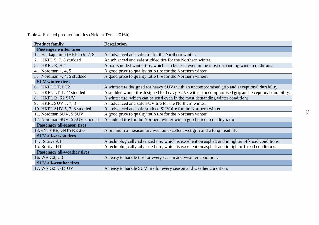
53

Table 4. Formed product families (Nokian Tyres 2016b).

Product family Description

Passenger winter tires

1. Hakkapeliitta (HKPL) 5, 7, 8 An advanced and safe tire for the Northern winter.

2. HKPL 5, 7, 8 studded An advanced and safe studded tire for the Northern winter.

3. HKPL R, R2 A non-studded winter tire, which can be used even in the most demanding winter conditions.

4. Nordman +, 4, 5 A good price to quality ratio tire for the Northern winter.

5. Nordman +, 4, 5 studded A good price to quality ratio tire for the Northern winter.

SUV winter tires

6. HKPL LT, LT2 A winter tire designed for heavy SUVs with an uncompromised grip and exceptional durability.

7. HKPL LT, LT2 studded A studded winter tire designed for heavy SUVs with an uncompromised grip and exceptional durability.

8. HKPL R, R2 SUV A winter tire, which can be used even in the most demanding winter conditions.

9. HKPL SUV 5, 7, 8 An advanced and safe SUV tire for the Northern winter.

10. HKPL SUV 5, 7, 8 studded An advanced and safe studded SUV tire for the Northern winter.

11. Nordman SUV, 5 SUV A good price to quality ratio tire for the Northern winter.

12. Nordman SUV, 5 SUV studded A studded tire for the Northern winter with a good price to quality ratio.

Passenger all-season tires

13. eNTYRE, eNTYRE 2.0 A premium all-season tire with an excellent wet grip and a long tread life.

SUV all-season tires

14. Rotiiva AT A technologically advanced tire, which is excellent on asphalt and in lighter off-road conditions.

15. Rotiiva HT A technologically advanced tire, which is excellent on asphalt and in light off-road conditions.

Passenger all-weather tires

16. WR G2, G3 An easy to handle tire for every season and weather condition.

SUV all-weather tires

17. WR G2, G3 SUV An easy to handle SUV tire for every season and weather condition.

54

Even though the formation of product families produced a time series long enough to use

extrapolation methods, the product family sales of Nokian Tyres in the US are relatively

small in comparison with the size of the country leading to highly intermittent sales in

most of the states. Therefore, so that extrapolation methods would provide good forecasts,

geographic sales aggregation is required. For this reason, the similarity of sales between

the US states were analyzed. Yet before this analysis could be done, the problem of lack

of state specific data has to be tackled. To overcome this, the similarity of the sales of

product families in the same state was analyzed in a view to combine homogenous time

series together (see Figure 13 below). If possible, this would allow tire sale comparisons

between states and the analysis of geographical market segmentation.

Figure 13. Sales of passenger winter tire product families in one of the US states. Analysis

by the author.

As it can be seen from Figure 13, the sales of winter tire product families within a state

indeed seem to be homogenous and hence, justify time series aggregation. This

conclusion is made because the sales of the product families peak (emphasized with a

blue oval) and diminish (green oval) at the same period. The same conclusion could be

made with other tire families also from other tire segments, within other states, and

between passenger and SUV tires. The latest finding though is not surprising because the

same causal forces affect both of the sales. Finally, when closely looking Figure 13 it also

55

seems that one of the product sales (dark blue line) would precede others. However,

because this did not appear in other states, it was determined to appear due to chance here.

The conclusion that sales of different product families can be aggregated within a state is

indeed a considerable finding as this enables sales analysis and seasonal component

estimation. In total, seven possible outliers were detected for which reasons for their

occurrence were asked from the supply chain planning director and the head of NA. yet

because all of them had a common explanation such as an acquisition of a new customer,

none of the outliers were adjusted. (Heinonen 2016; Larose 2016; Kim 2016)

4.3.2 Segmenting the US tire market geographically

4.3.2.1 Current market segmentation

As product family sales can be aggregated within a state, there is now sufficient amount

of data to analyze if product family sales can be aggregated between states. Even though

the company currently aggregates sales between states, the validity of this procedure has

never been confirmed before. It is expected however, that the customer behavior is

relatively homogenous between neighboring states that share a similar climate. This is

also expected because none of the US states has banned the use of studded winter tires.

In fact, the results are as expected, the product family sales can be aggregated within the

NE area as the customer behavior between the states are relatively homogenous there; the

sales peak (blue oval) and diminish (green oval) at the same period (see Figure 14 below).

The red circle in Figure 14 signs one of the spotted seven possible outliers, which was

further analyzed but was determined not to require adjustment.

56

Figure 14. Aggregate winter tire sales in three of the NE states while the yellow line

presents aggregate sales of the whole NE area. Analysis by the author.

The possibility to aggregate sales between states is indeed beneficial for the company.

This is because the aggregate sales quantity generally includes less randomness

increasing the efficiency of seasonality analysis and forecasting accuracy (Lapide 2006;

Zotteri & Kalchschmidt 2007, 81; Armstrong 2006, 591). Yet even though sales can be

aggregated within the NE area, it does not mean that the current market segmentation is

necessarily the optimal one.

When comparing the aggregate winter tire sales of the NE and OT areas, it is clear that

the time series differ considerably from each other (see section a in Figure 15 below).

This conclusion can be made because the sales peak and diminish in the OT area a few

months earlier. In addition, the durations of the peak seasons differ as it seems to be a

few months longer in the OT area. This difference may arise at least because of three

reasons. First, the OT market area includes states that sales are more homogenous with

the NE states. Second, the winter in the OT area is generally longer than in the NE, and

finally, the customer behavior differs between these areas for other reasons, for example,

because of different customer preferences. From these, the first one is considered causing

the difference and therefore, by enlarging the NE area, the difference should narrow and

hence, increase the seasonal component estimation and forecasting accuracy.

57

Figure 15. (a) Aggregate winter tire sales, and the sales of (b) all-weather (product family No. 16) and (c) all-season product families (product

family No. 13) in the OT (orange) and NE (blue) areas. Analysis by the author.

a

b c

58

Again when comparing the time series of all-weather and all-season tires between the NE

and OT areas, the time series did not seem to differ from each other (see sections b and c

in Figure 15 respectively). This is most likely because both of these are used around the

year; even the all-season tires even though it is against experts’ recommendations.

(Heinonen 2016; Bourassa 2016) Because the time series of all-season and all-weather

tires are similar between the OT and NE areas, the market aggregation is expected to

increase the forecasting accuracy the most when their sales are forecasted in the whole

US altogether.

Generally, the sales of all-season tires tend to peak in both the fall and spring because

customers prefer to buy new tires with better grip before the winter and summer vacation.

The sales of all-weather tires also tend to peak before winter. Even though all-weather

tires are targeted specifically to a year-round use, they show stronger seasonality than all-

season tires do. This most likely is because they have a shorter product life because of

their softer rubber composition that provides a better grip. Therefore, some of the

customers may use all-weather tires in the fall and all-season tires in the summer.

(Heinonen 2016; Bourassa 2016)

4.3.2.2 Proposed market areas for further analysis

An attentive reader may also have noticed the relatively strong yearly fluctuations in sales

from the previous Figure 15. This fluctuation is mostly due to the varying strength of the

winter. For instance, the winter in 2015 was extremely mild in the OT area, which led to

lower than normal winter and all-weather tire sales. The opposite can be seen in the

purchasing behavior of all-season tires. (Heinonen 2016) Therefore, because tire sales,

especially that of winter tire, are clearly dependent on the weather, the proposed new

market areas are built based on the US climate (see Figure 16 below).

59

a

b

Figure 16. (a) Current NE area and the proposed new market areas. (b) US climate. Snowy

winters are faced in blue and purple areas while red and peach represents arid climate. In

the green area the temperature is warm. (SciJinks 2016) Analysis by the author.

The proposed new market areas to be studied, in addition to the current segmentation, are

the New North East 1 (NNE1), NNE2, NNE3, which are the areas with the second, third,

and forth the lightest blues respectively where the previous area is always added to the

darker blue area (see section a in Figure 16). The states left after the NNE states have

been taken form the New Other 1 (NOT1), NOT2, and NOT3 areas. The green area was

also studied to be one market area alone, however, the sales there were too small for this

analysis to be done. The final market segmentation to be studied is the whole US.

4.4 Chosen forecasting methods

In this thesis, only extrapolative forecasting methods are used because causal methods

based on macroeconomic variables would not likely provide accurate forecasts. This is

because they usually work better when forecasting aggregate quantities such as the sales

of an industry than when forecasting product sales. However, even for this purpose, there

is relatively little proof that causal methods work well. For instance, the forecasting

accuracy of a causal method was limited when it was used to forecast the aggregate US

domestic automobile sales because the main economic indicators were only weakly

correlated with the sales. (Fildes, et al. 2011; Armstrong & Brodie 1999; Shahabuddin

2009) The same problem would most likely be when forecasting the sales of US tire

industry.

60

4.4.1 Naïve 1, 2, and classical decomposition methods

As aggregating sales most likely increases the forecasting accuracy, the optimal market

segmentation is studied first (Lapide 2006; Zotteri & Kalchschmidt 2007). For this

analysis, the Naïve 1 method (N1) is used (see Equation 2 below). The method is simple;

the forecast is the sales of the current month. The method assumes that both the trend and

seasonal components are stochastic, unforecastable. (Makridakis & Hibon 2000)

(2) Ft+m = Yt

Where Ft is the forecast made in time t with a forecast horizon of m and Yt is the sales of

the month t. The Naïve 2 (N2) method is the same as the N1, however, the time series is

seasonally adjusted (see Equation 3 below). The method assumes that the seasonal

component is forecastable and the trend component is stochastic as did the N1 method.

Therefore, by comparing the forecasting accuracy of the N1 and N2 methods, the effect

of the seasonal component estimation on the forecasting accuracy can be analyzed.

(Makridakis & Hibon 2000)

(3) Ft+m = SA Yt

Where SA Yt is the seasonal adjusted sales of the month t. It is expected that the N2 will

provide more accurate forecasts compared with the N1 method especially when

forecasting the winter and all-weather tire sales. This is because they seem to have

stronger seasonal components than all-season tires do (Makridakis, et al. 1993). The use

of N2 method may even decrease the forecasting accuracy when forecasting the sales of

all-season tires because the seasonal components may be too weak (Withycombe 1989).

In this research, the time series are seasonally adjusted with the classical decomposition

method. Even though there are numerous other methods, this is used because it is widely

used, its functionality has been proven, and finally, more complex methods usually do

not provide more accurate results in forecasting procedures (Makridakis, et al. 1998, 106;

Assimakopoulos & Nikolopoulos 2000, 524; Armstrong, et al. 2015). A time series can

be composed with three different ways. By 1) adding or 2) multiplying the components

together, or by using a 3) pseudo-additive approach, which is a mixture of both of the

former ones (see Equations 4–6 below respectively). (Makridakis, et al. 1998, 84–85;

U.S. Census Bureau 2016, 220–221)

61

(4) Yt = St + Tt + Et => Yt – St = SA Yt = Tt + Et

(5) Yt = St × Tt × Et => Yt St⁄ = SA Yt = Tt × Et

(6) Yt = Tt(St + Et – 1) => Yt – TtSt + Tt = SA Yt = Tt × Et

Where St is the seasonal, Tt trend, and Et the random component. Because the seasonal

component of an economic series is usually conditional on the trend, meaning that when

the sales trend upwards the effect of seasonality increases at the same time, the time series

is most commonly decomposed multiplicatively. However, because many of the product

sales here are intermittent, this cannot be used because sales cannot be divided with a

seasonal component of zero. In addition, dividing sales with a number close to zero biases

the forecasts considerably. Therefore, the pseudo-additive version of the decomposition

method is used here. (Makridakis, et al. 1998, 85; U.S. Census Bureau 2016, 220–221)

4.4.2 Forming seasonal indices

However, before seasonally adjusting the time series, the trend component should be

taken into account. This is because in case of an upward trend, the trend biases the

seasonal component of the first observations downwards and the latest upwards. (Bell &

Hillmer 2002, 99–110) In this thesis, the trend component is estimated with the most

commonly used trend estimation methods. First, a 12 centered moving average is used

(see Equation 7 below). However, because this method cannot be used close to the ends

of a time series, first the shorter 4 centered moving average and then the moving averages

of three and two months are used (see Equations 8–10 respectively). The latest used

observations from January to September 2015 are taken with a rolling basis so that the

forecasts do not include information from the future. Finally, if the trend component is

zero, then a longer moving average is used. (Makridakis, et al. 1998, 96)

(7) 2 × 12 MA: Tt = 1

12(0.5 × Yt–6 + Yt–5 + Yt–4 + … + Yt+4 + Yt+5 + 0.5 × Yt+6)

(8) 2 × 4 MA: Tt = 1

4(0.5 × Yt–2 + Yt–1 + Yt + Yt+1 + 0.5 × Yt+2)

(9) 3 MA: Tt = 1

3(Yt–1 + Yt + Yt+1)

(10) 2 MA: Tt = 1

2(Yt–1 + Yt)

After all of the seasonal components are estimated for every observation, then a seasonal

index is formed. In this research, seasonal indices are made by averaging the observations

62

from the monthly sales from 2013 to 2015. The mean is used because the seasonal

component is relatively stochastic as the weather cannot be forecasted accurately a year

ahead. Hence, the best estimate of the seasonal component is the mean. (Armstrong 2006;

Dekker, et al. 2004; Miller & Williams 2003)

The seasonal index in itself can be formed either from individual time series, when the

index is known as the individual seasonal index (ISI), or from an aggregated time series.

If the ISI of all of the time series of a group are estimated first and averaged after, the

index is known as the Dalhart's Group Seasonal Index (DGSI). Again if the time series

are combined first and the seasonal component is estimated after, then the seasonal index

is known as the Withycombe's Group Seasonal Index (WGSI). Both, the DGSI and WGSI,

have shown usually similar results; the use of a group seasonal index usually leads to

better forecasting accuracies when the variation of an individual time series is high. Yet

one of the latest studies of the seasonal indices argued that universally the DGSI is better

than WGSI. (Bunn & Vassilopulos 1999, 432; Withycombe 1989; Boylan, et al. 2014;

Chen & Boylan 2008)

4.4.3 Exponential smoothing methods

In addition to the N1 and N2 methods, also several exponential smoothing (ES) methods

are used to see if methods that are more sophisticated and the estimation of the trend

component increases the forecasting accuracy. Because a time series may include either

an additive or a multiplicative trend, or no trend at all, and the same goes for the seasonal

component, there are nine different trend and seasonal component combinations in total.

Each of these combinations has their own exponential smoothing method in addition to

methods, which either damp the trend and/or the seasonal component. (Gardner 2006)

In this research, nine ES methods and three equally weighted method combinations are

used. The combinations are equally weighted because they have been argued to usually

provide the best results (Blattberg & Hoch 1990, 895). The first ES method used is the

simple exponential smoothing method (SES), which assumes no seasonal or trend

component in a time series (Makridakis, et al. 1998, 147). The second method is the Holt’s

linear method (HLM), which assumes the time series to have a linear trend but no

63

seasonality (Holt 2004). If the time series includes a multiplicative seasonality but no

trend or a multiplicative seasonality and an additive trend, then the Winter’s

multiplicative method (WMM) and the Holt-Winters’ multiplicative method (HWMM)

should work well respectively. Finally, for a time series which include an additive trend

but no seasonality, the Gardner & McKenzie's damped additive trend method (GMD-AT)

should provide good results while the damped multiplicative trend method (DAT-MS)

should provide accurate forecasts for a time series with a linear trend and a multiplicative

seasonality. The Equations 11–16 below represents these six ES methods respectively.

(Gardner 2006, 640; Winters 1960; Gardner & McKenzie 1985)

(11) Lt = αYt + (1 – α)Lt–1

Ft+m = Lt

(12) Lt = αYt+(1 – α)(Lt–1 + bt–1) bt = β(Lt – Lt–1)+(1 – β)bt–1

Ft+m = Lt + btm

(13) Lt = α(Yt

St–p) + (1 – α)Lt–1⁄

St = γ(Yt

Lt) + (1 – γ)St–p⁄

Ft+m = LtSt–p+m

(14) Lt = α(Yt

St–p) + (1 – α)(Lt–1 + bt–1)⁄

bt = β(Lt – Lt–1) + (1 – β)bt–1

St = γ(Yt Lt)+(1 – γ)St–p⁄

Ft+m = (Lt + btm)St–p+m

(15) Lt = αYt + (1 – α)(Lt–1 + ϕbt–1

)

bt = β(Lt – Lt–1) + (1 – β)ϕbt–1

Ft+m = Lt + btm

(16) Lt = α(Yt

St–p) + (1 – α⁄ )(Lt–1 + ϕbt–1

)

bt = β(Lt – Lt–1) + (1 – β)ϕbt–1

St = γ(Yt Lt) + (1 – γ)St–p⁄

Ft+m = (Lt + ∑ ϕibt

m

i=1

) St–p+m

Where p is the number of periods in the seasonal cycle, α is the smoothing parameter for

the level, β for the trend, and γ for the seasonal indices of the series, and ϕ is the damping

parameter. Lt is the smoothed level of the series, bt is the slope of the additive trend and

St is the multiplicative seasonality at the end of period t. (Gardner 2006, 640–641) As the

reader may have noticed, the seasonal adjustments are made in the forecasting methods

multiplicatively. Therefore, it will also be studied if the methods are changed so that they

64

use pseudo-additive decomposition. Technically, this means that the (Yt/St – p) is changed

to (Yt – TtSt + Tt). This study can be seen to have a high theoretical contribution value

because such studies have not been provided before. Finally, as argued before, the St was

replaced with the seasonal mean because of the stochastic seasonal component (Dekker,

et al. 2004; Miller & Williams 2003).

From the smoothing parameters alpha, beta, and gamma may have a value between zero

and one while phi can have any positive value. A smaller alpha makes the forecasted time

series smoother and the forecasts to lag more. The forecasts with a larger alpha again lag

less but the risk them including noise in the forecasts increases. When the alpha is one

then the Holt’s linear method becomes the N1 method. (Makridakis, et al. 1998) As it can

be seen, the DAT-MS (Equation 15) is the same than HWMM (Equation 13) when the

damping parameter ϕ is set to one and WMM (Equation 12) when set to zero. If the value

of the phi is close to one, then the trend is expected to be relatively persistent, however,

if the data is noisy or the trend is expected to change the value of the phi is lowered

towards zero. The method assumes that there is no linear trend whatsoever if the phi value

is zero and an exponential trend when it is over one. (McKenzie & Gardner 2010)

These ES methods were chosen because the time series forecasted here include the

assumed characteristics. In addition, the damped trend methods are used because there

are numerous studies where they have shown to outperform traditional ES methods and

some of the more complicated methods have been able to provide only slight increases in

the forecasting accuracy in certain circumstances. The damped trend methods are robust

because they do not consider the trend to be persistent but rather takes uncertainty into

account and damps the trend. (Armstrong et al. 2015; Fildes, Nikolopoulos, Crone &

Syntetos 2008; Armstrong 2006; Gardner & McKenzie 1985) Even though they have

performed well, they are still rather unknown outside of a small group of academics

(Gardner 2015). Therefore, by studying its functionality and comparing it with other ES

methods, this thesis provides valuable theoretical contribution value.

65

4.4.4 Initializing and analyzing the forecasting methods

The research was done in a two-step process. First, the optimal market segmentation was

studied in August 2016 with both the N1 and N2 methods. The data used in this process

consisted of sales from January to July 2016. The results achieved were then used to

determine which market segmentation should be used in the second step of the study

where the different seasonal indices and the chosen ES methods were analyzed and their

accuracies were compared with the Naïve methods and current practices.

Before using the exponential smoothing methods, they should be fitted to the historical

data, which means that the smoothing and damping parameters will be determined. In this

research, the methods were fitted with the Excel solver tool and by using the data from

January to May 2016. Fitting was not done with earlier data because then there would

have not been three observations of each month to be used in the seasonal component

estimation. The in-sample data was also used to study the performance of different

seasonal indices from which the best ones were used in the ES methods. The forecasting

ability of all of the methods is finally analyzed from the out-of-sample data that consisted

of sales from June to September 2016.

The limited amount of historical sales data led the forecasting methods with forecast

horizons of 12 months to be fitted with a data that were not known at the time when the

forecasts were made. The result is that the method parameters include some information

not available beforehand. This however, most likely does not bias the forecasts

considerably because the monthly sales are well behaved, that is, they are quite similar

each year. However, to ensure the objectiveness of the research, the chosen ES and N2

methods are compared with the forecasts made with the current practices and at the end

of May 2016.

The ES methods are initialized so that the level of the trend is set to match the first

observation, L1 = Y1. The slope of the trend is estimated by using ordinary least squares

(OLS or just LS) with Excel and on the sales of 2013. The slope of the trend can also be

set according to the difference between the first two observations, Y2 – Y1, however, in

this case where the sales variability between observations is large, the slope would most

likely be too extreme and thus, decrease the forecasting accuracy. (Makridakis, et al.

1998, 159) The forecasting accuracy measure used here to fit the methods but also

66

measure their out-of-sample forecasting accuracy is the mean absolute error (MAE) (see

Equation 17 below).

(17) MAE = mean(|et|) = mean(|Yt – Ft|)

Where et is the forecasting error. In words, MAE measures how many tires have been

forecasted wrong. MAE is used in this research because it 1) can be used with intermittent

sales data, 2) is easy to interpret, and 3) is argued to be one of the best forecasting accuracy

measures. (Hyndman & Koehler 2006)

4.5 Results of the study

In this chapter, the performances of the methods presented are analyzed and compared

with both the currently used quantitative method alone and in combination with their

qualitative forecasts. First, the optimal market segmentation is studied and after, the

performance of the N2 method with several seasonal indices are analyzed. Finally, the ES

methods are tested and the total increase in the forecasting accuracy is achieved.

4.5.1 Naïve 1 and the optimal market segmentation

As it was argued earlier, the forecasting accuracy most likely increases the most when the

winter tire sales are aggregated in more evenly balanced areas and both the all-weather

and all-season tires are aggregated in the whole US. In the first part of the research, the

product family sales were aggregated in all of the proposed new market areas, forecasted

with the N1 method, and then the forecasting accuracies were compared with the currently

used quantitative method, N1 method, with the NE/OT market area aggregations (see

Table 5 below). In the following tables to be presented, a result of 0.8 means that the

forecasting error is 20 percent lower than that of the comparison method. The forecasting

method with the best forecasting accuracy will be highlighted with green while those

methods that decrease the forecasting accuracy are highlighted with red.

67

Table 5. MAE of the Naïve 1 method in various market area segmentations compared

with the current forecasting practices. Analysis by the author.

Naïve 1 Winter All-season All-weather ALL

NE/OT 1 1 1 1

NNE1/NOT1 1.04 1.09 1.03 1.06

NNE2/NOT2 1.01 1.11 1.04 1.06

NNE3/NOT3 0.98 1.00 1.12 1.01

Whole US 0.92 0.90 0.99 0.92

Effect size

with CI

0.10 ± 2.00

0.21 ± 2.87

0.02 ± 1.61

0.22 ± 1.78 CI = 95% confidence interval.

Against what was expected, the two wider NE areas actually decreased the forecasting

accuracies when forecasting winter tire sales. Some gain was achieved with the

NNE3/NOT3 area but the best forecasting accuracy was achieved with the whole US

market segmentation. This finding actually makes sense. If the weather fluctuations

between the climates witnessed in the US states are not perfectly correlated with each

other, then the sales aggregation in the whole US may indeed lead to better forecasting

results. This is because if some of the US states witness a stronger and others a milder

than average winter, this balances the aggregate effect on the level of sales, making the

time series smoother, and hence, increases the forecasting accuracy.

As expected, the whole US market segmentation led to the best results when forecasting

the all-season and all-weather tires. The forecasting error of the all-season tire group

decreased the most, approximately ten percent. The high increase in the forecasting

accuracy was most likely because both of the NE and OT time series showed relatively

high variance enabling a larger compensating errors effect. The smaller gain from

aggregating the sales of all-weather tires may be because the NE and OT sales seem to

correlate more or it is due to a normal sampling error.

On average, the US market segmentation decreased the forecasting error almost eight

percent. This finding has a small effect size but a considerable economic value for the

company (Cohen 1992, 157). The finding that the whole US is the optimal market

segmentation seems also to be robust as the same conclusion was achieved with using the

N2 method. The results of this analysis are not shown here.

68

4.5.2 Naïve 2 and the effect of seasonality analysis on the forecasting accuracy

The next phase in the research was to analyze the performance of the N2 method with

various seasonal indices (see Table 6 next page). The performances of the seasonal

indices were tested in the in-sample data first and then the best performing indices were

analyzed in the out-of-sample data (see underlined cells and Chosen N2 row). The all-

weather and all-season product categories do not include the single WGSI or DGSI

seasonal indices because both of the product groups included only one product family

with a long enough sales history for seasonal component estimation in each of the SUV

and passenger tire segment. Hence, they would be the same as the ISI.

The most prominent finding in Table 6 is the considerable positive effect of the seasonal

component estimation on the forecasting accuracy. Compared with the N1 method used

in the whole US, this procedure reduced the forecasting error 21 and 15 percentage points

on average when forecasting winter and all-weather tire sales respectively. As expected,

the effect was not as good with the all-season tire segment as the forecasting accuracy

decreased relatively little. The most likely reason for this finding is as argued before; the

time series are relatively noisy and the seasonal component is weak.

The possible gains mentioned above, however, could have only been achieved if the

forecaster would have been able to choose the most accurate seasonal indices beforehand.

Therefore, the more realistic measure of the achievable gains from seasonal component

estimation is achieved when the Chosen N2 group is compared with the N1 method. The

Chosen N2 group decreased the forecasting error nine percentage points in both winter

and all-weather tire segments while the forecasting error increased slightly when

forecasting the all-season tire sales. Universally, the group reduced the forecasting error

by five percentage points therefore providing proof of the importance of seasonal

component estimation in sales forecasting. Yet it has to be remembered that if the forecast

horizon would have been different, the increase in the forecasting accuracy would have

been considerably larger.

69

Table 6. MAE of the Naïve 2 method with various seasonal indices compared with the current forecasting practices. Analysis by the author.

Winter All-season All-weather

Product family 1 2 3 4 5 6 7 8 9 10 11 12 Avg. 13 14 15 Avg. 16 17 Avg. All

1. N1, whole US 0.99 0.92 0.80 0.92 0.78 0.94 0.71 0.90 0.90 0.98 0.96 0.83 0.88 0.95 0.85 0.92 0.92 0.86 0.98 0.91 0.92

N2 methods:

ISI 1.22 0.59 0.73 1.46 1.00 0.93 0.81 0.71 1.00 0.46 1.03 1.23 0.88 0.93 0.93 0.82 0.92 0.77 0.94 0.83 0.89

WGSI (S) 0.99 1.03 0.79 0.72 0.82 0.94 0.86 0.78 0.90 0.28 0.51 0.62 0.75 N/A N/A N/A N/A N/A N/A N/A 0.84

WGSI (B) 0.94 0.81 0.82 0.67 0.74 0.94 0.76 0.68 0.89 0.58 0.49 0.75 0.74 1.07 1.05 0.99 1.06 0.79 1.10 0.90 0.87

DGSI (S) 1.05 1.17 0.74 1.07 0.86 0.97 0.75 0.92 0.90 0.95 0.76 0.93 0.91 N/A N/A N/A N/A N/A N/A N/A 0.90

DGSI (B) 1.00 1.06 0.84 0.88 0.85 0.95 0.69 0.87 0.91 1.03 0.92 0.95 0.90 1.06 0.96 0.89 1.02 0.73 0.97 0.82 0.93

2. Best N2 method 0.94 0.59 0.73 0.67 0.74 0.93 0.69 0.68 0.89 0.28 0.49 0.62 0.67 0.93 0.93 0.82 0.92 0.73 0.94 0.81 0.77

Best methods 1–2 0.94 0.59 0.73 0.67 0.74 0.93 0.69 0.68 0.89 0.28 0.49 0.62 0.67 0.93 0.85 0.92 0.90 0.73 0.94 0.81 0.76

Chosen N2 1.22 1.17 0.74 0.72 0.82 0.93 0.69 0.71 1.00 0.46 1.03 0.75 0.79 1.06 0.93 0.82 1.00 0.73 0.97 0.82 0.87

Effect size

with CI

–0.14

±2.38

–0.44

±8.60

0.16

±1.25

0.51

±3.26

0.25

±0.34

0.05

±2.80

0.36

±2.84

0.18

±2.67

0.00

±2.90

1.03

±3.60

–0.05

±5.28

0.39

±2.80

0.27

±1.80

–0.14

±7.43

0.11

±4.46

0.44

±6.97

–0.02

±8.37

0.32

±2.51

0.02

±2.33

0.17

±1.84

0.22

±2.05 N1 = Naïve 1, N2 = Naïve 2, ISI = individual seasonal index, WGSI (S) and DGSI (S) = Withycombe's Group Seasonal Index and Dalhart's Group Seasonal Index of either SUV or passenger tire

segment depending to which category the product family belongs, WGSI (B) and DGSI (B) again are estimated from both the SUV and passenger tire sales, CI = 95% confidence interval.

70

In general, the universal use of ISI provides more accurate forecasts compared with the

N1 method, however, the variability of the performance is large; ISI tends to provide the

best but also the worst forecasting accuracies depending on the time series and sample

period. For instance, four of the seven time series for which the ISI provided the best

forecasting accuracies in the in-sample data, were less accurate than the N1 method in the

out-of-sample data. The same also occurred the other way around. The reason for this

fluctuation is clear; the ISI fits the time series better than group indices, however, the risk

of including noise in the seasonal component estimations also increases possibly leading

to highly inaccurate forecasts.

When analyzing the universal use of group seasonal indices, the first conclusion made is

that the universal use of WGSI seems to provide better results than the use of DGSI. This

finding is therefore similar with that of made by Bunn and Vassilopoulos (1993) and

against the more recent finding made by Chen and Boylan (2008). However, as the DGSI

provided universally two percentage points more accurate forecasts than the WGSI in the

in-sample data, this subject requires more research. Yet because the DGSI was even worse

than ISI in the out-of-sample data, from these two, the WGSI is still preferred.

It also seems that the benefit from estimating the seasonal component from group seasonal

indices is already achieved when estimating them from either SUV or passenger

aggregate tire sales data. Therefore, no further aggregations between these two tire

segments are necessarily required. This conclusion can be made as further aggregation

led to one percentage point increase in the forecasting accuracy in the out-of-sample data

while the reverse occurred in the in-sample data. Finally, because the Chosen N2 methods

led to the same forecasting accuracy than using the WGSI universally, more research is

required to analyze if choosing the best performing seasonal indices for each of the time

series by using in-sample data increases the forecasting accuracy or is the universal use

of WGSI more efficient.

71

4.5.3 Forecasting accuracy of various exponential smoothing methods

4.5.3.1 Exponential smoothing methods compared with the Naïve 1 method

Next, the chosen ES methods and three different forecasting method combinations were

tested and compared with the currently used N1 method with the NE/OT area sales

aggregations (see Table 7 next page). In total, the forecasting error could be reduced by

43 percent when the best ES and Chosen N2 methods were used. This result has a medium

effect size. The biggest increase in the forecasting accuracy was achieved when

forecasting the all-season tire segment in which the forecasting error over halved.

Compared with the Chosen N2 methods, the ES methods reduced the forecasting error 16

and 12 percentage points on average when forecasting winter and all-weather tires

respectively. As Table 7 clearly shows, most of the ES methods led to highly inaccurate

forecasts when forecasting all-weather tires. The reason is straightforward, against what

could have been expected from the historical data, the sales begun to trend upwards.

Universally used, three ES methods and one method combination provided more accurate

forecasts than the Chosen N2 methods. Again seven ES methods and one combination

provided less accurate forecasts than achieved with the currently used N1 method. The

most likely reason for the “bad” performance of the ES methods is that the Naïve methods

indeed provided relatively good forecasts. This was especially because of the length of

the forecast horizon but also because most of the time series included only a weak trend

component. The latter results in that the achievable gains from using ES methods are

limited because the previous sales observations do not include so much valuable

information to be included in the forecasts.

The result from the comparison between the SES and HLM methods supports the weak

trend argument. As the HLM assumes that a time series includes an additive trend while

the SES assumes no trend at all, the comparison between these methods shows the effect

of the trend estimation. Indeed, the result is clear, while the SES is universally the best

method, the HLM leads to highly inaccurate forecasts. The same conclusion can be made

when comparing the performance of the WMM and HWMM methods.

72

Table 7. MAE of exponential smoothing methods and method combinations compared with the current forecasting practices. Analysis by the

author.

Winter All-season All-weather

Product family 1 2 3 4 5 6 7 8 9 10 11 12 Avg. 13 14 15 Avg. 16 17 Avg. All

N1, whole US 0.99 0.92 0.80 0.92 0.78 0.94 0.71 0.90 0.90 0.98 0.96 0.83 0.88 0.95 0.85 0.92 0.92 0.86 0.98 0.91 0.92

Optimal N2 0.94 0.59 0.73 0.67 0.74 0.93 0.69 0.68 0.89 0.28 0.49 0.62 0.67 0.93 0.93 0.82 0.92 0.73 0.94 0.81 0.77

1. Chosen N2 1.22 1.17 0.74 0.72 0.82 0.93 0.69 0.71 1.00 0.46 1.03 0.75 0.79 1.06 0.93 0.82 1.00 0.73 0.97 0.82 0.87

2. SES 1.13 0.76 0.80 0.80 0.73 0.94 0.70 0.79 0.93 0.72 0.81 0.80 0.81 0.41 1.05 N/A 0.65 0.79 1.71 1.13 0.79

3. HLM 0.84 1.24 0.75 0.42 0.94 0.87 0.76 1.25 0.98 1.57 2.04 1.14 1.02 1.88 0.96 N/A 1.51 0.87 2.08 1.32 1.23

4. GMD-AT-NS 0.80 0.80 0.76 0.36 0.68 0.93 0.87 0.77 0.99 1.57 0.79 0.79 0.81 1.39 0.50 N/A 1.05 0.79 2.28 1.35 0.96

SES/GMD-AT-NS 0.80 0.76 0.80 0.36 0.73 0.94 0.70 0.79 0.99 1.57 0.81 0.80 0.82 1.39 1.05 N/A 1.24 0.79 2.28 1.35 1.03

5. WMM 0.82 0.82 0.80 0.92 0.75 0.93 1.48 0.81 0.93 0.90 0.87 0.83 0.87 0.92 0.45 N/A 0.76 1.14 1.16 1.15 0.86

6. WMM-PA 0.82 0.87 0.82 1.00 0.75 0.93 1.49 0.90 0.92 0.67 0.98 0.86 0.88 0.92 0.45 N/A 0.76 1.19 0.87 1.07 0.86

7. HWMM 0.93 1.36 0.76 2.03 1.02 0.87 0.80 1.47 1.09 1.62 2.08 1.43 1.32 1.63 1.01 N/A 1.37 1.39 1.89 1.58 1.38

8. HWMM-PA 0.84 1.51 0.80 0.25 1.04 0.87 1.46 1.45 0.90 1.07 2.14 1.50 1.05 1.86 1.01 N/A 1.51 1.19 2.05 1.51 1.27

9. DAT-MS 0.82 1.36 0.98 0.97 1.02 0.92 0.66 1.23 0.94 7.22 0.87 0.88 1.65 0.92 0.45 N/A 0.76 1.39 1.85 1.56 1.34

10. DAT-MS-PA 0.82 0.78 0.73 1.10 0.80 0.93 0.71 1.42 0.92 3.63 1.07 0.96 1.24 0.92 0.45 N/A 0.76 2.20 2.19 2.20 1.20

11. COMB1 0.82 1.10 0.71 0.64 0.82 0.91 0.65 1.09 0.94 2.58 1.33 0.96 1.05 0.41 0.65 N/A 0.51 0.89 1.85 1.25 0.89

12. COMB2 0.92 0.90 0.76 0.45 0.65 0.93 0.93 0.75 0.93 0.75 0.90 0.79 0.76 0.74 0.61 N/A 0.70 0.60 1.31 0.86 0.75

13. COMB3 0.90 1.90 0.68 0.22 0.78 0.91 0.55 0.92 0.93 1.29 1.22 0.85 0.88 1.30 0.80 N/A 1.10 0.76 2.03 1.24 1.00

Best methods 1–13 0.80 0.76 0.68 0.22 0.65 0.87 0.55 0.71 0.90 0.46 0.79 0.75 0.63 0.41 0.45 0.82 0.45 0.60 0.87 0.70 0.57

Effect size

with CI

0.12

±3.17

0.60

±6.04

0.20

±1.48

1.42

±0.62

0.49

±1.84

0.10

±2.73

0.51

±2.40

0.18

±2.67

0.06

±2.87

1.03

±3.60

0.34

±1.60

0.39

±2.80

0.49

±1.94

1.18

±1.83

0.85

±2.28

0.44

±6.97

1.15

±2.82

0.48

±3.60

0.08

±1.26

0.29

±2.85

0.72

±0.64 N1 = Naïve 1, N2 = Naïve 2, SES = Single exponential smoothing method, HLM = Holt’s linear method, GMD-AT-NS = Gardner & McKenzie's damped additive trend, SES/GMD-AT-NS = If

the smoothing parameter of the GMD-AT-NS is under 0.5 the SES is used, WMM = Winter’s multiplicative method, HWMM = Holt-Winters’ multiplicative method, HWMM-PA = Holt-Winters’

multiplicative method with a pseudo-additive seasonality, DAT-MS = Damped multiplicative trend, DAT-MS-PA = Damped multiplicative trend with a pseudo-additive seasonality, COMB1 =

Equally weighted combination of HLM, GMD-AT-NS, WMM, HWMM, AND DAT-MS, COMB2 = Equally weighted combination of the best in-sample N2, SES, and GMD-AT-NS, COMB3 =

Equally weighted combination of SES, HLM, and GMD-AT-NS, CI = 95% confidence interval.

73

Because of the weak and persistent trend components, the damped trend methods, that

have provided good forecasts in numerous studies, performed relatively poorly here; on

average, the damped additive trend lost to the chosen N2 methods in every tire segment.

To increase the overall performance, Gardner (2015, 1740) argued that if the damping

parameter phi of the method is under 0.5, then the SES can be used. This rule was tested

(see row SES/GMD-AT-NS in Table 7), but this resulted in a worse forecasting accuracy

than using either of the methods alone. The weak trend component is most likely also the

reason why the damped multiplicative trend and HWMM methods worked less well than

other methods. This is because then the time series were decomposed into too many

components (MacGregor 2001).

So in fact, from all of the methods tested, the simplest ES method, SES, led to the best

forecasting accuracy on average. Yet even though SES sounds overly simplistic, it has

performed well also in other studies. For instance, in the largest forecasting competition

in the world held so far, SES reduced the forecasting error of the N2 method by over 9

while HLM, WMM/HWMM, and Damped Additive Trend decreased it 7.5, under 9, and

13 percent respectively (Makridakis & Hibon 2000, 467). This finding therefore provides

further support to the commonly forgotten statement that increased sophistication does

not guarantee better forecasting accuracy (e.g. Armstrong et al. 2015). Still, how some of

the ES methods that do not take seasonality into account work so well even if most of the

time series clearly showed a strong seasonality? Because of the forecast horizon.

A considerable finding of the research however is the good performance of the studied

method combinations. As it was argued in the theoretical part of the thesis, there is a

common belief that method combinations lead to only average results (Larrick & Soll

2006). This research however, provides strong proof against this belief. The second

combination resulted in the best forecasting accuracy of all of the studied methods and

provided a worse forecasting accuracy than the currently used N1 method only once. Even

in this situation, the forecasting error was one of the smallest of the ES methods. In total,

the method combinations provided the best forecasting accuracy for six of the time series.

Finally, this research also clearly shows that the forecasting accuracy can be increase

considerably when the “normal” versions of the forecasting methods are replaced with

their pseudo-additive counterparts. Here two of the three pseudo-additive counterparts

resulted in considerable gains in the forecasting accuracies while the third provided

74

similar results than the “normal” counterpart. Therefore, this subject should be discussed

and studied more as it is currently mentioned only by a few.

4.5.3.2 Exponential smoothing methods compared with the current forecasting

practices

In the final part of the research, the best ES and N2 methods from the previous analysis

are compared with the forecasts made with the current practices. These forecasts are

quarter level and the result of the combination of the adjusted N1 forecast made by the

supply chain planning director and qualitative forecast made by the head of NA. As

argued before, the final forecast is usually closer to that of the head of NA, which is why

the final forecast is closer to a qualitative one. Hence, by comparing these forecasts with

the ES and N2 methods, the accuracy of the qualitative forecasts can be analyzed.

Because the quantitative forecasting methods were fitted with the data from January to

May 2016, they are compared with the forecasts made with the current practices at the

end of May 2016. To enable the comparison both of the forecasts are aggregated to a four-

month sales forecast. Some of the product family forecasts are also aggregated because

currently the forecasting team forecasts the aggregate quantity of “normal” and studded

winter tires. Because only one out-of-sample observation is available no effect sizes could

not be calculated. In addition, this is also why the results should be analyzed with caution

as the findings may have affected by randomness.

The result of the analysis is clear and supports the findings made by numerous studies

over a half a century; qualitative forecasts are less accurate than quantitative ones (Meehl

1957; 1996; Yaniv & Hogarth 1993; Lawrence, O'Connor & Edmudson 2000). The

current forecasting combination was over three and a half times less accurate than the N1

method alone and over six times than the best ES and N2 methods (see Table 8 below).

In total, the qualitative method provided better forecasts for only two time series out of

17, which can be regarded to be more due to chance than skill. In addition, as the head of

NA’s forecasts are weighted more, this research also provides indirect support for the

finding that weighting forecasts according to the job position does not provide accurate

forecasts (Ashton & Ashton 1985, 1504).

75

Table 8. MAE of the Chosen exponential methods compared with the current forecasting practices. Analysis by the author.

Winter All-season All-weather

Product family 1–2 3 4–5 6–7 8 9–10 11–12 Avg. 13 14 15 Avg. 16 17 Avg. All

N1, NE/OT 0.06 0.38 2.73 2.52 0.29 0.30 1.17 0.39 0.40 0.22 6.83 0.30 0.05 0.09 0.07 0.29

N1, whole US 0.06 0.39 2.73 2.53 0.30 0.30 1.17 0.39 0.40 0.22 6.86 0.31 0.07 0.09 0.08 0.29

Chosen N2 0.11 0.27 2.14 2.43 0.58 0.15 1.18 0.38 0.37 0.21 6.18 0.32 0.08 0.09 0.09 0.28

Chosen ES/N2 0.03 0.23 0.18 1.97 0.58 0.24 0.89 0.27 0.03 0.13 6.18 0.10 0.12 0.16 0.14 0.17

COMB ES/CP 0.51 0.61 0.59 1.48 0.79 0.38 0.94 0.58 0.52 0.43 2.59 0.49 0.44 0.42 0.43 0.51

Forecasting error divided by sales (negative values correspond overforecasting):

Current practices –3.58 0.57 –0.29 0.23 0.52 –1.67 –0.51 –0.30 –0.82 –1.61 –0.05 –0.99 –1.13 –1.40 –1.24 –0.78

Chosen ES/N2 –0.10 0.13 –0.05 0.46 0.30 0.40 –0.45 0.15 –0.03 0.21 0.30 0.06 0.13 0.22 0.17 0.12 N1 = Naïve 1, N2 = Naïve 2, ES = Exponential smoothing method, and COMB ES/CP = Equal combination between the current practices and the Chosen ES/N2 method.

76

To understand why the qualitative forecasts are so inaccurate, the forecasting errors were

further analyzed. Basically, because the head of NA uses a top-down forecasting design,

the forecasts can be inaccurate either because the total sales are forecasted wrong and/or

the product family sales relative to the aggregate sales are weighted inaccurately. Here,

the inaccuracy seems to be due to both of these reasons. First, the forecasts were mainly

too optimistic as 85 percent from the total forecasting error were the result of

overforecasting. If the forecasts had been unbiased, then this figure would have been

closer to 50 percent. In total, the tire sales were forecasted 78 percent over the actual

sales. Second, by multiplying the actual aggregate sales with the forecasted product

family weights, this still resulted in a 44 percent higher forecasting error compared with

that of the Chosen ES and N2 methods. By comparing this forecasting error with the total

current forecasting error, it can be argued that the qualitative forecast inaccuracy was 38

percent due to misweighting product families and 62 percent because of the inaccurate

aggregate forecast.

Because equal combinations of qualitative and quantitative methods have shown to work

well, they were also tested here (e.g. Franses & Legerstee 2011). The results were

however unconvincing as the combination had a forecasting error of three times that of

the best ES and N2 methods on average. Two reasons for this finding are that first, only

five times out of 17 the forecasts bracketed the final outcome, and second, the qualitative

forecasts are too biased and inaccurate. The desirability of increasing sales may have led

the head of NA and supply chain planning director to become overoptimistic (e.g.

Windschitl, Scherer, Smith & Rose 2013; Lawrence, et al. 2000; Galbraith & Merrill

1996). The other biases that have most likely had an effect are overconfidence on their

own abilities to sell more tires and the base-rate fallacy where the status quo sales forecast

has been disregarded almost altogether (Bar-Hillel 1980; Kahneman 2011; Bazerman &

Moore 2012; Moore & Healy 2008).

Finally, as could have been expected, Table 8 clearly shows the time aggregation reduces

the positive effect of geographical aggregation and seasonality analysis on the forecasting

accuracy. This finding captures well the fact that the functionality of sales forecasting is

dependent on several factors that are intertwined.

77

4.6 Using the forecasts and developing the forecasting process

The previous analyses clearly showed that simple quantitative sales forecasting methods

are accurate. It, however, also showed their core limitation. If the future changes

differently as it has changed to this day, quantitative methods may provide highly

inaccurate forecasts (Fildes & Makridakis 1995). The value of qualitative judgment has

therefore to be kept in mind. If the forecasters believe that it is likely a quantitative method

will result in an inaccurate forecast, then the forecast should be equally combined with a

qualitative one (Bunn & Wright 1991, 513; Sanders & Ritzman 2001, 411).

However, so that a qualitative forecast would add value to the forecasting process, it

should be accurate. As the last chapter clearly showed the current qualitative forecasts are

highly inaccurate which is why the forecasting process should be changed. First, the

amount of qualitative forecasting should be reduced considerably or their biasness be

lowered either by using proactive debiasing methods or combining more forecasters. One

possible way to reduce the amount of qualitative forecasts is to require the forecasters to

provide written reasoning why a qualitative forecasting is needed. This should increase

the accountability of the forecaster and therefore possibly reduce both the amount of

forecasts made and their biasness (e.g. Soll, et al. 2016). Second, the forecasts made by

various forecasters should be equally weighted and not, for example, according to the

position of the forecaster. Third, to ensure the best forecasting accuracies, the demand

planner should be encouraged to question the forecasts made and be affirmed that this is

acceptable and even desirable (e.g. Janis 1982).

Because tire models have various rim sizes and widths, the forecasts presented to the

production planning team should be in a disaggregated form. As there is not enough data

to forecast the sales of different rim sizes separately, given that they even should be in

the first place, the most effective way is to forecast the aggregate sales of a model first

and then segregate it. The segregation can be done, for example, by using the historical

distribution of the sales by rim size and/or qualitative judgment. (Lapide 2006; Zotteri &

Kalchschmidt 2007, 81; MacGregor 2001, 113; Armstrong, et al. 2015)

Finally, the forecasts made should be presented in a clear manner with confidence

intervals (Tetlock & Gardner 2015, 59; Chatfield 2001). The forecasting accuracies of

both, the quantitative and qualitative methods, should be measured and analyzed in a

78

continuous basis so that process learning and development can take place (Davis &

Mentzer 2007, 491). Indeed, as it was shown in the theoretical framework, the forecasting

process should be seen as a continuing process and not to end when the sales forecast has

been provided for its users.

79

5 CONCLUSIONS AND DISCUSSION

In the final chapter of the thesis a brief summary of the research and discussion of its

theoretical and economic contribution values are provided. In addition, topics for future

research are presented and the quality of the research will be analyzed.

5.1 Summary of the research

The purpose of the thesis was to explore how an accurate short-term sales forecast can be

provided and to exploit these findings when the short-term replacement tire sales of

Nokian Tyres in the US were forecasted. According to the theoretical part of the thesis,

among of other things, by aggregating homogenous time series, estimating seasonality

components, and using quantitative exponential smoothing methods, either alone or in

combinations, can increase the forecasting accuracy considerably. These findings were

then studied in the empirical part of the thesis where in total the research concluded the

study of five market area segmentations, five seasonal indices, 11 forecasting methods,

and three method combinations. The sales data consisted of 17 tire product families of

Nokian Tyres plc in the US replacement tire market.

The key findings of the research are as follows:

1) Simple quantitative methods are more accurate than qualitative methods because

the latter may be highly biased. In this research, the qualitative forecasts were

three and a half times less accurate than the Naïve 1 method.

2) Sales aggregation can increase the forecasting accuracy considerably. In this

research, it reduced the forecasting error eight percent on average.

3) The universal use of individual seasonal indices do not provide the most accurate

forecasts as their performance varies considerably.

80

4) There is no universal forecasting method, which would provide the most accurate

forecasts for every time series. Rather the performances of methods depend on

the forecast horizon and characteristics of the time series forecasted.

5) More sophisticated forecasting methods do not necessarily provide better results

than simple ones.

6) Pseudo-additive counterparts of forecasting methods can increase the forecasting

accuracy considerably.

7) Forecasting method combinations do not provide average results but rather the

contrary as they may often perform better than individual methods.

8) Quantitative methods can provide as good forecasts as the past data permits

which is why the value of qualitative judgment should not be disregarded.

In summary, this thesis showed that with simple actions and quantitative methods, a

company can increase its sales forecasting accuracy considerably, which again may result

in high economic gains for the company.

5.2 Theoretical contribution of the research and recommendations for

future research

The theoretical contribution of the research can be seen to be relatively high. In addition

to that, the research provided support for some of the common findings made in the

forecasting discipline already, the thesis also provided results to subjects, which have

been studied relatively little or not at all before. First, even though there have been

multiple articles about the positive effect of aggregating homogenous time series on

forecasting accuracy, only a few have quantified this effect. Hence, the finding that the

proper market area segmentation by itself reduced the forecasting error of monthly sales

forecasts by eight percentages on average is meaningful and shows that time series

aggregation is indeed an important subject. The same goes with other aggregations such

as periodic sales aggregation as well.

Second, this is most likely the first research, which provides quantifiable proof that using

pseudo-additive counterparts of the forecasting methods may increase the forecasting

81

accuracy considerably. In numerous occasions, they led to over two digit decreases in the

forecasting error compared with the “normal,” multiplicative methods. In the academic

literature, the pseudo-additive decomposition has attracted relatively little attention even

though circumstances where it should be used occurs in numerous industries. In fact, only

a few academics mention the subject altogether. Some academics argue that the pseudo-

additive counterparts should be used when some of the seasonal component values are

under 0.5. More research for this, however, is required as it was seen that just blindly

following a simple rule such as when to use either the damped additive trend or the Single

exponential smoothing method will most likely not provide the best results.

Third, this research clearly showed that the belief that method combinations only provide

average results is plainly speaking just wrong. Here the three tested forecasting method

combinations provided the best out-of-sample forecasting accuracies for six of the 17

time series. In addition, one of the combinations provided the most accurate forecasts on

average from all of the tested methods. Forecasting method combinations therefore

deserve far more attention in the academic literature. The issue on how the methods

should be weighted has been tackled thoroughly yet from which methods the combination

should be formed has been disregarded almost altogether. As it was argued in the

theoretical part, the best combinations bracket the actual sales, which is why a good

conservative forecasting method combined with a good optimistic method would most

likely result in good results. Yet, more research on this subject is required.

Fourth, the research also showed that the discussion about which of the group seasonal

indices, the WGSI or DGSI, is better, has not yet been settled. As several studies have

shown mixed results, more research on this issue is indeed required.

Finally, in addition to these, a more profound research recommendation is to study the

usefulness of the Naïve methods in determining the effects of various (marketing) actions,

activities, and events, such as promotions and crises, on product sales. If the Naïve

methods are robust, that is the forecasting error is relatively stable, then they could be

used to quantify these effects. To be precise, this could be done by first determining the

forecast horizon according to the expected duration of the specific effect under study.

Then the forecasting errors of that period would be compared with the forecasting errors

of a normal period. If the forecasting error is considerably larger, taking the standard

deviation of the forecasting errors into account, by using meta-analysis, the effects of

82

different marketing activities could be quantified. If possible, this would be a significant

finding especially because the marketing discipline has been criticized for decades being

unable to quantify their usefulness. Hence, this procedure would help the marketing

discipline to evolve but also companies in decision making.

5.3 Managerial implications

The economic contribution of the research for Nokian Tyres is eminent. In total, the tested

quantitative methods provided forecasts that were over six times more accurate than that

of the current practices. This enables the company to answer the customer demand better,

which most likely results in an increase in sales and decrease in costs such as storage,

logistic, and spoilage costs. Indeed, if these results are well exploited, this can

theoretically lead a yearly economic gain of hundreds of thousands of euros for the

company. (Rantala 2016). Yet, as the findings made are easily generalized to other market

areas, the value of the research can be considered to be considerably higher for the

company.

The analyzed quantitative forecasting methods should continue to provide good results

also in the future assuming that the time series remain relatively stationary and change as

they have changed to this point. In fact, as more observations turn up, longer in-sample

periods can be used in the fitting process, and therefore the forecasting accuracies can

even increase. As the quantitative methods are so much better than qualitative ones, the

use of qualitative forecasting should be reduced considerably or at least they should be

made more accurate. This, for example, can be done by requiring the forecasters to

provide written reasoning why qualitative forecasting should be used in the first place and

by teaching the forecasters about biases and best forecasting practices.

The qualitative forecasts should be continued to be checked by the demand planner who

should be encouraged to question their reasonableness. Both of the qualitative and

quantitative forecasts should be recorded clearly and analyzed both separately and in

combination. It however has to be noted that if the qualitative and quantitative forecasts

are always equally combined, this can make the qualitative forecasts even more biased as

83

the forecasters change their forecasts to be even more extreme so that the combination

would be “closer to the truth.”

The forecasting accuracy also increased because of other actions than just using simple

exponential smoothing methods. First, as it was found out, the best monthly sales

forecasting accuracies were achieved when the sales were aggregated in the whole US.

As the sales are homogenous even in so wide area than in the US, the company should

study the similarity of customer behavior between the US and Canada, but also in other

market areas such as Europe and Asia. Because the sales are forecasted in quantities and

selling prices are relatively fixed, there is no reason why the customer behavior should

differ considerably between neighboring areas assuming that other factors remain almost

the same. By doing this kind of segmentation analysis, the company can increase the

forecasting accuracy relatively easily around the world.

Second, the finding that sales of various products and product families can be combined

also made it possible for the company to use group seasonal indices. This increased the

forecasting accuracy considerably and therefore they should be used in the forecasting

methods rather than the individual seasonal indices. The forecasting methods should also

be modified in a way that the used seasonal index is the mean of the seasonal component

estimations because of the stochastic nature of the seasonal component. Finally, the

pseudo-additive counterparts of the exponential smoothing methods should also be used

as they increased the forecasting accuracy considerably. Indeed, as this research clearly

showed, there is no single method, which provides the best forecasts universally.

Therefore, to achieve the overall best sales forecasting accuracy, the company has to test

several forecasting methods and their combinations in each of the time series.

5.4 Quality of the research

As argued in the previous chapter, the findings of the research can be easily generalized

to other environments and subjects. The external validity, which refers to the extent to

which the findings can be generalized, of the research can be seen therefore to be high

(Bracht & Glass 2011). This is because the findings made can easily be exploited in other

84

market areas, companies, industries, and economic environments. Industries that

especially benefit from this research are those that witness a strong seasonality as tire

industry does. Such industries are, for example, beverage and energy businesses.

Which limits the external validity of the research is the used 12-month forecast horizon.

This is because the used forecast horizon leads the methods to take seasonality into

account indirectly. Therefore, methods that do not even take seasonality into account

provide relatively good forecasts in highly seasonal time series. Hence, the findings made

from the forecasting method comparison may not be generalizable to other forecast

horizons.

The quality of a research is usually also assessed by analyzing the reliability and validity

of the results. Reliability refers to how reliable the results are and how much they may

have been influenced, for example, by randomness, while validity refers to how well the

research actually measures the intended phenomenon (Thompson 2003). The validity of

this research is strong as only historical sales data is used in the forecasting process and

there were numerous time series in which the forecasting methods were studied. The

validity is also high because no adjustments to the past data were made, several

forecasting methods were used, and these were fitted with the Excel Solver tool, which

reduced the amount of judgment used in the forecasting process.

Which, however, reduced the validity of the research is the limited amount of past sales

data. This led to that the used exponential smoothing methods were fitted with the data

which could have not been known when the forecasts were made. Therefore, the 12-

month sales forecasts were not entirely objective. The biasing effect however, may not be

high because the time series were relatively stable. Nevertheless, their comparison with

the current practices with a forecast horizon of four months showed the true power of the

quantitative forecasting methods.

The reliability of the research was enhanced with several actions. First, replication was

made possible by describing the forecasting process in detail and providing the graphics

of product family sales. This is important because this enables the reader to analyze the

choices made, for example, concerning the time series aggregation (Vacha-Haase 2011,

7–9). Second, the forecasts made were provided for the demand planning manager in

Nokian Tyres, who is responsible for the forecasting processes around the world. This

85

reduces the probability of human errors in the forecasts made and hence, increases the

reliability of the research.

The reliability of the results is also high because the forecasting methods were studied

with out-of-sample data. Therefore, the results give a realistic view of the forecasting

ability of the studied methods. The reliability was also increased by providing effect sizes

with confidence intervals. However, a limitation of this is the limited amount of out-of-

sample observations, which led the confidence intervals to be quite wide. The limited

amount of out-of-sample data also reduced the reliability of the thesis because the

forecasting methods were not able to be tested in all of the sales conditions, that is when

sales peak and diminish. Therefore, the effect of sampling error and randomness on the

forecasting accuracy cannot be eliminated.

In summary, the research can be seen to be a great success. The quality of the research is

high and it provided both high theoretical contribution and economic value. The detailed

description of the forecasting process enables the case company but also readers to exploit

the research easily in other market areas and businesses. This again should narrow the

gap between the findings made in the forecasting discipline and the methods used in

practice. In addition, as some of the findings were new in the academic literature, this

research helps the forecasting discipline to evolve.

86

REFERENCES

Aigner, W., Miksch, S., Müller, W., Schumann, H., & Tominski, C. 2007. Visualizing

time-oriented data–A systematic view. Computers & Graphics, 31(3), 401–409.

Aiolfi, M., Capistrán, C., & Timmermann, A. 2011. Forecast combinations. In Clements,

M., & Hendry, D. (Eds.) The Oxford handbook of economic forecasting. New York:

Oxford University Press, 355–388.

Ajzen, I. 2001. Nature and operation of attitudes. Annual Review of Psychology, 52(1),

27–58.

Allen, P., & Fildes, R. 2001. Econometric forecasting. In Armstrong, J. (Ed.) Principles

of forecasting: A handbook for researchers and practitioners. New York: Kluwer

Academic Publishers, 303–362.

Ariely, D., Au, W., Bender, R., Budescu, D., Dietz, C. B., Gu, H., Wallsten, T., &

Zauberman, G. 2000. The effects of averaging subjective probability estimates

between and within judges. Journal of Experimental Psychology: Applied, 6(2), 130–

147.

Arkes, H., Faust, D., Guilmette, T., & Hart, K. 1988. Eliminating the hindsight bias.

Journal of Applied Psychology, 73(2), 305–307.

Armstrong, J. 1980. The seer-sucker theory: The value of experts in forecasting.

Technology Review, 83(6), 16–24.

Armstrong, J. 2001a. Evaluating forecasting methods. In Armstrong, J. (Ed.) Principles

of forecasting: A handbook for researchers and practitioners. New York: Kluwer

Academic Publishers, 443–472.

Armstrong, J. 2001b. Extrapolation for time-series and cross-sectional data. In

Armstrong, J. (Ed.) Principles of forecasting: A handbook for researchers and

practitioners. New York: Kluwer Academic Publishers, 217–243.

Armstrong, J. 2001c. Introduction. In Armstrong, J. (Ed.) Principles of forecasting: A

handbook for researchers and practitioners. New York: Kluwer Academic Publishers,

1–13.

Armstrong, J. 2001d. Selecting forecasting methods. In Armstrong, J. (Ed.) Principles of

forecasting: A handbook for researchers and practitioners. New York: Kluwer

Academic Publishers, 365–386.

Armstrong, J. 2001e. Standards and practices for forecasting. In Armstrong, J. (Ed.)

Principles of forecasting: A handbook for researchers and practitioners. New York:

Kluwer Academic Publishers, 679–732.

87

Armstrong, J. 2006. Findings from evidence-based forecasting: Methods for reducing

forecast error. International Journal of Forecasting, 22(3), 583–598.

Armstrong, J. 2007. Significance tests harm progress in forecasting. International Journal

of Forecasting, 23(2), 321–327.

Armstrong, J., Adya, M., & Collopy, F. 2001. Rule-based forecasting: Using judgment in

time-series extrapolation. In Armstrong, J. (Ed.) Principles of forecasting: A handbook

for researchers and practitioners. New York: Kluwer Academic Publishers, 259–282.

Armstrong, J., & Brodie, R. 1999. Forecasting for marketing. In Hooley, G., & Hussey,

M. (Eds.) Quantitative methods in marketing. London: International Thompson

Business Press, 92–119.

Armstrong, J., & Fildes, R. 2006. Making progress in forecasting. International Journal

of Forecasting, 22(3), 433–441.

Armstrong, J., Green, K., & Graefe, A. 2015. Golden rule of forecasting: Be conservative.

Journal of Business Research, 68(8), 1717–1731.

Armstrong, J., Morwitz, V., & Kumar, V. 2000. Sales forecasts for existing consumer

products and services: Do purchase intentions contribute to accuracy? International

Journal of Forecasting, 16(3), 383–397.

Ashton, A., & Ashton, R. 1985. Aggregating subjective forecasts: Some empirical results.

Management Science, 31(12), 1499–1508.

Assimakopoulos, V., & Nikolopoulos, K. 2000. The theta model: A decomposition

approach to forecasting. International Journal of Forecasting, 16(4), 521–530.

Balzer, W., Sulsky, L., Hammer, L., & Sumner, K. 1992. Task information, cognitive

information, or functional validity information: Which components of cognitive

feedback affect performance? Organizational Behavior and Human Decision

Processes, 53(1), 35–54.

Bar-Hillel, M. 1980. The base-rate fallacy in probability judgments. Acta Psychologica,

44(3), 211–233.

Bar-Hillel, M., & Neter, E. 1993. How alike is it versus how likely is it: A disjunction

fallacy in probability judgments. Journal of Personality and Social Psychology, 65(6),

1119–1131.

Bar-Hillel, M., & Wagenaar, W. 1991. The perception of randomness. Advances in

Applied Mathematics, 12(4), 428–454.

Barney, J. 1991. Firm resources and sustained competitive advantage. Journal of

Management, 17(1), 99–120.

Bazerman, M., & Moore, D. 2012. Judgment in managerial decision making. Hoboken:

John Wiley & Sons.

88

Bell, W., & Hillmer, S. 2002. Issues involved with the seasonal adjustment of economic

time series. Journal of Business & Economic Statistics, 20(1), 98–127.

Blanchard, O., & Johnson D. 2013. Macroeconomics. Boston: Pearson.

Blank, H., Nestler, S., von Collani, G., & Fischer, V. 2008. How many hindsight biases

are there? Cognition, 106(3), 1408–1440.

Blattberg, R., & Hoch, S. 1990. Database models and managerial intuition: 50% model +

50% manager. Management Science, 36(8), 887–899.

Blattberg, R., & Neslin, S. 1989. Sales promotion: The long and the short of it. Marketing

Letters, 1(1), 81–97.

Boylan, J., Chen, H., Mohammadipour, M., & Syntetos, A. 2014. Formation of seasonal

groups and application of seasonal indices. Journal of the Operational Research

Society, 65(2), 227–241.

Boylan, J., Goodwin, P., Mohammadipour, M., & Syntetos, A. 2015. Reproducibility in

forecasting research. International Journal of Forecasting, 31(1), 79–90.

Bracht, G., & Glass, G. 2011. The external validity of experiments. In Vogt, W. (Ed.)

SAGE quantitative research methods. Thousand Oaks: SAGE Publications, 438–473.

Bram, J., & Ludvigson, S. 1998. Does consumer confidence forecast household

expenditure? A sentiment index horse race. Economic Policy Review, 4(2), 59–78.

Brighton, H., & Gigerenzer, G. 2015. The bias bias. Journal of Business Research, 68(8),

1772–1784.

Buehler, R., Griffin, D., & Ross, M. 1994. Exploring the “planning fallacy”: Why people

underestimate their task completion times. Journal of Personality and Social

Psychology, 67(3), 366–381.

Bunn, D., & Vassilopoulos, A. 1993. Using group seasonal indices in multi-item short-

term forecasting. International Journal of Forecasting, 9(4), 517–526.

Bunn, D., & Vassilopoulos, A. 1999. Comparison of seasonal estimation methods in

multi-item short-term forecasting. International Journal of Forecasting, 15(4), 431–

443.

Bunn, D., & Wright, G. 1991. Interaction of judgemental and statistical forecasting

methods: Issues & analysis. Management Science, 37(5), 501–518.

Cain, D., Moore, D., & Haran, U. 2015. Making sense of overconfidence in market entry.

Strategic Management Journal, 36(1), 1–18.

Camerer, C., Loewenstein, G., & Weber, M. 1989. The curse of knowledge in economic

settings: An experimental analysis. The Journal of Political Economy, 97(5), 1232–

1254.

89

Carroll, C., Fuhrer, J., & Wilcox, D. 1994. Does consumer sentiment forecast household

spending? If so, why? The American Economic Review, 84(5), 1397–1408.

Carroll, C., & Kimball, M. 1996. On the concavity of the consumption function.

Econometrica, 64(4), 981–992.

Chambers, J., Windschitl, P., & Suls, J. 2003. Egocentrism, event frequency, and

comparative optimism: When what happens frequently is “more likely to happen to

me”. Personality and Social Psychology Bulletin, 29(11), 1343–1356.

Chandon, P., Morwitz, V., & Reinartz, W. 2005. Do intentions really predict behavior?

Self-generated validity effects in survey research. Journal of Marketing, 69(2), 1–14.

Chapman, L., & Chapman, J. 1969. Illusory correlation as an obstacle to the use of valid

psychodiagnostic signs. Journal of Abnormal Psychology, 74(3), 271–280.

Chatfield, C. 2001. Prediction intervals for time-series forecasting. In Armstrong, J. (Ed.)

Principles of forecasting: A handbook for researchers and practitioners. New York:

Kluwer Academic Publishers, 475–494.

Chen, H., & Boylan, J. 2007. Use of individual and group seasonal indices in

subaggregate demand forecasting. Journal of the Operational Research Society,

58(12), 1660–1671.

Chen, H., & Boylan, J. 2008. Empirical evidence on individual, group and shrinkage

seasonal indices. International Journal of Forecasting, 24(3), 525–534.

Clemen, R. 1989. Combining forecasts: A review and annotated bibliography.

International Journal of Forecasting, 5(4), 559–583.

Clemen, R. 2001. Simple versus complex methods. International Journal of Forecasting,

17(4), 549–550.

Clements, M., & Hendry, D. 2001. Explaining the results of the M3 forecasting

competition. International Journal of Forecasting, 17(4), 550–554.

Cohen, J. 1992. A power primer. Psychological Bulletin, 112(1), 155–159.

Constable, S., & Wright, R. 2011. The Wall Street Journal guide to the 50 economic

indicators that really matter: From Big Macs to “zombie banks,” the indicators smart

investors watch to beat the market. New York: HarperCollins.

Corstjens, M., & Lal, R. 2000. Building store loyalty through store brands. Journal of

Marketing Research, 37(3), 281–291.

Dane, E. 2010. Reconsidering the trade-off between expertise and flexibility: A cognitive

entrenchment perspective. Academy of Management Review, 35(4), 579–603.

Danziger, S., Levav, J., & Avnaim-Pesso, L. 2011. Extraneous factors in judicial

decisions. Proceedings of the National Academy of Sciences, 108(17), 6889–6892.

90

Davis, D., & Mentzer, J. 2007. Organizational factors in sales forecasting management.

International Journal of Forecasting, 23(3), 475–495.

Dawson, E., Gilovich, T., & Regan, D. 2002. Motivated reasoning and performance on

the Wason selection task. Personality and Social Psychology Bulletin, 28(10), 1379–

1387.

Dees, S., & Brinca, P. 2013. Consumer confidence as a predictor of consumption

spending: Evidence for the United States and the euro area. International Economics,

134, 1–14.

Dekker, M., van Donselaar, K., & Ouwehand, P. 2004. How to use aggregation and

combined forecasting to improve seasonal demand forecasts. International Journal of

Production Economics, 90(2), 151–167.

Ditto, P., & Lopez, D. 1992. Motivated skepticism: Use of differential decision criteria

for preferred and nonpreferred conclusions. Journal of Personality and Social

Psychology, 63(4), 568–584.

Dong, Y., Dresner, M., & Yao, Y. 2014. Beyond information sharing: An empirical

analysis of vendor‐managed inventory. Production and Operations Management,

23(5), 817–828.

Duhigg, C. 2012. The power of habit: Why we do what we do in life and business. New

York: Random House.

Duncan, G., Gorr, W., & Szczypula, J. 2001. Forecasting analogous time series. In

Armstrong, J. (Ed.) Principles of forecasting: A handbook for researchers and

practitioners. New York: Kluwer Academic Publishers, 195–213.

Dweck, C. 2006. Mindset: The new psychology of success. New York: Random House.

Eggleton, I. 1982. Intuitive time-series extrapolation. Journal of Accounting Research,

20(1), 68–102.

Eil, D., & Rao, J. 2011. The good news-bad news effect: Asymmetric processing of

objective information about yourself. American Economic Journal: Microeconomics,

3(2), 114–138.

Einhorn, H., & Hogarth, R. 1978. Confidence in judgment: Persistence of the illusion of

validity. Psychological Review, 85(5), 395–416.

Einhorn, H., & Hogarth, R. 1982. Prediction, diagnosis, and causal thinking in

forecasting. Journal of Forecasting, 1(1), 23–36.

Eisenhardt, K., & Martin, J. 2000. Dynamic capabilities: What are they? Strategic

Management Journal, 21(10–11), 1105–1121.

Epley, N., & Gilovich, T. 2006. The anchoring-and-adjustment heuristic: Why the

adjustments are insufficient. Psychological Science, 17(4), 311–318.

91

Eriksson, P., & Kovalainen, A. 2008. Qualitative methods in business research. London:

SAGE Publications.

Field, A. 2013. Discovering statistics using IBM SPSS statistics. London: SAGE

Publications.

Fildes, R., & Goodwin, P. 2007. Against your better judgment? How organizations can

improve their use of management judgment in forecasting. Interfaces, 37(6), 570–576.

Fildes, R., Goodwin, P., Lawrence, M., & Nikolopoulos, K. 2009. Effective forecasting

and judgmental adjustments: An empirical evaluation and strategies for improvement

in supply-chain planning. International Journal of Forecasting, 25(1), 3–23.

Fildes, R., & Makridakis, S. 1995. The impact of empirical accuracy studies on time series

analysis and forecasting. International Statistical Review, 63(3), 289–308.

Fildes, R., Nikolopoulos, K., Crone, S., & Syntetos, A. 2008. Forecasting and operational

research: A review. Journal of the Operational Research Society, 59(9), 1150–1172.

Fildes, R., Wei, Y., & Ismail, S. 2011. Evaluating the forecasting performance of

econometric models of air passenger traffic flows using multiple error measures.

International Journal of Forecasting, 27(3), 902–922.

Finucane, M., Alhakami, A., Slovic, P., & Johnson, S. 2000. The affect heuristic in

judgments of risks and benefits. Journal of Behavioral Decision Making, 13(1), 1–17.

Fischhoff, B. 1975. Hindsight ≠ foresight: The effect of outcome knowledge on judgment

under uncertainty. Journal of Experimental Psychology: Human Perception and

Performance, 1(3), 288–299.

Fischhoff, B. 1977. Perceived informativeness of facts. Journal of Experimental

Psychology, 3(2), 349–358.

Fisher, M., & C Keil, F. 2015. The curse of expertise: When more knowledge leads to

miscalibrated explanatory insight. Cognitive Science, 40(5), 1251–1269.

Franses, P., & Legerstee, R. 2009. Properties of expert adjustments on model-based SKU-

level forecasts. International Journal of Forecasting, 25(1), 35–47.

Franses, P., & Legerstee, R. 2011. Combining SKU-level sales forecasts from models and

experts. Expert Systems with Applications, 38(3), 2365–2370.

Galbraith, C., & Merrill, G. 1996. The politics of forecasting: Managing the truth.

California Management Review, 38(2), 29–43.

Gardner, E. 2006. Exponential smoothing: The state of the art–Part II. International

Journal of Forecasting, 22(4), 637–666.

Gardner, E. 2015. Conservative forecasting with the damped trend. Journal of Business

Research, 68(8), 1739–1741.

92

Gardner, E., & McKenzie, E. 1985. Forecasting trends in time series. Management

Science, 31(10), 1237–1246.

Genre, V., Kenny, G., Meyler, A., & Timmermann, A. 2013. Combining expert forecasts:

Can anything beat the simple average? International Journal of Forecasting, 29(1),

108–121.

Goodwin, P. 2000. Improving the voluntary integration of statistical forecasts and

judgment. International Journal of Forecasting, 16(1), 85–99.

Goodwin, P. 2002. Integrating management judgment and statistical methods to improve

short-term forecasts. Omega, 30(2), 127–135.

Goodwin, P., & Fildes, R. 1999. Judgmental forecasts of time series affected by special

events: Does providing a statistical forecast improve accuracy? Journal of Behavioral

Decision Making, 12(1), 37–53.

Goodwin, P., & Lawton, R. 2003. Debiasing forecasts: How useful is the unbiasedness

test? International Journal of Forecasting, 19(3), 467–475.

Graefe, A., & Armstrong, J. 2011. Comparing face-to-face meetings, nominal groups,

Delphi and prediction markets on an estimation task. International Journal of

Forecasting, 27(1), 183–195.

Green, K., & Armstrong, J. 2015. Simple versus complex forecasting: The evidence.

Journal of Business Research, 68(8), 1678–1685.

Griffin, D., & Tversky, A. 1992. The weighing of evidence and the determinants of

confidence. Cognitive Psychology, 24(3), 411–435.

Grove, W., & Meehl, P. 1996. Comparative efficiency of informal (subjective,

impressionistic) and formal (mechanical, algorithmic) prediction procedures: The

clinical–statistical controversy. Psychology, Public Policy, and Law, 2(2), 293–323.

Grove, W., Zald, D., Lebow, B., Snitz, B., & Nelson, C. 2000. Clinical versus mechanical

prediction: A meta-analysis. Psychological Assessment, 12(1), 19–30.

Gruenfeld, D., Mannix, E., Williams, K., & Neale, M. 1996. Group composition and

decision making: How member familiarity and information distribution affect process

and performance. Organizational Behavior and Human Decision Processes, 67(1), 1–

15.

Harrison, Y., & Horne, J. 2000. The impact of sleep deprivation on decision making: A

review. Journal of Experimental Psychology: Applied, 6(3), 236–249.

Harvey, N. 1995. Why are judgments less consistent in less predictable task situations?

Organizational Behavior and Human Decision Processes, 63(3), 247–263.

Harvey, N., & Bolger, F. 1996. Graphs versus tables: Effects of data presentation format

on judgemental forecasting. International Journal of Forecasting, 12(1), 119–137.

93

Harvey, N., Ewart, T., & West, R. 1997. Effects of data noise on statistical judgement.

Thinking & Reasoning, 3(2), 111–132.

Harvey, N., & Reimers, S. 2013. Trend damping: Under-adjustment, experimental

artifact, or adaptation to features of the natural environment? Journal of Experimental

Psychology: Learning, Memory, and Cognition, 39(2), 589–607.

Heer, J., Kong, N., & Agrawala, M. 2009. Sizing the horizon: The effects of chart size

and layering on the graphical perception of time series visualizations. In Greenberg S.,

Hudson, S., Hinckley, K., Morris, M., & Olsen D. (Eds.) Proceedings of the SIGCHI

Conference on Human Factors in Computing Systems. New York: ACM, 1303–1312.

Henderson, A., Raynor, M., & Ahmed, M. 2012. How long must a firm be great to rule

out chance? Benchmarking sustained superior performance without being fooled by

randomness. Strategic Management Journal, 33(4), 387–406.

Hibon, M., & Evgeniou, T. 2005. To combine or not to combine: Selecting among

forecasts and their combinations. International Journal of Forecasting, 21(1), 15–24.

Hoch, S. 1985. Counterfactual reasoning and accuracy in predicting personal events.

Journal of Experimental Psychology: Learning, Memory, and Cognition, 11(4), 719–

731.

Hoch, S. 1988. Who do we know: Predicting the interests and opinions of the American

consumer. Journal of Consumer Research, 15(3), 315–324.

Hoch, S., & Schkade, D. 1996. A psychological approach to decision support systems.

Management Science, 42(1), 51–64.

Hofer, P., Eisl, C., & Mayr, A. 2015. Forecasting in Austrian companies: Do small and

large Austrian companies differ in their forecasting processes? Journal of Applied

Accounting Research, 16(3), 359–382.

Hogarth, R., & Einhorn, H. 1992. Order effects in belief updating: The belief-adjustment

model. Cognitive Psychology, 24(1), 1–55.

Holt, C. 2004. Forecasting seasonals and trends by exponentially weighted moving

averages. International Journal of Forecasting, 20(1), 5–10.

Hubbard, R., & Ryan, P. 2000. The historical growth of statistical significance testing in

psychology–And its future prospects. Educational and Psychological Measurement,

60(5), 661–681.

Hyndman, R., & Koehler, A. 2006. Another look at measures of forecast accuracy.

International Journal of Forecasting, 22(4), 679–688.

Hyndman, R., & Kostenko, A. 2007. Minimum sample size requirements for seasonal

forecasting models. Foresight: The International Journal of Applied Forecasting, 6(2),

12–15.

94

Jacobson, R. 1992. The “Austrian” school of strategy. Academy of Management Review,

17(4), 782–807.

Janis, I. 1982. Groupthink: Psychological studies of policy decisions and fiascoes.

Boston: Houghton Mifflin Company.

Kahn, K. 1998. Revisiting top-down versus bottom-up forecasting. The Journal of

Business Forecasting, 17(2), 14–19.

Kahneman, D. 2011. Thinking, fast and slow. New York: Farrar, Straus and Giroux.

Kahneman, D., & Klein, G. 2009. Conditions for intuitive expertise: A failure to disagree.

American Psychologist, 64(6), 515–526.

Kahneman, D., & Tversky, A. 1982. Subjective probability: A judgment of

representativeness. In Kahneman, D., Slovic, P., & Tversky, A. (Eds.) Judgment under

uncertainty: Heuristics and biases. Cambridge: Cambridge University Press, 32–47.

Kalchschmidt, M. 2012. Best practices in demand forecasting: Tests of universalistic,

contingency and configurational theories. International Journal of Production

Economics, 140(2), 782–793.

Keim, D. 2002. Information visualization and visual data mining. IEEE Transactions on

Visualization and Computer Graphics, 7(1), 100–107.

Kent, S. 1964. Words of estimative probability. Studies in Intelligence, 8(4), 49–65.

Kerr, N., & Tindale, R. 2011. Group-based forecasting? A social psychological analysis.

International Journal of Forecasting, 27(1), 14–40.

King, G. 1995. Replication, replication. PS: Political Science & Politics, 28(3), 444–452.

Klayman, J., & Ha, Y. 1987. Confirmation, disconfirmation, and information in

hypothesis testing. Psychological Review, 94(2), 211–228.

Klein, G. 2007. Performing a project premortem. Harvard Business Review, 85(9), 18–

19.

Koller, T., Goedhart, M., & Wessels, D. 2010. Valuation: Measuring and managing the

value of companies. Hoboken: John Wiley & Sons.

Koriat, A., Lichtenstein, S., & Fischhoff, B. 1980. Reasons for confidence. Journal of

Experimental Psychology: Human Learning and Memory, 6(2), 107–118.

Kunda, Z. 1990. The case for motivated reasoning. Psychological Bulletin, 108(3), 480–

498.

Langer, E. 1975. The illusion of control. Journal of Personality and Social Psychology,

32(2), 311–328.

95

Lapide, L. 2006. Top-down & bottom-up forecasting in S&OP. The Journal of Business

Forecasting, 25(2), 14–16.

Larrick, R., & Soll, J. 2006. Intuitions about combining opinions: Misappreciation of the

averaging principle. Management Science, 52(1), 111–127.

Lawrence, M., & Makridakis, S. 1989. Factors affecting judgmental forecasts and

confidence intervals. Organizational Behavior and Human Decision Processes, 43(2),

172–187.

Lawrence, M., O'Connor, M., & Edmundson, B. 2000. A field study of sales forecasting

accuracy and processes. European Journal of Operational Research, 122(1), 151–160.

Lee, H., Padmanabhan, V., & Whang, S. 1997. The bullwhip effect in supply chains. MIT

Sloan Management Review, 38(3), 93–102.

Lee, S., Matsunaga, S., & Park, C. 2012. Management forecast accuracy and CEO

turnover. The Accounting Review, 87(6), 2095–2122.

Levitin, D. 2014. The organized mind: Thinking straight in the age of information

overload. New York: Penguin Press.

Levy, D. 1994. Chaos theory and strategy: Theory, application, and managerial

implications. Strategic Management Journal, 15(S2), 167–178.

Lieberson, S. 1991. Small N's and big conclusions: An examination of the reasoning in

comparative studies based on a small number of cases. Social Forces, 70(2), 307–320.

Lord, C., Lepper, M., & Preston, E. 1984. Considering the opposite: A corrective strategy

for social judgment. Journal of Personality and Social Psychology, 47(6), 1231–1243.

Mauboussin, M. 2012. The success equation: Untangling skill and luck in business,

sports, and investing. Boston: Harvard Business Press.

MacGregor, D. 2001. Decomposition for judgmental forecasting and estimation. In

Armstrong, J. (Ed.) Principles of forecasting: A handbook for researchers and

practitioners. New York: Kluwer Academic Publishers, 107–123.

Makridakis, S., Chatfield, C., Hibon, M., Lawrence, M., Mills, T., Ord, K., & Simmons,

L. 1993. The M2-competition: A real-time judgmentally based forecasting study.

International Journal of Forecasting, 9(1), 5–22.

Makridakis, S., & Hibon, M. 2000. The M3-Competition: Results, conclusions and

implications. International Journal of Forecasting, 16(4), 451–476.

Makridakis, S., Hogarth, R., & Gaba, A. 2009. Forecasting and uncertainty in the

economic and business world. International Journal of Forecasting, 25(4), 794–812.

Makridakis, S., & Taleb, N. 2009a. Decision making and planning under low levels of

predictability. International Journal of Forecasting, 25(4), 716–733.

96

Makridakis, S., & Taleb, N. 2009b. Living in a world of low levels of predictability.

International Journal of Forecasting, 25(4), 840–844.

Makridakis, S., & Wheelwright, S. 1977. Forecasting: Issues & challenges for marketing

management. Journal of Marketing, 41(4), 24–38.

Makridakis, S., Wheelwright, S., & Hyndman, R. 1998. Forecasting methods and

applications. New York: John Wiley & Sons.

Mannix, E., & Neale, M. 2005. What differences make a difference? The promise and

reality of diverse teams in organizations. Psychological Science in the Public Interest,

6(2), 31–55.

Maule, A., Hockey, G., & Bdzola, L. 2000. Effects of time-pressure on decision-making

under uncertainty: Changes in affective state and information processing strategy. Acta

Psychologica, 104(3), 283–301.

McCarthy, T., Davis, D., Golicic, S., & Mentzer, J. 2006. The evolution of sales

forecasting management: A 20‐year longitudinal study of forecasting practices.

Journal of Forecasting, 25(5), 303–324.

McGrath, R., Tsai, M., Venkataraman, S., & MacMillan, I. 1996. Innovation, competitive

advantage and rent: A model and test. Management Science, 42(3), 389–403.

McKenzie, C., Liersch, M., & Yaniv, I. 2008. Overconfidence in interval estimates: What

does expertise buy you? Organizational Behavior and Human Decision Processes,

107(2), 179–191.

Meade, N. 2000. Evidence for the selection of forecasting methods. Journal of

Forecasting, 19(6), 515–535.

Meehl, P. 1957. When shall we use our heads instead of the formula? Journal of

Counseling Psychology, 4(4), 268–273.

Meehl, P. 1978. Theoretical risks and tabular asterisks: Sir Karl, Sir Ronald, and the slow

progress of soft psychology. Journal of Consulting and Clinical Psychology, 46(4),

806–834.

Meehl, P. 1996. Clinical versus statistical prediction: A theoretical analysis and a review

of the evidence. Brattleboro: Echo Point Books & Media.

Mian, A., Rao, K., & Sufi, A. 2013. Household balance sheets, consumption, and the

economic slump. The Quarterly Journal of Economics, 128(4), 1687–1726.

Miller, D., & Williams, D. 2003. Shrinkage estimators of time series seasonal factors and

their effect on forecasting accuracy. International Journal of Forecasting, 19(4), 669–

684.

Moore, D., & Healy, P. 2008. The trouble with overconfidence. Psychological Review,

115(2), 502–517.

97

Morlidge, S., & Player, S. 2010. Future ready: How to master business forecasting.

Chichester: John Wiley & Sons.

Morrison, D. 1979. Purchase intentions and purchase behavior. Journal of Marketing,

43(2), 65–74.

Morwitz, V. 2001. Methods for forecasting from intentions data. In Armstrong, J. (Ed.)

Principles of forecasting: A handbook for researchers and practitioners. New York:

Kluwer Academic Publishers, 33–55.

Morwitz, V., Steckel, J., & Gupta, A. 2007. When do purchase intentions predict sales?

International Journal of Forecasting, 23(3), 347–364.

Neal, D., Wood, W., & Quinn, J. 2006. Habits–A repeat performance. Current Directions

in Psychological Science, 15(4), 198–202.

O'Connor, M., Remus, W., & Griggs, K. 1997. Going up–Going down: How good are

people at forecasting trends and changes in trends? Journal of Forecasting, 16(3), 165–

176.

Palepu, K., Healy, P., & Peek, E. 2013. Business analysis and valuation: IFRS Edition.

Hampshire: Cengage Learning.

Pan, J., & Yang, J. 2002. A study of an integrated inventory with controllable lead time.

International Journal of Production Research, 40(5), 1263–1273.

Phillips, P. 2005. Challenges of trending time series econometrics. Mathematics and

Computers in Simulation, 68(5), 401–416.

Porter, M. 1979. The structure within industries and companies' performance. The

Review of Economics and Statistics, 61(2), 214–227.

Pronin, E., Lin, D., & Ross, L. 2002. The bias blind spot: Perceptions of bias in self versus

others. Personality and Social Psychology Bulletin, 28(3), 369–381.

Rajan, R., Volpin, P., & Zingales, L. 2000. The eclipse of the US tire industry. In Kaplan,

S. (Ed.) Mergers and productivity. Chicago: University of Chicago Press, 51–92.

Redman, T. 1998. The impact of poor data quality on the typical enterprise.

Communications of the ACM, 41(2), 79–82.

Reibstein, D., Day, G., & Wind, J. 2009. Guest editorial: Is marketing academia losing

its way? Journal of Marketing, 73(4), 1–3.

Remus, W., O'Connor, M., & Griggs, K. 1996. Does feedback improve the accuracy of

recurrent judgmental forecasts? Organizational Behavior and Human Decision

Processes, 66(1), 22–30.

Roese, N., & Vohs, K. 2012. Hindsight bias. Perspectives on Psychological Science, 7(5),

411–426.

98

Ross, L., Lepper, M., & Hubbard, M. 1975. Perseverance in self-perception and social

perception: Biased attributional processes in the debriefing paradigm. Journal of

Personality and Social Psychology, 32(5), 880–892.

Rowe, G., & Wright, G. 1996. The impact of task characteristics on the performance of

structured group forecasting techniques. International Journal of Forecasting, 12(1),

73–89.

Rowe, G., & Wright, G. 1999. The Delphi technique as a forecasting tool: Issues and

analysis. International Journal of Forecasting, 15(4), 353–375.

Russo, J., & Schoemaker, P. 1992. Managing overconfidence. Sloan Management

Review, 33(2), 7–17.

Sanders, N., & Manrodt, K. 1994. Forecasting practices in US corporations: Survey

results. Interfaces, 24(2), 92–100.

Sanders, N., & Manrodt, K. 2003. The efficacy of using judgmental versus quantitative

forecasting methods in practice. Omega, 31(6), 511–522.

Sanders, N., & Ritzman, L. 2001. Judgmental adjustment of statistical forecasts. In

Armstrong, J. (Ed.) Principles of forecasting: A handbook for researchers and

practitioners. New York: Kluwer Academic Publishers, 405–416.

Sanna, L., & Schwarz, N. 2003. Debiasing the hindsight bias: The role of accessibility

experiences and (mis)attributions. Journal of Experimental Social Psychology, 39(3),

287–295.

Sawyer, A., & Ball, A. 1981. Statistical power and effect size in marketing research.

Journal of Marketing Research, 275–290.

Schmidt, F. 1992. What do data really mean? Research findings, meta-analysis, and

cumulative knowledge in psychology. American Psychologist, 47(10), 1173–1181.

Schmidt, F. 1996. Statistical significance testing and cumulative knowledge in

psychology: Implications for training of researchers. Psychological Methods, 1(2),

115–121.

Schwarz, N. 2011. Feelings-as-information theory. In Van Lange, P., Kruglanski, A., &

Higgins, E. (Eds.) Handbook of theories of social psychology. London: SAGE

Publications, 289–308.

Schwarz, N., Bless, H., Strack, F., Klumpp, G., Rittenauer-Schatka, H., & Simons, A.

1991. Ease of retrieval as information: Another look at the availability heuristic.

Journal of Personality and Social psychology, 61(2), 195–202.

Schwarz, N., & Clore, G. 2007. Feelings and phenomenal experiences. In Kruglanski, A.,

& Higgings, E. (Eds.) Social psychology: Handbook of basic principles. New York:

The Guilford Press, 385–407.

99

Schwarzkopf, A., Tersine, R., & Morris, J. 1988. Top-down versus bottom-up forecasting

strategies. The International Journal of Production Research, 26(11), 1833–1843.

Shah, A., & Oppenheimer, D. 2008. Heuristics made easy: An effort-reduction

framework. Psychological Bulletin, 134(2), 207–222.

Shahabuddin, S. 2009. Forecasting automobile sales. Management Research News, 32(7),

670–682.

Shanteau, J. 1992. Competence in experts: The role of task characteristics. Organizational

Behavior and Human Decision Processes, 53(2), 252–266.

Shneiderman, B. 1996. The eyes have it: A task by data type taxonomy for information

visualizations. In Sipple, R. (Ed.) Proceedings of IEEE Symposium on Visual

Languages. New Jersey: IEEE, 336–343.

Shu, L., Mazar, N., Gino, F., Ariely, D., & Bazerman, M. 2012. Signing at the beginning

makes ethics salient and decreases dishonest self-reports in comparison to signing at

the end. Proceedings of the National Academy of Sciences, 109(38), 15197–15200.

Simon, H. 1955. A behavioral model of rational choice. The Quarterly Journal of

Economics, 69(1), 99–118.

Simon, H. 1986. Rationality in psychology and economics. Journal of Business, 59(4),

209–224.

Slovic, P., Finucane, M., Peters, E., & MacGregor, D. 2002. Rational actors or rational

fools: Implications of the affect heuristic for behavioral economics. The Journal of

Socio-Economics, 31(4), 329–342.

Slovic, P., & Fischhoff, B. 1977. On the psychology of experimental surprises. Journal

of Experimental Psychology: Human Perception and Performance, 3(4), 544–551.

Smith, S. 1997. Further thoughts on simplicity and complexity in population projection

models. International Journal of Forecasting, 13(4), 557–565.

Soll, J., & Mannes, A. 2011. Judgmental aggregation strategies depend on whether the

self is involved. International Journal of Forecasting, 27(1), 81–102.

Soll, J., Milkman, K., & Payne, J. 2016. In User's Guide to Debiasing. In Keren, G., &

Wu, G. (Eds.) The Wiley Blackwell handbook of judgment and decision making.

Chichester: John Wiley & Sons, 924–951.

Stalk, G., & Hout, T. 1990. Competing against time: How time-based competition is

reshaping global markets. New York: The Free Press.

Stanovich, K. 2009. Rational and irrational thought: The thinking that IQ tests miss.

Scientific American Mind, 20(6), 34–39.

100

Stanovich, K., & West, R. 2002. Individual differences in reasoning: Implications for the

rationality debate? Behavioral and Brain Sciences, 23(5), 645–665.

Starcke, K., & Brand, M. 2012. Decision making under stress: A selective review.

Neuroscience & Biobehavioral Reviews, 36(4), 1228–1248.

Stasser, G., & Titus, W. 1985. Pooling of unshared information in group decision making:

Biased information sampling during discussion. Journal of Personality and Social

Psychology, 48(6), 1467–1478.

Stasser, G., Vaughan, S., & Stewart, D. 2000. Pooling unshared information: The benefits

of knowing how access to information is distributed among group members.

Organizational Behavior and Human Decision Processes, 82(1), 102–116.

Stewart, T., & Lusk, C. 1994. Seven components of judgmental forecasting skill:

Implications for research and the improvement of forecasts. Journal of Forecasting,

13(7), 579–599.

Tayi, G., & Ballou, D. 1998. Examining data quality. Communications of the ACM,

41(2), 54–57.

Tetlock, P. 1998. Close-call counterfactuals and belief-system defenses: I was not almost

wrong but I was almost right. Journal of Personality and Social Psychology, 75(3),

639–652.

Tetlock, P., & Boettger, R. 1989. Accountability: A social magnifier of the dilution effect.

Journal of Personality and Social Psychology, 57(3), 388–398.

Tetlock, P., & Gardner, D. 2015. Superforecasting: The art and science of prediction.

New York: Random House.

Theocharis, Z., & Harvey, N. 2016. Order effects in judgmental forecasting. International

Journal of Forecasting, 32(1), 44–60.

Thompson, B. 2003. In Thompson, B. (Ed.) Score reliability: Contemporary thinking on

reliability issues. Thousand Oaks: SAGE Publications, 3–23.

Thompson, S. 1999. Illusions of control: How we overestimate our personal influence.

Current Directions in Psychological Science, 8(6), 187–190.

Tiedens, L., & Linton, S. 2001. Judgment under emotional certainty and uncertainty: The

effects of specific emotions on information processing. Journal of Personality and

Social Psychology, 81(6), 973–988.

Todd, A., Hanko, K., Galinsky, A., & Mussweiler, T. 2011. When focusing on differences

leads to similar perspectives. Psychological Science, 22(1), 134–141.

Tokatli, N. 2007. Global sourcing: Insights from the global clothing industry–The case of

Zara, a fast fashion retailer. Journal of Economic Geography, 8(1), 21–38.

101

Trapero, J., Pedregal, D., Fildes, R., & Kourentzes, N. 2013. Analysis of judgmental

adjustments in the presence of promotions. International Journal of Forecasting, 29(2),

234–243.

Tsai, C., Klayman, J., & Hastie, R. 2008. Effects of amount of information on judgment

accuracy and confidence. Organizational Behavior and Human Decision Processes,

107(2), 97–105.

Tversky, A., & Kahneman, D. 1974. Judgment under uncertainty: Heuristics and biases.

Science, 185(4157), 1124–1131.

Tversky, A., & Kahneman, D. 1983. Extensional versus intuitive reasoning: The

conjunction fallacy in probability judgment. Psychological Review, 90(4), 293–315.

U.S. Census Bureau 2016. X-13ARIMA-SEATS reference manual. Washington: U.S.

Census Bureau.

Vacha-Haase, T. 2011. Reliability generalization: Exploring variance in measurement

error affecting score reliability across studies. In Vogt, W. (Ed.) SAGE quantitative

research methods. Thousand Oaks: SAGE Publications, 6–25.

Vogel, V., Evanschitzky, H., & Ramaseshan, B. 2008. Customer equity drivers and future

sales. Journal of Marketing, 72(6), 98–108.

Wang, R., & Strong, D. 1996. Beyond accuracy: What data quality means to data

consumers. Journal of Management Information Systems, 12(4), 5–33.

Wason, P. 1960. On the failure to eliminate hypotheses in a conceptual task. Quarterly

Journal of Experimental Psychology, 12(3), 129–140.

White, H., & Granger, C. 2011. Consideration of trends in time series. Journal of Time

Series Econometrics, 3(1), Article 2.

Whitson, J., & Galinsky, A. 2008. Lacking control increases illusory pattern perception.

Science, 322(5898), 115–117.

Wiggins, R., & Ruefli, T. 2002. Sustained competitive advantage: Temporal dynamics

and the incidence and persistence of superior economic performance. Organization

Science, 13(1), 81–105.

Windschitl, P., Scherer, A., Smith, A., & Rose, J. 2013. Why so confident? The influence

of outcome desirability on selective exposure and likelihood judgment. Organizational

Behavior and Human Decision Processes, 120(1), 73–86.

Winters, P. 1960. Forecasting sales by exponentially weighted moving averages.

Management Science, 6(3), 324–342.

Withycombe, R. 1989. Forecasting with combined seasonal indices. International Journal

of Forecasting, 5(4), 547–552.

102

Wood, W., & Neal, D. 2009. The habitual consumer. Journal of Consumer Psychology,

19(4), 579–592.

Yaniv, I., & Foster, D. 1995. Graininess of judgment under uncertainty: An accuracy-

informativeness trade-off. Journal of Experimental Psychology: General, 124(4), 424–

432.

Yaniv, I., & Hogarth, R. 1993. Judgmental versus statistical prediction: Information

asymmetry and combination rules. Psychological Science, 4(1), 58–62.

Yates, J., Price, P., Lee, J., & Ramirez, J. 1996. Good probabilistic forecasters: The

‘consumer's’ perspective. International Journal of Forecasting, 12(1), 41–56.

Yokum, J., & Armstrong, J. 1995. Beyond accuracy: Comparison of criteria used to select

forecasting methods. International Journal of Forecasting, 11(4), 591–597.

Zekos, G. 2014. Risk management and corporate governance in 21st century digital

economy. New York: Nova Science Publishers, Inc.

Zeldes, S. 1989. Consumption and liquidity constraints: an empirical investigation. The

Journal of Political Economy, 305–346.

Zotteri, G., & Kalchschmidt, M. 2007a. A model for selecting the appropriate level of

aggregation in forecasting processes. International Journal of Production Economics,

108(1), 74–83.

Web pages

Bank of Finland 2016. Exchange rates. Accessed: 9th June 2016.

<http://www.suomenpankki.fi/en/tilastot/valuuttakurssit/Pages/default.aspx>.

Bridgestone 2016. Annual reports. Accessed: 9th June 2016.

<http://www.bridgestone.com/corporate/library/annual_report/>.

Colwell, K. 2015. Winter-tire test: Six top brands tested, compared. Accessed: 9th June

2016. <http://www.caranddriver.com/features/winter-tire-test-six-top-brands-tested-

compared-feature-cold-war-page-2>.

Covert, A. 2013. Microsoft sinks 11% on earnings miss and huge Surface write-down.

CNN Money 19th July 2013. Accessed: 29th November 2015.

<http://money.cnn.com/2013/07/18/technology/microsoft-earnings/>.

Davis, B. 2015a. As the China-U.S. tire battle rolls on, American consumers pay more.

Accessed: 6th June 2016. <http://blogs.wsj.com/economics/2015/06/02/as-the-china-

u-s-tire-battle-rolls-on-american-consumers-pay-more/>.

103

Davis, B. 2015b. Bridgestone retains No. 1 status in global tire league. Accessed: 6th June

2016.

<http://www.tirebusiness.com/article/20150831/NEWS/150839999/bridgestone-

retains-no-1-status-in-global-tire-league>.

Forbes 2014. Two key executives leave Walgreen due to a $1 billion forecasting error.

Forbes 25th August 2014. Accessed: 29th November 2015.

<http://www.forbes.com/sites/greatspeculations/2014/08/25/two-key-executives-

leave-walgreen-due-to-a-1-billion-forecasting-error/>.

Goodyear 2016. Annual reports. Accessed: 6th June 2016.

<https://corporate.goodyear.com/en-US/investors/financial-reports/annual-

reports.html>.

Google 2012. Tire buyers today: The new path to purchase. Accessed: 2nd June 2016.

<https://ssl.gstatic.com/think/docs/2012-automotive-tires-path-to-purchase_research-

studies.pdf>.

IBM Institute for Business Value 2014. Pushing the frontiers: CFO insights from the

Global C-suite Study. Accessed: 2nd December 2015.

<http://www-01.ibm.com/common/ssi/cgi-

bin/ssialias?subtype=XB&infotype=PM&appname=GBSE_GB_TI_USEN&htmlfid

=GBE03590USEN&attachment=GBE03590USEN.PDF>.

Lacroix, Y. 2014. Economic insight: Tire industry on a roll. Euler Hermes: Euler Hermes

economic research. Accessed: 8th June 2016.

<http://www.eulerhermes.com/mediacenter/Lists/mediacenter-documents/Economic-

Insight-tire-industry-April14.pdf>.

Marketing Science Institute (MSI) 2014. Developing marketing analytics for a data-rich

environment. Accessed: 2nd December 2015.

<http://www.msi.org/research/2014-2016-research-priorities/tier-1-developing-

marketing-analytics-for-a-data-rich-environment/>.

Michelin 2016. Publications. Accessed: 9th June 2016.

<http://www.michelin.com/eng/media-room/press-and-news/michelin-reports>.

Kone 2016. Annual reports. Accessed: 20th January 2016.

<http://www.kone.com/en/investors/reports-and-presentations/annual-reports/>.

Modern Tire Dealer 2015. Facts issue 2015. Accessed: 8th June 2016.

<http://www.moderntiredealer.com/research/410102/49th-annual-mtd-facts-section>.

Modern Tire Dealer 2016. 50th annual MTD facts section. Accessed: 8th June 2016.

<http://www.moderntiredealer.com/research/710312/2016-mtd-facts-section>.

Moore 2015. ITC votes in favor of duties on China tire imports. Accessed: 2nd June 2016.

<http://www.tirebusiness.com/article/20150714/NEWS/150719974/itc-votes-in-

favor-of-duties-on-china-tire-imports-update>.

104

Nokian Tyres 2016a. Interim reports. Accessed: 20th January 2016.

<http://www.nokiantyres.com/company/publications/interim-reports/>.

Nokian Tyres 2016b. Product guide 2016/17. Accessed: 18th October 2016.

<https://dc602r66yb2n9.cloudfront.net/pub/web/attachments/others/pricelists/NT_U

S_Product_guide.pdf>.

Tire Technology International 2016. Tire Technology International Awards for

Innovation and Excellence 2016. Accessed: 9th June 2016.

<http://www.tiretechnology-expo.com/winners_16.php>.

Other references

Nokian Tyres 2015a. Brand survey: Winter tires 2015 USA. Nokia: Nokian Tyres.

Nokian Tyres 2015b. Customer satisfaction survey 2015. Nokia: Nokian Tyres.

105

APPENDIX 1: LIST OF PERSONS INTERVIEWED

Name Position in Nokian Tyres Date

Bourassa, S. Director of marketing in North America 3rd June 2016

Heinonen, T. Head of North America 8th June 2016

Kim, N. Demand planning manager 1st June 2016

Larose, N. Supply chain planning director 8th June 2016

Niemi, P. Head of product and price management 30th May 2016

Rantala, T. Head of supply chain 16th June 2016

Tarasova, M. Demand planner 14th June 2016

Trauss, M. Product engineer 17th May 2016

106

APPENDIX 2: TIME SERIES OF PRODUCT FAMILIES

Figure 17. Time series with linear trend lines from passenger winter tire product families 1–5 and SUV winter tire product family 6.

1 2 3

4 5 6

107

Figure 18. Time series with linear trend lines from SUV winter tire product families 7–12.

7 8 9

10 11 12

108

Figure 19. Time series with linear trend lines from passenger and SUV all-season and all-weather product families 13–15 and 16–17 respective.

13 14 15

16 17

109

APPENDIX 3: MARKETING MATERIAL OF NOKIAN

TYRES IN THE US

Figure 20. Nokian Tyres provides well performing tires for every season.

110

Figure 21. Hakkapeliitta tires are optimal for snowy, winter conditions.

111

Figure 22. A close picture of a snowy Nokian Hakkapeliitta R2 tire.