1

ULTIMATE CAUSES OF WASTE AND POLLUTION

John K. Buckner, Ph.D.

Introduction

This paper is abstracted from a soon to be published book entitled, The Ultimate Causes of Pollution (1). In the book, I apply the Second Law of Thermodynamics (“Second Law”) to an economy with population, P, and derive the equations for the rate of change of waste that the economy generates in producing its goods. The time dependent waste generation is shown to be the sum of three rate of change terms: a pure population effect, a pure consumption term, and a thermodynamic efficiency term.

Using data presented by Ayers and Warr (2), numerical results for total waste generation are calculated from 1901 to the year 2005 for the relative contributions of growing population, improving thermodynamic efficiency, and consumption over and above the consumption in the USA in 1900. Using existing values of CO2 generation, CO2 values relative to total waste are presented.

The object of my book is to show that the ultimate causes of pollution are the Second Law and certain characteristics of human nature that are invariant across cultures. The purpose of the book is to highlight the importance of ultimate versus proximate causes of pollution as well as the need for education and communication of the tradeoffs that must be considered in modulating the impact of modern life on the environment. The basic or ultimate drivers are both scientific and psychological. By considering the interplay and relative importance of these basic drivers of pollution, better programs can be devised and poor ones abandoned.

Impact

The most widely used environmental impact formulation is called IPAT or PAT. It can be attributed to Paul R. Ehrlich and John P. Holdren (3). IPAT stands for the equation:

I = PxAxT , (1)

where

I = environmental impact or “footprint”, P = the number of people in the population, A = the per capita affluence of these people, and T = the technology available to the populace.

The proper definition of A and T are problematic. E.O. Wilson (4) seems to define A as per capita consumption or income per person, which makes sense. However, his definition of T as the “voracity of the technology used in sustaining the consumption” is appealing but not very scientific. Reading the literature on IPAT makes it clear that T is meant to be the amplifying effect of technology. But how is it actually computed?

2

Most actual applications of IPAT end up defining A as the income per person or something proportional to it. Then, T tends to become impact per dollar of income. IPAT is just an identity. For example, Paul Gilding in his book, The Great Disruption (5), uses IPAT to discuss the production of CO2 from the driving of cars. He starts with

CO2 per year = population x income per person x CO2 / $ of income. (2)

This, of course, leads to the correct answer, but it reveals little about the underlying mechanisms. It is hard to see the “voraciousness” of the internal combustion engine at this level, and one might conclude that technology is just plain bad. This is an unfair conclusion as we shall see below. IPAT may be intuitively appealing, but it obscures a complicated picture of the role of technology in the generation of pollution. In fact, it will be shown that improving technological efficiency has been a substantial moderating factor in the growing rate of pollution generation in the United States. Something more powerful than IPAT is needed to confirm this assertion about impact.

The Second Law of Thermodynamics

Over the last several decades, the practical application of the Second Law has been based more and more on a thermodynamic function called “exergy”. See, for example, references (6) and (7). Exergy is a composite function which depends on the thermodynamic properties of the system or subsystem in question and on the characteristics of the reference system, usually taken to be the ambient environment. Exergy is the maximum amount of work that a system or subsystem can perform with respect to the thermodynamic properties of the environment taken to be constant. The lost exergy in any process is proportional to the entropy created due to energy and/or mass degradation in performing this maximum possible amount of work.

Because of this relationship to entropy, the Second Law can be stated as:

In all processes, the net effect is that the exergy of an isolated system decreases.

For any industrial process including an entire economy, a balance equation analogous to one for entropy can be written as:

Exergy Input – Exergy Output – Exergy Losses = Exergy Accumulation. (3)

For a steady state or cyclical process, Equation (3) becomes:

Exergy Input = Exergy Output + Exergy Losses. (4)

An economy with population P can be considered isolated if exports and imports are included, and equation (4) can be written as:

EI = EP + EW + ES, (5)

where,

EI = exergy of all natural resources and imports input to the economy,

3

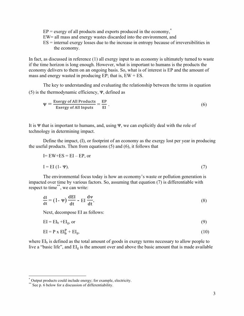
EP = exergy of all products and exports produced in the economy,* EW= all mass and energy wastes discarded into the environment, and

ES = internal exergy losses due to the increase in entropy because of irreversibilities in the economy.

In fact, as discussed in reference (1) all exergy input to an economy is ultimately turned to waste if the time horizon is long enough. However, what is important to humans is the products the economy delivers to them on an ongoing basis. So, what is of interest is EP and the amount of mass and energy wasted in producing EP; that is, EW + ES.

The key to understanding and evaluating the relationship between the terms in equation (5) is the thermodynamic efficiency, ᴪ, defined as

ᴪ = !"#$%&  !"  !""  !"#$%&'(!"#$%&  !"  !""  !"#$%&

= !"!"

. (6)

It is ᴪ that is important to humans, and, using ᴪ, we can explicitly deal with the role of technology in determining impact.

Define the impact, (I), or footprint of an economy as the exergy lost per year in producing the useful products. Then from equations (5) and (6), it follows that

I= EW+ES = EI – EP, or

I = EI (1- ᴪ). (7) The environmental focus today is how an economy’s waste or pollution generation is impacted over time by various factors. So, assuming that equation (7) is differentiable with respect to time**, we can write:

!"!"

= (1- ᴪ)  !"#!"

- EI !ᴪ!"

. (8)

Next, decompose EI as follows:

EI = EIb +EIg, or (9)

EI = P x EI!! + EIg, (10)

where EIb is defined as the total amount of goods in exergy terms necessary to allow people to live a “basic life”, and EIg is the amount over and above the basic amount that is made available

* Output products could include energy; for example, electricity. ** See p. 6 below for a discussion of differentiability.

4

by the economy*. EI!! is this basic amount of exergy per person. EIg could be defined as affluence or “greed”. P is the population of the economy.

Ecologists and ethicists can argue over the amount of, say, calories or goods any person needs to live a basic life, but since EI!! is basic and given in exergy terms (matter and energy) it can be called a constant in time and space. The consequence is that some countries will have a negative value for EIg ; their population lives on average below some agreed upon “basic” or sustainable level. There is on average no greed in such countries.

Since EI!! is a constant, it is possible to rewrite equation (10) as:

!"#!"

= EI!! !"!"

+ !"#$!"

. (11)

Combining equations (8) and (11) yields:

!"!"

= (1- ᴪ)EI!! !"!"

+ (1- ᴪ) !"#$!"

– EI !ᴪ!"

. (12)

Population Affluence Technology

Thus, in terms of the rate of change of impact, equation (12) provides a relationship that can be interpreted as a sum of terms proportional to the rate of change in population, affluence and technology if the rate of change in population, affluence and technology are characterized as indicated in equation (12).

There is a temptation to literally relate equation (12) to equation (1) by taking the time derivative of equation (1) and equating like terms. This makes no sense because equation (1) is not a true equation since there is no consistent and defensible definition of affluence (A) and technology (T). It is, in use, a tautology.

Equation (12), having been derived from a balance equation based on the Second Law, gives an explicit rate of change expression for impact based on population changes, changes in “greed”, thermodynamic efficiency and its rate of change, and computed exergy.

It is important to note that the thermodynamic efficiency, ψ, has an impact on all three factors in equation (12). Improving ψ decreases the effect of all three terms: by shrinking (1 – ψ) in the population and affluence (greed) terms and by making the third term larger (a greater negative effect on impact) assuming EI unchanged. Also, note that the technology term depends on the flux of exergy, EI, as well as the rate of change of thermodynamics efficiency, ψ.

* Basic life is defined as that which allows the average person to survive and propagate generation after generation using minimum resources. This is an arbitrary definition used by some ecologists in describing sustainable environments.

5

Ayers and Warr

After many years of work, Ayers and Warr have managed to fit the GDP data for the US and Japan with excellent agreement by adding “useful work” to labor and capital as factors of economic production. In their important book, The Economic Growth Engine, the authors define useful work as the exergy input to the economy times the thermodynamic efficiency of the economy, both terms being independently determined. In the terminology of this paper, useful work is just equal to:

EP = EI x ψ , and (13)

!"#!"

= ψ !"#!"

+ EI !!!"

. (14)

Then, utilize equation (11) to get:

!"#!"

= ψ EI!!dPdt + ψ !"#$

!" + EI !!

!" . (15)

These equations (14) and (15) describe the rate of change of a function (EP) related to GDP in exergy units. It is just the useful exergy output of the economy.

The ratio !"#!"

is a concave (U-shape) function of time over the 20th century with a minimum of about $.32 million per exajoule in the early 1970s in the USA (1)(2). However, between about 1920 and 2005, this ratio never exceeds $.5 million per exajoule. Thus, GDP is a strong function of EP over this timeframe. Additionally, a logical argument can be made that EP is as good an indicator of economic wealth as GDP. For example, Ayers and Warr (w) state:

Economic growth depends on producing continuously greater quantities of useful work.

I will use EP or GDP as a measure of economic wealth in the remainder of this paper.

In order to calculate useful work, EP, over time, time series data for P, EI, and ψ are required, and these are provided by Ayers and Warr. Our results for the calculation of EP using equation (15) are in excellent agreement with the results of Ayers and Warr for useful work and GDP (equal to EP multiplied by a time dependent function with units of dollars per joule). This lends credence to our usage of the same data for calculating impact, I, using equation (12).

Notice that the technology term EI!!!"

appears in both equation (15) and equation (12) but with a sign change. For positive changes in this term, EP and GDP are improved and the environmental impact of waste is reduced. As I discuss in reference (1), Ayers and Warr emphasize the importance of both EI and !!

!" in determining economic growth. Although not as

large, the importance of increasing EI!!!"

in reducing the growth of waste and pollution are

6

shown below. The sign change of EI !!!"

in equations (15) and (12) may have important policy ramifications.

Population Effect

It is fair to say that population, P, has attracted at least as much attention as the other factors in the debate and analysis of global pollution. See, for example, Paul R Eurlich’s book, The Population Bomb (8). It turns out that population changes can, indeed, be the most important driver for changes in pollution production. But this is not always true as seen below. Human nature and population are related in direct and in subtle ways that can be explored by decomposing !"

!" into constituent parts.

Consider the population, P, and its rate of change over time. This can be written as:

!"!"  = B− D+ IM− EM, (16)

where

B = birth rate, D = death rate, IM = immigration rate, and EM = emigration rate. Combining equations (12) and (16) yields:

( ) [ ] ( ) gPb

dEIdI d1- EI B-D+IM-EM 1- EIdt dt dt

Ψ= Ψ + Ψ − . (17)

Therefore, the rate of change of impact on an economy with a population P is dependent upon ψ, !!!"

, B, D, IM, EM, !!"!!"

, and EI. The first two terms, ψ and !!!"

, are the result of the Second Law, and the last six terms can be said to be the result of certain characteristics of human nature. Each of these terms are discussed in detail in reference (1).

Calculations

The question of differentiability is rendered mute because the preceding differentials are only used as differences in quantities between time t1 and time t2 or ∆t=t2 – t1. That is, in order to calculate the variables over the time horizon of the available data, difference equations are used; the variables are not integrated.

It is easy to prove that for equation (12), for example, the following is exact:

7

∆I = I2 – I1 = (1− ᴪ)   EI!! ∆P +(1− ᴪ)   ∆EIg - EI∆ᴪ , (18)

where Z is the average of Z over ∆t = t2 –t1 . Thus, equation (18) and analogous ones for equations (15) and (12) along with the data from reference (2) can be used to calculate the results presented below over the time horizon 1901 to 2005 if EI!! is chosen. Arbitrarily,  EI!! is set equal to the exergy input per person to the USA economy in 1900 which is equal to 0.2 exajoules per person, and ∆t = one year to conform with the time-series data.

Results of Calculations

Waste (Impact) and GDP

Figure D-1 contains the results of numerical calculations of equations 12 and 15 using difference equations like equation 18 and the time series data from Ayers and Warr. The total exergy waste or impact I produced in the USA from 1901 to 2005 is shown as the sum of a pure population effect and an affluence (or “greed”) effect offset by a technology factor [In Figure D-1, this technology term is shown as positive for ease of presentation]. Additionally, the input exergy EI and the output exergy EP are shown to emphasize their relationship with total waste (EI-EP). All major thermodynamics properties (IE, EP, and waste) along with greed show the major impacts of macro-economic and political events of the 20th century.

The early growth in waste in the twentieth century is dramatically stopped by the great depression of 1929. This, in turn, is followed by rapid growth initiated by WWII. This growth continues and accelerates beginning in about 1960, only to be interrupted by the oil shocks of 1973-74 and 1979. Growth returns in the early 1980s, achieving growth rates like those experienced just after WWII. However, there appears to be a slackening of the growth rates of waste, EP and greed, as the US economy approaches and enters the 21st century.

Referring to Figure D-1 and Equation 12, it is clear that pure population growth dominates the growth in waste until the 1960s. The pure consumption or affluence effect rises dramatically, equaling and exceeding the population effect after about 1968. Whereas the population effect rises smoothly, the affluence term is what contributes the macro-economic and political variations to waste generation. After about 1968, affluence is the major contributor to waste although population growth continues to be a very large contributor. Over the 20th century, the importance of the technology term is modest, but growing, due to constantly improving thermodynamic efficiency (as discussed below) and the rapidly growing input exergy, EI. The thermodynamic efficiency offsets and restrains the growth in population and affluence. By 2005, the three terms: population, affluence, and technology contribute approximately 47%, 58% and minus 5%, respectively, to waste generation.

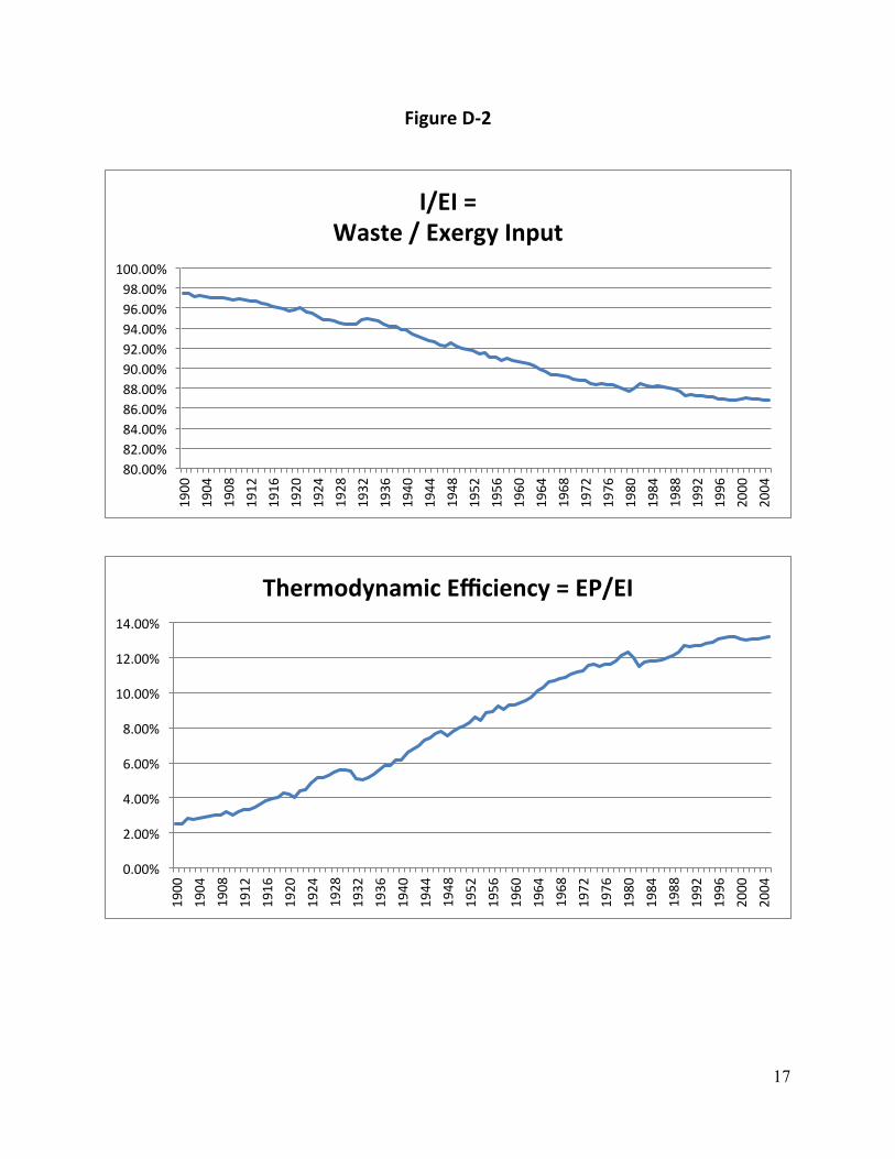
The next important trend in the data shown in Figure D-1 is the growing separation of the curves for EI, the input exergy, and waste (EI-EP). Figure D-2 explains this divergence as waste as a fraction of EI decreases monotonically over the time period. This effect is a direct result of the monotonically increasing thermodynamic efficiency,  Ψ =   !"

!". Said another way, over the

time-frame analyzed, more and more input exergy was converted to useful products, EP, as the US economy became more and more thermodynamically efficient. However, the growth rate in

8

this efficiency begins to decrease in about 1990 and appears to be approaching zero growth by the year 2000. This is a key observation.

A leveling off of thermodynamic efficiency impacts waste (EI-EP), EP as well as the population, greed and technology terms in Figure D-1. EI is not immediately impacted by a slowing in the growth of efficiency.* If !!

!" à 0, then the technology term in the equations for

 !"!"

and !"#!"

both go to zero. However, in the case of !"!"

the technology term is negative and small,

and in the case of !"#!"

the technology term is large and positive (compare Figures D-1 and D-3).

Thus, a decrease in !!!"

should and does effect EP more than waste, I. Furthermore, Ψ effects the

other two terms in the expressions for !"!"  and !"#

!".

In the expressions for the rate of change of waste and EP, Ψ impacts both the pure population term and the so-called greed term. In the case of waste, these two terms are multiplied by (1- Ψ); in the case of EP they are multiplied by Ψ. Over the time horizon presented, (1- Ψ) decreases about 11%, and Ψ increases more than 400%. Whereas the effect is modest in the case of waste, EP is greatly modified by slowing thermodynamics efficiency because of its impact on population and greed changes.

Because EP is directly related to GDP in exergy units, it can be concluded that thermodynamic efficiency is crucial to the growth in wealth as measured by GDP. Its changes are modest on the changes of waste. In fact, Ayers and Warr state:

Over the past two centuries, successive improvements in the efficiency of the various exergy-to-work conversion stages have apparently accounted for most of the economic growth our Western civilization has enjoyed.

If thermodynamic efficiency changes dominate economic growth, is it possible to make an analogous statement about the rate of change in impact or waste?

Consider equation 12 and Figure D-1. Here, the first term is dominated by pure population growth, !"

!", and the second term is dominated by greed changes, !"#$

!". This is because

(1-Ψ) changes so little. In the case of waste, the technology term is negative, small and dominated by EI since !!

!" is approximately a constant. Because the greed change is just the

change in input exergy over and above the exergy consumed in 1900, it is fair to say that waste is dominated by population growth, !"

!" , and the growth in input exergy, !"#$

!", since (1-Ψ) is large

and relatively unchanging.

* However, longer term, there could be an impact on EI due to slower growth in thermodynamic efficiency as discussed below. For example, to maintain growth of EP when !!

!"→ 0, EI must increase more rapidly.

9

The conclusions from this analysis are important because they indicate that Ψ and !!!"

have been crucial to GDP growth while EI and population growth, !"!"

, have been most important to the growth of waste. Waste is not the other side of the GDP growth coin at least for the 20th century. This difference in the past determinants of the growth in GDP verses the growth in waste could result in some important policy conclusions.

One of the major problems that global warming proponents face is how to curtail the growth of waste and pollutants when billions of people in the underdeveloped world are demanding living standards like those enjoyed in the developed world. This is often posed as an impossible conflict in goals. Perhaps the difference in the drivers of GDP versus waste can relieve some of this tension.

Pollution and GDP

Before developing the implications that EP (GDP) and waste (EI-EP) = Impact (I) have been dependent on different factors, pollution needs to enter the discussion. As developed in great detail in reference (1), not all waste is pollution. Furthermore, the definition of pollution is often subjective and subject to change depending on economics and cultural differences. Currently, the amount of CO2 in the atmosphere is considered the most important pollutant.

Separating out CO2 in exergy units from total waste is not an easy calculation. The exergy of CO2 generation in the US economy varies with time, location, the type and mix of conversions and the volume and exergetics of the conversion process in question. For example, fossil fuel-fired power plants are the largest producers of CO2 in the US today (9 ). However, the character of CO2 generated in the production of electricity from fossil fuels has changed greatly over the past century as engineers have driven up the boiler temperatures and regulations have begun to impact the relative concentration of CO2 in stack gases (10). The chemical exergy of CO2 is known and a constant, but CO2 in stacked gases possesses kinetic energy, too, and this has varied over time.

More to the point, in the case of CO2 and CO2 equivalents, it is not the exergy of the molecules that make CO2 a pollutant. CO2 is called a pollutant because of the man-made Greenhouse Effect. Some of the reradiated solar radiation and radiative heat transfer from external exergy losses of the global economy are trapped by the atmosphere, mainly by the H2O and CO2 equivalents. This thermal and electromagnetic energy, mainly in the infrared, keeps the earth at a comfortable +15º C as Reiner Kümmel explains (7). A small change in the earth’s atmospheric CO2 causes a small change in the earth’s average temperature. But, this small temperature change exponentially increases the partial pressure of atmosphere H2O, and the infrared absorption of water vapor increases with the square of the water vapor pressure. Reiner Kümmel concludes:

As a net result, the anthropogenic greenhouse effect caused by additional CO2 emissions increases with the logarithm of CO2 concentration, so, for every doubling of the atmospheric CO2 content, the temperature of Earth’s surface increases by the same amount (of approximately 2.5º C).

10

Therefore, in the case of CO2, what is important is the amount of CO2 and CO2 equivalents produced by the US economy.

According to the US Energy Information Agency (EIA), fossil fuels supplied 82% of the input energy to the US economy in 2011 and were responsible for 99% of the CO2 emissions. The CO2 breakdown by energy source was 43% petroleum, 31% coal, and 24% natural gas (9). The Carbon Dioxide Information Analysis Center (CDIAC) provides a breakdown of carbon emissions by these energy sources going back to 1800 (10). The total carbon emissions in the US from the burning of fossil fuels back to 1900 is taken from this source and plotted in Figure D-4. The data are given in metric tons of carbon and can be converted to metric tons of CO2 by multiplying by 3.667.

The history of carbon (and CO2) generated in Figure D-4 is reminiscent of the plots of the thermodynamic variables shown in Figure D-1, D-2 and D-3. So, as expected, the generation of CO2 reflects the eco-political events in its fine-structure changes (years) during the 20th century. However, the slope of the curve of CO2, or the rate of change, during the overall time frame is relatively modest and constant at about 140,000 metric tons of carbon per year. This conclusion about the constancy of CO2 generation rate by the US economy is the result of a confluence of trends over the 20th century including improving thermodynamic efficiency and the growth in, and changing mix of, the input fuels during the period. From the viewpoint of the trade-off between wealth and CO2 pollution, the reasoning is much easier to elucidate.

Over the time-fame considered here, 1901 to about 2005, CO2 production has increased only some 8- fold, but GDP and EP have increased some 35-fold. If EP can be taken as an indicator of wealth, then the economy has improved its performance dramatically on the basis of the amount of CO2 pollution created for an exajoule of greater wealth. This is shown clearly in Figure D-4 where the second graph is a plot of carbon in metric tons divided by EP in exajoules.

As discussed earlier, the rapid growth of EP over the 20th century is primarily due to the almost constant, rapid growth of thermodynamic efficiency (see Figure D-2 and D-3). This is not true for the relationship of CO2 production relative to the growth in waste (EI-EP) and the growth in input exergy (EI) as shown in Figure D-5.

During the timeframe considered here, waste has grown some 5+ fold and EI some 6+ fold, both more in line with the growth in CO2 for the period. Thus, looking at the year 2000 versus the year 1901, there has been only a modest change in the ratio of carbon to waste and carbon to EI. However, since mid-20th century, both ratios seem to have improved somewhat. So, for example, in the case of waste, the ratios of CO2 to total waste have gone from something like 55,000 metric tons of CO2 per exajoule of waste to about 50,000 tons per exajoule*.

Perhaps given the complexity of the measurement of the raw data used to arrive at carbon emissions in metric tons and exergy input and output numbers for the US economy for over 100 years, it might be prudent to say that the mass of carbon produced in the US economy for an exajoule of input exergy and for an exajoule of the total waste output have remained relatively constant from 1900 to about 2005. On the contrary, the mass of carbon produced in the US economy over the same period for an exajoule of GDP has decreased continually from a value of

* These numbers are taken from Figure D-5 by multiplying by 3.667 to convert from carbon to CO2.

11

about 1,650,000 metric tons of CO2 per exajoule of GDP in 1900. However, this reduction has been slowing down, apparently approaching an asymptote of something like 300,000 tons per exajoule as the 21st century was entered (see Figure D-4).

GDP Versus CO2 We are now in a position to discuss the issue of the possible trade-off between GDP and

lowered CO2 generation. How could GDP and CO2 be decoupled? If the goal is continued increases in EP (a surrogate for GDP) while decreasing CO2, then the first thing that comes to mind is decreasing overall waste while increasing EP. The key is the thermodynamic efficiency, Ψ ; all things being equal, increasing or accelerating the growth in Ψ greatly impacts EP positively, while modestly decreasing overall waste. Decreasing overall waste will decrease CO2, one of its components. However, this will not be an easy task. As discussed in references (1) and (2), heat engines in power generation and transportation account for the great majority of useful work in the US economy. Ayers and Warr state:

Electric power and mobile power (from internal combustion engines mostly for transportation or construction) are the two most important types of useful work.

Furthermore, these authors explain that the thermodynamic efficiencies of these two conversions in heat engines have peaked in about 1970 at 33% (electric power) and approximately 8% (mobil power). This peaking of efficiency is mainly due to Second Law constraints on heat engines. In fact Ayers and Warr state that:

Conventional energy conversion technologies are already so high that future improvements are almost certain to be marginal.

Thus, according to this analysis, just maintaining or moderately growing EP may be in jeopardy as the authors of reference (2) point out. Assuming the growth in Ψ can only be maintained but not accelerated (preserving growth in EP), we must look elsewhere for methods for reducing CO2. Today, heat engines dominate our economy, and they are powered by fossil fuels. However, there are large differences in CO2 generation for the various fuels: coal, petroleum and natural gas. For example, in electric power generation, coal produces 74% of the CO2 of the industry as opposed to natural gas’s 24%. However, coal is only responsible for 41% of the electricity produced while gas produces 24% of the electricity. Overall, for each unit of electricity produced, natural gas generates about 50% and petroleum about 75% of the CO2 generated by coal (9). Thus, if we cannot rely on the thermodynamic efficiency, the only answer, under this scenario, is to change the mix of fossil fuels*. Basically, if overall waste cannot be decreased, then CO2 can only be reduced with today’s technology by moving away from coal and toward petroleum and natural gas as the input fuels.

* This scenario excludes the possibility of substituting nuclear power and renewables for fossil fuels in generating the useful work that propels our economic growth. It is assumed that nuclear power cannot grow for political reasons. And, renewables will take decades to materially replace fossil fuels (see below).

12

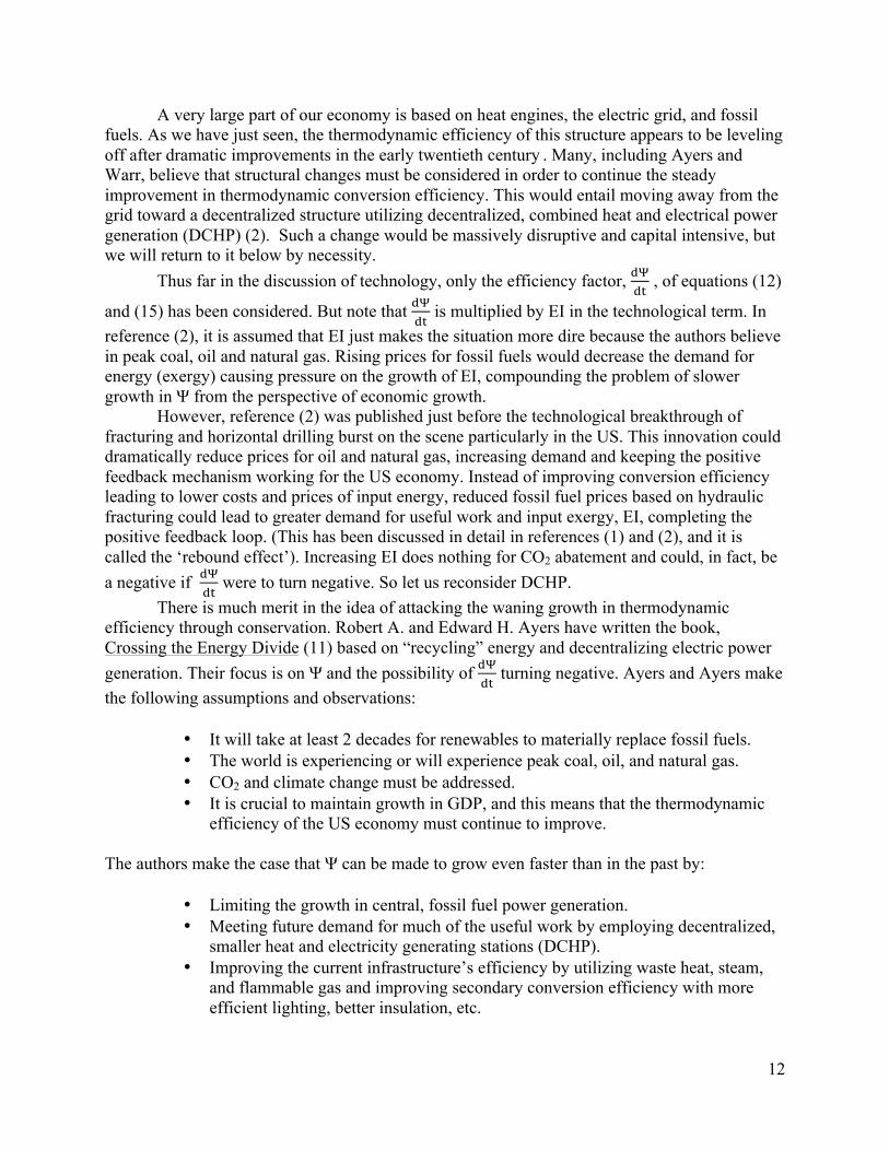
A very large part of our economy is based on heat engines, the electric grid, and fossil fuels. As we have just seen, the thermodynamic efficiency of this structure appears to be leveling off after dramatic improvements in the early twentieth century . Many, including Ayers and Warr, believe that structural changes must be considered in order to continue the steady improvement in thermodynamic conversion efficiency. This would entail moving away from the grid toward a decentralized structure utilizing decentralized, combined heat and electrical power generation (DCHP) (2). Such a change would be massively disruptive and capital intensive, but we will return to it below by necessity. Thus far in the discussion of technology, only the efficiency factor, !!

!" , of equations (12)

and (15) has been considered. But note that !!!"

is multiplied by EI in the technological term. In reference (2), it is assumed that EI just makes the situation more dire because the authors believe in peak coal, oil and natural gas. Rising prices for fossil fuels would decrease the demand for energy (exergy) causing pressure on the growth of EI, compounding the problem of slower growth in Ψ from the perspective of economic growth. However, reference (2) was published just before the technological breakthrough of fracturing and horizontal drilling burst on the scene particularly in the US. This innovation could dramatically reduce prices for oil and natural gas, increasing demand and keeping the positive feedback mechanism working for the US economy. Instead of improving conversion efficiency leading to lower costs and prices of input energy, reduced fossil fuel prices based on hydraulic fracturing could lead to greater demand for useful work and input exergy, EI, completing the positive feedback loop. (This has been discussed in detail in references (1) and (2), and it is called the ‘rebound effect’). Increasing EI does nothing for CO2 abatement and could, in fact, be a negative if !!

!" were to turn negative. So let us reconsider DCHP.

There is much merit in the idea of attacking the waning growth in thermodynamic efficiency through conservation. Robert A. and Edward H. Ayers have written the book, Crossing the Energy Divide (11) based on “recycling” energy and decentralizing electric power generation. Their focus is on Ψ and the possibility of !!

!" turning negative. Ayers and Ayers make

the following assumptions and observations:

• It will take at least 2 decades for renewables to materially replace fossil fuels. • The world is experiencing or will experience peak coal, oil, and natural gas. • CO2 and climate change must be addressed. • It is crucial to maintain growth in GDP, and this means that the thermodynamic

efficiency of the US economy must continue to improve.

The authors make the case that Ψ can be made to grow even faster than in the past by:

• Limiting the growth in central, fossil fuel power generation. • Meeting future demand for much of the useful work by employing decentralized,

smaller heat and electricity generating stations (DCHP). • Improving the current infrastructure’s efficiency by utilizing waste heat, steam,

and flammable gas and improving secondary conversion efficiency with more efficient lighting, better insulation, etc.

13

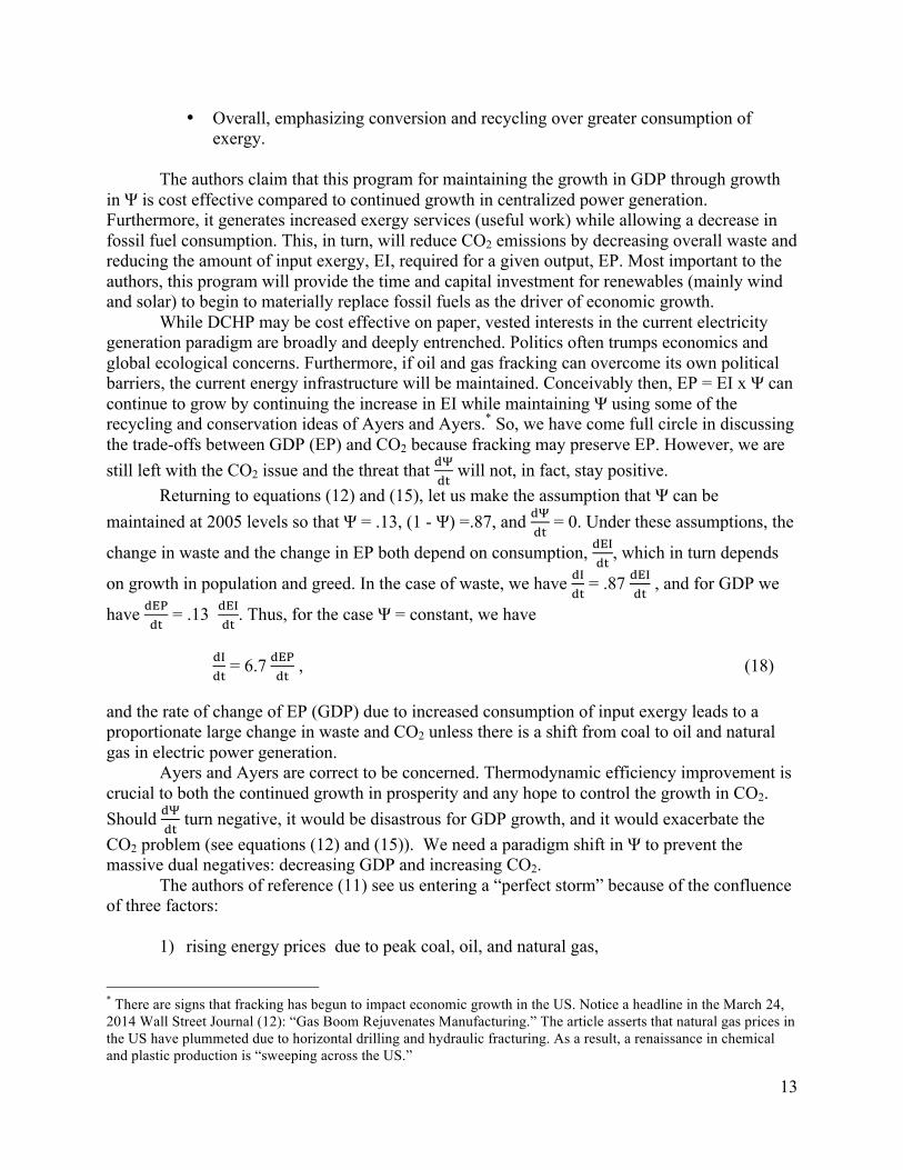
• Overall, emphasizing conversion and recycling over greater consumption of exergy.

The authors claim that this program for maintaining the growth in GDP through growth

in Ψ is cost effective compared to continued growth in centralized power generation. Furthermore, it generates increased exergy services (useful work) while allowing a decrease in fossil fuel consumption. This, in turn, will reduce CO2 emissions by decreasing overall waste and reducing the amount of input exergy, EI, required for a given output, EP. Most important to the authors, this program will provide the time and capital investment for renewables (mainly wind and solar) to begin to materially replace fossil fuels as the driver of economic growth. While DCHP may be cost effective on paper, vested interests in the current electricity generation paradigm are broadly and deeply entrenched. Politics often trumps economics and global ecological concerns. Furthermore, if oil and gas fracking can overcome its own political barriers, the current energy infrastructure will be maintained. Conceivably then, EP = EI x Ψ can continue to grow by continuing the increase in EI while maintaining Ψ using some of the recycling and conservation ideas of Ayers and Ayers.* So, we have come full circle in discussing the trade-offs between GDP (EP) and CO2 because fracking may preserve EP. However, we are still left with the CO2 issue and the threat that !!

!" will not, in fact, stay positive.

Returning to equations (12) and (15), let us make the assumption that Ψ can be maintained at 2005 levels so that Ψ = .13, (1 - Ψ) =.87, and !!

!" = 0. Under these assumptions, the

change in waste and the change in EP both depend on consumption, !"#!"

, which in turn depends

on growth in population and greed. In the case of waste, we have !"!"

= .87 !"#!"

, and for GDP we

have !"#!"

= .13 !"#!"

. Thus, for the case Ψ = constant, we have !"

!" = 6.7  !"#

!" , (18)

and the rate of change of EP (GDP) due to increased consumption of input exergy leads to a proportionate large change in waste and CO2 unless there is a shift from coal to oil and natural gas in electric power generation. Ayers and Ayers are correct to be concerned. Thermodynamic efficiency improvement is crucial to both the continued growth in prosperity and any hope to control the growth in CO2. Should !!

!" turn negative, it would be disastrous for GDP growth, and it would exacerbate the

CO2 problem (see equations (12) and (15)). We need a paradigm shift in Ψ to prevent the massive dual negatives: decreasing GDP and increasing CO2. The authors of reference (11) see us entering a “perfect storm” because of the confluence of three factors:

1) rising energy prices due to peak coal, oil, and natural gas,

* There are signs that fracking has begun to impact economic growth in the US. Notice a headline in the March 24, 2014 Wall Street Journal (12): “Gas Boom Rejuvenates Manufacturing.” The article asserts that natural gas prices in the US have plummeted due to horizontal drilling and hydraulic fracturing. As a result, a renaissance in chemical and plastic production is “sweeping across the US.”

14

2) the inability to increase thermodynamic efficiency of current technologies (heat engines) in the production of useful work, and

3) climate catastrophes due to CO2 production.

Factors 1) and 3) of the perfect storm of Ayers and Ayers are not needed. Their factor 2) is all that is needed to create chaos in the United States and the world. Factors 1) and 3) would just make things worse.

September 3, 2014

15

REFERENCES

(1) Buckner, John K., The Ultimate Causes of Pollution, under construction.

(2) Ayers, Robert U. and Benjamin Warr, The Economic Growth Engine, Edward Elgar Publishing, Inc., Northhampton, MA, 2009.

(3) Ehrlich, Paul R. and John P. Holdren, “Impact of Population Growth”, Science, 141:1212-17(1971).

(4) E.O. Wilson, Consilience, Alford A. Knopf, New York, 1998. (5) Gilding, Paul, The Great Disruption, Bloomsbury Press, New York, 2011. (6) Dincer, Ibrahim and Marc A. Roson, Exergy, Elsevier, Ltd., 2007. (7) Kümmel, Reiner, The Second Law of Economics, Springer, New York, 2011. (8) Ehrlich, Paul R., The Population Bomb, Buccaneer Books, 1968.

(9) U.S. Energy Information Agency, “Where Greenhouse Gases Come From –

Energy Explained, Your Guide to Understanding Energy”, August 2, 2013.

(10) Carbon Dioxide Information Analysis Center, Carbon Emissions Time Series Data, United States of America, 1800-2010.

(11) Ayers, Robert U. and Edward H. Ayers, Crossing the Energy Divide, Pearsons

Education Inc., publishing as Wharton School Publishing, Upper Saddle River, New Jersey, 2010.

(12) The Wall Street Journal, page B2, March 24, 2014.

16

 -­‐        

 20.000    

 40.000    

 60.000    

 80.000    

 100.000    

 120.000    

 140.000    

 160.000    1901  

1907  

1913  

1919  

1925  

1931  

1937  

1943  

1949  

1955  

1961  

1967  

1973  

1979  

1985  

1991  

1997  

2003  

Figure  D-­‐1  EI,  EP  and  Waste  and  its  Components  

Popula4on  Effect  (exjl's)  

Greed  Effect  (exjl's)  

Tech  Effect  (exjl's)  

Waste  (EI  -­‐  EP)  (exjl's)  

EI  =  Total  Exergy  Input  (exjl's)  

EP  =  Total  Exergy  Output  (exjl's)  

Nega4ve  Term  In  Waste  Calcula4on  

17

Figure  D-­‐2  

80.00%  82.00%  84.00%  86.00%  88.00%  90.00%  92.00%  94.00%  96.00%  98.00%  100.00%  

1900  

1904  

1908  

1912  

1916  

1920  

1924  

1928  

1932  

1936  

1940  

1944  

1948  

1952  

1956  

1960  

1964  

1968  

1972  

1976  

1980  

1984  

1988  

1992  

1996  

2000  

2004  

I/EI  =  Waste  /  Exergy  Input  

0.00%  

2.00%  

4.00%  

6.00%  

8.00%  

10.00%  

12.00%  

14.00%  

1900  

1904  

1908  

1912  

1916  

1920  

1924  

1928  

1932  

1936  

1940  

1944  

1948  

1952  

1956  

1960  

1964  

1968  

1972  

1976  

1980  

1984  

1988  

1992  

1996  

2000  

2004  

Thermodynamic  Efficiency  =  EP/EI  

18

Figure  D-­‐3  

 (2.000)  

 -­‐        

 2.000    

 4.000    

 6.000    

 8.000    

 10.000    

 12.000    

 14.000    

 16.000    

 18.000    

 20.000    

1900  

1905  

1910  

1915  

1920  

1925  

1930  

1935  

1940  

1945  

1950  

1955  

1960  

1965  

1970  

1975  

1980  

1985  

1990  

1995  

2000  

EP  and  its  Components  

Popula4on  Effect  (exjl's)  

Greed  Effect  (exjl's)  

Tech  Effect  (exjl's)  

EP    (Exjl's)  

19

Figure  D-­‐4  

Carbon  and  Carbon/EP  

 -­‐          200,000      400,000      600,000      800,000    

 1,000,000      1,200,000      1,400,000      1,600,000      1,800,000    

1900  

1904  

1908  

1912  

1916  

1920  

1924  

1928  

1932  

1936  

1940  

1944  

1948  

1952  

1956  

1960  

1964  

1968  

1972  

1976  

1980  

1984  

1988  

1992  

1996  

2000  

2004  

Carbon    (Metric  Tons)  

 -­‐          50,000      100,000      150,000      200,000      250,000      300,000      350,000      400,000      450,000      500,000    

1900  

1904  

1908  

1912  

1916  

1920  

1924  

1928  

1932  

1936  

1940  

1944  

1948  

1952  

1956  

1960  

1964  

1968  

1972  

1976  

1980  

1984  

1988  

1992  

1996  

2000  

2004  

Carbon/EP  (MT  per  exjl)  

20

Figure  D-­‐5  

Carbon/Waste  and  Carbon/EI  

 -­‐        

 2,000    

 4,000    

 6,000    

 8,000    

 10,000    

 12,000    

 14,000    

 16,000    

 18,000    

1900  

1906  

1912  

1918  

1924  

1930  

1936  

1942  

1948  

1954  

1960  

1966  

1972  

1978  

1984  

1990  

1996  

2002  

Carbon  /  Waste  (I)  (MT  per  exjl)  

Carbon  /  EI  (MT  per  exjl)