Sharpening the tomographic image of the subducting slab below Sumatra, the Andaman Islands and Burma

Geophys. J. Int. (2010) 182, 433–453 doi: 10.1111/j.1365-246X.2010.04630.x

GJI

Sei

smol

ogy

Sharpening the tomographic image of the subducting slab belowSumatra, the Andaman Islands and Burma

J. D. Pesicek,1 C. H. Thurber,1 S. Widiyantoro,2 H. Zhang,3 H. R. DeShon4

and E. R. Engdahl51Department of Geoscience, University of Wisconsin-Madison, 1215 W Dayton St., Madison, WI 53706, USA. E-mail: [email protected] of Mining and Petroleum Engineering, Bandung Institute of Technology, Jalan Cikapayan 15 , Bandung 40116, Indonesia3Department of Earth, Atmospheric, and Planetary Sciences, Massachusetts Institute of Technology, 77 Massachusetts Avenue,Cambridge, MA 02139-4307, USA4Center for Earthquake Research and Information, University of Memphis, Memphis, TN 38152, USA5Department of Physics, University of Colorado, Boulder, CO 80309-0390, USA

Accepted 2010 April 14. Received 2010 February 8; in original form 2009 September 21

S U M M A R YTaking advantage of the increased ray coverage due to seismicity following the 2004 Decemberand 2005 March great earthquakes, an improved iterative regional–global tomographic methodwas applied to the Sumatra–Andaman and adjacent regions to better constrain the 3-D mantlevelocity heterogeneity in the region. Velocity and hypocentral parameters were iterativelyperturbed to sharpen the image of the subducted slab. Several iterations were performed,and the effects of source mislocation were considered in the iterative process, an issue usuallyneglected in global tomography. We find that source relocation between iterations increases theamplitudes of slab anomalies and sharpens the definition of slab geometry beyond what can beachieved by a fixed-source iterative inversion alone. In addition, extensive restoration tests ofsynthetic data were conducted that emphasize enhancements obtained by our iterative process.These tests show significant increases in amplitude and decreased smearing of synthetic slabfeatures. Thus, when applied to the real data, similar enhancements are inferred in the resultingmodel, which better illustrates the complex slab geometry in the upper-mantle and transitionzone regions along the Sumatra, Andaman and Burma subduction zones.

Key words: Seismicity and tectonics; Seismic tomography; Subduction zone processes;Asia.

1 I N T RO D U C T I O N

The 2004–2005 Sumatra–Andaman great earthquake sequenceshave provided a wealth of new seismic data from the region. Thesedata have allowed us to obtain a detailed view of the complexstructure of the subducting slab below Sumatra and the adjacentregions (Pesicek et al. 2008). In this paper, we present a sharp-ened tomographic image of the slab obtained from an improvediterative technique employing full 3-D ray tracing, following thebasic approach of Widiyantoro et al. (2000). We have made severalimprovements to this methodology and have tested the solution ex-tensively through restoration tests on synthetic data. In addition, wehave included event relocation in the iterative procedure, an issueusually neglected in global tomography. In this paper, we discussour methodology improvements and their effects on our model forthe P-wave velocity structure of the western Indochina subductionzones along the Sumatra and Andaman Islands, and Burma. In addi-tion to an overall increase in slab amplitudes, our iterative solutionshows higher amplitude fast anomalies in many areas that previ-ously showed little or no velocity perturbation. Below Burma, our

new higher resolution iterative model reveals that the subductingslab there, which had previously been interpreted as torn, may infact be continuous.

2 DATA

The data used in this study are traveltimes and earthquake lo-cations reprocessed from global catalogues by the Engdahl, vander Hilst and Buland (EHB) method of single event relocation(Engdahl et al. 1998). The EHB catalogue of data is commonly usedin global tomography studies and is regarded as the most accurateglobal earthquake catalogue available. In the Sumatra region, thesedata have been further groomed to provide more accurate depths(Engdahl et al. 2007). For those data for which waveforms are pub-licly available, more precise arrival times have been determined bycross-correlation techniques (DeShon et al. 2007a; Pesicek et al.2010).

We used global EHB data from 1964–2006 and regional Indone-sian EHB data from 1964–2007 (Fig. 1). We have also included

C! 2010 The Authors 433Journal compilation C! 2010 RAS

Geophysical Journal International

434 J. D. Pesicek et al.

Figure 1. Data and regional tectonic setting. EHB bounce points (pP, pwP;blue), earthquake locations for events occurring before 2004 December 24(red) and after (green) through 2006 are plotted sequentially in that order.New data not used by Pesicek et al. (2008) are also shown: EHB eventlocations for 2007 (yellow) and for the Toba Caldera local network (pink).Cross-section locations (A–D) for all subsequent figures, plate boundaries,bathymetric features [Wharton Fossil Ridge (WFR) and Investigator FractureZone (IFZ)] and convergence rates are also shown.

data from a PASSCAL deployment in 1995 around Toba Caldera(Fauzi et al. 1996; Masturyono et al. 2001) to increase upper-mantlesampling in this region. The combined available data set is largerthan that used by Pesicek et al. (2008); however in this study weapplied more stringent selection criteria. Specifically, we requireda secondary azimuthal gap <180" and we only used events withsufficient depth control (e.g. located using later arriving phases inaddition to first arrivals). This has resulted in fewer data but ofhigher quality being used in the inversion. The combined data setconsists of 957 262 compressional phases from events within theIndonesia region, including 10 640 pP and 4239 pwP phases.

3 M E T H O D O L O G Y

Following Widiyantoro and van der Hilst (1997) and Widiyantoroet al. (2000), we use a nested regional–global model design and setup the following system of tomographic equations:!

"#Ai

!i Ii

"i Gi

$

%& xi =

!

"##ti

#!i#1 Ii#1xi#1

0

$

%& , (1)

where for the ith iteration, xi is the solution vector, Ai is the sen-sitivity matrix comprised of ray segment lengths in each modelcell (regional and global) and event relocation derivatives and #ti

is the data vector of traveltime residuals. Norm damping is appliedthrough the identity matrix I (weighted by !) and biased towards themodel used for ray tracing (xi#1). Gradient smoothing (Gi) is alsoapplied and weighted by " . For i > 1, we modified (1) slightly todownweight the importance of large residual outliers using a tech-nique known as iteratively reweighted least squares (IRLS), whichapproximates the 1-norm solution (Scales et al. 1988; Aster et al.2005). We further modified (1) by adding a term that independentlydamps the crustal layer. The system of equations then becomes!

"""#

Wi Ai

!i Ii

"i Gi

$i I ci Ac

i

$

%%%&xi =

!

"""#

Wi#ti

#!i#1 Ii#1xi#1

0#$i#1 I c

i#1xci#1

$

%%%&, (2)

where Wi is a diagonal matrix with elements

W ki =

'

1 +(

#t ki#1

5

)2*#1

for i > 1, (3)

$ is the crustal damping coefficient and the superscript c denotesthe crustal portion (0–35 km depth; Table 1) of the regional model.After choosing appropriate values for !, " and $ (discussed indetail in the following sections), we used the conjugate gradientleast-squares algorithm LSQR (Paige & Saunders 1982) to solve(2) jointly for perturbations to the slowness of each model cell andto the hypocentral parameters.

Table 1. Regional cell layer division (Widiyantoro & van der Hilst 1997)and average layer velocity from ak135 (Kennett et al. 1995).

Layer Depth Layer mid-point Average Vprange (km) depth (km) (km s#1)

1 0–35 17.5 6.31a

2 35–70 52.5 8.043 70–110 90 8.054 110–160 135 8.105 160–220 190 8.256 220–280 250 8.457 280–340 310 8.678 340–410 375 8.919 410–490 450 9.5010 490–570 530 9.7611 570–660 615 10.0612 660–750 705 10.9113 750–840 795 11.1114 840–930 885 11.2715 930–1020 975 11.4216 1020–1130 1075 11.5817 1130–1250 1190 11.7518 1250–1400 1325 11.9519 1400–1600 1500 12.19

aAdjusted by crustal model (CRUST 2.0; Bassin et al. 2000).

C! 2010 The Authors, GJI, 182, 433–453Journal compilation C! 2010 RAS

Sumatra, Andaman Islands and Burma topography 435

Previous studies have damped the relocation perturbations heav-ily (e.g. Widiyantoro & van der Hilst 1997; Widiyantoro et al. 2000)or removed them from the inversion completely (Weidle et al. 2005),fixing the event locations for each iteration. The arguments for ne-glecting or removing them are based on an analysis by Bijwaard& Spakman (2000) who found the relocation terms to be of lit-tle value for global tomography conducted with composite rays,event clusters and large cell sizes. However, it has been demon-strated for local earthquake tomography (LET) that solving jointlyfor hypocentre and velocity perturbations is necessary to assureconvergence (Thurber 1992; Thurber & Ritsema 2007). The cou-pled nature of the hypocentre-velocity structure problem argues forjoint determination of these parameters. Furthermore, for our finelygridded regional model, the use of event clusters and composite raysis an unnecessary restriction that may limit resolution. Tracing raysfor each event allows for a more straightforward implementation ofthe relocation problem and a more detailed investigation of the ef-fects of source mislocation on velocity determination. Accordingly,we included relocation perturbations in (2) for each event in thestudy region and have given them equal weight relative to the slow-ness perturbations. However, rather than applying them directly, weprefer to iteratively relocate events between tomography iterations,using a more precise double-difference (DD) technique (discussedin the following section) (DeShon et al. 2007b; Pesicek et al. 2010).This approach is quite common in LET (e.g. Thurber 1983).

3.1 Ray tracing

We employed the pseudo-bending 3-D ray tracing method of Um& Thurber (1987) extended to spherical coordinates by Koketsu& Sekine (1998). Outside the region of interest, we traced raysthrough the global P-wave model MITP08 (Li et al. 2008a), whichwe interpolated to fit our coarser global parametrization (5" $ 5"). Inthe Indonesia region, we initially traced rays from stations to sourcesthrough the global spherically symmetric model ak135 (Kennettet al. 1995). However, we replaced the shallowest layer with velocityvalues from the global crustal model CRUST 2.0 (Bassin et al.2000), converted to perturbations relative to ak135 and interpolatedto fit our parametrization (0.5" $ 0.5"; Table 1). Within the regionalmodel, pP and pwP (corrected for water traveltime) are traced toinitial bounce points provided in the EHB catalogue, and the bouncepoints are iteratively perturbed until the angle between the upgoingand downgoing ray segments are equivalent (Zhao & Lei 2004).Rays to bounce points and stations are traced to their true surfaceelevations in the newly modified crustal layer.

3.2 Regularization

Our system of eqs (2) includes three explicit and two implicit regu-larization coefficients (RCs). Minimum norm damping (!) and gra-dient smoothing (" ) operators were applied independently to boththe regional and global models, and an additional damping term ($)was added to penalize changes to the a priori crustal model. Wehave tested these values extensively, first to determine the range ofacceptable values and then to choose a preferred value. However,the choice of RCs remains subjective. Thus, we only interpret large-scale features of the regional model that are evident regardless ofthe choice of RCs (within the acceptable range). In the followingsections we discuss in detail how each of these RCs was chosen.

3.2.1 Global correction

Although the nested regional–global tomographic method we em-ployed allowed us to solve for a coarse global P-wave velocitymodel in addition to finer regional structure in the Indonesia region,global velocity structure was not the focus of our study. Thus, wehave applied twice as much damping and smoothing to the globalsolution as to the regional solution in our inversion. This has theeffect of forcing most of the perturbations to come from the regionalmodel. In this regard, it is similar to a crustal correction (discussedlater) or to heavily damping the relocation perturbations (‘locationcorrection’) (e.g. Widiyantoro et al. 2000), both strategies that havebeen previously applied in global tomography studies. The strategyassumes that the a priori global model is better than what we candetermine ourselves. However, as with the crustal correction andthe location correction, the ‘global correction’ is applied at the riskof forcing errors from the global data into the regional model. Wethink this risk is minimal because the MITP08 model was producedfrom a similar data set, but with an adaptive parametrization that ismuch finer than our coarse regular global design. In addition, theMITP08 model included several additional phases (PKP, Pdiff andPP). Thus, it is likely better constrained and is a better representa-tion of global P-wave speed than what we can achieve. Minimizingperturbations to this model likely increases our resolving power inthe region of interest.

3.2.2 Crustal correction

The biased distribution of receivers in the study region (i.e. only onislands), the near vertical incidence angles of teleseisms at the sur-face and the uneven distribution of large-magnitude shallow eventsseverely limits ray coverage at crustal depths, which in turn limitsresolution in the top model layer. However, the presence of strongcrustal heterogeneities relative to the reference model may causesmearing of crustal anomalies to greater depths. In the Sumatra re-gion, oceanic crustal velocities are faster than the global average,which led to a strong positive crustal anomaly in the Pesicek et al.(2008) model (Fig. 2). To better account for unmodelled crustalheterogeneity and to reduce smearing of crustal anomalies, we re-placed the crustal layer with an a priori crustal model (CRUST 2.0;Bassin et al. 2000) and added the crustal correction term in (2). Wetested a range of values for $ and chose a value that minimized mostcrustal perturbations, yet allowed the model to change in regionswhere sufficient ray coverage exists (Fig. 2).

Rather than correcting crustal traveltimes prior to inversion, Liet al. (2006, 2008a,b) biased their solution towards an a prioricrustal model upon inversion. For these linear single iteration stud-ies, this has the advantage of avoiding repeated ray tracing whenupdating the reference crustal model. In contrast, our iterative non-linear scheme requires repeated ray tracing for any update to thecrustal or global reference models, negating this advantage. Al-though these crustal corrections differ in implementation, both re-main susceptible to errors in the a priori crustal model and bothobtain similar results (Li et al. 2006). Application of the crustal cor-rection in this study reduces both the smearing of crustal anomaliesand the data misfit (Table 2).

3.2.3 Restoration tests

The most common way of choosing RCs in global tomography isby conducting restoration (a.k.a resolution or sensitivity) tests withsynthetic data. This process involves (1) calculating traveltimes



Figure 2. Crustal correction. (A) Ray sampling of the crustal layer shown as the log of the total ray length (km) for each cell. (B) Crustal layer from the modelof Pesicek et al. (2008) showing strong spurious positive perturbation (2 per cent scale; relative to ak135) in the SW where there is essentially no ray coverage.(C) Crustal layer used in the starting model in this study (CRUST 2.0, Bassin et al. 2000) shown as perturbations (4 per cent scale) relative to ak135 and (D)damped crustal perturbations (IT2) relative to the crustal model (shown in C) resulting from the applied crustal correction.

Table 2. Iteration comparison table. The iterations used to obtain the preferred model (IT5r) are shown in bold, other iterations are shown for comparison innormal font. Iterations for fixed location sources (IT1–IT5), relocated sources (IT3r–IT5r), no top layer crustal correction (IT1nc), half the preferred damping(IT1hd–IT2hd) and half the preferred smoothing (IT1hs–IT2hs) are shown. The bottom row shows the final iteration (IT5rni) of the preferred sequence withoutIRLS applied to any iteration (IT2ni–IT4rni not shown).

Iteration Source Average Average Maximum Minimum Data Weighted Predicted Misfit Model Averagelocations positive negative anomalya anomalya rms (s) Data misfit (s) reduction rms (s) absolute

anomalya anomalya rms (s) (per cent) residual (s)

IT1nc EHB 0.2285 #0.1881 11.0450 #7.6895 1.8477 1.6734b 1.4876 20.9711 0.1675 0.3815IT1 EHB 0.4286 #0.1973 12.3217 #6.9108 1.8242 1.6501b 1.4794 19.6219 0.1631 0.3602IT1hd EHB 0.5636 #0.3040 13.3129 #7.9752 1.8242 1.6501b 1.4583 21.8956 0.2333 0.4134IT1hs EHB 0.4453 #0.2133 13.4462 #8.4309 1.8242 1.6501b 1.4712 20.5123 0.1778 0.3721IT2 EHB 0.5057 #0.2647 15.1189 #8.6878 1.6637 1.1503 1.1305 3.4087 0.0590 0.0698IT2hd EHB 0.6595 #0.3962 16.0876 #9.6838 1.6493 1.1403 1.1205 3.4393 0.0781 0.0746IT2hs EHB 0.5293 #0.2874 13.3134 #10.1156 1.6587 1.1465 1.1258 3.5796 0.0667 0.0734IT3 EHB 0.5626 #0.3156 16.8416 #9.4806 1.6445 1.1366 1.1256 1.9173 0.0447 0.0409IT3r DD 0.5576 #0.3196 17.0131 #9.4673 1.6755 1.1559 1.1415 2.4764 0.0496 0.0555IT4 EHB 0.6063 #0.3577 18.0544 #10.5018 1.6352 1.1294 1.1219 1.3212 0.0365 0.0282IT4r DD 0.6031 #0.3612 18.2908 #10.4492 1.6621 1.1460 1.1377 1.4309 0.0387 0.0318IT5 EHB 0.6436 #0.3924 18.9342 #11.1564 1.6292 1.1249 1.1192 1.0132 0.0311 0.0215IT5r DD 0.6423 #0.3952 19.1879 #11.1553 1.6552 1.1409 1.1348 1.0613 0.0326 0.0230IT5rni DD 0.7044 #0.4632 21.5086 #12.7227 1.6626 1.4847b 1.4769 1.0448 0.0410 0.0269aWithin regional model only.bWeighted data rms is for 6 s residual cut-off threshold; IRLS not applied.

through synthetic velocity models with known anomalies, (2) form-ing traveltime residuals relative to the reference model, (3) addingnoise to the residuals and (4) inverting these residuals, usually us-ing a parametrization identical to the actual inversion. The degreeto which the synthetic model anomalies are restored can then beused to infer the lack of resolution of the real inversion. Due tonoise in the real data, regularization is required, and RCs are typi-cally chosen to best restore the shape and amplitude of the knownanomalies.

Ideally, a variety of synthetic models are constructed to ade-quately sample the full range of possible structural wavelengths.However, commonly only one wavelength is tested by constructinga so-called checkerboard model where uniformly sized anomalies

with opposite polarity are juxtaposed in a checkerboard patternthroughout the model. The degree of restoration of these checkersis used to infer the lack of spatial resolution. However, this typeof synthetic test only gives insight into the resolution of anoma-lies of the same size as the checkers and by itself is inadequatefor inferring spatial resolution at other wavelengths. In addition,checkerboard tests lack the ability to properly assess the degree ofsmearing of anomalies, because smearing is masked by adjacentanomalies.

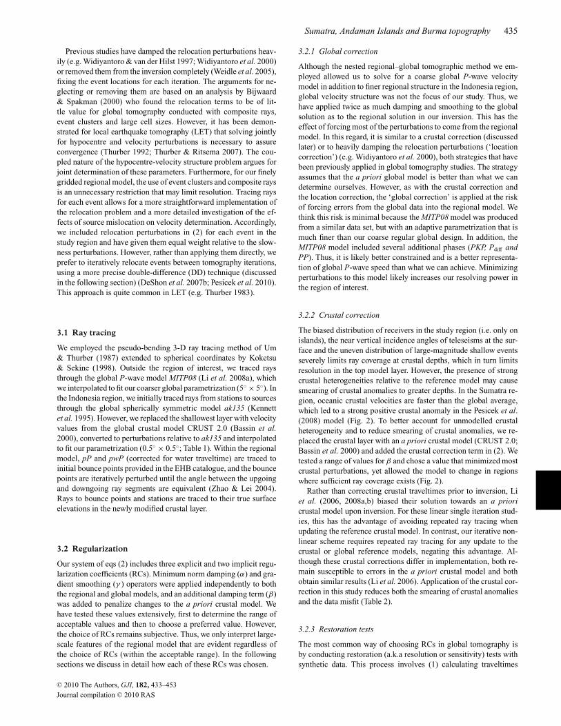
To adequately test the recovery and degree of smearing of small-scale anomalies and large fast slab-like anomalies, we have con-ducted restoration tests using two regular spike models (Fig. 3) anda synthetic subducting slab model (Fig. 4) that attempts to mimic



Figure 3. (a) Depth slices of spike restoration test after two iterations (source locations fixed). Synthetic 4 per cent velocity perturbation input anomalies(2.5 $ 2.5"; black contours) are separated by 2.5" in latitude and longitude and by two layers in depth. Depths with no input anomalies are shown andthe perturbations in these layers are an indication of vertical smearing from adjacent layers. (b) Depth slices of alternate spike restoration test, the same as(a) except the input pattern is shifted to be the opposite of (a), that is, layers with (without) anomalies in (a) now lack (have) them.

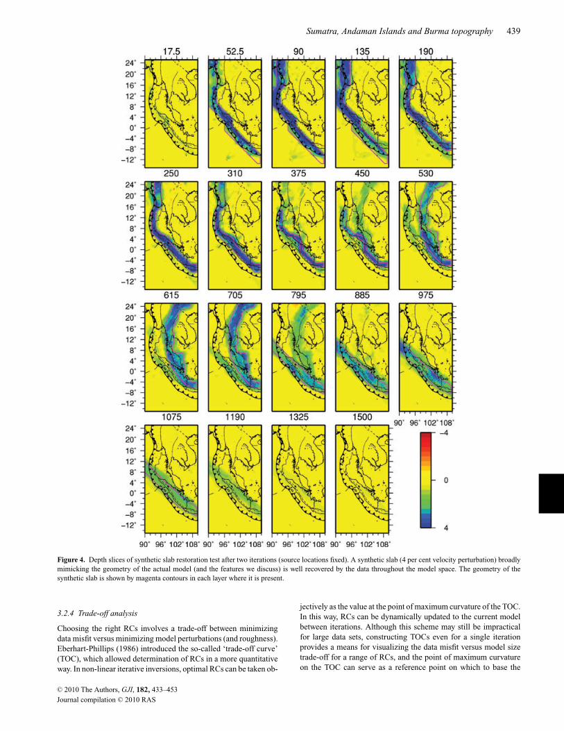
the shape of the slab imaged with the real data. We computedtheoretical traveltimes through these synthetic models and then cal-culated their residuals relative to ak135 (Kennett et al. 1995, Fig. 5).We then added noise to the residuals and repeated the first two it-erations of (2), replacing the data vector of residuals (#t) with thesynthetic residuals. Typically, Gaussian errors are added for globaltomography restoration tests (e.g. Spakman & Nolet 1988). How-

ever, it is well known that traveltime residual distributions are notwell matched by Gaussian functions due to outliers with large resid-uals (e.g. Buland 1986). To simulate a more realistic distribution ofnoise, we randomized the actual residuals from the real inversionand added them to the synthetic residuals (Fig. 5). When we com-pared the results of our synthetic slab model (Fig. 4) applying thisstrategy to the results of a case where a Gaussian noise distribution



Figure 3. (Continued.)

(variance = 2.25 s2) was added, and to results where no noise wasadded, we found that the addition of noise has little effect on the re-covery of the large-scale slab geometry (see also Widiyantoro et al.2000).

The results of the restoration tests demonstrate that our iterativeprocedure increases amplitude recovery of the synthetic anomaliessignificantly while generally reducing smearing and suppressingnoise. Figs 6 and 7 show the enhancements to the models fromiteration 1 to iteration 2 but also illustrate the limitations of our

resolution, despite these enhancements. For smaller features like thespikes (2.5"), improvement to recovery of any one spike is modest(Figs 6a and 7a). However, good restoration of the anomaly patternis achieved east of the subduction boundary in most areas, althoughamplitude recovery of slow spikes is smaller compared to fast ones.More importantly for our purposes, recovery of the large, fast slab isquite good (Fig. 6b) and much improved relative to iteration 1 (Figs6b and 7b). In fact, complete amplitude restoration of the syntheticslab is achieved in many areas (Fig. 6b).



Figure 4. Depth slices of synthetic slab restoration test after two iterations (source locations fixed). A synthetic slab (4 per cent velocity perturbation) broadlymimicking the geometry of the actual model (and the features we discuss) is well recovered by the data throughout the model space. The geometry of thesynthetic slab is shown by magenta contours in each layer where it is present.

3.2.4 Trade-off analysis

Choosing the right RCs involves a trade-off between minimizingdata misfit versus minimizing model perturbations (and roughness).Eberhart-Phillips (1986) introduced the so-called ‘trade-off curve’(TOC), which allowed determination of RCs in a more quantitativeway. In non-linear iterative inversions, optimal RCs can be taken ob-

jectively as the value at the point of maximum curvature of the TOC.In this way, RCs can be dynamically updated to the current modelbetween iterations. Although this scheme may still be impracticalfor large data sets, constructing TOCs even for a single iterationprovides a means for visualizing the data misfit versus model sizetrade-off for a range of RCs, and the point of maximum curvatureon the TOC can serve as a reference point on which to base the



0

40000

80000

120000

160000

200000

resi

dual

cou

nt

A)

0

40000

80000

120000

160000

200000

resi

dual

cou

nt

B)

0

40000

80000

120000

160000

200000

resi

dual

cou

nt

C)

0

40000

80000

120000

160000

200000

resi

dual

cou

nt

0 4 8residual(sec)

D)

Figure 5. (A) Residual distributions for the real iteration 2 inversion. Syn-thetic slab residuals (B) without noise (residuals are computed as the fastsynthetic slab traveltime minus the reference model traveltime), (C) with thereal residuals randomized and added and (D) with a Gaussian distribution ofnoise added (var = 2.25 s). The actual residual distribution (A) is not wellmatched by a Gaussian function (D). We therefore perform our synthetictests using the noise distribution in (C), which is the sum of the randomizedactual residuals (A) and the synthetic residuals (B).

choice of the RC. This approach is common in LET studies but weare unaware of any global study that has used TOCs to determineRCs. Checkerboard and similar tests appear to be the standard.

We have examined the trade-off between model size and data mis-fit for our regional RCs at several iterations of the real model. Wefound that the RCs that performed best in the restoration tests de-scribed above (i.e. by better restoring the shape and amplitude of thesynthetic anomalies) are lower than the optimal values determinedby our trade-off analyses conducted on the real data (Fig. 8). Ouranalysis showed that when applying the preferred RCs determinedsolely by synthetics to the real data, the resulting LSQR solution

appears underdamped; the resulting model seems oscillatory andnoisy relative to the distribution of expected mantle anomalies. Thissuggests to us that we are not adequately representing the populationof noise in the data in our synthetic tests.

Recently, Koulakov (2009) questioned the validity of TOCs forLET, and used synthetic tests similar to ours to suggest that RCsdetermined by TOCs are overestimated. In our view, the opposite istrue: RCs chosen only on their ability to restore synthetic anomaliesare underestimated, and produce a model that we view as too rough.The limitations of synthetic tests are well known (e.g. Leveque et al.1993). They are useful for assessing the ability of the sensitivitymatrix to recover specific features, but should not be used as the solebasis for determining RCs for the whole system, especially whenonly one structural wavelength is tested. Instead, we prefer usingTOCs in conjunction with synthetic tests to choose RCs because itbases the decision on the real data in addition to the synthetic data.We used this strategy at several iterations and found that the rangeof optimal RCs suggested by the corner region of the TOCs doesnot change significantly for subsequent iterations. Thus, we havechosen our RCs based on the first iteration, and have kept themfixed for all iterations.

3.3 Iteratively reweighted least squares

Least-squares (L2) solutions to (2) assume Gaussian data errorsand are thus susceptible to large residual outliers. Small errors inthe data can lead to large amplitude errors in the model. Typically,a residual cut-off threshold is applied a priori to the data and thesystem of equations is regularized to minimize such effects. How-ever, the choice of the residual threshold and of the RCs is highlysubjective. A more robust solution can be obtained by minimizingthe L1-norm, and an easy way to achieve this practically is to dy-namically reweight the data between least-squares inversions usingIRLS. This technique approximates the L1-norm solution (Scaleset al. 1988; Aster et al. 2005). Robust L1 solutions to global tomo-graphic problems have also been shown to be relatively insensitiveto regularization constraints (Pulliam et al. 1993; Vasco et al. 1994).Thus, in applying IRLS, we have obtained a more robust solutionthat better fits the data (Table 2) while simultaneously avoiding thechoice of residual cut-off threshold and further reducing the effectsof subjectively choosing RCs.

3.4 Earthquake relocation

To determine how source mislocation affects our solution, we haverelocated the initial EHB earthquake locations using a modified DDtechnique (Pesicek et al. 2010). The original DD method (Wald-hauser & Ellsworth 2000) has proven effective at determining pre-cise relative local and regional earthquake locations within manyseismic networks (e.g. Prejean et al. 2002; Schaff et al. 2002). Whenadapted to determine velocity structure and absolute event locationsin addition to relative locations (Zhang & Thurber 2003), the DDmethod has provided high-resolution tomographic images and high-precision event locations at a variety of scales and in a variety oftectonic settings (Zhang & Thurber 2006). More recently, the DDmethod (using a 1-D model) has proven effective at teleseismicevent relocation as well (Waldhauser & Schaff 2007).

The DD tomography algorithm tomoDD of Zhang & Thurber(2003) has been extended to teleseismic distances (DeShon et al.2007b; Pesicek et al. 2010). However, velocity determinationin the algorithm is currently limited to source regions where



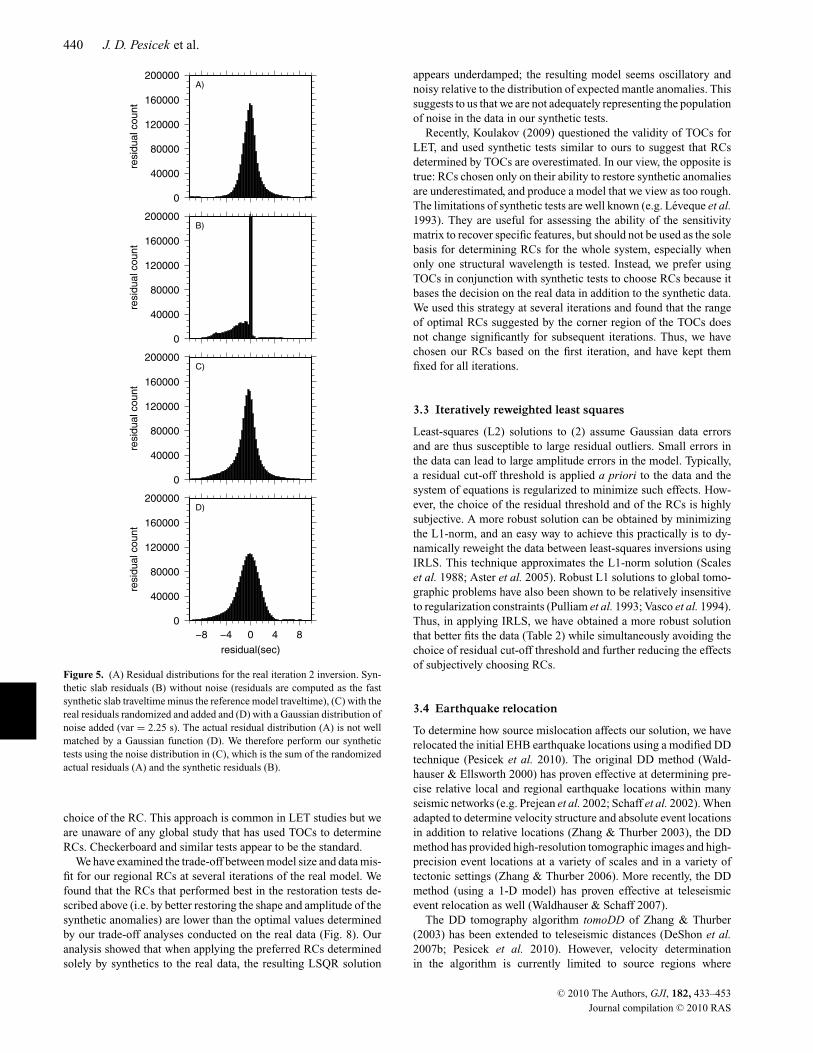
Figure 6. (a) Comparisons of spike restoration tests at several depths (synthetic model same as Fig. 3a) due to iterative method. (A) iteration 1 results, (B)iteration 2 results, (C) the difference between iteration 2 and iteration 1 models (B–A; 1 per cent scale) and (D) the difference between the synthetic inputmodel (black square contours; 4 per cent) and the recovered iteration 2 model (B). Anomalies in (C) represent new perturbations to the recovered model due toiterative process. Although enhancement to recovery and reduction of smearing of synthetic anomalies is widespread, enhancement of artefacts and smearing isalso prevalent. (D) Illustrates the deficiencies of recovery of the synthetic anomalies; zero amplitude checkers in (D) would represent perfect recovery. Spikesin (D) that are high (low) in amplitude are poorly (well) recovered. Areas outside the spikes in (D), where anomaly polarity has reversed, illustrate the degree ofsmearing of the checkers. (b) Comparison of slab restoration tests (synthetic model same as Fig. 4) due to iterative method, similar to (a). (C) Blues illustratethe increasing amplitude of the slab anomalies while reds indicate a decrease in smearing due to the iterative process. Although enhancement to slab recoveryand reduction of smearing of the synthetic slab is widespread, enhancement of artefacts and additional smearing outside of the synthetic slab is also prevalent.(D) Shows that in the upper mantle, nearly complete recovery (zero model difference) of the synthetic slab is achieved in many areas, but that vertical smearing(red) is significant.




differential times are available. In this study we use the teleseis-mic version of tomoDD, (named teletomoDD) solely to relocateevents in western Indochina using our 3-D model (iteration 2) andupdate the hypocentral parameters between subsequent velocity in-

version iterations. We limit our discussion to the effects that eventrelocation have on our improved tomographic model. An analy-sis of the relocations will be presented elsewhere (Pesicek et al.2010).



1

0

1

2

3

4

5

Per

turb

atio

n A

mpl

itude

(%

)

94 95 96 97 98 99 100

Longitude

1

0

1

2

3

4

5

1

0

1

2

3

4

5

1

0

1

2

3

4

5

Per

turb

atio

n A

mpl

itude

(%)

0 1 2 3 4 5 6 7 8 9 10 11 12 13 14

Distance (degrees) along strike

1

0

1

2

3

4

5

0 1 2 3 4 5 6 7 8 9 10 11 12 13 141

0

1

2

3

4

5

A)

B)

Figure 7. (A) Restoration of the spike anomaly centred at 97" E, 5.5" N,and 90 km depth (northern Sumatra). The synthetic spike (grey) is betterrecovered by iteration 2 (black) than iteration 1 (grey dashed). Outside ofthe actual spike, smearing is slightly reduced by iteration 2. Amplitude isshown as the latitude average of the 2.5" spike. (B) Restoration of syntheticslab along cross-section D (Fig. 1) at 450 km depth showing the increasein slab amplitude and reduction of smearing outside the synthetic slab foriteration 2.

4 R E S U LT S A N D D I S C U S S I O N

4.1 Model enhancements with fixed sources

Iterative global tomography studies have previously neglected orignored source mislocation for a variety of reasons (see Bijwaard &Spakman 2000). In Fig. 9, we present our model at various depthsfor several iterations. In Fig. 10, we present the differences betweenmodel iterations to illustrate the enhancements due to the iterativeprocess alone. Our second iteration model shows a %4 per centmisfit reduction (Table 2), comparable to, but less than, reductionsfound for similar non-linear global studies without source reloca-tion (Gorbatov et al. 2001; Weidle et al. 2005). The overall anomalypatterns are generally consistent with the first iteration model, alsoa conclusion of previous studies. All of the fast slab features dis-cussed by Pesicek et al. (2008) are generally enhanced in amplitudeand shape, including the fold below northern Sumatra and the rem-

0.00

0.05

0.10

0.15

0.20

0.25

Mod

el S

ize

1.10 1.12 1.14 1.16 1.18 1.200.00

0.05

0.10

0.15

0.20

0.25

Mod

el S

ize

1.10 1.12 1.14 1.16 1.18 1.200.00

0.05

0.10

0.15

0.20

0.25

Mod

el S

ize

1.10 1.12 1.14 1.16 1.18 1.20

0.0

0.51.0

10.012.0

15.017.0

2.0

20.030.0

4.05.0

50.0

7.0

75.0

Damping

0.04

0.06

0.08

0.10

Mod

el S

ize

1.13 1.14 1.15

Data Misfit

0.04

0.06

0.08

0.10

Mod

el S

ize

1.13 1.14 1.15

Data Misfit

0.04

0.06

0.08

0.10

Mod

el S

ize

1.13 1.14 1.15

Data Misfit

0.0

10.013.0

16.020.0

25.0

3.0

30.040.0

5.0

8.0

Smoothing

Figure 8. Trade-off curves (TOCs) for damping and smoothing parameters(RCs) tested on the real data. In LET studies, RCs are often objectively cho-sen as the point of maximum curvature of the TOC. In global tomography,RCs are commonly chosen as the values that best restore the known anoma-lies. Our synthetic tests suggest optimal synthetic anomaly restoration byRCs in the range shown by the grey-shaded areas. These values are belowthe ranges suggested by the regions of maximum curvature of the TOCs.We chose values (triangles) that compromise between optimally recoveredsynthetic anomalies and optimizing the trade-off between real data misfitand model size.

nant Neo-Tethys slab in the lower mantle. The observed changesare a result of increasing amplitudes at the centres of slab anoma-lies, although increases in the magnitude of negative mantle wedgeanomalies are also common (Fig. 10b). Being opposite in polarity,sharp gradients result where both of these amplitudes increase abovethe slab. These changes are largest in the upper mantle and decreasewith depth. Additional iterations with fixed sources were performed(e.g. Fig. 9) and the resulting model changes were similar in patternbut decreased in magnitude (Fig. 10) with each subsequent iteration(Table 2).

4.2 The effects of source relocation on iteration

Relocation of sources between iterations is commonplace in LETstudies, but quite uncommon in global tomography. Althoughhypocentral derivatives are usually included in non-linear global



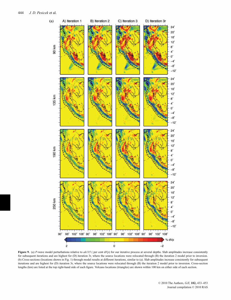
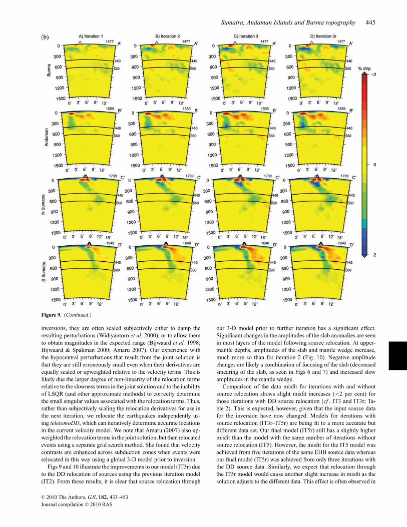
Figure 9. (a) P-wave model perturbations relative to ak135 ( per cent dVp) for our iterative process at several depths. Slab amplitudes increase consistentlyfor subsequent iterations and are highest for (D) iteration 3r, where the source locations were relocated through (B) the iteration 2 model prior to inversion.(b) Cross-sections (locations shown in Fig. 1) through model results at different iterations, similar to (a). Slab amplitudes increase consistently for subsequentiterations and are highest for (D) iteration 3r, where the source locations were relocated through (B) the iteration 2 model prior to inversion. Cross-sectionlengths (km) are listed at the top right-hand side of each figure. Volcano locations (triangles) are shown within 100 km on either side of each section.




inversions, they are often scaled subjectively either to damp theresulting perturbations (Widiyantoro et al. 2000), or to allow themto obtain magnitudes in the expected range (Bijwaard et al. 1998;Bijwaard & Spakman 2000; Amaru 2007). Our experience withthe hypocentral perturbations that result from the joint solution isthat they are still erroneously small even when their derivatives areequally scaled or upweighted relative to the velocity terms. This islikely due the larger degree of non-linearity of the relocation termsrelative to the slowness terms in the joint solution and to the inabilityof LSQR (and other approximate methods) to correctly determinethe small singular values associated with the relocation terms. Thus,rather than subjectively scaling the relocation derivatives for use inthe next iteration, we relocate the earthquakes independently us-ing teletomoDD, which can iteratively determine accurate locationsin the current velocity model. We note that Amaru (2007) also up-weighted the relocation terms in the joint solution, but then relocatedevents using a separate grid search method. She found that velocitycontrasts are enhanced across subduction zones when events wererelocated in this way using a global 3-D model prior to inversion.

Figs 9 and 10 illustrate the improvements to our model (IT3r) dueto the DD relocation of sources using the previous iteration model(IT2). From these results, it is clear that source relocation through

our 3-D model prior to further iteration has a significant effect.Significant changes in the amplitudes of the slab anomalies are seenin most layers of the model following source relocation. At upper-mantle depths, amplitudes of the slab and mantle wedge increase,much more so than for iteration 2 (Fig. 10). Negative amplitudechanges are likely a combination of focusing of the slab (decreasedsmearing of the slab, as seen in Figs 6 and 7) and increased slowamplitudes in the mantle wedge.

Comparison of the data misfit for iterations with and withoutsource relocation shows slight misfit increases (<2 per cent) forthose iterations with DD source relocation (cf . IT3 and IT3r; Ta-ble 2). This is expected, however, given that the input source datafor the inversion have now changed. Models for iterations withsource relocation (IT3r–IT5r) are being fit to a more accurate butdifferent data set. Our final model (IT5r) still has a slightly highermisfit than the model with the same number of iterations withoutsource relocation (IT5). However, the misfit for the IT5 model wasachieved from five iterations of the same EHB source data whereasour final model (IT5r) was achieved from only three iterations withthe DD source data. Similarly, we expect that relocation throughthe IT5r model would cause another slight increase in misfit as thesolution adjusts to the different data. This effect is often observed in



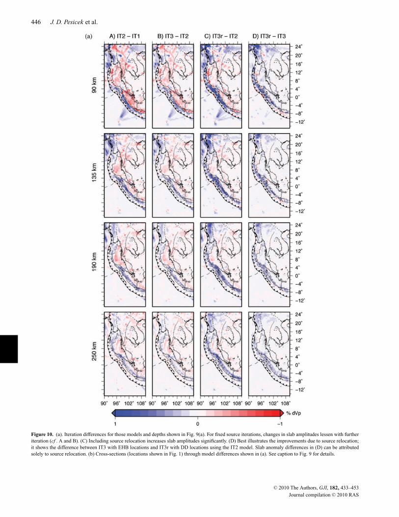
Figure 10. (a). Iteration differences for those models and depths shown in Fig. 9(a). For fixed source iterations, changes in slab amplitudes lessen with furtheriteration (cf . A and B). (C) Including source relocation increases slab amplitudes significantly. (D) Best illustrates the improvements due to source relocation;it shows the difference between IT3 with EHB locations and IT3r with DD locations using the IT2 model. Slab anomaly differences in (D) can be attributedsolely to source relocation. (b) Cross-sections (locations shown in Fig. 1) through model differences shown in (a). See caption to Fig. 9 for details.




non-linear LET where data and/or data weighting are dynamicallychanged throughout the iterative process as the solution convergesto the most accurate model with the most accurate locations. Over-all, the differences in misfit and model amplitudes for EHB versusDD source iterations are minor (Table 2), but the upper-mantle slabanomalies are significantly enhanced when source relocation is in-cluded (e.g. Fig. 10, Column C and D). This misfit mismatch canonly be resolved when the 3-D DD joint inversion can be appliedto the full data set, something that is not currently possible due tocomputational limitations.

4.3 Lithospheric slab folding below Sumatra

The final model resulting from our iterative method (Fig. 11) pro-vides an enhanced view of the subducting slab below the westernIndochina subduction zones. The image of the lithospheric slabfold subducting below northern Sumatra (Pesicek et al. 2008) isnow more focused, but its origin remains subject to debate. Thecomplexity of the regional tectonics makes it difficult to attributethe fold to any one feature or process. Subduction of the Investiga-

tor Fracture Zone (IFZ), the Wharton Fossil Ridge (WFR) and thediffuse deformational boundary between the Indian and Australianplates all occur in this region (Fig. 1), any of which may influencethis folding. Alternatively, the possibility that the fold is static anddue only to trench curvature (Fauzi et al. 1996) cannot be ruledout.

If we assume that the fold below Sumatra is a primary featureof the incoming plate, then the long-wavelength buckling or fold-ing (100–300 km) of the Indian Ocean lithosphere that has beendiscussed by many authors (e.g. Deplus et al. 1998; Deplus 2001;Krishna et al. 2001) may be pertinent. These folds have been in-ferred from gravity undulations and seismic reflection data through-out the Central Indian and Wharton basins. The orientations of theiraxes are perpendicular to regional compression axes and they areinterpreted as being caused by internal deformation of the Indianand Australian plates. Southwest of Sumatra, their axes are orientedNE–SW, parallel to the orientation of the axis of our imaged fold.Although similar in shape, orientation and possibly causal mecha-nism, they cannot be directly related to the lithospheric fold belowSumatra due to the timing of their formation. The onset of diffusedeformation between the Indian and Australian plates that caused



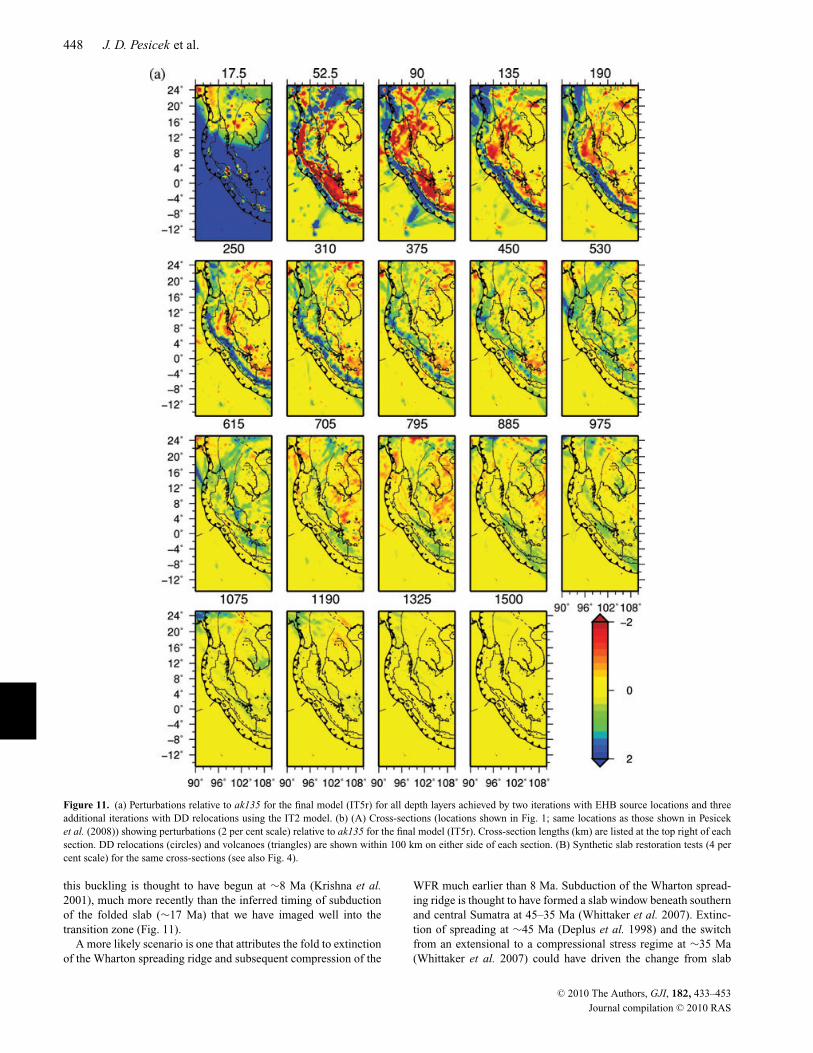
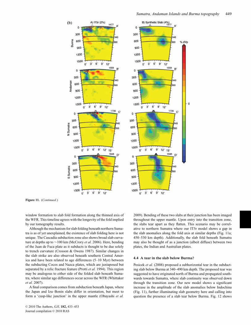
Figure 11. (a) Perturbations relative to ak135 for the final model (IT5r) for all depth layers achieved by two iterations with EHB source locations and threeadditional iterations with DD relocations using the IT2 model. (b) (A) Cross-sections (locations shown in Fig. 1; same locations as those shown in Pesiceket al. (2008)) showing perturbations (2 per cent scale) relative to ak135 for the final model (IT5r). Cross-section lengths (km) are listed at the top right of eachsection. DD relocations (circles) and volcanoes (triangles) are shown within 100 km on either side of each section. (B) Synthetic slab restoration tests (4 percent scale) for the same cross-sections (see also Fig. 4).

this buckling is thought to have begun at %8 Ma (Krishna et al.2001), much more recently than the inferred timing of subductionof the folded slab (%17 Ma) that we have imaged well into thetransition zone (Fig. 11).

A more likely scenario is one that attributes the fold to extinctionof the Wharton spreading ridge and subsequent compression of the

WFR much earlier than 8 Ma. Subduction of the Wharton spread-ing ridge is thought to have formed a slab window beneath southernand central Sumatra at 45–35 Ma (Whittaker et al. 2007). Extinc-tion of spreading at %45 Ma (Deplus et al. 1998) and the switchfrom an extensional to a compressional stress regime at %35 Ma(Whittaker et al. 2007) could have driven the change from slab




window formation to slab fold formation along the thinned axis ofthe WFR. This timeline agrees with the longevity of the fold impliedby our tomography results.

Although the mechanism for slab folding beneath northern Suma-tra is as of yet unexplained, the existence of slab folding here is notunique. The Cascadia subduction zone also shows broad slab curva-ture at depths up to %100 km (McCrory et al. 2006). Here, bendingof the Juan de Fuca plate as it subducts is thought to be due solelyto trench curvature (Crosson & Owens 1987). Similar changes inthe slab strike are also observed beneath southern Central Amer-ica and have been related to age differences (5–10 Myr) betweenthe subducting Cocos and Nazca plates, which are juxtaposed butseparated by a relic fracture feature (Protti et al. 1994). This regionmay be analogous to either side of the folded slab beneath Suma-tra, where similar age differences occur across the WFR (Whittakeret al. 2007).

A final comparison comes from subduction beneath Japan, wherethe Japan and Izu–Bonin slabs differ in orientation, but meet toform a ‘cusp-like junction’ in the upper mantle (Obayashi et al.

2009). Bending of these two slabs at their junction has been imagedthroughout the upper mantle. Upon entry into the transition zone,the slabs tear apart as they flatten. This scenario may be correl-ative to northern Sumatra where our IT5r model shows a gap inthe slab anomalies along the fold axis at similar depths (Fig. 11a;450–530 km depth). Additionally, the slab fold beneath Sumatramay also be thought of as a junction (albeit diffuse) between twoplates, the Indian and Australian plates.

4.4 A tear in the slab below Burma?

Pesicek et al. (2008) proposed a subhorizontal tear in the subduct-ing slab below Burma at 340–490 km depth. The proposed tear wassuggested to have originated north of Burma and propagated south-wards towards Sumatra, where slab continuity was observed downthrough the transition zone. Our new model shows a significantincrease in the amplitude of the slab anomalies below Indochina(Fig. 11), further illuminating slab geometry here and calling intoquestion the presence of a slab tear below Burma. Fig. 12 shows



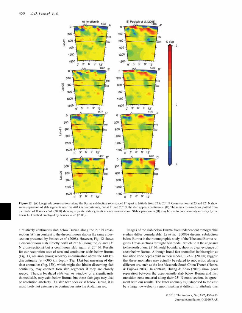
Figure 12. (A) Longitude cross-sections along the Burma subduction zone spaced 1" apart in latitude from 23 to 20" N. Cross-sections at 23 and 22" N showsome separation of slab segments near the 440 km discontinuity, but at 21 and 20" N, the slab appears continuous. (B) The same cross-sections plotted fromthe model of Pesicek et al. (2008) showing separate slab segments in each cross-section. Slab separation in (B) may be due to poor anomaly recovery by thelinear 1-D method employed by Pesicek et al. (2008).

a relatively continuous slab below Burma along the 21" N cross-section (A&), in contrast to the discontinuous slab in the same cross-section presented by Pesicek et al. (2008). However, Fig. 12 showsa discontinuous slab directly north of 21" N (along the 22 and 23"

N cross-sections) but a continuous slab again at 20" N. Resultsfor our restoration tests of torn and continuous slabs below Burma(Fig. 13) are ambiguous; recovery is diminished above the 440 kmdiscontinuity (at %300 km depth) (Fig. 13a) but smearing of dis-tinct anomalies (Fig. 13b), which might also hinder discerning slabcontinuity, may connect torn slab segments if they are closelyspaced. Thus, a localized slab tear or window, or a significantlythinned slab, may exist below Burma, but these slab gaps may alsobe resolution artefacts. If a slab tear does exist below Burma, it ismost likely not extensive or continuous into the Andaman arc.

Images of the slab below Burma from independent tomographicstudies differ considerably. Li et al. (2008b) discuss subductionbelow Burma in their tomographic study of the Tibet and Burma re-gions. Cross-sections through their model, which lie at the edge andto the north of our 25" N model boundary, show no clear evidence ofa tear below Burma. Although broad fast anomalies in this region attransition zone depths exist in their model, Li et al. (2008b) suggestthat these anomalies may actually be related to subduction along adifferent arc, such as the late Mesozoic South China Trench (Honza& Fujioka 2004). In contrast, Huang & Zhao (2006) show goodseparation between the upper-mantle slab below Burma and fasttransition zone material along their 25" N cross-section, in agree-ment with our results. The latter anomaly is juxtaposed to the eastby a large low-velocity region, making it difficult to attribute this



Figure 13. Synthetic slab tests for cross-sections presented in Fig. 12. (A) A synthetic slab (magenta contour; 4 per cent anomaly) that is continuous throughthe upper mantle and into the transition zone is used in restoration tests (two iterations) similar to Fig. 4 and described in the text. (B) A synthetic slab that isdiscontinuous through the upper mantle and into the transition zone is used. The results suggest that ray coverage and resolution are diminished in the regionwhere the tear was hypothesized by Pesicek et al. (2008), but may still be sufficient to distinguish a continuous slab from a torn slab. However, smearing ofdistinct anomalies is considerable. Thus a torn slab with minimal segment separation may appear continuous due to smearing.

remnant slab to subduction from the east. Neither of these modelsextends far enough to the south to show the southward continuationof these transition zone anomalies into our study region and canneither confirm nor refute our results. From our images, a com-pletely continuous slab throughout the region is unlikely but theexact geometry of the slab below Burma remains unclear.

5 S U M M A RY A N D C O N C LU S I O N S

We have presented an improved P-wave velocity model of the Suma-tra, Andaman and Burma subduction zones (Fig. 11) based on thenon-linear nested regional–global method of Widiyantoro et al.(2000). We have added residual reweighting and source relocation

to the iterative scheme, two processes common in LET studies buthitherto not usually applied in global tomography studies. We haveexamined in detail the model improvements obtained by conductingadditional iterations with and without source relocation. Althoughthe majority of the resolved velocity structure is recovered after oneiteration, significant increases in slab amplitude and slab sharpen-ing occur in some regions of the upper mantle from subsequentiterations, particularly after source relocation. Source relocationthrough the 3-D model prior to additional velocity iterations sub-stantially focuses the image of the subducting slab in the studyregion, beyond what is achieved by fixed source iteration alone.Below Burma, improvements due to our iterative technique extendslab anomalies beyond the boundaries of single iteration results,revising interpretations of slab geometry. Thus, source relocation



may be an important contributor to increasing accuracy of globaltomography models, which in turn may help clarify interpretationsof previously identified mantle structures or facilitate discovery ofnew ones.

A C K N OW L E D G M E N T S

We thank Wim Spakman and an anonymous reviewer for criti-cal reviews. This material is based upon work supported in partby the National Science Foundation under grants EAR-0608988(HD and CT) and EAR-0609613 (EE), and by NASA, under awardNNX06AF10G. The data were provided by the ISC and NEIC.Figures were produced using the GMT package (Wessel & Smith1998).

R E F E R E N C E S

Amaru, M.L., 2007. Global travel time tomography with 3-D referencemodels, PhD thesis. Utrecht University, Netherlands.

Aster, R.C., Borchers, B. & Thurber, C.H., 2005. Parameter Estimation andInverse Problems, Academic Press, Burlington, MA.

Bassin, C., Laske, G. & Masters, G., 2000. The current limits of resolutionfor surface wave tomography in North America, EOS, Trans. Am. geophys.Un., 81, F897.

Bijwaard, H. & Spakman, W., 2000. Non-linear global P-wave tomographyby iterated linearized inversion, Geophys. J. Int., 141, 71–82.

Bijwaard, H., Spakman, W. & Engdahl, E.R., 1998. Closing the gap be-tween regional and global travel time tomography, J. geophys. Res., 103,30 055–30 078.

Buland, R., 1986. Uniform reduction error analysis, Bull. seism. Soc. Am.,76, 217–230.

Crosson, R.S. & Owens, T.J., 1987. Slab geometry of the Cascadia subduc-tion zone beneath Washington from earthquake hypocenters and teleseis-mic converted waves, Geophys. Res. Lett., 14, 824–827.

Deplus, C., 2001. Indian Ocean actively deforms, Science, 292, 1850–1851.Deplus, C. et al., 1998. Direct evidence of active deformation in the eastern

Indian oceanic plate, Geology, 26, 131–134.DeShon, H.R., Thurber, C.H., Brudzinski, M.R. & Engdahl, E.R., 2007a. A

semi-automated technique for waveform cross-correlation of teleseismi-cally recorded depth phases, Seismol. Res. Lett., 78.

DeShon, H.R., Zhang, H., Thurber, C.H. & Engdahl, E.R., 2007b. Imag-ing the Andaman and Sunda subduction zones using regional double-difference tomography, EOS, Trans. Am. geophys. Un., abstract# S23D-0

Eberhart-Phillips, D. 1986. Three-dimensional velocity structure in northernCalifornia Coast Ranges from inversion of local earthquake arrival times,Bull. seism. Soc. Am., 76, 1025–1052.

Engdahl, E.R., Van Der Hilst, R.D. & Buland, R., 1998. Global teleseismicearthquake relocation with improved travel times and procedures for depthdetermination, Bull. seism. Soc. Am., 88, 722–774.

Engdahl, E.R., Villasenor, A., DeShon, H.R. & Thurber, C.H., 2007. Tele-seismic relocation and assessment of seismicity (1918–2005) in the regionof the 2004 Mw 9.0 Sumatra-Andaman and 2005 Mw 8.6 Nias Island greatearthquakes, Bull. seism. Soc. Am., 97, S43–S61.

Fauzi, R., McCaffrey, D. A., Wark, Sunaryo & Prih Haryadi, P. Y., 1996. Lat-eral variation in slab orientation beneath Toba Caldera, northern Sumatra,Geophys. Res. Lett., 23, 443–446.

Gorbatov, A., Fukao, Y. & Widiyantoro, S., 2001. Application of a three-dimensional ray-tracing technique to global P, PP and Pdiff traveltimetomography, Geophys. J. Int., 146, 583–593.

Honza, E. & Fujioka, K., 2004. Formation of arcs and backarc basins inferredfrom the tectonic evolution of Southeast Asia since the Late Cretaceous,Tectonophysics, 384, 23–25.

Huang, J. & Zhao, D., 2006. High-resolution mantle tomography ofChina and surrounding regions, J. geophys. Res., 111, B09305,doi:10.1029/2005JB004066.

Kennett, B.L.N., Engdahl, E.R. & Buland, R., 1995. Constraints on seis-mic velocities in the Earth from traveltimes, Geophys. J. Int., 122, 108–124.

Koketsu, K. & Sekine, S., 1998. Pseudo-bending method for three-dimensional seismic ray tracing in a spherical earth with discontinuities,Geophys. J. Int., 132, 339–346.

Koulakov, I. 2009. LOTOS Code for local earthquake tomographic inver-sion: benchmarks for testing tomographic algorithms, Bull. seism. Soc.Am., 99, 194–214.

Krishna, K.S., Bull, J.M. & Scrutton, R.A., 2001. Evidence for multi-phase folding of the central Indian Ocean lithosphere, Geology, 29, 715–718.

Leveque, J., Rivera, L. & Wittlinger, G., 1993. On the use of the checker-board test to assess the resolution of tomographic inversions, Geophys. J.Int., 115, 313–318.

Li, C., Van Der Hilst, R.D. & Toksoz, M.N., 2006. Constraining P-wavevelocity variations in the upper mantle beneath southeast Asia, Phys.Earth planet. Inter., 154, 180–195.

Li, C., Van Der Hilst, R.D., Engdahl, E.R. & Burdick, S., 2008a. A newglobal model for P wave speed variations in Earth’s mantle, Geochem.Geophys. Geosyst., 9, 1–21.

Li, C., Van Der Hilst, R.D., Meltzer, A.S. & Engdahl E.R., 2008b. Subduc-tion of the Indian lithosphere beneath the Tibetan Plateau and Burma,Earth planet. Sci. Lett., 274, 157–168.

Masturyono, McCaffrey, R., Wark, D.A., Roecker, S.W., Fauzi, Ibrahim, G.& Sukhyar, 2001. Distribution of magma beneath the Toba caldera com-plex, north Sumatra, Indonesia, constrainted by three-dimensional P wavevelocities, seismicity, and gravity data, Geochem. Geophys. Geosyst., 2,1014, doi:10.1029/2000GC000096.

McCrory, P.A., Blair, J.L., Oppenheimer, D.H. & Walter, S.R., 2006. Depthto the Juan De Fuca Slab Beneath the Cascadia Subduction Margin-A3-D Model for Sorting Earthquakes, U.S. Geological Survey, Data Series91, Version 1.2.

Obayashi, M., Yoshimitsu, J. & Fukao, Y., 2009. Tearing of stagnant slab,Science, 324, 1173–1175.

Paige, C. & Saunders, M.A., 1982. LSQR: An algorithm for sparse linearequations and least squares problems, ACM Trans. Math. Softw., 8, 43–71.

Pesicek, J.D., Thurber, C.H., Widiyantoro, S., Engdahl, E.R. & DeShon,H.R., 2008. Complex slab subduction beneath northern Sumatra,Geophys. Res. Lett., 35, L2030, doi:10.1029/2008GL035262.

Pesicek, J.D., Thurber, C.H., Zhang, H., DeShon, H.R., Engdahl, E.R. &Widiyantoro, S., 2010. Teleseismic double-difference relocation of earth-quakes along the Sumatra- Andaman subduction zone using a three-dimensional model, J. geophys. Res., in press.

Prejean, S.G., Ellsworth, W.L., Zoback, M.D. & Waldhauser, F., 2002. Faultstructure and kinematics of the Long Valley Caldera region, California,revealed by high-accuracy earthquake hypocenters and focal mechanismstress inversions, J. geophys. Res., 107, 19.

Protti, M., Guendel, F. & McNally, K., 1994. The geometry of the Wadati-Benioff zone under southern Central America and its tectonic signifi-cance: results from a high-resolution local seismographic network, 10years of GEOSCOPE-broadband seismology, Phys. Earth planet. Inter.,84, 271–287.

Pulliam, R.J., Vasco, D.W. & Johnson, L.R., 1993. Tomographic inversionsfor mantle P wave velocity structure based on the minimization of l2 andl1norms of International Seismological Centre travel time residuals, J.geophys. Res., 98, doi:10.1029/92JB01053.

Scales, J.A., Gerztenkorn, A. & Treitel, S., 1988. Fast 1p solution of large,sparse, linear systems: application to seismic travel time tomography, J.Comput. Phys., 75, 314–333.

Schaff, D.P., Bokelmann, G.H.R., Beroza, G.C., Waldhauser, F. & Ellsworth,W.L., 2002. High-resolution image of Calaveras Fault seismicity, J. geo-phys. Res, 107, 16.

Spakman, W. & Nolet, G., 1988. Imaging algorithms, accuracy and resolu-tion in delay time tomography, in Mathematical Geophysics: A Survey ofRecent Developments in Seismology and Geodynamics, pp. 155–187, edsVlaar, N.J., Nolet, G., Wortel, M.J.R. & Cloetingh, S.A.P.L., D. ReidelPublishers Co., Dordrecht, Netherlands (NLD).



Thurber, C.H., 1983. Earthquake locations and three-dimensional crustalstructure in the Coyote Lake area, central California, J. geophys. Res., 88,8226–8236.

Thurber, C.H., 1992. Hypocenter-velocity structure coupling in local earth-quake tomography, Phys. Earth planet. Inter., 75, 55–62.

Thurber, C. & Ritsema, J., 2007. Theory and observations: seismic tomogra-phy and inverse methods, in Treatise on Geophysics, Vol. 1, pp. 323–360,ed. Schubert,G., Elsevier Ltd., Oxford.

Um, J. & Thurber, C.H., 1987. A fast algorithm for two-point seismic raytracing, Bull. seism. Soc. Am., 77, 972–986.

Vasco, D.W., Johnson, L.R., Pulliam, R.J. & Earle, P.S., 1994. Robust in-version of IASP91 travel time residuals for mantle P and S velocitystructure, earthquake mislocations, and station corrections, J. geophys.Res., 99, doi:10.1029/93JB02023.

Waldhauser, F. & Ellsworth, W.L., 2000. A double-difference earthquakelocation algorithm: method and application to the northern Hayward Fault,California, Bull. seism. Soc. Am., 90, 1353–1368.

Waldhauser, F. & Schaff, D., 2007. Regional and teleseismicdouble-difference earthquake relocation using waveform cross-correlation and global bulletin data, J. geophys. Res., 112, B12301,doi:10.1029/2007JB004938.

Weidle, C., Widiyantoro, S. & CALIXTO Working Group, International

(III), 2005. Improving depth resolution of teleseismic tomography bysimultaneous inversion of teleseismic and global P-wave traveltime data;application to the Vrancea region in Southwestern Europe, Geophys. J.Int., 162, 811–882.

Wessel, P. & Smith, W.H.F., 1998. New, improved version of generic mappingtools released, EOS, Trans. Am. geophys. Un., 79, 579–579.

Whittaker, J.M., Muller, R.D., Sdrolias, M. & Heine, C., 2007. Sunda-Javatrench kinematics, slab window formation and overriding plate deforma-tion since the Cretaceous, Earth planet. Sci. Lett., 255, 445–457.

Widiyantoro, S. & Van Der Hilst, R.D., 1997. Mantle structure beneathIndonesia inferred from high-resolution tomographic imaging, Geophys.J. Int., 130, 167–182.

Widiyantoro, S., Gorbatov, A., Kennett, B.L.N. & Fukao, Y., 2000. Improv-ing global shear wave traveltime tomography using three-dimensional raytracing and iterative inversion, Geophys. J. Int., 141, 747–758.

Zhang, H. & Thurber, C.H., 2003. Double-difference tomography: themethod and its application to the Hayward Fault, California, Bull. seism.Soc. Am., 93, 1875–1889.

Zhang, H. & Thurber, C., 2006. Development and applications of double-difference seismic tomography, Pure appl. Geophys., 163, 373–340.

Zhao, D. & Lei, J., 2004. Seismic ray path variations in a 3D global velocitymodel, Phys. Earth planet. Inter., 141, 153–166.


Sharpening the tomographic image of the subducting slab below Sumatra, the Andaman Islands and Burma

Documents

Transcript of Sharpening the tomographic image of the subducting slab below Sumatra, the Andaman Islands and Burma