Sharing a Fish Stock with Density-dependent Distribution and Unit Harvest Costs

Sharing a Fish Stock with Density-dependent

Distribution and Unit Harvest Costs§

Xiaozi Liu1*, Marko Lindroos2, Leif Sandal1

April 20, 2012

1Norwegian School of Economics, Helleveien 30, N-5045 Bergen, Norway.

2Department of Economics and Management, University of Helsinki, P.O.Box 27, 00014

Helsinki, Finland;

* Address all correspondence to Xiaozi Liu, Norwegian School of Economics,

Helleveien 30, N-5045 Bergen, Norway. e-mail: [email protected]

§ We would like to thank Mikko Heino, Stein Ivar Steinshamn, Rognvaldur

Hannesson, and Sturla F. Kvamsdal for their input and comments. XL ac-

knowledges the financial support from the Nordic network on ‘Climate impacts

on fish, fishery industry and management in the Nordic seas’.

1

Sharing a stock with density-dependent distribution 1

Abstract

We study cooperative and competitive solutions for managing a fish stock

that has stock-size dependent distribution, using Norwegian spring-spawning

herring (Clupea harengus) as a case study. Three players in our game can be

asymmetric in stock ownership, efficiency (cost of harvesting) and stock con-

centration profile. The special feature of Norwegian spring-spawning herring is

that it comes under sole ownership of Norway when stock is sufficiently low. In

some important ways, our model is more realistic than earlier game-theoretic

harvesting models: catch function in our model is density-dependent, implying

unit harvest cost is no longer a constant; we use a reference fishing mortality

as the control parameter that determines annual catch quotas, making fishing

effort a dynamic variable that reflects changes in stock biomass. We find that

the likelihood of a stable grand coalition increases with the degree of asymme-

try in the players’ efficiency levels. When Norway, the player with the largest

stock share and inherently the highest fish density in her zone, is the least

efficient player, she is not guaranteed to receive the largest shares of grand

cooperation benefits. Low initial stock level increases Norwegian share of the

grand coalition benefits. In the present of dynamic stock distribution, it is

not the interest of any players to drive stock down below the biomass level in

which Norway becomes the sole owner.

Keywords : cooperative game, Shapley value for partition function games, dy-

namic stock distribution, international resource management

JEL classification code: C71, Q22, Q57


1 Introduction

Trans-boundary fishery resources challenge effective fishery management. The challenge

becomes even greater if distribution of the targeted fish stocks vary in space and time,

or more dramatically, migration patterns change. Several commercial fish stocks have

shown considerable shifts in their distribution. For example, Pacific salmon in Alaska

increased sharply in abundance from mid 1970s, whereas salmon stocks along the U.S.

west coast and in southern British Columbia showed strong declines; the situation was

completely reversed compared to the 1960s and early 1970s (Mantua et al. 1997). Norwe-

gian spring-spawning herring (NSSH) has undergone profound distributional shifts since

1950s: during years of the high stock abundance, NSSH stock can occupy five exclusive

economic zones (EEZ) as well as international waters, but when the stock abundance was

low, the stock was confined to the Norwegian EEZ (Dragesund et al. 1997). Finally,

Atlantic mackerel, which used to visit Icelandic waters only occasionally, has in recent

years become so abundant that it supports a sizeable Icelandic commercial fishery (ICES

2010). The underlying reasons for such distributional changes are likely multifaceted,

although climatic changes are often in the spotlight (Toresen and Østvedt, 2000; Perry

et al. 2005). Climatic shifts can trigger changes in ocean temperature and circulation

patterns, which can have significant impact on the dynamics of marine fish populations

(Miller and Munro 2004).

Overlooking distributional shifts can lead to distorted fisheries management decisions

(Hannesson 2007; Johnson and Welch 2010). Most of trans-boundary fisheries agreements

are based on the “zonal attachment” principle, that is, a country’s share of total quota

is proportional to the share of the total stock in its EEZ. Clearly, fish neither know

about nor would respect these boundaries. The displacement of fish from one zone to

another can then threaten the stability of existing fishing agreements, and further, it may

incentivize uncoordinated fishing practices that potentially harm the biological stocks and

economic outcomes. Pacific salmon moving from Canada to Alaska triggered breakdown

of a cooperative harvest agreement (Miller and Munro 2004); Scottish fishermen called

for “mackerel war” against the new entrant, Iceland, who together with the Faroe Islands

unilaterally set large catch quotas in their own waters; in the case of NSSH, competitive

open access fisheries during 1950s–1960s coupled with climate-driven low recruitment

eventually led to the collapse of NSSH stock (Dragesund et al. 1997).


Game theory has been widely used to tackle research questions in international fishery

management (Bailey et al. 2010), including several applications to herring fisheries (Lin-

droos and Kaitala 2000; Lindroos 2004; Bjørndal et al. 2004; Hannesson 2006). However,

studies addressing the implications of dynamic stock distribution on the trans-boundary

fishery decisions are few. One line of research addressed the implications in terms of strate-

gic interactions of non-cooperative players and the risk of stock depletion (Golubtsov and

McKelvey 2007; Hannesson 2007; Liu and Heino 2011). Another branch of literature

concerns implications on the stability of a cooperative arrangement and the resilience of

fishery agreements. Arnason et al.(2000) studied equilibrium strategies for various com-

petitive and cooperative situations in a stylized model of five exploiters. They modelled

herring migration as a stochastic process, but the dynamic stock distribution was not the

focus of their study. Hannesson (2006) studied the question in a two players’ game using a

biomass dynamic model for NSSH, including density-dependent migration, but his model

is based on steady-state equilibrium only. Ekerhovd (2010) used an age-structured model

to study the impacts of distributional shift for managing the blue whiting fishery. He

assumed two scenarios: one with a more westerly stock distribution in which Russia is

not a coastal state, and the other one where blue whiting spreads further east (as has

been happened in recent years; Heino et al. 2008) such that Russia becomes a coastal

state. He found that inclusion of Russia as a coastal state increases the likelihood of a

stable coastal state agreement.

The key question in this paper is the stability of a grand coalition (co-operation among

all the players) and the benefit sharing within the stable grand coalition when stock dis-

tribution is dynamic. We have chosen to use Norwegian spring-spawning herring (NSSH)

fishery as the example. As already mentioned, the distribution of NSSH is highly dynamic,

and the stock becomes under sole ownership at low stock abundance. Intriguingly, co-

operative management of herring has not always been stable: the coastal states agreement

(i.e., the grand coalition in the game parlance) was suspended during 2003–2006, primar-

ily because Norwegian fishermen were not satisfied with the share they received, given

that the stock spends critical stages of its life cycle near the Norwegian coast (Sissener

and Bjørndal 2005).

We address our research question using a three-player game for Norwegian spring-

spawning herring. We include Norway and Russia as independent players and group the

remaining players, Iceland, the Faroe Islands, and EU (hereafter referred to as IFE), as the


third one. It is important to treat Norway as an independent player (some earlier studies

have merged Norway and Russia), given the unique strategic position Norway has in the

game. Merging IFE countries helps to limit the complexity of the game. We use an age-

structure model where the stock distribution is dependent on spawning stock biomass.

The players in our model are asymmetric; in particular, Norway could monopolize the

stock. Unlike earlier studies, we consider unit harvest cost dependent on the stock size

and the stock elasticity of harvest. The benefit sharing is studied according to the Shapley

value generalized for partition function games. As a robustness check, we also consider

an alternative sharing rule.

2 The model set-up

Our bio-economic model is built upon three-player’s cooperative game framework in an

age-structured model. Model parameters and variables are summarized in the Appendix.

2.1 Spatial distribution rule

Norwegian coast is the only spawning area for NSSH, and also the main habitat for

juvenile herring. After spawning, adult herring may remain in Norwegian waters migrate

further away for foraging. In our setting, players are only allowed to harvest in their own

exclusive economic zones (EEZ)—even under full cooperation case—and the harvest takes

place after stock is redistributed. In the end of a fishing season (one year), NSSH from

different zones merge again in the Norwegian EEZ, before a new spawning season starts.

The NSSH is also partly accessible in the the international waters; our model has ignored

this component.

To model the dynamic stock distribution, we assume a spatial distribution rule spec-

ified by Patterson (1998). According to this rule, the share of total stock abundance (θ)

received by each player is a piece-wise linear function of total spawning stock biomass

(BSS), which is jointly determined by each player’s fishing policy ex-ante:

θj,t =

dj,1950+dj,1959+dj,1983

3if BSS

t > BSShigh

φdj,1950+dj,1959+dj,1983

3+ (1− φ)dj,1972 if BSS

low ≤ BSSt ≤ BSS

high

dj,1972 if BSSt < BSS

low,

(1)

where dj,t denotes empirically observed stock share in zone j in year t, an average over


all age classes, and φ =BSSt −BSSlowBSShigh−B

SSlow

. t = 1972 represents a year when Norway was the

sole owner of NSSH fishery, whereas the other years represent years when the stock had

a broad, trans-boundary distribution. BSShigh = 5.0Mt and BSS

low = 2.5Mt are the two

biomass thresholds; alternative values are considered in section 4.3.

The above formulation indicates two sources of dynamism in the stock distribution:

1) the distribution is the function of the spawning stock biomass, here characterized as

an endogenous force, and 2) the distributional rule might be driven by exogenous factors

such climate warming, giving potentially rise to new stock distribution patterns.

2.2 Non-linear density effects

The main features of our bio-economic model are similar to earlier game theoretical herring

papers. An important distinction is that we consider a non-linear relationship between

stock density and stock abundance. For example, we formulate zone specific density ρ as

follows:

ρj = h

(Nj

θjK

)αj, 0 ≤ αj ≤ 1, (2)

where Nj is stock abundance in fishing zone j, normalized with respect to θjK, the

environmental carrying capacity in zone j. The ‘global’ environmental carrying capacity

K corresponds to the population dynamical equilibrium in absence of fishing. Scaling

parameter h can be interpreted as the stock density when N = K.

α, stock elasticity of harvest, has special interpretation in our model. It depends on the

behaviour of the targeted fish as wellas the ability of fishermen to find the fish. Typically

α has a value between 0 and 1. α = 0 represents an extreme schooling species and where

fishermen can find even the last fish school with ease. α = 1 represents a non-schooling

fish which is uniformly distributed, or that the encounters between fishable schools and

fishermen are random.

Given that NSSH is known to be a schooling species and that the herring stock is

fairly accessible in Norwegian zone even in years of very low overall abundance (e.g., year

1972), we assume α = 0 for Norwegian zone; in contrast, α is set to 12

1 in other two

zones because distribution of NSSH is less predictable further away from the Norwegian

coast, fishermen thus having more difficulty in locating the schools. When two countries

1This particular value is chosen because it represents an intermediate stock elasticity of harvest and

because the catch expression for α = 12 is relatively simple.


have the same α, equation (2) suggests that fishermen in different fishing zones experience

same density in the beginning of a fishing season. However, situation changes during the

season if they apply different harvest policies.

2.3 Stock dynamics and harvest function

The assumption of non-linearity between stock density and abundance has a series of

implications, one of which is that we can no longer treat catchability as a constant,

except for the special case α = 1. Steinshamn (2011) has derived stock dynamic and

harvest model based on such non-linear relationship. Our model is an extension of his

model, with one important change: we allow fishermen to fish until the last fish of the

fishable stock is taken. In Steinshamn’s model, fishermen stop fishing when the first age

class in the fishable stock gets exhausted, even if other age classes are still present.

We specify stock dynamics as follows:

Ni+1,j,t+1 =

{[N

1−αji,j,t +

sihiEj,tMiθ

αjj,tK

αji

]e−Mi(1−αj)τi,j,t − sihiEj,t

Miθαjj,tK

αji

} 11−αj

,

0 ≤ αj < 1, i ∈ [0, 1, . . . , 15], (3)

where Ni,j,t indicates zone-specific stock abundance, and i, j, t are indexes for age, zone

and time, respectively. Effort Ej,t is assumed to be constant within a season t and zone

j. M is age-specific natural mortality. s is a knife-edge selectivity parameter defined such

that only fish i ≥ 2 years of age are fully fishable (s = 1) and fish i < 2 are fully protected

(s = 0). τi,j,t denotes the length of a fishing season, which ends when abundance at age i

becomes zero or the maximum season length is reached:

τi,j,t = min

[1,

1

Mi(1− αj)log (1 +

Miθαjj,tK

αji Ni,j,t

1−αj

sihiEj,t)

](4)

NSSH in our model distributes in multiple EEZs and its spawning only occurs in one

of the zones. In a new season, the total stock abundance is simply a sum of unharvested

fish over all zones: Ni+1,t+1 =∑j=3

j=1Ni+1,j,t+1, i ∈ [0, 1, ..., 15]. The abundance of newly

spawned recruits follows the Beverton-Holt stock-recruitment model:

BSSt =

16∑i=0

OiWSi Ni,t,

N0,t =βBSS

t

1 +BSStγ

, (5)


where BSSt is total spawning stock biomass at time t, Oi is maturity ogive (proportion

of maturity individuals) at age i, W Si is the (stock) weight at age i, and N0,t is the total

stock abundance at age 0. The respective values for parameter β and γ are: 78.4 1/kg

and 3044.867 million kg, taken from Patterson (1998). Further, we assume that NSSH at

age 2 years and younger do not spawn, only ages 6 or older are considered as fully mature

ages.

The seasonal harvest is obtained through integrating instantaneous catch rate over

the effective fishing season, C =∫ τi,j,t

0sρ(t)Edt. For specific values of stock elasticity α,

explicit harvest functions can be derived (Steinshamn 2011):

Ci,j,t =

sihiEj,tτi,j,t α = 02sihiEj,t

√Nj,t

Mi(θj,tKi)α(1− e−

Miτi,j,t2 ) + (

sihiEj,tMi(θj,tKi)α

)2(2− 2e−Miτi,j,t

2 −Miτi,j,t) α = 12

(6)

An important insight from the harvest equation is that when α = 0, the marginal yield

of effort is constant, independent of stock size, whereas when α = 12, the marginal yield

of effort depends on instantaneous stock biomass in an EEZ (the lower the biomass level,

the less catch a player can get from additional unit of effort). Further, marginal yield of

effort reduces with increases of α.

2.4 Decision rule

The control variable in our decision model is reference fishing mortality F ref . F ref is

zone-specific management target and we assume that it remains constant over the entire

decision horizon (here 40 years). It is common in real fisheries management to express

harvest policies in terms of a fixed target fishing mortality (Hilborn and Walters 1992).

We consider a NSSH management model with two decision layers. First, fishery man-

agers in each country choose their policy, F refj . Based on the chosen policies and the

fishable stock abundance2 in each zone, N totj,t , the managers derive catch quota Ctot

j,t ,

Ctotj,t = (1− e−F

refj )N tot

j,t , (7)

which is season and zone-specific but age-unspecific. The fishermen in each country then

collectively ‘decide’ the total effort Ej,t which yields total catch that satisfies the quota for

the season. We assume effort rate is constant within the season. Because the population’s

2Total fishable stock abundance, N totj,t , is a sum over all age classes with positive selectivity, i.e., si > 0


age structure is not fixed, total effort cannot be derived directly from the catch quota;

instead, it is necessary to solve it iteratively from equation:

Ctotj,t =

∑i

Ci,j,t(Ej,t). (8)

Notice that we have assumed equality in the equation (8) above. This implies that fish-

ermen are forced to fish, even if cash flow is negative in some years. We have made

this assumption in order to avoid a situation in which a manager chooses an unsustain-

able F ref , such that the stock is diminished early on and fishing ceases when it is no

longer profitable. In other words, we force the fisheries managers to adopt a long-term

perspective in their fishing policies.

Our formulation is different from typical fishery economic models where fishing effort

is used as control variable (fishing effort is costly and easy to convert into a monetary

value). However, sustainability of fishing is usually emphasized in fisheries management,

and it is customary to express management targets in terms of maximum allowable fishing

mortality. While the solutions we are aiming at are open-loop game equilibria—the control

variables F reft are constant over the decision horizon—the seasonal effort Et will vary over

the time with the biological stock. Allowing effort to be dynamic is important for the

research question of our interest, emphasizing the effect of dynamic stock distribution.

Finally, our economic decision is a constrained optimization problem. The objective

is to choose the reference fishing mortality so as to maximize net present value. For the

grand coalition, the problem can be specified as follows:

NPV = maxF refj

∑j

∑t

Seasonal profit︷︸︸︷p0

∑16i=0 W

Ci Ci,j,t(Ej,t)− cjEj,tτ ej,t

(1 + r)t−1(9)

subject to eqs. (3), (5) and (8)

where p0 = 1.3 NOK/kg, an exogenous price similar to the value used in earlier studies.

WC is age-specific catch weight, c is player/zone specific cost per unit effort, a constant,

and τ ej,t = max(τi,j,t) is the season length, determined by the age class that sustains

fishing longest3. Equation (3) and (5) are biological production functions. Effort rate Ej,t

is derived by applying root finding technique in equation (6).

3Steinshamn (2011) assumed τej,t = min(τi,j,t).


3 Partition function game and sharing rules

3.1 Game theoretic model

Three players in our coalition game are asymmetric. They are differentiated by stock

ownership (θ), cost per unit effort (c), and stock elasticity (α), reflecting different local

stock densities experienced by fishermen. In the paper, we interpret c in terms of economic

efficiency: a low c value corresponds to high efficiency, or vice versa.

Our three-player’s coalition game belongs to the class of partition function games

(P-game) according to Thrall and Lucas (1963). P-game is based on assumption of trans-

ferable utility, or transferable side payments in a risk neutral world. A P-game can be split

into two stages: a player chooses a membership in the first stage and a respective action

in the second stage. The optimal actions are computed in backward order. We assume a

simultaneous move “open-membership” game (Yi and Shin 2000), where a player is free

to join or leave a coalition. Different coalitions adopt Nash strategies in a competitive

game. The optimal coalition structure is self-enforcing.

We compute optimal solutions for each player under all possible coalition strategies

numerically using a gradient ascent algorithm. Gradient ascent in a single player maxi-

mization is a standard first-order optimization algorithm: given an initial search point,

step size, and tolerance, the search path follows the steepest ascent to a maximum after

a finite number of iterations. The exact procedure followed here depends on the coali-

tion structure. In the singleton case where all players maximize their own NPV (subject

to the other players’ strategies), the gradient ascent is in a player’s own NPV, with step

sizes being proportional to the gradients of each player. For partial coalitions, for example

when players 2 and 3 are in the same coalition and player 1 remains singleton, the optimal

policy is found with simultaneous gradient ascent in player 2 and 3’s joint NPV, and in

the single-player’s NPV function of player 1. For grand coalition, the gradient ascent is in

joint NPV function of all players. We overcome the problem local maxima by considering

several initial conditions. Method of simultaneous gradient ascent is commonly used in

evolutionary game theory (Brown and Vincent 1987, Dieckmann and Law 1996).


3.2 Stability conditions

Prior to definition of coalition stability, we first introduce some basic notation. Our

coalition game consists of a set of all players N = {1, ..., n} with n = 3. A coalition S

is a subset of N , a partition P is a set of disjoint coalitions which covers the whole set

of players, and P is a set of all partitions, i.e. S ⊆ N , S ∈ P, P ∈ P . A coalition S

being a part of a partition P is called an embedded coalition and denoted by (S;P ). For

convenience, we define S−jdef= S\{j}, similarly, P−S

def= P\{S}.

We distinguish two functions in a partition function game: partition function π, which

associates a real number to every embedded coalition, e.g., π(S;P ) denotes the aggregate

payoff of coalition S whose value also depends on how the rest of the players are organized;

valuation function v, which specifies how the above aggregate payoff distributed among

members of the same coalition. For ∀j ∈ S, vj(S;P ) denotes share of coalition payoffs j

receives that depends on which sharing rule we deploy. The two functions satisfy following

relationship:∑

j∈S vj(S;P ) = π(S;P ), and vj(S;P ) = π(S;P ) if S is a singleton.

Following D’Aspremont et al. (1983), we define stability conditions in forms of parti-

tion function and valuation function. A coalition S is considered stable with respect to

valuation function v if and only if:

internal stability (IS) : vj(S;P ) ≥ vj(j; {j ∪ S−j ∪ P−S}),∀j ∈ S, (10)

external stability (ES) : vj′(j′; {j′ ∪ S ∪ P−(S+j′)}) ≥ vj′(S+j′ ;P ),∀j′ /∈ S. (11)

That is, a coalition S is stable if no insider is interested in leaving the coalition to form

a singleton coalition, nor any outsider wants to join the coalition.

Eyckmans and Finus (2004) define a stability condition termed potential internal sta-

bility (PIS) that only links to partition function. Formally, a coalition is considered PIS

if and only if:

π(S;P ) ≥∑j∈S

π(j; {j ∪ S−j ∪ P−S}). (12)

That is, a coalition is PIS if the aggregated payoff to the coalition is no less than the sum

of free-rider payoffs of its members. It is easy to see that PIS is simply the sum of IS

condition in (10) over all j ∈ S. PIS is a necessary condition, but not sufficient condition

for IS to hold. If PIS holds for a coalition, it implies there exist some sharing rules which

make the coalition internally stable (Pintasilgo et al. 2010). For grand coalition, PIS

alone is sufficient to determine whether or not a grand coalition stable, since there is no


player, or only empty set, outside the grand coalition, ES is always satisfied; if PIS does

not hold for grand coalition, meaning grand coalition cannot be stable, then a player j

has to stay outside N−j coalition, the ES condition for N−j is met automatically. By

checking against PIS condition, we can tell whether coalition N−j is potentially stable.

Note we do not need to introduce any sharing rule in order to discuss the stability of the

grand coalition or a partial coalition.

Two forces shape the stability of a coalition: positive externality and superadditivity.

The former implies the remaining player gains from her fellows forming coalition. Thus,

positive externality encourages to deviate from a large coalition. In contrast, superad-

ditivity implies the aggregated payoffs of all players involving in forming larger coalition

increases (Eyckmans and Finus 2004). Positive externality gives incentive to deviate, and

super-additivity increases incentive to merge, the stability of a coalition then depends on

the relative force of the two.

3.3 Sharing rules

Sharing rules closely link to the valuation function. We consider two different sharing rules

in this paper: “externality-free” Shapley value that is generalized for partition function

game (Pham Do and Nordes 2007; De Clippel and Serrano 2008); the other one termed

“almost ideal sharing scheme” by Eyckmans and Finus (2004).

The classic Shapley value (Shapley 1953) assumes that players in game enter coalition

one by one in a random order and that the player receives her share of benefits that is

an average of the sum of all her marginal contributions resulting from different orders of

arrival. Note that classic Shapley value is associated with characteristic function where a

coalition payoff is independent of how the rest of players in game are organized (Greenberg

1994). In the literature extending the Shapley value for partition function games, an

important contribution is the “average approach” (Macho-Stadler et al. 2008). In line

with classic Shapley value, this approach allocates the benefits based on player’s marginal

contributions. Since the payoff by coalition S also depends on how coalition strategy of

other players in a partition P , and P that contains S is not unique. Macho-Stadler et

al. proposed to take a weighted average of the payoffs generated by all possible partitions

where S embedded.

A drawback is that the “average approach” does not produce a unique solution, due


to unspecified weight parameter. Pham Do and Nordes (2007) took an extreme stand

and gave full weight to a partition where players outside of coalition S remain singletons.

De Clippel and Serrano (2008) justify this treatment by proposing a two-step process:

in the first step, player j leaves the coalition S and remains alone; in the second step,

j joins coalition from P−S. They argue that only the first step is the intrinsic marginal

contribution, and the externality which arises from merging coalition in the second step

is an external effect, hence should not be captured. Using this “externality-free” Shapley

value (hereafter termed as Shapley value) as the main solution concept, we can specify

the sharing rule of our three-player’s partition function game as follows:

ϕShapj=x =π(x; {x, y, z})

3+π(xy; {xy, z})− π(y; {x, y, z})

6

+π(xz; {xz, y})− π(z; {x, y, z})

6+π(xyz; {xyz})− π(yz; {yz, x})

3(13)

where x, y and z are the players.

The other sharing rule, “almost ideal sharing scheme” (AISS), ascertains that players

in coalition at least receive their free-riding payoff, formally: ϕjAISS = vj(j; {j ∪ S−j ∪

P−S}) + λj(S)∆(S) where λj is a weight parameter. This can only be achieved if the

surplus ∆(S) is non-negative (coalition payoff less the sum of free-rider payoffs), or ∆(S)def=

πj∈S(S;P )−∑

j∈S vj(j; {j ∪ S−i ∪ P−S}) is non-negative. Because the weight parameter,

λj, can be any value between 0 and 1, AISS does not give a unique solution. Hence, we

follow Kronbak and Lindroos’ definition (2007) and let the surplus be evenly distributed

among players after each of them have secured their free-rider payoffs (i.e., let λj = 13

for

all players).

4 Results

We first study the stability of grand coalition regarding the degree of asymmetry among

players. Then we investigate the benefit distribution and the associated system dynamics

in cases when the grand coalition is stable and players are heterogeneous. In the sensitivity

analysis, we test how Shapley values respond to the initial stock size and critical biomass

levels. This gives insights to two interesting questions, whether Norway shall receive as

many benefit shares as her stock ownership would suggest, and whether Norway shall use

her strategic advantage to keep the stock so low that she becomes the sole owner?


Table 1: Heterogeneity and grand coalition stability: r = 5%, p0 = 1.3NOK/kg,BSS0 =

5.58Mt, j ∈ {Nor,Rus, IFE}. Stability criteria: + PIS/ES are satisfied, − not satisfied.

a) Example 1: αj = [0, 0, 0], cj = [2, 2, 2] NOK/e.

F ref (yr−1) NPV (109 NOK) Stability

Coalition Nor Rus IFE Nor Rus IFE PIS ES

Singleton 0.115 0.253 0.173 4.81 2.50 3.08 + +

{Nor Rus, IFE} 0.095 0.095 0.225 5.34 1.77 5.24 – +

{Nor IFE, Rus} 0.085 0.282 0.096 5.39 4.38 3.09 + +

{Nor, Rus IFE} 0.126 0.134 0.134 6.56 2.27 3.51 + +

Grand (unstable) 0.083 0.084 0.084 7.66 2.64 4.07 – +

b) Example 2: αj = [0, 0, 0], cj = [2, 2.8, 2.4] NOK/e.

Singleton 0.124 0.113 0.137 6.79 0.86 2.60 + +

{Nor Rus, IFE} 0.139 0 0.151 8.49 0 3.44 + –

{Nor IFE, Rus} 0.135 0.164 0.005 9.77 2.02 0.22 + –

{Nor, Rus IFE} 0.139 0.011 0.147 8.34 0.17 3.30 + –

Grand (stable) 0.152 0 0.011 13.43 0 0.58 + +

4.1 Cost asymmetry and stability of the grand coalition

In this section, we exam the role of asymmetry in shaping the stability of the grand

coalition—in the sense of potential internal stability (PIS). Recall that players exhibit

asymmetry in three dimensions: stock ownership, cost per unit effort and stock elasticity.

To begin with, we study the case in which players are only differentiated by their stock

ownership, represented by the point (1,1) in Figure 1 where all three players have same

cost per unit effort c = 2.0 and their harvest costs are all independent of stock size

(α = 0). Note that the ownership is dynamic, but Norway always owns the largest stock

share, followed by IFE countries, and then Russia. The minimum stock Norway owns is

54%, and maximum stock IFE and Russia own are respectively 28% and 18%.

Table 1a summarizes the results for the example of heterogeneous stock ownership:

in a singleton game, the largest stock owner Norway applies the lowest harvest rate

of F ref = 0.115, and the smallest stock owner, Russia, is the heaviest harvester with

F ref = 0.253. This reiterates a familiar phenomenon, namely that in competitive games


the major owner has more conservation incentive than the minor owner(s), a result often

seen in fishery games (e.g., Hannesson 2007). Another feature is that players in the same

coalition adopt similar harvest policies, mostly due to the same cost per unit effort we

have assumed. Notice that the most aggressive harvest policy a player adopts is not in a

fully competitive singleton game, but when she is playing against a two-player coalition.

This free-riding proves the game in this example is a game of positive externality. We

can further verify that the game is also superadditive since free-rider joining to grand

coalition does not reduce the aggregated payoff of the merging player. Because grand

coalition does not satisfy PIS (Table 1a), this implies that the effect of positive externality

exceeds the superadditive effect. Intuition is as follows: when players are in a coalition,

they harvest more responsibly than they would do in non-cooperative game; this creates

positive externalities in form of more stock spill-over to the zone of the free-rider in the

following period. If the free-rider is also a minor owner, she gains more from positive stock

spill-over because the proportion of total stock migrates into her zone may also increase.

According to equation (8), this means the free-rider can raise her catch quota and catch

more fish. When α = 0, the seasonal profit is proportional to the catch. The positive

externalities are then fully monetized.

In the next case, we allow heterogeneity both in stock ownership and cost per unit

effort c, keeping everything else unchanged. Table 1b is an example of this case where we

assume Norway be the most efficient(lowest c) and Russia be the least efficient(highest c).

One important contrast to the previous example is that the most efficient player is now

also the dominant player in any non-trivial coalition. Whenever Russia is in the same

coalition as Norway, it becomes optimal for her not to engage in harvest. We notice the

grand coalition becomes stable in this example. This suggests that asymmetric costs make

joining grand coalition more beneficial than being a free-rider, at least in this particular

example. To test whether the result also holds in a more general setting, we fix cost

per unit effort for Norway at c = 2 and run the model with different combination of c

for the other two players. The results (Figure 1) show that when α = 0 in all zones,

grand coalition is unstable in a roughly circular area centered around point (1,1), which

corresponds to homogeneous players in terms of cost per unit effort. The further a point

deviates from (1,1), the more likely the grand coalition becomes stable. This proves our

hypothesis that the degree of cost asymmetry improves the stability of the grand coalition.

Our interpretation is that in the presence of heterogeneous cost, harvest decision can be


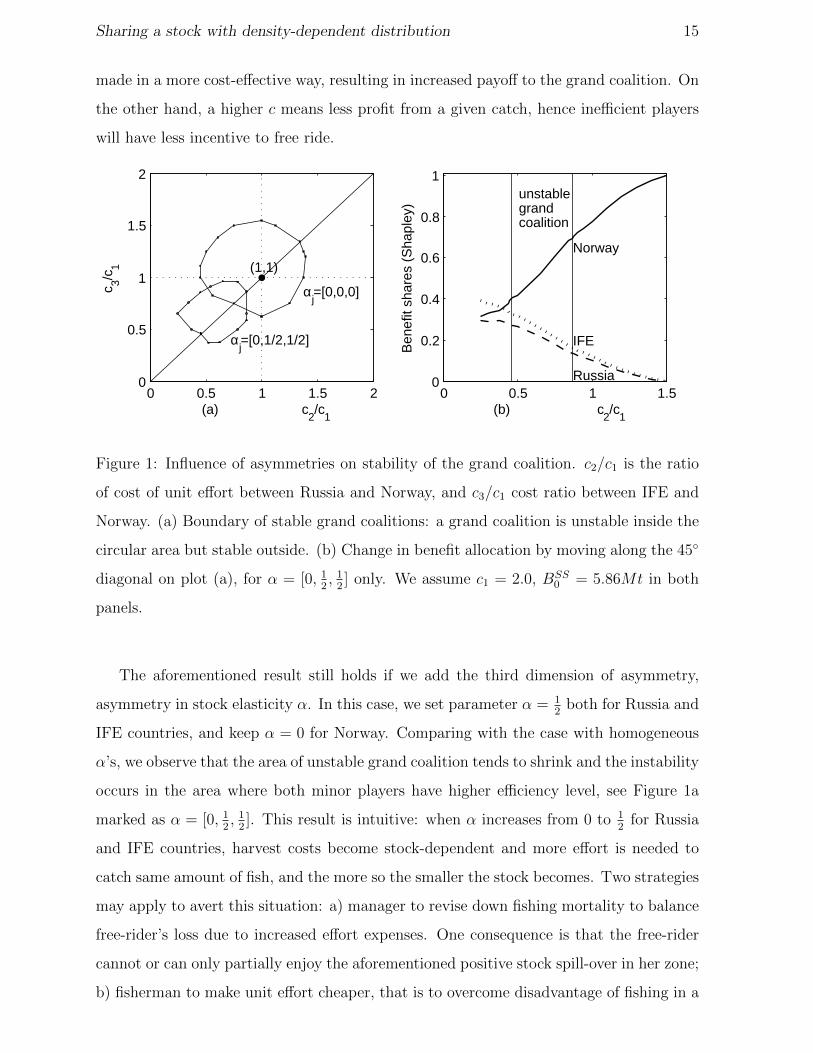
made in a more cost-effective way, resulting in increased payoff to the grand coalition. On

the other hand, a higher c means less profit from a given catch, hence inefficient players

will have less incentive to free ride.

0 0.5 1 1.5 20

0.5

1

1.5

2

αj=[0,0,0]

αj=[0,1/2,1/2]

(a) c2/c

1

c 3/c1 (1,1)

0 0.5 1 1.50

0.2

0.4

0.6

0.8

1

Norway

IFE

Russia

unstable grand coalition

(b) c2/c

1B

enef

it sh

ares

(S

hapl

ey)

Figure 1: Influence of asymmetries on stability of the grand coalition. c2/c1 is the ratio

of cost of unit effort between Russia and Norway, and c3/c1 cost ratio between IFE and

Norway. (a) Boundary of stable grand coalitions: a grand coalition is unstable inside the

circular area but stable outside. (b) Change in benefit allocation by moving along the 45◦

diagonal on plot (a), for α = [0, 12, 1

2] only. We assume c1 = 2.0, BSS

0 = 5.86Mt in both

panels.

The aforementioned result still holds if we add the third dimension of asymmetry,

asymmetry in stock elasticity α. In this case, we set parameter α = 12

both for Russia and

IFE countries, and keep α = 0 for Norway. Comparing with the case with homogeneous

α’s, we observe that the area of unstable grand coalition tends to shrink and the instability

occurs in the area where both minor players have higher efficiency level, see Figure 1a

marked as α = [0, 12, 1

2]. This result is intuitive: when α increases from 0 to 1

2for Russia

and IFE countries, harvest costs become stock-dependent and more effort is needed to

catch same amount of fish, and the more so the smaller the stock becomes. Two strategies

may apply to avert this situation: a) manager to revise down fishing mortality to balance

free-rider’s loss due to increased effort expenses. One consequence is that the free-rider

cannot or can only partially enjoy the aforementioned positive stock spill-over in her zone;

b) fisherman to make unit effort cheaper, that is to overcome disadvantage of fishing in a


low density stock by improving economic efficiency(a low c). By this way, the free-riding

incentive can still remain. Therefore, we observe that unstable grand coalition coincides

with the area in which Norway is the least efficient player (highest c).

If the grand coalition were not stable as the example showed in Table 1a, which

coalition will become the equilibrium coalition structure? Since the singleton is stable

by definition, hence it is always an equilibrium structure (Pintassilgo etal. 2010). Our

simulations show that singleton cannot be the optimal coalition structure, because Pareto

efficiency cannot be satisfied. Among three partial coalitions, some or all of them can be

the optimal coalition structures, depending on the model configuration. For the example

shown in Table 1, partial coalition formed by Norway and IFE is unstable, because PIS

condition cannot be satisfied, meaning Norway and Russia are worse off from forming a

coalition. The situation for other two partial coalitions is the opposite, hence both of

them can be the optimal coalition.

4.2 Sharing benefits

We will now focus on cases when the grand coalition is stable. We are particularly

interested in benefit allocation when Norway’s unique position and inherent advantage

are fully realized. Table 2 provides a such example where Norway, in addition to being

the largest stock owner, is the only player whose harvest costs are independent of stock

size, that is α = 0 for Norway and α = 12

for the other two players. But the two minor

players can compensate for their disadvantage by reducing their cost of fishing, namely

cost per unit effort c. The respective benefits shares received by Norway, IFE and Russia

are 38%, 34% and 28% according to Shapley value, and 37%, 30% and 33% according to

the Almost Ideal Sharing Scheme (AISS) with equal weights. The result suggests that,

in this particular example, none of the two benefit sharing rules can give Norway an

allocation of shares in excess of or in proportion to her shares of stock ownership which

is ≥ 54% of the total stock.

Figure 2 illustrates the model dynamics associated with the example in Table 2. Since

sharing benefits among the grand coalition members is also depends on the partition

functions of other coalition structures, it is helpful to compare dynamics of different

embedded coalitions. As expected, the grand coalition leads to the highest spawning

stock biomass (SSB) and singleton the lowest (Figure 2a). For any coalition, its total SSB


Table 2: Benefits allocation: αj = [0, 12, 1

2], cj = [2, 0.875, 0.875] NOK/e, j ∈

{Nor,Rus, IFE}. r = 5%, p0 = 1.3 NOK/kg, BSS0 = 5.58Mt.

Coalition F ref (yr−1) NPV (109 NOK)

structure Nor Rus IFE Nor Rus IFE

Singleton 0.143 0.318 0.233 5.21 2.67 3.39

{Nor Rus, IFE} 0.077 0.378 0.285 3.94 4.31 5.66

{Nor IFE, Rus} 0.048 0.409 0.318 2.85 4.95 6.70

{Nor, Rus IFE} 0.127 0.173 0.173 6.28 3.31 5.13

Grand (stable) 0.008 0.221 0.221 0.87 6.83 10.59

Sharing rule Benefit (109 NOK) Benefit share (%)

Shapley 6.98 5.15 6.16 38% 28% 34%

AISS 6.75 5.41 6.13 37% 30% 33%

converges to an equilibrium state after some fluctuations. Our model is deterministic and

this volatility is due to the age structure that makes equilibration of the biological model

slow.

We observed two features during the stock transition: first, the total SSB levels are

among the lowest in the transition years, but the total abundance of the fishable stock

still increases due to some transient effects (not shown in the figure); second, Norway

has higher stock shares due to lower total SSB levels, except the grand coalition case in

which stock distribution is uniform in time for each player (Figure 2c). These features,

together with assumption of heterogeneity in stock elasticity, i.e. αj = [0, 12, 1

2], enable

Norway to earn extra Shapley dividends during the two stock ’dips’. Because Norway has

higher fishable stock in her zone due to simultaneous increases of stock shares and total

fishable stock, Norway thus has her seasonal yields and profits increased in the initial

transition years. The two minor players, however, face double “belows”: on one hand,

both of them have to reduce their yields due to lower fishable stock in their zones and that

brings in less income; on the other hand, the marginal effort of yield increases with the

decreases of fishable stock in their zones, resulting in higher costs. A lower cost per unit

effort can help the two minor owners to reduce costs but does no help to improve their

incomes. Seasonal effort dynamics (Figure 2b) follow the development of yields described


above. For the two minor owners, they also adjust efforts against stock size in their zones.

As stock stabilizes, the difference in player’s seasonal Shapley values also becomes stable

(Figure 2d).

0 10 20 30 400

2

4

6

8

10x 109

SS

B

(a)

Grand

(Nor Rus, IFE)

Singleton

0 10 20 30 400

0.2

0.4

0.6

0.8

1

(c) Period

Sto

ck s

hare

in N

or. z

one

Grand(Nor Rus, IFE)Singleton

0 10 20 30 400

2

4

6x 108

Sea

sona

l effo

rt

(b)

Singleton

NorRusIFE

0 10 20 30 400

1

2

3

4x 108

Sea

sona

l Sha

pley

val

.

(d) Period

NorRusIFE

Figure 2: Model dynamics in terms of (a) spawning stock biomass, (b) fishing effort, (c)

proportion of the stock in Norwegian zone, and (d) seasonal Shapley value. Two horizontal

lines in (a) indicate two critical biomass levels; seasonal Shapley value in (d) is after

discounting. Parameter values: αj = [0, 12, 1

2], cj = [2, 0.875, 0.875], j ∈ {Nor,Rus, IFE};

BSS0 = 5.58Mt.

We will further investigate to what extent a lower cost per unit effort can help the two

minor players to offset their costs in face of inherent disadvantages. Figure 1b illustrates

how the benefit shares received by each country vary with the ratio c2/c1, assuming IFE

and Russia has the same cost per unit effort, i.e., c2 = c3. It shows that the benefit shares

for Norway, using Shapley value, sway from approximately 31% to 100%, depending on

her relative efficiency level in terms of c. If Norway’s efficiency level were far below that

of her competitors’ (e.g., c2/c1 / 0.4), her shares can even go below what IFE countries,

the second largest owner, obtain. The finding confirms that neither the largest stock

ownership, nor the inherently high fish density in Norwegian zone, can guarantee Norway


to receive the largest share of grand cooperation benefits. However, IFE countries always

receive a higher benefit share than Russia. This proves that the size of stock ownership

can finally take the lead if everything else is the same. But this result is not robust to

the alternative sharing rule, AISS.

4.3 Sensitivity

We choose to focus sensitivity test on three key parameters: the initial stock biomass, the

low critical biomass level and the discount rate.

0 10 20 30 40−2

0

2

4

6

8

10

12

14

16x 107

Sea

sona

l Sha

pley

val

., 19

69

Nor

IFE

Rus

0 10 20 30 400

2

4

6

8

10

12

14

16x 108

Sea

sona

l Sha

pley

val

., 19

50

(a) Period (b) Period

NorRusIFE

Figure 3: Effect of initial stock biomass on the seasonal Shapley values, assume

αj = [0, 12, 1

2], cj = [2.0, 0.875, 0.875], j ∈ {Nor,Rus, IFE}. (a) Low initial biomass:

BSS0 = 86Kt, ϕShapj = [44%, 25%, 31%]; (b) High initial biomass: BSS

0 = 16.6Mt,

ϕShapj = [28%, 31%, 41%].

So far, all results are based on assumption that the initial stock (BSS0 = 5.58Mt) is

slightly above the high critical biomass level (BSShigh = 5.0Mt). Due to discounting of

future payoffs, initial state is expected to matter for our results. Indeed, we find that

a low initial stock leads to higher benefit shares for Norway, while a high initial stock

has an opposite effect. The reason is three-fold: first, when stock is sufficiently small,

it takes time for the stock to recover and the period during which Norway controls the

stock is prolonged; second, it is more costly for IFE and Russia to harvest a small stock

due to lower fish density they experience in their zones; third, as stock recovers to certain

critical level over which the player is no longer constrained by the local density, her


fishing income increases with the decreases of harvest costs due to more fishable stock in

her zone. Figure 3 is a support of this reasoning, based on examples of two extreme years:

in year 1969 when the initial stock is extremely low (BSS0 = 0.086Mt), Norway’s seasonal

Shapley value surpasses her competitors’ with a great margin until the stock recovers. As

a result, Norway earns as much as 44% of the total benefits; in year 1950 when initial

stock is extremely high (BSS0 = 16.6Mt), Norway who is the least efficient(highest c)

player receives less than a third of the total benefits.

Is it in the interest of Norway to keep total stock so low that she becomes the sole

owner of the herring fishery? Norway is in the unique position in our model to achieve this.

To investigate this question, we vary BSSlow, the low critical biomass level, from 0.3Mt to

4.0Mt and compute singleton solutions for the representative case from Table 2 in section

4.2. The high critical level is kept unchanged. We find that, in a fully competitive game,

the stock biomass in the terminal year (B40) is always above the low critical biomass

level4 (BSSlow), see Figure 4a. However, we do see tendency that B40 approaches BSS

low as

the latter increases. Along the way, Norway increases the reference fishing mortality, but

other two countries harvest less (Figure 4b). Our results suggest that when BSSlow is low,

the opportunity cost is too high for Norway to push down the stock all the way to the

bottom in order to maintain her sole ownership. As a major owner with costs independent

of stock-size (α = 0), Norway is primarily interested in a relatively large, productive stock.

Whether the fish will spill over to other zones is immaterial; when BSSlow is high, Norway

has better control over the stock, because the sole ownership can be achieved now without

depressing the stock too much. Norway thus increases her harvest. If her competitors

would follow suit, they risk of loosing the stock. It can be seen here that a high BSSlow can

act as a threaten point for minor players. The described strategic interactions among the

players push the stock away from the low critical level.

5 Discussion and Conclusions

In this paper we have studied cooperation outcomes in the presence of dynamic stock

distribution, using NSSH fishery as a case study. In some important ways, our model

is more realistic than earlier game-theoretic harvesting models. Catch function in our

model is density-dependent, reflecting variable stock density in each zone that fishermen

4During the stock transition years, the total biomass can fall below BSSlow.


0 2 4 6

x 109

0

1

2

3

4

5

6x 109

(a) Low critical biomass

SS

B le

vel i

n ye

ar 4

0

SSB in yr 40

45° diagonal

0 1 2 3 4

x 109

0

0.05

0.1

0.15

0.2

0.25

0.3

0.35

0.4

(b) Low critical biomass

Fis

hing

mor

talit

y (F

ref )

Norway

IFE

Russia

Figure 4: Effect of low critical biomass on stock biomass and fishing mortality, αj =

[0, 12, 1

2], cj = [2.0, 0.875, 0.875], j ∈ {Nor,Rus, IFE}. BSS

high = 5Mt, BSS0 = 5.58Mt.

often experienced in practice, and allowing for unit costs of harvesting to depend on stock

size. Furthermore, we use a reference fishing mortality as the control parameter that

determines annual catch quotas, a practice that is common in real fishery management,

rather than control fishing effort. Treating fishing mortality as the control variable makes

fishing effort a dynamic variable that reflects changes in stock biomass.

We find that the likelihood of a stable grand coalition is positively correlated with

the degree of asymmetry in player’s cost per unit effort. The finding that ‘asymmetry

strengthens stability’ has also been reported in recent literature on international environ-

mental (McGinty 2007, Fuentes-Albero and Rubio 2010) and fishery agreements (Pintas-

silgo et al 2010). Indeed, increased asymmetry in harvesting costs enables a coalition to

exploit the resource in a more cost-effective way: the most efficient (the lowest c) player in

a coalition becomes the dominant exploiter of the coalition, and the least efficient (highest

c) player is compensated by receiving side-payment from the more efficient one(s). From

a single player perspective, an increase in c or α reduces her free-riding incentive due to

rising harvest costs, hence the player is more inclined to join a coalition. When a grand

coalition is not stable, a partial coalition always stands out as the optimal set-up, a sin-

gleton is an equilibrium strategy but not optimal because it always brings players worse

outcomes.

In case of stable grand coalitions, their “externality-free” Shapley values, a rule to


divide cooperative benefits for partition function games, respond drastically to players’

efficiency levels. It is not unexpected that a player’s potential benefits of cooperation

increase with her relative efficiency. We show that if Norway were the least efficient

player, it may happen that IFE countries (Iceland, Faroe Islands and EU) and Russia

would receive higher benefit shares than Norway. This finding is somewhat surprising

because Norway has a unique position in our model: first, she has a share of at least

54% of the stock (whatever distribution pattern prevails); second, the stock density in her

zone is inherently much higher than elsewhere. In 2003, the international agreement for

managing NSSH was suspended when Norway, based on the high affinity of NSSH to the

Norwegian EEZ, was requesting a higher quota than what the existing agreement gave

her (60%). However, our finding suggests that the high Norwegian ‘ownership’ cannot

secure her quota shares in excess of what stock distribution would suggest. Neither does

it guarantee that the economic benefits are shared in proportion to stock ownership. In

2007, Norway returned the NSSH agreement without an increased quota share. This

may be nothing more than a coincidence, but our model does show that the geographical

advantage of Norway might be offset by high cost of harvesting. Notice that in the model,

cost of harvesting only comes from cost per unit effort; in reality costs will also include

fixed labour costs, capital costs, etc.

The Shapley values are also sensitive to the initial stock state: a low initial stock

level brings greater benefit shares to Norway, and a high initial stock does the opposite.

A problematic effect can arise from a high stock: we found cases where a stable grand

coalition breaks down after the initial stock becomes sufficiently high. Similar observation

has been made by Hannesson (2006) who found that improved ocean condition (in terms

of higher environmental carrying capacity) can put full cooperation under strain. Indeed,

when stock is abundant, cooperation becomes less necessary for minor players, and a

more lucrative deal would probably have to be offered in order to ensure participation.

Under certain circumstances, full cooperation cannot generate sufficient payoffs to satisfy

all parties.

We find that it is not in the interest of Norway to push down the equilibrium stock

to the biomass level BSSlow, under which she becomes a sole owner. This result is robust

against change of BSSlow. Earlier herring studies presented mixed findings. Bjørndal et al.

(2004) showed non-migratory strategy is not attractive for Norway because ‘open access

with closures’ gives better outcomes. Their result is based on one particular biomass level,


i.e. BSSlow = 500 kt. We confirm that the result can also hold for other values, namely

any value in the range of 300 kt–4 Mt. Hannesson (2006) indicated it can be optimal for

Norway to keep stock at the BSSlow level if its level is high enough. However, he derived

optimal stock based on assumption both pla is ignored and the goal is to maximize rent

per year. In other words, fishing down the current stock has no economic consequence.

The goal in our model is to maximize net present values, and a high harvest rate in

current period will spoil future payoffs. Even though we found it is not optimal to keep

the equilibrium stock below the assumed low critical level, stock in transition years indeed

can sometimes go below it (typically between years 6–9), and the higher is the BSSlow level,

the longer duration in which the transition stock tends to stay.

Our model has provided new insights into management of a dynamic resource. Never-

theless, there are still many areas that can be looked into in future research. Our current

model is deterministic, whereas a key feature of Norwegian spring-spawning herring is

the highly variable, uncertain recruitment; Lindroos (2004) have already shown that bio-

logical uncertainty can reduce stability of full cooperation in herring. The management

regime in our model is quite rigid, and allowing for more flexibility may provide more

insights from real fishery management perspective. For example, one could allow players

to fish both in their own exclusive economic zones and the high seas, and to stop fishing

when it is not profitable.


A Appendix

Table A1: Stock share in representative years.

Stock shares (%)

Country 1950 1959 1972 1983

Norway 33.0 39.7 100 88.3

Russia 24.7 21.8 0 8.0

IFE 42.3 38.5 0 3.7

Table A2: Age-specific parameters

Age

class

Selectivity

s

Natural

mortality

M (yr−1)

Maturity

ogive O

Individual

weight in the

stock W S

(kg)

Individual

weight in the

catch WC

(kg)

0 0 0.9 0 0.001 0.007

1 0 0.9 0 0.0135 0.0548

2 0 0.9 0 0.025 0.1085

3 1 0.15 0.005 0.0745 0.159

4 1 0.15 0.155 0.152 0.2105

5 1 0.15 0.7125 0.2343 0.2508

6 1 0.15 1 0.2995 0.2955

7 1 0.15 1 0.3468 0.3237

8 1 0.15 1 0.3598 0.352

9 1 0.15 1 0.3825 0.3668

10 1 0.15 1 0.3875 0.376

11 1 0.15 1 0.4017 0.3718

12 1 0.15 1 0.4037 0.386

13 1 0.15 1 0.3945 0.39

14 1 0.15 1 0.4053 0.395

15 1 0.15 1 0.4033 0.3967

16 1 0.15 1 0.4138 0.3975


Table A3: Notational summary and age-unspecific parameters. ‘e’ denotes the unit of fishing

effort.

Subscripts definition Subscripts definition

i age 1 Norway

j country/player 2 Russia

t time 3 IFE

Variables definition unit

N abundance

N tot total fishable abundance

BSS spawning stock biomass Mt

Ctot catch target

C catch

E effort rate e

F ref reference fishing mortality yr−1

ρ local density

τ critical season length yr

τ e effective season length yr

π partition function NOK

v valuation function NOK

θ proportional stock share

NPV net present value NOK

Parameters definition value unit

α stock elasticity 0, 12

p0 price 1.3 NOK/kg

c cost per unit effort NOK/e

r discount rate 5%

h density parameter 1

β recruitment parameter 78.4 1/kg

γ recruitment parameter 3045 mill kg


References

Arnason R, Magnusson G, Agnarsson S (2000) The Norwegian spring-spawning herring

fishery: a stylized game model. Marine Resource Econ 15:293-319

Bailey M, Sumaila UR, Lindroos M (2010) Application of game theory to fisheries over

three decades. Fish Res 102:1–8

Bjørndal T, Gordon DV, Kaitala V, Lindroos M (2004) International management strate-

gies for a straddling fish stock: a bio-economic simulation model of the Norwegian spring-

spawning herring fishery. Environ Resource Econ 29:435–457

Brown, JS, Vincent TL (1987). Coevolution as an evolutionary game. Evolution 41:66–79

D’Aspremont C, Jacquemin A, Gabszewicz JJ, Weymark JA (1983) On the stability of

collusive price leadship. Can J Econ 16(1):17–25

De Clippel G, Serrano R (2008) Marginal contributions and externalities in the value.

Econometrica 76(6):1413-1436

Dieckmann U, Law R (1996) The dynamical theory of coevolution: a derivation from

stochastic ecological processes. J Math Biol 34:579–612

Dragesund O, Johannessen A, Ulltang Ø (1997) Variation in migration and abundance of

Norwegian spring spawning herring (Clupea harengus L). Sarsia 82:97–105

Ekerhovd NA (2010) The stability and resilience of management agreements on climate-

sensitive straddling fishery resources: the blue whiting (Micromesistius poutassou) coastal

state agreement. Can J Fish Aquat Sci 67:534–552

Eyckmans J, Finus M (2004) An almost ideal sharing scheme for coalition games with

externalities. Working paper no. 155.2004, Fondazione Eni Enrico Mattei, Italy. Version

presented at the 7th Meeting on game theory and practice dedicated to energy, environ-

ment and natural resources, May 2007, Montreal, Canada

Fuentes-Albero C, Rubio SJ (2010) Can international environmental cooperation be bought?

Europ J Oper Res 202:255–264

Golubtsov PV, McKelvey R (2007) The incomplete-information split-stream fish war:

examining the implications of competing risks. Natural Res Modeling 20:263–300


Greenberg J (1995) Coalition structures. In: Aumann R, Hart S (eds) Handbook of game

theory with applications, Vol 2. Amsterdam: North Holland, pp 1305-1337

Hannesson R (2006) Sharing the herring: fish migrations, strategic advantage and climate

change. In: Hannesson R (ed) Climate change and the economics of the world’s fisheries:

examples of small pelagic stocks. Edward Elgar Publishing, UK, pp 66–99

Hannesson R (2007) Global warming and fish migrations. Natural Res Modeling 20:301–

319

Heino M, Engelhard GH, Godø OR (2008) Migrations and hydrography determine the

abundance fluctuations of blue whiting (Micromesistius poutassou) in the Barents Sea.

Fish Oceanogr 17:153-163

Hilborn R, Walters CJ (1992) Quantitative fisheries stock assessment: Choice, dynamics

and uncertainty. Chapman and Hall, New York

ICES (2010) Report of the Working Group on Widely Distributed Stocks (WGWIDE), 28

August – 3 September 2010, Vigo, Spain. ICES CM 2010/ACOM:15, ICES, Copenhagen

Johnson JE, Welch DJ (2010) Marine fisheries management in a changing climate: a

review of vulnerability and future options. Rev Fish Sci 18:106–124

Kronbak LG, Lindroos M (2007) Sharing rules and stability in coalition games with ex-

ternalities. Marine Resource Econ 22:137-154

Lindroos M (2004) Sharing the benefits of cooperation in the Norwegian spring-spawning

herring fishery. Int Game Theory Rev 6:35–53

Lindroos M, Kaitala V (2000) Nash equilibria in a coalition game of the Norwegian spring-

spawning herring fishery. Marine Resource Econ 15:321–339

Liu X, Heino M (2011) Fishing game under changing climate: does anticipation of the

temperature change matter? Paper presented in the 18th Annual conference of European

association of environmental and resource economics, Rome, 29 June–2 July 2011

Macho-Stadler I, Perez-Castrillo D, Wettstein D (2007) Sharing the surplus: an extension

of the Shapley value for environments with externalities. J Econ Theory 135:339-356

Mantua NJ, Hare SR, Zhang Y et al(1997) A Pacific Interdecadal Climate Oscillation


with Impacts on Salmon Production. Bull Amer Meteor Soc 78(6):1069-79

McGinty M (2007) International environmental agreements among asymmetric nations.

Oxford Econ Pap 59:45-62

Miller KA, Munro GR (2004) Climate and cooperation: a new perspective on the man-

agement of shared fish stocks. Marine Resource Econ 19:367-393

Patterson K (1998) Biological modelling of the Norwegian spring-spawning herring stock.

Fisheries Research Services, Report 1/98, Aberdeen

Perry AL, Low PJ, Ellis JR, Reynolds JD (2005) Climate change and distribution shifts

in marine fishes. Science 308:1912–1915

Pham Do KH, Norde H (2007) The Shapley value for partition function form games. Int

Game Theory Rev 9(2):353-360

Pintassilgo P, Finus M, Lindroos M (2010) Stability and success of regional fisheries

management organizations. Environ Resource Econ 46:377–402

Sissener EH, Bjørndal T (2005) Climate change and the migratory pattern for Norwegian

spring-spawning herring–implications for management. Marine Pol 29:299–309

Shapley LS (1953) A value for n-person games. In: Roth A (ed) The Shapley Value —

Essays in Honor of Lloyd S. Shapley, Cambridge University Press, Cambridge), pp31-40

Steinshamn SI (2011) A conceptional analysis of dynamics and production in bioeconomic

models. Amer J Agr Econ 93:803–812

Thrall R, Lucas W (1963) n-person games in partition function form. Naval Res Logist

Quart 10:281-298

Toresen R, Østvedt OJ (2000) Variation in abundance of Norwegian spring-spawning

herring (Clupea harengus, Clupeidae) throughout the 20th century and the influence of

climatic fluctuations. Fish Fish 1:231–256

Yi S-S, Shin H (2000) Endogenous formation of research coalitions with spillovers. Int J

Ind Organ 18:229256

Sharing a Fish Stock with Density-dependent Distribution and Unit Harvest Costs

Documents

Transcript of Sharing a Fish Stock with Density-dependent Distribution and Unit Harvest Costs