Wo

rkin

g p

aper

sW

ork

ing

pap

ers

ng

pap

ers

Jorge González Chapela

Recreation, home production and intertemporal substitution of female labor supply: evidence on the intensive marginad

serie

WP-AD 2011-04

Los documentos de trabajo del Ivie ofrecen un avance de los resultados de las investigaciones económicas en curso, con objeto de generar un proceso de discusión previo a su remisión a las revistas científicas. Al publicar este documento de trabajo, el Ivie no asume responsabilidad sobre su contenido. Ivie working papers offer in advance the results of economic research under way in order to encourage a discussion process before sending them to scientific journals for their final publication. Ivie’s decision to publish this working paper does not imply any responsibility for its content. La Serie AD es continuadora de la labor iniciada por el Departamento de Fundamentos de Análisis Económico de la Universidad de Alicante en su colección “A DISCUSIÓN” y difunde trabajos de marcado contenido teórico. Esta serie es coordinada por Carmen Herrero. The AD series, coordinated by Carmen Herrero, is a continuation of the work initiated by the Department of Economic Analysis of the Universidad de Alicante in its collection “A DISCUSIÓN”, providing and distributing papers marked by their theoretical content. Todos los documentos de trabajo están disponibles de forma gratuita en la web del Ivie http://www.ivie.es, así como las instrucciones para los autores que desean publicar en nuestras series. Working papers can be downloaded free of charge from the Ivie website http://www.ivie.es, as well as the instructions for authors who are interested in publishing in our series. Edita / Published by: Instituto Valenciano de Investigaciones Económicas, S.A. Depósito Legal / Legal Deposit no.: V-845-2011 Impreso en España (febrero 2011) / Printed in Spain (February 2011)

WP-AD 2011-04

Recreation, home production, and intertemporal substitution of female labor supply: evidence on the intensive margin*

Jorge González Chapela**

Abstract The predicted labor supply responses to variations in wages and prices are important for discussions of the economic efficiency of taxes and subsidies, and their extent may be also relevant to the analysis of economic fluctuations. This paper presents new estimates of the wage intertemporal substitution elasticity (ISE) for the intensive margin of female labor supply, and explores this margin’s sensitivity to price changes of goods consumed in recreation and home production activities. Our estimated wage ISE, .9, implies that, at average values for the allocation of time, female labor force participants will increase annual labor supply by some 14 hours when faced with a 1% grow in the wage rate. Of this increase, approximately 7 hours will come from less leisure and the other 7 from less home production. Keeping constant the price of home consumption goods, the intensive margin of female labor supply is unaffected by variations in recreation goods prices. We also estimate an elasticity of substitution between time and goods in home production of approximately 2. Keywords: female labor supply, intertemporal substitution, system GMM estimation. JEL Classification: J22, C36. * This paper is a revised version of chapter 2 of my Universitat Pompeu Fabra dissertation. Its current shape owes a lot to the comments and encouragement of an anonymous Associate Editor and an anonymous Referee. I am also grateful to Kevin Reilly, Xavier Sala-i-Martin, Ernesto Villanueva, Antonio Ciccone, Lola Collado, David Domeij, Christian Dustmann, Daniel Hamermesh, Sergi Jiménez, Frank Kleibergen, Adriana Kugler, Alberto Meixide, Jose Maria da Rocha, seminar participants at the Universidad de Alicante, Universität Mannheim, Universidade de Santiago de Compostela, Universitat Pompeu Fabra, Mannheim Institute for the Economics of Aging, the Xth Spring Meeting of Young Economists, the 12th Panel Data Conference, the Work Pensions and Labour Economics Conference 2005, the Econometric Society World Conference 2005, and the 32nd International Association for Time Use Research Conference for helpful comments on previous versions of this paper and encouragement; to Donna Nordquist, of the Institute for Social Research at the University of Michigan, for diligent assistance with PSID data; to Joseph Altonji for generously provided unpublished material on married women’s intertemporal labor supply; and to Sharon Gibson and Mark Vendemia, of the U.S. Bureau of Labor Statistics, for able assistance with CPI and CE data. Support from the European Union (HPRN-CT-2002-00235), the Spanish Ministry of Education (ECO2008-05721/ECON), and the Instituto Valenciano de Investigaciones Economicas (Ivie) are gratefully acknowledged. ** J. González Chapela: University of Alicante. E-mail: jorge@merlin.fae.ua.es.

3

1 INTRODUCTION

The pioneering study on the intertemporal labor supply decisions of married women by

Heckman and MaCurdy (1980, 1982) estimated a wage elasticity that integrated the intensive

and extensive margins of labor supply in its response. Since the extent to which a labor supply

response is spread between marginal variations in market work and variations in the

probability of working is of considerable economic and policy interest, posterior research has

attempted to estimate the size of each individual margin. Zabel (1997), for example, estimated

wage elasticities for the intensive and extensive margins of married women’s intertemporal

labor supply centered, respectively, at .38 and .42. The corresponding estimates obtained by

Altonji (1982a) are .75 and .87. In both studies, the sum of the estimated elasticities is

substantially below the 2.23 estimate obtained (at 1,350 hours of market work) by Heckman

and MaCurdy (1982).1

The estimation procedure employed by Heckman and MaCurdy (1980, 1982) assumed

that labor supply falls continuously to zero in response to variations in wages. Yet, if there are

fixed costs associated with entry into the labor market, the lowest number of hours that a

worker will work may be substantially in excess of zero (see, e.g., Cogan, 1981). Hence,

Zabel (1997) and Altonji (1982a) relaxed the continuity assumption and estimated

discontinuous labor supply schedules.

Zabel’s (1997) estimates were obtained from household’s Euler equations for labor

supply and labor force participation. Recently, however, Domeij and Flodén (2006) have

demonstrated that the Euler equation approach induces a significant downward bias in the

1 The intertemporal substitution elasticity (ISE) that integrates the intensive and extensive

margins of labor supply in its response equals the sum of the two marginal ISEs. The proof is

straightforward and follows from the Law of Iterated Expectations (see Appendix A).

4

estimated elasticities when liquidity constraints are ignored.2 Although Altonji (1982a)

pursued an alternative approach, in which family expenditures on food are included in the

labor supply and participation equations to control for unobserved expectations and wealth,

his empirical results for married women were very preliminary.

In this paper, we present new estimates of the wage ISE for the intensive margin of

female labor supply. Similar to Altonji (1982a), we employ data on consumers’ expenditures

on restaurants to control for unobservable expectations and wealth. In addition, we test our

econometric model against a variety of specification failures. As discussed below, Zabel’s

(1997) and Altonji’s (1982a) estimates for the extensive margin may be further biased. The

estimation of the extensive margin is left for future research.

We also explore the sensitivity of women’s intertemporal labor supply to price

changes of goods consumed in recreation and home production activities. Gronau and

Hamermesh (2006) have recently documented that leisure is the daily activity (apart from

sleep) in which more time is consumed per dollar spent on the course of the activity. Hence,

variations in recreation goods prices might significantly alter the demand for leisure, and

demand, in turn, a reallocation of time to other pursuits. In González Chapela (2007), for

instance, the price of recreation goods was found to influence men’s intertemporal allocation

of time between market work and leisure. Since the extent to which women vary hours of

market work in response to wage changes has been found larger than that for men,3 this

2 The literature has pointed out other sources of downward bias. See Domeij and Flodén

(2006) for further discussion.

3 For men estimates, see e.g. MaCurdy (1981), Altonji (1986), Reilly (1994), Mulligan

(1999), and Ham and Reilly (2002). Blundell and MaCurdy (1999) survey the intertemporal

labor supply literature.

5

different response could extend to a model in which recreation goods and leisure were non-

separable within the period.

Although a simple dichotomy of market work and leisure may be a useful starting

point for analysis, Rupert et al. (2000) have shown that estimates of intertemporal substitution

elasticities obtained from life-cycle data on hours and wages may be problematic if work done

at home is neglected from the analysis. Hence, in the life-cycle labor supply model presented

in Section 2, consumers will be not only allowed to substitute leisure at one date for leisure at

other dates in response to wage or price changes, but also to substitute work in the market for

work in the home at a given date. Furthermore, they will be able to substitute time for

expenditures in response to fluctuations in the price of goods utilized in home production. The

result of the analysis will be a three-activity system—leisure, home production, and market

work, that will allow us to identify empirically labor force participants’ willingness to

substitute hours intertemporally in response to wage or price changes.

The data and econometric approach employed to estimate this system of structural

equations are discussed in Section 3. The main empirical results are presented in Section 4.

For the population of U.S. women of prime age, our estimated wage ISE for the intensive

margin of female labor supply in the neighborhood of .9. (For married women, the

corresponding estimate is approximately 1.2.) As predicted in Domeij and Flodén (2006), this

estimate is substantially higher than that obtained in Zabel (1997). It is also somewhat higher

than Altonji’s (1982a) preliminary estimate, a result that, as discussed below, seems driven by

the different instruments for wages and consumers’ expenditures. The intensive margin of

female intertemporal labor supply appears as unaffected by variations in recreation goods

prices, although it does react to changes in the price of home consumption goods: Our

estimated market time elasticity with respect to the price of home consumption goods is in the

neighborhood of -.7. If home production were excluded from the model’s specification, part

6

of this effect would be misleadingly attributed to recreation goods. A model detailed summary

is provided in Section 5.

2 THEORETICAL MODEL

Consider a consumer ( )i with preferences at age t represented by the utility function

1 11

1 11 1 1 11 11

1 11 1 1

1 1 1 1( )1 1 1

, , , , ( ) ( )it it itit it it it it it it it it it it

cU c x s l h x l s h

γ μη

σ θσ σ θ θψ κ

η γ μα χ

− −−

− −− − − −− −−

− −

− − −

− − − −= + +− − −

+ + , (1)

whose specific functional form allows giving concrete interpretations to the estimated

parameters. In this expression, recreation goods ( )x and leisure time ( )l are combined to

produce recreation such as the seeing of a play, whereas home consumption goods ( )s and

home production time ( )h are combined to produce home goods such as food. For

tractability, we assume that other consumption goods ( )c are not combined with time. The

parameters η , γ , and μ denote, respectively, the willingness to substitute c , recreation, and

home goods intertemporally, whereas σ and θ represent the ease of substitution at a given

date between market goods and time in the production of recreation and home goods,

respectively. Variables ψ , α , κ , and χ denote age-specific modifiers of tastes or household

production.

Consumer 'si intertemporal choice problem consists in maximizing expected lifetime

utility subject to an expected wealth constraint. Assuming that the lifetime preference

ordering is additively separable over periods of time,4 solutions for l and h are given by:

1 1 1( )xitit it it it it it

it

wl p w cσ σ γ

γ σ σ σ γ ησψ αα

− −− − −

⎛ ⎞⎟⎜ ⎟= +⎜ ⎟⎜ ⎟⎜⎝ ⎠ (2)

4 The intertemporal separability assumption is relaxed in the robustness analysis of the

empirical results.

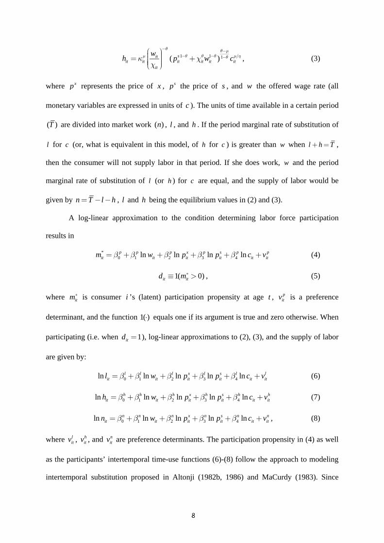
7

1 1 1( )sitit it it it it it

it

wh p w cθ θ μ

μ θ θ θ μ ηθκ χχ

− −− − −

⎛ ⎞⎟⎜ ⎟= +⎜ ⎟⎜ ⎟⎜⎝ ⎠, (3)

where xp represents the price of x , sp the price of s , and w the offered wage rate (all

monetary variables are expressed in units of c ). The units of time available in a certain period

( )T are divided into market work ( )n , l , and h . If the period marginal rate of substitution of

l for c (or, what is equivalent in this model, of h for c ) is greater than w when l h T+ = ,

then the consumer will not supply labor in that period. If she does work, w and the period

marginal rate of substitution of l (or h ) for c are equal, and the supply of labor would be

given by n T l h= − − , l and h being the equilibrium values in (2) and (3).

A log-linear approximation to the condition determining labor force participation

results in

*0 1 2 3 4ln ln ln lnp p p x p s p p

it it it it it itm w p p c vβ β β β β= + + + + + (4)

1( 0)it itd m∗≡ > , (5)

where itm∗ is consumer i ’s (latent) participation propensity at age t , pitv is a preference

determinant, and the function 1( )⋅ equals one if its argument is true and zero otherwise. When

participating (i.e. when 1itd = ), log-linear approximations to (2), (3), and the supply of labor

are given by:

0 1 2 3 4ln ln ln ln lnl l l x l s l lit it it it it itl w p p c vβ β β β β= + + + + + (6)

0 1 2 3 4ln ln ln ln lnh h h x h s h hit it it it it ith w p p c vβ β β β β= + + + + + (7)

0 1 2 3 4ln ln ln ln lnn n n x n s n nit it it it it itn w p p c vβ β β β β= + + + + + , (8)

where litv , h

itv , and nitv are preference determinants. The participation propensity in (4) as well

as the participants’ intertemporal time-use functions (6)-(8) follow the approach to modeling

intertemporal substitution proposed in Altonji (1982b, 1986) and MaCurdy (1983). Since

8

current decisions on c incorporate information on wealth and on expected prices, wages, and

preferences, c is taken as a “sufficient statistic” for unobservable expectations and wealth.

Important advantages of this approach are its independence of strong expectational

assumptions such as perfect foresight or rational expectations, and that liquidity constraints do

not enter the equations (Domeij and Flodén, 2006). An important disadvantage, the fact that

goods and time must be separable within the period in order to identify the intertemporal

substitution elasticities, is less marked in this study, where separability of goods from time

concerns c only.

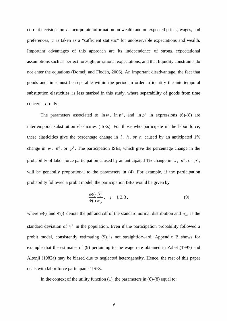
The parameters associated to ln w , ln xp , and ln sp in expressions (6)-(8) are

intertemporal substitution elasticities (ISEs). For those who participate in the labor force,

these elasticities give the percentage change in l , h , or n caused by an anticipated 1%

change in w , xp , or sp . The participation ISEs, which give the percentage change in the

probability of labor force participation caused by an anticipated 1% change in w , xp , or sp ,

will be generally proportional to the parameters in (4). For example, if the participation

probability followed a probit model, the participation ISEs would be given by

( ) , 1, 2,3( ) p

pj

v

jβφσ

⋅=

Φ ⋅, (9)

where ( )φ ⋅ and ( )Φ ⋅ denote the pdf and cdf of the standard normal distribution and pvσ is the

standard deviation of pv in the population. Even if the participation probability followed a

probit model, consistently estimating (9) is not straightforward. Appendix B shows for

example that the estimates of (9) pertaining to the wage rate obtained in Zabel (1997) and

Altonji (1982a) may be biased due to neglected heterogeneity. Hence, the rest of this paper

deals with labor force participants’ ISEs.

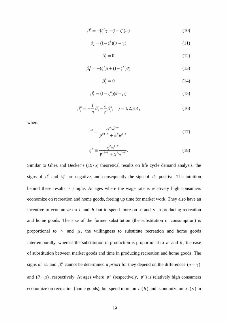
In the context of the utility function (1), the parameters in (6)-(8) equal to:

9

1 ( (1 ) )l l lβ ζ γ ζ σ=− + − (10)

2 (1 )( )l lβ ζ σ γ= − − (11)

3 0lβ = (12)

1 ( (1 ) )h h hβ ζ μ ζ θ=− + − (13)

2 0hβ = (14)

3 (1 )( )h hβ ζ θ μ= − − (15)

, 1, 2,3,4n l hj j j

l h jn n

β β β=− − = , (16)

where

1

1 1l

x

wp w

σ σ

σ σ σ

αζ

α

−

− −≡+

(17)

1

1 1h

s

wp w

θ θ

θ θ θ

χζ

χ

−

− −≡+

. (18)

Similar to Ghez and Becker’s (1975) theoretical results on life cycle demand analysis, the

signs of 1lβ and 1

hβ are negative, and consequently the sign of 1nβ positive. The intuition

behind these results is simple. At ages where the wage rate is relatively high consumers

economize on recreation and home goods, freeing up time for market work. They also have an

incentive to economize on l and h but to spend more on x and s in producing recreation

and home goods. The size of the former substitution (the substitution in consumption) is

proportional to γ and μ , the willingness to substitute recreation and home goods

intertemporally, whereas the substitution in production is proportional to σ and θ , the ease

of substitution between market goods and time in producing recreation and home goods. The

signs of 2lβ and 3

hβ cannot be determined a priori for they depend on the differences ( )σ γ−

and ( )θ μ− , respectively. At ages where xp (respectively, sp ) is relatively high consumers

economize on recreation (home goods), but spend more on l ( h ) and economize on x ( s ) in

10

producing recreation (home goods). In terms of the demand for l ( h ), which of these two

opposing substitution effects dominates is an empirical matter.5 The results 3 0lβ = and

2 0hβ = are a consequence of the block additivity of within-period preferences and can be

tested in the data. If the utility function were strictly concave and x , l , s , and h were normal

goods, 4lβ and 4

hβ would be positive, and 4nβ negative.

3 DATA AND ESTIMATION METHOD

3.1 Data

The data to estimate (6)-(8) are from two different sources and are aggregated at two different

levels: consumer-level data on hours, wages, and consumption expenditures from the Panel

Study of Income Dynamics (PSID), and metropolitan area-level price indices from the U.S.

Bureau of Labor Statistics (BLS). PSID information on hours refers to a typical week, and is

then annualized. Market work includes time on the main job, secondary job(s), and overtime,

whereas home production time is defined as “time spent cooking, cleaning, and doing other

work around the house.” Leisure is obtained as the residual category from total annual hours

( 8760T = ). Two indicators for the hourly wage are available. The first (denoted hereafter

*w ) is constructed as total labor earnings divided by hours worked in the market. The second

5 The signs of 2

lβ and 3hβ can be alternatively interpreted using, as in Heckman (1974), the

“direct” definition of complementarity. Consider for example the demand for l . When γ σ>

x and l are direct complements, in the sense that a reduction in the consumption of x

diminishes the marginal utility from consuming l . Thus, at ages where xp is relatively high

the consumer has an incentive to economize on both x and l , and 2 0lβ < . The opposite occurs

when σ γ> , i.e. when x and l are direct substitutes, for then the consumer has an incentive

to economize on x but to spend more on l at ages where xp is relatively high.

11

**( )w stems from the question “What is your hourly wage rate for your regular work?”, and is

only available for those who are paid on an hourly basis. PSID data on consumption

expenditures are limited to food used at home and expenditures on restaurants. The question

about expenditures on restaurants is: “About how much do you (or anyone else in your

family) spend eating out, not counting meals at work or at school?” Amounts generally refer

to a typical week or month, and are then annualized.6

Since expenditures on food at home can be considered a measure of s , we use

expenditures on restaurants as an empirical counterpart to c . For this approach to be

workable, however, the expenditures on restaurants data should be sufficiently accurate, plus

the limitation of c to expenditures on restaurants should not have an important effect on the

results. Regarding the first issue, Browning et al. (2003) note that the information about

specific expenditures collected by means of recall questions tends to be valid. Also, our first-

stage equation for consumption shows satisfying explanatory power and reasonable results.

The second issue hinges on the degree of separability between expenditures on restaurants

and expenditures on other goods belonging to c . The maintained assumption in this study is

that c is the sum of food expenditures on restaurants raised to an exponent plus expenditures

on some other market goods.

Since 1976, the BLS records the price variation of several groups of commodities,

such as “Entertainment” and “Food at home”, for the 27 metropolitan areas (MAs) listed in

the Data Appendix. Included in “Entertainment” are reading materials, sporting goods and

equipment, toys, hobbies, music equipment, photographic supplies and equipment, pet 6 Questions about expenditures on restaurants, **w , home production time, as well as the

residence area refer to the time of the interview (typically March), whereas market time and

labor earnings refer to the preceding calendar year. To avoid inconsistencies in timing, market

time and labor earnings are forwarded one year.

12

supplies and expense, club memberships, fees for participant sports, admissions, fees for

lessons or instructions, and other entertainment services.7 Included in “Food at home” are

cereals and bakery products, meats, poultry, fish, eggs, dairy products, fruits and vegetables,

and other food at home. For the period 1984-1993, “Entertainment” and “Food at home”

represented, respectively, an average of 5 and 9% of consumer expenditures (CE, 2010). We

take the log of the price indices for “Entertainment” and “Food at home” as empirical

counterparts to ln xp and ln sp . Figure 1 presents the evolution of both indices for selected

MAs (all monetary variables are deflated using the “Food away from home” component of the

CPI). Time-series as well as cross-sectional variation are evident, with the former sort of

variation being more important: the time-series sample standard deviations of xp and sp are,

respectively, 6.7 and 5.9, whereas the cross-sectional one amounts to 3.1 in both cases. Both

sorts of variation are considered exogenous to an individual consumer.

The MA-level price indices are combined with the data at the consumer level using the

geographical identifier available in the PSID. We use information from waves 9-26 of the

PSID for the calendar years 1976-19938 to construct two different samples. One sample is

limited to observations of women aged 25-60, residing in MAs with available price indices,

and reporting positive expenditures on restaurants. The other sample additionally requires that

women were paid by the hour at least one year of the study period.9 The positive expenditures 7 Until 1997, audio and video products were part of the “Housing” major group of the

Consumer Price Index (CPI).

8 The 1993 limit is due to contractual arrangements for the use of PSID Sensitive Data Files.

These data are not available from the author. Persons interested in obtaining PSID Sensitive

Data Files should contact through the Internet at PSIDHelp@isr.umich.edu.

9 The Data Appendix lists the full set of selection criteria and provides descriptive statistics of

the main variables used in this study.

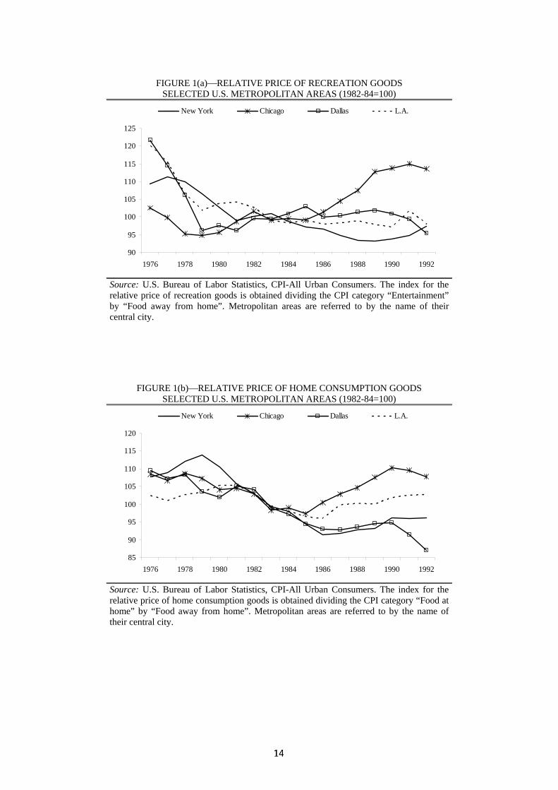
45

FIGURE 1(a)⎯RELATIVE PRICE OF RECREATION GOODS

SELECTED U.S. METROPOLITAN AREAS (1982-84=100)

90

95

100

105

110

115

120

125

1976 1978 1980 1982 1984 1986 1988 1990 1992

New York Chicago Dallas L.A.

Source: U.S. Bureau of Labor Statistics, CPI-All Urban Consumers. The index for the relative price of recreation goods is obtained dividing the CPI category “Entertainment” by “Food away from home”. Metropolitan areas are referred to by the name of their central city.

FIGURE 1(b)⎯RELATIVE PRICE OF HOME CONSUMPTION GOODS SELECTED U.S. METROPOLITAN AREAS (1982-84=100)

85

90

95

100

105

110

115

120

1976 1978 1980 1982 1984 1986 1988 1990 1992

New York Chicago Dallas L.A.

Source: U.S. Bureau of Labor Statistics, CPI-All Urban Consumers. The index for the relative price of home consumption goods is obtained dividing the CPI category “Food at home” by “Food away from home”. Metropolitan areas are referred to by the name of their central city.

13

on restaurants requirement is a consequence of the (notional) demand for restaurant meals

being only observed when it is positive. About 19 percent of the observations that satisfy the

other criteria for inclusion in the larger sample are excluded as a result. The requirement of

being paid by the hour at least once is a consequence of including an individual-specific

permanent component of the wage (denoted iw and its estimate **iw ) in the instrument set for

certain endogenous regressors pointed out below. The **iw are obtained from a regression of

**ln itw on dummy variables for each woman.10 Hence, if a woman is never paid by the hour

her iw is unknown. The resulting sample is much smaller and possibly less representative (42

percent of the observations that satisfy the other criteria for inclusion are excluded as a result),

but the inclusion of **iw in the instrument set will allow us to test overidentifying restrictions.

The full sample contains 3,917 women contributing a total of 19,286 observations. Of these,

14,224 correspond to labor force participants (i.e. women who worked for money some time

in the survey year). The hourly-paid subsample contains 1,868 women contributing a total of

11,282 observations. Of these, 9,724 correspond to participants and 5,486 to hourly-paid

participants.

3.2 Estimation Method

Assuming that the preference determinants are a linear function of observed and unobserved

characteristics of the person,

, , ,g v g git it v itv g l h nε′= + =x β , (19)

equations (6)-(8) can be written (more compactly) as 10 Included in this dummy-variable regression are also variables that fluctuate over time: year

and MA dummies, a capacity for work indicator, actual labor force experience and experience

squared, the interaction of experience with schooling, and controls for self-selection into the

labor force (an inverse Mills ratio term interacted with year dummies).

14

ln , , ,g git it itg g l h nε′= + =x β , (20)

with (1, ln , ln , ln , ln , )x s vit it it it it itw p p c ′ ′≡x x and 0 1 2 3 4( , , , , , )g g g g g g g

vβ β β β β ′ ′≡β β . Included in vx

are a quadratic in age, marital status, family size, number of children in different age intervals,

an indicator of capacity for work, a race indicator, as well as year and MA dummies. The

capacity for work indicator is constructed from answers to “Do you have a physical or

nervous condition that limits the type of work, or the amount of work you can do?” Although

there are a number of reasons to be suspicious about self-reported work limitations (see for

example Bound, 1991), alternative health measures are not available in most PSID waves. It

is assumed that ( ) 0git iE ε =x , where 1( , , )

ii i iT′ ′≡x x x… and iT is person si′ number of

periods in the panel.11

The evidence we have makes it clear that survey responses are not perfectly reliable

(see for instance Altonji, 1986; Bound, Brown, and Mathiowetz, 2001; French, 2004), and our

measures of hours, wages, and expenditures on restaurants may thus contain error:

ln ln , , ,git it itg g e g l h n∗ = + = , (21)

ln ln wit it itw w e∗ = + , (22)

ln ln cit it itc c e∗ = + . (23)

In these expressions, ge , we , and ce are measurement errors (assumed to be independent of

the true values), whereas *ln g , *ln w , and *ln c denote the natural log of observed hours,

average wage rates, and expenditures on restaurants, respectively. Correlation of we

11 The reason why (20) as well as the reduced-form labor force participation equation (24) do

not contain an explicit time-constant, unobserved effect is twofold. Cross-sectional variation

in wages and prices aids in identifying the ISEs. Results in Greene (2004) suggest that when

iT is small the pooled probit estimator of (24) is preferred to the fixed effects probit.

15

(respectively, ce ) with *ln w ( *ln c ) would tend to attenuate the estimated 1gβ ( 4

gβ ). Since *n

enters the definition of *w and *l , it is also plausible that ne and we be negatively correlated

and le and we positively correlated, further biasing the estimated 1nβ and 1

lβ . Also, if

consumers with a strong taste for c work more hours in the market and demand less leisure,

the estimated 4nβ (respectively, 4

lβ ) would be positively (negatively) biased if this taste were

imperfectly controlled for. We follow Altonji (1986) and Mroz (1987) and use **iw , actual

years of labor force experience, and experience squared to instrument *ln w and *ln c . More

precisely, these three variables are utilized in the hourly-paid sub-sample to predict *ln w and

*ln c , whereas in the full sample we instrument with experience and the square of this only.

Altonji (1986) argues that since the **iw estimate a permanent determinant of wages, they

should be orthogonal to unsystematic errors of measurement. Mroz (1987) does not reject the

validity of experience (measured as number of years worked for money since the 18th

birthday)12 and its square as an instrument for *ln w after controlling for self-selection into the

labor force. Both **iw and experience are important determinants of lifetime wages and should

be related to *ln w and *ln c .

As it is well-known, if the group of labor force participants is not (conditionally)

representative of the whole population, straightforward methods might result in inconsistent

estimation. To control for possible sample selectivity when estimating (20) using data on

participants only, let the reduced-form participation propensity be given by

it it itm v∗ ′= +z q , (24)

12 This information is asked of all heads/wives of PSID families in 1976 and 1985, and of all

new heads/wives in all other waves. Experience is then increased in one year when annual

market hours are positive.

16

where itv is an error term assumed standard normally distributed13 and independent of

1( , , )ii i iT′ ′≡z z z… . Besides an intercept, z includes ln xp , ln sp , and the instruments and

preference determinants listed above. Assuming that

( , ) , , ,g git i it itE v v g l h nλε β= =z , (25)

the estimating system of time-use equations becomes

ln , , ,g git it itg u g l h n′= + =x β , (26)

with ( , ( ))it it itλ′ ′ ′≡x x z q , ( , )g g gλβ′ ′≡β β , and ( )( )

( )φ

λ⋅

⋅ ≡Φ ⋅

(see Heckman, 1979). Substituting

(21)-(23) into (26), and defining * * * *(ln , ln , ln )it it it itl h n ′≡y , * *3( )it itI ′≡ ⊗X x , ( , , )l h n′ ′ ′ ′≡β β β β ,

and * * * *( , , )l h nit it it itu u u ′≡u , where the starred notation emphasizes that imperfect measures have

replaced true values and ⊗ is the Kronecker product symbol, we obtain

* * *it it it= +y X β u . (27)

The (pooled) probit estimate of q is obtained from the model ( 1 ) ( )it i itP d ′= =Φz z q

using all observations, and then ˆ( )itλ ′z q is included in *itx interacted with year dummies to

allow for time-varying selection effects. β is estimated by solving

* * * *

1 1 1 1

ˆmin ( ) ( )i iT TN N

it it it it it iti t i t= = = =

′⎡ ⎤ ⎡ ⎤⎢ ⎥ ⎢ ⎥′ ′− −⎢ ⎥ ⎢ ⎥⎣ ⎦ ⎣ ⎦∑∑ ∑∑b

Z y X b W Z y X b (28)

on the sample of participants, with 3( )it itI ′≡ ⊗Z z , 1ˆˆ −=W Λ , and where our estimator of

*( )it itVar ′≡Λ Z u ,

13 In their examination of women's labor supply decisions with PSID data, Newey et al.

(1990) conclude that parameter estimates are not sensitive to distributional assumptions of the

unobservable error terms.

17

1 * *

1 1 1 1

ˆ ˆ ˆ( ) (( )( ))i iT TN N

i it it it iti i t t

T −

= = = =

′′≡ ∑ ∑ ∑ ∑Λ Z u u Z , (29)

allows for arbitrary heteroskedasticity, permits * *( )it it itE ′u u Z changing across observations,

and allows for arbitrary correlation among observations belonging to i .14

4 EMPIRICAL RESULTS

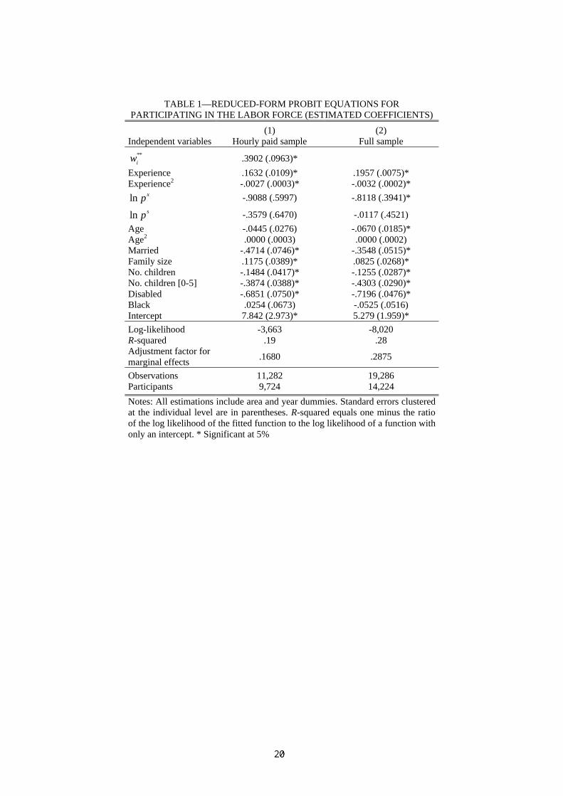
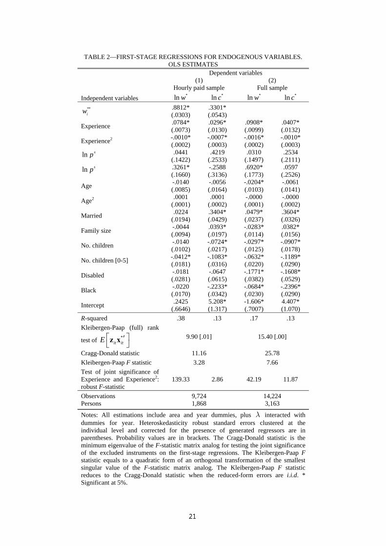
Tables 1 and 2 present, respectively, reduced-form probit regressions for the decision to

participate in the labor force and OLS regressions for *ln w and *ln c . Table 1 presents

estimated probit coefficients as well as an adjustment factor that allows computing the

marginal effect of continuous variables and an approximation to the marginal effect of

discrete variables. The marginal effect of a probit model is ( ) ( ) kk

qz

φ′∂Φ ′=

∂z q z q , and the

adjustment factor (evaluated at mean values of the regressors) is ( )φ ′z q . Standard errors,

shown in parentheses, are clustered at the individual level in Table 1, and are additionally

robust to heteroskedasticity and corrected for the presence of generated regressors in Table

2.15 Probability values are in brackets.

The reduced-form probit regressions yield similar results in both samples. Being

married or suffering from a limitation in the type or amount of work that can be done strongly

reduce the probability of labor force participation. The presence of children has a negative 14 Lee (2004) shows that this system Generalized Method of Moments (SGMM) estimator is

generally more efficient than the equation-by-equation GMM estimator, a result that still

holds in the presence of common instruments across equations.

15 When the interaction of λ with year dummies is statistically significant, standard errors are

corrected for the presence of estimated parameters in λ . The correct standard errors for the

most general model estimated in the paper are derived in Appendix D. The standard errors for

the other models are simple special cases.

39

TABLE 1—REDUCED-FORM PROBIT EQUATIONS FOR PARTICIPATING IN THE LABOR FORCE (ESTIMATED COEFFICIENTS)

Independent variables (1)

Hourly paid sample (2)

Full sample **iw .3902 (.0963)*

Experience .1632 (.0109)* .1957 (.0075)* Experience2 -.0027 (.0003)* -.0032 (.0002)* ln xp -.9088 (.5997) -.8118 (.3941)*

ln sp -.3579 (.6470) -.0117 (.4521) Age -.0445 (.0276) -.0670 (.0185)* Age2 .0000 (.0003) .0000 (.0002) Married -.4714 (.0746)* -.3548 (.0515)* Family size .1175 (.0389)* .0825 (.0268)* No. children -.1484 (.0417)* -.1255 (.0287)* No. children [0-5] -.3874 (.0388)* -.4303 (.0290)* Disabled -.6851 (.0750)* -.7196 (.0476)* Black .0254 (.0673) -.0525 (.0516) Intercept 7.842 (2.973)* 5.279 (1.959)* Log-likelihood -3,663 -8,020 R-squared .19 .28 Adjustment factor for marginal effects .1680 .2875

Observations 11,282 19,286 Participants 9,724 14,224 Notes: All estimations include area and year dummies. Standard errors clustered at the individual level are in parentheses. R-squared equals one minus the ratio of the log likelihood of the fitted function to the log likelihood of a function with only an intercept. * Significant at 5%

40

TABLE 2—FIRST-STAGE REGRESSIONS FOR ENDOGENOUS VARIABLES.

OLS ESTIMATES Dependent variables

(1)

Hourly paid sample (2)

Full sample Independent variables *ln w *ln c *ln w *ln c

**iw .8812*

(.0303) .3301* (.0543)

Experience .0784* (.0073)

.0296* (.0130)

.0908* (.0099)

.0407* (.0132)

Experience2 -.0010* (.0002)

-.0007* (.0003)

-.0016* (.0002)

-.0010* (.0003)

ln xp .0441 (.1422)

.4219 (.2533)

.0310 (.1497)

.2534 (.2111)

ln sp .3261* (.1660)

-.2588 (.3136)

.6920* (.1773)

.0597 (.2526)

Age -.0140 (.0085)

-.0056 (.0164)

-.0204* (.0103)

-.0061 (.0141)

Age2 .0001 (.0001)

.0001 (.0002)

-.0000 (.0001)

-.0000 (.0002)

Married .0224 (.0194)

.3404* (.0429)

.0479* (.0237)

.3604* (.0326)

Family size -.0044 (.0094)

.0393* (.0197)

-.0283* (.0114)

.0382* (.0156)

No. children -.0140 (.0102)

-.0724* (.0217)

-.0297* (.0125)

-.0907* (.0178)

No. children [0-5] -.0412* (.0181)

-.1083* (.0316)

-.0632* (.0220)

-.1189* (.0290)

Disabled -.0181 (.0281)

-.0647 (.0615)

-.1771* (.0382)

-.1608* (.0529)

Black -.0220 (.0170)

-.2233* (.0342)

-.0684* (.0230)

-.2396* (.0290)

Intercept .2425 (.6646)

5.208* (1.317)

-1.606* (.7007)

4.407* (1.070)

R-squared .38 .13 .17 .13 Kleibergen-Paap (full) rank

test of *it itE z x⎡ ⎤′

⎣ ⎦ 9.90 [.01] 15.40 [.00]

Cragg-Donald statistic 11.16 25.78 Kleibergen-Paap F statistic 3.28 7.66 Test of joint significance of Experience and Experience2: robust F-statistic

139.33 2.86 42.19 11.87

Observations 9,724 14,224 Persons 1,868 3,163

Notes: All estimations include area and year dummies, plus λ interacted with dummies for year. Heteroskedasticity robust standard errors clustered at the individual level and corrected for the presence of generated regressors are in parentheses. Probability values are in brackets. The Cragg-Donald statistic is the minimum eigenvalue of the F-statistic matrix analog for testing the joint significance of the excluded instruments on the first-stage regressions. The Kleibergen-Paap F statistic equals to a quadratic form of an orthogonal transformation of the smallest singular value of the F-statistic matrix analog. The Kleibergen-Paap F statistic reduces to the Cragg-Donald statistic when the reduced-form errors are i.i.d. * Significant at 5%.

18

effect too, with pre-school children having the strongest effect by far. The price of recreation

goods is negatively associated to the probability of participating: at mean values of the

regressors, a 1% increase in xp reduces the probability by .002.16 Estimates are imprecise,

but attain statistical significance in the full sample. Experience is a strong predictor for

participating in the labor force, whose likelihood increases with years of experience until

reaching some 30 years, and decreases from that moment on. Perhaps not surprisingly,

women with a higher **iw are more likely to participate, with a 1 standard deviation increase

in **iw raising the probability of participating by .032.17

In the first-stage regressions for endogenous variables (Table 2), all excluded

instruments present expected signs and are statistically significant at the .05 level. With two

endogenous regressors, however, the statistical significance of the excluded instruments is not

sufficient in general to identify β , for identification requires that the matrix *it itE z x⎡ ⎤′

⎣ ⎦ have

full rank (see, e.g., Wooldridge, 2002, p. 188).18 We have tested the null of *it itE z x⎡ ⎤′

⎣ ⎦ not

having full rank using the Kleibergen and Paap (2006) rank test, which is robust to arbitrary

heteroskedasticity and serial correlation in the errors of the reduced-form regressions. The test

statistic, a quadratic form of an orthogonal transformation of the smallest singular value of

16 Since the dependent variable is measured in levels and the explanatory variable is in logs,

this effect is obtained as the product of the estimated coefficient associated to ln xp times the

adjustment factor divided by 100.

17 The **iw , which are the fixed effects in a regression for **ln itw , are normalized and have a

mean of 0. Their sample standard deviation is .4896.

18 Equivalently, identification requires that the matrix with the reduced-form coefficients

associated to the excluded instruments have full rank (Wooldridge, 2002, p. 214).

19

*it itE z x⎡ ⎤′

⎣ ⎦, is asymptotically distributed as 2χ with degrees of freedom equal to the number

of overidentifying restrictions plus one. In the hourly paid sample, where the instrument set

contains **iw , experience, and experience squared, the p-value of the rank test is .007, whereas

in the full sample, where the instrument set contains experience and experience squared only,

it amounts to .000. Therefore, both instrument sets appear as adequate to identify β . The

other estimated effects in Table 2 are generally expected,19 including those for *ln c , which

provides some reassurance that the expenditures on restaurants data are sufficiently accurate

for the problem at hand.

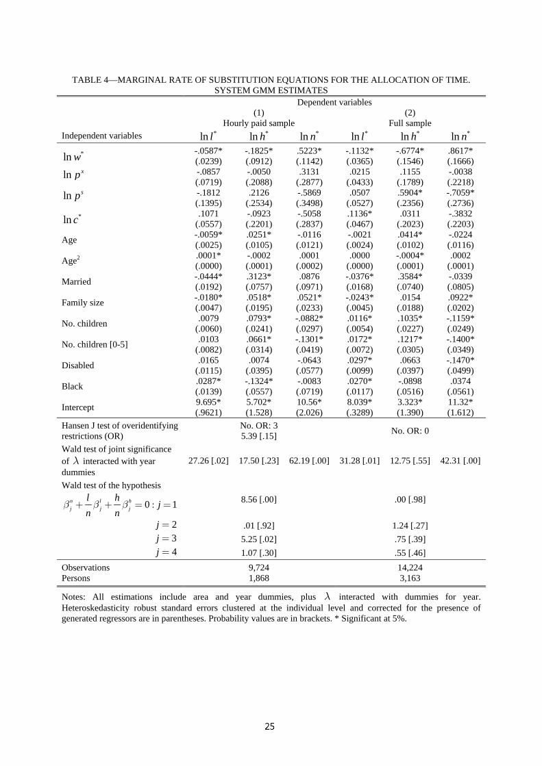
Tables 3 and 4 present the main estimates of the time-use equations (27). In Table 3,

OLS coefficients, which do not control for the endogeneity of *ln w and *ln c , are presented.

In the first three columns of Table 4, **iw , labor force experience, and experience squared are

used as instruments for *ln w and *ln c . Results presented in the last three columns of Table 4

are obtained instrumenting with experience and the square of this only. Heteroskedasticity

robust standard errors clustered at the individual level and corrected for the presence of

generated regressors are shown in parentheses, and probability values in brackets.

When *ln w and *ln c are treated as exogenous, the estimated wage effects on l , h ,

and n are around .01, -.16, and .14, respectively. Estimates are precise and attain statistical

significance at the .05 level. For labor force participants, the labor supply ISE with respect to

19 The negative association between the number of children and *ln w even after controlling

for experience is due to our notion of experience not accounting for the human capital

foregone in partial market time reductions. If, for example, experience were only augmented

when annual market hours were at least 2000, the partial correlations between children and

*ln w would not be statistically different from zero.

41

TABLE 3—MARGINAL RATE OF SUBSTITUTION EQUATIONS FOR THE ALLOCATION OF TIME.

OLS ESTIMATES Dependent variables (1)

Hourly paid sample (2)

Full sample Independent variables *ln l *ln h *ln n *ln l *ln h *ln n

*ln w .0080* (.0040)

-.1323* (.0184)

.1194* (.0220)

.0102* (.0029)

-.1788* (.0139)

.1552* (.0164)

ln xp .0252 (.0389)

-.0791 (.1942)

.2700 (.2518)

.0219 (.0325)

-.0040 (.1572)

.0653 (.1975)

ln sp -.0334 (.0461)

.2276 (.2418)

-.2913 (.3018)

-.0232 (.0376)

.2570 (.1950)

-.2624 (.2300)

*ln c .0010

(.0022) -.0265* (.0106)

.0233* (.0110)

-.0012 (.0018)

-.0234* (.0088)

.0333* (.0093)

Age -.0042* (.0019)

.0241* (.0105)

-.0141 (.0111)

-.0037* (.0015)

.0231* (.0081)

-.0061 (.0087)

Age2 .0000 (.0000)

-.0002 (.0001)

.0002 (.0001)

.0000 (.0000)

-.0002 (.0001)

.0001 (.0001)

Married -.0145* (.0056)

.2800* (.0319)

-.0387 (.0290)

-.0095* (.0044)

.3137* (.0246)

-.1017* (.0224)

Family size -.0115* (.0030)

.0519* (.0161)

.0177 (.0149)

-.0130* (.0024)

.0447* (.0128)

.0373* (.0122)

No. children -.0008 (.0034)

.0816* (.0172)

-.0376* (.0171)

.0011 (.0027)

.0996* (.0140)

-.0787* (.0141)

No. children [0-5] -.0040 (.0039)

.0647* (.0183)

-.0395 (.0248)

-.0032 (.0031)

.0714* (.0145)

-.0419* (.0192)

Disabled .0020 (.0075)

-.0001 (.0340)

.0332 (.0471)

.0095 (.0058)

.0252 (.0280)

-.0549 (.0367)

Black .0076 (.0056)

-.1142* (.0284)

.0943* (.0306)

.0061 (.0045)

-.0765* (.0232)

.0997* (.0244)

Intercept 8.892* (.1849)

5.514* (.9779)

7.005* (1.214)

8.853* (.1532)

5.053* (.7873)

7.575* (.9767)

R-squared .06 .24 .14 .05 .25 .14 Hausman test for endogeneity of *ln w and *ln c (robust Wald statistic)

21.77 [.00] 4.37 [.11] 30.03 [.00] 19.26 [.00] 17.00 [.00] 28.25 [.00]

Observations 9,724 14,224 Persons 1,868 3,163

Notes: All estimations include area and year dummies, plus λ interacted with dummies for year. Heteroskedasticity robust standard errors clustered at the individual level and corrected for the presence of generated regressors are in parentheses. Probability values are in brackets. * Significant at 5%.

42

TABLE 4—MARGINAL RATE OF SUBSTITUTION EQUATIONS FOR THE ALLOCATION OF TIME.

SYSTEM GMM ESTIMATES Dependent variables (1)

Hourly paid sample (2)

Full sample Independent variables *ln l *ln h *ln n *ln l *ln h *ln n

*ln w -.0587* (.0239)

-.1825* (.0912)

.5223* (.1142)

-.1132* (.0365)

-.6774* (.1546)

.8617* (.1666)

ln xp -.0857 (.0719)

-.0050 (.2088)

.3131 (.2877)

.0215 (.0433)

.1155 (.1789)

-.0038 (.2218)

ln sp -.1812 (.1395)

.2126 (.2534)

-.5869 (.3498)

.0507 (.0527)

.5904* (.2356)

-.7059* (.2736)

*ln c .1071

(.0557) -.0923 (.2201)

-.5058 (.2837)

.1136* (.0467)

.0311 (.2023)

-.3832 (.2203)

Age -.0059* (.0025)

.0251* (.0105)

-.0116 (.0121)

-.0021 (.0024)

.0414* (.0102)

-.0224 (.0116)

Age2 .0001* (.0000)

-.0002 (.0001)

.0001 (.0002)

.0000 (.0000)

-.0004* (.0001)

.0002 (.0001)

Married -.0444* (.0192)

.3123* (.0757)

.0876 (.0971)

-.0376* (.0168)

.3584* (.0740)

-.0339 (.0805)

Family size -.0180* (.0047)

.0518* (.0195)

.0521* (.0233)

-.0243* (.0045)

.0154 (.0188)

.0922* (.0202)

No. children .0079 (.0060)

.0793* (.0241)

-.0882* (.0297)

.0116* (.0054)

.1035* (.0227)

-.1159* (.0249)

No. children [0-5] .0103 (.0082)

.0661* (.0314)

-.1301* (.0419)

.0172* (.0072)

.1217* (.0305)

-.1400* (.0349)

Disabled .0165 (.0115)

.0074 (.0395)

-.0643 (.0577)

.0297* (.0099)

.0663 (.0397)

-.1470* (.0499)

Black .0287* (.0139)

-.1324* (.0557)

-.0083 (.0719)

.0270* (.0117)

-.0898 (.0516)

.0374 (.0561)

Intercept 9.695* (.9621)

5.702* (1.528)

10.56* (2.026)

8.039* (.3289)

3.323* (1.390)

11.32* (1.612)

Hansen J test of overidentifying restrictions (OR)

No. OR: 3 5.39 [.15] No. OR: 0

Wald test of joint significance of λ interacted with year dummies

27.26 [.02] 17.50 [.23] 62.19 [.00] 31.28 [.01] 12.75 [.55] 42.31 [.00]

Wald test of the hypothesis

0n l hj j j

l hn n

β β β+ + = : 1j = 8.56 [.00] .00 [.98]

2j = .01 [.92] 1.24 [.27] 3j = 5.25 [.02] .75 [.39] 4j = 1.07 [.30] .55 [.46]

Observations 9,724 14,224 Persons 1,868 3,163

Notes: All estimations include area and year dummies, plus λ interacted with dummies for year. Heteroskedasticity robust standard errors clustered at the individual level and corrected for the presence of generated regressors are in parentheses. Probability values are in brackets. * Significant at 5%.

20

xp ranges from .07 to .27, whereas that with respect to sp is in the neighborhood of -.26 to -

.29. These price effects are estimated with less precision and do not attain statistical

significance. The estimated coefficients associated to *ln c are small but statistically different

from zero in the regressions for h and n .

As the theoretically unexpected positive sign of 1̂lβ suggests, the previous estimates

may be biased as a consequence of *ln w and *ln c being endogenous. To test for endogeneity,

the residuals from regressing *ln w and *ln c on all the exogenous variables were added to

each of the regressions presented in Table 3. Then, the joint statistical significance of both

residual terms in each regression was tested using a robust Wald test (Wooldridge, 2002, p.

121). With the exception of the regression for *ln h in the hourly paid sample, where the p-

value of the test is .11, the evidence at the bottom of Table 3 strongly rejects the exogeneity of

*ln w and *ln c .

Instrumenting for *ln w and *ln c has a pronounced effect on the estimated elasticities.

In Table 4, the ISE of l with respect to the wage rate is in the neighborhood of -.06 to -.11,

being statistically different from zero at the .05 level. (When 5000T = , this elasticity is in

the neighborhood of -.16 to -.22, whereas other results are essentially unchanged.) Home

production and market time become more responsive to the wage rate too. The wage ISE of h

ranges from -.18 to -.68, whereas that of n ranges from .52 to .86. Both attain statistical

significance at the .05 level. The effect of the price of recreation goods on the intensive

margin of female labor supply ranges from -.00 to .31.20 Estimates are imprecise and do not

20 Our estimated price effects could be attenuated because, as argued by Geronimus, Bound,

and Neidert (1996), an errors-in-variables bias may arise when an aggregate proxy for a

microvariable is only imperfectly correlated with it. We think however that the size of this

21

attain statistical significance. If sp were excluded from the specification, part of its effect

would be misleadingly attributed to the price of recreation goods: The estimated 2nβ would

then range from -.36 to .02, and would attain statistical significance around the .05 level in the

full sample. The ISE of h with respect to sp ranges from .21 to .59, whereas that of n is in

the neighborhood of -.59 to -.71. Both are statistically different from zero at the .05 level in

the full sample. Except in the regression for *ln h , the estimates associated to *ln c have

theoretically expected signs and attain statistical significance at or around the .05 level.

Since the number of excluded instruments in the hourly paid sample (three per

equation) exceeds the number of endogenous variables (two per equation), it is possible to test

the overidentifying restrictions on the excluded instruments. The test statistic (Hansen’s,

1982, J-statistic) is the minimized value of (28), and is asymptotically distributed as 2χ with

degrees of freedom equal to the number of overidentifying restrictions (three in total). The p-

value for this test, .15, is above standard significance levels, and the validity of the

instruments can not be rejected.21

An additional specification check can be carried out by testing the cross-equation

restrictions on the coefficients in (16). These restrictions were derived assuming that T was

exogenous, which seems natural when 8760T = . Yet, estimation biases can impede their

verification in the data. Results of robust Wald tests for the hypothesis in (16) with 1, 2, 3,j =

and 4 (pertaining, respectively, to coefficients associated to *ln w , ln xp , ln sp , and *ln c ) are

bias could be small, for the kind of commodities included in “Entertainment” and “Food at

home” suggests that the metropolitan area may well approach the consumer’s market.

21 As shown below, the relevance of the instrument set utilized in the hourly paid sample is

low. In the context of Two Stage Least Squares (TSLS), Staiger and Stock (1997) find that

tests of overidentifying restrictions tend to overreject the null when instruments are weak.

22

presented in the bottom rows of Table 4. In performing the tests, the ratios l n and h n ,

computed from the samples of participants, were treated as constants. The restrictions on the

coefficients associated to *ln w and ln sp are questioned in the hourly paid sample, the test p-

values being .00 and .02, respectively. In the full sample, however, all tests are safely within

accepted bounds.

For certain elasticities, the cross-sample variation in estimates observed in Table 4 is

so large that might not be due to the different samples. Indeed, estimates obtained on the

hourly paid sample seem biased in the direction of OLS, and it is well-known that when the

vector of instruments is weakly correlated with the endogenous regressors, standard TSLS

and GMM point estimates tend to be biased toward ˆplim( )OLSβ even in very large samples

(see, e.g., Bound et al., 1995, Staiger and Stock, 1997, and Stock et al., 2002). Since weak

instruments can also distort the significance levels for tests based upon standard TSLS and

GMM, we test for weak instruments using the Stock and Yogo (2005) size-based test.22 Its

null hypothesis is that conventional 5%-level Wald tests for β based on TSLS statistics have

an actual size that exceeds a certain threshold, for example 10%. The test statistic with two

endogenous regressors is the Cragg and Donald (1993) statistic, whose value and definition

are provided in Table 2. Table 2 presents also the value and definition of the F-statistic form

of the Kleibergen and Paap (2006) statistic, which can be interpreted as a generalization of the

Cragg-Donald statistic to the case with non-i.i.d. errors in the reduced-forms for the

endogenous regressors.23 Critical values are taken from Stock and Yogo (2005, Table 5.2).

22 The alternative Stock and Yogo (2005) bias-based test requires at least four excluded

instruments when there are two endogenous regressors.

23 To put it in F-statistic form, the Kleibergen-Paap statistic was divided by the number of

excluded instruments and multiplied by a finite-sample adjustment. An alternative

23

Thus, for example, to assure that the actual size of 5%-level tests for β is no greater than 10%

(respectively, 15% and 25%), the test statistic must be greater than 13.43 (8.18 and 5.45) with

three excluded instruments, and must be greater than 7.03 (4.58 and 3.63) when there are two

excluded instruments.

When *ln w and *ln c are instrumented with **iw , experience, and experience squared,

the value of the Cragg-Donald statistic (11.16) indicates a size distortion between 5 and 10%,

though the value of the Kleibergen-Paap F statistic (3.28) suggests that the distortion could be

much larger. In the full sample, however, where the instrument set contains experience and

experience squared only, the null of correct size can not be rejected: the value of both

statistics (25.78 and 7.66, respectively) is above the 10% threshold critical value (7.03).

Therefore, the evidence suggests that estimates presented in the first three columns of Table 4

are biased because the instruments are weak. The reason under the low instruments relevance

in the hourly paid sample is twofold: reduced predictive capacity of experience in that sample

and collinearity between experience and **iw in predicting *ln c . To see this, Table 2 presents

the value of the F-statistic for testing the hypothesis that experience and experience squared

do not enter each of the first-stage regressions. This statistic, which evaluates the predictive

capacity of experience for *ln w and *ln c , amounts to 42.19 and 11.87, respectively, when

calculated on the full sample, and to 29.14 and 5.85 when computed on the hourly paid

sample, but excluding **iw from the instrument set. Including **

iw in the instrument set, the

values are 139.3 and 2.86.

generalization of the Cragg-Donald statistic proposed by Cragg and Donald (1997) was

discarded because its value, obtained by numerical optimization, may be unstable. I thank

Frank Kleibergen for clarification on this point.

24

For women and using PSID data, intertemporal labor supply responses to variations in

wages have been estimated by Heckman and MaCurdy (1980, 1982), Altonji (1982a), Hotz

and Miller (1988), Zabel (1997), and Mulligan (1999). Heckman and MaCurdy (1982)

obtained an elasticity of size 2.23 (computed at 1,350 hours of market work) for the

population of married women, Hotz and Miller’s (1988) estimate for the population of

mothers younger than 40 years old was around 1.23, and Mulligan’s (1999) estimated

elasticity for the population of mothers with some child aged 17 at home ranged from .26 to

1.66. In these three studies, the estimated elasticity integrated the intensive and extensive

margins of labor supply in its response. For the population of married women, Zabel (1997)

estimated a wage elasticity for the intensive margin of female labor supply ranging from .11

to .72 (and centered at .38), whereas Altonji (1982a) obtained an estimate of size .75.

Although referred to the whole population of women of prime age, our .86 estimate obtained

on the full sample is in line with Altonji (1982a), but is generally larger than those in Zabel

(1997). (For married women, our 1nβ estimated on the full sample is 1.18, . . .33S E = .)

Our estimated wage ISE for market time implies that, at average values for the

allocation of time, women participating in the labor force will rise her annual labor supply by

some 14 hours in periods where the wage rate is anticipated to increase by 1%. The estimated

wage ISEs for leisure (-.11) and home production time (-.68) suggest that, of this increase,

approximately 7 hours will come from less leisure and the other 7 from less time devoted to

home production. The estimated ISE of home production time with respect to the price of

home consumption goods (.59) means that, at average values for the allocation of time,

women participating in the labor force will rise her annual time devoted to home production

by some 6 hours when faced with a 1% increase in the price of home consumption goods. As

the corresponding estimated ISEs for leisure (.05) and market time (-.71) suggest, these extra

25

hours devoted to home production will be entirely subtracted from the supply of labor, which

will be therefore reduced in a similar amount.

The estimated coefficients can be related back to some structural parameters. For

example, rearranging conditions (10) and (11) we have 1 2( )l lγ β β=− + , and rearranging (13)

and (15) we obtain 1 3( )h hμ β β=− + . Results in Table 4 obtained on the full sample yield

ˆ .0917γ = , . . .0558S E = , and ˆ .0870μ = , . . .2169S E = . It is also possible to obtain an

estimate of the elasticity of substitution in home production, θ . To this aim, variable hζ ,

which equals the share of the money value of home production time in total expenditures on

home goods, is calculated assuming that the cost of time in home production is the market

wage and using expenditures on food at home as an empirical counterpart to sp s . Among

labor force participants in the full sample, hζ amounts to .6853 on average. Then, given for

instance the result in (13) and our estimates for 1hβ and μ obtained on the full sample,

ˆ 1.96θ = , which is in line with the 1.8 estimate reported in Aguiar and Hurst (2007).

Significant demographic effects associated to the marital status and to the composition

of the family are evident in Table 4. Since most of these effects are expected, they are not

discussed for brevity. Table 4 presents also the value of the Wald statistic for testing the joint

statistical significance of λ interacted with year dummies. Under the null of no selection

effects, this statistic has a 2χ distribution with 14 degrees of freedom (the sample period

covers 18 years, but there is no information on h for 1982, on food expenditures for 1988 and

1989, and on n for 1993). We find significant evidence of sample selectivity in the equations

for n and l , but the evidence against the null is milder in the equation for h .

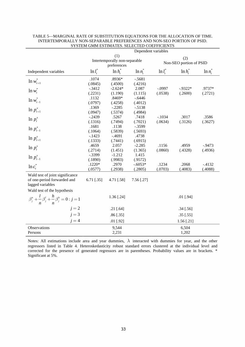
Our main results appear to be robust to the relaxation of the intertemporal separability

assumption and to the exclusion of the poverty subsample from the PSID. When preferences

are intertemporally separable, period t demands are not affected by prices from other periods.

26

A simple generalization of intertemporal separability is to include one-period forwarded and

lagged prices in demands, Browning (1991) argues. On the other hand, the core PSID sample

combines a nationally representative sample of households with some 2,000 low-income

families taken from the Survey of Economic Opportunities (SEO). Results calculated on the

full sample are presented in Table 5. For each activity, the assumption of intertemporal

separability can not be rejected. Although the exclusion of the poverty subsample rises the

imprecision of the estimates, the main findings are preserved.

5 SUMMARY AND CONCLUSIONS

For the population of U.S. women of prime age, this paper has estimated log-linearized

structural equations representing labor force participants’ intertemporal allocation of time in

an uncertain environment. A three-activity system—leisure, home production, and market

work, has been jointly estimated combining consumer-level data on hours, wages, and

consumption expenditures from the Panel Study of Income Dynamics with metropolitan area-

level price indices from the Bureau of Labor Statistics. We have employed data on

consumers’ expenditures on restaurants to control for unobservable expectations and wealth,

and used an instrumental variables approach based upon Altonji (1986) and Mroz (1987) to

deal with mismeasured explanatory variables. Our empirical model has passed standard tests

for instrumental variables regression, an adding-up test for the allocation of time, and a test

for the relaxation of the intertemporal separability assumption.

The estimated wage ISE for the intensive margin of female labor supply that we have

obtained, .86, implies that, at average values for the allocation of time, women participating in

the labor force will rise her annual labor supply by some 14 hours in periods where the wage

rate is anticipated to increase by 1%. Of this increase, the estimated wage ISEs for leisure and

home production time that we have obtained, -.11 and -.68 respectively, suggest that

approximately 7 hours will come from less leisure and the other 7 from less time devoted to

43

TABLE 5—MARGINAL RATE OF SUBSTITUTION EQUATIONS FOR THE ALLOCATION OF TIME.

INTERTEMPORALLY NON-SEPARABLE PREFERENCES AND NON-SEO PORTION OF PSID. SYSTEM GMM ESTIMATES. SELECTED COEFFICIENTS

Dependent variables (1)

Intertemporally non-separable preferences

(2) Non-SEO portion of PSID

Independent variables *ln tl *ln th *ln tn *ln tl *ln th *ln tn

*1ln tw + .1074

(.0845) .8936* (.4500)

-.5681 (.4216)

*ln tw -.3412 (.2231)

-2.624* (1.190)

2.087 (1.115)

-.0997 (.0538)

-.9322* (.2600)

.9737* (.2721)

*1ln tw− .1132

(.0797) .8469* (.4258)

-.6446 (.4012)

1ln xtp + .1369

(.0947) -.2285 (.5374)

-.5138 (.4984)

ln xtp -.2439

(.1316) .5267

(.7494) .7418

(.7021) -.1034 (.0634)

.3017 (.3126)

.3586 (.3627)

1ln xtp − .1681

(.1064) .1138

(.5839) -.3599 (.5693)

1ln stp + -.1423

(.1333) -.4691 (.7441)

.4738 (.6915)

ln stp .4659

(.2714) 2.057

(1.451) -2.285 (1.365)

.1156 (.0860)

.4959 (.4328)

-.9473 (.4936)

1ln stp − -.3399

(.1890) -1.212 (.9983)

1.415 (.9572)

*ln tc .1220* (.0577)

.2970 (.2938)

-.6053* (.2805)

.1234 (.0703)

.2068 (.4083)

-.4132 (.4088)

Wald test of joint significance of one-period forwarded and lagged variables

6.71 [.35] 4.71 [.58] 7.56 [.27]

Wald test of the hypothesis

0n l hj j j

l hn n

β β β+ + = : 1j = 1.36 [.24] .01 [.94]

2j = .21 [.64] .34 [.56] 3j = .86 [.35] .35 [.55] 4j = .01 [.92] 1.56 [.21]

Observations 9,544 6,504 Persons 2,231 1,202

Notes: All estimations include area and year dummies, λ interacted with dummies for year, and the other regressors listed in Table 4. Heteroskedasticity robust standard errors clustered at the individual level and corrected for the presence of generated regressors are in parentheses. Probability values are in brackets. * Significant at 5%.

27

home production. The low point estimate for the labor supply ISE with respect to the price of

recreation goods, -.00, suggests that the intensive margin of female intertemporal labor supply

is not affected by variations in the price of these goods. Yet, this margin does react to changes

in the price of home consumption goods. The estimated ISE of home production time with

respect to the price of home consumption goods that we have obtained, .59, implies that, at

average values for the allocation of time, women participating in the labor force will rise her

annual time devoted to home production by some 6 hours when faced with a 1% increase in

the price of home consumption goods. Moreover, the corresponding ISEs for leisure and

market time, .05 and -.71 respectively, suggest that the extra hours devoted to home

production will be entirely subtracted from market work, which will be therefore reduced in a

similar amount. If home production were excluded from the model’s specification, part of this

effect would be misleadingly attributed to the price of recreation goods.

A THE TOTAL LABOR SUPPLY ISE

This appendix shows that the total labor supply ISE (i.e. the labor supply ISE integrating the

intensive and extensive margins) equals the labor force participants’ labor supply ISE plus the

labor force participation ISE. In what follows, n represents market time, *m denotes (latent)

labor force participation propensity, and x is a vector containing the log of the wage rate

( ln w ), the log of expenditures on restaurants, and possibly other controls.

Let ( )E n x and *( 0 )P m > x denote, respectively, the population regression of n and

the population probability of labor force participation. Using the Law of Iterated Expectations

and the fact that *( , 0) 0E n m < =x , we have

** * *( ) ( ( , )) ( 0 ) ( , 0)

mE n E E n m P m E n m= = > >x x x x . (A.1)

Thus, the total labor supply ISE with respect to w is given by the labor force participants’

labor supply wage ISE plus the labor force participation wage ISE:

28

*** *

**

* *

**

* *

( 0 )( ) ( , 0)1 1 ( 0 ) ( , 0)( ) ln ( ) ln ln

( 0 )( ) ( , 0) ( )1( ) ( , 0) ln ln ( 0 )

( 0 )( , 0)1 1( , 0) ln ln ( 0 )

P mE n E n mP m E n m

E n w E n w w

P mE n E n m E nE n E n m w w P m

P mE n mE n m w w P m

xx xx x

x x

xx x xx x x

xxx x

⎡ ⎤∂ >∂ ∂ >⎢ ⎥= > + >

∂ ∂ ∂⎢ ⎥⎣ ⎦

⎡ ⎤∂ >∂ >⎢ ⎥= +

> ∂ ∂ >⎢ ⎥⎣ ⎦

∂ >∂ >= +

> ∂ ∂ >

(A.2)

where the first equality follows from the chain rule.

B LABOR FORCE PARTICIPATION ISEs: WHY ESTIMATES MAY BE

BIASED

This appendix shows that the labor force participation wage ISEs obtained in Zabel (1997)

and Altonji (1982a) may be biased as a consequence of neglected heterogeneity stemming

from mismeasured explanatory variables and reduced-form regression errors.

As showed in Section 2, a log-linear approximation to the condition determining labor

force participation is given by

*0 1 2 3 4ln ln ln lnp p p x p s p p

it it it it it itm w p p c vβ β β β β= + + + + + (B.1)

where itm∗ is consumer i ’s (latent) participation propensity at age t and pitv is a preference

determinant.24 If the participation probability followed a probit model, the participation ISEs

(evaluated at mean values of the regressors) would be given by

( )

, 1, 2,3( )

p

pp

p pjv

pvv

jφ σ β

σσ

′=

′Φ

x β

x β, (B.2)

24 Neither Zabel (1997) nor Altonji (1982a) included ln xp and ln sp in the labor force

participation equation. Zabel (1997) did not include ln c either. But this does not affect our

main argument.

29

where pvσ is the standard deviation of pv in the population. To understand our basic idea, it is

helpful to assume that measures of the wage rate w are available for all individuals in the

population, including non-participants. Yet, since w and c are generally measured with error

in survey data, (B.1) becomes

* * *0 1 2 3 4ln ln ln lnp p p x p s p p

it it it it it it itm w p p c vβ β β β β ζ= + + + + + + , (B.3)

where the unobserved term itζ is given by 1 4p w p c

it it ite eζ β β=− − , e denoting errors of

measurement.

To consistently estimate (B.2) for the wage rate, both Zabel (1997) and Altonji

(1982a) implicitly employed the same instrumental variables probit estimator, developed in

Lee (1981). Lee (1981) suggested writing (B.3) in reduced form,

*0 1 2 3 4( ) ln ln ( )p p w p x p s p c p

it it it it it it itm p p vβ β β β β ξ′ ′= + + + + + +π z π z , (B.4)

where π and z denote, respectively, vectors of reduced-form parameters and regressors, and

the unobserved term itξ is given by 1 4p w p c

it it it itu uξ ζ β β= + + , u representing reduced-form

errors. Given consistent estimates of π , the probit participation ISEs obtained from (B.4) are

( )

, 1, 2,3( )

p

pp

p pjv

pvv

jξ

ξξ

φ σ β

σσ

+

++

′=

′Φ

x β

x β (B.5)

where 1/ 2(var( ))pp

vv

ξσ ξ

+= + . (Using the procedure in Wooldridge, 2002, pp. 22-24,

expression B.5 could be alternatively written as

(( ) )

, 1, 2,3(( ) )

p

pp

p pjv

pvv

E jξ

φ ξ σ β

σξ σ

⎡ ⎤′ +⎢ ⎥ =⎢ ⎥⎢ ⎥′Φ +⎣ ⎦

x β

x β, (B.6)

where [ ]Eξ ⋅ denotes the expectation with respect to ξ .) The elasticities in (B.5) (or,

equivalently, B.6) are generally different from those in (B.2). Moreover, if ξ is independent

of pv , ppj vξ

β σ+

would be closer to zero than ppj v

β σ , but ( ) ( )p pp p

v vξ ξφ σ σ

+ +′ ′Φx β x β

30

would be larger than ( ) ( )p pp p

v vφ σ σ′ ′Φx β x β . Therefore, it is not clear the direction of the

bias.

C DATA APPENDIX

Our dataset contains the 26,918 women interviewed by the PSID between 1968 and 1993,

though variables included cover the period 1976-1993 only. There are a total of 484,524

observations (person-years). Observations must correspond to heads/wives of PSID families

(368,199 person-years lost), present in the family at the time of the interview (1,617 person-

years lost), and with known age (6 person-years lost). Observations must pertain to person-

years living in MAs with available price indices (64,064 person-years lost). Price indices in

Miami-Ft. Lauderdale start in 1977 (57 person-years lost). Observations must correspond to

women aged 25-60 (13,204 person-years lost) and have valid information on hours, earnings,

and expenditures on restaurants (10,611 person-years lost).25 Observations reporting no labor

earnings but positive market hours or vice versa are dropped (71 person-years lost).

Observations reporting no market hours but positive hourly wage rates are dropped (186

person-years lost). Hours of housework must not be zero (267 person-years lost).

Observations with hours, wages, or expenditures on restaurants below the 1st percentile (but

above zero) or above the 99th percentile of the corresponding sampling distribution are

dropped (1,449 person-years lost). Observations with missing marital status, number of

children, capacity for work,26 labor market experience, or race are deleted (996 person-years

25 Market hours and labor earnings are not available for the calendar year 1993. Expenditures

on restaurants are not asked in 1988 and 1989. Hours of housework are not asked in 1982.

26 Though the wife’s capacity for work indicator was not asked between 1977 and 1980, this

information is available at the individual level for the years 1977 and 1978. For 1979

(respectively, 1980), the wife’s capacity for work is taken from that reported in 1978 (1981).

31

lost). Expenditures on restaurants must not be zero (4,511 person-years lost). In the hourly

paid subsample, women must be paid by the hour at least one year (8,004 person-years lost).

Table C.1 presents descriptive statistics for the main variables used in this study.

The CPI-All Urban Consumers introduced by the BLS in 1987 is a statistical measure

of change, over time, of the prices of goods and services in major expenditure groups. The

indices of “Entertainment” (whose BLS item code is SA6), “Food at home” (SA111), and

“Food away from home” (SE19) are available since 1976 for the following 27 Metropolitan

Areas (as denominated by the U.S. Office of Management and Budget in June 1990; BLS area

codes are in parentheses): New York-Northern N.J.-Long Island (A101), Philadelphia-

Wilmington-Trenton (A102), Boston-Lawrence-Salem (A103), Pittsburgh-Beaver Valley

(A104), Buffalo-Niagara Falls (A105), Chicago-Gary-Lake County (A207), Detroit-Ann

Arbor (A208), St. Louis-East St. Louis (A209), Cleveland-Akron-Lorain (A210),

Minneapolis-St. Paul (A211), Milwaukee (A212), Cincinnati-Hamilton (A213), Kansas City

(A214), Washington (A315), Dallas-Fort Worth (A316), Baltimore (A317), Houston-

Galveston-Brazoria (A318), Atlanta (A319), Miami-Ft. Lauderdale (A320; price indices

available here since 1977), Los Angeles-Anaheim-Riverside (A421), San Francisco-Oakland-

San Jose (A422), Seattle-Tacoma (A423), San Diego (A424), Portland-Vancouver (A425),

Honolulu (A426), Anchorage (A427), and Denver-Boulder (A433). The price series utilized

(downloadable from ftp://ftp.bls.gov/pub/time.series/mu/) are coded MUURAxxxSyyy and

MUUSAxxxSyyy, where Axxx stands for an area code and Syyy for an item code; an “R” as

the fourth letter indicates the index is available monthly, an “S” semi-annually.

44

TABLE C.1—DESCRIPTIVE STATISTICS

Hourly paid sample Full sample Variable All Working Hourly paid All Working

*l 6,311 (837) 6,193 (754) 6,172 (717) 6,450 (888) 6,226 (751) *h 1,093 (742) 994 (650) 943 (594) 1,151 (801) 963 (648) *n 1,356 (799) 1,573 (632) 1,645 (566) 1,159 (888) 1,571 (649) *w 7.5 (3.9) 7.3 (3.6) 8.2 (4.5) **w 6.6 (2.6)

*c 840 (699) 849 (698) 823 (663) 874 (739) 896 (731) Age 37.5 (9.3) 37.5 (9.2) 37.5 (9.2) 38.2 (9.9) 37.6 (9.4) Experience (years) 13.5 (7.8) 14.1 (7.6) 14.1 (7.6) 12.7 (8.1) 14.1 (7.7) Married (%) 70.3 68.5 65.4 70.8 68.8 Family size 3.4 (1.5) 3.3 (1.5) 3.3 (1.5) 3.4 (1.6) 3.2 (1.5) Children 1.4 (1.3) 1.3 (1.2) 1.3 (1.2) 1.3 (1.3) 1.2 (1.2) Children [0-5] .4 (.7) .4 (.6) .4 (.7) .4 (.7) .3 (.6) Disabled (%) 9.5 8.3 7.9 12.1 8.4 Black (%) 38.3 39.0 40.1 35.2 35.4 Person-years 11,282 9,724 5,486 19,286 14,224 Persons 1,868 3,917 3,163 Notes: Figures are sample means or proportions (in %), plus standard deviations (in parentheses). Monetary variables are expressed in 1982-1984 dollars. *l : Annual hours of leisure, calculated as 8,760- *h - *n . *h : Annual hours of home production, including cooking, cleaning, and doing other work around the house. *n : Annual hours of market work, including time in the main job, secondary job(s), and overtime. *w : Average hourly wage. **w : Straight-time hourly wage of hourly-paid workers. *c : Annual expenditures on restaurants. Experience: Accumulated years with positive market time since age 18. Children (respectively, Children [0-5]): Number of persons in the family unit younger than 18 (6).

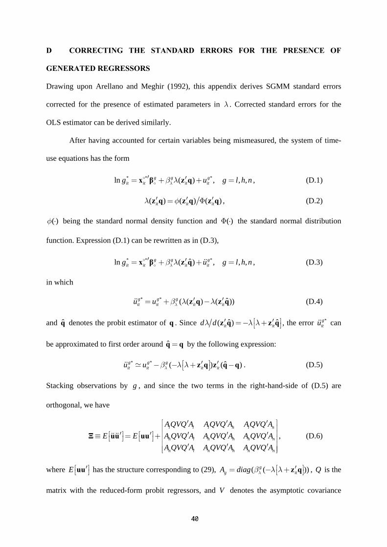
32

D CORRECTING THE STANDARD ERRORS FOR THE PRESENCE OF

GENERATED REGRESSORS

Drawing upon Arellano and Meghir (1992), this appendix derives SGMM standard errors

corrected for the presence of estimated parameters in λ . Corrected standard errors for the

OLS estimator can be derived similarly.

After having accounted for certain variables being mismeasured, the system of time-

use equations has the form

* * *ln ( ) , , ,g g git it it itg u g l h nλβ λ′ ′= + + =x β z q , (D.1)

( ) ( ) ( )it it itλ φ′ ′ ′= Φz q z q z q , (D.2)

( )φ ⋅ being the standard normal density function and ( )Φ ⋅ the standard normal distribution

function. Expression (D.1) can be rewritten as in (D.3),

* * *ˆln ( ) , , ,g g git it it itg u g l h nλβ λ′ ′= + + =x β z q , (D.3)

in which

* * ˆ( ( ) ( ))g g git it it itu u λβ λ λ′ ′= + −z q z q (D.4)

and q̂ denotes the probit estimator of q . Since ˆ ˆ( )it itd dλ λ λ⎡ ⎤′ ′=− +⎣ ⎦z q z q , the error *gitu can

be approximated to first order around ˆ =q q by the following expression:

* * ˆ( ) ( )g g git it it itu u λβ λ λ⎡ ⎤′ ′− − + −⎣ ⎦z q z q q . (D.5)

Stacking observations by g , and since the two terms in the right-hand-side of (D.5) are

orthogonal, we have

l l l h l n

h l h h h n

n l n h n n

AQVQ A AQVQ A AQVQ AE E A QVQ A A QVQ A A QVQ A

A QVQ A A QVQ A A QVQ A

⎡ ⎤′ ′ ′⎢ ⎥⎢ ⎥⎡ ⎤ ⎡ ⎤′ ′ ′ ′ ′≡ = +⎣ ⎦ ⎣ ⎦ ⎢ ⎥⎢ ⎥′ ′ ′⎢ ⎥⎣ ⎦

Ξ uu uu , (D.6)

where E ⎡ ⎤′⎣ ⎦uu has the structure corresponding to (29), ( ( ))gg itA diag λβ λ λ⎡ ⎤′= − +⎣ ⎦z q , Q is the

matrix with the reduced-form probit regressors, and V denotes the asymptotic covariance

33

matrix for q̂ . The estimated asymptotic covariance matrix of the SGMM estimator corrected

for the presence of generated regressors is given by expression (D.7),

1 1ˆ(( )( ) ( ))− −′ ′ ′X Z Z ΞZ Z X , (D.7)

in which all unknown parameters in Ξ have been replaced by consistent estimates, and X

and Z contain, respectively, all regressors in (D.1) and all exogenous variables stacked by g .

34

REFERENCES

Aguiar, Mark and Erik Hurst. 2007. Life-cycle prices and production. American Economic

Review 97(5):1533-1559.

Altonji, Joseph G. 1982a. Intertemporal substitution in labor supply: evidence from micro

data. Manuscript, Columbia University.

Altonji, Joseph G. 1982b. The intertemporal substitution model of labour market fluctuations:

an empirical analysis. The Review of Economic Studies 49(5):783-824.

Altonji, Joseph G. 1986. Intertemporal substitution in labor supply: evidence from micro data.

Journal of Political Economy 94, no. 3, pt. 2:S176-S215.

Arellano, Manuel, and Costas Meghir. 1992. Female labour supply and on-the-job search: an

empirical model estimated using complementary data sets. Review of Economic

Studies 59:537-557.

Blundell, Richard, and Thomas MaCurdy. 1999. Labor supply: a review of alternative

approaches. In Handbook of Labor Economics, vol. 3, ed. Orley Ashenfelter and

David Card. Amsterdam: Elsevier Science B. V.

Bound, John. 1991. Self-reported versus objective measures of health in retirement models.

The Journal of Human Resources XXVI(1):106-138.

Bound, John, David A. Jaeger, and Regina M. Baker. 1995. Problems with instrumental

variables estimation when the correlation between the instruments and the endogenous

explanatory variable is weak. Journal of the American Statistical Association 90:443-

450.

Bound, John, Charles Brown, and Nancy Mathiowetz. 2001. Measurement error in survey

data. In Handbook of Econometrics, vol. 5, ed. J.J. Heckman and E. Leamer.

Amsterdam: Elsevier Science B. V.

35

Browning, Martin. 1991. A simple nonadditive preference structure for models of household

behavior over time. Journal of Political Economy 99:607-637.

Browning, Martin, Thomas F. Crossley, and Guglielmo Weber. 2003. Asking consumption

questions in general purpose surveys. The Economic Journal 113(491):F540-F567.

Cogan, John F. 1981. Fixed costs and labor supply. Econometrica 49:945-963.

Consumer Expenditure Survey. CE Database. http://www.bls.gov/cex/#data, 11 Jan. 2010.

Cragg, John G., and Stephen G. Donald. 1993. Testing identifiability and specification in

instrumental variable models. Econometric Theory 9:222-240.

Cragg, John G., and Stephen G. Donald. 1997. Inferring the rank of a matrix. Journal of

Econometrics 76:223-250.

Domeij, David, and Martin Flodén. 2006. The labor-supply elasticity and borrowing

constraints: why estimates are biased. Review of Economic Dynamics 9:242-262.

French, Eric. 2004. The labor supply response to (mismeasured but) predictable wage

changes. Review of Economics and Statistics 86:602-613.

Geronimus, Arline T., John Bound, and Lisa J. Neidert. 1996. On the validity of using census

geocode characteristics to proxy individual socioeconomic characteristics. Journal of

the American Statistical Association 91: 529-537.

Ghez, Gilbert R. and Gary S. Becker. 1975. The allocation of time and goods over the life

cycle. New York. National Bureau of Economic Research.

González-Chapela, Jorge. 2007. On the price of recreation goods as a determinant of male

labor supply. Journal of Labor Economics 25:795-824.

Greene, William. 2004. The behaviour of the maximum likelihood estimator of limited

dependent variable models in the presence of fixed effects. Econometrics Journal

7:98-119.

36

Gronau, Reuben, and Daniel S. Hamermesh. 2006. Time vs. goods: The value of measuring

household production technologies. Review of Income and Wealth 52:1-16.

Ham, John C., and Kevin T. Reilly. 2002. Testing intertemporal substitution, implicit

contracts, and hours restriction models of the labor market using micro data. American

Economic Review 92:905-927.

Hansen, Lars P. 1982. Large sample properties of generalized method of moments estimators.

Econometrica 50:1029-1054.

Heckman, James. 1974. Life cycle consumption and labor supply: An explanation of the

relationship between income and consumption over the life cycle. American Economic

Review 64(1):188-194.

Heckman, James J. 1979. Sample selection bias as a specification error. Econometrica

47(1):153-161.

Heckman, James J., and Thomas E. MaCurdy. 1980. A life cycle model of female labour

supply. Review of Economic Studies 47 (January): 47-74.

Heckman, James J., and Thomas E. MaCurdy. 1982. Corrigendum on a life cycle model of

female labour supply. Review of Economic Studies 49 (October): 659-660.

Hotz, V. Joseph, and Robert A. Miller. 1988. An empirical analysis of life cycle fertility and

female labor supply. Econometrica 56 (January): 91-118.

Kleibergen, Frank, and Richard Paap. 2006. Generalized reduced rank tests using the singular

value decomposition. Journal of Econometrics 133:97-126.

Lee, Lung-Fei. 1981. Simultaneous equation models with discrete and censored dependent

variables. In Manski, C. and D. McFadden (eds.) Structural analysis of discrete data

with economic applications. MIT Press, Cambridge, MA, pp. 346-363.

Lee, Myoung-Jae. 2004. Efficiency gains of system GMM and MDE over individual equation

estimation. The Japanese Economic Review 55(4):451-459.

37

MaCurdy, Thomas E. 1981. An empirical model of labor supply in a life-cycle setting.

Journal of Political Economy 89 (December): 1059-1085.

MaCurdy, Thomas E. 1983. A simple scheme for estimating an intertemporal model of labor

supply and consumption in the presence of taxes and uncertainty. International

Economic Review 24(2):265-289.

Mroz, Thomas A. 1987. The sensitivity of an empirical model of married women's hours of

work to economic and statistical assumptions. Econometrica 55:765-799.

Mulligan, Casey B. 1999. Substitution over time: another look at life cycle labor supply. In

NBER macroeconomics annual 1998, ed. Ben S. Bernanke and Julio Rotemberg.

Cambridge: MIT Press, pp. 75-152.

Newey, Whitney K., James L. Powell, and James R. Walker. 1990. Semiparametric

estimation of selection models: some empirical results. American Economic Review

80:324-328.

Reilly, Kevin T. 1994. Annual hours and weeks in a life-cycle labor supply model: Canadian

evidence on male behaviour. Journal of Labor Economics 12:460-477.

Rupert, Peter, Richard Rogerson, and Randall Wright. 2000. Homework in labor economics:

Household production and intertemporal substitution. Journal of Monetary Economics

46:557-579.

Staiger, Douglas, and James H. Stock. 1997. Instrumental variables regression with weak

instruments. Econometrica 65:557-586.

Stock, James H., Jonathan H. Wright, and Motohiro Yogo. 2002. A survey of weak

instruments and weak identification in generalized method of moments. Journal of

Business and Economic Statistics 20:518-529.

38

Stock, James H. and Motohiro Yogo. 2005. Testing for weak instruments in linear IV

regression. In Donald W. K. Andrews and James H. Stock (eds.) Identification and

inference for econometric models: A festschrift in honor of Thomas Rothenberg.

Cambridge University Press, pp. 80-108.

Wooldridge, Jeffrey M. 2002. Econometric analysis of cross section and panel data.

Cambridge and London, The MIT Press.

Zabel, Jeffrey E. 1997. Estimating wage elasticities for life-cycle models of labour supply

behavior. Labour Economics 4:223-244.

PUBLISHED ISSUES *

WP-AD 2010-01 “Scaling methods for categorical self-assessed health measures” P. Cubí-Mollá. January 2010. WP-AD 2010-02 “Strong ties in a small world” M.J. van der Leij, S. Goyal. January 2010. WP-AD 2010-03 “Timing of protectionism”

A. Gómez-Galvarriato, C.L. Guerrero-Luchtenberg. January 2010. WP-AD 2010-04 “Some game-theoretic grounds for meeting people half-way” P.Gadea-Blanco, J.M. Jiménez-Gómez, M.C. Marco-Gil. February 2010. WP-AD 2010-05 “Sequential city growth: empirical evidence”

A. Cuberes. February 2010. WP-AD 2010-06 “Preferences, comparative advantage, and compensating wage differentials for job routinization” C. Quintana-Domeque. February 2010. WP-AD 2010-07 “The diffusion of Internet: a cross-country analysis” L. Andrés, D. Cuberes, M.A. Diouf, T. Serebrisky. February 2010. WP-AD 2010-08 “How endogenous is money? Evidence from a new microeconomic estimate” D. Cuberes, W.R. Dougan. February 2010. WP-AD 2010-09 “Trade liberalization in vertically related markets” R. Moner-Colonques, J.J. Sempere-Monerris, A. Urbano. February 2010. WP-AD 2010-10 “Tax evasion as a global game (TEGG) in the laboratory” M. Sánchez-Villalba. February 2010.

WP-AD 2010-11 “The effects of the tax system on education decisions and welfare” L.A. Viianto. March 2010. WP-AD 2010-12 “The pecuniary and non-pecuniary costs of job displacement. The risky job of

getting back to work” R. Leombruni, T. Razzolini, F. Serti. March 2010. WP-AD 2010-13 “Self-interest and justice principles”

I. Rodríguez-Lara, L. Moreno-Garrido. March 2010.

WP-AD 2010-14 “On spatial equilibria in a social interaction model” P. Mossay, P.M. Picard. March 2010. WP-AD 2010-15 “Noncooperative justifications for old bankruptcy rules” J.M. Jiménez-Gómez. March 2010. WP-AD 2010-16 “Anthropometry and socioeconomics in the couple: evidence from the PSID” S. Oreffice, C. Quintana-Domeque. April 2010.

* Please contact Ivie's Publications Department to obtain a list of publications previous to 2010.

WP-AD 2010-17 “Differentiated social interactions in the US schooling race gap” L.J. Hall. April 2010. WP-AD 2010-18 “Things that make us different: analysis of variance in the use of time” J. González Chapela. April 2010. WP-AD 2010-19 “The role of program quality and publicly-owned platforms in the free to air broadcasting industry” M. González-Maestre, F. Martínez-Sánchez. June 2010. WP-AD 2010-20 “Direct pricing of retail payment methods: Norway vs. US” F. Callado, J. Hromcová, N. Utrero. June 2010. WP-AD 2010-21 “Sexual orientation and household savings. Do homosexual couples save more? B. Negrusa, S. Oreffice. June 2010. WP-AD 2010-22 “The interaction of minimum wage and severance payments in a frictional labor market: theory and estimation” C. Silva. June 2010. WP-AD 2010-23 “Fatter attraction: anthropometric and socioeconomic matching on the marriage market” P.A. Chiappori, S. Oreffice, C. Quintana-Domeque. June 2010. WP-AD 2010-24 “Consumption, liquidity and the cross-sectional variation of expected returns” E. Márquez, B. Nieto, G. Rubio. July 2010.

WP-AD 2010-25 “Limited memory can be beneficial for the evolution of cooperation” G. Horváth, J. Kovárík, F. Mengel. July 2010. WP-AD 2010-26 “Competition, product and process innovation: an empirical analysis” C.D. Santos. July 2010. WP-AD 2010-27 “A new prospect of additivity in bankruptcy problems” J. Alcalde, M.C. Marco-Gil, J.A. Silva. July 2010. WP-AD 2010-28 “Diseases, infection dynamics and development” S. Chakraborty, C. Papageorgiou, F. Pérez Sebastián. September 2010. WP-AD 2010-29 “Why people reach intermediate agreements? Axiomatic and strategic justification” J.M. Jiménez-Gómez. September 2010. WP-AD 2010-30 “Mobbing and workers’ health: an empirical analysis for Spain” M.A. Carnero, B. Martínez, R. Sánchez-Mangas. September 2010. WP-AD 2010-31 “Downstream mergers in a vertically differentiated unionized oligopoly”

A. Mesa-Sánchez. October 2010. WP-AD 2010-32 “Endogenous quality choice under upstream market power” B. Mesa-Sánchez. November 2010. WP-AD 2010-33 “Itemised deductions: a device to reduce tax evasion” A. Piolatto. November 2010.

WP-AD 2010-34 “A unified theory of structural change” M.D. Guilló, C. Papageorgiou, F. Pérez-Sebastián. December 2010. WP-AD 2011-01 “Solving the multi-country real business cycle model using ergodic set methods” S. Maliar, L. Maliar, K. Judd. January 2011. WP-AD 2011-02 “Anti-piracy policy and quality differential in markets for information goods” J.M. López-Cuñat, F. Martínez-Sánchez. January 2011. WP-AD 2011-03 “Loyalty discounts” U. Akgun, I. Chioveanu. February 2011. WP-AD 2011-04 “Recreation, home production, and intertemporal substitution of female labor supply: evidence on the intensive margin” J. González Chapela. February 2011. WP-AD 2011-05 “On the effects of deposit insurance and observability on bank runs: an experimental study” H.J. Kiss, I. Rodríguez-Lara, A. Rosa-García. February 2011. WP-AD 2011-06 “The role of public and private information in a laboratory financial market” S. Alfarano, E. Camacho, A. Morone. February 2011.

IvieGuardia Civil, 22 - Esc. 2, 1º

46020 Valencia - SpainPhone: +34 963 190 050Fax: +34 963 190 055

Department of EconomicsUniversity of Alicante

Campus San Vicente del Raspeig03071 Alicante - Spain

Phone: +34 965 903 563Fax: +34 965 903 898

Website: www.ivie.esE-mail: publicaciones@ivie.es

adserie