Separable Potentials and a Triality in Two-Dimensional Spaces of Constant Curvature
23
Journal of Nonlinear Mathematical Physics Volume 12, Number 2 (2005), 230–252 Article Separable Potentials and a Triality in Two-Dimensional Spaces of Constant Curvature Jos´ e F. CARI ˜ NENA † , Manuel F RA ˜ NADA † , Mariano SANTANDER ‡ and Teresa SANZ-GIL ‡ † Departamento de F´ ısica Te´ orica, Facultad de Ciencias, Universidad de Zaragoza 50009 Zaragoza, Spain E-mail: [email protected], [email protected] ‡ Departamento de F´ ısica Te´ orica, Universidad de Valladolid 47011 Valladolid, Spain E-mail: [email protected], [email protected] Received December, 2004; Accepted February, 2005 Abstract We characterize and completely describe some types of separable potentials in two- dimensional spaces, S 2 [κ1 ]κ2 , of any (positive, zero or negative) constant curvature and either definite or indefinite signature type. The results are formulated in a way which applies at once for the two-dimensional sphere S 2 , hyperbolic plane H 2 , AntiDeSit- ter / DeSitter two-dimensional spaces AdS 1+1 / dS 1+1 as well as for their flat analogues E 2 and M 1+1 . This is achieved through an approach of Cayley-Klein type with two parameters, κ 1 and κ 2 , to encompass all curvatures and signature types. We dis- cuss six coordinate systems allowing separation of the Hamilton-Jacobi equation for natural Hamiltonians in S 2 [κ1 ]κ2 and relate them by a formal triality transformation, which seems to be a clue to introduce general “elliptic coordinates” for any CK space concisely. As an application we give, in any S 2 [κ1 ]κ2 , the explicit expressions for the Fradkin tensor and for the Runge-Lenz vector, i.e., the constants of motion for the harmonic oscillator and Kepler potential on any S 2 [κ1 ]κ2 . 1 Introduction The aim of this paper is to characterize and completely describe some types of separa- ble potentials in 2d spaces of constant curvature and either Riemannian or Lorentzian type metric using a unified and joint description. All these spaces are members of the two parametric family of Cayley-Klein (CK) two-dimensional spaces, with the parameters κ 1 ,κ 2 corresponding to the curvature of the space and to the signature type. All the results obtained by such procedure make sense for the whole family of spaces with any constant curvature (no matter positive, zero or negative) and any metric signature, no matter definite (Riemannian) or indefinite (pseudoRiemannian Lorentzian type). Separation of variables in the Hamilton-Jacobi equation has been discussed in the literature for some individual spaces on a case by case basis. The situation has been quite Copyright c 2005 by JF Cari˜ nena, MF Ra˜ nada, M Santander and T Sanz-Gil
-
Upload
independent -
Category
Documents
-
view
0 -
download
0
Transcript of Separable Potentials and a Triality in Two-Dimensional Spaces of Constant Curvature
Journal of Nonlinear Mathematical Physics Volume 12, Number 2 (2005), 230–252 Article
Separable Potentials and a Triality in
Two-Dimensional Spaces of Constant Curvature
Jose F. CARINENA †, Manuel F RANADA†, Mariano SANTANDER‡
and Teresa SANZ-GIL ‡
† Departamento de Fısica Teorica, Facultad de Ciencias, Universidad de Zaragoza50009 Zaragoza, SpainE-mail: [email protected], [email protected]
‡ Departamento de Fısica Teorica, Universidad de Valladolid47011 Valladolid, SpainE-mail: [email protected], [email protected]
Received December, 2004; Accepted February, 2005
Abstract
We characterize and completely describe some types of separable potentials in two-dimensional spaces, S2
[κ1]κ2, of any (positive, zero or negative) constant curvature and
either definite or indefinite signature type. The results are formulated in a way whichapplies at once for the two-dimensional sphere S2, hyperbolic plane H2, AntiDeSit-ter / DeSitter two-dimensional spaces AdS
1+1 / dS1+1 as well as for their flat analogues
E2 and M1+1. This is achieved through an approach of Cayley-Klein type with twoparameters, κ1 and κ2, to encompass all curvatures and signature types. We dis-cuss six coordinate systems allowing separation of the Hamilton-Jacobi equation fornatural Hamiltonians in S2
[κ1]κ2
and relate them by a formal triality transformation,which seems to be a clue to introduce general “elliptic coordinates” for any CK spaceconcisely. As an application we give, in any S2
[κ1]κ2
, the explicit expressions for theFradkin tensor and for the Runge-Lenz vector, i.e., the constants of motion for theharmonic oscillator and Kepler potential on any S2
[κ1]κ2.
1 Introduction
The aim of this paper is to characterize and completely describe some types of separa-ble potentials in 2d spaces of constant curvature and either Riemannian or Lorentziantype metric using a unified and joint description. All these spaces are members of thetwo parametric family of Cayley-Klein (CK) two-dimensional spaces, with the parametersκ1, κ2 corresponding to the curvature of the space and to the signature type. All theresults obtained by such procedure make sense for the whole family of spaces with anyconstant curvature (no matter positive, zero or negative) and any metric signature, nomatter definite (Riemannian) or indefinite (pseudoRiemannian Lorentzian type).
Separation of variables in the Hamilton-Jacobi equation has been discussed in theliterature for some individual spaces on a case by case basis. The situation has been quite
Copyright c© 2005 by JF Carinena, MF Ranada, M Santander and T Sanz-Gil
Separable Potentials and Triality 231
exhaustively studied when configuration space is Euclidean E2, starting in [3]. This hasbeen also extended to systems on the sphere S2 or on the hyperbolic plane H2 [4, 5, 6,7, 13, 14]. The case where configuration space has an Lorentzian (indefinite) constantcurvature metric is less known, albeit Drach potentials are linked to the Minkowski space[20, 22]. A list of inequivalent quadratically superintegrable systems in M1+1 exists [13]yet its interpretation in terms of generic ‘elliptic’ coordinates in Minkowski space and theirlimiting or special cases is still not fully understood. We do not know any previous studyneither for AntiDeSitter AdS1+1 or the DeSitter dS1+1 configuration spaces, nor a studyof their relation through contraction to the superintegrable systems in M1+1.
Why is this kind of approach worthwhile? From a more practical side, approachingthe problem on a case-by-case basis must be supplemented with a study of the limitingtransitions where, for instance, curvature vanishes. This need can be dispensed providedwe instead look to all cases as members of a parametrised full family of spaces withevery detail arranged so as to have limiting situations (vanishing curvature κ1 = 0 and/ordegenerating metric κ2 = 0) described smoothly at the same level as the generic ones. Inpapers [21, 23, 24, 25, 26] this is done for κ2 = 1 and only a curvature parameter κ = κ1.From a more structural perspective the approach we are proposing makes some essentialaspects to stand out clearly and put to the forefront a deep analogy between all the cases(any κ1, κ2), while a case by case approach risks to highlight some non essential differenceswhile hiding some essential similarities.
We deal with a system with a Lagrangian of mechanical type, i.e., a “kinetical” termminus a potential function, in a 2d space S2
[κ1]κ2of constant curvature κ1 and metric
with signature (+, κ2). When is the corresponding Hamilton-Jacobi equation separable?For S2 the answer has been long known: the potential V must be separable in Jacobielliptic coordinates, which are determined by two points (the focal points) on S2; thecoordinates themselves are (half) the sum and the difference of geodesic distances fromthe generic point P to the two foci; these potentials allow for an extra constant of motionfurther to the energy. The situation in H2 and in AntiDeSitter and DeSitter spacesAdS1+1, dS1+1 is apparently more complicated and, if elliptic is taken in a literal senseof (half) sum and difference of geodesic distances from the generic point P to the twofoci, then definitely there are other coordinate systems allowing separation of variablesin the Hamilton-Jacobi equation in H2. With the right interpretation, however, all thesesystems should be understood as general elliptic, in the sense of confocal conics, yet thefoci are not necessarily proper points in S2
[κ1]κ2[27]. In this paper we characterize, for all
values of κ1 and κ2, hence in all CK 2d spaces, several sets of potentials having extraquadratic constants of motion and separable in some specific coordinate systems, whichalso allow Hamilton-Jacobi separation. This should be taken as a first step towards the fullcharacterization of separable potentials in 2d configuration spaces of constant curvatureand any signature; it displays in the simplest situations the traits of the κ1, κ2 parametricapproach. The triality idea we introduce here is also essential to get the classification ofsuperintegrable systems bypassing the need of brute-force direct calculations.
The paper is arranged as follows. First we describe the required basics of the CKtype approach. Then we introduce six particular coordinate systems and give explicitlyall expressions pertinent for the geometry of S2
[κ1]κ2in their terms. In the next section
potentials separable in these six coordinates systems are shown to have an extra constantof motion additional to the “energy”, which is also given in explicit form; these systems
232 JF Carinena, MF Ranada, M Santander and T Sanz-Gil
allow Hamilton-Jacobi separation of variables for any value of κ1, κ2. Then we give a briefstatement of the basic triality which underlies most of the paper. To close we discusssome interesting examples and give, in any S2
[κ1]κ2, explicit expressions for the constants of
motion specific to the “curved potentials” analogues to harmonic oscillator (the so calledFradkin tensor) and to the Kepler problem (the Laplace-Runge-Lenz vector) in any S2
[κ1]κ2.
2 The geometry of S2[κ1]κ2
We first introduce the necessary details on the 2d spaces S2[κ1]κ2
with constant curvature κ1
and metric of signature type (+,κ2) (for more details and some applications see [8, 9, 10]).These are homogeneous spaces. Hence they admit a maximal three-dimensional isometrygroup, which we call SOκ1,κ2
(3) and which is generated by a three dimensional Lie algebrasoκ1,κ2
(3), given in a matrix realization as:
P1 =
0 −κ1 01 0 00 0 0
P2 =
0 0 −κ1κ2
0 0 01 0 0
J =
0 0 00 0 −κ2
0 1 0
, (2.1)
where we stress the association among generators P1, P2 and J and constants κ1, κ1κ2 andκ2. The commutators between the generators J, P1 and P2 are:
[J, P1] = P2 [J, P2] = −κ2P1 [P1, P2] = κ1J. (2.2)
This approach embodies essentially nine cases, because by scaling each of the constantsκ1, κ2 may be brought to their standard values 1, 0,−1; the essential information iswhether κ1 (resp. κ2) are positive, zero or negative, and this corresponds to the ellip-tic/parabolic/hyperbolic character of the measure of lenghts (resp. angles) within theformalism of projective metrics. This is depicted in Table 1.
Each entry of the Table gives the name of each homogeneous space G/H, its isom-etry group G and the isotropy subgroup H. The three rows accomodate spaces witheither a Riemannian, degenerate Riemannian and pseudoRiemannian (Lorentzian) met-ric, according to the sign of κ2, and the three instances along each row correspond tospaces with constant positive, zero or negative curvature. There are five non-isomorphicisometry groups, two generic simple ones SO(3), SO(2, 1), two limiting 1-quasisimple onesISO(2), ISO(1, 1) and one doubly limiting, 2-quasisimple, the Galilei group IISO(1), iso-morphic to the Heisenberg group. As far as the homogeneous spaces themselves, there areeight different ones; in 2d the DeSitter and AntiDeSitter spaces only differ by the changeof the sign in the metric and in this sense they might be considered as isomorphic spaces.
It may be relevant to remark that for G = SO(3) we have a single homogeneousspace of CK type associated to G, because all possible subgroups H are conjugate. Theother simple CK group SO(2, 1) has three associated homogeneous spaces which, albeitlinked by duality and by change of sign in the Lorentzian metric, should be considered asinequivalent from the CK viewpoint. For instance, H2 and DeSitter/AntiDeSitter spacehave the same isometry group SO(2, 1), but their isotopy subgroups SO(2) and SO(1, 1)are non conjugated. While H2 is a space with Riemannian metric and negative constantcurvature, AdS1+1 or dS1+1 are constant curvature spaces with a Lorentzian metric; thesethree spaces are related by a triality [28], a formal transformation which is not an isometry

Separable Potentials and Triality 233
Table 1. The nine two-dimensional CK spaces S2[κ1]κ2
.
Measure of distance & Sign of κ1
Measure of angle Elliptic Parabolic Hyperbolic& Sign of κ2 κ1 = 1 κ1 = 0 κ1 = −1
Elliptic Euclidean HyperbolicElliptic G = SO(3) G = ISO(2) G = SO(2, 1)κ2 = 1 H = SO(2) H = SO(2) H = SO(2)
G/H = S2 G/H = E
2 G/H = H2
Co-Euclidean Galilean Co-MinkowskianOscillating NH Expanding NH
Parabolic G = ISO(2) G = IISO(1) G = ISO(1, 1)κ2 = 0 H = R H = R H = R
G/H = ANH1+1 G/H = G
1+1 G/H = NH1+1
Co-Hyperbolic Minkowskian Doubly HyperbolicAnti-de Sitter De Sitter
Hyperbolic G = SO(2, 1) G = ISO(1, 1) G = SO(2, 1)κ2 = −1 H = SO(1, 1) H = SO(1, 1) H = SO(1, 1)
G/H = AdS1+1 G/H = M
1+1 G/H = dS1+1
in these three cases, but reduces to an isometry —the 3-fold rotation around the center of‘an octant’ spherical triangle— of the sphere S2.
From the previous description and from Table 1, it follows that when both constantsare positive, the space S2
[κ1]κ2is the two-dimensional sphere; the standard S2 corresponds
to κ1 = 1, κ2 = 1. In this case (2.2) reduces to the so(3) usual commutation relations.In the Euclidean case κ1 = 0, κ2 > 0, which can be reduced to the standard Euclideanspace E2 (κ1 = 0, κ2 = 1), the commutators (2.2) close iso(2) commutation relations,with commuting translations and (P1, P2) behaving as an so(2)-vector under rotations.When κ1 < 0, κ2 > 0 we get Lobachevski hyperbolic space, H2 whose isometry algebraso−1,1(3) is isomorphic to so(2, 1). When κ2 < 0, the commutation relations show that(P1, P2) is a Lorentzian so(1, 1)-vector under the rotations generated by J (now hyperbolictype) and the translations generators commute to a multiple of J according to the sign ofκ1. Minkowskian geometry appears for κ1 = 0, κ2 < 0; if conventional measures are usedfor the time P1 and space P2 translations, then κ2 = −1/c2 in terms of the relativisticconstant and the algebra (2.2) close the familiar Poincare iso(1, 1) commutation relationsin 1+1 dimensions.
We now introduce the κ-Cosine Cκ(x)l, Sine Sκ(x) and Tangent Tκ(x) functions:
Cκ(x) :=
cos√
κ x1cosh
√−κx, Sκ(x) :=
1√κ
sin√
κx κ > 0
x κ = 01√−κ
sinh√−κx κ < 0
, Tκ(x) :=Sκ(x)
Cκ(x). (2.3)
These functions include trigonometric κ > 0 and hyperbolic κ < 0 functions; we referto [8] and [9] for further details on this κ1, κ2 formalism. When κ = 0, the cosine reducesto the constant function 1 and the sine and tangent are the identity linear function of theirvariables.
Exponentials of matrices (2.1) lead to one-parametric subgroups exp(αP1), exp(βP2),
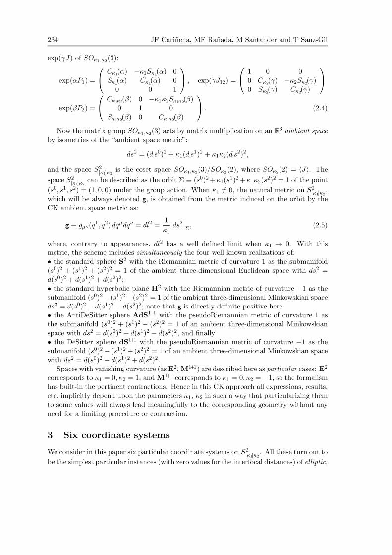
234 JF Carinena, MF Ranada, M Santander and T Sanz-Gil
exp(γJ) of SOκ1,κ2(3):
exp(αP1) =
Cκ1(α) −κ1Sκ1
(α) 0Sκ1
(α) Cκ1(α) 0
0 0 1
, exp(γJ12) =
1 0 00 Cκ2
(γ) −κ2Sκ2(γ)
0 Sκ2(γ) Cκ2
(γ)
exp(βP2) =
Cκ1κ2(β) 0 −κ1κ2Sκ1κ2
(β)0 1 0
Sκ1κ2(β) 0 Cκ1κ2
(β)
. (2.4)
Now the matrix group SOκ1,κ2(3) acts by matrix multiplication on an R3 ambient space
by isometries of the “ambient space metric”:
ds2 = (d s0)2 + κ1(d s1)2 + κ1κ2(d s2)2,
and the space S2[κ1]κ2
is the coset space SOκ1,κ2(3)/SOκ2
(2), where SOκ2(2) = 〈J〉. The
space S2[κ1]κ2
can be described as the orbit Σ ≡ (s0)2 +κ1(s1)2 +κ1κ2(s
2)2 = 1 of the point
(s0, s1, s2) = (1, 0, 0) under the group action. When κ1 6= 0, the natural metric on S2[κ1]κ2
,which will be always denoted g, is obtained from the metric induced on the orbit by theCK ambient space metric as:
g ≡ gµν(q1, q2) dqµdqν = dl2 =1
κ1ds2
∣∣Σ, (2.5)
where, contrary to appearances, dl2 has a well defined limit when κ1 → 0. With thismetric, the scheme includes simultaneously the four well known realizations of:• the standard sphere S2 with the Riemannian metric of curvature 1 as the submanifold(s0)2 + (s1)2 + (s2)2 = 1 of the ambient three-dimensional Euclidean space with ds2 =d(s0)2 + d(s1)2 + d(s2)2;• the standard hyperbolic plane H2 with the Riemannian metric of curvature −1 as thesubmanifold (s0)2− (s1)2− (s2)2 = 1 of the ambient three-dimensional Minkowskian spaceds2 = d(s0)2 − d(s1)2 − d(s2)2; note that g is directly definite positive here.• the AntiDeSitter sphere AdS1+1 with the pseudoRiemannian metric of curvature 1 asthe submanifold (s0)2 + (s1)2 − (s2)2 = 1 of an ambient three-dimensional Minkowskianspace with ds2 = d(s0)2 + d(s1)2 − d(s2)2, and finally• the DeSitter sphere dS1+1 with the pseudoRiemannian metric of curvature −1 as thesubmanifold (s0)2− (s1)2 + (s2)2 = 1 of an ambient three-dimensional Minkowskian spacewith ds2 = d(s0)2 − d(s1)2 + d(s2)2.
Spaces with vanishing curvature (as E2, M1+1) are described here as particular cases: E2
corresponds to κ1 = 0, κ2 = 1, and M1+1 corresponds to κ1 = 0, κ2 = −1, so the formalismhas built-in the pertinent contractions. Hence in this CK approach all expressions, results,etc. implicitly depend upon the parameters κ1, κ2 in such a way that particularizing themto some values will always lead meaningfully to the corresponding geometry without anyneed for a limiting procedure or contraction.
3 Six coordinate systems
We consider in this paper six particular coordinate systems on S2[κ1]κ2
. All these turn out to
be the simplest particular instances (with zero values for the interfocal distances) of elliptic,
Separable Potentials and Triality 235
parabolic and ultraelliptic type coordinate systems in S2[κ1]κ2
[27]. A complete discussion ofthe “general elliptic” coordinates in these spaces will be done elsewhere. Here we restrictourselves to a self-contained presentation of these six coordinate systems with the aim tointroduce a tool, the T -symmetry, which is essential to perform a meaningful comparisonbetween Jacobi elliptic coordinates on the sphere and the more general “elliptic” coordinatesystems allowing Hamilton-Jacobi separation of variables in S2
[κ1]κ2.
These six coordinates systems are built in any of the CK spaces out of canonical param-eters of suitable transformations (rotations around a fixed point O and translations alongtwo mutually intersecting orthogonal (oriented and cooriented) straight lines l1, l2 throughO). In all cases we take O ≡ (1, 0, 0) on the s0 axis and l1 (resp. l2) are the intersectionsof the CK sphere Σ with the 2-planes s0s1 (resp. s0s2) in the ambient CK space. The linel1 has a tangent vector with positive square length gµν qµqν > 0, but the square length ofthe tangent vector to l2 has the same sign as κ2; then when κ2 < 0 l1 and l2 are two linesof different type: in the language of relativity l1 is time-like and l2 is space-like. Thereforelengths along l2 computed for the intrinsic metric g of S2
[κ1]κ2are pure imaginary and only
become real for the associated metric g/κ2 (this is tantamount to the relation betweenmetrics determining directly proper time and proper length in relativity).
Parameters for the translations exp(αP1) along l1 carry a ‘label’ κ1; these coincide tothe distances —after g— along l1 between any point on l1 and its image under exp(αP1).
Parameters of the translations exp(βP2) along P2, carry a ‘label’ κ1κ2. The ‘distance’—after g— along the line l2 between any point on l2 and its image equals
√κ2 β, hence
these ‘distances’ differ from the canonical parameter β just by a constant factor whichbecomes pure imaginary when the metric is Lorentzian type. The quantity
√κ2 β should
be considered as having a label κ1; multiplication by√
κ2 serves to transfer the quantityβ with label κ1κ2 to another quantity
√κ2β with label κ1. Of course, these and similar
transfers require κ1, κ2 constants to be different from zero. While transfers by themselvesdo not apply for the nongeneric spaces in the CK family, when combined with the trialityto be discussed later they produce a result which is well defined for any value, even zero,of κ1, κ2.
Finally parameters for rotations around O carry ‘label’ κ2 and they coincide with theangle between any line through O and its rotated, again determined from g as usual.
Now we define, for any generic point P , six quantities r, φ; u, y; x, v so that the pointP can be obtained as the image of O by some products of one-parameter subgroups:
P = exp(φJ) exp(rP1)O = exp(uP1) exp(yP2)O = exp(vP2) exp(xP1)O (3.1)
Note that the six quantities, to be taken as coordinates, do not appear primarily aslengths but instead as canonical parameters and each one has a label, which would fit tothe label of the functions appearing in the associated isometries in (3.1) according to
r ↔ κ1, φ↔ κ2; u↔ κ1, y ↔ κ1κ2; x↔ κ1, v ↔ κ1κ2.
Their precise relation to the lengths as computed from the metric g is:• r is the length from P the origin O, measured along the line OP .• φ is the angle between the positive half-ray of l1 and the straight line OP through O.• x is the length from P to l2, measured along a straight line P2P which is orthogonalto l2 (P2 is the orthogonal projection of P on l2); this line can be obtained from l1 by atranslation exp(vP2) so that this is consistent with x having label κ1.

236 JF Carinena, MF Ranada, M Santander and T Sanz-Gil
• v is only “proportional” to the length between O and P2 along l2, with a factor√
κ2, sothe length itself is
√κ2v. This is consistent with v having the label κ1κ2; alternatively v
can be considered as the “space-like” distance measured with the metric g/κ2.• y is again only “proportional” to the length from P to P1 along the perpendicular tol1 through P , which intersects l1 at the point P1. The length is equal to
√κ2y so that
this is consistent with y having the label κ1κ2; alternatively y can be considered as the“space-like”–length measured with the metric g/κ2 along the line from P1 to P .• Finally u is the length between O and P1 along l1, which coincides with the canonicalparameter; this is consistent with u having the label κ1.
Now we introduce the coordinate systems themselves. These come in two groups ofthree systems, the mutual relationships of which are discussed later. Three coordinatesystems, called polar, parallel ‘1’ and parallel ‘2’, are the particularization to the spacesS2
[κ1]κ2of the systems known as geodesic polar coordinates and geodesic parallel (or Gaus-
sian) coordinates in differential geometry of surfaces. The remaining three coordinatesystems will be called equiparabolic ‘01’, equiparabolic ‘20’, and equiparabolic ‘12’. Theyare also distinguished particular instances of the “general elliptic” coordinate systems onS2
[κ1]κ2[27], but here they are introduced directly from their expressions.
3.1 Polar coordinates
The coordinates are (r, φ). By direct substitution of the isometries in the definition ofcoordinates we get:
s0
s1
s2
=
Cκ1(r)
Sκ1(r)Cκ2
(φ)Sκ1
(r)Sκ2(φ)
, dl2 = dr2 + κ2Sκ1
2(r)dφ2, (3.2)
where the metric g reduces to dr2 +sin2 r dφ2, dr2 + r2 dφ2, dr2 +sinh2 r dφ2 for the threestandard spaces S2, E2, H2, and to their Minkowskian versions, with opposite sign in theterms in dφ2, for the three pseudoRiemannian spaces AdS1+1, M1+1, dS1+1.
The generators of the one parameter subgroups of isometries, or Killing vector fields,are given as first-order differential operators in (r, φ) coordinates by:
XP1
XP2
XJ
=
Cκ2(φ)∂r − Sκ2
(φ)/Tκ1(r) ∂φ
κ2Sκ2(φ)∂r + Cκ2
(φ)/Tκ1(r) ∂φ
∂φ
,
and can be checked to close a Lie algebra isomorphic to soκ1,κ2(3).
3.2 Parallel ‘1’ coordinates
The coordinates are (x, v). In this system the expressions are:
s0
s1
s2
=
Cκ1(x)Cκ1κ2
(v)Sκ1
(x)Cκ1
(x)Sκ1κ2(v)
, dl2 = dx2 + κ2Cκ1
2(x)dv2. (3.3)
On the standard Euclidean plane E2, with κ1 = 0, κ2 = 1 the coordinates (x, v) arethe usual cartesian coordinates and the metric reduces to dl2 = dx2 + dv2. Likewise on
Separable Potentials and Triality 237
the standard Minkowskian plane M1+1 (κ1 = 0, κ2 = −1) x and v are time and spaceMinkowskian coordinates with dl2 = dx2− dv2. The Killing vector fields associated to thebasic one-parameter subgroups are:
XP1
XP2
XJ
=
Cκ1κ2(v)∂x + κ1Sκ1κ2
(v)Tκ1(x)∂v
∂v
−κ2Sκ1κ2(v)∂x + Cκ1κ2
(v)Tκ1(x)∂v
.
3.3 Parallel ‘2’ coordinates
The coordinates are (u, y). In this case the analogous expressions are:
s0
s1
s2
=
Cκ1(u)Cκ1κ2
(y)Sκ1
(u)Cκ1κ2(y)
Sκ1κ2(y)
, dl2 = Cκ1κ2
2(y)du2 + κ2dy2. (3.4)
Note that the coordinate system (u, y) does not coincide with (x, v) in general; coinci-dence happens only when κ1 = 0 and is a degeneracy of the flat spaces; for non zero valuesof κ1 we have u 6= x and v 6= y. On the standard sphere S2 (u, y) are the geographiclongitude and colatitude coordinates. For the vector fields XP1
,XP2,XJ :
XP1
XP2
XJ
=
∂u
κ1κ2Sκ1(u)Tκ1κ2
(y)∂u + Cκ1(u)∂y
−κ2Cκ1(u)Tκ1κ2
(y)∂u + Sκ1(u)∂y
,
which can be considered as the general version, valid for all CK spaces, of the well knownEuclidean expressions ∂u, ∂y, u∂y − y∂u for XP1
,XP2,XJ .
3.4 Equiparabolic ‘01’ coordinates
The coordinates, called here (a+, a−), are defined as:
a+ =1
2(r + x), a− =
1
2(r − x). (3.5)
and the point of the ambient CK space with coordinates (a+, a−) is given by
s0
s1
s2
=
Cκ1(a+ + a−)
Sκ1(a+ − a−)√
Sκ1(2a+)Sκ1
(2a−)κ2
=
Cκ1(r)
Sκ1(x)√
Sκ1(r+x)Sκ1
(r−x)κ2
, (3.6)
with metric:
dl2 = (Sκ1(2a+) + Sκ1
(2a−))
{d a+
2
Sκ1(2a+)
+d a−
2
Sκ1(2a−)
}. (3.7)
In spite of the presence of the constant κ2 inside a square root in (3.6), due to thetriangular inequality for lengths when κ2 > 0 and to its (reversed) Minkowskian versionwhen κ2 < 0, the sign of Sκ1
(2a+)Sκ1(2a−) turns out to be always the same as of κ2, hence
the three ambient space coordinates s0, s1, s2 are always real. The prefactor in the lineelement can be written also in the form
Sκ1(2a+) + Sκ1
(2a−) = 2Sκ1(a+ + a−) Cκ1
(a+ − a−) = 2Sκ1(r)Cκ1
(x). (3.8)
238 JF Carinena, MF Ranada, M Santander and T Sanz-Gil
Also note that the actual orthogonal coordinates are (a+, a−) and, although the positionof the generic point in the ambient space has been given in terms of (r, x) in (3.6), thecoordinate system (r, x) is not orthogonal. The same comment applies to the followingequiparabolic systems.
Equiparabolic ‘01’ coordinates are well defined and meaningful for any S2[κ1]κ2
. In the
standard Euclidean case E2 they reduce to the well known parabolic coordinates:
s0
s1
s2
∣∣∣∣∣∣E2
=
1a+ − a−2√
a+a−
, dl2
∣∣E2 = (a+ + a−)
{d a+
2
a++
d a−2
a−
}. (3.9)
The “parabolic” name is thus justified as these coordinates involve sum and differenceof distances to a focus and to a (focal) line. Here focus and focal line turn out to beincident and the prefix “equi” refers precisely to this incidence. In the general curvedS2
[κ1]κ2there are “parabolic” type coordinates with nonzero distance between the focal
point and the “focal line”, a distance which thus plays a similar role to the interfocaldistance for elliptic coordinates. Again we see that the Euclidean situation displays a zerocurvature degeneracy.
The basic Killing vector fields associated to the three generators are:
XP1=
1
Sκ1(2a+) + Sκ1
(2a−)
(Cκ1
(2a−)Sκ1(2a+)∂a+
− Cκ1(2a+)Sκ1
(2a−)∂a−
),
XP2=
√κ2
√Sκ1
(2a+)Sκ1(2a−)
Sκ1(2a+) + Sκ1
(2a−)Cκ1
(a+ − a−)(∂a+
+ ∂a−
)
XJ =
√κ2
√Sκ1
(2a+)Sκ1(2a−)
Sκ1(2a+) + Sκ1
(2a−)Sκ1
(a+ + a−)(− ∂a+
+ ∂a−
)
3.5 Equiparabolic ‘20’ coordinates
These coordinates, denoted (b+, b−), are given by
b+ =12(r +
√κ2 y), b− =
12(r −√κ2 y) (3.10)
and the point of the ambient CK space with coordinates (b+, b−) is given by
s0
s1
s2
=
Cκ1(b+ + b−)√
Sκ1(2b+)Sκ1
(2b−)1√κ2
Sκ1(b+ − b−)
=
Cκ1(r)√
Sκ1(r +
√κ2 y)Sκ1
(r −√κ2 y)Sκ1κ2
(y)
, (3.11)
for which the metric tensor follows from the line element:
dl2 = (Sκ1(2b+) + Sκ1
(2b−))
{d b+
2
Sκ1(2b+)
+d b−
2
Sκ1(2b−)
}; (3.12)
the prefactor can be rewritten as:
Sκ1(2b+) + Sκ1
(2b−) = 2Sκ1(b+ + b−) Cκ1
(b+ − b−) = 2Sκ1(r)Cκ1κ2
(y). (3.13)
Separable Potentials and Triality 239
In the particular standard Euclidean case E2 the previous expressions reduce to theparabolic coordinates with axis along the line l2:
s0
s1
s2
∣∣∣∣∣∣E2
=
1
2√
b+b−b+ − b−
, dl2
∣∣E2 = (b+ + b−)
{d b+
2
b++
d b−2
b−
}. (3.14)
The basic Killing vector fields associated to the three generators are:
XP1=
√Sκ1
(2b+)Sκ1(2b−)
Sκ1(2b+) + Sκ1
(2b−)Cκ1
(b+ − b−)(∂b+ + ∂b−
)
XP2=
√κ2
Sκ1(2b+) + Sκ1
(2b−)
(Cκ1
(2b−)Sκ1(2b+)∂b+ − Cκ1
(2b+)Sκ1(2b−)∂b−
),
XJ =
√κ2
√Sκ1
(2b+)Sκ1(2b−)
Sκ1(2b+) + Sκ1
(2b−)Sκ1
(b+ + b−)(∂b+ − ∂b−
)
3.6 Equiparabolic ‘12’ coordinates
Finally these coordinates, denoted (z+, z−), are defined as:
z+ =1
2(√
κ2 y + x), z− =1
2(√
κ2 y − x). (3.15)
The point on the ambient space is:
s0
s1
s2
=
√Cκ1
(2z+)Cκ1(2z−)
Sκ1(z+ − z−)
1√κ2
Sκ1(z+ + z−)
=
√Cκ1
(√
κ2 y + x)Cκ1(√
κ2 y − x)Sκ1
(x)Sκ1κ2
(y)
(3.16)
and the metric tensor follows from the line element:
dl2 = (Cκ1(2z+) + Cκ1
(2z−))
{d z+
2
Cκ1(2z+)
+d z−
2
Cκ1(2z−)
}, (3.17)
where the prefactor Cκ1(2z+) + Cκ1
(2z−) can be rewritten as 2Cκ1(x)Cκ1κ2
(y). In thestandard Euclidean E2 the coordinates (z+, z−) coincide with the cartesian ones relativeto a system the axis of which has been rotated by half a quadrant:
s0
s1
s2
∣∣∣∣∣∣E2
=
1z+ − z−z+ + z−
, (3.18)
but again this identification with some parallel coordinates is a degeneracy of the flat case;as soon as κ1 6= 0, these coordinates are essentially new and only in the flat spaces bearsome simple relation to a rotated cartesian type system. The name equiparabolic ‘12’ forthese coordinates is due to their relation, through T -symmetry to be mentioned later, tothe equiparabolic ‘20’ and ‘01’ coordinates.
To conclude, we give the Killing vector fields associated to the three generators:
XP1=
√Cκ1
(2z+)Cκ1(2z−)
Cκ1(2z+) + Cκ1
(2z−)Cκ1
(z+ + z−)(∂z+− ∂z−
)
240 JF Carinena, MF Ranada, M Santander and T Sanz-Gil
XP2=
√κ2
√Cκ1
(2z+)Cκ1(2z−)
Cκ1(2z+) + Cκ1
(2z−)Cκ1
(z+ − z−)(∂z+
+ ∂z−
),
XJ =
√κ2
Cκ1(2z+) + Cκ1
(2z−)
(−Sκ1
(2z−)Cκ1(2z+)∂z+
+ Sκ1(2z+)Cκ1
(2z−)∂z−
).
3.7 On the relation between this approach and the coordinate systems
separating the Laplacian
In each CK space (hence in all the spaces in Table 1) the orthogonal coordinate systemsseparating the Laplace-Beltrami (LB) equation can be understood as either generic orparticular/limiting cases of the general elliptic coordinates in each space. A completediscussion on this viewpoint on the classification will be given elsewhere [27]. Thesesystems are well known in the 2d sphere S2, Euclidean plane E2 and hyperbolic planeH2 [19]; for M1+1 see [12] and [16]. Now we relate these classifications to the coordinatesystems we have discussed. To ease this comparison, in this subsection the names wepropose are written in quotes, and the names found in these references are in plain text.Up to motions of the isometry group for each space, coordinate systems separating theLB operator belong to one of the several classes:
For the sphere S2, there are only two classes: polar and elliptic. The later is genericand depend on a modulus (the focal distance 2f); polar is the limiting instance 2f → 0.
In the Euclidean plane E2 there are four classes: polar, cartesian, parabolic and elliptic.The later is generic and depends on a modulus (the focal distance 2f); polar class is thelimiting case 2f → 0 and cartesian and parabolic are two different limiting cases 2f →∞.
For the hyperbolic plane H2 there are nine classes. Three of them (elliptic, hyperbolicand semi-hyperbolic) are generic and depend on a modulus, while the remaining six (polar,equidistant, elliptic parabolic, hyperbolic parabolic, osculating parabolic and horocyclic)are limiting or particular cases.
In the Minkowski space M1+1 there are generic class, which depend on a modulus (thiscan be interpreted also as the suitable focal separation for the generic ‘elliptic’ system[27]) and the remaining systems are limiting or particular cases.
It is interesting to mention here how the six coordinate systems we are discussing inthis paper are placed amongst these more general ones separating the LB equation.
On the sphere S2 the three ‘polar’, ‘parallel 1’ and ‘parallel 2’ coordinates are equivalent(they are related by triality which in S2 is a proper rotation belonging to the isometrygroup); they fall in the polar class. Likewise, the three ‘equiparabolic 01, 20 and 12’systems are equivalent and they are the very special self-complementary instance (withthe focal distance equal a quadrant) of elliptic class on the sphere.
On the Euclidean plane E2 our ‘polar’ is polar class, our ‘parallel 1’ and ‘parallel 2’are equivalent and are in the cartesian class, our ‘equiparabolic 01 and 20’ are equivalentand belong to the parabolic class, and finally our ‘equiparabolic 12’ is in the cartesianclass, though with rotated axis by an angle of half a quadrant relative to the ‘parallel 1’and ‘parallel 2’ cartesian ones. Thus our systems correspond to the polar, cartesian andparabolic class.
On the hyperbolic plane H2, our ‘polar’ is in the polar or pseudospheric class, our‘parallel 1 and 2’ are equivalent and are in the equidistant class, our ‘equiparabolic 01
Separable Potentials and Triality 241
and 20’ are equivalent and very special instances (with vanishing value for the modulus)of the semi-hyperbolic class, and finally our ‘equiparabolic 12’ is the very special self-complementary instance of hyperbolic class where the focal angle equals to a quadrant;hence on H2 our six sytems fall into four classes, two of them without modulus and twospecial instances, with specific values for the corresponding moduli, of the semi-hyperbolicand hyperbolic class.
4 Separable potentials
Starting from the Lagrangian
L =12
gµν(q1, q2)qµqν − V (q1, q2), (4.1)
we may define the Legendre transformation by pµ = ∂L/∂qµ and introduce the Hamilto-nian:
H =1
2gµν(q1, q2)pµpν + V (q1, q2), (4.2)
where as always the constants κ1 and κ2 are considered as parameters. This transitionis only possible for the non degenerate CK spaces for which κ2 6= 0. The “energy” isa constant of motion which is quadratic in the momenta. Are there other additionalconstants of motion also quadratic in the momenta?. To discuss this it is better to look firstfor the possible constants of motion which are linear in the momenta. This happens whenthe Lagrangian has a Killing vector field as an exact Noether symmetry. In particular theNoether constant associated to the invariance under the one-parameter subgroup generatedby XY can be expressed as the image ΘL(XT
Y ), under the Cartan semibasic one-formΘL := ∂L/∂qµ dqµ of the natural lift XT
Y to the tangent bundle (phase space) of the vectorfield XY [18]. By making some convenient abuse of language we call P1, P2, J the Noetherconstants associated to the invariance under the three one-parameter subgroups exp(αP1),exp(βP2) or exp(γJ). Directly we find the expressions for these possible constants in termseither of the momenta or of the coordinate velocities:
• In Polar coordinatespr = r, pφ = κ2Sκ1
2(r)φ
P1
P2
J
=
Cκ2(φ)pr − Sκ2
(φ)/Tκ1(r) pφ
κ2Sκ2(φ)pr + Cκ2
(φ)/Tκ1(r) pφ
pφ
=
Cκ2(φ)r − κ2Cκ1
(r)Sκ1(r)Sκ2
(φ)φ
κ2Sκ2(φ)r + κ2Cκ1
(r)Sκ1(r)Cκ2
(φ)φ
κ2Sκ1
2(r)φ
.
• In Parallel ‘1’ coordinates
px = x, pv = κ2Cκ1
2(x)v
P1
P2
J
=
Cκ1κ2(v)px + κ1Sκ1κ2
(v)Tκ1(x)pv
pv
−κ2Sκ1κ2(v)px+Cκ1κ2
(v)Tκ1(x)pv
=
Cκ1κ2(v)x + κ1κ2Sκ1κ2
(v)Sκ1(x)Cκ1
(x)vκ2Cκ1
2(x)v−κ2Sκ1κ2
(v)x+κ2Cκ1κ2(v)Sκ1
(x)Cκ1(x)v
.
• In Parallel ‘2’ coordinates
pu = Cκ1κ2
2(y)u, py = κ2y
242 JF Carinena, MF Ranada, M Santander and T Sanz-Gil
P1
P2
J
=
pu
κ1κ2Sκ1(u)Tκ1κ2
(y)pu+Cκ1(u)py
−κ2Cκ1(u)Tκ1κ2
(y)pu + Sκ1(u)py
=
Cκ1κ2
2(y)uκ1κ2Sκ1
(u)Sκ1κ2(y)Cκ1κ2
(y)u + κ2Cκ1(u)y
−κ2Cκ1(u)Sκ1κ2
(y)Cκ1κ2(y)u + κ2Sκ1
(u)y
.
In the next three ‘equiparabolic’ systems we give the expressions of the canonical mo-menta pa+
etc. and of the Noether momenta P1 etc. in terms of coordinate velocities.Noether momenta in terms of canonical momenta are obtained by letting ΘL act on theKilling vector fields XP1
etc., which amounts to replace partial derivative operators by thecorresponding canonical momenta ∂a+
→ pa+etc.
• In Equiparabolic ‘01’ coordinates
pa+= (Sκ1
(2a+) + Sκ1(2a−))
˙a+
Sκ1(2a+)
, pa−= (Sκ1
(2a+) + Sκ1(2a−))
˙a−Sκ1
(2a−),
P1 = Cκ1(2a−) ˙a+ − Cκ1
(2a+) ˙a−,
P2 =√
κ2
√Sκ1
(2a+)Sκ1(2a−) Cκ1
(a+ − a−)( a+
Sκ1(2a+)
+˙a−
Sκ1(2a−)
),
J =√
κ2
√Sκ1
(2a+)Sκ1(2a−) Sκ1
(a+ + a−)(− ˙a+
Sκ1(2a+)
+˙a−
Sκ1(2a−)
),
• In Equiparabolic ‘20’ coordinates
pb+ = (Sκ1(2b+) + Sκ1
(2b−))˙b+
Sκ1(2b+)
, pb− = (Sκ1(2b+) + Sκ1
(2b−))˙b−
Sκ1(2b−)
.
P1 =√
Sκ1(2b+)Sκ1
(2b−)Cκ1(b+ − b−)
( ˙b+
Sκ1(2b+)
+˙b−
Sκ1(2b−)
),
P2 =√
κ2
(Cκ1
(2b−) ˙b+ − Cκ1(2b+) ˙b−
),
J =√
κ2
√Sκ1
(2b+)Sκ1(2b−) Sκ1
(b+ + b−)( ˙b+
Sκ1(2b+)
−˙b−
Sκ1(2b−)
).
• In Equiparabolic ‘12’ coordinates
pz+= (Cκ1
(2z+) + Cκ1(2z−))
˙z+
Cκ1(2z+)
, pz− = (Cκ1(2z+) + Cκ1
(2z−))˙z−
Cκ1(2z−)
,
P1 =√
Cκ1(2z+)Cκ1
(2z−)Cκ1(z+ + z−)
( ˙z+
Cκ1(2z+)
− ˙z−Cκ1
(2z−)
),
P2 =√
κ2
√Cκ1
(2z+)Cκ1(2z−) Cκ1
(z+ − z−)( ˙z+
Cκ1(2z+)
+˙z−
Cκ1(2z−)
),
J =√
κ2
(− Sκ1
(2z−) ˙z+ + Sκ1(2z+) ˙z−
).
The Noether momentum P1 (resp. P2, J) is itself a constant of motion if the potentialis invariant under the one-parameter subgroup generated by P1 (resp. P2, J), i.e., whenXP1
V = 0 (resp.XP2V = 0, XJV = 0). Although this condition is meaningful in any
coordinates, it is simpler in the parallel ‘2’ (resp. parallel ‘1’ and polar), where it meansthat V has no dependence on u (resp. on v, φ) and depends only on y (resp. only on x, r).

Separable Potentials and Triality 243
Now we focus attention on potentials V (q1, q2) which are endowed with constants ofmotion quadratic in the velocities. The quadratic integral I that is given by
2I = k11(q1, q2) (q1)2 + 2k12(q
1, q2) q1q2 + k22(q1, q2) (q2)2 + 2W (q1, q2), (4.3)
can be, equivalently, expressed as a function quadratic in the Noether momenta
2I = a0J2 + a1P
22 + a2P
21 + 2a12P1P2 + 2a20JP1 + 2a01JP2 + 2W (q1, q2), (4.4)
where k11, k12 = k21, k22 and W depend on (q1, q2) and a0, a1, a2, a12, a20, a01 are numericalconstants. Any potential has always such a constant, the (κ1, κ2)-energy, the quadraticpart of which is the Casimir of the isometry algebra, but only very specific potentials allowadditional quadratic constants of motion of I type.
Why are these two forms equivalent to each other? If we enforce I = 0 in the first form,use the Euler-Lagrange equations and separate coefficients, we get two sets of equations.The first set involves only k11, k12 = k21, k22 and states the symmetric tensor kµν is aspecial conformal Killing tensor [1, 2, 17]. Once the general solution for these equationshas been found, this leads to:
k11(q1)2+2k12q
1q2+k22(q2)2 =a0J
2+a1P22 +a2P
21 +2a12P1P2+2a20JP1+2a01JP2, (4.5)
with a0, a1, . . . independent of coordinates. The second set determines ∂1W,∂2W in termsof V, kµν . The compatibility condition for this set of equations has the following form fororthogonal coordinate systems:
∂2
(k11
g11∂1V +
k12
g22∂2V
)= ∂1
(k21
g11∂1V +
k22
g22∂2V
)(4.6)
Thus in order to have I as a constant of motion, the potential must satisfy this differentialequation which depends linearly on the numerical constants a0, a1, a2, a12, a20, a01. Explicitcheckings require the knowledge of k11, k12 = k21, k22, but these are most convenientlyexpressed through (4.5) in terms of the Noether momenta the expressions of which havebeen given for the coordinate systems under consideration in the previous page.
For completeness we first state a trivial result:
Theorem 1. Any potential allows for a constant of motion of type I, the “energy” IE,whose quadratic part is of the form κ2P
21 + P 2
2 + κ1J2:
2IE = gµν(q1, q2)qµqν + 2V (q1, q2) =1
κ2
(κ1J
2 + κ2P21 + P 2
2
)+ 2V (q1, q2). (4.7)
A remark is in order here. In the standard Euclidean case the energy has the well knownexpression 1
2
{P 2
1 + P 22
}+V , which has a contribution from the two Noether translational
or linear momenta, P1 and P2, but none from the angular momentum J . This propertyis a degeneracy of the flat case and, as soon as the curvature of the configuration space isnonzero, the angular momentum has a quadratic contribution to the energy. In the theo-rem “energy” is in quotes because, when the configuration space is locally Minkowskian,the physical meaning of this constant is rather different to the usual energy. This constantshould be interpreted as the physical energy of a non relativistic particle moving in aconfiguration space with nonzero curvature κ1 only when κ2 > 0.
244 JF Carinena, MF Ranada, M Santander and T Sanz-Gil
The possibility of extra constants of motion is described in the following statements,where non-degenerate S2
[κ1]κ2means a CK 2d space with any curvature (either positive,
zero or negative) and a non degenerate metric (thus κ2 6= 0).
Theorem 2. For any non-degenerate S2[κ1]κ2
, potentials allowing for an extra constant
of motion IJ2 the quadratic part of which is of the form a0J2 are precisely those with a
dependency in the polar coordinate system given by:
V (r, φ) =1
Sκ12(r)
{A(r) + B(φ)
}, (4.8)
and the constant of motion is:
2IJ2 = J2 + 2κ2B(φ). (4.9)
Theorem 3. For any non-degenerate S2[κ1]κ2
, potentials allowing for an extra constant of
motion IP 22
the quadratic part of which is of the form a1P22 are precisely those those with
a dependency given in parallel ‘1’ coordinates by:
V (x, v) =1
Cκ12(x)
{A(x) + B(v)
}, (4.10)
and the constant of motion is:
2IP 22
= P 22 + 2κ2B(v). (4.11)
Theorem 4. For any non-degenerate S2[κ1]κ2
, potentials allowing for an extra constant
of motion IP 21
the quadratic part of which is of the form a2P21 are precisely those with a
dependency given in the parallel ‘2’ coordinate system by:
V (u, y) =1
Cκ1κ22(y)
{A(y) + B(u)
}, (4.12)
and the constant of motion is:
2IP 21
= κ2P21 + 2κ2B(u). (4.13)
Theorem 5. For any non-degenerate S2[κ1]κ2
, potentials allowing for an extra constant ofmotion the quadratic part of which is of the form a12P1P2 are precisely those separable inthe equiparabolic ‘12’ coordinate system, this is those with a dependency:
V (z+, z−) =1
Cκ1(2z+)+Cκ1
(2z−)
{A(z+)+B(z−)
}=
1
2Cκ1(x)Cκ1κ2
(y)
{A(z+)+B(z−)
},
(4.14)
and the constant of motion IP1P2is:
IP1P2= −√κ2P1P2 +
κ2
Cκ1(2z+)+Cκ1
(2z−)
{Cκ1
(2z+)B(z−)− Cκ1(2z−)A(z+)
}. (4.15)

Separable Potentials and Triality 245
Theorem 6. For any non-degenerate S2[κ1]κ2
, potentials allowing for an extra constantof motion the quadratic part of which is of the form a20JP1 are precisely those with adependency in equiparabolic ‘20’ coordinates as :
V (b+, b−) =1
Sκ1(2b+)+Sκ1
(2b−)
{A(b−)+B(b+)
}=
1
2Sκ1(r)Cκ1κ2
(y)
{A(b−)+B(b+)
},
(4.16)
and the constant of motion IJP1is:
IJP1=√
κ2JP1 +κ2
Sκ1(2b+)+Sκ1
(2b−)
{Sκ1
(2b−)B(b+)− Sκ1(2b+)A(b−)
}. (4.17)
Theorem 7. For any non-degenerate S2[κ1]κ2
, potentials allowing for an extra constantof motion the quadratic part of which is of the form a01JP2 are precisely those with adependency given in equiparabolic ‘01’ coordinates as:
V (a+, a−) =1
Sκ1(2a+)+Sκ1
(2a−)
{A(a−)+B(a+)
}=
1
2Sκ1(r)Cκ1
(x)
{A(a−)+B(a+)
}, (4.18)
and the constant of motion further to the energy is:
IJP2= −JP2 +
κ2
Sκ1(2a+)+Sκ1
(2a−)
{Sκ1
(2a−)B(a+)− Sκ1(2a+)A(a−)
}. (4.19)
All the proofs reduce to routine computation and indeed follow from the (Stackel) formof the metrics. While some of these results have been long known for particular spaces, thenovel part presented in this paper concerns the joint treatment, displaying aspects whichcannot be seen in each particular space and points clearly to the degeneracies specific ofthe flat spaces; therefore any study the philosophy of which is to start from the Euclideansituation meets unnecesary dificulties; the opposite approach, considering first the genericκ1, κ2 situation and only then specializing to each particular case, is likely to be muchmore illuminating.
4.1 Hamilton-Jacobi separability
The Hamilton-Jacobi equation associated to a potential V (q1, q2) is:
12gµν(q1, q2)
∂S
∂qµ
∂S
∂qν+ V (q1, q2) = E. (4.20)
Now this equation admits separation of variables if the general solution can be expressedby means of separated solutions, having the form:
S(q1, q2) ={M(q1) +N (q2)
}. (4.21)
From general results we may re state the results in the previous section as:
Theorem 8. For any non degenerate S2[κ1]κ2
, all the six coordinate systems described aboveallow separation of variables in the free Hamilton-Jacobi equation.
Theorem 9. For any non degenerate S2[κ1]κ2
, the polar coordinate system allows separation
of variables in the Hamilton-Jacobi equation whenever the potential has the form (4.8)
. . . and so on for the six coordinate systems.

246 JF Carinena, MF Ranada, M Santander and T Sanz-Gil
5 T -symmetry
When κ1 and κ2 are positive, the full group Oκ1,κ2(3) contains a discrete finite subgroup
Tκ1,κ2isomorphic to the octahedral group T . Further to the trivial reflections in the three
planes s0 = 0, s1 = 0, s2 = 0, this group is generated by an 3-fold rotation τ around the‘center’ of the first octant and a reflection σ, acting in the ambient space as:
s0
s1
s2
τ−→
√κ1s
1
√κ2s
2
(1/√
κ1κ2)s0
,
s0
s1
s2
σ→
s0
√κ2s
2
(1/√
κ2)s1
. (5.1)
Assume for the moment that κ1 > 0, κ2 > 0. Then τ transforms cyclically betweenthe coordinates in the three basic systems (r, φ), (u, y), (x, v) according to the rules (the√
κ1,√
κ2 factors ensure all quantities are transferred to have label κ1, or equivalently,that all quantities are measured in the ordinary angular scale used in S2 for lengths):
rτ−→ x
τ−→ √κ2 yτ−→ r,
√κ2
κ1φ
τ−→ √κ2 vτ−→ u
τ−→√
κ2
κ1φ, (5.2)
where, if x is any variable with label κ, x denotes the complement of x defined so that
x =π/2√
κ− x, with Cκ(x) =
√κSκ(x), Sκ(x) =
1√κ
Cκ(x), Tκ(x) =1
κ
1
Tκ(x),
The transformations on the cosines and sines of coordinates are derived directly from(5.2) and from the complement trigonometric relations; in some cases transfers of labelsare required (yet they follow from the formalism and are not introduced by hand). Wegive explicitly the action on (r, φ) coordinates:
Cκ1(r)
τ−→Cκ1(x) =
√κ1Sκ1
(x)
Sκ1(r)
τ−→ Sκ1(x) =
1√κ1
Cκ1(x)
Cκ2(φ) = Cκ1
(√
κ2κ1
φ)τ−→Cκ1
(√
κ2v) =√
κ1Sκ1(√
κ2v) =√
κ1κ2Sκ1κ2(v)
Sκ2(φ) =
√κ1κ2
Sκ1(√
κ2κ1
φ)τ−→√
κ1κ2
Sκ1(√
κ2v) = 1√
κ2Cκ1
(√
κ2v) = 1√
κ2Cκ1κ2
(v) (5.3)
on (x, v) coordinates:
Cκ1κ2(v) = Cκ1
(√
κ2v)τ−→Cκ1
(u) =√
κ1Sκ1(u)
Sκ1κ2(v) = 1
√κ2
Sκ1(√
κ2v)τ−→ 1
√κ2
Sκ1(u) = 1
√κ1κ2
Cκ1(u)
Cκ1(x)
τ−→Cκ1(√
κ2y) = Cκ1κ2(y)
Sκ1(x)
τ−→ Sκ1(√
κ2y) =√
κ2Sκ1κ2(y) (5.4)
and finally on (u, y):
Cκ1(u)
τ−→Cκ1(√
κ2κ1
φ) = Cκ2(φ)
Sκ1(u)
τ−→ Sκ1(√
κ2κ1
φ) =√
κ2Sκ1κ2( 1√
κ1φ) =
√κ2κ1
Sκ2(φ)
Cκ1κ2(y) = Cκ1
(√
κ2 y)τ−→Cκ1
(r) =√
κ1Sκ1(r)
Sκ1κ2(y) = 1
√κ2
Sκ1(√
κ2 y)τ−→ 1
√κ2
Sκ1(r) = 1
√κ1κ2
Cκ1(r). (5.5)

Separable Potentials and Triality 247
These expressions are transparent for the standard sphere, where κ1 = 1, κ2 = 1 and allare square roots of κ1, κ2 are replaced by 1: they reduce to the action on standard angularcoordinates of the threefold rotation around the center of the first octant. Similarly theaction of σ, which interchanges the lines l1 and l2, is:
rσ←→ r, x
σ←→ √κ2y, φσ←→ φ, u
σ←→ √κ2v, (5.6)
which for the sines and cosines leads to:
Cκ1(r)
σ←→Cκ1(r)
Cκ2(φ)
σ←→Cκ2(φ)=
√κ2Sκ2
(φ)
Cκ1(u)
σ←→Cκ1(√
κ2v)=Cκ1κ2(v)
Cκ1κ2(y)=Cκ1
(√
κ2y)σ←→Cκ1
(x)
Sκ1(r)
σ←→Sκ1(r)
Sκ2(φ)
σ←→Sκ2(φ)= 1√
κ2Cκ2
(φ)
Sκ1(u)
σ←→Sκ1(√
κ2v)=√
κ2Sκ1κ2(v)
Sκ1κ2(y)=
Sκ1(√
κ2y)√κ2
σ←→ 1√κ2
Sκ1(x).
In this way, as long as κ1, κ2 are positive, the transformations τ (resp. σ) are actualisometries belonging to SOκ1,κ2
(3) (resp. to Oκ1,κ2(3)). The new triality proposal consists
on considering τ and σ in all κ1, κ2 cases. Of course these should be taken as formaltransformations. However the essential point is that when the action of triality on theambient space is coupled with the action of triality on coordinates, involving also transferof labels all square roots disappear and the end result is meaningful again for the wholefamily of spaces. The perspective obtained that way helps to understand the situation foreach individual space and in their relation to others.
Therefore we formally enlarge the Lie group SOκ1,κ2(3) generated by (2.4) with the
transformations τ and σ, with any non zero value for κ1, κ2, and we consider the group soobtained Oκ1,κ2
(3) as the ‘full’ formal group of the CK space S2[κ1]κ2
. The transformationproperties of coordinates and their trigonometric functions are defined to be described bythe previous expressions. The action of these transformations on the Noether momentais:
JP1
P2
τ−→
(−1/√
κ1)P2
(√
κ1/√
κ2)J−√κ2P1
,
JP1
P2
σ→
−J(1/√
κ2)P2√κ2P1
. (5.7)
Then it is clear that the six coordinate systems discussed in the paper lie in two differentorbits under the action of the transformations τ and σ: For the first set τ cyclicallypermutes the three polar, parallel ‘1’ and parallel ‘2’ coordinates, while σ fixes the polarones (with reversal on φ) and interchanges parallel ‘1’ and parallel ‘2’ coordinates.
If we rename these coordinate systems using the new names polar ‘0’ for polar, polar‘1’ for parallel ‘1’ and polar ‘2’ for parallel ‘2’ coordinates, then the renaming highlightsthe similarities between the three systems.
We include a worked example going from polar ‘0’ to polar ‘1’ coordinates. We startfrom polar ‘0’ coordinates (3.2) and apply triality by letting τ−1 act on the ambient spacecoordinates and τ on the trigonometric functions of the coordinates (r, φ) themselves. Thisway we arrive to (3.3) in terms of the (x, v) polar ‘1’ or parallel ‘1’ coordinates. We displaythis in full detail:
Cκ1(r)
Sκ1(r)Cκ2
(φ)Sκ1
(r)Sκ2(φ)
→
√κ1κ2Sκ1
(r)Sκ2(φ)
1√κ1
Cκ1(r)
1√κ2
Sκ1(r)Cκ2
(φ)
→
√κ1κ2
Cκ1(x)√κ1
Cκ1κ2(v)√
κ2
1√κ1
√κ1Sκ1
(x)
1√κ2
Cκ1(x)√κ1
√κ1κ2Sκ1κ2
(v)
=
Cκ1(x)Cκ1κ2
(v)Sκ1
(x)Cκ1
(x)Sκ1κ2(v)
248 JF Carinena, MF Ranada, M Santander and T Sanz-Gil
The same proccess can be performed for the polar metric going to parallel ‘1’ metric:
dr2 + κ2Sκ1
2(r)dφ2 τ−→ d(x)2 + κ21
κ1Cκ1
2(x)
(√κ1
κ2
√κ2dv
)2
= dx2 + κ2Cκ1
2(x)dv2
and for the constant of motion (a constant κ1 has been absorbed in the function B(v)):
J2 + 2κ2B(φ)τ−→ 1
κ1
(P 2
2 + 2κ2B(v)),
Similarly for the second set τ cyclically permutes the three equiparabolic ‘12’, equipa-rabolic ‘20’ and equiparabolic ‘01’, while σ fixes the equiparabolic ‘12’ ones (with inter-change on (z+, z−)) and exchanges equiparabolic ‘01’ to equiparabolic ‘20’ coordinates. Inthis case the names suggesting triality have been introduced from the beginning.
This T -symmetry underlies the analogies between the three coordinate systems withineach set. All results concerning each individual coordinate system could have been derivedby using the T -replacement rules from any other in the same set. Indeed the paper has beenwritten as to implicitly stress this symmetry from the beginning. Within this wiewpoint,polar ‘0’, with constants of type J2 and equiparabolic ‘12’, with constant of type P1P2
might be considered as the truly basic coordinate systems amongst these six as they areinvariant under σ and generate under τ the complete set. The action of the T -symmetryallows to obtain the remaining coordinates starting from them. This T -symmetry playsan essential role to simplify the general study of “elliptic” coordinates on S2
[κ1]κ2.
6 Two examples: Harmonic oscillator and Kepler potentials
in S2[κ1]κ2
The harmonic oscillator V = 12ω2
0r2 and the Kepler potential V = −k/r are distinguished
in E3 (and in E2). All the properties responsible for this distinguished character arelinked to their superintegrability. Now we show that this property is generic from theCK viewpoint, i.e., there are κ1, κ2 “curved” versions of both harmonic oscillator andKepler potentials which keep the superintegrable character for all values of κ1, κ2. Theoutstanding properties of these Euclidean potentials are indeed generic for the harmonicoscillator and the Kepler potentials in any S2
[κ1]κ2.
6.1 The harmonic oscillator in curved spaces
In any non degenerate space of constant curvature the “harmonic oscillator” potential isdefined to be:
VHO =1
2ω2
0 Tκ1
2(r). (6.1)
Polar coordinates are natural to study this potential because the invariance of VHO underrotations around the potential center leads to constancy of the angular momentum. Triv-ially then there is a quadratic constant I = J2. In the standard sphere S2 this potentialwas first studied by Higgs [11] and Leemon [15].
Now in any S2[κ1]κ2
, trigonometric relations allow one to conclude the identities
Separable Potentials and Triality 249
Tκ12(r) =
Tκ12(u)
Cκ1κ22(y)
+ κ2Tκ1κ22(y) = Tκ1
2(x) + κ2Tκ1κ2
2(v)
Cκ12(x)
=1
2Cκ1(x)Cκ1κ2
(y)
{Sκ1
2(2z+)
Cκ1(2z+)
+Sκ1
2(2z−)
Cκ1(2z−)
}, (6.2)
displaying the separable nature of the harmonic oscillator not only in polar, but also inparallel ‘1’ and ‘2’ and equiparabolic ‘12’ coordinates as well. In parallel ‘1’ the samepotential has again the separable form (4.10), with a constant of motion (4.11):
A(x) =12ω2
0 Sκ1
2(x), B(v) =12ω2
0 κ2Tκ1κ2
2(v), 2IP 22
= P 22 + κ2
2ω20 Tκ1κ2
2(v). (6.3)
Analogously, in parallel ‘2’ VHO has the separable form with functions A, B (4.12) andconstant of motion I (4.13) given by:
A(y) =1
2ω2
0 κ2Sκ1κ2
2(y), B(u) =1
2ω2
0 Tκ1
2(u), 2IP 21
= κ2P21 + κ2ω
20 Tκ1
2(u). (6.4)
Finally in equiparabolic ‘12’ coordinates the harmonic oscillator potential has alsoseparable form (4.14), with:
A(z+) =12ω2
0 Tκ1(2z+)Sκ1
(2z+), B(z−) =12ω2
0 Tκ1(2z−)Sκ1
(2z−), (6.5)
and has the constant of motion (4.15)
IP1P2= −√κ2P1P2 − κ2
√κ2ω
20
Sκ1(x)Sκ1κ2
(y)
Cκ1(2z+)Cκ1
(2z−). (6.6)
Taken altogether the constants IP 21, IP 2
2, IP1P2
are the components of the Fradkin tensor
in any space S2[κ1]κ2
; in the standard Euclidean E2, taking into account of the accidentalcoincidences u = x, v = y, these constants reduce as they should to:
IP 21
∣∣∣E2
=1
2
(P 2
1 + ω20 x2
), IP 2
2
∣∣∣E2
=1
2
(P 2
2 + ω20 y2
), IP1P2
|E2 = −P1P2 − ω2
0 xy. (6.7)
Thus the essential property of the Euclidean harmonic oscillator, to have a tensor con-stant of motion, survives for any κ1, κ2. Note, however, that we have obtained the simplestexpressions for each component of this tensor, which are referred to different ccordinatesystems; to make meaningful use of this κ1,κ2–Fradkin tensor one must express all theircomponents in a common coordinate system. The equiparabolic ‘12’ offers the more sym-metric expressions. Thus the curved harmonic oscillator is superintegrable in any S2
[κ1]κ2.
6.2 The Kepler potential in curved spaces
In any S2[κ1]κ2
the Kepler potential is defined to be:
VK = −k/Tκ1(r). (6.8)
As in the harmonic oscillator case, invariance of VK under rotations around the potentialcenter leads to constancy of angular momentum and hence there is a quadratic constantI = J2. On the sphere this potential was first introduced by Schrodinger [29].
250 JF Carinena, MF Ranada, M Santander and T Sanz-Gil
Now in any S2[κ1]κ2
, the Kepler potential turns out to be separable also in the equipara-bolic ‘01’ and ‘20’ coordinate systems. It is not separable in the remaining three systems.
In the equiparabolic ‘20’ system the Kepler potential has separable form (4.16), withfunctions A, B and constant of motion I (4.17) given by:
A(b−) = −kCκ1(2b−), B(b+) = −kCκ1
(2b+), IJP1=√
κ2JP1 + κ2√
κ2kSκ2(φ). (6.9)
Analogously in equiparabolic ‘01’ coordinates the Kepler potential has separable form(4.18) with functions A, B and constant of motion I (4.19) given by:
A(a−) = −kCκ1(2a−), B(a+) = −kCκ1
(2a+), IJP2= −JP2 + κ2kCκ2
(φ). (6.10)
The constants IJP2, IJP1
, considered altogether, must be seen as the components ofthe Laplace-Runge-Lenz vector in any space S2
[κ1]κ2; in the standard Euclidean E2, these
constants reduce to:
IJP2|E2 = −JP2 + k cos φ, IJP1
|E2 = JP1 + k sin φ. (6.11)
Thus the essential property of the Kepler potential, to have an extra vector constant ofmotion, survives for any κ1, κ2. In this case the natural coordinates to take advantage ofthe existence of the Laplace-Runge-Lenz vector are polar ones.
We have therefore proven the superintegrability of the Kepler potential in any S2[κ1]κ2
.
Acknowledgments.
We acknowledge P. Leach for his very careful reading and suggestions. Support of projectsBFM-2003-02532, FPA-2003-02948, BFM-2002-03773 and CO2-399 is acknowledged.
References
[1] Benenti S, Intrinsic characterization of the variable separation in the Hamilton-Jacobi equa-tion, J. Math. Phys. 38 (1997), 6578–6602.
[2] Crampin M, Conformal Killing tensors with vanishing torsion and the separation of variablesin the Hamilton-Jacobi equation, Diff. Geom. Appl. 18 (2003), 87-102.
[3] Fris T I, Mandrosov V, Smorodinsky V A, Uhlir M and Winternitz P, On higher symmetriesin quantum mechanics, Phys. Lett. 16 (1965), 354–356.
[4] Grosche C, The path integral for the Kepler problem on the pseudosphere, Ann. Phys. 204
(1990), 208–222.
[5] Grosche C, On the path integral in imaginary Lobachevsky space, J. Phys. A: Math. Gen. 27
(1994), 3475–3489.
[6] Grosche C, Pogosyan G S and Sissakian A N, Path integral discussion for Smorodinsky-Winternitz potentials I, Fortschr. Phys. 43 (1995), 453–521.
[7] Grosche C, Pogosyan G S and Sissakian A N, Path integral discussion for Smorodinsky-Winternitz potentials II, Fortschr. Phys. 43 (1995), 523–563.
[8] Herranz F J, Ortega R and Santander M, Trigonometry of space-times: a new self-dualapproach to a curvature/signature (in)dependent trigonometry, J. Phys. A: Math. Gen. 33
(2000), 4525–4551.
Separable Potentials and Triality 251
[9] Herranz F J and Santander M, Conformal symmetries of space-times, J. Phys. A: Math. Gen.35 (2002), 6601-6618.
[10] Herranz F J and Santander M, Conformal compactification of space-times, J. Phys. A: Math.Gen. 35 (2002), 6619-6629.
[11] Higgs P W, Dynamical symmetries in a spherical geometry I, J. Phys. A: Math. Gen. 12
(1979), 309–323.
[12] Kalnins E G, On the separation of variables of the Laplace equation in two and three dimen-sional Minkowski space, SIAM J. Math. Anal., 6 (1975), 340-374.
[13] Kalnins E G, Kress J M, Pogosyan G S and Miller W, Completeness of superintegrabilityin two-dimensional constant-curvature spaces, J. Phys. A: Math. Gen. 34 (1979), 4705–4720(2001).
[14] Kalnins E G , Kress J M and Winternitz P, Superintegrability in a two-dimensional space ofnonconstant curvature, J. Math. Phys. 43 (2002), 970–983.
[15] Leemon H I, Dynamical symmetries in a spherical geometry II, J. Phys. A: Math. Gen. 12
(1979), 489–501.
[16] McLenaghan R G and Smirnov R G, Intrinsic Characterization of Orthogonal Separabilityfor Natural Hamiltonians with Scalar potentials on Pseudo-Riemannian Spaces, J. NonlinearMath. Phys., 9 (2002), 140–151.
[17] McLenaghan R G, Smirnov R G and The D, An extension of the classical theory of algebraicinvariants to pseudo-Riemannian geometry and Hamiltonian mechanics, J. Math. Phys. 45
(2004), 1079–1120.
[18] Marmo G, Saletan E, Simoni A and Vitale B, Dynamical Systems: A Differential GeometricApproach to Symmetry and Reduction, Wiley, Chichester, 1985.
[19] Olevski M N , Triorthogonal systems in spaces of constant curvature in which the equation∆3u + λu = 0 allows a complete separation of variables, Mat. Sb., 27 (1950), 379–426 (InRussian).
[20] Ranada M F , Superintegrable n = 2 systems, quadratic constants of motion, and potentialsof Drach, J. Math. Phys. 38 (1997), 4165–4178.
[21] Ranada M F and Santander M, Superintegrable systems on the two-dimensional sphere S2
and the hyperbolic plane H2, J. Math. Phys. 40 (1999), 5026–5057.
[22] Ranada M F and Santander M, Complex Euclidean superintegrable potentials, potentials ofDrach, and potential of Holt, Phys. Lett. A 278 (2001), 271–279.
[23] Ranada M F and Santander M, On some properties of harmonic oscillator on spaces of constantcurvature, Rep. Math. Phys. 49 (2002), 335-343.
[24] Ranada M F and Santander M, On the Harmonic Oscillator on the two-dimensional sphereS2 and the hyperbolic plane H2, J. Math. Phys. 43 (2002), 431–451.
[25] Ranada M F and Santander M, On the Harmonic Oscillator on the two-dimensional sphereS2 and the hyperbolic plane H2 II, J. Math. Phys. 44 (2003), 2149–2167.
[26] Ranada M F, Sanz-Gil T and Santander M, Superintegrable potentials and superposition ofHiggs oscillators on the sphere S2, in Classical and Quantum Integrability, Banach CenterPublications Vol. 59 (2003), 243-255.
[27] Sanz-Gil T, Superintegrability in spaces of constant curvature, In preparation.

252 JF Carinena, MF Ranada, M Santander and T Sanz-Gil
[28] Santander M, The Hyperbolic-AntiDeSitter-DeSitter triality, in Proceedings of the MeetingLorentzian Geometry (Benalmadena, Spain), Canadas-Pinedo M A, Gutierrez M and RomeroA Eds., Publications of the RSME, 5 (2003), 247-260.
[29] Schroedinger E, A method of determining quantum mechanical eigenvalues and eigenfunctions,Proc. R.I.A. A 46 (1940), 9–16.
[30] Slawianowski J J, Bertrand systems on spaces of constant sectional curvature, Rep. Math.Phys. 46 (2000), 429–460.