Optimal Separable Bases and Molecular Collisions - eScholarship
150
LBNL-41182 UC-411 ERNEST ORLANDO LAWRENCE NATIONAL LABORATORY BERKELEY Optimal Separable Bases and Molecular Collisions Lionel W. Poirier Chemical Sciences Division December 1997 Ph.D. Thesis .. ....... - () 0 "0 '<: r- ID z r- 1 ..... ..... CXl N
-
Upload
khangminh22 -
Category
Documents
-
view
6 -
download
0
Transcript of Optimal Separable Bases and Molecular Collisions - eScholarship

LBNL-41182 UC-411
ERNEST ORLANDO LAWRENCE NATIONAL LABORATORY BERKELEY
Optimal Separable Bases and Molecular Collisions
Lionel W. Poirier
Chemical Sciences Division
December 1997
Ph.D. Thesis
;~ ·-,;~-.'"~}:-:;. .. ~~ ~:::~; ~ .;-~-·· ....... -
() 0 "0 '<:
rID z r-1 ~. ..... ..... CXl N

DISCLAIMER
This document was prepared as an account of work sponsored by the United States Government. While this document is believed to contain correct information, neither the United States Government nor any agency thereof, nor the Regents of the University of California, nor any of their employees, makes any warranty, express or implied, or assumes any legal responsibility for the accuracy, completeness, or usefulness of any information, apparatus, product, or process disclosed, or represents that its use would not infringe privately owned rights. Reference herein to any specific commercial product, process, or service by its trade name, trademark, manufacturer, or otherwise, does not necessarily constitute or imply its endorsement, recommendation, or favoring by the United States Government or any agency thereof, or the Regents of the University of California. The views and opinions of authors expressed herein do not necessarily state or reflect those of the United States Government or any agency thereof or the Regents of the University of California.

Optimal Separable Bases and Molecular Collisions
Lionel William Poirier Ph.D. Thesis
Department of Physics and Department of Chemistry University of California, Berkeley
and
Chemical Sciences Division Ernest Orlando Lawrence Berkeley National Laboratory
University of California Berkeley, CA 94720
December 1997
LBNL-41182
This work was supported by the Director, Office of Energy Research, Office of Basic Energy Sciences, Chemical Sciences Division, of the U.S. Department of Energy under Contract No. DE-AC03-76SF00098.

OPTIMAL SEPARABLE BASES AND MOLECULAR COLLISIONS
by
Lionel William Poirier
Sc. B. (Brown University) 1988
A dissertation submitted in partial satisfaction of the
requirements for the degree of
Doctor of Philosophy
Ill
Physics
in the
GRADUATE DIVISION
of the
UNIVERSITY of CALIFORNIA at BERKELEY
Committee in charge:
Professor William H. Miller, Cochair Professor Robert G. Littlejohn, Cochair Professor Eugene D. Commins Professor Martin Head-Gordon
1997

Optimal Separable Bases and Molecular Collisions
Copyright © 1997
by
Lionel William Poirier
The U.S. Department of Energy has the right to use this docwnent for any purpose whatsoever including the right to reproduce
all or any part thereof

Abstract
OPTIMAL SEPARABLE BASES AND MOLECULAR COLLISIONS
by
Lionel William Poirier
Doctor of Philosophy in Physics University of California at Berkeley
Professor William H. Miller, Cochair Professor Robert G. Littlejohn, Cochair
1
A new methodology is proposed for the efficient determination of Green's functions
and eigenstates for quantum systems of two or more dimensions. For a given Hamiltonian,
the best possible separable approximation is obtained from the set of all Hilbert space
operators. It is shown that this determination itself, as well as the solution of the resultant
approximation, are problems of reduced dimensionality for most systems of physical interest.
Moreover, the approximate eigenstates constitute the optimal separable basis, in the sense
of self-consistent field theory. These distorted waves give rise to a Born series with optimized
convergence properties. Analytical results are presented for an application of the method
to the two-dimensional shifted harmonic oscillator system.
Our primary interest however, is quantum reactive scattering in molecular sys
tems. For numerical calculations, the use of distorted waves corresponds to numerical
preconditioning. The new methodology therefore gives rise to an optimized preconditioning
scheme for the efficient calculation of reactive and inelastic scattering amplitudes, especially
at intermediate energies. This scheme is particularly suited to discrete variable representa
tions (DVR's) and iterative sparse matrix methods commonly employed in such calculations.
State-to-state and cumulative reactive scattering results obtained via the opti
mized preconditioner are presented for the two-dimensional collinear H + Hz --+ Hz + H
system. Computational time and memory requirements for this system are drastically re
duced in comparison with other methods, and results are obtained for previously prohibitive
energy regimes.

2
The method is also applied to three-body systems in two different ways. First, nu
merical results are obtained for zero total angular momentum using optimized precondition
ing. The J =/= 0 results are then estimated using helicity-conserving and J-shifting approxi
mations, after minimizing the coriolis coupling via another application of the optimal basis
method. An "effective potential" interpretation of the helicity-conserving approximation is
employed, which leads to an improved J-shifting scheme that automatically incorporates
centrifugal distortion and other effects. Fixed-energy cumulative reaction probabilities and
thermal rate constants are presented for the 0 + HCl -+ OH + Cl reactive scattering system.

This work is dedicated to my parents,
two other Dr. Poiriers.
111

IV

Contents
Table of Contents
List of Figures
List of Tables
1 Introduction
2 Optimal Separable Basis Theory 2.1 Introduction . . . . . . . . . 2.2 Mathematical Preliminaries . .
2.2.1 Separability . . . . . . . 2.2.2 The Nature of Weak Separability 2.2.3 Defining the Operator Metric . .
2.3 Obtaining the Optimal Separable Basis . 2.3.1 Optimization with Respect to a Fixed Outer Basis. 2.3.2 Optimizing the Outer Basis . . . . . 2.3.3 Existence, Uniqueness, and Infinities 2.3.4 Self-Consistent Field Interpretation .
2.4 Series Expansions . . . . . . . . . . . . . . . 2.4.1 Time-independent Perturbation Theory . 2.4.2 Born Series Expansion . . .
2.5 Application to T + V Hamiltonians 2.5.1 Orthogonality Condition .. 2.5.2 Partitioning of Coordinates 2.5.3 Inelastic Scattering . . . . .
2.6 Results-Shifted Harmonic Oscillator 2.7 2.8
Conclusions . . . . . . . . . . . . . . . Appendix: The tanh2 Potential Hamiltonian 2.8.1 Solving the Eigenproblem 2.8.2 Obtaining the J~n',n) . . . . . . ...
.v
v
.. Vll
ix
1
7 7 9 9
12 13 14 15 16 18 20 22 22 23 25 25 27 28 29 36 39 39 43

VI
3 Reaction Probabilities 3.1 Introduction . . . . . . . . ..... . 3.2 DVR-ABC Formalism . . . . . .
3.2.1 Discrete Variable Representations 3.2.2 Absorbing Boundary Conditions .
3.3 Quantum Reactive Scattering Calculations 3.3.1 Asymptotic States ........ . 3.3.2 State-to-State Reaction Probabilities 3.3.3 Cumulative Reaction Probabilities .
3.4 Numerical Preconditioning . . . . . . . . . 3.4.1 Sparse Matrix Methods. . . .... 3.4.2 Preconditioning and Distorted Waves
3.5 Optimized Preconditioning . . . . 3.5.1 Multi-dimensional DVRs . 3.5.2 Jacobi Block Diagonalization
3.6 Results-Collinear H + H2 3.6.1 Reaction Probabilities 3.6.2 Numerical Issues
3. 7 Conclusions . . . . . . 3.8 Appendix: Operator Series Convergence
4 Thermal Rate Constants 4.1 Introduction . . . . . . . . . . . .. 4.2 Theory. . . . . . . . . . . . ..
4.2.1 Separation of Rotation and Vibration . 4.2.2 Helicity-conserving and J-shifting Approximations . 4.2.3 Determination of the N,K(E)'s 4.2.4 Optimized Preconditioning .
4.3 Numerical Details . . . . . . . 4.3.1 Coordinates ..... . 4.3.2 DVR Grid Parameters 4.3.3 Preconditioner Details 4.3.4 Estimating the Thermal Rate Constant .
4.4 Results . . . . . . . . . . . . . . . . . . . . . . . 4.4.1 Cumulative Reaction Probabilities for J = 0 4.4.2 Thermal Rate Constants . 4.4.3 HC and Improved JS Results
4.5 Conclusions . . . . . . . . . . .
5 Conclusions
References
45 45 48 48 49 52 52 54 56 57 57 58 61 61 64 68 70 82 85 85
91 91 94 94 98 99
100 101 101 102 103 104 105 105 108 108 117
119
125

List of Figures
2.1 Physical schematic of the shifted harmonic oscillator. 2 2 J (n' n) f t" f . v ' as a unc Ion o v . . . . . . . . 2.3 Eigenenergies of the tanh2 potential vs. action . . . .
3.1 State-to-state reaction probabilities for collinear H + H2 : v = 0 . 3.2 State-to-state reaction probabilities for collinear H + H2 : v = 1 . 3.3 State-to-state reaction probabilities for collinear H + H2 : v = 2 . 3.4 State-to-state reaction probabilities for collinear H + H2 : v = 3 . 3.5 State-to-state reaction probabilities for collinear H + H2 : v = 4 . 3.6 State-to-state reaction probabilities for collinear H + H2 : v = 5 . 3.7 State-to-state reaction probabilities for collinear H + H2 : v = 5, 6 3.8 State-to-state reaction probabilities for collinear H + H2 : v = 6 . 3.9 State-to-state reaction probabilities for collinear H + H2 : v = 9 . 3.10 Cumulative reaction probabilities for collinear H + H2
3.11 Largest A eigenvalue magnitudes 3.12 IAI as a function of energy . . . . . . . . . . . ....
4.1 Complicated arrangement of Jacobi coordinates . . . 4.2 Two sets of Jacobi-like coordinates: Jacobi and Radau 4.3 Cumulative reaction probabilities for 0 + HCl for J = 0. 4.4 Total cumulative reaction probabilities for 0 + HCl 4.5 Arrhenius plot of thermal rate constants for 0 + HCl . . 4.6 Boltzmann integrands for k00 (T) vs. energy . . . . . . . 4.7 Helicity-conserving cumulative reaction probabilities for 0 + HCl 4.8 Rotational shift energies as a function of J . . . 4.9 Rotational shift energies as a function of K . . . 4.10 Effective transition state geometries of 0 + HCl
Vll
30 35 42
71 72 73 74 75 76 77 78 79 80 88 89
96 97
106 109 110 111 113 114
•115 116

viii

List of Tables
3.1 DVR convergence data for collinear H + H2-grid spacing. 3.2 DVR convergence data for collinear H + H2-grid extent . 3.3 Krylov convergence data for collinear H + H2 calculations .
ix
81 81 83

X

XI
Acknowledgements
The array of physicists, physical chemists, and mathematicians here at UC
Berkeley is simply awe-inspiring. For those of us who are inclined towards the math
ematical sciences, it is hard to imagine a more valuable resource than the UC faculty.
Indeed, the faculty themselves should probably make greater use of this resource!
In any event, I have benefited greatly from having been able to run ideas through
many different minds, and to see them reflected back again from a myriad of unique
and unanticipated vantage points. This has been one very fulfilling aspect of my
interdepartmental status.
My research advisor, Professor William H. Miller, deserves much credit for
his willingness to adopt a "foreign" student from the physics department. Through
out my graduate career he has provided support, guidance, and computer resources,
whereas some of my compatriots in physics were faced with the prospect of either
starving, or teaching SA for the twelfth semester in a row. Bill is also without a
doubt one of the aforementioned great minds. In the last few years, I have learned a
lot from him, and also come to appreciate his very unique style of doing science.
In the physics department, I have Professor Robert G. Littlejohn to thank
for acting as my advisor of record-i.e. for convincing the department to grant
me a degree, even though my advisor was in chemistry. In an era when scientific
research seems increasingly fragmented, Robert has consistently maintained a very
interdisciplinary approach; and he is not afraid to accord the fundamentals their
proper status. I have Professor Littlejohn and also Professor Eugene Commins to
thank for some of the best lectures I have ever attended, and for being receptive to
unorthodox questions and comments (which might have remained unasked were it
not for the tenacity of Dr. Max Tegmark). Professor Alan Kaufman is singled out
however, for actually agreeing to sponsor one such idea in the form of an unusual,
ultimately unfruitful, but nevertheless very rewarding independent study project.
I should also acknowledge the many researchers who have been a part of the
Miller group over the last three-and-a-half years-by any reckoning, an interesting
and talented cast of characters. Graduate students Lionel F. X. "Lee" Gaucher and

X1l
Srihari Keshavamurthy, often confused with each other, shared my first office, adja
cent to which were Dan Gezelter, Ward Thompson, and Bruce Spath. More recent
additions include Sean Sun, Dave Skinner, and Kathy Sorge. I have also had the
opportunity to interact with a variety of post docs, visiting students, and the like (by
now a rather long list): Prof. Nick Handy, Dr. Uri Peskin, Dr. Hans Karlsson, Ake
Edlund, Johannes Natterer, Dr. Giinter Schmid, Dr. Joshua Wilkie, Dr. Tim Ger
mann, Dr. Stefan Krempl, Dr. Clemens Woywod, Victor Guillar, Dr. Haobin Wang:
Dr. Victor Batista, Prof. Dudley Herschbach, and Dr. Daniel Lidar. Holding it all
together throughout was Cheryn Gliebe, who together with Anne Takizawa in the
physics department, also managed somehow to hack through the interminable red
tape associated with an interdepartmental degree.
I would be remiss not to acknowledge a few individuals who were instrumen
tal in developing my interest in physics prior to attending graduate school. At the Uni
versity of ::\laryland, Professor Douglas Currie provided me with a research project,
and Doctor George Hinds could always be counted on for stimulating, provocative,
and often humorous discussion. At Brown University, Professor Frank Levin, and
especially my undergraduate thesis advisor Professor James Baird, were incredibly
supportive: they also let me get away with an unconventional thesis project. I owe an
even greater debt of gratitude, however, to my wonderful high school physics teacher,
Mr. Ralph Bunday, aka "Papa Smurf."
I have only my family to blame prior to high school-especially my uncles,
who have all been science teachers. My immediate family deserves a lot of credit for
encouraging the academic pursuit rather than dismissing my efforts as an incompre
hensible waste of time: especially my siblings Henry and Marie (and brother-in-law
Joe) who are not scientists. The same should be said of Joel Lutzker and of the
Longos, who have also provided gastronomic support on many occasions during the
past few years. Finally, I would like to give special thanks to my parents and to Anne
Longo, who have proven their persistence through all kinds of circumstances.
This work was supported by the Director, Office of Energy Research, Of
fice of Basic Energy Sciences, Chemical Sciences Division of the U.S. Department of
Energy under Contract No. DE-AC0376SF00098.

1
Chapter 1
Introduction
In the physical world, molecules are constantly colliding, interacting, and fly
ing apart from one another. The fact that there is an interaction, i.e. that molecules
are not simply invisible to each other, implies that they are transformed somehow as
a result of these collisions. There are many different ways in which such a change can
manifest itself, depending on the nature of the colliding particles and their interac
tions. Indeed, this variety is ultimately responsible for the wide diversity exhibited
by bulk matter.
Nevertheless, it may not be necessary to understand the details of the in
teractions in order to explain the bulk properties. All that may be required is a
specification of the overall change of state induced by the collision. This is the idea
underlying all of scattering theory, in its many forms. It is a particularly useful no
tion for systems in the gas phase. Here, the time of collisions is small compared to
the time between collisions, and similarly, the interaction length scale is often small
compared to the average interparticle distance. Consequently, each individual colli
sion is a well-defined event, and it is meaningful to ask what changes to the system
are induced by a single collision. Moreover, only a small number of constituents are
involved in a single collisional process-usually just two.
Our goal therefore, is to apply scattering theory to extract information about
the chemical and physical properties of molecular systems in the gas phase. This
could include the conventional scattering quantities such as transition amplitudes

2 CHAPTER 1. INTRODUCTION
and differential and total cross sections, as well as information of more interest to the
chemist, such as the thermal rate constant for a chemical reaction. These inquiries
are important in their own right, as there is much chemistry of practical interest that
takes place in the gas phase. However, a thorough understanding of these systems
can also serve as a stepping stone to more challenging realms such as the liquid phase,
for which the interactions are evidently more interrelated.
In any event, an accurate treatment of scattering for molecular systems
clearly requires quantum mechanical dynamics, which unfortunately poses a challenge
both analytically and numerically. Given the limitations of present-day computer
resources, researchers have adopted several different philosophies to deal with this
challenge. One approach is to tackle the quantum problem head-on, in which case
accurate results can be obtained, but only for small systems. Another approach is
to use approximation methods, such as those based on quasiclassical, semiclassical
or centroid dynamics.1 These can be applied to larger systems, and moreover, often
provide a pedagogical description that may be lacking in the direct quantum methods.
However, the results are only approximate and-more importantly-one does not
always have a reliable estimate for the error bound.
The approach that we shall adopt is in a certain sense a compromise be
tween these two philosophies. Ultimately, we calculate the exact quantum results;
however, insodoing we make use of a quantum mechanical approximation known as
the "optimal separable" approximation, which has both pedagogical and quantitative
significance. Quite literally, this involves finding from the set of all separable oper
ators on the Hilbert space, the particular operator which most closely approximates
the true Hamiltonian of interest. Albeit a bona fide quantum operator, the approxi
mate Hamiltonian is easy to evaluate by virtue of its separability. Moreover, an error
estimate is readily obtainable. One can also use the approximate results as the start
ing point in a perturbation expansion. Because the optimal separable choice is used,
convergence to the correct results is achieved more quickly than would otherwise be
the case.
For scattering applications, the perturbation series in question is the gen
eralized Born expansion of the energy Green's function. All scattering quantities of

3
interest to both physicists and chemists can be derived directly or indirectly from
this function. These quantities form a natural hierarchy, for which there is a corre
sponding hierarchy of the various kinds of transitions that can occur when molecules
collide. It is instructive to work through this chain of command in detail; however,
we shall first present a basic description of reactive chemical systems for the benefit
of those readers who are not physical chemists.
The simplest type of exchange reaction in chemistry can be represented
schematically via
A+B-tC+D (1.1)
where A and B represent reactants and C and D are products. During the course
of the collision, part of one reactant molecule gets transferred to the other, resulting
in two products of possibly new chemical species. The most fundamental exchange
reaction for example is H + H2 -+ H2 + H, which is the exchange chemistry analogue
of the hydrogen,or helium atom in atomic physics. To simplify matters, it is often
convenient (if artificial) to assume that the three hydrogen atoms lie on a straight
line.
The reaction rate for the bimolecular reaction of Equation 1.1 is given by2
R = [A][B]k(T), (1.2)
where [] denotes-molar concentration, and k(T) is the thermal rate constant. The
quantity k(T) is clearly statistical-formally involving all 1023 constituent particles.
However, under the ideal (rarefied) gas conditions which are assumed here, each
reactant collision process can be treated independently. One can therefore think of a
single pair of reactant molecules as constituting a legitimate subsystem, in thermal
equilibrium with the rest of the gas. Under these conditions, the thermal quantities
for the system as a whole (such as k(T)) are obtained by simply Boltzmann-averaging
the appropriate microcanonical (fixed-energy) scattering quantities for a single set of
reactants.
The true Hamiltonian describing Equation 1.1 involves all nucleons and elec
trons for a single set of reactants. However, for small molecular systems at typical

4 CHAPTER 1. INTRODUCTION
energies, the Born-Oppenheimer approximation is usually valid, and electronic tran
sitions are often improbable. In such cases, we need only consider nuclear dynamics
on the ground electronic potential energy surface. For each particular system consid
ered, a new ground state surface must be obtained over the relevant region of nuclear
configuration space. There are many "quantum chemistry" techniques available for
determining these surfaces, ranging from semiempirical to rigorous ab initio methods.
For our purposes, the ground surface is presumed to be known a priori.
Using the ground electronic surface to define an ·effective nuclear Hamilto
nian, we can characterize quantitatively what happens when reactants collide. The
various transitions that can occur as a result of collisions can be arranged (in increas
ing order of energy and complexity) as follows:
• Elastic Scattering-H + H2 --+ H2 + H (k--+ k')
• Inelastic Scattering-H + H2(v)--+ H + H2(v')
• Reactive (Exchange) Scattering-H + H2(v)--+ H2(v') + H
• Dissociation-H + H2 --+ H + H + H
Under elastic scattering, internal properties of the reactants are unaffected by the
collision. In inelastic scattering, the internal states (in the collinear H + H2 example,
the vibrational quantum number of the H2 molecule) can undergo transitions, as a
result of which the translational kinetic energy is also changed. In exchange scattering,
the molecules themselves are altered, although the number of reactants and products
is the same. Finally, if the energies are sufficiently high, dissociation of reactants into
a larger number of products can also occur.
All of these processes can be dealt with using quantum scattering theory,
albeit of increasing sophistication as one proceeds down the list. Obviously, the
number of possible transitions grows very rapidly; and the situation can become
very complicated even for fairly small molecules. Fortunately, one is not necessarily
always interested in calculating fully detailed information for such systems. In reactive
scattering for example, there is a hierarchy of increasingly averaged quantities that
can be derived from the multichannel S-matrix transition amplitudes Svv' as follows:

5
• State-to-state reaction probability-Pvv' = 1Svv'l2
• Cumulative reaction probability-N(E) = l:vv' Pvv'
• Thermal rate constant-k(T) = (N(E))Boltzmann
Moreover, methods have been developed for calculating each of these quantities di
rectly, i.e. without referring to the less averaged quantities which are lower in the
hierarchy.
We conclude this introduction with a brief overview of the remaining chap
ters. The general theory underlying the optimal separable approach is presented
in Chapter 2, which also includes a treatment of the Born expansion of the energy
Green's function relevant to scattering theory. In Chapter 3, we shall make use of
certain shortcuts for obtaining the averaged quantities of the preceding paragraph
directly. Moreover, the ideas of Chapter 2 are developed into an efficient numerical
algorithm. As a test application, the collinear H + H2 --+ H2 + H system is considered.
Finally, all of the ideas developed in the other chapters are applied to the challenging
O+HCl--+ OH+Cl reaction in Chapter 4, wherein we also make use of improvements
in the approximate separation of rotational and vibrational motions.

6 CHAPTER 1. INTRODUCTION

7
Chapter 2
Optimal Separable Basis Theory
2.1 Introduction
Since the time of Newton, if not earlier, physicists have tried to solve com
plicated problems by breaking them down into simpler components. The trick lies
in "carving up" the initial problem in just the right way so that the components are
independent of one another and can be solved separately. In classical mechanics, for
instance, one seeks the first integrals or action-angle variables because these partition
the Hamiltonian in the most natural way. Of course, finding the best way to slice a
particular problem may be very difficult, if not impossible. Even in such cases how
ever, one may still be able to find a separable substitute that accurately approximates
the true system.
In this chapter, we consider separable approximations of quantum mechan
ical systems. For a given multi-dimensional Hamiltonian ii, a separable approxima
tion flo is an operator whose eigenstates are products of coordinate functions. The
simplest class of such functions are the direct-product basis sets, which have been uti
lized, for example, in vibrational problems.3•4 These basis sets correspond to what we
shall in Section 2.2 call "strongly separable" fl0's. However, the general case also in
cludes weakly separable flo's which may provide more accurate approximations of H. One such flo gives rise to the "dressed" eigenfunctions of the truncation/recoupling
method.5

8 CHAPTER 2. OPTIMAL SEPARABLE BASIS THEORY
It would clearly be desirable if we could somehow examine all possible sepa
rable H0's, and select from that pool the best approximation to the true Hamiltonian.
Such a procedure would first require a rigorous definition of the metric, or "distance"
between two operators. The resultant search for the closest separable H0 could then
be effected by applying the variational calculus to the distance functional on the set of
all Hilbert-space operators. At first glance, this appears far more formidable than the
original problem! Nevertheless, we shall demonstrate that with a suitable operator
metric-specifically, the Frobenius norm of the residual (if- H0)-the variational
problem itself corresponds to a conventional quantum mechanics problem of reduced
dimensionality.
The optimal H0 obtained in this manner can be usefully exploited in a variety
of ways. The eigenstates of H 0 turn out to be the best mutually orthogonal separable
approximations to the true eigenstates, in the sense of self-consistent field theory. This
"optimal separable basis" is therefore a natural starting point for a time-independent
perturbation expansion of fi. In scattering applications, the stationary scattering
states of H0 are "distorted waves," 6 in a certain generalized sense (Section 2.4.2).
These give rise to an optimized distorted wave Born expansion of the energy Green's
function. This expansion may converge quickly even if the standard Born series is
slowly convergent or divergent, as is the case for many scattering systems of interest.
The optimal separable basis methodology is also well-suited to numerical
applications. In the calculation of quantum bound state energies for example, such
as those relevant to spectroscopy, the standard perturbation expansion is often re
placed by an iterative* Krylov-space algorithm for obtaining eigenvalues, such as
that originally proposed by Lanczos. 7•8 The efficiency of such algorithms is signifi
cantly improved by selecting a suitable starting vector, which we suggest could be
obtained from the H0 eigenstates (Section 2.4.1). In microcanonical scattering ap
plications, where one often requires energy Green's function calculations, the matrix
representation of H0 leads to an optimized preconditioner9 (Chapter 3), which can be
implemented separately from-or in conjunction with-the various other numerical
*though not "iterative" in the sense of Cullum and Willoughby.7

2.2. MATHEMATICAL PRELIMINARIES 9
Green's function techniques currently in use.
The remainder of this chapter is organized as follows. Section 2.2 provides
the mathematical preliminaries, including precise definitions of the operator metric
and separability. Section 2.3 comprises the bulk of the theory underlying the optimal
separable basis approach. Section 2.4 applies the method to series expansions, and
examines the issue of convergence. Section 2.5 discusses a simplification that arises
when the method is applied to Hamiltonians of a standard form. Section 2.6 presents
analytical results for a benchmark two-dimensional system. This "shifted harmonic
oscillator" problem has not, to the author's knowledge, been previously considered.
2.2 Mathematical Preliminaries
2.2.1 Separability
We begin with a completely general n-dimensional quantum mechanical
Hamiltonian
(2.1)
The position operators q1, ... , qn and associated Pll ... , Pn satisfy the following com
mutation relations:
[qi, qj]
[qi,Pi]
0 (2.2)
Under the simplest scenario, eli and 'A are canonically conjugate operators for which
Fi =in-i.e., standard rectilinear position and momenta. However, it is often conve
nient to use generalized q's, such as angular coordinates, which are not canonical in
the strictest sense.10 In small molecular systems for example, angular representations
of the Hamiltonian are very often employed, as a means of reducing the number" of
degrees of freedom. 11•12 In such cases, the corresponding momentum operators (if they
can be defined) do not equal -i1i8q, and the standard commutation relations simply
do not apply13 (Chapter 4). We do not wish to exclude such coordinates from consid-

10 CHAPTER 2. OPTIMAL SEPARABLE BASIS THEORY
eration, given the important role they play in molecular applications; consequently
in all that follows we require only that Fi =I 0.
We now divide the degrees of freedom into two categories. To be more
specific, we designate some set of k < n degrees of freedom as inner coordinates,
and the remaining (n- k) as outer coordinates. We represent this separation in the
operator functional form of the Hamiltonian with the following notation:
(2.3)
where q1 , ih, ... , qk, Pk are the inner coordinates. The precise determination of which
degrees of freedom are considered inner coordinates is completely arbitrary. In prac
tice the issue can and should be decided by analytic or computational convenience;
several practical schemes are presented in Section 2.5.2.
A "separable basis" is now defined as a basis which is separable in the
position representation by inner and outer coordinates. In other words, each basis
function can be expressed as the product of some inner coordinate function multiplied
by some outer coordinate function. We must distinguish between two distinct types
of separability: "strong" and "weak." The former corresponds to inner and outer
factors which are completely independent; i.e.,
(2.4)
This symmetric situation corresponds to the eigenfunctions of a strongly
separable H0 of the form
which follows directly from the commutation relations as specified in Equations 2.2.
If the classical system corresponding to H0 is (partially) integrable, then the indices
in Equation 2.4 above are to be considered composite indices. In this case, £ and m
represent collections of (up to) k and (n-k) quantum numbers, respectively. However,
we need not restrict ourselves to integrable approximations; the general case includes
nonintegrable H0's for which £and m must each represent a single index only.

2.2. MATHEMATICAL PRELIMINARIES 11
In any event, insofar as approximating fi is concerned, the class of strongly
separable Ho 's is somewhat limited. The range of possible eigenvalue spectra, for
example, is restricted to additive spectra only. In other words,
(2.6)
which may not describe the true spectrum very well, even qualitatively.
Fortunately, there is a much broader class of separable bases-i.e., those
satisfying the weak separability condition and characterized by eigenfunctions of the
form
(2.7)
where the inner coordinate functions are now labelled by m as well as f.. The meanings
of these two labels are very different however; the ¢}m) should be viewed as a family
of different basis sets ¢>e parametrized by m. Thus, the states corresponding to the
various values off are mutually orthogonal for fixed m, but not the other way around.
As before, the indices f and m may be either singular or composite.
In any event, Equations 2.2 now imply a corresponding weakly separable H0
conforming to
(2.8)
where the H~ut comprise an independent set of mutually commuting operators whose
simultaneous eigenstates are the <t'm(qk+b ... , qn)· Note that in addition to being
manifestly asymmetric, Equation 2.8 is seen to incorporate a much broader range of
operators than Equation 2.5. Moreover, the corresponding energy eigenspectra are
completely unrestricted, and need not in general conform to the additive restriction
of Equation 2.6. The weakly separable situation is therefore much improved with
respect to mimicking the energy spectrum of the true Hamiltonian.
In finding the best separable approximation H0 to the full Hamiltonian H, we must specify which definition of separability is to be used. There are undoubtedly
certain situations for which it is appropriate to consider symmetric separability only.
This might be the case for example, for a system possessing a natural symmetry to

12 CHAPTER 2. OPTIMAL SEPARABLE BASIS THEORY
begin with. Nevertheless, Equation 2.5 is a special case of Equation 2.8; and we
shall clearly do much better, in general, by extending the search to include the entire
weakly separable domain.
2.2.2 The Nature of Weak Separability
It is worth digressing a bit on the nature of the two forms of separability we
have just defined. The strong form is what we usually associate with independent,
or "uncoupled" systems. These systems can be "solved"-i.e. all relevant physical
quantities determined-by solving a single reduced-dimensional subsystem for each
category of coordinates, e.g. Hin and flout in Equation 2.5. Due to symmetry, it is
immaterial which of the two reduced problems is tackled first. In contrast, a lack
of symmetry arises in the weakly separable case because the inner functions depend
on the quantum numbers of the outer functions, but not vice-versa. Although this
situation is a familiar one encountered often in quantum mechanics-e.g., the Yim spherical harmonic functions-the generic form of the corresponding H0 as expressed
in Equation 2.8 is not usually considered.
In any event, the inherent asymmetry of the weakly separable situation is
very evident in H0 ; it is clear that such operators are in general neither indepen
dent nor uncoupled. Nevertheless, the coupling in such systems can be regarded as
trivial, in that the entire system can still be solved completely by solving a collec
tion of reduced-dimensional subsystems-although the number of subsystems that
must be solved is larger than in the strongly separable case. Specifically, by solving
the H~ut eigenproblems first, these operators can be replaced by their corresponding
eigenvalues (labelled by m) in the expression for H0 . Equation 2.8 then becomes an
m-parametrized collection of independent subsystems of the inner coordinates only.
Note that the asymmetry induces a natural ordering for the coordinate cat
egories, in that the outer coordinate problem must be tackled before the inner coordi
nate problem can be dealt with. This feature is characteristic of adiabatic approxima
tions; indeed, it is probably appropriate to view Equation 2.8 as a kind of generalized
adiabatic operator, where the fast and slow degrees of freedom correspond to inner

2.2. MATHEMATICAL PRELIMINARIES 13
and outer coordinates, respectively. The standard adiabatic approximation ensues in
the special case for which the H~ut are the position operators for the slow degrees of
freedom.
We conclude with a rough analogy-of solely pedagogical value--between
separable operators and systems of simultaneous linear equations. Solutions to the
latter satisfy the standard linear algebra equation
(2.9)
where x is the unknown. In the general case, the number of operational steps required
to solve Equation 2.9 scales as N 3 , where N is the number of equations and unknowns.
However, if A is diagonal, the solution requires only N operations. Moreover, each
component of x can be solved independently, in any order. Diagonal matrices are thus
like strongly separable operators. On the other hand, weakly separable operators
are like triagonal matrices, for which x can be efficiently solved on a component
by-component basis, but only if the components are evaluated in a particular order
(starting from the top of the triangle and ending at the base). The effort is greater
than the diagonal case, but far less than the general case, for which a component-by
component analysis is not even possible.
2.2.3 Defining the Operator Metric
Our ultimate goal is to apply the variational calculus in order find the weakly
separable H0 that most closely approximates fi. An operator metric must be defined;
i.e. some mapping that associates a non-negative real number with a pair of operators.
In analogy with the complex vector space notion of a dot product, we define the inner
product of two operators A and Bas follows:
A* iJ = tr(AtJ3) (2.10)
In keeping with the vector analogy, the norm of A is then given by IAI2 = tr(AtA),
and the distance between A and B by IE- AI.

14 CHAPTER 2. OPTIMAL SEPARABLE BASIS THEORY
In any explicit matrix representation, the above definition of the norm be-
comes
(2.11)
where the Aii are the individual matrix elements. In this form, Equation 2.11 is
known as the Frobenius, or "F-norm" .14 The Frobenius norm is but one of several
competing matrix norm definitions, of which the so-called "Euclidean Norm" 15•16 is
usually preferred in conjunction with Hilbert space operators. One reason is that
the Euclidean norm of such operators is often finite, whereas the Frobenius norm is
usually infinite.
Nevertheless, for our purposes, the Frobenius norm turns out to be the most
appropriate definition (Section 2.3.2). Despite the aforementioned infinities (which
do not pose a significant problem-Section 2.3.3), it has many advantages. Like the
standard vector norm, the Frobenius norm is representation-independent; yet it is
readily calculated in any given representation as the sum of the individual matrix
element square moduli .. Clearly, Equation 2.11 is the most intuitive extension of the
conventional complex vector norm, IVI2 = l::i lvil2• The most compelling justification
however, which at this stage is also the least obvious, is that different subblocks of A contribute independently to the total norm (Section 2.3.1).
2.3 Obtaining the Optimal Separable Basis
The problem of obtaining the optimal H0 is now well-formulated; namely,
we seek to minimize IJ{- Hoi with respect to variations of H0 subject to the weak
separability constraint. This is best approached in two stages. First, for a particular
choice of outer basis 'Pm, we determine the best H0 and corresponding inner bases
</>~m). This gives rise to a new interpretation of the relationship between ii and H0 ,
as is discussed in Section 2.3.1. The second stage, discussed in Section 2.3.2, is to
optimize with respect to a variation of the outer basis set.

2.3. OBTAINING THE OPTIMAL SEPARABLE BASIS 15
2.3.1 Optimization with Respect to a Fixed Outer Basis
For this subsection, a definite, fixed choice of the outer basis set 'Pm IS
assumed throughout; although the particular choice itself is arbitrary. Consider the
explicit representations of if and H0 in the partially diagonal basis
(2.12)
Now consider all weakly separable variations of H0 whose eigenfunctions incorporate
the particular outer basis set 'Pm selected above. While the form of if in the new basis
is generally quite arbitrary, the form of H0 is constrained to be block-diagonal in m
(i.e. a Omm' factor is present). Apart from this constraint however (as well as that of
hermiticity), the form of H0 is otherwise completely arbitrary. From Equation 2.11
however, it is clear that the minimal lif - Hoi ensues when H0 is defined as the
block-diagonal portion of if. This fact is true because the block-diagonal and the off-block-diagonal por
tions of if contribute to the total F-norm independently. Specifically, the contribution
of the latter to the norm of the residual must be the same for all choices of H0 , whereas
the former can clearly be reduced to nothing by simply declaring H0 to be the actual
diagonal blocks of if. Adopting this choice for H0 , the residual matrix b..= if- Ho is comprised of just the off-block-diagonal matrix elements of if.
We shall find it very convenient to interpret fi as a collection of coupled
k-dimensional subsystems. To be more specific, each block of H0 represents a par
ticular subsystem of the inner coordinates only (labelled Hmm); and the whole Ho represents an ( n - k )-dimensional collection of such subsystems parametrized by the
outer index m.
According to this interpretation, the off-block-diagonal elements b.. must
clearly represent the coupling constants between subsystem pairs. Since the full His
in general a rank-2n tensor, and H0-by virtue of being block-diagonal-is a tensor of
rank (n+k), the coupling constants are oflarger rank than the subsystems themselves,
generally speaking. t For most Hamiltonians of physical or chemical interest however,
trn this context "rank" refers to the dimensionality of a generalized tensor, rather than to the number of non-zero eigenvalues of a matrix.

16 CHAPTER 2. OPTIMAL SEPARABLE BASIS THEORY
fi is sparse in that the majority of the position representation matrix elements are
zero; and the inner coordinates can be chosen so that A is actually of rank (2n- k)
or less (Section 2.5.1).
Having determined the optimal H0 for a particular outer basis set CfJm, it
remains only to minimize IAI with respect to a variation of this outer basis. According
to the coupled subsystems picture, this is equivalent to minimizing the total subsystem
coupling in the usual least-squares sense. This intuitively satisfying interpretation
holds only by virtue of the Frobenius norm metric; indeed, the coupled subsystem
perspective itself would be inappropriate if one were to use a different definition of
the norm.
2.3.2 Optimizing the Outer Basis
In quantum mechanics, a general change of basis is effected via a unitary
transformation. For our purposes, since we are interested in varying the outer ba
sis only, we must restrict ourselves to unitary transformations involving only the
outer coordinates iik+bPk+b ... , iin,Pn· In other words we consider only those uni
tary transformationst
(2.13)
This restriction has two advantages, the first being that (J has no effect on
the ii.b'PI, ... , ijk,Pk due to Equations 2.2, so that the fi dependence on these coordi
nates is unaffected by the transformation. Classically, (J (if unitary) is analogous to
a canonical transformation of the following form:
Qi = qi } for i ~ k. Pi =Pi
The (passively) transformed fi can therefore be written as
fi = H'(ijl,Pl, · • ·, iJ.k,Pki Qk+b pk+b · · ·, Qn, Fn), ----------------------------
tstrictly speaking, (; may be isometric.
(2.14)
(2.15)

2.3. OBTAINING THE OPTIMAL SEPARABLE BASIS 17
for which the new position representation would correspond to what we have been
calling the "partially diagonal basis."
The second advantage is that determining the optimal outer basis is a
problem of reduced dimensionality. Mathematically, we have a constrained eigen
vector problem where the inner coordinates now play the role of parameters. The
k-dimensional constraint on (J generally disallows complete block-diagonalization of
H; nevertheless, minimizing ILil has the effect of removing all unessential non
separability from the system. Indeed, if fi happens to be weakly separable to begin
with, then it can be block-diagonalized by some (J of the Equation 2.13 form, in which
case all of the coupling is removed, as is intuitively appropriate. In the general case
ILil cannot be made to vanish altogether, but can be greatly reduced-via the optimal
choice of outer basis-so as to reflect only the minimal coupling actually inherent in
the system.
Note that since IHI2 is representation-independent and
(2.16)
minimizing ILil is equivalent to maximizing IHol·§ The latter approach is often more
convenient because the total H0 contribution above is simply 2:m 1Hmml2 , where the
norm is now a dimensionally-reduced version of Equation 2.11 acting on the inner
coordinates only.
In any event, we seek the optimal choice of the set 'Pm; and as with all
variational methods, optimization is signalled by candidates which satisfy an appro
priate stationarity condition. In our case, ILil must be stationary with respect to all
infinitesimal outer unitarity transformations, of which we need only consider the ele
mentary (pair-wise) transformations explicitly. By evaluating all pairs independently,
we obtain the following:
I Hmm1 * (Hmm- Hm'm') = 0 for all { m, m'} (2.17)
where Hmm' = ('Pm' I fi I 'Pm)· The operators Hmm' etc., being blocks of the full
Hamiltonian in the partially diagonal representation, act on the inner coordinates
§One must be careful when infinities are involved, however.

18 CHAPTER 2. OPTIMAL SEPARABLE BASIS THEORY
only. The '*' operation is simply the inner coordinate version of the Equation 2.10
matrix dot product affiliated with the Frobenius norm metric.
Equation 2.17 above is thus the desired optimization condition, and perhaps
the central result of this entire dissertation. Note that this equation can be naturally
interpreted as a mutual orthogonality condition on the blocks of fi. Alth~mgh Equa
tion 2.17 is simple and intuitive, it applies only in the 'Pm representation. It does not,
for instance, provide us with some differential equation in the original coordinates,
as do many other applications of the variational method.
Nevertheless, Equation 2.17 still serves as a very useful guide in particular
applications. The optimal outer basis can always be determined numerically, for
example, using a simple block algorithm17 that is the focus of Chapter 3. Analytically,
any intuitively selected candidate for the optimal 'Pm can always be checked directly
against Equation 2.17. Even if the equality fails, the lack of orthogonality can be
used a measure of "efficiency," or proximity to optimality. If the optimal basis is
analytically intractible, then a nearly optimal subsitute should do almost as well
(Section 2.5.2).
This situation is somewhat analogous to that of Weinberg's quasiparticle
approach to converging the Born series.18 Weinberg's approach allows us to define
a quasiparticle however we like; and a physically intuitive choice is almost always
beneficial even if the mathematically optimal solution is unattainable. In the Wein
berg formalism however, there is no analogue of Equation 2.17-and thus no way to
determine whether or not a given choice is close to optimal.
2.3.3 Existence, Uniqueness, and Infinities
It is important to note that Equation 2.17 is in principle applicable even to
non-square-integrable Hamiltonians-i.e., to systems for which the Frobenius norm of
fi is infinite. In numerical applications, for which the matrix representations must be
finite, these infinities do not arise of course. However, if one is interested in an exact
mathematical analysis of the true Hilbert space operators, this fact is very significant
because almost all Hamiltonians of physical interest are infinite!

2.3. OBTAINING THE OPTIMAL SEPARABLE BASIS 19
Note that the divergence of IHI does not imply that !AI is also infinite
indeed, !AI is finite for all systems that conform to the standard scattering criteria.6
This is easily shown using the optimal strongly separable basis, and the fact that said
basis is necessarily weakly separable. For standard T+V Hamiltonians (Section 2.5),
the optimal strongly separable H0 has the form T + ~n + Vout, so that the residual
(V-~n-Vcut) is a simple function of position. IAI2 is therefore just the integral of the
square of this function over configuration space. But this quantity is finite by virtue
of the asymptotic restrictions imposed upon the potential by standard scattering
theory.6
Nevertheless, there are undoubtedly certain physically interesting cases for
which IAI is infinite in all representations (Section 2.6), as a result of which it may not
be intuitively obvious which representation is the best. Even in such cases however,
the stationarity condition is still meaningful because Equation 2.17 relies only on the
orthogonality of the Hmm'' and not on their normalizability.
Normalizability in and of itself is therefore not the principal concern. Of
greater importance is whether or not an optimal solution actually exists for a given
system. Equation 2.17 is silent on this subject-it merely reflects the conditions that
would have to be satisfied, should a solution exist. There might be no stationary
solutions, or several. In the latter event, one would like to be able to distinguish the
true minimal solutions from the maxima and saddle points. Although we do not at
present know how to resolve these questions for a completely arbitrary system, we can
nevertheless prove that at least one stationary minimum exists if certain reasonable
conditions are maintained.
Consider a parametrized, outer coordinate unitary transformation operator
(2.18)
such that (J is periodic in each of the parameters (Pi, and such that any arbitrary
unitary operator can be obtained by plugging in an appropriate set of parameter
values. This could be constructed from a (possibly infinite) product of successive
elementary unitary transformations between different ( m, m') pairs. Each elementary
operator, being a 2 x 2 (unimodular) unitary matrix, is parametrized by three angles,

20 CHAPTER 2. OPTIMAL SEPARABLE BASIS THEORY
and is periodic in those angles. The collection of all such angles can thus be taken
to be the (/>i above; and by incorporating an arbitrarily large number and variety of
elementary operators, we can generate any desired U. (It does not matter if the set
of all U's is overspecified).
By incorporating the parametrized (J above, the residual norm in any rep
resentation is conveniently expressed as a real-valued function of the parameters; i.e.
J6.J 2 = F( ¢>1, ¢>2 , ••• ). A stationary outer basis is therefore presented to us whenever
the first partial derivatives of F with respect to the </:>i are all zero. If F is con
tinuous and differentiable everywhere, then at least one stationary minimum exists.
This is true because the parameter space, being a product of compact spaces, is itself
compact by virtue of Tychonoff's theorem.191f
The above result can be extended to non-continuous F's by requiring only
that continuous first partial derivatives
&F( ¢>1, </>2, ... ) _ !·(,~... ,~... ) &¢>i - l 'f'b '+'2' .•. (2.19)
exist everywhere, and by invoking the finite intersection property for the family of
contour sheets defined by (/i = 0).19 This enables us to prove the existence of a
stationary point even when F is non-finite. II However, the partial derivative condition
is still more restrictive than is necessary. Section 2.6 for example, presents a system
for which the partial derivatives can be infinite even though a stationary point exists.
Consequently, we suspect that a more comprehensive existence proof can be obtained;
and this possibility will be a subject for future investigation.
2.3.4 Self-Consistent Field Interpretation
We conclude this section with a brief comparison between the optimal sep
arable basis approach and the Hartree-Fock or self-consistent field theories. In the
latter, one considers separable approximations of the form
(2.20)
~This even holds for a non-countably infinite product of compact spaces. II An example of a non-finite function with well-defined first partial derivatives everywhere is
F(¢1,</>2, .. . ) =cos(¢!)+ cos(¢2) + ...

2.3. OBTAINING THE OPTIMAL SEPARABLE BASIS 21
The optimal ~Lm's are usually defined as those for which the expectation value of the
energy is stationary. Since both inner and outer functions depend on all the quantum
numbers, the ~lm are not generally orthogonal and do not form a basis.
In contrast, the optimal separable basis consists of ~lm wave-functions which
are mutually orthogonal. Moreover, the stationarity criterion is identical to that of
the self-consistent field. The comparison is most easily made by representing iJ in
the optimal separable basis itself. H0 now comprises the diagonal matrix elements of
iJ, which are nothing more than the energy expectation values of the ~lm· Because
IHI2 = IH012 + 1.6.12 is representation-independent, we have a stationarity condition
on the sum of the energy expectation value square moduli, rather than on the indi
vidual expectation values themselves. Our approach can therefore be considered a
self-consistent field approximation of the complete energy basis, rather than of the
individual energy eigenfunctions.
In numerical applications, which are of necessity finite, it is not the entire
Hilbert space basis that is optimized, but only some finite subset. This fact can ac
tually be used to advantage--for example, to optimize a separable basis for a specific
energy range. In comparison, Hartree-Fock theory offers two standard possibilities,
each with certain drawbacks. If Equation 2.20 is applied to each state in the given
energy range, the non-orthogonality of the resulting wavefunctions implies, for ex
ample, a non-trivial multi-configuration expansion. Alternatively, one can use the
Hartree-Fock ground state potential to obtain all of the states in a specified range,
not just the ground state. The resultant wavefunctions are now orthogonal, but are
no longer optimized for the excited states.
It is also interesting to ask, in light of Section 2.3.3, whether the existence of
Hartree-Fock solutions are in general guaranteed. Curiously, despite the long-standing
use of self-consistent methods, this question has only been addressed in comparatively
recent history. Indeed, the general question still remains unanswered; although for
atomic and molecular systems, Lieb proved the interesting result that a minimizing
solution is not guaranteed when the system has more electrons than protons. 20

22 CHAPTER 2. OPTIMAL SEPARABLE BASIS THEORY
2.4 Series Expansions
A separable .basis approximation of the eigenstates of a multi-dimensional
Hamiltonian is certainly desirable in its own right-particularly one that is "best" in
the self-consistent field sense. It is also of interest, however, to obtain more accurate
results via series expansions that use the optimal H0 as a starting point. When
actually performing such expansions, whether analytically or numerically, the issue
of series convergence always arises. Intuitively, we expect convergence to improve as
the residual A is diminished. Thus the optimal H0 suggested above should result,
heuristically speaking, in the fastest convergence. Rigorously speaking however, it is
not always clear what constitutes "optimal convergence" for an operator series, as the
situation is less straightforward than in the usual real or complex number case.
2.4.1 Time-independent Perturbation Theory
We shall first consider a time-independent perturbation expansion for the
eigenvalues and eigenfunctions of H. We designate the optimal separable H0 of Sec
tion 2.3 as the zeroth-order approximation to the full Hamiltonian. Thus, the optimal
separable basis itself comprises the zeroth-order eigenfunction approximations. The
zeroth-order energies Ej~, due to the definition of H0 (Section 2.3.1), are conve
niently expressed as the diagonal matrix elements of ii when the latter is represented
in the optimal separable basis. Note that once the cpm are known, one can get H0
directly in the partially diagonal basis without obtaining the </>~m). In a perturbation
treatment however, we must solve for the </>~m) explicitly by diagonalizing H0 . In the
partially diagonal representation, this is a comparatively simple task, in light of H0's
block-diagonal structure. The diagonalization problem-now separable--reduces to
a k-dimensional eigenproblem parametrized by the outer index m.
It can be shown that our choice for H0 is always sufficiently close to ii that
the first order perturbation theory corrections to the eigenenergies are all zero. These
are given by standard time-independent perturbation theory as follows:
(2.21)

2.4. SERIES EXPANSIONS 23
In the partially diagonal basis, the block-diagonal nature of H0 implies outer coordi
nate wavefunctions that are delta functions. On the other hand, the matrix elements
of Limm' = (1- 8mm' )Hmm' are by definition zero form equal to m'. Thus, the first
order energy corrections in Equation 2.21 above must be zero.
The first-order corrections to the eigenfunctions are as follows:
jg?nl)(l) = jg?nl) + L Cr.t,n'l'lq?n'l') (2.22) nl:f.n'l'
C (g?n'l'j,ilg?nt) nl,n'l' = (O) (O)
Ene - En'l' where (2.23)
Equation 2.23 informs us that the optimal basis is the one which minimizes, in
the usual least-squares sense, the collection of first-order eigenfunction corrections
weighted by the energy differences. This interpretation cannot be extended beyond
the first order. \Vhen higher orders are considered however, it is not at all clear that
"optimal convergence" is even well-defined; since the minimization condition varies
with the order of expansion (Chapter 3 appendix, page 85). Nevertheless, corrections
of any given order involve as many factors of the .& matrix elements; and it is clear
that convergence will improve, generally speaking, as i.&i is diminished.
2.4.2 Born Series Expansion
In microcanonical scattering applications (Chapter 3), the main object of
interest is the energy Green's operator
G(E) = lim(E + iE- fl)- 1•
e-+0 (2.24)
Although G(E) is actually a (non-Hermitian) operator, the position representation
is often referred to as the "Green's function." 21- 23 The diagonal representation, also
known as the "Lehmann representation" 24--26 is closely related to the spectral density ·
function.
In evaluating Equation 2.24, we shall find it useful to divide the Hamiltonian
fi into two pieces so that
(2.25)

24 CHAPTER 2. OPTIMAL SEPARABLE BASIS THEORY
where for the moment, flo is arbitrary. It is assumed only that flo is invertible
{non-singular), so that the corresponding G0(E) = lime-+o(E + iE- flo)- 1 is well
defined. In the standard approach, flo is the asymptotic form of the Hamiltonian,
whose characteristic functions are the asymptotic scattering states most frequently
associated with the S-matrix. 6•27--29
However, it is often more convenient to use so-called "distorted waves,"
corresponding to a more general fl0 . In the usual distorted wave methodology, the
residual A.' has the form of a potential {i.e. it depends on the iii only); and G0 is called
the "distorted wave Green's function." 6•30 However, we find it appropriate to make
use of the same terminology even when A and flo may take the completely general
form of Equation 2.25.
In any event, the full Green's function G can be expressed in terms of the
distorted wave Green's function G0 via the following "distorted wave Born expansion:"
(2.26)
In principle, one attempts to partition as much of fi into flo as possible, so that
the resultant expansion converges quickly. Thus, whereas in elastic scattering H0 is
typically just the kinetic energy, the usual distorted flo includes some of the potential
as well. On the other hand, Go must be known explicitly; so that nothing is gained
unless inverting ( E + iE-H0 ) is significantly more tractable than the original problem,
1.e. inverting ( E + iE - H) itself.
The optimal separable basis methodology provides us with a different kind
of candidate for fl0 . Note that this choice satisfies both of our criteria for a good
distorted wave Green's function. Specifically, block-diagonality can be exploited so
as to render the inversion a parametrized k-dimensional problem rather than an
n-dimensional one; yet at the same time, the minimization of IAI is expected to
improve the convergence of Equation 2.26. The optimal separable basis functions
themselves therefore constitute an optimized set of distorted waves.
Note that the optimal separable flo is not constrained to yield a potential
like residual; consequently Equation 2.26 will converge faster than for any conven
tional choice of distorted wave. However, there is one other unconventional dis-

2.5. APPLICATION TO T + V HAMILTONIANS 25
torted wave method-to our knowledge the only other one-which does not require a
potential-like residual. This method is the S-matrix version of the Kohn variational
principle.28- 35 It would be interesting to compare the present methodology versus an
application of the S-matrix Kohn method for a particular molecular system, although
this dissertation does not include such a direct comparison.
In any event, insofar as a rigorous analysis of convergence is concerned,
we can make some progress by acknowledging that Equation 2.26 is essentially a
geometric series of the dimensionless kernel matrix A= G0li (Section 3.4). In fact, if
Li satisfies certain conventional scattering criteria, then the convergence of the Born
series is determined solely by the eigenvalues of A.18,36 In particular, Equation 2.26
converges if and only if
for all i, (2.27)
where the Ai are the eigenvalues of A. One can derive, in terms of the >.i, an expression for the rate of conver
gence out to any finite-indexed term in the Equation 2.26 expansion-the details are
worked out in the appendix of Chapter 3 (page 85). Unfortunately, the resulting
minimization condition depends on the level of expansion, so that a general definition
of "optimal" convergence for all orders of expansion is not in general possible. Nev
ertheless, it is clear from Equation 2.26 that convergence will-as a rule-improve as
ilil is decreased, since both b.. and Go diminish with ib..i.
2.5 Application to T+ V Hamiltonians
2.5.1 Orthogonality Condition
Although the method presented in Section 2.3 is certainly applicable to
arbitrary quantum systems, we ask in this section whether the analysis can be at all
simplified if the Hamiltonian is of the form T + V where T and V are kinetic and
potential energies, respectively. Invariably, V is a function of the position coordinates
only; i.e. V = V(q1 , .•. , t?n)· If the qi and ·A are standard rectilinear coordinates,
26 CHAPTER 2. OPTIMAL SEPARABLE BASIS THEORY
then the kinetic energy usually takes the strongly separable form
n
T = T(:fJI, ... ,fin)= 2:Ti(Pi)· (2.28) i=l
If generalized coordinates are being used however, the kinetic energy will depend on
the position coordinates (Chapter 4). The most general kinetic energy is an arbitrary
position-dependent quadratic form in the Pi· In molecular applications however, one
often encounters orthogonal kinetic energies; i.e. there are no cross terms in the Pi,
so that T is a position-dependent version of Equation 2.28.
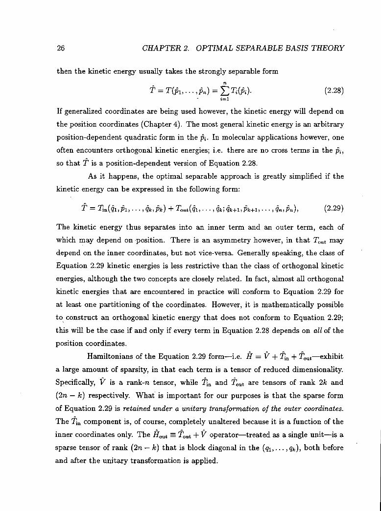
As it happens, the optimal separable approach is greatly simplified if the
kinetic energy can be expressed in the following form:
(2.29)
The kinetic energy thus separates into an inner term and an outer term, each of
which may depend on -position. There is an asymmetry however, in that Tout may
depend on the inner coordinates, but not vice-versa. Generally speaking, the class of
Equation 2.29 kinetic energies is less restrictive than the class of orthogonal kinetic
energies, although the two concepts are closely related. In fact, almost all orthogonal
kinetic energies that are encountered in practice will conform to Equation 2.29 for
at least one partitioning of the coordinates. However, it is mathematically possible
to_ construct an orthogonal kinetic energy that does not conform to Equation 2.29;
this will be the case if and only if every term in Equation 2.28 depends on all of the
position coordinates.
Hamiltonians of the Equation 2.29 form-i.e. if = V + Tin + Tout-exhibit
a large amount of sparsity, in that each term is a tensor of reduced dimensionality.
Specifically, V is a rank-n tensor, while Tin and Tout are tensors of rank 2k and
(2n - k) respectively. What is important for our purposes is that the sparse form
of Equation 2.29 is retained under a unitary transformation of the outer coordinates.
The Tin component is, of course, completely unaltered because it is a function of the
inner coordinates only. The flout= Tout+ V operator-treated as a single unit-is a
sparse tensor of rank ( 2n - k) that is block diagonal in the ( q1 , ... , qk), both before
and after the unitary transformation is applied.

2.5. APPLICATION TO T + V HAMILTONIANS 27
These facts are very beneficial from the standpoint of trying to find the
optimal outer basis. In particular, the preservation of sparsity ensures that the vast
majority of the coupling constants will be zero. Moreover, tin can be completely
ignored, as a result of which the orthogonality condition (Equation 2.17) reduces to
a simple integral:
for all { m, m'} (2.30)
where q = ( q1, ... , qk)·
Note that where the outer basis is concerned, flout has replaced if as the rel
evant operator. It is natural to view the former as a collection of ( n- k )-dimensional
outer subsystems parametrized by the inner coordinates. By optimizing the outer
basis, we are in effect trying to simultaneously diagonalize the entire collection collec
tion of ( n - k )-dimensional subsystems flout· In the general case, one cannot actually
diagonalize all of the subsystems using a single basis; but the optimal choice is the
best compromise in the least-squares sense.
2.5.2 Partitioning of Coordinates
For an n-dimensional problem, there are 2n distinct partitionings of coordi
nates into inner and outer categories, each of which can potentially lead to a different
optimal fi0 • In deciding which particular partitioning should be adopted, the results
of the previous subsection can serve as a useful guide.
One should, if possible, choose a (nontrivial) partitioning which satisfies
Equation 2.29; for in addition to simplifying the analysis, the majority of the coupling
constants will be zero by virtue of the sparse form of flout· The availability of such
choices is related to the separability of the kinetic energy. If Tis completely separable,
as in the standard rectilinear case, then any partitioning will do. Only when the
kinetic energy is completely non-separable can no such partitioning be found, m
which case a change of coordinates might be employed to induce a separation.
As is evident from Equation 2.29, the kinetic energy need not be strongly
separable, as Tout may depend on all of the position coordinates. If T does happen to

28 CHAPTER 2. OPTIMAL SEPARABLE BASIS THEORY
be strongly separable however, then exchanging the inner for the outer coordinates
also satisfies Equation 2.29. To determine which is the better choice, the simulta
neous diagonalization interpretation of Section 2.5.1 can be fruitfully called upon.
If (Tout + V) were to vary only slightly with the inner coordinate parameters, then
the various subsystems would be almost identical, and would therefore be almost
entirely diagonalized by the best-fit outer basis. One is thus led to select-as inner
coordinates-those Qi upon which the original Hamiltonian has the least dependence.
As a special case, consider the completely separable position-independent ki
netic energy of Equation 2.28, for which the coordinates have been mass-weighted so
that the Ti's are all of identical form. The subsystems of (Tout+ V) are now identical
except for the potential energy V which depends on the positions only; thus, selecting
inner coordinates involves nothing more than a straightforward analysis of the func
tion V(q11 ••• , qn)· A simple intuitive candidate for the optimal basis is suggested
namely, that basis which diagonalizes Tout+(V)q where (V)q is the collection-averaged
potential energy function. While this choice is not generally the optimal one--indeed,
the true optimum may not even be of the form Tout(Pk+b ... ,fin)+ V(qk+l, ... , qn)
it should nevertheless reduce the coupling significantly, and is in any case readily
obtainable even when a determinination of the true optimum is intractible.
2.5.3 Inelastic Scattering
In inelastic scattering applications, the above Tout+ (V)q candidate is closely
related to the coupled channel approximation, for which one uses the asymptotic,
rather than the average potential. In fact if we were to generate our outer basis
from Tout+ Vas(Qk+b ... qn), and restrict ourselves to the energetically accessible bound
states only (the open channels), then exactly the coupled channel approximation
would result. In such inelastic applications, a natural separation between internal
(intrafragment) and translational (interfragment) coordinates arises. The potential
usually varies less with the latter, which is why the internal coordinates are chosen
(perhaps counterintuitively) to be the outer coordinates. The asymptotic potential
is then defined as the limit of V as q approaches infinity.

2.6. RESULTS-SHIFTED HARMONIC OSCILLATOR 29
A primary advantage of the coupled channel approach is that G(E) can be
accurately determined using a small and finite outer basis, provided the energy E
is sufficiently lower than some cutoff value used to truncate the basis set. Although
finite, the various channels are still coupled together. An uncoupled approximation
can be obtained by ignoring the off-block-diagonal matrix elements of H. This is, in
fact, a standard way to define distorted waves in the multi-channel case.
It is clear that the uncoupled channel approximation above constitutes; in
our language, a choice of fl0 • We can therefore think of the optimal flo as the
choice which redefines the channels in the best possible way, vis-a-vis minimizing the
interchannel coupling. This should generally improve the convergence of the resultant
multichannel distorted wave Born expansion, although very little is rigorously known
about this subject.6
2.6 Results-Shifted Harmonic Oscillator
As an analytical benchmark system, we consider the two-dimensional shifted
harmonic oscillator Hamiltonian, i.e. A 2 A 2 2
il = ~ + Py + mw (il _ f(x))2 2m 2m 2
(2.31)
where f(x) is the shifting function. Physically, this Hamiltonian might describe a
particle in a surface channel etched along the curve y = f(x), or perhaps a simple
harmonic oscillator whose equilibrium position was somehow constrained to lie on the
curve (Figure 2.1). For the first part of our analysis we can allow the shifting function
to be arbitrary; although later a specific form will be provided. For now, it should
simply be mentioned that in the limit f(x) --t 0, H approaches the separable system
consisting of a free particle in x and a harmonic oscillator in y.
If /' ( x) approaches zero in the infinite limits, then separable asymptotic
states exist in those limits, and we can think of this as a scattering system with
channels defined along y. As a scattering system it is somewhat unusual however; for
although there is a clearly defined reaction path along y = f ( x), there is no transition
state or equilibrium geometry per se, as the potential is constant along the reaction

30 CHAPTER 2. OPTIMAL SEPARABLE BASIS THEORY
f(x)
X
Figure 2.1: Physical schematic of the shifted harmonic oscillator.
path. Adopting the reaction path perspective, any scattering that may arise is thus
solely attributable to the curvature of the path itself rather than the potential along
the path. Although the dynamical effects of curvature may be just as significant as
those of the potential itself in many real systems, the contribution of the former is
generally less well understood. The shifted harmonic oscillator system can therefore
serve as a useful benchmark application because it isolates the effects of curvature.
Since the kinetic energy is completely separable and position-independent,
Equation 2.29 is satisfied by any partitioning into inner and outer coordinates. The
only nontrivial value for k is unity; so we are left with deciding whether x or y is
the inner coordinate. We expect V(x, y) to vary less with x than with y, which is
particularly valid as f(x) becomes small. In light of Section 2.5.2, The natural choice
for the inner coordinate is thus x.
The first task is to optimize the outer basis via a unitary transformation
in f; and Py· As we have seen (Section 2.5.1), this is equivalent to finding the basis
which best diagonalizes the following x-parametrized collection of one-dimensional

2.6. RESULTS-SHIFTED HARMONIC OSCILLATOR 31
Hamiltonians: A 2 2
A Py mw A 2 Hout(x) =
2m+ -
2-(y- f(x)) (2.32)
In light of Section 2.5.3, we choose the eigenfunctions of Py 2 /2m + ~mw2 (y - (!) )2
as our initial guess, where (!) is the mean value of f(x ). For convenience, we force
(!) = 0 by constraining f(x) to be an odd function. This results in V(y) = ky2 /2
which, as it happens, is also equal to (V(y)) apart from an immaterial constant.
Our candidate outer basis functions then, are the well-known harmonic os
cillator eigenstates. We have not yet proven that this is an optimal choice; but we will
soon do so-even for f(x) not small-by demonstrating that Equation 2.30 is satis
fied. When expressed in the partially diagonal basis, flout takes on a block-tridiagonal
form, where the off-block-diagonal terms arise from the yf(x) cross terms in the
potential. Specifically, we have
ll' ( Hout x)
(2l + 1)1iw + mw2 f 2(x) 2
0
max(l, l')fiw3m f(x) 2
for l -l' = 0
for ll - l'l = 1
otherwise
(2.33)
(2.34)
(2.35)
where land l' index they-oscillator states. Clearly, Equation 2.30 is zero for ll-l'l # 1.
When ll -l'l = 1, the result is proportional to f f ( x) dx, which is also zero by virtue of
f ( x) being odd. The candidate outer basis is therefore optimal! The coupling-which
in the general two-dimensional case would be a tensor of rank four-is seen above to
be a rank-2 function of l and x only. Note also that H!~;=1 is proportional to f( x )-i.e.,
the inherent coupling vanishes as the shifting approaches zero, as expected.
Having obtained the best outer basis functions, we now examine the inner
coordinate problem; i.e. the diagonalization of the diagonal blocks 'fin+ fi~~t that
comprise fl0 . Note that even though the original potential involved cross terms, the
new potential fi~~t(x) is completely additive in x and l. Consequently, all blocks of
flo are diagonalized by the same inner basis. Thus, although the inner eigenstates are
formally parametrized by l; for this particular system the [-dependence happens to
disappear-i.e. the optimal weakly separable basis happens to be strongly separable.

32 CHAPTER 2. OPTIMAL SEPARABLE BASIS THEORY
Apart from an l-dependent constant, all H0 blocks are equivalent to the
following one-dimensional Hamiltonian in x:
~ 2 2 ir = Px + mw f2(x)
m 2m 2 (2.36)
Since f ( x) is odd, we have an even potential well that is concave and centered at the
origin. Such a well may admit bound state solutions.
To proceed any further however, we must specify a particular form of the
shifting function f ( x). The .choice f ( x) = T0 tanh( ax) is a useful one in that it
represents a smooth, sigmoid progression from a ( -T0)-centered oscillator to a To
centered one. The amount of coupling can be adjusted by varying the parameter
T0 , whereas the rate of change is determined by a. Moreover, the resultant inner
Hamiltonian ~ 2 2'7"2
~ ~ mw1 0 2 ~ Hin =- + tanh (ax)
2m 2 (2.37)
can be diagonalized analytically.
In the appendix of this chapter (page 39), the (normalized) bound state
eigenfunctions of Equation 2.37 are shown to be
(v) .j(v-n)r(2v-n+1) 2 -(v-n)(d)n 2 v
4>n ("7) = n!~2vr(v + 1) (1 -1} ) 2
dry (1 -ry ) (2.38)
where 1} = tanh(o:x), .jv(v+ 1) = mwT0jafi, and n = {0,1, ... ,int(v)}. Curiously,
a bound state always exists even in the limit T0a-+ 0 (page 43).
This fact reveals an interesting feature of H. If there is no shifting, there are
no bound states; however, any amount of shifting, no matter how small, necessarily
induces at least one bound state in H0 • In the small coupling limit, H0 becomes a
valid replacement for ii. However, since the latter has no actual bound states, the
bound states of H0 must correspond to long-lived resonances of H. This qualitative
result can be used as a benchmark for comparisons with other separable or adiabatic
approximation methods, such as those based on the "reaction path" .37- 39
The most rigorous adiabatic version of the reaction path Hamiltonian is
probably that of Miller.40 In this formalism, the reaction coordinate s is defined by
the reaction path together with nearby paths that are locally parallel to it. In two

2.6. RESULTS-SHIFTED HARMONIC OSCILLATOR 33
dimensions, the reaction coordinate contours are straight lines normal to the reaction
path, which also serve to define the perpendicular coordinate Q. The approximate
Hamiltonian of Miller is adiabatic in that the Q portion of the Hamiltonian (incor
porating quadratic terms only) is parametrized by s.
Upon solving the quadratic problem at each point along the reaction path,
one is left with an effective one-dimensional Hamiltonian in s
HRP = p; (1- (2n + 1)K2(s)) -3/2 + Veff(s), n 2m w(s)
(2.39)
where n and w( s) are respectively the vibrational quantum number and frequency
associated with the Q oscillator at each point s, and K( s) is the curvature of the
reaction path y = f(x).
For the shifted harmonic oscillator system, the effective potential in the
small shifting (T0a --+ 0) limit becomes
1 1i 'Vcff = (n+ 2)1iw(s) = 2wsec(B) (2.40)
where tan(B) is the magnitude of the slope of f(x). Note that the effective potential
that results is actually a barrier, rather than a well. This is in stark qualitative
contrast to the effective potential of Equation 2.37, and a somewhat surprising result.
In particular, the reaction path approximation does not predict any resonances, even
in the small coupling limit. Even if one were to change to the coordinate e(x ), defined
so as to render the kinetic energy of Equation 2.39 equivalent to that of Equation 2.37,
the resultant potential would still be a barrier due to the monotonicity of "Veff with
respect to jxj.
We now consider a perturbation theory expansion of the bound states of H. The optimal H0 leads to the following zeroth-order eigenfunctions and eigenvalues:
- <Pn(TJ)'Pz(Y) mw
2T.2 [ (v- n)2
] 0 1- ( ) + (l + 1/2)1iw 2 vv+1
(2.41)
(2.42)
where the <pz(y) are the harmonic oscillator eigenstates. Since the first-order energy
corrections are all zero, the additive Equation 2.42 result is correct to first order.

34 CHAPTER 2. OPTIMAL SEPARABLE BASIS THEORY
Moreover, the first-order eigenfunction corrections Cnl,n'l' are all zero except when
ll-l'l = 1 and ln-n'l is odd. We choose l = l'+l,
which are given by
n > n' and define Cz n'n = Cnz n'l' , ,
Jt!iwm/2 To J~n',n) Cln'n = [ ] ' 1i + mwT(f (n2 - n'2 )fv- 2(n- n') f(v + 1).
(2.43)
The first-order corrections specified in Equation 2.43 are obtained from the
one-dimensional integrals
(2.44)
whose closed-form expressions for the bound states are derived in the appendix. Gen
erally speaking, the magnitudes of these integrals are much less than unity (Fig
ure 2.2). The curves all reach an extremum at some Vmax on the order of n, and then
approach zero monotonically as v is increased. The largest magnitudes are of order
unity only when n ~ n' ~ v, and in general diminish as In- n'l or v is increased.
Thus, for a particular v, the most significant contributions to Equation 2.22 will be
from the n, n' ~ v terms.
The limits T0a ~ 0 and T0a ~ oo are of interest. The former limit is that in
which the shifting function and coupling-and thus, the first-order corrections-are
expected to approach zero. Indeed, we find that
(2.45)
Thus, it is possible to have a large number of bound states v, even as the Cl,n'n
approach zero. If we also impose a large v limit, we find that the highly excited
and continuum corrections to the low-lying eigenstates become negligible even in a
relative sense. The corresponding resonances of if are therefore expected to be very
long-lived indeed.
The second case of T0a ~ oo represents the other extreme, in which f ( x)
approaches. a step function. In this limit we have
c/ I ~ ~ l [ V + 1 l J(n',n) ,n n 2T0a n2 - n'2 - 2(n- n')v v
for v(Toa) >> 1. (2.46)

2.6. RESULTS-SHIFTED HARMONIC OSCILLATOR
-0.8
-0.6
-0.4
-0.2
0.0
0.2 0.0
,-- ...... r, I .. I ', j I ....... ....... ....... I
I ............ I -- ...... -----
--------------' ........... ----.... --
10.0 20.0 30.0 v
35
Figure 2.2: J~n',n) as a function of the action parameter v, for several values of (n',n): -- (0,1); ----- (0,5); ---- (2,5); --- (4,5); ----- (20,21). The curves all reach an extremum at some llmax on the order of n, and then approach zero monotonically as v is increased.
Curiously, the first-order corrections approach zero in this limit also. This is true
despite the fact that the A coupling terms are comparatively large, because in this
limit the energy separations between the bound states are even larger.
Our final task is to evaluate the kernel matrix A pertaining to the generalized
Born expansion of Equation 2.26. Because fi is block-tridiagonal, and also because
the H0 blocks can all be simultaneously diagonalized, it turns out to be convenient
to use the <I>nz basis. In this representation,
1 n'n ( · ) Ho' = E- Enz + 'LE 8n'n (2.47)
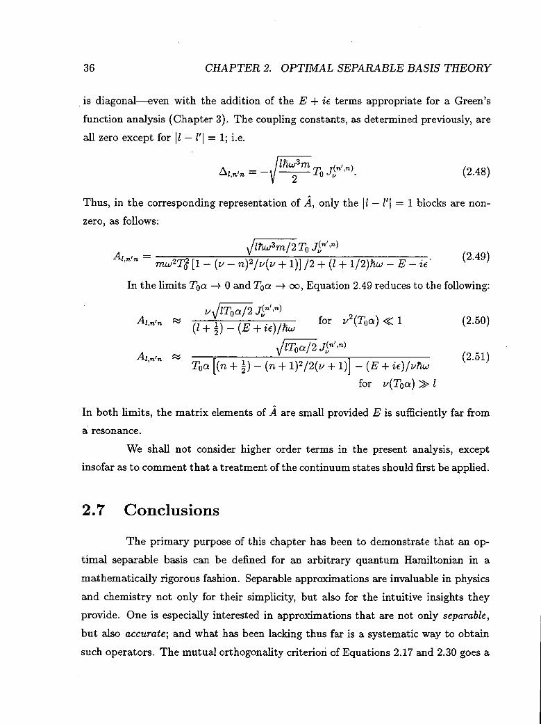
36 CHAPTER 2. OPTIMAL SEPARABLE BASIS THEORY
. is diagonal-even with the addition of the E + ie terms appropriate for a Green's
function analysis (Chapter 3). The coupling constants, as determined previously, are
all zero except for ll- l'l = 1; i.e.
A - -Jlfiw3m,..,., j(n',n) L..l.l,n1n -
2 .LQ v · (2.48)
Thus, in the corresponding representation of A, only the ll- l'l = 1 blocks are non
zero, as follows:
Jlnw3m/2 To J~n',n) Az,n'n = mw2T6 [1- (v- n)2 jv(v + 1)] /2 + (l + 1/2)fiw- E- ie ·
(2.49)
In the limits T0a --+ 0 and T0a --+ oo, Equation 2.49 reduces to the following:
Aln'n ~ ' (l + ~) - (E + ie)/fiw
(2.50)
Jr-l1:_o_a_/_2 J~ n' ,n)
~
T0a [(n + ~)- (n + 1)2/2(v + 1)]- (E + ie)jvfiw (2.51)
for v(T0a) » l
In both limits, the matrix elements of A are small provided E is sufficiently far from
a resonance.
We shall not consider higher order terms in the present analysis, except
insofar as to comment that a treatment of the continuum states should first be applied.
2. 7 Conclusions
The primary purpose of this chapter has been to demonstrate that an op
timal separable basis can be defined for an arbitrary quantum Hamiltonian in a
mathematically rigorous fashion. Separable approximations are invaluable in physics
and chemistry not only for their simplicity, but also for the intuitive insights they
provide. One is especially interested in approximations that are not only separable,
but also accurate; and what has been lacking thus far is a systematic way to obtain
such operators. The mutual orthogonality criterion of Equations 2.17 and 2.30 goes a

2. 7. CONCLUSIONS 37
long way towards this goal by providing the separable H0 which most closely approx
imates the true Hamiltonian, for a. given factorization of configuration space. Such
an operator is clearly imbued with a physical significance; as is the residual A, which
embodies the physically-relevant inherent coupling of the system.
The optimal separable basis also provides an advantageous starting point
for series expansions. The fact that this method is useful for both Green's function
and eigenfunction expansions is not surprising; as both involve the same perturbation
Li. Similarly, the applicability of the method to both analytical and computational
pursuits is also to be expected; as in either case it is of great benefit to be able to
lower the dimensionality. It is significant that in the latter case a computer algorithm
can be developed to perform the optimization automatically17 (Chapter 3). The cor
responding analytical problem may in individual cases prove to be intractible, albeit
dimensionally-reduced; but even then the physical picture developed in Sections 2.3
and 2.5 can be used to obtain a worthy substitute. It is also significant that the
method-though applicable to arbitrary multi-dimensional operators-is particularly
suited to sparse Hamiltonians, in that sparsity is maintained throughout.
The results for the shifted harmonic oscillator system of Section 2.6 are quite
encouraging. Not only were we able to obtain the analytically optimal outer basis for
any shifting function f ( x), our physical intuition led us immediately to the correct
answer. All that was required was a simple integral verification of Equation 2.30.
Although this situation is to some extent fortuitous, it nevertheless indicates that the
average potential candidate probably does lead to an excellent, if not optimal, outer
basis in the general case.
Having obtained the optimal outer basis for the generic shifted oscillator
system, the inner problem was also reduced to a particularly simple form. The strong
separability of the new potential allowed us to solve the full H0 problem by simply
diagonalizing a single one-dimensional system, rather than a collection of systems.
In addition, the inherent residual coupling was found to be of rank two only. Thus,
with comparatively little effort we were able to obtain the most accurate zeroth- and
first-order approximations for this non-trivial two-dimensional system, and to prove

38 CHAPTER 2. OPTIMAL SEPARABLE BASIS THEORY
the existence of resonances even in the limit of infinitesimal shifting.
Although the results were encouragin~ for the two-dimensional system dis
cussed in this chapter, the method is expected to be even more effective for higher
dimensionalities-at least for numerical applications. One reason is that there is
generally more freedom of choice with respect to coordinate partitionings as the di
mensionality is increased. Another reason is that the sparsity usually increases with
dimensionality; so that a greater percentage of the matrix elements of 6. will be zero.
We will investigate a non-trivial three-dimensional system in Chapter 4.
If the kinetic energy is more separable than indicated in Equation 2.29, one
might wonder whether the present approach could be modified to exploit this ad
ditional sparsity. Instead of just two tiers of coordinates, one could define three or
more layers. Under the most favorable scenario of Equation 2.28, each coordinate
would constitute a separate layer, to be "peeled off" one at a time. The tremendous
initial sparsity of such a system would be preserved throughout; moreover, the con
vergence at the top-most level should be very good, since the preconditioner involves
all but one of the coordinates. This recursive possibility is discussed in more detail
in Chapter 5.
Although a recursive approach may be beneficial in some cases, a straight
forward application as presented in this chapter should be suitable for just about
any reasonably small system of interest. Moreover, there are plenty of applications
for which a two-tiered approach is most natural. In molecular systems for example,
there is an obvious distinction between electronic and· nuclear degrees of freedom.
In non-rigid rotors, three global rotational degrees of freedom are naturally distin
guished from the others. This partitioning results in the so-called "Coriolis" coupling,
whose minimization via the optimal separable basis we shall consider in Chapter 4.
Scattering Hamiltonians also exhibit a separation between internal and translational
coordinates, by virtue of the asymptotic form of the potential. Numerical results for
a simple molecular reactive scattering system17 are obtained in Chapter 3, wherein
we also present an efficient algorithm for obtaining the optimal outer basis.

2.8. APPENDIX: THE TANH2 POTENTIAL HAMILTONIAN 39
2.8 Appendix: The tanh2 Potential Hamiltonian
The tanh2 potential is equivalent to a -sech2 potential, apart from a con
stant of unity. The latter potential, also known as the "Eckart well" or the "symmetric
Poschl-Teller hole," 41 was introduced by Rosen and Morse42 who first solved the quan
tum problem in an analysis of polyatomic molecular vibration energies. It has since
been reconsidered in various other fields, including soliton research.43
Traditionally, the eigenproblem is solved by transforming Schrodinger's dif
ferential equation in x to an equivalent differential equation in the variable sinh2( ax).
If W is divided by certain powers of cosh(ax) and sinh(ax), then this equation be
comes consistent with the generic hypergeometric differential equation. Unnormalized
solutions are therefore obtainable in terms of hypergeometric functions;44 although
the parameter values do not satisfy any special properties, and even and odd func
tions must be handled separately. Analytic normalization constants are also highly
nontrivial, as they involve integrations of hypergeometric and hyberbolic sinusoidal
functions. Indeed, these constants were not obtained for some time after the un
normalized solutions were first discovered-and even then, only as very complicated
expressions involving sums of products of eleven gamma functions.45
Our approach to the problem is much more straightforward, and involves
the substitution of tanh( ax) rather than sinh2 (ax). With no further massaging, we
are led directly to Legendre's differential equation, whose solutions for our particular
problem are simple algebraic expressions. Moreover, the normalization constants can
be obtained from algebraic integrals that are comparatively simple.
2.8.1 Solving the Eigenproblem
We wish to find the eigenfunctions and discrete eigenvalues of the following
one-dimensional differential equation:
1i2 ~ mw2Tl: --d
2¢(x) + 0 tanh2 (ax) ¢(x) = E¢(x).
2m x 2 (2.52)

40 CHAPTER 2. OPTIMAL SEPARABLE BASIS THEORY
By transforming to the coordinate 7J =tanh( ax), we obtain (with 7]1 = 1- 7]2 )
(2.53)
Dividing by -a27J'n2 /2m yields Legendre's differential equation46
(2.54)
provided v(v + 1) = (mwT0fan)2 and J-L2 = v(v + 1)[1- 2Ejmw2TJ].
If J-L and v are taken to be positive {imaginary) square roots, then the solu
tions to Equation 2.54 are the associated Legendre functions of the first and second
kind, P;=ll and Q;ll. For energies E > !mw2TJ, the parameter J-L is pure imaginary
as is appropriate for the continuum states. Bound states arise when E is less than
!mw2TJ, in which case J-L is real, and taken to be positive.
For integral v, the P/: are the standard Legendre polynomials, which are
well known to be square-integrable if IJ-LI is an integer less than or equal to v. The
generalization for non-integral values of v turns out to be that the difference between
v and J-L must be integral. This condition can be determined by evaluating the asymp
totic convergence of the Legendre functions. The asymptotic expression for the P;;ll
solutions, for example, is as follows:47•48
lim p+ll(z) = 21l7rl/2(z2- 1)-p/2 z~±l v
( . r(~)r(J-L)
x r2(~- ~- ~)r(-~ + ~)r(1 + ~- ~)
=r= 2r(~)r(J-L) ) (2 55) r(I+~+~)r{I+~-~)r(I-~+~)r(-~-~) ·
Given that the poles of the r function occur only at non-negative integers, it is easy
to show that convergence occurs only when both v and J-L are integers.
This condition is clearly too restrictive, since v is an arbitrary action param
eter that can take any positive value. We must therefore consider the P;ll solutions.
(Note that contrary to the special case of integral v, the P;P are not in general

2.8. APPENDIX: THE TANH2 POTENTIAL HAMILTONIAN 41
proportional to the P;;~'-!) The corresponding asymptotic expressions are47
/!;.
lim P;;~'-(z) (z- 1)
2 1 z-++1 2 f(1 + p,)
(2.56)
lim P;;~'-(z) = ( -z ) ~ f(p,) z--+-1 z + 1 f(1 + p, + v)f(p,- v)'
(2.57)
from which it is easily established that the bound states occur whenever (v- p,) is a
non-negative integer.
Defining n = (v- p,), the bound state solutions ¢n(7J) are thus proportional
to P;:-v ( 7J), where n ranges from zero to the largest integer less than v. These
functions are simple polynomials in 7J and J7ii (closely related to the Gegenbauer or
"ultraspherical" polynomials45 ) multiplied by 7J1vf2• The corresponding energy values
are 1 2 2 [ (v- n)
2] En = -mw T0 1 - ( ) , 2 vv+1
(2.58)
from which the ground state energy is seen to be Eo= 1i2a.2v /2m. Figure 2.3 depicts
the eigenenergies as a function of the action parameter v.
The bound state solutions satisfy a somewhat unusual orthonormality con
dition. Because the coordinate 7J is used instead of x, we have
[1 ,~..(v)( ) ,~,.(v)( ) 1 d - [> ' }_1 '+'n' 7] '+'n 7] (1- 7J2) 7]- nn
(2.59)
where a factor of fo is understood to be removed from the definition of ¢( 7J) to keep
things dimensionless. (This factor must be resupplied when working with ¢(x).) In
terms of the P;:-v, the above integral can be analytically evaluated to determine the
proper normalization constants. 49 This yields
(2.60)
Alternatively, we can use the Leibnitz and Rodrigues formulas50 to derive the excited
states by differentiating the following expression for the ground state:46
(2.61)
where

42
en -~ ~ Q) s:::::: Q) s:::::: Q) C)
[i]
0
-5
-10
-15
-20
-25 0.0
---...
CHAPTER 2. OPTIMAL SEPARABLE BASIS THEORY
...................... ..
1.0
.. .. ... ... ... ... ... ... ... ... ...
2.0
... ' ' ' ' ' ' ' ' ' ' ' ' ' ' ' ' ' ' ' '
3.0 Action (v)
' ' ' ' ' ' ' ' ' '
4.0
' ' ' \ \
' 5.0 6.0
Figure 2.3: Eigenenergies of the tanh2 potential Hamiltonian (in units where a 21i2 /2m = 1) as a function of the action parameter v, for the ground and several excited states (n = 0-5). Zero energy is defined at the continuum threshold. Solid lines represent eigenenergies; the dashed line represents the well-depth. Note the existence of a ground state even for v « 1.

2.8. APPENDIX: THE TANH2 POTENTIAL HAMILTONIAN 43
This results in the normalized formula of Equation 2.38.
The limiting case behaviour of the bound state solutions is also quite inter
esting. Since v must be positive, there is always a bound stat~even in the limit
as the well depth (To) or width (1/a) approaches zero, and the corresponding action
becomes arbitrarily small in relation to Planck's constant. This egregious departure
from WKB theory is in marked contrast to most other solved potentials. Only one
bound state remains in these limits however, since v -t 0. According to Equation 2.61,
it must be proportional to (1 -172)(v/2). Thus, the ground state is in essence simply a
power of the original potential! As v approaches zero, ¢0 approaches a uniform distri
bution; moreover, the corresponding energy is seen from Equation 2.58 to approach
the continuum threshold. These results are consistent with the limiting functional
form of the potential itself, which approaches a constant in the small-v limit.
2.8.2 Obtaining the J~n',n)
We wish to evaluate the Jv integrals of Equation 2.44. Using a well-known
recursion relation of the Pf: to expand ¢n' ,50 we can write
J(n',n) v
J(n1,n) v
1 (2v-n')(n'+l) J(n'+l,n) _ ~ (2v-n1+l)n1 J(n'-l,n) 2 (v-n'-l)(v-n') v 2 (v-n'+l)(v-n') v '
j_ll ¢!:;)(17) ¢t>(17) (1-172tl/2 d17.
(2.62)
(2.63)
The quantity lv is non-zero only when n,n';::: 0 and n-n' is even. Using the Leibnitz
formula, the ( unnormalized) eigenfunctions can be expressed as a sum of algebraic
functions of 17:
- {1 - 172) -(v2-n) (.!!._) n {1 - 172t d17 .
~(-1)i(n) ~ v! . {1- )I+[~-i](1 + )I-[~-i] L...J i (v-t)! (v-n+t)! 17 17 i=O
(2.64)
The integral in Equation 2.63 can be analytically evaluated by expanding both ¢n
and ¢n' using Equation 2.64 above. The result is the following:
(2.65)

44 CHAPTER 2. OPTIMAL SEPARABLE BASIS THEORY
The R.H.S. of Equation 2.65 is a somewhat unwieldy double summation
involving (n+ 1)(n' + 1) terms. A simpler expression involving a sum of only (!n' + 1)
terms can be obtained by deriving a recursion relation for the lv. It turns out to
be more convenient to derive the relation for the lv, defined via Equation 2.63 with
respect to the ¢n rather than the ¢n· Using integration by parts and Equation 2.62,
the following recursion relation is easily derived:
( ')f-(n'+l,n) _ '(2 '+l)(2 1 )f-(n1-l,n) 2( ')f-(n',n+l) n-n v - n v-n v-n -n v - v-n v (2.66)
Thus, an arbitrary L can always be expressed in terms of the L for which n' = 0.
These are analytically obtained via direct integration of Equation 2.63, resulting in51
j(O,n) = (- 1)~7rl/2[(n _ 1)11]2 (v- ~- !)! v ·· (v- ~ )! (2.67)
for n even.
By combining t.he results of the last paragraph, any particular lv value can
be determined. The first few are as follows:
j~O,O) = ;;-II2(v _ !)!jv!
j~0,2) = _,II2(v _ ~)!/(v _ 1)!
nl,l) = 2vi. 112 (v- ~)!j(v- 1)!
j~0,4) = 9r.l/2(v- ~)!/(v- 2)!
n1,3) = -6V1rlf2(v- ~)!/(v- 2)!
nz,z) = 12v(v- 1) [ 1- ~ (v;~(2) 2] 7r112(v- ~)!/(v- 2)!
} (n + n') = 0
} (n+ n') = 2
) (n+~) = 4
(2.68)
(2.69)
(2.70)
In general, the factor in brackets is .a sum over int(!n') + 1 terms. The properly
normalized formula for an arbitrary lv is
J~n',n) = ( -1) n-;n' 1r1/2 (n-n'-l)!!..J(2v-n)!(2v-n')!..J(v-n)(~;;~')(n'!/n!) X v.
(2.71) int(n' /2)
1 "'(-1)i2(n'-i) (v-(n+n')/2+i-~) (n+n'-2i-1)!! (v-(n+n')/2+i-2 )! L...J k (v-n' +i)!(n'-2i)! (v-(n+n')/2+i)! · i=O

45
Chapter 3
Reaction Probabilities and
Opti~ized Preconditioning
3.1 Introduction
In this chapter, we discuss how the optimal separable basis approach of
Chapter 2.3 can be usefully applied to actual numerical calculations for real molecu
lar systems. Although the method is certainly applicable to bound state calculations
(Chapter 2), this chapter addresses scattering calculations only-especially of chem
ical systems that undergo reactive scattering. W~ also limit the discussion to the
microcanonical scattering quantities described in Chapter 1.
The evaluation of the energy Green's operator G(E) is paramount in the
calculation of microcanonical quantum scattering quantities of all kinds, including
those pertinent to inelastic and reactive scattering systems. Using the discrete vari
able representation (DVR) grid methodology developed by Light and others,52-62 the
Hamiltonian operator and associated scattering states are represented as finite ma
trices and vectors, respectively. These are defined with respect to a grid of discrete
points over configuration space. Since scattering systems are by definition of infinite
extent, some method most be adopted for keeping the effective configuration space
finite in the asymptotic regions. A simple truncation of the grid will not do, as it will
introduce spurious reflections of outgoing waves that are obviously not physical.

46 CHAPTER 3. REACTION PROBABILITIES
One solution is to introduce complex optical potentials into the Hamiltonian,
which have the effect of absorbing the outgoing flux before it reaches the end of
the grid. This kind of approach has a very well established history in physics and
chemistry. 6•63- 68 Seideman and Miller developed a version for time-independent DVR
scattering applications, for which the i€ term in Equation 2.24 is replaced with the
(pure imaginary) absorbing potential.6g-71 A matrix representation of the Green's
operator G( E) can then be obtained numerically using straightforward linear algebra
techniques to perform the matrix inversion of Equation 2.24.
To obtain accurate results the absorbing potential must be positive and
"small," yet large enough that the flux is almost all absorbed before reaching the end
of the grid. The proper values for the parameters describing € and other aspects of
the DVR grid-such as the spacing between adjacent grid points, and the potential
cutoff used to truncate energetically inaccessible regions of the grid-are not known
a priori. In practice, these must be obtained empirically by sequentially varying the
parameters until "convergence" is attained-i.e. until a significant variation of any
of the parameters does not affect the final numerical results appreciably.
Proper convergence of the DVR parameters is a significant, but not insur
mountable, hurdle impeding accurate numerical determination of the microcanonical
scattering quantities. A far more significant difficulty however, is the fact that the
numerical burden of the DVR approach scales very unfavourably with energy and
dimensionality-primarily because the matrix sizes becomes inordinately large, even
to be handled by modern computers. This problem has been ameliorated somewhat
through the use of certain specialized linear algebra techniques, e.g. Krylov and other
sparse matrix methods.7•8•72-74 Nevertheless, scattering calculations to date have been
for the most part limited to small systems at relatively low energies.34•75- 79
In recent years however, a technique known as "numerical preconditioning"
has been explored in conjunction with DVR Green's function calculations.9•73•80•81
The use of preconditioners in chemical reactive scattering applications has thus far
exhibited significant promise.82•83 Unfortunately, selecting a good preconditioner for a
given system a priori has proven to be something of a "black art;" as it is numerically
unclear how to predict the quantitative effect of a particular choice of preconditioner,

3.1. INTRODUCTION 47
short of actually applying it and performing the calculation.
A major motivation of this work has been the desire to develop some quan
titative means of evaluating different preconditioning schemes, so that an optimally
efficient preconditioner can be systematically tailored for a given physical system.
This can be achieved by taking the view that the DVR Hamiltonian is a physical ob
ject rather than simply a numerical object. We should therefore look for something
physical that corresponds to the numerical process of preconditioning.
Such a correspondence can in fact be obtained;84 in Section 3.4 it will be
shown that numerical preconditioning is physically equivalent to the propagation
of distorted waves, as per the distorted wave Born expansion (Equation 2.26). In
particular, the preconditioner matrix represents the zeroth-order Green's operator G0 ,
defined in terms of the approximate H0 of Equation 2.25 whose stationary scattering
states are the distorted waves. 6
By exploiting this correspondence, we can estimate the performance of a
numerical preconditioner by analyzing the convergence of the corresponding distorted
wave Born expansion. Physical intuition can then be brought to bear on the problem
of developing an efficient preconditioner. In particular, an optimal preconditioning
scheme84 is suggested by Chapter 2: namely, that H0 be chosen to be the optimal
weakly separable approximation to the true H<'!.miltonian.
Obtaining the optimized preconditioner numerically is a two-stage process.
First, the optimal H0 is determined; then, the preconditioner G0 is obtained via
a matrix inversion. The crucial point is that both of these are reduced-dimensional,
well-defined algorithmic operations (Section 3.5). Thus, the optimized preconditioner
can be systematically computed using only a fraction of the CPU time and memory
required by the full problem.
Section 3.2 relates the fundamentals of the DVR formalism, together with
the modifications required for using absorbing potentials. Section 3.3 describes certain
unique aspects of reactive scattering, and also presents explicit DVR formulas for the
quantities of interest. Section 3.4 examines. the use of preconditioned sparse matrix
methods in DVR scattering calculations, and also explores the connection with the
distorted wave methodology of Section 2.4.2. The optimized preconditioning scheme

48 CHAPTER 3. REACTION PROBABILITIES
is considered in Section 3.5 wherein a numerical algorithm is developed in some detail.
Section 3.6 presents results for the benchmark collinear H + H2 -+ H2 + H
chemical reaction. Converged cumulative and state-to-state reaction probabilities
were computationally much more easily achieved when the optimized preconditioner
was employed. Moreover, the preconditioner enabled exact quantum results to be
calculated for energies as high as 6 eV, which is significantly higher than what has
thus far been reported in the literature.
3.2 DVR-ABC Formalism
3.2.1 Discrete Variable Representations
In the DVR formalism, a finite grid of points is laid out over the region of
interest in configuration space; and the density and extent of the points are presumed
sufficient to adequately represent the underlying continuous coordinates for a given
application. This DVR grid can then be used to obtain approximate, position-like
representations of quantum mechanical operators and wavefunctions. An operator is
represented in the DVR as an N x N matrix, where N is the total number of grid
points. Similarly, a wavefunction is represented by a vector of length N.56•57•85
Although there are numerically many ways that one could obtain such an
approximate representation, the DVR for~alism is appealing in that it uses physical
arguments as much as possible. One starts with the eigenstates of some soluble op
erator, usually the kinetic energy. These are then truncated in some fashion, usually
via energy considerations. The resultant collection of basis functions spans a finite
subspace of the true Hilbert space. By projecting an operator onto this subspace,
one obtains the so-called "finite basis representation" or FBR.57 The FBR projec
tion can not possibly represent the corresponding operator in its entirety, but may
adequately capture all features relevant to a particular application. For example, all
kinetic energy eigenstates above a certain energy can be ignored if one is interested in
calculating the spectrum of some Hamiltonian operator for some finite energy range
only.

3.2. DVR-ABC FORMALISM 49
The FBR is not the same as the DVR, for the explicit matrix form of the
former is not position-like. To obtain the DVR from the FBR, one applies a finite
unitary transformation, defined as the transformation which diagonalizes the FBR
projection of the position operator(s) q. The new basis functions are thus position
like, i.e. approximately equal to Dirac delta functions. Moreover, the corresponding
eigenvalues of the q FBR specify the discrete values of the DVR grid.
In the one-dimensional rectilinear case where T = p2 /2m for example, the
restriction to particle-in-a-box eigenstates results in a uniformly-spaced DVR grid
with sine function DVR basis functions. Specifically, if Qi is the location of the i'th
grid point, then the corresponding basis function lqi) is
(3.1)
where D.q is the spacing between successive grid points.34 Note that in the D.q --+ 0
limit, (qlqi) approaches the Dirac delta function, as expected.
The sine-function DVR representation of the one-dimensional rectilinear ki
netic energy34 is given .by
n?( -1)i-i' { 1r2 /3 i = i'
Iii'= 2mb.q2 2/(i- i')2 i =/; i' (3.2)
In general, a discrete representation of an arbitrary operator is obtained using the
DVR basis functions such as in Equation 3.1. When representing T + V Hamiltonians
however, an additional approximation is usually made: one uses actual Dirac delta
functions for the potential rather than DVR functions, to ensure that the matrix
representation of Vis diagonal. As a result, more DVR points are usually required
than would otherwise be necessary; but the advantage is that the resultant repre
sentation of the Hamiltonian is sparse, if there is more than one degree of freedom
(Section 3.5.1).
3.2.2 Absorbing Boundary Conditions
The DVR formalism as described in the last subsection is perfectly suited to
bound state calculations. The general procedure is to use a kinetic energy cutoff in

50 CHAPTER 3. REACTION PROBABILITIES
the FBR to limit the density of grid points, as well as a potential energy cutoff in the
DVR to limit the extent of the grid. Bound state problems are really "bound" in that
one can define a finite region of configuration space outside of which the probability
is arbitrarily small (for any finite energy).
Consequently, a finite DVR can be obtained for the Hamiltonian which is
adequate for say, calculating the bound state energies up to some point. One does
not know ahead of time exactly which grid spacing and potential cutoff values are
appropriate; but by decreasing the former and increasing the latter one will eventually
reach the point where the calculated eigenenergies remain essentially constant, to
within some predetermined tolerance. ·At this point the calculations are said to be
"converged." In practice, one should not push these parameters far beyond the point
of convergence, as the commensurate increase in grid size will result in a more difficult
linear algebra problem.
Although these comments apply equally well to scattering calculations, in
the latter case there is a more fundamental problem: namely, that the configuration
space regions are unbounded in the asymptotic channels (corresponding to reactants
and products in reactive scattering). As per Section 3.1, this situation is dealt with by
introducing a negative imaginary absorbing potential iE(q). This can be thought of as
a generalization of the constant parameter iE in the Green's function as expressed in
Equation 2.24. Indeed, our naive numerical procedure for obtaining G( E) is simply to
invert the complex symmetric DVR matrix for the inverse Green's function, with the
absorbing potential substituted for iE. Moreover, the restriction to negative imaginary
potentials will automatically provide the correct (retarded) boundary conditions for
a a+( E) Green's function. However, this procedure will only yield meaningful results
if the energy is suitably restricted and E( q) is sufficiently "small" in some sense.
On the other hand, iE(q) is solely responsible for the absorption of outgoing
flux, and must therefore be sufficiently large as to absorb the vast majority of the flux
before it can be reflected back at the edge of the grid. To see that this is the case, it
is helpful to use a different interpretation, wherein the Hamiltonian is conceptually

3.2. DVR-ABC FORMALISM 51
replaced with an effective Hamiltonian86- 88
Hef£ = if - i€ (3.3)
governing the evolution of a fictitious dynamical system. Note that Heff is no longer
Hermitian, so that probability is not conserved; and this is of course what accounts
for the absorption of flux. The degree to which flux is absorbed is thus depep.dent on
the size of the absorbing potential.
Armed with these perspectives, we can address the issue of selecting an
appropriate absorbing potential function E( q). In light of Equation 3.3, the absorbing
potential should clearly be zero or negligible in the interaction region, as the true and
fictitious dynamics should differ only in the asymptotic channel regions. Assuming
that the absorbing potentials are "turned on" as soon as one has comfortably entered
the asymptotic regions, and "turned off" again as soon as the flux has been adequately
absorbed (at which point the DVR grid can be truncated), how far out must one go?
Clearly, if E is increased-whatever the specific functional form-the absorb
ing boundary will be narrower, and vice-versa. A narrower boundary is desired from
the perspective of reducing the grid size. However, in light of Equation 2.24 we expect
that E should not be too big. In fact, one finds in practice that the abrupt changes
in the potential implied by a large E and narrow boundary induce a certain amount
of artificial reflection.67,69
In practical applications therefore, one finds it necessary to converge the
calculations with respect to the absorbing boundary width and heighth, as well as
grid spacing and potential energy cutoff. One could also vary the functional form of
E(q), in order to minimize reflection and maximize absorption for a given boundary
width. In the one-dimensional case, semiclassical arguments have been made in fa
vor of ql.5 potentials69 and other arguments support quadratic potentials,89 although
these do not extend readily to the multi-dimensional case. Numerical experiments
performed previously for power law and Woods-Saxon potentials seem to indicate
that the particular choice does not matter very much. 69 In any event, we have found
quartic potentials to be quite satisfactory; these are used throughout this work except
where explicitly stated otherwise.

52 CHAPTER 3. REACTION PROBABILITIES
3.3 Quantum Reactive Scattering Calculations
Having established the form of the DVR for the inverse Green's operator,
including absorbing boundary conditions, we are ready to calculate microcanonical
state-to-state and cumulative reaction probabilities. As discussed in Chapter 1, all
relevant microcanonical scattering quantities can be obtained from the energy Green's
operator G(E), which itself could be obtained directly by inverting the (E +if.- H)
DVR matrix. However, there are many practical reasons why such an approach is
not recommended for large systems. Apart from the poor scaling of a direct matrix
inversion (N3 where N is the number of grid points), the resultant Green's function
matrix is decidedly not sparse, and may thus require far more storage than its inverse.
From a computational standpoint, it is therefore more convenient to make
use of more specialized techniques that are specifically designed to elicit a particular
type of information. These techniques are based on corresponding analytical expres
sions which have been derived using scattering theory. In particular, we shall focus
on just two scattering quantities-reactive state-to-state probabilities, and cumula
tive reaction probabilities-as these are the only quantities that we have actually
calculated explicitly within the scope of this dissertation. Moreover, as these pertain
specifically to reactive scattering, the following discussion may be beneficial for the
general reader who may be more familiar with elastic or inelastic scattering.
3.3.1 Asymptotic States
As per Chapter 1, the elements of the scattering or S-matrix Snn'(E) repre
sent the transition amplitudes between asymptotic states, where the indices nand n'
label initial and final states, respectively. However, the quantity Snn' is only mean
ingful once the asymptotic states themselves have been suitably defined. In elastic or
inelastic scattering, defining appropriate asymptotic states is fairly 'straightforward:
one solves the asymptotic potential problem to obtain a mutually orthogonal set of
states.
In reactive scattering, however, where the initial and final states must cor-

3.3. QUANTUM REACTIVE SCATTERING CALCULATIONS 53
respond respectively to reactants and products, the situation is a little more com
plicated. The reason is that if the asymptotic scattering states are defined in the
usual way-i.e. as separable products of internal fragment bound states times plane
waves in the translationai coordinates between fragments-then the set of asymptotic
reactant states is not orthogonal to that of products.
To be more specific, let r and R symbolically represent the internal and
translational coordinates, respectively corresponding to a pair of reactants A and
B. In the large R limit, the potential approaches an asymptotic form Vas ( r) that is
independent of R. The asymptotic scattering states
cf>n(r, R) <X {lf:,_e-iknR'Pn(r) (3.4)
are therefore solutions to an approximate Hamiltonian H0 = if- V +Vas which gives
rise to an interaction potential A = (V- Vas) in the notation of Equation 2.25.
The description thus far would be completely adequate for inelastic scat
tering (Section 2.5.3). In reactive scattering however, A and B are transformed into
products C and D which are characterized by a completely different set of coordinates ~ I
r' and R'. These give rise to primed quantities such as V:S(r'), cf>n'(r', R'), and Ho
which are incompatible with those corresponding to reactants. In particular,
(</>n' I </>n) "# 0. (3.5)
One solution is to divide configuration space into two regions using some
"dividing surface," where one region corresponds to products and the other to re
actants. The asymptotic states described above are then modified by introducing a
step function centered along the dividing surface to ensure that reactant states have
zero probability in the product region, and vice-versa. In other words, we make the
substitution
cf>n(q,Q) -+ h(q,Q)</>n(q,Q)
cf>n'(q, Q) -+ (1- h(q, Q)) </>n1 (q, Q) (3.6)
where h(q, Q) represents a step function centered at the dividing surface which is zero
in the products region and unity in the reactant region. The coordinates (q, Q) are

54 CHAPTER 3. REACTION PROBABILITIES
arbitrary, and are introduced simply to demonstrate that products and reactants are
treated on an equal footing. The resultant asymptotic states are now orthogonal, but
no longer separable except in the corresponding asymptotic limits. Nevertheless, we
shall find them to be well-suited to reactive scattering applications.
Using the orthogonal asymptotic states as described above, we can now
proceed to obtain the S-matrix in a manner exactly analagous to that of elastic or
inelastic scattering. Note that since we are considering reactive transitions-i.e. in
Snn', n refers only to reactant states and n' only to products-the diagonal elements of
the S-matrix can be ignored. This means for example, that the S-matrix is effectively
proportional to the T -matrix, in that the additional o function term that appears in
the usual expression6 can be ignored.*
3.3.2 State-to-State Reaction Probabilities
As per Chapter 1, the state-to-state reaction probabilities are given by
(3.7)
Using the well-known relation6
T(E) = Li + LiG(E)Li (3.8)
(where T(E) is the transition operator, not the kinetic energy), the reactive S-matrix
can be expressed in terms of the energy Green's operator as follows:
(3.9)
At this point we must contend with a certain ambiguity, sometimes ignored, as to
whether Li = ('V- Vas) refers to reactants or products-it cannot be both! Moreover,
the use of one or the other introduces an undesirable reactant or product bias.
*Technically, the orthogonalizing modification discussed above requires the distorted wave methodology, for which the 8-function term is replaced with the zeroth-orderS-matrix S~n'· However, the distorted Hamiltonian H0 is specifically designed to preclude transitions between reactants and products-hence s~n' = 0.

3.3. QUANTUM REACTIVE SCATTERING CALCULATIONS 55
This dilemma, which is peculiar to reactive scattering, can be resolved in
various ways. One approach which we shall find useful is to use the reactant asymp
totic potential on the reactant side of the dividing surface, and similarly for products.
In particular, we make the substitution
~(q, Q) ~ h(q, Q)~(q, Q) + (1- h(q, Q)) ~'(q, Q)- Vos(q, Q), (3.10)
which is manifestly "covariant" with respect to exchanging reactants with products.
Note in particular the addition of a Vos term, which represents an infinite, or very
large potential barrier in the neighborhood of the dividing surface. By including such
a term in..&., the corresponding H0 automatically provides both reactant and product
states that satisfy Equation 3.6.
The Equation 3.10 choice of..&. is particular helpful with respect to evualating
Equation 3.9 above. The first term vanishes, because ..&. is a potential, and because at
every point of configuration space either cPn(q, Q) or cPn'(q, Q) is zero. We also have
(3.11)
by construction, where H0 now corresponds to the symmetric..&. of Equation 3.10.
We can therefore replace the..&. operator to the right of G(E) in Equation 3.9
above with the operator
(if- E)= (i€- c-1). (3.12)
We can also do the same for the ..&. to the left of G(E) however, since the product
states lc/Jn') are also characteristic functions of H0 .
Using the above substitutions, Equation 3.9 becomes
(3.13)
where the first two terms above both vanish, again due to the fact that l¢n) and 1¢~)
never share a common region of configuration space. In matrix form, we are thus left
with the elegant expression70
(3.14)

56 CHAPTER 3. REACTION PROBABILITIES
Here, Er and Ep are the absorbing potential functions in the reactant and product
regions, respectively. Similarly, in and in' are DVR vector representations of the
asymptotic scattering states (including weight factors). 70 These can refer to either
Equation 3.4 or Equation 3.6, since Er and Ep already incorporate the appropriate
h(q, Q) factors.
Equation 3.14 is very convenient from a DVR perspective. In order to calcu
late a particular state-to-state transition probability, it is only necessary to compute
the action of the Green's operator on a a single vector, rather than computing the
entire Green's function. This is equivalent to solving the standard linear algebra
problem of Equation 2.9-an operation which is, moreover, amenable to the sparse
numerical methods to be discussed in Section 3.4.
3.3.3 Cumulative Reaction Probabilities
Our next task is to develop a similar expression for a direct calculation of
the cumulative reaction probability
N(E) = L Pnn', (3.15) nn1
I.e., an expression that does not involve the explicit summation above. A suitable
starting point is the following expression in terms of tpe flux operator75•90
(3.16)
where F is the flux operator. The Green's function enters in via the identity
A 1 A
8(E- H)= --ImG(E). 7r
(3.17)
The flux operator F can be expressed in many ways. Seideman and Miller
found the form A t[Al A] F = "i, G- (E)- i€, h(q, Q) . (3.18)
where [ , ] denotes commutation, to be particularly useful.69 Indeed, when Equa
tions 3.18 and 3.17 are substituted into Equation 3.16, simplifications of the type

3.4. NUMERICAL PRECONDITIONING 57
encountered in Equation 3.9 are possible, giving rise to the following expression
which is well-suited to a DVR analysis.
In explicit matrix form, Equation 3.19 becomes
.. , t,t
(3.19)
(3.20)
where i and i' index the DVR grid points that lie in the reactant and product regions,
respectively. Note that although we are no longer acting G on a single vector, the
calculation is nevertheless simplified in that only a small portion of the G matrix
needs to be calculated. In particular, we only need the block of G corresponding to
reactant absorbing boundary rows and product absorbing boundary columns.
3.4 Numerical Preconditioning and the Distorted
Wave Born Expansion
3.4.1 Sparse Matrix Methods
For the DVR Hamiltonians considered in this dissertation, the matrix rep
resentations are all sparse. One obvious advantage is that less computer memory is
required to store the Hamiltonian than would be required by a full matrix of the
same size. Another advantage--less obvious, but equally important-is that the time
required for a Hamiltonian multiply is also greatly reduced. By "Hamiltonian multi
ply" we refer to the multiplication of a vector by the matrix representation for fi or
(;-1.
It may not be clear why this is helpful, as Equations 3.14 and 3.20 re
quire multiplications by G rather than 6-1. However, there is a class of numerical
methods loosely based on the conjugate gradient method91-e.g. GMRES,92 CGS,93
and QMR94-that accomplish a G multiply through an iterative sequence of multi
plications by 6- 1 . The linear subspace spanned by the sequence of vectors that is
generated by this process is known as the "Krylov space." 7•8

58 CHAPTER 3. REACTION PROBABILITIES
The first step is to rewrite the G multiply as a standard linear algebra
problem in the form of Equation 2.9. We have
ax g
(3.21)
where 6-1 and x are known explicitly, whereas y is the unknown vector that we
seek to obtain. One starts with a random initial guess y0, and calculates the error,
or length of the residual vector IG-1y0 - xl 2. To obtain a better approximation, a
correction ~~ is added, in the direction of steepest descent with respect to minimizing
the residual. This turns out to be just the "direction" of 6-1 multiplied by the
residual vector. The process can be repeated iteratively to obtain successively better
approximations iii until convergence is achieved.
The success of the conjugate gradient algorithms depends on the 6-1 mul
tiply being a comparatively fast operation, which is why these methods are ideal for
sparse matrices. However, they also demand that the total number of iterations re
quired for convergence be comparatively small with regard to the matrix size N; and
this is a more subtle issue. It is well-known91 that the convergence rate is generally
related to the condition number of the matrix. Thus, for ill-conditioned matrices con
vergence is usually slow and ineffectual. Unfortunately, for most molecular systems
the conditioning of 6-1(E) tends to deteriorate as the energy is increased, due to a
higher density of states.
3.4.2 Preconditioning and Distorted Waves
Fortunately, the convergence can be improved using a numerical technique
known as preconditioning. This consists of multiplying both sides of Equation 3.21
with the same matrix-the preconditioner-prior to obtaining the iterative conjugate
gradient solution. The basic strategy is to reduce the condition number of the new
matrix by as much as possible, so as to improve convergence. Apart from an imma
terial scaling factor, this is equivalent to minimizing the difference between the new
matrix and the identity matrix. The procedure is therefore most effective when the

3.4. NUMERICAL PRECONDITIONING 59
preconditioner matrix is closest to G. Multiplying both sides of Equation 3.21 on the left by the preconditioner
results in the new linear equation
(3.22)
where f is the identity, and A is the difference which is to be minimized by the choice
of preconditioner. If we now multiply both sides of Equation 3.22 by the expanded
inverse of (i- A), we obtain
(3.23)
Clearly, there is a close association between the convergence of the inverse
expansion in Equation 3.23 and the convergence of the conjugate gradient methods,
as both are improved by minimizing A. The advantage of Equation 3.23 however, is
that it corresponds directly to something physical: namely, the distorted wave Born
expansion of Equation 2.26.
It is worth taking a detailed look at this correspondence. The precondi
tioner matrix itself corresponds to the distorted wave Green's operator G0 , defined
in terms of some approximate Hamiltonian H0 (Section 2.4.2). The matrix A corre
sponds to the dimensionless kernel matrix G0A, whose eigenvalues alone determine
the convergence of the Born expansion. Finally, we note that Equation 3.23 above is
transformed into Equation 2.26 by simply making the substitution b = G0x. The correlation between the convergence of the Krylov-based conjugate gra
dient methods and the convergence of the distorted wave Born expansion provides us
with an analytic means of evaluating different numerical preconditioning schemes a
priori, wherein we can bring physical intuition to bear on the problem of obtaining a
good preconditioner for a given system. For example, the discussion in Section 2.4.2
vis-a-vis convergence is also completely relevant to this section. Generally speak
ing, the strategy is to incorporate as much of fi into H0 as possible, so that the
corresponding Born expansion converges quickly.
For example, for Hamiltonians of the standard T + V form, the Born series
proper22 is generated by choosing A= V. The corresponding preconditioner, known

60 CHAPTER 3. REACTION PROBABILITIES
as the "kinetic energy preconditioner," 83 is effective when Vis much smaller than T, as
would be predicted on physical grounds. In contrast the "diagonal preconditioner," 83
for which H0 consists of the diagonal matrix elements of ii in the DVR representation, A A
is effective when V is much larger than T. The "optimized preconditioner" derived
from the optimal separable H0 (to be introduced in the next section), is more efficient
than either of these; although it can be shown to subsume the other two in the
appropriate limits.
It should be mentioned that although the correspondence described herein is
very close, it is not exact. For instance, the analytic expansion of Equation 2.26 may
or may not converge; yet in DVR applications, the conjugate gradient methods are
guaranteed to converge to numerical precision after a known number of iterations-
usually the matrix size N. Usually, one expects convergence to acceptable limits with
far fewer than N iterations however. Given that Equation 3.23 is a geometric series,
the convergence properties of the Born series are fairly straighforward, albeit there
are some complications that arise due to the operator nature of A, as discussed in the
appendix (page 85). In contrast the various Krylov algorithms can display somewhat
erratic convergence behavior, depending on the specifics of how they are implemented.
Nevertheless, these methods share more similarities than differences-being
all variations of the iterative conjugate gradient approach. Moreover, we anticipate
that a good preconditioner will have a drastic effect on reducing the calculational
effort, that will far outweigh the differences associated with which particular algo
rithm is being used. This has certainly been observed in our calculations to date
(Section 3.6).
Note that since the convergence of Equation 2.26 is related to the norm of the
kernel, we can use the latter as a heuristic indicator of preconditioner performance.
The numerical value determined for IAI will depend on the various DVR parameters
such as grid density. On physical grounds however, IAI should not change very much
as these parameters are varied. This suggests that the convergence of the linear
algebra calculation should not vary significantly with the size of the matrix, as has
previously been thought to be the case. These assumptions are tested numerically in

3.5. OPTIMIZED PRECONDITIONING 61
Section 3.6.
3.5 Optimized Preconditioning via Jacobi Block
Diagonalization
In this section, we are concerned with one particular choice of precondi
tioner: namely, the optimized preconditioner corresponding to the optimal separable
H0 of Section 2.3. Simply put, this preconditioning scheme is generally expected to
outperform all others of comparable separability, because the interaction .& has been
reduced by as much as possible. To obtain G0 explicitly, it is not necessary to diago
nalize H0 ; however, we do need to obtain the inverse of (E+iE-H0 ). Once again, it is
convenient to perform the inversion in the partially diagonal representation wherein
H0 is block-diagonal. Consequently, the problem reduces to a k-dimensional one
parametrized by the outer index m.
Obtaining G0 is thus considerably easier than solving for G, as expected.
However, it is first necessary to find the optimal outer basis. A reduced-dimensional
algorithm for this procedure is presented in Section 3.5.2. Before getting into the
details of the algorithm however, we first present a brief but necessary discussion of
multi-dimensional DVR's.
3.5.1 Multi-dimensional Discrete Variable Representations
Consider a DVR representation of a multi-dimensional Hamiltonian of the
(T + V) form of Section 2.5. For multi-dimensional systems, a different DVR must be
constructed for each degree of freedom. The DVR basis functions are just products
of the individual functions for each degree of freedom. Thus, instead of being labelled
by a single index i, the multi-dimensional grid points are labelled by the collection
{ i~, ... , in}·
Since V = V(q~, ... , qn), the DVR matrix representation of Vis still diago
nal. In contrast, the representation ofT necessarily involves off-diagonal elements, as
per Section 3.2. Although the one-dimensional kinetic energies such as the rectilin-

62 CHAPTER 3. REACTION PROBABILITIES
ear case of Equation 3.2 are usually represented by full matrices, higher-dimensional
representations of the kinetic energy are usually sparse. This is particular true if the
kinetic energy is orthogonal, in which case each component T1 includes delta function
factors for all but the l'th degree of freedom.
Any explicit representation must depend, however, on a convention for rep
resenting rank-2n tensors as matrices-i.e. tensors of rank 2. We imagine the simplest
scenario for our DVR grid; i.e. an n-cubic lattice with d points per degree of freedom,
where N = dn. Each row index k of the N x N matrix representation must correspond
to a complete set of n indices (i1, ... , in) where each i ranges from 0 to (d- 1) and
labels a different degree of freedom. Similarly, each column index k' corresponds to
the set (i~, ... ,i~).
A convenient way to explicitly associate the ( i~, ... , in) with the composite
index k is to define
k . d" d2· ..m-1· = 't1 + 't2 + · 'l3 + · · · u 'tn (3.24)
which has the effect, as k is incremented, of traversing the lower-numbered indices
most quickly. In light of our prior distinction between inner and outer coordinates,
the matrix representation as defined by Equation 3.24 acquires a natural block struc
ture. Variation of the inner coordinates corresponds to motion within a single block;
whereas the outer coordinates are represented by the blocks themselves. Thus is the
use of the terms "inner" and "outer" justified.
Using Equation 3.24, the explicit matrix representation of tin takes on the
following block-diagonal form:

3.5. OPTIMIZED PRECONDITIONING
1in=
T~i 112 TJi TJ2
•
63
(3.25)
• •
Thus, the off-diagonal blocks-corresponding to m # m'-are all zero. The diag
onal blocks are all the same, since 'fin by presumption is independent of the outer
coordinates.
The explicit matrix form of 'fin above is to be contrasted with that of Tout
Tn 1
T12 1 •
r,n 2
T,12 2 •
• 'T?-1
1 r22
1 •
Tout= T,21 2
r,22 2 • (3.26)
•
• • •
• • • • • •
which can aptly be termed a "diagonal-blo.ck" matrix. Note that in both cases the
majority of the matrix elements are indeed zero; in fact the memory storage require
ments are proportional to cJ?k and cJ?n-k respectively.
The representation of the full Hamiltonian is just the matrix sum of 'iin, Tout, and V. The inverse Green's function is obtained by subtracting the Hamiltonian from

64 CHAPTER 3. REACTION PROBABILITIES
the diagonal matrix Ei + i€, where the absorbing potential € is a function of the qi.69
Note that the explicit matrix representations of both the Hamiltonian itself and the
inverse Green's function share the same sparse form. As discussed in Section 2.5, this
form is preserved under a change of basis involving the outer coordinates only. Thus,
when fi is represented in the new basis, the off-diagonal blocks remain diagonal.
If the new basis is chosen so as to minimize the off-diagonal block elements,
then the basis functions are the optimal f.Pm, and the new representation of the in
verse Green's function is the partially diagonal representation of Section 2.3.1. The
transformed diagonal blocks meanwhile, constitute the inverse of the preconditioner
G0 . The inversion is readily accomplished by inverting each of the diagonal blocks
separately. Since the CPU time required for numerical matrix inversion scales as the
linear dimension cubed, we have a dn-k X (dk) 3 = dn+2k dependence for obtaining the
full preconditioner. Note however that these blocks are complex symmetric rather
than Hermitian, as will be shown in the next subsection, wherein we also present a
reduced-dimensional algorithm for obtaining the optimal outer basis.
3.5.2 Block Jacobi Algorithm for Minimizing the Residual
The heart of optimized preconditioning-indeed, the heart of the success of
the optimal separable basis approach as a practical and widely-applicable numerical.
technique-lies in the fact that the optimal outer basis can be systematically obtained
using a simple algorithm whose operation is far less costly than a direct ·numerical
solution for G(E). As will be shown shortly, this "outer diagonalization" procedure is
a kind of reduced-dimensional diagonalization that is similar to solving a parametrized
collection of subsystem eigenproblems (Section 2.2.2), though not quite the same
thing.
We now present the details of the procedure. In essence, the algorithm is a
block version of the well-known iterative Jacobi method for diagonalizing a symmet
ric matrix.95 Fundamental to the latter is the "Jacobi rotation"-a one-parameter
orthogonal transformation involving just a single pair of indices (k, k'). The rotation
angle is chosen so as to zero the off-diagonal matrix elements H'kk' and H~'k in the

3.5. OPTIMIZED PRECONDITIONING 65
transformed representation. By applying N(N- 1)/2 separate Jacobi rotations, one
could zero all of the off-diagonal elements in succession.
The resulting matrix would still not be diagonal because a given Jacobi ro
tation may "unzero" elements that were previously zeroed. The off-diagonal elements
would be collectively smaller, however; and in fact, the Jacobi rotation angle is op
timal in precisely the Frobenius norm sense of Equation 2.11! Thus, by iteratively
applying successive sweeps of N(N- 1)/2 Jacobi rotations, one would obtain a ma
trix that is diagonal to arbitrary numerical precision. Furthermore, the product of
all of the successive Jacobi rotation matrices that define the diagonalizing unitary
transformation would also define the eigenvectors of the original matrix.
In our case however, the final transformation matrix is constrained in that it
can only involve the outer coordinates. Consequently, every block must be a multiple
of the inner coordinate identity matrix. This is required if the inner coordinates are
to be unaffected by the transformation; and it is clear that the corresponding Jacobi
rotations must operate at the block level. When the corresponding block Jacobi or
"outer diagonalization" procedure is applied, however, the transformed Hamiltonian
does not generally approach even block-diagonality-let alone diagonality-owing to
the fact that H is not generally weakly separable. What is approached to arbitrary
precision however, is the orthogonality condition of Equations 2.17 and 2.30, which
can be considered the proper generalization of the standard diagonality condition.
We are interested in applying Jacobi rotations that involve the outer coordi
nates only. Let i aild j represent the inner and outer coordinate indices respectively,
so that a single k is now associated with a pair of indices (i,j). Thus, if k and k'
specify a particular matrix element, then j and j' specify a particular block within
the full matrix, whereas i and i' locate a specific element within a block. A "block
rotation" can be defined as an orthogonal transformation involving a single pair of
outer indices (jb h) which is independent of the inner indices. We can write, in
explicit block form,

66 CHAPTER 3. REACTION PROBABILITIES
I
I cosO i sinO
i (3.27)
-I sinO i cosO
i
where the use of the tilde signifies that each entry above is an entire inner-coordinate
block; and the blocks that involve 0 correspond to j 1 and h· A block rotation thus transforms ii on a block-by-block basis. Only those
blocks in the same row or column as Hili2 or Hizil are affected. Specifically,
Hjj1 = Hj1i = Hjj1 cos 0- Hii2 sin 0
Hjj2
= Hj2j = Hjj1 sin B + Hii2 cos 0
Hjziz
iij1i2 (3.28)
Note that the block rotation-like the conventional Jacobi rotation-depends on a
single parameter 0. In the block case however, we cannot in general zero the entire
Hj1 ,iz block with some choice of B. Instead, 0 is chosen so as to minimize the compo
nents of Hit,i2 in the least squares sense84-a choice which also turns out. to minimize
the Frobenius norm of the entire residual.
It can be shown from Equation 3.28 that the minimizing choice of 0 satisfies
tan 40 = ( _. Tiliz . (~2 - ~1) ) 1Tilizl2
- IVi2 - Vi1l 2 /4 (3.29)
where the notation ~ = Hii and iji' = Hii' reflects the diagonal-block form of
(Tout+ V) which is preserved under R. Note that the present formulation assumes a

3.5. OPTIMIZED PRECONDITIONING 67
symmetric-rather than Hermitian-DVR matrix H in Equation 3.28. If if refers to
the Hamiltonian itself (as might be the case for bound state applications), then the
distinction is usually unimportant because most DVR Hamiltonians are real symmet
ric. However, in scattering calculations the if of Equation 3.28 should be replaced
with the inverse Green's function of Equation 2.24, which is actually complex sym
metric because of the i€ absorbing potential term.
The mathematically appropriate transformation is therefore a complex or
thogonal transformation defined by analytically continuing fJ. However, the transfor
mation must be unitary on physical grounds; and by imposing both of these conditions
we are left once again with real orthogonal rotations. The minimizing real angle fJ
turns out to be just the real component of the corresponding complex 8, as deter
mined by Equation 3.29 (with non-complex-conjugated dot products). Equivalently,
the real () can also be obtained by simply using (symmetrized) complex-conjuguted
dot products in Equation 3.29, which is the procedure that is actually adopted in
practice. In any event, the ratio of imaginary to real components of the complex
angle is generally small, because i€ is generally small in comparison with the rest of
H.
Having thus defined the Jacobi block rotation R, we proceed in a manner
analogous to the conventional Jacobi method. Every off-diagonal block is minimized
in a succession of dn-k(dn-k- 1)/2 block rotations. The process is repeated until
convergence is reached, signalled by fJ -+ 0 for all j 11 h· (Note that setting fJ = 0
in Equation 3.29 above duplicates the orthogonality condition of Equation 2.30.) In
practice, the convergence is quite fast-usually requiring no more than about three or
four sweeps. Since the CPU time required per block rotation scales as dk x dn-k = dn,
the full outer diagonalization scales as d3n-2k. In contrast, the CPU time and memory
required for a direct numerical linear algebra assault would scale as N 3 = d3n and
N 2 = ~n respectively.96 Thus for reasonable d values, both the outer diagonalization
and the block inversion are numerically quite easily achieved, in comparision with a
brute force linear algebra calculation.
Note that depending on the kinetic energy, one may be able to alter the

68 CHAPTER 3. REACTION PROBABILITIES
value of k, so as to minimize the total time required for obtaining the preconditioner
and performing the subsequent Krylov expansion. Generally speaking, increasing k
increases the CPU requirements of the inversion, but decreases those of the outer
diagonalization. An intermediate value of k such as k = n/2 usually makes the
fewest overall CPU demands with respect to obtaining the preconditioner; but the
subsequent Krylov expansion is often less efficient than it would be for a more lopsided
division of coordinates. The specific partitioning of coordinates into inner and outer
categories will also make a difference (Section 2.5).
3.6 Results-Collinear H + H2 ---+ H2 + H
In chemical dynamics, the collinear H + H2 -t H2 + H system is a standard
two-dimensional benchmark problem that is commonly used for evaluating theoret
ical reactive scattering methods. Within the Born-Oppenheimer approximation, an
accurate ground state potential energy surface describing the nuclear dynamics is
known,97•98 and has been used extensively. We have used all of the methods described
thus far in this chapter to calculate scattering quantities for this system: namely the
cumulative reaction probability N(E) and the state-to-state probabilities Pvvl, where
v and v' label respectively the reactant and product H 2 vibrational quantum numbers.
These reaction probabilities have previously been calculated for this system,
and can be found in the literature.69•71•99-101 Exact quantum results have thus far
been limited to relatively low energies however-typically less than about one e V
for which only one or two of the fifteen vibrational channels are energetically open. A
more comprehensive treatment involving the higher channels thus requires analysis at
higher energy. Unfortunately, the numerical difficulty of the linear algebra problem
increases very rapidly with increasing energy.
One reason is that a larger density of DVR points is required to obtain
meaningful results; in the present two-dimensional case for instance, the minimum
required grid density increases linearly with energy. Moreover, as the excited state
channels become available, the effective interaction region itself is enlarged. Thus,
whereas one or two hundred DVR points will suffice at low energies, :fifteen thousand

3.6. RESULTS-COLLINEAR H + H2 69
or so are required as the dissociation threshold is approached ( rv4. 7 4 e V). To make
matters worse, the density of energetic states becomes significantly prominent near
the threshold-a numerically "stiff" situation corresponding to ill-conditioned DVR
matrices that can be devastating for Krylov convergence. Fortunately, all of the above
complications have been mitigated by the use of the optimized preconditioner, which
has enabled us to obtain results for energies near and above the dissociation threshold.
In mass-weighted Jacobi coordinates2•102 (Chapter 4), the H + H2 Hamilto
nian has the simple form34
A 2 A 2
HA Px Py Vi (A A) = 2J-L + 21-L + LSTH X, Y (3.30)
where V1 sTH is the LSTH potential energy surface,97•98 J-L is the reduced mass, and x
and y are the Jacobi coordinates. Note that the form of Equation 3.30 is preserved
under a rotation of coordinates. One might therefore consider applying such a rota
tion before laying down the DVR grid, as is done for instance, when using the normal
mode coordinates of the transition state.34 As it happens however, the straightfor
ward Jacobi coordinates above yield the mQre efficient preconditioner. Note also that
Equation 3.30 satisfies Equation 2.28, thus allowing for a direct comparison of the
present method with other, less generally applicable methods that require the kinetic
energy to be strongly separable and translationally-invariant.83
The DVR grid is rectangular with approximately the same number of points
in each direction. However, V varies somewhat less with the Jacobi translational co
ordinate than with the vibrational coordinate; consequently, theformer ( x) is chosen
as the inner coordinate.84 A potential cutoff energy Vcut is assigned to those regions
of the rectangular grid which are either unphysical or energetically improbable. The
grid is truncated in the asymptotic reactant (product) regions using quartic absorbing
potentials in the translational Jacobi coordinate x (x').
The use ·of a rectangular grid is not ideal from a DVR perspective, but
constitutes-in the two-dimensional case only-a necessary limitation in the present
state of affairs. Unfortunately, the outer diagonalization procedure in its current im
plementation requires the use of identically-sized blocks, necessitating a rectangular
DVR grid. Consequently, extraneous DVR points are introduced which detract some-

70 CHAPTER 3. REACTION PROBABILITIES
what from the overall computational efficiency. In the present case, these have been
reduced by using unrotated Jacobi coordinates; and in any event the benefits of outer
diagonalization far outweigh the computational burden resulting from the enlarged
grid. Were this not the case, one could skip the outer diagonalization altogether and
proceed directly to the H0 inversion; for the latter is completely independent of the
former and can easily be performed on an arbitrarily-shaped grid.
3.6.1 Reaction Probabilities
Using the DVR as described in the preceding few paragraphs-in conjunc
tion with Equation 3.14 and the optimized preconditioner-we have obtained state-to
state reaction probabilities for energies ranging from 0-6 e V, and vibrationally excited
channels up to v = 9. Cumulative reaction probabilities have also been obtained, us
ing Equations 3.19 and 3.14. The results-presented in Figures 3.1 to 3.10-are in
qualitative agreement with other quantum-mechanical and quasi-classical calculations
for H + H2 --+ H2 + H.99,103,104
The data was obtained separately for each energy, in increments of .01 eV;
however, as the primary emphasis is evaluation of the method, convergence with
respect to the DVR parameters was only explicitly checked every .20 e V or so. Ev
idently, this led to satisfactory results for the most part. However, convergence is
notoriously difficult in the region just above the energy at which a given channel be
comes accessible. The reason is that the low translational kinetic energy associated
with the asymptotic states requires a very broad absorbing boundary region, and
hence a considerably larger DVR grid. Moreover, these energies are often associated
with resonant features. It was therefore necessary to reconverge the calculations near
the threshold energies.
Convergence is to within a few percent at all energies except near channel
thresholds. Tables 3.1 and 3.2 relate typical convergence features with respect to
various grid parameters. As has been observed previously,69 the grid spacing for a
given energy was found to be about 3.5-4.0 points per deBroglie wavelength. Gen
erally speaking, "Vcut was about 3.0 e V higher than the energy in question, and the

3.6. RESULTS-COLLINEAR H + H2 71
0.80
>. 0.60 ."!:::::
..0 «3
..0 0 '-
Cl.. 0.40
0.20
0.00 L.--L..----LL---L..--L---L---L..-..:1JL.~=-'=---L---L---L..-----I 0.0 0.5 1.0 1.5 2.0 2.5 3.0
Energy (eV)
Figure 3.1: State-to-state reaction probabilities for the collinear H + H2 -+ H2 + H system: ( 0-0)

72 CHAPTER 3. REACTION PROBABILITIES
0.60 .---~-~-~-~-..--,---,---,---,---,---,-----,
0.40 '\
>-=== \
::0 \ \ as I .0
0 I" lo... I I \ c.. I I \
0.20 I \ I \ ,, \ ,, \ ,, \
II \ II \ I
' \J 1
I \
0.00 0.0 0.5 1.0 1.5 2.0 2.5 3.0
Energy (eV)
Figure 3.2: State-to-state reaction probabilities for the collinear H + H2 -+ H2 + H system: (1-1); --- (1-0).

3.6. RESULTS-COLLINEAR H + H2 73
0.60 ~--r---.,....---r--...,..---r--...--.....---.-----r-----r----r----,
0.40
>-~
.c co .c 0 ~
a_
0.20 I I
I I,' -/'
/ 0.00
1.0 1.5 2.0 2.5 3.0 3.5 4.0 Energy (eV)
Figure 3.3: State-to-state reaction probabilities for the collinear H + H2 --7 H2 + H system: (2-2); --- (2-1); ---- (2-0).

74
p ..0 ccs
..0 e a..
CHAPTER 3. REACTION PROBABILITIES
0.60 ,...--~-.,--.,--.,--.,--.,--.,--.,--.,--.,--.,---,
0.40
0.20
1.5
/ ,., t/ 1,' ,, ,,
2.0 2.5 3.0 Energy (eV)
3.5 4.0
Figure 3.4: State-to-state reaction probabilities for the collinear H + H2 -+ H2 + H system: (3-3); --- (3-2); ---- (3-1); ----- (3-0).

3.6. RESULTS-COLLINEAR H + H2 75
0.40 >. ~
..c as
..c 0 ,_
a_
0.20
1.5 2.0 2.5 3.0 3.5 4.0 Energy (eV)
Figure 3.5: State-to-state reaction probabilities for the collinear H + H2 -t H2 + H system: (4-4); --- (4-3); ---- (4-2); ----- (4-1); ----(4-0).

76 CHAPTER 3. REACTION PROBABILITIES
0.40
>. ~
:.c (l3 .0 0 '-a..
0.20
1.5 2.0 2.5 . 3.0 3.5 4.0 Energy (eV)
Figure 3.6: State-to-state reaction probabilities for the collinear H + H2 -7 H2 + H system: (5-5); --- (5-4); ---- (5-3); ----- (5-2); ----(5-1).

3.6. RESULTS-COLLINEAR H + H2
0,004
0.002
' \ ' \ ' '. t \ 'I ' I, \ 'I ' I' \ ' I ' I ' '. i !
~"-- f I I \ . I ! \ \, : ' " I ,, \ .
I ' L'l
'.if \... _v \ /'. ~ . i i\J'b-'.'· ! : : "" , ......... 1 l i ,'-... I I: ' ............. ; \j ·,.,
3.0 Energy (eV)
3.5
77
Figure 3. 7: State-to-state reaction probabilities for the collinear H + H2 -+ H2 + H system (expanded graph): -----(5-1); (5-0); ----- (6-1); --(6-0).

78 CHAPTER 3. REACTION PROBABILITIES
0.60
0.020
I I
0.015 \ \ \
0.40 \ 0.010 \
>. \ ~ \ ..c \ ro 0.005 \ ..c \ 0 \ '-a.. \
0.000 ' 0.20 4.0 4.5 5.0 5.5 6.0
(
I
3.0 3.5 4.0 4.5 5.0 5.5 Energy (eV)
Figure 3.8: State-to-state reaction probabilities for the collinear H + H2 -+ H2 + H system: (6-6); --- (6-5); ---- (6-4); ----- (6-3); ----(6-2).

3.6. RESULTS-COLLINEAR H + H2 79
0.60
0.010
0.008
0.40 0.006
>. .-:: 0.004 :0 as ..c 0.002 e
I a.. 0.20
0.000 5.0 5.2 5.4 5.6 5.8 6.0
4.0 4.5 5.0 5.5 6.0 Energy (eV)
Figure 3.9: State-to-state reaction probabilities for the collinear H + H2 ---+ H2 + H system: (9-9); --- (9-8); ---- (9-7); ----- (9-6).

80
2.0 >.
+-'
..c ctS ..c 0 '-a..
1.0
CHAPTER 3. REACTION PROBABILITIES
0.0 ~----A-____ _. ____ ~ ______ ._ ____ ~ ____ _. ____ ~
0.0 1.0 2.0 Energy (eV)
3.0
Figure 3.10: Cumulative reaction probabilities for the collinear H + H2 -t H2 + H system.

3.6. RESULTS-COLLINEAR H + H2 81
Grid Spacing Transition Probabilities (ao) 4-0 4-1 4-2 4-3 4-4 .15 .0078 .0493 .0813 .1501 .4330 .13 .0077 .0492 .0807 .1489 .4311 .11 .0077 .0491 .0805 .1482 .4305
Table 3.1: DVR convergence data for collinear H + H2 -+ H2 + H calculations: convergence of state-to-state reaction probabilities with respect to grid spacing for the 4-v' transitions at 2.25 eV.
Grid Extent Transition Probabilities {ao) 4-0 4-1 4-2 4-3 4-4 9.5 .0080 .0510 .0830 .1508 .4330
10.0 .0078 .0499 .0827 .1541 .4479 10.5 .0078 .0503 .0843 .1593 .4596 11.0 .0080 .0512 .0859 .1627 .4627 11.5 .0080 .0519 .0867 .1633 .4597
Table 3.2: DVR convergence data for collinear H + H2 -+ H2 + H calculations: convergence of state-to-state reaction probabilities, with respect to the maximum grid extent into the asymptotic region, for the 4-v' transitions at 2.25 eV.
absorbing region extended out to 7-12 a0 , depending on the energy {for state-to-state
calculations).
Near the threshold energies however, a much larger grid was used-in some
cases extended out to 20 ao. This was particularly true of the higher vibrational
thresholds, for which the potential barrier is less significant, and the resultant step
function-like initial rise leads to non-negligible probabilities near the channel thresh
old energy. Despite the larger grid, convergence in these regions is somewhat less
accurate; although this is mitigated somewhat by the use of Tukey nearest-neighbor
smoothing. 91

82 CHAPTER 3. REACTION PROBABILITIES
3.6.2 Numerical Issues
In obtaining these results, we have made use of certain numerical "tricks"
to expedite the calculations. In Equation 3.14 for example, only a single action of
the Green's function on ¢v need be calculated for a variety of different ¢v,'s; though
in practice simultaneous convergence may be difficult if the range of v' values is too
great. Another technique is to use the same grid over a range of energies-in this
case spanning about one eV. We choose DVR parameters which are simultaneously
converged at both energy endpoints and in the middle. One can then go back and
attack the "trouble spots" with a more accurate, but computatationally expensive
DVR grid.
Using the same DVR grid for a range of energies also has positive ram
ifications for the preconditioner. Most notably, the outer diagonalization need be
performed only once for the entire set of calculations; as the various inverse Green's
functions differ only by a constant times the identity matrix. This represents a consid
erable computational reduction; for although both the outer diagonalization and the
H0 inversion are N 2 processes, the prefactor of the former is considerably larger. It
turns out however, that the H0 inversion can also be made much more efficient. This
is accomplished by diagonalizing the block-diagonal H0 matrix for a single energy-a
process that is also N 2• Then for any other energy, applying the inverse of H0 to a
vector is easily effected via straightforward matrix-vector multiplications. Thus for a·
particular energy calculation, preconditioning reduces to an N 312 process.
These fine-tunings provide only marginal benefit, however if the processing
time required by the subsequent, preconditioned Krylov routine is comparatively
slow. In our case for example, where we perform the outer diagonalization only
once but do not implement the H0 optimization, the Krylov step was consistently
about three times slower than the preconditioning step over the full range of energies
encountered. Nevertheless, Krylov convergence was still much faster than it would be
without preconditioning, as is clear from Table 3.3. Although the precise dependence
may vary somewhat with the particular algorithm, the CPU time required by most
iterative Krylov methods scales more than linearly-typically quadratically-with the

3.6. RESULTS-COLLINEAR H + H2 83
Transition Energy DVR Krylov Iterations Residual v-v' (eV) Points precond none Tolerance
0-0 0.0-1.0 430 rv40 rv 300 0.0001 1-0,1 1.0-2.0 1128 rv 70 rv 450 0.0001 2-0,1,2 1.3-2.1 1322 rv 85 rv 550 0.0001 3-0,1,2,3 1.8-2.8 2554 rv 130 rv 900 0.0001 6-5,6 4.0-6.0 5500 220-280 - 0.0001 9-6,7,8,9 3.8-4.8 14000 440-470 - 0.00005 9-6,7,8,9 4.8-6.0 12000 420-500 - 0.00005
Table 3.3: Krylov convergence data for state-to-state collinear H + H2 -+ H2 + H calculations: optimized preconditioner vs. no preconditioner.
number of iterations73,92 • Thus for intermediate grid sizes, Table 3.3 implies a CPU
time reduction factor of about fifty. The reduction would probably be even greater for
larger grids. Note that the Krylov approach is only computationally advantageous
when the number of iterations required for convergence is much smaller than N.
We can thus infer from Table 3.3 that without preconditioning, Krylov approach is
effectively useless as the energy approaches the dissociation threshold-in fact it does
no better than a direct N 3 inversion.
The CPU memory requirements should also be addressed. Use of the present
preconditioner requires storage of H0 and A, both of which scale as N 312 . This should
be compared with the Krylov memory, which depends greatly on the particular algo
rithm being employed. Those that admit preconditioners ( GMRES) have historically
scaled as K N, where K is the number of Krylov iterations. Recently, linear N al
gorithms such as CGS and QMR have been developed to work in conjunction with
preconditioners; however the convergence properties do not yet seem as stable as for
GMRES.92--94
From Table 3.3, we see that the preconditioned Krylov iterations increase
roughly linearly-with energy. We are led by earlier considerations to attribute this
to an increase in the density of available states rather than grid size; although the
latter certainly affects the processing time per iteration. In any event, in order to
determine whether this and the other assumptions of Section 3.4 are in fact justified,
we have performed several numerical tests.

84 CHAPTER 3. REACTION PROBABILITIES
The simplest test is to increase the density of grid points while keeping
all other factors including the energy constant, and to determine the effect on the
number of Krylov iterations required to converge to a specified tolerance. This was
done for the 0-0 transition for densities ranging by a factor of about twenty-five
(N = rv900-22000). For a tolerance of 10-4, the number of iterations was almost
constant-ranging from 42 to 44-suggesting that the convergence properties of the
preconditioner are independent of grid size, provided the other DVR parameters are
properly converged.
We also expect the eigenvalue structure of the kernel matrix A to be fairly
independent of grid density. As Figure 3.11 demonstrates, the largest eigenvalue is in
deed almost uniform for sufficiently converged grid densities. Figure 3.11 also presents
results where the potential strength has been artificially increased or decreased. Note
that in either limit the eigenvalues diminish. These are the limits in which the opti
mized preconditioner subsumes the diagonal and the kinetic energy preconditioners,
respectively.83 Finally, as the energy and Krylov iterations increase, we anticipate a
correlated increase in t'he eigenvalues and associated norm of A. Figure 3.12, which
depicts !AI as a function of energy, shows that this is indeed the case. In order to
obtain a fair comparison, the same DVR grid is used for all energies.
We have also tested the assumption that the translational coordinate should
be the more efficient choice of inner coordinate, by repeating the calculations with
the coordinates transposed. This did in fact lead to a 5% increase in the number of
Krylov iterations. In addition, we have also performed calculations using a normal
mode coordinate DVR grid. This grid has a larger number of extraneous points,
representing an increase in N of about 25%-but it also increases the number of
iterations by about 15%, presumably because the potential is less separable in these
coordinates. The net result is that the normal mode version is about 1.7 times slower.
As a final test, we compared the rectangular DVR grid plus full preconditioner, versus
the smaller, irregular DVR grid with H0 inversion only. Despite the slightly smaller
number of points, the latter required more than three times as many iterations, and
an even greater increase in CPU time.

3. 7. CONCLUSIONS 85
3.7 Conclusions
The primary purpose of this chapter has been to evaluate the effectiveness
of the optimal separable basis approach as applied to a realistic reactive scattering
calculation. In Section 3.4, a general quantitative method was suggested for evaluat
ing preconditioners; and based on that criteria, a particular optimized preconditioner
was developed. In Section 3.6, we have put these ideas into practice for a specific
chemical system, and tried to determine whether the theoretical arguments presented
herein are valid in the domain of computational linear algebra.
The results have been very reassuring. As indicated in Table 3.3, the op
timized preconditioner has been shown to improve performance dramatically in the
computational H + H2 -+ H2 + H system. Moreover, the benefits seem to be most
pronounced in precisely those situations which are numerically most challenging. In
addition to obtaining new scattering data for previously prohibitive energy regimes,
several important connections with theory have been validated. It is significant that
the principal assumptions84 of Section 2.3 and of Chapter 2 are evidently borne out
by our simple tests-even when sophisticated iterative algorithms are employed-for
it strongly suggests that the general preconditioner optimization problem can in fact
succumb to physical intuition.
Although the results were encouraging for the two-dimensional system dis
cussed in this chapter, the preconditioning scheme presented here is expected to be
even more useful for higher dimensionalities. In Chapter 4, we consider a more real
istic reactive three-body system, for which the optimized preconditioner is applied to
an explicit three-dimensional calculation.
3.8 Appendix: Convergence of a Geometric Oper
ator Series
We are interested in evaluating the convergence of a geometric series expan
sion of an operator A, such as the kernel in Equation 3.23. We are also interested

86 CHAPTER 3. REACTION PROBABILITIES
in establishing which definition of !AI is most closely correlated with the rate of con
vergence. Unfortunately, unlike the corresponding complex number series case, the
result depends on the level of expansion k. Consider the residual of the k'th-level
expansion of Equation 3.23-i.e., the vector
r = y- I+ A+ · · ·A b. (
A A Ak)-(3.31)
Regardless of how the norm !AI is defined, we view lf1 2 = r *. r as the quantity to be
minimized.
The residual can be rewritten as follows:
... Ak+l(A A)-1-r=A I-A b (3.32)
Strictly speaking, the quantity lf1-and hence the convergence properties of Equa
tion 3.23-depend on the vector b. We adopt the notion that nothing is known
about b a priori, so that a given component is statistically equivalent to any other.
In this sense, the residual magnitude depends on the matrix A only. Since IT! is
a representation-independent quantity, by transforming to the basis in which A is diagonal it is easy to see that
(3.33)
where the { >.i} are the eigenvalues of A. At this point, we acknowledge a similarity with the Helber "p-norm" :15
1
normp(A) = (~ !>.i!P) P, •
(3.34)
although the form above is usually associated with vectors. In any event, for a k
level expansion, the definition !AI = norm2k+2 (A) is most closely correlated with the
residual magnitude. The correspondence should be quite good particularly for larger
k values, because (1- >.1)/(1- >.2) ~ 1 for two eigenvalues >. 1 and >.2 which contribute
significantly to the sum in Equation 3.33.
The various p-norm definitions depend on the eigenvalues only, and are there
fore independent of representation as desired. Quantitatively however, they differ

3.8. APPENDIX: OPERATOR SERIES CONVERGENCE 87
significantly. In the limit k -t oo for example, IAI = max(I.Ail) is the so-called "Eu
clidean Norm." 16 The other limit (k = 0) would reproduce Equation 2.11-i.e. the
Frobenius norm14t _In any event, the most appropriate norm with which to minimize
A would appear to depend on the level of expansion k, which is usually not known in
advance.
Despite quantitative differences, we are interested not in the value of IAI
itself, but in minimizing IAI; and in this respect, the particular norm used may not
matter very much. If the condition number is fairly small, for instance, then all
p-norms will agree quite closely, apart from proportionality constants. Similarly, in
the other extreme case of only one non-zero .Xi, all p-norms become equivalent to the
Euclidean norm. Therefore, if A is optimized for the lowest level of expansion (i.e.
by using the Frobenius norm), the result is usually expected to be near optimal at
the higher expansion levels as well.
The quantity that is actually minimized however, is not IAI but ILil; so the
relevant question is, how good a measure is IAI of the convergence of Equation 2.26.
Again, if the condition numbers are fairly small the matrix behavior is number-like;
so the minimal norm representations for A and A = G0Li roughly coincide. But
this is precisely the limit in which the optimal separable method is most effective.
Even in the more general situation however, a strong correlation between IAI and IAI
certainly persists.
tTechnically, this requires that the matrix A be Hermitian, which it is not. However, the appropriate modification via lAY = tr(A.TA) is straightforward.

88
en ::I ::I "0 0 :2 Q) ::I ctS > c Q) 0'> iii E ::I E ·x ctS :2
1.0
0.8
0.6
0.4
0.2
0.0 0.0
CHAPTER 3. REACTION PROBABILITIES
1 0.0 20.0 30.0 40.0 50.0 DVR Grid Density(# pts/A.U~)
Figure 3.11: Largest A eigenvalue magnitude as a function of DVR grid density, for various potential energy strengths: ·-·-· V = VLSTH; 6-6-6 V = lOVLsTH; /:j.-/:j.-/:j. v = lOOVLSTH; 'V-'V-'V v = VLSTH/5; \1-\1-\1 v = VLSTH/25; 'V-'V-'V V = VLSTH/100.

3.8. APPENDIX: OPERATOR SERIES CONVERGENCE
--<( iC <( -...... 1--t:: 0" en II -<( -E ...... 0 c LL II
<(
60.0
40.0
20.0
0.0 0.0 1.0 2.0 3.0
Energy (eV) 4.0
89
5.0 6.0
Figure 3.12: lA I as a function of energy. The norm of the matrix A is the Frobenius norm.

90 CHAPTER 3. REACTION PROBABILITIES

91
Chapter 4
Thermal Rate Constants and
Coriolis Minimization
4.1 Introduction
In this chapter, we apply the optimal separable basis methods of the previous
chapters to a realistic three-body system that is not artificially constrained to lie on
a straight line.105 All of our explicit numerical calculations are for the microcanonical
quantities of Chapter 3. In practice, the thermal quantities such as the rate constant
k(T) are often more desirable; but these can be obtained via Boltzmann-averaging
the microcanonical quantities. It should be mentioned that DVR methods have also
been developed for obtaining the thermal quantities directly.106- 108 although we do
not make use of such methods here.
Although recent years have seen great strides in the use of computers to
obtain accurate quantum scattering quantities, calculations for arbitrary chemical
reactions have not yet progressed to the point of becoming routine. Using current
numerical techniques as described in Chapter 3, exact quantum calculations for the
full 3N -3 dimensional translationally-reduced Hamiltonian are still challenging for
most chemical systems, even when N = 3. Consequently, explicit numerical calcula
tions are usually only performed for certain dimensionally-reduced special cases, such
as the restriction to zero total angular momentum.
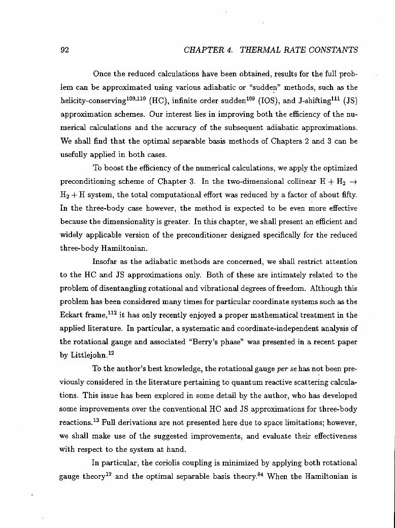
92 CHAPTER 4. THERMAL RATE CONSTANTS
Once the reduced calculations have been obtained, results for the full prob
lem can be approximated using various adiabatic or "sudde~" methods, such as the
helicity-conserving109•110 (HC), infinite order sudden109 (lOS), and J-shifting111 (JS)
approximation schemes. Our interest lies in improving both the efficiency of the nu
merical calculations and the accuracy of the subsequent adiabatic approximations.
We shall find that the optimal separable basis methods of Chapters 2 and 3 can be
usefully applied in both cases.
To boost the efficiency of the numerical calculations, we apply the optimized
preconditioning scheme of Chapter 3. In the two-dimensional collinear H + H2 -+
H2 + H system, the total computational effort was reduced by a factor of about fifty.
In the three-body case however, the method is expected to be even more effective
because the dimensionality is greater. In this chapter, we shall present an efficient and
widely applicable version of the preconditioner designed specifically for the reduced
three-body Hamiltonian.
Insofar as the adiabatic methods are concerned, we shall restrict attention
to the HC and JS approximations only. Both of these are intimately related to the
problem of disentangling rotational and vibrational degrees of freedom. Although this
problem has been considered many times for particular coordinate systems such as the
Eckart frame, 112 it has only recently enjoyed a proper mathematical treatment in the
applied literature. In particular, a systematic and coordinate-independent analysis of
the rotational gauge and associated "Berry's phase" was presented in a recent paper
by Littlejohn.12
To the author's best knowledge, the rotational gauge per se has not been pre
viously considered in the literature pertaining to quantum reactive scattering calcula
tions. This issue has been explored in some detail by the author, who has developed
some improvements over the conventional HC and JS approximations for three-body
reactions.13 Full derivations are not presented here due to space limitations; however,
we shall make use of the suggested improvements, and evaluate their effectiveness
with respect to the system at hand.
In particular, the coriolis coupling is minimized by applying both rotational
gauge theory12 and the optimal separable basis theory.84 When the Hamiltonian is

4.1. INTRODUCTION 93
represented in the new rotational and vibrational coordinates, an "effective" potential
emerges which corresponds physically to the two-body central force analogue. As is
true in the two-body case, the form of the three-body Hamiltonian strongly suggests
that a different equilibrium or transition state geometry be associated with each
distinct set of rotational quantum numbers.
All of the methods described in the preceding paragraphs are applied in
this chapter to the 0 + HCl-+ OH + Cl reactive scattering system. This particular
reaction, which is of interest to atmospheric and combustion chemists, is in many
respects an ideal testing ground for the new methods. There is no symmetry in
either the masses or the ground electronic potential energy surface. Moreover, the
masses/actions are large in comparison with other systems for which exact quantum
calculations have been performed,69•76 even though tunneling contributions may be
important. We use the (3 A") analytical potential surface developed by Koizumi et
al,113 for which there are multiple transition states, and whose reaction path has been
described as "tortuous." These features all contribute to the formidable numerical
difficulties associated with this system, although several other theoretical and exper
imental 0 + HCl-+ OH + Cl rate constant estimates are available from the literature
for comparison with the present results.107,l08,113-n9
The remainder of this chapter is organized as follows. In Section 4.2, we
present the requisite theoretical background. Section 4.2.1 summarizes some perti
nent aspects of the rotation/vibration separation problem, and Section 4.2.2 describes
the HC and JS approximations. The rest of Section 4.2 is concerned with the compu
tational techniques used in the explicit calculations, i.e. a DVR grid with absorbing
boundary conditions and optimized preconditioning. Section 4.3 discusses certain
numerical details, such as the choice of coordinates and DVR, grid parameter values,
etc. Finally, Section 4.4 contains the results for the 0 + HCl -+ OH + Cl system.
Cumulative reaction probabilities and thermal rate constants are presented, as well
as a comparison between the standard and improved JS approximation methods.

94 CHAPTER 4. THERMAL RATE CONSTANTS
4.2 Theory
4.2.1 Separation of Rotation and Vibration
The full three-body Hamiltonian is initially characterized by nine degrees
of freedom. Translational invariance reduces the effective dimensionality by three,
but rotational invariance generally yields a reduction of only two degrees of freedom.
This discrepancy exists despite the fact that translations and rotations are both three
parameter groups that can be used to define three translational and three rotational
coordinates, respectively. In the aforementioned paper,13 we discuss the reasons for
this fundamental difference, which is related to the existence of a non-trivial rotational
Berry's phase.12
Here, we simply reiterate some points that are pertinent to the present dis
cussiOn. To begin with, there are many different ways to define three rotational
coordinates, each of which is equivalent to specifying a set of body-fixed axes, or
to selecting a particular gauge. Quantum-mechanically, each gauge gives rise to a
different rotational basis set I J K M), defined (as for the symmetric top) as the si
multaneous eigenstates of the angular momentum operators { J2, Jz, J z}, where Jz and J z are the body-fixed and space-fixed z-axis components of angular momentum,
respectively.
In any gauge, J and M are conserved quantum numbers but K is not.
Consequently, the block form of the Hamiltonian ( J' K' M' Iii I J K M), although gauge
dependent, is always block-diagonal in J and M but not in K. Each block above
operates on the three-dimensional configuration space of internal or "vibrational"
coordinates. The diagonal blocks alone constitute the HC Hamiltonian
(4.1)
whereas the off-diagonal blocks comprise the coriolis coupling for the purposes of this
chapter. The coriolis coupling can in principle be reduced via a gauge transformation,
but can never be made to disappear altogether (excepting certain trivial special cases).
We shall make use of some set of Jacobi-like coordinates13 on the six
dimensional translationally-reduced configuration space. These could be any of the

4.2. THEORY 95
Jacobi or Radau arrangements, or possibly some interpolation.12•13 In Jacobi-like coor
dinates, the translationally-reduced kinetic energy has the completely separable form
of Equation 2.28. This comes about because these coordinates are in a certain sense
"balanced" with respect to the mass distribution of the N bodies (Figure 4.1). For
our purposes however, what is more useful is the fact that the fully-reduced kinetic
energy is also completely orthogonal, albeit position-dependent.
In Jacobi-like coordinates, the translationally-reduced three-body quantum
Hamiltonian is
(4.2)
Equation 4.2 can be thought of as a pair of coupled two-body rotors with relative
separations { r 1 , r 2 } and reduced masses { m1 , m2}.
Each set of Jacobi-like coordinates induces a rotational gauge and a set of
internal coordinates {rllr2 ,<p}, where <pis the angle between r 1 and r 2 (Figure 4.2).13
In this representation, the Hamiltonian of Equation 4.2 becomes block-tridiagonal in
K, and is given by
(4.3)
ii,K± - (J(K ± 1)MIHIJKM)
_1i_2
~2 .j J(J + 1)- K(K ± 1) (=Faa + K cot <p) , 2m1~ <p
(4.4)
where
(4.5)
Equations 4.3 and 4.4 indicate that the coriolis coupling is small if the mass
ratio mi/m2 is large. The problem of minimizing the coriolis coupling with respect
to gauge transformations induced by all possible Jacobi-like coordinates has been

96 CHAPTER 4. THERMAL RATE CONSTANTS
Figure 4.1: A particularly complicated arrangement of Jacobi coordinates, as exemplified by the Alexander Calder mobile entitled Dots and Dashes, 1959 (painted sheet metal, wire, 60") from the collection of Jean Lipman.120 A hierarchy of masses is established, with a node located at the center of mass for each subhierarchy.

4.2. THEORY 97
z z
Cl
··········· ..... H
0 0
Jacobi Coordinates Radau Coordinates
Figure 4.2: Two sets of Jacobi-like coordinates: on the left, the Jacobi coordinates for the OCI-H arrangement; on the right, Radau coordinates for 0 and Cl. The x and z axes refer to the body-fixed frame.

98 CHAPTER 4. THERMAL RATE CONSTANTS
solved.13 For heavy-light-heavy systems such as 0 + HCl-+ OH + Cl, the most intu
itive choice is to use the Jacobi coordinates associated with the OCl-H arrangement
(Figure 4.2). Although not quite optimal,13 this choice is very convenient, and is
moreover required for comparison with other results. One might also apply the opti
mal separable basis methodology (Section 4.2.4) to reduce the coriolis coupling even
further, by minimizing with respect to all unitary transformations of the rotational
basis set. It has been shown however, that Equation 4.3 is already in optimal formP
4.2.2 Helicity-conserving and J-shifting Approximations
The HC approximation (also known as the "centrifugal sudden" or "coupled
states" approximation) results by simply ignoring the coriolis coupling, and solving
each of the HC Hamiltonian blocks independently. Note that the iiJK are equivalent
to H00 , apart from the effective potential term of Equation 4.5. Since the diagonal
blocks are treated independently in the HC picture, we should think of each iiJK as
having its own "effective" transition state, defined as the saddle point of the effective
potential for that block.
For J =f:. 0, the effective transition state never corresponds to a linear geom
etry, because the effective potential diverges as cp approaches 0 or 1r. This is simply a
straightforward generalization of the analogous two-body central force situation (as
r -+ 0), and is by no means problematic for numerical applications; one simply uses
Yeff to truncate the DVR grid in the usual fashion. Consequently, there is no need to
resort to complicated, associated Legendre basis sets for the angular DVR that vary
with the value of K. S9,61
Using the numerical methods of Section 4.2.3, the cumulative reaction prob
abilities associated with each of the iiJK-i.e. the NJK(E)'s-are independently cal
culated and then summed to obtain the HC estimate of the total cumulative reaction
probability:
N(E) ~ I)2J + l)NJK(E). ( 4.6) J,K
Since our ultimate goal is the thermal rate constant, however, it is more convenient

4.2. THEORY 99
to define a block version of the rate constant
(4.7)
from which the HC estimate for k(T) is obtained as per Equation 4.6.
In the JS approximation, only the N00 block is calculated explicitly. The
N J K values are then estimated via
NJK(E) ~ Noo (E- Erot(J, K)) (4.8)
where the rotational shift energies Erot( J, K) must be specified somehow. The stan
dard JS method uses symmetric top kinetic energies; i.e.
(4.9)
where the rotor constants A and B usually correspond somehow to the transition
state geometry. However, an improved JS method has also been developed, 13 for
which Erot ( J, K) is defined as the value of ("Veff - V) at the effective transition state.
The improved method exploits the fact that the effective transition state varies with
J and K, and automatically incorporates centrifugal distortion effects and linear
transition state geometries.
4.2.3 Determination of the NJK(E)'s
The HC partial cumulative reaction probabilities NJK(E) are computed nu
merically using the DVR-ABC method of Section 3.2. Each fiJK is represented as a
matrix via a conventional sine-function DVR in the radial coordinates (rb r2), and a
gauss-legendre DVR in the angular coordinate t.p. The same general DVR scheme is
used for all J and K, although the grid parameters may vary slightly. Note, however,
that the kinetic energy is the same for each of the fiJK blocks (Equation 4.3).
To determine N1K(E), we make use of the reaction probability operator121
( 4.10)

100 CHAPTER 4. THERMAL RATE CONSTANTS
where Er and Ep are the reactant and product absorbing potentials, respectively. The
cumulative reaction probability is then given by
NJK(E) = tr [PJK(E)] = LPk(E), (4.11) k
where the Pk (E) are the eigenvalues of P, which are obtained using a reorthogonalizing
Lanczos iteration scheme.7•121 The advantage of this approach is that only a small
number of eigenvalues are usually required.
The Green's operator of Equation 2.24, or more accurately the action of
G(E) on a vector, is obtained numerically using the GMRES algorithm (Section 3.4).
This approach is efficient because the kinetic energy is completely orthogonal in the
internal coordinates (r17 r 2 , <p), and therefore sparse in the DVR representation. We
also make use of optimized preconditioning to reduce the number of Krylov iterations
required for convergence.
4.2.4 Optimized Preconditioning
\\'e are interested in obtaining an optimized preconditioner, as described in
Chapter 3, for explicit DVR calculations of NJK(E) for three-body systems. Since the
calculation involves three degrees of freedom, the algorithm developed in Section 3.5 is
expected to be very effective. However, the efficiency of the optimized preconditioning
algorithm requires that the kinetic energy be of the form expressed in Equation 2.29.
To determine whether flJK satisfies this form, we must first decide whice of the
{ r 1 , r2 , <p) are the inner coordinates and which are the outer coordinates.
A comparison between Equations 2.29 and 4.3 reveals that <p should defi
nitely be an outer coordinate. However, Equation 2.29 will be satisfied if either one
or neither of {r17 r 2 } is also an outer coordinate. Symmetry considerations might
persuade one to select (r17 r2 ; <p) as the most natural division. A good case could
also be made for {r1 ; r2 , <p) however, corresponding to r 1 and r 2 in the body-fixed
frame. In practice, the decision should also be based on numerical convenience. In
the 0 + HCl-+ OH + Cl case for example, we adopt the symmetric (r17 r2 ; <p) choice
because it results in the more efficient preconditioner.

4.3. NUMERICAL DETAILS 101
4.3 Numerical Details and the 0 + HCl System
4.3.1 Coordinates
In Section 4.2.1, we argued in favor of the rotational gauge induced by the
OCl-H Jacobi coordinates, and this is what we shall adopt from here on out. The
corresponding masses m1 = momcz/(mo + mcz) and m2 = (mo + mcz)mH/(mo + mc1+mH) yield a mass ratio of about twelve. Thus, the HC approximation is expected
to be quite accurate. To be consistent with previous theoretical results, 107•113 we use
the following values for the atomic masses (in atomic units): mo = 32805; mH = 1837; mcz = 64630.
Note that all of our explicit calculations involve the internal coordinates
only. Since these can be defined quite independently of the rotational gauge, 12•13
we can in principle use a different set of internal coordinates than those induced by
the OCl-H Jacobi arrangement. Indeed, for the 0 + HCl--+ OH + Cl system, the
Jacobi (r1,r2 , so) are less than ideal from a DVR perspective, because the singularity
in the kinetic energy as r2 --+ 0 is unfortunately not precluded by large values of the
potential.
As an alternate set of internal coordinates, it is natural to use the ( r~, r~, so')
associated with a different set of Jacobi-like coordinates. Thus, we use one set of
Jacobi-like coordinates to define the rotational gauge, and another to define the in
ternal coordinates. This approach is very advantageous, because the fiJK kinetic en
ergy is gauge-independent, and therefore equivalent to that of the H]K corresponding
to the primed gauge. Thus, to obtain an expression for if JK in the primed coordi
nates, one simply adds the primed kinetic energy to the unprimed effective potential
(rewriting the latter as a function of the primed coordinates).
The new internal coordinates can be defined using any desired set of Jacobi
like coordinates. A natural choice for a reactive scattering problem such as O+HCl--+
OH + Cl is the set that lies "halfway" between the reactant Jacobi arrangement
0-HCl and the product arrangement OH-Cl; it has been shown13 that these are
just Radau coordinates in 0 and Cl (Figure 4.2). Indeed, we have found the Radau

102 CHAPTER 4. THERMAL RATE CONSTANTS
coordinate DVR to be particularly effective. Not only is the kinetic energy singularity
and other problems completely alleviated, but we also find the resultant NJK(E)
calculations to be considerably more efficient.
Radau coordinates are often considered useful in light-heavy-light reactions,
where they are approximately equal to valence bond coordinates.122-124 In heavy
light-heavy applications, the light atom has to be fairly far away from the others to
achieve a large bend in <p1• Thus, we find ourselves restricted by the 0 + HCl -+
OH + Cl potential to a fairly narrow angular range between <p1 ::::::: 140° and <p' = 180°.
This greatly reduces the number of angular points required by the DVR; however these
gains are offset somewhat by the need for a larger density of points. All in all though,
fewer points are required by the Radau DVR than the Jacobi DVR; consequently, the
former has been employed for most of our numerical calculations (Section 4.4.1).
4.3.2 DVR Grid Parameters
Another advantage of using Rad~u coordinates is that ascertaining reactant
and product regions is a fairly straightforward matter; these correspond to large values
of ro and rc1 respectively. As in other DVR applications, we find that roughly four
points per de Broglie wavelength are required for the radial degrees of freedom. This
amounts to roughly 60 DVR points for each radial degree of freedom, corresponding
to about 5a0 (in ro). The angular DVR points are truncated by the potential to
about one-fourth of the total number lmax· Convergence with respect to lmax is a
subtle issue; however, lmax ::::::: 50 is usually sufficient (Section 4.4.1). Roughly 9,000
to 20,000 DVR points are required in all, depending on the energy.
The reactant and product absorbing strips are laid out in r0 and rc1 re
spectively, and are typically about lao wide (in ro ). The dividing surface is defined
VIa
rcdro = 0.57 ( 4.12)
which is appropriate throughout the allowed angular range. A quartic absorbing
potential is employed,69 with a maximum value of about 1.0 eV.
A potential cutoff energy Ycut is used to truncate the DVR grid. For the ener-

4.3. NUMERICAL DETAILS 103
gies appropriate to the temperatures under consideration (200-700°K), a Vc:ut value of
1.40~1.85 eV is sufficient. Energies are taken with respect to the reactant asymptote
minimum. Although the 0 + HCl-+ OH + Cl reaction is only slightly endothermic,
the OCl-H arrangement energy is quite large (1.77 eV). This is considerably higher
than our highest energy calculation, but lower than some of our cutoff energies. Con
sequently, DVR points are removed from the Vc:ut ~ 1. 77 e V grids if either the oxygen
or the chlorine is further away from the hydrogen than some specified distance ( 4ao
is virtually always sufficient).
4.3.3 Preconditioner Details
Of the two internal partitionings considered in Section 4.2.4, (rll r 2; <p) yields
the more efficient preconditioner, because a much larger portion of the Hamiltonian
is incorporated into H0 . This is particularly true for the 0 + HCl-+ OH + Cl Radau
DVR, for which there are far fewer angular points than radial points. On the other
hand G0 , although sparse by virtue of block-diagonality, is significantly less sparse
than ii. CPU limitations may therefore be an issue for numerical calculations.
Obtaining the above preconditioner for 0 + HCl-+ OH + Cl is considerably
faster than the resultant Krylov calculations, even with preconditioning; thus, speed
is not a major concern. However, the memory limitations of our platform (IBM
RS6000) definitely are a concern. This is largely because optimized preconditioning
constrains the DVR grid such that all inner coordinate "sheets" (outer coordinates
fixed) must contain the same points. Consequently, extraneous DVR points must be
included that would not occur with a straightforward potential cutoff. The three
dimensional constraint is a lot less severe than the rectangular grid requirement of
the two-dimensional case.17 Nevertheless, we find that the number of DVR points for
our application is increased by a factor of three or four-which unfortunately puts us
over the memory limit of our CPU.
In the future, we hope to develop an algorithm that avoids the grid constraint
limitation. For now we must find some other solution. One approach would be to
transform the internal coordinates yet again; another would be to use the less efficient

104 CHAPTER 4. THERMAL RATE CONSTANTS
(r1 ; r2 , cp) preconditioner. Instead, we adopt an earlier suggestion17 to skip the outer
diagonalization step altogether, and simply define H0 in the original representation.
The resultant DVR grid is completely unconstrained. Moreover, the efficiency loss of
the new preconditioner is fairly small in this case, as numerical tests reveal that outer
diagonalization only reduces the residual norm by about 10%.
4.3.4 Estimating the Thermal Rate Constant
Although some of the N(J>O)K(E) are explicitly calculated, we are mainly
interested in using a JS approximation to obtain the thermal rate constant. Con
sequently, our computational focus is primarily restricted to N00 (E). We use the
standard JS method with rotor constants (in atomic units)
A= 1.202 X 10⁻⁶ B = 2.929 X 10⁻⁴' ( 4.13)
rather than the improved JS version, so as to allow a direct comparison with other
theoretical estimates of k(T) .107,113
The essence of deriving a thermal rate constant from an explicit calculation
of N00 (E) is described by Equation 4.13 and Section 4.2.2. However, there are a couple
of additional modifications which must be implemented, once again to allow direct
comparison with previous results. Following Koizumi et al,113 we replace the sum over
J in Equation 4.6 with an integral, which is appropratefor O+HCl-+ OH+Cl because
the effective potential varies only slightly with J. This results in the expression
k(T) ~ koo~T) (1 + 2 f: e-f3n2(A+B)K2) (4.14) {31i A K=l
which converges to reasonable accuracy with a small number of K values.
An additional modification was also introduced to account for a second elec
tronic surface (3 A') that correlates between reactant and product ground states, and
lies fairly close to the ground electronic surface. In fact the two surfaces are coincident
for linear geometries.113 This surface clearly makes a significant contribution to the
overall reaction rate and cannot be ignored. As per Koizumi et al, we multiply the
above value for the rate constant by a statistical factor
f(T) = 3/(5 + 3e-228/T + e-326/T) (4.15)

4.4. RESULTS 105
representing the fraction of collisions that wind up on the ground electronic surface
e A").
4.4 Results
We have used the methods described in the previous sections to calculate
thermal rate constants and cumulative reaction probabilities for the 0 + HCl --+
OH + Cl reaction within the standard JS approximation. We have also compared
the thermal rate constants with other theoretical and experimental results from the
literature. In addition, we have used the HC approximation to calculate the N1K(E)
explicitly for some relevant values of J and K. These latter results are used to
evaluate the validity of the standard JS approximation, as well as the improved version
discussed in Section 4.2.2.
4.4.1 Cumulative Reaction Probabilities for J = 0
Explicit N00 (E) calculations have been obtained for energies in the range
0.30-0.60 eV, at 0.005 eV increments, and are depicted in Figure 4.3. The probability
associated withE = 0.30 eV is around 10-5 , below which the DVR-ABC methods
seem to be difficult to converge. By 0.60 e V, the cumulative reaction probability is
on the order of unity; but the DVR grids become inordinately large. Despite the
numerical difficulties associated with this particular reaction, we have been able to
obtain fairly well-converged N00(E) values in the specified energy range. Indeed,
these results are converged to within about 1-2% with respect to all grid parameters
except lmax·
The lmax convergence is quite unusual, and bears comment. For compara
tively small values of lmax (35-45), one typically finds the usual monotonic convergence
to within a few percent. However, there tends to be a critical value of lmax at which
N00(E) suddenly leaps up or down by as much 40%. This is not very desirable from a
convergence standpoint; although we have observed similar behaviour in Jacobi DVR
calculations for this reaction and others. In any event, we have extended lmax as far

106
~ 10-1
..0 as ..0 e 1o-2
c.. --w ~10-3
0
z
10-4
10-5
0.30
CHAPTER 4. THERMAL RATE CONSTANTS
0.35 0.40 0.45 0.50 0.55 0.60 Energy (eV)
Figure 4.3: Logarithmic plot of N00(E), the J = 0 cumulative reaction probability as a function of energy, for the 0 + HCl-+ OH + Cl system.

4.4. RESULTS 107
as 120 to ensure the convergence of our results for 0 + HCl -+ OH + Cl. For lower
energies, N00(E) tends to remain fiat over the entire region except for a few isolated
"spikes;" and we can probably safely claim convergence to within 10% or so. For large
energies, N00 ( E) tends to alternate suddenly between two values whose mean varia
tion increases from about 10% near E = 0.45 eV to about 25% near E = 0.60 eV.
Despite this variation, there is very little "mean drift" as lmax ranges from 50-120
at fixed energy; and in this sense our results are converged. In any case, Figure 4.3
incorporates the average of the two N00 (E) values for energies in the range E =
0.45-0.60 eV.
The above results were obtained with residual tolerances of about one part
in 105 for both the Lanczos and GMRES components of the calculation. Around 5-10
Lanczos iterations and 50-200 GMRES iterations were required, depending on the
values of E and lmax· Given the number of grid points ( rv15000) the preconditioner
is evidently very efficient. A detailed comparison versus no preconditioning was per
formed, albeit for a somewhat smaller grid ( 4856 points) due to CPU constraints.
Preconditioning on the reduced grid was found to reduce the number of GMRES iter
ations from 575 to 10. The preconditioner is so efficient that the GMRES bottleneck
is the linear Hamiltonian multiplication step, rather than the quadratic linear algebra ....
step.92 The corresponding speed increase is a factor of rvl10.
For comparison's sake, we have also obtained numerical N00(E) results using
DVR grids other than the one presented in Section 4.3.2. For instance, the Radau
DVR with Jacobi absorbing strips and a valence bond dividing surface
THCl - TQH = 0.29 ( 4.16)
yielded results that were within a per-cent or so of Figure 4.3, although CPU require
ments were somewhat higher. We also tried the OCl-H Jacobi DVR. This choice
required almost double the number of grid points, primarily in the angular coordinate,
resulting in i~creased CPU requirements and a comparatively less efficient precondi
tioner. Consequently, even the low energy results could only be converged to within
rv25% or so; although to this level of accuracy they seem to match the Radau values.

108 CHAPTER 4. THERMAL RATE CONSTANTS
4.4.2 Thermal Rate Constants
The total cumulative reaction probabilities and thermal rate constants for
0 + HCl --+ OH + Cl have been determined as per Sections 4.2.2 and 4.3.4. The
former were derived from Equation 4.6, and are presented in Figure 4.4. The thermal
rate constants were obtained for several temperatures in the range 200-700°K, and
are presented in Figure 4.5.
Within the JS approximation itself, we estimate an error of about 10% for
our k(T) results, except at the highest temperatures for which the error may be as
high as 25%. The most fundamental source of error arises from the N00 results. This
appears to be random rather than systematic, and is therefore mitigated somewhat
by the Boltzmann averaging of Equation 4.7. The integration itself introduces er
ror however, primarily due to the finite range of data available for the integrand.
Figure 4.6 depicts the integrand for multiple temperatures. The gaussian-like pat
tern suggests a loss of about 5-25% of the integrand depending on the temperature.
However, this error is significantly reduced by confining the integral of the reactant
partition function Qr(T), in the denominator of Equation 4.7, to the same energy
range as the numerator integral (0.3Q-0.60 eV) .
..,.. Our thermal rate constants are compared with other theoretical108•113 and
experimental116- 118 results in Figure 4.5. The theoretical values should in principle
match exactly. Reasonable agreement with the revised values of Thompson, et al108
has been observed; however, the discrepancy with Koizumi et al113 is not accounted
for. Our results evidently match experiment fairly well. Given the accuracy of the
JS and HC approximations for the present reaction (Section 4.4.3), this agreement
is to be expected. On the other hand, it should be noted that the potential surface
was empirically modified by Koizumi et al so as to force their results to agree with
experiment at T = 295° KY3
4.4.3 HC and Improved JS Results
In addition to calculating N00 (E), we have obtained explicit NJK(E) results
for some of the J # 0 H1K(E)'s (Figure 4.7). Specifically, we obtained fixed-K

4.4. RESULTS 109
105
104
- 103
>. ~
.c 10
2 ct:S .c 0 lo....
c.. 10
1 --w -z 10°
10-1
10-2
0.30 0.35 0.40 0.45 0.50 0.55 0.60 Energy (eV)
Figure 4.4: Logarithmic plot of the total cumulative reaction probability as a function of energy, in the standard JS approximation, for the 0 + HCl-+ OH + Cl system.

110 CHAPTER 4. THERMAL RATE CONSTANTS
-1 Q) 10-14
:::s (.) Q)
0 E 10-15
-I--.::t::. 10-17
1.0 2.0 4.0 5.0
Figure 4.5: Arrhenius plot of theoretical and experimental thermal rate constants for the 0 + HCl -+ OH + Cl reaction. Theoretical results: (present results); ------ (Thompson et al108); --- (Koizumi et al113). Experimental results: filled circles (Brown et al116•117); open squares (Mahmud et al118).

4.4. RESULTS
0.20 0.30
I~ II \A v· I v~
I~ \
I ~ I \ . ~
0.40 0.50 0.60 Energy (eV)
111
0.70
Figure 4.6: Renormalized Boltzmann integrands for k00 (T) as a function of energy, for two different temperatures: (T = 200°K); ------ (T = 500°K).

112 CHAPTER 4. THERMAL RATE CONSTANTS
(K = 0) results for various values of J, and fixed-J (J = 24 and J = 48) results for
various values of K. Due to time constraints, we have not evaluated convergence as
thoroughly as in the J = 0 case; however, the results are certainly accurate enough
to test the validity of the standard and improved JS approximations.
Note that qualitatively, the NJK(E) graphs really do resemble N00 (E) graphs
that have been shifted in energy. Quantitatively, this means that the variation in the
energy difference between points of comparable probability in N00 (E) and NJK(E) is
small, over the probability (or energy) range of interest. Some kind of energy-shifting
approach is therefore entirely justified; however, we must ensure that the shifting
energies themselves are chosen appropriately.
It is reasonable to associate the shift with rotational kinetic energy.13 In Fig
ure 4.8, we compare the fixed-K rotational shift energies obtained from the NJK(E)
graphs of Figure 4. 7 with those predicted by the standard and improved JS methods.
All three shift energies were found to agree fairly well. This indicates that there is
not much centrifugal distortion when K = 0, and that the standard value of A in
Equation 4.9 is comparable to that of the improved JS method. Both of these con
clusions are consistent with what one would expect for the large mass ratio of the
0 + HCI-+ OH + Cl system.
The situation is somewhat different for the fixed-J rotational shift energies,
presented in Figure 4.9. Note that the shifting energy varies much more quickly
with K than with J. This is again due to the large mass ratio of the system, which
causes the rotor constant B to be much larger than A. Consequently, an accurate
k(T) estimate requires about one hundred J's, but only six IKI's. Another important
difference is that the plot of shift energy versus K 2 is considerably non-linear, with
most of the curvature occuring for small values of K. This feature cannot be accounted
for in the standard JS theory, which necessarily predicts a straight line.
According to the improved JS theory however, the curvature is due to the
centrifugal distortion of the effective transition state, which is large because the K 2
term of the effective potential is large. Figure 4.10 depicts the effective transition
state geometries for several values of J and K, and clearly illustrates that K has
the larger effect on the distortion. In any event, Figure 4.9 demonstrates that the

4.4. RESULTS
:0 ctl .c
0.3
e o.2 a. --w -~ ...., z
0.1
0.0 ~--~--~----~--._~~----~~~~=---~--~ 0.20
113
Figure 4. 7: Helicity-conserving cumulative reaction probabilities as a function of energy, for several representative values of J and K: ( J = 0, K = 0); --(J = 48, K = 0); ---- (J = 72, K = 0); ------ (J = 24, K = 5); ---(J = 48, K = 5).

114 CHAPTER 4. THERMAL RATE CONSTANTS
0.08
- 0.06 > Q) ->. 0> - 0.04 Q) c w -::= ~ 0.02 en
0.00
-0.02 ..___ ......... _ ......... _--' __ ....._ _ _.__ _ __.__--' ___ .....__....L... _ ___, 0 500 1000 1500 2000 2500
J(J+1)
Figure 4.8: Rotational shift energies of the N1K(E)'s as a function of J, forK= 0. The error bars reflect the variation in the HC results over the relevant energy range: -- (improved JS); ---- (standard JS).

4.4. RESULTS
0.40
0.30
-> CD ->. 0') 0.20 '-CD c w -::: .c.
(f) 0.10
0.00
, ,
0
, , , , , ,
, , , , ,
10
, , , , ,
, , , , ,
, , ,
20
, , , , ,
, , , , ,
30
, , , , ,
, , , , ,
40
115
50
Figure 4.9: Rotational shift energies of the N;K(E)'s as a function of K, for J = 24 {lower graphs) and J = 48 (upper graphs). The error bars reflect the variation in the HC results over the relevant energy range: (improved JS); -- -(standard JS); . - - - - - - (HC).

116 CHAPTER 4. THERMAL RATE CONSTANTS
...._... J=O; K=O o-- -o J=200; K=O
2.0 ~--o J=48; K=10
-0
~ 1.0 X
0.0
H
Cl 0
Figure 4.10: Effective transition state geometries of the 0 + HCl -7 OH +Cl system for several values of J and K: (J = 0, K = 0); ---- (J = 200, K = 0); - - - ( J = 48, K = 10).

4.5. CONCLUSIONS 117
improved JS method does an excellent job of predicting the actual energy shifts-at
least in the most crucial region where K is small. The standard JS results are still
fairly good though; we estimate that the JS and HC values for k(T) agree to within
about 20%.
4.5 Conclusions
One of the principal goals of this chapter has been to evaluate the use of
optimized preconditioning for generic three-body quantum calculations, with respect
to both efficiency and practicality. By restricting consideration to Jacobi-like co
ordinates only, the Hamiltonian takes on the sparse, reduced-dimensional form of
Equations 4.3 and 4.4 regardless of the particular coordinates used; yet the range
of all possible Jacobi-like coordinates is quite broad.13 Moreover, the uniformity of
the flJK allows us to adopt the internal coordinate DVR of Sections 4.2.3 and 4.3.1
as a generic standard for the three-body case. From this standard, two candidate
preconditioners naturally suggest themselves, corresponding to the two partitionings
of Section 4.2.4.
We therefore have an optimized preconditioning scheme for three-body sys
tems that is both practical and general. The next logical consideration is whether
the method is also efficient. In general, one can always bolster efficiency by trans
forming from one set of Jacobi-like coordinates to another, as is done in Section 4.3.1.
However, performance ultimately depends on the details of the particular system.
Nevertheless, it is extremely encouraging to discover that even for a system such as
0 + HCl -+ OH + Cl which has no special properties, the optimized preconditioner
reduces the computational effort by two orders of magnitude.
Another major objective of this chapter has been to exploit theoretical ad
vances pertaining to rotational gauges and optimal separable bases in a practicable
manner. In particular, one of our ongoing concerns is the minimization of the off
diagonal coriolis coupling blocks (JK'M I fi I JKM). Once again, the restriction
to Jacobi-like coordinates has proven to be beneficial, in that the coriolis coupling
vanishes except when K- K' = ±1. Moreover, minimization with respect to either

118 CHAPTER 4. THERMAL RATE CONSTANTS
rotational gauge or outer diagonalization is a tractable, even solved problem.13 The
Jacobi-like restriction also gives rise to the effective potential picture of the HC ap
proximation, which in turn leads to the improved JS method and the notion of the
effective transition state.
The usefulness of the effective potential idea, apart from pedagogical value,
is apparent in the predicted rotational shift energies of Figures 4.8 and 4.9. Although
the improved JS predictions are accurate enough, it is perhaps even more relevant
that one can actually assign a reasonably well-defined shifting energy to the NJK(E)'s
in the first place. According to the effective potential picture, this is simply due to the
dominant role played by the transition state. We therefore anticipate a correlation
between the reliability of the improved JS. method and traditional transition state
theory, and this may explain why the NJK(E) predictions of the former are less
accurate for large K. In any event, the improved JS method is certainly much more
feasible than a full HC calculation from a computational perspective. The bottleneck
of the former lies in locating the saddle points of a three-dimensional potential surface,
which is far less costly than the corresponding exact quantum calculation.
In the future, we would like to apply the improved JS method as well as
optimized preconditioning to other three-body reactions, in order to better ascertain
the generality of the current results. It would be interesting to see whether the cur
vature of the rotational shift energies for fixed-] actually does increase in the small
coriolis coupling limit, as claimed. It would also be interesting to apply the new
JS approximation to a system with a linear transition state, for which the Equa
tion 4.9 dependences on J and K are no longer appropriate, and standard J-shifting
is problematic. On the theoretical front, we would like to find the best Jacobi-like
coordinates for more general mass distributions such as light-heavy-light, from the
standpoint of minimizing the coriolis coupling. Finally,. we would like to develop a
version of the optimized preconditioning algorithm that does not constrain the DVR
grid.

119
Chapter 5
Conclusions
As quantum mechanics is applied to ever increasingly complicated systems,
one fact becomes very clear: that some form of separable approximation is required, if
one is to make any headway. The reason is quite simply that the calculational effort
required for an exact treatment scales exponentially with the number of particles,
whereas a separable problem scales linearly, or in the worst case as a power law.
Even taking the current exponential growth of computer technology into account, we
will only be able to handle perhaps ten or twelve-body systems by the time that the
current trend levels off, due to the fact that computer technology itself is approaching
the quantum limit. Paralleiization will certainly play an increasingly important role
in bypassing this limitation. In parallel applications, however, separability is even
more crucial, as it is imperative that the full problem can be divided into pieces that
are as independent from one another as possible.
The use of separable approximations in physics is certainly nothing new. In
quantum mechanics, we are all familiar with the separable approximations that arise
from the Born-Oppenheimer approximation, Hartree-Fock theory, molecular orbital
theory, density functional theory, and the various quasiparticles used in countless ap
plications. These approximations have certainly enabled us to gain an understanding
of a tremendous number of real physical systems. Yet, there are also many real sys
tems for which the picture presented to us by these methods seems to break down.
Thus, whereas the distinction between charged particles and photons that occurs in

120 CHAPTER 5. CONCLUSIONS
quantum electrodynamics seems entirely appropriate {due to the smallness of the fine
structure constant a), in elementary particle physics where the interaction is often
much greater, the separation between particles and fields is far less compelling.
All of the separable approximation methods of the preceding paragraph rely
upon one basic assumption for their success: that the interaction or coupling between
separated pieces is small. If this is not the case, then the picture presented to us
by these methods is inappropriate. But there are plenty of real systems for which
the interaction is not small. However, there is a formal arbitrariness in the way
one chooses to define the interaction. Therefore, if the the interaction is large for a
particular system, one is naturally prompted to ask whether the definitions used by
the methods above are really the most appropriate ones.
The novel aspect of the optimal separable basis approach presented in this
dissertation is that it offers a systematic means of determining the most natural
definition of the interaction on a Hamiltonian-by-Hamiltonian basis. In particular,
no special assumptions about the form of the approximation are assumed a priori,
other than that of separability. Indeed, we have found that the most natural separable
approximation for a T + V Hamiltonian need not even be of the T + V form itself.
The optimal separable approximation thus obtained is useful in two distinct
ways. First, the approximation itself has pedagogical value with respect to under
standing the nature of the actual system. Since the interaction has been minimized,
the description is expected to be more accurate than for any other separable ap
proximation. For example, in Chapter 2, we found that the effective potential for
the x coordinate of the shifted harmonic oscillator is best described by the well of
Equation 2.37 rather than the barrier of Equation 2.39.
Second, if one is interested in calculating exact quantities, the use of the
optimal separable basis renders such calculations more efficient. In this dissertation,
we have only explored this aspect in one very specific manner, i.e. with respect to
calculating microcanonical scattering quantities for the molecular systems of Chap
ter 3 (H + H2 ) and Chapter 4 {0 + HCl). However, In Chapter 2, we showed how the
optimal separable approximation could improve the convergence of both the time
independent perturbation expansion and the Born series. More generally, we antici-

121
pate an improvement in computational efficiency regardless of the particular quantity
being calculated or algorithm being used, due to the fact that the interaction has
been minimized as much as possible.
For example, the direct k(T) methods referenced in Chapter 4 are quite
different from the microcanonical methods presented here, in that they make use of
split operator propagations (to calculate the flux-flux autocorrelation function) rather
than Green's function inversions. Nevertheless, the calculation could in principle be
improved by splitting the Hamiltonian along flo I A lines, rather than T I V lines.
The reason is that the commutator of the two pieces is reduced, as a result of which
a larger time step can be used to obtain the same level of accuracy.
As another example, bound state calculations are often obtained using the
Lanczos algorithm mentioned in Chapter 2. As suggested in that chapter, the optimal
separable flo could be used to obtain a starting vector which might reduce the number
of iterations substantially. The idea would be to use a superposition of the first
few states of flo as the starting vector in a conventional Lanczos scheme, or to use
the whole collection in an iterative* block application. Convergence is improved
because the initial Krylov space overlap with the subspace spanned by the lowest few
eigenvectors is expected to be fairly high.
Although both of these examples merit investigation, I have presented them
here primarily to demonstrate the relative ease with which the optimal separable
approach can be incorporated into current state-of-the-art numerical algorithms which
were obviously not designed with our approach in mind. Clearly, the scope of the
optimal separable basis methodology is much broader, however. In what follows, we
present a more general but less detailed description of a few additional molecular
applications which might benefit from an optimal separable treatment.
Based on the comments in Section 2.5.3, we expect the method to be partic
ularly well-suited to inelastic scattering applications. This is because the potential is
globally more separable than in reactive scattering, since there is only one asymptotic
form to worry about. Even the translationally-averaged potential approximation of
*this time, in the sense of Cullum and Willoughby.7

122 CHAPTER 5. CONCLUSIONS
Section 2.5 would result in a potential-like interaction that is small; although the
optimal separable residual would be even smaller, of course. In light of Section 2.4.2,
it would also be interesting to compare our performance for reactive and inelastic
scattering applications versus that of the Kohn variational principle.
It might also be instructive to use the optimal separable theory to generate
Hartree-Fock orbitals along the lines suggested in Section 2.3.4. By truncating the
excitation numbers, one obtains a finite set of mutually orthogonal separable basis
functions that is uniformly optimized over a range of energies. More accurate results
can be obtained using a conventional perturbation approach, rather than the more
complicated version required to handle non-orthogonal states. We have applied this
idea to the six-dimensional helium atom, optimizing over all bound states (including
doubly excited states). This work is still in progress; however, it is worth mentioning
here that a strongly separable treatment results in a screened coulombic potential
with Z* = 23/14. This should be contrasted with the variational minimal result
Z* = 27/16 which in effect optimizes for the ground state only.
One could also apply the optimal separable method to the separation of nu
clear and electronic motion in molecular systems-i.e. the Born-Oppenheimer prob
lem. In the standard approach, one starts with a weakly separable approximation
wherein the nuclear positions yield outer basis functions 8(Q- Q0 ), and the inner
coordinates are the electronic wavefunctions parametrized by Q. The "coupling" in
this case is the nuclear kinetic energy, which is not small. However, a more refined
approximation is obtained by solving the nuclear problem associated with each elec
tronic surface. The results are more accurate, but the wavefunctions are no longer
separable. The optimal separable approach, on the other hand, yields a separable ap
proximation of intermediate accuracy, which might be useful in certain applications.
Specifically, outer diagonalization of the nuclear coordinates yields compact Q eigen
functions which are more accurate than Dirac delta functions. The corresponding
electronic potentials are then improved, resulting in more accurate electronic states.
We conclude this chapter with a brief discussion of certain refinements of
the optimal separable basis method itself, which might be considered in future work.
It would certainly be useful to find a more general existence proof than the one

123
presented in Section 2.3.3; although a stationary point has been found to exist for
all scattering potentials satisfying the appropriate asymptotic conditions. It would
also be of interest to develop a version which takes a proper account of exchange and
related symmetries.
On a more practical note, it would be very beneficial to improve the outer
diagonalization routine so that an arbitrarily-shaped grid can be dealt with. The
present limitation as discussed in chapters 3 and 4, while not too severe, is nev
ertheless probably unnecessary. Since the diagonalization per se is not necessarily
computationally expensive (particularly if k ~ n), one practical approach would be
to apply an energy cutoff criterion to truncate the size of the basis after the outer di
agonalization has been performed. Such a procedure would be akin to the sequential
diagonalization and truncation methods,85 although the cutoff criterion would have
to be more complicated. Most likely, the truncation would have to occur at the block
level only.
Outer diagonalization is the one procedure which is common to all numerical
applications that incorporate the optimal separable basis idea. Practical improve
ments for implementing this procedure are therefore desired. Although formally the
off-diagonal blocks need not approach zero as a result of outer diagonalization, it is
interesting to note how many of these elements actually do disappear in practice.
It is hard to pin down precisely why this is the case, but it is clear that this must
correspond to some sort of inherent symmetry, unknown ahead of time, which the
outer diagonalization routine discovers automatically.
As a final improvement, we consider the recursive modification described
m Chapter 2. Instead of defining just two categories of coordinates, one could in
principle extend the number of categories, even to the point where each category
includes just a single degree of freedom. Both Equations 2.5 and 2.8 can be easily
generalized to incorporate this possibility. In the weakly separable case, the entire
set of categories becomes ordered; one must start from the outermost category first,
and work inwards.
Of course, the resultant approximation in and of itself is not as accurate as
that of a two-tiered approach. Nevertheless this approach is computationally more

124 CHAPTER 5. CONCLUSIONS
efficient if one also calculates the desired quantity itself recursively. In other words
if X is the quantity, then one obtains X for each of the outermost diagonal blocks,
after first minimizing the coupling via outer diagonalization. Since these outermost
blocks include all degrees of freedom except those in the outermost category, this
approximation is a very good one; and presumably convergence to the correct results
is very fast. The method is recursive in that it is also applied to the X problem for
each of the diagonal blocks.
It is to be hoped that some recursive procedure along these lines may even
tually overcome the exponential scaling problem discussed at the beginning of this
chapter, vis a vis exact quantum calculations. In any event, the optimal separa
ble basis approach has already demonstrated its value in the theory and application
pertaining to molecular collisions.

125
References
[1] G. A. Voth, in Advances in Chemical Physics (John Wiley & Sons, Inc., New
York, NY, 1996), pp. 135-218.
[2] J. I. Steinfeld et al, Chemical Kinetics and Dynamics (Prentice Hall, Englewood
Cliffs, NJ, 1989).
[3] Z. BaCic and J. C. Light, Annu. Rev. Phys. Chern. 40, 469 {1989).
[4] J. M. Bowman, Comp. Phys. Commun., Special Issue on "Molecular Vibrations"
51, (1988).
[5] J. Bowman and B. Gazdy, J. Chern. Phys. 94, 454 {1991).
[6] J. R. Taylor, Scattering Theory (John Wiley & Sons, Inc., New York, NY, 1972).
[7] J. K. Cullum and R. A. Willoughby, Lanczos Algorithms for Large Symmetric
Eigenvalue Computations (Burkhauser, Boston, MA, 1985).
[8] C. Lanczos, J. Res. Natl. Bur. Stand. 45, 255 {1950).
[9] B. N. Parlett, Lin. Alg. Appl. 34, 269 {1980).
[10] H. Goldstein, Classical Mechanics (Addison-Wesley, Reading, MA, 1980).
[11] E. B. Wilson et al, Molecular Vibrations (Dover Publications, New York, NY,
1980).
[12] R. G. Littlejohn and M. Reinsch, Rev. Mod. Phys. 69, 213 {1997).

126 REFERENCES
[13] B. Poirier, J. Chern. Phys. (1998), (submitted).
[14] R. Horn and C. Johnson, Topics of Matrix Analysis (Cambridge University
Press, Cambridge, England, 1991).
[15] N. J. Higham, Numerische Mathematik 62, S39 (1992).
[16] G. Strang, Linear Algebra and Its Applications (Academic Press, Orlando, FL,
1980).
[17] B. Poirier and W. H. Miller, Chern. Phys. Lett. 265, 77 (1997).
[18] S. Weinberg, Phys. Rev. 131, 440 (1963).
[19] S. Willard, General Topology (Addison-Wesley, Menlo Park, CA, 1970).
[20] E. H. Lieb and B. Simon, in The Stability of Matter: From Atoms to Stars,
edited by W. Thirring (Springer, New York, 1997), Chap. 4, pp. 299-308.
[21] G. Barton, Elements of Green's Functions and Propagation (Oxford University
Press, New York, 1989).
[22] J. J. Sakurai, Modern Quantum Mechanics (Addison-Wesley, Menlo Park, CA,
1985).
[23] S. M. Auerbach and W. H. Miller, J. Chern. Phys. 98, 6917 (1993).
[24] K. S. H. Lehmann and W. Zimmermann, Nuovo Cimento 1, 425 (1955).
[25] R. D. Mattuck, in A Guide to Feynman Diagrams in the Many-Body Problem
(Dover Publications, New York, NY, 1976), p. 158.
[26] L. H. Ryder, in Quantum Field Theory (Cambridge University Press, London,
1985), pp. 221-228.
[27] R. G. Newton, Scattering Theory of Waves and Particles (McGraw-Hill, New
York, 1996).

REFERENCES 127
[28] J. Z. H. Zhang, S.-1. Chu, and W. H. Miller, J. Chern. Phys. 88, 6233 (1988).
[29] J. Z. H. Zhang and W. H. Miller, J. Chern. Phys. 91, 1528 (1989).
(30] L. M. Hubbard, S. Shi, and W. H. Miller, J. Chern. Phys. 78, 2381 (1983).
[31] W. H. Miller and B. M. D. D. J. op de Haar, J. Chern. Phys. 86, 6213 (1987).
[32] J. Z. H. Zhang, D. L. Yeager, and W. H. Miller, Chern. Phys. Lett. 173, 489
(1990).
[33] W. Kohn, Phys. Rev. 74, 1763 (1948).
[34] D. T. Colbert and W. H. Miller, J. Chern. Phys. 96, 1982 (1992).
[35] G. C. Groenenboom and D. T. Colbert, J. Chern. Phys. 99, 9681 (1993).
[36] R. Jost and A. Pais, Phys. Rev. 82, 840 (1951).
[37] R. Marcus, J. Chern. Phys. 45, 4493 (1966).
[38] R. Marcus, J. Chern. Phys. 49, 2610 (1968).
[39] K. Yamashita and W. H. Miller, J. Chern. Phys. 82, 5475 (1985).
(40] W. H. Miller, N. C. Handy, and J. E. Adams, J. Chern. Phys. 72, 99 (1980).
[41] G. Poschl and E. Teller, Z. Physik. 83, 143 (1933).
(42] N. Rosen and P. Morse, Phys. Rev. 42, 210 (1932).
(43] E. Brezin and J. C. LeGuillou, Phys. Rev. D 15, 1544 (1977).
(44] S. Flugge, in Practical Quantum Mechanics (Springer-Verlag, New York, 1971),
Vol. 1, p. 94.
[45] M .. M. Nieto, Phys. Rev. A 17, 1273 (1978).
[46] in Handbook of Mathematical Functions, edited by M. Abramowitz and I. Stegun
(Dover Publications, New York, NY, 1972), pp. 332-341.

128 REFERENCES
(47] in Handbook of Mathematical Functions, edited by M. Abramowitz and I. Stegun
(Dover Publications, New York, NY, 1972), p. 332.
(48] in Handbook of Mathematical Functions, edited by M. Abramowitz and I. Stegun
(Dover Publications, New York, NY, 1972), p. 556.
(49] in Table of Integrals, Series, and Products, edited by I. Gradshteyn and I.
Ryzhik {Academic Press, New York, NY, 1980), p. 795.
(50] G. Arfken, Mathematical Methods for Physicists (Academic Press, New York,
NY, 1985), pp. 666-683.
(51] in Table of Integrals, Series, and Products, edited by I. Gradshteyn and I.
Ryzhik (Academic Press, New York, NY, 1980), p. 798.
(52] D. 0. Harris, G. G. Engerholm, and W. D. Gwinn, J. Chern. Phys. 43, 1515
(1965).
[53] A. S. Dickinson and P. R. Certain, J. Chern. Phys. 49, 4209 (1968).
[54] J. V. Lill, G. A. Parker, and J. C. Light, Chern. Phys. Lett. 89, 483 (1982).
[55] R. A. Friesner, Chern. Phys. Lett. 116, 39 (1985).
[56] J. C. Light, I. P. Hamilton, and J. V. Lill, J. Chern. Phys. 82, 1400 (1985).
[57] J. V. Lill, G. A. Parker, and J. C. Light, J. Chern. Phys. 85, 900 (1986).
[58] Z. Bacic and J. C. Light, J. Chern. Phys. 85, 4594 (1986).
[59] R. M. Whitnell and J. C. Light, J. Chern. Phys. 89, 3674 (1988).
[60] S. E. Choi, J. Chern. Phys. 92, 2129 (1990).
[61] C. Leforestier, J. Chern. Phys. 94, 6388 {1991).
[62] G. C. Corey and D. Lemoine, J. Chern. Phys. 97, 4115 (1992).

REFERENCES 129
[63] J. D. Jackson, in Classical Electrodynamics, 2 ed. (John Wiley & Sons, New
York, NY, 1975), Chap. 7.
[64] G. Arfken, Mathematical Methods for Physicists (Academic Press, New York,
NY, 1985), pp. 421-426.
[65] A. Goldberg and B. W. Shore, J. Phys. B 11, 3339 (1978).
[66] C. Leforestier and R. E. Wyatt, J. Chern. Phys. 78, 2334 (1983).
[67] D. Neuhauser and M. Baer, J. Chern. Phys. 90, 4351 (1989).
[68] D. Neuhauser, M. Baer, and D. J. Kouri, J. Chern. Phys. 93, 2499 (1990).
[69] T. Seideman and W. H. Miller, J. Chern. Phys. 96, 4412 (1992).
[70] T. Seideman and W. H. Miller, J. Chern. Phys. 97, 2499 (1992).
[71] W. H. Thompson and W. H. Miller, Chern. Phys. Lett. 206, 123 (1993).
[72] W. Hackbusch, Iterative Solution of Large Sparse Systems of Equations
(Springer-Verlag, New York, NY, 1994).
[73] B. N. Parlett, in The Symmetric Eigenvalue Problem (Prentice-Hall, Englewood
Cliffs, NJ, 1980), Chap. 12.
[74] T. J. Park and J. C. Light, J. Chern. Phys. 85, 5870 (1986).
[75] T. Seideman and W. H. Miller, J. Chern. Phys. 95, 1768 (1991).
[76] U. Manthe, T. Seideman, and W. H. Miller, J. Chern. Phys. 99, 10078 (1993).
[77] U. Manthe, T. Seideman, and W. H. Miller, J. Chern. Phys. 101, 4759 (1994).
[78] L. F. Gaucher, chemistry, University of California, Berkeley, California, 1994.
[79] W. H. Thompson and W. H. Miller, J. Chern. Phys. 101, 8620 (1994).
[80] H. Hunt and T. Szymanski, Comm. ACM 20, 171 (1977).

130 REFERENCES
[81] G. C. Groenenboom, Technical report, NWO (unpublished).
[82] P. P. Korambath, X. T. Wu, and E. F. Hayes, J. Phys. Chern. 100, 6116 (1996) ..
[83] U. Peskin, A. Edlund, and W. H. Miller, J. Chern. Phys. 103, 10030 (1995).
[84] B. Poirier, Phys. Rev. A 56, 120 (1997).
[85] J. C. Light et al, in Supercomputer Algorithms for Reactivity, Dynamics and
Kinetics of Small Molecules, edited by A. Lagana (Kluwer Academic Publishers,
New York, 1989), pp. 187-213.
[86} N. R. Wall and D. Neuhauser, J. Chern. Phys. ;1.02, 8011 (1995).
[87] V. A. Mandelshtam and H. S. Taylor, J. Chern. Phys. 102, 7390 (1995).
[88] V. A. Mandelshtam and H. S. Taylor, Phys. Rev. Lett. 78, 3274 (1997).
[89] B. Poirier, 1994, unpublished comment.
[90] C. \\'. l\'lcCurdy and B. C. Garrett, J. Chern. Phys. 84, 2630 (1986).
[91] W. H. Press et al, in Numerical Recipes, 1st ed. (Cambridge University Press,
Cambridge, England, 1989), pp. 539-546.
[92] Y. Saad and M. H. Schultz, SIAM J. Sci. Statist. Comput. 7, 856 (1986).
[93] P. Sonneveld, SIAM J. Sci. Comput. 10, 36 (1989).
[94] R. W. Freund and N. M. Nachtigal, Numer. Math. 60, 315 (1991).
[95] W. H. Press et al, in Numerical Recipes, 1st ed. (Cambridge University Press,
Cambridge, England, 1989), pp. 342-349.
[96] W. H. Press et al, in Numerical Recipes, 1st ed. (Cambridge University Press,
Cambridge, England, 1989), Chap. 2.
[97] P. Siegbahn and B. Liu, J. Chern. Phys. 68, 2457 (1978).

REFERENCES 131
[98] D. G. Truhlar and C. J. Horowitz, J. Chern. Phys. 68, 2566 (1978).
[99] D. K. Bondi and J. N. L. Connor, J. Chern. Phys. 82, 4383 (1985).
[100] T. J. Park and J. C. Light, J. Chern. Phys. 88, 4897 (1988).
[101] J. W. Tromp and W. H. Miller, Faraday Discuss. Chern. Soc. 84, 441 (1987).
[102] R. D. Levine and R. B. Bernstein, Molecular Reaction Dynamics and Chemical
Reactivity (Oxford University Press, New York, NY, 1987).
[103] J. E. Dove et al, J. Chern. Phys. 92, 7373 (1990).
[104] K. Sakimoto and K. Onda, J. Chern. Phys. 100, 1171 (1994).
[105] B. Poirier, J. Chern. Phys. (1997), (accepted).
[106] W. H. Thompson and W. H. Miller, J. Chern. Phys. 105, 16 (1996).
[107] W. H. Thompson and W. H. Miller, J. Chern. Phys. 106, 142 (1997).
[108] W. H. Thompson and W. H. Miller, J. Chern. Phys. 107, 2164 (1997).
[109] R. T. Pack, J. Chern. Phys. 60, 633 (1974).
[110] P. McGuire and D. J. Kouri, J. Chern. Phys. 60, 2488 (1974).
[111] J. M. Bowman, J. Phys. Chern. 95, 4960 (1991).
[112] C. Eckart, Phys. Rev. 47, 552 (1935).
[113] H. Koizumi, G. C. Schatz, and M. S. Gordon, J. Chern. Phys. 95, 6421 (1991).
[114] K. Moribayashi and H. Nakamura, J. Phys. Chern. 99, 15410 (1995).
[115] B. Ramachandran, J. Senekowitsch, and R. E. Wyatt, Theochem 388, 57
(1996).
[116] R. D. H. Brown and I. W. M. Smith, Inti. J. Chern. Kinet. 7, 301 (1975).

132 REFERENCES
[117) R. D. H. Brown and I. W. M. Smith, Intl. J. Chern. Kinet. 10, 1 (1978).
[118) K. Mahmud, J.-S. Kim, and A. Fontijn, J. Phys. Chern. 94, 2994 (1990).
[119) D. L. Singleton and R. J. Cvetanovic, Inti. J. Chern. Kinet. 13, 945 (1981).
[120) J. Lipman, in Calder's Universe (Viking Press, New York, NY, 1976), p. 299.
[121) U. Manthe and W. H. Miller, J. Chern. Phys. 99, 3411 (1993).
[122] R. Radau, Ann. Sci. Ecole Normale Superior 5, 311 (1868).
[123) F. T. Smith, Phys. Rev. Lett. 45, 1157 (1980).
[124) B. R. Johnson, J. Chern. Phys. 85, 4538 (1986).

@);;j~l#f:.-"tij' ~ ~;;J#J;'I!I§I!: f'9#1oJ::i#IL@ii1 ~ ~
@)93 ~ ~ ll @ll!ltU!!iiiY?Ni'o ~ @ce~