Seoul housing prices and the role of speculation
36
Electronic copy available at: http://ssrn.com/abstract=1600447 ADB Economics Working Paper Series Housing Prices and the Role of Speculation: The Case of Seoul Donghyun Park and Qin Xiao No. 146 | January 2009
-
Upload
independent -
Category
Documents
-
view
3 -
download
0
Transcript of Seoul housing prices and the role of speculation
Electronic copy available at: http://ssrn.com/abstract=1600447
ADB Economics Working Paper Series
Housing Prices and the Role of Speculation: The Case of Seoul
Donghyun Park and Qin XiaoNo. 146 | January 2009

Electronic copy available at: http://ssrn.com/abstract=1600447
About the Paper
Donghyun Park and Qin Xiao adopt the asset-price approach to empirically explore the role of rational speculation in the doubling of Seoul apartment prices during 1998–2006. They find rational speculation to be a significant driver of prices. However, their results also suggest that slightly more than 30% of the price surge can be attributed to irrational speculation.
About the Asian Development Bank
ADB’s vision is an Asia and Pacific region free of poverty. Its mission is to help its developing member countries substantially reduce poverty and improve the quality of life of their people. Despite the region’s many successes, it remains home to two thirds of the world’s poor. Nearly 877 million people in the region live on $1.25 or less a day. ADB is committed to reducing poverty through inclusive economic growth, environmentally sustainable growth, and regional integration. Based in Manila, ADB is owned by 67 members, including 48 from the region. Its main instruments for helping its developing member countries are policy dialogue, loans, equity investments, guarantees, grants, and technical assistance.
Asian Development Bank6 ADB Avenue, Mandaluyong City1550 Metro Manila, Philippineswww.adb.org/economicsISSN: 1655-5252Publication Stock No.: Printed in the Philippines

ADB Economics Working Paper Series No. 146
Housing Prices and the Role of Speculation: The Case of Seoul
Donghyun Park and Qin Xiao January 2009
Donghyun Park is Senior Economist in the Macroeconomics and Finance Research Division, Economics and Research Department, Asian Development Bank; Qin Xiao is Lecturer in Property in the Business School, University of Aberdeen, Scotland.
Asian Development Bank6 ADB Avenue, Mandaluyong City1550 Metro Manila, Philippineswww.adb.org/economics
©2008 by Asian Development BankJanuary 2009ISSN 1655-5252Publication Stock No.: WPS090099
The views expressed in this paperare those of the author(s) and do notnecessarily reflect the views or policiesof the Asian Development Bank.
The ADB Economics Working Paper Series is a forum for stimulating discussion and eliciting feedback on ongoing and recently completed research and policy studies undertaken by the Asian Development Bank (ADB) staff, consultants, or resource persons. The series deals with key economic and development problems, particularly those facing the Asia and Pacific region; as well as conceptual, analytical, or methodological issues relating to project/program economic analysis, and statistical data and measurement. The series aims to enhance the knowledge on Asia’s development and policy challenges; strengthen analytical rigor and quality of ADB’s country partnership strategies, and its subregional and country operations; and improve the quality and availability of statistical data and development indicators for monitoring development effectiveness.
The ADB Economics Working Paper Series is a quick-disseminating, informal publication whose titles could subsequently be revised for publication as articles in professional journals or chapters in books. The series is maintained by the Economics and Research Department.
Contents
Abstract v
I. Introduction 1
II. State of the Korean and Seoul Housing Markets 3
III. Literature Review 6
IV. Theory and Model 8
V. Empirical Analysis 11
A. Apartment, Single, and Row Houses 11 B. Building the Empirical Model 12 C. Estimation Results 14
VI. Conclusion 20
Appendix: Phillips-Perron Unit Root Test 21
References 27

Abstract
Between June 1998 and March 2006, the price index of apartment housing in Seoul, Republic of Korea more than doubled, while fundamentals such as, while fundamentals such as fundamentals such ass such as gross domestic product, wage, and population increased by less than 35�. This, and population increased by less than 35�. This and population increased by less than 35�. This study examines the role of a rational speculative bubble in this price surge. Weexamines the role of a rational speculative bubble in this price surge. We the role of a rational speculative bubble in this price surge. Wethe role of a rational speculative bubble in this price surge. Weof a rational speculative bubble in this price surge. Wein this price surge. We price surge. Wesurge. We. We find that unobservable information explains part of the price volatility, and that a rational bubble proxy is a significant driver of prices. However, neither latent information nor rational bubble is enough to explain the recent housing price is enough to explain the recent housing priceis enough to explain the recent housing price appreciation, even in conjunction with observable fundamentals.

I. Introduction
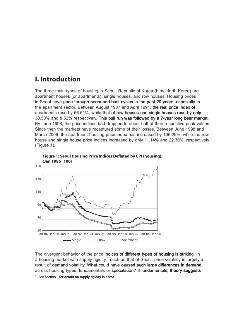
The three main types of housing in Seoul, Republic of Korea (henceforth Korea) are apartment houses (or apartments), single houses, and row houses. Housing prices in Seoul have gone through boom-and-bust cycles in the past 20 years, especially ingone through boom-and-bust cycles in the past 20 years, especially in boom-and-bust cycles in the past 20 years, especially in the apartment sector. Between August 1987 and April 1991, the real price index ofthe real price index ofreal price index ofof apartments rose by 66.61�, while that of row houses and single houses rose by onlyof row houses and single houses rose by onlyrow houses and single houses rose by only by onlyonly 38.50� and 8.52� respectively. This bull run was followed by a 7-year long bear market.. This bull run was followed by a 7-year long bear market. This bull run was followed by a 7-year long bear market. By June 1998, the price indices had dropped to about half of their respective peak values. Since then the markets have recaptured some of their losses. Between June 1998 and March 2006, the apartment housing price index has increased by 106.29�, while the row house and single house price indices increased by only 11.14� and 22.30�, respectively (Figure 1).
150
130
110
90
70
50Jan-86 Jan-88 Jan-90 Jan-92 Jan-94 Jan-96 Jan-98 Jan-00 Jan-02 Jan-04 Jan-06
Figure 1: Seoul Housing Price Indices De�ated by CPI (housing)(Jan 1986=100)
Single Row Apartment
The divergent behavior of the price indices of different types of housing is strikinindices of different types of housing is strikin of different types of housing is striking. In a housing market with supply rigidity,1 such as that of Seoul, price volatility is largely aa result of demand volatility. What could have caused such large differences in demand demand volatility. What could have caused such large differences in demand caused such large differences in demandsuch large differences in demand across housing types, fundamentals or speculation�� If fundamentals, theory suggests speculation�� If fundamentals, theory suggestsspeculation�� If fundamentals, theory suggestsIf fundamentals, theory suggestss, theory suggests, theory suggeststheory suggests � S�� S�����n �� ��r ���a���� �n ��u���y r������y �n ��r�a��� S�����n �� ��r ���a���� �n ��u���y r������y �n ��r�a�S�����n �� ��r ���a���� �n ��u���y r������y �n ��r�a������n �� ��r ���a���� �n ��u���y r������y �n ��r�a��� ��r ���a���� �n ��u���y r������y �n ��r�a� ��r ���a���� �n ��u���y r������y �n ��r�a�r������y �n ��r�a� �n ��r�a�
� | ADB Economics Working Paper Series No. 146
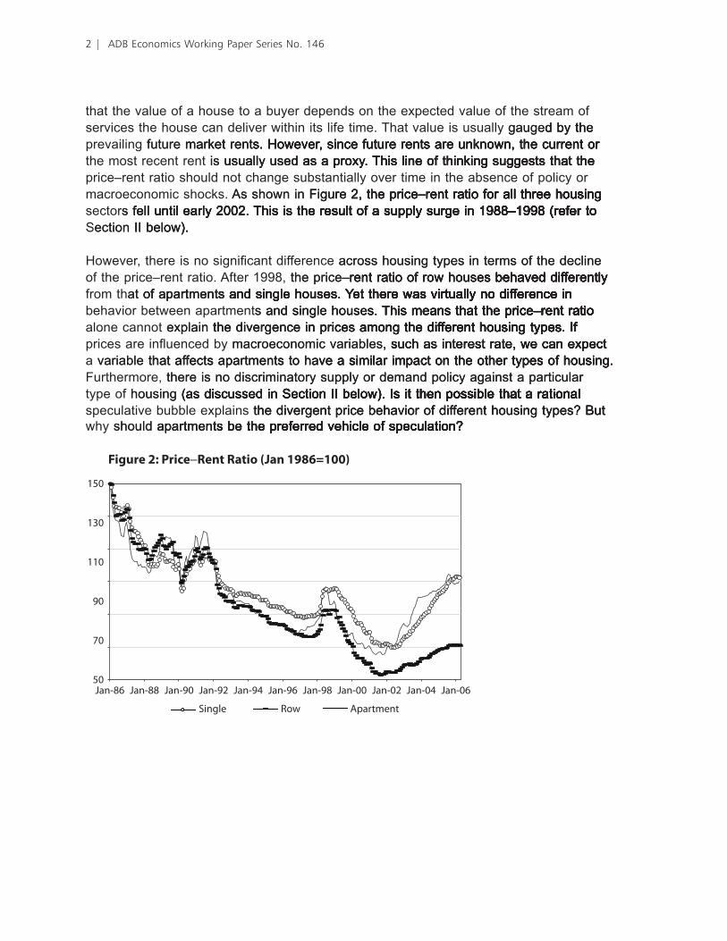
that the value of a house to a buyer depends on the expected value of the stream of services the house can deliver within its life time. That value is usually gauged by thegauged by thed by the prevailing future market rents. However, since future rents are unknown, the current orfuture market rents. However, since future rents are unknown, the current ormarket rents. However, since future rents are unknown, the current ors. However, since future rents are unknown, the current or. However, since future rents are unknown, the current oror the most recent rent is usually used as a proxy. This line of thinking suggests that theis usually used as a proxy. This line of thinking suggests that the usually used as a proxy. This line of thinking suggests that theas a proxy. This line of thinking suggests that the This line of thinking suggests that the price–rent ratio should not change substantially over time in the absence of policy or macroeconomic shocks. As shown in Figure 2, the price–rent ratio for all three housingAs shown in Figure 2, the price–rent ratio for all three housingFigure 2, the price–rent ratio for all three housing 2, the price–rent ratio for all three housingthe price–rent ratio for all three housing ratio for all three housingall three housing three housing sectors fell until early 2002. This is the result of a supply surge in 1988–1998 (refer tos fell until early 2002. This is the result of a supply surge in 1988–1998 (refer to fell until early 2002. This is the result of a supply surge in 1988–1998 (refer tofell until early 2002. This is the result of a supply surge in 1988–1998 (refer tountil early 2002. This is the result of a supply surge in 1988–1998 (refer tothe result of a supply surge in 1988–1998 (refer to result of a supply surge in 1988–1998 (refer to–1998 (refer to (refer to Section II below).ection II below).II below).).
However, there is no significant difference across housing types in terms of the declineacross housing types in terms of the decline of the price–rent ratio. After 1998, the price–rent ratio of row houses behaved differentlythe price–rent ratio of row houses behaved differently–rent ratio of row houses behaved differentlyrent ratio of row houses behaved differentlys behaved differently behaved differentlybehaved differently from that of apartments and single houses. �et there was virtually no difference inat of apartments and single houses. �et there was virtually no difference in of apartments and single houses. �et there was virtually no difference ins and single houses. �et there was virtually no difference in and single houses. �et there was virtually no difference in�et there was virtually no difference in there was virtually no difference inwas virtually no difference in virtually no difference in behavior between apartments and single houses. This means that the price–rent ratios and single houses. This means that the price–rent ratio and single houses. This means that the price–rent ratios. This means that the price–rent ratio. This means that the price–rent ratioThis means that the price–rent ratio means that the price–rent ratiothat the price–rent ratioprice–rent ratio–rent ratiorent ratio alone cannot explain the divergence in prices among the different housing types. Ifexplain the divergence in prices among the different housing types. If the divergence in prices among the different housing types. Ifin prices among the different housing types. Ifamong the different housing types. Ifthe different housing types. Ifdifferent housing types. Iftypes. If IfIf prices are influenced by macroeconomic variables, such as interest rate, we can expectmacroeconomic variables, such as interest rate, we can expect, such as interest rate, we can expect such as interest rate, we can expect we can expect a variable that affects apartments to have a similar impact on the other types of housing.variable that affects apartments to have a similar impact on the other types of housing. that affects apartments to have a similar impact on the other types of housing.ve a similar impact on the other types of housing.a similar impact on the other types of housing. Furthermore, there is no discriminatory supply or demand policy against a particularthere is no discriminatory supply or demand policy against a particular type of housing (as discussed in Section II below). Is it then possible that a rationalhousing (as discussed in Section II below). Is it then possible that a rational (as discussed in Section II below). Is it then possible that a rational(as discussed in Section II below). Is it then possible that a rationalas discussed in Section II below). Is it then possible that a rationalection II below). Is it then possible that a rationalII below). Is it then possible that a rational). Is it then possible that a rational. Is it then possible that a rational Is it then possible that a rationalIs it then possible that a rational speculative bubble explains the divergent price behavior of different housing types�� But the divergent price behavior of different housing types�� Butthe divergent price behavior of different housing types�� But But why should apartments be the preferred vehicle of speculation��should apartments be the preferred vehicle of speculation�� apartments be the preferred vehicle of speculation��s be the preferred vehicle of speculation�� be the preferred vehicle of speculation��the preferred vehicle of speculation�� preferred vehicle of speculation��
150
130
110
90
70
50Jan-86 Jan-88 Jan-90 Jan-92 Jan-94 Jan-96 Jan-98 Jan-00 Jan-02 Jan-04 Jan-06
Figure 2: Price Rent Ratio (Jan 1986=100)
Single Row Apartment
Housing Prices and the Role of Speculation: The Case of Seoul | 3
To answer these questions, we will adopt the asset-price approach to adopt the asset-price approach toadopt the asset-price approach to the asset-price approach to to housing price determination. The rationale for using this approach is given in the passage above. The rationale for using this approach is given in the passage aboveusing this approach is given in the passage above this approach is given in the passage abovethe passage above and will be further elaborated on in Section IV. �ur study compares two variants of theSection IV. �ur study compares two variants of theection IV. �ur study compares two variants of theIV. �ur study compares two variants of the. �ur study compares two variants of the�ur study compares two variants of the present value model. �ne assumes that only fundamentals drive the housing market while the other assumes that a rational speculative bubble plays an important role. According to the positive feedback theory (Shiller 1990), this bubble is approximated by lagged price appreciation. Xiao (2008) explicitly modeled the mechanism thatXiao (2008) explicitly modeled the mechanism thatthat rationalizes this approximation. �mpirical analysis shows that the coefficient on the�mpirical analysis shows that the coefficient on the rational speculative bubble is highly significant, and has the correct sign and magnitude suggested by Shiller (1990) and Xiao (2008). The inclusion of this variable boosts the and Xiao (2008). The inclusion of this variable boosts the. The inclusion of this variable boosts the in-sample fitting as well as the predictive power of the model. To capture some private information missing from both models, a latent state variable is included. �ur study showsmissing from both models, a latent state variable is included. �ur study shows, a latent state variable is included. �ur study shows that this variable helps to explain part of the price volatilities.
II. State of the �orean and Seoul Housing �arketsState of the �orean and Seoul Housing �arketsthe �orean and Seoul Housing �arkets�orean and Seoul Housing �arkets
A bubble is the deviation of a price from its fundamental value. Since the fundamental value is inherently subject to a great deal of uncertainty, price will in general contain a bubble element. In the absence of speculation, the rise and fall of that bubble should beof that bubble should beshould be purely random, and hence should be more correctly called market noise. �n the other, and hence should be more correctly called market noise. �n the otherand hence should be more correctly called market noise. �n the otherhence should be more correctly called market noise. �n the other. �n the other �n the other�n the other hand, a systematic deviation of a price from its fundamental value over sustained periods of time can only be the result of speculation. Such deviation constitutes a speculativeconstitutes a speculativespeculative bubble.
The primary motive for speculation is expected capital gain. While some argue that high transaction costs in the housing market will hinder speculation, Levin and Wright (1997),the housing market will hinder speculation, Levin and Wright (1997),housing market will hinder speculation, Levin and Wright (1997),speculation, Levin and Wright (1997),, Levin and Wright (1997), Caginalp et al. (2000), and Lei et al. (2001) show these costs may not have much of. (2000), and Lei et al. (2001) show these costs may not have much of (2000), and Lei et al. (2001) show these costs may not have much of. (2001) show these costs may not have much of (2001) show these costs may not have much of a deterrent effect. Malpe��i and Wachter (2005) point out that restricted supply is theeffect. Malpe��i and Wachter (2005) point out that restricted supply is theMalpe��i and Wachter (2005) point out that restricted supply is the key driver behind speculation in the housing market. In markets with elastic supply, speculative demand will have little impact on price. This fact should dampen the incentivedemand will have little impact on price. This fact should dampen the incentivewill have little impact on price. This fact should dampen the incentive little impact on price. This fact should dampen the incentiveshould dampen the incentive dampen the incentive to speculate in the first place.
The rigidity of housing supply in Korea is well documented in the literature. The government exercises almost full control over the housing supply, through its monopoly of the supply of land that can be developed for residential use. In the early stages of economic growth and development, the Korean government discouraged scarce capital from flowing into the housing sector. The underlying assumption was that the housing sector yields lower returns than the manufacturing or export industry. The government has yields lower returns than the manufacturing or export industry. The government hasyields lower returns than the manufacturing or export industry. The government has lower returns than the manufacturing or export industry. The government haslower returns than the manufacturing or export industry. The government has the lion’s share of the supply of housing credit, and this further strengthened its grip on the housing market. To keep demand within supply, the government also imposed punitive taxes and restricted housing market transactions (Kim 1993, Renaud 1993, Kim 2004a).a).).
4 | ADB Economics Working Paper Series No. 146
By 1988, the government came to reali�e the severity of the housing shortage that resulted from its policies. In response, it decided to build two million new dwellings in five years. In the next 10 years, the average annual production of houses jumped from 200,000–250,000 units to 500,000–600,000. The total number of dwellings stood at 6.1stood at 6.1 6.1 million by 1985. The number rose to 9.21 million by 1995 and 10.96 million by 2000 (Kim 2004, Kim and Kim 2002). This increased supply is the major cause of the housing price is the major cause of the housing pricethe housing pricehousing price decline between 1991 and 1998.
However, the increase in the number of houses represents a one-time right-shifting of a very steep supply curve rather than flattening of the supply curve. There are still more than 100 regulations regarding land use in Korea. For instance, the green belt in the city of Seoul takes up 50� of its developable land.2 At the same time, controlling the growth of the Capital Region,3 which covers 11� of the nation’s territory but is homes territory but is home territory but is home to 46� of its population, remains a top government priority (Kim and Kim 2002). Rigidits population, remains a top government priority (Kim and Kim 2002). Rigid population, remains a top government priority (Kim and Kim 2002). Rigid supply, coupled with concentrated demand, makes Seoul the perfect breeding ground forSeoul the perfect breeding ground forthe perfect breeding ground for speculation.
Be that as it may, speculation had been tame before the deregulation of the 1990s, largely due to the underdeveloped state of the formal mortgage market. With limited supply of housing credit, speculators do not have the financial wherewithal to speculate. The primary mortgage market used to be dominated by the National Housing Fund, which provided below-market rate loans to low- or moderate-income households, and the Koreaor moderate-income households, and the Korea moderate-income households, and the Korea Housing Bank, which served a somewhat higher income clientele. Credit rationing was. Credit rationing wasCredit rationing was also in place. A ceiling on loan amount per household was strictly enforced so that the loan-to-value ratio was typically below 30�. Furthermore, only new houses were eligible for loans. There were rules that restricted the eligibility of borrowers as well. As late asThere were rules that restricted the eligibility of borrowers as well. As late aswere rules that restricted the eligibility of borrowers as well. As late as rules that restricted the eligibility of borrowers as well. As late asthat restricted the eligibility of borrowers as well. As late as eligibility of borrowers as well. As late asAs late as 1999, the percentage of households with access to housing loan was only 50.8� (Kim 2004a).
In this situation, an informal housing finance arrangement known as c������������ emerged to fill the gap. Under this arrangement, the tenant gives the landlord a lump sum deposit (about 50� of the value of the house on average) in lieu of monthly rental payments. Owners can then use this deposit to finance the purchase of a second house. The deposit is fully refunded at the end of the lease. In 1997 total c������������� deposits were estimated to be 107.8 trillion won, about twice as large as the 64 trillion won of outstanding total mortgage loans. C������ claims on apartments alone amounted to 63.4 trillion won in mid-2001, compared with 54 trillion won of total outstanding housing loans (Kim and Suh 2002, Kim 2004a). According to the Population and Housing Census of 2 Un��r �h� Urban P�ann�n� A�� (�97�), �r��n b����� w�r� ������na��� ar�un� maj�r ��r�an ������� b��w��n �97� an�
�977� Th� A�� an� ���� a���m�any�n� ���r���� �r�h�b�� �an�-u��� ��nv�r����n��, �an� ��ub��v�����n��, an� ��n���ru����n a���v������ ��h�r �han r�bu����n� �r a���r�n� �x�����n� ���ru��ur��� �n����� �h� �r��n b����� w��h�u� �r��r a��r�va� �r�m �h� r���van� ��v�rnm�n� �ffi����� Gr��n b����� �n m���um-���z�� ������� w�r� ������ �n �999, wh��� �h���� �n �h� Ca���a� R����n an� ���x ��h�r �ar�� m��r������an ar�a�� ar� �n �h� �r������� �� b��n� r�v��w�� ��r �ar��a� ��b�ra��za���n�
� Th� S��u� Ca���a� R����n ��n�������� �� �h� ���y �� S��u�, �h� ���y �� �n�h��n, an� �h� �y�n�-�� Pr�v�n��� C�nv�r����n �� a�r��u��ura� an� ��r���� �an� ��� n�� a���w�� ��r �ar��-���a�� r������n��a� an� �n�u���r�a� ��v����m�n��� �n �h��� r����n�

Housing Prices and the Role of Speculation: The Case of Seoul | 5
2000, 41� of housing stock in urban areas is owner-occupied, 41� rented on c������ contracts, and 16� rented on monthly rental contracts.4 C������������ represents about 60� of new rental contracts in Seoul (Kim 2004a).
In January 2003, the Comprehensive Planning and Land Use Act took effect, markingook effect, marking effect, marking the onset of deregulation in the Korean real estate market. The essence of the new law is “no development without planning”, which, according to Kim and Kim (2002), could make the supply of land in the suburbs that can be developed even less elastic. �n the other hand, financial deregulation related to the real estate sector has made substantial progress since the early 1990s. The si�e of the primary mortgage market has increasedmortgage market has increasedmarket has increased substantially, more innovative products have been developed, and the loan-to-value ratio has increased.5 In 1997, the outstanding balance of mortgage loans amounted to 11.7% of gross domestic product (GDP), but rose to 13.4% by 2001. These figures are estimates, because the Bank of Korea publishes data only on the housing loans made on the housing loans made the housing loans made to consumers but not those to developers. Many lenders underreport housing loans as they declare loans with housing collateral as consumer loans. The figure also excludes the informal c������ market. While supply rigidity has sown the seed of speculation, the upsurge in housing credit has created a conducive climate for that seed to grow.created a conducive climate for that seed to grow.d a conducive climate for that seed to grow. a conducive climate for that seed to grow.a conducive climate for that seed to grow.climate for that seed to grow.for that seed to grow.that seed to grow.
Hwang et al. (2006) and Kim (2004a) provide excellent in-depth descriptions of the et al. (2006) and Kim (2004a) provide excellent in-depth descriptions of the (2006) and Kim (2004a) provide excellent in-depth descriptions of the current state of the housing markets in Korea and Seoul. The distinctive chonsei rental contract, described above, is the defining feature of the Korean housing market. The c������ contract has a legal term of 2 years and combines two separate transactions. The first transaction is the interest-free loan made by the tenant to the landlord. The second transaction is the lease that gives the tenant the use of the landlord’s residence in exchange for the implicit rent, i.e., the interest income the landlord earns on the c������ deposit. The implicit rent can thus be computed by multiplying the deposit by the prevailing market interest rate.6 C������ contracts still dominate the rental market in Seoul, despite the growing popularity of monthly rental contracts in recent years. This is especially true in the rental market for mid- and upper-level residences. Therefore, the Korean housing market is essentially a two-pillar market consisting of owner-occupiers and c������ renters. Finally, owner-occupiers do contribute to the housing price inflation since many owners who have only one home buy their home partly as an investment. However, it is unlikely that they drive and dominate the market in light of the large numbers of renters, which implies substantial numbers of multiple home owners. Indeed some owners use the c������ deposit to invest in additional homes.
� S�m� m�n�h�y r�n�a� ��n�ra���� a���� r�qu�r� a ����ara�� k�y m�n�y ���������� Th� ��an-��-va�u� ra��� ��� ������ r��a��v��y ��w� �n 200�, �h� ��an-��-va�u� ra��� wa�� m�r��y �2���� (��m 200�a)� ��� ������ r��a��v��y ��w� �n 200�, �h� ��an-��-va�u� ra��� wa�� m�r��y �2���� (��m 200�a)��n 200�, �h� ��an-��-va�u� ra��� wa�� m�r��y �2���� (��m 200�a)�n 200�, �h� ��an-��-va�u� ra��� wa�� m�r��y �2���� (��m 200�a)�� �n �a��, �h� r�n� �n��x, �ak�n �r�m �h� C��C �a�aba��� an� u���� �n �h��� ���u�y, ��� ��m�u��� u���n��n �a��, �h� r�n� �n��x, �ak�n �r�m �h� C��C �a�aba��� an� u���� �n �h��� ���u�y, ��� ��m�u��� u���n��h� C��C �a�aba��� an� u���� �n �h��� ���u�y, ��� ��m�u��� u���n�C��C �a�aba��� an� u���� �n �h��� ���u�y, ��� ��m�u��� u���n��a�aba��� an� u���� �n �h��� ���u�y, ��� ��m�u��� u���n�a�aba��� an� u���� �n �h��� ���u�y, ��� ��m�u��� u���n� chonsei ��n�ra�����
6 | ADB Economics Working Paper Series No. 146
III. Literature Review
Economists have long been fascinated by speculative bubbles in the real estate market. Perhaps due to the great deal of uncertainty surrounding the fundamental value, empirical studies often produce mixed evidence on the existence of bubbles (Abraham and often produce mixed evidence on the existence of bubbles (Abraham and Hendershott 1996, Levin and Wright 1997, Brooks et al. 2001, Bjorklund and Soderberg 1999, Bourassa and Hendershott 2001, Roche 2001, Himmelberg et al. 2005, Ito and et al. 2005, Ito and 2005, Ito and Iwaisako 1995, Chan et al. 2000).
There are quite a number of studies by Korean economists on the volatile behavior of thestudies by Korean economists on the volatile behavior of the by Korean economists on the volatile behavior of theKorean economists on the volatile behavior of theeconomists on the volatile behavior of theconomists on the volatile behavior of then the volatile behavior of thethe volatile behavior of the Korean housing market. Many believe that the boom in the housing market from the latemarket. Many believe that the boom in the housing market from the late. Many believe that the boom in the housing market from the late 1980s to the early 1990s was largely driven by speculative demand. Kim and Suh (1993) show that a bubble existed in both the nominal and relative price of land price between 1974 and 1989. Lee (1997) also rejects the hypothesis that land prices were driven solelyalso rejects the hypothesis that land prices were driven solelyrejects the hypothesis that land prices were driven solely by market fundamentals in Korea between 1964 and 1994.
Kim and Lee (2000) adapt the idea that the existence of an equilibrium relationship excludes the possibility of a price bubble. They conclude that Korea’s nominal and real land prices are cointegrated with market fundamentals (approximated by nominal and real GDP respectively) in the long run. However, such a cointegration relationship does not exist in the short run.
Lim (2003) conducted two bubble tests based on the present value relation on the housing price of Korea. One is a modified volatility test (MRS test) suggested by Mankiw et al. (1985), and the other combines the unit root test of Diba and Grossman (1988) and the cointegration test of Campbell and Shiller (1987). The MRS test shows that the null hypothesis of market efficiency is rejected, implying the existence of an irrational bubble. However, the unit root test and cointegration test does not support the existence of a bubble. This result is in contrast with the findings of �iao (200�), which employs a Markov. This result is in contrast with the findings of �iao (200�), which employs a Markov This result is in contrast with the findings of �iao (200�), which employs a Markov switching ADF approach. The variable Xiao uses in her analysis is the narrower Seoul housing price index, which perhaps explains the difference. This is because speculation in housing markets is usually concentrated in areas with limited land supply (Malpe��i and Wachter 2005). The other part of the explanation may be methodological. Blanchard and5). The other part of the explanation may be methodological. Blanchard and). The other part of the explanation may be methodological. Blanchard and The other part of the explanation may be methodological. Blanchard and may be methodological. Blanchard andmethodological. Blanchard andical. Blanchard and. Blanchard and Watson (1982) argue that a speculative bubble could collapse periodically. In that case,e periodically. In that case,. In that case, Evans (1991) shows that the usual unit root test has little power.s that the usual unit root test has little power. that the usual unit root test has little power.
Korean housing prices have experienced sustained, rapid increase since the end of the 1990s. It is commonly believed that the primary driving force behind this price inflation is speculation (Chung and Kim 2004). In response, the government has imposed a number of antispeculation measures. These include prohibiting the sale of housing pre-sale contracts, adjusting property taxes upward, and sharply raising capital gains tax. BanningBanning the sale of pre-sale contracts should discourage speculation since such contracts were widely used by speculators to buy housing they will not live in. Likewise, the increase in
Housing Prices and the Role of Speculation: The Case of Seoul | 7
capital gains tax rate from 9% to 36% to a flat rate of �0% for owners of two properties; and from 60� to 82� for owners of three or more properties, can also be expected to have a deterrent effect on speculation. The gradual increase in the property tax rate from the current 0.15� to 1� by 2019 should also help to discourage speculation.
In principle, anti-speculation measures should promote housing price stability. In practice, they have failed to do so. This fact echoes the observations by Levin and Wright (1997), This fact echoes the observations by Levin and Wright (1997), Caginalp et al. (2000), and Lei et al. (2001). Although most of the antispeculation. (2000), and Lei et al. (2001). Although most of the antispeculation (2000), and Lei et al. (2001). Although most of the antispeculation. (2001). Although most of the antispeculation (2001). Although most of the antispeculation Although most of the antispeculation measures are applicable to both the apartment sector and nonapartment sector, it was widely expected that their impact would fall primarily on the apartment sector. This is because apartments, especially apartments in the upscale Gangnam area of Seoul, have been the main arena for speculative activity. In this context, some antispeculative measures were targeted specifically at Gangnam and other areas characterized by large-scale speculation. Examples of such targeted measures include a higher capital gains tax and regulations against reconstructing old apartments for profit. The continued rise in housing prices, especially in the apartment sector, attests to the ineffectiveness of the antispeculation measures in reining in the speculative activities. The slower growth of nonapartment prices is more likely due to relative lack of speculation rather than greater effectiveness of antispeculative measures on the nonapartment sector.7
To repeat, the antispeculation measures have not resulted in stability of housing prices.resulted in stability of housing prices. Chung and Kim (2004) point out that their ineffectivness can partly be explained by the very low price elasticity of housing demand. As such, a good part of the increase in the capital tax has simply fuelled a further rise in housing prices. Chung and Kim (2004) estimate a simple model relating housing price to income and bond yield, the two representing “normal” demand variables. “Speculative” demand is captured by the lagged value of the housing price in the regression equation, as in Abraham and Hendershott (1996). Their results show that “what determines housing price hike in South Korea is not ‘normal’ demand but ‘speculative’ demand.” The ratio of speculative demand to normal demand is 1.24 for Korea as a whole and 2.85 for Seoul. The higher ratio for Seoul supports the notion that speculation has a bigger impact on demand and hence price in Seoul than in the rest of the country. Chung and Kim cite low interest rates and easy credit as two of the major reasons behind the increased speculation in the Korean housing market.
7 ��a� (2007) an� ��a� an� ��u (��r�h��m�n�) hav� a���� �b���rv�� �ha� �h� �r�m�um r������n��a� ������r �n ��n� ��n�,��a� (2007) an� ��a� an� ��u (��r�h��m�n�) hav� a���� �b���rv�� �ha� �h� �r�m�um r������n��a� ������r �n ��n� ��n�,, Ch�na ��� �ar m�r� �r�n� �� �����u�a���n �han �h� n�n�r�m�um �n�� Th�y �x��a�n �ha� buy�r�� �� u����a�� h�u����� ar� ��� �ar m�r� �r�n� �� �����u�a���n �han �h� n�n�r�m�um �n�� Th�y �x��a�n �ha� buy�r�� �� u����a�� h�u����� ar� w�a��h��r �n��v��ua��� �r �n�����u���na� �nv�����r�� wh� hav� mu�h b����r a������� �� �r����� ��n�� wh�n �h�y hav� �h���n�� wh�n �h�y hav� �h��n�� wh�n �h�y hav� �h� w��� �� �����u�a��, �h�y a���� hav� �h� finan��a� ��w�r �� �� ���� Th� �x��r��n�� �� S�n�a��r� �n 200��2007 a���� �a�n���Th� �x��r��n�� �� S�n�a��r� �n 200��2007 a���� �a�n���h� �x��r��n�� �� S�n�a��r� �n 200��2007 a���� �a�n����x��r��n�� �� S�n�a��r� �n 200��2007 a���� �a�n���x��r��n�� �� S�n�a��r� �n 200��2007 a���� �a�n����2007 a���� �a�n���7 a���� �a�n��� a ���m��ar ����ur�� �n �ha� ��r���, h�u���n� �r����� n�ar�y ��ub��� �n ��r�a�n ar�a�� �� �h� u����a�� r������n��a� mark�� bu��� n�ar�y ��ub��� �n ��r�a�n ar�a�� �� �h� u����a�� r������n��a� mark�� bu� n�ar�y ��ub��� �n ��r�a�n ar�a�� �� �h� u����a�� r������n��a� mark�� bu�u����a�� r������n��a� mark�� bu� r������n��a� mark�� bu� har��y m�v�� a� a�� �n ��h�r ar�a���
� | ADB Economics Working Paper Series No. 146
IV. Theory and �odel
The price of housing in any market is ultimately determined by supply and demand. When supply is rigid, as is the case in Korea, this market price is largely demand-driven.
What drives the demand for housing�� A housing market can be divided into owner-occupied and rental sectors. So the demand for housing includes the demand for bothSo the demand for housing includes the demand for botho the demand for housing includes the demand for both owner-occupied and rental housing. For a renter, the housing space he rents is a consumable good; for an owner, the house he owns is an asset that provides a streaman asset that provides a streamasset that provides a streamthat provides a streamprovides a streams a stream a stream of housing services. The market value of the stream of services is the return to thisThe market value of the stream of services is the return to thishe market value of the stream of services is the return to this housing asset. The demand for rental housing depends on the cost of housing services relative to that of other consumption goods. �n the other hand, the demand for owner-. �n the other hand, the demand for owner- demand for owner-occupied housing depends on the return to housing assets relative to that from others relative to that from other relative to that from otherfrom otherother types of assets. The rental sector determines the rents while the owner-occupied sectorsector determines the prices. The two sectors are linked by household choice between rentingThe two sectors are linked by household choice between renting two sectors are linked by household choice between rentingsectors are linked by household choice between renting renting and buying.
To illustrate, consider an economy with N identical households, each living for T periodsillustrate, consider an economy with N identical households, each living for T periods, consider an economy with N identical households, each living for T periods and each desiring exactly one unit of housing services. The total supply of rental anddesiring exactly one unit of housing services. The total supply of rental and housing services. The total supply of rental andsupply of rental andrental and owner-occupied housing services is fixed and e�ual to the number of households. At timeis fixed and e�ual to the number of households. At timeequal to the number of households. At time t, each new generation of households chooses to be either a renter or an owner. Thiss to be either a renter or an owner. This to be either a renter or an owner. Thiseither a renter or an owner. Thisa renter or an owner. This generation of households exits at time t+T, and is replaced by another generation withwith identical characteristics. The choice between renting and owning depends on their relativecharacteristics. The choice between renting and owning depends on their relative cost. The cost of renting, CR, and the cost of owning, C�, are respectively:of owning, C�, are respectively:owning, C�, are respectively:
CR = D +t t t+ jj=1
i
t+ii=1
T -1
δÕåæ
èçççç
ö
ø÷÷÷÷D (1)
CO P Pt t t jj
T
t T= -æ
èçççç
ö
ø÷÷÷÷+
=+Õd
1
(2)
where δ is a discounting factor that depends on the risk-free rate of return, δ∈(0,1) ; D is the rental payment; and P is the purchase price of housing space. The subscript t denotes the time the cost is incurred, and X means that X is a random variable.
Suppose households are risk-neutral, and suppose there exists no liquidity constraint., and suppose there exists no liquidity constraint..8 In a steady state, or the state in which none of the variables in the system has a tendency to deviate,
E CO E CR RPt t t t t[ ]= [ ]+ (3)
� ��r�an h�u��� buy�r�� �v�r�am� �h� ��qu����y ��n���ra�n� by an �n��n��u����r�an h�u��� buy�r�� �v�r�am� �h� ��qu����y ��n���ra�n� by an �n��n��u�� chonsei arran��m�n�� S�� S�����n �� ��rS�����n �� ��r�����n �� ��r�� ��r��r ���a���� �n chonsei ��n�ra�����

Housing Prices and the Role of Speculation: The Case of Seoul | 9
where Et[.] is the rational expectation operator conditional on Θ, or information available at time t – i.e., t – i.e., – i.e., Q=[ ]- -D D D P P Pt t t t, ,..., ; , ,....,1 0 1 0 , and RPt is the excess risk premium of renting over owning. To see why equation (3) constitutes a steady state, suppose. To see why equation (3) constitutes a steady state, supposeTo see why equation (3) constitutes a steady state, supposeequation (3) constitutes a steady state, suppose(3) constitutes a steady state, suppose3) constitutes a steady state, suppose) constitutes a steady state, suppose E CO E CR RPt t t t t[ ]< [ ]+ . In this case, it will be profitable for renters to become owners. Hence the demand for owner-occupied housing will rise, driving up housing prices. At the same time, the demand for rental housing will fall, driving down rents. The process will continue until the condition in e�uation (3) is satisfied. For ease of argument, the termor ease of argument, the term RPt will be dropped from now on. The central message will not be altered by doing so.
Thehe �t�ady �tat� pr�c�, defined as the price that results after all the necessary adjustments have taken place in response to an exogenous shock to the system, will hence satisfy the following condition: satisfy the following condition:satisfy the following condition:
P E CR E P
D
tf
t t t jj
T
t t T
t t jj
i
= [ ]+æ
èçççç
ö
ø÷÷÷÷
éë ùû
= +æ
è
+=
+
+=
Õ
Õ
d
d
1
1
ççççç
ö
ø÷÷÷÷
éëê
ùûú +
æ
èçççç
ö
ø÷÷÷÷+
=
-
+=
+å ÕE D E Pt ii
T
t jj
T
t t T
1
1
1
d ééë ùû (4)
This essentially describes the asset pricing model.
The asset pricing model is widely used to model the behavior of housing prices. Indeedmodel is widely used to model the behavior of housing prices. Indeedis widely used to model the behavior of housing prices. Indeed a large and well-established theoretical and empirical literature has emerged to explain house price dynamics on the basis of the asset pricing model. Recent examples of this literature include Flavin and Nakagawa (2008), Pia��esi et al. (2007), Guirguis et al. et al. (2007), Guirguis et al. (2007), Guirguis et al. et al. (2005), �ao and Zhang (2005), and Weeken (2004). The asset pricing model versionThe asset pricing model versionhe asset pricing model versionasset pricing model version used in this study is based on Campbell and Shiller (1988 a and b) and described in based on Campbell and Shiller (1988 a and b) and described in and described in detail below..
If economic agents are risk-neutral,
PE P D C
Rtt t t t
t
=+ ++
+[ ]1
1
a
, (5)
where Pt = the real price of the property asset at time t; Dt = the real rent received during period t; Rt = the time varying real discount rate; Ct = other economic variables that may impact the expectation formation; andmay impact the expectation formation; and; and α = coefficient showing how Ct relates to Pt. Without any loss of generality and for the sake of simplicity, the coefficient α will be omitted for the rest of the derivation. Define
r Rt tº +( )log 1 ; (6)
10 | ADB Economics Working Paper Series No. 146
Hence,
r E P D C Pt t t t t t= + +éë ùû( )- ( )+log log1 . (7)
In a static world, the rent grows at a constant rate. The log of Ct-to-price ratio and the log of rent-to-price ratio are also constants. In such a world, the log of the gross discount rate, rt, would also be a constant and linear in the logs of the variables in equation (3). If the transversality condition, lim
i
it t iE p
®µ +éë ùû =r 0 , is satisfied, we would have the following
fundamental solution for the price:
p p E d ct tf j
t t j t jj
= =--
+ - +éëê
ùûú+ +
=
µ
åk xr
r r1
10
( ) . (8)
where p = the log of P; d = the log of D; and c = the log of C.
However, the transversality condition may fail to hold. In this case, we expect the price to contain a rat���al �p�culat�v� bubbl�, b
p p bt tf
t= + , (9)
where the bubble component
E b bt t i i t+éë ùû =
1r
. (10)
This implies that
E b bt t t+éë ùû =1
1r . (11)
If the log of the property prices, rents and the other relevant economic variables are I(1), the following model may be estimated instead:
Dp p p
E d E d
tf
tf
tf
jt t j t t j
= -
= - éëê
ùûú -
éëê
ùûú
éëê
ùûú +
-
+ - + -
1
1 11( )r r EE c E ct t j t t jj
+ - + -=
µéëê
ùûú -
éëê
ùûú
éëê
ùûú{ }å 1 1
0
. (12)
Suppose the growth of the rents and the other relevant economic variables follow AR(p) and AR(q), respectively, then
D D Dp d ctf
ii
p
t i jj
q
t j= +=
-=
-å åq y0 0
. (13)
where θ and ψ are functions of the coefficients of the underlying processes of the price, the rent, and the other relevant variable. In the case when p = 1 and c is absent, we haveis absent, we haveabsent, we have, we have
Housing Prices and the Role of Speculation: The Case of Seoul | 11
D D D D Dp d d d dtf
t t t t=-
--
º + -- -
11 1
11 1frfrfr
y y( ) . (14)
If a bubble is present,
D D Dp p bt tf
t= + , (15)
and
E b bt t tD D+éë ùû =1
1r
(16)
Suppose there is some private information unavailable to the researcher and hence not included in equation (9). Let �t denotes this specification error, sothis specification error, so specification error, so
D D D Dp s d c bt t ii
p
t i jj
q
t j t= + + +=
-=
-å åq y0 0
(17)
and
D Ds st t+ =1 b (18)
This error is unobserved but can be inferred using the Kalman filter (refer to Harvey 1989, Hamilton 1994, and �iao 200� for technical details on this filter and the estimation procedure of the model).
V. Empirical Analysis
In this section, we describe our empirical methodology and report our main empirical results. The central objective of our empirical analysis, which is grounded in the theory and model of Section IV, is to test for the presence of speculative bubbles in the three different types of housing in Seoul.
A. Apartment�� Single�� and Row HousesApartment�� Single�� and Row Houses�� and Row Houses and Row Houses
In this subsection, we examine apartment, row, and single house price indices using monthly observations from January 1986 to March 2006. Between June 1998 and March 2006, the apartment housing price index increased by 106.29� in real terms. The corresponding values for single and row houses are 22.30� and 11.14�. During the same period, real earning, nonfarm population and real GDP increased by 32.56�, 13.09�, and 33.09�, respectively.

1� | ADB Economics Working Paper Series No. 146
According to the Population and Housing Census of Korea in 2000, the total number in 2000, the total number, the total number of houses stood at 10.9 million units, of which single houses accounted for 37.1�, apartments 47.7�, and row houses only 7.4�. Kim et al. (2000) show that the average single house-dwelling household had 4.64 family members and a monthly income of 2.15 million won. The average age of the household head was 52.1. �n the other hand, �n the other hand,�n the other hand, the average apartment-dwelling household had 4.14 members and a monthly income of 2.31 million won. The average age of the household head was 47.2. Therefore, Therefore,Therefore, apartments are preferred by the relatively young and better off. There is no specificThere is no specifichere is no specific policy or regulation that discriminates against one particular housing type, as explained in Section II. Therefore, there are no fundamental differences in the broader supplybroader supplysupply or macroeconomic conditions that can adequately explain the recent price divergencemacroeconomic conditions that can adequately explain the recent price divergence among the different housing types. Since the supply of housing is highly rigid in Korea, the origins of this divergence must lie in demand. This justifies the use of the model origins of this divergence must lie in demand. This justifies the use of the modelorigins of this divergence must lie in demand. This justifies the use of the modeldivergence must lie in demand. This justifies the use of the model must lie in demand. This justifies the use of the modelmust lie in demand. This justifies the use of the modellie in demand. This justifies the use of the model developed in Section IV.
B. Building the Empirical �odel
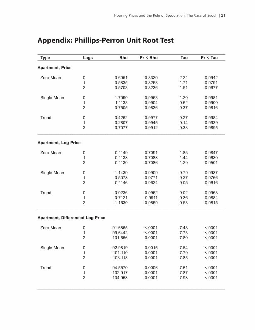
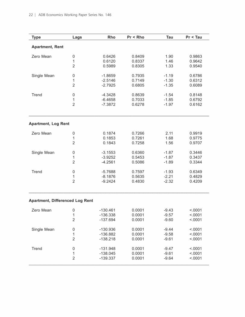
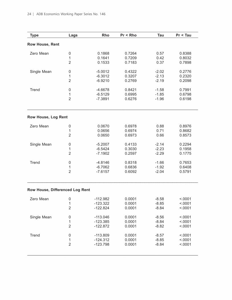
To decide between equations (9) and (15) as the basis of the model to be estimated,between equations (9) and (15) as the basis of the model to be estimated,equations (9) and (15) as the basis of the model to be estimated,s (9) and (15) as the basis of the model to be estimated, (9) and (15) as the basis of the model to be estimated,(9) and (15) as the basis of the model to be estimated,9) and (15) as the basis of the model to be estimated,) and (15) as the basis of the model to be estimated, and (15) as the basis of the model to be estimated,and (15) as the basis of the model to be estimated, (15) as the basis of the model to be estimated,(15) as the basis of the model to be estimated,15) as the basis of the model to be estimated,) as the basis of the model to be estimated, we use a Phillips-Perron test for unit root. At the conventional levels of significance, the null Phillips-Perron test for unit root. At the conventional levels of significance, the nulltest for unit root. At the conventional levels of significance, the nullunit root. At the conventional levels of significance, the null. At the conventional levels of significance, the nullt the conventional levels of significance, the null hypothesis of unit root can be accepted for the logarithm of each series but is rejected for the first log difference (please refer to the Appendix). Therefore, we estimate a model a model based on equation (15). �verall, the LR test rejects the restriction imposed by equation(15). �verall, the LR test rejects the restriction imposed by equation15). �verall, the LR test rejects the restriction imposed by equation). �verall, the LR test rejects the restriction imposed by equation. �verall, the LR test rejects the restriction imposed by equation�verall, the LR test rejects the restriction imposed by equation (14) that the coefficients on the current and the lagged changes of log real rent should4) that the coefficients on the current and the lagged changes of log real rent should) that the coefficients on the current and the lagged changes of log real rent should add up to 1 (please refer to Table 1). It was earlier argued that further lagged rents should be included as regressors if the rent process is if the rent process is AR(p), with p>1. However, the F test shows that although a regression of the changes in log real price on the changes in log real rent is significant with higher lags, there is only marginal increase in R2. For instance, increasing the number of lags from 1 to 11 raises the R-square of the row house series by a meager 0.07 and that of the other two series by less than 0.05. This observation echoes the comments Shiller (1990, 59) made on the regression of changes in log real stock price on the changes in log real dividends..
Table 1: LR Test for Parameter Restrictions Single House Row House Apartment�0: Ψ + Ψ _1=1 ��0�7�* 27��0�* ��7��2*�0: λ + 0 9��70* 7����* �0��79*
* �n���a���� ����n�fi�an�� a� �0��� N���: Th� �R ���a������� ��� �����r�bu��� χ(�) w��h �r����a� va�u��� 2�7�, ����, an� ���� a� �0��, ���, an�
���, r��������v��y� Th� ����� r�j����� �h� nu�� hy���h������ �ha� �h� ���ffi���n��� �n �h� �urr�n� an� �h� �a���� r�n� a�� u� �� un��y a� �0�� ��v��� �� a���� r�j����� �h� nu�� hy���h������ �ha� �h� ���ffi���n� �n �h� �a���� �r��� a��r���a���n ��� �n����n�fi�an��
Housing Prices and the Role of Speculation: The Case of Seoul | 13
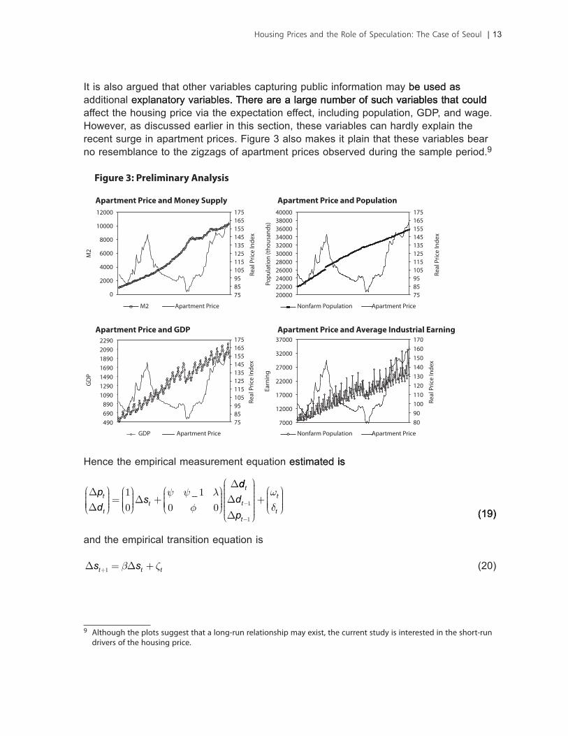
It is also argued that other variables capturing public information may be used asbe used as additional explanatory variables. There are a large number of such variables that couldexplanatory variables. There are a large number of such variables that could. There are a large number of such variables that could affect the housing price via the expectation effect, including population, GDP, and wage. However, as discussed earlier in this section, these variables can hardly explain the recent surge in apartment prices. Figure 3 also makes it plain that these variables bear no resemblance to the �ig�ags of apartment prices observed during the sample period.9
Apartment Price and Money Supply Apartment Price and Population
Apartment Price and Average Industrial EarningApartment Price and GDP
Figure 3: Preliminary Analysis
Nonfarm Population Apartment Price
Nonfarm Population Apartment Price
M2 Apartment Price
4000038000360003400032000300002800026000240002200020000
175165155145135125115105958575
Popu
latio
n (t
hous
ands
)
12000
10000
8000
6000
4000
2000
0
M2
2290209018901690149012901090
890690490
GD
P
37000
32000
27000
22000
17000
12000
7000
Earn
ing
Real
Pric
e In
dex
175165155145135125115105958575
Real
Pric
e In
dex
175165155145135125115105958575
Real
Pric
e In
dex
1701601501401301201101009080
Real
Pric
e In
dex
GDP Apartment Price
Hence the empirical measurement equation estimated isestimated isis
DD
D
Dp
dst
tt
æ
èçççç
ö
ø÷÷÷÷=æ
èççççö
ø÷÷÷÷ +
æ
èçççç
ö
ø÷÷÷÷
1
0
1
0 0
y y lf_
dd
d
p
t
t
t
t
t
D
D-
-
æ
è
ççççççç
ö
ø
÷÷÷÷÷÷÷÷+æ
èçççç
ö
ø÷÷÷÷1
1
wd
(19) (19)(19)
and the empirical transition equation is
D Ds st t t+ = +1 b z (20)
9 A��h�u�h �h� ������ ��u������ �ha� a ��n�-run r��a���n��h�� may �x����, �h� �urr�n� ���u�y ��� �n��r������ �n �h� ��h�r�-run �r�v�r�� �� �h� h�u���n� �r����
14 | ADB Economics Working Paper Series No. 146
where ∆pt and ∆dt are the first differences of the log real housing price and rent indices, respectively. It is assumed that ωt, δt and ξt are uncorrelated, and hence
R =æ
èçççç
ö
ø÷÷÷÷
ss
w
d
2
2
0
0 , V = sz2 . (21)
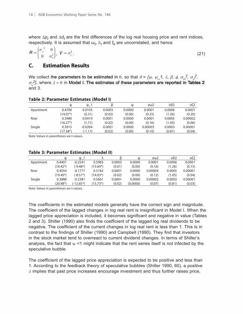
C. Estimation ResultsEstimation Results
We collect the parameters to be estimated inhe parameters to be estimated in θ, so that θ = {ψ, ψ_1, λ, β, φ, σω2, σδ
2, σζ
2}, where λ = 0 in Model I. The estimates of these parameters are reported in Tables 2Model I. The estimates of these parameters are reported in Tables 2odel I. The estimates of these parameters are reported in Tables 2reported in Tables 2 in Tables 2Tables 2ables 2s 2 2 and 3.
Table 2: Parameter Estimates (�odel I) ψ ψ_� β φ σω2 σδ2 σζ2A�ar�m�n� 0��700
(���07*)0�0�0�
(0���)0�000�
(0�02)0�0000
(0�00)0�000�
(0�2�)0�000�
(��2�)0�000�
(0�20)R�w 0��9�0
(���27*)0�0��9
(��7�)0�000�
(0�02)0�0000
(0�00)0�000�
(0���)0�000�
(��0�)0�00002
(0�0�)S�n��� 0��9��
(�7���*)-0�02��
(-���7)0�000�
(0�02)0�0000
(0�00)0�0000�
(0��0)0�000�
(0���)0�0000�
(0�0�)N���: Va�u��� �n �ar�n�h������ ar� �-va�u�����
Table 3: Parameter Estimates (�odel II) ψ ψ_� λ β φ σω2 σδ2 σζ2A�ar�m�n� 0���0�
(����2*)-0�2���(-9���*)
0��9��(����9*)
0�000�(0�0�)
0�0000(0�00)
0�000�(0���)
0�000�(��2�)
0�000�(0���)
R�w 0��0��(�9��0*)
-0��777(-����*)
0����2(���0�*)
0�000�(0�02)
0�0000(0�00)
0�0000�(0��2)
0�000�(��0�)
0�0000�(0�0�)
S�n��� 0�����(20�9�*)
-0�2���(-�2���*)
0�����(���7�*)
0�000�(0�02)
0�0000(0�0000)
0�00002(0�07)
0�000�(0���)
0�0000�(0�0�)
N���: Va�u��� �n �ar�n�h������ ar� �-va�u�����
The coefficients in the estimated models generally have the correct sign and magnitude. The coefficient of the lagged changes in log real rent is insignificant in Model I. When the lagged price appreciation is included, it becomes significant and negative in value (Tables 2 and 3). Shiller (1990) also finds the coefficient of the lagged log real dividends to be negative. The coefficient of the current changes in log real rent is less than 1. This is in contrast to the findings of Shiller (1990) and Campbell (1990). They find that investors in the stock market tend to overreact to current dividend changes. In terms of Shiller’s analysis, the fact that ψ <1 might indicate that the rent series itself is not infected by the speculative bubble.
The coefficient of the lagged price appreciation is expected to be positive and less than 1. According to the feedback theory of speculative bubbles (Shiller 1990, 60), a positive λ implies that past price increases encourage investment and thus further raises price,
Housing Prices and the Role of Speculation: The Case of Seoul | 15
while past price drops discourage investment and further reduce price. A value of less than 1 is re�uired to rule out irrational investor behavior. The estimate of this coefficient is highly significant, and has the expected magnitude and sign. Furthermore, it is larger in magnitude than Ψ and Ψ_1, implying that the bubble has a bigger impact on housing prices than the fundamentals. This result is consistent with Chung and Kim (2004), who find that the ratio of speculative demand to normal demand is larger than 1.
�verall, λ has the largest value for apartment, suggesting that apartments are moreapartments are more are more prone to speculation than the other two types of housing. The absolute values ofspeculation than the other two types of housing. The absolute values of than the other two types of housing. The absolute values of Ψ and Ψ_1 are also larger for apartments, which suggest that apartment prices are also more responsive to fundamentals (see Table 2 and 3). These observations explain why the price of apartments is much more volatile than the prices of row or single houses.or single houses. single houses.
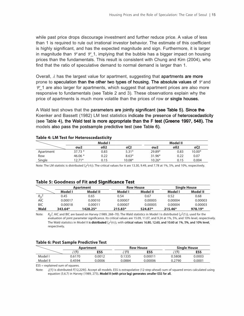
A Wald test shows that the parameters are jointly significant (see Table �). Since theparameters are jointly significant (see Table �). Since the are jointly significant (see Table �). Since thesee Table 5). Since theable 5). Since theSince the thehe Koenker and Bassett (1982) LM test statistics indicate the presence of heteroscedasticityindicate the presence of heteroscedasticity heteroscedasticity (see Table 4), the Wald test is more appropriate than the F test (Greene 1997, 548). Thesee Table 4), the Wald test is more appropriate than the F test (Greene 1997, 548). Theable 4), the Wald test is more appropriate than the F test (Greene 1997, 548). Thethe Wald test is more appropriate than the F test (Greene 1997, 548). Thetest is more appropriate than the F test (Greene 1997, 548). The is more appropriate than the F test (Greene 1997, 548). Thethan the F test (Greene 1997, 548). Thethe F test (Greene 1997, 548). TheF test (Greene 1997, 548). The(Greene 1997, 548). The models also pass the postsample predictive test (see Table 6). also pass the postsample predictive test (see Table 6).6).).
Table 4: L� Test for Heteroscedasticity�odel I �odel II
σω2 σδ2 σζ2 σω2 σδ2 σζ2A�ar�m�n� �7�7� * 0��� ����* 29��9* 0��� �0�00* R�w ���0� * 0�22 ����* ���9�* 0�22 0�07 S�n��� �2�7�* 0��� �0�0�* �0�2�* 0��� 0�00�
N���: Th� �M ���a������� ��� �����r�bu��� (χ2(4))� Th� �r����a� va�u��� ��r �� ar� ����0, 9��9, an� 7�7� a� ���, ���, an� �0��, r��������v��y��
Table 5: Goodness of Fit and Signi��cance Test and Signi��cance TestApartment Row House Single House
�odel I �odel II �odel I �odel II �odel I �odel IIRD
2 0��� 0��� 0��� 0��7 0��2 0���A�C 0�000�7 0�000�0 0�00007 0�0000� 0�0000� 0�0000�B�C 0�000�� 0�000�� 0�00007 0�0000� 0�0000� 0�0000�Wald 343.64* 1428.25* 215.83* 524.87* 215.46* 978.19*
N���: RD2, A�C an� B�C ar� ba���� �n �arv�y (�9�9, 2���70)� Th� Wa�� ���a��������� �n M���� � ��� �����r�bu��� (χ2(5)), u���� ��r �h�
�va�ua���n �� j��n� �aram���r ����n�fi�an��� ���� �r����a� va�u��� ar� ���09, ���07, an� 9�2� a� ���, ���, an� �0�� ��v��, r��������v��y� Th� Wa�� ���a��������� �n M���� �� ��� �����r�bu������ �����r�bu��������r�bu��� (χ2(6)), w��h �r����a� va�u��� ����0, �2��0, an� �0��0 a� ���, ���, an� �0�� ��v��,�r����a� va�u��� ����0, �2��0, an� �0��0 a� ���, ���, an� �0�� ��v��, r��������v��y��
Table 6: Post Sample Predictive TestApartment Row House Single House
ξ (1) ESS ξ (1) ESS ξ (1) ESSM���� � 0���70 0�00�2 0����� 0�000�� 0���0� 0�000�M���� �� 0���9� 0�000� 0�0��� 0�0000� 0�2790 0�000�
�SS = �x��a�n�� ��um �� ��quar����N���: ξ(1) ��� �����r�bu��� F(�2,229))� A����� a�� m������� �SS ��� �x�ra���a��v� (�2-�����-ah�a�) ��um �� ��quar�� �rr�r�� �a��u�a��� u���n�
�qua���n (����7) �n �arv�y (�9�9, 27�)� M���� �� (w��h �r��� �a�) ��n�ra���� ��ma���r �SS ��r a���� M���� �� (w��h �r��� �a�) ��n�ra���� ��ma���r �SS ��r a��� M���� �� (w��h �r��� �a�) ��n�ra���� ��ma���r �SS ��r a���
16 | ADB Economics Working Paper Series No. 146
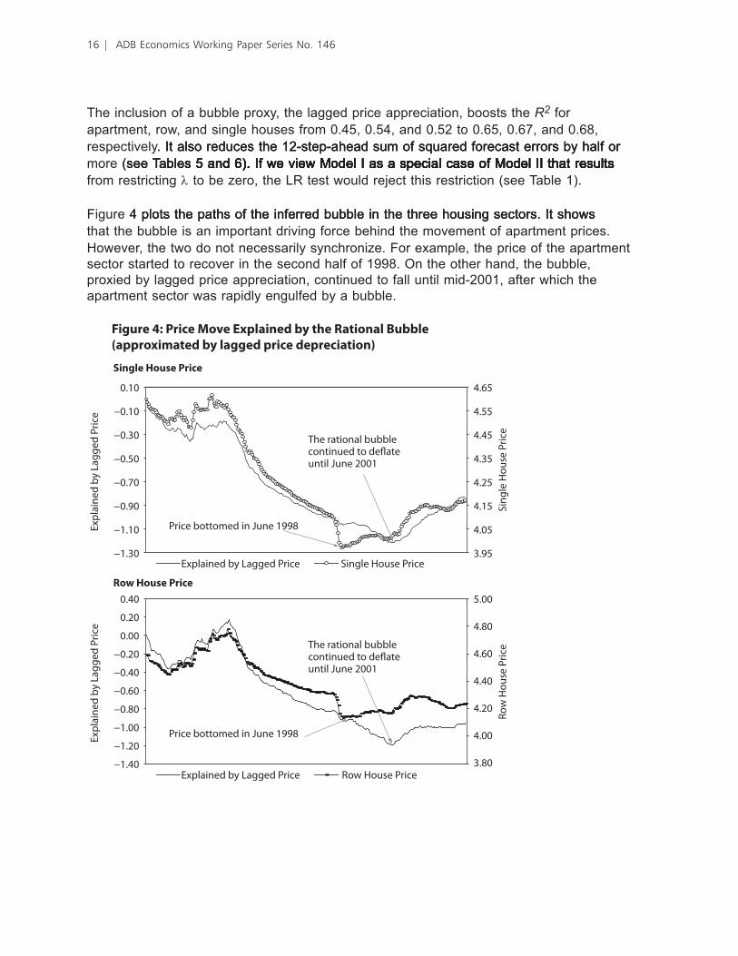
The inclusion of a bubble proxy, the lagged price appreciation, boosts the R2 for apartment, row, and single houses from 0.45, 0.54, and 0.52 to 0.65, 0.67, and 0.68, respectively. It also reduces the 12-step-ahead sum of squared forecast errors by half or. It also reduces the 12-step-ahead sum of squared forecast errors by half orIt also reduces the 12-step-ahead sum of squared forecast errors by half or more (see Tables 5 and 6). If we view Model I as a special case of Model II that results (see Tables 5 and 6). If we view Model I as a special case of Model II that resultssee Tables 5 and 6). If we view Model I as a special case of Model II that resultsables 5 and 6). If we view Model I as a special case of Model II that resultss 5 and 6). If we view Model I as a special case of Model II that results 5 and 6). If we view Model I as a special case of Model II that resultsand 6). If we view Model I as a special case of Model II that results 6). If we view Model I as a special case of Model II that results. If we view Model I as a special case of Model II that results from restricting λ to be �ero, the LR test would reject this restriction (see Table 1).
Figure 4 plots the paths of the inferred bubble in the three housing sectors. It shows4 plots the paths of the inferred bubble in the three housing sectors. It shows plots the paths of the inferred bubble in the three housing sectors. It shows that the bubble is an important driving force behind the movement of apartment prices. However, the two do not necessarily synchroni�e. For example, the price of the apartment sector started to recover in the second half of 1998. �n the other hand, the bubble, proxied by lagged price appreciation, continued to fall until mid-2001, after which the apartment sector was rapidly engulfed by a bubble.
0.10
−0.10
−0.30
−0.50
−0.70
−0.90
−1.10
−1.30
The rational bubblecontinued to de�ateuntil June 2001
Expl
aine
d by
Lag
ged
Pric
e
0.40
0.20
0.00
−0.20
−0.40
−0.60
−0.80
−1.00
−1.20
−1.40
Expl
aine
d by
Lag
ged
Pric
e
4.65
4.55
4.45
4.35
4.25
4.15
4.05
3.95
Sing
le H
ouse
Pric
e
5.00
4.80
4.60
4.40
4.20
4.00
3.80
Row
Hou
se P
rice
Figure 4: Price Move Explained by the Rational Bubble(approximated by lagged price depreciation)
Single House Price
Row House Price
Explained by Lagged Price Single House Price
Explained by Lagged Price Row House Price
The rational bubblecontinued to de�ateuntil June 2001
Price bottomed in June 1998
Price bottomed in June 1998

Housing Prices and the Role of Speculation: The Case of Seoul | 17
6.00
1.00
−4.00
−9.00
−14.00
−19.00
Expl
aine
d by
Lag
ged
Pric
e
5.2
5.1
5.0
4.9
4.8
4.7
4.5
4.4
4.3
Apa
rtm
ent P
rice
Figure 4. continued.
Apartment Price
The rational bubblecontinued to de�ateuntil June 2001
Price bottomed in June 1998
Explained by Lagged Price Apartment Price
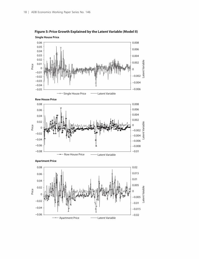
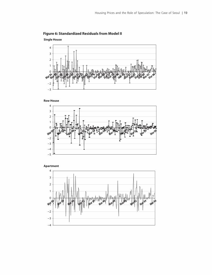
The latent variable, representing unobservable information, explains part of the prices part of the price part of the price volatilities (see Figure �). �ut the standardized plot (defined in Harvey 1989,2�7) for�). �ut the standardized plot (defined in Harvey 1989,2�7) for). �ut the standardized plot (defined in Harvey 1989,2�7) for both models show clustering in volatility, which suggests that none of these models is adequate (see Figure 6). Including more lagged rent and price growths does not mitigate6). Including more lagged rent and price growths does not mitigate). Including more lagged rent and price growths does not mitigate the problem. Neither do variabldo variables shown in Figure 3, which are fairly stable comparedFigure 3, which are fairly stable comparedigure 3, which are fairly stable compared with housing prices.
1� | ADB Economics Working Paper Series No. 146
0.060.050.040.030.020.01
0−0.01−0.02−0.03−0.04−0.05
Pric
e
0.08
0.06
0.04
0.02
0
−0.02
−0.04
−0.06
−0.08
Pric
e
0.08
0.06
0.04
0.02
0
−0.02
−0.04
−0.06
Pric
e
0.008
0.006
0.004
0.002
0
−0.002
−0.004
−0.006
Late
nt V
aria
ble
0.008
0.006
0.004
0.002
0
−0.002
−0.004
−0.006
−0.008
−0.01
Late
nt V
aria
ble
0.02
0.015
0.01
0.005
0
−0.005
−0.01
−0.015
−0.02
Late
nt V
aiab
le
Figure 5: Price Growth Explained by the Latent Variable (Model II)Single House Price
Row House Price
Apartment Price
Latent Variable
Latent Variable
Latent Variable
Row House Price
Apartment Price
Single House Price
Housing Prices and the Role of Speculation: The Case of Seoul | 19
Mar 01Mar 03
Mar 02Mar 86
Mar 88Mar 87
Mar 89Mar 91
Mar 90Mar 92
Mar 94Mar 93
Mar 95Mar 97
Mar 96Mar 98
Mar 00Mar 99
Mar 04Mar 06
Mar 05
Mar 86
4
3
2
1
0
−1
−2
−3
4
3
2
1
0
−1
−2
−3
−4
−5
4
3
2
1
0
−1
−2
−3
−4
Figure 6: Standardized Residuals from Model IIa) Single house
Row House
Apartment
Mar 02Mar 86
Mar 88Mar 90
Mar 92Mar 94
Mar 96Mar 98
Mar 00Mar 04
Mar 06
Mar 02Mar 00
Mar 04Mar 06
Mar 88Mar 90
Mar 92Mar 94
Mar 96Mar 98
Single House

�0 | ADB Economics Working Paper Series No. 146
VI. Conclusion
If the supply of housing is rigid, as is the case in Seoul, demand is likely to play a central role in the determination of market prices. Demand consists of both fundamental demand and rational speculative demand. In this study, we set out to gauge the relativerelative importance of fundamentals versus rational bubble in the determination of housing pricesce of fundamentals versus rational bubble in the determination of housing pricesversus rational bubble in the determination of housing prices rational bubble in the determination of housing prices in Seoul in the short run. �ur preliminary analysis reveals that fundamental demand factors such as GDP, wage, or population have only limited influence on housing prices, wage, or population have only limited influence on housing prices wage, or population have only limited influence on housing priceswage, or population have only limited influence on housing prices have only limited influence on housing prices in the short run. A present value model based on rentals and private information is able to explain less than 55� of the growth in housing prices in Seoul. Even when a rational speculative bubble is included, the present value model is capable of explaining only 65–68� of the growth. That leaves room for investigating the existence of irrationality in the Korean market, an issue that is beyond the scope of the current study.
Our main empirical finding is that in Seoul the price of apartments is more responsive in Seoul the price of apartments is more responsivein Seoul the price of apartments is more responsiveprice of apartments is more responsiveof apartments is more responsiveis more responsive to changes in both fundamental and speculative demand than the price of row houses than the price of row houses or single houses. This explains the divergence in price behavior between apartments. This explains the divergence in price behavior between apartmentsbehavior between apartmentsbetween apartmentsapartments and the other two housing types. But the deeper question is why apartment prices seem two housing types. But the deeper question is why apartment prices seem. But the deeper question is why apartment prices seemthe deeper question is why apartment prices seemwhy apartment prices seems seem seemseem to be more sensitive. �ne largely conjectural answer has to do with the demographicbe more sensitive. �ne largely conjectural answer has to do with the demographic. �ne largely conjectural answer has to do with the demographic �ne largely conjectural answer has to do with the demographic�ne largely conjectural answer has to do with the demographic conjectural answer has to do with the demographicconjectural answer has to do with the demographical answer has to do with the demographichas to do with the demographic demographic characteristic of buyers. As discussed in Section V, there is little difference between the of buyers. As discussed in Section V, there is little difference between the. As discussed in Section V, there is little difference between theSection V, there is little difference between theection V, there is little difference between theV, there is little difference between the, there is little difference between theis little difference between the little difference between thebetween the income levels of single house and apartment buyers. However, the average age of thelevels of single house and apartment buyers. However, the average age of the single house and apartment buyers. However, the average age of thehouse and apartment buyers. However, the average age of theand apartment buyers. However, the average age of theHowever, the average age of thehe average age of the household head of apartment buyers is about 5 years younger than that of single house about 5 years younger than that of single houseabout 5 years younger than that of single house buyers. Could it be that the younger generation is more watchful of market conditions and. Could it be that the younger generation is more watchful of market conditions and Could it be that the younger generation is more watchful of market conditions andit be that the younger generation is more watchful of market conditions and the younger generation is more watchful of market conditions andthe younger generation is more watchful of market conditions andyounger generation is more watchful of market conditions andconditions and opportunities, and hence more speculative�� Answering that question effectively wouldand hence more speculative�� Answering that question effectively wouldhence more speculative�� Answering that question effectively wouldmore speculative�� Answering that question effectively wouldeffectively wouldwould probably require a multi-disciplinary study that combines economic, psychological, andrequire a multi-disciplinary study that combines economic, psychological, andmulti-disciplinary study that combines economic, psychological, andstudy that combines economic, psychological, andthat combines economic, psychological, and sociological perspectives.
Housing Prices and the Role of Speculation: The Case of Seoul | 21
Appendix: Phillips-Perron Unit Root Test
Type Lags Rho Pr < Rho Tau Pr < Tau
Apartment, Price
Zero Mean 0 0.6051 0.8320 2.24 0.9942 1 0.5835 0.8268 1.71 0.9791 2 0.5703 0.8236 1.51 0.9677
Single Mean 0 1.7090 0.9963 1.20 0.9981 1 1.1138 0.9904 0.62 0.9900 2 0.7505 0.9836 0.37 0.9816
Trend 0 0.4262 0.9977 0.27 0.9984 1 -0.2807 0.9945 -0.14 0.9939 2 -0.7077 0.9912 -0.33 0.9895 ________________________________________________________________________________
Apartment, Log Price
Zero Mean 0 0.1149 0.7091 1.85 0.9847 1 0.1138 0.7088 1.44 0.9630 2 0.1130 0.7086 1.29 0.9501
Single Mean 0 1.1439 0.9909 0.79 0.9937 1 0.5078 0.9771 0.27 0.9766 2 0.1146 0.9624 0.05 0.9616
Trend 0 0.0236 0.9962 0.02 0.9963 1 -0.7121 0.9911 -0.36 0.9884 2 -1.1630 0.9859 -0.53 0.9815 ________________________________________________________________________________
Apartment, Differenced Log Price
Zero Mean 0 -91.6865 <.0001 -7.48 <.0001 1 -99.6442 <.0001 -7.73 <.0001 2 -101.656 0.0001 -7.80 <.0001
Single Mean 0 -92.9819 0.0015 -7.54 <.0001 1 -101.110 0.0001 -7.79 <.0001 2 -103.113 0.0001 -7.85 <.0001
Trend 0 -94.5570 0.0006 -7.61 <.0001 1 -102.917 0.0001 -7.87 <.0001 2 -104.953 0.0001 -7.93 <.0001
________________________________________________________________________________
�� | ADB Economics Working Paper Series No. 146
Type Lags Rho Pr < Rho Tau Pr < Tau
Apartment, Rent Zero Mean 0 0.6426 0.8409 1.90 0.9863 1 0.6120 0.8337 1.46 0.9642 2 0.5989 0.8305 1.33 0.9540
Single Mean 0 -1.8659 0.7935 -1.19 0.6786 1 -2.5146 0.7149 -1.30 0.6312 2 -2.7925 0.6805 -1.35 0.6089
Trend 0 -4.3428 0.8639 -1.54 0.8148 1 -6.4658 0.7033 -1.85 0.6792 2 -7.3872 0.6278 -1.97 0.6162
________________________________________________________________________________
Apartment, Log Rent
Zero Mean 0 0.1874 0.7266 2.11 0.9919 1 0.1853 0.7261 1.68 0.9775 2 0.1843 0.7258 1.56 0.9707
Single Mean 0 -3.1553 0.6360 -1.87 0.3446 1 -3.9252 0.5453 -1.87 0.3437 2 -4.2561 0.5086 -1.89 0.3344
Trend 0 -5.7688 0.7597 -1.93 0.6349 1 -8.1876 0.5635 -2.21 0.4829 2 -9.2424 0.4830 -2.32 0.4209
________________________________________________________________________________
Apartment, Differenced Log Rent
Zero Mean 0 -130.461 0.0001 -9.43 <.0001 1 -136.338 0.0001 -9.57 <.0001 2 -137.694 0.0001 -9.60 <.0001
Single Mean 0 -130.936 0.0001 -9.44 <.0001 1 -136.882 0.0001 -9.58 <.0001 2 -138.218 0.0001 -9.61 <.0001
Trend 0 -131.948 0.0001 -9.47 <.0001 1 -138.045 0.0001 -9.61 <.0001 2 -139.337 0.0001 -9.64 <.0001 ________________________________________________________________________________

Housing Prices and the Role of Speculation: The Case of Seoul | 23
Type Lags Rho Pr < Rho Tau Pr < Tau
Row House, Price
Zero Mean 0 -0.4018 0.5911 -1.88 0.0570 1 -0.4122 0.5888 -1.60 0.1037 2 -0.4193 0.5872 -1.48 0.1312
Single Mean 0 -1.1436 0.8719 -0.97 0.7653 1 -1.4651 0.8387 -1.02 0.7441 2 -1.6836 0.8145 -1.07 0.7282
Trend 0 -1.5032 0.9804 -0.76 0.9669 1 -2.4007 0.9584 -1.00 0.9404 2 -3.0115 0.9357 -1.14 0.9183
________________________________________________________________________________ Row House, Log Price
Zero Mean 0 -0.0792 0.6642 -1.97 0.0474 1 -0.0797 0.6641 -1.61 0.1014 2 -0.0799 0.6641 -1.46 0.1358
Single Mean 0 -1.0240 0.8833 -0.95 0.7695 1 -1.3134 0.8548 -1.00 0.7545 2 -1.5121 0.8336 -1.04 0.7401
Trend 0 -1.2367 0.9848 -0.66 0.9743 1 -2.1201 0.9666 -0.92 0.9509 2 -2.7270 0.9471 -1.07 0.9309
________________________________________________________________________________ Row House, Differenced Log Price
Zero Mean 0 -116.957 0.0001 -8.77 <.0001 1 -116.028 0.0001 -8.74 <.0001 2 -121.964 0.0001 -8.90 <.0001
Single Mean 0 -118.764 0.0001 -8.84 <.0001 1 -118.095 0.0001 -8.82 <.0001 2 -124.083 0.0001 -8.97 <.0001
Trend 0 -119.014 0.0001 -8.83 <.0001 1 -118.391 0.0001 -8.82 <.0001 2 -124.394 0.0001 -8.97 <.0001 ________________________________________________________________________________
�4 | ADB Economics Working Paper Series No. 146
Type Lags Rho Pr < Rho Tau Pr < Tau
Row House, Rent Zero Mean 0 0.1868 0.7264 0.57 0.8388 1 0.1641 0.7209 0.42 0.8032 2 0.1533 0.7183 0.37 0.7898
Single Mean 0 -5.0012 0.4322 -2.02 0.2776 1 -6.3012 0.3207 -2.13 0.2320 2 -6.9210 0.2769 -2.19 0.2098
Trend 0 -4.6678 0.8421 -1.58 0.7991 1 -6.5129 0.6995 -1.85 0.6798 2 -7.3891 0.6276 -1.96 0.6198
________________________________________________________________________________ Row House, Log Rent
Zero Mean 0 0.0670 0.6978 0.88 0.8976 1 0.0656 0.6974 0.71 0.8682 2 0.0650 0.6973 0.66 0.8573
Single Mean 0 -5.2007 0.4133 -2.14 0.2294 1 -6.5424 0.3030 -2.23 0.1958 2 -7.1902 0.2597 -2.29 0.1775
Trend 0 -4.8146 0.8318 -1.66 0.7653 1 -6.7062 0.6836 -1.92 0.6408 2 -7.6157 0.6092 -2.04 0.5791
________________________________________________________________________________ Row House, Differenced Log Rent
Zero Mean 0 -112.982 0.0001 -8.58 <.0001 1 -123.322 0.0001 -8.85 <.0001 2 -122.824 0.0001 -8.84 <.0001
Single Mean 0 -113.046 0.0001 -8.56 <.0001 1 -123.385 0.0001 -8.84 <.0001 2 -122.872 0.0001 -8.82 <.0001
Trend 0 -113.809 0.0001 -8.57 <.0001 1 -124.312 0.0001 -8.85 <.0001 2 -123.798 0.0001 -8.84 <.0001
________________________________________________________________________________
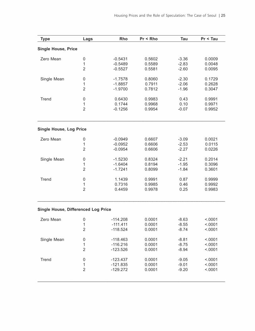
Housing Prices and the Role of Speculation: The Case of Seoul | 25
Type Lags Rho Pr < Rho Tau Pr < Tau
Single House, Price Zero Mean 0 -0.5431 0.5602 -3.36 0.0009 1 -0.5489 0.5589 -2.83 0.0048 2 -0.5527 0.5581 -2.60 0.0095
Single Mean 0 -1.7578 0.8060 -2.30 0.1729 1 -1.8857 0.7911 -2.06 0.2628 2 -1.9700 0.7812 -1.96 0.3047
Trend 0 0.6430 0.9983 0.43 0.9991 1 0.1744 0.9968 0.10 0.9971 2 -0.1256 0.9954 -0.07 0.9952
________________________________________________________________________________ Single House, Log Price
Zero Mean 0 -0.0949 0.6607 -3.09 0.0021 1 -0.0952 0.6606 -2.53 0.0115 2 -0.0954 0.6606 -2.27 0.0226
Single Mean 0 -1.5230 0.8324 -2.21 0.2014 1 -1.6404 0.8194 -1.95 0.3096 2 -1.7241 0.8099 -1.84 0.3601
Trend 0 1.1439 0.9991 0.87 0.9999 1 0.7316 0.9985 0.46 0.9992 2 0.4459 0.9978 0.25 0.9983
________________________________________________________________________________ Single House, Differenced Log Price
Zero Mean 0 -114.208 0.0001 -8.63 <.0001 1 -111.411 0.0001 -8.55 <.0001 2 -118.524 0.0001 -8.74 <.0001
Single Mean 0 -118.463 0.0001 -8.81 <.0001 1 -116.216 0.0001 -8.75 <.0001 2 -123.526 0.0001 -8.94 <.0001
Trend 0 -123.437 0.0001 -9.05 <.0001 1 -121.835 0.0001 -9.01 <.0001 2 -129.272 0.0001 -9.20 <.0001
________________________________________________________________________________

�6 | ADB Economics Working Paper Series No. 146
Type Lags Rho Pr < Rho Tau Pr < Tau
Single House, Rent
Zero Mean 0 -0.1207 0.6548 -0.39 0.5419 1 -0.1437 0.6496 -0.38 0.5454 2 -0.1532 0.6474 -0.38 0.5452
Single Mean 0 -2.6062 0.7036 -1.02 0.7446 1 -4.1714 0.5178 -1.35 0.6092 2 -4.8369 0.4483 -1.46 0.5516
Trend 0 -5.1927 0.8042 -1.82 0.6947 1 -7.1476 0.6474 -2.06 0.5681 2 -7.9698 0.5808 -2.15 0.5151
________________________________________________________________________________ Single House, Log Rent
Zero Mean 0 -0.0221 0.6772 -0.35 0.5572 1 -0.0232 0.6770 -0.30 0.5778 2 -0.0237 0.6769 -0.28 0.5838
Single Mean 0 -1.9705 0.7811 -0.85 0.8015 1 -3.3791 0.6090 -1.18 0.6822 2 -4.0602 0.5301 -1.32 0.6227
Trend 0 -4.3053 0.8663 -1.67 0.7634 1 -6.0525 0.7369 -1.90 0.6535 2 -6.8892 0.6686 -2.00 0.5980
________________________________________________________________________________ Single House, Differenced Log Rent
Zero Mean 0 -112.982 0.0001 -8.58 <.0001 1 -123.322 0.0001 -8.85 <.0001 2 -122.824 0.0001 -8.84 <.0001
Single Mean 0 -113.046 0.0001 -8.56 <.0001 1 -123.385 0.0001 -8.84 <.0001 2 -122.872 0.0001 -8.82 <.0001
Trend 0 -113.809 0.0001 -8.57 <.0001 1 -124.312 0.0001 -8.85 <.0001 2 -123.798 0.0001 -8.84 <.0001 ________________________________________________________________________________

Housing Prices and the Role of Speculation: The Case of Seoul | 27
References
Abraham, J. M., and P. H. Hendershott. 1996. “Bubbles in Metropolitan Housing Markets.” J�ur�al �f H�u���g R���arc� 7:191–207.
Bjorklund, K., and B. Soderberg. 1999. “Property Cycles, Speculative Bubbles and the Gross Income Multiplier.” J�ur�al �f R�al E�tat� R���arc� 18:151–74.
Blanchard, �. J., and M. W. Watson. 1982. Bubbles, Rational Expectations and Financial Markets. NBER Working Paper No. 945, National Bureau of Economic Research, Cambridge, MA.
Bourassa, S. C., P. H. Hendershott, and J. Murphy. 2001. “Further Evidence on the Existence of Housing Market Bubbles.” J�ur�al �f Pr�p�rty R���arc� 18:1–19.
Brooks, C., A. Katsaris, T. McGough, and S. Tsolacos. 2001. “Testing for Bubbles in Indirect Property Price Cycles.” J�ur�al �f Pr�p�rty R���arc� 18:341–56.
Caginalp, G., D. Porter, and V. Smith. 2000. “�verreactions, Momentum, Liquidity, and Price Bubbles in Laboratory and Field Asset Markets.” T�� J�ur�al �f P�yc��l�gy a�d F��a�c�al Mark�t� 1:24–48.
Campbell, J. �. 1990. “Measuring the Persistence of Expected Returns.” Am�r�ca� Ec���m�c R�v��w Pr�c��d��g� 80:43–47.
Campbell, J. �., and R. J. Shiller. 1987. “Cointegration and Tests of Present Value Models.” T�� J�ur�al �f P�l�t�cal Ec���my 95(5):1062–88.
———. 1988a. “Stock Prices, Earnings, and Expected Dividend.” In Papers and Proceedings of the 47th Annual Meeting of the American Finance Association, Chicago, Illinois. T�� J�ur�al �f F��a�c� 43(3):661–76.
_____. 1988b. “The Dividend-price Ratio and Eexpectations of Future Dividends and Discount Factors.” T�� R�v��w �f F��a�c�al Stud��� 1(3):195–228.
Chung, H. S., and J. H. Kim. 2004. Housing Speculation and Housing Price Bubble in Korea. KDI School of Public Policy and Management Paper No. 04-06. Available: ssrn.com/abstract=535882.
Diba, B.T., and H. I. Grossman. 1988. “Explosive Rational Bubbles in Stock Prices��” T�� Am�r�ca� Ec���m�c R�v��w 78(3):520–30.
Evans, G. W. 1991. “Pitfalls in Testing for Explosive Bubbles in Asset Prices.” T�� Am�r�ca� Ec���m�c R�v��w 81(4):922–30.
Flavin, M., and S. Nakagawa. 2008. “A Model of Housing in the Presence of Adjustment Costs: A Structural Interpretation of Habit Persistence.” Am�r�ca� Ec���m�c R�v��w 98(1):474–95.
Greene, W. H. 1997. Ec���m�tr�c A�aly���. 3rd ed. Prentice Hall.Guirguis, H., C. Giannikos, and R. Anderson. 2005. “The US Housing Market: Asset Pricing
Forecasts Using Time Varying Coefficients.” J�ur�al �f R�al E�tat� F��a�c� a�d Ec���m�c� 30(1):33–53.
Hamilton, J. D. 1994. T�m� S�r��� A�aly���. Princeton: Princeton University Press.Harvey, A. C. 1989. F�r�ca�t��g, Structural T�m� S�r��� M�d�l� a�d t�� Kalma� F�lt�r. New �ork:
Cambridge University Press.Himmelberg, C., C. Mayer, and T. Sinai. 2005. “Assessing High House Prices: Bubbles,
Fundamentals and Misperceptions.” J�ur�al �f Ec���m�c P�r�p�ct�v�� 19(4):67–92.Hwang, M., J. Quigley, and J. Son. 2006. “The Dividend Pricing Model: New Evidence from the
Korean Housing Market.” J�ur�al �f R�al E�tat� F��a�c� a�d Ec���m�c� 32(3):205–28.Ito, T. , and T. Iwaisako. 1995. “Explaining Asset Bubbles in Japan.” BOJ M���tary a�d Ec���m�c
Stud��� 14:143–93.Kim, J-C, D-H Kim, J-J Kim, J-S �e, and H-S Lee. 2000. “Segmenting the Korean Housing Market
Using Multiple Discriminant Analysis.” C���truct��� Ma�ag�m��t a�d Ec���m�c� 18:45–54.Kim, K-H. 1993. “Housing Prices, Affordability and Government Policy in Korea.” J�ur�al �f R�al
E�tat� F��a�c� a�d Ec���m�c� 6(1):55–72.
�� | ADB Economics Working Paper Series No. 146
_____. 2004a “Housing and the Korean Economy.” J�ur�al �f H�u���g Ec���m�c� 13:321–41.Kim, K-H, and C-H. Kim. 2002. “What Drives Korean Land Use Regulations��” Paper presented at
the Presidential Address at the AsRES-AREUEA, Joint International Conference, Seoul, 4–6 July.
Kim, K-H., and H. S. Lee. 2000. “Real Estate Price Bubble and Price Forecasts in Korea.” Paper presented at the 5th AsRES Conference, August, Beijing.
Kim, K-H., and S-H. Suh 1993. “Speculation and Price Bubbles in the Korean and Japanese Real Estate Markets.” J�ur�al �f R�al E�tat� F��a�c� a�d Ec���m�c� 6:73–87.
_____. 2002. Urba� Ec���m�c�: T���ry a�d P�l�cy. 3rd ed. Hong-Moon Sa, Seoul.Kim, N-H. 2004b. A� I�tr�duct��� �f t�� 2000 & 2005 P�pulat��� a�d H�u���g C���u� �� K�r�a.
Population Census Division, Korea National Statistical Office, Daejeon.Koenker, R., and G. Bassett. 1982. “Robust Tests for Heteroscedasticity Based on Regression
Quantiles.” Ec���m�tr�ca 50:43–61.Lee, J. S. 1997. “An �rdo-Liberal Perspective on Land Problems in Korea.” Urba� Stud���
34(7):1071–84.Lei V., C. N. Noussair, and C. R. Plott. 2001. “Nonspeculative Bubbles in Experimental Asset
Markets: Lack of Common Knowledge of Rationality vs. Actual Irrationality.” Ec���m�tr�ca 69(4):831–59.
Levin, E. J., and R. E. Wright. 1997. “Speculation in the Housing Market��” Urba� Stud��� 34(9):1419–37.
Lim, H. �. 2003. Asset Price Movements and Monetary Policy in South Korea. In Monetary Policy in a Changing Environment, BIS Papers No. 19. Available: www.bis.org/publ/bppdf/bispap19.htm.
Malppe��i, S., S. M. Wachter. 2005. “The Role of Speculation in Real Estate Cycles.” J�ur�al �f R�al E�tat� L�t�ratur� 13:143–66.
Mankiw, N. G., D. Romer, and M. D. Shapiro. 1985. “An Unbiased Reexamination of Stock Market Volatility.” J�ur�al �f F��a�c� 40:677–89.
Pia��esi, M., M. Schneider, and S. Tu�el. 2007. “Housing, Consumption and Asset Pricing.” J�ur�al �f F��a�c�al Ec���m�c� 83(3):531–69.
Renaud, B. 1993. “Confronting a Distorted Housing Market: Can Korean Polices Break with the Past��” In L. Krause, and F-K. Park, eds., S�c�al I��u�� �� K�r�a: K�r�a� a�d Am�r�ca� P�r�p�ct�v��. Seoul: KDI Press.
Roche, M. J. 2001. “The Rise in House Prices in Dublin: Bubble, Fad or Just Fundamentals.” Ec���m�c� M�d�ll��g 18:281–95.
Shiller, R. J. 1990. “Market Volatility and Investor Behavior.” T�� Am�r�ca� Ec���m�c R�v��w Pr�c��d��g� 80(2):58–62.
Weeken, �. 2004. “Asset Pricing and the Housing Market.” Ba�k �f E�gla�d Quart�rly Bull�t�� Spring.
Xiao, Q. 2005. “Property Market Bubbles: Some Evidence from Seoul and Hong Kong.” Nanyang Technological University, Singapore. PhD Thesis.
_____. 2007. “What Drives Hong Kong’s Residential Property Market—A Markov Switching Present Value Model.” P�y��ca A 383:108–14.
_____. 2008. “Determination of Price and Rental: Theory and Tests Using City Office Data.” Paper presented at the 15th Annual European Real Estate Society Conference, 18–21 June, Krakow.
Xiao, Q., and �. Liu. Forthcoming. “The Residential Market of Hong Kong: Rational or Irrational��” Appl��d Ec���m�c�.
�ao, R., and H. Zhang. 2005. “�ptimal Consumption and Portfolio Choices with Risky Housing and Borrowing Constraints.” R�v��w �f F��a�c�al Stud��� 18(1):197–239.