Environmental policy and speculation on markets for emission

permits1

Paolo Colla

Università Bocconi

Marc Germain

EQUIPPE, Universités de Lille and CORE, Université catholique de Louvain

Vincent van Steenberghe

Belgian National Fund for Scienti�c Research (FNRS)

1The authors wish to thank Parkash Chander, Jacques Drèze, Alphonse Magnus, Enrico Minelli and Bert

Willems for fruitful discussions, as well as seminar participants to the 5th International Financial Research

Forum at the Institut Europlace de Finance (2007) for useful comments and suggestions. Financial support

from the Belgian Scienti�c Policy under contract CLIMNEG2 is gratefully acknowleged by Marc Germain

and Vincent van Steenberghe, from the European Community�s Human Potential Programme under contract

HPRN-CT-2002-00232 (MICFINMA) by Paolo Colla and from the Institut Europlace de Finance (EIF) by

Paolo Colla and Marc Germain.

Abstract

Tradable emission permits share many characteristics with �nancial assets. As on �nancial markets,

speculators are likely to be active in large markets for emission permits such as those developing

under the Kyoto Protocol. We �rst show that the presence of speculators in markets for emission

permits a¤ects the price of these permits when �rms are risk averse. Since speculators help �rms

hedging the risk stemming from uncertain future demand, their entry reduces permits expected

returns as well as their volatility. Besides the traditional source of emission trading, i.e. di¤erences

across �rms in their marginal cost of pollution control, we thus identify risk-hedging as a second

motive to trade permits. Our main contribution is to characterize the optimal environmental policy

by the agency setting the total amount of permits to issue when speculators are active. Whenever

the agency is su¢ ciently risk tolerant, speculators improve aggregate welfare by fostering �rms

production. On the other hand, in the presence of a moderately risk averse agency the increase in

production volatility induced by speculators negatively a¤ects social welfare.

Introduction

Tradable permits have recently gained much interest for the control of various air pollutants, such as

sulfur dioxide, nitrogen oxides, volatile organic components and especially greenhouse gases (GHGs)

(see e.g. Stavins, 2003). Markets for GHGs emission permits have emerged following the signature

of the Kyoto Protocol in 1997. The reason carbon has a value is that governments have arti�cially

created scarcity by capping the volume of emissions that industries and other sectors are allowed

to produce. The assets �GHGs reductions �are created under government-established emissions

trading systems (carbon allowances) or by individual projects that can claim �carbon credits�by

demonstrating they are reducing GHGs. Although countries emission constraints are only binding

from 2008 to 2012, the Protocol has already given rise to the largest markets for emission permits.

Besides the international market related to countries commitments under the Kyoto Protocol,

the European Union has launched in 2005 an internal market for the trade of GHGs emission

permits between private entities: the Emissions Trading Scheme (ETS). Although the ETS Phase

I (2005-2007) is to be considered as a pilot period without strong emission reduction constraints,

the ETS has quickly developed and is by now the largest market for emission permits with a total

value of nearly US$92 billion in 2008, which represent an 87% growth over 2007. For the sake of

comparison, other allowance-based initiatives (most notably, the Chicago Climate Exchange and

the New South Wales Market) accounted for roughly US$1 billion total value during the same year

(see Capoor and Ambrosi, 2009).

Activity on the carbon market is expected to considerably increase when countries that rati�ed

the Kyoto Protocol have to comply with their emission reduction obligations, i.e. during the

�rst Kyoto commitment period (2008-2012). Moreover, since climate change is a very long term

challenge, very ambitious post-2012 strategies to curb GHG emissions will need to be adopted (see

the Intergovernmental Panel on Climate Change, 2007). A �rst step in this direction has been

recently made by the EU who has committed to signi�cant emission reductions by 2020. In its

recent so-called �climate and energy package�, the European Commission envisages to reach these

objectives with an extensive use of markets for emission permits by: 1) extending the scope of the

ETS, 2) linking the scheme to other existing or forthcoming national or regional initiatives (e.g.

the US Regional Greenhouse Gas Initiative (RGGI) in Northeastern and Mid-Atlantic states, or

the various proposals for a cap-and-trade scheme in the US or in Australia), and 3) allowing for a

1

signi�cant use of Certi�ed Emission Reductions (CERs). In such a context, the future of markets

for emission permits is promising.

Emission permits share many characteristics with �nancial assets. The permits are virtual

assets: an agent holds a permit if this permit is registered on the account of that agent by the

environmental agency. Hence, on a given market, emission permits are perfect substitutes and

their trade entails neither transportation nor inventory costs. Such characteristics are favorable to

the entry of investors whose trading activity is motivated by speculative rather than compliance

purposes. Analyses of existing emission programs reveal the presence of such agents on these

markets (see for instance Schmalensee et al., 1998, for the US Acid Rain Program, and Fusaro,

2005, for the Southern California�s RECLAIM program). The appeal of CO2 emissions markets for

investors is certi�ed by the growing number of emission indexes covering this segment: back in 2006,

Barclays Capital and UBS started tracking the most liquid emissions programmes with the BCGI

Global Carbon Index and UBS World Emissions Index, respectively; in April 2008, Merrill Lynch

and Société Générale introduced their benchmarks, the MLCX Global CO2 Emissions Index and

the SGI-Orbeo Carbon Credit Index. Most likely, the lack of correlation between tradable emissions

products and the traditional asset classes (see Daskalakis et al. 2009) lies behind the attractiveness

of carbon investing. Financial institutions and institutional investors are active on the international

GHGs markets through so-called "carbon funds", set up to �nance CO2 emission reduction projects

in developing countries and generate emission credits. Fusaro (2007) reports that over 60 carbon

funds were active during 2007, including three multi-billion funds (RNK Capital, Climate Change

Capital and Natsource). Since its inception in 2005, several large banks (Barclays, Merrill Lynch,

BNP, Fortis) have been heavily involved in market operations on the EU ETS and in 2006 potential

market speculators such as European and American "green hedge funds" have stepped in (see

Convery and Redmond, 2007). The beginning of a global carbon market brings in all the risks

of emerging markets, such as little price discovery, low liquidity and arbitrage opportunities. The

approach of speculators to green markets is to pro�t from a mismatch in pricing, and strategies

involve directional bets as well as cross-market arbitrage. For instance, there is some evidence

(Fusaro, 2007, and Parsons et al., 2009) of speculation against the high spot prices in April 2006,

even if scarcity of permits supply in this early phase of the EU ETS did not allow many players

to short allowances. Buying low-priced credits and simultaneously selling overvalued credits across

markets has also proven to be a successful arbitrage strategy: for instance, CER purchase against

2

European Allowance Unit sale allows for cashing in on the price di¤erential (see Clemens Huettner�s

commentary in July 2007 on the CER/EUA spread). Similarly, Fusaro (2005) notes the arbitrage

opportunity o¤ered under the US Renewal Portfolio Standard (RPS) mechanism by shortselling

energy credits in one state and buying in another.

Nevertheless, to our knowledge, the literature on the tradable emission permits instrument has

so far ignored these agents. Analyzing speculation on markets for emission permits would however

be particularly relevant because speculators have an impact on the equilibrium permits price and,

consequently, on �rms� investment/production choices. Speculators stand ready to accommodate

the excess demand of permits stemming from �rms, and as such they serve as market makers for

pollution allowances. In a di¤erent context, Bernardo and Welch (2004) consider the interaction

between a pool of investors facing potential liquidity shocks and a sector of risk-averse speculators

absorbing unwanted inventories. Among other things, Bernardo and Welch (2004) show that a stock

trades at a discount as a result of the ine¢ cient allocation of risk that forces market-makers to hold

positive inventories. Similarly to their work, we �nd that the permits equilibrium price includes

a premium for holding inventories �rms are willing to unload. Such a change in the price signal

in turn a¤ects �rms� investment and production decisions. Therefore, when the environmental

agency balances the environmental quality with the cost for the �rms of reducing pollution, it

should account for the impact of speculators. Investigating this last issue is precisely the aim of the

present paper.

We develop a cap-and-trade model with three types of agents: �rms, speculators and an environ-

mental agency. While considering a single commitment period, the model describes a multi-stage

decision process. At the beginning of the commitment period, the agency optimally sets the ag-

gregate amount of emission allowances and freely allocates them to polluting �rms. During the

commitment period, �rms invest, produce, pollute, and trade permits between themselves and with

(non-polluting) speculators on the allowance market which opens at two trading rounds.

All agents are risk-averse and have to take some decisions under uncertainty. This is the case

for the environmental agency when it chooses the optimal quantity of permits, for the �rms when

they invest in capital, and for both �rms and speculators when they exchange permits during the

�rst trading round. After uncertainty has been resolved, �rms produce, pollute and trade permits

during the second round, knowing that at the end of the commitment period they must surrender

an amount of permits equivalent to their emissions during the whole period.

3

The main results of our paper are as follows. The uncertainty �rms face when choosing their

level of capital makes them willing to sell (part of) their emission permits during the �rst trading

round. Once uncertainty is resolved and capital has been allocated, �rms purchase back the permits

at the second round. Speculators hold positive inventories of permits between the two dates and

earn positive expected returns as compensation for their risk bearing activity. While the environ-

mental literature has identi�ed di¤erent marginal costs of pollution control as the main source of

producers�emission trading, we isolate risk-hedging as a second motive to trade permits �similarly

to previous �ndings by Kawai (1983) for non-storable commodities. Regarding the environmental

agency problem, our analysis reveals that social welfare depends on the risk-bearing capacity of

the market (which in turn depends on the risk attitude of the market participants�, i.e. �rms and

speculators) as well as on the regulator�s attitude towards risk. Whenever the agency is su¢ ciently

risk tolerant, speculators improve aggregate welfare by fostering �rms production. On the other

hand, in the presence of a moderately risk averse agency the increase in revenue volatility induced

by speculators negatively a¤ects social welfare.

Our paper is closely related to previous contributions by Kawai (1983) and, more recently,

Baldursson and von der Fehr (2004). Kawai (1983) investigates the e¤ects of a futures market

on the price process of the underlying non-storable commodity. His setup involves futures trading

between risk-averse agents (commodity producers and "pure" speculators) in the presence of a

stochastic consumption demand. The futures market is shown to transfer risk from producers (who

supply the commodity under price uncertainty) to speculators, and the price for the insurance

o¤ered by speculators generates a positive risk premium. The main di¤erence between Kawai�s

contribution and our paper is that we are concerned with the control of producers�emissions, while

he ignores the environment. As a consequence of our focus, we depart from Kawai in at least three

aspects. Firstly, we consider storable pollution allowances instead of a non-storable commodity.

Secondly, �rms in our model employ a two input production function in lieu of a single input one.

This extension is important in our setting as a multiple input function allows to consider both output

and substitution e¤ects. Lastly �and more importantly�welfare depends not only on production (or

consumption) but also on environmental damages. Thus the environmental agency must balance

the social bene�ts of human activities with the social costs due to pollution when determining the

optimal amount of permits.

Our approach is similar to the one set forth by Baldursson and von der Fehr (2004) in that

4

we consider risk averse polluting �rms deciding on the amount of capital (or abatement) under

uncertainty. However our paper di¤ers from theirs both in its motivation and modelling framework.

Baldursson and von der Fehr (2004) analyze the performance of the tradable permits instrument

with respect to the tax instrument. Among other things, they show that accounting for risk aversion

tends to increase the relative performance of taxes. They use a rather general formalization with

respect to the objectives of the �rms, and consider uncertainty both at the aggregate (so called

"extraneous" risk) and �rm-speci�c level. On the other hand, they do not consider the interplay

between producers and non-polluting agents, i.e. speculators, and do not modelise the behavior

of the environmental agency. Our aim is to analyse the impact of speculation on permits markets

and, ultimately, on environmental policy. We make the additional assumption of constant absolute

risk aversion in order to get closed form solutions and enrich the framework in three directions: we

account for repeated permits trading rounds, we introduce risk averse speculators and we compute

the optimal amount of emission permits issued by the environmental agency.

The paper is organized as follows. In Section I we describe �rms and speculators features,

outline the sequence of decisions, and analyse the permits market equilibrium. Section II is devoted

to the policy pursued by the environmental agency when setting the optimal amount of allowances

to be issued. The impact of speculation and its interplay with optimal environmental policy is

investigated in Section III, where we consider how speculators a¤ect aggregate welfare as well as

permits expected returns and volatility. The robustness of our analysis to changes in the modelling

framework is further discussed in Section IV, together with the policy implications. Finally, Section

V summarizes our results and presents possible extensions to the current analysis.

I. The market for emission permits

A. Preliminaries: the agents

We consider three types of agents: �rms, speculators and an environmental agency. The agency is

in charge of de�ning a total amount of emission permits and of (freely) allocating them to �rms. We

assume for the time being that the agency has already de�ned the total amount of permits denoted

by S0. The behavior of the agency, leading to the de�nition of the optimal amount of permits by

taking into account the damage costs due to emissions of pollutants, is analyzed in Section II.

5

We �rst describe �rms and speculators, assuming that there is a continuum of each of them,

with nF (resp. nS) being the measure of �rms (resp. speculators).

Firms. Each �rm, indexed by i, produces an homogeneous good via the same Cobb-Douglas

constant returns to scale production function k�i e1��i , where ki and ei denote respectively the level

of capital and emissions used by �rm i. Let � be the competitive price of the good to be sold so

that �rm i value of output writes as

yi = �k�i e1��i with 0 < � < 1:

The price � is random and encapsulates a price shock stemming from demand uncertainty and

a¤ecting all �rms in the same way. Further, we assume that � is normally distributed with mean

� > 0 and variance �2.

When a �rm emits pollutants, it must hold an amount of permits which is not lower than the

level of emissions. Each �rm freely receives from the environmental agency an amount of emission

permits si0 and may sell some of its permits to �or purchase some additional ones from� other

agents active in the permits market. For simplicity, we assume the permits market opens at the

beginning and at the end of the commitment period. These two trading rounds are indexed by t

(t = 1; 2) and the unit price of permits on the market is then denoted by pt.

Firm i pro�t reads as

�Fi = �F (ki; si1; ei; �) = �k�i e1��i � ci (ki)� p1 (si1 � si0)� p2 (si2 � si1) ; (1)

where ci (ki) is the cost of capital of �rm i and sit (t = 1; 2) is the amount of permits held by �rm

i at the end of trading round t, i.e. �rm i inventory of permits at stage t. Therefore each �rm

purchases (resp. sells) allowances at the trading round t if sit � sit�1 > 0 (resp. sit � sit�1 < 0).

We assume that the cost of capital satis�es ci (ki) > 0; c0i (ki) > 0 and c00i (ki) � 0.

From eq. (1) each �rm total pro�t is composed of the revenues from the sales of the product,

yi, the cost of capital and the cost (resp. bene�ts) of the net permits purchases (resp. sales). As

long as permits prices are strictly positive, the requirement that each �rm must hold an amount

of permits greater or equal to its emissions level (si2 � ei) will hold with equality, and we set

si2 = ei in eq. (1). Equation (1) shows that a �rm can reduce its emissions in two ways: either by

substituting capital to emissions, or by decreasing its output. Investing in capital usually takes more

time than adjusting output. To account for that, we assume that ki is chosen under uncertainty

6

at the beginning of the commitment period, and that production yi and emissions ei result from

�short term decisions�taken once uncertainty is resolved.

Firms are risk-averse as captured by a constant absolute risk-aversion (CARA) function de�ned

over their pro�ts, and we let �Fi > 0 denote �rm i absolute risk-tolerance coe¢ cient (i.e. the inverse

of the absolute risk-aversion parameter). The �rms�aggregate risk-tolerance is then given by

�F �Z nF

0�Fidi: (2)

Speculators. Besides �rms, speculators are active on the market for emission permits. Unlike

�rms, speculators do not produce or pollute and their pro�ts result from their trading activity

only. Speculators have no initial endowments of permits, i.e. all permits issued by the agency

are allocated to �rms. Therefore speculator j pro�ts from the price di¤erence between the two

trading rounds, by purchasing (or short-selling) permits in the �rst trading round and unwinding

his position during the second trading round. Hence his pro�t function is given by

�Sj = �S (xj1; xj2; �) = �p2xj2 � p1xj1; (3)

where xjt is the purchase (xjt > 0) or sale (xjt < 0) of permits in trading round t, subject to

xj1 + xj2 � 0, i.e. speculators should hold non-negative inventories at the last stage. As long as

permits prices are strictly positive, speculators will set xj2 = �xj1.

We assume speculators are also risk-averse with CARA utility function de�ned over �nal pro�ts

�Sj and denote by �Sj > 0 the risk-tolerance coe¢ cient of speculator j. Finally we let �S denote

the speculators�aggregate risk-tolerance, i.e.

�S �Z nS

0�Sjdj: (4)

Timing. The sequence of decisions is based on three stages as follows. At stage 0, the agency

issues and allocates to �rms the total amount of permits S0 =R nF0 si0di. At stage 1 all agents

face uncertainty on the price shock �. Firms simultaneously choose the amount of capital, ki, and

the emission permits inventory level, si1. At the same time, speculators may also trade permits,

xj1. Then, the value of � is revealed to all agents. At stage 2, �rms decide on their output, or

equivalently on their amount of emissions, ei, and accordingly trade permits, ei � si1. Speculators

unwind their time 1 position submitting �xj1. This sequence of decisions is illustrated in Figure 1.

Rather than a sequence of two spot markets, our model can be equivalently thought of as one

where futures contracts are traded at date 1 for delivery at date 2. According to this alternative

7

interpretation, p1 and p2 correspond respectively to the futures and the spot price. At stage 1,

speculator j decides his long position in the futures contract, say fj , and his pro�t is given by

(p2 � p1) fj . This is equivalent to the speculator�s objective function in our two spot markets

model, just replacing fj with xj1 (see eq. (3) and recall that xj2 = �xj1). At date 1, �rm i

simultaneously chooses the level of capital ki and the long futures position fi, while at stage 2 it

sets emissions to the level ei and trades permits in the spot market, ei � si0. Thus �rm i pro�t

becomes �k�i e1��i � ci (ki) + (p2 � p1) fi � p2 (ei � si0). Again, this boils down to the objective

function in our model replacing fi with the net trade si1 � si0. Thus a situation with futures

contracts is isomorphic to the setup with two spot trading rounds we have described so far.

B. Second trading round

We solve the model by backward induction. At time t = 2 there is no uncertainty on �. Each �rm

maximizes pro�ts with respect to the emissions level, given its �rst stage choice for ki and si1:

maxei�F (ki; si1; ei; �) ;

with �F (�) as in eq. (1). The �rst order condition gives the following demand schedule for permits

chosen by the �rm1

ei (p2) =

�(1� �) �p2

� 1�

ki: (5)

Firm i net demand for permits is then ei� si1. At time 2; speculators unwind their date 1 position

in the permits, ending up with null inventories at the second trading round, i.e. xj2 = �xj1; where

xj1 is chosen in stage 1.

Accordingly, the permits market clearing condition at stage 2 reads as follows:Z nF

0(ei(p2)� si1)di+

Z nS

0�xj1dj = 0; (6)

or equivalentlyR nF0 ei(p2)di =

R nF0 si1di+

R nS0 xj1dj; i.e. �rms�emissions are equal to the stock of

permits held by �rms and speculators after the �rst trading round. As is clear, this stock must be

equal to the amount of permits the agency distributes to �rms at time 0, such that eq. (6) reduces

toR nF0 ei(p2)di = S0. Using the latter condition, �rm i demand schedule (5) and letting K denote

the aggregate level of capital

K �Z nF

0kidi; (7)

8

yields the second stage permits price

p2 = (1� �)�K

S0

���: (8)

Note that p2 could in principle be negative, since the demand shock parameter is normally distrib-

uted. However as pointed out in Kawai (1983) and Vives (1984) one can make the probability of

negative prices (or output) arbitrarily small by choosing � and �2 such that the ratio �=� is large.2

Finally, in equilibrium �rm i emissions are given by

ei =S0Kki: (9)

C. First trading round

Firms. At time t = 1, all agents face uncertainty about the date 2 product demand. Each �rm

solves maxki;si1 E (uFi (�Fi)) subject to the permit price and emissions level prevailing at date 2,

where uFi (�) denotes �rm i utility function. For reasons of tractability, we focus on the particular

case where ci (ki) = rki with r > 0. This corresponds to a linear capital cost function identical

across �rms. Therefore �rms di¤er only in their risk-tolerance coe¢ cient (�Fi) and in their initial

endowment of allowances (si0) (in Section IV we discuss the case of heterogeneous capital cost

functions). Substituting the equilibrium values for p2 and ei (see eqs. (8,9)) into the expression for

�Fi as given in eq. (1) yields

�Fi = �F (ki; si1; �) =�K�

S�0

��S0Kki + (1� �) si1

�� rki � p1 (si1 � si0) : (10)

Since the price shock is assumed to be normally distributed with mean � and variance �2, then

pro�ts in eq. (10) are also normally distributed. As is known (see for example Lintner, 1969),

optimization of a CARA utility function de�ned over a normal random variable allows to write �rm

i maximization problem as

maxki;si1

E (uFi (�Fi)) = maxki;si1

�F (ki; si1)� (2�Fi)�1 �2F (ki; si1) ; (11)

where �F (�) and �2F (�) denote respectively the mean and the variance of �rm i pro�ts.

Optimality conditions for the problem (11) allow to write aggregate capital in eq. (7) as

K (p1) =�p1S0(1� �) r ; (12)

9

while for aggregate permit inventories

S1 �Z nF

0si1di;

we have

S1 (p1) =�F

(1� �)2(1��) �2� r�

�2� 1

p�1

h(1� �)1��

��r

���� p1��1

i� �S01� �; (13)

where �F is given in eq. (2). The demand schedule in eq. (13) shows that the amount of permits

held by �rms at stage 1 is decreasing in the amount of permits issued (S0) as well as the permit

price (p1), increasing in the expected price shock (�) and decreasing in its uncertainty (�2).

Speculators. The speculators�problem is de�ned along the same lines as for �rms. Each spec-

ulator solves maxxj1 E (uSj (�Sj)), where uSj (�) denotes speculator j�s utility function. Given the

equilibrium price p2 (see eq. (8)), pro�ts �Sj as de�ned in eq. (3) are normal with �rst two moments

�S (�) and �2S (�). Hence, the maximization problem becomes

maxxj1

E (uSj (�Sj)) = maxxj1

�S (xj1)��2�Sj

��1�2S (xj1)

and the optimal demand (or inventory) of speculator j is

xj1 (p1) =�Sj

(1� �)2(1��) �2� r�

�2� 1

p�1

h(1� �)1��

��r

���� p1��1

i: (14)

Speculator j demand schedule in eq. (14) is negatively sloped, i.e. xj1 depends negatively on p1.

Moreover the dependence on � and �2 is analogous to the one found for �rms (see eq. (13)).

Finally, we let X1 denote the aggregate speculators�demand, i.e.

X1 �Z nS

0xj1dj:

Eq. (14) then yields

X1 (p1) =�S

(1� �)2(1��) �2� r�

�2� 1

p�1

h(1� �)1��

��r

���� p1��1

i; (15)

where �S is given in eq. (4).

Market equilibrium. The �rst stage market clearing condition isZ nF

0(s1(p1)� si0)di+

Z nS

0xj1(p1)dj = 0;

10

which can be equivalently rewritten in aggregate terms as

S1 (p1) +X1 (p1) = S0:

Let � denote the risk-bearing (or risk-tolerance) capacity of the market, i.e.

� � �F + �S (16)

where �F and �S are de�ned in eqs. (2) and (4). As is clear, the market risk-bearing capacity is

an increasing function of all agents�degree of risk-tolerance, �Fi and �Sj ; as well as their measure,

nF and nS .

Using the permit demand schedules in eqs. (13) and (15) together with the market risk-bearing

capacity (see eq. (16)), the �rst stage permits price solves the implicit function

S0 =�

�2

�(1� �) r�p1

�� "��

� r�

��� p11� �

�1��#: (17)

Equation (17) does not lend itself to explicitly compute3 the equilibrium price p1: However, the

existence and uniqueness of such an equilibrium price on the positive half-line are addressed in the

following Proposition:

Proposition 1 For any �nite positive S0, there exists a unique equilibrium price p1 2 <++.

We now investigate some comparative statics of the equilibrium price p1.

Corollary 1 For any �nite positive S0, the equilibrium price p1 increases with � .

The increase in the market risk-bearing tolerance reduces the negative e¤ect that the uncertainty

about production conditions, i.e. date 2 price movements, exerts on market participants�expected

utility. Therefore at date 1 �rms are more willing to hold on to their permits and/or speculators

are more prone to buy permits. Lower supply and higher demand would move p1 up. As it

clearly emerges from inspection of eq. (12), when permits become more expensive �rms substitute

allowances with capital, so that K increases as well together with aggregate production (in value)

Y �R nF0 yidi = �K

�S1��0 . (18)

This clari�es the role played by speculators in helping �rms hedging their production risk.

11

Corollary 2 For any given � , the equilibrium price p1 decreases with S0.

According to Corollary 2 the date 1 permit price decreases when the total supply of permits

increases. This is rather intuitive and stems from the fact that demand curves for permits are

downward sloped, as previously noted (see eqs. (13) and (15)).

We now turn to investigate the relationship between permit prices. Taking expectations on both

sides of eq. (8) yields

E(p2) = (1� �)�K

S0

���; (19)

while eq. (12) can be equivalently rewritten as

p�1 =

�(1� �) r

�

���KS0

��: (20)

Then combining eqs. (19,20) leads to

E(p2)

p�1= (1� �)1��

��r

���;

which says that the expected date 2 allowance price is an increasing and concave function of p1:

Let R = (p2=p1)� 1 denote the (net) return earned on permits between the two trading rounds, so

that expected returns are given by E (R). We establish some properties of the unique equilibrium

in the permits market by means of the following:

Proposition 2 In equilibrium:

i) permits expected returns are strictly positive, i.e. E (R) > 0,

ii) speculators buy permits at the �rst trading round, i.e. X1 > 0.

Proposition 2 generalizes previous results from Kawai (1983) to the case of our two-input pro-

duction function. Positive expected returns obtain as the compensation paid by �rms to speculators

for holding risky permit inventories. Besides the main source of emission trading, i.e. di¤erences

across �rms in their marginal cost of pollution control, Proposition 2 identi�es risk-hedging due to

uncertain demand conditions in the product market as a second motive to trade permits. More

precisely, if we additionally considered fully identical �rms (i.e. w.r.to the cost function and the

risk tolerance), permits trading will take place between �rms and speculators.

12

II. Optimal environmental policy

When de�ning the amount of permits to issue and allocate to �rms (S0), the environmental agency

balances the social gains from reducing the total amount of emissions with the losses in production

due to the constraint on emissions.

The role of the regulator within a cap-and-trade system is to determine the amount of permits S0,

i.e. the level of pollution (see Convery et al., 2008, for the role played by the European Commission

in reviewing NAPs and setting the aggregate cap). We assume the agency maximizes the �green�

revenue of the industry, i.e. the �rms�aggregate production (in value) less their consumption of

capital and the damage costs due to pollution. This welfare criterion has been used within partial

equilibrium models similar to ours (see for example Barrett, 1994, Ulph, 1996, Germain et al.,

2004a, and Germain et al., 2004b). For simplicity, we consider constant marginal damage costs. To

be consistent with our formalization for the agents�preferences in the economy, we also allow for

constant absolute risk-aversion (CARA) on the part of the agency as captured by the risk-tolerance

coe¢ cient �A > 0.

Since K =R nF0 kidi (see eq. (7)) and in equilibrium S0 =

R nF0 eidi, the agency objective is

de�ned in terms of the aggregate welfare

Y � rK � �S0; (21)

where �S0 is the total damage associated with pollution level S0. Letting �A (�) and �2A (�) denote

the �rst two moments of the aggregate welfare, i.e.

�A (S0) = E (Y )� rK � �S0�2A (S0) = V (Y )

(22)

the agency problem can be written as follows:

maxS0

W (S0) = maxS0

�A (S0)� (2�A)�1 �2A (S0)

subject to eqs. (12), (17) and S0 � 0:(23)

Let S0 be a solution to the optimization problem (23) and W (S0) the corresponding welfare, i.e.

W (S0) = �A(S0) � (2�A)�1 �2A(S0). The remainder of the analysis concerns the characterization

of a non-negative solution to (23), as well as the comparative statics of the aggregate welfare with

respect to the marginal damage �. The existence and uniqueness of a solution to the problem (23)

are addressed in the following:

13

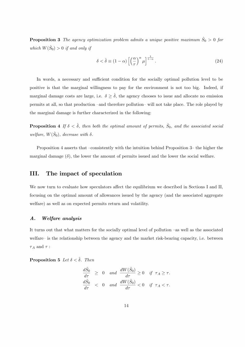
Proposition 3 The agency optimization problem admits a unique positive maximum S0 > 0 for

which W (S0) > 0 if and only if

� < � � (1� �)h��r

���i 11��

: (24)

In words, a necessary and su¢ cient condition for the socially optimal pollution level to be

positive is that the marginal willingness to pay for the environment is not too big. Indeed, if

marginal damage costs are large, i.e. � � �, the agency chooses to issue and allocate no emission

permits at all, so that production �and therefore pollution�will not take place. The role played by

the marginal damage is further characterized in the following:

Proposition 4 If � < �, then both the optimal amount of permits, S0, and the associated social

welfare, W (S0), decrease with �.

Proposition 4 asserts that �consistently with the intuition behind Proposition 3�the higher the

marginal damage (�), the lower the amount of permits issued and the lower the social welfare.

III. The impact of speculation

We now turn to evaluate how speculators a¤ect the equilibrium we described in Sections I and II,

focusing on the optimal amount of allowances issued by the agency (and the associated aggregate

welfare) as well as on expected permits return and volatility.

A. Welfare analysis

It turns out that what matters for the socially optimal level of pollution �as well as the associated

welfare�is the relationship between the agency and the market risk-bearing capacity, i.e. between

�A and � :

Proposition 5 Let � < �. Then

dS0d�

� 0 anddW (S0)

d�� 0 if �A � � :

dS0d�

< 0 anddW (S0)

d�< 0 if �A < �:

14

According to Proposition 5 pollution and social welfare exhibit a non-monotonic relationship

with the risk-bearing capacity of the market. In fact, both S0 and W (S0) increase in the market

risk-tolerance when � lies between �F and �A, reach a maximum at � = �A, and decrease4 for

� > �A. The intuition underlying such behavior goes as follows. Note from eqs. (22,23) that the

agency objective function can be equivalently rewritten as

W (S0) = �A (S0)� �S0; (25)

with

�A (S0) = [E (Y )� rK]� (2�A)�1 V (Y ) ; (26)

where both K and Y are functions of S0 (see eqs. (12) and (18)). Expression (25) clari�es that there

are two factors a¤ecting aggregate welfare. The �rst is the social utility of production, �A (S0),

which itself comprises two terms by eq. (26): the expected aggregate production (in value) net

of �rms�consumption of capital, E (Y ) � rK, and aggregate production variability as perceived

by the (risk-averse) environmental agency, (2�A)�1 V (Y ). Thus �A (S0) is the risk-adjusted social

utility of production. Firms�activity also brings social disutility (pollution) which accrues to the

second term in eq. (25), �S0. If marginal damage costs are not too large (see Proposition 3), then

the agency sets the initial amount of permits to the social optimum S0 equating marginal utility of

production to marginal disutility of pollution, i.e.

@

@S0�A(S0) = �: (27)

Consider an economy where the agency�s risk tolerance is aligned to the one of the market

(�A = �). In this case (and in this case only) one can show that the optimal amount of permits

coincides with the solution of the social planner �not to be confused with the environmental agency5�

problem, say S�0 , and welfare is maximal. Figure 2 (left panel) represents the optimality condition

(27) for �A = � .

Whenever �A 6= � the market do not react as expected by the agency. If � < �A; market

participants are too conservative from the agency standpoint: aggregate capital, production and a

fortiori the risk-adjusted social utility of production are too low. On the contrary, when � > �A

the agency is more risk-averse than the market. In such a case market participants are �too liberal�

from the agency�s point of view: both K and Y are too large and output volatility V (Y ) negatively

a¤ects the social utility of production by (26).

15

Moreover, the change in the market risk-tolerance a¤ects the marginal utility of production @�A@S0

as well. Starting from the situation �A = � ; either a decrease (�� < 0) or an increase (�� > 0)

in the market risk-tolerance implies that the market does not react any more as expected by the

agency, so that @@S0�A (S0) moves inwards as depicted in Figure 2 (right panel). The agency cannot

keep the same amount of permits because at S�0 the equality between social marginal bene�ts and

costs in eq. (27) is violated, i.e. @@S0�A(S

�0) < �. The agency reacts to the change in the market risk-

aversion by reducing the number of permits to S00 < S�0 . Note that this reduction further decreases

the risk-adjusted social utility of production as measured by the area under the solid curve @�A@S0over

the intervalhS00; S

�0

i. However this negative e¤ect on social welfare is more than compensated by

the simultaneous reduction in pollution as measured by the rectangle of width � and length S�0� S00.

Therefore the marginal social utility of production increases from @@S0�A(S

�0) < � to

@@S0�A(S

00) = �

and optimality is restored.

Speculation and policy implications. The policy implications of our analysis with respect to

speculation are therefore as follows. Suppose �rms only are allowed to trade in the permits market,

i.e. nS = 0, so that the market risk-bearing capacity coincides with �F . Provided marginal damage

costs are su¢ ciently low, the agency optimally sets the number of permits to S0 thus achieving

the aggregate welfare W (S0) (see Proposition 3). How does the agency react if the market opens

to speculators as well? As is clear from eq. (16) the entry of speculators increases the market

risk-bearing capacity, � > �F . If �A > �F , then the regulator should allow speculators on the

permit market under the condition that they do not increase the market risk-bearing capacity �

too much (that is, above �A). If �A < �F then �rms alone already make too �risky�decisions from

the agency�s perspective, and speculators�entry should be avoided.

B. Permits market analysis

Equilibrium price of permits. It is of particular interest to understand how speculators a¤ect

the equilibrium price p1. From eq. (17) it follows that

dp1d�

=@p1@�

+@p1@S0

dS0d�

(28)

Eq. (28) shows that the impact of speculation on p1 can be disentangled in two components. First,

a direct e¤ect (measured by @p1=@�) that is for a given amount of initial permits S0. Speculators�

demand for emission allowances has an impact on the equilibrium price p1. Changes in permit prices

16

a¤ect the optimal allocation of �rms�resources between capital and energy and changes in �rms�

production plans will in turn have an e¤ect on the aggregate welfare. The direct e¤ect therefore

brings in a second component measured by the second term of the RHS in eq. (28). This second

e¤ect takes into account the reaction of the agency to the entry (or exit) of speculators that modi�es

� . Such reaction translates in a variation of the optimal amount of permits (measured by dS0=d�)

which in turn induces a further change in p1 (measured by @p1=@S0). To summarize, speculation

exerts a direct e¤ect on the permits equilibrium price when speculators submit their demand, and

an indirect e¤ect through the amount of permits optimally chosen by the agency.

The overall e¤ect on p1 is non trivial. Indeed, from Corollary 1 one has that @p1=@� > 0 since

speculators help �rms hedging their production risk. Secondly, demand schedules for permits are

downward sloping and Corollary 2 yields @p1=@S0 < 0. Third, the impact of a change in � on S0 is

more articulated, as Proposition 5 reveals. Nevertheless we are able to prove the following:

Proposition 6 The equilibrium price p1 = p1(S0) increases with � .

We know from Proposition 5 that when the market risk-bearing capacity is su¢ ciently large,

i.e. � > �A, the agency reduces the amount of permits to slow down economic activity. In this case

p1 unambiguously increases due to the combined e¤ect of improved hedging motives and reduced

permit supply. However, when the agency is more risk-tolerant w.r. to the market, i.e. �A � � ,

the direct and indirect e¤ect of speculation act in opposite directions. On the one hand speculators

help �rms hedging their risk and permits trade at a higher price (see Corollary 1). On the other

hand the agency issues more permits in order to foster production thus lowering the equilibrium

permit price at date 1. The overall e¤ect on p1 is therefore a priori ambiguous once the agency�s

reaction is kept into account.

According to Proposition 6 the direct e¤ect dominates the indirect one, i.e. the price increase

due to the improved risk-hedging motives following the speculators�entry always o¤sets the price

decrease triggered by changes in the optimal amount of permits when �A � � .

Expected returns and volatility. We now focus on studying the impact of speculation on

expected returns, E (R), and their volatility, V (R) � var (R). From a policy oriented perspective,

it is of major importance to identify the impact of the underlying parameters on expected returns,

since they measure the speculators�pro�t opportunities �and thus a¤ect their incentives to enter the

17

emission permits market. The attention devoted to the impact of speculation on price �uctuations

in �nancial markets by a wide range of agents, including authorities monitoring markets�behavior

(see for example the recent UK FSA report on hedge funds and their impact on market volatility,

2005) motivates the analysis of return volatility as well.

In order to understand the impact of speculation on expected returns and volatility, note that

substituting aggregate capital (see eq. (12)) into the date 2 price (see eq. (8)) yields the following

1 +R =��r

���1� �p1

�1���; (29)

which says that the return on allowances is inversely related to the �rst trading round price. By

means of eq. (29) expected returns and volatility are

E (R) =��r

���1� �p1

�1���� 1; (30)

V (R) =��r

�2��1� �p1

�2(1��)�2 (31)

Since E (R) and V (R) are inverse functions of p1 according to eqs. (30,31), changes in the market

risk-bearing capacity that a¤ect the date 1 equilibrium price in one direction will exert the opposite

e¤ect on expected returns and volatility.

Thanks to Proposition 6 and eqs. (30,31) we can now understand the e¤ect of speculation on

expected returns and volatility:

Proposition 7 Both expected returns and volatility decrease with � .

When the market risk-bearing capacity increases, holding permit inventories becomes less risky

and the compensation for holding them, i.e. E (R), necessarily decreases. Moreover, as the market

risk-aversion lowers, we have from Proposition 6 that p1 increases. Therefore, the combined e¤ect

of higher date 1 prices and lower expected returns is a decrease in permits volatility V (R).

IV. Discussion

A. Results robustness

The sharp policy implications delivered by our model mainly hinge upon the comparative statics

we perform on several variables of interest. We turn to describe how our predictions are robust to

18

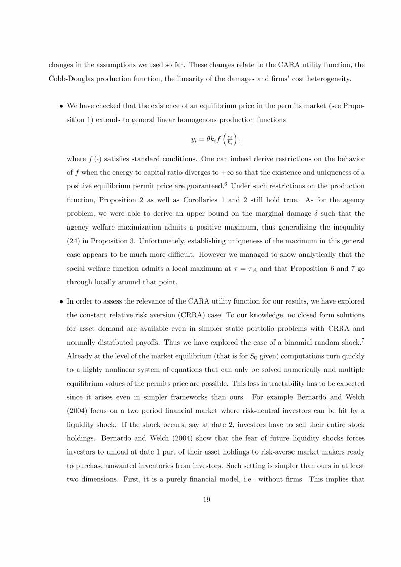
changes in the assumptions we used so far. These changes relate to the CARA utility function, the

Cobb-Douglas production function, the linearity of the damages and �rms�cost heterogeneity.

� We have checked that the existence of an equilibrium price in the permits market (see Propo-

sition 1) extends to general linear homogenous production functions

yi = �kif�eiki

�;

where f (�) satis�es standard conditions. One can indeed derive restrictions on the behavior

of f when the energy to capital ratio diverges to +1 so that the existence and uniqueness of a

positive equilibrium permit price are guaranteed.6 Under such restrictions on the production

function, Proposition 2 as well as Corollaries 1 and 2 still hold true. As for the agency

problem, we were able to derive an upper bound on the marginal damage � such that the

agency welfare maximization admits a positive maximum, thus generalizing the inequality

(24) in Proposition 3. Unfortunately, establishing uniqueness of the maximum in this general

case appears to be much more di¢ cult. However we managed to show analytically that the

social welfare function admits a local maximum at � = �A and that Proposition 6 and 7 go

through locally around that point.

� In order to assess the relevance of the CARA utility function for our results, we have explored

the constant relative risk aversion (CRRA) case. To our knowledge, no closed form solutions

for asset demand are available even in simpler static portfolio problems with CRRA and

normally distributed payo¤s. Thus we have explored the case of a binomial random shock.7

Already at the level of the market equilibrium (that is for S0 given) computations turn quickly

to a highly nonlinear system of equations that can only be solved numerically and multiple

equilibrium values of the permits price are possible. This loss in tractability has to be expected

since it arises even in simpler frameworks than ours. For example Bernardo and Welch

(2004) focus on a two period �nancial market where risk-neutral investors can be hit by a

liquidity shock. If the shock occurs, say at date 2, investors have to sell their entire stock

holdings. Bernardo and Welch (2004) show that the fear of future liquidity shocks forces

investors to unload at date 1 part of their asset holdings to risk-averse market makers ready

to purchase unwanted inventories from investors. Such setting is simpler than ours in at least

two dimensions. First, it is a purely �nancial model, i.e. without �rms. This implies that

19

agents�pro�ts (both investors�and market makers�) are linear in the choice variable, i.e. the

amount of the asset sold/purchased. In our case this holds true for speculators only (see eq.

(3)) while �rms�pro�ts are non-linear in both capital and emissions. Second, at least some

market participants �namely investors�are risk-neutral in Bernardo and Welch (2004), while

we consider risk-averse �rms (as well as speculators) which brings in additional complexity.

Bernardo and Welch (2004) get closed form solutions when market makers are CARA and the

asset payo¤ is normal while they have to resort to numerical solutions when market makers

are CRRA and the asset payo¤ is binomial. It is not surprising though, that we are unable

to go very far in the CRRA-binomial case as well. However, under CRRA it is easy to see

that the initial endowments of permits of the �rms will play a role in the determination of

the price of permits (as in Baldursson and von der Fehr, 2004, and contrary to our reference

case).

� Insofar we have assumed that damages are linearly related to pollution. To test whether this

restrictive assumption is crucial for our results, we have explored the case where damages are

expressed as D (S0) = �2S

20 and social welfare (21) becomes

Y � rK � �2S20 :

Under quadratic damages, it can be shown that the agency welfare function is continuous,

bounded from above and positive on some interval for S0 > 0. Therefore, the agency op-

timization problem admits a maximum like it happens in the linear damages case we have

hereby dealt with. However what is new with respect to the case where D (S0) = �S0 is that

the existence of a maximum obtains without imposing any condition on the parameter � like

the inequality (24).8 When dealing with comparative statics w.r.to � ; computations become

cumbersome. Thus we explored the problem numerically and observed that, for di¤erent pa-

rameter con�gurations, Propositions 5, 6 and 7 continue to hold. In particular W (bS0) reachesits maximum at � = �A just like in the linear damage case.

� Throughout our analysis �rms di¤er only in their risk-aversion (�Fi) and in their initial stock

of permits (si0). We have extended our model to another source of heterogeneity, allowing

�rms to have di¤erent capital cost functions. Speci�cally, we have focused on the case where

two types of �rms coexist : high capital cost (c(ki) = rki) and low capital cost (c(ki) = rki;

20

with r < r) �rms. Firstly, we can show that low cost �rms will sell all their permits in

the �rst round. Then, we have checked that a unique equilibrium in the permits market

can be obtained, and that Proposition 2 as well as Corollaries 1 and 2 are still veri�ed.

Unfortunately, the generalization of our results does not follow easily at the agency level.

This is due to complications arising when aggregating heterogenous �rms. Thus we explored

the problem numerically and, for several parameter con�gurations, social welfare exhibits the

same behavior as in Proposition 5, and Propositions 6 and 7 continue to hold.9

In summary, departures from our framework allowing for a general homogeneous production

function, a quadratic damage function or heterogenous capital cost functions are likely not to

impair our analysis. Indeed, all our results at the permits market level (in particular Proposition

2) generalize to these alternative settings. Moreover, even if we cannot replicate analytically all our

results at the agency level, our exploratory analyses strongly suggest that they are very likely to

be robust to the departures hereby considered. In particular, social welfare shows the same pattern

as in Proposition 5. However, since computations become immediately too cumbersome, we were

not able to investigate further if our results are robust when dropping the CARA in favour of the

CRRA utility function.

B. Policy implications

Three important issues deserve additional comments. The �rst two relate to our main results,

namely the comparative statics for permits prices, expected returns and volatility (Propositions 6

and 7) and social welfare (Proposition 5). The third issue concerns short-selling constraints and

the introduction of derivatives.

1. A careful look at existing markets such as the US market for SO2 permits or the European

market for CO2 permits reveals that permits prices may signi�cantly �uctuate through time.

Of course, numerous elements explain these �uctuations, such as changes in oil or electricity

prices, weather, political decisions, etc.10 Our �ndings suggest that, besides these exogenous

shocks, risk aversion and risk hedging behavior may explain part of the price movements

observed on markets for emission permits.11 Indeed, we have shown that (expected) permit

prices tend to rise through time (see Proposition 2). This result departs from the existing

21

contributions on transaction costs (see e.g. Stavins, 1995) or intermediation (see e.g. Germain

et al., 2004a) in markets for emission permits, which emphasizes the possible existence of a

spread (i.e., a di¤erence between the price at which permits are sold and the price at which

permits are purchased). Here, we observe an intertemporal spread, i.e., a situation in which

expected permit prices change through time. Moreover, we have also shown that the volatility

of the prices is in�uenced by the presence of speculators and, more generally, by the market

risk-tolerance. An increase in the risk-bearing capacity tends to stabilize prices, and vice-

versa.

2. Classical analyses of the tradable emission permits instrument do not account for the partici-

pation of speculators on the market. The main policy implications of our analysis depend on

the degree of risk aversion of the agency w.r. to the one of �rms and speculators. Since the

entry of speculators in the permits market increases the overall risk-bearing capacity, then

by Proposition 5 institutional rules should favor the presence of speculators on markets for

emission permits (by contrast with the situation where only polluting �rms are present on the

market). However, allowing speculators to operate on the emission permits market should be

granted only to a certain extent, i.e. only as long as the agency�s risk tolerance remains greater

than the market risk-bearing capacity. As previously noted, it is quite di¢ cult to measure

corporate risk attitudes from an empirical standpoint and therefore to assess whether the risk

tolerance of �rms is larger or smaller than the agency�s. One could argue that regulators

active on several markets have more possibilities than �rms to diversify production risk in

a single market, thus leading to larger risk tolerance for the environmental agency than for

�rms. In this case opening the permits market to speculators is welfare improving as long

as their entry doesn�t raise the overall market risk tolerance too much. In the limiting case

where the agency is risk-neutral, speculators always foster economic activity and welfare since

the agency is concerned with the level of production and not its volatility.

3. Another policy-oriented issue is the extent to which short-selling of emission permits is likely

to take place. As shown in Proposition 2, �rms �nd it optimal to unload some or the whole

stock of permits to speculators during the �rst trading round. Once uncertainty is resolved,

i.e. during the second trading round, �rms buy back permits and use them in the production

process. The (expected) price di¤erential compensates speculators for bearing the risk of

22

holding permits during the �rst stage. In some situations, typically when their degree of risk-

tolerance is high, speculators might be willing to hold more than the total amount of permits

available in the economy. One may therefore wonder if the total amount of permits purchased

by speculators should be constrained by the total amount of permits allocated by the agency.

However, such constraint is not likely to be relevant �as it happens for the vast majority of

existing �nancial markets. Firstly, the (�nancial) regulator can authorize intermediaries such

as brokers and dealers to lend securities. This way agents can de facto hold (temporarily)

a negative amount of emission permits in their account, i.e. short sell. Daskalakis and

Markellos (2007) mention restrictions on short-selling in the EU ETS. However, there is general

agreement that such restrictions will be levied in the near future as the market matures and

private trading grows (see Shapiro, 2007, among others). Secondly, the introduction of futures

contracts (with cash delivery) may play the same role in ruling out short-selling constraints.

The introduction of futures trading in our model is straightforward (see Subsection I-A. on

this point). When futures contracts allow for cash delivery (as opposed to physical delivery,

i.e., in terms of emission permits), speculators may purchase more permits than the amount

available in the economy.

V. Conclusion

We have analyzed how speculation in the permits market a¤ects the environmental policy. Within

this framework, our main results are the following. First, permits price are expected to increase

through time, so that there is some room for risk hedging by �rms. Second, an increase in the

risk-bearing capacity of the market (due for instance to an increase in the measure of speculators)

rises expected social welfare and pollution up to a certain point depending on the agency�s risk

tolerance. Whenever the agency is su¢ ciently risk tolerant, speculators improve aggregate welfare

by fostering �rms production. On the other hand, in the presence of a moderately risk averse agency

the increase in revenue volatility induced by speculators negatively a¤ects social welfare.

The setup we have developed relies on several speci�c assumptions that allow to obtain clear

cut predictions. Some of these assumptions (among others, Cobb-Douglas production function,

linear damages) do not appear to be crucial for most of our results. In particular our main �nding,

i.e. the fact that increasing the market risk bearing capacity rises expected social welfare up to a

23

certain point and decreases it afterwards, seems robust to such departures. However, extending our

analysis to alternative utility functions such as CRRA is a much more di¢ cult task that certainly

deserves further investigation.

Our model lends itself to other extensions, in particular on the role of speculation as well as

market design. We have focused on the social welfare implications of speculation, but the deter-

mination of an endogenous measure of speculators in the market would be of interest. Moreover,

one may introduce feedback (noise) traders à la De Long et al. (1990). These authors focus on

speculators who make their trading decision by simply extrapolating past prices. They show that

the presence of such traders may cause the emergence of a bubble. Whether feedback trading �or

other behavioral explanations� can be responsible for the long price swings observed in the EU

ETS during 2003-2005 is an open issue (on this point, see Sijm et al., 2005). A third extension

would be allowing speculators to invest in assets other than emission permits. This way one can

address the e¤ect of portfolio diversi�cation on our results. Portfolio choices would be driven by

the comovement of permits with other available assets so that to speculators the risk of permits

would be measured by a beta-like coe¢ cient rather than the price shock volatility as it is in our

current setup. Finally, we have focused here on a single commitment period, thereby ruling out

any role for storage (and speculation) across di¤erent commitment periods. Now most existing

cap-and-trade systems provide some sort of intertemporal �exibility (overlapping compliance cycles

in the Southern California�s RECLAIM program for NOx and SO2 reduction, banking of allowances

in the US SO2 market as well as the EU ETS from Phase II to Phase III). In a market for green

certi�cates Amundsen et al. (2006), show that banking may reduce price volatility and increase

welfare. In this sense, considering a multi-period extension to our model may shed light on some

interesting market design issues.

24

Notes

1All the computations (including the proofs of the following propositions and corollaries) are detailed in the

appendix.2Assuming the demand shock � to be lognormally distributed is another option to deal with non-negative output

and prices. However, to our knowledge this case can�t be analytically characterized. On this point, it could be noted

that the normal distribution provides a reasonable approximation to the lognormal when the coe¢ cient of variation

�=� is su¢ ciently small (see Johnson et al., 1994).3The way permits are shared among �rms is irrelevant and it does not play any role in the model solution. This is

in sharp contrast with Baldursson and von der Fehr (2004) and follows from the fact that transfers (permits allocation)

appear only linearly in our linear-quadratic setting.4 If �A < �F , then both S0 and W (S0) are monotonically decreasing in � .5Contrary to the problem of the agency (23) where the only decision variable is S0, the problem of the social

planner is to maximize welfare with respect to both the pollution level, S0, and the aggregate capital, K.6 In the case of CES production function, such condition restricts the elasticity of substitution between the two

inputs from below.7More speci�cally, we assume � can either be � + � or � � � with equal probabilities. In order to guarantee

non-negative output � � � should hold as well.8This arises because marginal damages are now linear homogenous, i.e. D0 (S0) = �S0. For a given �, allocating a

(su¢ ciently) low amount of permits to �rms reduces marginal damages so that the no production �and therefore no

pollution�issue does not arise here.9However we observed that the maximum of W (bS0) occurs at b� 6= �A; and that the di¤erence jb� � �Aj increases

with the heterogeneity of �rms.10On this topic, see for instance Albrecht et al. (2004) for the US SO2 market, and Convery and Redmond (2007),

as well as reports by PointCarbon (see www.pointcarbon.com) for the EU CO2 market.11Some authors, including Zhao (2003), have dealt with the consequences of a change in the permits price. Here,

we give a possible explanation for such changes.

25

References

Albrecht, J., Verbeke, T. and De Clercq, M. (2004). Informational e¢ ciency of the US SO2 permit

market. University of Gent W.P. 2004/250.

Amundsen, E., Baldursson F. and Mortensen, J. (2006). Price volatility and banking in green

certi�cate markets. Environmental and Resource Economics, 35(4), 259-287.

Baldursson, F. and von der Fehr, N.-H. (2004). Price volatility and risk exposure: on market-based

environmental policy instruments. Journal of Environmental Economics and Management,

48(1), 682-704.

Barrett, S. (1994). Strategic environmental policy and international trade. Journal of Public

Economics, 54(3), 325-338.

Bernardo, A. and Welch, I. (2004). Liquidity and �nancial market runs. Quarterly Journal of

Economics, 119(1), 135-158.

Capoor, K. and Ambrosi, P. (2009). State and trends of the carbon market 2009. The World

Bank.

Convery, F. and Redmond, L. (2007). Market and price developments in the European Union

Emissions Trading Scheme. Review of Environmental Economics and Policy, 1(1), 88-111.

Convery, F., Ellerman, D. and De Perthuis, C. (2008). The European carbon market in action:

lessons from the �rst trading period (Interim Report). Mimeo, MIT-Center for Energy and

Environmental Policy Research.

Daskalakis, G. and Markellos, R. N. (2007). Are the European carbon markets e¢ cient? Mimeo,

Athens University of Economics and Business.

Daskalakis, G., Psychoyios, D. and Markellos, R. N. (2009). Modeling CO2 emission allowance

prices and derivatives: Evidence from the European trading scheme, Journal of Banking and

Finance, 33(7), 1230-1241.

De Long, J., Shleifer, A. and Summers, L. Waldmann, R. (1990). Positive feedback investment

strategies and destabilizing rational speculation. Journal of Finance, 45(2), 375-395.

26

Fusaro, P.C. (2005). Green hedge funds: the new commodity play. Commodities Now, March, 1-2.

Fusaro, P.C. (2007). Energy and environmental hedge funds. Commodities Now, September, 1-2.

Germain, M., Lovo, S. and van Steenberghe, V. (2004a). De l�importance de la microstructure des

marchés de permis de polluer. Annales d�Economie et de Statistique, 74, 177-208.

Germain, M., van Steenberghe, V. and Magnus, A. (2004b). Optimal policy with tradable and

bankable pollution permits: taking the market microstructure into account. Journal of Public

Economic Theory, 6(5), 737-757.

Huettner, C. (2007). Carbon trading: CER-EUA spreads, Opalesque Research, 25.

Intergovernmental Panel on Climate Change (2007). Climate change 2007: mitigation of climate

change�summary for policymakers. Working Group III contribution to the Intergovernmental

Panel on Climate Change Fourth Assessment Report.

Johnson, N. L., Kotz, S. and Balakrishnan, N. (1994). Continuous univariate distributions, Vol.

1. John Wiley and Sons.

Kawai, M. (1983), Spot and Futures Prices of Nonstorable Commodities Under Rational Expec-

tations. Quarterly Journal of Economics, 98(2), 235-254.

Lintner, J. (1969). The Aggregation of Investor�s Diverse Judgements and Preferences in Purely

Competitive Security Markets. Journal of Financial and Quantitative Analysis, 4(4), 347-400.

Parsons, J.E., Ellerman, A.D. and Feilhauer, S. (2009). Designing a US market for CO2: Mimeo,

MIT-Center for Energy and Environmental Policy Research.

Schmalensee, R., Joskow, P., Ellerman, A., Montero, J. and Bailey, E. (1998). An interim evalua-

tion of sulfur dioxide emissions trading. Journal of Economic Perspectives, 12(3), 53-68.

Shapiro, R. J. (2007). Addressing the risks of climate change: the environmental e¤ectiveness

and economic e¢ ciency of emissions caps and tradable permits, compared to carbon taxes.

Available at www.theamericanconsumer.org/Shapiro.pdf.

Sijm, J. P. M., Bakker, S. J. A., Chen, Y., Harmsen, H. W. and Lise, W. (2005). CO2 price

dynamics: the implications of EU emissions trading for the price of electricity, report ECN-

C-05-081, Energy research Centre of the Netherlands.

27

Stavins, R. (1995). Transaction costs and tradable permits. Journal of Environmental Economics

and Management, 29(2), 133-148.

Stavins, R. (2003). Experience with market-based environmental policy instruments. In Mäler,

K.-G., and Vincent, J. (eds) Handbook of environmental economics, Vol. 1, Environmental

degradation and institutional responses. Elsevier.

UK Financial Services Authority (2005). Hedge funds: a discussion of risk and regulatory engage-

ment. FSA Discussion Paper 05/4.

Ulph, A. (1996). Environmental policy and international trade when governments and producers

act strategically. Journal of Environmental Economics and Management, 30(3), 265-281.

Vives, X. (1984). Duopoly information equilibrium: Cournot and Bertrand. Journal of Economic

Theory, 34(1), 71-94.

Zhao, J. (2003). Irreversible abatement investment under cost uncertainties: tradable emission

permits and emissions charges. Journal of Public Economics, 87(12), 2765-2789.

28

Appendix to �Environmental policy and speculation on markets foremission permits�

Appendix A: Derivation of the model: eqs. (5) to (17)

Date 2 analysis

Firm i pro�ts are

�Fi = �F (ki; si1; ei; �) = �k�i e

1��i � ci (ki)� p1 (si1 � si0)� p2 (ei � si1) : (A1)

At date 2 each �rm solves the following problem

maxei� exp (� F�Fi)

subject to eq. (A1).(A2)

Since the objective function in (A2) is strictly increasing in �Fi, then the problem (A2) is equivalent to pro�tmaximization with the following �rst order condition

(1� �) �k�i e��i � p2 = 0;

which gives �rm i demand schedule for permits in eq. (5).Speculator j pro�ts read

�Sj = �S (xj1;xj2; �) = �p2xj2 � p1xj1: (A3)

As long as permits prices are strictly positive, speculators will set xj2 = �xj1. The market clearing conditionfor permits is given by eq. (6) in the main text, or equivalentlyZ nF

0

ei(p2)di =

Z nF

0

si1di+

Z nS

0

xj1dj: (A4)

Since the stock of permits at date 2 must be equal to the amount of permits the agency distributes to �rms attime 0, eq. (A4) reduces to Z nF

0

ei(p2)di = S0:

Substituting �rm i optimal demand for permits (eq. (5)) in the latter and rearranging gives the date 2 price ineq. (8), where K denotes aggregate capital as de�ned in eq. (7). Finally, plugging the equilibrium price p2 (eq.(8)) in �rm i demand schedule (eq. (5)) yields the equilibrium level of �rm i emissions in eq. (9).

Date 1 analysis

Firms. Firm i solvesmaxki;si1

E [uFi (�Fi)]

subject to eqs. (8) and (9),(A5)

where uFi (�) denotes �rm i utility function. In the remainder, we consider the special case ci (ki) = rki.Substituting the equilibrium values for ei and p2 (eqs. (8) and (9)) into the expression for �Fi (eq. (A1)) yields

29

eq. (10) in the main text. Therefore �Fi � N��Fi; �

2Fi

�where

�Fi = �F (ki; si1) = �

�K

S0

����S0Kki + (1� �) si1

�� rki � p1 (si1 � si0) ; (A6a)

�2Fi = �2F (ki; si1) = �

2

�K

S0

�2���S0Kki + (1� �) si1

�2: (A6b)

and the optimization problem (A5) is equivalent to maximize (11) subject to eqs. (A6a) and (A6b). The �rstorder conditions are

��

�S0K

�1��� r � ��

2

�Fi

�S0K

�1�2���S0Kki + (1� �) si1

�= 0; (A7a)

(1� �)��S0K

���� p1 �

(1� �)�2�Fi

�S0K

��2���S0Kki + (1� �) si1

�= 0: (A7b)

Taking the ratio of the �rst order conditions (A7a, A7b) gives

���S0K

�1�� � r(1� �)�

�S0K

��� � p1 = �

1� �

�S0K

�;

which can be rearranged to yield aggregate capital as in eq. (12), so that the aggregate permits to capital ratiois

S0K=(1� �) r�p1

: (A8)

Rearranging the �rst order condition (A7b) yields the demand schedule for permits as

si1 (p1) =�Fi

(1� �)2 �2

�S0K

�2� "(1� �)�

�S0K

���� p1

#� �

1� �S0Kki: (A9)

Let S1 denote the �rms�aggregate demand for permits, i.e. S1 =R nF0si1di. Substituting the aggregate permits

to capital ratio (see eq. (A8)) in eq. (A9) and integrating over �rms yields eq. (13) in the main text where �Fis de�ned by eq. (2).Speculators. Speculator j solves

maxxj1

E (uSj (�Sj))

subject to eq. (8),(A10)

where uSj (�) denotes speculator j�s utility function. Plugging the second period price (see eq. (8)) into speculatorj pro�ts (see eq. (A3)) gives

�Sj = �S (xj1; �) =

�(1� �)

�K

S0

��� � p1

�xj1;

so that �Sj � N��Sj ; �

2Sj

�with

�Sj = �S (xj1) =

�(1� �)

�K

S0

���� p1

�xj1; (A11a)

�2Sj = �2S (xj1) = (1� �)

2

�K

S0

�2��2x2j1: (A11b)

30

The optimization problem (A10) is equivalent to maximize �S ��2�Sj

��1�2S subject to eqs. (A11a, A11b), with

associated �rst order condition

(1� �)��K

S0

��� p1 �

�2 (1� �)2

�Sj

�K

S0

�2�xj1 = 0;

which can be rearranged to give speculator j demand schedule for permits as

xj1 (p1) =�Sj

(1� �)2 �2

�S0K

�2� "(1� �)�

�S0K

���� p1

#:

Plugging the permits to capital ratio (eq. (A8)) in the latter yields

xj1 (p1) =�Sj

(1� �)2 �2

�(1� �) r�p1

�2��(1� �)�

��p1

(1� �) r

��� p1

�; (A12)

which can be rearranged as in eq. (14). Finally, let X1 denote the speculators�aggregate demand, i.e. X1 =R nS0xj1dj. Integrating eq. (14) across speculators gives eq. (15) in the main text, where �S is de�ned by eq. (4).

Market equilibrium. Market clearing condition for emission permits prescribes S1 (p1) +X1 (p1) = S0. Sub-stituting �rms�inventories (eq. (13)) and speculators demand schedules (eq. (15)) in the latter gives

S0 =�F + �S

(1� �)2(1��) �2� r�

�2� 1

p�1

h(1� �)1��

��r

���� p1��1

i� �S01� �: (A13)

Finally, using the expression for the market risk-tolerance � in eq. (16), the equilibrium condition (A13) yieldseq. (17).

Appendix B: Propositions 1-2 and Corollaries 1-2

Proof of Proposition 1. Premultiplying both sides of eq. (17) by (1��)�2� p�1 and rearranging gives�

(1� �) r�

�2�p1��1 +

(1� �)�2S0�

p�1 � (1� �)1+�

� r�

��� = 0: (B1)

Let F (p1) denote the LHS of eq. (B1). Taking limits of F (p1) ; one has limp1!+1

F (p1) = +1 and limp1!0+ F (p1) =

� (1� �)1+��r�

��� < 0: Moreover, the �rst derivative of F (p1) is

@F

@p1= (1� �)

�(1� �) r

�

�2�1

p�1+ �

(1� �)�2S0�

1

p1��1

> 0; (B2)

so that F (p1) is monotonically increasing over (0;+1). Since F (p1) is continuous, it follows that there exists aunique p1 2 (0;+1) such that F (p1) = 0. �

Proof of Proposition 2. Since E (R) = (E (p2) =p1)� 1; part i is equivalent to show that p1 is bounded aboveby E (p2). Taking expectations in eq. (8) and making use of the permit-to-capital ratio (see eq. (A8)) yields

E (p2)� p1 =�

�

(1� �) r

�2�p�1

((1� �)1+�

� r�

����

�(1� �) r

�

�2�p1��1

): (B3)

31

From the equilibrium condition (B1) the term in curly brackets on the RHS in eq. (B3) equals (1��)�2S0� p�1 so

that

E (p2)� p1 =�

�p1(1� �) r

�2�(1� �)�2S0

�

and E (p2)� p1 > 0 follows (part i).For part ii note that eq. (B3) allows to rewrite the speculators�demand schedule in eq. (A12) as

xj1 (p1) =�Sj

�2 (1� �)2�(1� �) r

�

�2�[E (p2)� p1] :

Since E (p2)� p1 > 0 by part i, then xj1 > 0 and a fortiori X1 �R nS0xj1 (p1) dj > 0 (part ii).

Proof of Corollary 1. Let F (p1; �) be the LHS of eq. (B1). By the implicit function theorem, one hasdp1d� = �

@F=@�@F=@p1

. Corollary 1 obtains from @F@p1

> 0 (see eq. (B2)) and @F@� = �

(1��)S0�2�2p�1

< 0. �

Proof of Corollary 2. Let F (p1; S0) be the LHS of eq. (B1). By the implicit function theorem, one hasdp1dS0

= �@F=@S0@F=@p1

. Corollary 2 obtains from @F@p1

> 0 (see eq. (B2)) and @F@S0

= (1��)�2�p�1

> 0. �

Appendix C: Proposition 3

Aggregate welfare is normally distributed with �rst two moments �A (�) and �2A (�) given by

�A (S0) = �K�S1��0 � rK � �S0; (C1a)

�2A (S0) = �2K2�S

2(1��)0 ; (C1b)

so that the problem of the agency can be written as

maxS0

W (S0) = maxS0

�A (S0)� (2�A)�1�2A (S0)

subject to eqs. (12), (17), (C1a), (C1b) and S0 � 0:(C2)

Let S0 be a solution to the optimization problem (C2) and W (S0) the corresponding welfare, i.e. W (S0) =�A(S0)� (2�A)

�1�2A(S0). The existence and uniqueness of a solution to problem (C2) are addressed in Propo-

sition 3.

Proof of Proposition 3. The proof consists of three steps. We �rst reduce the constrained optimizationde�ned in (C2) to an equivalent problem with fewer constraints. In the second step we determine the necessaryand su¢ cient conditions under which the welfare function is strictly positive. This way, we are able to giveconditions for which the problem of the agency admits at least one positive maximum -yielding a strictly positiveoptimal value of the aggregate welfare. Finally, we show that the maximum is unique.

Step 1: alternative formulation for the maximization problem

Firstly, note that the equilibrium condition (17) allows to rewrite the non-negativity constraint for the initialamount of permits, S0 � 0, as

��� r�

��� p11� �

�1��� 0: (C3)

32

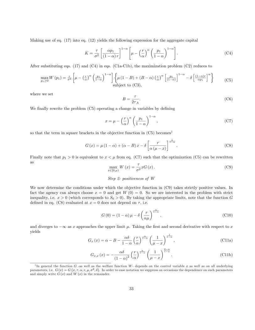
Making use of eq. (17) into eq. (12) yields the following expression for the aggregate capital

K =�

�2

��p1

(1� �) r

�1�� "��

� r�

��� p11� �

�1��#: (C4)

After substituting eqs. (17) and (C4) in eqs. (C1a-C1b), the maximization problem (C2) reduces to

maxp1�0

W (p1) =��2

���

�r�

�� � p11��

�1����� (1�B) + (B � �)

�r�

�� h p1(1��)

i1��� �

h(1��)r�p1

i��subject to (C3);

(C5)

where we setB =

�

2�A: (C6)

We �nally rewrite the problem (C5) operating a change in variables by de�ning

x = ��� r�

��� p11� �

�1��; (C7)

so that the term in square brackets in the objective function in (C5) becomes1

G (x) = � (1� �) + (��B)x� ��

r

� (�� x)

� �1��

: (C8)

Finally note that p1 > 0 is equivalent to x < � from eq. (C7) such that the optimization (C5) can be rewrittenas

maxx2[0;�)

W (x) =�

�2xG (x) : (C9)

Step 2: positiveness of W

We now determine the conditions under which the objective function in (C9) takes strictly positive values. Infact the agency can always choose x = 0 and get W (0) = 0. So we are interested in the problem with strictinequality, i.e. x > 0 (which corresponds to S0 > 0). By taking the appropriate limits, note that the function Gde�ned in eq. (C8) evaluated at x = 0 does not depend on � , i.e.

G (0) = (1� �)�� ��r

��

� �1��

; (C10)

and diverges to �1 as x approaches the upper limit �. Taking the �rst and second derivative with respect to xyields

Gx (x) = ��B ���

1� �

� r�

� �1��

�1

�� x

� 11��

; (C11a)

Gx;x (x) = ���

(1� �)2� r�

� �1��

�1

�� x

� 2��1��

: (C11b)

1 In general the function G -as well as the welfare function W - depends on the control variable x as well as on all underlyingparameters, i.e. G (x) = G

�x; � ; �; r; �; �2; �

�. In order to ease notation we suppress on occasions the dependence on such parameters

and simply write G (x) and W (x) in the remainder.

33

Note that according to the latter derivative, the function G is strictly concave over (0; �). One can easily checkfrom eq. (C10) that G (0) > 0 if and only if condition (24) holds true.On the other hand, � � � is su¢ cient for Gx (0) < 0. In such a case, given the global concavity of G, it is

then impossible that W has a positive maximum somewhere in (0; �). Thus it is necessary that � < �. Condition(24) is also su¢ cient. Indeed, � < � implies that Wx (0) =

��2G (0) > 0. As W (0) = 0, welfare W is strictly

positive on a subinterval of (0; �).

Step 3: existence and uniqueness of a global maximum

The �rst two derivatives of the welfare function W (x) are

Wx (x) =�

�2[G (x) + xGx (x)] ; (C12a)

Wx;x (x) =�

�2[2Gx (x) + xGx;x (x)]: (C12b)

From Step 2 above, we know that there exists an admissible interval over which the welfare function is strictlypositive if and only if � < �. Assuming that the latter condition is met, since W is continuous and di¤erentiableon [0; �) a candidate maximum for the welfare function is characterized by Wx (x) = 0 where x 2 (0; �) is suchthat W (x) > 0. From eq. (C12a) one has Gx (x) = �G (x) =x which is strictly negative since G (x) > 0. Itfollows that x is indeed a local maximum since Wx;x (x) < 0 by the strict concavity of the function G (�) (seeStep 2). For the same reason, there cannot be any local minima. Thus there cannot be several local maximaand x is the unique global maximum. �

Appendix D: Propositions 4-5

Lemma 1 Let x be the unique global maximum found in the proof of Proposition 3 and S0 = S0 (x) the corre-sponding optimal amount of permits. Then

dS0dx

> 0

Proof. Making use of eq. (C7) one rewrites S0 in eq. (17) in terms of x as

S0 =�

�2

� r�

� �1��

x

�1

�� x

� �1��

; (D1)

so thatdS0dx

=�

�2

� r�

� �1��

�1

�� x

� �1��

�1 +

�x

(1� �) (�� x)

�which is strictly positive for x 2 (0; �). �

Proof of Proposition 4. Given thatdS0d�

=dS0dx

dx

d�; (D2)

one makes use of eq. (D1) and gets

dS0d�

=�

�2

� r�

� �1��

�1

�� x

� �1��

�1 +

�x

(1� �) (�� x)

�dx

d�;

34

so that

sgn

dS0d�

!= sgn

�dx

d�

�:

The function to be maximised by the agency (see the objective function in (C9)), can be rewritten as

W (x; �) =�

�2xG (x; �) ; (D3)

with associated �rst order condition

Wx (x; �) =�

�2[G (x; �) + xGx (x; �)] = 0: (D4)

The implicit function theorem yieldsdx

d�= �Wx;� (x; �)

Wx;x (x; �);

where Wx;� (�) denotes the cross partial derivative of the welfare function de�ned in (D3) with respect to both xand �. Since Wx;x (x; �) < 0 by the proof of Proposition 3, it follows that sgn

�dxd�

�= sgn (Wx;� (x; �)) : In order

to determine the sign of Wx;� (x; �) we �rst di¤erentiate eq. (D4) with respect to �, i.e.

Wx;� (x; �) =�

�2[G� (x; �) + xGx;� (x; �)] : (D5)

From eqs. (C8) and (C11a) �with G and Gx functions of both x and �� we then have G� (x; �) < 0 andGx;� (x; �) < 0, so that Wx;� (x; �) < 0 by eq. (D5). Finally dS0

d� < 0 by eq. (D2) and Lemma 1.

For the e¤ect on social welfare, by the envelope theorem one has dW (x;�)d� = W� (x; �) : Making use of eq. (D3)

one gets W� (x; �) =��2 xG� (x; �) ; which is strictly negative for x 2 (0; �) because G� (x; �) < 0, thus completing

the proof. �

The following Lemma turns useful in the proof of Proposition 5:

Lemma 2 Let x be the unique global maximum found in the proof of Proposition 3. Then

dx

d�=

x�A

2 (��B)� � 2x(��B)+�(1��)�x+(1��)(��x)x+2(1��)(��x)(1��)(��x)

< 0:

Proof. The function to be maximised by the agency (see the objective function in (C9)), can be rewritten as

W (x; �) =�

�2xG (x; �) ; (D6)

where the dependence of G (�) with respect to � goes through B = �2�A

(see eq. (C6)). Then the associated �rstorder condition reads as

Wx (x; �) =�

�2[G (x; �) + xGx (x; �)] = 0: (D7)

The implicit function theorem yields dxd� = �

Wx;� (x;�)Wx;x(x;�)

: Making use of eq. (D7) one gets

Wx;� (x; �) =�

�2[G� (x; �) + xGx;� (x; �)] ;

35

and taking the partial derivative of eqs. (C8) and (C11a) with respect to � �with G and Gx functions of both xand � through B = �

2�A�gives

Wx;� (x; �) = �� x

�2�A< 0: (D8)

Thus dxd� < 0 from eq. (D8) and Wx;x (x; �) < 0 by the proof of Proposition 3:

To get a closed form for dxd� , we �rst use eqs. (C11a) and (C11b) to rewrite eq. (C12b) as

Wx;x (x; �) =�

�2

(2 (��B)� ��

1� �

� r�

� �1��

�1

�� x

� 11��

�2 +

x

(1� �) (�� x)

�): (D9)

Then, substituting eqs. (C8) and (C11a) in eq. (D7), yields

�

1� �

� r�

� �1��

�1

�� x

� 11��

=2x (��B) + � (1� �)�x+ (1� �) (�� x) : (D10)

Finally, plugging eq. (D10) into eq. (D9) gives

Wx;x (x; �) =�

�2

�2 (��B)� �2x (��B) + � (1� �)

�x+ (1� �) (�� x)

�2 +

x

(1� �) (�� x)

��;

so that Lemma 2 follows the latter and eq. (D8). �

Proof of Proposition 5. (i) Consider �rst the comparative statics for S0 with respect to the market risk-tolerance � . Making use of eq. (D1) and Lemma 2 yields

dS0d�

=x

�2

�r

� (�� x)

� �1��

8<:1 +��A

2 (��B)� � 2x(��B)+�(1��)�x+(1��)(��x)x+2(1��)(��x)(1��)(��x)

�1 +

�x

(1� �) (�� x)

�9=;Since 0 < x < � and

h2 (��B)� � 2x(��B)+�(1��)�x+(1��)(��x)

x+2(1��)(��x)(1��)(��x)

i< 0 by Lemma 2, it follows that

sgn

dS0d�

!= �sgn

�2 (��B)� �2x (��B) + � (1� �)

�x+ (1� �) (�� x)x+ 2 (1� �) (�� x)(1� �) (�� x) +

�

�A

�1 +

�x

(1� �) (�� x)

��:

Plugging eq. (C6) in the latter and rearranging leaves sgn�dS0d�

�= sgn

�1� �

�A

�, which gives the comparative

statics for S0 in Proposition 5.(ii) Consider now the comparative statics for W (S0) with respect to � . By the envelope theorem one hasdW (x;�)

d� =W� (x; �), and using the objective function as in eq. (D6) yields

W� (x; �) =x

�2[G (x; �) + �G� (x; �)] : (D11)

At the global optimum x one has Wx (x; �) = 0; or equivalently (see the �rst order condition (D7)) G (x; �) =�xGx (x; �) ; so that eq. (D11) rewrites as

W� (x; �) =x

�2[�xGx (x; �) + �G� (x; �)] ;

36

Di¤erentiating eq. (C11a) with respect to � and making use of eq. (C11a) allows to rewrite the latter as

W� (x; �) = ��x2

�2

"1� �

1� �

� r�

� �1��

�1

�� x

� 11��#:

Finally, eq. (D10) yields

W� (x; �) = ��x2

�2

�1� 2x (��B) + � (1� �)

�x+ (1� �) (�� x)

�;

and after some manipulation one gets sgn (W� (x; �)) = sgn�1� �

�A

�; thus completing the proof. �

Appendix E: Propositions 6-7

Proof of Proposition 6. Recall from the proof of Proposition 3 that x �i.e. the global maximum for theagency problem in (C9)�solves the following

G (x; �) + xGx (x; �) = 0 (E1)

where x; G (x; �) and Gx (x; �) are given in eqs. (C7), (C8) and (C11a). Totally di¤erentiating eq. (E1) yields

2Gx (x; �) dx+G� (x; �) d� + x [Gx;x (x; �) dx+Gx;� (x; �) d� ] = 0;

or equivalentlydx

d�= � G� (x; �) + xGx;� (x; �)

2Gx (x; �) + xGx;x (x; �): (E2)

Di¤erentiating eqs. (C8) and (C11a) with respect to � reveals that the numerator on the RHS reduces to � x�A; it

follows that dxd� < 0 as the denominator in eq. (E2) is clearly negative from eq. (C12b) andWx;x (x) < 0. Finally,

recall from eq. (C7) that x is decreasing in the price p1 so thatdp1dx < 0 and

dp1d� =

dp1dx

dxd� implies

dp1(S0)d� > 0.

Proof of Proposition 7. Since expected returns are inverse functions of the equilibrium price p1 according toeqs. (30)-(31) in the main text, Proposition 6 immediately yields Proposition 7.

37

Figures

Stage 0 Stage 1 Stage 2

Uncertainty isrevealed (θ )

Agency: S0 Firms: si1 , ki

Speculators: xj1

Firms: ei

Speculators: xj2

Figure 1: Sequence of decisions

0SA

∂Π∂

δ

0S*0S

0SA

∂Π∂

δ

0S*0S0'S

00 <∆>∆ ττ or

)ˆ( *0

0

SS

A

∂Π∂

Figure 2: Speculation and the optimal amount of permits

38