Semi-supervised Feature Analysis for Multimedia Annotation by Mining Label Correlation

Semi-supervised Feature Analysis

for Multimedia Annotation by Mining LabelCorrelation

Xiaojun Chang1, Haoquan Shen2, Sen Wang1, Jiajun Liu3, and Xue Li1

1 The University of Queensland, QLD 4072, Australia2 Zhejiang University, Zhejiang, China

3 CSIRO Brisbane

Abstract. In multimedia annotation, labeling a large amount of train-ing data by human is both time-consuming and tedious. Therefore, toautomate this process, a number of methods that leverage unlabeledtraining data have been proposed. Normally, a given multimedia sam-ple is associated with multiple labels, which may have inherent correla-tions in real world. Classical multimedia annotation algorithms addressthis problem by decomposing the multi-label learning into multiple in-dependent single-label problems, which ignores the correlations betweendifferent labels. In this paper, we combine label correlation mining andsemi-supervised feature selection into a single framework. We evaluateperformance of the proposed algorithm of multimedia annotation usingMIML, MIRFLICKR and NUS-WIDE datasets. Mean average precision(MAP), MicroAUC and MacroAUC are used as evaluation metrics. Ex-perimental results on the multimedia annotation task demonstrate thatour method outperforms the state-of-the-art algorithms for its capabilityof mining label correlations and exploiting both labeled and unlabeledtraining data.

Keywords: Semi-supervised Learning, Multi-label Feature Selection,Multimedia Annotation.

1 Introduction

With the booming of social networks, such as Facebook and Flickr, we havewitnessed a dramatical growth of multimedia data, i.e. image, text and video.Consequently, there are increasing demands to effectively organize and accessthese resources. Normally, feature vectors, which are used to represent afore-mentioned resources, are usually very large. However, it has been pointed outin [1] that only a subset of features carry the most discriminating information.Hence, selecting the most representative features plays an essential role in amulti-media annotation framework. Previous works [2,3,4,5] have indicated thatfeature selection is able to remove redundant and irrelevant information in thefeature representation, thus improves subsequent analysis tasks.

Existing feature selection algorithms are designed in various ways. For exam-ple, conventional feature selection algorithms, such as Fisher Score [6], compute

V.S. Tseng et al. (Eds.): PAKDD 2014, Part II, LNAI 8444, pp. 74–85, 2014.c© Springer International Publishing Switzerland 2014

Semi-supervised Feature Analysis for Multimedia Annotation 75

weights of all features, rank them accordingly and select the most discriminatingfeatures one by one. While dealing with multi-label problems, the conventionalalgorithms generally transform the problem into a couple of binary classificationproblems for each concept respectively. Hence, feature correlations and labelcorrelations are ignored [7], which will deteriorate the subsequent annotationperformance.

Another limitation is that they only use labeled training data for feature se-lection. Considering that there are a large number of unlabeled training dataavailable, it is beneficial to leverage unlabeled training data for multimedia an-notation. Over recent years, semi-supervised learning has been widely studiedas an effective tool for saving labeling cost by using both labeled and unlabeledtraining data [8,9,10]. Inspired by this motivation, feature learning algorithmsbased on semi-supervised framework, have been also proposed to overcome theinsufficiency of labeled training samples. For example, Zhao et al. propose analgorithm based on spectral analysis in [5]. However, similarly to Fisher Score[6], their method selects the most discriminating features one by one. Besides,correlations between labels are ignored.

Our semi-supervised feature selection algorithm integrates multi-label featureselection and semi-supervised learning into a single framework. Both labeled andunlabeled data are utilized to select features while label correlations and featurecorrelations are simultaneously mined.

The main contributions of this work can be summarized as follows:

1. We combine joint feature selection with sparsity and semi-supervised learn-ing into a single framework, which can select the most discriminating featureswith an insufficient amount of labeled training data.

2. The correlations between different labels are taken into account to facilitatethe feature selection.

3. Since the objective function is non-smooth and difficult to solve, we proposea fast iteration algorithm to obtain the global optima. Experimental resultson convergence validates that the proposed algorithm converges within veryfew iterations.

The rest of this paper is organized as follows. In Section 2, we introducedetails of the proposed algorithm. Experimental results are reported in Section3. Finally, we conclude this paper in Section 4.

2 Proposed Framework

To mine correlations between different labels for feature selection, our algorithmis built upon a reasonable assumption that different class labels have some in-herent common structures. In this section, our framework is described in details,followed by an iterative algorithm with guaranteed convergence to optimize theobjective function.

76 X. Chang et al.

2.1 Formulation of Proposed Framework

Let us define X = {x1, x2, · · · , xn} as the training data matrix, where xi ∈R

d(1 ≤ i ≤ n) is the i-th data point and n is the total number of training data.Y = [y1, y2, · · · , ym, ym+1, · · · , yn]T ∈ {0, 1}n×c denotes the label matrix and cis the class number. yi ∈ R

c (1 ≤ i ≤ n) is the label vector with c classes. Yij

indicates the j-th element of yi and Yij := 1 if xi is in the j-th class, and Yij := 0otherwise. If xi is not labeled, yi is set to a vector with all zeros. Inspired by [11],we assume that there is a low-dimensional subspace shared by different labels.We aim to learn c prediction functions {ft}ct=1. The prediction function ft canbe generalized as follows:

ft(x) = vTt x+ pTt QTx = wT

t x, (1)

where wt = vt+Qpt. v and p are the weights, Q is a transformation matrix whichprojects features in the original space into a shared low-dimensional subspace.

Suppose there are mt training data {xi}mt

i=1 belonging to the t-th class labeledas {yi}mt

i=1. A typical way to obtain the prediction function ft is to minimize thefollowing objective function:

arg minft,QTQ=I

c∑

t=1

(1

mt

mt∑

i=1

loss(ft(xi), yi) + βΩ(ft)) (2)

Note that to make the problem tractable we impose the constraint QTQ = I.Following the methodology in [2], we incorporate (1) into (2) and obtain theobjective function as follows:

min{vt,pt},QTQ=I

c∑

t=1

(1

mt

mt∑

i=1

loss((vt +Qpt)Txi, yi) + βΩ({vt, pt})) (3)

By defining W = V + QP , where V = [v1, v2, · · · , vc] ∈ Rd×c and P =

[p1, p2, · · · , pc] ∈ Rsd×c where sd is the dimension of shared lower dimensional

subspace, we can rewrite the objective function as follows:

minW,V,P,QTQ=I

loss(WTX,Y ) + βΩ(V, P ) (4)

Note that we can implement the shared feature subspace uncovering in differ-ent ways by adopting different loss functions and regularizations. Least squareloss is the most widely used in research for its stable performance and simplicity.By applying the least square loss function, the objective function arrives at:

arg minW,P,QT Q=I

‖XTW − Y ‖2F + α‖W‖2F + β‖W −QP‖2F (5)

As indicated in [12], however, there are two issues worthy of further consid-eration. First, the least square loss function is very sensitive to outliers. Second,it is beneficial to utilize sparse feature selection models on the regularization


term for effective feature selection. Following [12,13,14], we employ l2,1-norm tohandle the two issues. We can rewrite the objective function as follows:

arg minW,P,QTQ=I

‖XTW − Y ‖2F + α‖W‖2,1 + β‖W −QP‖2F (6)

Meanwhile, we define a graph Laplacian as follows: First, we define an affinitymatrix A ∈ R

n×n whose element Aij measures the similarity between xi and xj

as:

Aij =

{1, xi and xj are k nearest neighbours;0, otherwise.

(7)

Euclidean distance is utilized to measure whether two data points xi and xj arek nearest neighbours in the original feature space. Then, the graph Laplacian,L, is computed according to L = S − A, where S is a diagonal matrix withSii =

∑nj=1 Aij .

Note that multimedia data have been normally shown to process a manifoldstructure, we adopt manifold regularization to explore it. By applying mani-fold regularization to the aforementioned loss function, our objective functionarrives at:

arg minW,P,QTQ=I

Tr(WTXLXTW ) + γ[α‖W‖2,1+β‖W −QP‖2F + ‖XTW − F‖2F ]

(8)

We define a selecting diagonal matrix U whose diagonal element Uii = ∞, if xi

is a labeled data, and Uii = 0 otherwise. To exploit both labeled and unlabeledtraining data, a label prediction matrix F = [f1, · · · , fn]T ∈ R

n×c is introducedfor all the training data. The label prediction of xi ∈ X is fi ∈ R

c. Following [5],we assume that F holds smoothness on both the ground truth of training dataand on the manifold structure. Therefore, F can be obtained as follows:

argminF

tr(FTLF ) + tr((F − Y )TU(F − Y )). (9)

By incorporating (9) into (6), the objective function finally becomes:

arg minF,W,P,QTQ=I

tr(FTLF ) + tr(F − Y )TU(F − Y )

+γ[α‖W‖2,1 + β‖W −QP‖2F + ‖XTW − F‖2F ](10)

As indicated in [13], W is guaranteed to be sparse to perform feature selectionacross all data points by ‖W‖2,1 in our regularization term.

2.2 Optimization

The proposed function involves the l2,1-norm, which is difficult to solve in aclosed form. We propose to solve this problem in the following steps. By settingthe derivative of (10) w.r.t. P equal to zero, we have

P = QTW (11)

78 X. Chang et al.

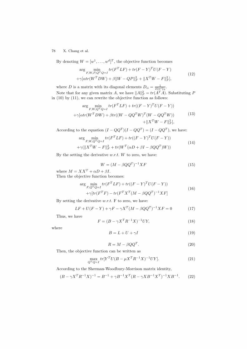
By denoting W = [w1, . . . , wd]T , the objective function becomes

arg minF,W,P,QTQ=I

tr(FTLF ) + tr(F − Y )TU(F − Y )

+γ[αtr(WTDW ) + β‖W −QP‖2F + ‖XTW − F‖2F ],(12)

where D is a matrix with its diagonal elements Dii =1

2‖wi‖2.

Note that for any given matrix A, we have ‖A‖2F = tr(ATA). Substituting Pin (10) by (11), we can rewrite the objective function as follows:

arg minF,W,QTQ=I

tr(FTLF ) + tr((F − Y )TU(F − Y ))

+γ[αtr(WTDW ) + βtr((W −QQTW )T (W −QQTW ))

+‖XTW − F‖2F ],(13)

According to the equation (I −QQT )(I −QQT ) = (I −QQT ), we have:

arg minF,W,QTQ=I


+γ(‖XTW − F‖2F + tr(WT (αD + βI − βQQT )W ))(14)

By the setting the derivative w.r.t. W to zero, we have:

W = (M − βQQT )−1XF (15)

where M = XXT + αD + βI.Then the objective function becomes:

arg minF,QTQ=I


+γ[tr(FTF )− tr(FTXT (M − βQQT )−1XF ](16)

By setting the derivative w.r.t. F to zero, we have:

LF + U(F − Y ) + γF − γXT (M − βQQT )−1XF = 0 (17)

Thus, we haveF = (B − γXTR−1X)−1UY, (18)

whereB = L+ U + γI (19)

R = M − βQQT . (20)

Then, the objective function can be written as

maxQTQ=I

tr[Y TU(B − μXTR−1X)−1UY ]. (21)

According to the Sherman-Woodbury-Morrison matrix identity,

(B − γXTR−1X)−1 = B−1 + γB−1XT (R− γXB−1XT )−1XB−1. (22)


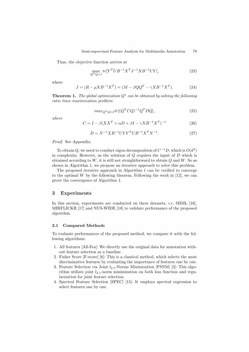
Thus, the objective function arrives at

maxQTQ=I

tr[Y TUB−1XTJ−1XB−1UY ], (23)

whereJ = (R − μXB−1XT ) = (M − βQQT − γXB−1XT ). (24)

Theorem 1. The global optimization Q∗ can be obtained by solving the followingratio trace maximization problem:

maxQTQ=I tr[(QTCQ)−1QTDQ], (25)

whereC = I − β(XXT + αD + βI − γXB−1XT )−1 (26)

D = N−1XB−1UY Y TUB−1XTN−1. (27)

Proof. See Appendix.

To obtainQ, we need to conduct eigen-decomposition of C−1D, which is O(d3)in complexity. However, as the solution of Q requires the input of D which isobtained according to W , it is still not straightforward to obtain Q and W . So asshown in Algorithm 1, we propose an iterative approach to solve this problem.

The proposed iterative approach in Algorithm 1 can be verified to convergeto the optimal W by the following theorem. Following the work in [12], we canprove the convergence of Algorithm 1.

3 Experiments

In this section, experiments are conducted on three datasets, i.e. MIML [16],MIRFLICKR [17] and NUS-WIDE [18] to validate performance of the proposedalgorithm.

3.1 Compared Methods

To evaluate performances of the proposed method, we compare it with the fol-lowing algorithms:

1. All features [All-Fea]: We directly use the original data for annotation with-out feature selection as a baseline.

2. Fisher Score [F-score] [6]: This is a classical method, which selects the mostdiscriminative features by evaluating the importance of features one by one.

3. Feature Selection via Joint l2,1-Norms Minimization [FSNM] [3]: This algo-rithm utilizes joint l2,1-norm minimization on both loss function and regu-larization for joint feature selection.

4. Spectral Feature Selection [SPEC] [15]: It employs spectral regression toselect features one by one.

80 X. Chang et al.

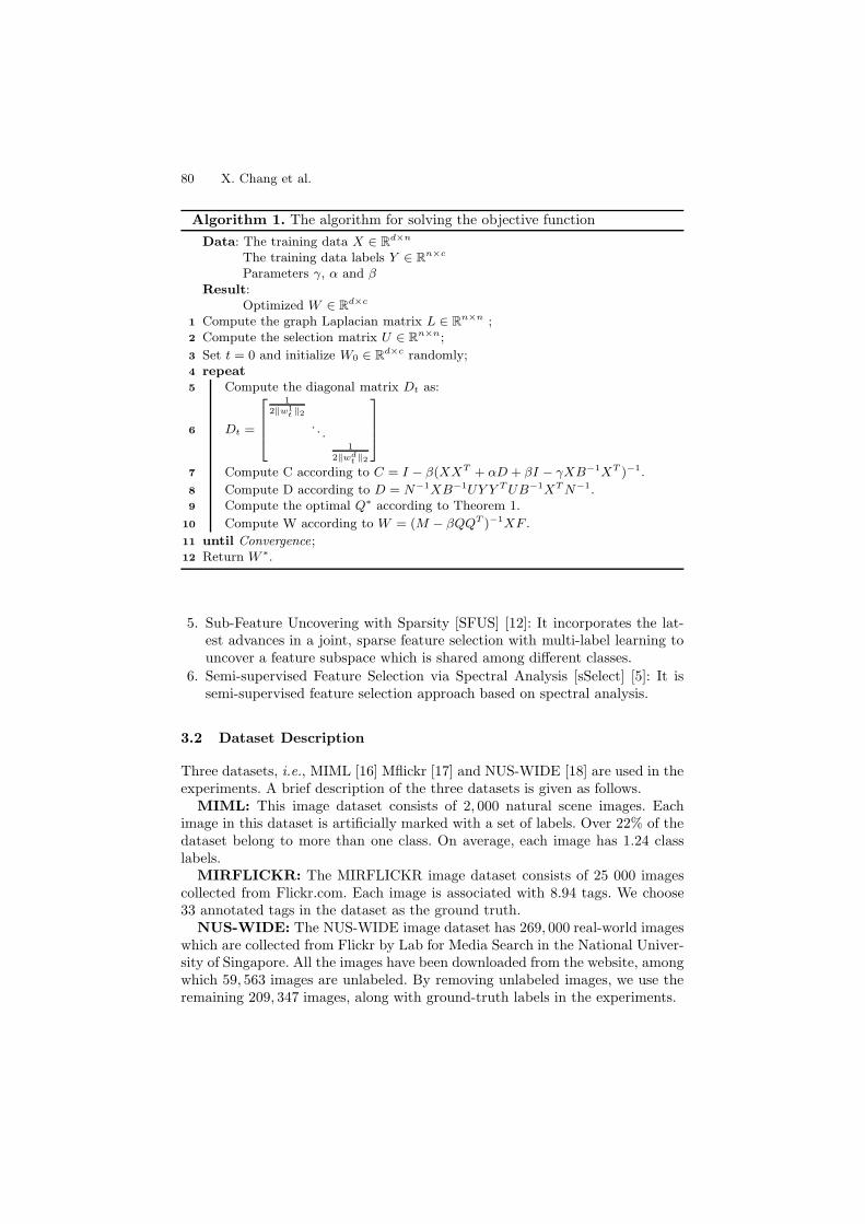
Algorithm 1. The algorithm for solving the objective function

Data: The training data X ∈ Rd×n

The training data labels Y ∈ Rn×c

Parameters γ, α and βResult:

Optimized W ∈ Rd×c

1 Compute the graph Laplacian matrix L ∈ Rn×n ;

2 Compute the selection matrix U ∈ Rn×n;

3 Set t = 0 and initialize W0 ∈ Rd×c randomly;

4 repeat5 Compute the diagonal matrix Dt as:

6 Dt =

⎡⎢⎢⎣

12‖w1

t ‖2. . .

1

2‖wdt ‖2

⎤⎥⎥⎦

7 Compute C according to C = I − β(XXT + αD + βI − γXB−1XT )−1.

8 Compute D according to D = N−1XB−1UY Y TUB−1XTN−1.9 Compute the optimal Q∗ according to Theorem 1.

10 Compute W according to W = (M − βQQT )−1XF .

11 until Convergence;12 Return W ∗.

5. Sub-Feature Uncovering with Sparsity [SFUS] [12]: It incorporates the lat-est advances in a joint, sparse feature selection with multi-label learning touncover a feature subspace which is shared among different classes.

6. Semi-supervised Feature Selection via Spectral Analysis [sSelect] [5]: It issemi-supervised feature selection approach based on spectral analysis.

3.2 Dataset Description

Three datasets, i.e., MIML [16] Mflickr [17] and NUS-WIDE [18] are used in theexperiments. A brief description of the three datasets is given as follows.

MIML: This image dataset consists of 2, 000 natural scene images. Eachimage in this dataset is artificially marked with a set of labels. Over 22% of thedataset belong to more than one class. On average, each image has 1.24 classlabels.

MIRFLICKR: The MIRFLICKR image dataset consists of 25 000 imagescollected from Flickr.com. Each image is associated with 8.94 tags. We choose33 annotated tags in the dataset as the ground truth.

NUS-WIDE: The NUS-WIDE image dataset has 269, 000 real-world imageswhich are collected from Flickr by Lab for Media Search in the National Univer-sity of Singapore. All the images have been downloaded from the website, amongwhich 59, 563 images are unlabeled. By removing unlabeled images, we use theremaining 209, 347 images, along with ground-truth labels in the experiments.


Table 1. Settings of the Training Sets

Dataset Size(n) Labeled Training Data (m) Number of Selected Features

MIML 1, 000 5× c, 10× c, 15× c {200, 240, 280, 320, 360, 400}NUS-WIDE 10, 000 5× c, 10× c, 15× c {240, 280, 320, 360, 400, 440, 480}

Mflickr 10, 000 5× c, 10× c, 15× c {200, 240, 280, 320, 360, 400}

3.3 Experimental Setup

In the experiment, we randomly generate a training set for each dataset con-sisting of n samples, among which m samples are labeled. The detailed settingsare shown in Table 1. The remaining data are used as testing data. Similar tothe pipeline in [2], we randomly split the training and testing data 5 times andreport average results. The libSVM [19] with RBF kernel is applied in the ex-periment. The optimal parameters of the SVM are determined by grid searchon a tenfold crossvalidation. Following [2], the graph Laplacian, k is set as 15.Except for the SVM parameters, the regularization parameters, γ, α and β, inthe objective funciton (10), are tuned in the range of {10−4, 10−2, 100, 102, 104}.The number of selected features can be found in Table 1.

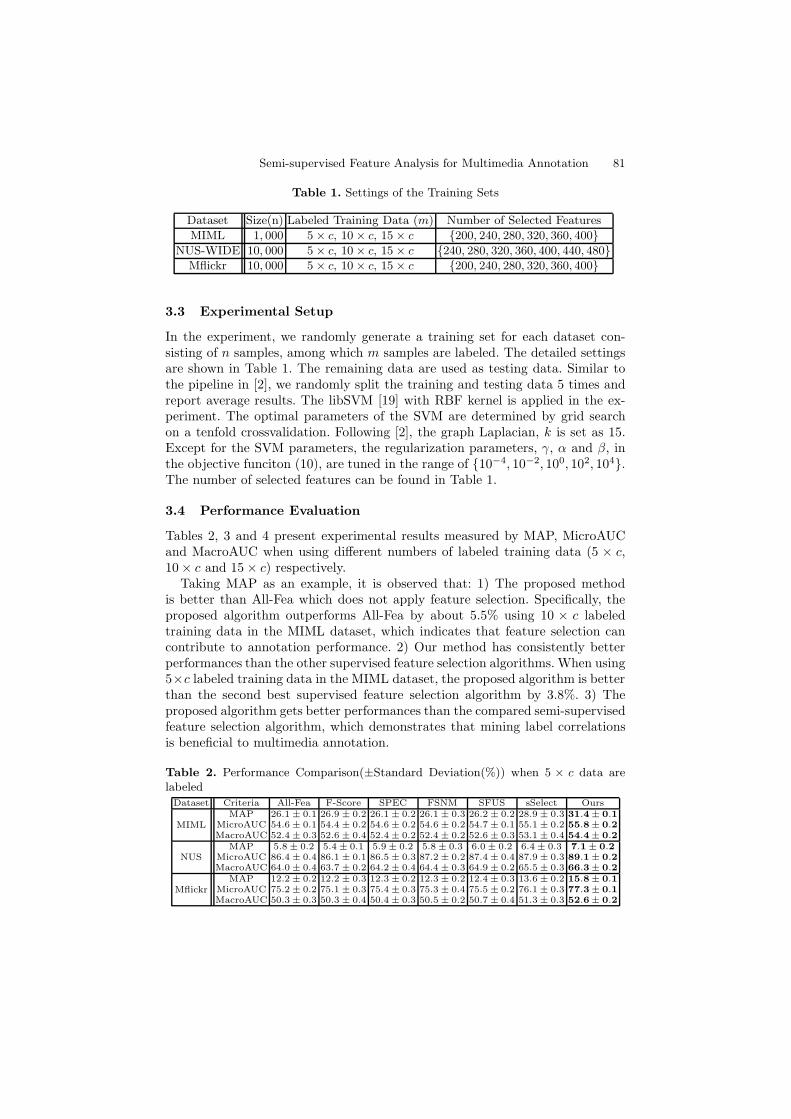
3.4 Performance Evaluation

Tables 2, 3 and 4 present experimental results measured by MAP, MicroAUCand MacroAUC when using different numbers of labeled training data (5 × c,10× c and 15× c) respectively.

Taking MAP as an example, it is observed that: 1) The proposed methodis better than All-Fea which does not apply feature selection. Specifically, theproposed algorithm outperforms All-Fea by about 5.5% using 10 × c labeledtraining data in the MIML dataset, which indicates that feature selection cancontribute to annotation performance. 2) Our method has consistently betterperformances than the other supervised feature selection algorithms. When using5×c labeled training data in the MIML dataset, the proposed algorithm is betterthan the second best supervised feature selection algorithm by 3.8%. 3) Theproposed algorithm gets better performances than the compared semi-supervisedfeature selection algorithm, which demonstrates that mining label correlationsis beneficial to multimedia annotation.

Table 2. Performance Comparison(±Standard Deviation(%)) when 5 × c data arelabeled

Dataset Criteria All-Fea F-Score SPEC FSNM SFUS sSelect Ours

MIMLMAP

MicroAUCMacroAUC

26.1 ± 0.154.6 ± 0.152.4 ± 0.3

26.9 ± 0.254.4 ± 0.252.6 ± 0.4

26.1 ± 0.254.6 ± 0.252.4 ± 0.2

26.1 ± 0.354.6 ± 0.252.4 ± 0.2

26.2 ± 0.254.7 ± 0.152.6 ± 0.3

28.9 ± 0.355.1 ± 0.253.1 ± 0.4

31.4± 0.155.8± 0.254.4± 0.2

NUSMAP

MicroAUCMacroAUC

5.8 ± 0.286.4 ± 0.464.0 ± 0.4

5.4 ± 0.186.1 ± 0.163.7 ± 0.2

5.9 ± 0.286.5 ± 0.364.2 ± 0.4

5.8 ± 0.387.2 ± 0.264.4 ± 0.3

6.0 ± 0.287.4 ± 0.464.9 ± 0.2

6.4 ± 0.387.9 ± 0.365.5 ± 0.3

7.1± 0.289.1± 0.266.3± 0.2

MflickrMAP

MicroAUCMacroAUC

12.2 ± 0.275.2 ± 0.250.3 ± 0.3

12.2 ± 0.375.1 ± 0.350.3 ± 0.4

12.3 ± 0.275.4 ± 0.350.4 ± 0.3

12.3 ± 0.275.3 ± 0.450.5 ± 0.2

12.4 ± 0.375.5 ± 0.250.7 ± 0.4

13.6 ± 0.276.1 ± 0.351.3 ± 0.3

15.8± 0.177.3± 0.152.6± 0.2

82 X. Chang et al.



MIMLMAP

MicroAUCMacroAUC

31.6 ± 0.359.3 ± 0.462.0 ± 0.3

33.0 ± 0.258.9 ± 0.361.0 ± 0.2

31.6 ± 0.259.3 ± 0.262.0 ± 0.2

31.6 ± 0.359.4 ± 0.362.0 ± 0.1

33.0 ± 0.159.8 ± 0.262.0 ± 0.2

35.2 ± 0.260.4 ± 0.262.6 ± 0.2

37.1± 0.161.7± 0.263.7± 0.2

NUSMAP

MicroAUCMacroAUC

6.6 ± 0.287.3 ± 0.367.5 ± 0.4

6.0 ± 0.187.2 ± 0.267.4 ± 0.3

6.5 ± 0.287.4 ± 0.567.7 ± 0.4

6.4 ± 0.387.3 ± 0.267.6 ± 0.2

7.0 ± 0.287.6 ± 0.367.9 ± 0.3

6.9 ± 0.388.2 ± 0.368.2 ± 0.4

8.0± 0.289.5± 0.369.4± 0.3

MflickrMAP

MicroAUCMacroAUC

12.8 ± 0.378.1 ± 0.255.1 ± 0.3

12.6 ± 0.278.2 ± 0.355.3 ± 0.2

12.3 ± 0.278.1 ± 0.255.2 ± 0.4

12.4 ± 0.378.4 ± 0.355.4 ± 0.3

12.9 ± 0.278.4 ± 0.255.6 ± 0.2

14.2 ± 0.378.8 ± 0.356.4 ± 0.4

16.1± 0.280.0± 0.157.3± 0.2



MIMLMAP

MicroAUCMacroAUC

33.0 ± 0.263.4 ± 0.462.3 ± 0.3

34.7 ± 0.163.3 ± 0.362.5 ± 0.2

33.0 ± 0.263.5 ± 0.162.3 ± 0.2

33.5 ± 0.363.4 ± 0.362.3 ± 0.4

34.1 ± 0.163.7 ± 0.262.5 ± 0.2

35.8 ± 0.264.2 ± 0.363.1 ± 0.3

37.9± 0.165.1± 0.264.2± 0.1

NUSMAP

MicroAUCMacroAUC

6.9 ± 0.189.4 ± 0.269.2 ± 0.3

6.5 ± 0.389.1 ± 0.369.1 ± 0.2

6.8 ± 0.289.5 ± 0.269.3 ± 0.1

6.9 ± 0.289.8 ± 0.469.5 ± 0.3

7.3 ± 0.390.1 ± 0.369.7 ± 0.5

7.4 ± 0.390.7 ± 0.470.2 ± 0.3

8.5± 0.291.9± 0.471.5± 0.5

MflickrMAP

MicroAUCMacroAUC

13.0 ± 0.279.2 ± 0.358.7 ± 0.4

12.9 ± 0.179.1 ± 0.358.5 ± 0.3

12.9 ± 0.179.2 ± 0.258.8 ± 0.2

12.8 ± 0.279.2 ± 0.459.1 ± 0.3

13.1 ± 0.379.5 ± 0.258.6 ± 0.3

14.8 ± 0.280.2 ± 0.459.9 ± 0.2

16.7± 0.481.6± 0.260.4± 0.3

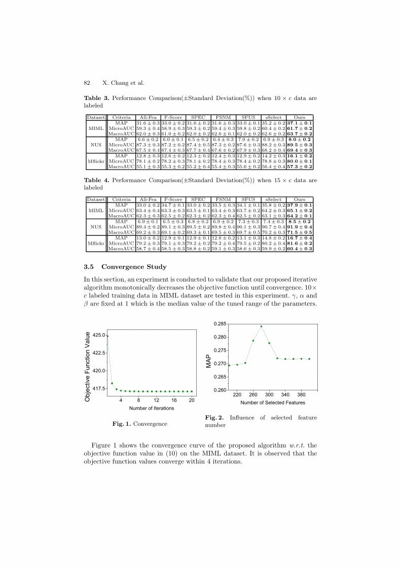
3.5 Convergence Study

In this section, an experiment is conducted to validate that our proposed iterativealgorithm monotonically decreases the objective function until convergence. 10×c labeled training data in MIML dataset are tested in this experiment. γ, α andβ are fixed at 1 which is the median value of the tuned range of the parameters.

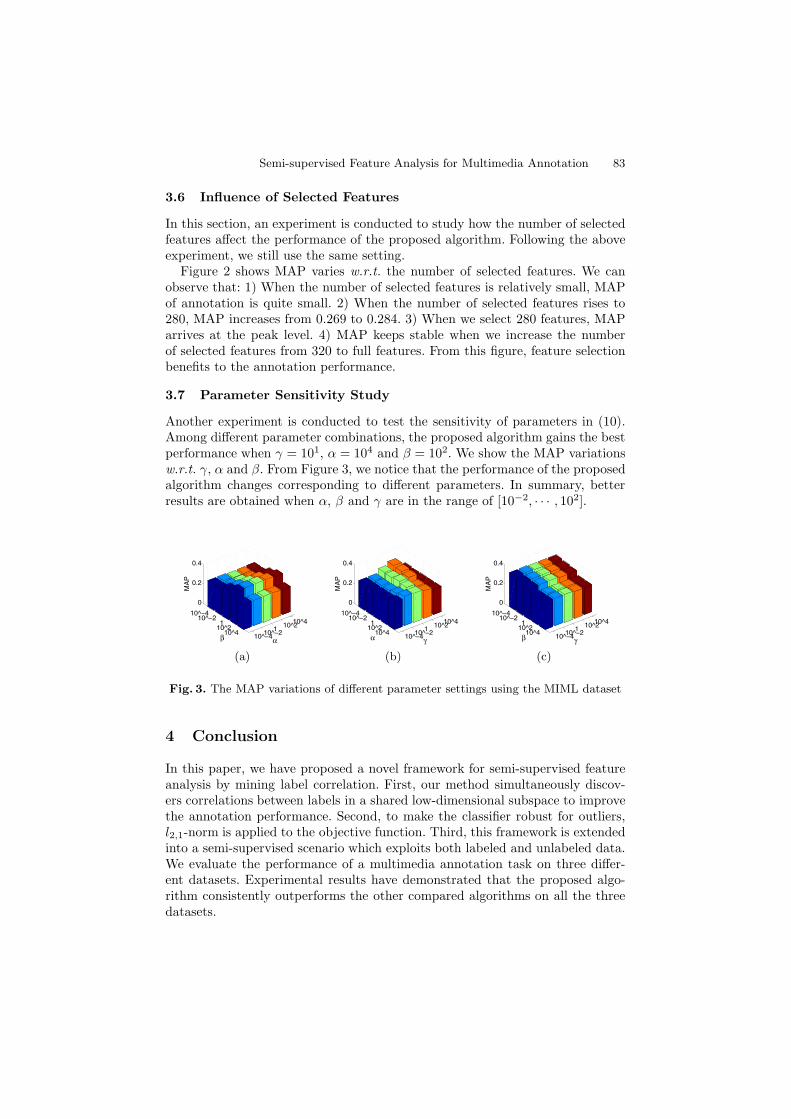
Fig. 1. ConvergenceFig. 2. Influence of selected featurenumber

Figure 1 shows the convergence curve of the proposed algorithm w.r.t. theobjective function value in (10) on the MIML dataset. It is observed that theobjective function values converge within 4 iterations.


3.6 Influence of Selected Features

In this section, an experiment is conducted to study how the number of selectedfeatures affect the performance of the proposed algorithm. Following the aboveexperiment, we still use the same setting.

Figure 2 shows MAP varies w.r.t. the number of selected features. We canobserve that: 1) When the number of selected features is relatively small, MAPof annotation is quite small. 2) When the number of selected features rises to280, MAP increases from 0.269 to 0.284. 3) When we select 280 features, MAParrives at the peak level. 4) MAP keeps stable when we increase the numberof selected features from 320 to full features. From this figure, feature selectionbenefits to the annotation performance.

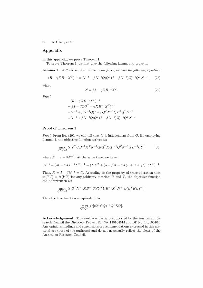
3.7 Parameter Sensitivity Study

Another experiment is conducted to test the sensitivity of parameters in (10).Among different parameter combinations, the proposed algorithm gains the bestperformance when γ = 101, α = 104 and β = 102. We show the MAP variationsw.r.t. γ, α and β. From Figure 3, we notice that the performance of the proposedalgorithm changes corresponding to different parameters. In summary, betterresults are obtained when α, β and γ are in the range of [10−2, · · · , 102].

10^−410^−21 10^210^410^−4

10^−21

10^210^4

0

0.2

0.4

αβ

MA

P

(a)

10^−410^−21 10^210^410^−4

10^−21

10^210^4

0

0.2

0.4

γα

MA

P

(b)

10^−410^−21 10^210^410^−4

10^−21

10^210^4

0

0.2

0.4

γβ

MA

P

(c)

Fig. 3. The MAP variations of different parameter settings using the MIML dataset

4 Conclusion

In this paper, we have proposed a novel framework for semi-supervised featureanalysis by mining label correlation. First, our method simultaneously discov-ers correlations between labels in a shared low-dimensional subspace to improvethe annotation performance. Second, to make the classifier robust for outliers,l2,1-norm is applied to the objective function. Third, this framework is extendedinto a semi-supervised scenario which exploits both labeled and unlabeled data.We evaluate the performance of a multimedia annotation task on three differ-ent datasets. Experimental results have demonstrated that the proposed algo-rithm consistently outperforms the other compared algorithms on all the threedatasets.

84 X. Chang et al.

Appendix

In this appendix, we prove Theorem 1.To prove Theorem 1, we first give the following lemma and prove it.

Lemma 1. With the same notations in the paper, we have the following equation:

(R− γXB−1XT )−1 = N−1 + βN−1Q(QT (I − βN−1)Q)−1QTN−1, (28)

where

N = M − γXB−1XT . (29)

Proof.

(R − γXB−1XT )−1

=(M − βQQT − γXB−1XT )−1

=N−1 + βN−1Q(I − βQTN−1Q)−1QTN−1

=N−1 + βN−1Q(QT (I − βN−1)Q)−1QTN−1

Proof of Theorem 1

Proof. From Eq. (29), we can tell that N is independent from Q. By employingLemma 1, the objective function arrives at:

maxQTQ=I

tr[Y TUB−1XTN−1Q(QTKQ)−1QTN−1XB−1UY ], (30)

where K = I − βN−1. At the same time, we have:

N−1 = (M − γXB−1XT )−1 = (XXT + (α+ β)I − γX(L+ U + γI)−1XT )−1.

Thus, K = I − βN−1 = C. According to the property of trace operation thattr(UV ) = tr(V U) for any arbitrary matrices U and V , the objective functioncan be rewritten as:

maxQTQ=I

tr[QTN−1XB−1UY Y TUB−1XTN−1Q(QTKQ)−1].

The objective function is equivalent to:

maxQTQ=I

tr[(QTCQ)−1QTDQ].

Acknowledgement. This work was partially supported by the Australian Re-search Council the Discovery Project DP No. 130104614 and DP No. 140100104.Any opinions, findings and conclusions or recommendations expressed in this ma-terial are those of the author(s) and do not necessarily reflect the views of theAustralian Research Council.


References

1. Yang, S.H., Hu, B.G.: Feature selection by nonparametric bayes error minimization.In: Proc. PAKDD, pp. 417–428 (2008)

2. Ma, Z., Nie, F., Yang, Y., Uijlings, J.R.R., Sebe, N., Hauptmann, A.G.: Discrimi-nating joint feature analysis for multimedia data understanding. IEEE Trans. Mul-timedia 14(6), 1662–1672 (2012)

3. Nie, F., Henghuang, C.X., Ding, C.: Efficient and robust feature selection via jointl21-norms minimization. In: Proc. NIPS, pp. 759–768 (2007)

4. Wang, D., Yang, L., Fu, Z., Xia, J.: Prediction of thermophilic protein with pseudoamino acid composition: An approach from combined feature selection and reduc-tion. Protein and Peptide Letters 18(7), 684–689 (2011)

5. Zhou, Z.H., Zhang, M.L.: Semi-supervised feature selection via spectral analysis.In: Proc. SIAM Int. Conf. Data Mining (2007)

6. Richard, D., Hart, P.E., Stork, D.G.: Pattern Classification. Wiley-Interscience,New York (2001)

7. Yang, Y., Wu, F., Nie, F., Shen, H.T., Zhuang, Y., Hauptmann, A.G.: Web andpersonal image annotation by mining label correlation with relaxed visual graphembedding. IEEE Trans. Image Process. 21(3), 1339–1351 (2012)

8. Cohen, I., Cozman, F.G., Sebe, N., Cirelo, M.C., Huang, T.S.: Semisupervisedlearning of classifiers: Theory, algorithms, and their application to human-computerinteraction. In: IEEE Trans. PAMI, pp. 1553–1566 (2004)

9. Zhao, X., Li, X., Pang, C., Wang, S.: Human action recognition based on semi-supervised discriminant analysis with global constraint. Neurocomputing 105,45–50 (2013)

10. Wang, S., Ma, Z., Yang, Y., Li, X., Pang, C., Hauptmann, A.: Semi-supervisedmultiple feature analysis for action recognition. IEEE Trans. Multimedia (2013)

11. Ji, S., Tang, L., Yu, S., Ye, J.: A shared-subspace learning framework for multi-labelclassification. ACM Trans. Knowle. Disco. Data 2(1), 8(1)–8(29) (2010)

12. Ma, Z., Nie, F., Yang, Y., Uijlings, J.R.R., Sebe, N.: Web image annotation viasubspace-sparsity collaborated feature selection. IEEE Trans. Multimedia 14(4),1021–1030 (2012)

13. Nie, F., Huang, H., Cai, X., Ding, C.: Efficient and robust feature selection viajoint l21-norms minimization. In: Proc. NIPS, pp. 1813–1821 (2010)

14. Yang, Y., Shen, H., Ma, Z., Huang, Z., Zhou, X.: L21-norm regularization discrim-inative feature selection for unsupervised learning. In: Proc. IJCAI (July 2011)

15. Zhao, Z., Liu, H.: Spectral feature selection for supervised and unsupervised learn-ing. In: Proc. ICML, pp. 1151–1157 (2007)

16. Zhou, Z.H., Zhang, M.L.: Multi-instance multi-label learning with application toscene classification. In: Proc. NIPS, pp. 1609–1616 (2006)

17. Huiskes, M.J., Lew, M.S.: The mir flickr retrieval evaluation. In: Proc. MIR, pp.39–43 (2008)

18. Chua, T.S., Tang, J., Hong, R., Li, H., Luo, Z., Zheng, Y.: Nus-wide: A real-worldweb image database from national university of singapore. In: Proc. CIVR (2009)

19. Chang, C.C., Lin, C.J.: LIBSVM: A library for support vector machines.ACM Transactions on Intelligent Systems and Technology 2, 27:1–27:27 (2011),http://www.csie.ntu.edu.tw/~cjlin/libsvm

http://www.csie.ntu.edu.tw/~cjlin/libsvm

Semi-supervised Feature Analysis for Multimedia Annotation by Mining Label Correlation

Documents

Transcript of Semi-supervised Feature Analysis for Multimedia Annotation by Mining Label Correlation