Semantic Decomposition and Marker Passing inan Artificial Representation of Meaning

vorgelegt vonDipl.-Inform.

Johannes FahndrichGeb. in Lahr im Schwarzwald

von der Fakultat IV — Elektrotechnik und Informatikder Technischen Universitat Berlin

zur Erlangung des akademischen Grades

Doktor der Ingenieurwissenschaften— Dr.-Ing. —

genehmigte Dissertation

Promotionsauschuss:

Vorsitzender: Prof. Dr. Klaus-Robert MullerGutachter: Prof. Dr. Dr. h.c. Sahin AlbayrakGutachter: Prof. Dr. Rainer UnlandGutachter: Prof. Dr.-Ing. Michael Weyrich

Tag der wissenschaftlichen Aussprache: 19. Feb. 2018

Berlin 2018

Abstract

The research area of Distributed Artificial Intelligence aims at building intelligent agent systems.

Multi-Agent Systems have been applied successfully in many domains, from an intermodal plan-

ning domain to cascading security thread simulations. But still, agents struggle with the meaning

of concepts used in language. Intelligence needs language to form thoughts. Thus, the challenge

addressed in this thesis is to provide a computable representation of meaning and evaluate its

usefulness. Based on the theory of a mental lexicon and the thesis that meaning is a combination

of symbolic and connectionist parts, I investigate the use of the theory of Natural Semantic Met-

alanguage (NSM) to build an artificial representation of meaning. I show that the use of NSM

for creating a semantic graph out of different information sources can be utilized as a basis for

Marker Passing algorithms.

The Marker Passing algorithm encodes symbolic meaning to guide the reasoning over the con-

nectionist semantic graph. Through the combination of a semantic graph and symbolic Marker

Passing, I can combine connectionist and symbolic approaches to AI research to create my arti-

ficial representation of meaning.

To test my approach, I build a semantic distance measure, a word sense disambiguation al-

gorithm and a sentence similarity measure which all go head to head with the state-of-the-art.

I apply those approaches to two use cases: A semantic service match marking and a context-

dependent heuristics. I evaluate my heuristic by utilizing them in AI problem-solving component

which uses AI planning guided by my heuristic.

iii

Zusammenfassung

Die Wissenschaft im Bereich der verteilten kunstlichen Intelligenz untersucht unter anderem

Multi-Agenten Systeme und deren Anwendung in verschiedenen Bereichen. Solche intelligen-

ten verteilten Systeme finden beispielsweise erfolgreich Einsatz bei der Planung intermodaler

Routen oder bei der Simulation von Kaskaden Effekten durch Sicherheitsbedrohungen. Dabei

entwickeln Agenten immer mehr Intelligenz zur autonomen Losunge von neuen Problemen.

Agenten kampfen jedoch noch immer mit der Bedeutung von Konzepten der naturlichen Sprache.

Intelligenz benotigt jedoch Sprache um Gedanken zu formen. Deshalb wird in dieser Arbeit die

Herausforderung angegangen eine kunstliche Reprasentation von Bedeutung zu erschaffen und

deren Nutzbarkeit zu evaluieren.

Basierend auf der Theorie eines mentalen Lexikons und darauf, dass Bedeutung aus zwei

Teilen besteht (Symbolischer und Konnektivistischer Bedeutung), untersucht diese Arbeit die

Verwendung der Natural Semantic Metalanguage (NSM) zum Erstellen einer kunstlichen Repra-

sentation von Bedeutung. Hauptaugenmerk liegt dabei auf der automatischen Erzeugung eines

semantischen Graphen, der durch Marker Passing Ansatze genutzt werden kann. Der semantis-

che Graph wird dabei basierend auf der NSM Theorie aus verschiedenen Informationsquellen

automatisch erstellt. Der Marker Passing Algorithmus beschreibt dabei den symbolischen Teil

unseres Ansatzes. Die symbolische Information der Marker wird dazu verwendet diese geeignet

uber den semantischen Graphen zu verteilen. Durch die Verteilung der Marker wird eine Art

von Schlussfolgerung modelliert. Durch die so entstandene Kombination aus Dekomposition

und Marker Passing kann eine Mischung aus symbolische und konnektivistische Bedeutung

entstehen.

Die so entstandene kunstliche Reprasentation von Bedeutung wird durch mehrere Experi-

mente getestet: Ich verwende sie um ein semantisches Distanzmaß zu bauen, erstellen einen

Ansatz zur Auflosung von Mehrdeutigkeit von Worten in naturlicher Sprache und erzeugen einen

neuen Ansatz zur Bestimmung von Satzahnlichkeit. Dabei konnte gezeigt werden, dass die so

entstandenen Ansatze dem Stand der Technik in nichts nachstehen. Des Weiteren teste ich an

zwei Anwendungen ob meine kunstliche Reprasentation von Bedeutung wirklich Bedeutung

formalisiert: erstens anhand einer Semantischen Service Matching-Komponente und zweitens

einer kontextabhangigen und zielorientierten Heuristik. Diese Heuristik wird durch den Einsatz

in einem Planungsalgorithmus evaluiert.

Acknowledgements

I want to express my gratitude and recognition to my doctoral supervisor Prof. Dr. Dr. h.c.

Sahin Albayrak from whom I have had the opportunity to learn a lot about science, academia

and the work I want to do in my life. I want to thank Prof. Dr. Rainer Unland for his support

in all those years mentoring me in the Doctoral Consortia. I wish to thank Prof. Dr. Michael

Weyrich, whose constructive criticism has kept me on my scientific toes. In addition, I want

to thank the team of scientists at the Technische Universitat Berlin for their constant support.

Especially Sebastian Ahrndt for his enthusiastic criticism and Dr. Frank Trollmann for the many

fruitful discussions and the scientific mentoring. Without all of them, this would have been less

fun.

v

Contents

I. Introduction 1

1. Introduction 31.1. Motivation . . . . . . . . . . . . . . . . . . . . . . . . . . . . . . . . . . . . . 51.2. Problem Statement . . . . . . . . . . . . . . . . . . . . . . . . . . . . . . . . 81.3. Research Statement . . . . . . . . . . . . . . . . . . . . . . . . . . . . . . . . 81.4. Research Questions . . . . . . . . . . . . . . . . . . . . . . . . . . . . . . . . 91.5. Research Approach . . . . . . . . . . . . . . . . . . . . . . . . . . . . . . . . 10

2. Thesis Document 132.1. Thesis Structure . . . . . . . . . . . . . . . . . . . . . . . . . . . . . . . . . . 132.2. Contributions . . . . . . . . . . . . . . . . . . . . . . . . . . . . . . . . . . . 15

II. Foundations 17

3. Basic Terms and Concepts 193.1. Agents . . . . . . . . . . . . . . . . . . . . . . . . . . . . . . . . . . . . . . . 193.2. Actions, Services and Capabilities . . . . . . . . . . . . . . . . . . . . . . . . 233.3. Planning . . . . . . . . . . . . . . . . . . . . . . . . . . . . . . . . . . . . . . 273.4. Graphs . . . . . . . . . . . . . . . . . . . . . . . . . . . . . . . . . . . . . . . 273.5. Concept . . . . . . . . . . . . . . . . . . . . . . . . . . . . . . . . . . . . . . 293.6. Ontology . . . . . . . . . . . . . . . . . . . . . . . . . . . . . . . . . . . . . 313.7. Semantic . . . . . . . . . . . . . . . . . . . . . . . . . . . . . . . . . . . . . 323.8. Context . . . . . . . . . . . . . . . . . . . . . . . . . . . . . . . . . . . . . . 333.9. Meaning . . . . . . . . . . . . . . . . . . . . . . . . . . . . . . . . . . . . . . 353.10. Natural Semantic Metalanguage . . . . . . . . . . . . . . . . . . . . . . . . . 45

4. State-of-the-Art 474.1. Semantic Theories . . . . . . . . . . . . . . . . . . . . . . . . . . . . . . . . 474.2. Ontology . . . . . . . . . . . . . . . . . . . . . . . . . . . . . . . . . . . . . 574.3. Semantic Service Description Languages . . . . . . . . . . . . . . . . . . . . 684.4. Semantic Decomposition . . . . . . . . . . . . . . . . . . . . . . . . . . . . . 704.5. Activation Propagation, Activation Spreading and Marker Passing . . . . . . . 714.6. Service Planning . . . . . . . . . . . . . . . . . . . . . . . . . . . . . . . . . 75

III. Approach 83

5. Abstract Approach 85

6. Semantic Decomposition 896.1. Natural Semantic Metalanguage . . . . . . . . . . . . . . . . . . . . . . . . . 916.2. NSM Semantic Primes in Artificial Languages . . . . . . . . . . . . . . . . . . 936.3. Data Sources used in the Semantic Decomposition . . . . . . . . . . . . . . . 956.4. Formalization of the Semantic Graph . . . . . . . . . . . . . . . . . . . . . . . 97

vii

6.5. Decomposition into Semantic Primes . . . . . . . . . . . . . . . . . . . . . . . 1026.6. Conclusion . . . . . . . . . . . . . . . . . . . . . . . . . . . . . . . . . . . . 114

7. Marker Passing 1157.1. Pragmatic Meaning Representation . . . . . . . . . . . . . . . . . . . . . . . . 1157.2. Marker Passing Algorithm . . . . . . . . . . . . . . . . . . . . . . . . . . . . 1197.3. Parameters of Marker Passing . . . . . . . . . . . . . . . . . . . . . . . . . . 1267.4. Conclusion . . . . . . . . . . . . . . . . . . . . . . . . . . . . . . . . . . . . 141

8. Implementation 1438.1. Semantic Decomposition . . . . . . . . . . . . . . . . . . . . . . . . . . . . . 1438.2. Marker Passing . . . . . . . . . . . . . . . . . . . . . . . . . . . . . . . . . . 146

IV. Evaluation 147

9. Experiments with the Decomposition 1499.1. Parameters of the Decomposition . . . . . . . . . . . . . . . . . . . . . . . . . 1499.2. Selecting Synonyms . . . . . . . . . . . . . . . . . . . . . . . . . . . . . . . . 1509.3. Selecting Decomposition Depth . . . . . . . . . . . . . . . . . . . . . . . . . 152

10.Experiments with the Marker Passing 15510.1. Experiment 1: Semantic Similarity Measure . . . . . . . . . . . . . . . . . . . 15710.2. Experiment 2: Word Sense Disambiguation . . . . . . . . . . . . . . . . . . . 18310.3. Experiment 3: Semantic Sentence Similarity Measure . . . . . . . . . . . . . . 18910.4. Experiment 4: Semantic Service Matching . . . . . . . . . . . . . . . . . . . . 19910.5. Experiment 5: Heuristics in AI Service Planning . . . . . . . . . . . . . . . . . 20810.6. Experimental Setup . . . . . . . . . . . . . . . . . . . . . . . . . . . . . . . . 24210.7. Evaluation Results . . . . . . . . . . . . . . . . . . . . . . . . . . . . . . . . 242

V. Conclusion 245

11.Summary 247

12.Discussion 251

13.Final Remarks and Future Work 255

VI. Bibliography, Glossary, Index, and Appendix 257

A. Appendix 259A.1. Tools . . . . . . . . . . . . . . . . . . . . . . . . . . . . . . . . . . . . . . . . 259A.2. Class Diagrams . . . . . . . . . . . . . . . . . . . . . . . . . . . . . . . . . . 260A.3. Algorithms . . . . . . . . . . . . . . . . . . . . . . . . . . . . . . . . . . . . 261A.4. Natural Semantic Metalanguage . . . . . . . . . . . . . . . . . . . . . . . . . 261

Bibliography 261

Index 293

viii

List of Figures

1.1. Hierarchy of arguments towards the need for artificial meaning. . . . . . . . . . 51.2. Abstract research approach. . . . . . . . . . . . . . . . . . . . . . . . . . . . . 11

2.1. The structure of this thesis. . . . . . . . . . . . . . . . . . . . . . . . . . . . . 14

3.1. Illustration of an agent in its environment. . . . . . . . . . . . . . . . . . . . . 203.2. Architecture of the means-ends reasoning of an agent. . . . . . . . . . . . . . . 213.3. Cognitive interpretation in an agent. . . . . . . . . . . . . . . . . . . . . . . . 223.4. Abstract example effect rule. . . . . . . . . . . . . . . . . . . . . . . . . . . . 263.5. Illustration of the EGraph morphisms taken from [66]. . . . . . . . . . . . . . 283.6. Illustration of the AGraph diagram taken from [66]. . . . . . . . . . . . . . . . 293.7. Overview of the state-of-the-art of semantic similarity measures. . . . . . . . . 313.8. Type graph of our ontology definition. . . . . . . . . . . . . . . . . . . . . . . 323.9. Illustration of a context for the definition of Mahr [250] . . . . . . . . . . . . . 34

4.1. Illustration of Bloomfields definition of meaning. . . . . . . . . . . . . . . . . 484.2. Illustration Chomsky’s grammatical hierarchy. . . . . . . . . . . . . . . . . . . 484.3. Illustration of two prototypes for the class of car and of fast. . . . . . . . . . . 504.4. Example of axiomatic semantics. . . . . . . . . . . . . . . . . . . . . . . . . . 514.5. Example for generative semantics. . . . . . . . . . . . . . . . . . . . . . . . . 544.6. Example in discourse representation semantic. . . . . . . . . . . . . . . . . . . 554.7. Example of distributed semantics. . . . . . . . . . . . . . . . . . . . . . . . . 554.8. The Semiotic Triangle. . . . . . . . . . . . . . . . . . . . . . . . . . . . . . . 604.9. An example ontology for living and not living things. . . . . . . . . . . . . . . 624.10. Formalisation the concepts to sing and to break taken from [387]. . . . . . . . 704.11. Script in the notation of Schank and Andelson [345]. . . . . . . . . . . . . . . 714.12. Abstract approach of activation spreading. . . . . . . . . . . . . . . . . . . . . 72

5.1. Abstract description of the knowledge part of this approach. . . . . . . . . . . 855.2. Abstract description of the reasoning part of this approach. . . . . . . . . . . . 865.3. Abstract approach to represent artificial meaning. . . . . . . . . . . . . . . . . 87

6.1. Classifiction of data sources in information type and formality. . . . . . . . . . 966.2. Example of a relation hierarchy. . . . . . . . . . . . . . . . . . . . . . . . . . 986.3. Minimal type graph for the description of a decomposition graph. . . . . . . . 986.4. Example of a typed graph. . . . . . . . . . . . . . . . . . . . . . . . . . . . . 1006.5. Abstract example of an decomposition of midday and noon. . . . . . . . . . . 1006.6. Example of a type graph (big). . . . . . . . . . . . . . . . . . . . . . . . . . . 1016.7. Example of a typed graph of noon and midday. . . . . . . . . . . . . . . . . . 1026.8. Example decomposition of one meaning of the concept “to go”. . . . . . . . . 1036.9. An example decomposition using the Cambridge Dictionary. . . . . . . . . . . 114

7.1. Abstract communication act adapted from [228]. . . . . . . . . . . . . . . . . 1167.2. Abstract description of our Marker Passing algorithm. . . . . . . . . . . . . . . 1207.3. Marker passing Example start and first step. . . . . . . . . . . . . . . . . . . . 1337.4. Marker passing Example step two and three . . . . . . . . . . . . . . . . . . . 135

ix

7.5. Marker passing Example step four and five . . . . . . . . . . . . . . . . . . . . 136

8.1. Architecture of the implementation. . . . . . . . . . . . . . . . . . . . . . . . 1438.2. Our IDictionary interface. . . . . . . . . . . . . . . . . . . . . . . . . . . . . . 1448.3. Class diagrams of concept and definition. . . . . . . . . . . . . . . . . . . . . 145

9.1. Example graph of an example decomposition of “noon” with depth 1. . . . . . 1539.2. Example graph of an example decomposition of “midday” with depth 1. . . . . 1539.3. Example graph of an example decomposition of “noon” with depth 2. . . . . . 1549.4. Example graph of an example decomposition of “midday” with depth 2. . . . . 154

10.1. Overview of the experiments making up the evaluation of our representation ofmeaning. . . . . . . . . . . . . . . . . . . . . . . . . . . . . . . . . . . . . . . 156

10.2. Overview of the algorithm to measure semantic similarity of two concepts. . . . 15810.3. Overview of the state-of-the-art of semantic similarity measures. . . . . . . . . 16010.4. Result and Error of the Marker Passing approach with the RG65 dataset. . . . . 17910.5. Result and Error of the BDOS approach with the RG65 dataset. . . . . . . . . . 18010.6. Result and Error of the Word2Vec with the RG65 dataset. . . . . . . . . . . . . 18210.7. Error of the ELKB approach with the RG65 dataset. . . . . . . . . . . . . . . . 18210.8. Overview of the algorithm for Word Sense Disambiguation. . . . . . . . . . . . 18410.9. Example sentence with word sense from the Senseval Task 3 data set . . . . . . 18710.10.Overview of the algorithm for our semantic sentence similarity measure. . . . . 19010.11.Detailed result of the SMTeuroparl data set. . . . . . . . . . . . . . . . . . . . 19710.12.Detailed result of the MSRpar data set. . . . . . . . . . . . . . . . . . . . . . . 19810.13.Detailed result of the MSRvid data set. . . . . . . . . . . . . . . . . . . . . . . 19910.14.Abstract Service Matching challenge. . . . . . . . . . . . . . . . . . . . . . . 20110.15.NDCG of the overall result with all Marker Passing experts and equal weights. 20710.16.Overview of our methodology to create a heuristic. . . . . . . . . . . . . . . . 22310.17.Abstract example of state space in a planning problem. . . . . . . . . . . . . . 22410.18.Abstract approach to a greedy A∗ heuristic. . . . . . . . . . . . . . . . . . . . 23110.19.Example state space with heuristic values. . . . . . . . . . . . . . . . . . . . . 23610.20.The transport part of the Scallop health domain start state. . . . . . . . . . . . 23610.21.The account part of the Scallop health domain start state. . . . . . . . . . . . . 23710.22.The location part of the Scallop health domain start state. . . . . . . . . . . . . 23710.23.The parameters part of the Scallop health domain start state. . . . . . . . . . . 23810.24.The patient and transport part of the Scallop health domain goal state. . . . . . 23810.25.The airport part of the Scallop health domain goal state. . . . . . . . . . . . . . 23810.26.The account part of the Scallop health domain goal state. . . . . . . . . . . . . 23910.27.The parameter and person part of the Scallop health domain goal state. . . . . . 23910.28.Example goal axioms which are different in our goal state to our start state. . . 24010.29.Experiment results overview. . . . . . . . . . . . . . . . . . . . . . . . . . . . 244

A.1. Service Development tools and their interplay. . . . . . . . . . . . . . . . . . . 259A.2. Class diagram of the decomposition. . . . . . . . . . . . . . . . . . . . . . . . 260

x

List of Tables

3.1. List of different types of antonyms. . . . . . . . . . . . . . . . . . . . . . . . . 423.2. Semantic primes for the English language [140]. . . . . . . . . . . . . . . . . . 46

4.1. Comparison of semantic approaches. . . . . . . . . . . . . . . . . . . . . . . . 574.2. Requirements for the chosen language for the representation of meaning. . . . . 674.3. Comparison of Service Composition approaches. . . . . . . . . . . . . . . . . 80

6.1. List of semantic primes and equivalent concepts found in OWL. . . . . . . . . 936.2. List of semantic primes and equivalent concepts found in PDDL. . . . . . . . . 946.3. List of semantic primes with and equivalent concepts found in MOF. . . . . . . 956.4. List of knowledge graphs. . . . . . . . . . . . . . . . . . . . . . . . . . . . . . 976.5. Semantic primes in the category substantive in the English language [140]. . . . 108

9.1. Example decomposition properties. . . . . . . . . . . . . . . . . . . . . . . . . 153

10.1. Node and edge count for different decomposition depth. . . . . . . . . . . . . . 16410.2. The parameters of the Marker Passing approach with replacement in the in-

function. . . . . . . . . . . . . . . . . . . . . . . . . . . . . . . . . . . . . . . 17210.3. Parameters of the Marker Passing for our semantic similarity measurement. . . 17710.4. The result of the semantic similarity measure experiment. . . . . . . . . . . . . 17810.5. Results of the WSD approaches on the Senseval Task 3 data set. . . . . . . . . 18810.6. Example sentences form the SemEval 2012 MSRvid data set. . . . . . . . . . . 19510.7. Example sentences form the SemEval 2012 SMTeuroparl data set. . . . . . . . 19510.8. Results of the semantic sentence similarity measure experiment. . . . . . . . . 19710.9. Fixed scoring assessments or matcher pats as proposed by [23]. . . . . . . . . . 20210.10.Service Matching results for the Marker Passing expert. . . . . . . . . . . . . . 20610.11.Service Matching results for the experts without Marker Passing. . . . . . . . . 20610.12.Comparison of heuristic approach. . . . . . . . . . . . . . . . . . . . . . . . . 21710.13.Planning results for an average over ten runs of planner (time is in seconds). . . 24010.14.Hardware description of the computer used for the experiments. . . . . . . . . 24210.15.Software description main external components used. . . . . . . . . . . . . . . 242

xi

List of Algorithms

1. A decompositional algorithm. . . . . . . . . . . . . . . . . . . . . . . . . . . 1042. Get the relations of a concept . . . . . . . . . . . . . . . . . . . . . . . . . . . 1063. Get the definitions of a concept . . . . . . . . . . . . . . . . . . . . . . . . . . 106

4. Marker Passing- adapted from Crestani’s Spreading Activation Algorithm . . . 1255. Marker Passing Algorithm . . . . . . . . . . . . . . . . . . . . . . . . . . . . 126

6. Semantic Similarity measure. . . . . . . . . . . . . . . . . . . . . . . . . . . . 1587. Setting initial Markers. . . . . . . . . . . . . . . . . . . . . . . . . . . . . . . 1688. Function to select the active concepts. . . . . . . . . . . . . . . . . . . . . . . 1699. Threshold calculation of concept nodes for our semantic similarity measure. . . 16910. Out-Function of concept nodes. . . . . . . . . . . . . . . . . . . . . . . . . . . 17011. Edge-Function. . . . . . . . . . . . . . . . . . . . . . . . . . . . . . . . . . . 17012. GetWeightOfRelation. . . . . . . . . . . . . . . . . . . . . . . . . . . . . . . 17113. In-Function of concept nodes. . . . . . . . . . . . . . . . . . . . . . . . . . . 17114. After-Send-Function of concept nodes. . . . . . . . . . . . . . . . . . . . . . . 17315. The termination condition for the semantic similarity measure. . . . . . . . . . 17416. Word Sense Disambiguation Marker Passing algorithm. . . . . . . . . . . . . . 18517. Semantic Sentence Similarity Marker Passing algorithm. . . . . . . . . . . . . 19118. Setting initial markers for sentences. . . . . . . . . . . . . . . . . . . . . . . . 19119. Marker Passing Expert - Name Matching. . . . . . . . . . . . . . . . . . . . . 20420. Service Planner algorithm. . . . . . . . . . . . . . . . . . . . . . . . . . . . . 22121. Goal oriented heuristic. . . . . . . . . . . . . . . . . . . . . . . . . . . . . . . 233

22. Spreading Activation - adapted from Crestani [61]. . . . . . . . . . . . . . . . 261

xiii

Listings

3.1. Definition of the OWL parameter class. . . . . . . . . . . . . . . . . . . . . . 243.2. Definition of the OWL-S output parameter class. . . . . . . . . . . . . . . . . 25

8.1. Example decomposition creation. . . . . . . . . . . . . . . . . . . . . . . . . . 1448.2. Example Marker Passing. . . . . . . . . . . . . . . . . . . . . . . . . . . . . . 146

10.1. Reference example of ontologies in an OWL syntax. . . . . . . . . . . . . . . 225

xv

List of Publications

This section lists the publications which are used in this dissertation.

Fahndrich, J., Masuch N., Borchert L., and Albayrak, S. Learning Mechanisms on OWL-S Service Descriptions for Automated Action Selection, Presented at the IoA at theConference on Autonomous Agents and MultiAgent Systems (AAMAS), pp. 41-57, 2017.[102]

Fahndrich, J., Kuster, T., Masuch N., and Albayrak, S. Semantic Service Management andOrchestration for Adaptive and Evolving Processes, In: International Journal on Ad-vances in Internet Technology, vol. 9, no. 4, pp. 75-88, 2016. [100]

Fahndrich, J., Kuster, T., Masuch N., and Albayrak, S. Semantic Service Management forEnabling Adaptive and Evolving Processes, Presented at the International Conferenceon Internet and Web Applications and Services, Valencia, pp. 46-53, 2016. [101] (BestPaper Award)

Fahndrich, J., Weber, S., Ahrndt, S., and Albayrak, S. Design and Use of a Semantic Similar-ity Measure for Interoperability Among Agents, Presented at the German Conferenceon Multiagent System Technologies (MATES), pp. 41- 57, 2016. [104]

Fahndrich, J., Ahrndt, S., and Albayrak, S. Self-Explanation through Semantic Annota-tion and (automated) Ontology Creation: A Survey. Presented at the InternationalSymposium Advances in Artificial Intelligence and Applications (AAIA), pp. 1-15, 2015http://doi.org/10.15439/2015F416 [99]

Fahndrich, J., Ahrndt, S., and Albayrak, S. Formal Language Decomposition into SemanticPrimes., In: Advances in Distributed Computing and Artificial Intelligence Journal (AD-CAIJ), 3(8), pp. 56, 2014 http://doi.org/10.14201/ADCAIJ2014385673 [98]

Fahndrich, J., Ahrndt, S., and Albayrak, S. Are There Semantic Primes in Formal Lan-guages?, Presented at the International Conference on Distributed Computing and Arti-ficial Intelligence (DCAI), 290 (Chapter 46), pp. 397-405, 2014, http://doi.org/10.1007/978-3-319-07593-8 46 [97] (Best Paper Award)

Fahndrich, J., Masuch, N., Yildirim, H., and Albayrak, S. Towards Automated Service Match-making and Planning for Multi-Agent Systems with OWL-S Approach and Chal-lenges., Presented at the International Conference on Service-Oriented Computing (IC-SOC) Workshops (Vol. 8377), pp. 240, 2013, http://doi.org/10.1007/978-3-319-06859-6 21 [103]

Fahndrich, J. Best First Search Planning of Service Composition Using Incrementally Re-fined Context-Dependent Heuristics, Presented at the German Conference MultiagentSystem Technologies (MATES), pp. 404, 2013 http://doi.org/10.1007/978-3-642-40776-5 34 [93]

Fahndrich, J., Ahrndt, S., and Albayrak, S. Towards Self-Explaining Agents., presented at theInternational Conference on Practical Applications of Agents and Multi-Agent Systems(PAAMS), 221 (Chapter 18), pp. 147-154, 2013, http://doi.org/10.1007/978-3-319-00563-8 18 [96]

xvii

Fahndrich, J., Ahrndt, S., and Albayrak, S. Self-Explaining Agents. Jurnal Teknologi (Scienceand Engineering), 63(3), pp. 53-64, 2013, http://doi.org/0.11113/jt.v63.1955 [95]

Fahndrich, J. Exploring Self-Explanation : The System Side., Presented at the German Con-ference on Multiagent System Technologies (MATES), p. 12, 2012 [94]

xviii

List of Supervised Theses

This section lists the supervised student theses which have been basis to some of the sections ofthis dissertation.

Hannes Kanthak, Ein semantischer Ansatz zum Losen von Winograd Schemen. TechnischeUniversitat Berlin, Bachelor (2017)

Maik Wischow, Konfliktlosung bei der Erweiterung von Wissensgraphen. Technische Uni-versitat Berlin, Bachelor (2016)

Tom Konig, Untersuchung semantischer Distanzmaße auf der Grundlage von Aktivierungsaus-breitung uber ontologiebasierten Hypergraphen. Technische Universitat Berlin, Bachelor(2016)

Nico Tobias Schneider, Quantifizierung semantischer Satzahnlichkeit basierend auf lexikalis-cher Dekomposition und Marker Passing. Technische Universitat Berlin, Bachelor (2016)

Benjamin Brand, Semantic Distance of Service Descriptions through Activation Spreading.Technische Universitat Berlin, Diploma (2016)

Florian Marienwald, How Does the Interpretation Of Word Relations Help Word Sense Dis-ambiguation via a Marker Passing Approach? Technische Universitat Berlin, Bachelor(2016)

Pascal Lukanek, Ein auf Marker-Passing basierender Word-Sense-Disambiguation Ansatz.Technische Universitat Berlin, Bachelor (2016)

Sabine Weber, The roles of Synonyms in a semantic decomposition. Technische UniversitatBerlin, Bachelor (2015)

Ghadh, Altayyar, An editor for manual semantic decomposition, Technische Universitat Berlin,Bachelor (2015)

Zeinab, Sawan, Goal driven Heuristics based on Service Descriptions, Technische Univer-sitat Berlin, Bachelor (2015)

xix

Part I.

Introduction

1

1. Introduction

Artificial Intelligence (AI) helps to solve ever more complex problems. The use of increasinglysophisticated software enables us to automate many tedious tasks, perform better research andgrasp a better understanding of the world, e.g., playing GO [395], or fighting cancer [90]. “De-spite all these developments, the promises of strong artificial intelligence set forth in the 1960shave not been fulfilled.” [68, p. 7], meaning that AI is not able to understand natural language[419], construct plans on dynamic domains [135], or do common sense reasoning like humans[356]. These kind of problems are solved by a so called “strong AI” [353]1. A strong AI isable to learn new problem-solving skills or can get to know new topics, in difference to specialpurpose AI like most chess AI which is, e.g., unable to drive a car.

One of the reasons for human intelligence might be the ability to think. Having a language toformulate thoughts, meaning and ideas helps us to handle unknown situations with adaptivenessand dynamic behavior. Part of the capacity to think is reasoning, which does not always “obeythe rules of classical logic” but gives us my common sense [128]. The foundation for languageto think is a representation of meaning. Consequently, research in AI analyzes how methodsfrom Mathematics, Linguistics, Psychology, Philosophy and Computer Science can be used tocreate machines with the ability to represent meaning.

One approach to AI is the intelligent component “agent” [338]. An agent models humanintelligence behavior, like goal orientation or autonomy [417], to act intelligently. Grasping themeaning of things, events or actions allows agents to react appropriately and makes them ableto react to change. As a result, agents become more robust in their problem-solving skills. Theadaption of an agent becomes easier if the agent can integrate new concepts into its knowledgeand use them for future reasoning processes. In humans, we2 call this understanding of concepts,meaning [234]. One possibility for an agent to reach its goal is to use the help of other agents.

In this work we will firstly have a look at how meaning is described, and on this basis I willdevelop two mechanisms to integrate a meaning representation into agents: one to formalizesemantic information and one to perform reasoning using this information.

During research on meaning, I found the difficulty to measure meaning directly [296], this iswhy the AI community has established experiments which allow us to collect evidence on theexistence of meaning in humans and machines by observing their behavior in specific test situa-tions. This can be seen in the testing of human knowledge, e.g., in schools and universities tests.For an AI these tests are challenges with defined data sets. Here we start out with my hardestexperiment (the creation of heuristics for AI planning) and explain why the other experimentsquestions have to be answered first.

Planning anticipates acting through reasoning [133]. Planning allows humans to approachcomplex problems and is envisioned as key for artificial agents to become more autonomous

1strong AI (sometimes called full AI or hard AI ) [213, p. 260] refers to a human level intelligence.2If the reference “we” is used in this thesis, this “we” references the author and the reader in the form of a pluralis

modestiae.

3

1. Introduction

and proactive [339]. The ability to plan enables agents to solve problems that have not beenprogrammed during design time; creating agents which adapt to changes in (dynamic) environ-ment. One dynamic environment is a Service Oriented Computing (SOA) [89] where distributedservices undergo change during runtime.

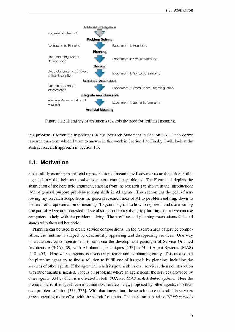
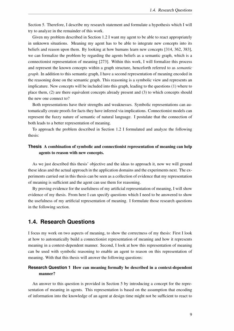
In complex planning problems heuristics are needed to solve a problem. The creation ofheuristics (see Section 10.5) during runtime may leads to the encounter of new concepts, whichthen lead us back to my original question: How can AI make sense of new concepts? Forheuristics this means interpreting the new concepts and adding additional information to clas-sical heuristic approaches: A function H : state → R+ is called heuristic [337, p. 92] andestimates the distance from a state to a given goal. I extend this definition of heuristic to:H : service × state × goal → R+ making the heuristic more dynamic since now it can adaptto changing goals and services. Here the heuristic determines the usefulness w.r.t. the goal ofthe given service in the current state (e.g. by comparing the service to a request). We integrateservice and goal description into the heuristic because if only a state is the information sourcefor the heuristic, we miss out on information like the description of the service. This leads tothe experiment to evaluate a service according to some service needs according to a goal in aplanning problem. This experiment is done by implementing a service match maker and testingit in one of my experiments in a Service Matching (see Section 10.4) context. Heuristics canbe build by simplifying the given problem [304]. Those implications are for example used byFast-Forward-Planner by removing the delete list of service effects [171]. Because of the openworld assumption, this does not work in service planning. Other heuristics guide specific prob-lems which then can not be used in problem independent (sometimes called general purpose)planning [304], because they do not adapt to e.g. changes in the goal or to new services. Thuswe need another way of gathering information about the available service and the goal. In thiswork, this information is the meaning of the concepts used to describe e.g. the service or goal.The service descriptions are e.g. given in sentences, means that we have to compare more thanjust single concepts. This leads to the need of comparing sentences, using a Sentence Similaritymeasure (see Section 10.3). Such a sentence similarity measure gives use a next experiment onhow well my meaning representation can capture the meaning of sentences. Ambiguous wordcarry different meanings in different contexts. Selecting the right word sense leads us to the nextexperiment: which word sense is the right one to select in a context of use. This leads us to mynext experiment for Word Sense Disambiguation (see Section 10.2). To be able to use servicesof agents programmed by other developers, using other models and with that other ontologies,the agent needs to integrate new concepts into its knowledge. The interpretation of new conceptsrequires to identify if a new concepts is equivalent to a already known concept (e.g. by using asemantic similarity measure). This leads us to my experiment with a Semantic Similarity mea-sure (see Section10.1). The recognition of similarity is a basic task to form more sophisticatedand abstract abilities for reasoning [131, p. 197]. All of those subproblems show an aspect ofmeaning. Each experiment analyzes the capability of the representation of meaning of a differ-ent use. With all those experiments we will gather evidence on whether my representation ofmeaning is a useful one or not.

In Section 1.1, I will motivate why we need an artificial representation of meaning, explainhow I derived the creation of an artificial representation of meaning as my main goal and explainhow the work, done in this doctoral thesis, fits into the bigger picture of AI research. Afterwards,I work out the problems we need to solve to create such representation Section 1.2. Regarding

4

1.1. Motivation

Service

Semantic Description

Integrate new Concepts

Problem Solving

Planning

Artificial Meaning

Artificial Intelligence

Focused on strong AI

Abstracted to Planning Experiment 5: Heuristics

Understanding what a Service does

Experiment 4: Service Matching

Understanding the conceptsof the description

Experiment 3: Sentence Similarity

Context dependent interpretation

Experiment 2: Word Sense Disambiguation

Machine Representation of Meaning

Experiment 1: Semantic Similarity

Figure 1.1.: Hierarchy of arguments towards the need for artificial meaning.

this problem, I formulate hypotheses in my Research Statement in Section 1.3. I then deriveresearch questions which I want to answer in this work in Section 1.4. Finally, I will look at theabstract research approach in Section 1.5.

1.1. Motivation

Successfully creating an artificial representation of meaning will advance us on the task of build-ing machines that help us to solve ever more complex problems. The Figure 1.1 depicts theabstraction of the here hold argument, starting from the research gap shown in the introduction:lack of general purpose problem-solving skills in AI agents. This section has the goal of nar-rowing my research scope from the general research area of AI to problem solving, down tothe need of a representation of meaning. To gain insight into how to represent and use meaning(the part of AI we are interested in) we abstract problem solving to planning so that we can usecomputers to help with the problem-solving. The usefulness of planning mechanisms falls andstands with the used heuristic.

Planning can be used to create service compositions. In the research area of service compo-sition, the runtime is shaped by dynamically appearing and disappearing services. One wayto create service composition is to combine the development paradigm of Service OrientedArchitecture (SOA) [89] with AI planning techniques [133] in Multi-Agent Systems (MAS)[110, 403]. Here we see agents as a service provider and as planning entity. This means thatthe planning agent try to find a solution to fulfill one of its goals by planning, including theservices of other agents. If the agent can reach its goal with its own services, then no interactionwith other agents is needed. I focus on problems where an agent needs the services provided byother agents [331], which is motivated in both SOA and MAS as distributed systems. Here theprerequisite is, that agents can integrate new services, e.g., proposed by other agents, into theirown problem solution [373, 372]. With that integration, the search space of available servicesgrows, creating more effort with the search for a plan. The question at hand is: Which services

5

1. Introduction

are useful for an agent given its current goal? I answer this question by creating a heuristic,which guides the search for useful combinations of services during the planning process. Inthe area of service composition, those heuristics cannot be created during design time, as thedesigners neither know about the available services nor know about the actual goals an agentpursues. Subsequently, these unknown components make it necessary to create heuristics duringruntime.

The creation of heuristics (Experiment 5) during runtime may lead to the encounter of newconcepts, which then lead us back to my original question: How can AI make sense of newconcepts? For heuristics this means interpreting the new concepts and adding additional infor-mation to classical heuristic approaches: A function H : state→ R+ is called heuristic [337, p.92] and estimates the distance from a state to a given goal. I extend this definition of heuristicto: H : service× state× goal→ R+ making the heuristic more dynamic since now it can adaptto changing goals and services. Here the heuristic determines the usefulness w.r.t. the goal ofthe given service in the current state (e.g., by comparing the service to a request). I integrateservice and goal description into the heuristic because if a state is the only information sourcefor the heuristic, we miss out on important information. This leads to the experiment to evaluatea service according to some service needs according to a goal in a planning problem. This exper-iment is done by implementing a service match maker and testing it in one of my experimentsin a service matching (Experiment 4) context.

To build a dynamic heuristic, we need to understand [234] the functionality encapsulated bya service to decide if the service is useful for my goal. For that, the service needs to describe itsfunctionality for others to analyze. The SOA community provides semantic service descriptionsto facilitate the understanding of services [255]. Those descriptions contain ontologies whichdescribe the concepts used, as a formal representation of semantic meaning. If an ontologycontains concepts unknown to an agent, the use of the service becomes difficult. Special to theproblem of creating a heuristic regarding semantic service description is that we have to handlereasoning with the Open World Assumption [74] and domain specific ontologies.

The difficulty is that the agent needs to integrate new concepts into its beliefs. An examplefor that could be, an agent providing a service. This service can be atomic and only dependon the agent itself, or the service is composed, meaning it depends on other services to provideits functionality. If the service is composed, it can be composed of services proposed by otheragents. Consequently, a service provided by an agent can rely on services of other agents.The use of services of other agents increases the reusability, resilience, and flexibility of thoseservices and creates a loosely coupled SOA like architecture. For my example: If an agentprovides the service of booking the cheapest flight available, the service might depend on otherairline agents, providing flight schedule and price information. Ensuring that the booked flight isthe cheapest available, the agent needs to find all airline agents, and call their services, comparethe results and return the cheapest flight. The distributed and dynamic nature of how this is donedepends on how well my agent can find new airline services or how well change in the serviceinterface can be integrated.

The precondition for an agent to use the functionality of a service is the ability to integratenew concepts into its beliefs. To integrate new concepts into the agent’s beliefs, we need toset the new concept into relation with already known concepts. This task is called OntologyMatching [91]. In this work, I try to create an artificial meaning representation with the goal ofenabling the agent to learn new concepts and use them by reasoning.

6

1.1. Motivation

Learning new concepts could mean looking up their definitions. This means that we haveto compare definitions of words, to find out if the meaning of a concept is known to the agentin form of another concept. Definitions, e.g., in Dictionaries are often given in sentence form.Choosing the right definition, therefore, requires semantically comparing sentences with eachother, using a Semantic Sentence Similarity Measure (Experiment 3). Such a sentence simi-larity measure gives us a next experiment on how well my representation of meaning can capturethe meaning of sentences.

Used in sentences, words can change their meaning. Ambiguous words carry different mean-ings in different contexts. Selecting the right word sense leads us to the next experiment: whichword sense is the right one to select in a context of use. This leads us to my next experiment forWord Sense Disambiguation (Experiment 2).

To be able to use services of agents programmed by other developers, using other models andwith that other ontologies, the agent needs to integrate new concepts into its knowledge. Theinterpretation of new concepts requires the detection if a new concept is equivalent to an alreadyknown concept (e.g., by using a semantic similarity measure). This leads us to my experimentwith a Semantic Distance Measure (Experiment 1). The recognition of similarity is a basictask to form more sophisticated and abstract abilities for reasoning [131, p. 197].

To be able to find relations between concepts, we need a fitting representation of the agent’sknowledge describing my representation of meaning (connectionist view) and a reasoning algo-rithm (symbolic view) to use the representation of meaning. Together those two parts representmy artificial representation of meaning.

All of those sub problems show an aspect of meaning. Each experiment analyzes the capabil-ity of the representation of meaning of a different use. With all those experiments we will gatherevidence on whether my representation of meaning is a useful one or not. In order to understandwhich kind of meaning is of interest for us, we look at properties of natural languages and howto correlate to technological developments in computer science.

In linguistics, the science concerned with language, Morris [275] has introduced three compo-nents of natural language: Syntax, concerning the interpretation of signals, Semantics, concern-ing the meaning and relationship between entities and Pragmatics, concerning the interpretationof entities. In computer science, or more precise in formal systems, those components of com-munications have been incorporated by many theories starting with the syntax of signals [54]leading to Berners-Lee [24] with the vision of a “Semantic Web” and could be extended to apragmatic reasoning [44]. The third element from linguistics, the pragmatics, can be seen as acontext-dependent interpretation of meaning. As noticed by Steel [369] interpretations of state-ments can become easier if the mutual context is taken into account. Context also might help myagent to integrate new concepts. As syntax is a well-researched scientific area, this work focuseson semantic and contextual information for describing meaning artificially.

For an agent to create pragmatic (context dependent) meaning of concepts, the descriptionof the concepts needs to be context dependent. Bouquet et al. [35] define context as a “local”description of meaning. Since this local knowledge of the domain encodes most of the back-ground knowledge needed by the agent to create a dynamic heuristic this domain knowledge isnecessary for the reasoning process [258].

The vision here is to create an ability of agents to self-explain new concepts, which might be astep towards an implicature, which I see as a pragmatic extension of logical implication. Havinga formal representation of context-dependent meaning, that is used by artificial reasoners for

7

1. Introduction

learning new concepts and comprehending their meaning, can be seen as a step towards AI inagents.

1.2. Problem Statement

To recapitulate the introduction: Agents perform badly in unknown situations [403, p. 3]. I pos-tulate that this is partly because they are unable to integrate new concepts into their knowledge[128, 276]. With that, it seems that modern agents fail to represent the meaning of (new) con-cepts and bring them in connection with concepts they already know. This task can be brokeninto two parts: the representation of meaning and the reasoning upon this representation.

Problem Statement: Agents struggle with the meaning of concepts and the reasoningupon it.

The way meaning is represented conditions the reasoning mechanisms an agent can use [273].Logic-based representations (henceforth I refer to the logic-based representation as symbolicrepresentation) have enabled reasoners to make an inference like theorem proving, e.g., with thesuperposition calculus [83]. Logicians, on the one hand, build upon the idea of symbolic repre-sentation where description logics describe languages and the meaning of symbols. Knowledgegraphs (henceforth I refer to the knowledge graph-based representation as connectionist repre-sentation) on the other hand allow inference on structural features, e.g., graph traversal. Thisneat (symbolic) vs. scruffy (connectionist) discussion is going on for the last 40 years [273].

In AI research a symbolic representation of meaning states that the symbols carry the meaning.In this case, a reasoner has a semantic for the symbols of a language and can use these symbolsfor inference. One example could be theorem proving in first order calculus [83]. Here examplesof such symbols are ∨ and ∧, which have a defined semantic and can be used by the reasoner.

Another representation of meaning is connectionist. In connectionist views the meaning of aconcept is defined by the concepts, it is in relation with. This kind of meaning representationcreates a network of concepts [120] which we can use for reasoning.

The research in both of those factions analyses different things like symbolic reasoning isable to provide consequences form a set of axioms [83] and connectionist using algorithms likePageRank to analyze clusters of topics by connecting concepts [73]. The problem we tackle inthis thesis is to combine those two approaches to enable more complex reasoning.

Reasoning is quite abstract and includes multiple tasks. We focus on the reasoning in the formof finding similar concepts, identifying word senses or validating logical correctness, with aninfluence of connectionist fuzziness in how concepts are seen. The fuzziness is needed becausethe symbolic reasoning has a fixed semantic for symbols. As soon as another agent uses othersymbols for the same concept, connectionist approaches are needed.

The problem with agents today is that without the ability to understand new concepts, itbecomes hard to cope with new situations and problems. One example of enabling an agentto react to new situations is to use AI planning to solve previously unsolved problems [134].

1.3. Research Statement

This section formulates the overall thesis of this work and its overarching aim. The goal of thissection is to pinpoint a scientific gap, which I will analyze further in the problem analysis in

8

1.4. Research Questions

Section 5. Therefore, I describe my research statement and formulate a hypothesis which I willtry to analyze in the remainder of this work.

Given my problem described in Section 1.2 I want my agent to be able to react appropriatelyin unknown situations. Meaning my agent has to be able to integrate new concepts into itsbeliefs and reason upon them. By looking at how humans learn new concepts [314, 362, 383],we can formalize the problem by regarding the agents beliefs as a semantic graph, which is aconnectionist representation of meaning [273]. Within this work, I will formalize this processand represent the known concepts within a graph structure, henceforth referred to as semanticgraph. In addition to this semantic graph, I have a second representation of meaning encoded inthe reasoning done on the semantic graph. This reasoning is a symbolic view and represents animplicature. New concepts will be included into this graph, leading to the questions (1) where toplace them, (2) are there equivalent concepts already present and (3) to which concepts shouldthe new one connect to?

Both representations have their strengths and weaknesses. Symbolic representations can au-tomatically create proofs for facts they have inferred via implications. Connectionist models canrepresent the fuzzy nature of semantic of natural language. I postulate that the connection ofboth leads to a better representation of meaning.

To approach the problem described in Section 1.2 I formulated and analyze the followingthesis:

Thesis A combination of symbolic and connectionist representation of meaning can helpagents to reason with new concepts.

As we just described this thesis’ objective and the ideas to approach it, now we will groundthese ideas and the actual approach in the application domains and the experiments next. The ex-periments carried out in this thesis can be seen as a collection of evidence that my representationof meaning is sufficient and the agent can use them for reasoning.

By proving evidence for the usefulness of my artificial representation of meaning, I will showevidence of my thesis. From here I can specify questions which I need to be answered to showthe usefulness of my artificial representation of meaning. I formulate those research questionsin the following section.

1.4. Research Questions

I focus my work on two aspects of meaning, to show the correctness of my thesis: First I lookat how to automatically build a connectionist representation of meaning and how it representsmeaning in a context-dependent manner. Second, I look at how this representation of meaningcan be used with symbolic reasoning to enable an agent to reason on this representation ofmeaning. With that this thesis will answer the following questions:

Research Question 1 How can meaning formally be described in a context-dependentmanner?

An answer to this question is provided in Section 5 by introducing a concept for the repre-sentation of meaning in agents. This representation is based on the assumption that encodingof information into the knowledge of an agent at design time might not be sufficient to react to

9

1. Introduction

new situations. In consequence, we want an agent to be able to update its knowledge duringruntime. The representation of meaning thus needs to be able to change with the integration ofnew concepts. Furthermore, this representation of meaning should be formal enough to enablereasoning in the context of different problems, which leads us to the following question:

Research Question 2 Can the reasoning be improved for the following tasks:

Experiment 1 Does my representation of meaning include information to create a state-of-the-art semantic similarity measure?

Experiment 2 Does my representation of meaning include information to create a state-of-the-art word sense disambiguation approach?

Experiment 3 Does my representation of meaning include information to create a state-of-the-art semantic sentence similarity measure?

Experiment 4 Can I improve the performance of service matchers by using the connec-tionist and symbolic representation of meaning as ontology matching?

Experiment 5

The second research question is concerned with the usefulness of the meaning representation.Having a representation of meaning, I need to show that the information encoded here is of someuse in reasoning tasks. Here I select a different task from AI research to compare my approachagainst the state-of-the-art. Starting with the task of creation of a semantic similarity measure(Experiment 1), I will test this on data sets like the Stanford Rare Word Similarity dataset [244]and SensEval [84]. To compare sentences, we need to be able to compare concepts [104]. Sincewords in natural language are ambiguous, we need to select the right word sense of the conceptused in context (Experiment 2) [282] which is tested on the SensEval Task 3 called “Word-SenseDisambiguation of WordNet Glosses” [267]. Experiment 3 extends the comparison of conceptsto the comparison of sentences which we test on the data sets MSRvid, MSRpar, SMTeuroparllike in [308]. To establish a semantic distance between, e.g., two service descriptions, the nat-ural language service description can be compared, like comparing the meaning of sentence[221]. Experiment 4 analyzes the usefulness of semantic similarity for finding appropriate ser-vices given a service request, which is tested on the “OWL-S Test Collection” (OWLS-TC) v43

which we call S3 test collection. To estimate the usefulness of a service w.r.t. a given goal, e.g.,for a heuristic the different meanings of concepts in a goal or in a precondition are of impor-tance (Experiment 5), which we test on the Secure Agent-Based Pervasive Computing (Scallop)domain4.

In the next section, I will introduce all experiments and their proposed method explicitly. Indoing so, I will deduce an overview about the research approach.

1.5. Research Approach

This section describes the overall approach on how I create an artificial representation of mean-ing and how I want to use it to enable better reasoning for agents.

3http://projects.semwebcentral.org/frs/?group id=89&release id=380, last visited on27.07.2017

4http://www.dfki.de/scallops/, last visited on 27.07.2017

10

1.5. Research Approach

Facts

Information

Knowledge representation

Reasoning

Answer

Question

Semantic Graph

Marker Passing

Symbolic Connectionist

Semantic Decomposition WordNet, Wikidata,…

Problem specific

Figure 1.2.: Abstract research approach.

Next, I will describe my research approach by recapitulating my problem statement: An artifi-cial notion of meaning needs to be created for an agent with strong AI to emerge [265]. Withouta language and with that the meaning of the words used in this language, an AI is unable tothink. Without thought, there is only reacting, no reasoning. AI today can syntactically capturelanguage for many specific problems but never establishes meaning for the words of these lan-guages or can abstract to concepts [44]. Creating an artificial representation of meaning requiresthe analysis of what meaning is and how it can be formally represented (see research question1). There are many terms associated with meaning, like semantics, pragmatics, knowledge, un-derstanding or word sense [240]. All of those describe an aspect and bear a multitude of theoriesexplaining what meaning could be. These theories need to be analyzed to develop an artificialnotion of meaning best fitted to my current state of knowledge.

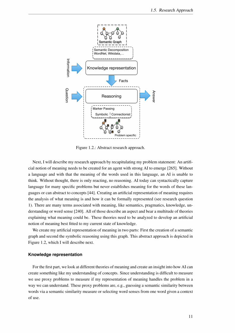
We create my artificial representation of meaning in two parts: First the creation of a semanticgraph and second the symbolic reasoning using this graph. This abstract approach is depicted inFigure 1.2, which I will describe next.

Knowledge representation

For the first part, we look at different theories of meaning and create an insight into how AI cancreate something like my understanding of concepts. Since understanding is difficult to measurewe use proxy problems to measure if my representation of meaning handles the problem in away we can understand. These proxy problems are, e.g., guessing a semantic similarity betweenwords via a semantic similarity measure or selecting word senses from one word given a contextof use.

11

1. Introduction

So my approach is to create a connectionist knowledge representation as a semantic graphconsisting of concepts and their relations, which will serve as a foundation for the represen-tation of meaning [95, 96, 98, 290, 373]. This knowledge representation represented as a se-mantic graph is based on a lexical decomposition [328]. Here the graph is created by lexicaldecomposition which breaks each concept semantically down until a set of semantic primes arereached. The primes are taken from the theory of the Natural Semantic Metalanguage [144, 407],which I have analyzed for their usefulness in formal languages [103]. Representing meaning asa graph is a connectionist way of AI, cognition, and linguistic researchers think about mean-ing [238, 256, 371].

The creation of a notion of artificial thoughts and with that, the representation of meaningis approached by giving an agent the ability to self-explain. This is done by including bothconnectionist and symbolic meaning: First, I use knowledge sources to create a semantic graph.I build this graph out of different knowledge sources like WordNet, Wiktionary, and BabelNET.Second, I use a Marker Passing algorithm to select relevant concepts out of this graph.

Reasoning

In the second part, I use this knowledge representation to extract facts about the given questionand use them to reason upon this knowledge. This is done by an algorithm encoding symbolicinformation on markers and specifying a set of rules how to move them over the semantic graphso that an interpretation of the resulting marked graph can answer my question about the givenproblem. I then use this approach to test its applicability in the experiments mentioned in Sec-tion 1.4 to answer research question 2. Upon this graph, Marker Passing [48, 99, 165, 167] isused to create the dynamic part of meaning representing thoughts [61]5.

The novelty of this approach is the automatic creation of a semantic graph and the MarkerPassing algorithm, where symbolic information is passed along relations from one concept toanother, which uses node and edge interpretation to guide its markers. The node and edgeinterpretation model the symbolic influence of certain concepts.

This doctoral thesis creates a notion of meaning combining the state-of-the-art knowledge ofnatural meaning with the symbolic and connectionist formalization of meaning for AI. Whetherthis representation of meaning really formalizes meaning has to be tested. Now we can ask if thehere selected experiments really represent problems which need strong AI to be solved. This canbe answered by looking at my second experiment which identifies Word Sense Disambiguation(WSD) — the differentiation of meaning of words — as a main problem of language understand-ing [5]. As an AI-complete problem WSD is a core problem of natural language understanding[179, 419]. Selecting the right word sense in a context of a sentence provides more informationthen guessing the semantic distance of two words, thus making the creation of a semantic dis-tance measure AI-complete as well. This argument can be extended to sentence similarity andwith that to my service matching and heuristic experiment. Therefore, solving such problemslets us evaluate my artificial representation of meaning.

5This approach is comparable to the way humans think in that it dynamically reasons about known concepts. Justlike the physical brain creates the basis for neural stimuli to activate.

12

2. Thesis Document

This chapter introduces the structure of the document (cf. Section 2.1) and list the contributions(cf. Section 2.2) that are provided within this dissertation.

2.1. Thesis Structure

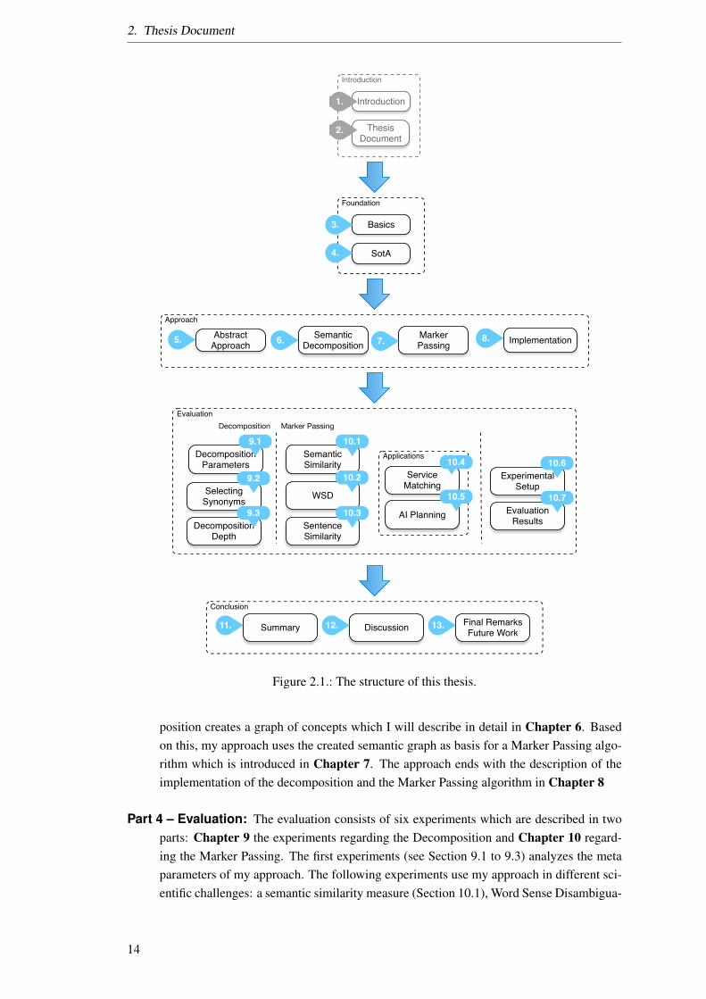
Now that we have a research approach, I can structure scientific endeavor. This section will givean overview of the thesis and explain why the research has been done in this order. Depicted inFigure 2.1 this thesis is structured in four logical parts:

Part 1 – Introduction: The first part introduces the problem and states my research questions,which is placed before this section in Section 1. This is done to form a common under-standing of the problem and scope of this thesis between reader and author. Easing thenavigation of the document, and letting the reader select the parts of interest to him/her,we have the current section which explains the organization of the thesis document inSection 2.

Part 2 – Foundation: The foundation establishes the basic terms used in this thesis in Chap-ter 3. The basic terms discussed in Chapter 3 start out with the definition of my fundamen-tal acting entity “Agent” in Section 3.1. Then we look at actions of agents in Section 3.2. Ithen describe how agents solve problems through “planning” with services in Section 3.3.my analysis continues with the description of the basic building blocks of ontologies agraph in Section 3.4 and the “concepts” in Section 3.5. Next, I describe my representa-tion of connectionist knowledge in form of “Ontologies” in Section 3.6. Since a conceptrepresents meaning, and can be interpreted in different ways, I describe how I will use“semantic” in Section 3.7. Because semantic meaning is independent of context and Iwant an agent to be able to represent pragmatic (context dependent) meaning I discusswhat I will use as context in Section 3.8. Afterwards, I discuss what is meant in this thesisby “meaning” in Section 3.9. In Section 3.10 I introduce the linguistic foundation of mysemantic theory called Natural Semantic Metalanguage (NSM).

We will analyze the different state-of-the-art of the different topics relevant to this thesisin Chapter 4, starting with semantic theories in Section 4.1. After this I look at formal-izations of semantic information in form of different ontologies in Section 4.2. I then havea look at the different semantic description languages in Section 4.3. Afterwards, I willlook at the state-of-the-art in the two main parts of my approach: the semantic decompo-sition in Section 4.4 and Marker Passing in Section 4.5. Because my use case on problemsolving is planning, I analyze the related work on AI planning in Section 4.6.

Part 3 – Approach: The approach is separated into four parts: A description of the abstractapproach will be provided in Chapter 5. This approach foresees that a semantic decom-

13

2. Thesis Document

Foundation

Basics

SotA

3.

4.

Approach

Abstract Approach5.

Semantic Decomposition6.

Marker Passing7. Implementation8.

Introduction

Introduction

Thesis Document

1.

2.

Conclusion

Summary11. Discussion12. Final Remarks Future Work

13.

Evaluation

Service Matching

AI Planning

Applications10.4

10.5

DecompositionParameters

9.1

Semantic Similarity

10.1

WSD

10.2

Sentence Similarity

10.3

Experimental Setup

10.6

Evaluation Results

10.7Selecting Synonyms

9.2

Decomposition Depth

9.3

Decomposition Marker Passing

Figure 2.1.: The structure of this thesis.

position creates a graph of concepts which I will describe in detail in Chapter 6. Basedon this, my approach uses the created semantic graph as basis for a Marker Passing algo-rithm which is introduced in Chapter 7. The approach ends with the description of theimplementation of the decomposition and the Marker Passing algorithm in Chapter 8

Part 4 – Evaluation: The evaluation consists of six experiments which are described in twoparts: Chapter 9 the experiments regarding the Decomposition and Chapter 10 regard-ing the Marker Passing. The first experiments (see Section 9.1 to 9.3) analyzes the metaparameters of my approach. The following experiments use my approach in different sci-entific challenges: a semantic similarity measure (Section 10.1), Word Sense Disambigua-

14

2.2. Contributions

tion (Section 10.2) or a Sentence Similarity Measure (Section 10.3). The experiments arefollowed by two experimental applications of my approach: The first experimental appli-cation is a Semantic Service Matchmaking described in Section 10.4, the second experi-mental application is a dynamic heuristic for service planning described in Section 10.5.

Part 5 – Conclusion: The conclusion summarizes the approach in Chapter 11, discusses theexperiments with respect to the research questions in Chapter 12 and provides a criticalreviews of my approach and an outlook into possible future work in Chapter 13.

2.2. Contributions

We can structure my scientific output by cutting the different parts into contributions. Thesecontributions will be discussed next. The main contribution of creating a theoretic sound rep-resentation of meaning can be split up into smaller contributions. To show the novelty of myapproach, I have surveyed technical semantic representation and analyzed their viability for mydomain. Creating the needed artificial representation of meaning presented hurdles, for instance,the acquisition of new facts had to be automated. The main contributions of this dissertation pro-vide an answer to the research questions formulated in Section 1.4 and are listed in the following:

Contribution 1. A formal representation of context-dependent meaning consisting of a semanticgraph and a Marker Passing algorithm.

Contribution 2. A semantic decomposition component that automatically creates a semanticgraph.

Contribution 3. A Marker Passing component that uses symbolic and connectionist informa-tion.

Contribution 4. An evaluation of my approach by comparison with the state-of-the-art basedon six different problems.

We base my contributions on the analyses of the applicability of NSM as a pragmatic meta-model for the utilization in service descriptions. Here I will outline an approach, able to createNSM-based context-dependent explanations which can be used by artificial reasoners to searchon it. One outcome is a context-dependent description of meaning which is my Contribution 1.

This work will compare different reasoning algorithms and their extension to cope with thenewly introduced concepts, eventually introducing a new approach to the creation of a semanticdecomposition algorithm in Contribution 2 and a reasoning algorithm which uses the so createdsemantic graph and builds Contribution 3. These two algorithms combined are compared to thestate-of-the-art in six AI challenges forming Contribution 4. Given these contributions, I canintegrate this thesis into the bigger picture of AI by comparing it w.r.t. existing contributions.

In conclusion, the following contributions can be drawn from this doctoral thesis: A newmeaning representation combining connectionism and symbolism is defined and automated inits creation. I extend the known Marker Passing algorithms and analyze their use for reasoning.This analysis gives insight into the notion of meaning and how it can be formalized to be usefulin AI research. I have published parts of this research [93, 94, 95, 96, 97, 98, 99, 100, 101, 102,103, 104].

15

Part II.

Foundations

17

3. Basic Terms and Concepts

To build a common ground on the terminology used, we will now look at the basic terms andconcepts used in our scientific strive. For that this chapter introduces relevant concepts fromthe fields of AI agents (Section 3.1), their actions and the relation to services (Section 3.2) andplanning (Section 3.3), formal descriptions of graphs (Section 3.4), the definition of concepts(Section 3.5) and ontologies (Section 3.6) as well as semantic representations (Section 3.7), anotion of context (Section 3.8), our notion of meaning (Section 3.9) and finally a short intro-duction to the Natural Semantic Metalanguage (Section 3.10). We will start out by looking atagents and AI Planning to understand the basic algorithms to compose actions into a plan andwith that understand why there are still problems in finding problem solutions through planning.We then look at the formal basis for our approach: Graphs and Ontologies. We use ontologies toencode semantic information. We, having ontologies as a basis, then discuss our understandingof semantic information, meaning, and context. The mixture of semantics and context brings usto an understanding of pragmatics.

We start with the definition of an agent since the fundamentally acting entity in this work iscalled agent.

3.1. Agents

Picking up the idea of Weiss [403, p. 3], agents are an approach to create more autonomous andintelligent software. The notion of an agent and the design paradigm of Multi-Agent SoftwareArchitectures [416] are well discussed in the related work. This section defines what we will useas a definition of an agent, which part of the agent will be further analyzed and how the agentsand services are interlinked to enable the transfer of semantic approaches to the agent world.

We concentrate on the deliberation part of the agent which selects a service1 executed next.This mechanism of an agent selects a service based on the information available to the agentwhich could be, e.g., the goal the agent wants to achieve. This mechanism is called planning orsometimes means end reasoning; meaning that the agent reasons about what service to performnext and its effect or its precondition, before executing it. Planning is a hard task for mosthumans and as the quote leading into this section of Weiss [403, p. 3] signifies: computer areeven worse at it. Pinpointing which part of the agent we are concerned with, we need to look atsome general definitions of agents and determine in which part of the agent the “reasoning” ishappening, being able to improve it.

Hayes-Roth [160] formulates the most fitting abstract definition of an agent. Here an agentacts continuously by:

Sense: Perception of the environment updating the knowledge of the agent.

1In the Agent community the services provided by agents are called actions. We use the word service to emphasizethe SOA part of an agent, where the action proposed by an agent can be seen as service.

19

3. Basic Terms and Concepts

Agent Environment

Act

SenseReason

Change

Figure 3.1.: Illustration of an agent in its environment.

Act: Acting as taking effect on the environment by executing services.

Reason: Reason with available information, e.g., the knowledge of the agent.

Figure 3.1 shows an abstract agent and its interplay with the environment. This definition ofagent is too broad and needs to be narrowed to grasp the aspects of agents used in this work.Since this work focuses on the reasoning part of the agent, we further focus on architecturesof agents concerned with the internal design of an agent, e.g., its service selection behavior.We see the reasoning as the mechanism which describes the inherent ability of the agent tochange his mental state. With a certain complexity of the reasoning of an agent, its ability torepresent meaning or act intelligently gets hard to prove. Because of this, we test such reasoningmechanisms through observation of the behavior of the agent [384].

We start out by separating natural from artificial agents. Artificial agents are agents which areman made, thus do not occur in nature with out the influence of higher intelligence like humanbeings. For example Cars, Robots and Software might fall into this category. Furthermore, sincewe are talking about software components, we reduce our definition of Agent to the virtual partof artificial agents. As a result, we restrict our notion of an agent to the definition of Wooldridgeand Jennings [417] who define an artificial “weak” software agent in more details by requestingthe following properties:

Autonomy: the agent can operate without interaction from some external or deterministicsource and can control his services and internal state.

Social ability: the agent can interact with other agents.

Reactivity: the agent can perceive the environment and adapt to change.

Pro-activeness: the agent has, in addition to reacting to the change in the environment, ini-tiative or goal-driven behavior.

We want an agent to have those properties since autonomy allows the agent to control itsbeliefs, social behavior allows the calling of other agents services, reactivity allows the agentto sense new concepts and reacts on service calls and finally pro-activity, so that the agent isable to plan and show goal driven behavior. We will especially postulate the social and pro-active properties of agents. On the one hand, we need agents to act together so that we can planincluding all of their services to achieve a given goal and on the other hand we need pro-activebehavior on the reasoning about the services descriptions of other agents.

20

3.1. Agents

With this definition, we can distinguish between software agents and software componentslike services which are not pro-active and autonomous. Looking at the variety of software whichhas been implemented using an agent paradigm, there are many different architectures whichestablish the properties of an agent differently [15]. However, all of them have in common, thatthe agent needs to interact with the environment through sensing and acting. We thus can stillbase our definition of an agent on Figure 3.1 to illustrate the notion of an agent.

Wooldridge and Jennings [417] further define a “strong notion of agency” as software whichhas the properties of the weak notion of an agent and also “...is either conceptualized or imple-mented by using concepts that are more usually applied to humans” [417, p. 117] like thinkingwhich again is similar to most AI principles, where human behavior is simulated. The strongnotion of agency is too abstract because being implemented with concepts to describe humanthinking introduces too many attributes, like a psychiatric disorder.

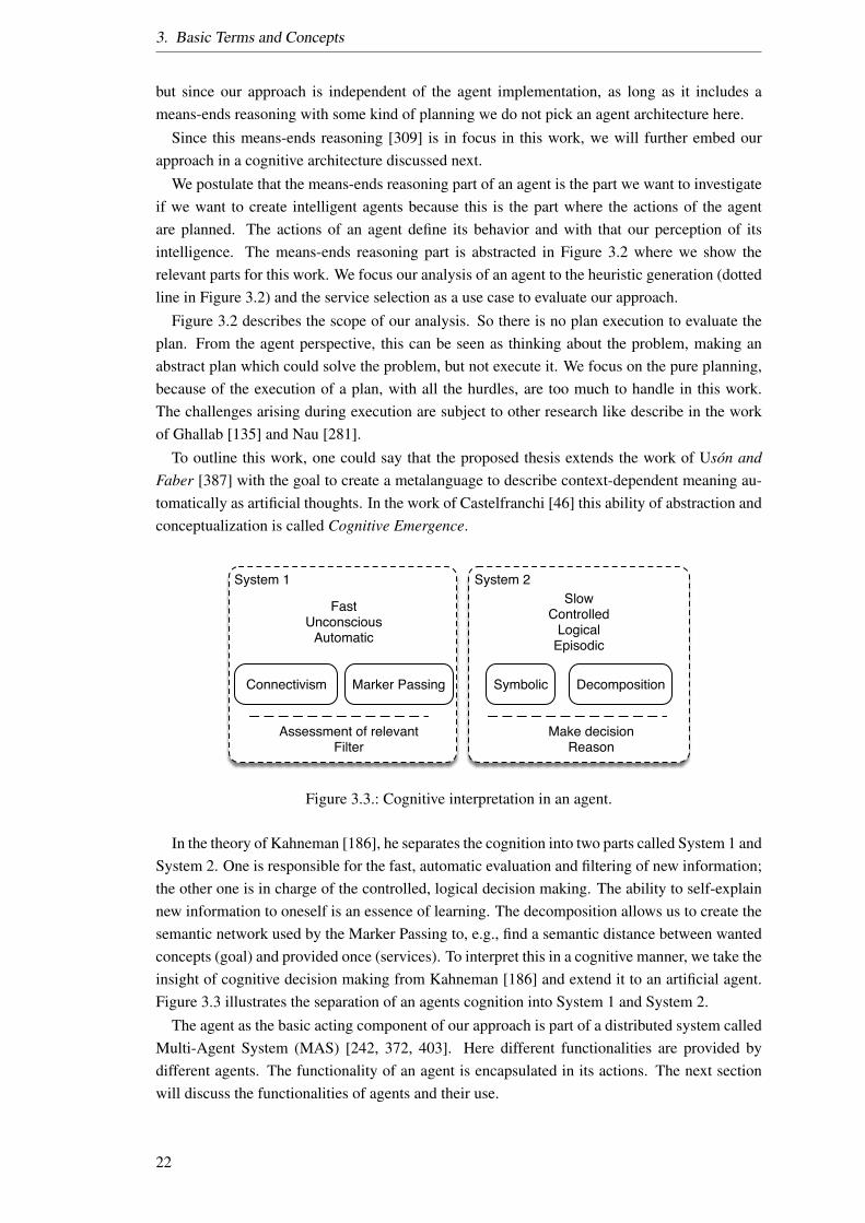
Intentions / GoalsOptions / possible Services

Plan

Means-ends Reasoning

Relevant Out of scope

Service selection

Service anlaysis

Heuristic generation

Initial state

state transition

state evaluation

goal reached

back tracking

Context

knowledge

Figure 3.2.: The rough architecture of the means-ends reasoning of an agent.

In addition to the requirements of Wooldridge and Jennings [417] we want an agent to be in-telligent, meaning to be able to find solutions for given problems on its own. With that autonomyis extended from the ability to make decisions on its own (autonomous, e.g., with a fixed set ofdecisions possibilities) and to create own decision possibilities (intelligent). Especially intelli-gence enables an agent to solve problems in a goal-directed way. Intelligent behavior mergesall the properties declared by Wooldridge and Jennings [417] in a way, that the adaption of theagent — in a proactive or reactive way — adapts towards a given goal of the agent. Conse-quently, an agent should be able to adapt existing plans or create new ones if necessary, leadingus to the planning problem which we see as one problem-solving method. Consequently, in thiswork, we try to make software agents more intelligent by giving them the ability to plan witha semantic and pragmatic understanding of service descriptions as service representations. Forthat, the representation of meaning in an artificial agent is subject to research, which leads us tothe analysis of formal information representations in the next section.

Weiss [403] identifies two general architectures for software agents: Belief-Desire-Intention(BDI) architecture [320] and Multi-Layer Agent which are discussed in Weiss [403] with theexample of TuringMachines [111] and InteRRaP [277]. There are many agent architectures [15],

21

3. Basic Terms and Concepts

but since our approach is independent of the agent implementation, as long as it includes ameans-ends reasoning with some kind of planning we do not pick an agent architecture here.

Since this means-ends reasoning [309] is in focus in this work, we will further embed ourapproach in a cognitive architecture discussed next.

We postulate that the means-ends reasoning part of an agent is the part we want to investigateif we want to create intelligent agents because this is the part where the actions of the agentare planned. The actions of an agent define its behavior and with that our perception of itsintelligence. The means-ends reasoning part is abstracted in Figure 3.2 where we show therelevant parts for this work. We focus our analysis of an agent to the heuristic generation (dottedline in Figure 3.2) and the service selection as a use case to evaluate our approach.

Figure 3.2 describes the scope of our analysis. So there is no plan execution to evaluate theplan. From the agent perspective, this can be seen as thinking about the problem, making anabstract plan which could solve the problem, but not execute it. We focus on the pure planning,because of the execution of a plan, with all the hurdles, are too much to handle in this work.The challenges arising during execution are subject to other research like describe in the workof Ghallab [135] and Nau [281].

To outline this work, one could say that the proposed thesis extends the work of Uson andFaber [387] with the goal to create a metalanguage to describe context-dependent meaning au-tomatically as artificial thoughts. In the work of Castelfranchi [46] this ability of abstraction andconceptualization is called Cognitive Emergence.

System 2

Symbolic

System 1

Connectivism

Slow Controlled

LogicalEpisodic

Fast Unconscious

Automatic

Make decisionReason

Assessment of relevantFilter

DecompositionMarker Passing

Figure 3.3.: Cognitive interpretation in an agent.

In the theory of Kahneman [186], he separates the cognition into two parts called System 1 andSystem 2. One is responsible for the fast, automatic evaluation and filtering of new information;the other one is in charge of the controlled, logical decision making. The ability to self-explainnew information to oneself is an essence of learning. The decomposition allows us to create thesemantic network used by the Marker Passing to, e.g., find a semantic distance between wantedconcepts (goal) and provided once (services). To interpret this in a cognitive manner, we take theinsight of cognitive decision making from Kahneman [186] and extend it to an artificial agent.Figure 3.3 illustrates the separation of an agents cognition into System 1 and System 2.

The agent as the basic acting component of our approach is part of a distributed system calledMulti-Agent System (MAS) [242, 372, 403]. Here different functionalities are provided bydifferent agents. The functionality of an agent is encapsulated in its actions. The next sectionwill discuss the functionalities of agents and their use.

22

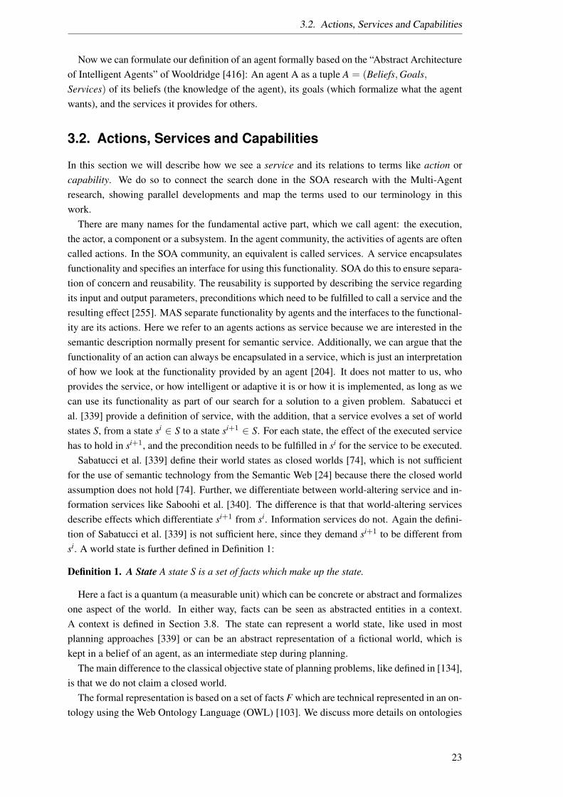
3.2. Actions, Services and Capabilities

Now we can formulate our definition of an agent formally based on the “Abstract Architectureof Intelligent Agents” of Wooldridge [416]: An agent A as a tuple A = (Beliefs,Goals,Services) of its beliefs (the knowledge of the agent), its goals (which formalize what the agentwants), and the services it provides for others.

3.2. Actions, Services and Capabilities

In this section we will describe how we see a service and its relations to terms like action orcapability. We do so to connect the search done in the SOA research with the Multi-Agentresearch, showing parallel developments and map the terms used to our terminology in thiswork.

There are many names for the fundamental active part, which we call agent: the execution,the actor, a component or a subsystem. In the agent community, the activities of agents are oftencalled actions. In the SOA community, an equivalent is called services. A service encapsulatesfunctionality and specifies an interface for using this functionality. SOA do this to ensure separa-tion of concern and reusability. The reusability is supported by describing the service regardingits input and output parameters, preconditions which need to be fulfilled to call a service and theresulting effect [255]. MAS separate functionality by agents and the interfaces to the functional-ity are its actions. Here we refer to an agents actions as service because we are interested in thesemantic description normally present for semantic service. Additionally, we can argue that thefunctionality of an action can always be encapsulated in a service, which is just an interpretationof how we look at the functionality provided by an agent [204]. It does not matter to us, whoprovides the service, or how intelligent or adaptive it is or how it is implemented, as long as wecan use its functionality as part of our search for a solution to a given problem. Sabatucci etal. [339] provide a definition of service, with the addition, that a service evolves a set of worldstates S, from a state si ∈ S to a state si+1 ∈ S. For each state, the effect of the executed servicehas to hold in si+1, and the precondition needs to be fulfilled in si for the service to be executed.

Sabatucci et al. [339] define their world states as closed worlds [74], which is not sufficientfor the use of semantic technology from the Semantic Web [24] because there the closed worldassumption does not hold [74]. Further, we differentiate between world-altering service and in-formation services like Saboohi et al. [340]. The difference is that that world-altering servicesdescribe effects which differentiate si+1 from si. Information services do not. Again the defini-tion of Sabatucci et al. [339] is not sufficient here, since they demand si+1 to be different fromsi. A world state is further defined in Definition 1:

Definition 1. A State A state S is a set of facts which make up the state.

Here a fact is a quantum (a measurable unit) which can be concrete or abstract and formalizesone aspect of the world. In either way, facts can be seen as abstracted entities in a context.A context is defined in Section 3.8. The state can represent a world state, like used in mostplanning approaches [339] or can be an abstract representation of a fictional world, which iskept in a belief of an agent, as an intermediate step during planning.

The main difference to the classical objective state of planning problems, like defined in [134],is that we do not claim a closed world.

The formal representation is based on a set of facts F which are technical represented in an on-tology using the Web Ontology Language (OWL) [103]. We discuss more details on ontologies

23

3. Basic Terms and Concepts

in Section 3.6.The facts f ∈ F which make up the state Si are subjective to the agent i believing fact f . The

facts making up Si are subjective2, since from another perspective or in other contexts, factsmight differ in their evaluation. This means that not only the selection of facts describing a statebut also their manifestation may differ from agent to agent.

Let S be the set of states of the environment and let Services = s1 . . . sn be the set of servicesof an agent. We argue that we are not interested in the service implementation itself but ratherin the functionality it provides. Thus, we define a service with its service description. Martin etal. define a service si as a sextuple in the manner of an OWL-S description [255]. We adopt thisdefinition as follows:

Definition 2. A service si := (Input, Output, Precondition, Effect, Name, Description).

The Input, Output, Precondition, and Effect (IOPE) are equivalent to the profile of an OWL-SService profile [255]. Here the input describes the information needs of the agent to perform aservice, and the output describes the change done by the service. The precondition and effect, onthe other hand, describes the state change the service might invoke. The name and the descriptionof a service natural language description of the functionality the service encapsulates. Since,this so-called “profile” of a service, describes what it can do we will have a closer look at it,to determine if this description of a service can help the agent to think about the service andto decide to execute the service, or not. The name of a service is the natural language name ofthe service, e.g., ”BookFlightService”. The description is a natural language description of theservice thought for humans.

Here the input describing the required information, objects (individuals), all parameters of theservice needs to be executed.

Definition 3. Input parameters are a set Input of facts Input = i1 . . . in.

These facts3 making up the inputs can be abstract in the form of free variables or concrete asin grounded statements on individuals4. All input parameters are a subclass of the more generalclass parameter. Listing 3.1 illustrates the OWL-S definition of a parameter.

Listing 3.1: Definition of the OWL parameter class.

<owl:Class rdf:ID="Parameter">

<rdfs:subClassOf>

<owl:Restriction>

<owl:onProperty rdf:resource="#parameterType" />

<owl:minCardinality

rdf:datatype="&xsd;#nonNegativeInteger">1</owl:minCardinality>

</owl:Restriction>

</rdfs:subClassOf>

</owl:Class>

<owl:Class rdf:about="#Parameter">

<rdfs:subClassOf rdf:resource="&swrl;#Variable"/>

2This means the facts depend on the beliefs of the agent.3The inputs describes restricted facts which we reduce to class assertions.4Individuals are further discussed in Section 3.6.

24

3.2. Actions, Services and Capabilities

</owl:Class>

<owl:Class rdf:ID="Input">

<rdfs:subClassOf rdf:resource="#Parameter"/>

</owl:Class>

<owl:DatatypeProperty rdf:ID="parameterType">

<rdfs:domain rdf:resource="#Parameter"/>

<rdfs:range rdf:resource="&xsd;anyURI"/>

</owl:DatatypeProperty>

Listing 3.1 describes the parameter class, which has a parameter type with a cardinality of one.This parameter is a variable and the input. The parameter type is given (here with the example“anyURI”), which describes that the “Variable” is of this parameter type. The “parameter type”is defined as “DatatypeProperty” which describes a domain and a range. The domain and rangedefined which type of facts are connected with this “parameterType” relation.

The output is the optional return values of a service. It is similarly defined to the input param-eters:

Definition 4. Output parameters are a set Output of facts Output = o1 . . . on.

Like for the input parameters the output parameters are defined as a subclass of OWL param-eters as shown in Listing 3.2.

Listing 3.2: Definition of the OWL-S output parameter class.<owl:Class rdf:ID="Output">

<rdfs:subClassOf rdf:resource="#Parameter"/>

</owl:Class>

Listing 3.2 shows the change from an input to an output parameter. The rest of the descriptionwould be similar to Listing 3.1.

As an example of a service description, the interested reader can look at one example servicefrom the Semantic Service Selection (S3) Contest5.

Definition 5. Preconditions are a set Precondition of SWRL rules Precondition = p1 . . . pn.

OWL-S describes the precondition and effect in the Semantic Web Rule Language (SWRL).These rules are made of the form: Body→Head, which means that if the body evaluates to truethe head is executed. The precondition describes a set of conditions which have to be fulfilled (inthe current state) for the service to be executable. Such a condition can be formulated as a rule[175] without a head. The semantic here is that if the body of the rule holds, then the service canbe executed. Therefore we define preconditions with an empty head, because we want nothingto be changed by the rule in our ontology6.

Similar to the preconditions of a service, the effect of a service describes which facts arefulfilled after the execution of the service.

Definition 6. Effects are a set Effect of SWRL rules Effect = e1 . . . en.5see: http://www-ags.dfki.uni-sb.de/˜klusch/s3/ last visited: 22.07.20176Because the SWRL specification states that if a rule has an empty head, the rule is only true if all facts in the body

of the rule are evaluated to false, we fill the head of a precondition with a fictional fact, which states somethinglike the rule is fulfilled.

25

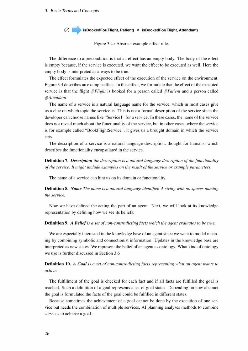
3. Basic Terms and Concepts

? isBookedFor(Flight, Patient) isBookedFor(Flight, Attendant)

v

Figure 3.4.: Abstract example effect rule.

The difference to a precondition is that an effect has an empty body. The body of the effectis empty because, if the service is executed, we want the effect to be executed as well. Here theempty body is interpreted as always to be true.

The effect formulates the expected effect of the execution of the service on the environment.Figure 3.4 describes an example effect. In this effect, we formulate that the effect of the executedservice is that the flight #Flight is booked for a person called #Patient and a person called#Attendant.

The name of a service is a natural language name for the service, which in most cases giveus a clue on which topic the service is. This is not a formal description of the service since thedeveloper can choose names like “Service1” for a service. In these cases, the name of the servicedoes not reveal much about the functionality of the service, but in other cases, where the serviceis for example called “BookFlightService”, it gives us a brought domain in which the serviceacts.

The description of a service is a natural language description, thought for humans, whichdescribes the functionality encapsulated in the service.

Definition 7. Description the description is a natural language description of the functionalityof the service. It might include examples on the result of the service or example parameters.

The name of a service can hint us on its domain or functionality.

Definition 8. Name The name is a natural language identifier. A string with no spaces namingthe service.

Now we have defined the acting the part of an agent. Next, we will look at its knowledgerepresentation by defining how we see its beliefs:

Definition 9. A Belief is a set of non-contradicting facts which the agent evaluates to be true.

We are especially interested in the knowledge base of an agent since we want to model mean-ing by combining symbolic and connectionist information. Updates in the knowledge base areinterpreted as new states. We represent the belief of an agent as ontology. What kind of ontologywe use is further discussed in Section 3.6

Definition 10. A Goal is a set of non-contradicting facts representing what an agent wants toachive.

The fulfillment of the goal is checked for each fact and if all facts are fulfilled the goal isreached. Such a definition of a goal represents a set of goal states. Depending on how abstractthe goal is formulated the facts of the goal could be fulfilled in different states.

Because sometimes the achievement of a goal cannot be done by the execution of one ser-vice but needs the combination of multiple services, AI planning analyses methods to combineservices to achieve a goal.

26

3.3. Planning

3.3. Planning

This section will describe planning as a problem-solving method. Since this work will not en-gage in defining a new planning algorithm, we will only look at state space planning to motivatewhich information is available for the creation of a heuristic.

Planning represents a problem-solving approach; where we think about how to solve a prob-lem by determining which services we can use to solve the problem. By ordering the availableservice and choosing the right input parameters, planning tries to find a combination of servicesto reach a goal state.

A planning problem is formalized in the following way based on the description of a statetransition system given in [134, p. 17]:

Definition 11. A planning problem P = (S, A, γ, sstart, sgoal) with,

S = s1, s2, . . . a finite or recursively enumerable set of states,

A = a1, a2, . . . a finite or recursively enumerable set of services,

γ: S× A→ S a state transition function,

sstart: an initial state, and

sgoal: a goal state.

The goal here, since it is a state, is a set of facts. It encodes all states in which these facts aretrue. We can imagine this planning problem as a directed graph, where the services determinewhich state is connected to which state by the state transition function. We changed the definitionfrom [134] to fit the terminology here. Since actions of agents are services to us, we call theactions here services as well.

For the use of services of other agents, the agents need to describe their services to eachother, so that they can evaluate if the service might be useful to them. To do that the agentneeds, on the one hand, a formalization of meaning in its beliefs, goals, and functionality needsand on the other a semantic description of the services. Both are described by using semanticrepresentations of meaning like ontologies.

3.4. Graphs

This section defines attributed typed graphs with node type inheritance. We will use this for-malism as a basis for representing semantic networks in Section 6 and 7. The definitions in thissection are taken from De Lara et al [66]. We start with the definition of a graph, consisting ofsets of nodes and edges and a source and target function.

Definition 12 (Graph (Definition 1 in [66])). A graph G = (V,E, s, t) with a set V of nodes anda set E of edges and a source and target function s, t : E → V

The nodes represent the vertices of the graph and the edges represent the lines between thenodes. The two functions s and t give the edges a direction by assigning a node as target andsource to each edge. Giving two graphs a graph morphism maps the nodes and edges of onegraph onto another graph by preserving the structures of the first graph. Like in De Lara etal. [66] we define a e-graph morphism in the following way:

27

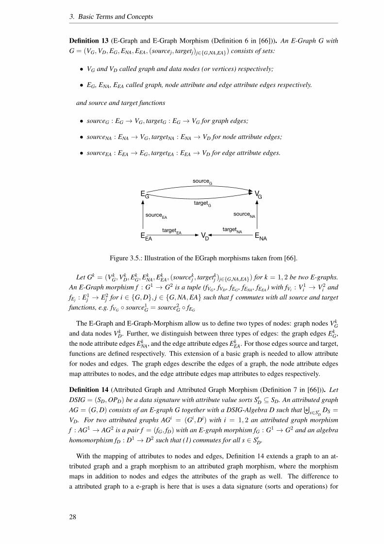
3. Basic Terms and Concepts

Definition 13 (E-Graph and E-Graph Morphism (Definition 6 in [66])). An E-Graph G withG = (VG,VD,EG,ENA,EEA, (sourcej, targetj)j∈G,NA,EA) consists of sets:

• VG and VD called graph and data nodes (or vertices) respectively;

• EG, ENA, EEA called graph, node attribute and edge attribute edges respectively.

and source and target functions

• sourceG : EG → VG, targetG : EG → VG for graph edges;

• sourceNA : ENA → VG, targetNA : ENA → VD for node attribute edges;

• sourceEA : EEA → EG, targetEA : EEA → VD for edge attribute edges.

VG

ENA

EG

EEA VD

sourceG

targetG

sourceEA

targetEA targetNA

sourceNA

Figure 3.5.: Illustration of the EGraph morphisms taken from [66].

Let Gk = (VkG,V

kD,E

kG,E

kNA,E

kEA, (sourcek

j , targetkj )j∈G,NA,EA) for k = 1, 2 be two E-graphs.

An E-Graph morphism f : G1 → G2 is a tuple (fVG , fVD , fEG , fENA , fEEA) with fVi : V1i → V2

i andfEj : E1

j → E2j for i ∈ G,D, j ∈ G,NA,EA such that f commutes with all source and target

functions, e.g. fVG source1G = source2

G fEG

The E-Graph and E-Graph-Morphism allow us to define two types of nodes: graph nodes VkG

and data nodes VkD. Further, we distinguish between three types of edges: the graph edges Ek

G,the node attribute edges Ek

NA, and the edge attribute edges EkEA. For those edges source and target,

functions are defined respectively. This extension of a basic graph is needed to allow attributefor nodes and edges. The graph edges describe the edges of a graph, the node attribute edgesmap attributes to nodes, and the edge attribute edges map attributes to edges respectively.

Definition 14 (Attributed Graph and Attributed Graph Morphism (Definition 7 in [66])). LetDSIG = (SD,OPD) be a data signature with attribute value sorts S′D ⊆ SD. An attributed graphAG = (G,D) consists of an E-graph G together with a DSIG-Algebra D such that

⊎s∈S′D

DS =

VD. For two attributed graphs AGi = (Gi,Di) with i = 1, 2 an attributed graph morphismf : AG1 → AG2 is a pair f = (fG, fD) with an E-graph morphism fG : G1 → G2 and an algebrahomomorphism fD : D1 → D2 such that (1) commutes for all s ∈ S′D.

With the mapping of attributes to nodes and edges, Definition 14 extends a graph to an at-tributed graph and a graph morphism to an attributed graph morphism, where the morphismmaps in addition to nodes and edges the attributes of the graph as well. The difference toa attributed graph to a e-graph is here that is uses a data signature (sorts and operations) for

28

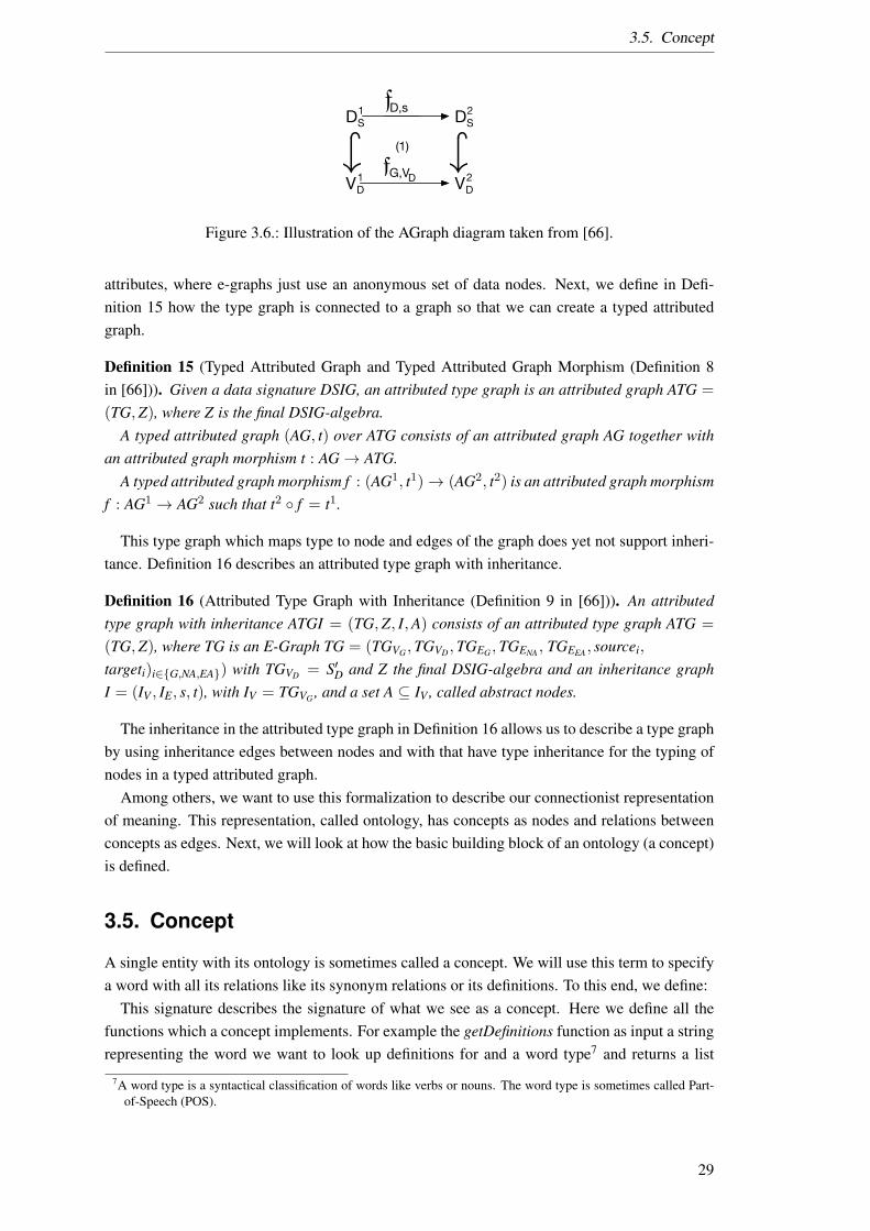
3.5. Concept

DS1 DS

2

VD1 VD

2

(1)

,!,! fD,s

fG,VD

Figure 3.6.: Illustration of the AGraph diagram taken from [66].

attributes, where e-graphs just use an anonymous set of data nodes. Next, we define in Defi-nition 15 how the type graph is connected to a graph so that we can create a typed attributedgraph.

Definition 15 (Typed Attributed Graph and Typed Attributed Graph Morphism (Definition 8in [66])). Given a data signature DSIG, an attributed type graph is an attributed graph ATG =

(TG, Z), where Z is the final DSIG-algebra.A typed attributed graph (AG, t) over ATG consists of an attributed graph AG together with

an attributed graph morphism t : AG→ ATG.A typed attributed graph morphism f : (AG1, t1)→ (AG2, t2) is an attributed graph morphism

f : AG1 → AG2 such that t2 f = t1.

This type graph which maps type to node and edges of the graph does yet not support inheri-tance. Definition 16 describes an attributed type graph with inheritance.

Definition 16 (Attributed Type Graph with Inheritance (Definition 9 in [66])). An attributedtype graph with inheritance ATGI = (TG, Z, I,A) consists of an attributed type graph ATG =

(TG, Z), where TG is an E-Graph TG = (TGVG , TGVD , TGEG , TGENA , TGEEA , sourcei,

targeti)i∈G,NA,EA) with TGVD = S′D and Z the final DSIG-algebra and an inheritance graphI = (IV , IE, s, t), with IV = TGVG , and a set A ⊆ IV , called abstract nodes.

The inheritance in the attributed type graph in Definition 16 allows us to describe a type graphby using inheritance edges between nodes and with that have type inheritance for the typing ofnodes in a typed attributed graph.

Among others, we want to use this formalization to describe our connectionist representationof meaning. This representation, called ontology, has concepts as nodes and relations betweenconcepts as edges. Next, we will look at how the basic building block of an ontology (a concept)is defined.

3.5. Concept

A single entity with its ontology is sometimes called a concept. We will use this term to specifya word with all its relations like its synonym relations or its definitions. To this end, we define:

This signature describes the signature of what we see as a concept. Here we define all thefunctions which a concept implements. For example the getDefinitions function as input a stringrepresenting the word we want to look up definitions for and a word type7 and returns a list

7A word type is a syntactical classification of words like verbs or nouns. The word type is sometimes called Part-of-Speech (POS).

29

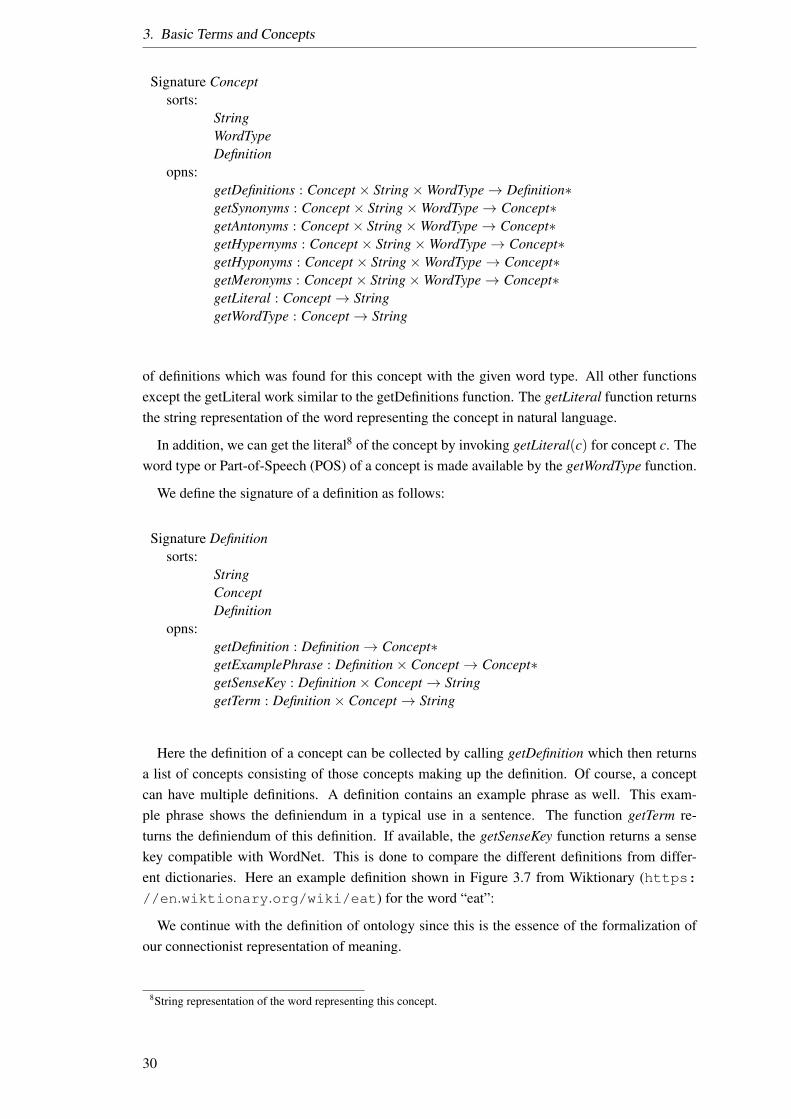
3. Basic Terms and Concepts

Signature Conceptsorts:

StringWordTypeDefinition

opns:getDefinitions : Concept × String×WordType→ Definition∗getSynonyms : Concept × String×WordType→ Concept∗getAntonyms : Concept × String×WordType→ Concept∗getHypernyms : Concept × String×WordType→ Concept∗getHyponyms : Concept × String×WordType→ Concept∗getMeronyms : Concept × String×WordType→ Concept∗getLiteral : Concept→ StringgetWordType : Concept→ String

of definitions which was found for this concept with the given word type. All other functionsexcept the getLiteral work similar to the getDefinitions function. The getLiteral function returnsthe string representation of the word representing the concept in natural language.

In addition, we can get the literal8 of the concept by invoking getLiteral(c) for concept c. Theword type or Part-of-Speech (POS) of a concept is made available by the getWordType function.

We define the signature of a definition as follows:

Signature Definitionsorts:

StringConceptDefinition

opns:getDefinition : Definition→ Concept∗getExamplePhrase : Definition× Concept→ Concept∗getSenseKey : Definition× Concept→ StringgetTerm : Definition× Concept→ String

Here the definition of a concept can be collected by calling getDefinition which then returnsa list of concepts consisting of those concepts making up the definition. Of course, a conceptcan have multiple definitions. A definition contains an example phrase as well. This exam-ple phrase shows the definiendum in a typical use in a sentence. The function getTerm re-turns the definiendum of this definition. If available, the getSenseKey function returns a sensekey compatible with WordNet. This is done to compare the different definitions from differ-ent dictionaries. Here an example definition shown in Figure 3.7 from Wiktionary (https://en.wiktionary.org/wiki/eat) for the word “eat”:

We continue with the definition of ontology since this is the essence of the formalization ofour connectionist representation of meaning.

8String representation of the word representing this concept.

30

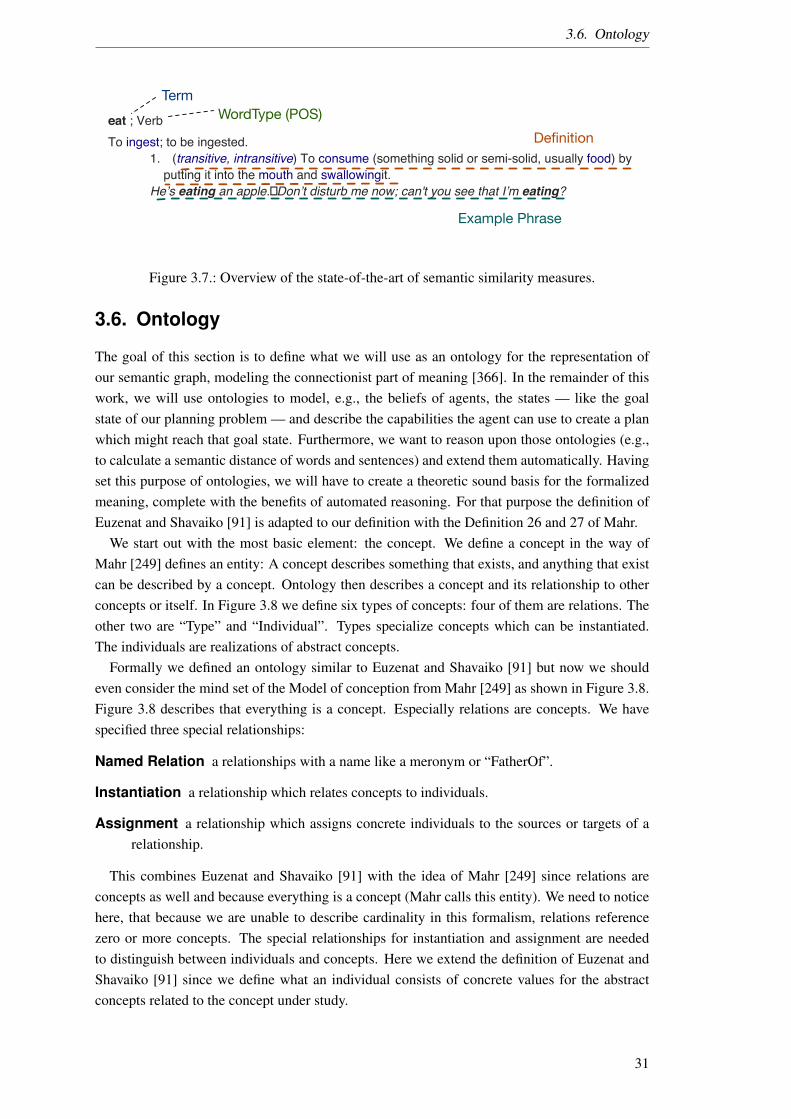
3.6. Ontology

eat ; VerbTo ingest; to be ingested.

1. (transitive, intransitive) To consume (something solid or semi-solid, usually food) by putting it into the mouth and swallowingit.

He’s eating an apple.  Don’t disturb me now; can't you see that I’m eating?

Example Phrase

TermWordType (POS)

Definition

Figure 3.7.: Overview of the state-of-the-art of semantic similarity measures.

3.6. Ontology

The goal of this section is to define what we will use as an ontology for the representation ofour semantic graph, modeling the connectionist part of meaning [366]. In the remainder of thiswork, we will use ontologies to model, e.g., the beliefs of agents, the states — like the goalstate of our planning problem — and describe the capabilities the agent can use to create a planwhich might reach that goal state. Furthermore, we want to reason upon those ontologies (e.g.,to calculate a semantic distance of words and sentences) and extend them automatically. Havingset this purpose of ontologies, we will have to create a theoretic sound basis for the formalizedmeaning, complete with the benefits of automated reasoning. For that purpose the definition ofEuzenat and Shavaiko [91] is adapted to our definition with the Definition 26 and 27 of Mahr.

We start out with the most basic element: the concept. We define a concept in the way ofMahr [249] defines an entity: A concept describes something that exists, and anything that existcan be described by a concept. Ontology then describes a concept and its relationship to otherconcepts or itself. In Figure 3.8 we define six types of concepts: four of them are relations. Theother two are “Type” and “Individual”. Types specialize concepts which can be instantiated.The individuals are realizations of abstract concepts.

Formally we defined an ontology similar to Euzenat and Shavaiko [91] but now we shouldeven consider the mind set of the Model of conception from Mahr [249] as shown in Figure 3.8.Figure 3.8 describes that everything is a concept. Especially relations are concepts. We havespecified three special relationships:

Named Relation a relationships with a name like a meronym or “FatherOf”.

Instantiation a relationship which relates concepts to individuals.

Assignment a relationship which assigns concrete individuals to the sources or targets of arelationship.

This combines Euzenat and Shavaiko [91] with the idea of Mahr [249] since relations areconcepts as well and because everything is a concept (Mahr calls this entity). We need to noticehere, that because we are unable to describe cardinality in this formalism, relations referencezero or more concepts. The special relationships for instantiation and assignment are neededto distinguish between individuals and concepts. Here we extend the definition of Euzenat andShavaiko [91] since we define what an individual consists of concrete values for the abstractconcepts related to the concept under study.

31

3. Basic Terms and Concepts

Relation

Concept- Literal: String

Refernce- Name: String

Individual

Assignment source

target Instantiationtarget

source

Named Relation

Typesource

target

InheritanceRelates

Figure 3.8.: Type graph of our ontology definition.

3.7. Semantic

Semantics, in general, is the theory studying the meaning of symbols [240]. For computerscience, on the other hand, semantics can be understood as an enrichment of data with meta-information, for example, to describe the meaning of words used in a programming language.Here the meaning of the word of the programming language is defined by the calculation acomputer will do when seeing that word. For natural language, this meta-information can beformalized in an ontology represented in abstract conceptualization. For more details, pleasesee Section 3.6.

Semantics for formal languages can be seen as an investigation of the interpretation of theformal statements making up something formulated in this language like an ontology. Meaningcan be used in a wide range, whenever a reasoner tries to understand a relationship of entitiesor, e.g., action might have a meaning as well. However, this work focuses on the meaning ofconcepts. In this regard semantic is a linguistic area concerned with the meaning of words orutterances. We define semantic meaning as in compliance with [45, 240]:

Definition 17. Semantic is the context independent meaning of concepts.

To establish our notion of meaning, we analyze different semantic theories in Section 4.1 togain insight into how meaning is formalized, how it can be used and which inference is possiblewith each of these theories. For that, we want a formalization of symbolic and connection-ist meaning which can represent meaning in an expressiveness of natural language and still istractable for the reasoning done upon it as well as for us working with it. This means semanticinformation is the information a reasoner can extract from an utterance without knowledge ex-tending the syntax. For example the sentence “Ich bin ein Berliner” (engl. I am a Berliner9) canbe analyzed in the following way: There is a speaker (here the denoted by the “I”) who sees him-self as part of the group with the name “Berliner”. The German grammar additionally allows theconclusion that the speaker is a male because of the use of “ein”. This completes the semanticanalysis. The meaning for which this sentence has become famous: “We as America (Capi-

9An utterance made by U.S. President John F. Kennedy on June 26, 1963

32

3.8. Context

talists) stand beside you (Germany) in the fight against the UdSSR (Communist), and we willsupport you (also capitalists),” is only extractable with a vast amount of contextual information.

The problem with the contextual information is that the uttering agent and the listening agent10

might have different contexts like depicted in Figure 4.1 on Page 48. In linguistics, the contextof the uttering agent is called “Außerungskontext” (context at utterance) [240]. The semanticof the utterance itself is called “Ausdrucksbedeutung” (meaning of the utterance) which is themeaning of the utterance with the addition of relevant facts form the context at utterance [240, p.11]. The pragmatic (context depending meaning) can then be seen to build up on the semanticmeaning in the “Kommunikativer Sinn” (the wanted effect of the communication of the speechact) [240]. The receiving part from the view of the uttering agent is the effect the uttering agentwanted to create in the listening agents.

The semantic information does not have this problem because it describes the meaning of theconcepts used in the utterance in general. Thus, it is not context dependent. The problem here isthat now we need to describe the meaning of every concept we encounter. The question here is:Can we create a semantic where we do not have to describe the semantic of each word, but deriveit. The semantic part of our artificial representation of meaning thus needs to be wisely chosen tobe able to represent these three layers (Semantic, Syntax, and Pragmatic) of meaning. FollowingTarski [377] a sufficiently expressive language can define its semantic in itself. Leading to thequestion of how expressive our language has to be, to be used in the artificial representation ofmeaning.

3.8. Context

Context has many definitions and is often used to describe all information available. One ofthe basics for defining context is the work of Dey [71]. Dey uses “relevance” of informationto “describe a situation of an entity” as criteria for the definition of context. This is a vaguedefinition since it lets us not distinguish between other information since all relevant informationbecomes contextual information. Here it becomes important to describe what relevance means,which is a other research question [385].

The context in Natural Language Understanding is often interpreted as the words surround-ing a target word or in distributed models (with word embedding) the concurrence of a wordwith another word in texts in a given window [39]. The size of the context then is subject todiscussion [270].

Miller [270] defined a linguistic context as a set of sounding words in which a concept canbe used. This is sometimes referred to as Topical Context [270]. Here the vocabulary used todiscuss a topic provides additional information to the creation of meaning.

In this work we use the Model of Conception of Mahr [250] as a formal representation ofcontext. This section is meant for a short introduction of the notion of context used in this workso that we can understand the problem statement in Section 1.2. For further details Section 3.8describes the notion of context in more detail.

To illustrate how we will use context in this work we will now look at an example of contextualinformation in our use case: A taxi calling service which takes two locations as input, the startingaddress, and the destination address.

10Here listening agent is not restricted to audio signal but means the receiver of an abstract message.

33

3. Basic Terms and Concepts

Service Consumer

Domain

Relevant Information

User

Service

Subject

Object

Context

SeMa2

DynamicDerived

Conception

Figure 3.9.: Illustration of a context in regard to an object using the example of a service and itsconsumers.

For service planning an action selection component is needed. This action selection compo-nent selects the best fitting service for a given request. Depending on the contextual informationgiven, let’s say the location of the user, different services can be selected. As shown in Figure 3.9the service is conceived by a subject — in this case, the Service consumer or an service matchercalled SeMa2 — and the relevant information of this service the location of the user makes upthe context. Figure 3.9 illustrates the transferred model of conception as one definition of contextfrom Mahr [250] by using an example of a service.

Definition 18. Conception

1. A Conception is a relationship consisting of three entities:

• An entity called subject of the conception

• An entity called object of the conception

• A complex called the context of the conception

2. The content of a conception is a complex consisting of the relationships of the context, ofwhich the object of the conception is an element of.

This can be imagined as an observer (the subject) observing an entity (the content) which ismade up of the object and the context surrounding this object (all entities which stand about theobject). The conception, therefore, is something like a perspective and depending on the subjectthe object might appear in a different context. If an entity (or for our purpose a concept) is partof different conceptions, the context regarding the subject might change. In consequence, oneobject can be part of multiple contexts. An example of such a construction is the meaning ofa word, from the view of a speaker and a listener. An effect of different contexts for the wordcould be a misunderstanding. For structure with multiple conceptions Mahr [250] has definedthe term: Universe

Definition 19. Universe:

3. A universe is a complex to which with every entity which belongs to the universe, a con-ception belongs to it as well, which has this entity as content.

4. A universe is called reflexive, if it belongs to itself.

34

3.9. Meaning

A universe, therefore, is everything which is part of a conception. In our example the follow-ing three components are part of the universe: the word uttered by the speaker, the speaker andthe listener and the context of all three. From these definitions we can extract the definition of acontext as follows:

Definition 20. A context is a subset C of complexes.

C is the set of complex with C ⊂ E where E is the set of entities.

A is the set of conception (german: “Auffassung”) with A ⊂ R where R is the set of relations.

⊆ is a relation over (E × E) ∪ (R× R)) denoting if an entity is part of the relationship orentity called ’belongs to’.

As argued above, semantic concepts as part of a description of a service can be extended toreflect the changes in context. This could, for example, happen if the viewpoint of the subjectchanges. In a connectionist view point, the meaning of an entity is defined by its relationships toother entities leading to the conclusion that the context of a conception defines the meaning of itsobject. This context-dependent meaning can be seen like the pragmatic extension of semantics inlinguistics. Coleman et al. [57] notice that within communication between agents which are notcontext aware, the meaning cannot extend beyond the meaning explicitly carried by the message.Thus, the meaning needs to be predefined or explained within the message, which forms the cruxof this approach. Following the argumentation of Robertson [330] adaptive software requiresknowledge of the context as in: “what does the application/capability do?”, how to react/adaptto change and runtime support for detecting change as well as modifying parameters to adaptto that change. On the one hand contextual meaning can be seen to be twofold: First, wecan define abstract domain specific meaning, e.g., if we are talking about opening somethingin the smart home domain we talk about windows and doors. Second, during runtime, theabstract values have to be filled with concrete contextual information, e.g., this sensor measuresif door A is open. With context-aware communicating agents, context-dependent meaning mightchange over time, since the context may change. Figure 3.9 illustrates the transferred model ofconception as one definition of context from Mahr [250] by using an example of a service.

3.9. Meaning

Since the main goal of this doctoral thesis is to formalize meaning of an AI to use, this sectionanalyzes the different definition of meaning. The goal of this section is too close the knowledgegap about meaning. Then we are able to answer our first research questions so that the approachto represent meaning selected in this thesis can be understood.

From the point of view of Minsky [273], we will use two aspects of meaning in this doctoralthesis:

Definition 21. Connectionist meaning of a concept (definiendum) is given thought its definitionsand other concepts it stands in relation with.

Based on the Meaning Text Theory [262] the Definition 21 of the scope of meaning we in-terpret conceptual meaning as context-dependent since the definiendum might have relationsto contextual concepts. This can be seen in an example like the concept “grandma” which in

35

3. Basic Terms and Concepts

my context has the relation “reference to” connecting to my two grandmas and since the readermost likely does not know my grandmothers, it will reference other persons in the readers con-text. Even though we might have the same definition of a grandmother in our semantic repre-sentation, they are used differently. This part of meaning is represented by our second part ofmeaning:

Definition 22. Symbolic meaning of a concept (definiendum) is given thought the use of theconnectionist representation of meaning with a pragmatic reasoning algorithm.

This second part of our artificial representation of meaning described in Definition 22 rep-resents the symbolic view on meaning. Looking at our “grandma” example, even though wehave the same definition of grandmother representing our concept of grandma, the way we thinkabout it differs, e.g., with the contextual concepts activated regarding the grandma concept likecake or elderly. Depending on those contextual concepts our meaning of “grandma” changes.This change might be from happy situations with coffee to sad situations in hospitals.

The remainder of this section is spent discussing why we have selected our definition ofmeaning like described in Definition 21 and 22 and a concludes our view of meaning.

There are many definitions of meaning. This section states our view of meaning and discussesdifferent views meaning. The goal of this section is to grasp the notion of meaning formally. Wewill see that not one single definition of meaning fits and that we need to switch from measuring“the right meaning” to e.g. “the same meaning” or “a different meaning”. To identify thedefinition of meaning; we look at the study of language because we are interested in the meaningof words and text not images or events. Meaning is often seen as something virtual, like an“idea” or a “thought” rather concrete objects which are referenced by an utterance [297]. Sincemeaning seems not to be an inherent property of things, the meaning is formed by observingthings and within the head of the observer. This makes meaning a subjective matter whichmight be subject to change since we do not stop observing and with each observation, theremight by new information which lets us change our preformed meaning about something. Thedefinition of the term “meaning” needs further investigation into the different fields of researchwhich meaning is subject of. In this section, we will look at different definitions of meaning tocrystallize how we define meaning of words by comparing them.

The philosophical meaning has been discussed in a multitude of publications [136]. Some ofthem discuss the location of meaning from being inside ones head to being part of nature in theobjects which are referenced by concepts [124] or as part of the communication act [414]. ForWittgenstein, the use of language as well as the use in the specific speech act itself representsthe meaning. Grice [151] separates the “conventional meaning” from the meaning intended bythe speaker.

Labov [217, p 342] noticed that the linguistic endeavors into meaning lead to a classificationinto categories, which are “... discrete, invariant, qualitatively distinct, conjunctively defined,composed of atomic primes.” Rieger [327, pp. 161] discusses this as a classical view of mod-eling. He differentiates between internal semantics (called a theory of meaning) and externalsemantics (called a theory of reference).

Theory of meaning states that expressions or symbols carry their meaning. There are twokinds of theory of meaning: semantic theories of meaning which explain the meaningof a symbol and a foundational theory of meaning which tries to explain what meaningis [422].

36

3.9. Meaning

Theory of reference states that the meaning of words lies in the object (called the reference)which it points out in the world.

This type of theory is further discussed in the remainder of this section.Since the meaning in both theories, seems to be connected to cognitive elements — carrying

the meaning or holding the reference — we have to define the basis for such cognition: themind: Without launching into a philosophical discussion this work is based on a theory ofmind which is called monism. In that theory of mind — the most consistent ontological thesisat the beginning of the 21th century — the physicalism is, where, in opposite to the dualism,the mind is based on physical events [352]. With that, we can define the use of mind in thisthesis as: A mind is every cognitive (mental) process of thought like reasoning, remembering orconsciousness based on the physical stimulus of the body containing the mind.

With the physicalism as the basic theory of mind, meaning as part of thought has to be basedon physical events. Hence meaning can be seen to be built up with the cognition we endure dur-ing our life. Majumdar et al. [251] call this “prelinguistic knowledge.” Based on this assumptionwe analyze different theories of meaning and how they fit in an artificial application in AI.

Meanings of meaning

In this section, we will try to describe what meaning is about after the role model Ogden andRichards [291]. Furthermore, how it is used in AI and we will try to find a definition which isformal enough for this thesis to work with.

First of all the meaning is a vaguely defined concept. There are many words enclosing thatwe know as common sense meaning:

relevance a measure of how pertinent, con-nected, or applicable something is.

distinction two or more things being differ-ent from one another.

intension any property or quality connotedby a word, phrase, or another symbol.

consequence a result or effect, importanceor relevance.

reason the power of the mind to think, un-derstand, and form judgments logically

signify a symbol of an indication of some-thing

deduction the action of deducting or sub-tracting something

implication the conclusion that can be drawnfrom something although it is not explic-itly stated

purpose the reason for which something isdone or created or for which somethingexists

substance the essential nature underlyingphenomena

definition a statement of the exact meaningof a word, especially in a dictionary

sense a way in which an expression or a sit-uation can be interpreted

These are just a few of them11. These words all collectively describe what we mean byquestions like: “What is the meaning of ...?” [335, p. 21].

11Definitions of the words were selected from the Oxford Online Dictionary.

37

3. Basic Terms and Concepts

It seems peculiar that in philosophy the meaning of a sentence depends on the words used inthe sentence and on the other hand, the meaning of a word depends on the sentence (context) itis used in [370].

Looking at the effect of meaning, we might notice that the speaker of an utterance and its lis-tener have a common understanding of the utterance if they have a common interpretation of theutterance [335, p. 24]. Grasping this idea in a theory of meaning, the meaning is made up of theknowledge, beliefs, and experience or other cognition which is used by both speaker and listenerto interpret the utterance. Therefore, the listener can interpret the utterance of the speaker, andwith that extract the intended meaning of the speaker, if they use similar interpretation.

Scientifically, e.g., from linguistics, philosophy or other structural sciences, there are manydifferent definitions of meaning, starting from semantics (context independent meaning) to prag-matics (context-dependent meaning). As our example from the short introduction to seman-tics 3.7 shows, semantics is a rather formal process, which lets us extract the information ofwords which is part of the common ground. For example, the utterance “I am a Berliner” showsa self-reference, namely a speaker (imaginary or real, alive or dead) had to excise, and the sym-bol “I” stands for the reference (the speaker). This distinguishes the speaker from someone elsesince he did not use the word we. There are further implications, or consequences to this utter-ance: since the speaker references himself he seems to be self-aware. For humans12 this meansthe speaker is probably older than 30 months, since this is the age human children might need tolearn to use the self-reference “I” instead of their names.

However, all this does not come close enough the questions: What did Kennedy mean withhis sentence “Ich bin ein Berliner.”? The sense of connectedness, such a statement might givethe people of Berlin in those times of war. This sentence was said with the purpose of reinsuringwestern Germany that they have an ally, support and especially financial assistance. That theyare not left alone, and there is hope that change will come. On the other hand, it states the policyregarding the Soviet Union and with that against communism. Further the age of the speakermight not be relevant here.

All this can be reasoned with contextual knowledge, explaining what this visit of the Ameri-can president to West Berlin might signify to the inhabitants of West Berlin. If this has been theintension of Kennedy is likely but not certain since we did not ask him to explain his actions butused deduction on his state of mind, thought reasoning on what he said.

We can see that the different concepts describing meaning are all entangled in the explanationabove, and we need to formalize them. Further, we can see that the right meaning of an utteranceoften lets us reduce the vast amount of information which could be deduced from it. We stop thesearch for explanations once we think we have extracted the fitting meaning to the context.

Defining the meaning for concepts with the result of having a lexicon to look up conceptsand have their explanation given by the description in the lexicon is one aspect of meaning 13.Here the definition of the meaning of a word is dogmatic, an axiom for most concepts, since theconcept itself, does often not introduce the meaning it carries. Especially, to learn a language,certain concepts need to be learned by heart to be able to understand the language. In our lexicon,this is the case. Here the meaning is defined [235, p. 157].

12That the speaker is human is context information, and should be ignored here, but for the sake of the argument andsince humans are the only English speaking species we know of, we can argue that we talk about semantics forhumans here.

13This is based on the meaning text theory [262], which states in abstracted sense that meaning of a concept can beexplained using words.

38

3.9. Meaning

This is different with dynamic compositions of concepts (e.g. sentences or larger texts). Herethe meaning of the composition comes from the way the concepts are composed. There is aninfinite amount of compositions which could be built. As a result, those compositions build alexicon to look up the meaning of such text (composites of words).

Deyne et al. [65] describe a semantic network representation of the knowledge representa-tion (called a mental lexicon). They try to analyze the structure of the mental lexicon to ex-plain psychological phenomena like developmental shifts [280]. Collins et al. [58] argue thata network representation is psychologically plausible as a representation of a mental lexicon.Dowty [76, 77] on the other hand uses Montague grammars to describe a Decomposition ofmeaning.

From now on we can differentiate the meaning of words and the meaning of sentences. Thecomposition principle implies that the meaning of sentences, phrases, and larger texts can becomposed out of the components it is built on and the way they are composed (the gram-mar) [235, p. 157]. We will convene on the composition principle and with that analyze at firstthe meaning of concepts and have a glance at the composition to sentences and their meaning.

In the next sections, we analyze different definitions of meaning to their purpose of formal-ization for the use in AI.

Linguistics

In linguistics, the definition of meaning is often pushed aside to other research fields as Bloom-field [30] noticed 1933: Meaning of an utterance for linguists is, therefore “The situation inwhich the speaker utters it and the response which it calls forth in the hearer.” [297].

The remainder of this chapter discusses context-dependent meaning with the goal of definingthe difference between semantics and pragmatics for machine learning, knowledge representa-tion, and artificial reasoning. The last few decades of research in computer science have beendedicated to the analysis of semantics as context-independent meaning. In this research effortterms like the Semantic Web [24] have been coined and we want to look at this achievementsand work on a definition of meaning for AI.

As lexical context, we use a sentence which utilizes the concept in question c1. This is chosenbecause a sentence has a distinct meaning and stands as one unit of meaning. Here a sentenceencapsulates the formulation of one fact. If more than one fact is described in a sentence, thenthe sentence is broken down into multiple sentences, where each one represents one fact. Here ina lexical context the concept c1 is only used in one sense. The lexical context could be extendedto larger linguistic units if the concept c1 is not used in two different senses. Since that wouldlead to the need for identifying sub-context for each sense of c1 to identify the different senses.

From this philosophical discussion, we take away, that there is no sufficient formal definitionof meaning to be used in our AI research. The formal definition of meaning is out of scopefor this doctoral thesis. That is the way we try to find a way measuring meaning without aproper definition. Instead of defining the meaning of a concept, we look at the difference ofmeaning amongst concepts. The next discussions will try to analyze: When is the meaning oftwo concepts the same?, When is the meaning of two concepts the opposite?, When is themeaning of a concept more or less abstract?, When is the meaning of a concept part ofanother concept? and finally How is the meaning of a concept explained? We start out bylooking at words which have supposed to have the same meaning: Synonyms.

39

3. Basic Terms and Concepts

Synonyms

Two concepts which have the same meaning are called synonyms. A closer look on what “thesame meaning” means leads us to the different definitions of synonyms, later in this section. Theproblem of having to define synonyms comes from the imprecise nature of natural language.Since one concept might have different representations in a language, and different representa-tions might reference the same concept we have a function defining which concepts referencethe same entity and vice versa. Let’s call this function synonym.

Since we define meaning to be two fold (connectionist and symbolic), and there is “true mean-ing” we use the notion of synonymy to measure the correctness of our definition of meaning,or more precise our artificial representation of meaning, by selecting synonyms of concept, sen-tence, and semantic service descriptions. This is why we need to define in this section what wemean by meaning and with that by synonymy.

One definition of a synonym is often traced back to Leibniz which states: “two expressions aresynonymous if the substitution of one for the other never changes the truth value of a sentence inwhich the substitution is made” [271]. A concept consequently seems to be a synonym to itself.However, other than that, it will be hard to find concepts which “never changes the truth valueof a sentence.”

Lobner [240, p. 117] defines a synonym as: “two expressions are synonymous if and only ifthey have the same meaning.” With having no precise definition of meaning this definition is toofuzzy for us to use. Lobner further elaborates that two concepts with a denotational equivalent,hence referencing the same entities do not have to be synonyms. For instance, in German,the word for “Weihnachtsengel” (Engl. Christmas angel) and the “geflugelte Jahresendpuppe”(Engl. winged doll for the end of the year) reference the same entities but are not synonyms,because the synonyms need conceptual equivalence.

Linke et al. [235, p. 167] define synonyms in the compositional semantic (see section 4.1.3)as concepts with the same semantic attributes.

Linke’s definition of a synonym is restrictive because only equivalents can be substituted.Miller et al. [271] relax this definition by making the equivalence of a concept relative to thecontext of use: “two expressions are synonymous in a linguistic context C if the substitution ofone for the other in C does not alter the truth value.”

This definition still has synonyms in a true or false state, meaning that a concept c1 is asynonym to a concept c2 or not. This is a problem because with that the synonyms are synonymsin all contexts or in none. Thus, there are only a view words which are synonyms, not regardingtheir word sense. We extend this definition to a fuzzy one. Further the definition of Miller etal. [271] does refer to an undefined “linguistic context” which we cannot refer to. We rather useour definition of context formalized in Definition 20. So that we use the definition of a synonymas follows.

Definition 23. Synonym(c1,c2): Concept × Concept→ [0,1]:

Synonym(c1, c2) =

∑c∈C

synonymMiller(c1, c2, c)

|Cc1 |+ |Cc2 |

Where C is the set of all contexts and Cci is the set of all context including concept ci. WithsynonymMiller(c1, c2, c) being the definition of Miller et al. [271] where two concepts are syn-

40

3.9. Meaning

onyms if there exists a context where the two concepts are substitutable. Definition 23 state thattwo concepts are more synonymous if they can be replaced in more contexts. This makes thesynonym relation understandable since we can use our distance measure to look at all contextsin which a concept is used, and then create a discrete synonym measure.

To grasp a more rigorous definition of synonymMiller(c1, c2, c) we define synonymMiller(c1, c2, c)

in Definition 24 with a semantic distance d:

Definition 24.

synonymMiller(c1, c2, c) =

1 , if d(c1, c2, c) = 0

0 , else.

Where d(c1, c2, c) is a context-dependent semantic distance measure. Two concepts are thensynonymous when there is a context in which they can be replaced.

Accordingly, we have a true synonym if concept c1 and concept c2 can be exchanged in allcontexts they are used in (Synonym(c1,c2) = 1) and we are having conceptual equivalence, infact, fulfilling the definition of Lobner [240, p. 117].

Synonyms of concepts are the first step towards the synonymy of phrases. As in natural lan-guage, most utterances can be expressed in different sentences (sometimes called paraphrasing).There has to be a synonym relation between sentences as well. Since this work analyses seman-tic relations and leaves out the syntactic analysis, we define the problem of sentence synonymyas out of scope for this work. Nevertheless, the results of this work can be seen as the first stepof a connectionist representation of semantic sentence equivalence, mixed with the symbolicrepresentation of syntactical information. Besides, we believe that the representation introducedin this work might be able to represent sentence synonymy, but leave the proof to our futurework.

Antonyms

An antonym relation states an opposite relation like: “The antonym of a word x is sometimesnot-x.” [271]. Miller et al. state with their example of rich and poor of antonyms that rich is theopposite of poor but not rich does not imply poor [271].

In the same way, concepts can be in a synonym relationship with others they can be in antonymrelationship with each other. Like in synonymy there are no “true” antonyms as one can see inthe example of good being not bad. The example sentence “This example is not bad.” does notmean that this example is a good one.

To state that antonyms are semantically distant as an opposite of synonyms poses problemsas well since “Elephant” and “build” seem semantically distant, but they are not consideredantonyms. With that, one could ask the questions of what the antonym of a chair is. The list ofanswers would be massive: since words like “the,” “lonely” or “like” seem all alike not to be achair.

However, there seems to be a difference in word type in relation to antonym. For example,consider that “hot” and “cold” are semantically closer to each other than “hot” and “which” andthey are labeled as antonyms. Table 3.1 shows the different antonym types.

Further discussions on antonyms for artificial reasoning can be found for instance in Heim [162]and Novak [287].

For our purpose, we define a threshold similar to what we have done for synonyms but on theother side of the semantic spectrum.

41

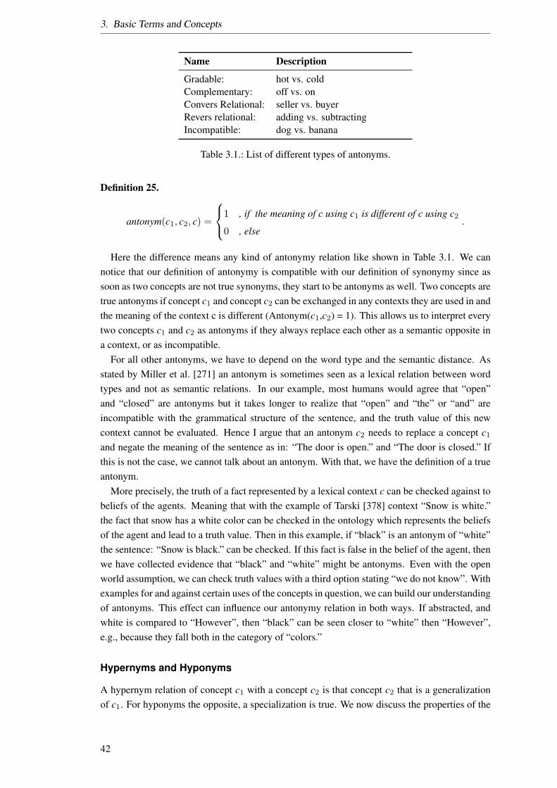
3. Basic Terms and Concepts

Name Description

Gradable: hot vs. coldComplementary: off vs. onConvers Relational: seller vs. buyerRevers relational: adding vs. subtractingIncompatible: dog vs. banana

Table 3.1.: List of different types of antonyms.

Definition 25.

antonym(c1, c2, c) =

1 , if the meaning of c using c1 is different of c using c2

0 , else.

Here the difference means any kind of antonymy relation like shown in Table 3.1. We cannotice that our definition of antonymy is compatible with our definition of synonymy since assoon as two concepts are not true synonyms, they start to be antonyms as well. Two concepts aretrue antonyms if concept c1 and concept c2 can be exchanged in any contexts they are used in andthe meaning of the context c is different (Antonym(c1,c2) = 1). This allows us to interpret everytwo concepts c1 and c2 as antonyms if they always replace each other as a semantic opposite ina context, or as incompatible.

For all other antonyms, we have to depend on the word type and the semantic distance. Asstated by Miller et al. [271] an antonym is sometimes seen as a lexical relation between wordtypes and not as semantic relations. In our example, most humans would agree that “open”and “closed” are antonyms but it takes longer to realize that “open” and “the” or “and” areincompatible with the grammatical structure of the sentence, and the truth value of this newcontext cannot be evaluated. Hence I argue that an antonym c2 needs to replace a concept c1

and negate the meaning of the sentence as in: “The door is open.” and “The door is closed.” Ifthis is not the case, we cannot talk about an antonym. With that, we have the definition of a trueantonym.

More precisely, the truth of a fact represented by a lexical context c can be checked against tobeliefs of the agents. Meaning that with the example of Tarski [378] context “Snow is white.”the fact that snow has a white color can be checked in the ontology which represents the beliefsof the agent and lead to a truth value. Then in this example, if “black” is an antonym of “white”the sentence: “Snow is black.” can be checked. If this fact is false in the belief of the agent, thenwe have collected evidence that “black” and “white” might be antonyms. Even with the openworld assumption, we can check truth values with a third option stating “we do not know”. Withexamples for and against certain uses of the concepts in question, we can build our understandingof antonyms. This effect can influence our antonymy relation in both ways. If abstracted, andwhite is compared to “However”, then “black” can be seen closer to “white” then “However”,e.g., because they fall both in the category of “colors.”

Hypernyms and Hyponyms

A hypernym relation of concept c1 with a concept c2 is that concept c2 that is a generalizationof c1. For hyponyms the opposite, a specialization is true. We now discuss the properties of the

42

3.9. Meaning

generalization, but the same might be argued for a specialization. This means c2 is more general,more abstract and can be obtained through the introduction. Meaning can be generated fromdifferent aspects, like the observation of something specific a general rule, common properties,a super ordinate, governing law, conceptualization, a broader meaning, and an abstraction or aconception.

Most of these hypernyms leave at least one aspect of the specialization unspecified. Therefore,it is possible to choose between the different forms for this aspect. These hypernyms especiallymean something similar than their specialization but are fuzzier or cover more realizations. Theystand in contrast to the hyponym relations. This means that not all facts about a specializationare true about the hypernym as well. However, on the other hand, all facts about the hypernymare true for all specialization. Let’s look at a little example: Let’s suppose a “dachshund” isa specialization of a “dog, ” and surely dog is a hypernym of a dachshund. Furthermore, let’sdefine that dogs have four legs. This means dachshunds have four legs, too. Now let’s describethe physic of a dachshund as “sausage-shaped”. However, we are not able to say that all dogsare sausage-shaped. This is a special attribute of dachshunds.

This means that in most contexts a concept can be replaced with its hypernym, without chang-ing the sentence truth value. E.g. “this dachshund is sausage-shaped” will become “this dog issausage-shaped” which is still true if the dog is a dachshund. Of course, this can be done transi-tively. Let’s suppose dogs are carnivores. Then the sentence “this carnivore is sausage-shaped”is equally true.

This means that with hypernyms/hyponyms we can create generalizations about a group ofsub-concepts or entities, without having to specify it for all those entities. In ontological terms,the hypernym and hyponym relations are mostly combined into a single relation referred to as“is-a” relation. Meaning that a dachshund is a dog.

Meronyms and Holonyms

A meronym relation of concept c1 with a concept c2 states that c2 is part of concept c1. The in-verse relation to a meronym is the holonym relation. Starting with Winston [413, 415] meronymshave been analyzed and classified in different types. Priss [311] brings those relation types intoa formal construct. Here the relation types, e.g., collection, group, ingredient, and organization,are set into relation with formal attributes like inclusion, parting, possession, and property. Prissdefines the formal context of meronyms as Triple: (G,M, I) where G is the set of objects, M theset of attributes and I is a binary relation I(g,m) with g ∈ G and m ∈ M which states: “the objectg has the attribute m”. Priss continues by analyzing the relation of sub- and super-concepts andthe effect on meronyms.

Watrouse-deVersterre et al. [400] separates these relations into the “has-a” (meronym) and“part-of” (holonym) relation. This means with the meronym/holonym relation we can describea sense of whole-to-part relationship in either direction. Since in some semantics concepts areperceived to be more similar the more properties they have in common [232], meronyms arerelevant to the formalization of meaning.

Explanations

The meaning of word or the concepts it stands for can be given by explanations. In the caseof an explanation being provided with other words, we have to assume the Meaning-Text The-

43

3. Basic Terms and Concepts

ory [262] which states that language consists of a mapping between meaning and text. Thismapping can be given by an explanation. Several definitions of explanations have been pro-posed. Each one specialized for the needs of some domain. To start with, in statistics we canidentify evidence weights in a Bayesian believe network as explanations [161]. These weightsrepresent the logarithmic likelihood ratio of the influence of an observation on a specific vari-able. Therefore, they can be and indeed are used to explain in which way the occurrence of anevent influences the current systems state [79]. To ease the access of humans to these statisticalexplanations, different classes of techniques can be applied (e.g., verbal explanations [88] andgraphical explanations [56]). Beyond, Druzdzel [79] identified two categories in which suchexplanations can be separated: Explanation of Assumptions focusing on the communication ofthe domain model of the system and Explanation of Reasoning focusing on how conclusionsare made from those assumptions. It might be worthwhile to transfer these categories to self-explanation14 since the meaning of concepts used might differ depending on the exogenous orendogenous origin of the fact explained. Therefore, the reasoner has to distinguish between theexplanations of the system itself and how it can be interpreted related to the current context. Thiswork focuses on the explanation of assumptions since the audience of such a description is seenas an external system component. As those approaches are quite fundamental and thus general,we further want to list some more practical approaches on explaining capabilities from the agentcommunity:

• Braubach et al. [38] uses the beliefs, desires, and intents to formulate goals, knowledge,and capabilities for a multi-agent system,

• Gruninger et al. [153] uses First-order Logic Ontology for Web Services (FLOWS) todescribe the functionalities of a service,

• Sycara et al. [373] formulates agent and service capabilities utilizing the Input, Output,Precondition and Effect (IOPE) approach,

• Martin et al. [255] uses the Ontology Web Language to structure the description of ser-vices.

The above-listed approaches are used to describe services and with that are used to createexplanations. They can be seen as having some level of self-explanation [93]. Taking this intoaccount, we can clarify that self-explanation enables the integration of new agents autonomouslyinto the existing infrastructure [193, 279]. Following the idea of self-explanation this means thatnew agents, as well as existing ones, are able to learn the capabilities of each other and tocomprehend in which way they can interact (e.g., which data format and concepts match). Theexplanation of new concepts then implies a new problem of interpreting the concepts in a newcontext.

Conclusion

In conclusion, we can say that it is hard to define meaning and that many different ways ofdefining meaning have different purposes. However, as we have seen, we can define similarityof meaning. Defining similarity of meaning or more precise synonyms of words is still sub-ject to discussion. Synonyms can be extended with other semantic relations like meronyms and14Self-explanation describes a learning process as an act of learning new concepts by explaining them to oneself.

44

3.10. Natural Semantic Metalanguage

hyponyms. Relations like those represent the connectionist interpretation of meaning (see Def-inition 21). The second part of meaning can be seen as the literal definition of the meaning ofwords (see Definition 22). The definition of meaning in a symbolic view that needs some kindof logic to reason upon. In consequence, creation of a formal representation of meaning leadsto the “neat vs. scruffy” discussion of Minsky [273]. Both Definitions 21 and 22 together formour representation of meaning combining the neat and the scruffy view of meaning. They rep-resent the knowledge we learn in a connectionist view and the thoughts using this knowledgein the symbolic view. Both combined enable our representation of meaning to share semanticinformation and to reason depending on context. How we approach this definition for an AI issubject of Part III of this doctoral thesis.

This notion of meaning coincides with the NSM theory since here the references are contex-tual. We will use the NSM theory through this work as a basis for our formal representationof meaning in the research done here exceeds the other theories with its empiric evaluation.Furthermore, the theory leads to the convenience that the meaning of complex concepts can bedescribed with less complex concepts, which ends in the benefit for our artificial meaning repre-sentation that we require ca. 65 definitions of concepts, leaving the construction of meaning ofmore complex concepts to the AI. This discussion and the here presented description of meaningleads to the approach of the here presented doctoral thesis. The approach is further described inSection 5.

3.10. Natural Semantic Metalanguage

The Natural Semantic Metalanguage (NSM) is a linguistic theory originated in the early 1970s[137, 138, 142, 141, 143, 144, 145, 146, 406, 407, 408, 409, 410, 411]. It stated that eachexpression created in a natural language can be represented using a set of atomic terms – so-called universal semantic primes. These primes have an indefinable word-meaning and can beidentified in all natural languages [140]. In conjunction with associated grammatical properties,NSM presents a decompositional system able to describe all expressions built in the appropriatelanguage. Here an expression is decomposed into less complex expressions, where the processends if the expression is decomposed to the atomic level of semantic primes which cannot befurther analyzed. One can imagine that the Decomposition builds a tree, where all leafs aresemantic primes. Consequently, for each natural language, a meta language exists which consistsof the semantic primes in the specific syntax and their appropriated grammatical properties. Inthis work, those semantic primes are predefined by the applications domain. About 63 semanticprimes exist which can be divided into 16 categories. Table 3.2 lists these semantic primes forthe English language.

This theory has been tested on natural languages [140, 144, 406, 407, 408] and in manydifferent cultures. The essential conclusion of NSM is that the primes used to build the meaningof more complex concepts are limited.

45

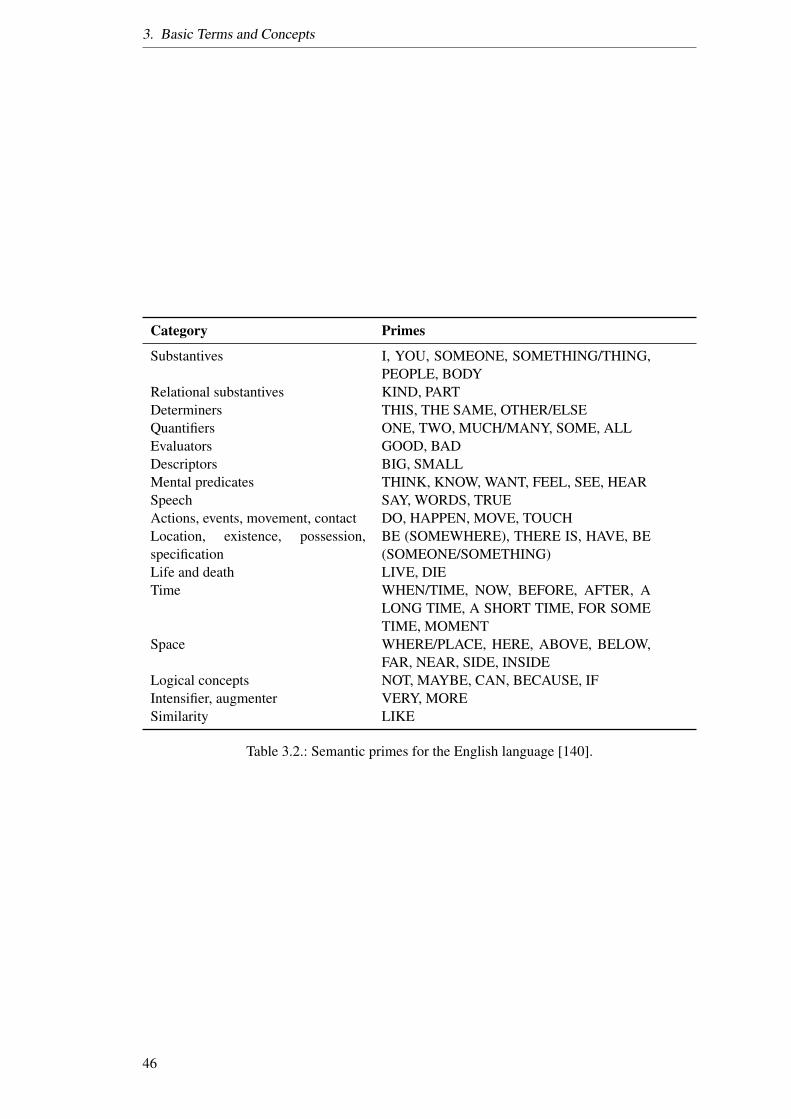
3. Basic Terms and Concepts

Category Primes

Substantives I, YOU, SOMEONE, SOMETHING/THING,PEOPLE, BODY

Relational substantives KIND, PARTDeterminers THIS, THE SAME, OTHER/ELSEQuantifiers ONE, TWO, MUCH/MANY, SOME, ALLEvaluators GOOD, BADDescriptors BIG, SMALLMental predicates THINK, KNOW, WANT, FEEL, SEE, HEARSpeech SAY, WORDS, TRUEActions, events, movement, contact DO, HAPPEN, MOVE, TOUCHLocation, existence, possession,specification

BE (SOMEWHERE), THERE IS, HAVE, BE(SOMEONE/SOMETHING)

Life and death LIVE, DIETime WHEN/TIME, NOW, BEFORE, AFTER, A

LONG TIME, A SHORT TIME, FOR SOMETIME, MOMENT

Space WHERE/PLACE, HERE, ABOVE, BELOW,FAR, NEAR, SIDE, INSIDE

Logical concepts NOT, MAYBE, CAN, BECAUSE, IFIntensifier, augmenter VERY, MORESimilarity LIKE

Table 3.2.: Semantic primes for the English language [140].

46

4. State-of-the-Art

This section describes the state-of-the-art in the different parts of our approach. Some of thedecisions we have made in Chapter 3, are the product of a discussion and a related work analy-sis. These discussions and the literature reviews are part of this chapter. For a theoretic base ofour representation of meaning, discussion on the choices in design decisions as well as compar-ison with other approaches, we will look at different semantic theories in Section 4.1. Semanticinformation in computer science is mostly encoded in ontologies. Section 4.2 discusses differ-ent ontological representations. Then we will look at semantic service description language inSection 4.3 to decide how to describe our services. Next, we will look at related work for thefirst part of our approach: approaches on semantic decomposition in Section 4.4 and the formal-ization semantic primes. We then look in Section 4.5 at related work on the second part of ourapproach: Marker Passing. Finally, in Section 4.6 we will look at different service compositionmechanisms which use AI Planning. State-of-the-art on the different experiments is describedin the respective section of the experiment.

4.1. Semantic Theories

There is a multitude of theories which describe meaning in a semantic sense for computer sci-ence. This section will describe some of them, which could be an alternative to how we createour artificial representation of meaning. These theories can be seen as a formal basis on whichwe will base later design decisions. This state-of-the-art section shows that the challenge ofcreating a formal representation of meaning has been researched and builds a foundation onwhich we can build upon. We will start our by describing 11 different semantic theories fromSection 4.1.1 to Section 4.1.11 and classifying them how they represent meaning: connectionistor symbolic or both.

4.1.1. Formal Semantic

This section contains approaches to formal semantics, which have no name but are grouped bythe main contributors of certain schools of semantics. This is done to get a general overviewof the development of formal semantics and stipulate a notion of formal semantics. Formalsemantic has many explications. In this thesis, we will only look at a few of them, which arerelevant to this work. We will hence not dive into the philosophical discussion as, e.g., presentedby Frege [124] and the same but rather start out with 20th-century definitions of semantic andmeaning with Bloomfield [29, 31, 32] who tried a definition of meaning with its “stimulus-response” model as follows:

“We have defined the meaning of a linguistic form as the situation in which thespeaker utters it and the response which it calls forth in the hearer [32]”.

47

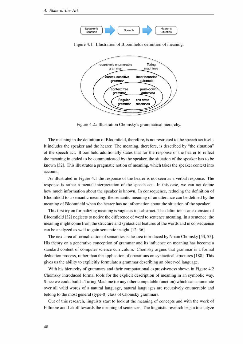
4. State-of-the-Art

Speaker’s Situation Speech Hearer’s

Situation

Figure 4.1.: Illustration of Bloomfields definition of meaning.

Regulargrammar

finit state machines

context freegrammar

push-down automata

contex-sensitive grammar

linear bounded automata

Regulargrammar

finit state machines

context freegrammargrammargrammar

push-down automataautomata

contex-sensitive contex-sensitive grammargrammar

linear bounded automataautomata

recursively enumerablegrammar

Turingmachines

Figure 4.2.: Illustration Chomsky’s grammatical hierarchy.

The meaning in the definition of Bloomfield, therefore, is not restricted to the speech act itself.It includes the speaker and the hearer. The meaning, therefore, is described by “the situation”of the speech act. Bloomfield additionally states that for the response of the hearer to reflectthe meaning intended to be communicated by the speaker, the situation of the speaker has to beknown [32]. This illustrates a pragmatic notion of meaning, which takes the speaker context intoaccount.

As illustrated in Figure 4.1 the response of the hearer is not seen as a verbal response. Theresponse is rather a mental interpretation of the speech act. In this case, we can not definehow much information about the speaker is known. In consequence, reducing the definition ofBloomfield to a semantic meaning: the semantic meaning of an utterance can be defined by themeaning of Bloomfield when the hearer has no information about the situation of the speaker.

This first try on formalizing meaning is vague as it is abstract. The definition is an extension ofBloomfield [32] neglects to notice the difference of word to sentence meaning. In a sentence, themeaning might come from the structure and syntactical features of the words and in consequencecan be analyzed as well to gain semantic insight [12, 36].

The next area of formalization of semantics is the area introduced by Noam Chomsky [53, 55].His theory on a generative conception of grammar and its influence on meaning has become astandard content of computer science curriculum. Chomsky argues that grammar is a formaldeduction process, rather than the application of operations on syntactical structures [188]. Thisgives us the ability to explicitly formulate a grammar describing an observed language.

With his hierarchy of grammars and their computational expressiveness shown in Figure 4.2Chomsky introduced formal tools for the explicit description of meaning in an symbolic way.Since we could build a Turing Machine (or any other computable function) which can enumerateover all valid words of a natural language, natural languages are recursively enumerable andbelong to the most general (type-0) class of Chomsky grammars.

Out of this research, linguists start to look at the meaning of concepts and with the work ofFillmore and Lakoff towards the meaning of sentences. The linguistic research began to analyze

48

4.1. Semantic Theories

the difference of natural and artificial language and become aware, that the differences are not asbig as Chomsky has postulated [52]. This leads to the research done today and as we will showlater on, to the contextual meaning named pragmatics, as we attempt in this work. Since Bloom-field and Chomsky still lack the expressiveness (Chomsky) or are too abstract (Bloomfield),they can only be used as an abstract framework for our artificial representation of meaning. Thismeans we have to analyze the other schools of thought which might be a basis for the contribu-tions of this work. This leads to the next section describing cognitive semantics.

4.1.2. Cognitive Semantic

Cognitive semantics arrises form the field of cognitive linguistics. Here the focus of research ison the relation between language, cognition and meaning [8]. Supporter of cognitive semanticsargue that not only meaning can be described in a conceptual structure but syntax, morphol-ogy, and phonology are conceptual as well [62]. The conceptualization of syntax makes thisrepresentation a symbolic one. There are three major hypotheses guiding cognitive semantics[62]:

Nonautonomous language processing means that the language is part of the whole cog-nition. This connects the language to the nonlinguistic cognitive abilities. Especially theway we see things, smell or feel (by touch) does influence our conception of our language.In simpler words: how we experience the world forms our language.

Syntax is conceptualization means that grammar can not be simply mapped to truth valuesof a model of the world. In particular, the syntax of a language forms its meaning and cannot be described without semantics.

Language is learned means that the grammar of a language needs to be used to gain knowl-edge about it. As a result, there can not be an abstract or general description of syntacticalproperties of a language. This is needed because of the contextual manner the language isseen in cognitive semantics.

With this basis cognitive semantics constructs meaning out of a conceptualization which in-cludes syntax. This construction is not independent of congestion and depends on how theworld is observed. Different to other models cognitive semantics do not represent meaningthrough truth evaluations of statements. One of the most popular versions of cognitive seman-tics is the Frame-Semantic [62]. Two basic concepts from cognitive semantics are introduced inour approach: The notion of meaning-construction and knowledge representation. However, themix-up of semantic and syntax is making the insight into meaning more complicated. This iswhy cognitive semantics are not chosen as used semantic for our endeavor to creating artificialmeaning.

4.1.3. Compositional Semantic

The compositional semantic describes the semantic meaning of concepts as in the structuralisttheory of meaning [67], with its relations. The founding axiom of a compositional semantic:“Meaning of all elements in languages are not atoms, but are composed.” [235, p. 164]. Hencethe meaning of a concept is defined by its relations with other concepts.

49

4. State-of-the-Art

light

Jet

Bulett

VW BeetlePorsche 911

Truck

Dredger

Car

fast

Snail

Figure 4.3.: Illustration of two prototypes for the class of car and of fast.

The theory of compositional semantic defines, therefore, distinctive semantic features calledSeme to extract the elements making up the composition (semantic meaning) of a concept. Forexample, such a Seme could be +

−BIG to differentiate the meaning of a river (+BIG) and a creek(−BIG) [235, p. 164].

The semantic analysis in the compositional semantic works well for nouns, adjectives, andverbs so-called Autosemantica which have a conclusive lexical morpheme1. The theory is lessused to analyze functional words like preposition and articles so called Synsemantica [235].Further, there is no fuzziness in the use of Seme. A concept has a relation with a Seme, or itdoes not. The theory of compositional semantic neglects this indistinct aspect of language andin fact seems not well fitted to describe a semantic for an AI. The compositional Semantic canbe seen as a defuzzified version of the Prototypical Semantic, which we will analyze next.

4.1.4. Prototype Semantic

The prototype semantic denotes meaning of concepts with fitting references called prototypes.The other concepts then are set in relation to this prototype creating a semantic distance to theprototype [235, pp. 175]. This, in addition to being a connectionist representation, gives themeaning of a concept a fuzzy notion since a concept might be related to multiple prototypes.

In Figure 4.3 we can see two concepts (car and fast) and different prototypes for the twoconcepts (light and the VW Beetle). In this example, a Porsche is close to a car and faster thana Dredger.

The distance to a prototype and its discretization are problematic in this semantic representa-tion since the different concepts need to be set into a relation. Here the snail is two times as farfrom light than a Porsche, which would introduce a distorted measure of speed.

The prototype semantic as a result, lets us define fuzzy concept relations but lacks a formaldefinition of distance between concepts and has the deficit that the prototype needs to be knownto all which use the representation. This might not be the case in different cultural contexts.

Prototypical semantic has the benefit, that abstract concepts can be directly reference by in-stances. Making it easy to compare their properties even if they are vague or fuzzy. For arepresentation of meaning in AI, this would mean to create a data structure for each conceptwith all other concepts. With languages like German, with an infinite amount of words, this

1A morpheme is the minimal meaningful linguistic sound

50

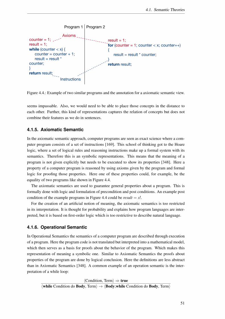
4.1. Semantic Theories

counter = 1; result = 1; while (counter < x) counter = counter + 1; result = result * counter; return result;

result = 1; for (counter = 1; counter < x; counter++) result = result * counter; return result;

Axioms

Instructions

Program 1 Program 2

Figure 4.4.: Example of two similar programs and the annotation for a axiomatic semantic view.

seems impassable. Also, we would need to be able to place those concepts in the distance toeach other. Further, this kind of representations captures the relation of concepts but does notcombine their features as we do in sentences.

4.1.5. Axiomatic Semantic

In the axiomatic semantic approach, computer programs are seen as exact science where a com-puter program consists of a set of instructions [169]. This school of thinking got to the Hoarelogic, where a set of logical rules and reasoning instructions make up a formal system with itssemantics. Therefore this is an symbolic representations. This means that the meaning of aprogram is not given explicitly but needs to be executed to show its properties [348]. Here aproperty of a computer program is reasoned by using axioms given by the program and formallogic for proofing those properties. Here one of these properties could, for example, be theequality of two programs like shown in Figure 4.4.

The axiomatic semantics are used to guarantee general properties about a program. This isformally done with logic and formulation of precondition and post conditions. An example postcondition of the example programs in Figure 4.4 could be result = x!.

For the creation of an artificial notion of meaning, the axiomatic semantics is too restrictedin its interpretation. It is thought for probability and explains how program languages are inter-preted, but it is based on first-order logic which is too restrictive to describe natural language.

4.1.6. Operational Semantic

In Operational Semantics the semantics of a computer program are described through executionof a program. Here the program code is not translated but interpreted into a mathematical model,which then serves as a basis for proofs about the behavior of the program. Which makes thisrepresentation of meaning a symbolic one. Similar to Axiomatic Semantics the proofs aboutproperties of the program are done by logical conclusion. Here the definitions are less abstractthan in Axiomatic Semantics [348]. A common example of an operation semantic is the inter-pretation of a while loop:

〈Condition, Term〉 ⇒ true〈while Condition do Body, Term〉 → 〈Body;while Condition do Body, Term〉

51

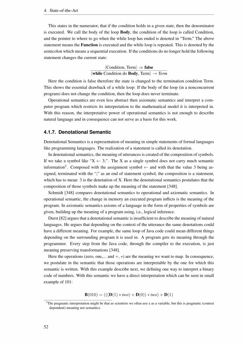
4. State-of-the-Art

This states in the numerator, that if the condition holds in a given state, then the denominatoris executed. We call the body of the loop Body, the condition of the loop is called Condition,and the pointer to where to go when the while loop has ended is denoted in “Term.” The abovestatement means the Function is executed and the while loop is repeated. This is denoted by thesemicolon which means a sequential execution. If the conditions do no longer hold the followingstatement changes the current state:

〈Condition, Term〉 ⇒ false〈while Condition do Body, Term〉 → Term

Here the condition is false therefore the state is changed to the termination condition Term.This shows the essential drawback of a while loop: If the body of the loop (in a nonconcurrentprogram) does not change the condition, then the loop does never terminate.

Operational semantics are even less abstract then axiomatic semantics and interpret a com-puter program which restricts its interpretation to the mathematical model it is interpreted in.With this reason, the interpretative power of operational semantics is not enough to describenatural language and in consequence can not serve as a basis for this work.

4.1.7. Denotational Semantic

Denotational Semantics is a representation of meaning in simple statements of formal languageslike programming languages. The realization of a statement is called its denotation.

In denotational semantics, the meaning of utterances is created of the composition of symbols.If we take a symbol like “X ← 3;”. The X as a single symbol does not carry much semanticinformation2. Composed with the assignment symbol ← and with that the value 3 being as-signed, terminated with the “;” as an end of statement symbol, the composition is a statement,which has to mean: 3 is the denotation of X. Here the denotational semantics postulates that thecomposition of those symbols make up the meaning of the statement [348].

Schmidt [348] compares denotational semantics to operational and axiomatic semantics. Inoperational semantic, the change in memory an executed program inflicts is the meaning of theprogram. In axiomatic semantics axioms of a language in the form of properties of symbols aregiven, building up the meaning of a program using, i.e., logical inference.

Durst [82] argues that a denotational semantic is insufficient to describe the meaning of naturallanguages. He argues that depending on the context of the utterance the same denotations couldhave a different meaning. For example, the same loop of Java code could mean different thingsdepending on the surrounding program it is used in. A program gets its meaning through theprogrammer. Every step from the Java code, through the compiler to the execution, is justmeaning preserving transformations [348].

Here the operations (zero, one,... and +, ∗) are the meaning we want to map. In consequence,we postulate in the semantic that those operations are interpretable by the one for which thissemantic is written. With this example describe next, we defining one way to interpret a binarycode of numbers. With this semantic we have a direct interpretation which can be seen in smallexample of 101:

B(010) = (((D(1) ∗ two) + D(0)) ∗ two) + D(1)

2The pragmatic interpretation might be that as scientists we often use x as a variable, but this is pragmatic (contextdependent) meaning not semantics.

52

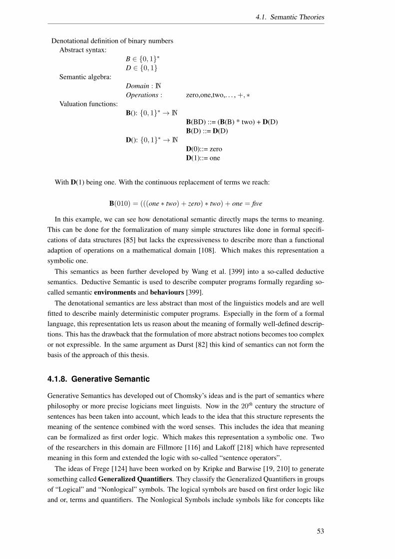
4.1. Semantic Theories

Denotational definition of binary numbersAbstract syntax:

B ∈ 0, 1∗D ∈ 0, 1

Semantic algebra:Domain : NOperations : zero,one,two,. . . , +, ∗

Valuation functions:B(): 0, 1∗→ N

B(BD) ::= (B(B) * two) + D(D)B(D) ::= D(D)

D(): 0, 1∗→ N

D(0)::= zeroD(1)::= one

With D(1) being one. With the continuous replacement of terms we reach:

B(010) = (((one ∗ two) + zero) ∗ two) + one = five

In this example, we can see how denotational semantic directly maps the terms to meaning.This can be done for the formalization of many simple structures like done in formal specifi-cations of data structures [85] but lacks the expressiveness to describe more than a functionaladaption of operations on a mathematical domain [108]. Which makes this representation asymbolic one.

This semantics as been further developed by Wang et al. [399] into a so-called deductivesemantics. Deductive Semantic is used to describe computer programs formally regarding so-called semantic environments and behaviours [399].

The denotational semantics are less abstract than most of the linguistics models and are wellfitted to describe mainly deterministic computer programs. Especially in the form of a formallanguage, this representation lets us reason about the meaning of formally well-defined descrip-tions. This has the drawback that the formulation of more abstract notions becomes too complexor not expressible. In the same argument as Durst [82] this kind of semantics can not form thebasis of the approach of this thesis.

4.1.8. Generative Semantic

Generative Semantics has developed out of Chomsky’s ideas and is the part of semantics wherephilosophy or more precise logicians meet linguists. Now in the 20th century the structure ofsentences has been taken into account, which leads to the idea that this structure represents themeaning of the sentence combined with the word senses. This includes the idea that meaningcan be formalized as first order logic. Which makes this representation a symbolic one. Twoof the researchers in this domain are Fillmore [116] and Lakoff [218] which have representedmeaning in this form and extended the logic with so-called “sentence operators”.

The ideas of Frege [124] have been worked on by Kripke and Barwise [19, 210] to generatesomething called Generalized Quantifiers. They classify the Generalized Quantifiers in groupsof “Logical” and “Nonlogical” symbols. The logical symbols are based on first order logic likeand or, terms and quantifiers. The Nonlogical Symbols include symbols like for concepts like

53

4. State-of-the-Art

“most”, “many” or “few” [19]. The proposed semantic for those Generalized Quantifiers extendsthe idea of Frege for sense, connotation, and denotation. This leads to formalizations like shownin Figure 4.5.

Many men don’t see Harry.

Many(men) x [~see(x, Harry)]

Figure 4.5.: Formalisation of the sentence “Many men do not know Harry” with the formaliza-tion of Barweise [19].

With that, we can see the notion in which the 20th century has continued to develop the notionof meaning. We can see in Figure Figure 4.5 that the logic contains operator “Many(x)” whichis such an Generalized Quantifiers. It extends the First order logic by a fuzzy construct whichreaches from more than one to not all.

This lets us describe more aspects of semantic formally, but is restricted to symbolic meaning.Leading to a theory where in an application for AI every concept needs modeling like in anExplanatory Combinatorial Dictionary [261] or another model theoretic semantics which try tomodel an exhaustive formalization of meaning [188]. Also, the reasoning for many of thoseGeneralized Quantifiers becomes undecidable because the extend the description logic and withthat runs into the decision problems.

4.1.9. Discourse Representation Semantic

Further development in this direction of Kripke and Barwise [19, 210] has become researchabout Discourse Representation Semantics [188] which lead to the formalization of two prob-lems: the first one is how to handle fuzzy concepts like some. The second one is a conceptwith tenses and aspects3. The Discourse Representation Semantic focuses on the integrationof interpretational aspects of representations of meaning [188]. Here a mental abstraction ofthe “discourse” is part of the formal description of the semantics. Making this representation asymbolic one. This is done to be able to describe meaning on larger entities like sentences orparagraphs. The formal model describes two types of information: the “reference” which arethe subject of the discourse and the “conditions” holding information about those references.

As shown in Figure 4.6 the references are kept separated from the descriptions of informationabout those references. In this way, the reference can overarch multiple sentences, and form adiscourse. Sadly this good idea does not contain a set of grounded primes since it is specially de-signed to represent discourse. Which leads us to the conclusion that the discourse representationsemantic can not be used as a basis for the here created artificial notion of meaning. However, itcan be part of its extension, when the notion of meaning is extended from concepts and sentencesto larger textual units and finally could be part of future work.

3This analyses grammatical structures like the difference between two types of past tenses like the French “PasseSimple” and the “Imparfait”.

54

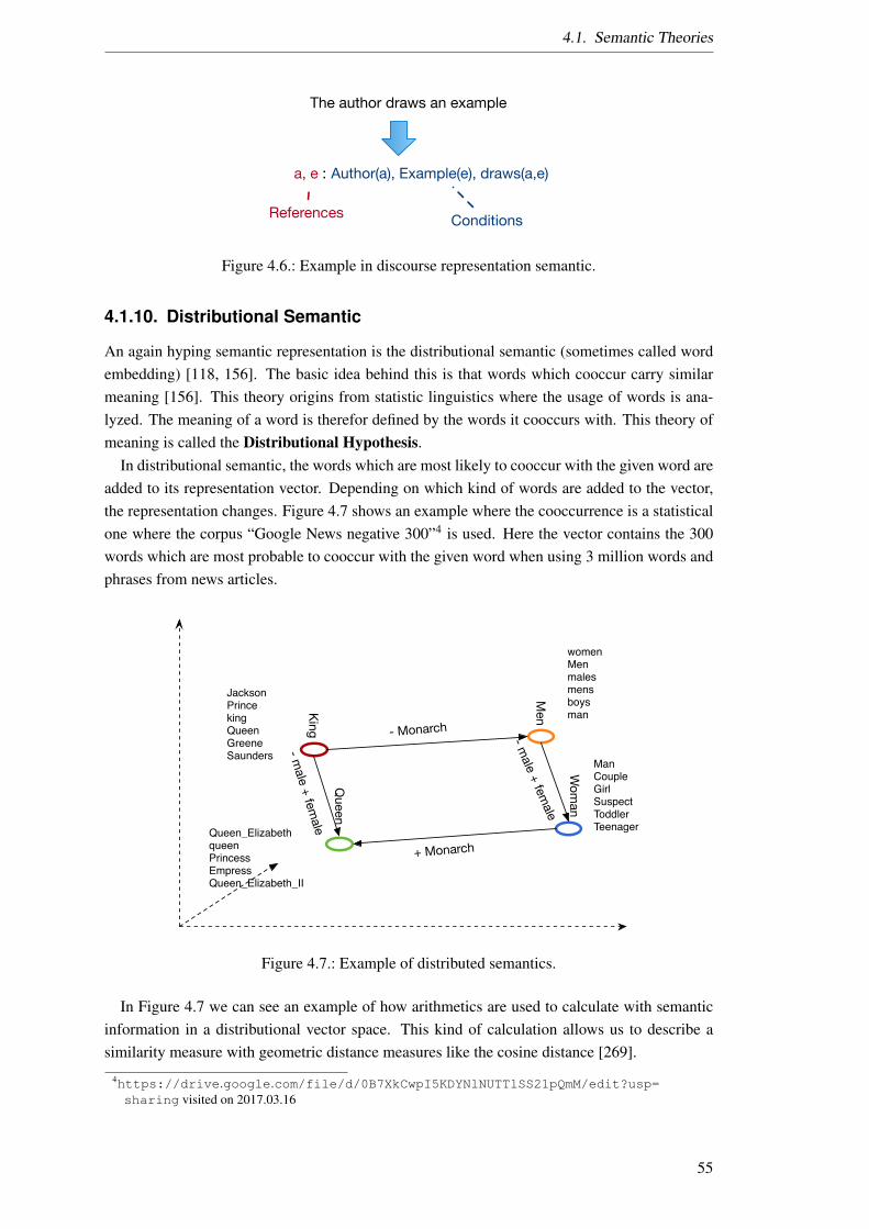
4.1. Semantic Theories

The author draws an example

a, e :

References

Author(a), Example(e), draws(a,e)

Conditions

Figure 4.6.: Example in discourse representation semantic.

4.1.10. Distributional Semantic

An again hyping semantic representation is the distributional semantic (sometimes called wordembedding) [118, 156]. The basic idea behind this is that words which cooccur carry similarmeaning [156]. This theory origins from statistic linguistics where the usage of words is ana-lyzed. The meaning of a word is therefor defined by the words it cooccurs with. This theory ofmeaning is called the Distributional Hypothesis.

In distributional semantic, the words which are most likely to cooccur with the given word areadded to its representation vector. Depending on which kind of words are added to the vector,the representation changes. Figure 4.7 shows an example where the cooccurrence is a statisticalone where the corpus “Google News negative 300”4 is used. Here the vector contains the 300words which are most probable to cooccur with the given word when using 3 million words andphrases from news articles.

womenMenmalesmensboysman

JacksonPrincekingQueenGreeneSaunders

King

Men

Queen_ElizabethqueenPrincessEmpressQueen_Elizabeth_II

Queen

Man CoupleGirlSuspectToddlerTeenager

Wom

an

- Monarch

- male + fem

ale

+ Monarch

- male + fem

ale

Figure 4.7.: Example of distributed semantics.

In Figure 4.7 we can see an example of how arithmetics are used to calculate with semanticinformation in a distributional vector space. This kind of calculation allows us to describe asimilarity measure with geometric distance measures like the cosine distance [269].

4https://drive.google.com/file/d/0B7XkCwpI5KDYNlNUTTlSS21pQmM/edit?usp=sharing visited on 2017.03.16

55

4. State-of-the-Art

The drawback of the distributional semantics, as a connectionist model, is that they encoderelatedness not semantic. We can see this in Figure 4.7 that in the corpus which was scannedfor this example Jackson was related to the concept king probably because Michael Jackson wascalled “the king of pop”. This disqualifies the distributional semantic for our approach.

4.1.11. Structural Semantic

Structural semantics are semantic which search for semantic meaning full components. We willlook at two of these semantic theories which have a basis for many extensions. First, we willlook at the conceptual semantic, because it is closer to the formal semantics. This is intriguingfor the formalization of meaning for an AI since it lets us structure the semantics of a conceptup a whole phrase.

Conceptual Semantic

Conceptual semantics theory after Jackendoff who was looking for the smallest semanticallyrich elements (morphemes) is based on the axiom that semantic meaning is built upon a fi-nite set of basic semantic concepts called conceptual primitives. Jackendoff beliefs that theseconceptual primitives are based on human cognition and therefore have to be universal [182].These conceptual primitives are further order and categorized by Jackendoff. As an example,we look at the movement of objects and with that the primitive GO taken from the StudienbuchLinguistik [235, pp. 188]:

[ActionCAUSE(PAUL, [(Event)GO([Thingbutter], [PathTO([Placebread])])])]

In the example above we can see that there are Action, Event, Thing, and Place primitives,which carry meaning which makes this representation a symbolic one. The CAUSE (as in causal-ity) is classified as an Action and GO is classified as an event. The primitive GO seems to havetwo parameters: First a Thing and second a Path primitive. In our example, butter is a thing,and bread seems to be a place. This leads to the conclusion that example above formalizes thefollowing sentence: Paul butters the bread. The example of movement and the primitive GO isfurther discussed in Goddard’s semantic on coming and going [138].

This approach is more formal then the others looked at so far, but it is mainly concerned withverbs that can not (without extension) be generalized [235, pp. 188]. Because of its degree offormalization, this is a candidate for our representation of meaning. The primitives used here aresubsumed by the primitives used in the Natural Semantic Metalanguage which will be discussedin Section 6.1.

4.1.12. Conclusion

In conclusion we can define the scope of connectionist meaning for this work as describedin Section 3.9. From the literature review done in this section, we can see that no approachtakes account for both sides of meaning: the connectionist and the symbolic. Table 4.1 lists allanalyzed theories and our classification of them into the two sides. Which leads to the gap filledin this work: the need for an artificial representation of meaning combining connectionist andsymbolic views. Therefore the semantic representation and the language which describes this

56

4.2. Ontology

Table 4.1.: Comparison of semantic approaches regarding the classification into symbolic andconnectionist theories.

Theory

Symbo

lic

Conne

ction

ist

4.1.1 Formal Semantic X ×4.1.2 Cognitive Semantic Section X ×4.1.3 Compositional Semantic Section X ×4.1.4 Prototype Semantic Section × X4.1.5 Axiomatic Semantic Section X ×4.1.6 Operational Semantic Section X ×4.1.7 Denotational Semantic Section X ×4.1.8 Generative Semantic Section X ×4.1.9 Discourse Representation Semantic Section X ×4.1.10 Distributed Semantic Section × X4.1.11 Structural Semantic Section X ×

representation consists of two parts: The connectionist part (represented by an ontology) and thesymbolic part represented by the Marker Passing.

Semantic or with that meaning is hard to grasp - especially if we are looking for a formaldefinition. We started with definition 17 and looked at different theories of semantics. Now wehave a broader understanding on what different theories focus on in semantics. The differenttheories of semantic look at different aspects of semantics depending on the aspect they want toexplain regarding meaning.

We have seen in this section that the formalized description of semantics are still too abstractlike the Chomsky hierarchy or are too specific for one part of language like conceptual semantics.To represent our definition of meaning as defined in Section 3.9 we need a semantic theory whichincorporates both, a symbolic and a connectionist interpretation of meaning.

In computer science, this kind of semantic has been described in special semantic languages,e.g., for the description of functionalities in services. We will look at some of those descriptionlanguages next.

4.2. Ontology

The goal of this section is to select an ontology language for the representation of our semanticgraph, modeling the connectionist part of the meaning. We do so by surveying the formal defi-nitions of ontologies since they are the theoretical foundation for most connectionist knowledgerepresentations [366]. At first, we will identify a set of language requirements that are relevantfor our semantic graph. We structure our survey by starting with the simpler, more abstract def-initions and will find our way to more precise and complex definitions, leading to the definitionof an ontology we apply in this work described in Section 3.6. Furthermore, we use the derivedset of language requirements to substantiate the selection of the concrete ontology language,which we use to model our semantic graph.

We have defined an ontology in Section 3.6 and now we derive language requirements from

57

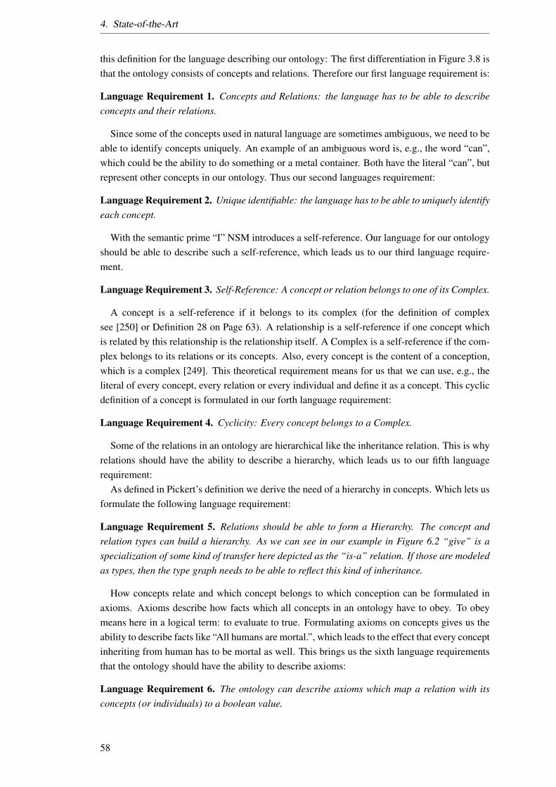
4. State-of-the-Art

this definition for the language describing our ontology: The first differentiation in Figure 3.8 isthat the ontology consists of concepts and relations. Therefore our first language requirement is:

Language Requirement 1. Concepts and Relations: the language has to be able to describeconcepts and their relations.

Since some of the concepts used in natural language are sometimes ambiguous, we need to beable to identify concepts uniquely. An example of an ambiguous word is, e.g., the word “can”,which could be the ability to do something or a metal container. Both have the literal “can”, butrepresent other concepts in our ontology. Thus our second languages requirement:

Language Requirement 2. Unique identifiable: the language has to be able to uniquely identifyeach concept.

With the semantic prime “I” NSM introduces a self-reference. Our language for our ontologyshould be able to describe such a self-reference, which leads us to our third language require-ment.

Language Requirement 3. Self-Reference: A concept or relation belongs to one of its Complex.

A concept is a self-reference if it belongs to its complex (for the definition of complexsee [250] or Definition 28 on Page 63). A relationship is a self-reference if one concept whichis related by this relationship is the relationship itself. A Complex is a self-reference if the com-plex belongs to its relations or its concepts. Also, every concept is the content of a conception,which is a complex [249]. This theoretical requirement means for us that we can use, e.g., theliteral of every concept, every relation or every individual and define it as a concept. This cyclicdefinition of a concept is formulated in our forth language requirement:

Language Requirement 4. Cyclicity: Every concept belongs to a Complex.

Some of the relations in an ontology are hierarchical like the inheritance relation. This is whyrelations should have the ability to describe a hierarchy, which leads us to our fifth languagerequirement:

As defined in Pickert’s definition we derive the need of a hierarchy in concepts. Which lets usformulate the following language requirement:

Language Requirement 5. Relations should be able to form a Hierarchy. The concept andrelation types can build a hierarchy. As we can see in our example in Figure 6.2 “give” is aspecialization of some kind of transfer here depicted as the “is-a” relation. If those are modeledas types, then the type graph needs to be able to reflect this kind of inheritance.

How concepts relate and which concept belongs to which conception can be formulated inaxioms. Axioms describe how facts which all concepts in an ontology have to obey. To obeymeans here in a logical term: to evaluate to true. Formulating axioms on concepts gives us theability to describe facts like “All humans are mortal.”, which leads to the effect that every conceptinheriting from human has to be mortal as well. This brings us the sixth language requirementsthat the ontology should have the ability to describe axioms:

Language Requirement 6. The ontology can describe axioms which map a relation with itsconcepts (or individuals) to a boolean value.

58

4.2. Ontology

Form the Semiotic Triangle (see Figure 4.8) from Ogden and Richards [291] we derive thatwe want to be able to distinguish between concepts and individuals. This differentiation isequivalent to the difference of symbol and the reference in the Semiotic Triangle, which givesus our sixth language requirement:

Language Requirement 7. The difference between concepts and instance should be made ex-plicit.

Since natural language relations do not only connect two concepts but sometimes more, e.g., ifwe can express something like: “John writes with chalk on a blackboard.” [189] in one relation,we need n-ary relations which are formulated in our seventh language requirement:

Language Requirement 8. N-ary relations: the language has to be able to describe relationswith arbitrary many entities.

Because of n-ary relation in natural language like the example as depicted in Figure 6.2:give( teacher, advice, student), a relation can relate more than two concepts orrelations, making it necessary for our formalism to connect multiple concepts or other relationswith one relation.

Furthermore, the definition of Euzenat and Shavaiko identifies types which are a more prag-matic notion of a relationship (is-of-type) between a typed concept and a concept of this type.This is reflected in our definition by the instantiation, which leads us to our ninth languagerequirement:

Language Requirement 9. Typed concepts: the language has to be able to describe types foreach concept.

Language Requirement 9 describes that the formal representation of concepts and relationsare typed. This enables a different interpretation for each concept and relation type. We cansee the example decomposition depicted in Figure 6.9 on Page 114 where the different concepttypes could be stop-words, negation, syntactic relations or semantic primes.

In addition to typing of concepts, concepts can have additional attributes. The possibility ofmodeling those attributes is formulated in Language Requirement 10.

Language Requirement 10. Attributes: In addition the entities and relations need attributes,e.g., for us to be able to give them names.

The need for modeling relations as concepts can be seen in Figure 6.2 on Page 98 where therelation “give” as a relation is itself a concept. Concepts which represent relations can again haverelations to other concepts or relations. Making it necessary to introduce a relation-to-relationconnection.

Language Requirement 11. Relations are Concepts: Each relation might be interpreted as aconcept as well, hence the set of concepts and relations are not disjunct.

Language Requirement 11 comes from the need of natural language relations are concepts aswell, and therefore can be described by concepts, a relation should be a concept as well.

With those requirements in mind, we will now analyze different ontology representations andevaluate their usefulness for our representation of connectionist meaning.

59

4. State-of-the-Art

The representation of information or more accurate of knowledge is a well-researched topic.Starting with Philosophy5 as a part of structural science our knowledge is formalized in modelscalled ontologies. The term Ontology is taken from philosophy where an ontology can be seenas a theory of the things in nature [152]. With this theory, we try to understand the worldand remove errors in our thoughts. For example, the color green is often seen as a property ofsomething, but a coat of green paint can be modeled as layers of color [41] even though the objectis called green. If we have the knowledge of an object which is of the color red and is covered bya coat of green paint, would it fall under the description: “This is a green object.”? To formalizesuch knowledge, the research in ontologies has fostered many languages and engineering tools.

With an ontology, we try to analyze the meaning of entities. We define entities like Mahr [249]as everything that is. This includes the real object of interest, e.g., the apple and the worddescribing the apple as well as the relations the objects have with each other. The meaning ofthings is strongly coupled with our language and the symbols we use. Ogden and Richards [291]have studied this relationship to conclude the semiotic triangle 6 as shown in Figure 4.8.

SymbolWord

ConceptThought or Reference

ReferenceObjectStands for

Reference to

(a causal relation)

Symbo

lises

(a ca

usal

relat

ion)

Figure 4.8.: The Semiotic Triangle.

In the Semiotic Triangle entities which exist are referenced by symbols like words, for ex-ample, “Apple” which symbolizes every fruit which falls under the definition of an apple. If weread the word “Apple” and we have a reference for that word, then there might be thought, whichreferences the actual reference (the apple). Here the symbols themselves are entities, which havereferences and we consider thoughts as entities as well, hence having symbols and references forthem as well. We investigate the process where the thought is created regarding a symbol andits references to grasp the notion of meaning which lets us connect symbols to references andreason upon them. We use the terminology of concepts to describe a symbol and an instance todescribe the reference.

Peacock [303] analyses a philosophical description of concepts, e.g., by Kante as basic build-ing blocks of an ontology: “...concepts have pride-of-place in epistemology, semantics, and thephilosophy of mind: they function as rules for organizing perceptions, as the primary object ofrational analysis, as singular or general propositional terms and as the basic constituents ofbeliefs.” [303, pp. 266]. For our work, we want to transform such a philosophical definition in

5The study of existence or being.6some times called Semantic triangle or triangle of reference.

60

4.2. Ontology

a more formal one, to be able to implement AI reasoning upon it. This is the way we definelanguage requirements so that we can select which kind of ontology definition we need.

In computer science, an ontology can be seen as a practical application of such a theoreticalview [365]. In computer science ontologies have earned their place in an own layer of thetechnology stack of the Semantic Web [25], which gives the notion of its importance in thescientific community regarding artificial semantics. However, now let us look more closely atthe definitions of ontologies starting with abstract ones to more technical.

A quite general description of ontologies has been given by Gruber with “an explicit specifi-cation of a conceptualization” of entities of concern and their relationships7. This definition isquite abstract and does not formalize the notion of an ontology but rather explains what is doneto create an ontology which can be done by a multitude of modeling techniques.

To grasp the notion of ontologies more formally than the definition of Gruber, we need to lookat similar terms first, to distinct them from ontologies:

Model: A model can be seen as an abstraction of an entity. Containing the relevant informationregarding a given context. Favre [106, 107] would describe it as “a system that enables togive answers about a system under study without the need to consider directly this systemunder study.” [107, p. 3] and further Miller [272, p. 3] describes a model as “... a modelis a formal specification of the function, structure and/or behavior of a system”.

Epistemology: Epistemology can be seen as “the field of philosophy which deals with na-ture and source of knowledge” [289] (cited in [355, p. 6]). Regarding AI research theknowledge is interpreted as consisting of propositions and logical reasoning upon thosepropositions to create new knowledge in the form of formal structures [154].

Taxonomy: A Taxonomy is the science of classification of entities into classes. Taxonomiesstructure entities into an order which can be but does not have to be hierarchical [354].Further Euzenat and Shavaiko [91, p. 27] define a taxonomy as “a partially ordered setof taxons (classes) in which one taxon is greater than another one only if what it denotesincludes what is denoted by the other.”

A model as defined above is on the one side to general to examine the meaning, since thereis no formal or better-structured definition of what the model consists of. However, on the otherside, we can define an ontology as a kind of model since an ontology is an abstraction as well.Euzenat and Shavaiko [91] define an ontology as a conceptual model with features of an entity-relation model. The ontology is thereby seen as a logical theory with model theoretic semantics.

For this work, Epistemology is, on the one hand, a use case in which an ontology is used toreason upon and on the other hand, the process of ontology creation8 where the output of thisprocess is an ontology.

A Taxonomy seems to restricted since the classification of entities is not enough if we needmore details in our ontology then the sub-class or “is-a” relation to represent relationships. Thisis necessary for example if we want to reason upon relations like “part of” or concepts like therelation “give” in an example like: “A teacher gives advice to a student.”

Figure 4.9 illustrates a simple taxonomy using the “is-a” relation which identifies two kindsof things: living ones and not living ones. Also, a salad and a pig are classified as living and

7http://www-ksl.stanford.edu/kst/what-is-an-ontology.html last visited 2017.09.018sometimes called ontology engineering

61

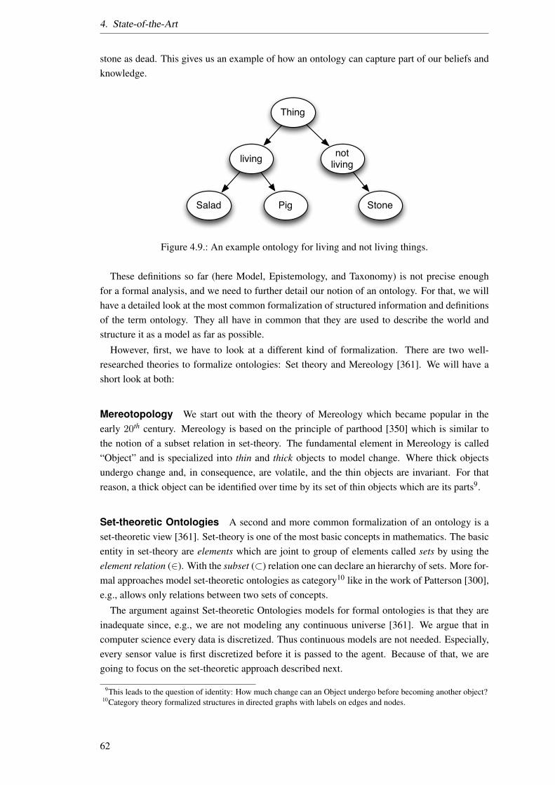
4. State-of-the-Art

stone as dead. This gives us an example of how an ontology can capture part of our beliefs andknowledge.

Thing

living not living

StoneSalad Pig

Figure 4.9.: An example ontology for living and not living things.

These definitions so far (here Model, Epistemology, and Taxonomy) is not precise enoughfor a formal analysis, and we need to further detail our notion of an ontology. For that, we willhave a detailed look at the most common formalization of structured information and definitionsof the term ontology. They all have in common that they are used to describe the world andstructure it as a model as far as possible.

However, first, we have to look at a different kind of formalization. There are two well-researched theories to formalize ontologies: Set theory and Mereology [361]. We will have ashort look at both:

Mereotopology We start out with the theory of Mereology which became popular in theearly 20th century. Mereology is based on the principle of parthood [350] which is similar tothe notion of a subset relation in set-theory. The fundamental element in Mereology is called“Object” and is specialized into thin and thick objects to model change. Where thick objectsundergo change and, in consequence, are volatile, and the thin objects are invariant. For thatreason, a thick object can be identified over time by its set of thin objects which are its parts9.

Set-theoretic Ontologies A second and more common formalization of an ontology is aset-theoretic view [361]. Set-theory is one of the most basic concepts in mathematics. The basicentity in set-theory are elements which are joint to group of elements called sets by using theelement relation (∈). With the subset (⊂) relation one can declare an hierarchy of sets. More for-mal approaches model set-theoretic ontologies as category10 like in the work of Patterson [300],e.g., allows only relations between two sets of concepts.

The argument against Set-theoretic Ontologies models for formal ontologies is that they areinadequate since, e.g., we are not modeling any continuous universe [361]. We argue that incomputer science every data is discretized. Thus continuous models are not needed. Especially,every sensor value is first discretized before it is passed to the agent. Because of that, we aregoing to focus on the set-theoretic approach described next.

9This leads to the question of identity: How much change can an Object undergo before becoming another object?10Category theory formalized structures in directed graphs with labels on edges and nodes.

62

4.2. Ontology

We now will have a look at different set-theoretic definitions of ontologies next. Again startingfrom a more abstract and getting more practical. Starting with an abstract definition of whatentities and their relations are (Section 4.2.1). To a more mathematical definitions (Section 4.2.2,4.2.3 and 4.2.4) ending in a conclusion in Section 4.2.5.

4.2.1. Mahrs Model of Conception

The first definition we will look at is from the Model of Conception. The model of conceptionhas been introduced by Mahr [249]. The basic building blocks here are entities.

The first definition of the Model of Conception is an Entity:

Definition 26. Entity:

1. An entity is anything that is.

2. Any two entities are different.

This gives us the basic building block for further investigation. We formalize this in a set Eof all entities. Further entities can have relationships with each other and with them selfs, withthis in mind, Mahr defines a “Relationship” as follows:

Definition 27. Relationship:

1. A relationship is an entity by which entities are related.

2. An entity is an element of a relationship if it is one of the entities related by the relation-ship.

Since every thing is an entity, a relationship is an entity as well. This is quite general and needsa formalization. Because the natural language representation of the definitions of Mahr allowsinterpretation, let us look at the formalization of the model of Mahr by defining a Signature [85,pp. 14–15] like it has been done in [189, 405]:

Definition 28. Complex:

1. A complex is an entity by which entities belong to relationships.

2. A relationship is an element of a complex, if the entities which belong to this relationshipbelong to this relationship by this complex.

3. An entity is an element of a complex, if it belongs to a relationship which is an element ofthe complex.

A complex can be seen as a bigger structure which includes concepts and their relationships.An example of a complex could be a topic, where certain concepts belong to the topic withrelationships among the concepts, but other do not. In a topic, for example, some word sensescould be excluded so that when we talk about the topic of bank robbery, we do not connectconcepts of rivers or the sea into the complex.

The definition of a model of conception of Mahr [249] describes an abstract view on a con-ceptualization. This maps to natural language, where each concept can be described by a set ofconcepts [262]. With that, we can describe, e.g., the relation “is teacher of” in “Bob is teacher ofAlice.” which in itself is a set of concepts. To be able to implement reasoning upon the connec-tionist part of our representation of meaning we will further restrict this general description to amore technical one in the next sections; starting with the definition of an ontology by Pickert.

63

4. State-of-the-Art

4.2.2. Pickert’s Definition

The next definition we look at, is the one of Pickert. We look at this definition because itintroduces a taxonomy and its properties into the definition of an ontology. Pickert11 defines anontology as a seven tuple O := L,C,R,F,G,H,A with:

L: the lexicon is a set of lexical symbols for concepts LC and relational symbols LR withL := LC ∪ LR,

C: the set of concepts which are used in the ontology,

R: the set of binary relations over C,

F: a function F : 2LC → 2C which maps symbols to concepts,

G: a function G : 2LR → 2R which maps symbols to relations,

H: a taxonomy which is an irreflexive, acyclic and transitive relation H :⊂ C × C,

A: is the set of axioms defined in the ontology.

Here function F and G map symbols from the lexicon L to concepts (F) and to relations (G).This mapping can be seen as a naming of concepts and relations with the symbols.

The first thing to notice in this definition is the distinction between concepts and symbols justlike illustrated in the semiotic triangle shown in Figure 4.8 on Page 60. The second interestingfact of this formalization is that there is a hierarchy which lets us, for example, build a classhierarchy like in Figure 4.9 on Page 62. It should be noticed that it is unclear what the set ofaxioms A contains. One interpretation of A could be a set of all relations and concepts whichcan be extracted out of the hierarchy H. However, the definition is incomplete at this point.

Building such a taxonomy over each relation allows us to define, e.g., a hierarchy in relationslike the “is-a” or “is-part” relations. Next, we look at the definition of an ontology by Maedcheund Staab [245] because they define what an axiom is.

4.2.3. Maedche und Staab

Maedche and Staab [246, 245] use an ontology definition with two semiotic levels. First, thelexical level which describes how terms are used to convey meaning. Second, the conceptuallevel describing the conceptual relations between terms. The definition of an ontology by Maed-che and Staab can be seen as a formal basis for a Web Ontology Languages (OWL), which hasbecome a quasi-standard for the semantic web [25]. Maedche and Staab present a conceptuallanguage with an interpretation. In their formalization, they start out with Definition 29.

Definition 29. A concept Language CL is defined by starting from a domain U which is madeup by individuals, atomic concept and roles, where concepts are unary predicates and roles areunary predicates over a domain U . A concept symbol is an element ofA ⊆ U and a role symbolis an element of the subset P ⊆ U . The languages Interpretation I is a function that assignseach concept symbol a subset of the domain U : I : A → 2U and each role symbol a binary

11Taken form a technical report from http://www.dbis.informatik.hu-berlin.de/dbisold/lehre/WS0203/SemWeb/artikel/2/Pickert Ontologien final.pdf “Einfhrung in Ontologie”, GregorPickert, last visited on 02.03.2012

64

4.2. Ontology

relation of U : I : A → 2U×U . Concept terms and role terms are defined inductively withterminological axioms and using operators. C and D denote concept terms, R and S denoteroles.

The concept Language from Definition 29 describes how the interpretation of concepts ismapped to a domain and range, telling the interpreter, on what entities the concepts are definedon. An example could be the formalization of a relation “IsBookedFor(Flight,Person)” wherethe relation has the domain of a flight and the range of a person. Meaning that we can not usethe “IsBookedFor” for trains and cats. Each of these related concepts additional can have a rolelike “booked flight” and “ticket owner”.

For Maedche and Staab an atomic concept has as interpretation a subset of I(Catom), whichare elements of the domain and are a result of the interpretation. Here the domain can be seen,for example, as the real world object and the concepts Catom as a symbol denotating the objectsof one kind. Let Catom be “Apple” then the interpretation I(Catom) are on the one side applesinheriting from Fruit and inheriting from a company.

Here Maedche and Staab introduce two kinds of symbols: Firstly the equivalent, which lets toconcepts or roles be equivalent if their interpretation is equivalent. Secondly, the subset relationwhich defines one concept or role being subsumed by another one if all its interpretations are asubset of the other. The lexicon of the language can then be defined as set of terms consisting ofconcepts and relations of the given concept Language CL. A LexiconL consists of a set of termsfor concepts LC and a set of terms for relations LR thus the lexicon is the union? L := LC ∪LR

Next, we need a reference function linking the lexical entries to the concepts and relation-ships. A Reference Function links a set of lexical entries LI ⊂ L to concepts and relationships.Therefore F and G are reference functions with F : sL

C → 2A linking concepts to lexical entriesand G : 2L

∫ → 2P linking relationships to lexical entries.

Here one lexical entry can reference multiple concepts or relationships and one concept or re-lationship can reference multiple lexical entries. A Core OntologyO is a six-tuple (A,P,D,L,F ,G) which consists of a set of concept symbols A, a set of relation symbols P , a set of dataor facts D in the concept language with its interpretation function, a lexicon L and two corre-sponding reference functions F and G

Upon this core Ontology, a concept hierarch can be defined. A Concept hierarchy H isdefined by H := (C,D) | C,D ∈ A ∧ CI ⊆ DI . The domain of a relation and its range aredefined as Domain and Range. Domain d(R) and Range r(R) of a relation R are defined byd(R) := d | ∃ e(d, e)∈ RI and r(R) := e | ∃ d(d, e) ∈ RI .

This allows us how to map relationships with their arguments to truth values like “isHu-man(Johannes)” modeling the belief that Johannes is a human is true. Here we have to empha-size that we do not derive that the fact is false because it is not modeled.

With the addition of the domain and range of relations and the concept hierarchy, this for-malization of the notion of ontology can be seen as one formal definition of an ontology. Thereare some unclear statements in this definition since the definition lacks to describe UI and, e.g.,what atomic means. The use of a semi-standard set-theoretic definition of semantic formalizesthe meaning of used terms in a sound and appropriate way.

65

4. State-of-the-Art

4.2.4. Euzenat and Shavaiko

Euzenat and Shavaiko define a more practical notion of ontology in their book “Ontology Match-ing” [91] which is meant for the comparison of ontologies.

Definition 30. Ontology: An ontology is a nine-tuple o := C, I,R, T,V,≤,⊥,∈,= Where

C is the set of classes,

I is the set of individuals,

R is the set of relationships,

T is the set of datatypes,

V is the set of values (with C, I, R, T and V being pairwise disjoint),

≤ is a relation on (C × C) ∪ (R× R) ∪ (T × T) called specialization,

⊥ is a relation on (C × C) ∪ (R× R) ∪ (T × T) called exclusion,

∈ is a relation over ((I × C) ∪ (V × T) called instantiation,

= is a relation over I × (I ∪ V) called assignment.

Euzenat and Shavaiko include the typical entities of ontologies: Classes which are interpretedas a set of individuals. Individuals are with this a synonym for object and instances and representthe entities referenced by classes. Classes and individuals are connected via relations which areinterpreted as subsets of the products of the domain. For the more practical part, Euzenat andShavaiko include in their definition data types and Data values, which are individuals withoutidentities and make up the individuals. Additionally, Euzenat and Shavaiko do not define whatan individual is, neither what a variable represents.

The functions defined are the relations concepts can have in ontologies using this definition.The function ≤ describes the inheritance of classes, relationships, and data types. Meaning thatclasses can be put into a hierarchy, where the one is a specialization of the other, and the otheris a generalization of the first one. The function ⊥ defines an exclusion of classes, relationships,and data types. The exclusion states that elements of the one class, relationships, and data typesare not part of the other one. The function ∈ describes the instantiations of individuals or values.Individuals are instances of classes and values are instances of types. An example instantiationof a human could be the reader. The function = describes an assignment which maps moreindividuals with a relation to other individuals or values. This can be seen like a relation, e.g.,assigning a variable: int x = 1.

We can see that this definition is more practical and is meant for the comparison of ontologiessince there is an explicit difference between classes and instances as well as between an instanti-ation and an assignment. Furthermore, Euzenat and Shavaiko declare datatypes and data valuesas part of the ontology, which is a kind of relations and entities with the purpose of comparingthe individuals of an ontology.

4.2.5. Conclusion

Regarding our requirements and how we have defined an ontology in Section 3.6 we chooseOWL as ontology description language.

66

4.2. Ontology

This leaves us with an ontology with a model-theoretic semantics after Tarski [378] whichneed an interpretation of the language given by an ontology. An interpretation allows us todefine the meaning of expression formulated in the language defined by the ontology. Tarski,e.g., does this for atomic well-formed formulas and defines that if A is a fell formed formulaso is 6 A. Formal or logical semantics define here the truth value of such an expression. Forexample, from first-order predicate logic an expression “A or B” is true if A is true or if B istrue. However, we would probably not agree with this statement. Adding further information,e.g., by the name a A and B this could change. In our example ontology, we could formulate:“things are living (A) or are not living (B)”.

All these formalizations have entities which might have some kind of relation with other en-tities or themselves. The relations are quite general and might differ depending on the languageused to describe the ontology. We will use such an ontology to represent the knowledge andbeliefs of an agent. We will describe reasoning by inference upon such ontologies and representthe semantics of a capability description with such ontologies.

In such an ontology we can state facts (individuals and their relationships) about entities(TBox) and facts about the abstract classes (ABox) (concepts and their relationships). We call afact grounded if an individual exists in the ontology, which makes the fact true, meaning thereis an axiom mapping the fact to true.

As a language to formulate the ontology in, we chose the OWL because the W3C SemanticWeb suggests OWL [148] as a standard language for the formulation of ontologies. There aremany versions of OWL varying in expressive power and domain specialization [259] and ourchoice, OWL 2, is a practical one since OWL 2 suffices most our requirements and the evaluationframework, as well as the basis for our implementation, is based on OWL 2. Furthermore, allrequirements are met by OWL 2 as shown in Table 4.2:

Table 4.2.: Requirements for the chosen language for the representation of meaning.Requirement Name Language FeatureRequirement 1 Concepts and Relations OWL Entity [148]Requirement 2 Unique identifiable OWL IRI [173]Requirement 3 Self-Reference OWL ObjectHasSelf [173]Requirement 4 Cyclicity OWL PropertyChain [148]Requirement 5 Hierarchy OWL SubClassOf [148, p. 312]Requirement 6 Axioms RDF Axioms [148, p. 311]Requirement 7 Individuals OWL Individuals [148, p. 312]Requirement 8 N-ary relations OWL N-ary relations [288]Requirement 9 Typed concepts OWL entity [173]Requirement 10 Attributes OWL DataProperties [148]Requirement 11 Relation are concepts ×

The Language Requirement 11 is not fulfilled by OWL 2 because it the OWL 2 ObjectPropertyis defined for individuals and not for classes. OWL 2 literals are analog to typed RDF literals andthus could be expressed by a URI. Further, there are drawbacks to using OWL as languages aswell. Now here are a view things that OWL can not do: Being a fragment of first-order predicatelogic, the DL cannot express the following:

Fuzzy expressions OWL does not support fuzzy concepts. This hinders us to express “Itoften rains in autumn”.

67

4. State-of-the-Art

Non-monotonicity Exceptions are hard to model in OWL. For instance, something like “Birdsfly, a penguin is a bird, but penguins do not fly.” has to be modeled in the fundamentalclass structure.

Propositional attitudes are attributes which are not supported by OWL. This is because theontology describes facts in triples which can describe propositional attitudes like: “Evethinks that 2 is not a prime number.” (It is true that she thinks it, but what she thinks is nottrue.)

Modal logic like possibility and necessity like in the example of “It is possible that it willrain today.” Alternatively, epistemic modalities with something like “Eve knows that 2is a prime number.” Further temporal logic is not supported by basic OWL to formulatesomething like: “I am always hungry.”. This is the fuzzy representation handled in otherwork extending OWL with temporal logic or fuzzy concepts. The same is done withdeontic logic allowing us to model something like: “You must do this.”

Logical relations are relations which have different levels of complexity. An example of amore complex relationship is the so-called uncle problem [174]. These tasks need reason-ing or an extension to OWL like a rule language.

Some ontologies are used to describe domain specific object; we will use it to describe oursemantic graph and services. There are many languages describing the functionality of a service.Next, we will look at some of them.

4.3. Semantic Service Description Languages

In this section, we select a semantic service description language, which is the technical basis forour semantic representation of services. We do so by looking at the different semantic descrip-tion languages. These languages are different from service description languages like the Rep-resentational State Transfer (REST) [115] or Web Service Definition Language (WSDL) [51]which describe the technical interface of a service. These technical descriptions might be refer-enced in the grounding of a service. The semantic description languages describe the meaning ofthose technical parameters. In an example of a flight-booking-service, the technical descriptionof a service parameter “Destination” might of type String, e.g., BER. The semantic descrip-tion of this parameter, in contrast, could be, that this parameter is a name of a destination Airport,e.g., connecting BER as Airport of Berlin to the city of Berlin.

There are many semantic descriptions of a service [290]. We have selected the most prominentonce since there is a multitude of special purpose description languages, which are less relevantto the state-of-the-art of service descriptions available in practice or in golden standard datasets. These description languages can be separated into two groups: Bottom-Up and Top-down.The Bottom-Up approaches start from a technical description and build upon those with, e.g.,annotations. The Top-down approaches start from a specification and describe a binding to thetechnical description.

Bottom-Up approaches are:

• Semantic Annotations for WSDL (SAWSDL) [205]

68

4.3. Semantic Service Description Languages

• Web Service Modeling Ontology (WSMO-Lite) [81, 390]

• Micro Web Service Modeling Ontology (MicroWSMO) 12

• Reference Service Model (RSM) [241]

Top-down approaches are:

• Semantic Web Services Language (SWSL)13

• Web Service Modeling Ontology (WSMO)14

• Web Service Modeling Language (WSML) [109]

• DIANE Service Description Language (SDS) [214]

• Planning Description Language (PDDL) [132]

• A PDDL XML dialect (PDDXML) [196]

• Linked Universal Service Description Language (USDL) [18]

• Web Ontology Language for Services (OWL-S) [255]

All those description languages have their benefits and drawbacks. Selecting one of them todescribe semantic services might depend on how the tools support it, what will be done with theservice description, how much resources can be allocated for the description or which reasonersare available.

Conclusion

We chose the OWL-S approach [255]. In OWL-S a service is described by an abstraction ofits interface and side-effects. This kind of description is called Input, Output, Precondition andEffect Description (short IOPE Description). We selected OWL-S as a description languagesince it is standard for service descriptions in the semantic web. This means that most modernreasoners are implemented to reason upon OWL [2]. This selection fits to the selection of theontology description language selected in Section 3.6. In difference to planning languages likePDDL, it additionally specifies semantic information which will be used in our heuristic we wantto build in this work.

The semantic description language only forms the basis for how to describe the meaning theconcepts carry. The description still needs to be created by humans. To ease this task, researchon the automatization of such a description will be discussed in the next section.

12http://www.wsmo.org/TR/d38/v0.1/ last visited on 09.09.201713http://www.w3.org/Submission/SWSF/ last visited on 09.09.201714http://www.w3.org/Submission/WSMO/ last visited on 09.09.2017

69

4. State-of-the-Art

sing: do’ (x,[sing’(x)])

break: do’ ((x, ) CAUSE [BECOME broken’(y)])

Figure 4.10.: Formalisation the concepts to sing and to break taken from [387].

4.4. Semantic Decomposition

In this section, we will look at mechanisms which can split up a meaning of complex conceptsinto less complex concepts. The decomposition is checked for its foundation in a linguistictheory, its implementation of an algorithm, and the amount of automatism it conducts the de-composition in. We start out by analyzing existing approaches.

Uson et al. [387] present a first approach on formalizing decomposition of meaning usingNSM Primes. They tackle the challenge of finding an interface between the syntax and semanticsby using a generalized syntax called Roles and Reference Grammar (RRG) [388]. The resultingdecomposition creates a theoretical decomposition of concepts into a formal construct based onGenerative Semantic. The result is a formalism which uses some primitive symbols to formlanguages. Those primitives are based on the semantic primes of NSM but are restricted to afew of them.

Figure 4.10 shows two examples of the description of the concepts sing and break. Here wecan see that for more complex concepts (state before the colon), semantic primes like CAUSEand BECOME (stated in all upper case) are used to describe the concept to sing or break (predi-cated depicted in bold). The example follows the syntax of the RRG [388], where square bracketdescribes a nesting of syntactical structures. However, it is not explained if concepts are createdin their past participle. For the simpler example of the word sing, the only information encodedis here that something has to do the singing. This is a decomposition by using the same term,which leads to a cycle of definitions. Upon this language, Uson et al. [387] describe lexical rulesand morphosyntactic structures which allow a more compact description of the decomposition.The approach is highly theoretical and a methodology on how they are created not included.

Mel’cuk and Polguere [262] describes in their paper the structure of an Explanatory Com-position Dictionary (ECD) regarding the Meaning-Text Theory. The focus of the paper is thesemantic representation. The different elements of an ECD are described regarding an example.The formal definition of an ECD is seen as a decomposition of lexemes in a semantic network.The network is defined in a hierarchical manner so that the definition of a concept is made up ofsimpler concepts down to the point of a level of primes. The primes are not given as in NSM butrather learned from the decomposition. A Maximal block Principle is used to guarantee that ifa more complex element is described, that it is used as a shortcut for other definitions of higherlexemes. This is an early work and does not include any automatic creation of an ECD part ofany kind but rather formulates the formal basis for an ECD.

Schank and Andelson [345] describe the decomposition of sentences to derive a structuredrepresentation of its meaning. The analysis of a sentence reaches from causal connections amongwords, over planning and goal representations to story telling. Schank and Andelson separatethe knowledge to be used for human-like understanding into general and specific scripts. Eachscript describes knowledge about situations, constructed or real. The scripts are made up ofconceptualizations which have dependencies.

70

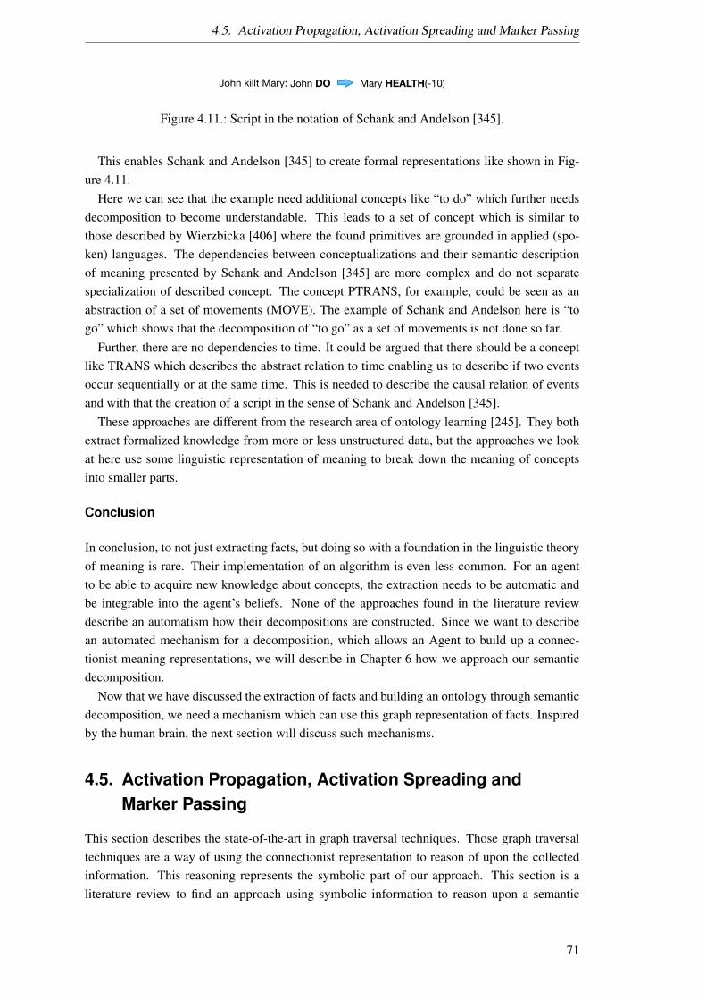
4.5. Activation Propagation, Activation Spreading and Marker Passing

John killt Mary: John DO Mary HEALTH(-10)

Figure 4.11.: Script in the notation of Schank and Andelson [345].

This enables Schank and Andelson [345] to create formal representations like shown in Fig-ure 4.11.

Here we can see that the example need additional concepts like “to do” which further needsdecomposition to become understandable. This leads to a set of concept which is similar tothose described by Wierzbicka [406] where the found primitives are grounded in applied (spo-ken) languages. The dependencies between conceptualizations and their semantic descriptionof meaning presented by Schank and Andelson [345] are more complex and do not separatespecialization of described concept. The concept PTRANS, for example, could be seen as anabstraction of a set of movements (MOVE). The example of Schank and Andelson here is “togo” which shows that the decomposition of “to go” as a set of movements is not done so far.

Further, there are no dependencies to time. It could be argued that there should be a conceptlike TRANS which describes the abstract relation to time enabling us to describe if two eventsoccur sequentially or at the same time. This is needed to describe the causal relation of eventsand with that the creation of a script in the sense of Schank and Andelson [345].

These approaches are different from the research area of ontology learning [245]. They bothextract formalized knowledge from more or less unstructured data, but the approaches we lookat here use some linguistic representation of meaning to break down the meaning of conceptsinto smaller parts.

Conclusion

In conclusion, to not just extracting facts, but doing so with a foundation in the linguistic theoryof meaning is rare. Their implementation of an algorithm is even less common. For an agentto be able to acquire new knowledge about concepts, the extraction needs to be automatic andbe integrable into the agent’s beliefs. None of the approaches found in the literature reviewdescribe an automatism how their decompositions are constructed. Since we want to describean automated mechanism for a decomposition, which allows an Agent to build up a connec-tionist meaning representations, we will describe in Chapter 6 how we approach our semanticdecomposition.

Now that we have discussed the extraction of facts and building an ontology through semanticdecomposition, we need a mechanism which can use this graph representation of facts. Inspiredby the human brain, the next section will discuss such mechanisms.

4.5. Activation Propagation, Activation Spreading andMarker Passing

This section describes the state-of-the-art in graph traversal techniques. Those graph traversaltechniques are a way of using the connectionist representation to reason of upon the collectedinformation. This reasoning represents the symbolic part of our approach. This section is aliterature review to find an approach using symbolic information to reason upon a semantic

71

4. State-of-the-Art

…

F(x)

Activation

Node Function

NodeRelation

Figure 4.12.: Abstract approach of activation spreading.

graph. The approaches described in this section build the foundation upon which we have buildour Marker Passing algorithm in Chapter 7 and motivate why an extension of the existing ap-proaches is needed. Therefore we are going to analyze research done on Spreading Activationand token passing over semantic networks in combination with automatic ontology creation akasemantic decomposition. Activation spreading is a type of graph search. The basis is a graph,where information is passed from a set of start node to connected nodes. This spreading ofinformation follows rules which guide the information through the graph. If the information issome activation, then mostly the nodes have some activation threshold like in Artificial NeuronalNetworks [80].

Figure 4.12 shows the abstract approach of activation spreading. Here the set of start nodes(blue) carry activation (orange box) to adjacent nodes. Each node has a node function whichdecides how to propagate its activation to its neighbors. The result of the activation spreadingcan be the activation of specific nodes (in Artificial Neuronal Networks called output-layer) orthe activation of the network. Figure 4.12 shows the activation of two interpreted nodes in greenand red for an exemplary classification task. If one node is more activated than the other, weneed some interpretation for the result.

Using examples from nature, which seem to work well as a prototype for algorithms in Artifi-cial Intelligence, has become a standard approach. Since the dissertation of M.R. Quillian [314]about “Semantic memory” at the Carnegie Institute of Technology in 1966, the idea of represent-ing knowledge in a network and using the connection in the network, has spilled to the ArtificialIntelligence community. Multiple questions have been subject to research like the structure ofthe network [59] which has been refined from Collins and Loftus [58], how similarity modelsover features of concepts can be determined [362] or how the connection of concepts is influ-enced by episodic memory [316]. Rogers et al. [333] further extends the features from which thesemantic knowledge is derived to perceptual features. Up to modern neuroscience which maps

72

4.5. Activation Propagation, Activation Spreading and Marker Passing

how the human brain organizes knowledge [301].All this research has influenced the theory of Artificial Intelligence. Since we are going

to use such an approach in our artificial representation of meaning, we discuss its connectionto our approach next: Creating two theories of how Artificial Intelligence can be formalized:“Logical versus analogical or symbolic versus connectionist or neat versus scruffy” like the titleof the paper of Minsky [273] suggests. The first one thinks that symbols carry meaning andthat the use of logic like in first order logic can represent intelligence and if the intelligenceis not sufficient, then the logic needs to become more complex. The second one thinks thatthe meaning of things is represented in the connection a concept has with other concepts. Ourapproach emulates the one of Minsky by trying to connect the both sides and creates a spreadingactivation mechanism over a semantic network with the symbolic logic to steer the spreadingactivation. This mechanism is used to enable an AI planner to choose actions of a plan wisely;meaning we create a heuristic to improve the AI action selection step of an AI planning algorithmin regards to precision a recall [97].

Liu et al. [239] use activation spreading over a semantic network, build from a mix of domainontologies and WordNet resources, to identify extension point for semi-automatic ontology re-finement. The analysis of Liu et al. [239] is limited to nouns only.

Marker Passing is a more general term for activation propagation or activation spreading,where more general information can be encoded into a maker than just its activation. We aregoing to use the more general term Marker Passing from now on to describe that kind of ap-proaches. P. Maes [247] uses activation spreading for action selection in a task network. Maesdescribes an additional parameter of her Marker Passing which is a mean level of activation,regarding the entire network. Fahlman [92] uses Marker Passing on semantic networks with afocus on massively parallel computing. Fahlman was the first to use the markers to reason morecomplex relations on a knowledge graph. By combining Marker Passing with a special type ofedge, a so-called cancellation edge, reasoning can be done in a more complex manner.

There is much different application of this Marker Passing or activation spreading technique.One of them is Wang et al. [398], for example, use such an activation spreading for ontologymatching. Another area of Natural Language processing is Fischer [119] like the querying of anontology.

Anderson [10] proposed a Theory of memory using Marker Passing to model delay behaviorof human brains. The idea behind the work of Anderson is that the semantic network and thedistance of two concepts in its encoded semantic information can be structured by measuringhow long it takes for a token to reach a given concept from a given start concept. Measuringthe time is such a graph, abstracts the step count. Which is why Anderson’s work has beensubsumed by other more general approaches like the one of Thiel and Berthold [379].

Thiel and Berthold [379] proposes two-word similarity measures which use activation spread-ing as a basis: node signatures similarity and node activation similarity. The first one is basedon the comparison of norms of the velocity vectors of the activation spreading and can be in-terpreted as structural similarity. The second one compares the accumulated activation and canbe interpreted as a spatial distance measure. This approach is evaluated through the analysis ofSchools-Wikipedia15 (2008/09) as a data set to firstly find nodes which are structurally similarto a query node and secondly to find closely connected to the query node. The resulting graphsare displayed in a centrality layout and analyzed manually for structural similarity.15http://schools-wikipedia.org/ last visited on 09.09.2017

73

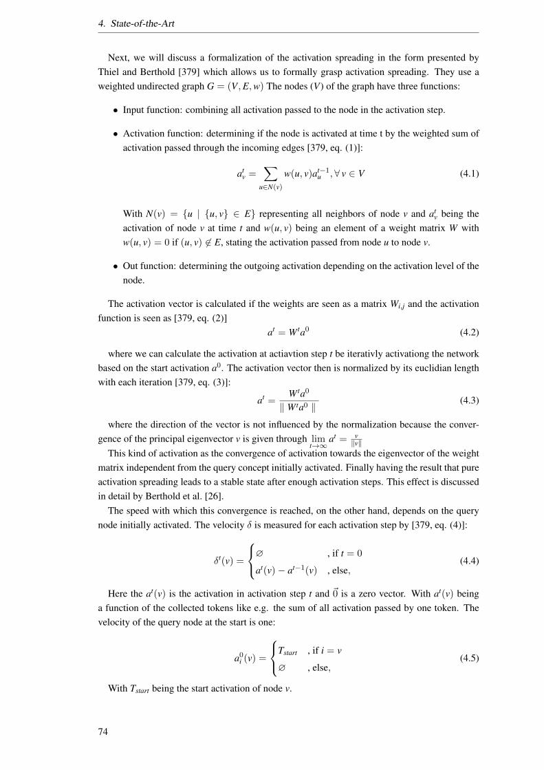
4. State-of-the-Art

Next, we will discuss a formalization of the activation spreading in the form presented byThiel and Berthold [379] which allows us to formally grasp activation spreading. They use aweighted undirected graph G = (V,E,w) The nodes (V) of the graph have three functions:

• Input function: combining all activation passed to the node in the activation step.

• Activation function: determining if the node is activated at time t by the weighted sum ofactivation passed through the incoming edges [379, eq. (1)]:

atv =

∑u∈N(v)

w(u, v)at−1u , ∀ v ∈ V (4.1)

With N(v) = u | u, v ∈ E representing all neighbors of node v and atv being the

activation of node v at time t and w(u, v) being an element of a weight matrix W withw(u, v) = 0 if (u, v) 6∈ E, stating the activation passed from node u to node v.

• Out function: determining the outgoing activation depending on the activation level of thenode.

The activation vector is calculated if the weights are seen as a matrix Wi,j and the activationfunction is seen as [379, eq. (2)]

at = W ta0 (4.2)

where we can calculate the activation at actiavtion step t be iterativly activationg the networkbased on the start activation a0. The activation vector then is normalized by its euclidian lengthwith each iteration [379, eq. (3)]:

at =W ta0

‖ W ta0 ‖ (4.3)

where the direction of the vector is not influenced by the normalization because the conver-gence of the principal eigenvector v is given through lim

t→∞at = v

‖v‖This kind of activation as the convergence of activation towards the eigenvector of the weight

matrix independent from the query concept initially activated. Finally having the result that pureactivation spreading leads to a stable state after enough activation steps. This effect is discussedin detail by Berthold et al. [26].

The speed with which this convergence is reached, on the other hand, depends on the querynode initially activated. The velocity δ is measured for each activation step by [379, eq. (4)]:

δt(v) =

∅ , if t = 0

at(v)− at−1(v) , else,(4.4)

Here the at(v) is the activation in activation step t and ~0 is a zero vector. With at(v) beinga function of the collected tokens like e.g. the sum of all activation passed by one token. Thevelocity of the query node at the start is one:

a0i (v) =

Tstart , if i = v

∅ , else,(4.5)

With Tstart being the start activation of node v.

74

4.6. Service Planning

Thiel and Berthold [379] additionally introduce a post processing step, in which they normal-ize the activation of a node by its number of edges the nodes have. The normalisation is done bythe division of the “weighted degree Matrix” D which is a diagonal matrix with each non zero

element being di,i =n∑

j=1wi,j. The normalized activation then is calculated as [379, eq. (7)]:

a∗i (v) = D−12

(tmax∑t=1

αtat(v)

)(4.6)

This normalization has the effect that well connected node are not over estimated by theactivation. With the decayed activation a∗i (v) multiplyed with an decay 0 ≥ α ≤ 1 [379, eq.(6)]:

a∗i (v) =

tmax∑t=1

αtat(v) (4.7)

With tmax being the maximum amount of activation steps done before evaluating the result.Hence tmax represents the termination condition of this activation algorithm. This formalizationof activation spreading with its double valued activation is not able to encode further informationinto the activation.

The approach of Fahlman [92] extends this activation spreading to Marker Passing but de-scribes its Marker Passing with a two-way linked list M for each marker, representing all nodeswhich are marked with this marker. The Marker Passing is then done by setting and removing el-ements in those lists. With that Fahlman is able to create queries which state: “if the node holdsmarker X, then...”. With that, he can create queries based on multiple markers, but can onlyencode the presents of a marker type, no further symbolic information because the informationencoded depends on the order in which the markers are put on the semantic graph.

Conclusion

In conclusion, the current Marker Passing approaches can carry more information than the basicactivation, but we were unable to identify an approach which uses the symbolic information forreasoning, except the work of Fahlman [92] which has special purpose symbolic informationencoded on the markers. Fahlman encodes the edge information onto the marker, to describewhich edge should be traversed. This is not enough since not only the edge which has to be tra-versed my change, but the reaction of a concept concerning markers may change as well. All ofthose algorithms are thought for the passing of markers and an analysis of the resulting markersor the marker distribution. Furthermore, none of the approaches used semantic information onthe markers except Anderson [10] more than 30 years ago. The structured analysis of the use ofMarker Passing did not reveal any use of more symbolic information on markers since then.

Additionally, we can see the analyzes done on the Marker Passing so far. The main concernseems to be an application of Marker Passing for some use case and not the Marker Passingitself, its benefits, prerequisites or limitations.

4.6. Service Planning

This section surveys the state-of-the-art of service planning approaches. The goal of this surveyis to find planning algorithms which make use of semantic information provided by semantic

75

4. State-of-the-Art

service descriptions to build a heuristic. We do this survey to make sure that we are not rein-venting some problem-solving mechanism, which uses semantic heuristics for problem-solving.The heuristic is our point of application; making one step towards filling the performance gapbetween static and learning planners [112]. We try to narrow this gap by creating a serviceplanner using semantic heuristics like it is done in service composition techniques. The relatedwork on service composition is well researched, but there are only a view approaches using plan-ning as composition mechanism. The literature provides a set of different service compositionapproaches and concepts.

Those planning and composition approaches are analyzed to their composition type describ-ing if they are (semi-) automatic or manual. Furthermore, we analyze how dynamic an approachis (Adaption) and on which Basis the planning builds up on, e.g., a Workflow or heuristic search.

Heuristics can be build by simplifying the given problem [304]. Those implications are forexample used by Fast-Forward-Planner by removing the delete list of service effects [171]. Be-cause of the open world assumption, this does not work in service planning. Other heuristicsguide specific problems which then can not be used in problem independent (sometimes calledgeneral purpose) planning [304], because they do not adapt to, e.g., changes in the goal or tonew services. Thus we need another way of gathering information about the available serviceand the goal. In this work, this information is the meaning of the concepts used to describe, e.g.,the service or goal.

One service composition approach is WSPlan, developed by Peer [305]. WSPlan uses aknowledge base and services described in WSDL extended by semantic annotations in a PDDLsyntax. The knowledge base and the annotations of web services are transformed into PDDLdocuments. It uses an online planning method for service composition which means that theplanning and execution are interleaved.

There are other solutions which also transform service descriptions into another descriptionlanguage for service composition. The solution developed by Okutan et al. [293] transformsOWL-S descriptions of services into the Event Calculus framework in which actions and theireffects are expressed, the solution by Kuzu and Cicekli [216] transforms OWL-S descriptionsinto PDDL and the solution by Sirin et al. [360] transforms OWL-S descriptions into the SHOP2domain to use SHOP2 as an HTN planner.

Rodriguez et al. [331] state the Quality of Service (QoS) parameters are a significant researchchallenge which is not reflected in the approaches found in our state-of-the-art analysis. HavingQoS parameters in a service description and having planner use this information would be a wayto create an optimization problem out the service composition problem. Markou and Refanidis[254] analyze nondeterminists methods and whether a heuristic is used or not. Neglecting whichinformation the heuristic build upon or how it is used.

Zou et al. [430, 431, 432, 433] analyze the performance of different planning methods, butneglect any semantic information from the service descriptions, which leads to a focus on ap-proaches which are based on the planning language PDDL. With the translation from OWL andSWRL to PDDL, most semantic information gets lost and with that the ability of the planningapproach to create a semantic heuristic. Another service composition solution based on such atranslation is OWLS-XPlan, developed by Klusch [196]. It transforms OWL-S descriptions ofservices into PDDLXML, an XML dialect for PDDL. For service composition, it uses a combi-nation of a Fast-Forward-planner and an HTN planner.

Rodriguez-Mier et al. [332] neglects nonfunction parameters but uses a general heuristic

76

4.6. Service Planning

in an A∗ search. This heuristic is build so that the evaluation function f (n) = g(n) + h(n)

counts the already executed service in state n in g(n) and the still needed service execution tothe goal in h(n). Creating the heuristics includes creating a service dependency graph, in whichthe mappings from out- to in-put parameters are the edges between the service calls, which arerepresented as nodes. With that, the services form layers in the dependency graph and allow anestimation which layers the current service to call is located in. With this heuristic, the planningminimizes the number of web service calls. Calculating the service dependency graph includessolving the planning problem, making the heuristic useful in the path selection, if multiple pathsfrom start to goal state are found.

Meyer and Weske [264] use a similar heuristic: The number of service calls to achieve thegoal state. The idea is similar to Rodriguez-Mier et al. [332] since graph plan is used in a relaxedplanning problem, by ignoring the negative effects. Then the service dependency graph is usedto estimate the number of service calls to the goal.

Hoffmann and Nebel [171] neglect the delete list of service effects as well to form a fast-forward planner. This is possible because a PDDL effect consists only of deleted and addedaxioms. It can be argued that with the open world assumption of OWL such a heuristic is notpossible since no delete and add list can be identified. Klusch et al. [201] use the heuristic ofHoffeman and Nebel and use a breadth-fist search in case of heuristic equivalence of to states.Mediratta and Srivastrava [260] also use the heuristic of Hoffmann and Nebel to buidl an AND/OR-graph. The heuristic than takes the minimal cost of an OR-branch and a sum of the cost incase of an AND branch.

Bonet and Geffner calculate their heuristic by taking each fact of the goal state and search-ing backward to the state space until they find a service which fulfills this fact. The functionsgetPrecondition() and getEffect() get the fact describing the service. Services describes here theset of all available services. Selecting the maximum of all the path reaching to the service whichfulfills the preconditions of the current service guarantees an admissible heuristic. This heuris-tic uses the semantic information of precondition and effect but neglects the input and output.Additionally, they ignore any semantic similarity and only check for equivalence of the facts inprecondition and effect.

Akkiraju et al. [6] present an approach called SEMAPLAN, which uses WSDL-S16 serviceto create a service description. The focus in SEMAPLAN is on the combination of in- andoutput parameters through ontology matching using WordNet or domain specific ontologies.The planning is done with in iterative forward search using all services which are semanticallyclose to the wanted ones. The algorithm terminates if all facts in a goal are created through aneffect of a service or if there are no more service to try.

Cavallaro et al. [47] propose a dynamic service composition framework, called Connect,which focuses more on the software development perspective of a service composition. Thegoals of the service composition are formulated as “expectations” and describe requirements ofthe services used. The Connect framework then searches for services fulfilling the requirementsduring runtime. Goals are formulated as operation calls. Thus the planning at runtime consistsof finding a service providing the operation and connecting they’re in- and output.

Fernandez-Olivares et al. [113] describe a system call SIADEX which can use multiple plan-ning methods form the domain of Hierarchical Task Network (HTN) to create service composi-tions. The translation from OWL-S is here to an HTN. A goal is can be formulated in OWL-S16see https://www.w3.org/Submission/WSDL-S/ for more details. Last visited on 09.09.2017

77

4. State-of-the-Art

syntax and is translated to an HTN goal. The result of the HTN planner then is translated backinto a service composition. A benefit of SIADEX is that it includes a monitoring component tomeasure plan failure and trigger a replanning at runtime. The benefit of using HTN as planningproblem formalization is that SIADEX can execute services in parallel.

Kuter et al. [215] describe an HTN based planning called ENQUIRER. Like in the SIADEXapproach the OWL-S descriptions are translated into an HTN, the goal is translated as well, andan HTN planner is used to create a service composition. Novel in the ENQUIRER approach isthat during the planning, services can be executed to gather dynamic information for the planningprocess.

The Eclipse-plugin WS-Engineer proposed from Foster et al. [121] is a manual approachto service composition. A service composition is described in the Business Process ExecutionLanguage (BPEL) and UML Message Sequence Charts. As a basis for an execution of a servicecomposition, Foster et al. focus on the development and distribution of service compositionswith execution details like authentication.

Wang et al. [396] propose a web service composition based on Markov Decision Process(WSC-MDP). The approach is based on an explicit description of service alternatives and theuse of reinforcement learning to learn the best alternative during runtime. The service composi-tion is modeled as Markov Decision Process, with state transitions modeling service calls. Thereinforcement learning then defines the transition probability, which describes the availabilityor performance of the service. Through this learning, better performing services have a highexecution probability. The used languages for service description and implementation detailsare omitted by Wang et al.

Rao et al. [321] describe an approach called “Web Service Synthesis Architecture” (WSSA)which uses linear logic theorem proving to create service compositions. The WSSA approachtranslates OWL-S service descriptions into linear logic axioms and goals in theorems. A theoremprover is then used to find a proof for the given theorem with the given axioms. If a proof isfound, then a service composition can be derived which fulfills the goal. During the provefinding process semantic reasoning is used to identify type hierarchies which are formalized asimplications and ease the proving. The paper does not describe how the Effect and preconditionare translated, e.g., from SWRL to logical axioms. The analysis of Rao et al. is restricted to alevel of input, output, precondition, and effect as a whole.

El Falou et al. [87] describe a decentralized multi agent approach to handle the ever growingamount of services. Concerning the heuristic used, the approach assumes that the relevant ser-vices have been selected beforehand. The plan is separated into partial plans which are handledby different agents. The result of the partial plan is then combined to a service compositionreaching the given goal. The approach is quite abstract and misses a description of the mecha-nisms of finding the services or how to evaluate their goal archival.

Papadopoulos et al. [299] describe a decontrolled multi-agent service composition (DMASC),which implements an self-organizing distributed service composition. Prerequisite is that theservice provides logic to be part of the decomposition where Papadopoulos et al. talk of acoalition. Each agent then searches for predecessor or predecessor by matching in- and out-puts.

Hatzi et al. [159] describe the PORSCE II service composition approach which also translatesOWL-S description int PDDL. PORSCE II then uses different external planners to solve theplanning problem. The focus of Hatzi et al. is on the specification of the start and goal state, for

78

4.6. Service Planning

which they provide a user interface. The user interface also provides a visual representation ofthe service composition and allows a manual adaption.

Fujii and Suda [126, 127] describe a service composition system called Component ServiceModel with Semantics (CoSMoS). The focus of CoSMoS is to create goal descriptions fromnatural language. The goal is described in a logical predicate, which they derive from naturallanguage requests. CoSMoS uses semantic analysis to verify the used service to fit the contextin which the services are called.

Fanjiang and Syu [105] use genetic algorithms for service composition without any heuristic[226]. Here the logical structure of precondition and effect rules are evaluated to create a correctplan. By this logical analysis, a causal links are created. This leads to a valid plan but does notcreate a heuristic.

Luca and Massimo [339] base their approach upon the BDI agent model. The approach usesthe beliefs of the agent about goals and capabilities to analyze a goal hierarchy by orderingthe goals in an AND/OR-Graph and moving down the graph towards the leaves to see whichgoal can be reached. For each step in this search, a “goal-capability deliberation” is done bysimulating the execution of a classical forward search, where the amount of used service toreach a goal is then used as a heuristic value. Since this approach uses planning on subproblemsas a heuristic, the algorithm might be used for one-shot-planning but does not describe how ituses the semantic information available. Further, they do not describe how the “selectcapabilities”function is implemented, which would tell us how the approach selects service to be executedand they do use some kind of “domain-specific utility function” which lets them rate the services.Because of these two reasons this heuristic is not a general purpose heuristic.

Oh et al. [292] describe a Web-Service Planner augmented with A* algorithm (WSPR*) basedon WSDL services and OWL parameter descriptions. The main contribution of this paper is aheuristic based on the QoS parameters of the services. The approach analyzes in input an outputof services but neglects preconditions and effects.

Wang et al. [397] propose an automated web service composition based on uncertainty exe-cution effects which can handle uncertain and contradicting service effects. The planning usedto create the service composition is the GraphPlan algorithm, which is extended to be able tosupport service with multiple effects. The approach translates OWL-S to STRIPS and a STRIPSplanner is used to solve the planning problem.

Wagner et al. [393] describe a QoS-aware automatic service composition by applying func-tional clustering to the functional description of services and their QoS parameters. Services areclustered by their functionality, and those clusters are combined to create a service composition.A cluster represents service alternatives. The service composition neglects the variable bindingsfor parameters, and the evaluation of precondition and effect is not described.

Rodriquez et al. [331] provide a survey on automatic service composition and AI methodsin software development. The existence of heuristics in the surveyed planning approaches ischecked, not how they are used or which information the heuristic is based on.

Conclusion

In conclusion, we can say that there are many approaches which use planning for problem-solving, but only a few of them use semantic information in search of the state space (see Ta-ble 4.3). Semantic information is used for service composition but is mostly static. There are

79

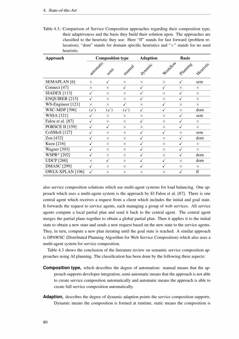
4. State-of-the-Art

Table 4.3.: Comparison of Service Composition approaches regarding their composition type,their adaptiveness and the basis they build their solution upon. The approaches areclassified to the heuristic they use: Here “ff” stands for fast forward (problem re-laxation), “dom” stands for domain specific heuristics and “×” stands for no usedheuristic.

Approach Composition type Adaption Basis

autom

atic

semi

manua

l

dyna

mic

Work

flow

Plannin

g

Heuris

tic

SEMAPLAN [6] × X × × × X semConnect [47] × × X X X × ×SIADEX [113] X × × X × X ×ENQUIRER [215] X × × X × X ×WS-Engineer [121] × × X × X × ×WSC-MDP [396] (X) (X) (X) X X × domWSSA [321] X × × × × X semFalou et al. [87] X × × X × X ×PORSCE II [159] X X × × × X ×CoSMoS [127] X × × X X × semZou [432] X × × X × X domKuzu [216] X × × X × X ×Wagner [393] X × × X × X ×WSPR* [292] X × × X × X domUDCP [260] × X × X X × domDMASC [299] X × × X X × ×OWLS-XPLAN [196] X × × × × X ff

also service composition solutions which use multi-agent systems for load balancing. One ap-proach which uses a multi-agent system is the approach by El Falou et al. [87]. There is onecentral agent which receives a request from a client which includes the initial and goal state.It forwards the request to service agents, each managing a group of web services. All serviceagents compute a local partial plan and send it back to the central agent. The central agentmerges the partial plans together to obtain a global partial plan. Then it applies it to the initialstate to obtain a new state and sends a new request based on the new state to the service agents.They, in turn, compute a new plan iterating until the goal state is reached. A similar approachis DPAWSC (Distributed Planning Algorithm for Web Service Composition) which also uses amulti-agent system for service composition.

Table 4.3 shows the conclusion of the literature review on semantic service composition ap-proaches using AI planning. The classification has been done by the following three aspects:

Composition type, which describes the degree of automatism: manual means that the ap-proach supports developer integration, semi-automatic means that the approach is not ableto create service composition automatically and automatic means the approach is able tocreate full service composition automatically.

Adaption, describes the degree of dynamic adaption points the service composition supports.Dynamic means the composition is formed at runtime, static means the composition is

80

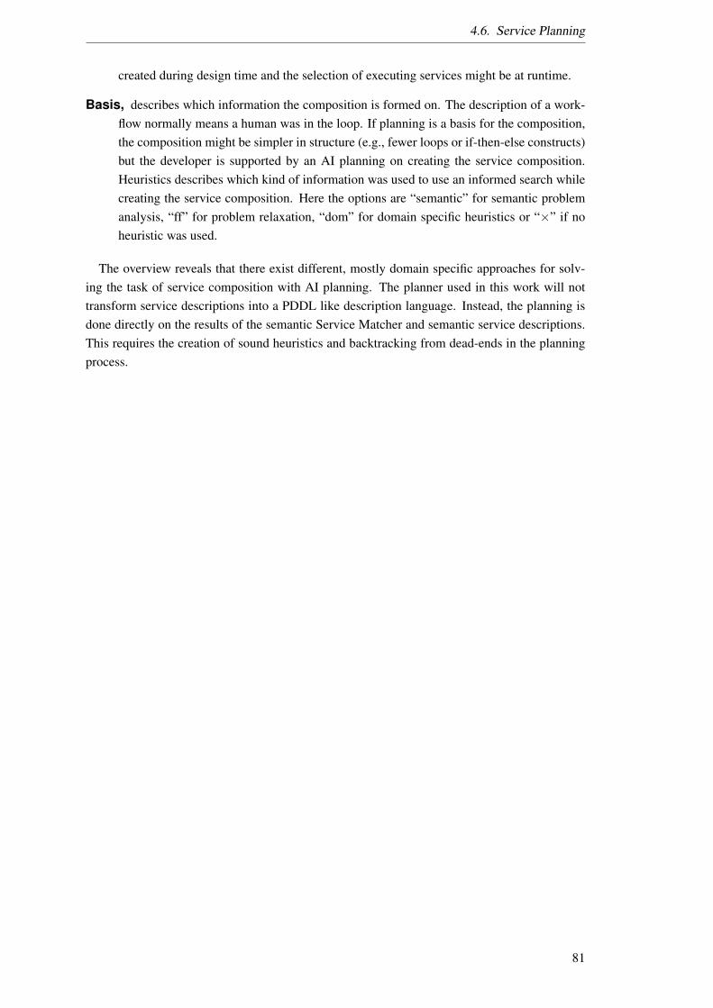
4.6. Service Planning

created during design time and the selection of executing services might be at runtime.

Basis, describes which information the composition is formed on. The description of a work-flow normally means a human was in the loop. If planning is a basis for the composition,the composition might be simpler in structure (e.g., fewer loops or if-then-else constructs)but the developer is supported by an AI planning on creating the service composition.Heuristics describes which kind of information was used to use an informed search whilecreating the service composition. Here the options are “semantic” for semantic problemanalysis, “ff” for problem relaxation, “dom” for domain specific heuristics or “×” if noheuristic was used.

The overview reveals that there exist different, mostly domain specific approaches for solv-ing the task of service composition with AI planning. The planner used in this work will nottransform service descriptions into a PDDL like description language. Instead, the planning isdone directly on the results of the semantic Service Matcher and semantic service descriptions.This requires the creation of sound heuristics and backtracking from dead-ends in the planningprocess.

81

Part III.

Approach

83

5. Abstract Approach

This section describes how I will approach the creation of an artificial representation of mean-ing. Described in Figure 1.2 my approach has two parts: The first part is the connectionistrepresentation of knowledge. The second part is the symbolic reasoning. As a theoretical foun-dation I use the Natural Semantic Metalanguage (NSM) (see Section 3.10) theory. The NSMtheory states that from the set of semantic primes, explanations can be created to describe morecomplex concepts. I transfer this “bottom-up” approach, to a ”top-down” approach, start withthe complex concepts, facing the problem to find a way to describe complex concepts using lesscomplex concepts down to the semantic primes of NSM. This process is called decompositionand identifies the task of describing a concept using less complex, but related concepts. Hence,the question that is approached with this task is: Which concepts are related to the concept weare interested in? Figure 5.1 describes the knowledge representation part of Figure 1.2 in Sec-tion 1.5 in more detail. This part represents how the connectionist part of my representation ofmeaning is created. The knowledge acquisition is inspired by the way we adult humans learn anew concept: If we encounter a new word, we look it up in some resource like a dictionary andconnect the there found explanation with our current knowledge.

Information

Knowledge representation

Semantic Decomposition WordNet, Wikidata,…

Domain dependentGather definitions of the conceptCollect semantic relations between concepts

Semantic Decomposition WordNet, Wikidata,…

Create a semantic graph of concepts and relationsSemantic Decomposition

WordNet, Wikidata,… WordNetWiktionaryDomain OntologiesWikidataConceptNetFrameNetBabelNet

Define a formal semantic graph

Semantic Decomposition WordNet, Wikidata,…

Normalize Information

Decide on termination conditionSemantic Decomposition WordNet, Wikidata,…

Corpus linguistic

Figure 5.1.: Abstract description of the knowledge part of this approach.

Figure 5.1 describes which information can be used in the decomposition as input, e.g., Word-Net or Wikidata. Most of these knowledge sources are general-purpose dictionaries. However,the input for the decomposition could also be a domain-specific ontology, giving facts about theconcepts needed. This creates a domain dependent representation of knowledge.

The so created knowledge can be seen as the belief of an agent and the process as beliefupdate. The main steps of this decomposition are the gathering of new information which in-cludes integrating new concepts and their relations into the agent’s beliefs. Here one problem isto describe when to stop with this information gathering process to avoid integrating unneededinformation.

The knowledge presentation is the collected information in the form of a semantic graph. Nat-urally, since the approach collecting connectionist information, we might represent this knowl-

85

5. Abstract Approach

edge as a graph. In this first part, I will describe my graph formally and show how I formalizethe fuzzy semantics of natural language with its concept and relational hierarchies, semantic re-lations like Synonyms and Meronyms and more complex relations like “giving advice”. In this,I normalize the information gained from natural language resources to a strict formal model.Further details for this semantic decomposition are described in Section 6.

Figure 5.2 details the second part of Figure 1.2 in Section 1.5. Here the reasoning part of thisapproach is described in more detail. This part has as input the connectionist representation ofmeaning from the first part and a problem specific question. These two component are then usedto specify the parameters of a Marker Passing algorithm. These parameters include symbolicinformation encoded on the markers.

Reasoning

Question

Marker Passing

Symbolic Connectionist

Problem specific

Semantic DistanceSentence SimilartyWord Sense DisambiguationService MatchingSemantic Heuristic

Define Marker Passing Algorithm

Interpret Markers for Problem

Specify Parameters of Algorithm for a given Problem

Formalize Symbolic Information on MarkersUse Semantic Graph for reasoning

Figure 5.2.: Abstract description of the reasoning part of this approach.

This symbolic information is then passed through the graph where each node and edge canchange the information on the marker depending on their interpretation. The resulting markerdistribution and the information encoded upon them is used for answering the given questions.If the first part represents the knowledge of an agent the second part could be seen as the processof thought over this knowledge. This approach on semantic reasoning is further detailed inSection 7.

The example problems listed in Figure 5.2 as input for the reasoning is then tested in theexperiments in Section 9. These example applications are selected because they all show someunderstanding of the meaning of concepts. The task to determine a semantic distance of twowords, for example, shows that without context, we can still estimate if two concepts are similaror not. The task of Word Sense Disambiguation as another example shows if we can select theright word senses of words given a linguistic context.

The so created representation of meaning reflects a cognitive model of humans in the waythat the semantic graph represents an abstracted physical part of our brains, and the MarkerPassing represents the electronic or chemical parts of our brain[315]. Thus the one side repre-sents learned knowledge (concepts) the other processes like thought to create coherent reasoning[295].

As illustrated in Figure 5.3 the creation of artificial meaning as defined in Definitions 21and 22, starts with building a model for all meanings of a concept by decomposing it. HereFigure 5.3 focuses on temporal dependencies on the approach described in Figure 5.1 and 5.2.This leads to a semantic graph representation (Ontology) of its denotation that represents theconnectionist knowledge representation of meaning. Such a decomposition is done to create a

86

Semantic Graph

Marker Passing

Symbolic Connectionist

Priming

Meaning rep.

Decomposition

Concept

Meaning

Interpretation

Figure 5.3.: Abstract approach to represent artificial meaning.

semantic graph [98]. One challenge here is to select the right definitions of the word1 from theutilized data sources to be used in the decomposition.

This semantic graph is used to pass markers through to relevant concepts.2 The informationcarried by the markers is denoted by the different colors of markers in Fig. 5.3. The marker(represented as chips next to each concept in the depiction) might carry symbolic informationthat steers the Marker Passing. To be able to react to different markers, each concept in thesemantic graph has an interpretation function reflecting its behavior. The interpretation functioninflects how the concept processes incoming markers, how outgoing markers are passed on toother concepts and whether it is activated. In this way, e.g., a “NOT” concept passes its markersto the next concept so that this one activates its opposites (in linguistics named “antonyms”).Since semantic relations like synonym and antonym relations have different meanings as well,the relation interpretation function allows specifying how a relation passes on markers. In thisway, symbolic information like temporal logic can be encoded in the graph. One challenge atthis step is the amalgamation of the connectionist representation in the semantic graph and thesymbolic representation provided by a concept and edge in the semantic graph.

During the activation, we can influence how the amalgamation of symbolic and connectionistrepresentation of meaning is contextualized. By activating the right concepts out of context,the Marker Passing will activate different concepts in the semantic graph and thus contextualizethe representation of meaning. Here the selection of parameters and concepts to activate ischallenging. Finally, we need an interpretation of the output of the Marker Passing to extract therepresented meaning.

If we want to extract the meaning of the word ‘Bank’ in a text discussing the financial crisis,the Marker Passing will have more markers on ‘Bank’ as a financial institute then on the seatingaccommodation. This is because the activation of contextual concepts will probably activateconcepts like money, accounting, currency or equivalents from the text during the Marker Pass-ing. Through this combination of activated concepts and interpretation functions, we create apragmatic representation, which leads to a context-dependent interpretation of the knowledgeencoded in the graph.

1This challenge is related to the word sense disambiguations and is one reason for the need of contextual informationduring the decomposition.

2Marker passing subsumes activation spreading since the classical activation spreading can be modeled with amarker that carries the activation level as a numeric value.

87

5. Abstract Approach

This part is organized as follows: In Section 6 I will describe the semantic decompositionand Section 7 describes the Marker Passing algorithm. I then evaluate my approach in Part IVof this thesis. In Part IV I test the reasoning upon the newly learned facts by letting the AI wecreated solve different example problems like the estimation of a word and Sentence Similarityor Word Sense Disambiguation problems. The implementation of this approach is described inSection 8 consisting of two parts: The Semantic Decomposition and the Marker Passing. Theshort introduction should give the reader the ability to use the implementation of this approachand apply it to other problems.

88

6. Semantic Decomposition

Semantic decomposition is a process to take apart the meaning of complex concepts into mul-tiple less complex ones. This section describes the semantic decomposition proposed in thiswork. I will look at how knowledge sources like WordNet or Wikidata are used to gather infor-mation about the target concepts. Then I will look at the result and analyze the outcome, and itsusefulness for our creation of a heuristic.

The goal of the decomposition is to collect all facts about a Concept of Interest (COI) neededto form an accurate representation of the meaning of these concepts in a given context. Further,the goal of this decomposition is specialized to an artificial audience, our agents. The decompo-sition has the purpose of describing the connectionist part of meaning by connecting a conceptwith other concepts, which are simpler, or less complex in the notion of the NSM theory [410].How this is done will be discussed in this section.

The method in which the decomposition is created is the following: We collect all informationavailable about a COI. Then I filter this information for its relevance to remove unnecessary factsby, e.g., removing stop words or stopping at semantic primes. The collection of informationabout a COI is done by looking up the COI in different information sources, e.g., dictionaries. Adecomposition represents the paraphrases which describe a concept [328, p. 213]. Riemer [ibid.]describes in the decomposition as it has been practice in dictionaries in the following way: “themeaning of the definiendum is recast in terms of several defining terms which, if the definitionis to be explanatorily successful, must each in some sense be simpler than the definiendum or,at least, already understood by the definition’s user.” Here the term simpler is still too unspecificto understand how we can describe meaning, which I will elaborate closer next: In the theory ofNSM, the simplest concepts are those that make up the semantic primes. I build my approachto this theory by assuming that the meaning of these primes is known. Based on those primes Ican describe more complex concepts only by using primes. These are then less simple than theprimes itself. I then, define the meaning of more complex concepts by describing concepts whichI was unable to describe by only using primes and the first set of more complex concepts [410,p. 7]. I repeat this process until all concepts have a definition. The so created hierarchy buildsmy scale of complexity (simplicity in anti-proportionally).

There are two reasons for inverting the direction of the theory of NSM in my decomposition:First in the theory of Wierzbicka [406] and Goddard [145] the idea is that upon semantic primesevery concept of a natural language can be described. This forms different complexity levels,where the semantic primes are the least complex. Since we are looking for an explanation of acomplex concept, searching from the bottom up (from the primes in complexity upwards) wouldresult in a big search space since we do not know which concepts are needed, which meanswe would need to build all concepts which are solely described by semantic primes and buildour way upwards to the COI. Narrowing the search space, the decomposition tries to find adecomposition of all concepts defining the COI, top down.

The second reason is: Semantic approaches often struggle with their use in AI since the

89

6. Semantic Decomposition

appropriate knowledge or needed cognition is still not accessible for computers. In combinationwith the Natural Semantic Meta Language (NSM) theory, a decompositional approach seemspromising in representing meaning for AI. Decompositional approaches describe lexical contentby splitting it up into smaller parts [328].

Using the theory of NSM, I can use the semantic primes to describe all other concepts in anatural language from bottom-up, to building the meaning of complex concepts. The funda-mental idea of the semantic decomposition for AI is: if the meaning of the semantic primes isgiven, I want to enable my agent to build the meaning of more complex concepts on its own byfirst creating a decomposition and then using the semantic primes to give the complex conceptmeaning. The decomposition is seen as a way of an agent to self-explain new concepts by in-corporating its definition or some other explanation into its beliefs. This means that by lookingup explanations of unknown concepts, e.g., in a dictionary, the agent extend his semantic graphto include the unknown concept.

In the Cambridge Dictionary1 to explain is defined as follows: ‘to make something clear oreasy to understand by describing or giving information about it’. By examining this definition,we notice, that explaining is the act of giving information about a COI to an audience with theintend to foster both the knowledge and the understanding about the COI. The explanation givenhere seems to be a description of the relations the COI has with other concepts. This explanationhas to consist of concepts already known to the audience, else the explanations of those conceptsneed to follow recursively. This means that the explanation can be context dependent becauseif other concepts are known by the audience, the explanation of the same fact about a COI canchange. This can be seen in the way we explain the concept of numbers to children in secondgrade and during a course of algebra in mathematic studies. Each new fact about concepts givesthe agent a new connection point, which might allow it to connect the new concept to its beliefs.

Some other approaches have been investigating decompositions and how semantic primesinfluence the expressiveness and the reasoning upon such semantic graphs. Schmidtke [349]represents such meaning in logical concepts and proposes a reasoning with primes for qualita-tive reasoning on the example of spatial concepts. For this Schmidtke extends the first orderlogic with primes, e.g., spatial reasoning. The extension from Schmidtke are pragmatic but arelimited to his use case. Ferrand [114] analyzes priming effects from a psycholinguistic viewby using a decomposition level of letters, words, and semantic-level decomposition. The otherway around the theory of compositionally state the meaning of expressions is composed by themeaning of its parts and the syntax composing them [208]. But Kracht [209] argues as well, thatlogical languages are typically not compassable. This means we can not take an arbitrary logicallanguage and build our decomposition upon it.

The decomposition of meaning is used here as a basis and is not subject to the research itself.Andrews [11] analyzes the formal representation of NSM primes and their properties. He startedthe analysis of combining NSM semantic with formal semantics. Even though this is only a startfor a subset of primes, it shows that the logico-semantic features of NSM might be formalized.

These approaches show that theories from linguistics are used to describe formal semantics ina decompositional manner, but these approaches all lack a construction mechanism which allowsthe agent to extend its known concepts. The decomposition we propose creates an automatedmechanism which collects explanations for concepts and integrates them into the beliefs of theagent, i.e., the semantic graph. Depending on the context of the explanations, different facts

1Cambridge Dictionary Online, visit http://dictionary.cambridge.org/ last visited on 09.09.2017

90

6.1. Natural Semantic Metalanguage

about the concepts and its relations to others is described.Now for us humans, the decompositions to explain new concepts can be based on a multi-

tude of information sources. We can learn through conversations, by processing arguments of adiscussion, by reading a text, by thinking about the information we already know or by experi-ence. For AI this is different since the cognition is restricted to the implementation of the agentwhich encapsulates the AI. The here presented decomposition represents a mechanism whichis motivated by the way adult humans learn new concepts and use dictionaries and at the sametime builds upon the theory of NSM which allows us to give the agent a set of basic concepts,creating the foundation to bootstrap the creation of an artificial meaning representation for morecomplex concepts.

The definition of a dictionary is most likely not of this form since they take into account thecommon sense knowledge of humans and therefore do not try to use as many primes as possible.This is anticipated in the decomposition, and that is why the decomposition replaces conceptsclose to semantic primes with semantic primes.

The next sections are structured in the following manner: Now that our objective is clear wetake a deeper look at NSM in Section 6.1. Semantic primes have already been used in artificiallanguages which is shown in our analysis of three example semantic description languages fortheir containment of semantic primes in Section 6.2. We then take a look at the used data sourcesin Section 6.3. In Section 6.4 we look at the formalization of the output of our semantic decom-position algorithm. This formalization finally allows us to describe an algorithm which willcreate such a decomposition automatically in Section 6.5. We conclude our automatic semanticdecomposition in Section 6.6 and describe its benefits and shortcomings.

6.1. Natural Semantic Metalanguage

Above we have described an explanation as breaking a complex concept down into simpler con-cepts. To determine the complexity hierarchy of concepts, we use a theory from linguistics calledNatural Semantic Metalanguage. To recapitulate: we have looked at NSM in Section 3.10. Intheir works, Wierzbicka [411] and Goddard [143] for example have analyzed natural languagesfor a common semantic crux, and they found approximately 65 semantic primes. Making up ahierarchy of concepts only described with primes, then concept described with those ”first-level”concepts and primes, making up the second level and so forth [p. 7][410]. Our decompositionwill thus stop at those words since they do not need a further decomposition. This leads to thedecision that synonyms of semantic primes are replaced with the prim.

An example of the first level might be the description of surprise [139]:

[X] was surprised:

[X] felt something at that time

like people can feel when they think like this:

‘‘something happened now

I did not think this would happen."

In this example, the complex concept of “surprise” has been described by only using semanticprimes. Accordingly, in future descriptions “surprise” can be used to describe further concepts.Of course, this example description does not fit our need for AI. We do not restrict our explana-tion to syntactically well-formatted sentences and add additional information needed by an AI

91

6. Semantic Decomposition

which is naturally available in humans, like the grammatical forms of “to feel” and synonymsand references for concepts like “time”. This is why we abstract from syntax in our decompo-sition. Even with this simplification, a decomposition of complex concepts could still becomelarge. To decompose every concept into solely semantic primes seems like a rather theoreticalgoal like creating an Explanatory combinatorial dictionary (ECD), which is not needed since thelevel of decomposition can be adapted to the reasoning task the agent has to do.

Utilizing this theory for AI, we have multiple benefits besides the hierarchy of concepts:First, to bootstrap our natural language understanding we only need to describe the meaning of65 concepts. Second, the primes fall into categories, which lets us describe syntactical rulesfor them in a more abstract way. This could be done, e.g., for logical primes, which might behandled in other manner or by other components than the other primes because they could bemore universal. Third, those primes are natural language, which makes them understandable byhumans, allowing understanding and analysis of the decomposition it self. This is a benefit overrepresentations which are regarded black box approaches like artificial neural networks. Fourth,we have an example decomposition done by humans as in the example of surprised above. Thisallows an automatic decomposition since humans can help the automatic decomposition if itgets stuck. Fifth, the NSM theory gives the decomposition a theoretic grounding, separatingthis kind of ontology creation from other ontology learning methods. The theoretic groundingensures that the selected primes are not arbitrary or can not be understood by humans. Since theprimes have been shown to occur in many natural languages [144].

A Drawback of our decomposition approach is that it highly depends on the quality of in-formation sources it can use. Furthermore, since we are using multiple data sources, multipledefinitions of the same concept, which could lead to ambiguity. By using information sourceswhich are created by humans, the decomposition contains faulty information, contained in thoseinformation sources and hence can be manipulated.

NSM is defined for natural languages. It is not clear if this property of semantic primes is alsopresent in artificial languages, and if primes exist in artificial languages if they are the same asin natural languages. Nor is it clear if we can transfer the insight we have gained form naturallanguages through the NSM theory, to artificial languages. To see if the primes are as wellpresent in artificial languages, e.g., as keywords in programming languages, we analyze threeartificial example languages used for semantic modeling if they contain semantic primes. Withthat, we want to show, that the theory of NSM can be applied to artificial languages used in AIby showing that artificial languages already use semantic primes as keywords. Also, we want toanswer the questions which semantic primes are already in use in artificial languages. By findingsemantic primes in artificial languages, we ensure that those primes are not solely representativefor a human fundamental semantic core and with that make it more likely that the rest of ourwork will not end into domain specific interpretation of some arbitrary concepts. Furthermore,with the NSM theory we would only need to provide the semantic for the ca. 65 primes, and withthe right composition, we could create the meaning of all other concepts automatically. With theanalysis of which primes already exists in artificial languages, we have a list of primes for whichwe have an explicit semantic defined already. Leaving us with the remaining NSM primes forwhich we still have to define a semantic.

92

6.2. NSM Semantic Primes in Artificial Languages

Table 6.1.: List of semantic primes and equivalent concepts found in OWL.

Category Semantic prime OWL

Substantive I self.entrySOMETHING/ THING owl:thing

Relational KIND owl:SubClassOfsubstantives PART owl:topObjectPropertyDeterminers THIS owl:entityURI

THE SAME owl:equivalentClass

6.2. NSM Semantic Primes in Artificial Languages

In this section, we look at how NSM semantic primes (see Section 3.10) are used in artificiallanguages. Artificial languages have semantic primes which need to be defined with a clearsemantic for a compiler or interpreter to be able to use these languages. In computer science,such primes are called keywords. Since the NSM theory states that primes make up naturallanguages, we are going to analyze which role primes play in artificial languages. The retrievalof semantic primes as a subset of the natural semantic primes form NSM theory, in artificiallanguages shows that those primes are not reserved to natural language and that the implicationsdrawn from the NSM theory could apply to artificial languages as well. We do so by lookingat OWL as our ontology description language, PDDL as the most common planning descriptionlanguage and MOF as one of the most used modeling languages. This part of this work has beenpublished in [97].

We are doing this because we want to show that the implications from NSM theory can beapplied to artificial languages. The existence of semantic primes shows us that primes can beused in artificial languages as well and that those primes are not only used in natural languages.Which forms the theoretic basis for our representation of meaning. We use this basis, e.g., in thedecomposition to argue when to stop decomposing,

Our analysis is done in the following way: We select a semantic prime and search for anequivalent in the given language. All found primes are contained, all not found primes are notcontained, and the other concepts of the language are not primes, they are merely shortcuts ormore complex concepts.

This experiment will allow us to declare the semantic primes from natural language alsorelevant for artificial languages and acts as a starting point for further discussions on whichsemantic primes are needed in artificial languages and which ones can be ignored. We start outwith the analysis of the Web Ontology Language.

Semantic Primes in the Web Ontology Language (OWL) OWL is a semantic markuplanguage to create structured knowledge representations and enrich them with semantics. OWLis a W3C standard since 2004 and has been continuously developed since [148]. OWL is anextension of the Resource Description Framework [220] and has become one of the most usedlanguages to describe knowledge for AI. Since OWL is meant to describe structured knowledgethe concepts used are abstract. Table 6.1 list all equivalents found in comparison with NSMprimes.

93

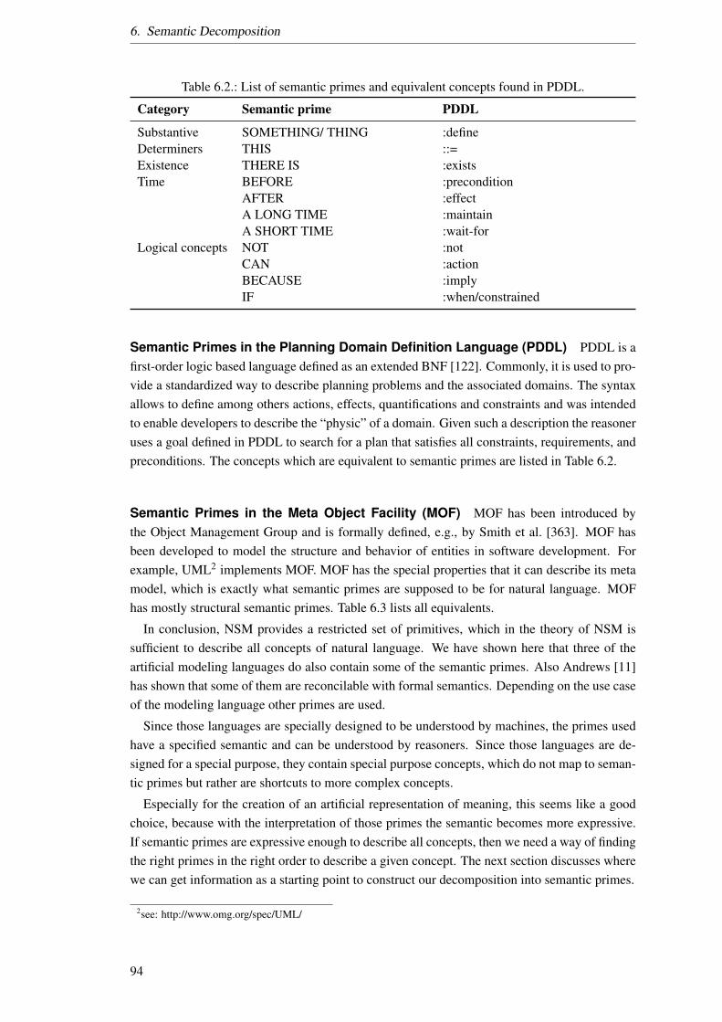
6. Semantic Decomposition

Table 6.2.: List of semantic primes and equivalent concepts found in PDDL.

Category Semantic prime PDDL

Substantive SOMETHING/ THING :defineDeterminers THIS ::=Existence THERE IS :existsTime BEFORE :precondition

AFTER :effectA LONG TIME :maintainA SHORT TIME :wait-for

Logical concepts NOT :notCAN :actionBECAUSE :implyIF :when/constrained

Semantic Primes in the Planning Domain Definition Language (PDDL) PDDL is afirst-order logic based language defined as an extended BNF [122]. Commonly, it is used to pro-vide a standardized way to describe planning problems and the associated domains. The syntaxallows to define among others actions, effects, quantifications and constraints and was intendedto enable developers to describe the “physic” of a domain. Given such a description the reasoneruses a goal defined in PDDL to search for a plan that satisfies all constraints, requirements, andpreconditions. The concepts which are equivalent to semantic primes are listed in Table 6.2.

Semantic Primes in the Meta Object Facility (MOF) MOF has been introduced bythe Object Management Group and is formally defined, e.g., by Smith et al. [363]. MOF hasbeen developed to model the structure and behavior of entities in software development. Forexample, UML2 implements MOF. MOF has the special properties that it can describe its metamodel, which is exactly what semantic primes are supposed to be for natural language. MOFhas mostly structural semantic primes. Table 6.3 lists all equivalents.

In conclusion, NSM provides a restricted set of primitives, which in the theory of NSM issufficient to describe all concepts of natural language. We have shown here that three of theartificial modeling languages do also contain some of the semantic primes. Also Andrews [11]has shown that some of them are reconcilable with formal semantics. Depending on the use caseof the modeling language other primes are used.

Since those languages are specially designed to be understood by machines, the primes usedhave a specified semantic and can be understood by reasoners. Since those languages are de-signed for a special purpose, they contain special purpose concepts, which do not map to seman-tic primes but rather are shortcuts to more complex concepts.

Especially for the creation of an artificial representation of meaning, this seems like a goodchoice, because with the interpretation of those primes the semantic becomes more expressive.If semantic primes are expressive enough to describe all concepts, then we need a way of findingthe right primes in the right order to describe a given concept. The next section discusses wherewe can get information as a starting point to construct our decomposition into semantic primes.

2see: http://www.omg.org/spec/UML/

94

6.3. Data Sources used in the Semantic Decomposition

Table 6.3.: List of semantic primes with and equivalent concepts found in MOF.

Category Semantic prime MOF

Substantive YOU uriSOMETHING/ THING objectBODY instance

Relational KIND type, extentsubstantives PART propertyDeterminers THE SAME element.equalsQuantifiers ONE multiplicityElementLocation BE (SOMEWHERE) linkExistence THERE IS element

HAVE classifierBE (SOMEONE/SOMETHING) extend

Life and death LIVE createDIE delete

Logical concepts CAN operationIF event

6.3. Data Sources used in the Semantic Decomposition

For the decomposition we have to choose the data sources we can use to look up informationabout a concept. Here the first idea is to use structured knowledge, which has already beenformalized, sparing us from the effort of formalizing it. This could, e.g., be done by usingontologies which model information we need. The second idea is to use information in text formwhich is semi-structured. Such an information source could be a dictionary, where informationabout words is given in the form of definitions, words with the same meaning and how they areused in example phrases. The third idea then is to structure unstructured information like videos,speech or figures. Next, we will discuss our selection of data sources and how they are used.

For the structured information, there are many ways of formally describing facts about con-cepts and the relation between them (see Section 6.4). This ranges from data base schemas, overannotations to descriptions logics which use formal representations like logic. The decision onwhich information sources to include is based on information available and the amount of ef-fort needed to integrate it into the decomposition. Figure 6.1 describes an estimate of effort tostructure and specificness of the information of data sources. Here, the colors describe the effortneeded for integration into the decomposition: green for less effort and red for more effort.

In Figure 6.1 we draw the line, of which information sources we integrate, between structuredtext and text for ontology learning. We selected to integrate the first three types of information(above the line) ontological, taxonomical and structured text because the fourth one ((unstruc-tured) text) is still subject to research [245, 274, 28] which is not in the focus of this disserta-tional thesis. Since the mining of text is less complex than the analysis of audio, where mostapproaches translate the audio into a text to do semantic analysis, we will not look at audio in-formation. The same arguments can be held for visual information. The colored areas symbolizethe range a given information type can be argued to describe. Here, e.g., taxonomical informa-tion consists of only one relation, which makes its description more specific then ontologicalinformation.

95

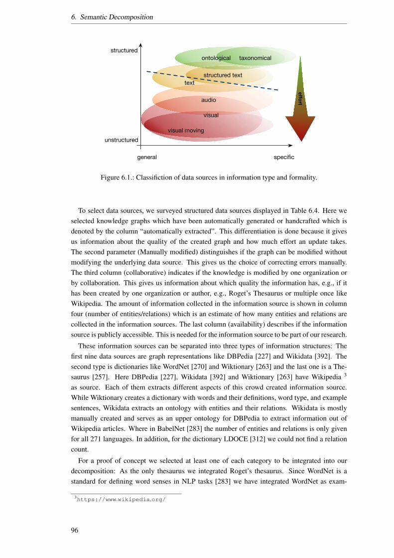
6. Semantic Decomposition

general specific

structured

unstructured

effort

visual moving

visual

audio

structured text

ontological taxonomical

text

Figure 6.1.: Classifiction of data sources in information type and formality.

To select data sources, we surveyed structured data sources displayed in Table 6.4. Here weselected knowledge graphs which have been automatically generated or handcrafted which isdenoted by the column “automatically extracted”. This differentiation is done because it givesus information about the quality of the created graph and how much effort an update takes.The second parameter (Manually modified) distinguishes if the graph can be modified withoutmodifying the underlying data source. This gives us the choice of correcting errors manually.The third column (collaborative) indicates if the knowledge is modified by one organization orby collaboration. This gives us information about which quality the information has, e.g., if ithas been created by one organization or author, e.g., Roget’s Thesaurus or multiple once likeWikipedia. The amount of information collected in the information source is shown in columnfour (number of entities/relations) which is an estimate of how many entities and relations arecollected in the information sources. The last column (availability) describes if the informationsource is publicly accessible. This is needed for the information source to be part of our research.

These information sources can be separated into three types of information structures: Thefirst nine data sources are graph representations like DBPedia [227] and Wikidata [392]. Thesecond type is dictionaries like WordNet [270] and Wiktionary [263] and the last one is a The-saurus [257]. Here DBPedia [227], Wikidata [392] and Wiktionary [263] have Wikipedia 3

as source. Each of them extracts different aspects of this crowd created information source.While Wiktionary creates a dictionary with words and their definitions, word type, and examplesentences, Wikidata extracts an ontology with entities and their relations. Wikidata is mostlymanually created and serves as an upper ontology for DBPedia to extract information out ofWikipedia articles. Where in BabelNet [283] the number of entities and relations is only givenfor all 271 languages. In addition, for the dictionary LDOCE [312] we could not find a relationcount.

For a proof of concept we selected at least one of each category to be integrated into ourdecomposition: As the only thesaurus we integrated Roget’s thesaurus. Since WordNet is astandard for defining word senses in NLP tasks [283] we have integrated WordNet as exam-

3https://www.wikipedia.org/

96

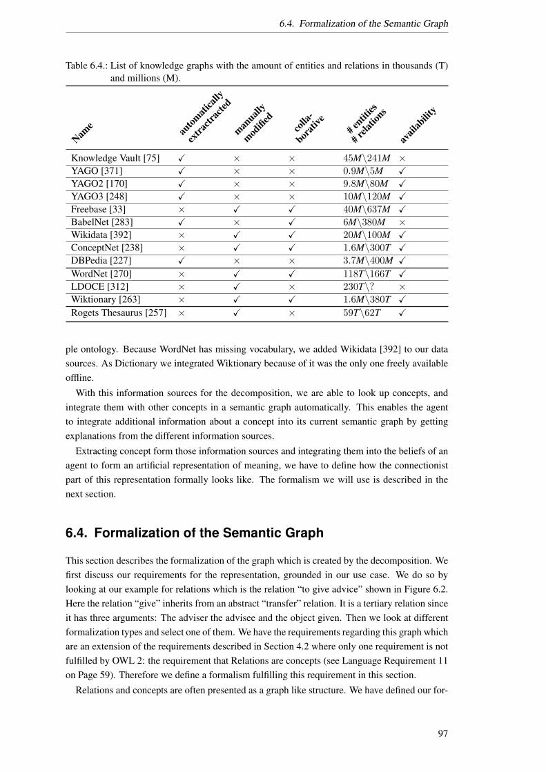
6.4. Formalization of the Semantic Graph

Table 6.4.: List of knowledge graphs with the amount of entities and relations in thousands (T)and millions (M).

Name au

tomati

cally

extra

ctrac

ted

manuall

y

modified

colla

-

borati

ve# en

tities

# relati

ons

avail

abilit

y

Knowledge Vault [75] X × × 45M\241M ×YAGO [371] X × × 0.9M\5M XYAGO2 [170] X × × 9.8M\80M XYAGO3 [248] X × × 10M\120M XFreebase [33] × X X 40M\637M XBabelNet [283] X × X 6M\380M ×Wikidata [392] × X X 20M\100M XConceptNet [238] × X X 1.6M\300T XDBPedia [227] X × × 3.7M\400M XWordNet [270] × X X 118T\166T XLDOCE [312] × X × 230T\? ×Wiktionary [263] × X X 1.6M\380T XRogets Thesaurus [257] × X × 59T\62T X

ple ontology. Because WordNet has missing vocabulary, we added Wikidata [392] to our datasources. As Dictionary we integrated Wiktionary because of it was the only one freely availableoffline.

With this information sources for the decomposition, we are able to look up concepts, andintegrate them with other concepts in a semantic graph automatically. This enables the agentto integrate additional information about a concept into its current semantic graph by gettingexplanations from the different information sources.

Extracting concept form those information sources and integrating them into the beliefs of anagent to form an artificial representation of meaning, we have to define how the connectionistpart of this representation formally looks like. The formalism we will use is described in thenext section.

6.4. Formalization of the Semantic Graph

This section describes the formalization of the graph which is created by the decomposition. Wefirst discuss our requirements for the representation, grounded in our use case. We do so bylooking at our example for relations which is the relation “to give advice” shown in Figure 6.2.Here the relation “give” inherits from an abstract “transfer” relation. It is a tertiary relation sinceit has three arguments: The adviser the advisee and the object given. Then we look at differentformalization types and select one of them. We have the requirements regarding this graph whichare an extension of the requirements described in Section 4.2 where only one requirement is notfulfilled by OWL 2: the requirement that Relations are concepts (see Language Requirement 11on Page 59). Therefore we define a formalism fulfilling this requirement in this section.

Relations and concepts are often presented as a graph like structure. We have defined our for-

97

6. Semantic Decomposition

transference

give

is-a

teacher

advice

student

object

source target

hyponym

hypernym

Figure 6.2.: Example for a relation which connects three concepts and is it self reference by arelation.

Minimum Type Graph

Concept Relation

Figure 6.3.: Minimal type graph for the description of a decomposition graph.

malization of an ontology in Section 3.6, which is used here. Since a graph with nodes and edgeswhere each edge connects two nodes is not expressive enough to satisfy our requirements (e.g.,n-ary relations and relations between nodes and edges), we need something like an attributedgraph [66]. Attributes allow us to model, e.g., concepts with literals and relations with names.Further, we need types of concepts and relations which lead us to typed attributed graphs. Fur-ther, the types we describe for concepts and relations describe a hierarchy which leads us toattributed typed graphs with a type hierarchy.

Therefore based on the requirements described in Section 4.2 we formalize the graph structureas an Attributed Type Graph with Type Inheritance introduced by De Lara et al. [66]. For aformal definition see Section 3.4.

The requirement of having an n-ary relation (multi-graphs or hyper-graph) and the require-ment of having edges among edges leads to the need of describing more complex edges. Thefact that relations are concepts as well is problematic for standard graph representations. Havingedges which are nodes makes it necessary to extend a hyper-graph. The requirement of having atype hierarchy and types of concepts and relations leads us to specify a base type graph, whichcan be adapted to a specific use case. This basic type graph is shown in Figure 6.3.

To distinguish concepts from relations, we define a minimal type graph shown in Figure 6.3.This minimal type graph can be extended regarding its use. In this minimal type graph, therelations inherit from concepts and account for the requirement of “relations are concepts”.

We define a minimal type graph so that we can guarantee for our algorithms, that we have atleast the type of concepts and relations.

Definition 31. Minimum Type graph: The minimum type graph TGmin for describing a semanticdecomposition is the attributed type graph with inheritance depicted in Figure 6.3.

98

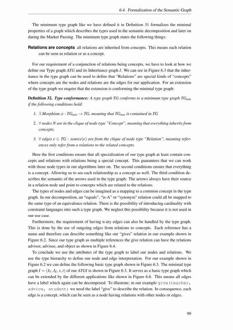
6.4. Formalization of the Semantic Graph

The minimum type graph like we have defined it in Definition 31 formalizes the minimalproperties of a graph which describes the types used in the semantic decomposition and later onduring the Marker Passing. The minimum type graph states the following things:

Relations are concepts all relations are inherited from concepts. This means each relationcan be seen as relation or as a concept.

For our requirement of a conjunction of relations being concepts, we have to look at how wedefine our Type graph ATG and its Inheritance graph I. We can see in Figure 6.3 that the inher-itance in the type graph can be used to define that “Relations” are special kinds of “concepts”where concepts are the nodes and relations are the edges for our application. For an extensionof the type graph we require that the extension is conforming the minimal type graph:

Definition 32. Type conformance: A type graph TG conforms to a minimum type graph TGmin

if the following conditions hold:

1. ∃ Morphism φ : TGmin → TG, meaning that TGmin is contained in TG

2. ∀ nodes N are in the clique of node type ”Concept”, meaning that everything inherits fromconcepts.

3. ∀ edges e ∈ TG : source(e) are from the clique of node type ”Relation”, meaning refer-ences only refer from a relations to the related concepts.

Here the first conditions ensure that all specialization of our type graph at least contain con-cepts and relations with relations being a special concept. This guarantees that we can workwith those node types in our algorithms later on. The second conditions ensure that everythingis a concept. Allowing us to see each relationship as a concept as well. The third condition de-scribes the semantic of the arrows used in the type graph: The arrows always have their sourcein a relation node and point to concepts which are related to the relations.

The types of nodes and edges can be imagined as a mapping to a common concept in the typegraph. In our decomposition, an “equals”, “is-A” or “synonym” relation could all be mapped tothe same type of an equivalence relation. There is the possibility of introducing cardinality withconstraint languages into such a type graph. We neglect this possibility because it is not used inour use case.

Furthermore, the requirement of having n-ary edges can also be handled by the type graph.This is done by the use of outgoing edges from relations to concepts. Each reference has aname and therefore can describe something like our “gives” relation in our example shown inFigure 6.2. Since our type graph as multiple references the give relation can have the relationsadvisor, advisee, and object as shown in Figure 6.4.

To conclude we use the attributes of the type graph to label our nodes and relations. Weuse the type hierarchy to define our node and edge interpretation. For our example shown inFigure 6.2 we can define the following basic type graph shown in Figure 6.3. The minimal typegraph I = (IV , IE, s, t) of our ATGI is shown in Figure 6.3. It serves as a basic type graph whichcan be extended by the different applications like shown in Figure 6.6. This means all edgeshave a label which again can be decomposed. To illustrate, in our example give(teacher,advice, student) we need the label “give” to describe the relation. In consequence, eachedge is a concept, which can be seen as a node having relations with other nodes or edges.

99

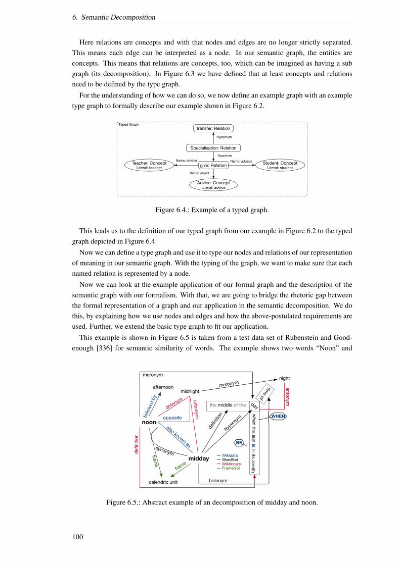
6. Semantic Decomposition

Here relations are concepts and with that nodes and edges are no longer strictly separated.This means each edge can be interpreted as a node. In our semantic graph, the entities areconcepts. This means that relations are concepts, too, which can be imagined as having a subgraph (its decomposition). In Figure 6.3 we have defined that at least concepts and relationsneed to be defined by the type graph.

For the understanding of how we can do so, we now define an example graph with an exampletype graph to formally describe our example shown in Figure 6.2.

give: Relation

Advice: Concept Literal: advice

Teacher: Concept Literal: teacher

Student: Concept Literal: student

Name: object

Name: advicer

Hypernym

transfer: Relation

Specialisation: Relation

Name: adviseeHyponym

Typed Graph

Figure 6.4.: Example of a typed graph.

This leads us to the definition of our typed graph from our example in Figure 6.2 to the typedgraph depicted in Figure 6.4.

Now we can define a type graph and use it to type our nodes and relations of our representationof meaning in our semantic graph. With the typing of the graph, we want to make sure that eachnamed relation is represented by a node.

Now we can look at the example application of our formal graph and the description of thesemantic graph with our formalism. With that, we are going to bridge the rhetoric gap betweenthe formal representation of a graph and our application in the semantic decomposition. We dothis, by explaining how we use nodes and edges and how the above-postulated requirements areused. Further, we extend the basic type graph to fit our application.

This example is shown in Figure 6.5 is taken from a test data set of Rubenstein and Good-enough [336] for semantic similarity of words. The example shows two words “Noon” and

noon

midday

opposite

defin

ition

hypern

ym

holonym

synonym

meronym

midnight

antonym

nightmeronym

defin

ition

antonymantonym

follo

wed

by

afternoon

also known as

calendric unit

frame

frame

the middle of the

time ofw

hen the sun is in its zenith

day

WikidataWordNetWiktionaryFrameNet

BE

WHEN

Figure 6.5.: Abstract example of an decomposition of midday and noon.

100

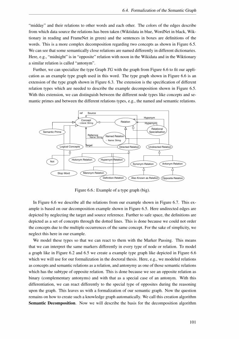
6.4. Formalization of the Semantic Graph

“midday” and their relations to other words and each other. The colors of the edges describefrom which data source the relations has been taken (Wiktidata in blue, WordNet in black, Wik-tionary in reading and FrameNet in green) and the sentences in boxes are definitions of thewords. This is a more complex decomposition regarding two concepts as shown in Figure 6.5.We can see that some semantically close relations are named differently in different dictionaries.Here, e.g., “midnight” is in “opposite” relation with noon in the Wikidata and in the Wiktionarya similar relation is called “antonym”.

Further, we can specialize the type Graph TG with the graph from Figure 6.6 to fit our appli-cation as an example type graph used in this word. The type graph shown in Figure 6.6 is anextension of the type graph shown in Figure 6.3. The extension is the specification of differentrelation types which are needed to describe the example decomposition shown in Figure 6.5.With this extension, we can distinguish between the different node types like concepts and se-mantic primes and between the different relations types, e.g., the named and semantic relations.

Concept- Literal: String Hypernym

Named Relation- Name: String

Relational Specialisation

Refernce - Name: String

Directed Relation

Source

Stop Word

Not

Relation

Meronym Relation

Synonym Relation Antonym Relation

Also Known as Relation

Hypernym Relation

Opposite Relation

Holonym Relation

Hyponym

Target Undirected Relation

ref

Semantic Prime

Logical Concepts

Definition Relation

Figure 6.6.: Example of a type graph (big).

In Figure 6.6 we describe all the relations from our example shown in Figure 6.7. This ex-ample is based on our decomposition example shown in Figure 6.5. Here undirected edges aredepicted by neglecting the target and source reference. Further to safe space, the definitions aredepicted as a set of concepts through the dotted lines. This is done because we could not orderthe concepts due to the multiple occurrences of the same concept. For the sake of simplicity, weneglect this here in our example.

We model these types so that we can react to them with the Marker Passing. This meansthat we can interpret the same markers differently in every type of node or relation. To modela graph like in Figure 6.2 and 6.5 we create a example type graph like depicted in Figure 6.6which we will use for our formalization in the doctoral thesis. Here, e.g., we modeled relationsas concepts and semantic relations as a relation, and antonymy as one of those semantic relationswhich has the subtype of opposite relation. This is done because we see an opposite relation asbinary (complementary antonyms) and with that as a special case of an antonym. With thisdifferentiation, we can react differently to the special type of opposites during the reasoningupon the graph. This leaves us with a formalization of our semantic graph. Now the questionremains on how to create such a knowledge graph automatically. We call this creation algorithmSemantic Decomposition. Now we will describe the basis for the decomposition algorithm

101

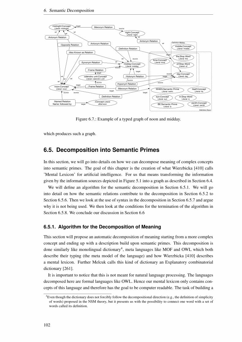
6. Semantic Decomposition

Definition Noon

Definition Midday

noon:Concept Literal: noon

midday:Concept Literal: midday

midnight:Concept Literal: midnight

calendric unit:Concept Literal: calendric unit

:Concept Literal: afternoon

night:Concept Literal: night

the:Stop Word Literal: the

middle:Concept Literal: middle

WHEN:Semantic Prime Literal: wehn

sun:Concept Literal: sun

BE:Semantic Prime Literal: is

in:Stop Word Literal: in

itself:Concept Literal: its

zenith:Concept Literal: zenith

:Frame Relation

: Frame Relation

:Antonym Relation:Antonym Relation

:Opposite Relation

:Named RelationName: followed by

:Also Known as Relation

:Meronym Relation

time:Concept Literal: time of:Stop Word

Literal: of

day:Concept Literal: day

:Meronym Relation

:Definition Relation

:Definition Relation

:Hyponym Relation

:Synonym Relation

:Antonym Relation

:Holonym Relation

source

target

sourcetarget

source

target

sourcetarget

source

target

source

targetsource target

source

ref

target

target

refref

ref

ref

refref

ref

ref

ref

source

ref

Figure 6.7.: Example of a typed graph of noon and midday.

which produces such a graph.

6.5. Decomposition into Semantic Primes

In this section, we will go into details on how we can decompose meaning of complex conceptsinto semantic primes. The goal of this chapter is the creation of what Wierzbicka [410] calls’Mental Lexicon’ for artificial intelligence. For us that means transforming the informationgiven by the information sources depicted in Figure 5.1 into a graph as described in Section 6.4.

We will define an algorithm for the semantic decomposition in Section 6.5.1. We will gointo detail on how the semantic relations contribute to the decomposition in Section 6.5.2 toSection 6.5.6. Then we look at the use of syntax in the decomposition in Section 6.5.7 and arguewhy it is not being used. We then look at the conditions for the termination of the algorithm inSection 6.5.8. We conclude our discussion in Section 6.6

6.5.1. Algorithm for the Decomposition of Meaning

This section will propose an automatic decomposition of meaning starting from a more complexconcept and ending up with a description build upon semantic primes. This decomposition isdone similarly like monolingual dictionary4, meta languages like MOF and OWL which bothdescribe their typing (the meta model of the language) and how Wierzbicka [410] describesa mental lexicon. Further Melcuk calls this kind of dictionary an Explanatory combinatorialdictionary [261].

It is important to notice that this is not meant for natural language processing. The languagesdecomposed here are formal languages like OWL. Hence our mental lexicon only contains con-cepts of this language and therefore has the goal to be computer readable. The task of building a

4Even though the dictionary does not forcibly follow the decompositional direction (e.g., the definition of simplicityof words) proposed in the NSM theory, but it presents us with the possibility to connect one word with a set ofwords called its definition.

102

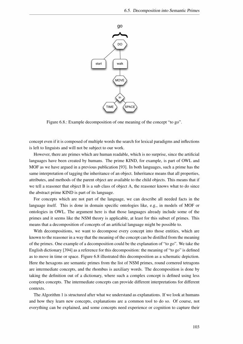
6.5. Decomposition into Semantic Primes

DO

walk

go

MOVE

TIME SPACE

in

start

Figure 6.8.: Example decomposition of one meaning of the concept “to go”.

concept even if it is composed of multiple words the search for lexical paradigms and inflectionsis left to linguists and will not be subject to our work.

However, there are primes which are human readable, which is no surprise, since the artificiallanguages have been created by humans. The prime KIND, for example, is part of OWL andMOF as we have argued in a previous publication [93]. In both languages, such a prime has thesame interpretation of tagging the inheritance of an object. Inheritance means that all properties,attributes, and methods of the parent object are available to the child objects. This means that ifwe tell a reasoner that object B is a sub class of object A, the reasoner knows what to do sincethe abstract prime KIND is part of its language.

For concepts which are not part of the language, we can describe all needed facts in thelanguage itself. This is done in domain specific ontologies like, e.g., in models of MOF orontologies in OWL. The argument here is that those languages already include some of theprimes and it seems like the NSM theory is applicable, at least for this subset of primes. Thismeans that a decomposition of concepts of an artificial language might be possible to.

With decompositions, we want to decompose every concept into those entities, which areknown to the reasoner in a way that the meaning of the concept can be distilled from the meaningof the primes. One example of a decomposition could be the explanation of “to go”. We take theEnglish dictionary [394] as a reference for this decomposition: the meaning of “to go” is definedas to move in time or space. Figure 6.8 illustrated this decomposition as a schematic depiction.Here the hexagons are semantic primes from the list of NSM primes, round cornered tetragonsare intermediate concepts, and the rhombus is auxiliary words. The decomposition is done bytaking the definition out of a dictionary, where such a complex concept is defined using lesscomplex concepts. The intermediate concepts can provide different interpretations for differentcontexts.

The Algorithm 1 is structured after what we understand as explanations. If we look at humansand how they learn new concepts, explanations are a common tool to do so. Of course, noteverything can be explained, and some concepts need experience or cognition to capture their

103

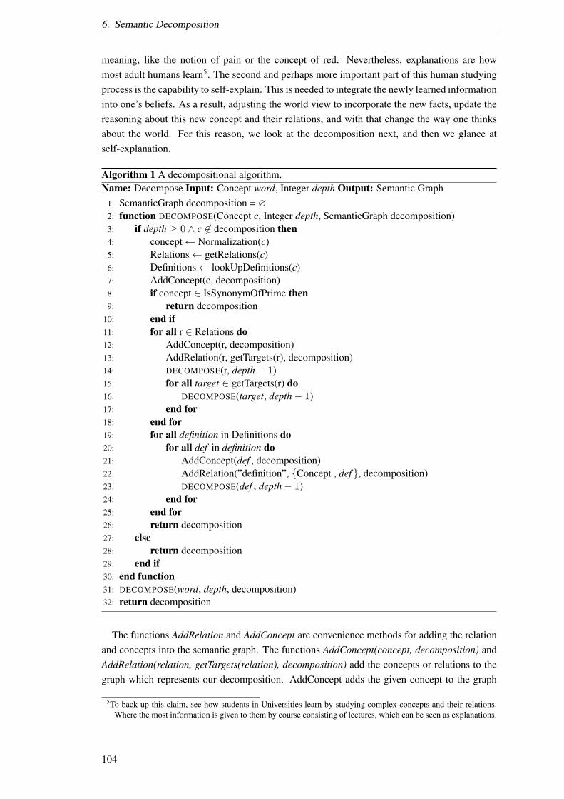
6. Semantic Decomposition

meaning, like the notion of pain or the concept of red. Nevertheless, explanations are howmost adult humans learn5. The second and perhaps more important part of this human studyingprocess is the capability to self-explain. This is needed to integrate the newly learned informationinto one’s beliefs. As a result, adjusting the world view to incorporate the new facts, update thereasoning about this new concept and their relations, and with that change the way one thinksabout the world. For this reason, we look at the decomposition next, and then we glance atself-explanation.

Algorithm 1 A decompositional algorithm.Name: Decompose Input: Concept word, Integer depth Output: Semantic Graph

1: SemanticGraph decomposition = ∅2: function DECOMPOSE(Concept c, Integer depth, SemanticGraph decomposition)3: if depth ≥ 0 ∧ c 6∈ decomposition then4: concept← Normalization(c)5: Relations← getRelations(c)6: Definitions← lookUpDefinitions(c)7: AddConcept(c, decomposition)8: if concept ∈ IsSynonymOfPrime then9: return decomposition

10: end if11: for all r ∈ Relations do12: AddConcept(r, decomposition)13: AddRelation(r, getTargets(r), decomposition)14: DECOMPOSE(r, depth− 1)15: for all target ∈ getTargets(r) do16: DECOMPOSE(target, depth− 1)17: end for18: end for19: for all definition in Definitions do20: for all def in definition do21: AddConcept(def , decomposition)22: AddRelation(”definition”, Concept , def, decomposition)23: DECOMPOSE(def , depth− 1)24: end for25: end for26: return decomposition27: else28: return decomposition29: end if30: end function31: DECOMPOSE(word, depth, decomposition)32: return decomposition

The functions AddRelation and AddConcept are convenience methods for adding the relationand concepts into the semantic graph. The functions AddConcept(concept, decomposition) andAddRelation(relation, getTargets(relation), decomposition) add the concepts or relations to thegraph which represents our decomposition. AddConcept adds the given concept to the graph

5To back up this claim, see how students in Universities learn by studying complex concepts and their relations.Where the most information is given to them by course consisting of lectures, which can be seen as explanations.

104

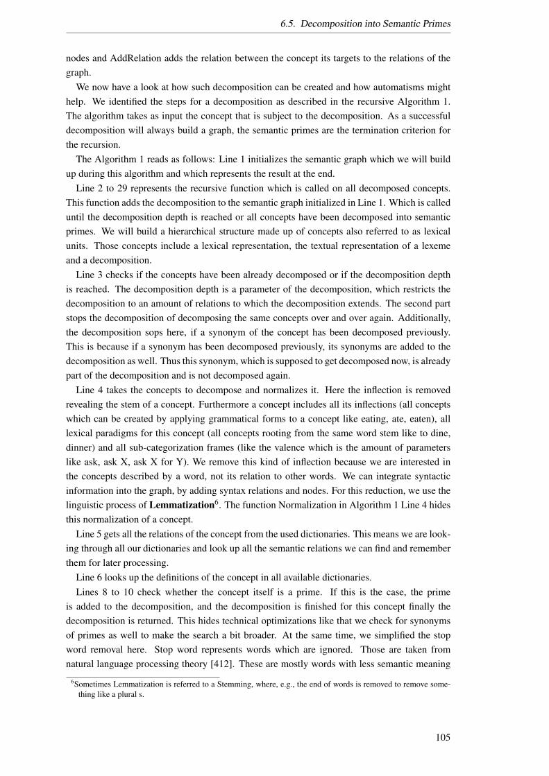
6.5. Decomposition into Semantic Primes

nodes and AddRelation adds the relation between the concept its targets to the relations of thegraph.

We now have a look at how such decomposition can be created and how automatisms mighthelp. We identified the steps for a decomposition as described in the recursive Algorithm 1.The algorithm takes as input the concept that is subject to the decomposition. As a successfuldecomposition will always build a graph, the semantic primes are the termination criterion forthe recursion.

The Algorithm 1 reads as follows: Line 1 initializes the semantic graph which we will buildup during this algorithm and which represents the result at the end.

Line 2 to 29 represents the recursive function which is called on all decomposed concepts.This function adds the decomposition to the semantic graph initialized in Line 1. Which is calleduntil the decomposition depth is reached or all concepts have been decomposed into semanticprimes. We will build a hierarchical structure made up of concepts also referred to as lexicalunits. Those concepts include a lexical representation, the textual representation of a lexemeand a decomposition.

Line 3 checks if the concepts have been already decomposed or if the decomposition depthis reached. The decomposition depth is a parameter of the decomposition, which restricts thedecomposition to an amount of relations to which the decomposition extends. The second partstops the decomposition of decomposing the same concepts over and over again. Additionally,the decomposition sops here, if a synonym of the concept has been decomposed previously.This is because if a synonym has been decomposed previously, its synonyms are added to thedecomposition as well. Thus this synonym, which is supposed to get decomposed now, is alreadypart of the decomposition and is not decomposed again.

Line 4 takes the concepts to decompose and normalizes it. Here the inflection is removedrevealing the stem of a concept. Furthermore a concept includes all its inflections (all conceptswhich can be created by applying grammatical forms to a concept like eating, ate, eaten), alllexical paradigms for this concept (all concepts rooting from the same word stem like to dine,dinner) and all sub-categorization frames (like the valence which is the amount of parameterslike ask, ask X, ask X for Y). We remove this kind of inflection because we are interested inthe concepts described by a word, not its relation to other words. We can integrate syntacticinformation into the graph, by adding syntax relations and nodes. For this reduction, we use thelinguistic process of Lemmatization6. The function Normalization in Algorithm 1 Line 4 hidesthis normalization of a concept.

Line 5 gets all the relations of the concept from the used dictionaries. This means we are look-ing through all our dictionaries and look up all the semantic relations we can find and rememberthem for later processing.

Line 6 looks up the definitions of the concept in all available dictionaries.Lines 8 to 10 check whether the concept itself is a prime. If this is the case, the prime

is added to the decomposition, and the decomposition is finished for this concept finally thedecomposition is returned. This hides technical optimizations like that we check for synonymsof primes as well to make the search a bit broader. At the same time, we simplified the stopword removal here. Stop word represents words which are ignored. Those are taken fromnatural language processing theory [412]. These are mostly words with less semantic meaning

6Sometimes Lemmatization is referred to a Stemming, where, e.g., the end of words is removed to remove some-thing like a plural s.

105

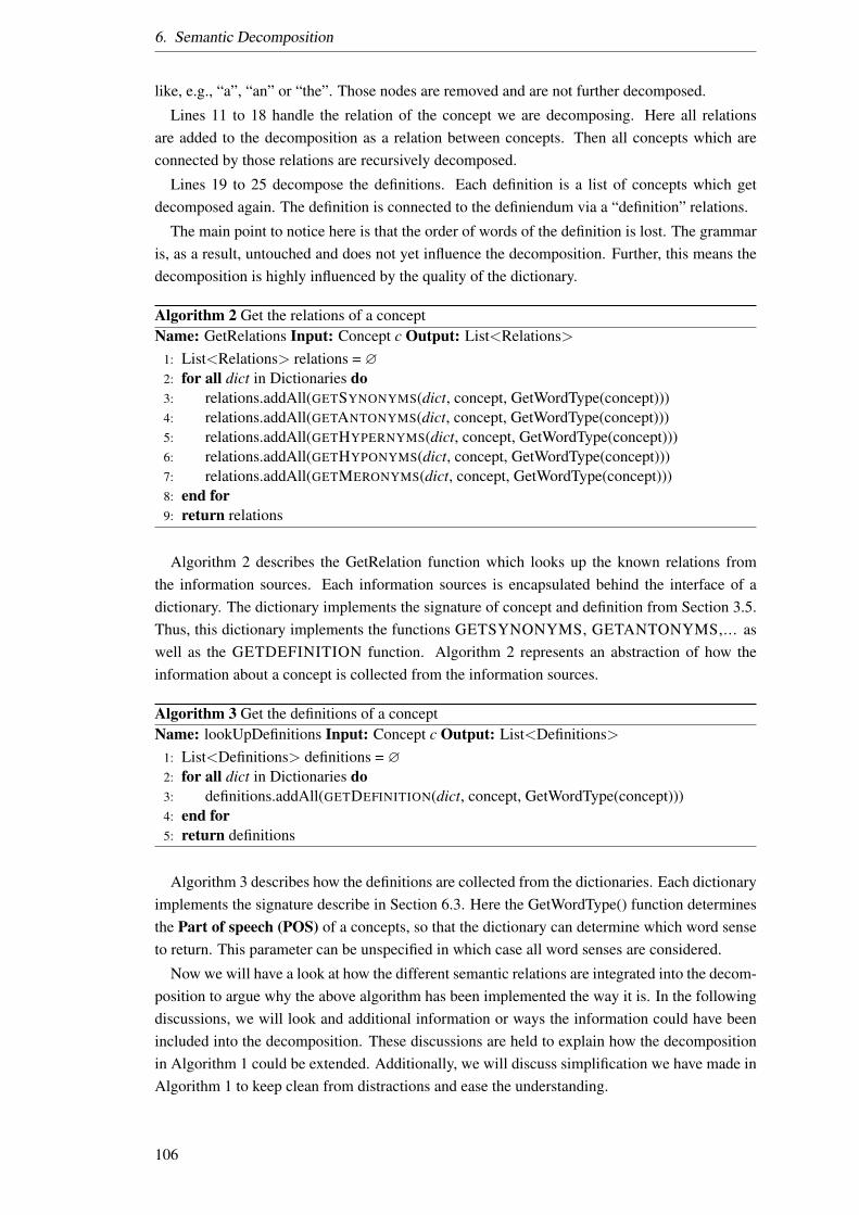
6. Semantic Decomposition

like, e.g., “a”, “an” or “the”. Those nodes are removed and are not further decomposed.

Lines 11 to 18 handle the relation of the concept we are decomposing. Here all relationsare added to the decomposition as a relation between concepts. Then all concepts which areconnected by those relations are recursively decomposed.

Lines 19 to 25 decompose the definitions. Each definition is a list of concepts which getdecomposed again. The definition is connected to the definiendum via a “definition” relations.

The main point to notice here is that the order of words of the definition is lost. The grammaris, as a result, untouched and does not yet influence the decomposition. Further, this means thedecomposition is highly influenced by the quality of the dictionary.

Algorithm 2 Get the relations of a conceptName: GetRelations Input: Concept c Output: List<Relations>

1: List<Relations> relations = ∅2: for all dict in Dictionaries do3: relations.addAll(GETSYNONYMS(dict, concept, GetWordType(concept)))4: relations.addAll(GETANTONYMS(dict, concept, GetWordType(concept)))5: relations.addAll(GETHYPERNYMS(dict, concept, GetWordType(concept)))6: relations.addAll(GETHYPONYMS(dict, concept, GetWordType(concept)))7: relations.addAll(GETMERONYMS(dict, concept, GetWordType(concept)))8: end for9: return relations

Algorithm 2 describes the GetRelation function which looks up the known relations fromthe information sources. Each information sources is encapsulated behind the interface of adictionary. The dictionary implements the signature of concept and definition from Section 3.5.Thus, this dictionary implements the functions GETSYNONYMS, GETANTONYMS,... aswell as the GETDEFINITION function. Algorithm 2 represents an abstraction of how theinformation about a concept is collected from the information sources.

Algorithm 3 Get the definitions of a conceptName: lookUpDefinitions Input: Concept c Output: List<Definitions>

1: List<Definitions> definitions = ∅2: for all dict in Dictionaries do3: definitions.addAll(GETDEFINITION(dict, concept, GetWordType(concept)))4: end for5: return definitions

Algorithm 3 describes how the definitions are collected from the dictionaries. Each dictionaryimplements the signature describe in Section 6.3. Here the GetWordType() function determinesthe Part of speech (POS) of a concepts, so that the dictionary can determine which word senseto return. This parameter can be unspecified in which case all word senses are considered.

Now we will have a look at how the different semantic relations are integrated into the decom-position to argue why the above algorithm has been implemented the way it is. In the followingdiscussions, we will look and additional information or ways the information could have beenincluded into the decomposition. These discussions are held to explain how the decompositionin Algorithm 1 could be extended. Additionally, we will discuss simplification we have made inAlgorithm 1 to keep clean from distractions and ease the understanding.

106

6.5. Decomposition into Semantic Primes

6.5.2. Decomposing using Synonyms

This section discusses our use of synonyms in our algorithm. We focus on things we have notexplicitly integrated into the algorithm. This is done to show potential improvement points orour Decomposition.

Since synonyms are equivalent in meaning regarding the context of use, the synonyms canbe replaced in an utterance, without changing the meaning of the utterance. Consequently syn-onyms play an important role in the decomposition. The decomposition could be stoped, if themeaning of synonyms is known. Imagine if one concept is not known in an utterance, but by pro-viding a known synonym, the utterance can be understood completely. Synonyms are collectedwith the function getSynonyms : Concept,WordType→ Concept∗ in Algorithm 2.

With that synonyms make the search for primes broader. Depending on the type of semanticsimilarity measure and the threshold, from which we call two concepts synonyms the breadthof the decomposition can be controlled. This again is defined by the information source whichdecided which two concepts are seen to be a synonym. Line eight of Algorithm 1 hides thisimplementation detail. Here we check if a concept is a prime, but at the same time, we checkwhether one of its synonyms is prime or if a synonym of primes contains the concept.

On improvement point of the Algorithm 1 could be the selection of the word sense beforechoosing the synonyms narrows the breadth but focuses on the right synonyms for the decom-position. In detail, there are two parts of the decomposition where synonyms can be used:Regarding the concept subject of decomposition and regarding the semantic primes. In the firstcase we can use the context of uses of the concept to select the word sense, and with that, theright synonyms, check if one of those synonyms is a prime and if so, we can stop decomposingsince we could replace this concept with a prime without changing any meaning. Another im-provement point is the caching of concepts we already have decomposed, which is done in ourimplementation but neglected in the Algorithm 1 for simplicity.

For further improvement, we could identify all synonyms of the primes, classified in theircontext and word sense. Then when decomposing, we can check if, for the given context andword sense, there is a prime or a synonym of a prime which leads us to again stop the decompo-sition. Analyzing, the synonyms of primes allows us to specify in which word sense the prime isused. Since there is a relatively small set of primes (ca. 65), we can do this for all of them in aninsignificant amount of time. At the same time, defining synonyms for semantic primes allowsus to downsize the effect of the neglecting of syntax during the decomposition because all thosesynonyms cause the decomposition to stop and do not need further analysis. In Table 6.5 thiscan be seen for example for the prime “I”. Here we can define syntactic variations as synonymswhich spare us the effort to find ”yours truly” as one concept and its syntactic analysis.

Further Algorithm 1 neglects the fact that if a synonym is a replaceable concept in a givencontext, then the hyperonym and hyponyms can be treated as synonyms, e.g., almost all nounscould be replaced by SOMETHING/THING. If or when it makes sense to use specialization,and generalization can be looked at separately, which is done in Section 6.5.4 and Section 6.5.5.

Using a synonym is like explaining what a truck is by explaining something like: “A truckis like a bus but for transporting goods instead of people.” If the concept bus has already beendecomposed, this can lead the reasoner to extract multiple facts for a truck. If the concept wordtype (POS) is known, then this gives some insight into its relations, because not all definitionshave to be looked at, since the definitions with a different POS can be neglected. The implemen-

107

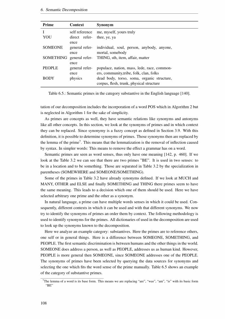
6. Semantic Decomposition

Prime Context Synonym

I self reference me, myself, yours trulyYOU direct refer-

encethee, ye, ya

SOMEONE general refer-ence

individual, soul, person, anybody, anyone,mortal, somebody

SOMETHING general refer-ence

THING, sth, item, affair, matter

PEOPLE general refer-ence

populace, nation, mass, lede, race, common-ers, community,tribe, folk, clan, folks

BODY physics dead body, torso, soma, organic structure,corpus, flesh, trunk, physical structure

Table 6.5.: Semantic primes in the category substantive in the English language [140].

tation of our decomposition includes the incorporation of a word POS which in Algorithm 2 butis neglected in Algorithm 1 for the sake of simplicity.

As primes are concepts as well, they have semantic relations like synonyms and antonymslike all other concepts. In this section, we look at the synonyms of primes and in which contextthey can be replaced. Since synonymy is a fuzzy concept as defined in Section 3.9. With thisdefinition, it is possible to determine synonyms of primes. Those synonyms then are replaced bythe lemma of the prime7. This means that the lemmatization is the removal of inflection causedby syntax. In simpler words: This means to remove the effect a grammar has on a word.

Semantic primes are seen as word senses, thus only have one meaning [142, p. 460]. If welook at the Table 3.2 we can see that there are two primes ”BE”. It is used in two senses: tobe in a location and to be something. Those are separated in Table 3.2 by the specialization inparentheses (SOMEWHERE and SOMEONE/SOMETHING).

Some of the primes in Table 3.2 have already synonyms defined. If we look at MUCH andMANY, OTHER and ELSE and finally SOMETHING and THING there primes seem to havethe same meaning. This leads to a decision which one of them should be used. Here we haveselected arbitrary one prime and the other as a synonym.

In natural language, a prime can have multiple words senses in which it could be used. Con-sequently, different contexts in which it can be used and with that different synonyms. We nowtry to identify the synonyms of primes an order them by context. The following methodology isused to identify synonyms for the primes. All dictionaries of used in the decomposition are usedto look up the synonyms known to the decomposition.

Here we analyze an example category: substantives. Here the primes are to reference others,one self or in general things. Here is a difference between SOMEONE, SOMETHING, andPEOPLE. The first semantic discrimination is between humans and the other things in the world.SOMEONE does address a person, as well as PEOPLE, addresses us as human kind. However,PEOPLE is more general then SOMEONE, since SOMEONE addresses one of the PEOPLE.The synonyms of primes have been selected by querying the data sources for synonyms andselecting the one which fits the word sense of the prime manually. Table 6.5 shows an exampleof the category of substantive primes.

7The lemma of a word is its base form. This means we are replacing “are”, “was”, “am”, “is” with its basic form“BE”

108

6.5. Decomposition into Semantic Primes

The rest of the tables can be found in Appendix A Section A.4. Next, we will look at thedecomposition using antonyms explaining why antonyms are used in the decomposition andwhich theoretical role they play in the decomposition.

6.5.3. Decomposing using Antonyms

Using antonyms is similar to using synonyms during the decomposition. Here again, an antonymis not well defined, and there is a degree of antonymy to every concept pair. Choosing a thresholdof which concepts are an antonym to each other is one parameter which defines the output of adecomposition.

Also, we will see that selecting how to use antonyms in a decomposition is not as simple as itis with synonyms. This is because there is a multitude of different antonyms.

From the discussion of antonymy in Section 3.9 we know that this only works for someprimes. If we look at the change of evaluations a sentence to true or false statements, the re-placement of an antonym again has to depend on the context the concept to be replaced is usedin. If we take the example sentence: “Now it is sunny”, and replace sunny with a negatedantonym cloudy this changes the situations in which this sentence is evaluated to true or false.You can imagine that it can be not cloudy at night, but it is most of the time not sunny. This non-symmetrical antonyms special cases we will look at next. In those cases, the antonymy mightnot be a undirected edge, but rather has different roles. That antonyms are not symmetric can beseen on the example of to buy which is not equal to “not to sell”. Where to buy and to sell aretwo parts of the same transaction. In consequence to buy and to sell might be antonyms in somelexical contexts, but they can not be handled by negating them.

Namely, the function getAntonyms : Concept,WordType → Concept∗ in Algorithm 2, getsthe appropriate antonym relation for a given antonym. This is implemented by the signature ofa dictionary described in Section 6.3.

As we have seen in Section 3.9 there are different types of antonyms. Not all antonyms canbe used the same way. Therefore we can not like with synonyms (see Section 6.5.2) stop thedecomposition when we find an antonym of a prime.

Next, we discuss the different types of antonyms and why they could not be used during thedecomposition.

Gradable

Gradable antonyms are antonyms which can not be separated into two classes. A commonexample is a temperature: “hot” and “cold”. Since we do not include fuzzy concepts into ourdecomposition, these antonyms are handled by a simple default antonym relationship.

Complementary

The complementary concepts are not in an antonym relation as in being the opposite, but ratherto complete a set of states. For a machine to be “off” or “on” are examples of a complementaryantonym. Another example is “dead” and “alive”, where the one can not be without the other.In opposite to purely relational antonyms, complementary antonyms are not restricted to rela-tionships. Because of the open world assumption, there is alway a third option of modeling notknowing if something is “off” or “on”. Since an ontology can explicitly model union of classes,

109

6. Semantic Decomposition

we can model state which exists only of “off” or “on”. In this case, the antonym is part of thestandard antonymy relations, and the complement is explicitly defined.

Converse Relational

The converse relationship describes a relation from its different views. An example of sucha relationship could be the “inheritance” which has two different views: parent and children.Special about the converse relationship as an antonym is the form the existence of one part; theother has to exist. As an illustration, in the example of inheritance there is no child withoutparents, and if there are no children, then the nodes are just nodes and not parents because wedo not know if the next node in the graph will be inserted as its parent or its child. Converseantonyms are neglected concerning our decomposition.

Reverse Relational

The reverse relations describes antonyms on relations. Thus if concepts are in one relation ofthe relations being in a reverse relationship, they are in the other relationship as well. As thename implies, the relations in these cases are directed. In particular, if the one relationship is inone direction, then the other one is in the other direction. An example here is the Hyponym- andHypernym-Relation. We neglect reverse relationships in our decomposition because they can beexplicitly described in the ontology by relating them to a reverse relationship if needed.

Incompatible

Incompatibility as an antonym relation is a standard interpretation of classes in OWL. Thereforeif not specified otherwise if to concepts inherit from two independent classes, they are incom-patible. Thus incompatibility is included in our antonym relations.

Semantically this does not describe all the antonyms we have looked at in this section. Sadlythe information sources unify those types of antonyms in one relation. This unified relation willbe used in our approach until the identification of the different types of antonyms is possible.Until then we might have an occasional mix in of some other antonym from our dictionariessince, e.g., Wikipedia is described by humans, which works in such inconsistent ways.

Besides antonyms and synonyms, the most used relation in ontologies is the inheritance rela-tions. Those can be split into specialization and generalization. The next section will discuss thegeneralization and its role in the decomposition.

6.5.4. Decomposing using Hypernyms

Using a more general concept to explain a specialized one allows the explainer to be abstract dur-ing an explanation. This is done with function getHypernyms : Concept,WordType→ Concept∗in Algorithm 2. Explanations like: “A human is an animal” are useful since now the reasonercan infer properties of the more general concept. The hypernyms can lead to primes or can be aprime, which again stops the decomposition in the direction of a generalization.

The recursive level of which Hypernyms are used during the decomposition effects the ab-straction the decomposition will have. Abstracting concept will eventually lead to the primeTHING/SOMETHING which can lead to decompositions like: “Someone does a thing to some-thing.” These decompositions are not useless; a reasoner can now determine the different actors

110

6.5. Decomposition into Semantic Primes

and the action. The interpretation of such a decomposition is that we describe an event whichhas two agents, an active and a passive one. This is different too: “A thing is done to some-thing” since here the active agent is missing. This leads to smaller detailed differentiations ina decomposition like active or passive, which we neglect in our decomposition since they aresyntactical.

6.5.5. Decomposing using Hyponym

To use hyponyms in the decomposition is a bit like using examples during an explanation. Hy-ponyms can be collected with function getHyponyms : Concept,WordType → Concept∗ inAlgorithm 2. It eases the access to a reference. By describing abstract entities, the reasonermight lack the ability to find fitting references. Since some semantic theories like the prototypesemantic 4.1.4 insist on references to describe the meaning of something, we can argue that witha hyponym these references can be included in the decomposition.

A hyponym describes different manifestations of the decomposed concept. Hence a hyponymcan be added to the decomposition by noting that some of the entities described by this conceptsare of the hyponym type. Therefore in the decomposition, we can add the hyponym by adding:SOME to it.

This can be used by the reasoner to test examples of the abstract description. If the reasonerfinds an inconsistency with a meronym then he has found a counter example in his beliefs,which makes additional reasoning necessary for deciding to neglect the property of the hyponymin favor of integrating new information or if the new fact described by the concept changesfundamental beliefs which the reasoner is not willing to change. In this case, the decompositioncan not be integrated into its beliefs, but the contradicting part can be extracted and explained,via an example (the hyponym).

For example, if someone with pointy ears is going to tell you that feelings are bad since hewants you to make a rational decision you might reason the following: Feelings are bad. Loveis a feeling. Consequently, love is bad. Love is the precipitation of my body of some hormones.This leads to new entities of my species. This ensures the existing of my species. This cannot be bad for me. Hence love is not bad. Thus not all feelings are bad. If we can createreasoner which can reason such implications, we can check the decomposition for plausibility.In contrast to the hypernym, where we check if its logical structure is valid for more abstract orgeneral statements.

6.5.6. Decomposing using Meronyms

Decomposing a concept by describing its parts is a top-down approach to a definition. Meronymscan be collected with function getMeronyms : Concept,WordType→ Concept∗ in Algorithm 2.Since a part of a system is always less or equally as complex as the system itself, the decomposi-tion can break down a concept into its parts and decompose them to reach the goal of describingthe concept with simpler concepts.

Meronyms describe parts of relations (see section 3.9 for more details). The meronyms areintegrated into the decomposition with an own relation. Showing that a part of the conceptdecomposed is the meronym. This can be thought of as an explanation which includes describingall the parts of a concept if it has some. For example, a computer consists of a hardware andsoftware part. The hardware part in the von Neumann architecture contains memory and a

111

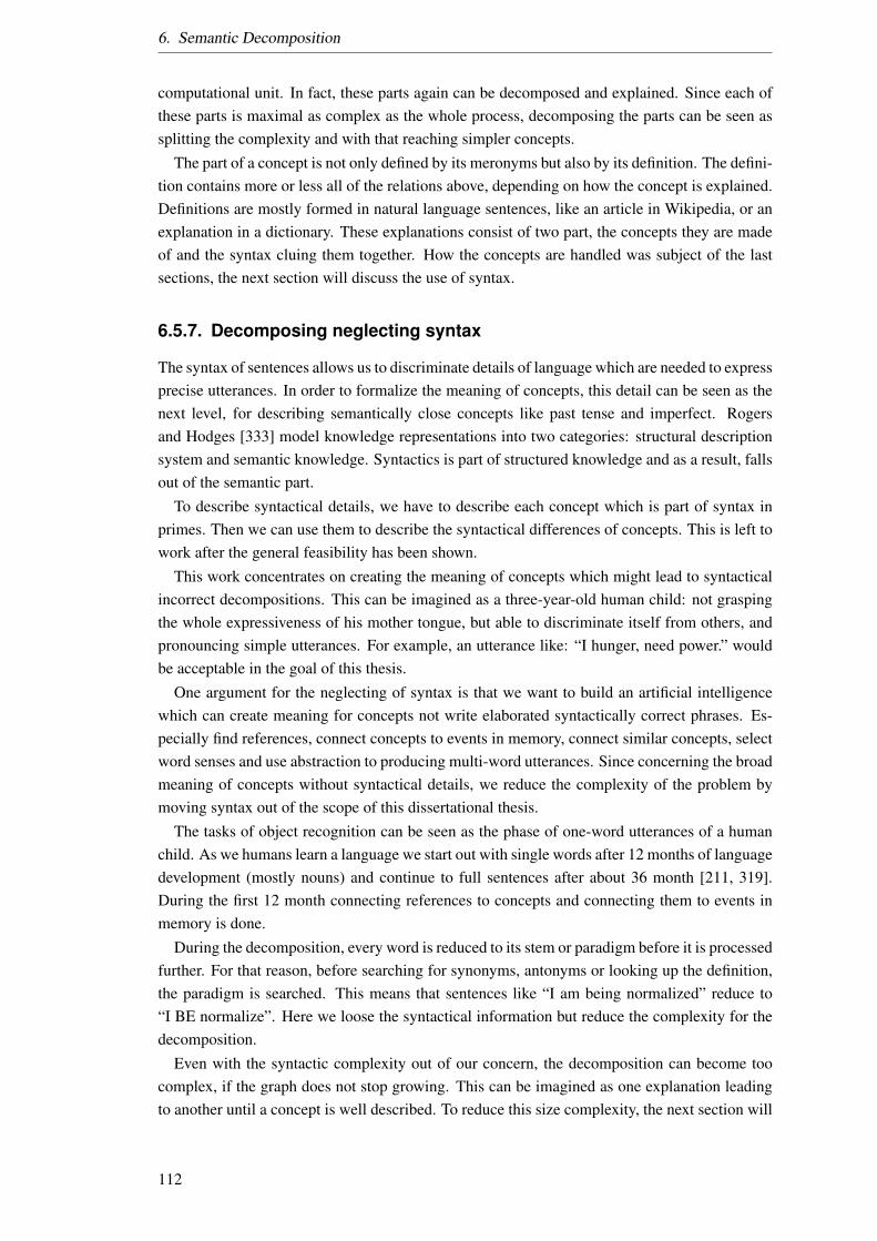
6. Semantic Decomposition

computational unit. In fact, these parts again can be decomposed and explained. Since each ofthese parts is maximal as complex as the whole process, decomposing the parts can be seen assplitting the complexity and with that reaching simpler concepts.

The part of a concept is not only defined by its meronyms but also by its definition. The defini-tion contains more or less all of the relations above, depending on how the concept is explained.Definitions are mostly formed in natural language sentences, like an article in Wikipedia, or anexplanation in a dictionary. These explanations consist of two part, the concepts they are madeof and the syntax cluing them together. How the concepts are handled was subject of the lastsections, the next section will discuss the use of syntax.

6.5.7. Decomposing neglecting syntax

The syntax of sentences allows us to discriminate details of language which are needed to expressprecise utterances. In order to formalize the meaning of concepts, this detail can be seen as thenext level, for describing semantically close concepts like past tense and imperfect. Rogersand Hodges [333] model knowledge representations into two categories: structural descriptionsystem and semantic knowledge. Syntactics is part of structured knowledge and as a result, fallsout of the semantic part.

To describe syntactical details, we have to describe each concept which is part of syntax inprimes. Then we can use them to describe the syntactical differences of concepts. This is left towork after the general feasibility has been shown.

This work concentrates on creating the meaning of concepts which might lead to syntacticalincorrect decompositions. This can be imagined as a three-year-old human child: not graspingthe whole expressiveness of his mother tongue, but able to discriminate itself from others, andpronouncing simple utterances. For example, an utterance like: “I hunger, need power.” wouldbe acceptable in the goal of this thesis.

One argument for the neglecting of syntax is that we want to build an artificial intelligencewhich can create meaning for concepts not write elaborated syntactically correct phrases. Es-pecially find references, connect concepts to events in memory, connect similar concepts, selectword senses and use abstraction to producing multi-word utterances. Since concerning the broadmeaning of concepts without syntactical details, we reduce the complexity of the problem bymoving syntax out of the scope of this dissertational thesis.

The tasks of object recognition can be seen as the phase of one-word utterances of a humanchild. As we humans learn a language we start out with single words after 12 months of languagedevelopment (mostly nouns) and continue to full sentences after about 36 month [211, 319].During the first 12 month connecting references to concepts and connecting them to events inmemory is done.

During the decomposition, every word is reduced to its stem or paradigm before it is processedfurther. For that reason, before searching for synonyms, antonyms or looking up the definition,the paradigm is searched. This means that sentences like “I am being normalized” reduce to“I BE normalize”. Here we loose the syntactical information but reduce the complexity for thedecomposition.

Even with the syntactic complexity out of our concern, the decomposition can become toocomplex, if the graph does not stop growing. This can be imagined as one explanation leadingto another until a concept is well described. To reduce this size complexity, the next section will

112

6.5. Decomposition into Semantic Primes

discuss our termination conditions of the decomposition.

6.5.8. Termination conditions

The termination of the Algorithm 1 has been chosen in a way that the decompositions are keptas short and precise as possible. However, the theoretical termination condition is the totaldecomposition of the given concept. For some tasks, this might be disadvantageous, and theorder of steps in the algorithm needs to be changed appropriately.

The manner in which a decomposition is created depends – as always in ontology engineering– on the skills of the engineer, his domain and cultural background in which the informationsources have been described. Although, with this strict framework of decomposition we mightget different results for the same concepts depending on the parameters of the Decompositionand the included Information Sources. We postulate that those results differ in such a way thatan artificial reasoner can create equivalence classes from those decompositions. This meansthat the decompositions might vary in different domains, by syntax, which is irrelevant to themeaning the decomposition represents. The selection of information sources and the selectionof the decomposition depth thus dictate the termination of the decomposition.

The Algorithm 1 does not have to terminate with the total decomposition of a concept. Werather define a parameter describing the decomposition depth to terminate earlier. This meanswe can decide how often the main recursion is run through and with that shorten the span of thecreated graph.

We could think of having multiple termination conditions, e.g., with multiple decompositiondepths for different relations, for the different “directions” of the decomposition. In this way, wecould parametrize the use of synonyms differently than the use of the other relevant concepts.However, new problems arise, e.g., with the combination of different relations types. Further,we are not analyzing this kind of threshold and leave research in this direction to future work.

We have mentioned that the result of the decomposition is a graph. To ease the understanding,we are going to look at a handcrafted example next. For more complex examples the reader isreferred to Figure 9.3 and Figure 9.4.

6.5.9. Example decomposition

Now we will have a look at an example of a decomposition done manually to illustrate how theresult of a decomposition could look like from an abstract view. In Figure 6.9 we illustrate anexample of a decomposition of the concept to use in the sense of putting something to a purpose.We did remove the formal description we introduced above to restrict the example to the coreconcept and show an abstract view on the result of the decomposition. Figure 6.9 even reducesthe edges to only one unlabeled type. In this example, we decomposed the concept used as averb and selected a definition out of the Cambridge advanced learner’s dictionary [394]. Here weneglect the modal particles like to. The decomposition has been created by recursively applyingthe decomposition algorithm. The result is a relative short decomposition because we did selectthe definitions which are used for the decomposition. Further, we selected the words to use fromthe definition by hand. Here the graph reads as follows: To put is to move something inside aplace.

The example from Figure 6.9 shows a theoretic result of the decomposition. In a real decom-position the decomposition becomes more complex, since, e.g., the same concept is not added

113

6. Semantic Decomposition

to put somthing to

MOVE

INSIDESOMETHING

PLACE

to use: a particular purpose

SOMETHING AND

THIS NO

OTHER

WHY

YOU

DO

SOMETHING

ONE

Figure 6.9.: Example of decomposition using a definition out of the Cambridge Dictionary [394].

twice like the ”SOMETHING” node. The example in Figure 6.9 has been simplified from ourformalism to describe semantic graphs, to ease the readability. However, there are further chal-lenges, which need to be addressed. Next, we will have a look at the remaining challenges: Theselection of the definition to be used, for the decomposition influences the meaning which isdecomposed. Here the different information sources must use the same sense of the word for thedecomposition. In this way, ambiguities are neglected.

There are many parameters, which need specification reaching the depth of the search for,i.e., synonyms and the recursion depth for crawling through the dictionary. Further manualdecompositions are needed in case of a deadlock in the recursion of the algorithm. Here weneed to find a way on how a human can be queried for his input. This has been subject toresearch in the work of Ghadah Altaiari [9]. Integration of context-dependent meaning is notyet considered by our algorithm. If context-dependent meaning needs to be described, or ifthe decomposition is context dependent, then context needs to be integrated into the recursion,which could lead to a different termination condition, e.g., if we consider the beliefs of an agent,we could terminate earlier if some concepts are already known.

6.6. Conclusion

In this section, we have built an algorithm which can create semantic graphs automatically byusing existing ontologies and information sources like Wikipedia or WordNet. This has beendone by others like Alani et al. [7] and has been subject to research until today [63, 212, 307].However, none of those approaches used a theoretic grounding in a linguistic theory like NSM.This makes this approach unique and helps us understand more about the structure of semanticgraphs, which leads to more insight on how meaning can be represented for AI. Also, this ap-proach gives us the ability to define only ca. 65 concepts, to enable the agent to build its meaningof concepts.

For the goal we have set, we fulfill the first part of our abstract approach shown in Figure 5.1with this algorithm. We create a semantic graph with includes the collection of definitions wegather from the information sources and all semantic relations we can extract from them. Wehave defined a formal representation of our graph and decided on a mechanism to terminate thedecomposition namely the decomposition depth.

114

7. Marker Passing

The second part of my approach is to use the automatically created semantic graph representationof the connectionist meaning for reasoning. This section is structured in the following way: Westart our by describing the pragmatic way of representing meaning in Section 7.1. Then welook at the marker passing algorithm in Section 7.2. Section 7.3 then details the parameters ofmy marker passing algorithm. Finally we conclude the pragmatics of my symbolic approach inSection 7.4.

7.1. Pragmatic Meaning Representation

Building up on the semantic graph representation discussed in Section 6.4 and the automaticcreation of such a semantic graph described in Section 6.5 we now look at an example of whatpragmatics means in natural language and carry this idea over to our representation of mean-ing. The goal of this section is to show how pragmatic meaning can be described using MarkerPassing. Furthermore, it describes the theoretic basis for the interpretation of the internal mech-anisms and the result of the Marker Passing and gives the theoretic background to understandwhy the algorithm has been created the way it is.

In this thought experiment, I will utter: “I am cold.” moreover, you are sitting next to an openwindow which lets cold air into the room. The implicature which you could reason out of myspeech act could be: ‘Would you please close the window because I am cold.” It is easy to see thatsuch a reasoning is not possible without contextual knowledge, in this case, the knowledge thatthe window is open, that is is colder outside and that it would get warmer if the window is closed.This chapter will look into this kind of contextual reasoning of meaning called pragmatics.

In the agent paradigm, we model two minds: one who utters, the other one understands. Ifsomething is known about the context of the utterance, then the understanding (interpreting)entity can use this context to create pragmatic meaning. Here the communication can be seenas: “the successful interpretation by an addressee of a speaker’s intent in performing a linguisticact.” [149] To clarify this we can adapt the conceptualization of a communication act from MartaLenartowicz [228] where communication is seen as a single act, where the uttering uses seman-tic information to encode information in symbols (signifiers) and the listening agent interpretsthose symbols. Both agents use a context in which they concretize the semantics to pragmaticinformation. However, this context might differ.

Hence the observing agent can have access to the same contextual information as the utteringagent, which eases the interpretation, or the current contextual information of the understand-ing agent needs to suffice. Depicted in Figure 7.1 the two agents might use the same context,symbols and semantic to communicate. Then there can be three factors to differentiate the com-munication:

Different Symbols is the fact that different symbols (signifier) are used for the communica-tion. This can be seen as in different languages where different words reference the same

115

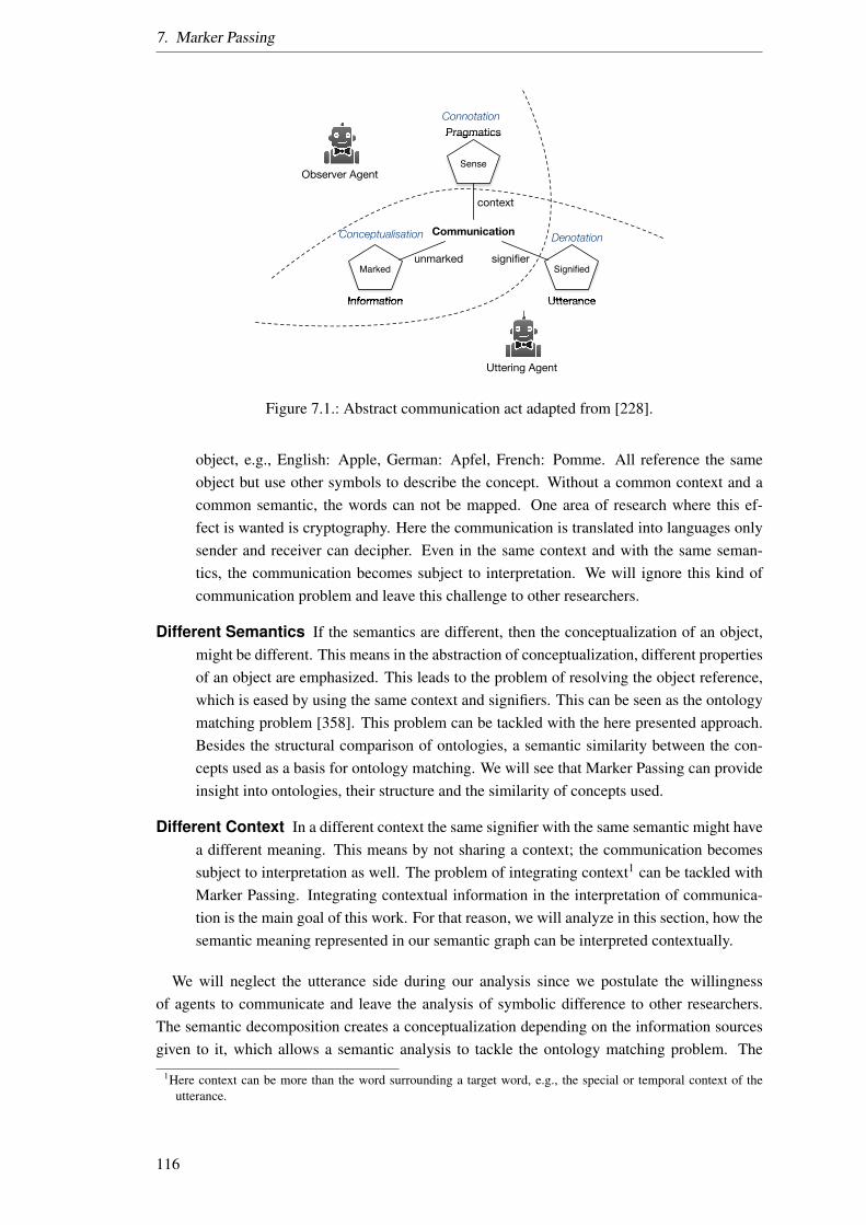
7. Marker Passing

Pragmatics

UtteranceInformationInformation

Marked

Utterance

Signified

Pragmatics

Sense

Communication

signifierunmarked

context

Connotation

DenotationConceptualisation

Observer Agent

Utterance

Uttering Agent

Figure 7.1.: Abstract communication act adapted from [228].

object, e.g., English: Apple, German: Apfel, French: Pomme. All reference the sameobject but use other symbols to describe the concept. Without a common context and acommon semantic, the words can not be mapped. One area of research where this ef-fect is wanted is cryptography. Here the communication is translated into languages onlysender and receiver can decipher. Even in the same context and with the same seman-tics, the communication becomes subject to interpretation. We will ignore this kind ofcommunication problem and leave this challenge to other researchers.

Different Semantics If the semantics are different, then the conceptualization of an object,might be different. This means in the abstraction of conceptualization, different propertiesof an object are emphasized. This leads to the problem of resolving the object reference,which is eased by using the same context and signifiers. This can be seen as the ontologymatching problem [358]. This problem can be tackled with the here presented approach.Besides the structural comparison of ontologies, a semantic similarity between the con-cepts used as a basis for ontology matching. We will see that Marker Passing can provideinsight into ontologies, their structure and the similarity of concepts used.

Different Context In a different context the same signifier with the same semantic might havea different meaning. This means by not sharing a context; the communication becomessubject to interpretation as well. The problem of integrating context1 can be tackled withMarker Passing. Integrating contextual information in the interpretation of communica-tion is the main goal of this work. For that reason, we will analyze in this section, how thesemantic meaning represented in our semantic graph can be interpreted contextually.

We will neglect the utterance side during our analysis since we postulate the willingnessof agents to communicate and leave the analysis of symbolic difference to other researchers.The semantic decomposition creates a conceptualization depending on the information sourcesgiven to it, which allows a semantic analysis to tackle the ontology matching problem. The

1Here context can be more than the word surrounding a target word, e.g., the special or temporal context of theutterance.

116

7.1. Pragmatic Meaning Representation

interpretation done by the listening agent to the utterance done by the uttering agent should yieldto be context dependent. So that our artificial meaning is represented by the context-dependentinterpretation of an utterance. For that, we need an approach to integrate contextual information,to be able to tackle a problem like WSD. We are looking for two types of usage of our semanticgraph: Semantic similarity2 and WSD.

We start out by describing the result of the semantic decomposition and the use of MarkerPassing and how this can be used to describe a representation of meaning. However, first, welook at how the context-independent meaning is transferred into a pragmatic one.

Since semantics is the theory on how meaning is transferred, a semantic transference andinterpretation process is required. There are four parts for the meaning of a word which are ofconcern to an AI:

Denotation The denotation represents the primary or basic meaning of a word. It can be seenas the definition of a word that is represented in some mental lexicon (or a dictionary).Denotation is the explicit meaning of a word, the shared explanation of the what is refer-enced. A dictionary holds denotations for the words described in it. In our representationof meaning the denotation is described by the definitions in the semantic graph.

Connotation The connotation is the abstract idea presented by the word. It can be seen as theconceptual representation of the meaning of a word. The connotation is the idea or quality;the associations brought to mind. It is private, depending on memory and experience andmost of all context dependent. This includes the connectionist interpretation of meaningsince here the meaning is interpreted as the unity of its relations to other concepts. Theconnotation in our approach is the result of a Marker Passing of one concept. It consistsof the marked graph which is subject to interpretation.

Conceptualization To be able to come up with a conceptual representation of the meaningof a word, one needs to abstract from the word to a specific concept (i.e., one needs toconnect the word with a known concept). This process is named Conceptualization andhelps to clarify a word within a language. In our approach, the conceptualization is theresult of the decomposition of one word. It consists of a semantic graph holding all knowninformation about this word, building its conception.

Pragmatics The meaning of words is not independent of the context the words are used in.In particular, a context-dependent representation of meaning (a pragmatic one) has to becreated (e.g., mouse (computer) vs. mouse (pet)). The Pragmatics in our approach isdescribed as the result of a Marker Passing where a concept and its context have beenactivated. It consists of the marked graph which is subject to interpretation.

Meaning itself needs to be represented appropriately (in a formal manner) to be handled byan agent. Since meaning is not precisely defined, this is subject to research. We will look atmeaning in the linguistic sense, which can be defined as follows: Meaning is what the sourceof an expression (message) wanted the observer to infer from the expression [240]. This viewis shown in Figure 7.1. Here the inference an observer can make about the communicatedinformation is seen as meaning. If the observer has access to the context the uttering has beenmade in, then the interpretation becomes simpler. This context involves all relevant information

2Here we argue that semantic similarity measures are the core problem of ontology matching.

117

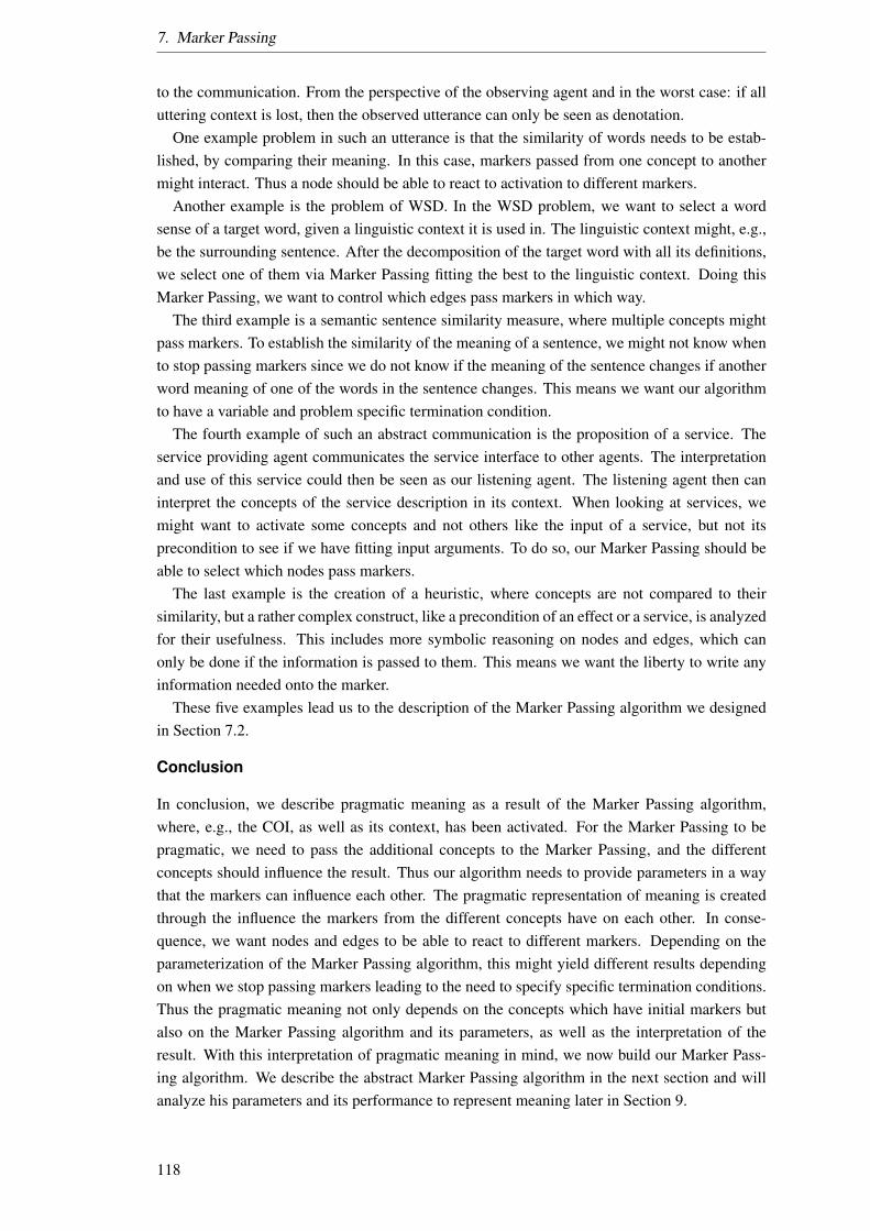
7. Marker Passing

to the communication. From the perspective of the observing agent and in the worst case: if alluttering context is lost, then the observed utterance can only be seen as denotation.

One example problem in such an utterance is that the similarity of words needs to be estab-lished, by comparing their meaning. In this case, markers passed from one concept to anothermight interact. Thus a node should be able to react to activation to different markers.

Another example is the problem of WSD. In the WSD problem, we want to select a wordsense of a target word, given a linguistic context it is used in. The linguistic context might, e.g.,be the surrounding sentence. After the decomposition of the target word with all its definitions,we select one of them via Marker Passing fitting the best to the linguistic context. Doing thisMarker Passing, we want to control which edges pass markers in which way.

The third example is a semantic sentence similarity measure, where multiple concepts mightpass markers. To establish the similarity of the meaning of a sentence, we might not know whento stop passing markers since we do not know if the meaning of the sentence changes if anotherword meaning of one of the words in the sentence changes. This means we want our algorithmto have a variable and problem specific termination condition.

The fourth example of such an abstract communication is the proposition of a service. Theservice providing agent communicates the service interface to other agents. The interpretationand use of this service could then be seen as our listening agent. The listening agent then caninterpret the concepts of the service description in its context. When looking at services, wemight want to activate some concepts and not others like the input of a service, but not itsprecondition to see if we have fitting input arguments. To do so, our Marker Passing should beable to select which nodes pass markers.

The last example is the creation of a heuristic, where concepts are not compared to theirsimilarity, but a rather complex construct, like a precondition of an effect or a service, is analyzedfor their usefulness. This includes more symbolic reasoning on nodes and edges, which canonly be done if the information is passed to them. This means we want the liberty to write anyinformation needed onto the marker.

These five examples lead us to the description of the Marker Passing algorithm we designedin Section 7.2.

Conclusion

In conclusion, we describe pragmatic meaning as a result of the Marker Passing algorithm,where, e.g., the COI, as well as its context, has been activated. For the Marker Passing to bepragmatic, we need to pass the additional concepts to the Marker Passing, and the differentconcepts should influence the result. Thus our algorithm needs to provide parameters in a waythat the markers can influence each other. The pragmatic representation of meaning is createdthrough the influence the markers from the different concepts have on each other. In conse-quence, we want nodes and edges to be able to react to different markers. Depending on theparameterization of the Marker Passing algorithm, this might yield different results dependingon when we stop passing markers leading to the need to specify specific termination conditions.Thus the pragmatic meaning not only depends on the concepts which have initial markers butalso on the Marker Passing algorithm and its parameters, as well as the interpretation of theresult. With this interpretation of pragmatic meaning in mind, we now build our Marker Pass-ing algorithm. We describe the abstract Marker Passing algorithm in the next section and willanalyze his parameters and its performance to represent meaning later in Section 9.

118

7.2. Marker Passing Algorithm

7.2. Marker Passing Algorithm

After creating the graph representing the semantic knowledge of the agent, this section willdescribe how this graph is used to select relevant concepts in a given context. These relevantconcepts are specified as a subgraph of the original graph including the markers passed to them.We will first describe the Marker Passing algorithm at a higher level to name the different partsand get an overview of the needed components in Section 7.2.1. Then we dive into the imple-mentation and all the details of this algorithm in Section 7.2.2.

7.2.1. High Level Marker Passing Algorithm

To start the algorithm, we have to create the underlying graph and prepare it with a set of startmarkers, which then are propagated through the graph. Figure 7.2 shows an abstract represen-tation of our algorithm. Here the idea is to propose a naming of the parts of the algorithm to beable to discuss those parts later on in more detail.

This algorithm is a generalization of the algorithm described by F. Crestani [61][Figure 5,p. 461]. Crestani describes the Marker Passing in four steps: Pre-adjustment, spreading, post-adjustment and termination condition evaluation. This is quite general and can result in inaccu-rate interpretations of the algorithm. Consequently, we introduce a more precise description ofthe algorithm by breaking the activation down into multiple steps without losing generality.

Crestani’s algorithm is based on the following principle: Starting from a start activation, aconcept has a threshold (seen as an upper limit of activation in a node to decide if the nodeis activated), with each incoming activation the activation level of the node builds up. If thethreshold is reached the node is selected as activated and is spreading in the next spreadingstep. This means that the node passes all its markers on to its neighbors. This is done until atermination condition is reached [61].

Figure 7.2 shows the input and output of our algorithm3, like documents, named with thecontent for the input. At first glance we look at the algorithm from the outside, specifying itsinterface.

Marked Graph (input) This is the input representing the graph, which is used to determineconcepts and edges which are used to hold and conduct markers. This graph has to containa set of markers to start from. These markers are called the start markers. The graphspecifies which concept can pass markers to which concept. This is the basic restrictionof this kind of algorithm: A concept can never pass markers to a concept when it has noconnection to this concept.

Node Interpretation The underlying graph can contain different concepts and edges. Eachconcept or edge can have a different Marker Passing behavior. To specify this behavior, thealgorithm gets a set of concept interpretations as input. Here each concept type specifiesits interpretation by defining what it does with markers passed to it, with that when it isactivated and how it passes marker to other concepts. These two functions allow eachconcept (or concept type) to react to different markers or the same markers differently.

Termination condition For our Marker Passing algorithm to terminate the algorithm needsa specification when it has reached its goal. The goal is to mark the sub graph which

3Our algorithm is based upon Crestani’s work but details some of the design discussions in the algorithm.

119

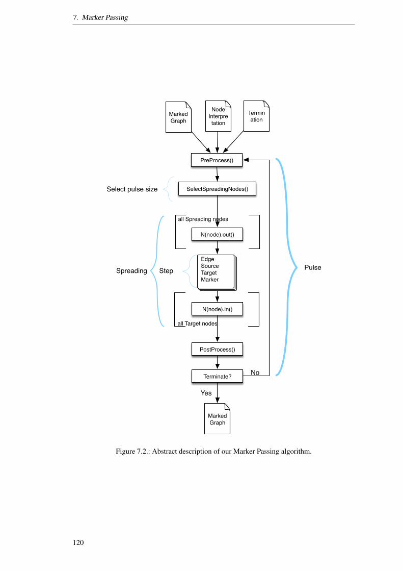
7. Marker Passing

all Spreading nodes

all Target nodes

N(node).in()

N(node).out()

EdgeSourceTargetMarker

PreProcess()

PostProcess()

Terminate?

SelectSpreadingNodes()

No

Marked Graph

Marked Graph

Node Interpretation

Termination

Yes

Spreading Pulse

Select pulse size

Step

Figure 7.2.: Abstract description of our Marker Passing algorithm.

120

7.2. Marker Passing Algorithm

is relevant to the given start activation. If no termination condition is given, the activa-tion spreads infinitely until no concept is activated anymore. This can be specified ina termination condition but does only in some cases accomplish the goal of the MarkerPassing [26].

Marked Graph (output) The output of the Marker Passing algorithm is again a marked graph,with the updated markers. This graph now can be interpreted to determine the answer to aquestion which has been encoded in the markers and the graph, to begin with. By lookingat this graph and the markers on it, we can, e.g., decide which other relevant conceptscontain markers on them.

All in all, the algorithm described in this section can be seen to move around markers in agraph regarding given rules. How the start markers are placed, in which way the markers arepassed over the network and how the result is interpreted is problem specific. Five exampleapplications can be found in Section 10, e.g., for the application of this algorithm to create asemantic similarity measure, which has been published in [104].

Now that we have looked at the Marker Passing algorithm from its interface, we can have alook at the algorithm itself. We start out by looking at the different phases the algorithm can beseparated into.

Pulse The pulse is defined as one iteration from the preprocessing to the check of the termi-nation condition. All other phases are sub-phases of the Marker Passing pulse. This termhas been coined by F. Crestani in his survey on activation spreading approaches [61]. Thepulse can be imagined as one activation of a set of concepts, where each concept is imagedto light up if it activates. In this visualization within each pulse, all the activated conceptslight up at the same time, creating a pulsing light which “wander” through the graph.This visualization gives the Marker Passing pulse its name. The pulse has two interme-diary steps: the Pre- and Post-Processing here the algorithm can integrate nonactivationspecific tasks like cleaning up the graph or normalizing the activation.

Pulse Size Selection Since during one pulse the termination condition is not checked, weneed the ability to change the pulse size. This means selecting the concepts which activateduring the next pulse. If all concepts which are active, activate then it could be that theconditions of the termination condition are met without noticing, because further conceptsare activated, where the result does not meet the termination condition anymore when itis checked, after the pulse. The smallest pulse size is to activate each concept in its pulse,meaning that after each activation the termination condition is checked. This option hasthe problem that the activated concepts are needed to be brought into an order, where theorder influences the result.

Spreading The spreading describes the Marker Passing of all activated concepts. During thespreading, all active concepts calculate their out-function and specify which markers arepassed to which concepts concurrently. Afterwards, all concepts which have markerspassed to them (these concepts are called targets) activate their in-function and collecttheir markers and update their internal activation level.

Spreading Step The spreading consists of one spreading step. The spreading step containsall markers which were passed by the out-function of all active concepts during this pulse.

121

7. Marker Passing

The spreading step contains all needed information for the in-function to process the in-coming markers. Here each marker is mapped to an edge (the edge represents an edgebetween two concepts in the underlying graph) over which the marker has been passedand the target it is destined to reach. The link contains sources and targets of an edge, butsince there can be multiple of them, the step needs to specify which target should be thedestination of the marker and from which source it has been spread.

After having an informal overview of the functioning principle of the abstract Marker Passingalgorithm in our extension of Crestani’s algorithm, we now formalize the Marker Passing in thenext section.

7.2.2. Implementation of our Marker Passing Algorithm

To start with the formalization, we start by defining the information stored on a nodes Data inthe following signature:

Signature Information =sorts:

DataMarker

opns:getMarker : Data→ Marker∗setMarker : Data×Marker∗ → Data

At the same time, we define how we describe a marker. This is done by defining Marker asthe sort of the marker object since the marker is defined regarding the problem specific imple-mentation of the information encoded on the Marker.

This Marker as a sort can be implemented with any data type which is needed. To implementa spreading activation, this sort could be a decimal value. This decimal value then can be in-terpreted as the activation level passed from one concept to another. For another example, themarker might have an integer type which could be interpreted as markers for a Petri net.

The sort NodeData maps the information encoded in markers (Data) to the concepts. TheData sort specifies the information encoded on a marker. The method getMarkers allows us toget the markers of a type of a concept. Equivalent the method setMarkers allows us to set themarkers of a concept.

The marker is typically represented by information objects from the marker signature andusually assigned to the concepts of the graph structure and passed on via the relations. ThisGraph represents the ontology or semantic graph which is the output of the decomposition. Wehave defined this graph formally in Section 6.4.

Here the signature Graph is the result of the semantic decomposition and is represented inthe formalism described in Section 6.4. From this graph the two sorts Concept and Relation aretaken as specified in the Figure 6.3 in our minimal type graph.

To enable the assignment of markers to concepts of a graph, we define a signature Marked-Graph which extends Graph and Marker and is defined as follows:

The function getNodeData gets the Data of a given node.The Marker Passing algorithm then transforms markers on a concept in a way specified by,

e.g., the implementation of the marker, the concept-interpretation, the in- and out-functions

122

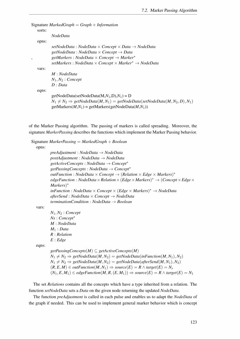
7.2. Marker Passing Algorithm

Signature MarkedGraph = Graph + Informationsorts:

NodeDataopns:

setNodeData : NodeData× Concept × Data→ NodeDatagetNodeData : NodeData× Concept→ Data

, getMarkers : NodeData× Concept→ Marker∗

setMarkers : NodeData× Concept ×Marker∗ → NodeDatavars:

M : NodeDataN1,N2 : ConceptD : Data

eqns:getNodeData(setNodeData(M,N1,D),N1) = DN1 6= N2 ⇒ getNodeData(M,N1) = getNodeData(setNodeData(M,N2,D),N1)getMarkers(M,N1) = getMarkers(getNodeData(M,N1))

of the Marker Passing algorithm. The passing of markers is called spreading. Moreover, thesignature MarkerPassing describes the functions which implement the Marker Passing behavior.

Signature MarkerPassing = MarkedGraph + Booleanopns:

preAdjustment : NodeData→ NodeDatapostAdjustment : NodeData→ NodeDatagetActiveConcepts : NodeData→ Concept∗

getPassingConcepts : NodeData→ Concept∗

outFunction : NodeData× Concept→ (Relation× Edge×Markers)∗

edgeFunction : NodeData×Relation× (Edge×Markers)∗ → (Concept×Edge×Markers)∗

inFunction : NodeData× Concept × (Edge×Markers)∗ → NodeDataafterSend : NodeData× Concept→ NodeDataterminationCondition : NodeData→ Boolean

vars:N1,N2 : ConceptNs : Concept∗

M : NodeDataM1 : DataR : RelationE : Edge

eqns:getPassingConcepts(M) ⊆ getActiveConcepts(M)N1 6= N2 ⇒ getNodeData(M,N2) = getNodeData(inFunction(M,N1),N2)N1 6= N2 ⇒ getNodeData(M,N2) = getNodeData(afterSend(M,N1),N2)(R,E,M) ∈ outFunction(M,N1)⇒ source(E) = R ∧ target(E) = Ns

(N1,E,M1) ∈ edgeFunction(M,R, (E,M1))⇒ source(E) = R ∧ target(E) = N1

The set Relations contains all the concepts which have a type inherited from a relation. Thefunction setNodeData sets a Data on the given node returning the updated NodeData.

The function preAdjustment is called in each pulse and enables us to adapt the NodeData ofthe graph if needed. This can be used to implement general marker behavior which is concept

123

7. Marker Passing

independent like a normalization of NodeData over the graph. The preAdjustment uses the cur-rent markers of the graph and produces an updated NodeData. The postAdjustment is similar tothe preAdjustment but is called after the spreading, since here again; we can change the markersof the graph before the termination condition is checked. For more details see Section 7.3.7.

The getActiveConcepts function filters the concepts which have been activated from the Marked-Graph. All these concepts have reached their spreading threshold and can potentially spread inthe next pulse.

The getPassingConcepts function then selects from all active concepts the ones which willpass markers in the next pulse. The passing concepts are always a subset of the active concepts,which is guaranteed by the first equation.

The outFunction implements the concept behavior on how markers are passed on to its neigh-bors if the concept is selected as passing concept. For more details see Section 7.3.4. The fourthequation of this signature describes that the edges always have a source in a relation R and targetthe concepts which are related with the relation R.

The edgeFunction describes the behavior of the edge when markers are passed over it. Thisallows us to implement, e.g., edge weights. For more details see Section 7.3.5. The fifth equationof this signature enforces that markers are only passed from an edge to its targets over the edgesof the relation R.

The inFunction and outFunction is the place where we can implement the behavior of theconcept when markers are passed to it. This in-function takes the concept, the markers passedto it and the edge the marker is passed over as input and converts the incoming markers into aform which lets the algorithm determine the activation of the node. For more details see e.g.Section 7.3.3.

The function afterSend can be used to update the markers of a concept after its out functionhas been called. It is called with the current markers and respective concept and updates themarkers accordingly. This could be used, e.g., if markers are rejected by the destination andshould be given back to the passing concept.

The terminationCondition defines when the spreading process has finished. It is based on thecurrent markers. For more details see Section 7.3.6.

The first function enforces that the passing concepts are a subset of the active concepts sothat all passing concepts need to be activated first. The second and third equation of this signa-ture ensures the compatibility of the inFunction and afterSend functions with the getNodeDatafunction. The fourth function ensures that markers are passed by the out function which havetheir source in the edge and are passed to the target of this edge. The fifth equation ensures thatedgeFunction only passes markers to targets of their edges.

In conclusion, we can say, the Marker Passing is a way of marking concepts in a graph, regard-ing some rules. These rules are problem specific and change depending on the implementationof the different points of the algorithm. There is one rule which has to be always true: Markerscan only be passed between concepts connected with a relation.

The pseudo-code of Crestani’s algorithm can be found in Appendix A with Algorithm 22 andour extension is described in Algorithm 5. The implementation of the algorithm is available4.

With this formalization, we can describe a wide range of algorithms ranging from Petri-Netsor Artificial Neural Networks to Spreading Activation mechanisms like PageRank-Algorithms.

4git•gitlab.tubit.tu-berlin.de:johannes faehndrich/semantic-decomposition.gitPlease contact the author to gain access to the source code.

124

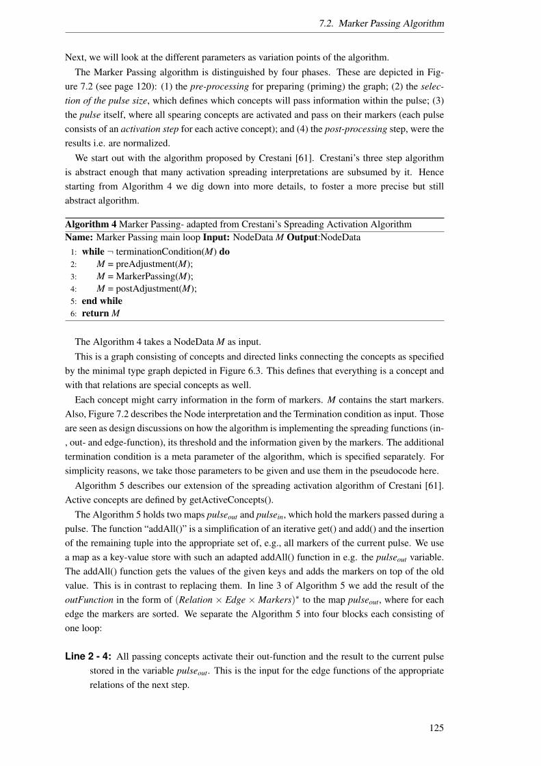
7.2. Marker Passing Algorithm

Next, we will look at the different parameters as variation points of the algorithm.The Marker Passing algorithm is distinguished by four phases. These are depicted in Fig-

ure 7.2 (see page 120): (1) the pre-processing for preparing (priming) the graph; (2) the selec-tion of the pulse size, which defines which concepts will pass information within the pulse; (3)the pulse itself, where all spearing concepts are activated and pass on their markers (each pulseconsists of an activation step for each active concept); and (4) the post-processing step, were theresults i.e. are normalized.

We start out with the algorithm proposed by Crestani [61]. Crestani’s three step algorithmis abstract enough that many activation spreading interpretations are subsumed by it. Hencestarting from Algorithm 4 we dig down into more details, to foster a more precise but stillabstract algorithm.

Algorithm 4 Marker Passing- adapted from Crestani’s Spreading Activation AlgorithmName: Marker Passing main loop Input: NodeData M Output:NodeData

1: while ¬ terminationCondition(M) do2: M = preAdjustment(M);3: M = MarkerPassing(M);4: M = postAdjustment(M);5: end while6: return M

The Algorithm 4 takes a NodeData M as input.This is a graph consisting of concepts and directed links connecting the concepts as specified

by the minimal type graph depicted in Figure 6.3. This defines that everything is a concept andwith that relations are special concepts as well.

Each concept might carry information in the form of markers. M contains the start markers.Also, Figure 7.2 describes the Node interpretation and the Termination condition as input. Thoseare seen as design discussions on how the algorithm is implementing the spreading functions (in-, out- and edge-function), its threshold and the information given by the markers. The additionaltermination condition is a meta parameter of the algorithm, which is specified separately. Forsimplicity reasons, we take those parameters to be given and use them in the pseudocode here.

Algorithm 5 describes our extension of the spreading activation algorithm of Crestani [61].Active concepts are defined by getActiveConcepts().

The Algorithm 5 holds two maps pulseout and pulsein, which hold the markers passed during apulse. The function “addAll()” is a simplification of an iterative get() and add() and the insertionof the remaining tuple into the appropriate set of, e.g., all markers of the current pulse. We usea map as a key-value store with such an adapted addAll() function in e.g. the pulseout variable.The addAll() function gets the values of the given keys and adds the markers on top of the oldvalue. This is in contrast to replacing them. In line 3 of Algorithm 5 we add the result of theoutFunction in the form of (Relation × Edge × Markers)∗ to the map pulseout, where for eachedge the markers are sorted. We separate the Algorithm 5 into four blocks each consisting ofone loop:

Line 2 - 4: All passing concepts activate their out-function and the result to the current pulsestored in the variable pulseout. This is the input for the edge functions of the appropriaterelations of the next step.

125

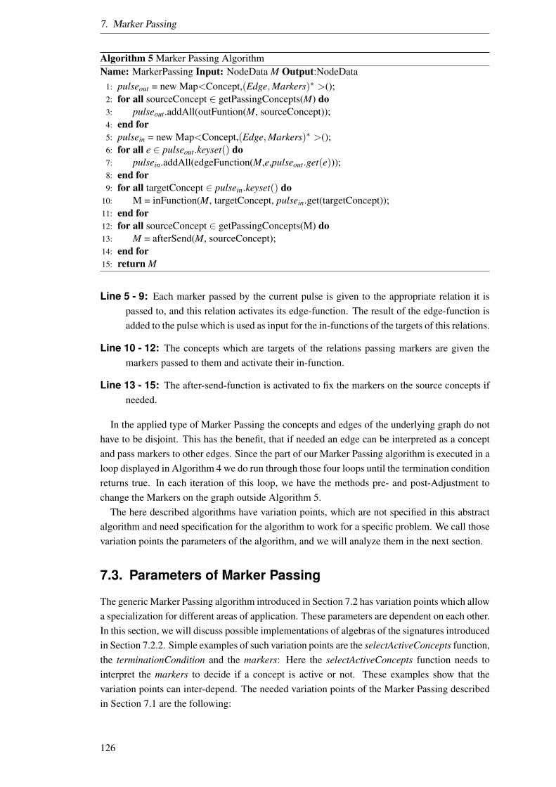
7. Marker Passing

Algorithm 5 Marker Passing AlgorithmName: MarkerPassing Input: NodeData M Output:NodeData

1: pulseout = new Map<Concept,(Edge,Markers)∗ >();2: for all sourceConcept ∈ getPassingConcepts(M) do3: pulseout.addAll(outFuntion(M, sourceConcept));4: end for5: pulsein = new Map<Concept,(Edge,Markers)∗ >();6: for all e ∈ pulseout.keyset() do7: pulsein.addAll(edgeFunction(M,e,pulseout.get(e)));8: end for9: for all targetConcept ∈ pulsein.keyset() do

10: M = inFunction(M, targetConcept, pulsein.get(targetConcept));11: end for12: for all sourceConcept ∈ getPassingConcepts(M) do13: M = afterSend(M, sourceConcept);14: end for15: return M

Line 5 - 9: Each marker passed by the current pulse is given to the appropriate relation it ispassed to, and this relation activates its edge-function. The result of the edge-function isadded to the pulse which is used as input for the in-functions of the targets of this relations.

Line 10 - 12: The concepts which are targets of the relations passing markers are given themarkers passed to them and activate their in-function.

Line 13 - 15: The after-send-function is activated to fix the markers on the source concepts ifneeded.

In the applied type of Marker Passing the concepts and edges of the underlying graph do nothave to be disjoint. This has the benefit, that if needed an edge can be interpreted as a conceptand pass markers to other edges. Since the part of our Marker Passing algorithm is executed in aloop displayed in Algorithm 4 we do run through those four loops until the termination conditionreturns true. In each iteration of this loop, we have the methods pre- and post-Adjustment tochange the Markers on the graph outside Algorithm 5.

The here described algorithms have variation points, which are not specified in this abstractalgorithm and need specification for the algorithm to work for a specific problem. We call thosevariation points the parameters of the algorithm, and we will analyze them in the next section.

7.3. Parameters of Marker Passing

The generic Marker Passing algorithm introduced in Section 7.2 has variation points which allowa specialization for different areas of application. These parameters are dependent on each other.In this section, we will discuss possible implementations of algebras of the signatures introducedin Section 7.2.2. Simple examples of such variation points are the selectActiveConcepts function,the terminationCondition and the markers: Here the selectActiveConcepts function needs tointerpret the markers to decide if a concept is active or not. These examples show that thevariation points can inter-depend. The needed variation points of the Marker Passing describedin Section 7.1 are the following:

126

7.3. Parameters of Marker Passing

Data: describes the marker and with that the information available to marked node.

Pulse size: selecting which nodes pass markers.

In-Function: describes how the node handles incoming markers.

Out-Function and After-Send: describe how the nodes pass markers and what happens onthe node after passing them.

Edge-Function: describes how the edges handle markers passed over them.

Termination Condition: describes when to stop the passing of markers.

Pre- and Post-Adjustment: describes what happens before and after a pulse.

The selection on how those parameters are implemented influences the behavior of the MarkerPassing, regarding the problem at hand.

Regarding the variety of the parameter, which could be selected, we restrict our discussionhere to general rules and dependencies which are necessary to understand to make informeddesign decisions for the application of this algorithm on a domain specific problem.

This section is structured in the following way: We start out with the discussion on the typeof information encoded on the markers in Section 7.3.1. Section 7.3.2 discusses the pulse sizeand in Sections 7.3.3 to 7.3.5 we then analyze the In-, Out- and Edge-Function. Afterwardswe analyze the termination condition in Section 7.3.6 and the Pre- and Post-Adjustment in Sec-tion 7.3.7. We then look at an example of how the Marker Passing can be used in Section 7.3.8.After the example we discuss the interpretation of marker, concept and edge in Section 7.3.9,Section 7.3.10 and Section 7.3.11.

7.3.1. Data

The data sort described in the signature NodeData in Section 7.2.2 contains the data sort whichformalizes the information encoded on a marker. The information modeled here influences thewhole Marker Passing algorithm in the spreading functions, the termination condition or theinterpretation of the result. One of the design decisions during the implementation of a MarkerPassing algorithm is, therefore, which information should be encoded in which way.

Examples of data on the markers are a boolean value of tokens assigned to places in Petri-Nets, or double values like in Artificial Neural Networks (ANN) which describe the activationof a neuron. We can not describe which information should be implemented on the marker sincethis is highly problem-specific. But we will describe an example in Section 7.3.8.

7.3.2. Pulse size

Selecting which nodes pass markers influences which nodes could be active next. Consequently,it might make a difference if two concepts are activated concurrently or sequentially. Selectingwhich nodes are counted as active, meaning they could pass markers and selecting which one doare two steps towards deciding the pulse size.

A standard way, e.g., in ANN or Petri-Nets is to give a threshold when a node is active. Thisthreshold is calculated by the function getActiveConcepts. The result of the getActiveConceptsfunction is a list of concepts which could pass markers in the next pulse. Which one of them are

127

7. Marker Passing

passing markers is determined by the function getPassingConcepts. The function getPassingConceptshas the active nodes as input and returns those of them, which should pass markers.

7.3.3. In-Function

The in-function of a concept describes how the markers are processed once they have beenpassed to the concept. The in-function is dependent on the concept interpretation. This meansevery concept type can have his own implementation of an in-function.

Here, we have to decide how the incoming markers influence the selection of active or passingconcepts. Depending on how these two functions (getActiveConcepts and getPassingConcepts)are implemented, the in-function can prepare the markers on the node to reflect the new activa-tion level of the node, to be used in the next selection of the active passing concepts.

Some of the design decisions which can be made in the in-function are discussed next.

Edge interpretation The in-function gets the information over which edge a marker has beenforwarded. This can be interesting information if different edge types exist. The in-function is the part of the Marker Passing, where this information is available, and wherethe edge type might influence how markers are handled on the node. An example wouldbe that the role of the edges of a relation might make a difference like in the example inFigure 6.2 (p. 98) where we can interpret in which role of the relation “give” we passmarker to, e.g., source and target.

Marker interpretation The feature which is unique to the in-function is that it can influencethe activation level of the concept by interpreting the symbolic information passed by themarker. In particular, depending on the marker types and the information encoded onit, the implementation of the in-function is responsible for interpreting the markers andrecalculating the activation level for the next pulse. One example decision is whether themarkers of an earlier spreading step are combined with the current markers, or whether theactivation level of a concept depends only on the current markers. We call this behaviorcumulative vs. replacing. If the markers are replaced, then the old markers are ignored,and the activation level of a concept only depends on the current markers. If the markersare aggregated with old ones, then the marker interpretation is called cumulative.

Symbolic Information The in-function is one of the places where the symbolic informationon the markers can be changed. Here we could, e.g., write the current marker in a concepthistory of markers, to detect loops. The markers passed to a concept do not need to beinterpreted in the same way for each concept. Depending on the information passed by themarker, the concept the marker was passed over and the concept itself, different markerscan be integrated differently in the activation level of the concept. An example couldbe that if a loop is detected with one of the markers, the marker can be marked for theafter-send function to give it back to its previous concept.

The in-function hence depends on the marker, edges and the concept interpretation. The in-function can only interpret the markers passed to it by the out-function. Both of these functionsare complementary concepts of influencing the marker distribution on the graph. Since betweenthe out-function and the in-function, there is a potential edge-function, one can not predict themarker flow from either perspective without knowing how all those functions are implemented.

128

7.3. Parameters of Marker Passing

7.3.4. Out-Function and After-Send

The out-function implements the behavior of a concept when it is passing markers. This meansthis function is only executed if the concept is active and has been selected as a passing conceptfor this pulse. The out-function takes the current activation level (the set of markers at theconcept in question at pulse t) and specifies how markers are passed over connecting edges ofthe concept.

Similar to the in-function, the out-function depends on the concept interpretation as well. Theout-function is one of the places in the algorithm where the symbolic information encoded on themarkers can be interpreted. There the implementation of the concept specific out-function givesus the possibility to adapt to the markers on the concept and the outgoing edges of the concept.If for example, the edges connecting concepts specify a weight for a maximal capacity of theedge, the out-function can distribute the markers of the concept proportional to these weights.

Some of the design decisions which can be made in the out-function are discussed next.

Output to which edge The out-function decides which edge is used to pass markers. Thiscould depend on the markers available on the concept. This enables us, e.g., to propagate“antonym-Markers” which only pass over antonym relations between concepts to onlythose edges.

Marker creation We need to decide if the out-function is allowed to create new markers or ifit can only modify the way existing markers are passed to the neighbors. This can be doneby copying existing markers or by creating a new kind of marker. Creating new markersallows us to react to the existing marker combinations. This could, e.g., be helpful if acommon ancestor in a tree structure is searched. When markers are passed to other con-cepts, one design decision is whether the markers are removed from the passing concept,or if they are copied to be passed on.

Edge interpretation The out-function can depend on the edge type it passes markers to. Thisallows us to pass different markers over different edges types. Like the in-function whichinterprets markers depending on the edge they passed over, the out-function can passdifferent markers or different amount of markers to different edges. This enables us to,e.g., pass markers to outgoing edges and not back to the incoming edges.

Discrete vs. Continuous In the out-function, we have to decide if we pass on markers as awhole, or if we can split markers up, e.g., into new smaller markers. This is correlatedwith the design decision if the out-function can create new markers. Additionally, thisdepends on how the symbolic information on the markers is specified.

Marker interpretation To be able to react to different markers on the concept, the symbolicinformation on a marker needs to be analyzed in the out-function. If for example we wantto implement a negation-concept used to integrate syntactic information into the MarkerPassing, the out-function can look through the concept history of the marker, to see if anegation concept has been passed right before this concept and with that change the outputof the out-function depending the wished behavior of nested negations. This means thatmarkers passed to the edges can be modified before they are passed to the neighbors. Thisenables us to create something like a decay of markers by, e.g., reducing the activation ofthe markers each time it is passed to another concept.

129

7. Marker Passing

Relative vs. Absolute When a node is activated, the out-function can pass an absolute amountof markers, e.g., proportional to the edge weights meaning that a fixed number of markersare passed, independent of the markers on the concept. A second design decision could beto pass a relative amount of markers depending on the markers available on the concept.With this propagation mode, the weights of the edges can be seen as a distribution of theexisting markers.

After the out-function has given the markers to spreading step, the edge functions distributethem to the in-functions of the targets of the edges. Now after the in-functions have completedtheir work, there could be the case that we want to manipulate the markers of the passing nodesagain. This could be the case, e.g., if a transition is not fired in a Petri-Net, the markers inthe input places are not consumed but could be given back to where they came from. Anotherexample could be to remove markers from concepts which have been passed on but have notbeen deleted by the out-function.

In such cases, the function afterSend is used to update the markers of the passing concepts,again, after the spreading step has been executed.

7.3.5. Edge-Function

The edge-function implements the behavior of edges when markers are passed over them. Thismeans the edge-function is invoked during the spreading and passes markers from its sources toits targets. To decide how the markers are passed, the edge has the information which markersare passed to it, which concepts passed the markers to it, which concepts are its target conceptsand its own type. Depending on this information the edge-function can change how the markersare passed to its target concepts.

The edge-function is activated after the out-function of all spreading concepts is activated, andbefore all in-function of the target concepts are activated. Here we have to emphasize that theedge-function of one edge does not have access to all the information encoded in the spreadingstep. The edge function has only access to the spreading steps, where it is the declared edge ofthe step. Some of the questions which could be answered by the edge function are: How aremultiple markers aggregated when they pass over an edge? How does the aggregated markingchange when it passes over an edge? Which concepts to forward the changed marking to?How to distribute the changed marking among those edges? Because there can be no answer tothose question without a specific problem which should be solved, we now look at the availableinformation which could be used to answer such questions.

Dynamic behavior An edge-function can implement dynamic or static behavior. Static meansthe edge-function reacts in the same way regarding the same spreading step (e.g., this ishow most Artificial Neural Networks (ANN) work). Dynamic behavior could mean thatthe edge-function becomes stateful and passes markers depending on, e.g., when it hasbeen activated the last time (e.g., this is how ANN with inhibitors work). Inhibitors inANN reduce the probability of a neuron to be activated depending on the time of the lastactivation.

Marker propagation The edge-function controls only the markers placed on it by the out-function of its source concepts. Here we can decide how the markers are passed to its

130

7.3. Parameters of Marker Passing

referenced concepts. This allows us to, e.g., implement something like an edge weight inthe edge, not the out-function.

Roles The edge-function has to interpret the type of which the different concepts are connectedto it. In a simple example, these types are source and target of the edge. However, inexamples like described in Figure 6.4, where the edge “give” of type “Relation” has threedifferent references to concepts, the edge-function implements the marker behavior onsuch an edge.

The edge-function depends on the implementation of the underlying graph, and its edges. Inour Knowledge Graph defined in Section 6.4 we can have multiple sources, over which markersare passed to an edge and multiple targets to which the edge passes markers depending on theedge type on the type of relation the concepts are connected to the edge.

7.3.6. Termination Condition

The termination condition encodes when the Marker Passing algorithm should stop propagatingmarkers. The type of termination condition depends on the use case of the Marker Passing, e.g.,if relevant concepts in a semantic graph should be identified, we could choose a terminationcondition which terminates after a few spreading steps to localize the markers around the contextof the initial concepts. We can define the termination condition as a function which maps themarked graph to boolean values which indicate if the termination condition is satisfied.

If a desired goal condition is reached, regarding the markers in the graph, and the terminationcondition is amiss, the markers can change with the next pulse, and the goal might never bereached. The same is true for a termination condition which stops at pulses too early. Thismeans the termination condition depends on the pulse size (here the selection of active andpassing concepts).

Furthermore, the termination condition should identify the goal we want to achieve with theMarker Passing. If for example, the goal is to calculate the length of the shortest path in a graph,the algorithm should stop if markers of the two starting concepts meet.

During the calculation of the termination condition, all information on the marked graph isavailable. In addition to the markers on the graph and the graph itself, the termination conditionmight be stateful, for example counting the activation steps. This gives us the ability to react toany change done in one pulse.

One basic decision here is which information is taken into account by the termination con-dition. Depending on this, we have to decide under which condition the termination conditionevaluates to true. The termination condition than might have the following properties:

Dynamic behavior The termination condition might not be a fixed kind of threshold butmight develop with the changes of markers in the graph. It might, e.g., be dependent onthe start activation, depend on the markers distribution velocity or simply be probabilistic.

Interactive The termination condition might be interactive so that a user might stop the MarkerPassing by choice. This might be of interest if the problem is computational complex anda tradeoff between precision and resources has to be made.

Time based In some problems, the termination condition is simply a time interval which de-termines how long markers are allowed to spread.

131

7. Marker Passing

The termination condition is highly problem-specific. Therefore it might be canny to havemultiple termination conditions, which guarantees a termination of the algorithm.

7.3.7. Pre- and Post-Adjustment

The pre- and post- adjustment are like the termination condition two phases of the algorithmwhere the entire graph and its markers are available for analysis. Here we can implement changeswe want to happen to the marking in between pulses. The design decision to make here is howto change the markers of the graph before and after the result. The pre-adjustment can be usedto change the markers to influence the active and with that the spreading concepts. The post-adjustment, on the other hand, might influence when the termination condition is fulfilled.

When using these adjustment phases, we have to be careful to not contradict the terminationcondition or the thresholds of the concepts. Since with the “right” pre- and post-adjustment wecan render each termination condition useless and at the same time make the spreading pointlessby creating a condition where the marker is passing only consumes resources without producingresults.

7.3.8. Example Marker Passing

Now we are looking at a simple example of this Marker Passing algorithm. This is done so thatthe more complicated discussions are founded on a concrete idea on how this algorithm works,what the effect on the parameters are and how the result could look like. In this example, wewant to find similar concepts to a pair of concepts given. For this reason, we want to answerthe question: Given two concepts, which concepts are similar to those two? We selected thisexample because we want to show that markers can carry more than decimal values like in stan-dard activation spreading algorithms or neural networks. The example is based on the exampledecomposition shown in Figure 6.5 on page 100.

We start out by describing the parameters of this example:

Graph The graph is given by the decomposition of the two target concepts, e.g., ”midday” and”noon” and has the concepts and relations like shown in Figure 6.2 on page 98.

Type-Graph We have an Attributed Type Graph with Inheritance ATGI = (TG, Z, I,A) likespecified by our example in Figure 6.6 on Page 101.

Data The markers encode the concept they have started from as color. The marker count isrepresented by a decimal value. We implement the signature Data as a tuple: M =

(Origin,Activation) where Origin is the concept where the marker is created upon whichis depicted by the color of the marker.

Pulse size The pulse size is selected to be all active concepts. This means that all activeconcepts are passing concepts in one pulse. Here we have selected an activation functionwhich uses a threshold for each concept which, if reached, activates the concept. Theactivation threshold is τ(n) = 5.0. This means concepts with more than a sum of fiveactivation of a color are considered active. Here we use the threshold in the absolute valueof activation. For instance, if a concept is activated with -7.5 then it reaches the thresholdas well.

132

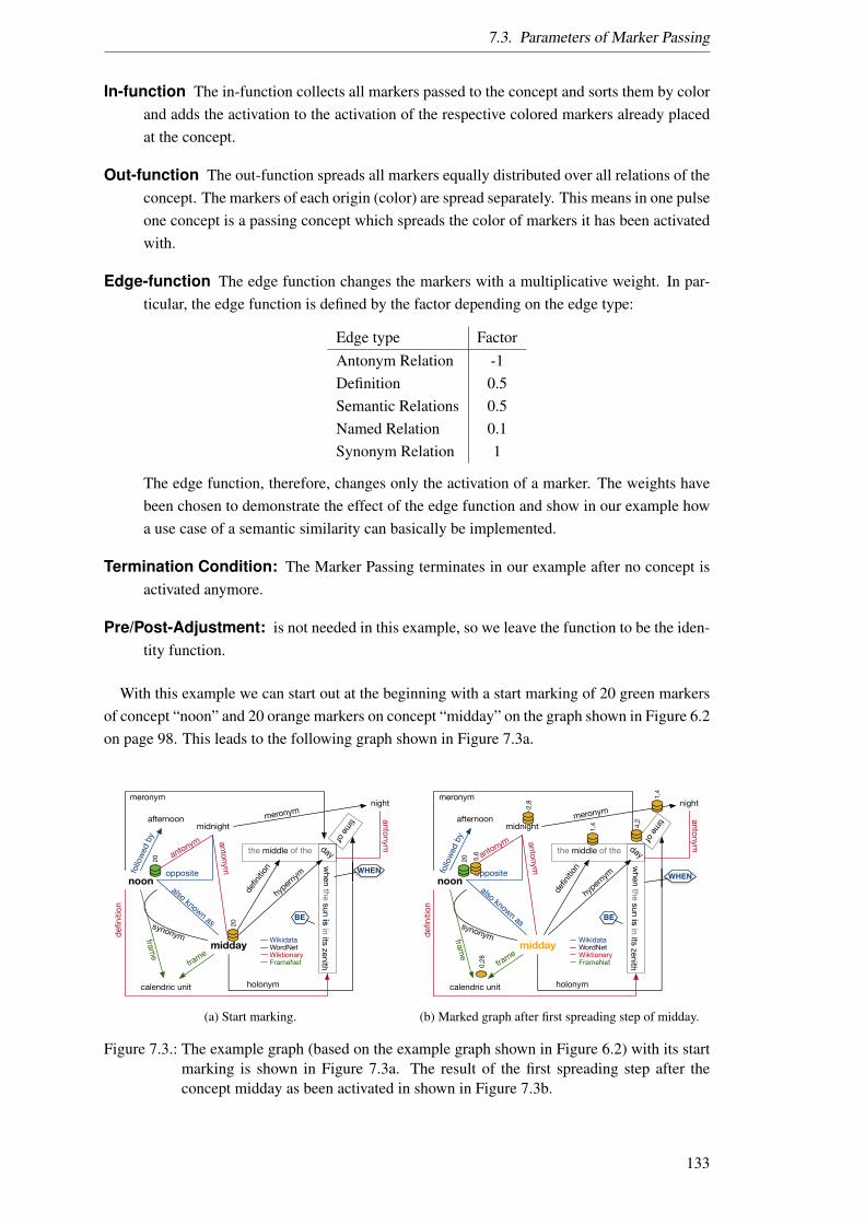
7.3. Parameters of Marker Passing

In-function The in-function collects all markers passed to the concept and sorts them by colorand adds the activation to the activation of the respective colored markers already placedat the concept.

Out-function The out-function spreads all markers equally distributed over all relations of theconcept. The markers of each origin (color) are spread separately. This means in one pulseone concept is a passing concept which spreads the color of markers it has been activatedwith.

Edge-function The edge function changes the markers with a multiplicative weight. In par-ticular, the edge function is defined by the factor depending on the edge type:

Edge type FactorAntonym Relation -1Definition 0.5Semantic Relations 0.5Named Relation 0.1Synonym Relation 1

The edge function, therefore, changes only the activation of a marker. The weights havebeen chosen to demonstrate the effect of the edge function and show in our example howa use case of a semantic similarity can basically be implemented.

Termination Condition: The Marker Passing terminates in our example after no concept isactivated anymore.

Pre/Post-Adjustment: is not needed in this example, so we leave the function to be the iden-tity function.

With this example we can start out at the beginning with a start marking of 20 green markersof concept “noon” and 20 orange markers on concept “midday” on the graph shown in Figure 6.2on page 98. This leads to the following graph shown in Figure 7.3a.

noon

midday

opposite

defin

ition

hypern

ym

holonym

synonym

meronym

midnight

antonym

nightmeronym

defin

ition

antonymantonym

follo

wed

by

afternoon

also known as

calendric unit

frame

frame

the middle of the

time ofw

hen the sun is in its zenith

day

WikidataWordNetWiktionaryFrameNet

20

20

BE

WHEN

(a) Start marking.

noon

midday

opposite

defin

ition

hypern

ym

holonym

synonym

meronym

midnight

antonym

nightmeronym

defin

ition

antonymantonym

follo

wed

by

afternoon

also known as

calendric unit

frame

frame

the middle of the

time ofw

hen the sun is in its zenith

day

WikidataWordNetWiktionaryFrameNet

-2,8

20

1,4 4,2

1,4

5,6

0,28

BE

WHEN

(b) Marked graph after first spreading step of midday.

Figure 7.3.: The example graph (based on the example graph shown in Figure 6.2) with its startmarking is shown in Figure 7.3a. The result of the first spreading step after theconcept midday as been activated in shown in Figure 7.3b.

133

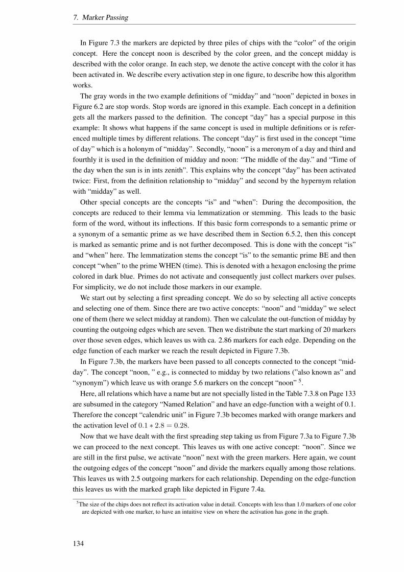
7. Marker Passing

In Figure 7.3 the markers are depicted by three piles of chips with the “color” of the originconcept. Here the concept noon is described by the color green, and the concept midday isdescribed with the color orange. In each step, we denote the active concept with the color it hasbeen activated in. We describe every activation step in one figure, to describe how this algorithmworks.

The gray words in the two example definitions of “midday” and “noon” depicted in boxes inFigure 6.2 are stop words. Stop words are ignored in this example. Each concept in a definitiongets all the markers passed to the definition. The concept “day” has a special purpose in thisexample: It shows what happens if the same concept is used in multiple definitions or is refer-enced multiple times by different relations. The concept “day” is first used in the concept “timeof day” which is a holonym of “midday”. Secondly, “noon” is a meronym of a day and third andfourthly it is used in the definition of midday and noon: “The middle of the day.” and “Time ofthe day when the sun is in ints zenith”. This explains why the concept “day” has been activatedtwice: First, from the definition relationship to “midday” and second by the hypernym relationwith “midday” as well.

Other special concepts are the concepts “is” and “when”: During the decomposition, theconcepts are reduced to their lemma via lemmatization or stemming. This leads to the basicform of the word, without its inflections. If this basic form corresponds to a semantic prime ora synonym of a semantic prime as we have described them in Section 6.5.2, then this conceptis marked as semantic prime and is not further decomposed. This is done with the concept “is”and “when” here. The lemmatization stems the concept “is” to the semantic prime BE and thenconcept “when” to the prime WHEN (time). This is denoted with a hexagon enclosing the primecolored in dark blue. Primes do not activate and consequently just collect markers over pulses.For simplicity, we do not include those markers in our example.

We start out by selecting a first spreading concept. We do so by selecting all active conceptsand selecting one of them. Since there are two active concepts: “noon” and “midday” we selectone of them (here we select midday at random). Then we calculate the out-function of midday bycounting the outgoing edges which are seven. Then we distribute the start marking of 20 markersover those seven edges, which leaves us with ca. 2.86 markers for each edge. Depending on theedge function of each marker we reach the result depicted in Figure 7.3b.

In Figure 7.3b, the markers have been passed to all concepts connected to the concept “mid-day”. The concept “noon, ” e.g., is connected to midday by two relations (”also known as” and“synonym”) which leave us with orange 5.6 markers on the concept “noon” 5.

Here, all relations which have a name but are not specially listed in the Table 7.3.8 on Page 133are subsumed in the category “Named Relation” and have an edge-function with a weight of 0.1.Therefore the concept “calendric unit” in Figure 7.3b becomes marked with orange markers andthe activation level of 0.1 ∗ 2.8 = 0.28.

Now that we have dealt with the first spreading step taking us from Figure 7.3a to Figure 7.3bwe can proceed to the next concept. This leaves us with one active concept: “noon”. Since weare still in the first pulse, we activate “noon” next with the green markers. Here again, we countthe outgoing edges of the concept “noon” and divide the markers equally among those relations.This leaves us with 2.5 outgoing markers for each relationship. Depending on the edge-functionthis leaves us with the marked graph like depicted in Figure 7.4a.

5The size of the chips does not reflect its activation value in detail. Concepts with less than 1.0 markers of one colorare depicted with one marker, to have an intuitive view on where the activation has gone in the graph.

134

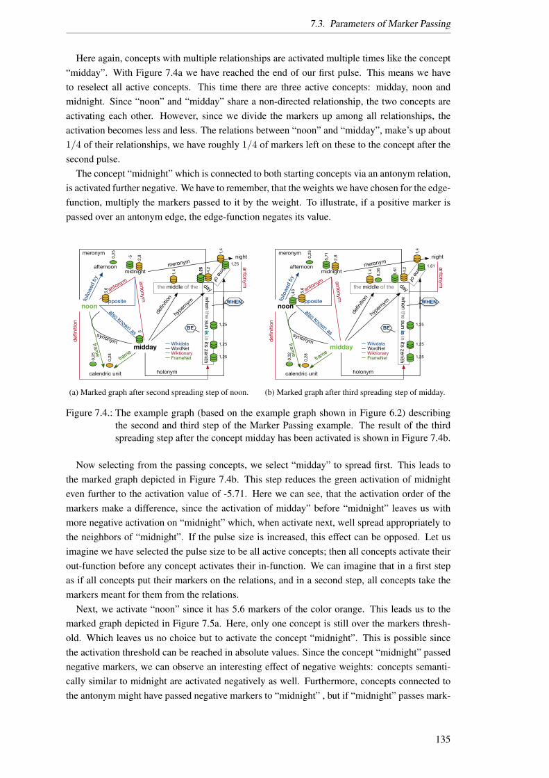
7.3. Parameters of Marker Passing

Here again, concepts with multiple relationships are activated multiple times like the concept“midday”. With Figure 7.4a we have reached the end of our first pulse. This means we haveto reselect all active concepts. This time there are three active concepts: midday, noon andmidnight. Since “noon” and “midday” share a non-directed relationship, the two concepts areactivating each other. However, since we divide the markers up among all relationships, theactivation becomes less and less. The relations between “noon” and “midday”, make’s up about1/4 of their relationships, we have roughly 1/4 of markers left on these to the concept after thesecond pulse.

The concept “midnight” which is connected to both starting concepts via an antonym relation,is activated further negative. We have to remember, that the weights we have chosen for the edge-function, multiply the markers passed to it by the weight. To illustrate, if a positive marker ispassed over an antonym edge, the edge-function negates its value.

noon

midday

opposite

defin

ition

hypern

ym

holonym

synonym

meronym

midnight

antonym

nightmeronym

defin

ition

antonymantonym

follo

wed

by

afternoon

also known as

calendric unit

frame

frame

the middle of the

time ofw

hen the sun is in its zenith

day

WikidataWordNetWiktionaryFrameNet

-2,80,

25

1,4 4,

2

1,4

5,6

0,28

1,25

-5

5

0,25

1,25

1,25

1,25

1,25

1,25

BE

WHEN

(a) Marked graph after second spreading step of noon.

noon

midday

opposite

defin

ition

hypern

ym

holonym

synonym

meronym

midnight

antonym

nightmeronym

defin

ition

antonymantonym

follo

wed

by

afternoon

also known as

calendric unit

frame

frame

the middle of the

time ofw

hen the sun is in its zenith

day

WikidataWordNetWiktionaryFrameNet

-2,80,

25

1,4 4,

2

1,4

5,6

0,28

-5,7

1

0,32

1,61

1,25

1,43

0,36

1,25

1,25

1,61

BE

WHEN

(b) Marked graph after third spreading step of midday.

Figure 7.4.: The example graph (based on the example graph shown in Figure 6.2) describingthe second and third step of the Marker Passing example. The result of the thirdspreading step after the concept midday has been activated is shown in Figure 7.4b.

Now selecting from the passing concepts, we select “midday” to spread first. This leads tothe marked graph depicted in Figure 7.4b. This step reduces the green activation of midnighteven further to the activation value of -5.71. Here we can see, that the activation order of themarkers make a difference, since the activation of midday” before “midnight” leaves us withmore negative activation on “midnight” which, when activate next, well spread appropriately tothe neighbors of “midnight”. If the pulse size is increased, this effect can be opposed. Let usimagine we have selected the pulse size to be all active concepts; then all concepts activate theirout-function before any concept activates their in-function. We can imagine that in a first stepas if all concepts put their markers on the relations, and in a second step, all concepts take themarkers meant for them from the relations.

Next, we activate “noon” since it has 5.6 markers of the color orange. This leads us to themarked graph depicted in Figure 7.5a. Here, only one concept is still over the markers thresh-old. Which leaves us no choice but to activate the concept “midnight”. This is possible sincethe activation threshold can be reached in absolute values. Since the concept “midnight” passednegative markers, we can observe an interesting effect of negative weights: concepts semanti-cally similar to midnight are activated negatively as well. Furthermore, concepts connected tothe antonym might have passed negative markers to “midnight” , but if “midnight” passes mark-

135

7. Marker Passing

ers, they receive positive markers back. This is because our antonym relation is not directedso markers can be passed to it in any direction and because the edge-function does multiplythe weight on the markers. This leads to the effect that after the fourth activation the concept“midday” is activated positively again.

noon

midday

oppositede

finitio

n

hypern

ym

holonym

synonym

meronym

midnight

antonym

nightmeronym

defin

ition

antonymantonym

follo

wed

by

afternoon

also known as

calendric unit

frame

frame

the middle of the

time ofw

hen the sun is in its zenith

day

WikidataWordNetWiktionaryFrameNet

-3,50,

25

1,4 4,55

1,4

1,4

0,35

-5,7

1

0,32

1,61

1,43

0,36

0,35

0,07

1,25

1,25

1,25

0,35

0,35

1,61

BE

WHEN

(a) Marked graph after third spreading step of noon.

noon

midday

opposite

defin

ition

hypern

ym

holonym

synonym

meronym

midnight

antonym

nightmeronym

defin

ition

antonymantonym

follo

wed

by

afternoon

also known as

calendric unit

frame

frame

the middle of the

time ofw

hen the sun is in its zenith

day

WikidataWordNetWiktionaryFrameNet

-3,50,

25

1,4 4,55

1,4

1,4

0,35

-0,3

6

0,32

1,61

2,86

0,36

0,07

0,71

0,351,25

1,25

1,25

0,35

0,35

1,61

BE

WHEN

(b) Marked graph after fourth spreading step of midday.

Figure 7.5.: The example graph (based on the example graph shown in Figure 6.2) describingthe second and third step of the Marker Passing example. The result of the thirdspreading step after the concept midday has been activated is shown in Figure 7.4b.

The result of our fourth Marker Passing step can be seen in Figure 7.5b. With the edge-functions being all smaller or equal to one, the active concepts become less and less until wedo not find any active concepts anymore. So that we can stop since our termination condition isreached.

Now it is time to interpret our result. The result of our example execution of the MarkerPassing algorithm is shown in Figure 7.5b. Therefore our next objective is to see how we canuse this marked graph to answer questions we want to ask. First, let’s look at the things wedecomposed: First, we decomposed two words: “noon” and “midday”. Then we placed markerson those concepts and propagated them in a way that similar concepts get more markers thanopposite ones. In fact, the question we have been asking for this example is: What are similarconcepts to noon and midday?

Depending on the questions we ask, the interpretation of the resulting marked graph differs.For our questions, we wanted to know similar concepts to noon and midday. Then our interpre-tation of the result could be to select the concepts with a maximum total amount of all colorsof markers as similar and the concept with a minimal amount of markers as not similar. Thiswould lead to the result that concepts like the day, time, sun and zenith are similar concepts andthat midnight and night are un-similar concepts. This interpretation is just one example of howthe decomposition and the Marker Passing (and their selection of parameters) can work togetherto represent meaning. With the result that different decompositions, different marker-passingalgorithms, and different interpretations can be found.

Since we are not the first ones to use Marker Passing on semantic graphs [21, 59, 286, 301,314, 329, 333, 362, 421], we now look at the contribution of this work in more detail. Startingout by looking at the difference of our approach to others, we will look at the combination ofconnectionist models of meaning with symbolic ones. We do that by looking at the symbolic

136

7.3. Parameters of Marker Passing

information encoded in the markers in Section 7.3.9 and continue by looking at the interpre-tation of concepts in Section 7.3.10 to finally extend this connections model through an edgeinterpretation in Section 7.3.11.

7.3.9. Markers Interpretation in Marker Passing

We have seen above that the definition of the information encoded on the markers is problemspecific and influences further design decisions. Some examples of markers could be: booleantokens which are passed over a graph like it is done in Petri Nets [306], a decimal activationlike in Artificial Neural Networks [347] or the information passed on by a Marker Passing canbecome more complex like proposed by Minsky [273]. Depending on the use case, differentinformation can be encoded on our marker. In our example in Section 7.3.8, we have used twotypes of symbolic information: the information of an amount of activation, and the origin as astart concept the markers were placed on. Depending on this information, the rest of our MarkerPassing algorithm has been developed. This means that for example, the threshold of a conceptuses both parts, the amount of activation collected by all markers received from one origin. Theconcept interpretation does not stop there: We also used the origin in the in- and out-function.

The main difference to the state-of-the-art here is that this information on the markers is flexi-ble and if we can have a dynamic interpretation, this interpretation of the markers by the MarkerPassing algorithm enables more expressiveness. We now take a look at which information aboutand from markers is available for the Marker Passing algorithm and how this information can beused to interpret the resulting marked graph.

We separate the information into four parts: First, the symbolic information encoded in themarkers which enable us, e.g., to create specific markers of one or more sorts. Second, themeta information about markers, like their count. Thirdly, the information about the markersdistribution over the semantic graph, which lets us analyze active areas. Moreover, fourth, thechange in markers over the pulses or time. Each of that information about and from markers canbe used independently on what the markers hold as a sort of symbolic information.

In the simple example, where markers only carry the boolean information if it is present ornot (like in a Petri-Net), there are still all other three information types available regarding themarkers. With more complex marker sorts the symbolic information becomes more complexand with that its meta information. Looking at the information available we can analyze thefollowing four groups:

1. Symbolic Information The sort of the markers is the most complex and domain dependentpart of the marker’s information. Choosing which information to model in the marker, andhow to interpret it depends on the questions asked with a query and the answer we wantfrom the interpretation of the Marker Passing result. The symbolic information of themarkers is the only information available at all time during the Marker Passing algorithm.Hence we can use it from the pre-adjustment phase to the check of the termination condi-tion. In our example in Section 7.3.8 the origin (depicted as color) and the activation level(depicted as a decimal number above the markers) are the symbolic information encodedby a marker.

2. Meta Information Meta information about the markers and the graph include informationlike the total amount of start markers, the number of different types of markers, the total

137

7. Marker Passing

number of edges or concepts in the graph, the pulse size and so on. Depending on thisinformation, the Marker Passing algorithm can change its behavior. However, there aresome restrictions rooted in the way we have defined the Marker Passing algorithm. Sincewe have defined the in-, out- and edge-function (see Section 7.2.2) in a way that theirresult depends only on their local information. This means the meta information availablehere depends on the current concept which is activated. Thus only some meta informationis available during those functions. Let’s call this information local meta information.Consequently, we need to define the difference in the meta information:

Global meta information is information about the graph or its marking which takeinto account the whole graph and its markers not encoded as symbolic informationon the marker.

With global meta information, we can express things like the total amount of markerscurrently marking the graph, the number of concepts or edges in the graph or the numberof the current pulse. Global meta information is available in the pre- and post- adjustmentas well as the selection of active and spreading concepts and the termination condition.

Not all meta information needs to be global. A concept can collect meta information aswell. The concept in its in-function could, for example, keep track of the markers typesand react differently the first time it is activated with a new markers type. For this reason,we need to define local meta information as well:

Local meta information is information about the concept or its marking which takeinto account this concept and its markers not encoded as symbolic information onthe marker.

The local meta information is available to in-, out- and edge-function and can be calcu-lated for each of those functions and each concept and edge independently. An exampleof a global meta information which can not be calculated locally is the total amount ofpulses passed. Since the local concept can only act in the pulses, it has been active. Allmeta information can be made available to all phases of the Marker Passing algorithm bymodeling them as symbolic information on the markers. Depending on the informationmodeled, this can be done in the pre- and post-adjustment Marker Passing phases.

3. Distribution As markers pass through the graph, the markers form a distribution. Thisdistribution can foster further information and can be used to influence the Marker Passing.Distributional information can be seen as a type of global meta information. It describesthe markers about other meta information. Enabling us to define something like a hot-spot6 or a focus point during the Marker Passing or to express relationships of markers toconcept types. This information is available during the pre- and post-adjustment and thetermination condition.

4. Change The information about markers’ change is another meta information which we wantto discuss separately. We define meta information change as:

Meta information about change is global or local meta information about conceptsand markers which change over time or pulses.

6A hot-spot can be seen as a subgraph which exceeds an activation limit.

138

7.3. Parameters of Marker Passing

We analyze this information separately from other meta information since it takes into ac-count the change of meta information as well. This enables us to define something like ve-locity of markers. This lets us analyze information about the markers change which leadsto further meta information like attention points where concepts are more often marked asactive than others. Because this information needs to be collected pulse overarching thisinformation can only be collected during the pre- and post-adjustment and the terminationcondition phases.

Under changing information, we can also include the change in markers’ interpretation.Here the markers include information on how to react to other markers. An exampleapplication of this use of meta information about markers can be found in the work ofFahlman [92] where the interpretation of the markers is dependent on the query, and withthat, if modeled in our Marker Passing paradigm, the interpreting information of a markeris passed on the markers itself.

One could imagine a Marker Passing where markers are added and removed dynamically. Inthis case, new marker types can be introduced during the Marker Passing. One use case for sucha scenario is the distributed query7 of one graph by multiple users, where the queries influenceeach other. This would enable a conversational behavior of the answers given by the algorithmwhich leaves us with an implementation of abstract markers interpretation8, which is left tofuture research efforts.

We can conclude that the markers’ interpretation takes place in multiple parts of the MarkerPassing algorithm and that the information passed on with markers is specific to the problem.The problem inclines the question we ask, which is about to be answered by the interpretationof the marked graph as a result of the Marker Passing algorithm.

Where Fahlman [92] can encode the presence of a marker type for each node, the noveltyin our extension is, that more information than the presence of a marker type at a node can beused for the Marker Passing. This includes but is not limited to the information discussed in thissection.

Next we look at how the state-of-the-art marker-passing algorithms is extended by the intro-duction of concept (see Section 7.3.10) and edge types (see Section 7.3.11).

7.3.10. Concept Interpretation in Marker Passing

In difference to the approach of Fahlman [92] where the symbolic information on the markers isused to enable reasoning on an entire knowledge graph, we introduce concept types, where eachconcept can react differently to markers. In the approach of Fahlman, every concept reacts to thepresent markers in the same way. With that, different markers passing through the knowledge,a graph can cause different marked concepts to react differently to a new marker. We extendthis approach with a concept type which has its own “interpretation” of its marking. We defineinterpretation as follows:

7A query can be distributed in parallel or over time. Having one graph queried by multiple queries enables us tomodel something like attention or focus to analyze which parts of the knowledge graph or the semantic graph areof interest, form correlations, topics or causal relations.

8The markers could need to be typed by a hierarchy, and this hierarchy needs interpretation, or the interpretation ofthe markers is encoded as symbolic information in the marker.

139

7. Marker Passing

An concept interpretation is the effect of in- and out-function of a concept, given its currentmarking, the getActiveConcepts- and getPassingConcepts function and a set of markers.

The interpretation of a concept, therefore, depends on the implementation of the in- and out-function. The effect of the in- and out-function is again a marking on the graph but with therestriction of the local context of the concept under study.

To formalize the concept interpretation, we introduce concept types. A concept type is amapping of the type graph discussed in Section 6.4 to the concepts of the knowledge graph.

Here we introduced the example concept types: Stop Words, Semantic Primes, Logical Con-cepts and Not. Additionally, we added the relevant properties of a concept type9 in Figure 6.6 bygiving a Concept it’s in- and out-function and the active- and passing-ConceptFunction. Theseconclude the concept interpretation with respect to the definition above.

In our example of ”midday” and ”noon” from Section 7.3.8 on Page 133 a Semantic Primesconcept has an in-function where all incoming markers are ignored. In particular a SemanticPrime concept is never activated and therefore never passes markers with its out-function.

Like the concept interpretation, we introduce an edge interpretation where different edges canreact differently to markers. How this is done and what can be modeled with that is subject tothe next section.

7.3.11. Edge Interpretation in Marker Passing

Derived forms of the Marker Passing like artificial neural networks, use weights for each edge tochange the behavior of, e.g., the activation spreading over the network to adapt to a given trainingset [347]. Like with the concept interpretation we introduce an edge interpretation giving eachedge type the possibility to define its behavior exceeding the setting of weights. In this section,we will analyze how this edge interpretation influences the Marker Passing.

A Edge interpretation is the effect of edge-function of an edge given an edge and its mark-ers.

Like with the concept interpretation, the edge interpretation is given by the edge types. Theedge type is defined in the type graph shown in Figure 6.6 on page 101. Here each edge isassigned to exactly one edge type.

Since the edges are defined in an inheritance hierarchy, like with concepts, the inherited edge-function can be overwritten in a specialization. An example of such relations is shown in Fig-ure 6.6 on page 101 where we have a general relation which inherits the edge function to itschildren i.e. the semantic relation which can be further specialized like shown in Figure 6.7 onpage 102.

The edge interpretation function allows us to modify the markers passed to the edge by anout function. It allows each edge to change the symbolic information passed by the markers orchange its connectionist information by choosing to which target of the edge the markers arepassed to. Here the restriction is that only markers passed to the realization can be modified, andthe edge can only pass markers to concepts which are part of its target function codomain.

In our example Marker Passing in Section 7.3.8 the edge-function of, e.g., the antonym re-lations changes the symbolic information on the markers into a negative activation. Here we

9In our example of a semantic graph the concepts are made up of concepts, and the different concept types arereflected by different concepts.

140

7.4. Conclusion

selected all activation of all source concepts and then passed the modified information on to thetarget concepts.

As we have described in Section 6.4 an edge of our graph can be seen as a concept as well.Therefore an edge can act as an edge when it is activated by a concept, and it can act as a conceptif it is activated as a concept (if markers are passed to it by an edge).

Also, the edge-function might choose to activate another edge which is part of its targetsdepending on the markers passed to it and the implementation of the edge function. In ourexample relation in Figure 6.2 the “give” relation inherits from a “transfer” relation. If the“give” relation is now activated, it can activate the transfer relation by sending markers over theis-a-relation to the transfer relation. The transfer relation is then handled like every other relationwhich has markers passed to it by an out-function in this spreading step.

As the activation of concept cycles, the information about a passed markers in the historyof markers can help to detect loops in edge cycles. This means that for the Marker Passingalgorithm cycles in concepts or edges do not have to influence the termination behavior.

The effect of edge interpretations can be seen in the Marker Passing example shown in Fig-ures 7.3 to 7.5. In this example, one case of an edge interpretation is the antonym relation. Herethe edge function negates the activation value of the marker, leading to the effect that antonymsof concepts with decreasing activation.

With this Marker Passing algorithm over the here defined graph structure, we can modelmany problems. We will focus our analysis on one kind of problem which veins this thesis: Themodeling of meaning. This is done next, where the graph and the Marker Passing are specializedto the use case of modeling pragmatic meaning after a short conclusion of this section.

7.4. Conclusion

In this section, we have proposed an abstract Marker Passing algorithm, which uses a semanticgraph to guide the Marker Passing. This extends the state-of-the-art of marker-passing algo-rithms by having defined four functions (In- Out- Edge- and After Send-Function) which allowa specialization of the algorithm to a given problem. Also, we have added the marker data typewhich allows us to encode symbolic information onto the markers and use this information inthe spreading functions.

This Marker Passing algorithm together with the semantic decomposition present the twoparts of our artificial meaning representation: The semantic decomposition automatically createsa semantic graph encoding connectionist information. The Marker Passing allows symbolicinformation to be encoded on the markers and the spreading functions to use this informationregarding the structure of the semantic graph. Together they form two parts of a thought processlike learning new knowledge (extending the graph) and thinking of this knowledge (MarkerPassing).

Because of its general nature, the algorithm leaves many parameters to the developer forspecification. Selecting the right information on the marker, the spreading functions and howthe result is interpreted are just a few of them. This fosters broader applicability of the algorithmbut generates more effort on using it in special applications.

Next, we will evaluate our approach in the different experiments described in Part IV.

141

8. Implementation

This section describes the implementation of the approach which was used to evaluate the hy-pothesis in the here performed experiments. For each component, we look at how it can beused and at the main classes used in the component. With that, we want to give an overviewon the application interfaces and enable other scientists to reuse the results created here. Theimplementation has been realized using Java 1.8. The semantic graph is implemented usingJGraph [14]. All dependencies have been managed using Apache Maven1.

Decomposition

Marker Passing

DictionariesExperimentsWord

Marked Graph

RelationsDefinitions

Graph creation

Concept

Marked Graph

Interpretation

Initial Marking

Figure 8.1.: Architecture of the implementation.

Figure 8.1 shows the architecture of our implementation. We start ours with an experiment,which needs to decompose some words. Those words are given to the decomposition. At thesame time, the experiment defines how the result of the Marker Passing is interpreted. The wordswere given by the experiment then are decomposed by the decomposition component, using theattached dictionaries. The result of the decomposition is a graph containing all informationgathered during the decomposition. This concept can be transformed into a graph, which thenis passed to the Marker Passing. The result of the Marker Passing is a graph marked with theappropriate markers. This result then can be interpreted by the experiment.

We first look at the implementation of the Decomposition and how it can be used in Sec-tion 8.1. We then look at the Implementation of the Marker Passing algorithm in Section 8.2.

8.1. Semantic Decomposition

This section describes the implementation of the semantic decomposition. All components usedin this thesis can be found online2. We will look at the API for the different components andexplain how they are used. An Overview of the classes used by the decomposition can be foundin Figure A.2 and Section A.

1see: https://maven.apache.org/2To get access to the GIT repositories, please contact the author.

143

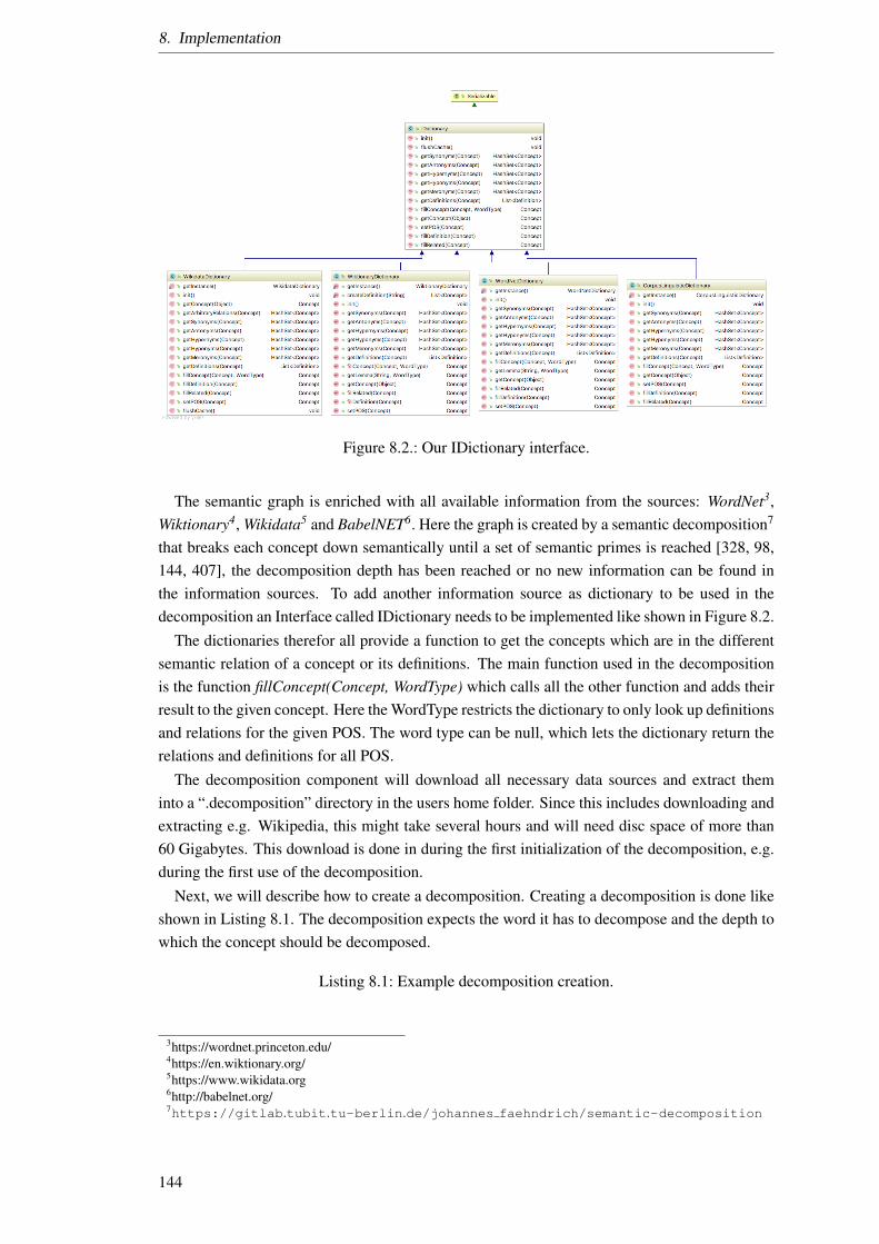
8. Implementation

Figure 8.2.: Our IDictionary interface.

The semantic graph is enriched with all available information from the sources: WordNet3,Wiktionary4, Wikidata5 and BabelNET6. Here the graph is created by a semantic decomposition7

that breaks each concept down semantically until a set of semantic primes is reached [328, 98,144, 407], the decomposition depth has been reached or no new information can be found inthe information sources. To add another information source as dictionary to be used in thedecomposition an Interface called IDictionary needs to be implemented like shown in Figure 8.2.

The dictionaries therefor all provide a function to get the concepts which are in the differentsemantic relation of a concept or its definitions. The main function used in the decompositionis the function fillConcept(Concept, WordType) which calls all the other function and adds theirresult to the given concept. Here the WordType restricts the dictionary to only look up definitionsand relations for the given POS. The word type can be null, which lets the dictionary return therelations and definitions for all POS.

The decomposition component will download all necessary data sources and extract theminto a “.decomposition” directory in the users home folder. Since this includes downloading andextracting e.g. Wikipedia, this might take several hours and will need disc space of more than60 Gigabytes. This download is done in during the first initialization of the decomposition, e.g.during the first use of the decomposition.

Next, we will describe how to create a decomposition. Creating a decomposition is done likeshown in Listing 8.1. The decomposition expects the word it has to decompose and the depth towhich the concept should be decomposed.

Listing 8.1: Example decomposition creation.

3https://wordnet.princeton.edu/4https://en.wiktionary.org/5https://www.wikidata.org6http://babelnet.org/7https://gitlab.tubit.tu-berlin.de/johannes faehndrich/semantic-decomposition

144

8.1. Semantic Decomposition

Decompos i t i on d e c o m p o s i t i o n = new Decompos i t ion ( ) ;Concept dog = d e c o m p o s i t i o n . decompose ( ” dog ” , 2 ) ;

In the example shown in Listing 8.1 we decompose the word “dog” with depth two. A classdiagram of the decomposition can be found in the appendix in Section A.2 on Page 260.

The decomposition returns a concept. A concept implemented as shown in Figure 8.3a incap-sulates all relations the concept has with other concepts. This implements the signature describedin Section 3.5. The concept holds the literal (the word) it represents, as well as its lemma (thebase form of the word) and its named entity id (NER). The class additionally hold organizationalfields like a list of IDs of the word in the different dictionaries, the highest decomposition level ithas been decomposed with and the element count of the decomposition. The “namedRelation”is a relation extracted from Wikidata, where the relation itself is not a semantic one, but a namedrelation like “is-president-of-country”.

(a) Class diagram of a concept. (b) Class diagram of a definition.

Figure 8.3.: Class diagrams of concept and definition.

In addition, a concept has a word type which encapsulates the Part-of-Speech (POS) of theconcept. Here the word type includes the POS representations of the different data sources. Theword type class proposes functions to convert one POS data structure into another.

The concept includes its definitions. A definition is implemented like shown in Figure 8.3athe concept, it defines is held here as “term” and a list of concepts making up the definition. Thedefinitions implement the signature described in Section 3.5. A definition additionally includesa sense key which references the WordNet send key. This is needed if a definition should beselected in a Word Sense Disambiguation task.

145

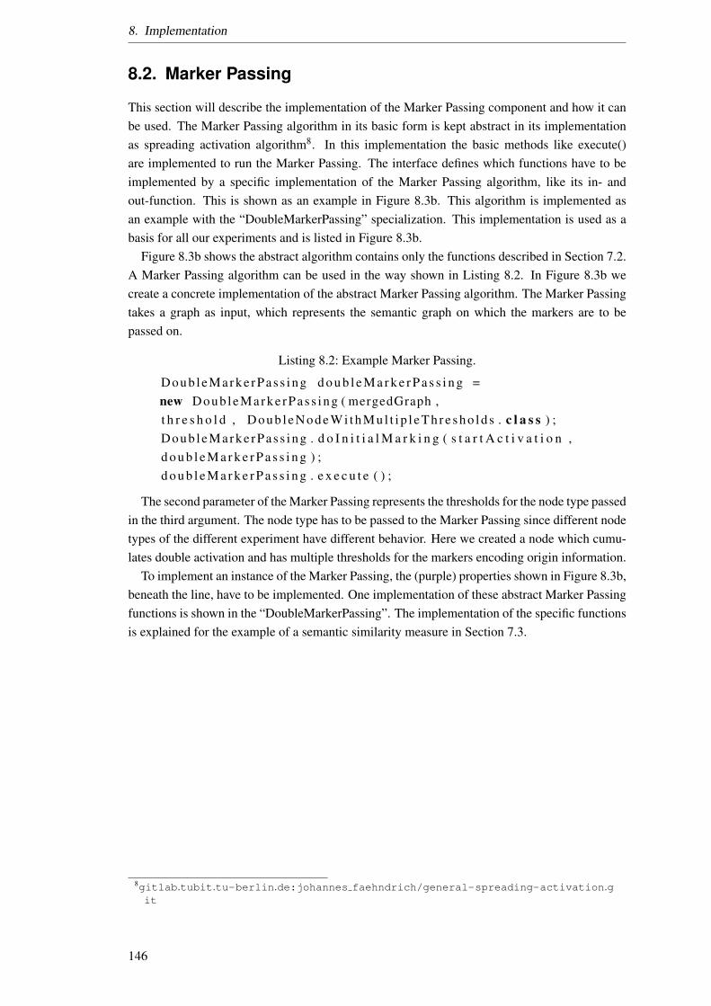
8. Implementation

8.2. Marker Passing

This section will describe the implementation of the Marker Passing component and how it canbe used. The Marker Passing algorithm in its basic form is kept abstract in its implementationas spreading activation algorithm8. In this implementation the basic methods like execute()are implemented to run the Marker Passing. The interface defines which functions have to beimplemented by a specific implementation of the Marker Passing algorithm, like its in- andout-function. This is shown as an example in Figure 8.3b. This algorithm is implemented asan example with the “DoubleMarkerPassing” specialization. This implementation is used as abasis for all our experiments and is listed in Figure 8.3b.

Figure 8.3b shows the abstract algorithm contains only the functions described in Section 7.2.A Marker Passing algorithm can be used in the way shown in Listing 8.2. In Figure 8.3b wecreate a concrete implementation of the abstract Marker Passing algorithm. The Marker Passingtakes a graph as input, which represents the semantic graph on which the markers are to bepassed on.

Listing 8.2: Example Marker Passing.

Doub leMarke rPas s ing d o u b l e M a r k e r P a s s i n g =new Doub leMarke rPas s ing ( mergedGraph ,t h r e s h o l d , D o u b l e N o d e W i t h M u l t i p l e T h r e s h o l d s . c l a s s ) ;Doub leMarke rPas s ing . d o I n i t i a l M a r k i n g ( s t a r t A c t i v a t i o n ,d o u b l e M a r k e r P a s s i n g ) ;d o u b l e M a r k e r P a s s i n g . e x e c u t e ( ) ;

The second parameter of the Marker Passing represents the thresholds for the node type passedin the third argument. The node type has to be passed to the Marker Passing since different nodetypes of the different experiment have different behavior. Here we created a node which cumu-lates double activation and has multiple thresholds for the markers encoding origin information.

To implement an instance of the Marker Passing, the (purple) properties shown in Figure 8.3b,beneath the line, have to be implemented. One implementation of these abstract Marker Passingfunctions is shown in the “DoubleMarkerPassing”. The implementation of the specific functionsis explained for the example of a semantic similarity measure in Section 7.3.

8gitlab.tubit.tu-berlin.de:johannes faehndrich/general-spreading-activation.git

146

Part IV.

Evaluation

147

9. Experiments with the Decomposition

This chapter will describe the first part of our evaluation of my approach: This first part willexperiment with the parameters of the Decomposition (Section 9). Those parameters are funda-mental for all other experiments including the decomposition. Since the decomposition is thebasis for all other experiments, its parameters and their effect on the resulting semantic graphshould be analyzed to be able to select the parameter later in the other experiments.

In this chapter we will first look at the parameters of the decomposition in Section 9.1 . Wethen analyze in more detail the selection of synonyms in Section 9.2 and the decompositiondepth in Section 9.3.

9.1. Parameters of the Decomposition

In this section, we will describe our experiments with the parameters of the decomposition. Thesexperiments are done before our semantic experiments because these parameters influence allof those experiments through the output of the decomposition: the semantic graph. Here wewant to analyze how the parameters of the decomposition change resulting semantic graph. Theparameters which are analyzed are the recursion of the semantic relations on the example ofsynonyms and which influence the decomposition depth has on the output graph. The analysisof all semantic relations could further gain insight into the creation of artificial meaning but isleft to future work.

With this experiments, we want to foster more understanding of our decomposition. The re-sults should enable us to improve its performance and find drawbacks which could be removed infuture specializations. The parameters of the decomposition (e.g., synonyms and decompositiondepth) are general properties and hence are not tied to a specific application.

The theoretic semantic decomposition introduced in Section 6 is not usable in practice becauseof two reasons: it takes a long time to create a total decomposition into semantic primes or evenworse, it can not be done with the given information sources. The information source is unusablefor the decomposition, e.g., if no definitions or explanations for concepts are given in them. Inthis case, the information source will only replace words with other words without describingtheir meaning. If words are only replaced by an agent, meaning can not be established which isargued in the philosophical ”Chinese Room” argument [353]. For the decomposition to becomemore usable we have restricted the theoretic decomposition with a decomposition depth shownin Algorithm 1. This experiment analysis the effect of the decomposition depth on the resultingsemantic graph.

We start out by looking at the different relations used in the decomposition to identify thescope of the decomposition depth. Here for the termination of the decomposition we look forsemantic primes or their synonyms because synonyms of primes are handled by the decomposi-tion like primes themselves.

Finding synonyms depends on the used information sources. The information sources like

149

9. Experiments with the Decomposition

Wikipedia and WordNet describe different relations between concepts. Relations can be of syn-tactical nature like Part Of Speech (POS) relations or of semantic nature like the “is-part-of”relation of Synonymy. The selection of the relations used during decomposition makes up thesemantic graph. Using this graph with the Marker Passing influences the result of the MarkerPassing and the information it can encode. Therefore, the selection of the relations during de-composition and when to stop decomposing influences the result of the Marker Passing. As anexample leaving out the Hypernym (generalization) and the Hyponym (specialization) relationshas the consequence that generalizations like the similarity between “bird” and “cock” is harderto find and the markers take other routes between the two concepts. Bringing about that the sameMarker Passing algorithm creates a different marker distribution on the graph.

Since we can configure the Marker Passing in a way to ignore relations1 We will first add allrelations to the decomposition and filter them out later if not needed. This is done since we mightnot know all application contexts the decomposition is used in. Consequently, we can not decidewhich relation will be needed and which one can be left out. One example for this argument isthe Marker Passing done by Fahlman [92] where the edge “eats” connects “bird” and “worm”in the sense of birds eat worms. If this edge had not been added during the decomposition,the connection between worms and birds would have been lost, and the reasoning that birds eatworms but penguins eat fish would not be possible.

The remainder of this section discusses the use of the synonym relation in Section 9.2 andthe decomposition depth in Section 9.3 since both influence the output of our decomposition.The synonymy relation analyzed here is a surrogate for other semantic relations, which needfurther analysis as well but are out of scope for this work. First, we analyze how synonymsare chosen, since the synonyms of primes are also seen as primes and as a result terminate thedecomposition.

9.2. Selecting Synonyms

The first parameter of the decomposition algorithm we look at is the properties of relations inthe example of the synonym relation. Selecting words which have an equivalent meaning is notprecise enough for a semantic decomposition. The goal of this section is to determine if syn-onyms have certain properties with the information sources we use in the Decomposition. Mostconcepts have different meanings in different contexts, consequently, synonyms of a concept dotoo. A synonym might be equivalent in one context of use but not in another one, as discussedin Section 3.9. As a result, we use the Definition 23 to define a synonym.

Nevertheless, there is a set of agreed on synonyms which are held in different databases likethe Roget’s Thesauri on which WordNet has build its synonym relations [192]. These synonymscan be used to bootstrap other synonyms from unstructured text like the definitions used in thesemantic decomposition. Kennedy and Szpakowictz [192] suggest adding new word into theRoget’s Thesaurus by using word context and already known words and their synonyms. Themajor drawback of this approach is that the synonymy relation is not dependent on the contextin which the words are used. Because we first have to create our semantic similarity measureto use Definition 23 as synonyms, we will start out by using the pre defined synonyms by theinformation source. In this section, we will discuss the properties of synonyms and analyze if

1This can be done, e.g., by setting the weight for a relation to zero in the out-function of the Marker Passing.

150

9.2. Selecting Synonyms

those properties are given by the synonyms we extract from our information sources.We consider partial synonymy as defined by Lobner [240] since total synonymy is either

trivial, i.e., abbreviations (e.g., AI is a synonym for Artificial Intelligence) or nonexistent if weconsider if two concepts have the same meaning. If two concepts have the same meaning theyare equivalent hence again a trivial case: each concept is a synonym to itself. To words, on theother hand, might be equivalent and not be synonyms as this is the case, e.g., for ambiguouswords. In particular, if we talk about synonyms we talk about partial synonyms as defined inDefinition 23 with a fixed context. This means we can look at the following properties to analyzeif they are given by our data sources:

Reflexive: Synonyms are reflexive since a concept can be replaced with it self without chang-ing the meaning of its word sense. A concept, in consequence, is a synonym to itself sincethe semantic similarity of a concept c and itself should be one. This is of cause only thecase if the same word sense is selected.

Symmetry: Replacing one concept with another in a given context without changing its mean-ing should be symmetric if the context is fixed. Hence if two concepts c1 and c2 are syn-onyms in a given context, replacing the one with the other does not change the meaning ofthe sentence, neither does changing it back to the original concept as long as we select theappropriate word sense. We can see in Figure 9.1 and Figure 9.2 that both concepts (mid-day and noon) are synonyms since they are connected by a synonym edge, but a specialityof the information sources used for our decomposition is that midnight is an antonym ofmidday, but not of noon, even though they are synonyms. This means the informationsources we used do not see synonyms as semantically equal because if they would, noonshould have the same antonyms as midday.

Transitivity: Synonyms are transitive in a fixed context. Because of the symmetry of syn-onyms, if a concept c1 is synonym to a concept c2 in a given context and c2 is synonymto c3 in the same context then c1 is synonym to c3 as well. This can be proven by theHypothetical syllogism [237].

Closure: Has the set of synonym closure under the synonym relations. This means: does thesynonym relation always add new elements or is the set at some point complete and finite.With our information sources, the synonym sets are complete. This can be shown addingall synonyms of synonyms to a set of concepts. After running several tests, this recursivelookup of synonyms terminates and results in a finite set of concepts. E.g., the word “dog”(as a noun) as 193 recursive synonyms, the word “fly” (as a verb) has 62, and “nice” (asan adjective) has 150. There could be only two outcomes of this experiment: First, if thesynonyms build a recursive chain and are not complete, then all words of the informationsources become part of the synonym. Second, the recursion at one point does not add anynew synonyms.

Having a measure of semantic similarity, we need to decide which recursion depth of a syn-onym can still be counted as a synonym. If our definition of a synonym is symmetric, a numberof synonyms regarding one threshold of Definition 23 discussed in Section 3.9 should be finite.Never the less infinite chains of similarity could be created.

151

9. Experiments with the Decomposition

Concluding we can summarize: Until now synonym relations are given by ontologies likeWordNet. These relations have been modeled by humans like in thesauri where for each conceptthere is a set of synonym concepts. If done well, the so defined synonym relation is symmetric.But with the generalization from context this representation is error-prone: As described inSection 3.9 two concepts might be synonyms in one context but not in another [176]. In referenceto a financial institution, one would perhaps utter: “This counting house was robbed!” using“counting house” as a synonym for a bank. But in reference to a bench in the park or a slope ofthe earth, this would probably confuse the audience.

The goal of this evaluation is to show the usefulness of our representation of meaning by find-ing semantic similarity between concepts e.g. of a goal state and some concepts of a service;we analyze concepts, sentences, word senses and semantic service descriptions for their simi-larity. We are still using all of the relations available, but do not define their semantics. Withthat the analysis of Meronyms, Hypernyms und Hyponyms is left for others to be researched.The question if a synonym of a synonym is still a synonym of the original concept can be askedfor all semantic relations. The restriction on when we stop following a semantic relation in thedecomposition is discussed in the next section.

9.3. Selecting Decomposition Depth

The decomposition as described in Algorithm 1 is a recursion which ends the decomposition ifa concept is a semantic prime or the decomposition depth is reached. The total decompositionof a concept includes all concepts found on the path to the prime. The resulting decompositiongraph might become huge depending on the information sources available. Therefore we specifya parameter describing how often the recursive decomposition should be called. This parameteris called decomposition depth.

The restriction on the recursion depth allows us to narrow the recursion to exclude conceptswhich are too far from the concept which should be decomposed. Including more conceptsleads to the effect similar to the “curse of dimensionality” described by Bellman [22], wherewith more dimensions valid data (for us the right concept) becomes sparse since more abstractconcepts are included in the decomposition which adds more and more unwanted concepts. Theinclusion of more abstract or further away concepts leads to additional concepts, which mightnot be part of the meaning of the original decomposed concept, hence since the decompositionshould represent the meaning of a concept, adding noise to the decomposition.

To see the effect of the decomposition depth, we will now look at two examples shown inTable 9.1. Here “Nodes” is the number of nodes and “Edges” the number of edges in the graph.“Depth” is the parameter of the decomposition depth limit and “Diameter” is the diameter of theso constructed graph. The “avg Degree” is the average degree of incoming and outgoing edgesper node and “avg Path Length” is the average path length between nodes.

As we can see in Table 9.1 the number of concepts grows fast with the increase of decompo-sition depth. The average degree of on the other hand grows only slowly. This lets us concludethat a number of leave nodes grow faster than a number of inner nodes.

Figure 9.1 shows the decomposition of the word noon in a graph representation with depthone. Here edges in orange are definitions, green are synonyms, red are antonyms, and blue arehyper- and hyponyms. Figure 9.2 shows an example of the decomposition of the word midday.We can see in Table 9.1 that for depth of one the degree is smaller than one since the avg degree

152

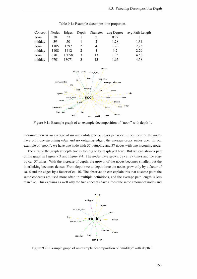
9.3. Selecting Decomposition Depth

Table 9.1.: Example decomposition properties.

Concept Nodes Edges Depth Diameter avg Degree avg Path Lengthnoon 38 37 1 2 0.97 1midday 39 50 1 2 1.28 1.34noon 1105 1392 2 4 1.26 2,25midday 1108 1412 2 4 1.2 2.29noon 6701 13058 3 13 1.95 4.58midday 6701 13071 3 13 1.95 4.58

Figure 9.1.: Example graph of an example decomposition of “noon” with depth 1.

measured here is an average of in- and out-degree of edges per node. Since most of the nodeshave only one incoming edge and no outgoing edges, the average drops under one. In ourexample of “noon”, we have one node with 37 outgoing and 37 nodes with one incoming node.

The size of the graph at depth two is too big to be displayed here. But we can show a partof the graph in Figure 9.3 and Figure 9.4. The nodes have grown by ca. 29 times and the edgeby ca. 37 times. With the increase of depth, the growth of the nodes becomes smaller, but theinterlinking becomes denser. From depth two to depth three the nodes grow only by a factor ofca. 6 and the edges by a factor of ca. 10. The observation can explain this that at some point thesame concepts are used more often in multiple definitions, and the average path length is lessthan five. This explains as well why the two concepts have almost the same amount of nodes and

Figure 9.2.: Example graph of an example decomposition of “midday” with depth 1.

153

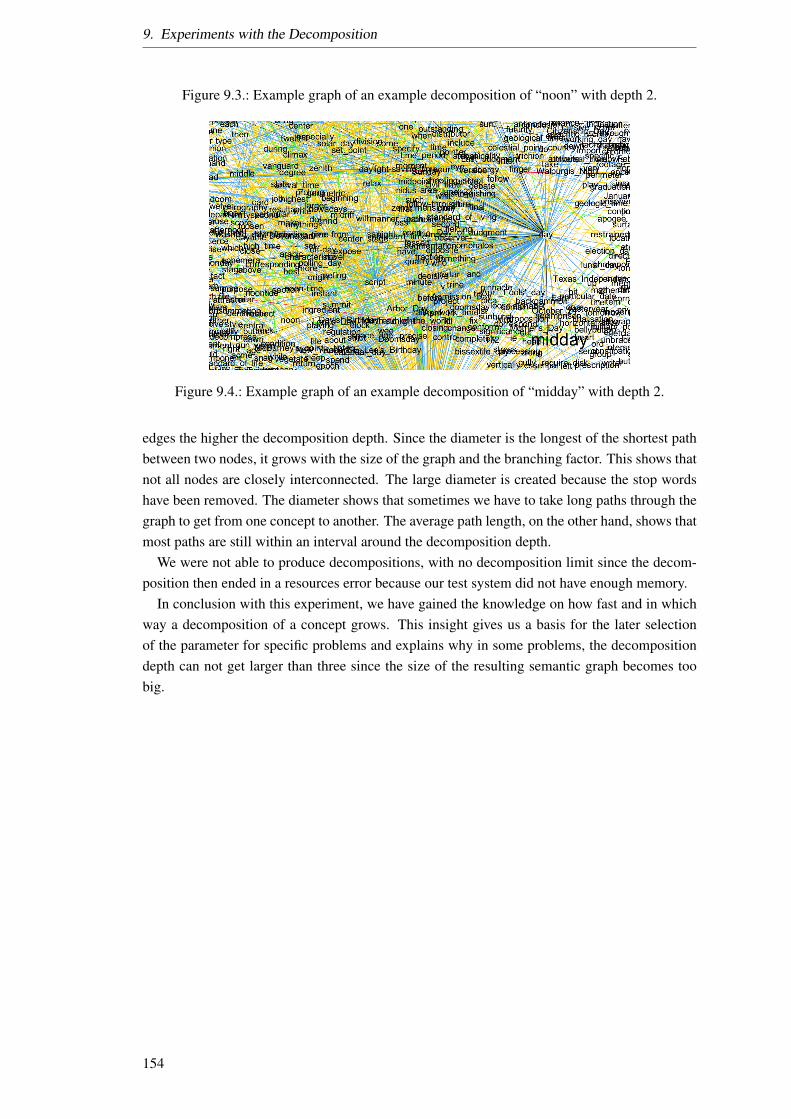
9. Experiments with the Decomposition

Figure 9.3.: Example graph of an example decomposition of “noon” with depth 2.

Figure 9.4.: Example graph of an example decomposition of “midday” with depth 2.

edges the higher the decomposition depth. Since the diameter is the longest of the shortest pathbetween two nodes, it grows with the size of the graph and the branching factor. This shows thatnot all nodes are closely interconnected. The large diameter is created because the stop wordshave been removed. The diameter shows that sometimes we have to take long paths through thegraph to get from one concept to another. The average path length, on the other hand, shows thatmost paths are still within an interval around the decomposition depth.

We were not able to produce decompositions, with no decomposition limit since the decom-position then ended in a resources error because our test system did not have enough memory.

In conclusion with this experiment, we have gained the knowledge on how fast and in whichway a decomposition of a concept grows. This insight gives us a basis for the later selectionof the parameter for specific problems and explains why in some problems, the decompositiondepth can not get larger than three since the size of the resulting semantic graph becomes toobig.

154

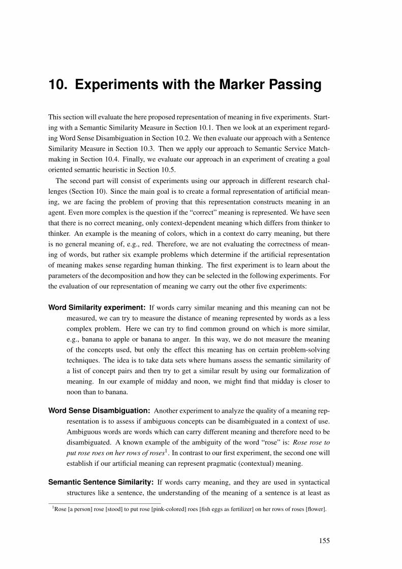
10. Experiments with the Marker Passing

This section will evaluate the here proposed representation of meaning in five experiments. Start-ing with a Semantic Similarity Measure in Section 10.1. Then we look at an experiment regard-ing Word Sense Disambiguation in Section 10.2. We then evaluate our approach with a SentenceSimilarity Measure in Section 10.3. Then we apply our approach to Semantic Service Match-making in Section 10.4. Finally, we evaluate our approach in an experiment of creating a goaloriented semantic heuristic in Section 10.5.

The second part will consist of experiments using our approach in different research chal-lenges (Section 10). Since the main goal is to create a formal representation of artificial mean-ing, we are facing the problem of proving that this representation constructs meaning in anagent. Even more complex is the question if the “correct” meaning is represented. We have seenthat there is no correct meaning, only context-dependent meaning which differs from thinker tothinker. An example is the meaning of colors, which in a context do carry meaning, but thereis no general meaning of, e.g., red. Therefore, we are not evaluating the correctness of mean-ing of words, but rather six example problems which determine if the artificial representationof meaning makes sense regarding human thinking. The first experiment is to learn about theparameters of the decomposition and how they can be selected in the following experiments. Forthe evaluation of our representation of meaning we carry out the other five experiments:

Word Similarity experiment: If words carry similar meaning and this meaning can not bemeasured, we can try to measure the distance of meaning represented by words as a lesscomplex problem. Here we can try to find common ground on which is more similar,e.g., banana to apple or banana to anger. In this way, we do not measure the meaningof the concepts used, but only the effect this meaning has on certain problem-solvingtechniques. The idea is to take data sets where humans assess the semantic similarity ofa list of concept pairs and then try to get a similar result by using our formalization ofmeaning. In our example of midday and noon, we might find that midday is closer tonoon than to banana.

Word Sense Disambiguation: Another experiment to analyze the quality of a meaning rep-resentation is to assess if ambiguous concepts can be disambiguated in a context of use.Ambiguous words are words which can carry different meaning and therefore need to bedisambiguated. A known example of the ambiguity of the word “rose” is: Rose rose toput rose roes on her rows of roses1. In contrast to our first experiment, the second one willestablish if our artificial meaning can represent pragmatic (contextual) meaning.

Semantic Sentence Similarity: If words carry meaning, and they are used in syntacticalstructures like a sentence, the understanding of the meaning of a sentence is at least as

1Rose [a person] rose [stood] to put rose [pink-colored] roes [fish eggs as fertilizer] on her rows of roses [flower].

155

10. Experiments with the Marker Passing

3. Sentence Similarity

1. Similarity

Concept

Context

Concept

Concept

Goal

5. Service Planning use case?

Service Service?

4. Service Matching use case

Service

? ?

2. Disambiguation

Figure 10.1.: Overview of the experiments making up the evaluation of our representation ofmeaning.

hard as the understanding of the meaning of the words making up this sentence. In addi-tion, similar to word similarity the meaning of a sentence is hard to measure, leading us toour experiment of comparing the similarity of sentences. Calculating sentence similarityis a common task in AI research, and standard datasets exist. Our experiment will, there-fore, evaluate our approach on such a data set to see if we can represent the meaning ofsentences as well.

Semantic Service Match Making: The words used to describe the functionality in a serviceconnect humans with machines. In a service description, concepts in ontologies, logicalaxioms and natural language sentences are combined to describe the functionality of aservice. In service descriptions, the position of concepts influences their interpretation,e.g., the same concept in a precondition vs. an effect. Our first use case explores ourapproach applied to service description and its use to find a fitting service given a servicerequest.

Heuristic for service planning: The assessment, if a service is helpful for a given goal in-cludes the understanding of the goal, the descriptions of the services and then a reasoningon how well the described service can “help” to reach the goal. This includes findingsimilar concepts (with a semantic similarity measure) and to select the right word sensefor the concepts describing the services or the goal. Further sentence similarity is used tocompare axioms like ”IsBookedFor(Flight, Perter)” reformulated as sentence ”The flightis booked for Peter.”. Finally, parts of the service matching experiments are used to assessthe services available, e.g., on their preconditions and effects. Consequently, this exper-

156

10.1. Experiment 1: Semantic Similarity Measure

iment is more an application of the results of the first four experiments to a real worldproblem: The general purpose service planning.

The evaluation section is structured as depicted in Figure 10.1. First, we describe the pa-rameters of the decomposition. Second and third, we describe how a similarity measure can becreated and third we describe the experiment of word sense disambiguation. Fourthly, we de-scribe how we extended the word similarity measure to a sentence similarity measure. Finally,we dive into the applications of those results and use the insight gained from those experimentsto improve our service matching and a semantic heuristic for service planning.

In more detail, the evaluation in our five experiments has each time a set of parameters whichneed specification, a data set, and an evaluation goal. Here parameters are selected with our usecases in mind. As the parameters have been discussed in Chapter 6 the evaluation keeps thisstructure, and we will elaborate the best parameters for each part of the approach through anexperiment.

10.1. Experiment 1: Semantic Similarity Measure

In this section, we will build a semantic similarity measure based on our decomposition andMarker Passing algorithm. This has been published in Fahndrich et al. [104]2. A semanticsimilarity measure returns how similar two concepts are regarding their meaning [336]. Partof this task is selecting the best word sense fitting the context first discussed by Waver in 1949in his essay “Translation” in the Cambridge collection “Machine Translation of Languages:Fourteen Essays”. We divide the problem from Waver into two experiments where the first part- a semantic similarity measure - is subject to this section and the second part - selection of wordsenses - is the experiment in Section 10.2.

To use our Marker Passing in this experiment, we need to choose the information modeledon the markers, the node, and edge interpretation to guide its markers and the termination con-dition as well as the final interpretation of the markers. In this experiment, we base the nodeand edge interpretation which models the symbolic influence of certain concepts on the idea ofCharniak [48].

First, we define the signature of the semantic similarity measure we want to create:

SemanticSimilarity : Concept × Concept→ Double

Here the semantic similarity measure is context independent because the input allows onlytwo concepts, therefore, the entire measure is only based on the two concepts for which we wantto calculate the semantic similarity. Next, we describe how we modeled the different parts ofthe Marker Passing algorithm, starting with the information encoded in the marker. With thatwe describe all the parameters specified in Table 10.2.

Figure 10.2 depicts our abstract approach, from the input of two concepts, which are decom-posed using the approach described in Section 6. We call these two concepts for which we wantto calculate a semantic similarity between the string concepts. They are the two concepts givento the algorithm as input parameters. The result is a semantic graph. The only parameter weselected from the decomposition is its depth. This influences the size of the graph, used for theMarker Passing.

2This section is based on the thesis of Konig [203] and Weber [402].

157

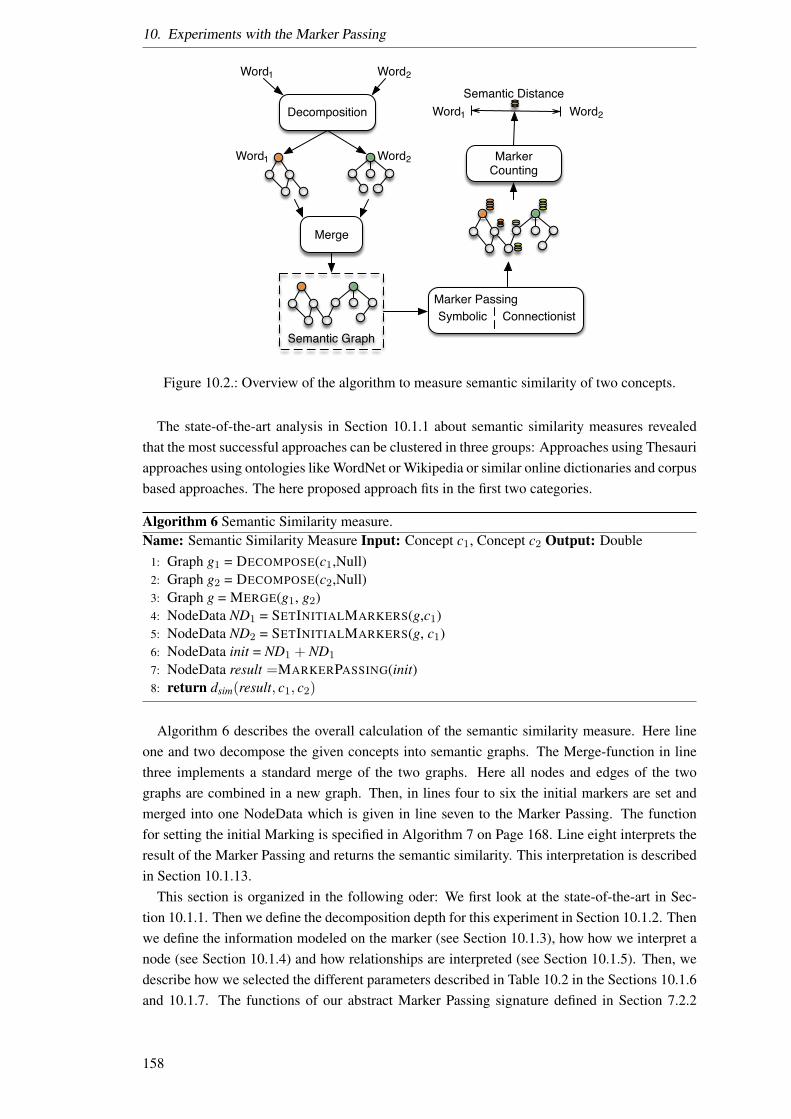
10. Experiments with the Marker Passing

Decomposition

Semantic Graph

Marker PassingSymbolic Connectionist

Merge

Word1 Word2

Word2Word1 Marker Counting

Word1 Word2

Semantic Distance

Figure 10.2.: Overview of the algorithm to measure semantic similarity of two concepts.

The state-of-the-art analysis in Section 10.1.1 about semantic similarity measures revealedthat the most successful approaches can be clustered in three groups: Approaches using Thesauriapproaches using ontologies like WordNet or Wikipedia or similar online dictionaries and corpusbased approaches. The here proposed approach fits in the first two categories.

Algorithm 6 Semantic Similarity measure.Name: Semantic Similarity Measure Input: Concept c1, Concept c2 Output: Double

1: Graph g1 = DECOMPOSE(c1,Null)2: Graph g2 = DECOMPOSE(c2,Null)3: Graph g = MERGE(g1, g2)4: NodeData ND1 = SETINITIALMARKERS(g,c1)5: NodeData ND2 = SETINITIALMARKERS(g, c1)6: NodeData init = ND1 + ND1

7: NodeData result =MARKERPASSING(init)8: return dsim(result, c1, c2)

Algorithm 6 describes the overall calculation of the semantic similarity measure. Here lineone and two decompose the given concepts into semantic graphs. The Merge-function in linethree implements a standard merge of the two graphs. Here all nodes and edges of the twographs are combined in a new graph. Then, in lines four to six the initial markers are set andmerged into one NodeData which is given in line seven to the Marker Passing. The functionfor setting the initial Marking is specified in Algorithm 7 on Page 168. Line eight interprets theresult of the Marker Passing and returns the semantic similarity. This interpretation is describedin Section 10.1.13.

This section is organized in the following oder: We first look at the state-of-the-art in Sec-tion 10.1.1. Then we define the decomposition depth for this experiment in Section 10.1.2. Thenwe define the information modeled on the marker (see Section 10.1.3), how how we interpret anode (see Section 10.1.4) and how relationships are interpreted (see Section 10.1.5). Then, wedescribe how we selected the different parameters described in Table 10.2 in the Sections 10.1.6and 10.1.7. The functions of our abstract Marker Passing signature defined in Section 7.2.2

158

10.1. Experiment 1: Semantic Similarity Measure

will be specialized in Sections 10.1.8 to 10.1.12. Then, we use Marker Passing to identifyrelevant sub-graphs and describe the parameters use to interpret the marker information (Sec-tion 10.1.13). We then look at the test data sets available in Section 10.1.14. How the parametersof the Marker Passing are learned will be described in Section 10.1.15. The whole experiment isused to create a semantic similarity measure that is experimentally evaluated in Section 10.1.16.The results are then critically discussed in Section 10.1.17.

10.1.1. State-of-the-Art

This section will give a literature overview of existing semantic similarity or distance measures.This analysis is done to find the best approaches we can compare our approach against. Thereare many definitions of semantic similarity. In this section, we will choose the once we compareour results against, and we will take a deeper dive into some of their details to gain insight intohow the work. The deeper analysis of the results is done to gain insight into the shortcomingsand benefits of the different approaches, in contrast to a single value correlation value over thewhole data set. This insight is needed later on to create a problem specific Marker Passingalgorithm for a semantic similarity measure.

We do not agree with the simplification done by Ballatore [16] who reduces semantic sim-ilarity measures to hypernym and hyponym relations. This simplification reduces a semanticsimilarity measure to a taxonomic measure, contradicting the ontological principle of identityof indiscernibles which states that as if entities have all properties in common, they are thesame entity. Without taking Meronyms (the part-of relation) into account, a taxonomical simi-larity measure based on “is-a” relations can not identify if two entities are similar with all theirproperties.

There are many surveys on semantic similarity or semantic distance measure like [72] who de-scribes multiple semantic distance measures or [424] who survey on semantic relatedness. Oth-ers describe specific approaches using a certain information source like [130, 420] who describeWordNet based semantic similarity measure. We surveyed all of those approaches, categorizedthem to their basic approach and selected the best performing of each category. These threesimilarity measures are explained in more detail and are selected for the comparison against ourapproach.

Other works describe semantic distance measures like weighted randomized heuristic seman-tic walks over Wikipedia articles [123] or survey such approaches in a specific application likedone in [155]. Work like those have been reviewed but are not further discussed in the sectionbecause their topic is too far of from our approach.

The research literature on word similarity metrics ranges from thesaurus based approaches(cf. [183]) to neuronal networks (cf. [269]). These approaches can be classified based on theused data structure. Most commonly the differentiation is made between knowledge-based andcorpus-based approaches [268]. Zhang et al. [427] use the same classification in their survey,further subdividing the domain of knowledge-based approaches into taxonomies and ontologies.Both work on a graph representation of the domain knowledge but taxonomies are organizedby the generalization-specialization relationship only, while ontologies are taxonomic structuresenriched with other semantic relationships [342]. Taxonomical approaches can be specialized tothe part-of (mereological view) relation as well. Based on this classification, we will look at threestate-of-the-art approaches to understand how they work. The insight we gain by understanding

159

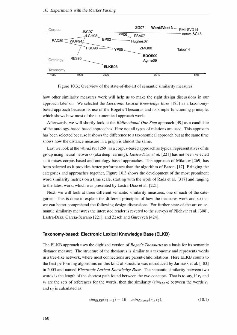
10. Experiments with the Marker Passing

RAD89

RES95

WUP94

HSO98

LCH98BP02

ELKB03

PP06

YP05

ZG07

ESA07

Word2Vec13 PMI-SVD14

Hughes07

ZMG08

BDOS09Agirre09

Taieb14

coswJ&C15Corpus

Ontology

Taxonomytime1980 1990 2000 2010

J&C97

Figure 10.3.: Overview of the state-of-the-art of semantic similarity measures.

how other similarity measures work will help us to make the right design discussions in ourapproach later on. We selected the Electronic Lexical Knowledge Base [183] as a taxonomy-based approach because its use of the Roget’s Thesaurus and its simple functioning principle,which shows how most of the taxonomical approach work.

Afterwards, we will shortly look at the Bidirectional One-Step approach [49] as a candidateof the ontology-based based approaches. Here not all types of relations are used. This approachhas been selected because it shows the difference to a taxonomical approach but at the same timeshows how the distance measure in a graph is almost the same.

Last we look at the Word2Vec [269] as a corpus-based approach as typical representatives of itsgroup using neural networks (aka deep learning). Lastra-Diaz et al. [221] has not been selectedas it mixes corpus-based and ontology-based approaches. The approach of Mikolov [269] hasbeen selected as it provides better performance than the algorithm of Baroni [17]. Bringing thecategories and approaches together, Figure 10.3 shows the development of the most prominentword similarity metrics on a time scale, starting with the work of Rada et al. [317] and rangingto the latest work, which was presented by Lastra-Diaz et al. [221].

Next, we will look at three different semantic similarity measures, one of each of the cate-gories. This is done to explain the different principles of how the measures work and so thatwe can better comprehend the following design discussions. For further state-of-the-art on se-mantic similarity measures the interested reader is revered to the surveys of Pilehvar et al. [308],Lastra-Dıaz, Garcıa-Serrano [221], and Zesch and Gurevych [424].

Taxonomy-based: Electronic Lexical Knowledge Base (ELKB)

The ELKB approach uses the digitized version of Roget’s Thesaurus as a basis for its semanticdistance measure. The structure of the thesaurus is similar to a taxonomy and represents wordsin a tree-like network, where most connections are parent-child relations. Here ELKB counts tothe best performing algorithms on this kind of structure was introduced by Jarmasz et al. [183]in 2003 and named Electronic Lexical Knowledge Base. The semantic similarity between twowords is the length of the shortest path found between the two concepts. That is to say, if r1 andr2 are the sets of references for the words, then the similarity (simELKB) between the words c1

and c2 is calculated as:

simELKB(c1, c2) = 16− mindistance(r1, r2), (10.1)

160

10.1. Experiment 1: Semantic Similarity Measure

Where 16 is the maximum distance in Roget’s Thesaurus and with that defines the maximaldistance of this approach. Here mindistance is the minimal distance from one word r1 to anotherword r2 in the thesaurus, following the network in the Thesaurus. Later, the authors comparedtheir approach to other state-of-the-art approaches like Hirst-St. Onge [168], Jiang-Conrath,Leacock-Chororow [223], Lin [233] and Resnik [324] to show that their approach yields betterresults.

If a word is not contained in the Thesaurus, the approach can not find a semantic similarity forit. This is why Kennedy and Szpakowicz [192] introduce an approach to integrate new wordsinto the Roget’s thesaurus with the help of Wikipedia. This would lead to a broader thesaurusbut does not extend its height.

Ontology-based: Bidirectional One-Step (BDOS)

Another data base used to find semantic similarity between words is WordNet3, a lexical database developed at Princeton University. Similar to Roget’s Thesaurus words in WordNet are con-nected through their relations to each other, creating a graph. Here the relations of concepts aresemantic relations like “synonym” or “antonym” relations. Because of the graph representationof concepts and their relations, most approaches are similar to taxonomy based approaches: Thedistance of the words in the graph is proportional to their semantic similarity. The approachesdiffer in how they use the edges of the graph to calculate the distance between words.

One of these approaches is the Bidirectional One-Step algorithm introduced by Chen etal. [49] in 2009. It uses the hypernym, hyponym and synonym relations and expands up anddown the hierarchy simultaneously. The algorithm starts with two sets each containing one ofthe start words. Then in an iteration, each step adds adjacent nodes to the respective sets. Aftereach iteration, the sets are compared and if an overlap exists the algorithm terminates. The over-all step count is then the distance which defines the semantic similarity. Chen et al. comparetheir results to the results achieved byYang et al..

Corpus-based: Word2Vec

With an ever growing amount of digital information (aka corpora), statistical methods becomemore popular in linguistics. Thereupon a way to obtain knowledge about the human perceptionof semantic similarity refrains from the use of predefined networks but utilizes the vast amountsof language data produced by humans. Corpus-based approaches are based on the assumptionthat two words are similar if they are used in similar contexts [156].

Most of the corpus-based approaches create a vector representation or a bag of words foreach concept which represents those words occurring in similar contexts. This vectors can becompared, to define a similarity among words.

We will look at the approach of Mikolov et al. [269] where a neuronal network is trainedto learn the vector space representation of words occurring in the training set. Here differentneural network architectures are proposed like probabilistic feedforward neural or RecurrentNeural networks. These vectors are trained to learn the co-occurrence probability of the wordsin the corpus. Word similarity is then found by taking a distance measure in the vector spaceembedding the vectors.

3http://wordnet.princeton.edu/wordnet/

161

10. Experiments with the Marker Passing

Such vector approaches work well on tasks where the relatedness of words is well representedin the corpora. One such example set of tasks is the Sentence Completion Challenge [434]which searches for semantic relation by example. The tasks include examples like “France -Paris, where an equivalent relation would be “Berlin - Germany”. Other relations are, e.g. “big- bigger” where “quick - quicker” would be an equivalent. The dataset contains other exampleslike “Japan - Sushi” and “Germany - Bratwurst” where now equivalent relations are searchedwithout naming the relations.

Here Mikolov et al. [269] propose vector arithmetics to find such semantic similarities. Henceto answer the question: What relates to small like big to bigger? They formulate the calculation:

X = vector(bigger)− vector(big) + vector(small) (10.2)

A semantic similarity measure can then be created, by using a norm to measure the distancebetween two vectors. Mikolov et al. use the cosine distance measure between the word vectors.

simcos(c1, c2) =~c1 ~c2

‖~c1‖‖~c2‖(10.3)

The cosine distance measure describes the cosine of the angel between the vectors.Not all semantic distance measures can be categorized in only one of these three categories.

One mixture of used information sources is so-called Information based approaches. Three ofthem are described next.

Information based similarity measures

Resnik [324] proposes that the semantic similarity of two concepts is the overlap or intersectionof the information which is contained in the concept. In this measure, external informationis used to estimate the similarity. In this context the probability p(c) denoting the likelihoodof a concept c occurring in a text. The entropy or information of a concept is defined as thenegative log likelihood of the concept −log(p(c)). The measure of Resnik uses the inheritancehierarchy for example of WordNet to find the first common ancestors denoted in set S(c1, cc).He postulates that the further up this common ancestor is found in the hierarchy the less similartwo concepts are.

simresnik(c1, cc) = maxc∈S(c1,cc)[− log(p(c))] (10.4)

Practically the measure is elaborated by counting the occurrences of a concept in a corpus. Tocalculate this occurrence probability Resnik uses the BrownCorpus of American English. Everytime an occurrence is encountered the counter of this concept, and all hypernym concepts areincremented. The likelihood p(c) then can be calculated as follows: p(c) = count(c)∑

c∈Ccount(c) where

C is the set of all concepts in the corpus. Subsequently if the first common ancestor of to notes

is the root note the similarity is − log(

∑c∈C

count(c)∑c∈C

count(c)) = − log(1) = 0. Since the root note in

WordNet subsumes every word in the corpus. This is interpreted as an similarity of 0 thereforeno similarity at all.

Lin [232] introduces a similarity measure which uses external information as well. Lin definesthe term similarity in an information theoretic sense, meaning that we need a probabilistic modelof the entropy of a concept link with the similarity measure of Resnik [324]. Here the similaritymeasure is defined by using assumptions about similarity, rather the formulas, which “if the

162

10.1. Experiment 1: Semantic Similarity Measure

assumptions seems reasonable the similarity measure necessarily follows” [232]. Lin calls thisa “Theoretical Justification” of a measure. The assumptions of Lin are

related The similarity between concept A and concept B is related to their commonality. Themore commonality they share, the more similar they are.

opposite The similarity between concept A and concept B is related to the differences betweenthem. The more differences they have, the less similar they are.

identity The maximum similarity between concept A and concept B is reached when A and Bare identical, no matter how much commonality they share.

Lin then proposes a similarity measure by:

simlin(c1, cc) =log(p(common(c1, cc)))

log(p(description(c1)) + p(description(cc)))(10.5)

Lin’s theory of similarity is only applicable if the domain is described with a theoretic model.Furthermore, the similarity measure is defined with the notion of “commonality” stating whattwo concepts have in common, ergo needing a similarity measure for those commonalities. Thefunction description(c1) describes the concepts which describe our concept c1.

Ziegler et al. [429] describes an approach in which named entities are included in the tax-onomy used for the calculation of a similarity measure. The measure builds upon the resultsof a query of different taxonomies like the google Directory and a manually created directorycreated out of the ’Open Directory Project’ called DMOZ (http://www.dmoz.org/). A concept isqueried, and the returned results are used to build a profile of the concept. The profile is formal-ized as a vector v which contains the ranked results of the query. Then the ’is-a’ relation of thetaxonomies used are traversed and used for the calculation of a similarity. Here the “symbolic”and “related” relationships are neglected so far. Spreading activation is used to activate relatedconcepts to create a ranking for the profile of a concept. The resulting ranked vector~v is used tocalculate a similarity by using the Pearson’s correlation coefficient in the following way:

d(vx, vy) =

|v|∑k=0

(~vx,k − vx) · (~vy,k − vy)√|v|∑

k=0

(~vx,k − vx)2 ·|v|∑

k=0

(~vy,k − vy)2

(10.6)

Where | vx | is the length of the profile vector and vx is the mean values of the profile vectorof concept x. Using the ranking of search engines like wwww.google.de to calculate similaritiesmakes the similarity measure dependable of this ranking. The foundation of the similarity mea-sure is consequently a black box and can only be empirically evaluated. This leads to a similaritymeasure but not into more insight into how such a measure works.

We have only found one approach which uses activation spreading: Thiel and Berthold [379].They use activation spreading like we described in Section 4.5. They use a double valued acti-vation like in an ANN, to propagate through a semantic graph. This activation is then used tocalculate the cosine similarity in the following way [379, Eq. (8)]:

dact(u, v) = cos(a∗i (v), a∗i (u)) =〈a∗i (v), a∗i (u)〉H

‖ a∗i (v) ‖ L2 ‖ a∗i (u) ‖ L2

(10.7)

163

10. Experiments with the Marker Passing

With (Ω,A, ati(v)) being the separable L2-space over the weights v ∈ W with the created

Hilbert-space (H, 〈., .〉H).Thiel and Berthold [379] then use the l2 norm to represent the amount of change of one acti-

vation step towards the eigen vector and call this “velocity vector norm”. Here the convergencespeed is measured in:

τt(v) =‖ δt(v) ‖ L2 = ∩Ω〈δt(v), δt(v)〉H dati(v) (10.8)

This normalized activation then is used to calculate the cosine similarity or the Jaccard in-dex [181], which then is used in a cosine similarity [379, eq. (9)]:

dsig(u, v) = cos(τt(u), τt(v)) =〈τt(u), τt(v)〉H

‖ τt(u) ‖ ‖ τt(v) ‖ (10.9)

Which allows detecting if the activation of two concepts results in a similar activation ofthe activated nodes. Since Thiel and Berthold [379] use undirected graphs, this similarity issymmetric.

Consequently, two parts of the activation are analyzed: The activation vector of the activatedconcepts are similar (activation similarity), or the change of activation is similar (signature sim-ilarity).

Conclusion

In conclusion, we have analyzed the state-of-the-art of semantic similarity measures, catego-rized them and selected three approaches - one of each category - to learn how they calculate thesimilarity. Those three approaches have been explained in more detail to get insight into theirfunctioning to be able to create our semantic similarity measure similarly. All these approachesare not context-dependent and, in consequence, cannot select a semantic similarity specific to agiven context. Based on this insight, we now can configure our Marker Passing approach startingwith Section 10.1.3.

10.1.2. Decomposition Depth

The decomposition depth has been evaluated in depth one and two. With the insight of Sec-tion 9.3 we are not able to decompose with hight decomposition depth, due to resource restric-tions. Decomposing the RG65 test data set [336] yielding 48 graphs. Those 48 graphs have anelement count like shown in Table 10.1.

Table 10.1.: Node and edge count for different decomposition depth.

Depth Nodes Edges1 6195 67042 1288873 4515376

The growth of node and edge count restricts the decomposition depth to three due to compu-tations resources available. To connect the so created graphs, we merged them into one graphby building the union of the set of nodes and edges.

164

10.1. Experiment 1: Semantic Similarity Measure

10.1.3. Marker information

With the decision to test our approach with a semantic similarity measure, one type of designdecision is to select the data type of a Marker. This means we have to think about which in-formation we want to use at the end of the Marker Passing, to interpret the result as a semanticsimilarity measure. We select the symbolic information carried by the marker as two fold: First,we modeled a token activation level as a double value. Second, we defined a token origin whichcontains the concepts, from which the token has first started. The datatype of the marker Markerthen is defined as tuple (Activation:Double, Origin:Concept)

These markers have been chosen because most of the state-of-the-art approaches use somedistance of two concepts in an ontology or a thesaurus. Modeling activation, which can decayfor every concept it passes, allows us to determine a sense of path length the marker has traveled.This is not to be confused with a simple step count done in other approaches like [129, 183, 374,423]. This is because, the markers can be changed with the in-, out- and edge-function. Thismeans the path length can be modeled as one of the information of the activation, but that’s notall: The importance of the edge, the abstraction level, the degree of connectedness, and a numberof nodes all can play their part in a number of markers passed from one node to another.

The second part of symbolic information “the origin” lets us track which marker has startedfrom which initial concept. This lets us see which markers of the two starting concepts meetwhere and how many markers of which origin have passed over a specific concept. Furthermore,the origin of the maker gives us the information which concept this marker has started from. Thisgives us the possibility to activate multiple different concepts and finding out if their markersmeet somewhere in the graph. With that, we can analyze how fast they meet or if some specificconcept gets in contact with a marker of a specific origin.

Enabling the analysis of which markers have passed over which node, we have to model thenode- and edge-interpretation with an implementation of the NodeData signature. The algebraimplementing NodeData is defined in the Algebra NodeData.

Here the symbol | denotes the list concatenation operation. The symbol ∅ denotes an emptylist. Additionally, we did shortcut extending the NodeData signature by introducing new opera-tion signatures directly in the algebra.

The Data describes the symbolic information modeled on a concept. Consequently, it is partof the node-interpretation. In addition, we model a history, which keeps all markers ever passedto the concept as a copy of the marker passed.

An object of type Markers is a function that for each origin specifies the activation of allmarkers for this origin. This encapsulates what we have called “Markers” is a function whichallows a simpler description of the formalization of the algorithm below. Never the less, this ismerely a shortcut to modeling the information on a marker data type. The Markers function canbe applied to the current markers or the history. This is a convenience method which allows usto access the activation sorted by origin without having to iterate over all markers and origins.

The function getMarkers, setMarkers, getHistory and setHistory are the convenience func-tions to set the Data” of a node. Here for each function, we can get or set a Markers data typewhich includes the appropriate markers. For the current marking of a concept, this includes allmarkers currently marking this concept.

165

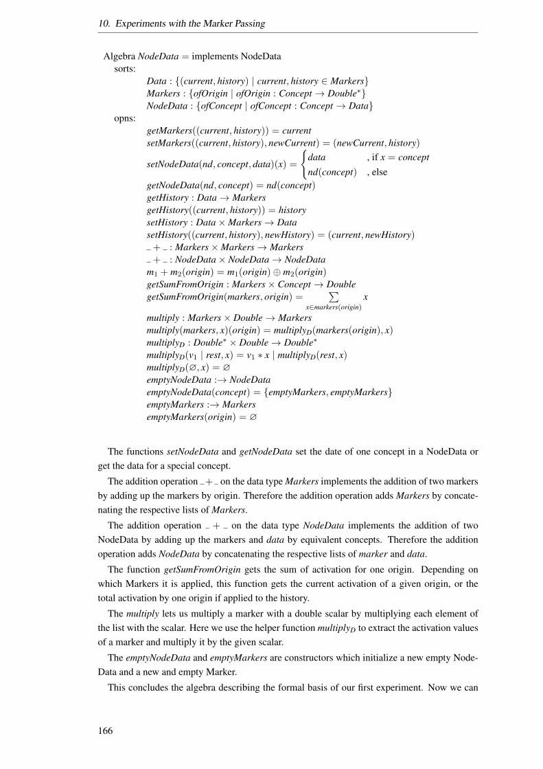
10. Experiments with the Marker Passing

Algebra NodeData = implements NodeDatasorts:

Data : (current, history) | current, history ∈ MarkersMarkers : ofOrigin | ofOrigin : Concept→ Double∗NodeData : ofConcept | ofConcept : Concept→ Data

opns:getMarkers((current, history)) = currentsetMarkers((current, history), newCurrent) = (newCurrent, history)

setNodeData(nd, concept, data)(x) =

data , if x = conceptnd(concept) , else

getNodeData(nd, concept) = nd(concept)getHistory : Data→ MarkersgetHistory((current, history)) = historysetHistory : Data×Markers→ DatasetHistory((current, history), newHistory) = (current, newHistory)

+ : Markers×Markers→ Markers+ : NodeData× NodeData→ NodeData

m1 + m2(origin) = m1(origin)⊕ m2(origin)getSumFromOrigin : Markers× Concept→ DoublegetSumFromOrigin(markers, origin) =

∑x∈markers(origin)

x

multiply : Markers× Double→ Markersmultiply(markers, x)(origin) = multiplyD(markers(origin), x)multiplyD : Double∗ × Double→ Double∗

multiplyD(v1 | rest, x) = v1 ∗ x | multiplyD(rest, x)multiplyD(∅, x) = ∅emptyNodeData :→ NodeDataemptyNodeData(concept) = emptyMarkers, emptyMarkersemptyMarkers :→ MarkersemptyMarkers(origin) = ∅

The functions setNodeData and getNodeData set the date of one concept in a NodeData orget the data for a special concept.

The addition operation + on the data type Markers implements the addition of two markersby adding up the markers by origin. Therefore the addition operation adds Markers by concate-nating the respective lists of Markers.

The addition operation + on the data type NodeData implements the addition of twoNodeData by adding up the markers and data by equivalent concepts. Therefore the additionoperation adds NodeData by concatenating the respective lists of marker and data.

The function getSumFromOrigin gets the sum of activation for one origin. Depending onwhich Markers it is applied, this function gets the current activation of a given origin, or thetotal activation by one origin if applied to the history.

The multiply lets us multiply a marker with a double scalar by multiplying each element ofthe list with the scalar. Here we use the helper function multiplyD to extract the activation valuesof a marker and multiply it by the given scalar.

The emptyNodeData and emptyMarkers are constructors which initialize a new empty Node-Data and a new and empty Marker.

This concludes the algebra describing the formal basis of our first experiment. Now we can

166

10.1. Experiment 1: Semantic Similarity Measure

describe the needed function of the Marker Passing algorithm formally.

10.1.4. Relationship Interpretation Function

The relationship- or edge-interpretation influences how markers are passed from one node toanother. This influence is formalized with the weights shown in Table 10.2 on Page 172. Thoseweights are not chosen but learned in the experiment. This is done because it is difficult topredict the influence of the weights to the performance of the similarity measure. Therefore wecan not describe the concrete values of the weights here. They will be selected by a learningmechanism in Section 10.1.16.

For the experiment of building a semantic similarity measure, the following relationshipsweights have been modeled:

Definition edge weight describes how markers are passed over definition relationships. Eachconcept in a definition of a concept has a relation to the definiendum. For this reason, alldefining concepts are activated independently of which definition they belong to.

Synonym edge weight describe how relevant synonyms are to measure semantic similarity.Because of the transitivity of the synonym relation, there is the possibility of the twoconcepts we measure the semantic similarity for are connected by a synonym relationchain. Since synonyms are mostly not complete synonyms, but rather are only replaceablein some word meanings and context, the meaning might change with each synonym step.For more details see Section 3.9. This difference in meaning should be reflected throughthose synonym weights.

Antonym edges weights are similar to synonym edge weights since the antonym relation-ship is negatively proportional to the synonym relations. It is transitive as well, and it ischanging the meaning of an antonym depending on context since there are rarely any trueantonyms. See Section 3.9.

Hypernym edges weight reflect how the abstraction is used in the similarity measure. Inmost ontologies, there is one root concept, which if two concepts are not related at all, aconnection can be found over this root node. In particular, if markers pass over to abstractconcepts, the weight should reflect this abstraction.

Hyponym edges weight are similar to hypernym weights. Except that they are the oppositerelation. This means they are reflecting the specialization in a semantic graph.

All weights are of type double and are multiplied with the activation level of each markerpassed by them. We do not differentiate the origin of the markers. How the actual weights areselected, we will discover in Section 10.1.16.

10.1.5. Node Interpretation Function

The node interpretation influences how markers are handled by the nodes. Given a problem wehave to decide which node types are relevant for this problem. In this experiment we have twotypes of node interpretations:

167

10. Experiments with the Marker Passing

Concept nodes represent a concept and hold the markers passed to it. The threshold of aconcept node is reached if one of the marker origin reaches the numeric activation thresh-old τ . Furthermore, the markers passed to concept nodes are added to the activation valueof the last pulse. The markers are sorted after their origin. All the functions implementedhere in the following sections will be implemented for concept nodes.

Prime nodes represent semantic primes from the NSM, which act as leave nodes and collectmarkers without passing them. They collect markers of the different origins, and like aconcept, node sort them by origin and add new markers to the old once. This is reflectedin Algorithm 9 where the concepts are only checked for a threshold if they do not belongto the set of NSM primes.

As a result, the concept markers can tell us from which origin they have been activated andhow much activation in summation they carried. There is no information about time (in whichpulse the markers arrived) nor about over which edge(s) the markers arrived. Since there are onlynouns in the RG65 data set, we did not include Part-of-Speech nodes in our node interpretation.The edge types are used in the edge function, where each edge type has an own weight determin-ing how markers are passed over it. How many markers are passed over the edge also dependson the amount of markers which are placed on the node. Starting with the initial marking givento the Marker Passing algorithm as start markers.

10.1.6. Start Marker

Because the semantic Decomposition produces an unmarked graph, we need to define initialmarkers. For the calculation of a semantic similarity measure, our algorithm has two start mark-ers. The parameter called start activation defines how much activation is placed on those twomarkers. The origin of the initial markers is set to the concept they are placed on.

Algorithm 7 Setting initial Markers.Name: InitialMarkingInput: Concept c1

Output: NodeData1: function SETINITIALMARKERS(g,c1)2: ND = emptyNodeData

3: m1 = λ(x).

startActivation , if x = c1 ∧ x ∈ g∅ , else

4: ND = setMarking (ND, c1,m1)5: ND = setHistory (ND, c1,m1)6: return ND7: end function

Algorithm 7 creates the initial markers and places them on the given concept which is to beanalyzed via our semantic similarity measure. Here the parameter startActivation is the amountof initial activation of these concepts. This parameter is one which is subject to our analysis andtherefore can vary during our experiment. The value of the variable startActivation is selectedby the learning mechanism discussed later in Section 10.1.16.

168

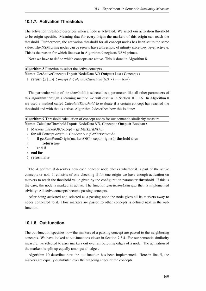
10.1. Experiment 1: Semantic Similarity Measure

10.1.7. Activation Thresholds

The activation threshold describes when a node is activated. We select our activation thresholdto be origin specific. Meaning that for every origin the markers of this origin can reach thethreshold. Furthermore, the activation threshold for all concept nodes has been set to the samevalue. The NSM prime nodes can be seen to have a threshold of infinity since they never activate.This is the reason for which line two in Algorithm 9 neglects NSM primes.

Next we have to define which concepts are active. This is done in Algorithm 8.

Algorithm 8 Function to select the active concepts.Name: GetActiveConcepts Input: NodeData ND Output: List<Concepts>

1: return x | x ∈ Concept ∧ CalculateThreshold(ND, x) == true

The particular value of the threshold is selected as a parameter, like all other parameters ofthis algorithm through a learning method we will discuss in Section 10.1.16. In Algorithm 8we used a method called CalculateThreshold to evaluate if a certain concept has reached thethreshold and with that is active. Algorithm 9 describes how this is done:

Algorithm 9 Threshold calculation of concept nodes for our semantic similarity measure.Name: CalculateThreshold Input: NodeData ND, Concept c Output: Boolean t

1: Markers markerOfConcept = getMarkers(ND,c)2: for all Concept origin ∈ Concept ∧ c 6∈ NSMPrimes do3: if getSumFromOrigin(markersOfConcept, origin) ≥ theshold then4: return true5: end if6: end for7: return false

The Algorithm 9 describes how each concept node checks whether it is part of the activeconcepts or not. It consists of one checking if for one origin we have enough activation onmarkers to reach the threshold value given by the configuration parameter threshold. If this isthe case, the node is marked as active. The function getPassingConcepts then is implementedtrivially: All active concepts become passing concepts.

After being activated and selected as a passing node the node gives all its markers away tonodes connected to it. How markers are passed to other concepts is defined next in the out-function.

10.1.8. Out-function

The out-function specifies how the markers of a passing concept are passed to the neighboringconcepts. We have looked at out-functions closer in Section 7.3.4. For our semantic similaritymeasure, we selected to pass markers out over all outgoing edges of a node. The activation ofthe markers is split up equally amongst all edges.

Algorithm 10 describes how the out-function has been implemented. Here in line 5, themarkers are equally distributed over the outgoing edges of the concepts.

169

10. Experiments with the Marker Passing

Algorithm 10 Out-Function of concept nodes.Name: Out-FunctionInput: NodeData ND, Concept cOutput: List<Relation × Edge ×Markers>

1: List<Relation × Edge ×Markers> result2: Set<Edge> edges = e | c ∈ targets(e)3: for all Edge e ∈ edges do4: Relation r = source(e)5: Markers mnew = multiply(getMarkers(ND,c), 1

|edges| )6: result.add(r,e,mnew)7: end for8: return result

10.1.9. Edge-Function

The edge function determines how markers are passed from one concept to another. For thesemantic similarity measure, we have modeled a list of relation types described in Table 10.2.Those relations are weighted with a double value which is a parameter of this experiment. Eachmarker passed over a relation has its activation value multiplied by the relations weight. Thedifferent weights are part of the algorithm parameters like specified in Table 10.2. Algorithm 11describes how to calculate the edge function in our case for a semantic similarity measure.

Algorithm 11 Edge-Function.Name: EdgeFunctionInput: Marking ND, Relation r, List<Edge ×Markers> passedMarkersOutput: Map<Concept, List<Edge, Markers>>

1: Map<Concept, List<Edge × Markers>> result = new Map<Concept, List<Edge ×Markers>> ()

2: for all (e,m) ∈ passedMarkers do3: Markers mnew = multiply(m, getWeightOfRelation(r))4: for all Concept target ∈ c ∈ Concept | ∃ e2 ∈ Edge : e2 6= e ∧ source(e2) =

r ∧ target(e2) = c do5: result.get(target).add(e × mnew)6: end for7: end for8: return result

The getWeightOfRelation function is specified in Algorithm 12. Here the appropriate weightfor the given relation is selected. In line 4 of Algorithm 11 this weight is multiplied withthe markers passed over this relation. The weights are limited to be chosen from the interval−1, 1.

10.1.10. In-function

The in-function of a node collects the markers in the Marker Passing step, for which the currentnode is the target of. With the node interpretation of the concept nodes and the prime nodesincoming markers of all edges are sorted regarding their origin, and their activation is summedup in regards to the origin and added to the previous activation of this origin.

In Algorithm 13 the calculation of the in-function is defined in a recursive manner. Here the

170

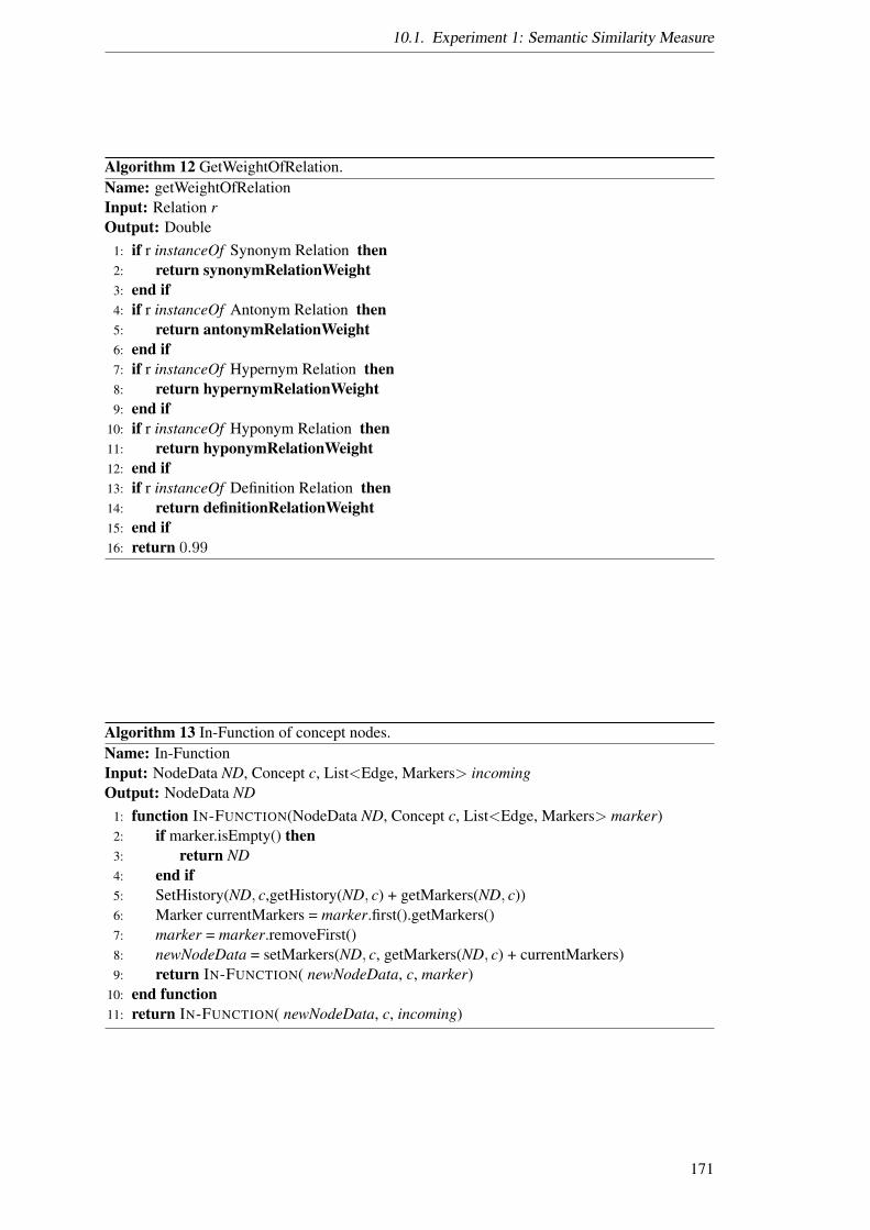
10.1. Experiment 1: Semantic Similarity Measure

Algorithm 12 GetWeightOfRelation.Name: getWeightOfRelationInput: Relation rOutput: Double

1: if r instanceOf Synonym Relation then2: return synonymRelationWeight3: end if4: if r instanceOf Antonym Relation then5: return antonymRelationWeight6: end if7: if r instanceOf Hypernym Relation then8: return hypernymRelationWeight9: end if

10: if r instanceOf Hyponym Relation then11: return hyponymRelationWeight12: end if13: if r instanceOf Definition Relation then14: return definitionRelationWeight15: end if16: return 0.99

Algorithm 13 In-Function of concept nodes.Name: In-FunctionInput: NodeData ND, Concept c, List<Edge, Markers> incomingOutput: NodeData ND

1: function IN-FUNCTION(NodeData ND, Concept c, List<Edge, Markers> marker)2: if marker.isEmpty() then3: return ND4: end if5: SetHistory(ND, c,getHistory(ND, c) + getMarkers(ND, c))6: Marker currentMarkers = marker.first().getMarkers()7: marker = marker.removeFirst()8: newNodeData = setMarkers(ND, c, getMarkers(ND, c) + currentMarkers)9: return IN-FUNCTION( newNodeData, c, marker)

10: end function11: return IN-FUNCTION( newNodeData, c, incoming)

171

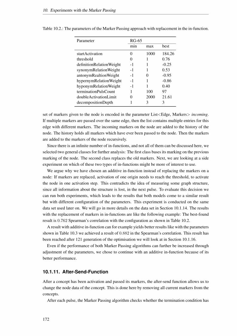
10. Experiments with the Marker Passing

Table 10.2.: The parameters of the Marker Passing approach with replacement in the in-function.

Parameter RG-65min max best

startActivation 0 1000 184.26threshold 0 1 0.76definitionRelationWeight -1 1 -0.25synonymRelationWeight -1 1 0.53antonymRealtionWeight -1 0 -0.95hypernymRelationWeight -1 1 -0.86hyponymRelationWeight -1 1 0.40terminationPulsCount 1 100 97doubleActivationLimit 0 2000 21.61decompositionDepth 1 3 3

set of markers given to the node is encoded in the parameter List<Edge, Markers> incoming.If multiple markers are passed over the same edge, then the list contains multiple entries for thisedge with different markers. The incoming markers on the node are added to the history of thenode. The history holds all markers which have ever been passed to the node. Then the markersare added to the markers of the node recursively.

Since there is an infinite number of in-functions, and not all of them can be discussed here, weselected two general classes for further analysis: The first class bases its marking on the previousmarking of the node. The second class replaces the old markers. Next, we are looking at a sideexperiment on which of these two types of in-functions might be more of interest to use.

We argue why we have chosen an additive in-function instead of replacing the markers on anode: If markers are replaced, activation of one origin needs to reach the threshold, to activatethe node in one activation step. This contradicts the idea of measuring some graph structure,since all information about the structure is lost, in the next pulse. To evaluate this decision wecan run both experiments, which leads to the results that both models come to a similar resultbut with different configuration of the parameters. This experiment is conducted on the samedata set used later on. We will go in more details on the data set in Section 10.1.14. The resultswith the replacement of markers in in-functions are like the following example: The best-foundresult is 0.762 Spearman’s correlation with the configuration as shown in Table 10.2.

A result with additive in-function can for example yields better results like with the parametersshown in Table 10.3 we achieved a result of 0.882 in the Spearman’s correlation. This result hasbeen reached after 121 generation of the optimisation we will look at in Section 10.1.16.

Even if the performance of both Marker Passing algorithms can further be increased throughadjustment of the parameters, we chose to continue with an additive in-function because of itsbetter performance.

10.1.11. After-Send-Function

After a concept has been activation and passed its markers, the after-send function allows us tochange the node data of the concept. This is done here by removing all current markers from theconcepts.

After each pulse, the Marker Passing algorithm checks whether the termination condition has

172

10.1. Experiment 1: Semantic Similarity Measure

Algorithm 14 After-Send-Function of concept nodes.Name: AfterSend-FunctionInput: NodeData ND, Concept c Output: NodeData

1: SetMarkers(ND, c,∅)2: return ND

been reached. We look at how this is done for the semantic similarity measure, next.

10.1.12. Termination Condition

The termination condition of our algorithm is two fold: First, there is a limit to the pulse count.We introduce a global variable which is call currentPulse which counts the pulses is increasedwith each executed pulse. This restricts how many pulses can be created, before the algorithmterminates4. A pulse count limit allows us to stop the algorithm from passing markers from oneconcept to another even thou there could be active concepts. This limit is given by the parameterterminationPulsCount. We can imagine a graph of decomposition depth of one, where thereare still connections between the two decomposed concepts. In such a graph the markers arepassed from one side to the other and back. To eliminate such a back and forth the second partof the termination prevents such behavior.

Second, there is a double activation limit. Here we look at the total amount of concepts,which have activation of multiple origins. Since we are putting start markers only on two con-cepts, we named this condition “double activation limit”. This part of the termination conditionhelps the algorithm to track how much the two subgraphs have to be activated by the oppo-site concept before the algorithm terminates. Depending on the choice of the relations weights,the overall activations of the graph can increase, degrees or rest the same. Since we chose ourweights from wi ∈ −1, 1, this means the activation decreases if not all weights are 1.0. Fur-ther, the markers which are adapted through the Out-, Edge-, and In-function are removed bythe after sent, which makes the overall marker activation on increasing. If this parameter is setto a number near zero, the Marker Passing will terminate with the first contact of markers of thetwo origins. If the parameter is selected to be close to the activation of the start markers, almostall markers have to be passed to double activated nodes before termination. The terminationcondition is implemented as shown in Algorithm 15.

Here the currentPulse counts the Marker Passing pulses of the Marker Passing algorithm. Forsimplicity, the counting and initialization of the counting variable are neglected in Algorithm 15.If the double activation limit is set higher than the amount of activation in the start marker, thefirst termination condition terminates the algorithm. This lets the algorithm terminate even ifmultiple origins have activated no concept.

10.1.13. Interpretation

The interpretation is how we use the result of the Marker Passing to determine a distance betweenthe two concepts. For our semantic distance measure, we want to collect all those nodes whichhave been activated by multiple origins. Since we have only two origins, this means we want toget all activation of the nodes, ever passed to the node, if the node has been activated by both

4This should happen before the markers are equally distributed over all nodes [26]

173

10. Experiments with the Marker Passing

Algorithm 15 The termination condition for the semantic similarity measure.Name: TerminationConditionInput: NodeData NDOutput: Boolean result

1: if currentPulse ≥ terminationPulsCount then2: return true3: end if4: Double doubleActivationSum = 05: for all Concept c ∈ Concepts do6: Double activation = 07: Integer numberOfOrigins = 08: for all Concept origin ∈ Concepts do9: if getMarkers(ND,c)(origin) 6= ∅ then

10: activation += getSumFromOrigin(getMarkers(ND,c), origin)11: numberOfOrigins++12: end if13: end for14: if numberOfOrigins ≥ 2 then15: doubleActivationSum += activation16: end if17: end for18: return doubleActivation ≥ doubleActivationLimit

starting concepts. In consequence, we want to calculate the following overall activation of anode given NodeData ND:

a∗(v) =∑∀ o∈V

getSumFromOrigin(getHistory(ND, v), o) (10.10)

where a∗t (v) represents the sum of activation of node v ever passed to it.

This activation can then be used to calculate the semantic similarity between concept o1 ando2 given the NodeDate ND in the following way:

dsim(ND, o1, o2) =

∑c∈V

Φ(ND, (o1, o2, c))

2 ∗ startActivation(10.11)

where,

Φ(ND, (o1, o2, c)) =a∗(c) , if getHistory(ND, c)(o1) 6= ∅ ∧ getHistory(ND, c)(o2) 6= ∅

0 , else(10.12)

Φ(ND, (o1, o2, x)) filters out of all nodes which have not been activated by at least two of thestart activations. This leaves us with the set of nodes having markers of both origins in theirhistory set. In this way, if we activate two concepts (in our example “noon” and “midday”) atthe beginning, this set contains all nodes which have been activated by markers of both concepts.This is normalized by the amount of start activation to obtain the semantic distance. In sometheoretical cases, this value could become bigger than 1 or negative. This could, e.g., be the

174

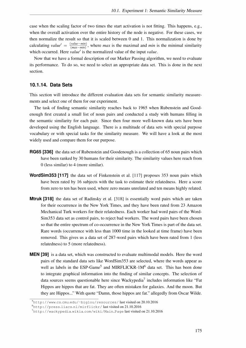
10.1. Experiment 1: Semantic Similarity Measure

case when the scaling factor of two times the start activation is not fitting. This happens, e.g.,when the overall activation over the entire history of the node is negative. For these cases, wethen normalize the result so that it is scaled between 0 and 1. This normalization is done bycalculating value′ = (value−min)

(max−min) , where max is the maximal and min is the minimal similaritywhich occurred. Here value′ is the normalized value of the input value.

Now that we have a formal description of our Marker Passing algorithm, we need to evaluateits performance. To do so, we need to select an appropriate data set. This is done in the nextsection.

10.1.14. Data Sets

This section will introduce the different evaluation data sets for semantic similarity measure-ments and select one of them for our experiment.

The task of finding semantic similarity reaches back to 1965 when Rubenstein and Good-enough first created a small list of noun pairs and conducted a study with humans filling inthe semantic similarity for each pair. Since then four more well-known data sets have beendeveloped using the English language. There is a multitude of data sets with special purposevocabulary or with special tasks for the similarity measure. We will have a look at the mostwidely used and compare them for our purpose.

RG65 [336] the data set of Rubenstein and Goodenough is a collection of 65 noun pairs whichhave been ranked by 30 humans for their similarity. The similarity values here reach from0 (less similar) to 4 (more similar).

WordSim353 [117] the data set of Finkenstein et al. [117] proposes 353 noun pairs whichhave been rated by 16 subjects with the task to estimate their relatedness. Here a scorefrom zero to ten has been used, where zero means unrelated and ten means highly related.

Mtruk [318] the data set of Radinsky et al. [318] is essentially word pairs which are takenfor their occurrence in the New York Times, and they have been rated from 23 AmazonMechanical Turk workers for their relatedness. Each worker had word pairs of the Word-Sim353 data set as control pairs, to reject bad workers. The word pairs have been chosenso that the entire spectrum of co-occurrence in the New York Times is part of the data set.Rare words (occurrence with less than 1000 time in the looked at time frame) have beenremoved. This gives us a data set of 287-word pairs which have been rated from 1 (lessrelatedness) to 5 (more relatedness).

MEN [39] is a data set, which was constructed to evaluate multimodal models. Here the wordpairs of the standard data sets like WordSim353 are selected, where the words appear aswell as labels in the ESP-Game5 and MIRFLICKR-1M6 data set. This has been doneto integrate graphical information into the finding of similar concepts. The selection ofdata sources seems questionable here since Wackypedia7 includes information like “FatHippos are hippos that are fat. They are often mistaken for galaxies. And the moon. Butthey are Hippos...” With quote “Damn, those hippos are fat.” allegedly from Oscar Wilde.

5http://www.cs.cmu.edu/˜biglou/resources/ last visited on 20.10.20166http://press.liacs.nl/mirflickr/ last visited on 21.10.20167http://wackypedia.wikia.com/wiki/Main Page last visited on 21.10.2016

175

10. Experiments with the Marker Passing

This might be a good linguistic resource for contemporary humor and modern slang, butfor embedding words in a distributed meaning, this seems not fitting.

Stanford Rare Word Similarity Dataset [244] Luong et al. [244] composed a data set ofrare words, where words with low frequencies but still having at least one synset in Word-Net [270]. Consequently, these are words, which are rare but are no proper names orsomething similar. The word pairs are constructing by selecting words of WordNet with astep size of at least one and maximally two apart from the first word. In this way for eachrare word, two pairs are created adding up to 3145-word pairs. Luong et al. [244] usedAmazon’s Mechanical Turk to get a rating of ten humans for each word pair. As a resultof quality measures, this leaves us with 2034 ranked word pairs.

We have selected the RG65 [336] the data set of Rubenstein and Goodenough to compare ourapproach with the state-of-the-art since all other data sets are special purpose datasets, which aremostly used by the authors of the data set but not many other approaches. Therefore, the onlyway of comparing our result to the best available semantic similarity measures was to use theRG65 [336] data set without having to reimplement all other approaches.

The use of the RG65 [336] data set seems insufficient since only nouns are compared. Morecomplex datasets exist, which could be used in the future for comparison. Using part-of-speechindependent data sets will worsen thesauri approaches like ELKB since mostly nouns are for-malized in thesauri. For future work, creating more complex data sets with different POS anddifferent similarity types would be a benefit for the community. But this would mean that ex-isting approach should be reevaluated for the new data set, which sometimes is not possiblebecause they are not accessible.

10.1.15. Parameter learning

In this section, we will look at how the parameters of our approach are learned. For the eval-uation result, we learned the set of parameters with a genetic algorithm. Here the parametersare interpreted as the DNA of our individuals. Then we use N-Fold-Cross-Validation to separatethe data set into training and test data. Each individual is evaluated regarding its performanceon the data set via its Spearman’s correlation. The best individual is kept alive and mutated togenerate newer generations. The mutation is done by modifying its DNA within the limits ofour configuration shown, e.g., in Table 10.3. Here each parameter has a mutation probability of0.5. The population size was held at ten, and if no increase in performers has been measuredwithin 1000 generations, the DNA was reset to random values.

The parameters selected in Table 10.3 depend on the design decisions which we have looked atin the last few sections. Because of the vast amount of possible combinations of the parametersthe search space is too big to search. Because of the size and its only partially predictablelandscape, many combinations of parameters can yield the same or better results, and we cannot claim that our parameters produce the optimal result.

Since the parameters are learned, we can only interpret why they work well. Some of theparameter selected depend on others like the double activation limit on the start activation. Someof the parameters may be randomly chosen and might have done almost none effect on the result.E.g. Since the double activation limit in the best parameter set we learn in Table 10.3 is almost

176

10.1. Experiment 1: Semantic Similarity Measure

Table 10.3.: Parameters of the Marker Passing approach used for the task of semantic similaritymeasurement.

Parameter RG-65min max best

startActivation 0 1000 33.81threshold 0 1 0.21definitionRelationWeight -1 1 -0.78synonymRelationWeight -1 1 -0.62antonymRelationWeight -1 0 -0.90hypernymRelationWeight -1 1 0.02hyponymRelationWeight -1 1 0.79terminationPulseCount 1 100 80doubleActivationLimit 0 2000 1999.99decompositionDepth 1 3 3

2000, but the start activation is only ca. 34, and additionally half of the edge weights are negative,and all of them are less than one, it is unlikely that the double activation limit was ever triggered.

Some of the parameters are unintuitive. That a synonym weight is negative seems far fromwhat humans do if they assess similarity. But since the antonym weight is more negative thannegative synonym and definition relations can be explained by them make similar concepts stillmore similar than an antonym relations, having the effect that the semantic distance measurestill works.

Also curious in this parameter configuration is that hyponyms seem to play a more impor-tant role than hypernyms. This could be interpreted, that example of abstract classes help theassessment of similarity more.

10.1.16. Evaluation Results

This section describes the evaluation results and compares it with the state-of-the-art. The exper-iment has been implemented in Java using the WordNet 3.1 and the MIT Java Wordnet Interface(JWI)8. For the Wiktionary implementation the Java-based Wiktionary Library (JWKTL)9 hasbeen used with a Wiktionary dump10. With the above-introduced parameter selection, we wereable to reach the results shown in Table 10.4. The other results are taken from [308, p. 116,Table 9] and from [221, p. 148, Table 4] and present the state-of-the-art in this experiment. Wesort the approaches in Table 10.4 by their Spearman’s correlation because they are given by allapproaches in the related work.

The Spearman’s ranked correlation coefficient ρ is an overall ranking measure. Together withthe Pearson’s r Table 10.4 shows the performance of the state-of-the-art semantic similaritymeasures in comparison to each other. The Pearson’s and Spearman’s correlation are used toseeing how well the approach correlates with the human evaluation of semantic similarity andthe Spearman’s correlation how well the algorithm can bring the pairs of similarity in the rightorder. The Spearman’s correlation is more abstract because the actual value of the semantic

8http://projects.csail.mit.edu/jwi/ last visited on 09.09.20179https://www.ukp.tu-darmstadt.de/software/jwktl/ last visited on 09.09.2017

10https://dumps.wikimedia.org/ downloaded on 2015.12.19

177

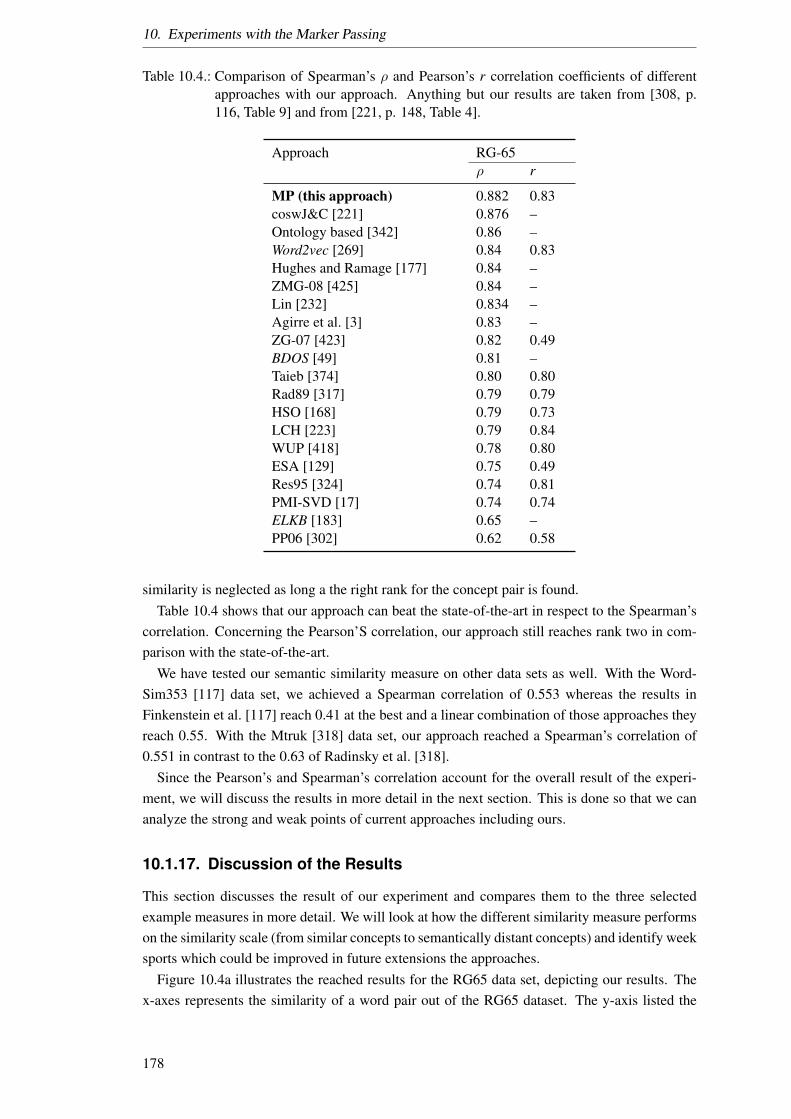
10. Experiments with the Marker Passing

Table 10.4.: Comparison of Spearman’s ρ and Pearson’s r correlation coefficients of differentapproaches with our approach. Anything but our results are taken from [308, p.116, Table 9] and from [221, p. 148, Table 4].

Approach RG-65ρ r

MP (this approach) 0.882 0.83coswJ&C [221] 0.876 –Ontology based [342] 0.86 –Word2vec [269] 0.84 0.83Hughes and Ramage [177] 0.84 –ZMG-08 [425] 0.84 –Lin [232] 0.834 –Agirre et al. [3] 0.83 –ZG-07 [423] 0.82 0.49BDOS [49] 0.81 –Taieb [374] 0.80 0.80Rad89 [317] 0.79 0.79HSO [168] 0.79 0.73LCH [223] 0.79 0.84WUP [418] 0.78 0.80ESA [129] 0.75 0.49Res95 [324] 0.74 0.81PMI-SVD [17] 0.74 0.74ELKB [183] 0.65 –PP06 [302] 0.62 0.58

similarity is neglected as long a the right rank for the concept pair is found.Table 10.4 shows that our approach can beat the state-of-the-art in respect to the Spearman’s

correlation. Concerning the Pearson’S correlation, our approach still reaches rank two in com-parison with the state-of-the-art.

We have tested our semantic similarity measure on other data sets as well. With the Word-Sim353 [117] data set, we achieved a Spearman correlation of 0.553 whereas the results inFinkenstein et al. [117] reach 0.41 at the best and a linear combination of those approaches theyreach 0.55. With the Mtruk [318] data set, our approach reached a Spearman’s correlation of0.551 in contrast to the 0.63 of Radinsky et al. [318].

Since the Pearson’s and Spearman’s correlation account for the overall result of the experi-ment, we will discuss the results in more detail in the next section. This is done so that we cananalyze the strong and weak points of current approaches including ours.

10.1.17. Discussion of the Results

This section discusses the result of our experiment and compares them to the three selectedexample measures in more detail. We will look at how the different similarity measure performson the similarity scale (from similar concepts to semantically distant concepts) and identify weeksports which could be improved in future extensions the approaches.

Figure 10.4a illustrates the reached results for the RG65 data set, depicting our results. Thex-axes represents the similarity of a word pair out of the RG65 dataset. The y-axis listed the

178

10.1. Experiment 1: Semantic Similarity Measure

jewel

noon

car

graveyard

pillow

lad

rooster

tool

woodland

shore

signature

voyage

slave

smile

tumbler

string

mound

wizard

stove

madhouse

monk

fruit

cock

crane

sage

wizard

lad

implement

oracle

jewel

mound

journey

woodland

rooster

implement

hill

woodland

voyage

woodland

rooster

graveyard

wizard

shore

cushion

sage

oracle

woodland

lad

forest

cemetery

slave

jewel

rooster

magician

madhouse

monk

fruit

implement

stove

wizard

shore

furnace

string

voyage

smile

0

0,2

0,4

0,6

0,8

1

gem

midday

automobile

cemetery

cushion

boy

cock

implement

forest

coast

autograph

journey

serf

grin

glass

cord hill

magician

furnace

asylum

brother

food

bird

bird

oracle

sage

brother

crane

magician

glass

cemetery

car

hill

crane

furnace

coast

bird

shore

cemetery

food

forest

lad

mound

automobile

boy

monk

shore

grin

coast

asylum

monk

cushion

boy

glass

graveyard

asylum

asylum

grin

mound

automobile

autograph

fruit

noon

rooster

cord

MarkerPassing Humans

(a) Result of the Marker Passing approach with the RG65 dataset.

0

0,2

0,4

0,6

0,8

1

ErrorMP

(b) Error of the Marker Passing approach with the RG65 dataset.

Figure 10.4.: Result and Error of the Marker Passing approach with the RG65 dataset.

65 different word pairs ordered from semantically close concepts (synonyms in the best case) toconcepts at greater semantic distances. The underestimation gets worse the smaller the semanticsimilarity is until at the far end the measure overestimates the similarity. However, we cansee that the linear progression (dark blue line) of the MP approach is closest to the human(green line) guess of similarity. Overall the MP approach is in average close to the humanaverage compared by their line progressions ( the light blue line is the linear progression of thehuman estimate). The best average performance of the other approaches is reached by the ELKBapproach shown in Figure 10.7a, which overestimates the similarity most of the time. BDOSand Word2Vec (see Figure 10.5a and Figure 10.6a ) overestimate the semantic similarity of farconcepts consistently. This happens because the general knowledge sources like WordNet orcorpora always find a path between two concepts in the example of BDOS.

Figure 10.4b shows the error of our approaches. At this point, we can identify the conceptswhere the approaches deliver good/bad results. For example, it can be noticed that the error ofMP is greater in the mid-range of the semantic similarity and that the reference measures getworse with a rising semantic distance.

There are two pairs of words which create an especially high error. Those are “serf - slave” and“furnace - stove”. In both cases, one of the concepts is a hypernym of the other one. If we analyzethe information sources, e.g. slave and surf, we can see that the definition of WordNet does notcontain a connection to slave and Wikipedia only noticed slavery as a hypernym of serfdom.WordNet has no connection between serf and slave not even as a synonym. This explains whythe Marker Passing approach does not find similarity between those two words. This is a goodexample of what happens if the underlying information sources of the decomposition are missingfacts or an incomplete. In this case, the Marker Passing approach fails.

Another curiosity the results in the Marker Passing similarity measure is that starting from asimilarity of ca. 0.7 or less the measure produces a greater error. Which then reduces until thesimilarity of dissimilar concepts are overestimated at the end. It seems like concepts with thissemantic similarity are so far apart in the created decomposition, that it becomes harder for themarkers to reach common concepts except in some exceptions, which are over estimated like”asylum” and ”fruit”.

179

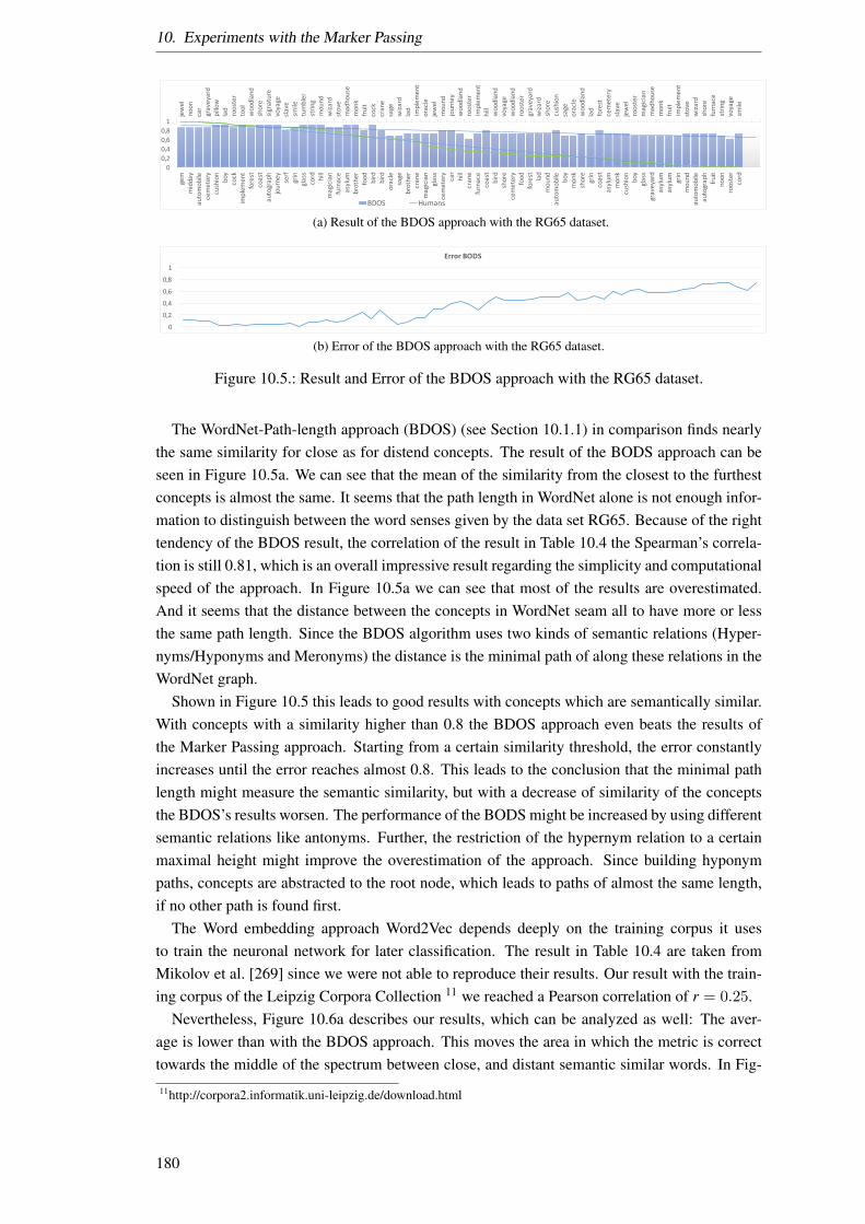
10. Experiments with the Marker Passing

jewel

noon

car

graveyard

pillow

lad

rooster

tool

woodland

shore

signature

voyage

slave

smile

tumbler

string

mound

wizard

stove

madhouse

monk

fruit

cock

crane

sage

wizard

lad

implement

oracle

jewel

mound

journey

woodland

rooster

implement

hill

woodland

voyage

woodland

rooster

graveyard

wizard

shore

cushion

sage

oracle

woodland

lad

forest

cemetery

slave

jewel

rooster

magician

madhouse

monk

fruit

implement

stove

wizard

shore

furnace

string

voyage

smile

0

0,2

0,4

0,6

0,8

1

gem

midday

automobile

cemetery

cushion

boy

cock

implement

forest

coast

autograph

journey

serf

grin

glass

cord hill

magician

furnace

asylum

brother

food

bird

bird

oracle

sage

brother

crane

magician

glass

cemetery

car

hill

crane

furnace

coast

bird

shore

cemetery

food

forest

lad

mound

automobile

boy

monk

shore

grin

coast

asylum

monk

cushion

boy

glass

graveyard

asylum

asylum

grin

mound

automobile

autograph

fruit

noon

rooster

cord

BDOS Humans

(a) Result of the BDOS approach with the RG65 dataset.

0

0,2

0,4

0,6

0,8

1

ErrorBODS

(b) Error of the BDOS approach with the RG65 dataset.

Figure 10.5.: Result and Error of the BDOS approach with the RG65 dataset.

The WordNet-Path-length approach (BDOS) (see Section 10.1.1) in comparison finds nearlythe same similarity for close as for distend concepts. The result of the BODS approach can beseen in Figure 10.5a. We can see that the mean of the similarity from the closest to the furthestconcepts is almost the same. It seems that the path length in WordNet alone is not enough infor-mation to distinguish between the word senses given by the data set RG65. Because of the righttendency of the BDOS result, the correlation of the result in Table 10.4 the Spearman’s correla-tion is still 0.81, which is an overall impressive result regarding the simplicity and computationalspeed of the approach. In Figure 10.5a we can see that most of the results are overestimated.And it seems that the distance between the concepts in WordNet seam all to have more or lessthe same path length. Since the BDOS algorithm uses two kinds of semantic relations (Hyper-nyms/Hyponyms and Meronyms) the distance is the minimal path of along these relations in theWordNet graph.

Shown in Figure 10.5 this leads to good results with concepts which are semantically similar.With concepts with a similarity higher than 0.8 the BDOS approach even beats the results ofthe Marker Passing approach. Starting from a certain similarity threshold, the error constantlyincreases until the error reaches almost 0.8. This leads to the conclusion that the minimal pathlength might measure the semantic similarity, but with a decrease of similarity of the conceptsthe BDOS’s results worsen. The performance of the BODS might be increased by using differentsemantic relations like antonyms. Further, the restriction of the hypernym relation to a certainmaximal height might improve the overestimation of the approach. Since building hyponympaths, concepts are abstracted to the root node, which leads to paths of almost the same length,if no other path is found first.

The Word embedding approach Word2Vec depends deeply on the training corpus it usesto train the neuronal network for later classification. The result in Table 10.4 are taken fromMikolov et al. [269] since we were not able to reproduce their results. Our result with the train-ing corpus of the Leipzig Corpora Collection 11 we reached a Pearson correlation of r = 0.25.

Nevertheless, Figure 10.6a describes our results, which can be analyzed as well: The aver-age is lower than with the BDOS approach. This moves the area in which the metric is correcttowards the middle of the spectrum between close, and distant semantic similar words. In Fig-

11http://corpora2.informatik.uni-leipzig.de/download.html

180

10.1. Experiment 1: Semantic Similarity Measure

ure 10.6b this can be seen in the error rate reducing towards the end of the first half of the dataset. Further, there seem to be words for which the approach works better than for others inde-pendent of the semantic distance between those words. This can be seen on the error droppingto almost zero from time to time, e.g., for magician and wizard but as well for asylum and ceme-tery, where magician has 42 occurrences and wizard hat 184. On the other hand, asylum had376 occurrences and cemetery had 512. Since slave has 434 occurrences and monk 365, the oc-currence rate is not the source of the error. From the approach of word embedding, it should beclear that words not occurring in the same context should not be seen as similar. Consequently,this depends on the length of the tests and the vocabulary used.

The Word2Vec approach has its benefits as well: The embedding is independent of wordtype or grammatical form. Hence on data sets with multiple word types, they might performbetter [17]. Additionally, the performance can continuously improve if new training data isfound. In contrast to the Thesaurus approach ELKB, where the Thesaurus needs to be improved,which is subject to research [192].

The Word2Vec similarity performance depends on the data set on which the ANN has beentrained. We selected the English one million word News corpus from the Leipzig Corpora Col-lection12 [313]. Since our selection might have been suboptimal, we used the results of theoriginal references [269] to compare them to our results.

As a final remark to the results of the Word2Vec approach, we need to notice that the co-occurrence is not a semantic similarity measure but a measure of relatedness. This relatednesscan be seen in words often co-occurring like homeless and shelter, which are semantically ratherthe opposite since a homeless person is one without the shelter provided by a home. But theystill seem related in the Word2Vec approach. For our evaluation, this observation does not makeany difference, since the performance against humans is measured and not an objective or logicalsemantic distance. Accordingly, the result measures how well an approach can simulate humansemantic similarity guesses. Because of the co-occurrence of certain words, even humans mightbe influenced to guess the semantic similarity wrong. This is also true for words like sun, star,and planet. Where a human all sees them as round objects of astronomy, where an expert woulddisagree on their similarity. Since this argument could be held for most concepts, we rest ourexperiment on the simulation of average human estimates.

We can see that the thesaurus based approach (ELKB) (see Section 10.1.1) estimates wellwhen closely related concepts are the problem, whereas the semantic similarity gets smaller themetric becomes less accurate and unable to connect two concepts. In Figure 10.7b we can seethat ELKB’s error increases with the decrease of semantic similarity of the concepts. There areerrors even in the semantically close concepts when the thesaurus does not include a concept.Then the similarity is set to zero. This explains the two error peaks at the beginning of theFigure 10.7b.

The ELKB approach comes close to the human’s similarity estimates in average but onlyreaches a Spearman’s ρ = 0.65. The first thing to notice about the result is that there are discretesteps in similarity. The steps size is 0.125 since there are only eight steps in the thesaurusreaching from no connection to being in the same frame. This has the effect that there can notbe a fine grained result like provided by human estimates. This can be seen in Figure 10.7a inthe first 21 word pairs, where most of the estimates are mapped to 1.0.

If one of the words is not contained in the Thesaurus then the ELKB similarity measure returns12http://wortschatz.uni-leipzig.de/en/download/

181

10. Experiments with the Marker Passing

jewel

noon

car

graveyard

pillow

lad

rooster

tool

woodland

shore

signature

voyage

slave

smile

tumbler

string

mound

wizard

stove

madhouse

monk

fruit

cock

crane

sage

wizard

lad

implement

oracle

jewel

mound

journey

woodland

rooster

implement

hill

woodland

voyage

woodland

rooster

graveyard

wizard

shore

cushion

sage

oracle

woodland

lad

forest

cemetery

slave

jewel

rooster

magician

madhouse

monk

fruit

implement

stove

wizard

shore

furnace

string

voyage

smile

0

0,2

0,4

0,6

0,8

1

gem

midday

automobile

cemetery

cushion

boy

cock

implement

forest

coast

autograph

journey

serf

grin

glass

cord hill

magician

furnace

asylum

brother

food

bird

bird

oracle

sage

brother

crane

magician

glass

cemetery

car

hill

crane

furnace

coast

bird

shore

cemetery

food

forest

lad

mound

automobile

boy

monk

shore

grin

coast

asylum

monk

cushion

boy

glass

graveyard

asylum

asylum

grin

mound

automobile

autograph

fruit

noon

rooster

cord

Word2Vec Humans

(a) Result of the Word2Vec approach with the RG65 dataset.

0

0,2

0,4

0,6

0,8

1errorWord2Vec

(b) Error of the Word2Vec approach with the RG65 dataset.

Figure 10.6.: Result and Error of the Word2Vec with the RG65 dataset.

jewel

noon

car

graveyard

pillow

lad

rooster

tool

woodland

shore

signature

voyage

slave

smile

tumbler

string

mound

wizard

stove

madhouse

monk

fruit

cock

crane

sage

wizard

lad

implement

oracle

jewel

mound

journey

woodland

rooster

implement

hill

woodland

voyage

woodland

rooster

graveyard

wizard

shore

cushion

sage

oracle

woodland

lad

forest

cemetery

slave

jewel

rooster

magician

madhouse

monk

fruit

implement

stove

wizard

shore

furnace

string

voyage

smile

0

0,2

0,4

0,6

0,8

1

gem

midday

automobile

cemetery

cushion

boy

cock

implement

forest

coast

autograph

journey

serf

grin

glass

cord hill

magician

furnace

asylum

brother

food

bird

bird

oracle

sage

brother

crane

magician

glass

cemetery

car

hill

crane

furnace

coast

bird

shore

cemetery

food

forest

lad

mound

automobile

boy

monk

shore

grin

coast

asylum

monk

cushion

boy

glass

graveyard

asylum

asylum

grin

mound

automobile

autograph

fruit

noon

rooster

cord

ELKB Humans

(a) Result of the ELKB approach with the RG65 dataset.

0

0,2

0,4

0,6

0,8

1

ErrorELKB

(b) Error of the ELKB approach with the RG65 dataset.

Figure 10.7.: Error of the ELKB approach with the RG65 dataset.

a zero. Which can be seen on examples like cemetery and graveyard or forest and woodland inFigure 10.7a. In our dataset, these zero estimates occur more often the farther the words aresemantically apart. This is because the algorithm cuts the search for a path from one word toanother when it reaches a set count of eight. In particular, paths longer then eight are countedas no path found and with that to a similarity of zero. This can be seen on grin and implements0.125 and grin an lad 0, lad and brother 0.125 and smile and grin 1.0. Here grin and lad are bothparts of the Thesaurus, but grin and lad are too far apart for the approach to find a similarity atall.

The ELKB approach has less error for distance word pairs as it returns zero if no distance isfound. As a result, the missing error for semantically distant word pairs here is due to failure ofthe approach to handle distant words. BDOS, on the other hand, has almost no error for closeconcepts. Here short paths between two concepts can be found in WordNet. But the further thedistance of the words, the less accurate BDOS becomes.

A preliminary analysis with the Stanford Rare Word Similarity dataset [244] of 2034 wordshas yield the result of Spearman correlation of 0.17 and a Pe arson correlation of 0.19, which

182

10.2. Experiment 2: Word Sense Disambiguation

is subject to improvement now. Furthermore, the extension to have a WSD algorithm whichuses context can be created through the following steps: The contextual words are decomposed,the results are merged into the graph and markers are passed to them. Then the word senseis selected with the most semantic similarity by identifying the nodes that received the mostactivation from multiple origins. The parameters for such an algorithm are subject to futurework.

Conclusion

In conclusion, we can say, that the Marker Passing approach combines with a semantic de-composition can be used to build a semantic similarity measure. Although the success in theperformance of our measure, the vast amount of potential parameters and the different designdecisions, leave still room for improvement. With the infinite specialization methods for theMarker Passing, there could be other interpretations which are even more successful. More ef-fort could go into designing more sophisticated similarity measures, but we see this as a proofof concept. Through the learning of the parameters, the parameters might be specific to the dataset, we used for the evaluation, but never the less, we can show that our approach is applicablefor measuring semantic similarity.

As a result, we were able to show that the MP approach can beat the state-of-the-art on theRG65 data set concerning the Spearman’s correlation. A detailed analysis of the result hasshown that with growing distance of the words compared, the error of the approach gets worsestarting from a distance of approximately 0.7.

The errors in our semantic similarity measure could be from including word senses which arenot relevant in human semantic similarity estimates. The next section will, therefore, tackle theproblem of word sense disambiguation.

10.2. Experiment 2: Word Sense Disambiguation

Word Sense Disambiguation (WSD) is the act of selecting a word sense of one word in a contextof use13. Therefor we can describe our WSD with the following signature:

WSD : Concept × Concept∗ → Definition

The first concept is the target concept, the second list of concepts is the context in which thetarget word is used. The result of the WSD is one of the word senses (here called definition) ofthe target word.

Now that we can distinguish the semantic similarity of word pairs, we start a new experiment:Finding the right word sense of a single word in a linguistic context. Since a sense of a word canbe described by its definition, this experiment selects one definition of the target word fitting tothe meaning of the word used in a context14, and then look up the sense key of the word sensedescribed by the definition to see if we have selected the right one.

Figure 10.8 describes the Marker Passing approach of a word sense disambiguation algorithm.Here the target Word, its context, and all its definitions are decomposed. The semantic graphs

13This work is based on the bachelor thesis of Lukanek [243] and Marienwald [252] who have implanted a firstversion of the marker passing algorithm for WSD.

14Here the context might be the sentence the word is used in

183

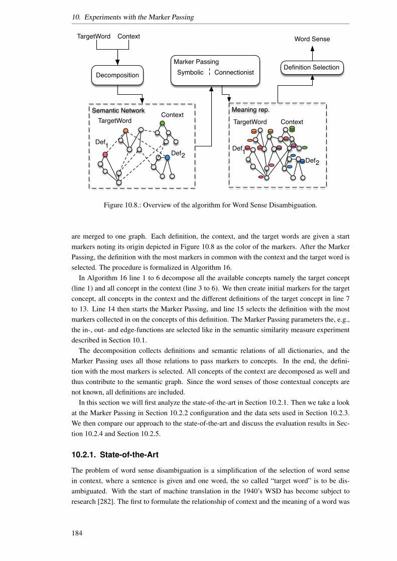
10. Experiments with the Marker Passing

Semantic Network

Marker PassingSymbolic Connectionist

Meaning rep.

Decomposition

TargetWord

Definition Selection

Context

TargetWord

Def1Def2

ContextTargetWord

Def1Def2

Context

Word Sense

Figure 10.8.: Overview of the algorithm for Word Sense Disambiguation.

are merged to one graph. Each definition, the context, and the target words are given a startmarkers noting its origin depicted in Figure 10.8 as the color of the markers. After the MarkerPassing, the definition with the most markers in common with the context and the target word isselected. The procedure is formalized in Algorithm 16.

In Algorithm 16 line 1 to 6 decompose all the available concepts namely the target concept(line 1) and all concept in the context (line 3 to 6). We then create initial markers for the targetconcept, all concepts in the context and the different definitions of the target concept in line 7to 13. Line 14 then starts the Marker Passing, and line 15 selects the definition with the mostmarkers collected in on the concepts of this definition. The Marker Passing parameters the, e.g.,the in-, out- and edge-functions are selected like in the semantic similarity measure experimentdescribed in Section 10.1.

The decomposition collects definitions and semantic relations of all dictionaries, and theMarker Passing uses all those relations to pass markers to concepts. In the end, the defini-tion with the most markers is selected. All concepts of the context are decomposed as well andthus contribute to the semantic graph. Since the word senses of those contextual concepts arenot known, all definitions are included.

In this section we will first analyze the state-of-the-art in Section 10.2.1. Then we take a lookat the Marker Passing in Section 10.2.2 configuration and the data sets used in Section 10.2.3.We then compare our approach to the state-of-the-art and discuss the evaluation results in Sec-tion 10.2.4 and Section 10.2.5.

10.2.1. State-of-the-Art

The problem of word sense disambiguation is a simplification of the selection of word sensein context, where a sentence is given and one word, the so called “target word” is to be dis-ambiguated. With the start of machine translation in the 1940’s WSD has become subject toresearch [282]. The first to formulate the relationship of context and the meaning of a word was

184

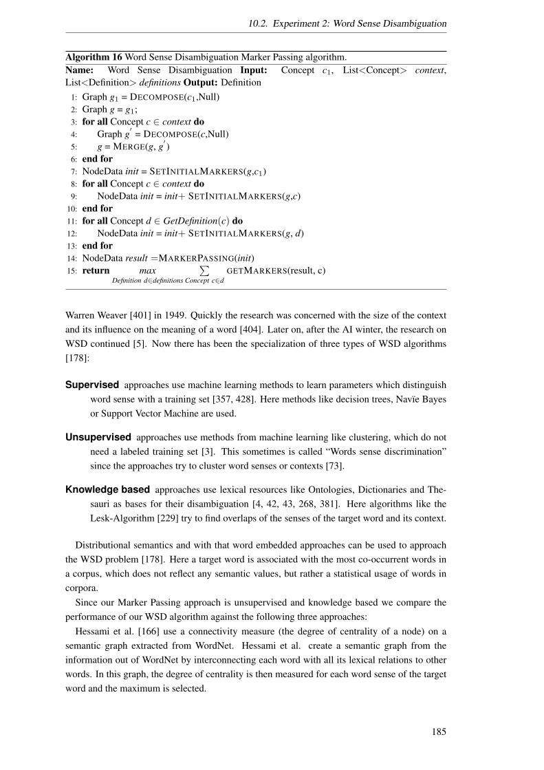
10.2. Experiment 2: Word Sense Disambiguation

Algorithm 16 Word Sense Disambiguation Marker Passing algorithm.Name: Word Sense Disambiguation Input: Concept c1, List<Concept> context,List<Definition> definitions Output: Definition

1: Graph g1 = DECOMPOSE(c1,Null)2: Graph g = g1;3: for all Concept c ∈ context do4: Graph g

′= DECOMPOSE(c,Null)

5: g = MERGE(g, g′)

6: end for7: NodeData init = SETINITIALMARKERS(g,c1)8: for all Concept c ∈ context do9: NodeData init = init+ SETINITIALMARKERS(g,c)

10: end for11: for all Concept d ∈ GetDefinition(c) do12: NodeData init = init+ SETINITIALMARKERS(g, d)13: end for14: NodeData result =MARKERPASSING(init)15: return max

Definition d∈definitions

∑Concept c∈d

GETMARKERS(result, c)

Warren Weaver [401] in 1949. Quickly the research was concerned with the size of the contextand its influence on the meaning of a word [404]. Later on, after the AI winter, the research onWSD continued [5]. Now there has been the specialization of three types of WSD algorithms[178]:

Supervised approaches use machine learning methods to learn parameters which distinguishword sense with a training set [357, 428]. Here methods like decision trees, Navıe Bayesor Support Vector Machine are used.

Unsupervised approaches use methods from machine learning like clustering, which do notneed a labeled training set [3]. This sometimes is called “Words sense discrimination”since the approaches try to cluster word senses or contexts [73].

Knowledge based approaches use lexical resources like Ontologies, Dictionaries and The-sauri as bases for their disambiguation [4, 42, 43, 268, 381]. Here algorithms like theLesk-Algorithm [229] try to find overlaps of the senses of the target word and its context.

Distributional semantics and with that word embedded approaches can be used to approachthe WSD problem [178]. Here a target word is associated with the most co-occurrent words ina corpus, which does not reflect any semantic values, but rather a statistical usage of words incorpora.

Since our Marker Passing approach is unsupervised and knowledge based we compare theperformance of our WSD algorithm against the following three approaches:

Hessami et al. [166] use a connectivity measure (the degree of centrality of a node) on asemantic graph extracted from WordNet. Hessami et al. create a semantic graph from theinformation out of WordNet by interconnecting each word with all its lexical relations to otherwords. In this graph, the degree of centrality is then measured for each word sense of the targetword and the maximum is selected.

185

10. Experiments with the Marker Passing

Veronis and Ide [389] do WSD via a “very large neural network extracted from machinereadable dictionaries”. The word senses of the Collins English Dictionary are connected to thewords in the definition of this word sense. This is repeated with all words which have definitionsin the dictionary. This is equivalent to creating a decomposition by only using definition nodes.All words (nodes of the ANN) are reduced to their lemma. The sense nodes of a word areinterlinked with inhibitory links (edges with negative weights). The activation then is passedfrom the input words and passed along the network. The paper of Veronis and Ide [389] does notspecify the concrete parameters of the approach, e.g., the number of cycles and the inhabitationfactor or the start activation is not specified.

There is one contribution which uses spreading activation to create a WSD approach. Wewill look at this approach more closely next: Tsatsaronis et al. [380, 381, 382] describe a WSDapproach which utilizes WordNet as a semantic graph. With that the approach of Tsatsaronis etal. falls into the knowledge based category. In their publication Tsatsaronis et al. [380] theyextend their approach to be unsupervised and with that fall in a second of the above categoriesand with that into the related work for our approach.

Tsatsaronis et al. construct a semantic graph from WordNet by adding all directly relatedconcepts of the concepts making up the sentence, to the semantic graph. Each word sense ofa word is connected with the concept itself, with edges weighted with positive weights (calledactivatory edges). The senses of one word are then interlinked with edges with negative weights(called inhibitory edges).

The activation spreading is then done by checking if a node j activation Aj(p) has reached thethreshold τ at pulse p. The Equation 10.13 describes how the activation is then propagated:

Oj(p) =

0 , if Aj(p) < τ

(1−CjCT

)

p+1 ∗ Aj(p) , else(10.13)

With Cj being the number of directly connected nodes and CT being the total amount of nodes.Here p is the pulse count so that with each activation pulse the activation decreases. The edgesare then weighted by their term frequency (the frequency to which the edge type is used) timesits log-inverse of the total frequency of node occurrence. This approach has been evaluated usingthe Senseval 2 data set and reached an accuracy of 0.493.

The drawback of the approach described in Tsatsaronis et al. [380, 381, 382] is that a POStagging needs to be present for the approach to work. Also, only WordNet is used to build thesemantic graph; this means only words which are described in WordNet are part of the semanticgraph.

The WSD experiment proposed here can be classified as a knowledge based approach sincewe are using our semantic decomposition as a basis for our disambiguation. Further, the MarkerPassing is unsupervised. We propose an offline learning phase for the parameters of the MarkerPassing algorithm, but the resulting algorithm can function without a human in the loop.

10.2.2. Marker Passing Configuration

The Marker Passing configuration in this experiment is the same as in the semantic similaritymeasure experiment. See Section 10.1 for more details. Every parameter of the Marker Pass-

186

10.2. Experiment 2: Word Sense Disambiguation

ing is here the same as in Section 10.1. From the start Marker, the activation threshold to thetermination condition, the approach here only changes by the amount of start markers initiallydistributed and the result interpretation.

The parameters of the weights and amount of start activation, as well as the termination pulsecount and double activation limit, are learned with a genetic algorithm as described in Sec-tion 10.1.15.

10.2.3. Data Sets

The golden standard for word sense disambiguation is evaluated each year in the SemEval chal-lenge15. This challenge is organized by Association for Computational Linguistics (ACL) Spe-cial Interest Group on the Lexicon (SIGLEX). Since our approach is based on English lexicalresources like WordNet or Wikipedia, we had to select an English WSD challenge.

Sadly the Semantic Evaluation Exercises (SemEval-2016) held on the International Workshopon Semantic Evaluation is again a SemEval without WSD task. This reduces the choice of datasets to older versions of the data sets provided by SemEval challenge. This is the reason why thestate-of-the-art in word sense disambiguation is tested on the Senseval Task 3 (Senseval-3 Task)called “Word-Sense Disambiguation of WordNet Glosses” [267].

This task consists of example sentences where one word, the so called target word is ambigu-ous. The corpus is taken from the British National Corpus, the Penn Treebank corpus, the LosAngeles Times collection and the Open Mid Common Sense corpus [267]. These are combinedwith the word senses of WordNet creating example sentences like the one shown in Figure ??.

These beliefs so dominate our educational establishment , our media , our politicians , and even…

belie

f%1:0

9:00::

so%4:02:02::

dominate%2:42:01::

(19)05950141 <noun.cognition>[09] S: (n) belief#1 (belief%1:09:00::) (any cognitive content held as true)

(322)00147630 <adv.all>[02] S: (adv) so#1 (so%4:02:02::) (to a very great extent or degree) "the idea is so obvious"; "never been so happy"; "I love you so"; "my head aches so!"

(6)02653015 <verb.stative>[42] S: (v) dominate#2 (dominate%2:42:01::) (be in control) "Her husband completely dominates her"

Figure 10.9.: Example sentence with word sense from the Senseval Task 3 data set

In the Senseval data set most of the words of the example sentence are tagged with a WordNetword sense like in the example in Figure ?? the word “belief” with the sense key “1:09:00::”which references the definition “any cognitive content held as true.”. The task now is, to identifythe right word sense for each tagged word. For us, this means choosing the right definition wehave found in the decomposition and looking up its sense key to return it as an answer.

15http://www.senseval.org/senseval3/tasks.html last visited on 02.03.2017

187

10. Experiments with the Marker Passing

10.2.4. Evaluation Results

This section describes the evaluation results of our Algorithm 16 on the Senseval Task 3 dataset. We compare our results to the best performing of each of the three categories describedin Section 10.2.1. Here we compare the approaches depending on their accuracy regarding theselection of word senses for the target words in the different sentences.

Table 10.5.: Results of the WSD approaches on the Senseval Task 3 data set.WSD approach AccuracyHessami et al. [166] 0.482MP 0.385Tsatsaronis et al. [382] 0.365Veronis & Ide [389] 0.308

Table 10.5 shows that the overall performance of our Marker Passing approach (MP) performssecond best in the state-of-the-art. The results are reported in the respective papers proposingthe approach16. Here further optimization of the Marker Passing parameters could result in ahigher accuracy, but this is left to future work.

10.2.5. Discussion of the results

The selection of a definition or word sense of a word is a hard task which can be seen in the lowoverall accuracy reached by the here compared approaches. A perfect match has been reached,e.g., on the sentence “Here the experience of New York City is decisive.” with the target wordbeing experience with the word sense: “the accumulation of knowledge or skill that results fromdirect participation in events or activities”. This works well because the word experience isalready in lemma form. In other cases like in the sentence “Community involvement is an evenworse idea.”, with the target word ”idea” with word sense “the content of cognition; the mainthing you are thinking about”, our approach does not even select the right word: The MarkerPassing resulted in maximally activating the synonym of ideas “thought” with the same wordsense “the content of cognition; the main thing you are thinking about.”. This means we haveselected some word sense which does not have a sense key in WordNet, consequently is nota possible solution to the question. This means out results could be improved, if additionalproblem specific knowledge would be added to the algorithm, selecting only definitions whichhave a WordNet sense key.

The calculation of the maximum activation seems to be too general since sometimes synonymsdo have the same definition but are not considered a right response by the dataset. This drawbackcould be overcome by altering the result interpretation and filtering the synonyms.

Our result has been achieved without any syntactical information, which makes our approacha purely semantical one. In future work, the decomposition could be extended by syntacticinformation to improve the results.

Since the decomposition collects definitions of all dictionaries, a mapping to WordNet sensekeys is needed if a definition is selected which has its origin, not in WordNet. In addition, theresults could be optimized if the contextual concepts are disambiguated first, or at least theirPOS identified so that the decomposition does not contain all relations for all word senses.

16For further details the interested reader is referred to the Thesis of Marienwald [252]

188

10.3. Experiment 3: Semantic Sentence Similarity Measure

In conclusion, we can say that the performance of an unsupervised approach do not reach theresults of supervised approaches [20] but improves over the last years. Overall there is still spacefor improvement regarding the performance of unsupervised methods.

10.3. Experiment 3: Semantic Sentence Similarity Measure

This section describes the experiment on semantic sentence similarity. After having experi-mented with a word meaning similarity in Section 10.1 and word senses in Section 10.2 thisexperiment establishes if the here presented approach can be applied to represent the meaningof sentences. This means that the experiment conducted in this section analyzes how the MarkerPassing approach can be used to create a sentence similarity measure. This is done to show thatthe approach is not restricted to single concept similarity. Here we take the idea of the semanticsimilarity presented in Section 10.1 and extends this approach to measure sentence similarity17.

The signature of the given problem is defined as follows:

SemanticSentenceSimilarity : Concept∗ × Concept∗ → Double

Here the input is two sentences (given thought two list of concepts), and the result representsa measure of similarity as a double value. The resulting measure is zero if the sentence is notsimilar and is one if the sentences are equivalent in meaning.

Again, this experiment represents only a proof-of-concept to show that the here presentedapproach to representing artificial meaning can be used to measure the difference in sentencemeanings. This means we do not optimize parameters of the Marker Passing to fit the data set.We will see that there are a multitude of design decisions which do not claim completeness noroptimality. We can regard this experiment as a starting point for future research on specializingthe decomposition, the Marker Passing and its interpretation of to represent sentence meaning.

One result of the WSD experiment in Section 10.2 is that we want to identify sentences (in thiscase definitions) with the same meaning so that we can aggregate them and have less redundantdefinitions in the semantic graph. The resulting disambiguation could also be used during thedecomposition itself since we want to eliminate duplicates in the definitions there as well to haveless noise in the decomposition.

Figure 10.10 shows our abstract approach to a semantic sentence similarity measure. First,we decompose every word of both sentences. The resulting graphs are merged into one graph.In this graph, the concepts of the two sentences are marked with different markers. Our basicapproach is depicted in Figure 10.10 where the different markers are shown as orange and greenmarked nodes.

17This section is based on the thesis of Schneider [351]

189

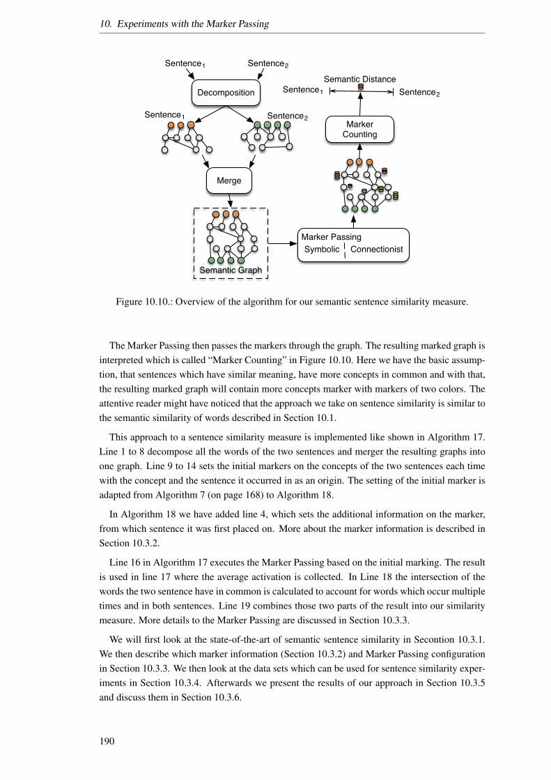
10. Experiments with the Marker Passing

Decomposition

Semantic Graph

Marker PassingSymbolic Connectionist

Merge

Sentence1 Sentence2

Marker Counting

Semantic Distance

Sentence1 Sentence2

Sentence2Sentence1

Figure 10.10.: Overview of the algorithm for our semantic sentence similarity measure.

The Marker Passing then passes the markers through the graph. The resulting marked graph isinterpreted which is called “Marker Counting” in Figure 10.10. Here we have the basic assump-tion, that sentences which have similar meaning, have more concepts in common and with that,the resulting marked graph will contain more concepts marker with markers of two colors. Theattentive reader might have noticed that the approach we take on sentence similarity is similar tothe semantic similarity of words described in Section 10.1.

This approach to a sentence similarity measure is implemented like shown in Algorithm 17.Line 1 to 8 decompose all the words of the two sentences and merger the resulting graphs intoone graph. Line 9 to 14 sets the initial markers on the concepts of the two sentences each timewith the concept and the sentence it occurred in as an origin. The setting of the initial marker isadapted from Algorithm 7 (on page 168) to Algorithm 18.

In Algorithm 18 we have added line 4, which sets the additional information on the marker,from which sentence it was first placed on. More about the marker information is described inSection 10.3.2.

Line 16 in Algorithm 17 executes the Marker Passing based on the initial marking. The resultis used in line 17 where the average activation is collected. In Line 18 the intersection of thewords the two sentence have in common is calculated to account for words which occur multipletimes and in both sentences. Line 19 combines those two parts of the result into our similaritymeasure. More details to the Marker Passing are discussed in Section 10.3.3.

We will first look at the state-of-the-art of semantic sentence similarity in Secontion 10.3.1.We then describe which marker information (Section 10.3.2) and Marker Passing configurationin Section 10.3.3. We then look at the data sets which can be used for sentence similarity exper-iments in Section 10.3.4. Afterwards we present the results of our approach in Section 10.3.5and discuss them in Section 10.3.6.

190

10.3. Experiment 3: Semantic Sentence Similarity Measure

Algorithm 17 Semantic Sentence Similarity Marker Passing algorithm.Name: Semantic Similarity Measure Input: List<Concept> sentence1, List<Concept>sentence2 Output: Double

1: for all Concept c ∈ sentence1 do2: Graph g

′= DECOMPOSE(c,Null)

3: Graph g = MERGE(g, g′)

4: end for5: for all Concept c ∈ sentence2 do6: g

′= DECOMPOSE(c,Null)

7: g = MERGE(g, g′)

8: end for9: NodeData init = emptyNodeData

10: for all Concept c ∈ sentence1 do11: NodeData init = init+ SETINITIALMARKERS(g, c)12: end for13: for all Concept c ∈ sentence2 do14: NodeData init = init+ SETINITIALMARKERS(g, c)15: end for16: NodeData result =MARKERPASSING(init)17: double avgActivation = GETAVGACTIVATION(result)18: double intersection = (size(sentence1+size(sentence2)−(size(sentence1∩sentence2))

size(sentence1)+size(sentence2)2

19: return intersection + ( avgActivation(size(sentence1∩sentence2)∗StartActivation )

Algorithm 18 Setting initial markers for sentences.Name: InitialMarkingInput: Concept c1

Output: NodeData1: function SETINITIALMARKERS(c1, sentencei)2: ND = emptyNodeData(c1, sentencei)

3: m1 = λ(x).

startActivation | ∅ , if x = c1

∅ , else4: ND = setOriginSentence(c1,sentencei)5: ND = setMarking (ND, c1,m1)6: ND = setHistory (ND, c1,m1)7: return ND8: end function

191

10. Experiments with the Marker Passing

10.3.1. State-of-the-Art

This section will analyze the related work of semantic sentence similarity measure. The literatureanalysis will show which properties of sentences are used in the different measures and findsuitable state-of-the-art to compare our approach against.

Sentence similarity has recently become subject to research. Most approaches origin fromword similarity measures or represent Information Retrieval Methods which are originally usedto compare bigger text documents [294]. Sentence similarity measures can be divided into twotypes of approaches:

Vector Space Models which are corpus-based methods also known as word embedding. InVector space models the sentence is seen as a vector where each component of the vectoris one word of the sentence. These vectors are then compared to each other mostly basedon cooccurrence statistical information in corpora and some geometrical measures like thecosine similarity.

Feature Based approaches split the sentence into its words, and compare features of thosewords to each other and aggregate this comparison to become the sentence similaritymeasure.

Besides the standard classification into unsupervised and supervised methods in machinelearning, the focus here is on the two types of approaches. As mostly in machine learning,the supervised approaches have a better performance on the test data sets and bare the usualdeficits like the size of needed training data and the effort to creating this training data.

Gomaa and Fahmy [147] present a survey on text similarity measures older than the year 2013.These approaches are superseded and therefore are not part of this state-of-the-art analysis.

Corley et al. [60] introduce a semantic similarity measure for larger texts which can be usedfor sentences as well. They extract all verbs and nouns from the two sentences and select acorresponding (semantically the most similar) verb or noun in the other sentence. To choose thesemantic similar verb or noun they use eight different distance measures. Amongst others theyuse Wu Palmer [418] and Jiang and Conrath [185, 418]. The rest of the words of the sentenceare compared with a “word-to-word similarity” [60].

Mihalcea et al. [268] present a corpus based approach, so a semantic similarity measure oftexts extending the one of Corley et al. [60] by integrating more part-of-speech classes in theword similarity, with the result of loosening the restriction of only comparing nouns with nouns.The result is weighted by the inverse occurrence frequency (so simulate entropy or amountinformation content) and normalized.

Approaches like the one of Islam and Inkpen [180, 334, 368] are all using different semanticdistance measures of the text like the length of a “congest common subsequence”, the semanticsimilarity of words, or the order in which the words occur. Stabcgev [368], for example, extractsa similarity graph from WordNet and bases its clustering on the occurrence of words in categoriesin this graph.

Oliva et al. [294], on the other hand, describe a syntax-based semantic similarity measure.Here the abstract syntax tree is calculated then the similarity of the words with the same syntacticfunctions are calculated, and the result is summed up and normalized. Here the part-of-speechare weighted differently. Oliva et al. introduce a fixed penalty factor of 0.3 for syntactic elements

192

10.3. Experiment 3: Semantic Sentence Similarity Measure

which are present in one sentence but not in the other. Those are then subtracted from theweighted sum of word similarities.

Taib et al. [375] describe a “features-based measure of sentences semantic similarity” (FMS3)combines word similarity of verbs and nouns and the order of words. Taib et al. [375] use aPageRank-Algorithm where the links referencing a concept (originally a web page) determinethe amount of similarity of a concept. Hence, if a concept is used in a definition of a word, thenit is seen as referencing this concept. The referencing concepts are weighted according to thecount of incoming references and the weight of the concept which is referencing this concept. Ifa word has multiple definitions, the definitions are ranked according to their weights which leadto a sort of disambiguation of word senses.

Pilehvar et al. [308] as well describe an “Alignment-based Disambiguation of the two lin-guistic items and random walk” (ADW). Here the words of a sentence are represented by theirdefinitions (they call this a semantic signature). This semantic network is the represented as avector space where the vector contains elements which the definitions have in common. Thisis different form the concurrence vector spaces because it is based on properties found in thesemantic network. The ADW seems to be working well on the datasets according to Pilehvar etal. [308] but the results are not reproducible with the open source variant 18. For that reason, weneglect from listing those results in our state-of-the-art.

In conclusion, the state-of-the-art of sentence similarity does use a multitude of propertieslike word order and part-of-speech or syntax of the sentence and has analyzed different wordsimilarity measures. In addition to the contribution of Taib et al. [375] even word sense dis-ambiguation is used to select the right definition of the word in the context of the sentence.Missing in this approaches is the symbolic part of the meaning of the sentences. This means thatlogical concepts like negation can not be appropriately integrated into the sentence similaritymeasure. Representing the best sentence similarity measures researched so far, they form thebest candidates as a comparison to our approach.

We selected the paper of Cloey and Mihalecea [268] and Pilehvar et al. [308] for the compar-ison with our approach since these are the most recent surveys on sentence similarity, and theyuse the same data set.

10.3.2. Marker information

The marker information for the sentence equivalent experiment is similar to the of the semanticdistance with the addition that the marker carries the information from which sentence it hasstarted. Consequently, we can define our marker as follows:

This is done to be able to treat those markers separately. If a concept is present in bothsentences, markers of both “colors” are placed on it.

10.3.3. Marker Passing Configuration

The Marker Passing configuration in this experiment is the same as in the semantic similaritymeasure experiment, except the interpretation of the markers after the Marker Passing has been

18https://github.com/pilehvar/ADW/

193

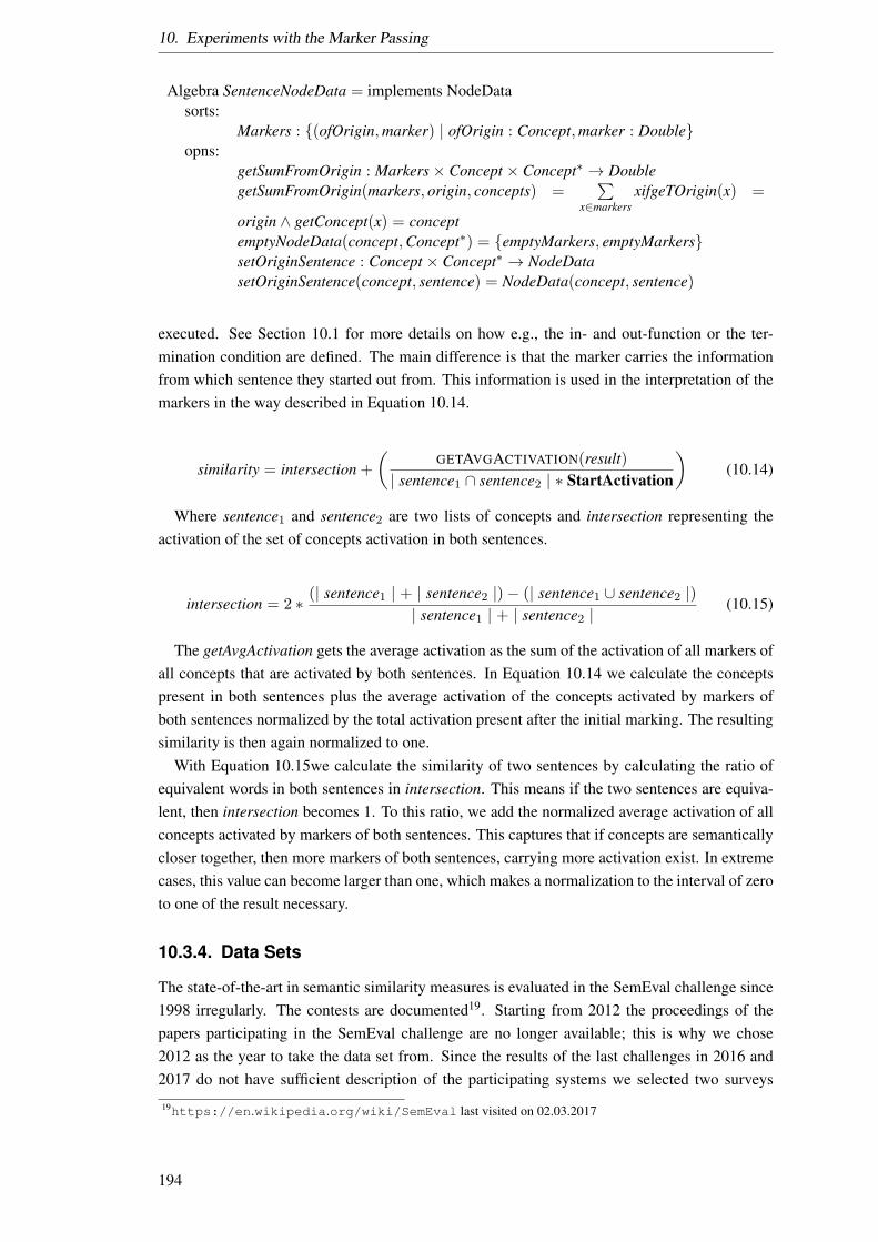
10. Experiments with the Marker Passing

Algebra SentenceNodeData = implements NodeDatasorts:

Markers : (ofOrigin,marker) | ofOrigin : Concept,marker : Doubleopns:

getSumFromOrigin : Markers× Concept × Concept∗ → DoublegetSumFromOrigin(markers, origin, concepts) =

∑x∈markers

xifgeTOrigin(x) =

origin ∧ getConcept(x) = conceptemptyNodeData(concept,Concept∗) = emptyMarkers, emptyMarkerssetOriginSentence : Concept × Concept∗ → NodeDatasetOriginSentence(concept, sentence) = NodeData(concept, sentence)

executed. See Section 10.1 for more details on how e.g., the in- and out-function or the ter-mination condition are defined. The main difference is that the marker carries the informationfrom which sentence they started out from. This information is used in the interpretation of themarkers in the way described in Equation 10.14.

similarity = intersection +

(GETAVGACTIVATION(result)

| sentence1 ∩ sentence2 | ∗ StartActivation

)(10.14)

Where sentence1 and sentence2 are two lists of concepts and intersection representing theactivation of the set of concepts activation in both sentences.

intersection = 2 ∗ (| sentence1 | + | sentence2 |)− (| sentence1 ∪ sentence2 |)| sentence1 | + | sentence2 |

(10.15)

The getAvgActivation gets the average activation as the sum of the activation of all markers ofall concepts that are activated by both sentences. In Equation 10.14 we calculate the conceptspresent in both sentences plus the average activation of the concepts activated by markers ofboth sentences normalized by the total activation present after the initial marking. The resultingsimilarity is then again normalized to one.

With Equation 10.15we calculate the similarity of two sentences by calculating the ratio ofequivalent words in both sentences in intersection. This means if the two sentences are equiva-lent, then intersection becomes 1. To this ratio, we add the normalized average activation of allconcepts activated by markers of both sentences. This captures that if concepts are semanticallycloser together, then more markers of both sentences, carrying more activation exist. In extremecases, this value can become larger than one, which makes a normalization to the interval of zeroto one of the result necessary.

10.3.4. Data Sets

The state-of-the-art in semantic similarity measures is evaluated in the SemEval challenge since1998 irregularly. The contests are documented19. Starting from 2012 the proceedings of thepapers participating in the SemEval challenge are no longer available; this is why we chose2012 as the year to take the data set from. Since the results of the last challenges in 2016 and2017 do not have sufficient description of the participating systems we selected two surveys

19https://en.wikipedia.org/wiki/SemEval last visited on 02.03.2017

194

10.3. Experiment 3: Semantic Sentence Similarity Measure

Sentence one Sentence two Similarity

A man with a hard hat is dancing. A man wearing a hard hat is dancing. 5.0A woman is cutting up a chicken. A woman is slicing meat. 2.75A woman is slicing big pepper. A dog is moving its mouth. 0.0

Table 10.6.: Example sentences form the SemEval 2012 MSRvid data set.

Sentence one Sentence two Similarity

Neither was there a qualified majoritywithin this House to revert to Article272.

It did not not more of the qualified ma-jority in this Parliament to return to theArticle 272.

4.333

We often pontificate here about beingthe representatives of the citizens of Eu-rope.

We are often here to represent the Euro-pean citizens.

2.750

That provision could open the door wideto arbitrariness.

This paves the way for the of the Rulesof Procedure here.

1.500

Table 10.7.: Example sentences form the SemEval 2012 SMTeuroparl data set.

which compare state-of-the-art approaches as a reference like described in Section 10.3.1 thesepapers are Cloey and Mihalecea [268] and Pilehvar et al. [308].

The data set was first presented at the SemEval 201220 as task six. This evaluation dataset consists of a set of sentence pairs and their similarity. Table 10.6 shows three example ofsentences of the data set and their similarity measure.

Here 5.0 is the maximum similarity, and 0.0 is the low bound. For our experiment, we havenormalized this scale to the interval of [0, 1] by dividing by 5 to make the results easier tointerpret and comparable with other data sets. We have chosen the data sets: MSRvid, MSRpar,SMTeuroparl like in [308]. This selection has been made to be able to compare the resultsto the state-of-the-art. These tasks are from SemEval-2012 Task 621 which is an “SemanticTextual Similarity” task and from SEM 2013 Shared Task22 which is also an “Semantic TextualSimilarity” task.

Here the data set MSRvid and MSRpar contain stances out of the press and news like shownin Table 10.6. The data set SMTeuroparl, on the other hand, contains generic sentences, whichis a harder task. The SMTeuroparl data set consists of sentences like those shown in Table 10.7.

The complexity of words used and the increase in grammatical complexity of the sentencesexplains why this data set is harder for similarity measures.

The golden standard rates these sentences from 0 to 5. With the following meaning takenfrom the SemEval-2015 Task 2 website23:

5 The two sentences are completely equivalent, as they mean the same thing.

• The bird is bathing in the sink.

• Birdie is washing itself in the water basin.20https://www.cs.york.ac.uk/semeval-2012/index.html last visited on 10.09.201721http://www.cs.york.ac.uk/semeval-2012/task6/ last visited on 10.09.201722http://ixa2.si.ehu.es/sts/ last visited on 10.09.201723http://alt.qcri.org/semeval2015/task2/index.php?id=semantic-textual-similarit

y-for-english last visited on 03.03.2017

195

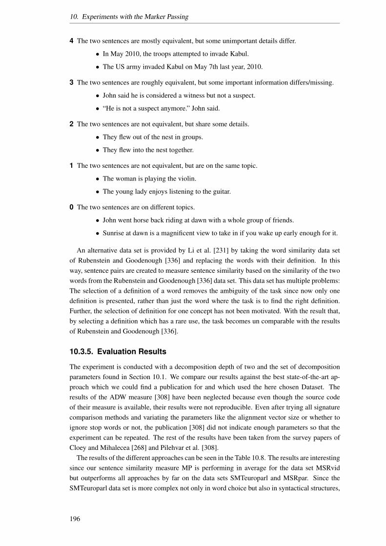
10. Experiments with the Marker Passing

4 The two sentences are mostly equivalent, but some unimportant details differ.

• In May 2010, the troops attempted to invade Kabul.

• The US army invaded Kabul on May 7th last year, 2010.

3 The two sentences are roughly equivalent, but some important information differs/missing.

• John said he is considered a witness but not a suspect.

• “He is not a suspect anymore.” John said.

2 The two sentences are not equivalent, but share some details.

• They flew out of the nest in groups.

• They flew into the nest together.

1 The two sentences are not equivalent, but are on the same topic.

• The woman is playing the violin.

• The young lady enjoys listening to the guitar.

0 The two sentences are on different topics.

• John went horse back riding at dawn with a whole group of friends.

• Sunrise at dawn is a magnificent view to take in if you wake up early enough for it.

An alternative data set is provided by Li et al. [231] by taking the word similarity data setof Rubenstein and Goodenough [336] and replacing the words with their definition. In thisway, sentence pairs are created to measure sentence similarity based on the similarity of the twowords from the Rubenstein and Goodenough [336] data set. This data set has multiple problems:The selection of a definition of a word removes the ambiguity of the task since now only onedefinition is presented, rather than just the word where the task is to find the right definition.Further, the selection of definition for one concept has not been motivated. With the result that,by selecting a definition which has a rare use, the task becomes un comparable with the resultsof Rubenstein and Goodenough [336].

10.3.5. Evaluation Results

The experiment is conducted with a decomposition depth of two and the set of decompositionparameters found in Section 10.1. We compare our results against the best state-of-the-art ap-proach which we could find a publication for and which used the here chosen Dataset. Theresults of the ADW measure [308] have been neglected because even though the source codeof their measure is available, their results were not reproducible. Even after trying all signaturecomparison methods and variating the parameters like the alignment vector size or whether toignore stop words or not, the publication [308] did not indicate enough parameters so that theexperiment can be repeated. The rest of the results have been taken from the survey papers ofCloey and Mihalecea [268] and Pilehvar et al. [308].

The results of the different approaches can be seen in the Table 10.8. The results are interestingsince our sentence similarity measure MP is performing in average for the data set MSRvidbut outperforms all approaches by far on the data sets SMTeuroparl and MSRpar. Since theSMTeuroparl data set is more complex not only in word choice but also in syntactical structures,

196

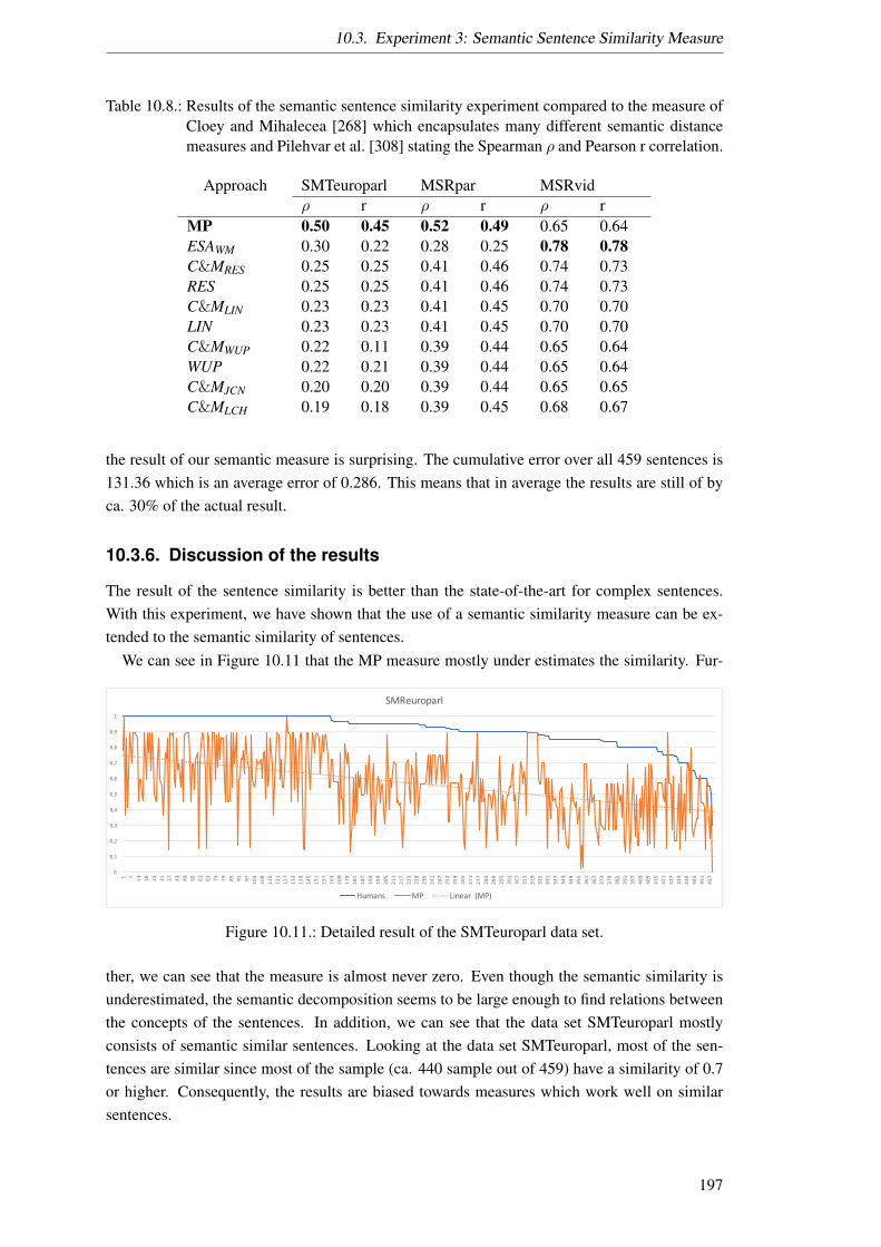
10.3. Experiment 3: Semantic Sentence Similarity Measure

Table 10.8.: Results of the semantic sentence similarity experiment compared to the measure ofCloey and Mihalecea [268] which encapsulates many different semantic distancemeasures and Pilehvar et al. [308] stating the Spearman ρ and Pearson r correlation.

Approach SMTeuroparl MSRpar MSRvidρ r ρ r ρ r

MP 0.50 0.45 0.52 0.49 0.65 0.64ESAWM 0.30 0.22 0.28 0.25 0.78 0.78C&MRES 0.25 0.25 0.41 0.46 0.74 0.73RES 0.25 0.25 0.41 0.46 0.74 0.73C&MLIN 0.23 0.23 0.41 0.45 0.70 0.70LIN 0.23 0.23 0.41 0.45 0.70 0.70C&MWUP 0.22 0.11 0.39 0.44 0.65 0.64WUP 0.22 0.21 0.39 0.44 0.65 0.64C&MJCN 0.20 0.20 0.39 0.44 0.65 0.65C&MLCH 0.19 0.18 0.39 0.45 0.68 0.67

the result of our semantic measure is surprising. The cumulative error over all 459 sentences is131.36 which is an average error of 0.286. This means that in average the results are still of byca. 30% of the actual result.

10.3.6. Discussion of the results

The result of the sentence similarity is better than the state-of-the-art for complex sentences.With this experiment, we have shown that the use of a semantic similarity measure can be ex-tended to the semantic similarity of sentences.

We can see in Figure 10.11 that the MP measure mostly under estimates the similarity. Fur-

0

0,1

0,2

0,3

0,4

0,5

0,6

0,7

0,8

0,9

1

1 7

13

19

25

31

37

43

49

55

61

67

73

79

85

91

97

103

109

115

121

127

133

139

145

151

157

163

169

175

181

187

193

199

205

211

217

223

229

235

241

247

253

259

265

271

277

283

289

295

301

307

313

319

325

331

337

343

349

355

361

367

373

379

385

391

397

403

409

415

421

427

433

439

445

451

457

SMReuroparl

Humans MP Linear(MP)

Figure 10.11.: Detailed result of the SMTeuroparl data set.

ther, we can see that the measure is almost never zero. Even though the semantic similarity isunderestimated, the semantic decomposition seems to be large enough to find relations betweenthe concepts of the sentences. In addition, we can see that the data set SMTeuroparl mostlyconsists of semantic similar sentences. Looking at the data set SMTeuroparl, most of the sen-tences are similar since most of the sample (ca. 440 sample out of 459) have a similarity of 0.7or higher. Consequently, the results are biased towards measures which work well on similarsentences.

197

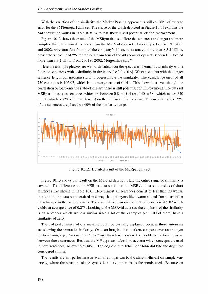
10. Experiments with the Marker Passing

With the variation of the similarity, the Marker Passing approach is still ca. 30% of averageerror for the SMTeuroparl data set. The shape of the graph depicted in Figure 10.11 explains thebad correlation values in Table 10.8. With that, there is still potential left for improvement.

Figure 10.12 shows the result of the MSRpar data set. Here the sentences are longer and morecomplex than the example phrases from the MSRvid data set. An example here is: “In 2001and 2002, wire transfers from 4 of the company’s 40 accounts totaled more than $ 3.2 billion,prosecutors said.” and “Wire transfers from four of the 40 accounts open at Beacon Hill totaledmore than $ 3.2 billion from 2001 to 2002, Morgenthau said.”

Here the example phrases are well distributed over the spectrum of semantic similarity with afocus on sentences with a similarity in the interval of [0.4, 0.8]. We can see that with the longersentence length our measure starts to overestimate the similarity. The cumulative error of all750 examples is 105.97, which is an average error of 0.141. This shows that even though thecorrelation outperforms the state-of-the-art, there is still potential for improvement. The data setMSRpar focuses on sentences which are between 0.8 and 0.4 (ca. 140 to 680 which makes 540of 750 which is 72% of the sentences) on the human similarity value. This means that ca. 72%of the sentences are placed on 40% of the similarity range.

0,1

0,2

0,3

0,4

0,5

0,6

0,7

0,8

0,9

1

1

10

19

28

37

46

55

64

73

82

91

100

109

118

127

136

145

154

163

172

181

190

199

208

217

226

235

244

253

262

271

280

289

298

307

316

325

334

343

352

361

370

379

388

397

406

415

424

433

442

451

460

469

478

487

496

505

514

523

532

541

550

559

568

577

586

595

604

613

622

631

640

649

658

667

676

685

694

703

712

721

730

739

748

MSRpar

Humans MP Linear(MP)

Figure 10.12.: Detailed result of the MSRpar data set.

Figure 10.13 shows our result on the MSRvid data set. Here the entire range of similarity iscovered. The difference to the MSRpar data set is that the MSRvid data set consists of shortsentences like shown in Table 10.6. Here almost all sentences consist of less than 20 words.In addition, the data set is crafted in a way that antonyms like “woman” and “man” are ofteninterchanged in the two sentences. The cumulative error over all 750 sentences is 205.07 whichyields an average error of 0.273. Looking at the MSRvid data set, the emphasis of the similarityis on sentences which are less similar since a lot of the examples (ca. 100 of them) have asimilarity of zero.

The bad performance of our measure could be partially explained because those antonymsare skewing the semantic similarity. One can imagine that markers can pass over an antonymrelation from, e.g., “woman” to “man” and therefore increase the double activation measurebetween those sentences. Besides, the MP approach takes into account which concepts are usedin both sentences, so examples like: “The dog did bite John.” or “John did bite the dog.” areconsidered similar.

The results are not performing as well in comparison to the state-of-the-art on simple sen-tences, where the structure of the syntax is not as important as the words used. Because on

198

10.4. Experiment 4: Semantic Service Matching

0

0,2

0,4

0,6

0,8

11

10

19

28

37

46

55

64

73

82

91

100

109

118

127

136

145

154

163

172

181

190

199

208

217

226

235

244

253

262

271

280

289

298

307

316

325

334

343

352

361

370

379

388

397

406

415

424

433

442

451

460

469

478

487

496

505

514

523

532

541

550

559

568

577

586

595

604

613

622

631

640

649

658

667

676

685

694

703

712

721

730

739

748

MSRvid

Humans MP Linear(MP)

Figure 10.13.: Detailed result of the MSRvid data set.

more complex sentences, the syntactic analysis of state-of-the-art becomes more difficult, theirperformance decreases more than in the MP approach. Also, the words in those examples aremore basic so that they are mostly included in WordNet. This means measures based on Word-Net can perform well on those examples. Since WordNet is mainly hand crafted, this showsthat the quality of our automatically generated information sources for semantic tasks are stillimprovable.

Furthermore, this experiment shows that with a simple extension of the same principle in tokeninformation and Marker Passing algorithm configuration, the problem of sentence similarity isnot yet solved. This leads to the conclusion that further experiments are needed, where themarker information is extended to logical, perhaps syntactical information. In addition to that,the in-, out- and edge-function could make use of this additional symbolic information andfurther improve the results.

Further, we can conclude that the semantic representation of the words making up the sentenceis not enough to represent the meaning described by the sentence. The addition of syntacticinformation thus is necessary to capture the logical content of the sentence. An example of thisis a negation, which could be included in a sentence like: “John did not bite the dog.” With theMarker Passing approach, the negation is not reflected in comparison with, e.g., the sentence:“The dog did bite John.”.

10.4. Experiment 4: Semantic Service Matching

The experiments in Section 10.1, 10.2 and 10.3 showing the applicability of our approach onacademic challenges. To show that our approach can also be used in challenges with more directapplications, we selected service matching as one use case. Service matching describes theproblem of selecting the right service regarding a service request. This shows that our approachcan also be used for more relevant problems in service oriented architectures24. Parts of thissection are published in [101, 102, 103].

Extending the argumentation of Jennings [184], the development of pervasive, complex anddistributed computing systems is ‘one of the most complex construction tasks humans under-take’. Challenges which directly evolve from the pervasive nature of applications are currentlycountered by development paradigms, such as Service Oriented Architectures (SOA) or Agent-

24This section is based on the thesis of Brand [37]

199

10. Experiments with the Marker Passing

Oriented Software Engineering (AOSE), to name but a few. The basic idea of such developmentparadigms is to decrease the level of complexity of programming in dynamic environments.Euzenat and Shvaiko [91] refer to this principle as ‘level of dynamics’. This level of dynam-ics increases the number of details that are left unspecified until the runtime of the application.Applications that we want to put our focus on are those which evolve and subsequently createadditional heterogeneous problems. These problems are mainly due to the many different de-velopers who are involved in the programming, each one making use of individually preferredtechnologies. However, it has been argued that systems with a high level of the dynamic atruntime and a heterogeneous character, should account for so-called self-* properties [346].

Getting services to connect is a hard problem lacking automatization. Even with standards likeXML25 and W3C Recommendation XSD26 or the Semantic Annotations for WSDL (SAWSDL)[205] there is to few formalization to remove all the ambiguity entailed in a service description.This formalization is needed to automize the selection and execution of services, which is neededby dynamic distributed software as we have motivated earlier.

The problem at hand is the selection of a fitting service. The signature of the service matchingproblem is as follows:

ServiceMatching : ServiceDescription× ServiceDescription∗ → ServiceDescription∗

This means given service request and a list of services the list of services are sorted accordingto their fit to the request. We call this kind of algorithm, ranking services to their equivalence toa given request, Service Matcher.

Reasoning algorithms utilized by Service Matchers use different metrics for different aspectsof the service descriptions. One approach is to describe services in four components: Input andOutput parameters, Preconditions and Effects (IOPE) [373] defined in Section 3.2.

Some effort has been made to formalize semantic service descriptions. One of them is metadescription languages we look at in Section 3.2. Such a language is OWL-S [255]. For thelanguage to be less static, descriptions can be enriched with ontologies which structure semanticinformation of the concepts used in such a language [200]. These service descriptions lackcontextual information which makes the information available for interpretation more abstractand context independent [240], with this in mind; the name is semantic service descriptions.

Semantic Service Matchmaking (we call it service matching) formalizes the problem of find-ing fitting services in an academic challenge [200]. The special case of the here extended Ser-vice Matcher is called “Semantic Service Match Maker” (short SeMa2). For more details on theSeMa2, the interested reader is referred to [102].

Figure 10.14 shows an abstraction of how service matching (blue) is described: A ServiceMatcher (here the example of the SeMa2 matcher) gets a request for a service (green) and rates alist of advertising services (white) according to how well they fulfill the request. Here the ServiceMatcher can use a multitude of mechanisms like logical reasoning, metrics about function andnon-function parameters like Quality of service (QoS) parameters or semantic models of theservice interface to analyze the purpose of the service.

Each component of the SeMa2 matcher matches a part of an advertised service description to

25https://www.w3.org/TR/xml/, last visited on 10.09.201726https://www.w3.org/XML/Schema, last visited on 10.09.2017

200

10.4. Experiment 4: Semantic Service Matching

Service

Input Output

Prec Effect1

Service

Input Output

Prec Effect2

Service

Input Output

Prec Effect3

Service

Input Output

Prec Effect4

Request

Output

Effect

SeMa2

0.8

0.7

0.2

0.1

Ontologies

Metrics

Reasoning

Semantics

Figure 10.14.: Abstract Service Matching challenge.

a given request [103]. Here, each part of a service description is analyzed by a so-called expert.This expert provides an opinion about their degree of belief on how well the service requestmatches the service advertisement. Figure 10.14 shows that the request does not describe allparameters of the service, e.g., in Figure 10.14 the request is missing inputs and preconditions.This means that for example there is an expert looking at the service outputs and judging howwell they fit together, but the inputs are neglected. The opinions of the relevant experts are thenaggregated by aggregating experts who take the opinions of other experts and weight themtogether to create their opinion. This could be for example that the “input expert” consolidatethe opinion of an input parameter name expert and a type expert. The first one checks if thenames of the parameter are similar like “StartDate” and the second one checks whether the datatype of the parameter is the same os similar.

We start out by looking at the state-of-the-art in Section 10.4.1. We then continue in Sec-tion 10.4.2 with the description of the Marker Passing experts. Then we specify the data set totest our Service Matcher in Section 10.4.3. The performance evaluation on this data set of ourService Matcher is done in Section 10.4.4. Finally we discuss the results in Section 10.4.5.

10.4.1. State-of-the-Art

In this section, we will look at the state-of-the-art of service matching and analyze how wellthose Service Matchers can be adapted to the domain of use. The goal of this section is toidentify relevant related work on service matching to compare our approach against.

The challenge of service matching is well researched [200]. Further state-of-the-art can befound in [103] and [198]. The here proposed related work has one thing in common: all ServiceMatchers analyze the different aspects of a service description. Therefore, all of them needsome semantic description of the functionality encapsulated in the service. To the best of ourknowledge, there exist only two approaches that utilize machine-learning techniques to cope

201

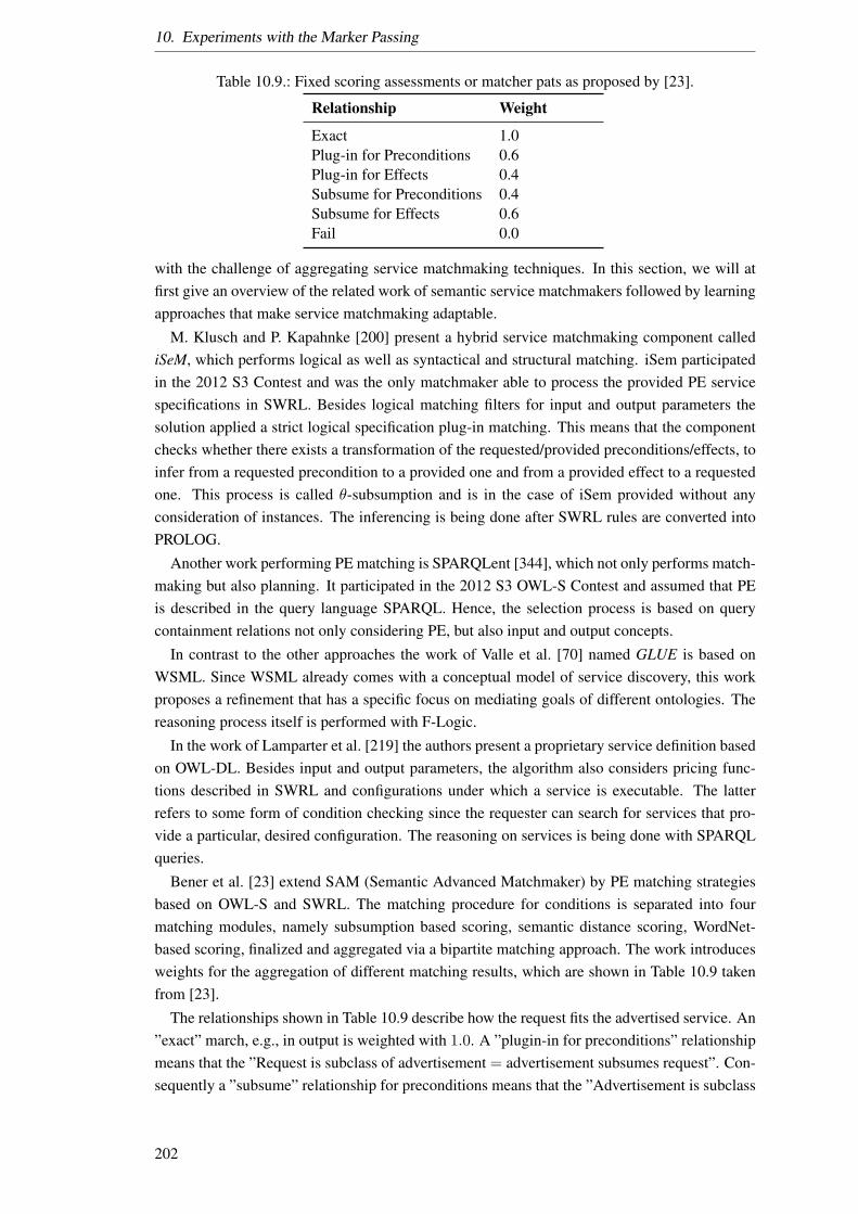
10. Experiments with the Marker Passing

Table 10.9.: Fixed scoring assessments or matcher pats as proposed by [23].

Relationship Weight

Exact 1.0Plug-in for Preconditions 0.6Plug-in for Effects 0.4Subsume for Preconditions 0.4Subsume for Effects 0.6Fail 0.0

with the challenge of aggregating service matchmaking techniques. In this section, we will atfirst give an overview of the related work of semantic service matchmakers followed by learningapproaches that make service matchmaking adaptable.

M. Klusch and P. Kapahnke [200] present a hybrid service matchmaking component callediSeM, which performs logical as well as syntactical and structural matching. iSem participatedin the 2012 S3 Contest and was the only matchmaker able to process the provided PE servicespecifications in SWRL. Besides logical matching filters for input and output parameters thesolution applied a strict logical specification plug-in matching. This means that the componentchecks whether there exists a transformation of the requested/provided preconditions/effects, toinfer from a requested precondition to a provided one and from a provided effect to a requestedone. This process is called θ-subsumption and is in the case of iSem provided without anyconsideration of instances. The inferencing is being done after SWRL rules are converted intoPROLOG.

Another work performing PE matching is SPARQLent [344], which not only performs match-making but also planning. It participated in the 2012 S3 OWL-S Contest and assumed that PEis described in the query language SPARQL. Hence, the selection process is based on querycontainment relations not only considering PE, but also input and output concepts.

In contrast to the other approaches the work of Valle et al. [70] named GLUE is based onWSML. Since WSML already comes with a conceptual model of service discovery, this workproposes a refinement that has a specific focus on mediating goals of different ontologies. Thereasoning process itself is performed with F-Logic.

In the work of Lamparter et al. [219] the authors present a proprietary service definition basedon OWL-DL. Besides input and output parameters, the algorithm also considers pricing func-tions described in SWRL and configurations under which a service is executable. The latterrefers to some form of condition checking since the requester can search for services that pro-vide a particular, desired configuration. The reasoning on services is being done with SPARQLqueries.

Bener et al. [23] extend SAM (Semantic Advanced Matchmaker) by PE matching strategiesbased on OWL-S and SWRL. The matching procedure for conditions is separated into fourmatching modules, namely subsumption based scoring, semantic distance scoring, WordNet-based scoring, finalized and aggregated via a bipartite matching approach. The work introducesweights for the aggregation of different matching results, which are shown in Table 10.9 takenfrom [23].

The relationships shown in Table 10.9 describe how the request fits the advertised service. An”exact” march, e.g., in output is weighted with 1.0. A ”plugin-in for preconditions” relationshipmeans that the ”Request is subclass of advertisement = advertisement subsumes request”. Con-sequently a ”subsume” relationship for preconditions means that the ”Advertisement is subclass

202

10.4. Experiment 4: Semantic Service Matching

of request = request subsumes advertisement”. Those relationships are defined for effects of aservice respectively. The relation ship fail” means no match could be found [23].

The weights, in this case, are fixed and in fact not learned. Furthermore, those weights onlyconcern discrete level of matches.

In conclusion, the described approaches rely on different languages for the description ofconditions ranging from decidable ones, such as OWL-DL and WSML-DL to undecidable ones,such as SWRL, F-Logic, and PROLOG. However, in most of the related work on service match-makers regarding PE matching the undecidable rule languages have been limited in its expres-siveness to guarantee termination. So far, the service matchmakers have included different simi-larity measures and have introduced some weights to model their importance against each other.The weights started out to classify two types of similarity measures and got more detailed to thepoint where different parts of the service description like preconditions and effect are weighteddifferently. These approaches have one fact in common: the choice of the weights are fixed anddo not adapt to the context of use.

To optimize the result of the service matching a learning phase can be introduced to adjustthe parameters of a service matchmaker to the properties of the domain. The parameters to learndepend on the service matchmaker and accordingly its flexibility depends on the parameters thatcan be observed.

In Klusch et al. [199] the authors introduced a formal model of defining weights for the aggre-gation of different similarity measures with the names ww−similarity and ws−structural similaritymeasure. The aggregation method has been learned using a Support Vector Machine (SVM)approach based on training data. The matchmaker component that invokes this approach isdesigned to match SA-WSDL services.

M. Klusch and P. Kapahnke [197] introduce another learning service matchmaker by extend-ing the approach of a prior work [195] for OWL-S service descriptions. Here matching results ofdifferent matching types are aggregated using a weighted mean. The authors introduce differenttypes of matching results that are weighted. Firstly, approximated logical matching, which is di-vided into approximated logical plug-in and subsumed-by matching. Secondly, non-logic-basedapproximated matching, which is text and structural semantic similarity-based signature match-ing. The weights of this aggregation are also learned using an SVM. This supervised learningapproach is replicated in our work, but with a different learning algorithm. The relevance setthat is used to rank the matching results is reused with a genetic algorithm and a hill-climbingsearch.

I extended the winner concerning the average precision of graded relevance of the last servicematching challenge 27 SeMa2 and analyzed its components. Using the same dataset our approachcan be compared to the state-of-the-art of service matches.

The extension of the SeMa2 Service Matcher is described in [102]. Next, we will concentrateon the implementation of the components which implement our approach: the so called MarkerPassing experts.

10.4.2. MarkerPassing Experts

In this section, we will look at how our decomposition and Marker Passing approach can beintegrated into the Service Matcher SeMa2. As a basis for our comparison of service we take

27http://www.dfki.de/˜klusch/s3/s3c-2012-summary-report.pdf, last visited on 10.09.2017

203

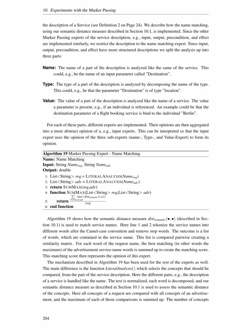
10. Experiments with the Marker Passing

the description of a Service (see Definition 2 on Page 24). We describe how the name matching,using our semantic distance measure described in Section 10.1, is implemented. Since the otherMarker Passing experts of the service description, e.g., input, output, precondition, and effectare implemented similarly, we restrict the description to the name matching expert. Since input,output, precondition, and effect have more structured descriptions we split the analysis up intothree parts:

Name: The name of a part of the description is analyzed like the same of the service. Thiscould, e.g., be the name of an input parameter called ”Destination”.

Type: The type of a part of the description is analyzed by decomposing the name of the type.This could, e.g., be that the parameter ”Destination” is of type ”location”.

Value: The value of a part of the description is analyzed like the name of a service. The valuea parameter is present, e.g., if an individual is referenced. An example could be that thedestination parameter of a flight booking service is bind to the individual ”Berlin”.

For each of these parts, different experts are implemented. Their opinions are then aggregatedinto a more abstract opinion of a, e.g., input experts. This can be interpreted so that the inputexpert uses the opinion of the three sub-experts (name-, Type-, and Value-Expert) to form itsopinion.

Algorithm 19 Marker Passing Expert - Name Matching.Name: Name MatchingInput: String Namereq, String NameadvOutput: double

1: List<String> req = LITERALANALYSIS(Namereq)2: List<String> adv = LITERALANALYSIS(Nameadv)3: return SUMMAX(req,adv)4: function SUMMAX(List<String> req,List<String> adv)

5: return

∑r∈req

maxa∈adv

(distsemantic(r,a))

|req|6: end function

Algorithm 19 shows how the semantic distance measure distsemantic(•, •) (described in Sec-tion 10.1) is used to match service names. Here line 1 and 2 tokenize the service names intodifferent words after the Camel-case convention and remove stop words. The outcome is a listof words, which are contained in the service name. This list is compared pairwise creating asimilarity matrix. For each word of the request name, the best matching (in other words themaximum) of the advertisement service name words is summed up to create the matching score.This matching score then represents the opinion of this expert.

The mechanism described in Algorithm 19 has been used for the rest of the experts as well.The main difference is the function LiteralAnalysis() which selects the concepts that should becompared, from the part of the service description. Here the different parts, e.g., the descriptionof a service is handled like the name. The text is normalized, each word is decomposed, and oursemantic distance measure as described in Section 10.1 is used to assess the semantic distanceof the concepts. Here all concepts of a request are compared with all concepts of an advertise-ment, and the maximum of each of those comparisons is summed up. The number of concepts

204

10.4. Experiment 4: Semantic Service Matching

normalizes this, and the resulting double is the value of the expert’s opinion. The preconditionand effect use Algorithm 19 as well but use the axiom names and parameter names as inputs.The same is done for the input and output parameters of a service.

10.4.3. Data Set

For the evaluation of the Service Matcher we used the OWL-S service retrieval test collection“OWL-S Test Collection” (S3) v428 which consists of 1083 services and 48 queries. This testset has been selected because the state-of-the-art Service Matchers have been tested using thisdataset and by providing our results our approach can be compared to other matchers. Since inthe test collection, the services are described in OWL-S 1.1, and we used the OWLAPI 4.1, wehad to translate the services to OWL-S 1.2. The services are ranked with two kinds of rankingregarding the 1083 services: First, there is a binary rating where a service is either relevant toa query or not. The second part is a graded relevance where a service can be nonrelevant (0),potentially relevant (1), relevant (2) and highly relevant (3).

The S3 is the standard for semantic service matching with OWL-S. The preconditions andeffects of the services are described in the Semantic Web Rule Language (SWRL). To compareour approach to the state-of-the-art, we used this test collection for our evaluation. This use caseutilizes our approach to counter the semi-optimal performance of Service Matchers regardingthe usage of different ontologies in the service description. The performance of the differentService Matcher can found in the results of the Service matching Contest S329. We, therefore,compare our results with the performance of the SeMa2 without the Marker Passing experts.We use the Semantic Service Selection (S3) contest [200, 376] to evaluate our extension of theSeMa2.

10.4.4. Evaluation Results

The comparison of the SeMa2 to the state-of-the-art in service matching is made with the S3contest [200]. With an normalized discounted cumulative gain (NDCG) of 0.927 the SeMa2 wasable to outperform the state-of-the-art. This section, therefore, will compare the Marker Passingexperts to the experts of SeMa2 without the Marker Passing. We compare the performance of theMarker Passing experts to our experts because we do not have data about other implementationsof the state-of-the-art.

We evaluated the performance of the different Marker Passing experts separately on the S3data set to determine for which parts of the service description our approach is applicable. Tobe able to compare the resulting performance of the experts with the other experts of the SeMa2

architecture, we will measure the NDCG to capture how well the similarity of services is es-timated. To evaluate the introduced calculation overhead, we also measure the total executiontime for the data set, the time it takes to evaluate one service advertisement and one servicerequest. The performance of the Marker Passing experts are shown in Table 10.10.

In more details, the Marker Passing expert has been evaluated separately to the other experts.Here we analyze the average time it takes to compare one service advertisement (Avg timeadv)

28http://projects.semwebcentral.org/frs/?group id=89&release id=380, last visited on10.09.2017

29http://www.dfki.de/˜klusch/s3/s3c-2012-summary-report.pdf, last visited on 27.06.2017

205

10. Experiments with the Marker Passing

and the average time it takes to respond to one request (Avg timereq (sec)) as well as the totaltime it took to evaluate all 42 queries (total time (min)).

Table 10.10.: Service Matching results for the Marker Passing expert. The average time for arequest timereq is calculated over the 42 requests of the S3 data set. The averagetime for an advertisement timeadv is calculated for the 1083 service advertisementsof the S3 data set.

Expert NDCG total time (min) avg timeadv (ms) avg timereq (sec)Name 0.819 8.12 34 10.7Description 0,844 39.71 320 55.88Input 0.521 4.177 36 5.03Output 0.717 4.23 33 5.30Precondition 0.628 4.43 34 5.44Effect 0.877 4.82 33 6.03

In Table 10.10 the correlation between execution time and input size can be seen as the resultof the description expert: A description consists of one or more sentences, which consists ofmore concepts than a service name or an input description. This is reflected in the averageresponse time per request, which is ca. 56 seconds for the service description and only 10seconds for a service name. In comparison to the other experts (shown in Table 10.11) theyperform well, but with more time consumption.

When compared to the performance of the Marker Passing in comparison to the reasoningmechanisms of the SeMa2 in its functional matching parts shown in Table 10.11 the MarkerPassing can outperform the name, description and effect parts. Since the ”Text Similarity” expertcombined name and description similarity, the evaluation with the Marker Passing experts ismore detailed.

Table 10.11.: Service Matching results for the experts without Marker Passing. The averagetime for a request timereq is calculated over the 42 requests of the S3 data set.The average time for an advertisement timeadv is calculated for the 1083 serviceadvertisements of the S3 data set.

Expert NDCG total time (min) avg timeadv (ms) avg timereq (sec)Text Similarity 0.814 3.78 35 4.46Input 0.793 3.89 34 4.66Output 0.756 3.73 33 4.45Precondition 0.635 4.4 39 5.26Effect 0.565 4.06 38 4.82

From Table 10.10 and 10.11 we can see that the overall performance depends on the semanticinformation available to the approach. Where the Marker Passing is outperformed, we can seethat the reasoning on, e.g., the input and output type beats the semantic information solely givenby the input itself. If we analyze the structure of inputs, it is defined by its type and the variablename. The variable name can be something like “arg0” or “var1”, and the type can be somethinglike “books.owl:Title.” This reduces the semantic information available for the Marker Passingto be analyzed.

A surprising result is the effect analysis. Here the intuition was that the logical reasoning

206

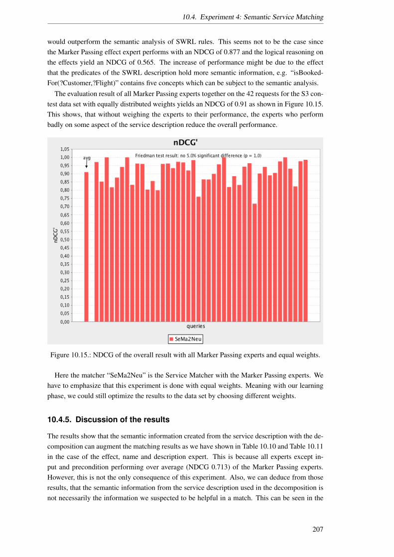
10.4. Experiment 4: Semantic Service Matching

would outperform the semantic analysis of SWRL rules. This seems not to be the case sincethe Marker Passing effect expert performs with an NDCG of 0.877 and the logical reasoning onthe effects yield an NDCG of 0.565. The increase of performance might be due to the effectthat the predicates of the SWRL description hold more semantic information, e.g. “isBooked-For(?Customer,?Flight)” contains five concepts which can be subject to the semantic analysis.

The evaluation result of all Marker Passing experts together on the 42 requests for the S3 con-test data set with equally distributed weights yields an NDCG of 0.91 as shown in Figure 10.15.This shows, that without weighing the experts to their performance, the experts who performbadly on some aspect of the service description reduce the overall performance.

Figure 10.15.: NDCG of the overall result with all Marker Passing experts and equal weights.

Here the matcher “SeMa2Neu” is the Service Matcher with the Marker Passing experts. Wehave to emphasize that this experiment is done with equal weights. Meaning with our learningphase, we could still optimize the results to the data set by choosing different weights.

10.4.5. Discussion of the results

The results show that the semantic information created from the service description with the de-composition can augment the matching results as we have shown in Table 10.10 and Table 10.11in the case of the effect, name and description expert. This is because all experts except in-put and precondition performing over average (NDCG 0.713) of the Marker Passing experts.However, this is not the only consequence of this experiment. Also, we can deduce from thoseresults, that the semantic information from the service description used in the decomposition isnot necessarily the information we suspected to be helpful in a match. This can be seen in the

207

10. Experiments with the Marker Passing

difference of performance for the input and output. However, we can see in Table 10.10 that theoutput experts outperforms the input experts.

The here introduced Marker Passing experts measure the semantic similarity of the wordsused to describe the different parts of the service description. These experts do not guaranteethat a service can be replaced by another one since the logical truth value of precondition andeffect are not evaluated. Neither does the Marker Passing expert analyzing the description, usesyntax on the description. Therefore it is unable to determine exact details of the descriptionslike, e.g., negation.

The evaluation of the matching performance shown in Table 10.10 can be seen as an indicationof the fact that humanly created service descriptions use natural language and that the hereencoded information can be useful for finding similar services. The overall performance of anNDCG of 0.91 shows that there is still performance optimization necessary. This optimizationcan be done by selecting the right weights for the Marker Passing experts, or by integrating theMarker Passing experts into logical experts.

In this experiment, we have pragmatic interpretations of the concepts used in a service descrip-tion. Because of the markers set to additional concepts (e.g., on advertisement side), differentconcepts in a semantic graph get activated. Meaning like depicted Figure 3.9, we can interpretconcepts in a context dependent manner. Consequently, having a conception of the conceptsmaking up the service. In the service matching experiment, the effect is, that for different ad-vertisement the concepts of the request are connected differently, and with that markers mightpass over other word senses, or other relations creating a context dependent interpretation of theconcepts.

In conclusion, the results speak for the use of some ontology matching since we could useour approach on semantic decomposition and Marker Passing to increase the performance ofthe semantic service matchmaking. Future work could be the combination of Marker Passingexperts with other experts, e.g., where they perform better. This combination could be the casein the input- and output-Expert since the Marker Passing experts here perform less well than thenon-marker passing experts. From matching one request to decide which service is suitable tobe used in a plan will be the topic of the next section, where we extend the semantic analysis ofservice descriptions to create a semantic goal oriented heuristic.

10.5. Experiment 5: Heuristics in AI Service Planning

This section describes the experiment on the creation of a heuristic for service planning. Withthis experiment, we are going to use some of the results established earlier like our semanticsimilarity measure and the semantic sentence similarity measure. The goal of this section isto create a semantic heuristic which takes into account the start and goal state as well as thesemantic service description. Consequently, this section defines what we see as our extension tothose heuristics and which properties of heuristics are important for our approach.

We see a heuristic as a relaxed problem solution, which can estimate the usefulness of anaction to a given goal. Pearl [304] describes a heuristic as “rule of thumb to guide one’s search.”Russell and Norvig [337] describe a heuristic as a function “h(n) guessing the cheapest cost ofa path from node n to a goal node.” This means that a heuristic is a function: H(n) : State →Double

The function H(n) maps a node to the length of the path to the goal. This notation shows how

208

10.5. Experiment 5: Heuristics in AI Service Planning

static heuristics are: Their heuristic does not need the goal as an input, because, the goal is fixedin the heuristic and cannot change. The heuristic is therefore primarily designed for one goal.Ghallab et al. [134, p. 199] describe such a heuristic as “node selection heuristic” which selectsthe node n with the minimal heuristic value H(n).

To create a heuristic we are going to look at the state-of-the-art in Section 10.5.1 We then arguewhy those heuristics need to be created at runtime and how this could be done in Section 10.5.2and analyzes then search problems and their properties in Section 10.5.3. With that, we candescribe an abstract approach on how to use this information to create a heuristic for serviceplanning in Section 10.5.4. After that, we analyze the information available to the heuristiclike the service description and the start- and goal-state, in Section 10.5.5. Then we look at thecontextual information and analyze how pragmatic our heuristic could become in Section 10.5.6.Afterwards, we can describe our algorithm calculating our heuristic in Section 10.5.7. Then weselect a data set which allows us to evaluate our heuristic in Section 10.5.8. The performance ofthe so created heuristic is thereafter evaluated in our experiment described in Section 10.5.9.

10.5.1. State-of-the-Art

In this section we want to find heuristics for AI planning to which we can compare our heuristic.Sometimes the heuristic and the search used are entangled. One example could be greedy search.We will analyze entire classes of heuristics if possible (e.g., greedy heuristics) to describe theirproperties. The goal of this section is to find heuristics which use as much semantic informationas possible, by staying usable for general purpose planning.

Additionally, we want to gain insight into how general purpose heuristics are created. Thatsupports the ability to describe our heuristic appropriately and makes our design decisions un-derstandable. This means taking heuristics build for optimization problems and adapt them towork on our non-optimization problem. In other words, we reformulate our nonoptimizationproblem in a way, that we can adapt these heuristics for optimization problems.

The state-of-the-art of heuristics is twofold [341]: One part is well researched and theoreti-cally founded. This part is concerned with the properties of heuristics and the abstract searchmethods like A∗ [304]. The other part is concerned with domain specific problem solving likethe research of Hyper Heuristics and Meta Heuristics. These approaches try to find heuristicsby combining old ones with machine learning approaches or optimizing hyper parameters. Thesecond part can again be classified into the following categories [341]:

Deterministic vs. stochastic: Deterministic means that the heuristic returns the same out-put for the same input. Stochastic means that this is not the case, like when using randomwalks to search the state space.

Parallel vs. one solution at the time: Parallel means that the heuristic returns multiple so-lutions at the same time like in populations of genetic algorithms. Other heuristics justreturn one solution.

Fast vs. powerful: Fast heuristics provide less information about the problem but save re-sources. Powerful heuristics provide more insight but use more resources.

Classical vs. modern: Classical heuristics are problem specific and use, e.g., abstraction,landmarking, cost clusters or problem relaxation. Modern heuristics are Hyper- and Meta-

209

10. Experiments with the Marker Passing

Heuristics which use the combination of classical heuristics and machine learning to selecttheir parameters.

We will have a look at all of those categories of heuristics, concerning the use of semanticinformation and the domain independence. Afterwards, we will classify all the here discussedapproach according to these categories. This is done because we want a powerful heuristicswhich is not stochastic and uses as much semantic information as possible. Why we do not wantstochastic approach is explained in Section 10.5.2. Since service planning is not an optimizationproblem, we want our heuristic to find one possible solution as fast as possible, and we are notinterested in parallel solutions.

Since we are looking for heuristics in non-optimization problems, this section focuses on thestate-of-the-art of heuristics which can be applied in general purpose planning and do not neces-sarily need an optimization problem. Planning as a non-optimization problem is one particulartype of planning. An overview of different planning problems can be found in [133, 222, 266].

Heuristics are needed if a problem is too hard to solve, and therefore an approximate solutioncan suffice [341], where heuristics can be seen as an approximation solution for such problems.Heuristic search is a fundamental methodology in problem-solving for hard AI [206]. Heuristicsearch means analyzing the abstraction of a search for a solution, by solving a similar but lesscomplicated problem [34].

One way to create a heuristic is by relaxing the original planning problem [34]. One examplerelaxation is to ignore the negative effects of an action. In the language PDDL, this meansignoring the delete list of the effect of an action. Delete relaxation is a quite simple way ofcreating domain independent heuristics. The drawback is that we need to know which negativeeffects of an action are. In the case of planning with services, we do not know which effects arenegative.

Another way to create heuristics is by abstracting the problem at hand automatically [202].The idea is that we abstract the problem from a so called ground-level problem to a simpler tosolve the abstract-level problem with fewer details. Abstraction in the sense of Knoblock [202]is to remove some facts from the description languages of the problem and with that makingthe problem easier. This abstraction assumes that ”[t]he existence of an abstract-level solutionimplies the existence of a ground-level solution.” (this is called the Downward Solution Property)[202, p. 54]. An example of such an abstraction is, e.g., if we want to plan a journey we canabstract from which exact airplane we plan to book, and rather plan the journey with its stopsand how long we want to stay at each stop. This plan can be concretized to actual flights lateron. Of course, there is the probability that there are no fitting flights for our abstract plan and inconsequence, no plan can be found. Accordingly, the abstraction works only in problems wherethe Downward Solution Property holds.

Planning problems present many dead ends in the search space, ignoring facts like the deletelist of effects results in bad planning performance [163]. Translation to a SAS+ problem30

restricts the search space and allows a mechanism to prove when tasks are unsolvable. That canbe used for dead end detection. Because the effects of a service might depend on the input andcould be entangled, a service cannot simply be split up unto N services which each having justone effect. Thus this is not an applicable approach.

30In SAS+ each service has, e.g., only one effect.

210

10.5. Experiment 5: Heuristics in AI Service Planning

Greedy Algorithm

A greedy algorithm has a selection strategy (heuristic) which selects the best next possible move(for use service to add to the plan). We see a greedy heuristic as a heuristic, which selects thebest fitting service first. Since greedy algorithms are a general class of algorithms, we specifywhat we mean by ”best fitting service” next.

Greedy algorithms describe a best first search graph traversal algorithm. Here each node ismarked with a heuristic value regarding its path length to the goal state. The successor functiongets the next best state, for which the successors are part of the frontier. From this new frontier,we select the next best state. The successor function for a nonoptimization problem has beenselected to be the overlap of facts in the state with the facts in the goal state. This means that thealgorithm is greedy, because it selects those services first, which fulfill more facts of the goal.

This kind of heuristic has the drawback that no looking-ahead is taking place. That meanschoosing what is best in a current state might be suboptimal for following states. In consequence,greedy algorithms do not always find an optimal solution. In other words: the choice of everylocal optimum in one state does not guarantee a global optimum.

A* Algorithm

Evolved from the greedy approaches, the A∗ algorithm overcomes some of the drawbacks of thesimpler “take the best fit first” heuristics [338]. The A∗ algorithm can still be seen as a greedyalgorithm but with the difference that it uses an additional informative function which allows itto decide better how a greedy option is affecting the global optimum. This informative functionsums up the cost of the path so far from the start state to the current state. The cost function ofthe A∗ algorithm is, therefore, the cost function displayed in Equation 10.16.

f (x) = g(x) + h(x) (10.16)

In Equation 10.16 g(x) represents the cost of the path through the search space so far to nodex and h(x) the heuristic value of node x. A∗ has some interesting properties one of them beingthe optimality guarantee of the solution of the heuristic h(x) is admissible: A∗ finds the optimalsolution if guided by a monotonic heuristics [304, Theorem 10].

There are further properties of heuristics which can be analyzed:

Completeness is the property of a heuristic if it finds a solution when a solution exists. By asolution, we define a path in the search space from state to goal state.

Dominance is the property of a heuristic H1 compared to a heuristic H2 if H2 extends all nodesin the search space that H1 expands. Thus H2 does at least evaluate the same node as H1.

Optimality is the property of a heuristic H1 if it dominates all heuristics of a certain class HC.Then we call H1 optimal over the class HC of heuristics.

There are additional properties of heuristics which allow proving optimality for certain searchstrategies using a heuristic with those properties. We will now list those properties and explainthem:

211

10. Experiments with the Marker Passing

Admissibility: A heuristic h is admissible if

h(n) ≤ C(n), ∀ n (10.17)

where C(n) is the minimal cost of the path n to the goal [304].

Consistent: A heuristic h is consistent if

h(n) ≤ c(n, n′) + h(n

′), ∀(n, n

′), (10.18)

with c(n, n′) is the cheapest cost of the state transition from nodes n to nodes n

′.

Monotone: A heuristic h is monotone if

h(n) ≤ c(n, n′) + h(n

′), ∀(n, n

′) | n′ ∈ successor(n), (10.19)

where successor(n) denotes all nodes which are successors to n towards the goal.

With those properties, we can prove that, e.g., all consistent heuristics are admissible [304,Theorem 9 p. 83] or that the search algorithm A∗ finds an optimal solution if it uses an admissibleheuristic [304, Theorem 2 p. 78].

Admissibility is solely concerned with the quality of the out coming solution. However, inmost problems, the best solution is not the only acceptable one. By looking for the best solutionsearch strategies like A∗ waste resources on evaluating many solutions which are semi-optimalon the way to find the best solution. By leaving the restriction of optimality the admissibility andmonotony of a heuristic can be relaxed as well. This requires more general search mechanismsthan an A∗ [69] or the best first search [304, Section 3.3].

Lipovetzky and Geffner [236] extend the heuristics by a width-based exploration if the heuris-tic reaches a plateau. A heuristic plateau is given when in the search a set of service executionsdoes not get closer to the goal state. Lipovetzky and Geffner shorten such plateaus by adding awidth based search to the heuristic, by adding a novelty measure to the state. States with newfacts meaning which differ more from the current state are visited first. The LAMA System[326], e.g., uses multiple heuristics to overcome this problem. Both approaches are not satis-fying because they do not use information about the problem to speed up the search but usestatistical improvements to speed up the search.

Redavid et al. [323] describe how service composition can be done by implementing plancontrol structures with OWL-S. Redavid et al. describe how rules in SWRL can be combinedand propose a control structure on how they can be ordered. They create an “SWRL rules plan”by creating all possible rule combinations to fulfill the goal (the goal is formulated in SWRLatoms). The focus of this work lies in the description of service composition using OWL-S aslanguage. The result is some kind of semantic heuristic because the SWRL rules are combinedwithout variable binding. To explain, the resulting graph of connections between effect andprecondition can be used to speed up the search for a plan. But here the approach neglects thevariable binding and with that cannot produce an executable plan.

Srivastava and Kambhampati [367] separate the planning task into planning and scheduling.This separation leaves the planner with the task of finding all relevant services and gives thescheduler the task of bringing them in a specific order. This separation of tasks results in an

212

10.5. Experiment 5: Heuristics in AI Service Planning

abstraction of the problem in both parts: the planner does not have to care about the order ofthe services, relaxing the planning problem. The scheduler gets all relevant actions and theirinterdependence and needs to find a fitting schedule. Depending on the execution resources andthe planning this approach might create plans which cannot be scheduled, and for that reason,fails to find a solution at all. If the planner checks for the schedulability of his plan, then theapproach cannibalizes itself.

Since the example application of this thesis is the creation of heuristics for service planning,we have to look at alternative solution possibilities for the domain and problem independentcreation of heuristics.

The other approach of guiding the search through the state space is called landmarking [190].In landmarking known plans are analyzed, and services call these which have most in commonand marke them as landmarks. The landmarks, e.g., present states, have to be passed to find asolution. Sometimes the landmarks can be brought into an order [172]. Landmarks are factswhich must be true on the way of reaching a goal. The two sub problems of landmarks are:How to find landmarks, e.g., [310] and how to use the information given by a landmark to createa heuristic, e.g., [426]. These landmarks then can be used to decompose the search problemand use a local search to search from landmark to landmark [190] iteratively. The problem withlandmarking heuristics is that the problem we want to solve has to be solved already to createlandmarks. Because we want to create heuristics, which can be provided for the first time aproblem is solved; landmarks are merely an optimization to our approach later on.

The state-of-the-art in general heuristics for planning problems is limited. The main Confer-ence on AI planning and heuristic search is the International Conference on Automated Planningand Scheduling (ICAPS) / Conference on Artificial Intelligence Planning Systems (AIPS) [1].Here starting from 1990 the last 27 years the community of AI planning has to discuss the dif-ferent approaches to problem solving31. Here multiple specializations of the general planningdomain have been identified. This leads to a classification of planning problems described inSection 3.3.

A common approach on heuristics creates an evaluation function through combination of theheuristic and the path cost [125] like described in Equation 10.16 on Page 211. With h(n) ≥ 0

is the heuristic function (see Section 10.5.1 for more details). If h(n) = 0 the search is callednot informed. The function g(n) represents the cost of the path from the start state to the currentstate. In our example in Figure 10.19 for our current state (blue) g(n) is 0.7. Korf [206] proposesa real time A∗ which, e.g., takes the distance from the current state to node n as g(n). In thisway the real time A∗ is relative to the current state, and once the planning algorithm leaves theinitial state, every evaluation function is relative to the current state. With this, the real time A∗

becomes more like a best-first search which is semi optimal because the heuristic is almost theonly guidance through the search space.

Nilsson et al. [285] argue that the cost of the path might be ignored since we are interested in asolution, not a cost effective solution. The purpose of the heuristic is then to speed up the searchfor a solution, not to guarantee an optimal solution. There are heuristics like the minimum stepcount to the goal which is called a uniform action cost [304]. These heuristics are equal to thestep count if an action cost is equal to 1 [194]. With the uniform cost function of 1, the heuristicis admissible since it predicts that the next action is always only one step from the goal. Anadmissible heuristic is sometimes also called “optimistic”.31See www.icaps-conference.org for the proceedings. Last visited on 10.09.2017

213

10. Experiments with the Marker Passing

Greedy heuristics are those which count the overlap of the effect of a service to the goaland hence the usefulness of a service is how much of the goal it achieves [125]. Such a greedyheuristic is a quite simple heuristic which performs well, regarding its calculation effort. Thesearch traverses the states by looking first at states which are similar to the goal.

As a baseline we use a random heuristic to get a lower bound on the problem. The ran-dom heuristic assigns each action a random usefulness in the interval [0, 1] for any state. Sucha baseline is needed because it is not possible to compare the here created results to results ofplanning competitions. The different nature of a STRIPS-like planning problem without seman-tic and service planning addresses the problem of a search for a plan in different ways. Classicalplanners are highly optimized to solve problems like the 15-puzzle [322] or the four-peg towersof Hanoi problem [207].

Haslum and Geffner [158] describe a greedy heuristic which they derive from STRIPS plan-ning problems, where they ignore the delete list of a service effect and add only the add list to thecurrent state to create a new state. This heuristic creates a relaxed planning problem compared tothe original problem. The relaxed problem can show which services are minimally needed andthen shows which items of the delete list of the used services need to further resolution. With therelaxed problem, the heuristic counts as a greedy heuristic since the search executes the serviceswith the most overlap of their add list and the goal, first. This heuristic is admissible and is ap-plicable for all STRIPS planning problems. Planners using such a search are sometimes calledFast-Forward-planners (or short: FF-planners). FF-planners are the basis of the most successfulplanners according to the International Planning Competition [164].

Another relaxation heuristic is the forward chaining heuristic proposed by Sierra-Santibanez[359]. Here services are rated “Good(a,s)”, “Bad(a,s)” or “Better(a,b,s)”. Good means here anoptimal service a in state s. Bad services cannot be part of an optimal plan. The annotationbetter creates a partial order among the services. These ratings are generated manually by socalled “action selection strategies” and are very problem-specific.

The approach of Haslum et al. [158] has been extended by an optimization in which abstrac-tion of the effects called Patterns [157]. Those patterns are then subtracted from each effectand the start and goal state, creating abstract states which are mapped to the state space throughthese patterns. The patterns represent sub problem of the original planning problems, which arealready solved. A pattern is a set of variable assignments which reoccurs in different states, e.g.,the start and goal state, creating homomorphism abstractions. The drawback of those PatternDatabase Heuristics (PDB) is that they do not scale up to real world problems [191].

The approach of Katz et al. [191] again optimizes the result of [157] by adding a CausalGraph structure and the Domain transition graph to the PDB heuristics. By including thecausal graph, Katz et al. can create “causal graph structural patterns”, which approximatesthe original problem but are more abstract. This abstraction is done on SAS+ formalizationof the planning problems [13] which has an additional restriction for the domain descriptions.The simplification SAS+ has the effect that abstractions like those done by Katz et al. [191]are possible. Here, e.g. “Post-uniqueness” means that an effect is only given by at most oneaction. Additionally, the “Binariness” restriction demands that all state variables have exactlytwo possible values. With an open world assumption and a distributed service development, wecannot fulfill those limitations, so these results cannot apply to our problem.

Learning the domain structure by observing plans is still subject to research [150]. HereGregory and Lindsay [150] propose a model of action cost, which learns through the observation

214

10.5. Experiment 5: Heuristics in AI Service Planning

of plan traces. Even though the resulting cost function can be used as a heuristic, its creation,the observation of executed plans, puts this heuristic into the runtime. This interleaving of aplan- and runtime is out of scope for this work because we want to study the understandingof services and measure the degree of understanding by their use in a plan, not the other wayaround. Despite this being a valid approach, the idea is a trial and error mechanisms of learningthe usefulness of services, because the services have to be executed to see if the plan succeeds.For certain services, e.g., indeterministic services, this might be appropriate, but we restrict ourdomain to planning problems where deterministic action are analyzed.

The same argument can be applied to approaches learning other planning properties thanplan optimality [284]. The research of Marinescu and Coles [253], for example, is focused onheuristic creation in uncertainty with numerical effects, which we neglect here.

Using landmarks for creating a heuristic is done for instance, in the LAMA planner formRichter and Westphal [325] which performed well in the IPC 2008 [190]. Landmarks are usedas a heuristic by Richter through counting fulfilled landmarks in contrast to unfulfilled ones[325]. In [325] Richter et al. combine this greedy heuristic search with landmarks with preferredoperators, which take into account the usefulness of services by keeping them in a “preferred-operator queue”. Those preferred operators are in consequence always tried first. Here a constantvalue of 1000 is added to the heuristic value of the service if it is a preferred one. Deciding whichservice is preferred, is part of the heuristic. Here again, the problem is formalized as a SAS+

problem, which lets Richter et al. decide which service is a landmark (because its effect isunique). This is not given in our planning problem. In consequence, this kind of heuristic needsadaptation to be able to function with, e.g., the open world assumption.

Two research areas which analyze the automatic creation of heuristics are called Hyper-Heuristics and Meta-Heuristics. We will look at both of these research areas with the focus onunderstanding the underlying mechanism, which leads to the creating of a heuristic. The goalof this analysis is to extract ideas on how heuristics are adapted to the specific problem and howthe needed information for the abstraction of a problem is found.

Hyper-Heuristics

Hyper-Heuristics can be seen to have the goal to automate the generation of heuristics. Mostapproaches do this by using some machine learning. The motivation here is to be able to gen-erate more general search strategies to solve hard computational problems [40]. The basic ideabehind Hyper-Heuristics is to use machine learning methods on a set of heuristics to generate aproblem-specific heuristic. Burke et al. [40] separate the Hyper-Heuristics into two parts: heuris-tic selection and heuristic generation, which both are again separable into constructive heuristicsand perturbative heuristics. Constructive heuristics start with an empty set of solutions and addnew solutions until the problem is solved. Here the optimization is on selecting the best solu-tions to add. Perturbative heuristics start with a solution and optimize this solution by usinglocal search and some optimization to improve the quality of the solution.

The drawback of Hyper-Heuristics is that the selection and generation of heuristics out of aheuristic part needs an learning phase. This learning phase forces us to create test examples ofour problem or to optimize the heuristic during execution of the planning and the execution ofthe plan to create a feedback for the learning and selection components of the Hyper-HeuristicApproach.

215

10. Experiments with the Marker Passing

Meta-Heuristics

Meta-Heuristics sample a search space and optimize a heuristic to fit a problem-solving approach[27]. Here methods like stochastic optimization can be used to search through possible parametersets of a heuristic to generate a sufficiently accurate heuristic for a given problem. For theoptimization to work the Meta-Heuristic algorithms need a reward signal to be able to search thespace of possible heuristic parameters. An overview of Meta-Heuristics sorted by the problemor machine learning approach can be found in [298, 391].

The drawback of the Meta-Heuristics approach is that it needs a learning phase, where the out-come of the underlying problem is needed to be able to optimize the parameters of the heuristics.For our problem in AI planning, this means we need a learning phase, where we monitor planexecution or learn on old plans to create a Meta-Heuristic. Solving a problem finally becomesonly better if the problem is already solved. The second argument against this kind of optimiza-tion is that it is done without the semantic knowledge and still can be improved by the selectionof the right samples of the search space.

Conclusion

We now can conclude that building a heuristic is often problem-specific. Creating problem-specific heuristics has the benefit of having highly specific and performant heuristics. The draw-back is their lack of generalizability. The approaches like Hyper- and Meta-Heuristics can createmore abstract heuristics from special ones by using machine learning. Meta-Heuristics have thebenefit of not having to design a heuristic but have the drawback that they introduce a learningphase.

As a conclusion, the state-of-the-art in the heuristic generation bases its approach mainlyon the relaxation, abstraction, and landmarks of an original problem. Some of them use thedomain description to structure the search space; others analyze services to identify landmarks,which help to break down the search problem. However, no heuristic found so far has usedthe semantics of the planning problem. The lacking use of semantics can be explained withthe academic community of AI planning, which is mostly concerned with academic problemsformulated in PDDL, which do not have a semantic description. This fact reflects in the datasets available for example planning problems discussed next32.

The result of this state-of-the-art analysis is that we will compare our approach to a randomheuristic to have a baseline for the search space, the uniform action cost heuristic and the greedyheuristic.

Table 10.12 lists the here looked at approaches from the view of the classification proposed bySalhi [341]. Some of the listed elements are entire classes of approaches, which are discussedearlier in this section. If an approach might fulfill properties or some of the approaches of a classdo, and some do not, then we set the check mark in parentheses.

None of these approaches use semantics of the domain and problem description to create amore informed heuristic. Most of the approaches do not even use the semantics of the state, pre-condition or the goal to select services which could be of interest. The relaxation technique tocreating heuristics additionally needs to decide which facts to ignore from the domain descrip-tion of the planning problem. If we neglect the wrong ones, then the problem does not fulfill

32The interested reader is reflected to the international planning competition: http://www.icaps-conference.org/index.php/Main/Competitions, last visited on 24.07.2017

216

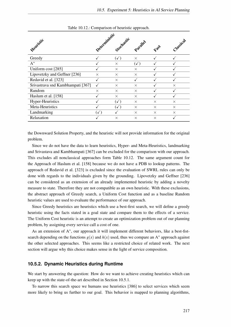
10.5. Experiment 5: Heuristics in AI Service Planning

Table 10.12.: Comparison of heuristic approach.

Heuris

tic

Determ

inistic

Stochast

ic

Parall

el

Fast Classic

al

Greedy X (X) × X XA∗ X × (X) X XUniform cost [285] X × × X XLipovetzky and Geffner [236] × × × X XRedavid et al. [323] X × X X XSrivastrava snd Kambhampati [367] X × × X ×Random × × × X XHaslum et al. [158] X × × X XHyper-Heuristics X (X) × × ×Meta-Heuristics X (X) × × ×Landmarking (X) X × × ×Relaxation X × × × X

the Downward Solution Property, and the heuristic will not provide information for the originalproblem.

Since we do not have the data to learn heuristics, Hyper- and Meta-Heuristics, landmarkingand Srivastava and Kambhampati [367] can be excluded for the comparison with our approach.This excludes all nonclassical approaches form Table 10.12. The same argument count forthe Approach of Haslum et al. [158] because we do not have a PDB to lookup patterns. Theapproach of Redavid et al. [323] is excluded since the evaluation of SWRL rules can only bedone with regards to the individuals given by the grounding. Lipovetzky and Geffner [236]can be considered as an extension of an already implemented heuristic by adding a noveltymeasure to state. Therefore they are not compatible as an own heuristic. With these exclusions,the abstract approach of Greedy search, a Uniform Cost function and as a baseline Randomheuristic values are used to evaluate the performance of our approach.

Since Greedy heuristics are heuristics which use a best-first search, we will define a greedyheuristic using the facts stated in a goal state and compare them to the effects of a service.The Uniform Cost heuristic is an attempt to create an optimization problem out of our planningproblem, by assigning every service call a cost of one.

As an extension of A∗, our approach it will implement different behaviors, like a best-fist-search depending on the functions g(x) and h(x) used, thus we compare an A∗ approach againstthe other selected approaches. This seems like a restricted choice of related work. The nextsection will argue why this choice makes sense in the light of service composition.

10.5.2. Dynamic Heuristics during Runtime

We start by answering the question: How do we want to achieve creating heuristics which cankeep up with the state-of-the-art described in Section 10.5.1.

To narrow this search space we humans use heuristics [386] to select services which seemmore likely to bring us further to our goal. This behavior is mapped to planning algorithms,

217

10. Experiments with the Marker Passing

by defining problem-specific heuristics like the Manhattan distance [78] (for more details onheuristics see Section 10.5.1). Those heuristics are selected for specific problems estimatingthe distance of every state to the goal. Classically finding the right heuristic is done during theproblem specification.

In a dynamic environment, where services and the goal are not known during design time, thisapproach fails, because fitting heuristics cannot be created during design because the servicesand the goal are unknown during design time. One possible approach is to create heuristicsduring runtime, taking into account the available services and the goal state. Both parts canchange and above all need a mechanism for interpretation. Consequently, the problem of creat-ing heuristics can be seen to be at least threefold:

Goal dependence: The goal is unknown during design time. Creating a heuristic whichcorrectly estimates the usefulness of a service makes it necessary to know the goal.

Service interpretation: The available services are not known during design time. Using onlythe services which are known at design time, would reduce the adaptability of our agentto changing environments where services appear or disappear. If all needed services areknown at design time, the developer can integrate them into a heuristic. At run time there isno developer. Therefore an explicit description of what the service does is required. Beingable to include unknown services the interpretation of service descriptions is needed.

State/Context awareness: For general purpose planning to be an appropriate approach theproblem and its rules are not known during design time. Hence the agent must be ableto integrate unknown concepts into its knowledge representation to be able to reason withthem. This allows the heuristic to adapt to changing problems and contexts.

Because it is difficult to pass all domain knowledge to the run-time by the developer, or ser-vices out of other domains might appear during runtime, the interpretation of domain knowledgehas to be extendable during runtime.

As a result, there are three main tasks before we can create a heuristic measure of the useful-ness of a service: the interpretation of goal, service, and context. We assume that these threedescriptions are again made up of semantic concepts which allow our interpretation. The agentcreating the heuristic for that reason needs to explain unknown concepts of those descriptions toitself. For this, the service description can contain the information needed, or the agent needs tocreate this information. What we want a service to have, is: A self-explanatory description pro-viding all information necessary for a reasoner in a given context. This includes self-describingservices like discussed in Oake et al. [290].

These self-explanatory descriptions can be created in two ways: The description providesall the needed information to the receiver, or the receiver adds this information. The first onewe call the activity to self-explain: Self-explanation identifies the process when an agent givesinformation about itself and its functionalities to other agents or human beings.

During design time we can create the service description and change which information itcontains. Indeed, we can include contextual information into the description giving the agentthe ability of self-explanation.

How such self-explanatory descriptions can be created and how development tools can helpcreate them, is described in [101]. Regarding the self-explanation, we have done some engineer-

218

10.5. Experiment 5: Heuristics in AI Service Planning

ing work on providing tools to ease the semantic description of services. For a summary of thesetools see Section A.1.

With such a tool chain it becomes easier to develop self-explanatory descriptions. Neverthe-less, some problems remain: At design time we cannot foresee all the possible uses of a servicenor the contexts the service is used in. The interpretation of service descriptions can be differentthan the intended service the developer wanted to create. Looking at the travel domain again,wanting to go from A to B could include the service of an ambulance, e.g., if B is the locationof a hospital. This might not be intended by the service provider, but describing an ambulanceservice a travel planning agent could interpret the service in this way.

This makes the ability to understand new concepts in new contexts still necessary. We humansas reasoners need contextual information for interpreting most of the information around us, too.For example, the number ’4870.88’ might be interpreted in many ways. However, if we knowthe context: this number stands in a table with the row monthly income, we can reason with itmore specifically. Sooriamurthi et al. [364] follow this fragmentation and present in an earlywork their view point on explanations in the AI research domain. One part of a self-explanatorydescription is thereby that contextual information is incorporated in the interpretation and cre-ation of explanations to enable systems to adapt to dynamic situations and therefore introducethe use of pragmatics as a context-dependent interpretation of meanings. This is important sincethe explaining system might have to cope with partial observable situations while creating anexplanation. Leake [224] substantiates this finding while arguing that with changing systemgoals the interpretation of explanation should be changed, too. The author also emphasizes thatthis requirement holds in different research fields like Psychology, Philosophy, and AI. At thesame time, Leake [225] uses the factors plausibility, relevance and usefulness for explanationsconcerning COI regarding a given goal. Coming to the conclusion that “(m)any explanations canbe generated for any event, and only some of them are plausible” [225]. The requirement weidentify here is that a self-explanatory description must include not only regular information butalso semantic information (about the meaning of the regular information) and context informa-tion for the context-dependent meaning. This correlates with the overall goal of self-explanationproposed by Muller-Schloer et al. [278] to enable systems to explain their current state, whichseems to be difficult without providing contextual information.

To project the result of this discussion on to our agents: We want the agent to be able to self-explain new concepts. To self-explain identifies the ability of an agent acquire new concepts andtheir relations and to integrate them into its beliefs. The ability to self-explain is then used tocreate heuristics about new services.

We at least have two views on self-explaining: The first one is the learning part where thesystem learns new concepts. This part is used to analyze service description in hindsight whenthe description has been written, and the context of the author is lost. In this situation, the agenthas to try to recreate the meaning the author of the description had in mind while writing thedescription. The second one is the one where semantic and contextual information is added toa service description to better explain the services of an agent to another. Both approaches ongetting an agent to better understand the meaning of concepts used in service descriptions couldbe subject to research.

It should be noticed, that the self-explanation researched in this work does not explain theadaption of the system to some user as proposed by Sawyer [343] but rather to artificial reasonerswhich utilize the self-explaining descriptions for matching or planning tasks.

219

10. Experiments with the Marker Passing

10.5.3. Dynamic Heuristics for Service Planning

This section will describe how we can create a heuristic which can estimate the usefulness ofservices given a planning problem. We look at the kind of search we want to use and then lookat the theoretical properties this search has. We do so by looking at our planning algorithm. Wefinish up this section by describing how we build our goal oriented heuristic.

In service planning the actions which are choreographed in a plan are implemented by ser-vices. These services do not necessarily provide some cost function. This is because we donot take into account Quality of Service (QoS) description or Service Level Agreement becausewe are interested in a solution for a given problem, not the best solution. Therefore we cannotoptimize for some quality parameter. This means that our planning problem is not an optimiza-tion problem. Since some of the services, like booking a plane ticket, are expensive and cannotalways be reverted, we need a one-shot planning algorithm33. This means we cannot try out ourplans to find better combinations of services.

Next, we look at some of the properties of a heuristic introduced in Section 10.5.1 and discusstheir usefulness in non-optimization problems: A heuristic estimates the distance from a state tothe goal state. Since we want to build a heuristic which can be used in general purpose planning,we do not have an optimization value, to which we can compare our heuristic. Since we donot have a cost function for our services, there is no actual cost for a state transition in ourplanning problem. Neither can we use an abstract optimization function like the step count sincewe do not know if the execution of one expensive service is better than executing two cheaperones. This means asking for an optimal solution does not make sense in our case. Regardingadmissibility, a heuristic is called admissible if it never overestimates the distance to the goal[304]. It is then sometimes called optimistic. This property is wanted because we can proofthat with an admissible heuristic the A∗ Algorithm returns an optimal solution [304]. Since wedo not have an optimality citerion for our solution, the question of admissibility does not makesense in our case, and neither does monotone.

Since we are not interested in an optimal solution, because we do not have an optimizationproblem, we do not need our heuristic to be admissible. What we want to find is a solutionwithout looking at too many services. This is the way we evaluate our heuristic: by how manynodes are extended during the search for the goal state [50].

The kind of heuristic we are looking for is mostly used in pure heuristic search or sometimescalled best-first-search [304]. Creating such a heuristic includes analyzing the planning algo-rithm using the heuristic. This is because the search algorithm which does the exploration ofservice combinations use a heuristic differently. One example of state space planning is the ideaof minimizing risk or maximizing the usefulness of the plan. This is why we explain out theplanning algorithm first:

The Algorithm 20 describes a standard state-space planning approach [133, pp. 70] appliedto service planning. Here, the planning is entirely in the service world without translating theservice to the Planning Domain Description Language (PDDL) or similar to solve the planningproblem.

This is done because the semantics used in the SOA domain and the available service doexceed the actions described in PDDL in expressiveness and semantic information. Furthermore,PDDL does not provide any semantics for the domain. Even though there exist extensions of

33One-shot planning, means we want to find a possible solution to our problem, before executing it.

220

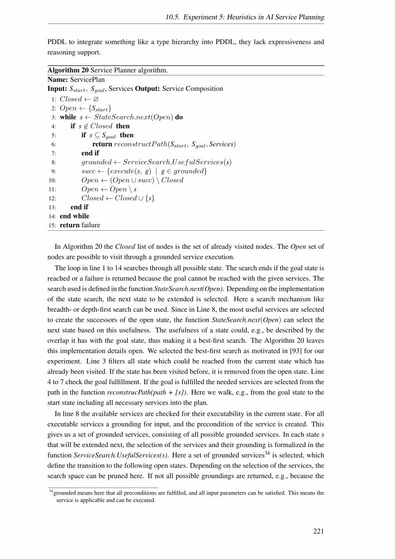
10.5. Experiment 5: Heuristics in AI Service Planning

PDDL to integrate something like a type hierarchy into PDDL, they lack expressiveness andreasoning support.

Algorithm 20 Service Planner algorithm.Name: ServicePlanInput: Sstart, Sgoal, Services Output: Service Composition

1: Closed← ∅2: Open← Sstart3: while s← StateSearch.next(Open) do4: if s 6∈ Closed then5: if s ⊆ Sgoal then6: return reconstructPath(Sstart, Sgoal, Services)7: end if8: grounded← ServiceSearch.UsefulServices(s)9: succ← execute(s, g) | g ∈ grounded

10: Open← (Open ∪ succ) \ Closed11: Open← Open \ s12: Closed← Closed ∪ s13: end if14: end while15: return failure

In Algorithm 20 the Closed list of nodes is the set of already visited nodes. The Open set ofnodes are possible to visit through a grounded service execution.

The loop in line 1 to 14 searches through all possible state. The search ends if the goal state isreached or a failure is returned because the goal cannot be reached with the given services. Thesearch used is defined in the function StateSearch.next(Open). Depending on the implementationof the state search, the next state to be extended is selected. Here a search mechanism likebreadth- or depth-first search can be used. Since in Line 8, the most useful services are selectedto create the successors of the open state, the function StateSearch.next(Open) can select thenext state based on this usefulness. The usefulness of a state could, e.g., be described by theoverlap it has with the goal state, thus making it a best-first search. The Algorithm 20 leavesthis implementation details open. We selected the best-first search as motivated in [93] for ourexperiment. Line 3 filters all state which could be reached from the current state which hasalready been visited. If the state has been visited before, it is removed from the open state. Line4 to 7 check the goal fulfillment. If the goal is fulfilled the needed services are selected from thepath in the function reconstrucPath(path + [s]). Here we walk, e.g., from the goal state to thestart state including all necessary services into the plan.

In line 8 the available services are checked for their executability in the current state. For allexecutable services a grounding for input, and the precondition of the service is created. Thisgives us a set of grounded services, consisting of all possible grounded services. In each state sthat will be extended next, the selection of the services and their grounding is formalized in thefunction ServiceSearch.UsefulServices(s). Here a set of grounded services34 is selected, whichdefine the transition to the following open states. Depending on the selection of the services, thesearch space can be pruned here. If not all possible groundings are returned, e.g., because the

34grounded means here that all preconditions are fulfilled, and all input parameters can be satisfied. This means theservice is applicable and can be executed.

221

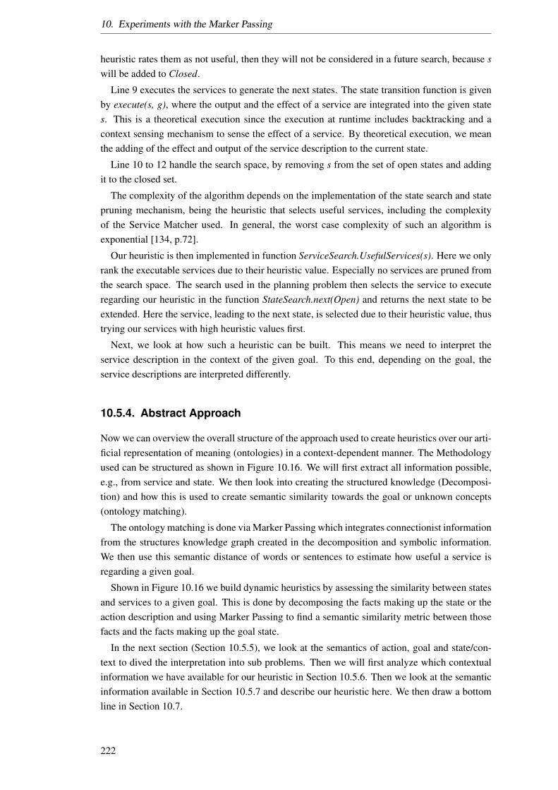
10. Experiments with the Marker Passing

heuristic rates them as not useful, then they will not be considered in a future search, because swill be added to Closed.

Line 9 executes the services to generate the next states. The state transition function is givenby execute(s, g), where the output and the effect of a service are integrated into the given states. This is a theoretical execution since the execution at runtime includes backtracking and acontext sensing mechanism to sense the effect of a service. By theoretical execution, we meanthe adding of the effect and output of the service description to the current state.

Line 10 to 12 handle the search space, by removing s from the set of open states and addingit to the closed set.

The complexity of the algorithm depends on the implementation of the state search and statepruning mechanism, being the heuristic that selects useful services, including the complexityof the Service Matcher used. In general, the worst case complexity of such an algorithm isexponential [134, p.72].

Our heuristic is then implemented in function ServiceSearch.UsefulServices(s). Here we onlyrank the executable services due to their heuristic value. Especially no services are pruned fromthe search space. The search used in the planning problem then selects the service to executeregarding our heuristic in the function StateSearch.next(Open) and returns the next state to beextended. Here the service, leading to the next state, is selected due to their heuristic value, thustrying our services with high heuristic values first.

Next, we look at how such a heuristic can be built. This means we need to interpret theservice description in the context of the given goal. To this end, depending on the goal, theservice descriptions are interpreted differently.

10.5.4. Abstract Approach

Now we can overview the overall structure of the approach used to create heuristics over our arti-ficial representation of meaning (ontologies) in a context-dependent manner. The Methodologyused can be structured as shown in Figure 10.16. We will first extract all information possible,e.g., from service and state. We then look into creating the structured knowledge (Decomposi-tion) and how this is used to create semantic similarity towards the goal or unknown concepts(ontology matching).

The ontology matching is done via Marker Passing which integrates connectionist informationfrom the structures knowledge graph created in the decomposition and symbolic information.We then use this semantic distance of words or sentences to estimate how useful a service isregarding a given goal.

Shown in Figure 10.16 we build dynamic heuristics by assessing the similarity between statesand services to a given goal. This is done by decomposing the facts making up the state or theaction description and using Marker Passing to find a semantic similarity metric between thosefacts and the facts making up the goal state.

In the next section (Section 10.5.5), we look at the semantics of action, goal and state/con-text to dived the interpretation into sub problems. Then we will first analyze which contextualinformation we have available for our heuristic in Section 10.5.6. Then we look at the semanticinformation available in Section 10.5.7 and describe our heuristic here. We then draw a bottomline in Section 10.7.

222

10.5. Experiment 5: Heuristics in AI Service Planning

State Service

Semantic Decomposition

Context

Marker Passing

Semantic Distance

Dynamic Heuristics

Figure 10.16.: Overview of our methodology to create a heuristic.

10.5.5. Semantics of States, Service and Context

Now we will have a look at the information available in a planning problem. As we have seen inSection 3.3 a planning problem is defined by the services available and the start and goal state.These descriptions contain all information needed to create a solution.

The states are represented as ontologies describing all facts known in the state (see Defini-tion 1). We have looked at the definition of an ontology in Section 3.6 on Page 31. The start andgoal state are states with a special meaning since the goal state is something we want to achieveto solve our problem and the start state is the facts the agent knows. In this section, we will lookat those separately.

As we have discussed in Section 4.6 our action descriptions are encapsulated in a semanticservice description. Here we look at these service descriptions and discuss how they can beinterpreted to help solve the planning problem. Last we look at the contextual information of theplanning problem.

As depicted in Figure 10.17 the state space is built from a start state by invoking the statetransition function to all possible state. The state transition function is defined by the set ofservices available. This means in each state where the preconditions of a service are fulfilled,and all inputs are available, meaning the service can be grounded and the resulting state is aconsistent state, the service is executed and creates a new state with the application of its effect.Thereby a graph is built where nodes are states and edges are service calls. Services in this viewof planning, therefore, create or change facts from a state with known facts to goal facts. Sincewe look at the planning task as a mental process, information services (services without an effect)are excluded from the plan because they do not generate a new state. As a mental process, theplanning is hypothetical. For that reason, services execution is simulated by declaring its effectas known facts.

This lets us create a hypothetical graph like depicted in Figure 10.17 where we then select apath from the start state to the goal state. We now look at the four different parts of this view

223

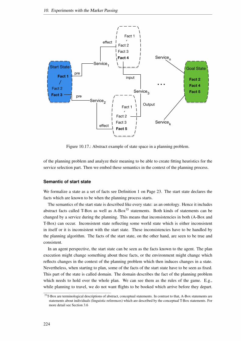
10. Experiments with the Marker Passing

Start State

Fact 1

Fact 2Fact 3

Fact 4

Fact 1

Fact 2Fact 3

Fact 1

Fact 2Fact 3Fact 5

pre

pre

effect

effect

… Fact 2Fact 4Fact 5

Goal State

Service2 Output

Service1

Service3

input

Servicen

Servicek

Figure 10.17.: Abstract example of state space in a planning problem.

of the planning problem and analyze their meaning to be able to create fitting heuristics for theservice selection part. Then we embed these semantics in the context of the planning process.

Semantic of start state

We formalize a state as a set of facts see Definition 1 on Page 23. The start state declares thefacts which are known to be when the planning process starts.

The semantics of the start state is described like every state: as an ontology. Hence it includesabstract facts called T-Box as well as A-Box35 statements. Both kinds of statements can bechanged by a service during the planning. This means that inconsistencies in both (A-Box andT-Box) can occur. Inconsistent state reflecting some world state which is either inconsistentin itself or it is inconsistent with the start state. These inconsistencies have to be handled bythe planning algorithm. The facts of the start state, on the other hand, are seen to be true andconsistent.

In an agent perspective, the start state can be seen as the facts known to the agent. The planexecution might change something about these facts, or the environment might change whichreflects changes in the context of the planning problem which then induces changes in a state.Nevertheless, when starting to plan, some of the facts of the start state have to be seen as fixed.This part of the state is called domain. The domain describes the fact of the planning problemwhich needs to hold over the whole plan. We can see them as the rules of the game. E.g.,while planning to travel, we do not want flights to be booked which arrive before they depart.

35T-Box are terminological descriptions of abstract, conceptual statements. In contrast to that, A-Box statements arestatements about individuals (linguistic references) which are described by the conceptual T-Box statements. Formore detail see Section 3.6

224

10.5. Experiment 5: Heuristics in AI Service Planning

This domain is linked to the start state within import. This import ensures that the facts of thisontology are known but cannot be changed. An example is shown in Listing 10.1.

Listing 10.1: Reference example of ontologies in an OWL syntax.

<Ontology xmlns="http://www.w3.org/2002/07/owl#"

xml:base="http://www.w3.org/2002/07/owl#"

<Prefix name="j.0" IRI="/ontology/Health-Scallops_Ontology.owl#"/>

<Import>"/ontology/MedicalTransportCompany_Ontology.owl"</Import>

<Import>"/ontology/Health-Scallops_Ontology.owl"</Import>

<Import>"/ontology/FlightCompany_Ontology.owl"</Import>

<Import>"/ontology/MedicalFlightCompany_Ontology.owl"</Import>

<Declaration>

<NamedIndividual abbreviatedIRI="j.0:ArrivalAirport"/>

</Declaration>

</owl:Ontology>

Listing 10.1 shows how, e.g., the SCALLOPS36 domain is integrated into a state ontology,making all the facts stated in this ontology accessible in the importing ontology.

As an example, an agent could plan how to get to work on Monday, but a state in the statespace states that gravity has ceased to exist. In this fictional start state, everything might bedescribed as always, but setting the effect of gravity to FG = 0 m

ss . Now starting to plan forthis start state, the heuristic for service selections might need to adapt. With enough conceptualknowledge about the world, one might consider the bus to go to work on a normal day. However,planning for the “0G-Monday” this needs to change. Knowing about the propulsion system ofa bus, we can reason that without gravity the friction between bus tires and the ground will stopas soon as the bus hits a bump since it will not fall back to earth. Consequently, all servicesprovided by this kind of vehicles will be neglected in the creation of the plan.

If this is not the case, and the start state contains contradicting facts or inconsistent statements,the service selection becomes probabilistic, since one has to determine which fact is more likelyto be true.

To be able to reason upon a consistent start state it needs to state all facts relevant to theplanning problem. If facts are not included the contextual information needs to be involved toenabling the reasoning process. In our “0G-Monday” scenario the facts about vehicles and basicphysics are included in the domain description, and therefore they are part of the contextualinformation which is further discussed in Section 10.5.5.

Classical planning approaches describe their state as a mixture of the domain description, thetype declarations, causal rules or contextual facts [86]. Since the start state is described in anontology other ontologies are a reference. This is an easy way to separate the domain descriptionfrom the start state. This means that we can include an ontology describing the basic physics ofthe world we plan for, simply by referencing the ontology describing those facts.

In conclusion, we can say that a start state describes the knowledge of an agent or a fictionalstate for which it wants to plan. The start state needs to include all necessary facts for theplanning algorithm to solve the problem efficiently. The less abstract the facts are described 37

in the start state the more efficient the planning can be done.

36http://www.dfki.de/scallops/, last visited on 29.06.201737The more abstract class in ontology is the more individuals could be found to instantiate it.

225

10. Experiments with the Marker Passing

Semantic of a Service

In Section 3.2 we have looked at a definition of service (see definition 2 on page 24). Nowwe want to describe the semantics of a service: We start out by separating the service from itsdescription. The reason for that is that one service can have multiple descriptions. An examplefor such a service provider could be a freezer. It provides the service to cool things. Themanufacturer of this freezer might provide a service description describing what cooling meansand which things can be cooled. Now we imagine this freezer in an environment, where we haveto control the grid stability of an electronic grid. Here the freezer can be used to store energyby cooling it down more than normal when energy needs to be consumed and later on, stoppingthe cooling process, if energy is needed by others. In this why the freezer works like an energybuffer. A new service it can provide, without having to change the freezer or the description byits manufacturer. This new service needs a description, which we can provide if the service isseparated from the description.

We have looked at how a service is described in Section 3.2. Now we want to analyze thisdescription on what its parts contain as information for us to use to create a heuristic. We are ne-glecting informal parts of the service description like quality parameters or the natural languagedescription because they are collected in the contextual information described in Section 10.5.5.

Input: The input describes the parameters we need to invoke the service. The input is givenby a set of facts. It also describes the parameters on which the service can base its changein the world upon. This means the input parameters should contain all facts a service willuse. For our heuristic, the inputs are those facts which need a grounding to be able touse a certain service. Input parameters can be seen as variables. If the variable is free,meaning not grounded to an individual, then the service does not know how to use thisvariable. This means all variables of the input need to be replaced by individuals (TBox)for the service to be executed. If we have a flight-booking-service as an example, its inputcould be start and destination location and a time interval. The description of the inputmeans then that we have to decide on a start and destination location, to be able to use thisservice. This means a concrete manifestation of these facts needs to be specified. Thesefacts can be part of a state, or we can interpret them as a new sub-goal to be fulfilled byanother service.

Output: The output of a service describes the facts it contributes to a state. Here we candescribe new or changed facts of a state by the executed service. In our example of theflight-booking-service, the output could be a traveling route. This traveling route mightnot have been known before the service invocation, and now it is a fact of the state. Hencea new fact was created as the outcome of the service. For our heuristic, we might want toanalyze outputs in situations we want new facts in our state. The output of a service needsto be distinct from its effect. The effect might change the state of the world as well. Theoutput is the direct return value of a service, not its side effects.

Precondition: The precondition describes rules about the state which have to be true to in-voke a service. Here the same semantics as for the input applies: If a fact, which is used ina precondition has no individual who fulfills this fact in the current state, then the serviceis not executable. In addition to that, the precondition can describe rules upon those facts,which restrict the grounding of a fact. These rules need to be fulfilled for the service to be

226

10.5. Experiment 5: Heuristics in AI Service Planning

semantically sound. In our example of the flight-booking-service one precondition couldbe that the departure date is before the arrival date in the time interval given as input.Such a precondition allows us to analyze facts like arrival and departure dates and to ex-tract knowledge about those facts. Thus we can extract that arrival might only come aftera departure. For our heuristic, we want to analyze preconditions as an extension of ourgoal regarding the relations between facts if output or effect of the service is useful.

Effect: The effect describes side-effects of a service. These are changes which might not havebeen described as output because they do not include the creation or change of facts butdescribe relationships between those facts. In our example of the flight-booking-serviceone effect concerning the traveling route might be that tickets are still available for eachroute segment and that some of those tickets are now reserved for us. For our heuristic,we want to analyze an effect if new relations between facts are wanted.

Each part of the IOPE description has its own semantic about the described service. To sep-arate this specific purpose of each description part multiple conditions need to hold for theimplementation. For the input to have the semantics described above, the service needs to de-clare all facts, which it bases its calculation upon as input. In consequence, the preconditionshould describe the relations between those facts extensively. The same should hold for outputand effect. Also, all effects should be formalized in the effect of the service.

Also a service in OWL-S contains a natural language description and a name. Those can beused as additional contextual information by the creation of a heuristic. This contributes to theneed for a semantic distance measure for words and sentences.

Here we have analyzed the four formal parts of a service description, for their semanticsregarding their role in creating a heuristic.

Semantic of goals state

The goal state describes a set of states of the world which we want to achieve with our planningapproach. The goal is formalized as a set of facts. A state fulfills a goal state if the facts of astate, subsume the facts described in a goal state. An example could be, that if the goal state”IsAt(?x, Berlin)” stating that something should be in Berlin, the state ”IsAt(Johannes, Berlin)”fulfills the goal.

This means we restrict our goal to goals which describe facts to achieve. These goals aresometimes called achievement goals. It can be argued that maintenance goals [64] are differentbecause we want to maintain the state described in the goal.

The facts described in the goal can be subject to our semantic analysis. This analysis leadsto conclusions regarding the semantic relations of the facts in the goal with, e.g., facts from theeffect of a service. If for example some fact is described by a concept which could be describedwith the word “open” and can deduce that the antonym, e.g. “closed” might be some unwantedfact.

Like in every state (e.g., external changes in the context) the facts of the goal state mightchange as well. We assume the goal to be fixed throughout the planning process. If the goalchanges at runtime a new planning process can be triggered. To change the current state of theworld to the desired one, change has to occur. This change can be proactively or autonomouslyinfluenced by services the agent can execute.

227

10. Experiments with the Marker Passing

For the heuristic the goal describes wanted facts. Particularly, it defines what the problemdescribes as “good”. In our flight-booking-service example, the goal might define that we wantto be in Berlin in two weeks. The fact “being in Berlin” therefore might be seen as wantedin contrast to being somewhere else. The information from the goal affects the selection ofparameters for services or the selection of services itself. However, this representation entails afew challenges:

Axioms If an effect is described on not grounded facts, the goal can be fulfilled by multiplegroundings of this fact.

Individuals in goals An individual differs from a general ABox fact since it describes oneconcrete entity TBox. In our flight-booking-Service example, a generic goal might be tobring someone to Berlin. However, if the goal is to bring the author of this work to Berlin,then we need to specify this individual to book the flight for. As a result, the goal does notonly consist of abstract facts (Abox) but also on individuals. This calls for an extensionof the reasoning for individuals, meaning that the grounding of certain rules (e.g., aneffect of some service) needs to create individuals. Individuals cannot be created in aneffect because the SWRL language does support such an extension only in an extension(SWRLB) and the Pellet reasoner does not support them.

This leaves us with the goal as the main guidance of the heuristic. Besides the domain descrip-tion which defines the “rules of the game”, the goal forms the heuristics and the interpretationof the services. This includes especially which facts are wanted (meaning which services areuseful) and which facts are not wanted (meaning which services should be avoided).

Semantic of context

In Section 3.8 we have defined in Definition 20 on Page 35 what we see as context. This contextdefinition is now applied to our problem of using service description and a planning problem tocreate a heuristic. Therefore we will now collect the information which represents this contextualinformation and analyzes its semantics.

First of all, a context is formalized like a state as a set of facts (see Section 3.8 for moredetails). These facts include domain descriptions taken from the planning problem, descriptionparts like the natural language description of a service or Quality of Service parameters. Thiscontextual information is not problem specific. This means in the same context; multiple plan-ning problems can occur as well as one planning problem can be seen in different contexts. Thisincludes the conception of a service from Section 3.8, where the agent using the service hashis conception of the service and creates its context. In our flight-booking-service example, thecontext in which the flight might be booked might be spare time and with that count as vacationor it might be a business trip and count as work. In consequence, depending on this contextualinformation, the credit card to pay for the flights might differ. This means our interpretation of“the right credit card” to be used to pay for the flight, might differ.

We generalize this observation: The contextual information influences how we interpret theservice description. With other words, depending on the context, the words making up thedescription can be interpreted in different ways, if those words have multiple word senses. Thesemantics of the context will be used by our approach to select the right word senses from adescription, the states or whatever resources we are analyzing. Indeed, the context might change

228

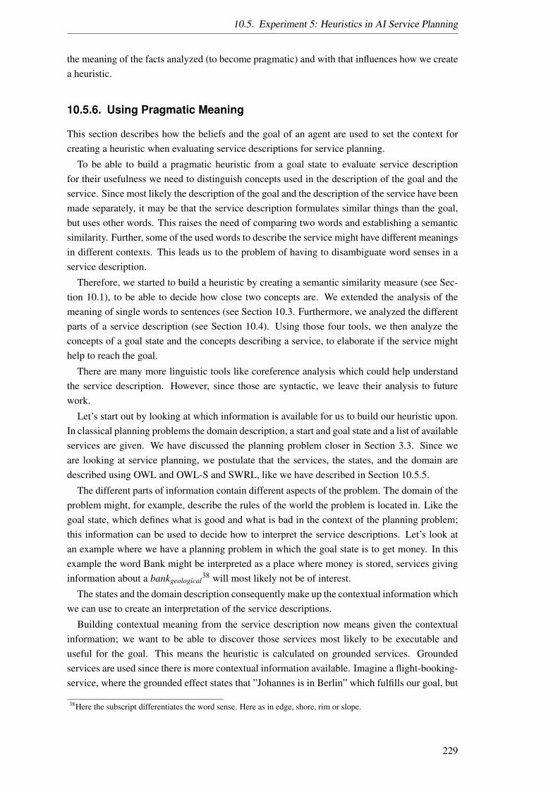
10.5. Experiment 5: Heuristics in AI Service Planning

the meaning of the facts analyzed (to become pragmatic) and with that influences how we createa heuristic.

10.5.6. Using Pragmatic Meaning

This section describes how the beliefs and the goal of an agent are used to set the context forcreating a heuristic when evaluating service descriptions for service planning.

To be able to build a pragmatic heuristic from a goal state to evaluate service descriptionfor their usefulness we need to distinguish concepts used in the description of the goal and theservice. Since most likely the description of the goal and the description of the service have beenmade separately, it may be that the service description formulates similar things than the goal,but uses other words. This raises the need of comparing two words and establishing a semanticsimilarity. Further, some of the used words to describe the service might have different meaningsin different contexts. This leads us to the problem of having to disambiguate word senses in aservice description.

Therefore, we started to build a heuristic by creating a semantic similarity measure (see Sec-tion 10.1), to be able to decide how close two concepts are. We extended the analysis of themeaning of single words to sentences (see Section 10.3. Furthermore, we analyzed the differentparts of a service description (see Section 10.4). Using those four tools, we then analyze theconcepts of a goal state and the concepts describing a service, to elaborate if the service mighthelp to reach the goal.

There are many more linguistic tools like coreference analysis which could help understandthe service description. However, since those are syntactic, we leave their analysis to futurework.

Let’s start out by looking at which information is available for us to build our heuristic upon.In classical planning problems the domain description, a start and goal state and a list of availableservices are given. We have discussed the planning problem closer in Section 3.3. Since weare looking at service planning, we postulate that the services, the states, and the domain aredescribed using OWL and OWL-S and SWRL, like we have described in Section 10.5.5.

The different parts of information contain different aspects of the problem. The domain of theproblem might, for example, describe the rules of the world the problem is located in. Like thegoal state, which defines what is good and what is bad in the context of the planning problem;this information can be used to decide how to interpret the service descriptions. Let’s look atan example where we have a planning problem in which the goal state is to get money. In thisexample the word Bank might be interpreted as a place where money is stored, services givinginformation about a bankgeological

38 will most likely not be of interest.

The states and the domain description consequently make up the contextual information whichwe can use to create an interpretation of the service descriptions.

Building contextual meaning from the service description now means given the contextualinformation; we want to be able to discover those services most likely to be executable anduseful for the goal. This means the heuristic is calculated on grounded services. Groundedservices are used since there is more contextual information available. Imagine a flight-booking-service, where the grounded effect states that ”Johannes is in Berlin” which fulfills our goal, but

38Here the subscript differentiates the word sense. Here as in edge, shore, rim or slope.

229

10. Experiments with the Marker Passing

if someone else is in Berlin, this does not. The service description is used with the followingcourse of action:

1. Decompose each new service description output and effect

2. Merge this decomposition with the decomposition of the goal state.

3. Decompose each new service description input and precondition

4. Merge this decomposition with the decomposition of the current state.

5. Using our Marker Passing to measure the amount of fulfilled goals by the effect and mea-suring a number of preconditions which are fulfilled.

6. The heuristic is built by a weighted sum of the “usefulness for the goal” (amount of sub-goals fulfilled) and “executability” (amount of preconditions fulfilled) to create a heuristicfor the service.

This approach might vary, depending on the kind of heuristic we are looking for. This meansthat if we are using a backward search, we probably want to start the Marker Passing from thegoal state. If we are looking for a heuristic for a FF-planner, we want to start markers from thecurrent state we are in. We selected a forward search during our plan. The approach suggestedhere can be modified to be used with other planning algorithms. In the next section, we will lookat the details on how this heuristic is built for a forward search.

10.5.7. Building Context-Dependent Heuristics

We have motivated our work by the need of a heuristic for AI planning. Since the search spaceof domain independent planners for large problems becomes computationally intractable [187]we need heuristics to guide our search through the state space. The heuristics are needed be-cause we cannot search the whole search space; therefore the heuristic narrows the search spaceto a required part we need to search to find the goal state. We have defined heuristics in Sec-tion 10.5.1. The interested reader is referred to [304] for a formal description of heuristics andtheir properties. During our analysis of this topic (see Section 10.5.2 and Section 10.5.3) wewant to create an heuristic which is goal dependence, service interpretation and State/Contextawareness.

We have found that understanding the described functionality of a service is AI-hard task[419]. The interpretation of what a description creator might have understood the service to beis not entirely reflected in the description. Furthermore, the service can have multiple interpre-tations in different contexts. The context we defined is the additional information relevant to ourproblem. As an example strategy for problem solving, we have selected planning. This meansour context consists of the start and goal state which includes a domain description. With thiswe are able to extend the signature of a heuristic from the classical one H : State→ Double to:

H : State× State× Service→ R (10.20)

In this work a heuristic is defined as a function H which estimates the usefulness of a servicea ∈ A for a goal state sgoal ∈ S, with the contextual information of a current state s. Our heuristicfunction H is calculated upon the description of the service a and the description of the current

230

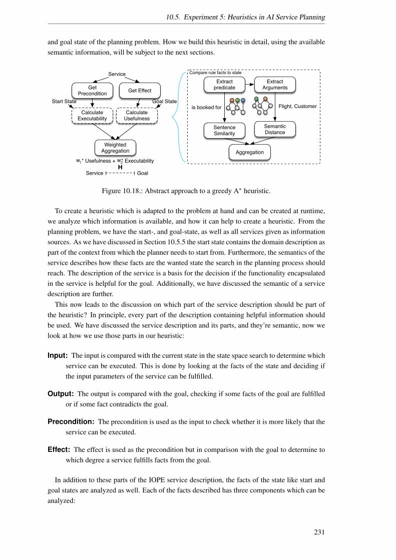
10.5. Experiment 5: Heuristics in AI Service Planning

and goal state of the planning problem. How we build this heuristic in detail, using the availablesemantic information, will be subject to the next sections.

Compare rule facts to state

Sentence Similarity

Service

Goal State

Extract predicate

Extract Arguments

Semantic Distance

Aggregation

GoalService

* Usefulness + * Executability

Start Stateis booked for Flight, Customer

H

Get Precondition Get Effect

Calculate Executability

Calculate Usefulness

Weighted Aggregation

w1 w2

Figure 10.18.: Abstract approach to a greedy A∗ heuristic.

To create a heuristic which is adapted to the problem at hand and can be created at runtime,we analyze which information is available, and how it can help to create a heuristic. From theplanning problem, we have the start-, and goal-state, as well as all services given as informationsources. As we have discussed in Section 10.5.5 the start state contains the domain description aspart of the context from which the planner needs to start from. Furthermore, the semantics of theservice describes how these facts are the wanted state the search in the planning process shouldreach. The description of the service is a basis for the decision if the functionality encapsulatedin the service is helpful for the goal. Additionally, we have discussed the semantic of a servicedescription are further.

This now leads to the discussion on which part of the service description should be part ofthe heuristic? In principle, every part of the description containing helpful information shouldbe used. We have discussed the service description and its parts, and they’re semantic, now welook at how we use those parts in our heuristic:

Input: The input is compared with the current state in the state space search to determine whichservice can be executed. This is done by looking at the facts of the state and deciding ifthe input parameters of the service can be fulfilled.

Output: The output is compared with the goal, checking if some facts of the goal are fulfilledor if some fact contradicts the goal.

Precondition: The precondition is used as the input to check whether it is more likely that theservice can be executed.

Effect: The effect is used as the precondition but in comparison with the goal to determine towhich degree a service fulfills facts from the goal.

In addition to these parts of the IOPE service description, the facts of the state like start andgoal states are analyzed as well. Each of the facts described has three components which can beanalyzed:

231

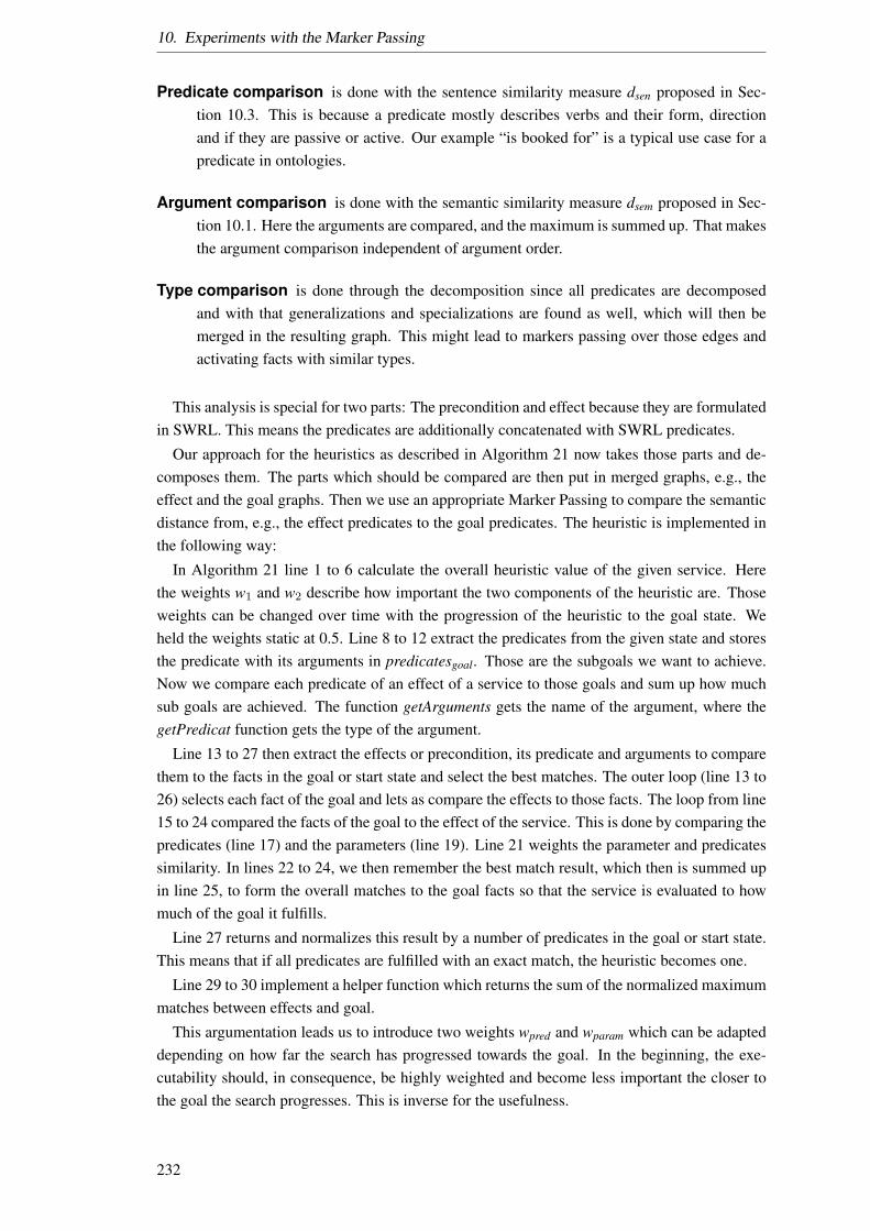
10. Experiments with the Marker Passing

Predicate comparison is done with the sentence similarity measure dsen proposed in Sec-tion 10.3. This is because a predicate mostly describes verbs and their form, directionand if they are passive or active. Our example “is booked for” is a typical use case for apredicate in ontologies.

Argument comparison is done with the semantic similarity measure dsem proposed in Sec-tion 10.1. Here the arguments are compared, and the maximum is summed up. That makesthe argument comparison independent of argument order.

Type comparison is done through the decomposition since all predicates are decomposedand with that generalizations and specializations are found as well, which will then bemerged in the resulting graph. This might lead to markers passing over those edges andactivating facts with similar types.

This analysis is special for two parts: The precondition and effect because they are formulatedin SWRL. This means the predicates are additionally concatenated with SWRL predicates.

Our approach for the heuristics as described in Algorithm 21 now takes those parts and de-composes them. The parts which should be compared are then put in merged graphs, e.g., theeffect and the goal graphs. Then we use an appropriate Marker Passing to compare the semanticdistance from, e.g., the effect predicates to the goal predicates. The heuristic is implemented inthe following way:

In Algorithm 21 line 1 to 6 calculate the overall heuristic value of the given service. Herethe weights w1 and w2 describe how important the two components of the heuristic are. Thoseweights can be changed over time with the progression of the heuristic to the goal state. Weheld the weights static at 0.5. Line 8 to 12 extract the predicates from the given state and storesthe predicate with its arguments in predicatesgoal. Those are the subgoals we want to achieve.Now we compare each predicate of an effect of a service to those goals and sum up how muchsub goals are achieved. The function getArguments gets the name of the argument, where thegetPredicat function gets the type of the argument.

Line 13 to 27 then extract the effects or precondition, its predicate and arguments to comparethem to the facts in the goal or start state and select the best matches. The outer loop (line 13 to26) selects each fact of the goal and lets as compare the effects to those facts. The loop from line15 to 24 compared the facts of the goal to the effect of the service. This is done by comparing thepredicates (line 17) and the parameters (line 19). Line 21 weights the parameter and predicatessimilarity. In lines 22 to 24, we then remember the best match result, which then is summed upin line 25, to form the overall matches to the goal facts so that the service is evaluated to howmuch of the goal it fulfills.

Line 27 returns and normalizes this result by a number of predicates in the goal or start state.This means that if all predicates are fulfilled with an exact match, the heuristic becomes one.

Line 29 to 30 implement a helper function which returns the sum of the normalized maximummatches between effects and goal.

This argumentation leads us to introduce two weights wpred and wparam which can be adapteddepending on how far the search has progressed towards the goal. In the beginning, the exe-cutability should, in consequence, be highly weighted and become less important the closer tothe goal the search progresses. This is inverse for the usefulness.

232

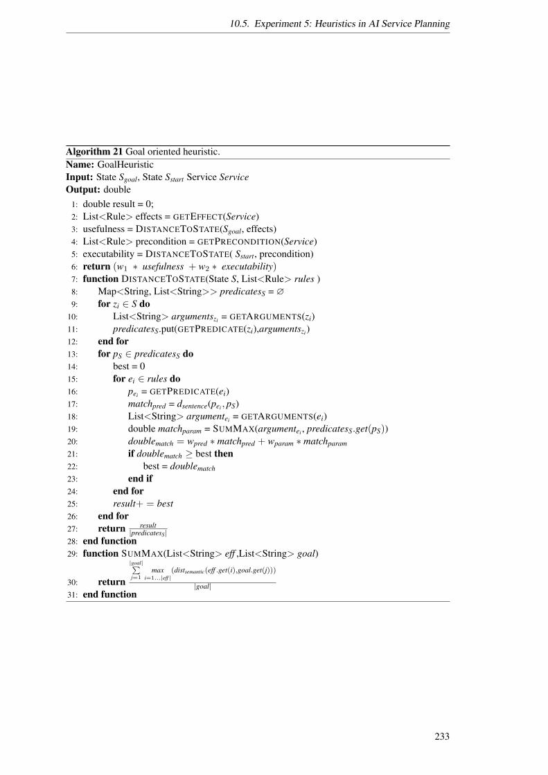
10.5. Experiment 5: Heuristics in AI Service Planning

Algorithm 21 Goal oriented heuristic.Name: GoalHeuristicInput: State Sgoal, State Sstart Service ServiceOutput: double

1: double result = 0;2: List<Rule> effects = GETEFFECT(Service)3: usefulness = DISTANCETOSTATE(Sgoal, effects)4: List<Rule> precondition = GETPRECONDITION(Service)5: executability = DISTANCETOSTATE( Sstart, precondition)6: return (w1 ∗ usefulness + w2 ∗ executability)7: function DISTANCETOSTATE(State S, List<Rule> rules )8: Map<String, List<String>> predicatesS = ∅9: for zi ∈ S do

10: List<String> argumentszi = GETARGUMENTS(zi)11: predicatesS.put(GETPREDICATE(zi),argumentszi)12: end for13: for pS ∈ predicatesS do14: best = 015: for ei ∈ rules do16: pei = GETPREDICATE(ei)17: matchpred = dsentence(pei , pS)18: List<String> argumentei = GETARGUMENTS(ei)19: double matchparam = SUMMAX(argumentei , predicatesS.get(pS))20: doublematch = wpred ∗ matchpred + wparam ∗ matchparam

21: if doublematch ≥ best then22: best = doublematch23: end if24: end for25: result+ = best26: end for27: return result

|predicatesS|28: end function29: function SUMMAX(List<String> eff ,List<String> goal)

30: return

|goal|∑j=1

maxi=1...|eff |

(distsemantic(eff .get(i),goal.get(j)))

|goal|31: end function

233

10. Experiments with the Marker Passing

Both parts use the same kind of mechanism to check rather a fact is fulfilled (in the precon-dition or effect of a service) which is given by the goal or start state. To check this fulfillment,we extract the predicates from the service precondition (effects) and the start (goal) axioms andtheir arguments and compare them. The comparison is made in two ways: first, for the predicatesname, we separate the word included in the predicate, e.g. “IsBookedFor(Flight x, Customer c)”become the predicate “is booked for”. Since this resembles a sentence, the sentence distancemeasure dsen is used to compare predicates (see Section 10.3 on Page 189). Second we comparethe arguments with our semantic similarity measure dsem (see Section 10.1 on Page 157). Theresult of those both similarities is then aggregated.

The interpretation of the marker resulting from the Marker Passing is done like described inEquation 10.21 which describes how we calculate the heuristic for a service S:

H(Start,Goal, S) = w1 ∗ Usefulness(S,Goal) + w2 ∗ Executability(S, Start) (10.21)

Usefulness(S,Goal) =

=

∑g∈Goal

maxe∈S.effct

(wprd ∗ dsen(n(e), n(g)) + warg ∗

( ∑argg∈Args(g)

maxarge∈Args(e)

dsem(argg,arge)

|Args(g)|

))| Goal |

(10.22)

The name of the axiom denoted with n(•). Here the comparison of an axiom is threefoldas described above: The predicate comparison, the Argument comparison, and the Type com-parison. In OWL typing is described by, e.g., class assertion predicates. That is why in theEquation 10.22 we have combined all predicate comparison including type comparison into onepart. This means that we include the comparison of all three parts of an axiom. A similar equa-tion to Equation 10.22 can be formulated for the Executability where the normalization is doneover a number of preconditions. This means that if the sum of w1 and w1 equals to one, theoverall heuristic has values between zero and one.

We selected this two measures for our heuristic, because if we leave out one of the aspectstwo effects happen:

Goal overcommitment If we only look at the usefulness the services fulfilling subgoals willbe tried first. Even though the probability of them being on the end of the plan is higher.This means we are not talking about a planning problem which is trivial because all ser-vices in the plan are independent. This means that one or more services need to be exe-cuted to enable a useful service. By only looking at the usefulness the search will alwaystry services we can not yet execute, first.

Low hanging fruits If we only look at the executability, services which are executable arealways tried first. This is good at the beginning of the planning process because reachingthe goal is less probable at this point. However, the more services are executed, the moreservice preconditions have the chance of enablement, and all of them are tried first. Thesearch then becomes like a breadth-first-search, where most services are tried before weget closer to the goal.

234

10.5. Experiment 5: Heuristics in AI Service Planning

Now we analyze the different properties of our heuristic. We have discussed at the beginningof Section 10.5.3 that we do not have an optimization problem. That does not mean that thisheuristic can not be used for optimization problems as well. Depending on the search mechanismused during the planning, we can have different properties of the outcome. This is why werestrict our analysis to sub classes of the best-first-search.

The A∗ search algorithm is thought for optimization planning, where each service s executedhas a specific cost. We have discussed earlier that our planning problem is not an optimizationproblem. This means we do not have a service cost. In consequence, we need to adapt the A∗

algorithm. The modification is done by selecting the different function g(s) for the optimizationfunction f (s) = g(s) + (1 − H(Start,Goal, s)) used. By selecting an appropriate g(s), ourplanning problem can become like an optimizing problem, since then the cost of the path to thecurrent state can be estimated. In our problem, where we do not know the cost to the currentstate, we analyze the following options:

g(s) = 0: makes the search only rely on heuristic and as a result is a best-first-search.

g(s) =| P |: with P being the shortest known path to state s. This is equivalent to a cost of onefor each service call, in this case, the A∗ optimizes the path length which does not have tobe optimal in cases where service might fulfill many subgoals but are more expensive.

g(s) =∑a∈P

(| Precondition(a) |): with P being the shortest known path to state s. Where we

look at the sum of needed preconditions of services leading to state s.

The first option neglects the service cost and thus behaves like a pure heuristic search. Thepure heuristic search is greedy because the services with the best heuristic value are used first.The second option has a constant service cost of one. In this case, the amount of service isminimized. The third option is an educated guess for the selection of g. Here any function couldhave been selected. The third option punishes the execution of services with a precondition; thusservices with more preconditions are punished as well. During the path to the goal, this g(s)increases, since more service have been executed. With that the number of services executed isminimized as well, but also services with fewer preconditions to fulfill are preferred. Becauseof its better performance, the third option for g has been selected for the rest of the experiments.

In conclusion, the heuristic produces one value which states how executable and useful aservice call is. Figure 10.19 shows an example of how a state space might look like duringplanning. Here the green state is the start state, and the red state is the goal state. Black statesare states to which we already know a heuristic value and gray states are not yet known. Blackstates are possible next state (sometimes called open states) in the search. Unknown states arestates which can not be reached with a single service call. The blue state represents the currentstate a search algorithm has expanded. In Figure 10.19 shows states which have been visited butdo not reach a gaol as crossed out states. Those state are sometimes called closed states.

Now we need an example problem to test our heuristic upon. The data set used for ourevaluation will be discussed next.

10.5.8. Data Sets

There is one data set which uses semantic service descriptions for service composition usingOWL-S as service description language. This data set is called Secure Agent-Based Pervasive

235

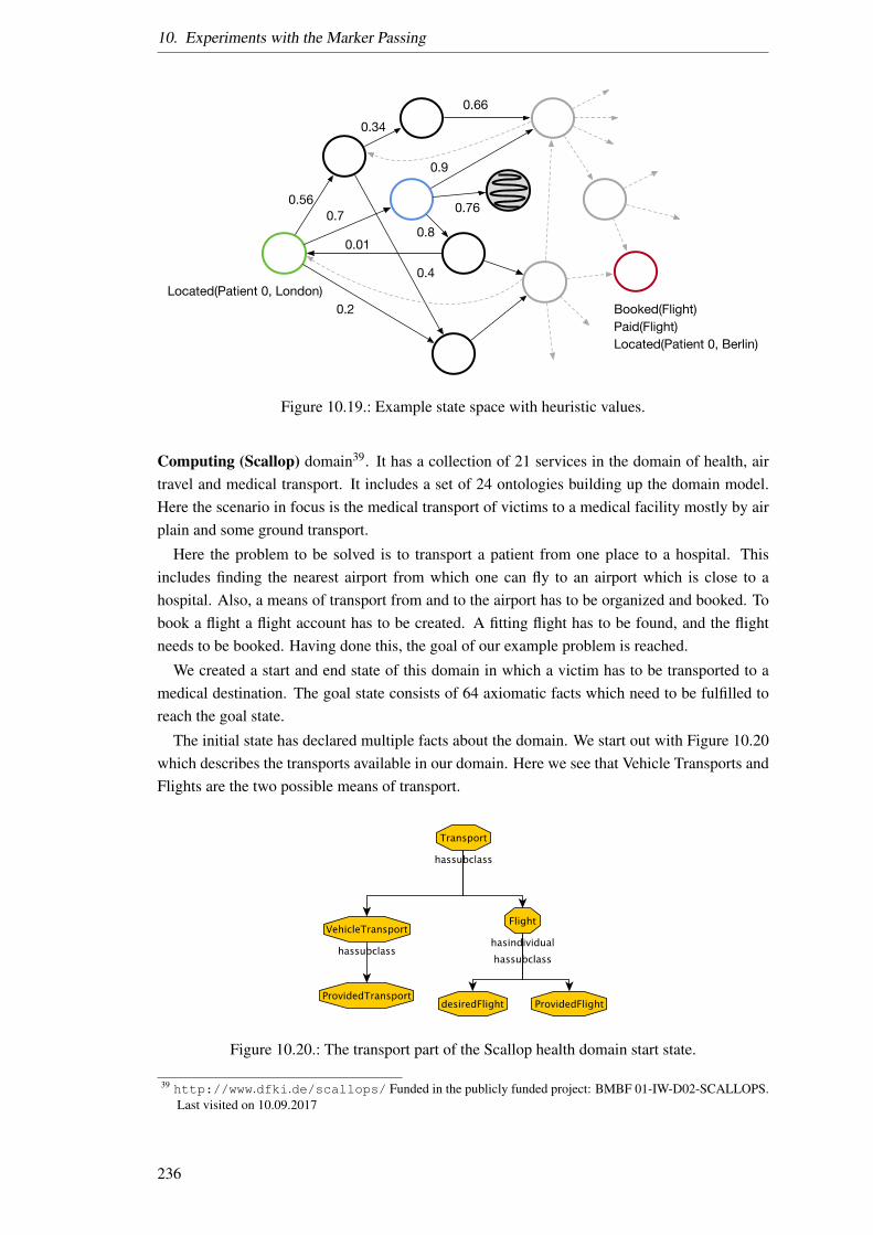
10. Experiments with the Marker Passing

0.560.7

0.2

0.34

0.9

0.66

0.76

0.8

Booked(Flight)Paid(Flight)Located(Patient 0, Berlin)

Located(Patient 0, London)

0.01

0.4

Figure 10.19.: Example state space with heuristic values.

Computing (Scallop) domain39. It has a collection of 21 services in the domain of health, airtravel and medical transport. It includes a set of 24 ontologies building up the domain model.Here the scenario in focus is the medical transport of victims to a medical facility mostly by airplain and some ground transport.

Here the problem to be solved is to transport a patient from one place to a hospital. Thisincludes finding the nearest airport from which one can fly to an airport which is close to ahospital. Also, a means of transport from and to the airport has to be organized and booked. Tobook a flight a flight account has to be created. A fitting flight has to be found, and the flightneeds to be booked. Having done this, the goal of our example problem is reached.

We created a start and end state of this domain in which a victim has to be transported to amedical destination. The goal state consists of 64 axiomatic facts which need to be fulfilled toreach the goal state.

The initial state has declared multiple facts about the domain. We start out with Figure 10.20which describes the transports available in our domain. Here we see that Vehicle Transports andFlights are the two possible means of transport.

Figure 10.20.: The transport part of the Scallop health domain start state.

39 http://www.dfki.de/scallops/ Funded in the publicly funded project: BMBF 01-IW-D02-SCALLOPS.Last visited on 10.09.2017

236

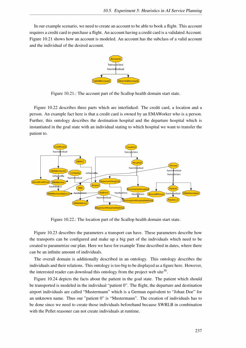
10.5. Experiment 5: Heuristics in AI Service Planning

In our example scenario, we need to create an account to be able to book a flight. This accountrequires a credit card to purchase a flight. An account having a credit card is a validated Account.Figure 10.21 shows how an account is modeled. An account has the subclass of a valid accountand the individual of the desired account.

Figure 10.21.: The account part of the Scallop health domain start state.

Figure 10.22 describes three parts which are interlinked: The credit card, a location and aperson. An example fact here is that a credit card is owned by an EMAWorker who is a person.Further, this ontology describes the destination hospital and the departure hospital which isinstantiated in the goal state with an individual stating to which hospital we want to transfer thepatient to.

Figure 10.22.: The location part of the Scallop health domain start state.

Figure 10.23 describes the parameters a transport can have. These parameters describe howthe transports can be configured and make up a big part of the individuals which need to becreated to parametrize our plan. Here we have for example Time described in dates, where therecan be an infinite amount of individuals.

The overall domain is additionally described in an ontology. This ontology describes theindividuals and their relations. This ontology is too big to be displayed as a figure here. However,the interested reader can download this ontology from the project web site39.

Figure 10.24 depicts the facts about the patient in the goal state. The patient which shouldbe transported is modeled in the individual “patient 0”. The flight, the departure and destinationairport individuals are called “Mustermann” which is a German equivalent to “Johan Doe” foran unknown name. Thus our ”patient 0” is “Mustermann”. The creation of individuals has tobe done since we need to create those individuals beforehand because SWRLB in combinationwith the Pellet reasoner can not create individuals at runtime.

237

10. Experiments with the Marker Passing

Figure 10.23.: The parameters part of the Scallop health domain start state.

Figure 10.24.: The patient and transport part of the Scallop health domain goal state.

Next, we model the individuals who are needed to reach our destination. In Figure 10.25 wemodel the departure and arrival airport.

Figure 10.25.: The airport part of the Scallop health domain goal state.

Since we need a valid account to book a flight, we model our account we need in our planin Figure 10.26. Here we want that our patient “Max Mustermann” has a personal account totransport our patient zero and book the relevant flights and transports from and to the airport.

There are many ways to model such a fact. In Figure 10.26 we have modeled the fact thatwe want a valid account as sub class relations. In consequence, our account must be of type“ValidAccount”.

Next, we model the more complex parameters the flight has to fulfill in Figure 10.27. Herewe state that we wish the flight to be booked for “Max Mustermann”, who owns the credit cardthe flight can be booked with and that the flight arrives at our goal destination at our goal time.

Figure 10.27 is a way of specifying that we want to be at a certain location at a certain time.All the modeling around those facts is necessary because we have to make sure all individual areavailable so that we can evaluate a potential execution of a service and with that reason upon theeffect of this service.

When starting to plan, the start and goal state already overlap with 57 axioms. The goal stateconsists of 64 axioms. Consequently, the plan to be made has to fulfill seven axioms to reach

238

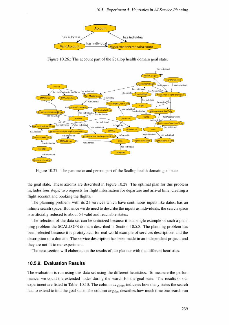
10.5. Experiment 5: Heuristics in AI Service Planning

Figure 10.26.: The account part of the Scallop health domain goal state.

Figure 10.27.: The parameter and person part of the Scallop health domain goal state.

the goal state. These axioms are described in Figure 10.28. The optimal plan for this problemincludes four steps: two requests for flight information for departure and arrival time, creating aflight account and booking the flights.

The planning problem, with its 21 services which have continuous inputs like dates, has aninfinite search space. But since we do need to describe the inputs as individuals, the search spaceis artificially reduced to about 54 valid and reachable states.

The selection of the data set can be criticized because it is a single example of such a plan-ning problem the SCALLOPS domain described in Section 10.5.8. The planning problem hasbeen selected because it is prototypical for real world example of services descriptions and thedescription of a domain. The service description has been made in an independent project, andthey are not fit to our experiment.

The next section will elaborate on the results of our planner with the different heuristics.

10.5.9. Evaluation Results

The evaluation is run using this data set using the different heuristics. To measure the perfor-mance, we count the extended nodes during the search for the goal state. The results of ourexperiment are listed in Table 10.13. The column avgsteps indicates how many states the searchhad to extend to find the goal state. The column avgtime describes how much time one search run

239

10. Experiments with the Marker Passing

hasParameters(MustermannFlight,MustermannFlightParameters) v

isBookedFor(MustermannFlight,Max_Mustermann) v

hasArrivalTime(MustermannFlightParameters,MustermannArrivalTime) v

hasCategory(MustermannFlightParameters,FlightCategory) v

hasDepartureTime(MustermannFlightParameters,MustermannDepartureTime) v

ValidAccount(MustermannPersonalAccount) v

ProvidedFlight(MustermannFlight) v

Figure 10.28.: Example goal axioms which are different in our goal state to our start state.

to has taken on average in seconds. The average has been created over ten runs40. All heuristicsare tested on the same start and goal state. Hence there is no difference in the planning problemstate space the search has to traverse.

From the state-of-the-art analysis for general purpose heuristics (described in Section 10.5.1)the greedy heuristic [304], which checks the overlap of the effects of a service, with the factswanted in the goal state, is performing well on this data set regarding the time consumption. Anadditional comparison is the Uniform Cost Distribution, where each execution of a service iscalculated to cost one abstract cost measure. With that admissible heuristic, A∗ finds an optimalsolution. The random heuristic has been added to the comparison so that we can evaluate howfar from the base line we are with our approach.

Table 10.13 shows the results of the average planner performance of ten runs. The variation ofthe performance is rooted in the fact that there are different ways to achieve the goal, dependingon which service is used first. If two services have the same heuristic value41, one of them isselected randomly. Table 10.13 shows the mean µ and standard derivation σ of the experimentresults regarding a number of steps and execution time.

Table 10.13.: Planning results for an average over ten runs of planner (time is in seconds).

Heuristic µtime σtime µstep σstep

MP 120 31 20.3 5.2Greedy 292 51.9 43.3 6Uniform Cost 325.4 27.5 51.4 2.6Random 358.9 9.7 53.9 0.32

Concerning the overall result, our MP approach is at least twice as fast and looks at half of thenodes the other heuristics do. This reduction of the search space has to be emphasized becausethis shows that less than half of the nodes are extended during the search. Now we will discussthe rest of the results and analyze what they mean.

10.5.10. Discussion of the results

We start by comparing the different heuristics:

40We have tried the random experiment with 100 runs, which did not yield any different result, which leads to theconclusion to save the time of running all experiments over 100 runs.

41Two services having the same heuristic value seems unlikely, but the data set shows services which are almostcopies of each other, thus making this likelihood bigger.

240

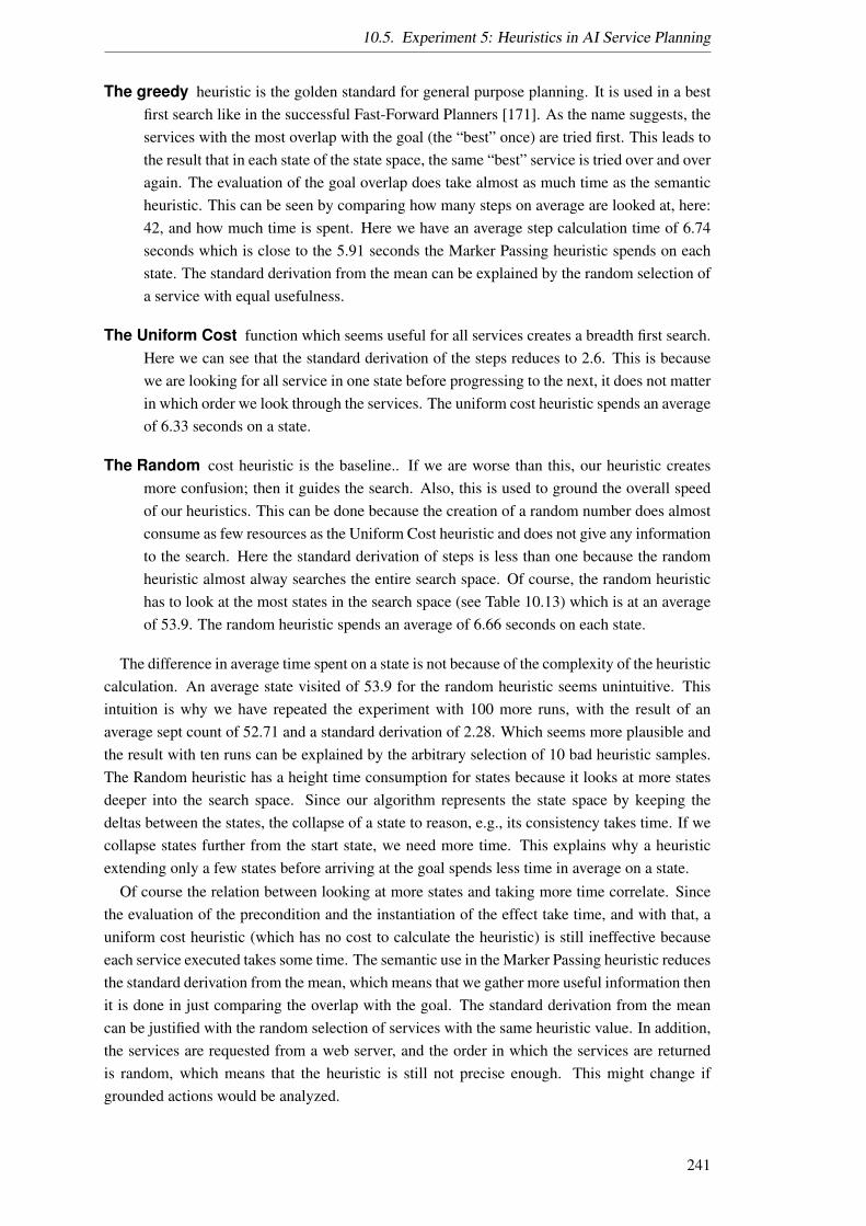
10.5. Experiment 5: Heuristics in AI Service Planning

The greedy heuristic is the golden standard for general purpose planning. It is used in a bestfirst search like in the successful Fast-Forward Planners [171]. As the name suggests, theservices with the most overlap with the goal (the “best” once) are tried first. This leads tothe result that in each state of the state space, the same “best” service is tried over and overagain. The evaluation of the goal overlap does take almost as much time as the semanticheuristic. This can be seen by comparing how many steps on average are looked at, here:42, and how much time is spent. Here we have an average step calculation time of 6.74seconds which is close to the 5.91 seconds the Marker Passing heuristic spends on eachstate. The standard derivation from the mean can be explained by the random selection ofa service with equal usefulness.

The Uniform Cost function which seems useful for all services creates a breadth first search.Here we can see that the standard derivation of the steps reduces to 2.6. This is becausewe are looking for all service in one state before progressing to the next, it does not matterin which order we look through the services. The uniform cost heuristic spends an averageof 6.33 seconds on a state.

The Random cost heuristic is the baseline.. If we are worse than this, our heuristic createsmore confusion; then it guides the search. Also, this is used to ground the overall speedof our heuristics. This can be done because the creation of a random number does almostconsume as few resources as the Uniform Cost heuristic and does not give any informationto the search. Here the standard derivation of steps is less than one because the randomheuristic almost alway searches the entire search space. Of course, the random heuristichas to look at the most states in the search space (see Table 10.13) which is at an averageof 53.9. The random heuristic spends an average of 6.66 seconds on each state.

The difference in average time spent on a state is not because of the complexity of the heuristiccalculation. An average state visited of 53.9 for the random heuristic seems unintuitive. Thisintuition is why we have repeated the experiment with 100 more runs, with the result of anaverage sept count of 52.71 and a standard derivation of 2.28. Which seems more plausible andthe result with ten runs can be explained by the arbitrary selection of 10 bad heuristic samples.The Random heuristic has a height time consumption for states because it looks at more statesdeeper into the search space. Since our algorithm represents the state space by keeping thedeltas between the states, the collapse of a state to reason, e.g., its consistency takes time. If wecollapse states further from the start state, we need more time. This explains why a heuristicextending only a few states before arriving at the goal spends less time in average on a state.

Of course the relation between looking at more states and taking more time correlate. Sincethe evaluation of the precondition and the instantiation of the effect take time, and with that, auniform cost heuristic (which has no cost to calculate the heuristic) is still ineffective becauseeach service executed takes some time. The semantic use in the Marker Passing heuristic reducesthe standard derivation from the mean, which means that we gather more useful information thenit is done in just comparing the overlap with the goal. The standard derivation from the meancan be justified with the random selection of services with the same heuristic value. In addition,the services are requested from a web server, and the order in which the services are returnedis random, which means that the heuristic is still not precise enough. This might change ifgrounded actions would be analyzed.

241

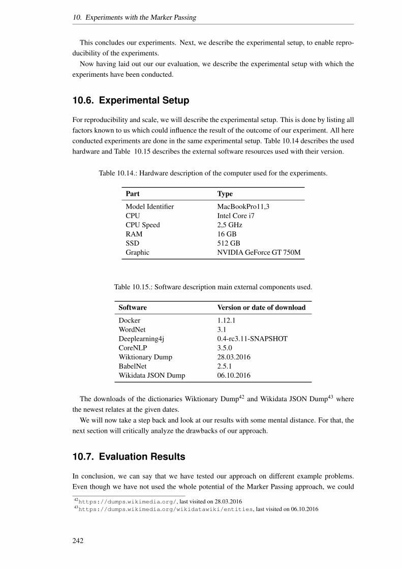
10. Experiments with the Marker Passing

This concludes our experiments. Next, we describe the experimental setup, to enable repro-ducibility of the experiments.

Now having laid out our our evaluation, we describe the experimental setup with which theexperiments have been conducted.

10.6. Experimental Setup

For reproducibility and scale, we will describe the experimental setup. This is done by listing allfactors known to us which could influence the result of the outcome of our experiment. All hereconducted experiments are done in the same experimental setup. Table 10.14 describes the usedhardware and Table 10.15 describes the external software resources used with their version.

Table 10.14.: Hardware description of the computer used for the experiments.

Part Type

Model Identifier MacBookPro11,3CPU Intel Core i7CPU Speed 2,5 GHzRAM 16 GBSSD 512 GBGraphic NVIDIA GeForce GT 750M

Table 10.15.: Software description main external components used.

Software Version or date of download

Docker 1.12.1WordNet 3.1Deeplearning4j 0.4-rc3.11-SNAPSHOTCoreNLP 3.5.0Wiktionary Dump 28.03.2016BabelNet 2.5.1Wikidata JSON Dump 06.10.2016

The downloads of the dictionaries Wiktionary Dump42 and Wikidata JSON Dump43 wherethe newest relates at the given dates.

We will now take a step back and look at our results with some mental distance. For that, thenext section will critically analyze the drawbacks of our approach.

10.7. Evaluation Results

In conclusion, we can say that we have tested our approach on different example problems.Even though we have not used the whole potential of the Marker Passing approach, we could

42https://dumps.wikimedia.org/, last visited on 28.03.201643https://dumps.wikimedia.org/wikidatawiki/entities, last visited on 06.10.2016

242

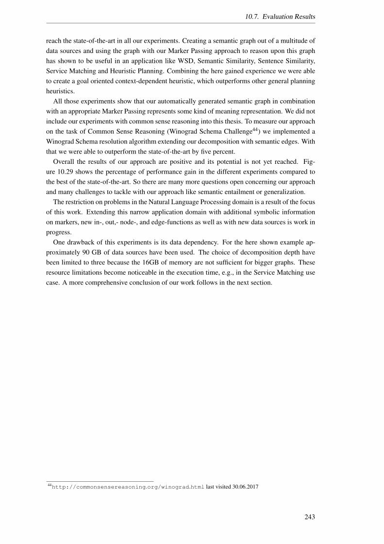
10.7. Evaluation Results

reach the state-of-the-art in all our experiments. Creating a semantic graph out of a multitude ofdata sources and using the graph with our Marker Passing approach to reason upon this graphhas shown to be useful in an application like WSD, Semantic Similarity, Sentence Similarity,Service Matching and Heuristic Planning. Combining the here gained experience we were ableto create a goal oriented context-dependent heuristic, which outperforms other general planningheuristics.

All those experiments show that our automatically generated semantic graph in combinationwith an appropriate Marker Passing represents some kind of meaning representation. We did notinclude our experiments with common sense reasoning into this thesis. To measure our approachon the task of Common Sense Reasoning (Winograd Schema Challenge44) we implemented aWinograd Schema resolution algorithm extending our decomposition with semantic edges. Withthat we were able to outperform the state-of-the-art by five percent.

Overall the results of our approach are positive and its potential is not yet reached. Fig-ure 10.29 shows the percentage of performance gain in the different experiments compared tothe best of the state-of-the-art. So there are many more questions open concerning our approachand many challenges to tackle with our approach like semantic entailment or generalization.

The restriction on problems in the Natural Language Processing domain is a result of the focusof this work. Extending this narrow application domain with additional symbolic informationon markers, new in-, out,- node-, and edge-functions as well as with new data sources is work inprogress.

One drawback of this experiments is its data dependency. For the here shown example ap-proximately 90 GB of data sources have been used. The choice of decomposition depth havebeen limited to three because the 16GB of memory are not sufficient for bigger graphs. Theseresource limitations become noticeable in the execution time, e.g., in the Service Matching usecase. A more comprehensive conclusion of our work follows in the next section.

44http://commonsensereasoning.org/winograd.html last visited 30.06.2017

243

10. Experiments with the Marker Passing

State-of-the-Art

Performance Gain in %

Sem

antic

Sim

ilarti

y

0.882

0.385

Sem

antic

Sen

tenc

e Si

mila

rtiy

Serv

ice

Mat

chin

g

Wor

d Se

nse

Disa

mbi

guat

ion

SMTeuroparl

0.8760.482… …

0.50

0.30

Spearman

0.45

0.22

0.877

0.565

Effect

…

20.3

43.3…

Serv

ice

Plan

ning

Heu

ristic

States extended

Pearson

Accuracy

10%

-10%

-20%

50%

90% Pearson

20%

ND

CG

Measure usedState-of-the-ArtResults

Figure 10.29.: Overview of example results in the different experiments in percentage of perfor-mance difference to the state-of-the-art baseline.

244

Part V.

Conclusion

245

11. Summary

This section concludes the here presented work. We will look at my hypotheses and the contri-butions I have made. However, first I give a short overview of my approach:

I have created an approach for automatically generating a semantic graph focused on a contextand a reasoning using Marker Passing to answer questions about the knowledge encoded (for anabstract descriptions see Section 1.5). This approach has two parts:

Knowledge representation: This is the first part of the approach which tackled the chal-lenge of automatically creating a knowledge representation. I did so by looking at thedifferent semantic theories, selected the NSM approach and created a semantic decompo-sition to build a semantic graph automatically.

Reasoning: This is the second part of my approach which tackled the challenge of using se-mantic graphs to create reasoning capabilities for an agent. I approached this challenge byextending a cognitive mechanism of activation spreading with more symbolic informationto Marker Passing. The resulting common sense reasoning has been shown by identify-ing subproblems in AI research, like the Sentence Similarity, Word Sense Disambiguationand Semantic Similarity for which I have proposed solutions which keep up or beat thestate-of-the-art.

To use this approach one has to select data sources, set up the decomposition and create anapplication specific Marker Passing by selecting, e.g., the information on the Marker and in- andout-functions.

Next, we will look at my hypotheses and discuss the contributions of this work and theirrelation to those hypotheses. We start out with my experimental thesis:

I claim in my hypothesis that: “Symbolic and Connectionist representation of meaningcan help agents to reason with new concepts.” I support this claim with a set of experimentswhich include the decomposition of new concepts and their integration into the semantic graphrepresenting the agent’s belief.

I am now able to answer my research questions proposed in Section 1.4, which have guidedmy research.

How can meaning formally be described in a context-dependent manner? The formaliza-tion of the result of the decomposition (see Section 6.4) allows us to encode factual knowledge inan semantic graph (see Section 6). The context dependence of meaning comes from the MarkerPassing (see Section 7) and finally from the distribution of marker over the graph. This structurecan represent meaning, which has been tested in multiple experiments (see Section 9).

I was able to show the usefulness of the so created artificial representation of meaning byshowing that context-dependent heuristics can be created by observing service descriptions. Theuse of the artificial meaning representation to build a heuristic has been done by comparing thesemantic distance of goal concepts and the concept describing a service (see Section 10.5.3). Ad-ditionally, I was able to show that the performance of agent planner and Service Matcher can be

247

11. Summary

improved by using dynamic heuristics. The performance of Service Matcher improves by addinga kind of ontology matching to the comparison of service descriptions (see Section 10.4). Theperformance of my planner is improved since the heuristic lets us select only relevant services.This selection is done by combining all approaches build in this work (see Section 10.5).

Of course, there are many more questions which can be asked now like: How do we handleinconsistency in such a graph? How can logical reasoning be implemented using such a semanticgraph? Which classes of problems are destined to be addressed with such an approach? We willdiscuss some of more concrete extensions next.

I did analyze the usefulness of the newly gained meaning representation in five experimentsand with that answered the second research questions: Can the reasoning be improved for thefollowing tasks:

In my experiment 1 I asked: “Does the representation of meaning include information tocreate a state-of-the-art semantic similarity measure?” This question was assured by myexperiment in Section 10.1. Here I am able to use my approach to create a semanticsimilarity measure which outperforms the state-of-the-art. I show in Table 10.4 that thesemantic similarity guessed by humans can be reproduced and with that, the meaning ofconcepts can be grasped.

In my experiment 2 I asked: “Does the representation of meaning include information tocreate a state-of-the-art Word Sense Disambiguation approach?” This was answered bymy experiment in Section 10.2. Here I was able to use my decomposition to capture thedifferent word meanings in the different definitions of the information sources. Table 10.5shows that my approach can keep up with the state-of-the-art, even though there are betterperforming results. Here we can conclude that the decomposition is still too broad and thata selection of definitions to decompose should be made during decomposition to specializethe resulting semantic graph.

In my experiment 3 I asked “Does the representation of meaning include information to cre-ate a state-of-the-art semantic sentence similarity measure?” This question was answeredby my experiment in Section 10.3. Here I was able to use my approach (including theresults of my first experiment) to create a sentence similarity measure which matches thestate-of-the-art. Table 10.11 shows the results on different data sets. Here we can con-clude that the more difficult the data set, the more the state-of-the-art is outperformed bymy approach.

In my experiment 4 I asked: “Can we improve the performance of Service Matchers by usingthe connectionist and symbolic representation of meaning as Ontology Matching?” Thisquestion was answered by my experiment in Section 10.4. Here I was able to use myapproach to compare name, description, input, output precondition and effect of a servicedescription. Except for input and precondition I was able to increase the performance ofthe Service Matcher. Here we gained the insight that some of the service description partscontain more semantic information to be analyzed with Marker Passing, other performbetter with logical reasoning. Here the natural language part of the description of a serviceoutperformed all other experts.

In my experiment 5 I asked: “Can heuristics for general purpose planners profit from usinga connectionist and symbolic representation of meaning?” This question was answered by

248

my experiment in Section 10.5. Here I were able to show that the newly created heuristicutilizing semantic information narrows the search space in a state space planning problem.To check this hypothesis, I build a service planner described in Algorithm 20 because Ihad to preserve the semantic information of service descriptions. I then build a dynamicheuristic that takes into account the goal of the given planning problem and uses the resultsof my experiments to search for semantically useful services. I showed that this heuristicperforms well in Table 10.13.

With those experiments, I have shown that my approach is useful in different AI problems.These are convincing arguments for the usefulness of my artificial representation of meaning.I started out with the idea of an approach, which has more potential than I was able to use inthe here described experiments. By adding additional interpretations for semantic primes, thisapproach could prosper further. For now, the specific interpretations of the primes are reduced toa general rule on how to handle all primes. But there are experiments in progress, which use thehere proposed approach in common sense reasoning problems (e.g., the solution of WinogradSchemas1) to outperform the state-of-the-art.

After having accomplished all that, I have found drawbacks of the design decision I madeduring my scientific endeavor. I will discuss these drawbacks regarding the here analyzed ex-periments next.

1http://commonsensereasoning.org/winograd.html, last visited on 30.06.2017

249

12. Discussion

This section discusses design decision, drawbacks and the experiments and their relation to theoverall goal of this thesis. Here we will emphasize on the drawbacks of the experiments. Thisincludes the implicit design decisions which could be altered in a future application or furtherresearch of the here proposed approach.

Starting out from my approach, I had to select some data sources which are used during thedecomposition. Those data sources are imperfect, they contain errors or include beliefs whichare false. Furthermore, the here selected data sources do not forcibly align with the hierarchy ofthe NSM theory and the idea of Wierzbicka of a mental lexicon [410]. This has the consequencethat a complete decomposition is unlikely and sometimes impossible. Because of the parameterof decomposition depth, it becomes questionable how much the NSM primes are beneficial tomy approach. Perhaps this can be answered with an example: In the decomposition of thesemantic similarity data set RG65 of 65 similarity pairs, a total of 227 semantic primes havebeen used at a decomposition depth of one. This number increases with decomposition depth oftwo to 17317.

Another drawback is the dependence of the Marker Passing on the decomposition. Thus ifthe performance of the approach is not as expected, it might at first be unclear if a faulty decom-position or a misconfigured Marker Passing is the cause. Solving such development problemsneeds experience on which data sources contain which kind of information so that the decom-position can be changed to fit the needs of the problem. Additionally, the developer needs asufficient understanding of the Marker Passing and the effect change in parameters have on theresult. During the design of the algorithm, the needed information in the decomposition can beestimated, and with that information, the needed data sources can be specified. Based on theavailable information in the semantic graph the Marker Passing can be specified.

Another uncertainty in the approach is the completeness of the data sources. The decomposi-tion fails if none of the data sources contain a description of the given concept.

Next, we will look critically at the experiments I conducted and evaluated their outcome.

Experiment 1: Semantic Similarity Measure I tested my semantic similarity measure witha data set which states the similarity of word pairs as perceived by humans. A critical viewon this approach could argue that the perception of the meaning of humans (especially theaverage of multiple human opinions) does not have to be the semantic distance of thoseconcepts. The response of the humans depends on their education and beliefs. The av-erage of multiple opinions mixes those different levels of knowledge and beliefs, whichdoes no longer represent the semantic distance of those words in the sense of a semanticmeasure an expert or scientists would evaluate. For instance, an astronomer would notagree that the sun and a planet are semantically close, but for an average citizen, they areboth round and in the sky, which might make them similar. Those two opinions can bediscussed to be more or less correct, but the average will not yield a similarity representingwhat both subjects intended. Measuring an artificial representation of meaning on those

251

12. Discussion

semantic similarities, can in consequence, only partially measure the performance of therepresentation. It only shows that the approach can make the same mistakes as humansdo. We would need a set of word pairs, where the semantic similarity is defined by expertsregarding facts about the objects referenced by those words so that the artificial represen-tation of meaning can be evaluated on how well it can represent the expert knowledge ofhumans. Another critique could be that the found weights for the semantic relations arenot intuitive. Further investigations on which information in the semantic graph can beused by the Marker Passing is needed. This implies that there is room for improvement.The found result is most likely only a local optimum.

Experiment 2: Word Sense Disambiguation The data sets used in WSD comparisons arebased on WordNet sense keys to identify the word sense. This, of course, is not the casein other information sources, where different definitions can occur. Those definitions arethen not mapped to the WordNet sense keys; as a result, the do not count as a right answer.The missing syntactical information makes it even harder for my approach to use all infor-mation available in the surrounding words of the sentence. The results could be improvedby integrating syntactic information and thus giving the approach more information inwhich context the word is used in.

Experiment 3: Semantic Sentence Similarity Measure My approach is a purely seman-tic approach. This might be good for analyzing the semantics of single concepts, but withsentences, the order of words, the inflection, and the syntax make up the meaning of thesentence. Most of this is disregarded in the here proposed results. With the reduction ofconcepts to their stem, the inflection is lost. Additionally, the decomposition is combinedto one graph, losing all information about word order or syntax. Hence this approachcan not make a difference between the sentences: “Johannes bit the dog” and “The dogbit Johannes.” Even though the performance of the semantic sentence similarity measureshows the ability to outperform the state-of-the-art in some cases, the logical (in meansof truth-value) meaning of a sentence is not captured by it. This shortcoming could becountered by extending the semantic decomposition with syntactic information and createa Marker Passing algorithm which uses this syntactic information.

Experiment 4: Semantic Service Matching The results of the service matching experi-ment have shown that the semantic analysis performs well on semantically rich parts ofthe service description, but need far more resources than the compared approaches. Ta-ble 10.10 shows that the Marker Passing on natural language descriptions takes up to tentimes more time than the other experts. This could be avoided by combining those toexpert types on the different description parts. Also, the overall performance could be im-proved by learning the expert’s weights. The Marker Passing does some kind of ontologymatching between the concepts used in the service description. This means that beforeusing such an approach, the service description needed to use the same ontologies. Withthe Marker Passing, this is no longer needed since the decomposition creates a mergingontology. This ability exceeds the state-of-the-art of Service Matcher and should be an-alyzed further. For example to answer the question on how the inputs are transformed ifthey are semantically similar, but have different data types.

Experiment 5: Heuristics in AI service planning The planning problem discussed here

252

is not a straight forward optimization problem because we do not have costs for the ser-vices. The kind of problem solved here means there is no optimization goal for the solutionplan. The problem can be made to an optimization goal if, e.g., the services provide Qual-ity of Service parameters which directly include a cost or can be used to calculate a serviceexecution cost. Additionally, the evaluation data set does not provide a cost function forthe services. The selection of the data set is another weak point of this thesis since I wereunable to find any other OWL-S based planning problem. The work on this topic has pro-duced an entire tool chain to describe such data sets for the future (see Appendix A.1 fora short introduction).

253

13. Final Remarks and Future Work

“Because this world doesn’t belong to you, or the people who came before. Itbelongs to someone who is yet to come.”

- DOLORES

Stepping back from the research done in this thesis, we can again ask if the overhead of creating,e.g., semantic service description, an OWLS description of start and goal state and the ontologiesneeded for that, is worth the while, regarding the problem to be solved. We can question if thisoverhead can be countered by the benefit of reusing services. I have encountered this problemin applications of this approach in publicly funded research projects. Those projects developedtools to ease the description of services and their composition as described in the methodologyin Section A.1.

In comparison to PDDL problem descriptions, often used in academic examples, the problemdescription includes only services needed to solve the problem. Consequently, a selection of theappropriate service is not part of the problem. Additionally, the problems typically describedin PDDL are lacking semantics, like the 15-puzzle [322] which is more about making the samefour moves in a particular order, which was difficult to conclude from the semantics of the move.

Making a plan and executing it are two different things. It seems unrealistic to prepare aplan for the most likely eventualities, meaning that during the execution the environment couldchange and a plan could fail. This work presents a mechanism to choose from the large set ofpossible services available to an agent.

In the case of incomplete information in the data sources, I have extended the decompositionwith a component which then provides the user with a user interface where a definition can bedescribed manually. There are multiple points, which can be handled semi-automatically: firstthe selection of the concept type. Here the word type needs to be specified. This parameterinfluences the definition selection as well as the search for synonyms, antonyms hypernyms, andhyponyms. Second semi-automatization could be the selection of the definition. Here the senseof a word is selected. The user can select which definition to use. In the example of “well” thiscould be the meaning of in a satisfactory way or a hole in the ground with water in it. The thirdsemi-automatization point could be the decomposition of a concept which has no definition orwhere the definition is circular. A concept could have no definition if the used dictionary does notcontain a description of the word. In this case, the decomposition stops at this prime and mightonly continue with the decomposition after a manual definition or decomposition is introduced.Fourthly the breadth of the recursion needs to be defined. This parameter specifies how manysynonyms and antonyms are searched for in each decomposition step. Fifthly the amount ofadditional information included. This parameter specifies how many examples of hypernymsand hyponyms are included in the decomposition. Further, the information sources need tobe specified. The specification includes the used dictionary and a mapping of the informationsources to the information retrieval parts of the decomposition.

255

13. Final Remarks and Future Work

With every scientific endeavor at the end, there are always more questions to be answered. Iwill split the future work into two parts: First the improvement of the approach and second theimprovements for the heuristics in service planning.

Artificial Meaning: This work is restricted to the semantic analysis. This needs to be ex-tended with a syntactical analysis. The Marker Passing has not yet been tested for its fullpotential, e.g., encoding logical symbolic information of negation on a marker and usingit in in-, out- and edge-functions. The selection of the right parameters or a guide howto select them concerning a type of problem could be investigated in the future. Reason-ing with the Marker Passing could be tested on more complex problems like WinogradSchemas [230]. Last but not least, additional data sources can be added to the decompo-sition to improve future results. For example, the integration of the semantic of the NSMprimes could be an addition to the Marker Passing, since then meaning could be reasonedbottom up.

Heuristics: This work has stopped with the planning, which leaves the execution and monitor-ing as well as plan repair to future work. The question to answer here is: How can thosepart profits from the semantic information given by the problem? The expressiveness ofthe description language can further be developed since modern reasoners do not imple-ment all SWRL built-ins making the description of a planning problem more complexthan it needs to be. In the end, better data sets are needed to evaluate the drawbacks andbenefits of service planning and proposed heuristics.

256

Part VI.

Bibliography, Glossary, Index, andAppendix

257

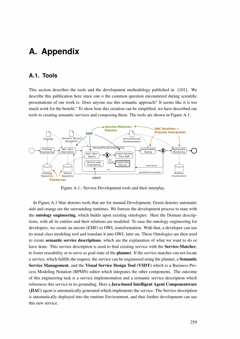
A. Appendix

A.1. Tools

This section describes the tools and the development methodology published in [101]. Wedescribe this publication here since one o the common question encountered during scientificpresentations of our work is: Does anyone use this semantic approach? It seems like it is toomuch work for the benefit.” To show how this creation can be simplified, we have described ourtools to creating semantic services and composing them. The tools are shown in Figure A.1.

Figure A.1.: Service Development tools and their interplay.

In Figure A.1 blue denotes tools that are for manual Development, Green denotes automaticaids and orange are the surrounding runtimes. We foresee the development process to state withthe ontology engineering, which builds upon existing ontologies. Here the Domain descrip-tions, with all its entities and their relations are modeled. To ease the ontology engineering fordevelopers, we create an encore (EMF) to OWL transformation. With that, a developer can useits usual class modeling tool and translate it into OWL later on. These Ontologies are then usedto create semantic service descriptions, which are the explanation of what we want to do orhave done. This service description is used to find existing service with the Service-Matcher,to foster reusability or to serve as goal state of the planner. If the service matcher can not locatea service, which fulfills the request, the service can be engineered using the planner, a SemanticService Management, and the Visual Service Design Tool (VSDT) which is a Business Pro-cess Modeling Notation (BPMN) editor which integrates the other components. The outcomeof this engineering task is a service implementation and a semantic service description whichreferences this service in its grounding. Here a Java-based Intelligent Agent Componentware(JIAC) agent is automatically generated which implements the service. The Service descriptionis automatically deployed into the runtime Environment, and thus further development can usethis new service.

259

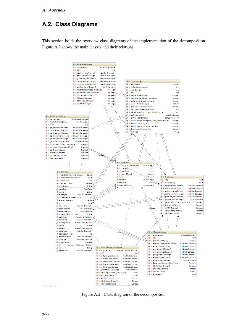
A. Appendix

A.2. Class Diagrams

This section holds the overview class diagrams of the implementation of the decomposition.Figure A.2 shows the main classes and their relations.

Figure A.2.: Class diagram of the decomposition.

260

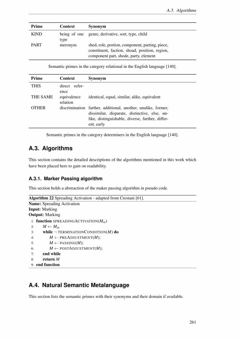
A.3. Algorithms

Prime Context Synonym

KIND being of onetype

genre, derivative, sort, type, child

PART meronym shed, role, portion, component, parting, piece,constituent, faction, shoad, position, region,component part, shode, party, element

Semantic primes in the category relational in the English language [140].

Prime Context Synonym

THIS direct refer-ence

THE SAME equivalencerelation

identical, equal, similar, alike, equivalent

OTHER discrimination farther, additional, another, unalike, former,dissimilar, disparate, distinctive, else, un-like, distinguishable, diverse, further, differ-ent, early

Semantic primes in the category determiners in the English language [140].

A.3. Algorithms

This section contains the detailed descriptions of the algorithms mentioned in this work whichhave been placed here to gain on readability.

A.3.1. Marker Passing algorithm

This section holds a abstraction of the maker passing algorithm in pseudo code.

Algorithm 22 Spreading Activation - adapted from Crestani [61].Name: Spreading ActivationInput: MarkingOutput: Marking

1: function SPREADINGACTIVATION(Min)2: M← Min

3: while ¬ TERMINATIONCONDITION(M) do4: M← PREADJUSTMENT(M);5: M← PASSING(M);6: M← POSTADJUSTMENT(M);7: end while8: return M9: end function

A.4. Natural Semantic Metalanguage

This section lists the semantic primes with their synonyms and their domain if available.

261

A. Appendix

Prime Context Synonym

ONE Number single, unity, 1, ace,TWO Number II, 2MANY Number a lot, loads, plenty, a great deal, greatly, much,

highly, very muchSOME quantifiers a fewALL quantifiers completely

Semantic primes in the category quantifiers in the English language [140].

Prime Context Synonym

GOOD evaluators commodity, not bad, accomplished, well, sat-isfactory, decent, good, all right, trade good,goodness

BAD evaluators badness, spurious, malodorous, wanting, bad,odious, awful, faulty, foul, wretched, coarse,poor, horrible, dreadful, unsatisfactory, aban-doned, badass, terrible, lousy, inadequate, vi-cious, miserable, ill, dismal, abysmal, horrid,hideous, detestable, punk, unfavorable, loath-some, evil, rotten, substandard, incompetent,inelegant, negative, dire, disgusting, vile, ur-gent, ungodly, crummy, deficient, wicked,sloppy, unacceptable, corrupt, inferior, abom-inable, false, disagreeable, off, wrong, severe,hopeless, intolerable, base

Semantic primes in the category evaluators in the English language [140].

Prime Context Synonym

BIG size big, prominent, jumbo, bad, large, grown up,heavy, massive, ample, major leagues, huge,sizeable, stoor, adult

SMALL size slight, mini, compact, lowercase, insignifi-cant, young, slim, minuscule, minute, mod-est, wee, tiny, miniature, small-scale, micro-scopic, petty, little

Semantic primes in the category descriptors in the English language [140].

262

A.4. Natural Semantic Metalanguage

Prime Context Synonym

THINK cognition imagine, cogitate, deem, ponder, suppose,opine, reflect, guess, find, regard, ruminate,judge, consider, reckon

KNOW cognitionWANT cognition wish, set one’s heart on, deficiency, need,

would like, deprivation, neediness, privation,wishing, lack

FEEL cognition flavor, flavour, tone, tactile property, spirit,feel, feeling, smell, look

SEE cognition descry, view, get, espy, understand, behold,follow, observe

HEAR cognition get word, discover, find out, pick up, see, getwind, get a line, learn

TOUCH cognition trace, touching, cutaneous senses, skinsenses, sense of touch, touch modality

Semantic primes in the category mental predicates in the English language [140].

Prime Context Synonym

SAY speechWORDS speech wrangle, lyric, dustup, quarrel, languageTRUE logic

Semantic primes in the category speech in the English language [140].

Prime Context Synonym

DO action to-do, bash, do, DO, brawlHAPPEN event fall out, befall, pass, hap, occur, go on, come

about, take place, pass offMOVE action motion, affect, instigate, impel, actuate, re-

location, propose, persuade, influence, offer,rouse, induce, transfer, incite, removal, motil-ity, trouble, incline, stir, agitate, movement,prompt

[Semantic primes in the category actions, events in the English language [140].]Semantic primesin the category actions, events, movement, contact in the English language [140].

Prime Context Synonym

BEat locationTHERE IS exsistenceHAVE possessionBEis−a specification

[Semantic primes in the category location, possession, in the English language [140].]Semanticprimes in the category location, existence, possession, specification in the English lan-guage [140].

263

A. Appendix

Prime Context Synonym

LIVE survive, living, last, alive, inhabit, in the flesh,dwell, in person, live on, populate, endure

DIE live pass away, die, join the choir invisible, passon, dice, bite the big one, lose one’s life, snuffit, pop one’s clogs, cross over, keel over, de-cease, check out, go the way of all flesh, bitethe dust, cash in, perish, go the way of the di-nosaurs, go the way of the dodo, croak, shuf-fle off this mortal coil, pass, buy it, meet one’smaker, kick the bucket, draw one’s last breath,give up the ghost, forfare, disincarnate, knockoff, expire, buy the farm, bite the biscuit, cashin one’s chips, cark, yield up the ghost, take adirt nap, succumb, give one’s all, cease to be

Semantic primes in the category life and death in the English language [140].

Prime Context Synonym

WHENNOWBEFORE earlier, previously, before, ahead, in front, by,

in front, lest, in front of, ahead ofAFTERA LONGTIMEA SHORTTIMEFOR SOMETIMEMOMENT stound, bit, second, moment, minute, instant,

tic, sec, overnight, trice, blink of an eye, hereand now, present moment, moment of force,jiffy, nothing flat, flash

Semantic primes in the category time in the English language [140]

264

A.4. Natural Semantic Metalanguage

Prime Context Synonym

WHEREHEREAVOCEBELOW down the stairs, beneath, on a lower floor, to

a lower place, below, at a lower place, down-wards, downstream, infra, under, downstairs,underneath

FARNEAR near side, come on, come near, near, go up,

approach, draw close, draw nearSIDEINSIDE indoors, inside, interior

Semantic primes in the category space in the English language [140].

Prime Context Synonym

NOT nonMAYBE perhaps, perchance, mayhaps, peradventure,

mayhap, possiblyCAN may, be able to,BECAUSE causality as, for that, for, therefore, forthy, inasmuch

as, since, forwhyIF

Semantic primes in the category logical in the English language [140].

Prime Context Synonym

VERY identical, very, swith, selfsame, ilk, main,sore, ever so

MORE

Semantic primes in the category intensifier in the English language [140].

Prime Context Synonym

LIKE such as

Semantic primes in the category similarity in the English language [140].

265

Bibliography

[1] Proceedings of the Twenty-Sixth International Conference on Automated Planning andScheduling, ICAPS 2016, London, UK, June 12-17, 2016. In Amanda Coles, AndrewColes, Stefan Edelkamp, Daniele Magazzeni, and Scott Sanner, editors, Proceedingsof the Twenty-Sixth International Conference on Automated Planning and Scheduling,ICAPS 2016, London, UK, June 12-17, 2016. AAAI Press, 2016.

[2] Sunitha Abburu. A survey on ontology reasoners and comparison. International Journalof Computer Applications, 57(17), 2012.

[3] Eneko Agirre, Enrique Alfonseca, Keith Hall, Jana Kravalova, Marius Pasca, and AitorSoroa. A study on similarity and relatedness using distributional and WordNet-basedapproaches. In NAACL ’09: Proceedings of Human Language Technologies: The 2009Annual Conference of the North American Chapter of the Association for ComputationalLinguistics, pages 19–27. Charles University in Prague, Association for ComputationalLinguistics, 2009.

[4] Eneko Agirre, Oier de Lacalle, and Aitor Soroa. Random Walks for Knowledge-BasedWord Sense Disambiguation. Computational Linguistics, 40(1):57–84, 2014.

[5] Eneko Agirre and Philip Edmonds. Word sense disambiguation: Algorithms and appli-cations, volume 33. Springer Science & Business Media, 2007.

[6] Rama Akkiraju, Biplav Srivastava, Anca-Andreea Ivan, Richard Goodwin, and Tan-veer Syeda-Mahmood. SEMAPLAN: Combining Planning with Semantic Matching toAchieve Web Service Composition. In 2006 IEEE International Conference on Web Ser-vices (ICWS’06), pages 37–44. IEEE, 2006.

[7] Harith Alani, Sanghee Kim, D Millard, M Weal, W Hall, P Lewis, and N Shadbolt. Auto-matic ontology-based knowledge extraction from Web documents. IEEE INTELLIGENTSYSTEMS, 18(1):14–21, 2003.

[8] Jens Allwood and Peter Gardenfors. Cognitive Semantics, volume 55 of Meaning andCognition. John Benjamins Publishing, 1999.

[9] Gahadah Altaiari. Editor zur semantischen Dekomposition. Bachelors thesis, 2014. Tech-nische Universitat Berlin.

[10] John Anderson. A spreading activation theory of memory. Journal of Verbal Learningand Verbal Behavior, 22(3):261–295, 1983.

[11] Avery Andrews. Reconciling NSM and Formal Semantics. Australian Journal of Lin-guistics, 36(1):79–111, 2015.

[12] Mark Aronoff and Janie Rees-Miller. The handbook of linguistics. Blackwell PublishersLtd, 2003.

[13] Christer Backstrom and Bernhard Nebel. Complexity results for SAS+ planning. Com-putational Intelligence, 11(4):625–655, 1995.

267

Bibliography

[14] Jay Bagga and Adrian Heinz. JGraph— A Java Based System for Drawing Graphs andRunning Graph Algorithms. In Graph Drawing, pages 459–460. Springer, Berlin, Hei-delberg, Berlin, Heidelberg, 2001.

[15] Tina Balke and Nigel Gilbert. How Do Agents Make Decisions? A Survey. Journal ofArtificial Societies and Social Simulation, 17(4), 2014.

[16] Andrea Ballatore, Michela Bertolotto, and David Wilson. An evaluative baseline for geo-semantic relatedness and similarity. arXiv preprint arXiv:, cs.CL(4):747–767, 2014.

[17] Marco Baroni, Georgiana Dinu, and German Kruszewski. Don’t count, predict! A sys-tematic comparison of context-counting vs. context-predicting semantic vectors. In Pro-ceedings of the 52nd Annual Meeting of the Association for Computational Linguistics(Volume 1: Long Papers), pages 238–247, Stroudsburg, PA, USA, 2014. Association forComputational Linguistics.

[18] Alistair Barros and Daniel Oberle. Handbook of Service Description. USDL and ItsMethods. Springer Science & Business Media, Boston, MA, 2012.

[19] Jon Barwise and Robin Cooper. Generalized Quantifiers and Natural Language. In Philos-ophy, Language, and Artificial Intelligence, pages 241–301. Springer Netherlands, Dor-drecht, 1988.

[20] Osman Baskaya and David Jurgens. Semi-supervised Learning with Induced Word Sensesfor State of the Art Word Sense Disambiguation. Journal of Artificial Intelligence Re-search, 55:1025–1058, 2016.

[21] Nicole Beckage and Eliana Colunga. Language Networks as Models of Cognition: Un-derstanding Cognition through Language. In Towards a Theoretical Framework for An-alyzing Complex Linguistic Networks, pages 3–28. Springer Berlin Heidelberg, Berlin,Heidelberg, 2016.

[22] Richard Bellman. Dynamic programming. Rand research study. Princeton Univ. Press,Princeton, NJ, 1957.

[23] Ayse Bener, Volkan Ozadali, and Erdem Ilhan. Semantic matchmaker with preconditionand effect matching using SWRL. 36(5):9371–9377, 2009.

[24] Tim Berners-Lee. Semantic Web Road map: A road map for the future, an architecturalplan untested by anything except thought experiments, 1998. http://www.w3.org/DesignIssues/Semantic.html Last visited: 07.07.2017.

[25] Tim Berners-Lee, James Hendler, and Ora Lassila. The semantic web. Scientific Ameri-can, 2001.

[26] Michael Berthold, Ulrik Brandes, Tobias Kotter, Martin Mader, Uwe Nagel, and KilianThiel. Pure spreading activation is pointless. CIKM, pages 1915–1918, 2009.

[27] Leonora Bianchi, Marco Dorigo, Luca Gambardella, and Walter Gutjahr. A survey onmetaheuristics for stochastic combinatorial optimization. Natural Computing, 8(2):239–287, 2009.

[28] Chris Biermann. Ontology Learning from Text: A Survey of Methods. LDV-Forum,20(2):75–93, 2005.

[29] Leonard Bloomfield. Sentence and Word. Transactions and Proceedings of the AmericanPhilological Association, 45:65, 1914.

268

Bibliography

[30] Leonard Bloomfield. Language. University of Chicago Press, New York: Holt, 1933.

[31] Leonard Bloomfield. Language or Ideas? Language, 12(2):89–95, 1936.

[32] Leonard Bloomfield. Meaning. Monatshefte fur deutschen Unterricht, 35(3/4):101–106,1943.

[33] Kurt Bollacker, Colin Evans, Praveen Paritosh, Tim Sturge, and Jamie Taylor. Freebase- a collaboratively created graph database for structuring human knowledge. SIGMODConference, page 1247, 2008.

[34] Blai Bonet and Hector Geffner. Planning as heuristic search. Artificial Intelligence,129(1-2):5–33, 2001.

[35] Paolo Bouquet, Fausto Giunchiglia, Frank Van Harmelen, Luciano Serafini, and HeinerStuckenschmidt. C-OWL: Contextualizing ontologies. In International Semantic WebConference, volume 2870, pages 164–179, 2003.

[36] Ros Bramwell. Education and some aspects of meaning: A background study. BritishJournal of Educational Studies, 20(1):12–26, 1972.

[37] Benjamin Brand. Semantic Distance of Service Descriptions through Activation Spread-ing. Master’s thesis, 2017. Technische Universtitat Berlin.

[38] Lars Braubach, Alexander Pokahr, Daniel Moldt, and Winfried Lamersdorf. Goal Rep-resentation for BDI Agent Systems. volume 3346, pages 44–65. Springer Berlin Heidel-berg, 2004.

[39] Elia Bruni, Nam Tran, and Marco Baroni. Multimodal Distributional Semantics. Journalof Artificial Intelligence Research, 49(2014):1–47, 2014.

[40] Edmund Burke, Michel Gendreau, Matthew Hyde, Graham Kendall, Gabriela Ochoa,Ender Ozcan, and Rong Qu. Hyper-heuristics: a survey of the state of the art. Journal ofthe Operational Research Society, 64(12):1695–1724, 2013.

[41] Johannes Busse, Bernhard Humm, Christoph Lubbert, Frank Moelter, Anatol Reibold,Matthias Rewald, Veronika Schluter, Bernhard Seiler, Erwin Tegtmeier, and Thomas Zeh.Was bedeutet eigentlich Ontologie? Informatik Spektrum, 37(4):286–297, 2014.

[42] Jose Camacho-Collados, Mohammad Pilehvar, and Roberto Navigli. NASARI - a NovelApproach to a Semantically-Aware Representation of Items. In Annual Conference ofthe North American Chapter of the Association for Computational Linguistics: HumanLanguage Technologies (HLT-NAACL), pages 567–577, 2015.

[43] Jose Camacho-Collados, Mohammad Pilehvar, and Navigli Roberto. A unified multilin-gual semantic representation of concepts. In International Joint Conference on NaturalLanguage Processing (ACL), pages 741–751, 2015.

[44] Erik Cambria and Bebo White. Jumping nlp curves: A review of natural language pro-cessing research. IEEE Computational intelligence magazine, 9(2):48–57, 2014.

[45] Ronnie Cann. Formal Semantics. An introduction. Cambridge University Press, Cam-bridge, 2009.

[46] Cristiano Castelfranchi. Simulating with Cognitive Agents - The Importance of CognitiveEmergence. MABS, 1534(Chapter 3):26–44, 1998.

269

Bibliography

[47] Luca Cavallaro, Pete Sawyer, Daniel Sykes, Nelly Bencomo, and Valerie Issarny. Satis-fying requirements for pervasive service compositions. In Workshop on Models at run.time, pages 17–22, New York, New York, USA, 2012. ACM Press.

[48] Eugene Charniak. A Neat Theory of Marker Passing. Association for the Advancementof Artificial Intelligence, pages 584–588, 1986.

[49] Dong Chen, Yan Jianzhuo, Fang Liying, and Shi Bin. Measure semantic distance inwordnet based on directed graph search. 2009 International Conference on E-learning,E-Business, Enterprise Information Systems, and E-Government, EEEE 2009, pages 57–60, 2009.

[50] Jingwei Chen, Robert Holte, Sandra Zilles, and Nathan Sturtevant. Front-to-EndBidirectional Heuristic Search with Near-Optimal Node Expansions. arXiv.org, pagearXiv:1703.03868, 2017.

[51] Roberto Chinnici, Jean-Jacques Moreau, Arthur Ryman, and Sanjiva Weerawarana. Webservices description language (wsdl) version 2.0 part 1: Core language. W3C recommen-dation, 2007.

[52] Noam Chomsky. Logical Syntax and Semantics: Their Linguistic Relevance. language,31(1):36, 1955.

[53] Noam Chomsky. Syntactic Structures. Language, 33(3 Part 1):375–408, 1957.

[54] Noam Chomsky. Aspects of the Theory of Syntax, volume 119. MIT press, 1969.

[55] Noam Chomsky. Syntactic Structures. Walter de Gruyter, 2002.

[56] William Cole. Understanding Bayesian reasoning via graphical displays. volume 20,pages 381–386, New York, NY, USA, 1989. ACM.

[57] Joe Coleman, Michael O Rourke, and Dean Edwards. Pragmatics and Agent Commu-nication Languages. In Proceedings of the ESSLLI Workshop on Formal Ontologies forCommunicating Agents, pages 1–13, 2006.

[58] Allan Collins and Elizabeth Loftus. A spreading-activation theory of semantic processing.Psychological Review, 82(6):407–428, 1975.

[59] Allan Collins and Ross Quillian. Retrieval time from semantic memory. Journal of VerbalLearning and Verbal Behavior, 8(2):240–247, 1968.

[60] Courtney Corley and Rada Mihalcea. Measuring the semantic similarity of texts. InProceedings of the ACL workshop on empirical modeling of semantic equivalence andentailment, pages 13–18, Morristown, NJ, USA, 2005. Association for ComputationalLinguistics.

[61] Fabio Crestani. Application of Spreading Activation Techniques in Information Retrieval.Artificial Intelligence Review, 11(6):453–482, 1997.

[62] William Croft and Alan Cruse. Cognitive Linguistics. Cambridge University Press, 2004.

[63] Mohamed Dahab, Hesham Hassan, and Ahmed Rafea. TextOntoEx: Automatic ontologyconstruction from natural English text. Expert Systems with Applications, 34(2):1474–1480, 2008.

[64] Anne Dardenne, Axel van Lamsweerde, and Stephen Fickas. Goal-directed requirementsacquisition. Science of Computer Programming, 20(1-2):3–50, 1993.

270

Bibliography

[65] Simon De Deyne, Yoed Kenett, David Anaki, and Miriam Faust. Large-scale networkrepresentations of semantics in the mental lexicon. Big data in cognitive science: Frommethods to insights, pages 174–202, 2016.

[66] Juan de Lara, Roswitha Bardohl, Hartmut Ehrig, Karsten Ehrig, Ulrike Prange, andGabriele Taentzer. Attributed graph transformation with node type inheritance. Theor.Comput. Sci. (), 376(3):139–163, 2007.

[67] Ferdinand de Saussure, Charles Bally, Albert Sechehaye, Albert Reidlinger, and WadeBaskin. Course in General Linguistics. The Journal of American Folklore, 73(289):274,1960.

[68] Joost de Winter and Dimitra Dodou. Why the Fitts list has persisted throughout the historyof function allocation. Cognition, Technology & Work, 16:1–11, 2014.

[69] Rina Dechter and Judea Pearl. Generalized best-first search strategies and the optimalityaf A*. Journal of the ACM, 32(3):505–536, 1985.

[70] Emanuele Della Valle, Dario Cerizza, and Irene Celino. The mediators centric approachto automatic web service discovery of glue. International Workshop on. Mediation inSemantic Web Services (MEDIATE2005), 168:35–50, 2005.

[71] Anind Dey. Understanding and Using Context. Personal and Ubiquitous Computing,5(1):4–7, 2001.

[72] Michel Deza and Elena Deza. Encyclopedia of distances. Springer-Verlag, Berlin, Berlin,Heidelberg, 2009.

[73] Antonio Di Marco and Roberto Navigli. Clustering and Diversifying Web Search Resultswith Graph-Based Word Sense Induction. Computational Linguistics, 39(3):709–754,2013.

[74] Patrick Doherty, Witold Lukaszewicz, and Andrzej Szalas. Efficient Reasoning Usingthe Local Closed-World Assumption. In International Conference on Artificial Intelli-gence: Methodology, Systems, and Applications, pages 49–58. Springer Berlin Heidel-berg, Berlin, Heidelberg, 2003.

[75] Xin Dong, Evgeniy Gabrilovich, Geremy Heitz, Wilko Horn, Ni Lao, Kevin Murphy,Thomas Strohmann, Shaohua Sun, and Wei Zhang. Knowledge vault. In the 20th ACMSIGKDD international conference, pages 601–610, New York, New York, USA, 2014.ACM Press.

[76] David Dowty. Mantague Grammar and The Lexical Decomposition of causative Verbs.In Montague Grammar, pages 201–245. Academic Press Inc., 1976.

[77] David Dowty. Lexical Decomposition in Montague Grammar. In Word Meaning andMontague Grammar, pages 193–234. Springer Netherlands, Dordrecht, 1979.

[78] Zvi Drezner, Peter Hahn, and Eeric Taillard. Recent Advances for the Quadratic Assign-ment Problem with Special Emphasis on Instances that are Difficult for Meta-HeuristicMethods. Annals of Operations Research, 139(1):65–94, 2005.

[79] Marek Druzdzel. Qualitative Verbal Explanations in Bayesian Belief Networks. ArtificialIntelligence and Simulation of Behaviour Quarterly, 94:43–54, 1996.

[80] Richard Duda, Peter Hart, and David Stork. Pattern classification. Wiley-Interscience,New York, second edition, 2001.

271

Bibliography

[81] Roman Dumitru, Jacek Kopecky, Tomas Vitvar, John Domingue, and Dieter Fensel.WSMO-Lite and hRESTS: Lightweight semantic annotations for Web services andRESTful APIs. Web Semantics: Science, Services and Agents on the World Wide Web,31:39–58, 2015.

[82] Uwe Durst. The Natural Semantic Metalanguage approach to linguistic meaning. Theo-retical Linguistics, 29(3):157–200, 2003.

[83] Mnacho Echenim and Nicolas Peltier. A Superposition Calculus for Abductive Reason-ing. J. Autom. Reasoning, 57(2):97–134, 2016.

[84] Philip Edmonds. SENSEVAL: The evaluation of word sense disambiguation systems.European Language Resources Association (ELRA) newsletter, 7, 2002.

[85] Hartmut Ehrig and Bernd Mahr. Fundamentals of algebraic specification 1 . SpringerScience & Business Media, 1985.

[86] Thomas Eiter, Wolfgang Faber, Nicola Leone, Gerald Pfeifer, and Axel Polleres. A logicprogramming approach to knowledge-state planning: Semantics and complexity. ACMTransactions on Computational Logic (TOCL), 5(2):206–263, 2004.

[87] Mohamad El Falou, Maroua Bouzid, Abdel-Illah Mouaddib, and Thierry Vidal. Auto-mated Web Service Composition: A Decentralised Multi-agent Approach. 1:387–394,2009.

[88] Chris Elsaesser. Explanation of Probabilistic Inference. In Association for Uncertainty inArtificial Intelligence, pages 387–400, 1987.

[89] Thomas Erl. Service-oriented architecture. concepts, technology, and design. PrenticeHall, 2005.

[90] Andre Esteva, Brett Kuprel, Roberto Novoa, Justin Ko, Susan Swetter, Helen Blau, andSebastian Thrun. Dermatologist-level classification of skin cancer with deep neural net-works. Nature, 542(7639):115–118, 2017.

[91] Jerome Euzenat and Pavel Shvaiko. Ontology Matching. Springer-Verlag Berlin Heidel-berg, 2007.

[92] Scott Fahlman. Marker-Passing Inference in the Scone Knowledge-Base System. InKnowledge Science, Engineering and Management, pages 114–126. Springer Berlin Hei-delberg, Berlin, Heidelberg, 2006.

[93] Johannes Fahndrich. Best First Search Planning of Service Composition Using Incre-mentally Refined Context-Dependent Heuristics. In 14th German Conference MultiagentSystem Technologies, pages 404–407, Berlin, Heidelberg, 2013. Springer Berlin Heidel-berg.

[94] Johannes Fahndrich, Sebastian Ahrndt, and Sahin Albayrak. Mining Application Devel-opment for Research. In Highlights in Practical Applications of Agents and Multi-AgentSystems. 10th International Conference on Practical Applications of Agents and Multi-Agent Systems, pages 171–178. DAI-Labor, Technische Universitat Berlin, Ernst-Reuter-Platz 7, 10587 Berlin, Germany, Springer Berlin / Heidelberg, 2012.

[95] Johannes Fahndrich, Sebastian Ahrndt, and Sahin Albayrak. Self-Explaining Agents.Jurnal Teknologi (Science & Engineering), 63(3):53–64, 2013.

272

Bibliography

[96] Johannes Fahndrich, Sebastian Ahrndt, and Sahin Albayrak. Towards Self-ExplainingAgents. International Conference on Practical Applications of Agents and Multi-AgentSystems (PAAMS), 221:147–154, 2013.

[97] Johannes Fahndrich, Sebastian Ahrndt, and Sahin Albayrak. Are There Semantic Primesin Formal Languages? 11th International Conference Distributed Computing and Artifi-cial Intelligence (DCAI), 290:397–405, 2014.

[98] Johannes Fahndrich, Sebastian Ahrndt, and Sahin Albayrak. Formal Language Decompo-sition into Semantic Primes. ADCAIJ: Advances in Distributed Computing and ArtificialIntelligence Journal, 3(8):56, 2014.

[99] Johannes Fahndrich, Sebastian Ahrndt, and Sahin Albayrak. Self-Explanation throughSemantic Annotation and (automated) Ontology Creation: A Survey. In 10th Interna-tional Symposium Advances in Artificial Intelligence and Applications, pages 1–15. ACM,2015.

[100] Johannes Fahndrich, Tobias Kuster, and Nils Masuch. Semantic Service Management andOrchestration for Adaptive and Evolving Processes. International Journal on Advancesin Internet Technology, 9(4):75–88, 2016.

[101] Johannes Fahndrich, Tobias Kuster, and Nils Masuch. Semantic Service Managementfor Enabling Adaptive and Evolving Processes. In The 11th International Conference onInternet and Web Applications and Services, pages 46–53, Valencia, 2016.

[102] Johannes Fahndrich, Nils Masuch, Lars Borchert, and Sahin Albayrak. Learning Mecha-nisms on OWL-S Service Descriptions for Automated Action Selection. In 16th Confer-ence on Autonomous Agents and MultiAgent Systems, pages 41–57, 2017.

[103] Johannes Fahndrich, Nils Masuch, Hilmi Yildirim, and Sahin Albayrak. Towards Auto-mated Service Matchmaking and Planning for Multi-Agent Systems with OWL-S - Ap-proach and Challenges. In Service-Oriented Computing – ICSOC 2013 Workshops, pages240–247. Springer International Publishing, Cham, 2014.

[104] Johannes Fahndrich, Sabine Weber, and Sebastian Ahrndt. Design and Use of a SemanticSimilarity Measure for Interoperability Among Agents. In Multiagent System Technolo-gies, pages 41–57. Springer International Publishing, 2016.

[105] Yong-Yi FanJiang and Yang Syu. Semantic-based automatic service composition withfunctional and non-functional requirements in design time: A genetic algorithm approach.Information and Software Technology, 56(3):352–373, 2014.

[106] Jean-Mari Favre. Towards a basic theory to model model driven engineering. In Workshopin Software Model Engineering, WiSME, pages 262–271, 2004.

[107] Jean-Marie Favre. Foundations of meta-pyramids: languages vs. metamodels. In EpisodeII. Story of Thotus the Baboon, Procs. Dagstuhl Seminar, 2004.

[108] Matthias Felleisen. On the expressive power of programming languages. Science ofComputer Programming, 17(1-3):35–75, 1991.

[109] Dieter Fensel, Federico Facca, Elena Simperl, and Ioan Toma. Semantic Web Services.Springer Science & Business Media, Berlin, Heidelberg, 2011.

[110] Jacques Ferber. Multi-agent systems - an introduction to distributed artificial intelligence.,volume 1. Addison Wesley Longman, 1999.

273

Bibliography

[111] Innes Ferguson. Touring Machines: autonomous agents with attitudes. Computer,25(5):51–55, 1992.

[112] Alan Fern, Roni Khardon, and Prasad Tadepalli. The first learning track of the interna-tional planning competition. Machine Learning, 84(1-2):81–107, 2011.

[113] Juan Fernandez-Olivares, Tomas Garzon, Luis Castillo, Oscar Garcıa-Perez, and Fran-cisco Palao. A Middle-Ware for the Automated Composition and Invocation of SemanticWeb Services Based on Temporal HTN Planning Techniques. CAEPIA, 4788(Chapter8):70–79, 2007.

[114] Ludovic Ferrand and Boris New. Semantic and Associative Priming in the Mental Lexi-con. Mental lexicon: Some words to talk about words, pages 25–43, 2003.

[115] Roy Fielding and Richard Taylor. Principled design of the modern Web architecture.ACM Transactions on Internet Technology (TOIT), 2(2):115–150, 2002.

[116] Charles Fillmore, C Wooters, and C Baker. Building a Large Lexical Databank whichProvides Deep Semantics. In Proceedings of the Pacific Asian conference on language,information and computation, pages 3–25, 2001.

[117] Lev Finkelstein, Evgeniy Gabrilovich, Yossi Matias, Ehud Rivlin, Zach Solan, Gadi Wolf-man, and Eytan Ruppin. Placing search in context: the concept revisited. ACM Trans.Inf. Syst. (), 20(1):116–131, 2002.

[118] John Firth. A Synopsis of Linguistic Theory, 1930-1955. Studies in linguistic analysis,1952-59:1–32, 1957.

[119] Wolf Fischer and Bernhard Bauer. Ontology based Spreading Activation for NLP relatedScenarios. In The Fifth International Conference on Advances in Semantic Processing(SEMAPRO), pages 56–61, 2011.

[120] Jerry Fodor and Zenon Pylyshyn. Connectionism and cognitive architecture: A criticalanalysis. Cognition, 28(1):3–71, 1988.

[121] Howard Foster, S Uchitel, J Magee, and J Kramer. An Integrated Workbench for Model-Based Engineering of Service Compositions. Services Computing, IEEE Transactions on,3(2):131–144, 2010.

[122] Maria Fox and Derek Long. PDDL2.1: An Extension to PDDL for Expressing TemporalPlanning Domains. 20:61–124, 2003.

[123] Valentina Franzoni, Marco Mencacci, Paolo Mengoni, and Alfredo Milani. SemanticHeuristic Search in Collaborative Networks: Measures and Contexts. In IEEE/WIC/ACMInternational Joint Conferences on Web Intelligence (WI) and Intelligent Agent Technolo-gies (IAT), volume 1, pages 141–148. IEEE, 2014.

[124] Gottlob Frege. Funktion, Begriff, Bedeutung. Vandenhoeck und Ruprecht, Gottingen,1892.

[125] Stefan Fricke. Symbolische Kunstliche Intelligenz Probleme reprasentieren und losen(lassen) , volume 1. 2016.

[126] Keita Fujii and Tatsuya Suda. Component service model with semantics (CoSMoS): anew component model for dynamic service composition. In International Symposium onApplications and the Internet Workshops, pages 348–354. IEEE, 2004.

274

Bibliography

[127] Keita Fujii and Tatsuya Suda. Semantics-based context-aware dynamic service composi-tion. ACM Transactions on Autonomous and Adaptive Systems (TAAS), 4(2):1–31, 2009.

[128] Ulrich Furbach and Claudia Schon. Commonsense Reasoning Meets Theorem Proving.In Agents and Computational Autonomy, pages 3–17. Springer International Publishing,Cham, 2016.

[129] Evgeniy Gabrilovich and Shaul Markovitch. Computing semantic relatedness usingwikipedia-based explicit semantic analysis. volume 7, pages 1606–1611, San Francisco,CA, USA, 2007. Morgan Kaufmann Publishers Inc.

[130] Jian-Bo Gao, Bao-Wen Zhang, and Xiao-Hua Chen. A WordNet-based semantic similar-ity measurement combining edge-counting and information content theory. EngineeringApplications of Artificial Intelligence, 39:80–88, 2015.

[131] Dedre Gentner and Susan Goldin-Meadow. Language in mind: Advances in the study oflanguage and thought. MIT Press, 2003.

[132] Malik Ghallab, Adele Howe, Drew Knoblock, Ashwin Ram, Manuela Veloso, DanielWeld, and David Wilkins. PDDL – The Planning Domain Definition Language. Technicalreport, Yale Center for Computational Vision and Control, 1998.

[133] Malik Ghallab, Dana Nau, and Paolo Traverso. Automated Planning: Theory & Practice.Morgan Kaufmann Series in Artificial Intelligence. Morgan Kaufmann, San Francisco,CA, USA, 2004.

[134] Malik Ghallab, Dana Nau, and Paolo Traverso. Automated Planning: Theory & Practice.Morgan Kaufmann Series in Artificial Intelligence. Morgan Kaufmann, San Francisco,CA, USA, 2008.

[135] Malik Ghallab, Dana Nau, and Paolo Traverso. The actor’s view of automated planningand acting: A position paper. Artificial Intelligence, 208:1–17, 2014.

[136] Thomas Gil. Strukturen sprachlicher Bedeutung. Wehrhan Verlag, Hannover, 2011.

[137] Cliff Goddard. The universal syntax of semantic primitives. Language Sciences,19(3):197–207, 1996.

[138] Cliff Goddard. The semantics of coming and going. Pragmatics, 7(2):147–162, 1997.

[139] Cliff Goddard. A culture-neutral metalanguage for mental state concepts. In MentalStates, volume 2, pages 11–35. John Benjamins Publishing Company, Amsterdam, 2008.

[140] Cliff Goddard. Cross-linguistic Semantics. John Benjamins Publishing, 2008.

[141] Cliff Goddard. Semantic molecules and semantic complexity (with special reference toenvironmental molecules). Review of Cognitive Linguistics, 8(1):123–155, 2010.

[142] Cliff Goddard. The Natural Semantic Metalanguage Approach. The Oxford handbook oflinguistic analysis, pages 459–484, 2010.

[143] Cliff Goddard. Semantic primes, semantic molecules, semantic templates: Key conceptsin the NSM approach to lexical typology. Linguistics, 50(3):711–743, 2012.

[144] Cliff Goddard and Anna Wierzbicka. Semantic and Lexical Universals. Theory andEmpirical Findings. John Benjamins Publishing, 1994.

275

Bibliography

[145] Cliff Goddard and Anna Wierzbicka. Semantic and lexical universals: Theory and em-pirical findings, volume 25. John Benjamins Publishing Company, 1994.

[146] Edited Goddard. Cross-Linguistic Semantics (Studies in Language Companion Series).Technical report, 2008.

[147] Wael Gomaa and Aly Fahmy. A Survey of Text Similarity Approaches. InternationalJournal of Computer Applications, 68(13):13–18, 2013.

[148] Bernardo Grau, Ian Horrocks, Boris Motik, Bijan Parsia, Peter Patel-Schneider, and Ul-rike Sattler. OWL 2: The next step for OWL. Web Semantics: Science, Services andAgents on the World Wide Web, 6(4):309–322, 2008.

[149] Georgia Green. Pragmatics and Natural Language Understanding. Psychology Press,1996.

[150] Peter Gregory and Alan Lindsay. Domain model acquisition in domains with action costs.In Proceedings of the Twenty-Sixth International Conference on International Conferenceon Automated Planning and Scheduling, pages 149–157. AAAI Press, 2016.

[151] Herbert Grice. Meaning. The Philosophical Review, 66(3):377–388, 1957.

[152] Tom Gruber. Ontology. Encyclopedia of Database Systems, 2008.

[153] Michael Gruninger, Richard Hull, and Sheila Mcilraith. A Short Overview of FLOWS: AFirst-Order Logic Ontology for Web Services. IEEE Data Engineering Bulletin, 31(3):3–7, 2008.

[154] Nicola Guarino. Formal ontology, conceptual analysis and knowledge representation.International Journal of Human-Computer Studies, 43(5-6):625–640, 1995.

[155] Sebastien Harispe, Sylvie Ranwez, Stefan Janaqi, and Jacky Montmain. Semantic Mea-sures for the Comparison of Units of Language, Concepts or Entities from Text andKnowledge Base Analysis. Computing Research Repository (CoRR), pages 1–102, 2013.

[156] Zellig Harris. Distributional Structure. Word, 10(2-3):146–162, 1954.

[157] Patrik Haslum, Adi Botea, Malte Helmert, Blai Bonet, and Sven Koenig. Domain-independent construction of pattern database heuristics for cost-optimal planning. InAssociation for the Advancement of Artificial Intelligence (AAAI), volume 7, 2007.

[158] Patrik Haslum and Hector Geffner. Admissible heuristics for optimal planning. In Pro-ceedings of the 5th International Conference of AI Planning Systems (AIPS), pages 140–149, 2000.

[159] Ourania Hatzi, Dimitris Vrakas, Nick Bassiliades, Anagnostopoulos Dimosthenis, andIoannis Vlahavas. The PORSCE II framework: Using AI planning for automated se-mantic web service composition. The Knowledge Engineering Review, 28(02):137–156,2013.

[160] Barbara Hayes-Roth. An architecture for adaptive intelligent systems. Artificial Intelli-gence, 72(12):329–365, 1995.

[161] David Heckerman, Eric Horvitz, Stanford University. Computer Science Dept. Knowl-edge Systems Laboratory, and Bharat Nathwani. Toward Normative Expert Systems:Part I, the Pathfinder Project, 1992.

276

Bibliography

[162] Irene Heim. Decomposing antonyms. In Proceedings of Sinn und Bedeutung, volume 12,pages 212–225, 2008.

[163] Malte Helmert. A Planning Heuristic Based on Causal Graph Analysis. InternationalConference on Automated Planning and Scheduling (ICAPS), 4:161–170, 2004.

[164] Malte Helmert, Gabriel Roger, and Erez Karpas. Fast Downward Stone Soup: A baselinefor building planner portfolios. In Erez Karpas, Sergio Jimenez Celorrio, and SubbaraoKambhampati, editors, International Conference on Automated Planning and Scheduling,pages 28–35. International Conference on Automated Planning and Scheduling, Proceed-ings of the ICAPS-2011 Workshop on Planning and Learning (PAL 2011), 2011.

[165] James Hendler. Integrating marker-passing and problem-solving: A spreading activationapproach to improved choice in planning. Hillsdale, N.J. : Lawrence Erlbaum Associates,1988.

[166] Ehsan Hessami, Faribourz Mahmoud, and Amir Jadidinejad. Unsupervised Graph-basedWord Sense Disambiguation Using lexical relation of WordNet. International Journal ofComputer Science, 8(3), 2011.

[167] Graeme Hirst. Semantic Interpretation and the Resolution of Ambiguity. Studies in Nat-ural Language Processing. Cambridge University Press, 1992.

[168] Graeme Hirst and David St-Onge. Lexical chains as representations of context for thedetection and correction of malapropisms. WordNet An Electronic Lexical Database,pages 305–332, 1998.

[169] Sir Charles Hoare. An axiomatic basis for computer programming. Communications ofthe ACM, 12(10):576–580, 1969.

[170] Johannes Hoffart, Fabian Suchanek, Klaus Berberich, and Gerhard Weikum. YAGO2- A spatially and temporally enhanced knowledge base from Wikipedia. Artif. Intell.,194:28–61, 2013.

[171] Jorg Hoffmann and Bernhard Nebel. The FF planning system: Fast plan generationthrough heristic search. Ammerican Association for Artificial Intelligence (AAAI) AI Mag-azine, 14(1):253–302, 2001.

[172] Jorg Hoffmann, Julie Porteous, and Laura Sebastia. Ordered landmarks in planning. Jour-nal of Artificial Intelligence Research, 22:215–278, 2004.

[173] Matthew Horridge and Peter Patel-Schneider. OWL 2 Web Ontology Language: Manch-ester Syntax. W3C Working Group Note. Technical report, 2009.

[174] Ian Horrocks and Peter Patel-Schneider. A proposal for an owl rules language. In Pro-ceedings of the 13th international conference on World Wide Web (WWW), pages 723–731, New York, New York, USA, 2004. ACM Press.

[175] Ian Horrocks, Peter Patel-Schneider, Harold Boley, Said Tabet, Benjamin Grosof, andMike Dean. SWRL: A Semantic Web Rule Language Combining OWL and RuleML.Technical report, 2004.

[176] Eric Huang, Richard Socher, Christopher Manning, and Andrew Ng. Improving wordrepresentations via global context and multiple word prototypes. Proceedings of the 50thAnnual Meeting of the Association for Computational Linguistics, 1:873–882, 2012.

277

Bibliography

[177] Thad Hughes and Daniel Ramage. Lexical Semantic Relatedness with Random GraphWalks. Proceedings of the 2007 Joint Conference on Empirical Methods in Natural Lan-guage Processing and Computational Natural Language Learning, pages 581–589, 2007.

[178] Ignacio Iacobacci, Mohammad Pilehvar, and Roberto Navigli. Embeddings for WordSense Disambiguation: An Evaluation Study. In Proceedings of the th Annual Meeting ofthe Association for Computational Linguistics, pages 897–907, 2016.

[179] Nancy Ide and Jean Veronis. Introduction to the special issue on word sense disambigua-tion: the state of the art. Computational Linguistics, 24(1):2–40, 1998.

[180] Aminul Islam and Diana Inkpen. Semantic text similarity using corpus-based word sim-ilarity and string similarity. ACM Transactions on Knowledge Discovery from Data,2(2):1–25, 2008.

[181] Paul Jaccard. Etude comparative de la distribution florale dans une portion des alpes et desjura. Bulletin del la Societe Vaudoise des Sciences Naturelles, 37(142):547–579, 1901.

[182] Ray Jackendoff. Parts and boundaries. Cognition, 41(1-3):9–45, 1991.

[183] Mario Jarmasz and Stan Szpakowicz. Roget ’ s Thesaurus and Semantic Similarity Roget’ s Thesaurus Relations as a Measure of Semantic Distance. Proceedings of the Interna-tional Conference on Recent Advances in Natural Language Processing (RANLP 2003),pages 212–219, 2003.

[184] Nicholas Jennings. An agent-based approach for building complex software systems.Communications of the ACM, 44(4):35–41, 2001.

[185] Jay Jiang and David Conrath. Semantic Similarity Based on Corpus Statistics and LexicalTaxonomy. 1997.

[186] Daniel Kahneman. Thinking, Fast and Slow. Farrar, Straus and Giroux, 2011.

[187] Subbarao Kambhampati and James Hendler. A Validation-Structure-Based Theory ofPlan Modification and Reuse. Artif. Intell., 55(2-3):193–258, 1992.

[188] Hans Kamp and Uwe Reyle. From discourse to logic: Introduction to modeltheoreticsemantics of natural language, formal logic and discourse representation theory, vol-ume 42. Kluwer Academic Publischers, 2013.

[189] Thomas Karbe. Context and Context Management. PhD thesis, Shaker Verlag, 2014.Technische Universtitat Berlin.

[190] Erez Karpas and C Domshlak. Cost-Optimal Planning with Landmarks. In InternationalJoint Conference on Artificial Intelligence (IJCAI), pages 1728–1733, 2009.

[191] Michael Katz and Carmel Domshlak. Structural Patterns Heuristics via Fork Decompo-sition. International Conference on Automated Planning and Scheduling (ICAPS), pages182–189, 2008.

[192] Alistair Kennedy and Stan Szpakowicz. Evaluation of automatic updates of Roget’s The-saurus. Journal of Language Modelling, 2(1):1–49, 2014.

[193] Jeffrey Kephart and David Chess. The Vision of Autonomic Computing. Computer,36(1):41–50, 2003.

[194] Emil Keyder and Hector Geffner. Heuristics for Planning with Action Costs. CAEPIA,4788(Chapter 15):140–149, 2007.

278

Bibliography

[195] Matthias Klusch, Benedikt Fries, and Katia Sycara. OWLS-MX: A hybrid Semantic Webservice matchmaker for OWL-S services. Web Semantics: Science, Services and Agentson the World Wide Web, 7(2):121–133, 2009.

[196] Matthias Klusch, Andreas Gerber, and Marcus Schmidt. Semantic web service compo-sition planning with owls-xplan. In International Conference on Web Intelligence andIntelligent Agent Technology Workshops, pages 55–62, 2005.

[197] Matthias Klusch and Patrick Kapahnke. The iSeM matchmaker: A flexible approach foradaptive hybrid semantic service selection. Web Semantics: Science, Services and Agentson the World Wide Web, 15:1–14, 2012.

[198] Matthias Klusch, Patrick Kapahnke, Stefan Schulte, Freddy Lecue, and Abraham Bern-stein. Semantic Web Service Search: A Brief Survey. KI - Kunstliche Intelligenz,30(2):139–147, 2015.

[199] Matthias Klusch, Patrick Kapahnke, and Ingo Zinnikus. SAWSDL-MX2: A Machine-Learning Approach for Integrating Semantic Web Service Matchmaking Variants. In 2009IEEE International Conference on Web Services (ICWS), pages 335–342. IEEE ComputerSociety, IEEE, 2009.

[200] Matthias Klusch, Ulrich Kuster, Alain Leger, David Martin, and Massimo Paolucci. 5th

International Semantic Service Selection Contest - Performance Evaluation of SemanticService Matchmakers. In Semantic web services, pages 17–34. Springer, 2012.

[201] Mattias Klusch and Andreas Gerber. Fast Composition Planning of OWL-S Services andApplication. In Fast Composition Planning of OWL-S Services and Application, pages181–190. IEEE, 2006.

[202] Craig Knoblock. Generating Abstraction Hierarchies: An Automated Approach to Re-ducing Search in Planning. Springer Science & Business Media, LLC, 1993.

[203] Tom Konig. Untersuchung semantischer Distanzmaße auf der Grundlage von Ak-tivierungsausbreitung uber ontologiebasierte Hypergraphen. Bachelors thesis, 2017.Technische Universtitat Berlin.

[204] Thomas Konnerth. An Agent-Based Approach to Service-Oriented Architectures. PhDthesis, 2012. Technische Universtitat Berlin.

[205] Jacek Kopecky, Tomas Vitvar, Carine Bournez, and Joel Farrell. SAWSDL: SemanticAnnotations for WSDL and XML Schema. IEEE Internet Computing (), 11(6):60–67,2007.

[206] Richard Korf. Real-time heuristic search. Artificial Intelligence, 42(2-3):189–211, 1990.

[207] Richard Korf and Ariel Felner. Recent Progress in Heuristic Search - A Case Studyof the Four-Peg Towers of Hanoi Problem. International Joint Conference on ArtificialIntelligence, pages 2324–2329, 2007.

[208] Andras Kornai and Marcus Kracht. Lexical Semantics and Model Theory: Together atLast? In Proceedings of the 14th Meeting on the Mathematics of Language (MoL 2015),pages 51–61, Stroudsburg, PA, USA, 2015. Association for Computational Linguistics.

[209] Marcus Kracht. Are logical languages compositional? Studia Logica. An InternationalJournal for Symbolic Logic, 101(6):1319–1340, 2013.

279

Bibliography

[210] Saul Kripke. Naming and Necessity. In Semantics of Natural Language, pages 253–355.Springer Netherlands, Dordrecht, 1973.

[211] Patricia Kuhl, Barbara Conboy, Denise Padden, Tobey Nelson, and Jessica Pruitt. Earlyspeech perception and later language development: Implications for the critical period.Language Learning and Development, 1(3):237–264, 2005.

[212] Ram Kumar, Shailesh Jaloree, and Thakur. Developing Context Ontology using Infor-mation Extraction. nternational Journal of Computer Science and Information Security(IJCSIS), 14(3), 2016.

[213] Ray Kurzweil. The singularity is near. Gerald Duckworth & Co, 2005.

[214] Ulrich Kuster, Birgitta Konig-Ries, Michael Klein, and Mirco Stern. Diane: Amatchmaking-centered framework for automated service discovery, composition, bind-ing, and invocation on the web. International Journal of Electronic Commerce, 12(2):41–68, 2007.

[215] Ugur Kuter, Evren Sirin, Dana Nau, Bijan Parsia, and James Hendler. Information Gath-ering During Planning for Web Service Composition. In International Semantic WebConference (ISWC), pages 335–349. Elsevier, 2005.

[216] Mehmet Kuzu and Nihan Cicekli. Dynamic planning approach to automated web servicecomposition. Applied Intelligence, 36(1):1–28, 2012.

[217] William Labov. The boundaries of words and their meanings. New Ways of analyzingvariation in English, pages 340–373, 1973.

[218] George Lakoff and Mark Johnson. Metaphors We Live By. University of Chicago Press,2008.

[219] Steffen Lamparter and Anupriya Ankolekar. Automated selection of configurable webservices. In Internationale Tagung Wirtschaftsinformatik, pages 441–458, 2007.

[220] Ora Lassila and Ralph Swick. Resource description framework (RDF) model and syntaxspecification, 1999.

[221] Juan Lastra-Dıaz and Ana Garcıa-Serrano. A novel family of IC-based similarity mea-sures with a detailed experimental survey on WordNet. Engineering Applications of Arti-ficial Intelligence, 46:140–153, 2015.

[222] Steven LaValle. Planning algorithms. Cambridge University Press, Cambridge, Cam-bridge, 2006.

[223] Claudia Leacock, George Miller, and Martin Chodorow. Using corpus statistics andWordNet relations for sense identification. Computational Linguistics, 24(1):147–165,1998.

[224] David Leake. Goal-based explanation evaluation. Cognitive science, 15(4):509–545,1991.

[225] David Leake. Evaluating Explanations A Content Theory. Psychology Press, 1992.

[226] Freddy Lecue, Alain Leger, and Alexandre Delteil. DL Reasoning and AI Planning forWeb Service Composition. In 2008 IEEE/WIC/ACM International Conference on WebIntelligence and Intelligent Agent Technology, pages 445–453. IEEE, 2008.

280

Bibliography

[227] Jens Lehmann, Robert Isele, Max Jakob, Anja Jentzsch, Dimitris Kontokostas, PabloMendes, Sebastian Hellmann, Mohamed Morsey, Patrick van Kleef, Soren Auer, andChristian Bizer. DBpedia - A large-scale, multilingual knowledge base extracted fromWikipedia. Semantic Web, 6(2):167–195, 2015.

[228] Marta Lenartowicz. Creatures of the semiosphere: A problematic third party in the ‘hu-mans plus technology’ cognitive architecture of the future global superintelligence. Tech-nological Forecasting and Social Change, 114:35–42, 2017.

[229] Michael Lesk. Automatic sense disambiguation using machine readable dictionaries: howto tell a pine cone from an ice cream cone. In Proceedings of the 5th annual internationalconference on Systems documentation, how to tell a pine code from an ice cream cone,pages 24–26, New York, New York, USA, 1986. ACM.

[230] Hector Levesque, Ernest Davis, and Leora Morgenstern. The winograd schema challenge.In Proceedings of the Thirteenth International Conference on Principles of KnowledgeRepresentation and Reasoning, volume 46, pages 552–561, 2011.

[231] Yuhua Li, David McLean, Zuhair Bandar, James O’shea, and Keeley Crockett. Sentencesimilarity based on semantic nets and corpus statistics. IEEE Transactions on Knowledgeand Data Engineering, 18(8):1138–1150, 2006.

[232] Dekang Lin. An information-theoretic definition of similarity. In International Confer-ence on Machine Learning (ICML), volume 98, pages 296–304, 1998.

[233] Dekang Lin, Shaojun Zhao, Lijuan Qin, and Ming Zhou. Identifying synonyms amongdistributionally similar words. IJCAI International Joint Conference on Artificial Intelli-gence, (4):1492–1493, 2003.

[234] Robert Lindsay. Understanding Understanding. Natural and Artificial Intelligence. Cre-ateSpace Independent Publishing Platform, 2012.

[235] Angelika Linke, Markus Nussbaumer, and Paul Protmann. Studienbuch Linguistik. ReiheGermanistische Linguisitk, 5. erweiterte Auflage. De Gruyter, 2004.

[236] Nir Lipovetzky and Hector Geffner. Best-First Width Search: Exploration and Exploita-tion in Classical Planning. In Association for the Advancement of Artificial Intelligence(AAAI), pages 3590–3569, 2017.

[237] Baoding Liu. Uncertain entailment and modus ponens in the framework of uncertainlogic. Journal of Uncertain Systems, 3(4):243–251, 2009.

[238] Hugo Liu and Push Singh. ConceptNet - A Practical Commonsense Reasoning Tool-Kit.BT technology journal, 22(4):211–226, 2004.

[239] Wei Liu, Albert Weichselbraun, Arno Scharl, and Elizabeth Chang. Semi-automatic on-tology extension using spreading activation. Journal of Universal Knowledge Manage-ment, 1(1):50–58, 2005.

[240] Sebastian Lobner. Semantik: Eine Einfuhrung. Walter de Gruyter GmbH & Co KG, 2013.

[241] Nikolaos Loutas, Vassilios Peristeras, and Konstantinos Tarabanis. Towards a referenceservice model for the Web of Services. Data & Knowledge Engineering, 70(9):753–774,2011.

281

Bibliography

[242] Marco Luetzenberger, Tobias Kuester, Nils Masuch, and Johannes Fahndrich. Multi-Agent System in Practice – When Research Meets Reality. In John Thangarajah, KarlTuyls, Catholijn Jonker, and Stacy Marsella, editors, Proceedings of the 15th Interna-tional Conference on Autonomous Agents and Multiagent Systems (AAMAS 2016), Sin-gapore, pages 796–805. IFAAMAS, 2016.

[243] Pascal Lukanek. Ein auf Marker-Passing basierender Word-Sense-DisambiguationAnsatz. Bachelors thesis, Berlin, 2017. Technische Universtitat Berlin.

[244] Thang Luong, Richard Socher, and Christopher Manning. Better word representationswith recursive neural networks for morphology. The SIGNLL Conference on Computa-tional Natural Language Learning, pages 104–113, 2013.

[245] Alexander Maedche. Ontology Learning for the Semantic Web. IEEE Intelligent systems,16(2):72–79, 2001.

[246] Alexander Maedche and Steffen Staab. Learning ontologies for the semantic web. In Pro-ceedings of the Second International Conference on Semantic Web, pages 51–60. CEUR-WS.org, 2001.

[247] Pattie Maes. How to do the Right Thing. Connection Science, 1(3):291–323, 1989.

[248] Farzaneh Mahdisoltani, Joanna Biega, and Fabian Suchanek. YAGO3 - A KnowledgeBase from Multilingual Wikipedias. CIDR, 2015.

[249] Bernd Mahr. Gegenstand und Kontext - Eine Theorie der Auffassung. In K. Eyferth,Bernd Mahr, R. Posner, and F. Wysotzki, editors, Prinzipien der Kontextualisierung.Technische Universitat Berlin, 1997.

[250] Bernd Mahr. Intentionality and modeling of conception. Technical report, 2010.

[251] Arun Majumdar, John Sowa, and John Stewart. Pursuing the Goal of Language Un-derstanding. In Conceptual Structures: Knowledge Visualization and Reasoning, pages21–42. Springer Berlin Heidelberg, Berlin, Heidelberg, 2008.

[252] Florian Marienwald. How Does the Interpretation of Word Relations Help Word SenseDisambiguation Via a Marker Passing Approach? Bachelors thesis, 2017.

[253] Liana Marinescu and Andrew Coles. Heuristic guidance for forward-chaining planningwith numeric uncertainty. In Proceedings of the Twenty-Sixth International Conference onInternational Conference on Automated Planning and Scheduling (ICAPS), pages 230–234. AAAI Press, 2016.

[254] George Markou and Ioannis Refanidis. Non-deterministic planning methods for auto-mated web service composition. Artificial Intelligence Research, 5(1):14, 2016.

[255] David Martin, Massimo Paolucci, Sheila McIlraith, Mark Burstein, Drew McDermott,Deborah McGuinness, Bijan Parsia, Terry Payne, Marta Sabou, Monika Solanki, NaveenSrinivasan, and Katia Sycara. Bringing Semantics to Web Services: The OWL-S Ap-proach. In Semantic Web Services and Web Process Composition, pages 26–42. SpringerBerlin Heidelberg, Berlin, Heidelberg, 2004.

[256] Cynthia Matuszek, John Cabral, Michael Witbrock, and John DeOliveira. An Introduc-tion to the Syntax and Content of Cyc. In AAAI Spring Symposium - Formalizing andCompiling Background Knowledge and Its Applications to Knowledge Representationand Question Answering, 2006.

282

Bibliography

[257] Sylvester Mawson and Peter Roget. Roget’s international thesaurus. 1911.

[258] John McCarthy. Notes on formalizing context. Technical report, 1993.

[259] Deborah McGuinness, Frank Van Harmelen, and others. OWL web ontology languageoverview. W3C recommendation, 10(2004-03):10, 2004.

[260] Anupam Mediratta and Biplav Srivastava. Applying planning in composition of webservices with a user-driven contingent planner. Technical report, IBM Research DivisionIBM India Research Lab, 2006.

[261] Igor Mel cuk. Explanatory Combinatorial Dictionary. Open problems in linguistics andlexicography, pages 225–355, 2006.

[262] Igor Mel’cuk and Alain Polguere. A Formal Lexicon in the Meaning-Text Theory (orHow to Do Lexica with Words). Computational Linguistics, 13(3-4):261–275, 1987.

[263] Christian Meyer and Iryna Gurevych. Wiktionary: A new rival for expert-built lexicons?Exploring the possibilities of collaborative lexicography. In Electronic Lexicography,pages 259–292. Oxford University Press, 2012.

[264] Harald Meyer and Mathias Weske. Automated Service Composition Using HeuristicSearch. In International Conference on Business Process Management, volume 4102,pages 81–96. Springer Berlin Heidelberg, Berlin, Heidelberg, 2006.

[265] Loizos Michael. Jumping to Conclusions. In Proceedings of the 2015 InternationalConference on Defeasible and Ampliative Reasoning, volume 1423, pages 43–49, BuenosAires, 2015.

[266] Zbigniew Michalewicz and David Fogel. How to Solve It: Modern Heuristics. SpringerBerlin Heidelberg, Berlin, Heidelberg, 2004.

[267] Rada Mihalcea, Timothy Chklovski, and Adam Kilgarriff. The Senseval-3 English lex-ical sample task. In Proceedings of Senseval-3, the third international workshop on theevaluation of systems for the semantic analysis of text. Association for ComputationalLinguistics, 2004.

[268] Rada Mihalcea, Courtney Corley, and Carlo Strapparava. Corpus-based and Knowledge-based Measures of Text Semantic Similarity. Association for the Advancement of ArtificialIntelligence, pages 775–780, 2006.

[269] Tomas Mikolov, Kai Chen, Greg Corrado, and Jeffrey Dean. Efficient Estimation of WordRepresentations in Vector Space. arXiv.org, page arXiv:1301.3781, 2013.

[270] George Miller. WordNet: a lexical database for English. Communications of the ACM,38(11):39–41, 1995.

[271] George Miller, Richard Beckwith, Christiane Fellbaum, Derek Gross, and KatherineMiller. Introduction to WordNet: An On-line Lexical Database*. International Jour-nal of Lexicography, 3(4):235–244, 1989.

[272] Joaquin Miller and Jishnu Mukerji. Model Driven Architecture (MDA). Technical report,2001.

[273] Marvin Minsky. Logical versus analogical or symbolic versus connectionist or neat versusscruffy. AI Magazine, 12(2):34, 1991.

283

Bibliography

[274] Sonam Mittal and Guarav Sahu. Ontology Learning. International Research Journal ofEngineering and Technology (IRJET), 3(10), 2016.

[275] Charles Morris. Foundations of the Theory of Signs. University of Chicago Press, 1938.

[276] Erik Mueller. Commonsense Reasoning. An Event Calculus Based Approach. MorganKaufmann, 2014.

[277] Jorg Muller and Markus Pischel. The agent architecture InteRRaP : concept and applica-tion. Technical report, 2011.

[278] Christian Muller-Schloer, Christoph Schmeck, and Hartmut Ungerer. Organic Comput-ing. Springer-Verlag, 2004.

[279] Christian Muller-Schloer and Hartmut Schmeck. Organic Computing: A Grand Chal-lenge for Mastering Complex Systems. IT – Information Technology, 52(3):135–141,2010.

[280] Letitia Naigles, Anne Fowler, and Atessa Helm. Developmental shifts in the constructionof verb meanings. Cognitive Development, 7(4):403–427, 1992.

[281] Dana Nau, Malik Ghallab, and Paolo Traverso. Blended Planning and Acting: Prelimi-nary Approach, Research Challenges. Association for the Advancement of Artificial In-telligence (AAAI), pages 4047–4051, 2015.

[282] Roberto Navigli. Word sense disambiguation: A survey. ACM Computing Surveys(CSUR), 41(2):1–69, 2009.

[283] Roberto Navigli and Simone Ponzetto. BabelNet - The automatic construction, evaluationand application of a wide-coverage multilingual semantic network. Artificial Intelligence,193:217–250, 2012.

[284] Srinivas Nedunuri, William Cook, and Douglas Smith. Cost-based learning for planning.In International Conference on Automated Planning and Scheduling, pages 68–75, 2011.

[285] Nils Nilsson and Richard Fikes. Problem-Solving Methodes in Artificial Intelligence.Artificial Intelligence, 2(3-4):189–208, 1971.

[286] Peter Norvig. Marker Passing as a Weak Method for Text Inferencing. Cognitive science,13(4):569–620, 2010.

[287] Vilem Novak. Antonyms and linguistic quantiers in fuzzy logic. Journal of Web Seaman-tics, 124(3):335–351, 2001.

[288] Natasha Noy, Alan Rector, Pat Hayes, and Chris Welty. Defining N-ary Relations on theSemantic Web. Technical report, 2006.

[289] Ervin Nutter. Epistemology. Encyclopedia of Artificial Intelligence, 1:460–468, 1987.

[290] Phillipa Oaks, Arthur ter Hofstede, and David Edmond. Capabilities: Describing WhatServices Can Do. In Service-Oriented Computing - ICSOC 2003, pages 1–16. SpringerBerlin Heidelberg, Berlin, Heidelberg, 2003.

[291] Charles Ogden and Ivor Richards. The Meaning of Meaning. Harcourt Brace Jovanovich,Publishers, 1923.

284

Bibliography

[292] Seog-Chan Oh, Ju-Yeon Lee, Seon-Hwa Cheong, Soo-Min Lim, Min-Woo Kim, Sang-Seok Lee, Jin-Bum Park, Sang-Do Noh, and Mye Sohn. WSPR*: Web-Service PlannerAugmented with A* Algorithm. In EEE Conference on Commerce and Enterprise Com-puting, pages 515–518. IEEE, 2009.

[293] Cagla Okutan and Nihan Cicekli. A monolithic approach to automated composition ofsemantic web services with the Event Calculus. Knowledge-Based Systems, 23(5):440–454, 2010.

[294] Jesus Oliva, Jose Serrano, Marıa del Castillo, and Angel Iglesias. SyMSS: A syntax-basedmeasure for short-text semantic similarity. Data & Knowledge Engineering, 70(4):390–405, 2011.

[295] Michael Ollinger and Albrecht von Muller. Search and Coherence-Building in Intuitionand Insight Problem Solving. Frontiers in psychology, 8:827, 2017.

[296] Charles Osgood. The nature and measurement of meaning. Psychological bulletin,49(3):197–237, 1952.

[297] Charles Osgood, George Suci, and Percy Tannenbaum. The Measurement of Meaning.University of Illinois Press, 1957.

[298] Ibrahim Osman and Gilbert Laporte. Metaheuristics: A bibliography. Annals of Opera-tions Research, 63(5):511–623, 1996.

[299] Petros Papadopoulos, Huaglory Tianfield, David Moffat, and Peter Barrie. Decentralizedmulti-agent service composition. Multiagent and Grid Systems An International Journal,9(1):45–100, 2013.

[300] Evan Patterson. Knowledge Representation in Bicategories of Relations. Technical report,2017.

[301] Karalyn Patterson, Peter Nestor, and Timothy Rogers. Where do you know what youknow? The representation of semantic knowledge in the human brain. Nature ReviewsNeuroscience, 8(12):976–987, 2007.

[302] Siddharth Patwardhan and Ted Pedersen. Using WordNet-based context vectors to esti-mate the semantic relatedness of concepts. In Proceedings of the Eleventh Conferenceof the European Chapter of the Association for Computational Linquistics, volume 1501,pages 1–8, 2006.

[303] Christopher Peacocke. A Study of Concepts. The MIT Press, 1992.

[304] Judea Pearl. Heuristics. Intelligent search strategies for computer problem solving. TheAddison-Wesley Series in Artificial Intelligence, 1985.

[305] Joachim Peer. A PDDL based tool for automatic web service composition. Principlesand Practice of Semantic Web Reasoning, 3208(Chapter 11):149–163, 2004.

[306] Carl Petri. Kommunikation mit Automaten. PhD thesis, Technische Hochschule Darm-stadt, 1962.

[307] Giulio Petrucci. Information Extraction for Learning Expressive Ontologies. In Agentsand Computational Autonomy, pages 740–750. Springer International Publishing, Cham,2015.

285

Bibliography

[308] Mohammad Pilehvar and Roberto Navigli. From senses to texts: An all-in-one graph-based approach for measuring semantic similarity. Artificial Intelligence, 228:95–128,2015.

[309] Martha Pollack and Marc Ringuette. Introducing the Tileworld: Experimentally Evalu-ating Agent Architectures. In Association for the Advancement of Artificial IntelligenceConference on Artificial Intelligence, volume 90, pages 183–189, 1990.

[310] Julie Porteous, Laura Sebastia, and Joerg Hoffmann. On the Extraction, Ordering, andUsage of Landmarks in Planning. In Sixth European Conference on Planning, pages174–182, 2014.

[311] Uta Priss. Classification of meronymy by methods of relational concept analysis. InMidwest Artificial Intelligence and Cognitive Science Conference. unknown, 1996.

[312] Paul Procter. Longman dictionary of contemporary English. Harlow [Eng.] : Longman,1978.

[313] Uwe Quasthoff, Dirk Goldhahn, and Thomas Eckart. Building Large Resources for TextMining: The Leipzig Corpora Collection. In Text Mining, pages 3–24. Springer Interna-tional Publishing, Cham, 2014.

[314] Ross Quillian. Semantic Memory. PhD thesis, Bolt Beranek And Newman Inc. Unpub-lished doctoral dissertation, Carnegie Institute of Technology. (Reprinted in part in M.Minsky [Ed.], Semantic information processing. Cambridge, Mass.: M.I.T. Press, 1968.).Carnegie Institute of Technology.

[315] Rodrigo Quian Quiroga. Concept cells: the building blocks of declarative memory func-tions. Nature reviews. Neuroscience, 13(8):587, 2012.

[316] Jeroen Raaijmakers and Richard Shiffrin. Search of associative memory. PsychologicalReview, 88(2):93–134, 1981.

[317] Roy Rada, Hafedh Mili, Ellen Bicknell, and Maria Blettner. Development and applicationof a metric on semantic nets. IEEE Transactions on Systems, Man, and Cybernetics,19(1):17–30, 1989.

[318] Kira Radinsky, Eugene Agichtein, Evgeniy Gabrilovich, and Shaul Markovitch. A wordat a time: computing word relatedness using temporal semantic analysis. In Proceedingsof the 20th international conference on World wide web, computing word relatednessusing temporal semantic analysis, pages 337–346, New York, New York, USA, 2011.ACM.

[319] Nairan Ramırez-Esparza, Adrian Garcıa-Sierra, and Patricia Kuhl. Look who’s talking:speech style and social context in language input to infants are linked to concurrent andfuture speech development. Developmental science, 17(6):880–891, 2014.

[320] Anand Rao and Michael Georgeff. BDI Agents: From Theory to Practice. In Victor Lesserand Les Gasser, editors, Proceedings of the First International Conference on MutiagentSystems (ICMAS), pages 312–319. The MIT Press, 1995.

[321] Jinghai Rao, Peep Kungas, and Mihhail Matskin. Composition of semantic web servicesusing linear logic theorem proving. Information Systems, 31(4-5):340–360, 2006.

[322] Daniel Ratner and Manfred Warmuth. Finding a Shortest Solution for the NxN Extensionof the 15-Puzzle Is Intractable. In Association for the Advancement of Artificial Intelli-gence (AAAI), pages 168–172, 1986.

286

Bibliography

[323] Domenico Redavid, Stefano Ferilli, and Floriana Esposito. SWRL Rules Plan Encodingwith OWL-S Composite Services. In Agents and Computational Autonomy, pages 476–482. Springer Berlin Heidelberg, Berlin, Heidelberg, 2011.

[324] Philip Resnik. Using Information Content to Evaluate Semantic Similarity in a Taxon-omy. In Proceedings of the 14th International Joint Conference on Artificial Intelligence,page 6, 1995.

[325] Silvia Richter, Malte Helmert, and Matthias Westphal. Landmarks Revisited. In Associ-ation for the Advancement of Artificial Intelligence, pages 975–982, 2008.

[326] Silvia Richter and Matthias Westphal. The LAMA Planner - Guiding Cost-Based Any-time Planning with Landmarks. Journal of Artificial Intelligence Research, 39(1):127–177, 2014.

[327] Burghard Rieger. Unscharfe Semantik. Die empirische Analyse, quantitative Beschrei-bung, formale Reprasentation und prozedurale Modellierung vager Wortbedeutungen inTexten. Peter Lang, Frankfurt am Main, 1990.

[328] Nick Riemer. The Routledge Handbook of Semantics. Routledge, 2015.

[329] Christopher Riesbeck and Charles Martin. Direct Memory Access Parsing. Experience,Memory, and Reasoning, pages 209–226, 1986.

[330] Paul Robertson, Howard Shrobe, and Robert Laddaga. Self-adaptive Software, volume1936 of Revised Papers. Oxford, UK, April 17-19, 2000. Springer Science & BusinessMedia, Berlin, Heidelberg, 2001.

[331] Guillermo Rodrıguez, Alvaro Soria, and Marcelo Campo. Artificial intelligence inservice-oriented software design. Engineering Applications of Artificial Intelligence,53(C):86–104, 2016.

[332] Pablo Rodriguez-Mier, Manuel Mucientes, and Manuel Lama. Automatic Web ServiceComposition with a Heuristic-Based Search Algorithm. In 2011 IEEE International Con-ference on Web Services (ICWS), pages 81–88. IEEE, 2011.

[333] Timothy Rogers, John Hodges, Karalyn Patterson, and Matthew Lambon Ralph. Objectrecognition under semantic impairment: The effects of conceptual regularities on percep-tual decisions. Language and Cognitive Processes, 18(5-6):625–662, 2003.

[334] Chuitian Rong, Yasin Silva, and Chunqing Li. String similarity join with different sim-ilarity thresholds based on novel indexing techniques. Frontiers of Computer Science,11(2):307–319, 2016.

[335] Louise Roska-Hardy. Die Bedeutung in naturlicher Sprache. Athenaums monografien:Philosophie. Athenaum Verlag GmbH, Frankfurt am Main, 1988.

[336] Herbert Rubenstein and John Goodenough. Contextual correlates of synonymy. Commu-nications of the ACM, 8(10):627–633, 1965.

[337] Stuart Russel and Peter Norvig. Artifical Intelligence: A Modern Approach, volume 2.Prentice Hall, 2002.

[338] Stuart Russell and Peter Norvig. Artificial Intelligence. A Modern Approach, GlobalEdition. 2016.

287

Bibliography

[339] Luca Sabatucci and Massimo Cossentino. From Means-End Analysis to Proactive Means-End Reasoning. In 2015 IEEE/ACM 10th International Symposium on Software Engineer-ing for Adaptive and Self-Managing Systems (SEAMS), pages 2–12. IEEE, 2015.

[340] Hadi Saboohi and Sameem Kareem. A Resemblance Study of Test Collections for World-altering Semantic Web Services. In Proceedings of the International MultiConference ofEngineers and Computer Scientists IMECS, volume 1, pages 1–5, 2011.

[341] Saıd Salhi. Heuristic Search: The Emerging Science of Problem Solving. Springer, 2017.

[342] David Sanchez, Montserrat Batet, David Isern, and Aida Valls. Ontology-based se-mantic similarity: A new feature-based approach. Expert Systems With Applications,39(9):7718–7728, 2012.

[343] Pete Sawyer, Nelly Bencomo, Jon Whittle, Emmanuel Letier, and Anthony Finkelstein.Requirements-Aware Systems: A Research Agenda for RE for Self-adaptive Systems.2010 IEEE 18th International Conference on Requirements Engineering (RE), pages 95–103, 2010.

[344] Marco Sbodio, David Martin, and Claude Moulin. Discovering Semantic Web servicesusing SPARQL and intelligent agents. Web Semantics: Science, Services and Agents onthe World Wide Web, 8(4):310–328, 2010.

[345] Roger Schank and Robert Abelson. Scripts, Plans, Goals, and Understanding . AnInquiry into Human Knowledge Structures. 1977.

[346] Hartmut Schmeck. Organic computing - a new vision for distributed embedded systems.pages 201–203, 2005.

[347] Jurgen Schmidhuber. Deep learning in neural networks: An overview. Neural Networks,61:85–117, 2015.

[348] David Schmidt. Denotational Semantics. A Methodology for Language Development.1997.

[349] Hedda Schmidtke. Contextual Reasoning in Context-Aware Systems. In Workshop Pro-ceedings of the 8th International Conference on Intelligent Environments, pages 82–93,2012.

[350] Luc Schneider. How to Build a Foundational Ontology. In Agents and ComputationalAutonomy, pages 120–134. Springer Berlin Heidelberg, Berlin, Heidelberg, 2003.

[351] Nico Schneider. Quantifizierung semantischer Satzahnlichkeit basierend auf lexikalischerDeckomposition und Marker Passing. Bachelors thesis, 2017. Technische UniverstitatBerlin.

[352] Susan Schneider. Non-Reductive Physicalism and the Mind Problem. Nous, 47(1):135–153, 2013.

[353] John Searle. Minds, brains, and programs. Behavioral and brain sciences, 3(3):417–424,1980.

[354] David Shanks and Koen Lamberts. Knowledge, Concepts, and Categories. PsychologyPress, 1997.

[355] Raj Sharman, Rajiv Kishore, and Ram Ramesh. Ontologies: A Handbook of Principles,Concepts and Applications in Information Systems. Springer Science + Business Media,LLC, New York, 2007.

288

Bibliography

[356] Lokendra Shastri and Venkat Ajjanagadde. From simple associations to systematic rea-soning: A connectionist representation of rules, variables and dynamic bindings usingtemporal synchrony. Behavioral and brain sciences, 16(03):417–451, 2010.

[357] Hui Shen, Razvan Bunescu, and Rada Mihalcea. Coarse to Fine Grained Sense Disam-biguation in Wikipedia. In Conference of the North American Chapter of the Associationfor Computational Linguistics - Human Language Technologies (NAACL HLT), pages22–31, 2013.

[358] Pavel Shvaiko and Jerome Euzenat. Ontology Matching: State of the Art and Future Chal-lenges. IEEE Transactions on knowledge and data engineering, 25(1):158–176, 2013.

[359] Josefina Sierra-Santib ez. Heuristic planning: A declarative approach based on strategiesfor action selection. Artificial Intelligence, 153(1-2):307–337, 2004.

[360] Evren Sirin and Bijan Parsia. Planning for semantic web services. In Semantic WebServices Workshop at 3rd International Semantic Web Conference, pages 33–40, 2004.

[361] Barry Smith. Basic Concepts of Formal Ontology. Formal Ontology in InformationSystems, pages 19–28, 1998.

[362] Edward Smith, Edward Shoben, and Lance Rips. Structure and process in semantic mem-ory: A featural model for semantic decisions. Psychological Review, 81(3):214–241,1974.

[363] Jeffrey Smith, Scott DeLoach, Mieczyslaw Kokar, and Ken Baclawski. Category theo-retic approaches of representing precise UML semantics. In Proceedings of the ECOOPWorkshop on Defining Precise Semantics for UML, 2000.

[364] Raja Sooriamurthi and David Leake. Towards Situated Explanation. In Midwest ArtificialIntelligence and Cognitive Science Conference, page 1492, 1994.

[365] John Sowa. Conceptual Structures. Information Processing in Mind and Machine. Addi-son Wesley Publishing Company, 1984.

[366] John Sowa. Knowledge Representation: Logical, Philosophical, and ComputationalFoundations. Thomson Learning, 2000.

[367] Biplav Srivastava and Subbarao Kambhampati. Scaling up Planning by Teasing out Re-source Scheduling. ECP, 1809(Chapter 14):172–186, 1999.

[368] Lubomir Stanchev. Semantic Document Clustering Using a Similarity Graph. In IEEETenth International Conference on Semantic Computing (ICSC), pages 1–8. IEEE, 2016.

[369] Luc Steels. Modeling the cultural evolution of language. Physics of Life Reviews,8(4):339–356, 2011.

[370] Peter Strawson. Meaning and Truth. Logico-Linguistic Papers. London: Methuen, 1971.

[371] Fabian Suchanek, Gjergji Kasneci, and Gerhard Weikum. Yago. In the 16th internationalconference, pages 697–706, New York, New York, USA, 2007. ACM Press.

[372] Katia Sycara. Multiagent Systems. AI Magazine, 19(2):79–92, 1998.

[373] Katia Sycara, Matthias Klusch, Seth Widoff, and Jianguo Lu. Dynamic service match-making among agents in open information environments. SIGMOD Record, 28(1):47–53,1999.

289

Bibliography

[374] Mohamed Taieb, Mohamed Ben Aouicha, and Abdelmajid Ben Hamadou. A new se-mantic relatedness measurement using WordNet features. Knowledge and InformationSystems, 41(2):467–497, 2014.

[375] Mohamed Taieb, Mohamed Ben Aouicha, and Yosra Bourouis. FM3S: Features-BasedMeasure of Sentences Semantic Similarity. In Hybrid Artificial Intelligent Systems, pages515–529, Cham, 2015. Springer International Publishing.

[376] Electra Tamani and Paraskevas Evripidou. Combining Pragmatics and Intelligence inSemantic Web Service Discovery. Springer Berlin Heidelberg, Berlin, Heidelberg, 2007.

[377] Alfred Tarski. Der Wahrheitsbegriff in den formalisierten Sprachen. Leopoli, 1936.

[378] Alfred Tarski. The Semantic Conception of Truth: and the Foundations of Semantics.Philosophy and phenomenological research, 4(3):341, 1944.

[379] Kilian Thiel and Michael Berthold. Node Similarities from Spreading Activation. Biso-ciative Knowledge Discovery, 7250(Chapter 17):246–262, 2012.

[380] George Tsatsaronis, Iraklis Varlamis, and Kjetil Nørvag. An Experimental Study on Un-supervised Graph-based Word Sense Disambiguation. CICLing, 6008(Chapter 16):184–198, 2010.

[381] George Tsatsaronis, Iraklis Varlamis, and Michalis Vazirgiannis. Word Sense Disam-biguation with Semantic Networks. In Text, Speech and Dialogue, pages 219–226.Springer Berlin Heidelberg, Berlin, Heidelberg, 2008.

[382] George Tsatsaronis, Michalis Vazirgiannis, and Ion Androutsopoulos. Word Sense Dis-ambiguation with Spreading Activation Networks Generated from Thesauri. In Interna-tional Joint Conference on Artificial Intelligence, pages 1725–1730, 2007.

[383] Endel Tulving and Daniel Schacter. Priming and Human Memory Systems. Science,247(4940):301–306, 1990.

[384] Alan Turing. Computing Machinery and Intelligence. Mind, LIX(236):433–460, 1950.

[385] Peter Turney. Mining the Web for Synonyms: PMI-IR versus LSA on TOEFL. In Pro-ceedings of the 14th International Joint Conference on Artificial Intelligence, pages 491–502, 2002.

[386] Amos Tversky and Daniel Kahneman. Judgment under Uncertainty: Heuristics and Bi-ases. 11(4157):141–162, 1974.

[387] Ricardo Uson and Pamela Faber. Decomposing semantic decomposition: Towards a se-mantic metalanguage in RRG. In International Course and Conference on Role andReference Grammar. Institute of Linguistics, Academia Sinica, Nankang, Taipei, Taiwan,pages 1–28, 2005.

[388] Robert Van Valin Jr. An Overview of Role and Reference Grammar. Technical report, De-partment of General Linguistics Institute for Language and Information Heinrich-Heine-University Dusseldorf Universitatsstr. 1 40225 Dusseldorf, 2008.

[389] Jean Veronis and Nancy Ide. Word sense disambiguation with very large neural networksextracted from machine readable dictionaries. In Proceedings of the 13th conferenceon Computational linguistics-Volume 2, pages 389–394, Morristown, NJ, USA, 1990.Association for Computational Linguistics.

290

Bibliography

[390] Tomas Vitvar, Jacek Kopecky, Jana Viskova, and Dieter Fensel. WSMO-Lite Annotationsfor Web Services. In The Semantic Web: Research and Applications, pages 674–689.Springer Berlin Heidelberg, Berlin, Heidelberg, 2008.

[391] Stefan Voß. Meta-heuristics: The State of the Art. In Workshop on Local Search forPlanning and Scheduling, pages 1–23. Springer, Berlin, Heidelberg, 2001.

[392] Denny Vrandecic and Markus Krotzsch. Wikidata. Communications of the ACM,57(10):78–85, 2014.

[393] Florian Wagner, Fuyuki Ishikawa, and Shinichi Honiden. QoS-Aware Automatic Ser-vice Composition by Applying Functional Clustering. International Conference on WebServices (ICWS), pages 89–96, 2011.

[394] Elizabeth Walter. Cambridge advanced learner’s dictionary. Ernst Klett Sprachen, 2008.

[395] Fei-Yue Wang, Jun Zhang, Xinhu Zheng, Xiao Wang, Yong Yuan, Yiaoxiao Dai, JieZhang, and Liuqing Yang. Where does AlphaGo go: from church-turing thesis to Al-phaGo thesis and beyond. IEEE/CAA Journal of Automatica Sinica, 3(2):113–120, 2016.

[396] Hongbing Wang, Xuan Zhou, Xiang Zhou, Weihong Liu, Wenyo Li, and AthmanBouguettaya. Adaptive Service Composition Based on Reinforcement Learning. In In-ternational Conference on Service-Oriented Computing, pages 92–107, 2010.

[397] Pengwei Wang, Zhijun Ding, Changjun Jiang, Mengchu Zhou, and Yuwei Zheng. Auto-matic Web Service Composition Based on Uncertainty Execution Effects. IEEE Trans.Services Computing, 9(4):551–565, 2015.

[398] Ying Wang, Weiru Liu, and David Bell. A Structure-Based Similarity Spreading Ap-proach for Ontology Matching. In Scalable Uncertainty Management, pages 361–374.Springer Berlin Heidelberg, Berlin, Heidelberg, 2010.

[399] Yingxu Wang and Y Wang. Discoveries and Breakthroughs in Cognitive Informatics andNatural Intelligence. Information Science Reference, 2009.

[400] Lori Watrous-deVersterre, Chong Wang, and Min Song. Concept chaining utilizingmeronyms in text characterization. In Proceedings of the 12th ACM/IEEE-CS joint con-ference on Digital Libraries, pages 241–248, New York, New York, USA, 2012. ACM.

[401] Warren Weaver. Translation. Machine translation of languages, 14:15–23, 1955.

[402] Sabine Weber. Die Rolle von Synonymen bei der Dekomposition. Bachelors thesis, 2016.Technische Universtitat Berlin.

[403] Gerhard Weiss. Multiagent Systems. Intelligent Robotics and Autonomous Agents series.MIT Press, 2 edition, 2013.

[404] Heinz Werner and Edith Kaplan. Development of Word Meaning Through Verbal Con-text: An Experimental Study. The Journal of Psychology, 29(2):251–257, 1950.

[405] Tina Wieczorek. On Foundational Frames for Formal Modelling: Sets, Epsilon-sets anda Model of Conception. PhD thesis, Technische Universitat Berlin, 2009. TechnischeUniverstitat Berlin.

[406] Anna Wierzbicka. Semantic primitives. Athenaum-Verlag, 1972.

[407] Anna Wierzbicka. Semantics: Primes and Universals. Oxford University Press, USA,1996.

291

Bibliography

[408] Anna Wierzbicka. English : Meaning and Culture. Oxford University Press, 2006.

[409] Anna Wierzbicka. NSM Semantics versus Conceptual Semantics: Goals and standards(A response to Jackendoff). Intercultural Pragmatics, 4(4):521–529, 2007.

[410] Anna Wierzbicka. The Theory of the Mental Lexicon. The Slavic Languages: An inter-national handbook of their history, their structure and their investigation, pages 848–863,2009.

[411] Anna Wierzbicka. Common language of all people: The innate language of thought.Problems of Information Transmission, 47(4):378–397, 2011.

[412] Wilbur Wilbur and Karl Sirotkin. The automatic identification of stop words. Journal ofinformation science, 18(1):45–55, 1991.

[413] Morton Winston, Roger Chaffin, and Douglas Herrmann. A taxonomy of part-wholerelations. Cognitive science, 11(4):417–444, 1987.

[414] Ludwig Wittgenstein. Philosophische Untersuchungen . Akademie Verlag GmbH Berlin,Frankfurt, 1998.

[415] William Woods. Understanding Subsumption and Taxonomy. The Morgan KaufmannSeries in Representation and Reasoning, pages 45–94, 1991.

[416] Michael Wooldridge. An Introduction to MultiAgent Systems. Wiley Publishing, 2ndedition, 2009.

[417] Michael Wooldridge and Nicholas Jennings. Intelligent Agents: Theory and Practice.10(2):115–152, 1995.

[418] Zhibiao Wu and Martha Palmer. Verbs Semantics and Lexical Selection. In Proceedingsof the 32nd Annual Meeting on Association for Computational Linguistics, pages 133–138, Stroudsburg, PA, USA, 1994. Association for Computational Linguistics.

[419] Roman Yampolskiy. AI-Complete, AI-Hard, or AI-Easy - Classification of Problems inAI. In Twenty-third Midwest Artificial Intelligence and Cognitive Science Conference,pages 94–101, 2012.

[420] Dongqiang Yang and David Powers. Measuring semantic similarity in the taxonomy ofWordNet. In Proceedings of the Twenty-eighth Australasian conference on ComputerScience, pages 315–322. Australian Computer Society, Inc., 2005.

[421] Yeong-Ho Yu and Robert Simmons. Truly Parallel Understanding of Text. In Associationfor the Advancement of Artificial Intelligence, pages 996–1001, 1990.

[422] Edward Zalta. The Stanford Encyclopedia of Philosophy. Winter 2015 Edition. TheMetaphysics Research Lab Center for the Study of Language and Information StanfordUniversity, Stanford, 2015.

[423] Torsten Zesch and Iryna Gurevych. Analysis of the Wikipedia category graph for NLP ap-plications. In TextGraphs-2: Graph-Based Algorithms for Natural Language Processing,pages 1–8, 2007.

[424] Torsten Zesch and Iryna Gurevych. Wisdom of crowds versus wisdom of linguists -measuring the semantic relatedness of words. Natural Language Engineering, 16(1):25–59, 2010.

292

Bibliography

[425] Torsten Zesch, Christof Muller, and Iryna Gurevych. Using Wiktionary for Comput-ing Semantic Relatedness. In Association for the Advancement of Artificial Intelligence(AAAI), volume 8, pages 861–866, 2008.

[426] Lei Zhang, Chong-Jun Wang, and Jun-Yuan Xie. Cost optimal planning with multi-valuedlandmarks. AI Communications, 28(3):579–590, 2015.

[427] Ziqi Zhang, Anna Gentile, and Fabio Ciravegna. Recent advances in methods of lexicalsemantic relatedness – a survey. Natural Language Engineering, 19(4):411–479, 2013.

[428] Zhi Zhong and Hwee Ng. It makes sense: a wide-coverage word sense disambiguationsystem for free text. In Proceedings of the Association for Computational Linguistics,System Demonstrations, pages 78–83. Association for Computational Linguistics, 2010.

[429] Cai-Nicolas Ziegler, Kai Simon, and Georg Lausen. Automatic computation of semanticproximity using taxonomic knowledge. In Proceedings of the 15th ACM internationalconference on Information and knowledge management, pages 465–474. ACM, 2006.

[430] Guobing Zou, Yixin Chen, Yang Xiang, Ruoyun Huang, and You Xu. AI Planningand Combinatorial Optimization for Web Service Composition in Cloud Computing. InAnnual International Conference on Cloud Computing and Virtualization (CCV 2010),pages 28–35. Global Science and Technology Forum, 2010.

[431] Guobing Zou, Yixin Chen, You Xu, Ruoyun Huang, and Yang Xiang. Towards AutomatedChoreographing of Web Services Using Planning. In Association for the Advancement ofArtificial Intelligence, pages 178–184, 2012.

[432] Guobing Zou, Yanglan Gan, Yixin Chen, and Bofeng Zhang. Dynamic composition ofWeb services using efficient planners in large-scale service repository. Knowledge-BasedSystems, 62:98–112, 2014.

[433] Guobing Zou, Qiang Lu, Yixin Chen, Ruoyun Huang, You Xu, and Yang Xiang. QoS-aware dynamic composition of Web services using numerical temporal planning. IEEETransactions on Service Computing, 5, 2012.

[434] Geoffry Zweig and Christopher Burges. The Microsoft Research sentence completionchallenge. Technical report, Technical Report MSR-TR-2011-129, Microsoft, 2011.

293

Index

A∗, 209, 211, 212, 220, 235, 240Admissibility, 77, 211, 214, 220Agent, 19, 27, 31, 80, 90, 218, 259AI planning, iii, 3, 5, 8, 19, 73, 81, 157, 209,

213, 216, 230Artificial Intelligence Planning, see AI plan-

ning

Closure, 151Completeness, 211, 251

Decomposition, 39, 45, 143, 149, 152, 157,168, 247

Decomposition Depth, 113, 149, 152, 164,173, 196, 243

Edge-Function, 128, 130, 138, 165, 170Executability, 221, 234

Heuristic, 81, 89, 208, 211, 215, 220, 228

In-function, 121, 128, 130, 170, 172Irreflexive, 64

Learning, 167, 192

Natural Semantic Metalanguage , see NSMNSM, 45, 70, 90, 91, 93, 94, 168, 169, 247,

261

Ontology, 6, 31, 32, 42, 57, 62, 66, 71, 86,92, 224, 248, 252, 259

Out-function, 121, 129, 133, 150, 169OWL, 24, 67, 93, 103, 225, 229OWL-S, 24, 25, 69, 76, 200, 205, 227, 229

PDDL, 69, 76, 93, 220, 255Planning Domain Description Language, see

PDDL

Reasoning, 206Reflexive, 151

S3 contest, 202, 205SeMa2, 200, 203, 206Semantic Service Match Maker, see SeMa2

Semantic Web Rule Language, see SWRLService Matcher, 10, 81, 200, 203, 205, 207,

222, 247, 248SWRL, 25, 205, 207, 229Symmetry, 151Synonyms, 40, 91, 150, 167, 179, 188, 255

Transitivity, 151, 167

Web Ontology Language, see OWLWeb Ontology Language for Services, see

OWL-S

295