
National And Organizational Culture As An Attractor For Foreign Direct Investments
Upload
independentCategory
view
2download
0
INSTITUTE OF PHYSICS PUBLISHING NETWORK COMPUTATION IN NEURAL SYSTEMS
Network Comput Neural Syst 13 (2002) 429ndash446 PII S0954-898X(02)52010-8
Self-organizing continuous attractor networks andpath integration two-dimensional models of placecells
S M Stringer E T Rolls1 T P Trappenberg and I E T de Araujo
Oxford University Department of Experimental Psychology South Parks RoadOxford OX1 3UD UK
E-mail EdmundRollspsyoxacuk
Received 5 November 2000 in final form 25 June 2002Published 27 August 2002Online at stacksioporgNetwork13429
AbstractSingle-neuron recording studies have demonstrated the existence of neurons inthe hippocampus which appear to encode information about the place where arat is located and about the place at which a macaque is looking We describelsquocontinuous attractorrsquo neural network models of place cells with Gaussianspatial fields in which the recurrent collateral synaptic connections betweenthe neurons reflect the distance between two places The networks maintain alocalized packet of neuronal activity that represents the place where the animalis located We show for two related models how the representation of thetwo-dimensional space in the continuous attractor network of place cells couldself-organize by modifying the synaptic connections between the neurons andalso how the place being represented can be updated by idiothetic (self-motion)signals in a neural implementation of path integration
1 Introduction
Place cells which respond when the animal is in a particular location are found in the rathippocampus (OrsquoKeefe and Dostrovsky 1971 McNaughton et al 1983 OrsquoKeefe 1984 Mulleret al 1991 Markus et al 1995) and spatial view cells that respond when the monkey is lookingtowards a particular location in space are found in the macaque hippocampus (Rolls et al 1997Georges-Francois et al 1999 Robertson et al 1998) As the rat moves without visual inputin the dark the place cells that are firing change based on idiothetic (self-motion) cues torepresent the new place Similarly spatial view cells still respond when the monkey moves hiseyes to look towards the same location in the dark (Robertson et al 1998) The spatial viewcells are tuned to the two spatial dimensions of the horizontal and vertical dimensions of the
1 Author to whom any correspondence should be addressed
0954-898X02040429+18$3000 copy 2002 IOP Publishing Ltd Printed in the UK 429
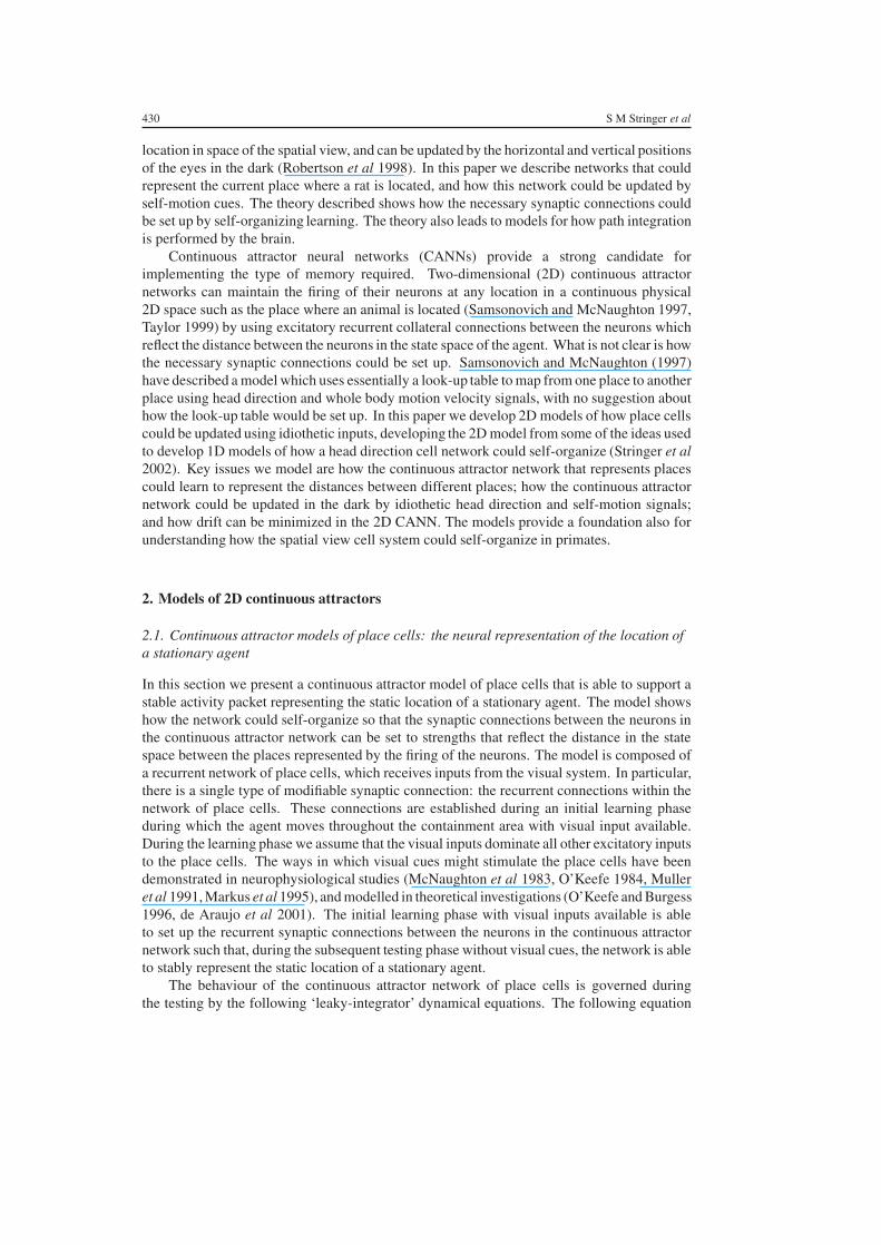
430 S M Stringer et al
location in space of the spatial view and can be updated by the horizontal and vertical positionsof the eyes in the dark (Robertson et al 1998) In this paper we describe networks that couldrepresent the current place where a rat is located and how this network could be updated byself-motion cues The theory described shows how the necessary synaptic connections couldbe set up by self-organizing learning The theory also leads to models for how path integrationis performed by the brain
Continuous attractor neural networks (CANNs) provide a strong candidate forimplementing the type of memory required Two-dimensional (2D) continuous attractornetworks can maintain the firing of their neurons at any location in a continuous physical2D space such as the place where an animal is located (Samsonovich and McNaughton 1997Taylor 1999) by using excitatory recurrent collateral connections between the neurons whichreflect the distance between the neurons in the state space of the agent What is not clear is howthe necessary synaptic connections could be set up Samsonovich and McNaughton (1997)have described a model which uses essentially a look-up table to map from one place to anotherplace using head direction and whole body motion velocity signals with no suggestion abouthow the look-up table would be set up In this paper we develop 2D models of how place cellscould be updated using idiothetic inputs developing the 2D model from some of the ideas usedto develop 1D models of how a head direction cell network could self-organize (Stringer et al2002) Key issues we model are how the continuous attractor network that represents placescould learn to represent the distances between different places how the continuous attractornetwork could be updated in the dark by idiothetic head direction and self-motion signalsand how drift can be minimized in the 2D CANN The models provide a foundation also forunderstanding how the spatial view cell system could self-organize in primates
2 Models of 2D continuous attractors
21 Continuous attractor models of place cells the neural representation of the location ofa stationary agent
In this section we present a continuous attractor model of place cells that is able to support astable activity packet representing the static location of a stationary agent The model showshow the network could self-organize so that the synaptic connections between the neurons inthe continuous attractor network can be set to strengths that reflect the distance in the statespace between the places represented by the firing of the neurons The model is composed ofa recurrent network of place cells which receives inputs from the visual system In particularthere is a single type of modifiable synaptic connection the recurrent connections within thenetwork of place cells These connections are established during an initial learning phaseduring which the agent moves throughout the containment area with visual input availableDuring the learning phase we assume that the visual inputs dominate all other excitatory inputsto the place cells The ways in which visual cues might stimulate the place cells have beendemonstrated in neurophysiological studies (McNaughton et al 1983 OrsquoKeefe 1984 Mulleret al 1991 Markus et al 1995) and modelled in theoretical investigations (OrsquoKeefe and Burgess1996 de Araujo et al 2001) The initial learning phase with visual inputs available is ableto set up the recurrent synaptic connections between the neurons in the continuous attractornetwork such that during the subsequent testing phase without visual cues the network is ableto stably represent the static location of a stationary agent
The behaviour of the continuous attractor network of place cells is governed duringthe testing by the following lsquoleaky-integratorrsquo dynamical equations The following equation
Self-organizing continuous attractor networks and path integration two-dimensional models of place cells 431
describes the dynamics of the activation hPi of each place cell i
τdhP
i (t)
dt= minushP
i (t) +φ0
CP
sumj
(wRCi j minus wINH)rP
j (t) + I Vi (1)
where rPj is the firing rate of place cell j wRC
i j is the excitatory (positive) synaptic weight fromplace cell j to cell i wINH and φ0 are constants CP is the number of synaptic connectionsreceived by each place cell from other place cells I V
i represents a visual input to place cell i and τ is the time constant of the system When the agent is in the dark then the term I V
i isset to zero The firing rate rP
i of cell i is determined from the activation hPi and the sigmoid
function
rPi (t) = 1
1 + exp[minus2β(hPi (t) minus α)]
(2)
where α and β are the sigmoid threshold and slope respectively The equations (1) and (2)governing the internal dynamics of the 2D continuous attractor network of place cells are of anidentical form to the corresponding equations (1) and (2) in Stringer et al (2002) which governthe behaviour of the 1D continuous attractor network of head direction cells Thus it is onlythe external inputs to these networks that determine the dimension of the space represented bythe cell response properties For the network of place cells to behave as a continuous attractornetwork the recurrent synaptic weight profile must be self-organized during the learning phasein a similar manner to that described by Stringer et al (2002) for the head direction cell modelsThe details of how this is done for the place cell models are given later
The dynamical equations (1) and (2) are used to model the behaviour of the placecells during testing However we assume that when visual cues are available the visualinputs I V
i stimulate the place cells to fire when the agent is at specific locations within theenvironment Therefore in the simulations presented below rather than implementing thedynamical equations (1) and (2) during the learning phase we set the firing rates of the placecells according to typical Gaussian response profiles as observed in neurophysiological studies(McNaughton et al 1983 OrsquoKeefe 1984 Muller et al 1991 Markus et al 1995)
22 Self-organization of the recurrent synaptic connectivity in the continuous attractornetwork of place cells to represent the topology of the environment
To model a biologically plausible way of setting up the synaptic weights between the neuronsin the continuous attractor network of place cells we used an associative (Hebb-like) synapticmodification rule The rationale is that neurons close together in the state space (the spacebeing represented) would tend to be co-active during learning due to the large width of thefiring fields so that after the associative synaptic modification the synaptic strength betweenany two neurons represents the distance between the places represented in the state space ofthe agent (cf Redish and Touretzky 1998 and Stringer et al 2002) During learning the spatialfields are forced onto each neuron by for example visual inputs
In the models proposed here the agent visits all parts of the environment During thelearning phase the visual input drives the place cells such that they fire maximally at particularlocations Hence each place cell i is assigned a unique location (xi yi ) in the environmentat which the cell is stimulated maximally by the visual cues Then the firing rate rP
i of eachplace cell i is set according to the following Gaussian response profile
rPi = exp[minus(sP
i )22(σ P)2] (3)
432 S M Stringer et al
where sPi is the distance between the current location of the agent (x y) and the location at
which cell i fires maximally (xi yi) and σ P is the standard deviation sPi is given by
sPi =
radic(xi minus x)2 + (yi minus y)2 (4)
An associative learning rule that may be used for updating the weights wRCi j from place
cell j with firing rate rPj to place cell i with firing rate rP
i is the Hebb rule (Zhang 1996 Redishand Touretzky 1998)
δwRCi j = krP
i rPj (5)
where δwRCi j is the change of synaptic weight and k is the learning rate constant This rule
operates by associating together place cells that tend to be co-active and this leads to cellswhich respond to nearby locations developing stronger synaptic connections A second rulethat may be used to update the recurrent weights wRC
i j is the trace rule
δwRCi j = krP
i rPj (6)
where rP is the trace value of the firing rate of a place cell given by
rP(t + δt) = (1 minus η)rP(t + δt) + ηrP(t) (7)
where η is a parameter set in the interval [01] which determines the contribution of the currentfiring and the previous trace See Stringer et al (2002) for more details about the significanceof η
23 Stabilization of the activity packet within the continuous attractor network when theagent is stationary
As described for the head direction cell models (Stringer et al 2002) the recurrent synapticweights within the continuous attractor network will be corrupted by a certain amount of noisefrom the learning regime because of the irregularity it introduces because for example cellsin the middle of the containment area receive more updates than those towards the edges ofthe area This in turn can lead to drift of the activity packet within the continuous attractornetwork of place cells when there are no visual cues available even when the agent is notmoving We propose that in real nervous systems this problem may be solved by enhancingthe firing of neurons that are already firing as suggested by Stringer et al (2002) This mightbe implemented through mechanisms for short-term synaptic enhancement (Koch 1999) orthrough the effects of voltage-dependent ion channels in the brain such as NMDA receptors(Lisman et al 1998) We simulate these effects by resetting the sigmoid threshold αi at eachtimestep depending on the firing rate of place cell i at the previous timestep That is at eachtimestep t + δt we set
αi =
αHIGH if rPi (t) lt γ
αLOW if rPi (t) γ
(8)
where γ is a firing rate threshold This helps to reinforce the current position of the activitypacket within the continuous attractor network of place cells The sigmoid slopes are set to aconstant value β for all cells i
24 Continuous attractor models of place cells with idiothetic inputs the neuralrepresentation of the time-varying location of a moving agent
In the basic continuous attractor model of place cells presented above we did not address theissue of path integration that is the ability of the network to track and represent the time-varying location of a moving agent in the absence of visual input A possible solution to the
Self-organizing continuous attractor networks and path integration two-dimensional models of place cells 433
problem of how the representation of place cells might be updated in the dark is provided bytwo possible inputs
(i) head direction cells whose activity in the dark may be updated by rotation cells and(ii) idiothetic cues carrying information about the forward velocity of the agent
Such information could in principle be used to update the activity within a network of placecells in the absence of visual input (Samsonovich and McNaughton 1997) In this section wepresent a model of place cells Model 2A that is able to solve the problem of path integrationin the absence of visual cues through the incorporation of idiothetic inputs from head directioncells and forward velocity cells and which develops its synaptic connections through self-organization When an agent is moving in the dark the idiothetic inputs are able to shift theactivity packet within the network to track the state of the agent A closely related modelModel 2B is presented later in section 4 Models 2A and 2B employ mechanisms similarto those employed in the 1D head direction cell Models 1A and 1B of Stringer et al (2002)respectively
The general neural network architecture is shown in figures 1 and 2 There is a recurrentcontinuous attractor network of place cells which receives three kinds of input
(i) visual inputs from the visual system used to force place cell firing during learning(ii) idiothetic inputs from a network of head direction cells and
(iii) idiothetic inputs from a population of forward velocity cells
For the place cell models presented below we assume that the synaptic connectivity of thenetwork of head direction cells has already become self-organized as described by Stringeret al (2002) such that the head direction cells are already able to accurately represent thehead direction of the agent during the learning and testing phases This is achieved in thesimulations presented below by fixing the firing rates of the head direction cells to reflect thetrue head direction of the agent ie according to the Gaussian response profile
rHDi = exp[minus(sHD
i )22(σ HD)2] (9)
where sHDi is the difference between the actual head direction x (in degrees) of the agent and
the optimal head direction xi for head direction cell i and σ HD is the standard deviation sHDi
is given by
sHDi = MIN(|xi minus x | 360 minus |xi minus x |) (10)
This is the same Gaussian response profile that was applied to the head direction cells duringlearning for the 1D continuous attractor models of head direction cells presented in Stringer et al(2002) The firing rates of head direction cells in both rats (Taube et al 1996 Muller et al 1996)and macaques (Robertson et al 1999) are known to be approximately Gaussian However anadditional collection of cells required for the place cell models that was not needed for thehead direction cell models is the population of forward velocity cells These cells fire as theagent moves forward with a firing rate that increases monotonically with the forward velocityof the agent Whole body motion cells have been described in primates (OrsquoMara et al 1994)The basic continuous attractor model of place cells described by equations (1) and (2) doesnot include idiothetic inputs However when the agent is moving and the location is changingwith time and there is no visual input available then idiothetic inputs (from head directionand forward velocity cells) are used to shift the activity packet within the network to track thestate of the agent We now show how equation (1) may be extended to include idiothetic inputsfrom the head direction and forward velocity cells
The first place cell model Model 2A is similar to Model 1A of Stringer et al (2002)in that it utilizes SigmandashPi neurons In this case the dynamical equation (1) governing the
434 S M Stringer et al
x
Visual input
Head direction cells
θ
Forward velocity cells
with self-organised continuous
Containment area for agent
attractor dynamical behaviourIn the simulations presented in this paper
locations within a square containment
x
y
θW E
N
S
Recurrent network of place cells
the place cells map onto a grid of
area for the agent as shown
xy
y
Figure 1 General network architecture for 2D continuous attractor models of place cells There isa recurrent network of place cells which receives external inputs from three sources (i) the visualsystem (ii) a population of head direction cells and (iii) a population of forward velocity cells Theplace cells are distributed throughout a square containment area for the agent where each placecell fires maximally when the agent is at a particular location in the area denoted by the Cartesianposition coordinates x y
activations of the place cells is now extended to include inputs from the head direction andforward velocity cells in the following way For Model 2A the activation hP
i of a place cell iis governed by the equation
τdhP
i (t)
dt= minushP
i (t) +φ0
CP
sumj
(wRCi j minus wINH)rP
j (t) + I Vi +
φ1
CPtimesHDtimesFV
sumjkl
wFVi jklr
Pj rHD
k rFVl
(11)
where rPj is the firing rate of place cell j rHD
k is the firing rate of head direction cell k rFVl is the
firing rate of forward velocity cell l and wFVi jkl is the corresponding overall effective connection
strength φ0 and φ1 are constants and CPtimesHDtimesFV is the number of idiothetic connectionsreceived by each place cell from combinations of place cells head direction cells and forwardvelocity cells The first term on the right of equation (11) is a decay term the second describesthe effects of the recurrent connections in the continuous attractor the third is the visual input(if present) and the fourth represents the effects of the idiothetic connections implemented bySigmandashPi synapses Thus there are two types of synaptic connection to place cells
(i) recurrent connections from place cells to other place cells within the continuous attractornetwork whose effective strength is governed by the terms wRC
i j and
(ii) idiothetic connections dependent upon the interaction between an input from another placecell a head direction cell and a forward velocity cell whose effective strength is governedby the terms wFV
i jkl
Self-organizing continuous attractor networks and path integration two-dimensional models of place cells 435
HD
RCw
r
VVisual input I
P
w FVrFV
r
Figure 2 Neural network architecture for 2D continuous attractor models of place cells There isa recurrent network of place cells with firing rates rP which receives external inputs from threesources (i) the visual system (ii) a population of head direction cells with firing rates rHD and(iii) a population of forward velocity cells with firing rates rFV The recurrent weights betweenthe place cells are denoted by wRC and the idiothetic weights to the place cells from the forwardvelocity cells and head direction cells are denoted by wFV
y
x
Line along which synaptic weights are plotted The post-synaptic
place cell that is set to fire maximally
line during the learning phase
at the centre of the containment areaduring the learning phase
i
The pre-synaptic neuron is the
Containment area for agent
j
neurons are those place cells that are set to fire maximally along this
Figure 3 The line through containment area along which synaptic weights are plotted in figure 4(The containment area is as shown in figure 1 where x and y denote the Cartesian positioncoordinates) The weights plotted in figure 4 are for synapses with the following pre-synapticand post-synaptic neurons All of the synapses have the same pre-synaptic neuron j which is theplace cell set to fire maximally at the centre of the containment area during the learning phase Thepost-synaptic neurons i are those place cells set to fire maximally at various positions along thedashed line through the centre of the containment area
At each timestep once the place cell activations hPi have been updated the place cell firing
rates rPi are calculated according to the sigmoid transfer function (2) Therefore the initial
learning phase involves the setting up of the synaptic weights wRCi j and wFV
i jkl
436 S M Stringer et al
25 Self-organization of synaptic connectivity from idiothetic inputs to the continuousattractor network of place cells
In this section we describe how the idiothetic synaptic connections to the continuous attractornetwork of place cells self-organize during the learning phase such that when the visual cuesare removed the idiothetic inputs are able to shift the activity packet within the network ofplace cells such that the firing of the place cells is able to continue to represent the location ofthe agent A qualitative description occurs first and then a formal quantitative specificationof the model The proposal is that during learning of the synaptic weights the place wherethe animal is located is represented by the post-synaptic activation of a place cell and this isassociated with inputs to that place cell from recently active place cells (detected by a temporaltrace in the presynaptic term) and with inputs from the currently firing idiothetic cells In thisnetwork the idiothetic inputs come from head direction and forward velocity cells The resultof this learning is that if idiothetic signals occur in the dark the activity packet is movedfrom the currently active place cells towards place cells that during learning had subsequentlybecome active in the presence of those particular idiothetic inputs
During the learning phase the response properties of the place cells head direction cellsand forward velocity cells are as follows As the agent moves through the environment thevisual cues drive individual place cells to fire maximally for particular locations with the firingrates varying according to Gaussian response profiles of the form (3) Similarly as discussedfor the head direction cell models we assume the visual cues also drive the head directioncells to fire maximally for particular head directions with Gaussian response profiles of theform (9) Lastly the forward velocity cells fire if the agent is moving forward and with a firingrate that increases monotonically with the forward velocity of the agent In the simulationsperformed later the firing rates of the forward velocity cells during the learning and testingphases are set to 1 to denote a constant forward velocity
For Model 2A the learning phase involves setting up the synaptic weights wFVi jkl for all
ordered pairs of place cells i and j and for all head direction cells k and forward velocitycells l At the start of the learning phase the synaptic weights wFV
i jkl may be set to zero orrandom positive values Then the learning phase continues with the agent moving throughthe environment with the place cells head direction cells and forward velocity cells firingaccording to the response properties described above During this the synaptic weights wFV
i jklare updated at each timestep according to
δwFVi jkl = krP
i rPj rHD
k rFVl (12)
where δwFVi jkl is the change of synaptic weight rP
i is the instantaneous firing rate of place cell i rP
j is the trace value of the firing rate of place cell j given by equation (7) rHDk is the firing rate
of head direction cell k rFVl is the firing rate of forward velocity cell l and k is the learning
rate If we consider two place cells i and j that are stimulated by the available visual cues tofire maximally in nearby locations then during the learning phase cell i may often fire a shorttime after cell j depending on the direction of movement of the agent as it passes throughthe location associated with place cell j In this situation the effect of the above learning rulewould be to ensure that the size of the weights wFV
i jkl would be largest for head direction cells kwhich fire maximally for head directions most closely aligned with the direction of the locationrepresented by cell i from the location represented by cell j The effect of the above learningrules for the synaptic weights wFV
i jkl should be to generate a synaptic connectivity such that theco-firing of (i) a place cell j (ii) a head direction cell k and (iii) a forward velocity cell lshould stimulate place cell i where place cell i represents a location that is a small translationin the appropriate direction from the location represented by place cell j Thus the co-firing
Self-organizing continuous attractor networks and path integration two-dimensional models of place cells 437
Table 1 Parameter values for Model 2A
σHD 20σ P 005Learning rate k 0001
Learning rate k 0001Trace parameter η 09τ 10φ0 50 000φ1 1000 000wINH 005γ 05αHIGH 00αLOW minus20β 01
of a set of place cells representing a particular location a particular cluster of head directioncells and the forward velocity cells should stimulate the firing of further place cells such thatthe pattern of activity within the place cell network evolves continuously to faithfully reflectand track the changing location of the agent
3 Simulation results
The experimental set-up is as illustrated in figures 1 and 2 The neural network architecture ofthe simulated agent consists of a continuous attractor network of place cells which receivesinputs from the visual system (during the learning phase) a population of head directioncells and a population of forward velocity cells (in fact only a single forward velocity cellis simulated) During the simulation the agent moves around in a square 1 unit times 1 unitcontainment area This area is covered by a square 50 times 50 grid of nodes At each nodei there is a single place cell that is set to fire maximally at that location (xi yi) during thelearning phase with a Gaussian response profile given by equation (3) The standard deviationσ P used for the place cell Gaussian response profiles (3) is 005 units This gives a total of2500 place cells within the place cell continuous attractor network of the agent In additiondue to the large computational cost of these simulations we include only eight head directioncells The head direction cells k = 1 8 are set to fire maximally for the eight principalcompass directions in a clockwise order as follows k = 1 fires maximally for head direction0 (North) k = 2 fires maximally for head direction 45 (NorthndashEast) and so on up to k = 8which fires maximally for head direction 315 (NorthndashWest) The head direction cells areset to fire maximally for these directions according to the Gaussian response profile (9) Thestandard deviation σ HD used for the head direction cell Gaussian response profiles (9) is 20These head direction cell response profiles are implemented for both the initial learning phasein the light and the subsequent testing phase in the dark Finally we include only 1 forwardvelocity cell which is the minimal number required for the model to work For the simulationsdiscussed below we present results only for the SigmandashPi Model 2A further simulations (notshown here) have confirmed that Model 2B gives very similar results The model parametersused in the simulations of Model 2A are given in table 1
The numerical simulation begins with the initial learning phase in which the recurrent andidiothetic synaptic weights which are initialized to zero at the beginning of the simulationare self-organized During this phase visual cues are available to the agent to help guidethe self-organization of the weights However as described earlier we do not model the
438 S M Stringer et al
visual cues explicitly and the simulations are simplified in the following manner During thelearning phase rather than implementing the dynamical equations (2) and (11) for Model 2Aexplicitly we set the firing rates of the place cells to typical Gaussian response profiles inaccordance with the observed behaviours of such cells in physiological studies as describedabove The learning phase then proceeds as follows Firstly the agent is simulated movingalong approximately 50 equi-distant parallel paths in the northwards direction These pathsfully cover the containment area That is each of the parallel paths begins at the boundaryy = 0 and terminates at the boundary y = 1 In addition the separate paths are spread evenlythrough the containment area with the first path aligned with the boundary x = 0 and thelast path aligned with the boundary x = 1 The agent moves along each path with a constantvelocity for which the firing rate rFV of the forward velocity cell is set to 1 (Although regulartraining was used this is not necessary for such networks to learn usefully as shown by resultswith 1D continuous attractor networks and in that the trace rule can help when the trainingconditions are irregular (Stringer et al 2002)) Each path is discretized into approximately 50steps (locations) at which the synaptic weights are updated At each step the following threecalculations are performed
(i) the current position of the agent is calculated from its location head direction and speedat the previous timestep
(ii) the firing rates of the place cells head directions cells and the forward velocity cell arecalculated as described above and
(iii) the recurrent and idiothetic synaptic weights are updated according to equations (6)and (12)
Further model parameters are as follows The learning rates k and k for both the recurrentand idiothetic weights are set to 0001 Also the trace learning parameter η used in the traceupdate equation (7) is set to 09 This value of η is used in both learning rules (6) and (12) forboth the recurrent and idiothetic synaptic weights A similar procedure is then repeated foreach of the seven other principal directions in a clockwise order This completes the learningphase
Examples of the final recurrent and idiothetic synaptic weights are shown in figure 4 Theplot on the left compares the recurrent and idiothetic synaptic weight profiles as follows Thefirst graph shows the recurrent weights wRC
i j where the pre-synaptic neuron j is the place cellset to fire maximally at the centre of the containment area during the learning phase and thepost-synaptic neurons i are those place cells set to fire maximally at various positions alongthe dashed line through the centre of the containment area shown in figure 3 It can be seen thatthe learning has resulted in nearby cells in location space which need not be at all close to eachother in the brain developing stronger recurrent synaptic connections than cells that are moredistant in location space Furthermore it can be seen that the graph of the recurrent weightsis symmetric about the central node and is approximately a Gaussian function of the distancebetween the cells in location space This is important for stably supporting the activity packetat a particular location when the agent is stationary The second graph shows the idiotheticweights wFV
i jkl where the pre- and post-synaptic neurons j and i are as above and the headdirection cell k is 1 (North) Here it can be seen that the idiothetic weight profile for k = 1(North) is highly asymmetric about the central node and that the peak lies to the north of thecentral node This is essential to enable the idiothetic inputs to shift the activity packet withinthe network of place cells in the correct direction when the agent is moving northwards Theplot on the right compares three different idiothetic synaptic weight profiles as follows Thefirst second and third graphs show the idiothetic weights wFV
i jkl where the pre- and post-synapticneurons j and i are as above and the head direction cells k are respectively k = 1 (North)
Self-organizing continuous attractor networks and path integration two-dimensional models of place cells 439
10 20 30 40 500
001
002
003
004
005
006
Y node
Syn
aptic
wei
ght
Recurrent and idiothetic synaptic weight profiles
Recurrent weights Idiothetic weights k=1 (North)
10 20 30 40 500
0002
0004
0006
0008
001
0012
Y node
Syn
aptic
wei
ght
Idiothetic synaptic weight profiles
Idiothetic weights k=1 (North)Idiothetic weights k=3 (East) Idiothetic weights k=5 (South)
Figure 4 Synaptic weight profiles plotted along the dashed curve through the centre of thecontainment area shown in figure 3 Left the plot on the left compares the recurrent and idiotheticsynaptic weight profiles as follows The first graph shows the recurrent weights wRC
i j where thepre-synaptic neuron j is the place cell set to fire maximally at the centre of the containment areaduring the learning phase and the post-synaptic neurons i are those place cells set to fire maximallyat various positions along the dashed curve through the centre of the containment area shown infigure 3 The second graph shows the idiothetic weights wFV
i jkl where the pre- and post-synapticplace cells j and i are as above and the head direction cell k is 1 (North) Right the plot on theright compares three different idiothetic synaptic weight profiles as follows The first second andthird graphs show the idiothetic weights wFV
i jkl where the pre- and post-synaptic place cells j and iare as above and the head direction cells k are respectively k = 1 (North) k = 3 (East) and k = 5(South)
k = 3 (East) and k = 5 (South) Here it can be seen that the idiothetic weight profiles fork = 1 (North) and k = 5 (South) are both asymmetric about the central node but that whilefor k = 1 the peak lies to the north of the central node for k = 5 the peak lies to the south ofthe central node In addition for k = 3 (East) the idiothetic weight profile is in fact symmetricabout the central node with a lower peak value than for either k = 1 or 5 Hence the effect ofthe learning rule for the idiothetic weights has been to ensure that sizes of the weights wFV
i jkl arelargest for head direction cells k which fire maximally for head directions most closely alignedwith the direction of the location represented by cell i from the location represented by cell j
After the learning phase is completed the simulation continues with the testing phase inwhich visual cues are no longer available and the continuous attractor network of place cellsmust track the location of the agent solely through the idiothetic inputs For the testing phasethe full dynamical equations (2) and (11) for Model 2A are implemented At each timestepthe following four calculations are performed
(i) the activations hPi of the place cells are updated
(ii) the firing rates rPi of the place cells are updated according to the sigmoid function (2)
(iii) the firing rates rHDk of the head direction cells are set according to their Gaussian response
profiles (9) as described above(iv) the firing rate rFV
l of the forward velocity cell is set to 1 if the agent is moving and set to0 if the agent is stationary
The testing phase then proceeds as follows Firstly the activations and firing rates of the placecells are initialized to zero Then the agent is placed in the containment area for 500 timesteps
440 S M Stringer et al
at the location x = 02 y = 02 with visual input available While the agent rests at thisposition the visual input terms I V
i for each place cell i in equations (11) is set to a Gaussianresponse profile identical (except for a constant scaling) to that used for place cells duringthe learning phase given by equation (3) Next the visual input is removed by setting all ofthe terms I V
i to zero and then the agent is allowed to rest in the same location for another500 timesteps This process leads to a stable packet of activity within the continuous attractornetwork of place cells The agent was then moved along a three stage multi-directional trackthrough the containment area as follows
(i) during the first stage the agent moves eastwards for 150 timesteps(ii) during the second stage the agent moves northwards for 150 timesteps and
(iii) during the third stage the agent moves NorthndashEastwards for 150 timesteps
Between each successive pair of stages the agent was kept stationary for 100 timesteps todemonstrate that the place cell network representation can be stably maintained for differentstatic locations of the agent During these periods of rest and movement the firing rates ofthe place cells head direction cells and the forward velocity cell were calculated as describedabove Further parameter values are as follows The parameter τ is set to 10 φ0 is set to50 000 φ1 is set to 1000 000 and wINH is set to approximately 005 The sigmoid transferfunction parameters are as follows αHIGH is 00 αLOW is minus200 β is 01 and γ is 05 Finallythe timestep was approximately 02
Figure 5 shows the firing rate profiles within the continuous attractor network of placecells that occurred during the testing phase In the top left is shown a stable firing rate profilewithin the continuous attractor network of place cells just before the agent starts to move onthe first stage of its track That is the plot shows the network activity after the initial visualinput has stimulated activity within the network for 500 timesteps and the network has thenbeen allowed to settle for a further 500 timesteps without visual input available The activitypacket is stable allowing the place cell network to reliably maintain a representation of thestatic location of the stationary agent However the stability of the activity packet relies onthe reinforcement of the firing of those neurons that are already highly active by setting αLOW
to be for example minus200 If the sigmoid parameter αLOW is set to 0 (so that there is noreinforcement of the firing of those neurons that are already highly active) then the activitypacket within the continuous attractor network is not stably maintained In this case theactivity packet drifts quickly towards the centre of the containment area in location spaceThis is due to a particular kind of systematic inhomogeneity that accumulates in the recurrentweights of the continuous attractor network during the learning phase because with the currentlearning regime the agent will spend a greater amount of time near to the central nodes ofthe containment area than nodes at the boundaries of the containment area This means thatplace cells that fire maximally when the agent is near the centre of the containment area willreceive more recurrent synaptic updates during learning than neurons that fire maximally nearto boundaries Hence the neurons that represent the centre of the containment area will tend todevelop stronger recurrent weights and will therefore tend to attract the activity packet awayfrom the boundaries of the containment area However this drift of the activity packet can beprevented by enhancing the firing of those neurons that already have a relatively high firingrate by setting αLOW to be for example minus200
In the top right of figure 5 the maximum firing rates that occurred during the testing phaseas the agent moved along a fixed track within the containment area are shown The maximumfiring rate is calculated over all timesteps for each x y location This plot clearly shows thepath taken by the agent It can be seen that the activity packet can accurately track the pathof the agent in the containment area even as the agent changes direction In the simulation
Self-organizing continuous attractor networks and path integration two-dimensional models of place cells 441
Figure 5 Firing rate profiles within the continuous attractor network of place cells Top leftstable firing rate profile within the network of place cells before the agent starts to move Top rightmaximum firing rates that occurred during the testing phase as the agent moved along a fixed trackwithin the containment area The maximum firing rate is calculated over all timesteps for each x ylocation This plot clearly shows the path taken by the agent Bottom left maximum firing ratesthat occurred during the testing phase as the agent moved along a fixed track but with the maximumfiring rate now calculated over all y nodes for each x location and for each timestep Bottom rightmaximum firing rates that occurred during the testing phase as the agent moved along a fixed trackbut with the maximum firing rate now calculated over all x nodes for each y location and for eachtimestep
presented here the agent was kept stationary for 100 timesteps between successive stages ofthe track However in further simulations (not shown here) it has been found that this restingperiod for the agent between different directions is not necessary for the place cell networkto accurately track the location of the agent The bottom left of figure 5 shows the maximumfiring rates that occurred during the testing phase as the agent moved along the same fixed
442 S M Stringer et al
track but with the maximum firing rate now calculated over all y nodes for each x locationand for each timestep In the bottom right of figure 5 the maximum firing rates are shownthat occurred during the testing phase as the agent moved along the fixed track but with themaximum firing rate now calculated over all x nodes for each y location and for each timestepThe bottom two plots of figure 5 reveal more detail about the movement of the activity packetwithin the continuous attractor network through time Firstly it can be seen that for eachinterval of 100 timesteps between successive stages of movement of the agent along its trackthe activity packet is able to stably represent the static location of the stationary agent Thismay be seen for example from timesteps 150 to 250 where the activity packet remains staticin both of the bottom two plots of figure 5 Another detail revealed by the bottom two plotsof figure 5 is the elongation of the activity packet in the direction of motion of the agent whenthe agent is moving For example for timesteps 1ndash150 when the agent is moving eastwards inthe x direction the projection of the activity packet onto the x-axis at any particular timestep(bottom left) is broader than the projection of the activity packet onto the y-axis (bottomright) A further interesting observation is that during the subsequent resting stage (timesteps150ndash250) the resting activity packet appears to keep the shape from the preceding movementstage That is for timesteps 150ndash250 when the agent is stationary the projection of the activitypacket onto the x-axis at any particular timestep (bottom left) is still broader than the projectionof the activity packet onto the y-axis (bottom right) This is due to the short term memoryeffect implemented by the nonlinearity in the activation function of the neurons that couldreflect the operation of NMDA receptors effected by equation (8) This phenomenon can beseen again for timesteps 400ndash500 where the agent is again stationary but the projection of theactivity packet onto the x-axis at any particular timestep (bottom left) is now less broad thanthe projection of the activity packet onto the y-axis (bottom right) This reflects the fact thatin the preceding timesteps 250ndash400 the agent was moving northwards in the y-direction
4 Model 2B
The second place cell model Model 2B is similar to Model 1B of Stringer et al (2002) in thatit incorporates synapse modulation effects into the calculation of the neuronal activations inthe recurrent network In this case the dynamical equation (1) governing the activations ofthe place cells is now extended to include inputs from the head direction and forward velocitycells in the following way For Model 2B the activation hP
i of a place cell i is governed by theequation
τdhP
i (t)
dt= minushP
i (t) +φ0
CP
sumj
(wRCi j minus wINH)rP
j (t) + I Vi (13)
where rPj is the firing rate of place cell j and where wRC
i j is the modulated strength of thesynapse from place cell j to place cell i The modulated synaptic weight wRC
i j is given by
wRCi j = wRC
i j
(1 +
φ2
CHDtimesFV
sumkl
λFVi jklr
HDk rFV
l
)(14)
where wRCi j is the unmodulated synaptic strength set up during the learning phase rHD
k is thefiring rate of head direction cell k rFV
l is the firing rate of forward velocity cell l and λFVi jkl is the
corresponding modulation factor Thus there are two types of synaptic connection betweenplace cells
(i) recurrent connections from place cells to other place cells within the continuous attractornetwork whose strength is governed by the terms wRC
i j and
Self-organizing continuous attractor networks and path integration two-dimensional models of place cells 443
(ii) idiothetic connections from the head direction and forward velocity cells to the place cellnetwork which now have a modulating effect on the synapses between the place cellsand whose strength is governed by the modulation factors λFV
i jkl
As for Model 2A once the place cell activations hPi have been updated at the current timestep
the place cell firing rates rPi are calculated according to the sigmoid transfer function (2)
The initial learning phase involves the setting up of the synaptic weights wRCi j and the
modulation factors λFVi jkl The synaptic weights wRC
i j and the modulation factors λFVi jkl are set
up during an initial learning phase similar to that described for Model 2A above where therecurrent weights are updated according to equation (5) and the modulation factors λFV
i jkl areupdated at each timestep according to
δλFVi jkl = krP
i rPj rHD
k rFVl (15)
where rPi is the instantaneous firing rate of place cell i rP
j is the trace value of the firing rateof place cell j given by equation (7) rHD
k is the firing rate of head direction cell k rFVl is the
firing rate of forward velocity cell l and k is the learning rate
5 Discussion
In this paper we have developed 2D continuous attractor models of place cells that can learn thetopology of a space We have also shown how they are able to self-organize during an initiallearning phase with visual cues available such that when the agent is subsequently placed incomplete darkness the continuous attractor network is able to continue to track and faithfullyrepresent the state of the agent using only idiothetic cues The network thus performs pathintegration The motivation for developing such self-organizing continuous attractor modelsstems from the problems of biological implausibility associated with current models whichtend to rely on pre-set or hard-wired synaptic connectivities for the idiothetic inputs whichare needed to shift the activity packet in the absence of visual input In this paper we havepresented models that operate with biologically plausible learning rules and an appropriatearchitecture to solve the following two problems
The first problem is how the recurrent synaptic weights within the continuous attractorshould be self-organized in order to represent the topology of the 2D environment (or moregenerally the 2D state space of the agent) In the models presented here a continuousattractor network is used for the representation and it is trained with associative synapticmodification rules such as those shown in equations (5) and (6) to learn the distances betweenthe places represented by the firing of neurons based on the coactivity of neurons with tapering(eg Gaussian) place fields produced by the visual input
The self-organizing continuous attractor networks described in this paper are in somesenses an interesting converse of Kohonen self-organizing maps (Kohonen 1989 1995 Rollsand Treves 1998) In Kohonen maps a map-like topology is specified by the connections beingstrong between nearby neurons and weaker between distant neurons This is frequently con-ceptualized as being implemented by short-range fixed excitatory connections between nearbyneurons and longer range inhibition (implemented for example by inhibitory interneurons)The Kohonen map operates in effect as a competitive network but with local interactions ofthe type just described (Rolls and Treves 1998) The result is that neurons which respond tosimilar vectors or features in the input space become close together in the map-like topologyIn contrast in the self-organizing continuous attractor networks described here there is nomap-like topology between the spatial relations of the neurons in the continuous attractor andthe space being represented Instead the representations in the continuous attractor of different
444 S M Stringer et al
locations of the state space are randomly mapped with the closeness in the state space beingrepresented by the strength of the synapses between the different neurons in the continuous at-tractor and not by the closeness of the neurons in the network A major difference between thetwo networks is that a Kohonen map has a dimensionality that is preset effectively by whetherthe neighbour relations are described between neurons in a 1D array (a line) a 2D array (a2D space) etc Whatever the dimensionality of the inputs that are to be learned they will berepresented in such (typically low order) spaces In contrast in the self-organizing continuousattractor networks described here the continuous attractor takes on the dimensionality of theinputs In this way there is no presetting of the dimensionality of the solutions that can be rep-resented and the system will self-organize to represent as high a dimensionality as is presentin the input space (subject to the number of connections onto each neuron in the continuousattractor from other neurons in the continuous attractor) Self-organizing continuous attractornetworks thus provide a much more flexible system for representing state spaces includingfor example capturing the geometry and the complex spatial arrangements of an irregular en-vironment Indeed the recurrent connections in the continuous attractor network describedhere could learn the topological relations even in highly irregular and warped spaces suchas spaces partially intersected by barriers Self-organizing continuous attractor networks thusprovide a flexible system for representing state spaces including for example in the case ofplace cells capturing the geometry and the complex spatial arrangements of a cluttered naturalenvironment We also note that as in the continuous attractor networks described here nearbycells in the hippocampus do not represent nearby places and indeed there is no clear topologyin the way that place cells are arranged in the rat hippocampus (OrsquoKeefe and Conway 1978Muller and Kubie 1987 Markus et al 1994) Indeed with respect to place cells in the rathippocampus it is not feasible that the rat could be born with an innate synaptic encodingof the different environments it will encounter during its lifetime Thus a recurrent synapticconnectivity that reflects the relationship between neuronal responses and the state of an agentmay need to arise naturally through learning and self-organization for example by modifyingthe strengths of connections based on the similarity in the responses of the neurons
The second problem is how idiothetic synaptic connections could be self-organized insuch a way that self-motion of the agent moves the activity packet in the continuous attractorto represent the correct location in state space Without a suggestion for how this is achieveda hard-wired model of this process must effectively rely on a form of lsquolook-uprsquo table to beable to move the activity packet in the correct way (Samsonovich and McNaughton 1997)The apparent absence of any spatial regularity in the cell response properties of the continuousattractor networks makes such innate hard-wiring unlikely as discussed by Stringer et al(2002) In this paper we present two models that can self-organize to solve the problem of theidiothetic update of the representation of the current position of the agent in a 2D state space
The neural architecture implied by Model 2A utilizes SigmandashPi synapses with four firingrate terms as seen in equations (11) and (12) If this seems complicated one can note thatif there was a population of cells that represented combinations of linear motion and headdirection (eg moving North fast) then two of the terms rFV
l and rHDk would collapse together
leaving only three firing rate terms for modified versions of equations (11) and (12) Anequivalent reduction can be made for Model 2B Biophysical mechanisms that might be ableto implement such three-term (or even possibly four-term) synapses have been discussed byStringer et al (2002) and include for three-term synapses presynaptic contacts
We note that it is a property of the models described in this paper as well as in the companionpaper on 1D models of head direction cells (Stringer et al 2002) that they move the currentrepresentation at velocities that depend on the magnitude of the driving idiothetic input (whichreflects the linear velocity of the agent for the 2D models and the angular velocity of the agent
Self-organizing continuous attractor networks and path integration two-dimensional models of place cells 445
for head direction cells) This occurs even when the network is tested with magnitudes of theidiothetic inputs with which it has not been trained For the models of head direction cellspresented it was found that the relation between the idiothetic driving input and the velocity ofthe head direction representation in the continuous attractor network is approximately linear ifNMDA receptor non-linearity is not used to stabilize the network (see figure 7 of Stringer et al(2002)) and shows a threshold non-linearity if NMDA receptor like non-linearity is includedin the neuronal activation function (see figure 10 of Stringer et al (2002))
The models described here have been applied to place cells in rats However the modelsare generic and can be applied to other problems For example the spatial view cells ofprimates are tuned to the two spatial dimensions of the horizontal and vertical dimensions ofthe location in space of the spatial view and can be updated by the horizontal and verticalpositions of the eyes in the dark (Robertson et al 1998) The 2D models described hereprovide a foundation for understanding how this spatial view system could self-organize toallow idiothetic update by eye position We note that very few idiothetic SigmandashPi synapseswould suffice to implement the mechanism for path integration described in this paper Thereason for this is that the introduction of any asymmetry into the continuous attractor functionalconnectivity will suffice to move the activity packet The prediction is thus made that theconnectivity of the idiothetic inputs could be quite sparse in brain systems that perform pathintegration
In this paper we show how path integration could be achieved in a system that self-organizesby associative learning The path integration is performed in the sense that the representationin a continuous attractor network of the current location of the agent in a 2D environment canbe continuously updated based on idiothetic (self-motion) cues in the absence of visual inputsThe idiothetic cues used to update the place representation are from head direction cell firingand from linear whole body velocity cues We note that whole body motion cells are present inthe primate hippocampus (OrsquoMara et al 1994) and that head direction cells are present in theprimate presubiculum (Robertson et al 1999) In the companion paper (Stringer et al 2002) weshowed how a continuous attractor network representing head direction could self-organize toallow idiothetic update by head rotation signals Together these two proposals provide muchof what is needed for an agent to perform path integration in a 2D environment In particularan agent that implemented the proposals described in these two papers could continuouslyupdate its head direction and position in a 2D space in the dark using head rotation and linearvelocity signals
Acknowledgments
This research was supported by the Medical Research Council grant PG9826105 by theHuman Frontier Science Program and by the MRC Interdisciplinary Research Centre forCognitive Neuroscience
References
de Araujo I E T Rolls E T and Stringer S M 2001 A view model which accounts for the spatial fields of hippocampalprimate spatial view cells and rat place cells Hippocampus 11 699ndash706
Georges-Francois P Rolls E T and Robertson R G 1999 Spatial view cells in the primate hippocampus allocentricview not head direction or eye position or place Cereb Cortex 9 197ndash212
Koch C 1999 Biophysics of Computation (Oxford Oxford University Press)Kohonen T 1989 Self-Organization and Associative Memory 3rd edn (Berlin Springer)Kohonen T 1995 Self-Organizing Maps (Berlin Springer)
446 S M Stringer et al
Lisman J E Fellous J M and Wang X J 1998 A role for NMDA-receptor channels in working memory Nature Neurosci1 273ndash5
Markus E J Barnes C A McNaughton B L Gladden V L and Skaggs W 1994 Spatial information content andreliability of hippocampal CA1 neurons effects of visual input Hippocampus 4 410ndash21
Markus E J Qin Y L Leonard B Skaggs W McNaughton B L and Barnes C A 1995 Interactions between locationand task affect the spatial and directional firing of hippocampal neurons J Neurosci 15 7079ndash94
McNaughton B L Barnes C A and OrsquoKeefe J 1983 The contributions of position direction and velocity to singleunit activity in the hippocampus of freely-moving rats Exp Brain Res 52 41ndash9
Muller R U and Kubie J L 1987 The effects of changes in the environment on the spatial firing of hippocampalcomplex-spike cells J Neurosci 7 1951ndash68
Muller R U Kubie J L Bostock E M Taube J S and Quirk G J 1991 Spatial firing correlates of neurons in thehippocampal formation of freely moving rats Brain and Space ed J Paillard (Oxford Oxford University Press)pp 296ndash333
Muller R U Ranck J B and Taube J S 1996 Head direction cells properties and functional significance Curr OpinNeurobiol 6 196ndash206
OrsquoKeefe J 1984 Spatial memory within and without the hippocampal system Neurobiology of the Hippocampus edW Seifert (London Academic) pp 375ndash403
OrsquoKeefe J and Burgess N 1996 Geometric determinants of the place fields of hippocampal neurons Nature 381 425ndash8OrsquoKeefe J and Conway D H 1978 Hippocampal place units in the freely moving rat why they fire where they fire
Exp Brain Res 31 573ndash90OrsquoKeefe J and Dostrovsky J 1971 The hippocampus as a spatial map preliminary evidence from unit activity in the
freely moving rat Brain Res 34 171ndash5OrsquoMara S M Rolls E T Berthoz A and Kesner R P 1994 Neurons responding to whole-body motion in the primate
hippocampus J Neurosci 14 6511ndash23Redish A D and Touretzky D S 1998 The role of the hippocampus in solving the Morris water maze Neural Comput
10 73ndash111Robertson R G Rolls E T and Georges-Francois P 1998 Spatial view cells in the primate hippocampus effects of
removal of view details J Neurophysiol 79 1145ndash56Robertson R G Rolls E T Georges-Francois P and Panzeri S 1999 Head direction cells in the primate presubiculum
Hippocampus 9 206ndash19Rolls E T Robertson R G and Georges-Francois P 1997 Spatial view cells in the primate hippocampus Eur J Neurosci
9 1789ndash94Rolls E T and Treves A 1998 Neural Networks and Brain Function (Oxford Oxford University Press)Samsonovich A and McNaughton B 1997 Path integration and cognitive mapping in a continuous attractor neural
network model J Neurosci 17 5900ndash20Stringer S M Trappenberg T P Rolls E T and de Araujo I E T 2002 Self-organizing continuous attractor networks and
path integration one-dimensional models of head direction cells Network Comput Neural Syst 13 217ndash42Taube J S Goodridge J P Golob E G Dudchenko P A and Stackman R W 1996 Processing the head direction signal
a review and commentary Brain Res Bull 40 477ndash86Taylor J G 1999 Neural lsquobubblersquo dynamics in two dimensions foundations Biol Cybern 80 393ndash409Zhang K 1996 Representation of spatial orientation by the intrinsic dynamics of the head-direction cell ensemble a
theory J Neurosci 16 2112ndash26
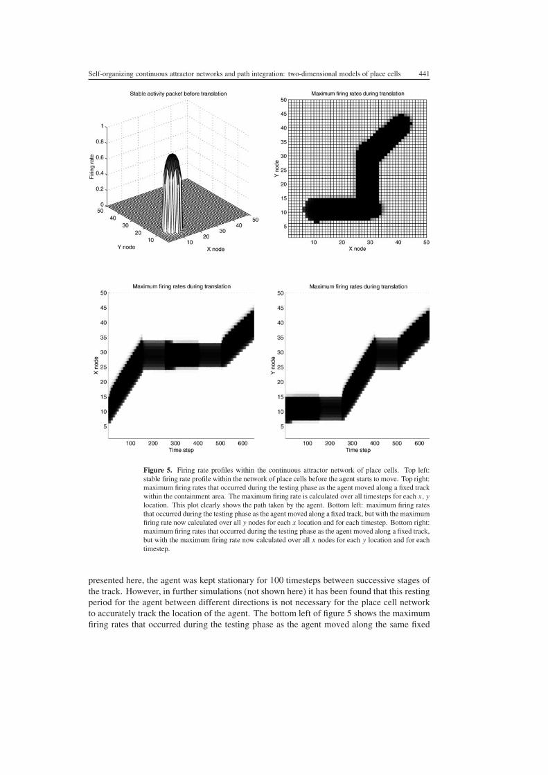
Copyright © 2022 FDOKUMEN