CERN-TH/96-95

HUTP-96/A014

USC-96/008

hep-th/9604034

Self-Dual Strings and N=2 Supersymmetric Field Theo

Albrecht Klemma, Wolfgang Lerchea, Peter Mayra;

Cumrun Vafab and Nicholas Warnerc

aTheory Division, CERN, 1211 Geneva 23, SwitzerlandbLyman Laboratory of Physics, Harvard University, Cambridge, MA 02138

cPhysics Department, U.S.C., University Park, Los Angeles, CA 90089

We show how the Riemann surface � of N = 2 Yang-Mills �eld theory

arises in type II string compacti�cations on Calabi-Yau threefolds. The

relevant local geometry is given by �brations of ALE spaces. The 3-branes

that give rise to BPS multiplets in the string descend to self-dual strings

on the Riemann surface, with tension determined by a canonically �xed

Seiberg-Witten di�erential �. This gives, e�ectively, a dual formulation of

Yang-Mills theory in which gauge bosons and monopoles are treated on

equal footing, and represents the rigid analog of type II-heterotic string

duality. The existence of BPS states is essentially reduced to a geodesic

problem on the Riemann surface with metric j�j2. This allows us, in partic-

ular, to easily determine the spectrum of stable BPS states in �eld theory.

Moreover, we identify the six-dimensional space IR4�� as the world-volume

of a �ve-brane and show that BPS states correspond to two-branes ending

on this �ve-brane.

CERN-TH/96-95

April 1996

1. Introduction

It is becoming increasingly clear that dualities in �eld theory and string theory are

very strongly interrelated. A particular case of this, and perhaps the one with both inter-

esting physics and exactly computable vacuum structure, is that of N = 2 supersymmetric

theories in 4-dimensions. On the �eld theory side one has the results of Seiberg and Witten

[1] and its generalizations. On the string theory side we have the N = 2 type II/heterotic

duality proposed in [2,3] and further explored in [4].

Since one can consider the point particle limit of strings (by considering �0 ! 0 limit),

one would expect to rederive the non-perturbative �eld theory results from string theory.

This was partially done for some classes of examples in [5]. There is one basic puzzle:

The �eld theory results are naturally phrased in terms of a Riemann surface, and in some

of the examples considered in [5] (for instance, one with an SU(3) gauge symmetry) this

did not appear. Here we remedy this by adopting a slightly di�erent viewpoint and show

how one can obtain the Riemann surface more canonically from the Calabi-Yau space.

In particular, we �nd that the Riemann surface times IR4 can be viewed in the string

language as a symmetric �ve-brane and the N = 2 e�ective �eld theory corresponds to the

low energy lagrangian of this �ve-brane theory.

Furthermore, we use the string theory technology of D-branes to shed light on the

BPS states of �eld theory. This is a re�nement of the �eld theory results in that, in this

context alone, it is extremely di�cult to �nd the spectrum of the stable BPS states,1 even

though one can �nd the quantum numbers and masses of the allowed ones. We show that

the BPS states of �eld theory can be best understood as the two-branes whose boundaries

are self-dual strings on the Riemann surface. Moreover the di�erential one-form on the

Riemann surface can be viewed, roughly speaking, as the tension of this string. Considering

geodesics on the Riemann surface with the metric determined by this one-form allows one

to explicitly study the spectrum of stable BPS states.

In short, the moral is that the natural arena of the Seiberg-Witten theory is string

theory, where the Riemann surface has a concrete physical meaning (this is in the spirit

of refs. [7,8,9]). The BPS states correspond to self-dual2 strings [10,9,11,12] that wind

1 However within SW theory the stable BPS states can be determined using symmetry argu-

ments [6].2 Note that these self-dual strings are not the usual critical strings involving gravity that

needs to be decoupled at some point, but rather are non-critical strings without gravity that give

a \dual" formulation of gauge theory.

2

geodesically around the homology cycles. The relationship between such self-dual strings

and ordinary Yang-Mills �eld theory is the rigid analog of the duality [2] between type II

and heterotic strings, and is, as we will show, actually a consequence of it.

The organization of this paper is as follows: In section 2 we review an example of

type II/heterotic duality that was studied in [5] and show how one can deduce in this

and many similar cases the existence of a Riemann surface anticipated from �eld theory.

In section 3 we show how the Riemann surface can be used to give us insight into the

structure of three-cycles on the Calabi-Yau, which allows us to formulate the condition

for having stable BPS states directly in terms of the Riemann surface and the di�erential

form on it. Moreover, we show the relation of the e�ective N = 2 SYM �eld theory with

the �eld theory living on the �ve-brane, and the relation between two-branes ending on

�ve-branes and the BPS states. In section 4 we apply the corresponding results to study

the spectrum of stable BPS states for pure SU(2) gauge theory.

2. Local Seiberg-Witten Geometry and Fibrations of ALE Spaces

2.1. K3-�brations revisited

We begin by explicitly illustrating our point by considering a simple example, namely

the K3-�bration threefold X24(1; 1; 2; 8; 12) with Hodge numbers h1;1 = 3; h2;1 = 243.

This is one of the basic examples of heterotic-type IIA string duality [2,4]. Equivalently,

we consider the type IIB theory on the mirror manifold with h2;1 = 3; h1;1 = 243, whose

de�ning polynomial can be written as

W � � 1

24(x241 + x242 ) +

1

12x123 +

1

3x34 +

1

2x25

� 0(x1x2x3x4x5)�1

6 1(x1x2x3)

6 � 1

12 2(x1x2)

12 = 0 :

(2:1)

Introducing a suitable parametrization, a = � 06= 1, b = 2�2 and c = � 2= 12, we

exhibit the K3-�bration by setting x1=x2 = �1=12 b�1=24 and x12 = x0�

1=12:

W �(�; a; b; c) � 1

24(� +

b

�+ 2)x0

12 +1

12x123 +

1

3x34 +

1

2x25

+1

6pc(x0x3)

6 +� ap

c

�1=6x0x3x4x5 = 0 :

(2:2)

3

Here, � is the coordinate on the base space IP1 and �logb corresponds to the volume of

the IP1 in the type IIA formulation. Regarding � as a parameter, (2.2) represents a K3

with discriminant

�K3 =�2 � + �2 + b

��2 � c+ �2 c+ b c� 2 �

���

4 � a� 2 � a2 + 2 � c+ �2 c+ b c� 2 ��

�6Yi=1

�� � ei(a; b; c)

�(2:3)

Over points ei in the base IP1 where �K3 = 0 the K3 �ber is singular; note that there is a

symmetry under exchanging ei with 1=ei. The total space, ie. the threefold, is non-singular,

unless zeros ei coincide:

�CY =Yi<j

�ei � ej

�2 / (b� 1)�(1� c)2 � b c2

� ��(1� a)

2 � c�2 � b c2

�:

We now investigate the �bration in the local neighborhood of the Seiberg-Witten regime

in the moduli space. Speci�cally, we consider the theory near its SU(3) point by setting

[5]

a = �2�u3=2

b = �2�6

c = 1� �(�2u3=2 + 3p3v)

for � � (�0)3=2 ! 0 (the SU(2) line at c = 1 and the SU(2)SU(2) point at c = 1; a = 2

can be treated in exactly the same way). Here, u and v are the gauge invariant Casimir

variables of SU(3). Expanding in �, we get for the singular points on IP1:

e0 = 0 ; e1 = 1

e�1 = 2u3

2 + 3p3v �

r�2u

3

2 + 3p3v�2� �6

e�2 = �2u 3

2 + 3p3v �

r�2u

3

2 � 3p3v�2� �6

up to some irrelevant rescalings. These are precisely the branch points (in the z-plane) of

the SU(3) Seiberg-Witten curve �, when written in the form [13,14]

z +�6

z+ 2PA2

(x; u; v) = 0 : (2:4)

4

Here, PA2= x3 � ux � v is the simple singularity [15] associated with SU(3); replacing

z ! y � P gives back the original form of the curve given in [16,17]. The structure of the

curve given by (2.4) can easily be related to the Calabi-Yau manifold described by (2.2),

by considering a local neighborhood of the singularity in the �bration. That is, we expand

around the singular point of W �(� = 0; a; b = 0; c), and going to the patch x0 = 1 this

gives (modulo trivial rede�nitions):

W � = ��z +

�6

z+ 2PA2

(x; u; v) + y2 + w2�

+O(�2) (2:5)

where � = � z. This is of the same singularity type as (2.4), which means that the local

geometry of the threefold in the SW regime of the moduli space is equivalent to the one

of the Seiberg-Witten curve. This point will be elaborated further in section 3.

The appearance of local SW geometry can be seen to hold for other K3-�brations as

well. This is obvious for type IIA compacti�cations on K3-�bered threefolds in [18] that

are of Fermat form, whose type IIB mirrors can be written as

W � =1

2k

�x1

2k + x22k +

2pb(x1x2)

k�+ ~W (

x1x2

b1=2k; x3; x4; x5; uk) : (2:6)

Writing x1=x2 = �1=k b�1=2k and x12 = x0�

1=k one immediately obtains

W �

K3 =1

2k

�� +

b

�+ 2

�x0

k + ~W �(x0; x3; x4; x5; uk) : (2:7)

The piece of W �

K3 that is independent of � and b describes the underlying K3 in some

parametrization. Going to the patch x0 = 1 and assuming that the K3 is singular of type

An�1 in some neighborhood in the vector moduli space, we can expand the K3 around the

critical point and thereby replace it by the ALE normal form of the singularity:

1

k+ ~W � = �

�2PAn�1

(x; uk) + y2 + w2�+O(�2) ;

PAn�1(x; uk) � xn �

nXk=2

uk xn�k :

(2:8)

Rescaling y = �2�2n and � = � z, we obtain the SU(n) generalization of (2.5), ie., the naive

�bration of the corresponding ALE space.

For non-Fermat threefolds the story is quite similar. The mirrors can always be

represented in terms of a quasi-homogenous \Landau-Ginzburg" polynomial, only that the

weights w�i of the mirror will in general be di�erent as compared to the original weights

5

wi. Moreover it is shown in ref. [19] for a much larger class of K3-�brations constructed

in toric varieties that the mirror generically takes the form

W � =�� +

b

�+ 2

�+ ~W � (2:9)

in some appropriate coordinate patch. Thus, the same arguments as above can be applied.

Here we have concentrated mainly on pure N = 2 Yang-Mills theory, but the situation

is not much di�erent for theories with extra matter; the local ADE singularity will still

be the same, but the �bering data over the � plane will be di�erent [19]. Nevertheless the

arguments developed in the present paper also apply to those cases.

2.2. Geometrical Interpretation

We can understand what happens in geometrical terms if we view the SW curves as

�brations as well, namely �brations over IP1 with �bers given by the\spectral set" that

characterizes classical Yang-Mills theory. More speci�cally, the spectral set is given by the

set of points

V =�x : PRG (x; uk) = 0

;

where

PRG (x; uk) = det(x� �0)

is the characteristic polynomial of the Higgs �eld, �0, evaluated in some representation

R of the gauge group G. For G = SU(n), the picture is particularly simple: if we write

�0 = ai(�i �H), where �i are the weights of the de�ning fundamental representation3 and

H are the generators of the CSA, then gauge symmetry enhancement occurs whenever

ai � aj = 0 for some i and j. Furthermore,

Pn

SU(n)(x; uk) =

nYi=1

�x� ai(uk)

�� PAn�1

(x; uk) (2:10)

It is useful to think of the (base-pointed) homology, H0(V;ZZ), of V , which is generated by

the formal di�erences ai+1�ai and which may be identi�ed with the root lattice of SU(n):

H0(V;ZZ) �= �R [15]. Symmetry enhancement of the classical theory is thus equivalent to

having a vanishing 0-cycle in V [20]. Note that describing gauge symmetry enhancement

for the An series in terms of coinciding points also has a natural interpretation in terms of

D-branes [21], which we will make use of in the next section.

3 As explained in [14], the choice of the representation is actually irrelevant.

6

The spectral surface of N = 2 quantum Yang-Mills theory in the form [13,14]

WSW = z +�2n

z+ 2PAn�1

(x; uk) = 0 ; (2:11)

can then simply be viewed as �bration of the classical spectral set V over the IP1 base

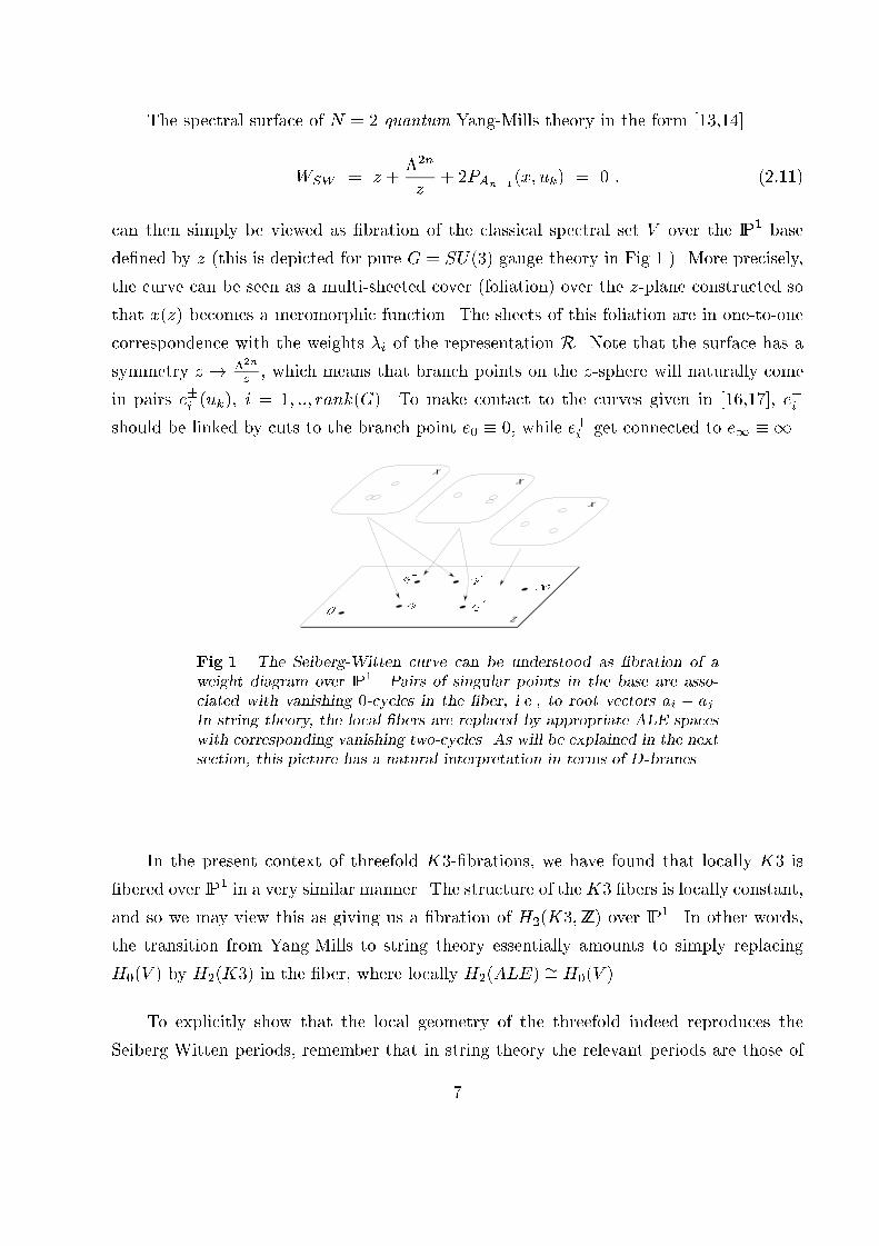
de�ned by z (this is depicted for pure G = SU(3) gauge theory in Fig.1.). More precisely,

the curve can be seen as a multi-sheeted cover (foliation) over the z-plane constructed so

that x(z) becomes a meromorphic function. The sheets of this foliation are in one-to-one

correspondence with the weights �i of the representation R. Note that the surface has asymmetry z ! �2n

z, which means that branch points on the z-sphere will naturally come

in pairs e�i (uk), i = 1; ::; rank(G). To make contact to the curves given in [16,17], e�i

should be linked by cuts to the branch point e0 � 0, while e+i get connected to e1 � 1.

z

1

0

e�

1

e+1

e+2

e�

2

x

xx

Fig.1. The Seiberg-Witten curve can be understood as �bration of a

weight diagram over IP1. Pairs of singular points in the base are asso-

ciated with vanishing 0-cycles in the �ber, i.e., to root vectors ai � aj .

In string theory, the local �bers are replaced by appropriate ALE spaces

with corresponding vanishing two-cycles. As will be explained in the next

section, this picture has a natural interpretation in terms of D-branes.

In the present context of threefold K3-�brations, we have found that locally K3 is

�bered over IP1 in a very similar manner. The structure of theK3 �bers is locally constant,

and so we may view this as giving us a �bration of H2(K3;ZZ) over IP1. In other words,

the transition from Yang-Mills to string theory essentially amounts to simply replacing

H0(V ) by H2(K3) in the �ber, where locally H2(ALE) �= H0(V ).

To explicitly show that the local geometry of the threefold indeed reproduces the

Seiberg-Witten periods, remember that in string theory the relevant periods are those of

7

the holomorphic 3-form, . On the other hand, in the supersymmetric gauge theory the

corresponding quantities can be expressed as integrals of the meromorphic 1-form,

� = xdz

z; (2:12)

over the cycles of the Riemann surface [1]. Given that W �K3 = 0 di�ers from the equation

of the Seiberg-Witten curve (2.11) by \trivial" quadratic pieces, one should expect to be

able to relate and � directly by integrating over homology cycles in the K3 �ber. It

is indeed easy to demonstrate this explicitly.

In the coordinate patch de�ned above, the (un-normalized) holomorphic 3-form can

be written as

=dz

z^�dy ^ dx@W�

@w

�: (2:13)

To isolate the non-trivial 2-cycles on the K3, it is useful to recall that for the singularity

y2 + w2 + x2 = 1, the non-trivial 2-cycle is simply the 2-sphere obtained by taking the

y; w; x to be real. Equivalently, taking w =p(1� x2)� y2, one maps out the two-sphere

by �rst �xing x and running around the cut in the y-plane, and then varying x between

limits where the x-cut collapses to a point. For �bered ALE spaces of the local form

W � = z +�2n

z+ 2PAn�1

(x; uk) + y2 + w2 ; (2:14)

the surface W � = 0 has n� 1 independent two-spheres in each K3 �ber: If one �xes the

z and x and solves W � = 0 for y, then the latitude circles of the spheres circulate around

the w-cuts. The poles (as in North and South, as opposed to as in singularity) of the

spheres occur when these circles (or cuts) collapse, that is, when WSW = 0 (2.11). For

�xed z there are n such values of x, any pair of which de�nes a homology 2-sphere. Thus

the Seiberg-Witten Riemann surface may be thought of as de�ning the poles (in the x

direction) of the homology 2-spheres in the K3-�bration.

To integrate over these spheres, one solves for w using W � = 0, and substitutes into

(2.13). The integral over y around each latitude, or cut, is trivial, and is equal to 2�. This

leaves us with the two form (up to constant factors)

Zy

=dx dz

z= d(

x dz

z) (2:15)

We can integrate this further between the limits of x that are pairs of roots of (2.11): that

is, integrating over the �ber one is left with the di�erence of the values of (x dz)=z for

any pair of roots of (2.11).

8

We mentioned above that the Riemann surface can be thought of as a n-sheeted

foliation over the z-sphere, with each leaf corresponding to a root of (2.11). Consider now

a closed path in the base space (z-space), and imagine lifting this to the various sheets in

the foliation. Integrating the di�erence between the values of (x dz)=z for pair of sheets

will produce a non-zero result if and only if the path circulates around a piece of Riemann

surface plumbing that connects the two sheets. Putting this all together one sees that the

integral of on a 3-cycle of the Calabi-Yau collapses directly to an integral of � over the

cycles of the Riemann surface (2.11).

It is perhaps less obvious that similar arguments apply when the �ber develops a Dn

or En-type singularity { this will be addressed in ref. [19].

The description of the three-cycles in the �bration in terms of the Riemann surface

and its projection onto the z-plane will be discussed in more detail in the next section.

3. Riemann Surfaces, p-Branes and the Calabi-Yau three-Fold

We have seen that in type IIB string theory, the Seiberg-Witten regime in the Calabi-

Yau three-fold is locally4 equivalent to an ALE space5 (characterized by ADE type) that

is �bered over the complex z-plane. Furthermore, the moduli of the ALE space vary

holomorphically with z. Clearly, in the rigid N = 2 �eld theory in four dimensions, all

the geometry should be understood just from these local �bration data. In particular,

the relation between the coupling constants of the gauge �elds is simply special geometry

applied in this particular limit [5]. Moreover, the BPS states of the N = 2 e�ective �eld

theory should arise as particular limits of three-branes wrapped around the three-cycles of

the Calabi-Yau [23].

In order to have a better understanding of the e�ective N = 2 system, we want to

�nd a simpler system that replaces the Calabi-Yau in this limit but captures the geometry

of the relevant three-cycles. This system is ought to reproduce the �eld theory properties

such as the spectrum of BPS states or the gauge coupling constants. The discussion will

lead us to the usefulness of the Riemann surface discussed in the previous section, and will

make the connection between string theory concepts and �eld theory states more concrete.

The three-cycles in the Calabi-Yau can be viewed, roughly speaking, as a combination

of two-cycles coming from the ALE space and a one-cycle from the z-plane. As we vary

4 Note that the limit �! 0 corresponds to �0 ! 0 and thus to switching o� gravity.5D-branes on ALE spaces have recently been considered in [22].

9

the z-parameter, the ALE space varies, and the two-cycles of the ALE space will vanish

at some points e�i in the z-plane. Let us denote the totality of vanishing two-cycles by C,and denote the ADE group of the ALE space by G and its Weyl group by W (G). If we

consider a vanishing cycle C 2 C, then as we go around a curve on the z-plane, C in

general transforms to another vanishing cycle, given by g( )C where g 2W (G).

It is convenient to de�ne a Riemann surface � using these data: namely by de�nition

� is the Riemann surface associated with the given monodromies in the z-plane, with the

property that curves on � get mapped to curves on the z-plane such that g( ) = 1.

To be concrete, let us consider the case where the ALE space is of type An�1. The

Riemann surface is then of course precisely the one given in eq. (2.11). As discussed in

the previous section, the local description of the Calabi-Yau manifold is given by (2.14),

which in view of (2.10) can be represented by

nYi=1

(x� ai(z)) + y2 + w2 = 0 ;

where ai(z) � ai(u2; : : : ; un � 12(z + 1

z�2n)). Note that in this form of the surface, the

equation for the Calabi-Yau is well de�ned but the functions ai(z) are not single-valued as

functions of z; onlyQni=1(x� ai(z)) is well de�ned over z. As any two ai approach each

other, we get a vanishing two-cycle (for a discussion of this, see for example [21]). As we

go around in the z-plane, the set of ai comes back to itself, but the individual ai(z) do not

necessarily come back to themselves. In general they are permuted by an element of Sn,

which is the Weyl group W (An�1). Moreover, the action on the vanishing cycles is also

clear, since each vanishing cycle is associated with a pair of ai.

The Riemann surface � de�ned above is simply the surface de�ned by

� :

nYi=1

(x� ai(z)) = 0 ; (3:1)

which has genus g = n � 1. Clearly this Riemann surface projects onto the z-plane, and

moreover it has the property that any curve on it corresponds on the z-plane to a curve

with trivial monodromy action on the ai.

We will now see why this Riemann surface, which has been constructed using the data

of how the Calabi-Yau is locally described as an ALE �ber space over the z-plane, leads

to a tremendous insight into the three-cycles of the Calabi-Yau in the rigid limit.

10

Let us recall some aspects of our discussion from the previous section. For a �xed value

of z there are n points on �, i.e., the map is n to 1; these points are given by x = ai(z)

(see Fig.1.). Moreover, as noted above, a two-cycle in the ALE space corresponds to a

pair of points in the x-plane. In particular, for a �xed z, the image of a two-cycle on the

Riemann surface is a 0-cycle consisting of the class [ai] � [aj]. Consider a three-cycle C3

in the Calabi-Yau. The image of this three-cycle on the z-plane will be a curve, which can

in principle be of two types: either it is an open curve or it is a closed curve. This will

depend on what C3 precisely is.

For example, if the three-cycle is S2�S1, where S2 can be identi�ed with a vanishing

two-cycle of the ALE space, then the image of this on the z-plane is a circle; moreover this

circle also lifts to a closed curve on the Riemann surface, because the S2 comes back to itself

as we go around this circle. Let us consider the vanishing two-cycle associated with ai; aj

and parameterize the S1 by �. From what we have said it follows that that the image of the

three-cycle on the Riemann surface can be viewed as the class [ai(�)]� [aj(�)] = [Ci]� [Cj ],where Ci; Cj are two closed curves on the Riemann surface. If the class [Ci] 6= [Cj ] we get

a non-trivial three-cycle of the Calabi-Yau.

On the other hand, the three-cycle on the Calabi-Yau might be an S3, which can be

viewed from the ALE perspective by slicing S3 into S2's given by going from the `north

pole' of S3, corresponding to a vanishing S2, to the `south pole' which again corresponds

to a vanishing S2. The image of this three-cycle on the z-plane will then be an open curve,

with boundaries at the points e�i in the z-plane where the Riemann surface is branched

over and where pairs of the ai come together. On the Riemann surface this corresponds to

a cycle which starts from the pre-image of a branch point where two sheets come together

and ends on another branch point where the same two sheets meet again. Independently

of which of these two types of three-cycles we consider, we thus see that we have a map

f : H3(M)! H1(�)

Now recall from the previous section that on the Riemann surface � there is a one-form �

with the property that the integral over the holomorphic three-form of the Calabi-Yau

over a three-cycle C3 is equivalent to

(C3) = �(f(C3)) ;

where f(C3) is the one-cycle on the Riemann surface discussed above.

11

We now argue that the kernel of the map f is trivial for the relevant classes of three-

cycles in the rigid limit and that this implies that the Riemann surface � faithfully rep-

resents all the data about three-cycles of interest. This is essentially clear when we recall

that over a trivial cycle C1 on the Riemann surface, the one-form �, being meromorphic

with only second order poles, will integrate to zero over it and thus integrated over the

pre-image f�1(C1) also vanishes; this implies (generically) the triviality of the three-cycle.

It is also easy to see that by the map f the canonical bilinear form on H3(M) gets mapped

to the canonical bilinear form on H1(�).

3.1. Type IIB Perspective

The importance of three-cycles for type IIB theories is that three-branes can wrap

around them and thereby give rise to BPS states [23]. The three-branes wrapped around

cycles of type S2 � S1 can in principle give vector- or a hypermultiplets [21,24,25]; in our

case they give rise to vector multiplets. Remember that the images of these cycles on the

z-plane are closed curves. On the other hand, the three-branes wrapped around S3 are of

the type discussed in [23] and correspond to hypermultiplets. We have seen that the images

of these cycles on the z-plane are open curves that end on the branch points e�i . Moreover,

given the above map between the three-cycles on the Calabi-Yau and the one-cycles on �,

we can view the three-branes wrapped around the A-cycles of � as electrically charged and

those wrapped around the B-cycles as magnetically charged states. Note that the mass of

any BPS state corresponding to a one-cycle C1 on � is simply given by

M =�� Z

C1

��� ;

which is the familiar BPS formula.

So far we have discussed how the three-cycles of the Calabi-Yau manifold are repre-

sented through curves on the Riemann surface, together with a projection on the z-plane.

From the physics point of view it is crucial to know whether we really do get a BPS state,

or not, from wrapping a three-brane around a given three-cycle in the threefold. In other

words, we would like to �nd the spectrum of BPS states in the theory. Here is where for

the �rst time the advantage of the string perspective on the SW theory becomes clear: A

three-brane partially wrapped around an S2 of the ALE space becomes a self-dual string

[10,9,11,12] on the z-plane. In the present case the tension of this string will depend on

where on the z-plane we are, since the volume of S2 varies over the z-plane.6

6 This is in contrast to N = 4 Yang Mills theory considered in [9], where the compacti�cation

manifold, K3� T2, is a direct product.

12

More speci�cally, consider a point on the z-plane and consider a three dimensional

space given by a vanishing two-cycle Sij , corresponding to the pair (ai(z); aj(z)), plus an

interval dz on the z-plane. Let us ask what the mass of this string is. To �nd the tension,

we �rst have to integrate the holomorphic three-form over the two-sphere Sij corresponding

to this pair, and, as discussed in the previous section, this is nicely summarized in terms

of a one-form �. For a given point on the z-plane, the one-form � has n-di�erent values

(as � is well-de�ned only over the Riemann surface � and � is an n-fold covering of the

z-plane). Namely � = xdz=z, and so for a �xed z the pre-images of x are given by ai(z).

The integral of the three-form over the two-cycle Sij is thus given by

Sij = �ij� = �ij(x)dz

z= (ai(z)� aj(z))

dz

z: (3:2)

Therefore the tension of an i� j type of self-dual string, which by de�nition is the leftover

piece of the three-brane wrapped around the two-sphere Sij , is given by

Tij =��ai � aj j ; (3:3)

where the metric on the z-plane is given by jdzzj2. In other words, an i � j type of string

stretched between z and z + dz has mass Tij jdz=zj. We will give an explanation of the

simple formula (3.3) for the tension of the i� j string when we will talk below about the

type IIA interpretation of all this.

In order to make our points a bit more concrete, let us concentrate on the A1 case.

There is then only one two-cycle, S12, and only one type of self-dual string. With the

coordinates we have chosen, we have a1 = �a2, so the energy of a piece of an in�nitesimal

piece of string is simply 2�����.

Now we come to the point of what concrete advantage the string viewpoint has over

mere �eld theory. What we are e�ectively interested in is constructing minimal-volume

three-cycles. For each point over the z-plane, the �ber has a minimal two-sphere, which is

thus part of the minimal volume three-cycle. To minimize the whole three-volume, we can

thus equivalently minimize the mass of the string on the z-plane, whose tension is given

by 2�����. This is equivalent to looking for the geodesics on the z-plane, for the metric given

by

gz�z = 4�z���z : (3:4)

Moreover, as discussed above, depending on whether we are interested in hypermultiplets

or vector multiplets, we should look for open geodesics that end at the branch points e�i in

the z-plane (HM), or for closed geodesics on the z-plane which lift to closed curves on the

13

Riemann surface (VM). If we cannot �nd a (primitive) geodesic in each class this simply

means that the corresponding three-cycle does not give rise to a BPS state. This gives us

a method to �nd which BPS states are occupied in the �eld theory and which are not; we

will exemplify this method in section 4 below.

Note that the metric (3.4) is at because @ �@log g = 0. This implies that the geodesic

lines can be found by simply integrating � (i.e. by going to the special coordinates where

the at metric is in the canonical form):

Z z

� = �t+ � ; (3:5)

for arbitrary constants � and �, where t parameterizes the geodesic. For the open geodesics

that correspond to hypermultiplets we thus expect to �nd a discrete number of primitive

curves, corresponding to stable BPS states.

For the closed geodesics corresponding to vector multiplets, given the fact that the

metric is at, we will get a family of such curves and we will then need to quantize

the moduli space of this family, as is familiar from similar examples for D-branes [26].

For simplicity, we will mainly concentrate on the hypermultiplet spectrum in this paper,

postponing the study of vector multiplets for future work.

Note that the relation between the BPS mass and charge simply follows from the fact

that the absolute value of the integral of � around the corresponding cycle on � corresponds

to the mass of the string, and that is in turn �xed by the meromorphicity of � in terms of

cohomology classes.

In section 4 we study solutions to this equation for the A1 case and con�rm the

spectrum of hypermultiplet BPS states anticipated for this theory. Clearly the above

picture easily generalizes to An, where the role of 2� for A1 case is played by �ij .

3.2. Type IIA Perspective

So far we have been discussing type IIB string theory near an �bered ALE space with

An�1 singularity. We would also like to discuss the type IIA perspective. There are two

such perspectives. One is simply by going back to study type IIA on the original manifold.

This turns out not to be particularly helpful. Instead we will consider a further T-duality

transform, now acting on the ALE �ber instead of on the base, which will give us another

type IIA description of the same limit of the compacti�cation: It was shown in [27] that

14

type IIB (IIA) on an An�1 ALE space is equivalent to type IIA (IIB) near n symmetric

�vebranes. More speci�cally, the n �vebranes are described by

w = y = 0 ; x = ai :

This was used in [21] to map the An�1 gauge symmetry enhancement in type IIA theory

near an An�1 singularity to type IIB with n-symmetric �vebrane which, by strong/weak

duality, becomes the statement that n coincident Dirichlet �ve-branes have an enhanced

SU(n) gauge symmetry [28]. This transforms the two-cycles wrapped around the vanishing

S2's of An�1 to elementary strings going between the �ve-branes in the type IIB dual

description. Also the similarity of the description of the open strings stretched between

pairs of ai and the vanishing two-cycles was explained there.

In our case we are in the opposite situation because we are considering type IIB near

an An�1 singularity, which is equivalent to type IIA with n symmetric �vebranes [27]. It

was observed in [11] that IIB three-branes partially wrapped around the vanishing two-

spheres (giving the non-critical strings [9]) correspond in IIA to Dirichlet two-branes that

end on the symmetric �ve-brane. Speci�cally, the left-over one-brane piece of the three-

brane corresponds to the boundary of the two-brane living on the �ve-brane. Note that

if we consider a Dirichlet two-brane, of which a one-brane piece is stretched between ai

and aj, we are left with a self-dual string in six dimensions with tension��ai � aj

��; this isa simple explanation of the tension formula (3.3).

Let us recall that ai vary holomorphically over z. This implies, if we take the non-

trivial monodromy properties of the z-plane into account, that the world-volume of the n

�ve-branes located at the ai e�ectively forms a single �ve-brane given by

�� IR4 ;

where the IR4 is the uncompacti�ed spacetime and � is the Riemann surface discussed

above.

Note that in this way we can make immediate contact with the low energy description

of the rigid N = 2 �eld theory. We have to recall [29] that as far as the low energy (bosonic)

�elds of the symmetric �vebrane is concerned, we have an antisymmetric two-form B��

with self-dual �eld strength, plus in addition 5 scalars. Similar to the considerations of

[26], out of these scalars 2 are twisted and correspond to one-forms on �, while the other

15

three remain ordinary scalars7. The gauge �elds of the N = 2 low-energy lagrangian on

IR4 originate from the zero modes corresponding to harmonic one-forms ! on � with

B�� = !�A(4)� :

Taking into account the self-duality of B, this implies that on IR4 we have as generic

gauge group U(1)g, with A- and B-cycles corresponding to electric and magnetic states,

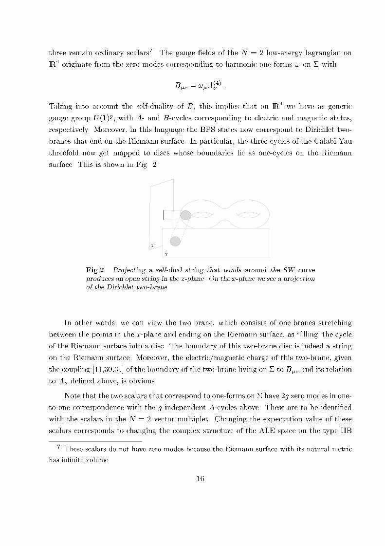
respectively. Moreover, in this language the BPS states now correspond to Dirichlet two-

branes that end on the Riemann surface. In particular, the three-cycles of the Calabi-Yau

threefold now get mapped to discs whose boundaries lie as one-cycles on the Riemann

surface. This is shown in Fig. 2.

x

z

Fig.2. Projecting a self-dual string that winds around the SW curve

produces an open string in the z-plane. On the x-plane we see a projection

of the Dirichlet two-brane.

In other words, we can view the two-brane, which consists of one-branes stretching

between the points in the x-plane and ending on the Riemann surface, as `�lling' the cycle

of the Riemann surface into a disc. The boundary of this two-brane disc is indeed a string

on the Riemann surface. Moreover, the electric/magnetic charge of this two-brane, given

the coupling [11,30,31] of the boundary of the two-brane living on � to B�� and its relation

to A� de�ned above, is obvious.

Note that the two scalars that correspond to one-forms on � have 2g zero modes in one-

to-one correspondence with the g independent A-cycles above. These are to be identi�ed

with the scalars in the N = 2 vector multiplet. Changing the expectation value of these

scalars corresponds to changing the complex structure of the ALE space on the type IIB

7 These scalars do not have zero modes because the Riemann surface with its natural metric

has in�nite volume.

16

side. From this viewpoint it is natural to identify � de�ned above as the expectation value

of the scalars:

< �z >= �z

This is in line with the fact that variation of � with respect to the zero mode of �z

(corresponding to varying in the Coulomb phase of N = 2 YM) gives rise to harmonic

forms on the Riemann surface [1].

Summarizing, the main message of this discussion is that instead of considering the

N = 2 SYM �eld theory, we can consider a �ve-brane given by � � IR4 living in the 8-

dimensional space (x; z; IR4). Moreover, the metric on the x-plane is the at metric and

on the z-plane the metric is cylindrical, given by jdz=zj2. The BPS states correspond to

two-branes that live in the (x; z) space, whose boundaries lie on the Riemann surface as

non-trivial cycles. Moreover, the minimal two-branes correspond to ruled surfaces (straight

lines on the x-plane) which bound non-trivial cycles on the Riemann surface and whose

surface tension is given by jdxdz=zj. As we will see in the next section, these facts allow

us to perform explicit computations to obtain results for the spectrum of BPS states in

rigid N = 2 Yang-Mills theory.

4. BPS states in SU(2) Yang-Mills Theory

To demonstrate the power of the techniques hinted at in the previous section, we will

consider the example of pure SU(2) N = 2 Yang-Mills theory [1]. It is crucial to use the

precise form of the one-form di�erential � as given in (2.12), and not just some modi�cation

of it that gives the same periods, because the geodesics that we will study will depend on

the choice of the di�erential. It is quite satisfying to see that string theory has picked a

canonical form of �, which enters via the metric of the �ve-brane world-volume theory.

For pure SU(2) SYM it is given by

� =

r2u� z � 1

z

dz

z:

According to the discussion in the previous section, the geodesics of the self-dual strings

on the SU(2) curve (2.11) are governed by the following di�erential equation:

r2u� z � 1

z

�z�1

@

@tz�

= � : (4:1)

If we want to study trajectories emanating from, say, the �rst branch point, we impose

the boundary condition z(0) = e�1 (u), where e�

1 (u) � u �pu2 � 1. Di�erent choices of

17

� correspond to di�erent angles of the straight trajectories (3.5) in the Jacobian, so up to

an overall factor we can take � = g � 2a(u)aD(u)

q for a dyon with charges (g; q).

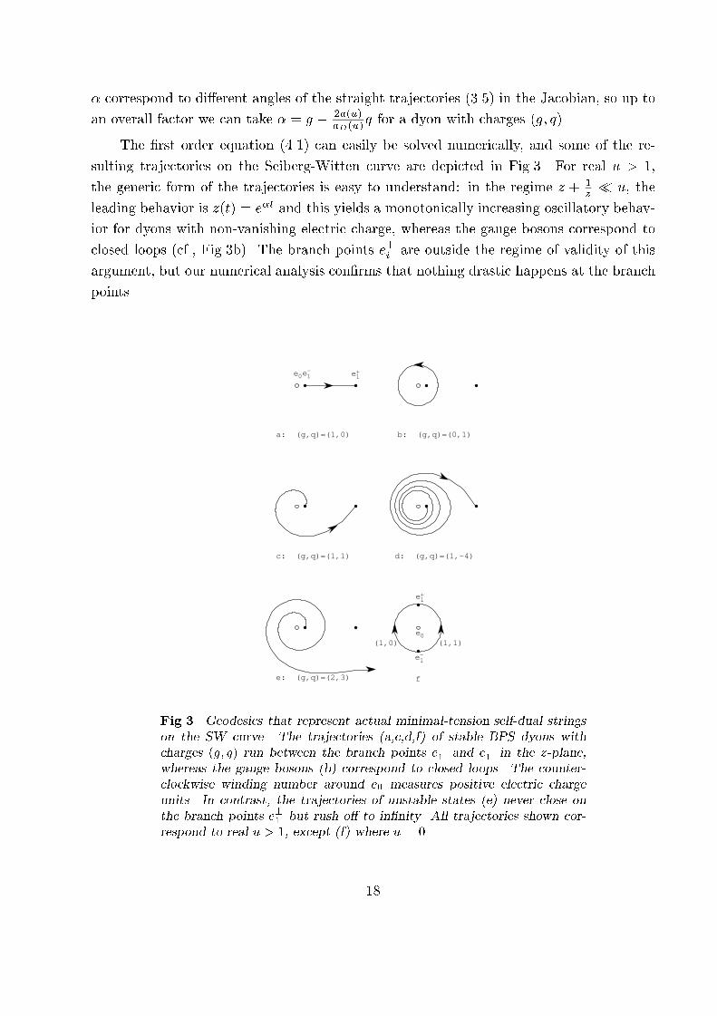
The �rst order equation (4.1) can easily be solved numerically, and some of the re-

sulting trajectories on the Seiberg-Witten curve are depicted in Fig.3. For real u > 1,

the generic form of the trajectories is easy to understand: in the regime z + 1z� u, the

leading behavior is z(t) = e�t and this yields a monotonically increasing oscillatory behav-

ior for dyons with non-vanishing electric charge, whereas the gauge bosons correspond to

closed loops (cf., Fig.3b). The branch points e�i are outside the regime of validity of this

argument, but our numerical analysis con�rms that nothing drastic happens at the branch

points.

e: (g,q)=(2,3) f

(1,1)(1,0)

c: (g,q)=(1,1) d: (g,q)=(1,-4)

a: (g,q)=(1,0) b: (g,q)=(0,1)

e0-e1 e+

1

e0

e+1

-e1

Fig.3. Geodesics that represent actual minimal-tension self-dual strings

on the SW curve. The trajectories (a,c,d,f) of stable BPS dyons with

charges (g; q) run between the branch points e�1

and e+

1in the z-plane,

whereas the gauge bosons (b) correspond to closed loops. The counter-

clockwise winding number around e0 measures positive electric charge

units. In contrast, the trajectories of unstable states (e) never close on

the branch points e�1 but rush o� to in�nity. All trajectories shown cor-

respond to real u > 1, except (f) where u = 0.

18

We can in this way easily reproduce the expected stable dyon spectrum in the Higgs

regime, given by (g; q) = (1; n), n 2 Z, by �nding that the corresponding trajectories close

on e�1 (cf., Fig.3a, c and d). In contrast, for non-stable dyons the trajectories do not close

but wander o� to in�nity (cf., Fig.3e). Viewing the world-brane theory in Hamiltonian

formulation, such trajectories correspond to in�nite time and do not represent physical

BPS states.

On the other hand, we expect the situation to be quite di�erent when u is on or inside

of the curve of marginal stability [1,32]. Obviously, on this curve where aD(u)=a(u) is

real, the Jacobian lattice degenerates, so that for all (g; q) the trajectories are on top of

each other (looping through e�1 ). This means in particular that the closed trajectory of

the gauge boson (0; 1) cannot be distinguished from the trajectory of the dyon (1; 1) from

e�1 to e+1 plus the trajectory of the monopole (�1; 0) from e+1 to e�1 . That is, the string

representation of the Yang-Mills BPS states degenerates for real aD(u)=a(u), and we see

the \decay" of the gauge boson (and other BPS dyons) into the monopole/dyon pair in a

very simple and direct way. We thus have, in fact, mapped the jumping phenomenon in

four dimensions [1] back to two dimensions [33].

Inside of the curve of marginal stability the spectrum of BPS states will be quite

di�erent. This can be easily seen from the possible trajectories for u = 0. We parametrize

z(t) = ei�(t) to rewrite (4.1) asp2R p

cos � d� = ��t; only for � real or purely imaginary

one can have a real solution8 for �(t), which means that z(t) runs with some parametriza-

tion along the unit circle. In fact, one obtains a semi-circular trajectory running from

e�1 = �i to e+1 = i that is associated with the monopole with charges (1; 0), and, by

symmetry, another semi-circle associated with the dyon of type (1; 1), cf., Fig.3f. This

con�rms the statements about the BPS spectrum from consistency [1,32] and symmetry

[6] considerations.

8 For u = 0, eq. (4.1) can easily be integrated in terms of standard elliptic functions, see e.g.

[34].

19

5. Outlook

Note how easy it is to make non-perturbative statements about N = 2 gauge theory

by using a \dual" string formulation, in which gauge bosons and monopoles are treated

on equal footing! With ordinary �eld theoretic methods, statements about the stability of

quantum BPS states are much harder to derive; see for example Sen's work [35] on N = 4

Yang-Mills theory, or the highly non-trivial computation of BPS states with magnetic

charge 2 in some N = 2 systems [36,37]. Obviously, many interesting questions can now

be very directly addressed, like for example the appearance and decay of BPS states in

theories with extra matter multiplets.

On the more abstract level, there is a known connection with integrable �eld theories

[13,14,38]. As remarked above, the analysis of the BPS states crucially depends on using

precisely � = xdz=z, without modi�cations by exact pieces. This particular form of the

di�erential is very natural in Toda theory: it is the Hamilton-Jacobi function of the system.

It thus seems possible that the � � IR4 world-brane dynamics of the �ve-brane can be

described in terms of an integrable Toda theory. At any rate, we have seen that for the

Yang-Mills theory the existence of BPS geodesics corresponds to the existence of semi-

classical \states" in the complexi�ed Toda theory. Thus we are �nding a much more direct

connection between integrable theories and N = 2 supersymmetric QCD.

More generally, we are once again discovering that string theory is not only an intrin-

sically interesting subject, but that it can give us new insights into fundamental issues in

�eld theory.

Acknowledgements

We like to thank Mike Douglas, Andrei Johansen, Savdeep Sethi and Erik Verlinde for

discussions. WL and NW also would like to thank the ITP at Santa Barbara for hospitality,

where part of this research was carried out; this part was supported by NSF under grant No.

PHY-94-07194. Moreover, WL, PM and CV thank Dieter L�ust for hospitality at Humboldt

University. The research of CV was supported in part by NSF grant PHY-92-18167, and

the research of NW was supported in part by DOE grant DE-FG03-84ER-40168.

Note: As we were �nishing this paper, we obtained a pre-release draft [39] that ad-

dresses related issues.

20

References

[1] N. Seiberg and E. Witten, Nucl. Phys. B426 (1994) 19, hep-th/9407087; Nucl. Phys.

B431 (1994) 484, hep-th/9408099.

[2] S. Kachru and C. Vafa, Nucl. Phys. B450 (1995) 69, hep-th/9505105.

[3] S. Ferrara, J. A. Harvey, A. Strominger and C. Vafa, Phys. Lett. B361 (1995) 59,

hep-th/9505162.

[4] M. Billo, A. Ceresole, R. D'Auria, S. Ferrara, P. Fr�e, T. Regge, P. Soriani, and A. Van

Proeyen, preprint SISSA-64-95-EP, hep-th/9506075;

V. Kaplunovsky, J. Louis, and S. Theisen, hep-th/9506110;

A. Klemm, W. Lerche and P. Mayr, Phys. Lett. B357 (1995) 313, hep-th/9506112;

C. Vafa and E. Witten, preprint HUTP-95-A023, hep-th/9507050;

G. Cardoso, D. L�ust and T. Mohaupt, hep-th/9507113;

I. Antoniadis, E. Gava, K. Narain and T. Taylor, Nucl. Phys. B455 (1995) 109, hep-

th/9507115;

I. Antoniadis and H. Partouche,Nucl. Phys. B460 (1996) 470, hep-th/9509009;

G. Curio, Phys. Lett. B366 (1996) 131, hep-th/9509042; Phys. Lett. B368 (1996) 78,

hep-th/9509146;

G. Aldazabal, A. Font, L.E. Ibanez and F. Quevedo, hep-th/9510093; P. Aspinwall

and J. Louis, Phys. Lett. B369 (1996) 233, hep-th 9510234;

I. Antoniadis, S. Ferrara and T. Taylor,Nucl. Phys. B460 (1996) 489, hep-th/9511108;

C. Vafa, preprint HUTP-96-A004, hep-th/9602022;

M. Henningson and G. Moore, preprint YCTP-P4-96, hep-th/9602154;

D. Morrison and C. Vafa, preprints DUKE-TH-96-106 and DUKE-TH-96-107, hep-

th/9602114 and hep-th/9603 161;

G. Cardoso, G. Curio, D. L�ust and T Mohaupt, preprint CERN-TH-96-70, hep-

th/9603108;

P. Candelas and A. Font, preprint UTTG-04-96, hep-th/9603170.

[5] S. Kachru, A. Klemm, W. Lerche, P. Mayr and C. Vafa, Nucl. Phys. B459 (1996) 537,

hep-th/9508155.

[6] A. Bilal and F. Ferrari, preprint LPTENS-96-16, hep-th/9602082.

[7] A. Ceresole, R. D'Auria, S. Ferrara and A. Van Proeyen, Nucl. Phys. B444 (1995) 92,

hep-th/9502072.

[8] E. Verlinde, Nucl. Phys. B455 (1995) 211, hep-th/9506011.

[9] E. Witten, preprint IASSNS-HEP-95-63, hep-th/9507121.

[10] M. Du� and J. Lu, Nucl. Phys. B416 (1994) 301, hep-th/9306052.

21

[11] A. Strominger, hep-th/9512059.

[12] O. Ganor and A. Hanany, preprint IASSNS-HEP-96-12, hep-th/9602120;

N. Seiberg and E. Witten, preprint RU-96-12, hep-th/9603003;

M. Du�, H. Lu and C.N. Pope, preprint CTP-TAMU-9-96, hep-th/9603037.

[13] A. Gorskii, I. Krichever, A. Marshakov, A. Mironov and A. Morozov, Phys. Lett. B355

(1995) 466, hep-th/9505035;

H. Itoyama and, A. Morozov, preprints ITEP-M5-95 and ITEP-M6-95, hep-th/9511126

and hep-th/9512161.

[14] E. Martinec and N.P. Warner, Nucl. Phys. B459 (1996) 97, hep-th/9509161

[15] See e.g., V. Arnold, A. Gusein-Zade and A. Varchenko, Singularities of Di�erentiable

Maps I, II, Birkh�auser 1985.

[16] A. Klemm, W. Lerche, S. Theisen and S. Yankielowicz, Phys. Lett. B344 (1995) 169,

hep-th/9411048.

[17] P. Argyres and A. Faraggi, Phys. Rev. Lett. 74 (1995) 3931, hep-th/9411057.

[18] A. Klemm, W. Lerche and P. Mayr, as in [4].

[19] A. Klemm, W. Lerche, P. Mayr and N. Warner, to appear.

[20] A. Klemm, W. Lerche and S. Theisen, hep-th/9505150.

[21] M. Bershadsky, C. Vafa and V. Sadov, preprint HUTP-95-A035, hep-th/9510225.

[22] M. Douglas and G. Moore, preprint RU-96-15, hep-th/9603167 .

[23] A. Strominger, Nucl. Phys. B451 (1995) 96, hep-th/9504090.

[24] A. Klemm and P. Mayr, preprint CERN-TH-96-02, hep-th/9601014.

[25] S. Katz, D. Morrison and R. Plesser, preprint OSU-M-96-1, hep-th/9601108.

[26] M. Bershadsky, C. Vafa and V. Sadov, preprint HUTP-95-A047, hep-th/9511222.

[27] H. Ooguri and C. Vafa, preprint HUTP-95-A045, hep-th/9511164.

[28] J. Polchinski, Phys. Rev. Lett. 75 (1995) 4724, hep-th/9510017;

J. Dai, R. Leigh and J. Polchinski, Mod. Phys. Let. AA4 (1989) 2073;

P. Horava, preprint HUTP-95-A035, hep-th/9510225.

[29] C. Callan, J. Harvey and A. Strominger, Nucl. Phys. B359 (1991) 611;

G. Horowitz and A. Strominger, Nucl. Phys. B360 (1991) 197;

S. Giddings, and A. Strominger, Phys. Rev. Lett. 67 (1991) 2930;

C. Callan, J. Harvey and A. Strominger, preprint EFI-91-66, hep-th/9112030.

[30] P. Townsend, preprint R/95/59, hep-th/9512062.

[31] R. Dijkgraaf, Erik and Herman Verlinde, preprint CERN-TH-96-74, hep-th/9603126.

22

[32] U. Lindstrom and M. Rocek, Phys. Lett. B355 (1995) 492, hep-th/9503012;

A. Fayyazuddin, preprint NORDITA 95/22, hep-th/9504120;

P. Argyres, A. Faraggi and A. Shapere, preprint IASSNS-HEP-94/103, hep-th/9505190;

M. Matone, preprint DFPD/95/TH/38, hep-th/9506181.

[33] S. Cecotti and C. Vafa, Comm. Math. Phys. 158 (1993) 569, hep-th/9211097.

[34] I. Gradshteyn and I. Ryzhik, Tables of integrals, series and products, Academic Press,

New York (1965).

[35] A. Sen, Phys. Lett. B329 (1994) 217, hep-th/9402032.

[36] S. Sethi, M. Stern and E. Zaslow, Nucl. Phys. B457 (1995) 484, hep-th/9508117.

[37] J. Gauntlett and J. Harvey, preprint EFI-95-56, hep-th/9508156.

[38] T. Nakatsu and K. Takasaki, hep-th/9509162;

R. Donagi and E. Witten, Nucl. Phys. B460 (1996) 299, hep-th/9510101.

[39] M. Douglas and M. Li, preprint BROWN-HET-1032.

23