SeismoSoil User Manual, v1.3

SeismoSoil is a site-specific response analysis software application, which performs 1-D linear elastic,equivalent linear, and nonlinear site response analyses.

By downloading or using this software, you acknowledge acceptance of the following DISCLAIMEROF WARRANTY AND LIABILITY:

THIS SOFTWARE AND/OR RELATED MATERIALS ARE PROVIDED “AS-IS” WITHOUTWARRANTY OF ANY KIND. WE MAKE NO WARRANTIES, EXPRESS OR IMPLIED, THAT THEYARE FREE OF ERROR, OR ARE CONSISTENT WITH ANY PARTICULAR BUILDING CODESAND/OR STANDARDS, OR ARE SUITABLE FOR A PARTICULAR USE OR PURPOSE OR FORANY PURPOSE WHATSOEVER, HOWEVER USED.

IN NO EVENT SHALL THE CALIFORNIA INSTITUTE OF TECHNOLOGY OR THE AUTHORSOF THIS SOFTWARE BE LIABLE FOR ANY DIRECT, INDIRECT, INCIDENTAL, SPECIAL,EXEMPLARY, OR CONSEQUENTIAL DAMAGES (INCLUDING, BUT NOT LIMITED TO, PRO-CUREMENT OF SUBSTITUTE GOODS OR SERVICES; LOSS OF USE, DATA, OR PROFITS;DAMAGE TO COMPUTING EQUIPMENT, COMPUTER SYSTEMS, SOFTWARE, OR STOREDDIGITAL DATA; OR BUSINESS INTERRUPTION) HOWEVER CAUSED AND ON ANY THEORYOF LIABILITY, WHETHER IN CONTRACT, STRICT LIABILITY, OR TORT (INCLUDING NEGLI-GENCE OR OTHERWISE) ARISING IN ANY WAY OUT OF THE USE OF THIS SOFTWARE,EVEN IF ADVISED OF THE POSSIBILITY OF SUCH DAMAGE.

USER BEARS ALL RISK RELATING TO QUALITY AND PERFORMANCE OF THIS SOFT-WARE AND/OR RELATED MATERIALS.

To reference the SeismoSoil software, please use the following format:D. Asimaki and J. Shi (2017) “SeismoSoil User Manual, v1.3”

c© 2014–2017, GeoQuake Research Group, California Institute of Technology

Contents

1 Introduction 4

1.1 Main features . . . . . . . . . . . . . . . . . . . . . . . . . . . . . . . . . . . . . . . . . . . 4

1.2 Functionality structure . . . . . . . . . . . . . . . . . . . . . . . . . . . . . . . . . . . . . . 6

2 Quick tutorial 7

2.1 Installation . . . . . . . . . . . . . . . . . . . . . . . . . . . . . . . . . . . . . . . . . . . . 7

2.1.1 Windows users . . . . . . . . . . . . . . . . . . . . . . . . . . . . . . . . . . . . . . 7

2.1.2 Mac users . . . . . . . . . . . . . . . . . . . . . . . . . . . . . . . . . . . . . . . . . 7

2.2 Input files preparation . . . . . . . . . . . . . . . . . . . . . . . . . . . . . . . . . . . . . . . 7

2.2.1 Ground motion . . . . . . . . . . . . . . . . . . . . . . . . . . . . . . . . . . . . . . 9

2.2.2 Shear-wave velocity (VS) profile . . . . . . . . . . . . . . . . . . . . . . . . . . . . . 10

2.2.3 Nonlinear soil properties: G/Gmax and damping curves . . . . . . . . . . . . . . . . . 12

2.2.4 Nonlinear constitutive model parameters . . . . . . . . . . . . . . . . . . . . . . . . 12

2.2.5 Obtaining HH G parameters . . . . . . . . . . . . . . . . . . . . . . . . . . . . . . . 15

2.2.6 Obtaining HH x parameters . . . . . . . . . . . . . . . . . . . . . . . . . . . . . . . 16

2.2.7 Shear strength . . . . . . . . . . . . . . . . . . . . . . . . . . . . . . . . . . . . . . . 16

2.3 Run simulations . . . . . . . . . . . . . . . . . . . . . . . . . . . . . . . . . . . . . . . . . . 17

2.4 Notes on parallel computing . . . . . . . . . . . . . . . . . . . . . . . . . . . . . . . . . . . 19

2.5 Notes on Fortran kernel . . . . . . . . . . . . . . . . . . . . . . . . . . . . . . . . . . . . . . 19

2.6 Notes on bedrock type and input motion location . . . . . . . . . . . . . . . . . . . . . . . . 20

2.7 Output files . . . . . . . . . . . . . . . . . . . . . . . . . . . . . . . . . . . . . . . . . . . . 21

2.8 Post processing tool . . . . . . . . . . . . . . . . . . . . . . . . . . . . . . . . . . . . . . . . 23

3 Technical Manual 24

3.1 Linear method . . . . . . . . . . . . . . . . . . . . . . . . . . . . . . . . . . . . . . . . . . . 24

3.1.1 Frequency domain linear method . . . . . . . . . . . . . . . . . . . . . . . . . . . . . 24

3.1.2 Time domain linear method . . . . . . . . . . . . . . . . . . . . . . . . . . . . . . . 25

3.2 Equivalent linear method . . . . . . . . . . . . . . . . . . . . . . . . . . . . . . . . . . . . . 26

3.2.1 Original equivalent linear method . . . . . . . . . . . . . . . . . . . . . . . . . . . . 26

3.2.2 Equivalent linear method with frequency dependent modulus and damping . . . . . . 27

3.3 Nonlinear method . . . . . . . . . . . . . . . . . . . . . . . . . . . . . . . . . . . . . . . . . 28

3.4 The hybrid hyperbolic (HH) stress-strain model . . . . . . . . . . . . . . . . . . . . . . . . . 28

3.5 Miscellaneous technical details . . . . . . . . . . . . . . . . . . . . . . . . . . . . . . . . . . 31

2

3.5.1 Baseline correction . . . . . . . . . . . . . . . . . . . . . . . . . . . . . . . . . . . . 31

3.5.2 Konno-Ohmachi smoothing of frequency spectra . . . . . . . . . . . . . . . . . . . . 32

3.5.3 Automatic re-discretization of soil layers . . . . . . . . . . . . . . . . . . . . . . . . 33

3.5.4 Deconvolution of rock-outcrop motions . . . . . . . . . . . . . . . . . . . . . . . . . 33

References 34

Bibliography 34

3

1 Introduction

SeismoSoil is a one-dimensional (1D) site response analysis simulation and visualization application.

1.1 Main features

• Linear analysis

– Frequency domain analysis, which performs the most basic and simplest type of analysis, followingthe Haskell-Thompson formulation (Haskell, 1953; Thomson, 1950)

– Time domain analysis, useful when the “wrap-around” phenomenon of Fourier transform is pro-nounced and needs to be addressed

• Equivalent linear analysis (frequency domain)

– Original Seed and Idriss (1970) equivalent linear method

– Frequency dependent moduli and damping method (Assimaki and Kausel, 2002)

• Nonlinear analysis (time domain)

– H2: modified hyperbolic (MKZ) stress-strain model (Matasovic and Vucetic, 1993) + Masingunloading/reloading rule, or

– H4: MKZ + Muravskii (2005) unloading/reloading rule (non-Masing)

– EPP: Elasto-perfectly plastic stress-strain model + Masing unloading/reloading rule

– HH: Hybrid hyperbolic stress-strain model (Shi and Asimaki, 2017) that takes into account soil shearstrength + non-Masing rule

• Auto-generation of modulus reduction and damping curves

– Generates G/Gmax curves conforming to the MKZ model, using empirical formulas proposed byDarendeli (2001)

– Generates damping curves using formulas proposed by Darendeli (2001)

– Generates G/Gmax curves conforming to the HH model, using the empirical procedures proposed inShi and Asimaki (2017)

• Various tools that aid the simulation of site response

– Baseline correction, digital signal filtering

– Motion deconvolution, response spectra calculations, etc.

– Ground motion format conversion (from PEER and SMC format to two-columns)

• Fast and easy-to-use graphical user interface (GUI)

– The GUI is intuitive and self-explanatory

4

– SeismoSoil utilizes parallel computing, enabling fast processing speed even for nonlinear analyses

– All input and output data files are in plain text format, allowing easy pre-processing and post-processing in Excel/MATLAB/Python/etc.

– Figures generated can be directly saved to hard drive

5

1.2 Functionality structure

SeismoSoil

Input file preperation

Manually enter VS profile

Generate G/Gmax and ξ curves

MKZ and HH parameter fitting

Analyses

LinearFrequency domain

Time domain

Equivalent linearTraditional

Frequencydependent

Nonlinear

H2

H4

EPP

HH

Tools

Plot ground motions

Plot VS profiles

Plot linear amplification factors

Fourier transform

Baseline correction

Response spectra

Filtering signals

Motion deconvolution

Ground motion unit conversion

Ground motion data file conversion (PEER format to 2-column)

Ground motion data file conversion (SMC format to 2-column)

Ground motion goodness-of-fit score

6

2 Quick tutorial

2.1 Installation

2.1.1 Windows users

1. Install MATLAB Compiler Runtime (MCR), which can be downloaded from MathWorks website for free1.Please choose “R2017b (9.3), 64-bit”. If your computer has a full MATLAB R2017b (64-bit) installation,you can skip this step.

2. Open SeismoSoil.exe. (Please keep the other auxiliary files, TDLinear.exe, FDEQ.exe, NLEPP.exe,NLH2.exe, NLH4.exe, and NLHH.exe, in the same directory as SeismoSoil.exe)

2.1.2 Mac users

1. Install MATLAB Compiler Runtime (MCR), which can be downloaded from MathWorks website for free.Please choose “R2017b (9.3), 64-bit”. If your computer has a full MATLAB R2017b (64-bit) installation,you can skip this step.

2. Place the APP file (the file with the MATLAB icon) in the Applications folder. (This is a must; otherwisethere will be strange errors.)

3. From the Terminal, execute the following (without the quotation marks):“/Applications/SeismoSoil.app/Contents/MacOS/applauncher”.(Please start SeismoSoil only from the Terminal. If you open it by double-clicking the icon, someunexpected errors will occur during runtime.)

The system requirement for SeismoSoil is: Windows 7/8/8.1/10 (64-bit) or macOS (64-bit Mavericks ornewer), with enough disk space (recommended 4 GB). There is no requirement for minimum CPU and memory,but SeismoSoil runs much faster on more advanced machines (especially with more CPU cores).

The screenshot of the main panel of SeismoSoil (shown on the next page) will appear after startup.

2.2 Input files preparation

Input file examples are provided in the folder “Sample Input Files”. Users can start trying SeismoSoil right awayusing these sample files, or can follow the following paragraphs in this section to learn to prepare new input files.

All input files should be plain text files (such as .txt files). Acceptable column delimiters include spaces,commas, and horizontal tabs, but users should not mix different types of delimiters in a same input file.

The output files generated by SeismoSoil will use horizontal tabs as delimiters.

1http://www.mathworks.com/products/compiler/mcr

7

8

2.2.1 Ground motion

Ground motion data files should have exactly two columns—the left column is the time vector in units of seconds,and the right column is the acceleration, in units of m/s2, gal (= 1 cm/s2), or g (= 9.81 m/s2). Users canchoose their corresponding unit in simulation graphical panels.2

Main→ tools→ ground motion plotter provides plots of acceleration time history, as well as velocityand displacement time histories, which are integrated from the acceleration. Arias intensity and RMS accelerationcan also be calculated. An example output of the ground motion plotter is shown below.

Under main→ tools , users can also find signal filter and baseline correction , which filter or baseline-

correct the ground motion accelerations; in addition, they can plot the Fourier spectra with Fourier transform

2There is a PEER to 2-column converter panel under main → tools , which converts the .AT2 format used by PEER/NGAdatabase into 2-column format. Similarly, the SMC to 2-column converter converts the SMC format into 2-column format.

9

and elastic response spectra (with any damping ratio value) with elastic response spectra . An example ofthe baseline correction output is shown below. The algorithm of the baseline correction is listed in Section 3.5.1.

0 50 100

Accele

ration

-5

0

5Uncorrected

0 50 100

Velo

city

-0.2

0

0.2

0.4

Time (s)

0 50 100

Dis

pla

cem

ent

-2

-1

0

1

0 50 100

Velo

city

-0.2

0

0.2

0.4

Time (s)

0 50 100

Dis

pla

cem

ent

-0.05

0

0.05

Period (s)

10-2

10-1

100

101S

pectr

al A

ccele

ration

0

5

10

15Response Spectrum (5% damping)

Frequency (Hz)

10-2

10-1

100

101

102

0

100

200

300Fourier Amplitude Spectrum

0 50 100

Accele

ration

-5

0

5

"MYGH041103100316.SH1.dat"

Baseline corrected

2.2.2 Shear-wave velocity (VS) profile

The input file containing the soil property profile should be in the following five-column format:

The five columns from left to right mean: (1) soil layer thickness (m), (2) shear wave velocity Vs (m/s), (3)low-strain damping ratio, ξ , (4) soil mass density, ρ , and (5) “material number”, respectively. The units of ξ

can be either % or unity (i.e., 1), and the unit of ρ can be either g/cm3 or kg/m3. The users can specify theunits of ξ and ρ on the simulation panels, before the analysis starts. The last thickness value should always be

10

0, which indicates the last layer (i.e., the halfspace) has infinite depth. (It can have the same VS, ξ , and ρ as thelayer above it.)

The fifth column, the “material number”, should be a series of positive integers, not necessary in a continuousand ascending order, with the exception of the last value, which should always be 0. The material number refersto the nonlinear dynamic soil parameters, namely the G/Gmax and damping curves. For example, the layers with“material number”=5 correspond to the 5th set of G/Gmax and damping curves in the “curve file”, which will beexplained in Section 2.2.3.

The soil profile can be manually entered through main→ input files preparation→ manually enter Vs profile .A screenshot of this panel is shown below. Alternatively, users can prepare the input files in external applicationslike Excel or Notepad, and save them as plain text files.

The “Auto calculate damping/density” button on the panel (in the red box) can generate damping and densityfor soil layers based on their VS, using the following rules:

• Damping ratio ξ = 1/(2QS), and QS =

– 0.06VS, when VS 6 1000 m/s

– 0.04VS, when 1000 m/s <VS < 2000 m/s

– 0.16VS, when VS > 2000 m/s

• Mass density

– 1.6 g/cm3, when VS < 200 m/s

– 1.8 g/cm3, when 200 m/s 6VS < 800 m/s

– 2.0 g/cm3, when VS > 800 m/s

The QS-VS correlation above comes from Archuleta and Liu (2004).

11

2.2.3 Nonlinear soil properties: G/Gmax and damping curves

The two input files mentioned in Sections 2.2.1 and 2.2.2 are the only files required for linear site responseanalysis. For the equivalent linear analysis, dynamic soil properties, namely G/Gmax and ξ curves, are required.In SeismoSoil, these properties are specified in a single text file (the “curve file”).

Below is the format of a “curve file”. The headers are just for demonstration and should not be included inthe actual input file.

Each group of four columns corresponds to one material: G/Gmax and ξ vs shear strain. Different soil layerscan share a same set of G/Gmax and ξ curves, and this mapping is provided by the 5th column in the input soilprofile file: if the 5th column of a certain layer in the profile file is “2”, then that layer’s G/Gmax and ξ curvesare the second set of 4 columns in the “curve file”.

If the user does not know the G/Gmax and ξ curves for each layers, SeismoSoil can generate them using theformulas by Darendeli (2001) (pages 220–272), in main→ input files preparation→modulus and damping (Darendeli, 2001) . SeismoSoil chooses the following default values to use in Daren-

deli’s formulas:

• Total stress analysis (deep groundwater table)

• OCR: 1.0 (normally consolidated)3

• N (number of cycles): 10

• f = 1 Hz

The ground motion, soil profile and dynamic soil properties are the necessary input files for equivalent linearanalyses. For nonlinear analyses, the users should also specify the constitutive model parameters, as will bediscussed in Sections 2.2.4, 2.2.5, and 2.2.6.

2.2.4 Nonlinear constitutive model parameters

Apart from the ground motion, soil profile, dynamic curves, the nonlinear analysis in SeismoSoil requiresadditional information—the constitutive soil parameters. The H2 nonlinear method requires one file, H2 n.txt,

3The users are welcome to contact us, if they would like to calculate curves using different OCR, N, or f values.

12

the H4 nonlinear method requires two files, H4 G.txt and H4 x.txt, and similarly, the HH nonlinear methodrequires two files, HH G.txt and HH x.txt.

The format of H2 n.txt, H4 G.txt, and H4 x.txt looks like the figure blow:

The file should have exactly 4 rows, and each column of the file corresponds to a set of 4 columns in the“curve file”, and in the same order as the “curve file”.

The four rows correspond to the three parameters in the MKZ model: γref is the reference strain, and s and β

are two shape parameters. (Due to legacy reasons, the second row should be all 0’s.) The units for them are allSI units (and strains should use the unit of 1, instead of percent).

These three parameters can be obtained by curve-fitting: using the main→ input files preparation→MKZ (“H2” or “H4”) curve fitting panel (shown in the figure below), which takes a “curve file” as input, and

generates a H2 n.txt file (using H2 curve fitting) or H4 G.txt and H4 x.txt files (using H4 curve fitting).

13

The format of HH G.txt and HH x.txt looks like below:

The file should have exactly 9 rows, and each column of the file corresponds to a set of 4 columns in the“curve file”, and in the same order as the “curve file”.

These 9 rows correspond to the 9 parameters of the hybrid hyperbolic (HH) stress-strain model proposedby Shi and Asimaki (2017). The units for them are all SI units (and strains should use the unit of 1, instead ofpercent). The details of the HH model will be explained in Section 3.4, as well as in the original paper (Shi andAsimaki, 2017).

The HH G.txt and HH x.txt parameters are obtained in different ways, which is explained in Sections 2.2.5and 2.2.6 respectively.

14

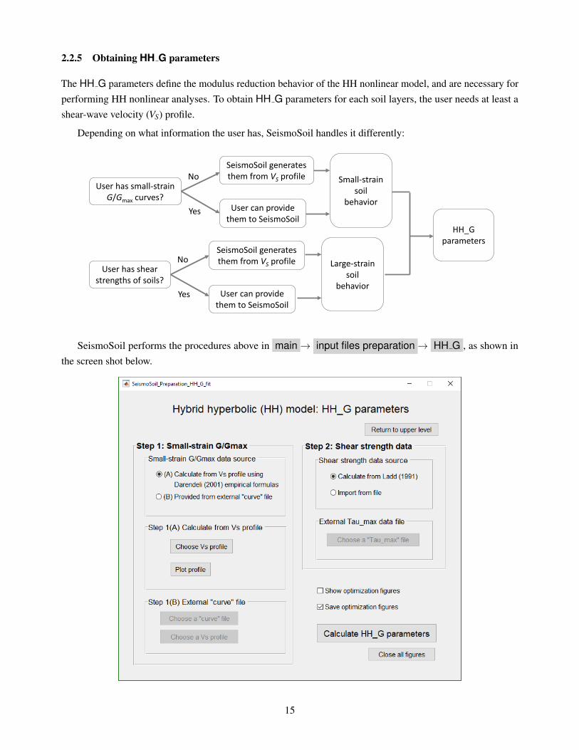
2.2.5 Obtaining HH G parameters

The HH G parameters define the modulus reduction behavior of the HH nonlinear model, and are necessary forperforming HH nonlinear analyses. To obtain HH G parameters for each soil layers, the user needs at least ashear-wave velocity (VS) profile.

Depending on what information the user has, SeismoSoil handles it differently:

No

Yes

User has small-strain G/Gmax curves?

User has shear strengths of soils?

User can provide them to SeismoSoil

No

Yes User can provide them to SeismoSoil

SeismoSoil generates them from VS profile

Small-strain soil

behavior

Large-strain soil

behavior

HH_G parameters

SeismoSoil generates them from VS profile

SeismoSoil performs the procedures above in main→ input files preparation→ HH G , as shown inthe screen shot below.

15

2.2.6 Obtaining HH x parameters

The HH x parameters defines the damping behavior of the HH nonlinear model, and are necessary for performingHH nonlinear analyses.

The HH x parameters come from curve fitting to damping curves (for each soil layer). If the user does notknow the damping for the soils, please follow the procedures in Section 2.2.3 to generate empirical dampingcurves.

The HH x curve-fit panel is in main→ input files preparation→ HH x , as shown in the screen shotbelow. And the user can follow the instructions on the panel. Curve-fitting HH x will invoke multiple CPUprocessors , and will likely take some time to finish (depending on the user’s hardware).

2.2.7 Shear strength

Shear strength files (usually named Tau max.txt) are useful in EPP (elastio-perfectly plastic) nonlinear methodas well as HH nonlinear method (if the user knows the shear strength of each soil layer).

The file should have only one column, with each number being the shear strength (unit: Pa) to each soil layer.

16

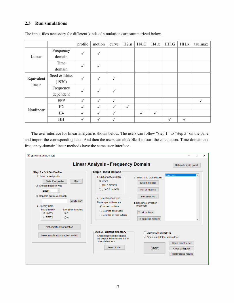
2.3 Run simulations

The input files necessary for different kinds of simulations are summarized below.

profile motion curve H2 n H4 G H4 x HH G HH x tau max

LinearFrequency

domainX X

Timedomain

X X

Equivalentlinear

Seed & Idriss(1970)

X X X

Frequencydependent

X X X

Nonlinear

EPP X X X X

H2 X X X X

H4 X X X X X

HH X X X X X

The user interface for linear analysis is shown below. The users can follow “step 1” to “step 3” on the paneland import the corresponding data. And then the users can click Start to start the calculation. Time-domain andfrequency-domain linear methods have the same user interface.

17

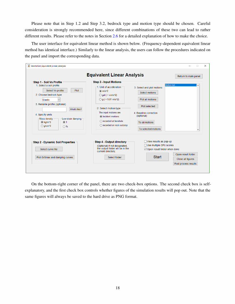
Please note that in Step 1.2 and Step 3.2, bedrock type and motion type should be chosen. Carefulconsideration is strongly recommended here, since different combinations of these two can lead to ratherdifferent results. Please refer to the notes in Section 2.6 for a detailed explanation of how to make the choice.

The user interface for equivalent linear method is shown below. (Frequency-dependent equivalent linearmethod has identical interface.) Similarly to the linear analysis, the users can follow the procedures indicated onthe panel and import the corresponding data.

On the bottom-right corner of the panel, there are two check-box options. The second check box is self-explanatory, and the first check box controls whether figures of the simulation results will pop out. Note that thesame figures will always be saved to the hard drive as PNG format.

18

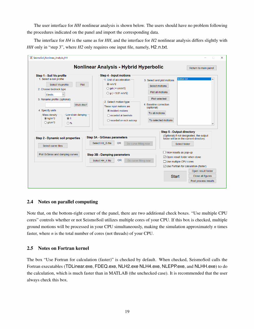
The user interface for HH nonlinear analysis is shown below. The users should have no problem followingthe procedures indicated on the panel and import the corresponding data.

The interface for H4 is the same as for HH, and the interface for H2 nonlinear analysis differs slightly withHH only in “step 3”, where H2 only requires one input file, namely, H2 n.txt.

2.4 Notes on parallel computing

Note that, on the bottom-right corner of the panel, there are two additional check boxes. “Use multiple CPUcores” controls whether or not SeismoSoil utilizes multiple cores of your CPU. If this box is checked, multipleground motions will be processed in your CPU simultaneously, making the simulation approximately n timesfaster, where n is the total number of cores (not threads) of your CPU.

2.5 Notes on Fortran kernel

The box “Use Fortran for calculation (faster)” is checked by default. When checked, SeismoSoil calls theFortran executables (TDLinear.exe, FDEQ.exe, NLH2.exe NLH4.exe, NLEPP.exe, and NLHH.exe) to dothe calculation, which is much faster than in MATLAB (the unchecked case). It is recommended that the useralways check this box.

19

2.6 Notes on bedrock type and input motion location

SeismoSoil has two options of bedrock in the numerical scheme: rigid and elastic. It also accepts three typesof input motion: incident motion at the bedrock, total motion at the bedrock (or borehole recorded motion, orsometimes referred as the “within motion”), and total motion on rock outcrop—as shown in the figure below. Sothere are six combinations:

A) Borehole recorded motion, with:

1. Rigid bedrock – suitable when the borehole motion is known and prescribed (for example, you are usinga KiK-net borehole recording as the input ground motion)

2. Elastic bedrock – for this combination, the software generates a error message and does not do thesimulation. Because elastic/viscoelastic bedrock means that the rock outcrop site has its own site response.The traditional approach of dividing the motion by 2 and using it as incident, or directly using the rockoutcrop motion as total motion at the base of the profile are not correct and should be avoided if needed.The users are encouraged to remove this response by performing rock outcrop deconvolution to the incidentmotion, and then run the analysis with other appropriate motion-bedrock combinations.

B) Incident motion, with:

1. Rigid bedrock – in this case, the borehole motion,i.e., the total motion, is equal to the outcrop motion,and twice the incident motion

2. Elastic bedrock – in this case, the input motion isthe borehole motion free of downgoing waves

C) Rock outcrop motion, with:

1. Rigid bedrock – this combination is identical to com-bination A1

2. Elastic bedrock – use with caution: the actual mo-tion at the soil-rock interface is slightly different fromthe outcrop motion, so it is recommended that theusers deconvolve the rock outcrop motion to incidentmotion, and use combination B2

The choice of different combinations affects how SeismoSoil calculates the site response, and thus the resultsof simulations. Figure 2 on page 26 shows three different types of linear amplification factors corresponding todifferent choices of bedrock-motion combinations.

20

2.7 Output files

The output data files include the following (assuming the input motion name is M1):

• M1 accel on surface.txt - Acceleration time history on ground surface. Two columns: time array (on the left) andacceleration (on the right).

• M1 max a v d.txt - Maximum acceleration, velocity, and displacement of each layer

• M1 max gamma tau.txt - Maximum strain and stress of each layer

• M1 nonlinear TF raw.txt - Nonlinear transfer function (absolute value, and unprocessed). Two columns: frequencyarray (on the left) and amplification factor (on the right)

• M1 nonlinear TF smoothed.txt - Nonlinear transfer function (absolute value, smoothed, using Konno-Ohmachialgorithm4). The format is the same as the raw transfer function.

• M1 re-discretized profile.txt - Re-discretized soil profile used internally in the simulation, usually finer than theoriginal layering5

• M1 time history accel.txt - Acceleration time history of every layer. Each column represents the time history ofone layer. And the columns from left to right represent the soil layers from the surface to the bedrock. The timearray is not included.

• M1 time history veloc.txt - Velocity time history of every layer. Format same as above.

• M1 time history displ.txt - Displacement time history of every layer. Format same as above.

• M1 time history strain.txt - Strain time history of every layer. Format same as above.

• M1 time history stress.txt - Stress time history of every layer. Format same as above.

There are also three .png figures corresponding to the data files.

Note on the units The units in the output files are all SI units (sec, Hz, m, m/s, m/s/s, and Pa), and the unit ofthe output strains is 1 (not %).

Along with the output text files, there are also three output figures generated for each analysis, as shownbelow:

4Please refer to Section 3.5.2 on page 32 for details of the Konno-Ohmachi smoothing algorithm5Please refer to Section 3.5.3 on page 32 for details of layer re-discretization.

21

0 20 40 60 80 100

Time (s)

-2

-1

0

1

2

Accele

ration (

m/s

2)

Input and Output Accelerations

Accel_02_weak_motion_(unit_gal)

Output

Rock Outcrop

10-1 100 101

Frequency (Hz)

0

2

4

6

8

Am

plif

ica

tio

n F

acto

r

Nonlinear Amplification Factor

Accel_02_weak_motion_(unit_gal)

5 10 15 20 25

Frequency (Hz)

0

2

4

6

8A

mp

lific

atio

n F

acto

r

0 1 2

Max. accel. (m/s2)

0

20

40

60

80

100

De

pth

(m

)

0 5 10

Max. veloc. (cm/s)

0

20

40

60

80

100

0 0.5 1

Max. displ. (cm)

0

20

40

60

80

100

Accel_02_weak_motion_(unit_gal)

0 0.02 0.04

max (%)

0

20

40

60

80

100

0 50

max (kPa)

0

20

40

60

80

100

22

2.8 Post processing tool

A simple post processing panel is available, from clickng the “Post process results” results on the lower-rightcorner of any analysis panels (linear, equivalent linear, etc.). The post process results panel is shown below.

Click “Select folder”, and choose a folder containing SeismoSoil output files. Click “Plot loops” to viewthe stress-strain loops of each layer (left). Click “View movie” to see animations of the ground deformationprofile (right).

Strain [%]

-1.5 -1 -0.5 0 0.5 1 1.5 2

Str

ess [kP

a]

-80

-60

-40

-20

0

20

40

60

80Layer #10. Depth = 9.00 m

23

3 Technical Manual

3.1 Linear method

In linear approach, the soil is assumed as a Kelvin-Voigt solid, whose dynamic behavior is is described usinga purely elastic spring and a purely viscous dashpot (Kramer, 1996), having two defining parameters, G (soilmodulus) and ξ (soil damping ratio). Linear approach assumes G and ξ to remain unchanged in dynamicprocesses, which is not the case, especially when the ground motion intensity is strong.

In many cases, only the shear wave velocity (VS) is known, but not the damping and density. Then theempirical rule proposed at the end of 2.2.2 can be used to calculate damping and density from VS.

3.1.1 Frequency domain linear method

In frequency domain linear analysis, the amplification of ground motions by the soil layers are computed viatransfer functions, using the following formula,

aout (t) = IFT [H (ω) ·FT [ain(t)]] (1)

where ain(t) and aout are the input and output ground motions in time domain, FT[ ] and IFT[ ] represent Fouriertransform and inverse Fourier transform, and H(ω) is the complex-valued transfer function in frequency domain,which can be solely determined by the soil property profile.

The following paragraphs show the derivation of H(ω) from the soil properties.

Let j denote the soil layer index, and A j and B j the upgoing and downgoing SH wave displacementamplitudes at the j-th layer. In this case, the following relationship holds for every j:{

A j+1

B j+1

}=

[12(1+α∗j )e

ik∗j h j 12(1−α∗j )e

−ik∗j h j

12(1−α∗j )e

ik∗j h j 12(1+α∗j )e

−ik∗j h j

]·

{A j

B j

}def== D j ·

{A j

B j

}(2)

where α∗j =ρ jV ∗S, j

ρ j+1V ∗S, j+1is the complex impedance ratio of two successive layers j and ( j+1);

V ∗S, j = VS, j ·√

1+2iξ j is the complex shear wave velocity of layer j; h j is the thickness of layer j; and

k∗j =ω

V ∗S, j=

k j

1+ iξ jis the complex wave number of layer j, where ω is the angular frequency.

Hence {A j

B j

}= D j−1

{A j−1

B j−1

}= D j−1Dm−2

{A j−2

B j−2

}= · · ·= D j−1D j−2 · · ·D1

{A1

B1

}(3)

where A1 = B1 = S/2, and S is the total surface displacement amplitude.

Let E j−1 = D j−1D j−2 · · ·D1, thus Equation (3) becomes{A j

B j

}= E j−1

{A1

B1

}=

[E〈11〉

j−1 E〈12〉j−1

E〈21〉j−1 E〈22〉

j−1

]{S/2S/2

}(4)

24

Equation (4) relates the displacement amplitudes at the top of the j-th layer to the layer on ground surface.Using this equation we can also relate the displacement amplitudes of any two layers, j and k,{

A j

B j

}= E j−1 ·E−1

k−1 ·

{Ak

Bk

}(5)

And if m is the total number of soil layers (excluding the underlying bedrock), the displacement amplitudesbetween the top of bedrock and the top of ground surface is{

Am

Bm

}= Em−1

{A1

B1

}=

[E〈11〉

m−1 E〈12〉m−1

E〈21〉m−1 E〈22〉

m−1

]{S/2S/2

}(6)

Referring to Figure 1, three types of transfer functions can be written,

Figure 1: Three types of input motions

(A) The “surface to borehole” (surface motion to total borehole motion) transfer function:

HA(ω) =Ampl(u1)

Ampl(um−(total))=

S/2+S/2Am +Bm

=2

E〈11〉m−1 +E〈12〉

m−1 +E〈21〉m−1 +E〈22〉

m−1

(7)

(B) The “surface to incident” (surface motion to incident motion at borehole) transfer function is

HB(ω) =S/2+S/2

Am=

2

E〈11〉m−1 +E〈12〉

m−1

(8)

(C) The “surface to rock outcrop” (motion at soil surface to motion at rock outcrop site’s surface) transferfunction is

HC(ω) =S/2+S/2

2Am=

1

E〈11〉m−1 +E〈12〉

m−1

(9)

The three types of amplification functions of a same site, plotted together on the same graph, are shown inFigure 2.

3.1.2 Time domain linear method

The time domain linear approach solves the wave propagation functions directly in the time domain, using thefinite difference scheme. The soil properties remain unchanged during the entire duration of shaking. In order

25

0 5 10 15 20 25 300

2

4

6

8

10

12

14

16

18

20

Frequency (Hz)

Am

plifi

catio

n F

acto

r

BoreholeOutrcopIncident

Figure 2: Three types of linear transfer functions

to incorporate G and ξ information from the input into the time domain scheme, a numerical model aiming atapproximating the frequency independent damping behavior of soil is used. The degree of approximation issatisfactory, however not perfect. Therefore there is a slight difference between the result of frequency domainlinear approach and time domain linear approach.

The merit of time domain linear approach is that it prevents the “wrap-around” phenomenon that frequency-domain linear approach sometimes has. Because of the underlying assumption of Fourier transform, that thesignal in time domain being transformed “starts from the beginning of time and lasts forever”, the response thatcorresponds to the end of the input ground motion appears at the beginning part of the output ground motion, i.e.,“wrapped-around”. This phenomenon is especially pronounced when the input ground motion is synthetic andshort, e.g., a Ricker wavelet.

For more details concerning how the temporal-spatial finite difference is carried out, please refer to Section 3.3on page 28.

3.2 Equivalent linear method

3.2.1 Original equivalent linear method

The equivalent linear approach, originally proposed by Harry Bolton Seed and Izzat M. Idriss in 1970, and firstprogrammed in SHAKE (Schnabel et al., 1972; Idriss and Sun, 1992), is a modified linear approach whichpartly incorporates the nonlinear properties of soil. This approach accepts that modulus and damping of soilin a dynamic process are no longer the same as their initial values, which are Gmax and ξsmall strain. In order todetermine the appropriate values for G and ξ , the equivalent linear approach calculates linear site response (infrequency domain) once, obtaining the strain time histories at the center of each soil layer. Then, an “effective”strain value is picked for each layer, which is subsequently used to obtain an updated G value and an updated ξ

value from the modulus reduction and damping curves. Linear site response is carried out once more, obtaining

26

updated strain time histories and effective strains, which are used to update G and ξ again. This process isrepeated until convergence. The ground response after convergence is the result of the equivalent linear approach.

The detailed procedure of the equivalent linear approach in SeismoSoil is as follows.

1. Re-discretize the existing soil layers based on shear wave velocities of each layer (for details, seeSection 3.5.3 on page 33)

2. Calculate linear transfer functions between each intermediate layer and the input point (can either be“borehole”, or “incident”, or “outcrop”)

3. Use Equation (1) to calculate acceleration time histories on the top of each soil layer

4. Integrate acceleration time histories twice to get displacement time histories

5. Use the displacements between two neighboring layers to calculate the approximate strain time historiesat the mid-point of each layer

6. Pick 65% of the maximum absolute strain as the “effective” strain (for every layer)

7. Pick updated G and ξ values according to the “effective” strains of each layer

8. Check if the relative differences between two successive G and ξ values fall below 7.5% (for every layer)

9. If true, end the iteration; of not, repeat steps 2–8

10. After 10 iterations, break out of the loop, regardless of convergence

The equivalent linear approach does not reflect the real-world soil behavior in that it assumes constant G andξ values for each layer, during the entire duration of the dynamic response. In fact, modulus and damping of soilchange instantaneously with the strain level that the soil has. Also, different frequency components in the inputmotion are associated with different strain levels, thus increasing damping values indiscriminatively causes thehigh frequency components in a ground motions, which are usually not as intense as the low frequency ones, toattenuate excessively. This is especially obvious for deep and soft sites.

An example of linear, equivalent linear and true amplification factors is shown in Figure 3. The trueamplifications factor is calculated from actual surface and borehole seismographs. From the figure, we can seethat how much equivalent linear approach overdamps the high frequency components, and how linear approachmight overestimate ground response at some particular frequencies.

3.2.2 Equivalent linear method with frequency dependent modulus and damping

The most obvious disadvantage of the original equivalent linear method is that it artificially suppresses higherfrequencies, i.e., the higher frequency components in the simulated ground motion is unrealistically low comparedto true outputs. Assimaki and Kausel (2002) proposed a frequency- and pressure-dependent equivalent linearmethod, which significantly improved the predictions of higher frequency contents. For the technical details ofthis method, please refer to the original paper

The kernel of this method within SeismoSoil is written in Fortran by Fabian Bonilla, for which the authorsare very grateful.

27

10−1

100

101

0

20

40

60

80

Frequency (Hz)

True (unsmoothed)True (smoothed)LinearEquivalent linear

Figure 3: Comparison of amplifications factors. The “true” amplification factor is calculated from actualrecordings.

3.3 Nonlinear method

The nonlinear analysis is performed in the time domain, using finite difference method (FDM). The features ofthe nonlinear method in SeismoSoil are

• A memory-variable technique proposed by Liu and Archuleta (2006) to model small-strain damping isused, which, compared to Rayleigh and Caughey damping (both are frequency dependent), better simulatesthe frequency-independent small-stain damping in reality;

• The hysteresis (i.e., unloading/reloading) behavior model, proposed by Li and Assimaki (2010), basedon the original model by Muravskii (2005), is capable of simultaneously matching G/Gmax and dampingcurves, yielding narrower and more realistic hysteresis loops than the loops by Masing rules.

• The stress-strain and damping behaviors of the soils are described by either the modified hyperbolic (MKZ)model (Matasovic and Vucetic, 1993), or the hybrid hyperbolic (HH) model (Shi and Asimaki, 2017). 6

3.4 The hybrid hyperbolic (HH) stress-strain model

The hybrid hyperbolic (HH) model is a new 1D stress-strain model proposed by Shi and Asimaki (2017). Thismodel can capture both small-strain soil behaviors (i.e., soil stiffness) and large-strain soil behaviors (i.e., shearstrength), which is a step up from the currently popular MKZ model (proposed by Matasovic and Vucetic, 1993)that only captures soil stiffness.

The nine parameters of the HH model all have clear physical meanings, which makes the HH model easy tocalibrate using laboratory data. Also, when only the shear-wave (VS) velocity profile is available at a site, the

6The elasto-perfectly plastic model in SeismoSoil is only for demonstration purposes, and should not be used in practice due to itspoor prediction accuracy.

28

HH model parameters can also be calibrated using the empirical correlations listed in the Appendix of Shi andAsimaki (2017).

The HH model can be used in the equivalent linear method as well as the nonlinear method. The benchmark-ing study in Shi and Asimaki (2017) has showed that the HH model significantly outperformed the MKZ modelfor both the equivalent linear and nonlinear methods.

Two examples of very strong motions (the 2011 Mw 9.0 Tohoku Earthquake and 2003 Mw 8.3 HokkaidoEarthquake) are shown below in Figure 4.

0 50 100 150 200 250 300Time [s]

6420246

Acce

l. [m

/s/s

]

(a) 2011/3/11 Tohoku Mw 9.0 FKSH11

RecordingLN

0 50 100 150 200 250 300Time [s]

6420246

Acce

l. [m

/s/s

]

RecordingEQMKZ

EQHH

0 50 100 150 200 250 300Time [s]

6420246

Acce

l. [m

/s/s

]

RecordingNLMKZ

NLHH

0.5 1 10 25Frequency [Hz]

102

101

100

101

102

103

Four

ier s

pect

ra

RecordingEQMKZ

EQHH

NLMKZ

NLHH

30 40 50 60 70 80 90 100Time [s]

6420246

Acce

l. [m

/s/s

]

(b) 2003/9/26 Hokkaido Mw 8.3 KSRH10

RecordingLN

30 40 50 60 70 80 90 100Time [s]

6420246

Acce

l. [m

/s/s

]

RecordingEQMKZ

EQHH

30 40 50 60 70 80 90 100Time [s]

6420246

Acce

l. [m

/s/s

]

RecordingNLMKZ

NLHH

0.5 1 10 25Frequency [Hz]

102

101

100

101

102

103

Four

ier s

pect

ra

RecordingEQMKZ

EQHH

NLMKZ

NLHH

Figure 4: Time history and Fourier spectra (smoothed) for the (a) 2011/3/11 Mw 9.0 Tohoku Earthquake recordedat FKSH11 and (b) 2003/9/26 Mw 8.3 Hokkaido Earthquake recorded at KSRH10. Recording and simulationsare plotted together for comparison. (Figure adapted from Shi and Asimaki, 2017)

29

From Figure 4 we can see that, for both equivalent linear (EQ) and nonlinear (NL) methods, the use of HHmodel (i.e., EQHH and NLHH) resulted in better prediction accuracy than using MKZ (EQMKZ and NLMKZ).Namely, the MKZ model would severely under-predict ground motions for strong events, because it does notcapture the shear strength of soils. And for strong events, soils deform so much that they often approach or reachtheir shear strength.

Figure 5 below shows two comparisons MKZ versus HH stress-strain curves for two different soil layers. Onthe left is a shallow soil layer with low overburden stress, and on the right is a deep layer with high overburdenstress. In both cases, HH can capture the shear strength of soils, while MKZ can not. And this is the reason forMKZ to under-predict strong ground motions.

103

102

101

100

101

102

Strain [%]

0

5

10

15

20

25

Stre

ss [k

Pa]

Shear strengthMKZHH

103

102

101

100

101

102

Strain [%]

0

2000

4000

6000

8000

Stre

ss [k

Pa]

Shear strengthMKZHH

Figure 5: MKZ versus HH stress-strain curves.

Figure 6 below shows the comprehensive goodness-of-fit scores of different site response analysis methods.The horizontal axis is the level of ground motions, and the vertical axis is the goodness-of-fit score (0 is perfectprediction, positive numbers are over-prediction, and negative numbers are under-prediction). And we canclearly see that equivalent linear or nonlinear methods that use the MKZ model under-predicts medium-to-strongground motions, while simulations using the HH model provide quite satisfactory predictions.

103

102

101

100

Maximum shear strain, max [%]

6

4

2

0

2

4

6

GoF

sco

re: R

thres=0.04%

LNEQMKZ

EQHH

NLMKZ

NLHH

Figure 6: MKZ versus HH stress-strain curves. (Adapted from Shi and Asimaki, 2017)

30

3.5 Miscellaneous technical details

3.5.1 Baseline correction

For various reasons, there are usually baseline offsets in the acceleration recordings, resulting in non-realisticshifts in the velocity and displacement time histories integrated from acceleration. To address this issue, we usehigh-pass filtering to remove the low frequency components in the acceleration recordings.

The procedures are as follows:

• Remove “pre-event” mean value, which is defined as the average acceleration of the “silent” part of therecording, where the acceleration should be zero

• Cut off the beginning and end of the motion using the first zero-crossings as bounds

• Pad zeros at both ends of the acceleration array

• Apply zero-phase high-pass filtering (default cut-off frequency: 0.2 Hz; users can use other values)

• Adjust the filtered time series so that it is aligned chronologically with the original time series

The result of the baseline correction is shown in Figure 7.

0 50 100

Acce

lera

tio

n

-5

0

5Uncorrected

0 50 100

Ve

locity

-0.2

0

0.2

0.4

Time (s)

0 50 100

Dis

pla

ce

me

nt

-2

-1

0

1

0 50 100

Ve

locity

-0.2

0

0.2

0.4

Time (s)

0 50 100

Dis

pla

ce

me

nt

-0.05

0

0.05

Period (s)

10-2

10-1

100

101S

pe

ctr

al A

cce

lera

tio

n

0

5

10

15Response Spectrum (5% damping)

Frequency (Hz)

10-2

10-1

100

101

102

0

100

200

300Fourier Amplitude Spectrum

0 50 100

Acce

lera

tio

n

-5

0

5

"MYGH041103100316.SH1.dat"

Baseline corrected

Figure 7: Baseline correction result

31

3.5.2 Konno-Ohmachi smoothing of frequency spectra

Fourier spectra of a ground motion or spectral ratios (ratios of two Fourier spectra) usually have lots of spikes. Asmoothing window applied to the spectral ratio is able to address this problem, making the spectra more easilyunderstandable.

SeismoSoil uses two different kinds of spectral smoothing: uniform sine window and Konno-Ohmachiwindow in its Fourier spectra panel.

Frequency [Hz]

10-2 10-1 100 101

Fourier

spectr

a

0

1000

2000

3000

4000

5000

6000

7000

Konno-Ohmachi (b=20)

Konno-Ohmachi (b=40)

Uniform sine window

Raw

Figure 8: Comparison of different smoothing windows

The most basic type of smoothing window is the uniform window, which means that the window width fordifferent frequencies stays constant, thus having the same “smoothing intensity” for all frequencies. The shapesof the window vary: there are boxcar window, triangle window, or sine window.

However, since the Fourier spectra are often plotted in log-frequency scales, and (more importantly) theengineering importance of frequency contents decay as frequency increases, it is advantageous to use a class ofsmoothing windows that has the same left and right span in logarithmic scale. The Konno-Ohmachi smoothingwindow (Konno and Ohmachi, 1998) is one of this kind. The function for Konno-Ohmachi smoothing window is

w( f , fc) =

(sin(b log10( f/ fc))

b log10( f/ fc)

)4

(10)

where fc is the frequency at which the spectral ratio will be smoothed, f is the frequency variable, and b is thesmoothing factor which adjusts the width of w( f , fc). The larger b is, the less “intense” the smoothing would be.In SeismoSoil, the default b value is 40.

Figure 8 shows a comparison of a raw (unsmoothed) Fourier spectrum, a uniform-window smoothed(uniform sine window), and two Konno-Ohmachi smoothed (b = 20 and 40). From the figure, we can see thatthe uniform-window smoothing does not smooth the high-frequency (above 5 Hz) components enough, thus thetwo fundamental frequency modes cannot be clearly observed. On the other hand, Konno-Ohmachi smoothingdoes a better job in smoothing the spectral spikes at higher frequencies.

32

However, the users should note that the choice of smoothing functions should serve the purpose of the smooth-ing, Konno-Ohmachi smoothing is appropriate for spectral ratios, but might produce physically meaninglessresults for other applications.

3.5.3 Automatic re-discretization of soil layers

The time-domain methods in SeismoSoil are finite difference methods (FDM), and hence the spatial discretizationsize directly relates to the accuracy of the numerical scheme. Referring to Figure 9, at least 5 points are neededto crudely “represent” trend of a full sine wave, and 10 points can reconstruct the sine wave to a satisfactorydegree. Therefore, the spatial grid size in SeismoSoil is

∆h = λ/10

where λ is the wavelength of the sine wave.

0 π/2 π 3π/2 2π-1

-0.5

0

0.5

1

Continuous

5-point

10-point

Figure 9: Example of different spatial discretization

The value of λ is different for different frequencies:

λ =VS/ f

where f is the frequency of the harmonic wave component, and VS is the shear wave velocity of a specific layer.The default maximum frequency that SeismoSoil is set to resolve is 30 Hz, thus

∆h [m] =VS [m/s]300sec−1

Layers with smaller VS will be discretized to finer sublayers. This process is done internally withinSeismoSoil.

If the users have needs for simulating frequencies higher than 30 Hz, please contact the authors.

3.5.4 Deconvolution of rock-outcrop motions

Oftentimes, the rock-outcrop motions, or the “reference station” motions, are used as the input motion tocalculate the response of the softer soil site (see Figure 1 on page 25). The rock has a low value of damping

33

ratio, therefore using rock-outcrop motions as input motions is acceptable, but not exactly accurate. If the rockproperties (i.e., VS, damping ratio) are known, and also the depth of the soil deposit is known, the users areadvised to deconvolve (i.e., “propagate downwards”) the rock-outcrop motion to the rock-soil interface, and thenuse the motion as the input incident motion. This results in a slightly stronger input motion, because the energyloss within the rock is accounted for and corrected.

Bibliography

Archuleta, R. J., and P. Liu (2004), Improved predication method for time histories of near-field ground motionswith application to southern California, Tech. rep., United States Geological Survey.

Assimaki, D., and E. Kausel (2002), An equivalent linear algorithm with frequency- and pressure-dependentmoduli and damping for the seismic analysis of deep sites, Soil Dynamics and Earthquake Engineering,22(9–12), 959–965.

Darendeli, M. B. (2001), Development of a new family of normalized modulus reduction and material dampingcurves, Ph.D. thesis, University of Texas at Austin.

Haskell, N. A. (1953), The dispersion of surface waves on multilayered media, Bulletin of the seismologicalSociety of America, 43(1), 17–34.

Idriss, I., and J. I. Sun (1992), User’s manual for SHAKE-91: a computer program for conducting equivalentlinear seismic response analyses of horizontally layered soil deposits.

Konno, K., and T. Ohmachi (1998), Ground-motion characteristics estimated from spectral ratio betweenhorizontal and vertical components of microtremor, Bulletin of the Seismological Society of America, 88(1),228–241.

Kramer, S. L. (1996), Geotechnical Earthquake Engineering, Prentice Hall, Upper Saddle River, New Jersey.

Li, W., and D. Assimaki (2010), Site- and motion-dependent parametric uncertainty of site-response analyses inearthquake simulations, Bulletin of the Seismological Society of America, 100(3), 954–968.

Liu, P.-C., and R. J. Archuleta (2006), Efficient modeling of Q for 3D numerical simulation of wave propagation,Bulletin of the Seismological Society of America, 96(4A), 1352–1358.

Matasovic, J., and M. Vucetic (1993), Cyclic characterization of liquefiable sands, Journal of GeotechnicalEngineering, 119(11), 1805–1822.

Muravskii, G. (2005), On description of hysteretic behavior of materials, International Journal of Solids andStructures, 42, 2625–2644.

Schnabel, P. B., J. Lysmer, and H. B. Seed (1972), SHAKE: A computer program for earthquake responseanalyses of horizontally layered sites, Report No. EERC 72-12, Earthquake Engineering Research Center,University of California at Berkeley.

34

Seed, H. B., and I. M. Idriss (1970), Soil moduli and damping factors for dynamic response analyses, UCB/EERC-70/10, Earthquake Engineering Research Center, University of California at Berkeley.

Shi, J., and D. Asimaki (2017), From stiffness to strength: Formulation and validation of a hybrid hyperbolicnonlinear soil model for site-response analyses, Bulletin of the Seismological Society of America, 107(3),1336–1355, doi:10.1785/0120150287.

Thomson, W. T. (1950), Transmission of elastic waves through a stratified solid medium, Journal of appliedPhysics, 21(2), 89–93.

35