Seismic Calibration Shots Conducted in 2009 in the Imperial ...

Seismic Calibration Shots Conducted in 2009 in the Imperial Valley, Southern California, for the Salton Seismic Imaging Project (SSIP)

By Janice Murphy, Mark Goldman, Gary Fuis, Michael Rymer, Robert Sickler, Summer Miller, Lesley Butcher, Jason Ricketts, Coyn Criley, Joann Stock, John Hole, and Greg Chavez

Open-File Report 2010–1295

U.S. Department of the Interior U.S. Geological Survey

U.S. Department of the Interior KEN SALAZAR, Secretary

U.S. Geological Survey Marcia K. McNutt, Director

U.S. Geological Survey, Reston, Virginia: 2011

For product and ordering information: World Wide Web: http://www.usgs.gov/pubprod Telephone: 1-888-ASK-USGS

For more information on the USGS—the Federal source for science about the Earth, its natural and living resources, natural hazards, and the environment: World Wide Web: http://www.usgs.gov Telephone: 1-888-ASK-USGS

Suggested citation: Murphy, J., Goldman, M., Fuis, G., Rymer, M., Sickler, R., Miller, S., Butcher, L., Ricketts, J., Criley, C., Stock, J., Hole, J., and Chavez, G., 2011, Seismic calibration shots conducted in 2009 in the Imperial Valley, southern California, for the Salton Seismic Imaging Project (SSIP): U.S. Geological Survey Open-File Report 2010-1295, 79 p. and spreadsheet [http://pubs.usgs.gov/of/2010/1295/].

Any use of trade, product, or firm names is for descriptive purposes only and does not imply endorsement by the U.S. Government.

Although this report is in the public domain, permission must be secured from the individual copyright owners to reproduce any copyrighted material contained within this report.

http://www.usgs.gov/pubprod

http://www.usgs.gov

http://pubs.usgs.gov/of/2010/1295/

iii

Contents Abstract ......................................................................................................................................................... 1 Introduction .................................................................................................................................................... 2 Geologic Setting ............................................................................................................................................ 2 Prior Work ...................................................................................................................................................... 3 Goals of Calibration Shots ............................................................................................................................. 3 Project Planning and Design ......................................................................................................................... 3

Permitting ................................................................................................................................................... 3 Shot-Point Drilling and Shots ..................................................................................................................... 4 Seismic Receivers ..................................................................................................................................... 4 Engineered Structures ............................................................................................................................... 5

Data Processing ............................................................................................................................................ 5 Shot Times ................................................................................................................................................. 5 Seismic Data .............................................................................................................................................. 5

Results ........................................................................................................................................................... 6 Seismograms ............................................................................................................................................. 6 Discussion of Amplitudes ........................................................................................................................... 6 Effects on Clay Drainage Pipes ................................................................................................................. 6

Clean Up ........................................................................................................................................................ 7 Conclusions ................................................................................................................................................... 7 Acknowledgments ......................................................................................................................................... 7 References .................................................................................................................................................... 7

Figures 1. Map of Salton Trough. ............................................................................................................................ 10 2. Map of Imperial Valley in the vicinity of the shot points. .......................................................................... 11 3. Diagram of loaded shothole. ................................................................................................................... 12 4. Map showing the north-south profile. ...................................................................................................... 13 5. Map showing the far-field scatter array. .................................................................................................. 14 6. Map of the shot point area showing the location of the trench. ............................................................... 15 7. Seismic amplitudes of vertical ground-velocity. ...................................................................................... 16 8. Photographs of the partially exposed clay drainage pipe. ....................................................................... 17

Appendixes 1. Details of Geologic Setting ...................................................................................................................... 18 2a. USGS Proposal to Caltrans ................................................................................................................... 20 2b. CalTrans Encroachment Permit ............................................................................................................. 25 3a. Near Source Acceleration Plots ............................................................................................................. 34 3b. Near Source Velocity Plots .................................................................................................................... 53 4. Near Source High Resolution Receiver Velocity Plots ............................................................................. 72 5. Velocity Plots for N-S Linear Profile ......................................................................................................... 76

iv

Tables 1a. Shotpoint locations and shot times ............................................................................. linked spreadsheet 1b. Shotpoint depths and water contents .......................................................................... linked spreadsheet 1c. Charge size and additional remarks ............................................................................. linked spreadsheet 2. Seismic receiver locations ............................................................................................ linked spreadsheet 3a. Seismic Receiver – type, number, and recording parameters ..................................... linked spreadsheet 3b. Seismic Receiver geophone – type and parameters ................................................... linked spreadsheet 4a. Peak-to-peak acceleration amplitude ........................................................................... linked spreadsheet 4b. Peak-to-peak velocity amplitude .................................................................................. linked spreadsheet

http://pubs.usgs.gov/of/2010/1295/of2010-1295_tables/

Seismic Calibration Shots Conducted in 2009 in the Imperial Valley, Southern California, for the Salton Seismic Imaging Project (SSIP)

By Janice Murphy1, Mark Goldman1, Gary Fuis1, Michael Rymer1, Robert Sickler1, Summer Miller2, Lesley Butcher1, Jason Ricketts1, Coyn Criley1, Joann Stock3, John Hole4, and Greg Chavez5

Abstract The Salton Seismic Imaging Project (SSIP) is a large-scale collaborative project with the

goal of developing a detailed 3-D structural image of the Salton Trough (including both the Coachella and Imperial Valleys). The image will be used for earthquake hazard analysis, geothermal studies, and studies of plate-boundary transition from an ocean-ocean to a continent-continent plate-boundary.

As part of SSIP, a series of calibration shots were detonated in June 2009 in the southern Imperial Valley for four specific reasons: (1) to measure peak particle velocity and acceleration at various distances from the shots, (2) to calibrate the propagation of energy through sediments of the Imperial Valley, (3) to test the effects of seismic energy on buried clay drainage pipes, which are abundant throughout the irrigated parts of the Salton Trough, and (4) to test the ODEX drilling technique, which uses a downhole casing hammer for a tight casing fit.

Currently, we are using information obtained from the calibration shots to plan the data collection phase of the SSIP project. We have validated the use of ground-motion tables developed with Los Angeles Region Seismic Experiment (LARSE) data for use in the Imperial Valley and we have demonstrated that seismic energy from shots will not damage the drainage pipes used throughout the Salton Trough for irrigation.

________________ 1U.S. Geological Survey 2California Institute of Technology; now at University of Alaska Fairbanks 3California Institute of Technology 4Virginia Polytechnic Institute and State University 5IRIS-PASSCAL

2

Introduction Rupture of the southern section of the San Andreas Fault, from the Coachella Valley to

the Mojave Desert, is believed to be the greatest natural hazard facing California in the near future. With an estimated magnitude between 7.2 and 8.1, such an event would result in violent shaking, loss of life, and disruption of lifelines (freeways, aqueducts, power, petroleum, and communication lines) that would bring much of southern California to a standstill. As part of the Nation’s efforts to prevent a catastrophe of this magnitude, a number of projects are underway to increase our knowledge of Earth processes in the area and to mitigate the effects of such an event.

One such project is the Salton Seismic Imaging Project (SSIP), which is a collaborative venture between the United States Geological Survey (USGS), California Institute of Technology (Caltech), and Virginia Polytechnic Institute and State University (Virginia Tech). This project will generate and record seismic waves that travel through the crust and upper mantle of the Salton Trough. With these data, we will construct seismic images of the subsurface, both reflection and tomographic images. These images will contribute to the earthquake-hazard assessment in southern California by helping to constrain fault locations, sedimentary basin thickness and geometry, and sedimentary seismic velocity distributions. Data acquisition is currently scheduled for winter and spring of 2011.

The design and goals of SSIP resemble those of the Los Angeles Region Seismic Experiment (LARSE) of the 1990’s (Murphy and others, 1996; Henyey and others, 1999; Fuis and others, 2001a,b; Murphy and others, 2002; Fuis and others, 2003). LARSE focused on examining the San Andreas Fault system and associated thrust-fault systems of the Transverse Ranges. LARSE was successful in constraining the geometry of the San Andreas Fault at depth and in relating this geometry to mid-crustal, flower-structure-like decollements in the Transverse Ranges that splay upward into the network of hazardous thrust faults that caused the 1971 M 6.7 San Fernando and 1987 M 5.9 Whittier Narrows earthquakes. The project also succeeded in determining the depths and seismic-velocity distributions of several sedimentary basins, including the Los Angeles Basin, San Fernando Valley, and Antelope Valley. These results advanced our ability to understand and assess earthquake hazards in the Los Angeles region.

In order to facilitate permitting and planning for the data collection phase of SSIP, in June of 2009 we set off calibration shots and recorded the seismic data with a variety of instruments at varying distances (fig. 1). We also exposed sections of buried clay drainage pipe near the shot points to determine the effect of seismic energy on the pipes. Clay drainage pipes are used by the irrigation districts in both the Coachella and Imperial Valleys to prevent ponding and remove salts and irrigation water. This report chronicles the calibration project. We present new near-source velocity data that are used to test the regression curves that were determined for the LARSE project. These curves are used to create setback tables (Fuis and others, 2001a) to determine explosive charge size and for placement of shot points. We also found that our shots did not damage the irrigation pipes and that the ODEX drilling system did well in the clay rich soils of the Imperial Valley.

Geologic Setting The Salton Trough is a tectonically complex basin that is affected by three geologic

systems: the Colorado River depositional region, the San Andreas transform fault system, and the Gulf of California extensional province (fig. 1). Compressional tectonics associated with a

3

major bend in the San Andreas Fault in the north end of the Salton Trough competes with extensional tectonics farther south. For more detail on the geologic setting, see appendix 1.

Prior Work Early seismic work in the Salton Trough by Biehler and others (1964) consisted of short

(10 to 30 km) seismic-refraction lines. A more extensive seismic-refraction study in 1979 (Fuis and others, 1982, 1984; Fuis and Kohler, 1984) consisted of longer (30 to 90 km) profiles, 1-km-spaced seismic receivers, and seven shot points that were fired repeatedly. In 1991, additional shot points and profiles augmented this survey, as described in Parsons and McCarthy (1996). These two later surveys chiefly addressed structures—faults and sedimentary-basin depths and shapes—of the Imperial Valley.

The SSIP will extend the prior studies geographically into the Coachella Valley and to upper-mantle depths throughout the Salton Trough. The project will also provide higher resolution tomographic and reflection images because it includes a significant increase in the number of shot points (170) and a significant decrease in seismic receiver spacing (100 to 200 m).

Goals of Calibration Shots In June 2009, before the data collection phase of SSIP, several test shots were fired and

recorded with four different types of instrumentation. The information gained from these test shots is needed to design several important aspects of the final project. First, these test shots measured peak particle velocity and acceleration at various distances from the shot points. During the LARSE project, we developed tables of particle motion versus shot size and distance that enable us to determine ground shaking from our shots at nearby buildings and engineered structures (Fuis and others, 2001a). With the calibration data, we will update the tables for expected ground motion in the Imperial Valley. Second, the shot data are used to calibrate the propagation of energy through sediments of the Imperial Valley. With these data, we can make adjustments to the SSIP plan that will allow us to maximize our imaging results. Third, the shots were used to test the effect of seismic energy on buried clay drainage pipes. Understanding this effect is essential to the permitting process because drainage pipes are present throughout the Salton Trough. Finally, we tested the ODEX drilling technique, which uses a downhole casing hammer for installation of casing during drilling and for a tight casing fit. It is necessary to find a suitable drilling technique because the lake clays of the Salton Trough are mobile and can quickly close a drilled hole.

Project Planning and Design Permitting

The three shots points were located in a fallow field on land owned by the California Department of Public Transportation (CalTrans). All of the 6-channel receivers, the Geometrics cabled array, two Texans, and some of the 3-channel receivers were deployed in this field. All other instruments were deployed along roads in the Caltrans right-of-way. See appendix 2 for our proposal to Caltrans and the Caltrans Encroachment Permit.

4

Shot-Point Drilling and Shots Three buried explosive charges (shots) were used as sources of seismic energy. The three

shot points were located near the southeast corner of Highway 7 and Heber Road (table 1a, fig. 2), ~18 km southeast of El Centro, Calif. fig. 1). They were arranged linearly in an approximately north-south array, with an average spacing of 16 m (fig. 2). Each hole was drilled to a depth between 20 and 27 m and filled with an ammonium nitrate-based blasting agent, embedded boosters, and a detonating cord (fig. 3). The northernmost shot point (SP1) was drilled to a depth of 20.7 m and filled with 27 kg (60 lbs) of explosive (tables 1b and 1c). The second shot point (SP2) was drilled to a depth of 23.5 m and filled with 68 kg (150 lbs) of explosive. The third and southernmost shot point (SP3) was drilled to a depth of 27 m and filled with 123 kg (270 lbs) of explosive.

We used the ODEX drilling system, which employs an air-hammer drill and a downhole casing hammer. It was necessary to lubricate the air-hammer drill with water to control the adherence of clay to the drill stem. Drilling of the third and deepest shot hole caused an initial rise of a sand and water slurry to a depth of ~15 m in the cased hole. This slurry was washed out with water, and a water column was left in the hole to prevent further slurry rise. Each hole was plugged with bentonite pellets before and after loading the explosives (plugs were placed at the bottom of the hole and at the top of the explosive column; see fig. 3). After loading the hole, the top of each explosive column was approximately of 18 m (60 ft) below the surface. Washed gravel was shoveled on top of the upper bentonite seal to a depth of 1.5 m below the ground surface. Minutes before the shot time, a detonating cap was attached to the detonating cord in each hole. To reduce possible airwaves, the cord and cap were lowered into the borehole and covered with gravel. Detonation of all three holes ejected a mixture of water and gravel to heights of ~ 6 to 9 m (20 to 30 ft). After detonation the holes at SP1 and SP3 retained some gravel; SP2 ejected all the gravel and was open to the bottom after detonation.

Seismic Receivers We deployed a diverse group of seismic receivers to record the shots (table 2; fig. 2).

These instruments included six 6-channel REF TEK RT130’s, seven 3-channel REF TEK RT130’s, thirty-five 1-channel REF TEK RT125’s (“Texans”), and a 60-channel Geometrics StrataView cabled array. The 6-channel instruments recorded velocity from an external 3-component 2-Hz Mark Products L22 velocity sensor (tables 3a and 3b) and recorded acceleration from an internal 3-component 1500-Hz Colibrys SF 1500 accelerometer (FBA; force-feedback)(J. Evans, Oral commun., 2010). The accelerometer has a sensitivity of 1.2 V/g (differential), and the response is essentially flat with 1 pole and no zeros (F. Klein, Oral commun., 2010). The 3-channel instruments recorded velocity from an external 3-component 4.5-Hz Mark Products L28 velocity sensor (tables 3a and 3b). The Texans recorded velocity from external single-component 4.5-Hz OYO Geospace GS11 velocity sensors (tables 3a and 3b). The StrataView recorded velocity from 60 cabled vertical-component 40-Hz L40A velocity sensors.

The 6-channel instruments were deployed at distances of 3 m to 130 m southwestward from the shot points and recorded strong motion on-scale with the accelerometers. To extend the region of 3-component recording, the 3-channel instruments were deployed at distances of 0.27 km to 3.4 km farther southwestward from the shots (fig. 2). Station 106 is a collocation site for a 6-channel receiver and a 3-channel receiver. To obtain data in the transition range from the near field to the far field, 24 Texans were deployed in a north-south line extending to 40 km north of

5

the blast site (fig. 4). To sample far-field wave propagation, eight Texans were deployed at scattered locations east, north, and west of the shot points, at distances ranging from 35 km to 90 km (fig. 5). Two of the remaining three Texans (201 and 252) were collocated with the end-point sensors (1001 and 1060) of the cabled array and within close proximity to the blast site. The cabled array was deployed in a 300-m-long line extending from the center of the blast area northwestward (fig. 2).

The REF TEK seismic receivers were placed in pits ~60 cm deep in firm sandy ground. The accelerometers are attached to the base of the 6-channel receivers. Therefore, to attain good coupling, the 6-channel receivers were bolted to a paver stone that was set in mortar and carefully leveled. For the sites nearest the shots (101, 102, and 103; see fig. 2), rebar was driven ~1 m into the sand, and the paver stones were wired to the rebar to prevent potential uncoupling during shooting of the nearby shots. Sensors at all multicomponent sites were oriented with a Brunton compass to magnetic north.

For the north-south array, the single-channel Texan receivers were deployed in shallow holes along a northward trending line at intervals of 0.5 to 1 km within the first 2 kilometers of the shot point area. At distances greater than 2 kilometers, Texans were spaced 2 km apart. The single-component geophones of the cabled array were deployed at 5-m intervals along a northwest trending line (fig. 2).

Engineered Structures In addition to recording seismic energy from the blasts, another major goal of the

calibration shots was to directly observe the effect of seismic waves on buried clay drainage pipes. These pipes are used for irrigation purposes throughout the Imperial Valley and are abundant in our study area. The drainage pipes are buried at depths of 1 to 3 m and are used to carry away water and salts from irrigated areas. To obtain permits for detonating shots in the Salton Trough, it was first necessary to demonstrate to landowners that our shots would not damage these pipes. Toward that end, we exposed a drain near the shot points with a backhoe (fig. 6). The exposed pipe was located at distances of 7 m, 13 m, and 15 m from SP1, SP2, and SP3, respectively (distances are perpendicular from the trench to each shot point).

Data Processing Shot Times

Normally, shot times are determined from the USGS blaster’s box. During our test shots, the timing equipment (USGS master clock) failed and the shots were fired manually. The 6-component receiver nearest to the shot point was used to determine the time of each shot. Shot times were calculated by subtracting the travel time between the receiver station and the shot point from the arrival time at the receiver. A near-surface velocity of 600 m/s was used to calculate the travel time. This velocity is based on results of a high-resolution seismic project in the Imperial Valley 23 km northeast of our study area (Gary Fuis, Oral commun. 2010; Michael Rymer, Oral commun., 2010; Rymer and others, 2008). Shot information is listed in table 1a.

Seismic Data After retrieving the seismic receivers and downloading the data, the 6-component, 3-

component, and Texan data were post-processed with PASSCAL programs that associated GMT time to the traces and converted the data to standard SEG-Y format (Barry and others, 1975).

6

Normally, a USGS master clock is used to provide timing for the Geometrics StrataView. However, because the master clock failed in the field, the StrataView was operated manually. Therefore, timing for traces of the cabled array was relative to the end-point traces (1001 and 1060) and the Geometrics data were written to SEG-Y format without absolute time (GMT). The SEG-Y data were read into the seismic processing package, ProMAX*. For each shot, the collocated Texan receiver traces (stations 201 and 252) were cross-correlated with the two cabled-array end-point traces (station 1001 to 252 and station 1060 to 201) to get absolute time for the cabled array.

All seismograms were processed in ProMAX* to remove DC bias and convert counts to volts/m/sec for the velocity traces and volts/g for the acceleration traces. Maximum peak-to-peak amplitudes (table 4) were determined from the vertical-component seismogram.

Results Seismograms

The 6-component REF TEKs recorded seismograms from the near-source area. Acceleration and velocity plots are shown in appendix 3 (acceleration in appendix 3a, velocity in appendix 3b). Receiver gathers from the StrataView cabled array are shown in appendix 4. The transition from the near field to the far field is shown in appendix 5. These plots contain traces from the Texans and the vertical-components of the 3-component REF TEKs.

Discussion of Amplitudes An empirical model of maximum vertical ground motion from explosive sources was

developed in the late 1980s (Kohler and Fuis, 1989) and the early 1990s (Kohler and Fuis, 1992). These studies found that ground velocities are proportional to the amount of explosive and they show a strong dependence on site conditions. The models were used to create tables of shot size versus distance for a number of site conditions (setback tables). The setback tables are used to determine how much explosive can be put in a borehole and how far a shot point must be from buildings and other manmade structures. During the LARSE project, before the second LARSE transect, the model was updated with data from the first transect and a new set of setback tables were developed (Fuis, 2001a). These setback tables were used in the planning phase of LARSE II. In figure 7, we plot amplitude data from the calibration shots (shots 1 & 2) and overlay the regression curves from the LARSE model. Amplitudes from shots 1 and 2 were picked within 3 seconds of the shot time. Because of drilling complications, shot 3 failed to produce the expected energy from a 250-lb shot, and so the data are not plotted. We find the no distance-weighted regression curve fits the Imperial Valley data best at distances less than 200 meters. These data validate the use of our setback tables (Fuis, 2001a) in the Imperial and Coachella valleys.

Effects on Clay Drainage Pipes After each shot, the exposed section of pipe closest to the shot point was examined

visually (figs. 6 and 8). We found no damage to any parts of the pipe. Inspection of the exposed pipe by an engineer from the Imperial Irrigation District (IID) the following morning also found that our shots did not damage the pipe.

7

Clean Up After our tests, the drillhole casing for each shot point was cut off ~1 m below the ground

surface and a cap was welded to the top of the casing. Rebar and pavers were removed from the 6-component receiver holes. All holes and trenches were filled in and returned to their approximate original state. One year after the project, the area looked undisturbed (Michael Rymer, Oral commun., 2010).

During excavation of the drainage pipes, a section of pipe in the northern trench (near SP1) was damaged by the backhoe. The broken section of pipe was replaced with PVC pipe during the clean-up phase.

Conclusions Our tests demonstrated that the planned SSIP work will not damage the irrigation pipes

used throughout the Imperial and Coachella Valleys. We find that the ODEX drilling system is a useful drilling technique for boreholes drilled in clay-rich soils. Finally, we find that setback tables determined from other projects are valid in the Imperial Valley. This information is important because the tables are used to determine the size of the explosive charge and the location of shot points relative to buildings and other structures.

Acknowledgments We thank Caltrans (State of California) for allowing us to operate on their land and put

seismic recorders in their road right-of-way. We are grateful to the staff at the IRIS-PASSCAL Instrument Center for their help with the instrumentation and software. We especially thank Caltech students Steven Skinner, Yunung Nina Lin, and Wang Yu for their help in the field. They worked tirelessly in temperatures well over 100 degrees and late into the night to the early hours of the morning.

References Barry, K.M., Cavers, D.A., and Kneale, C.W., 1975, Recommended standards for digital tape

formats: Geophysics, v. 32, p. 1073-1084. Biehler, Shawn, Kovach, R.L., and Allen, C.R., 1964, Geophysical framework of northern end of

Gulf of California structural province, in van Andel, T.H., and Shor, G.G., Jr., eds., Marine geology of the gulf of California, American Association of Petroleum Geologists Memoir 3, p.126-143.

Brothers, D.S., Driscoll, N.W., Kent, G.M., Harding, A.J., Babcock, J.M., and Baskin, R.L., 2009, Tectonic evolution of the Salton Sea inferred from seismic reflection data: Nature Geoscience, v. 2, p. 581-584.

Dair, L., and Cooke, M.L., 2009, San Andreas Fault geometry through the San Gorgonio Pass, California: Geology, v. 37, p. 119-122.

Elders, W.A., Rex, R.W., Meidav, T., Robinson, P.T., and Biehler, S., 1972, Crustal spreading in Southern California: Science, v. 178, p. 15-24.

Fuis, G.S., and Kohler, W.M., 1984, Crustal structure and tectonism of the Imperial Valley region, California, in Rigsby, C.A., ed., The Imperial Basin-tectonics, sedimentation and thermal aspects: Pacific Section SEPM, p. 1-13.

Fuis, G.S., Mooney, W.D., Healy, J.H., McMechan, G.A., and Lutter, W.J., 1982, Crustal structure of the Imperial Valley region, in The Imperial Valley, California, earthquake of October 15, 1979: U.S. Geological Survey Professional Paper 1254, p. 25-49.

8

Fuis, G. S., Mooney, W. D., Healy, J. H., McMechan, G. A., and Lutter, W. J., 1984, A seismic refraction survey of the Imperial Valley region, California: Journal of Geophysical Research, v. 89, pg. 1165-1189.

Fuis, G.S., Murphy, J.M., Okaya, D.A., Clayton, R.W., Davis, P.M., Thygesen, K., Baher, S.A., Ryberg, T., Benthien, M.L., Simila, G., Perron, J.T., Yong, A., Reusser, L., Lutter, W., Kaip, G., Fort, M.D., Asudeh, I., Sell, R., Vanschaack, J.R., Criley, E.E., Kaderabek, R., Kohler, W.M., and Magnuski, N.H., 2001a, Report for borehole explosion data acquired in the 1999 Los Angeles Region Seismic Experiment (LARSEII), southern California; Part I, description of survey: U.S. Geological Survey Open-File Report 01-408, 81 p.

Fuis, G.S; Ryberg, T., Godfrey, N.J., Okaya, N.J., and Murphy, J.M., 2001b, Crustal structure and tectonics from the Los Angeles Basin to the Mojave Desert, Southern California: Geology, v. 29, p. 15-18.

Fuis, G.S., Clayton, R.W., Davis, P.M., Ryberg, T., Lutter, W.J., Okaya, D.A., Hauksson, E., Prodehl, C., Murphy, J.M., Benthien, M.L., Baher, S.A., Kohler, M.D., Thygesen, K., Simila, G., and Keller, G.R., 2003, Fault systems of the 1971 San Fernando and 1994 Northridge earthquakes, southern California; relocated aftershocks and seismic images from LARSE II: Geology, v. 31, p. 171-174.

Helenes, J., and Carreño, A.L., 1999, Neogene sedimentary evolution of Baja California in relation to regional tectonics: Journal of South American Earth Sciences, v. 12, p. 589-605.

Henyey, T.L., Fuis, G.S., Benthien, M.L., Christofferson, S.A., Clayton, R.W., Davis, P.M., Hendley, J.W., II, Kohler, M.D., Lutter, W.J., McRaney, J.K., Murphy, J.M., Okaya, D.A., Ryberg, T., Simila, G.W., and Stauffer, P.H., 1999, The “LARSE” Project—working toward a safer future: U.S. Geological Survey Fact Sheet 110-99.

Johnson, C.E., and Hadley, D.M., 1976, Tectonic implications of the Brawley earthquake swarm, Imperial Valley, California, January 1975: Bulletin of the Seismological Society of America, v. 66, p. 1133-1144.

Kohler, W.M., and Fuis, G.S., 1989, Empirical relationship among shot size, shotpoint, site condition, and recording distance for 1984-1987 U.S. Geological Survey seismic-refraction data: U.S. Geological Survey Open-File Report 89-675, 107 p.

Kohler, W.M., and Fuis,G.S., 1992, Empirical dependence of seismic ground velocity on the weight of explosive, shotpoint site condition, and recording distance for seismic-refraction data: Bulletin of the Seismological Society of America, v. 82, p. 2032-2044.

Lee, J., Miller, M., Crippen, R., Hacker, B., and Vazquez, J., 1996, Middle Miocene extension in the gulf extensional province, Baja California; evidence from southern Sierra Juarez: Geological Society of America Bulletin, v. 108, p. 505-525.

Lin, G., Shearer, P.M., and Hauksson, E., 2007, Applying a three-dimensional velocity model, waveform cross correlation, and cluster analysis to locate Southern California seismicity from 1981 to 2005: Journal of Geophysical Research, v. 112, no. B12, B12309.

Lomnitz, C., Mooser, F., Allen, C.R., Brune, K.N., and Thatcher, W., 1970, Seismicity and tectonics of the northern Gulf of California region, Mexico-—preliminary results: Geophysics International, v. 10, p. 37-48.

Magistrale, H., 2002,The relation of the southern San Jacinto Fault zone to the Imperial and Cerro Prieto faults, in Barth, A., ed., Contributions to crustal evolution of the Southwestern United States: Geological Society of America Special Paper 365, p. 271-278.

9

Merriam, R., and Bandy, O.L., 1965, Source of the upper Cenozoic sediments in Colorado River Delta region: Journal of Sedimentary Petrology, v. 35, p. 911-916.

Muffler, L.J.P., and Doe, B.R., 1968, Composition and mean age of detritus of the Colorado River delta in the Salton Trough, southeastern California: Journal of Sedimentary Petrology, v. 38, p. 384-399.

Murphy, J.M., Fuis, G.S., Ryberg, T., Okaya, D.A., Criley, E.E., Benthien, M.L., Alvarez, M., Asudeh, I., Kohler, W.M., Glassmoyer, G.N., Robertson, M.C., and Bhowmik, J., 1996, Report for explosion data acquired in the 1994 Los Angeles Region Seismic Experiment (LARSE94), Los Angeles, California: U.S. Geological Survey Open-File Report 96-536, 120 p.

Murphy, J.M., Fuis, G.S., Okaya, D.A., Thygesen, K., Baher, S.A., Ryberg, T., Kaip, G., Fort, M.D., Asudeh, I., and Sell, R., 2002, Report for borehole explosion data acquired in the 1999 Los Angeles Region Seismic Experiment (LARSEII), southern California. Part II, data tables and plots: U.S. Geological Survey Open-File Report 02-179, 257 p.

Nava-Sanchez, E.H., Gorsline, D. S., and Molina-Cruz, A., 2001, The Baja California peninsula borderland; structural and sedimentological characteristics: Sedimentary Geology, v. 144, p. 63-82.

Oskin, M., Stock, J., and Martin-Barajas, A., 2001, Rapid localization of Pacific-North America plate motion in the Gulf of California: Geology, v. 38, p. 459-462.

Parsons, T., and McCarthy, J., 1996, Crustal and upper mantle velocity structure of the Salton Trough, Southeast California: Tectonics, v. 15, p. 456-471.

Rymer, M.J., Goldman, M.R., Catchings, R.D., Sickler, R.R., Criley, C.J., Kass, J.B., and Knepprath, N., 2008, High-resolution, shallow seismic imaging of the Imperial Fault, Imperial County, California [abs.]: Eos (American Geophysical Union Transactions), v. 89, Fall Meeting 2008, abstract #S13D-08.

Sharp, R.V., 1982, Tectonic setting of the Imperial Valley region, in The Imperial Valley, California, earthquake of October 15, 1979: U.S. Geological Survey Professional Paper 1254, p. 5-14.

Stock, J.M., and Hodges, K.V., 1989, Pre-Pliocene extension around the Gulf of California and the transfer of Baja California to the Pacific Plate: Tectonics, v. 8, p. 99-115.

Van de Camp, P.C., 1973, Holocene continental sedimentation in the Salton basin, California—a reconnaissance: Geological Society of America Bulletin, v. 84, p. 827-848.

Weldon, R.J., II, Meisling, K.E., and Alexander, J., 1993, A speculative history of the San Andreas Fault in the central Transverse Ranges, California, in Powell, R.E., and others, eds., The San Andreas fault system; displacement, palinspastic reconstruction, and geologic evolution: Geological Society of America Memoir 178, p. 161-198.

Winker, C.D., 1987, Neogene stratigraphy of the Fish Creek-Vallecito Section, southern California; implications for early history of the northern Gulf of California and the Colorado Delta: Tucson, University of Arizona, Ph.D. dissertation, 622 p.

33°0

0’116°00’ 115°00’

CF

EF

IF

BRW

LEY SEISMIC

ZON

E

A

CPF

LSF

SAF

IMPERIAL

EXPLANATION

Texan seismographShotFault

VALLEY

VALLEY

MEXICALI

Shot Point Area (�gure 2).

El Centro

Brawley

MexicaliSALTON SEA

San Luis

CHOCOLATE MTS

COACHELLAVALLEY

MEXICO

CALIFORNIA

AZ

Co

lora

do

Riv

er

GEO

THERM

AL

CERRO

PRIETO

AREA

SHF

CCF

AREAOF MAP

CAL IFORNIA

Figure 1. Map of Salton Trough. The locations of the shots, in the southern Imperial Valley, are shown with red stars. Locations of the Texan receivers are shown with yellow circles. The box outlines the shot point area map shown in figure 2. CPF, Cerro Prieto Fault; CF, Clark Fault; CCF, Coyote Creek Fault; EF, Elsinore Fault; IF, Imperial Fault; LSF, Laguna Salada Fault; SAF, San Andreas Fault; SHF, Supersition Hills Fault.

0 5025

KILOMETERS

10

MEXICO

CALIFORNIA

~~

2521001

1002

1004

1003

10601059

1058

1054

1053

101

103

104

102

SP 1

SP 3

SP 2201

245 m

112

Figure 2. Map of Imperial Valley in the vicinity of the shot points. The Immediate shot point area is shown in the diagram on the right. Shot points and receivers are shown as described in explanation.

Heber Road

kilometers

0 1 2 3

203

106107

108

253

202

105

109

110

111

251

7

Shot Point

6-component RefTek 3-component Reftek Texan Cabled array geophone

EXPLANATION

0 20

Meters

10

N

11

4

Figure 3. Diagram of loaded shothole.

12

78

78

98

98

115115

115115

86

7

Heber

Cou

nty

Hw

yS

30

County Hwy S28

County Hwy S27

Hunt

Bow

ker

Evan Hewes

County Hwy S26

Bon

ds

Cor

ner

Connelly

Ogier

Cou

nty

Hw

y33

Shank

Will

s

Mccabe

215

211

210

209

208

206

205

204

203202

224223

253

222221

220

219

218

217

216

214

213

212

207

251

El Centro

Brawley

30 KM150

Figure 4. Map showing the north-south profile. Shot points and Texan seismic receivers are described in expanation.

EXPLANATION

Texan seismic receiverShotFault

CALIFORNIA

MEXICO

13

115

78

78

78

115

111

111

278

277

276

275

274

273

272

271

115

251

86

Brawley

El Centro

Mexicali

30 KM150

111

Figure 5. Map showing the far-field scatter array.

SALTON SEA

CALIFORNIA

MEXICO

AREAOF MAP

CAL IFORNIA

9898

8

86

EXPLANATION

Texan seismic ReceiverShotFault

8

14

SP 1

SP 3

SP 2

Figure 6. Map of the shot point area with the location of the trench where clay drainage pipes were exposed (orange bar). Shot points and receivers are shown as described in explanation.

N

Shot Point

6-component RefTek Texan Cabled array geophone

EXPLANATION

Trench exposing clay pipe

0 20

Meters

10

15

10-3 10-2 10-1 100 10110-4

10-3

10-2

10-1

100

101

102

103

104

105

106

Charge size 68 kg (150 lb)

10-3 10-2 10-1 100 10110-4

10-3

10-2

10-1

100

101

102

103

104

105

EXPLANATION

6-component RefTek3-Component Reftek TexanCabled array

no distance weight weighted by distance

LARSE Regression Curves

Distance (km)

Distance (km)

Velo

city

(cm

/s)

Velo

city

(cm

/s)

Figure 7. Seismic amplitudes of vertical ground velocity versus distance for seismic receivers within 5 km of shot points. Curves are determined from the LARSE data as described in the explanation. A, shot 1, charge size 27 kg (60 lb); and B, shot 2, charge size 68 kg (150 lb).

EXPLANATION

6-component RefTek3-Component Reftek TexanCabled array

no distance weight weighted by distance

LARSE Regression Curves

Charge size 27 kg (60 lb )

A

B

16

Figure 8. Photographs of the partially exposed clay drainage pipe located west of shot point 2. Left, pipe before shot; right, pipe after shot. Dark spots in right photograph are water stains from spray while the shot geysered. Pipe in photos is approximately 75 cm long (3.5 ft). The diameter of the pipe is 13.5 cm (5.5 in).

17

18

Appendixes Appendix 1. Details of Geologic Setting

The Salton Trough is a tectonically complex basin that is affected by three geologic systems: the Colorado River depositional region, the San Andreas transform fault system, and the Gulf of California extensional province. Compressional tectonics associated with a major bend in the San Andreas Fault at the north end of the Salton Trough competes with extensional tectonics farther south (see for example, Dair and Cooke, 2009).

Initial dextral displacement and extension in the Gulf of California began as early as 12 Ma (Stock and Hodges, 1989; Weldon and others, 1993; Lee and others, 1996; Helenes and Carreño, 1999; Oskin and others, 2001) and subsequent trans-tensional faulting opened the Gulf of California and moved Baja California north relative to the stable North American Plate. The deep basins of the southern Gulf are underlain by oceanic lithosphere due to continued extension (Nava-Sanchez and others, 2001), whereas transitional crust, consisting of Colorado River sediments and intrusive magmatic rock, is thought to underlie the Salton Trough (Fuis and others, 1984).

The opening of the Gulf of California created a marine incursion on the North American continent in the late Neogene, and marine sedimentary rocks can be found at various outcrops throughout the Salton Trough today. The Colorado River’s prograding delta has created a divide between the Salton Trough and the Gulf of California and has filled the Salton Trough with Pliocene and Pleistocene fluvial and lacustrine deposits (Merriam and Bandy, 1965; Muffler and Doe, 1968; Van de Camp, 1973; Winker, 1987).

Sedimentary units derived from different sources are present in the Imperial Valley, which forms part of the Salton Trough and lies south of the Salton Sea, east of the Peninsular Ranges, and north of the Mexican border (fig. 1). Late Cenozoic sedimentary deposits within the Imperial Valley originated in continental lacustrine and marine environments from nearby and distant sources (Sharp, 1982). Mountainous areas surrounding the valley contribute a large proportion of coarser grained detritus along the flanks of the Salton Trough. Sediment within the central part of the Trough derives mostly from the Colorado River (Merriam and Bandy, 1965; Muffler and Doe, 1968).

Scientific drilling within the Imperial Valley reveals that the thick sedimentary cover increases in metamorphic grade with depth (Elders and Sass, 1988). Seismic velocities of “basement” in the Imperial Valley are low (5.6-5.8 km/s), in contrast to basement velocities outside of the Imperial Valley (5.9-6.1 km/s), and there is no velocity discontinuity between this “basement” and the sedimentary rocks above. Fuis and others (1984) therefore interpret the valley “basement” to be greenschist-facies-metamorphosed Colorado River sedimentary rocks. Below 10- to 16-km depth, this interpreted metamorphic sedimentary basement is underlain by a mid-crustal subbasement composed of mafic intrusions that resembles oceanic crust. This subbasement is largely confined to the central axis of the Valley (Fuis and others, 1984; Parsons and McCarthy, 1996). The 1979 seismic refraction survey of the Imperial Valley by Fuis and others (1982, 1984) suggests that the total thickness of both unmetamorphosed and metamorphosed sedimentary rocks ranges from 10 km at the northern end of the Imperial Valley to 16 km at the Mexican border.

Two series of northwest-striking dextral faults associated with the San Andreas and related fault zones also characterize the Imperial Valley. Along the western flank, the Elsinore

19

Fault zone and the Superstition Hills and Superstition Mountain segments of the San Jacinto Fault zone originate in the Salton Trough and continue northwest to, or nearly to, the Transverse Ranges of southern California. The southernmost segment of the San Andreas Fault originates along the eastern shore of the Salton Sea in the northeast margin of the Valley. Additionally, the Imperial Fault lies along the central axis of the Valley. These faults make up a diffuse plate boundary in southern California (Lomnitz and others,1970; Elders and others,1972) that is highly active seismically (Lin and others, 2007).

Extensional tectonics occurring in the stepover regions between northwest-striking dextral faults in the Imperial Valley constitute the northernmost rifting associated with the Gulf of California extensional province. For example, the right steps between the San Andreas and Imperial Faults and between the Imperial and Cerro Prieto Faults are occupied by geothermal systems (including volcanoes) and local depressions (see, for example, Fuis and Kohler, 1984). One important puzzle is that these stepover regions are characterized chiefly by strike-slip earthquake focal mechanisms, which do not produce subsidence. For example, the Brawley Seismic Zone (BSZ), in the stepover region between the San Andreas and Imperial Faults, consists of a “ladder”-shaped pattern of strike-slip faults (Johnson and Hadley, 1976; Magistrale, 2002; Lin and others, 2007). Just west of this zone, however, normal faulting has been imaged using marine seismic-reflection techniques (Brothers and others, 2009). Most normal faulting may be aseismic.

The Salton Trough has and will continue to produce devastating earthquakes, yet the complex tectonic structure is not known well enough, particularly in the Coachella Valley, to accurately assess earthquake hazards. SSIP will improve our knowledge of tectonics, including subsurface shapes and interconnections of faults, sedimentary basin thicknesses and shapes, and seismic velocities in the sedimentary basins, and therefore help us understand the potential effects of a large earthquake.

20

Appendix 2a. USGS Proposal to Caltrans

DEPARTMENT OF THE INTERIOR

UNITED STATES GEOLOGICAL SURVEY

EARTHQUAKE HAZARDS TEAM

June 3, 2009

Bill Owen

Geophysics and Geology Branch

California Department of Transportation

Sacramento, CA

916.227.0227

[email protected]

Dear Bill:

Thanks for your input to our original proposal to detonate 3 buried explosions within the

footprint of the Brawley Bypass Project, in southern California. I hope this revised

proposal addresses your concerns adequately.

The U.S. Geological Survey (USGS) Earthquake Hazards team is planning a major

seismic-imaging survey of the Salton Trough (Coachella and Imperial Valleys) in the

Winter/Spring of 2010. I have attached an “Info Sheet” describing the goals of this large

project. This survey would utilize buried shots as sources of vibrations to produce

images of the subsurface.

To initiate the permitting process for buried explosions in the Imperial Valley, which is

underlain almost everywhere with buried clay and plastic drain tiles, we propose to

detonate 3 test shots within short distances (50-100) ft of these tiles. The Caltrans’

Brawley Bypass Project would present a unique opportunity to detonate test shots near

some of the abandoned, or soon to be abandoned, drain tiles that occur within the

footprint of this project. After consulting with the Bypass Project engineers, we propose

to conduct our test shots in a former irrigated field southwest of the junction of Shank and

Groshen roads (~630 ft south of Shank Rd and ~970 ft west of Groshen Rd).

The objectives of this project are the following:

1) To observe how the buried drain tiles fare during nearby shots of varying size. We

plan to expose a length of these pipes and examine them before and after each shot.

Proposed shotpoint sizes are 60 lbs, 150 lbs, and 270 lbs. We would also invite engineers

from the Imperial Irrigation District to examine these pipes.

2) To test drilling techniques in the sediments of the Imperial Valley. We plan to use a

downhole casing hammer (Odex system) in as many locations as feasible during the main

survey in 2010, in order to obtain tight fits of casing to drill hole and to prevent borehole

collapse. Thus, we propose to test this drilling technique for the test shots, and would

switch to standard rotary drilling if unsuccessful.

3) To calibrate our “setback” curves for the Imperial Valley, which we use to ensure that

we do not exceed thresholds of peak particle velocities for various structures and for

21

human complaints. (Our current curves are in the attached Preliminary Environmental

Assessment. More detail on our drilling, loading, and shooting can be found at

http://geopubs.wr.usgs.gov/open-file/of01-408/)

4) To examine logistics required for drilling, loading, instrument deployment, shooting,

and cleanup in the Imperial Valley.

We propose to begin drilling during the week of June 15, and anticipate no more than 2-3

days of drilling. The footprint of the drilling would be approximately 50 x 50 ft. The

proposed holes would be 70, 80, and 90 ft in depth and would be arranged in a triangle or

line about 40 ft. apart. They would be cased to the bottom with 6-inch steel casing,

plugged with bentonite, and pumped dry using an air compressor (the water would be

disposed of by evaporation in fine spray).

The explosives would arrive in our own (placarded) rental truck early in the week of June

22 from Alpha Explosives, in Mojave, CA. We would load sensitized blasting agent

(Titan 100 SD, a product of Alpha Explosives) into each of the drill holes. The blasting

agent would be packaged in 5 x 30-inch plastic “sausages” or “chubs” (30 lbs each) and

would be strung (taped) together in 3 strings (for the 3 holes) with single strands of

detonating cord that are inserted into or through boosters arranged along each string. We

would use a non-ferrous, non-sparking tool for cutting the detonating cord. All explosive

would be loaded below 60 ft depth beneath the ground surface. Above the explosive, we

would load bentonite followed by gravel, filled to the top of the drillhole. We would lock

steel caps on the tops of the loaded drill holes and would cover each with a pile of dirt, as

shown in the attached Info Sheet and the Preliminary Environmental Assessment, in

order to reduce visibility of the shotholes. No explosives would be stored onsite except

during the loading period.

The Blasting Officer will be Coyn Criley. Blasting assistants may include Robert

Sickler, Michael Rymer, Janice Murphy, Rufus Catchings, and myself. All of these

personnel are USGS employees who have had regular explosives training courses and

who have had years to decades of experience in handling explosives. Coyn Criley has

had 10.5 years experience as a supervisory blaster.

Personal Protective Equipment would include hardhats, safety glasses, earplugs, and

appropriate clothing.

For emergencies, we would retain onsite at least one appropriate fire extinguisher (in our

truck) and a first-aid kit.

Licenses are not required for USGS explosives handlers, as stated in Cal/OSHA

Explosives Orders Title 8, Group 18, Article 113, Part 5236, Item b: 5A, 5B, and 5C,

which states that specified standards “shall not apply to operations governed by the

provisions of Group 18 under contract with federal government agencies requiring

compliance with DOD Contractors Safety Manual.” (The Manual can be found at

http://www.ddesb.pentagon.mil/2008-03-13%20-%20DoD%204145.26-M.pdf). In actual

practice, we follow the more detailed Cal/OSHA regulations (Title 8) and, in particular,

22

the explosives training manual put out by Alpha Explosives. Our explosives handlers take

explosives training courses every couple of years or so. Further requirements (in 5B and

5C, above) for DOD surveillance and inspections are met in that we commonly perform

explosives handling on military bases.

We would obtain all necessary permits from the Imperial Irrigation District, with whom

we are cooperating on this project, and any other local agencies with concerns. We

would notify the sheriff and local police and fire departments of our activity. We would

activate Underground Services Alert prior to our drilling.

While loading the drillholes, we would deploy approximately 6 seismographs capable of

recording on-scale strong ground motion within a 1-km radius of the test holes, and 5-10

other seismographs at greater distances. We may deploy an additional 45 seismographs

(“Texans”—see Info Sheet) along one or more lines extending to ranges of as much as

10-20 km from the shots to test signal propagation, if these instruments are available.

(Their availability is uncertain at the moment.)

We plan to detonate the shots at night, when wind and cultural noise is at its lowest level

near our seismographs. (Ground-noise conditions in the Imperial Valley during the

daytime are too high for us to see our signals at distances of 10-20 km, our most distant

proposed seismograph sites.)

Our standard shooting procedure, which follows Cal/OSHA Explosive Orders, Title 8,

Group 18, Article 116, Part 5291, includes the following

1) Check the weather to ensure that no thunderstorms are approaching or within 25 miles

(see Cal/OSHA Explosive Orders, Title 8, Group 18, Article 116, Part 5278). Storms

within 50 miles would be monitored.

2) Limit access to the loaded shotholes about 1 hour prior to shot time with persons

standing guard at the entrances to the field in which the shots would be detonated.

3) Turn off all radios and cell phones.

4) Reel out ~500 ft of shooting wire, which is shunted at our shooting box. (No

powerlines are close enough to the testing site to be of concern.)

5) Test for stray currents, following Cal/OSHA Explosive Orders, Title 8, Group 18,

Article 116, Part 5299.

6) Five minutes prior to shot time, attach the electrical blasting cap to the detonation cord

and cover cap and cord with sandbags. Attach cap wire to shooting wire, insulating the

connection from the ground.

7) Test the cap and shooting wire for continuity.

8) Check the area for presence of persons and use the signaling system recommended in

Cal/OSHA Explosive Orders, Title 8, Group 18, Article 116, Part 5291.

9) Fire the shots using our specially designed shooting boxes, which receive Universal

Greenwich Mean Time via a GPS receiver. When the shooting button is depressed, the

box fires the shot on the upcoming minute mark. (We need to shoot on absolute time in

order to calculate traveltimes of signals from our shotpoints to our seismographs.)

10) For a period of 5 minutes after the shot, no personnel would be allowed at the blast

site until it is inspected and cleared by the Blast Officer.

23

11) A misfire would be handled according to Cal/OSHA Explosive Orders, Title 8,

Group 18, Article 116, Part 5293.

We would repeat this procedure for all three shotholes.

Our cleanup procedure would include one or more of the following:

1) We would expose the casing 2 ft below ground surface, cut it off with a welding torch,

and cap the hole.

2) Prior to the shot, we would remove a “stub” of casing a few feet long, that is not

welded to the string of casing below it. This eliminates the need for excavation required

in 1).

3) In all cases, we would return the site to as near its original condition as possible. In

~90% of our shots, there is no disturbance of the surface. In the other ~10%, the casing

may be pushed up (1-10 ft) and/or there may be a small slump crater in the immediate

vicinity of the shothole. We would fill in any such disturbances with off-site material.

Our Preliminary Environmental Assessment has additional details, including FAQ’s.

To expose the drain tiles near our test holes for observation purposes, we propose to dig

one or more trenches near our test shotholes, using a combination of backhoe and hand

shoveling. We would use proper shoring of trenches more than 5 ft in depth (Cal OSHA

Construction Safety Orders, Section 1541.1). We would rope off the trenching area. We

would examine and photograph the drain tiles after each test shot. Finally, we would

restore the trenched area to as near its original condition as possible.

We appreciate your taking time from your schedule to consider this proposal. We have

always enjoyed and benefited from working with Caltrans.

Yours truly,

Gary Fuis, Geophysicist

U.S. Geological Survey

345 Middlefield Rd.

Menlo Park, CA 94025

Ph. 650-329-4758

Fax 650-329-5163

[email protected]

24

Appendix 2b. CalTrans Encroachment Permit

25

Appendix 3a. Near Source Acceleration Plots [From 6-component RefTeks]

34

0.8 1 1.2 1.4 1.6 1.8 2−1

−0.5

0

0.5

1

1.5

sec

0.8 1 1.2 1.4 1.6 1.8 2

−0.6

−0.4

−0.2

0

0.2

0.4

0.6

sec

0.8 1 1.2 1.4 1.6 1.8 2−0.8

−0.6

−0.4

−0.2

0

0.2

0.4

sec

Shot name: sh1−sta101a.sgy Vertical Accel. max accel: 1.6255 g min accel: −1.0911 g

g

Shot name: sh1−sta101a.sgy Horizontal 1 Accel. max accel: 0.69566 g min accel: −0.74289 g

g


g

35

0.8 1 1.2 1.4 1.6 1.8 2

−0.3−0.2−0.1

00.10.20.30.4

sec

0.8 1 1.2 1.4 1.6 1.8 2

−0.2

−0.15

−0.1

−0.05

0

0.05

0.1

sec

0.8 1 1.2 1.4 1.6 1.8 2

−0.1

−0.05

0

0.05

0.1

0.15

sec


g


g


g

36

0.8 1 1.2 1.4 1.6 1.8 2

−0.15

−0.1

−0.05

0

0.05

0.1

0.15

0.2

sec

0.8 1 1.2 1.4 1.6 1.8 2

−0.1

−0.05

0

0.05

0.1

sec

0.8 1 1.2 1.4 1.6 1.8 2

−0.05

0

0.05

0.1

sec


g


g


g

37

0.8 1 1.2 1.4 1.6 1.8 2

−0.1

−0.05

0

0.05

sec

0.8 1 1.2 1.4 1.6 1.8 2

−0.04

−0.02

0

0.02

0.04

0.06

sec

0.8 1 1.2 1.4 1.6 1.8 2−0.05

0

0.05

sec


g


g


g

38

0.8 1 1.2 1.4 1.6 1.8 2

−0.02

−0.01

0

0.01

0.02

sec

0.8 1 1.2 1.4 1.6 1.8 2

−0.03

−0.02

−0.01

0

0.01

0.02

0.03

sec

0.8 1 1.2 1.4 1.6 1.8 2

−0.02

−0.01

0

0.01

0.02

sec


g


g


g

39

0.8 1 1.2 1.4 1.6 1.8 2−0.05

−0.04

−0.03

−0.02

−0.01

0

0.01

0.02

sec

0.8 1 1.2 1.4 1.6 1.8 2

−0.015

−0.01

−0.005

0

0.005

0.01

0.015

sec

0.8 1 1.2 1.4 1.6 1.8 2

−0.01

−0.005

0

0.005

0.01

sec


g


g


g

40

0.8 1 1.2 1.4 1.6 1.8 2

−0.5

0

0.5

1

sec

0.8 1 1.2 1.4 1.6 1.8 2−0.8

−0.6

−0.4

−0.2

0

0.2

0.4

0.6

sec

0.8 1 1.2 1.4 1.6 1.8 2

−1

−0.5

0

0.5

sec


g


g


g

41

0.8 1 1.2 1.4 1.6 1.8 2−1

−0.5

0

0.5

1

1.5

sec

0.8 1 1.2 1.4 1.6 1.8 2−0.4

−0.2

0

0.2

0.4

sec

0.8 1 1.2 1.4 1.6 1.8 2−0.4

−0.2

0

0.2

0.4

sec


g


g


g

42

0.8 1 1.2 1.4 1.6 1.8 2

−0.6

−0.4

−0.2

0

0.2

0.4

0.6

sec

0.8 1 1.2 1.4 1.6 1.8 2−0.2

−0.1

0

0.1

0.2

sec

0.8 1 1.2 1.4 1.6 1.8 2

−0.2

−0.1

0

0.1

0.2

sec


g


g


g

43

0.8 1 1.2 1.4 1.6 1.8 2

−0.2

−0.15

−0.1

−0.05

0

0.05

0.1

0.15

sec

0.8 1 1.2 1.4 1.6 1.8 2

−0.05

0

0.05

0.1

sec

0.8 1 1.2 1.4 1.6 1.8 2

−0.06

−0.04

−0.02

0

0.02

0.04

0.06

0.08

sec


g


g


g

44

0.8 1 1.2 1.4 1.6 1.8 2

−0.03

−0.02

−0.01

0

0.01

0.02

0.03

sec

0.8 1 1.2 1.4 1.6 1.8 2

−0.04

−0.02

0

0.02

0.04

sec

0.8 1 1.2 1.4 1.6 1.8 2−0.03

−0.02

−0.01

0

0.01

0.02

0.03

0.04

sec




gg

g

45

0.8 1 1.2 1.4 1.6 1.8 2

−0.06

−0.04

−0.02

0

0.02

0.04

sec

0.8 1 1.2 1.4 1.6 1.8 2

−0.02

−0.01

0

0.01

0.02

0.03

sec

0.8 1 1.2 1.4 1.6 1.8 2−0.02

−0.015

−0.01

−0.005

0

0.005

0.01

0.015

sec


g


g


g

46

0.8 1 1.2 1.4 1.6 1.8 2

−0.05

0

0.05

0.1

sec

0.8 1 1.2 1.4 1.6 1.8 2−0.15

−0.1

−0.05

0

0.05

0.1

0.15

sec

0.8 1 1.2 1.4 1.6 1.8 2

−0.2

−0.1

0

0.1

sec


g


g


g

47

0.8 1 1.2 1.4 1.6 1.8 2−0.4

−0.2

0

0.2

0.4

sec

0.8 1 1.2 1.4 1.6 1.8 2

−0.2

−0.1

0

0.1

0.2

sec

0.8 1 1.2 1.4 1.6 1.8 2

−0.1

−0.05

0

0.05

0.1

sec


g


g


g

48

0.8 1 1.2 1.4 1.6 1.8 2

−0.4

−0.2

0

0.2

0.4

0.6

0.8

sec

0.8 1 1.2 1.4 1.6 1.8 2

−0.3

−0.2

−0.1

0

0.1

0.2

0.3

sec

0.8 1 1.2 1.4 1.6 1.8 2−0.3

−0.2

−0.1

0

0.1

0.2

sec


g


g


g

49

0.8 1 1.2 1.4 1.6 1.8 2

−0.04

−0.02

0

0.02

0.04

sec

0.8 1 1.2 1.4 1.6 1.8 2

−0.1

−0.05

0

0.05

0.1

sec

0.8 1 1.2 1.4 1.6 1.8 2

−0.03

−0.02

−0.01

0

0.01

0.02

0.03

sec


g


g


g

50

0.8 1 1.2 1.4 1.6 1.8 2

−0.01

−0.005

0

0.005

0.01

sec

0.8 1 1.2 1.4 1.6 1.8 2−0.02

−0.01

0

0.01

0.02

sec

0.8 1 1.2 1.4 1.6 1.8 2

−0.02

−0.01

0

0.01

0.02

sec


g


g


g

51

0.8 1 1.2 1.4 1.6 1.8 2

−6

−4

−2

0

2

4

6

sec

0.8 1 1.2 1.4 1.6 1.8 2−8

−6

−4

−2

0

2

4

6

sec

0.8 1 1.2 1.4 1.6 1.8 2−6

−4

−2

0

2

4

sec




g(x

10

)−3g

(x 1

0 )−3

g(x

10

)−3

52

Appendix 3b. Near Source Velocity Plots [From 6-component RefTeks]

53

0.8 1 1.2 1.4 1.6 1.8 2

−10

−5

0

5

sec

s

0.8 1 1.2 1.4 1.6 1.8 2−1.5

−1

−0.5

0

0.5

1

1.5

2

sec

s

0.8 1 1.2 1.4 1.6 1.8 2

−1.5

−1

−0.5

0

0.5

1

sec

s

Shot name: sh1−sta101v.sgy Vertical Vel. max vel: 8.1632 min vel: −11.8689 cm/s

cm/

Shot name: sh1−sta101v.sgy Horizontal 1 Vel. max vel: 2.2437 min vel: −1.6223 cm/s

cm/


cm/

54

0.8 1 1.2 1.4 1.6 1.8 2

−3

−2

−1

0

1

2

sec

s

0.8 1 1.2 1.4 1.6 1.8 2

−0.6

−0.4

−0.2

0

0.2

0.4

0.6

sec

s

0.8 1 1.2 1.4 1.6 1.8 2

−0.4

−0.2

0

0.2

0.4

0.6

sec

s


cm/


cm/


cm/

55

0.8 1 1.2 1.4 1.6 1.8 2

−1

−0.5

0

0.5

1

sec

s

0.8 1 1.2 1.4 1.6 1.8 2

−0.6

−0.4

−0.2

0

0.2

0.4

0.6

0.8

sec

s

0.8 1 1.2 1.4 1.6 1.8 2−0.3

−0.2

−0.1

0

0.1

0.2

sec

s


cm/


cm/


cm/

56

0.8 1 1.2 1.4 1.6 1.8 2

−0.4

−0.2

0

0.2

0.4

sec

s

0.8 1 1.2 1.4 1.6 1.8 2

−0.1

0

0.1

0.2

0.3

sec

s

0.8 1 1.2 1.4 1.6 1.8 2

−0.05

0

0.05

sec

s


cm/


cm/


cm/

57

0.8 1 1.2 1.4 1.6 1.8 2

−0.2

−0.1

0

0.1

sec

s

0.8 1 1.2 1.4 1.6 1.8 2

−0.1

−0.05

0

0.05

0.1

0.15

0.2

sec

s

0.8 1 1.2 1.4 1.6 1.8 2

−0.1

−0.05

0

0.05

0.1

0.15

sec

s


cm/


cm/


cm/

58

0.8 1 1.2 1.4 1.6 1.8 2

−0.1

−0.05

0

0.05

0.1

sec

s

0.8 1 1.2 1.4 1.6 1.8 2−0.06

−0.04

−0.02

0

0.02

0.04

0.06

sec

s

0.8 1 1.2 1.4 1.6 1.8 2

−0.02

−0.01

0

0.01

0.02

sec

s


cm/


cm/


cm/

59

0.8 1 1.2 1.4 1.6 1.8 2−10

−5

0

5

sec

s

0.8 1 1.2 1.4 1.6 1.8 2

−1

−0.5

0

0.5

sec

s

0.8 1 1.2 1.4 1.6 1.8 2

−1

−0.5

0

0.5

1

1.5

sec

s


cm/


cm/


cm/

60

0.8 1 1.2 1.4 1.6 1.8 2

−10

−5

0

5

sec

s

0.8 1 1.2 1.4 1.6 1.8 2−0.5

0

0.5

1

sec

s

0.8 1 1.2 1.4 1.6 1.8 2

−1

−0.5

0

0.5

sec

s


cm/


cm/


cm/

61

0.8 1 1.2 1.4 1.6 1.8 2

−4−3−2−1

0

123

sec

s

0.8 1 1.2 1.4 1.6 1.8 2−1.5

−1

−0.5

0

0.5

1

sec

s

0.8 1 1.2 1.4 1.6 1.8 2

−0.2

−0.1

0

0.1

0.2

0.3

0.4

sec

s


cm/


cm/


cm/

62

0.8 1 1.2 1.4 1.6 1.8 2

−1

−0.5

0

0.5

sec

s

0.8 1 1.2 1.4 1.6 1.8 2

−0.1

0

0.1

0.2

sec

s

0.8 1 1.2 1.4 1.6 1.8 2

−0.1

−0.05

0

0.05

0.1

sec

s


cm/


cm/


cm/

63

0.8 1 1.2 1.4 1.6 1.8 2−0.2

−0.15

−0.1

−0.05

0

0.05

0.1

0.15

sec

s

0.8 1 1.2 1.4 1.6 1.8 2−0.1

−0.05

0

0.05

sec

s

0.8 1 1.2 1.4 1.6 1.8 2−0.1

−0.05

0

0.05

0.1

sec

s


cm/


cm/


cm/

64

0.8 1 1.2 1.4 1.6 1.8 2

−0.05

0

0.05

sec

s

0.8 1 1.2 1.4 1.6 1.8 2−0.04

−0.02

0

0.02

0.04

sec

s

0.8 1 1.2 1.4 1.6 1.8 2

−0.02

−0.01

0

0.01

0.02

0.03

sec

s


cm/


cm/


cm/

65

0.8 1 1.2 1.4 1.6 1.8 2−0.8

−0.6

−0.4

−0.2

0

0.2

0.4

sec

s

0.8 1 1.2 1.4 1.6 1.8 2

−0.4

−0.2

0

0.2

0.4

sec

s

0.8 1 1.2 1.4 1.6 1.8 2

−0.3

−0.2

−0.1

0

0.1

0.2

0.3

sec

s


cm/


cm/


cm/

66

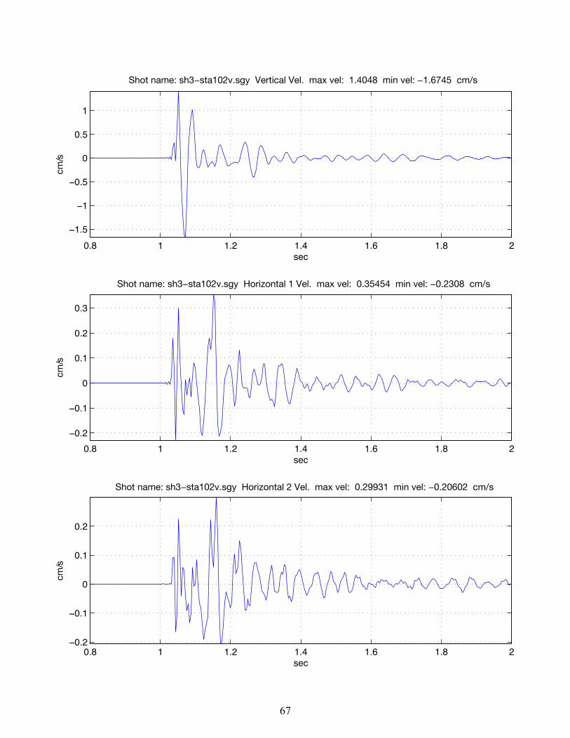
0.8 1 1.2 1.4 1.6 1.8 2−1.5

−1

−0.5

0

0.5

1

sec

s

0.8 1 1.2 1.4 1.6 1.8 2−0.2

−0.1

0

0.1

0.2

0.3

sec

s

0.8 1 1.2 1.4 1.6 1.8 2−0.2

−0.1

0

0.1

0.2

sec

s


cm/


cm/


cm/

67

0.8 1 1.2 1.4 1.6 1.8 2

−1.5

−1

−0.5

0

0.5

1

1.5

sec

s

0.8 1 1.2 1.4 1.6 1.8 2−1

−0.5

0

0.5

sec

s

0.8 1 1.2 1.4 1.6 1.8 2

−0.15

−0.1

−0.05

0

0.05

0.1

0.15

0.2

sec

s


cm/


cm/


cm/

68

0.8 1 1.2 1.4 1.6 1.8 2−0.3

−0.2

−0.1

0

0.1

0.2

sec

s

0.8 1 1.2 1.4 1.6 1.8 2

−0.4

−0.2

0

0.2

0.4

sec

s

0.8 1 1.2 1.4 1.6 1.8 2

−0.15

−0.1

−0.05

0

0.05

0.1

0.15

sec

s


cm/


cm/


cm/

69

0.8 1 1.2 1.4 1.6 1.8 2

−0.05

0

0.05

sec

s

0.8 1 1.2 1.4 1.6 1.8 2−0.06

−0.04

−0.02

0

0.02

0.04

0.06

sec

s

0.8 1 1.2 1.4 1.6 1.8 2

−0.06

−0.04

−0.02

0

0.02

0.04

0.06

0.08

sec

s


cm/


cm/


cm/

70

0.8 1 1.2 1.4 1.6 1.8 2

−0.02

−0.01

0

0.01

0.02

sec

s

0.8 1 1.2 1.4 1.6 1.8 2

−0.03

−0.02

−0.01

0

0.01

0.02

0.03

sec

s

0.8 1 1.2 1.4 1.6 1.8 2

−0.02

−0.01

0

0.01

0.02

0.03

sec

s


cm/


cm/


cm/

71

Appendix 4. Near Source High Resolution Receiver Velocity Plots [Seismic traces are from the cabled array. Zero time is the moment of detonation of the shot.]

72

TIM

E (s

ec)

NW SE

−1

0

1

2

31010 1020 1030 1040 1050 1060

STATION NUMBER

CABLE ARRAYSHOT 1

trace equalization

1001

73

TIM

E (s

ec)

NW SE

0

−1

1

2

3

SHOT 2

trace equalizationCABLE ARRAY

1010 1020 1030 1040 1050 1060

STATION NUMBER

1001

74

−1

0

1

2

3

TIM

E (s

ec)

CABLE ARRAYSHOT 3

trace equalization

NW SE

1010 1020 1030 1040 1050 1060

STATION NUMBER

1001

75

Appendix 5. Velocity Plots for N-S Linear Profile [Near-field to far-field transition. Zero time is the moment of detonation of the shot.]

76

0

3

6

9

12

15

TIM

E (s

ec)

−4 0 4 8 12 16 20 24 28 32 36 40

SOUTH TO NORTH ARRAYSHOT 1

trace equalization, bandpass 2−4−8−16

OFFSET (km)

S N

77

0

3

6

9

12

15

TIM

E (s

ec)

−4 0 4 8 12 16 20 24 28 32 36 40



OFFSET (km)

78

3

6

9

12

15

TIM

E (s

ec)

−4 4 8 12 16 20 24 28 32 36 40



OFFSET (km)0

0

79

Seismic Calibration Shots Conducted in 2009 in the Imperial ...

Documents

Transcript of Seismic Calibration Shots Conducted in 2009 in the Imperial ...