Seismic anisotropy of the lithosphere around the Trans-European Suture Zone (TESZ) based on...

Seismic anisotropy of the lithosphere around the Trans-European

Suture Zone (TESZ) based on teleseismic body-wave data

of the TOR experiment

J. Plomerova *, V. Babuska, L. Vecsey, D. KoubaTOR Working Group

Geophysical Institute, Czech Academy of Sciences, Bocnı II, CP 1401 Sporilov, 141 31 Prague 4, Czech Republic

Received 28 August 2000; accepted 21 November 2001

Abstract

A passive teleseismic experiment (TOR), traversing the northern part of the Trans-European Suture Zone (TESZ) in Germany,

Denmark and Sweden, recorded data for tomography of the upper mantle with a lateral resolution of few tens of kilometers as

well as for a detailed study of seismic anisotropy. A joint inversion of teleseismic P-residual spheres and shear-wave splitting

parameters allows us to retrieve the 3D orientation of dipping anisotropic structures in different domains of the sub-crustal

lithosphere. We distinguish three major domains of different large-scale fabric divided by first-order sutures cutting the whole

lithosphere thickness. The Baltic Shield north of the Sorgenfrei–Tornquist Zone (STZ) is characterised by lithosphere thickness

around 175 km and the anisotropy is modelled by olivine aggregate of hexagonal symmetry with the high-velocity (ac) foliation

plane striking NW–SE and dipping to NE. Southward of the STZ, beneath the Norwegian–Danish Basin, the lithosphere thins

abruptly to about 75 km. In this domain, between the STZ and the so-called Caledonian Deformation Front (CDF), the

anisotropic structures strike NE–SWand the high-velocity (ac) foliation dips to NW. To the south of the CDF, beneath northern

Germany, we observe a heterogeneous lithosphere with variable thickness and anisotropic structures with high velocity dipping

predominantly to SW. Most of the anisotropy observed at TOR stations can be explained by a preferred olivine orientation frozen

in the sub-crustal lithosphere. Beneath northern Germany, a part of the shear-wave splitting is probably caused by a present-day

flow in the asthenosphere.

D 2002 Elsevier Science B.V. All rights reserved.

Keywords: P-residual spheres; Shear-wave splitting; Seismic anisotropy; Sub-crustal lithosphere; Joint inversion of anisotropic characteristics

1. Introduction

The TOR teleseismic experiment was designed to

investigate the deep lithosphere traces of the broad-

scale geology of the Trans-European Suture Zone

(TESZ) area (Gregersen et al., 1999) by means of

high-resolution tomography based on data of seismic

stations deployed in the region from northern Germany

across Denmark to southern Sweden. The TESZ is

interpreted as a broad and complex zone of terrane

accretion separating ancient lithosphere of the Baltic

Shield and East European Craton from the younger

lithosphere of western and southern Europe (Pharaoh,

0040-1951/02/$ - see front matter D 2002 Elsevier Science B.V. All rights reserved.

PII: S0040 -1951 (02 )00349 -9

* Corresponding author. Tel.: +42-6710-3049; fax: +42-2-

761549.

E-mail address: [email protected] (J. Plomerova).

www.elsevier.com/locate/tecto

Tectonophysics 360 (2002) 89–114

1999). This zone, which extends deep into the mantle

(Zielhuis and Nolet, 1994; Arlitt, 1999), is also ex-

pressed in a distinct change of the polarisation aniso-

tropy. The polarisation anisotropy is defined as a value

proportional to a difference between two quasi shear

wave velocities, with which Love and Rayleigh waves

propagate in anisotropic media, and which could be

retrieved from the surface wave tomography (e.g.,

Montagner, 1994). The Phanerozoic part of Europe to

the south–west of the TESZ is characterised by

vSH>vSV in the uppermost mantle, with the maximum

polarisation anisotropy at a depth of about 70 km. The

Precambrian units to the northeast of the TESZ mostly

indicate vSVf vSH or even vSVz vSH. The maximum

deviation of the relative polarisation anisotropy is at

depths of about 100 km (Babuska et al., 1998).

One of objectives of the TOR experiment was to

study body-wave seismic anisotropy in the sub-crustal

lithosphere and asthenosphere. Anisotropy of physical

properties is inherent to rock-forming minerals and

their systematic preferred orientation is reflected in the

large-scale anisotropy of physical parameters. It has

been shown by many observations (see, e.g., Savage,

1999, for a review) that major signal of seismic ani-

sotropy comes from the upper mantle. The crustal ani-

sotropy is almost one order smaller and it is considered

as contaminant. Wylegalla et al. (1999) investigated

directions of azimuthal anisotropy in the uppermost

Fig. 1. Locations of broad-band (BB, circles) and short-period (SP, triangles) stations forming the TOR antenna. The hatching marks

schematically the Trans-European Suture Zone (TESZ) consisting of several parts, where Sorgenfrei–Tornquist Zone (STZ) represents the

northern branch of the Tornquist fan (Thybo, 1997) to the NW, the Caledonian Deformation Front (CDF) its southern branch and the Teisseyre–

Tornquist Zone (TTZ). The Protogine Zone (PZ), Elbe Lineament (EL) and Elbe Fault Zone (EFZ) are marked schematically.

J. Plomerova et al. / Tectonophysics 360 (2002) 89–11490

mantle across the TESZ by analysing split SKS and

SKKS phases recorded at broad-band stations of the

TOR antenna and additional intermediate-period sta-

tions, as well as broad-band permanent European

observatories. They found that the azimuths of the fast

split waves tend to be parallel to Sorgenfrei–Tornquist

and Tornquist–Teisseyre zones (Fig. 1). The authors

conclude that the observed azimuthal anisotropy

around the TESZ is not governed by present-day

mantle flow in the asthenosphere, but rather is frozen

into the sub-crustal lithosphere during the last episode

of tectonic activity. Though the main anisotropic signal

beneath the continents comes from the lithosphere

(Debayle and Kennett, 2000), in general, we cannot

exclude a sub-lithospheric contribution to the observed

anisotropy.

In this paper we analyse P residuals and shear-wave

splitting from recordings of the TOR experiment with

the aim to retrieve three-dimensional (3D) self-con-

sistent anisotropic models of mantle anisotropy and to

study its lateral variations. As shown by Plomerova et

al. (2001) for the Protogine Zone in south-central

Sweden, the orientation of body-wave anisotropy is

consistent within individual blocks of the sub-crustal

lithosphere and it changes at important tectonic boun-

daries. We also present estimates of the lithosphere

thickness and its variation across the TESZ.

2. Data and method

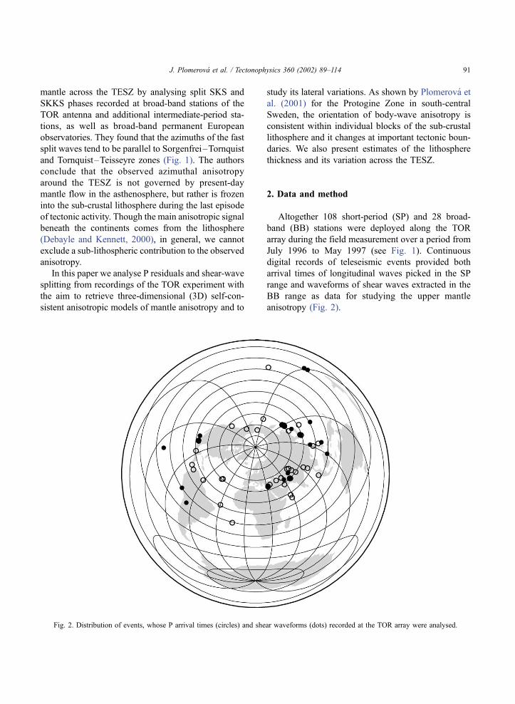
Altogether 108 short-period (SP) and 28 broad-

band (BB) stations were deployed along the TOR

array during the field measurement over a period from

July 1996 to May 1997 (see Fig. 1). Continuous

digital records of teleseismic events provided both

arrival times of longitudinal waves picked in the SP

range and waveforms of shear waves extracted in the

BB range as data for studying the upper mantle

anisotropy (Fig. 2).

Fig. 2. Distribution of events, whose P arrival times (circles) and shear waveforms (dots) recorded at the TOR array were analysed.

J. Plomerova et al. / Tectonophysics 360 (2002) 89–114 91

2.1. Analysis of P-wave travel time residuals

We study P-velocity anisotropy of the sub-crustal

lithosphere by applying a method proposed by

Babuska et al. (1984). This method enables us to

estimate the anisotropic structure of the sub-crustal

lithosphere as seen by the short-period teleseismic

longitudinal waves. To evaluate the lithosphere aniso-

tropy from data of the TOR experiment, we analysed

the high-quality picks of P arrivals (Arlitt, 1999) of

individual events separately (Fig. 2), without their

grouping as it is possible in case of large data sets.

Regional tomographic studies of the upper mantle

focus on travel time deviations from spherical iso-

tropic models of the Earth (e.g., Jeffreys-Bullen,

Herrin, IASP91). Therefore, effects originating out-

side the volume beneath the investigated region have

to be minimised by a normalisation. The normalisa-

tion is a standard procedure in any regional tomo-

graphic study based on P-wave residuals, which is

used to solve this problem (Iyer and Hirahara, 1993).

It is a way to minimise the source-side effects, such as

mislocation, structure in focal region and effects

originating in the deep mantle. After the normalisa-

tion, errors coming from these effects do not exceed

0.1 s for most stations (Raikes, 1980). Certainly, some

effects could remain, similarly to those coming from

the crust. However, as demonstrated in several studies

(e.g., Engdahl et al., 1977; Raikes and Bonjer, 1983;

Judenherc et al., 2002), they are one order lower than

effects of structures below a study area. For example,

random mislocations would be manifested as a scatter

with maximum error of about F 0.1 s. A systematic

bias would not cause a scatter but an error up to 0.2–

0.3 s, which would be constant or change gradually

across the array (Raikes, 1980). Therefore, abrupt

lateral changes of relative residuals observed at boun-

daries of tectonic regions (Babuska et al., 1993;

Plomerova et al., 2000, 2001) can hardly be associated

with the effects mentioned above. Creager and Jordan

(1984, 1986) evaluate residual spheres showing the

travel time residuals as a function of takeoff angle and

azimuth at the source to estimate the teleseismic

signature of descending slab. The observed and mod-

elled residuals relative to spherical Earth models

exhibit smooth deviations reflecting the high-velocity

‘‘anomaly’’ due to the subducting slab. On the con-

trary, the residual spheres on receiver side at tele-

seismic distances show the relative travel time de-

viations as a function of incidence angle and back

azimuth in narrow bands of the takeoff angles and azi-

muths (from source). Therefore, remnants of source-

side effects after normalisation should have to be very

much different for different source regions and foci

location within subducting slabs. However, we ob-

serve a consistent pattern of residual spheres for a

broad range of azimuth and incidence angles. The

TOR antenna is large, but still acceptable for this kind

of tomographic study (Arlitt, 1999), especially after

applying corrections for the Earth’s ellipticity.

When performing the normalisation, generally, a

mean absolute residual over all stations that recorded

an event, or over a selected set of reference stations, is

subtracted from absolute residuals observed at indi-

vidual stations. Consequently, relative residuals, i.e.

relative to a reference level, are analysed. We tested

different reference Earth’s models (Jeffreys-Bullen,

IASP91) and normalisation’s following criteria of

residual stability with the aim to retain as much data

as possible. Similarly to Raikes (1980), we found that

the processed relative residuals were independent of

the reference 1D Earth model used. Before normal-

ising, corrected each arrival time for crustal effects.

The crustal corrections are based on models compiled

from many results of DSS (Abramovicz et al., 1999;

Arlitt et al., 1999; Pedersen, 1999; Pedersen et al.,

1999) and receiver functions (Goessler et al., 1999).

The corrections reduce effects due to sediments and

variable crustal thickness as compared to the crustal

thickness and velocities of the reference 1D Earth

model.

To evaluate seismic anisotropy we construct resid-

ual spheres for each station. The spheres show that

part of the relative P residuals (directional terms of the

relative residuals), which depend on the direction of

propagation through the lower lithosphere defined by

azimuth and angle of propagation measured from the

vertical. We can assume that the anisotropy in the sub-

lithospheric mantle beneath continents is governed

mainly by a sub-horizontal flow. In such a medium,

the maximum velocity is also sub-horizontal and the

sub-lithospheric anisotropy thus affect only negligible

variations in the teleseismic P arrivals. Therefore, the

main source of directional variations in the P-residual

spheres (the residuals are corrected for crustal effects)

can be attributed to the mantle lithosphere. A refer-


ence base created by 56 stations with at least 30

observations was chosen for the P-anisotropy study.

This reference base was stable and retained sufficient

amount of observations for various directions in the

residual spheres. No effects of different crustal cor-

rections applied (Arlitt et al., 1999; Pedersen, 1999)

were found in the pattern of the residual spheres.

Possible effects of the corrections were retained into a

directional mean of an individual station, which was

subtracted from the relative residuals at the station.

The directional mean is computed at each station as an

azimuth-propagation angle filtered average computed

from relative residual over all events.

The directional terms map the high- and low-

velocity directions of propagation for angles between

20j and 50j, which correspond to P-wave propaga-

tion through the sub-crustal lithosphere from tele-

seismic distances. The residual spheres can be con-

sidered as a measure of anisotropy beneath individual

stations. Changes of their pattern allow us to map

lateral variations of the lithospheric anisotropy (e.g.,

Babuska et al., 1984, 1993; Plomerova et al., 1996,

2000). Often we observe a bipolar patter of the residual

spheres. By the bipolar pattern we understand such

distribution of the directionally terms of residuals,

which shows negative (early arrivals) in one side of

the lower hemisphere and positive (delayed arrivals) in

the opposite side of the hemisphere. The azimuth

separating the positive and negative side of the spheres

can be associated with the strike of dipping anisotropic

structures, specifically with the strike of dipping fast

(ac) foliation plane of olivine aggregate in case of

hexagonal symmetry. For more details, we refer to

Babuska et al. (1984, 1993).

2.2. Evaluating shear-wave splitting

Detecting splitting of shear waves of teleseismic

events generally evidences upper mantle anisotropy. If

the core shear waves (SKS, SKKS) propagate through

solely isotropic mantle, they should exhibit linear SV

polarisation with no energy on transverse component,

as they are generated by P-to-SV conversion at the

core–mantle boundary. Therefore, if we observe shear

waves with elliptical polarisation resulted from the

shear-wave splitting, it has to be attributed to the

receiver side of the ray path. The elliptical polarisation

results from an interference of two quasi-shear waves.

One is polarised in the vertical plane, often referred as

the wave with the SV polarisation and the second one

is polarised perpendicular to it having the SH polar-

isation. The waves propagate with slightly different

velocities and thus a time shift between the wave-

forms is produced. Therefore, evaluating the shear-

wave splitting parameters, i.e., the orientation of the

polarised fast shear wave and the time delay between

the fast and slow shear waves, allows us to measure

upper mantle anisotropy. However, the core shear

waves represent only a sub-vertical propagation

through the upper mantle. To retrieve the 3D orienta-

tion of anisotropic structures, we also use direct shear

waves (S) whose rays illuminate volume of the ani-

sotropic mantle beneath the receivers under various

angles of propagation. However, waveforms of the

direct shear waves might be contaminated by an

anisotropy beneath the source region and source char-

acteristics. Therefore, for their including into further

processing, an internal consistency of splitting param-

eters evaluated for direct and core shear waves arriving

from close directions is decisive. The internal coher-

ency between the evaluated splitting parameters for

SKS and S waves from the same source is an addi-

tional argument which proves that the anisotropic

signals produced by structures beneath the stations

dominate (Plomerova et al., 1998).

To measure the upper mantle anisotropy, we ana-

lysed three-component records of shear waveforms

associated to all events with body-wave magnitude of

at least 6. Besides records of the BB portable stations

operating during the TOR experiment, we used

records of permanent observatories, which operated

in the region (see Fig. 1) and provided their records to

the TOR database. Based on the generalised method

by Silver and Chan (1991), we search for the fast

shear-wave polarisation direction in plane (Q–T)

perpendicular to the vertical ray path plane (L–Q)

of the quasi shear phase. A rotation of the coordinate

system in the plane (Q–T) by an angle w, and a time

shift yt, imposed on the shear-wave components, yield

the splitting parameters (polarisation vector) deter-

mined in 3D. Orientation of the fast shear-wave

polarisation vector is described by spherical angles h(measured upward from the positive axis z orientated

downward) and / (azimuth from the north). The time

shift between the fast and slow split waves is

described by the time delay yt in seconds (Sıleny


and Plomerova, 1996). To evaluate the splitting

parameters, we applied three methods: the correlation

method (Vinnik et al., 1989), eigenvalue method

(Silver and Chan, 1991) and a method based on

minimising the transverse component (Savage and

Silver, 1993). The last one is applicable only in case

of core phases and was found as the most stable. The

results were checked by the eigenvalue method. The

correlation method was refused as unreliable.

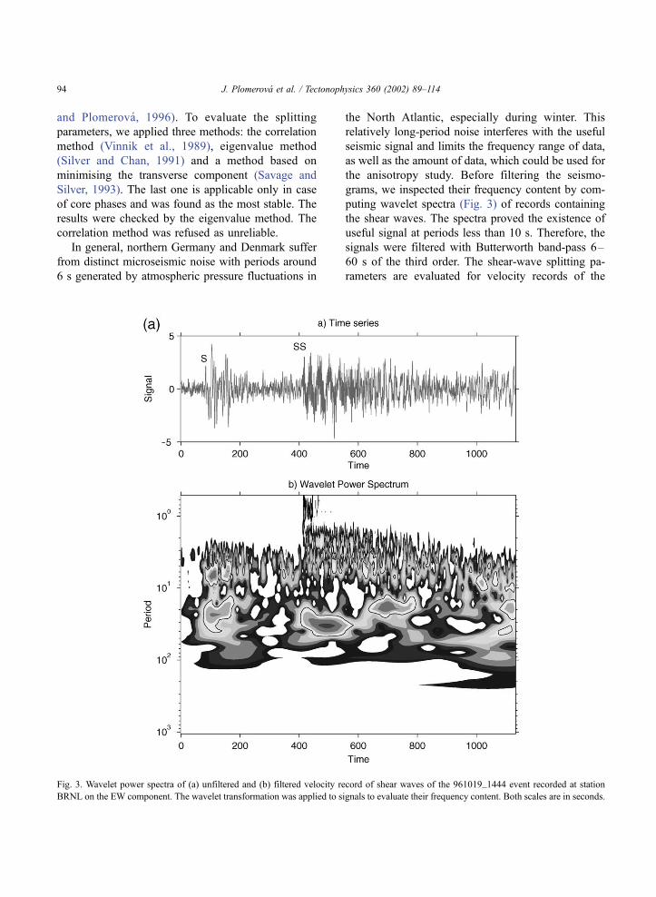
In general, northern Germany and Denmark suffer

from distinct microseismic noise with periods around

6 s generated by atmospheric pressure fluctuations in

the North Atlantic, especially during winter. This

relatively long-period noise interferes with the useful

seismic signal and limits the frequency range of data,

as well as the amount of data, which could be used for

the anisotropy study. Before filtering the seismo-

grams, we inspected their frequency content by com-

puting wavelet spectra (Fig. 3) of records containing

the shear waves. The spectra proved the existence of

useful signal at periods less than 10 s. Therefore, the

signals were filtered with Butterworth band-pass 6–

60 s of the third order. The shear-wave splitting pa-

rameters are evaluated for velocity records of the

Fig. 3. Wavelet power spectra of (a) unfiltered and (b) filtered velocity record of shear waves of the 961019_1444 event recorded at station

BRNL on the EW component. The wavelet transformation was applied to signals to evaluate their frequency content. Both scales are in seconds.


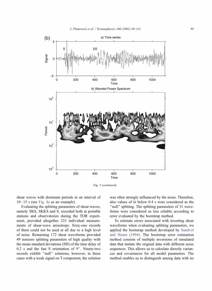
shear waves with dominant periods in an interval of

10–15 s (see Fig. 4a as an example).

Evaluating the splitting parameters of shear-waves,

namely SKS, SKKS and S, recorded both at portable

stations and observatories during the TOR experi-

ment, provided altogether 233 individual measure-

ments of shear-wave anisotropy. Sixty-one records

of them could not be used at all due to a high level

of noise. Remaining 172 shear waveforms provided

49 nonzero splitting parameters of high quality with

the mean standard deviations (SD) of the time delay of

0.2 s and the fast S orientation of 9j. Ninety-tworecords exhibit ‘‘null’’ solutions, however, in these

cases with a weak signal on T component, the solution

was often strongly influenced by the noise. Therefore,

also values of yt below 0.4 s were considered as the

‘‘null’’ splitting. The splitting parameters of 31 wave-

forms were considered as less reliable according to

error evaluated by the bootstrap method.

To estimate errors associated with inverting shear

waveforms when evaluating splitting parameters, we

applied the bootstrap method developed by Sandvol

and Hearn (1994). The bootstrap error estimation

method consists of multiple inversions of simulated

data that imitate the original data with different noise

sequences. This allows us to calculate directly varian-

ces and covariances for all model parameters. The

method enables us to distinguish among data with no

Fig. 3 (continued).


apparent splitting, reliably split shear waves and noisy

data (Fig. 4). Careful measuring of reliability of

evaluated splitting parameters is very important espe-

cially in noisy regions. Evaluated errors input as

weights into the joint inversion.

2.3. Joint inversion of anisotropic data to retrieve the

3D orientation of anisotropic structures

To retrieve 3D orientation of anisotropic structures,

we invert jointly anisotropic parameters evaluated in

the P-residual spheres, i.e., for P-velocity dependent

on directions of longitudinal wave propagation

through the lithosphere, and the shear-wave splitting

parameters, which measure the shear-wave anisotropy

in the upper mantle. Anisotropic medium is approxi-

mated by hexagonal or orthorhombic symmetry, char-

acterised by various magnitude of anisotropy (Ben

Ismail and Mainprice, 1998; Babuska and Plomerova,

2000). Due to the lack of high-quality shear-wave data

at single stations, we inverted jointly anisotropic

parameters of stations, which exhibit similar aniso-

tropic characteristics. To retrieve orientation of sym-

metry axes and a thickness of anisotropic medium, we

have searched for a minimum of a misfit function

J ¼XKi¼1

ARansi � RC

i A2

ðriÞ2

þXNi¼1

AiuobsS �i uSA2

ðrangi Þ2

þ Aytobsi � dtiA2

ðrtiÞ2

" #

where Rans and RC are observed directional terms of

relative residuals and calculated residuals of P waves

propagating through the anisotropic medium, respec-

tively; uobs and ytobs are the orientation of the fast

shear-wave polarisation vector and the time delay

between the two split waves, respectively; and rstands for error estimates. The 3D orientation of the

polarisation vector is given by the Euleur angles /and h.

2.4. Modelling the lithosphere thickness

Lithosphere thickness estimate links lateral varia-

tions of relative residual means at individual stations,

which we called static means, to lateral variations of

lithosphere thickness. Negative and positive values of

the static terms reflect, respectively, relative abundance

or lack of high-velocity lithospheric material compared

to low-velocity material in the asthenosphere. The

static means are computed as average relative residuals

from steeply incident rays (to avoid effects arising from

possible variably dipping anisotropic structures) arriv-

ing from evenly distributed azimuth. They reflect

average isotropic velocity in a volume beneath a sta-

tion. This basic assumption locates main heterogeneity

due to the relief of the lithosphere–asthenosphere

boundary (LAB) within a cone of steeply incident rays

at depths below the Moho.

Contrary to the anisotropic residual spheres, the

residual means depend on the crustal corrections

applied. When computing static means, beneath the

TOR region, we used velocities and thickness of the

crust and sediments according to Pedersen et al.

(1999). To compromise between the stability of the

reference level of the relative residuals and retaining

sufficient number of data, we choose a reference base

formed by 13 normalising stations providing the

highest number of observations in the TOR data set

and distributed evenly in the region.

To estimate the lithosphere thickness we applied an

empirical relation, which associates relative changes

of the delays with changes of lithosphere thickness

(Babuska and Plomerova, 1992). In the relation, a

gradient of 9.4 km/0.1 s was found and applied in

several other regions (e.g., Babuska et al., 1987, 1993;

Plomerova et al., 1993, 1998). A velocity contrast of

Fig. 4. Example of evaluating (a) shear wave splitting and (b) standard deviations of the splitting parameters (orientation of the fast S in the (Q–

T) plane, given by the angle w (j) and time delay yt (s), by a bootstrap method developed by Sandvol and Hearn, 1994). Broad-band (BB)

velocity records were filtered using of the 3rd order Butterworth band-pass of 6–60 s. The original elliptically polarised signal at LQT

coordinate system (upper left) and linearly polarised signal (lower left) after a rotation by an angle w in the (Q–T) plane and applying a time

shift yt. The lower left signal corresponds to the minimum of the misfit function marked by a white circle (lower right). Theta and phi (denoted

in the text as h and u) are Euleur angles defining orientation of the polarisation vector in 3D. (b) Dashed lines in the centre between solid lines

mark the values and standard deviations of DT (stands for yt here) and PSI (stands for w here) in seconds and degrees, respectively. The dashed

lines out of the centres are the values evaluated in (a). Intervals of 0–2 s and 85–175j were tested.


0.6 km/s between anisotropic lithosphere and astheno-

sphere is required in the relation. This is in agreement

with velocities of P waves propagating steeply

through the asthenosphere characterised by mainly

horizontal high-velocity directions and the lithosphere

with dipping high-velocity (ac) foliation planes

(Babuska et al., 1998; Plomerova et al., 2002). Values

of the relative residuals depend on a choice of the

reference level. When converting the static means into

the lithosphere thickness model, we need to fix the

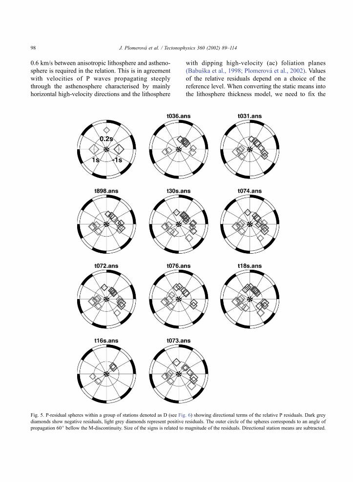
Fig. 5. P-residual spheres within a group of stations denoted as D (see Fig. 6) showing directional terms of the relative P residuals. Dark grey

diamonds show negative residuals, light grey diamonds represent positive residuals. The outer circle of the spheres corresponds to an angle of

propagation 60j bellow the M-discontinuity. Size of the signs is related to magnitude of the residuals. Directional station means are subtracted.


intercept of the linear relation. A way how to proceed

from relative values (thicker– thinner) to absolute

values (depths) is to fix the residual-depth value

through residuals computed in a part of the region

which overlaps with another model based on ob-

servations of a different station set in a different time

period. To link the relative static means with ‘‘ab-

solute’’ values of the lithosphere thickness, we assign

the static mean of 0.4 s in the south–west (stations

BUG, IBBN, t7bg, see Fig. 12) to the lithosphere

thickness of 80 km (52jN 8jE). This value was

found in previous estimates of the lithosphere thick-

ness in Europe based on the P-residuals (Babuska and

Plomerova, 1992) and surface waves (Panza et al.,

1980).

3. Anisotropic structure of the sub-crustal

lithosphere

Directional dependence of P-wave velocities in the

sub-crustal lithosphere beneath individual stations can

Fig. 6. Anisotropic P-residual spheres of groups of stations with a similar pattern (labelled from A to L). Individual stations within a group are

coloured. Stations in grey or marked with empty symbols cannot be associated with any group due to the lack or total absence of data,

respectively. While north of the TESZ (STZ, see Fig. 1), the early arrivals (blue), i.e., high velocities, are orientated prevailingly to NE, south of

the TESZ (CDF) they are orientated mostly to SW. Within the Tornquist fan, i.e., between the STZ and CDF, the high velocities point to NW.

We observe no distinct anisotropy at stations south of the Elbe Lineament (EL, group J) and at the northernmost tip of the antenna (groups A and

partly B). For more about the spheres, see caption of Fig. 5.


be traced in the P-residual spheres constructed for

majority of the TOR stations. Surveying the spheres

shows that neighbouring stations form groups accord-

ing to their pattern. Fig. 5 presents single spheres

within group D (see Fig. 6), as an example. The

residuals are relatively small, but consistent in their

distribution and form the clear bipolar pattern. For

example, positive values shown in the sphere of

Fig. 7. Lateral variations of particle motion of the horizontal components in the N–E plane along the array. Directions to the north are on the

verticals and to the east are on the horizontals.


station t30s attain 0.4 s and negative values � 0.3 s,

on average. Positive residuals (low-velocity direc-

tions) prevail in a part of the lower hemisphere

between azimuths 120–300j, while negative residuals(high-velocity directions) were found in opposite

azimuths.

Fig. 6 presents groups of stations with similar

pattern of the spheres. It shows spheres with data

merged for all stations within individual groups. This

step is feasible due to subtracting the directional mean

at each station. In southern Sweden, we observe the

distinct bipolar pattern (groups B, C and D), except of

the northernmost part of the TOR antenna (group A).

The distribution of positive and negative residuals in

the spheres changes abruptly (group E) at the STZ. In

a region beneath the Tornquist fan (Thybo, 1997), i.e.,

between the STZ and Caledonian Deformation Front

(CDF), the positive residuals are observed in the SE

azimuths (group F). Further to the south, between the

CDF and the Elbe line (EL), the bipolar pattern of the

P-spheres rotates and the negative residuals prevail in

SE–SW azimuths (135–215j, group H). This pattern

is opposite to that observed in southern Sweden and is

similar to that observed in the south-eastern part of the

TOR array, north of the EL (group I). Group G with

less data tends to this pattern too. Anisotropic pattern

in the southernmost part of the TOR antenna, south of

the EL is not evident. While the distribution of nega-

tive and positive residuals is almost reversed in the

spheres of group K compared to group L (the south-

western part), no anisotropic pattern, i.e., a separation

between the positive and negative residual terms, can

be found in group J (the south-eastern part), at all. No

decision about orientation of the high- and low-

velocity directions can be made for many stations in

the south-central part due to a lack of data, or due to

unclear patterns of the residuals. Only three stations at

the very south–east end of the TOR antenna tend to

exhibit the pattern similar to that of group I.

When studying the shear-wave anisotropy, we

observe two types of variations of the splitting param-

eters—both in magnitude (yt) and in orientation of the

fast S (h, u). First, various orientations of anisotropicstructures in different lithospheric domains are

reflected in lateral variations of particle motion and

consequently, in variations of the splitting parameters

of an event along the array (Fig. 7). While an elliptical

polarisation is evident especially at stations in south-

ern Sweden, it almost disappears at stations in Den-

mark, whereas waveforms recorded at stations in

northern Germany again exhibit an elliptical polar-

isation (Fig. 7). A weak effect of the Protogine Zone

probably disturbs the particle motion shown for sta-

tion t30s (Plomerova et al., 1996, 2001). Second, at

individual sites, effects of dipping fabrics are reflected

in a dependence of the splitting parameters on direc-

tion of propagation through anisotropic mantle (Fig.

8). This directional dependence of splitting parameters

indicate a more complex anisotropic structure of the

upper mantle than that which could be modelled by a

single layer with a horizontal fast symmetry axis. Two

layered models might account for the splitting varia-

tions (Savage and Silver, 1993). However, these

models do not fit the P-residual spheres (Plomerova

et al., 1998). Lateral variations related to prominent

sutures support a concept of the lithospheric mantle

Fig. 8. Variation of individual fast S polarisation vectors evaluated at

two stations, belonging to group D (see Fig. 6) in southern Sweden,

in the equal-angle projection of lower hemisphere. Full arrows mark

solutions evaluated with average standard deviations of yt and wequal to 0.2 s and 9j, respectively, empty arrows show less reliable

solutions.


formed by individual domains with different orienta-

tion of frozen-in anisotropy (Plomerova et al., 2000).

Fig. 9 summarises results of splitting measurements

(the time delay yt and fast shear-wave azimuth /),including reliable ‘‘null’’ solutions. Reliability of

evaluated yt and w (given by azimuth / and inclina-

tion from vertical h) of each waveform was tested by

determining their standard deviations by the bootstrap

method (Sandvol and Hearn, 1994). However, even

after the filtering and careful analysis of the wave-

forms, evaluated splitting parameters exhibit distinct

variations in this region.

Only reliably determined splitting parameters of

shear-waves (Table 1) were considered in the inver-

sions for 3D orientation of anisotropic structure

beneath individual stations. Although as many as

37 BB stations were involved in the field measure-

ment lasting for 10 months, they did not provide

Fig. 9. Azimuths of the fast shear-wave polarisation vectors, pointing in the dip direction, as determined from shear-wave splitting, evaluated in

3D (see also Table 1). Thin lines mark ‘‘null solutions’’, i.e., two possible solutions of orientation of the fast and slow shear waves, if they split.

Solutions evaluated with average standard deviations of yt and w equal to 0.2 s and 9j, respectively, are contoured, less reliable solutions arewithout contours.


Table 1

Shear-wave splitting parameters evaluated for events with body-wave magnitude larger than 5.9 recorded at stations involved in the TOR

experiment

Station Latitude (jN)/longitude (jE)

DIST

(j)BAZ

(j)Event

identification

Phase yt(s)

F yt(s)

w(j)

Fw(j)

h(j)

u(j)

good//

fair

BRG 50.874 13.946 102.6 48.7 970423_1944 sks 0.9 0.08 130.3 4.8 84.9 278.7 g

BRNL 52.200 13.500 76.4 29.4 961002_1124 s 2.0 0.15 73.1 11.3 84.7 135.5 f

BRNL 52.200 13.500 80.3 49.7 961019_1444 s 1.8 0.19 138.6 14.4 76.8 272.5 g

BRNL 52.200 13.500 100.7 48.1 970123_0215 sks 1.0 0.54 107.7 17.1 87.6 140.5 g

BRNL 52.200 13.500 45.4 97.4 970227_2130 s 2.4 0.29 90.2 22.3 89.9 7.2 f

BRNL 52.200 13.500 98.3 66.0 970311_1922 sks 0.9 0.13 137.2 8.4 83.8 289.1 g

BRNL 52.200 13.500 101.9 48.1 970423_1944 sks 0.8 0.10 115.4 4.5 86.6 292.9 g

BRNL 52.200 13.500 89.8 300.9 970522_0750 sks 0.5 0.19 120.6 10.7 84.9 179.8 g

BSD 55.108 14.909 77.8 51.1 961019_1444 s 2.1 0.27 164.6 12.5 72.3 247.3 g

BSD 55.108 14.909 23.8 142.7 961009_1310 s 2.1 0.20 142.5 14.5 65.9 4.5 g

BSEG 53.935 10.320 75.8 27.5 961002_1124 s 2.0 0.42 84.5 13.7 88.2 122.7 f

BSEG 53.935 10.320 24.7 132.8 961009_1310 s 3.4 0.15 117.6 4.4 77.5 18.0 f

BSEG 53.935 10.320 80.6 47.6 961019_1444 s 1.9 0.17 180.2 9.1 72.3 227.4 g

BSEG 53.935 10.320 99.7 246.0 970123_0215 sks 1.0 1.77 103.5 34.8 88.1 142.6 f

BUG 51.446 7.264 126.0 279.6 960905_0814 sks null g

BUG 51.446 7.264 78.9 25.2 961002_1124 s 2.1 0.13 57.3 9.8 80.3 146.6 g

BUG 51.446 7.264 102.1 61.0 970311_1922 sks 2.5 0.63 164.2 4.8 82.4 256.9 g

BUG 51.446 7.264 105.2 42.7 970423_1944 sks 0.8 0.39 156.7 13.6 83.1 246.2 g

BUG 51.446 7.264 86.8 296.0 970522_0750 sks 0.9 0.44 73.7 19.2 80.3 93.7 g

CLZ 51.843 10.374 98.8 245.7 970123_0215 s 2.1 0.09 14.1 2.2 76.4 50.5 g

CLZ 51.843 10.374 44.8 85.5 970513_1413 s 1.9 0.33 60.9 3.9 78.6 202.0 g

IBBN 52.307 7.757 101.4 61.2 970311_1922 sks 1.0 0.54 147.9 14.6 83.1 273.6 g

IBBN 52.307 7.757 104.3 43.0 970423_1944 sks 1.3 0.11 161.1 1.7 82.8 242.1 g

IBBN 52.307 7.757 86.7 296.4 970522_0750 sks 0.4 0.58 72.4 37.8 83.3 65.9 g

LEN 53.091 11.478 102.2 46.2 970423_1944 sks 1.0 0.08 138.0 3.5 84.1 268.4 g

LEN 53.091 11.478 88.3 299.3 970522_0750 sks null g

OLDS 56.619 16.499 76.1 52.6 961019_1444 s 2.4 0.08 125.7 7.4 79.3 288.3 g

RGN 54.548 13.321 74.4 29.6 961002_1124 s 2.7 0.11 65.3 7.3 82.2 143.1 f

RGN 54.548 13.321 23.9 139.0 961009_1310 s 1.7 0.41 145.6 24.1 64.9 357.6 f

RGN 54.548 13.321 101.5 260.4 961112_1659 sks null g

RGN 54.548 13.321 42.9 90.6 970513_1413 s 1.9 0.31 51.4 4.4 74.7 216.5 g

T14S 56.259 13.623 25.1 141.9 961009_1310 s 2.8 0.25 137.4 9.3 70.2 7.9 f

T14S 56.259 13.623 77.6 50.4 961019_1444 s 3.0 0.16 135.7 9.2 76.9 276.2 g

T14S 56.259 13.623 102.3 249.0 970123_0215 skks 1.4 0.27 112.9 5.5 85.4 136.5 g

T14S 56.259 13.623 96.5 65.7 970311_1922 sks 2.8 0.33 104.5 1.8 87.8 321.3 f

T18S 56.520 13.566 128.4 289.1 960905_0814 sks null g

T18S 56.520 13.566 25.4 142.2 961009_1310 s 2.6 0.21 125.2 10.9 74.6 20.1 f

T18S 56.520 13.566 77.5 50.4 961019_1444 s 2.7 0.12 106.9 8.6 84.7 304.3 g

T18S 56.520 13.566 102.4 249.0 970123_0215 skks 0.9 0.65 151.9 21.7 80.3 97.5 f

T18S 56.520 13.566 96.5 65.6 970311_1922 sks 1.3 0.25 118.9 5.1 85.8 307.0 g

T18S 56.520 13.566 153.7 25.5 970503_1646 skks 1.6 0.26 27.6 4.9 82.0 177.6 g

T18S 56.520 13.566 87.6 300.8 970522_0750 sks 1.0 0.35 167.1 5.5 80.0 133.9 g

T1BD 55.863 12.240 46.7 99.8 970227_2130 s 3.2 0.59 146.3 10.6 69.8 316.0 f

T1BD 55.863 12.240 97.4 64.5 970311_1922 sks 1.4 0.20 145.1 6.4 82.9 279.7 g

T2BD 55.703 11.548 78.9 48.7 961019_1444 s 2.9 0.29 118.9 23.2 81.3 291.0 g

T2BD 55.703 11.548 47.0 99.0 970227_2130 s 4.0 0.47 57.3 38.7 77.2 219.3 f

T2BD 55.703 11.548 97.8 64.0 970311_1922 sks 0.9 0.27 123.9 27.1 85.2 300.4 g

T2BG 54.223 10.074 101.0 72.7 960722_1419 sks 1.1 0.38 163.0 11.3 82.2 269.9 g

T2BG 54.223 10.074 47.7 96.3 970227_2130 s 3.2 0.25 75.0 13.5 83.9 200.0 g

T30S 57.095 13.946 25.7 143.6 961009_1310 s 2.6 0.07 108.7 3.2 81.5 36.9 f

(continued on next page)


enough reliable splitting parameters of shear waves,

which could be inverted separately beneath the

stations (Sıleny and Plomerova, 1996). To model

the anisotropy of the upper mantle along the TOR

antenna, we inverted jointly the P-residual spheres

and the shear-wave splitting parameters. First, data

Table 1 (continued )

Station Latitude (jN)/longitude (jE)

DIST

(j)BAZ

(j)Event

identification

Phase yt(s)

F yt(s)

w(j)

Fw(j)

h(j)

u(j)

good//

fair

T30S 57.095 13.946 76.9 50.8 961019_1444 s 2.3 0.21 144.6 7.9 74.9 267.7 g

T30S 57.095 13.946 102.8 249.4 970123_0215 sks 2.7 0.56 172.6 1.2 82.2 76.9 g

T30S 57.095 13.946 87.5 301.1 970522_0750 sks null g

T3BD 55.536 12.078 46.7 99.3 970227_2130 s 2.0 0.61 148.1 12.3 69.4 313.7 g

T3BD 55.536 12.078 97.6 64.4 970311_1922 sks 0.9 0.30 127.4 13.2 84.7 297.3 g

T3BD 55.536 12.078 43.7 90.6 970513_1413 s 0.8 0.70 59.3 35.9 77.6 208.9 g

T3BD 55.536 12.078 87.4 299.6 970522_0750 sks null g

T40S 57.581 15.039 38.3 108.8 970510_0757 s 2.4 0.41 106.7 25.0 82.8 3.7 f

T42S 57.761 14.664 76.2 51.4 961019_1444 s 2.3 0.12 151.9 6.8 73.7 260.8 g

T42S 57.761 14.664 38.5 108.6 970510_0757 s 2.3 0.56 126.9 17.3 74.8 344.6 f

T42S 57.761 14.664 89.6 12.6 970525_2322 skks 0.8 0.74 136.0 21.3 81.2 237.3 g

T4BD 55.219 11.595 100.8 247.2 970123_0215 sks null g

T4BD 55.219 11.595 43.9 89.9 970513_1413 s 1.0 0.14 68.4 11.4 81.1 199.6 g

T4BD 55.219 11.595 87.3 299.3 970522_0750 s 0.4 0.58 174.0 29.4 74.1 125.2 g

T4BG 53.135 9.800 78.9 37.1 960810_1812 s 1.3 0.85 91.3 65.9 89.6 305.9 f

T4BG 53.135 9.800 102.9 44.7 970423_1944 sks 0.4 0.34 111.7 32.3 87.1 293.2 g

T4BG 53.135 9.800 87.4 297.9 970522_0750 sks 1.3 0.09 82.0 0.8 88.6 35.8 f

T5BG 53.188 9.336 87.1 297.6 970522_0750 sks 0.5 0.34 18.7 17.5 81.0 88.5 g

T60S 58.758 15.943 72.4 42.4 960810_1812 s 2.1 0.23 29.4 3.7 73.2 191.5 f

T60S 58.758 15.943 79.2 65.6 960905_2342 s 0.5 0.81 36.2 35.9 75.6 208.0 f

T60S 58.758 15.943 70.1 32.0 961002_1124 s 2.9 0.25 55.0 11.9 78.8 155.4 f

T60S 58.758 15.943 38.2 111.2 970510_0757 s 1.9 1.03 147.3 38.0 68.4 326.7 f

T60S 58.758 15.943 88.5 13.7 970525_2322 skks 0.9 0.13 127.4 9.2 82.6 246.9 g

T6BD 54.887 11.255 100.5 246.9 970123_0215 sks null g

T6BG 53.380 9.595 76.5 26.9 961002_1124 s 2.5 0.14 60.7 2.4 81.0 144.9 g

T6BG 53.380 9.595 99.0 245.4 970123_0215 sks null g

T6BG 53.380 9.595 87.2 297.8 970522_0750 sks 2.3 0.41 8.7 1.1 79.8 108.9 f

T7BD 52.259 8.557 100.1 245.5 970123_0215 sks null g

T7BG 52.259 8.557 102.4 71.8 960722_1419 sks 1.1 0.13 135.4 4.9 84.4 296.7 f

T7BG 52.259 8.557 104.0 43.7 970423_1944 sks 0.7 0.13 128.1 13.2 85.3 275.8 g

T7BG 52.259 8.557 104.0 43.7 970423_1944 skks 1.0 0.58 153.0 12.8 79.6 251.2 g

T7BG 52.259 8.557 89.9 301.7 970501_1137 ss 3.3 0.60 178.5 10.4 65.2 123.4 f

T7BG 52.259 8.557 87.1 297.0 970522_0750 sks 0.9 0.32 78.0 6.5 87.9 38.8 g

T8BG 53.851 12.905 101.0 248.0 970123_0215 sks 0.9 2.06 99.8 55.4 88.6 148.3 f

T8BG 53.851 12.905 97.9 65.3 970311_1922 sks null g

T897 58.380 12.509 76.7 49.9 961019_1444 s 1.7 0.52 60.9 6.8 81.1 167.7 g

T897 58.380 12.509 102.5 248.5 970123_0215 sks null g

T9BG 52.723 11.479 102.4 46.2 970423_1944 sks 1.0 0.82 99.2 8.4 87.6 298.5 f

T9BG 52.723 11.479 88.5 299.3 970522_0750 sks 0.7 0.22 113.6 6.1 85.9 186.0 g

TBBG 52.870 10.632 102.7 45.4 970423_1944 sks 1.1 0.10 107.5 1.7 87.6 298.1 g

Fig. 10. Results of the joint inversion given by orientation of anisotropic models with hexagonal symmetry in projection of lower hemisphere for

all groups of stations except of G and L (models with orthorhombic symmetry). The upper left sphere shows the misfit functions, where the

minimum marks the orientation of the low-velocity symmetry axis b of the hexagonal model fitting the data of the group C. The corresponding

distribution of the anisotropic velocities dipping to the NE shows the sphere in the upper right. The latter is shown for all groups labelled as D

through L (see also Figs. 6 and 11). In case of groups G and L, better solutions, according to the misfit functions, were achieved with

orthorhombic models.


clustered according to the residual pattern (see Fig.

6) along with the high-quality shear-wave splitting

parameters of SKS and SKKS phases were inverted.

Then, the evaluated splitting parameters of a medium

quality core phases and of all S waves were tested as

to their compatibility with the model. Finally, the

joint inversion, as described in Section 2, was

performed.

Fig. 11. Orientation of dipping high-velocity directions in individual domains of the mantle lithosphere along with thickness (km) of the

anisotropic medium which is required to accommodate the observed anisotropy assuming hexagonal model with kP= 7% and orthorhombic

model with kP= 9% anisotropy.


The inversion retrieved 3D anisotropic structures

with inclined symmetry axes in the sub-crustal litho-

sphere. Hexagonal models with dipping high-velocity

(ac) foliation planes fit the majority of the data.

Resulting orientations of the anisotropic structures

are presented in projection of lower hemisphere for

each population of stations. Fig. 10 shows the mini-

mum of the misfit functions, i.e., in this case orienta-

tion of axis b of the hexagonal model fitting both the P

data of the group C and splitting parameters evaluated

at stations T40–42S, and corresponding distribution

of anisotropic velocities. The velocity distribution

retrieved for other groups of station is shown as well.

In case of groups G and L, a better solution according

to the misfit function was achieved with orthorhombic

model. It is evident from anisotropic models that we

detected three lithospheric domains with differently

orientated dipping high-velocity directions. Fig. 11

shows schematically strikes of the anisotropic struc-

tures and dips of the high velocities. The arrows point

in dip directions of the (ac) foliation plane of the

hexagonal peridotite aggregate or in the dip of the

lineation (a axis) in case of the orthorhombic aggre-

gate. Beneath southern Sweden, i.e. north of the STZ,

the (ac) planes dip to NE at angles of 55j from

horizontal. This structure is similar to that found in

south-central Sweden around a latitude of 60jN(Plomerova et al., 2001). The high-velocity plane

plunging to NW at angles of about 30j was retrieved

in a region between the STZ and CDF. Anisotropic

structure between the CDF and EL can be character-

ised by the (ac) foliation dipping to SW at about 45j.South of the EL and around the junction of the CDF

and STZ, a model with orthorhombic symmetry meets

the anisotropic data better. However, in region G,

neither hexagonal nor orthorhombic solutions are

stable. This seems to reflect very complex structure

around the triple junction of the CDF, STZ and TTZ.

We present also thickness of the modelled aniso-

tropic layer required in the inversions to accommo-

date the observed anisotropy. Thickness of the

anisotropic structures shown in Fig. 11 resulted from

computation using hexagonal and orthorhombic

aggregates with the coefficient of anisotropy kP= 7%

and kP= 9%, respectively. There is always a trade-off

between the magnitude of anisotropy and thickness of

the anisotropic medium. Computations with various

magnitudes of anisotropy and resulting thickness of

anisotropic layers confirm that the main source of the

observed body-wave anisotropy is located within the

sub-crustal lithosphere (cf. with lithosphere thickness

in Section 4). This relates to anisotropy mapped in the

residual spheres and reflected in directionally depend-

ent splitting parameters.

4. Lithosphere thickness

The absolute P travel-time anomalies of 1–2 s, ob-

served in the TOR area, can be divided between known

crustal effects and lower lithosphere–asthenosphere

differences (Gregersen et al., 2002). After applying

crustal corrections, we can attribute the remaining

anomalies to effects of the upper mantle structure.

The dense distribution of stations of the TOR array

allows us to map in detail lateral changes of the static

means of the relative residuals. Although the reference

level of the relative residuals is arbitrary, negative

residuals, i.e., the early arrivals, are observed in the

Baltic Shield, reflecting thus the high velocity material

of the thick Proterozoic lithosphere. On the other hand,

positive residuals, i.e., the delayed arrivals, are

detected in Phanerozoic Europe (Fig. 12). The STZ

appears as a sharp boundary between delayed and

early mean arrivals. The most delayed residuals are

observed at a group of stations in the south-central part

of the TOR array, south of the EL. Majority of stations

with scarce or less reliable data is concentrated around

the CDF, considered as a southern margin of the

Tornquist fan. The delay pattern of the static means

is very similar to distribution of the velocity perturba-

tions at a depth of 120 km of the 3D tomographic

image of the upper mantle by Arlitt et al. (1999,

submitted).

Keeping the gradient of the ‘residual mean-litho-

sphere thickness’ relation of 9.4 km/0.1 s (Babuska

and Plomerova, 1992), we model the thickest litho-

sphere at the north–east of the TOR, towards the Bay

of Bothnia (Fig. 13). In the model with 80 km thick

lithosphere at the southern end of the TOR array (see

Section 2.4), the observed change in the residual

means along the TOR array resulted in a 175-km

thick lithosphere beneath the Baltic Shield, on the

average. This is in agreement with our previous

estimates of the lithosphere thickness in this region

(Babuska et al., 1988; Plomerova et al., 2001) as well


as a lithosphere thickness model based on surface

wave analysis by Calcagnile et al. (1997) and Plomer-

ova et al. (2002). The transition from the Baltic Shield

to Phanerozoic Europe is marked by an abrupt change

of lithosphere thickness. While the average thickness

beneath the STZ is about 125 km, the region of

Norwegian–Danish Basin, between the STZ and the

southern limit of the Ringkobing-Fyn High, is char-

acterised by a thickness of about 75 km. We have

observed a similar average thickness between 70 and

80 km beneath the stations surveying the TESZ suture

further to the east near Rugen (station RGN). The

thinnest lithosphere (around 55 km) is modelled in the

North German Basin (Mecklenburg region), as well as

in the area around Hamburg (about 60 km). The

thickest lithosphere, at about 120 km, detected by

the TOR antenna south of the CDF, lies near the offset

of the EL and EFZ. This local thickening may be

related to the offset of the EL and EFZ or it can be an

artefact produced by a local high velocity heteroge-

Fig. 12. Distribution of the static means along the TOR array after applying crustal corrections by Pedersen et al. (1999). Majority of empty

circles, denoting stations with not enough data or less reliable data are concentrated around the CDF, considered as a southern margin of the

Tornquist fan.


neity detected in the P-velocity tomography of Arlitt

(1999) at depths between 130 and 300 km (see also

Arlitt et al., submitted). Continuing along the profile

to NE, we observe a thinner lithosphere (at about 95

km) at stations north of the EL. This tendency of

lithosphere thinning continues towards the CDF. The

northward decreasing of a depth of the layer of

increased electrical conductivity in the upper mantle,

which relates to the shallowing of the top of the

asthenosphere, is documented also in magnetotelluric

measurements beneath the North German Basin (Jord-

ing et al., 1996). A great similarity of the presented

model with results achieved by independent methods

(see, e.g., the model from surface waves by Cotte et

al., 2001 or P-tomography results by Arlitt 1999;

Gregersen et al., 2002) has never ever been observed

in such detail. This speaks for validity of the model of

the lithosphere.

Fig. 13. Model of the lithosphere thickness (km) along the TOR antenna derived from the static means of relative P residuals (see Fig. 12). A

distinct lithosphere thinning relates to STZ (the northern branch of the TESZ) and denotes the sharp and steep boundary between lithosphere of

the Precambrian Baltic Shield to the north–east and Phanerozoic Europe to the south–west.


5. Discussion

With the exception of two relatively small regions,

beneath the northern tip of the TOR antenna and

beneath the stations situated around the offset of the

EL and EFZ (see Fig. 1), observations at all other

stations of the TOR experiment reflect anisotropic

propagation of body waves. The analysis of P-residual

spheres and S-wave splitting, as well as results of joint

inversion of anisotropic data, indicate that major ani-

sotropic effects are located in the sub-crustal litho-

sphere. This is valid namely for the Baltic Shield,

where majority of anisotropic signal extracted from

surface waves was also detected down to a depth of

220 km (Babuska et al., 1998). There is a trade-off

between the thickness of an anisotropic layer and

magnitude of anisotropy. We compared independent

results of the joint inversion, providing thickness of

the anisotropic layer (Fig. 11), with the isotropic

model thickness of the lithosphere (Fig. 13), as well

as we considered observed values of yt of the split

shear waves. This allows us to speculate about thick-

ness of anisotropic structure of main lithospheric

domains and about magnitude of anisotropy.

The sub-crustal lithosphere beneath the Baltic

Shield is thick enough, 80–135 km, to accommodate

the observed anisotropic signal. The required model

anisotropy does not exceed kP= 5% (kS = 3%). This is

in agreement with our previous studies of anisotropy

of the Baltic Shield (Babuska et al., 1998; Plomerova

et al., 1996, 2001).

Beneath the Norwegian–Danish basin and Ring-

kobing-Fyn High, between the STZ and the CDF

sutures, we estimate the lithosphere thickness at about

75 km (Fig. 13). Since the Moho lies at a depth of

26–28 km (Pedersen et al., 1999), the anisotropic sub-

crustal lithosphere might be less than 50 km thick.

Such layer would be sufficiently thick to explain the

observed anisotropy if kP attains at least 7%. This is

the value which we found as typical magnitude of

anisotropy of sub-crustal lithosphere around a contact

of Saxothuringian and Moldanubian, two units of

Variscan central Europe (Babuska and Plomerova,

2001).

It is evident that the thin lithosphere in northern

Germany, about 55 km (Fig. 13), is not sufficient to

explain the observed anisotropic signal. About 100

km thick layer with kP anisotropy of 7–9% is required

in the joint inversion (Fig. 11). As a higher anisotropy

can hardly be expected in a large volume of the mantle

lithosphere, we assume that a part of the observed

anisotropy can be caused by an asthenospheric mantle

flow beneath the lithosphere (Babuska et al., 1998;

Plomerova et al., 1998). Bormann et al. (1996) and

Brechner et al. (1998) interpret variations of azimuthal

anisotropy of long-period shear waves in central

Europe by changes of the asthenospheric mantle flow

due to a relief of the lithosphere–asthenosphere

transition. The lithospheric root of the Baltic Shield

can act as an obstacle increasing the flow south of it

and producing an enhanced anisotropic signal de-

tected on the surface. Multilayer anisotropic models

with a contribution of the asthenospheric flow to ob-

served shear-wave splitting have been interpreted in

several complex orogenic regions. For example in Var-

iscan Europe (Granet et al., 1998; Brechner et al.,

1998; Plomerova et al., 1998), the Urals and Appala-

chians (Levin et al., 1999), and the western United

States (Savage and Sheehan, 2000).

Nevertheless, the abrupt lateral changes of the

anisotropic patterns at the STZ and the CDF support

our interpretation that most anisotropic effects are

frozen in the sub-crustal lithosphere of individual

domains separated by both sutures. Wylegalla et al.

(1999), who studied azimuthal anisotropy of SKS and

SKKS waves in the TOR region, also explain the

observed shear-wave splitting by anisotropic structure

of the sub-crustal lithosphere.

There are three major domains, characterised by

different orientations of dipping anisotropic structures

and different lithosphere thickness, separated by the

STZ and the CDF sutures. The northern domain—the

southern part of the Baltic Shield covered by the TOR

stations—shows the gradually increasing lithosphere

thickness towards NE and E (Fig. 13). It can be

divided into two parts as to the anisotropy. Most of

the stations there indicate a layer of hexagonal aniso-

tropy with the high-velocity (ac) planes dipping to NE

(Figs. 10 and 11). This orientation of anisotropic

structure is close to that found west of the Protogine

Zone (PZ) in Varmland, south-central Sweden (Plo-

merova et al., 2001). However, contrary to results

obtained for the Varmland region, surveyed around

latitude of 60j, the PZ in the southern part of

Scandinavia does not divide distinctly the lithosphere

into two domains with different orientations of aniso-


tropy (Figs. 7 and 10). A change in anisotropic

structure was detected further to NE of the PZ, where

the lack of anisotropy beneath the northernmost sta-

tions was observed also by Wylegalla et al. (1999).

This change in the lithosphere structure can be related

to the transition from anisotropic domain beneath the

Trans-Scandinavian granite–porphyry belt to a do-

main beneath the South Svecofennian Subprovince

volcanic district (Gaal and Gorbatchev, 1987), where

anisotropy in the sub-crustal lithosphere is missing or

is very weak.

Not only the change in the anisotropic structure of

the lithosphere relates to the STZ. The transition from

the Baltic Shield across the STZ to the Norwegian–

Danish Basin is marked by a large change of both the

lithosphere (Fig. 13) and crustal thickness (e.g., Kind

et al., 1997; Thybo,1997; Arlitt et al., 1999; Pedersen

et al., 1999). The STZ thus seems to be the major,

sharp and steep, boundary of the complex zone of

terrane accretion (TESZ) separating the lithospheres

of the Precambrian Baltic Shield and Phanerozoic

western Europe (Babuska et al., 1998; Pharaoh,

1999; Gregersen et al., 2002). There are also distinct

differences, on both sides of the STZ, in the P-velocity

perturbations of the tomographic model at depths

between 70 and 270 km (Arlitt, 1999; Arlitt et al.,

submitted).

The CDF is the second boundary where the ori-

entation of anisotropic structures changes abruptly

(Fig. 11). It separates the central and southern

domains. However, the change in lithosphere thick-

ness across the CDF is less pronounced than across

the STZ. The region of northern Germany covered by

the TOR stations is heterogeneous both as to the

estimated lithosphere thickness and the orientations

of anisotropic structures (Figs. 12 and 13). We assume

that the deep lithosphere of northern Germany is

composed of several domains with different thickness

and orientations of frozen-in anisotropic structures.

Besides the CDF, probably also the EL and EFZ (Fig.

1) play an important role in the deep tectonics.

Arlitt (1999) interprets his seismic model derived

by a tomographic inversion of teleseismic P-wave

travel times, and similarly to our findings, he asso-

ciates low velocity perturbations at depths of 50 and

120 km with the lithosphere–asthenosphere boundary

(LAB) in the southern and central part of the TOR

array. However, the LAB beneath the northern part,

i.e., beneath the Baltic Shield, is not interpreted in his

model reaching depths down to 300 km. However,

there is a decrease in velocity perturbations at depths

of 200–220 km in the reliably resolved part of the

model. We propose to interpret this velocity decrease

as the bottom of the lithosphere beneath the shield,

where a distinct low-velocity asthenosphere is not

observed (Babuska et al., 1998). Then, such estimate

of the lithosphere thickness (200–220 km) beneath

the Baltic shield would be compatible with the model

we show in Fig. 13.

It seems that neglecting the anisotropic propagation

of P waves can also play a role in isotropic tomo-

graphic images of the upper mantle beneath the TOR.

A part of positive perturbations at the bottom-NE end

of the model of Arlitt (1999) and Arlitt et al. (sub-

mitted) can be ascribed to artefacts due to a high-

velocity propagation through anisotropic structures

dipping to NE (Sobolev et al., 1999). The anisotropic

propagation of longitudinal waves can also be respon-

sible for ambiguous determination of a dip of the STZ.

According to Arlitt et al. (submitted) it plunges steeply

to SW and according to Pedersen et al. (1999) it dips

to NE (see Fig. 3 in Gregersen et al., 2002).

6. Conclusions

Both P and SKS/S wave analyses detected aniso-

tropy within the deep lithosphere beneath majority of

stations of the TOR array. We found three major

sharply bounded domains of different thickness and

with different orientations of dipping anisotropy:

– North of the STZ, beneath the Baltic Shield, the

anisotropic structure can be modelled by hexagonal

symmetry with the high-velocity (ac) foliation

planes of olivine aggregate striking NW–SE and

dipping to NE;

– Within the Tornquist fan (Thybo, 1997), between

the STZ and the CDF, the high-velocity (ac) planes

strike NE–SW and dip towards NW;

– South of the CDF suture, the high velocities dip

predominantly to SW, but orientation of anisotropic

structures varies in this region.

No distinct anisotropy was found in two relatively

small regions: beneath the northernmost tip of the


antenna and beneath the southern part of TOR, south

of the EL, close to the EFZ offset.

The lithosphere thickness increases from about 55–

75 km beneath northern Germany and Denmark to

about 175 km beneath the Baltic Shield, on average.

There, the lithosphere thickens towards the Bay of

Bothnia. We observe the most distinct change in the

lithosphere thickness across the STZ, while across the

CDF the change in thickness is less pronounced.

We interpret the observed seismic anisotropy by

frozen-in preferred orientations of olivine crystals

within the sub-crustal lithosphere of the three major

domains separated by two sutures cutting the whole

lithosphere at the northern (STZ) and the southern

(CDF, recently also called Thor suture) margins of the

Trans-European Suture Zone (TESZ). These also seis-

mological distinct sutures may represent boundaries

between domains of different large-scale fabric and of

a different origin accreted during formation of the

lithosphere of north-western Europe.

Acknowledgements

The detailed study of structure of the lithosphere

around the TESZ zone was feasible thanks to broad

international cooperation within the EUROPROBE’s

TESZ project. We would like to thank Robert Arlitt

for providing measurements of P-arrival times, Se-

bastien Judenherc for a computer code and Jirı Bok for

a modification of software. Our sincere thanks go toW.

Rabbel and to an anonymous referee for their critical

reviews and constructive remarks, which improved

substantially the original manuscript. We used GMT

(Wessel and Smith, 1995) to plot the majority of

figures in this paper. The research was partly supported

by Grant No. A3012908 of the Czech Academy of

Sciences and Grant No. 205/98/K004 of the Grant

Agency of the Czech Republic.

This is a EUROPROBE publication.

References

Abramovicz, T., Landes, M., Thybo, H., Jacob, A.W.B., Prodehl,

C., 1999. Crustal velocity structure across the Tornquist and

Iapetus Suture Zones—a comparison based on MONA LISA

and VARNET data. Tectonophysics 314, 69–82.

Arlitt, R., 1999. Teleseismic body wave tomography across the

Trans-European Suture Zone between Sweden and Denmark.

PhD Thesis of ETH Zurich No. 13501, 110 pp.

Arlitt, R., et al., TOR Working Group, 1999. Three-dimensional

crustal structure beneath the TOR array and effects on teleseis-

mic wavefronts. Tectonophysics 314, 309–319.

Arlitt, R., et al., TOR Working Group, submitted. P-wave velocity

structure of the lithosphere–asthenosphere system across the

TESZ in Denmark. Tectonophysics.

Babuska, V., Plomerova, J., 1992. The lithosphere in central Eu-

rope—seismological and petrological aspects. Tectonophysics

207, 141–163.

Babuska, V., Plomerova, J., 2000. Saxothuringian–Moldanubian

suture and predisposition of seismicity in the western Bohemian

Massif. Stud. Geophys. Geod. 44, 292–306.

Babuska, V., Plomerova, J., 2001. Subcrustal lithosphere around the

Saxothuringian–Moldanubian Suture Zone—a model derived

from anisotropy of seismic wave velocities. Tectonophysics

332, 185–199.

Babuska, V., Plomerova, J., Sıleny, J., 1984. Large-scale oriented

structures in the subcrustal lithosphere of central Europe. Ann.

Geophys. 2, 649–662.

Babuska, V., Plomerova, J., Sıleny, J., 1987. Structural model of the

subcrustal lithosphere in central Europe. In: Froidevaux, C.,

Fuchs, K. (Eds.), The Composition, Structure and Dynamics

of the Lithosphere –Asthenosphere System. AGU Geophys.

Ser., vol. 16, pp. 239–251. Washington, DC.

Babuska, V., Plomerova, J., Pajdusak, P., 1988. Seismologically de-

termined deep lithosphere structure in Fenoscandia. GFF Meet-

ing proceedings. Geol. Foren. Stockh. Forh. 110, 380–382.

Babuska, V., Plomerova, J., Sıleny, J., 1993. Models of seismic

anisotropy in deep continental lithosphere. Phys. Earth Planet.

Int. 78, 167–191.

Babuska, V., Montagner, J.-P., Plomerova, J., Girardin, N., 1998.

Age-dependent large-scale fabric of the mantle lithosphere as

derived from surface-wave velocity anisotropy. Pure Appl. Geo-

phys. 151, 257–280.

Ben Ismail, W., Mainprice, D., 1998. An olivine fabric database, an

overview of upper mantle fabrics and seismic anisotropy. Tec-

tonophysics 296, 145–157.

Bormann, P., Grunthal, G., Kind, R., Montag, H., 1996. Upper

mantle anisotropy beneath central Europe from SKS wave split-

ting: effects of absolute plate motion and lithosphere–astheno-

sphere boundary topography? J. Geodyn. 22, 11–32.

Brechner, S., Klinge, K., Kruger, F., Plenefisch, T., 1998. Back-

azimuthal variations of splitting parameters of teleseismic SKS

phases observed at the broadband stations in Germany. Pure

Appl. Geophys. 151, 305–331.

Calcagnile, G., Del Gaudio, V., Pierri, P., 1997. Lithosphere–asthe-

nosphere systems in shield areas of North America and Europe.

Ann. Geofis. XL, 1043–1056.

Cotte, N., Pedersen, H.A., TOR Working Group, 2001. Very sharp

lateral changes of the lithospheric structure across the TESZ

determined by surface wave dispersion. Geophys. Res. Abstr. 3.

Creager, K.C., Jordan, T.H., 1984. Slab penetration into the lower

mantle. J. Geophys. Res. 89 (B5), 3031–3049.

Creager, K.C., Jordan, T.H., 1986. Slab penetration into the lower


mantle beneath the Mariana and other island arcs of the north-

west Pacific. J. Geophys. Res. 91 (B3), 3573–3589.

Debayle, E., Kennett, B., 2000. Anisotropy in the Australian upper

mantle from Love and Rayleigh waveform inversion. Earth

Planet. Sci. Lett. 184, 339–351.

Engdahl, E.R., Sinndorf, J.G., Eppley, R.A., 1977. Intrepretation

of relative teleseismic P-wave residuals. J. Geophys. Res. 82,

5671–5682.

Gaal, G., Gorbatchev, R., 1987. An outline of the Precambrian

evolution of the Baltic Shield. Precambr. Res. 35, 15–52.

Goessler, J., et al., TOR Working Group, 1999. Major crustal fea-

tures between the Hartz Mountains and the Baltic Shield derived

from receiver functions. Tectonophysics 314, 321–333.

Granet, M., Glahn, A., Achauer, U., 1998. Anisotropic measure-

ments in the Rhine Graben area and the French Massif Central:

geodynamic implications. Pure Appl. Geophys. 151, 333–364.

Gregersen, S., Pedersen, L.B., Roberts, R.G., Shomali, H., Berthel-

sen, A., Thybo, H., Mosegaard, K., Pedersen, T., Voss, P., Kind,

R., Bock, G., Gossler, J., Wylegala, K., Rabbel, W., Woelbern,

I., Budweg, M., Busche, H., Korn, M., Hock, S., Guterch, A.,

Grad, M., Wilde-Piorko, M., Zuchniak, M., Plomerova, J., An-

sorge, J., Kissling, E., Arlitt, R., Waldhauser, F., Ziegler, P.,

Achauer, U., Pedersen, H., Cotte, N., Paulssen, H., Engdahl,

E.R., 1999. Important findings expected from Europe’s largest

seismic array. EOS, Trans. Am. Geophys. Union 80 (1) pp. 1

and 6.

Gregersen, S., Voss, P., TOR Working Group, 2002. Project TOR:

on the sharpness of the deep lithosphere transition across Ger-

many–Denmark–Sweden. Tectonophysics 360, 61 –73 (this

volume).

Iyer, H.M., Hirahara, K. (Eds.), 1993. Seismic Tomography, Theory

and Practice. Chapman & Hall, London, 842 pp.

Jording, A., Guxk, M., Joedicke, H., 1996. Auf bau einer Magneto-

telluric-Apparatur zur Registrierung langer Perioden und Mes-

sungen auf dem Profil Nienburg/Weser-Lanenburg/Elbe.

Electromagnetische Tiefenforschung, Kolloquim, Burg Ludwig-

stein, 9.–12. April 1996.

Judenherc, S., Granet, M., Brun, J.-P., Poupinet, G., Plomerova, J.,

Mosquet, A., Achauer, U., 2002. Images of lithospheric hetero-

geneities in the Armorican segment of the Hercynian Range in

France. Tectonophysics, in press.

Kind, R., Gregersen, S., Hanka, W., Bock, G., 1997. Seismological

evidence for a very sharp Sorgenfrei –Tornquist Zone in south-

ern Sweden. Geol. Mag. 134, 591–595.

Levin, V., Menke, W., Park, J., 1999. Shear wave splitting in Ap-

palachians and Urals: a case for multilayer anisotropy. J. Geo-

phys. Res. 104, 17975–17994.

Montagner, J.-P., 1994. Can seismology tell us anything about con-

vection in the mantle? Reviews of Geophysics 32, 115–137.

Panza, G., Mueller, S., Calcagnile, G., 1980. The gross features of

the lithosphere–asthenosphere system in Europe from seismic

surface waves and body waves. Pure Appl. Geophys. 118,

1209–1213.

Pedersen, T., 1999. Lithospheric variations around the Tornquist

Zone. Masters thesis, Niels Bohrs Institut for Astronomi, Fysik

og Geofysik, University of Copenhagen, 70 pp.

Pedersen, T., Gregersen, S., TOR Working Group, 1999. Project

Tor: deep lithospheric variation across the Sorgenfrei –Torn-

quist Zone, southern Scandinavia. Bull. Geol. Soc. Den. 46,

13–24.

Pharaoh, T.C., 1999. Palaeozoic terranes and their lithospheric

boundaries within the Trans-European Suture Zone (TESZ): a

review. Tectonophysics 314, 17–41.

Plomerova, J., Babuska, V., Dorbath, C., Dorbath, L., Lillie, R.J.,

1993. Deep lithosphere structure across the Central African

shear zone in Cameroon. Geophys. J. Int. 115, 381–390.

Plomerova, J., Sıleny, J., Babuska, V., 1996. Joint interpretation of

upper mantle anisotropy based on teleseismic P-travel time de-

lays and inversion of shear-wave splitting parameters. Phys.

Earth Planet. Int. 95, 293–309.

Plomerova, J., Babuska, V., Sıleny, J., Horalek, J., 1998. Seismic

anisotropy and velocity variations in the mantle beneath the

Saxothuringicum–Moldanubicum contact in central Europe.

Pure Appl. Geophys. 151, 365–394.

Plomerova, J., Granet, M., Judenherc, S., Achauer, U., Babuska, V.,

Jedlicka, P., Kouba, D., Vecsey, L., 2000. Temporary array data

for studying seismic anisotropy of Variscan Massifs—the Ar-

morican Massif, French Massif Central and Bohemian Massif.

Stud. Geophys. Geod. 44, 195–209.

Plomerova, J., Arvidsson, R., Babuska, V., Granet, M., Kulhanek,

O., Poupinet, G., Sıleny, J., 2001. An array study of lithospheric

structure across the Protogine zone, Varmland, south-central

Sweden—signs of a paleocontinental collision. Tectonophysics

332, 1–21.

Plomerova, J., Kouba, D., Babuska, V., 2002. Mapping the litho-

sphere – asthenosphere boundary (LAB) through changes in

seismic anisotropy. Tectonophysics, in press.

Raikes, S.A., 1980. Regional variations in the upper mantle struc-

ture beneath Southern California. Geophys. J. R. Astron. Soc.

63, 187–216.

Raikes, S.A., Bonjer, K.-P., 1983. Large-scale mantle heterogeneity

beneath the Rhenish Massif and its vicinity from teleseismic P-

residual measurements. In: Fuchs, K. (Ed.), Plateau Uplift.

Springer-Verlag, Berlin, pp. 288–302.

Sandvol, E., Hearn, T., 1994. Bootstrapping shear-wave splitting

errors. Bull. Seismol. Soc. Am. 84, 1971–1977.

Savage, M.K., 1999. Seismic anisotropy and mantle deformation:

what have we learned from shear wave splitting? Rev. Geophys.

37, 65–106.

Savage, M.K., Sheehan, A.F., 2000. Seismic anisotropy and mantle

flow from the Great Basin and the Great Plains, western United

States. J. Geophys. Res. 105, 13715–13734.

Savage, M.K., Silver, P.G., 1993. Mantle deformation and tectonics:

constraints from seismic anisotropy in western United States.

Phys. Earth Planet. Int. 78, 207–227.

Sıleny, J., Plomerova, J., 1996. Inversion of shear-wave splitting

parameters to retrieve three-dimensional orientation of aniso-

tropy in continental lithosphere. Phys. Earth Planet. Int. 95,

277–292.

Silver, P.G., Chan, W.W., 1991. Shear wave splitting and subcon-

tinental mantle deformation. J. Geophys. Res. 96, 16429–16454.

Sobolev, S.V., Gresillaud, A., Cara, M., 1999. How robust is iso-

tropic delay time tomography for anisotropic mantle? Geophys.

Res. Lett. 26, 509–512.


Thybo, H., 1997. Geophysical characteristics of the Tornquist Fan

area, northwest Trans-European Suture Zone: indication of late

Carboniferous to early Permian dextral transition. Geol. Mag.

134, 597–606.

Vinnik, L.P., Kind, R., Kosarev, G.L., Makeyeva, L.I., 1989. Azi-

muthal anisotropy in the lithosphere from observations of long

period S waves. Geophys. J. Int. 99, 549–559.

Wessel, P., Smith, W.H.F., 1995. The generic mapping tools

(GMT) version 3.0. Technical references and cookbook. SOEST/

NOAA.

Wylegalla, K., et al., TORWorking Group, 1999. Anisotropy across

the Sorgenfrei–Tornquist Zone from shear wave splitting. Tec-

tonophysics 314, 335–350.

Zielhuis, A., Nolet, G., 1994. Shear-wave velocity variations in the

upper mantle beneath central Europe. Geophys. J. Int. 117,

695–715.


Seismic anisotropy of the lithosphere around the Trans-European Suture Zone (TESZ) based on...

Documents

Transcript of Seismic anisotropy of the lithosphere around the Trans-European Suture Zone (TESZ) based on...