Sediments as monitors of heavy metal contamination in the Averiver basin (Portugal): multivariate analysis of data

H.M.V.M. Soares a, R.A.R. Boaventura b,*, A.A.S.C. Machado c,J.C.G. Esteves da Silva c

aCTQAAÐCenter of Chemical, Environmental and Food Technology, Department of Chemical Engineering, Faculdade de Engenharia,

Universidade do Porto, P4099 Porto Codex, PortugalbLSREÐLaboratory of Separation and Reaction Engineering, Department of Chemical Engineering, Faculdade de Engenharia,

Universidade do Porto P4099 Porto Codex, PortugalcLAQUIPAI, Chemistry Department, Faculdade de CieÃncias do Porto, P4050 Porto, Portugal

Received 28 October 1998; accepted 10 February 1999

Abstract

The concentrations of heavy metals (Cd, Cr, Cu, Ni, Pb, Zn) were determined in river sediments collected at the Ave riverbasin (Portugal) to obtain a general classi®cation scenery of the pollution in this highly polluted region. Multivariate data analysis

techniques of clustering, principal components and eigenvector projections were used in this classi®cation. Five general areas withdi�erent polluting characteristics were detected and several individual heavy metal concentration abnormalities were detected inrestricted areas. A good correlation between the overall metal contamination determined by multivariate analysis and metal pol-lution indexes for all sampling stations was obtained. Some preliminary experiments showed that the metal concentrations nor-

malised to the volatile matter content in the sediment fraction with grain size <63 mm seems to be an adequate method for assessingmetal pollution. # 1999 Elsevier Science Ltd. All rights reserved.

Keywords: Sediments; Heavy metals; River pollution; Clustering analysis; Principal component analysis

1. Introduction

Heavy metals are present in streams as a resultof chemical leaching of bed rocks, water drainageand runo� from the banks, and discharge of urban andindustrial wastewaters. Sediments have been widelyused as environmental indicators and their ability totrace contamination sources and monitor contaminantsis largely recognised. They play an important role in theassessment of metal contamination in natural waters(Duzzin et al., 1988; Lietz and Galling, 1989; Jha et al.,1990; Pardo et al., 1990; GoncË alves et al., 1992, 1994;Huang et al., 1994; Lapaquellerie et al., 1995; Borovec,1996; Wardas et al., 1996). Indeed sediments show ahigh capacity to accumulate and integrate on time thelow concentrations of trace elements in water and,therefore, they allow the determination of metals even

when the levels in water are extremely low and undetect-able with current methods of analysis. The enrichmentrate of pollutants in river sediments re¯ects the up-stream contamination sources.Heavy metals resulting from anthropogenic con-

tamination are either associated with organic matterpresent in the thin fraction of the sediments, or ad-sorbed on Fe/Mn hydrous oxides, or precipitated ashydroxides, sulphides and carbonates (FoÈ rstner, 1985).The correlation between the metal concentration andthe organic matter content in the sediments has beenshown by various research teams (Suzuki et al., 1979;Rubinstein et al., 1983; Duzzin et al., 1988; Martincic etal., 1990). Although most adsorbed pollutants on thesediments are not readily available for aquatic organ-isms, the variation of some physical and chemical char-acteristics (pH, salinity, redox potential and the contentof organic chelators) of the overlying water may pro-voke the release of the metals back to the aqueousphase, hence under changing environmental conditionssediments may become themselves important pollutionsources. Previously reported studies conducted in the

0269-7491/99/$ - see front matter # 1999 Elsevier Science Ltd. All rights reserved.

PI I : S0269-7491(99 )00048-2

Environmental Pollution 105 (1999) 311±323

* Corresponding author. Tel.: +351-2-2041683; fax: +351-2-

2041674.

E-mail address: bventura@fe.up.pt (R.A.R. Boaventura)

Ave river basin (GoncË alves and Boaventura, 1991;GoncË alves et al., 1992) showed that surface sedimentstaken up at di�erent times of the year are good envir-onmental indicators for heavy metal contamination.Since studies of heavy metal contamination in the

environment must account for data sets of severalvariables determined in parallel, multivariate chemomet-rical methods become very helpful to assess for inter-relationships among the measured data. Factor andcluster analysis have been widely used to identify thesources and typology of pollution (GoncË alves et al.,1994; Garcia et al., 1996; Reisenhoper et al., 1996) aswell as to indicate associations between samples and/orvariables (Huang et al., 1994; HoÈ drejaÈ rv, 1996; Baronaand Romero, 1996; Borovec, 1996).The main purposes of this work are: (1) to con®rm the

important role of the organic matter content as a refer-ence parameter against which the metal concentrationcan be expressed; (2) to assess the pollution distributionin the study area using pattern recognition techniquesof cluster analysis, principal component analysis andeigenvector projections; (3) to highlight relationshipsamong metals; and (4) to compare results from a multi-variate analysis of data with those of a sediment-basedmetal pollution index.

2. Materials and methods

2.1. Study area

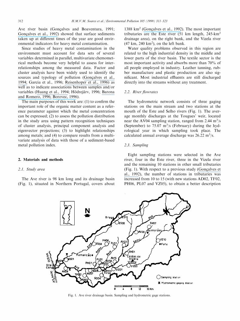
The Ave river is 98 km long and its drainage basin(Fig. 1), situated in Northern Portugal, covers about

1388 km2 (GoncË alves et al., 1992). The most importanttributaries are the Este river (51 km length, 245-km2

drainage area), on the right bank, and the Vizela river(47 km, 240 km2), on the left bank.Water quality problems observed in this region are

related to the high industrial density in the middle andlower parts of the river basin. The textile sector is themost important activity and absorbs more than 70% ofall people employed in industry. Leather tanning, rub-ber manufacture and plastic production are also sig-ni®cant. Most industrial e�uents are still dischargeddirectly into the streams without any treatment.

2.2. River ¯owrates

The hydrometric network consists of three gagingstations on the main stream and two stations at themouth of the Este and Selho rivers (Fig. 1). The aver-age monthly discharges at the Tougues' weir, locatednear the AV04 sampling station, ranged from 2.44 m3/s(September) to 75.07 m3/s (February) during the hyd-rological year in which sampling took place. Thecalculated annual average discharge was 26.22 m3/s.

2.3. Sampling

Eight sampling stations were selected in the Averiver, four in the Este river, three in the Vizela riverand the remaining 10 stations in other small tributaries(Fig. 1). With respect to a previous study (GoncË alves etal., 1992), the number of stations in tributaries wasincreased from 10 to 15 (with new stations AD02, TF02,PH06, PL07 and VZ05), to obtain a better description

Fig. 1. Ave river drainage basin. Sampling and hydrometric gage stations.

312 H.M.V.M. Soares et al. / Environmental Pollution 105 (1999) 311±323

of the basin. Moreover, in the Ave river, two stationssituated upstream of station AV28, in an unpollutedriver stretch, were replaced by new stations, AV14and AV22, in the middle reach of the river. Sedimentsamples were collected at an average ¯owrate atTougues' weir of 15.51 m3/s and kept until analysis,as described by GoncË alves et al. (1992).

2.4. Sieving procedure

In a preliminary investigation for studying the rep-resentativeness of the dry sieved <63-mm fraction of thesediments for determinations, both wet and dry sievingwere used. A sample (from the AV04 station) was sievedwith sieves of 500-, 250-, 150- and 63-mm mesh openingto compare the distribution of the fractions obtained bythe two procedures. Moreover, a set of seven samplesfrom di�erent locations (AV04, AV15, AV22, ES04,PH01, SH01, SH07) was wet and dry sieved using a63-mm mesh size sieve and determinations were per-formed in both sets of <63-mm fractions for compar-ison. Upon the results of this preliminary study, theremaining samples were separated only by 63-mm meshdry sieving.For wet sieving, a volume of 0.5 l of deionized water

was used and the samples were sieved during 45 min.Dry sieved samples were ®rst dried at room temperatureand then sieved using a steel sieve. Sieving was per-formed during 30 min.

2.5. Analytical methods

The analyses of volatile matter (VM) and trace metalswere performed on dehydrated fractions (at 105�C).The organic matter content was calculated as the VM

released by calcinating the samples at 550�C. Quad-ruplicate analyses of 17 samples were carried out forevaluating the precision of the analytical method. Sincethe relative standard deviation varied from 0.64 to4.8%, which means enough precision for this type ofstudy, for the remaining samples the VM determina-tions were performed only in duplicate.For metal analysis, the samples were digested as

described elsewhere (GoncË alves and Boaventura, 1991).Metal content was measured by atomic absorption spec-troscopy (AAS) using a double-beam spectrophotometer(IL 551). Cu, Ni, Pb and Zn were determined withan air±acetylene ¯ame and Cr with a nitrous oxide±acetylene ¯ame. For the determination of Cd, AAS witheither air±acetylene ¯ame or with tubular graphite fur-nace electrothermal atomisation (AAS-EA) were used.Background interferences on Cd and Zn measurementswere corrected with a deuterium arc-lamp.A certi®ed ¯uvial sediment (NBS 2704) was used for

evaluating the precision and accuracy of the analyticalprocedure. Four replicates of the reference sample were

digested and analysed by the same procedure as thesediment samples. The results obtained for Cd, Cr, Cu,Ni, Pb and Zn were within the ranges of the certi®edvalues.

2.6. Data treatment and programs

The hierarchical cluster analysis program was basedon a literature algorithm (Zupan, 1982) and allowscalculations with the following seven clustering strate-gies: single/complete linkage; unweighted/weighted pair-group average; unweighted/weighted pair-group cen-troid method; and Ward's method. Eigenvalues andeigenvectors were calculated by associating House-houlder and QL algorithms (Press et al., 1988). Eigen-vector projections were made as described in theliterature (Muhammad et al., 1986). All software waswritten and compiled using Turbo Pascal (BorlandInternational, USA). An IBM PC-compatible computerwas used for calculations.

3. Results and discussion

3.1. Sieving tests

A major problem occurring when sediment-basedmetal pollution results from di�erent studies are usedfor comparative purposes is the non-uniformity of thegrain size of the analysed fractions (Groot et al., 1982).It has been observed (Salomons, 1980; Groot et al.,1982; Robbe, 1984; Lucas et al., 1986) that heavymetals, either of natural or anthropogenic origin, accu-mulate more extensively in the thinner fractions ofsediments and, therefore, metal concentrations decreasewith the increase of the grain size. A way for over-coming di�erences in composition due to di�erences inthe fraction grain size is to adopt a speci®c grain size.This procedure allows the comparison of polluted sedi-ments from di�erent origins (Robbe et al., 1983) andreduces the number of samples to analyse. FoÈ rstner andSalomons (1980) suggested the use of the fraction withgrain size <63-mm, which presents several advantages:(1) heavy metals are mainly linked to silt and clay; (2)this grain size is like that of the suspended matter inwater; and (3) it has been used in many studies on heavymetal contamination. The separation of the <63-mmfraction can be carried out by dry sieving or by wetsieving (Groot et al., 1982; Golterman et al., 1983;Lucas et al., 1986). Since both methods present somedisadvantages, a preliminary study was performed tochoose the sieving method to be adopted and to test therepresentativeness of the <63-mm fraction.In a ®rst experiment for this purpose, two aliquots of

a sample (AV04) were wet and dry sieved with sievesof 500-, 250-, 150- and 63-mm mesh opening and the ®ve

H.M.V.M. Soares et al. / Environmental Pollution 105 (1999) 311±323 313

fraction distributions were compared, as well as analy-tical results for the two thinner fractions. The grain sizedistributions are presented in Table 1. Dry and wetsieving gave di�erent results for the individual fractionsbut the sums of the relative weights of all retained<500-mm particles were practically the same. Wet siev-ing seems to be more e�cient for separating the thinnerfractions (<63 and 63±150 mm), with a mass jointrecovery 63% higher than for dry sieving. Both frac-tions from the two types of sieving were analysed for Cr,Cu, Ni, Pb and Zn, and for VM (Table 2). All metals,expressed as mg/100 g of fraction, present higher con-centrations in the wet sieved <63-mm fraction. A simi-lar pattern was also observed by De Gregori et al.(1996). These higher values can probably be explainedby a more e�cient desaggregation of the thin clay par-ticles by wet sieving (Golterman et al., 1983), but metalleaching from the coarser particles and even from thesieves cannot also be excluded (Robbe et al., 1983;Lucas et al., 1986). However, if the metal concentrationsare reported with respect to the VM content of eachfraction, the results become quite similar (Table 2, lowersection).In another experiment, aliquots of seven samples

from di�erent locations (AV04, AV15, AV22, ES04,PH01, SH01, SH07) were also wet and dry sieved using

a 63-mm mesh sieve, both <63-mm fractions were ana-lysed and the results compared. These samples wereanalysed also for Cd, except for stations AV04 andES04, but Zn was only determined for these two sta-tions. Moreover, the values of Cr for station SH01 (veryhigh due to heavy contamination from leather tanninge�uents) were not included in the following calcula-tions. In Fig. 2 the metal concentrations obtained forthe <63-mm fractions separated by the two sievingprocedures are compared when expressed both in mg ofmetal/100 g of fraction (Fig. 2A) or in g of metal/kg ofVM (Fig. 2B). As shown by the plots and by the resultsof the least squares regressions (�values in parenthesisare 95% con®dence limits, n � 34 in both cases),respectively:

WET �mg=100 g fraction� � 1:4 ��0:1� DRYÿ 2 ��3�r � 0:959

WET �g=kg VM� � 0:94 ��0:05� DRYÿ 0:02 ��0:1�r � 0:982

although linear correlations are obtained in both caseswith high correlation coe�cients, the second is better.However, as the slope for the ®rst case is signi®cantlylarger than one (at the 95% level), only when results are

Table 1

In¯uence of the sieving procedure on the fraction distribution (weight, %) of the AV04 sample

Procedure Fraction (mm)

<63 63±150 150±250 250±500 >500

Wet 0.67 0.29 0.12 0.67 98.2

Dry 0.18 0.41 0.14 1.17 98.1

Table 2

Metal content and volatile matter (VM) in the <63 and 63±150-mm wet and dry sieved fractions of the AV04 sample

VM/metal Fraction (mm)

<63 63±150

Wet sieving Dry sieving Wet sieving Dry sieving

VM (%) 19.8 11.0 6.4 8.5

Relative to fraction weight (mg/100 g fraction)

Cr 32.8 16.7 3.4 7.3

Cu 16.4 11.1 6.9 7.3

Ni 10.4 3.9 3.4 4.9

Pb 9.0 5.6 6.9 7.3

Zn 58.2 33.3 58.6 34.1

Relative to VM (g/kg of VM)

Cr 1.66 1.52 0.54 0.86

Cu 0.83 1.01 1.08 0.86

Ni 0.53 0.35 0.54 0.57

Pb 0.45 0.51 1.08 0.86

Zn 2.94 3.03 9.16 4.02

314 H.M.V.M. Soares et al. / Environmental Pollution 105 (1999) 311±323

expressed in g of metal/kg of VM are both sieving pro-cedures comparable. Besides, since in the second plotthe points are less unevenly distributed along the axes,the second regression is more meaningful.It has been observed (HakaÈ nson, 1984; GoncË alves and

Boaventura, 1991) that the heavy metal uptake by thethin fraction of sediments is clearly related to its organicmatter content and, therefore, VM can be used as abasis of reference. Hence, when metal concentrationsare normalised to the VM content, di�erences in the

organic matter concentration due to di�erent samplingor sieving procedures are much attenuated. This wascon®rmed by analysing all the dry sieved <500 mmsediment fractions from ES04 sampling site for metalsand VM (Table 3) and investigating the correlationsbetween the concentration of each metal and the VMcontent of the selected fractions. Good correlationswere obtained which, together with the results displayedin Fig. 2B, con®rm that normalising the metal con-centration in the thin fraction of sediments to the VMcontent is an appropriate technique for comparingresults from several sampling sites within a river basinor for assessing long-term trends at a particular site.The relative abundance of the various metals in the

analysed sediment fractions can be obtained fromTable 3. The values of the straight-line slopes suggest abinding capacity to the organic matter in the followi-ng order: Cu>Zn>Pb>Cr>Ni>Cd. The Cu>Znbinding capacity to organic matter follows the stabilitysequence of Irwing-Williams. However, this fact is notso evident from the results expressed in mg of metal/100 g of fraction.In conclusion, dry sieving, which is a more expedite

method than wet sieving, can adequately be used in theprocedure for assessing metal content variations in dif-ferent sediment samples. Therefore, all the subsequentwork was carried out upon dry sieved sediment frac-tions with grain size <63 mm and the metal concentra-tions were referred to the organic matter contentexpressed as VM.

3.2. Metal concentrations

Data for metal concentrations in the sediment sam-ples are presented in Table 4. Contamination by cad-mium is clear in the Este river (sampling stations ES08,ES04, ES01) and also in the Ave river downstream fromthe con¯uence (station AV01). E�uents from cadmiumplating industries in the urban area of Braga (Fig. 1) areresponsible for the presence of this metal in the river.

Fig. 2. Relationship between metal concentrations in dry and

wet sieved sediment fractions (grain size <63 mm). (A) Concentra-

tions expressed as mg of metal/100 g of fraction. (B) Concentrations

expressed as g of metal/kg volatile matter (VM).

Table 3

Metal concentrations and volatile matter (VM) of fractions of the ES04 sample

Fraction (mm) Metal (mg/100 g fraction) VM (weight %)

Cd Cr Cu Ni Pb Zn

<63 0.160 20.2 166 4.60 24.5 154 16.3

63±75 0.115 12.8 113 3.01 16.8 110 11.3

75±150 0.125 12.6 98.5 2.75 14.6 101 11.1

150±300 0.105 10.1 86.3 2.36 12.4 88.8 10.5

300±500 0.110 11.8 93.4 2.94 11.7 91.5 10.5

Parameters of metal vs VM regression

Slope 0.009 1.6 12.8 0.33 2.0 10.6

Intercept 0.02 5.1 ÿ41 0.9 8.2 ÿ17Correlation coe�cient 0.97 0.98 0.98 0.97 0.97 0.98

H.M.V.M. Soares et al. / Environmental Pollution 105 (1999) 311±323 315

Smaller concentrations also denoting a contaminationwere found at stations TF02 (Trofa river), SG01 (San-guinhedo river), AV14 and AV15 (Ave river).High chromium concentrations are present in sedi-

ment samples from the Selho river (station SH01) andthe Ave river (all stations downstream from the con-¯uence, AV01 to AV05). Chromium contamination isoriginated by leather tanning companies located inGuimaraÄ es (Fig. 1).Copper and zinc in sediments are associated with the

cadmium contamination in the Este river and resultfrom the pickling process of brass pieces before metalplating. A similar pattern occurs for nickel and lead butthe e�ect downstream from station ES08 is stronglyattenuated. Nickel also originates from the nickel plat-ing processes and lead may result from the anodes usedin the chromium plating tanks. Surprisingly, the sedi-ment from station ES08 denotes only slight chromiumcontamination.

3.3. Statistical analysis of data

As stations ES08 and SH01 have some metal con-centrations much higher than all the others, they wereconsidered as outliers and, although included in theclassi®cation and exploration analysis, they were exclu-ded from the statistical calculations.

The basic statistics of the data are summarised inTable 5 and provide global information about the pre-sent pollution problem. Cadmium is the metal respon-sible for the strongest contamination because it showsthe largest average concentration (2.89) and variance(5.19), while zinc, copper and chromium have nearlyhalf of these values. Lead and nickel have relativelysmall average concentrations (0.66 and 0.22, respec-tively) and variances (0.11 and 0.02, respectively). Interms of the contamination of the area under study,cadmium seems to be the most problematic pollutantfollowed by zinc, copper and chromium. The correla-tion matrix shows that there are no signi®cant correla-tions between metal concentrations except that zinc hasa relatively high correlation with copper (0.85), lead(0.78) and cadmium (0.68), and copper with lead (0.71).Sampling station ES04 shows three of the highest

values and, as mentioned before, corresponds to one ofthe most polluted areas. In contrast, sampling stationAD02 has four of the lowest values and corresponds toone of the most pristine zones.For classi®cation and exploration of the pollution

distribution in the area under analysis, pattern recogni-tion techniques of cluster analysis, principal componentanalysis and eigenvector projections (Karhunen±Loevetransformation) were applied to the data of Table 4.Three data sets were analysed: Set 1Ðconcentrations of

Table 4

Metal concentrations (mg/kg for Cd and g/kg volatile matter [VM] dry weight for other metals) and VM contents (weight %) in the <63-mmfractions

Sampling station Station No. Cd Cr Cu Ni Pb Zn VM (%)

AV01 1 6.52 2.16 1.21 0.23 0.64 3.06 22.0

ES01 2 5.96 0.82 5.24 0.28 1.15 ± 15.6

ES04 3 7.63 0.77 7.46 0.24 1.40 7.05 23.8

ES08 a 144.00 1.84 518.10 2.36 16.38 ± 12.3

ES11 4 3.19 0.42 2.00 0.14 0.77 1.60 14.8

AV04 5 3.33 2.40 0.74 0.20 0.40 1.25 22.0

AD02 6 0.03 0.30 1.00 0.07 0.30 0.65 14.9

TF02 7 6.75 0.21 0.87 0.32 0.45 2.43 14.1

AV07 8 2.09 2.59 0.87 0.22 0.68 ± 19.2

PH01 9 2.98 1.28 1.48 0.40 0.84 2.37 16.8

PH06 10 0.69 0.18 0.92 0.10 0.35 0.78 19.1

PL01 11 2.49 0.69 0.88 0.73 0.54 1.90 11.5

PL07 12 0.02 0.21 0.94 0.09 0.25 0.60 21.3

SG01 13 5.16 0.40 0.70 0.27 0.89 ± 10.4

SG04 14 1.11 0.24 0.77 0.11 0.40 0.90 12.6

AV12 15 2.83 3.17 0.83 0.16 0.76 1.51 16.9

AV14 16 3.51 4.08 1.94 0.27 1.48 ± 13.0

VZ01 17 0.57 0.36 0.86 0.25 0.46 3.70 19.3

VZ05 18 0.55 0.67 1.03 0.18 0.44 ± 14.9

VZ10 19 0.03 0.41 0.46 0.11 0.41 0.75 14.6

AV15 20 4.13 4.35 0.83 0.21 0.59 ± 12.5

SH01 a 2.54 15.87 0.69 0.12 1.73 1.79 21.4

SH07 21 1.44 0.27 0.82 0.13 0.65 0.90 14.5

AV22 22 2.30 0.79 2.11 0.17 0.72 ± 15.0

AV28 23 3.24 0.21 0.44 0.11 0.55 0.67 13.0

a Data from sampling stations ES08 and SH01 were subsequently excluded from the multivariate analysis.

316 H.M.V.M. Soares et al. / Environmental Pollution 105 (1999) 311±323

the ®ve elements present in 23 sampling stations (zinc isexcluded because it was not measured for all stations);Set 2Ðthe same data set but after autoscaling; Set 3Ðconcentration of the six elements present in 16 samplingstations for which the levels of zinc were measured.

3.4. Hierarchical cluster analysis of raw data

The clustering process of the raw data without zinc(Set 1), will be strongly weighted by cadmium con-centration and, at a lower scale, by copper and chro-mium concentrations, according to their variances.

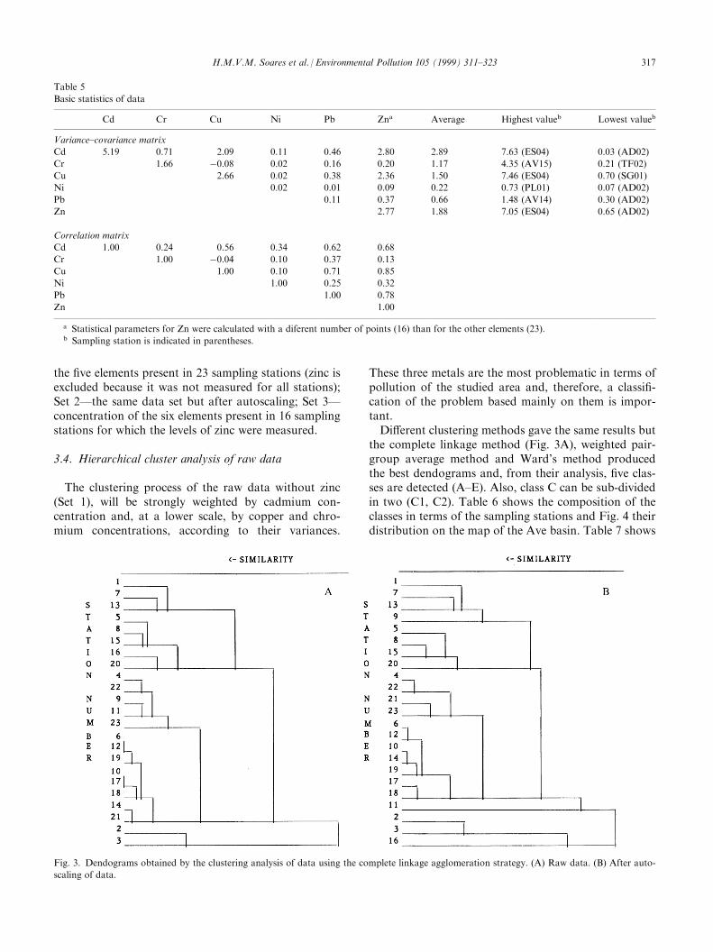
These three metals are the most problematic in terms ofpollution of the studied area and, therefore, a classi®-cation of the problem based mainly on them is impor-tant.Di�erent clustering methods gave the same results but

the complete linkage method (Fig. 3A), weighted pair-group average method and Ward's method producedthe best dendograms and, from their analysis, ®ve clas-ses are detected (A±E). Also, class C can be sub-dividedin two (C1, C2). Table 6 shows the composition of theclasses in terms of the sampling stations and Fig. 4 theirdistribution on the map of the Ave basin. Table 7 shows

Table 5

Basic statistics of data

Cd Cr Cu Ni Pb Zna Average Highest valueb Lowest valueb

Variance±covariance matrix

Cd 5.19 0.71 2.09 0.11 0.46 2.80 2.89 7.63 (ES04) 0.03 (AD02)

Cr 1.66 ÿ0.08 0.02 0.16 0.20 1.17 4.35 (AV15) 0.21 (TF02)

Cu 2.66 0.02 0.38 2.36 1.50 7.46 (ES04) 0.70 (SG01)

Ni 0.02 0.01 0.09 0.22 0.73 (PL01) 0.07 (AD02)

Pb 0.11 0.37 0.66 1.48 (AV14) 0.30 (AD02)

Zn 2.77 1.88 7.05 (ES04) 0.65 (AD02)

Correlation matrix

Cd 1.00 0.24 0.56 0.34 0.62 0.68

Cr 1.00 ÿ0.04 0.10 0.37 0.13

Cu 1.00 0.10 0.71 0.85

Ni 1.00 0.25 0.32

Pb 1.00 0.78

Zn 1.00

a Statistical parameters for Zn were calculated with a diferent number of points (16) than for the other elements (23).b Sampling station is indicated in parentheses.

Fig. 3. Dendograms obtained by the clustering analysis of data using the complete linkage agglomeration strategy. (A) Raw data. (B) After auto-

scaling of data.

H.M.V.M. Soares et al. / Environmental Pollution 105 (1999) 311±323 317

the averages, standard deviations and relative standarddeviations of the detected classes.Class A has the lowest concentration levels and small

standard deviations which indicates an homogeneousclass. As shown by Fig. 4, the region belonging to classA corresponds to areas near the springs of the rivers andthe Vizela river basin and de®nes the natural con-centration levels (NCLs) for the measured metals. Forclassi®cation purposes an index was attributed to eachclass (Table 8): low (L), concentration of up to threetimes the NCL; intermediate (I), concentration betweenthree and 10 times the NCL; and high (H), concentra-tion larger than 10 times the NCL. Table 8 shows theexistence of an ordered crescent pollution problem inthe identi®ed classes: B<C1<C2=D<E.

The classi®cation pattern obtained shows a generalproblem of pollution by cadmium in the whole Avebasin and, additionally, two more localised problems inthe Ave and Este rivers, which are the most import-ant rivers in the area under analysis, characterised asfollows:

1. Ave river: chromium pollution with its origin inthe Selho river, upstream sampling station SH01,since the concentrations of this metal decreasealong classes C2, C1 and D; and

2. Este river: lead and copper pollution with its originupstream of the sampling station ES08, since leadand copper concentrations decrease along classesE and D.

A similar classi®cation pattern was obtained in theclustering of Set 3, which includes zinc concentration,but sampling station VZ01 separated from class A tobecome a one-element class. This result shows the exis-tence of a zinc concentration abnormality in that sam-pling station.

3.5. Hierarchical cluster analysis of auto-scaled data

After autoscaling of data, to remove the naturalweights, cluster analysis was applied to Set 2 (Fig. 3B).A classi®cation similar to the previous one wasobtained, but four sampling stations are classi®ed dif-ferently: SH07 is transferred from class A to class B andPH01 from class B to class D; PL01 and AV14, whichbelonged, respectively, to classes B and C2, became sin-gle element classes. Comparing the metal concentrations

Fig. 4. Ave river drainage basin: class distribution according to the clustering analysis classi®cation.

Table 6

Composition of sampling station classes obtained from cluster analysis

Class Sampling stationsa

A AD02, PH06, PL07, SG04, VZ01(1), VZ05, VZ10, SH07(2)

B ES11, PH01(3), PL01(4), AV22, AV28

C1 AV04, AV07, AV12

C2 AV14(5), AV15

D AV01, TF02, SG01

E ES01, ES04

O1 SH01

O2 ES08

a Sampling stations with some element concentration abnormalities:

(1) Zn; (2) Cd and Pb; (3) Cr; (4) Ni; (5) Cu and Pb.

318 H.M.V.M. Soares et al. / Environmental Pollution 105 (1999) 311±323

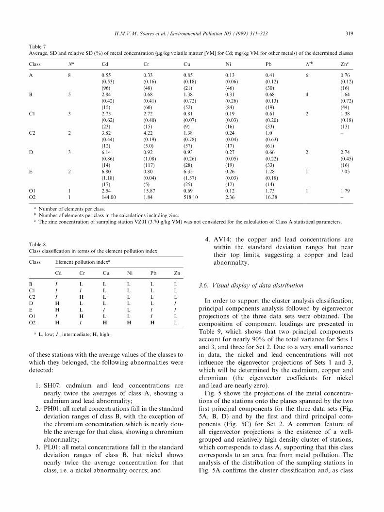
of these stations with the average values of the classes towhich they belonged, the following abnormalities weredetected:

1. SH07: cadmium and lead concentrations arenearly twice the averages of class A, showing acadmium and lead abnormality;

2. PH01: all metal concentrations fall in the standarddeviation ranges of class B, with the exception ofthe chromium concentration which is nearly dou-ble the average for that class, showing a chromiumabnormality;

3. PL01: all metal concentrations fall in the standarddeviation ranges of class B, but nickel showsnearly twice the average concentration for thatclass, i.e. a nickel abnormality occurs; and

4. AV14: the copper and lead concentrations arewithin the standard deviation ranges but neartheir top limits, suggesting a copper and leadabnormality.

3.6. Visual display of data distribution

In order to support the cluster analysis classi®cation,principal components analysis followed by eigenvectorprojections of the three data sets were obtained. Thecomposition of component loadings are presented inTable 9, which shows that two principal componentsaccount for nearly 90% of the total variance for Sets 1and 3, and three for Set 2. Due to a very small variancein data, the nickel and lead concentrations will notin¯uence the eigenvector projections of Sets 1 and 3,which will be determined by the cadmium, copper andchromium (the eigenvector coe�cients for nickeland lead are nearly zero).Fig. 5 shows the projections of the metal concentra-

tions of the stations onto the planes spanned by the two®rst principal components for the three data sets (Fig.5A, B, D) and by the ®rst and third principal com-ponents (Fig. 5C) for Set 2. A common feature ofall eigenvector projections is the existence of a well-grouped and relatively high density cluster of stations,which corresponds to class A, supporting that this classcorresponds to an area free from metal pollution. Theanalysis of the distribution of the sampling stations inFig. 5A con®rms the cluster classi®cation and, as class

Table 7

Average, SD and relative SD (%) of metal concentration (mg/kg volatile matter [VM] for Cd; mg/kg VM for other metals) of the determined classes

Class Na Cd Cr Cu Ni Pb N0b Znc

A 8 0.55 0.33 0.85 0.13 0.41 6 0.76

(0.53) (0.16) (0.18) (0.06) (0.12) (0.12)

(96) (48) (21) (46) (30) (16)

B 5 2.84 0.68 1.38 0.31 0.68 4 1.64

(0.42) (0.41) (0.72) (0.26) (0.13) (0.72)

(15) (60) (52) (84) (19) (44)

C1 3 2.75 2.72 0.81 0.19 0.61 2 1.38

(0.62) (0.40) (0.07) (0.03) (0.20) (0.18)

(23) (15) (9) (16) (33) (13)

C2 2 3.82 4.22 1.38 0.24 1.0 ±

(0.44) (0.19) (0.78) (0.04) (0.63)

(12) (5.0) (57) (17) (61)

D 3 6.14 0.92 0.93 0.27 0.66 2 2.74

(0.86) (1.08) (0.26) (0.05) (0.22) (0.45)

(14) (117) (28) (19) (33) (16)

E 2 6.80 0.80 6.35 0.26 1.28 1 7.05

(1.18) (0.04) (1.57) (0.03) (0.18)

(17) (5) (25) (12) (14)

O1 1 2.54 15.87 0.69 0.12 1.73 1 1.79

O2 1 144.00 1.84 518.10 2.36 16.38 ±

a Number of elements per class.b Number of elements per class in the calculations including zinc.c The zinc concentration of sampling station VZ01 (3.70 g/kg VM) was not considered for the calculation of Class A statistical parameters.

Table 8

Class classi®cation in terms of the element pollution index

Class Element pollution indexa

Cd Cr Cu Ni Pb Zn

B I L L L L L

C1 I I L L L L

C2 I H L L L L

D H L L L L I

E H L I L I I

O1 I H L L I L

O2 H I H H H L

a L, low; I , intermediate; H, high.

H.M.V.M. Soares et al. / Environmental Pollution 105 (1999) 311±323 319

E, which corresponds to the Este river stations, is wellseparated from the others, shows that this river has adi�erent pollution problem, as discussed above.The plots in Fig. 5B and C show that the e�ect of data

autoscaling on the distribution of the four stations withmetal concentration abnormalities is the same as foundin the cluster analysis: PL01 and AV14, which belongedto class B and C2, respectively, became single elementclasses, well separated from the others; PH01, whichbelonged to class B, moved to an area close to classD; and SH07, which belonged to class A, moved intoclass B.Fig. 5D con®rms the existence of a zinc concentration

abnormality in station VZ01 because it moved awayfrom class A, to which it belonged, to become a singleelement class.

3.7. Contamination factors and metal pollution index

A contamination factor (CF), calculated as the ratiobetween the sediment metal content at a given samplingstation and the NCLs, re¯ects the metal enrichment inthe sediment at that site. When CF>1 for a particular

metal, it means that a contamination exists; otherwise, ifCF41, there is no metal enrichment of natural oranthropogenic origin. The CF results are presented inTable 10. The highest contamination factors for Cd(261.8), Cu (609.5), Ni (18.2) and Pb (40.0) were foundin station ES08, which denotes a strong contaminationby these metals upstream. This contamination is stillapparent at the mouth of the Este river and even a�ectsthe Ave river downstream from the con¯uence. A con-tamination by chromium is also evident at station ES08.As mentioned before, such results are a consequence ofthe existence of metal plating industries along the Esteriver, in the area of Braga. The strongest contamination

Table 9

Results of the principal components analysis

Variable Eigenvector composition

1 2 3

Set 1

Cd 0.87 0.24

Cr 0.12 0.74

Cu 0.48 ÿ0.62Ni 0.02 0.01

Pb 0.09 ÿ0.01

%Eigenvalue 67.4 20.3

Cumulative% 87.7

Set 2

Cd 0.54 0.02 0.08

Cr 0.24 ÿ0.79 ÿ0.44Cu 0.50 0.51 ÿ0.12Ni 0.27 ÿ0.32 0.86

Pb 0.58 0.02 ÿ0.20

%Eigenvalue 49.3 21.0 18.1

Cumulative% 70.3 88.4

Set 3

Cd 0.75 0.60

Cr 0.08 0.30

Cu 0.44 ÿ0.62Ni 0.02 0.02

Pb 0.08 ÿ0.04Zn 0.48 ÿ0.41

%Eigenvalue 74.4 16.7

Cumulative% 91.1

Fig. 5. Eigenvector projections of data onto the planes spanned by:

(A, B, D) the two ®rst principal components for Sets 1±3; and (C) the

®rst and third principal components for Set 2.

320 H.M.V.M. Soares et al. / Environmental Pollution 105 (1999) 311±323

by chromium (CF=48.1), however, was observed forstation SH01, which re¯ects wastewater discharges fromleather tanning industries in GuimaraÄ es. The e�ect ofthese chromium releases on the Ave river, downstreamfrom the con¯uence, is clearly detected. In fact, at theAve river mouth, the contamination factor for chro-mium is still 6.5. The Selho river also shows a lead

content in the sediments largely higher (CF=4.2) thanthe background level. The Sanguinhedo river (sta-tion SG01) is also a cadmium contamination source(CF=9.4) but, due to its low ¯owrate (annual averagedischarge estimated as 0.4 m3/s), it seems not to a�ectthe Ave river downstream. The Pele river (station PL01)is contaminated by nickel (CF=5.6) but by the samereason (annual average discharge estimated as 1.4 m3/s)the in¯uence on the main stream is imperceptible. Thecontamination factors for zinc are not available for allthe sampling stations. The highest value (CF=9.3) wasencountered at station ES04, which probably denotes acontamination upstream, as was observed for the othermetals.An evaluation of the overall metal contamination was

carried out by calculating a metal pollution index (MPI)de®ned as a linear sum of the contamination factorsweighted to take into account the di�erences in toxicityof the various metals, i.e.:

MPI � �i�wi=wt� � CFi;

where CFi is the contamination factor for metal i; wi isthe weight for metal i; and wt � �iwi.The weights (Zn, 1; Cu, 5; Cr, Pb and Ni, 100; Cd,

500) were established as previously reported (GoncË alveset al., 1992), assuming that they are inversely propor-tional to the maximum permissible level in surfacewaters for domestic supply (EPA, 1976). Fig. 6 showsthe MPI variations over the Ave river basin. Sites whereMPI41 (AD02, PL07, VZ10) must be classi®ed asunpolluted as regards the six heavy metals measured inthis study. Sediments with the highest MPIs were col-lected in the Este (stations ES08, ES04, ES01) and Selho

Table 10

Contamination factors (CFs)

Sampling station Cd Cr Cu Ni Ph Zn

AV01 11.9 6.5 1.4 1.8 1.6 4.0

ES01 10.8 2.5 6.2 2.2 2.8 ±

ES04 13.9 2.3 8.8 1.8 3.4 9.3

ES08 261.8 5.6 609.5 18.2 40.0 ÿES11 5.8 1.3 2.4 1.1 1.9 2.1

AV04 6.1 7.3 0.9 1.5 1.0 1.6

AD02 0.1 0.9 1.2 0.5 0.7 0.9

TF02 12.3 0.6 1.0 2.5 1.1 3.2

AV07 3.8 7.8 1.0 1.7 1.7 ±

PH01 5.4 3.9 1.7 3.1 2.0 3.1

PH06 1.3 0.5 1.1 0.8 0.9 1.0

PL01 4.5 2.1 1.0 5.6 1.3 2.5

PL07 0.0 0.6 1.1 0.7 0.6 0.8

SG01 9.4 1.2 0.8 2.1 2.2 ±

SG04 2.0 0.7 0.9 0.8 1.0 1.2

AV12 5.1 9.6 1.0 1.2 1.9 2.0

AV14 6.4 12.4 2.3 2.1 3.6 ±

VZ01 1.0 1.1 1.0 1.9 1.1 4.9

VZ05 1.0 2.0 1.2 1.4 1.1 ±

AV10 0.1 1.2 0.5 0.8 1.0 1.0

AV15 7.5 13.2 1.0 1.6 1.4 ±

SH01 4.6 48.1 0.8 0.9 4.2 2.4

SH07 2.6 0.8 1.0 1.0 1.6 1.2

AV22 4.2 2.4 2.5 1.3 1.8 ±

AV28 5.9 0.6 0.5 0.8 1.3 0.9

Fig. 6. Metal pollution index (MPI) based on the metal content in the <63-mm fraction of sediments.

H.M.V.M. Soares et al. / Environmental Pollution 105 (1999) 311±323 321

(station SH01) rivers and in the Ave river (AV01)downstream from the con¯uence. MPI in station ES08(174.1) largely exceeds the range of the calculated valuesfor the other sampling sites (0.3±9.6). Fig. 6 shows thatTrofa (TF02), Sanguinhedo (SG01) and Selho (SH01)rivers lead to an increase of the metal contamination inthe Ave river downstream from their con¯uences.A comparative analysis of the metal contamination

shows that the ®ve classes (A±E) determined by clusteranalysis (Table 6) are well correlated with speci®c inter-vals of MPI values (Fig. 6). All the stations of class Ahave MPI values 42.1 con®rming that it is a low-contamination homogeneous class. In a general way,the MPI values in classes B, C, D, and E follow anincreasing range: 2.1±4.5, 3.8±6.7, 6.5±8.6 and 7.7±9.6,respectively. Nevertheless, stations AV04, SG01 andES01 belonging to classes C, D and E, respectively, haveMPI values lower than the maximum values of the pre-ceding classes (B, C, D, respectively). Moreover, theMPI for station SH01, which is an outlier constituting asingle element class, is slightly lower (9.5) than theupper limit of class E.

4. Conclusion

The fractionation of the sediment samples by wetsieving yields higher metal concentrations in the <63-mm fraction, when compared with the correspondingdry sieved fraction. However, as metal uptake by thethin fractions of river sediments is usually dependent onits VM content, the di�erences due to the sieving pro-cedure are much attenuated by normalising the metalconcentrations to the VM content. The binding capacityof the selected metals to the organic matter decreases inthe following order: Cu>Zn>Pb>Cr>Ni>Cd.The multivariate analysis procedure used in this work

shows itself to be a very useful tool for the classi®cationof the pollution levels in the Ave river basin. In fact, ageneral classi®cation of the whole area was achievedand the most critical zones were identi®ed. Also, theexploratory analysis of the data sets allowed the identi-®cation of metal concentration abnormalities in somesampling stations, showing the existence of speci®c pol-luting sources in the area under study.Metal pollution indexes calculated as a weighted

mean of the metal contamination factors in each sam-pling station are well correlated with the ®ve classesobtained by cluster analysis.

References

Barona, A., Romero, F., 1996. Distribution of metals in soils and

relationships among fractions by principal component analysis. Soil

Technology 8, 303±319.

Borovec, Z., 1996. Evaluation of the concentrations of trace elements

in stream sediments by factor and cluster analysis and the sequential

extraction procedure. Science of the Total Environment 177, 237±

250.

De Gregori, I., Pinochet, H., Arancibia, M., Vidal, A., 1996. Grain

size e�ect on trace metals distribution in sediments from two coastal

areas of Chile. Bulletin of Environmental Contamination and Tox-

icology 57, 163±170.

Duzzin, B., Pavoni, B., Donazzolo, R., 1988. Macroinvertebrate com-

munities and sediments as pollution indicators for heavy metals in

the River Adige (Italy). Water Research 22 (11), 1353±1363.

EPA, 1976. Quality Criteria for Water. US Environmental Protection

Agency, Washington, D.C. 20460.

FoÈ rstner, U., 1985. Chemical forms and reactivities of metals in sedi-

ments. In: Leschber, R., Davis, R.D., L'Hermite, P. (Eds.), Chemi-

cal Methods for Assessing Bioavailable Metals in Sludges and Soils.

Elsevier, London, pp. 1±30.

FoÈ rstner, U., Salomons, W., 1980. Trace metal analysis on polluted

sediments. Part I: assessment of sources and intensities. Environ-

mental Technology Letters 1, 494±505.

Garcia, R., Maiz, I., Millan, E., 1996. Heavy metal contamination

analysis of roadsoils and grasses from Gipuzkoa (Spain). Environ-

mental Technology 17, 763±770.

Golterman, H.L., Sly, P.G., Thomas, R.L., 1983. Study of the rela-

tionship between water quality and sediment transport. Unesco,

Paris.

GoncË alves, E.P.R., Boaventura, R., 1991. Sediments as indicators of

the river Ave contamination by heavy metals. In: Bau, J., Ferreira,

J.P.L., Henriques, J.D., Raposo, J.O. (Eds.), Integrated Approaches

to Water Pollution Problems. Elsevier, London, pp. 209±218.

GoncË alves, E.P.R., Boaventura, R.A.R., Mouvet, C., 1992. Sediments

and aquatic mosses as pollution indicators for heavy metals in the

Ave River basin (Portugal). Science of the Total Environment 114,

7±24.

GoncË alves, E.P.R., Soares, H.M.V.M., Boaventura, R.A.R., Mach-

ado, A.A.S.C., Silva, J.C.G.E., 1994. Seasonal variations of heavy

metals in sediments and aquatic mosses from the Ca vado river basin

(Portugal). Science of the Total Environment 142, 143±156.

Groot, A.J., Zschuppe, K.H., Salomons, W., 1982. Standardization of

methods of analysis for heavy metals in sediments. Hydrobiologia

92, 689±695.

HakaÈ nson, L., 1984. Sediment sampling in di�erent aquatic environ-

ments: statistical aspects. Water Resources Research 20, 41±46.

HoÈ drejaÈ rv, H., 1996. A chemometrical look at heavy metals in soils.

Proceedings of the Estonian Academy of Science and Chemistry 45,

97±106.

Huang, W., Campredon, R., Abrao, J.J., Bernat, M., Latouche, C.,

1994. Variation of heavy metals in recent sediments from Piratininga

Lagoon (Brazil): interpretation of geochemical data with the aid of

multivariate analysis. Environmental Geology 23, 241±247.

Jha, P.K., Subramanian, V., Sitasawad, R., Van Grieken, R., 1990.

Heavy metals in sediments of the Yamuna River (a tributary of the

Ganges), India. Science of the Total Environment 95, 7±27.

Lapaquellerie, Y., Jouanneau, J.M., Maillet, N., Latouche, C., 1995.

Cadmium pollution in sediments of the Lot river (France). Estimate

of the mass of cadmium. Environmental Technology 16, 1145±1154.

Lietz, W., Galling, G., 1989. Metals from sediments. Water Research

23, 247±252.

Lucas, M.F., Caldeira, M.F., Hall, A., Duarte, A.C., Lima, C., 1986.

Distribution of mercury in sediments and ®shes of the Lagoon of

Aveiro, Portugal. Water Science and Technology 18, 141±148.

Martincic, D., Kwokal, Z., Branica, M., 1990. Distribution of zinc,

lead, cadmium and copper between di�erent size fractions of sedi-

ments. I. The Limski Kanal (North Adriatic Sea). Science of the

Total Environment 95, 201±215.

Muhammad, A.S., Illman, D.L., Kowalski, B.R., 1986. Chemo-

metrics. Wiley, New York.

322 H.M.V.M. Soares et al. / Environmental Pollution 105 (1999) 311±323

Pardo, R., Barrado, E., PeÁ rez, L., Vega, M., 1990. Determination and

speciation of heavy metals in sediments of the Pisuerga River. Water

Research 24, 373±379.

Press, W.H., Flannery, B.P., Teukolsky, S.A., Vetterling, W.T., 1988.

Numerical RecipesÐthe Art of Scienti®c Computing. Cambridge

University Press, Cambridge.

Reisenhoper, E., Adami, G., Favretto, A., 1996. Heavy metals and

nutrients in coastal, surface seawaters (Gulf of Trieste, Northern

Adriatic Sea): an environmental study by factor analysis. Fresenius

Journal of Analytical Chemistry 354, 729±734.

Robbe, D., 1984. Interpretation des teneurs en e le ments me talliques

associe s aux se diments, Rapport des Laboratoires. Se rie I: Envir-

onnement et Ge nie Urbaine, EG-1, LCPC, Paris, pp. 20±45.

Robbe, D., Divet, L., Marchandise, V., 1983. In¯uence du tamisage

sur les teneurs en e le ments me talliques observe es dans les se diments.

Environmental Technology Letters 4, 27±34.

Rubinstein, N.I., Lores, E., Gregory, N.R., 1983. Accumulation of

PCBs, Hg and Cd by Nereis virens, Mercenaria mercenaria and

Palaemonetes pugio from contaminated harbour sediments. Aquatic

Toxicology 3, 249±260.

Salomons, M., 1980. Biochemical processes a�ecting metal concentra-

tions in lake sediments (Ijsselmeer, The Netherlands). Science of the

Total Environment 16, 217±229.

Suzuki, M., Yamada, T., Miyazaki, T., Kawazoe, K., 1979. Sorption

and accumulation of cadmium in the sediment of the Tama River.

Water Research 13, 57±63.

Wardas, M., Budek, L., Rybicka, E.H., 1996. Variability of heavy

metals content in bottom sediments of the Wilga River, a tributary

of the Vistula River (Krako w area, Poland). Applied Geochemistry

11, 197±202.

Zupan, J., 1982. Clustering of Large Data Sets. Research Studies

Press, Wiley, New York.

H.M.V.M. Soares et al. / Environmental Pollution 105 (1999) 311±323 323