Section 3.2.2: Oxidation Models.
148
Section 3.2.2: Oxidation Models Version 1.2 April 4, 1997 3.2.2.1 Introduction U0 2 spent fuels oxidize to higher uranium oxide phases in an oxygen atmosphere. The oxidation response of spent fuels impacts the radionuclide release performance in potential repository environments because of two independent functional properties of the higher oxides. The first performance impact is due to a geometrical property and results from the surface area and volume changes that occur as the higher oxides form. The second impact is due to a chemical property that results from the higher dissolution rate of the U 3 0 8 oxide and the U0 3 oxide hydrates. In order to include these known impacts from U0 2 spent fuel oxidation for performance assessment analyses, a model for fuel oxidation response is being developed. The basis of model development depends strongly on experimental data obtained from thermogravimetric analysis (TGA) and oven dry bath (ODB) oxidation testing methods. The modeling approach derives functional forms, as well as using functional relationships consistent with the observed spent fuel oxidation processes. These functional relationships have parametric constants (for example, the activation energy in the Arrhenius rate expression) which are evaluated by using subsets of the experimental data. The models for spent fuel oxidation response described in the following subsection provide response functions for the elapsed time to higher oxidation phases as a function of temperature and nominal grain size, and for the quantity (volume) of a higher oxidation phase as a function of time, temperature, and nominal grain size. The model development is idealized, but considered representative of the observed experimental processes that occur in spent fuel oxidation. With the idealizations, the oxidation response models for the different phase transformations can be easily applied to provide bounding evaluations and best estimate values for oxidation impacts of spent fuel performance in potential repository environments. The two spent fuel oxidation phase responses discussed in the following subsections are the U0 2 to U 4 0 9 phase transformation and the U 4 0 9 to U 3 0 8 phase transformation. The U 4 0 9 to U 3 0 8 phase transformation model used only the thermogravimetric analysis (TGA) oxidation data to evaluate kinetic parameters. To partially substantiate the model, the oxidation data of Einziger and Hanson (1996) are compared to the predictions of the U 4 0 9 to U 3 0, oxidation model for a range of grainsizes at 255°C. This comparison with oven drybath (ODB) data provides preliminary confirmation of the oxidation modeling development that uses kinetic parameters evaluated from TGA data. 3.2.2-1
-
Upload
khangminh22 -
Category
Documents
-
view
1 -
download
0
Transcript of Section 3.2.2: Oxidation Models.
Section 3.2.2: Oxidation Models
Version 1.2 April 4, 1997
3.2.2.1 Introduction
U0 2 spent fuels oxidize to higher uranium oxide phases in an oxygen atmosphere. The oxidation response of spent fuels impacts the radionuclide release performance in potential repository environments because of two independent functional properties of the higher oxides. The first performance impact is due to a geometrical property and results from the surface area and volume changes that occur as the higher oxides form. The second impact is due to a chemical property that results from the higher dissolution rate of the U30 8 oxide and the U0 3 oxide hydrates. In order to include these known impacts from U0 2 spent fuel oxidation for performance assessment analyses, a model for fuel oxidation response is being developed.
The basis of model development depends strongly on experimental data obtained from thermogravimetric analysis (TGA) and oven dry bath (ODB) oxidation testing methods. The modeling approach derives functional forms, as well as using functional relationships consistent with the observed spent fuel oxidation processes. These functional relationships have parametric constants (for example, the activation energy in the Arrhenius rate expression) which are evaluated by using subsets of the experimental data. The models for spent fuel oxidation response described in the following subsection provide response functions for the elapsed time to higher oxidation phases as a function of temperature and nominal grain size, and for the quantity (volume) of a higher oxidation phase as a function of time, temperature, and nominal grain size. The model development is idealized, but considered representative of the observed experimental processes that occur in spent fuel oxidation. With the idealizations, the oxidation response models for the different phase transformations can be easily applied to provide bounding evaluations and best estimate values for oxidation impacts of spent fuel performance in potential repository environments. The two spent fuel oxidation phase responses discussed in the following subsections are the U0 2 to U40 9 phase transformation and the U40 9 to U3 0 8 phase transformation.
The U40 9 to U30 8 phase transformation model used only the thermogravimetric analysis (TGA) oxidation data to evaluate kinetic parameters. To partially substantiate the model, the oxidation data of Einziger and Hanson (1996) are compared to the predictions of the U40 9 to U30, oxidation model for a range of grainsizes at 255°C. This comparison with oven drybath (ODB) data provides preliminary confirmation of the oxidation modeling development that uses kinetic parameters evaluated from TGA data.
3.2.2-1

3.2.2.2 Oxidation Response of U to U..
The first oxidation phase transition of U0 2 spent fuel produces a U409 lattice structure with a weight gain "oxide" of UO2.4 2 . Thus, the U 40 9 phase is not stoichiometric. This U40 9 phase transition time response has an Arrhenius temperature dependence and a geometrical dependence on grain size. At early times, the U40 9 phase progresses very rapidly down the grain boundaries of the UO2 spent fuels. This elapsed time to oxidize grain boundaries is neglected in the following oxidation response models. The rapid grain boundary oxidation is partly due to the existence of fission gas bubbles which form on grain boundaries in spent fuels during reactor operation. These gas bubbles enhance porosity and decrease density of material in a grain boundary relative to material in an adjacent grain volume. In addition, the phase transformations to U 40 9 lattice is more dense (less specific volume) than the initial U0 2, by about 1.5 to 2.0%. This higher density phase promotes grain boundary cracking and an opening up of grain boundary pathways for oxygen transport to the surfaces of all grain volumes contained in a spent fuel fragment. The subsequent U40 9 oxidation of grain volumes is observed to progress as a U40 9 phase front that propagates into each U0 2 grain. Behind this phase front is the U40 9 crystal lattice structure with a weight gain "oxide" of UO_2.4 2 .
The rate of propagation of the U40 9 front was conservatively evaluated as part of the oven dry bath testing (Einziger, et al., 1992; and Thomas, et al., 1992).
The experimental approach measured the position of the U409 - U0 2 oxidation front relative to the grain boundary for a sequence of spent fuel samples; each sample in the sequence was oxidized for a different time duration. These measurements of widths of U40 9 oxidation fronts relative to the grain boundary versus oxidation time had an approximate square root time dependence at constant temperature. The temperature dependence was assumed to be an Arrhenius exponential function. Using this time and temperature dependence, the data in an upper bounding band were used to evaluate parameters k and Q in the following equations for the width W of the U40 9 oxidation front
W = 2 k-t 3.2.2-1
where
t = time (hours, h)
k = k0exp (-Q 49/RT)
ko = 1.04x10' (Ltm 2 /h)
Q49 = 24.0 kcal/mole (Arrhenius activation energy)
3.2.2-2

R = 1.986 cal/mole/°K (gas constant)
T = temperature (Kelvin)
The time derivative of Eq. 3.2.2-1 gives the rate that the U40 9 propagates into a grain volume of U0 2, which at constant temperature, is
W kl= t 3.2.2-2
which has an initial square root in time singularity. This is typical for surface film formations that are rate controlled by diffusion through a film of increasing thickness.
From Eq. 3.2.2-1, the elapsed time for oxidation of U0 2 grains to U40 9 can be evaluated by solving for time. Thus, the elapsed time, t 2.4, to fully oxidize a U0 2 grain of nominal dimension 2Wo to U40 9 in atmospheric air at constant temperature, T, is
t2.4 = W/(4ko exp(-Q 49/RT)) 3.2.2-3
Table 3.2.2-1 has values of t2. for different temperatures and different nominal grain sizes.
The use of constant temperature for elapsed times is an easy way to conservatively bound the time for full oxidation; pick the highest temperature value in the time interval. For repository evaluations, after the initial heat up time period, the temperatures are expected to be monotonically decreasing so the temperature value when the spent fuel is initially exposed is a conservative high temperature value for the shortest elapsed time. To obtain a better approximation for the t 2 .4 elapsed time, the rate equation 3.2.2-2 can be assumed valid for quasisteady temperature processes. Then the elapsed time t2 4 can be found by integration over the time dependent temperature history, such that W at t2 4 equals W,.
The grain size is the other variable dependence in Eq. 3.2.2-3 used to calculate elapsed times for oxidation of grains to U40 9. Samples of spent fuels have a statistical distribution of grain sizes and geometrical shapes. Oxidation testing with large samples spatially integrate, and thus average, over the grain size distribution. This averaging process would tend to conceal second order, or small, effects related to a detailed dependence on the statistical distribution attributes other than the mean or average grain size of a sample. Similarly, the various geometrical shapes, from six-sided cubical to many-sided approaching spherical, tend to be averaged over when testing with large samples. In the following, which is considered an effective or "macro" representation for oxidation response, grain size distribution attributes are reduced to one, the nominal or average dimension of the grains. The
3.2.2-3

nominal grain size will vary from sample to sample and does depend on the Approved Testing Material (ATM) of the sample. Finally, to reduce modeling complexities, the geometrical shape of the individual grains is assumed to be cubical; each of which will be subdivided into six pyramids with square bases. The cubes fill space contiguously; and simplify the visualization of an idealized U40 9 phase boundary propagating into a pyramidal subdivision of a cubical U0 2 grain.
With the simplification of only nominal grain size and cubic-shaped grains, oxidation response for the volumetric quanfity of U40 9 at any time will be represented first as a rate and then as a time integral. Figures 3.2.2-1 through 3.2.2-3 provide sketches of the generic approach to create triangular (two dimensional) spatial subsets and pyramidal (three dimensional) spatial subsets of U0 2 to U40 9 oxidation fronts.
The size attributes of the pyramids shown in Figure 3.2.2-3 are vector sets {a,b_,-}; a and 1b are the bases vectors of the pyramid and _ is the height vector from a base (face of a cube) to the center of the grain, with six vector sets per cube. In the case of cubical grains, the length W0 of vector c is one-half the length of vector a or b.
The rate of oxygen weight gain for a single pyramid is equal to the instantaneous area of the front moving at its frontal velocity along vector _ times the weight of oxygen added to convert U0 2 to U 40 9 at "oxide" weight of U0 24. The instantaneous area is linearly reduced in both vectors a and h as the front moves along vector Q. This area reduction can be written in terms of a scalar function of time, C(t), which has a value between zero and one, and scales the length of vector g that has been converted to U40 9 from U0 2. When C equals zero, the pyramid is all U0 2, and when C equals one, the pyramid is all U40 9. Thus, •C(t) is the current width of the U40 9 front. At width _C(t), the reduced length of a and b would be
a(1-C) and b(1-C), respectively. The U40 9 frontal velocity would be ¢ C(t). From Eq.
3.2.2-2 for W, the function of Q(t) is given by
c(t) -1/1c2 = k /ldcl 3.2.2-4
where 1!21 is the scalar magnitude of vector c and k is a function of temperature. The amount of oxygen added per atom of uranium to form the U0 2 oxide at the points on the U0 2 to U40 9 phase front is chemically known to be
U0 2 + 0.420 -4 U02. 4 2 3.2.2-5
or 0.42 oxygen atoms per each uranium atom. Thus, when the phase boundary is at Cz the rate that oxygen atoms are added per cubical grain of U0 2 is
[6] = 0.42[U]C(t)ceja, (1- C(t))bk (1- C(t)) 3.2.2-6
3.2.2-4

where an alternating tensor eijk is used to write the vector dot product of c with the vector cross product of vectors a(1-C) and b(1 -C) for the six pyramidal pieces of a cube and [U] is the number of uranium atoms per unit volume of the U0 2 spent fuel. To find the change in [O]/[U] ratio for a partially oxidized sample of U0 2 and U40 9, Eq. 3.2.2-6 must be multiplied by the number of grains in the sample and integrated over the time interval during which partial oxidation has occurred. This time interval is less than the value of t2.4 evaluated from Eq. 3.2.2-3. For G number of grains in the samples, this integration results in the following expression [Stout, et al., 1989].
[O]/[U](U02 - U-42;t)" 0.42(6Gcie kabk (3C(t) - 3C2 (t) + C3 (t))/3) 3.2.2-7
For a sample of G (total number) cubical grains, this ratio is
[O]/[U] VU0 2 (G) = 0.42(3C(t) - 3C 2 (t) + C3 (t)) 3.2.2-8a
where the initial volume of U02 is
VU02 (G) = 6Gc~eijk ajbk/3 3.2.2-8b
From Eq. 3.2.2-7, the volume amount of UO 2.4 formed for a sample of G grains at time t< t24 is
VU024 (G, t) = 6Gc, eja bk (3C(t) - 3C 2 (t) + C3 (t))/3 3.2.2-9
which is also a parametric function of the temperature history and neglects the small volume decrease (-2%) from the phase transformation. The function C(t) is the time integration of Eq. 3.2.2-4, with C(t=0) equal to zero, which is
C(t) = 24k-tl/jc and C(t) = 1 for t _ t24 3.2.2-10
where k is given as a function of temperature in Eq. 3.2.2-1, and Ic[ is one half the nominal length dimension of an effective cubical grain. From Eqs. 3.2.2-8 and 3.2.2-9, the volume fraction of a sample of cubical grains that is UO2 at time t is given by
VU0 2.4 (G, t)/V 0 2 (G) = 3C(t) - 3C 2 (t) + C 3 (t) 3.2.2-11
which, from Eq. 3.2.2-10, depends on grain size and temperature (k is temperaturedependent).
Eq. 3.2.2-11 can be inverted to find the elapsed time, tv, during which a prescribed volume fraction of U02.4 has transformed from U02 at constant temperature. The inverse is found by adding one to the negative of equation 3.2.211 to obtain,
3.2.2-5
(I - C(t))3 = (1- VU024IVU02) 3.2.2-12a
Then
C(t)= 1 - (1- V02.4/VU02 3.2.2-12b
Using equation 3.2.2-1 and 3.2.2-10, the elapsed time t2.4 for a prescribed volume fraction of U0 24 at constant temperature is
t = Ic2 (1. -(1- V, 024/1V 2)•) 2/(4k, exp(_Q49/RT)) 3.2.2-13
Note that as the volume fraction of U0 2 4 approaches unity, Eq. 3.2.2-13 becomes the same as Eq. 3.2.2-3, since Wo equals 1cl. Tables 3.2.2-2 to 3.2.2-4 have elapsed times tv2.4 for 25%, 50%, and 75% volume fractions of U,0 9.
In summarizing the above oxidation model for the phase transition of U0 2 to U40 9 (often written as UO_2.4 or U0 2 42 ), Eq. 3.2.2-3 can be evaluated for the elapsed time t 2 A for complete transformation of U0 2 to U40 9. Eqs. 3-2-2-10 (for C(t)) and 3.2.2-11 can be evaluated for the volume fraction of U02.4 relative to UO2 at times t less than t2 4; and Eq. 3.2.2-13 can be evaluated for the time t,2.4, at which a prescribed fractional volume of U02.4 relative to U0 2 is attained. In each case, the results calculated from these equations depend on grain size 1cj and temperature history T. A full comparison of this model with future TGA oxidation weight gain and the ODB oxidation weight gain data will be provided as part of a model validation process. Because grain size is a parameter of the model and has a distribution in any sample, a bounding model will most likely be proposed. For now, a nominal value for grain size is recommended to be an estimated average value of the particular spent fuel sample's grain size. The grain size is not a parameter readily known for all commercial spent fuels. A best estimate may be obtainable by a survey of nuclear fuel vendors. Otherwise, the range of grain size in the current ATM could be used as a sparse data set from which to stochastically evaluate the oxidation impact on spent fuel performance in a suitable repository.
3.2.2.3 Oxidation Response of U41x to_1+Oa+x.
Following the U0 2 to U40 9+x phase transformation, the second oxidation phase transition of spent fuels is from U 40 9+x to a U308+x phase. The transition time to initiate the U 30 8 phase change has a temperature dependent delay time. Although the kinetics of this delay time response is not understood in detail, it is believed related to the elapsed time for diffusion of oxygen into grain volumes and surface adsorption of oxygen onto grain surfaces of the U40 9+x. During the delay time interval, these diffusional and adsorption processes increase the local spatial concentration of oxygen atoms sufficiently for the U308 oxidation transformation to occur. The early observations indicated that the delay time was relatively
3.2.2-6

monotonic with respect to temperature; that is, lower constant temperature tests showed longer elapsed times to initiate the transformations of U30 8 [Einziger, et al., 1992; and Einziger, et al., 1995]. The duration of this elapsed time was estimated to be long at low temperatures (6x10 7 years at 100'C). However, recent TGA test data are showing variations in the elapsed times for U308 initiation.* The elapsed time duration is the length of time that a plateau exists in the oxygen to metal (O/M) weight gain time response plots of the test data. The variations in elapsed times are observed for a sequence of TGA tests, all at the same constant temperature, on small (-200 mg) spent fuel samples broken from pellet fragments at nearly the same spatial location along a fuel rod. This suggests that the variability is associated with small spatial differences of the spent fuel test samples. The current conjecture is that the radial location of a test sample influences the U30, oxidation response. This radial dependence is linked to a well known "rim" region on the circumference of the pellet where higher U-238 resonance capture of incoming neutrons occurs. This locally increases the density of plutonium isotopes and correspondingly enriches fissile isotopic density in the rim region (-200 [tm). The consequences of this enriched fissile density radial gradient is a radial burnup gradient with higher concentrations of fission products and actinides in the rim region relative to the central portion of a pellet. Thus, it is hypothesized that the sample to sample variations in observed U30 8 oxidation response are due to radial chemical compositional variations from the burnup gradient.
Until these variations are understood, no credible model for the plateau delay time to initiate U30 8 oxidation response can be analytically represented. In terms of time response models of oxidation, the neglect of this plateau delay time is conservative. This leads to a modeling assumption that the U30, oxidation response is initiated at the time the U4Og9 x phase transformation is completed. This elapsed time is t14 evaluated from Eq. 3.2.2-3.
For times, t, greater than t2.4, the following preliminary model of U308 oxidation response is based on five assumptions.
1) the oxide which forms on the outer surfaces of the U40 9 grains is essentially U30 8 phase. (U30 8 lattice has been identified in the TGA test samples, however, some powders found in the ODB 255°C test samples remain an enigma.)
2) the oxide surface is non-protective; this follows for a U30 8+x phase because the large (-30%) volume increase of U30 8 relative to U4O 9 causes the U.08 oxide surface to crack and spall, leaving the U40 9 surface continuously exposed.
3) the U30 8 boundary proceeds at constant speed into the U40 9+x grain volumes, which is really a consequence of the second assumption.
"These data and the associated conceptual modeling concepts for the U308 oxidation kinetics are part
of the TGA work being completed by Brady D. Hanson at PNNL for a doctoral thesis.
3.2.2-7
4) the high temperature data (300'C to 2500C) can be extrapolated to lower temperatures (100-25 0C).
5) the phase transition to U40 9 must be completed before the phase transition to U308 is initiated.
Note that these assumptions make the U30 8 oxidation geometrical response similar to that of U40 9, that is, an oxidation front that propagates into a grain volume. Thus, Figures 3.2.2-1 to 3.2.2-3 illustrate the frontal propagation, only now the U30, replaces U40 9 and U40 9 release replaces UO2 of the figures.
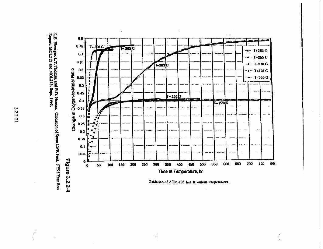
Given these five assumptions, the TGA data can be used to provide preliminary estimates of the U3O8+X oxidation response. The data shown in Figure 3.2.2-4 [Einziger, et al., 1995] shows TGA oxidation data at five temperatures for spent fuel samples from ATM-105. The three higher temperature curves (325°C, 305'C, and 283°C) show that the U30 8 oxidation response rate is less than the U40 9 oxidation response rate.
From these three curves, two methods exist to estimate the U 30 8 oxidation rate response. One method is to graphically estimate the early time slopes of these curves as U30O÷x forms and to use these values to calculate an Arrhenius activation energy. With additional analysis, an estimate for the speed of the U30 8 oxidation can be derived. The estimated slope and temperature values for the activation energy were (1.65x10"2/h, 598.2 K), (8.47x10 3/h, 578.2 K), and (1.46x10 3/h, 556.2 K). The activation energy estimate from these data was 38540 cal/mole. However, when this was used to estimate the frontal speed, this approach provided highly conservative rates for the U30 8 oxidation response compared to the data.
For this reason, a second method was used to estimate the frontal speed of the U 30 8 oxidation process. This method used graphical estimates for the elapsed times to full oxidation from the U,0 9 plateau to a UJ3Ox. phase; the elapsed time consisted of only the time interval from estimated initiation of U30 to estimated completion of U 308+x. This elapsed time neglects the delay elapsed time of the plateau and is a conservative estimate for the elapsed time to fully oxidize to U3O8 +x. The three values for time intervals and temperatures were (33.33 h, 598.2 K), (106.25 h, 578.2 K), and (425.0 h, 556.2 K). The activation energy from these data was 40057 cal/mole, which is similar to the active energy of the previous method. The samples of spent fuel for these test data were all from ATM-105, which has a nominal grain size of 13 Rim. For constant temperature histories, the speed of the U30 8 oxidation front was previously assumed constant, hence the frontal speed VV38 or ICIC 3, is given by an Arrhenius expression. The rate 1438 is given by
W3,=38 exp(-Q38/RT) 3.2.2-14a
where Q38 and k3 8 can be estimated from the ATM-105
3.2.2-8

Q38 = 40057 cal/mole
k38 = 8.58 x 10¹³ ptm/h using Idc = 6.5 prm for ATM-105
R = 1.986 cal/mole K
T - temperature Kelvin
The U30 8 frontal speed W,, for any grain size is constant and C is given by
C38 = W3./A 3.2.2-14b
The above values for k38 and Q3. are preliminary and will be evaluated again as additional data become available. The above activation energy value is considered bounding with respect to a possible bumup dependence based on the available U30 8 oxidation rates reported (Einziger, et al., 1995).
The oxidation rate, in terms of [0] to [M] response for U308 is analogous to that of Eq. 3.2.2-6 for U409 except that the factor for the number of oxygen atoms added per uranium atom changes from 0.42. For the U30, oxidation response, which is also not stoichiometric, the oxidation curves plateau around U0 275, which chemically implies
U02.4 2 "0.330 -> U0 275 3.2.2-15
Thus, each uranium atom will require, on the average, 0.33 of an oxygen atom to form a U30, lattice cell at the U02.42 oxidation front. With this value for oxygen atoms added per uranium atom for U30 8 phase transformation, and the frontal speed of Eq. 3.2.2-14, the rate of U3O1 oxidation for a pyramidal section of a cubic grain follows analogously from Eq. 3.2.2-6 as
[][U](UO9 --i 38 iU=k a,(1- C38(t))bk (1- C38(t)) 3.2.2-16
for times t > t2.4 of the U40 9 oxidation.
In Eq. 3.2.2-16, C38 is constant for a prescribed constant temperature and a nominal grain dimension I C I as given in Eq. 3.2.2-14, i.e.
(38 -(k3./ICl)exp(-a3./RZ) 3.2.2-17a
and C38 (t) is the time integration of e3, for t > t2., which for constant temperature is
C38(t) = (t - t24 )C38 for t2.4 <t < tot3.8 3.2.2-17b
3.2.2-9

The time tot 3.8 occurs at the time C38 equals unity, and is the total elapsed time from initial exposure of the UO2 at time t set to zero for the UO to change fully through the U40 9 and U308 phases. It does not include any estimate of the delay elapsed time of the plateau region, so for a model response, it is conservative. Thus, tot 38 consists of a t24 time and t,.8; the former given by Eq. 3.2.2-3, and the latter incremental time, from Eq. 3.2.2-17a when C 38 is one, is given by
t3.8 = IC/(k 38 exp(- Q3 /IRT)) 3.2.2-18a
(recall that I cI is Wo, half the grain size) and then tot38 is
tOt 3.8 =t2.4 + t3.8 3.2.2-18b
Values of elapsed time t38 are given in Table 3.2.2-5 for different constant temperature histories and nominal grain sizes.
Given the U30 8 frontal speed expression 3.2.2-14, and the above expression 3.2.2-17b for C3sM(t) the [O]/[U] ratio of a U40 9 sample transforming to U30 8 is the time integration of Eq. 3.2.2-16, and is analogous to that of Eq. 3.2.2-7, namely;
[O]/[U](U 4 09 -* U0 2 75 ;t)= 0.33(6Gcejjkajbk (BC38 (t) - 3C 8 (t) + C38 (t)/3)) 3.2.2-19
for a sample containing G number of grains.
The U0 2 , volume expressions of Eq. 3.2.2-8b and 3.2.2-9 are analogs for the VU30 8 expressions, except the function (t) is replaced by C3s(t). Thus, the volume of U0 2 converted to U30 8 for times t greater than t2.4 is
VU.308 (G, t) = 6Gci e Ik ajbk (3C 38(t) - 3C38 (t) + C38 (t))/3 3.2.2-20
where the dimensional lengths of grains for vectors , at, and b are those of the U0 2 phase. Thus, the volume of U 30 8 that exist at time t would be approximately 1.30 larger than VU30 8 evaluated from Eq. 3.2.2-20.
Finally, the volume ratio relative to the U0 2 phase transformed to U30 8 is an analog of Eq. 2.2.2-11, namely
VU3 08(Gt)/VU0 2(G) = 3C 38(t)- 3C38(t) + C33(t) for t2.4 < t < t3.8 3.2.2-21
and depends on grain size and temperature history of C38 and C38 given in Eqs. 3.2.2-17a and b.
Similar to the elapsed time t2.4 for a prescribed volume fraction of U02.4, Eq. 3.2.2-21 can be inverted to find the elapsed time, t,3.8, after U30 8 initiation to attain a
3.2.2-10

prescribed volume fracture of U30 8 . The expression is analogous to that of Eq. 3.2.2-13, exceptthe speed of the U308 front is constant, rather than depending on the square root in time. Thus, the expression is
t38 = I( -(1- VU3 0 /V, 02 )X)/(k38 exp(-Q 38 /RT)) 3.2.2-22
Values for tV3., fractional volumes of U30 8 at 25%, 50%, and 75% are given in Tables 3.2.2-6 to 3.2.2-8 at different constant temperatures and grain sizes.
Comparing the elapsed times for full oxidation of U0 2 to the U40 9 and U30 8 phases, t2.4 values of Table 3.2.2-1 and t3., values of Table 3.2.2-5, the t3 8 values are significantly greater at lower temperatures (T less 100'C) than the t24 values. It appears that large amounts of U40 9 will exist within thousands of years of exposure at -100'C temperatures, whereas it will take hundreds of thousands of years for large amounts of U 30 8 at low (-100'C) temperatures.
3.2.2.4 Comparison of Model Response to Oven Drybath Data
The confirmation of a model is primarily dependent on how well it explains existing data and its potential to explain future experiments. In this case, the U40 9 and U30 8 oxidation model based on kinetic data from the small sample TGA experiments successfully bounded the ODB data that were obtained over a larger scale and variety of spent fuel sample sizes. This comparison confirms the "bounding approximations" of the oxidation response model.
The kinetic parameters that were obtained for the model response for the conversion of U40 9 to U30 8, see Eq.3.2.2-18, were evaluated at higher temperatures (above 283°C) using TGA measurements. The TGA tests used very small samples, approximately 200 mg of spent fuel. Compared to the TGA experiments, the oven drybath (ODB) experiments accommodated much larger spent fuel samples that include both edge and center spent fuel fragments. Thus, the ODB experiments are more representative of integral or averaged spent fuel. However, the amount of U40 9 to U3,O8 0DB data are limited because these were obtained at a lower temperature (255°C) where the time response of U0 2 conversion to U308 is much slower. The ODB data have been provided by Einziger and Hanson (1996) for the following fuels: Turkey Point PWR fuel, ATM-104, ATM-105, and ATM-106. These ODB data are additional independent experimental measurements, relative to the TGA measurements, for the oxidation of U40 9 to U30 8 . The ODB samples had initial A(O/M) ratios of 0.0 or 0.42 relative to U0 2. Some of the spent fuel samples that they used were as-removed fragments, while other samples were pulverized fragments. The majority of these ODB samples had nominal grain halfsizes primarily in the range of 5-30 microns. The fact that there is a spectrum of grain halfsizes is an important point when comparing the ODB data to the model response that used kinetic parameters obtained from TGA data.
3.2.2-11

In the next four figures, Figures 3.2.2-5 to 3.2.2-8, the change in oxygen to metal ratio, A(O/M), is plotted against time (thousands of hours). The A(O/M) versus time curves represent the cumulative effect of the consecutive reactions: U0 2 -- > U409 --*
U30 8. At the ODB temperature, T = 255°C (528.26K), the reaction rate, k, 4.9, for UO2 U40 9, is kv4.9 = 1.205x10 2 lim 2/hr; the reaction rate, kv3.8, for U 409 --4 U 30 8, is kv3.8 =
3.4414x10"4 pm/hr. The front propagation speeds for the respective reactions are given by Eq (3.2.2-4) and Eq (3.2.2-14a and 3.2.2-14b), respectively. A A(O/M) of 0.42 represents the complete conversion of UO2 -- > U40 9 (no U0 2 or U30 8 assumed to be present) and the time to achieve complete conversion is represented by ttotal 4.9. A A(O/M) of 0.75 represents the complete conversion of U40 9 --> U30 8 (no U0 2 or U30 8 assumed to be present). Thus, using Eq. 3.2.2-13 and 3.2.2-22, the cumulative elapsed time for any A(O/M) > 0.42 is given by Eq (3.2.2-18b).
The experimental ODB A(O/M) versus time results are represented as symbols without lines; the various monosized grain halfsize A(O/M) versus time curves are represented as continuous lines (solid, dotted, dashed, dot-dash, etc.). At time, t = 0.0, the data have samples that were initially UO2 (Figures 3.2.2-5 to 3.2.2-7) or oxidized to U40 9 (Figure 3.2.2.-8).
As pointed out previously, the initial U0 2 grain size determines the time scale required for the complete transformation of U0 2 to U40 9, and the subsequent transformation of U40 9 to U308. The progressively larger grain halfsize A(O/M) versus time curves show that the completion of the U0 2 -- U40 9 reaction and the initiation of the U40 9 -- U30 8 reaction require progressively longer times. This model dependence upon grain halfsize becomes quite pronounced for grain halfsizes larger than 16 microns. The figures to be discussed next show that the model A(O/M) versus time curves (4 micron to 24 micron grain half sizes) form envelopes that bound the experimental A(O/M) versus time curves.
Figure 3.2.2-5 shows the plots of A(O/M) versus time for the experimental samples (P2-100, P2-002A, F-003A, and F-017A) from Turkey Point spent fuel. Figure 3.2.2-6 shows the plots of A(O/M) versus time for the ATM 106 samples (106F-022A, 106P2-10, and 106P2-21). Figure 3.2.2-7 shows similar plots for the SNF samples (104F-100, 106P2-100, 105F-100, P2-100, 106F-022A, and 106P2-21A). These figures show that the ODB experimental data are bounded by an envelope of model A(O/M) versus time curves for grain halfsizes of 2 microns to 24 microns. Because the grains of the various samples of U40 9 are distributed over a spectrum of grain sizes, the very small grains of U40 9 oxidize relatively rapidly to form U 30, whereas the larger grains require a longer time. Thus, three different sets of A(O/M) versus time plots of oxidizing spent fuel samples are bounded by the envelope of model curves ranging from 2 microns to 24 microns.
3.2.2-12

Figure 3.2.2-8 shows the plots of A(O/M) versus time for SNF samples (104F100, 104F-005, and F-003A). Samples 104F-005 and F-003A had an initial A(O/M) = 0.395 and 0.396, respectively; whereas sample 104F-100 had an initial A(O/M) = 0.0. These ODB data are bounded by the envelope of model curves having grain halfsizes from 2 microns to 24 microns. Although the distribution of grain halfsizes varies from sample to sample, it appears that most of the ODB data at 255°C can be bounded by an envelope of monosized model response A(O/M) versus time curves for grain halfsizes of 2 microns to 24 microns.
The kinetics used for the comparison of 0DB data with model results were obtained independently from the higher temperature TGA experiments. The ODB experiments used various spent fuel samples that were obtained from different types of reactors under different operating conditions. Yet, all the available ODB data were bounded within a model response envelope of grain halfsizes ranging 2.0 to 24 microns. The results of the model comparison with the ODB data give confidence that the model accounts for the essential features of spent fuel oxidation; namely, the response history depends upon both the temperature history and initial grain halfsizes.
Table 3.2.2-9 shows the time required, for various grain halfsizes, to reach different volume fractions VU30 8 /Vuo 2 = 0.00, 0.20, 0.40. 0.60. 0.80, and 1.00, for a ODB temperature held at 255°C. The time for the volume fraction, Vu 3o8/Vuo 2 = 0.00, represents the time required for the different grain halfsizes to undergo the complete conversion of UO2 to U40 9, given by Eq.2.2.-13 for Vu4o9 /Vuo 2 = 1.0. The time required for a 5 micron grain halfsize of U0 2 to form U40 9 is 519 hrs; the time to convert U40 9 to U30 8 is 15,048 hrs. However, the time required for a 30 micron grain halfsize of UO, to form U40 9 is 18,676 hrs; the time to convert U40 9 to U30 8 is 105,850 hrs.
3.2.2.5 Model Predictions of Spent Fuel Oxidation in a Constant 100'C Temperature Environment
The rates of conversion of U0 2 to U40 9 and U40 9 to U308 depend exponentially with the inverse absolute temperature, (1/T 'Kl). Consequently, the rates of conversion are considerably reduced when the temperature is held fixed at 100'C in contrast to the 255°C results. At 100 'C, the reaction rate for UO to U40 9, kv4 .9 =
8.9979x10 7 gm 2 /hr; the reaction rate for U40 9 to U30 8, kv3.8 =4.4568x10u j•m/hr.
Table 3.2.2-10 shows the time required, for various grain halfsizes, to reach different volume fractions of U40 9 relative to U0 2. In contrast, Table 3.2.2-9 shows the results for grain halfsizes for which the temperature was held constant at 255°C. Consider the time required to convert UO2 to U40 9 for grain halfsize of 5 microns: at 100'C, the total conversion time required to convert U0 2 completely to U40 9 is 6.9x10⁶ hrs, whereas at 255°C the conversion time is 519 hrs. Consider the time
3.2.2-13

required to convert U0 2 to U40 9 for grain halfsize of 10 microns: at 100 'C, the total conversion time is 2.8x10⁷ hrs, whereas at 255°C the conversion time is 2075 hrs.
Table 3.2.2-11 shows the total elapsed time as a function of grain halfsize to convert U0 2 to U30 8 at 100'C. The conversion time to 100% U 30 8 is significantly longer for the 100'C as compared to the 255°C (Table. 3.2.2-9). Consider a grain halfsize of 5 microns: the complete conversion time at 255'C is 15,048 hrs, but the time 100'C is 1.1x10'0 hrs. Consider a grain halfsize of 10 microns: the conversion time at 255°C is 31,113 hrs, but the conversion time at 100'C is 2.2x101" hrs.
3.2.2.6 Environmental Impacts of Oxidation of UOZ
Given the present limited data on the dissolution rates, the dissolution of UO2 and U40 9 appear similar. However, an increase in exposed surface area for potential wetting and dissolution will occur from U40 9 oxidation. The impact remains to be evaluated in a release rate model. Interpretation of dissolution rate data from flow testing (Gray and Wilson, 1995) indicated that from three to fourteen grain depths may be possible. For reasonable large pellet fragments relative to grains size, a factor of approximately six times the nominal exterior surface area per grain layer penetrated is an approximate factor to increase the release rate due to U40 9 oxidation for high water volume saturated dissolution/release rate response. For unsaturated dissolution/release rate response, this may not be a conservative estimate of spent fuel degradation impacts from grain boundary effects.
The impacts of U30 8 phase are from the increases in volume, about 30% from U0 2 to U30 8, from the increased surface area of sub-grain particle sizes, the U30 8 does not form a protective film on the U40 9, based on limited data, and from the slightly higher dissolution rate of U308 relative to U0 2 spent fuels. Of these impacts, the first two are considered more significant. The U30 8 volume increase of -30% will create significantly larger openings in failed cladding, and therefore, the amount of spent fuel surface potentially exposed to wetting relative to that which remains protectively covered by small flaw failures. The small flaw failures of the cladding are due to pressurized creep and/or zirconium hydride mechanisms. The U30 8 sub-grain particle sizes that result from the U30 8 spalling and surface fracturing at the U30 8 --> U40 9 oxidation front creates several orders of magnitude increases in surface area relative to the nominal grain sized surface area of U,0 9. From the Tables 3.2.2-5 through 3.2.2-8, the extent of 11308 is significantly delayed for temperature histories less than 100'C. Clearly, it is important to maintain spent fuel containment for time periods until the local repository temperatures are below 100'C. The oxidation response models discussed in this section provide expressions to calculate conservative time estimates for the U40 9 and U30 8 oxidation phase transformations. These models are simplistic in form, based on limited experimental data, but useful for the current stage of design and performance assessment analyses. Updates, refinements, and impacts of these oxidation models will be completed as additional TGA and ODB data become available.
3.2.2-14
3.2.2.7 Referefices
Adachi, T., M. Ohnuki, et al., Dissolution Study of Spent PWR Fuel: Dissolution Behavior and Chemical Properties on Insoluble Residues, J. Nucl. Mater., 174, 60-71 (1990). (Readily available.)
Aronson, S., R.B. Roof, and J. Belle. Kinetic Study of the Oxidation of Uranium Oxide, 1. Chem. Phys. 27, 137 (1957). (Readily available)
Boltzmann, L. Lectures on Gas Theory, translated by S.G. Brush, Univ. of California Press, Berkeley, CA (1964). NNA.920401.0117
Carslaw, H.S. and J.C. Jaeger. Conduction of Heat in Solids, second edition, Oxford University Press, New York (1959). NNA.900522.0259
Einziger, R.E. and H.C. Buchanan. Long-Term, Low Temperature Oxidation of PWR Spent Fuel, Westinghouse Hanford Co. Report, WHC-EP-0070 (June,1987). NNA.900620.0297
Einziger, R.E. and B.D. Hanson. Oxidation of Spent LWR Fuel: FY96 Year End Report-DRAFT, (September 5, 1996).
Einziger, R.E. and R.E. Woodley. Predicting Spent Fuel Oxidation States in a Tuff Repository, Westinghouse Hanford Co. Report HEDL-SA-3627, (April, 1985). NNA.870915.0073
Einziger, R.E. Technical Test Description of Activities to Determine the Potential for Spent Fuel Oxidation in a Tuff Repository, Westinghouse Hanford Co. Report HEDL-7540 (June, 1985). NNA.920302.0060
Einziger, R.E. Test Plan for Series 2 Thermogravimetric Analyses of Spent Fuel Oxidation, Westinghouse Hanford Co. Report HEDL-7556 (February, 1986). NNA.920302.0061
Einziger, R.E., Test Plan for Long-Term, Low-Temperature Oxidation of Spent Fuel, Series 1, Westinghouse Hanford Co. Report HEDL-7560 (June, 1986). NNA.920302.0062
Einziger, R.E. and R.V. Strain, Nucl. Technol., 75, 82 (1986). (Readily available)
Einziger, R.E., L.E. Thomas, H.C. Buchanan and R.B. Stout, J. NucI. Mater., 190, 53 (1992) (Readily available)
Einziger, R.E., L.E. Thomas, and B.D. Hanson, Oxidation of Spent LWR Fuel, FY95 Year End Report, MOL212 and MOL213, Combined Interim Report, Sept. 1995. MOL 19960611.0215
3.2.2-15
Finch, R., and R. Ewing, Alteration of Natural UO2 Under Oxidizing Conditions from Shinkolobwe, Katanga, Zaire: A Natural Analogue for the Corrosion of Spent Fuel, Radiochim. Acta, 52/53, 395-401 (1991). NNA.900507.0149
Gleiter, H. and B. Chalmers. High-Angle Grain Boundaries, in Prog. in Mat. Sci., Vol. 16, Pergamon Press, New York (1972). (Readily available)
Grambow, B. Spent Fuel Dissolution and Oxidation: An Evaluation of the Literature, SKB Tech. Rept. 89-13, Svensk. Kirnbrinslehantering AB, Stockholm, 42 pgs. (1989). NNA.891013.0094
Grambow, B., R. Forsyth, et al. Fission Product Release from Spent U0 2 Fuel Under Uranium-Saturated Oxic Conditions, Nucl. Tech., 92, 204-213 (November, 1990). (Readily available)
Gray, W.J. and C.N. Wilson, Spent Fuel Dissolution Studies FY1991 to 1994, Pacific Northwest Laboratory Report PNL-10540 (Dec., 1995)
Jena, A.K. and M.C. Charturvedi, Phase Transformations in Materials, Prentice-Hall, Inc., New Jersey, 1992.
Olander, D.R. Combined Grain-Boundary and Lattice Diffusion in Fine-Grained Ceramics, Advances in Ceramics, 17, 271 (1986). (Readily available)
Slattery, J.C. Momentum, Energy and Mass Transfer in Continua, R.E. Krieger Pub. Co., New York (1978). NNA.920401.0115
Stout, R.B., H.F. Shaw, and R.E. Einziger, LLNL Report UCRL-100859, September, 1989. (Readily available)
Stout, R.B., E. Kansa, R.E. Einziger, H.C. Buchanan, and L.E. Thomas, LLNL Report UCRL-104932. (Readily available)
Stout, R.B. Statistical Model for Particle-Void Deformation Kinetics in Granular Materials During Shock Wave Propagation, Lawrence Livermore National Laboratory Report UCRL-101623 (July, 1989). NNA.900517.0267
Thomas, L., R. Einziger, and R. Woodley, Microstructural Examination of Oxidized Spent PWR Fuel by Transmission Electron Microscopy, J. Nucl. Mat., 166, 243-251 (1989). NNA.900709.0482
Thomas, L., 0. Slagle, and R. Einziger, Nonuniform Oxidation of LWR Spent Fuel in Air, J. Nucl. Mat., 184 117-126 (1991). NNA.910509.0071
Thomas, L.E., and R.E. Einziger, Grain Boundary Oxidation of Pressurized-Water Reactor Spent Fuel in Air, Material Charact. 28, 149-156 (1992).
3.2.2-16

Thomas, L.E., R.E. Einziger, and R.E. Woodley. Microstructural Examinations of Oxidized Spent Fuel by Transmission Electron Microscopy, J. Nucl. Mat., in press. YMPO Accession NML 880707.0043.
Wood, P. and G.H. Bannister, Investigation of the Mechanism of UO2 Oxidation in Air: The Role of Grain Size, Proc. Workshop on Chemical Reactivity of Oxide Fuel and Fission Product Release, K.A. Simpson and P. Wood, eds., Berkeley Nuclear Lab., U.K., p. 19 (1987). NNA.920401.0116
Woodley, R.E., R.E. Einziger, and H.C. Buchanan. Measurement of the Oxidation of Spent Fuel Between 140' and 225°C by Thermogravimetric Analysis, Westinghouse Hanford Co. Report WHC-EP-0107 (Sept., 1988). NNA.880927.0069
3.2.2-17

Grain set decomposed to pyramidal volume subsets
A set of grain volumes (In cross section)
Put a point at the center of each grain, and decompose Into a set of pyramids (triangles in cross section).
C! ((p
-L
00

Density function: probable number of grain pyramids
Exists a large number of grain pyramids, many of which will be of
the same "size" (compact domain set).
A "size" can be Identified by attributes (a, b_ _), as illustrated below.
Let G(&, II a, ho g) denote the probably number of pyramids of size "3 (a, ( , b ,.) in a u n it s p atia l v o lu m e o f g ra in s a b o u t p o in t x a t tim e t.
G
size D (a_, bc) k)
kxs
(

Grain volume oxidation front
Pyramidal volume in an oxidizing grain and its associated physical attributes.
0 0
040
Care
uro "' ••3
$a
,i,
H0.75 =30 C- T-28 _
0.35 T&6 C--20
0.25
b.0.45- ---
0.4 wo m - - - - - - - - - - - - - - -2 0- ---- ---- -- - ---
CD 0 0.25ss fAMlO a lvaou cmcaus I0.2

Figure 3.2.2-5
0.8 -
0.7 -do, , m -- P2-100
13 0 P2-002A 0.6 0' .S ] P-o, wo0-' X A F-003A
0 0.5 .x - X F-017A 0. 'Q4 -. dT - K "-- - "
c 0.3 -2 micron = 0.3 ------ 4 Micron 00.2 --- 16 micron
0.1 ,-----24 micron 0.
0 5000 10000 15000 20000
Time (Hours)
Figure 3.2.2-5. A(O/M) versus time for U02 -- U40 9 -> U30 8: model response and experimental data
corresponding to Figure 10 (Turkey Point SNF sample) of Einziger and Hanson (1996) 0DB tests
conducted at 255 0C.
3.2.2-22
(

Figure 3.2.2-6
O 106P2-10
E3 106P2-21
106F-022A 4 Micron
-------- 10 ---- 16
----- 20
micron micron micron
----- 24 micron0.11 0 C
Figure 3.2.2-6. corresponding conducted at
5000 10000 15000 20000
Time (Hours)
A(O/M) versus time for U0 2 -+ U40 9 -> U30 8 : model response and experimental data
to Figure 11 (ATM-106 SNF samples) of Einziger and Hanson (1996) ODB tests 2550C.
3.2.2-23
0.8
0.7
0.6
00.5
cc0.4
0.3
0.2

Figure 3.2.2-7
0 5000 10000 15000
o 104F-100 o 105F-100
A 106P2-100
X P2-100
0.8
0.7
0.6
0.5
0.4
0.3
0.2
0.1
0
n n
20000
Time (Hours)
Figure 3.2.2-7. A(O/M) versus time for U0 2 -+ U40 9 -* U30,: model response and experimental data
corresponding to Figure 14 (SNF samples) of Einziger and Hanson (1996) ODB tests conducted at
255° C.
3.2.2-24
2 micron
------. 4 Micron
-----. 16 micro
---- 24 micro
a) 0
.

Figure 3.2.2-8
A X
104F-005 104F-100
2 micron
--.---- 4 Micron
14 micron ---- 20 micron
----- 24 micron
20000
Time (Hours)
Figure 3.2.2-8. A(OIM) versus time for U0 2 -) U40 9 -> U3 8O: model response and experimental data
corresponding to Figure 15 (SNF samples, initial A(O/M)=0.4) of Einziger and Hanson (1996) ODB
tests conducted at 2550C.
3.2.2-25
(
0.8
0.7
-0.6
O 0.5
cc
0.4
0.3
0.2
0.1
0
0 5000 10000 15000
i

Table 3.2.2-1. Elapsed Time, t2.4, for U409 273.2 Parameters: Q49=24000 catmole, ko=1,04E+8 micronA2/h, R=1.986 caVmole/K
Phase Transformation of U02 for Grain Size TinC 250 200 150 100 75 50 25
2Wo And Constant Temperature. Tin K 523.2 473.2 423.2 373.2 348.2 323.2 298.2
Wo=Grainsize/2 DVU409NUO2 DW/Wo DW I
IOE-6 meters 1OE-6 m t2.4 Times in Hours, One Year = 24*365 = 8760 hours
5 1 1 5 6,4558E+02 7.4109E+03 1.5144E+05 6.9461E+06 7.1027E+07 1.0407E+09 2.3916E+10
10 1 1 10 2,5823E+03 2.9643E+04 6.0577E+05 2.7784E+07 2.8411E+08 4.1627E+09 9.5663E+10
15 1 1 15 5.8102E+03 6.6698E+04 1.3630E+06 6.2515E+07 6.3924E+08 9.3660E+09 2.1524E+11
20 1 1 20 1.0329E+04 1.1857E+05 2.4231E+06 1.1114E+08 1.1364E+09 1.6651E+10 3.8265E+11
25 1 1 25 1.6139E+04 1.8527E+05 3.7860E+06 1.7365E+08 1.7757E+09 2.6017E+10 5.9789E+11
30 1 1 30 2.3241E+04 2.6679E+05 5.4519E+06 2.5006E+08 2,5570E+09 3.7464E+10 8.6097E+11
35 1 1 35 3.1633E+04 3.6313E+05 7.4206E+06 3.4036E+08 3.4803E+09 5.0993E+10 1.1719E+12
_124 Times in Yeas _ ..... 7.3696E-02 8.4599E-01 1.7288E+01 7.9293E+02 8.1081E+03 1.1880E+05 2.7301E+06
2.9478E-01 3.3840E+00 6.9151E+01 3.1717E+03 3.2433E+04 4.7519E+05 1.0920E+07
6.6326E-01 7.6139E+00 1.5559E+02 7,1364E+03 7.2973E+04 1.0692E+06 2.4571E+07
1.1791E+00 1.3536E+01 2.7661E+02 1.2687E+04 1.2973E+05 1.9008E+06 4.3682E+07
1.8424E+00 2.1150E+01 4.3220E+02 1.9823E+04 2.0270E+05 2.9699E+06 6.8253E+07
2.6530E+00 3.0456E+01 6.2236E+02 2.8546E+04 2,9189E+05 4.2767E+06 9.8284E+07
3.6111E+00 4.1453E+01 8.4710E+02 3.8854E+04 3.9730E+05 5.8211E+06 1.3378E+08
3.2.2-26

Table 3.2.2-2. Elapsed Time, tv2.4, 25% U409 273.2 Parameters: Q49=-24000 cal.mole, ko=1.04E+8 micronA2.h, R=1.986 caL/mole/K
Phase Transformation of U02 for Grain Size TaiC 250 200 150 100 75 50 25
2Wo And Constant Temperature. T in K 523.2 473.2 423.2 373.2 348.2 323.2 298.2
Wo=Grainsize/2 DVU409NUO2 DW/Wo DW I
1OE.6 meters 1OE-6 m Av2.4 Times in Hours, One Year = 24365 = 8760 hours
5 0.25 0.091439695 0.457198474 5.3978E+00 6.1964E+01 1.2662E+03 5.8078E+04 5.9387E+05 8.7012E+06 1.9997E+08
10 0.25 0.091439695 0.914396949 2.1591E+01 2.4786E+02 5,0649E+03 2.3231E+05 2.3755E+06 3.4805E+07 7.9986E+08
15 0.25 0.091439695 1.371595423 4.8580E+01 5.5767E+02 1.1396E+04 5.2270E+05 5.3449E+06 7.8311E+07 1.7997E+09
20 0.25 0.091439695 1.828793897 8.6365E+01 9.9142E+02 2.0260E+04 9.2924E+05 9.5020E+06 1.3922E+08 3.1994E+09
25 0.25 0.091439695 2.285992372 1.3494E+02 1.5491E+03 3.1656E+04 1.4519E+06 1.4847E+07 2.1753E+08 4.9991E+091
30 0.25 0.091439695 2.743190846 1.9432E+02 2.2307E+03 4.5584E+04 2.0908E+06 2.1379E+07 3.1324E+08 7.1987E+09
35 0.25 0.091439695 3.20038932 1 2.6449E+02 3.0362E+03 6.2046E+04 2.8458E+06 2.9100E+07 4.2636E+08 9.7983E+09
tv2.4 limes in Years 6.1619E-04 7.0735E-03 1.4455E-01 6.6299E+00 6.7794E+01 9.9329E+02 2.2827E+04
2.4647E-03 2.8294E-02 5.7819E-01 2.6519E+01 2.7118E+02 3.9732E+03 9.1308E+04
5.5457E-03 6.3661 E-02 1.3009E+00 5.9669E+01 6.1014E+02 8.9396E+03 2.0544E+05
9.8590E-03 1.1318E-01 2.3128E+00 1.0608E+02 1.0847E+03 1.5893E+04 3.6523E+05
1.5405E-02 1-7684E-01 3.6137E+00 1.6575E+02 1.6948E+03 2.4832E+04 5.7068E+05
2.2183E-02 2.5465E-01 5.2037E+00 2.3868E+02 2.4406E+03 3.5758E+04 8.2177E+05
3.0193E-02 3.4660E-01 7.0828E+00 3.2486E+02 3.3219E+03 4.8671E+04 1.1185E+06
3.2.2-27

3.2.2-28
Table 3.2.2-3. Elapsed Time, tv2.4, 50% U409 273.2 Parameters: -49=24000 cal/mole. ko=1.04E+8 micron^2/h, R=1.986 callmole/K
Phase Transformation of U02 for Grain Size TinC 250 200 150 100 75 50 25
2Wo And Constant Temperature. TinK 523.2 473.2 423.2 373.2 348.2 323.2 298.2
Wo=Grainsiz~e2 DVU409NUO2 DW)Wo DIN 1OE-6 meters 1OE-6 m tv2.4 Times in Hours, One Year = 24365 = 8760 hours
5 0.5 0.206299456 1.031497278 2.7475E+01 3.1540E+02 6.4453E+03 2.9562E+05 3.0229E+06 4.4290E+07 1.0178E+09
10 0.5 0.206299456 2.062994557 1.0990E+02 1.2616E+03 2.5781E+04 1.1825E+06 1.2092E+07 1.7716E+08 4.0714E+09
15 0.5 0.206299456 3.094491835 2.4728E+02 2.8386E+03 5.8007E+04 2.6606E+06 2.7206E+07 3.9861E+08 9.1606E+09
20 0.5 0.206299456 4.125989114 4.3961E+02 5.0464E+03 1.0312E+05 4.7299E+06 4.8366E+07 7.0864E+08 1.6285E+10
25 0.5 0.206299456 5.157486392 6.8688E+02 7.8851 E+03 1.6113E+05 7.3905E+06 7.5572E+07 1.1073E+09 2.5446E+10
30 0.5 0.206299456 6.18898367 9.8911E+02 1.1354E+04 2.3203E+05 1.0642E+07 1.0882E+08 1.5944E+09 3.6642E+10
35 0.5 0.206299456 7.220480949 1.3463E+03 1.5455E+04 3.1582E+05 1.4485E+07 1.4812E+08 2.1702E+09 4.9874E+10
tv2.4 Times in Years 3.1365E-03 3.6005E-02 7.3576E-01 3.3747E+01 3.4508E+02 5.0560E+03 1.1619E+05
1.2546E-02 1.4402E-01 2.9430E+00 1.3499E+02 1.3803E+03 2.0224E+04 4.6477E+05
2.8228E-02 3.2404E-01 6.6219E+00 3.0372E+02 3.1057E+03 4.5504E+04 1.0457E+06
5.0183E-02 5.7608E-01 1.1772E+01 5.3995E+02 5.5212E+03 8.0895E+04 1.8591E+06
7.8411 E-02 9.0012E-01 1.8394E+01 8.4367E+02 8.6269E+03 1.2640E+05 2.9048E+06
1.1291E-01 1.2962E+00 2.6487E+01 1.2149E+03 1.2423E+041 1.8201E+05 4.1829E+06
1.5369E-01 1.7642E+00 3.6052E+01 1.6536E+031 1.6909E+041 2.4774E+05 5.6934E+06

Table 3.2.2-4. Elapsed Time, tv2.4, 75% U409 273.2 Parameters: Q49=24000 cafmole ko=1.04E+8 micr A2/h, R=1.986 caVmole/K
Phase Transformation of U02 for Grain Size Tint 250 200 150 100 75 50 25
2Wo And Constant Temperature. Tin K 523.2 473.2 423.2 373.2 348.2 323.2 298.2
Wo=Grainsizel2 DVU409NUO2 DW[Wo DW_ _
IOE-6 meters 10E-6 m tv2.4 Times in Hours, One Year = 24*365 = 8760 hours
5 0.75 0.370039446 1.85019723 8.8398E+01 1.0148E+03 2.0737E+04 9.5112E+05 9.7257E+06 1.4250E+08 3.2748E+09
10 0.75 0.370039446 3.700394459 3.5359E+02 4.0591E+03 8.2947E+04 3.8045E+06 3.8903E+07 5.6999E+08 1.3099E+10
15 0.75 0.370039446 5.550591689 7.9558E+02 9.1329E+03 1.8663E+05 8.5601E+06 8.7531E+07 1.2825E+09 2.9473E+10
20 0.75 0.370039446 7.400788919 1.4144E+03 1.6236E+04 3.3179E+05 1.5218E+07 1.5561E+08 2.2800E+09 5.2396E+10
25 0.75 0.370039446 9.250986149 2.2100E+03 2.5369E+04 5.1842E+05 2.3778E+07 2.4314E+08 3.5624E+09 8.1869E+10
30 0.75 0.370039446 11.10118338 3.1823E+03 3.6531E+04 7.4652E+05 3.4240E+07 3.5013E+08 5.1299E+09 1,1789E+11
35 0.75 0.370039446 12.95138061 4.3315E+03 4.9723E+04 1.0161E+06 4.6605E+07 4.7656E+08 6.9824E+09 1.6046E+11
tv2.4 Times in Years
1.0091E-02 1,1584E-01 2.3672E+00 1.0858E+02 1.1102E+03 1,6267E+04 3.7383E+05
4.0364E-02 4.6336E-01 9,4688E+00 4.3430E+02 4.4410E+03 6.5067E+04 1.4953E+06
9.0820E-02 1.0426E+00 2.1305E+01 9.7718E+02 9.9922E+03 1.4640E+05 3.3645E+06
1.6146E-01 1.8534E+00 3.7875E+01 1.7372E+03 1.7764E+04 2.6027E+05 5.9813E+06
2.5228E-01 2.8960E+00 5.9180E+01 2.7144E+03 2.7756E+04 4.0667E+05 9.3458E+06
3.6328E-01 4.1703E+00 8.5220E+01 3.9087E+03 3.9969E+04 5,8561E+05 1.3458E+07
4.9446E-01 5.6762E+00 1.1599E+02 5.3202E+03 5.4402E+04 7.9707E+05 1.8318E+07
3.2.2-29
(

A B C 0 E F G H I J K L 1 Table 3.2.2-5. Elapsed Time. t3.8. for U30E 273.2 Parameters: Q38=40057 cal/mole. k38=8.58E+13 micron/h R=1.986 cal/mole/K
2 Phase Transformation of U02 for Grain Size _ _ T in C 250 20 150 100 75 530 295
3 2Wo And Constant Temperature. T in K 523.2 473.22 423.2 373.21 348.2 323.2 298.2
4 Wo=Grainsize/2 DVU308VUO2 DW/Wo DW I I
5 1OE-6 meters 10E-6 m t3.8 Elapsed Times in Hours, One Year = 24*365 = 8760 hours
6 5 1 1 5 3.2196E+03 1.8917E+05 2.9103E+07 1.7260E+10 8.3607E+11 7.3817E+13 1.3815E+16
7 10 1 1 10 6.4393E+03 3.7835E+05 5.8205E+07 3.4520E+10 1.6721E+12 1.4763E+14 2.7630E+16
8 15 1 1 15 9.6589E+03 5.6752E+05 8.7308E+07 5.1780E+10 2.5082E+12 2.2145E+14 4.1444E+16
9 20 1 1 20 1.2879E+04 7.5669E+05 1.1641E+08 6.9039E+10 3.3443E+12 2.9527E+14 5.5259E+16
1 0 25 1 1 25 1.6098E+04 9.4587E+05 1.4551E+08 8.6299E+10 4.1804E+12 3.6908E+14 6.9074E+16
1 1 30 1 1 30 1 1.9318E+04 1.1350E+06 1.7462E+08 1.0356E+11 5.0164E+12 4.4290E+14 8.2889E+16
1 2 35 1 1 35 1 2.2537E+04 1.3242E+06 2.0372E+08 1.2082E+11 5.8525E+12 5.1672E+14 9.6704E+16 1 3 1
1 4 t3.8 Elapsed Times in Years 1 5
1 6 3.68E-01 2.16E+01 3.32E+03 1.97E+06 9.54E+07 8426597454 1.577E+12
1 7 7.35E-01 4.32E+01 6.64E+03 3.94E+06 190883958 1.6853E+10 3.1541E+12
1 8 1.10E+00 6.48E+01 9.97E+03 5.91 E+06 286325937 2.528E+10 4.7311 E+1 2
1 9 1.47E+O0 8.64E+01 1.33E+04 7.86E+06 381767916 3.3706E+10 6.3081E+12
20 1.84E+00 1.08E+02 1.66E+04 9.85E+06 477209896 4.2133E+10 7.8852E+12
2 1 1 1 1 1 2.21E+00 1.30E+02 1.99E+04 1.18E+07 572651875 5.056E+10 9.4622E+12
22 1 1 _ 2.57E+00 1.51E+02 2.33E+04 1.38E+07 668093854 5.8986E+10 1.1039E+13
3.2.2-30

2
Table 3.2.2-6. Elapsed Time, tv3.8, 25% U308 273.2 Parameters: 038=40057 cavmole, k38=8.58E+13 micron/h, R=1.986 cal/mole/K
Phase Transformation of U02 for Grain Size TinC 250 200 150 100 75 50 25
2Wo And Constant Temperature. I _ _ TinK 523.2 473.2 423.2 373.2 348.2 323.2 298.2
Wo=Grainsize/2 DVU308NUO2 DW/Wo DW I _
1OE-6 meters 1OE-6 m tv3.8 limes in Hours, One Year = 24*365 = 8760 hours
5 0.25 0.091439695 0.457198474 2.9440E+02 1.7298E+04 2.6611E+06 1.5782E+09 7.6450E+10 6.7498E+12 1.2632E+15
10 0.25 0.091439695 0.914396949 5.8881E+02 3.4596E+04 5.3223E+06 3.1565E+09 1.5290E+11 1.3500E+13 2.5264E+15
15 0.25 0.091439695 1.371595423 8.8321E+02 5.1894E+04 7.9834E+06 4.7347E+09 2.2935E+11 2.0249E+13 3.7897E+15
20 0.25 0.091439695 1.828793897 1.1776E+03 6.9192E+04 1.0645E+07 6.3129E+09 3.0580E+11 2.6999E+13 5.0529E+15
25 0.25 0.091439695 2.285992372 1.4720E+03 8.6490E+04 1.3306E+07 7.8912E+09 3.8225E+11 3.3749E+13 6.3161E+15
30 0.25 0.091439695 2.743190846 1.7664E+03 1.0379E+05 1.5967E+07 9.4694E+091 4.5870E+11 4.0499E+13 7.5793E+15
35 0.25 0.091439695 3.20038932 2.0608E+03 1.2109E+05 1.8628E+07 1.1048E+10 5.3515E+11 4.7249E+13 8.8426E+15
-- _tv3.8 limes in Years
3.3608E-02 1.9747E+00 3.0378E+02 1.8016E+05 8.7272E+06 7.7053E+08 1.4420E+11
6.7215E-02 3.9493E+00 6.0757E+02 3.6033E+05 1.7454E+07 1.5411E+09 2.8841E+11
1.0082E-01 5.9240E+00 9.1135E+02 5.4049E+05 2,6182E+07 2.3116E+09 4.3261E+11
1.3443E-01 7.8986E+00 1.2151E+03 7.2066E+05 3.4909E+07 3.0821E+09 5.7681E+11
1.6804E-01 9.8733E+00 1.5189E+03 9.0082E+05 4.3636E+07 3.8526E+09 7.2102E+11
2.0165E-01 1.1848E+01 1.8227E+03 1.0810E+06 5.2363E+07 4.6232E+09 8.6522E+1 1
2.3525E-01 1.3823E+01 2.1265E+03 1.2611E+06 6,1090E+07 5.3937E+09 1.0094E+12
3.2.2-31

Table 3.2.2-7. Elapsed Time, tv3.8, 50% U308 273.2 Parameters: 038=40057 caVmole, k38=8.58E+13 micron/h, R=1.986 calmole/(
Phase Transformation of U02 for Grain Size TinC 250 200 150 100 75 50 25
2Wo And Con ant Temperature. TinK 523.2 473.2 423.2 373.2 348.2 323.2 298.2
Wo=Grainsize/2 DVU308NUO2 DWIWo DW I
1OE-6 meters 1 OE-6 m tv3.8 Times in Hours, One Year = 24*365 = 8760 hours
5 0.5 0.206299456 1.031497278 6.6421E+02 3.9026E+04 6.0039E+06 3.5607E+09 1.7248E+11 1.5228E+13 2.8500E+15
10 0.5 0.206299456 2.062994557 1.3284E+03 7.8053E+04 1.2008E+07 7.1214E+09 3.4496E+11 3.0457E+13 5.7000E+15
15 0.5 0.206299456 3.094491835 1.9926E+03 1.1708E+05 1.8012E+07 1.0682E+10 5.1744E+11 4.5685E+13 8.5500E+15
20 0.5 0.206299456 4.125989114 2.6568E+03 1.5611E+05 2.4015E+07 1.4243E+10 6.8992E+11 6.0914E+13 1.1400E+16
25 0.5 0.206299456 5.157486392 3.3210E+03 1.9513E+05 3.0019E+07 1.7803E+10 8.6241E+11 7.6142E+13 1.4250E+16
30 0.5 0.206299456 6.18898367 3.9853E+03 2.3416E+05 3.6023E+07 2.1364E+10 1.0349E+12 9.1370E+13 1.7100E+16
35 15 0.26299456 7.220480949 4.6495E+03 2.7319E+05 4,2027E+07 2.4925E+10 1.2074E+12 1.0660E+14 1.9950E+16
tv3.8 Times in Years
7.5823E-02 4.4551 E+00 6.8537E+02 4.0647E+05 1,9690E+07 1.7384E+09 3.2534E+1 I
1.5165E-01 8.9101E+00 1.3707E+03 8.1294E+05 3.9379E+07 3.4768E+09 6.5068E+11
2.2747E-01 1.3365E+01 2.0561E+03 1.2194E+06 5.9069E+07 5.2152E+09 9.7602E+11
3.0329E-01 1.7820E+01 2.7415E+03 1.6259E+06 7.8759E+07 6.9536E+09 1.3014E+12
3.7912E-01 2.2275E+01 3.4269E+03 2.0324E+06 9.8448E+07 8.6920E+09 1.6267E+12
4.5494E01 2.6730E+01 4.1122E+03 2.4388E+06 1.1814E+08 1.0430E+10 1.9520E+12
5.3076E-01 3.1186E+01 4.7976E+03 2.8453E+06 1.3783E+08 1.2169E+10 2.2774E+12
3.2.2-32
1

Table 3.2.2-8. Elapsed Time, tv3.8, 75% U308 273.2 Parameters: Q38=4a057 cahmole, k38=8.58E+13 micron/h, R=1.986 caVmole/K
Phase Transformation of U02 for Grain Size TinC 250 200 150 100 75 50 25
2Wo And Constant Temperature. TinK 523.2 473.2 423.2 373.2 348.2 323.2 298.2
Wo=Grainsize/2 DVU308NUO2 DWtvo DW _
1OE-6 meters 1OE-6 m tv3.8 Times in Hours, One Year = 24*365 = 8760 hours
5 0.75 0.370039446 1.85019723 1.1914E+03 7.0002E+04 1.0769E+07 6.3868E+09 3.0938E+11 2.7315E+13 5.1120E+15
10 0.75 0.370039446 3.700394459 2.3828E+03 1.4000E+05 2.1538E+07 1.2774E+10 6.1876E+11 5.4630E+13 1.0224E+16
15 0.75 0.370039446 5,550591689 3.5742E+03 2.1001E+05 3.2307E+07 1.9160E+10 9.2814E+11 8.1946E+13 1.5336E+16
20 0.75 0.370039446 7.400788919 4.7656E+03 2.8001E+05 4.3077E+07 2.5547E+10 1.2375E+12 1,0926E+14 2.0448E+16
25 0.75 0.370039446 9.250986149 5.9570E+03 3.5001E+05 5.3846E+07 3.1934E+10 1.5469E+12 1.3658E+14 2.5560E+16
30 0.75 0.370039446 11.10118338 7.1484E+03 4.2001E+05 6.4615E+07 3.8321E+10 1.8563E+12 1.6389E+14 3.0672E+16
35 0.75 0.370039446 12.95138061 8.3398E+03 4.9001E+05 7.5384E+07 4.4708E+10 2.1657E+12 1.9121E+14 3.5784E+16
tv3.8 Times in Years
1.3600E-01 7.9911E+00 1.2294E+03 7.2909E+05 3.5317E+07 3.1182E+09 5.8357E+11
2.7201E-01 1.5982E+01 2.4587E+03 1.4582E+06 7.0635E+07 6.2363E+09 1.1671E+12
4.0801E-01 2.3973E+01 3.6881E+03 2.1873E+06 1.0595E+08 9.3545E+09 1.7507E+12
5.4402E-01 3.1964E+01 4.9174E+03 2.9164E+06 1.4127E+08 1.2473E+10 2.3343E+12
6.8002E-01 3.9955E+01 6.1468E+03 3.6454E+06 1.7659E+08 1.5591E+10 2.9178E+12
8.1602E-01 4.7946E+01 7.3761E+03 4.3745E+06 2.1190E+08 1.8709E+10 3.5014E+12
9.5203E-01 5.5937E+01 8.6055E+03 5d1036E+06 2.4722E+08 2.1827E+10 4.0850E+12
3.2.2-33
ii)

Table 3.2.2-9. Total elapsed time (hrs) as a function of grain half-size to convert U02 to various
volume fractions of U3Os, assuming temperature of 255"C (528.2MK).
grainsize/2 V /3 /Vu, 02 VU308/Vo 0 2 Vu308/Vu 02 Vu308/VU0 2 = Vu30/VU0 2 Vu30o/VU0 2
(microns) = 0.0 =0.2 = 0.4 0.6 =0.8 =1.0
3.0 187 812 1552 2481 3806 8904
4.0 332 1165 2152 3391 5158 11955
5.0 519 1560 2794 4343 6551 15048
6.0 747 1997 3477 5336 7986 18182
7.0 1017 2475 4201 6370 9462 21357
8.0 1328 2994 5968 7446 10980 24574
9.0 1681 3556 5775 8564 12539 27833
10.0 2075 4158 6625 9723 14140 31133
15.0 4669 7794 11493 16141 22766 48256
20.0 8301 12467 17400 23596 32430 66416
30.0 18676 24925 32325 41620 54871 105850
3.2.2-34

Table 3.2.2-10. Total elapsed time (hrs) as a function of grain half-size to convert U0 2 to various
volume fractions of UO, assuming temperature of 100°C (373.2°K).
grainsize/2 Vu4o9 /Vuo 2 VU409 /Vuo 2 VU4o9 /VU0 2 VU4 9 /VUo2 = Vu4o9 /VU0 2 Vu4o9 /VU 0 2
(microns) =0.0 =0.2 =0.4 0.6 =0.8 =1.0
3.0 0 1.3E+04 6.1 E+04 1.7E+05 4.3E+05 2.5E+06
4.0 0 2.3E+04 1. IE+05 3.1E+05 7.7E+05 4.4E+06
5.0 0 3.6E+04 1.7E+05 4.8E+05 1.2E+06 6.9E+06
6.0 0 5.1E+04 2.5E+05 6.9E+05 2.7E+06 2.0E+07
7.0 0 7.OE+04 3.3E+05 9.4E+05 2.3E+06 1.4E+07
8.0 0 9.1E+04 4.4E+05 1.2E+06 3.1 E+06 1.8E+07
9.0 0 1.2E+05 5.5E1-05 1.6E+06 3.9E+06 2.3E+07
10.0 0 1.4E+05 6.8E+05 1.9E+06 4.8E+06 3.8E+07
15.0 0 3.2E+05 1.5E+06 4.3E+06 1.1 E+07 6.3E+07
20.0 0 5.7E+05 2.7Ei+06 7.7E+06 1.9E+07 i.1E+08
3.2.2-35

Table 3.2.2-11. Total elapsed time (hours) as a function of grain half-size to convert U0 2 to various volume
fractions of U,0 8 assuming a constant temperature of 100°C
grainsize/2 V308 /VU 0 2 VU308 /VU2 VU308 /VU 0 2 VU308 /VU0 2 VU308 /VUc2
(microns) = 0.0 =0.25 = 0.50 = 0.75 = 1.0
4.0 4.445E+06 8.211E+09 1.852E+10 3.322E+10 8.976E+10
5.0 6.946E+06 1.027E+10 2.315E+10 4.152E+10 1.122E+11
6.0 1.000E+07 1.232E+10 2.778E+10 4.983E+10 1.346E+11
7.0 1.361E+07 1.438E+10 3.242E+10 5.813E+10 1.571E+11
8.0 1.778E+07 1.643E+10 3.705E+10 6.644E+10 1.795E+11
9.0 2.251E+07 1.849E+10 4.168E+10 7.475E+10 2.020E+11
10.0 2.778E+07 2.054E+10 4.632E+10 .8.306E+10 2.244E+11
11.0 3.362E+07 2.260E+10 5.095E+10 9.137E+10 2.468E+11
12.0 4.001E+07 2.466E+10 5.559E+10 9.967E+10 2.693E+11
13.0 4.696E+07 2.672E+10 6.022E+10 1.080E+11 2.917E+11
14.0 5.446E+07 2.878E+10 6.486E+10 1.163E+11 3.142E+11
15.0 6.251E+07 3.084E+10 6.950E+10 1.246E+11 3.366E+11
16.0 7.113E+07 3.290E+10 7.413E+10 1.329E+11 3.591E+11
17.0 8.030E+07 3.496E+10 7.877E+10 1.412E+11 3.815E+11
18.0 9.002E+07 3.702E+10 8.341E+10 1.495E+11 4.040E+11
19.0 1.003E1+08 3.908E+10 8.805E+10 1.579E+11 4.264E+11
20.0 1.111E+08 4.115E+10 9.269E+10 1.662E+11 4.489E+11
3.2.2-36

Section 3.4.2: Spent Fuel Dissolution Models
Version 1.2 April 4, 1997
3.4.2.1 Introduction
This section discusses modeling of the aqueous dissolution and release rate
responses of uranium oxide spent fuel waste forms. The dissolution and release
responses are not thermodynamic equilibrium processes.
The approach for dissolution rate model development uses concepts from
nonequilibrium thermodynamics. The objective is to derive function forms for the
dissolution rate that are consistent with quasi-static thermodynamic processes.
These function forms will contain thermodynamic chemical potentials of both the
solid (spent fuels) and the solution (water chemistries) along with a set of
coefficients and parameters that can be evaluated by numerical regression of
dissolution test data. Currently, detailed knowledge is not available for the atomic (mechanistic) steps and the sequence of chemical/electrochemical reaction steps to
describe the dissolution process over the range of spent fuel inventory, potential water chemistries, and temperatures. The existing approach is to obtain an
experimental data base (flow through tests) of dissolution rates for a subset of specific spent fuels (ATMs) over a range of controlled, aggressive water chemistries and temperatures. With a numerical regression algorithm, these data are used to
evaluate empirical parameters in a rate law for each specific spent fuel ATM [Gray,
Leider & Steward, 1992; Steward & Gray, 1994]. The function form of this rate law is
a product polynomial of the bulk water chemistry concentrations and temperature [Stumm & Morgan, 1981]. In its present form, this function form does not have an explicit dependence on the thermodynamic properties of the uranium oxide waste form. In addition, the use of bulk concentrations in the function form for the regression analysis of the dissolution data would not explicitly account for a dependence from possible surface to bulk concentration differences due to surface adsorption and dipole layers. These shortcomings will be briefly addressed in the following section. Several simplifying assumptions will be made. The following thermodynamic model uses analysis methods and physical concepts taken primarily from classical mechanics [Jackson, 1962; Eringen, 1967; Bikerman, 1970; Sedov, 1972], colloidal foundations [Hunter, 1993], thermodynamics [Gibbs, 1961; Lewis & Randall, 1961; deGroot & Mazur, 1962; Denbigh, 1968; Lupis, 19831, electrochemistry [Bikerman, 1970; Bockris & Reddy, 1970; Antropov, 1972; Pourbaix, 1973] and geochemistry [Stumm & Morgan, 1981; Lasaga & Kirkpatrick, 1981; Hochella & White, 1990].
The development of a release rate model is more complex than a dissolution rate model. The release model includes dissolution rates, precipitation rates,
3.4.2-1

colloidal kinetics, and adsorption rates. At this time, the approach is semi-empirical and depends strongly on the unsaturated testing experiments to provide data and chemical process models.
The spent fuel waste form dissolution/release rate responses impact both design and performance assessment evaluations and consequences of the substantially complete containment time period (SCCTP) [NRC 10CFR60.1131 and the controlled release time period (CTRP) [NRC 1OCFR60.113]. These two regulatory requirements are coupled because waste package failures during the SCCTP will potentially expose spent fuel waste forms to atmospheric conditions in the repository. During this time period, the waste forms may be altered by oxidation and/or water vapor adsorbed to the spent fuel surface and dissolution and release of radionuclides from the waste form as a result of wetting by water. In these cases, alteration, hydration and dissolution of the spent fuel waste-form lattice-structure will take place. The development of a thermodynamically-based dissolution and release model relates to the design requirements, as well as the subsystem release and total system performance assessment (TSPA) model development needs.
3.4.2.2 Nonequilibrium Thermodynamic Dissolution Rate Function Forms
In the following, thermodynamic internal energy functionals are used to represent the energy responses for a generic solid and a generic liquid. The solid and liquid are assumed to be in contact at an idealized wetted surface. The analysis will assume that the wetted surface has a solid surface side and liquid surface side. The wetted surface is a material discontinuity, and it is also a dissolution front that propagates at an idealized dissolution velocity, Y; which for assumed quasi-steady state, rate processes will be taken as a constant.
The generic solid will have bulk constituents of typical U0 2 spent fuel, namely minor concentrations of actinides, fission products, and defects in the bulk lattice structure. For purposes here, and as described elsewhere (Stout, 1996), the bulk lattice is assumed to be nominally that of the U0 2 lattice structure; however, other oxide phases and adsorbed complexes may exist on and in spatial neighborhoods of the wetted surface. The generic liquid will be represented with a subset of arbitrary initial/bulk constituents; plus two subsets of dissolution products from the solid.
In particular, for the waste form solid with mass density, r, let the (1 x I) column matrix fs = {fs5 } denote the densities (number per unit volume) of the atomic lattices, other actinide atoms, fission product atoms, and conduction electrons; and for now, neglect the possible defect structures. The column matrix fs is an atomic fraction density, or equivalent to mass fraction densities for the solid. For the liquid, let the (1 x I) column matrix fL = {fj} denote the densities (number
per unit volume) of the aqueous state (H20,H30÷,OH-) plus the added constituents. During dissolution, the solid constituents will react with the liquid constituents;
3.4.2-2

although the exact details of these reactions are presently unknown. For purposes of
a generic analysis, let the set of products on the solid side of the wetted surface be fsL
which are created by reactions of general form
A fs +BfL4-*C 3.4.2-1
where As,Bs, and CsL coefficient matrices of the reactions. The set {fsL} represent
complexes, compounds, and/or phase change species on the solid side of the wetted
surface. These will also be argument functions in the solid's internal energy
functional. Similarly on the liquid side of the wetted surface, let f" denote the set
of liquid solution products which are created by reactions of the general form,
As +B LfL " CLsfEs 3.4.2-2
where A4 , BL and Cts are coefficient matrices. In addition to the liquid-solid species
set {fLs} created directly from the solid constituents fs, there also exists the solid
surface constituent set {fsL} which can react to create liquid species. These new
species are denoted by a column matrix {f•L}, and are created by reactions of the
form
ASLfsL + BsLfL < Cts-fsL 3.4.2-3
where AsL, &sL and CtsL are coefficient matrices. Thus, the dissolution process
creates two species subsets {f~s} and {fsL} in the liquid; and these concentrations
will be included as function arguments of the liquid's internal energy functional.
Each of the constituent densities of the solid and the liquid will be assumed to move with the particle velocity of its spatial neighborhood, v plus its intrinsic
diffusional velocity, y relative to the particle velocity. Thus the argument variables of the constituent functions fsfsLfL'fLS, and f~sL are the spatial point X, at time, t,
and the species associated diffusional velocities, YSYSVLsVYL_ and X-LSL, respectively.
Finally, the thermodynamic internal energy functional also has argument functions for the entropy and the elastic (recoverable) strain tensor. The entropy functions are denoted by hs(x_,t) and hL(X,t), and the strain tensors by gs(x,t) and gL(x,t), for points x
at time t of the solid and liquid, respectively. Note that entropy and strain are material particle potential functions and do not have diffusional velocities relative to this material particle located at point x with velocity v(x, t). These can be added; however, a later assumption will consider the dissolution process as a chemical reaction that is rate-controlled at the wetted solid-liquid surface front. Therefore, the diffusion flux terms will be removed for the final dissolution rate model.
3.4.2-3
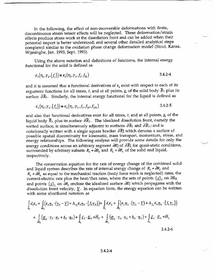
In the following, the effect of non-recoverable deformations with finite, discontinuous strain tensor effects will be neglected. These deformation/strain effects produce stress work at the dissolution front and can be added when their potential import is better understood; and several other detailed analytical steps completed similar to the oxidation phase change deformation model (Stout, Kansa,
Wijesinghe, Jan. 1993, Sept. 1993).
Using the above notation and definitions of functions, the internal energy functional for the solid is defined as
es (7s, 7's, {If) s(rls,Ys,fs, fsL) 3.4.2-4
and it is assumed that a functional derivatives of F- exist with respect to each of its
argument functions for all times, t, and at all points, x, of the solid body Rs plus its
surface dRs. Similarly, the internal energy functional for the liquid is defined as
EL(77L'7L,{fL}) EL(7L,)YL, ffL,'fLSL) 3.4.2-5
and also that functional derivatives exist for all times, t, and at all points, x, of the
liquid body RL plus its surface dRL. The idealized dissolution front, namely the
wetted surface, is simultaneously adjacent to surfaces ARs and dRL; and is notationally written with a single square bracket dI] which denotes a surface of possible spatial discontinuity for kinematic, mass transport, momentum, stress, and energy relationships. The following analysis will provide some details for only the
energy conditions across an arbitrary segment dRJ of dW] for quasi-static conditions, surrounded by arbitrary subsets Rs + dRs and RL + dRL of the solid and liquid, respectively.
The conservation equation for the rate of energy change of the combined solid and liquid system describes the rate of internal energy change of R. + dRs and RL + dRL as equal to the mechanical traction (body force work is neglected) rates, the current-electric rate plus the heat/flux rates, where the sets of points {_xhs on aRs
and points {4}L on dRL enclose the idealized surface dR] which propagates with the dissolution front velocity, Y. In equation form, the energy equation can be written with some shorthand notation as
f dEs + f (Es~s - (ys - Y) + A f5esL~'fl.{SV )+ fJd1EL + f (EL'(L (y-Y)+Af-LeLZL -fLYL}) Rs ORs RL dRL
f f(gs'Ys'Es+ hs, Ls)+ f~s -fs +Its+ f q L*U L*E)+fL*E 'ý
dRs Rs dRL RL
3.4.2-6
3.4.2-4

where the new functions symbols are n, and nL for the outward normal unit
vectors of surfaces dRs and dRL, respectively; die denotes total time derivatives, Afe
denotes functional derivatives; {fii} denotes the diffusional mass fluxes of
constituents of the solid (subscript S) and of liquid (subscript L); o- is the stress
tensor, h is the heat flux vector, H is heat generation rate, Jis the current vector
(flux of charged constituents), and E is the electric field vector, which will have a
moving idealized dipole surface due to charges concentrated on 9Rs and 9RL. For
points X in RS and RL, the rate and flux volume integrals are regular. However,
across moving surfaces dRs and dRL, discontinuity conditions may exist for quasi
static internal energy rate changes due to entropy, strain, constituents masses, stress,
heat flux, and current-electric field energy contributions. This is written, again with
shorthand notation, for the discontinuity across the surface dR] between surfaces dRs and dRL as
f ((A7r + A'eY" + A1ef)(V_- V). n]L 3.4.2-7
+ A. Efj!] ,v-n LL. _]L +1_0. n 0
where terms for internal energy discontinuities with particle velocity, v, minus front velocity, V_ contributions are separated from the diffusional flux velocity, n,
terms and from the energy rate terms from stress, heat flux and the quasi-static
electric current/field work term. The current/field work term is simplified by
replacing the electric field vector, E, with -YO, the gradient of the scalar potential for
the charge density and by assuming that there is no rate or charge changes on the
surfaces dRs and dRL as the dissolution front dR] propagates. Eq. 7 can be further
reduced by assuming that the heat flux vector is continuous across dR] and that the
internal energy change due to elastic strain is equal to the traction work at the
surfaces ARs and dRL. Finally the current J is equal to the flux of charged particles
transported across dRs and dR, which can be written as
is = e{zf'}s(Vs - V) + e{zfV}s 3.4.2-8
or as
= e(zsfs + ZSLfSL)(!S - V) + e(zsfsLs + ZsLfs.vsL)
and
-L = e{zf} L(vL - Y) + e{zf v}L 3.4.2-9
or as
= e(ZLfL + zLfS + ZfSLf•L)(YL - v) + e(zfL•VL + zLfLSvL + ZLSLfSLLSL)
3.4.2-5
where the subsets {z}s and {z}L are the number of unit charges of magnitude e (plus
for cations and minus for electrons and anions) of the associated species subsets
{fIS' {f--}IS {f}L, and {f---}L" Using these assumptions and the shorthand notation
of Eq. 8 and 9, Eq. 7 can be written as an entropy rate expression across an arbitrary
subset dR'] of surface NR].
J Aferi(v-V). _ (Af ef-e{zf}I)(:v- V). _n] 3.4.2-10 OR'] OR']
f (A~ef El} - elzfv}O). n]L
Equation 3.4.2-10 has an entropy production/dissipation energy term given by the dissolution reaction term moving with essentially nominally velocity, Y, of surface dR] and a diffusional mass flux of dissolution product and supply species across surface dR]. There are two approaches for developing kinetic (rate) models from Eq. 3.4.2-10. One is the classical Onsager approach that couples rate terms to thermodynamic forces. This is the first regression modeling approach. The second approach is to use the entropy production term across the dissolution surface as the thermodynamic measure for the dissolution propagation velocity. This latter approach results in the classical Butler-Volmer equation, when the Boltzmann configuration form for entropy is used. Both will be formulated in the following. For reasons discussed later, the Butler-Volmer equation provided the better model.
For an Onsager-type model, the kinetics of the surface propagation velocity, V_ and the diffusional flux velocities {fy} are thusly coupled thermo-electrochemical rate processes, but yet are independent kinematic (motion) variables that provide independent contributions to entropy production. Therefore, a general nonequilibrium thermodynamic formulation of dissolution would take the function rate forms {p}(y - E) .n and {fv}. n, which are specific mass dissolution front velocity terms and diffusion flux velocity terms as nonequilibrium thermodynamic rate functions for entropy production/dissipation. Corresponding to the rates, there exist the nonequilibrium thermodynamic forces driving the thermo-electrochemical processes toward an equilibrium thermodynamic state. These thermodynamic forces are functional multipliers of the rate functions given
in Eq. 10; namely ((Afe - e{z}o)). In terms of the shorthand notation, the coefficients
appear to be the same for both rate terms. However, when the stoichiometric equation forms for the reactions of Eq. 1, 2, and 3 are formally incorporated, the thermodynamic force functionals describe an independent energy change for chemical reaction kinetics and an independent energy change for diffusional mass transport kinetics. Using Onsager's concepts to describe nonequilibrium or irreversible thermodynamic processes, the two rate functions are coupled by function or functional coefficients to the two thermodynamic forces of energy kinetics and diffusion mass transport kinetics. Formally these are
3.4.2-6

{p}(_ - E) n = Lff[(Ase- ejzyO){f}]eegy + Lft[Af e - e{z}POjf,,,Of 3.4.2-11a
{fv} n = Ls [(Af - - ejzj){f}],,y+ L[AfE - e{z}jOldfsus,on 3.4.2-11b
where the four coefficients Lff, Lfv,Lvf, and Lvv (which can be functions of the
atomic fraction VI) couple the rate functions to the thermodynamic forces. For
strictly non-negative entropy production, the Onsager coupling coefficients have a
symmetry such that formally, Lvf is equal to Lfv.
Eq. 3.2.4-11a provides an Onsager-type thermodynamic function form that
should be evaluated at the dissolution front for the dissolution rate function, which
is essentially the dissolution front velocity when the details of the surface particle
velocities are neglected. These function forms have internal energy thermodynamic chemical potential functions Ases for the solid constituents
(f = {fsIfsL1) and Af EL for the waste form liquid constituents (f = {fLfs, fLsL1}), as
well as parameters related to the surface dipole potential of the dissolution front.
For numerical regression analyses in the simplest, ideal cases, particular chemical
reactions with some regression parameters could be assumed; and the regression
parameters evaluated based on the available thermodynamic values and dissolution
data sets. For the complex case of spent fuel waste form dissolution, Eq. 3.4.2-11a was reduced to the following for regression analysis,
pV = Lff[Afef - e{zf }1]1 3.4.2-12
which represents the dissolution rate as proportional to the chemical potential energy change of the waste form solid relative to the liquid; and the Onsager coefficient function Lff can be represented as a general function of the densities
functions {fs} and {fL} of the spent fuel waste form and the liquid.
The second approach also assumes that only the energy change term has the significant contribution to the production of entropy as waste form solid dissolves into a liquid. Then, from Eq. 3.4.2-10, the entropy term propagating at velocity
(E - V) is set equal to only the energy term propagating also at velocity (E - as
follows at any point on the surface R*];
A, qm(v - V). n]L = -(Asef - e1zf}o)(2- V). n]L 3.4.2-13
The velocity term (v - V) n is common to both sides of Eq. 3.4.2-13, therefore, the
entropy energy change from liquid to solid in Eq. 3.4.2-13 is set equal to the negative chemical potential changes (defined from internal energy) as constituents of the solids react with and dissolve into the liquid, thus
3.4.2-7

A IL 6 - ef 10)] 3.4.2-14
Using Boltzmann's definition of entropy (Denbigh, 1968), it can be expressed in
terms of a configurational or thermodynamic state probability function, Q2,
17= k In Q 3.4.2-15
where k is Boltzmann's constant. Then, Eq. 3.4.2-14 can be rewritten in terms of fQ as
AkLn•]• = -(Af4a -elzflo)]L 3.4.2-16
The dissolution process is considered far from equilibrium, and the dissolution rate
given by the propagation velocity of wetted surface is assumed to be functionally
related to the change in the configurational entropy as the solid dissolves into the
liquid. From Eq. 3.4.2-16, the ratio of configurational entropy is
n,/Q, = exp[(-(Afaf - e{zf} )/kAe)]L 3.4.2-17
The simplest form for the quasi-static dissolution response is to assume that the
dissolution front velocity is linearly dependent on this configurational entropy
ratio. This is the same as assuming that the rate of changing configurational entropy states of a solid into a liquid is related to the dissolution rate. Then the dissolution rate, in terms of normal velocity and waste form mass density is assumed to be of form
pV.n= CQL/s
:c exp[(-(Af f - e{zf }O)/kT)]• 3.4.2-18
where the temperature function, T, of classical thermodynamics is substituted for the change of internal energy with respect to changes in entropy, and c is a parametric constant of the dissolution rate response. Eq 3.4.2-18 is a Butler-Volmer model (Bockris and Reddy, 1970) used in electrochemical studies of corrosion rates.
In equations 3.4.2-12 and 3.4.2-18, the functional argument of the Onsager model and the Butler-Volmer model is the internal energy change as a solid surface reacts and dissolves into an adjacent solution. The functional argument includes the chemical potential and electrochemical potential energy contributions for the solid to liquid surface reactions. The chemical potential terms are defined relative
to the internal energy, Aef, where Afe is the energy change per unit (atomic or molar) of reacted species in set {f}, and f denotes the relative amounts of reacted species for members in the set {f}. The relative ratios for the amounts are, in theory, established by the chemical reaction equations 3.4.2-1 to 3.4.2-3. In practice, the
3.4.2-8

chemical reactions are often not stoichiometrically ideal not well-known.
Furthermore, even the functional forms for the chemical potentials AX are not explicitly available in many situations. Similar uncertainties exist for the
electrochemical potential term e{zfl@, which represents the electric field work at the solid-liquid dipole surface. The magnitude of the dipole charge between the liquid
and solid, 0]. = OL - 0' is the effective surface charge of the liquid minus the
effective surface charge of the solid. Both of these charge fields are complex, and depend on the ionic and electronic charges distributions in the liquid and solid, respectively. In particular, the charge distribution in the liquid is non-linearly dependent on the ionic species in the liquid set fL}" These changes can also be spatially distributed in the liquid and adjacent to the solid surface [Antropov, 1972]. Thus, selecting chemical and electrochemical functional forms for data regressions is somewhat arbitrary. However, the function variables of the functional forms used in the regression analysis are constrained to be the controlled variables of the experiments performed for dissolution rate data.
The simplest forms for regression analysis are polynomials in the bulkcontrolled concentration variables of the liquid and the spent fuel, and the temperature. Thus, a quadratic function, including cross terms, with parametric coefficients was selected to represent the chemical potential and electrochemical energy functional terms for an Onsager model and an initial or first Butler-Volmer model. In addition to this first Butler-Volmer model, a second Butler-Volmer model was selected that had the concentration dependent chemical potential terms represented as logarithmic functions of concentrations. The logarithmic functions correspond to accepted function representations for both ideal and non-ideal solutions often used for both liquids and solids (Antropov, 1972; Lewis and Randall, 1961; Stumm and Morgan, 1981; and Lupis, 1983). Because of the logarithmic dependence as an exponential argument, the second Butler-Volmer model reduces to a product of concentrations, each raised to a regression parametric power.
The results of regression analysis using these three models, the quadraticconcentration polynomial, Onsager model, the first Butler-Volmer model with a quadratic-concentration polynomial and the second Butler-Volmer model with logarithmic dependent concentrations, are discussed in the next sub-section. Each of these models is consistent with nonequilibrium thermodynamics concepts and provide function forms for regression analyses. These models do not contain an explicit dependence on radiolysis effects. Radiolysis effects from spent fuel radionuclide decay will alter the concentrations of bulk controlled concentrations in a boundary layer at the liquid-solid interface due to the deposition energy of radiation. The effects of this bulk to boundary layer concentration are contained in the dissolution rate data, however, no functional dependence due to radiolysis and these altered concentrations has been modeled. Hence, this radiolysis problem remains to be explicitly represented in a functional model. However, since the dissolution data are obtained with radioactive spent fuel, a radiolysis dependence is
3.4.2-9

implicitly contained as the burnup variable in the regression fits of data for each model.
3.4.2.3 Regression Fit of Data to ModeIs
3,4.2.3.1 UO_ and Spent Fuel Data
Using nonequilibrium thermodynamics, two different function forms were developed to describe the dissolution response of spent fuel waste forms. Eq. 3.4.2-12 provides a classical Onsager relationship for dissolution rate that is linearly related to the energy change of the solid dissolving into a liquid. This is expected to be descriptive of dissolution response close to thermodynamic equilibrium. Eq. 3.4.2-18 provides a classical Butler-Volmer relationship for the dissolution rate that is exponentially related to the energy change of the solid dissolving into a liquid. Eqs. 3.4.2-12 and 3.4.2-18 provide a consistent thermodynamic basis for the function forms of dissolution rate models. Function forms based on both Eqs. 3.4.2-12 and 3.4.2-18 were used for regression analyses over subsets of unirradiated U0 2 and spent fuel U0 2 dissolution rate data.
The initial data-modeling efforts to represent available U0 2 and spent fuel dissolution data used simplified equations based on the Onsager-type thermodynamic function forms of Eqs. 3.4.2-11 and 3.4.2-12. The data sets consisted of macroscopic measurements of dissolution rates and the controlled independent variables, temperature and bulk solution chemistry, consisting of total carbonate, dissolved oxygen, and hydrogen ion concentrations. Therefore, Lff was initially represented by a product of solution chemical concentrations times an exponential energy term, exp(-Q/RT), to include the teraperature dependence. The solid potential energy, 1is, was represented by a constant and a coefficient times the
burnup. The liquid or solid chemical potential energy for a concentration C1, g(Ci),
was represented by pi0 + RTln{-CJ}. The solid-liquid chemical potential energy change term, PLs-g 1-, was the difference of these representations. Thus, the dissolution rate was represented essentially as Lff (g.ts-jL1). Several polynomial variations for the forms of Lff, ts and gt1 were explored. Non-linear regression analysis was used with these forms. These models all produced substantial differences from the measured dissolution rates. Because these models consisted of many products of the polynomial terms from Lff (tsi-tl), a simple quadratic polynomial was selected as a close approximation of the model. A polynomial is much easier to analyze using multilinear regression. All of the regression fits of these polynomial Onsager-type models resulted in low correlation coefficients. Furthermore, these dissolution models would often predict negative dissolution rates. For these reasons, only results with the regression analyses with the two Butler-Volmer expressions are provided as representative dissolution rate models over the available data sets.
3.4.2-10

The test data for dissolution response was best represented by Eq. 3.4.2-18, which has the form of the Butler-Volmer equation used in correlation of corrosion and electrochemical rate data. The normal derivation of the Butler-Volmer equation assumes that the electrochemical processes are near thermodynamic equilibrium. In the above approach, thermodynamic nonequilibrium was assumed for the dissolution process. Also, the functional form to relate the dissolution velocity to the ratio of nonequilibrium configurational entropy was assumed.
Rather than regress on the exponential function in the Butler-Volmer
equation, the natural logarithm of the dissolution rate [mg/(m2 .day)] was used as the fitted response. The chemical and electrochemical potentials of the exponential function of the first Butler-Volmer model were represented as a polynomial in the bulk concentration and burnup variables. Burnup was represented as a concentration term as well, because it is proportional to the aggregated production and concentration of fission products. This approach also eliminated the possibility of a model yielding negative dissolution rates. The initial regressions used a full 21term quadratic polynomial of five variables.1 A third-order term with burnup, oxygen concentration, and inverse temperature was included to better represent the apparent effects of radiolysis. The equation with the smallest root-mean-square error and largest correlation coefficient (r2=0.91) was a 13-term model:
In(Rate UO2) = a0 + al.BU + a2.IT + a3 .CO3 4- a4 .02 + a5 .H + a6.BU.IT + a7.BU.02
+ a8 .BU.H + a9.CO3.O2 + al 0.CO32 + a11 O02 2 + a12 .BU.O2.IT 3.4.2-19
1 The dissolution data used for this regression analysis with the first Butler-Volmer model were the 42
combined flowthrough tests of UO and spent fuel (ATM-103) in Table 2.1.3.5-4 of Section 2.1.3.5, Dissolution Radionucide Release from UO2, plus the one dissolution rate of 7 mg.m2.d"A for ATM-105 (burnup of 31 MWd/kgM also reported in that section.
3.4.2-11

")
with the following coefficients, term descriptions and regression statistics:
Table 3.4.2-1
Coefficient (a1) Std. Error T-value Significance Term Description
0 1 2 3
1 BU IT C03
402 5H
6 BU*IT 7 BU*O2 8 BU*H 9 C03"O2 10 C03**2 11 02**2 12 BU*02*IT
No. cases = 43 Resid. df = 30
13.848639 -0.479226
-4536.815865 823.431331
50.158103 -1.148737E+08
147.090980 1.794646 6.120887E+06 204.202747 -38928.713074 -206.190757 -614.563609
1.534127 0.082894 480.481755 132.396019
12.594141 2.398216E+07
26.299886 0.550020 1.12358E+06 86.865356 6393.94265 59.419902 172.992767
R-sq. = 0.9114 R-sq-adj. = 0.8759
9.03 -5.78 -9.44 6.22
3.98 -4.79
5.59 3.26 5.45 2.35 -6.09 -3.47 -3.55
0.0001 0.0001 0.0001 0.0001
0.0004 0.0001
0.0001 0.0028 0.0001 0.0255 0.0001 0.0016 0.0013
Regression Constant Burnup (MWD/kg) Inverse Temperature (K-1) Total Carbonate Concentration (mol/L) Oxygen Partial Pressure (atm) Hydrogen Ion Concentration (mol/L) I ->2nd Order Interaction
I ->Quadratic
->3rd Order Interaction
RMS Error = 0.4787 Cond. No. = 118.3
3.4.2-12
Term

The standard error provides a measure of the uncertainty of the coefficient
estimate, in the same units as the estimate. The fourth and fifth columns provide
statistics related to the test of the hypothesis that the coefficient being estimated is
zero. A high significance value indicates that there is reason to believe that the
coefficient is zero, and so the term can be dropped from the model. Conversely, the
closer the significance value in column 5 is to zero, the more important the term.
The notes of the table provide some statistics to help assess the fit. First, the
number of cases or runs are given. Second, the residual degrees of freedom (cases
less the number of terms in the model) are enumerated. The R-square value (R2)
and adjusted R-square value are numbers that indicate how well the fitted values
produced by the model are correlated with the actual response values. An R2 value
is always between zero and one. An adjusted R2 value (which is adjusted for the
number of terms in the model) is less than R2, but is the better of the two for
selecting the model with the most significant terms. The closer a value is to one,
the better the fit. The best model is usually the one that maximizes both the R
square (R2) and adjusted R-square value . The Root Mean Square (RMS) error is a
measure of the response variability that is not explained by the fit, in the units of the
fit. The Condition Number can vary from one, which indicates a perfectly mathematical orthogonal experimental design, to infinity, which indicates a model
containing singularities.
This first Butler-Volmer type model describes some features of the chemical
dissolution processes far from thermodynamic equilibrium and provides a reasonably good fit to the available data. However, the model is nonlinear, because the Butler-Volmer model's energy change term is in the exponent and contains
quadratic terms. Depending on the terms and coefficients in the model, extrapolation outside the measured independent variable space could cause large
prediction errors and should be used with caution.
With five adjustable independent variables in the above first Butler-Volmer model (Eq. 3.4.2-19), it is difficult to show the effect on the dissolution rate of changing all of them systematically. Therefore, variable changes relevant to a repository are illustrated in accompanying figures, particularly at plausible
conditions that the model predicts would increase the dissolution rate significantly. In each of the figures the total carbonate, oxygen level, and pH are held constant, and the burnup and inverse absolute temperature varied. The vertical dissolution rate axis is linear and in the usual units of mg.m2.d'.
Figure 3.4.2-1 shows the dissolution response within the range of measured variables only and at fixed variables typical of repository conditions. The oxygen level is atmospheric and at the high boundary of the measurements. The pH is 8,
near typical values for groundwaters, such as J-13, and at its low measurement boundary. Total carbonate is set at 0.001 M, again typical for groundwaters and in the midrange of the measurements. Temperature is between 25 and 75°C and the
3.4.2-13

range of the burnup is 0 to 30 MWd/kgM.2 The response-surface varies only
modestly under those conditions. For consistency all figures presented (Figures
3.4.2-1 to 6) have the minimum value of burnup plotted as 1 MWd/kgM. The
reason for this is discussed later in this section.
Figure 3.4.2-2 shows the results of extrapolating the model to expected high
burnups (70 MWd/kgM) and 100°C. The shape of the response surface is similar,
and the dissolution rate increases gradually to more than twice as large at the
highest burnup and temperature. Increasing carbonate levels twenty-fold to 0.02 M
does not appreciably change the shape of the response-surface in Figure 3.4.2-2, but
raises it by increasing the dissolution rate uniformly by a factor of 2-3. Increasing the
oxygen level to 0.25 to approximate radical oxygen formation from radiolysis shows
a modest increase in curvature towards higher temperature and burnup, but mainly decreases the dissolution rate by a factor of about five.
Major deviations from extrapolating the model come at pH's less than 8.
Figure 3.4.2-3 shows the effect of doubling the hydrogen ion concentration to 2 x 10⁻⁸
or a pH of 7.7. Incremental increases in the hydrogen ion concentration (lower pH)
make the dissolution rate accelerate even more rapidly at high burnups and temperatures. This model is not preferred, because of these deviations.
A second Butler-Volmer model was examined as well. By substitiuting the traditional chemical potentials that include a logarithmic dependence on activities or concentrations for the chemical potential changes in equation 3.4.2-18, the classic chemical kinetic rate law was derived:
Rate = k[Ala[BIb[c]c...exp(Ea/RT). 3.4.2-20a
Burnup was represented as a concentration term as well, because it is proportional to the aggregated production and concentration of fission products. For regression purposes equation 3.4.2-20a was linearized by taking logarithms of each term and fitting that equation. That approach was used here, but allowing interaction and quadratic terms to improve the fit.
The resulting model was (note base 10 logarithms):
log, 0(Rate U0 2) = a0 + a,'PCO3 + a2"PO2 + a3 "PH + a4 "PO2"IT + a5 "LBU'IT
+ a6.LBU.PCO3 + a7 .LBU.PO2 + a8.LBU.PH + ag.IT2 + al 0.PCO32 3.4.2-20b
2 For consistency, the bumup axis in all figures is plotted with a minimum of 1 MWd/kgM for reasons
presented in the later discussion of the second Butler-Volmer model.
3.4.2-14

)
with the following coefficients and regression statistics:
Ta
Tr, Coeff_ (a Std. Error T-
ble 3.4.2-2
value Signif. Term Description
01 1 PC03 2 P02 3 PH 4 IT*PO2
5 IT*LBU
6 PCO3*LBU 7 PO2*LBU 8 PH*LBU 9 IT**2
10 PCO3**2
No. cases = 49 Resid. df = 38
1.161868 1.547418
-1.672304 0.260294
384.146973
584.818339
0.147972 0.174971
-0.285106
-3.727218E+05 -0.345209
0.803471 0.434866 0.565034 0.053553
179.898661
123.912588
0.050678 0.056308 0.043195
52092.019943 0.080324
R-sq. = 0.8649 R-sq-adj. = 0.8293
1.45 3.56
-2.96 4.86
2.14
4.72
2.92 3.11
-6.60 -7.16 -4.30
0.1564 Regression Constant 0.0010 [-Log10] of Total Carbonate Conc. (mol/L)
0.0053 [-Log10] of Oxygen Partial Pressure (atm)
0.0001 [-Log10] of Hydrogen Ion Conc. (mol/L)
0.0392 Inverse Temperature (K-1)
I ->2nd Order Interaction 0.0001 [Logl0] of Burnup (MWd/kgM)
I ->2nd Order Interaction 0.0059 I ->2nd Order Interaction0.0036 0.0001
0.0001 i ->Quadratic 0.0001 I
RMS Error = 0.2309 Cond. No.= 147.9
3.4.2-15
• IU-Jt lit K

This second Butler-Volmer model is the best representation of the existing data for performance assessment purposes.3 It has a relatively high correlation coefficient; it is based on chemical and physical principles; and it is stable when used to extrapolate to variable values outside the original data space. This model, like the others, should be used only at alkaline conditions and not be used at acidic conditions, i.e. less than pH = 7, which is a chemically different regime.
Figures 3.4.2-4 through 6 show the second Butler-Volmer model (eq. 3.4.2-20b) at even more aggressive conditions than the first Butler-Volmer model (eq. 3.4.2-19). Figures 3.4.2-4 through 6 show equation 3.4.2-21 at ten times the carbonate level (0.02 M) at three pH's and extrapolated to a burnup of 70 MWd/kgM and 100'C. Figure 3.4.2-4 is at a pH of 7. Figures 3.4.2-5 and 6 are similar but at pH = 8 and 10 respectively. All figures are at atmospheric oxygen partial pressure. Calculations at even 0.30 atm oxygen show only a modest increase in dissolution rates. The dissolution rates at these extrapolated conditions obviously remain much more stable than those from the first Butler-Volmer model (eq. 3.4.2-19) shown at a pH of 7.7 shown in Figure 3.4.2-3.
3 For the regression fit to this model, all 49 runs from Tables 2.1.3.5-4 and 4a in Section 2.1.3.5 were used. Because unirradiated UO2 represents zero or no burnup, logarithmic values of zero U0 2 burnup used in this second Butler-Volmer model would produce infinitely negative values for the terms in the regression fit of such data, and could not be allowed. For this reason a value of 1 MWd/kgM (log10(1)=O) was substituted for the bumup of U0 2 in the regression data set for the second Butler-Volmer model.
3.4.2-16

3.4.2.3.2 U." Data
For the higher oxide data shown in Table 2.1.3.5-5 only the fourteen U308
dissolution rate data were modeled. Because the U03-H20 dissolved so rapidly, their dissolution rates are estimates or minima and not appropriate for modeling. As with the U0 2 and spent fuel dissolution data, different approaches to U 30 8
dissolution modeling are being explored. Here the classical observed chemical kinetic rate law was used (eq. 3.4.2-20a).
Model parameters are presented, based on the pH's of the original carbonate solutions before contact with the samples, as used previously for the UO2 and spent fuel data. The pH's of the fresh carbonate leaching solutions are probably more representative of the pH at the sample than the pH of the leachate analysis sample that has been exposed to dissolved CO 2 from the air.
Using the pH's of the prepared carbonate solutions given in the Table 2.1.3.5-5, the following equation is obtained from regression analysis:
U30 8 (carbonate soln. pH's):
log 10(Rate){mgU/m 2"day} = a0 + a1. PCO3 + a2. PHC - a3yIT 3.4.2-21a
with the following coefficients and regression statistics:
Table 3.4.2-3
i Term 1 Coeff. (ai) 2 Std. Error 3 T-value 4 Signif. 0 1 7.950863 1.433419 1 IT -1333.106149 337.537767 -3.95 0.0027 2 PCO3 -0.649162 0.084716 -7.66 0.0001 3 PHC -0.106466 0.094032 -1.13 0.2840
No. cases = 14 R-sq. = 0.8757 RMS Error = 0.2924 Resid. df = 10 R-sq-adj. = 0.8384 Cond. No. = 44.47
As with the earlier UO2 and spent fuel dissolution data, the pH did not have much effect on the model. However, carbonate concentration, not temperature, had the strongest effect on the Up08 dissolution rate. The temperature had half the effect of carbonate concentration on the uranium dissolution rate. The pH was only about one-sixth as effective as carbonate concentration in explaining the changes in U108 dissolution rates. Leaving out the pH term had a negligible effect on the other regression coefficients and was absorbed in the constant:
U 30 8 (carbonate soln. pH's):
log10 (Rate){mgU/m 2 "day} = a0 + a1.logjO[CO3] - a2.IT 3.4.2-21b
3.4.2-17
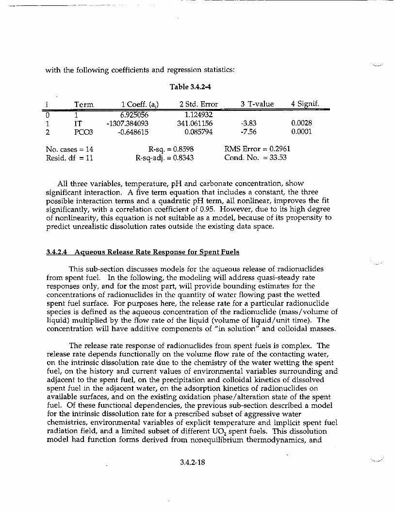
with the following coefficients and regression statistics:
Table 3.4.2-4
i Term 1 Coeff. (as) 2 Std. Error 3 T-value 4 Signif.
0 1 6.925056 1.124932 1 IT -1307.384093 341.061156 -3.83 0.0028 2 PCO3 -0.648615 0.085794 -7.56 0.0001
No. cases = 14 R-sq. = 0.8598 RMS Error = 0.2961 Resid. df = 11 R-sq-adj. = 0.8343 Cond. No. = 33.53
All three variables, temperature, pH and carbonate concentration, show significant interaction. A five term equation that includes a constant, the three possible interaction terms and a quadratic pH term, all nonlinear, improves the fit significantly, with a correlation coefficient of 0.95. However, due to its high degree of nonlinearity, this equation is not suitable as a model, because of its propensity to predict unrealistic dissolution rates outside the existing data space.
3.4.2.4 Aqueous Release Rate Response for Spent Fuels
This sub-section discusses models for the aqueous release of radionuclides from spent fuel. In the following, the modeling will address quasi-steady rate responses only, and for the most part, will provide bounding estimates for the concentrations of radionuclides in the quantity of water flowing past the wetted spent fuel surface. For purposes here, the release rate for a particular radionuclide species is defined as the aqueous concentration of the radionuclide (mass/volume of liquid) multiplied by the flow rate of the liquid (volume of liquid/unit time). The concentration will have additive components of "in solution" and colloidal masses.
The release rate response of radionuclides from spent fuels is complex. The release rate depends functionally on the volume flow rate of the contacting water, on the intrinsic dissolution rate due to the chemistry of the water wetting the spent fuel, on the history and current values of environmental variables surrounding and adjacent to the spent fuel, on the precipitation and colloidal kinetics of dissolved spent fuel in the adjacent water, on the adsorption kinetics of radionuclides on available surfaces, and on the existing oxidation phase/alteration state of the spent fuel. Of these functional dependencies, the previous sub-section described a model for the intrinsic dissolution rate for a prescribed subset of aggressive water chemistries, environmental variables of explicit temperature and implicit spent fuel radiation field, and a limited subset of different U0 2 spent fuels. This dissolution model had function forms derived from nonequilibrium thermodynamics, and
3.4.2--18

parameters of the function forms were evaluated by regression analyses over subsets of experimental dissolution rate data. The dissolution rate is a fundamental component of the release rate, as the dissolution rate provides a bounding estimate for the concentrations of the high soluble radionuclides for a thick film quantity of water flowing past a wetted spent fuel surface. This statement will be substantiated in the following discussion. The other functional dependencies of the release rate response are not well represented or isolated by available models nor available experimental data. It is for this reason that a bounding approach is being used to develop a model of release rate response.
The mass balance equation is the basis of the following release rate model for radionuclides being transported in water from a mass (or volume) of wetted spent fuel. The mass balance equation, as written here, will initially contain expressions for all the functional dependencies discussed above. However, since detailed models for each of these functional dependencies are not known, bounding approximations will be assumed to simplify and uncouple expressions in the mass balance equations for the restricted conditions of quasi-steady rate responses. This model development approach will provide equations with parameters that can be evaluated from the available, but limited, experimental data obtained from the fully saturated testing and from the unsaturated testing performed on spent fuels.
The mass balance equation, as written below, describes the time rate of change of a generic radionuclide in an arbitrary volume of fluid VF with fluid flow surface AP. The fluid has an arbitrary (space x and time t dependent) velocity field v(x_,t) in contact with spent fuel surfaces A. and adsorption surfaces AA. The concentration of a generic "in solution" radionuclide is denoted by a density distribution function
C(x,tyc), where x, t, and yc are space, time, and diffusional velocity variables. The units of C are mass per unit fluid volume per unit diffusional velocity. The "in solution" radionuclide denotes ionic, atomic, or molecular components with dimensions less than a few nanometers. If a particular "in solution" concentration is to be denoted, the elemental symbol (or isotope symbol) will be enclosed in square brackets, for example, the "in solution" concentration of uranium is [U].
The colloidal radionuclide concentration is more complex, and is generically denoted by K(x, t, yK, g, r) where K is the density distribution function for the
number of colloids at point x and time t with diffusional velocity Y, effective area and orientation ., and effective areal radionuclide density per unit area on area a of radionuclide r. For reasons of notational simplicity, it is assumed that only radionuclide colloids form, and that each colloidal species is comprised of only one radionuclide elemental species. Thus, by assumption no pseudo-colloidal kinetics are represented in the following analyses and colloids with multiply radionuclide species on area a are assumed not to form. These assumptions of no pseudo-colloids and no multi-species colloids are consistent with the limited test data. If additional data or new interpretations of existing data are advanced, than these modeling
assumptions can be readily revisited. The use of subspecies variables vc, y., and r
3.4.2-19
to denote physical attributes of a particular subset for diffusion velocities and for generic colloids is notationally cumbersome. However, the notational scheme will be simplified as the model development progresses to reflect experimentally
measured concentrations by integration over the domains of attributes variables y-,
v, a, and r. These domains are considered broad number sets, and denoted by curly
brackets, i.e. {yjc, {IvK, {al, and {r}. For example, the colloidal concentration of a
generic radionuclide at a given diffusion velocity yK is given by the integration of the density distribution K times the two attributes variables over their attribute domains. This is denoted in a couple of different ways, depending on the context of the discussion;
KV(x,t,VK) =- arK -= J arK(x,t,vK, a, r)dadr 3.4.2-22 {a}{r}
Similarly, the "in solution" concentration of a generic species for all diffusional velocities is given by the integration of density distribution C times the diffusional velocity attribute over its domain,
C(x,t) - C(x,t,vc)dvc 3.4.2.23 {1 c}
Likewise, the colloidal concentration of a generic species for all generic diffusional species is given by the integration
K2(x,t) = J Kv (X,t,vK) d vK 3.4.2.24
From the last two equations, the averaged diffusional velocities for "in solution" and colloidal concentrations vC and YK are defined from the following expressions
_cC =- VC f Vc C(_x,t,_vc)dvc 3.4.2-25
and
YKK vKKV M f VK Kv(X,t,VK)dvK 3.4.2-26 _.VK}
In the above, the radionuclide decay/growth exponential time responses are implicitly imbedded in the inventory terms. For short term analysis of experiments, these decay/growth responses can be neglected in the following.
3.4.2-20

Using the above notation for concentrations, the aggregate, mass balance equation for an arbitrary generic radionuclide can be written as
f dtC+doKdVF + (vF +--C)rFC+(e+-VF+K)"nFKdAF
VF AF
= f PcYs"RS + VKKnsKdAs- SYCnP½C+VK'!nPdAP
As Ap
- ECnKC +VKnKKdAK- ZVcnAC+_VK.nAKdAA 3.4.2-27
AK AA
which is a statement that the time rate of change for the total concentration in fluid volume V. occurs from fluid concentrations transported through a fluid-flow boundary A, with outward directed normal nF, from the congruent dissolution at velocity _y, of spent fuel surface A. with inward directed normal nns for generic species C where the solid has fractional mass density Pc for species C, from aggregated colloidal spallation and formation K at the spent fuel surface area As, from precipitation kinetics of the "in solution" and colloidal concentrations transported to all accessible precipitate surfaces Ap with outward directed normal nv, from interchange colloidal kinetics of the "in solution" and colloidal concentrations transported to all accessible colloidal surfaces AK with outward directed normal n-K, and finally, from all adsorption kinetics for both "in solution" and colloidal concentrations transported to all accessible adsorption surfaces AA with outward directed normal na.
In the aggregate measure of total concentration, the interchange kinetics terms would determine the relative components rate values for the "in solution" concentration C and the colloidal concentration K. However, the value of the total concentration, "in solution" plus colloidal, would remain invariant with respect to all models for interchange kinetics. Thus, only the dissolution rate, the precipitation rate, and the adsorption rate integral terms add and/or subtract mass from the total concentration when represented as an aggregate measure of "in solution" and colloidal components.
When spent fuel is present and dissolving into solution under quasi-steady conditions, it is reasonable to assume that any precipitation and adsorption rate processes will be positive in the sense these processes will. be subtracting mass from the solution. Given this assumption, it can be seen from Eq. 3.4.2-27 that a bounding model for the total concentration of a radionuclide in solution is provided by neglecting the precipitation and adsorption kinetic terms, since these would subtract
3.4.2-21

mass from the total concentration. Of course, for the highly soluble fission product radionuclides and for cases of significantly high fluid flow rates, the precipitation integral would be zero. Furthermore, the highly soluble radionuclides, for a bounding model, is assumed not to form colloidal species. Thus, Eq. 3.4.2-27 for a quasi-static rate state will have bounding release rate terms that depend on the areas of fluid flow AF and spent fuel dissolution As only, and would reduce to
J (YF + -C )'!!F dAF S PC Es'nsdAs 3.4.2-28 AF As
Eq. 3.4.2-28 can be area integrated over an inlet fluid boundary A. in and an outlet fluid boundary AF out and for flows which have fluid velocities significantly greater than the diffusional velocities. The quasi-steady change in concentration between the inlet and outlet fluid boundaries becomes
Gout - Cin = l/QF J pc-Vs.1s dAs 3.4.2-29
As
where the volumetric flow rate QF is defined as
QF J YvF'nF dAF 3.4.2-30 AF
For quasi-steady flows, Q, has the same value at the inlet and outlet areas.
Eq. 3.4.2-29 is used to evaluate the dissolution rate and/or the dissolution velocity v.s for the flowthrough testing experiments when solid area As is assumed not to evolve in time. In these tests the flow rate QF is controlled, the dissolution area is measured, and the water chemistry is prescribed at the inlet surface. Thus, Ls can be evaluated for the prescribed set of testing conditions for which the precipitation, colloidal, and adsorption terms do not have contributions.
For these same conditions, the release rate concentration for fluid flowing over exposed spent fuel in a waste package can be modeled by integrating equation 3.4.2-28 in a slightly different manner. For this integration, consider a uniformity thick film of fluid flowing on arbitrary wetted path 1(x) of exposed spent fuel surface in a waste package. For a film thickness of h, and an arbitrary film width w that also wets a width of fuel, w, the change in averaged concentration of the film as the fluids flows from a point x to neighboring point x + dx on wetted path 1(x) is
d -- C(x) vF .nF hw dx = PcVs .ns w d& 3.4.2-31
In Eq. 3.4.2-31, the area A, of the fluid flow is film thickness times film width, hw, and the dissolution area As is film width w, times the wetted path length, wdt. This is ideally valid, but from observation of dissolution samples and in interpretation of
3.4.2-22

flowthrough samples, it has been conjectured that the exposed surface is enhanced by the rapid dissolution along grain boundaries up to a depth of three to five grain boundaries. Therefore, on empirical factor multiplied times the dissolution area should be applied. This factor would have a dependence on grain size, but based on flow through tests (Gray and Wilson 1995) a value of four is recommended. A
generic parameter 8s will be used for a value of this empirical factor in the
following. The integration of equation 3.4.2-31 between arbitrary points Xin to xout with a corresponding path length of ,e(Iout) - £(Xin) is
(Xout) - •(Xin) = ((PcVs _ns4sW)/(YF •nFhw) (M(Xout) - A(Xin))) 3.4.2-32
Equation 3.4.2-32 evaluates the change in concentration as fluid flows past and dissolves spent fuel with a wetted contact length of (ý(Xout) - ý(Xin). For waste packages with horizontally emplaced fuel rods, the contact length would be the crack opening of the failed rods in a radial direction. For those cases that may be conjectured in which the generic radionuclide concentration evaluated by equation 3.4.2-32 exceeds a solubility limit, than it is recommended that the outlet concentration be limited such that
C(xout) -< Csolubility limit 3.4.2-33
A colloidal release concentration expression that is an analog to equation 3.4.2-38
exists for the case of colloidal spallation and formation adjacent to the surface As. It is given by
K(xout) - K(xin) = ((VKK .nsKw)/(VF .nFhw)) ('(X(out) - £x(in))) 3.4.2.34
In some conjectured situations, there is a potential for a fixed volume V. of fluid to be in constant contact with spent fuel. This situation corresponds to the fully saturated tests on spent fuels performed by Wilson (1990) and possibly in the alteration layer of the unsaturated tests (Finn et al., 1992). In these Wilson tests, the highly soluble fission product radionuclides did not appear to exceed solubility limits. However, the actinide radionuclides did attain constant total concentration values, which for release rate modeling purposes will be taken as effective release
concentrations and generically denoted as Cerc obtained from fully saturated test by Wilson (1990) are for "in solution" plus colloidal concentration. For most cases, the colloidal components were small. For a quasi-steady rate analysis of these tests, equation 3.4.2-27 reduces to:
J dtC + dtKdVF = " Pcys'ns + vKn1sKdAs VF AS
3.4.2-23

- f vc'npCP + VK'IIPKdAp f _K'n!KC+VK'nKKdAK 3.4.2-35 Ap AK
where surface adsorption is assumed to be zero for this quasi-steady rate analysis. For highly soluble fission products, no colloidal and no precipitation kinetic is
assumed, and for constant area of spent fuel A. the rate of change in radionuclide concentration is a constant that depends proportionally on the dissolution rate, thus
f v Q C(x,t)dVF = (PcE}s '-sAs/VF)t 3.4.2-36 V F VF
where the initial concentration at time zero is taken as zero. In applications, the
surface area As should be multiplied by the empirical 8s parameter to have a bounding model.
For actinide radionuclides, where precipitation and some colloidal kinetics are occurring, equation 3.4.2-35 requires additional assumptions to constrain and formulate a model. From the experimental data (Wilson 1990), the total concentration of (C + K) attains an effective release concentration Cerc, thus, the value of the concentration rate integral over fluid volume VF after this time is zero, and
C(t) + K(t) = Cerc fort > terc 3.4.2-37
where terc, is the time determined from experimental data that the total concentration (C + K) is less than Cerc. Based on experiment, this time is of order days or weeks for these fuel area to water volume ratios, thus, the value of terc can for most cases be set to zero. This is bounding, since for times t less than trc, the total concentrations C + K is less than Cerc*
From equation 3.4.2-35, the above experimentally based assumption that the left-hand-side term for concentration changes is zero means that the sum of terms on the right is also zero. Thus, for quasi-steady rates and fixed fluid volumes, the rate of spent fuel dissolution and colloidal spalling is equal to the rate of precipitation and colloidal kinetics. Although it has not been explicitly stated previously, it will be assumed that the dissolution process is such that the spent fuel radionuclides of the spent fuel dissolve directly to "in solution" concentrations, and add to only Cý at the surface of the spent fuel. To maintain quasi-steady constant C, then the precipitation and colloidal kinetic terms on neighboring surfaces Ap and
AK must balance this dissolution rate, thus
f Vc -nPC dAp + f _K -nKC dAK = f Pcys dAs 3.4.2-38 A, AK As
3.4.2-.24
similarly, the rate of aggregated colloidal interchanges to surfaces Ap and AK must balance the spallation and formation rate of aggregated colloidal increase, thus
J vKnpdAp + J VK'rKKdAK = S___KnSKdAs 3.4.2-39
A, AK As
Without additional microscopic details on precipitation and colloidal surface kinetics, equations 3.4.2-38 and 39 cannot be developed further to partition into components the dissolution rate concentration into precipitation and colloidal concentrations for quasi-steady state release. These equations do show that for fixed fluid-volume processes the concentrations of both "in solution" species C and aggregated colloidal species K are constants for quasi-static rate processes. Quasistatic rate processes are attainable in a short period of elapsed time when the fluid
volume, VF, wetting the spent-fuel surface is small in thickness relative to a lengthscale metric of the spent fuel surface. Hence, for thin film flows or stagnated thin
wetting films, dissolution on surface As would potentially be immediately followed by precipitation and colloidal kinetic processes in the wetted film adjacent to a spent fuel surface, As . This will be assumed to be the case for the analysis in the following paragraphs. This analysis will result in a bounding model for the release rate measurements performed in the unsaturated/drip testing on spent fuels that are briefly discussed in the following paragraph.
The unsaturated/drip test is a closed-vessel 100% humidity experiment. The closed vessel contains fragments of spent fuel placed in a Zircalloy tube and an equilibrated J-13 water is dripped onto the spent fuel surface. During the first couple of years, the drips flowed over a visually unaltered spent fuel surface. Release rates were measured for the total "in solution" and colloidal concentrations that were transported to an outlet basin of the vessel. These concentrations also include the mass contribution that was adsorbed onto the surface of the outlet vessel. This total concentration is the measured release rate for the drips flowing pass the mass of spent fuel in the Zircalloy tube. The concentrations are being measured approximately every two to three months for the high drip rate tests and slightly less often for the low drip tests. After a period of about a year and a half to two years, a visible layer of alteration products was observed to form on the spent fuel surface. These alteration products were precipitates that contain fission products and actinide isotopes, all of which have not been fully identified. The alteration layer is highly porous and appears somewhat as a fibrous mat of precipitation species that adhere to the wetted spent fuel surface.
The following simplified analysis and model of these unsaturated/drip tests has several assumptions. For the first assumption, which covers the transient time period of approximately two-years during which the surface visually appears unaltered, the release rate concentration will be assumed to be given by equations 3.4.2-32 and 34 for the "in solution" and co]loidal concentrations, respectively. This
3.4.2-25

is considered a transient period. However, a two year time increment is small in comparison to many thousands of years for a repository time period. Thus, the averaging of experimental release data for this time period would be an approximate way to provide nominal data for this initial, short-period transient time-period before the alteration layers form on the spent fuel surface. The detailed analysis to evaluate the path length (Xout) - Ax._) and to estimate consistent rate parameters from the high and low drip rate tests has not been completed. This data evaluation requires some additional assumptions. For example, it appears that the high driprate test had sufficient flow rate to pool aroumd the spent fuel surface in the Zircalloy tube. Thus, the high-drip water remained in contact (has a long residencetime interval) with the spent fuel longer, compared to the low drip rate water. Thus, concentrations estimated from the high drip rate would be the bounding concentrations for release rates independent of the path length and the flow rate. However, for lower drip rates, estimates of the path length and fluid flow rates can be used to reduce the release concentrations. For example, it can be seen from equation 3.4.2-32 that for high flow rates (v,,. nlFhw), the release concentration is reduced. Note, however, that the release rate, which is concentration multiplied by flow rate, depends only on the dissolution rate and the path length. This initial unaltered surface dissolution/release rate is also enhanced due to "rapid release" from gap and grain boundary radionuclide inventories. The use of the high drip release data thus would incorporate approximately some nonhomogeneous spatial radionuclide densities into this transient release rate.
Following the transient release rate period, the spent fuel surface is assumed to be altered and a dense mat of precipitated products are assumed to be adhered to the spent fuel surface. The porosity of this alterated layer is assumed to be fully saturated with water, and the dissolution process is assumed to be actively reacting at the spent fuel surface As. This dissolution process beneath the alteration layer is assumed to be a quasi-steady rate process in a stagnate (non-flowing) thin film of water. Thus, the concentrations of the "in solution" and colloidal components are assumed to attain constant values within the alteration layer. Thus, equation 3.4.237 for the total concentrations, Cerc is assumed to be valid for the radionuclides in the water of the porous altered layer.
Next, the dripping water is assumed to flow on the exterior surface of the alteration layer. Thus, transport of "in solution" and colloidal radionuclides is assumed to occur by mass transport from the alteration layer into the moving drip of water flowing over the alteration layer. tn the linear case of inter-surface mass transfer, the rate of diffusion exchange (or with slight surface-to-surface fluid mixing) is represented as proportional to the difference between the concentration of the water in the alteration layer and the concentration of the water in the flowing film (or drip in this case). The equation for this transport process is similar to that of Eq. 3.4.2-31, except the right-hand-side is replaced with the diffusional exchange term, thus
3.4.2-26

-C(x)vF !Fhwd• = AC(Cfim - C(x))wdU 3.4.2-40 dx
where Xc is a mass transfer coefficient to be evaluated from data of the high and low
flow rate saturated drip tests. For quasi-steady rates, Eq. 3.4.2-40 can be integrated to
C(_xout ) = Cirm (I - exp(-Ac (e(Xout) - £(Xin)))) 3.4.3-41
where Ac is Xw /(VF - nFhw) and the concentration at the inlet point x. is assumed
to be zero. Similarly, equation 3.4.2-34 for colloidal concentrations can be reformulated analogously, and the aggregated colloidal concentration transferred from the altered surface to the fluid is
K(X)out = Kfilm(I - exp(-AK( (xout) - '(iin)))) 3.4.2-42
where Kfilm is the aggregate concentration of colloidal species in the water of the
porous altered layer and AK is a transfer coefficient to be evaluated from the high
and low saturated drip data. The term AK has the parameter XK and flow rate
incorporated into it as KW /(vF• nFhw) and is similar to Ac.
The parameters Cfilm and Kfilm in Eqs. 3.4.2-41 and 42 will be estimated with release concentration data from the high drip rate tests. In the high drip rate tests, the water was observed to remain in contact with the alterated layer on the fragments and pool around the spent fuel surface. Therefore, the residence time interval of the water contact on the porous alteration layer is assumed to be
sufficiently long that the concentrations of C and K of the water become equal to the
concentrations Cfilm and Kfilm in the porous layer. A long residence time interval is functionally equivalent to a long path length interval in terms of the water concentrations becoming equal to the film concentrations as expressed in equations 3.4.2-41 and 42. This assumption needs to be substantiated, in order to defensibly evaluate the film concentration values. Future experiments are planned to provide better estimates of the "in solution" and colloidal concentrations parameters. For now, the available data of the high drip rate tests can be used to provide preliminary estimates of release concentrations.
For cases where the flow is in contact with the altered layer for shorter time intervals, or equivalently, shorter path lengths, then the concentration at the outlet
point xut will be reduced. To calculate the reductions in concentrations with Eqs.
3.4.2-41 and 42, values for parameters Ac and AK are required. In some cases, the release concentration data from the low drip rate test can be used to estimate values
of Ac and AK for different radionuclides. This approach uses experimental data to provide release concentration estimates for cases where the path length interval is
3.4.2-27

conjectured to be short in a horizontally emplaced waste package. For example, when cladding failure flaws are expected to be represented as narrow cracks along the axis of spent fuel rods.
The above simplified release models for "in solution" and colloidal concentrations have parameters that can be estimated from the limited data now becoming available from the unsaturated testing methods. The observations and measurements of colloidal concentrations have greatly added to the complexities of developing waste form release concentrations and release rates. The colloidal contributions to total concentration means that the release concentration constraint imposed by idealized solubility limits is not strictly conservative. Of course, once the areal size classes of colloids are established and validated, it may be possible to design filtration beds or adsorption materials to reduce the colloidal concentration near the waste package. Then solubility limits would be applicable. This remains to be evaluated.
Finally, the alteration rate of spent fuel, in the above model of an altered
layer, is assumed to progress at the rate of t[he dissolution velocity v.s. Thus, the alteration life time of a spent fuel fragment is roughly its half size dimension
divided by the magnitude of K. Hence, the altered layer is assumed to continue to increase in thickness until all of the fuel particle is transformed into precipitation and colloidal alteration products. Subsequent to this alteration life time interval, it will be assumed that the release concentrations from the fully altered spent fuel
fragments will be long path length limited to the Crfim and Kfihm concentrations for a time interval whose time span is limited by the inventory of the radionuclide. For short path lengths of fluid flow, the release concentrations would be reduced with values calculated from equations 3.4.2-41 and 42. This means that although the dissolution rate process is assumed to be essentially congruent, the release concentrations and release rate concentrations are not necessarily a congruent process with respect to the initial inventory of the radionuclides. This should pose no problem for the fission product releases, however, the releases of fissile isotopes should be evaluated with respect to their concentration time history released and remaining in the altered spent fuel.
3.4.2-28

3.4.2.5 References
Antropov, L.I., Theoretical Electrochemistry, Mir Publishers, Moscow, 1972.
Bikerman, J.J., Physical Surfaces Academic Press, New York, 1970.
Bockris, J.O. and A.K. Reddy, Modern Electrochemistry, Vols. 1 & 2, Plenum Press, New York, 1970.
deGroot, S.R., and P. Mazur, Non-equilibrium Thermodynamics North Holland, Amsterdam, 1962.
Denbigh, K., The Principles of Chemical Equilibrium University Press, Cambridge,
1968.
Eringen, A.C., Mechanics of Continua, John Wiley & Sons, New York, 1967.
Gibbs, J.W., The Scientific Papers of I. Willard GibbsVols. 1 & 2, Dover Pub., New York, 1961.
Gray, W.J., H.R. Leider, and S.A. Steward, "Parametric study of LWR spent fuel dissolution kinetics," J. Nucl. Mater., 190, 46-52, 1992.
Gray, W.J. and C.N. Wilson, "Spent Fuel Dissolution Studies FY1991 to 1994," Pacific Northwest National Laboratory Report PNL-10540 (December 1995).
Hochella, M.F., and A.F. White, eds, Reviews in Mineralogy, Vol. 23, Mineral-Water Interface Geochemistry, Mineral. Soc. of America, Washington, DC, 1990.
Hunter, R.J., Foundations of Colloid Science, Clarendon Press, Oxford, England,
1993.
Jackson, J.D., Classical Electrodynamics, John Wiley & Sons, New York, 1962.
Lasaga, A.C., R.A. Berner, G.W. Fisher, D.E. Anderson, and R.J. Kirkpatrick, Kinetics of Geo-chemical Processes, Vol. 8, A.C. Lasaga & R.J. Kirkpatrick eds., Mineral. Soc. of America, Washington, DC, 1981.
Lewis, G.N., and M. Randall, Thermodynamics, McGraw-Hill, New York, 1961.
Lupis, C.H.P., Chemical Thermodynamics of Materials. North-Holland, New York,1983.
Pourbaix, M., Lectures on Electrochemical Corrosion. Plenum Press, New York, 1973.
3.4.2-29

Sedov, L.I., and J.R.M. Radok, A Course in Continuum Mechanics. Vol. II Physical Foundations and Formulations of Problems, Wolters-Noordhoff Pub., Gr6ningen, The Netherlands, 1972.
Steward, S.A., and W.J. Gray, "Comparison of Uranium Dissolution Rates from
Spent Fuel and Uranium Dioxide," Proc. 5th Annual Int'l. High-Level Rad.
Waste Mgmt. Conf. (IHLRWM), Las Vegas, NV, May 22-26, 1994, 4, 2602-2608.
Stout, R.B., E.J. Kansa, and A.M. Wijesinghe, "Kinematics and Thermodynamics of Non-stoichiometric Oxidation Phase Transformation in Spent Fuel," LLNL report UCRL-JC-110678, Jan. 1993.
Stout, R.B., E.J. Kansa, and A.M. Wijesinghe, "Kinematics and Thermodynamics Across a Propagating Non-stoichiometric Oxidation Phase Front in Spent Fuel Grains," LLNL report UCRL-JC-112821, Sept. 1993.
Stout, R.B., "Nonequilibrium Thermodynamical Model for Spent Fuel Dissolution Rate," Proc. 7th Annual Int'l. High-Level Rad. Waste Mgmt. Conf. (IHLRWM), Las Vegas, NV, April 1996, pp3 9 3 -6 .
Stumm, W., and J.J. Morgan, Aquatic Chemistry: An Introduction Emphasizing Chemical Equilibria in Natural Waters, John Wiley & Sons, New York, 1981.
Wilson, C.N., Results from NNWSI Series 3 Spent Fuel Dissolution Tests, Report PNL-7170 (June 1990), Pacific Northwest Laboratory, Richland, Washington.
3.4.2-30
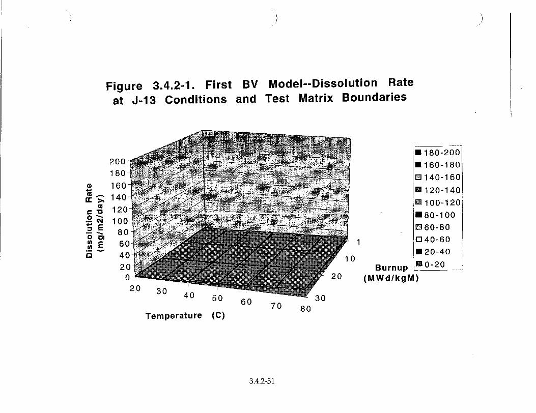
Figure 3.4.2-1. First at J-13 Conditions
BV Model--Dissolution Rate and Test Matrix Boundaries
Burnup (MWd/kgM
U 180-200 0 160-180
E0 140-160
U 120-140
El 100-120
E 80-100
060-80
1"140-60
2 20-40
0-2 0
I)
60 70 80
Temperature (c)
3.4.2-31
0 4-6
7F)
200o 180
160
1401 1 201
1008060
40
20 0
V
cm~ E 0D E S.- 1

Figure 3.4.2-2. First BV at J-13 Conditions
04
E
E
200-f 180
160
140 120'U
100-1 80A
6040
20
0
00 OZJ
Model--Dissolution Rate and Extrapolated
Burnup (MWd/kgM)
E 180-200
N 160-180
E140-160
U 120-140 U 100-120
iU 80-100
E60-80
r140-60
U]20-40
M0-20
0 CD
Temperature (C)
3.4.2-32
U)
a 4.'
0 0 E

Figure 3.4.2-3.
J-13 Carbon
First BV Model--Dissolution at pH=7.7,
ate Levels and Extrapolated
1000
9000
800
700 600]
500
400300
200
100 0-1
Tm r 0 (C
Temperature (C)
1 0
U 900-1000
0 800-900
M700-800
E 600-700
E 500-600
E 400-500 E3 300-400
I0200-300
0100-200
M0- 10 0
Burnup (MWd/kgM)
0 0
3.4.2-33
Rate
4)'
.0 *6
i
cm
%.0

Figure 3.4.2-4. Second BV Atmospheric Oxygen
Model--Dissolution Rate at pH=7, and 0.02M Total Carbonate
200
N (5
E E
0
0
4
.o °5 (5
180°
1601
140
120
100
80
60
40
20
0
-1 10
Burnup (MWd/kgM)
Temperature
60 70 80 90 100
"kI
3.4.2-34
U 180-200
m160-180 03140-160
B 120-140
M 100-120
m80-100 D360-80 040-60
020-40
M 0-20
70
l

)
Figure 3.4.2-5. Second BV Atmospheric Oxygen
=E 0 oE
200o
180
160
140
120-i
100-.
80
60
40
20
0
Model--Dissolution Rate at pH=8, and 0.02M Total Carbonate
1 10
Burnup (MWd/kgM)
=180-200
E 160-180 13140-160
0120-140
M 100-120
m80-100 160-80
0340-60
020-40 M 0°-_2_0
Temperature (C)
)
" 7O 0 0
3.4.2-35

)
Figure 3.4.2-6. Atmosp
200
Second BV Model--Dissolution Rate at pH-10, heric Oxygen and 0.02M Total Carbonate
,; 1 10
50 60 7 80 70 80
90 100Temperature (C)
1 180-200
E 160-180
E3 140-160
8 120-140
0 100-120
U 80-100 E 60-80
1D40-60
U 20-40
U 90-20o .-
Burnup (MWd/kgM)
70
3.4.2-36
04
E
E
n.
cc Co
.0
0 Q0• Co
180
160
140
120
100
80
60
40
20

Section 3.5.1: Experimental Parameters for Glass Dissolution
Version 1.2 April 4, 1997
3.5.1.1 Introduction
The goal of the YMP glass task has been to develop a mechanistic model at the level where the model predicts an alteration/dissolution rate for a glass given localized conditions. That is, for any spot on the glass, a packet of water with some composition and temperature will cause the glass to react at some rate, and produce some set of alteration products. Integration of this localized process would provide the overall behavior of the glass waste form on a repository scale. Parameters like SA/V ratio and f (fraction of Si in precipitates discussed below) are not input parameters but instead are derived parameters based on the fundamental mechanisms incorporated in the glass reaction model. Although this amount of detail will not be appropriate for PA models, we need some way to progress from the fundamental model to the simplified model which involves some other approach than the purely empirical approach used in this memo.
Current mechanistic glass dissolution models are complex, too complex to be incorporated into current performance assessment (PA) models of repository behavior without substantial simplification (see section 3.5.2 below). The current models requires detailed knowledge of the evolving fluid composition. The model is incorporated into a chemical modeling code (i.e. EQ3/6; (Wolery, 1992) ) which computes the solution composition along the reaction path. This information is needed in order to calculate the rate of glass alteration. However, a rigorous implementation of the glass dissolution model in PA codes requires that this detailed information on the composition of the fluid phase is available in the PA model. This level of information and complexity is not available in current repository PA models. Simplification of the model is necessary in order for it to be interfaced into present PA codes. The simplified model described here is meant to be a first step in making this connection.
Although the topic of this section of the WFCR is that of experimental parameters, we include here a succinct summary of the fundamental rate equations in the model in order to provide a context with which to place the parameters. With this discussion, both the proper use and the effective limitations of the present model and model parameters can be understood. More information on the model and its development is present in section 3.5.2 of the WFCR "Glass Dissolution Models".
3.5.1-1

3.5.1.2 Rate equation for simplified glass dissolution model
The glass alteration rate changes as the solution composition changes, making it necessary to couple closely the evolving solution composition with glass dissolution. The rate of glass dissolution depends on the concentrations in solution of all the elements present in the surface gel layer of the dissolving glass, and also the solution pH. However, some simplifications can be made. Experimental and modeling work on borosilicate glass to date shows that the two most important solution compositional parameters which need to be considered in order to predict radionuclide release rates from glass are pH and dissolved silica concentration (temperature and reactive glass surface area must also be known). So we can restrict the feedback of solution composition to glass dissolution rate by regressing experimental rate data in terms of only these two parameters. Below are the equations and parameters needed to calculate conservative release rates of radionuclides from glass with this simplified model. Also included are suggestions as to how to further simplify the model to make it appropriate for input into a firstcut comprehensive performance assessment model of a repository.
Long-term dissolution models for borosilicate glass employ a rate equation consistent with transition state theory. A simplified rate equation is given as:
where R = alteration rate of glass (g/yr), s = surface area of reactive glass (m2 ), k = glass surface alteration rate constant (g/m 2 /yr),
a function of temperature and pH of the solution, Q = concentration of dissolved silica (g/m 3 water), K = solubility constant for borosilicate glass, here it equals the solubility of amorphous silica (g/m 3 water) a = experimentally determined constant rl = long-term dissolution rate (under "silica saturated"
conditions in units of g/m 2/yr)
Each of these parameters must be known or estimated in order to calculate radionuclide release rates from glass. At present, the value of a is not well determined based on the available experimental data. The value of y is therefore set to one in this model. Suggested values for each of the other parameters are discussed below.
3.5.1-2

3.5.1.3 Parameters for simplified glass dissolution model
Surface Area, s
As the molten glass cools in the melter, it undergoes fracturing. Estimates for the increase in glass surface area due to fracturing range from 2 to 100 times the uncracked surface area. A reasonable average value to use for the extent of fracturing is 25 (Baxter, 1983) . The initial total glass surface area per waste package, Ao, is made up of a nominal area per glass log, number of glass logs per package, n,
and a cracking factor, a multiplier on the nominal area (>1, typically around 25).
A, = 25. n.21rr,21 +k• (3.5.1.2)
where Ao = total glass surface area (m2), ro = radius of the glass log, Lo = length of the glass log, and n = number of glass logs per waste package.
The glass log is assumed the same cylindrical shape with a constant length to radius ratio, Lo/ro, during the dissolution process. Assuming the glass retains a constant density throughout alteration, then
2
A, = A. ( EMI ) (3.5.1.3)
where A1 = surface area after dissolution, m 2 ,
Ao = initial surface area, m2, M1 = glass mass after dissolution, kg, Mo = initial glass mass, kg.
In the bathtub water contact mode, the total surface area of the glass log is in contact with water when the container is filled. For the flow-through mode, only a fraction of surface contacts water. The wetted area depends on the groundwater flow rate. We assume the wetted area remains the same for a given water influx, q, until the total glass surface area decreases to below the initial wetted area due to the glass dissolution. Then the wetted area equals the total area until the glass completely dissolved.
Rate Constant, k
The rate constant, k, has been measured over a range of pH and temperature
conditions. Table 3.5.1.1 and Figure 3.5.1.1 show the values of k in units of g/m 2 /day
3.5.1-3

from flow-through experiments by (Knauss, et al., 1990). for an analog SRL-165 glass composition.
The data are plotted in Figure 3.5.1.1, and the following regression relations are obtained:
k = 365 x 10' (g/m 2/yr) (3.5.1.4a) where m is the higher value of the following two equations:
2600 m = 8.632- 00 . 65pH (3.5.1.4b)
T + 27:3
4550 m = 7.268- 4 -+.50pH (3.5.1.4c)
T + 27:3
and where T = solution temperature (°C).
Table 3.5.1.1. Log10 glass dissolution rate in g/m 2 /day (from (Knauss, et al., 1990) )
pH T = 25'C 500C 700C 1 -1.25 0.02 0.51 2 -1.73 -0.68 -0.18 3 -2.21 -1.38 -0.87 4 -2.69 -2.08 -1.56 5 -3.17 -2.78 -2.25 6 - - -2.94 7 -4.53 -3.43 -2.3 8 -4.02 -2.92 -1.9 9 -3.51 -2.41 -1.5 10 -3 -1.9 -1.1 12 -1.98 -0.88 -0.3
Solution Chemistry, Q and K
The major effect of groundwater chemistry on the glass dissolution rate (other than pH) is the concentration of dissolved silica. In this simple model, Q equals the concentration of dissolved silica in the water contacting the glass. The local groundwater chemistry in the vicinity of the repository will likely be dominated by the host rocks (Wilder, 1992) and the silica concentration is therefore expected to be close to cristobalite saturation at the ambient temperature. Cristobalite is a common constituent of the host rocks at Yucca Mountain. Table 3.5.1.2 lists concentrations of silica in equilibrium with. cristobalite at temperatures from 0 to
1500C from the thermodynamic database SUPCRT92 (Johnson, et al., 1992)
3.5.1-4

"K" in equation (1) for the waste glass is assumed equal to the equilibrium constant for amorphous silica in this simple model. K actually varies as a function of glass composition, but for most waste glass compositions, the experimentally determined value of K is of the same general magnitude but less than the value of K for amorphous silica. Our simplification therefore gives conservative estimates.
Table 3.5.1.2 lists values of logloK (in molality) for temperatures from 0 to 1500C.
As an example, at 600C, Q/K= 10-3.02/10-2.43 = 0.26. The term (1-Q/K)= (1-0.26) or 0.74. The glass reaction rate therefore is about 74% of the rate under silica-free conditions.
2
E
2
0
0
-1
1
0
-1
-2
-3
-4
-5
-6
2
Figure 3.5.1.1.
4 6 8 10 12 14pH
Loglo(dissolution rate, g/m 2 /day) versus solution pH from Knauss et al., 1990.
Figure 3.5.1.2 shows the relation between Q/K and temperature. For a temperature between 0 and 100'C, the relation can be expressed as:
(3.5.1.5)Q = 0. 128 + 0.0021T K
3.5.1-5
S I m I' I * i '
log10k = 8.632 - 2600/(T+ 273) - 0.65pH
. T = 70'C
%%, ' 5000
a•,N '•N'I,,...,K r'"25°C
log 10k =7.268 - 4550/(T+273) + 0.5OpH
. I , l • I , I , I ,
0

Table 3.5.1.2. Cristobalite and Amorphous Silica Solubilities (from Johnson, et al.,
0.5
0 .4 . ........................................................................................................................ ... ..................... ------ .. .. .. .
0.3 ................................. ................ .........
-- QK=0. 128 +0.0021 T 0 .2 . ................................ ......................... .................................... I . . . .. . ... .. .. .. ..........................................
0 .1 . ................................. ........... ........... ............................................................. ............. ....................... ...... ......... ... .
0.1
0I I I I
0 50 100 150 Temperature, 0C
Figure 3.5.1.2. Relation between Q/K and temperature.
Solution pH
Experimental studies of tuff-water interactions have shown that the pH of reacted J-13 water maintains a pH slightly higher than neutral (Knauss, et al., 1987) Therefore for anticipated repository conditions, a slightly alkaline pH of about 8 is recommended as a substitute for the lack of a more rigorous calculation of groundwater chemistry. This pH value should be used to estimate rate constants for glass dissolution from Table 3.5.1.1 (it should also be consistent with any data for solubility limited radionuclide concentrations which are also highly dependent on pH). Note however that glass dissolution rates and radionuclide release rates are very sensitive to pH and nothing more than a qualitative estimate of release rates is possible without a more rigorous treatment of solution chemistry in the repository performance assessment model.
3.5.1-6
p I I I I

Temperature Dependence of Glass Dissolution Rate
Experiments have shown that glass dissolution rates follow the Arrhenius
relation ratege-E/RT where R is the gas constant, T is temperature (Kelvins) and the activation energy (E) is about 20 kcal/mole. This corresponds roughly to dissolution rate increasing by a factor of 2 for a ten degree rise in temperature. This simple rule can be used to describe the effect of temperature on glass dissolution rate if the data in Table 3.5.1.1 cannot be explicitly used.
Radionuclide Content of Glass
Table 3.5.1.3 lists anticipated radionuclide contents for SRL glasses. More information on glass compositions is provided in the Wasteform Characteristics Report. Conservative estimates for release rates for radionuclides from the glass wasteform are given by multiplying the glass dissolution rate (R) by the weight fraction of radionuclide in the glass from Table 3.5.1.3.
3.5.1.4 Example Calculation
What is the rate of release of 2 3 5 U from one canister of glass at 700C in cristobalite-saturated groundwater of pH=8? The rate constant for glass dissolution
at 700 C and pH=8 is 10-1.9 g/m 2 /day. The affinity term (1-Q/K) has a value of (1-102.93/10-2.37) or 0.72. The bulk dissolution rate of glass is therefore 0.0091g/m 2 /day.
Surface area for one canister is 125m 2 , so that the total rate of glass dissolution is
1.13g/ day/canister. Predicted 23 5 U content of SRL waste glass is 72.78g/canister.
Total weight of glass in a canister is 1682kg so that the weight fraction of 2 35 U is
4.3x10"5 . Release rate of 2 3 5U is therefore 1.13x4.3x10-5 = 4.89x10- 5 g/day or .018g/year.
Further simplification of the model can be achieved by making the following assumptions: constant pH of 8 and cristobalite saturation of the groundwater. Use Table 3.5.1.1 to provide the rate constant as a function of temperature at pH = 8. Use Table 3.5.1.2 to provide the factor that accounts for the lowering of glass dissolution rate due to dissolved silica. This provides a simple function of glass dissolution rate with temperature and no other variables need to be considered.
3.5.1.5 Limitations of the Simplified Model
This simplified treatment of estimating glass dissolution rates provides conservative estimates for release rates of radionuclides. It ignores solubility limits of some radioactive species (such as the actinides) and instead uses the conservative assumption that the radionuclides will be released no faster than the break down of the glass structure. This is consistent with the measured rates of diffusion of
3.5.1-7

actinides in the glass, which are negligible under repository temperatures. Experiments have shown that during glass corrosion the actinides are commonly included in alteration phases at the surface of the glass either as minor components of other phases or as phases made up predominantly of actinides. We do not take any credit for this process in this simple glass dissolution model. In order to perform accurate estimates of solubility-limited release rates, we need to know detailed information on water chemistry (pH, Eh, etc.) which demands a much more complex PA model that explicitly accounts for coupled chemical interactions between all of the repository materials (spent fuel, glass, metals, etc.).
This simple model also ignores all solution chemistry other than pH and silica concentration of the leachate. We know from a variety of experiments that species such as dissolved Mg and Fe can change glass dissolution rates by up to several orders of magnitude. Mg decreases the rate, Fe increases the rate. We do not account for effects such as these in this model. Because these effects have not yet been quantified, it is currently impossible to include them in PA models of any level of complexity.
We also ignore vapor phase alteration of the glass. If a canister containing glass is breached and humid air reaches the glass, the glass will react and form a thick alteration rind composed of hydrated glass and secondary phases. The durability of this material with respect to later contact with liquid water may be much greater or much less than the unaltered glass. We do not account for this effect here.
3.1.5.6 Incorporation of Simplified Glass Model into Performance Assessment Models
[Much of the information presented in this section was developed jointly by Tzou-Shin Ueng, William J. O'Connell, William L. Bourcier, and Jim Gansemer. A more complete derivation of the equations which are used to predict borosilicate glass dissolution in the YMIM performance assessment code is available in Ueng et al. "Performance assessment model for a glass waste package" at Lawrence Livermore National Laboratory currently in draft form.]
Three more pieces of information are needed in order to incorporate a simple glass dissolution model into the current performance assessment model. They are: (1) a functional relationship between the amount of silica released into solution versus the amount which remains in solid alteration phases and layers; (2) a functional relationship between the pH and the amount of glass dissolved; (3) estimates of long-term rates determined from experimental data. This information is necessary in order to apply the glass model to the range of hydrologic conditions from bathtub to flow-through mode using a single model. The fraction of silica released to solution is needed to compute the silica concentration in the evolving leachate. The pH is needed in order to compute the reaction rate constant for the glass during reaction progress.
3.5.1-8

Isotope g/canister Isotope g/canister U-234 .549el Tc-99 .182e3 U-235 .727e2 Pd-107 .286e2 U-236 .174e2 Sn-126 .156e2 U-238 .312e5 Cs-135 .863e2 Np-237 .126e2 Cs-137 .499e3 Pu-238 .867e2 Ce-143 .401e3 Pu-239 .208e3 Ce-144 .309el Pu-240 .381e2 Nd-144 .411e3 Pu-241 .162e2 Pm-147 .261e2 Pu-242 .321el Sm-147 .877e2 Am-241 .321el Sm-148 .192e2 Cm-244 .132el Sm-149 .742el Se-79 .243el Sm-151 .941el Rb-87 .996el Eu-154 .229el Sr-90 .343e3 Eu-155 .102el Zr-93 .444e3 I
Silica Distribution Between Alteration Phases And Solution
The relationship between the amount of silica released to solution and the amount tied up in secondary phases is complex. It depends on the composition of the glass, the temperature, the pH, the composition of the starting solution, and probably other factors.
As the glass dissolves, secondary phases begin to precipitate. The types of phases which form depend on the glass composition. These phases lower the concentration of dissolved silica. Presently we cannot predict the exact phases which will precipitate for a given glass in a given fluid composition. We use data from experiments to identify the phases.
In spite of these complexities however, it is generally true that given enough time, the solution in any closed system test approaches the condition where the amount of silica released from the glass equals the amount taken up in alteration phases. This is referred to as the "silica-saturated" or "long-term" dissolution rate. This is the slowest rate at which glasses are known to react. Because high surface area to volume ratio (SA/V) test conditions act to accelerate the test, high SA/V conditions generally show behavior where 'f" approaches one (silica is almost
3.5.1-9
Table 3.5.1.3. Radioisotope content per HLW -container for borosilicate glass from the Savannah River Site (from (Stout & Leider, 1991) Wasteform Characteristics Report, Table 6.14). Contents in grams of each isotope. Mass of glass in each canister is 1682 kilograms. Only elements with more than 1 gram per canister are reported here.

entirely in the alteration phases). "f" is the ratio of total released silica in the alteration phases to silica in solution. Under these conditions, the PA model should predict that the glass will react at the long-term rate (see discussion of item 3 below).
The plot in Figure 3.5.1.3 (from (Delage, et al., 1992) ) shows the silica fraction trapped in alteration layers versus silica concentration in solution. The relationship is one which shows an increasing fraction of silica trapped in the alteration layer with increasing SA/V ratio. This is consistent with the higher SA/V tests being more advanced in terms of the extent of reaction and therefore having both higher silica concentrations in solution and higher values of "f" as the tests approach silica saturation. Unfortunately, the test conditions and raw data from which this plot was made are not published so no more interpretation is possible.
The simple linear trend reported in the Delage et al. paper should not be over interpreted. The tests are for a very restricted range of experimental conditions, in distilled water, and over a very narrow range of SA/V conditions. This simple trend cannot be reliably extrapolated to more complex conditions where fluid composition depends on other materials as well as glass, and the history of glass reaction is not known. This is because most of the initial pH increase is due to ion exchange of the outermost few microns of glass surface. After this zone is depleted of alkali, the pH increase will be reduced. In a repository with variable hydrologic regimes, evolving input fluid composition, variable temperature, and other more complex conditions, a simple linear trend between Si concentration in solution and "f" is not expected.
Some data on the value of "f" for Savannah River glasses are available. For example, data for the SRL-202 glass based on closed system tests at SA/V ratios of 10,
2000, and 20,000 m-1 give f values of 0.42, 0.54, and 0.98 respectively, after about 1-2 years of reaction. SRL-202 is currently the target glass composition for the DWPF.
Based on the above discussion, it is recommended that the current PA model use a simple relationship between SA/V and "f" for the SRL-202 glass using the data in the above paragraph (or Figure 3.5.1.3 below). However, the numerous conditions and limitations discussed above indicate that although the relationship provides what is a correct trend, the absolute magnitude of the value of 'T' at a particular value of SA/V is only an estimate. However, this is perhaps an adequate approximation for this initial glass dissolution model. And if we limit the application to an SRL-202 glass at near-neutral to weakly alkaline pHs, the results are probably correct in a semi-quantitative sense. More experimental work and analysis of existing data are needed in order to better define whether any simple relationship between SA/V and "f" exists.
pH versus Extent of Reaction
As glasses dissolve in closed system tests, the pH of the leachant solution increases. This is due to two effects; (1) ion exchange between cations in the glass and H+ in solution, and (2) bulk glass dissolution. Precipitation of secondary phases tends to lower the pH. For most glasses, a near-neutral unbuffered pH solution will quickly rise to pHs of between 9 and 11, depending on the alkali content of the glass (Na, Li, K) and the SA/V ratio of the test. The higher the SA/V ratio the higher the
3.5.1-10

pH. The pH of the leachant quickly reaches a limiting (steady state) and nearly constant value.' For tests around 1OO°C, this plateau is reached in a matter of a few days to a few weeks.
SRL-202 Glass in J-13 Water SI I Ii i ll I n • i h n~i h n Ih Si i ,ii ,
S0.9
0 4 0.8
41-J
"' 0.7
o4" 0.6
0
u 0.5
10 100 1000 104 105
SA/V Figure 3.5.1.3. Experimental data for fraction of silica released from glass which is incorporated into alteration layer, as a function of surface area to volume ratio of the test.
This pH effect is not important in flow-through tests. The very low effective SA/V ratios of these tests cause the ion exchange effect to be much less effective in modifying the solution pH.
An additional factor to be considered is that the solution entering the glass canister will have some initial pH and pH buffering capacity that will be greater than the buffering capacity of the distilled water used in most of the test results. This buffer capacity will oppose pH changes due to glass dissolution and ion exchange. The change in pH will be a complex function of the flow rate, buffer capacity of the fluid, and alkali content of the glass. Again, there is also no simple relationship obvious from test results
The dominant effect in this complex situation will most likely be the ion exchange capacity of the glass. If we assume the other factors are negligible, the pH that the solution will reach can be interpreted as a simple function of SA/V ratio. At
3.5.1-11

high SA/V the pH will increase to some higher constant value, at low SA/V (below about 0.Olm- 1)the pH will not change at all.
It is impossible to consider all of these effects in the current PA model. Therefore the following simplified approach is recommended. Data for the steadystate pH for closed system tests of SRL-202 glass at 90°C are as follows (see also Figure 3.5.1.4):
Table 3.5.1.4. Steady state pH vs. surface area to volume ratio of test. Surface Area to Volume Ratio Steady State pH
(m-1) 10 9
2000 10.5 20,000 12
For bathtub-type hydrologic scenarios, a reasonable value for the solution pH can be estimated directly from the relationship between pH and SA/V in Table 3.5.1.4. For flow-through and intermediate 'hydrologic scenarios, the situation is more difficult. This is because the ion exchange process which is the dominant mechanism causing the pH to rise takes place early on in the glass-water reaction. The initial packets of reacting fluids will carry away the alkalis as high pH solutions. Later fluids will contact alkali-depleted glass which will not have nearly as great an effect on the pH of the solution. Again, because a rigorous analysis is not possible in the PA code (although it is currently something we can do in the glass submodel), I recommend extending the SA/V vs. pH relationship to the extreme end member of essentially SA/V=0 for flow-through conditions where the pH will be equal to the initial pH. A curve regressed to these data will provide a reasonable value of the pH of the reacting fluid for any given effective SA/V ratio of the system.
Estimate of Long-Term Reaction Rate
Experimental data showed that even when the solution is saturated with silica after a long period of time, there is still a long-term dissolution rates for several glass compositions. Because we currently do not have a mechanistic model that can predict the variation of the long-term rates with environmental parameters, an averaged experimental value must be used.
Table 3.5.1.5 lists measured long-term (silica saturation) dissolution rates for several glass compositions. The SRL-202 glass is the current most likely composition for glasses to be produced at WSRL and should be used for estimating glass behavior
at the YMP site. Based on the data in this table, a value of 0.002 g glass/m 2 /day for the long-term (silica saturated) rate for SRL-202 glass is recommended for a temperature of 30'C.
3.5.1 -12

Effect of SA/V on pH 1 3 . ....... . . , . .. .. I
12
11
Zio
9
8
7 . LLL L LI__ uLe_• .___ L__ _ tUiLt L..j. -j--L~LL -LuI i.j• i - L
0.001 0.01 0.1 1 10 100 1000 104 105
SA/V (m1 ) Figure 3.5.1.4. Steady state pH vs. surface area to volume ratio of test.
For other temperatures, the same temperature dependency relation for the long term rate is assumed for the saturation rate. That is,
kg = 2.5 x 0 8 gn 2 / yr (3.5.1.6a)
6 = 12- 4550 (3.5.1.6b) T + 273
Note that here klong is identical to r, in Eqn. 3.5.1.1. More experimental data are needed in order to improve these numbers.
Clearly, a simplified model of glass dissolution will have numerous conditions and limitations that will make it unable to predict accurate behavior outside a clearly defined and restricted set of conditions. A single mechanistic model that covers the range of hydrologic conditions from flow-through to bathtub-type scenarios does not currently exist. However, by making several simplifying assumptions, we have developed a simple model based on mechanistic glass dissolution reaction that can be used to predict both closed-system (bathtub) type conditions and flow-through test conditions with some ability to model hydrologic condition between those two end member scenarios.
3.5.1-13
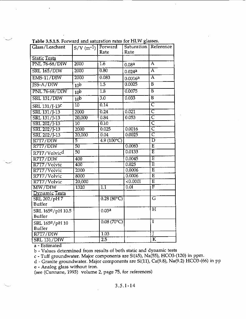
Table 3.5.1.5. Forward and saturation rates for HLW glasses. Glass/Leachant S/V (m-1) Forward Saturation Reference
Rate Rate Static Tests PNL 76-68/DIW 2000 1.6 0 .08a A
SRL 165/DIW 2000 0.80 0.024a A
EMS-11/DIW 2000 0.083 0.0016a A
JSS-A/DIW job 1.5 0.0025 B
PNL 76-68/DIW 10b 1.8 0.0075 B
SRL 131/DIW 10b 3.0 0.033 B
SRL 131 /J-13c 10 0.14 C
SRL 131/J-13 2000 0.24 0.021 C SRL 131/J-13 20,000 0.84 0.053 C SRL 202/J-13 10 0.10 C SRL 202/J-13 2000 0.025 0.0016 C SRL 202/J-13 20,000 0.04 0.0025 C R7T7/DIW 5 4.9 (100-C) D R7T7/DIW 50 0.0083 E
R7T7/Volvicd 50 0.0133 E
R7T7/D1W 400 0.0045 E R7T7/Volvic 400 0.025 E R7T7/Volvic 2000 0.0006 E R7T7/Volvic 8000 0.0006 E R7T7/Volvic 20,000 <0.0001 E MW/DIW 1320 1.1 0.01 F Dynamic Tests SRL 202/pH 7 0.28 (80°C) G Buffer
SRL 165e/pH 10.5 0.05a H
Buffer SRL 165e/pH 10 0.08 (70°C) I Buffer R7T7/DIW _1.03 J SRL 131/DIW 12.5 K a - Estimated b - Values determined from results of both static and dynamic tests c - Tuff groundwater. Major components are Si(45), Na(55), HCO3-(120) in ppm. d - Granite groundwater. Major components are Si(11), Ca(9.8), Na(9.2) HCO3-(66) in pp e - Analog glass without iron. (see (Cunnane, 1993) volume 2, page 75, for references)
3.5.1-14

Glass Release From A Waste Package
Two water contact modes, flow-through and bathtub, are modeled here, adapting data from batch and flow-through tests. In the flow-though mode, as shown in Fig. 3.5.1.5, we assume the water flowing down the side of a waste glass log without mixing, and keeping a surface area, s, wet. In the bathtub mode, the waste package develops a breach and water flows in and fills up over time and eventually overflows as illustrated in Fig. 3.5.1.6. The water inside the container is assumed well mixed.
The units used in the performance assessment model are meters, grams, years, and degrees Celsius (°C).
Inflow Rate = q Silica Concentration= Qi
,--Water Thickness =A I:A Total Volume = sA
. -Unit Volume = s'A
Outflow Rate = q Silica Concetration= Q0
Figure 3.5.1.5. Flow-through Water Contact Mode
Eqn. 3.5.1.1 predicts that the dissolution rate will slow down as the dissolution adds to the silica in solution. Silica (SiO 2) is one of the components of glass waste. For example, the DWPF glass contains about 50 wt% of silica (Cunnane, 1993) . After water flows inside the waste package, the change of silica concentration in the solution comes from the dissolution of silica released from the glass during alteration process. As the glass dissolves, secondary phases begin to precipitate. A fraction of the silica, fp, contained in the glass will be trapped in the secondary
3.5.1-15

phases. That is, only (1 - fp) of silica in altered glass actually dissolves in the
solution. The value of fp increases with increasing surface area to volume ratio and
silica concentration in solution. Since there is not sufficient data for consideration of
the change of fp, a constant intermediate value of fp is assumed in our model.
Inflow Rate = q Overflow Rate = q Silica Concentration =Qi Silica Concentration = Qo
Container () &-" "Volume = Vf
Figure 3.5.1.6. Bathtub Water Contact Mode
On the other hand, the dissolution rate will change because of changes of pH in the solution. However, the change in pH will be a complex function of the flow rate, buffer capacity of the fluid, and alkali content of the glass. There is insufficient data to obtain a relationship for the change of pH due to the dissolution of glass. Therefore, only the initial pH value of the inflow groundwater is used in the calculation. This is probably true for the flow-through mode with a high flow rate.
Flow-through Mode
The area of the glass log wetted by water, s, is usually unknown in the flowthrough water contact mode. It is to be determined within the model for in-package hydrology. A larger wetted area generally produces a larger release. For glass, the larger area produces a slowdown of alteration rate due to the silica in solution nearing saturation. The two effects oppose each other. Also there is a long-term alteration rate which provides a minimum on the rate factor. The net release rate which results as a consequence of these three factors must be evaluated with the numerical model. It cannot be predicted in a simple way.
With a thickness of the water film on the glass of A, the volume of water
covering the glass is s.A. When groundwater of a flow rate of q covers a portion of surface area as shown in Fig. 3.5.1.5, the time for the water to flow in and out of the package is tin = s A/q. As the water proceeds downward, the silica increases and the
reaction rate slows down. For a steady state flow condition, the glass dissolution
3.5.1-16

condition can be considered like a unit volume Of water (s'A) contacting the glass for a duration of tin. The increase of silica concentration during a time interval, dt,
dQ s kfsi(1- fP) 1- Qdt (3.5.1.7)
dQ = AsKA
where fsi = fraction of silica in glass. Therefore,
- nIQ kAs~ l) (3.5.1.8)
where C is a constant depending on the initial conditions. If the silica concentration of incoming groundwater is Qi, and that of outgoing is Qo after a duration of tin, then
Qo- Q= K(1- Q)[I - exp(-a)] (3.5.1.9)
where a = fsi(I-fp) ks cx~~i~~fPKq
Let 13 = k s/K q, then we can see that a high water refresh rate gives a low
value of P3. When P3 is high the system approaches a saturated condition. Also fp starts changing toward high values but there are not very precise data for fp. We use the intermediate value of 0.5.
Since only a fraction of silica, fsi (1- fp), in the waste glass dissolves in the solution, the total mass of dissolved glass per unit volume of outgoing water should be
G. - (3.5.1.10)
The dissolution rate (g/yr) from the whole waste glass in the waste package for the flow-through water contact mode is,
R=qGo = q(Qo-Q) _ qK _ _ l - exp(-a)] (3.5.1.11) fs,•(i- fp) - sj -(- f P) (
According to data in Table 3.5.1.2, K (g/m 3) can be expressed as a function of T (°C):
K = 6.0x10⁻⁵ + 1.90x10-; T + 1.25x10⁻⁸ T2 (3.5.1.12)
3.5.1-17
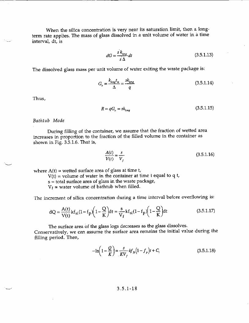
When the silica concentration is very near its saturation limit, then a longterm rate applies. The mass of glass dissolved in a unit volume of water in a time interval, dt, is
dG = s'kt°!L dt (3.5.1.13) sA
The dissolved glass mass per unit volume of water exiting the waste package is:
G,= lo-g--n = Lkong (3.5.1.14) A q
Thus,
R = qGo = sk,,ng (3.5.1.15)
Bathtub Mode
During filling of the container, we assume that the fraction of wetted area increases in proportion to the fraction of the filled volume in the container as shown in Fig. 3.5.1.6. That is,
A(t)= s (3.5.1.16) V(t) Vf
where A(t) = wetted surface area of glass at time t, V(t) = volume of water in the container at time t equal to q t, s = total surface area of glass in the waste package, Vf = water volume of bathtub when filled.
The increment of silica concentration during a time interval before overflowing is:
dQ = A-t)kfsi(1-_ f _ dt s kfsi (1-fp) 1- dt (3.5.1.17) V(t) K) Vf
The surface area of the glass logs decreases as the glass dissolves. Conservatively, we can assume the surface area remains the initial value during the filling period. Then,
-I j_!2 = -S-kfj. (1 - f, )t + C, (3.5.1.18) K) .KVf
3.5.1-18

where C1 is a constant depending on the initial conditions. The time for filling up the container is tf = Vf/q. If the silica concentration of incoming groundwater is Qi,
and that at the time of overflow is Qf, then
Qf - Qi = K12- 1-exp S1 fp)f K 1 - - exp(--K)]
where a= fs,(1 fp) ks (3.5.1.19)
To estimate the mass of glass dissolved during filling, we consider the possible maximum increase of silica concentration of the solution inside the container:
(Qf - Q0ax (3.5.1.20)
According to Table 3.5.1.2, the silica concentration increase at 90'C is 0.000225 g/m 3 . For four glass logs of 0.3 m in radius and 2.2 m in length inside a container with a
radius of 0.80 m and a length of 3.76 m, the bathtub volume, Vf, is 5.072 m3 ' Assuming fsi = 0.45 and fp = 0.5, we obtain the mass of dissolved glass during filling
= 0.000225x5.072/(0.45x0.5) = 0.0051 g. This loss of mass is negligible compared with the initial mass of the four glass logs of 6720 kg. Therefore, the assumption of constant surface area of glass is appropriate during the filling period.
After filling, i.e., t > tf, the change of silica in the water inside the container will be:
Vf dQ = skfi (1 - f,)( I (Q~- ~Qi)q dt =[(cxK + Q) -(tx+ )Qjqdt (3.5.1.21)
The loss of mass of glass long time after filling can be significant. To deal with changes of surface area resulting from the dissolved mass of the glass logs, calculations can be performed with time steps. Again, the surface area can be conservatively assumed constant as the initial value. Then, solving the differential equation with the boundary conditions at the time of overfilling, we obtain
Q0- Qi =a-K I1+ 9-1[-exp(-r)] + (Qf - Q,)exp(-'r) (3.5.1.22)
where " = . For a steady state when t-*oo, exp(-r) --4 0, then ti
3.5.1-19

Q, -Q, =a'+ (I 2KO(3.5.1.23)
The release rate (g/yr) of the waste glass out from the waste package for the bathtub mode is,
R= q(a - Qi) (3.5.1.24)
f~ (I - fp)
For the long-term silica-saturated condition,
R = s k,,g (3.5.1.25)
3.5.1.7 Solubility-limited radionuclide release from glass.
The data below provide radionuclide solubility limits for the elements U, Pu, Np, Am, Sr, and Cs calculated for SRL-202-type high level waste glasses reacting in J13 water. The data from the calculations are compared with radionuclide concentrations measured in laboratory glass dissolution.
Radionuclide concentrations are calculated for four scenarios. Two are closed systems in which the redox state and total carbon were controlled entirely through reactions between J-13 water and the glass reactant. The other two scenarios are for open conditions where the total carbon and redox state of the fluid are controlled by atmospheric gases assumed to be present in the proposed underground repository at Yucca Mountain. For the open system simulations, the pressures of carbon dioxide and oxygen gases are assumed to be 0.00032 bars and 0.20 bars respectively, their average atmospheric values. The compositions of J-13 water and the SRL-202 glass used in the simulations are given in Tables 1 and 2 respectively.
Table 3.5.1.6. Composition of J-13 well water used in the simulation, from Delaney, 1985. Component Concentration
(mg/L) Li 0.042 Na 43.9 K 5.1
Ca 12.5 M~g 1.9 Sr 0.035 Al 0.012 Fe 0.006 Si 27.0
3.5.1-20

NO3 9.6 F 2.2 Cl 6.9 HCO3 125.3 SO 4 18.7 pH 7.6
3.5.1-21

Table 3.5.1.7. Composition of SRL-202 glass used in simulation. Glass SRL-202 Reduced Component Set
Oxide Element oxide oxide element element cation wt% mole % wt% mole % mole %
SiO2 Si 48.9500 56.53 22.88 17.21 40.72 A1203 Al 3.8400 2.61 2.03 1.59 3.76 B203 B 7.9700 7.94 2.48 4.84 11.44 Mn203 Mn 1.0033 0.44 0.70 0.27 0.64 Fe203 Fe 11.4100 4.96 7.98 3.02 7.14 Na20 Na 8.9200 9.99 6.62 6.08 14.39 K20 K 3.7100 2.73 3.08 1.66 3.94
i20 Li 4.2300 9.82 1.97 5.98 14.15 ,Ts20 C~s 0.0720 0.02 0.07 0.01 0.03
aO Ca 1.2000 1.48 0.86 0.45 1.07 M g 1.3200 2.27 0.80 0.69 1.64
rrO Sr 0.1100 0.07 0.09 0.02 0.05 MnO Mn 0.9016 0.88 0.70 0.27 0.64 U308 U 1.9300 0.16 1.64 0.15 0.34 Np02 Np 0.0080 0.00 0.01 0.00 0.00 Pu02 Pu 0.0220 0.01 0.02 0.00 0.00 Am203 Am 0.0004 0.00 0.00 0.00 0.00 Th02 Th 0.2600 0.07 0.23 0.02 0.05 Totals 95.8573 100.00 95.86 100.00 100.00
Two types of calculations were carried out for both the closed and open systems. In the first, all possible mineral phases that can form were allowed to precipitate as alteration minerals, including those which for kinetic reasons generally do not form at low temperatures or over short time periods. In the second simulation, phases that are known or suspected not to precipitate rapidly at low temperatures were suppressed from the simulation. These phases are listed in Table 3. Note that the list includes some highly insoluble actinide oxide phases (PuO2, NpO 2, and Am20 3), which results in predictions of much higher actinide solubilities for the second case than for the first case. The list also includes phases such as quartz and andradite that do not contain radionuclides, but which are known from observations of natural analogs not to form. readily at low temperatures. One consequence of suppressing these phases is that the solution concentrations of some elements, such as Si and Al, increase to higher values during the simulation than is the case for simulations when the phases are not suppressed. This affects the solubility limits for the radionuclides by changing both the amounts of ligands available for complexation, the solution pH1, and the concentrations of competing metals. The ultimate effect of the suppression of these phases on radionuclide solubilities is therefore complex, as discussed below.
3.5. 1-22

Table 3.5.1.8. Phases suppressed in glass dissolution simulation in "metastable" calculation.
Name Formula Name Formula Am 2C3 - PuO 2 -
Am 20 3 -- NpO AmO 2 -- Quartz SiO 2
Andradite Ca 3Fe 2(SiO 4 )3 Rhodonite MnSiO 3
Dolomite CaMg(C0 3)2 Talc Mg3 Si40 10(OH)2 K-Feldspar KAISi 30 8 Tephroite Mn 2SiO4 Np20 5 -- Thorianite ThO2
Petalite LiAlSiO 1 o Tridymite SiO 2
Each simulation begins with one liter of J-13 water and one gram of SRL-202 glass. All calculations were performed using the GEMBOCHS version EQ3/6 V8-R6 composite data file. The glass and water were allowed to react at a fixed rate until the one gram of glass has completely reacted. The system is then composed of a modified water composition in equilibrium with a set of alteration minerals that formed during the reaction. The choice of one gram of glass per liter fluid is arbitrary. Simulations using a smaller amount of glass show that the pH and Eh of the system are not yet dominated by the glass; whereas the system is relatively insensitive to reacting greater amounts of glass. The results thus provide an approximation of "bathtub type" repository situations where water has breached the glass containment and sits in contact with the glass for extended periods of time under relatively stagnant conditions. A more precise time of reaction is impossible to estimate without including more details of hydrologic conditions, such as flow rates.
Table 4 shows the results of the four simulations; 4A shows the closed system results, 4B shows the open system results. The line labeled "Total" in Table 4 gives the total amount of radionuclide in the one gram of glass. For each element, this is the conservative maximum available for colloidal transport. The next four lines provide the solubility of each radionuclide (if solubility limited), the stable phase containing that element that controls the solubility, and the dominant aqueous complex of that element. The first case is for control by metastable solids (as discussed above) and the second case allowing all potential precipitates to form. Note that because the systems are constrained differently (closed vs. open) the solutions for the two cases are at much different values of pH, fo0 , and fco2. (see Table 4 caption). The radionuclide solubilities are thus being compared under much different conditions. The difference in values can provide an indication of the sort of variability in solution concentrations which can be expected for differing repository conditions.
3.5.1-23
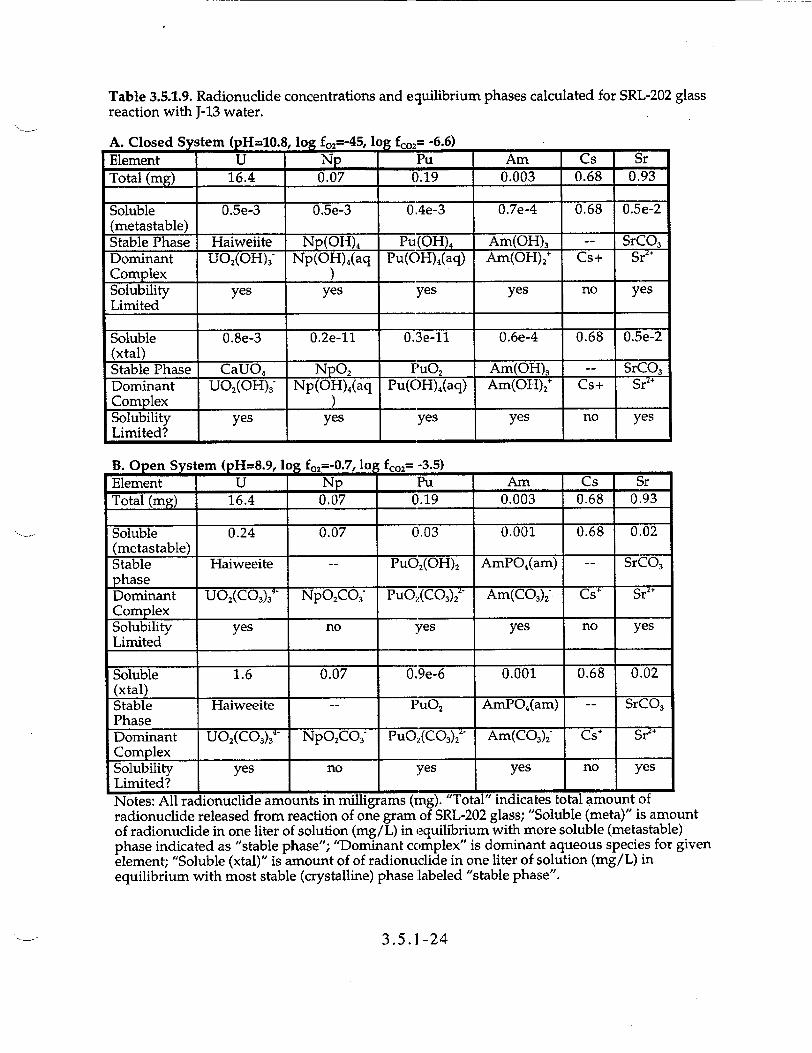
Table 3.5.1.9. Radionuclide concentrations and equilibrium phases calculated for SRL-202 glass reaction with J-13 water.
A. Closed Sytem (pH=10.8, log f02=-45, 1o fc0 2= -6.6)
Element U Np Pu Am Cs Sr Total (mg) 16.4 0.07 0.19 0.003 0.68 0.93
Soluble 0.5e-3 0.5e-3 0.4e-3 0.7e-4 0.68 0.5e-2 (metastable) Stable Phase Haiweiite Np(OH)4 Pu.(OH)4 Am(OH)3 -- SrCO 3 Dominant UO2(OH)3 Np(OH),(aq Pu(OH)4(aq) Am(OH),* Cs+ Sr7Complex ) Solubility yes yes yes yes no yes Limited
Soluble 0.8e-3 0.2e-11 0.3e-11 0.6e-4 0.68 0.5e-2 (xtal) Stable Phase CaUO4 NpO2 PuO 2 Am(OH)3 -- SrCO3 Dominant UO2(OH)3- Np(OH)4(aq Pu(OHX)(aq) Am(OH)24 Cs+ Sr Complex _ ) Solubility yes yes yes yes no yes Limited? I _
B. Open System (pH=8.9, log f,,=-0.7, lo fc2= -3.5) Element U Np Pu Am Cs Sr Total (mg) 16.4 0.07 0.19 0.003 0.68 0.93
Soluble 0.24 0.07 0.03 0.001 0.68 0.02 (metastable) Stable Haiweeite -- PuO2(OH)2 AmPO4(am) -- SrCO3 phase 4_________
Dominant U0 2(C0 3)3 NpO2CO PuOC3)2" Am(COA)2 Cs' Sr Complex Solubility yes no yes yes no yes Limited
Soluble 1.6 0.07 0.9e-6 0.001 0.68 0.02 (xtal) Stable Haiweeite -- PuO2 AmPO,(am) -- SrCO3 Phase Dominant UO(CO3)34- NpO 2CO3 PuO.(CO 3))"7 Am(C0 3)2 Cs+ Sr,2 Complex Solubility yes no yes yes no yes Limited?
Notes: All ractionucliae amounts in miuigrams kmg). - otai maicates totat amount or radionuclide released from reaction of one gram of SRL-202 glass; "Soluble (meta)" is amount of radionuclide in one liter of solution (mg/L) in equilibrium with more soluble (metastable) phase indicated as "stable phase"; "Dominant complex" is dominant aqueous species for given element; "Soluble (xtal)" is amount of of radionuclide in one liter of solution (mg/L) in equilibrium with most stable (crystalline) phase labeled "stable phase".
3.5.1-24

For all four simulations, U, Pu, Am and Sr are always solubility controlled, generally to a -much lower value than the total element available. Of the actinides, only Np is found not to be solubility controlled. Under open system conditions, the relatively high solubility of oxidized Np combined with high carbonate concentrations due to additions of CO. from air stabilizes the NpO2 CO3 complex to where the least soluble Np phase, NpO2 is still a half log unit undersaturated at 0.07 mg/L aqueous Np concentration. Under reducing conditions (closed system) the Np is always solubility controlled.
An important conclusion from Table 4 is that actinide solubilities are extremely sensitive to whether highly ordered anhydrous crystalline phases (i.e. PuO,) or metastable phases such as Pu(OH)4 control actinide solubilities. These differences can be as high as 7 log units for Pu and Np.
Notice that unlike the other actinides, uranium solubilities actually decrease when the metastable phases are used to control solubilities. This is true for uranium mainly because of the increased silica concentrations in the metastable phase alteration simulations due to suppression of quartz. Greater silica in solution increases the stability of uranium silicate phases such as Haiweeite, which lowers uranium solubility.
Figure 1 shows the results of Table 4 graphically. The soluble fraction of total radionuclide inventory available from one gram of glass is plotted for both the metastable solids assemblage and stable solids assemblage. If the element is not solubility controlled (i.e. Cs ) the entire inventory is available and no bar is shown.
3.5.1.8 Comparison With Laboratory Results
Measured actinide releases from long-term drip tests of high-level waste glasses have been reported (Fortner et al., 1996). Data from their N2-10 test are shown in Figure 1. These were unsaturated (drip) tests of EJ-13 water onto SRL-165 glass. Unfortunately, for several reasons, these experimental data cannot be directly compared to our model calculations. First, the tests report the entire released inventory of actinides, including soluble, colloidal, and adsorbed masses. We calculate only the soluble amounts in EQ3/6 models. Precipitated actinide solids are included in the masses of precipitated secondary phases. EQ3/6 cannot predict the relative amounts of these solids which remain on the glass monolith versus those which flake off and fall to the bottom of the test vessel. Second, the tests are of older formulation SRL-165 glasses and cannot be compared directly with our model calculations, which are for the current SRL-202 glass composition. The finally, the data reported do not include the amounts of fluid in which the total masses of actinides were measured, so that they cannot be converted to concentration units, needed to determine the relative saturation states of the actinides. These apparent shortfalls are a consequence of the defined purpose of these tests. The tests are meant to simulate as close as possible anticipated repository conditions, and are therefore not optimum for validation of modeling studies. However, it is still useful to compare trends and relative solubilities of actinides between the experiments and these simulations. The drip test procedure calls for periodic
3.5.1-25

refreshing of the test vessel with air. The drip test methodology therefore correlates best with our open system simulations, where the system stays equilibrated with air. The Fortner results show that Np is the most soluble actinide, in agreement with the simulation results. there is no indication of solubility control of Np release in these tests, consistent with our calculated results. Am and Pu are generally released at rates 3-4 log units slower than Np. Their release is probably solubility controlled. This is consistent with Pu solubility control by some metastable solid somewhat less stable than pure crystalline PuG2. The amount of released uranium is intermediate between Np and Pu, again in agreement with the modeling results.
The increase release of Pu and Am occurring after about 8 years shown in Figure 2 is thought to be due to spallation of the actinide-containing rinds of alteration minerals to the bottom of the test vessel. The spalled material is potentially available for colloidal transport.
More exact comparison of the model results with the experiments depends on the better characterization of the alteration products which control actinide solubilities (work which is in progress), and a better estimate of the effective oxidation state and pH of the fluid inside the test vessel. Actinide solubilities are highly dependent on Eh and pH. overall, the model results are in qualitative agreement with the experimental observations.
3.5.1-26

0.1
0.0
ob 07!.~ ............. .(."a)..clo.s..ed...system
6. • • : m Metastable Solid
0 .0 .. .. . . . . . . ................. . . i ' ........... .. .... ..................... ........ ...
........... .................. ................ ........... Stable Solid S10i ......... ... .. ... .. -.
S........................ ................ . .......... .......................... ".......................... .:-....................... '
U Np Pu Am Cs Sr 0 1 0 . . ....... .......................... .............. ........................ e m
...... ................ ........ e s.st.m 0Metastbe Solids
1 9 ........................ ................ . . ................ .. . ...... S
......... :. ..........o....e .......s........s..m......................
....ooo.... . .. . ........ ...............
[Li! []~ Mtstable Solids
10 "11 . .2 .. ....... ... .. S t b l d
lf 6 J. I_. •a_ U Np Pu A m Cs Sr
Figure 3.5.1.7. Histogram showing fractions of radionuclide inventory in
glass available for transport for (a) closed system simulation, and (b) open system simulation. Three cases are shown for each element: 1. no solubility control (all values = 1), 2. solubility control by metastable solids, and 3. solubility control by stable solids. Data are from Table 4.
3.5. 1t-27

100N2-10
~10
0 1
S0.1 - 7 ... .......... .......... .... .. . ..... ..
N
S0.01 ---- Am 0 +
0.001
0 2 4 6 8 10 Time(years)
Figure 3.5.1.8. Experimental data modified from Figure 1-7 in Fortner et al.(1996) showing the normalized release of actinides from SRL-165 glass in an unsaturated (drip) test. Release values shown include cumulative soluble, sorbed, and colloidal release.
3.5.1.9 References
Bates, J. K., Bourcier, W. L., Bradley, C. R., Brown, N. R., Buck, E. C., Carroll, S. A., Cunnane, J. C., Dietz, N. L., Gerding, T. J., Gong, M., Hafenrichter, L. D., Hoh, J. C., Mazer, J. C., Newton, L., Phillips, B. L., Pletcher, R., and Wronkiewicz, D. J. (1994). ANL Technical Support Program of DOE Environmental Restoration and Waste Management Report No. ANL-94/19. Argonne National Laboratory.
Bates, J. K., Bourcier, W. L., Bradley, C. R., Buck, E. C., Cunnane, J. C., Dietz, N. L., Ebert, W. L., Emery, J. W., Ewing, R. C., Feng, X., Gerding, T. J., Gong, M., Hoh, J. C., Li, H., Mazer, J. J., Morgan, L. E., Newton, L., Nielsen, J. K., Phillips, B. L., Tomozawa, M., Wang, L. M., and Wronkiewicz, D. J. (1993). ANL Technical Support Program for DOE Environmental Restoration and Waste Management; Annual Report, October 1991-September 1992 No. ANL-93/13. Argonne National Laboratory.
Bates, J. K., and Gerding, T. J. (1989). NNWSI waste form test method for unsaturated disposal conditions No. UCRL-15723. Lawrence Livermore National Laboratory.
Baxter, R. G. (1983). Description of defense waste processing facility reference waste form and container. Report No. Dp-1606. Savannah River Plant.
3.5.1 -28

Bethke, C. M. (1992). The Geochemist's Workbench: A users gide to Rxn, Act2, Tact, React. and Gtplot. U. of Illinois Press.
Bourcier, W. L. (1994). Critical review of glass performance modeling Report No. ANL-94/17. Argonne National Laboratory.
Cunnane, J. C. e. (1993). High-level waste borosilicate glass: a compendium of corrosion characteristics. No. DOE-EM-0177. DOE-EM-0177USDOE Office of Waste Management.
Delage, F., Ghaleb, D., Dussossoy, J. L., Chevallier, 0., and Vemaz, E. (1992). A mechanistic model for understanding nuclear waste. J. Nuc. Materials, 190:191197.
Delaney, J. M. (1985) reaction of Topopah Spring Tuff with J-13 water: a geochemical modeling approach using the EQ3/6 reaction path code. Lawrence Livermore National laboratory Report UCRL-53631, 46 p.
Fortner, J. A., J. K. Bates and S. F. Wolf (1996) Annual Progress Report, FY96, "Yucca Mountain Project - Argonne National Laboratory (draft).
Jantzen, C. M. (1992). Thermodynamic approach to glass corrosion. In D. E. Clark & B. K. Zoitos (Eds.), Corrosion of Glass, Ceramics, and Ceramic Superconductors (pp. 153-215). Park Ridge, New Jersey: Noyes Publications.
Johnson, J. W., Oelkers, E. H., and Helgeson, H. C. (1992). SUPCRT92: A software package for calculating the standard molal thermodynamic properties of minerals, gases, aqueous species, and reactions from 1 to 5000 g=bars and 0 to 1000C. Computers and Geosciences, 18:890-947.
Knauss, K. G., Beiringer, W. J., and Peifer, D. W. (1987). Hydrothermal interaction of solid wafers of Topopah Spring Tuff with 1-13 water at 90 and 150C using Dicksontype gold bag rocking autoclaves: Long-term experiments. Report No. UCRL53722. Lawrence Livermore National Laboratory.
Knauss, K. G., Bourcier, W. L., McKeegan, K. D., Merzbacher, C. I., Nguyen, S. N., Ryerson, F. J., Smith, D. K., Weed, H. C., and Newton, L. (1990). Dissolution kinetics of a simple nuclear waste glass as a function of pH, time, and temperature. Mat. Res. Soc. Symp. Proc., 176:371-381.
Lamont, A. D., and Gansemer, J. D. (1994). User guide to the Yucca Mountain Integrating Model (YMIM), version 2.1. Report No. UCRL-LR-116446. Lawrence Livermore National Laboraotory.
Plodinec, M. J., Jantzen, C. M., and Wicks, G. G. (1984). Stability of radioactive waste glasses assessed from hydration thermodynamics. Mat. Res. Soc. Symp. Proc., 26:755-762.
Stout, R. B., and Leider, H. R. (1991). Preliminary Waste Form Characteristics Report Version 1.0 Report UCRL-ID-108314 Rev. 1. Lawrence Livermore National Laboratory.
Wilder, D. G. ed. (1992). Near-field environment report volume I: Technical basis for BES design No. UCRL-LR-107476. Lawrence Livermore National Laboratory.
3.5.1-29

Wolery, T. J. (1992). E03/6, A software package for geochemical modeling of aqueous systems: Package overview and installation guide. No. UCRL-MA-110662 PT 1. Lawrence Livermore National Laboratory.
Woodland, A. B., Bates, J. K., and Gerding, T. J. (1991). Parametric effects on glass reaction in the unsaturated test method. No. ANL-91/36. Argonne National Laboratory.
3.5.1-30

Section 3.5.2: Glass Dissolution Models
Version 1.2 April 4, 1997
3.5.2.1 Overview Of Glass Dissolution
A chemical model of glass corrosion will be used to predict the rates of release of radionuclides from borosilicate glass waste forms in high-level waste repositories. The model will be used both to calculate the rate of degradation of the glass, and also to predict the effects of chemical interactions between the glass and repository materials such as spent fuel, canister and container materials, backfill, cements, grouts, and others. Coupling between the degradation processes affecting all these materials is expected. The glass corrosion model must therefore be mechanistic, and not a simple empirical extrapolation of experimental glass degradation rates.
This overview is concerned with dissolution behavior of borosilicate glass compositions currently anticipated for use as waste forms under repository-relevant conditions. The models described here cannot be expected to predict glass corrosion rates under conditions significantly different from these.
Figure 3.5.2.1 illustrates the major processes taking place during glass corrosion. The reaction initiates with water diffusion into the glass and alkali ion exchange. Evidence for water diffusion comes from SIMS and ion probe profiling of reacted glasses which show diffusion profiles for water in a surface zone generally less than 1 micron thick 1, 2. Ion exchange is indicated by the early rapid release of alkalis relative to other glass components which is commonly observed in glass dissolution tests3 . Hydration and ion exchange result in the formation of two layers on the glass surface; an inner diffusion layer where concentration gradients for alkalis and water are observed, and an outer hydrated "gel layer" where network hydrolysis (breakage of Si-O-Si) bonds takes place. The gel layer is depleted in alkalis and boron and enriched in insoluble elements such as Al, Ca, Mg, and heavy metals (e.g. actinides).
With time, some elements released into solution re-precipitate on the hydrated glass surface and elsewhere as a variety of secondary phases. These phases are commonly clays, zeolites, and metal oxides/hydroxides. The reaction of glass to form secondary phases is driven by the thermodynamically unstable nature of glasses. Water allows glass to react and transform into a set of crystalline phases which are thermodynamically more stable. Water acts as a flux and allows the glass to react at a measurable rate. Under anhydrous conditions, even glass compositions
4 5 that are relatively non-durable in water are stable for billions of years , . Steady-state conditions are commonly observed during glass dissolution where
the rates of water diffusion and ion exchange are equal to the rate at which the glass network dissolves. Steady state conditions are evidenced by the tendency for the glass diffusion layer to remain constant in thickness while the glass dissolves away and the mass of secondary phases increases with time 6. In open system
3.5.2-1

experiments, the rate of release of most elements is approximately constant or slowly decreasing with time. In closed system experiments, the release rates slow down more rapidly with time due to "saturation" effects, the buildup of dissolved glass species in solution (Fig. 3.5.2.2). Increased silica concentrations are the primary reason for decreased dissolution rates 7 although other elements have an effect as
well 8. Elemental releases from glasses in closed system tests also show nonstoichiometric behavior, some elements are released much more rapidly than others (Fig. 3.5.2.2). Most of this non-stoichiometry is due to the precipitation of the less soluble glass components as secondary mineral phases, although a small amount is accounted for in the formation of leached layers.
Ti Glass begins to react with water
.................. I gel layer
jc jdiffusion la er ..... Hydration and ion l ............
¶ secondary phases Diffusion layer thickens until rate
7 .of diffusion of alkalis ........... equals rate of network
dissolution.
Diffusion layer maintains =11 •constant thickness as
....... glass dissolves at steady state. Secondary phases continue to grow.
Figure 3.5.2.1. Glass dissolution mechanism.
3.5.2-2

0 5 10 15 20 25 30 Time (days)
Figure 3.5.2.2. Normalized elemental release from SRL-165 glass reacted in 0.003m NaHCO3 at 1500C, SA/V 0.01cm- 1 .9
Nuclear magnetic spectroscopy (NMR) shows that network dissolution reactions taking place in the gel layer are complex. 170-doped experiments show that both breakage and re-formation of Si-O-Si linkages are taking place 10. Hydrolysis of the highly stressed glass structure allows relaxation and removal of incompatible elements. The original glass is transformed into a hydrous silica-rich phase plus local areas enriched in transition and other heavy metals such as actinides which eventually crystallize into a variety of solid phases, or are released into solution. In some flow-through glass dissolution tests, the gel layer appears to serve as a transport barrier that limits the overall dissolution rate ". However, in most closedsystem experiments, elemental release data and electron microscopic examination of the surface layers show that the overall reaction rate is not controlled by diffusion of elements through the alteration layers 7,12,13
Recent NMR data has also shown that boron in waste glasses is clustered into boron-rich regions 14. Boron occurs in both three and four-fold coordination with alkalis in a sodium di-borate-type structure. The high reactivity and solubility of these zones gives rise to the relatively rapid release of boron from borosilicate glasses in waste glass leach tests.
Rates of glass dissolution may also be strongly affected by certain dissolved elements. For example, dissolution rates of silicate glasses are strongly decreased in the presence of dissolved Mg, Pb, and Zn, and strongly enhanced, under some
3.5.2-3
conditions, by dissolved Fe (see below). Likewise, anions such as phosphate and sulfide are known to affect mineral dissolution rates and may likewise affect glass dissolution rates. Depending upon the specific metal, these effects may be attributable to several processes; the formalion of surface complexes, the precipitation of a surface layer providing a transport barrier, or the reaction of dissolved glass species with the dissolved metals causing the precipitation of
colloids or secondary phases which affect the glass dissolution affinity 15. These types of effects are potentially important in repository environments where a variety of dissolved species will be present from other repository materials.
In summary, a model for borosilicate glass dissolution must account for the following processes: (1) kinetically-controlled network dissolution, (2) precipitation of secondary phases, (3) ion exchange of selected elements, (4) in some cases, ratelimiting diffusive transport through a hydrous surface reaction layer, and (5) specific glass surface interactions with dissolved cations and anions. This set of coupled processes should be able to quantitatively predict observations of glass dissolution which include the saturation effect (glass dissolution rates slows down as dissolved glass species build up in solution); the increase in pH which accompanies glass dissolution in closed-system tests; the variability of glass dissolution rate as a function of glass composition; and rate-affecting interactions of the glass surface with dissolved cations and anions. We will first look at examples of how the five processes are incorporated into current models and then critically review modeling results using a representative set of examples for modeling of experimental data.
3.5.2.2 Modeling Of Glass Corrosion
Current long-term corrosion models for borosilicate glass employ a rate equation consistent with transition state theory embodied in a geochemical reactionpath modeling program that calculates aqueous phase speciation and mineral precipitation/dissolution. These models ignore early diffusion-controlled dissolution behavior which is more important for less durable glass compositions such as alkali-silicates and is important only in the very early stages of reaction of borosilicate waste glasses. Diffusion in this case refers to solid state diffusion of ions through the partially hydrated glass surface layer, not diffusion of aqueous species through the more hydrated and re-structured gel layer. We therefore do not discuss the many studies which solve the equations for the formation of a moving and thickening transport-limiting surface layer.
The Rate Law The rate law commonly used to model network hydrolysis, assumed to be rate
controlling during glass dissolution, has the general form 16,17:
d A Avik" ai -e(-1 - (3.5.2.1)
3.5.2-4

where ni is the number of moles of species i in solution released from the glass, t is time, A is the reactive surface area of glass, ni is the concentration of species i in the
glass, k is the rate coefficient for the glass, Il a,. is the product of the activities i
(concentrations) of dissolved aqueous species which make up the activated complex of the rate-limiting microscopic dissolution reaction, A is the reaction affinity defined as RTln(Q/K) where Q is the activity product and K the equilibrium constant for the rate-determining glass dissolution reaction, a is a stoichiometric factor that relates the rate-controlling microscopic reaction to the overall solid dissolution reaction (usually it is assumed a=1) R is the gas constant, and T is the temperature in Kelvin. The form of Eqn. 3.5.2.1 predicts that the dissolution rates of solids have the following characteristics: (1) the amount of solid dissolved is proportional to exposed surface area, (2) the dissolution rate slows down as the solid approaches saturation, and (3) the dissolution rate is constant under conditions far from saturation (Q/K << 1). An expression having this general form is used in all of the major glass modeling computer codes at this time (e.g. PHREEQE/GLASSOL 11, EQ3/6 9, DISSOL 18, REACT, 19 LIXIVER 20 .
This rate law implies that at equilibrium there is a reversible microscopic dissolution reaction which is rate-limiting. However, because glass is thermodynamically unstable and cannot reach saturation, the overall glass dissolution reaction is clearly not reversible. Therefore, when this rate law is applied to glass dissolution, it must be applied not to the overall reaction, but to some ratelimiting microscopic reversible reaction.
Many of the parameters in Eqn. 3.5.2.1 are not known either from theory or from experiments, so that in practice the equation is simplified to:
d .-= A vik(pH) 1- ) (3.5.2.2)
where the product term 1" a, is reduced to include only the pH dependence of the
rate coefficient, and the affinity expression is simplified and re-expressed in terms of the saturation index (Q/K) of the dissolving solid. This form of rate law is commonly used as an expression to which experimental elemental release data are fitted, i.e. values of k, K, r and s are determined by regression of experimental data.
Current modeling codes may further simplify Eqn. 3.5.2.2. GLASSOL assumes no solution compositional dependence of k, which is assumed to vary only with temperature. DISSOL, EQ3/6, LIXIVER, and REACT treat k as a function of both pH and T. No models account for any further dependencies of k on solution composition as indicated in Eqn. 3.5.2.1 above.
To use Eqn. 3.5.2.2 to predict glass dissolution rates, an assumption must be made as to what phase becomes saturated in order to evaluate the Q/K term. Several phases have been tried, ranging from the initial unreacted glass composition 9,18 ,to the composition of the alkali-depleted surface layer 21 to simple hypothetical silica
3.5.2-5
phases 11, 22-24 It is clear from these modeling studies that using the unreacted glass
composition gives results that deviate from experimental observations (see below). However, the other two approaches give comparable agreement with experiments.
Secondary Phases Precipitation of secondary phases takes place as glasses dissolve and the
concentrations of species build up in solution. Geochemical modeling codes used to model glass dissolution incorporate algorithms that track saturation states for these possible mineral phases and predict the most stable phase assemblage based on mineral thermodynamic data. The types and amounts of phases are continually adjusted during the reaction path calculation to maintain the most stable phase assemblage. While this approach works well for simulations of high-temperature hydrothermal systems, experience has shown that this approach often leads to incorrect phase assemblage predictions for the lower temperature (<1500C) glass dissolution tests 25,9. Thermodynamically less stable phases tend to precipitate instead.
Alternative methods of predicting secondary phases have therefore been used in the simulations. One method, termed "inverse modeling", uses the measured solution composition to identify which phases are near saturation 26. These phases are then assumed to be those actively precipitating and controlling the solution composition, and only these phases are then allowed to precipitate during the glass reaction. Another approach is to simply restrict the database of mineral phases allowed to precipitate to those actually observed experimentally. Obviously neither approach has any predictive capability for secondary phases, but no reliable theory is currently available to enable predictions of the most likely secondary phases in these complex systems (see Steefel et al. 27 for a possible new approach).
Ion Exchange The formation of secondary phases is the primary cause for the observed non
stoichiometric release of elements during glass dissolution. However, the formation of an alkali-depleted surface layer also contributes to non-stoichiometric release and also affects the pH of the solution through ion exchange reactions:
Glass - Na+ + H+ = Na÷ + Glass - H" (3.5.2.3)
Similar reactions take place for other alkalis including lithium, potassium, and cesium. The ion-exchanged zone has variable thickness depending on the glass composition and test conditions, but is generally a couple microns or less in extent. The net effect of the ion exchange reaction is to raise the pH of the surrounding solution. The pH effect is bigger as the surface area to volume ratio (SA/V) of the test increases.
Although the ion exchange process is complex and involves diffusion of ions and water through a partially hydrated and inhomogeneous medium, the chemical effect of the process can be modeled simply. And unless the ion exchange process is rate limiting, only the chemical effects need to be incorporated into the model. A
3.5.2-6

simple method for incorporating this effect first suggested a few years ago 28 was recently reported 19. In this approach, an ion exchange reactant in addition to the glass reactant is used in the simulation. This reactant is composed only of the elements released during ion exchange. The mass of this reactant is fixed by the experimentally measured thickness of ion exchanged zone. The reactant is allowed to react rapidly at first to simulate the rapid initial formation of an ion exchanged zone. The predicted pH and elemental concentration of species predicted using this method agree fairly well with experimental results"9 . Also, the results show that inclusion of ion exchange effects is only necessary for simulations of fairly high SA/V ratio.
Transport-limited corrosion Experimental evidence suggests that under certain flow-through test conditions,
the dissolution rate of some glasses is controlled by transport. Grambow " has hypothesized that it is the transport of silica through the surface alteration layers which is rate-limiting. The transport-limited rate is modeled by a simple diffusion law:
rD (a,-ab) + rf, (3.5.2.4) L
where (rt) is the dissolution rate, D and L are the diffusion constant and thickness of the hydrous alteration layer, (as-ab) is the dissolved silica concentration gradient across the layer from the surface (s) to the bulk solution (b). rfin is the "final rate", an experimentally estimated empirical parameter to account for the observed finite rate of glass reaction even at "saturation" where Eqn. 3.5.2.1 would predict zero reaction rate.
The affinity-based rate control (Eqn. 3.5.2.2) is combined with this simple diffusion rate control in the GLASSOL model 11. The model tests for whether the rate is controlled by transport or surface reaction and makes the appropriate calculation. Delage et al. 20 have also combined transport and affinity-based rate control in the LIXIVER code. In their model, the thickness and rate of silica diffusion through the gel layer control the concentration of silica at the gel layer/solution interface, which they use for the value of 'Q' in Eqn. 3.5.2.2. This approach thus assumes that silica diffusion through the gel layer affects the concentration of dissolved silica at the gel/solution interface thereby coupling the effects of silica transport and affinity rate control.
Surface Interactions Dissolved ions present in solution are known to affect glass dissolution rates.
For example, Mg and Zn are known to decrease glass dissolution rates 30,31 while dissolved iron is known to increase it 32. Current glass dissolution models all account for the effect of dissolved silica on glass dissolution, but currently do not account for the effects of other ions. Although silica effects are important, and in most cases dominate over the effects of other ions, this is not always the case, and it is necessary to provide for these other ions if the model is to be generally applicable.
3.5.2-7

This is especially important in repositories where the effects of species produced from corrosion of other repository materials, such as metals and cements, are available to interact with the dissolving waste forms.
Three general mechanisms by which dissolved species affect glass alteration rates have been proposed.
The first is that ions sorb onto the dissolving glass surface and affect the strength of the Si-O bonds at the glass surface (see Figure 3.5.2.3 below). It is the hydrolysis of these bonds which controls the overall rate of glass dissolution and radionuclide release. This effect is particularly significant for long-term performance, where the rate at "near saturation" conditions is likely to be strongly affected by the nature of the glass-solution interface, and therefore the types and concentrations of sorbed species, and the surface charge. Some attempts have been made to understand and model deviations in dissolution behavior believed to be due to surface complex formation 15, 32-35
The second mechanism is the reaction of dissolved species with the glass surface to form a protective layer. The protective layer armors the glass surface and reduces the rate of further attack. The overall dissolution process then becomes rate-limited by transport through the protective layer. It is believed that magnesium affects glass dissolution through this process.
The third mechanism involves the formation of colloids by reaction with the dissolved ion in question and species dissolving from the glass. An example of this is iron. Dissolved iron reacts with silica from the dissolving glass to form iron-silica colloids. The silica-containing colloids act as a sink for silica and maintain a low dissolved silica concentration in solution. This effectively reduces the glass saturation state and therefore causes the glass dissolution rate to remain high (see equation 3.5.2.1). Note that these colloids will also tend to sorb actinide species, and thus pose a potential migration pathway for otherwise insoluble actinide species.
Qualitative data for the effects of several dissolved metals on glass durability are listed in Table 3.5.2.1. This table summarizes a broad variety of data from experiments that in many cases are difficult to interpret due to lack of supporting data. Many of the studies for example do not report pH. In some cases the data conflict; the same dissolved species may cause the dissoluton rate to increase in one type of test and decrease in another. In other cases the glass dissolution rate may change with time. An aqueous component that first decreases glass reaction rate may later on enhance it (i.e. the case of lead reported by Zwicky et al. 1992, see table 3.5.2.1 notes). Another complication is that species may only have an effect if it is at a sufficiently high concentration to cause precipitation of an armouring surface solid, as is apparently the case for magnesium. At low dissolved Mg concentration, Mg has no noticeable effect " but at higher concentrations where the magnesium silicate phase sepiolite is supersaturated, Mg greatly decreases the glass reaction rate presumably due to precipitation of a surficial Mg-silicate phase such as sepiolite.
Note in Table 3.5.2.1 that there is a lack of data for many metals likely to be present in the repository (i.e. alloying metal in stainless steels such as Cr, Mn, Ni, Mo etc.).
3.5.2-8
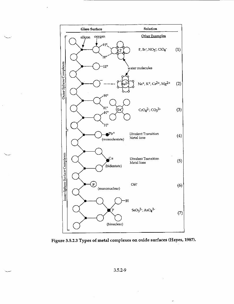
Figure 3.5.2.3 Types of metal complexes on oxide surfaces (Hayes, 1987).
3.5.2-9

Although this qualitative information is available, it alone is not sufficient for incorporation of these effects into models of glass dissolution. Experiments are needed which both identify the mechanisms through which dissolved species affect dissolution rates, and provide the parameters needed to quantify these effects in the glass dissolution models. Explicit provision for surface interactions will be especially critical in order to account for coupled effects of glass with other repository materials in performance assessment calculations.
Table 3.5.2.1 Effects of dissolved ions on glass dissolution rate. Metal Low pH Near-neutral pH High pH Reference
B none none unknown 1 Mg none major - major - 1,2,3,18 Ca none none minor - 1,3,13 Si none major - major - 1,12 Al major- minor - none/minor + 1,3,11,15 Na unknown minor - minor - 3 Zn unknown minor + major - 3,11,14 Li unknown unknown minor + 4 Fe unknown major/minor + major + 5,6,7,9,10,16,17 Pb unknown major - major - 7,8,10,11,15 Cu unknown unknown none 15 Sn unknown unknown none 15 Ti unknown unknown none 15
Notes: minor - less than factor of 10 effect; major - greater than factor of 10 effect; + means glass dissolution rate is increased, - means rate is decreased; none - no effect observed; unknown - no data or data uninterpretable. References for Table 3.5.2.1: (1) Bourcier et al., 1992, Proc. 7th Int. Symp. Water-Rock Interaction, p. 81-84. (2) Barkatt et. al., 1989, Applied Geochem. 4:593-603. (3) Lee and Clark, 1986, Adv. in Ceramics Vol 20, p. 541-550. (4) Feng and Barkatt (1987) Mat. Res.Soc Symp. Proc, Vol 84, p. 519-531. (5) Bunker and Arnold (1983) Mat. Res.Soc Symp. Proc, Vol 15, p. 151-158 (6) McVay and Buckwalter (1983), J. Am. Cer. Soc., 66:170-174. (7) Bart et al. (1987) Mat. Res.Soc Symp. Proc, Vol 84, p. 459-470. (8) Lehman and Kuchinski (1985) Mat. Res.Soc Symp. Proc, Vol 44, p. 179-186 (9) Bibler and Jantzen (1987) Mat. Res.Soc Symp. Proc, Vol 84, p. 47-66 (10) Burns et al. (1986) J. Noncryst. Solids 84:258-267. (11) Zwicky et al., (1992) Mat. Res.Soc Symp. Proc, Vol 257, p. 83-90. (12) Lanza et al., (1988) Mat. Res.Soc Symp. Proc, Vol 112, p. 685-691. (13) Oka et al., (1979) J. Am. Cer. Soc. 62:631-632. (14) Tait and Jensen (1982) J. Noncryst. Solids 49:363-377. (15) Buckwalter and Pederson (1982) J. Am. Cer. Soc., 65:431-436. (16) Hermansson et al. (1985) Nuc. and Chem. Waste Manag. 5:315-332. (17) Inagaki et al., (1996) Mat. Res.Soc Symp. Proc, Vol 412, p. 257-264. (18) Sang et al., (1994) Mat. Res.Soc Symp. Proc, Vol 333, p. 519-524.
3.5.2-10
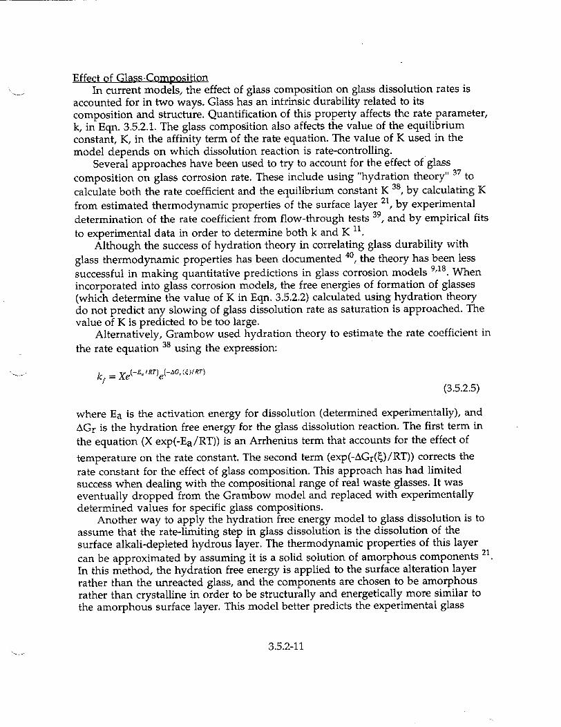
Effect of Glass-Composition In current models, the effect of glass composition on glass dissolution rates is
accounted for in two ways. Glass has an intrinsic durability related to its composition and structure. Quantification of this property affects the rate parameter, k, in Eqn. 3.5.2.1. The glass composition also affects the value of the equilibrium constant, K, in the affinity term of the rate equation. The value of K used in the model depends on which dissolution reaction is rate-controlling.
Several approaches have been used to try to account for the effect of glass
composition on glass corrosion rate. These include using "hydration theory" 37 to
calculate both the rate coefficient and the equilibrium constant K 38, by calculating K
from estimated thermodynamic properties of the surface layer 21, by experimental determination of the rate coefficient from flow-through tests 3 and by empirical fits
to experimental data in order to determine both k and K 11 Although the success of hydration theory in correlating glass durability with
glass thermodynamic properties has been documented 40, the theory has been less
successful in making quantitative predictions in glass corrosion models 9,18. When incorporated into glass corrosion models, the free energies of formation of glasses (which determine the value of K in Eqn. 3.15.2.2) calculated using hydration theory do not predict any slowing of glass dissolution rate as saturation is approached. The value of K is predicted to be too large.
Alternatively, Grambow used hydration theory to estimate the rate coefficient in
the rate equation 38 using the expression:
kf = Xe(-Eý RT)e((-AG (ý)IRT)
(3.5.2.5)
where Ea is the activation energy for dissolution (determined experimentally), and
AGr is the hydration free energy for the glass dissolution reaction. The first term in
the equation (X exp(-Ea/RT)) is an Arrhenius term that accounts for the effect of
temperature on the rate constant. The second term (exp(-AGr(4)/RT)) corrects the
rate constant for the effect of glass composition. This approach has had limited success when dealing with the compositional range of real waste glasses. It was eventually dropped from the Grambow model and replaced with experimentally determined values for specific glass compositions.
Another way to apply the hydration free energy model to glass dissolution is to assume that the rate-limiting step in glass dissolution is the dissolution of the surface alkali-depleted hydrous layer. The thermodynamic properties of this layer
can be approximated by assuming it is a solid solution of amorphous components 21
In this method, the hydration free energy is applied to the surface alteration layer rather than the unreacted glass, and the components are chosen to be amorphous rather than crystalline in order to be structurally and energetically more similar to the amorphous surface layer. This model better predicts the experimental glass
3.5.2-11

dissolution rates than does the hydration free energy model applied to the unaltered glass. However, the relationship between starting glass composition and glass dissolution rate in this model is complex. The composition of the alteration layer (which is used to calculate the glass dissolution affinity and therefore dissolution rate) is affected both by the glass composition and solution composition. No attempt has yet been made to quantify this effect in the glass dissolution model. The composition of the alteration layer is determined by analysis of reacted glasses.
Deviant glass dissolution behavior Several studies have shown that glass dissolution rates may abruptly increase in
rate after showing normal behavior over extended periods of time at what appeared
to be nearly constant "final" dissolution rates , , 2, .43 These rate changes may be
accompanied by abrupt changes in pH 43 and the onset of precipitation of new
secondary phases 29. The rate changes are not well understood, but may be related to
physical changes in the surface layers , secondary phase precipitation 29, or as yet unidentified processes.
3.5.2.3 Limitations Of Current Models
The most important problems of current models fall into three categories: (1) the fact that most model parameters are obtained from the same experiments as those being modeled, (2) the lack of a precise definition of the concept of "silica saturation", and (3) the poorly defined and quantified long-term release rate. These areas need to be addressed with additional experimental and modeling work.
Although the GLASSOL approach has successfully predicted glass corrosion tests results, some questions have been raised as to its suitability for long-term
predictions. Curti45 used the GLASSOL code to model the dissolution of the French COGEMA and British MW borosilicate glasses in order to assess whether GLASSOL can be applied to safety analysis of the Swiss high-level waste repository. Curti found three areas where improvement was needed before GLASSOL could be suitable for safety analysis, these included: (1) better accounting for the effects of silica sorption on bentonite backfill, (2) inclusion of provisions for partitioning radionuclides into alteration phases (currently stoichiometric release is assumed), and (3) the problem that the final rate of corrosion is poorly defined and has no mechanistic basis. Curti also notes that "a significant drawback of the modeling exercises reported ... is that the relevant parameters (k, Rfin, K) are derived ad hoc from the experiment to be modeled."
The most serious limitation of these three is that of estimation of the long-term or "final" reaction rate, both in terms of providing a mechanism controlling this
rate and a numerical value to be used in modeling. More recent work by Grambow 46
illustrates this problem using data from dissolution tests in saline fluids and suggests that the rate control may switch from surface reaction control to water diffusion control over long time periods. Clearly the exact mechanism which controls dissolution rates over long time periods is not yet known.
3.5.2-12

Godon et al. 47 have observed that R7T7 glass dissolution in contact with eleven different materials shows no systematic "silica saturation" level. Although the dissolved silica concentration reaches a nearly constant value in each test, that value varies greatly from test to test depending on the type of additional material present. The "silica saturation" level therefore is not a parameter related to glass composition only, but also depends on test conditions. The silica saturation level for a particular test probably results from a balance between the rate of formation of silica-containing secondary phases (including colloids) and the rate of release of silica from the glass. The silica saturation value (K) from Eqn. 3.5.2.2 above is therefore not a constant for a given glass composition but will change as a function of test conditions. Long-term predictions based on a constant value of K in the rate equation are therefore of questionable reliability.
3.5.2.4 Conclusions
It is clear that further progress in developing quantitative predictive models for glass dissolution depends on obtaining results from systematic interpretable experiments that confirm and quantify the postulated glass reaction mechanisms. Some work has been done in this area 48 39 but much remains to be done. Some specific suggestions for future work are given in 49 and include: '
(1) Flow-through tests of glasses in continuously stirred reactors with controlled pHs which are designed to measure the rate constant for glass dissolution over a matrix of temperatures, pHs and glass compositions. Similar tests should be performed in pH buffer solutions doped with relevant cations and anions to systematically determine the effects of dissolved species on dissolution rate. These tests should be combined with surface titrations to characterize glass surface speciation.
(2) Closed-system tests of a matrix of glass compositions with controlled pH (pH stat) to investigate the effect of glass composition on glass dissolution rate under conditions where secondary phases form (unlike the flow-through tests above). These tests should be combined with nuclear magnetic resonance (NMR) analysis of unreacted glasses in order to correlate glass structure and coordination with glass durability as measured in both the flow-through and closed system tests.
(3) Additional closed system tests should be performed where stable secondary phases such as calcite, quartz, and clays are added to control solution composition. The data from these tests should help to define and quantify the affinity term in the rate expression.
(4) Molecular orbital calculations of glass surface speciation and molecular dynamics simulations of glass dissolution behavior should be performed to help constrain macroscopic glass dissolution models and support validation of proposed dissolution mechanisms.
In all cases, experiments should include as complete an analysis of both solid and aqueous phases as possible. Too many experiments have been performed where incomplete characterization of either solids or solution phases have made
3.5.2-13
interpretation of the results ambiguous, both for mechanistic interpretation of the results, and for use of results in model validation attempts.
The results of these experimental investigations should be combined with
additional model development to produce a workable and sufficiently comprehensive glass dissolution model for use in repository performance assessment simulations.
3.5.2.5 References
(1) V.M. Oversby and D.L. Phinney, J. Nuc. Materials, 190, 247-268 (1992).
(2) T.A. Abrajano and J.K. Bates, Mat. Res. Soc. Symp. Proc., 84, 533-546 (1987).
(3) J.E.(. Mendel, "Final Report on the Defense High Level Waste Leaching
Mechanisms Program", Pacific Northwest Laboratory, PNL-5157, (1984).
(4) L.C. Klein, in Advances in CeramicsAmerican Ceramic Society: 1986; Vol. 20; pp
693-698.
(5) H.C. Palmer, K. Tazaki, W.S. Fyfe and Z. Zhou, Geology, 16, 221-224 (1988).
(6) T. Abrajano, J.K. Bates, W.L. Ebert and T. Gerding, "The effect of gamma radiation on groundwater chemistry and glass leaching as related to the NNWSI
repository site.", Argonne National Laboratory, SANL-510-001, (1986).
(7) L.A. Chick and L.R. Pederson, Materials Research Society Symposium Proceedings, 26, 635-642 (1984).
(8) W.L. Bourcier, H.C. Weed, S.N. Nguyen, J.K. Nielsen, L. Morgan, L. Newton and
K.G. Knauss, in Seventh Annual Water-Rock Conference; A.A. Balkema: 1992; pp 81-84.
(9) W.L. Bourcier, "Geochemical modeling of radioactive wasteglass dissolution using EQ3/6: Preliminary results and data needs", Lawrence Livermore National Laboratory, UCID-21869, (1989).
(10) B.C. Bunker, D.R. Tallant, T.J. Headley, G.L. Turner and R.J. Kirkpatrick, Phys. Chem. Glasses, 29, 106-120 (1988).
(11) B. Grambow, "Nuclear waste glass dissolution: Mechanism, model and application.", JSS Project, Swedish Nuclear Fuel and Waste Management Co.,
87-02, (1987).
(12) T. Murakami, R.C. Ewing and B.C. Bunker, Mat. Res. Soc. Symp. Proc., 112, 737748 (1988).
(13) T.A. Abrajano, J.K. Bates, A.K. Woodland, J.K. Bradley and W.L. Bourcier, Clays and Clay Minerals, 38, 537-548 (1990).
(14) B.L. Phillips, in ANL Technical Support Program for DOE Environmental Restoration and Waste Management. Annual Report October 1991-September
1992.2 J. K. Bates, Ed.; Argonne National Laboratory: 1993; Vol. ANL-93/13; pp 153-164.
(15) G.L. McVay and C.Q. Buckwalter, J. Am. Cer. Soc., 66, 170-174 (1982).
(16) P. Aagaard and H.C. Helgeson, Am. J. Science, 282, 237-285 (1982).
3.5.2-14

(17) A.C. Lasaga, J. Geophys. Res., 89,4009-4025 (1984).
(18) T. Advocat, J.L. Crovisier, B. Fritz and E. Vernaz, Mat. Res. Soc. Symp. Proc., 176,
241-248 (1990).
(19) W.L. Bourcier, W.L. Ebert and X. Feng, Proceedings of the Materials Research Society Symposium, 294:577-582 (1993).
(20) F. Delage, D. Ghaleb, J.L. Dussossoy, 0. Chevallier and E. Vernaz, J. Nuc.
Materials, 190, 191-197 (1992).
(21) W.L. Bourcier, D. Peiffer, K. Knauss, K. McKeegan and D. Smith, Mat. Res. Soc.
Symp. Proc., 176, 209-216 (1990).
(22) T. Advocat, J.L. Crovisier, E. Vernaz, G. Ehret and H. Charpertier, Mat. Res. Soc. Symp. Proc., 212, 57-64 (1991).
(23) E.Y. Vernaz and J.L. Dussossoy, Appl. Geochem., 1, 13-22 (1992).
(24) L. Michaux, E. Mouche and J.-C. Petit, Appl. Geochem., 1, 41-54 (1992).
(25) C.J. Bruton, Mat. Res. Soc. Symp. Proc., 112, 607-619 (1988).
(26) B. Grambow and D.M. Strachan, "A comparison of the performance of nuclear
waste glasses by modeling", Pacific Northwest Laboratories, PNL-6698, (1988).
(27) C.I. Steefel and P. Van Cappellen, Geochim. Cosmochim. Acta, 54, 2657-2677 (1990).
(28) D.M. Strachan, B.P. McGrail, M.J. Apted, D.W. Engel and P.W. Eslinger, "Preliminary assessment of the controlled release of radionuclides from waste
packages containing borosilicate waste glass", Pacific Northwest Laboratory, PNL-7591, (1990).
(29) W.L. Ebert, J.K. Bates, E.C. Buck and C.R. Bradley, Mat. Res. Soc. Symp. Proc., (in
press), (1993).
(30) A. Barkatt, E.E. Saad, R. Adiga, W. Sousanpour, A. Barkatt and M.A. Adel
Hadadi, Appl. Geochem., 4, 593-603 (1989).
(31) J.C. Tait and C.D. Jensen, J. Non-Cryst. Solids, 49, 363-377 (1982).
(32) C.T. Lee and D.E. Clark, in Advances in Ceramics. Vol. 20American Ceramic
Society: 1986.
(33) G. Bart, H.U. Zwicky, E.T. Aerne, T. Graber, D. Z'Berg and M. Tokiwai, Mat. Res.
Soc. Symp. Proc., 84, 459-470 (1987).
(34) B. Grambow, H.U. Zwicky, G. bart, I.K. Bjbrner and L.O. Werme, Mat. Res. Soc.
Symp. Proc., 84, 471-481 (1987).
(35) Z. Andriambololona, N. Godon and E. Vernaz, Mat. Res. Soc. Symp. Proc., 257, 151-158 (1992).
(36) Bourcier, W. L., H. C. Weed, S. N. Nguyen, J. K. Nielsen, L. Morgan, L. Newton,
and K. G. Knauss Water-Rock Int. 7th ]nt Symp. 81-84 (1992).
(37) C.M. Jantzen and M.J. Plodinec, Journal of Non-Crystalline Solids, 67, 207-223 (1984).
(38) B. Grambow Ph.D. Thesis, Freien Universitit Berlin, 1984.
3.5.2-15

(39) K.G. Knauss, W.L. Bourcier, K.D. McKeegan, C.I. Merzbacher, S.N. Nguyen, F.J.
Ryerson, D.K. Smith, H.C. Weed and L. Newton, Mat. Res. Soc. Syrnp. Proc., 176, 371-381 (1990).
(40) C.M. Jantzen, in Corrosion of Glass. Ceramics. and Ceramic Superconductors: D. E. Clark and B. K. Zoitos, Ed.; Noyes Publications: Park Ridge, New Jersey, 1992; pp 153-215.
(41) A. Barkatt, A. Olszowka, W. Sousanpour, M.A. Adel-Hadadi, R. Adiga, A. Baraktt, G.S. Marbury and S. Li, Mat. Res. Soc. Symp. Proc., 212, 65-76 (1991).
(42) J. Patyn, P. Van Iseghem and W. Timmermans, Mat. Res. Soc. Symp. Proc., 176, 299-307 (1990).
(43) P. Van Iseghem, T. Amaya, Y. Suzuki and H. Yamamoto, J. Nuc. Materials, 190, 269-276 (1992).
(44) J.C. Sang, A. Barkatt, I.G. Talmy and M.K. Norr, Mat. Res. Soc. Symp. Proc., 294, 583-589 (1993).
(45) E. Curti, "Modelling the dissolution of borosilicate glasses for radioactive waste disposal with the PHREEQE/GLASSOL code: theory and practice", Paul Scherrer Institute, PSI-Bericht Nr. 86, (1991).
(46) B. Grambow, W. Lutze and R. MUller, Mat. Res. Soc. Symp. Proc., 257, 143-150 (1992).
(47) N. Godon, E. Vernaz, J.H. Thomassin and J.C. Touray, Mat. Res. Soc. Symp. Proc., 127, 97-104 (1989).
(48) L. Trotignon Ph.D. Thesis, Paul Sabatier University, 1990.
(49) D.M. Strachan, W.L. Bourcier and B.P. McGrail, Radioactive Waste Management and the Fuel Cycle, (in press), (1993).
3.5.2-16

DRAFT DISCLAIMER
This contractor document was prepared for the U.S. Department of Energy (DOE), but has not
undergone programmatic, policy, or publication review, and is provided for information only.
The document provides preliminary information that may change based on new information or
analysis, and is not intended for publication or wide distribution; it is a lower level contractor
document that may or may not directly contribute to a published DOE report. Although this
document has undergone technical reviews at the contractor organization, it has not undergone a
DOE policy review. Therefore, the views and opinions of authors expressed do not necessarily
state or reflect those of the DOE. However, in the interest of the rapid transfer of information,
we are providing this document for your information.

MOL. 19970716.0414 TRW TRW Environmental 1180 Town Center Drive WBS: 1.2.4.7 Safety Systems Inc. Las Vegas, NV 89134 QA: N/A
702.295.5400
Contract #: DE-AC01-91RW00134
LV.RD.DGM.3/97.007
March 25, 1997
Dr. Stephan J. Brocoum Assistant Manager for Licensing U.S. Department of Energy Yucca Mountain Site Characterization Office, M/S 523 P.O. Box 30308 North Las Vegas, NV 89036-0307
Attention: Technical Publications Management
Dear Dr. Brocoum:
Subject: Transmittal of Subsurface Engineered Barrier (EB) Segment Design, Deliverable RP120M3E, WBS 1.2.4.7
Enclosed with this letter are five repository design engineering drawings submitted to satisfy acceptance criteria for the above deliverable, due to the Yucca Mountain Site Characterization Office (YMSCO) on March 31, 1997. The drawings are Management and Operating Contractor (M&O) developed, reviewed, and approved and are listed below.
1. Backfilling Flow Diagram BCAHOOOOO-01717-2700-81019 Rev 00
2. General Arrangement Emplacement Drift Backfill Operations BCAHOOOOO-01717-2700-81020 Rev 00
3. Backfill Equipment BCAHOOOOO-01717-2700-81021 Rev 00
4. Emplacement Drift Steel Invert Plan, Elev, Sect BBDCOOOOO-01717-2700-82001 Rev 00
5. Emplacement Drift Concrete Invert Plan, Elev, Sect BBDCOOOOO-01717-2700-82002 Rev 00
These drawings were produced under Summary Account TR47FBI "Subsurface Engineered Barrier (EB) Segment Design." Two design analyses were also prepared as a part of this workscope. These M&O reviewed and approved analyses provided the primary input for the drawings listed above.
TRW Inc.

LV.RD.DGM.3/97.007 March 25, 1997 Page 2
The analyses are:
1. Backfill Strategy and Preliminary Design Analysis BCAOOOOOO-01717-0200-00006 Rev 00
2. Emplacement Drift Invert Structural Design Analysis BCAAOOOOO-01717-0200-00001 Rev 00
Members of your staff were involved in appropriate review of all drawings and analyses listed above, as required in the Deliverable Acceptance Criteria. The analyses are not part of the deliverable package and therefore are not submitted to the YMSCO with the drawings. However, Controlled or Managed copies of these analyses are available through the Document Control Center.
The scope of the Subsurface EB Segment design task involved development of preliminary design of the subsurface facility portion of the EB segment. Under the current state of design assumptions and requirements, the subsurface facility part of the EB segment consists of drift invert and backfill. Therefore, the scope of work and the deliverable includes both the design of the drift invert, upon which the waste package piers and support structures will rest, and a potential EBS enhancement-emplacement drift backfill.
The use of backfill in emplacement drifts is not currently required. However, a key assumption is that repository design should not preclude the use of backfill in the emplacement drifts at the end of the preclosure period. The attached backfill-related drawings depict a viable backfill placement methodology which is integrated with the current repository emplacement drift configuration. If needs for additional engineered barrier enhancements are developed, appropriate design analyses and drawings will be prepared as a part of future repository design effort.
Two options for emplacement drift invert construction are presented. A precast concrete option, compatible with a concrete lining ground support concept, is shown as well as a steel invert concept which could be used if concrete is ultimately found unsuitable for widespread repository use. Both are structurally designed to accommodate the loads associated with Tunnel Boring Machine (TBM) movement, waste package emplacement operations, thermal loading, seismic events, and potential retrieval operations. Both invert options have been integrated with ongoing Waste Package EB segment design of the waste package and support structures.

LV.RD.DGM.3/97.007 March 25, 1997 Page 3
If you or your staff have any questions regarding this deliverable, please contact Dr. Kal Bhattacharyya, Repository Design Manager, at 295-4414.
Sincerely,
Richard D. Snell, Manager Engineering & Integration Operations Management and Operating Contractor
Enclosures: 1. YAR for Deliverable RP120M3E 2. Participant Planning Sheet For Deliverable RP120M3E 3. Subsurface EBS Design Deliverable (5 Drawings)
DGM/mrb
cc w/o encls: W. E. Barnes, DOE/YMSCO, Las Vegas, NV H. A- Benton, M&O, Las Vegas, NV V. A. Dulock M&O, Las Vegas, NV L. D. Foust, M&O, Las Vegas, NV J. T. Gardiner, DOE/YMSCO, Las Vegas, NV J. A. Gonzales, DOE/YMSCO, Las Vegas, NV P. G. Harrington, DOE/YMSCO, Las Vegas, NV B. D. Rhoads, M&O, Las Vegas, NV I. T. Sullivan, DOE/YMSCO, Las Vegas, NV B. J. Verna, DOE/YMSCO, Las Vegas, NV R. C. Wagner, M&O, Las Vegas, NV S. L. Klapproth, M&O, Las Vegas, NV K. K. Bhattacharyya, M&O, Las Vegas, NV D. G. McKenzie, M&O, Las Vegas, NV R. S. Saunders, M&O, Las Vegas, NV A. M. Segrest, M&O, Las Vegas, NV

DRAFT DISCLAIMER
This contractor document was prepared for the U.S. Department of Energy (DOE), but has not
undergone programmatic, policy, or publication review, and is provided for information only.
The document provides preliminary information that may change based on new information or
analysis, and is not intended for publication or wide distribution; it is a lower level contractor
document that may or may not directly contribute to a published DOE report. Although this
document has undergone technical reviews at the contractor organization, it has not undergone a
DOE policy review. Therefore, the views and opinions of authors expressed do not necessarily
state or reflect those of the DOE. However, in the interest of the rapid transfer of information,
we are providing this document for your information.

MOL .19970728.0021
TRW Environmental 1180 Town Center Drive Safety Systems Inc. Las Vegas, NV 89134
702.295.5400 WBS: 1.2.2.4.1
QA: N/A
Contract #: DE-ACOI-91RW00134 LV.WPD.DS,04/97-074
April 7, 1997
Dr. Stephan J. Brocoum Assistant Manager for Licensing Yucca Mountain Site Characterization
Office, M/S 523 P.O. Box 30307 North Las Vegas, NV 89036-0307
Attention: Technical Publications Management
Dear Dr. Brocoum:
Subject: Completion of M&O Deliverable WP0035A3, "Issue Waste Form Characteristics Report, Revision 1" (WBS 1.2.2.4.1)
This letter is to document the on-schedule completion of Level 3 Deliverable WP0035A3, Issue Waste Form Characteristics Report, Revision 1, with a due date of April 8, 1997.
The revision provides up-to-date results from all waste form materials testing and modeling activities in a format readily available to waste package design and performance assessment. It incorporates comments received from the draft version submitted on February 26, 1997.
If you have any questions regarding this submittal, please contact me on (702) 295-5601.
Sincer
Richard D. Snell, Manager Engineering & Integration Operations Management and Operating Contractor
DS/RDS/jab
TRW Inc.

LV.WPD.DS.04/97-074 April 7, 1997 Page 2
Enclosures: 1) Deliverable Acceptance Review (YAR) 2) Participant Planning Sheets
cc w/enclosures: J. N. Bailey, M&O, Las Vegas, NV H. A. Benton, M&O, Las Vegas, NV R. L. Fish, M&O, Las Vegas, NV D. C. Haught, DOEIYMSCO, Las Vegas, NV A. M. Segrest, M&O, Las Vegas, NV David Stahl, M&O, Las Vegas, NV Files: Deliverables
cc w/o enclosures: W. E. Barnes, DOE/YMSCO, Las Vegas, NV B. A. Bryan, M&O, Livermore, CA P. R. Burke, M&O, Las Vegas, NV W. J. Clarke,M&O, Livermore, CA L. J. Evans, M&O, Las Vegas, NV L. D. Foust, M&O, Las Vegas, NV D. J. Harrison, DOE/YMSCO, Las Vegas, NV S. L. Klapproth, M&O, Las Vegas, NV G. I. Lindenburg, DOE/YMSCO, Las Vegas, NV P. R. Russell, DOEIYMSCO, Las Vegas, NV R. M. Spiro, M&O, Las Vegas, NV R. B. Stout, M&O, Livermore, CA M. D. Valentine, DOE/YMSCO, Las Vegas, NV B. J. Verna, DOE/YMSCO, Las Vegas, NV

0OVERSIZE" DOCUMENT
PAGE(S) PULLED
SEE APERTURE CARD FILES
APERTURE CARD/PAPER COPY AVAILABLE THROUGH NRC FILE CENTER
NUMBER OF OVERSIZE PAGES FILMED ON APERTURE CARD(S)
ACCESSION NUMBERS OF OVERSIZE PAGES:
S•?/F403O IO
24z&2L~______
D2~YZ•ŽA /-0

0 LVERSIZEDOCIMENT
PAGE(S) PULLED
SSEE APER'TRE CARD FILES
APERTURE CARD/PAPER COPY AVAILABLE THROUGH NRC FILE CENTER
NUMBER OF OVERSIZE PAGESFILMED ON APERTURE CARD(S)
ACCESSION NUMBERS OF OVS1ZE PAGES.
O o/o37
DRP-O8

THIS PAGE IS AN OVERSIZED DRAWING
OR FIGURE, THAT CAN BE VIEWED AT
THE RECORD TITLED:
01717-2700-81022, REV. 00: REPOSITORY DESIGN
REPOSITORY SITING VOLUME PLAN
WITHIN THIS PACKAGE...OR, BY SEARCHING USING THE
DRAWING NUMBER: 01717-2700-81022, REV. 00
NOTE: Because of this page's large file size, it may be more convenient to copy the file to a local drive and use the Imaging (Wang) viewer, which can be accessed from the Programs/Accessories menu.
D-1

THIS PAGE IS AN OVERSIZED DRAWING
OR FIGURE, THAT CAN BE VIEWED AT
THE RECORD TITLED: 01717-2700-81023, REV. 00:
REPOSITORY DESIGN REPOSITORY SITING VOLUME
CROSS SECTIONS
WITHIN THIS PACKAGE...OR, BY SEARCHING USING THE
DRAWING NUMBER: 01717-2700-81023, REV. 00
NOTE: Because of this page's large file size, it may be more convenient to copy the file to a local drive and use the Imaging (Wang) viewer, which can be accessed from the Programs/Accessories menu.
D-29801280336
THIS PAGE IS AN OVERSIZED DRAWING
OR FIGURE, THAT CAN BE VIEWED AT
THE RECORD TITLED: 01717-2700-81024, REV. 00:
REPOSITORY DESIGN SUBSURFACE REPOSITORY VA
DESIGN LAYOUT PLAN
WITHIN THIS PACKAGE...OR, BY SEARCHING USING THE
DRAWING NUMBER: 01717-2700-81024, REV. 00
NOTE: Because of this page's large file size, it may be more convenient to copy the file to a local drive and use the Imaging (Wang) viewer, which can be
accessed from the Programs/Accessories menu.
D-39801280339
THIS PAGE IS AN OVERSIZED DRAWING
OR FIGURE, THAT CAN BE VIEWED AT
THE RECORD TITLED: 01717-2700-81025, REV. 00:
REPOSITORY DESIGN USABLE EMPLACEMENT AREA FOR 70,000
MTU PLAN
WITHIN THIS PACKAGE...OR, BY SEARCHING USING THE
DRAWING NUMBER: 01717-2700-81025, REV. 00
NOTE:: Because of this page's large file size, it may be more convenient to copy the file to a local drive and use the Imaging (Wang) viewer, which can be accessed from the Programs/Accessories menu.
D-49801280341

THIS PAGE IS AN OVERSIZED DRAWING
THAT CAN BE VIEWED AT THE RECORD TITLED:
01717-2700-81026, REV. 00: REPOSITORY DESIGN
AVAILABLE EMPLACEMENT EXPANSION AREAS W/
GEOLOGY LOWER BLOCK PLAN
WITHIN THIS PACKAGE...OR, BY SEARCHING USING THE
DRAWING NUMBER: 01717-2700-81026, REV. 00
NOTE: Because of this page's large file size, it may be more convenient to copy the file to a local drive and use the Imaging (Wang) viewer, which can be accessed from the Programs/Accessories menu.
D-59801280343

THIS PAGE IS AN OVERSIZED DRAWING
THAT CAN BE VIEWED AT THE RECORD TITLED:
01717-2700-81027, REV. 00: REPOSITORY DESIGN
AVAILABLE EMPLACEMENT EXPANSION AREAS W/
GEOLOGY UPPER BLOCK PLAN
WITHIN THIS PACKAGE...OR, BY SEARCHING USING THE
DRAWING NUMBER: 01717-2700-81027, REV. 00
NOTE: Because of this page's large file size, it may be more convenient to copy the file to a local drive and use the Imaging (Wang) viewer, which can be accessed from the Programs/Accessories menu.
D-69801280346

THIS PAGE IS AN OVERSIZED DRAWING
THAT CAN BE VIEWED AT THE RECORD TITLED:
01717-2700-81028, REV. 00: REPOSITORY DESIGN DRAINAGE
PATTERNS VA DESIGN LAYOUT PLAN
WITHIN THIS PACKAGE...OR, BY SEARCHING USING THE
DRAWING NUMBER: 01717-2700-81028, REV. 00
NOTE: Because of this page's large file size, it may be more convenient to copy the file to a local drive and use the Imaging (Wang) viewer, which can be accessed from the Programs/Accessories menu.
D-79801280348

THIS PAGE IS AN OVERSIZED DRAWING
THAT CAN BE VIEWED AT THE RECORD TITLED:
01717-2700-81029, REV. 00: REPOSITORY DESIGN TYPICAL
RAMPS AND MAINS CONST/DEVELOP MODES
SECTIONS
WITHIN THIS PACKAGE...OR, BY SEARCHING USING THE
DRAWING NUMBER: 01717-2700-81029, REV. 00
NOTE: Because of this page's large file size, it may be more convenient to copy the file to a local drive and use the Imaging (Wang) viewer, which can be accessed: from the Programs/Accessories menu.
D-89801280349

THIS PAGE IS AN OVERSIZED DRAWING
THAT CAN BE VIEWED AT THE RECORD TITLED:
01717-2700-81030, REV. 00: REPOSITORY DESIGN TYPICAL
RAMPS AND MAINS EMPLACEMENT MODE
SECTIONS
WITHIN THIS PACKAGE...OR, BY SEARCHING USING THE
DRAWING NUMBER: 01717-2700-81030, REV. 00
NOTE: Because of this page's large file size, it may be more convenient to copy the file to a local drive and use the Imaging (Wang) viewer, which can be accessed from the Programs/Accessories menu.
D-99801280352

THIS PAGE IS AN OVERSIZED DRAWING
THAT CAN BE VIEWED AT THE RECORD TITLED:
01717-2700-81031, REV. 00: REPOSITORY DESIGN
EMPLA CEMENT/DEVELOPMENT SHAFTS AND ACCESS DRIFTS
PLANS, ELEVS, SECTION
WITHIN THIS PACKAGE...OR, BY SEARCHING USING THE
DRAWING NUMBER: 01717-2700-81031, REV. 00
NOTE: Because of this page's large file size, it may be more convenient to copy the file to a local drive and use the Imaging (Wang) viewer, which can be accessed from the Programs/Accessories menu.
D-109801280355

THIS PAGE IS AN OVERSIZED DRAWING
THAT CAN BE VIEWED AT THE RECORD TITLED:
01717-2700-81032, REV. 00: REPOSITORY DESIGN
OPERATIONAL ALCOVES AND SUPPORT FACILITIES PLANS,
ELEVATIONS, SECTS
WITHIN THIS PACKAGE...OR, BY SEARCHING USING THE
DRAWING NUMBER: 01717-2700-81032, REV. 00
NOTE: Because of this page's large file size, it may be more convenient to copy the file to a local drive and use the Imaging (Wang) viewer, which can be accessed from the Programs/Accessories menu.
D-119801280356
THIS PAGE IS AN OVERSIZED DRAWING
THAT CAN BE VIEWED AT THE RECORD TITLED:
01717-2700-81033, REV. 00: REPOSITORY DESIGN 7.62 m TBM ASSEMBLY AND DISASSEMBLY CHAMBERS PLANS, SECTIONS
WITHIN THIS PACKAGE...OR, BY SEARCHING USING THE
DRAWING NUMBER: 01717-2700-81033, REV. 00
NOTE: Because of this page's large file size, it may be more convenient to copy the file to a local drive and use the Imaging (Wang) viewer, which can be accessed from the Programs/Accessories menu.
D-129801280357
THIS PAGE IS AN OVERSIZED DRAWING
THAT CAN BE VIEWED AT THE RECORD TITLED:
01717-2700-81034, REV. 00: REPOSITORY DESIGN
PERFORMANCE CONFIRMATION FACILITIES FOR VA
DESIGN PLAN, SECTION
WITHIN THIS PACKAGE...OR, BY SEARCHING USING THE
DRAWING NUMBER: 01717-2700-81034, REV. 00
NOTE: Because of this page's large file size, it may be more convenient to copy the file to a local drive and use the Imaging (Wang) viewer, which can be accessed from the Programs/Accessories menu.
D-139801280359

THIS PAGE IS AN OVERSIZED DRAWING
THAT CAN BE VIEWED AT THE RECORD TITLED:
01717-2700-81035, REV. 00: REPOSITORY DESIGN TYPICAL
EMPLACEMENT DRIFT AND VENTILATION RAISE SECTIONS,
ELEVATIONS
WITHIN THIS PACKAGE...OR, BY SEARCHING USING THE
DRAWING NUMBER: 01717-2700-81035, REV. 00
NOTE: Because of this page's large file size, it may be more convenient to copy the file to a local drive and use the Imaging (Wang) viewer, which can be accessed from the Programs/Accessories menu.
D-149801280361
THIS PAGE IS AN OVERSIZED DRAWING
THAT CAN BE VIEWED AT THE RECORD TITLED:
01717-2700-81036, REV. 00: REPOSITORY DESIGN
EMPLACEMENT DRIFT TURNOUTS PLANS, SECTIONS
WITHIN THIS PACKAGE...OR, BY SEARCHING USING THE
DRAWING NUMBER: 01717-2700-81036, REV. 00
NOTE: Because of this page's large file size, it may be more convenient to copy the file to a local drive and use the Imaging (Wang) viewer, which can be accessed from the Programs/Accessories menu.
D-159801280364

THIS PAGE IS AN OVERSIZED DRAWING
THAT CAN BE VIEWED AT THE RECORD TITLED:
01717-2700-81020, REV. 00: REPOSITORY DESIGN GENERAL ARRANGEMENT EMPLACEMENT DRIFT BACKFILL OPERATIONS
WITHIN THIS PACKAGE...OR, BY .SEARCHING USING THE
DRAWING NUMBER. 01717-2700-81020, REV. 00
NOTE: Because of this page's large file size, it may be more convenient to copy the file to a local drive and use the Imaging (Wang) viewer, which can be accessed from the Programs/Accessories menu.
D-169801290044

THIS PAGE IS AN OVERSIZED DRAWING
THAT CAN BE VIEWED AT THE RECORD TITLED:
01717-2700-81021, REV. 00: REPOSITORY DESIGN BACKFILL
EQUIPMENT
WITHIN THIS PACKAGE...OR, BY SEARCHING USING THE
DRAWING NUMBER: 01717-2700-81021, REV. 00
-NOTE: Because of this page's large file size, it may be more convenient to copy the file to a local drive and use the Imaging (Wang) viewer, which can: be accessed from the Programs/Accessories menu.
D-179801290045

THIS PAGE IS ANOVERSIZED DRAWING
THAT CAN BE VIEWED AT THE RECORD TITLED:
01717-2700-82001, REV. 00: REPOSITORY DESIGN
EMPLACEMENT DRIFT STEEL INVERT PLAN, ELEV, SECT
WITHIN THIS PACKAGE...OR, BY SEARCHING USING THE
DRAWING NUMBER: 01717-2700-82001, REV. 00
NOTE: Because of this page's large file size, it may be more convenient to copy the file to a local drive and use the Imaging (Wang) viewer, which can be accessed from the Programs/Accessories menu.
D-189801290046

THIS PAGE IS AN OVERSIZED DRAWING
THAT CAN BE VIEWED AT THE RECORD TITLED:
01717-2700-81019, REV. 00: REPOSITORY DESIGN
BACKFILLING FLOW DIAGRAM
WITHIN THIS PACKAGE...OR, BY SEARCHING USING THE
DRAWING NUMBER: 01717-2700-81019, REV. 00
NOTE: Because of this page's large file size, it may be more convenient to copy the file to a local drive and use the Imaging (Wang) viewer, which can be accessed from the Programs/Accessories menu.
D-19 9801290038

THIS PAGE IS AN OVERSIZED DRAWING
THAT CAN BE VIEWED AT THE RECORD TITLED:
01717-2700-82002, REV. 00: REPOSITORY DESIGN
EMPLACEMENT DRIFT CONCRETE INVERT PLAN, ELEV,
SECT
WITHIN THIS PACKAGE...OR, BY SEARCHING USING THE
DRAWING NUMBER. 01717-2700-82002, REV. 00
NOTE: Because of this page's large file size, it may be more convenient to copy the file to a local drive and use the Imaging (Wang) viewer, which can be accessed from the Programs/Accessories menu.
D-209801290037

THIS PAGE IS AN OVERSIZED DRAWING
THAT CAN BE VIEWED AT THE RECORD TITLED:
01717-2700-81019, REV. 00: REPOSITORY DESIGN
BACKFILLING FLOW DIAGRAM
WITHIN THIS PACKAGE...OR, BY SEARCHING USING THE
DRAWING NUMBER: 01717-2700-81019, REV. 00
NOTE: Because of this page's large file size, it may be more convenient to
copy the file to a local drive and use the Imaging (Wang) viewer, which can be
accessed from the Programs/Accessories menu.
D-21
9801290038