SOCIAL SCIENCE RESEARCH, 2, 257-275 (1973)

Seats and Votes: A Generalization of the Cube Law of Elections

REIN TAAGEPERA

University of California, Irvine, California 92664

The empirical “cube law” applies to parliamentary elections in Anglo-Saxon countries. It says that the ratio of assembly seats of two major parties is approximately the cube of the ratio of votes. This paper presents a more general semi-empirical “seat-vote equation” which includes the cube law as a special case but which also applies to the U.S. Electoral College, labor union, direct presidential, and proportional representation elections. The paper defines “constituency” as the smallest unit within which the party with plurality wins all the seats. The smaller the number of such constituencies is, the more dramatic is the attrition of minority party representation. Thus changes in the number of constituencies can be used to bring about a desired degree of minority representation. The prediction of the average long-range effects of such changes could be an important practical application of the seat-vote equation.

The number of seats won by a political party depends on its share of the popular vote, but also on the election rules. With one-seat constituencies a minor party usually wins fewer seats than it would get under proportional representation. This discrimination is considered useful in many political systems because it leads to clearer majorities. The effect is visible in the elections to the United States Congress. The discrimination becomes extreme, of course, when the President himself is elected-the losing party gets zero percent of the one seat at stake.

In the case of the parliamentary elections in Anglo-Saxon countries an empirical “cube law” has been observed to apply. This rule says that if two political parties compete in elections based on one-seat constituencies, the ratio of seats won by the two parties can be approximately calculated by taking the cube of the ratio of popular vote for the two parties. First formulated by James Parker Smith in 1910 with respect to the British elections, it has been found to apply to later elections in Great Britain, in New Zealand and, to some extent, in the United States.l It has recently

IKendall, M. G. and Stuart, A. (1950), “The Law of Cubic Proportions in Election Results.” British Journal of Sociology 1, 183-197; March, J. C. (1957), “Party Legislative Representation as a Function of Election Results.” Public Opinion Quarterly 21, 521-524; Butler, D. E. (1963), The Electoral System in Britain Since 1918, London, pp. 196-202.

257

Copyright @ 1973 by Seminar Press, Inc. All rights of reproduction in any form reserved.

258 TAAGEPERA

been extended to countries such as Canada where no two parties dominate clearly.2

Previous Explanations of the Cube Law

There is no obvious reason for the regularity expressed by the cube law. The following avenues have been investigated, with partial success, in order to prove the cube law on a theoretical basis.

Kendall and Stuart (1950) have observed that, if constituencies are assumed to be random samples from the universe of voters, then the distribution of party votes over constituencies will be normal, with a variance determined by the sample size. The distribution function defined by the cube law is, indeed, almost identical with the distribution function of a normal distribution. However, random sampling would result in a normal distribution with a much narrower variance than the one which corresponds to the cube law. In fact, it would predict that a party receiving 51% of the vote would win all the seats, leaving nothing to the minority party with the other 49% of the vote. This is not what happens in practice, or is predicted by the cube law.

Two different stochastic models were suggested by Kendall and Stuart, to improve the agreement with observed distribution. The first is a sequence of tests with high correlation between the outcomes of successive trials. However, the level of correlation between successive “drawings” would have to be improbably high (0.999). The second approach is to divide the population into socioeconomic groups which have different party preference ratios. A difficulty is that social groupings are not identical in nature and size in the various countries in which the cube law is observed to apply and different researchers would disagree on the number of groupings in a particular country. We would, in effect, be proving a law between precisely measurable quantities in terms of something we cannot as yet measure unequivocally.

In an approach somewhat akin to the Markov chain approach, Coleman (1964) has fitted labor union election results to a “contagious binomial” model, where people influence each other’s vote, within a group.3 As larger labor locals are considered, the observed value of the contagion parameter decreases and tends toward a value which agrees with the cube law. But the model offers no way to predict the value of the parameter for a given shop or local size.

March (1957) has pointed out that the U.S. Congressional election data

ZQualter, T. H. (1968), “Seats and Votes: An application of the Cube Law to the Canadian Electoral System.” Canadian Journal of Political Science 1, 336-344.

3Coleman, J. S. (1964), Introduction to Mathematical Sociology, New York, The Free Press of Glencoe, pp. 343-353.

SEATS AND VOTES 259

fit a Poisson distribution rather than a normal one. But for the particular value of the mean observed, the distribution is sufficiently similar to the normal so that the results are again in agreement with the cube law. March discusses a model of interaction between the interparty negotiations and the intraconstituency pressures. While the model is quite attractive, the factors involved have not yet been measured so that no quantitative testing can be carried out.

A game theory approach has been investigated by Sankoff and Mellos (1972). Two players with limited resources “invest” secretly in a number of boxes, and whoever puts more into a particular box wins the box. An exponent value of two rather than three results. Additional assumptions regarding the percentage of “hard-core” voters can raise the exponent to three (or any other value). The problem of measuring how many voters are hard-core again prevents quantitative testing.4

Theil has presented two approaches (1969, 1970) which for some reason have not been correlated to each other. One (1970) assumes a basically uniform change in voting results for all districts from one election to the next. Assuming only two parties of any importance present, the exponent 3 results for a plausible distribution of district characteristics. The other paper (1969) does not even mention the cube law, but it proves (through two completely different approaches) that any rule correlating seats and votes must have the same form as the cube law, except for the value of the exponent itself (which is left open).5 Among other advantages, the exponent form is shown to be the only one which could be applied to more than two parties without running into inconsistencies. We will return to this important finding.

For further work some guidelines can be drawn from previous work. First of all, there should be some degree of universality and of testability.

1. Measurability of causes. Since the cube law gives a relation between measurable quantities, any explanation of it by means of quantities that cannot be (or have not been) measured must be considered less than complete. A qualitative argument is not to be considered proof for a quantitative relation. The value of such approaches lies in giving ideas for further inquiry and also in reversing the direction and determining the numerical values of the nonmeasurable “causes” indirectly from the cube law. Thus Sankoff and Mellos (1972) find that for the cube law countries one-third of the voters must be “hard-core.” Their model really represents an opera- tional definition of what they mean by “hard-core,” leading to a numerical

‘&nkoff, D. and Mellos, K. (1972), “The Swing Ratio and the Game Theory,” American Political Science Review 66, 551; Theil, H. (1970), “The Cube Law Revisited,” Journal of American Statistical Association 65, 1213.

5Theil, H (1969), “The Desired Political Entropy.” American Political Science Review 63, 521-525.

260 TAAGEPERA

determination of this interesting quantity. But it does not prove the cube law itself, unless the hard-core fraction can be determined through independent means.

2. Applicability to any number of parties. Major and minor parties should be considered as animals of the same species until the contrary is proven. The British Liberal Party did not undergo a change in its basic nature when it was reduced to a minor party half a century ago; it just started getting fewer votes. While random error is likely to be larger for a smaller baseline, the cube law can easily be rearranged to account for more than two parties (Qualter, 1968) and Theil’s work (1969) underlines the basic need for a multiparty approach. Proofs which apply to two-party systems only are too limited.

3. Applicability to any range of popular vote. Models valid only when popular vote is close to 50-50 (this seems to be the case for the Theil 1970 model) are too restrictive.

4. Applicability to any size or number of constituencies. The normal distribution approach of Kendall and Stuart (1950) already suggests that variance depends upon the number of constituencies. March (1957) also proposed that “perhaps the constituency per se is a meaningful unit.” Coleman’s work with small groups (1964) indicates that the cube law does not work for very small “constituencies.” A law that would apply for all constituency sizes and numbers would obviously be preferable. In addition to Coleman’s data, a simple thought experiment shows that the cube law in its present form could not satisfy this condition.

Suppose that constituencies are gradually reduced in size, until eventu- ally every voter is a constituency of his own. In this extreme case the exponent “3” of the cube law would have changed to “1.” On the other hand, suppose that constituencies are gradually increased in size, until eventually the whole country is a single constituency (as is the case in direct presidential elections). In this other extreme case, the exponent would have changed from “3” to “infinity,” to account for the l-to-0 ratio between the number of successful presidential candidates of winning and losing parties.

Since discontinuities rarely occur in nature, it looks likely that all values of the exponents, from one to infinity, could be observed, given a suitable constituency size, and that the exponent “3” of the cube law is due only to the prevalence of certain intermediate constituency sizes in most Anglo-Saxon countries. The rest of this article consists of a theoretical and observational confirmation of this hypothesis.

Formulation of a Generalized “Seat- Vote Equation”

The basic problem to be solved is the following. Two or more political parties compete for a total popular vote V. The distribution of these V votes

SEATS AND VOTES 261

among the parties determines the distribution of the S seats at stake. If party A gets VA votes, what is its share (S,) of the seats?

Independently of specific electoral rules, an equation of the form

(1)

applies to many elections. In this equation A and B designate two out of two or more competing parties, and the exponent n depends on the electoral rules. When n equals one, the equation expresses the outcome of elections with ideal proportional representation. With n equal to three, it yields the “cube law.” With an infinite n, it expresses the outcome of direct presidential elections.

With n = 2, the equation above has been proposed as an arbitrary constitutional rule to strengthen the major parties in Dutch elections, and with n = l/2 it is actually used by the International Federation of Operational Research Societies. In the latter case no elections are involved, and VA represents the size of the national member society A; the purpose is to strengthen the representation of minor nations. In the Dutch proposal, parties would be administratively allocated seats in proportion to the square of their popular vote, in contrast to the Anglo-Saxon countries where the one-seat constituency system leads to the cube law without outside interference. In general, for 12 larger than one, major parties are overrepresented, while with n smaller than one minor parties are overrepresented.

Equation (1) has interesting theoretical properties, too, as shown by TheiL6 Of all the relations of the type

g= f(2) (2)

(which simply says that the distribution of seats depends on the distribution of votes in a nonarbitrary way), Eq. (1) is the one which produces the “least surprising” results. In information theory terms, Eq. (1) represents the outcome with the least information content. This is a desirable feature, since the electorate ought to be surprised as little as possible about the way their votes are translated into seats. In Theil’s view the exponent y1 could be arbitrarily manipulated to overrepresent or underrepresent the minority parties. He does not discuss the nonarbitrary spontaneous appearance of the exponent “3” in the form of the cube law.

Let us now consider the effect of constituency size on the exponent n. Throughout this paper, a constituency is defined in the following way:

262 TAAGEPERA

DEFINITION. A constituency is a group or a region within which the party with plurality of popular votes is given all the seats or delegates at stake.

In the case of Anglo-Saxon parliamentary elections this definition agrees with the usual one. For the U.S. presidential Electoral College, every state is a single constituency according to our definition. For direct presidential elec- tions the whole country is a single constituency. In the case of the ideal proportional system, every voter is effectively a separate constituency accord- ing to the definition above.

The exponent n in Eq. (1) is subject to the following boundary conditions, in terms of the number of voters (v) and of constituencies (S):

If S = I’, then n = 1 (proportional representation). If S = 1, then n = infinity (direct presidential election),

Thus n is clearly a function of V and of S. In the absence of other evidence, it will be assumed that n(V,S) depends on no other variable.

Consider now elections carried out in two stages, with Vvoters electing S subrepresentatives who in turn elect T parliament members. If a unique function n(V,S) exists, it would have to apply to both stages separately:

SA -= 0

VA n(v,s)

TA SA

SE VB and -= -

0

n (S. 0

TB sB (3)

and also to the whole election:

(4)

Combining Eq. (3) and (4) results in

n(V,T) = n(V,S) - n(S,T) (5)

or, if n(S,T) is nonzero,

#= n(VS) 9 . (6)

Now take T to be a standard number of constituencies, against which elections with other constituency numbers are compared. Then n(V,:T) = n(V, const.) = m(v) only, and similarly n(S,T) = m(S). Hence Eq. (6) leads to

i.e., the function n(V,S) of the starting and ending stages of elections can be separated into functions which depend only on the starting stage and only on the final stage, respectively.

SEATS AND VOTES 263

Equations (7) and (1) can be combined. By taking the logarithm on both sides of Eq. (l), and then introducing the value of n from Eq. (7) one can obtain the symmetrical expression

m(s) log (~,/&I) = m(V) 1% (vA/vB)* (8)

This is a remarkable expression. Each side of it contains only terms relevant to one election stage. In elections by successive stages, expressions at all consecutive stages are equal to each other. In particular, if the stages are extended to include the election of a president (S = 1, with SA = 1 and S, = 0 or vice versa), log (SA/S,) becomes infinite and m(S) for S = 1 has to be zero,‘l in order for their product to be equal to the finite values in Eq. (8).

It remains to determine the form of the function m(S), subject to the condition m(1) = 0. For reasons presented in Appendix, the form

m(s) = log S (9)

was chosen, leading to the generalized “seat-vote equation”

log s * log (s, &) = log v * log (VA /v,). (10)

This is equivalent to saying that, in Eq. (1) the exponent n must have the value

nJsv logs . (11)

In the following section, this theoretical expression is tested against observa- tional data.8

Observational Data and the Seat-Vote Equation

For a test of Eq. (lo), it is convenient to consider the following quantities:

h=!%& log v

k = log cvA ivB)

log @A /‘%3) ’

(12)

(13)

As the number of constituencies (S) varies from 1 to V, both h and k vary from 0 to 1, so that the whole range can easily be represented graphically. The quantity h is just the inverse of the exponent n in Eq. (11). According to

7This is improper mathematically, since it was earlier assumed that n(S,‘j”) is nomero. But improper mathematics often has been used by pioneers in physical sciences, as long as the results agreed with experimental observations.

%re seat-vote equation was fast proposed by Taagepera, “The Seat-Vote Equa- tion,” M.A. Thesis, University of Delaware, 1969.

264 TAAGEPERA

Fig. 1. Observational Data and the Seat-Vote Equation. Cube law and union data from Tables 1 and 3. Other data as discussed in text.

P Direct presidential elections 0 Cube law assemblies + U.S. electoral college (average) X Typographical union elections p Ideal proportional representation.

the seat-vote equation, h and k must be equal, for any value of h. Figure 1 shows the degree of agreement with this hypothesis, for various sets of data which are going to be discussed,

Three sets of data are involved: parliamentary elections which fit the cube law, the United States Electoral College, and some trade union elections. The seat-vote equation also obviously applies to direct presidential elections and to ideal proportional representation, if “constituency” is defined as above. These cases may look trivial, but it is imperative for any theory on seats and votes to be able to account for these extreme cases, too.

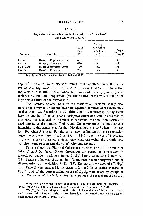
The cube law. Table 1 shows the values of h = l/n as calculated from Eq. (12), for the electoral systems which have been observed to follow the cube law (i.e., the observed value of k is l/3). The calculated values of h are close to l/3 in all these cases, in good agreement with the cube law. Thus all the data in support of the cube law also support the seat-vote equation.

It so happens that the majority of the representative assemblies in the world are of such size (s), in comparison with the total population (P), that the approximation

s e:pl I3 (14)

SEATS AND VOTES 265

TABLE 1

Population and Assembly Size for Cases where the “Cube Law” Has Been Found to Apply

Country Assembly

No. of seats (9

Voting population in millions

(0 h-1-S

log v

U.S.A. House of Representatives 435 Britain House of Commons 630 N. Zealand House of Representatives 80 Canada House of Commons 265

Data from The Europa Year Book, 1965 and 1967.

70 .30 27 .38

1.3 .31 7.7 .35

applies.9’ The cube law of elections results from a combination of this “cubes law of assembly sizes” with the seat-vote equation. It should be noted that the value of h is little affected when the number of voters (I’) in Eq. (12) is replaced by the total population (P). This relative insensitivity is due to the logarithmic nature of the relationship..

The Electoral College. Data on the presidential Electoral College elec- tions offer a way to check the seat-vote equation at values of h considerably smaller than l/3. According to our definition of constituency, S represents here the number of states, since all delegates within one state are assigned to one party. As discussed in the previous paragraph, the total population P is used instead of the number I’ of voters. Under modern U.S. conditions h is insensitive to this change; e.g., for the 1960 elections, h is .217 when V is used for .206 when P is used. For the earlier days of limited franchise somewhat larger discrepancies result (.222 vs .196, in 1840) but the use of P actually may yield a more consistent picture, since what was technically a single vote was also meant to represent the voter’s wife and servants.

Table 2 shows the Electoral College results since 1820.1° The value of h=log S/log P has been .20+.01 throughout this period. It is necessary to smooth out random variations in log(sA/SB) before calculating k from Eq. (13) because otherwise these random fluctuations become magnified out of all proportion by the division in Eq. (13). Therefore, the values of (V, /I’,) from Table 2 were arranged in increasing order, and the geometric averages of I’, /I’, and of the corresponding values of S,/S, were taken by groups of three. The values of k calculated for these groups still range from .lO to .73,

9Data and a theoretical model in support of J?q. (14) are given in Taagepera, R. (1972), “The Size of National Assemblies.” Social Science Research 1, 385-40.

~OSA/.SB has been interpreted as the ratio of electoral votes. The outcome is very similar when ratio of states carried is used instead, for the period during which data on states carried was available (1912-1968).

TABLE 2

U.S. Population, Number of States and Presidential Elections Results

Total population Number Popular Electoral

in of vote vote Ratio of millions states log s ratio states

(PI (3 h = log P (VA/V,) carried k = 1% (VA/Vd

1% cs, /s,,

1820 1824 1828 1832 1836 1840 1844 1848 1852 1856 1860 1864 1868 1872 1876 1880 1884 1888 1892 1896 1900 1904 1908 1912 1916 1920 1924 1928 1932 1936 1940 1944 1948 1952 1956 1960 1964 1968

9.6

17.1

31.4

50.2

76.0

106

132

179

23

26

33

38

45

48

48

50

,195

,195

.20

.205

.21

.21

.21

.20.5

1.48 1.27 1.30 1.39 0.89 1.03 0.90 1.16 1.38 0.14 0.81 0.90 0.79 1.06 1.002 1.013 1.02 1.07 0.92 0.89 0.61 0.83 1.49 1.07 0.56 0.53 0.70 1.45 1.66 1.22 1.16 1.10 0.81 0.73 1.003 1.59 0.984

1.18 2.36 2.15 .31 4.47 .18 2.33 .39 0.26 .09 1.62 .06 0.78 .43 6.05 .08 1.53 .76 0.07 .ll 0.10 .09 0.37 .ll - -

1.006 9.00 0.74 -.Ol 1.20 .08 0.72 -.06 1.91 .lO 0.65 .I9 0.53 .18 0.42 .46 0.50 .27 4.95 6.7 .25 1.09 1.7 .76 0.31 0.30 ..52 0.36 0.34 .62 0.20 0.20 .22 8.0 7.0 .18

65 23 .12 5.5 3.8 .12 4.36 3.0 .lO 1.60 1.7 .21 0.20 0.23 .13 0.16 0.17 .I7 1.38 0.88 .Ol 9.4 7.5 .21 0.63 0.44 .03

Ratios of votes and states won by the Democratic and by the other major candidate (usually Republican) are shown.

Figures based on The World Almanac 1967, New York: Newspaper Enterprise Assoc., 1966, pp. 246, 324, 325, and 385-414; and WaN Street Journal, December 12, 1968 and January 7, 1969.

No information is available on popular vote before 1824. In 1872 one candidate died before Electoral College meeting. District of Columbia is counted as a state from 1964 on.

SEATS AND VOTES 267

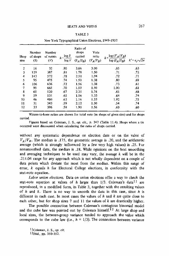
TABLE 3

New York Typographical Union Elections, 1949-1952

Ratio of Number Number shops Vote

Shop of shops of voters h =w carried ratio k=log (VA/VB) size 69 WI log v @A/S,) (VAIVB) log (S, IS,) k’ = o,r J5

2 16 32 .80 3.66 3.00 .85 .63 3 129 381 .81 1.78 1.50 .71 .72 4 143 572 .78 2.5 1 1.94 .I2 .71 5 95 475 .74 1.50 1.38 .80 .69 6 106 636 .72 1.56 1.38 .73 .61 7 95 665 .70 1.50 1.50 1.00 .61 8 65 520 .67 2.35 1.74 .65 .68 9 59 531 .65 1.56 1.33 .64 .74

10 46 460 .63 1.16 1.33 1.92 .75 11 31 343 .59 2.12 1.50 .54 .74 12 33 396 .58 1.90 1.56 .69 .60

Winner-to-loser ratios are shown for total vote (in shops of given size) and for shops carried.

Figures based on Coleman, J. S., op. cit., p. 347 (Table 11.4). Shops where a tie occurred were discounted when calculating the ratio of shops carried.

without any systematic dependence on election date or on the value of V,/VB. The median is .175, the geometric average is .20, and the arithmetic average (which is strongly influenced by a few very high values) is .25. For nonsmoothed data, the median is .18. While opinions on the best smoothing and averaging techniques to be used may vary, the average k will be in the .21+.04 range for any approach which is not wholly dependent on a couple of data points which deviate the most from the median. Within this range of error, k equals h for Electoral College elections, in conformity with the seat-vote equation.

Labor union elections. Data on union elections offer a way to check the seat-vote equation at values of h larger than l/3. Coleman’s data1 1 are reproduced, in a modified form, in Table 3, together with the resulting values of h and k. There is no way to smooth the data in this case, since h is different in each case. In most cases the values of h and k are quite close to each other, but for shop sizes 7 and 11 the values of k are drastically higher.

The possible connection between Coleman’s contagious binomial model and the cube law was pointed out by Coleman himself.12 At large shop and local sizes, the between-group variance tended to approach the value which corresponds to the cube law (i.e., h = l/3). The connection between variance

llColeman, J. S., op. cit. l%bid., pp. 350-352.

268 TAAGEPERA

and the factor h is easily seen when the quantity S,/S is plotted against VA/V, at a constant value of h, assuming a two-party system and the validity of Eq. (1). For small values of h (h<<l) the resulting curves can almost be superimposed to normal error integral curves, especially in the maximum-slope region. Since the maximum slope of the constant-h curves is l/h and that of the error integral curve with variance a2 is k’ = l/u&, the following equality should hold, according to the seat-vote equation.

log s Fv=h=k’=ufi. (15)

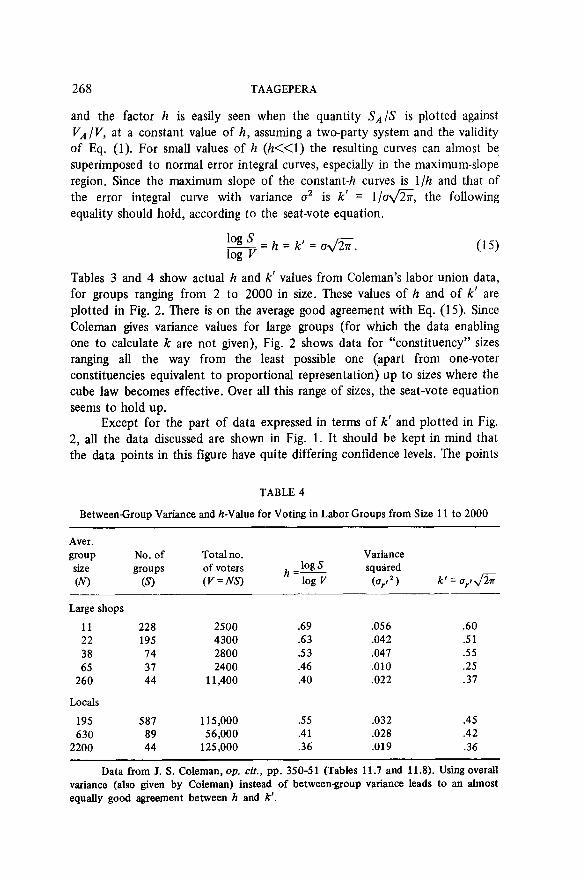
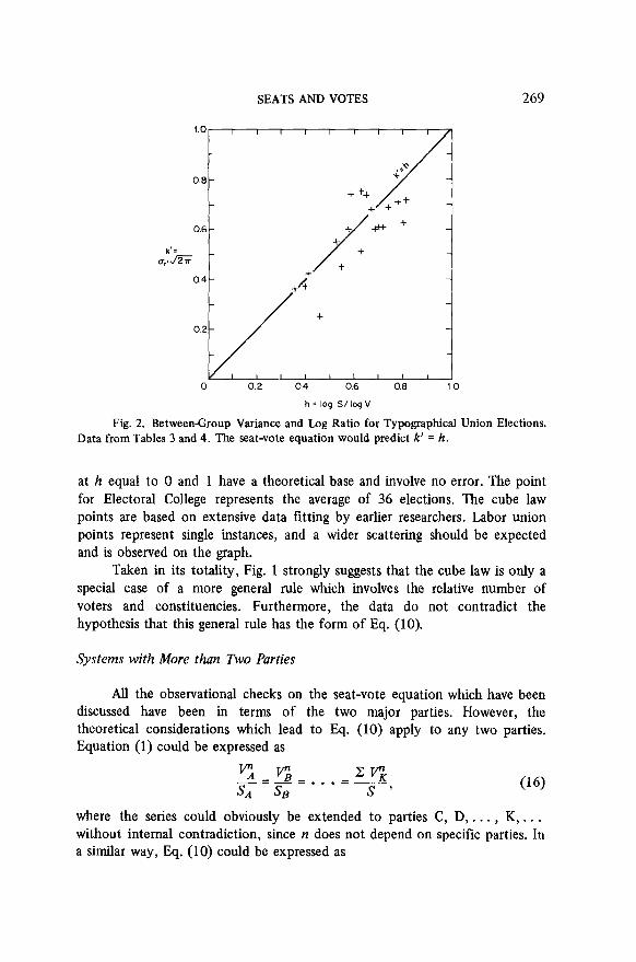
Tables 3 and 4 show actual h and k’ values from Coleman’s labor union data, for groups ranging from 2 to 2000 in size. These values of h and of k’ are plotted in Fig. 2. There is on the average good agreement with Eq. (15). Since Coleman gives variance values for large groups (for which the data enabling one to calculate k are not given), Fig. 2 shows data for “constituency” sizes ranging all the way from the least possible one (apart from one-voter constituencies equivalent to proportional representation) up to sizes where the cube law becomes effective. Over all this range of sizes, the seat-vote equation seems to hold up.

Except for the part of data expressed in terms of k’ and plotted in Fig. 2, all the data discussed are shown in Fig. 1. It should be kept in mind that the data points in this figure have quite differing confidence levels. The points

TABLE 4

BetweenGroup Variance and h-Value for Voting in Labor Groups from Size 11 to 2000

Aver. group No. of Total no. Variance size groups of voters log s h=- squared 09 (S) (V=NS) log v (0,f2) k’ = o,., ,hi

Large shops 11 228 2500 .69 .056 .60 22 195 4300 .63 .042 51 38 74 2800 .53 .041 .55 65 37 2400 .46 .OlO .25

260 44 11,400 .40 .022 .37

Locals

195 587 115,000 s.5 .032 .45 630 89 56,000 .41 .028 .42

2200 44 125,000 .36 .019 .36

Data from J. S. Coleman, op. cit., pp. 350-51 (Tables 11.7 and 11.8). Using overall variance (also given by Coleman) instead of between-group variance leads to an almost equally good agreement between h and k’.

SEATS AND VOTES 269

+

11 0 0.2 0.4 0.6 0.8 10

h = log WlogV

Fig. 2. Between-Group Variance and Log Ratio for Typographical Union Elections. Data from Tables 3 and 4. The seat-vote equation would predict k’ = h.

at h equal to 0 and 1 have a theoretical base and involve no error. The point for Electoral College represents the average of 36 elections. The cube law points are based on extensive data fitting by earlier researchers. Labor union points represent single instances, and a wider scattering should be expected and is observed on the graph.

Taken in its totality, Fig. 1 strongly suggests that the cube law is only a special case of a more general rule which involves the relative number of voters and constituencies. Furthermore, the data do not contradict the hypothesis that this general rule has the form of Eq. (10).

Systems with More than Two Parties

All the observational checks on the seat-vote equation which have been discussed have been in terms of the two major parties. However, the theoretical considerations which lead to Eq. (10) apply to any two parties. Equation (1) could be expressed as

Tl G- = G -=--...z- sA SB s '

(16)

where the series could obviously be extended to parties C, D, . . . , K, . . . without internal contradiction, since n does not depend on specific parties. In a similar way, Eq. (10) could be expressed as

270 TAAGEPERA

log S * log S, - log V * log V, =

= log S * log S, - log V * log V, = . 1 . ) (17)

where again the equalities can be extended to further parties. In practice, however, there is one difficulty, if only a small number of

elections are considered: all votes and seats come in integer numbers only. For a minor party D, the average value of SD predicted by Eq. (17) might be considerably smaller than one, which means that in most elections party D will get no seats, but in some elections it will get some. A test of the equation in the case of such a minor party would require extremely long time series of elections, in order to get meaningful long-range averages. In the case of, say, the U.S. Electoral College, this cannot be done because minor parties just have not stayed around for sufficiently long time periods. In the case of Canadian parliamentary elections, however, the cube law (and hence the seat-vote equation) has been shown to apply to third parties.13

Unless the minor parties can be shown to be inherently different from the two major parties, one would expect the same rules of seat distribution apply to all parties. Theoretical consistency and the Canadian data suggest that this is the case.

Practical Implications

The cube law has been a piece of curiosity with little practical use. By the time the popular vote figures are in, the seat distribution is, too, and there is no need to estimate it by indirect means. The cube law may have predictive ability, though, in the preelection stage: the popular vote figures estimated by polls can be converted into seats estimates through the use of the cube law.

If the seat-vote equation is valid it extends this predictive use to a wider range of elections. The 1968 presidential elections provide one example of such possible use. In late September many observers estimated correctly Humphrey’s share of the popular vote, but some underestimated his electoral vote to the point of rating him third, behind Wallace.14 With the same popular vote estimate, the seat-vote equation would have yielded an answer much closer to the actual outcome. However, predicting the outcome of specific elections is not the most important potential use of the seat-vote equation. This equation expresses the time average of long series of elections, and a quick check of data in Table 2 shows how widely individual elections can deviate from the average.

In contrast to the immutable cube law, the seat-vote equation enables one to alter the time average of a series of elections by a predetermined

13Qualter, T. H., op. cit. 14E.g., “Will HHH Come In Third?” Newsweek, September 23, 1968, pp. 26-27.

SEATS AND VOTES 271

amount, simply by manipulating the number of constituencies. Such manipula- tion may be desirable, e.g., if a country faces a problem of weak majorities or a problem of underrepresented restless minorities.

Suppose that a country has a parliament of a size which leads to the cube law. As long as the country has only two dominant parties, clear parliamentary majorities are likely to result. However, if a third party starts to receive an appreciable fraction of votes, the country may be in for prolonged unstable majorities and coalitions. One possible solution would be to reduce the number of constituencies, either by reducing the size of the parliament, or by introducing multiseat constituencies (with all seats in a constituency going by definition to the majority party).

As an example, suppose the country has 20 million inhabitants and a representative assembly with 272 seats, so that log P/log S is 3.00. Suppose a typical distribution of votes among the three parties is 39, 35, and 26%, with the two major parties in close competition (with either party occasionally victorious) and the thud party always netting about a quarter of votes. For the above distribution of votes the average expected seat distribution for one-seat constituencies is, on the basis of the seat-vote equation (or the cube law, since h = l/3), 49, 36, and 15%. This means that in more than half the elections no absolute majority emerges in the assembly. If the election rules were changed to have 136 two-seat constituencies, S would be 136 (although the assembly size remains unchanged). The ratio log P/log S now is 3.42 and the seat-vote equation indicates an average seat distribution of 51, 35, and 13%, for the same vote distribution as above. This means that in more than half of the elections an absolute majority emerges in the assembly. Since the third party representation is most affected by the change to fewer constitu- encies, a number of third party voters may be induced to switch to one of the two major parties so that their vote “be not lost.” This would lead to even more clear-cut majorities.

Now suppose that another country contains two different ethnic popula- tions, and that voting tends to follow the ethnic lines, with one party regularly getting about 60% and the other 40% of the vote. Again assuming a population of 20 million and 272 one-seat constituencies, the minor party would regularly obtain only about 23% of the seats, on the basis of the seat-vote equation. Being regularly reduced to effective legislative impotency, the minor ethnic group may resort to violent tactics and/or demand propor- tional representation. The major party may object to proportional representa- tion, but may concede that the minor party should have somewhat higher representation. The two sides may reach a compromise on a 33% average representation. The problem would be how to reach this average outcome, without introducing rigid quotas which might effectively force people to vote along ethnic lines even more than they already do.

According to the seat-vote equation, an average 67-33 distribution of

272 TAAGEPERA

seats would be obtained if the country were divided into 20,000 constitu- encies. This does not mean that the parliament would have to be that large. The people could elect 20,000 local councilors on one-seat constituency basis, and those councilors could then proceed to elect the parliament, on a proportional representation basis. The fact that only the average outcome of elections is predictable is an advantage. The ethnic minority knows that its long-range representedness is assured. However, in any single election the ability to vote along nonethnic lines is preserved, and could be used if one’s “own” party should be locally corrupt or inept.

The solutions proposed in the two examples may not be the best ones, given the situations described. Examples of an infinite variety could be discussed. The point is that whenever changes in election rules are made, the average effect of these changes must and will be considered. While up to now the considerations were perforce intuitive and qualitative, the seat-vote equation would often enable one to inject some quantitativeness into the argument.

Ebeoretical Implications

The long-range significance of the seat-vote equation can be expected to lay in its theoretical aspects. The cube law has been one of the few cases in political science where a simple deterministic equation has been set up between measurable quantities. One could say that the cube law has been the only political science law that looks like a physics law. The seat-vote equation not only extends the applicability of this earlier law on seats and votes, but also ties new measurable quantities (number of constituencies and of voters) into this deterministic framework. The fact that the deterministic equation applies only to the average outcome of elections does not reduce its significance; all thermodynamics laws are in the same category. While physicists would be interested in following a single particle and political scientists would be interested in following a single election, average behavior of large quantities of particles and elections is also of interest. The previous section has indicated some possible uses of a law applying to the average outcome of elections.

“Conserved quantities” which remain constant during a process of change have a great importance in physics. The conserved quantities range from energy and momentum to parity and “strangeness” in nuclear physics. The seat-vote equation also offers two types of conserved quantities.

During a process of gradual boosting of majorities by elections in stages with ever decreasing number of constituencies, the quantity log S * log(SA /S& is conserved, according to Eq. (lo), since it is equal to the similar expression in V, regardless of the value of S. If we define “complexity” as

SEATS AND VOTES 273

(18)

then Eq. (10) is a statement of conservation of complexity during the elections. Complexity is high for close runs (c = 86 for the 1960 Kennedy- Nixon contest) and low for large popular vote margins (c = 0.60 for the 1964 Johnson-Goldwater contest.). In 1968, Nixon-Humphrey rated 16, and the total complexity was hardly altered by an additional Nixon-Wallace term of 0.2.

Another conserved quantity emerges from Eq. (17), for multiparty elections. Between any two stages of elections with S and V constituencies, respectively, the expression d = (log V * log V, - log S * log SK) has the same value for all parties involved. If V designates the stage with the higher number of constituencies (which could be individual voters), then d is positive and could be said to express the quantity of decision-making accomplished from one stage to the next. This quantity is conserved from party to party.

The full implications of conservation of complexity (on the average) from one elections stage to the next, and of conservation of d from party to party are materials for another research project.

CONCLUSIONS

Starting from the empirical cube law which applied to certam parliamen- tary elections, a more general equation to correlate seats to votes has been devised on grounds which are partly analytical and partly intuitive. The exponent 3 characteristic of the cube law emerges naturally from this generalized equation, for the elections where the cube law has been observed to apply, and only for these elections. The generalized seat-vote equation also agrees with the data on other elections where, if a cube-law-like exponential fit were attempted, the exponent would be smaller or larger than 3. The equation also agrees with the outcome of direct presidential elections and of elections with proportional representation, as theoretical extreme cases. Central to the development of the seat-vote equation is the notion of “constituency” as the smallest unit where the party with plurality wins all the seats at stake. The smaller the number of such constituencies is, the more drastic is the attrition of minority parties. The changes in the number of constituencies can be used to bring about a desired degree of minority representation in an assembly. The prediction of the average long-range effects of such changes could be an important application of the seat-vote equation.

274 TAAGEPERA

APPENDIX: THEORETICAL ARGUMENTS IN FAVOR OF ~(2’) = log X

There is as yet no clear-cut proof that the function in Eqs.(7) and (8) is the logarithm of X. However a number of plausibility arguments will be presented in favor of such identification, and I have found no similar arguments pointing to any other functional relationship.

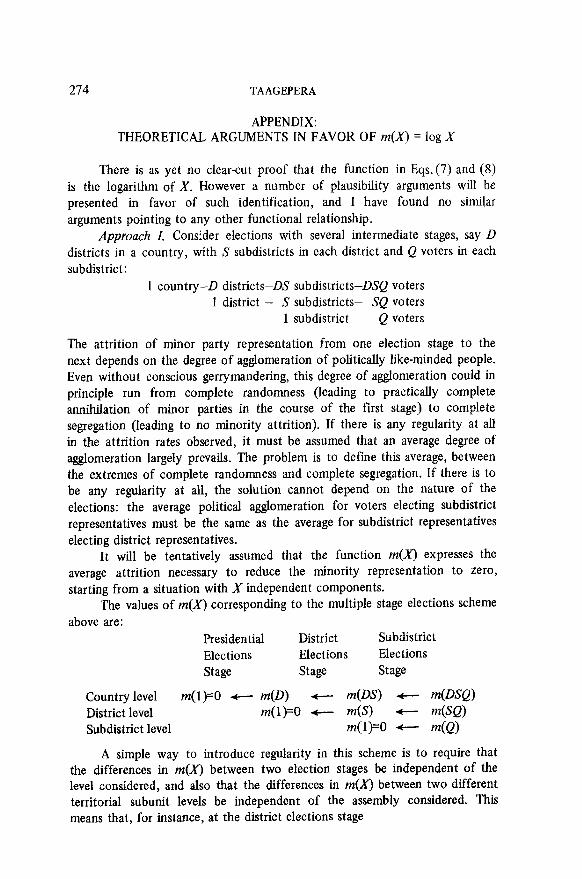
Approach I. Consider elections with several intermediate stages, say D districts in a country, with S subdistricts in each district and Q voters in each subdistrict:

1 country-D districts-D,9 subdistricts-D,SQ voters 1 district - S subdistricts- SQ voters

1 subdistrict - Q voters

The attrition of minor party representation from one election stage to the next depends on the degree of agglomeration of politically like-minded people. Even without conscious gerrymandering, this degree of agglomeration could in principle run from complete randomness (leading to practically complete annihilation of minor parties in the course of the first stage) to complete segregation (leading to no minority attrition). If there is any regularity at all in the attrition rates observed, it must be assumed that an average degree of agglomeration largely prevails. The problem is to define this average, between the extremes of complete randomness and complete segregation. If there is to be any regularity at all, the solution cannot depend on the nature of the elections: the average political agglomeration for voters electing subdistrict representatives must be the same as the average for subdistrict representatives electing district representatives.

It will be tentatively assumed that the function mQ expresses the average attrition necessary to reduce the minority representation to zero, starting from a situation with X independent components.

The values of m(x) corresponding to the multiple stage elections scheme above are:

Presidential District Subdistrict Elections Elections Elections Stage Stage Stage

Country level m(l)=0 e m(D) t- m(DS) +- m(DSQ) District level m(l)=0 W m(S) - m(sQ> Subdistrict level m(l)=0 - m(Q)

A simple way to introduce regularity in this scheme is to require that the differences in mQ between two election stages be independent of the level considered, and also that the differences in naQ between two different territorial subunit levels be independent of the assembly considered. This means that, for instance, at the district elections stage

SEATS AND VOTES 275

m(m) - m(D) = m(S) - m(1)

and that, between district and subdistrict levels,

(19)

m(s) - m(1) = m(SQ) - m(Q). cm

These equations are equivalent to saying that, for any values of Q and S,

m(SQ) = 49 + m(Q). (21)

The only function m(X) which satisfies this equation and also the condition rn(l)=Ois~~(X)=logX.~~

An alternative simple way to introduce regularity in the scheme above would be to assume equal ratios instead of equal differences. This assumption would not be compatible with the condition m(l) = 0. All other ways to introduce regularity into the scheme above are more complex, and should be tried only if simple approaches do not work.

The situation is reminiscent of the evolution of the notion of informa- tion, from Hartley’s definition (1928) as the logarithm of the number of issues, to Shannon’s definition (1949) as the sum of (p log p) terms where p is the probability of one particular outcome.16 Intuition and usefulness in applications were major factors in prompting the change, and many a popular presentation still preserves the intuitive “proof” of the notion of information. Thus Yaglom asserts that (with my italics) “It is therefore natural to admit that the degree of uncertainty of experiment AB equals the sum of the uncertainties which characterize the experiments A and B.“I7 The assumption of addition of uncertainties (rather than, say, multiplication or some more complex combination method) has little self-evident about it, except that it is a simple approach and, above all, that it works out in practice. The same can be said about m(X) = log X.

Approach II. When there are V different issues having equal proba- bilities of occurrence, the uncertainty on the outcome is log I/. In our case a single issue consists of the outcome of the vote by a single voter. At the assembly level (with S seats), the degree of uncertainty is reduced to log S. The minimum number of questions which have to be asked in order to reduce the uncertainty from log V to log S is n = log V/log ,S.l* The probability that a given voter votes for the party A is V,/V while the probability of voting for B is V,/V. Thus the probable ratio of answers received to one question is VA /VB. If n questions are asked the probable ratio of combined answers is (VA/V~)~. This would lead directly to Eqs. (1) and (11).

l5Yaglom, A. M. and Yaglom, I. M. (1969), Probabilitk et information, Dunod, Paris, pp. 34 and 95-97.

%bid., p. 43 f f . 17Zbid., p. 34. IsIbid., p. 106.