Seasonal resolution of Eastern Mediterranean climate change since 34 ka from a Soreq Cave speleothem

Available online at www.sciencedirect.com

www.elsevier.com/locate/gca

Geochimica et Cosmochimica Acta 89 (2012) 240–255

Seasonal resolution of Eastern Mediterranean climatechange since 34 ka from a Soreq Cave speleothem

Ian J. Orland a,⇑, Miryam Bar-Matthews b, Avner Ayalon b,Alan Matthews c, Reinhard Kozdon a, Takayuki Ushikubo a, John W. Valley a

a WiscSIMS, Department of Geoscience, University of Wisconsin, 1215 W Dayton St., Madison, WI 53706, USAb Geological Survey of Israel, 30 Malchei Israel St., Jerusalem 95501, Israel

c The Institute of Earth Sciences, The Hebrew University, Givat Ram, Jerusalem 91904, Israel

Received 21 October 2011; accepted in revised form 15 April 2012; available online 21 April 2012

Abstract

The combination of ion microprobe analysis of d18O and confocal laser fluorescent microscope imaging of annual growthbands in a Soreq Cave speleothem provides sub-annual-scale climate information between 34 and 4 ka. This high-resolutionmethodology is ideal both for comparing seasonal climate patterns across broad windows of time and examining rapid climateevents, such as the Younger Dryas termination, in detail. The sub-annual d18O gradients we report represent a combination ofseasonal variability in rainfall amount and air temperature. A distinct change in both the pattern of fluorescent banding andthe gradient of d18O measured in situ across single, annual growth bands indicates a change in seasonal climate patterns of theEastern Mediterranean region following Heinrich event 1 and again after the Younger Dryas. Throughout the Holocene, wetwinters and dry summers characterized regional climate. During the Younger Dryas, we find that regional climate may havebeen more arid than in the Holocene, but the fluorescent banding pattern indicates that the supply of dripwater to the cavewas more consistent year-round. We suggest that a reduced gradient of seasonal precipitation, occasional snowfall, and veg-etation differences may have all contributed to the isotope and fluorescent banding patterns observed during Heinrich event 1and the last glacial stadial. Detailed investigation of the Younger Dryas termination reveals a rapid onset of regional envi-ronmental change. Fluorescent band counting indicates that the Younger Dryas termination, as recorded by rainfall in theEastern Mediterranean, spanned a minimum of 12 years.� 2012 Elsevier Ltd. All rights reserved.

1. INTRODUCTION

1.1. Background

Model predictions of climate change over the next cen-tury are in broad agreement with respect to globallyaveraged surface temperatures, showing an increase of

0016-7037/$ - see front matter � 2012 Elsevier Ltd. All rights reserved.

http://dx.doi.org/10.1016/j.gca.2012.04.035

Abbreviations: CLFM, confocal laser fluorescent microscopy; EM, Easte

1; S1, Sapropel event 1; YD, Younger Dryas⇑ Corresponding author. Tel.: +1 608 262 8960; fax: +1 608 262 0693.

E-mail addresses: [email protected] (I.J. Orland), [email protected] (A. Matthews), [email protected] (R. Kozedu (J.W. Valley).

�2–4 �C given projected greenhouse gas emissions, but keydetails remain uncertain (IPCC, 2007). Likewise, modelspredict a climate response that varies by both region andrate. It follows that high-resolution proxy records of past cli-mate events are essential for calibrating model forecasts ofseasonal and abrupt climate change on both regional andglobal scales. In this paper, we present a high-resolution

rn Mediterranean; LGM, last glacial maximum; H1, Heinrich event

[email protected] (M. Bar-Matthews), [email protected] (A. Ayalon),don), [email protected] (T. Ushikubo), [email protected].


mailto:[email protected]






mailto:[email protected]. edu

mailto:[email protected]. edu

http://dx.doi.org/016/j.gca.2012.04.035

I.J. Orland et al. / Geochimica et Cosmochimica Acta 89 (2012) 240–255 241

geochemical climate proxy from a cave deposit in the East-ern Mediterranean (EM) region that is a record of seasonalprecipitation from 34 to 4 ka. Combined with data presentedin Orland et al. (2009), we build a regional record of seasonalclimate from 34 to 1 ka.

Cave deposits (speleothems) are valuable records of mul-tiple paleoclimate variables in numerous locations aroundthe globe (e.g., Baker et al., 1993; Wang et al., 2001;McDermott, 2004; Fairchild et al., 2006; Baldini et al.,2008; Cheng et al., 2009; Lachniet, 2009; Wong et al.,2011). In many cases, geochemical tracers in speleothemsare used to identify changes in global and regional climatetrends on a decadal to millennial scale. Given conventionaldrill-sampling techniques (mm-scale spatial resolution) andtypical speleothem growth rates, however, most speleo-them-based proxy studies from semi-arid climates are un-able to resolve seasonal or sub-annual information.Following the methodology established by Orland et al.(2009), this study examines the utility of in situ micron-scale(sub-annual temporal resolution) ion microprobe oxygenisotope (d18O) analysis for interpreting seasonal climatepatterns in a Soreq Cave (Israel) stalactite (“sample 2N”,Fig. 1) that grew during the last glacial period, deglaciationand Holocene.

1.2. Related environmental proxy records

The record of seasonal climate from this study repre-sents new information for interpreting mid-latitude climatedynamics during Northern Hemisphere deglaciation. Spele-othem sample 2N provides a relevant record of both regio-nal- and hemisphere-scale climate responses to deglaciation(Bar-Matthews et al., 1999, 2000, 2003). The existing d18Orecord from Soreq Cave generally agrees with that of other

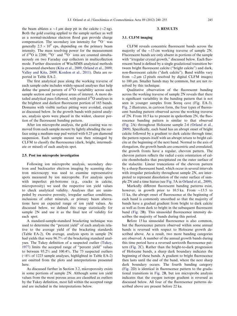
Fig. 1. Stalactite sample 2N from Soreq cave, Israel, cut inhorizontal cross-section. Samples from the matching face weredrilled for geochronology (Table 1). The “working traverse” for ionmicroprobe analysis of d18O is highlighted with a white dashed lineand the location of the 1 cm cubes (A–P) cut for ion microprobemounts are outlined in black. Areas of irregular calcite crystalgrowth, indicated by white arrows, are visible in cubes M, N, andO. Inset, left: picture of a 25 mm round epoxy mount for ionmicroprobe analysis with cubes E and F positioned with theworking traverse centered and UWC-3 calcite standard grains inthe middle. Inset, right: map of Israel showing the location of SoreqCave (SC), Jerusalem (J), the Eastern Mediterranean Sea (EM) andthe Dead Sea (DS).

speleothems in the region (Frumkin et al., 2000; Verheydenet al., 2008). Soreq Cave is located such that it is influencedby the eastward advection of complex climatic variability inthe North Atlantic. Further, the Soreq Cave isotope recordmay respond indirectly to an enhanced African MonsoonalSystem (Almogi-Labin et al., 2004, 2009) and movement ofthe Intertropical Convergence Zone, a major climate tele-connection mechanism examined and invoked by manypaleoclimate workers (Wang et al., 2006; Anderson et al.,2009; Cheng et al., 2009; Waldmann et al., 2010; Dentonet al., 2010).

Nearby regional paleoclimate records include lake level,marine sediment, and pollen environmental proxies. Shore-line sediments from the Dead Sea, which is in a terminal ba-sin �45 km east of Soreq Cave, are used to reconstructpaleo-Dead Sea levels and regional water balance (Enzelet al., 2003; Bartov et al., 2003; Bookman et al., 2004;Lisker et al., 2009; Torfstein et al., 2009; Stein et al.,2010; Waldmann et al., 2010). Understanding the contribu-tions of both precipitation and evaporation is imperativefor interpreting Dead Sea levels; since this is ambiguousin Dead Sea shoreline records, the interpretation of past re-gional rainfall amount is uncertain. Curiously, however,Dead Sea level is highest during the last ice age when highd18O values in Soreq Cave speleothems are interpreted byBar-Matthews et al. (1997, 2003) to indicate a drier EMclimate. In order to reconcile this dispute, workers haveturned to marine and lacustrine sediment records.

Kolodny et al. (2005) use marine and terrestrial sedi-ments to suggest that the long-term d18O trends observedin Soreq Cave speleothems are a result of changes in d18Oof the Mediterranean Sea. Based on foraminiferal geochem-istry, however, Almogi-Labin et al. (2009) argue that thed18O values observed in Soreq Cave cannot be explained so-lely by Mediterranean Sea surface d18O, and that sea-landdistance and relative elevation change due to lower sea lev-els must be accounted for as water vapor is transportedfrom the EM to Soreq Cave.

Studies of pollen records near Soreq Cave (Baruch andBottema, 1991, 1999; Bottema, 1995; Rossignol-Strick,1995; Hajar et al., 2008; Langgut et al., 2011) show an in-crease in the abundance of temperate vegetation from thelast glacial maximum (LGM) into the Holocene, indicatingwetter climate in the Holocene. Rossignol-Strick (1995)concludes that oxygen isotope and pollen records fromthe EM and Arabian seas show two distinct climate regimesduring the last deglaciation: a cold, arid Younger Dryas,and a temperate early Holocene with warm winters andwet summers.

The implication by Rossignol-Strick (1995) that sea-sonal climate differed between the Younger Dryas, the earlyHolocene, and the modern is a major motivation for thework presented here. Although some studies (Atkinsonet al., 1987; Denton et al., 2005) have reported significantchanges in Northern Hemisphere seasonality associatedwith millennial-scale warming (Bølling-Allerød) and cool-ing (Younger Dryas) events, few proxy records are capableof resolving seasonal climate across the Northern Hemi-sphere deglaciation. Denton et al. (2005) suggest that winterArctic sea ice extended much further south in the Atlantic

242 I.J. Orland et al. / Geochimica et Cosmochimica Acta 89 (2012) 240–255

during the Younger Dryas, resulting in relatively frigid win-ters but mild summers. Tierney et al. (2011) introduce thepairing of paleoclimate proxy data with an isotope-enabledclimate model in order to identify seasonal climate changesas the cause for the East African Humid Period, 11-5 ka.The main goal of this study is to determine if Soreq Cavespeleothems show the d18O signal of any significant season-ality changes during Northern Hemisphere deglaciationthat can inform us about EM climate dynamics since theLGM.

Speleothem sample 2N preserves a record of calcitedeposition across the last deglaciation. Although there arehiatuses in the growth record along the analytical traverse,we are able to interpret seasonality information from areasof consistent growth. The micro-imaging techniques used inthis study allow us to recognize growth hiatuses, areas ofirregular crystal growth, and non-calcite inclusions in aspeleothem; we can then target ion microprobe analysesaccordingly. Hence, this study utilizes the unparalleled spa-tial resolution of micro-analytical methodology to: (1)examine seasonality data over long time spans, and (2)reconstruct hemisphere-scale climate events that took placeover short time spans. Prior studies from Soreq Cave, de-scribed in the following section, are integral to our climateinterpretations.

1.3. Prior work at Soreq Cave

This investigation builds on prior characterization ofSoreq Cave hydrology (Ayalon et al., 1998, 2004), the con-ventionally sampled 185 ka record of d18O from Soreq Cavespeleothems (Bar-Matthews et al., 2003; Almogi-Labinet al., 2009), and analyses of both fluid inclusions (McGarryet al., 2004) and mass-47 CO2 isotopologue anomalies (D47)in Soreq speleothem calcite (Affek et al., 2008). These stud-ies make Soreq an ideal natural laboratory to apply newprocedures for high-precision analysis of d18O in 10 lmspots by ion microprobe and imaging of annual growthbands by confocal laser fluorescence microscopy (CLFM).Orland et al. (2009) developed the high-resolution method-ology as part of a detailed study of d18O in a Soreq Cavestalagmite that grew from 2.2 to 0.9 ka. This study appliesthe high-resolution methodology to a stalactite that formedbetween 33.8 and 4.4 ka.

The geological and hydrological setting of Soreq Cave,located in the Judean Hills 20 km west of Jerusalem, is welldescribed by numerous studies of Soreq speleothems andhydrology (Bar-Matthews et al., 1996, 1997, 2003; Ayalonet al., 1998, 1999, 2004; Matthews et al., 2000; Kolodnyet al., 2003; McGarry et al., 2004; Orland et al., 2009;Bar-Matthews and Ayalon, 2011). In the modern EM,�95% of the annual rainfall occurs during the winter “wetseason,” which extends from November until April. Overthe past 15 years, average annual rainfall above the caveis �500 mm. Furthermore, modern precipitation demon-strates an “amount effect,” a negative linear correlation ofthe amount and d18O value of annual rainfall (Ayalonet al., 1998, 2004; Orland et al., 2009).

Critical for this study is the work of Ayalon et al. (1998,2004) to examine rainfall and dripwater d18O values in and

above Soreq Cave on a sub-annual timescale. They find thatrainfall d18O values vary seasonally above Soreq Cave, withthe lowest d18O values occurring during the peak of thewinter wet season. Furthermore, Ayalon et al. (1998) andOrland et al. (2009) show that the modern pattern of sea-sonal d18O variability in rainfall is transmitted to dripwa-ters in the cave. We assume that seasonal d18O variabilityin paleorainfall was likewise transmitted to dripwaters.Next, we assert that the seasonal dripwater d18O signal isreliably recorded in Soreq speleothems.

Prior work in Soreq Cave indicates that it is reasonableto assume that d18O values in sample 2N reflect isotopicequilibrium with dripwater. Although Affek et al. (2008)find evidence for kinetic isotope effects in their measure-ments of D47 in Soreq Cave speleothems, they determinethe corresponding effect on d18O to be negligible and ulti-mately conclude that their samples precipitated at near-equilibrium conditions for d18O. Moreover, Bar-Matthewset al. (1996, 1997) established that sample 2N both passesthe Hendy test for equilibrium precipitation (Hendy,1971) and replicates the d18O variability of other samplesfrom Soreq. Work in other caves (Mickler et al., 2006; Ban-ner et al., 2007; Baldini et al., 2008) highlights the potentialinfluence of seasonal pCO2variability in a cave atmosphereon both isotopic equilibrium and seasonal growth rates.Since Soreq Cave had no natural entrance before it was dis-covered during a quarrying operation in 1968, seasonal ven-tilation of the cave atmosphere is presumed to have beeninsignificant. Additionally, Orland et al. (2009) demonstratethat the spatial resolution of our micro-analytical techniquewill allow us to account for changes in seasonal growthrates and avoid seasonally biasing the d18O record in sam-ple 2N. Given these observations, we suggest that sample2N precipitated in isotopic equilibrium and the d18O mea-surements we present here faithfully record a seasonalpaleorainfall signal.

Orland et al. (2009) established guidelines to interpretcombined d18O and CLFM data from the analysis of a lateHolocene Soreq Cave calcite stalagmite (sample 2-6).CLFM imaging along the analytical traverse from theHolocene sample reveals a consistent sawtooth pattern offluorescence intensity across concentric growth bands.The beginning of each growth band is marked by a sharponset of bright-fluorescent calcite (“bright calcite”), fol-lowed by a gradual reduction in fluorescence intensity todark-fluorescent calcite (“dark calcite”) (Fig. 2A). Theend of each growth band is marked by the sharp changeto bright calcite in the next band. Ion microprobe analysisof the same analytical traverse shows that d18O values varyin a similar sawtooth pattern; the lowest d18O values occurat the sharp onset of bright calcite and then gradually in-crease as fluorescence gradually decreases.

Orland et al. (2009) interpret that these cycles representannual banding and attribute the covarying patterns offluorescence and d18O to a strongly seasonal rainfall patternsimilar to the modern EM rainfall regime. They suggestthat the onset of intense, low-d18O precipitation in thewet season flushes organic acids that accumulate in theupper soil column during the dry summer into the cave,causing the sharp onset of bright fluorescent, low-d18O

Fig. 2. Four patterns (A–D) of fluorescence and d18O variabilitywithin annual growth bands; each pattern is assigned a symbol foruse in Figs. 3B and 5. A schematic illustration of each pattern isshown above an example from sample 2N. In each plot of d18O,blue crosses and green triangles represent dark and brightfluorescent calcite, respectively. Error bars indicate 2 s.d. of eachactual d18O analysis. Red spots in CLFM images show the locationof ion microprobe analyses (�10 lm diameter). Note the definitionof |D18O| illustrated by the vertical bars.


calcite. Fluorescence intensity decreases and d18O values in-crease in the speleothem following the wet season flush, andthe cycle repeats itself at the beginning of the following wetseason.

In order to quantify seasonality, Orland et al. (2009) de-fined the variable D18O. Within a single annual growth band,D18O(dark-bright) = d18O(dark calcite) � d18O(bright cal-cite) (Fig. 2A). In sample 2-6, higher values of D18O(dark-bright) indicate more rain during the wet season, and thusa wetter year, while lower D18O(dark-bright) values indicategenerally dryer conditions. This proxy of seasonality relieson the assumption that the modern pattern of distinct wetand dry seasons is consistent with the climate regime of thelast 2.2 ka. In support of this assumption, Orland et al.(2009) observed that d18O values in dark-fluorescent calciteare relatively constant compared to d18O values of brightcalcite (see their Supplementary Material). Thus, dark calcitereflects dry season dripwater from a mixed vadose zone res-ervoir and provides a “baseline” d18O value that changes

slowly on a decadal scale. Therefore, in sample 2-6, it is thed18O value of bright calcite that varies from year to year, cre-ating differences in D18O(dark-bright). This model offluorescence and d18O values previously established insample 2-6 will be evaluated with data from the past 34 kyrin sample 2N.

2. MATERIALS AND METHODS

2.1. U–Th dating

New U–Th disequilibrium ages of sample 2N, a stalac-tite composed of low-magnesium calcite (Bar-Matthewset al., 2000), were acquired by multi-collector inductivelycoupled plasma mass spectrometer analysis at the Geologi-cal Survey of Israel. The analytical method is described inBar-Matthews et al. (2010). Twenty-four calcite aliquotswere collected along a radial traverse of a 1 cm-thick slabof the speleothem, sawed orthogonally to the verticalgrowth axis. Calculated ages range from 4.5 ± 0.2 ka to31.0 ± 0.9, and are corrected for excess 232Th. The assumedinitial 230Th/232Th activity ratio is 1.69, established in thedetailed isochron study of Soreq Cave speleothems byKaufman et al. (1998).

We define an “age model” for sample 2N based on lin-ear interpolation between 11 selected U–Th dates. Of the24 total ages measured, this simplified age model excludes:five measurements that incorporated irregular calcitegrowth (see Section 4.1.1 for further discussion) and eightages that were bracketed by adjacent spots with overlap-ping error bars. The electronic annex Fig. EA-1 illustratesthe overlap between the linear interpolation age modeland a more complex Bayesian age model (Scholz andHoffman, 2011) that includes all 24 ages. Given the excel-lent agreement between model types as well as our focuson the comparison of extended time periods, we thinkthe linear interpolation model is suitable. Linear extrapo-lation of observed growth rates to the core and outer rimindicate that the d18O analyses presented here span from33.8 to 4.4 ka. Table 1 lists the measured isotope ratios,uncorrected and corrected U–Th disequilibrium ages ofall 24 measurements.

2.2. Sample preparation

A second 1-cm thick slab of stalactite 2N was cut adja-cent to the piece dated at the Geological Survey of Israeland sent to the University of Wisconsin-Madison (UW-Madison) for ion microprobe analysis. At UW-Madisonthis slab was cut along its longest radius (13.8 cm) into 13�1 cm3 cubes using a thin-kerf jeweler’s saw. Fig. 1 showswhere the 13 cubes (A-I, M-P) were cut from the slab ofsample 2N and indicates the “working traverse” (whitedashes) along which ion microprobe analysis wascompleted. The 13 cubes were mounted in pairs in seven1-inch-diameter epoxy rounds (Fig. 1, inset). In each epoxymount, 3–4 grains of UWC-3 (calcite standard;d18O = 12.49&, VSMOW; Kozdon et al., 2009) and theworking traverse were placed within �5 mm of the centerof each mount to prevent instrument bias during ion micro-

Table 1U/Th age data from multi-collector inductively coupled plasma mass spectrometry analysis of sample 2N.

Samplename

Distancefromedge (mm)

U conc. (ppm) 234U/238U 230Th/234U 230Th/232Th Age (yr)uncorrected

Age (yr)corrected

2N-1 4.6 0.4200 ± 0.0003 1.02401 ± 0.00120 0.04735 ± 0.00070 13.10 ± 0.20 5300 ± 300 4500 ± 200

2N-3B 13.7 0.3898 ± 0.0003 1.01753 ± 0.00113 0.05845 ± 0.00094 10.29 ± 0.17 6500 ± 200 5400 ± 300

2N-4C 17.0 0.3785 ± 0.0003 1.01523 ± 0.00130 0.05800 ± 0.00074 11.63 ± 0.15 6500 ± 200 5500 ± 3002N-5B 18.9 0.3687 ± 0.0004 1.01733 ± 0.00135 0.06283 ± 0.00081 12.21 ± 0.16 7100 ± 200 6000 ± 3002N-6 23.1 0.3682 ± 0.0002 1.01920 ± 0.00131 0.06597 ± 0.00117 13.71 ± 0.24 7400 ± 300 6000 ± 4002N-7+8 27.2 0.5841 ± 0.0004 1.01891 ± 0.00120 0.05557 ± 0.00062 19.81 ± 0.22 600 ± 140 5600 ± 2002N-11 36.3 0.3516 ± 0.0002 1.01923 ± 0.00152 0.06140 ± 0.00068 10.44 ± 0.12 6900 ± 180 5700 ± 3002N-12 40.8 0.3536 ± 0.0004 1.04713 ± 0.00150 0.08501 ± 0.00121 5.05 ± 0.08 9700 ± 280 6300 ± 400

2N-13 45.3 0.3219 ± 0.0002 1.03091 ± 0.00070 0.11127 ± 0.00094 6.05 ± 0.05 12900 ± 260 9200 ± 400

2N-15 65.7 0.3757 ± 0.0002 1.05584 ± 0.00184 0.11004 ± 0.00129 7.01 ± 0.08 12700 ± 300 9600 ± 4002N-16 73.9 0.3898 ± 0.0003 1.03186 ± 0.00124 0.10284 ± 0.00074 16.40 ± 0.12 11800 ± 180 10600 ± 300

2N-16+17 75.7 0.4195 ± 0.0002 1.03399 ± 0.00092 0.09253 ± 0.00062 19.65 ± 0.13 10600 ± 150 9600 ± 3002N-17 77.6 0.3898 ± 0.0003 1.03454 ± 0.00136 0.14110 ± 0.00167 4.77 ± 0.06 16500 ± 420 10600 ± 5002N-17B 82.7 0.3611 ± 0.0004 1.02960 ± 0.00124 0.15299 ± 0.00172 4.40 ± 0.05 18000 ± 470 11200 ± 600

2N-18 88.2 0.3826 ± 0.0003 1.04747 ± 0.00163 0.14812 ± 0.00164 6.41 ± 0.07 17400 ± 500 12900 ± 500

2N-20* 97.1 0.5672 ± 0.0004 1.05566 ± 0.00129 0.14313 ± 0.00123 18.46 ± 0.16 16800 ± 300 15300 ± 4002N-20+21* 99.8 0.6384 ± 0.0007 1.05845 ± 0.00208 0.17045 ± 0.00184 7.50 ± 0.08 20300 ± 480 15800 ± 6002N-21 103.9 0.7739 ± 0.0006 1.05889 ± 0.00111 0.14585 ± 0.00094 27.70 ± 0.19 17100 ± 240 16100 ± 400

2N-22* 108.5 0.5413 ± 0.0003 1.05795 ± 0.00107 0.20533 ± 0.00115 4.29 ± 0.03 24900 ± 350 15400 ± 6002N-23* 113.9 0.3824 ± 0.0002 1.07316 ± 0.00118 0.20665 ± 0.00109 5.95 ± 0.03 21000 ± 300 18200 ± 4002N-24* 121.3 0.4034 ± 0.0003 1.07005 ± 0.00199 0.18878 ± 0.00104 7.45 ± 0.04 22700 ± 300 17700 ± 4002N-25 124.7 0.5966 ± 0.0005 1.07111 ± 0.00147 0.19409 ± 0.00217 41.63 ± 0.49 23400 ± 600 22500 ± 700

2N-26 127.4 0.6305 ± 0.0004 1.06448 ± 0.00114 0.24987 ± 0.00330 17.45 ± 0.24 31200 ± 1000 28400 ± 1100

2N-27 129.8 0.5113 ± 0.0005 1.06262 ± 0.00089 0.25501 ± 0.00291 53.26 ± 0.67 32000 ± 840 31000 ± 1000

All errors are listed at the 2r confidence level. Ages used in the age model are in bold (see text for explanation, also Fig. EA-1). Ages fromareas of irregular crystal growth are asterisked. The positions of age analyses in sample 2N are indicated in Fig. EA-4.


probe analysis related to sample position (Valley and Kita,2005, 2009; Treble et al., 2007; Kita et al., 2009). Eachround was polished using diamond paste in a progressionfrom 6 to 1 lm grits and a final polish was applied usinga colloidal alumina (0.05 lm) solution. Warm tap waterand a soft toothbrush were used to remove any colloidalalumina residue. The polishing method was previouslyverified with sample 2-6 when imaging by reflected lightprofilometer confirmed a surface relief of less than 3 lmin the analytical portion of three epoxy rounds.

2.3. Confocal laser fluorescent microscopy

Imaging of the fluorescent growth bands in sample 2Nwas performed in the Keck Bioimaging Lab at UW-Madi-son with a Bio-Rad MRC-1024 scanning confocal micro-scope. A 40 mW laser with a wavelength of 488 nmcoupled with an emission filter, which allows the transmis-sion of fluorescent light with wavelengths between 505 and539 nm, produced images of green growth bands. As we areunaware of a suitable method for fluorescence standardiza-tion, the focal plane depth, laser power, and signal gainwere held constant in order to normalize image intensity.A series of 10–14 overlapping images (959 � 1199 lm) werecollected with a 10� objective lens (100� total magnifica-tion) along the working traverse of each 1 cm-long samplechip. Stitched together, the fluorescence images – combinedwith reflected light image maps from an optical microscope

– were used to select domains for ion microprobe d18Oanalyses.

2.4. Ion microprobe analysis of d18O

High spatial resolution analyses of oxygen isotope ratioswere completed on the CAMECA ims-1280 large radiusmulticollector ion microprobe at UW-Madison. Beforeinsertion in the ion microprobe, each polished epoxy roundwas: (1) cleaned in a sonicator with both distilled water andethanol; (2) gold coated with a coating thickness of�60 nm; and (3) imaged with a reflected-light microscopefor mapping purposes. The d18O analysis spots are ovalwith an approximate length of 10 lm in the long dimension;the sample was oriented so that the shorter dimension ofthe analysis spots was parallel to the working traverse.Using the standard-sample-standard bracketing techniqueoutlined by prior workers (Kita et al., 2009; Kozdonet al., 2009; Orland et al., 2009; Valley and Kita, 2009),each block of sample analyses is assigned the precision ofthe bracketing standards. Thus, the spot-to-spot reproduc-ibility of the 8 standard analyses bracketing each block of10–15 sample analyses is assigned as the precision for thoseanalyses. The average precision for the d18O spots on sam-ple 2N is ±0.30& (2 standard deviations, s.d.).

Each d18O analysis spot is sputtered with a �1.7 nA pri-mary beam of 133Cs+ ions, focused to �10 lm diameter atthe sample surface. Over the course of each 4 min analysis,


the beam ablates a �1 lm deep pit in the calcite (�2 ng).Both the gold coating applied to the sample surface as wellas a normal-incidence electron flood gun provide chargecompensation. The secondary ion intensity for 16O� wasgenerally 2.5 � 109 cps, depending on the primary beamintensity. The mass resolving power for the measurementof d18O is 2200; 16O� and 18O� ions are counted simulta-neously on two Faraday cup collectors in multicollectionmode. Further discussion of WiscSIMS analytical methodsis presented elsewhere (Kita et al., 2009; Orland et al., 2009;Valley and Kita, 2009; Kozdon et al., 2011). Data are re-ported in Table EA-2.

The first analytical pass along the working traverse ofeach sample cube includes widely-spaced analyses that helpdefine the general pattern of d18O variability across eachsample section and to explore areas of interest. A more de-tailed analytical pass followed, with paired d18O analyses inthe brightest and darkest fluorescent portion of 165 bands.Domains with visible surface pitting were avoided, exceptas discussed below. In the growth bands with paired analy-ses, analysis spots were placed in the widest, clearest por-tion of the fluorescent banding pattern.

After ion microprobe analysis, the gold coating was re-moved from each sample mount by lightly abrading the sur-face using a medium-nap pad wetted with 0.25 lm diamondsuspension. Each sample mount was then reimaged byCLFM to classify the fluorescence (dark, bright, intermedi-ate or mixed) of each analysis spot.

2.5. Post ion microprobe investigation

Following ion microprobe analysis, secondary elec-tron and backscatter electron imaging by scanning elec-tron microscopy was used to examine representativespots measured by ion microprobe. For analysis spotswith imperfect pit-bottoms (e.g., cracks in calcite,microporosity) we used the respective ion yield valuesto check analytical validity. Analyses that are unim-peded by excessive porosity, irregular surface conditions,inclusions of other minerals, or primary beam aberra-tions have an expected range of ion yield values. Asdiscussed below, we defined this range statistically forsample 2N and use it as the final test of validity foreach spot.

A standard-sample-standard bracketing technique wasused to determine the “percent yield” of each analysis rela-tive to the average yield of the bracketing standards(Table EA-2). On average, analysis spots in sample 2Nhad yields that were 96.7% of the bracketing standard anal-yses. The Tukey definition of a suspected outlier (Tukey,1977) limits the accepted range of “percent yield” valuesto between 93.2% and 100.4%. The 73 suspected outliers(<6% of 1223 sample analyses, highlighted in Table EA-2)are omitted from the plots and interpretations presentedhere.

As discussed further in Section 3.2, microporosity existsin some portions of sample 2N. Although some ion yieldvalues from the most porous areas are classified as outliersby the Tukey definition, most fall within the accepted rangeand are included in the interpretations below.

3. RESULTS

3.1. CLFM imaging

CLFM reveals concentric fluorescent bands across themajority of the �13 cm working traverse of sample 2N.Fluorescent bands are only absent in portions of the samplewith “irregular crystal growth,” discussed below. Each fluo-rescent band is defined by a single gradational transition be-tween bright fluorescent calcite (“bright calcite”) and dark,non-fluorescent calcite (“dark calcite”). Band widths varyfrom �2 lm (2 pixels resolved by digital CLFM images)to 100 lm. Smaller bands may be common, but are not re-solved by this technique.

Qualitative observation of the fluorescent bandingacross the working traverse of sample 2N reveals that thereis significant variability in the banding pattern that is notseen in younger samples from Soreq cave (Fig. EA-3).Fig. 2 illustrates, in cartoon form, the four types of fluores-cent banding pattern observed across the working traverseof 2N. From 10.5 ka to present in speleothem 2N, the fluo-rescence banding pattern is similar to that observed(Fig. 2A) throughout Holocene sample 2-6 (Orland et al.,2009). Specifically, each band has an abrupt onset of brightcalcite followed by a gradient to dark calcite through time;the pattern repeats itself with an abrupt return to bright cal-cite at the beginning of the next band. Normal to the axis ofelongation, the growth bands are concentric and crenulated;the growth fronts have a regular, chevron pattern. Thechevron pattern reflects the radial c-axis orientation of cal-cite rhombohedra that precipitated on the outer surface ofthe stalactite. Linear truncations of the chevron patternby a sharp fluorescent band, which occur in several intervalswith irregular periodicity throughout sample 2N, are inter-preted to represent dissolution of the outer surface of sam-ple 2N and a time hiatus (see Fig. 5A in Orland et al., 2009).

Markedly different fluorescent banding patterns exist,however, in growth prior to 10.5 ka. From �13.5 to11 ka, the abrupt onset of fluorescence at the beginning ofeach band is commonly smoothed so that the majority ofbands have a gradual gradient from bright to dark calciteas well as from dark to bright in the subsequent fluorescentband (Fig. 2B). This sinusoidal fluorescence intensity de-scribes the majority of bands during this period.

Before 15 ka sinusoidal fluorescence is also common,but the fluorescence pattern observed within some annualbands is reversed with respect to Holocene growth de-scribed above. As a result, two more banding categoriesare observed. A number of the annual growth bands duringthis time period have a reversed sawtooth fluorescence pat-tern (Fig. 2C). Rather than the bright-to-dark progressionof Holocene bands, a sharp dark boundary indicates thebeginning of these bands. A gradient to bright fluorescencethen lasts until the end of the band, where the next sharpdark boundary occurs. The fourth banding category(Fig. 2D) is identical in fluorescence pattern to the grada-tional transitions in Fig. 2B, but ion microprobe analysisindicates that the oxygen isotope gradient is reversed asdiscussed below. All four of the fluorescence patterns de-scribed above are present before 22 ka.


These banding pattern classifications are first made byvisual examination of the CLFM images and then interro-gated by ion microprobe analysis of d18O. The difference be-tween the banding patterns described in Figs. 2B and 2D isdetermined by whether the bright calcite has a lower d18Ovalue than the adjacent dark calcite (2B) or vice versa (2D).

There are three areas of the working traverse wherecalcite crystals have an irregular habit and do not containconcentric fluorescent bands (arrows in Fig. 1). There areno calculated values of D18O in these areas. This irregularcalcite is identified by CLFM and indicated as “irregularcrystal growth” in Fig. 3A (hashed vertical rectangles), cal-cite crystals form a cross-hatched pattern with a much high-er porosity relative to the rest of the sample. The irregularcrystal growth, discernable to the naked eye on a polishedsurface, is clearly identified in both reflected-light (Fig. 1)and CLFM imaging (Fig. EA-3). Further discussion of thismaterial is in Section 4.1.1.

3.2. Ion microprobe analysis of d18O

Results of the 1223 d18O sample analyses and 589 stan-dard measurements are recorded in chronological order ofanalysis in Table EA-2. The d18O values measured in sam-ple 2N range from �9.1& to �2.5& (VPDB). Figure EA-4plots the d18O value and the fluorescence classification ofeach ion microprobe spot. In Fig. 3A, which shows analyseswith either dark or bright fluorescence classifications, an 11-point running average is plotted for only dark calcite spots

Fig. 3. (A) shows the measured d18O (&, VPDB) values for ion microcrosses) fluorescent calcite within each band across sample 2N (34–4 ka).0.9 ka to illustrate the continuity of d18O and fluorescence patterns in did18O values represent drier climates while lower d18O values are characteaverage of dark calcite from �14-4 ka, shows the general trend of “baconsistently higher d18O values. Zones of irregular calcite growth are outli2r errors and the average 2 s.d. for d18O measurements (0.30&) arD18O = d18O(dark calcite) � d18O(bright calcite)] of individual bands. SeeYounger Dryas (YD), Heinrich 1 (H1), and Sapropel 1 (S1) events are hig(2000), and dates for S1 are from Bar-Matthews et al. (2000).

between 14 and 0 ka. The running average illustrates thehigh d18O “baseline” of this dataset since 14 ka.

Imaging of ion microprobe pits by backscatter electronimaging reveals that some dark fluorescent calcite in olderportions of sample 2N contains microporosity (Fig. EA-5). Void spaces in the microporous regions tend to haveelongated shapes with long axes parallel to the radialgrowth direction of calcite crystals. Inspection of backscat-ter electron images from areas with microporosity indicatesthat most void spaces have a maximum dimension less than1 lm in length, do not appear to be interconnected, andamount to at most �7% of the total area in a single pit-bot-tom. To ensure that the microporosity, which varied in itsdistribution along single bands, did not affect ion micro-probe analyses, we made a total of 63 d18O measurementsalong seven 0.5–2 mm traverses parallel to bands displayingmicroporosity (Table EA-6). The mean value of two stan-dard deviations of the seven groups of d18O analyses alongindividual bands is 0.71&, approximately two times theaverage spot-to-spot precision (2 s.d.) of the bracketingUWC-3 calcite standard analyses obtained during theseanalyses (0.31&).

Some excess in variability of the along-band analyses ascompared to standard analyses is expected. Orland et al.(2009) showed that d18O within annual growth bands iszoned, thus, slight variability in the positions of analysisspots along the strike of an annual band results in greaterheterogeneity than the homogeneous calcite standard.Furthermore, the greatest intra-band d18O variability is ob-

probe analysis of the brightest (green triangles) and darkest (blueData from sample 2-6 (Orland et al., 2009) is included from 2.2 tofferent samples during the Holocene. During the Holocene, higherristic of wetter climates. The heavy black line, an 11-point runningseline” d18O values during periods of time when dark calcite hasned by the hashed rectangles between 22 and 14 ka. U–Th ages withe shown at the top. Panel (B) shows values of |D18O| [whereFig. 2 for the explanation of the symbols used to plot |D18O|. The

hlighted with yellow shaded bars. Dates for H1 are from Bard et al.


served along bands that have the highest degree of micropo-rosity in sample 2N (as inferred from optical microscopyand anomalously low ion yield values). These are bandsthat would otherwise be avoided by the analyst. Thus, weare confident in measurements of d18O within bands thatdisplay lesser degrees of microporosity.

3.3. Calculating D18O(dark-bright)

Orland et al. (2009) proposed that the difference in d18Ovalues between the bright and dark fluorescent calciteof a single annual band [D18O(dark-bright) = d18O(dark) � d18O(bright)] represents a quantitative measureof seasonality. While all values of D18O(dark-bright) are po-sitive in sample 2-6, fluorescent banding patterns are occa-sionally reversed (i.e., dark-to-bright, Figs. 2C and D) insample 2N such that D18O(dark-bright) values are negativein 52 (32%) of the 165 analyzed bands. Where the fluores-cent banding pattern is reversed, d18O values in bright cal-cite are higher than d18O values in dark calcite. Note,however, that the sawtooth pattern of d18O variability re-mains the same across each band, irrespective of fluores-cence; lower d18O values always precede higher d18O values.

We simplify visual comparison of D18O across sample2N by plotting |D18O|(dark-bright), the magnitude of thed18O gradient within single annual bands, in Fig. 3B.Fig. 2 illustrates how |D18O| values are calculated fromdifferent fluorescent banding patterns. The calculated val-ues of |D18O| range from 0.0&. to 2.5&. No relationshipis evident between |D18O| values and band widths.

4. DISCUSSION

Coupled changes in |D18O| and fluorescent banding insample 2N indicate multiple significant environmentalchanges above Soreq Cave in the last 34 kyr. Given thecomplexities of the ocean-atmosphere-soil-cave systemand the lack of similar seasonal records in the literature,the interpretations we outline below are ripe for furtherinterrogation. We examine the results from the perspectiveof, first, only the fluorescent banding data, and second,after incorporating the oxygen isotope data.

4.1. Interpretation of fluorescent banding

The occurrence of fluorescence at the excitation and emis-sion wavelengths used in CLFM imaging of sample 2N indi-cates that the fluorescent bands we observe are likely a resultof seasonal variability of organic acids in cave dripwaters(Senesi et al., 1991; Baker et al., 1996; McGarry and Baker,2000; Tan et al., 2006). The combination of the hydrologicsetting of Soreq Cave with distinct seasonal rainfall furthersupports the idea that fluorescent banding in Soreq speleo-thems is caused by annually variable organic acid infiltration(Orland et al., 2009). For much of sample 2N, fluorescentbands are easily discernable and many have widths of 10–50 lm. Two features of the fluorescent banding are discussedin more detail below: (1) areas of irregular banding where cal-cite crystal growth is atypical, and (2) variability in the pat-tern of fluorescent banding (as in Fig. 2).

4.1.1. Irregular banding pattern

There are portions of sample 2N, highlighted by threehashed rectangles between 22 and 14 ka in Fig. 3A, wherethe crystal habit of speleothem calcite takes on an irregular,lattice-type structure (Figs. 1, EA-3). Fig. 1 shows thatthese domains are lenses that pinch out. Thus, while anycontinuous-growth age model would assign long periodsto these zones, their growth duration is uncertain, especiallybefore Heinrich event 1 (H1). There are three likely expla-nations for the irregular crystal growth habit. First, Bar-Matthews et al. (2003) find that speleothems with regulargrowth during these time periods have consistent isotopicprofiles. Hence, the most likely explanation for the irregularcrystal growth habit is a change in the local hydrologiccharacter of the cave-groundwater system (i.e. drip supply)where sample 2N was growing.

Second, a change in environmental factors within thecave (i.e. cave humidity, pCO2 of the cave atmosphere)may have resulted in a different physical or chemical mech-anism of calcite precipitation. Interestingly, these irregularportions are coincident with periods of time, the LGM(�20 ka) and Bølling–Allerød (�14 ka), which otherNorthern Hemisphere proxies (McGarry et al., 2004; Affeket al., 2008; Almogi-Labin et al., 2009) identify as havingvastly different environmental conditions: the LGM wascold and dry, while the Bølling–Allerød was warm andwet. Perhaps the resumption of concentric banding at theonset of Heinrich 1 (H1) and Younger Dryas (YD) climateevents (Fig. 3) is a clue for the cause of banding variability.

Third, it is possible that the irregular crystals formed as aresult of calcite recrystallization in the speleothem. U–Thages determined from irregular calcite crystals are within er-ror of the ages in adjacent, “regular” crystal growth, sug-gesting that if this material was recrystallized, either theU/Th ratio was preserved or calcite replacement happenedsoon after primary precipitation of the speleothem calcite.Furthermore, the irregular calcite does not cut across adja-cent banding patterns, suggesting that it accumulated on theouter surface of the speleothem and was later covered byregular calcite growth. Since the cause of the irregular crys-tal growth may be a change in the local hydrological envi-ronment and/or regional climate, we avoid interpreting thed18O data analyzed in these zones. Notably, d18O values thatwere measured in the irregular calcite (included in Figs. 3,EA-4) do not change the interpretations that follow.

4.1.2. Fluorescent pattern variability

This section outlines hypothetical climatic interpreta-tions of the fluorescent banding patterns that are character-istic of different portions of sample 2N (Fig. 2). Discussionin subsequent sections will include oxygen isotope data.

Throughout the portion of sample 2N that grew after10.5 ka, annual growth bands are characterized by a sharponset of bright fluorescence followed by a gradual return todark fluorescence (Fig. 2A). Here we adopt the fluores-cence-climate interpretation of Orland et al. (2009). Specif-ically, the onset of heavy rain events at the beginning of thewinter wet season transports organic acids, which accumu-lated in the upper soil column during the dry season, intothe cave where they are trapped in speleothem calcite.


Based on the consistency of speleothem fluorescent band-ing, we suggest that the modern, annual pattern of distinctwet and dry seasons was the dominant climate regime in theEM for at least the last 10.5 ka.

Before 10.5 ka, sample 2N records two additionalpatterns of fluorescent banding: fluorescence intensity thatvaries sinusoidally across bands (Figs. 2B and D) anddark-to-bright fluorescence patterns (Figs. 2C and D) thatare reversed relative to the bright-to-dark Holocene pat-tern. Gradual sinusoidal transitions between bright anddark calcite suggest that rainfall was more consistent duringthe onset and termination of organic acid production in thesoil, perhaps due to a reduced gradient in seasonal rainfallor a change in organic acid production. During the YD,when pollen records (Rossignol-Strick, 1995; Langgutet al., 2011) indicate that semi-arid species dominate EMvegetation, a different plant population may have causeddistinct fluorescent patterns by altering the timing, type oramount of organic acid delivery into the cave.

The reversed fluorescence patterns suggest multiple pos-sible changes in the manner that organic acids are deliveredinto Soreq Cave. We present four potential explanations forthe intermittent reversals in the order of fluorescence band-ing before 15 ka. (1) A change in the timing or rate of or-ganic acid production in the soil column relative to wetseason rainfall events. (2) Reduced seasonality of rainfall(i.e. less distinct wet and dry seasons). (3) Snowfall or fro-zen ground during the winters of H1 and YD. (4) A changein the dominant type or amount of vegetation. Hypothesesfor both reversed and sinusoidal fluorescence patterns areevaluated in the following section by considering d18Oand D18O values within annual bands.

Fig. 4. Plot of d18O(calcite) vs. |D18O|(dark-bright) for every pair ofanalyses within a single annual band between 10.5 and 4 ka(n = 49). As in Fig. 3, green triangles represent d18O measurementsmade in bright calcite and blue crosses represent d18O measure-ments made in dark calcite. Linear best-fit regressions of eachpopulation illustrate trends discussed in the text. The dashed line isfit to measurements in bright fluorescent calcite (R2 = 0.33) and thesolid line (mean = �6.08&, s.d. = 0.42&) is fit to measurements indark calcite.

4.2. Interpretation of d18O and D18O values

Almogi-Labin et al. (2009) examined conventionallymeasured d18O values in sample 2N and found that theyagree with the (inverse) NGRIP Greenland ice core d18O re-cord. Thus, the d18O data reported in Fig. 3A, which in-clude all ion microprobe measurements in bright anddark fluorescent calcite from samples 2N and 2-6, are usedto help guide the identification of the major climatic peri-ods. Following the LGM, Fig. 3A illustrates that d18O val-ues record: (1) the end of the LGM, H1; (2) the onset,duration, and termination of the YD; and (3) the Holoceneup to �0.9 ka.

By themselves, d18O values from the late Holocene can beused to interpret a regional history of seasonal climate basedon the modern “amount effect”. But what about before theHolocene, when the climate modes in the North Atlanticand EM were significantly different? Can we apply the pres-ent-day amount effect as suggested by Bar-Matthews et al.(2003)? Recent studies suggest caution (Vaks et al., 2006;Almogi-Labin et al., 2009). They note that lower sea levelsduring the LGM effectively moved Soreq Cave inland andto a higher elevation relative to its Holocene position. Thiswould increase Rayleigh fractionation of water vapor duringtransport to the cave and decrease local rainfall d18O valuesby �1–1.5& during the LGM, independent of rainfallamount (Vaks et al., 2006; Almogi-Labin et al., 2009).

The advantage of the micro-analytical approach pre-sented here is that we are able to consider two features inaddition to d18O values: the fluorescent pattern of annualgrowth bands discussed above and calculated values of|D18O|(dark-bright). We consider all three factors in parallelfor the climate interpretations below.

4.2.1. The Holocene

Orland et al. (2009) found that d18O and D18O(dark-bright) values could be used together to examine hydrolog-ical characteristics of Soreq Cave. A plot of d18O vs.D18O(dark-bright) using data from late Holocene sample2-6 (Fig. 7 in Orland et al., 2009) illustrates that the d18Oof dark calcite is relatively consistent while the d18O ofbright calcite is more variable and, thus, dictates D18O val-ues. Orland et al. (2009) describe dark calcite as represent-ing “baseline” dripwater that entered the cave from avadose zone reservoir during the dry season and bright cal-cite reflects infiltration of wet-season precipitation. It isclear that the distinct wet/dry seasonal climate of the lateHolocene is reflected in D18O data.

For sample 2N, a similar plot of d18O vs. |D18O|(dark-bright) for analyses dated between 10.5 and 4 ka (Fig. 4)shows a nearly identical pattern to the late Holocene sam-ple examined by Orland et al. (2009). Namely, the d18O val-ues of dark calcite in 2N after 10.5 ka are relativelyconsistent, while the d18O values of bright calcite are morevariable and dictate |D18O| values. Thus, the isotope dataconfirm the fluorescent banding interpretation describedabove: the climate regime of distinct wet and dry seasonspersists throughout the Holocene in the EM. This conclu-sion does not point to a persistence of wet summers inthe early Holocene as proposed by Rossignol-Strick (1995).

We note two additional features of Holocene d18O and|D18O| values. First, the running average of baseline (dark)d18O values increases �1& from 10.5 to 5 ka (Fig. 3A).Lower d18O values in the early Holocene likely reflect con-tributions of meteoric water (low d18O) from a combination

Fig. 5. Oxygen isotope data and CLFM imaging of sample 2N across the Sapropel 1 (panel A) and Younger Dryas (panel B) events. In bothpanels A and B, the upper portion of the graph shows d18O(calcite) values across the climate event as recorded in sample 2N. The solid linesindicate running averages of the d18O data values with dark and bright fluorescent classifications. The lower portion of each graph plots|D18O|(dark-bright) across the same time period. The red dotted lines indicate the difference between the running averages of dark and bright d18Oanalyses. In panel B, the heavy dashed line illustrates an interesting pattern of |D18O| variability at the onset and termination of the Younger Dryas(see text for discussion). The corresponding CLFM images from sample 2N are stitched together above the graphs and the shaded boxes indicatecorresponding portions of the d18O record. The white arrows in the CLFM images show the location of banding discontinuities.



of enhanced westerlies that cause rainfall over the entireMediterranean (Kallel et al., 1997) and increased freshwaterrunoff from the Nile into the EM as a result of the orbitallydriven African Monsoon (Marino et al., 2008).

Second, there is an interesting isotopic change acrossSapropel event 1 (S1, 8.5–7.0 ka; Bar-Matthews et al.,2000), which is identified in other Soreq speleothems(Bar-Matthews et al., 1999, 2000) and highlighted in Figs. 3and 5A. S1 is defined stratigraphically by anoxic marinesediments that form as a result of Nile runoff and increasedEM density stratification (Rossignol-Strick et al., 1982; DeLange et al., 2008). Hence, lower d18O values are expectedin Soreq speleothems. Indeed, there is an excursion of d18Oanalyses in bright calcite to lower values, but d18O values ofdark “baseline” calcite remain relatively unchanged. As aresult, |D18O| values are larger during S1 with a peak at8.3 ka. Although the increase in |D18O| values across thistime period agrees with the interpretation that S1 is a wetperiod at Soreq (Bar-Matthews et al., 2000), it is curiousthat the dark baseline d18O values do not change. The con-sistent d18O values in dark domains suggest that either: (1)the residence time of baseline vadose groundwater is longenough that deluge events during S1 winters do not perturbd18O values of summer dripwater; (2) Rayleigh distillationincreases the d18O of summer rainfall to balance the d18Odecrease of EM source water; (3) the d18O value of sourcewater did not decrease significantly due to freshwater inputfrom the Nile; or (4) sample 2N does not fully record S1.The number and length of growth hiatuses in this sectionof the sample are unknown; although the pattern of d18Ovalues across this section of the speleothem may be repre-sentative of the entire S1 event, it is possible that sample2N only records a portion of the S1 event. We can pinthe location of S1 in sample 2N if future ion probe analysisof d13C identifies the large, positive d13C excursion that isreported in other Soreq speleothems (Bar-Matthews et al.,2000).

4.2.2. The Younger Dryas

Prior to 10.5 ka, both the fluorescent banding patternsand |D18O| values in sample 2N are consistently differentthan in the Holocene. Qualitative observation of CLFMimaging from the YD, the duration of which is inferredfrom d18O values shown in Fig. 5B, indicates that themajority of bands have sinusoidal fluorescence intensity.Notably, the scarcity of measurable |D18O| values fromthe height of the YD is due to narrow banding; reliablepaired analyses of d18O within individual bands duringthe YD are rare in sample 2N. The onset and terminationof the YD event are characterized in sample 2N with widerfluorescent banding, and thus, reliable |D18O| analyses.

The onset of the YD is marked by a decrease in |D18O|values (Fig. 5B). Although there are few |D18O| measure-ments from the height of the YD, the convergence of therunning averages of bright and dark d18O analyses (dottedline, Fig. 5B) suggests |D18O| is low during this period. Incombination with the sinusoidal fluorescence pattern ofthe YD, the transition to low |D18O| values may indicate adecrease in seasonality and reduced annual rainfall. Colderconditions year-round during the YD (Denton et al., 2005;

Almogi-Labin et al., 2009) could reduce evaporation-in-duced fractionation of rainwater and shallow groundwater,thus lowering |D18O|. Furthermore, since cooler conditionswould reduce organic decomposition rates in the soil(Davidson and Janssens, 2006) and widen the temporalwindow of organic acid production in the overlying soil,the sinusoidal fluorescent banding pattern is likely causedby a more consistent year-round supply of dripwater tothe cave. While the narrow bands and reduced |D18O| valuesin sample 2N point to lower annual rainfall totals duringthe YD, we cannot make a quantitative estimate of annualrainfall for this period.

The pollen records that were briefly discussed in theintroduction indicate that YD vegetation in the EM is notonly different from that in the Holocene, but also suggesta more arid regional climate. This agrees with our hypo-thetical explanation of YD seasonal climate and providesanother potential cause for the sinusoidal fluorescent band-ing pattern. Perhaps decomposition of the herbaceous veg-etation of the YD (Hajar et al., 2008) produces differenttypes or amounts of organic acids in a different seasonaltime window. For now, however, we prefer the reduced sea-sonality explanation for sinusoidal fluorescent bandingsince it better explains the combined fluorescence and isoto-pic results.

Fig. 5B illustrates that sample 2N records the YD termi-nation in two stages. First, there is a period (“bright termi-nation”) where the d18O values of bright calcite decrease�2& while dark calcite d18O is relatively unchanged. Thisfirst stage causes a steady increase in maximum |D18O| val-ues, mirroring the gradual decrease at the YD onset (seedashed line, Fig. 5B). In the second stage (“dark delay”),dark calcite d18O values remain high while bright calcited18O values remain low. Near the end of the second stage,the d18O value of dark calcite abruptly reduces by �1.5&

so that both bright and dark calcite d18O have approachedtheir approximate Holocene values. The delayed responseof dark band d18O values fits with the interpretation of Sor-eq Cave hydrology (Orland et al., 2009). The integrated“baseline” d18O value of vadose groundwater is representedby dark calcite growth and lags the surface-driven signal re-corded in bright calcite. We interpret that a combination ofrapid reduction of EM surface water d18O values and in-creased seasonal rainfall drives the large drop in brightd18O values, and the residence time of the vadose zone pre-vents an immediate response of dark d18O values. It is un-clear why a similar delay is not observed at the onset of theYD.

We highlight two further observations from the CLFMimaging in Fig. 5B: (1) the pattern of banding across theYD termination, and (2) the number of bands across thetermination. Following the duration of the YD, where fluo-rescent bands are closely spaced with subtle fluorescencegradients, bands become wider and brighter at the termina-tion. This suggests that the termination was a period of sig-nificant, rapid climatic change and that the coincident shiftin d18O values does not just reflect a shift in the d18O valueof the rainwater source (i.e., EM surface waters).

We estimate a minimum duration of the YD terminationin the EM by counting the number of fluorescent bands


across the d18O gradients identified by ion microprobe anal-ysis. Across the first stage, “bright termination”, there are12 fluorescent bright-dark couplets following an apparentdiscontinuity. Thus, at a minimum (assuming no hiatusesor years of little growth during this stage), the full passageof the YD termination as reflected in EM rainfall tookplace over 12 years. This time span is consistent with otherclimate proxies that constrain environmental responses tothe YD termination to a decadal scale (Taylor et al.,1997; Severinghaus et al., 1998; Steffensen et al., 2008).Across the second stage, “dark delay”, there are 10 morefluorescent bright-dark couplets that represent the extratime required to complete the isotopic shift in dripwatersthat reached sample 2N.

4.2.3. Heinrich event 1 and last glacial period

Prior to 15 ka, D18O values are different from those inthe Holocene and YD in two important ways: first, themean of |D18O| values is higher, and second, “reversal” ofthe fluorescent banding pattern is common and results innegative values of D18O (open circles and open trianglesin Fig. 3B). These differences in |D18O| and fluorescentbanding must be due to environmental changes, which arehypothesized below.

Before 15 ka, the mean value of |D18O| is 1.0 with a stan-dard deviation of 0.6; after the YD event, the mean value of|D18O| decreases to 0.7 with a standard deviation of 0.4. Astudent t-test suggests that we can reject the null hypothesis(that populations have equivalent mean values) with >99%confidence. Further, a Kolmogorov-Smirnov test indicatesthat the cumulative distributions of each population differsignificantly, with >98% confidence.

One possible cause of higher mean |D18O| values before15 ka is a more intense seasonal rainfall gradient; wetterwet seasons (with lower d18O values) would cause larger|D18O| values. Similarly, a pulse of spring meltwater in peri-ods with winter snowfall would introduce lower d18O valuesto the cave, resulting in increased |D18O| values. Consider an-other scenario however, where rainfall persists year-roundand there is no discernable dry season or baseline dripwaterd18O value. Increased rainfall during warm months, whend18O(rain) is higher than in winter months, would cause awider annual range of dripwater d18O and thus, larger|D18O| values. Therefore, in order to identify the most likelyclimatic interpretation of higher |D18O| values, we must con-sider the reversal in fluorescent banding pattern.

Here, we examine four hypothetical environmentalcauses for the “reversed” fluorescent banding patterns(Figs. 2C, 2D) before 15 ka. (1) A change in the relativetiming of the wet season and the production of organicacids above the cave might cause the organic acids to ap-pear in a different location in the growth band. (2) A re-duced gradient of annual rainfall amount (i.e. less distinctwet and dry seasons) could change the timing of organicacid delivery into the cave. (3) Snowfall during H1 andYD winters might delay delivery of organic-poor dripwa-ters each year until spring melt, causing a sharp onset ofdark calcite. (4) A change in the dominant type or amountof vegetation could alter the type and timing of organic acidproduction and the resultant fluorescent banding.

The first suggestion (hypothesis #1) is that given bimo-dal wet and dry seasons, a change in the timing of wet sea-son rainfall events relative to the production of organicacids would change the pattern of fluorescence relative tothe d18O value of calcite. Although such a scenario seemspossible, it is unrealistic since the wet season determinesthe timing of the growing season. As long as low-d18O rain-fall is coincident with wet seasons that flush accumulatedorganic acids into the cave, then low d18O calcite will havebright fluorescence.

The second suggestion (hypothesis #2) is that a reducedgradient of annual rainfall may contribute to the shift in thetiming of fluorescence delivery relative to the observed d18Ogradient. Even with lower annual rainfall totals than in theHolocene, it is conceivable that relatively consistent year-round rainfall would result in organic acids being deliveredto the cave as they are produced rather than after accumu-lating during a dry season (as in the Holocene). Althoughyear-round rainfall would probably not cause sharp fluores-cent boundaries (as in Fig. 2C), such a scenario could resultin the “reversed” sinusoidal pattern of fluorescence inten-sity illustrated in Fig. 2D. Furthermore, given consistentyear-round rainfall, we would anticipate a plot of d18Ovs. D18O to show no evidence of the consistent baselined18O values observed in Holocene growth (Fig. 4). Indeed,for “reversed sinusoidal” (Fig. 2D) bands between 34 and15 ka there is not a consistent d18O baseline (Fig. EA-7D). Therefore, a reduced gradient of seasonal rainfallmay cause the “reversed sinusoidal” bands. But what aboutthe “reversed sawtooth” (Fig. 2C) bands, which exhibit ad18O baseline in bright calcite (Fig. EA-7C)?

If snow cover and frozen ground persisted through thewinter above Soreq Cave (hypothesis #3) this would reduceor stop both water flow and organic decomposition abovethe cave during the season that presently has the highestdrip rates and forms bright calcite. The melting of snowin spring would then contribute a large amount of low-d18O water to the cave. If late fall rains removed organicacids from overlying groundwaters, then the snowmeltwould contain few organic acids. This scenario would ac-count for the sharp onset of dark calcite. Bands with asharp onset of dark fluorescence occur during the cold gla-cial period and H1 event, when snowfall was possible.

A change in vegetation (#4) is another hypothesizedcause of the fluorescence reversal. Perhaps different plantspecies delivered a distinct suite of organics to the soil be-fore 15 ka, or perhaps the same organics were deliveredon an alternate schedule. At present, d13C values providethe only record of vegetation changes measured in Soreqspeleothems; given the assumption of isotopic equilibriumin Soreq samples, there would be a notable signal in d13Cvalues if a shift in the ratio of C3- and C4-type plants oc-curred. Conventional analyses of d13C in Soreq speleothems(Bar-Matthews et al., 1997) show that vegetation changesgradually from a mix of C3 and C4 plants during glacialperiods to C3-dominated interglacial periods. This gradualchange does not fit the discreet difference in banding pat-terns before and after 15 ka. If the plant population wereto change abruptly without altering the C3/C4 ratio, how-ever, isotopic data alone would not distinguish the shifting


ecosystem. Langgut et al. (2011) offer the most reliable re-gional pollen record across the deglaciation. Interestingly,they document a more rapid change to temperate vegeta-tion than indicated by Soreq d13C measurements. Goingforward, one way to resolve this discrepancy – albeit atlow resolution – might be by direct analysis of lipid com-pounds in sample 2N (e.g., Rushdi et al., 2011).

It is evident that, independent of other regional paleocli-mate records, the fluorescence reversal represents a regionalclimatic response. We suggest that “reversed sinusoidal”fluorescent bands (Fig. 2D) during H1 may indicate a year-round supply of dripwater to the upper soil column and cave.Furthermore, bands with “reversed sawtooth” fluorescence(Fig. 2C), most common during the H1 event, may indicatespring snowmelt. Future work will determine if vegetationchanges play a role in the fluorescent banding reversals.For now, we look to test our interpretations with evidencefrom other regional and global environmental proxies.

Denton et al. (2010) compile prior work (includingCrowley, 1992; Broecker, 1998; Clark et al., 2004; Wanget al., 2006; Toggweiler et al., 2006; Anderson et al., 2009;Cheng et al., 2009) and present an intriguing global-scalemodel of the last deglaciation from which we can infer sea-sonality in the EM. In this model, glacial meltwater input tothe North Atlantic slows Atlantic Meridional OverturningCirculation, causes the H1 and YD stadials, and inducesthe spread of winter sea ice in the North Atlantic and severewinters in the Northern Hemisphere. Reduced heat trans-port to the Northern Hemisphere, a result of the bipolarseesaw (Broecker, 1998), causes the Intertropical Conver-gence Zone to shift south, which in turn moves atmosphericcirculation cells, including the westerlies in both hemi-spheres, to the south. In the Afro-Asian monsoon region,these changes result in widespread drought during H1(Stager et al., 2011). In the EM, shifting the NorthernHemisphere westerlies to the south during the H1 andYD events could move these winds and their characteristicweather systems over Soreq Cave and bring moisture to theregion on a year-round basis. The sinusoidal fluorescence insample 2N during both the H1 and YD may indicate year-round rainfall, but it is important to note that this scenariocould still result in less total annual rainfall than during theBølling–Allerød or Holocene. Our snowmelt explanationfor bands with “reversed sawtooth” fluorescence (Fig. 2C)also fits the Denton et al. model, although the increasedoccurrence of this band pattern before 15 ka suggests H1winters above Soreq had more snowfall than YD winters.

Although it is instructive to test our climate hypothesesagainst a simplified explanation of the Denton et al. (2010)model, we acknowledge the need for more rigorous tests.Other regional paleoclimate proxies, including both DeadSea level and pollen records, can potentially contribute tothese tests. Drawbacks with these alternative proxies, how-ever, confound any strong conclusions at this time. Ongoinganalysis of trace elements in sample 2N will provide moreinformation to evaluate on both millennial and sub-annualtimescales, and may further explain hydrologic and vegeta-tion changes. Finally, examining isotope-enabled climatesimulations (Schmidt et al., 2007; LeGrande and Schmidt,2008; Tierney et al., 2011) of the last deglaciation at seasonal

resolution may provide additional constraints for our sea-sonal climate hypotheses, the interpretation of EM climateproxies, and the mechanisms that drive EM climate change.

5. CONCLUSIONS

This study presents the first detailed record of seasonal-scale environmental information from a speleothem thatgrew during the last deglaciation. The combination of10 lm-diameter spot analyses of d18O by ion microprobeand CLFM imaging allows for the study of sub-domains ofindividual annual growth bands. The large data set providesnew constraints for interpreting climate change at the sub-an-nual scale. This high-resolution analytical method is ideal forexamining both rapid climate change events (e.g., YoungerDryas termination) as well as seasonal climate differences be-tween broad time slices (e.g., Younger Dryas vs. Holocene).

High-precision ion microprobe analyses of d18O (0.3&,2 s.d., 10 lm-diameter spot) in samples 2N (34–4 ka) and2-6 (2.2–0.9 ka) show regular fluctuations across fluorescentbands that record seasonal rainfall variability. Calculatedvalues of |D18O|, the magnitude of the d18O difference withinindividual annual growth bands, indicate the seasonalcharacter of rainfall. The fluorescent patterns of individualgrowth bands contribute further to paleoclimateinterpretations:

(1) In the Holocene, the ubiquitous sawtooth pattern ofboth d18O and fluorescence variability (Fig. 2A) indi-cates that the modern seasonal regime of wet wintersand dry summers has been consistent since 10.5 ka.Smaller |D18O| values indicate dryer years.

(2) Small values of |D18O| and narrow banding indicatethat climate during the Younger Dryas may have beendrier than during the Holocene. Sinusoidal intensityof fluorescent banding, however, suggests that drip-water supply from the overlying soil column was moreconsistent throughout the year than in the Holocene.

(3) The isotope record of the YD termination in sample2N occurs in multiple stages, which supports theinterpretation of cave hydrology presented by Orlandet al. (2009). Band-counting across the YoungerDryas termination, constrained by the in situ d18Odata, gives a minimum estimate of 12 years for theisotope shift associated with the hemisphere-widerapid warming event.

(4) The Heinrich 1 event is characterized by a regularreversal in the fluorescent banding pattern (i.e.dark-before-bright banding) relative to that in theHolocene. Furthermore, the mean |D18O| value dur-ing this period is higher than during the YD andHolocene. Decreased seasonal rainfall gradients, reg-ular snow cover, and different overlying vegetationare proposed as possible causes for these observa-tions. The banding patterns and |D18O| values indi-cate that the modern amount effect – an empiricalrelationship of annual rainfall d18O value to rainfallamount – is unreliable when applied to Soreq Cavespeleothems during either Heinrich 1 or the lastglacial period.


(5) The fluorescent banding and |D18O| values during thelast glacial stadial are most similar to that duringHeinrich 1, suggesting comparable climate.

ACKNOWLEDGMENTS

We thank N. Kita for help with ion microprobe set-up andoperation; F. He, A. Carlson, S. Meyers, J. Williams and C.Johnson for fruitful conversation and guidance; A. Trzaskusfor help with an ion microprobe analysis session; B. Hess, J.Kern, and M. Spicuzza for assistance with sample preparation;L. Rodenkirch for guidance at the Keck Bioimaging Lab atUW-Madison; J. Fournelle and D. Ortiz for guidance at theUW-Madison SEM lab. V. Ersek and two anonymous reviewersprovided helpful comments that improved this manuscript. Fund-ing support came from Comer Science and Education Founda-tion, NSF (AGS-1003487, EAR-0838058), DOE (93ER14389),and the United States-Israel Binational Science Foundation(2010316). WiscSIMS is partially supported by NSF-EAR(0319230, 0744079, 1053466).

APPENDIX A. SUPPLEMENTARY DATA

Supplementary data associated with this article can befound, in the online version, at http://dx.doi.org/10.1016/j.gca.2012.04.035.

REFERENCES

Affek H. P., Bar-Matthews M., Ayalon A., Matthews A. and EilerJ. M. (2008) Glacial/interglacial temperature variations inSoreq cave speleothems as recorded by ‘clumped isotope’thermometry. Geochim. Cosmochim. Acta 72, 5351–5360.

Almogi-Labin A., Bar-Matthews M., and Ayalon A. (2004)Climate variability in the Levant and northeast Africa duringthe Late Quaternary based on marine and land records. InHuman Paleoecology in the Levantine Corridor (eds.N. Goren-Inbar and J. D. Speth). Oxbow Press, Oxford. pp.117-134.

Almogi-Labin A., Bar-Matthews M., Shriki D., Kolosovsky E.,Paterne M., Schilman B., Ayalon A., Aizenshtat Z. andMatthews A. (2009) Climatic variability during the last �90ka of the southern and northern Levantine basin as evidentfrom marine records and speleothems. Quat. Sci. Rev. 28, 2882–

2896.

Anderson R. F., Ali A., Bradtmiller L. I., Nielsen S. H. H., FleisherM. Q., Anderson B. E. and Burckle L. H. (2009) Wind-drivenUpwelling in the Southern Ocean and the Deglacial Rise inAtmospheric CO2. Science 323, 1443–1448.

Atkinson T. C., Briffa K. R. and Coope G. R. (1987) Seasonaltemperatures in Britain during the past 22,000 years, recon-structed using beetle remains. Nature 325, 587–592.

Ayalon A., Bar-Matthews M. and Sass E. (1998) Rainfall-recharge relationships within a karstic terrain in the EasternMediterranean semi-arid region, Israel: d18O and dD charac-teristics. J. Hydro. 207, 18–31.

Ayalon A., Bar-Matthews M. and Kaufman A. (1999) Petrography,strontium, barium and uranium concentrations, and strontiumand uranium isotope ratios in speleothems as palaeoclimaticproxies: Soreq Cave, Israel. Holocene 9, 715–722.

Ayalon A., Bar-Matthews M. and Schilman B. (2004) Rainfallisotopic characteristics at various sites in Israel and the

relationships with unsaturated zone water. In Geological Survey

of Israel Reports, GSI/16/04. The Ministry of National Infra-structures, Jerusalem.

Baker A., Smart P. L., Edwards R. L. and Richards D. A. (1993)Annual growth banding in a cave stalagmite. Nature 364, 518–

520.

Baker A., Barnes W. L. and Smart P. L. (1996) Speleothemluminescence intensity and spectral characteristics: signal cal-ibration and a record of palaeovegetation change. Chem. Geol.

130, 65–76.

Baldini J. U. L., McDermott F., Hoffman D. L., Richards D. A.and Clipson N. (2008) Very high-frequency and seasonal caveatmosphere PCO2 variability: implications for stalagmitegrowth and oxygen isotope-based paleoclimate records. Earth

Planet. Sci. Lett. 272, 118–129.

Banner J. L., Guilfoyle A., James E. W., Stern L. A. and MusgroveM. (2007) Seasonal variations in modern speleothem calcitegrowth in central Texas, USA. J. Sed. Res. 77, 615–622.

Bard E., Rostek F., Turon J.-L. and Gendreau S. (2000) Hydro-logical impact of Heinrich Events in the subtropical northeastAtlantic. Science 289, 1321–1324.

Bar-Matthews M. and Ayalon A. (2011) Mid-Holocene climatevariations revealed by high-resolution speleothem records fromSoreq Cave, Israel and their correlation with cultural changes.Holocene 21, 163–171.

Bar-Matthews M., Ayalon A., Matthews A., Sass E. and Halicz L.(1996) Carbon and oxygen isotope study of the active water-carbonate system in a karstic Mediterranean cave: implicationsfor paleoclimate research in semiarid regions. Geochim. Cos-

mochim. Acta 60, 337–347.

Bar-Matthews M., Ayalon A. and Kaufman A. (1997) LateQuaternary paleoclimate in the eastern Mediterranean regionfrom stable isotope analysis of speleothems at Soreq Cave,Israel. Quat. Res. 47, 155–168.

Bar-Matthews M., Ayalon A., Kaufman A. and Wasserburg G. J.(1999) The Eastern Mediterranean paleoclimate as a reflectionof regional events: Soreq Cave, Israel. Earth Planet. Sci. Lett.

166, 85–95.

Bar-Matthews M., Ayalon A. and Kaufman A. (2000) Timing andhydrological conditions of sapropel events in the EasternMediterranean, as evident from speleothems, Soreq cave, Israel.Chem. Geol. 169, 145–156.

Bar-Matthews M., Ayalon A., Gilmour M., Matthews A. andHawkesworth C. J. (2003) Sea–land oxygen isotopic relation-ships from planktonic foraminifera and speleothems in theEastern Mediterranean region and their implication for paleo-rainfall during interglacial intervals. Geochim. Cosmochim. Acta

67, 3181–3199.

Bar-Matthews M., Marean C. W., Jacobs Z., Karkanas P., FisherE. C., Herries A. I. R., Brown K., Williams H. M., BernatchezJ., Ayalon A. and Nielssen P. J. (2010) A high resolution andcontinuous isotopic speleothem record of paleoclimate andpaleoenvironment from 90–53 ka from Pinnacle Point on thesouth coast of South Africa. Quat. Sci. Rev. 29, 2131–2145.

Bartov Y., Goldstein S. L., Stein M. and Enzel Y. (2003)Catastrophic arid episodes in the Eastern Mediterranean linkedwith the North Atlantic Heinrich events. Geology 31,

439–442.

Baruch U. and Bottema S. (1991) Palynological evidence forclimatic changes in the Levant ca. 17,000–9000 B. P. In The

Natufian Culture in the Levant. International Monographs in

Prehistory, Archaeological Series 1 (eds. O. Bar-Yosef andF. R. Valla). Ann Arbor, Michigan. pp. 11–20.

Baruch U. and Bottema S. (1999) A new pollen diagram from LakeHula: vegetational, climatic, and anthropogenic implications.In Ancient Lakes: Their Cultural and Biological Diversity (eds.




H. Kawanabe, G. W. Coulter and A. C. Roosevelt). Kenobi

Productions, Ghent, pp. 75–86.

Bookman R., Enzel Y., Agnon A. and Stein M. (2004) LateHolocene lake-levels of the Dead Sea. GSA Bull. 116, 555–571.

Bottema S. (1995) The Younger Dryas in the eastern Mediterra-nean. Quat. Sci. Rev. 14, 883–891.

Broecker W. S. (1998) Paleocean circulation during the lastdeglaciation: a bipolar seesaw? Paleocean 13, 119–121.

Cheng H., Edwards R. L., Broecker W. S., Denton G. H., KongX., Wang Y., Zhang R. and Wang X. (2009) Ice ageterminations. Science 326, 248–252.

Clark P. U., McCabe A. M., Mix A. C. and Weaver A. J. (2004)Rapid rise of sea level 19,000 years ago and its globalimplications. Science 304, 1141–1144.

Crowley T. J. (1992) North Atlantic deep water cools the SouthernHemisphere. Paleocean 7, 489–497.

Davidson E. A. and Janssens I. A. (2006) Temperature sensitivityof soil carbon decomposition and feedbacks to climate change.Nature 440, 165–173.

De Lange G. J., Thomson J., Reitz A., Slomp C. P., Principato M.S., Erba E. and Corselli C. (2008) Synchronous basin-wideformation and redox-controlled preservation of a Mediterra-nean sapropel. Nature Geo. 1, 606–610.

Denton G. H., Alley R. B., Comer G. C. and Broecker W. S. (2005)The role of seasonality in abrupt climate change. Quat. Sci. Rev.

24, 1159–1182.

Denton G. H., Anderson R. F., Toggweiler J. R., Edwards R. L.,Schaefer J. M. and Putnam A. E. (2010) The last glacialtermination. Science 328, 1652–1656.

Enzel Y., Bookman R., Sharon D., Gvirtzman H., Dayan U.,Baruch Z. and Stein M. (2003) Late Holocene climates of theNear East deduced from Dead Sea level variations and modernregional winter rainfall. Quat. Res. 60, 263–273.

Fairchild I. J., Smith C. L., Baker A., Fuller L., Spotl C., MatteyD. and McDermott F. (2006) Modification and preservation ofenvironmental signals in speleothems. Earth Sci. Rev. 75, 105–

153.

Frumkin A., Ford D. C. and Schwarcz H. P. (2000) Paleoclimateand vegetation of the last glacial cycles in Jerusalem from aspeleothem record. Glob. Biogeochem. Cycl. 14, 863–870.

Hajar L., Khater C. and Cheddadi R. (2008) Vegetation changesduring the late Pleistocene and Holocene in Lebanon: a pollenrecord from the Bekaa Valley. Holocene 18, 1089–1099.

Hendy C. H. (1971) The isotopic geochemistry of speleothems – I.The calculation of the effects of different modes of formation onthe isotopic composition of speleothems and their applicabilityas paleoclimate indicators. Geochim. Cosmochim. Acta 35, 801–

824.

IPCC (2007) Climate Change 2007: the physical science basis.Summary for policymakers. Contribution of working group I tothe fourth assessment report. The Intergovernmental Panel onClimate Change.

Kallel N., Paterne M., Duplessy J.-C., Vergnaud-Grazzini C., PujolC., Labeyrie L., Arnold M., Fontugne M. and Pierre C. (1997)Enhanced rainfall in the Mediterranean region during the lastsapropel event. Ocean. Acta 20, 697–712.

Kaufman A., Wasserburg G. J., Porcelli D., Bar-Matthews M.,Ayalon A. and Halicz L. (1998) U–Th isotope systematics fromthe Soreq cave, Israel and climatic correlations. Earth Planet.

Sci. Lett. 156, 141–155.

Kita N. T., Ushikubo T., Fu B. and Valley J. W. (2009) Highprecision SIMS oxygen isotope analyses and the effect of sampletopography. Chem. Geol. 264, 43–57.

Kolodny Y., Bar-Matthews M., Ayalon A. and McKeegan K. D.(2003) A high spatial resolution d18O profile of a speleothemusing an ion microprobe. Chem. Geol. 197, 21–28.

Kolodny Y., Stein M. and Machlus M. (2005) Sea-rain-lakerelation in the Last Glacial East Mediterranean revealed byd18O–d13C in Lake Lisan aragonites. Geochim. Cosmochim.

Acta 69, 4045–4060.

Kozdon R., Ushikubo T., Kita N. T., Spicuzza M. and Valley J. W.(2009) Intratest oxygen isotope variability in the planktonicforaminifer N. pachyderma: real vs. apparent vital effects by ionmicroprobe. Chem. Geol. 258, 327–337.

Kozdon R., Kelly D. C., Kita N. T., Fournelle J. H. and Valley J.W. (2011) Planktonic foraminiferal oxygen isotope analysis byion microprobe technique suggests warm tropical sea surfacetemperatures during the Early Paleogene. Paleocean 26,

PA3206.

Lachniet M. S. (2009) Climatic and environmental controls onspeleothem oxygen-isotope values. Quat. Sci. Rev. 28, 412–432.

Langgut D., Almogi-Labin A., Bar-Matthews M. and Weinstein-Evron M. (2011) Vegetation and climate changes in the SouthEastern Mediterranean during the Last Glacial-Interglacialcycle (86 ka): new marine pollen record. Quat. Sci. Rev. 30,

3960–3972.

LeGrande A. N. and Schmidt G. A. (2008) Ensemble, waterisotope-enabled, coupled general circulation modeling insightsinto the 8.2 ka event. Paleocean 23, PA3207.

Lisker S., Vaks A., Bar-Matthews M., Porat R. and Frumkin A.(2009) Stromatolites in caves of the Dead Sea Fault Escarp-ment: implications to latest Pleistocene lake levels and tectonicsubsidence. Quat. Sci. Rev. 28, 80–92.

Marino G., Rohling E. J., Sangiorgi F., Hayes A., Casford J. L.,Lotter A. F., Kucera M. and Brinkhuis H. (2008) Early andmiddle Holocene in the Aegean Sea: interplay between high andlow latitude climate variability. Quat. Sci. Rev. 28, 3246–3262.

Matthews A., Ayalon A. and Bar-Matthews M. (2000) D/H ratiosof fluid inclusions of Soreq Cave Israel speleothems as a guideto the Eastern Mediterranean Meteoric Line relationships in thelast 120 ky. Chem. Geol. 166, 183–191.

McDermott F. (2004) Palaeo-climate reconstruction from stableisotope variations in speleothems: a review. Quat. Sci. Rev. 23,

901–918.

McGarry S. F. and Baker A. (2000) Organic acid fluorescence.applications to speleothem palaeoenvironmental reconstruc-tion. Quat. Sci. Rev. 19, 1087–1101.

McGarry S. F., Bar-Matthews M., Matthews A., Vaks A.,Schilman B. and Ayalon A. (2004) Constraints on hydrologicaland paleotemperature variations in the eastern Mediterraneanregion in the last 140ka given by the dD values of speleothemfluid inclusions. Quat. Sci. Rev. 23, 919–934.

Mickler P. J., Stern L. A. and Banner J. L. (2006) Large kineticisotope effects in modern speleothems. GSA Bull. 118, 65–81.

Orland I. J., Bar-Matthews M., Kita N. T., Ayalon A., MatthewsA. and Valley J. W. (2009) Climate deterioration in the easternMediterranean as revealed by ion microprobe analysis of aspeleothem that grew from 2.2 to 0.9 ka in Soreq Cave, Israel.Quat. Res. 71, 27–35.

Rossignol-Strick M. (1995) Sea-land correlation of pollen recordsin the Eastern Mediterranean for the glacial–interglacial tran-sition: biostratigraphy versus radiometric time-scale. Quat. Sci.

Rev. 14, 893–915.

Rossignol-Strick M., Nesteroff W., Olive P. and Vergnaud-Grazz-ini C. (1982) After the deluge: Mediterranean stagnation andsapropel formation. Nature 295, 105–110.

Rushdi A. I., Clark P. U., Mix A. C., Ersek V., Simoneit B. R. T.,Cheng H. and Edwards R. L. (2011) Composition and sourcesof lipid compounds in speleothem calcite from southwesternOregon and their paleoenvironmental implications. Environ.

Earth Sci. 62, 1245–1261.


Schmidt G. A., LeGrande A. N. and Hoffman G. (2007) Waterisotope expressions of intrinsic and forced variability in acoupled ocean–atmosphere model. J. Geophys. Res. 112,

D10103.

Scholz D. and Hoffman D. L. (2011) StalAge – an algorithmdesigned for construction of speleothem age models. Quat.

Geochron. 6, 369–382.

Senesi N., Miano T. M., Provenzano M. R. and Brunetti G. (1991)Characterisation, differentiation and classification of humicsubstances by fluorescence spectroscopy. Soil Sci. 152, 259–271.

Severinghaus J. P., Sowers T., Brook E. J., Alley R. B. and BenderM. L. (1998) Timing of abrupt climate change at the end of theYounger Dryas interval from thermally fractionated gases inpolar ice. Nature 391, 141–146.

Stager J. C., Ryves D. B., Chase B. M. and Pausata F. S. R. (2011)Catastrophic drought in the Afro-Asian monsoon region duringHeinrich event 1. Science 331, 1299–1302.

Steffensen J. P., Andersen K. K., Bigler M., Clausen H. B., Dahl-Jensen D., Fischer H., Goto-Azuma K., Hansson M., JohnsenS. J., Jouzel J., Masson-Delmotte V., Popp T., Rasmussen S.O., Rothlisberger R., Ruth U., Stauffer B., Siggaard-AndersenM.-L., Sveinbjornsdottir A. E., Svensson A. and White J. W. C.(2008) High-resolution Greenland ice core data show abruptclimate change happens in few years. Science 321, 680–684.

Stein M., Torfstein A., Gavrieli I. and Yechieli Y. (2010) Abruptaridities and salt deposition in the post-glacial Dead Sea andtheir North Atlantic connection. Quat. Sci. Rev. 29, 567–575.

Tan M., Baker A., Genty D., Smith C., Esper J. and Cai B. (2006)Applications of stalagmite laminae to paleoclimate reconstruc-tions: comparison with dendrochronology/climatology. Quat.

Sci. Rev. 25, 2103–2117.

Taylor K. C., Mayewski P. A., Alley R. B., Brook E. J., Gow A. J.,Grootes P. M., Meese D. A., Saltzman E. S., Severinghaus J. P.,Twickler M. S., White J. W. C., Whitlow S. and Zielinski G. A.(1997) The holocene-younger dryas transition recorded atSummit, Greenland. Science 278, 825–827.

Tierney J. E., Lewis S. C., Cook B. I., LeGrande A. N. and SchmidtG. A. (2011) Model, proxy and isotopic perspectives on the EastAfrican Humid period. Earth Planet. Sci. Lett. 307, 103–112.

Toggweiler J. R., Russell J. L. and Carson S. R. (2006) Midlatitudewesterlies, atmospheric CO2, and climate change during the iceages. Paleocean 21, PA2005.

Torfstein A., Haase-Schramm A., Waldmann N., Kolodny Y. andStein M. (2009) U-series and oxygen isotope chronology of the

mid = Pleistocene Lake Amora (Dead Sea basin). Geochim.

Cosmochim. Acta 73, 2603–2630.

Treble P. C., Schmitt A. K., Edwards R. L., McKeegan K. D.,Harrison T. M., Grove M., Chen H. and Wang Y. J. (2007)High resolution SIMS d18O analyses of Hulu Cave speleothemat the time of Heinrich event 1. Chem. Geol. 238, 197–212.

Tukey J. W. (1977) Exploratory Data Analysis. Addison-WesleyPublishing Co., Reading.

Vaks A., Bar-Matthews M., Ayalon A., Matthews A., Frumkin A.,Dayan U., Halicz L., Almogi-Labin A. and Schilman B. (2006)Paleoclimate and location of the border between Mediterraneanclimate region and the Saharo-Arabian Desert as revealed byspeleothems from the northern Negev Desert, Israel. Earth

Planet. Sci. Lett. 249, 384–399.

Valley J. W. and Kita N. T. (2005) First Results from the UW

CAMECA IMS-1280. Fourth Biennial Geochemical SIMSWorkshop.

Valley J. W. and Kita N. T. (2009) In situ oxygen isotopegeochemistry by ion microprobe. In MAC Short Course:

Secondary Ion Mass Spectrometry in the Earth Sciences, vol.41 (ed. M. Fayek). Mineralogical Association of Canada,Toronto. pp. 19–63.

Verheyden S., Nader F. H., Cheng H., Edwards L. R. and SwennenR. (2008) Paleoclimate reconstruction in the Levant regionfrom the geochemistry of a Holocene stalagmite from the Jeitacave, Lebanon. Quat. Res. 70, 368–381.

Waldmann N., Torfstein A. and Stein M. (2010) Northwardintrusions of low- and mid-latitude storms across the Saharo-Arabian belt during past interglacials. Geology 38, 567–570.

Wang Y. J., Cheng H., Edwards R. L., An Z. S., Wu J. Y., Shen C.-C. and Dorale J. (2001) A high-resolution absolute-dated latepleistocene monsoon record from Hulu Cave, China. Science

294, 2345–2348.

Wang X., Auler A. S., Edwards R. L., Cheng H., Ito E. andSolheid M. (2006) Interhemispheric anti-phasing of rainfallduring the last glacial period. Quat. Sci. Rev. 25, 3391–3403.

Wong C. I., Banner J. L. and Musgrove M. (2011) Seasonaldripwater Mg/Ca and Sr/Ca variations driven by cave venti-lation: implications for and modeling of speleothem paleocli-mate records. Geochim. Cosmochim. Acta 75, 3514–3529.

Associate editor: James McManus

Seasonal resolution of Eastern Mediterranean climate change since 34 ka from a Soreq Cave speleothem

Documents

Transcript of Seasonal resolution of Eastern Mediterranean climate change since 34 ka from a Soreq Cave speleothem