Available online at www.sciencedirect.com

Progress in Oceanography 75 (2007) 470–485

www.elsevier.com/locate/pocean

Progress inOceanography

Seasonal and inter-annual variation of mesozooplanktonin the coastal upwelling zone off central-southern Chile

Ruben Escribano *, Pamela Hidalgo, Humberto Gonzalez, Ricardo Giesecke,Ramiro Riquelme-Bugueno, Karen Manrıquez

Center for Oceanographic Research in the Eastern South Pacific (COPAS), Departamento de Oceanografıa, Universidad de Concepcion,

Estacion de Biologıa Marina-Dichato, P.O. Box 42, Dichato, Chile

Available online 2 September 2007

Abstract

Zooplankton sampling at Station 18 off Concepcion (36�30 0S and 73�07 0W), on an average frequency of 30 days(August 2002 to December 2005), allowed the assessment of seasonal and inter-annual variation in zooplankton biomass,its C and N content, and the community structure in relation to upwelling variability. Copepods contributed 79% of thetotal zooplankton community and were mostly represented by Paracalanus parvus, Oithona similis, Oithona nana, Calanus

chilensis, and Rhincalanus nasutus. Other copepod species, euphausiids (mainly Euphausia mucronata), gelatinous zoo-plankton, and crustacean larvae comprised the rest of the community. Changes in the depth of the upper boundary ofthe oxygen minimum zone indicated the strongly seasonal upwelling pattern. The bulk of zooplankton biomass and totalcopepod abundance were both strongly and positively associated with a shallow (<20 m) oxygen minimum zone; these val-ues increased in spring/summer, when upwelling prevailed. Gelatinous zooplankton showed positive abundance anomaliesin the spring and winter, whereas euphausiids had no seasonal pattern and a positive anomaly in the fall. The C contentand the C/N ratio of zooplankton biomass significantly increased during the spring when chlorophyll-a was high(>5 mg m�3). No major changes in zooplankton biomass and species were found from one year to the next. We concludedthat upwelling is the key process modulating variability in zooplankton biomass and its community structure in this zone.The spring/summer increase in zooplankton may be largely the result of the aggregation of dominant copepods within theupwelling region; these may reproduce throughout the year, increasing their C content and C/N ratios given high diatomconcentrations.� 2007 Elsevier Ltd. All rights reserved.

Regional index terms: Eastern South Pacific; Humboldt Current; Central-southern Chile

Keywords: Biomass; Community structure; Copepods; Mesozooplankton; Seasonal variation; Time series; Upwelling

0079-6611/$ - see front matter � 2007 Elsevier Ltd. All rights reserved.

doi:10.1016/j.pocean.2007.08.027

* Corresponding author. Tel.: +56 41 268 3342; fax: +56 41 268 3902.E-mail address: rescribano@udec.cl (R. Escribano).

R. Escribano et al. / Progress in Oceanography 75 (2007) 470–485 471

1. Introduction

Metazoan mesozooplankton play a pivotal role in the functioning of the marine ecosystem by controllingsecondary production and, hence, C transfer through the pelagic food web. This recognition, in present bio-logical oceanography, has motivated numerous studies on zooplankton ecology worldwide, as evidenced inthe recent scientific literature and reports from international network programs (GLOBEC, ICES, PICES,SCOR, amongst others). Lately, increased research efforts have resulted in new scientific questions and issuesconcerning zooplankton ecology. Among these issues, the biogeochemical and ecological implications of alter-ations in zooplankton biomass and community structure, driven by climate change, are considered to be cru-cial for predicting marine ecosystem responses to global scale variability (e.g., Beaugrand et al., 2002;Richardson and Schoeman, 2004; Hays et al., 2005). Linked to the modulating role of C fluxes in the marinefood web, zooplankton must also sustain the production of heavily harvested fish populations in the worldocean (Pauly et al., 2002). This function is critical in highly productive coastal upwelling systems, whichare subjected to strong fisheries that, in several cases, support national economies (Chavez et al., 2003; Hutch-ings et al., 2006). Our understanding, however, of the factors and mechanisms controlling zooplankton var-iation and production in these regions is particularly limited, precluding reliable predictions as to the future ofmost fish populations whose productivity depends on a zooplankton supply (e.g., Beaugrand et al., 2003; Ara-ujo et al., 2006).

The highly productive coastal upwelling zone off central/southern Chile (30–40�S) sustains a strong fisherybased on pelagic and demersal fishes (Arcos et al., 2001). Secondary production of zooplankton must be highas well, providing large amounts of carbon to be transferred to fish populations. However, studies dealing withzooplankton dynamics and seasonal and inter-annual variability in this region are scarce and limited to shortperiods of time (e.g., Peterson et al., 1988; Castro et al., 1993). This seriously impedes making comparisonswith other regions and integrating global patterns of zooplankton phenological responses to environmentalforcing, such as climate change, as discussed by Perry et al. (2004) and Hays et al. (2005). Indeed, the lackof zooplankton data from the South Pacific, compared to other regions, over seasonal, inter-annual, andlong-term scales is a major limitation when analyzing global trends (see Perry et al., 2004). In this work,we assess seasonal and inter-annual variation of zooplankton biomass, its community structure, and its Cand N contents at Station 18 off Concepcion after a ca. 3-year time series study. The parallel assessment ofoceanographic conditions also allows us to examine the influence of upwelling variation on zooplankton var-iation over the same time scales. In addition to contributing recent zooplankton data from the region, thestudy aims to provide insight as to the role of environmental forcing in determining seasonal zooplankton var-iation in this very productive upwelling region.

2. Methods

2.1. Oceanographic data

The COPAS time series at Station 18 includes CTD profiling down to 85 m and the deployment of a car-ousel sampler and Niskin bottles to obtain discrete samples for chemical and biological analyses. Details onprocedures for CTD deployment and physical and chemical data are described thoroughly in Sobarzo et al.(2007), as is chlorophyll-a data in Montero et al. (2007).

2.2. Field sampling and laboratory procedures

The information for this research comes from the COPAS time series study at Station 18. The data are fromAugust 2002 to December 2005. During this period, zooplankton samples were obtained at Station 18 using aTucker Trawl zooplankton net, having a 1 m2 opening mouth and equipped with 200 lm mesh-size nets. Thevolume of water sampled was estimated with a calibrated digital flowmeter attached to the net. The three netson the Tucker Trawl device can be opened and closed by messengers. This equipment was used to make obli-que tows from near the bottom (�90 m) to the surface. The same protocol was observed throughout the study.Zooplankton were thus obtained from an integrated water-column (ca. 0–80 m) sample. All samples were

472 R. Escribano et al. / Progress in Oceanography 75 (2007) 470–485

obtained during daylight. During the first year (August–December 2002), the samples were immediately pre-served in 10% neutralized formalin, but from the second year (2003) to the present, samples have been keptalive until sub-sampled for dry weight. This sub-sample was usually 1/4 the original sample and the remaining3/4 of the sample was thereafter fixed with formalin for composition analysis.

To obtain the dry weight, the sub-samples were kept frozen (�20 �C) in centrifuge vials until processing(within a few days). For processing, the samples were filtered on a pre-weighed GF/C glass-fiber filter anddried to a constant weight (about 24 h) at 60 �C. After weighing, a fraction of the sample was removed fromthe dried filter and placed in a sterile 2-mL vial and the filter was weighed again. This sub-sample was thenused for direct measurements of C and N in a mass spectrometry CHN. Measurements of C and N contentswere obtained from April 2004 until November 2005.

The composition analysis was carried out under microscopes and, in some cases, sub-samples were analyzedusing a Folsom splitter. As a first step, major taxa were counted; these were Copepoda, Euphausiids, Cte-nophora, Salpidae, Chaetognata, Amphipoda, Hydrozoa, Siphonofora, Decapoda larvae, and Polychaeta.Thereafter, for each taxa, the most abundant species were identified and counted; Copepoda was emphasizedand all species were identified and counted.

2.3. Data analysis

The complete data set was examined in terms of mean values and variance for oceanographic and zoo-plankton data. Inter-annual and seasonal variability were examined by breaking down the data by yearsand seasons. To illustrate seasonal and annual changes, seasonal anomalies were calculated for both ocean-ographic and zooplankton data. Since approximately 3.5 years of monthly data were available, all seasonswere covered with at least three observations per season. Inter-annual and seasonal comparisons of oceano-graphic conditions and C and N contents were made through analysis of variance. For this, data were in mostcases log-transformed to comply with ANOVA assumptions and to avoid serial correlations. Correlationsbetween oceanographic and biological variables and among taxa were assessed by the Pearson cross-correlation.

Zooplankton biomass was expressed as C content in mg m�3, as a mean value for the water column (0–80 m). C content that was not measured directly was assumed to be 40% of the total dry weight, and taxaabundances were all expressed in individuals m�3. The C/N ratio was also used to describe eventual seasonaland inter-annual changes in the chemical/nutritional conditions of the zooplankton.

3. Results

3.1. Oceanographic variability

Data (mean values, variance) on the oceanographic variables for the complete time series (August 2002 toNovember 2005) are summarized in Table 1. The mean sea surface temperature (SST) had a range of about

Table 1Oceanographic conditions at Station 18 during the zooplankton time series in the coastal upwelling zone off Concepcion

Variable Winter Spring Summer Fall

SST (�C) 12.2 ± 0.38 13.0 ± 0.73 13.5 ± 1.25 13.1 ± 1.16T10 (�C) 12.4 ± 0.34 12.0 ± 0.83 12.5 ± 0.68 12.9 ± 0.99SAL0 32.11 ± 1.25 33.96 ± 0.54 34.42 ± 0.21 33.33 ± 2.17SAL50 34.29 ± 0.25 34.52 ± 0.07 34.60 ± 0.04 34.47 ± 0.10OMZ (m) 65 ± 17.4 33 ± 12.9 24 ± 6.3 44 ± 17.7Chl-a0 (mg m�3) 1.13 ± 0.53 5.82 ± 6.76 9.63 ± 9.62 4.38 ± 7.55Chl-a10 (mg m�3) 0.86 ± 0.52 4.12 ± 3.99 10.13 ± 8.78 3.70 ± 5.80

Values are mean ± SD. SST and T10 are sea surface temperature and temperature at 10 m, respectively; salinity was measured at thesurface (Sal0) and at 50 m depth (Sal50), OMZ depth defines the depth of 1 mL O2 L�1, and Chl-a is the total chlorophyll-a measured atthe surface (Chl-a0) and at 10 m depth (Chl-a10).

R. Escribano et al. / Progress in Oceanography 75 (2007) 470–485 473

1.5 �C between winter and summer. Mean salinity, however, varied mainly in the surface waters according tothe season, with much less variation at 50 m depth. The lowest salinity values (<32 psu) were related to heavyrain and runoff during the winter in the region (Sobarzo et al., 2007). The upper OMZ boundary (here defined

Fig. 1. Oceanographic variability during the COPAS time series study at Station 18, off Concepcion, central/southern Chile, from August2002 to December 2005. Contours for temperature (a), salinity (b), dissolved oxygen (c) and chlorophyll-a (d) were constructed fromCTDO profiles and discrete samples from the surface to 85 m on an average time interval of 30 days. The dotted vertical lines separateyears, whereas seasons are indicated at the bottom bar of each graph: W = winter, SP = spring, SU = summer and F = fall.

474 R. Escribano et al. / Progress in Oceanography 75 (2007) 470–485

as depth of 1 mL O2 L�1) varied substantially and, at times (during the summer), was able to enter the upper20 m, within the photic zone. Finally, phytoplankton biomass, measured as total Chl-a at 10 m depth, alsoexhibited large seasonal variability, ranging from <1 mg Chl-a m�3 in the winter to up to 25 mg Chl-a m�3

in early summer.Oceanographic conditions in the water column showed both seasonal and year-to-year variation. This var-

iability was reflected in the vertical distribution of the 11 �C isotherm, which rose abruptly during late winter,triggering the onset of the upwelling season, and remained shallow (<50 m) during most of the spring/summerperiod (Fig. 1a). This pattern may be repeated every year, although there appear to be inter-annual changes inthe duration of the upwelling season and its persistence through the spring/summer. The upwelling seasonseems to end by early fall after the deepening of the 11 �C isotherm (Fig. 1a).

Temporal variability in salinity could indicate changes in dominant water masses, although the clearest sig-nal was that of the sharp winter decrease in the upper 50 m depth (Fig. 1b) due to heavy rain and river runoff(Sobarzo et al., 2007). During the upwelling season, greater salinity values (>34.3 psu) predominated, indicat-ing the ascent of equatorial subsurface waters (ESSW) associated with upwelling (Fig. 1b).

Chl

orop

hyll-

a (m

g m

-3)

0

5

10

15

20

25

SS

T (

°C)

11

12

13

14

15

16WinterSpringSummerFall

SA

LIN

ITY

34.2

34.5

34.8

OM

Z D

EP

TH

(m

)

20

40

60

80

100

2002 2003 2004 2005

2002 2003 2004 2005

Fig. 2. Inter-annual and seasonal variations in sea surface temperature (SST), surface salinity, depth of the upper boundary of the oxygenminimum zone (OMZ) defined by depth of the 1 mL O2 L�1 isoline, and the chloropyll-a concentration at 10 m depth during the COPAStime series study at Station 18, off Concepcion, central/southern Chile, from August 2002 to December 2005. Mean values were obtainedfrom monthly samplings. Vertical bars show standard errors.

R. Escribano et al. / Progress in Oceanography 75 (2007) 470–485 475

The depth of the upper boundary of the OMZ exhibited a remarkable seasonality, closely associated withthe behavior of temperature and salinity. During the upwelling season, the OMZ remained within the upper50 m and deepened beyond 80 m during most of the winter (Fig. 1c).

The phytoplankton biomass also showed a strong seasonal signal, with maximal Chl-a peaks in the upper20 m by early summer (December/January) every year (Fig. 1d). Inter-annual variation in Chl-a levels wasalso apparent.

Mean values of SST, salinity at 50 m depth, OMZ depth, and Chl-a at 10 m depth for each season and yearwere used to examine, in detail, the seasonal and inter-annual changes in oceanographic conditions (Fig. 2).Only the OMZ depth changed significantly from year to year; it was significantly shallower in spring 2004. Incontrast, strong, highly significant seasonal effects were observed for all the variables. Table 2 summarizes theANOVA results for inter-annual and seasonal effects.

The seasonal pattern for each oceanographic variable was obtained after calculating the mean anomaliesfor each season by subtracting the mean values of the entire series (Fig. 3). Temperatures at the surfaceand 10 m depth showed a clear seasonal signal, being colder-than-average in winter and warmer-than-averagein summer. Surface salinity decreased noticeably in the winter, whereas at 50 m depth it tended to increase toslightly higher-than-average in spring and even higher in summer due to upwelling; Chl-a peaked during thesummer. The most neutral conditions (near average) were found in fall for most variables (Fig. 3).

3.2. Zooplankton variability

Changes in zooplankton abundance were first examined in terms of the bulk of biomass and the numericalabundance of major taxa. During the whole period, zooplankton biomass varied by two orders of magnitude,whereas copepods were the dominant taxa in terms of numerical abundance. Appendicularia and siphonoforafollowed copepods in relative abundance. Euphausiids were much less abundant, but were considered to beimportant because of their large size and likely substantial contribution to the total biomass (Table 3).

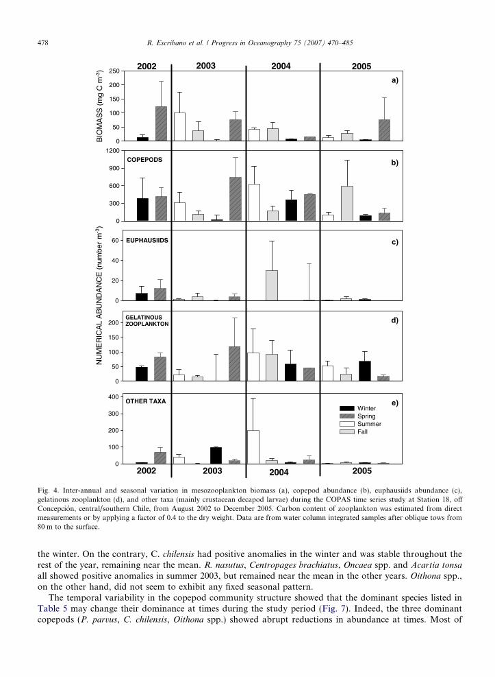
There was no clear pattern in biomass variation over the seasons, although a spring maximum was appar-ent except in spring 2004, when values were low (<20 mg m�3) (Fig. 4a). Copepods also seemed to reach max-imal abundances in spring (Fig. 4b). Euphausiids were more variable and had lower numbers with no clearseasonal pattern (Fig. 4c). Gelatinous zooplankton (including ctenophores, chaetognath, hydrozoa, siphono-fora) were more abundant and tended to increase in the spring although they were also abundant in the winter(Fig. 4d). Variations of other taxa (mostly crustacean larvae) were also observed (Fig. 4e).

Seasonal anomalies were also estimated for zooplankton components to elucidate seasonal patterns. Zoo-plankton biomass was greater-than-average in the spring and summer and lower-than-average in the winter

Table 2Two-way ANOVA to test inter-annual and seasonal effects on oceanographic conditions at Station 18 during the zooplankton time seriesin the coastal upwelling zone off Concepcion

Source of variation Independent variable d.f. F-ratio P

Inter-annual SST 3 1.86 0.15T10 3 0.93 0.44OMZ depth 3 0.57 0.64Chl-a0 3 0.11 0.86Chl-a10 3 0.15 0.93Salinity 3 0.87 0.47

Seasonal SST 3 4.57 0.008T10 3 3.14 0.037*

OMZ depth 3 18.36 0.000*

Chl-a0 3 2.88 0.049*

Chl-a10 3 5.94 0.002*

Salinity 3 9.90 0.000*

SST and T10 are sea temperature at the surface and 10 m, respectively; OMZ depth defines the depth of 1 mL O2 L�1, and Chl-a is totalchlorophyll-a measured at the surface (Chl-a0) and at 10 m depth (Chl-a10).

* Indicates significant effects (P < 0.05).

476 R. Escribano et al. / Progress in Oceanography 75 (2007) 470–485

and fall (Fig. 5a). Copepod abundance reached its maximum in spring, was lower than average in winter andfall, and was nearly average in the summer (Fig. 5b). In contrast, euphausiids seemed to reach annual maximaduring the fall (Fig. 5c). Gelatinous zooplankton exhibited positive anomalies in the winter and in the spring.Other grouped taxa showed positive anomalies in the summer, possibly related to increased decapod larvaeabundance (Fig. 5e).

When examining inter-annual and seasonal patterns (Figs. 4 and 5), the lowest zooplankton biomass wasfound in winter 2005 with 4.9 ± 0.51 mg C m�3 (mean ± SD) and the highest in spring 2002 with123.4 ± 0.43 mg C m�3 (mean ± SD). Copepods exhibited high variability from year to year, although theywere most abundant in spring/summer, as shown by the seasonal anomalies (Fig. 5). The groups of euphausi-ids and chaetognath were less abundant in 2005 than in previous years, whereas, in terms of seasonality, eup-

-1.0-0.8-0.6-0.4-0.20.00.20.40.60.81.0

SST T10

SE

AS

ON

AL

AN

OM

ALY

-2.0

-1.5

-1.0

-0.5

0.0

0.5

1.0

1.5

Sal0Sal50

-30

-20

-10

0

10

20

30

40

OMZ

-6

-4

-2

0

2

4

6

8

10Chla0 Chl10

WINTER SPRING SUMMER FALL

WINTER SPRING SUMMER FALL

Fig. 3. Seasonal anomalies in sea surface temperature (SST), temperature at 10 m depth (T10), surface salinity (Sal0), salinity at 50 mdepth (Sal50), depth of the OMZ (defined as in Fig. 2), surface chlorophyll-a (Chl-a0) and chlorophyll-a a 10 m depth (Chl-a10) during theCOPAS time series study at Station 18, off Concepcion, central/southern Chile from August 2002 to December 2005. Mean seasonalanomalies were estimated after subtracting mean values of the whole time series from each monthly sampling. Vertical bars show standarderrors.

Table 3Total mesozooplankton biomass and numerical abundance (individual m�3) of major taxa found at Station 18 during the zooplanktontime series in the coastal upwelling zone off Concepcion

Group Minimum Maximum Mean SD RA

Biomass (mg C m�3) 3.13 387.50 47.22 74.427Copepods 7.40 1587.80 328.69 385.29 78.7Euphausiids 0.00 31.18 1.46 4.792 0.4Appendicularian 0.00 345.10 26.37 58.979 6.2Siphonofora 0.00 397.70 26.11 66.596 6.3Decapoda larvae 0.00 87.07 7.76 16.681 1.9Chaetognata 0.00 40.45 5.26 7.874 1.3Hydrozoa 0.00 53.90 2.42 8.402 0.6Ctenophora 0.00 4.30 0.50 0.922 <0.3

SD is the standard deviation and RA the relative abundance (%) from the complete time series.

R. Escribano et al. / Progress in Oceanography 75 (2007) 470–485 477

hausiids peaked in fall 2004 with 30.1 ± 50.31 individuals m�3 (mean ± SD) and were lowest in summer 2004with <0.1 ± 0.01 individuals m�3 (mean ± SD).

In order to examine eventual correlations between zooplankton components and oceanographic variables,the cross-correlation function was estimated for paired variables (Table 4). This function allows estimatingtime lags, which can have significant associations. Zooplankton biomass was significantly and positively asso-ciated with changes in log-transformed data of the numerical copepod abundance (F1,41 = 4.22, P = 0.046) attime lag = 0. Euphausiids were also significantly correlated to biomass (F1,41 = 5.34, P = 0.026) at timelag = 0. Gelatinous zooplankton, which included Siphonofora, Chaetognath, and Hydrozoa, were also animportant component of the time series but they, too, were not correlated to C biomass (F1,43 = 0.04,P > 0.05). The data for the other taxa (decapod larvae, appendicularians) were pooled and showed no corre-lation with biomass (Table 4).

When analyzing the influence of oceanographic variables on zooplankton components, biomass was onlysignificantly associated with OMZ depth (Table 4). The negative correlation indicated that biomass mayincrease as the OMZ becomes shallower. A similar correlation was found between OMZ depth and the abun-dance of copepods and euphausiids (Table 4). Copepods appeared to be positively related to SST with a timelag = 4 months, indicating that these organisms increase in abundance four months before surface tempera-tures peak, usually in mid-summer. Finally, there was no significant relationship between zooplankton bio-mass and Chl-a; copepods and euphausiids also failed to correlate with Chl-a (Table 4). The correlationbetween biomass and OMZ depth, however, was strong. A regression analysis between the OMZ depthand the log-transformed biomass yielded a negative slope and was highly significant (F1,44 = 6.79, P < 0.01).

3.3. Changes in copepod community structure

Because copepods were the dominant taxa, their composition could be analyzed in greater detail forchanges in community structure associated with oceanographic variation. The numerically dominant speciesand their relative contributions during the whole sampling period are shown in Table 5. One of the most abun-dant species, Paracalanus parvus, is a rather small and widely spread copepod in the Southern Hemisphere(Heinrich, 1973); another, Oithona spp., comprises at least two small-sized species, of which the cosmopolitanO. similis and O. nana may be the most abundant (Arcos, 1975); and, finally, Calanus chilensis is a much largercopepod endemic to the Humboldt Current (Marın et al., 1994). These three copepods made up more than85% of the total copepod abundance. The less abundant Rhincalanus nasutus should also be mentioned.Despite its low occurrence, it may contribute considerably to total biomass at times because of its relativelylarge size (>4 mm in body length) compared to the other species.

Table 5 also shows the mean and maximal numerical abundance of each species. The mean value was usedto estimate mean abundance anomalies for each season and year (Fig. 6). Mean seasonal anomalies in speciesabundance could provide information on the season(s) in which a given species’ abundance may peak. Forexample, the very abundant P. parvus tended to show positive anomalies in the spring and negative ones in

0

100

200

300

400

BIO

MA

SS

(m

g C

m-3

)

0

50

100

150

200

250

WinterSpringSummerFall

0

300

600

900

1200

NU

ME

RIC

AL

AB

UN

DA

NC

E (

num

ber

m-3

)

0

20

40

60

0

50

100

150

200

COPEPODS

EUPHAUSIIDS

GELATINOUSZOOPLANKTON

OTHER TAXA

2002 2003 2004 2005

2002 2003 2004 2005

a)

b)

c)

d)

e)

Fig. 4. Inter-annual and seasonal variation in mesozooplankton biomass (a), copepod abundance (b), euphausiids abundance (c),gelatinous zooplankton (d), and other taxa (mainly crustacean decapod larvae) during the COPAS time series study at Station 18, offConcepcion, central/southern Chile, from August 2002 to December 2005. Carbon content of zooplankton was estimated from directmeasurements or by applying a factor of 0.4 to the dry weight. Data are from water column integrated samples after oblique tows from80 m to the surface.

478 R. Escribano et al. / Progress in Oceanography 75 (2007) 470–485

the winter. On the contrary, C. chilensis had positive anomalies in the winter and was stable throughout therest of the year, remaining near the mean. R. nasutus, Centropages brachiatus, Oncaea spp. and Acartia tonsa

all showed positive anomalies in summer 2003, but remained near the mean in the other years. Oithona spp.,on the other hand, did not seem to exhibit any fixed seasonal pattern.

The temporal variability in the copepod community structure showed that the dominant species listed inTable 5 may change their dominance at times during the study period (Fig. 7). Indeed, the three dominantcopepods (P. parvus, C. chilensis, Oithona spp.) showed abrupt reductions in abundance at times. Most of

-60

-40

-20

0

20

40

60

SE

AS

ON

AL

AN

OM

ALY

-300

-150

0

150

300

450

-10

-5

0

5

10

15

20

-40

-20

0

20

40

60

WINTER SPRING SUMMER FALL

WINTER SPRING SUMMER FALL-40

-20

0

20

40

60

80

Taxa

a) BIOMASS

b) COPEPODS

c) EUPHAUSIIDS

d) GELATINOUS ZOOPLANKTON

e) OTHER TAXA

Fig. 5. Seasonal anomalies in abundance of mesozooplankton biomass, copepods, euphausiids, gelatinous zooplankton, and other taxa(mainly crustacean decapod larvae) during the COPAS time series study at Station 18, off Concepcion, central/southern Chile, fromAugust 2002 through December 2005. Mean seasonal anomalies were estimated after subtracting mean values of the whole time seriesfrom each monthly sampling. Vertical bars show standard errors.

R. Escribano et al. / Progress in Oceanography 75 (2007) 470–485 479

these incidents took place during the spring/summer period, depending on the year (Fig. 7). During the wholeperiod, these three species appeared to control total copepod abundance; the percentage of occurrence of otherspecies remained low. These alternate changes in dominance may indicate either positive or negative correla-tions among species. To examine such associations, a correlation matrix among the species was constructed(Table 6). Only significant correlations (P < 0.05) are shown after applying the Bonferroni correction to theprobability estimates. All significant correlations were positive and, in most cases, occurred between numer-ically dominant species and scarce ones, thereby indicating that species tend to co-occur temporarily, i.e.,changes in abundance may affect all species similarly.

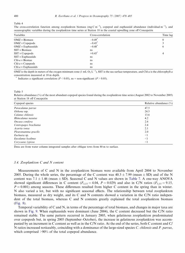
Table 4The cross-correlation function among zooplankton biomass (mg C m�3), copepod and euphausiid abundance (individual m�3), andoceanographic variables during the zooplankton time series at Station 18 in the coastal upwelling zone off Concepcion

Variables Cross-correlation Time lag

OMZ · Biomass �0.49* 0OMZ · Copepods �0.45* 3OMZ · Euphausiids �0.48* 6SST · Biomass nsSST · Copepods +0.45* 4SST · Euphausiids nsChl-a · Biomas nsChl-a · Copepods nsChl-a · Euphausiids ns

OMZ is the depth in meters of the oxygen minimum zone (1 mL O2 L�1), SST is the sea surface temperature, and Chl-a is the chlorophyll-aconcentration measured at 10 m depth.

* Indicates a significant correlation (P < 0.05), ns = non-significant (P > 0.05).

Table 5Relative abundance (%) of the most abundant copepod species found during the zooplankton time series (August 2002 to November 2005)at Station 18 off Concepcion

Copepod species Relative abundance (%)

Paracalanus parvus 47.5Oithona ssp. 24.5Calanus chilensis 13.6Rhincalanus nasutus 4.2Oncaea conifera 2.6Centropages brachiatus 2.4Acartia tonsa 2.1Pleuromamma gracilis 2.0Euchaeta sp. <1Eucalanus hyalinus <1Corycaeus typicus <1

Data are from water column integrated samples after oblique tows from 80 m to surface.

480 R. Escribano et al. / Progress in Oceanography 75 (2007) 470–485

3.4. Zooplankton C and N content

Measurements of C and N in the zooplankton biomass were available from April 2004 to November2005. During the whole series, the percentage of the C content was 40.3 ± 7.99 (mean ± SD) and of the Ncontent was 7.1 ± 1.46 (mean ± SD). Seasonal C and N values are shown in Table 7. A one-way ANOVAshowed significant differences in C content (F3,15 = 4.04, P = 0.029) and also in C/N ratios (F3,15 = 9.15,P = 0.001) among seasons. These differences resulted from higher C content in the spring than in winter.N also varied a lot, but with no significant seasonal effects. The relationship between total zooplanktonbiomass, measured as dry weight, and its C and N contents showed a variation in the C/N ratio indepen-dent of the total biomass, whereas C and N contents greatly explained the total zooplankton biomass(Fig. 8).

Temporal variability of C and N, in terms of the percentage of total biomass, and changes in major taxa areshown in Fig. 9. When euphausiids were dominant (June 2004), the C content decreased but the C/N ratioremained stable. The same pattern occurred in January 2005, when gelatinous zooplankton predominatedover copepods but, in spring 2005 (September–October), the increase in gelatinous zooplankton was accom-panied by an increment in C content as well as in the C/N ratio. At the end of the series, both C content and C/N ratios increased noticeably, coinciding with a dominance of the large-sized species C. chilensis and P. parvus,which comprised >90% of the total copepod abundance.

-200

0

200

400

600

-50

0

50

100

150

-200

0

200

400

WinterSpringSummerFall

AN

OM

ALI

ES

IN A

BU

ND

AN

CE

(nu

mbe

r m

-3)

-150

0

150

300

-100

-50

0

50

100

2002 2003 2004 2005

2002 2003 2004 2005

Paracalanus parvus

Oithona spp

Calanus chilensis

Rhyncalanus nasutus

-50

0

50

100

-50

0

50

100

150

Centropages brachiatus

Oncaea sp

Acartia tonsa

Fig. 6. Inter-annual and seasonal anomalies in numerical abundance of dominant copepod species during the COPAS time series study atStation 18, off Concepcion, central/southern Chile, from August 2002 through December 2005. Mean anomalies were estimated aftersubtracting mean values of the whole time series from each monthly sampling. Vertical bars show standard errors.

R. Escribano et al. / Progress in Oceanography 75 (2007) 470–485 481

4. Discussion

During the upwelling season, the zooplankton distribution is highly aggregated within upwelled waters(Peterson, 1998; Escribano et al., 2002; Hutchings et al., 2006). Under this condition, the highly patchyzooplankton distribution (Abraham, 1998; Giraldo et al., 2002) can affect the observations of temporalvariation of zooplankton based on a fixed location (e.g., Station 18). The Tucker Trawl net, which is ableto integrate the water column and sample a relatively large volume of water (>300 m3), reduces some ofthe bias introduced by small-scale patchiness, although meso-scale variation can certainly account forsome of the observed zooplankton distribution patterns. However, despite these limitations, long-termstudies based on single, fixed stations have proven useful to examine trends in zooplankton temporal var-iability (see Perry et al., 2004 for summary). Our data also contained at least 3 · 3 replicated observations

0.0

0.5

1.0

1.5

2.0

2.5

3.0

A S O N D J F M A M J J A S O N D J F M A M J J A S O N D J F M A M J J A S O N

2002 2003 2004 2005

AB

UN

DA

NC

E (

Nu

mb

er m

-3)

(lo

g s

cale

)

0.0

0.5

1.0

1.5

2.0

2.5

3.0

A S O N D J F M A M J J A S O N D J F M A M J J A S O N D J F M A M J J A S O N

0.0

0.5

1.0

1.5

2.0

2.5

3.0

A S O N D J F M A M J J A S O N D J F M A M J J A S O N D J F M A M J J A S O N

0.0

0.5

1.0

1.5

2.0

2.5

3.0

A S O N D J F M A M J J A S O N D J F M A M J J A S O N D J F M A M J J A S O N

a) Paracalanus parvus

b) Calanus chilensis

c) Oithona spp..

d) Other species

Fig. 7. Variability in dominance of the three most abundant copepods, Paracalanus parvus (a), Calanus chilensis (b), and Oithona spp. (c)during the COPAS time series study at Station 18, off Concepcion, central/southern Chile, from August 2002 to December 2005. Othercopepod species (d) were comprised by at least 10 species in low abundances. Oithona spp. were mainly comprised by two species: O. similis

and O. nana.

Table 6Correlation matrix among copepod species found during the zooplankton time series study off Concepcion at Station 18

CC PP AT CB CT OSP OC EH

AT 0.51CB 0.90CT 0.55 0.68OSP 0.57OC 0.66EH 0.52RN 0.61 0.74 0.50PSP 0.53

The Pearson correlation was applied on log-transformed data of copepod abundances. Only significant (P < 0.05) correlations are shown.Probabilities were estimated with a Bonferroni correction. CC = Calanus chilensis, PP = Paracalanus parvus, AT = Acartia tonsa,CB = Centropages brachiatus, OSP = Oithona spp., OC = Oncaea conifera, EH = Eucalanus hyalinus, RN = Rhincalanus nasutus,PSP = Pleuromamma sp.

482 R. Escribano et al. / Progress in Oceanography 75 (2007) 470–485

Table 7Seasonal changes in C and N content of the zooplankton biomass during the zooplankton time series at Station 18 off Concepcion

Season C (mg m�3) N (mg m�3) C/N

Fall 27.06 ± 25.77 5.24 ± 5.29 5.56Winter 6.04 ± 2.75 1.24 ± 0.42 4.73Spring 53.23 ± 74.14* 7.34 ± 10.12 7.19*

Summer 10.71 ± 4.34 1.82 ± 0.85 5.60

* Indicates significant seasonal differences after ANOVA and the Tukey test.

Biomass (mg dry weight m-3)

0 20 40 60 80 100 120 140

C/N

rat

io

0

2

4

6

8

10

C (

mg

m-3

)

0

50

100

150

200

N (

mg

m-3

)

0

5

10

15

20

25

30

C/NCr2 =0.95Nr2 =0.98

Fig. 8. The relationship between mesozooplankton biomass in dry weight, its C and N contents, and the C/N ratio during the COPAStime series study at Station 18, off Concepcion, central/southern Chile, from August 2002 to December 2005. Samples were obtained on anaverage time interval of 30 days. The regression lines for C and N vs. biomass are highly significant (P < 0.01), whereas the C/N ratio didnot significantly correlate to biomass.

R. Escribano et al. / Progress in Oceanography 75 (2007) 470–485 483

per season and per year, which may also have helped reduce uncertainty caused by sampling bias whenassessing seasonal patterns.

The analysis of oceanographic variables clearly showed a strongly seasonal upwelling process characterizedby an intense and persistent pulse in spring/summer and very weak or absent upwelling during the fall/winter.All oceanographic variables exhibited this seasonal signal, but the most remarkable one was the vertical dis-tribution of the OMZ. Indeed, a shallow depth (<20 m) of the upper OMZ boundary at Station 18 appeared tobe the clearest indicator of upwelling. The bulk of zooplankton biomass and the abundance of copepods, themain contributors to the total biomass, were both strongly correlated to OMZ depth and exhibited a majorincrease in spring/summer, when upwelling prevails. The strong positive correlation among several species(Table 6) suggested that the increased spring abundances may occur because of aggregation of the populationswithin the upwelling zone. Likewise, gelatinous zooplankton tended to concentrate in spring, although theywere also abundant in the winter. In contrast, euphausiids, dominated by the endemic Humboldt Current spe-cies, E. mucronata, did not seem to show any seasonal pattern associated with upwelling, but exhibited positiveanomalies in the fall.

When looking at individual species, most copepods showed peaks of abundance in any season, even in win-ter time, when phytoplankton biomass is low (<1 mg Chl-a m�3). These abundance peaks may result fromcontinuous, year-round reproduction of at least two of the dominant species in the upwelling zone (Hidalgoand Escribano, 2007), in spite of low Chl-a at times of the year. In this area, most copepods switch their dietfrom diatoms (spring/summer) to heterotrophic nanoplankton and microplankton (fall/winter) (Vargas et al.,

C/N

rat

io

0

2

4

6

8

10

12

14

16

18

C %

0

20

40

60

80

100

120

N %

0

5

10

15

20

C/N ratioCN

Rel

ativ

e ab

unda

nce

(%)

0

20

40

60

80

100

Copepods Euphausiids Gelatinous Other taxa

Winter 2004 Spring 04-Summer 2005 Winter 2005

A M J J A S O N D J F M A M J J A S O N

Fig. 9. Temporal changes in C and N content (%) and the C/N ratio of the mesozooplankton biomass (upper panel) and changes in therelative abundance of major zooplankton taxa (lower panel), during the COPAS time series (August 2002 to November 2005) at Station 18off Concepcion. Other taxa are mainly crustacean decapod larvae.

484 R. Escribano et al. / Progress in Oceanography 75 (2007) 470–485

2006). Heterotrophic components remain abundant year-round in this area (Gonzalez et al., 2007; Bottjer andMorales, 2007), providing a continuous food supply for copepods. Thus, Chl-a alone does not seem a suitableindex of food availability for copepods in this area. Vargas et al. (2007) recently showed that copepodsincrease their biomass and production rate during the spring/summer when diatoms are abundant, suggestingthat low Chl-a in the winter may be a limiting factor for copepod growth. In our study, however, it was clearthat copepod abundance determined the significant increase in C content and the C/N ratio in spring with highconcentrations of Chl-a and diatoms (Gonzalez et al., 2007). This increase in C content, largely associated withthe ingestion of fatty acids produced by diatoms (Vargas et al., 2006), may explain increased growth rates andsecondary production during the spring. This spring increment in C and the C/N ratio has also been found inother studies (Schneider, 1989; Postel et al., 2000 for review) and was linked to the capacity of copepods tostore lipids with high C contents (Postel et al., 2000).

In summary, wind-driven upwelling in this region seems to be a key process modulating variability in thezooplankton standing stock and its community structure. The seasonal upwelling signal is well reflected in thespring increase of total zooplankton biomass and its C content. Such increments, however, may result fromstrongly aggregated populations near the upwelling region and not necessarily from increased populationgrowth of dominant species, which appear to be reproducing throughout the year. However, the connectionbetween spring increments in C content, the estimates of individual growth rates (based on C measurements),and actual population growth deserves further attention in highly productive upwelling zones.

Acknowledgements

This work is part of the COPAS Time Series Study off Concepcion and was funded by FONDAP-CONI-CYT. Complementary funding was provided by FIP (Fishery Research Fund of Chile) through Grants FIP2004-20 and FIP 2005-1. We are grateful to many enthusiastic students and COPAS researchers who have sup-ported the COPAS Time Series. We also thank the Kay Kay crew for their extremely valuable cooperation andwillingness. Two anonymous reviewers have substantially helped to improve earlier versions of the manu-script. This study is a contribution to the GLOBEC International program.

R. Escribano et al. / Progress in Oceanography 75 (2007) 470–485 485

References

Abraham, E.R., 1998. The generation of plankton patchiness by turbulent stirring. Nature 391, 577–580.

Araujo, J.N., Mackinson, S., Stanford, R.J., Sims, D.W., Southward, A.J., Hawkins, S.J., Ellis, J.R., Hart, P.J.B., 2006. Modelling food

web interactions, variation in plankton production, and fisheries in the western English Channel ecosystem. Mar. Ecol.-Progr. Ser. 309,

175–187.

Arcos, D.F., 1975. Copepodos calanoideos de la Bahıa de Concepcion, Chile. Conocimiento sistematico y variacion estacional. Gayana

(Zoologıa) 32, 43.

Arcos, D.F., Cubillos, L.A., Nunez, S.P., 2001. The jack mackerel fishery and El Nino 1997–98 effects of Chile. Prog. Oceanogr. 49, 597–

617.

Beaugrand, G., Reid, P.C., Ibanez, F., Lindley, J.A., Edwards, M., 2002. Reorganization of North Atlantic marine copepod biodiversity

and climate. Science 296, 1692–1694.

Beaugrand, G., Brander, K.M., Lindley, J.A., Souissi, S., Reid, P.C., 2003. Plankton effect on cod recruitment in the North Sea. Nature

426, 661–664.

Bottjer, D., Morales, C.E., 2007. Nanoplanktonic assemblages in the upwelling area off Concepcion (�36�S), central Chile: abundance,

biomass, and grazing potential during the annual cycle. Prog. Oceanogr. 75, 415–434.

Castro, L.R., Bernal, P.A., Troncoso, V.A., 1993. Coastal intrusion of copepods: mechanisms and consequences on the population biology

of Rhincalanus nasutus. J. Plank. Res. 15, 501–515.

Chavez, F.P., Ryan, J., Lluch-Cota, S.E., Niquen, C.M., 2003. From Anchovies to Sardines and Back: multidecadal Change in the Pacific

Ocean. Science 299, 217–221.

Escribano, R., Marin, V., Hidalgo, P., Olivares, G., 2002. Physical–biological interactions in the nearshore zone of the northern Humboldt

Current ecosystem, in: Castilla, J.C., Largier, J.L. (Eds), The Oceanography and Ecology of the Nearshore and Bays in Chile,

Ediciones Universidad Catolica de Chile, pp. 145–175.

Giraldo, A., Escribano, R., Marın, V., 2002. Spatial distribution of Calanus chilensis off Mejillones Peninsula (northern Chile): ecological

consequences upon coastal upwelling. Mar. Ecol.-Prog. Ser. 230, 225–234.

Gonzalez, H.E., Menschel, E., Aparicio, A., Barrıa, C., 2007. Spatial and temporal variability of microplankton and detritus, and their

export to the shelf sediments in the upwelling area off Concepcion, Chile (�36�S), during 2002–2005. Progr. Oceanogr. 75, 435–451.

Hays, G.C., Richardson, A.J., Robinson, C., 2005. Climate change and marine plankton. Trends Ecol. Evol. 20, 337–344.

Heinrich, A.K., 1973. Horizontal distribution of copepods in the Peru current region. Oceanology 13, 97–103.

Hidalgo, P., Escribano, R., 2007. Coupling of life cycles of the copepods Calanus chilensis and Centropages brachiatus to upwelling induced

variability in the central-southern region of Chile. Prog. Oceanogr. 75, 501–517.

Hutchings, L., Verheye, H., Huggett, J.A., Demarcq, H., Barlow, R.G., da Silva, A., 2006. Variability of plankton with reference to fish

variability in the Benguela Current Large Marine Ecosystem – an overview. In: Shannon, V., Hempel, G., Malanotte-Rizzoli, P.,

Moloney, C., Woods, J. (Eds.), The Benguela: Predicting a Large Marine Ecosystem. Elsevier, pp. 91–124.

Marın, V.H., Espinoza, S., Fleminger, A., 1994. Morphometric study of Calanus chilensis males along the Chilean coast. Hydrobiologia

292/293, 75–80.

Montero, P., Daneri, G., Cuevas, L.A., Gonzalez, H.E., Jacob, B., Lizarraga, L., Menschel, E., 2007. Productivity cycles in the coastal

upwelling area off Concepcion: the importance of diatoms and bacterioplankton in the organic carbon flux. Prog. Oceanogr. 75, 518–

530.

Pauly, D., Christensen, V., Guenette, S., Pitcher, T.J., Sumaila, U.R., Walters, C.J., Watson, R., Zeller, D., 2002. Towards sustainability

in world fisheries. Nature 418, 689–695.

Perry, I.R., Batchelder, H.P., Mackas, D.L., Chiba, S., Durbin, E., Greve, W., Verhey, H.M., 2004. Identifying global synchronies in

marine zooplankton populations: issues and opportunities. ICES J. Mar. Sci. 61, 445–456.

Peterson, W., 1998. Life cycle strategies of copepods in coastal upwelling zones. J. Mar. Syst. 15, 313–326.

Peterson, W., Arcos, D., McManus, G., Dam, H., Bellantoni, D., Johnson, T., Tiselius, P., 1988. The nearshore zone during coastal

upwelling; Daily variability and coupling between primary and secondary production off Central Chile. Progr. Oceanogr. 20, 1–40.

Postel, L., Fock, H., Hagen, W., 2000. Biomass and abundance. In: Harris, R.P., Wiebe, P.H., Lenz, J., Skjoldal, H.R., Huntley, M.

(Eds.), ICES Zooplankton Methodology Manual. Academic Press, NY, pp. 83–174.

Richardson, A.J., Schoeman, D., 2004. Climate impacts on plankton ecosystems in the northeast Atlantic. Science 305, 1609–1612.

Schneider, G., 1989. Carbon and nitrogen content of marine zooplankton dry material: a short review. Plankton Newsletter 11, 4–7.

Sobarzo, M., Bravo, L., Donoso, D., Garces-Vargas, J., Schneider, W., 2007. Coastal upwelling and seasonal cycles that influence the

water column over the continental shelf off central Chile. Progr. Oceanogr. 75, 363–382.

Vargas, C., Escribano, R., Poulet, S., 2006. Phytoplankton diversity determines time-windows for successful zooplankton reproductive

pulses. Ecology 87, 2992–2999.

Vargas, C., Martınez, R., Cuevas, L., Pavez, M., Cartes, C., Gonzalez, H.E., Escribano, R., Daneri, G., 2007. Interplay among microbial,

omnivorous, and gelatinous metazoan food webs in a highly productive coastal upwelling area. Limnol. Oceanogr. 52, 1495–1510.