arX

iv:1

101.

3650

v2 [

astr

o-ph

.HE

] 2

Feb

201

1

Search for Lorentz Invariance breaking with a likelihood

fit of the PKS 2155-304 flare data taken on MJD 53944

HESS Collaboration, A. Abramowskia, F. Acerob, F. Aharonianc,d,e,A.G. Akhperjanianf,e, G. Antong, A. Barnackah,i, U. Barres de Almeidaj,1,A.R. Bazer-Bachik, Y. Becherinil,m, J. Beckern, B. Beherao, K. Bernlohrc,p,A. Bochowc, C. Boissonq, J. Bolmontr,∗, P. Bordass, V. Borrelk, J. Bruckerg,

F. Brunm, P. Bruni, R. Buhlerc,2, T. Bulikt, I. Buschingu, S. Carriganc,S. Casanovac, M. Cerrutiq, P.M. Chadwickj, A. Charbonnierr,

R.C.G. Chavesc, A. Cheesebroughj, L.-M. Chounetm, A.C. Clapsonc,G. Coignetv, J. Conradw, M. Daltonp, M.K. Danielj, I.D. Davidsx,

B. Degrangem, C. Deilc, H.J. Dickinsonj,w, A. Djannati-Ataıl, W. Domainkoc,L.O’C. Druryd, F. Duboisv, G. Dubusy, J. Dyksh, M. Dyrdaz, K. Egbertsaa,

P. Egerg, P. Espigatl, L. Fallond, C. Farnierb, S. Feganm, F. Feinsteinb,M.V. Fernandesa, A. Fiassonv, G. Fontainem, A. Forsterc, M. Fußlingp,

S. Gabicid, Y.A. Gallantb, H. Gastc, L. Gerardl, D. Gerbign, B. Giebelsm,J.F. Glicensteini, B. Gluckg, P. Goreti, D. Goringg, J.D. Haguec, D. Hampfa,

M. Hausero, S. Heinzg, G. Heinzelmanna, G. Henriy, G. Hermannc,J.A. Hintonab, A. Hoffmanns, W. Hofmannc, P. Hofverbergc, D. Hornsa,A. Jacholkowskar,∗, O.C. de Jageru, C. Jahng, M. Jamrozyac, I. Jungg,

M.A. Kastendiecka, K. Katarzynskiad, U. Katzg, S. Kaufmanno, D. Keoghj,M. Kerschhagglp, D. Khangulyanc, B. Khelifim, D. Klochkovs, W. Kluzniakh,

T. Kneiskea, Nu. Kominv, K. Kosacki, R. Kossakowskiv, H. Laffonm,G. Lamannav, J.-P. Lenainq, D. Lennarzc, T. Lohsep, A. Lopating, C.-C. Luc,

V. Marandonl, A. Marcowithb, J. Masbouv, D. Maurinr, N. Maxtedae,T.J.L. McCombj, M.C. Medinai, J. Mehaultb, R. Moderskih, E. Moulini, C.L.Naumannr, M. Naumann-Godoi, M. de Nauroism, D. Nedbalaf, D. Nekrassovc,

N. Nguyena, B. Nicholasae, J. Niemiecz, S.J. Nolanj, S. Ohmc, J-F. Olivek,E. de Ona Wilhelmic, B. Opitza, M. Ostrowskiac, M. Panterc,

M. Paz Arribasp, G. Pedalettio, G. Pelletiery, P.-O. Petrucciy, S. Pital,G. Puhlhofers, M. Punchl, A. Quirrenbacho, M. Rauea, S.M. Raynerj,

A. Reimeraa, O. Reimeraa, M. Renaudb, R. de los Reyesc, F. Riegerc,ag,J. Ripkenw, L. Robaf, S. Rosier-Leesv, G. Rowellae, B. Rudakh, C.B. Rultenj,

J. Ruppeln, F. Rydeah, V. Sahakianf,e, A. Santangelos, R. Schlickeisern,F.M. Schockg, A. Schonwaldp, U. Schwankep, S. Schwarzburgs,

S. Schwemmero, A. Shalchin, M. Sikorah, J.L. Skiltonai, H. Solq, G. Spenglerp, L. Stawarzac, R. Steenkampx, C. Stegmanng, F. Stinzingg, I. Sushchp,A. Szostekac,y, P.H. Tamo, J.-P. Tavernetr, R. Terrierl, O. Tibollac,

M. Tluczykonta, K. Valeriusg, C. van Eldikc, G. Vasileiadisb, C. Venteru,

∗Corresponding authorEmail addresses: bolmont@in2p3.fr (J. Bolmont), agnieszka.jacholkowska@cern.ch

(A. Jacholkowska)1Supported by CAPES Foundation, Ministry of Education of Brazil2Present address: Kavli/SLAC, 2575 Sand Hill Road, Menlo Park, CA 94025, USA

Preprint submitted to Elsevier February 3, 2011

J.P. Viallev, A. Vianai, P. Vincentr, M. Vivieri, H.J. Volkc, F. Volpec,S. Vorobiovb, M. Vorsteru, S.J. Wagnero, M. Wardj, A. Wierzcholskaac,

A. Zajczykb,h, A.A. Zdziarskih, A. Zechq, H.-S. Zechlina

a Universitat Hamburg, Institut fur Experimentalphysik, Luruper Chaussee 149, D 22761Hamburg, Germany

b Laboratoire de Physique Theorique et Astroparticules, Universite Montpellier 2,CNRS/IN2P3, CC 70, Place Eugene Bataillon, F-34095 Montpellier Cedex 5, France

c Max-Planck-Institut fur Kernphysik, P.O. Box 103980, D 69029 Heidelberg, Germanyd Dublin Institute for Advanced Studies, 31 Fitzwilliam Place, Dublin 2, Irelande National Academy of Sciences of the Republic of Armenia, Yerevan, Armenia

f Yerevan Physics Institute, 2 Alikhanian Brothers St., 375036 Yerevan, Armeniag Universitat Erlangen-Nurnberg, Physikalisches Institut, Erwin-Rommel-Str. 1, D 91058

Erlangen, Germanyh Nicolaus Copernicus Astronomical Center, ul. Bartycka 18, 00-716 Warsaw, Poland

i CEA Saclay, DSM/IRFU, F-91191 Gif-Sur-Yvette Cedex, Francej University of Durham, Department of Physics, South Road, Durham DH1 3LE, UK

k Centre d’Etude Spatiale des Rayonnements, CNRS/UPS, 9 av. du Colonel Roche, BP4346, F-31029 Toulouse Cedex 4, France

l Astroparticule et Cosmologie (APC), Universite Paris 7 Denis Diderot, CNRS/IN2P3,CEA, Observatoire de Paris, 10 rue Alice Domon et Leonie Duquet, F-75205 Paris Cedex

13, Francem Laboratoire Leprince-Ringuet, Ecole Polytechnique, CNRS/IN2P3, F-91128 Palaiseau,

Francen Institut fur Theoretische Physik, Lehrstuhl IV: Weltraum und Astrophysik,

Ruhr-Universitat Bochum, D 44780 Bochum, Germanyo Landessternwarte, Universitat Heidelberg, Konigstuhl, D 69117 Heidelberg, Germanyp Institut fur Physik, Humboldt-Universitat zu Berlin, Newtonstr. 15, D 12489 Berlin,

Germanyq LUTH, Observatoire de Paris, CNRS, Universite Paris Diderot, 5 Place Jules Janssen,

F-92190 Meudon, Francer LPNHE, Universite Pierre et Marie Curie Paris 6, Universite Denis Diderot Paris 7,

CNRS/IN2P3, 4 Place Jussieu, F-75252, Paris Cedex 5, Frances Institut fur Astronomie und Astrophysik, Universitat Tubingen, Sand 1, D 72076

Tubingen, Germanyt Astronomical Observatory, The University of Warsaw, Al. Ujazdowskie 4, 00-478

Warsaw, Polandu Unit for Space Physics, North-West University, Potchefstroom 2520, South Africav Laboratoire d’Annecy-le-Vieux de Physique des Particules, Universite de Savoie,

CNRS/IN2P3, F-74941 Annecy-le-Vieux, Francew Oskar Klein Centre, Department of Physics, Stockholm University, Albanova University

Center, SE-10691 Stockholm, Swedenx University of Namibia, Department of Physics, Private Bag 13301, Windhoek, Namibiay Laboratoire d’Astrophysique de Grenoble, INSU/CNRS, Universite Joseph Fourier, BP

53, F-38041 Grenoble Cedex 9, Francez Instytut Fizyki Jadrowej PAN, ul. Radzikowskiego 152, 31-342 Krakow, Poland

aa Institut fur Astro- und Teilchenphysik, Leopold-Franzens-Universitat Innsbruck, A-6020Innsbruck, Austria

ab Department of Physics and Astronomy, The University of Leicester, University Road,Leicester, LE17RH, UK

ac Obserwatorium Astronomiczne, Uniwersytet Jagiellonski, ul. Orla 171, 30-244 Krakow,Poland

ad Torun Centre for Astronomy, Nicolaus Copernicus University, ul. Gagarina 11, 87-100Torun, Poland

ae School of Chemistry & Physics, University of Adelaide, Adelaide 5005, Australiaaf Charles University, Faculty of Mathematics and Physics, Institute of Particle and

Nuclear Physics, V Holesovickach 2, 180 00 Prague 8, Czech Republic

2

ag European Associated Laboratory for Gamma-Ray Astronomy, jointly supported by CNRSand MPG

ah Oskar Klein Centre, Department of Physics, Royal Institute of Technology (KTH),Albanova, SE-10691 Stockholm, Sweden

ai School of Physics & Astronomy, University of Leeds, Leeds LS2 9JT, UK

Abstract

Several models of Quantum Gravity predict Lorentz Symmetry breaking at en-ergy scales approaching the Planck scale (∼ 1019 GeV). With present photondata from the observations of distant astrophysical sources, it is possible toconstrain the Lorentz Symmetry breaking linear term in the standard photondispersion relations. Gamma-ray Bursts (GRB) and flaring Active GalacticNuclei (AGN) are complementary to each other for this purpose, since theyare observed at different distances in different energy ranges and with differ-ent levels of variability. Following a previous publication of the High EnergyStereoscopic System (H.E.S.S.) collaboration [1], a more sensitive event-by-eventmethod consisting of a likelihood fit is applied to PKS 2155-304 flare data ofMJD 53944 (July 28, 2006) as used in the previous publication. The previouslimit on the linear term is improved by a factor of ∼3 up to Ml

QG > 2.1 × 1018

GeV and is currently the best result obtained with blazars. The sensitivity tothe quadratic term is lower and provides a limit of Mq

QG > 6.4×1010 GeV, whichis the best value obtained so far with an AGN and similar to the best limitsobtained with GRB.

Keywords: active galaxies, PKS 2155-304, H.E.S.S., quantum gravity,Lorentz invariance breaking

1. Introduction

1.1. Lorentz Invariance and Quantum Gravity

A development of new space-borne and ground-based experiments in thelast decade, covering a large domain of gamma-ray astronomy, opened a newwindow for fundamental physics tests. In particular, the confrontation of theresults from astrophysical sources with challenging predictions of various modelsin the frame of Quantum Gravity theories became of general interest [2]. Thetheory of Quantum Gravity (see e.g. [3]), which is still incomplete, would give aunified picture based on both Quantum Mechanics and General Relativity, thusleading to a common description of the four fundamental forces.

Quantum Gravity effects in the framework of String Theory [4], where thegravitation is considered as a gauge interaction, result from a graviton-like ex-change in a classical space-time. In most String Theory models involving largeextra-dimensions, these effects would take place at the Planck scale, thus not

3

leading to “spontaneous” Lorentz Symmetry breaking, as may happen in mod-els with “foamy” structure [5, 4] of quantum space-time. In this second classof models, photons propagate in a vacuum which may exhibit a non-negligiblerefractive index due to its foamy structure on a characteristic scale approachingthe Planck length or equivalently the Planck energy EP = 1.22 × 1019 GeV.This implies a group velocity of light changing as a function of energy of thephotons, in analogy to the dispersion effects in any theoretical description ofplasma media.

On the other hand, in models based on General Relativity with Loop Quan-tum Gravity [6, 7] which postulate discrete (cellular) space-time in the Planck-ian regime, the fluctuations would introduce perturbations to the propagationof photons. The light wave going through the discrete space matrix would feelan induced perturbation which increases with decreasing wavelength or equiva-lently with increasing energy of photons. In consequence, photons with differentwavelengths propagate with different velocity.

As a result, one may expect a spontaneous violation of Lorentz Symmetryat high energies to be the generic signature of the Quantum Gravity.

In four dimensions, the Quantum Gravity scale is presumed to be close to thePlanck mass and the standard photon dispersion relations up-to second ordercorrections in energy can be written as:

c2p2 = E2(

1 ± ξ(E/M) ± ζ(E/M)2 ± ...)

, (1)

where ξ and ζ are positive parameters.This implies an energy-dependent speed-of-light with

v = c (1 − ξ(E/M)) (2)

considering only the linear term in the expansion. Alternatively assuming thelinear correction equal to zero, the quadratic term leads to:

v = c(

1 − ζ(E/M)2)

. (3)

High-energy photons could propagate either slower (the sub-luminal case)or faster (the super-luminal case) than low-energy photons. In this study, acausality conserving scheme was adopted following to the theoretical argumentsof the non-critical string models, developed in [8]. The sign minus in equations2 and 3 is required to avoid Cherenkov radiation in vacuum [9]. As results ofthis analysis and as in case of most of other quoted results in Table 1, onlylimits on Quantum Gravity scale for the sub-luminal photons will be given.

As suggested by Amelino-Camelia [5], the tiny effects due to Quantum Grav-ity can add up to measurable time delays for photons from cosmological sources.The energy dispersion is best observed in sources that show fast flux variability,that are at cosmological distances and are observed over a wide energy range.This is the case of Gamma Ray Bursts (GRB) and Very High Energy (VHE)flares of Active Galactic Nuclei (AGN). Both types of sources are the preferredtargets of these time-of-flight studies, which provide the least model-dependent

4

tests of the Lorentz Symmetry. The case of pulsed emission by Pulsars has alsobeen considered, and provided valuable results [10].

It should be underlined that studying both GRB and AGN is of fundamentalinterest. GRB are observed with satellites at very large distances (up to z ∼ 8)but with very limited statistics above a few tens of GeV. On the contrary,AGN flares can be detected by ground based instruments with large statisticsup to a few tens of TeV. Due to the absorption of the high energy photons byExtragalactic Background Light (EBL), TeV observations are limited to sourceswith low redshifts. Thus, GRB and AGN are complementary since they allowto test different energy and redshift ranges.

It should be noted that time-of-flight measurements are subject to a biasrelated to a potential dispersion introduced from the intrinsic source effects,which could cancel-out or enhance the dispersion due to modifications to thespeed of light.

When considering sources at cosmological distances, the analysis of time lagsas a function of redshift requires a correction due to the expansion of the universe[11], which depends on the cosmological model. Following the analysis of theBATSE data and recently of the HETE-2 and Swift GRB data [12, 13, 14, 15]and within a framework of the Standard Cosmological Model [16] with a flatexpanding universe and a cosmological constant, the difference in the arrivaltime of two photons emitted at the same time is given by

∆t

∆E≈

ξ

EPH0

∫ z

0

(1 + z′) dz′√

Ωm(1 + z′)3 + ΩΛ

(4)

for a linear effect, and by

∆t

∆E2≈

3ζ

2E2PH0

∫ z

0

(1 + z′)2 dz′√

Ωm(1 + z′)3 + ΩΛ

(5)

for a quadratic effect. In the present study the cosmological parameters wereset to Ωm = 0.3, ΩΛ = 0.7 and H0 = 2.3 × 10−18 s−1. ∆E and ∆E2 representlinear and quadratic energy ranges respectively.

1.2. Present results

The most important results obtained so far with transient astrophysicalsources are given in Table 1. The most robust limits to date have been ob-tained by Ellis et al. [13, 14] and Bolmont et al. [15], with the use of severalGRB at different redshifts, resulting in limits of the order of Ml

QG > 1016 GeV.In case of a significant detection, using several sources at different redshifts al-lows in principle to take into account the possible time-lags originating fromsource effects.

Fermi is now in operation and has provided the best limits so far [17, 18].However, for the moment the results are obtained with no study of the variationof the time-lag with redshift and with limited statistics in the GeV range. Therecent studies with flares of Mrk 501 [19, 20] and the former result of H.E.S.S.

5

Table 1: A selection of limits obtained with various instruments and methods for both GRB and AGNSource(s) Experiment Method Results (95% CL limits) Reference NoteGRB 021206 RHESSI Fit + mean arrival time in a spike Ml

QG > 1.8×1017 GeV [21] a,b

GRB 080916C Fermi GBM + LAT associating a 13 GeV photon with the MlQG > 1.3×1018 GeV [17]

trigger time MqQG > 0.8×1010 GeV

GRB 090510 Fermi GBM + LAT associating a 31 GeV photon with the MlQG > 1.5×1019 GeV [18] c

start of any observed emission, DisCan MqQG > 3.0×1010 GeV c

9 GRBs BATSE + OSSE wavelets MlQG > 0.7×1016 GeV [12] a

MqQG > 2.9×106 GeV

15 GRBs HETE-2 wavelets MlQG > 0.4×1016 GeV [15] d

17 GRBs INTEGRAL likelihood MlQG > 3.2×1011 GeV [22] e

35 GRBs BATSE + HETE-2 wavelets MlQG > 1.4×1016 GeV [13, 14] f ,g

+ Swift

Mrk 421 Whipple likelihood MlQG > 0.4×1017 GeV [31] a,h

Mrk 501 MAGIC ECF MlQG > 0.2×1018 GeV [19]

MqQG > 0.3×1011 GeV

likelihood MlQG > 0.3×1018 GeV [20]

MqQG > 5.7×1010 GeV

PKS 2155-304 H.E.S.S. MCCF MlQG > 7.2×1017 GeV [1]

MqQG > 1.4×109 GeV

wavelets MlQG > 5.2×1017 GeV

likelihood MlQG > 2.1×1018 GeV i

MqQG > 6.4×1010 GeV

aLimit obtained not taking into account the factor (1 + z) in the integral of equations 4 and 5. bThe pseudo-redshift estimator[32] was used. This estimator can be wrong by a factor of 2. cOnly the most conservative limits are given here. The bestlimits given in [18] which can still be considered as secure are Ml

QG > 10 EP and MqQG > 8.8×1010 GeV. dPhoton tagged data

was used. eThe pseudo-redshift estimator [32] was used for 6 GRB out of 11. fFor HETE-2, fixed energy bands were used.gThe limits of Ellis et al. [13] were updated in [14] taking into account the factor (1 + z) in the integral of equation 4. Onlythe limit obtained for a linear correction is given. hA likelihood procedure was used, but not on an event-by-event basis. iThiswork.

6

with PKS 2155-304 [1] provide results setting a lower limit on the linear Quan-tum Gravity scale at a few 1017 GeV for each source.

Table 1 also shows the different analysis techniques used to measure theenergy-depend time-lags. The analysis methods can be divided in two categories,analyses applied on binned data on the one hand and unbinned analyses on theother hand.

Binned analyses are applied on binned light curves and consist of findingthe position of local extrema in two different energy bands and deducing thevalue of the lag. A simple fit [21] or a more sophisticated technique such asContinuous Wavelet Transform (CWT) can be used to localize extrema. CWTwas used for GRB [12, 13, 14, 15] and PKS 2155-304 [1]. The Modified CrossCorrelation Function (MCCF) was also used for PKS 2155-304 to determinedirectly the lag from two light curves in two different energy bands [1].

Unbinned analyses have also been used for both GRB and AGN. Likelihoodfits require a parameterization of the light curves and this parameterization canbe taken from a binned [20] or unbinned fit [22] to the light curve. Anothermethod, the Energy Cost Function (ECF), was recently used by Albert et al.[19]. In this method one introduces a time lag τ for each photon and adds uptheir energies if they fall into a given time interval. The maximum of ECF(τ)gives the value of the measured lag. The recently developed method calledDisCan [23] was used for the analysis of Fermi data [18]. As discussed in [23],this method applies successfully to the analysis of very sharp peaks as can befound in GRB light curves.

It is important to point out here that the use of at least two methods isrecommended since different methods can probe different aspects of the lightcurve. The present analysis completes previously published studies [1] wheretwo different methods were employed.

As no significant time-lag was detected so far, careful error calibration studiesusing Monte Carlo simulations are mandatory for the extraction of the limits,as will be further discussed in the following.

1.3. Overview of the paper

In this paper, a new analysis of PKS 2155-304 data is presented, using alikelihood fit to determine both linear and quadratic corrections to the dispersionrelations. In section 2, the method is described. The data in use as well as theselections applied are detailed in section 3. Then, in section 4, the procedureused to calibrate the method and to evaluate systematics is presented. Theresults are given in section 5 and finally discussed in section 6.

2. Method description

To study the correlations between the arrival time and the energy of thephotons, a method relying on a probability density function (p.d.f.) on anevent-by-event basis is used. Following Martinez and Errando [20], the p.d.f. is

7

defined by:

P (t, E) = N

∫

∞

0

A(ES)Λ(ES)G(E − ES , σ(ES))FS(t− τlES)dES , (6)

where Λ(ES) is the emission spectrum, G(E−ES , σ(ES)) is the smearing func-tion in energy (a usual point spread function for an energy resolution of 10%),A(ES) is the acceptance of the H.E.S.S. array, FS is a parameterization of theemission time distribution (or light curve) and N is a normalization factor. thetime shift was re-parameterized as ∆t = −τlE and ∆t = −τqE

2 for linear andquadratic effects respectively, where τl and τq are expressed in s TeV−1 ands TeV−2. The value of N was computed in view of unbiased τ -parameter es-timation. It guarantees the correct normalization of the p.d.f. and takes intoaccount its model dependence. Here, integration over measured domain of en-ergy and time has been performed.

The function FS is a function of time at the source tS = t − τES . Theprobability P (t, E) depends only on the relative delay of photons for differentenergies. As the light curve at the emission time is not known, the best estimateof the time structure at the source can be taken from the time distribution ofthe lowest energy photons. In the propagation models, the change of the QGscale induces basically a sliding effect in time of the light curve. This point hasbeen checked to be valid by the Monte Carlo simulations described below.

An important assumption of this study should be underlined: the intrinsiclight curves have been considered to have the same shape in different energybands. As no lag is found, this can be partially justified by comparing the lightcurve at low energy (Fig. 2) and in the full energy range of the instrumentwhere the statistics is five times higher [24]. In both cases the light curve showsa five peak structure with maxima located roughly at the same times.

The likelihood function is given by the product of probability density func-tions over all photons:

L =∏

i

Pi(t, E). (7)

The maximum of L provides the time-lag parameter τl and τq for linear andquadratic models respectively.

The likelihood method is in principle very sensitive and allows a lag to bemeasured even if the number of selected photons is limited, which is not thecase for wavelet or MCCF analyses. As a consequence of this high statisticalsensitivity, it would be possible to probe a light curve locally, introducing aselection in time. The main aspect of the method to be taken into account is aneed for a very precise parameterization of the photon distributions.

3. Data sample used in the analysis

PKS 2155-304 is a high-peaked BL Lac object located at redshift z = 0.116.On July 28, 2006 (MJD 53944), an extreme flare of this source was observed byH.E.S.S. [24]. The full data sample was obtained using a combination of two

8

Table 2: Selections applied to the data

Selection Number of selected eventsTotal sample 8148 (100 %)(1) = Time in 0–4000 s 7713 (95 %)(2) = (1) and θ2 < 0.005 deg.2 5974 (73 %)(2) and Em in 0.25–4.0 TeV 3526 (43 %)(2) and Em in 0.25–0.28 TeV 561 (7 %)

analysis methods [25]: the standard Hillas analysis [26] and the Model analysis[27]. This technique greatly improves the signal to background ratio and resultsin 8148 on-source events recorded in ∼85 minutes (three data-taking runs) withan energy threshold of ∼120 GeV. The signal-to-background ratio in the flaredata exceeds 300. The effect of the background contribution will be investigatedin the next section. The average zenith angle of selected events is θz ≈ 11.

Table 2 summarizes the different cuts applied to the data. In this study,only the first 4000 s of data (7713 events) are considered, where the flux andvariability are the highest. To further improve the signal-to-background ratio, acut θ2 < 0.005 deg.2 is applied. This cut reduces the number of photons to 5974events but allows a very good fit of the light curve and of the energy spectrum.A total of 3526 events pass the cut on θ2 in the first 4000 s of data in the range0.25–4.0 TeV. All events in the data sample fulfilling the selection were used inthe analysis.

As shown in Figure 1, the reconstructed spectrum is compatible with a powerlaw of index Γ = 3.46 in the range of 0.25–4.0 TeV (with χ2/dof = 16.7/23).This result is compatible with the high energy part of the broken power lawspectrum obtained for the same flare by Aharonian et al. [24] with a differentevent selection and energy reconstruction method, and also with the spectrumobtained for the whole 2005–2007 period [28]. The dependence of the spectralindex as a function of time has been studied extensively in [24] and no significantvariation was found during the flare.

Figure 2 shows the light curve in the range 0.25–0.28 TeV with a binningof 61 s. The shape of this light curve will be used later as a template for thetime-lag determination (§5). To estimate the main parameters of the light curve(widths and asymmetry of the pulses, distance between consecutive spikes), aparameterization was performed with a sum of asymmetric Gaussian functions.For this, the number of spikes was first determined using a peak-finding proce-dure based on a Markov chain algorithm [29]. Five pulses were found and theirpositions were used as initial parameters for the light curve fit.

The fit function F is a sum of asymmetric Gaussian curves, defined as follows:

Fn(t) =

n∑

i=1

fi(t, Ai, µi, αi, βi), (8)

9

E (TeV)-110×2 1 2 3 4 5

dN/d

E

-110

1

10

210

310

PKS 2155-304 Data 0.04± = 3.46 Γ

/dof = 16.7/232χ

Figure 1: Spectrum of PKS 2155-304 flare of MJD 53944, taking into account the cut on theoff-axis angle mentioned in the text. Points are fitted with a power law E

−Γ.

10

Time (s)0 500 1000 1500 2000 2500 3000 3500 4000

dN/d

t

0

5

10

15

20

25

30

PKS 2155-304 Data0.25-0.28 TeV

/dof = 48.8/382χ

Figure 2: Light curve of PKS 2155-304 flare of MJD 53944 in the range 0.25–0.28 TeV, witha bin width of 61 s and taking into account the cut on θ2 described in the text. Black pointsshow the positions of the extrema as determined by the peak-finding procedure of Morhac etal. [29]. The light curve is fitted with a function F5(t) + B where B is a constant and F5 isdefined by equation 8. The zero of the time axis corresponds to MJD 53944.024.

11

Table 3: Parameters of the function F5(t)+B fitted on PKS 2155-304 light curve in the range0.25–0.28 TeV

Parameter Value ErrorA1 27.1 1.4µ1 430.4 35.8α1 399.9 25.4β1 352.9 75.7A2 26.0 0.8µ2 1456.1 16.0α2 342.9 92.8β2 193.3 44.9A3 28.0 0.7µ3 2113.1 19.2α3 276.1 46.2β3 296.8 29.3A4 20.0 0.7µ4 2639.7 77.0α4 130.3 34.3β4 899.8 23.7A5 9.4 1.3µ5 3302.3 19.9α5 87.1 36.5β5 999.9 80.4B −14.1 0.8

where n is the number of spikes, and where

f(t, A, µ, α, β) =

y = A e−(t−µ)2

2α2 , if t < µ

y = A e−

(t−µ)2

2β2 , if t ≥ µ.(9)

In this definition, A and µ are the normalization factor and the position ofthe pulse and α and β are the left-hand and right-hand widths of the pulserespectively. The asymmetry of the curve can be quantified by the parameterν = β/α. When ν = 1, f becomes a Gaussian function with a width α = β = σ0.

The parameterization was carried out with a function F5 plus a constant termB. Values of the parameters are given in Table 3, leading to χ2/dof = 48.8/38.This fit gives the following information about the light curve:

• width of the pulses in the range 250–600 s,

• time difference between consecutive spikes in the range 500–1000 s, and

• ratio ν in the range 0.6–7.

These intervals were investigated for the calibration procedure described inthe next section.

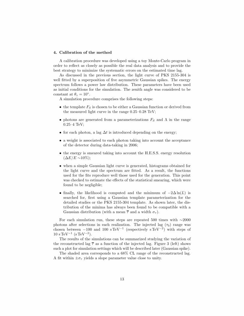
4. Calibration of the method

A calibration procedure was developed using a toy Monte-Carlo program inorder to reflect as closely as possible the real data analysis and to provide thebest strategy to minimize the systematic errors on the estimated time lag.

As discussed in the previous section, the light curve of PKS 2155-304 iswell fitted by a superposition of five asymmetric Gaussian spikes. The energyspectrum follows a power law distribution. These parameters have been usedas initial conditions for the simulation. The zenith angle was considered to beconstant at θz = 10.

A simulation procedure comprises the following steps:

• the template FS is chosen to be either a Gaussian function or derived fromthe measured light curve in the range 0.25–0.28 TeV;

• photons are generated from a parameterizations FS and Λ in the range0.25–4 TeV;

• for each photon, a lag ∆t is introduced depending on the energy;

• a weight is associated to each photon taking into account the acceptanceof the detector during data-taking in 2006;

• the energy is smeared taking into account the H.E.S.S. energy resolution(∆E/E ∼10%);

• when a simple Gaussian light curve is generated, histograms obtained forthe light curve and the spectrum are fitted. As a result, the functionsused for the fits reproduce well those used for the generation. This pointwas checked to estimate the effects of the statistical smearing, which werefound to be negligible;

• finally, the likelihood is computed and the minimum of −2∆ ln(L) issearched for, first using a Gaussian template parameterization for thedetailed studies or the PKS 2155-304 template. As shown later, the dis-tribution of the minima has always been found to be compatible with aGaussian distribution (with a mean τ and a width στ ).

For each simulation run, these steps are repeated 500 times with ∼2000photons after selections in each realization. The injected lag (τ0) range waschosen between −100 and 100 s TeV−1 (respectively s TeV−2) with steps of10 s TeV−1 (s TeV−2).

The results of the simulations can be summarized studying the variation ofthe reconstructed lag τ as a function of the injected lag. Figure 3 (left) showssuch a plot for simulation settings which will be described later (Gaussian spike).

The shaded area corresponds to a 68% CL range of the reconstructed lag.A fit within ±στ yields a slope parameter value close to unity.

13

)-1 (s TeVlτInjected -100 -50 0 50 100

)-1

(s

TeV

lτR

econ

stru

cted

-100

-50

0

50

100

Gaussian pulseLinear Model

-1 = 0) = 5.0 s TeVlτ(τσ

)-1Reconstructed Lag (s TeV-15 -10 -5 0 5 10 150

20

40

60

80

100

(s)0σ0 200 400 600 800 1000 1200

)-1

(s

TeV

τσ

0

5

10

15

20

25

30

FWHM (s)0 500 1000 1500 2000 2500

Gaussian pulseLinear Model

Figure 3: Left: reconstructed lag as a function of the injected lag for a Gaussian light curvein the modelling mode (68% CL range). The plot in the bottom right corner shows thedistribution of the minima for the 500 realizations with a generated lag of 0 s TeV−1. Thedashed line shows the linear response function. Right: parameter στ as a function of the widthof the Gaussian pulse. The axis at the top gives the full width at half maximum (FWHM) ofthe pulse.

A small systematic shift of the slope is observed; however, the bias on thereconstructed time lag is much smaller than the statistical uncertainty στ fortime lags between −50 s TeV−1 and 50 s TeV−1.

In the following sub-sections, different features of the error calibration proce-dure are detailed. First, the influence of the pulse shape (width and asymmetry)and the superposition of pulses is investigated. Then, the dependence on thespectral index is evaluated. In the end, the effect of background events is stud-ied. The simulation of light curves with five pulses provide the value of thecalibrated statistical error which is used in §5 to compute the limits on EQG.

4.1. Pulse shape and superposition of pulses

Figure 3 (left) shows the reconstructed lag as a function of the injectedlag for a Gaussian pulse of a mean width σ0 of 300 s for a linear model. Thecalibration slope is 0.97±0.02, showing the likelihood fit provides efficient meansfor the reconstruction of a lag. No deviation from linearity is observed in thiscase. The same figure shows an example of the distribution of the minimaof −2∆ ln(L) fitted with a Gaussian curve, for an injected lag of 0 s TeV−1.This distribution is fitted by a Gaussian curve with τ = 0.6 ± 0.2 s TeV−1 andστ = 5.1 ± 0.2 s TeV−1.

For a given value of the pulse width σ0, the spread στ is very stable. On theother hand, as shown in Figure 3 (right), στ increases rapidly with the width ofthe pulse. For a single pulse width of 600 s, στ rises to ∼ 13 s TeV−1.

When assuming asymmetry in the pulse shape, the calibration slope remainsvery stable and close to unity. The maximal asymmetry factor observed forPKS 2155-304 is ν = 7, leading to στ ≈ 10 s TeV−1 for σ0 of 300 s.

14

)-1 (s TeVlτInjected -100 -50 0 50 100

)-1

(s

TeV

lτR

econ

stru

cted

-100

-50

0

50

100

PKS 2155-304 TemplateLinear Model

-1 = 0) = 10.9 s TeVlτ(τσ

)-2 (s TeVqτInjected -100 -50 0 50 100

)-2

(s

TeV

qτR

econ

stru

cted

-100

-50

0

50

100

PKS 2155-304 TemplateQuadratic Model

-2 = 0) = 6.3 s TeVqτ(qτσ

Figure 4: Reconstructed lag (68% CL range) as a function of the injected lag for a light curveF5(t) + B obtained from real data and for a linear (left) and a quadratic (right) effect. Thedashed line shows the linear response function.

The superposition of spikes requires detailed studies concerning the evolu-tion of the calibration slope and the error in case of complex light curves suchas the one measured with PKS 2155-304 flare. In order to check the effect ofspike superposition, light curves were generated from the sum of several asym-metric Gaussian curves. Various configurations were tested and the resultingcalibration curves were compared to those obtained when injecting the realPKS 2155-304 light curve.

The plots of Figure 4 were obtained with light curves generated from realdata in the range 0.25–0.28 TeV for the linear and quadratic modelling. Thesesimulations were used to investigate the effect of superimposing two to five pulseswith realistic parameters leading to similar calibrated error values.

In the quadratic case, the slope is somewhat smaller than 1. The spread στ

is smaller than in the linear case close to τ0 = 0 but increases at larger valuesof |τ0| where the calibration curve becomes non-linear.

In the linear case, a systematic shift of the calibration values of the order of1/2στ is observed. This effect will be included in the overall calculation of thesystematic errors (see Table 4).

The error values obtained from Figure 4 were used in the following to derivethe limits for linear and quadratic corrections. The error στ was found to dependmainly on individual pulse widths rather than on the addition of the widths ofthe five pulses, leading to 10.9 s TeV−1 for the linear and 6.3 s TeV−2 for thequadratic case respectively. Anticipating the results from data, these valueswere taken in the vicinity of the injected time-lag τ0 = 0.

In addition, other functional forms were used when fitting template lightcurve: Norris parameterization as also used in [24] and Landau function. Nodetectable effect was found when deriving the results. Moreover, the effect ofthe different functional forms was evaluated with MC simulations.

15

Γ0.5 1 1.5 2 2.5 3 3.5 4 4.5

)-1

(s

TeV

τσ

1

2

3

4

5

6

7

8

Gaussian pulseLinear Model

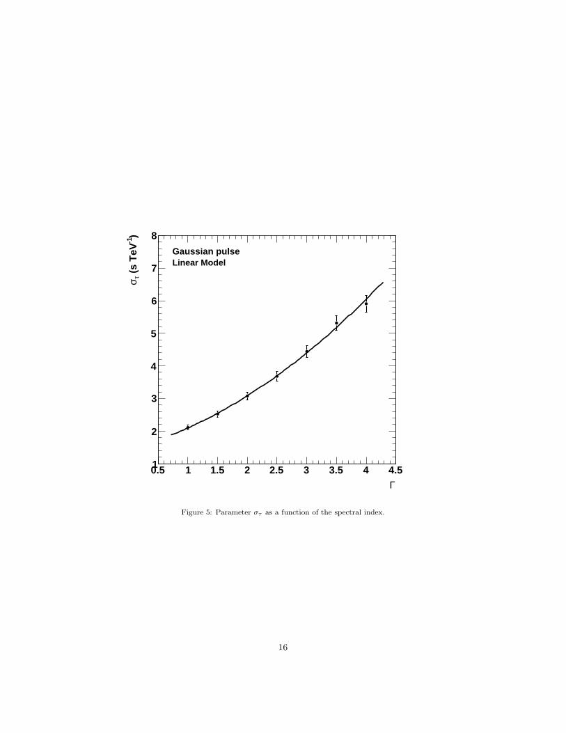
Figure 5: Parameter στ as a function of the spectral index.

16

4.2. Dependence on spectral index

Varying the spectral index of the generated light curves from 1 to 4.5 re-sulted in no significant change in the calibration slope (below 5%) for a singleGaussian pulse. The systematic error due to the uncertainty on the spectralindex determination can then be considered as negligible. In contrast, the er-ror value is a strong function of the spectral index as also shown in Figure 5.A harder spectrum gives a higher precision, due to the fact that the photonsare spread more uniformly between high and low energies. This enhances thepotential of studies with closer AGN such as Mrk 421 and Mrk 501.

4.3. Effect of background contribution

Even though the signal to background ratio is very high for the studieddata sample, it is possible that a small contribution of mis-identified photonsintroduces a small bias in the measurement of the time-lag. To study the impactof this effect, light curves were simulated with a fraction of particles with noenergy-dependant time-lag as is expected for charged cosmic-rays. A realisticpower law spectrum with an index of 2.7 was used to generate these particles.When 1% of the particles are considered as protons, no significant change ineither slope or parameter στ is observed.

4.4. Summary of calibration studies

In this section, the most important features of the calibrations with thelikelihood method are summarized.

As the emission light curve at the source is not known, the function FS wasderived from real data in the range 0.25–0.28 TeV. In this case, it is shown thatthe likelihood fit can reconstruct the injected lag extremely well. In the future,if a satisfying emission model is proposed, the likelihood approach can be veryuseful to test propagation and emission models as well.

The error on the measured lag (στ ) depends strongly on the width of indi-vidual pulses.This result is very important and allows competitive results to beobtained with the PKS 2155-304 light curve. On the other hand, the asymmetryof the pulses and the superposition of several pulses has been shown to have lessimportant effect on the results. The parameter στ also depends on the spectralindex, which is another source of uncertainty. However, for PKS 2155-304 flarein 2006, the spectral index can be determined with a very good precision.

The systematic uncertainties in the method employed were quantified byvarying selections and cuts and treating the light curve shape parameterizationin different ways. The various contributions are detailed in Table 4. The mainuncertainty was found to be related to event selections and to the light curveparameterizations.

In order to get a precise estimation of the systematic uncertainty related tothe FS parameterization, the covariance matrix of the fit presented in Figure 2was studied. The values of the fit parameters were varied following to thegaussian distributions with parameters derived from the covariance matrix after

17

Table 4: Systematic uncertainties of the event-by-event likelihood

Estimated error Change in estimated τl (s TeV−1) Change in estimated τq (s TeV−2)Selection cuts < 5 < 5Background contribution 1% < 1 < 1Acceptance factors 2% < 1 < 1Energy resolution 1% < 1 < 1Energy calibration 10% < 2 < 2Spectral index 1% < 1 < 1Calibration systematics (constant, shift) 10% < 5 < 1FS(t) parameterization ≈7 ≈3Total < 10.3 < 6.6

18

)-1 (s TeVlτ-60 -40 -20 0 20 40 60

ln(L

)∆

-2

0

5

10

15

20

25Number of passing events = 2462

7.1 s/TeV± = -5.5 l0τMinimum at

)-2 (s TeVqτ-60 -40 -20 0 20 40 60

ln(L

)∆

-2

0

5

10

15

20

25Number of passing events = 2462

-2 3.5 s TeV± = 1.7 q0τMinimum at

Figure 6: −2∆ ln(L) as a function of τ when the measured light curve is fitted in 0.25–0.28TeV and the likelihood is computed in 0.3–4.0 TeV for a linear (left) and quadratic (right)correction. Points are fitted with a third-degree polynomial with a minimum at τl0 = −5.5±7.1sTeV−1 and τq0 = 1.7 ± 3.5 sTeV−2. The errors on these values are obtained requesting−2∆ ln(L) = 1.

its diagonalization. The values in Table 4 were obtained with this procedure forthe linear and the quadratic case separately.

The overall systematic error is estimated to be < 10.3 s TeV−1 and < 6.6 s TeV−2

for the linear and quadratic effects respectively. These values will be combinedwith the statistical calibrated error given in §4.1 when determining the QuantumGravity scales.

5. Results with PKS 2155-304 flare of MJD 53944

The final result was obtained with a parameterization of the light curvein the range 0.25-0.28 TeV (E1 = 0.26 TeV, see light curve in Figure 2) anda likelihood computed in 0.3-4.0 TeV (E2 = 0.49 TeV). The choice of theseranges was dictated by the balance found between lever-arm in energy and thestatistics used in the likelihood fit. These choices were studied and optimizedwith the simulations described above.

Figure 6 shows the −2∆ ln(L) curve as a function of the injected τ for thelinear and quadratic cases, leading to the value for the minimum of

τ ′0l = −5.5 ± 10.9(stat) ± 10.3(sys) s TeV−1

for the linear and

τ ′0q = 1.7 ± 6.3(stat) ± 6.6(sys) s TeV−2

for the quadratic effect.

19

These results imply that there is no significant time-lag measured. Conse-quently, the 95% CL limits on the Quantum Gravity energy scales are derived:

MlQG > 2.1 × 1018 GeV (ξ < 5.7)

andMq

QG > 6.4 × 1010 GeV (ζ < 3.6 × 1016).

The more conservative 99% CL limits are

MlQG 99% > 1.3 × 1018 GeV (ξ < 9.2)

andMq

QG 99% > 5.3 × 1010 GeV (ζ < 5.2 × 1016).

These results were found to be very stable when considering different energydomains and time selections. The stability studies of the estimated systematiceffects allows the quoted values to be considered as conservative.

The limit on the linear term, while lower by a factor of ten in comparisonwith the one obtained by Fermi with GRB 090510 [18], shows that with AGNtoo, the conclusion about the models predicting a linear effect with energy [4]tends to be confirmed. As far as the limit on the quadratic term is concerned,it is the best one obtained so far with AGN and GRB, even if it still remainsfar from the Planck scale value.

As stated in the introductory part, the presented paper focused on modelsproposed in [12, 13] where predictions of linear Lorentz Invariance Violationeffects were expected and the causality condition was conserved. Moreover, itmay be noticed that because of negligible negative values found both for thelinear and quadratic terms, the super-luminal case limits will differ only slightlyfrom those provided for the sub-luminal case.

6. Summary and prospects

The limits obtained in this study are the most constraining ever obtainedwith an AGN. They are almost ten times higher than those obtained by Martinezand Errando [20] with the same method for the Mrk 501 flare recorded byMAGIC, and consistent with their rough estimate for the PKS 2155-304 flareobserved by H.E.S.S.. They are also a factor of ∼3 higher than the previousH.E.S.S. result [1]. The increase in sensitivity as compared to the MAGIC resultis mainly due to excellent parameters of the data taken on July 28, 2006: lowzenith angle (∼ 10) which leads to a low energy threshold and high statisticswith high variability. On the other hand, the steepness of the PKS 2155-304energy spectrum was one of the penalizing factors in this study.

Given the complexity of the PKS 2155-304 light curve, a detailed calibra-tion study of the method was necessary. For this purpose, a toy Monte-Carloprogram was developed. The simulations allowed the influence of different pa-rameters on the likelihood performance to be investigated, such as the shape of

20

the light curve or spike superposition. In particular, a very interesting conclu-sion for a light curve with multiple spikes is that the error on the lag dependsmainly on the width of the individual pulses. This feature of the likelihood fitallows a smaller error on the lag measurement to be obtained, yielding higherlimits on MQG.

It should still be noticed that the superposition of different spikes leadsto a decrease in sensitivity due to a limited number of “useful events” whichcontribute to the likelihood fit. Despite this loss in statistical power, the methodallows robust and precise results on the fitted time-lag to be obtained.

Another important conclusion about the method is the possibility to obtainrobust results even with low photon statistics. The use of different time selec-tions showed that a large decrease in the number of selected events entering thefit had only a small influence on the error value of the time-lag measurement.

The main difficulty of time of flight studies with photons from AGN andGRB is that the origin of the measured lag is unknown. If the measured time-lag is not related to Quantum Gravity induced propagation effect, it can be dueto an emission effect at the source. The measured lag can also be a superpositionof source and propagation effects. As no lag was found in the studied sample,either the source effects compensate exactly the propagation effects (“conspir-acy scenario”), or there are no source or propagation induced effects detectedwithin present experimental sensitivity. In this study the second hypothesis wasretained, which leads to a conclusion that any measured lag would be entirelydue to Lorentz Invariance Violation effects.

In future, modelling of the emission light curve could bring new insight in thepropagation and emission time studies. Population studies of AGN examiningthe effect of the distance on the lag measurement could allow this assumptionto be avoided but would require that intrinsic effects are similar for differentAGN. Better results on propagation effects will then come in parallel with abetter understanding of the emission models.

More and more results on Lorentz symmetry breaking are published whichgive limits for the linear correction that are very close to the Planck energyscale. In particular, the latest results from Fermi observations of distant GRBprovide exclusion limits for a large class of linear models above the Planck energy[17, 18]. However, as pointed out by Ellis et al. [30], ‘extraordinary claimsrequire extraordinary evidence’, so more studies will be needed in the future togive more robust results and to be able to definitively reject or validate proposedmodels.

The time-lag measurements with photons are far from being sensitive enoughto constrain the quadratic term of the dispersion relations and do not excludeany model in this case. Multi-messenger and multi-wavelength campaigns willbe necessary in future to constrain this quadratic term. Combining resultsobtained with GRB and AGN detected by Fermi and ground-based detectorswould allow considering common scheme with photon energies ranging from thesub-GeV range to the multi-TeV range and from sources with higher redshiftvalues. Future observations with neutrino telescopes of GRB and AGN flareswould further extend the energy range to extreme, multi-hundred TeV domain.

21

However, at present, the multi-messenger and multi-wavelength procedures arestill to be developed.

Concerning the increase of the experimental potential in observations ofthe AGN, a key step towards a better understanding of the emission and thepropagation effects will be achieved with a new generation of instruments, whichwill allow the observation of a larger number of AGN flares. HESS-II, with anenergy threshold of ∼30 GeV and later the large Cherenkov array CTA 3 willincrease dramatically the sensitivity to energy-dependent time-lags. A roughestimation obtained by extrapolating results from the PKS 2155-304 flare to theextended domain in energy from a few GeV to a hundred TeV, and assuming again in sensitivity of a factor of ten, would rise the limit on the quadratic termby two orders of magnitude. This type of results may be further confronted withpresent and future theoretical models. It may also be underlined here that thiswill open a new unexplored domain for Lorentz Invariance Violation searches.

7. Acknowledgments

The support of the Namibian authorities and of the University of Namibiain facilitating the construction and operation of H.E.S.S. is gratefully acknowl-edged, as is the support by the German Ministry for Education and Research(BMBF), the Max Planck Society, the French Ministry for Research, the CNRS-IN2P3 and the Astroparticle Interdisciplinary Programme of the CNRS, theU.K. Science and Technology Facilities Council (STFC), the IPNP of the CharlesUniversity, the Polish Ministry of Science and Higher Education, the SouthAfrican Department of Science and Technology and National Research Founda-tion, and by the University of Namibia. We appreciate the excellent work ofthe technical support staff in Berlin, Durham, Hamburg, Heidelberg, Palaiseau,Paris, Saclay, and in Namibia in the construction and operation of the equip-ment.

References

[1] Aharonian, F. et al. (H.E.S.S. Collaboration) 2008, Phys. Rev. Lett., 101,170402

[2] Amelino-Camelia, G. 2008, arXiv:0806.0339

[3] Smolin, L. 2001, Three Roads to Quantum Gravity (Basic Books)

[4] Ellis, J., Mavromatos, N.E. & Nanopoulos, D.V. 1999, Phys. Rev. D, 61,027503

[5] Amelino-Camelia, G. et al. 1998, Nature, 395, 525

3http://www.cta-observatory.org/

22

[6] Alfaro, J. et al. 2002, Phys. Rev. D, 65, 103509

[7] Gambini, R. & Pullin, J. 1999, Phys. Rev. D, 59, 124021

[8] Sarkar S. 2002, Mod. Phys. Lett. A, 17, 1025

[9] Amelino-Camelia, G., Ellis, J., Mavromatos, N. E.& Nanopoulos, D. V.1997, Int. J. Mod. Phys. A, 12, 607

[10] Kaaret, P. 1999, A&A, 345, L32

[11] Jacob, U. & Piran, T. 2008, JCAP, 01, 031

[12] Ellis, J., Mavromatos, N.E., Nanopoulos, D.V. & Sakharov, A.S. 2003,A&A, 402, 409

[13] Ellis, J. et al. 2006, Astropart. Phys., 25, 402

[14] Ellis, J. et al. 2008 , Astropart. Phys., 29, 158

[15] Bolmont, J., Jacholkowska, A., Atteia, J.-L. et al. 2008, ApJ, 676, 532

[16] Bahcall, N.A., Ostriker, J.P., Perlmutter, S. & Steinhardt, P.J. 1999, Sci-ence 284, 1481

[17] Abdo, A.A. et al. 2009a, Science Express, 02/19/2009

[18] Abdo, A.A. et al. 2009b, Nature, 462, 331, including supplementary infor-mation

[19] Albert, J. et al. (MAGIC Collaboration) 2008, Phys. Lett. B, 668, 253

[20] Martinez, M. & Errando, M. 2009, Astropart. Phys., 31, 226

[21] Boggs, S., Wunderer, C., Hurley, K., & Coburn, W. 2004, ApJ, 611, L77

[22] Lamon, P. et al., (INTEGRAL Collaboration) 2008, Gen. Rel. Grav. 40,1731

[23] Scargle, J. D., Norris, J. P. & Bonnell, J. T. 2008, ApJ, 673, 972

[24] Aharonian, F. et al. (H.E.S.S. Collaboration) 2007, ApJL, 664, L71

[25] De Naurois, M. et al. 2005, in Proc. Towards a Network of AtmosphericCherenkov Detectors VII (Palaiseau), 149

[26] Hillas, A. 1985, in Proc. 19th I.C.R.C. (La Jolla), Vol. 3, 445

[27] De Naurois, M. et al. 2003, in Proc. 28th I.C.R.C. (Tsukuba), Vol. 5, 2907

[28] Abramowski A. et al. (H.E.S.S. Collaboration) 2010, A&A, submitted

[29] Morhac, M. et al. 2000, NIM A, 443, 108

23

[30] Ellis, J. et al. 2009, Phys. Lett. B, 674, 83

[31] Biller, S.D. et al. (Whipple Collaboration) 1999, Phys. Rev. Lett., 83, 2108

[32] Pelangeon, A., Atteia, J.-L., Lamb, D.Q. et al. 2006, Gamma-Ray Burstsin the Swift Era. AIP Conf. Proc. 836, 149

24