Search for gravitational-wave bursts in the first year of the fifth LIGO science run

Strathprints Institutional Repository

Lockerbie, N.A. (2009) Search for gravitational-wave bursts in the first year of the fifth LIGO sciencerun. Physical Review D: Particles and Fields, 80 (10). p. 102001. ISSN 0556-2821

Strathprints is designed to allow users to access the research output of the University of Strathclyde.Copyright c© and Moral Rights for the papers on this site are retained by the individual authorsand/or other copyright owners. You may not engage in further distribution of the material for anyprofitmaking activities or any commercial gain. You may freely distribute both the url (http://strathprints.strath.ac.uk/) and the content of this paper for research or study, educational, ornot-for-profit purposes without prior permission or charge.

Any correspondence concerning this service should be sent to Strathprints administrator:mailto:[email protected]

http://strathprints.strath.ac.uk/



mailto:[email protected]


Search for gravitational-wave bursts in the first year of the fifth LIGO science run

B. P. Abbott,17 R. Abbott,17 R. Adhikari,17 P. Ajith,2 B. Allen,2,60 G. Allen,35 R. S. Amin,21 S. B. Anderson,17

W.G. Anderson,60 M.A. Arain,47 M. Araya,17 H. Armandula,17 P. Armor,60 Y. Aso,17 S. Aston,46 P. Aufmuth,16

C. Aulbert,2 S. Babak,1 P. Baker,24 S. Ballmer,17 C. Barker,18 D. Barker,18 B. Barr,48 P. Barriga,59 L. Barsotti,20

M.A. Barton,17 I. Bartos,10 R. Bassiri,48 M. Bastarrika,48 B. Behnke,1 M. Benacquista,42 J. Betzwieser,17

P. T. Beyersdorf,31 I. A. Bilenko,25 G. Billingsley,17 R. Biswas,60 E. Black,17 J. K. Blackburn,17 L. Blackburn,20 D. Blair,59

B. Bland,18 T. P. Bodiya,20 L. Bogue,19 R. Bork,17 V. Boschi,17 S. Bose,61 P. R. Brady,60 V. B. Braginsky,25 J. E. Brau,53

D.O. Bridges,19 M. Brinkmann,2 A. F. Brooks,17 D. A. Brown,36 A. Brummit,30 G. Brunet,20 A. Bullington,35

A. Buonanno,49 O. Burmeister,2 R. L. Byer,35 L. Cadonati,50 J. B. Camp,26 J. Cannizzo,26 K. C. Cannon,17 J. Cao,20

L. Cardenas,17 S. Caride,51 G. Castaldi,56 S. Caudill,21 M. Cavaglia,39 C. Cepeda,17 T. Chalermsongsak,17 E. Chalkley,48

P. Charlton,9 S. Chatterji,17 S. Chelkowski,46 Y. Chen,1,6 N. Christensen,8 C. T. Y. Chung,38 D. Clark,35 J. Clark,7

J. H. Clayton,60 T. Cokelaer,7 C. N. Colacino,12 R. Conte,55 D. Cook,18 T. R. C. Corbitt,20 N. Cornish,24 D. Coward,59

D. C. Coyne,17 J. D. E. Creighton,60 T. D. Creighton,42 A.M. Cruise,46 R.M. Culter,46 A. Cumming,48 L. Cunningham,48

S. L. Danilishin,25 K. Danzmann,2,16 B. Daudert,17 G. Davies,7 E. J. Daw,40 D. DeBra,35 J. Degallaix,2 V. Dergachev,51

S. Desai,37 R. DeSalvo,17 S. Dhurandhar,15 M. Dıaz,42 A. Di Credico,36 A. Dietz,7 F. Donovan,20 K. L. Dooley,47

E. E. Doomes,34 R.W. P. Drever,5 J. Dueck,2 I. Duke,20 J.-C. Dumas,59 J. G. Dwyer,10 C. Echols,17 M. Edgar,48 A. Effler,18

P. Ehrens,17 E. Espinoza,17 T. Etzel,17 M. Evans,20 T. Evans,19 S. Fairhurst,7 Y. Faltas,47 Y. Fan,59 D. Fazi,17 H. Fehrmann,2

L. S. Finn,37 K. Flasch,60 S. Foley,20 C. Forrest,54 N. Fotopoulos,60 A. Franzen,16 M. Frede,2 M. Frei,41 Z. Frei,12

A. Freise,46 R. Frey,53 T. Fricke,19 P. Fritschel,20 V. V. Frolov,19 M. Fyffe,19 V. Galdi,56 J. A. Garofoli,36 I. Gholami,1

J. A. Giaime,21,19 S. Giampanis,2 K.D. Giardina,19 K. Goda,20 E. Goetz,51 L.M. Goggin,60 G. Gonzalez,21

M. L. Gorodetsky,25 S. Goßler,2 R. Gouaty,21 A. Grant,48 S. Gras,59 C. Gray,18 M. Gray,4 R. J. S. Greenhalgh,30

A.M. Gretarsson,11 F. Grimaldi,20 R. Grosso,42 H. Grote,2 S. Grunewald,1 M. Guenther,18 E. K. Gustafson,17

R. Gustafson,51 B. Hage,16 J.M. Hallam,46 D. Hammer,60 G. D. Hammond,48 C. Hanna,17 J. Hanson,19 J. Harms,52

G.M. Harry,20 I.W. Harry,7 E. D. Harstad,53 K. Haughian,48 K. Hayama,42 J. Heefner,17 I. S. Heng,48 A. Heptonstall,17

M. Hewitson,2 S. Hild,46 E. Hirose,36 D. Hoak,19 K.A. Hodge,17 K. Holt,19 D. J. Hosken,45 J. Hough,48 D. Hoyland,59

B. Hughey,20 S. H. Huttner,48 D. R. Ingram,18 T. Isogai,8 M. Ito,53 A. Ivanov,17 B. Johnson,18 W.W. Johnson,21

D. I. Jones,57 G. Jones,7 R. Jones,48 L. Ju,59 P. Kalmus,17 V. Kalogera,28 S. Kandhasamy,52 J. Kanner,49 D. Kasprzyk,46

E. Katsavounidis,20 K. Kawabe,18 S. Kawamura,27 F. Kawazoe,2 W. Kells,17 D.G. Keppel,17 A. Khalaidovski,2

F. Y. Khalili,25 R. Khan,10 E. Khazanov,14 P. King,17 J. S. Kissel,21 S. Klimenko,47 K. Kokeyama,27 V. Kondrashov,17

R. Kopparapu,37 S. Koranda,60 D. Kozak,17 B. Krishnan,1 R. Kumar,48 P. Kwee,16 P. K. Lam,4 M. Landry,18 B. Lantz,35

A. Lazzarini,17 H. Lei,42 M. Lei,17 N. Leindecker,35 I. Leonor,53 C. Li,6 H. Lin,47 P. E. Lindquist,17 T. B. Littenberg,24

N.A. Lockerbie,58 D. Lodhia,46 M. Longo,56 M. Lormand,19 P. Lu,35 M. Lubinski,18 A. Lucianetti,47 H. Luck,2,16

B. Machenschalk,1 M. MacInnis,20 M. Mageswaran,17 K. Mailand,17 I. Mandel,28 V. Mandic,52 S. Marka,10 Z. Marka,10

A. Markosyan,35 J. Markowitz,20 E. Maros,17 I.W. Martin,48 R.M. Martin,47 J. N. Marx,17 K. Mason,20 F. Matichard,21

L. Matone,10 R. A. Matzner,41 N. Mavalvala,20 R. McCarthy,18 D. E. McClelland,4 S. C. McGuire,34 M. McHugh,23

G. McIntyre,17 D. J. A. McKechan,7 K. McKenzie,4 M. Mehmet,2 A. Melatos,38 A. C. Melissinos,54 D. F. Menendez,37

G. Mendell,18 R.A. Mercer,60 S. Meshkov,17 C. Messenger,2 M. S. Meyer,19 J. Miller,48 J. Minelli,37 Y. Mino,6

V. P. Mitrofanov,25 G. Mitselmakher,47 R. Mittleman,20 O. Miyakawa,17 B. Moe,60 S. D. Mohanty,42 S. R. P. Mohapatra,50

G. Moreno,18 T. Morioka,27 K. Mors,2 K. Mossavi,2 C. MowLowry,4 G. Mueller,47 H. Muller-Ebhardt,2 D. Muhammad,19

S. Mukherjee,42 H. Mukhopadhyay,15 A. Mullavey,4 J. Munch,45 P. G. Murray,48 E. Myers,18 J. Myers,18 T. Nash,17

J. Nelson,48 G. Newton,48 A. Nishizawa,27 K. Numata,26 J. O’Dell,30 B. O’Reilly,19 R. O’Shaughnessy,37 E. Ochsner,49

G.H. Ogin,17 D. J. Ottaway,45 R. S. Ottens,47 H. Overmier,19 B. J. Owen,37 Y. Pan,49 C. Pankow,47 M.A. Papa,1,60

V. Parameshwaraiah,18 P. Patel,17 M. Pedraza,17 S. Penn,13 A. Perraca,46 V. Pierro,56 I.M. Pinto,56 M. Pitkin,48

H. J. Pletsch,2 M.V. Plissi,48 F. Postiglione,55 M. Principe,56 R. Prix,2 L. Prokhorov,25 O. Puncken,2 V. Quetschke,47

F. J. Raab,18 D. S. Rabeling,4 H. Radkins,18 P. Raffai,12 Z. Raics,10 N. Rainer,2 M. Rakhmanov,42 V. Raymond,28

C.M. Reed,18 T. Reed,22 H. Rehbein,2 S. Reid,48 D.H. Reitze,47 R. Riesen,19 K. Riles,51 B. Rivera,18 P. Roberts,3

N. A. Robertson,17,48 C. Robinson,7 E. L. Robinson,1 S. Roddy,19 C. Rover,2 J. Rollins,10 J. D. Romano,42 J. H. Romie,19

S. Rowan,48 A. Rudiger,2 P. Russell,17 K. Ryan,18 S. Sakata,27 L. Sancho de la Jordana,44 V. Sandberg,18 V. Sannibale,17

L. Santamarıa,1 S. Saraf,32 P. Sarin,20 B. S. Sathyaprakash,7 S. Sato,27 M. Satterthwaite,4 P. R. Saulson,36 R. Savage,18

P. Savov,6 M. Scanlan,22 R. Schilling,2 R. Schnabel,2 R. Schofield,53 B. Schulz,2 B. F. Schutz,1,7 P. Schwinberg,18 J. Scott,48

PHYSICAL REVIEW D 80, 102001 (2009)

1550-7998=2009=80(10)=102001(26) 102001-1 � 2009 The American Physical Society

S.M. Scott,4 A. C. Searle,17 B. Sears,17 F. Seifert,2 D. Sellers,19 A. S. Sengupta,17 A. Sergeev,14 B. Shapiro,20

P. Shawhan,49 D.H. Shoemaker,20 A. Sibley,19 X. Siemens,60 D. Sigg,18 S. Sinha,35 A.M. Sintes,44 B. J. J. Slagmolen,4

J. Slutsky,21 J. R. Smith,36 M. R. Smith,17 N.D. Smith,20 K. Somiya,6 B. Sorazu,48 A. Stein,20 L. C. Stein,20

S. Steplewski,61 A. Stochino,17 R. Stone,42 K.A. Strain,48 S. Strigin,25 A. Stroeer,26 A. L. Stuver,19 T. Z. Summerscales,3

K.-X. Sun,35 M. Sung,21 P. J. Sutton,7 G. P. Szokoly,12 D. Talukder,61 L. Tang,42 D. B. Tanner,47 S. P. Tarabrin,25

J. R. Taylor,2 R. Taylor,17 J. Thacker,19 K.A. Thorne,19 A. Thuring,16 K.V. Tokmakov,48 C. Torres,19 C. Torrie,17

G. Traylor,19 M. Trias,44 D. Ugolini,43 J. Ulmen,35 K. Urbanek,35 H. Vahlbruch,16 M. Vallisneri,6 C. Van Den Broeck,7

M.V. van der Sluys,28 A. A. van Veggel,48 S. Vass,17 R. Vaulin,60 A. Vecchio,46 J. Veitch,46 P. Veitch,45 C. Veltkamp,2

A. Villar,17 C. Vorvick,18 S. P. Vyachanin,25 S. J. Waldman,20 L. Wallace,17 R. L. Ward,17 A. Weidner,2 M. Weinert,2

A. J. Weinstein,17 R. Weiss,20 L. Wen,6,59 S. Wen,21 K. Wette,4 J. T. Whelan,1,29 S. E. Whitcomb,17 B. F. Whiting,47

C. Wilkinson,18 P. A. Willems,17 H. R. Williams,37 L. Williams,47 B. Willke,2,16 I. Wilmut,30 L. Winkelmann,2

W. Winkler,2 C. C. Wipf,20 A.G. Wiseman,60 G. Woan,48 R. Wooley,19 J. Worden,18 W. Wu,47 I. Yakushin,19

H. Yamamoto,17 Z. Yan,59 S. Yoshida,33 M. Zanolin,11 J. Zhang,51 L. Zhang,17 C. Zhao,59 N. Zotov,22 M. E. Zucker,20

H. zur Muhlen,16 and J. Zweizig17

(LIGO Scientific Collaboration)*

1Albert-Einstein-Institut, Max-Planck-Institut fur, Gravitationsphysik, D-14476 Golm, Germany2Albert-Einstein-Institut, Max-Planck-Institut fur, Gravitationsphysik, D-30167 Hannover, Germany

3Andrews University, Berrien Springs, Michigan 49104, USA4Australian National University, Canberra, 0200, Australia

5California Institute of Technology, Pasadena, California 91125, USA6Caltech-CaRT, Pasadena, California 91125, USA

7Cardiff University, Cardiff, CF24 3AA, United Kingdom8Carleton College, Northfield, Minnesota 55057, USA

9Charles Sturt University, Wagga Wagga, NSW 2678, Australia10Columbia University, New York, New York 10027, USA

11Embry-Riddle Aeronautical University, Prescott, Arizona 86301 USA12Eotvos University, ELTE 1053 Budapest, Hungary

13Hobart and William Smith Colleges, Geneva, New York 14456, USA14Institute of Applied Physics, Nizhny Novgorod, 603950, Russia

15Inter-University Centre for Astronomyand Astrophysics, Pune - 411007, India16Leibniz Universitat Hannover, D-30167 Hannover, Germany

17LIGO - California Institute of Technology, Pasadena, California 91125, USA18LIGO - Hanford Observatory, Richland, Washington 99352, USA

19LIGO - Livingston Observatory, Livingston, Louisiana 70754, USA20LIGO - Massachusetts Institute of Technology, Cambridge, Massachusetts 02139, USA

21Louisiana State University, Baton Rouge, Louisiana 70803, USA22Louisiana Tech University, Ruston, Louisiana 71272, USA23Loyola University, New Orleans, Louisiana 70118, USA

24Montana State University, Bozeman, Montana 59717, USA25Moscow State University, Moscow, 119992, Russia

26NASA/Goddard Space Flight Center, Greenbelt, Maryland 20771, USA27National Astronomical Observatory of Japan, Tokyo 181-8588, Japan

28Northwestern University, Evanston, Illinois 60208, USA29Rochester Institute of Technology, Rochester, New York 14623, USA

30Rutherford Appleton Laboratory, HSIC, Chilton, Didcot, Oxon OX11 0QX United Kingdom31San Jose State University, San Jose, California 95192, USA

32Sonoma State University, Rohnert Park, CA94928, USA33Southeastern Louisiana University, Hammond, Louisiana 70402, USA

34Southern University and A&M College, Baton Rouge, Louisiana 70813, USA35Stanford University, Stanford, California 94305, USA36Syracuse University, Syracuse, New York 13244, USA

37The Pennsylvania State University, University Park, Pennsylvania 16802, USA38The University of Melbourne, Parkville VIC 3010, Australia

39The University of Mississippi, University, Mississippi 38677, USA40The University of Sheffield, Sheffield S10 2TN, United Kingdom

B. P. ABBOTT et al. PHYSICAL REVIEW D 80, 102001 (2009)

102001-2

41The University of Texas at Austin, Austin, Texas 78712, USA42The University of Texas at Brownsville and Texas Southmost College, Brownsville, Texas 78520, USA

43Trinity University, San Antonio, Texas 78212, USA44Universitat de les Illes Balears, E-07122 Palma de Mallorca, Spain

45University of Adelaide, Adelaide, SA 5005, Australia46University of Birmingham, Birmingham, B15 2TT, United Kingdom

47University of Florida, Gainesville, Florida 32611, USA48University of Glasgow, Glasgow, G12 8QQ, United Kingdom49University of Maryland, College Park, Maryland 20742 USA

50University of Massachusetts - Amherst, Amherst, Massachusetts 01003, USA51University of Michigan, Ann Arbor, Michigan 48109, USA

52University of Minnesota, Minneapolis, Minnesota 55455, USA53University of Oregon, Eugene, Oregon 97403, USA

54University of Rochester, Rochester, New York 14627, USA55University of Salerno, 84084 Fisciano (Salerno), Italy

56University of Sannio at Benevento, I-82100 Benevento, Italy57University of Southampton, Southampton, SO17 1BJ, United Kingdom

58University of Strathclyde, Glasgow, G1 1XQ, United Kingdom59University of Western Australia, Crawley, WA 6009, Australia

60University of Wisconsin-Milwaukee, Milwaukee, Wisconsin 53201, USA61Washington State University, Pullman, Washington 99164, USA

(Received 27 May 2009; published 11 November 2009)

We present the results obtained from an all-sky search for gravitational-wave (GW) bursts in the 64–

2000 Hz frequency range in data collected by the LIGO detectors during the first year (November 2005—

November 2006) of their fifth science run. The total analyzed live time was 268.6 days. Multiple

hierarchical data analysis methods were invoked in this search. The overall sensitivity expressed in terms

of the root-sum-square (rss) strain amplitude hrss for gravitational-wave bursts with various morphologies

was in the range of 6� 10�22 Hz�1=2 to a few� 10�21 Hz�1=2. No GW signals were observed and a

frequentist upper limit of 3.75 events per year on the rate of strong GW bursts was placed at the 90%

confidence level. As in our previous searches, we also combined this rate limit with the detection

efficiency for selected waveform morphologies to obtain event rate versus strength exclusion curves. In

sensitivity, these exclusion curves are the most stringent to date.

DOI: 10.1103/PhysRevD.80.102001 PACS numbers: 04.80.Cc

I. INTRODUCTION

After many years of preparation, interferometricgravitational-wave (GW) detectors have now begun anera of long-duration observing. The three detectors of theLaser Interferometer Gravitational-Wave Observatory(LIGO) [1] reached their design sensitivity levels in 2005and began a ‘‘science run’’ that collected data through late2007. This run is called ‘‘S5’’ since it followed a sequenceof four shorter science runs that began in 2002. TheGerman/British GEO600 detector [2] joined the S5 run inJanuary 2006, and the Italian/French Virgo detector [3]began its first science run (denoted VSR1) in May 2007,overlapping the last 4.5 months of the S5 run. The datacollected by these detectors provide the best opportunityyet to identify a GW signal—though detection is still farfrom certain—and is a baseline for future coordinated datacollection with upgraded detectors.

Gravitational waves in the frequency band of LIGO andthe other ground-based detectors may be produced by avariety of astrophysical processes [4]. See for example [5]

for inspiralling compact binaries, [6] for spinning neutronstars, [7] for binary mergers, and [8–11] for core-collapsesupernovae.The GW waveform emitted by a compact binary system

during the inspiral phase can be calculated accurately inmany cases, allowing searches with optimal matched filter-ing; see, for example, [12]. The waveform from the sub-sequent merger of two black holes is being modeled withever-increasing success using numerical relativity calcula-tions, but is highly dependent on physical parameters andthe properties of strong-field gravity. The uncertainties forthe waveforms of other transient sources are even larger. Itis thus desirable to explore more generic search algorithmscapable of detecting a wide range of short-duration GWsignals from poorly modeled sources—such as stellar corecollapse to a neutron star or black hole—or unanticipatedsources. As GW detectors extend the sensitivity frontier, itis important to not rely too heavily on assumptions aboutsource astrophysics or about the true nature of strong-fieldgravity, and to search as broadly as possible.In this paper, we report on a search for GW ‘‘burst’’

signals in the LIGO data that were collected during the first12 months of the S5 science run. A search for GW bursts in*http://www.ligo.org

SEARCH FOR GRAVITATIONAL-WAVE BURSTS IN THE . . . PHYSICAL REVIEW D 80, 102001 (2009)

102001-3

http://dx.doi.org/10.1103/PhysRevD.80.102001

the remainder of the S5 data set, along with the VirgoVSR1 data, will be published jointly by the LSC andVirgo collaborations at a later date.

The GW burst signals targeted are assumed to havesignal power within LIGO’s frequency band and durationsshorter than �1 s, but are otherwise arbitrary. This analy-sis, like most of our previously published searches for GWbursts, focuses on low frequencies—in this case 64 Hz to2000 Hz—where the detectors are the most sensitive. Adedicated search for bursts above 2000 Hz is presented in acompanion paper [13].

Interferometric GW detectors collect stable, high-sensitivity (‘‘science-mode’’) data typically for severalhours at a time, with interruptions due to adverse environ-mental conditions, maintenance, diagnostics, and the needto occasionally regain the ‘‘locked’’ state of the servocontrols. In this analysis we searched the data at all timeswhen two or more LIGO detectors were operating, adeparture from the all-sky GW burst searches from earlierscience runs [14–18], which required coincidence amongthree (or more) detectors. In this paper, the term ‘‘net-work’’ is used to describe a set of detectors operating inscience mode at a given time. A network may include anycombination of the Hanford 4 km (H1) and 2 km (H2)detectors, the Livingston 4 km (L1) detector and GEO600.Because the GEO600 detector was significantly less sensi-tive than LIGO during the S5 run (a factor of 3 at 1000 Hz,and almost 2 orders of magnitude at 100 Hz), we do not useits data in the initial search but reserve it for evaluating anyevent candidates found in the LIGO data.

This paper presents results from three different ‘‘analy-sis pipelines,’’ each representing a complete search. Whilethe pipelines analyzed the data independently, they beganwith a common selection of good-quality data and applieda common set of vetoes to reject identifiable artifacts. Eachpipeline was tuned to maximize the sensitivity to simulatedGW signals while maintaining a fixed, low false alarm rate.The tuning of the pipelines, the choice of good data and thedecision on the veto procedure were made before lookingat potential candidates.

No GW signal candidates were identified by any of theanalysis pipelines with the chosen thresholds. In order tointerpret this nondetection, we evaluate the sensitivity ofeach pipeline for simulated signals of various morpholo-gies, randomly distributed over the sky and over time. Asexpected, there are some sensitivity differences among thepipelines, although the sensitivities rarely differ by morethan a factor of 2 (see Sec. VII) and no single pipelineperforms best for all of the simulated signals considered.We combine the results of the pipelines to calculate upperlimits on the rate of GW bursts as a function of signalmorphology and strength.

The rest of the paper is organized as follows: Afterspecifying the periods of data, forming the first year ofthe S5 science run in Sec. II, Sec. III describes the state of

the detectors during that period. Section IV summarizes theelements of this GW burst search which are common to allof the analysis pipelines. The analysis pipelines themselvesare detailed in Sec. V and Appendixes C, D, and E.Section VI describes how each pipeline is tuned, whileSec. VII presents the sensitivity curves for simulated sig-nals and Sec. VIII describes the systematic errors in thesesensitivity curves. The results of the search are given inSec. IX, and some discussion including estimates of theastrophysical reach for burst candidates in Sec. X.

II. S5 FIRST-YEAR DATA SET

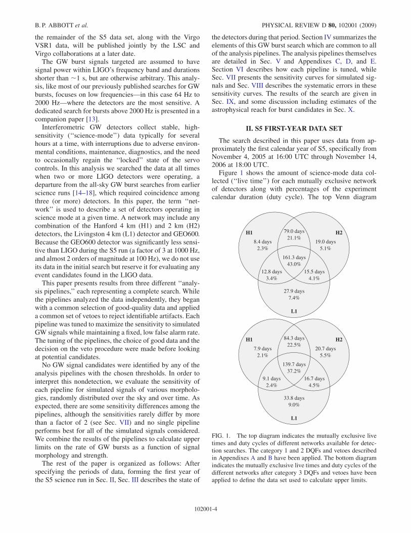
The search described in this paper uses data from ap-proximately the first calendar year of S5, specifically fromNovember 4, 2005 at 16:00 UTC through November 14,2006 at 18:00 UTC.Figure 1 shows the amount of science-mode data col-

lected (‘‘live time’’) for each mutually exclusive networkof detectors along with percentages of the experimentcalendar duration (duty cycle). The top Venn diagram

2H1H

L1

8.4 days2.3%

19.0 days5.1%

27.9 days7.4%

79.0 days21.1%

12.8 days3.4%

15.5 days4.1%

161.3 days43.0%

2H1H

L1

7.9 days2.1%

20.7 days5.5%

33.8 days9.0%

84.3 days22.5%

9.1 days2.4%

16.7 days4.5%

139.7 days37.2%

FIG. 1. The top diagram indicates the mutually exclusive livetimes and duty cycles of different networks available for detec-tion searches. The category 1 and 2 DQFs and vetoes describedin Appendixes A and B have been applied. The bottom diagramindicates the mutually exclusive live times and duty cycles of thedifferent networks after category 3 DQFs and vetoes have beenapplied to define the data set used to calculate upper limits.


102001-4

represents the data with basic data quality and veto con-ditions (see Sec. IV and Appendices A and B), including268.6 days of data during which two or more LIGO de-tectors were in science mode; this is the sample which issearched for GW burst signals. An explicit list of theanalyzed intervals after category 2 DQFs is available at[19]. The bottom Venn diagram shows the live times afterthe application of additional data quality cuts and vetoesthat provide somewhat cleaner data for establishing upperlimits on GW burst event rates. In practice, only theH1H2L1 and H1H2 (not L1) networks—encompassingmost of the live time, 224 days—are used to set upperlimits.

III. THE DETECTORS

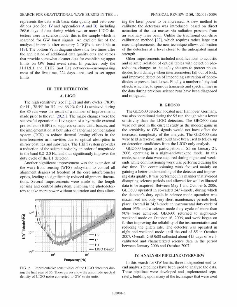
A. LIGO

The high sensitivity (see Fig. 2) and duty cycles (78.0%for H1, 78.5% for H2, and 66.9% for L1) achieved duringthe S5 run were the result of a number of improvementsmade prior to the run [20,21]. The major changes were thesuccessful operation at Livingston of a hydraulic externalpre-isolator (HEPI) to suppress seismic disturbances, andthe implementation at both sites of a thermal compensationsystem (TCS) to reduce thermal lensing effects in theinterferometer arm cavities due to optical absorption inmirror coatings and substrates. The HEPI system providesa reduction of the seismic noise by an order of magnitudein the band 0.2–2.0 Hz, and thus significantly improves theduty cycle of the L1 detector.

Another significant improvement was the extension ofthe wave-front sensing (WFS) subsystem to control allalignment degrees of freedom of the core interferometeroptics, leading to significantly reduced alignment fluctua-tions. Several improvements were made to the lengthsensing and control subsystem, enabling the photodetec-tors to take more power without saturation and thus allow-

ing the laser power to be increased. A new method tocalibrate the detectors was introduced, based on directactuation of the test masses via radiation pressure froman auxiliary laser beam. Unlike the traditional coil-drivecalibration method [22], which requires rather large testmass displacements, the new technique allows calibrationof the detectors at a level closer to the anticipated signalstrength.Other improvements included modifications to acoustic

and seismic isolation of optical tables with detection pho-todiodes, changes to the safety shutters to protect photo-diodes from damage when interferometers fall out of lock,and improved detection of impending saturation of photo-diodes to prevent lock losses. Finally, a number of physicaleffects which led to spurious transients and spectral lines inthe data during previous science runs have been diagnosedand mitigated.

B. GEO600

The GEO600 detector, located near Hannover, Germany,was also operational during the S5 run, though with a lowersensitivity than the LIGO detectors. The GEO600 datawere not used in the current study as the modest gains inthe sensitivity to GW signals would not have offset theincreased complexity of the analysis. The GEO600 datawere held in reserve, and could have been used to follow upon detection candidates from the LIGO-only analysis.GEO600 began its participation in S5 on January 21,

2006, operating in a night-and-weekend mode. In thismode, science data were acquired during nights and week-ends while commissioning work was performed during theday time. The commissioning work focused mainly ongaining a better understanding of the detector and improv-ing data quality. It was performed in a manner that avoideddisrupting science periods and allowed for well-calibrateddata to be acquired. Between May 1 and October 6, 2006,GEO600 operated in so-called 24=7-mode, during whichthe detector’s duty cycle in science-mode operation wasmaximized and only very short maintenance periods tookplace. Overall in 24=7-mode an instrumental duty cycle ofabout 95% and a science-mode duty cycle of more than90% were achieved. GEO600 returned to night-and-weekend mode on October 16, 2006, and work began onfurther improving the reliability of the instrumentation andreducing the glitch rate. The detector was operated innight-and-weekend mode until the end of S5 in October2007. Overall, GEO600 collected about 415 days of well-calibrated and characterized science data in the periodbetween January 2006 and October 2007.

IV. ANALYSIS PIPELINE OVERVIEW

In this search for GW bursts, three independent end-to-end analysis pipelines have been used to analyze the data.These pipelines were developed and implemented sepa-rately, building upon many of the techniques that were used

Frequency [Hz]

210 310

]H

z [

stra

in/

1/2

S(f

)

-2310

-2210

-2110

H2

L1

H1LIGO Design

Frequency [Hz]

210 310

]H

z [

stra

in/

1/2

S(f

)

-2310

-2210

-2110

H2

L1

H1LIGO Design

FIG. 2. Representative sensitivities of the LIGO detectors dur-ing the first year of S5. These curves show the amplitude spectraldensity of LIGO noise converted to GW strain units.


102001-5

in previous searches for bursts in the S1, S2, S3, and S4runs of LIGO and GEO600 [14,16–18,23], and prove tohave comparable sensitivities (within a factor of �2; seeSec. VII). One of these pipelines is fully coherent in thesense of combining data (amplitude and phase) from alldetectors and accounting appropriately for time delays andantenna responses for a hypothetical gravitational-waveburst impinging upon the network. This provides a power-ful test to distinguish GW signals from noise fluctuations.

Here we give an overview of the basic building blockscommon to all of the pipelines. The detailed operation ofeach pipeline will be described later.

A. Data quality evaluation

Gravitational-wave burst searches are occasionally af-fected by instrumental or data acquisition problems as wellas periods of degraded sensitivity or nonstationary noisedue to bad weather or other environmental conditions.These may produce transient signals in the data and/ormay complicate the evaluation of the significance of othercandidate events. Conditions which may adversely affectthe quality of the data are catalogued during and after therun by defining ‘‘data quality flags’’ (DQFs) for lists oftime intervals. DQFs are categorized according to theirseriousness; some are used immediately to select the datato be processed by the analysis pipelines (a subset of thenominal science-mode data), while others are applied dur-ing postprocessing. These categories are described in moredetail in Appendix A. In all cases the DQFs were definedand categorized before analyzing unshifted data to identifyevent candidates.

B. Search algorithms

Data that satisfies the initial selection criteria are passedto algorithms that perform the signal-processing part of thesearch, described in the following section and in threeappendixes. These algorithms decompose the data streaminto a time-frequency representation and look for statisti-cally significant transients, or ‘‘triggers.’’ Triggers areaccepted over a frequency band that spans from 64 Hz to2000 Hz. The lower-frequency cutoff is imposed by seis-mic noise which sharply reduces sensitivity at low frequen-cies, while the upper cutoff corresponds roughly to thefrequency at which the sensitivity degrades to the levelfound at the low-frequency cutoff. (A dedicated search forbursts with frequency content above 2000 Hz is presentedin a companion paper [13].)

C. Event-by-event DQFs and vetoes

After gravitational-wave triggers have been identified byan analysis pipeline, they are checked against additionalDQFs and ‘‘veto’’ conditions to see if they occurred withina time interval which should be excluded from the search.The DQFs applied at this stage consist of many short

intervals which would have fragmented the data set ifapplied in the initial data selection stage. Event-by-eventveto conditions are based on a statistical correlation be-tween the rate of transients in the GW channel and noisetransients, or ‘‘glitches,’’ in environmental and interfero-metric auxiliary channels. The performance of vetoes (aswell as DQFs) are evaluated by the extent to which theyremove the GW channel transients of each interferometer,as identified by the KleineWelle (KW) [24] algorithm. KWlooks for excess signal energy by decomposing a timeseries into the Haar wavelet domain. For each transient,KW calculates a significance defined as the negative of thenatural logarithm of the probability, in Gaussian noise, ofobserving an event as energetic or more than the one inconsideration. The veto conditions, like the DQFs, werecompletely defined before unshifted data was analyzed toidentify gravitational-wave event candidates. A detaileddescription of the implementation of the vetoes is givenin Appendix B.

D. Background estimation

In order to estimate the false trigger rate from detectornoise fluctuations and artifacts, data from the various de-tectors are artificially shifted in time so as to remove anycoincident signals. These time shifts have strides muchlonger than the intersite time-of-flight for a truegravitational-wave signal and thus are unlikely to preserveany reconstructable astrophysical signal when analyzed.We refer to these as time-shifted data. Both unshifted andtime-shifted data are analyzed by identical procedures,yielding the candidate sample and the estimated back-ground of the search, respectively. In order to avoid anybiases, no unshifted data are used in the tuning of themethods. Instead, combined with simulations (see below),background data are used as the test set over which allanalysis cuts are defined prior to examining the unshifteddata set. In this way, our analyses are ‘‘blind.’’

E. Hardware signal injections

During the S5 run, simulated GW signals were occa-sionally injected into the data by applying an actuation tothe mirrors at the ends of the interferometer arms. Thewaveforms and times of the injections were cataloged forlater study. These were analyzed as an end-to-end valida-tion of the interferometer readout, calibration, and detec-tion algorithms.

F. Simulations

In addition to analyzing the recorded data stream in itsoriginal form, many simulated signals are injected in soft-ware—by adding the signal to the digital data stream—inorder to simulate the passage of gravitational-wave burststhrough the network of detectors. The same simulatedsignals are analyzed by all three analysis pipelines. This


102001-6

provides a means for establishing the sensitivity of thesearch by measuring the probability of detection as afunction of the signal morphology and strength. Thesewill also be referred to as efficiency curves.

V. SEARCH ALGORITHMS

Unmodeled GW bursts can be distinguished from in-strumental noise if they show consistency in time, fre-quency, shape, and amplitude among the LIGO detectors.The time constraints, for example, follow from the maxi-mum possible propagation delay between the Hanford andLivingston sites which is 10 ms.

This S5 analysis employs three algorithms to search forGW bursts: BlockNormal [25], QPipeline [26,27], andcoherent WaveBurst [28]. A detailed description of eachalgorithm can be found in the appendixes. Here we limitourselves to a brief summary of the three techniques. Allthree algorithms essentially look for excess power [29] in atime-frequency decomposition of the data stream. Eventsare ranked and checked for temporal coincidence andcoherence (defined differently for the different algorithms)across the network of detectors. The three techniques differin the details of how the time-frequency decompositionsare performed, how the excess power is computed, and howcoherence is assessed. Each analysis pipeline was indepen-dently developed, coded, and tuned. Because the threepipelines have different sensitivities to different types ofGW signals and instrumental artifacts, the results of thethree searches can be combined to produce stronger state-ments about event candidates and upper limits.

BlockNormal (BN) performs a time-frequency decom-position by taking short segments of data and applying aheterodyne basebanding procedure to divide each segmentinto frequency bands. A change-point analysis is used toidentify events with excess power in each frequency bandfor each detector, and events are clustered to form single-interferometer triggers. Triggers from the various interfer-ometers that fall within a certain coincidence window arethen combined to compute the ‘‘combined power,’’ PC,across the network. These coincident triggers are thenchecked for coherence using CorrPower, which calculatesa cross correlation statistic � that was also used in the S4search [17]. A detailed description of the BN algorithm canbe found in Appendix C.

QPipeline (QP) performs a time-frequency decomposi-tion by filtering the data against bisquare-enveloped sinewaves, in what amounts to an oversampled wavelet trans-form. The filtering procedure yields a standard matchedfilter signal to noise ratio (SNR), �, which is used toidentify excess power events in each interferometer(quoted in terms of the quantity Z ¼ �2=2). Triggersfrom the various interferometers are combined to givecandidate events if they have consistent central times andfrequencies. QPipeline also looks for coherence in theresponse of the H1 and H2 interferometers by comparing

the excess power of sums (the coherent combination Hþ )and differences (the null combination H� ) of the data.Rather than using the single-interferometer H1, H2, L1,signal to noise ratios, the QPipeline analysis uses the SNRsin the transformed channelsHþ ,H� , and L1. A detaileddescription of the QPipeline algorithm can be found inAppendix D.Coherent WaveBurst (cWB) performs a time-frequency

decomposition using critically sampled Meyer wavelets.The cWB version used in S5 replaces the separate coinci-dence and correlation test (CorrPower) used in the S4analysis [17] by a single coherent search statistic basedon a Gaussian likelihood function. Constrained waveformreconstruction is used to compute the network likelihoodand a coherent network amplitude. This coherent analysishas the advantage that it is not limited by the performanceof the least sensitive detector in the network. In the cWBanalysis, various signal combinations are used to measurethe signal consistency among different sites: a networkcorrelation statistic cc, network energy disbalance �NET,H1-H2 disbalance �HH, and a penalty factor Pf. These

quantities are used in concert with the coherent networkamplitude � to develop efficient selection cuts that caneliminate spurious events with a very limited impact on thesensitivity. It is worth noting that the version of cWB usedin the S5 search is more advanced than the one used onLIGO and GEO data in S4 [18]. A detailed description ofthe cWB algorithm can be found in Appendix E.Both QPipeline and coherent WaveBurst use the free-

dom to form linear combinations of the data to construct‘‘null streams’’ that are insensitive to GWs. These nullstreams provide a powerful tool for distinguishing betweengenuine GW signals and instrument artifacts [30].

VI. BACKGROUND AND TUNING

As mentioned in Sec. IV, the statistical properties of thenoise triggers (background) are studied for all networkcombinations by analyzing time-shifted data, while thedetection capabilities of the search pipelines for varioustypes of GW signals are studied by analyzing simulatedsignals (described in the following section) injected intoactual detector noise. Plots of the parameters for noisetriggers and signal injections are then examined to tunethe searches. Thresholds on the parameters are chosen tomaximize the efficiency in detecting GWs for a predeter-mined, conservative false alarm rate of roughly 5 events forevery 100 time shifts of the full data set, i.e. �0:05 eventsexpected for the duration of the data set.For a given energy threshold, all three pipelines ob-

served a much larger rate of triggers with frequenciesbelow 200 Hz than at higher frequencies. Therefore, eachpipeline set separate thresholds for triggers above andbelow 200 Hz, maintaining good sensitivity for higher-frequency signals at the expense of some sensitivity forlow-frequency signals. The thresholds were tuned sepa-


102001-7

rately for each detector network, and the cWB pipeline alsodistinguished among a few distinct epochs with differentnoise properties during the run. A more detailed descrip-tion of the tuning process can be found in Appendixes C, D,and E.

VII. SIMULATED SIGNALS AND EFFICIENCYCURVES

In this section we present the efficiencies of the differentalgorithms in detecting simulated GWs. As in previousscience runs, we do not attempt to survey the completespectrum of astrophysically motivated signals. Instead, weuse a limited number of ad hoc waveforms that probe therange of frequencies of interest, different signal durations,and different GW polarizations.

We choose three families of waveforms: sine-Gaussians,Gaussians, and ‘‘white-noise bursts.’’ An isotropic skydistribution was generated in all cases. The Gaussian andsine-Gaussian signals have a uniformly distributed randomlinear polarization, while the white-noise bursts containapproximately equal power in both polarizations. We de-fine the amplitude of an injection in terms of the totalsignal energy at the Earth observable by an ideal optimallyoriented detector able to independently measure both sig-nal polarizations:

h2rss ¼Z þ1

�1ðjhþðtÞj2 þ jh�ðtÞj2Þdt

¼Z þ1

�1ðj~hþðfÞj2 þ j~h�ðfÞj2Þdf: (7.1)

In reality, the signal observed at an individual detector

depends on the direction � to the source and the polariza-tion angle � through ‘‘antenna factors’’ Fþ and F�:

hdet ¼ Fþð�;�Þhþ þ F�ð�;�Þh�: (7.2)

In order to estimate the detection efficiency as a functionof signal strength, the simulated signals were injected at 22

logarithmically spaced values of hrss ranging from 1:3�10�22 Hz�1=2 to 1:8� 10�19 Hz�1=2, stepping by factorsof �p

2. Injections were performed at quasirandom timesregardless of data quality or detector state, with an averagerate of one injection every 100 seconds. The efficiency of amethod is then defined as the fraction of waveforms thatare detected out of all that were injected into the dataanalyzed by the method.

Simulated signals

The first family of injected signals are sine-Gaussians.These are sinusoids with a central frequency f0, dimen-sionless width Q, and arrival time t0, defined by

hþðt0 þ tÞ ¼ h0 sinð2�f0tÞ exp½�ð2�f0tÞ2=2Q2�: (7.3)

More specifically f0 was chosen to be one of (70, 100, 153,

(a)

]Hz [strain/rssh

−2210 −2110 −2010 −1910

Det

ectio

n E

ffici

ency

0

0.2

0.4

0.6

0.8

1 70 Hz

153 Hz

235 Hz

945 Hz

1451 Hz

2000 Hz

70 Hz

153 Hz

235 Hz

945 Hz

1451 Hz

2000 Hz

70 Hz

153 Hz

235 Hz

945 Hz

1451 Hz

2000 Hz

70 Hz

153 Hz

235 Hz

945 Hz

1451 Hz

2000 Hz

70 Hz

153 Hz

235 Hz

945 Hz

1451 Hz

2000 Hz

70 Hz

153 Hz

235 Hz

945 Hz

1451 Hz

2000 Hz

Sine−Gaussians, Q=3

(b)

]Hz [strain/rssh

−2210 −2110 −2010 −1910

Det

ectio

n E

ffici

ency

0

0.2

0.4

0.6

0.8

1 70 Hz

153 Hz

235 Hz

945 Hz

1451 Hz

2000 Hz

70 Hz

153 Hz

235 Hz

945 Hz

1451 Hz

2000 Hz

70 Hz

153 Hz

235 Hz

945 Hz

1451 Hz

2000 Hz

70 Hz

153 Hz

235 Hz

945 Hz

1451 Hz

2000 Hz

70 Hz

153 Hz

235 Hz

945 Hz

1451 Hz

2000 Hz

70 Hz

153 Hz

235 Hz

945 Hz

1451 Hz

2000 Hz

Sine−Gaussians, Q=8.9

(c)

]Hz [strain/rssh

−2210 −2110 −2010 −1910

Det

ectio

n E

ffici

ency

0

0.2

0.4

0.6

0.8

1 70 Hz

153 Hz

235 Hz

945 Hz

1451 Hz

2000 Hz

70 Hz

153 Hz

235 Hz

945 Hz

1451 Hz

2000 Hz

70 Hz

153 Hz

235 Hz

945 Hz

1451 Hz

2000 Hz

70 Hz

153 Hz

235 Hz

945 Hz

1451 Hz

2000 Hz

70 Hz

153 Hz

235 Hz

945 Hz

1451 Hz

2000 Hz

70 Hz

153 Hz

235 Hz

945 Hz

1451 Hz

2000 Hz

Sine−Gaussians, Q=100

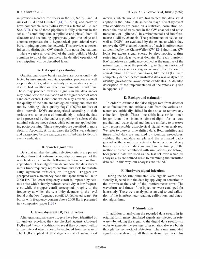
FIG. 3. Combined efficiencies of the three pipelines and twonetworks (H1H2L1 and H1H2) used in the upper limit analysisfor selected sine-Gaussian waveforms with (a) Q ¼ 3,(b) Q ¼ 9, (c) Q ¼ 100. These efficiencies have been calculatedusing the logical OR of the pipelines and networks for thesubset of simulated signals that were injected in time intervalsthat were actually analyzed, and thus approach unity for largeamplitudes.


102001-8

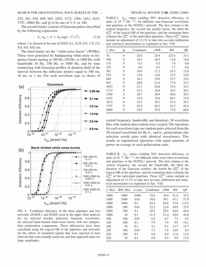
235, 361, 554, 849, 945, 1053, 1172, 1304, 1451, 1615,1797, 2000) Hz; and Q to be one of 3, 9, or 100.

The second family consists of Gaussian pulses describedby the following expression:

hþðt0 þ tÞ ¼ h0 expð�t2=�2Þ; (7.4)

where � is chosen to be one of (0.05, 0.1, 0.25, 0.5, 1.0, 2.5,4.0, 6.0, 8.0) ms.

The third family are the ‘‘white-noise bursts’’ (WNBs).These were generated by bandpassing white noise in fre-quency bands starting at 100 Hz, 250 Hz, or 1000 Hz, withbandwidth 10 Hz, 100 Hz, or 1000 Hz, and by timewindowing with Gaussian profiles of duration (half of theinterval between the inflection points) equal to 100 ms,10 ms, or 1 ms. For each waveform type (a choice of

central frequency, bandwidth, and duration), 30 waveformfiles with random data content were created. The injectionsfor each waveform type use random pairs selected from the30 created waveforms for the hþ and h� polarizations (theselection avoids pairs with identical waveforms). Thisresults in unpolarized injections with equal amounts ofpower on average in each polarization state.

(a)

]Hz [strain/rssh

−2210 −2110 −2010 −1910

Det

ectio

n E

ffici

ency

0

0.2

0.4

0.6

0.8

1 0.05 ms

0.1 ms

0.5 ms

1.0 ms

2.5 ms

6.0 ms

0.05 ms

0.1 ms

0.5 ms

1.0 ms

2.5 ms

6.0 ms

0.05 ms

0.1 ms

0.5 ms

1.0 ms

2.5 ms

6.0 ms

0.05 ms

0.1 ms

0.5 ms

1.0 ms

2.5 ms

6.0 ms

0.05 ms

0.1 ms

0.5 ms

1.0 ms

2.5 ms

6.0 ms

0.05 ms

0.1 ms

0.5 ms

1.0 ms

2.5 ms

6.0 ms

Gaussians

(b)

]Hz [strain/rssh

−2210 −2110 −2010 −1910

Det

ectio

n E

ffici

ency

0

0.2

0.4

0.6

0.8

1

Band−limited white noise bursts

250−260 Hz,0.1 s

250−350 Hz,0.01 s

100−200 Hz,0.01 s

1000−2000 Hz,0.001 s

1000−2000 Hz,0.01 s

1000−2000 Hz,0.1 s

FIG. 4. Combined efficiency of the three pipelines and twonetworks (H1H2L1 and H1H2) used in the upper limit analysisfor (a) selected linearly polarized Gaussian waveforms;(b) selected band-limited white-noise bursts with two indepen-dent polarization components. These efficiencies have beencalculated using the logical OR of the pipelines and networksfor the subset of simulated signals that were injected in timeintervals that were actually analyzed, and thus approach unity forlarge amplitudes.

TABLE I. hrss values yielding 50% detection efficiency, inunits of 10�22 Hz�1=2, for different sine-Gaussian waveformsand pipelines in the H1H2L1 network. The first column is thecentral frequency, the second the quality factor, the third theh50%rss of the logical OR of the pipelines, and the remaining threecolumns the h50%rss of the individual pipelines. These h50%rss valuesinclude an adjustment of 11.1% to take into account calibrationand statistical uncertainties as explained in Sec. VIII.

f (Hz) Q Combined cWB BN QP

70 9 25.8 25.9 227.4 33.1

100 9 10.3 10.5 13.6 14.0

153 9 6.3 6.5 7.8 8.8

235 9 6.0 6.3 7.7 6.8

361 9 10.9 11.2 16.3 12.0

554 9 12.0 12.6 15.5 12.9

849 9 18.1 19.0 23.7 19.2

945 9 20.6 21.6 27.8 22.2

1053 9 23.3 24.8 33.4 24.1

1172 9 25.2 26.8 36.5 26.3

1304 9 28.7 30.9 40.8 29.5

1451 9 32.0 35.0 48.1 32.9

1615 9 35.2 38.2 51.5 36.3

1797 9 42.0 44.2 62.2 45.4

2000 9 54.5 55.9 77.6 68.8

TABLE II. hrss values yielding 50% detection efficiency, inunits of 10�22 Hz�1=2, for different white-noise burst waveformsand pipelines in the H1H2L1 network. The first column is thecentral frequency, the second the bandwidth, the third theduration of the Gaussian window, the fourth the h50%rss of thelogical OR of the pipelines, and the remaining three columns theh50%rss of the individual pipelines. These h50%rss values include anadjustment of 11.1% to take into account calibration and statis-tical uncertainties as explained in Sec. VIII.

f (Hz) BW (Hz) d (ms) Combined cWB BN QP

1000 1000 0.001 32.0 34.4 51.8 33.2

1000 1000 0.01 38.6 39.1 47.1 51.9

1000 1000 0.1 63.4 65.8 73.0 113.6

1000 100 0.01 22.2 22.6 30.9 25.9

1000 100 0.1 28.5 28.5 44.6 44.6

1000 10 0.1 21.5 21.4 30.8 44.8

100 100 0.01 6.5 6.7 7.5 9.2

100 100 0.1 7.9 7.9 9.9 14.1

100 10 0.1 9.1 9.1 13.7 12.7

250 100 0.01 7.3 7.6 18.6 8.5

250 100 0.1 8.8 8.9 11.6 13.4

250 10 0.1 5.9 5.9 9.0 17.6


102001-9

Each efficiency curve, consisting of the efficienciesdetermined for a given signal morphology at each of the22 hrss values, was fitted with an empirical four-parameterfunction. The efficiency curves for the Logical OR (union)combination of the three pipelines and for the combinedH1H2 and H1H2L1 networks are shown for selected wave-forms in Figs. 3 and 4. The hrss values yielding 50%detection efficiency, h50%rss , are shown in Tables I and IIfor sine-Gaussians with Q ¼ 9 and for white-noise burstsinjected and analyzed in H1H2L1 data. The study of theefficiency for all the waveforms shows that the combina-tion of the methods is slightly more sensitive than the bestperforming one, which is QPipeline for some of the sine-Gaussians, and cWB for all other waveforms considered.

VIII. STATISTICAL AND CALIBRATION ERRORS

The h50%rss values presented in this paper have beenadjusted to conservatively reflect systematic and statisticaluncertainties. The dominant source of systematic uncer-tainty is from the amplitude measurements in thefrequency-domain calibration. The individual amplitudeuncertainties from each interferometer can be combinedinto a single uncertainty by calculating a combined root-sum-square (rss) amplitude SNR and propagating the in-dividual uncertainties assuming each error is independent.In addition, there is a small uncertainty (about 1%) intro-duced by converting from the frequency-domain to thetime-domain strain series on which the analysis was ac-tually run. There is also phase uncertainty on the order of afew degrees in each interferometer, arising both from theinitial frequency-domain calibration and the conversion tothe time domain. However, this is not a significant concernsince the phase uncertainties at all frequencies correspondto phase shifts on the order of less than half a sampleduration. We therefore do not make any adjustment tothe overall systematic uncertainties due to phase error.Finally, statistical uncertainties on the fit parameters (aris-ing from the binomial errors on the efficiency measure-ments) affect h50%rss by approximately 1.4% on average andare not much different for any particular waveform.

The frequency-domain amplitude uncertainties areadded in quadrature with the other smaller uncertaintiesto obtain a total 1-sigma relative error for the SNR. Therelative error in the hrss is then the same as the relative errorin the SNR. Thus, we adjust our sensitivity estimates byincreasing the h50%rss values by the reported percent uncer-tainties multiplied by 1.28 (to rescale from a 1-sigmafluctuation to a 90% confidence level upper limit, assumingGaussian behavior), which amounts to 11.1% in the fre-quency band explored in this paper.

IX. SEARCH RESULTS

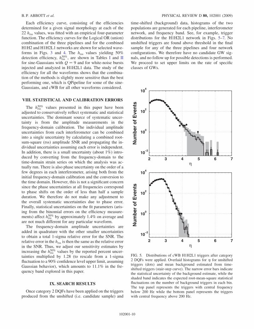
Once category 2 DQFs have been applied on the triggersproduced from the unshifted (i.e. candidate sample) and

time-shifted (background) data, histograms of the twopopulations are generated for each pipeline, interferometernetwork, and frequency band. See, for example, triggerdistributions for the H1H2L1 network in Figs. 5–7. Nounshifted triggers are found above threshold in the finalsample for any of the three pipelines and four networkconfigurations. We therefore have no candidate GW sig-nals, and no follow up for possible detections is performed.We proceed to set upper limits on the rate of specificclasses of GWs.

2 3 4 5 6 7

10−2

100

102

104

Nu

mb

er o

f E

ven

ts

η

2 3 4 5 6 7

10−2

100

102

104

Nu

mb

er o

f E

ven

ts

η

FIG. 5. Distributions of cWB H1H2L1 triggers after category2 DQFs were applied. Overlaid histograms for � for unshiftedtriggers (dots) and mean background estimated from time-shifted triggers (stair-step curve). The narrow error bars indicatethe statistical uncertainty of the background estimate, while theshaded band indicates the expected root-mean-square statisticalfluctuations on the number of background triggers in each bin.The top panel represents the triggers with central frequencybelow 200 Hz while the bottom panel represents the triggerswith central frequency above 200 Hz.


102001-10

Upper limits

Our measurements consist of the list of triggers detectedby each analysis pipeline (BN, QP, cWB) in each networkdata set (H1H2L1, H1H2, H1L1, H2L1). BN analyzed theH1H2L1 data, QP analyzed H1H2L1 and H1H2, and cWBanalyzed all four data sets. In general, the contribution tothe upper limit due to a given pipeline and data set in-creases with both the detection efficiency of the pipelineand the live time of the data set. Since the duty cycle of theH1L1 and H2L1 data sets is small (2.4% and 4.5% aftercategory 3 DQFs and category 3 vetoes, vs 37.2% and

22.5% in H1H2L1 and H1H2), and the data quality notas good, we decided a priori to not include these data setsin the upper limit calculation. We are therefore left withfive analysis pipeline results: BN-H1H2L1, QP-H1H2L1,QP-H1H2, cWB-H1H2L1, and cWB-H1H2. We wish tocombine these 5 results to produce a single upper limit onthe rate of GW bursts of each of the morphologies tested.We use the approach described in [31] to combine the

results of the different search detection algorithms andnetworks. Here we give only a brief summary of thetechnique.The procedure given in [31] is to combine the sets of

triggers according to which pipeline(s) and/or network

101

100

101

102

103

104

Nu

mb

er o

f E

ven

ts

H1H2 Correlated energy

101

100

101

102

103

104

Nu

mb

er o

f E

ven

ts

H1H2 Correlated energy

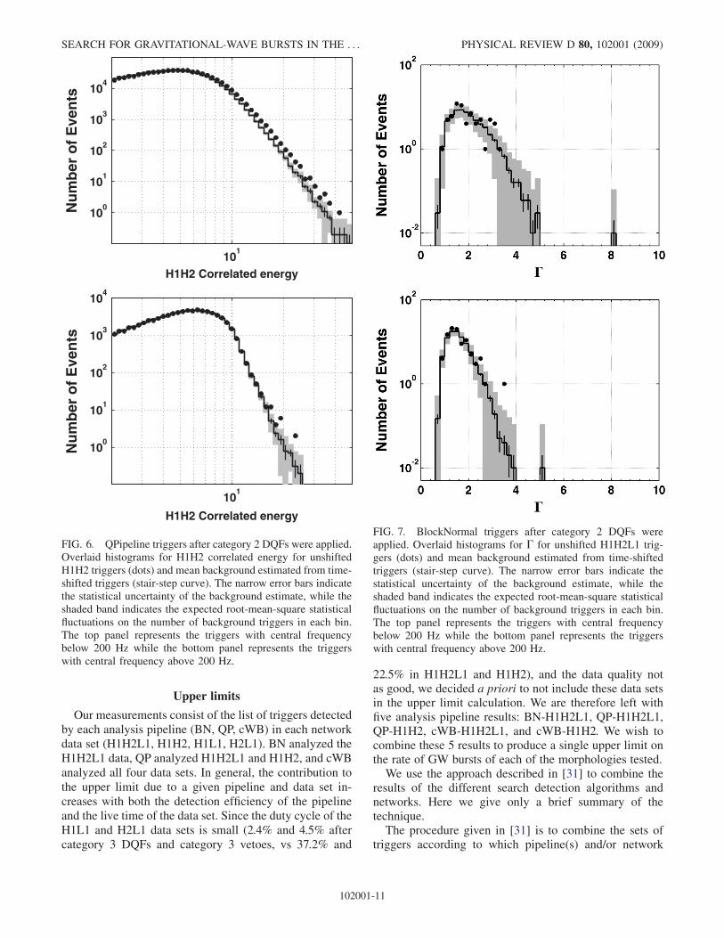
FIG. 6. QPipeline triggers after category 2 DQFs were applied.Overlaid histograms for H1H2 correlated energy for unshiftedH1H2 triggers (dots) and mean background estimated from time-shifted triggers (stair-step curve). The narrow error bars indicatethe statistical uncertainty of the background estimate, while theshaded band indicates the expected root-mean-square statisticalfluctuations on the number of background triggers in each bin.The top panel represents the triggers with central frequencybelow 200 Hz while the bottom panel represents the triggerswith central frequency above 200 Hz.

FIG. 7. BlockNormal triggers after category 2 DQFs wereapplied. Overlaid histograms for � for unshifted H1H2L1 trig-gers (dots) and mean background estimated from time-shiftedtriggers (stair-step curve). The narrow error bars indicate thestatistical uncertainty of the background estimate, while theshaded band indicates the expected root-mean-square statisticalfluctuations on the number of background triggers in each bin.The top panel represents the triggers with central frequencybelow 200 Hz while the bottom panel represents the triggerswith central frequency above 200 Hz.


102001-11

detected any given trigger. For example, in the case of twopipelines ‘‘A’’ and ‘‘B,’’ the outcome of the countingexperiment is the set of three numbers ~n ¼ ðnA; nB; nABÞ,where nA is the number of events detected by pipeline Abut not by B, nB is the number detected by B but not by A,and nAB is the number detected by both. (The extension toan arbitrary number of pipelines and data sets is straight-forward.) Similarly, one characterizes the sensitivity of theexperiment by the probability that any given GW burst willbe detected by a given combination of pipelines. We there-fore compute the efficiencies ~� ¼ ð�A; �B; �ABÞ, where �Ais the fraction of GW injections that are detected bypipeline A but not by B, etc.

To set an upper limit, one must decide a priori how torank all possible observations, so as to determine whether agiven observation ~n contains ‘‘more’’ or ‘‘fewer’’ eventsthan some other observation ~n0. Denote the ranking func-tion by �ð ~nÞ. Once this choice is made, the actual set ofunshifted events is observed, giving ~n, and the rate upperlimit R� at confidence level � is given by

1� � ¼ X~Nj�ð ~NÞ��ð ~nÞ

Pð ~Nj ~�; R�~TÞ: (9.1)

Here Pð ~Nj ~�; R�~TÞ is the prior probability of observing ~N

given the true GW rate R�, the vector containing the live

times of different data sets ~T (this is a scalar if we arecombining results of methods analyzing the same livetime), and the detection efficiencies ~�. The sum is taken

over all ~N for which �ð ~NÞ � �ð ~nÞ; i.e., over all possibleoutcomes ~N that result in ‘‘as few or fewer’’ events thanwere actually observed.

As shown in [31], a convenient choice for the rankordering is

�ð ~nÞ ¼ ~� � ~n: (9.2)

That is, we weight the individual measurementsðnA; nB; nAB; . . .Þ proportionally to the corresponding effi-ciency ð�A; �B; �AB; . . .Þ. This simple procedure yields asingle upper limit from the multiple measurements. Fromthe practical point of view, it has the useful properties thatthe pipelines need not be independent, and that combina-tions of pipelines and data sets in which it is less likely for asignal to appear (relatively low �i) are naturally given lessweight.

Note that for the purpose of computing the upper limiton the GW, we are ignoring any background. This leads toour limits being somewhat conservative, since a nonzerobackground contribution to ~n will tend to increase theestimated limit.

In the present search, no events were detected by any

analysis pipeline, so ~n ¼ ~0. As shown in [31], in this casethe efficiency weighted upper limit procedure given byEqs. (9.1) and (9.2) gives a particularly simple result: theprocedure is equivalent to taking the logical OR of all fivepipeline/network samples. The � ¼ 90% confidence level

upper limit for zero observed events, R90%, is given by

0:1 ¼ expð��totR90%TÞ (9.3)

) R90% ¼ 2:30

�totT; (9.4)

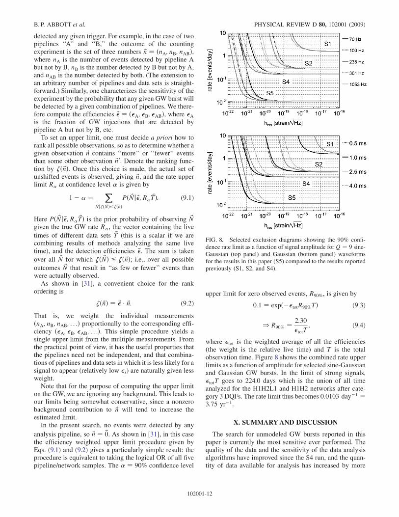
where �tot is the weighted average of all the efficiencies(the weight is the relative live time) and T is the totalobservation time. Figure 8 shows the combined rate upperlimits as a function of amplitude for selected sine-Gaussianand Gaussian GW bursts. In the limit of strong signals,�totT goes to 224.0 days which is the union of all timeanalyzed for the H1H2L1 and H1H2 networks after cate-gory 3 DQFs. The rate limit thus becomes 0:0103 day�1 ¼3:75 yr�1.

X. SUMMARYAND DISCUSSION

The search for unmodeled GW bursts reported in thispaper is currently the most sensitive ever performed. Thequality of the data and the sensitivity of the data analysisalgorithms have improved since the S4 run, and the quan-tity of data available for analysis has increased by more

FIG. 8. Selected exclusion diagrams showing the 90% confi-dence rate limit as a function of signal amplitude forQ ¼ 9 sine-Gaussian (top panel) and Gaussian (bottom panel) waveformsfor the results in this paper (S5) compared to the results reportedpreviously (S1, S2, and S4).


102001-12

than an order of magnitude. These improvements are re-flected in the greater strain sensitivity (with hrss50% values as

low as �6� 10�22 Hz�1=2) and the tighter limit on therate of bursts (less than 3.75 events per year at 90% con-fidence level) with large enough amplitudes to be detectedreliably. The most sensitive previous search, using LIGOS4 data, achieved hrss50% sensitivities as low as a few times

10�21 Hz�1=2 and a rate limit of 55 events per year. Wenote that the IGEC network of resonant bar detectors hasset a more stringent rate limit, 1.5 events per year at 95%confidence level [32], for GW bursts near the resonant

frequencies of the bars with hrss >�8� 10�19Hz�1=2

(see Sec. X of [14] for the details of this comparison). Alater joint observation run, IGEC-2, was a factor of �3more sensitive but had shorter observation time [33].

In order to set an astrophysical scale to the sensitivityachieved by this search, we now repeat the analysis and theexamples presented for S4. Specifically, we can estimatewhat amount of mass converted into GW burst energy at agiven distance would be strong enough to be detected bythe search with 50% efficiency. Following the same stepsas in [17], assuming isotropic emission and a distance of10 kpc we find that a 153 Hz sine-Gaussian with Q ¼ 9would need 1:9� 10�8 solar masses, while for S4 thefigure was 10�7M�. For a source in the Virgo galaxycluster, approximately 16 Mpc away, the same hrss wouldbe produced by an energy emission of roughly 0:05M�c2,while for S4 it was 0:25M�c2.

We can also update our estimates for the detectability oftwo classes of astrophysical sources: core-collapse super-novae and binary black-hole mergers. We consider first thecore-collapse supernova simulations by Ott. et al. [9]. Inthis paper, gravitational waveforms were computed forthree progenitor models: s11WW, m15b6, and s25WW.From S4 to S5 the astrophysical reach for the s11WWand m15b6 models improved from approximately 0.2 to0.6 kpc while for s25WW it improved from 8 to 24 kpc.Second, we consider the binary black-hole merger calcu-lated by the Goddard numerical relativity group [7]. Abinary system of two 10-solar-mass black holes (total20M�) would be detectable with 50% efficiency at a dis-tance of roughly 4 Mpc compared to 1.4 Mpc in S4, while asystem with total mass 100M� would be detectable out to�180 Mpc, compared to �60 Mpc in S4. In each case theastrophysical reach has improved by approximately a fac-tor of 3 from S4 to S5.

At present, the analysis of the second year of S5 is wellunderway, including a joint analysis of data from Virgo’sVSR1 run which overlaps with the final 4.5 months of S5.Along with the potential for better sky coverage, positionreconstruction and glitch rejection, the joint analysis bringswith it new challenges and opportunities. Looking furtherahead, the sixth LIGO science run and second Virgo sci-ence run are scheduled to start in mid 2009, with the twoLIGO 4 km interferometers operating in an ‘‘enhanced’’

configuration that is aimed at delivering approximately afactor of 2 improvement in sensitivity, and comparableimprovements for Virgo. Thus we will soon be able tosearch for GW bursts farther out into the Universe.

ACKNOWLEDGMENTS

The authors gratefully acknowledge the support of theUnited States National Science Foundation for the con-struction and operation of the LIGO Laboratory and theScience and Technology Facilities Council of the UnitedKingdom, the Max-Planck-Society, and the State ofNiedersachsen in Germany for support of the constructionand operation of the GEO600 detector. The authors alsogratefully acknowledge the support of the research by theseagencies and by the Australian Research Council, theCouncil of Scientific and Industrial Research of India,the Istituto Nazionale di Fisica Nucleare of Italy, theSpanish Ministerio de Educacion y Ciencia, theConselleria d’Economia Hisenda i Innovacio of theGovern de les Illes Balears, the Royal Society, theScottish Funding Council, the Scottish UniversitiesPhysics Alliance, the National Aeronautics and SpaceAdministration, the Carnegie Trust, the LeverhulmeTrust, the David and Lucile Packard Foundation, theResearch Corporation, and the Alfred P. SloanFoundation. This document has been assigned LIGOLaboratory Document No. LIGO-P080056-v12.

APPENDIX A: DATA QUALITY FLAGS

Data quality flags are defined by the LIGO DetectorCharacterization group by carefully processing informa-tion on the behavior of the instrument prior to analyzingunshifted triggers. Some are defined online, as the data areacquired, while others are formulated offline. Awide rangeof DQFs have been defined. The relevance of each avail-able DQF has been evaluated and classified into categorieswhich are used differently in the analysis, which we nowdescribe.Category 1 DQFs are used to define the data set pro-

cessed by the search algorithms. They include out-of-science mode, the 30 seconds before loss of lock, periodswhen the data are corrupted, and periods when test signalsare injected into the detector. They also include shorttransients that are loud enough to significantly distort thedetector response and could affect the power spectral den-sity used for normalization by the search algorithm, such asdropouts in the calibration and photodiode saturations.Category 2 flags are unconditional postprocessing data

cuts, used to define the ‘‘full’’ data set used to look fordetection candidates. The flags are associated with unam-biguous malfunctioning with a proven correlation withloud transients in the GW channel, where we understandthe physical coupling mechanism. They typically onlyintroduce a fraction of a percent of dead time over the


102001-13

run. Examples include saturations in the alignment controlsystem, glitches in the power mains, time-domain calibra-tion anomalies, and large glitches in the thermal compen-sation system.

Category 3 DQFs are applied to define the ‘‘clean’’ dataset, used to set an upper limit in the absence of a detectioncandidate. Any detection candidate found at a time markedwith a category 3 DQF would not be immediately rejectedbut would be considered cautiously, with special attentionto the effect of the flagged condition on detection confi-dence. DQF correlations with transients in the GW chan-nels are established at the single-interferometer level.Examples include the 120 s prior to lock loss, noise inpower mains, transient drops in the intensity of the lightstored in the arm cavities, times when one Hanford instru-ment is unlocked and may negatively affect the otherinstrument, times with particularly poor sensitivity, andtimes associated with severe seismic activity, high windspeed, or hurricanes. These flags introduce up to �10%dead time.

Category 4 flags are advisory only: We have no clearevidence of a correlation to loud transients in the GWchannel, but if we find a detection candidate at these times,we need to exert caution. Examples are certain data vali-dation issues and various local events marked in the elec-tronic logs by operators and science monitors.

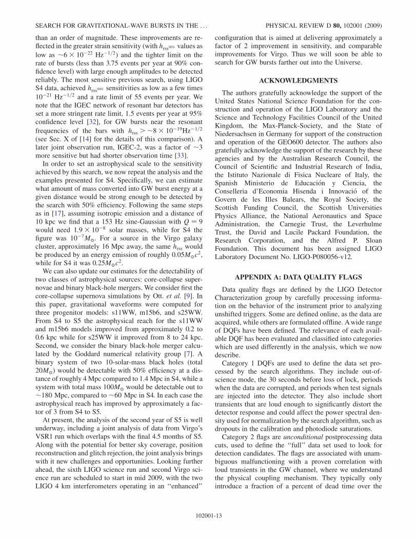
Figure 9 shows the fraction of KleineWelle triggers thatare eliminated by category 2 and 3 DQFs, respectively, inthe L1 interferometer, as a function of the significance ofthe energy excess identified by the trigger, which is eval-uated assuming stationary, random noise. To ensure DQFsare independent of the presence of a true GW, we verifiedthey are not triggered by hardware injections.

APPENDIX B: EVENT-BY-EVENT VETOES

Event-by-event vetoes attempt to discard GW channelnoise events by using information from the many environ-

mental and interferometric auxiliary channels which mea-sure non-GW degrees of freedom. Good vetoes are foundby looking for situations in which a short (�ms)noise transient in an auxiliary channel, identified by theKW algorithm, often coincides within a short interval(� 100 ms) with noise transients in the GW channel.The work, then, is in identifying useful auxiliary channelswhich are well correlated with noise transients in the GWdata, choosing the relevant veto parameters to use, andfinally establishing that the veto procedure will not sys-tematically throw out true GWs. As for the data qualityflags, vetoes are defined prior to generating triggers fromunshifted data. The trigger properties used for veto studiesare the KW signal energy-weighted central time and theKW statistical significance. The correlation between noiseevents in the GW channel and an auxiliary channel isdetermined by a comparison of the coincidence rate mea-sured properly and coincidence rate formed when one ofthe time series has been artificially time shifted with re-spect to the other. Alternatively, we can compare thenumber of coincidences with the number expected bychance, assuming Poisson statistics.As for the DQFs, category 2 vetoes are defined using

only a few subsets of related channels, showing the moreobvious kinds of mechanisms for disturbing the interfer-ometers—either vibrational or magnetic coupling.Furthermore, for this S5 analysis we insist that multiple(3 or more) channels from each subset be excited incoincidence before declaring a category 2 veto, to ensurethat a genuine disturbance is being measured in each case.By contrast, the category 3 vetoes use a substantially largerlist of channels. The aim of this latter category of veto is toproduce the optimum reduction of false events for a chosentolerable amount of live-time loss.

1. Veto effectiveness metrics

Veto efficiency is defined for a given set of triggers as thefraction vetoed by our method. We use a simple veto logic

FIG. 9. The two examples in the figure show the fraction of single-interferometer (L1) KleineWelle triggers eliminated by category 2(left panel) and category 3 (right panel) DQFs, as a function of a threshold on the significance. The cumulative impact on the lifetime isless then 7% (mostly from category 3 DQFs), and the cuts are most effective for the loudest triggers. For example, a significance of1000 means that if the detector noise were Gaussian, the noise would have a probability e�1000 of fluctuating to produce such a loudtrigger.


102001-14

where an event is vetoed if its peak time falls within a vetowindow, and define the veto dead-time fraction to be thefraction of live time flagged by all the veto windows.Assuming that real events are randomly distributed intime, dead-time fraction represents the probability of veto-ing a true GWevent by chance. We will refer to the flaggeddead time as the veto segments. A veto efficiency greaterthan the dead-time fraction indicates a correlation betweenthe triggers and veto segments.

Under either the assumption of randomly distributedtriggers, or randomly distributed dead time, the numberof events that fall within the flagged dead time is Poissondistributed with mean value equal to the number of eventstimes the fractional dead time, or equivalently, the eventrate times the duration of veto segments. We define thestatistical significance of actually observing N vetoedevents as SðNÞ ¼ �log10½PPoissðx � NÞ�.

We must also consider the safety of a veto condition:auxiliary channels (besides the GW channel) could inprinciple be affected by a GW, and a veto condition derivedfrom such a channel could systematically reject a genuinesignal. Hardware signal injections imitating the passage ofGWs through our detectors, performed at several predeter-mined times during the run, have been used to establishunder what conditions each channel is safe to use as a veto.Nondetection of a hardware injection by an auxiliarychannel suggests the unconditional safety of this channelas a veto in the search, assuming that a reasonably broadselection of signal strengths and frequencies were injected.But even if hardware injections are seen in the auxiliarychannels, conditions can readily be derived under which notriggers caused by the hardware injections are used asvetoes. This involves imposing conditions on thestrength of the triggers and/or on the ratio of the signalstrength seen in the auxiliary channel to that seen in theGW channel.

Veto safety was quantified in terms of the probability ofobserving � N coincidence events between the auxiliarychannel and hardware injections vs the number of coinci-dences expected from time shifts.

The observed coincidence rate is a random variable itselfthat fluctuates around the true coincident rate. In the vetoanalysis we use the 90% confidence upper limit on thebackground coincidence rate which can be derived fromthe observed coincidence rate. This procedure makes iteasier to consider a veto safe than unsafe and the reasonfor this approach was to lean toward vetoing questionableevents. A total of 20 time shifts were performed. Theanalysis looped over 7 different auxiliary channelthresholds and calculated this probability, and a probabilityof less than 10% caused a veto channel at and below thegiven threshold to be judged unsafe. A fixed 100 ms win-dow between the peak time of the injection and the peaktime of the KleineWelle trigger in the auxiliary channelwas used.

All channels used for category 2 vetoes were found to besafe at any threshold. Thresholds for category 3 vetochannels were chosen so as to ensure that the channelwas safe at that threshold and above.

2. Selection of veto conditions

For the purpose of defining conservative vetoes appro-priate for applying as category 2 (before looking for GWdetections), we studied environmental channels. We foundthat these fall into groups of channels that each veto a largenumber of the same events. Based on this observation,three classes of environmental channels were adopted asvetoes. For LHO these classes were 24 magnetometers andvoltmeters with a KW threshold of 200 and timewindow of100 ms, and 32 accelerometers and seismometers with athreshold on the KW significance of 100 and a time win-dow of 200 ms. For LLO these were 12 magnetometers andvoltmeters with a KW threshold of 200 and a time windowof 100 ms. We used all of the channels that should havebeen sensitive to similar effects across a site, with theexception that channels known to have been malfunction-ing during the time period were removed from the list.To ensure that our vetoes are based on true environmen-

tal disturbances, a further step of voting was implemented.An event must be vetoed by three or more channels in aparticular veto group in order to be discarded from thedetection search. These conditions remove �0:1% fromthe S5 live time.In the more aggressive category 3 vetoes, used for

cleaning up the data for an upper limit analysis, we drawfrom a large number of channels (about 60 interferometricchannels per instrument, and 100 environmental channelsper site). This task is complicated by the desire to chooseoptimal veto thresholds and windows, and the fact that theveto channels themselves can be highly correlated witheach other so that applying one veto channel changes theincremental cost (in additional dead time) and benefit (inadditional veto efficiency) of applying another. Applyingall vetoes which perform well by themselves often leads toan inefficient use of dead time as dead time continues toaccumulate while the same noise events are vetoed overand over.For a particular set of GW channel noise events, we

adopt a ‘‘hierarchical’’ approach to choose the best subsetof all possible veto conditions to use for a target dead time.This amounts to finding an ordering of veto conditions(veto channel, threshold, and window) from best to worstsuch that the desired set of veto conditions can be made byaccumulating from the top veto conditions so long as thedead time does not exceed our limit, which is typically afew percent.We begin with an approximately ordered list based on

the performance of each veto condition (channel, window,and threshold) considered separately. Incremental vetostatistics are calculated for the entire list of conditions


102001-15

using the available ordering. This means that for a givenveto condition, statistics are no longer calculated over theentire S5 live time, but only over the fraction of live timethat remains after all veto conditions earlier in the list havebeen applied. The list is then re-sorted according to theincremental performance metric and the process is re-peated until further iterations yield a negligible change inordering.

The ratio of incremental veto efficiency to incrementaldead time is used as a performance metric to sort vetoconditions. This ratio gives the factor by which the rate ofnoise events inside the veto segments exceeds the averagerate. By adopting veto conditions with the largest incre-mental efficiency/dead-time ratio, we maximize total effi-ciency for a target dead time. We also set a threshold ofprobability P< 0:001 on veto significance (not to be con-fused with the significance of the triggers themselves).This is particularly important for low-number statisticswhen large efficiency/dead-time ratios can occasionallyresult from a perfectly random process.

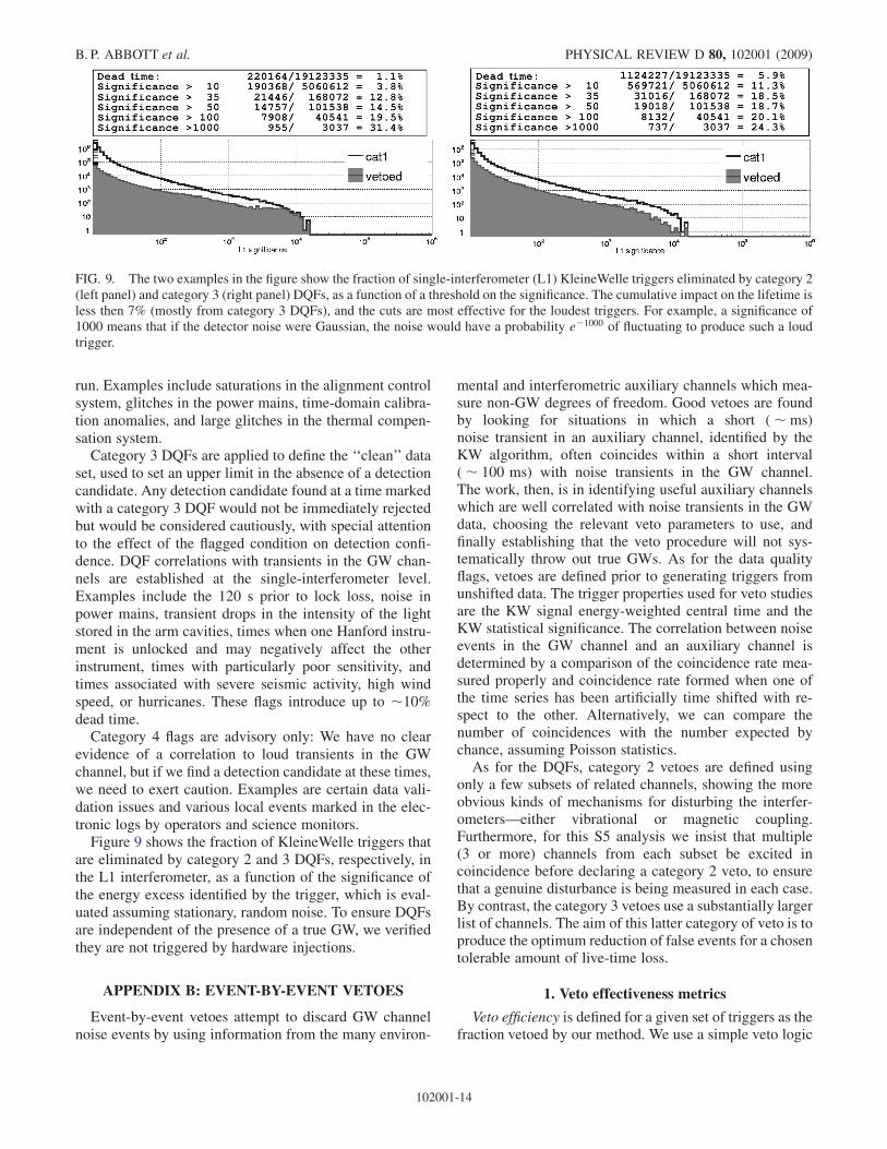
Vetoes were optimized over several different sets of GWchannel noise events including low-threshold H1H2L1coherent WaveBurst time-shifted events, H1H2 coherentWaveBurst playground events, as well as QPipeline andKleineWelle single-interferometer triggers. For example,the effect of data quality flags and event-by-event vetoes onthe sample of coherent WaveBurst time-shifted events isshown in Fig. 10. Our final list of veto segments to excludefrom the S5 analysis is generated from the union of theseindividually tuned lists.

APPENDIX C: THE BLOCKNORMAL BURSTSEARCH ALGORITHM

1. Overview

The BlockNormal analysis pipeline follows a similarlogic to the S4 burst analysis [17] by looking for burststhat are both coincident and correlated. The BlockNormalpipeline uses a change-point analysis to identify coincidenttransient events of high significance in each detector’s data.The subsequent waveform correlation test is the same asthat used in the S4 analysis.A unique feature of the BlockNormal analysis is that it

can be run on uncalibrated time-series data—neither thechange-point analysis nor the correlation test are sensitiveto the overall normalization of the data.

2. Data conditioning

The BlockNormal search operated on the frequencyrange 80 to 2048 Hz. To avoid potential issues with theadditional processing and filtering used to create calibrateddata, and to be immune to corrections in the calibrationprocedure, the analysis was run on the uncalibrated GWchannel from the LIGO interferometers.The data conditioning began with notch filters to sup-

press out-of-band (below 80 Hz or above 2048 Hz) spectralfeatures such as low-lying calibration lines, the strong60 Hz power-line feature, and violin-mode harmonicsjust above 2048 Hz. The time-series data were then downsampled to 4096 Hz to suppress high-frequency noise. The

q

FIG. 10. Left panel: Accumulated veto efficiency versus dead time as vetoes are applied cumulatively down the veto list. The bestvetoes are applied first, so we see a general decrease in the effectiveness of vetoes at higher dead time. Vetoes from environmentalchannels are artificially prioritized over interferometric channels, giving rise to the knee in the plot around 0.8% dead time where theenvironmental vetoes are exhausted. Right panel: Histogram of coherent network amplitude, �, for coherent WaveBurst time-shifted(background) events representing 100 S5 live times. The different shades show events removed by data quality cuts and vetoes atvarious stages in the analysis.


102001-16

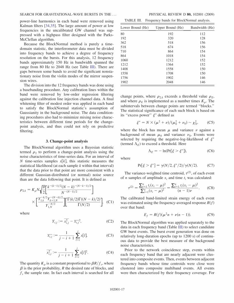
power-line harmonics in each band were removed usingKalman filters [34,35]. The large amount of power at lowfrequencies in the uncalibrated GW channel was sup-pressed with a highpass filter designed with the Parks-McClellan algorithm.

Because the BlockNormal method is purely a time-domain statistic, the interferometer data must be dividedinto frequency bands to achieve a degree of frequencyresolution on the bursts. For this analysis, 12 frequencybands approximately 150 Hz in bandwidth spanned therange from 80 Hz to 2048 Hz (see Table III). There aregaps between some bands to avoid the significant nonsta-tionary noise from the violin modes of the mirror suspen-sion wires.

The division into the 12 frequency bands was done usinga basebanding procedure. Any calibration lines within theband were removed by low-order regression filteringagainst the calibration line injection channel data. A finalwhitening filter of modest order was applied in each bandto satisfy the BlockNormal statistic’s assumption ofGaussianity in the background noise. The data condition-ing procedures also had to minimize mixing noise charac-teristics between different time periods for the change-point analysis, and thus could not rely on predictivefiltering.

3. Change-point analysis

The BlockNormal algorithm uses a Bayesian statistictermed �2 to perform a change-point analysis using thenoise characteristics of time-series data. For an interval ofN time-series samples x½k�, this statistic measures thestatistical likelihood (at each sample k within that interval)that the data prior to that point are more consistent with adifferent Gaussian-distributed (or normal) noise sourcethan are the data following that point. It is defined as

�2;k ¼ K�N

ffiffiffiffi�

2

r �k�ðk�1Þ=2ðN � kÞ�ðN�k�1Þ=2

N�ðN�1Þ=2

�

��Y�k=21;k Y�ðN�kÞ=2

kþ1;N

Y�N=21;N

��ðk=2Þ�ððN � kÞ=2Þ

�ðN=2Þ�; (C1)

where

Yi;j :¼ x2i;j � xi;j2; (C2)

xi;j :¼ 1

j� iþ 1

Xjl¼i

x½l�; (C3)

x2i;j :¼1

j� iþ 1

Xjl¼i

x½l�2: (C4)

The quantityK� is a constant proportional to�R=fs, where

� is the prior probability, R the desired rate of blocks, andfs the sample rate. In fact each interval is searched for all

change points, where �2;k exceeds a threshold value �E,

and where �E is implemented as a number times K�. The

subintervals between change points are termed ‘‘blocks.’’The statistical significance of each such block is based onits ‘‘excess power’’ defined as

¼ N � ð2 þ �Þ=ð20 þ �0Þ � �2

N; (C5)

where the block has mean and variance � against abackground of mean 0 and variance �0. Events wereselected by requiring the negative-log-likelihood of (termed �E) to exceed a threshold. Here

�E ¼ � lnðPr½ > �Þ; (C6)

where

Pr½ > � ¼ ðN=2; =2Þ= ðN=2Þ: (C7)

The variance-weighted time centroid, �ð2Þ, of each eventof n samples of amplitude xi and time ti was calculated:

�ð2Þ ¼P

ni¼1 tiðxi �Þ2Pni¼1ðxi �Þ2 ¼

Pni¼1 tiðxi �Þ2ðn� 1Þ� : (C8)

The calibrated band-limited strain energy of each eventwas estimated using the frequency-averaged response RðfÞover that band:

Ef ¼ RðfÞð2nþ �ðn� 1ÞÞ: (C9)

The BlockNormal algorithm was applied separately to thedata in each frequency band (Table III) to select candidateGW burst events. The burst event generation was done onrelatively long-duration epochs (up to 1200 s) of continu-ous data to provide the best measure of the backgroundnoise characteristics.Prior to the network coincidence step, events within

each frequency band that are nearly adjacent were clus-tered into composite events. Then, events between adjacentfrequency bands whose time centroids were close wereclustered into composite multiband events. All eventswere then characterized by their frequency coverage. For

TABLE III. Frequency bands for BlockNormal analysis.

Lower Bound (Hz) Upper Bound (Hz) Bandwidth (Hz)

80 192 112

192 320 128

362 518 156

518 674 156

710 864 154

864 1018 154

1060 1212 152

1212 1364 152

1408 1558 150

1558 1708 150

1756 1902 146

1902 2048 146


102001-17

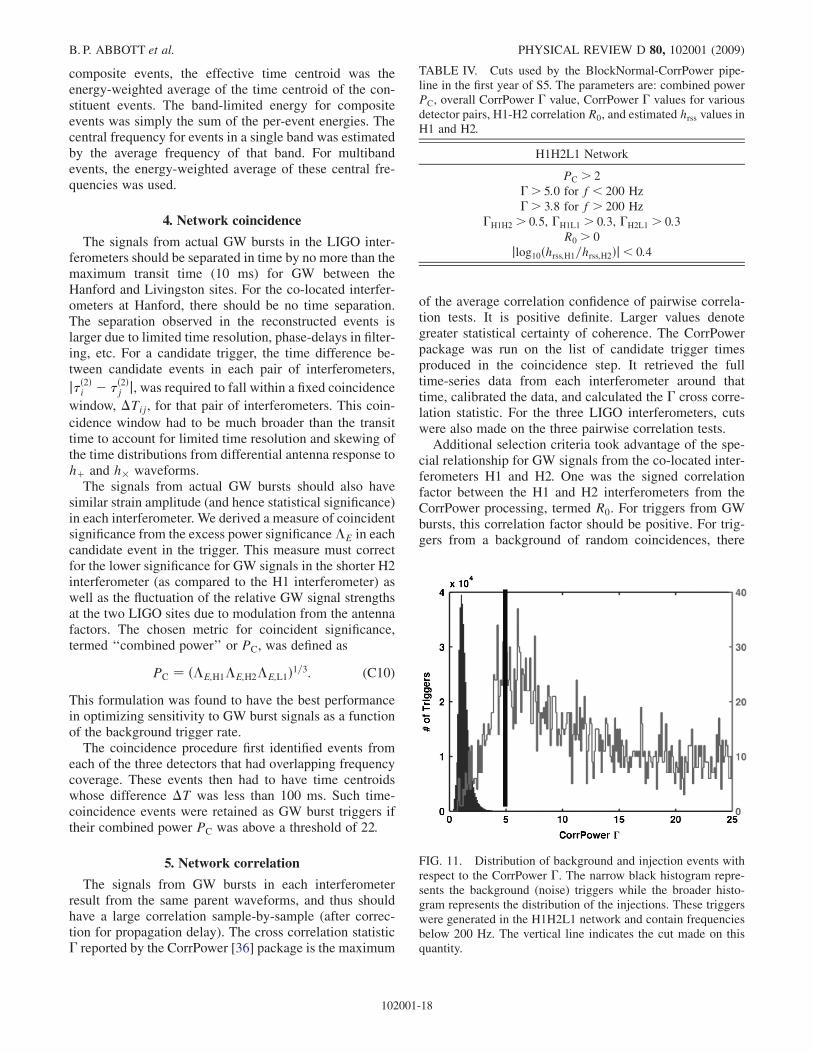
composite events, the effective time centroid was theenergy-weighted average of the time centroid of the con-stituent events. The band-limited energy for compositeevents was simply the sum of the per-event energies. Thecentral frequency for events in a single band was estimatedby the average frequency of that band. For multibandevents, the energy-weighted average of these central fre-quencies was used.

4. Network coincidence

The signals from actual GW bursts in the LIGO inter-ferometers should be separated in time by no more than themaximum transit time (10 ms) for GW between theHanford and Livingston sites. For the co-located interfer-ometers at Hanford, there should be no time separation.The separation observed in the reconstructed events islarger due to limited time resolution, phase-delays in filter-ing, etc. For a candidate trigger, the time difference be-tween candidate events in each pair of interferometers,

j�ð2Þi � �ð2Þj j, was required to fall within a fixed coincidencewindow, �Tij, for that pair of interferometers. This coin-

cidence window had to be much broader than the transittime to account for limited time resolution and skewing ofthe time distributions from differential antenna response tohþ and h� waveforms.

The signals from actual GW bursts should also havesimilar strain amplitude (and hence statistical significance)in each interferometer. We derived a measure of coincidentsignificance from the excess power significance�E in eachcandidate event in the trigger. This measure must correctfor the lower significance for GW signals in the shorter H2interferometer (as compared to the H1 interferometer) aswell as the fluctuation of the relative GW signal strengthsat the two LIGO sites due to modulation from the antennafactors. The chosen metric for coincident significance,termed ‘‘combined power’’ or PC, was defined as

PC ¼ ð�E;H1�E;H2�E;L1Þ1=3: (C10)

This formulation was found to have the best performancein optimizing sensitivity to GW burst signals as a functionof the background trigger rate.

The coincidence procedure first identified events fromeach of the three detectors that had overlapping frequencycoverage. These events then had to have time centroidswhose difference �T was less than 100 ms. Such time-coincidence events were retained as GW burst triggers iftheir combined power PC was above a threshold of 22.

5. Network correlation

The signals from GW bursts in each interferometerresult from the same parent waveforms, and thus shouldhave a large correlation sample-by-sample (after correc-tion for propagation delay). The cross correlation statistic� reported by the CorrPower [36] package is the maximum

of the average correlation confidence of pairwise correla-tion tests. It is positive definite. Larger values denotegreater statistical certainty of coherence. The CorrPowerpackage was run on the list of candidate trigger timesproduced in the coincidence step. It retrieved the fulltime-series data from each interferometer around thattime, calibrated the data, and calculated the � cross corre-lation statistic. For the three LIGO interferometers, cutswere also made on the three pairwise correlation tests.Additional selection criteria took advantage of the spe-

cial relationship for GW signals from the co-located inter-ferometers H1 and H2. One was the signed correlationfactor between the H1 and H2 interferometers from theCorrPower processing, termed R0. For triggers from GWbursts, this correlation factor should be positive. For trig-gers from a background of random coincidences, there

TABLE IV. Cuts used by the BlockNormal-CorrPower pipe-line in the first year of S5. The parameters are: combined powerPC, overall CorrPower � value, CorrPower � values for variousdetector pairs, H1-H2 correlation R0, and estimated hrss values inH1 and H2.

H1H2L1 Network

PC > 2�> 5:0 for f < 200 Hz�> 3:8 for f > 200 Hz

�H1H2 > 0:5, �H1L1 > 0:3, �H2L1 > 0:3R0 > 0

jlog10ðhrss;H1=hrss;H2Þj< 0:4

FIG. 11. Distribution of background and injection events withrespect to the CorrPower �. The narrow black histogram repre-sents the background (noise) triggers while the broader histo-gram represents the distribution of the injections. These triggerswere generated in the H1H2L1 network and contain frequenciesbelow 200 Hz. The vertical line indicates the cut made on thisquantity.


102001-18

should be an equal number of positive and negative corre-lation factors. Also, since the H1 and H2 interferometersreceive the same GW signal, the ratio of hrss;H2 to hrss;H1should be close to 1 for a true GW burst. In contrast, fortriggers from a random background this ratio will becentered around one-half. This arises because the H2 in-terferometer is approximately half as sensitive as H1, sosignals of the same statistical significance (near thethreshold) will have only one-half the amplitude in H2 asthey do in H1. To simplify thresholding, the absolute valueof the logarithm of the ratio was calculated RH1H2 ¼jlog10ðhrss;H1=hrss;H2Þj for later use.

The choices of tuning parameters are described inTable IV. Figure 11 illustrates an example of plots usedto tune the figures of merit for the H1H2L1 network.

APPENDIX D: THE QPIPELINE BURST SEARCHALGORITHM

1. Overview

QPipeline is an analysis pipeline for the detection of GWbursts in data from interferometric gravitational-wave de-tectors [26]. It is based on the Q transform [27], a multi-resolution time-frequency transform that projects the dataunder test onto the space of bisquare-windowed complexexponentials characterized by central time �, central fre-quency f0, and quality factor Q:

Xð�; f0; QÞ ¼Z þ1

�1~xðfÞ ~wðf; f0; QÞeþi2�f�df; (D1)

where the bisquare window ~wðf; f0; QÞ is

¼�A½1� ð fQ

f0ffiffiffiffiffi5:5

p Þ2�2 for f < f0ffiffiffiffiffi5:5

pQ

0 otherwise(D2)

with

A ¼�

315

128ffiffiffiffiffiffiffi5:5

p Q

f0

�1=2

: (D3)

The bisquare window is a close approximation to aGaussian window in frequency space; the QPipeline iseffectively a templated matched filter search [37] for sig-nals that are Gaussian enveloped sinusoids in the whitenedsignal space.

2. Data conditioning

Before applying the Q transform, the data are firstwhitened by zero-phase linear predictive filtering [26,38].In linear predictive whitening, the nth sample of a discretedata sequence is assumed to be well modeled by a linearcombination of the previous M samples:

x½n� ¼ XMm¼1

c½m�x½n�m�: (D4)

The resulting whitened data stream is the prediction error

sequence e½n� ¼ x½n� � x½n� that remains after selectingthe coefficients c½m� to minimize the error in the least-squares sense.The prediction error lengthM is taken to be equal to the

length of the longest basis function under test, which isapproximately 1 s. This ensures that the data are uncorre-lated on the time scales of the analysis.In order to avoid introducing phase errors between de-

tectors, a modified zero-phase whitening filter is con-structed by zero-padding the initial filter, converting to thefrequency domain, and discarding all phase information.

3. Measurement basis

The space of Gaussian enveloped complex exponentialsis an over-complete basis of waveforms, whose duration�t and bandwidth �f have the minimum possible time-

frequency uncertainty, �t�f ¼ 1=4�, where Q ¼f0=

ffiffiffi2

p�f. As a result, they provide the tightest possible

constraints on the time-frequency area of a signal, max-imizing the measured SNR and minimizing the probabilitythat false triggers are coincident in time and frequencybetween multiple detectors.In practice, the Q transform is evaluated only for a finite

number of basis functions, which are more commonlyreferred to as templates or tiles. These templates are se-lected to cover a targeted region of signal space, and arespaced such that the fractional signal energy loss ��Z=Zdue to the mismatch ��, �f0, and �Q between an arbitrarybasis function and the nearest measurement template,

��Z

Z’ 2�2f20

Q2��2 þ 1þQ2

2f20�f20 þ

1

2Q2�Q2

� 1

f0Q�f0�Q; (D5)

is no larger than �20%. This naturally leads to a tiling ofthe signal space that is logarithmic in Q, logarithmic infrequency, and linear in time.For this search, the QPipeline was applied to search the

space of sinusoidal Gaussians with central frequency from

48 Hz to 2048 Hz, and with Q fromffiffiffiffiffiffiffi5:5

pto 100=

ffiffiffi2

p.

4. Trigger generation

The statistical significance of Q transform projectionsare given by their normalized energy Z, defined as the ratioof squared projection magnitude to the mean squaredprojection magnitude of other templates with the samecentral frequency and Q. For the case of ideal white noise,Z is exponentially distributed and is related to the matchedfilter SNR quantity � [37] by the relation

Z ¼ jXj2=hjXj2i� ¼ � lnPr½Z0 > Z� ¼ �2=2: (D6)

The Q transform is applied to the whitened data andnormalized energies are computed for each measurement


102001-19

template as a function of time. Templates with statisticallysignificant signal content are then identified by applying athreshold on the normalized energy. Finally, since a singleevent may potentially produce multiple overlapping trig-gers due to the overlap between measurement templates,only the most significant of overlapping templates arereported as triggers.

Clustering of nearby triggers is not used in evaluatingthe significance of events. As a result, the detectability ofGW burst signals depends on their maximum projectiononto the space of Gaussian enveloped sinusoids.

5. Coherence

For this search, the QPipeline took advantage of the co-located nature of the two LIGO Hanford detectors to formtwo linear combinations of the data streams from the twodetectors. This coherent analysis makes use of correlationsin the data to distinguish true GW signals from instrumen-tal glitches.

a. Coherent signal stream

The first combination is the coherent signal stream,Hþ ,a frequency dependent weighted sum of the data from theHanford detectors which maximizes the effective SNR.The weighting is inversely proportional to the noise powerspectral density, SðfÞ:

~x HþðfÞ ¼�1

SH1þ 1

SH2

��1�~xH1ðfÞSH1ðfÞ þ

~xH2ðfÞSH2ðfÞ

�: (D7)

The resulting combination is treated as the output of anew hybrid, ‘‘coherent’’ detector. Under the assumptionthat the power spectral density is approximately flat acrossthe window bandwidth, applying the Q transform to thisdata stream leads to a coherent energy value, jXcoh

Hþj2,which takes the following form:

jXcohHþj2 ¼

�1

SH1þ 1

SH2

��2

��jXH1j2

S2H1þ jXH2j2

S2H2þ X

H1XH2 þ XH1XH2

SH1SH2

�;

(D8)

where XH1, XH2, and XcohHþ are functions of �, f0, andQ, and

the asterisk denotes complex conjugation. The last termrepresents the contribution of the cross term, and is con-ceptually similar to a frequency-domain representation of across correlation of the H1 and H2 data streams.

The energy expected in the coherent data stream if therewere no correlations in the data can be characterized by the‘‘incoherent’’ terms in Eq. (D8):

jXincHþj2 ¼

�1

SH1þ 1

SH2

��2�jXH1j2

S2H1þ jXH2j2

S2H2

�: (D9)

The coherent and incoherent energies can then be normal-

ized in the manner of Eq. (D6):

ZcohHþ ¼ jXcoh

Hþj2=hjXcohHþj2i�; (D10)

ZincHþ ¼ jXinc

Hþj2=hjXincHþj2i�: (D11)

The correlation between the detectors can then be mea-sured by the correlated energy, Zcorr

Hþ , given by

ZcorrHþ ¼ Zcoh

Hþ � ZincHþ ’ X

H1XH2 þ XH1XH2

SH1 þ SH2: (D12)

b. Null stream

The second combination is the difference between thecalibrated data from the two detectors, known as the nullstream, and is defined as

~x H�ðfÞ ¼ ~xH1ðfÞ � ~xH2ðfÞ: (D13)

By subtracting the co-located streams, any truegravitational-wave signal should be canceled. The result-ing combination is treated as the output of a new hybrid‘‘H�’’ detector, which shows significant energy content inthe presence of instrumental glitches but does not respondto gravitational waves. Glitches are identified by thresh-olding on the corresponding normalized ‘‘null energy,’’ZcohH�, calculated in an analogous manner to Zcoh

Hþ.Signal tiles found to be in coincidence with significant

null stream tiles are vetoed as instrumental glitches, andare not considered as candidate events. The threshold onZcohH� can be expressed as

ZcohH� >�þ �Zinc

H�; (D14)

where� is chosen to limit the veto rate in Gaussian noise to�1 per 2048 tiles and � is a parameter corresponding tothe allowed tolerance in calibration uncertainty. This is anenergy factor, and corresponds to an amplitude calibrationuncertainty of approximately 22%.We expect that highly energetic instrumental glitches

could leak energy into adjacent time-frequency bins, so theveto coincidence requirement between signal and nullstreams is scaled to give more-significant null stream tilesmore area of veto influence in time-frequency space:

j�H� � �Hþj< ð��0H� þ ��HþÞ=2; (D15)

jf0;H� � f0;Hþj< ð�f00;H� þ �f0;HþÞ=2; (D16)

where � and f0 are the central time and frequency of a tile,�� and �f are the duration and bandwidth of a tile, and theinflated null stream tile duration and bandwidth are definedas

��0H� ¼ maxð1; 0:5ffiffiffiffiffiffiffiffiffiffiffiffi2Zcoh

H�q

Þ � ��H�; (D17)

�f00;H� ¼ maxð1; 0:5ffiffiffiffiffiffiffiffiffiffiffiffi2Zcoh

H�q

Þ � �f0;H�: (D18)


102001-20

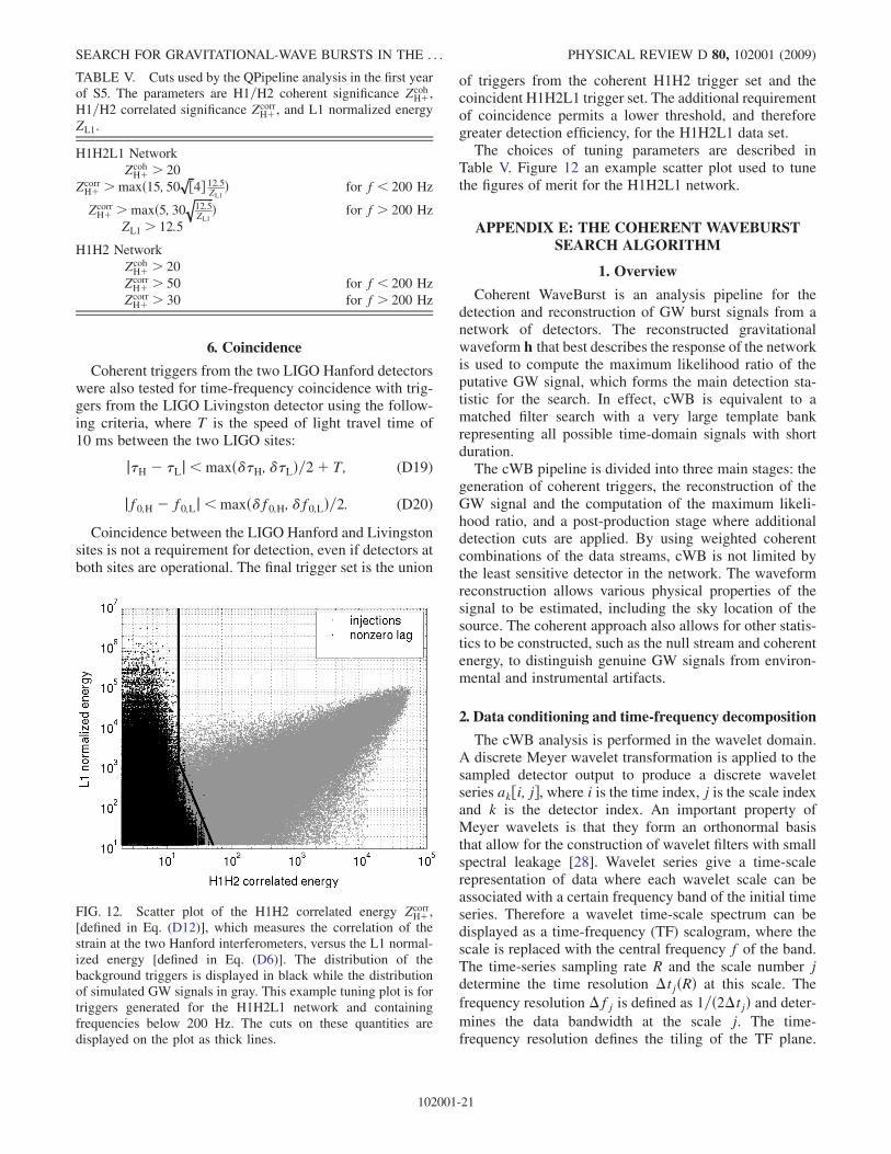
6. Coincidence

Coherent triggers from the two LIGO Hanford detectorswere also tested for time-frequency coincidence with trig-gers from the LIGO Livingston detector using the follow-ing criteria, where T is the speed of light travel time of10 ms between the two LIGO sites:

j�H � �Lj<maxð��H; ��LÞ=2þ T; (D19)

jf0;H � f0;Lj<maxð�f0;H; �f0;LÞ=2: (D20)

Coincidence between the LIGO Hanford and Livingstonsites is not a requirement for detection, even if detectors atboth sites are operational. The final trigger set is the union

of triggers from the coherent H1H2 trigger set and thecoincident H1H2L1 trigger set. The additional requirementof coincidence permits a lower threshold, and thereforegreater detection efficiency, for the H1H2L1 data set.The choices of tuning parameters are described in

Table V. Figure 12 an example scatter plot used to tunethe figures of merit for the H1H2L1 network.

APPENDIX E: THE COHERENT WAVEBURSTSEARCH ALGORITHM

1. Overview

Coherent WaveBurst is an analysis pipeline for thedetection and reconstruction of GW burst signals from anetwork of detectors. The reconstructed gravitationalwaveform h that best describes the response of the networkis used to compute the maximum likelihood ratio of theputative GW signal, which forms the main detection sta-tistic for the search. In effect, cWB is equivalent to amatched filter search with a very large template bankrepresenting all possible time-domain signals with shortduration.The cWB pipeline is divided into three main stages: the

generation of coherent triggers, the reconstruction of theGW signal and the computation of the maximum likeli-hood ratio, and a post-production stage where additionaldetection cuts are applied. By using weighted coherentcombinations of the data streams, cWB is not limited bythe least sensitive detector in the network. The waveformreconstruction allows various physical properties of thesignal to be estimated, including the sky location of thesource. The coherent approach also allows for other statis-tics to be constructed, such as the null stream and coherentenergy, to distinguish genuine GW signals from environ-mental and instrumental artifacts.

2. Data conditioning and time-frequency decomposition

The cWB analysis is performed in the wavelet domain.A discrete Meyer wavelet transformation is applied to thesampled detector output to produce a discrete waveletseries ak½i; j�, where i is the time index, j is the scale indexand k is the detector index. An important property ofMeyer wavelets is that they form an orthonormal basisthat allow for the construction of wavelet filters with smallspectral leakage [28]. Wavelet series give a time-scalerepresentation of data where each wavelet scale can beassociated with a certain frequency band of the initial timeseries. Therefore a wavelet time-scale spectrum can bedisplayed as a time-frequency (TF) scalogram, where thescale is replaced with the central frequency f of the band.The time-series sampling rate R and the scale number jdetermine the time resolution �tjðRÞ at this scale. The

frequency resolution �fj is defined as 1=ð2�tjÞ and deter-

mines the data bandwidth at the scale j. The time-frequency resolution defines the tiling of the TF plane.

TABLE V. Cuts used by the QPipeline analysis in the first yearof S5. The parameters are H1=H2 coherent significance Zcoh

Hþ,H1=H2 correlated significance Zcorr

Hþ , and L1 normalized energy

ZL1.

H1H2L1 Network

ZcohHþ > 20

ZcorrHþ >maxð15; 50 ffiffi½p 4� 12:5ZL1

Þ for f < 200 Hz

ZcorrHþ >maxð5; 30

ffiffiffiffiffiffiffi12:5ZL1

qÞ for f > 200 Hz

ZL1 > 12:5

H1H2 Network

ZcohHþ > 20

ZcorrHþ > 50 for f < 200 Hz

ZcorrHþ > 30 for f > 200 Hz

FIG. 12. Scatter plot of the H1H2 correlated energy ZcorrHþ ,

[defined in Eq. (D12)], which measures the correlation of thestrain at the two Hanford interferometers, versus the L1 normal-ized energy [defined in Eq. (D6)]. The distribution of thebackground triggers is displayed in black while the distributionof simulated GW signals in gray. This example tuning plot is fortriggers generated for the H1H2L1 network and containingfrequencies below 200 Hz. The cuts on these quantities aredisplayed on the plot as thick lines.


102001-21

The individual tiles (pixels) represent data samples in thewavelet domain. In the cWB pipeline a uniform tiling isused [�fjðRÞ ¼ R=2n, where n is the wavelet decomposi-

tion depth], which is obtained with the Meyer packet trans-formation [39]. In this case the TF resolution is the samefor all wavelet scales. For optimal localization of the GWenergy in the TF plane, the cWB analysis is performed atsix different frequency resolutions: 8, 16, 32, 64, 128, and256 Hz.

Before the coherent analysis is performed, two dataconditioning algorithms are applied to the data in thewavelet domain: a linear prediction error (LPE) filter anda wavelet estimator of the power spectral density Sk½j�.LPE filters are used to remove ‘‘predictable’’ componentsfrom an input data series. In the cWB pipeline they areconstructed individually for each wavelet layer and removesuch components in the data as power-line harmonics andviolin-mode lines. A more detailed description of the LPEfilters can be found elsewhere [28,40]. The wavelet esti-mator of the one-sided power spectral density associatedwith each wavelet layer j is

Sk½j� ¼ 2�2

k½j�R

; (E1)

where �2k½j� is the variance of the detector noise. In the

analysis we assume that the detector noise is Gaussian andquasistationary. The variance estimator may vary with timeand therefore it is calculated for each sample in the waveletlayer: �2

k½i; j�. The estimation of the noise variance is

performed on data segments of length 60 seconds, with40 seconds overlap. Linear interpolation is used betweentwo measurements to obtain �2

k½i; j�.

3. Coherent triggers

The first step in the analysis is to identify segments ofdata that may contain a signal. The triggers are evaluatedusing the whitened data vector w½i; j�

w½i; j�ð�;�Þ ¼�a1½i; j; �1ð�;�Þ�

�1½i; j� ; . . . ;aK½i; j; �Kð�;�Þ�

�K½i; j��:

(E2)

The sampled detector amplitudes in the wavelet domainak½i; j; �k� take into account the time delays �k due to thetime-of-flight between the detectors, which in turn dependon the source coordinates � and �. Coherent triggers aregenerated for the entire network by maximizing the normjw½i; j�j over the entire sky for each time-frequency loca-tion ½i; j�. To do this, the sky is divided into square degreepatches and the quantity jwj is calculated for each patchfrom the delayed detector amplitudes ak½i; j; �k�. By select-ing clusters of pixels with the max�;�jwj above some

threshold, one can identify coherent triggers in the time-frequency plane. The data pixels wk½i; j� selected by this

procedure are then used to reconstruct the GW signal andcompute the maximum likelihood statistic.

4. Maximum likelihood ratio functional

For the case of Gaussian quasistationary noise, the like-lihood that data a is purely instrumental noise is propor-tional to expf�ðajaÞ=2g, while the likelihood that a GWsignal h is present is proportional to expf�ða� hja�hÞ=2g. The ratio of these likelihoods can be used as adetection statistic. Here ðxjyÞ defines a noise weightedinner product, which for K detectors with uncorrelatednoise can be written in the wavelet domain as

ðxjyÞ ¼ XKk¼1

Xi;j2�TF

xk½i; j�yk½i; j��2

k½i; j�: (E3)

where time i and frequency j indices run over some time-frequency area�TF selected for the analysis. The coherentWaveBurst pipeline definesL as twice the (log) likelihoodratio, and treats it as a functional in hdetðhÞ [40]:

L ½h� ¼ 2ðajhdetÞ � ðhdetjhdetÞ; (E4)

where hkdet½i; j� are the detector responses [Eq. (7.2)]. The

network sensitivity is characterized by the noise-scaledantenna pattern vectors fþ and f�:

fþð�Þ½i; j� ¼�F1;þð�Þð ~�;�Þ

�1½i; j� ; . . . ;FK;þð�Þð ~�;�Þ

�K½i; j��: (E5)

Since the detector responses hkdet are independent of rota-

tion by an arbitrary polarization angle in the wave frame, itis convenient to perform calculations in the dominantpolarization frame (DPF) [40]. In this frame the antennapattern vectors fþ and f� are orthogonal to each other:

ðfþð�DPFÞ � f�ð�DPFÞÞ ¼ 0 (E6)

and we refer to them as f1 and f2, respectively. Thecorresponding solutions for the GW waveforms, h1 andh2, are found by variation of the likelihood functional[Eq. (E4)] that can be written as the sum of two terms,L ¼L1 þL2, where

L 1 ¼X�TF

½2ðw � f1Þh1 � jf1j2h21�; (E7)

L 2 ¼X�TF

½2ðw � f2Þh2 � jf2j2h22�: (E8)

The estimators of the GW waveforms for a particularsky location are then the solutions of the equations�L1=�h1 ¼ 0 and �L2=�h2 ¼ 0:

h1 ¼ ðw � f1Þ=jf1j2; (E9)

h2 ¼ ðw � f2Þ=jf2j2: (E10)

Note, the norms jf1j and jf2j characterize the network


102001-22

sensitivity to the h1 and h2 polarizations, respectively. Themaximum likelihood ratio statistic for sky location ð�;�Þis calculated by substituting the solution for h into L½h�.The result can be written as

Lmaxð�;�Þ ¼ XKn;m¼1

Lmn ¼XK

n;m¼1

X�TF

wnwmPnm; (E11)

where the matrix P is the projection constructed from thecomponents of the unit vectors e1 and e2 along the direc-tions of the f1 and f2, respectively:

Pnm ¼ e1ne1m þ e2ne2m: (E12)

The kernel of the projection P is the signal plane definedby these two vectors. The null space of the projection Pdefines the reconstructed detector noise which is referred toas the null stream.

The projection matrix is invariant with respect to therotation in the signal plane where any two orthogonal unitvectors can be used for construction of the Pnm. Thereforeone can select vectors u and v such that ðw � vÞ ¼ 0 and

Pnm ¼ unum: (E13)

The unit vector u defines the vector

¼ ðw � uÞu (E14)

whose components are estimators of the noise-scaled de-tector responses hkdet½i; j�=�k½i; j�.

5. Regulators

In principle the likelihood approach outlined above canbe used for the reconstruction of the GW waveforms andcalculation of the maximum likelihood statistic. In practicethe formal solutions (E9) and (E10) need to be regularizedby constraints that account for the way the network re-sponds to a generic GW signal [40]. For example, thenetwork may be insensitive to GW signals with a particularsky location or polarization, resulting in an ill-posed in-version problem. These problems are addressed by usingregulators and sky-dependent penalty factors.

A classical example of a singular inversion problem is anetwork of aligned detectors where the detector responseshkdet are identical. In this case the algorithm can be con-

strained to search for one unknown function rather than forthe two GW polarizations h1 and h2, which span a largerparameter space. Note that in this case jf2j ¼ 0, Eq. (E10)is ill conditioned and the solution for the h2 waveformcannot be found. Regulators are important not only foraligned detectors, but also for networks of misaligneddetectors, for example, the LIGO and Virgo network.Depending on the source location, the network can bemuch less sensitive to the second GW component (jf2j2 jf1j2) and the h2 waveform may not be reconstructablefrom the noisy data.

In the coherent WaveBurst analysis we introduce aregulator by modifying the norm of the f2 vector:

jf02j2 ¼ jf2j2 þ �; (E15)

where � is a tunable parameter. For example, if � ¼ 1, thesecond GW component is entirely suppressed and theregulator corresponds to the ‘‘hard constraint’’ describedin Ref. [40]. In this case the unit vector u [see Eq. (E13)] ispointing along the fþ direction. In the cWB analysis theparameter � is chosen to be

� ¼�0:01þ 2

jwj2�X

k

1

�2k½i; j�

: (E16)

This regulator is more stringent for weak events which aregenerated by the pipeline at much higher rate than the loudevents.The introduction of the regulator creates an obvious

problem for the construction of the projection matrix.Namely, the vector e02 ¼ f2=jf02j and the corresponding

vector u0 obtained by rotation of e1 and e02 in the signal

plane are not unit vectors if � � 0. To fix this problem werenormalize the vector u0 to unity and use it for calculationof the maximum likelihood ratio and other coherentstatistics.

6. Coherent statistics

When the detector noise is Gaussian and stationary, themaximum likelihood Lmax is the only statistic required fordetection and selection of the GW events. In this case thefalse alarm and the false dismissal probabilities are con-trolled by the threshold on Lmax which is an estimator ofthe total SNR detected by the network. However, the realdata are contaminated with instrumental and environmen-tal artifacts and additional selection cuts should be appliedto separate them from genuine GW signals [28]. In thecoherent WaveBurst method these selection cuts are basedon coherent statistics constructed from the elements of thelikelihood and the null matrices. The diagonal terms of thematrix Lmn describe the reconstructed normalized incoher-ent energy. The sum of the off-diagonal terms is thecoherent energy Ecoh detected by the network.The next step is to optimize the solution over the sky.

Often, depending on the network configuration, the recon-struction of source coordinates is ambiguous. For example,for two separated detectors the relative time delay thatyields maximum correlation between the data streamscorresponds to an annulus on the sky. In this case, an‘‘optimal’’ source location is selected, where the recon-structed detector responses are the most consistent with theoutput detector data streams. To properly account for thedirectional sensitivity of the network the optimization oversky locations has to be more than a simple maximization ofLmaxð�;�Þ. In the cWB analysis the statistic that is maxi-mized has the form


102001-23

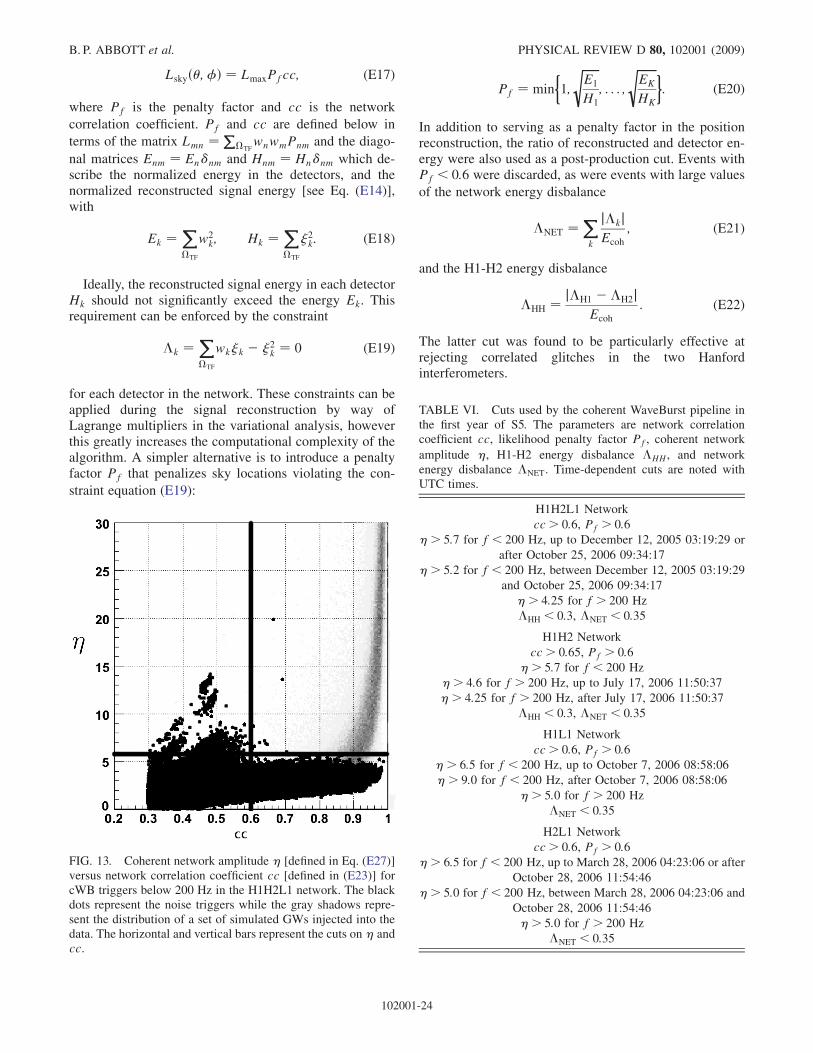
Lskyð�;�Þ ¼ LmaxPfcc; (E17)

where Pf is the penalty factor and cc is the network

correlation coefficient. Pf and cc are defined below in

terms of the matrix Lmn ¼ P�TF

wnwmPnm and the diago-

nal matrices Enm ¼ En�nm and Hnm ¼ Hn�nm which de-scribe the normalized energy in the detectors, and thenormalized reconstructed signal energy [see Eq. (E14)],with

Ek ¼X�TF

w2k; Hk ¼

X�TF

2k: (E18)

Ideally, the reconstructed signal energy in each detectorHk should not significantly exceed the energy Ek. Thisrequirement can be enforced by the constraint

�k ¼X�TF

wkk � 2k ¼ 0 (E19)

for each detector in the network. These constraints can beapplied during the signal reconstruction by way ofLagrange multipliers in the variational analysis, howeverthis greatly increases the computational complexity of thealgorithm. A simpler alternative is to introduce a penaltyfactor Pf that penalizes sky locations violating the con-

straint equation (E19):

Pf ¼ min

�1;

ffiffiffiffiffiffiE1

H1

s; . . . ;

ffiffiffiffiffiffiffiEK

HK

s �: (E20)

In addition to serving as a penalty factor in the positionreconstruction, the ratio of reconstructed and detector en-ergy were also used as a post-production cut. Events withPf < 0:6 were discarded, as were events with large values

of the network energy disbalance

�NET ¼ Xk

j�kjEcoh

; (E21)

and the H1-H2 energy disbalance

�HH ¼ j�H1 ��H2jEcoh

: (E22)

The latter cut was found to be particularly effective atrejecting correlated glitches in the two Hanfordinterferometers.

FIG. 13. Coherent network amplitude � [defined in Eq. (E27)]versus network correlation coefficient cc [defined in (E23)] forcWB triggers below 200 Hz in the H1H2L1 network. The blackdots represent the noise triggers while the gray shadows repre-sent the distribution of a set of simulated GWs injected into thedata. The horizontal and vertical bars represent the cuts on � andcc.

TABLE VI. Cuts used by the coherent WaveBurst pipeline inthe first year of S5. The parameters are network correlationcoefficient cc, likelihood penalty factor Pf, coherent network

amplitude �, H1-H2 energy disbalance �HH, and networkenergy disbalance �NET. Time-dependent cuts are noted withUTC times.

H1H2L1 Network

cc > 0:6, Pf > 0:6�> 5:7 for f < 200 Hz, up to December 12, 2005 03:19:29 or

after October 25, 2006 09:34:17

�> 5:2 for f < 200 Hz, between December 12, 2005 03:19:29

and October 25, 2006 09:34:17

�> 4:25 for f > 200 Hz�HH < 0:3, �NET < 0:35

H1H2 Network

cc > 0:65, Pf > 0:6�> 5:7 for f < 200 Hz

�> 4:6 for f > 200 Hz, up to July 17, 2006 11:50:37

�> 4:25 for f > 200 Hz, after July 17, 2006 11:50:37

�HH < 0:3, �NET < 0:35

H1L1 Network

cc > 0:6, Pf > 0:6�> 6:5 for f < 200 Hz, up to October 7, 2006 08:58:06

�> 9:0 for f < 200 Hz, after October 7, 2006 08:58:06

�> 5:0 for f > 200 Hz�NET < 0:35

H2L1 Network

cc > 0:6, Pf > 0:6�> 6:5 for f < 200 Hz, up to March 28, 2006 04:23:06 or after

October 28, 2006 11:54:46

�> 5:0 for f < 200 Hz, between March 28, 2006 04:23:06 and

October 28, 2006 11:54:46

�> 5:0 for f > 200 Hz�NET < 0:35


102001-24

The network correlation coefficient is also used toweight the overall likelihood for each sky location. It isdefined as

cc ¼ Ecoh

Nnull þ jEcohj ; (E23)

where Nnull is the sum of all elements in the null matrix

Nnm ¼ Enm � Lnm; (E24)

which represents the normalized energy of the recon-structed noise. Usually for glitches little coherent energyis detected and the reconstructed detector responses areinconsistent with the detector output, which results in alarge value for the null energy. In addition to helping selectthe optimal sky location, the correlation coefficients cc areused for a signal consistency test based on the comparisonof the null energy and the coherent energy.

The coherent terms of the likelihood matrix can be alsoused to calculate the correlation coefficients

rnm ¼ LnmffiffiffiffiffiffiffiffiffiffiffiffiffiffiffiffiffiLnnLmm

p (E25)

which represent Pearson’s correlation coefficients in thecase of aligned detectors. We use the coefficients rnm toconstruct the reduced coherent energy

ecorr ¼Xn�m

Lnmjrnmj: (E26)

Combined with the network correlation coefficient cc andthe number of detectors in the network, K, it yields aquantity which we call the coherent network amplitude,

� ¼ffiffiffiffiffiffiffiffiffiffiffiffiffiffiecorrcc

K

r: (E27)

Figure 13 shows the �-cc distribution of the backgroundevents (see Sec. VI) and simulated GW events (seeSec. VII) for the L1H1H2 network. Loud backgroundevents due to detector glitches with low values of thenetwork correlation coefficient are rejected by a thresholdon cc. Relatively weak background events are rejected by athreshold on �. Table VI describes the full set of tuningparameters for cWB.

[1] B. Abbott et al. (LIGO Scientific Collaboration), Rep.Prog. Phys. 72, 076901 (2009).

[2] H. Grote (for the LIGO Scientific Collaboration),Classical Quantum Gravity 25, 114043 (2008).

[3] F. Acernese et al., Classical Quantum Gravity 23, S63(2006).

[4] C. Culter and K. Thorne, in General Relativity andGravitation, edited by N. T. Bishop and D.M. Sunil(World Scientific Publishing Company, London, 2002),p. 72.

[5] L. Blanchet, Living Rev. Relativity 9, 4 (2006), http://relativity.livingreviews.org/Articles/lrr-2006-4/.

[6] A. Jaranowski, P. Krolak, and B. Schutz, Phys. Rev. D 58,063001 (1998).

[7] J. Baker, J. Centrella, D. Choi, M. Koppitz, and J. vanMeter, Phys. Rev. D 73, 104002 (2006).

[8] C. D. Ott, A. Burrows, E. Livne, and R. Walder,Astrophys. J. 600, 834 (2004).

[9] C. D. Ott, A. Burrows, L. Dessart, and E. Livne, Phys. Rev.

Lett. 96, 201102 (2006).[10] C. D. Ott, H. Dimmelmeier, A. Marek, H-T Janka, B.

Zink, I. Hawke, and E. Schnetter, Classical QuantumGravity 24, S139 (2007).

[11] C. D. Ott, Classical Quantum Gravity 26, 063001(2009).

[12] B. Abbott et al. (LIGO Scientific Collaboration), Phys.Rev. D 77, 062002 (2008).

[13] B. Abbott et al. (LIGO Scientific Collaboration), follow-ing Article, Phys. Rev. D 80, 102002 (2009).

[14] B. Abbott et al. (LIGO Scientific Collaboration), Phys.Rev. D 72, 062001 (2005).

[15] B. Abbott et al. (LIGO Scientific Collaboration and

TAMA Collaboration), Phys. Rev. D 72, 122004 (2005).[16] B. Abbott et al. (LIGO Scientific Collaboration), Classical

Quantum Gravity 23, S29 (2006).[17] B. Abbott et al. (LIGO Scientific Collaboration), Classical

Quantum Gravity 24, 5343 (2007).[18] B. Abbott et al. (LIGO Scientific Collaboration), Classical

Quantum Gravity 25, 245008 (2008).[19] B. Hughey, LIGO DCC Report No. T0900468-V1, 2009.[20] D. Sigg et al., Classical Quantum Gravity 23, S51 (2006).[21] S. Waldman et al., Classical Quantum Gravity 23, S653

(2006).[22] R. Adhikari, G. Gonzalez, M. Landry, and B. O’Reilly,

Classical Quantum Gravity 20, S903 (2003).[23] B. Abbott et al. (LIGO Scientific Collaboration), Phys.

Rev. D 69, 102001 (2004).[24] L. Blackburn et al., Report No. LIGO-G050158-00-Z,

2005, http://www.ligo.caltech.edu/docs/G/G050158-00.[25] S. Desai, S. Finn, J. McNabb, A. Stuver, T. Summerscales,

and K. Thorne, Classical Quantum Gravity 21, S1705(2004).

[26] S. K. Chatterji, Ph.D. thesis, Massachusetts Institute ofTechnology, 2005.

[27] S. Chatterji, L. Blackburn, G. Martin, and E.Katsavounidis, Classical Quantum Gravity 21, S1809

(2004).[28] S. Klimenko, I. Yakushin, A. Mercer, and G.

Mitselmakher, Classical Quantum Gravity 25, 114029

(2008).[29] W.G. Anderson, P. R. Brady, J. D. Creighton, and E. E.

Flanagan, Phys. Rev. D 63, 042003 (2001).


102001-25

[30] S. Chatterji, A. Lazzarini, L. Stein, P. J. Sutton, A. Searle,and M. Tinto, Phys. Rev. D 74, 082005 (2006).

[31] P. J. Sutton, arXiv:0905.4089.[32] P. Astone et al., Phys. Rev. D 68, 022001 (2003).[33] P. Astone et al., Phys. Rev. D 76, 102001 (2007).[34] R. E. Kalman, Trans. Am. Soc. Mech. Eng. Ser. D 82, 35

(1960).[35] L. S. Finn and S. Mukherjee, Phys. Rev. D 63, 062004

(2001); 67, 109902 (2003).

[36] L. Cadonati, Classical Quantum Gravity 21, S1695 (2004).[37] L. Wainstein and V. Zubakov, Extraction of Signals from

Noise (Prentice-Hall, Englewood Cliffs, USA, 1962).[38] J. Makhoul, Proc. IEEE 63, 143 (1975).[39] B. Vidakovic, Statistical Modeling by Wavelets (Wiley,

New York, 1999).[40] S. Klimenko, S. Mohanty, M. Rakhmanov, and G.

Mitselmakher, Phys. Rev. D 72, 122002 (2005).


102001-26

Search for gravitational-wave bursts in the first year of the fifth LIGO science run

Documents

Transcript of Search for gravitational-wave bursts in the first year of the fifth LIGO science run