Screening for abnormal heart sounds and murmurs by ... - CORE
123
Screening for abnormal heart sounds and murmurs by implementing Neural Networks by Claude Visagie Thesis presented at the University of Stellenbosch in partial fulfilment of the requirements for the degree of Master of Science in Mechanical Engineering Department of Mechanical Engineering University of Stellenbosch Private Bag X1, 7602 Matieland, South Africa Study leader: Prof. C. Scheffer April 2007
-
Upload
khangminh22 -
Category
Documents
-
view
1 -
download
0
Transcript of Screening for abnormal heart sounds and murmurs by ... - CORE
Screening for abnormal heart sounds and murmurs
by implementing Neural Networks
by
Claude Visagie
Thesis presented at the University of Stellenbosch
in partial fulfilment of the requirements for the
degree of
Master of Science in Mechanical Engineering
Department of Mechanical EngineeringUniversity of Stellenbosch
Private Bag X1, 7602 Matieland, South Africa
Study leader: Prof. C. Scheffer
April 2007

Copyright © 2007 University of Stellenbosch
All rights reserved.
Stellenbosch University http://scholar.sun.ac.za

Declaration
I, the undersigned, hereby declare that the work contained in this thesis is my own original
work and that I have not previously in its entirety or in part submitted it at any university
for a degree.
Signature: . . . . . . . . . . . . . . . . . . . . . . . . . . . . . . . . . .
C. Visagie
Date: . . . . . . . . . . . . . . . . . . . . . . . . . . . . . . . . . . . . . .
ii
Stellenbosch University http://scholar.sun.ac.za
Abstract
Screening for abnormal heart sounds and murmurs
by implementing Neural Networks
C. Visagie
Department of Mechanical Engineering
University of Stellenbosch
Private Bag X1, 7602 Matieland, South Africa
Thesis: MScEng (Mech)
April 2007
This thesis is concerned with the testing of an “auscultation jacket” as a means of recording
heart sounds and electrocardiography (ECG) data from patients. A classification system
based on Neural Networks, that is able to discriminate between normal and abnormal heart
sounds and murmurs, has also been developed . The classification system uses the recorded
data as training and testing data. This classification system is proposed to serve as an aid to
physicians in diagnosing patients with cardiac abnormalities. Seventeen normal participants
and 14 participants that suffer from valve-related heart disease have been recorded with the
jacket. The “auscultation jacket” shows great promise as a wearable health monitoring
aid for application in rural areas and in the telemedicine industry. The Neural Network
classification system is able to differentiate between normal and abnormal heart sounds
with a sensitivity of 85.7% and a specificity of 94.1%.
iii
Stellenbosch University http://scholar.sun.ac.za

Uittreksel
Sifting vir abnormale hartklanke en geruise
deur die implementering van Neurale Netwerke
(“Screening for abnormal heart sounds and murmurs
by implementing Neural Networks”)
C. Visagie
Departement Meganiese Ingenieurswese
Universiteit van Stellenbosch
Privaatsak X1, 7602 Matieland, Suid Afrika
Tesis: MScIng (Meg)
April 2007
Hierdie tesis het te make met die toets van ’n “stetoskoop baadjie” as ’n manier om hart-
klanke en elektrokardiografie (EKG) data van pasiënte te bekom. ’n Klassifikasiesisteem wat
gebasseer is op Neurale Netwerke, wat die data wat met die baadjie opgeneem is gebruik
as leer- en toetsdata, is ook ontwikkel . Sewentien normale deelnemers en 14 deelnemers
wat lei aan klep-verwante hartsiektes is met die baadjie opgeneem. Die “stetoskoop baadjie”
toon baie potensiaal as ’n drabare gesondheidsmonitering sisteem, spesifiek vir gebruik in
verafgeleë gebiede en in die telemedisyne industrie. Die klassifikasiesisteem is bevoeg om
te diskrimineer tussen normale en abnormale hartklanke en geruis met ’n sensitiwiteit van
85.7% en ’n spesifisiteit van 94.1% en is beoog as ’n hulpmiddel vir dokters om hartabnor-
maliteite te diagnoseer.
iv
Stellenbosch University http://scholar.sun.ac.za

Acknowledgements
I would like to express my sincere gratitude to the following people and organisations who
have contributed to making this work possible:
• To my parents, Wally and Juanita, thank you for granting me this opportunity.
• To my promoter, Prof. Cornie Scheffer. Thank you for your great leadership and
giving me the freedom to do the research in my own way and allowing me to perform
to the best of my abilities.
• I would like to thank Dirk Koekemoer and Hugo Pienaar from GeoAXon. Thanks to
Dirk for thinking of this great concept, thereby giving me an opportunity to perform
this research. Thanks to Hugo for all the technical help. Without your help this would
have been a long, hard struggle.
• Sebastian Stärz, for designing and building a great prototype jacket. Without it this
research would not have been possible.
• Thanks to Dr. Wayne Lubbe for sourcing the patients and performing the auscultation
and ECG examinations. Miranne, thank you for performing the echo-cardiograms so
diligently and thank you to Prof. Doubell for his willingness to work with us on this
research project.
• To Gert-Jan, thanks for the initial help with LATEXand thanks to Adriana for all the
help with the construction of the jacket and putting us in touch with the right people.
It is much appreciated. Thank you also to Carine’s mother, Lucinda, for all the moral
support.
• Thanks to Dr Renier Verbeek for helping us finalise the positions of the stethoscopes
on the jacket.
v
Stellenbosch University http://scholar.sun.ac.za

Dedications
To Carine
vi
Stellenbosch University http://scholar.sun.ac.za

Contents
Declaration ii
Abstract iii
Uittreksel iv
Acknowledgements v
Dedications vi
Contents vii
List of Figures ix
List of Tables xiii
Nomenclature xiv
1 Introduction 1
1.1 Motivation . . . . . . . . . . . . . . . . . . . . . . . . . . . . . . . . . . . . . 1
1.2 Objectives . . . . . . . . . . . . . . . . . . . . . . . . . . . . . . . . . . . . . 2
1.3 Thesis outline . . . . . . . . . . . . . . . . . . . . . . . . . . . . . . . . . . . 3
2 Literature review 4
2.1 The cardiovascular system . . . . . . . . . . . . . . . . . . . . . . . . . . . . 4
2.2 The cardiac cycle . . . . . . . . . . . . . . . . . . . . . . . . . . . . . . . . . 5
2.3 Heart sounds . . . . . . . . . . . . . . . . . . . . . . . . . . . . . . . . . . . 6
2.4 Auscultation and phonocardiography . . . . . . . . . . . . . . . . . . . . . . 8
2.5 Previous research . . . . . . . . . . . . . . . . . . . . . . . . . . . . . . . . . 10
3 Hardware and Data Acquisition 20
3.1 Stethoscopes . . . . . . . . . . . . . . . . . . . . . . . . . . . . . . . . . . . . 20
3.2 Auscultation jacket . . . . . . . . . . . . . . . . . . . . . . . . . . . . . . . . 22
vii
Stellenbosch University http://scholar.sun.ac.za

CONTENTS viii
3.3 Data acquisition . . . . . . . . . . . . . . . . . . . . . . . . . . . . . . . . . . 27
4 Methodology 32
4.1 Denoising of recorded data . . . . . . . . . . . . . . . . . . . . . . . . . . . . 32
4.2 Feature extraction . . . . . . . . . . . . . . . . . . . . . . . . . . . . . . . . 39
5 Feature selection and classification 59
5.1 Feature selection . . . . . . . . . . . . . . . . . . . . . . . . . . . . . . . . . 59
5.2 Artificial Neural Network classification . . . . . . . . . . . . . . . . . . . . . 61
5.3 Construction and training of the neural network . . . . . . . . . . . . . . . . 67
6 Conclusions and Recommendations 70
6.1 Data analysis and classification system . . . . . . . . . . . . . . . . . . . . . 70
6.2 Recommendations concerning the auscultation jacket . . . . . . . . . . . . . 74
6.3 Application to telemedicine? . . . . . . . . . . . . . . . . . . . . . . . . . . . 76
6.4 Other applications . . . . . . . . . . . . . . . . . . . . . . . . . . . . . . . . 77
Appendices 79
A Relevant technologies 80
A.1 Electrocardiogram (ECG) . . . . . . . . . . . . . . . . . . . . . . . . . . . . 80
A.2 Echo-cardiography . . . . . . . . . . . . . . . . . . . . . . . . . . . . . . . . 87
A.3 Impedance cardiography (ICG) . . . . . . . . . . . . . . . . . . . . . . . . . 89
B Data sheets and data tables 93
C Gradient descent algorithm 96
List of References 98
Stellenbosch University http://scholar.sun.ac.za

List of Figures
2.1 Cardiovascular circulatory system [10] . . . . . . . . . . . . . . . . . . . . . . . 5
2.2 Frontal-section of the human heart showing the internal anatomy [10] . . . . . . 6
2.3 Single cardiac cycle showing S1 and S2 . . . . . . . . . . . . . . . . . . . . . . . 7
2.4 Actual heart valve positions together with auscultation positions [15] . . . . . . 9
2.5 FFT of recorded heart sound . . . . . . . . . . . . . . . . . . . . . . . . . . . . 12
2.6 STFT of recorded heart sound . . . . . . . . . . . . . . . . . . . . . . . . . . . . 13
2.7 Wigner distribution of recorded heart sound . . . . . . . . . . . . . . . . . . . . 13
2.8 Choi-Williams Distribution of recorded heart sound . . . . . . . . . . . . . . . . 14
2.9 Continuous Wavelet Transform (CWT) of recorded heart sound . . . . . . . . . 15
2.10 Discrete Wavelet Transform (DWT) of recorded heart sound . . . . . . . . . . . 16
2.11 Graphical presentation of FWT implementation . . . . . . . . . . . . . . . . . . 17
3.1 Conventional analogue stethoscope [45] . . . . . . . . . . . . . . . . . . . . . . . 21
3.2 Standard condenser microphone [46] . . . . . . . . . . . . . . . . . . . . . . . . 21
3.3 Back electret condenser microphone [47] . . . . . . . . . . . . . . . . . . . . . . 21
3.4 Digital stethoscope used in study . . . . . . . . . . . . . . . . . . . . . . . . . . 22
3.5 Inside view of digital stethoscope . . . . . . . . . . . . . . . . . . . . . . . . . . 22
3.6 Stethographics Inc. multi-channel stethograph [48] . . . . . . . . . . . . . . . . . 23
3.7 Tapuz Medical Technology Ltd. ECG belt [49] . . . . . . . . . . . . . . . . . . . 23
3.8 Medes - VTMAN project [50] . . . . . . . . . . . . . . . . . . . . . . . . . . . . 24
3.9 Initial positions for stethoscopes and electrodes in jacket . . . . . . . . . . . . . 24
3.10 Final positions for stethoscopes and electrodes in jacket . . . . . . . . . . . . . . 25
3.11 Front piece of jacket (inside) . . . . . . . . . . . . . . . . . . . . . . . . . . . . . 26
3.12 Front piece of jacket (outside) . . . . . . . . . . . . . . . . . . . . . . . . . . . . 26
3.13 Back piece of jacket (inside) . . . . . . . . . . . . . . . . . . . . . . . . . . . . . 26
3.14 Back piece of jacket (outside) . . . . . . . . . . . . . . . . . . . . . . . . . . . . 26
3.15 Dual stethoscopes . . . . . . . . . . . . . . . . . . . . . . . . . . . . . . . . . . . 26
3.16 Sample 12-lead ECG recorded with auscultation jacket . . . . . . . . . . . . . . 27
3.17 S2 at expiration . . . . . . . . . . . . . . . . . . . . . . . . . . . . . . . . . . . . 29
ix
Stellenbosch University http://scholar.sun.ac.za

LIST OF FIGURES x
3.18 S2 at inspiration . . . . . . . . . . . . . . . . . . . . . . . . . . . . . . . . . . . 29
3.19 28-port USB hub used to connect stethoscopes to computer . . . . . . . . . . . 31
4.1 Implemented methodology . . . . . . . . . . . . . . . . . . . . . . . . . . . . . . 32
4.2 Denoising methods implemented . . . . . . . . . . . . . . . . . . . . . . . . . . . 33
4.3 Original recorded signal . . . . . . . . . . . . . . . . . . . . . . . . . . . . . . . 33
4.4 Bandpass filtered signal . . . . . . . . . . . . . . . . . . . . . . . . . . . . . . . 33
4.5 Flowdiagram of wavelet threshold denoising technique . . . . . . . . . . . . . . . 34
4.6 Wavelet threshold denoised signal . . . . . . . . . . . . . . . . . . . . . . . . . . 35
4.7 Cycle extraction flowdiagram . . . . . . . . . . . . . . . . . . . . . . . . . . . . 36
4.8 Original recorded ECG . . . . . . . . . . . . . . . . . . . . . . . . . . . . . . . . 37
4.9 ECG signal after first-derivative operator applied . . . . . . . . . . . . . . . . . 37
4.10 ECG signal after first-derivative operator and smoothing MA filter . . . . . . . 37
4.11 Algorithm to set all values below 15% of maximum value to zero . . . . . . . . . 38
4.12 Algorithm to detect QRS starting-points and end-points . . . . . . . . . . . . . 38
4.13 Feature extraction process . . . . . . . . . . . . . . . . . . . . . . . . . . . . . . 40
4.14 Procedure followed to extract S1 and S2 . . . . . . . . . . . . . . . . . . . . . . 41
4.15 Identified S1’s for a patient with a normal heart . . . . . . . . . . . . . . . . . . 42
4.16 Identified S1’s for a patient with an abnormal heart . . . . . . . . . . . . . . . . 42
4.17 Extracted S1 for a patient with a normal heart . . . . . . . . . . . . . . . . . . . 43
4.18 Extracted S1 for a patient with an abnormal heart . . . . . . . . . . . . . . . . 43
4.19 Start of S2 identified for a patient with an abnormal heart . . . . . . . . . . . . 44
4.20 Extracted portion of signal for S2 extraction . . . . . . . . . . . . . . . . . . . . 45
4.21 Shannon energy envelope of a patient with an abnormal heart . . . . . . . . . . 45
4.22 Identified peaks in the Shannon energy envelope of a patient with an abnormal
heart . . . . . . . . . . . . . . . . . . . . . . . . . . . . . . . . . . . . . . . . . . 46
4.23 Extracted second heart sound for an abnormal patient . . . . . . . . . . . . . . 46
4.24 FFT of S1 for a normal and an abnormal patient . . . . . . . . . . . . . . . . . 48
4.25 FFT of S2 for a normal and an abnormal patient . . . . . . . . . . . . . . . . . 48
4.26 Three heart cycles of abnormal patient to illustrate S1 beat-to-beat variation . . 49
4.27 ECG of patient that suffers from atrial fibrillation (see lead V1) . . . . . . . . . 49
4.28 CWT coefficients with peaks indicated that correspond to A2 and P2 of the
second heart sound . . . . . . . . . . . . . . . . . . . . . . . . . . . . . . . . . . 52
4.29 Ejection systolic murmur of a patient suffering from aortic stenosis, showing the
crescendo-decrescendo nature of the murmur . . . . . . . . . . . . . . . . . . . . 52
4.30 Pansystolic murmur of a patient suffering from mitral regurgitation . . . . . . . 53
4.31 Systole extracted from the cardiac cycle showing three sections for which rms-
value are calculated to determine shape of murmur . . . . . . . . . . . . . . . . 54
Stellenbosch University http://scholar.sun.ac.za

LIST OF FIGURES xi
4.32 Systole extracted from normal patient with subsections indicated . . . . . . . . 55
4.33 FFT of each subsection in systolic region of cardiac cycle for a normal patient . 55
4.34 Diastole extracted from abnormal patient with subsections indicated . . . . . . 55
4.35 FFT of each subsection in diastolic region of cardiac cycle for an abnormal patient 55
4.36 Splitting of heart cycle . . . . . . . . . . . . . . . . . . . . . . . . . . . . . . . . 57
4.37 Cardiac cycle shown with extra sounds search areas . . . . . . . . . . . . . . . . 58
5.1 Feature reduction and ANN training and testing methodology . . . . . . . . . . 59
5.2 Values of feature that exhibited the greatest degree of separation between the
normal and abnormal groups . . . . . . . . . . . . . . . . . . . . . . . . . . . . . 60
5.3 Values of feature that exhibited the smallest degree of separation between the
normal and abnormal groups . . . . . . . . . . . . . . . . . . . . . . . . . . . . . 60
5.4 ANN with an input layer and an output layer . . . . . . . . . . . . . . . . . . . 62
5.5 ANN with one hidden layer . . . . . . . . . . . . . . . . . . . . . . . . . . . . . 63
5.6 f(x) = 21+e−ax − 1 for a = 1, 2.5, 5 . . . . . . . . . . . . . . . . . . . . . . . . . . 63
5.7 ROC curve for classification scheme used . . . . . . . . . . . . . . . . . . . . . . 69
6.1 Recorded GeoAxon ECG showing artifacts that prohibited cycle extraction . . . 71
6.2 QRS-peaks with artifacts that resulted in wrongly extracted cycles . . . . . . . 71
6.3 Recording of normal patient at 2nd right intercostal space showing noise gener-
ated by insufficient contact between stethoscope and skin . . . . . . . . . . . . . 72
6.4 Recording of normal patient at 4th right intercostal space showing that less noise
is generated with sufficient contact between stethoscope and skin . . . . . . . . 72
6.5 Denoised recording showing that no information could be extracted due to poor
original recording . . . . . . . . . . . . . . . . . . . . . . . . . . . . . . . . . . . 72
6.6 Denoised recording showing sufficient information to be extracted . . . . . . . . 72
6.7 CWT of S2 showing multiple peaks . . . . . . . . . . . . . . . . . . . . . . . . . 73
A.1 Schematic of the electrical system of the human heart [75] . . . . . . . . . . . . 81
A.2 Normal ECG wave . . . . . . . . . . . . . . . . . . . . . . . . . . . . . . . . . . 82
A.3 V1-V6 positions [77] . . . . . . . . . . . . . . . . . . . . . . . . . . . . . . . . . 82
A.4 Configuration for ECG electrodes on wrists and feet [77] . . . . . . . . . . . . . 83
A.5 Configuration for ECG electrodes on shoulders and hips [77] . . . . . . . . . . . 83
A.6 Heart axes as viewed by different leads . . . . . . . . . . . . . . . . . . . . . . . 83
A.7 Potential difference between two sides of ventricular muscle mass is zero when
there is no depolarisation wave, and positive when depolarisation moves towards
the positive electrode [78] . . . . . . . . . . . . . . . . . . . . . . . . . . . . . . 84
A.8 Spread of atrial depolarisation and repolarisation waves and resulting deflections
in ECG tracing [78] . . . . . . . . . . . . . . . . . . . . . . . . . . . . . . . . . . 84
Stellenbosch University http://scholar.sun.ac.za

LIST OF FIGURES xii
A.9 Spread of ventricular depolarisation wave showing resulting deflections in ECG
tracing [78] . . . . . . . . . . . . . . . . . . . . . . . . . . . . . . . . . . . . . . 85
A.10 Standard bipolar limb leads for a 12-lead ECG configuration [78] . . . . . . . . . 86
A.11 Einthoven’s Triangle and the Axial Reference System [78] . . . . . . . . . . . . . 87
A.12 Unipolar augmented limb leads position [78] . . . . . . . . . . . . . . . . . . . . 88
A.13 Precordial unipolar chest leads positions [78] . . . . . . . . . . . . . . . . . . . . 88
A.14 Sweeping of echo-cardiography transducer beam and how resulting image is
formed [79] . . . . . . . . . . . . . . . . . . . . . . . . . . . . . . . . . . . . . . 89
A.15 Echo-cardiogram of normal heart showing different chambers [80] . . . . . . . . 89
A.16 Electrode positions for ICG measurements . . . . . . . . . . . . . . . . . . . . . 90
C.1 Contour plot of function, showing how gradient descent algorithm steps towards
the minimum function value . . . . . . . . . . . . . . . . . . . . . . . . . . . . . 97
Stellenbosch University http://scholar.sun.ac.za

List of Tables
4.1 Energy values of different components in extracted second heart sound signal . . 46
4.2 Calculate P-R intervals for normal and abnormal patients . . . . . . . . . . . . 50
4.3 RMS-values of different sections of systole of an abnormal patient . . . . . . . . 54
4.4 Average power of different sections to search for extra heart sounds (Abnormal) 57
4.5 Average power of different sections to search for extra heart sounds (Normal) . . 57
5.1 Network outputs for network with 15 hidden neurons and 2, 3, 4 and 5 input
features . . . . . . . . . . . . . . . . . . . . . . . . . . . . . . . . . . . . . . . . 61
5.2 Selected features and their respective SOF . . . . . . . . . . . . . . . . . . . . . 61
5.3 Neural network training algorithm parameters . . . . . . . . . . . . . . . . . . . 67
B.1 Extracted features and their respective SOF . . . . . . . . . . . . . . . . . . . . 94
B.2 Extracted features and their respective SOF (continued) . . . . . . . . . . . . . 95
xiii
Stellenbosch University http://scholar.sun.ac.za

Nomenclature
Constants
exp = 2.718 281 828
j =√−1
Variables
AN approximation at level N
A2 aortic component of the second heart sound
α regularisation parameter or momentum term (indicated in text)
b bias in ANN
C Fourier coefficient magnitude
CW (t, ω) Choi-Williams distribution of a time-domain signal
CWT (b, a) Continuous Wavelet Transform of a signal
DN detail at level N
δwrj correction term in estimation of unknown weights
E energy of a signal
ε error function of ANN
εp error function of weights in ANN
Fratio ratio of frequency bands
f frequency
fanalysis frequency intervals
fs sampling frequency
g(n) ECG signal after first-order derivative operator and MA filter have been
applied
g1(n) ECG signal after first-order derivative operator have been applied
h∗(
t−ba
)complex conjugate of wavelet function
i index operator
xiv
Stellenbosch University http://scholar.sun.ac.za

NOMENCLATURE xv
J cost function of ANN
k counter in algorithms
kr number of neurons in layer r of ANN
Ld length of diastole
Ls length of systole
M size of moving-average filter
M1 first group of identified murmur
M2 second group of identified murmur
µ learning rate of ANN
N length of signal or size of FFT (indicated in text)
n index operator
n(t) noise signal
o(t) original uncorrupted signal
P power of a signal
P2 pulmonary component of the second heart sound
Q vector containing indices of start-points of QRS wave of ECG
QRSstart start of QRS-complex in ECG wave
RMS(f) root-mean-square value of a function f
r layer in ANN
S indices at fs = 2000 Hz
S vector containing indices of end-points of QRS wave of ECG
S1, S2, S3, S4 first, second, third and fourth heart sounds
S1duration duration of the first heart sound
s indices at fs = 100 Hz
s(t) time-domain signal
sign(x) signum operator on a signal x
σ factor to reduce interference terms or standard deviation
T threshold value
Tn noise threshold value
TP-wave duration of atrial depolarisation wave in ECG
TP-Q interval time between start of P-wave and start of QRS-complex in ECG
TP-Q segment time between end of P-wave and start of QRS-complex in ECG
TQRS duration of QRS-wave in ECG
Stellenbosch University http://scholar.sun.ac.za

NOMENCLATURE xvi
TQ-T interval time between start of the QRS-wave and end of the T-wave in ECG
TQ-Tc corrected Q-T interval duration according to Bazett’s formula
TRR R-R interval duration in ECG wave
Ts signal threshold value
TS-T segment time between end of QRS-wave and start of T-wave in ECG
TT-wave duration of ventricular repolarisation wave in ECG
τ time step at which window function is centred
VN ECG chest electrode position for N = 1, 2, . . . , 6
vrj input to activation function of node j in layer r in ANN
W (t, ω) Wigner distribution of a time-domain signal
wrjk weight in ANN from node k in layer r − 1 to node j in layer r
wrj (new) new estimate of unknown weight
wrj (old) current estimate of unknown weight
w∗(t − τ) complex conjugate of window function
X(f) Fourier coefficient
x signal value
x vector of indices of values of g greater than zero or distribution mean
x(i) individual sample i of recorded signal
xmax maximum value of recorded signal
x(t) time-domain signal
yrj output of node j in layer r in ANN
Abbreviations
ANN artificial neural network
AR auto-regressive
ARMSCOR Armaments Corporation of South Africa
AV atrio-ventricular
CHR Committee for Human Research
CI cardiac index - normalised
CVD cardiovascular disease
CWD Choi-Williams distribution
CWT continuous wavelet transform
Stellenbosch University http://scholar.sun.ac.za

NOMENCLATURE xvii
DFT discrete Fourier transform
DWT discrete wavelet transform
dbn Daubechies wavelet of order n
ECG electrocardiography
EF ejection fraction estimate
EPCI ejection phase contractility index
ES ejection sound
FFT fast Fourier transform
FNF false-negative fraction
FPF false-positive fraction
FT Fourier transform
FWT fast wavelet transform
HMM hidden Markov model
HR heart rate
ICA independent component analysis
ICG impedance cardiography
IDWT inverse discrete wavelet transform
ISDN integrated services digital network
ISI inotropic state index
kg kilogram
MA moving-average
MC midsystolic click
MRC Medical Research Council
msec millisecond
OS opening snap
OTRI Online Telemedicine Research Institute
PC personal computer
PCA principal component analysis
PEP pre-ejection period
RMSS RSA Military Steering Committee
RR respiratory rate
SARS severe acute respiratory syndrome
SI stroke index - normalised
Stellenbosch University http://scholar.sun.ac.za

NOMENCLATURE xviii
SOF statistical overlap factor
STFT short-time Fourier transform
SURE Stein’s unbiased estimate of risk
TFC thoracic fluid conductivity
TNF true-negative fraction
TPF true-positive fraction
USB universal serial bus
VET ventricular ejection time
VSAT very small aperture terminal
WD Wigner distribution
Stellenbosch University http://scholar.sun.ac.za

Chapter 1
Introduction
1.1 Motivation
Every 12 minutes someone in South Africa suffers a heart attack; every 12 minutes someone
suffers a stroke. One in three men and one in four women will have a heart condition
before the age of 60 [1]. According to the World Health Organisation estimates of 2003,
cardiovascular disease accounts for approximately 16.7 million deaths globally, which equals
over 29% of all deaths globally [2]. The mortality rate in South Africa due to cardiovascular
disease (CVD) is 199 per 100000 people and the total mortality rate is 481 per 100000
people 1 [3]. Thus the mortality rate due to CVD accounts for 41% of the total deaths in
South Africa. In the United States of America 5 million people are diagnosed with valvular
heart disease each year.
These facts alone show that CVD is a major global threat and any development to aid
the prevention of these diseases is of great importance. Along with the increase in CVD,
the ability of physicians to diagnose heart disease by auscultation is also decreasing [4].
Proficiency in auscultation is a difficult skill to master, since heart and lung sounds are
short-duration sounds and several sounds occur in a short time interval [5]. Also the human
ear is poorly suited for cardiac auscultation and does not enable the physician to obtain
both qualitative and quantitive information about heart sounds [6]. For this reason, any
means that will aid physicians in making better diagnosis will prove extremely beneficial.
Tavel [7] evaluated the use of electronic stethoscopes and visual displays of heart sounds
and came to the conclusion that it can aid physicians in diagnosing and can also be used in
educational circumstances. For example, the acquired signals can be stored, played back at
a later stage and transmitted to distant sites. According to Tavel, the application of signal
analysis also shows promise for clinical application in cases such as the assessment of the
severity of aortic stenosis and in the differentiation between innocent and organic murmurs
1These statistics are pre-2002
1
Stellenbosch University http://scholar.sun.ac.za

CHAPTER 1. INTRODUCTION 2
[7].
Many pathological conditions of the cardiovascular system cause murmurs and aberra-
tions in heart sounds much before they are reflected as other symptoms such as changes
in the electrocardiogram (ECG) signal [8]. Early detection of these sounds is therefore
critical to the diagnosis and sufficient treatment of patients that suffer from these types of
cardiovascular diseases.
Auscultation with a stethoscope is a well-known occurrence to each of us that has visited
a physician. It all began in the early 1800’s when the French physician René Laînnec had to
examine a female patient that showed symptoms of heart disease. According to Dr. Laînnec
“the patient’s age and sex did not permit direct application of the ear to the chest”, as was
the norm in examining heart and lung sounds in those days [9]. Determined to do his utmost
for the patient, Laînnec rolled up a sheet of paper to form a tube and pressed this against
the patient’s chest and held his ear to the other side. He later said that he “was surprised
and gratified at being able to hear the beating of the heart with much greater clearness and
distinctness than ever before”[9].
The first “electronic stethoscope” was developed in 1910 by S.G. Brown in London. He
was actually trying to overcome a problem in long distance telephony where the telephone
signals could not be transmitted further than 20 miles [9]. He developed a repeater, amplifier
and receiver that would allow transmission over 50 miles and further. As an experiment,
heart sounds were transmitted to physicians in various parts of London and all of them
reported that the received sounds were just as clear as when they were physically examining
the patient. Mr. Brown concluded that “this trial proved that it is now possible for a
specialist to examine a patient in the country and to arrive at a correct diagnosis”[9].
In many rural areas very few or no health care facilities exist. According to the Medical
Research Council of South Africa, the South African government is “committed to providing
basic health care to all South African citizens” and “to achieve this goal, the government
has identified telemedicine as a strategic tool for facilitating the delivery of equitable health
care and educational services”. Just as Mr. Brown did in the early 1900’s, it is our aim to
deliver recorded data from patients in rural areas to physicians in faraway locations to aid
in the diagnosing and treatment of these people.
1.2 Objectives
The primary objective of this project is to:
• Develop a classification scheme based on Neural Networks to screen for abnormal heart
sounds. The system has to use the data recorded by an “auscultation jacket”. The
Stellenbosch University http://scholar.sun.ac.za

CHAPTER 1. INTRODUCTION 3
data has to be denoised and useful information (features) has to be extracted from
the recordings. The system must be tested with unknown data.
The secondary objective of this project is to:
• Test and validate the concept of the auscultation jacket as a means to record all
the necessary information from a patient and determine the validity of its use as an
application in the telemedicine industry.
1.3 Thesis outline
Chapter 2 presents a literature review covering the basic principles of the cardiovascular
system, how the different heart sounds are produced and gives an introduction to ausculta-
tion and phonocardiography. The current methods used to analyse heart sounds such as the
Fourier Transform and the Wavelet Transform are discussed, as well as other techniques.
Neural Networks and its application to heart sound classification is briefly discussed and
other classification techniques used for heart sounds are also mentioned.
In Chapter 3 the hardware used in the recording procedure is discussed. The develop-
ment of the auscultation jacket is also discussed in some detail.
Chapter 4 discusses the methodology used in the analysis of the recorded heart sounds.
This includes the denoising of the data, the extraction of individual cycles from the data by
using the ECG signal and the extraction of the features used in the classification system.
Some of these features include the extraction of the individual first and second heart sounds,
the extraction of the time difference between the different components of the second heart
sound and the extraction of extra heart sounds.
The theory behind Neural Networks and their application to this study is presented
in Chapter 5. The construction and training of the Neural Network as well as Statistical
Overlap Factor (SOF) as a feature reduction technique are discussed.
The report concludes in Chapter 6 with an evaluation of the techniques used in the
feature extraction process and an evaluation of the classification system. Application to the
telemedicine industry is discussed.
Stellenbosch University http://scholar.sun.ac.za

Chapter 2
Literature review
This chapter presents an overview of the human circulatory system, how the heart works,
how heart sounds are produced and where to listen for them. Signal processing techniques
used in the analysis of heart sounds are discussed, as well as methods implemented in
different classification schemes to differentiate between normal and abnormal heart sounds
as well as individual pathologies.
2.1 The cardiovascular system
Two circuits exist through which blood flows in the human body, namely the systemic circuit
and the pulmonary circuit. Both of these circuits begin and end at the heart. The pulmonary
circuit carries blood to and from the lungs while the systemic circuit carries blood to and
from the rest of the body. Figure 2.1 shows a schematic view of the circulatory system.
These two circuits are interconnected, so the blood that passes through one circuit, has to
pass through the other as well.
There are three types of vessels that transport blood. Arteries (efferent vessels) carry
blood away from the heart while veins(afferent vessels) carry blood to the heart. Capillar-
ies are small, thin-walled vessels between the smallest arteries and veins that permit the
exchange of nutrients and gases between the blood and the surrounding tissues [10].
The human heart is situated in the middle of the chest with the apex (bottom) shifted
slightly to the left. The heart consists of four chambers: the left and right atria and the
left and right ventricles. Each atrium and its corresponding ventricle is separated by an
atrioventricular (AV) valve. The right atrium and right ventricle are separated by the
tricuspid valve and the left atrium and left ventricle are separated by the mitral (bicuspid)
valve. The two ventricles and the arteries that carry blood from the are also separated by
valves. The right ventricle and the pulmonary artery are separated by the pulmonary valve,
while the left ventricle and the aorta are separated by the aortic valve. A frontal-section of
4
Stellenbosch University http://scholar.sun.ac.za

CHAPTER 2. LITERATURE REVIEW 5
Figure 2.1: Cardiovascular circulatory system [10]
the heart is shown in Figure 2.2.
The right atrium receives deoxygenated blood from the body via the superior and inferior
vena cavae. From the right atrium the blood is pumped through the tricuspid valve to the
right ventricle, from where it goes through the pulmonary valve into the pulmonary artery,
which takes the blood to the lungs where it receives oxygen. The oxygenated blood is
transported to the left atrium via the pulmonary vein. The oxygenated blood is pumped
through the mitral valve to the left ventricle. When the left ventricle contracts, the blood
is pumped through the aortic valve into the aorta, from where it is distributed to the rest
of the body.
2.2 The cardiac cycle
The cardiac cycle can be divided into two phases for any chamber of the heart. These
two phases are known as systole (contraction) and diastole (dilation). During systole, the
chamber pushes blood into an adjacent chamber or arterial trunk. During diastole, the
chamber relaxes and is filled with blood.
A cardiac cycle begins with atrial systole which lasts for approximately 100 msec. At
this time, the ventricles are partially filled with blood and the atrial contraction fills the
ventricles. After the 100 msec of atrial systole, ventricular systole and atrial diastole begins.
Ventricular systole lasts for 275 msec and atrial diastole for 700 msec. During ventricular
systole, the pressure in the ventricles increases and forces the mitral and tricuspid valves
Stellenbosch University http://scholar.sun.ac.za

CHAPTER 2. LITERATURE REVIEW 6
Figure 2.2: Frontal-section of the human heart showing the internal anatomy [10]
shut. The high pressures also force open the pulmonary valve and the aortic valve and the
blood flows into the pulmonary artery and aorta. At this point, ventricular diastole begins
and the ventricles as well as the atria are in diastole. The pressures in the ventricles decline
and fall below the pressures in the pulmonary artery and aorta and the pulmonary valve and
aortic valve close as a result of this. As ventricular pressure continues to fall, the pressure
drops below the pressure in the atria and the mitral and tricuspid valve open, allowing
blood to flow from the major veins through the atria to the relaxed ventricles. When atrial
systole begins another cardiac cycle, the total time that has passed from the start of the
previous atrial systole is approximately 800 msec. The ventricles are roughly 70% filled at
this time [10]. Atrial systole contributes a relatively small amount to ventricular volume
and this explains why individuals that have severely damaged atria can continue to lead
normal lives, while damage to one or both ventricles can leave the heart unable to maintain
adequate cardiac ouput [10].
2.3 Heart sounds
There are four different heart sounds known as S1, S2, S3 and S4. S1 and S2 are the
normal sounds one associates with a heartbeat. In the “lubb-dupp” sound one associates
with a heart sound, “lubb” corresponds to S1 and “dupp” corresponds to S2. Contradictory
explanations exist as to the origin of these sounds. It was historically believed that S1
and S2 were produced solely by the closure of the mitral and tricuspid and the aortic and
Stellenbosch University http://scholar.sun.ac.za
CHAPTER 2. LITERATURE REVIEW 7
0 0.1 0.2 0.3 0.4 0.5 0.6 0.7 0.8−1
−0.8
−0.6
−0.4
−0.2
0
0.2
0.4
0.6
0.8
1
Time [sec]
Am
plitu
de
S1
S2
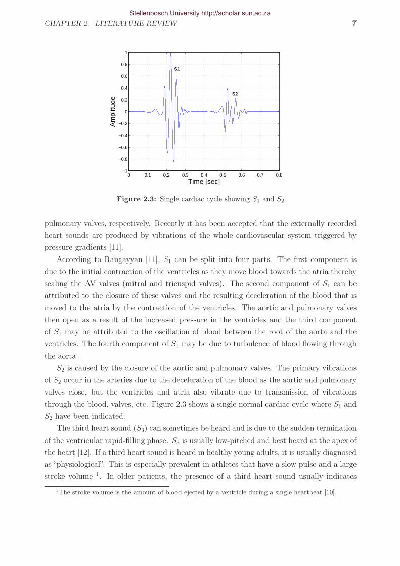
Figure 2.3: Single cardiac cycle showing S1 and S2
pulmonary valves, respectively. Recently it has been accepted that the externally recorded
heart sounds are produced by vibrations of the whole cardiovascular system triggered by
pressure gradients [11].
According to Rangayyan [11], S1 can be split into four parts. The first component is
due to the initial contraction of the ventricles as they move blood towards the atria thereby
sealing the AV valves (mitral and tricuspid valves). The second component of S1 can be
attributed to the closure of these valves and the resulting deceleration of the blood that is
moved to the atria by the contraction of the ventricles. The aortic and pulmonary valves
then open as a result of the increased pressure in the ventricles and the third component
of S1 may be attributed to the oscillation of blood between the root of the aorta and the
ventricles. The fourth component of S1 may be due to turbulence of blood flowing through
the aorta.
S2 is caused by the closure of the aortic and pulmonary valves. The primary vibrations
of S2 occur in the arteries due to the deceleration of the blood as the aortic and pulmonary
valves close, but the ventricles and atria also vibrate due to transmission of vibrations
through the blood, valves, etc. Figure 2.3 shows a single normal cardiac cycle where S1 and
S2 have been indicated.
The third heart sound (S3) can sometimes be heard and is due to the sudden termination
of the ventricular rapid-filling phase. S3 is usually low-pitched and best heard at the apex of
the heart [12]. If a third heart sound is heard in healthy young adults, it is usually diagnosed
as “physiological”. This is especially prevalent in athletes that have a slow pulse and a large
stroke volume 1. In older patients, the presence of a third heart sound usually indicates
1The stroke volume is the amount of blood ejected by a ventricle during a single heartbeat [10].
Stellenbosch University http://scholar.sun.ac.za

CHAPTER 2. LITERATURE REVIEW 8
impaired ventricular function if there are other signs of cardiac failure [12]. A third heart
sound can originate from either ventricle and the one responsible is usually deduced from
the circumstances, rather than the quality of the sound [12].
The fourth heart sound (S4) occurs at the same time as, and is due to, atrial systole.
It can be heard only in the presence of a sinus rhythm 2. Phonocardiography can detect
a quiet S4 in many normal subjects but it tends to become particularly prominent when
a hypertrophied 3 left atrium pumps blood through an unobstructed mitral valve into a
stiff left ventricle. These conditions are most often fulfilled in ischaemic heart disease or
systemic hypertension [12]. S4 is usually a low-pitched sound and best heard at the apex
of the heart. In patients with a sufficiently slow heart rate it is sometimes possible to make
out fourth, first, second and third heart sounds, but as the heart rate increases, the third
and fourth sounds tend to merge [12].
2.4 Auscultation and phonocardiography
Heart auscultation (listening to heart and lung sounds of a patient through a stethoscope)
is the primary method by which physicians diagnose a patient as having an underlying
pathology associated with heart diseases. When auscultating a patient, one listens at specific
locations on the thorax and back. Only the thorax positions will be discussed here, since we
are dealing with heart sounds. Lung sounds are heard when auscultating the back. Figure
2.4 shows the positions of the actual valves as well as the auscultation positions. The aortic
valve is situated in the middle of the chest between the aorta and left ventricle but is best
heard in the second intercostal space (between the 2nd and 3rd ribs) to the right of the
sternum (the bone in the middle of the chest). The pulmonary valve is situated between
the pulmonary artery and right ventricle and is best heard in the second intercostal space
to the left of the sternum. The tricuspid valve, situated between the right atrium and right
ventricle is best heard at the fifth intercostal space (between the 5th and 6th ribs) just to
the left of the sternum, while the mitral valve that separates the left atrium and ventricle
is also best heard in the fifth intercostal space but further to the left of the sternum.
There is, however, a widespread belief that the skill of auscultation is of secondary
importance since the same information can be obtained through newer technological means
[16]. The reason auscultation remains a primary method by which to diagnose patients,
is due to the higher costs and limited availability of other screening procedures such as
an electrocardiogram (ECG) and an echo-cardiogram. Together with the overall bedside
2Sinus rhythm is a term used in medicine to describe the normal beating of the heart, as measured byan electrocardiogram (ECG)[13].
3Enlargement or overgrowth of an organ or part of the body due to the increased size of the constituentcells. Hypertrophy occurs in the biceps and heart due to increased work [14].
Stellenbosch University http://scholar.sun.ac.za

CHAPTER 2. LITERATURE REVIEW 9
Figure 2.4: Actual heart valve positions together with auscultation positions [15]
examination, the use of the stethoscope is not only cost-effective, but is also not totally
replacable by alternative technological methods [7]. However, auscultation is a very difficult
skill to acquire and the necessary skills to make a proper diagnosis take years of practice
to develop [17]. The human ear is also poorly suited for cardiac auscultation [6]. The
conventional stethoscope also cannot store, play sounds back, offer a visual display, process
the acoustic signal and transmit the sounds simultaneously to multiple listeners [7].
Phonocardiography is the graphical recording of the vibrations caused by the beating
human heart. A microphone or piezo-electric sensor is placed on the thorax of a patient
and the vibrations caused by the beating heart are recorded and displayed as a sound wave.
Having digital recordings of patients’ heart sounds will prove beneficial in a multitude of
ways. First of all, it can be played back simultaneously to multiple listeners, which is ideal
for the training of auscultation skills. The teaching of cardiac auscultation skills seems
to be a difficult process as noted in [7], where it is stated that (referring to the lack of
after-recording playback):
“This lack of a common “audio platform” is the most serious obstacle to effective
teaching of cardiac auscultation, a deficiency that has reached serious proportions
throughout our educational institutions."
The unnecessary referrals of patients with innocent murmurs,4 etc. to cardiac specialists
by general practitioners poses a big problem, since this constitutes extra money and time
that have to be spent by both parties concerned. According to de Vos [18], any unnecessary
referrals should be minimised because:
4Innocent heart murmurs are murmurs found in people with normal hearts and are harmless [18].
Stellenbosch University http://scholar.sun.ac.za

CHAPTER 2. LITERATURE REVIEW 10
1. Specialists are a very scarce and expensive resource that should be used only when
required.
2. The distribution of specialists and medical practitioners are not in ratio with the
regional demographic composition. The distribution of specialists are economically
driven with poorer regions having a much larger people-to-specialist ratio.
3. The anxiety of the patient and family can be minimised if unnecessary referrals are
eliminated.
2.5 Previous research
2.5.1 Signal processing techniques
A multitude of different techniques have been implemented to analyse and characterise heart
sounds. These include Fourier analysis, Short-time Fourier analysis, Wigner distributions,
Choi-Williams distributions and Wavelet analysis.
The Fourier Transform (FT) is used to determine which frequencies are contained in a
given time-domain signal. Fourier coefficients are indicative of the frequency content of a
signal and are calculated by:
X(f) =
∫ ∞
−∞
x(t)e−2jπftdt (2.5.1)
At a more practical level, the Discrete Fourier Transform (DFT) is implemented to
calculate the Fourier coefficients for discrete signals. Discrete signals comprise most of the
signals one works with, since they are recorded by a computer. The formula by which the
Fourier coefficients are calculated for discrete signals is:
X(m) =
N−1∑
k=0
x(k)e−2jπmk
N (2.5.2)
where m = 0, 1, ..., N2, N is the size of the FT one wishes to calculate. The value
N effectively determines the resolution of the FT. For example, if you have a signal that
has been sampled at fs = 2000 Hz, the frequencies at which the FT will be calculated is
determined by [19]:
fanalysis(m) =mfs
N(2.5.3)
For example, if you perform an 8-point FT on your data, the first frequency term will be
calculated at a frequency of 1×20008
= 250 Hz, the second frequency term will be calculated
Stellenbosch University http://scholar.sun.ac.za

CHAPTER 2. LITERATURE REVIEW 11
at a frequency of 2×20008
= 500 Hz etc. If you decide to perform a 512-point FT on your
signal instead, the first frequency term will be calculated at a frequency of 1×2000512
= 3.91
Hz, the second frequency term will be calculated at a frequency of 2×2000512
= 7.81 Hz, etc.
Thus the larger N , the better the resolution of the FT that is calculated. However, the size
of the FT that you wish to calculate is bounded by the length of the signal that is being
analysed.
The Fourier coefficients are calculated for a set of pre-defined frequencies, as determined
by equation 2.5.3. At each frequency, the time-domain signal is multiplied by a complex
exponential function and integrated over all time to yield the corresponding Fourier coeffi-
cient. If the Fourier coefficient is relatively large, the time-domain signal contains a major
component of the frequency that is currently under consideration. Should the Fourier coef-
ficient be relatively small, the contribution of the frequency under consideration is small. If
the signal does not contain a component of a specific frequency, the Fourier coefficient will
be zero. The complex exponential function e−2jπft is defined as:
e−2jπft = cos(2πft) − j sin(2πft) (2.5.4)
This definition implies that any time-domain signal can be represented as a sum of sine
and cosine functions at specific frequencies. The FT of a signal is computed in a fast and
efficient manner by the Fast Fourier Transform (FFT), which is an algorithm developed by
J.W. Cooley and J.W. Tukey in 1965. The details of the algorithm will not be discussed
here and can be found in [20].
The frequency information is very important, since different actions of the heart (e.g.
the opening or closing of valves) will produce sounds at different frequencies. It is thus
critical to have the frequency information contained in a heart sound at your disposal in
order to identify certain pathologies. Bhatikar et al. [21] used the FT coefficients as input
to a classification scheme differentiating between innocent and pathological murmurs and
obtained a correct classification rate of 83% sensitivity and 90% specificity. Refer to Section
2.5.2 for a definition of sensitivity and specificity.
The major drawback of Fourier analysis is the fact that all temporal information in the
signal is lost [22]. The FT can only be applied to a signal if it is assumed that the signal is
stationary [6]. A stationary signal is defined as a signal whose statistical properties do not
change with time [23]. Heart sounds exhibit extremely non-stationary characteristics and
Fourier analysis is thus not suited for the analysis of these signals [24]. Figure 2.5 shows
the FFT of the denoised normal heart recording in Figure 2.3. The recording was done at
the 4th right intercostal space.
In an effort to correct the disadvantage (that temporal information is lost) of the FT,
the Short-Time Fourier transform (STFT) was developed. The STFT is implemented by
Stellenbosch University http://scholar.sun.ac.za

CHAPTER 2. LITERATURE REVIEW 12
0 100 200 300 400 5000
0.01
0.02
0.03
0.04
0.05
0.06
0.07
0.08
Frequency [Hz]
Mag
nitu
de
Figure 2.5: FFT of recorded heart sound
performing the FT on only a small part of the signal. The signal under analysis is subdivided
into a number of small records where it is assumed that each sub-record is stationary. The
signal is multiplied by a short-duration time window that is centered on the time instant of
interest. This is called windowing. The window is subsequently slid along the time axis to
cover the entire duration of the signal and to obtain an estimate of the spectral content of
the signal at every time instant. The formula by which the STFT is computed is:
X(τ, ω) =
∫ ∞
−∞
[x(t)w∗(t − τ)]e−j2πftdt (2.5.5)
The STFT cannot track very sensitive changes in the time direction [25] and hence is not
suitable for the analysis of the non-stationary and rapidly changing heart signals. However,
Turkoglu et al. [26] used the STFT to calculate the features that were used as input into
their classification algorithm for heart sounds. The authors used a back propagation neural
network as their classification scheme and obtained a correct classification rate of 94% for
normal heart sounds and 95.9% for abnormal heart sounds. The STFT of the recorded
signal in Figure 2.3 is shown in Figure 2.6. The window that was used is a Hanning window
with a duration of 64 ms and an overlap between windows of 32 ms.
The Wigner Distribution (WD) is another technique that provides a two-dimensional
view of the frequency and the temporal information of the signal under analysis. It provides
better resolution than the STFT, but is limited by the appearance of cross-terms. These
cross-terms are due to the non-linear behaviour of the WD and bear no physical meaning
[6]. The WD has also been evaluated by Bentley et al. [27] as a time-frequency technique
to extract information from recorded native and bioprosthetic heart sounds. The WD is
Stellenbosch University http://scholar.sun.ac.za

CHAPTER 2. LITERATURE REVIEW 13
Time [sec]
Fre
quen
cy [H
z]
0 0.2 0.4 0.6 0.80
50
100
150
200
250
300
350
400
450
500
−300
−250
−200
−150
−100
−50
0
Figure 2.6: STFT of recorded heart sound
calculated by:
W (t, ω) =
∫x∗
(t − 1
2τ
)x
(t +
1
2τ
)e−jωtdτ (2.5.6)
Figure 2.7 shows the WD of the signal in Figure 2.3. It can be seen that at 0.4 sec
there is a component present that is not physically present in the recorded sound. This is
the cross-terms mentioned previously. Thus the WD is unsuitable for analysis since these
cross-terms may alter the information extracted from the signal.
The Choi-Williams Distribution (CWD) is another technique capable of displaying time-
Time [sec]
Fre
quen
cy [H
z]
0 0.2 0.4 0.6 0.8 10
50
100
150
200
250
300
350
400
450
500
−50
−45
−40
−35
−30
−25
−20
−15
−10
−5
0
Figure 2.7: Wigner distribution of recorded heart sound
Stellenbosch University http://scholar.sun.ac.za

CHAPTER 2. LITERATURE REVIEW 14
Time [sec]
Fre
quen
cy [H
z]
0 0.2 0.4 0.6 0.8 10
50
100
150
200
250
300
350
400
450
500
−35
−30
−25
−20
−15
−10
−5
0
Figure 2.8: Choi-Williams Distribution of recorded heart sound
frequency information of heart sound signals. The CWD is calculated by [28]:
CW (t, ω) =
√2
π
∫ ∞∫
−∞
σ
|τ |e−2σ2(s−t)2/τ2
x(s +
τ
2
)x∗
(s − τ
2
)e−j2πωτds dτ (2.5.7)
The difference between the CWD and the WD is the use of the kernel function√2π
σ|τ |
e−2σ2(s−t)2/τ2−j2πωτ . In the WD the kernel function is e−jωt. The use of σ in the
CWD kernel function reduces the interference problems without reducing the resolution
[27]. Figure 2.8 shows the CWD of the signal in Figure 2.3. The value for σ used in these
calculations was σ = 6.061. It can be seen that the interference at 0.4 sec is significantly
reduced in the CWD, while the resolution still remains significantly better than the STFT.
Wavelet analysis provides a time-scale representation instead of a time-frequency repre-
sentation of the signal under analysis. Scale can be thought of as the inverse of frequency,
where the low scales constitute the high-frequency components and the high scales the
low-frequency components. When switching between frequency and scale, the scale cannot
simply be inverted to yield the frequency. Instead, one has to think in terms of pseudo-
frequencies to determine which frequencies a specific scale represents. To calculate the
pseudo-frequency associated with a specific scale, equation 2.5.8 can be used:
Fa =Fc
∆a(2.5.8)
where Fc is the wavelet centre frequency, a is the specified scale and Fa is the pseudo-
frequency corresponding to scale a. It is attempted to associate with each wavelet a purely
Stellenbosch University http://scholar.sun.ac.za
CHAPTER 2. LITERATURE REVIEW 15
Absolute Values of Ca,b Coefficients for a = 15 16 17 18 19 ...
time (or space) b
scal
es a
200 400 600 800 1000 1200 1400 1600 1800 2000 15
20
25
30
35
40
45
50
55
60
65
70
75
80
85
90
95
100
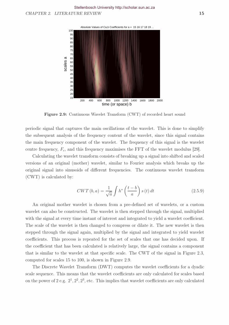
Figure 2.9: Continuous Wavelet Transform (CWT) of recorded heart sound
periodic signal that captures the main oscillations of the wavelet. This is done to simplify
the subsequent analysis of the frequency content of the wavelet, since this signal contains
the main frequency component of the wavelet. The frequency of this signal is the wavelet
centre frequency, Fc, and this frequency maximises the FFT of the wavelet modulus [29].
Calculating the wavelet transform consists of breaking up a signal into shifted and scaled
versions of an original (mother) wavelet, similar to Fourier analysis which breaks up the
original signal into sinusoids of different frequencies. The continuous wavelet transform
(CWT) is calculated by:
CWT (b, a) =1√a
∫h∗
(t − b
a
)s (t) dt (2.5.9)
An original mother wavelet is chosen from a pre-defined set of wavelets, or a custom
wavelet can also be constructed. The wavelet is then stepped through the signal, multiplied
with the signal at every time instant of interest and integrated to yield a wavelet coefficient.
The scale of the wavelet is then changed to compress or dilate it. The new wavelet is then
stepped through the signal again, multiplied by the signal and integrated to yield wavelet
coefficients. This process is repeated for the set of scales that one has decided upon. If
the coefficient that has been calculated is relatively large, the signal contains a component
that is similar to the wavelet at that specific scale. The CWT of the signal in Figure 2.3,
computed for scales 15 to 100, is shown in Figure 2.9.
The Discrete Wavelet Transform (DWT) computes the wavelet coefficients for a dyadic
scale sequence. This means that the wavelet coefficients are only calculated for scales based
on the power of 2 e.g. 21, 22, 23, etc. This implies that wavelet coefficients are only calculated
Stellenbosch University http://scholar.sun.ac.za

CHAPTER 2. LITERATURE REVIEW 16
Discrete Transform, absolute coefficients.
Leve
l
Samples200 400 600 800 1000 1200 1400 1600 1800 2000
7
6
5
4
3
2
1
Figure 2.10: Discrete Wavelet Transform (DWT) of recorded heart sound
for scales = 2, 4, 8, 16, etc. The resolution of the DWT is not as good as the resolution of
the CWT, but the computation time is far shorter since the coefficients are not calculated
for every scale. Nevertheless, the analysis is equally accurate as the CWT [29]. Figure 2.10
shows the DWT of the signal in Figure 2.3. The wavelet used was the Daubechies wavelet
of order 7, and the breakdown level was also level 7. This means that the coefficients were
calculated for scales of 21, 22, ..., 27.
Mallat developed an efficient way to implement the DWT by using the subband co-
ding scheme [30]. This is known as the Fast Wavelet Transform (FWT). The signal under
analysis is broken down into low-frequency (approximations) and high-frequency (details)
components by passing the signal through a low- and high-pass filter respectively. At each
breakdown level, the signal bandwidth is split in half. For example, if you have a signal
sampled at 2000 Hz, the maximum frequency present in the signal is 1000 Hz according
to the Nyquist criterion. This means that after the first set of filters in the DWT, the
approximations will contain the components between 0-500 Hz and the details will contain
the components between 500-1000 Hz. For the following breakdown level, the approximation
of the previous level is broken down further, yielding another set of approximations and
details. The approximation of this level contains the frequency components between 0-250
Hz and the details the frequency components between 250-500 Hz. This process continues
until the remaining samples are equal to one. The signal has to be downsampled at each
level to ensure that the number of samples at the breakdown level is half the amount of
samples contained in the signal that is passed through the filters. If this is not done, one
ends up with twice the amount of data that one started with, since convolving a signal with
a filter yields the same number of samples of the original signal. Every second sample is
Stellenbosch University http://scholar.sun.ac.za

CHAPTER 2. LITERATURE REVIEW 17
thus kept to ensure the correct sizes at each level. This process is explained graphically in
Figure 2.5.1.
HP filter
LP filter
2 ?
2 ?
HP filter
LP filter
2 ?
2 ?
rr
rr
f(n)
D1[500-1000 Hz] D2
[250-500 Hz]
A2[0-250 Hz]
Figure 2.11: Graphical presentation of FWT implementation
In the literature reviewed, wavelets have been used extensively to denoise phonocardio-
gram signals or highlight certain features in the signals. Debbal and Bereksi-Reguig [25]
showed that the number of major components present in each sound of the second heart
sound (A2 and P2) can be identified. The frequency range and the localisation of these
sounds can also be determined by use of the continuous wavelet transform. Doppler heart
sounds were decomposed using wavelet analysis and certain components were implemented
in a neural-network based classification scheme [26]. These authors obtained a correct classi-
fication rate of 94% using these components. Messer et al. [24] studied the effects of different
wavelets on denoising recorded heart sounds. They found that certain wavelets from the
Coiflet, Daubechies and Symlet families provide the best results. The best denoising results
were obtained by implementing wavelet analysis together with averaging5.
Other techniques that have been implemented to extract information from heart sounds,
include the Hilbert Transform [24] and homomorphic filtering [31].
2.5.2 Classification techniques
Artificial Neural Networks (ANNs) are the primary tool implemented in the classification of
heart sounds [32; 33; 34; 35; 36] although other techniques, such as Hidden Markov Models
(HMMs), have been implemented as well [37]. ANNs are adaptive systems that can model
complex non-linear systems [38]. Refer to Chapter 5 for a detailed discussion of ANNs. As
an example, Cathers [32] used the heart sound amplitude envelope as input to the ANN.
5This is when a number of points in a signal is replaced by the average of all those points concerned.
Stellenbosch University http://scholar.sun.ac.za

CHAPTER 2. LITERATURE REVIEW 18
The output of the system was a 3 x 1 column vector. The sequence
0
0
1
denoted a normal heart sound whereas the sequence
1
0
1
denoted a systolic murmur. The ANN is thus trained to give these outputs for the correct
inputs, so that when it is presented with similar input data, it will give the same output,
classifying the heart sound as either normal, or as a systolic murmur, for instance.
In a study performed by Bhatikar et al. [21] to distinguish between innocent and patho-
logical murmurs, the input to the ANN was the frequency spectrum of the heart sound that
consisted of the 252 bins in the discrete energy spectrum with a range of 0-252 Hz and a
bin-size of 1 Hz. In this case, the output was a single number, either 0 or 1, where 0 indi-
cated an innocent murmur and 1 indicated a pathological murmur. The network consisted
of 252 input neurons, 15 hidden layer neurons and 1 output neuron. The authors obtained a
correct classification rate of 83% sensitivity and 90% specificity. Sensitivity and specificity
are defined as:
Sensitivity =# of true positives
# of true positives + # of false negatives(2.5.10)
Specificity =# of true negatives
# of true negatives + # of false positives(2.5.11)
Sensitivity specifies the percentage of unhealthy patients that are recognised as un-
healthy and specificity determines the number of healthy patients that are recognized as
healthy [34].
In other studies, Leung et al. [36] obtained a sensitivity of 97.3% and a specificity
of 94.4% in classifying innocent and pathological systolic murmurs. The authors used a
probability neural network in classifying their data.
Akay et al. [35] achieved a sensitivity of 85.5% and a specificity of 88.9% in detecting
coronary artery disease. The authors used a Fuzzy Min-Max Neural Network in their study.
The fuzzy min-max classification neural netork is an on-line supervised learning classifier
that is based on hyperbox fuzzy sets. Tripathy [39] used a feed-forward neural network
trained with the backpropagation algorithm to differentiate between normal heart sounds
Stellenbosch University http://scholar.sun.ac.za
CHAPTER 2. LITERATURE REVIEW 19
and certain pathologies. A correct classification rate of 81.86% was obtained.
HMMs have mainly been used in the field of speech recognition. When working with
HMMs, one has a sequence of observable events, or observed vectors, that have been gen-
erated by a Markov model. The Markov model consists of a set of states and these states
produce a certain observation vector/s. In the Markov model, state is changed every time
unit and each time the state is changed, an observation vector is generated that depends on
the probability of that observation vector being produced. The transition from one state to
another is also determined by the probability that such a transition will occur. The HMM
then calculates the best sequence of states that maximises the probability of generating the
specific observation sequence. El-Hanjouri et al. [37] achieved a correct recognition rate of
99.1% in classifying pathological heart sounds by implementing HMMs. HMMs were also
used in [40] to segment heart sounds into their constituent parts.
Other classification techniques implemented in phonocardiogram analysis includes decision-
tree classifiers. Pavlopoulos et al. [41] achieved a correct classification rate of 90% in
discriminating between aortic stenosis and mitral regurgitation.
Voss et al. [42] achieved a correct classification rate of 100% for patients suffering
from moderate or severe aortic stenosis and a correct classification rate of 75% for patients
suffering from mild aortic stenosis. Their desicion-making scheme was based on a linear
discriminant function being applied to the feature vectors extracted from the heart sounds.
Bentley et al. [27] used Bayes’ decision rule in classifying their data as either normal or
abnormal. They obtained a correct classification rate of between 61% and 100%, depending
on which feature extraction method was followed.
Stellenbosch University http://scholar.sun.ac.za

Chapter 3
Hardware and Data Acquisition
This chapter describes in broad terms the procedure followed in the design of the ausculta-
tion jacket. The hardware implemented as well as the procedure followed in recording the
patient data is discussed.
3.1 Stethoscopes
It was desired to record the heart sounds from patients in order to develop an automated
screening procedure capable of differentiating between normal and abnormal heart sounds.
There are different methods of obtaining the heart sounds from a patient. It could be done
via the use of a digital stethoscope or an accelerometer. Accelerometers are not as widely
used as digital stethoscopes, but have been implemented in studies to record heart and lung
sounds [43].
Conventional analogue stethoscopes are mainly used for auscultating patients in hos-
pitals and clinics. A conventional analogue stethoscope simply converts sound waves into
pressure waves that can be heard and processed by the human ear and is shown in Figure
3.1. Digital stethoscopes can work on two different principles;(a) implementing a micro-
phone to convert the acoustic waves generated by the beating heart to electrical signals;(b)
using a piezo-electric crystal in converting the sound waves to electric signals. Most phono-
cardiograph transducers implement the crystal piezo-electric or dynamic piezo-electric mi-
crophones [44]. For this project, the digital stethoscopes implemented were designed and
supplied by GeoAxon. The stethoscopes made use of a condenser microphone to convert
the pressure waves to electrical signals and the microphone used in the stethoscope was the
Panasonic WM-61 B back electret condenser microphone. These microphones have a range
of 20 − 20000 Hz and a flat frequency response up to 5000 Hz. The data sheet for the
microphone is given in Appendix B.
A normal condensor microphone uses a capacitor to produce a change in voltage. One of
20
Stellenbosch University http://scholar.sun.ac.za

CHAPTER 3. HARDWARE AND DATA ACQUISITION 21
Figure 3.1: Conventional analoguestethoscope [45]
Figure 3.2: Standard condenser mi-crophone [46]
the materials used in the capacitor is the diaphragm. As sound waves reach the diaphragm, it
moves back and forth, thereby changing the distance between the two plates of the capacitor.
As the distance decreases, the capacitance increases, producing a charge current;when the
distance increases, capacitance decreases and a discharge current is produced. The change
in voltage across a resistor is measured and converted to an audible sound (refer Figure 3.2).
In order to produce the charge or discharge current a voltage is required and is normally
supplied by a battery in the microphone or by phantom power [46].
In the back electret microphone a dielectric material is placed behind the diaphragm
on the backplate of the microphone housing (refer Figure 3.3). This dielectric material
serves as the capacitor. The only difference between a normal condenser microphone and
an electret condensor microphone is that the latter does not require an external voltage
source to produce the charge and discharge currents, since the voltage is manufactured into
the dielectric material [46].
The stethoscopes used in this study are USB-enabled stethoscopes. The stethoscopes
connect to the PC via the USB connection and each stethoscope is registered by the com-
puter as a separate recording device. The analogue-to-digital conversion of the signal takes
Figure 3.3: Back electret condenser microphone [47]
Stellenbosch University http://scholar.sun.ac.za

CHAPTER 3. HARDWARE AND DATA ACQUISITION 22
Figure 3.4: Digital stethoscope usedin study
Figure 3.5: Inside view of digitalstethoscope
place in the stethoscope itself. These digital signals were then recorded by a computer,
using recording software. The digital stethoscopes used in the study are shown in Figure
3.4. Figure 3.5 shows the electronic chip inside the digital stethoscope. The recorded signals
were sampled at 16-bit and 2000 Hz.
3.2 Auscultation jacket
When auscultating a patient or recording the heart sounds of a patient, only one position
is normally listened to or recorded at a specific time. This is not necessarily a deficiency,
but during the research it was decided to obtain a “snapshot” of the heart (or lungs) of
a patient by simultaneously recording the heart and lung sounds at the positions where a
physician would normally auscultate a patient. To achieve this, 21 digital stethoscopes were
embedded into a jacket to record the heart and lung sounds of a patient.
The result is the “auscultation jacket” that is capable of recording the heart and lung
sounds at all the necessary positions simultaneously, as well as a 12-lead ECG (refer to
Figure 2.4). An Impedance Cardiogram (ICG) was also built into the jacket but due to
unforeseen hardware problems the ICG could not be recorded with the jacket but had to
be recorded separately. Please refer to Appendix A for a detailed explanation of ECG and
ICG technology.
3.2.1 Previous approaches
Similar approaches to the auscultation jacket have been developed previously. These include
designs from companies such as Stethographics Inc., Tapuz Medical Technology Ltd. and
Medes.
Stethographics Inc. developed a multi-channel stethograph that consists of 14 stetho-
scopes embedded within sponge. The sponge is placed behind the patient’s back and two
Stellenbosch University http://scholar.sun.ac.za

CHAPTER 3. HARDWARE AND DATA ACQUISITION 23
seperate stethoscopes are placed on the patient’s chest. All recordings are done simul-
taneously, which will make true comparisons possible and provides the basis for three-
dimensional analysis and display. Figure 3.6 shows the multi-channel stethograph from
Stethographics Inc..
Tapuz Medical Technology Ltd. developed a universal ECG electrode belt, which has
six ECG electrodes moulded into the structure. The electrode positions correspond to the
positions where the chest electrodes would be placed for a normal 12-lead ECG. Fitting
sockets for the leads onto the electrodes are provided for. Figure 3.7 shows this ECG belt.
Medes is a French organisation that has been working on the VTMAN project. The
objective is to enhance the autonomy of patients by integrating medical equipment in the
patients’ clothes. This achievement should significantly reduce the medical follow-up of pa-
tients who are medically dependent and should contribute to optimising medical procedures
[50]. Figure 3.8 shows some of the different elements of the VTMAN project.
3.2.2 Design procedure
In the design of the jacket, it was difficult to decide where the positions for the stethoscopes
and electrodes in the jacket should be. The positions of the stethoscopes should coincide
with the auscultation locations as explained in section 2.4, as well as some of the positions
Figure 3.6: Stethographics Inc. multi-channel stethograph [48]
Figure 3.7: Tapuz Medical Technology Ltd. ECG belt [49]
Stellenbosch University http://scholar.sun.ac.za

CHAPTER 3. HARDWARE AND DATA ACQUISITION 24
Figure 3.8: Medes - VTMAN project [50]
where the ECG electrodes should be placed. These positions proved to be extremely difficult
to pin down, since these positions differ from person to person.
The final positions were decided upon with the help of a medical doctor, Dr Renier
Verbeek. A tight-fitting shirt was worn by a volunteer of average build and the normal
auscultation positions were indicated on the shirt. These markings resulted in 18 possible
auscultation/ECG/ICG positions on the torso and 14 auscultation/ECG positions on the
back. The positions marked were converted to a sketch and can be seen in Figure 3.9.
It was decided that all of these positions were not necessary and the final positions
decided upon are shown in Figure 3.10. These positions are the most likely auscultation
positions, as well as the positions of the ECG and ICG electrodes. These positions were
thus deemed sufficient to obtain all data necessary to make a proper diagnosis.
The physical size of the jacket was based on anthropometric data obtained from the RSA
Military Steering Committee (RMSS), which forms part of the Armaments Corporation of
South Africa (ARMSCOR). The data used is contained in the RSA-Mil-Std. 127 Volume
Figure 3.9: Initial positions for stethoscopes and electrodes in jacket
Stellenbosch University http://scholar.sun.ac.za

CHAPTER 3. HARDWARE AND DATA ACQUISITION 25
Figure 3.10: Final positions for stethoscopes and electrodes in jacket
1 and measurements based on the 50th percentile was used. It was thus ensured that the
jacket will fit the greater part of the South African population.
3.2.3 The auscultation jacket
The jacket consists of a neck piece, front piece, back piece and two side pieces. The neck
piece contains two stethoscopes with electrodes embedded and two smaller electrodes for
ICG purposes. The left side piece contains two stethoscopes with electrodes embedded.
The top stethoscope serves a dual purpose: it serves as the electrode at the V6 position
for the ECG, as well as the electrode that measures the impedance during the ICG. The
bottom stethoscope serves as one of the electrodes that generate the small current that is sent
through the thorax during the ICG procedure. The right side piece contains one stethoscope
with an electrode embedded and one stethoscope casing with only an electrode. The front
piece contains seven stethoscopes. Five of these stethoscopes have electrodes embedded,
since they serve the purpose of the V1-V5 electrodes needed for the ECG purposes. The
back piece contains 12 stethoscopes that are situated in a symmetrical pattern for the
recording of the lung sounds. Figures 3.11 and 3.12 show the inside and outside of the front
piece of the jacket. The inside and outside of the back piece is shown in Figures 3.13 and
3.14 respectively.
Some of the stethoscopes are stereo stethoscopes, i.e. two stethoscopes connect to the
PC via one USB cable. One stethoscope uses the left channel and the other the right channel
in the recording procedure. Figure 3.15 shows a pair of these stethoscopes. This was done
so that the total number of USB cables running to the PC remain at a minimum. Please
refer to [51] for a detailed explanation of the procedure followed during the design of the
jacket.
Stellenbosch University http://scholar.sun.ac.za

CHAPTER 3. HARDWARE AND DATA ACQUISITION 26
Figure 3.11: Front piece of jacket (in-side)
Figure 3.12: Front piece of jacket(outside)
The electrodes necessary for the ECG and ICG purposes were built into the jacket, except
for two of the limb leads necessary for the ECG. If the auscultation positions coincided with
the position for an electrode, the electrode was simply embedded into the stethoscope. This
proved to be a satisfactory approach, since the ECG recorded with the jacket was of a good
standard. The system used for the ECG recording was supplied by IQteq and the system
Figure 3.13: Back piece of jacket (in-side)
Figure 3.14: Back piece of jacket (out-side)
Figure 3.15: Dual stethoscopes
Stellenbosch University http://scholar.sun.ac.za

CHAPTER 3. HARDWARE AND DATA ACQUISITION 27
for the ICG recording by Hemo Sapiens Inc. A sample ECG recording of a normal patient
is shown in Figure 3.16.
3.3 Data acquisition
The aim was to record the heart and lung sounds of 60 male volunteers, 30 of them patients
with no heart problems and 30 of them patients with valve-related heart disease or some form
of auscultatory abnormality. The design of the jacket did not accommodate the recording
of female test subjects. A study protocol, explaining the goals as well as the procedures
followed during the course of the study, was submitted to the Committe for Human Research
(CHR) of the University of Stellenbosch. The study protocol was approved by the CHR
and the project number is N06/02/030.
To establish whether a participant belonged to the normal or abnormal study group,
each participant had to be individually examined by a physician for any auscultatory ab-
normalities and undergo a 12-lead ECG and an echo-cardiogram. All patients had to sign a
consent form before the recording and examination procedure took place. Each patient was
also fitted with a 3-lead ECG, that could simultaneously be recorded with the stethoscope
data, built by GeoAxon. This served as a trigger to determine when S1 was produced.
The further use of this information is explained in Chapter 4.
The inclusion criteria for the participants were:
• 60 kg < mass of participant < 110 kg
• Participants above 18 years of age
Figure 3.16: Sample 12-lead ECG recorded with auscultation jacket
Stellenbosch University http://scholar.sun.ac.za

CHAPTER 3. HARDWARE AND DATA ACQUISITION 28
• Participants who had given written informed consent
• Patients determined fit to participate in this study by a physician
• Patients with a normal echo-cardiogram
• Patients with have an abnormal echo-cardiogram
• Any person willing to participate in this study, i.e. any person from the Mechanical
Engineering Department, Tygerberg Hospital, or any person who was aware of the
study and wished to take part
The exclusion criteria for the participants were:
• 60 kg > Mass of participant > 110 kg
• Participants without written informed consent
• Patients found physically unfit for the study
• Subordinates to any of the researchers
Unfortunately, due to time limits, not all sixty volunteers could be recorded. Thirty-four
normal volunteers were recorded, but the data of only 17 of these patients could be used in
the analysis procedure. This was due to the positions in which the patients were recorded
being changed after it was realised that the number of positions in which the recordings
were being done was not necessary. Ideally all the volunteers had to be recorded in the
same positions so as to not bias the results in any way. Another reason for omitting some
of the recorded data is that some of the data was still too noisy to extract any meaningful
information despite the denoising procedure. Of the 21 abnormal patients recorded, only
14 patients’ data could be used due to either the data that have been recorded being too
noisy despite the denoising procedure, or that the ECG recorded with GeoAxon’s ECG was
too noisy and artifacts were produced that corrupted the data.
Each participant was fitted with the jacket and was asked to lie on his back on an
examination bed. The patients were recorded in 3 supine positions:
1. Patient breathing normally
2. Patient holding breath at end of expiration
3. Patient holding breath at end of inspiration
Stellenbosch University http://scholar.sun.ac.za

CHAPTER 3. HARDWARE AND DATA ACQUISITION 29
0 0.02 0.04 0.06 0.08 0.1 0.12−0.6
−0.4
−0.2
0
0.2
0.4
0.6
0.8
Time [sec]
Am
plitu
deA2
P2
Figure 3.17: S2 at expiration
0 0.02 0.04 0.06 0.08 0.1 0.12 0.14 0.16 0.18−0.6
−0.4
−0.2
0
0.2
0.4
0.6
0.8
Time [sec]
Am
plitu
de
A2
P2
Figure 3.18: S2 at inspiration
Positions 2 and 3 were performed so as to determine whether the splitting of S2 widens
during inspiration or vice versa. As was explained in section 2.3, the second heart sound
is produced by the closure of the aortic and pulmonary valves (refer Figure 2.2), in that
order. In some cases it is possible to hear the split between the closure of these two valves.
During expiration the split is virtually inseparable, but during inspiration the pulmonary
component, P2, tends to be delayed [12]. During inspiration, the intrathoracic pressure
decreases, below atmospheric pressure, to allow air into the lungs. This drop in intrathoracic
pressure leads to the expansion of the lungs, the cardiac chambers and superior and inferior
vena cavae [52]. Due to this expansion of the chambers, the pressure inside the right atrium
and the veins leading to the right atrium are decreased. The venous return can be defined
as:
V R =PV − PRA
RV
(3.3.1)
where V R is the venous return1, PV is the pressure inside the vena cava, PRA is the pressure
inside the right atrium and RV is the venous resistance [52]. It can easily be seen from
equation 3.3.1 that a decrease in PRA will lead to an increase in V R. It has to be noted
that the decrease in PV during inspiration has to be smaller than the decrease in PRA to
facilitate an increase in venous return.
Due to this increase in venous return, the right atrium and ventricle fill slightly more
with blood and consequently it takes slightly longer to eject this blood during systole.
Because of the slightly longer ejection period, the pulmonary valve stays open a bit longer
and this leads to a split in the second heart sound that is audible in normal healthy people.
Splitting of the second heart sound occurs in patients with heart disease as well and may
be a good indicator of whether heart disease is present. Figures 3.17 and 3.18 show the
extracted second heart sound of a patient at expiration and inspiration respectively. The
aortic and pulmonary components are shown (A2 and P2 respectively) and it can be seen
that the split increased noticably with inspiration.
1Venous return is defined as the amount of blood reaching the right atrium during a single beat in thecardiac cycle [52].
Stellenbosch University http://scholar.sun.ac.za

CHAPTER 3. HARDWARE AND DATA ACQUISITION 30
Splitting of S2 occurs when there is obstruction to emptying of the right ventricle, as
in pulmonary stenosis (when the pulmonary valve does not open properly). It may also
occur if there is delayed electrical activation of the right ventricle as in right bundle branch
block [12]. These diseases tend to increase the split of S2, but the split still increases with
inspiration and decreases with expiration.
Fixed splitting of S2 also occurs e.g. in patients who suffer from atrial septal defect.
In patients who suffer from atrial septal defect there is a hole in the muscle wall (septum)
that seperates the atria from each other. This causes blood to flow from one atrium to the
other. In cases such as these, the right ventricle has to pump harder to compensate for the
loss of blood to the left atrium. This causes the pulmonary valve to stay open longer, but
the split is fixed during inspiration and expiration since the blood moves between the atria
permanently.
Reversed splitting of S2 can also occur. That is when the pulmonary valve closes before
the aortic valve and the split increases during expiration and decreases during inspiration.
This commonly occurs in patients who suffer from hypertrophic obstructive cardiomyopathy.
This is when a portion of the myocardium (the heart muscle) is enlarged. It may also occur
in left bundle branch block and in aortic stenosis, but can be difficult to detect since the
aortic component is very soft due to the rigidity of the stenosed valve [12].
The amplitude values of the recorded heart sounds were normalised by:
x(i) =x(i)
xmax
(3.3.2)
where x(i) is the current value under consideration and xmax is the maximum value of
the specific recording. The recording software recorded the values in decibels, but after the
normalisation procedure all recorded values were between -1 and 1. All the stethoscopes were
first connected to a custom-built 28-port USB hub from which only four cables connected to
the PC. These four cables then transmitted all the recorded information to the computer.
The hub is shown in Figure 3.19.
After the recording procedure, the ICG recording was performed on each patient. ICG
technology is based upon a drop in the thoracic resistance during each beat of the heart. The
resistance drops because, during ejection of the blood, the red blood cells align themselves in
a parallel fashion thereby making the blood more conductive [53]. Please refer to Appendix
A for a detailed explanation of ICG technology.
Stellenbosch University http://scholar.sun.ac.za

CHAPTER 3. HARDWARE AND DATA ACQUISITION 31
Figure 3.19: 28-port USB hub used to connect stethoscopes to computer
Stellenbosch University http://scholar.sun.ac.za
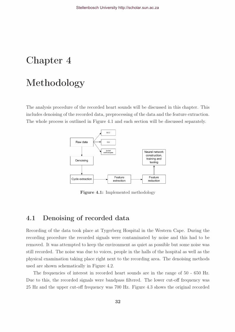
Chapter 4
Methodology
The analysis procedure of the recorded heart sounds will be discussed in this chapter. This
includes denoising of the recorded data, preprocessing of the data and the feature extraction.
The whole process is outlined in Figure 4.1 and each section will be discussed separately.
Figure 4.1: Implemented methodology
4.1 Denoising of recorded data
Recording of the data took place at Tygerberg Hospital in the Western Cape. During the
recording procedure the recorded signals were contaminated by noise and this had to be
removed. It was attempted to keep the environment as quiet as possible but some noise was
still recorded. The noise was due to voices, people in the halls of the hospital as well as the
physical examination taking place right next to the recording area. The denoising methods
used are shown schematically in Figure 4.2.
The frequencies of interest in recorded heart sounds are in the range of 50 - 650 Hz.
Due to this, the recorded signals were bandpass filtered. The lower cut-off frequency was
25 Hz and the upper cut-off frequency was 700 Hz. Figure 4.3 shows the original recorded
32
Stellenbosch University http://scholar.sun.ac.za

CHAPTER 4. METHODOLOGY 33
Figure 4.2: Denoising methods implemented
signal and Figure 4.4 shows the signal after it was bandpass filtered. The signal was sent
through the filter, reversed and sent back through the filter so that zero phase distortion
would be present at the end of the filtering process. The signal shown is a signal recorded
with the auscultation jacket at the 4th left intercostal space. The recorded ECG signals
(IQteq and GeoAxon) were also filtered. These signals were low-pass filtered with a 4th
order Butterworth filter with a cut-off frequency of 40 Hz so as to remove any electrical
noise that might have occurred.
0 0.2 0.4 0.6 0.8 1−1.2
−1
−0.8
−0.6
−0.4
−0.2
0
0.2
0.4
0.6
0.8
Time [sec]
Am
plitu
de
Figure 4.3: Original recorded signal
0 0.2 0.4 0.6 0.8 1−0.8
−0.6
−0.4
−0.2
0
0.2
0.4
0.6
0.8
Time [sec]
Am
plitu
de
Figure 4.4: Bandpass filtered signal
Stellenbosch University http://scholar.sun.ac.za

CHAPTER 4. METHODOLOGY 34
Original signal
?
DWT
A D
? ?Threshold Threshold
IDWT
?Denoised signal
Figure 4.5: Flowdiagram of wavelet threshold denoising technique
4.1.1 Wavelet threshold denoising
After the signals were bandpass filtered, the signal were denoised with the wavelet threshold
denoising method. The wavelet threshold denoising technique is a relatively simple and
effective technique for denoising data. It has been used by de Vos [18] and Messer et al. [24]
in denoising phonocardiograms. When using the wavelet threshold technique, the wavelet
is first broken down to a specified level by the discrete wavelet transform. The threshold
is then applied to the approximation and detail coefficients. The signal is reconstructed by
the Inverse Discrete Wavelet Transform (IDWT) and the denoised signal is produced. The
process is described figuratively in Figure 4.5.
Two types of thresholding techniques exist, hard thresholding and soft thresholding.
Hard thresholding is defined as (x being the signal value, T being the threshold value) [24]:
x =
{x if |x| > T
0 if |x| 6 T(4.1.1)
and soft thresholding is defined as (x being the signal value, T being the threshold value)
[24]:
x =
{sign (x) (|x| − T ) if |x| > T
0 if |x| 6 T(4.1.2)
Stellenbosch University http://scholar.sun.ac.za

CHAPTER 4. METHODOLOGY 35
0 0.2 0.4 0.6 0.8 1−0.8
−0.6
−0.4
−0.2
0
0.2
0.4
0.6
Time [sec]
Am
plitu
de
Figure 4.6: Wavelet threshold denoised signal
Coefficients of the DWT that lie below the threshold value are removed and the resulting
coefficients are then reconstructed to constitute the denoised signal. This is a very powerful
concept, because signals with energy concentrated in a small number of wavelet dimensions
will have coefficients that are relatively large compared to any other signal present that
has its energy concentrated over a larger number of wavelet dimensions [22]. Applying the
thresholding operation to the DWT will, therefore, effectively remove any unwanted signal
or noise, even if the instantaneous frequency spectra of the two signals overlap.
When using the threshold denoising technique, the following assumptions are made [54]:
1. The recorded signal is modelled as: x (t) = o (t) + n (t) where x (t) is the recorded
signal, o (t)is the original uncorrupted signal and n (t) is the noise signal.
2. The energy of the original signal is effectively captured in a transform whose values
lie above a specified threshold Ts > 0.
3. The transform values of the noise signal have magnitudes that lie below a specified
threshold Tn that satisfy the following condition Tn < Ts.
The result of denoising by the wavelet threshold method for the signal shown in Figure
4.4 is shown in Figure 4.6. For the denoising of the recorded data, Stein’s Unbiased Estimate
of Risk (SURE) was used to calculate the threshold value. The calculated threshold value
was multiplied by 0.3 to reduce the value, since the larger value resulted in some signals
losing the first or second heart sound. In some instances this value was still a bit large
and removed some murmur information as well, but setting this value lower resulted in
more signals that were not denoised properly. It was thus decided to adhere to the selected
threshold and apply that to every signal processed.
Stellenbosch University http://scholar.sun.ac.za

CHAPTER 4. METHODOLOGY 36
Figure 4.7: Cycle extraction flowdiagram
A second technique was used to calculate a threshold value. The standard deviation,
σ, of the first-level detail coefficients was calculated. It is assumed that most of the noise
is captured at this level, since it contains the high-frequency components. The threshold
is then set to T = 4σ as suggested in [54]. The larger of the the two calculated threshold
values was chosen as the value to use in the denoising procedure.
4.1.2 Cycle extraction
After the recorded signals had been denoised, four cycles of heart sounds were extracted.
This was done by identifying the QRS-peaks in the ECG recordings to identify the onset
of a heartbeat cycle. The process is outlined in Figure 4.7. The detection algorithm used
is based upon a weighted and squared first-derivative operator and a moving-average (MA)
filter and is described by Rangayyan [11]. The first-derivative operator accentuates the areas
of greatest change (the QRS-peaks) and attenuates the slow-varying components. The MA
filter smooths the signal further to attenuate any small artifacts or noise that may still be
present. The signal after applying the filtered-derivative operator is:
g1(n) =N∑
i=1
|x(n − i + 1) − x(n − i)|2 (N − i + 1) (4.1.3)
where x(n) is the ECG signal and N is the width of a window within which first-order
differences are computed, squared and weighted by the factor (N−i+1). Further smoothing
of the result was performed by an MA filter over M points. The signal after application of
the MA filter:
Stellenbosch University http://scholar.sun.ac.za

CHAPTER 4. METHODOLOGY 37
g(n) =1
M
M−1∑
j=0
g1(n − j) (4.1.4)
The recorded ECG signals were resampled to fs = 100 Hz, since this makes the calcula-
tion considerably faster. The window widths were set to N = 1 and M = 5. In Rangayyan
[11] the window widths were set to N = M = 8. This, however, resulted in the QRS-peaks
being smoothed to such a degree that the start of S1 was calculated incorrectly by roughly
100 msec. The window widths were thus changed to avoid this. Figures 4.8, 4.9 and 4.10
show the original recorded ECG signal recorded by GeoAxon’s ECG, the signal after the
first-derivative operator and the signal after smoothing with the MA filter respectively.
After this procedure, the starting-points and end-points of the peaks were identified.
All values below 15% of the maximum value in the signal were first set to zero in order to
0 1 2 3 4 5−0.4
−0.2
0
0.2
0.4
0.6
0.8
1
Time [sec]
Nor
mal
ised
am
plitu
de
Figure 4.8: Original recorded ECG
0 1 2 3 4 50
0.05
0.1
0.15
0.2
0.25
0.3
0.35
0.4
0.45
Time [sec]
Am
plitu
de
Figure 4.9: ECG signal after first-derivative operator applied
0 1 2 3 4 50
0.02
0.04
0.06
0.08
0.1
0.12
0.14
0.16
0.18
0.2
Time [sec]
Am
plitu
de
Figure 4.10: ECG signal after first-derivative operator and smoothing MA filter
Stellenbosch University http://scholar.sun.ac.za

CHAPTER 4. METHODOLOGY 38
x(i) = 0
?
@@
@@
@@
��
��
��
��
��
��
@@
@@
@@
x(i) ≥ 0.15xmaxx(i) - -x(i) = x(i)YES
NO
Figure 4.11: Algorithm to set all values below 15% of maximum value to zero
remove any artifacts in the signal. This algorithm is shown in Figure 4.11 where x(i) is the
function value and xmax is the maximum function value.
The algorithm to detect the starting-points and end-points of the QRS-peaks is explained
in Figure 4.12. Here the vector x contains the indices of all the values of g (after the bottom
k = 1
x(i) = i|g(i) > 0 - Q(1) = x(1)
?for j = 1 to N − 1 -�
��
��
�
@@
@@
@@
@@
@@
@@
��
��
��
x(j + 1) − x(j) > 0 -YES
k = k + 1
S(k) = x(j)
Q(k + 1) = x(j + 1)
6
Figure 4.12: Algorithm to detect QRS starting-points and end-points
Stellenbosch University http://scholar.sun.ac.za

CHAPTER 4. METHODOLOGY 39
15% have been removed, refer equation 4.1.4) that are greater than zero. The vector Q
contains the indices of the starting-points of the QRS-complex and the vector S contains
the indices of the end-points of the QRS-complex. N is the length of the vector x.
The indices of the starting-points and end-points of the QRS-peaks were identified. To
extract four cycles of the recorded heart sounds, the indices had to be reworked to the
sampling frequency fs = 2000 Hz. This was done by equation 4.1.5.
S =2000 × s
100(4.1.5)
where s is the sample indices at fs = 100 Hz and S is the sample indices at fs = 2000
Hz. In cases where a patient suffers from atrial fibrillation or any other disease that results
in an unstable heartbeat, the extracted heart cycle might not contain all the necessary
information. In order to extract four cycles that contain information that is comparable to
one another, the interval duration of a cycle was calculated and compared to the interval
prior to that and the interval next to it. If these ratios fell within the range, 0.85 ≤Interval ≤ 1.15, the centre cycle was extracted. If none of the heart cycles fell within that
ratio, 4 cycles were simply extracted from the first QRS-peak to the fourth QRS-peak.
4.2 Feature extraction
It was decided to follow a more physiological process during the feature extraction process.
This implies that the features extracted are features that a physician would listen to when
auscultating the heart. It was then attempted to describe these features in a mathematical
manner so that they might be used in the classification process. The feature extraction
process is described schematically in Figure 4.13.
4.2.1 Ratio of power between S1 and S2
The power ratio of S1 to S2 as a feature was decided upon, since this indicates where S1 or
S2 is the loudest. The second heart sound should be loudest at the 2nd intercostal space
near the base of the heart and the first heart sound at the fifth intercostal space near the
apex of the heart. This is a result of the sound of the closing valves radiating through the
thorax. Refer to Figure 2.4 and Section 2.4 for an explanation. If S1 increased in intensity
(louder than S2 at the base), it might indicate the following [55]:
• Anaemia, pregnancy, anxiety, fever and hyperthyroidism, which in turn result in in-
creased contractility and myocardial tension development.
• Mitral stenosis: S1 may be louder due to mitral valve leaflet thickening and scarring.
Stellenbosch University http://scholar.sun.ac.za

CHAPTER 4. METHODOLOGY 40
Figure 4.13: Feature extraction process
• The opening of mitral valve at the onset of ventricular contraction. This occurs when
there is a short P-R interval in the ECG (between 0.11-0.13 seconds).
If S1 is decreased in intensity (S2 louder than S1 at the apex) it may indicate the
following:
• Impaired ventricular contractility, which means a decrease in myocardial tension de-
velopment, that could indicate congestive heart failure.
• Severe mitral stenosis, which results in complete mitral valve immobility.
• The mitral valve is nearly closed at the onset of ventricular contraction. This results
in a prolonged P-R interval (> 0.2 seconds).
To calculate the power ratio, the first and second heart sounds had to be extracted first.
The extraction of S1 and S2 was based on the timing relationships of the heart sounds to
the ECG. The extraction process is shown schematically in Figure 4.14.
The start of the first heart sound can be taken as the start of the QRS-complex in the
ECG [11]. Refer to Appendix A for an explanation of the constituent parts of the ECG. The
QRS-complexes have been identified as explained in Section 4.1.2. It was decided to use
the power ratios of three consecutive cycles and calculate the average power ratio between
Stellenbosch University http://scholar.sun.ac.za

CHAPTER 4. METHODOLOGY 41
Figure 4.14: Procedure followed to extract S1 and S2
S1 and S2 at the apex and the base of the heart. This was done to ensure that the ratio
calculated is representative of the actual beating of the heart. The start of S1 can be related
to the QRS-complex by keeping in mind that ventricular contraction forces blood upwards,
which, in turn, closes the mitral and tricuspid valves (resulting in the main component
of the S1 sound). The end of S1 cannot be attributed to any specific event in the ECG.
We know that the start of the T-wave corresponds to ventricular repolarisation [10], which
means that the ventricles relax and cause the aortic and pulmonary valves to shut, thereby
causing S2. The end of S1 thus has to occur prior to that. It was decided to calculate the
end of S1 as:
S1 end = QRSstart + 1.5 × TS-T segment (4.2.1)
This ensures that enough of the information contained in S1 is extracted without con-
taining a portion of S2.
Burke and Nasor [56] developed second-order equations to calculate the time relation-
ships of the different components of the human electrocardiogram. The equations developed
for the different sections of the ECG (refer Appendix A) are (all times are in seconds):
TP-wave = 0.57T1/2R-R − 0.33TR-R − 0.14 (4.2.2)
TP-Q segment = 0.56T1/2R-R − 0.33TR-R − 0.17 (4.2.3)
Stellenbosch University http://scholar.sun.ac.za

CHAPTER 4. METHODOLOGY 42
0 0.5 1 1.5 2 2.5 3 3.5−1
−0.8
−0.6
−0.4
−0.2
0
0.2
0.4
0.6
0.8
1
Time [sec]
Am
plitu
de
S SSS
EEEE
Figure 4.15: Identified S1’s for a pa-tient with a normal heart
0 0.5 1 1.5 2 2.5 3 3.5−1.5
−1
−0.5
0
0.5
1
Time [sec]
Am
plitu
de
S S S S
E E E E
Figure 4.16: Identified S1’s for a pa-tient with an abnormal heart
TP-Q interval = 1.12T1/2R-R − 0.65TR-R − 0.31 (4.2.4)
TQRS = −0.02T1/2R-R + 0.02TR-R + 0.08 (4.2.5)
TQ-T interval = 1.65T1/2R-R − 0.84TR-R − 0.46 (4.2.6)
TT-wave = 1.29T1/2R-R − 0.66TR-R − 0.42 (4.2.7)
TS-T segment = 0.34T1/2R-R − 0.17TR-R − 0.10 (4.2.8)
This approach proved to be very uncomplicated and efficient in extracting the first heart
sound. The start and end of S1 are shown in Figure 4.15 (for a normal heart sound) and
in Figure 4.16 for an abnormal heart sound, where S denotes the start of S1 and E denotes
the end of S1. The corresponding extracted first heart sounds are shown in Figures 4.17
and 4.18 respectively.
For the extraction of the second heart sound, the procedure was not as straightforward.
The start of S2 was taken as the end of the T-wave in the ECG. The end of the T-wave can
be taken as the start of S2 since this is when the ventricles start to relax and the pressure
in the ventricles drop [11]. This action causes the aortic and pulmonary valves to shut,
since the pressure in the aorta and the pulmonary artery is higher than the pressure in the
ventricles. In calculating the end of the T-wave, the start of the QRS-complex was identified
and the duration of the Q-T interval was added. The corrected Q-T interval, Q-Tc, was
used in the calculation. This is equal to the Q-T interval divided by the square root of the
Stellenbosch University http://scholar.sun.ac.za
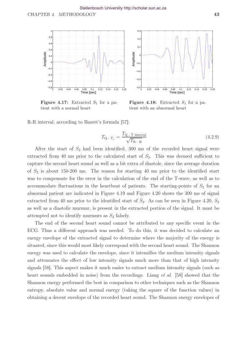
CHAPTER 4. METHODOLOGY 43
0 0.02 0.04 0.06 0.08 0.1 0.12 0.14 0.16 0.18−0.8
−0.6
−0.4
−0.2
0
0.2
0.4
0.6
0.8
1
Time [sec]
Am
plitu
de
Figure 4.17: Extracted S1 for a pa-tient with a normal heart
0 0.02 0.04 0.06 0.08 0.1 0.12 0.14 0.16 0.18−0.4
−0.3
−0.2
−0.1
0
0.1
0.2
0.3
Time [sec]
Am
plitu
de
Figure 4.18: Extracted S1 for a pa-tient with an abnormal heart
R-R interval, according to Bazett’s formula [57]:
TQ - Tc
=TQ - T interval√
TR - R
(4.2.9)
After the start of S2 had been identified, 300 ms of the recorded heart signal were
extracted from 40 ms prior to the calculated start of S2. This was deemed sufficient to
capture the second heart sound as well as a bit extra of diastole, since the average duration
of S2 is about 150-200 ms. The reason for starting 40 ms prior to the identified start
was to compensate for the error in the calculation of the end of the T-wave, as well as to
accommodate fluctuations in the heartbeat of patients. The starting-points of S2 for an
abnormal patient are indicated in Figure 4.19 and Figure 4.20 shows the 300 ms of signal
extracted from 40 ms prior to the identified start of S2. As can be seen in Figure 4.20, S2
as well as a diastolic murmur, is present in the extracted portion of the signal. It must be
attempted not to identify murmurs as S2 falsely.
The end of the second heart sound cannot be attributed to any specific event in the
ECG. Thus a different approach was needed. To do this, it was decided to calculate an
energy envelope of the extracted signal to determine where the majority of the energy is
situated, since this would most likely correspond with the second heart sound. The Shannon
energy was used to calculate the envelope, since it intensifies the medium intensity signals
and attenuates the effect of low intensity signals much more than that of high intensity
signals [58]. This aspect makes it much easier to extract medium intensity signals (such as
heart sounds embedded in noise) from the recordings. Liang et al. [58] showed that the
Shannon energy performed the best in comparison to other techniques such as the Shannon
entropy, absolute value and normal energy (taking the square of the function values) in
obtaining a decent envelope of the recorded heart sound. The Shannon energy envelopes of
Stellenbosch University http://scholar.sun.ac.za

CHAPTER 4. METHODOLOGY 44
the extracted signals for an abnormal patient are shown in Figure 4.21. The bottom 25%
of the envelope values were discarded to eliminate small noise that might interfere in the
extraction process.
Due to the possibility of noise, it was decided to identify the peaks in the Shannon
energy envelope and group the peaks together. If two peaks were less than 40 ms apart, it
was assumed that they formed part of the same group. If not, they were put into separate
groups. The energy of the different groups were then calculated and the group with the
highest energy was extracted as S2. This assumption proved to be sufficient in extracting the
correct group as S2. Figure 4.22 shows the identified peaks for a patient with an abnormal
heart and the corresponding identified groups. It can be seen that each component identified
in Figure 4.20 forms its own separate group (with the murmur forming two groups).
The energy of the different groups were calculated by:
Egroup =
N∑
i=1
x(i)2 (4.2.10)
where x(i) is the amplitude of a specific peak i, and N is the number of peaks in a specific
group. The energy values for S2, the murmur (M1 and M2) and S1 are shown in Table 4.1.
Figure 4.23 shows the extracted second heart sound.
Now that both S1 and S2 had been extracted for three heart cycles at each location and
in each recording position, the power ratio between S1 and S2 could be calculated. The
power of each of the extracted heart sounds was calculated by calculating the energy and
0 0.5 1 1.5 2 2.5 3−1
−0.8
−0.6
−0.4
−0.2
0
0.2
0.4
0.6
0.8
1
Time [sec]
Am
plitu
de
S S S S
Figure 4.19: Start of S2 identified for a patient with an abnormal heart
Stellenbosch University http://scholar.sun.ac.za

CHAPTER 4. METHODOLOGY 45
0.45 0.5 0.55 0.6 0.65 0.7 0.75 0.8 0.85 0.9−0.6
−0.4
−0.2
0
0.2
0.4
0.6
0.8
Time [sec]
Am
plitu
de
S2
Murmur
Figure 4.20: Extracted portion of signal for S2 extraction
dividing it by the duration of the extracted sound as in equation 4.2.11:
Pheart sound =
∑Nt=0 x(t)2
ttotal(4.2.11)
where x(t) is the heart sound amplitude at a specific time instant t, ttotal is the duration of
the heart sound and N is the length of the signal. This calculation was performed for each
extracted sound at a specific location. The average power of the three extracted sounds was
calculated and used as the feature. The heart sounds recorded at the 2nd left and right
intercostal spaces and 5th and 6th left intercostal spaces were used in this calculation, since
S2 should be the loudest at the base of the heart (2nd left and right intercostal spaces) and
S1 should be the loudest at the apex of the heart (5th & 6th left intercostal spaces). The
0.45 0.5 0.55 0.6 0.65 0.7 0.75 0.8 0.85 0.90
0.05
0.1
0.15
0.2
0.25
0.3
0.35
0.4
Time [sec]
Am
plitu
de
S2
M1
M2
Figure 4.21: Shannon energy envelope of a patient with an abnormal heart
Stellenbosch University http://scholar.sun.ac.za

CHAPTER 4. METHODOLOGY 46
0.5 0.55 0.6 0.65 0.7 0.75 0.8 0.850
0.05
0.1
0.15
0.2
0.25
0.3
0.35
0.4
Time [sec]
Am
plitu
de
S2
M1
M2
Figure 4.22: Identified peaks in the Shannon energy envelope of a patient with an abnormal heart
Energy valueS2 0.76M1 0.02M2 0.12
Table 4.1: Energy values of different components in extracted second heart sound signal
0.46 0.48 0.5 0.52 0.54 0.56 0.58 0.6 0.62 0.64−0.6
−0.4
−0.2
0
0.2
0.4
0.6
0.8
Time [sec]
Am
plitu
de
Figure 4.23: Extracted second heart sound for an abnormal patient
power ratio thus contributed to a total of four features used in the classification process.
Other studies that have also successfully identified the different heart sounds in the
phonocardiogram have been published . Liang et al. [58] obtained 93% correct identifcation
ratio in splitting the heart cycle into S1, systole, S2 and diastole. The algorithm was based
on the normalised average Shannon energy of the phonocardiogram signal. The correct S1’s
Stellenbosch University http://scholar.sun.ac.za

CHAPTER 4. METHODOLOGY 47
and S2’s were identified by a cardiologist and then compared to the heart sounds extracted
by the algorithm. Haghighi-Mood et al. [59] segmented the heart sound by using an auto-
regressive (AR) model to estimate the power spectral density of the signal and calculate
the energy in specific frames of the signal. The authors did not obtain statistical results
in quantifying the validity of their algorithm. Huiying et al. [8] developed an algorithm
for detecting S1, systole, S2 and diastole from the phonocardiogram signal. The discrete
wavelet transform was used to calculate intensity enevelopes of the signals and identify
components within the envelope. A correct identification ratio of 93 % was obtained. The
correct locations of S1 and S2 were identified by a cardiologist and the result was then
compared to the S1’s and S2’s extracted by the algorithm. The algorithm developed in
this study have not yet been assessed by a cardiologist, but preliminary results show that
the algorithm extracts S1 and S2 correctly in approximately 90% of the cases. This was
determined by visual inspection.
4.2.2 Frequency band ratio of S1 and S2
It was deemed necessary to extract the frequency information from S1 and S2 as well, since
S2 is normally higher pitched (higher frequency) than S1 [55] and a noticeable deviation
from this could indicate pathology. Johnson et al. [60] extracted frequency bands in their
study of the systolic murmur of aortic stenosis. It was decided to follow the same approach
in this study, as this would identify heart sounds that have higher frequency content than
normal.
The FFT of each extracted S1 and S2 was calculated. The magnitudes of the Fourier
coefficients in the frequency range between 0-100 Hz as well as between 100-800 Hz were
summed. These two values were then divided to yield a ratio that describes the frequency
content of the extracted signal as in equation 4.2.12.
Fratio =
∑100f=0 C
∑800f=100 C
(4.2.12)
where C indicates the Fourier coefficient magnitude at a specific frequency f . The higher
this value, the more normal the extracted heart sound should be, since normal heart sounds
should not contain frequencies higher than about 100 Hz. Should this ratio be low, it should
indicate that higher than normal frequencies are present and could be an indication of a
murmur. Figure 4.24 shows the FFT of S1 for a normal and an abnormal patient and Figure
4.25 shows the FFT of S2 for a normal and an abnormal patient.
Stellenbosch University http://scholar.sun.ac.za

CHAPTER 4. METHODOLOGY 48
0 100 200 300 400 500 600 700 8000
0.05
0.1
0.15
0.2
0.25
0.3
0.35
0.4
0.45
0.5
Frequency [Hz]
FF
T m
agni
tude
NormalAbnormal
Figure 4.24: FFT of S1 for a normaland an abnormal patient
0 100 200 300 400 500 600 700 8000
0.05
0.1
0.15
0.2
0.25
Frequency [Hz]
FF
T m
agni
tude
NormalAbnormal
Figure 4.25: FFT of S2 for a normaland an abnormal patient
4.2.3 Power comparison between first heart sounds of different
cycles
Variation in the intensity of S1 from beat-to-beat is also an indication of abnormality [55].
S1 varies from beat-to-beat when the position of the mitral and tricuspid valves is variable
at the onset of ventricular contraction. This occurs in patients with atrial fibrillation1, third
degree heart block 2 and ventricular pacemakers [55]. No fixed relationship exists between
atrial excitation and ventricular contraction. The position of the mitral and tricuspid valves
at the beginning of ventricular systole varies, sometimes being partially shut and at other
times being completely open, resulting in a variation in the intensity of S1.
The power of S1 was calculated for the phonocardiograms, as explained in Section 4.2.1.
The ratios between the first heart sounds of the different cycles were calculated and the
average of the three ratios was taken to yield the feature used in the classification process.
The recordings at the 5th and 6th intercostal spaces were used in the calculation, since this
is where S1 should be heard most clearly (refer Section 2.4).
Figure 4.26 shows 4 cycles of a patient with the first heart sounds indicated. It can be
seen that the amplitude of the different S1’s differ from beat-to-beat. Figure 4.27 shows the
recorded ECG of the patient. Lead V1 shows the characteristic “ripples” that are present
during atrial fibrillation. This patient suffers from severe mitral stenosis, as was confirmed
by an echocardiogram, which causes atrial fibrillation [12]. The ratios were calculated asCycle2Cycle1
, Cycle3Cycle2
and Cycle3Cycle1
. The average of these three values was calculated for the recordings
1Atrial fibrillation occurs when the atria are not depolarised in a rhythmic manner. Multiple electricalimpulses spread across the atria causing the atria to contract at random rates and in effect “flutter” [61].
2Third degree heart block, also known as complete heartblock, is when the electrical impulse thatactivates atrial and ventricular contraction does not pass through the AV node. This leads to the ventriclesnot necessarily contracting after the atria but at their own rhythm. The QRS-complex of the ECG thusdoes not necessarily follow the P-wave [62].
Stellenbosch University http://scholar.sun.ac.za
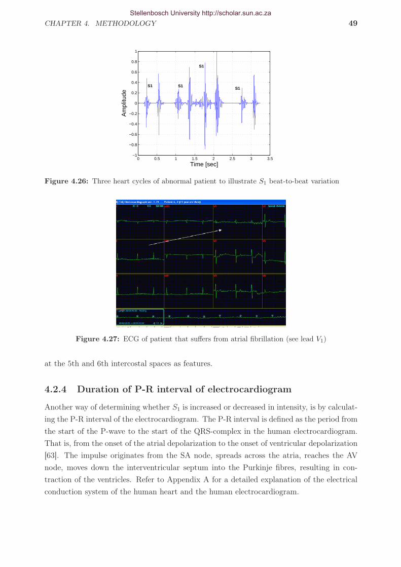
CHAPTER 4. METHODOLOGY 49
0 0.5 1 1.5 2 2.5 3 3.5−1
−0.8
−0.6
−0.4
−0.2
0
0.2
0.4
0.6
0.8
1
Time [sec]
Am
plitu
de
S1 S1
S1
S1
Figure 4.26: Three heart cycles of abnormal patient to illustrate S1 beat-to-beat variation
Figure 4.27: ECG of patient that suffers from atrial fibrillation (see lead V1)
at the 5th and 6th intercostal spaces as features.
4.2.4 Duration of P-R interval of electrocardiogram
Another way of determining whether S1 is increased or decreased in intensity, is by calculat-
ing the P-R interval of the electrocardiogram. The P-R interval is defined as the period from
the start of the P-wave to the start of the QRS-complex in the human electrocardiogram.
That is, from the onset of the atrial depolarization to the onset of ventricular depolarization
[63]. The impulse originates from the SA node, spreads across the atria, reaches the AV
node, moves down the interventricular septum into the Purkinje fibres, resulting in con-
traction of the ventricles. Refer to Appendix A for a detailed explanation of the electrical
conduction system of the human heart and the human electrocardiogram.
Stellenbosch University http://scholar.sun.ac.za
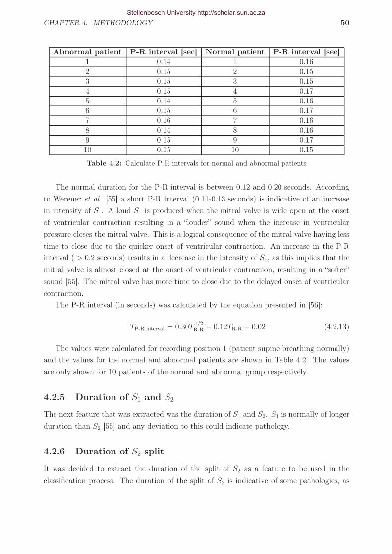
CHAPTER 4. METHODOLOGY 50
Abnormal patient P-R interval [sec] Normal patient P-R interval [sec]1 0.14 1 0.162 0.15 2 0.153 0.15 3 0.154 0.15 4 0.175 0.14 5 0.166 0.15 6 0.177 0.16 7 0.168 0.14 8 0.169 0.15 9 0.1710 0.15 10 0.15
Table 4.2: Calculate P-R intervals for normal and abnormal patients
The normal duration for the P-R interval is between 0.12 and 0.20 seconds. According
to Werener et al. [55] a short P-R interval (0.11-0.13 seconds) is indicative of an increase
in intensity of S1. A loud S1 is produced when the mitral valve is wide open at the onset
of ventricular contraction resulting in a “louder” sound when the increase in ventricular
pressure closes the mitral valve. This is a logical consequence of the mitral valve having less
time to close due to the quicker onset of ventricular contraction. An increase in the P-R
interval ( > 0.2 seconds) results in a decrease in the intensity of S1, as this implies that the
mitral valve is almost closed at the onset of ventricular contraction, resulting in a “softer”
sound [55]. The mitral valve has more time to close due to the delayed onset of ventricular
contraction.
The P-R interval (in seconds) was calculated by the equation presented in [56]:
TP-R interval = 0.30T1/2R-R − 0.12TR-R − 0.02 (4.2.13)
The values were calculated for recording position 1 (patient supine breathing normally)
and the values for the normal and abnormal patients are shown in Table 4.2. The values
are only shown for 10 patients of the normal and abnormal group respectively.
4.2.5 Duration of S1 and S2
The next feature that was extracted was the duration of S1 and S2. S1 is normally of longer
duration than S2 [55] and any deviation to this could indicate pathology.
4.2.6 Duration of S2 split
It was decided to extract the duration of the split of S2 as a feature to be used in the
classification process. The duration of the split of S2 is indicative of some pathologies, as
Stellenbosch University http://scholar.sun.ac.za

CHAPTER 4. METHODOLOGY 51
explained in Section 3.3. The problem was how to identify the two components of S2 and
measure the time difference between them. Debbal et al. [25] investigated the differences
between the components of the second heart sound of a normal heart, a patient that suffers
from aortic-coarctation and a patient that suffers from mitral stenosis. The aortic and
pulmonary components were identified by using the continuous wavelet transform (CWT),
but no automatic identification algorithm was presented in the study.
It was decided to identify the aortic and pulmonary components by also using the CWT,
but to add a degree of automaticity to the algorithm. When calculating the CWT of a signal,
a set of coefficients that indicate the degree of comparison of the signal to the analysing
wavelet at a specific scale and at a specific instant in time are generated. By taking the
absolute values of these coefficients, a “comparison envelope” is obtained. This indicates
where in frequency and time the major components of the analysed signal is situated. The
higher in value the coefficient, the higher the degree of comparison at that specific scale and
time instant.
The CWT of the extracted second heart sounds (refer Section 4.2.1) was calculated
and the absolute values taken to obtain the envelope. The Daubechies wavelet of order
7 (db7) was used and the scales at which the CWT was calculated, were from 5 to 100.
This corresponded to pseudo-frequencies between 14 and 277 Hz. It was assumed that the
two highest peaks corresponded to A2 and P2, as was done in [25]. To obtain the time
difference between the two components, the highest peak was first identified. It was then
stepped through the entire data set to identify the second highest peak. The maximum
points were identified and subsequently set to zero until two maxima differed by 10 msec or
more. This maxima was then identified as the second peak. The absolute value of the time
difference between the two components was then taken as the time difference between A2
and P2. According to Werner et al. [55], A2 and P2 differ by 10-20 msec during expiration
and 40-50 msec during inspiration during normal conditions. The 10 msec time difference
ensured that the two peaks were identified during inspiration as well as expiration. Figure
4.28 shows the “comparison envelope” as viewed from the top (a contour plot), with the
two peaks identified (the X’s) for an abnormal patient. The timing difference between these
peaks was calculated as 12.5 msec.
4.2.7 Determining the shape of systolic and diastolic murmurs
Murmurs can either be classified as systolic murmurs or diastolic murmurs, depending on
where in the cardiac cycle the murmur occurs. Depending on which pathology causes the
murmur, the shape of the murmur may vary. For instance, the intensity of the murmur
might increase from its origin (crescendo murmur) or decrease from its origin (decrescendo
murmur) or it may be a combination of the two. The intensity of the murmur may also stay
Stellenbosch University http://scholar.sun.ac.za

CHAPTER 4. METHODOLOGY 52
Samples
Sca
les
50 100 150 200 250 300
10
20
30
40
50
60
70
80
90
0.2
0.4
0.6
0.8
1
1.2
1.4
1.6
1.8
XX
Figure 4.28: CWT coefficients with peaks indicated that correspond to A2 and P2 of the secondheart sound
0 0.05 0.1 0.15 0.2 0.25 0.3 0.35 0.4−0.4
−0.3
−0.2
−0.1
0
0.1
0.2
0.3
0.4
Time [sec]
Am
plitu
de
S1
Figure 4.29: Ejection systolic murmur of a patient suffering from aortic stenosis, showing thecrescendo-decrescendo nature of the murmur
constant for the duration of the murmur.
Systolic murmurs can be divided into ejection systolic murmurs, pansystolic murmurs
and late systolic murmurs. Ejection systolic murmurs occur due to turbulent bloodflow
through stenotic aortic and pulmonary valves. The murmur increases to a crescendo at more
or less the middle of systole and then decreases (decrescendo) and ends just before the start
of S2. Pathologies that exhibit such murmurs are aortic stenosis, pulmonary stenosis and
atrial septal defect. Figure 4.29 shows the recording of a patient that suffers from moderate
aortic stenosis. The crescendo-decrescendo shape of the murmur can clearly be seen as
indicated by the dashed lines.
Pansystolic murmurs are murmurs that extend throughout systole. The murmurs
Stellenbosch University http://scholar.sun.ac.za

CHAPTER 4. METHODOLOGY 53
0 0.05 0.1 0.15 0.2 0.25 0.3 0.35 0.4−0.4
−0.3
−0.2
−0.1
0
0.1
0.2
0.3
0.4
Time [sec]
Am
plitu
de
S2
S1
Murmur
Figure 4.30: Pansystolic murmur of a patient suffering from mitral regurgitation
have a slight accentuation in mid-systole, but the ejection systolic murmur is more pro-
nounced. This type of murmur is caused by blood leaking through a valve that is not closed
properly during ventricular contraction, such as in mitral regurgitation or tricuspid regur-
gitation. It may sometimes occur in patients that suffer from ventricular septal defect in
which the hole between the left and right ventricles is relatively small. The murmur starts
simultaneously with S1 and extends throughout systole and may even obscure a bit of S2
[12]. Figure 4.30 shows the recording of a patient that suffers from mitral regurgitation. The
pansystolic nature of the murmur can clearly be seen. It obscures S1, extends throughout
systole and ends just before S2.
To calculate the shape of the murmur it was decided to extract the systole and diastole
portions from the heart cycle, break them up into three sections and calculate the root-
mean-square value (rms-value) of each. The rms-value of a function is defined as [64]:
RMS(f) =
√∫ b
af 2(x)dx
b − a(4.2.14)
By calculating three values, one can draw a line which shows whether the murmur is
either increasing (crescendo), decreasing (decrescendo), a combination of the two (crescendo-
decrescendo), or if it stays constant throughout systole or diastole. Figure 4.31 shows the
extracted systole component from the cardiac cycle of a patient. Three sections are indicated
and it can easily be seen that the murmur is of a decrescendo nature. The calculated rms-
values are presented in Table 4.3. From the values in Table 4.3 it can be seen that the
murmur is of a decrescendo nature, since the line that is plotted through the three values
has a negative gradient.
This process was repeated for each of the three extracted cardiac cycles of both systole
Stellenbosch University http://scholar.sun.ac.za

CHAPTER 4. METHODOLOGY 54
0 0.05 0.1 0.15 0.2 0.25 0.3 0.35 0.4−1.5
−1
−0.5
0
0.5
1
Time [sec]
Am
plitu
de
0 0.05 0.1 0.15 0.2 0.25 0.3 0.35 0.4−1.5
−1
−0.5
0
0.5
1
Time [sec]
Am
plitu
de
0 0.05 0.1 0.15 0.2 0.25 0.3 0.35 0.4−1.5
−1
−0.5
0
0.5
1
Time [sec]
Am
plitu
de
0 0.05 0.1 0.15 0.2 0.25 0.3 0.35 0.4−1.5
−1
−0.5
0
0.5
1
Time [sec]
Am
plitu
de
Section 1 Section 2 Section 3
Figure 4.31: Systole extracted from the cardiac cycle showing three sections for which rms-valueare calculated to determine shape of murmur
Section rms-valueSection 1 0.46Section 2 0.33Section 3 0.07
Table 4.3: RMS-values of different sections of systole of an abnormal patient
and diastole. The recordings used in the calculations were the recordings at the 2nd left
and right intercostal spaces and the recordings at the 5th and 6th left intercostal spaces. It
was thought necessary to use the recordings, since some murmurs are heard at one location,
but not at another. Since three values for each section of either systole or diastole of a
recording were obtained (due to the tree cycles that were extracted), it was decided to take
the average of the three calculated values to use as a feature. This was done in order to
reduce the number of features used, as well as to obtain an overview of the nature of the
murmur under consideration. The average was simply calculated by taking the sum of the
three values and dividing the total by three. This process resulted in a total of 24 features
being generated; 12 of them from the systole part of the cardiac cycle and 12 of the diastole
part of the cardiac cycle.
4.2.8 Calculating maximum frequency in different sections of
systole and diastole
The maximum frequency in each section of systole and diastole was calculated. The FFT
of each extracted section was calculated and the frequency with the maximum amplitude
was identified and extracted. This was done for all three extracted cycles of the recorded
Stellenbosch University http://scholar.sun.ac.za

CHAPTER 4. METHODOLOGY 55
0 0.05 0.1 0.15 0.2 0.25 0.3 0.35−1
−0.8
−0.6
−0.4
−0.2
0
0.2
0.4
0.6
0.8
1
Time [sec]
Am
plitu
de
0 0.05 0.1 0.15 0.2 0.25 0.3 0.35−1
−0.8
−0.6
−0.4
−0.2
0
0.2
0.4
0.6
0.8
1
Time [sec]
Am
plitu
deSection 1 Section 2 Section 3
Figure 4.32: Systole extracted fromnormal patient with subsections indi-cated
0 100 200 300 400 5000
0.05
Mag
nitu
de
FFT of section 1
0 100 200 300 400 5000
0.5
Mag
nitu
de
FFT of section 2
0 100 200 300 400 5000
5
x 10−4
Mag
nitu
de
Frequency [Hz]
FFT of section3
Figure 4.33: FFT of each subsectionin systolic region of cardiac cycle for anormal patient
phonocardiogram.
0 0.05 0.1 0.15 0.2 0.25 0.3 0.35−0.8
−0.6
−0.4
−0.2
0
0.2
0.4
0.6
0.8
Time [sec]
Am
plitu
de
Section 1 Section 2 Section 3
Figure 4.34: Diastole extracted fromabnormal patient with subsections indi-cated
0 100 200 300 400 5000
0.2
Mag
nitu
de
FFT of section 1
0 100 200 300 400 5000
0.1
Mag
nitu
de
FFT of section 2
0 100 200 300 400 5000
0.05
0.1
Mag
nitu
de
FFT of section 3
Frequency [Hz]
Figure 4.35: FFT of each subsectionin diastolic region of cardiac cycle foran abnormal patient
The recordings used for the calculations were the recordings at the 2nd left and right
intercostal spaces, the 4th left and right intercostal spaces and the 5th left intercostal space.
Figure 4.32 shows the extracted systolic portion of the cardiac cycle of a patient with no
abnormalities, with the different sections into which it was subdivided, indicated. Figure
4.33 shows the FFT of each subsection. Figure 4.34 shows the diastolic portion of the
cardiac cycle of a patient that suffers from aortic regurgitation, with the different sections
indicated. Figure 4.35 shows the FFT of each different subsection.
Stellenbosch University http://scholar.sun.ac.za

CHAPTER 4. METHODOLOGY 56
4.2.9 Identifying extra sounds: ejection sound, midsystolic click
and opening snap
When auscultating the heart, extra sounds that should not be present during normal func-
tioning of the human heart may occur. These sounds include the ejection sound, midsystolic
click and the opening snap.
Extra heart sounds can be attributed to specific events in the cardiac cycle and therefore
occur at specific times during the cardiac cycle. Ejection sounds are high-pitched sounds
that follow S1 by 0.04-0.06 seconds [55] and can be attributed to abnormalities of the aortic
and pulmonary valves [12]. Ejection sounds associated with the aortic valve are primarily
due to congenitally bicuspid aortic valves or congenital aortic stenosis, and are principally
due to the opening of the abnormal valves [12]. Ejection sounds due to abnormal pulmonary
valves are most commonly due to pulmonary stenosis, but can also be heard in patients with
idiopathic dilatation 3 of the pulmonary artery, or with pulmonary artery dilatation caused
by pulmonary hypertension [12].
Midsystolic clicks are extra heart sounds that occur in midsystole. The most com-
mon cause of a midsystolic click is mitral valve prolapse, where one of the mitral valve
leaflets moves into the left atrium during systole causing an extra sound. This is caused by
elongation or rupture of the chordae tendinae (muscles that hold the valve in place) [12].
Opening snaps are high-pithced sounds which occur in patients who suffer from mitral
stenosis. The hardened (stenosed) valve moves forward towards the left ventricle at the
beginning of diastole as the pressure decreases, resulting in an extra sound prior to S1 [12].
To check whether any of these extra sounds were present, it was argued that within the
interval in which the sounds would occur, the power of the sections would be higher if these
sounds were present than if they were not present. The systolic and diastolic regions of each
cardiac cycle were identified and broken up into different sections, as shown in Figure 4.2.9,
to search for these extra sounds. ES refers to the ejection sound, MC to the midsystolic
click and OS to the opening snap. S1s refers to the start of S1 and S1e to the end of S1.
The same numbering is applicable to S2.
For the ejection sound, 0.06 seconds was extracted from the end of S1. The power was
calculated, as was done in Section 4.2.1, by using equation 4.2.11. For the midsystolic click,
the portion of systole from Ls
4to 3Ls
4, with Ls being the length of systole, was extracted, and
the power calculated by equation 4.2.11. The opening snap follows A2 by 0.03-0.15 seconds
[12]. To search for any opening snap sounds, 0.15 seconds were extracted from the end
of S2 and the power of the extracted section was calculated by equation 4.2.11. This was
done for each of the three extracted cardiac cycles and the average of the three cycles was
3Idiopathic dilatation of the pulmonary artery is an uncommon cause of a large main pulmonary artery.The reason for the enlargement of the artery is unknown. [65]
Stellenbosch University http://scholar.sun.ac.za

CHAPTER 4. METHODOLOGY 57
ES
MC
S1s S1e S2s S2e
OS
� -
-�
-�
Figure 4.36: Splitting of heart cycle
AbnormalPatient ES power [1/sec] MC power [1/sec] OS power [1/sec]
1 8.96 67.26 21.592 60.41 38.30 0.303 215.16 32.96 0.164 18.25 1.78 0.115 48.88 263.01 2.94
Table 4.4: Average power of different sections to search for extra heart sounds (Abnormal)
calculated. For the ejection sound calculations, the recording at the 2nd right intercostal
space was used, for the midsystolic click, the recording at the 5th left intercostal space was
used and for the opening snap, the recording at the 4th right intercostal space was used.
Tables 4.4 and 4.5 show the calculated power of the different sections for abnormal and
normal patients respectively. The values are shown only for five patients of each group.
Figure 4.37 shows an extracted heart cycle with the sections indicated, where MC refers to
the midsystolic click search area, ES refers to the ejection sound search area and OS refers
to the opening snap search area.
NormalPatient ES power [1/sec] MC power [1/sec] OS power [1/sec]
1 23.37 184.88 0.112 21.10 77.37 0.013 75.68 202.18 23.614 62.45 175.56 0.015 42.26 257.70 0.22
Table 4.5: Average power of different sections to search for extra heart sounds (Normal)
Stellenbosch University http://scholar.sun.ac.za

CHAPTER 4. METHODOLOGY 58
0 0.1 0.2 0.3 0.4 0.5 0.6 0.7 0.8 0.9 1−1.5
−1
−0.5
0
0.5
1
1.5
Systole Diastole
MC
ES
OS
Figure 4.37: Cardiac cycle shown with extra sounds search areas
Stellenbosch University http://scholar.sun.ac.za

Chapter 5
Feature selection and classification
This chapter describes the method used in reducing the dimension of the input vector to the
classification scheme. Neural Networks are introduced as the classification scheme used, the
theory is discussed and some preliminary results are given. Statistical Overlap Factor (SOF)
is discussed as the feature reduction technique. The process is described schematically in
Figure 5.1.
Figure 5.1: Feature reduction and ANN training and testing methodology
5.1 Feature selection
It was decided to reduce the extracted features as input to the classification scheme to a
smaller set, since it was deemed unnecessary and computationally intensive to have a large
set of features as input. A variety of feature reduction methods exists: Principal Component
Analysis (PCA), Independent Component Analysis (ICA) and the Statistical Overlap Factor
59
Stellenbosch University http://scholar.sun.ac.za

CHAPTER 5. FEATURE SELECTION AND CLASSIFICATION 60
(SOF). SOF was used to reduce the features in this project, since it was easy and efficient
to implement and proved to have satisfactory results.
5.1.1 Statistical overlap factor
The Statistical Overlap Factor (SOF) is used to determine the variability or degree of
separation between two distributions, and is defined as [66]:
SOF =
∣∣∣∣x1 − x2
(σ1 + σ2) /2
∣∣∣∣ (5.1.1)
where x1 and x2 are the means of distributions x1 and x2, and σ1 and σ2 are the respective
standard deviations. The higher the SOF, the better the degree of separation between the
two distributions [66].
As an example, the SOF of two of the features extracted in Section 4.2 will be shown.
This will illustrate the degree of separation between the features from the different groups
(normal and abnormal). The reason for implementing the SOF to reduce the features is to
extract those features that differ most from one another in the respective groups. This will
ensure a better performance in classification.
The number of features extracted in Section 4.2 amounted to a total of 70 features.
The number of features used in the eventual classification scheme was reduced to 3. This
was determined experimentally and proved to produce the best results. To determine the
amount of features, the network was trained and tested with a different number of hidden
nodes and features to establish which combination provided the best results. The network
was trained and tested with 2, 3, 4 and 5 input features and 10, 15 and 20 hidden neurons.
0 2 4 6 8 10 12 14 16 180
0.02
0.04
0.06
0.08
0.1
0.12
0.14
0.16
0.18
0.2
Patient
Fea
ture
val
ue
AbnormalNormal
Figure 5.2: Values of feature that ex-hibited the greatest degree of separa-tion between the normal and abnormalgroups
0 2 4 6 8 10 12 14 16 1825
30
35
40
45
50
55
60
65
70
75
Patient
Fea
ture
val
ue
AbnormalNormal
Figure 5.3: Values of feature that ex-hibited the smallest degree of separa-tion between the normal and abnormalgroups
Stellenbosch University http://scholar.sun.ac.za

CHAPTER 5. FEATURE SELECTION AND CLASSIFICATION 61
Number of features Run 1 Run 2 Run 3 Run 4 Run 5 Desired value2 0.1369 0.1525 0.1430 0.1506 0.1764 02 0.3437 0.2698 0.3137 0.2857 0.2347 13 0.2644 0.2568 0.2987 0.2445 0.2584 03 0.8097 1.0350 0.8700 0.8711 0.9298 14 1.0121 1.1424 0.9547 0.8631 0.9969 04 0.5409 0.6969 0.7510 1.0214 1.0392 15 1.0853 1.0280 0.9760 0.9397 0.9478 05 0.5270 0.2885 0.1480 0.2345 0.2271 1
Table 5.1: Network outputs for network with 15 hidden neurons and 2, 3, 4 and 5 input features
Feature SOFRMS-value of 3rd section of diastole - 2nd IC right 1.6153RMS-value of 3rd section of diastole - 2nd IC left 1.6153
Max frequency of 1st section of diastole - 4th IC right 1.3869
Table 5.2: Selected features and their respective SOF
Each combination was tested five times to determine if repeatable results were achieved.
The network was trained to give an output of 0 for a normal heart sound and an output
of 1 for an abnormal heart sound. The number of features to be used were selected on the
basis of the number that gave the most correct and repeatable results, i.e. if the network
gave results that varied between 0 and 1 and the results for each training and testing run
were more or less in the same range, that number of features were selected. Table 5.1 shows
the results for the testing run for a network with 15 hidden nodes and 2, 3, 4 and 5 input
features respectively. It can clearly be seen that 3 features as input provided the best results.
The three features that were used in the final classification scheme are shown in Table
5.2. Figure 5.2 shows the different values for the RMS-value of the third section of diastole
of the recording at the 2nd right intercostal space. Figure 5.3 shows the different values for
the maximum frequency of the first section of diastole of the recording at the 4th intercostal
space. The SOF calculated for the first feature was 1.6153 and for the last feature was
1.3869. Tables B.1 and B.2 in Appendix B show the full set of extracted features and their
respective SOF.
5.2 Artificial Neural Network classification
Artificial Neural Networks (ANNs) are mathematical models inspired by biological nervous
sytems. ANNs attempt to simulate the learning process of biological systems, and can
learn to recognise certain inputs to produce particular outputs [67]. Therefore, ANNs are
commonly used for pattern detection and classification of signal features.
Stellenbosch University http://scholar.sun.ac.za

CHAPTER 5. FEATURE SELECTION AND CLASSIFICATION 62
ANNs consist of multiple interconnected processing units, known as neurons, arranged
in two or more layers. The simplest network consists of an input layer and an output
layer, as shown in Figure 5.4. The circle in the output layer represents a single neuron.
The input layer has one input and the output layer has one output. The output neuron
normally contains a transfer function that changes the input to a certain output. The
transfer function is denoted by the symbol f . Normally ANNs contain one or more hidden
layers. A hidden layer is another layer of neurons inserted between the input and output
layers.
Feed-forward networks (FFNs) are the simplest type of multiple-layer ANNs. A FFN
consists of an input layer, one or more hidden layers and an output layer. As the name
implies, a specific layer is only connected to the layer in front of it, no feedback or layer-
skipping is present. A simple FFN with one hidden layer is shown in Figure 5.5. One can
see that a specific layer is only connected to the layer in front of it.
Associated with each neuron is a specific transfer function. In Figure 5.5 the transfer
function is denoted by f . A variety of transfer functions can be used in the neurons, each
with its own benefits. The selected transfer functions have to be differentiable, though. The
most common transfer functions used is the family of sigmoid transfer functions [68]. A
typical representation is,
f(x) =2
1 + e−ax− 1 (5.2.1)
which belongs to the family of hyperbolic tangent functions. These functions are known as
squashing functions, since their output is limited in a finite range of values [68]. The output
of the function in equation 5.2.1 varies between −1 and 1. Figure 5.6 shows the function
for different values of a.
The learning process of the ANN can either be supervised or unsupervised. During
supervised learning, a target output value is set for each input given to the ANN. The
ANN then tries to minimise the error between the output it calculates and the desired
response by minimising a certain cost function. The cost function can be any function that
is dependent on the calculated output of the network and the target values. This is done
by iteratively adjusting the weights and biases of each neuron until a specified tolerance has
Input layer
����Output layer
"!#
- -f
Figure 5.4: ANN with an input layer and an output layer
Stellenbosch University http://scholar.sun.ac.za

CHAPTER 5. FEATURE SELECTION AND CLASSIFICATION 63
x(i) -��
��
��7
SS
SS
SSw������������
?
?
?
"!# "!# "!#
-
-
-
������������
-
��
��
���
@@
@@
@@R
AAU
���
AAU
���
AAU
���
-
-
-
"!# "!# "!#
?
?
?
AAAU
����
AAAU
����
AAAU
����
-
-
-∑
∑
∑
∑
∑
∑
f
f
f
f
f
f
r-1 r
b4
b5
b6
b1
b2
b3
vr−1k
vrj
wrjk
yr−1k
yrj
Figure 5.5: ANN with one hidden layer
−5 0 5−1
−0.8
−0.6
−0.4
−0.2
0
0.2
0.4
0.6
0.8
1
x−values
f(x)
a = 1a = 2.5a = 5
Figure 5.6: f(x) = 21+e−ax − 1 for a = 1, 2.5, 5
Stellenbosch University http://scholar.sun.ac.za

CHAPTER 5. FEATURE SELECTION AND CLASSIFICATION 64
been met. During unsupervised learning the weights and biases are adapted only according
to the inputs, since no target values are available for training purposes. The biases for each
neuron are indicated as b1, b2 etc.
The most common way in which the weights are calculated and adapted, is probably the
backpropagation algorithm [68]. Standard backpropagation is a gradient descent algorithm1
in which the network weights are adjusted in accordance with the negative of the gradient of
the cost function. The term “backpropagation” refers to the manner in which the gradient is
computed for nonlinear multilayer networks. The gradient is first calculated for the last layer
of the network and subsequently moved to the first layer, hence the term backpropagation.
During training, when an input vector x(i) is applied to the input, the output of the
network will be y(i), which is different from the desired value y(i). The weights of the
connections are computed such that an appropriate cost function,J, which is dependent on
the values y(i) and y(i), i = 1, 2, . . . , N , is minimised [68]. In Figure 5.5 the weight vector
of the jth neuron in layer r can be denoted by wrj , which includes the thresholds. The
weight between neuron k in layer r-1 and neuron j in layer r is denoted by wrjk, which states
that the weight is applicable from neuron k to neuron j in layer r. The weight vector for
neuron j in layer r is defined as wrj =
[wr
j0, wrj1, . . . , w
rjkr−1
]T
, where kr−1 are the number of
neurons in layer r-1.
At each iteration the weight vector is updated by
wrj (new) = wr
j (old) + ∆wrj (5.2.2)
where wrj (old) is the current estimate of the unknown weights and ∆wr
j is the correction
term to obtain the new estimate of the weights wrj (new).
5.2.1 The backpropagation algorithm
The backpropagation algorithm works as follows (refer to Fifure 5.5):
• Initialisation: Initialise all the weights with small random values.
• Forward computations : For each of the training feature vectors x(i), i = 1, 2, . . . , N ,
compute all the vrj (i), yr
j (i) = f(vrj (i)), j = 1, 2, . . . , kr, r = 1, 2, . . . , L, from
vrj =
kr−1∑
k=1
wrjky
r−1k (i) + wr
j0 ≡kr−1∑
k=0
wrjky
r−1k (i) (5.2.3)
where kr is the number of neurons in layer r and L is the number of layers. By
definition yr0(i)≡ 1, ∀ r, i; so as to include the thresholds in the weights [68]. For the
1Please refer to Appendix C for an explanation of the gradient descent algorithm.
Stellenbosch University http://scholar.sun.ac.za

CHAPTER 5. FEATURE SELECTION AND CLASSIFICATION 65
output layer, r = L and yrk(i) = yk(i), k = 1, 2, . . . , kL, i.e. the outputs of the neural
network, and for r = 1, yr−1k (i) = xk(i), k = 1, 2, . . . , k0, i.e. the network inputs. k0 is
the number of nodes in the input layer [or the length of x(i)].
Compute the cost function for the current estimate of weights from
J =N∑
i=1
ε(i) (5.2.4)
where
ε(i) =1
N
kL∑
m=1
e2m(i) =
1
N
kL∑
m=1
(f(vLm(i)) − ym(i))2 (5.2.5)
and ym(i) is the target value of output neuron m, and kL is the number of neurons
in the last layer of the network, layer L. In this case, the function ε(i) is the mean-
squared error function. Equation 5.2.4 thus states that the cost function is defined
as the sum of the N values that the function ε takes on for each training pair, (x(i),
y(i)). Other functions can be used for ε(i) as well, such as the sum of squared errors
defined as:
ε(i) =1
2
kL∑
m=1
(f(vLm(i)) − ym(i))2 (5.2.6)
or the cross-entropy function defined by:
ε(i) =
kL∑
m=1
(ym(i) ln ym(i) + (1 − ym(i)) ln(1 − ym(i))) (5.2.7)
• Backward computations: For each i = 1, 2, . . . , N and j = 1, 2, . . . , kL compute δLj (i)
from:
δLj (i) = ej(i)f
′(vLj (i)) (5.2.8)
where f ′ is the first derivative of transfer function f .
and subsequently compute δr−1j (i) for r = L, L − 1, . . . , 2, (r = 1 is the input layer)
and j = 1, 2, . . . , kr from:
δr−1j (i) = er−1
j (i)f ′(vr−1j (i)) (5.2.9)
where
er−1j (i) =
kr∑
k=1
δrk(i)w
rkj (5.2.10)
Stellenbosch University http://scholar.sun.ac.za

CHAPTER 5. FEATURE SELECTION AND CLASSIFICATION 66
where wrkj = wr
jk. The subscript kj simply states that the calculation is moving from
neuron j to neuron k (i.e. backwards, as would be expected).
• Update the weights: For r = 1, 2, . . . , L and j = 1, 2, . . . , kr calculate the new estimate
of the weights from equation 5.2.2 where
∆wrj = −µ
N∑
i=1
δrj (i)y
r−1(i) (5.2.11)
where µ is defined as the learning rate of the training scheme.
5.2.2 Backpropagation variations
The convergence speed of the backpropagation scheme can sometimes be very slow [68] and
therefore variations to this scheme have been developed. Some of these variations include
the use of a momentum term, the use of an adaptive learning rate, the delta-delta rule and
the delta-bar-delta rule. Only the momentum term and adaptive learning rate strategies
will be discussed here.
5.2.2.1 Backpropagation with a momentum term
When the convergence of the cost function is slow with the backpropagation algorithm, it
is usually due to the fact that the change of the cost function gradient is highly oscillatory
between successive iterations [68]. To overcome this, a momentum term can be added to
the algorithm. This updates the weights and smooths the oscillatory behaviour and speeds
up convergence. The weights are then updated by:
∆wrj = α∆wr
j (old) − µN∑
i
δrj (i)y
r−1(i) (5.2.12)
The constant α is the momentum factor and usually takes on a value between 0.1 and
0.8 [68]. This approach was attempted with the training of the network in this study, but
did not give satisfactory results.
5.2.2.2 Backpropagation with an adaptive learning rate
The adaptive learning rate was also attempted with the training of the network in this study
and had very good results and was thus adopted as the training algorithm for the network.
This variation works on the principle that the learning rate, µ, is adapted, depending on
Stellenbosch University http://scholar.sun.ac.za
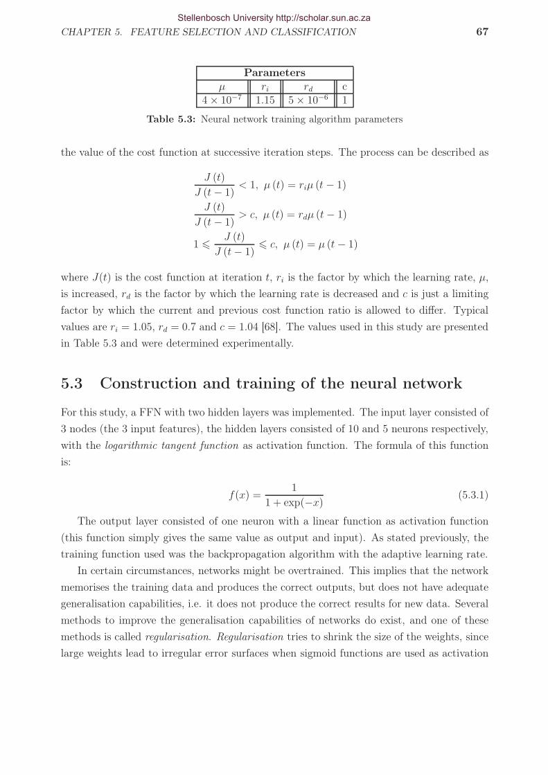
CHAPTER 5. FEATURE SELECTION AND CLASSIFICATION 67
Parametersµ ri rd c
4 × 10⁻⁷ 1.15 5 × 10⁻⁶ 1
Table 5.3: Neural network training algorithm parameters
the value of the cost function at successive iteration steps. The process can be described as
J (t)
J (t − 1)< 1, µ (t) = riµ (t − 1)
J (t)
J (t − 1)> c, µ (t) = rdµ (t − 1)
1 6J (t)
J (t − 1)6 c, µ (t) = µ (t − 1)
where J(t) is the cost function at iteration t, ri is the factor by which the learning rate, µ,
is increased, rd is the factor by which the learning rate is decreased and c is just a limiting
factor by which the current and previous cost function ratio is allowed to differ. Typical
values are ri = 1.05, rd = 0.7 and c = 1.04 [68]. The values used in this study are presented
in Table 5.3 and were determined experimentally.
5.3 Construction and training of the neural network
For this study, a FFN with two hidden layers was implemented. The input layer consisted of
3 nodes (the 3 input features), the hidden layers consisted of 10 and 5 neurons respectively,
with the logarithmic tangent function as activation function. The formula of this function
is:
f(x) =1
1 + exp(−x)(5.3.1)
The output layer consisted of one neuron with a linear function as activation function
(this function simply gives the same value as output and input). As stated previously, the
training function used was the backpropagation algorithm with the adaptive learning rate.
In certain circumstances, networks might be overtrained. This implies that the network
memorises the training data and produces the correct outputs, but does not have adequate
generalisation capabilities, i.e. it does not produce the correct results for new data. Several
methods to improve the generalisation capabilities of networks do exist, and one of these
methods is called regularisation. Regularisation tries to shrink the size of the weights, since
large weights lead to irregular error surfaces when sigmoid functions are used as activation
Stellenbosch University http://scholar.sun.ac.za

CHAPTER 5. FEATURE SELECTION AND CLASSIFICATION 68
functions [69]. During regularisation the cost function is calculated by:
J = αN∑
i=1
ε(i) + (1 − α)εp(w) (5.3.2)
where εp(w) is the error function, dependent on the weights of the network and is equal to:
εp(w) =1
K
K∑
k=1
w2k (5.3.3)
and α is the regularisation parameter. This method improved the results and hence was
implemented in the final network structure. In the final network structure α was set to 0.5,
giving equal importance to the weights and the network errors.
The number of features to be used in the network were determined, as explained in
Section 5.1.1. The number of hidden layers and nodes in the hidden layers were determined
by trial-and-error. The configuration that provided the best results were two hidden layers
with 10 and 5 nodes respectively. The network was trained by implementing a variation of
the leave-one-out algorithm, as was done in [70] and [39]. Thirteen abnormal data sets and
16 normal data sets were randomly selected as training data and one normal data set and
one abnormal data set were selected as test data. This process was repeated 50 times in
order to test a wide variety of combinations of normal and abnormal datasets.
It had to be decided which threshold would be used to differentiate between normal and
abnormal data, e.g. for a threshold of value t, all values below t would be set to 0 and
all values equal and above t would be set to 1, where t is a value between 0 and 1. One
way of determining the optimal threshold value is by constructing a Receiver Operating
Characteristic (ROC) curve. An ROC curve is a measure of how well a specific decision-
making system classifies between different classes. It is based on detecting the optimal
threshold to distinguish between two probability density functions. The aim is to maximise
the true-positive fraction (TPF) while at the same time minimising the false-positive fraction
(FPF). The TPF is the number of patients who are classified correctly as having the disease,
i.e. the sensitivity. The FPF is the number of people who have the disease, but are classified
as not having the disease. The FPF is related to the true-negative fraction (TNF) by the
following relation:
FPF + TNF = 1 (5.3.4)
The optimal threshold was calculated as 0.35, producing a TPF of 0.8571 and a FPF
of 0.1765. However, it was noted that the FPF was 0 and TPF was 0.7857 at a threshold
of 0.4 and, therefore, it was decided to examine the threshold in this range more closely to
Stellenbosch University http://scholar.sun.ac.za

CHAPTER 5. FEATURE SELECTION AND CLASSIFICATION 69
0 0.2 0.4 0.6 0.8 10
0.1
0.2
0.3
0.4
0.5
0.6
0.7
0.8
0.9
1
FPF
TP
F
ROCIdeal ROC
Figure 5.7: ROC curve for classification scheme used
ascertain if better results could be achieved. The thresholds in the range from 0.4 to 0.25
were varied in steps of 0.01 and, indeed, better results were achieved. Thresholds equal to
0.39 and 0.38 resulted in a FPF of 0.0588 and a TPF of 0.8571 and were thus deemed as
the optimal.
A measure of the effectiveness of a specific test is given by the area under the ROC curve
[11]. This value can only be between 0 and 1. The closer this value is to 1, the better the
test. The area under the curve in Figure 5.7 was calculated as 0.9076, which indicates that
the test is of a very good standard. The ideal curve is also shown in comparison with the
ROC curve of this test.
The optimal threshold value was calculated to be 0.38, resulting in a TPF of 0.8571 and
FPF of 0.0588. This in turn resulted in a sensitivity of:
Sensitivity = TPF = 85.7%
and a specificity of:
Specificity = (1 − FPF ) × 100% = (1 − 0.0588) × 100% = 94.1%
This means that 85.7% of the abnormal patients were classified correctly as abnormal and
94.1% of the normal patients were classified correctly as normal.
Stellenbosch University http://scholar.sun.ac.za

Chapter 6
Conclusions and Recommendations
Problems regarding the cycle and feature extraction processes, as well as the ANN, are
discussed and possible solutions are presented. An overview of the positive and negative
aspects of the auscultation jacket and its application to telemedicine is also given.
6.1 Data analysis and classification system
6.1.1 Cycle extraction
In some instances cycle extraction was not possible, since the ECG recorded simultaneously
with the heart sounds produced artifacts as shown in Figure 6.1. When this signal was passed
through the first-derivative operator and the MA filter (refer Section 4.1.2) it produced
artifacts that were incorrectly labelled as QRS-peaks and this resulted in the extraction of
incorrect cycles. Recordings in which the ECG did not record properly, had to be discarded
and could not be used in the training of the Neural Network. Figure 6.1 shows the originally
recorded ECG signal after it had been low-pass filtered (refer Section 4.1). Figure 6.2 shows
the signal after it had been passed through the first derivative operator and MA filter (refer
Section 4.1.2). It can clearly be seen that peaks are presented that cannot be attributed to
QRS-peaks.
One might ask why the threshold was not simply increased. In some instances the
amplitude of the consecutive QRS-peaks differed from the maximum peak amplitude to
such an extent that when the threshold was increased, the peaks were also removed and the
cycle extraction process missed some cycles. Because of the fact that the successive ECG
cycle intervals were compared with one another, these intervals fell outside the allowed
range and resulted in no extracted cycles. All such erroneous cycles as mentioned had to
be discarded.
Two ECG recordings were taken, because it was only realised after the ECG had been
built into the jacket that the ECG recording would be needed to identify the start of S1.
70
Stellenbosch University http://scholar.sun.ac.za

CHAPTER 6. CONCLUSIONS AND RECOMMENDATIONS 71
0 1 2 3 4 5 6 7 8 9−0.5
0
0.5
1
Time [sec]
Nor
mal
ised
am
plitu
de
Figure 6.1: Recorded GeoAxon ECGshowing artifacts that prohibited cycleextraction
0 1 2 3 4 5 6 7 8 90
1
2
3
4
5
6
7
Time [sec]
Nor
mal
ised
am
plitu
de
Figure 6.2: QRS-peaks with artifactsthat resulted in wrongly extracted cy-cles
Because this was only a prototype of the auscultation jacket, it was the easiest and quickest
solution to the problem to record an extra ECG together with the stethoscope data instead
of attempting to access the recording process of the built-in ECG and trying to synchronise
that with the recording of the stethoscopes. This would be the most sophisticated solution
and would nullify the effects of artifacts. This procedure should definitely be attempted in
the following version of the auscultation jacket.
6.1.2 Denoising
The denoising procedure of the recorded heart sounds presented a problem in that if the
wavelet threshold was set too high, some of the information was discarded. The use of high-
or low-pass filters did not solve this problem either, since the noise frequencies were in the
same range as the frequencies of interest. Averaging was not used and might provide better
results as indicated in [24].
Some of the stethoscopes (especially the stethoscopes at the 2nd left and right intercostal
spaces) did not make sufficient contact with the patient’s skin. This resulted in “noisy
scrathes” in the data, as the patient’s chest moved up and down during breathing. This
situation was exarcebated if the patient had a significant amount of chest hair. Figure
6.3 shows the recording of a normal patient at the 2nd right intercostal space, where the
stethoscope did not make sufficient contact with the skin. Figure 6.4 shows the recording
at the 4th right intercostal space for the same patient, where the stethoscopes did make
sufficient contact with the patient’s skin. Figures 6.5 and 6.6 show the denoised signals. It
can be seen that no information could be extracted from the recording at the 2nd intercostal
space in comparison to the recording at the 4th intercostal space. The recording at the 2nd
intercostal space (and thus the whole feature set) could thus not be used to train the Neural
Stellenbosch University http://scholar.sun.ac.za

CHAPTER 6. CONCLUSIONS AND RECOMMENDATIONS 72
0 0.5 1 1.5 2 2.5−1
−0.8
−0.6
−0.4
−0.2
0
0.2
0.4
0.6
0.8
1
Time [sec]
Am
plitu
de
Figure 6.3: Recording of normal pa-tient at 2nd right intercostal spaceshowing noise generated by insufficientcontact between stethoscope and skin
0 0.5 1 1.5 2 2.5−2
−1.5
−1
−0.5
0
0.5
1
Time [sec]
Am
plitu
de
Figure 6.4: Recording of normalpatient at 4th right intercostal spaceshowing that less noise is generatedwith sufficient contact between stetho-scope and skin
Network.
0 0.5 1 1.5 2 2.5−0.5
−0.4
−0.3
−0.2
−0.1
0
0.1
0.2
0.3
0.4
Time [sec]
Am
plitu
de
Figure 6.5: Denoised recording show-ing that no information could be ex-tracted due to poor original recording
0 0.5 1 1.5 2 2.5−0.8
−0.6
−0.4
−0.2
0
0.2
0.4
0.6
Time [sec]
Am
plitu
de
Figure 6.6: Denoised recording show-ing sufficient information to be ex-tracted
6.1.3 Feature extraction
6.1.3.1 Duration of S2 split
The calculation of the S2 split proved to be more difficult than initially anticipated. The
procedure implemented in section 4.2.6 gave reasonable results but in some instances the
correct peaks in the CWT were not identified sufficiently. For example, if a value that
Stellenbosch University http://scholar.sun.ac.za
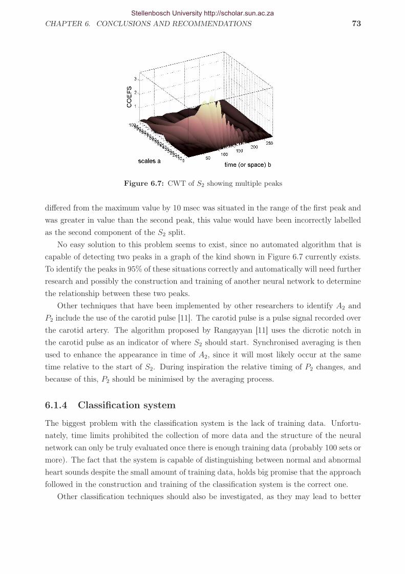
CHAPTER 6. CONCLUSIONS AND RECOMMENDATIONS 73
Figure 6.7: CWT of S2 showing multiple peaks
differed from the maximum value by 10 msec was situated in the range of the first peak and
was greater in value than the second peak, this value would have been incorrectly labelled
as the second component of the S2 split.
No easy solution to this problem seems to exist, since no automated algorithm that is
capable of detecting two peaks in a graph of the kind shown in Figure 6.7 currently exists.
To identify the peaks in 95% of these situations correctly and automatically will need further
research and possibly the construction and training of another neural network to determine
the relationship between these two peaks.
Other techniques that have been implemented by other researchers to identify A2 and
P2 include the use of the carotid pulse [11]. The carotid pulse is a pulse signal recorded over
the carotid artery. The algorithm proposed by Rangayyan [11] uses the dicrotic notch in
the carotid pulse as an indicator of where S2 should start. Synchronised averaging is then
used to enhance the appearance in time of A2, since it will most likely occur at the same
time relative to the start of S2. During inspiration the relative timing of P2 changes, and
because of this, P2 should be minimised by the averaging process.
6.1.4 Classification system
The biggest problem with the classification system is the lack of training data. Unfortu-
nately, time limits prohibited the collection of more data and the structure of the neural
network can only be truly evaluated once there is enough training data (probably 100 sets or
more). The fact that the system is capable of distinguishing between normal and abnormal
heart sounds despite the small amount of training data, holds big promise that the approach
followed in the construction and training of the classification system is the correct one.
Other classification techniques should also be investigated, as they may lead to better
Stellenbosch University http://scholar.sun.ac.za

CHAPTER 6. CONCLUSIONS AND RECOMMENDATIONS 74
results than ANNs. Other techniques that have been implemented in other studies, include
decision tree classifiers [41], linear discriminant functions [42] and Hidden Markov Models
[37]. Unsupervised pattern classification techniques such as the k-means algorithm and
the maximin-distance algorithm could also be researched. Feature reduction techniques
such as principal component analysis and independent component analysis should also be
considered.
The features that were eventually used as inputs to the ANN only evaluated information
from the diastolic region of the heart cycle. It was decided to train and test the ANN with
systolic information added to the inputs, to determine whether this would increase the
sensitivity and specificity of the ANN. Different combinations of systolic data, together
with the diastolic information already present, was presented to the ANN as input data.
Satisfactory results were not achieved. This can be attributed to the fact that there is not
sufficient discrimination between the systolic data of the normal and abnormal heart sounds
that enables the ANN to properly discriminate between the two classes. Better recording
procedures and denoising procedures could improve this result.
6.2 Recommendations concerning the auscultation
jacket
Since this is only the first attempt at a prototype of the auscultation jacket, numerous
improvements could be made. The greatest weakness of the jacket is that the stethoscopes,
and thus the electrodes embedded into the stethoscopes, move relative to the body surface
as the patient breathes. This in turn, causes the ECG recorded with the jacket to be
unreliable. The afore-mentioned is the reason why not more of the ECG information was
used as features in the classification scheme. Examples of these are the height of the P-wave,
where the P-wave occurs with respect to the QRS-complex, whether the QRS-complex is
inverted or not, etc. All of these features could be used to extend the screening capabilities of
the jacket beyond simple auscultation abnormalities. The screening of other cardiovascular
diseases such as myocardial infarction (heart attack) which may be diagnosed by a significant
decrease in the R-wave amplitude due to the loss of tissue would also be possible.
The side pieces of the jacket also present a problem. They move around and do not
necessarily correspond to the correct position for V6. To correct this problem it is proposed
that the stethoscopes should be fitted with double-sided tape that is capable of fixing the
position of the stethoscope (and thus the electrode) to the skin surface of the patient. This
material should be of such a nature that it could be easily removed from the stethoscope
between recordings.
The two stethoscopes, which correspond to the auscultation positions at the 2nd left
Stellenbosch University http://scholar.sun.ac.za

CHAPTER 6. CONCLUSIONS AND RECOMMENDATIONS 75
and right intercostal spaces (pulmonary and aortic areas respectively), present a two-fold
problem. Firstly, these two stethoscopes are the main reason why the jacket cannot be used
on women. The current size of the stethoscopes prohibit the stethoscopes from making
sufficient contact with the body between the breasts. The second problem is that these
two stethoscopes do not make sufficient contact with some male patients when they are in
the supine positions. This leads to noisy data that cannot be used. It is proposed that
the contour surface of the jacket be changed in such a way that it follows the contour of
the body better. This could be done by installing an inflatable bladder, that can press
the stethoscopes down until sufficient contact is made, in the jacket . Each stethoscope
could also have its own inflatable bladder and could be inflated individually. However, this
concept brings about a number of problems, such as the number of pipes needed to inflate
the jacket, whether it would be possible to seal off the bladder to avoid leakage, what size
pump would be needed to inflate the jacket, etc. All these factors will have to be taken into
account and assessed individually before making use of this idea. Another idea is to embed
the stethoscopes in sponge that is thicker at the positions that correspond to the 2nd left
and right intercostal spaces. This would also ensure that better contact is made with the
skin. Another strap could also be inserted on the side of the jacket at the height of the
2nd intercostal space. This strap could then be tightened around the body to ensure that
sufficient contact is made with the skin at these locations.
The number of cables is also a definite problem. Keeping in mind that this was a first
attempt at a prototype, the number of cables was not a major problem, but it would be
more practical to reduce the number of cables. Implementing wireless technology could pose
a solution. The hub to which the stethoscopes and ECG are connected, could be placed on
the jacket instead of hanging loose, as it is in the current prototype.
As the jacket was fitted on healthy as well as unhealthy patients, it was noted that if
the patient is significantly weakened, as in the case of someone with severe valvular heart
disease, it gets difficult to fit the person with the jacket. Since it is proposed to develop
this jacket to be used on patients who do suffer from valvular or other heart disease, this
problem is something that has to be considered and addressed.
Other aspects to think about are the stethoscopes themselves. During the recording
process the diaphragms of some of the stethoscopes became dislodged because of multiple
usage. The ECG electrode gel reacted with the glue that held the diaphragms in place and
this also aggravated the problem. To counter this, the diaphragm could be built into the
stethoscope by creating a small slot on the inside of the stethoscope casing and inserting the
flexible diaphragm. The diaphragm could also be discarded, since it only acts as a low-pass
filter and any noise that is recorded can be filtered out after the recording.
The stethoscopes are also very bulky and add a lot of weight to the jacket although the
casings are manufactured of aluminium. It might be beneficial to consider using accelerom-
Stellenbosch University http://scholar.sun.ac.za

CHAPTER 6. CONCLUSIONS AND RECOMMENDATIONS 76
eters instead of microphones to record the heart sounds, as they are much smaller, but this
still has to be researched. Accelerometers have been used in a previous study to record
lung sounds as described in Pourazad et al. [43]. The authors used two Siemens EMT 25
C piezoelectric contact accelerometers to record the lung sounds.
6.3 Application to telemedicine?
Telemedicine is defined as “the use of telecommunication technology (involving audio, video,
and graphic data) to deliver healthcare services, health education, and administrative ser-
vices to sites that are physically distant from the host or educator” [71]. According to the
Medical Research Council of South Africa, the South African government is “committed
to providing basic health care to all South African citizens” and “to achieve this goal, the
government has identified Telemedicine as a strategic tool for facilitating the delivery of
equitable healthcare and educational services”.
Telemedicine has proved useful and necessary in developing countries. In India, for
example, the Online Telemedicine Research Institute (OTRI) has made a great impact on
the lives of people. In January of 2001, an earthquake hit the city of Bhuj in Western India
and left thousands dead and homeless. Within a day, the OTRI in Ahmedabad established
satellite telephone links and set up all equipment necessary to provide emergency medical
care through telemedicine. Ahmedabad is 300 km from Bhuj. The satellite phones were soon
replaced by VSAT with phone lines and ISDN. A fully-fledged telemedicine system was used
for teleconsultation in pathology, radiology, and cardiology over ISDN lines, and between
district hospitals near Bhuj and other in Ahmedabad. Seven-hundred and fifty sessions
consisting primarily of X-rays and ECGs of patients, were transmitted in one month to
specialists in Ahmedabad [71].
Although telemedicine has proved helpful in some cases, it also has its limitations. In
some areas, the infrastructure is extremely poor and it is very difficult to implement a
telemedicine centre in an area that has little or no infrastructure. The problem is that
physicians tend to leave the rural areas for bigger cities and improperly trained technicians
are left in charge of health facilities. These technicians rarely have any experience working on
computers [72]. In the Alto Amazonas province of Peru, 64.9% of the healthcare personnel
have never used a computer and 89% of the healthcare personnel have never used e-mail. It
may be argued that since Peru is also a developing country, more or less the same conditions
exist in South Africa. This poses a big problem in setting up a telemedicine centre in the
rural areas of South Africa.
No roads, administrative problems (information being sent has to be paid for by the
health staff themselves) and no feedback to the rural health centres are just some of the
Stellenbosch University http://scholar.sun.ac.za

CHAPTER 6. CONCLUSIONS AND RECOMMENDATIONS 77
challenges in such areas. A delay of 13 months on the arrival of information is common
practice in these areas. Many healthcare personnel have to pay their travel costs themselves.
On average this accounts to 17% of his or her salary [72]. The use of electronic mail could
reduce the amount of time needed to travel by coordinating certain travels with others.
Training of healthcare personnel could also be improved by supplying the information better
and faster to rural areas. 59% of the healthcare staff in Alto Amazonas said they do not
attend courses because the information arrives too late or not at all.
On the practical side, many of these areas do not have electricity, no public telecommu-
nication infrastructure, have limiting purchasing power, maintenance costs are high due to
the poor infrastructure and few well-trained people in managerial positions are available.
To combat this, any telemedicine equipment installed has to fulfil the following conditions
[72]:
• Be highly robust
• Any technological platform must demand low infrastructure, maintenance and opera-
tion costs
• Low energy consumption
• Technical personnel will have to be trained in system management, maintenance, and
repair
However, in sub-Saharan Africa telemedicine has been implemented in several countries
to address the extremely poor medical infrastructure. Sub-Saharan Africa is home to 33 of
the 48 least developed countries in the world and telemedicine would thus have far-reaching
effects in these countries by making proper healthcare accessible to everyone [71].
The final aim of the auscultation jacket is to distribute the jacket to rural areas that do
not have sufficient healthcare facilities. Patients will then be recorded with the jacket and the
data will be sent via a communication link to physicians who are able to interpret the data
and provide feedback on each patient. Many factors have to be taken into consideration
before such a system can be implemented, but the possibility is real and will have far-
reaching positive effects if the process is managed and implemented correctly.
6.4 Other applications
The application of the auscultation jacket can be expanded to include educational appli-
cations as well. For instance, if patient contact is prohibited or limited due to a specific
disease as in [73] where patient contact was prohibited due to severe acute respiratory syn-
drome (SARS), the monitoring of patients could be done with the help of the auscultation
Stellenbosch University http://scholar.sun.ac.za

CHAPTER 6. CONCLUSIONS AND RECOMMENDATIONS 78
jacket. In the mentioned study, cardiac sounds were recorded with Littmann model 4000
stethoscopes and played back to students to assist in teaching auscultation skills. The aus-
cultation jacket could have been implemented to record all the heart and lung sounds, ECG
and ICG for educating purposes at a later stage.
The auscultation jacket, together with the classification system, can be used as a train-
ing tool for students to determine whether a patient has cardiovascular (or pulmonary)
pathology or not. According to Tuchinda et al. teaching cardiac auscultation skills has
been difficult “due to time constraints and the impracticability of examining large numbers
of patients with cardiac pathology”[74]. A database consisting of recordings made with the
auscultation jacket can be made and students can thus access recordings made at different
locations on the body in their own time. This would enable them to make their own diag-
nosis and check it against the results of the classification system. This eliminates the need
for examination of a large number of patients. The doctor-patient relationship is a very
necessary and important one and it is not proposed to do away with this relationship.
According to March et al. “the ability of many of today’s health care professionals
to correctly identify normal and abnormal heart sounds continues to diminish” [4]. The
auscultation jacket and classification system can help overcome this obstacle by providing
diagnostic information to physicians who are uncertain of a specific pathology.
Stellenbosch University http://scholar.sun.ac.za

Appendices
79
Stellenbosch University http://scholar.sun.ac.za

Appendix A
Relevant technologies
Many techniques that are used to diagnose heart disease exist. These techniques in-
clude electrocardiography (ECG), echo-cardiography, impedance cardiography (ICG), nu-
clear stress testing, coronary angiogram, computed tomography (CT) scan, PET (positron
emission tomography)/CT scan and magnetic resonance imaging (MRI). Only the ECG,
echo-cardiography and ICG will be discussed here.
A.1 Electrocardiogram (ECG)
The Electrocardiogram (ECG) measures the electrical activity of the human heart. The
electrical impulses that make the heart contract spread across the heart in a specific manner
and any deviation from this could indicate pathology. To explain and understand the ECG
waveform, the electrical system of the heart first has to be explained. Refer to Figure A.1
for a diagram of the heart and its electrical system. A normal ECG graph is shown in Figure
A.2. This ECG was recorded with the auscultation jacket. The heart’s pacemeaker is the
Sinoatrial (SA) node. Action potentials 1 are generated here and travel from here through
the rest of the electrical system. The action potential first travels down the anterior, middle
and posterior internodal tract as well as Bachmann’s bundle. In doing so, the muscle cells of
the atria depolarise (the action potential is raised from -90 mV towards 0 mV) and the atria
begin to contract. This corresponds to the P-wave in the ECG waveform and is shown as
section C in Figure A.2. The P-wave has a duration of 60−80 ms. When the action potential
arrives at the AV node, there is a delay of approximately 60− 80 ms [11]. This is known as
the P-Q segment and is shown as section D in Figure A.2. The action potential now travels
down the left and right bundle branches in the interventricular septum, into the conduction
pathways (also known as Purkinje fibres). As the action potential moves upward through
1A change in the membrane potential of cells (from the normal -90 mV), initiated by a change in themembrane permeability to sodium ions [10].
80
Stellenbosch University http://scholar.sun.ac.za

APPENDIX A. RELEVANT TECHNOLOGIES 81
Figure A.1: Schematic of the electrical system of the human heart [75]
the heart from the apex, the ventricles contract, resulting in the QRS-complex in the ECG
waveform (section E in Figure A.2) lasting about 80 ms. The QRS-complex is relatively
large in comparison to the other waveforms in the ECG, since the mass of the ventricles is
much larger than the mass of the atria. The action potential duration of ventricular muscle
cells is relatively long (300 − 350 ms) [11]. This results in a section of little activity after
the QRS-complex known as the S-T segment (section F ) and lasts for about 100 − 120
ms. Repolarisation (membrane potential of cardiac muscle cells return to -90 mV) of the
ventricles lasts for about 120− 160 ms and can be seen in the ECG as the T-wave (section
G). Section A is known as the P-Q interval and shows the electrical potential of the atria.
Section B is known as the Q-T interval and shows the electrical potential of the ventricles
during a single cardiac cycle.
Sometimes a U-wave is present after the T-wave (not present in Figure A.2), but the
origin of the U-wave is still a topic of debate [76]. Three hypotheses exist on the genesis of
the U-wave: late repolarisation of Purkinje fibres, late repolarisation of other portions of the
left ventricle and alteration in the normal action potential shape by after-potentials, which
are most likely generated by mechano-electric feedback [76]. The U-wave has the same
polarity as the T-wave in normal subjects; when the polarity of the U-wave is reversed, it
is, therefore, of great clinical importance [76].
The electrical potentials are measured by electrodes placed on the surface of the skin.
The electrodes are placed at different positions on the body, depending on which ECG
configuration is being used, e.g. 12-lead ECG, 6-lead ECG, 3-lead ECG or 1-lead ECG. For
a 12-lead ECG 6 electrodes are placed on the thorax in the V1-V6 positions (refer to Figure
A.3). For the remaining four electrodes there are two possible combinations: one electrode
Stellenbosch University http://scholar.sun.ac.za

APPENDIX A. RELEVANT TECHNOLOGIES 82
0 0.1 0.2 0.3 0.4 0.5 0.6 0.7 0.8 0.90
0.5
1
1.5
2
2.5
Time [sec]
Am
plitu
de
PQ
R
S T
A B
C D E F G
Figure A.2: Normal ECG wave
can be placed on each wrist and foot, or one electrode can be placed on each shoulder and
hip (refer to Figure A.4 and Figure A.5).
The graphs that are displayed on the standard ECG recording correspond to how the
action potentials spread through different axes of the heart. In effect, one looks at how
the heart contracts from different angles around the heart. Specific patterns are associated
with each view and any deviation from this could indicate pathology. The different axes are
shown in Figure A.6.
To understand how the deflections for specific axes are formed, the volume conductor
principle has to be explained. Consider a mass of ventricular muscle placed in a bath of salt
Figure A.3: V1-V6 positions [77]
Stellenbosch University http://scholar.sun.ac.za

APPENDIX A. RELEVANT TECHNOLOGIES 83
Figure A.4: Configuration for ECGelectrodes on wrists and feet [77]
Figure A.5: Configuration for ECGelectrodes on shoulders and hips [77]
water. In the resting state of the ventricular muscle, the outside of the cells is positively
charged with respect to the inside of the cell. For heart muscle cells, the resting membrane
potential (RMP) is approximately -90 mV [10]. If two electrodes are placed on either side
of the ventricular mass, no potential difference will be measured between the electrodes, as
in Figure A.7. When an action potential spreads across the heart (from negative to positive
in this case), however, some of the muscle cells on the left side of the ventricular mass is
charged negatively with respect to the inside (due to the in- and outflow of sodium and
potassium ions) and a positive deflection is measured on the positive electrode.
A.1.1 Atrial depolarisation
Atrial depolarisation starts with the activation of the SA node. As the wave of depolarisation
spreads across the atria, some of the muscle cells are negatively charged with respect to the
inside (depolarised) and some of the muscle cells are still at their RMP(polarised) and,
therefore, positive with respect to the inside. A positive deflection is thus seen on the ECG
Figure A.6: Heart axes as viewed by different leads
Stellenbosch University http://scholar.sun.ac.za

APPENDIX A. RELEVANT TECHNOLOGIES 84
Figure A.7: Potential difference between two sides of ventricular muscle mass is zero when thereis no depolarisation wave, and positive when depolarisation moves towards the positive electrode[78]
tracing. Once all of the atrial muscle cells are depolarised, the net potential difference is
again zero and no deflection is seen. Figure A.8 explains this, as well as the spread of the
repolarisation wave schematically. When repolaristaion occurs, the opposite happens. The
muscle cells that were first depolarised are first to repolarise and their net charge with respect
to the inside of the cell is once again positive. Because the cells that are still negative are
now closer to the positive electrode, and a net negative potential difference exists between
the two electrodes, a negative deflection is seen in the ECG tracing. Once all the cells are
positive with respect to the inside (repolarisation has stopped), the net potential difference
is zero and no deflection is seen on the ECG tracing.
Figure A.8: Spread of atrial depolarisation and repolarisation waves and resulting deflections inECG tracing [78]
Stellenbosch University http://scholar.sun.ac.za

APPENDIX A. RELEVANT TECHNOLOGIES 85
Figure A.9: Spread of ventricular depolarisation wave showing resulting deflections in ECG tra-cing [78]
A.1.2 Ventricular depolarisation
The spread of the repolarisation wave across the ventricles is as shown in Figure A.9. This
explanation is based on lead II of the ECG axis. The ventricular depolarisation waves
originate at the AV node and first spread down the interventricular septum through the
left and right bundle branches (refer Figure A.1). The septum thus depolarises from left to
right, as shown in sketch A of Figure A.9. When viewing Figure A.9, it should be kept in
mind that the left side of the heart is to the right of the sketch. The plus and minus in each
sketch shows the position of the positive and negative electrodes for the lead II orientation.
The mean electrical vector is orientated in such a way that it moves away from the positive
electrode and the result is a negative deflection in the ECG tracing. This corresponds to
the Q-wave in the QRS-complex.
The repolarisation wave now moves further down the septum and reaches the apex of
the heart and begins to move through the Purkinje fibres (sketch B in Figure A.9). The
mean electrical vector is almost parallel to the orientation of lead II and moves towards the
positive electrode, thus resulting in a considerable positive deflection in the ECG tracing.
This corresponds to the R-wave in the QRS-complex of the ECG tracing.
Next the wave moves up the ventricles, almost totally depolarising the right ventricle
and partially depolarising the left ventricle. This is because the left ventricle is much larger
than the right ventricle. The mean electrical vector is orientated as shown in sketch C of
Figure A.9 and results in a small positive deflection in the ECG tracing. The last regions to
depolarise are the topmost areas of the ventricles and the resulting mean electrical vector
points upwards (towards the negative electrode) and to the left, resulting in a minor negative
deflection in the QRS-complex (the S-wave).
During ventricular repolarisation, the cells that were depolarised last are the first ones
to repolarise, therefore, the repolarisation waves move in the opposite direction to the
depolarisation waves, thus resulting in a positive deflection in the ECG tracing, whereas
Stellenbosch University http://scholar.sun.ac.za

APPENDIX A. RELEVANT TECHNOLOGIES 86
Figure A.10: Standard bipolar limb leads for a 12-lead ECG configuration [78]
atrial repolarisation results in a negative deflection in the ECG tracing.
As the heart contracts (depolarises), a multitude of depolarisation waves spread across
the heart. The mean electrical vector is the sum of all these vectors (waves) of depolarisation
at a specific instant in time [78]. Physicians often refer to the mean electrical axis of a
patient. This refers to the average of all the mean electrical vectors and is normally in
the range of 0 ◦ to +90 ◦. If the mean electrical axis is less than 0 ◦ it is termed left axis
deviation and may be indicative of diseases such as inferior myocardial infarction or left
anterior hemiblock [57]. If the mean electrical axis is greater than +90 ◦ it is termed right
axis deviation. In order to determine the mean electrical axis, one should first find the
electrical axis that is biphasic (equal positive and negative deflections). Next, the electrical
axis that is perpendicular to the afore-mentioned axis, that has a net positive deflection,
should be established. The latter axis is then the mean electrical axis.
A.1.3 The lead system
The volume conductor principle also applies when viewing the deflections of a specific ECG
lead (or axis). For the different ECG axes (I, II, V1, aVF etc.), the positive and negative
electrodes are placed at different locations on the body and, thus, different deflections will
be seen by each one. For example, the standard bipolar limb leads are known as Leads I, II
and III and their electrodes are placed on the body as shown in Figure A.10.
As can be seen in Figure A.10, for lead I the positive electrode is situated on the left arm
(LA) and the negative electrode is situated on the right arm (RA). For leads II and III the
positive electrode is situated on the left leg (LL) and the negative electrodes are placed on
the right arm and left arm respectively. Together these three leads form what is known as
Einthoven’s Triangle and examine the depolarisation of the heart from different angles and
Stellenbosch University http://scholar.sun.ac.za

APPENDIX A. RELEVANT TECHNOLOGIES 87
Figure A.11: Einthoven’s Triangle and the Axial Reference System [78]
together they form the Axial Reference System, as shown in Figure A.11. According to the
volume conductor principle, a wave of depolarisation that is moving towards the positive
electrode of lead I, will produce a positive deflection in lead I. The same applies to all the
other leads. If the wave of depolarisation moves towards a positive electrode, a positive
deflection will be seen and if the wave of depolarisation moves away from the positive
electrode, a negative deflection will be seen. Just the same, if a wave of repolarisation
moves towards the positive electrode, a negative deflection will be seen, whereas if the
repolarisation wave moves towards the negative electrode, a positive deflection will be seen.
These rules are universally accepted and apply to all ECG measurements [78].
The leads aVR , aVL and aVF are known as the unipolar augmented limb leads. They
are termed “unipolar” because there a single positive electrode is referenced against a com-
bination of all the other limb electrodes [78]. The positive electrodes are situated on the
left arm (aVL ), right arm (aVR ) and left leg (aVF ). The position of these electrodes and
their positions on the Axial Reference System are shown in Figure A.12.
The three limb leads and the three augmented limb leads view the electrical activity of
the heart form the frontal plane. In addition to this, there are 6 precordial unipolar chest
leads (V1 - V6) that view the electrical activity of the heart in a plane perpendicular to the
frontal plane. Their position on the chest and in the perpendicular plane is shown in Figure
A.13.
The deflections in these tracings are produced in the same way as for all the other leads.
Leads V1 and V2 view the anterior septal region of the heart, leads V3 and V4 view the
anterior apical (apex) region of the heart and leads V5 and V6 view the anterior lateral
region of the heart.
A.2 Echo-cardiography
The echo-cardiogram uses ultrasound waves to examine the heart of a patient. An echo-
cardiogram is also used in evaluating the fetus of a pregnant female. Ultrasonic gel is
applied to the thorax of the individual on the area of interest to aid in the transmitting of
the ultrasonic waves. A transducer then sends ultrasonic waves through the body and these
Stellenbosch University http://scholar.sun.ac.za

APPENDIX A. RELEVANT TECHNOLOGIES 88
Figure A.12: Unipolar augmentedlimb leads position [78]
Figure A.13: Precordial unipolarchest leads positions [78]
are reflected back by the heart, collected by the transducer and transformed to an image of
the heart.
The single dimension (1-D) echo-cardiogram is known as M-mode echo-cardiography. In
M-mode echo-cardiography a narrow beam is directed towards the region of interest and the
output is the movement of the structures through which the beam passes as a function of
time. Characteristic patterns are associated with certain pathologies such as mitral stenosis
and pericardial effusions, which are easily recognised [12].
A more advanced type of echo-cardiography, 2-D echo, gives a two-dimensional sectional
view of the heart. This is probably the most well-known type of echo-cardiogram. In
this type of echo-cardiogram the transducer beam moves across the chest wall in a sweeping
manner, updating the picture with each sweep. The transducer can either be of the sweeping
or rotating type. In the rotating transducer the head has a multitude of transducers inside
a liquid-filled dome. One transducer emits a beam and receives the echo back and the next
transducer in line takes over and does the same and so on and so forth. In this manner
the picture is continuously updated so that the movement of the structures are displayed
in real-time [79]. Figure A.14 shows how the transducer beam sweeps across the heart and
the resulting image formed. Figure A.15 shows an echo-cardiogram of the four chambers of
the heart.
Stellenbosch University http://scholar.sun.ac.za

APPENDIX A. RELEVANT TECHNOLOGIES 89
Figure A.14: Sweeping of echo-cardiography transducer beam and how resulting image is formed[79]
Figure A.15: Echo-cardiogram of normal heart showing different chambers [80]
A.3 Impedance cardiography (ICG)
Impedance cardiography is a technique by means of which the resistance of the thorax to
a small current is measured. From this measurement, parameters such as cardiac output,
stroke volume, etc. are calculated. Eight electrodes are placed on the thorax and neck for
use in the measurements (see Figure A.16). The inner electrodes (white & red) are the
sensing electrodes, while the outer electrodes (black & green) are the source and sink of the
measurement current. The white electrodes must be placed along the line of the root of
the neck and the red electrodes are placed on either side (midaxillary line) of the patient
at the xiphoid process level (diaphragm level). The black electrodes are placed above the
white electrodes at 5 cm distance and the green electrodes are similarly placed below the
Stellenbosch University http://scholar.sun.ac.za

APPENDIX A. RELEVANT TECHNOLOGIES 90
Figure A.16: Electrode positions for ICG measurements
red electrodes.
A high-frequency current (65 kHz, 7 µA RMS) is introduced between the black and
the green electrode pairs. The current flows through the thorax, parallel to the spine,
primarily through the aorta and superior and inferior vena cavae, since this is the path of
least resistance. Due to this high-frequency current, a high-frequency voltage is developed
across the thorax and sensed by the white and red electrode pairs. This voltage is directly
proportional to the impedance of the thorax [81]. As the impedance, known as Thoracic
Electrical Bioimpedance (TEB), in the thorax changes, the changes are measured and certain
parameters are calculated.
Before one starts an ICG test, the height(H) in cm and weight(W) in kg of the patient
have to be entered into the program. The ideal weight of a male of the specified height is
calculated by:
Wideal male = 0.524 × H − 16.58 (A.3.1)
The volume of electrically participating tissue (VEPT) is then calculated as:
V EPTmale =(0.17 × H)3
4.25× (1 + 0.65 × (
W
Wideal male
− 1)) (A.3.2)
The body surface area (BSA) is calculated from the DuBois & DuBois [81] formula as:
BSA = W 0.425 × H0.725 × 0.007184 (A.3.3)
The stroke index (SI ) 2 and cardiac index (CI ) 3 can then be calculated by:
2The amount of blood pumped by the left ventricle in one heart beat interval, indexed by the BSA[ml/m2].
3The amount of blood delivered by the heart to the body in one minute, indexed by the BSA [l/min/m2].
Stellenbosch University http://scholar.sun.ac.za

APPENDIX A. RELEVANT TECHNOLOGIES 91
SIactual =2
BSA× V EPTmale
6800× SITEBCO (A.3.4)
and
CIactual =2
BSA× V EPTmale
6800× CITEBCO (A.3.5)
where SITEBCO and CITEBCO are standardised values for a male of height (H) = 180 cm and
weight (W) = 80 kg, transmitted by TEBCO and are equal to 49 ml/m2 and 4.9 l/min/m2
respectively.
The parameters that were measured are (definitions were obtained from [53; 82; 81]):
• Heart rate: The heart rate is the number of times the heart beats in one minute and
is measured in beats per minute.
• Ventricular ejection time (VET): VET is the time from aortic valve opening to
closure during the systolic portion of the cardiac cycle. The duration of VET is
shortened by heart failure.
• Pre-ejection period (PEP): PEP represents the time from onset of electrical ac-
tivity of the heart (measured by the start of the QRS-complex) to the opening of the
aortic valve (the onset of left ventricular ejection). PEP is shortened by hyperadre-
nergic4 states and prolonged by heart failure.
• Thoracic fluid conductivity (TFC): This is the total conductivity of the thorax,
measured at 65 kHz between the root of the neck and the diaphragm. TFC represents
the total contribution of all the conductive fluids in the thorax.
• Ejection phase contractility index (EPCI): This represents a combination signal
and takes into account the maximum rate of volumetric change of blood within the
aorta and the maximum rate of alignment of red blood cells. The measurement is
normalised by TFC to produce a per second rate.
• Inotropic State Index (ISI): ISI represents a normalised image of maximum acce-
leration of aortic blood flow and is measured in 1/sec2.
• Ejection Fraction (EF): This is the percentage of blood held within the ventricle
at the end of diastole, which is ejected into the vasculature.
4Adrenergic refers to a synaptic terminal that releases norepinephrine upon stimulation [10]. Hypera-drenergic will then refer to such a state when abnormally large amounts of norepinephrine is released uponstimulation.
Stellenbosch University http://scholar.sun.ac.za

APPENDIX A. RELEVANT TECHNOLOGIES 92
• Stroke Index (SI): The SI is the volume of blood pumped by the left ventricle, over
one heart beat interval indexed by the body surface area (BSA). It is measured in
ml/m2.
• Cardiac Index (CI): This is the amount of blood pumped by the left ventricle in
one minute, indexed by the body surface area (BSA) and is measured in l/min/m2.
• Respiratory Rate (RR): This is the number of breaths per minute.
Stellenbosch University http://scholar.sun.ac.za

Appendix B
Data sheets and data tables
The data sheet for the condenser microphones used and tables with the extracted features
and their respective SOF are given. The selected features are indicated.
93
Stellenbosch University http://scholar.sun.ac.za

APPENDIX B. DATA SHEETS AND DATA TABLES 94
Feature SOF Selected(Y/N)RMS-value of 3rd section of diastole - 2nd IC right 1.6153 YRMS-value of 3rd section of diastole - 2nd IC left 1.6153 YMax frequency of 1st section of diastole - 4th IC right 1.3869 YS1 duration 1.3213 NP-R interval duration 1.2296 NRMS-value of 2nd section of diastole - 2nd IC right 1.1271 NRMS-value of 2nd section of diastole - 2nd IC left 1.1271 NFrequency band ratio of S2 0.9828 NMax frequency of 2nd section of diastole - 2nd IC right 0.9289 NMax frequency of 2nd section of diastole - 2nd IC left 0.9289 NRMS-value of 2nd section of systole - 5th IC left 0.9142 NMax frequency of 3rd section of systole - 2nd IC right 0.9033 NMax frequency of 3rd section of systole - 2nd IC left 0.9033 NAverage power of S1 to S2 ratio - 2nd IC right 0.8986 NAverage power of S1 to S2 ratio - 2nd IC left 0.8986 NRMS-value of 2nd section of diastole - 6th IC left 0.7827 NMax frequency of 2nd section of systole - 5th IC left 0.7801 NMax frequency of 3rd section of diastole - 2nd IC right 0.7434 NMax frequency of 3rd section of diastole - 2nd IC left 0.7434 NAverage power of S1 to S2 ratio - 5th IC left 0.7245 NRMS-value of 3rd section of diastole - 6th IC left 0.6951 NAverage power of S1 to S2 ratio - 6th IC left 0.6941 NMax frequency of 1st section of systole - 4th IC right 0.6859 NMax frequency of 2nd section of systole - 4th IC left 0.6754 NEjection sound power 0.6511 NMax frequency of 3rd section of diastole - 4th IC left 0.6496 NRMS-value of 2nd section of systole - 6th IC left 0.6415 NRMS-value of 2nd section of systole - 2nd IC right 0.6389 NRMS-value of 2nd section of systole - 2nd IC left 0.6389 NMax frequency of 1st section of systole - 4th IC left 0.6207 NMax frequency of 3rd section of diastole - 4th IC right 0.5942 NRMS-value of 3rd section of systole - 2nd IC right 0.5619 NRMS-value of 3rd section of systole - 2nd IC left 0.5619 NS1 beat-to-beat power comparison - 5th IC left 0.5345 NMax frequency of 1st section of systole - 2nd IC right 0.5314 N
Table B.1: Extracted features and their respective SOF
Stellenbosch University http://scholar.sun.ac.za

APPENDIX B. DATA SHEETS AND DATA TABLES 95
Feature SOF Selected(Y/N)Max frequency of 1st section of systole - 2nd IC left 0.5314 NMax frequency of 3rd section of systole - 4th IC right 0.5255 NMidsystolic click power 0.4822 NMax frequency of 2nd section of diastole - 4th IC left 0.4655 NA2- P2 split timing - 2nd IC right 0.4416 NMax frequency of 1st section of diastole - 4th IC left 0.4345 NRMS-value of 1st section of systole - 5th IC left 0.4244 NMax frequency of 2nd section of diastole - 4th IC left 0.4147 NRMS-value of 3rd section of diastole - 5th IC left 0.4126 NMax frequency of 3rd section of systole - 4th IC left 0.4121 NFrequency band ratio of S1 0.4115 NRMS-value of 1st section of diastole - 2nd IC right 0.4101 NRMS-value of 1st section of diastole - 2nd IC left 0.4101 NMax frequency of 3rd section of diastole - 5th IC left 0.3972 NMax frequency of 2nd section of systole - 2th IC right 0.3932 NMax frequency of 2nd section of systole - 2th IC left 0.3932 NOpeningsnap power 0.3931 NRMS-value of 1st section of systole - 6th IC left 0.3800 NRMS-value of 1st section of diastole - 5th IC left 0.3534 NMax frequency of 2nd section of systole - 4th IC right 0.3253 NMax frequency of 1st section of systole - 5th IC left 0.2810 NS1 beat-to-beat power comparison - 6th IC left 0.2790 NMax frequency of 1st section of diastole - 5th IC left 0.2719 NRMS-value of 2nd section of diastole - 5th IC left 0.2324 NMax frequency of 3rd section of systole - 5th IC left 0.2311 NRMS-value of 3rd section of systole - 6th IC left 0.2183 NS2 duration 0.1979 NMax frequency of 2nd section of diastole - 5th IC left 0.1820 NMax frequency of 1st section of diastole - 2nd IC right 0.1360 NMax frequency of 1st section of diastole - 2nd IC left 0.1360 NA2- P2 split timing - 2nd IC left 0.1104 NRMS-value of 3rd section of systole - 4th IC right 0.1014 NRMS-value of 1st section of diastole - 6th IC left 0.0595 NRMS-value of 1st section of systole - 2nd IC right 0.0218 NRMS-value of 1st section of systole - 2nd IC left 0.0218 N
Table B.2: Extracted features and their respective SOF (continued)
Stellenbosch University http://scholar.sun.ac.za
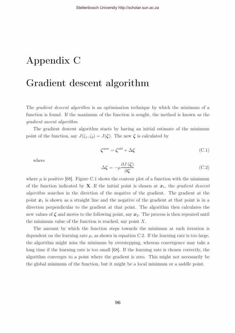
Appendix C
Gradient descent algorithm
The gradient descent algorithm is an optimisation technique by which the minimum of a
function is found. If the maximum of the function is sought, the method is known as the
gradient ascent algorithm.
The gradient descent algorithm starts by having an initial estimate of the minimum
point of the function, say J(ζ1, ζ2) = J(ζ). The new ζ is calculated by
ζnew = ζold + ∆ζ (C.1)
where
∆ζ = −µ∂J (ζ)
∂ζ(C.2)
where µ is positive [68]. Figure C.1 shows the contour plot of a function with the minimum
of the function indicated by X. If the initial point is chosen at x1, the gradient descent
algorithm searches in the direction of the negative of the gradient. The gradient at the
point x1 is shown as a straight line and the negative of the gradient at that point is in a
direction perpendicular to the gradient at that point. The algorithm then calculates the
new values of ζ and moves to the following point, say x2. The process is then repeated until
the minimum value of the function is reached, say point X.
The amount by which the function steps towards the minimum at each iteration is
dependent on the learning rate µ, as shown in equation C.2. If the learning rate is too large,
the algorithm might miss the minimum by overstepping, whereas convergence may take a
long time if the learning rate is too small [68]. If the learning rate is chosen correctly, the
algorithm converges to a point where the gradient is zero. This might not necessarily be
the global minimum of the function, but it might be a local minimum or a saddle point.
96
Stellenbosch University http://scholar.sun.ac.za

APPENDIX C. GRADIENT DESCENT ALGORITHM 97
ζ1
ζ 2
10 20 30 40 50 60 70 80 90 100
10
20
30
40
50
60
70
80
90
100
−4
−2
0
2
4
6
x1
x2
X
Figure C.1: Contour plot of function, showing how gradient descent algorithm steps towards theminimum function value
Stellenbosch University http://scholar.sun.ac.za

List of References
[1] Kearney, M.: Medical research council statistics of 2003. Heart Foundation South Africa,
April 25 2006. E-mail.
[2] American Heart Association: International Cardiovascular Disease Statistics. April 2006.
Available at: http://www.americanheart.org/downloadable/heart/1140811583642-
InternationalCVD.pdf
[3] Leeder, S., Raymond, S. and Greenberg, H.: A race against time: The
challenge of cardiovascular disease in developing economies. Available at:
http://www.ahpi.health.usyd.edu.au/pdfs/colloquia2004/
leederracepaper.pdf [2006, April 25], 2004.
[4] March, S., Bedynek, J. and Chizner, M.: Teaching cardiac auscultation:effectiveness of a
patient-centered teaching conference on improving cardiac auscultatory skills. Mayo Clinical
Proceedings, vol. 80, pp. 1443–1448, 2005.
[5] Saha, G. and Kumar, P.: An efficient heart sound segmentation algorithm for cardiac diseases.
In: Proceedings of the IEEE India Annual Conference. 2004.
[6] Obaidat, M.: Phonocardiogram signal analysis: techniques and performance comparison.
Journal of Medical Engineering & Technology, vol. 17, pp. 221–227, 1993.
[7] Tavel, M.E.: Cardiac auscultation: A glorious past - and it does have a future! Circulation,
vol. 113, pp. 1255–1259, 2006.
[8] Huiying, L., Sakari, L. and Iiro, H.: A heart sound segmentation algorithm using wavelet
decomposition and reconstruction. In: Computers in Cardiology, pp. 1630–1633. 1997.
[9] Abbruscato, C.: The history of auscultation. October 2006.
Available at: http://www.telemedtoday.com/articles/telesteth.html
[10] Martini, F.H. and Bartholomew, E.F.: Essentials of Anatomy and Physiology. 3rd edn. Pren-
tice Hall, New Jersey, 2003.
[11] Rangayyan, R.M.: Biomedical Signal Analysis: A Case-Study Approach. Wiley-Interscience,
New York, 2002.
98
Stellenbosch University http://scholar.sun.ac.za

LIST OF REFERENCES 99
[12] Munro, J. and Edwards, C.: Macleod’s Clinical Examination. 8th edn. Churchill Livingstone,
New York, 1993.
[13] University of Chicago: Sinus Rhythm. April 2006.
Available at: http://pediatriccardiology.uchicago.edu/PP/abnl%20rhythm%20for%20pa-
rents%20body.htm
[14] Medterms: Definition of Hypertrophy. May 2006.
Available at: http://www.medterms.com/script/main/art.asparticlekey=25464
[15] Human: October 2006.
Available at: http://www.humans.be/images/sites.jpg
[16] Tavel, M.E.: Cardiac auscultation: A glorious past - but does it have a future? Circulation,
vol. 93, pp. 1250–1253, 1996.
[17] Reed, T.R., Reed, N.E. and Fritzon, P.: Heart sound analysis for symptom detection and
computer-aided diagnosis. Simulation Modelling Practice and Theory, vol. 12, pp. 129–146,
2004.
[18] de Vos, J.P.: Automated Pediatric Cardiac Auscultation. Master’s thesis, Electric & Electronic
Engineering, University of Stellenbosch, Stellenbosch, South Africa, 2005.
[19] Lyons, R.G.: Understanding Digital Signal Processing. 1st edn. Prentice Hall PTR, New
Jersey, 2001.
[20] Smith, S.W.: The Scientist and Engineer’s Guide to Digital Signal Processing. 2nd edn.
California Technical Publishing, San Diego, 1999.
[21] Bhatikar, S.R., DeGroff, C. and Mahajan, R.L.: A classifier based on the artificial neural
network approach for cardiologic auscultation in pediatrics. Artificial Intelligence in Medicine,
vol. 33, pp. 251–260, 2005.
[22] Hall, L.T., Maple, J.L., J., A. and Abbott, D.: Sensor system for heart sound biomonitor.
Microelectronics Journal, vol. 31, pp. 583–592, 2000.
[23] Kutz, M.: Standard Handbook of Biomedical Engineering & Design. 1st edn. McGraw-Hill,
New York, 2003.
[24] Messer, S.R., Agzarian, J. and Abbott, D.: Optimal wavelet denoising for phonocardiograms.
Microelectronics Journal, vol. 32, pp. 931–941, 2001.
[25] Debbal, S.M. and Bereksi-Reguig, F.: Heartbeat sound analysis with the wavelet transform.
Journal of Mechanics in Medicine and Biology, vol. 4, pp. 133–141, 2004.
[26] Turkoglu, I., Arslan, A. and Ilkay, E.: An expert system for diagnosis of the heart valve
diseases. Expert Systems with Applications, vol. 23, pp. 229–236, 2002.
Stellenbosch University http://scholar.sun.ac.za

LIST OF REFERENCES 100
[27] Bentley, P., Grant, P. and McDonnell, J.: Time-frequency and time-scale techniques for the
classification of native and bioprosthetic heart valve sounds. IEEE Transactions on Biomedical
Engineering, vol. 45, no. 1, pp. 125–128, 1998.
[28] Auger, F., Flandrin, P., Goncalves, P. and Lemoine, O.: Time-Frequency Toolbox for use with
Matlab. CNRS, 1996.
[29] Wavelet Toolbox User’s Guide, Chapter 1. Wavelets: A New Tool for Signal Analysis. Math-
works Inc., 1996.
[30] Gonzalez, R.C. and Woods, R.E.: Digital Image Processing. 2nd edn. Prentice Hall, New
Jersey, 2002.
[31] Gupta, C.N., Palaniappan, R., Swaminathan, S. and Krishnan, S.M.: Neural network clas-
sification of homomorphic segmented heart sounds. Applied Soft Computing, vol. Article in
Press, 2005.
[32] Cathers, I.: Neural network assisted cardiac auscultation. Artificial Intelligence in Medicine,
vol. 7, pp. 53–66, 1995.
[33] Ölmez, T. and Dokur, Z.: Classification of heart sounds using an artificial neural network.
Pattern Recognition Letters, vol. 24, pp. 617–629, 2003.
[34] Andrisevic, N., Ejaz, K., Rios-Gutierrez, F., Alba-Flores, R., Nordehn, G. and Burns, S.:
Detection of heart murmurs using wavelet analysis and artificial neural networks. Journal of
Biomechanical Engineering, vol. 127, pp. 899–904, 2005.
[35] Akay, Y.M., Akay, M., Welkowitz, W. and Kostis, J.: Noninvasive detection of coronary artery
disease. IEEE Engineering in Medicine and Biology, vol. November/December, pp. 761–764,
1994.
[36] Leung, T.S., White, P., Collis, W., Brown, E. and Salmon, A.P.: Classification of heart
sounds using time-frequency method and artificial neural networks. In: Proceedings of the
22nd Annual EMBS International Conference, July 23-28, pp. 988–991. Chicago IL, 2000.
ISBN 0-7803-6465-1.
[37] El-Hanjouri, M., Alkhaldi, W., Hamdy, N. and Alim, O.A.: Heart diseases diagnosis using
hmm. In: IEEE Melecon, May 7-9, pp. 489–492. Cairo, Egypt, 2002. ISBN 0-7803-7527-0.
[38] C., D.R. (ed.): The Electrical Engineering Handbook, chap. 20. CRC Press LLC, New York,
2000.
[39] Tripathy, S.S.: System for diagnosing valvular heart disease using heart sounds. Master’s thesis,
Department of Computer Science & Engineering, Indian Insitute of Technology, Kanpur, India,
2005.
Stellenbosch University http://scholar.sun.ac.za

LIST OF REFERENCES 101
[40] Ricke, A.D., Povinelli, R.J. and Johnson, M.T.: Automatic segmenta-
tion of heart sound signals using hidden markov models. Available at:
http://povinelli.eece.mu.edu/publications/papers/cinc2005b.pdf, [2006, May
08], 2005.
[41] Pavlopoulos, S.A., Stasis, A.C.H. and Loukis, E.N.: A decision tree-based method for the dif-
ferential diagnosis of aortic stenosis from mitral regurgitation using heart sounds. BioMedical
Engineering Online, vol. 3, no. 21, 2004.
[42] Voss, A., Mix, A. and Hübner, T.: Diagnosing aortic valve stenosis by parameter extraction
of heart sound signals. Annals of Biomedical Engineering, vol. 33, no. 9, pp. 1167–1174, 2005.
[43] Pourazad, M., Moussavi, Z., Farahmand, F. and Ward, R.: Heart sounds seperation from lung
sounds using independant component analysis. In: Proceedings of the 2005 IEEE Engineering
in Medicine and Biology 27th Annual Conference. 2005.
[44] Carr, J. and Brown, J.: Introduction to Biomedical Equipment Technology. 4th edn. Prentice
Hall, Upper Saddle River, New Jersey, 2001.
[45] Digitize Data.com Inc.: October 2006.
Available at: http://www.digitizedata.com/images/stethoscope.jpg
[46] How condenser microphones work.
[47] Kingstate Electronic Corp.: Electret condenser Microphone structure and theory introduction.
October 2006.
Available at: http://www.kingstate.com.tw/9-5.htm
[48] Stethographics: Multichannel STG system overview. October 2006.
Available at: http://www.stethographics.com/main/productsmultioverview.html
[49] Tapuz Medical Technology Ltd.: ECG electrodes belt. October 2006.
Available at: http://www.tapuz.com/ecg.htm
[50] Medes: VTAMN PROJECT (RNTS 2000) : "Medical Teleassistance Suit". October 2006.
Available at: http://www.medes.fr/home_en.html
[51] Stärz, S.: Development of an Auscultation Jacket for Medical Examination. Master’s thesis,
Mechanical Engineering, University of Stellenbosch, Stellenbosch, South Africa, 2005.
[52] Klabunde, R.: Cardiovascular Physiology Concepts: Factors Promoting Venous Return.
November 2006.
Available at: http://www.cvphysiology.com/Cardiac%20Function/CF018.htm
[53] Buell, J.: A guide to interpreting computerized impedance cardiographic data. Available
at:http://www.cardiobeat.com/Impedance.htm, [2006, September 13], 2002.
Stellenbosch University http://scholar.sun.ac.za

LIST OF REFERENCES 102
[54] Walker, J.S.: A Primer on Wavelets and their Scientific Applications. Chapman & Hall/CRC,
New York, 1999.
[55] Werner, L., Pitts, B. and Gilsdorf, D.: Heartsounds: An interactive auscultation program.
CD-ROM, 2004.
[56] Burke, M.J. and Nasor, M.: The time relationships of the constituent components of the
human electrocardiogram. Journal of Medical Engineering & Technology, vol. 26, no. 1, pp.
1–6, 2002.
[57] van Schalkwyk, J.: The whole ecg - a really basic ecg primer. October 2006.
Available at: http://www.anaesthetist.com/icu/organs/heart/ecg
[58] Liang, H., Lukkarinen, S. and Hartimo, I.: Heart sound segmentation algorithm based on
heart sound envelogram. In: Computers in Cardiology, vol. 24, pp. 105–108. 1997.
[59] Haghighi-Mood, A. and Torry, J.: A sub-band energy tracking algorithm for heart sound
segmentation. In: Computers in Cardiology, pp. 501–504. 1995.
[60] Johnson, G., Adolph, R. and Campbell, D.: Estimation of the severity of aortic valve stenosis
by frequency analysis of the murmur. Journal of the American College of Cardiology, vol. 1,
no. 5, pp. 1315–1323, 1983.
[61] Lazar, J.: Atrial fibrillation. October 2006.
Available at: http://www.emedicine.com/EMERG/topic46.htm
[62] Levine, M.: Third degree heart block. October 2006.
Available at: http://www.emedicine.com/emerg/topic235.htm
[63] Molson Medical Informatics Project: The EKG waveform. October 2006.
Available at: http://sprojects.mmi.mcgill.ca/cardiophysio/EKGPRinterval.htm
[64] Zill, D. and Cullen, M.: Advanced Engineering Mathematics. 2nd edn. Jones and Bartlett,
Sudbury, Massachusetts, 2000.
[65] Ring, N. and Marshall, A.: Idiopathic Dilatation of the Pulmonary Artery. October 2006.
Available at: http://www2.umdnj.edu/ shindler/padil.html
[66] Mdlazi, L., Marwala, T., Stander, C., Scheffer, C. and Heyns, P.: The principal compo-
nent analysis and automatic relevance determination for fault identification in structures.
In: Proceedings of the 21st International Modal Analysis Conference (IMAC 21), pp. 37–42.
Kissimmee, Florida, U.S.A, 2003.
[67] Enderle, J., Blanchard, S. and Bronzino, J.: Introduction to Biomedical Engineering. 2nd edn.
Elsevier Academic Press, San Diego, 2005.
Stellenbosch University http://scholar.sun.ac.za

LIST OF REFERENCES 103
[68] Theodoridis, S. and Koutroumbas: Pattern Recognition. 1st edn. Academic Press, San Diego,
1999.
[69] Ingrassia, S. and Morlini, I.: Neural network modeling for small datasets. Technometrics,
vol. 47, no. 3, pp. 297–311, 2005.
[70] Shen, L., Rangayyan, R. and Leo Desautels, J.: Detection and classification of mammographic
calcifications. International Journal of Pattern Recognition and Artificial Intelligence, vol. 7,
no. 6, pp. 1403–1416, 1993.
[71] Pal, A., Mbarika, W., Cobb-Payton, F. and McCoy, S.: Telemedicine diffusion in a developing
country: The case of india (march 2004). IEEE Transactions on Information Technology in
Biomedicine, vol. 9, pp. 59–65, 2005.
[72] Martinez, A., Villarroel, V., Seoane, J. and del Pozo, F.: Analysis of information and com-
munication needs in rural primary health care in developing countries. IEEE Transactions on
Information Technology in Biomedicine, vol. 9, pp. 66–72, 2005.
[73] Lam, C., Cheong, P., Ong, B. and Ho, K.: Teaching cardiac auscultation without patient
contact. Medical Education, vol. 38, pp. 1184–1185, 2004.
[74] Tuchinda, C. and Reid Thompson, W.: Cardiac auscultatory recording database: Delivering
heart sounds through the internet. In: Proceedings of the 2001 AMIA Annual Symposium.
2001.
[75] Ohio State University Medical Center: Arrhythmias. November 2006.
Available at: http://medicalcenter.osu.edu/images/greystone/ei_0018.jpg
[76] di Bernardo, D. and Murray, A.: Origin on the electrocardiogram of u-waves and abnormal
u-wave inversion. Cardiovascular Research, vol. 53, pp. 202–208, 2002.
[77] Numed: ECG electrode placement. October 2006.
Available at: http://www.numed.co.uk/electrodepl.html
[78] Klabunde, R.: Cardiovascular physiology concepts. October 2006.
Available at: http://www.cvphysiology.com/Arrhythmias/A013a.htm
[79] Kisslo, J., Adams, D. and Leech, G.: Essentials of echocardiography. October 2006.
Available at: http://www.echoincontext.com/beginner.pdf
[80] University of Kansas Medical Center: Ebstein’s anomaly. October 2006.
Available at: http://www.kumc.edu/kumcpeds/cardiology/pedcardioecho/normalheart-
4c.gif
[81] TEBCO OEM Module. Hemo Sapiens Inc., 1995.
Stellenbosch University http://scholar.sun.ac.za

LIST OF REFERENCES 104
[82] Cardiobeat: Glossary of Terms. October 2005.
Available at: http://www.cardiobeat.com/definitionsofterms.htm
Stellenbosch University http://scholar.sun.ac.za