Scilab Textbook Companion for Energy Management by W. R. ...

Scilab Textbook Companion forEnergy Management

by W. R. Murphy and G. A. Mckay1

Created byRicha Bharti

B.TechChemical Engineering

IIT GuwahatiCollege Teacher

NACross-Checked byChaya Ravindra

July 31, 2019

1Funded by a grant from the National Mission on Education through ICT,http://spoken-tutorial.org/NMEICT-Intro. This Textbook Companion and Scilabcodes written in it can be downloaded from the ”Textbook Companion Project”section at the website http://scilab.in

Book Description

Title: Energy Management

Author: W. R. Murphy and G. A. Mckay

Publisher: Butterworth, Gurgaon Haryana

Edition: 2

Year: 2009

ISBN: 978-81-312-0738-3

1

Scilab numbering policy used in this document and the relation to theabove book.

Exa Example (Solved example)

Eqn Equation (Particular equation of the above book)

AP Appendix to Example(Scilab Code that is an Appednix to a particularExample of the above book)

For example, Exa 3.51 means solved example 3.51 of this book. Sec 2.3 meansa scilab code whose theory is explained in Section 2.3 of the book.

2

Contents

List of Scilab Codes 4

1 Energy auditing 5

2 Energy Sources 15

3 Economics 22

4 Heat transfer theory 41

5 Heat transfer media 51

6 Heat transfer equipment 67

7 Energy utilisation and conversion systems 91

8 Electrical energy 100

9 Building construction 112

10 Air conditioning 126

11 Heat recovery 130

3

List of Scilab Codes

Exa 1.1 Energy Conversion . . . . . . . . . . . . . . 5Exa 1.2 Energy conversion . . . . . . . . . . . . . . 5Exa 1.3 Energy Index . . . . . . . . . . . . . . . . . 6Exa 1.4 Energy Costs . . . . . . . . . . . . . . . . . 7Exa 1.5 Cost Index . . . . . . . . . . . . . . . . . . 8Exa 1.6 Pie chart . . . . . . . . . . . . . . . . . . . 9Exa 1.7 Pie chart . . . . . . . . . . . . . . . . . . . 10Exa 1.8 General auditing . . . . . . . . . . . . . . . 10Exa 1.9 General Auditing . . . . . . . . . . . . . . . 11Exa 1.10 Detailed energy audits . . . . . . . . . . . . 12Exa 2.1 Energy audit scheme . . . . . . . . . . . . . 15Exa 2.2 Energy audit scheme . . . . . . . . . . . . . 16Exa 2.3 Choice of fuels . . . . . . . . . . . . . . . . 17Exa 2.4 Choice of fuels . . . . . . . . . . . . . . . . 18Exa 2.5 Economic saving . . . . . . . . . . . . . . . 19Exa 2.6 Cycle Efficiency . . . . . . . . . . . . . . . . 20Exa 3.1 Simple interest . . . . . . . . . . . . . . . . 22Exa 3.2 Compound interest . . . . . . . . . . . . . . 22Exa 3.3 Capital recovery . . . . . . . . . . . . . . . 23Exa 3.4 Depreciation . . . . . . . . . . . . . . . . . . 23Exa 3.5 Depreciation and Asset value . . . . . . . . 24Exa 3.6 Rate of Return . . . . . . . . . . . . . . . . 26Exa 3.7 Pay back method . . . . . . . . . . . . . . . 27Exa 3.8 Discounted cash flow . . . . . . . . . . . . . 27Exa 3.9 Discounted cash flow . . . . . . . . . . . . . 28Exa 3.10 Net present value . . . . . . . . . . . . . . . 29Exa 3.11 Net present value . . . . . . . . . . . . . . 30Exa 3.12 Profitability index . . . . . . . . . . . . . . 31

4

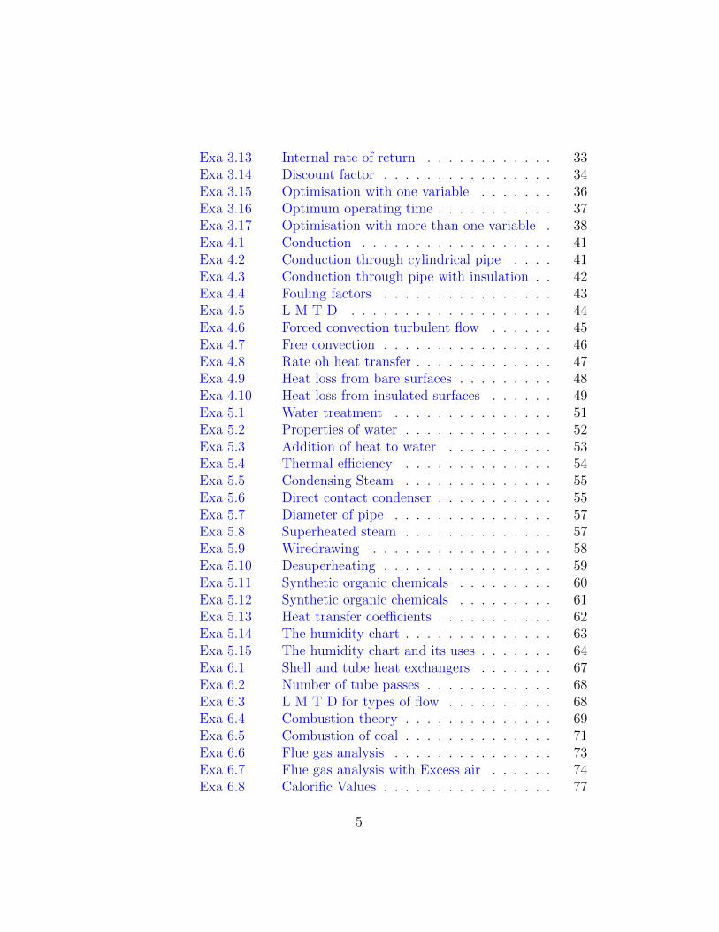
Exa 3.13 Internal rate of return . . . . . . . . . . . . 33Exa 3.14 Discount factor . . . . . . . . . . . . . . . . 34Exa 3.15 Optimisation with one variable . . . . . . . 36Exa 3.16 Optimum operating time . . . . . . . . . . . 37Exa 3.17 Optimisation with more than one variable . 38Exa 4.1 Conduction . . . . . . . . . . . . . . . . . . 41Exa 4.2 Conduction through cylindrical pipe . . . . 41Exa 4.3 Conduction through pipe with insulation . . 42Exa 4.4 Fouling factors . . . . . . . . . . . . . . . . 43Exa 4.5 L M T D . . . . . . . . . . . . . . . . . . . 44Exa 4.6 Forced convection turbulent flow . . . . . . 45Exa 4.7 Free convection . . . . . . . . . . . . . . . . 46Exa 4.8 Rate oh heat transfer . . . . . . . . . . . . . 47Exa 4.9 Heat loss from bare surfaces . . . . . . . . . 48Exa 4.10 Heat loss from insulated surfaces . . . . . . 49Exa 5.1 Water treatment . . . . . . . . . . . . . . . 51Exa 5.2 Properties of water . . . . . . . . . . . . . . 52Exa 5.3 Addition of heat to water . . . . . . . . . . 53Exa 5.4 Thermal efficiency . . . . . . . . . . . . . . 54Exa 5.5 Condensing Steam . . . . . . . . . . . . . . 55Exa 5.6 Direct contact condenser . . . . . . . . . . . 55Exa 5.7 Diameter of pipe . . . . . . . . . . . . . . . 57Exa 5.8 Superheated steam . . . . . . . . . . . . . . 57Exa 5.9 Wiredrawing . . . . . . . . . . . . . . . . . 58Exa 5.10 Desuperheating . . . . . . . . . . . . . . . . 59Exa 5.11 Synthetic organic chemicals . . . . . . . . . 60Exa 5.12 Synthetic organic chemicals . . . . . . . . . 61Exa 5.13 Heat transfer coefficients . . . . . . . . . . . 62Exa 5.14 The humidity chart . . . . . . . . . . . . . . 63Exa 5.15 The humidity chart and its uses . . . . . . . 64Exa 6.1 Shell and tube heat exchangers . . . . . . . 67Exa 6.2 Number of tube passes . . . . . . . . . . . . 68Exa 6.3 L M T D for types of flow . . . . . . . . . . 68Exa 6.4 Combustion theory . . . . . . . . . . . . . . 69Exa 6.5 Combustion of coal . . . . . . . . . . . . . . 71Exa 6.6 Flue gas analysis . . . . . . . . . . . . . . . 73Exa 6.7 Flue gas analysis with Excess air . . . . . . 74Exa 6.8 Calorific Values . . . . . . . . . . . . . . . . 77

5

Exa 6.9 Boiler efficiency . . . . . . . . . . . . . . . . 78Exa 6.10 Equivalent evaporation . . . . . . . . . . . . 79Exa 6.11 Thermal balance sheet . . . . . . . . . . . . 80Exa 6.12 Thermal balance sheet for coal analysis . . . 82Exa 6.13 Desuperheaters . . . . . . . . . . . . . . . . 88Exa 7.1 Combustion process . . . . . . . . . . . . . 91Exa 7.2 Financial saving and capital cost . . . . . . 92Exa 7.3 Heat loss in flue gas and ashes . . . . . . . . 93Exa 7.4 Furnace efficiency . . . . . . . . . . . . . . 94Exa 7.5 Insulation . . . . . . . . . . . . . . . . . . . 95Exa 7.6 Heat recovery . . . . . . . . . . . . . . . . . 96Exa 7.7 Steam turbines as alternatives to electric mo-

tors . . . . . . . . . . . . . . . . . . . . . . 97Exa 7.8 Economics of a CHP system . . . . . . . . . 97Exa 8.1 Ohms law . . . . . . . . . . . . . . . . . . . 100Exa 8.2 Kirchhoff law . . . . . . . . . . . . . . . . . 100Exa 8.3 Power factor . . . . . . . . . . . . . . . . . . 101Exa 8.4 Cost of electrical energy . . . . . . . . . . . 102Exa 8.5 Annual saving . . . . . . . . . . . . . . . . . 103Exa 8.6 Illumination . . . . . . . . . . . . . . . . . . 103Exa 8.7 Natural lighting . . . . . . . . . . . . . . . . 104Exa 8.8 Motive power and power factor improvement 105Exa 8.9 Capacitor rating . . . . . . . . . . . . . . . 105Exa 8.10 Effects of power factor improvement . . . . 106Exa 8.11 Effects of power factor improvement . . . . 106Exa 8.12 Effects of power factor improvement . . . . 107Exa 8.13 Optimum start control . . . . . . . . . . . . 108Exa 8.14 Induction heating . . . . . . . . . . . . . . . 108Exa 8.15 Atmosphere generators . . . . . . . . . . . . 110Exa 9.1 Fabric loss . . . . . . . . . . . . . . . . . . . 112Exa 9.2 U value calculation . . . . . . . . . . . . . . 114Exa 9.3 Ventilation loss . . . . . . . . . . . . . . . . 115Exa 9.4 Environmental temperature . . . . . . . . . 116Exa 9.5 The degree day method . . . . . . . . . . . 118Exa 9.6 Surface condensation . . . . . . . . . . . . . 119Exa 9.7 Interstitial condensataion . . . . . . . . . . 121Exa 9.8 Glazing . . . . . . . . . . . . . . . . . . . . 122Exa 9.9 Design data . . . . . . . . . . . . . . . . . . 123

6

Exa 10.1 Sensible heating . . . . . . . . . . . . . . . . 126Exa 10.2 Sensible cooling . . . . . . . . . . . . . . . . 127Exa 11.1 Shell and tube heat exchangers . . . . . . . 130Exa 11.2 Multiple effect evaporation . . . . . . . . . . 131Exa 11.3 Vapour recompression . . . . . . . . . . . . 132Exa 11.4 Thermal wheel . . . . . . . . . . . . . . . . 133Exa 11.5 Heat pipes . . . . . . . . . . . . . . . . . . . 134Exa 11.6 Heat pumps and COP . . . . . . . . . . . . 135Exa 11.7 Coefficient of performance . . . . . . . . . . 136Exa 11.8 Incineration plant . . . . . . . . . . . . . . . 136Exa 11.9 Regenerators . . . . . . . . . . . . . . . . . 137Exa 11.10 Waste heat boilers . . . . . . . . . . . . . . 138

7

Chapter 1

Energy auditing

Scilab code Exa 1.1 Energy Conversion

1

2 clc;

3 // Example 1 . 14 printf( ’ Example 1 . 1\ n\n ’ );5 printf( ’ Page No . 08\n\n ’ );6 // S o l u t i o n7

8 // Given9 m1= 40*10^3; // f u e l o i l i n g a l l o n s per yea r

10 ga= 4.545*10^ -3; // mˆ311 m= m1*ga;// f u e l o i l i n mˆ3 per yea r12 Cv1= 175*10^3; // Btu per g a l l o n s13 Bt= .2321*10^6; // J per mˆ314 Cv= Cv1*Bt;// i n J per yea r per mˆ315 q=m*Cv;// i n J per yea r16 printf( ’ Heat a v a i l a b l e i s %3 . 2 e J per yea r \n ’ ,q)

Scilab code Exa 1.2 Energy conversion

8

1 clear ;

2 clc;


8 // Given9 Eo1= 1.775*10^9; // Annular ene rgy consumption o f o i l

i n Btu10 Btu= 1055; // 1 Btu = 1055 J o u l e s11 Eo= Eo1*Btu;// Annular ene rgy consumption o f o i l i n

J o u l e s12 Eg1= 5*10^3; // Annular ene rgy consumption o f gas i n

Therms13 Th= 1055*10^5; // 1 Th = 1055∗10ˆ3 J o u l e s14 Eg= Eg1*Th;// Annular ene rgy consumption o f gas i n

J o u l e s15 Ee1= 995*10^3; // Annular ene rgy consumption o f

e l e c t r i c i t y i n KWh16 KWh= 3.6*10^6; // 1 KWh = 3 . 6∗1 0ˆ 6 J o u l e s17 Ee= Ee1*KWh;// Annular ene rgy consumption o f

e l e c t r i c i t y i n J o u l e s18 Et= ( Eo + Eg + Ee);// Tota l ene rgy consumption19 P1= (Eo/Et)*100; // p e r c e n t a g e o f o i l consumption20 P2= (Eg/Et)*100; // p e r c e n t a g e o f gas consumption21 P3= (Ee/Et)*100; // p e r c e n t a g e o f e l e c t r i c i t y

consumption22 printf( ’ p e r c e n t a g e o f o i l consumption i s %3 . 1 f \n ’ ,

P1)

23 printf( ’ p e r c e n t a g e o f gas consumption i s %3 . 1 f \n ’ ,P2)

24 printf( ’ p e r c e n t a g e o f e l e c t r i c i t y consumption i s %3. 1 f \n ’ ,P3)

9

Scilab code Exa 1.3 Energy Index

1 clear ;

2 clc;


8 // Given9 Et = 100*10^3; // t o t a l ene rgy p r o d u c t i o n i n tonne s

per annum10 Eo= 0.520*10^9; // o i l consumption i n Wh11 Eg= 0.146*10^9; // gas consumption i n Wh12 Ee= 0.995*10^9; // e l e c t r i c i t y consumption i n Wh13 Io= Eo/Et;

14 Ig= Eg/Et;

15 Ie= Ee/Et;

16 Et1= Eo + Eg + Ee;// t o t a l ene rgy consumption17 It= Et1/Et;

18 printf( ’ o i l ene rgy index i s %3 . 0 f Wh per tonne \n ’ ,Io)

19 printf( ’ gas ene rgy index i s %3 . 0 f Wh per tonne \n ’ ,Ig)

20 printf( ’ e l e c t r i c i t y ene rgy index i s %3 . 0 f Wh pertonne \n ’ ,Ie)

21 printf( ’ t o t a l ene rgy index i s %3 . 0 f Wh per tonne ’ ,It)

Scilab code Exa 1.4 Energy Costs

1 clear ;

2 clc;

3 // Example 1 . 44 printf( ’ Example 1 . 4\ n\n ’ );

10

5 printf( ’ Page No . 10\n\n ’ );6 // S o l u t i o n7

8 // Given9 mc= 1.5*10^3; // coke consumption i n tonne s10 mg= 18*10^3; // gas consumption i n therms11 me= 1*10^9; // e l e c t r i c i t y consumption i n Wh12 Cc1= 72; // c o s t o f coke i n Pound per tonne13 Cg1= 0.20; // c o s t o f gas i n Pound per therm14 Ce1= 2.25*10^ -5 ;// c o s t o f e l e c t r i c i t y i n Pound per

Wh15 Cc= mc*Cc1;// i n Pound16 Cg= mg*Cg1;// i n Pound17 Ce= me*Ce1;// i n Pound18 Ct= Cc+Cg+Ce;// i n Pound19 printf( ’ c o s t o f coke consumption i s %. 0 f Pound \n ’ ,

Cc)

20 printf( ’ c o s t o f gas consumption i s %. 0 f Pound \n ’ ,Cg)

21 printf( ’ c o s t o f e l e c t r i c i t y consumption i s %. 0 fPound \n ’ ,Ce)

22 printf( ’ t o t a l c o s t i s %3 . 0 f Pound \n ’ ,Ct)

Scilab code Exa 1.5 Cost Index

1 clear ;

2 clc;


8 // Given9 Cc= 108.0*10^3; // c o s t o f coke i n Pound

10 Cg= 3.6*10^3; // c o s t o f gas i n Pound

11

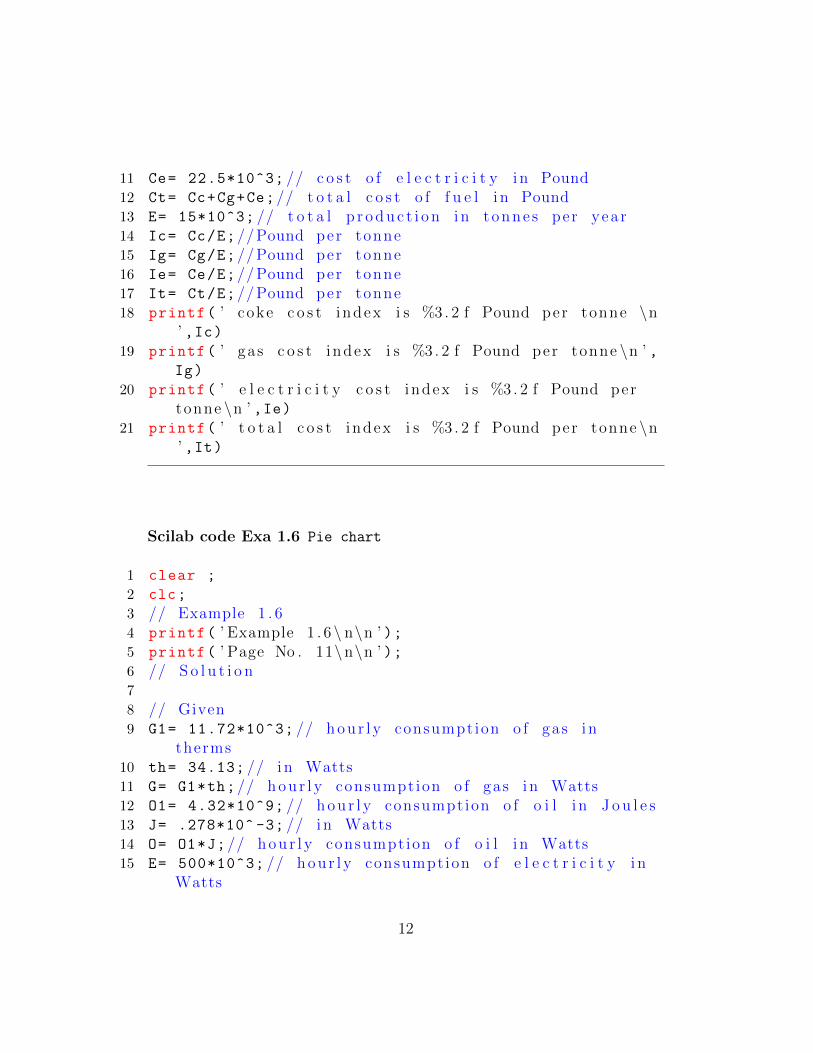
11 Ce= 22.5*10^3; // c o s t o f e l e c t r i c i t y i n Pound12 Ct= Cc+Cg+Ce;// t o t a l c o s t o f f u e l i n Pound13 E= 15*10^3; // t o t a l p r o d u c t i o n i n tonne s per yea r14 Ic= Cc/E;//Pound per tonne15 Ig= Cg/E;//Pound per tonne16 Ie= Ce/E;//Pound per tonne17 It= Ct/E;//Pound per tonne18 printf( ’ coke c o s t index i s %3 . 2 f Pound per tonne \n

’ ,Ic)19 printf( ’ gas c o s t index i s %3 . 2 f Pound per tonne \n ’ ,

Ig)

20 printf( ’ e l e c t r i c i t y c o s t index i s %3 . 2 f Pound pertonne \n ’ ,Ie)

21 printf( ’ t o t a l c o s t index i s %3 . 2 f Pound per tonne \n’ ,It)

Scilab code Exa 1.6 Pie chart

1 clear ;

2 clc;


8 // Given9 G1= 11.72*10^3; // h ou r l y consumption o f gas i n

therms10 th= 34.13; // i n Watts11 G= G1*th;// h o u r l y consumption o f gas i n Watts12 O1= 4.32*10^9; // h o u r l y consumption o f o i l i n J o u l e s13 J= .278*10^ -3; // i n Watts14 O= O1*J;// h o u r l y consumption o f o i l i n Watts15 E= 500*10^3; // h o u r l y consumption o f e l e c t r i c i t y i n

Watts

12

16 // Pie Chart R e p r e s e n t a t i o n : one input argument x=[G O E ]

17 pie([G O E],[” gas ” ” o i l ” ” e l e c t r i c i t y ”]);// P l e a s es e e the g r a p h i c s window

18 printf( ’ The Pie c h a r t i s p l o t t e d i n the f i g u r e ’ );

Scilab code Exa 1.7 Pie chart

1 close

2 clear ;

3 clc;


9 // Given10 O= 150*10^3; // ene rgy consumption i n o f f i c e h e a t i n g

i n Watts11 L= 120*10^3; // ene rgy consumption i n l i g h t i n g i n

Watts12 B= 90*10^3; // ene rgy consumption i n b o i l e r house i n

Watts13 P= 180*10^3; // ene rgy consumption i n p r o c e s s i n

Watts14 // Pie Chart R e p r e s e n t a t i o n : one input argument x

=[O L B P ]15 pie([O L B P],[” o f f i c e h e a t i n g ” ” l i g h t i n g ” ” b o i l e r

h e a t i n g ” ” p r o c e s s ”]);// P l e a s e s e e the g r a p h i c swindow

16 printf( ’ The Pie c h a r t i s p l o t t e d i n the f i g u r e ’ );

Scilab code Exa 1.8 General auditing

13

1 clear ;

2 clc;

3 // Example 1 . 84 printf( ’ Example 1 . 8\ n\n ’ );5 printf( ’ Page No . 16\n\n ’ );6 // g i v e n7

8 qunty= [40 10000 400 90000]

9 unit_price= [29 0.33 0.18 0.025]

10 cost= (unit_price .* qunty)// i n Pound11 common_basis= [310 492 11.7 90] // i n 10ˆ6 Wh12 per_unit_cost= (unit_price .* qunty) ./ common_basis

// Pound per 10ˆ6 Wh13 p= 150; // p r o d u c t i o n i n tonne s14 EI= sum(common_basis)*10^6/150

15 CI= sum(unit_price .* qunty)/150

16 printf( ’ ene rgy index i s %3 . 2 f Wh per tonne \n ’ ,EI)17 printf( ’ c o s t index i s %3 . 2 f Wh per tonne \n ’ ,CI)

Scilab code Exa 1.9 General Auditing

1 clear ;

2 clc;

3 function [coefs]= regress(x,y)

4 coefs =[]

5 if (type(x) <> 1)|(type(y) <>1) then error(msprintf

(gettext(”%s : Wrong type f o r i nput arguments :Numer ica l expec t ed . \ n”),” r e g r e s s ”)), end

6 lx=length(x)

7 if lx<>length(y) then error(msprintf(gettext(”%s :Wrong s i z e f o r both input arguments : same s i z eexpec t ed . \ n”),” r e g r e s s ”)), end

8 if lx==0 then error(msprintf(gettext(”%s : Wrongs i z e f o r i nput argument #%d: Must be > %d. \ n”),” r e g r e s s ”, 1, 0)), end

14

9 x=matrix(x,lx ,1)

10 y=matrix(y,lx ,1)

11 xbar=sum(x)/lx

12 ybar=sum(y)/lx

13 coefs (2)=sum((x-xbar).*(y-ybar))/sum((x-xbar).^2)

14 coefs (1)=ybar -coefs (2)*xbar

15 endfunction

16 // Example 1 . 917 printf( ’ Example 1 . 9\ n\n ’ );18 printf( ’ Page No . 17\n\n ’ );19 // g i v e n20

21 p= [50, 55, 65, 50, 95, 90, 85, 80, 60, 90, 70, 110,

60, 105]; // weakly p r o d u c t i o n i n tonne s22 s= [0.4, 0.35, 0.45, .31, 0.51 ,0.55 , 0.45, 0.5, 0.4,

0.51, 0.4, 0.6, 0.45, 0.55]; // weakly steamconsumption i n 10ˆ6 kg

23 coefs = regress(p,s);

24 new_p = 0:120

25 new_s = coefs (1) + coefs (2)*new_p;

26 plot(p,s, ’ r ∗ ’ );27 mtlb_hold on

28 plot(new_p ,new_s);// p l e a s e s e e the c o r r e s p o n d i n ggraph i n g r a p h i c window

29 xtitle( ’ weakly steam consumption−p r o d u c t i o n ’ , ’ weaklyoutput ( tonne s ) ’ , ’ steam consumption / week (10ˆ6

kg ) ’ )30 l = legend ([_( ’ Given data ’ ); _( ’ F i t t i n g f u n c t i o n ’ )

],2);

31

32 in= coefs (1) *10^6; // i n t e r c e p t o f graph i n kg /weak33 printf( ’ At z e r o output the steam consumption i s %3 . 0

f i n kg /weak \n ’ ,in)

Scilab code Exa 1.10 Detailed energy audits

15

1 clear ;

2 clc;

3 // Example 1 . 1 04 printf( ’ Example 1 . 1 0\ n\n ’ );5 printf( ’ Page No . 19\n\n ’ );6 // g i v e n7

8 // Monthly Energy Usage9 qunty = [15*10^3 4*10^3 90*10^3]

10 cost = [4950 720 2250] // i n Pound11 common_basis1 = [738 117 90] // i n 10ˆ6 Wh12 common_basis= [2655 421 324] // c o n v e r t e d i n t o 10ˆ9

J o u l e s13 unit_cost = cost ./ common_basis1 // i n Pound per

10ˆ6 Wh14 p= 80; // p r o d u c t i o n i n tonne s15 EI = ((sum(common_basis))/p)*10^9;

16 CI = sum(cost)/80;

17 printf( ’ Monthly ene rgy index i s %3 . 2 e J per tonne \n’ ,EI)

18 printf( ’ Monthly c o s t index i s %. 0 f Pound per tonne \n\n ’ ,CI)// D e v i a t i o n i n answer i s due toc a l c u l a t i o n e r r o r f o r sum o f c o s t i n the book

19

20 // B o i l e r House Energy Audit21 qunty_b = [15000 10000]

22 Com_basis_b_1 = [2655 36] // i n 10ˆ9 J23 Com_basis_b = [738 10] // i n 10ˆ6 Wh24 Cost_b = [4950 250] // i n Pound25 b_output = 571*10^6; // i n Wh26 EI_b = (b_output /(sum(Com_basis_b)*10^6));

27 CI_b = (sum(Cost_b)/b_output)*10^3; // Poundc o n v e r t e d i n t o p

28 printf( ’ Energy index f o r b o i l e r i s %. 3 f \n ’ ,EI_b)29 printf( ’ Cost index f o r b o i l e r i s %3 . 2 e p per Wh\n \n

’ ,CI_b)30

31 // Power House Energy Audit

16

32 P_gen = 200*10^6; // Power g e n e r a t e d i n Wh33 Com_basis_p_1 = [14.4 2055 -1000] // i n 10ˆ9 J34 Com_basis_p = [4.0 571 -278] // i n 10ˆ6 Wh35 Cost_p = [100 5196 -2530] // i n Pound36 CI_p = (sum(Cost_p)/P_gen)*10^3; // Pound c o n v e r t e d

i n t o p37 printf( ’ Cost index f o r power house i s %3 . 2 e p per Wh

\n\n ’ ,CI_p)// D e v i a t i o n i n answer i s due to wrongc a l c u l a t i o n i n the book

38

39 // Space Heat ing Energy Audit40 deg_days = 260; // Number o f degree−days41 Com_basis_s_1 = [36 100 105] // i n 10ˆ9 J42 Com_basis_s = [10.0 27.8 29.2] // i n 10ˆ6 Wh43 Cost_s = [250 253 179] // i n Pound44 EI_s = ((sum(Com_basis_s)*10^6)/deg_days)

45 CI_s = (sum(Cost_s)/deg_days)

46 printf( ’ Energy index f o r space h e a t i n g i s %3 . 2 e Whper degree−day\n ’ ,EI_s)

47 printf( ’ Cost index f o r space h e a t i n g i s %3 . 2 f Poundper degree−day\n\n ’ ,CI_s)

48

49 // P r o c e s s Energy Audit50 T_pdt_output = 100; // i n tonne51 Com_basis_pr_1 = [216 720 810 316] // i n 10ˆ9 J52 Com_basis_pr = [60 200 225 88] // i n 10ˆ6 Wh53 Cost_pr = [1500 2766 2047 540] // i n Pound54 EI_pr = ((sum(Com_basis_pr)*10^6)/T_pdt_output);

55 CI_pr = (sum(Cost_pr)/T_pdt_output);

56 printf( ’ Energy index f o r P r o c e s s Energy Audit i s %3. 2 e Wh per tonne \n ’ ,EI_pr)

57 printf( ’ Cost index f o r P r o c e s s Energy Audit i s %. 2 fPound per tonne \n ’ ,CI_pr)

17

Chapter 2

Energy Sources

Scilab code Exa 2.1 Energy audit scheme

1 clear ;

2 clc;

3 // Example 2 . 14 printf( ’ Example 2 . 1\ n\n ’ );5 printf( ’ Page No . 44\n\n ’ );6

7 // g i v e n8 C= 35000; // c o s t o f b o i l e r9 C_grant =.25; // C a p i t a l g r an t a v a i l a b l e from

goverment10 E= -(C-( C_grant*C));// Net e x p e n d i t u r e11 Fs= 15250; // Fue l Sav ing12 r_i = 0.15; // i n t e r e s t13 r_t = 0.55; // tax14

15 a = [0 E Fs 0 E+Fs r_i*(E+Fs) 0 ]

16 bal_1 = a(5)+a(6)-a(7) // Tota l Ba lance a f t e r 1 s tyea r

17

18 c_all = 0.55; // c a p i t a l a l l o w a n c e i n 2nd year19 C_bal= (bal_1 +0+Fs+(-( c_all*E)));// Cash Balance

18

a f t e r 2nd year20 b = [bal_1 0 Fs -(c_all*E) C_bal r_i*C_bal r_t*(Fs+(

r_i*C_bal))];

21 bal_2 = b(5)+b(6)-b(7) // Tota l Ba lance a f t e r 2ndyea r

22

23 c = [bal_2 0 Fs 0 bal_2+Fs r_i*(bal_2+Fs) r_t*(Fs+(

r_i*(bal_2+Fs)))]

24 bal_3= c(5)+c(6)-c(7) // Tota l Ba lance a f t e r 3 rdyea r

25

26 if(bal_2 >0) then

27 disp( ’ Pay back p e r i o d i s o f two yea r ’ )28 else

29 disp( ’ Pay back p e r i o d i s o f t h r e e yea r ’ )30 end

31

32 printf( ’ Tota l s a v i n g at the end o f s econd year i s %3. 0 f Pound\n ’ ,bal_2);

33 printf( ’ Tota l s a v i n g at the end o f t h i r d yea r i s %3. 0 f Pound\n ’ ,bal_3);

34 // D e v i a t i o n i n answer due to d i r e c t s u b s t i t u t i o n

Scilab code Exa 2.2 Energy audit scheme

1 clear ;

2 clc;


7 // g i v e n8 C= 35000; // c o s t o f b o i l e r9 C_grant =0; // C a p i t a l g r an t a v a i l a b l e from goverment

10 E= -(C-( C_grant*C));// Net e x p e n d i t u r e

19

11 Fs= 15250; // Fue l Sav ing12 r_i = 0.15; // i n t e r e s t13 r_t = 0.55; // tax14

15 a = [0 E Fs 0 E+Fs r_i*(E+Fs) 0 ]


17

18 c_all = 0.55; // c a p i t a l a l l o w a n c e i n 2nd yea r19 C_bal= (bal_1 +0+Fs+(-(c_all*E)));// Cash Balance


r_i*C_bal))];


22


r_i*(bal_2+Fs)))]

24 bal_3= c(5)+c(6)-c(7) // Tota l Ba lance a f t e r 3 rdyea r

25


27 disp( ’ pay back p e r i o d i s o f two year ’ )28 else

29 disp( ’ pay back p e r i o d i s o f t h r e e yea r ’ )30 end

31


33 printf( ’ Tota l s a v i n g at the end o f t h i r d yea r i s %3. 2 f Pound\n ’ ,bal_3);

34 // D e v i a t i o n i n answer due to d i r e c t s u b s t i t u t i o n

Scilab code Exa 2.3 Choice of fuels

20

1 clear ;

2 clc;


7 // g i v e n8 F= 350*10^3; // f u e l o i l s i n g a l l o n s9 Ci= 5000; // c o s t o f i n s u l a t i o n o f tanks

10

11 As= 7500; // Annual Sav ing i n Pound12

13 if(As> Ci) then

14 disp(”The inve s tment has a pay−back p e r i o d o f l e s sthan 1 year ”);

15 else

16 disp(”The inve s tment has not a pay−back p e r i o d o fl e s s than 1 year ”);

17 end

18 // Note− S i n c e he r e pack back p e r i o d i s l e s s than 1yea r and the company i s i n p r o f i t so they can gowith t h i s f u e l o i l ,

19 // a l though i t can be noted tha t t h e r e a r e moreprob lems h a n d l i n g heavy f u e l s o i l s

20 // and tha t the pay−back i n c r e a s e s c o n s i d e r a b l y thes m a l l e r the i n s t a l l a t i o n .

21 // So the company can changeove r from o i l to c o a l asa f u e l .

Scilab code Exa 2.4 Choice of fuels

1 clear ;

2 clc;

3 // Example 2 . 44 printf( ’ Example 2 . 4\ n\n ’ );

21

5 printf( ’ Page No . 47\n\n ’ );6

7 // g i v e n8 F1= 500*10^3; // f u e l o i l i n g a l l o n s9 F2= 500*10^3; // c o a l i n g a l l o n s i n Pound10 C1= 165*10^3; // c o s t o f o i l pe r yea r i n Pound11 C2= 92*10^3; // c o s t o f an e q u i v a l e n t o f c o a l i n

Pound12 Ce= 100*10^3; // c a p i t a l c o s t o f e x t r a h a n d l i n g

eqiupment13

14 Cm= (Ce*0.2);// Maintenance , i n t e r e s t c o s t s peryea r

15 As= C1 -C2;// Annual Sav ing i n Pound16 printf( ’ Annual Sav ing i s %3 . 0 f Pound\n ’ ,As)17

18 if((2*As)> Ce) then

19 disp(” Rep l a c ing an o b s o l e t e b o i l e r p l a n t i sc o n s i d e r a b l e ”);

20 else

21 disp(” Rep l a c ing an o b s o l e t e b o i l e r p l a n t i s notc o n s i d e r b l e ”);

22 end

Scilab code Exa 2.5 Economic saving

1 clear ;

2 clc;


7 // g i v e n8 F= 10*10^3; // f u e l o i l s i n g a l l o n s9 Cs= 2200; // c o s t o f m a i n t a i n i n g tanks per yea r i n

22

Pound10 Ci= 1850; // c o s t o f i n s u l a t i o n o f p ip e i n Pound11

12 As= (Cs*.85);// company s a v i n g i s 85 per c en t to thec o s t

13 printf( ’ Annual Sav ing on h e a t i n g i s %3 . 0 f Pound\n ’ ,As)

14

15

16 if(As> Ci) then

17 disp(”The inve s tment has a pay−back p e r i o d o f l e s sthan 1 year ”);

18 else

19 disp(”The inve s tment has not a pay−back p e r i o d o fl e s s than 1 year ”);

20 end

Scilab code Exa 2.6 Cycle Efficiency

1 clear ;

2 clc;


7 // g i v e n8 P1= 50; // Dry s a t u r a t e d steam p r e s s u r e i n bar9 P2= 0.5; // c ond en s e r p r e s s u r e i n bar

10

11 //By u s i n g the steam t a b l e s s a t u r a t i o n t empera tu rei s o b t a i n e d at g i v e n p r e s s u r e s

12 T1= 537 //The s a t u r a t i o n temperatue i n K at 50 bar13 T2= 306 //The s a t u r a t i o n temperatue i n K at 0 . 5 bar14

15 // For Carnot Cyc le

23

16 n=(1-(T2/T1))*100;

17 printf( ’ E f f i c i e n c y p e r c e n t a g e o f Carnot Cyc le i s %3. 0 f \n ’ ,n)

18

19

20 // For Rankine Cyc le21 // By u s i n s steam t a b l e s , the t o t a l heat and the

s e n s i b l e s heat and o t h e r r ema in ing parameter hasbeen c a l c u l a t e d

22 h1= 2794*10^3; // the t o t a l heat i n dry steam at 50bar i n J/ kg

23 d= 0.655; // d r y n e s s f r a c t i o n24 h2= 1725*10^3; // the ent ropy at s t a t e 2 i n J/ kg25 h3= 138*10^3; // the s e n s i b l e heat at 0 . 5 bar i n J/ kg26 Vf= 1.03*10^ -3; // volume o f f l u i d im mˆ3 , c a l c u l a t e d

from steam t a b l e27 W= (Vf*(P1 -P2))*10^5; // pump work i n J/ kg28 E=(((h1-h2)-(W))/((h1-h3)-(W)))*100;

29 printf( ’ E f f i c i e n c y p e r c e n t a g e o f Rankine Cyc le i s %3. 0 f \n ’ ,E)

24

Chapter 3

Economics

Scilab code Exa 3.1 Simple interest

1 clear ;

2 clc;


7 // g i v e n8 P = 10000; // P r i n c i p a l Amount9 i = 0.15; // I n t e r e s t Rate

10 n = 4; // y e a r s11 I = P*i*n;// Simple I n t e r e s t12 Ts= P+I;// The t o t a l repayment13 printf( ’ The t o t a l repayment i s %. 0 f Euro\n ’ ,Ts)

Scilab code Exa 3.2 Compound interest

1 clear ;

2 clc;

25


7 // g i v e n8 P = 10000; // P r i n c i p a l Amount i n Pound9 i = 0.15; // I n t e r e s t Rate

10 n = 4; // y e a r s11 Tc = P*(1+i)^n;

12 printf( ’ The t o t a l repayment a f t e r adding compondi n t e r e s t i s %. 0 f Pound\n ’ ,Tc)

Scilab code Exa 3.3 Capital recovery

1 clear ;

2 clc;

3 // Example 3 . 34 printf( ’ Example 3 . 3\ n\n ’ );5 // Page No . 596

7 // g i v e n8 P = 60000; // / P r i n c i p a l Amount i n Pound9 i = 0.18; // I n t e r e s t Rate

10 n = 10; // y e a r s11 R = P*((i*(1+i)^n)/((1+i)^n -1));// Rate o f C a p i t a l

Recovery12 printf( ’ The annual i nve s tment r e q u i r e d i s %. 1 f Pound

\n ’ ,R)

Scilab code Exa 3.4 Depreciation

1 clear ;

2 clc;

26


7 // g i v e n8 P = 100000; // / P r i n c i p a l Amount o f b o i l e r p l a n t i n

Pound9 n = 10; // s e r v i c e l i f e i n y e a r s

10 S = 0; // Zero Sa l vage v a l u e11 nT = (n*(n+1) /2);//sum o f y e a r s12 for i = 0:9

13 d_(i+1) = ((P-S)/nT)*(n-i);

14 end

15 printf( ’ The Annual d e p r e c i a t i o n f o r f i r s t yea r i s %. 0 f Pound\n ’ ,d_(1))

16 printf( ’ The Annual d e p r e c i a t i o n f o r second yea r i s %. 0 f Pound\n\n ’ ,d_(2))

17 printf( ’ The Annual d e p r e c i a t i o n f o r t h i r d yea r i s %. 0 f Pound\n ’ ,d_(3))

18 printf( ’ The Annual d e p r e c i a t i o n f o r ten yea r i s %. 0 fPound\n ’ ,d_(10))

19 // D e v i a t i o n i n answer due to some . approx imat ion o fv a l u e s i n the book

Scilab code Exa 3.5 Depreciation and Asset value

1 clear ;

2 clc;


7 // g i v e n8 P = 40000; // / P r i n c i p a l Amount o f b o i l e r p l a n t i n

Pound

27

9 nT = 10; // s e r v i c e l i f e i n y e a r s10 S = 4000; // Sa l vage v a l u e11 n = 6; // y e a r s a f t e r which Asse t v a l u e has to be

c a l c u l a t e d12

13 // ( a ) S t r a i g h t l i n e method14 d = ((P-S)/nT);// D e p r e c i a t i o n15 Aa = (d*(nT-n)) + S;

16 printf( ’ The Asse t v a l u e at the end o f s i x y e a r su s i n g S t r a i g h t l i n e method i s %. 0 f Pound\n ’ ,Aa)

17

18 // ( b ) D e c l i n i n g b a l a n c e t e c h n i q u e19 f = 1-(S/P)^(1/nT);// Fixed f r a c t i o n o f the r e s i d u a l

a s s e t20 Ab = P*(1-f)^n;

21 printf( ’ The Asse t v a l u e at the end o f s i x y e a r su s i n g D e c l i n i n g b a l a n c e t e c h n i q u e i s %. 0 f Pound\n\n ’ ,Ab)

22

23 // ( c ) Sum o f the y e a r s d i g i t24 sum_nT = (nT*(nT+1)/2);//sum o f 10 y e a r s25 sum_n = 45; //sum a f t e r 6 y e a r s26 dc = (( sum_n/sum_nT)*(P-S));// D e p r e c i a t i o n a f t e r 6

y e a r s27 Ac = P-dc;

28 printf( ’ The Asse t v a l u e at the end o f s i x y e a r su s i n g Sum o f the y e a r s d i g i t i s %. 0 f Pound\n ’ ,Ac)// D e v i a t i o n i n answer due to d i r e c t s u b s t i t u t i o n

29

30 // ( d ) S i n k i n g Fund Method31 r_i = 0.06; // Rate o f i n t e r e s t32 Ad = P-((P-S)*(((1+ r_i)^n-1) /((1+ r_i)^nT -1)));

33 printf( ’ The Asse t v a l u e at the end o f s i x y e a r su s i n g S i n k i n g Fund Method i s %. 0 f Pound\n ’ ,Ad)//D e v i a t i o n i n answer due to d i r e c t s u b s t i t u t i o n

28

Scilab code Exa 3.6 Rate of Return

1 clear ;

2 clc;


7 // g i v e n8 P = 9000; // C a p i t a l Cost i n Pound9 n = 5; // P r o j e c t l i f e t i m e

10 Less_dep = 8000; // Les s D e p r e c i a t i o n11

12 // For P r o j e c t A13 d1 = [4500 3750 3000 1500 750 ]// Sav ing i n eve ry

yea r ( b e f o r e d e p r e c i a t i o n )14 dT1 = sum (d1)

15 Net_S1 = dT1 - Less_dep;// Tota l Net Sav ing16 Avg1 = Net_S1/n;// Average net annual s a v i n g17 R_R1 = (Avg1/P)*100;

18

19 // For P r o j e c t20 d2 = [750 2250 4500 4500 1500 ]// Sav ing i n eve ry

yea r ( b e f o r e d e p r e c i a t i o n )21 dT2 = sum (d2)

22 Net_S2 = dT2 - Less_dep;// Tota l Net Sav ing23 Avg2 = Net_S2/n;// Average net annual s a v i n g24 R_R2 = (Avg2/P)*100;

25

26 printf( ’ The p e r c e n t a g e o f Rate o f Return on o r i g i n a li nve s tment f o r P r o j e c t A i s %3 . 1 f \n ’ ,R_R1)

27 printf( ’ The p e r c e n t a g e o f Rate o f Return on o r i g i n a li nve s tment f o r P r o j e c t B i s %3 . 1 f \n ’ ,R_R2)

29

Scilab code Exa 3.7 Pay back method

1 clear ;

2 clc;


7 // g i v e n8 Pc = 10000; // C a p i t a l c o s t f o r p r o j e c t C i n Pound9 Pd = 10000; // C a p i t a l c o s t f o r p r o j e c t d i n Pound

10 nc = 3; // pay back p e r i o d f o r C11 nd = 3; // pay back p e r i o d f o r D12 Ca = [4500 3500 2000 2000 1000]; // Annual Cash f l o w

f o r C i n Pound13 Cc = [4500 8000 10000 12000 13000] // Cumulat ive Cash

f l o w f o r C i n Pound14 Da = [1500 4000 4500 2200 1800 1000]; // Annual Cash

f l o w f o r D i n Pound15 Dc = [1500 5500 10000 12200 14000 15000] //

Cumulat ive Cash f l o w f o r D i n Pound16 Ac = Cc(5)-Pc;// i n Pound17 Ad = Dc(6)-Pd;// i n Pound18 printf( ’ A d d i t i o n a l amount from C a f t e r the pay back

t ime i s %3 . f Pound\n ’ ,Ac)19 printf( ’ A d d i t i o n a l amount from D a f t e r the pay back

t ime i s %3 . f Pound\n ’ ,Ad)

Scilab code Exa 3.8 Discounted cash flow

1 clear ;

2 clc;

30


7 // Re f e r f i g u r e 3 . 68 // g i v e n9 n = 5; // y e a r s

10 C = 80000; // COst o f the p r o j e c t i n Pound11 S = 0; // Zero Sa lvage Value12 A_E = [10000 20000 30000 40000 50000] // Annual Net

cash f l o w f o r p r o j e c t E i n Pound13 C_E = [10000 30000 60000 100000 150000] //

Cummulative Net cash f l o w f o r p r o j e c t E i n Pound14 A_F = [50000 40000 30000 20000 10000] // Annual Net

cash f l o w f o r p r o j e c t F i n Pound15 C_F = [50000 90000 120000 140000 150000] //

Cummulative Net cash f l o w f o r p r o j e c t F i n Pound16

17 //From the f i g u r e 3 . 6 ( i n t e r c e p t o f x−a x i s )18 P_F = 1.75; // i n y e a r s19 P_E = 3.5; // i n y e a r s20 printf( ’ The pay−back t ime o f p r o j e c t F i s %. 2 f \n ’ ,

P_F)

21 printf( ’ The pay−back t ime o f p r o j e c t E i s %. 1 f \n\n ’,P_E)

22

23 printf( ’ As the pay−back t ime i s l e s s f o r p r o j e c t F , \n P r o j e c t F would a lways be choosen i n p r a c t i c e \n s i n c e p r e d i c t i o n o f s a v i n g s i n the e a r l y y e a r sa r e more r e l i a b l e than long−term p r e d i c t i o n s . ’ )

Scilab code Exa 3.9 Discounted cash flow

1 clear ;

2 clc;

31


7 // g i v e n8 P = 1; // / P r i n c i p a l Amount i n Pound9

10 r_i = 0.1; // Compound i n t e r e s t r a t e11 for i = [1:1:4]

12 c = P*(1+ r_i)^i;

13 printf( ’ compound i n t r e s t a f t e r yea r %. 0 f i se q u a l to %. 2 f Pound\n ’ ,i,c)

14 end

15

16 new_P = 1000*P;// i n Pound17 new_c = 1000*c;// i n Pound18 printf( ’ The new amount at the compound i n t e r e s t

a f t e r f o u r t h yea r i s %. 0 f Pound\n\n ’ ,new_c)19

20 // Di scount r a t e21 r_d = 0.10; // Di scount r a t e22 for j= 1:1:4

23 d = P*(1/(1+ r_d)^j);

24 printf( ’ The amount r e c e i v a b l e at d i s c o u n t i nyea r %. 0 f i s %. 3 f Pound\n ’ ,j,d)

25 end

26

27 new_P1 = new_c;// i n Pound28 new_d = new_P1*d;// i n Pound29 printf( ’ The new amount r e c e i v a b l e at d i s c o u n t i n

f o u r t h yea r i s %. 0 f Pound\n ’ ,new_d)

Scilab code Exa 3.10 Net present value

1 clear ;

32

2 clc;

3 // Example 3 . 1 04 printf( ’ Example 3 . 1 0\ n\n ’ );5 printf( ’ Page No . 71\n\n ’ );6

7 // g i v e n8 C = 2500; // Cost o f the p r o j e c t9 P = 1000; // Cash i n f l o w

10 r_r = 0.12; // Rate o f r e t u r n11 S = 0; // Zero s a l v a g e v a l u e12 n = 4; // y e a r s13

14 for j= 1:1:4 // as f o r f o u r y e a r s15 d_(j) = P*(1/(1+ r_r)^j);

16 end

17

18

19 P_v = d_(1)+d_(2)+d_(3)+d_(4);// P r e s e n t v a l u e o fcash i n f l o w

20 N = P_v -C;

21 printf( ’ Net p r e s e n t v a l u e i s %. 0 f Pound\n ’ ,ceil(N))22

23 if(P_v >C) then

24 disp( ’ The p r o j e c t may be under taken ’ )25 else

26 disp( ’ The p r o j e c t may not be under taken ’ )27 end

Scilab code Exa 3.11 Net present value

1 clear ;

2 clc;

3 // Example 3 . 1 14 printf( ’ Example 3 . 1 1\ n\n ’ );5 printf( ’ Page No . 72\n\n ’ );

33

6

7 // g i v e n8 Cash_out = 80000; // P re s e n t v a l u e o f cash o u t f l o w

f o r both p r o j e c t s E and F9 r_r = .2; // Rate o f r e t u r n10 n = 5; // y e a r s11

12 d = [0.833 0.694 0.579 0.482 0.402] // Di scountFacto r f o r 20% o f r a t e o f r e t u r n f o r 5 y e a r s

13 Ce = [10000 20000 30000 40000 50000] // Cash f l o w f o rp r o j e c t E i n Pound

14 Pe = [8330 13880 17370 19280 20100] // P re s e n t v a l u ef o r p r o j e c t E i n Pound

15

16 Cf = [50000 40000 30000 20000 10000] // Cash f l o w f o rp r o j e c t F i n Pound

17 Pf = [41650 27760 17370 9640 4020] // P re s e n t v a l u ef o r p r o j e c t F i n Pound

18

19 Cash_inE = sum(Pe)// P r e s e n t v a l u e o f cash i n f l o w i nPound

20 Cash_inF = sum(Pf)// P r e s e n t v a l u e o f cash i n f l o w i nPound

21

22 Net_E = Cash_inE - Cash_out;// net p r e s e n t v a l u e f o rp r o j e c t E i n Pound

23 Net_F = Cash_inF - Cash_out;// net p r e s e n t v a l u e f o rp r o j e c t F i n Pound

24

25 if (Net_E >Net_F) then

26 disp( ’ P r o j e c t E i s s e l e c t e d based on NPV ’ )27 else

28 disp( ’ P r o j e c t F i s s e l e c t e d based on NPV ’ )29 end

34

Scilab code Exa 3.12 Profitability index

1 clear ;

2 clc;


7 // g i v e n8 Cash_inG = 43000; // P re s e n t v a l u e o f cash i n f l o w f o r

p r o j e c t G i n Pound9 Cash_outG = 40000; // P re s e n t v a l u e o f cash o u t f l o w

f o r p r o j e c t G i n Pound10 Net_G = Cash_inG - Cash_outG;// Net p r e s e n t v a l u e

f o r G i n Pound11 PI_G = (Cash_inG/Cash_outG);// P r o f i t a b i l i t y index

f o r G12

13 Cash_inH = 23000; // P re s e n t v a l u e o f cash i n f l o w f o rp r o j e c t H i n Pound

14 Cash_outH = 20000; // P re s e n t v a l u e o f cash o u t f l o wf o r p r o j e c t H i n Pound

15 Net_H = Cash_inH - Cash_outH;// Net p r e s e n t v a l u ef o r H i n Pound

16 PI_H = (Cash_inH/Cash_outH);// P r o f i t a b i l i t y indexf o r H

17

18 //The h i g h e r the p r o f i t a b i l i t y index the mored e s i r a b l e i s the p r o j e c t .

19 if (PI_G >PI_H) then

20 disp( ’ P r o j e c t G i s more a t t r a c t i v e than P r o j e c tH ’ )

21 else

22 disp( ’ P r o j e c t H i s more a t t r a c t i v e than P r o j e c tG ’ )

23 end

35

Scilab code Exa 3.13 Internal rate of return

1 clear ;

2 clc;


7 // g i v e n8 Cash_out = 80000; // P re s e n t v a l u e o f cash o u t f l o w

f o r p r o j e c t F i n Pound9 n = 5; // y e a r s

10 Cash_in= [50000 40000 30000 20000 10000] // Cashn i n\ f l o w f o r p r o j e c t F i n Pound

11 NPV = 0; //At the end o f 5 y e a r s12

13 // Let the unknown r a t e f o r p r o j e c t F be rm .14

15 //The amount s t a n d i n g at the end o f 5 y e a r s i s \n =>0 = 80000∗(1+rm) ˆ5 − 50000∗(1+rm) ˆ4 − 40000∗(1+rm) ˆ3 − 30000∗(1+rm) ˆ2 − 20000∗(1+rm) ˆ1 − 10000

16 // By t a k i n g (1+rm) = x\n =>8∗xˆ5 − 5∗xˆ4 − 4∗xˆ3 −3∗xˆ2 − 2∗x − 1 = 0\n\n ’ )

17

18 function y=fsol1(x)

19 y= 8*x^5 - 5*x^4 - 4*x^3 - 3*x^2 - 2*x - 1;

20 endfunction

21 [xres]= fsolve (100, fsol1);

22 xres

23 rm = (xres - 1)*100;

24 printf( ’ The v a l u e o f rm f o r p r o j e c t F i s %3 . 0 f perc en t \n ’ ,ceil(rm))

36

Scilab code Exa 3.14 Discount factor

1 clear ;

2 clc;

3 function [coefs]= regress(x,y)

4 coefs =[]

5 if (type(x) <> 1)|(type(y) <>1) then error(msprintf

(gettext(”%s : Wrong type f o r i nput arguments :Numer ica l expec t ed . \ n”),” r e g r e s s ”)), end

6 lx=length(x)

7 if lx<>length(y) then error(msprintf(gettext(”%s :Wrong s i z e f o r both input arguments : same s i z eexpec t ed . \ n”),” r e g r e s s ”)), end

8 if lx==0 then error(msprintf(gettext(”%s : Wrongs i z e f o r i nput argument #%d: Must be > %d. \ n”),” r e g r e s s ”, 1, 0)), end

9 x=matrix(x,lx ,1)

10 y=matrix(y,lx ,1)

11 xbar=sum(x)/lx

12 ybar=sum(y)/lx

13 coefs (2)=sum((x-xbar).*(y-ybar))/sum((x-xbar).^2)

14 coefs (1)=ybar -coefs (2)*xbar

15 endfunction


20 // g i v e n21 n = 5; // y e a r s22 C = 80000; // Cost o f the p r o j e c t i n Pound23 Cash_in = [10000 20000 30000 40000 50000] // Cash

i n f l o w i n Pound24 r_d1 = 15; // Di scount f a c t o r o f 15%25 r_d2 = 18 ;// Di scount f a c t o r o f 18%

37

26 r_d3 = 20; // Di scount f a c t o r o f 20%27

28 //At d i s c o u n t o f 15%29 df_1 = [0.870 0.756 0.658 0.572 0.497] // Di scount

f a c t o r f o r eve ry yea r30 PV_1 = [8700 15120 19740 22880 24850] // P re s e n t

v a l u e31 Net_1 = sum (PV_1);// net p r e s e n t v a l u e32

33




39




45 // f = N. P .V. cash i n f l o w − N. P .V. cash o u t f l o w46 // ( 1 ) By Numer ica l Method47 ff = 2*(( sum (PV_2) - C)/(sum (PV_2) - sum(PV_3)));

// i n p e r c e n t a g e48 f = 18 + ff;

49 printf( ’ the i n t e r n a l r a t e o f r e t u r n i n p e r c e n t a g e i s%3 . 2 f \n\n ’ ,f)// D e v i a t i o n i n answer due to

d i r e c t s u b s t i t u t i o n50

51 // ( 2 ) By Grap h i ca l I n t e r p o l a t i o n52 f_1 = (sum (PV_1) - C)/10^3; //At d i s c o u n t f a c t o r o f

15%53 f_2 = (sum (PV_2) - C)/10^3; //At d i s c o u n t f a c t o r o f

38

18%54 f_3 = (sum (PV_3) - C)/10^3; //At d i s c o u n t f a c t o r o f

20%55

56 x = [f_1 f_2 f_3];

57 y = [r_d1 r_d2 r_d3];

58 plot(x,y, ’ r ∗ ’ );59

60 plot2d (x,y);// p l e a s e s e e the c o r r e s p o n d i n g graphi n g r a p h i c window

61 xtitle( ’ D i s count f a c t o r a g a i n s t f ’ , ’ f ( ∗10ˆ3 Pound )’ , ’ D i s count f a c t o r (%) ’ )

62 regress(x,y)

63 coefs = regress(x,y);

64 printf( ’ the i n t e r n a l r a t e o f r e t u r n i n p e r c e n t a g e i s%3 . 1 f \n ’ ,coefs (1))// D e v i a t i o n i n answer due tod i r e c t s u b s t i t u t i o n

Scilab code Exa 3.15 Optimisation with one variable

1 clear ;

2 clc;


7 // g i v e n8 i_t = [20 40 60 80 100]; // I n s u l a t i o n t h i c k n e s s i n

mm9 f_c = [2.2 3.5 4.8 6.1 7.4]; // Fixed c o s t s i n (10ˆ3

Pound / yea r )10 h_c = [10.2 6.5 5.2 4.6 4.2]; // Heat c o s t s i n (10ˆ3

Pound / yea r )11 t_c = [12.4 10 10 10.7 11.6]; // Tota l c o s t s i n (10ˆ3

Pound / yea r )

39

12

13 // ( a ) Graph i ca l s o l u t i o n14 // Re f e r f i g u r e 3 . 815 C_T = 9750; // Minimum t o t a l c o s t i n Pound16 t = 47; // Cor r e spond ing t h i c k n e s s o f i n s u l a t i o n i n

mm17 printf( ’ The most economic t h i c k n e s s o f i n s u l a t i o n i s

%. 0 f mm \n ’ ,t)18

19 // ( b ) Numer ica l s o l u t i o n20 // The c o s t due to heat l o s s e s , C1 , and the f i x e d

c o s t s , C2 , vary a c c o r d i n g to the e q u a t i o n s ;−21 // C1 = ( a/x ) + b and C2 = ( c∗x ) + d22 // S u b s t i t u t i n g the v a l u e s o f C1 and C2 t o g e t h e r

with the c o r r e s p o n d i n g i n s u l a t i o n t h i c k n e s sv a l u e s , the f o l l o w i n g e q u a t i o n s a r e o b t a i n e d :−

23 // C1 = (150∗10ˆ3/ x ) + 2 . 7∗1 0ˆ 3 and C2 = (65∗ x) + 0 . 9∗1 0ˆ 3

24 //And to o b t a i n the t o t a l c o s t s25 //CT = C1 + C2 = (150∗10ˆ3/ x ) + (65∗ x ) + 3 . 6∗1 0ˆ 326 // D i f f e r e n t i a t e to op t im i s e , and put dCT/dx e q u a l

to z e r o27 //dCT/dx =−((150∗10ˆ3) /x ˆ2) + 65 = 028

29 // Let y = dCT/dx30 function y=fsol1(x)

31 y = -((150*10^3)/x^2) + 65;

32 endfunction


34 x = xres;

35 printf( ’ The optimum t h i c k n e s s o f i n s u l a t i o n i s %. 0 fmm \n ’ ,x)

Scilab code Exa 3.16 Optimum operating time

40

1 clear ;

2 clc;


7 // g i v e n8 tb = [36*10^3 72*10^3 144*10^3 216*10^3]; //

o p e r a t i n g t ime i n s9 U = [971 863 727 636]; // Mean o v e r a l l heat t r a n s f e r

r a t e i n W/mˆ2−K10 A = 50; // a r ea i n mˆ211 dT = 25; // t empera tu r e d i f f e r e n c e i n d e g r e e c e l c i u s12 ts = 54*10^3; // Time i n s e c ( h c o n v e r t e d to s e c )13 //As Q = U∗A∗dT14 for i = [1:1:4]

15 Q(i) = (U(i)*A*dT)/10^6;

16 Q_a(i) = ((tb(i)*Q(i)*10^6) /(tb(i) + ts))/10^6;

17 printf( ’ the ave rage heat t r a n s f e r r a t e i s %. 3 f∗10ˆ6 W \n ’ ,Q_a(i))

18 end

19

20 // Re f e r f i g u r e 3 . 921 printf( ’ \n ’ )22 Q_max = 0.67*10^6; // Maximum v a l u e o f Q i n W23 T_opt = 33; // Time i n h24 printf( ’ The maximum v a l u e o f Q o b t a i n e d i s %3 . 2 e W \

n ’ ,Q_max)25 printf( ’ The most econnomic o p e r t a i n g t ime f o r the

heat exchange r to run i s %. 0 f h ’ ,T_opt)

Scilab code Exa 3.17 Optimisation with more than one variable

1 clear ;

2 clc;

41


7 // g i v e n8 // C T = 7∗x + ( 4 0 0 0 0 / ( x∗y ) ) + 6∗y + 109 // D i f f e r e n t i a t i n g C T with r e s p e c t to x and y:−10 //dC T/dx = 7 − ( 4 0 0 0 0 / ( x ˆ2∗y ) )11 //dC T/dy = − ( 4 0 0 0 0 / ( x∗y ˆ2) ) + 612

13 // For optimum c o n d i t i o n s :− dC T/dx = dC T/dy = 014 //dC T/dx = 0 => 7 − ( 4 0 0 0 0 / ( x ˆ2∗y ) ) = 015 //=> y = 40000/(7∗ x ˆ2) . . . . . . . ( 1 )16 //dC T/dy = 0 =>− ( 4 0 0 0 0 / ( y ˆ2∗x ) ) +6 = 017 //=> y = (40000/ (6∗ x ) ) ˆ 0 . 5 . . . . . . . ( 2 )18

19 //From e q u a t i o n ( 1 ) and ( 2 )20 //=> 40000/(7∗ x ˆ2) − ( 40000/ (6∗ x ) ) ˆ 0 . 5 = 021

22 function y=fsol1(x)

23 y = 40000/(7*x^2) - (40000/(6*x))^0.5 ;

24 endfunction


26 x = xres;

27

28 // from e q u a t i o n ( 1 )29 y = 40000/(7*x^2);

30

31 // a = dˆ2C T/dx ˆ2 = 80000/( x ˆ3∗y )32 //b = dˆ2C T/dy ˆ2 = 80000/( x∗y ˆ3)33 a = 80000/(x^3*y);

34 b = 80000/(x*y^3);

35 if a > 0

36 if b > 0

37 //The optimum c o n d i t i o n s must oc cu r at a p o i n t o fminimum cos t− C T m

38 C_T_m = 7*x + (40000/(x*y)) + 6*y + 10; // i n Pound39 printf( ’ The minimum c o s t i s %. 1 f Pound ’ ,C_T_m)

42

40 end

41 end

43

Chapter 4

Heat transfer theory

Scilab code Exa 4.1 Conduction

1 clear ;

2 clc;


7 // g i v e n8 K = 45 // Thermal C o n d u c t i v i t y i n W/m−K9 L = 5*10^ -3; // t h i c k n e s s i n metre

10 T1 = 100; // i n d e g r e e c e l c i u s11 T2 = 99.9; // i n d e g r e e c e l c i u s12 A = 1; // Area i n mˆ213

14 //By F o u r i e r law o f co nduc t i on15 Q = ((K*A*(T1-T2))/L);// i n Watts16 printf( ’ The r a t e o f c o n d u c t i v e heat t r a n s f e r i s %. 0 f

W \n ’ ,Q)

Scilab code Exa 4.2 Conduction through cylindrical pipe

44

1 clear ;

2 clc;

3 // Example 4 . 24 printf( ’ Example 4 . 2\ n\n ’ );5 printf( ’ Page No . 89\n\n ’ );6 // g i v e n7 K1 = 45 // Thermal C o n d u c t i v i t y o f mi ld s t e e l i n W/m

−K8 K2 = 0.040 // Thermal C o n d u c t i v i t y o f i n s u l a t o n i n W

/m−K9 L1 = 5*10^ -3; // t h i c k n e s s o f mi ld s t e e l i n metre

10 L2 = 50*10^ -3; // t h i c k n e s s o f i n s u l a t i o n i n metre11 T1 = 100; // i n d e g r e e c e l c i u s12 T2 = 25; // i n d e g r e e c e l c i u s13 A = 1; // Area i n mˆ214

15 //By F o u r i e r law o f c onduc t i on16 Q = (((T1-T2)/((L1/(K1*A))+(L2/(K2*A)))))// i n Watts17 printf( ’ The r a t e o f c o n d u c t i v e heat t r a n s f e r i s %. 0 f

W \n ’ ,Q)

Scilab code Exa 4.3 Conduction through pipe with insulation

1 clear ;

2 clc;


7 // g i v e n8 K1 = 26; // Thermal C o n d u c t i v i t y o f s t a i n l e s s s t e e l

i n W/m−K9 K2 = 0.038; // Thermal C o n d u c t i v i t y o f i n s u l a t o n i n

W/m−K10 L1 = 3*10^ -3; // t h i c k n e s s o f s t a i n l e s s s t e e l i n

45

metre11 L2 = 40*10^ -3; // t h i c k n e s s o f i n s u l a t i o n i n metre12 T1 = 105; // i n d e g r e e c e l c i u s13 T2 = 25; // i n d e g r e e c e l c i u s14 L = 15; // Length o f p ip e i n metre15 d1 = 50*10^ -3; // I n t e r n a l d i amete r o f p ip e i n metre16 d2 = 56*10^ -3; // E x t e r n a l d i amete r o f p ip e i n metre17

18 r1 = d1/2; // i n metre19 r2 = d2/2; // i n metre20

21 rm_p = ((r2-r1)/log(r2/r1));// l o g a r i t h m i c meanr a d i u s o f p ip e i n m

22 rm_i = (((r2+L2)-r2)/log((r2+L2)/r2));// l o g a r i t h m i cmean r a d i u s o f i n s u l a t i o n i n m

23

24 //By F o u r i e r law o f c onduc t i on25 Q = (((T1-T2)/((L1/(K1*2* %pi*rm_p))+(L2/(K2*2* %pi*

rm_i)))));// i n W/m26 Q_L = Q*L;

27 printf( ’ The r a t e o f c o n d u c t i v e heat t r a n s f e r per 15m l e n g t h o f p i e i s %3 . 2 f W\n ’ ,Q_L)// D e v i a t i o n i n

answer due to d i r e c t s u b s t i t u t i o n

Scilab code Exa 4.4 Fouling factors

1 clear ;

2 clc;


7 // g i v e n8 dH = 12*10^ -3; // Outer d i amete r o f p ip e i n m9 dC = 10*10^ -3; // I n n e r d i amete r o f p ip e i n m

46

10 L = 1*10^ -3; // im m11 h_H = 10*10^3; // Heat T r a n s f e r C o e f f i c i e n t on

vapour s i d e i n W/mˆ2−K12 h_C = 4.5*10^3; // Heat T r a n s f e r C o e f f i c i e n t on

vapour s i d e i n W/mˆ2−K13 K = 26; // Thermal C o n d u c t i v i t y o f meta l i n W/m−K14 dM = (dH + dC)/2; // mean d iamete r i n m15 h_Hf = 6*10^3; // Fou l i ng f a c t o r f o r hot s i d e16 h_Cf = 6*10^3; // Fou l i ng f a c t o r f o r c o l d s i d e17

18 U = (1/h_H)+((L*dH)/(K*dM))+(dH/(dC*h_C));

19 Uh = (1/U);// i n W/mˆ2−K20 printf( ’ The o r i g i n a l heat t r a n s f e r c o e f f i c i e n t i s %3

. 0 f W/ sq .m K \n ’ ,Uh )// D e v i a t i o n i n answer dueto d i r e c t s u b s t i t u t i o n

21

22 u = (1/h_H)+(1/ h_Hf)+((L*dH)/(K*dM))+(dH/(dC*h_C))+(

dH/(dC*h_Cf));

23 Uf = (1/u);// i n W/mˆ2−K24 printf( ’ The f i n a l heat t r a n s f e r c o e f f i c i e n t due to

f o u l i n g i s %3 . 0 f W/mˆ2−K \n ’ ,ceil(Uf))

Scilab code Exa 4.5 L M T D

1 clear ;

2 clc;


7 // g i v e n8 m_h = 1.05; // Mass f l o w r a t e o f hot l i q u i d i n kg / s9 Thi = 130; // I n l e t Temperature o f hot l i q u i d i n

d e g r e e c e l c i u s10 Tho = 30; // Out l e t Temperature o f hot f l u i d i n

47

d e g r e e c e l c i u s11 Cph = 2.45*10^3; // S p e c i f i c heat c a p a c i t y o f hot

l i q u i d i n J/kg−K12

13 m_c = 4.10; // Mass f l o w r a t e o f c o l d l i q u i d i n kg / s14 Tci = 20; // I n l e t Temperature o f c o l d l i q u i d i n

d e g r e e c e l c i u s15 Cpc = 4.18*10^3; // S p e c i f i c heat c a p a c i t y o f c o l d

l i q u i d i n J/kg−K16

17 A = 6.8; // Area o f heat exchange r i n mˆ218 Q = m_h*Cph*(Thi -Tho);// i n Watts19

20 //From heat b a l a n c e21 // m c∗Cpc ∗ ( Tci−Tco )= m h∗Cph∗ ( Thi−Tho )= UAlTm = Q22 Tco = ((Q/(m_c*Cpc))+Tci);

23 printf( ’ The Out l e t Temperature o f c o l d f l u i d i s %. 0f d e g r e e c e l c i u s \n ’ ,Tco)

24 // As c o u n t e r f l o w heat exchange r25 T1 = Thi -Tco;

26 T2 = Tho -Tci;

27 Tm = ((T1-T2)/log(T1/T2));

28

29 U = (Q/(A*Tm));

30 printf( ’ The o v e r a l l heat t r a n s f e r c o e f f i c i e n t i s %. 0f W/ sq .m K \n ’ ,U)// D e v i a t i o n i n answer due tod i r e c t s u b s t i t u t i o n

Scilab code Exa 4.6 Forced convection turbulent flow

1 clear ;

2 clc;

3 // Example 4 . 64 printf( ’ Example 4 . 6\ n\n ’ );5 printf( ’ Page No . 98\n\n ’ );

48

6

7 // g i v e n8 v = 1.23; // v e l o c i t y i n m/ s9 d = 25*10^ -3; // d iamete r i n m10 p = 980; // d e n s i t y i n kg /mˆ311 u = 0.502*10^ -3; // v i s c o s i t y i n Ns/mˆ212 Cp = 3.76*10^3; // S p e c i f i c heat c a p a c i t y i n J/kg−K13 K = 0.532; // Thermal c o n d u c t i v i t y i n W/m−K14

15 Re = (d*v*p)/u;// Reynolds Number16 Pr = (Cp*u)/K;// Prandt l Number17 Re_d = (Re)^0.8;

18 Pr_d = (Pr)^0.4;

19

20 // By Dit tus−B o e l t e r Equat ion21 //Nu = 0 . 0 2 3 2 ∗ Re ˆ 0 . 8 Pr ˆ 0 . 4 = ( hd ) /K22 Nu = 0.0232 * Re_d * Pr_d;// N u s s e l t Number23 h = (Nu*K)/d;//W/mˆ2−K24 printf( ’ The f i l m heat t r a n s f e r c o e f f i c i e n t i s %3 . 2 f

W/ sq .m K\n ’ ,h)// D e v i a t i o n i n answer due tod i r e c t s u b s t i t u t i o n

Scilab code Exa 4.7 Free convection

1 clear ;

2 clc;


7 // ( a ) w i thout i n s u l a t i o n8 // g i v e n9 d_a = 0.150; // Diameter o f p ip e i n m

10 T1_a = 60; // S u r f a c e t empera tu r e i n d e g r e e c e l c i u s11 T2_a = 10; // Ambient t empera tu r e i n d e g r e e c e l c i u s

49

12

13 // For l amina r f l o w i n pipe , h= 1 . 4 1 ∗ ( ( T1−T2) /d ) ˆ 0 . 2 514 h_a = 1.41*(( T1_a -T2_a)/d_a)^0.25; //W/mˆ2−K15 A_a = %pi * d_a;// S u r f a c e Area per u n i t l e n g t h i n m

ˆ2/m16 Q_a = h_a*A_a*(T1_a - T2_a);// i n W/m17 printf( ’ The heat l o s s per u n i t l e n g t h wi thout

i n s u l a t i o n i s %. 0 f W/m \n ’ ,ceil(Q_a))18

19 // ( b ) with i n s u l a t i o n20 // g i v e n21 d_b = 0.200; // Diameter o f p ip e i n m22 T1_b = 20; // S u r f a c e t empera tu r e i n d e g r e e c e l c i u s23 T2_b = 10; // Ambient t empera tu r e i n d e g r e e c e l c i u s24

25 // For l amina r f l o w i n pipe , h= 1 . 4 1 ∗ ( ( T1−T2) /d ) ˆ 0 . 2 526 h_b = 1.41*(( T1_b -T2_b)/d_b)^0.25; //W/mˆ2−K27 A_b = %pi * d_b;// S u r f a c e Area per u n i t l e n g t h i n m

ˆ2/m28 Q_b = h_b*A_b*(T1_b - T2_b);// i n W/m29 printf( ’ the heat l o s s per u n i t l e n g t h with

i n s u l a t i o n i s %. 1 f W/m’ ,Q_b)30 // D e v i a t i o n i n answer due to d i r e c t s u b s t i t u t i o n

Scilab code Exa 4.8 Rate oh heat transfer

1 clear ;

2 clc;


7 // g i v e n8 d = 0.100; // Diameter o f p ip e i n m9 T1 = 383; // S u r f a c e t empera tu re i n Ke lv in

50

10 T2 = 288; // Sur round ing a i r t empera tu r e i n Ke lv in11 e = 0.9; // E m i s s i v i t y o f p ip e12 A = %pi * d;// S u r f a c e Area per u n i t l e n g t h i n mˆ2/m13

14 // By Ste fan−Blotzmann law , the r a d i a t i v e heatt r a n s f e r r a t e i s Q = 5 . 6 6 9∗ e∗A∗ ( ( T1 /100) ˆ4−(T2/100) ˆ4)

15 Q = 5.669*e*A*((T1 /100)^4-(T2 /100) ^4);// i n W/m16 printf( ’ The r a d i a t i v e heat l o s s per u n i t l e n g t h i s %

. 0 f W/ sq .m’ ,ceil(Q))

Scilab code Exa 4.9 Heat loss from bare surfaces

1 clear ;

2 clc;


7 // g i v e n8 A = 1; // Area i n mˆ29 T1 = 423; // S u r f a c e t empera tu re i n Ke lv in

10 T2 = 293; // Sur round ing a i r t empera tu r e i n Ke lv in11 T1_c = 150; // S u r f a c e t empera tu re i n d e g r e e c e l c i u s12 T2_c = 20; // Ambient t empera tu r e i n d e g r e e c e l c i u s13 e = 0.9; // E m i s s i v i t y o f p ip e14

15 // ( a ) H o r i z o n t a l Pipe16 d = 0.100; // Diameter o f p ip e i n m17 // For l amina r f l o w i n pipe ,Q= ( 1 . 4 1 ∗ ( ( T1−T2) /d )

ˆ 0 . 2 5 ) ∗ (T1−T2)18 Q_Ca = (1.41*(( T1_c -T2_c)/d)^0.25) *(T1_c -T2_c);//

Convec t i v e heat t r a n s f e r r a t e i n W/mˆ219 // By Ste fan−Blotzmann law , the r a d i a t i v e heat

t r a n s f e r r a t e i s Q = 5 . 6 6 9∗ e ∗ ( ( T1 /100) ˆ4−(T2

51

/100) ˆ4)20 Q_Ra = 5.669*e*((T1 /100)^4-(T2 /100) ^4);// i n W/mˆ221 Q_Ta = Q_Ra + Q_Ca;// IN W/mˆ222 printf( ’ The t o t a l heat l o s s from per s qua r e meter

a r ea i s %. 2 f W/ sq .m\n ’ ,Q_Ta)// D e v i a t i o n i nanswer due to d i r e c t s u b s t i t u t i o n

23

24

25 // ( b ) V e r t i c a l Pipe26 // For t u r b u l e n t f l o w i n pipe ,Q= ( 1 . 2 4 ∗ ( T1−T2) ˆ 1 . 3 3 )27 Q_Cb = (1.24*(T1 -T2)^1.33);// Convec t i v e heat

t r a n s f e r r a t e i n W/mˆ228 // By Ste fan−Blotzmann law , the r a d i a t i v e heat

t r a n s f e r r a t e i s Q = 5 . 6 6 9∗ e ∗ ( ( T1 /100) ˆ4−(T2/100) ˆ4)

29 Q_Rb = 5.669*e*((T1 /100)^4-(T2 /100) ^4);// i n W/mˆ230 Q_Tb = Q_Rb + Q_Cb;// IN W/mˆ231 printf( ’ The t o t a l heat l o s s from per s qua r e meter

a r ea i s %. 0 f W/ sq .m\n ’ ,floor(Q_Tb))

Scilab code Exa 4.10 Heat loss from insulated surfaces

1 clear ;

2 clc;


7 // g i v e n8 T1 = 150; // S u r f a c e t empera tu re i n d e g r e e c e l c i u s9 T2 = 20; // Ambient t empera tu re i n d e g r e e c e l c i u s

10 d = 0.100; // Outs ide d iametr o f p ip e i n m11 h = 10; // Outs ide f i l m c o e f f i c i e n t i n W/mˆ2−K12 t = 25*10^ -3; // t h i c k n e s s o f i n s u l a t i o n i n m13 K = 0.040; // Thermal c o n d u c t i v i t y o f i n s u l a t i o n i n W

52

/m−K14

15 r2 = d/2; // i n m16 r1 = r2+t;// i n m17 Q = ((T1-T2)/((1/(2* %pi*r1*h))+(log(r1/r2)/(2* %pi*K)

)));// i n W/m18 printf( ’ The heat l o s s per u n i t l e n g t h i s %. 0 f W/m’ ,Q

)

53

Chapter 5

Heat transfer media

Scilab code Exa 5.1 Water treatment

1 clear ;

2 clc;


7 // g i v e n8 Q = 0.30*10^6; // Heat t r a n s f e r r a t e i n W/ sq .m9 T1 = 540; // Mean gas t empera tu re i n d e g r e e c e l c i u s

10 T2 = 207; // Steam tempera tu r e i n d e g r e e c e l c i u s11 K_tube = 40; // Thermal c o n d u c t i v i t y o f tube i n W/m−K12 K_scale = 2.5 ;// Thermal c o n d u c t i v i t y o f s c a l e i n W

/m−K13 L_tube = 4*10^ -3; // Length o f tube i n m14

15 // By F o u r i e r e q u a t i o n and n e g l e c t i n g c u r v a t u r ee f f e c t , Q/A = [ ( T1− T2) / ( ( L tube / K tube ) +( L s c a l e/ K s c a l e ) ) ]

16 L_scale = K_scale *(((T1-T2)/Q)-(L_tube/K_tube));

17 printf( ’ The t h i c k n e s s o f s c a l e i s %. 4 f m ’ ,L_scale)

54

Scilab code Exa 5.2 Properties of water

1 clear ;

2 clc;


7 // g i v e n8 T1 = 10; // i n d e g r e e c e l c i u s9 T2 = 70; // i n d e g r e e c e l c i u s

10 d = 25*10^ -3; // I n s i d e d i amete r i n m11 v = 1.5; // v e o c i t y i n m/ s12

13 Tm = (T1+T2)/2; // A r i t h m e t i c Mean tempera tu r e i nd e g r e e c e l c i u s

14 // At Tm, A l l p h y s i c a l p r o p e r t i e s o f water i sc a l c u l a t e d by u s i n g steam t a b l e

15

16 // ( a ) Heat absorbed by water17 p = 992; // Dens i ty o f water i n kg /mˆ3 At Tm18 A = (%pi*d^2) /4; // Area i n mˆ219 m = p*v*A;// Mass f l o w r a t e i n kg / s20 h_70 = 293*10^3; // S p e c i f i c en tha lpy o f water i n J/

kg at 70 d e g r e e c e l c i u s ( from steam t a b l e )21 h_10 = 42*10^3; // S p e c i f i c en tha lpy o f water i n J/ kg

at 10 d e g r e e c e l c i u s ( from steam t a b l e )22 Q = m*(h_70 - h_10);// i n W23 printf( ’ Heat absorbed by water i s %. 0 f W \n ’ ,Q)24

25 // ( b ) Film heat t r a n s f e r26 //At Tm, the f o l l o w i n g p r o p e r i t e s o f water a r e found

by u s i n g steam t a b l e27 u = 650*10^ -6; // v i s c o s i t y i n Ns/m

55

28 Cp = 4180; // S p e c i f i c heat i n J/kg−s29 K = 0.632; // Thermal c o n d u c t i v i t y i n W/m−s30

31

32 Re = (d*v*p)/u;// Reynolds Number // answer wronglyc a l c u l a t e d i n the t e x t book

33 Pr = (Cp*u)/K;// Prandt l Number34 Re_d = (Re)^0.8;

35 Pr_d = (Pr)^0.4;

36

37 // By Dit tus−B o e l t e r Equat ion38 //Nu = 0 . 0 2 3 2 ∗ Re ˆ 0 . 8 Pr ˆ 0 . 4 = ( hd ) /K39 Nu = 0.0232 * Re_d * Pr_d;// N u s s e l t Number40 h = (Nu*K)/d;//W/mˆ2−K41 printf( ’ The f i l m heat t r a n s f e r c o e f f i c i e n t i s %. 0 f W

/ sq .m K\n ’ ,h)// D e v i a t i o n i n answer due to d i r e c ts u b s t i t u t i o n and wrongly c a l c u l a t e d i n the t e x t

book

Scilab code Exa 5.3 Addition of heat to water

1 clear ;

2 clc;



10 x = 0.96; // d r y n e s s f r a c t i o n11 m = 1.25; // Mass f l o w r a t e i n kg / s12

13 // from steam t a b l e14 hL_212 = 907*10^3; // S p e c i f i c en tha lpy at 212 d e g r e e

56

c e l c i u s i n J/ kg15 hL_25 = 105*10^3; // S p e c i f i c en tha lpy at 25 d e g r e e

c e l c i u s i n J/ kg16 l_212 = 1890*10^3; // Latent heat o f v a p o u r i s a t i o n at

212 d e g r e e c e l c i u s i n J/ kg17

18 Q = m*(( hL_212 +(x*l_212))-hL_25);// i n W19 printf( ’ The r e q u i r e d heat i s %. 0 f W’ ,Q)

Scilab code Exa 5.4 Thermal efficiency

1 clear ;

2 clc;


7 // g i v e n8 T = 25; // i n d e g r e e c e l c i u s9 x = 0.96; // d r y n e s s f r a c t i o n

10 m = 3.15; // Mass f l o w r a t e i n kg / s11 CV = 42.6*10^6; // C a l o r i f i c v a l u e i n J/ kg12 P = 15; // P r e s s u r e i n bar13 n = 0.8; // E f f i c i e n c y14

15 // from steam t a b l e16 hL_1 = 843*10^3; // S p e c i f i c en tha lpy i n J/ kg17 hL_2 = 293*10^3; // S p e c i f i c en tha lpy i n J/ kg18 l_1 = 1946*10^3; // Latent heat o f v a p o u r i s a t i o n at


20 Q = m*(( hL_1+(x*l_1))-hL_2);// i n W21 Q_Ac = Q/n// Actua l heat r e q u i r e d i n Watts22 Oil = Q_Ac/CV;

23 printf( ’ The o i l r e q u i r e d i s %. 3 f kg / s ’ ,Oil)

57

Scilab code Exa 5.5 Condensing Steam

1 clear ;

2 clc;



10 x = 0.96; // d r y n e s s f r a c t i o n11 m = 0.75; // Mass f l o w r a t e i n kg / s12



c e l c i u s i n J/ kg16 l_134 = 2162*10^3; // Latent heat o f v a p o u r i s a t i o n at


18 Q = m*(( hL_134 +(x*l_134))-hL_100);// i n W19 printf( ’ The r e q u i r e d heat i s %. 0 f W’ ,Q)// D e v i a t i o n

i n answer due to d i r e c t s u b s t i t u t i o n and someapprox imat ion i n answer i n book

Scilab code Exa 5.6 Direct contact condenser

1 clear ;

2 clc;

58


7 // g i v e n8 x = 0.90; // d r y n e s s f r a c t i o n9 m = 0.25; // Mass f l o w r a t e i n kg / s

10 P = 0.7; // p r e s s u r e i n bar11 T1 = 10; // i n d e g r e e c e l c i u s12

13 // from steam t a b l e14 h_10= 42*10^3; // S p e c i f i c en tha lpy o f water at 10

d e g r e e c e l c i u s i n J/ kg15 h_25 = 105*10^3; // S p e c i f i c en tha lpy o f water at 25

d e g r e e c e l c i u s i n J/ kg16 h_30 = 126*10^3; // S p e c i f i c en tha lpy o f water at 30

d e g r e e c e l c i u s i n J/ kg17 h_s = 2432*10^3; // S p e c i f i c en tha lpy o f steam i n J/

kg18

19 // ( a )T2 = 2 5 ;20 T2 = 25; // i n d e g r e e c e l c i u s21 // By heat ba lance , heat t r a n s f e r e d at 10 d e g r e e

c e l c i u s = heat ga ined at 25 d e g r e e c e l c i u s ; ” (m∗h s ) +( h 10 ∗y )= (m∗ h 25 ) +( h 25 ∗y ) ” ; where ’ y ’ i sthe q u q n t i t y o f water to be used at 25 d e g r e ec e l c i u s i n kg / s

22 y = (m*(h_s -h_25)/(h_25 -h_10));

23 printf( ’ the q u a n t i t y o f water to be used at 25d e g r e e c e l c i u s i s %. 2 f kg / s \n ’ ,y)

24

25

26 // ( b )T2 = 3 0 ;27 T2 = 30; // i n d e g r e e c e l c i u s28 // By heat ba lance , heat t r a n s f e r e d at 10 d e g r e e

c e l c i u s = heat ga ined at 30 d e g r e e c e l c i u s ; ” (m∗h s ) +( h 10 ∗y )= (m∗ h 30 ) +( h 30 ∗y ) ” ; where ’ z ’ i sthe q u q n t i t y o f water to be used at 30 d e g r e e

59

c e l c i u s i n kg / s29 z = (m*(h_s -h_30)/(h_30 -h_10));

30 printf( ’ the q u a n t i t y o f water to be used at 30d e g r e e c e l c i u s i s %. 2 f kg / s \n ’ ,z)

Scilab code Exa 5.7 Diameter of pipe

1 clear ;

2 clc;


7 // g i v e n8 x = 0.97; // d r y n e s s f r a c t i o n9 m = 4.0; // Mass f l o w r a t e i n kg / s

10 v = 40; // v e l o c i t y i n m/ s11 P = 10; // p r e s s u r e i n bar12

13 // from steam t a b l e14 Sp_vol = 0.194; // s p e c i f i c volume at 10 bar dry

steam i n mˆ3/ kg15

16 Q = Sp_vol*x*m// Vo lumet r i c f l o w r a t e o f steam i n mˆ3/ s

17 d = sqrt((Q*m)/(v*%pi));

18 printf( ’ the r e q u i r e d d iamete r o f p ip e i s %. 3 f m ’ ,d)

Scilab code Exa 5.8 Superheated steam

1 clear ;

2 clc;

3 // Example 5 . 8

60

4 printf( ’ Example 5 . 8\ n\n ’ );5 printf( ’ Page No . 122\n\n ’ );6


10 m = 7.5; // Mass f l o w r a t e i n kg / s11

12 // from steam t a b l e13 hL_450 = 3303*10^3; // S p e c i f i c en tha lpy at 450

d e g r e e c e l c i u s i n J/ kg14 hL_25 = 105*10^3; // S p e c i f i c en tha lpy at 25 d e g r e e

c e l c i u s i n J/ kg15

16 Q = m*( hL_450 - hL_25);// i n W17 printf( ’ The r e q u i r e d heat i s %. 0 f W’ ,Q)// D e v i a t i o n

i n answer due to d i r e c t s u b s t i t u t i o n and someapprox imat ion i n answer i n book

Scilab code Exa 5.9 Wiredrawing

1 clear ;

2 clc;


7 // g i v e n8 P1 = 15; // P r e s s u r e at s t a t e 1 i n bar9 P2 = 1.5; // P r e s s u r e at s t a t e 2 i n bar

10 T1 = 198; // i n d e g r e e c e l c i u s11

12 // as the p r o c e s s i s a d i a b a t i c ; => Q = 0 ; =>eh tha lpy at s t a t e 1 = entha lpy at s t a t e 2

13 h_1 = 2789*10^3; // s p e c i f i c en tha lpy at s t a t e 1 i n J

61

/ kg14 h_2 = h_1;// s p e c i f i c en tha lpy at s t a t e 2 i n J/ kg15

16 T3 = 150; // i n d e g r e e c e l c i u s17 T4 = 200; // i n d e g r e e c e l c i u s18 h_3 = 2773*10^3; // s p e c i f i c en tha lpy at s t a t e 3 i n J

/ kg19 h_4 = 2873*10^3; // s p e c i f i c en tha lpy at s t a t e 4 i n J

/ kg20

21 // Assuming a l i n e r r e a l t i o n s h i p between tempera tu r eand en tha lpy f o r the t empera tu r e range 150−200

d e g r e e c e l c i u s22 h = ((h_4 - h_3)/(T4 - T3));// s p e c i f i c en tha lpy per

d e g r e e c e l c i u s i n J/kg−degC23 t = ((h_2 - h_3)/h);// i n d e g r e e c e l c i u s24 T2 = T3 + t;// i n d e g r e e c e l c i u s25 printf( ’ the t empera tu re o f the f i n a l s u p e r h e a t e d

steam at 1 . 5 bar i s %. 0 f deg C ’ ,T2)

Scilab code Exa 5.10 Desuperheating

1 clear ;

2 clc;


7 // g i v e n8 m = 0.45; // Mass f l o w r a t e i n kg / s9 P = 2; // p r e s s u r e i n bar

10 T1 = 60; // i n d e g r e e c e l c i u s11 T2 = 250; // i n d e g r e e c e l c i u s12 h_s = 2971*10^3; // S p e c i f i c en tha lpy o f s u p e r h e a t e d

steam i n J/ kg

62

13 h_d = 2706*10^3; // S p e c i f i c en tha lpy o f drys a t u r a t e d steam i n J/ kg

14 h_e = h_s - h_d;// e x c e s s S p e c i f i c en tha lpy i n J/ kg15 h = 251*10^3; // i n J/ kg16 V_s = 0.885; // s p e c i f i c volume o f dry s a t u r a t e d

steam at 2 bar i n mˆ3/ kg17

18 h_r = h_d - h;// heat r e q u i r e d to c o n v e r t water at 60deg C i n t o dry s a t u r a t e d steam at 2 bar

19 w = (h_e/h_r);// i n kg / kg20 printf( ’ the q u a n t i t y o f water r e q u r i e d i s %. 3 f kg / kg

\n\n ’ ,w)21

22 M = m*w;// i n kg / s23 printf( ’ the t o t a l mass f l o w r a t e o f water r e q u i r e d

i s %. 3 f kg / s \n\n ’ ,M)24

25 M_d = M + m;// mass f l o w r a t e o f d e s u p e r h e a t e d steami n kg / s

26 V = M_d*V_s;// i n mˆ3/ s27 printf( ’ the t o t a l mass f l o w r a t e o f d e s u p e r h e a t e d

steam r e q u i r e d i s %. 4 f mˆ3/ s \n ’ ,V)28 // D e v i a t i o n i n answer due to some approx imat i on i n

answer i n the book

Scilab code Exa 5.11 Synthetic organic chemicals

1 clear ;

2 clc;


7 // g i v e n8 T1 = 180; // i n d e g r e e c e l c i u s

63

9 T2 = 350; // i n d e g r e e c e l c i u s10 m = 0.5; // Mass f l o w r a t e i n kg / s11

12



c e l c i u s i n J/ kg16

17 Q = m*( hL_350 - hL_180);// i n W18 printf( ’ The r e q u i r e d heat i s %. 0 f W’ ,Q)

Scilab code Exa 5.12 Synthetic organic chemicals

1 clear ;

2 clc;



10 m_l = 0.55; // Mass f l o w r a t e o f l i q u i d i n kg / s11 P = 3; // p r e s s u r e i n bar12 Cp = 2.34*10^3; // Mean haet c a p a c i t y i n J/kg−K13 h = 272*10^3; // Latent heat o f e u t e c t i c mixture at 3

bar14

15 Q = m_l*Cp*(T2 -T1);// i n Watts16 m = Q/h;// i n kg / s17 printf( ’ The mass f l o w r a t e o f dry s a t u r a t e d e u t e c t i c

mixture i s %. 2 f kg / s ’ ,m)

64

Scilab code Exa 5.13 Heat transfer coefficients

1 clear ;

2 clc;


7 // g i v e n8 T = 300; // i n d e g r e e c e l c i u s9 v = 2; // v e l o c i t y i n m/ s

10 d = 40*10^ -3; // d iamete r i n m11

12 // From the t a b l e 5 . 3 and 5 . 4 g i v e n i n the book13 K_d = [2.80 2.65 2.55 2.75] // i n W/mˆ2−k14 Re = [117*10^3 324*10^3 159*10^3 208*10^3] // Reynolds

number15 Pr = [12 4.50 10.0 7.3] // Prandt l Number16

17 // By Dit tus−B o e l t e r Equat ion18 //Nu = 0 . 0 2 3 2 ∗ Re ˆ 0 . 8∗ Pr ˆ 0 . 3 = ( hd ) /K19 //h = 0 . 0 2 3 2 ∗ Re ˆ 0 . 8∗ Pr ˆ 0 . 3 ∗ (K/d )20

21 h_T = 0.0232 * Re(1) ^0.8*Pr(1) ^0.3* K_d (1);// //W/mˆ2−K

22 printf( ’ The f i l m heat t r a n s f e r c o e f f i c i e n t u s i n gT r a n s c a l N i s %. 0 f W/ sq .m K \n ’ ,h_T)// D e v i a t i o ni n answer due to d i r e c t s u b s t i t u t i o n

23

24

25 h_D = 0.0232 * Re(2) ^0.8*Pr(2) ^0.3* K_d (2);// //W/mˆ2−K

26 printf( ’ The f i l m heat t r a n s f e r c o e f f i c i e n t u s i n gDowtherm A i s %. 0 f W/ sq .m K \n\n ’ ,h_D)//

65

D e v i a t i o n i n answer due to d i r e c t s u b s t i t u t i o n27

28

29 h_M = 0.0232 * Re(3) ^0.8*Pr(3) ^0.3* K_d (3);// //W/mˆ2−K

30 printf( ’ The f i l m heat t r a n s f e r c o e f f i c i e n t u s i n gMarlotherm S i s %. 0 f W/ sq .m K \n ’ ,h_M)//D e v i a t i o n i n answer due to d i r e c t s u b s t i t u t i o n

31

32

33 h_S = 0.0232 * Re(4) ^0.8*Pr(4) ^0.3* K_d (4);// //W/mˆ2−K

34 printf( ’ The f i l m heat t r a n s f e r c o e f f i c i e n t u s i n gSantotherm 60 i s %. 0 f W/ sq .m K \n ’ ,h_S)//D e v i a t i o n i n answer due to d i r e c t s u b s t i t u t i o n

Scilab code Exa 5.14 The humidity chart

1 clear ;

2 clc;


7 // g i v e n8 T1 = 25; // Wet−bulb t empera tu r e i n d e g r e e c e l c i u s9 T2 = 40; //Dry−bulb t empera tu r e i n d e g r e e c e l c i u s

10

11 //By u s i n g the humidi ty c h a r t and steam t a b l e s f o ra i r−water m ix tu r e s at the g i v e n tempera ture s , the

a l l f o l l o w i n g data can be o b t a i n e d12

13 // ( a ) humid i ty14 w = 0.014; // i n kg / kg15 printf( ’ the r e q u i r e d humid i ty i s %. 3 f kg / kg \n ’ ,w)

66

16

17

18 // ( b ) r e l a t i v e humidi ty19 R_H = 30; // i n p e r c e n t a g e20 printf( ’ the r e q u i r e d r e l a t i v e humidi ty i n p e r c e n t a g e

i s %. 0 f \n\n ’ ,R_H)21

22 // ( c ) the dew p o i n t23 T_w = 20; // i n d e g r e e c e l c i u s24 printf( ’ the r e q u i r e d dew−p o i n t t empera tu r e i s %. 0 f

deg C\n ’ ,T_w)25

26 // ( d ) the humid heat27 Cpa = 1.006*10^3; // Heat Capac i ty o f bone dry a i r i n

J/kg−K28 Cpwv = 1.89*10^3; // Heat Capac i ty o f water vapour i n

J/kg−K29 S = Cpa + (w*Cpwv);// i n J/kg−K30 printf( ’ the humid heat i s %. 0 f J/kg−K\n\n ’ ,S )

31

32 // ( e ) the humid volume33 V_G = ((1/29) +(w/18))*22.41*(( T2 + 273) /273);// i n m

ˆ3/ kg34 printf( ’ the humid volume i s %. 3 f mˆ3/ kg \n ’ ,V_G)35

36 // ( f ) a d i a b a t i c p r o c e s s37 w_A = 0.020; // i n kg / kg38 printf( ’ the humidi ty o f the mixture i f s a t u r a t e d

a d i a b a t i c a l l y i s %. 3 f kg / kg \n\n ’ ,w_A)39

40 // ( h ) i s o t h e r m a l p r o c e s s41 w_i = 0.049; // i n kg / kg42 printf( ’ the humidi ty o f the mixture i f s a t u r a t e d

i s o t h e r m a l l y i s %. 3 f kg / kg \n ’ ,w_i)

67

Scilab code Exa 5.15 The humidity chart and its uses

1 clear ;

2 clc;


7 // g i v e n8 T = 25; // Wet−bulb t empera tu r e i n d e g r e e c e l c i u s9 T1 = 30; //Dry−bulb t empera tu r e i n d e g r e e c e l c i u s

10 V = 5; // Vo lumet r i c f l o w r a t e o f i n i t i a l a i r−watermixture i n mˆ3/ s

11 T2 = 70; // F i n a l Dry−bulb t empera tu r e i n d e g r e ec e l c i u s

12

13 //By u s i n g the humidi ty c h a r t and steam t a b l e s f o ra i r−water m ix tu r e s at the g i v e n tempera ture s , the

a l l f o l l o w i n g data can be o b t a i n e d14 w = 0.018; // humidi ty at 25/30 d e g r e e c e l c i u s i n kg /

kg15 Cpa_1 = 1.00*10^3; // Heat Capac i ty o f bone dry a i r

at 30 d e g r e e c e l c i u s i n J/kg−K16 Cpwv_1 = 1.88*10^3; // Heat Capac i ty o f water vapour

at 30 d e g r e e c e l c i u s i n J/kg−K17 Cpa_2 = 1.008*10^3; // Heat Capac i ty o f bone dry a i r

at 70 d e g r e e c e l c i u s i n J/kg−K18 Cpwv_2 = 1.93*10^3; // Heat Capac i ty o f water vapour

at 70 d e g r e e c e l c i u s i n J/kg−K19 lo = 2.50*10^6; // S p e c i f c Latent heat o f

v a p o u r i s a t i o n o f water at 0 d e g r e e c e l c i u s i n J/kg

20

21 S_1 = Cpa_1 + (w*Cpwv_1);// the humid heat at 30d e g r e e c e l c i u s i n J/kg−K

22 S_2 = Cpa_2 + (w*Cpwv_2);// the humid heat at 70d e g r e e c e l c i u s i n J/kg−K

23

68

24 hG_1 = ((S_1*T1) + (w*lo));// the s p e c i f i c en tha lpyat 30 d e g r e e c e l c i u s i n J/ kg

25 hG_2 = ((S_2*T2) + (w*lo));// the s p e c i f i c en tha lpyat 70 d e g r e e c e l c i u s i n J/ kg

26 VG_1 = ((1/29) +(w/18))*22.41*(( T1 + 273) /273);//Humid volume at 30 d e g r e e c e l c i u s i n mˆ3/ kg

27 m = V/VG_1;// Mass f l o w r a t e i n kg / s28 Q = m*(hG_2 - hG_1);// i n Watts29 printf( ’ The r e q u i r e d heat i s %3 . 2 f W \n ’ ,Q)//

D e v i a t i o n i n answer i s due to some approx imat i oni n c a l c u l a t i o n i n the book

30

31 w_2 = w;// g i v e n i n the q u e s t i o n32 VG_2 = ((1/29) +(w_2 /18))*22.41*(( T2 + 273) /273);//

Humid volume at 70 d e g r e e c e l c i u s i n mˆ3/ kg33 V_f = m*VG_2;; // i n mˆ3/ s34 printf( ’ The v o l u m e t r i c f l o w r a t e o f i n i t i a l a i r−

water mixture i s %3 . 2 f mˆ3/ s ’ ,V_f)

69

Chapter 6

Heat transfer equipment

Scilab code Exa 6.1 Shell and tube heat exchangers

1 clear ;

2 clc;


7 // g i v e n8 L = 2.5; // Length o f tube s i n metre9 Do = 10*10^ -3; // I n t e r n a l d i amete r o f tube s i n metre

10 m = 3.46; // mass f l o w r a t e i n kg / s11 Th = 120; // Temperature o f conden ing steam i n d e g r e e

c e l c i u s12 Tl_i = 20; // I n l e t t empera tu r e o f l i q u i d i n d e g r e e

c e l c i u s13 Tl_o = 80; // Out l e t t empera tu re o f l i q u i d i n d e g r e e

c e l c i u s14 Cp = 2.35*10^3; // S p e c i f i c heat c a p a c i t y o f l i q u i d

i n J/kg−K15 U = 950; // O v e r a l l heat t r a n s f e r c o e f f i c e n t i n W/m

ˆ2−K16

70

17 T1 = Th- Tl_i;// i n d e g r e e c e l c i u s18 T2 = Th- Tl_o;// i n d e g r e e c e l c i u s19 Tm = ((T2-T1)/log(T2/T1));// l o g a r i t h m i c mean

tempera tu re o f p ip e i n d e g r e e c e l c i u s20 a = %pi*Do*L;// S u r f a c e a r ea per tube i n mˆ221 A = ((m*Cp*(Tl_o - Tl_i))/(U*Tm));// i n mˆ222 N = A/a;

23 printf( ’ The number o f tube s r e q u i r e d i s %3 . 0 f ’ ,N)

Scilab code Exa 6.2 Number of tube passes

1 clear ;

2 clc;


7 // g i v e n8 v = 1.50; // v e l o c i t y i n m/ s9 N_t = 100; // Number o f tube s

10 Do = 10*10^ -3; // I n t e r n a l d i amete r o f tube s i n metre11 m = 3.46; // mass f l o w r a t e i n kg / s12 p = 1180; // d e n s i t y i n kg /mˆ313

14 A = (N_t*%pi*Do^2)/4; // o t a l c r o s s−s e c t i o n a l a r ea i nmˆ2

15 V = m/p;// Vo lumet r i c f l o w r a t e i n mˆ3/ s16 Fv = V/A;// F lu id v e l o c i t y i n m/ s17 N_p = v/Fv;

18 printf( ’ the number o f p a s s e s i s %. 0 f ’ ,N_p)

Scilab code Exa 6.3 L M T D for types of flow

71

1 clear ;

2 clc;


7 // g i v e n8 Th_i = 130; // I n l e t t empera tu r e o f hot l i q u i d i n

d e g r e e c e l c i u s9 Th_o = 90; // Out l e t t empera tu re o f hot l i q u i d i n

d e g r e e c e l c i u s10 Tc_i = 20; // I n l e t t empera tu r e o f c o l d l i q u i d i n

d e g r e e c e l c i u s11 Tc_o = 50; // Out l e t t empera tu re o f c o l d l i q u i d i n

d e g r e e c e l c i u s12

13 // For Couter−c u r r e n t f l o w14 T1 = Th_i - Tc_o;

15 T2 = Th_o - Tc_i;

16 Tm_1 = ((T2-T1)/log(T2/T1));

17 printf( ’ The l o g a r i t h m i c mean tempera tu r e d i f f e r e n c ef o r counter−c u r r e n t f l o w i s %. 0 f d e g r e e c e l c i u s \n ’ ,Tm_1)

18

19

20 // For Co−c u r r e n t f l o w21 T3 = Th_i - Tc_i;

22 T4 = Th_o - Tc_o;

23 Tm_2 = ((T3-T4)/log(T3/T4));

24 printf( ’ The l o g a r i t h m i c mean tempera tu r e d i f f e r e n c ef o r co−c u r r e n t f l o w i s %. 0 f d e g r e e c e l c i u s \n ’ ,Tm_2)

Scilab code Exa 6.4 Combustion theory

72

1 clear ;

2 clc;


7 // g i v e n8 F = 1; // Fue l f e e d r e q u i r e d i n kg9 //By u l t i m a t e a n a l y s i s o f f e e d

10 C = 0.86; // Carbon p e r c e n t a g e − [%]11 H2 = 0.05; // Hydrogen p e r c e n t a g e − [%]12 S = 0.001; // Sulphur p e r c e n t a g e − [%]13 O2 = 0.08; // Oxygen p e r c e n t a g e − [%]14

15 w_C = 12; // mol . we ight o f C16 w_H2 = 2; // mol . we ight o f H217 w_O2 = 32; // mol . we ight o f O218 w_S = 32; // mol . we ight o f S19 // Bas i s− Per kg o f f u e l20 mol_C = C / w_C;// kmol o f C21 mol_H2 = H2 /w_H2;// kmol o f H222 mol_O2 = O2 /w_O2;// kmol o f O223 mol_S = S /w_S;// kmol o f S24 // C a l c u l a t i o n o f e x c e s s a i r25 C_req = mol_C *1; //O2 r e q u i r e d by e n t e r i n g C g i v e n by

r e a c t i o n C+O2−>CO2 i n kmol26 H_req = mol_H2 *0.5; //O2 r e q u i r e d by e n t e r i n g H2

g i v e n by r e a c t i o n H2+(1/2)O2−>H20 i n kmol27 S_req = mol_S *1; //O2 r e q u i r e d by e n t e r i n g S g i v e n by

r e a c t i o n S+O2−>SO2 i n kmol28 O2_req = (C_req + H_req + S_req) - mol_O2;// i n kmol29 printf( ’ Tota l number o f kmol o f O2 r e q u i r e d per kg

o f f u e l i s %3 . 3 f kmol \n ’ ,O2_req)30 m_O2 = O2_req*w_O2;// Mass o f O2 r e q u i r e d per kg o f

f u e l31 printf( ’ Mass o f O2 r e q u i r e d per kg o f f u e l i s %3 . 1 f

kg \n\n ’ ,m_O2)32 // C a l c u l a t i o n o f a i r

73

33 m_air = m_O2 /0.232; // i n kg34 printf( ’ Mass o f a i r r e q u i r e d per kg o f f u e l i s %3 . 1 f

kg \n ’ ,m_air ’)35 // C o n s i d e r i n g a i r as an i d e a l gas , c a l c u l a t i n g volume

o f a i r by i d e a l gas equat i on−P∗V = n∗R∗T36 R = 8310; // U n i v e r s a l gas c o n s t a n t i n J/kmol−K37 T = (273+20);// i n K38 P = 1.013*10^5; // i n N/mˆ239 n = 1; // 1 kmol o f a i r40 V_kmol = (n*R*T)/P;// In mˆ3/ kmol41 M_air = 29; // Mol . we ight o f a i r42 V_kg = V_kmol/M_air;// i n mˆ3/ kg43 V_air = m_air*V_kg;// i n mˆ344 printf( ’ Volume o f a i r r e q u i r e d i s %3 . 1 f mˆ3 \n ’ ,

V_air ’)

45 // D e v i a t i o n i n answer i s due to some approx imat ioni n c a l c u l a t i o n i n the book

Scilab code Exa 6.5 Combustion of coal

1 clear ;

2 clc;


7 // g i v e n8 F = 1; // Weight o f c o a l i n kg9 //By a n a l y s i s o f c o a l i n we ight b a s i s

10 C = 0.74; // Carbon p e r c e n t a g e − [%]11 H2 = 0.05; // Hydrogen p e r c e n t a g e − [%]12 S = 0.01; // Sulphur p e r c e n t a g e − [%]13 N2 = 0.001; // N i t r ogen p e r c e n t a g e − [%]14 O2 = 0.05; // Oxygen p e r c e n t a g e − [%]15 H20 = 0.09; // Moi s tu re p e r c e n t a g e − [%]

74

16 Ash = 0.05; // Ash p e r c e n t a g e − [%]17

18 w_C = 12; // mol . we ight o f C19 w_H2 = 2; // mol . we ight o f H220 w_O2 = 32; // mol . we ight o f O221 w_S = 32; // mol . we ight o f S22 // Bas i s− Per kg o f f u e l23 mol_C = C / w_C;// kmol o f C24 mol_H2 = H2 /w_H2;// kmol o f H225 mol_O2 = O2 /w_O2;// kmol o f O226 mol_S = S /w_S;// kmol o f S27 // C a l c u l a t i o n o f e x c e s s a i r28 C_req = mol_C *1; //O2 r e q u i r e d by e n t e r i n g C g i v e n by



r e a c t i o n S+O2−>SO2 i n kmol31 O2_req = (C_req + H_req + S_req) - mol_O2;// Tota l

number o f kmol o f O2 r e q u i r e d per kg o f f u e l i nkmol

32 m_O2 = O2_req*w_O2;// Mass o f O2 r e q u i r e d per kg o ff u e l

33 printf( ’ Mass o f O2 r e q u i r e d per kg o f f u e l i s %3 . 2 fkg \n ’ ,m_O2)

34 // C a l c u l a t i o n o f a i r35 m_air = m_O2 /0.232; // i n kg36 printf( ’ Mass o f a i r r e q u i r e d per kg o f f u e l i s %3 . 1 f

kg \n ’ ,m_air ’)37 // C o n s i d e r i n g a i r as an i d e a l gas , c a l c u l a t i n g volume

o f a i r by i d e a l gas equat i on−P∗V = n∗R∗T38 R = 8310; // U n i v e r s a l gas c o n s t a n t i n J/kmol−K39 T = (273+0);// i n K40 P = 1.013*10^5; // i n N/mˆ241 n = 1; // 1 kmol o f a i r42 V_kmol = (n*R*T)/P;// In mˆ3/ kmol43 M_air = 29; // Mol . we ight o f a i r44 V_kg = V_kmol/M_air;// i n mˆ3/ kg

75

45 V_air = m_air*V_kg;// i n mˆ346 printf( ’ Volume o f a i r r e q u i r e d i s %3 . 1 f mˆ3\n ’ ,V_air

’)

Scilab code Exa 6.6 Flue gas analysis

1 clear ;

2 clc;


7 // g i v e n8 F = 1; // Fue l f e e d i n kg9 C = 0.86; // Mass o f Carbon i n kg

10 H2 = 0.05; // Mass o f Hydrogen i n kg11 S = 0.01; // Mass o f Su lphur i n kg12 O2 = 0.08; // Mass o f Oxygen i n kg13

14 w_C = 12; // mol . we ight o f C15 w_H2 = 2; // mol . we ight o f H216 w_O2 = 32; // mol . we ight o f O217 w_S = 32; // mol . we ight o f S18 // Bas i s− Per kg o f f u e l19 mol_C = C / w_C;// kmol o f C20 mol_H2 = H2 /w_H2;// kmol o f H221 mol_O2 = O2 /w_O2;// kmol o f O222 mol_S = S /w_S;// kmol o f S23 //By kmol o f product24 CO2 = mol_C *1; // CO2 formed by the r e a c t i o n C + O2

−> CO225 H2O = mol_H2 *1; // H2O formed by the r e a c t i o n H2 +

( 1 / 2 ) O2 −> H2O26 SO2 = mol_S *1; // SO2 formed by the r e a c t i o n S + O2

−> SO2

76

27 Pdt = CO2 + H2O + SO2;// Tota l kmol o f combust ionp r o d u c t s i n kmol

28 // C a l c u l a t i o n o f e x c e s s a i r29 C_req = mol_C *1; //O2 r e q u i r e d by e n t e r i n g C g i v e n by



r e a c t i o n S+O2−>SO2 i n kmol32 O2_req = (C_req + H_req + S_req) - mol_O2 // Tota l


33

34 N2 = (O2_req *79) /21; // i n kmol ( c o n s i d e r i n g a i rc o n s i s t s o f 79% N2 and 21% O2 by moles )

35 Wet_pdts = Pdt + N2;// Wet combust ion p r o d u c t s i nkmol

36

37 // C o n s i d e r i n g a i r as an i d e a l gas , c a l c u l a t i n g volumeo f a i r by i d e a l gas equat i on−P∗V = n∗R∗T

38 R = 8310; // U n i v e r s a l gas c o n s t a n t i n J/kmol−K39 T = (273+0);// i n K40 P = 1.013*10^5; // i n N/mˆ241 n_wet = Wet_pdts;// i n kmol42 V_wet = (n_wet*R*T)/P;// In mˆ343 n_dry = n_wet - H2O;// i n kmol44 V_dry = (n_dry*R*T)/P;// In mˆ345

46 printf( ’ Volume o f wet f l u e gas i s %3 . 2 f mˆ3 \n ’ ,V_wet)

47 printf( ’ Volume o f dry f l u e gas i s %3 . 2 f mˆ3 ’ ,V_dry)

Scilab code Exa 6.7 Flue gas analysis with Excess air

1 clear ;

77

2 clc;


7 // g i v e n8 F = 1; // Weight o f f u e l i n kg9 e = 0.5; // e x c e s s a i r p e r c e n t a g e

10 C = 0.74; // Mass o f Carbon i n kg11 H2 = 0.05; // Mass o f Hydrogen i n kg12 S = 0.01; // Mass o f Su lphur i n kg13 N2 = 0.001; // Mass o f N i t r og en i n kg14 O2 = 0.05; // Mass o f Oxygen i n kg15 H2O = 0.09; // Mass o f Mo i s tu re i n kg16 Ash = 0.05; // Mass o f Ash i n kg17

18 w_C = 12; // mol . we ight o f C19 w_H2 = 2; // mol . we ight o f H220 w_O2 = 32; // mol . we ight o f O221 w_S = 32; // mol . we ight o f S22 w_N2 = 28; // mol . we ight o f N223 w_H20 = 18; // mol . we ight o f H2O24 // Bas i s− Per kg o f f u e l25 mol_C = C / w_C;// kmol o f C26 mol_H2 = H2 /w_H2;// kmol o f H227 mol_O2 = O2 /w_O2;// kmol o f O228 mol_S = S /w_S;// kmol o f S29 mol_N2 = N2 /w_N2;// kmol o f N230 mol_H2O = H2O /w_H20;// kmol o f H2031

32 //By kmol o f product33 CO2 = mol_C *1; // CO2 formed by the r e a c t i o n C + O2

−> CO234 H2O_air = mol_H2 *1; // H2O formed by the r e a c t i o n H2

+ ( 1 / 2 ) O2 −> H2O35 SO2 = mol_S *1; // SO2 formed by the r e a c t i o n S + O2

−> SO236 Pdt = CO2 + H2O_air + SO2 + mol_N2 + mol_H2O;//

78

Tota l kmol o f combust ion p r o d u c t s i n kmol37 // C a l c u l a t i o n o f e x c e s s a i r38 C_req = mol_C *1; //O2 r e q u i r e d by e n t e r i n g C g i v e n by



r e a c t i o n S+O2−>SO2 i n kmol41 O2_req = (C_req + H_req + S_req) - mol_O2;// Tota l


42

43 Ex_O2 = O2_req*e;// Amount o f e x c e s s oxygen i n kmol44

45 N2_air = (O2_req *(1+e)*79) /21; // i n kmol (c o n s i d e r i n g a i r c o n s i s t s o f 79% N2 and 21% O2 bymoles )

46 N2_flue = mol_N2 + N2_air;// Tota l N2 i n f l u e gas i nkmol

47 H2O_flue = mol_H2O+ H2O_air;// Tota l H2O i n f l u egas i n kmol

48

49 T_wet = CO2 + H2O_flue + SO2 + Ex_O2 + N2_flue;//Tota l components o f f l u e gas on a wet b a s i s i nkmol

50 T_dry = CO2 + SO2 + Ex_O2 + N2_flue;// Tota lcomponents o f f l u e gas on a dry b a s i s i n kmol

51 H2O_dry = 0;

52 C_wet = ((CO2 / T_wet)*100);// i n p e r c e n t a g e53 H_wet = (( H2O_flue/T_wet)*100);// i n p e r c e n t a g e54 S_wet = ((SO2/T_wet)*100);// i n p e r c e n t a g e55 N_wet = (( N2_flue/T_wet)*100);// i n p e r c e n t a g e56 O_wet = ((Ex_O2/T_wet)*100);// i n p e r c e n t a g e57

58 C_dry = ((CO2 / T_dry)*100);// i n p e r c e n t a g e59 H_dry = (( H2O_dry/T_dry)*100);// i n p e r c e n t a g e60 S_dry = ((SO2/T_dry)*100);// i n p e r c e n t a g e61 N_dry = (( N2_flue/T_dry)*100);// i n p e r c e n t a g e

79

62 O_dry = ((Ex_O2/T_dry)*100);// i n p e r c e n t a g e63 T1 = C_wet + H_wet + S_wet + N_wet + O_wet;// i n

p e r c e n t a g e64 T2 = C_dry + S_dry + N_dry + O_dry;// i n p e r c e n t a g e65 printf( ’ \ t \ t kmol \ t \ t p e r c e n t c o m p o s i t i o n by

volume\n Component \ t Wet \ t Dry \ t \ t Wet\ t Dry \n CO2 \ t %. 4 f %. 4 f \ t \ t %. 1 f \

t %. 1 f \n H2O \ t %. 4 f %. 0 f \ t \ t \ t %. 1 f\ t \ t %. 1 f \n SO2 \ t %. 4 f %. 4 f \ t \ t %. 1 f\ t \ t %. 1 f \n N2 \ t \ t %. 4 f %. 4 f \ t \ t %

. 1 f \ t %. 1 f \n O2 \ t \ t %. 4 f %. 4 f \ t \ t %

. 1 f \ t \ t %. 1 f \n TOTAL \ t %. 4 f %. 4 f \ t \ t%. 0 f \ t \ t %. 0 f ’ ,CO2 ,CO2 ,C_wet ,C_dry ,H2O_flue ,

H2O_dry ,H_wet ,H_dry ,SO2 ,SO2 ,S_wet ,S_dry ,N2_flue ,

N2_flue ,N_wet ,N_dry ,Ex_O2 ,Ex_O2 ,O_wet ,O_dry ,T_wet

,T_dry ,T1,T2)

66 // D e v i a t i o n i n answes i s due to some c a l c u l a t i o napprox iamat ion i n the book .

Scilab code Exa 6.8 Calorific Values

1 clear ;

2 clc;


7 // g i v e n8 H = 0.05; // Hydrogen p e r c e n t a g e − [%]9 O = 0.08; // Oxygen p e r c e n t a g e − [%]

10 C = 0.86; // Carbon p e r c e n t a g e − [%]11 S = 0.001; // Sulphur p e r c e n t a g e − [%]12

13 G_CV = ((33.9*C)+143*(H-(O/8))+(9.1*S))*10^6;

14 printf( ’ The g r o s s c a l o r i f i c v a l u e i s %3 . 2 e J/ kg \n ’ ,

80

G_CV)

15

16

17 N_CV = ((33.9*C)+121*(H-(O/8))+(9.1*S))*10^6;

18 printf( ’ The net c a l o r i f i c v a l u e i s %3 . 1 e J/ kg ’ ,N_CV)

Scilab code Exa 6.9 Boiler efficiency

1 clear ;

2 clc;


7 // g i v e n8 P = 10; // B o i l e r p r e s s u r e i n bar9 Ts = 180; // Steam tempera tu r e i n d e g r e e c e l c i u s

10 Tf = 80; // Feed water t empera tu r e i n d e g r e e c e l c i u s11 X = 0.95; // Steam d r y n e s s f r a c t i o n12 m_s = 4100; // steam r a t e i n kg /h13 m_f = 238; // Gas r a t e i n kg /h14 G_CV = 53.5*10^6; // In J/ kg15 N_CV = 48*10^6; // i n J/ kg16

17 // from steam t a b l e ,AT 10 bar and at t empera tu r e T =Ts

18 h2 = (763+(X*2013))*10^3; // S p e c i f i c en tha lpy o fsteam i n J/ kg

19 //At tempera tu r e T = Tf20 h1 = 335*10^3; // S p e c i f i c en tha lpy o f f e e d steam i n J

/ kg21

22 E_G = ((m_s*(h2-h1)*100)/(m_f*G_CV));//23 printf( ’ The g r o s s e f f i c i e n c y p e r c e n t a g e i s %. 0 f \n ’

,E_G)

81

24

25

26 E_N = ((m_s*(h2-h1)*100)/(m_f*N_CV));//27 printf( ’ The net e f f i c i e n c y p e r c e n t a g e i s %. 0 f ’ ,E_N)

Scilab code Exa 6.10 Equivalent evaporation

1 clear ;

2 clc;


7 // g i v e n8 // f o r B o i l e r −19 P_1 = 15; // B o i l e r p r e s s u r e i n bar10 Ts_1 = 300; // Steam tempera tu r e i n d e g r e e c e l c i u s11 Tf_1 = 80; // Feed water t empera tu r e i n d e g r e e

c e l c i u s12 X_1 = 0; // Steam d r y n e s s f r a c t i o n13 m_s1 = 9000; // steam r a t e i n kg /h14 m_f1 = 700; // Gas r a t e i n kg /h15 G_CV1 = 43.0*10^6; // In J/ kg16 // from steam t a b l e , a t P = 15 bar and at g i v e n

t e m p e r a t u r e s17 h2_1 = 3039*10^3; // S p e c i f i c en tha lpy o f steam i n J/

kg18 h1_1 = 335*10^3; // S p e c i f i c en tha lpy o f f e e d steam i n

J/ kg19

20 E_G1 = ((m_s1*(h2_1 -h1_1)*100) /(m_f1*G_CV1));//21 printf( ’ The g r o s s e f f i c i e n c y p e r c e n t a g e i s %. 0 f \n ’

,E_G1)

22 Ee_1 = ((m_s1/m_f1)*(h2_1 -h1_1))/(2257*10^3);

23 printf( ’ the e q u i v a l e n t e v a p o r a t i o n f o r b o i l e r −1 i s

82

%3. 1 f kg \n\n ’ ,Ee_1)24

25 // f o r B o i l e r −226 P_2 = 10; // B o i l e r p r e s s u r e i n bar27 Ts_2 = 180; // Steam tempera tu r e i n d e g r e e c e l c i u s28 Tf_2 = 60; // Feed water t empera tu r e i n d e g r e e

c e l c i u s29 X_2 = 0.96; // Steam d r y n e s s f r a c t i o n30 m_s2 = 7000; // steam r a t e i n kg /h31 m_f2 = 510; // Gas r a t e i n kg /h32 G_CV2 = 43.0*10^6; // In J/ kg33 // from steam t a b l e ,AT 10 bar and at t empera tu r e T =

Ts 234 h2 = (763+( X_2 *2013))*10^3; // S p e c i f i c en tha lpy o f

steam i n J/ kg35 //At tempera tu r e T = Tf 236 h1 = 251*10^3; // S p e c i f i c en tha lpy o f f e e d steam i n J

/ kg37

38 E_G2 = ((m_s2*(h2 -h1)*100)/(m_f2*G_CV2));//39 printf( ’ The g r o s s e f f i c i e n c y p e r c e n t a g e i s %. 0 f \n ’ ,

E_G2)

40 Ee_2 = ((m_s2/m_f2)*(h2-h1))/(2257*10^3);

41 printf( ’ the e q u i v a l e n t e v a p o r a t i o n f o r b o i l e r −2 i s%3 . 1 f kg ’ ,Ee_2)

Scilab code Exa 6.11 Thermal balance sheet

1 clear ;

2 clc;


7 // g i v e n

83

8 m = 10*10^3; // Produc t i on o f b o i l e r i n kg /h9 X = 0.95; // Dryness f r a c t i o n10 P = 10; // P r e s s u r e i b bar11 T_fw = 95; // Feed water t empera tu r e i n d e g r e e

c e l c i u s12 T_mf = 230; // Mean f l u e gae t empera tu r e i n d e g r e e

c e l c i u s13 T_mb = 25; // Mean b o i l e r house t empera tu r e i n d e g r e e

c e l c i u s14 Coal_c = 900; // Coal consumption i n kg /h15 A = 0.08; // Ash c o n t e n t i n c o a l16 C_c = 0.15; // carbon c o n t e n t i n c o a l17 CV_coal = 33.50*10^6; // C a l o r i f i c v a l u e o f c o a l i n J18 M = 28; // Mass o f f l u e gas per kg c o a l i n kg19 Cp = 1.05*10^3; // Mean S p e c i f i c heat c a p a c i t y o f the

f l u e gas i n J/kg−K20 CV_c = 34*10^6; // C a l o r i f i c v a l u e o f carbon i n J/ kg21

22 M_s = m/Coal_c;// Mass o f steam produced per kg c o a li n kg

23 H_w = (M_s *(763+(X*2013) - 398) *10^3) /10^6; // Heatabsorbed by water per kg c o a l i n 10ˆ6 J ( fromsteam t a b l e at g i v e n p r e s s u r e and d r y n e s sf r a c t i o n )

24 H_f = (M*Cp*(T_mf - T_mb))/10^6; // Heat i n f l u e gasi n 10ˆ6 J

25 H_uc = (A*C_c*CV_c)/10^6; // Heat i n unburnt carbon i n10ˆ6 J

26 h_sup = (CV_coal)/10^6; // Heat s u p p l i e d by c o a l i n10ˆ6 J

27 un_acc = (h_sup - (H_w + H_f + H_uc));// unaccountedheat l o s s e s i n 10ˆ6 J

28 a = (h_sup/h_sup)*100;

29 b = (H_w/h_sup)*100;

30 c = (H_f/h_sup)*100;

31 d = (H_uc/h_sup)*100;

32 e = (un_acc/h_sup)*100;

33 T = b + c + d + e;

84

34 printf( ’ THERMAL BALANCE SHEET : \ n\ t \ t \ t \ t 10ˆ6 J \ tp e r c e n t a g e \n\n Heat s u p p l i e d by c o a l \ t \ t %. 2 f\ t \ t %. 0 f \n Heat absorbed by water \ t %. 1 f \ t \ t %. 1 f \n Heat i n f l u e gas \ t \ t %. 2 f \ t \ t %. 0 f \nHeat i n unburnt carbon \ t %. 2 f \ t \ t %. 1 f \nunaccounted heat l o s s e s \ t %. 2 f \ t \ t %. 1 f \nTOTAL \ t \ t \ t \ t %. 2 f \ t \ t %. 1 f ’ ,h_sup ,a,H_w ,b,H_f ,c,H_uc ,d,un_acc ,e,h_sup ,T);

Scilab code Exa 6.12 Thermal balance sheet for coal analysis

1 clear ;

2 clc;


7 // g i v e n8 C_Rate = 2920; // Coal consumption r a t e i n kg /h9 S_Rate = 22.5*10^3; // Steam consumption r a t e i n kg /h

10 Ps = 20; // Steam p r e s s u r e i n bar11 Ts = 350; // Steam Temperature i n d e g r e e c e l c i u s12 Tf_in = 70; // Feed water t empera tu r e i n l e t

e conomi s e r i n d e g r e e c e l c i u s13 Tf_out = 110; // Feed water t empera tu r e o u t l e t

e conomi s e r i n d e g r e e c e l c i u s14 Tm_b = 25; // Mean B o i l e r house t empera tu re i n d e g r e e

c e l c i u s15 Tm_f = 260; // Mean e x i t f l u e gas t empera tu r e i n

d e g r e e c e l c i u s16 CO2_f = 15.8; // CO2 c o n t e n t o f dry e x i t f l u e gas by

volume17 CO_f = 0; // CO c o n t e n t o f dry e x i t f l u e gas by

volume18 C_ash = 0.025; // Carbon i n ash i n [%]

85

19 G = 0.005; // Gr i t produced i n [%]20 // A n a l y s i s o f c o a l ( as f i r e d )21 M = 0.105; // Moi s tu re [%]22 VM = 0.308; // V o l a t i l e matter [%]23 FC = 0.497; // FIxed carbon [%]24 Ash =0.09; // ASh [%]25 C = 0.66; // Carbon p e r c e n t a g e − [%]26 H2 = 0.042; // Hydrogen p e r c e n t a g e − [%]27 S = 0.015; // Sulphur p e r c e n t a g e − [%]28 N2 = 0.012; // N i t r ogen p e r c e n t a g e − [%]29 O2 = 0.076; // Oxygen p e r c e n t a g e − [%]30 H20 = 0.105; // Moi s tu re p e r c e n t a g e − [%]31 G_CV = 26.90; // Gross C a l o r i f i c Value i n 10ˆ6 J/ kg32 CV_C = 33.8*10^6; // C a l o r i f Value o f carbon i n J/ kg33 CV_G = 33.8*10^6; // C a l o r i f Value o f Gr i t i n J/ kg34 Ps_l = 20; // P r e s s u r e o f steam l e a v i n g the b o i l e r i n

bar35

36 // ( a ) C a l c u l a t i o n o f e x c e s s a i r usage37 // ( a . 1 ) T h e o r e t i c a l oxygen r e q u i r e m e n t38 F = 1; // Fue l f e e d r e q u i r e d i n kg39 w_C = 12; // mol . we ight o f C40 w_H2 = 2; // mol . we ight o f H241 w_S = 32; // mol . we ight o f S42 w_N2 = 28; // mol . we ight o f N243 w_O2 = 32; // mol . we ight o f O244 // Bas i s− Per kg o f f u e l45 mol_C = C / w_C;// kmol o f C46 mol_H2 = H2 /w_H2;// kmol o f H247 mol_S = S /w_S;// kmol o f S48 mol_N2 = N2 /w_N2;// kmol o f N249 mol_O2 = O2 /w_O2;// kmol o f O250 // C a l c u l a t i o n o f e x c e s s a i r51 C_req = mol_C *1; //O2 r e q u i r e d by e n t e r i n g C g i v e n by



86

r e a c t i o n S+O2−>SO2 i n kmol54 O2_req = (C_req + H_req + S_req) - mol_O2;// i n kmol55 N2_air = (O2_req *76.8) /23.2; // i n kmol ( c o n s i d e r i n g

a i r c o n s i s t s o f 7 6 . 8% N2 and 2 3 . 2% O2 )56 printf( ’ ( a . 1 ) \n ’ )57 printf( ’ Tota l number o f kmol o f O2 r e q u i r e d per kg

o f f u e l i s %3 . 4 f kmol \n ’ ,O2_req)58 printf( ’N2 a s s o c i a t e d with O2 i s %3 . 4 f kmol \n ’ ,

N2_air)

59

60 // ( a . 2 ) T h e o r e t i c a l CO2 c o n t e n t o f dry f l u e gas61 T = C_req + S_req + mol_N2 + N2_air;// Tota l f l u e

gas i n kmol62 CO2 = (C_req/T)*100; // i n [%]63 printf( ’ ( a . 2 ) \n ’ )64 printf( ’ T h e o r e t i c a l CO2 c o n t e n t o f dry f l u e gas i n

p e r c e n t a g e i s %3 . 1 f \n ’ ,CO2)65

66 // ( a . 3 ) Exces s a i r based on CO2 c o n t e n t67 Ex_air = ((CO2 - CO2_f)/CO2_f)*100; // i n [%]68 printf( ’ ( a . 3 ) \n ’ )69 printf( ’ Exces s a i r based on CO2 c o n t e n t i n

p e r c e n t a g e i s %. 0 f \n\n ’ ,floor(Ex_air))70

71

72 // ( b ) Fue l gas components73 // ( b . 1 ) Compos i t ion per kg f u e l74 w_CO2 = 44; // mol . we ight o f CO275 w_SO2 = 64; // mol . we ight o f SO276 // FOR DRY GAS77 CO2_d = C_req * w_CO2;// In kg / kg78 SO2_d = S_req * w_SO2;// In kg / kg79 N2_d = mol_N2 * w_N2;// N2 from f u e l In kg / kg80 N2_air_d = N2_air * w_N2;// N2 from a i r In kg / kg81 T_N2 = N2_d + N2_air_d;// In kg / kg82 T_dry = CO2_d + SO2_d + T_N2;// In kg / kg83 printf( ’ ( b . 1 ) \n ’ )84 printf( ’ Compos i t ion o f dry gas \n ’ )

87

85 printf( ’CO2 %. 3 f \n ’ ,CO2_d)86 printf( ’ SO2 %. 2 f \n ’ ,SO2_d)87 printf( ’N2 from f u e l %. 2 f \n ’ ,N2_d)88 printf( ’N2 from a i r %. 2 f \n ’ ,N2_air_d)89 printf( ’ Tota l dry a i r %. 2 f kg / kg \n\n ’ ,T_dry)90

91 //FOR WET GAS92 w_H2O = 18; // mol . we ight o f H2O93 H2O_f = M;// H2O from f u e l94 H2O_H2 = mol_H2 * w_H2O;// H2O from H295 T_H2O = H2O_f + H2O_H2;// i n kg / kg96 printf( ’ Compos i t ion o f wet gas \n ’ )97 printf( ’H2O from f u e l %. 3 f \n ’ ,H2O_f)98 printf( ’H2O from H2 %. 3 f \n ’ ,H2O_H2)99 printf( ’ Tota l H2O i n wet gas %. 3 f kg / kg \n\n ’ ,

T_H2O)

100

101 //FOR DRY EXCESS AIR102 O2_dry_ex = O2_req * w_O2 *0.3; // i n kg / kg103 N2_dry_ex = N2_air * w_N2 *0.3; // i n kg / kg104 T_dry_ex = O2_dry_ex + N2_dry_ex;// i n kg / kg105 printf( ’ Compos i t ion o f dry e x c e s s a i r \n ’ )106 printf( ’O2 %. 3 f \n ’ ,O2_dry_ex)107 printf( ’N2 %. 3 f \n ’ ,N2_dry_ex)108 printf( ’ Tota l dry e x c e s s a i r %. 3 f kg / kg \n\n ’ ,

T_dry_ex)

109

110 // ( b . 2 ) Enthalpy111 // From steam t a b l e or from the appendix C . 2 ; a t the

g i v e n p r e s s u r e and tempera ture s , the f o l l o w i n gs p e c i f i c heat c a p a c i t y f o r d i f f e r e n t g a s e s a r eo b t a i n e d

112 Cp_CO2_T1 = 1.04*10^3; // S p e c i f i c heat Capac i ty o fCO2 at t empera tu r e Tm f i n J/kg−K

113 Cp_CO2_T2 = 0.85*10^3; // S p e c i f i c heat Capac i ty o fCO2 at t empera tu r e Tm b i n J/kg−K

114 Cp_SO2_T1 = 0.73*10^3; // S p e c i f i c heat Capac i ty o fSO2 at t empera tu r e Tm f i n J/kg−K

88

115 Cp_SO2_T2 = 0.62*10^3; // S p e c i f i c heat Capac i ty o fSO2 at t empera tu r e Tm b i n J/kg−K

116 Cp_N2_T1 = 1.07*10^3; // S p e c i f i c heat Capac i ty o f N2at t empera tu r e Tm f i n J/kg−K

117 Cp_N2_T2 = 1.06*10^3; // S p e c i f i c heat Capac i ty o f N2at t empera tu r e Tm b i n J/kg−K

118 Cp_O2_T1 = 0.99*10^3; // S p e c i f i c heat Capac i ty o f O2at t empera tu r e Tm f i n J/kg−K

119 Cp_O2_T2 = 0.91*10^3; // S p e c i f i c heat Capac i ty o f O2at t empera tu r e Tm b i n J/kg−K

120

121 Cp_dry_T1 = ((CO2_d * Cp_CO2_T1) + (SO2_d *

Cp_SO2_T1) + (T_N2 * Cp_N2_T1))/T_dry;// i n J/kg−K

122 Cp_dry_T2 = ((CO2_d * Cp_CO2_T2) + (SO2_d *

Cp_SO2_T2) + (T_N2 * Cp_N2_T2))/T_dry;// i n J/kg−K

123 Cp_air_T1 = (( O2_dry_ex * Cp_O2_T1) + (N2_dry_ex *

Cp_N2_T1))/T_dry_ex;// i n J/kg−K124 Cp_air_T2 = (( O2_dry_ex * Cp_O2_T2) + (N2_dry_ex *

Cp_N2_T2))/T_dry_ex;// i n J/kg−K125 printf( ’ ( b . 2 ) \n ’ )126 printf( ’ S p e c i f i c heat Capac i ty o f dry gas at 260 deg

C i s %. 0 f J/kg−K \n ’ ,Cp_dry_T1)127 printf( ’ S p e c i f i c heat Capac i ty o f dry gas at 25 deg

C i s %. 0 f J/kg−K \n ’ ,Cp_dry_T2)128 printf( ’ S p e c i f i c heat Capac i ty o f dry e x c e s s a i r a t

260 deg C i s %. 0 f J/kg−K \n ’ ,Cp_air_T1)129 printf( ’ S p e c i f i c heat Capac i ty o f dry e x c e s s a i r a t

25 deg C i s %. 0 f J/kg−K \n\n ’ ,Cp_air_T2)130

131 // From Steam t a b l e or Appendix B. 3 , Enthalpy o fs u p e r h e a t e d steam i s o b t a i n e d at 260 deg C and 1bar

132 E_s = 2995*10^3; // i n J/kg−K133

134 // ( c ) Heat t r a n s f e r r e d to water135 E_w = S_Rate / C_Rate;// Evapora t i on o f water per kg

89

o f f u e l i n kg136 E = (E_w *(461 - 293) *10^3) /10^6; // i n 10ˆ6 J137 B = (E_w *(2797 - 461) *10^3) /10^6; // i n 10ˆ6 J138 S = (E_w *(3139 - 2797) *10^3) /10^6; // i n 10ˆ6 J139 printf( ’ ( c ) \n ’ )140 printf( ’ Heat to water i n Economiser i s %. 1 f ∗10ˆ6 J

\n ’ ,E)141 printf( ’ Heat to water i n B o i l e r i s %. 2 f ∗10ˆ6 J \n ’ ,

B)

142 printf( ’ Heat to water i n S u p e r h e a t e r i s %. 2 f ∗10ˆ6 J\n\n ’ ,S)

143

144 // ( d ) Heat l o s s i n f l u e gas145 hl = 105*10^3; // Enthalpy o f steam at 25 deg C ( from

steam t a b l e ) i n J/kg−K146 loss_dry = T_dry *(( Tm_f*Cp_dry_T1) - (Tm_b*Cp_dry_T2

))/10^6; // i n 10ˆ6 J147 loss_wet = T_H2O *(E_s - hl)/10^6; // i n 10ˆ6 J148 loss_ex_air = T_dry_ex *(( Tm_f*Cp_air_T1) - (Tm_b*

Cp_air_T2))/10^6; // i n 10ˆ6 J149 printf( ’ ( d ) \n ’ )150 printf( ’ Heat l o s s i n dry f l u e gas i s %. 2 f ∗10ˆ6 J \n

’ ,loss_dry)151 printf( ’ Heat l o s s i n wet f l u e gas i s %. 2 f ∗10ˆ6 J \n

’ ,loss_wet)152 printf( ’ Heat l o s s i n dry e x c e s s a i r i s %. 2 f ∗10ˆ6 J

\n\n ’ ,loss_ex_air)153

154 // ( e ) Heat l o s s i n c o m b u s t i l e matter i n ash155 loss_ash = (Ash * C_ash * CV_C)/10^6; // i n 10ˆ6 J156 printf( ’ ( e ) Heat l o s s i n c o m b u s t i l e matter i n ash i s

%. 2 f ∗10ˆ6 J \n ’ ,loss_ash)157

158 // ( f ) Heat l o s s i n g r i t159 loss_grit = (G * CV_G)/10^6; // i n 10ˆ6 J160 printf( ’ ( f ) Heat l o s s i n g r i t i s %. 2 f ∗10ˆ6 J \n\n ’ ,

loss_grit)

161

90

162 // ( g ) Rad i a t i on and unaccounted heat l o s s163 h_sup = G_CV;// Heat s u p p l i e d by the c o a l i n 10ˆ6 J164 loss_rad = (h_sup - (E + B + S + loss_dry + loss_wet

+ loss_ex_air + loss_ash + loss_grit));//Rad i a t i on and unaccounted l o s s i n 10ˆ6 J

165 a = (h_sup/h_sup)*100;

166 b = (E/h_sup)*100;

167 c = (B/h_sup)*100;

168 d = (S/h_sup)*100;

169 e = (loss_dry/h_sup)*100;

170 f = (loss_wet/h_sup)*100;

171 g = (loss_ex_air/h_sup)*100;

172 h = (loss_ash/h_sup)*100;

173 i = (loss_grit/h_sup)*100;

174 j = (loss_rad/h_sup)*100;

175 T = b + c + d + e + f + g + h + i + j;

176 printf( ’ ( g ) THERMAL BALANCE SHEET : \ n\ t \ t \ t \ t 10ˆ6 J\ t p e r c e n t a g e \n Heat s u p p l i e d by c o a l \ t \ t %. 2 f\ t \ t %. 0 f \n Heat to l o s s i n : e c onomi s e r \ t %

. 2 f \ t \ t %. 1 f \n \ t \ t b o i l e r \ t %. 2 f \ t \ t%. 0 f \n \ t \ t s u p e r h e a t e r %. 2 f \ t \ t %. 1 f \n

Heat l o s s i n : dry f l u e gas %. 2 f \ t \ t %. 1 f\n \ t \ t wet f l u e gas %. 2 f \ t \ t %. 1 f \n \ t

dry e e c e s s a i r %. 2 f \ t \ t %. 1 f \n Heatl o s s i n ash \ t \ t %. 2 f \ t \ t %. 1 f \n Heat l o s s i n

g r i t \ t \ t %. 2 f \ t \ t %. 1 f \n Rad i a t i on andunaccounted l o s s %. 1 f \ t \ t %. 1 f \n TOTAL \ t \ t \t \ t %. 2 f \ t \ t %. 1 f ’ ,h_sup ,a,E,b,B,c,S,d,loss_dry ,e,loss_wet ,f,loss_ex_air ,g,loss_ash ,h,loss_grit ,i

,loss_rad ,j,h_sup ,T)

Scilab code Exa 6.13 Desuperheaters

1 clear ;

2 clc;

91


7 // g i v e n8 P = 1.5; // P r e s s u r e i n bar9 T = 111; // Temperature i n d e g r e e c e l c i u s

10 m = 2; // mass f l o w r a t e o f p r o c e s s l i q u i d i n kg / s11 Cp = 4.01*10^3; // Mean S p e c i f i c heat c a p a c i t y i n J/

kg K12 Tl_i = 20; // I n l e t t empera tu r e o f l i q u i d i n d e g r e e

c e l c i u s13 Tl_o = 90; // Out l e t t empera tu re o f l i q u i d i n d e g r e e

c e l c i u s14 Ps = 15; // P r e s s u r e o f steam i n bar15 X = 0.97; // Dryness f r a c t i o n o f steam16 Pa = 1.5; // P r e s s u r e a f t e r a d i a b a t i c expans i on i n bar17 Ta = 80; // Temperature o f i n j e c t i n g conden sa t e i n

d e g r e e c e l c i u s18

19 // ( a )20 Q = m*Cp*(Tl_o - Tl_i);// i n W21 L = 2227*10^3; // Latent heat o f 1 . 5 bar steam i n J/

kg22 m_a = Q/L;

23 printf( ’ ( a ) Mass f l o w r a t e o f 1 . 5 bar steam i s %. 3 fkg / s \n ’ ,m_a)

24

25 // ( b )26 // from steam t a b l e , S p e c i f i c en tha lpy o f 0 . 9 7 dry 15

bar a b s o l u t e steam27 h = ((843+(X*1946))*10^3);// i n J/ kg28 // the b a l a n c e f o r the d e s u p e r h e a t e r , when y i s the

mass f l o w r a t e ( kg / s ) o f c onden sa t e at 80 deg C i s, on the b a s i s o f 1 kg / s o f s u p e r h e a t e d steam : =>( 1∗2731∗10ˆ3 ) +(335∗10ˆ3∗y )=(1+y ) ∗2693∗10ˆ3

29 y = (((2731 -2693) *10^3) /((2693 -335) *10^3))// i n kg / s30 m_b = m_a /(1+y);// i n kg / s

92

31 printf( ’ ( b ) Mass f l o w r a t e o f 15 bar steam i s %. 3 fkg / s \n ’ ,m_b)

32

33 // ( c )34 m_c = y*m_b;// i n kg / s35 printf( ’ ( c ) Mass f l o w r a t e o f c o n d e n s a t e i s %. 3 f kg / s

\n ’ ,m_c)36

37 // ( d )38 v = 30; // steam v e l o c i t y i n m/ s39 // from steam t a b l e40 V = 1.16; // S p e c i f i c volum o f 1 . 5 bar s a t u r a t e d

steam i n mˆ3/ kg41 V_d = V*m_a;// i n mˆ3/ s42 d = ((V_d*4)/(v*%pi))^0.5; // im m43 printf( ’ ( d ) The vapour main d iamete r i s %3 . 2 f m \n ’ ,

d)

44

45 // ( e )46 l = 2.5; // Length o f tube s i n m47 d_i = 10*10^ -3; // I n t e r n a l Diameter o f tube i n m48 U = 1500; // O v e r a l l heat t r a n s f e r c o e f f i c e n t i n W/m

ˆ2−K49

50 a = %pi*d_i*l;// i n mˆ251 T1 = T - Tl_i;// i n d e g r e e c e l c i u s52 T2 = T - Tl_o;// i n d e g r e e c e l c i u s53 Tm = ((T2-T1)/log(T2/T1));// l o g a r i t h m i c mean

tempera tu re o f p ip e i n d e g r e e c e l c i u s54 A = Q/(U*Tm);// i n mˆ255 N = A/a;

56 printf( ’ ( e ) The number o f tube s r e q u i r e d i s %3 . 0 f \n’ ,N)

93

Chapter 7

Energy utilisation andconversion systems

Scilab code Exa 7.1 Combustion process

1 clear ;

2 clc;


7 // g i v e n8 C = 220*10^3; // O r i g i n a l annua l c o s t o f f u e l i n Pound9 O_E = 73; // O r i g i n a l E f f i c i e n c y

10 Fl_i = 20; // I n i t i a l F lue l o s s11 Fl_f = 18.7; // F i n a l Flue l o s s12 N_E = O_E + (Fl_i - Fl_f);// New E f f i c i e n c y13 F_save = C*((N_E -O_E)/N_E);

14 printf( ’ Fue l s a v i n g i s %. 0 f Pound ’ ,F_save)15 // D e v i a t i o n i n answer i s due to some wrong

c a l c u l a t i o n the book , i n s t e a d o f new e f f i c i e n c yi n the denominator i n l i n e 13 , the book has taken

o r i g i n a l e f f i c i e n c y

94

Scilab code Exa 7.2 Financial saving and capital cost

1 clear ;

2 clc;


7 //From Example 2 . 18

9 // g i v e n10 C= 35000; // c o s t o f b o i l e r i n Pound11 C_grant =.25; // C a p i t a l g r an t a v a i l a b l e from

goverment12 E= -(C-( C_grant*C));// Net e x p e n d i t u r e13 Fs= 15250; // Fue l Sav ing14 r_i = 0.15; // i n t e r e s t15 r_t = 0.55; // tax16

17 a = [0 E Fs 0 E+Fs r_i*(E+Fs) 0 ]


19

20 c_all = 0.55; // c a p i t a l a l l o w a n c e i n 2nd year21 C_bal= (bal_1 +0+Fs+(-(c_all*E)));// Cash Balance


r_i*C_bal))];


24


r_i*(bal_2+Fs)))]

26 bal_3= c(5)+c(6)-c(7) // Tota l Ba lance a f t e r 3 rd

95

yea r27


29 disp( ’ Pay back p e r i o d i s o f two yea r ’ )30 else

31 disp( ’ Pay back p e r i o d i s o f t h r e e yea r ’ )32 end

33


35 printf( ’ Tota l s a v i n g at the end o f t h i r d yea r i s %3. 0 f Pound\n\n ’ ,bal_3);

36 // D e v i a t i o n i n answer due to d i r e c t s u b s t i t u t i o n37

38

39 printf( ’ The data i n example 2 . 1 i n d i c a t e d tha t :− \nSav ing cou ld be made by r e p l a c i n g e x i s i n g o i l −f i r e d b u r n e r s by new b u r n e r s r e q u i r i n gc o n s i d e r a b l y l e s s a t o m i s i n g steam . \ n Thef i n a n c i a l s a v i n g a r e 15 . 25∗10ˆ3 Pound per yea rf o r an i n s u l a t i o n and c a p i t a l c o s t o f 35∗10ˆ3Pound . ’ )

Scilab code Exa 7.3 Heat loss in flue gas and ashes

1 clear;

2 clc;


7 // g i v e n8 C = 250*10^3; // O r i g i n a l annua l c o s t o f f u e l i n Pound9 O_E = 71.5; // O r i g i n a l E f f i c i e n c y

10 Fl_i = 20; // I n i t i a l F lue l o s s

96

11 Fl_f = 17.5; // F i n a l Flue l o s s12 N_E = O_E + (Fl_i - Fl_f);// New E f f i c i e n c y13 F_save = C*((N_E -O_E)/N_E);// i n Pound14 printf( ’ Fue l s a v i n g i s %. 0 f Pound per yea r ’ ,F_save)15 // D e v i a t i o n i n answer i s due to some c a l c u l a t i o n

approx imat ion the book

Scilab code Exa 7.4 Furnace efficiency

1 clear;

2 clc;


7 // This q u e s t i o n doe sno t c o n t a i n any c a l c u l a t i o npa r t .

8 // Re f e r f i g u r e 7 . 3 , 7 . 4 , 7 . 59 T_max = 200; // Flue gas e x i t t empera tu r e i n d e g r e e

c e l c i u s10 printf( ’ The company i n v e s t i g a t e f o u r a l t e r n a t i v e

methods o f heat a b s t r a c t i o n u s i n g the f l u e gas . \ n\n System−1 The e f f i c i e n c y o f the f u r n a c ewi thout any a i r p r e h e a t e r i s 7 9 . 2 per c en t . \ nSystem−2 The e f f i c i e n c y o f the fu rnace , withthe a i r p r e h e a t e r on ly i n the system o p e r a t i n g as

shown i n f i g u r e 7 . 3 , i s i n c r e a s e d to 8 6 . 6 perc en t . \ n System−3 By the i n c o r p o r a t i o n o f theheat exchanger , the f u r n a c e e f f i c i e n c y i si n c r e a s e d to 9 3 . 3 per c en t u s i n g the arrangementshown i n f i g u r e 7 . 4 . \ n System−4 Using nop r e h e a t i n g , f i n a l l y a c h i e v i e d an o v e r a l l the rma le f f i c i e n c y o f 9 3 . 7 per c en t . \ n \ t The newa i r p r e h e a t e r scheme i s shown i n f i g u r e 7 . 5 . \ n\nThe pay−back p e r i o d i n a l l i n s t a n c e s i s l e s s than

97

3 . 5 y e a r s . ’ )

Scilab code Exa 7.5 Insulation

1 clear ;

2 clc;


7 //The tempera tu re d i f f e r e n c e i s not g i v e n theq u e s t i o n .

8 // Re f e r Table 7 . 19 T1 = 1000; // Furnace o p e r a t i n g t empera tu r e i n d e g r e e

c e l c i u s10 //T2 i s back c a l c u l a t e d by the f i r s t c o n d i t i o n

g i v e n i n t a b l e 7 . 1 and a p p l y i n g Four i e r , s law o fc o n d i t i o n

11 T2 = 997.9545; // i n d e g r e e C e l c i u s ( )12 dT = T1 - T2;// i n d e g r e e c e l c i u s13 t = 120; // Cont inuous c y c l e t ime i n h14 K1 = 44; // Thermal c o n d u c t i v i t y (W/m−K)15 K2 = 11; // Thermal c o n d u c t i v i t y (W/m−K)16 K3 = 4; // Thermal c o n d u c t i v i t y (W/m−K)17 x1 = 250*10^ -3; // mm c o n v e r t e d i n t o m18 x2 = 50*10^ -3; // mm c o n v e r t e d i n t o m19 dT = T1 - T2;// i n K20

21 //By Four i e r , s law o f heat conduct ion− Q = (dT ∗K) /xi n W/ sq .m

22

23 // For 250 mm f i r e b r i c k24 Q1 = (dT *K1)/x1;// im W/ sq .m25 printf( ’ Energy l o s s e s by 250 mm f i r e b r i c k i s %. 0 f W/

sq .m \n ’ ,Q1)

98

26

27 // For 250 mm hot−f a c e i n s u l a t i o n28 Q2 = (dT *K2)/x1;// im W/ sq .m29 printf( ’ Energy l o s s e s by 250 mm hot−f a c e i n s u l a t i o n

i s %. 0 f W/ sq .m \n ’ ,Q2) // D e v i a t i o n i n answer i sdue to assumpt ion o f T2 as i t s not ment ioned i nthe q u e s t i o n

30

31 // For 250 mm hot−f a c e i n s u l a t i o n backed by 50 mmi n s u l a t i o n

32 //As the r e s i s t a n c e s a r e i n s e r i e s − R = ( x1 /K1)+ (x2 /K2) and Q = dt /R i n W/ sq .m

33 R = (x1/K2)+ (x2/K3);// i n ohm34 Q3 = dT/R;// i n W/ sq .m35 printf( ’ Energy l o s s e s by 250 mm hot−f a c e i n s u l a t i o n

backed by 50 mm i n s u l a t i o n i s %. 0 f W/ sq .m \n\n ’ ,Q3) // D e v i a t i o n i n answer i s due to assumpt ion o f

T2 as i t s not ment ioned i n the q u e s t i o n

Scilab code Exa 7.6 Heat recovery

1 clear ;

2 clc;


7 // g i v e n8 P = 150*10^3; // Power o f compre s so r i n W9 F_load = .78; // f u l l l o ad p e r c e n t a g e o f the t ime

10 Re = .7; // Heat Recovery11 T = 2200; // Compressor o p e r a t i n g t ime i n h/ year12 C = 20*10^ -6; // Energy c o s t i n Pound/Wh13

14 H_Re = P*F_load*Re;// i n W

99

15 printf( ’ Heat r e c o v e r e d i s %. 0 f W \n ’ ,H_Re)16 E_save = H_Re*T*C;// i n Pound/ year17 printf( ’ Economic Sav ing i s %3 . 2 f Pound per yea r ’ ,

E_save)

18 // D e v i a t i o n i n answer i s due to some c a l c u l a t i o napprox imat ion the book

Scilab code Exa 7.7 Steam turbines as alternatives to electric motors

1 clear ;

2 clc;


7 // g i v e n8 C_S = 1/10^3; // Cost o f steam p r o d u c t i o n i n p/Wh9 P = 75*10^3; // Power r e q u i r e d i n W

10 T = 4*10^3; // Produc t i on t ime i n h/ yea r11 C_T = 7*10^3; // Cost o f t u r b i n e i n Pound12 R_T = 4*10^3; // Annual runn ing c o s t o f t u r b i n e i n W13 C_M = 1.5*10^3; // Cost o f e l e c t r i c motor i n Pound14 R_M = 14*10^3; // Running c o s t o f e l e c t r i c motor i n

Pound15 C_M_A = 3.5/10^3; // Auunal runn ing c o s t o f e l e c t i c

motor i n p/Wh16 Save_R = R_M - R_T;// i n Pound per yea r17 printf( ’ The s a v i n g i n runn ing c o s t s would be %3 . 1 e

Pound per yea r ’ ,Save_R)

Scilab code Exa 7.8 Economics of a CHP system

1 clear ;

100

2 clc;


7 // g i v e n8 m_s = 5.3; // Factory r e q u i r e m e n t o f p r o c e s s steam i n

kg / s9 Pr_s_1 = 2.5; // P r e s s u r e o f p r o c e s s steam at bar

a b s o l u t e10 E_load_1 = 1.10*10^3; // E l e c t r i c a l l o ad r e q u i r e m e n t

i n W11 E_load_2 = 1.5*10^3; // E l e c t r i c a l l o ad r e q u i r e m e n t

i n W12 m_e = 6.0; // Mass f l o w r a t e o f g e n e r a t e d e l e c t r i c i t y

i n kg / s13 Pr_e = 14; // P r e s s u r e o f g e n e r a t e d e l e c t r i c i t y at

bar a b s o l u t e14 T_heat = 2.790*10^6; // Tota l heat c o n t e n t i n J/ kg15

16 //The 14 bar a b s o l u t e steam would undergo ana d i a b a t i c heat drop and the steam w i l l beexpanded

17 h_drop = 306*10^3; // A d i a b a t i c heat drop i n J/ kg18 Pr_2 = 2.5; // Expanded p r e s s u r e at bar a b s o l u t e19 Ex_stm = 0.11; // Exhaust steam p e r c e n t20 Ef_T = 0.65; // Tubine e f f i c i e n c y21 R_h_drop = h_drop * Ef_T;// Real heat drop i n J/ kg22 P_T = m_e * R_h_drop;// Power g e n e r a t e d by t u r b i n e

i n W23 Ef_G = 0.94; // Generator e f f i c i e n c y24 P_G = 1.13*10^6; // Output o f g e n e r a t o r i n W25

26 // ( a ) Combined heat and power system27 Eq_Eva = 8; // E q u i v a l e n t e v a p o r a t i o n o f steam per kg

c o a l i n kg28 C_req = m_e/Eq_Eva;// i n kg / s29 printf( ’ Coal Requ i red i s %. 2 f kg / s \n ’ ,C_req)

101

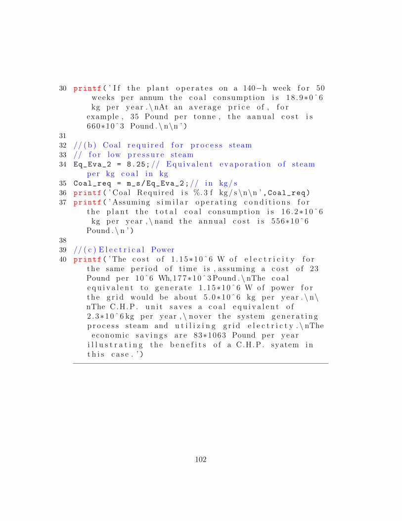
30 printf( ’ I f the p l a n t o p e r a t e s on a 140−h week f o r 50weeks per annum the c o a l consumption i s 18 . 9∗0 ˆ6kg per yea r . \ nAt an ave rage p r i c e of , f o r

example , 35 Pound per tonne , the aanua l c o s t i s660∗10ˆ3 Pound . \ n\n ’ )

31

32 // ( b ) Coal r e q u i r e d f o r p r o c e s s steam33 // f o r low p r e s s u r e steam34 Eq_Eva_2 = 8.25; // E q u i v a l e n t e v a p o r a t i o n o f steam

per kg c o a l i n kg35 Coal_req = m_s/Eq_Eva_2;// i n kg / s36 printf( ’ Coal Requ i red i s %. 3 f kg / s \n\n ’ ,Coal_req)37 printf( ’ Assuming s i m i l a r o p e r a t i n g c o n d i t i o n s f o r

the p l a n t the t o t a l c o a l consumption i s 16 . 2∗10ˆ6kg per year , \ nand the annua l c o s t i s 556∗10ˆ6

Pound . \ n ’ )38

39 // ( c ) E l e c t r i c a l Power40 printf( ’ The c o s t o f 1 . 15∗10ˆ6 W o f e l e c t r i c i t y f o r

the same p e r i o d o f t ime i s , assuming a c o s t o f 23Pound per 10ˆ6 Wh,177∗10ˆ3 Pound . \ nThe c o a le q u i v a l e n t to g e n e r a t e 1 . 15∗10ˆ6 W o f power f o rthe g r i d would be about 5 . 0∗1 0ˆ 6 kg per yea r . \ n\nThe C.H. P . u n i t s a v e s a c o a l e q u i v a l e n t o f2 . 3∗1 0ˆ 6 kg per year , \ nover the system g e n e r a t i n gp r o c e s s steam and u t i l i z i n g g r i d e l e c t r i c t y . \ nThe

economic s a v i n g s a r e 83∗1063 Pound per yea ri l l u s t r a t i n g the b e n e f i t s o f a C .H. P . syatem i nt h i s c a s e . ’ )

102

Chapter 8

Electrical energy

Scilab code Exa 8.1 Ohms law

1 clear ;

2 clc;


7 // g i v e n8 V = 240; // Vo l tage i n V o l t s9 I = 8; // Current i n Amps

10 //By ohm ’ s law−> V = I ∗R11 R = V/I;// In ohms12 printf( ’ The r e s i s t a n c e o f the g i v e n c i r c u i t i s %. 0 f

ohms ’ ,R)

Scilab code Exa 8.2 Kirchhoff law

1 clear ;

2 clc;

103


7 // g i v e n8 V1 = 100; // In V o l t s9 V2 = 50; // In V o l t s

10 R1 = 8; // R e s i s t a n c e i n ohm11 R2 = 5; // R e s i s t a n c e i n ohm12 R3 = 10; // R e s i s t a n c e i n ohm13 R4 = 50; // R e s i s t a n c e i n ohm14 //By r e f e r i n g f i g u r e 8 . 3 , and a p p l y i n g k i r c h o f f ’ s

c u r r e n t law and k i r c h o f f ’ s v o l t a g e law i n theg i v e n c i r c u i t diagram , we g e t f o l l o w i n g e q u a t i o n s:

15 // I1 = I2 + I316 //V1 − R1∗ I 1 − V2 − R3∗ I 3 = 017 //V2 − R4∗ I 3 + R3∗ I 3 − R2∗ I 2 = 018 A = [1 -1 -1;8 0 10;0 55 -10];

19 b = [0;50;50];

20 x = A\b

21 printf( ’ The c u r r e n t s i n I1 i s %. 1 f A \n ’ ,x(1))22 printf( ’ The c u r r e n t s i n I2 i s %. 1 f A \n ’ ,x(2))23 printf( ’ The c u r r e n t s i n I3 i s %. 1 f A \n ’ ,x(3))

Scilab code Exa 8.3 Power factor

1 clear ;

2 clc;


7 // g i v e n8 R = 6; // R e s i s t a n c e i n ohm

104

9 Xc = 16; // C a p a c i t i v e r e s i s t a n c e i n ohm10 Xl = 24; // I n d u c t i v e r e s i s t a n c e i n ohm11 Z = ((R^2) + (Xc - Xl)^2) ^0.5; // Impedance i n ohm12 P_f = R/Z;// Power f a c t o r = co s ( x ) = 0 . 613 x = acos (0.6);

14 y = sqrt(1 - P_f ^2);//y = s i n ( x )15 V = 200; // i n V o l t s ( s i n wave v o l t a g e = ( ( 2 0 0 ∗ 2 ˆ 1 . 5 ) ∗

s i nwt )16 I = V/Z;// Current i n Amperes17 P = I^2 * R;// i n W18 Q = V * I * y;// i n VAR19 S = V * I;// i n VA20 printf( ’ The a c t u a l power i s %. 0 f W \n ’ ,P)21 printf( ’ The r e a c t i v e power i s %. 0 f VAR \n ’ ,Q)22 printf( ’ The apparent power i s %. 0 f VA \n ’ ,S)

Scilab code Exa 8.4 Cost of electrical energy

1 clear ;

2 clc;


7 // g i v e n8 pump_1 = 100*10^3; // Requ i red pump i n W9 T_1 = 8; // Pump Operat ing t ime o f each day

10 Inc_op = 0.5; // I n c r e a s e d output per c en t11 pump_ex = 50*10^3; // Extra pump r e q u r i e d i n W12


14 printf( ’ t h e r e i s no computa t i ona l pa r t i n theproblem ’ )

105

Scilab code Exa 8.5 Annual saving

1 clear ;

2 clc;


7 // g i v e n8 P = 600*10^3; // Power demand o f pump i n W9 T = 8; // Operat ing t ime i n hour per day

10 red = 1.00/10^3; // o f f−peak r e d u c t i o n i n Pound per10ˆ3 W month

11 M_save = P*red;// Monthly s a v i n g Pound per month12 A_save = M_save *12; // Annual s a v i n g i n Pound per

yea r13 printf( ’ Annual s a v i n g i s %. 0 f Pound per yea r ’ ,A_save

)

Scilab code Exa 8.6 Illumination

1 clear ;

2 clc;


7 // g i v e n8 T_lamp = 12*10^3; // Output f o r the t u n g s t e n f i l a m e n t

lamp i n lm per 10ˆ3 W9 F_tube = 63*10^3; // Output f o r the f l u o r e s c e n t tube s

i n lm per 10ˆ3 W

106

10 Save = F_tube - T_lamp;// i n W11 printf( ’ Energy s a v i n g i s %. 0 f lm per 10ˆ3 W \n ’ ,Save

)

12

13 Save_pcent = (Save/F_tube)*100;

14 printf( ’ Energy s a v i n g per c en t i s %. 0 f ’ ,floor(Save_pcent))

Scilab code Exa 8.7 Natural lighting

1 clear ;

2 clc;


7 // g i v e n8 N = 40; // Number o f lamps9 T1 = 15; // Operat ing t ime i n h per day

10 P = 500; // POwer from the lamps i n W11 T2 = 300; // Tota l o p e r a t i n g t ime i n days per yea r12 C = 2.5/10^3; // E l e c t r i c i t y c o s t i n p per Wh13

14 An_Cost = N*P*T1*T2*C*10^ -2; // In euro15 printf( ’ The Annual Cost i s %. 0 f Euro \n ’ ,An_Cost)16

17 // Improvement i n l i g h t by i n s t a l l i n g g l a s s f i b r es k y l i g h t s

18 T3 = 5; // Extra Time f o r n a t u r a l l i g h t i n g i n h perday

19 New_An_Cost = N*P*(T1-T3)*T2*C*10^ -2; // In euro20 printf( ’ The New Annual Cost i s %. 0 f Euro \n ’ ,

New_An_Cost)

21

22 Save = An_Cost - New_An_Cost;// i n euro

107

23 printf( ’ The annual s a v i n g f o r a pay−back p e r i o d o f2 . 5 y e a r s i s %. 0 f ’ ,Save)

Scilab code Exa 8.8 Motive power and power factor improvement

1 clear ;

2 clc;



8

9 //By r e f e r i n g f i g u r e 8 . 7 which shows Poer f a c t o r−l o ad curve f o r a motor with a c a p a c i t o r and onewi thout a c a p a c i t o r .

10 printf( ’ t h e r e i s no computa t i ona l pa r t i n theproblem ’ )

Scilab code Exa 8.9 Capacitor rating

1 clear ;

2 clc;



8 // g i v e n9 l = 500*10^3; // Load i n VA

10 P_F = 0.6; // Power Facto r

108

11 Req_P_F = 0.9; // Requ i red power f a c t o r12 // Re f e r to f i g u r e 8 . 813 BC = 2.5; // u n i t s14 C_rt = 250*10^3; // i n VAR ( o b t a i n e d from f i g u r e 8 . 8 )15 printf( ’ The r e q u i r e d con den s e r r a t i n g i s %. 0 f \n ’ ,

C_rt)

Scilab code Exa 8.10 Effects of power factor improvement

1 clear ;

2 clc;


7 P = 100; // Power i n 10ˆ3 W8 C = 5; // Charge i n Euro per 10ˆ3 per month9 PF = [1.0 0.9 0.8 0.7 0.6 0.5]; // Power f a c t o r

10 for i = [1:1:6]

11 VA = (PF(i)\P)*C

12 printf( ’ Charge per month f o r power f a c t o r %. 1 fi s %. 0 f Euro \n ’ , PF(i),VA)

13 end


1 clear ;

2 clc;


109


8 // g i v e n9 P_F_1 = 0.7; // I n i t i a l power f a c t o r10 P_F_2 = 0.95; // F i n a l power f a c t o r11 // Re f e r F i gu r e 8 . 1 012 red_I = 26; // r e d u c t i o n i n c u r r e n t i n per c en t13 printf( ’ The r e d u c t i o n i n c u r r e n t i s %. 0 f per c en t \n

’ ,red_I)14 P_F_3 = 1.0; // I n c r e a s e d power f a c t o r15 // From f i g u r e 8 . 1 016 Save = 4; // per c en t17 printf( ’ I n c r e a s e i n power f a c t o r from 0.95 −1 .0 on ly

i n c r e a s e s s a v i n g f u r t h e r by a %. 0 f per c en t ’ ,Save)


1 clear ;

2 clc;



8 // g i v e n9 C = 10000; // I n s t a l l a t i o n c o s t o f c a p a c i t o r s i n

Pound10 P_F_1 = 0.84; // I n i t i a l power f a c t o r11 P_F_2 = 0.97; // F i n a l power f a c t o r12 // Re f e r F i gu r e 8 . 1 013 red_dem = 14; // r e d u c t i o n i n maximum demand i n per

c en t14 T = 9; // pay−back t ime i n months

110

15

16 printf( ’ The r e d u c t i o n i n maximum demand i s %. 0 f perc en t \n ’ ,red_dem)

17 printf( ’ The pay−back t ime was %. 0 f months ’ ,T)18 // This q u e s t i o n does not c o n t a i n any c a l c u l a t i o n

pa r t .

Scilab code Exa 8.13 Optimum start control

1 clear ;

2 clc;


7 // g i v e n8 T1 = 21; // i n d e g r e e c e l c i u s9 t1 = 8; // t ime i n h per day10 c = 3.5; // c o s t i n p per u n i t11 C1 = 38; // Tota l c o s t i n Pound per 10ˆ3 W12

13 T2 = 16; // i n d e g r e e c e l c i u s14 t2 = 8; // t ime i n h per day15 C2 = 27; // Tota l c o s t i n Pound per 10ˆ3 W16

17 Save = C1 - C2;// Sav ing i n Pound per 10ˆ3 W18 Save_deg = Save/(T1 - T2);// Tota l Sav ing i n Pound

per 10ˆ3 W f o r each d e g r e e drop19 Save_per = (Save_deg/C1)*100; // Sav ing i n p e r c e n t20 printf( ’ For each d e g r e e drop , an ene rgy s a v i n g o f %

. 0 f per c en t i s a c h i e v e d ’ ,floor(Save_per))

Scilab code Exa 8.14 Induction heating

111

1 clear ;

2 clc;



8 // r e f e r Table 8 . 69 O_1 = 1750;

10 O_2 = 0;

11 O_3 = 2;

12 O_4 = 150;

13 O_5 = 1900;

14 O_6 = 0;

15 I_1 = 580;

16 I_2 = 1658;

17 I_3 = 0.5;

18 I_4 = 40;

19 I_5 = 1698;

20 I_6 = 11;

21 D_1 = 300;

22 D_2 = 869;

23 D_3 = 0.5;

24 D_4 = 40;

25 D_5 = 900;

26 D_6 = 37;

27 printf( ’ \ t ENERGY COSTS FOR HEATING STEEL BILLETS\n\n Components (10ˆ3 W/ tonne ) \ t ( 1 ) O i l f i r e d \ t( 2 ) I n d u c t i o n \ t ( 3 ) D i r e c t r e s i s t a n c e \n Fuel (e l e c t r i c i t y ) \ t \ t %. 0 f \ t \ t %. 0 f \ t \t% . 0 f \n E l e c t r i c i t y ( as pr ime ene rgy ) %. 0 f \ t \ t \ t%. 0 f \ t \t% . 0 f \n Metal l o s s ( p e r c e n t ) \ t \ t %. 0 f\ t \ t \ t %. 1 f \ t \t% . 1 f \n Metal l o s s ( as ene rgy) \ t \ t %. 0 f \ t \ t \ t %. 0 f \ t \t% . 0 f \n Tota lene rgy needs \ t \ t %. 0 f \ t \ t \ t %. 0 f \ t \t% . 0 f \n

Energy s a v i n g to ( 1 ) \ t \ t %. 0 f \ t \ t \ t %. 0 f \ t \t \t% . 0 f \n ’ ,O_1 ,I_1 ,D_1 ,O_2 ,I_2 ,D_2 ,O_3 ,I_3 ,D_3 ,

112

O_4 ,I_4 ,D_4 ,O_5 ,I_5 ,D_5 ,O_6 ,I_6 ,D_6)

Scilab code Exa 8.15 Atmosphere generators

1 clear ;

2 clc;



8 // r e f e r Table 8 . 79 El = 35; // Pe r c en tage o f e l e c t r i c i t y produced from

pr imary f u e l10 En_1 = 50; // Endothermic gas (mˆ3)11 En_2 = 100; // Endothermic gas (mˆ3)12 En_3 = 200; // Endothermic gas (mˆ3)13 G_1 = 97; // Gas use (10ˆ3 Wh)14 G_2 = 194; // Gas use (10ˆ3 Wh)15 G_3 = 386; // Gas use (10ˆ3 Wh)16 El_1 = 24; // E l e c t r i c i t y use (10ˆ3 Wh)17 El_2 = 48; // E l e c t r i c i t y use (10ˆ3 Wh)18 El_3 = 95; // E l e c t r i c i t y use (10ˆ3 Wh)19 P_1 = 69; // Primary ene rgy (10ˆ3 Wh)20 P_2 = 137; // Primary ene rgy (10ˆ3 Wh)21 P_3 = 271; // Primary ene rgy (10ˆ3 Wh)22 printf( ’ USE OF ELECTRICITY AND GAS FOR HEATING

ENDOTHERMIC GAS GENERATORS\n\n Endothermic gas (mˆ3) \ t %. 0 f \ t %. 0 f \ t %. 0 f \n Gas use (10ˆ3 Wh) \ t %. 0 f \ t %. 0 f \ t %. 0 f \n E l e c t r i c i t yuse (10ˆ3 Wh) \ t %. 0 f \ t %. 0 f \ t %. 0 f \n Primary

ene rgy (10ˆ3 Wh) \ t %. 0 f \ t %. 0 f \ t %. 0 f \n ’ ,En_1 ,En_2 ,En_3 ,G_1 ,G_2 ,G_3 ,El_1 ,El_2 ,El_3 ,P_1 ,P_2

,P_3)

113

Chapter 9

Building construction

Scilab code Exa 9.1 Fabric loss

1 clear;

2 clc;


7 // g i v e n8 a = 40; // i n m9 b = 25; // i n m

10 c = 20; // i n m11 d = 10; // i n m12 e = 5; // i n m13 f = 2; // i n m14 g = 3; // i n m15 h = 6; // i n m16

17 // ( 1 ) Produc t i on Area18 T1 = 21; // Temperature d i f f e r e n c e i n d e g r e e c e l c i u s19 T2 = -3; // Temperature d i f f e r e n c e i n d e g r e e c e l c i u s20 U1 = 1.2; // heat t r a n s f e r c o e f f i c e n t i n W/m−K21 U2 = 5.6; // heat t r a n s f e r c o e f f i c e n t i n W/m−K

115

22 U3 = 2.0; // heat t r a n s f e r c o e f f i c e n t i n W/m−K23 U4 = 0.7; // heat t r a n s f e r c o e f f i c e n t i n W/m−K24 U5 = 0.9; // heat t r a n s f e r c o e f f i c e n t i n W/m−K25 // As Q = U∗A∗T26 Q1 = (b*h)*U1*T1;// Heat l o s s i n W. w a l l i n W27 Q2 = (((a-c)*h) + (d*h) + (d*f))*U1*T1;// Heat l o s s

i n N. w a l l i n W28 Q3 = (c*f)*U2*T1;// Heat l o s s i n N. window i n W29 Q4 = (b*g)*U3*T2;// Heat l o s s i n N. w a l l / i n t e r n a l i n

W30 Q5 = (b*g)*U1*T1;// Heat l o s s i n E . w a l l / e x t e r n a l i n

W31 Q6 = (((a-c)*h) + (d*h) + (d*f))*U1*T1;// Heat l o s s

i n S . w a l l i n W32 Q7 = (c*f)*U2*T1;// Heat l o s s i n S . window i n W33 Q8 = (b*a)*U4*T1;// Heat l o s s i n r o o f i n W34 Q9 = (b*a)*U5*T1;// Heat l o s s i n f l o o r i n W35 T_Q_P = Q1 + Q2 + Q3 + Q4 + Q5 + Q6 + Q7 + Q8 + Q9;

// i n W36

37 // For O f f i c e s u r f a c e38 T3 = 24; // Temperature d i f f e r e n c e i n d e g r e e c e l c i u s39 T4 = 3; // Temperature d i f f e r e n c e i n d e g r e e c e l c i u s40 // As Q = U∗A∗T41 Q_1 = (b*g)*U3*T4;// Heat l o s s i n W. w a l l i n W42 Q_2 = (d*g)*U1*T3;// Heat l o s s i n N. w a l l i n W43 Q_3 = (((b-(2*e))*g) +(e*f))*U1*T3;// Heat l o s s i n E

. Wall i n W44 Q_4 = (e*f)*U2*T3;// Heat l o s s i n E . window i n W45 Q_5 = (e*f)*U2*T3;// Heat l o s s i n E . window i n W46 Q_6 = (d*g)*U1*T3;// Heat l o s s i n S . w a l l i n W47 Q_7 = (b*d)*U4*T3;// Heat l o s s i n S . r o o f i n W48 Q_8 = (b*d)*U5*T3;// Heat l o s s i n f l o o r i n W49 T_Q_O = Q_1 + Q_2 + Q_3 + Q_4 + Q_5 + Q_6 + Q_7 +

Q_8; // i n W50

51 T_Q = T_Q_P + T_Q_O;// i n W52 printf( ’ Tota l b u i l d i n g f a b r i c l o s s i s %. 0 f W’ ,T_Q)

116

Scilab code Exa 9.2 U value calculation

1 clear ;

2 clc;


7 // g i v e n8 L_Br = 0.105; // Length o f b r i ckwork i n m9 L_Bl = 0.100; // Length o f b lockwork i n m10 L_C = 0.05; // Length o f c a v i t y i n m11 K_Br = 0.84; // Thermal c o n d u c t i v i t y o f b r i ckwork i n

W/m−K12 K_Bl = 0.22; // Thermal c o n d u c t i v i t y o f b lockwork i n

W/m−K13 K_C_in = 0.033; // Thermal c o n d u c t i v i t y o f i n s u l a t i o n

i n c a v i t y i n W/m−K14 R_Ex = 0.055; // R e s i s t a n c e o f e x t e r n a l s u r f a c e i n W/

mˆ2−K15

16 //As R = L/K17 R_Br = (L_Br/K_Br);// R e s i s t a n c e o f b r i ckwork i n W/m

ˆ2−K18 R_Bl = (L_Bl/K_Bl);// R e s i s t a n c e o f b lockwork i n W/m

ˆ2−K19 R_C = 0.18; // R e s i s t a n c e o f c a v i t y i n W/mˆ2−K20

21 // Without i n s u l a t i o n o f c a v i t y22 R_T = 0.938; // Tota l R e s i s t a n c e i n W/mˆ2−K23 // Thermal t r a n s m i t t a n c e − U = (1/ R T)24 U = (1/R_T);// i n W/mˆ2−K25 printf( ’ The U−v a l u e o f e x t e r n a l w a l l i s %. 2 f W/ sq .m

K \n ’ ,U)

117

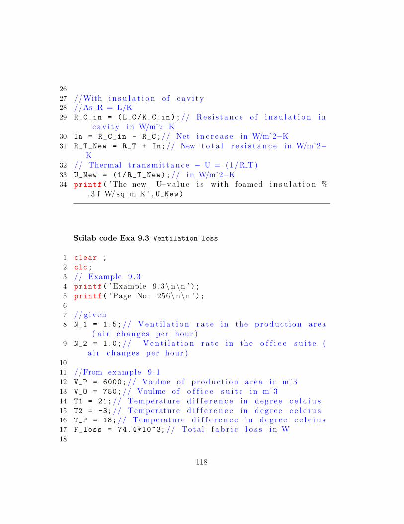
26

27 // With i n s u l a t i o n o f c a v i t y28 //As R = L/K29 R_C_in = (L_C/K_C_in);// R e s i s t a n c e o f i n s u l a t i o n i n

c a v i t y i n W/mˆ2−K30 In = R_C_in - R_C;// Net i n c r e a s e i n W/mˆ2−K31 R_T_New = R_T + In;// New t o t a l r e s i s t a n c e i n W/mˆ2−

K32 // Thermal t r a n s m i t t a n c e − U = (1/ R T)33 U_New = (1/ R_T_New);// i n W/mˆ2−K34 printf( ’ The new U−v a l u e i s with foamed i n s u l a t i o n %

. 3 f W/ sq .m K ’ ,U_New)

Scilab code Exa 9.3 Ventilation loss

1 clear ;

2 clc;


7 // g i v e n8 N_1 = 1.5; // V e n t i l a t i o n r a t e i n the p r o d u c t i o n a r ea

( a i r changes per hour )9 N_2 = 1.0; // V e n t i l a t i o n r a t e i n the o f f i c e s u i t e (

a i r changes per hour )10

11 //From example 9 . 112 V_P = 6000; // Voulme o f p r o d u c t i o n a r ea i n mˆ313 V_O = 750; // Voulme o f o f f i c e s u i t e i n mˆ314 T1 = 21; // Temperature d i f f e r e n c e i n d e g r e e c e l c i u s15 T2 = -3; // Temperature d i f f e r e n c e i n d e g r e e c e l c i u s16 T_P = 18; // Temperature d i f f e r e n c e i n d e g r e e c e l c i u s17 F_loss = 74.4*10^3; // Tota l f a b r i c l o s s i n W18

118

19 // As Q vent = 0 . 3 3 ∗ N ∗ V ∗ (T1 − T2)20 Q_vent_P = 0.33 * N_1 * V_P * (T_P - T2);//

V e n t i l a t i o n l o s s i n p r o d u c t i o n a r ea i n W21 Q_vent_O = 0.33 * N_2 * V_O * (T1 - T2);//

V e n t i l a t i o n l o s s i n o f f i c e s u i t e i n W22 V_loss = Q_vent_P + Q_vent_O;// Tota l v e n t i l a t i o n

l o s s i n W23 T_loss = F_loss + V_loss;// Tota l heat l o s s i n W24 p = (V_loss/T_loss)*100;

25 printf( ’ p e r c e n t a g e o f v e n t i l a t i o n l o s s i s %. 0 fp e r c e n t ’ ,p)

Scilab code Exa 9.4 Environmental temperature

1 clear ;

2 clc;


7 // ( a ) Des ign l o s s8 T1 = 18; // I n t e r n a l t e empe ra tu r e ( s p e c i f i e d as an

Envi ronmenta l t empera tu r e ) i n d e g r e e c e l c i u s9 //From example 9 . 1

10 A = [150 200 40 75 75 200 40 1000 1000]; // i n mˆ211 U = [1.2 1.2 5.6 2 1.2 1.2 5.6 0.7 0.9]; // i n W/m−K12 Qf = 58.3*10^3; // Fabr i c l o s s i n p r o d u c t i o n a r ea i n

W13 T2 = -3; // i n d e g r e e c e l c i u s14 s1 =0;

15 s2 = 0;

16 for i = [1:1:9]

17 s1 = s1+A(i);

18 s2 = s2+U(i)*A(i);

19 end

119

20 A_T = s1;// Tota l a r ea i n mˆ221 UA_T = s2;// sum o f U∗A i n W/m−K ( answer wrongly

c a l c u l a t e d i n the book )22

23 //From example 9 . 324 N_1 = 1.5; // V e n t i l a t i o n r a t e i n the p r o d u c t i o n a r ea

( a i r changes per hour )25 V_P = 6000; // Voulme o f p r o d u c t i o n a r ea i n mˆ326

27 //As Qvent = C ∗ (T1 − T2) & C = 0 . 3 3∗N∗V∗ (1 + ( (UA T) / ( 4 . 8 ∗A T) ) )

28 C = 0.33* N_1*V_P*(1 + ((UA_T)/(4.8* A_T)));

29 Q_vent = C * (T1 - T2);// i n W30 T_Q1 = Qf + Q_vent;// i n W31 printf( ’ The t o t a l d e s i g n l o s s i s %. 0 f W \n ’ ,T_Q1) //

( d e v i a t i o n i n answer i s due to e r r o r i nc a l c u l a t i o n i n the book )

32

33 // ( b ) Reduced heat l o s s34 // The heat t r a n s f e r c o e f f i e i n t i n t h i s problem has

been changed as U135 U1 = [0.44 0.44 2.8 2 0.44 0.44 2.8 0.44 0.9]; // i n W

/mˆ2−K36 T = [21 21 21 -3 21 21 21 21 21]; // Temperature

d i f f e r e n c e i n d e g r e e c e l c i u s37 s3 = 0;

38 s4 = 0;

39 for i = [1:1:9]

40 s3 = s3+U1(i)*A(i);

41 s4 = s4+U1(i)*A(i)*T(i);

42 end

43 U1A_T = s3;// i n W/m−k ( answer wrongly c a l c u l a t e d i nthe book )

44 Q_loss = s4 // i n W45

46

47 //As Qvent = C ∗ (T1 − T2) & C = 0 . 3 3∗N∗V∗ (1 + ( (UA T) / ( 4 . 8 ∗A T) ) )

120

48 C = 0.33* N_1*V_P*(1 + ((U1A_T)/(4.8* A_T)))

49 Q_vent = C * (T1 - T2)// i n W50 T_Q2 = Q_loss + Q_vent // i n W51

52 Red = T_Q1 - T_Q2;// In W53 printf( ’ The r e d u c t i o n i n l o s s i s %. 0 f W’ ,Red) // (

d e v i a t i o n i n answer i s due to e r r o r i nc a l c u l a t i o n i n the book )

Scilab code Exa 9.5 The degree day method

1 clear ;

2 clc;


7 // g i v e n8 T = 21; // Temperature d i f f e r e n c e i n d e g r e e c e l c i u s9 Deg_d = 2186; // Tota l degree−days base ( 1 5 . 5 deg C)

S e p t e m b e r A p r i l10 T_D = 18; // Des ign Temperature i n d e g r e e c e l c i u s11 T_O = 4; // base o f f s e t t empera tu r e i n d e g r e e c e l c i u s12 T_b = T_D - T_O;// Base t empera tu re i n d e g r e e

c e l c i u s13

14 // From Table 9 . 1 1 C o r r e c t i o n f a c t o r f o r baset empra tu r e s o t h e r than 1 5 . 5 deg C i s o b t a i n e d . So

f o r 14 deg c i t s 0 . 8 215 C = 0.82; // C o r r e c t i o n f a c t o r16 Do = Deg_d * C// C o r r e c t e d degree−days17

18 // ( a ) O r i g i n a l c o n s t r u c t i o n19 // from example 9 . 420 Q_d_1 = 133.7*10^3; // Des ign heat l o s s i n W

121

21

22 H_1 = Q_d_1/T;

23 //As E = 24 ∗ H ∗ Do − E = Energy consumption i n (Wh)

24 E1 = (24* H_1 *Do)/10^6; // i n 10ˆ6 Wh ( from t h i ss t e p ’Do ’ i s m i s t a k e l y taken as 1972 i n p l a c e o f1792 i n the s o l u t i o n o f the book , so t h e r e i sd e v i a t i o n i n answer )

25 E_1 = (E1 * 3600) *10^6; // i n J26 printf( ’ The t o t a l ene rgy consumption i n o r i g i n a l

c o n s t r u c t i o n i s %. 0 e J \n ’ ,E_1)// D e v i a t i o n i nthe answer i s due to some c a l c u l a t i o n e r r o r asment ioned above

27

28 // ( b ) Improved i n s u l a t i o n29 // from example 9 . 430 Q_d_2 = 104.4*10^3; // Des ign heat l o s s i n W31

32 H_2 = Q_d_2/T;

33 //As E = 24 ∗ H ∗ Do − E = Energy consumption i n (Wh)

34 E2 = (24* H_2 *Do)/10^6; // i n 10ˆ6 Wh ( from t h i ss t e p ’Do ’ i s m i s t a k e l y taken as 2972 i n p l a c e o f2792 i n the s o l u t i o n o f the book , so t h e r e i sd e v i a t i o n i n answer )

35 E_2 = (E2 * 3600) *10^6; // i n J36 printf( ’ The t o t a l ene rgy consumption i n improved

i n s u l a t i o n i s %. 4 e J \n ’ ,E_2)// D e v i a t i o n i n theanswer i s due to some c a l c u l a t i o n e r r o r asment ioned above

Scilab code Exa 9.6 Surface condensation

1 clear ;

2 clc;

122


7 // g i v e n8 U1 = 5.6; // S i n g l e g l a z i n g heat t r a n s f e r c o e f f i c i e n t

i n W/mˆ2 K9 U2 = 2.8; // Double g l a z i n g heat t r a n s f e r c o e f f i c i e n t

i n W/mˆ2 K10 Ti = 21; // I n t e r n a l Temperature i n d e g r e e c e l c i u s11 To = -1; // E x t e r n a l Temperature i n d e g r e e c e l c i u s12 R_H = 0.5; // R e l a t i v e humid i ty13 Rs_i = 0.123; // S u r f a c e r e s i s t a n c e i n (W/mˆ2−K) ˆ−114

15 // At 21 Degree c e l c i u s and R.H. = 0 . 5 , the dewp o i n t i s 1 0 . 5 d e g r e e c e l c i u s

16 Dew_pt = 10.5; // Dew p o i n t i n d e g r e e c e l c i u s17 //As T s i = Ti − ( R s i ∗ U ∗ ( Ti − To) )18

19 // ( a ) S i n g l e G laz ing20 Ts_i_S = Ti - (Rs_i * U1 *(Ti - To));// i n d e g r e e

c e l c i u s21 printf( ’ The i n t e r n a l s u r f a c e t empera tu r e f o r s i n g l e

g l a z i n g i s %. 1 f deg C \n ’ ,Ts_i_S)22 if (Dew_pt > Ts_i_S) then

23 disp( ’ S u r f a c e c o n d e n s a t i o n w i l l o c cu r s i n c e i ti s l e s s than 1 0 . 5 deg C. ’ )

24 else

25 disp( ’No s u r f a c e c o n d e n s a t i o n i s expec t ed as i ti s g r e a t e r than 1 0 . 5 deg C. ’ )

26 end

27

28 // ( b ) Double G laz ing29 Ts_i_D = Ti - (Rs_i * U2 *(Ti - To));// i n d e g r e e

c e l c i u s30 printf( ’ The i n t e r n a l s u r f a c e t empera tu r e f o r s i n g l e

g l a z i n g i s %. 1 f deg C \n ’ ,Ts_i_D)31 if (Dew_pt > Ts_i_D) then

123

32 disp( ’ S u r f a c e c o n d e n s a t i o n w i l l o c cu r s i n c e i ti s l e s s than 1 0 . 5 deg C. ’ )

33 else

34 disp( ’No s u r f a c e c o n d e n s a t i o n i s expec t ed s i n c ei t i s g r e a t e r than 1 0 . 5 deg C. ’ )

35 end

Scilab code Exa 9.7 Interstitial condensataion

1 clear ;

2 clc;


7 // g i v e n8 l_1 = 240; // e x i s t i n g l e n g t h o f s o l i d b r i c k i n mm9 l_u = 25; // upgraded i n t e r n a l l i n i n g i n mm

10 l_e = 9.5; // Expanded p o l y s t y r e n n e i n mm11 T_i = 20; // I n t e r n a l t empera tu r e i n deg r e c e l c i u s12 R_H_i = 50; // I n t e r n a l R e l a t i v e humid i ty i n p e r c e n t13 T_e = 0; // E x t e r n a l t empera tu re i n deg r e c e l c i u s14 R_H_e = 90; // E x t e r n a l R e l a t i v e humid i ty i n p e r c e n t15

16 K = [0.123 0.059 0.714 0.286 0.055]; // Thermalr e s i s t a n c e i n W/mˆ2−K

17 V_r = [0.0 0.475 3.57 9.60 0.0]; // Vapour R e s i s t a n c ei n 10ˆ9 N−s / kg

18

19 // Re f e r F i gu r e 9 . 320 //From Figu r e 9 . 3 , the tempeature , dew po int , vapour

p r e s s u r e f o r d i f f e r e n t i n t e r f a c e a r e o b t a i n e d21 T = [18.01 17.06 5.51 0.89]; // Temperature i n d e g r e e

c e l c i u s22 V_p = [1170 1148 986 550]; // Vapour p r e s s u r e i n N/mˆ2

124

23 D_P = [9.5 9.2 7.1 -1.5]; // Dew p o i n t i n d e g r e ec e l c i u s

24

25 h = (T_i - T_e)/sum(K);// i n W/mˆ226 printf( ’ The heat f l o w i s %. 2 f W/mˆ2 \n ’ ,h)27 V_p_i = V_p (1);// I n t e r n a l vapour p r e s s u r e i n N/mˆ228 V_p_e = V_p (4);// E x t e r n a l vapour p r e s s u r e i n N/mˆ229 m = ((V_p_i - V_p_e)/sum(V_r))*10^ -9; // i n kg / s30 printf( ’ The vapour mass f l o w i s %. 1 e kg / s ’ ,m)

Scilab code Exa 9.8 Glazing

1 clear ;

2 clc;


7 // g i v e n8 A = 10; // i n mˆ29 S = 0.77;

10 Sa = 0.54;

11 // f o r South12 printf( ’ \ t \ t \ t SOUTH \n ’ )13 I1 = [200 185 165 155 165 185 200]; // i n W−mˆ214 I2 = [500 455 405 385 405 455 500]; // i n W−mˆ215 for i = [1:1:7]

16 A_G_S (i) = (A*I1(i)*S) + (A*I2(i)*Sa)

17 end

18

19 printf( ’ The monthly peak c o o l i n g l o a d s f o r the monthMarch i s %. 0 f W \n ’ ,A_G_S (1))

20 printf( ’ The monthly peak c o o l i n g l o a d s f o r the monthA p r i l i s %. 0 f W \n ’ ,A_G_S (2))

21 printf( ’ The monthly peak c o o l i n g l o a d s f o r the month

125

May i s %. 0 f W \n ’ ,A_G_S (3))22 printf( ’ The monthly peak c o o l i n g l o a d s f o r the month

June i s %. 0 f W \n ’ ,A_G_S (4))23 printf( ’ The monthly peak c o o l i n g l o a d s f o r the month

Ju ly i s %. 0 f W \n ’ ,A_G_S (5))24 printf( ’ The monthly peak c o o l i n g l o a d s f o r the month

Aug . i s %. 0 f W \n ’ ,A_G_S (6))25 printf( ’ The monthly peak c o o l i n g l o a d s f o r the month

Sept . i s %. 0 f W \n\n ’ ,A_G_S (7))26

27 // For e a s t28 printf( ’ \ t \ t \ t EAST \n ’ )29 I3 = [110 150 180 190 180 150 110]; // i n W−mˆ230 I4 = [435 510 515 505 515 510 435]; // i n W−mˆ231 for j = [1:1:7]

32 A_G_E(j) = (A*I3(j)*S) + (A*I4(j)*Sa);

33 end

34 printf( ’ The monthly peak c o o l i n g l o a d s f o r the monthMarch i s %. 0 f W \n ’ ,A_G_E (1))

35 printf( ’ The monthly peak c o o l i n g l o a d s f o r the monthA p r i l i s %. 0 f W \n ’ ,A_G_E (2))

36 printf( ’ The monthly peak c o o l i n g l o a d s f o r the monthMay i s %. 0 f W \n ’ ,A_G_E (3))

37 printf( ’ The monthly peak c o o l i n g l o a d s f o r the monthJune i s %. 0 f W \n ’ ,A_G_E (4))

38 printf( ’ The monthly peak c o o l i n g l o a d s f o r the monthJu ly i s %. 0 f W \n ’ ,A_G_E (5))

39 printf( ’ The monthly peak c o o l i n g l o a d s f o r the monthAug . i s %. 0 f W \n ’ ,A_G_E (6))

40 printf( ’ The monthly peak c o o l i n g l o a d s f o r the monthSept . i s %. 0 f W \n\n ’ ,A_G_E (7))

Scilab code Exa 9.9 Design data

1 clear ;

126

2 clc;


7 // g i v e n8 A = 15; // g l a z i n g a r ea i n mˆ29 l = 10; // Length o f o f f i c e i n m

10 h = 6; // h e i g h t o f o f f i c e i n m11 w = 3.5; // width o f o f f i c e i n m12 Y_w = 4; // Admittance o f w a l l i n W/mˆ2−K13 Y_f = 3; // Admittance o f f l o o r i n W/mˆ2−K14 Y_c = 3; // Admittance o f c e i l i n g i n W/mˆ2−K15 N = 1.5; // V e n t i l a t i o n r a t e ( a i r changes per hour )16 V = l*h*w;// Volume i n mˆ317 U_G = 5.6; // Transmi t tance i n W/mˆ2−K18

19 //From t a b l e 9 . 1 8 and t a b l e 9 . 1 620 To = 16.5; // E x t e r n a l t empera tu re o f June i n d e g r e e

c e l c i u s21 T_O = 7.5; // Swing t empera tu r e i n deg r e c e l c i u s22 I = 155; // V e r t i c a l S i n W−mˆ223 Is = 385; // V e r t i c a l S i n W−mˆ224 S = 0.77; // S o l a r ga in f a c t o r25 Sa = 0.54; // S o l a r ga in f a c t o r26

27 //As For the mean i n t e r n a l t empera tu r e −Ti = To +( (A∗ I ∗S ) / ( ( 0 . 3 3 ∗N∗V) + (A∗U G) ) )

28 Ti = To + ((A*I*S)/((0.33*N*V) + (A*U_G)));// i nd e g r e e c e l c i u s

29 printf( ’ the mean i n t e r n a l t empera tu r e i s %. 1 f deg C\n ’ ,Ti)

30

31 A_G = (A*Is*Sa) + ((A*U_G) + (0.33*N*V))*T_O;//Swing i n ga in i n W

32 Net_A = 2*((w*h) + (l*w)) - A;// Net w a l l a r ea i n mˆ2

33 A_f = l*h;// f l o o r a r ea i n mˆ2

127

34 A_c = l*h;// c e i l i n g a r ea i n mˆ235 A_Y_w = Net_A * Y_w;// Wall AY i n W/K36 A_Y_f = A_f * Y_f;// F loo r AY i n W/K37 A_Y_c = A_c * Y_c;// c e i l i n g AY i n W/K38 A_Y_wi = 84; // Window AY i n W/K39 Net_AY = A_Y_w + A_Y_f + A_Y_c + A_Y_wi // i n W/K40 Ti_s = ((A_G)/((0.33*N*V) + (Net_AY)))// I n t e r n a l

Temperature swing i n deg C41 T_p = Ti + Ti_s;// i n deg C42 printf( ’ Peak i n t e r n a l t empera tu r e i s %. 1 f deg C ’ ,T_p

) // D e v i a t i o n i n the answer i s due to somec a l c u l a t i o n approx imat ion i n the book

128

Chapter 10

Air conditioning

Scilab code Exa 10.1 Sensible heating

1 clear ;

2 clc;

3 // Example 1 0 . 14 printf( ’ Example 1 0 . 1\ n\n ’ );5 printf( ’ Page No . 293\n\n ’ );6

7 // g i v e n8 m = 1; // mass f l o w r a t e o f i n i t i a l a i r mixture i n kg

/ s9 T = 23.5; // I n i t i a l t empera tu r e i n d e g r e e c e l c i u s

10 m1 = 0.6; // Pe r c en tage o f f r e s h a i r mixture11 T1 = 5; // Dry Bulb Temperature o f f r e s h a i r i n

d e g r e e c e l c i u s12 w1 = 0.005; // Humidity o f f r e s h a i r at t empera tu r e

T1 i n kg / kg13 m2 = 0.4; // Pe r c en tage o f r e c i r c u l a t e d a i r mixture14 T2 = 25; // Dry Bulb Temperature o f r e c i r c u l a t e d a i r

i n d e g r e e c e l c i u s15 w2 = 0.015; // Humidity o f r e c i r c u l a t e d a i r at

t empera tu re T2 i n kg / kg16

129

17 // In a i r c o n d i t i o n i n g => m1∗w1 + m2∗w2 = m∗w18 w = (m1*w1 + m2*w2)/m;// i n kg / kgs19 printf( ’ The humid i ty o f the a i r mixture i s %. 3 f kg /

kg \n ’ ,w)20

21 //The s p e c i f i c en tha lpy i n J/ kg can be c a l c u l a t e d bythe fo rmu la => h = ( 1 . 0 0 5∗1 0 ˆ 3∗T) +(w∗ ( ( 2 . 5 0 ∗ 1 0 ˆ 6 ) +(1 .86∗10ˆ3∗T) ) ) ; where the T i s the

t empera tu re and w i s the humid i ty at t empera tu r eT

22 h_f = (1.005*10^3* T1) +(w1 *((2.50*10^6) +(1.86*10^3*

T1)));// S p e c i f i c en tha lpy o f f r e s h a i r i n J/ kg23 h_r = (1.005*10^3* T2) +(w2 *((2.50*10^6) +(1.86*10^3*

T2)));// S p e c i f i c en tha lpy o f r e c i r c u l a t e d a i ri n J/ kg

24 h_m = (1.005*10^3*T) +(w*((2.50*10^6) +(1.86*10^3*T))

);// S p e c i f i c en tha lpy o f f i n a l a i r mixture i n J/ kg

25

26 h_t = (m1*h_f) + (m2*h_r);// Tota l en tha lpy o fi n i t i a l a i r m i x t u r e i n J/ kg

27 Q = m*(h_m - h_t);// i n Watts28 printf( ’ The l oad on the h e a t e r is% . 3 f W’ ,Q)29 // D e v i a t i o n i n answer due to d i r e c t s u b s t i t u t i o n

and some approx imat i on i n answer i n book

Scilab code Exa 10.2 Sensible cooling

1 clear ;

2 clc;


7 // g i v e n

130

8 m1 = 0.75; // Pe r c en tage o f f r e s h a i r mixture9 T1 = 31; // Dry Bulb Temperature o f f r e s h a i r i n

d e g r e e c e l c i u s10 w1 = 0.0140; // Humidity o f f r e s h a i r at t empera tu r e

T1 i n kg / kg11 m2 = 0.75; // Pe r c en tage o f r e c i r c u l a t e d a i r mixture12 T2 = 22; // Dry Bulb Temperature o f r e c i r c u l a t e d a i r

i n d e g r e e c e l c i u s13 w2 = 0.0080; // Humidity o f r e c i r c u l a t e d a i r at

t empera tu re T2 i n kg / kg14 m = 1.50; // mass f l o w r a t e o f f i n a l a i r mixture i n

kg / s15 T = 10; // Dew Point t empera tu r e i n d e g r e e c e l c i u s16

17 // In a i r c o n d i t i o n i n g => m1∗w1 + m2∗w2 = m∗w18 w = (m1*w1 + m2*w2)/m// i n kg / kgs19 printf( ’ The humid i ty o f the a i r mixture i s %. 4 f kg /

kg \n ’ ,w)20

21

22 // from the p s y c h r o m e t r i c char t , a t w = 0 . 0 1 1 kg /kg ,the dry bulb t empera tu r e i s = 2 6 . 5 d e g r e ec e l c i u s a l s o the humidi ty o f s a t u r a t e d a i r at 10

d e g r e e c e l c i u s i s 0 . 0 0 7 5 kg / kg23 T_w = 26.5; // Dry Bulb t emera tu r e i n d e g r e e c e l c i u s24 w_10 = 0.0075; // humidi ty at temperatue T i n kg / kg25

26 // the s p e c i f i c en tha lpy i n J/ kg can be c a l c u l a t e d bythe fo rmu la => h = ( 1 . 0 0 5∗1 0 ˆ 3∗T) +(w∗ ( ( 2 . 5 0 ∗ 1 0 ˆ 6 ) +(1 .87∗10ˆ3∗T) ) ) ; where the T i s the

t empera tu re and w i s the humid i ty at t empera tu r eT

27

28 h_a = (1.005*10^3* T_w) +(w*((2.50*10^6) +(1.88*10^3*

T_w)));// S p e c i f i c en tha lpy o f r e c i r c u l a t e d a i ri n J/ kg

29 h_s = (1.005*10^3*T) +(w_10 *((2.50*10^6) +(1.87*10^3*

T)));// S p e c i f i c en tha lpy o f s a t u r a t e d a i r at 10

131

d e g r e e c e l c i u s i n J/ kg30

31 Q = m*(h_a - h_s);// i n Watts32 printf( ’ The c o o l i n g l oad on the washer i s %. 0 f W’ ,Q)33 // Answer wrongly c a l c u l a t e d i n the book

132

Chapter 11

Heat recovery

Scilab code Exa 11.1 Shell and tube heat exchangers

1 clear ;

2 clc;


7 // g i v e n8 V = 205; // Flow r a t e i n mˆ39 T1 = 74; // i n d e g r e e c e l c i u s

10 T2 = 10; // i n d e g r e e c e l c i u s11 m = 1000; // Steam i n kg12 p = 950; // Dens i ty o f steam i n kg /mˆ313 C = 85; // Cost i n Pound per mˆ314 C_V = 43.3*10^6; // C a l o r i f i c v a l u e i n J/ kg15 Cp = 4.18*10^3; // heat c a p a c i t y o f water J/kg−K16 h = 2.33*10^6; // Heat o f the steam i n J/ kg17 n = 0.65; // Average b o l i e r e f f i c i e n c y18

19 S_cost = ((m*h*C)/(C_V*p*n));// Steam c o s t i n Poundper 1000 kg

20 E_save = V*m*(T1 - T2)*Cp;// Energy s a v i n g i n J per

133

day21 S_save = E_save/h;// i n kg per day22 printf( ’ the steam s a v i n g i s %. 0 f kg per day \n ’ ,

S_save)

23 G_save = (S_cost*S_save)/m;// Pound per day24 printf( ’ The g r o s s s a v i n g i s %. 0 f Pound per day per

yea r ’ ,G_save)

Scilab code Exa 11.2 Multiple effect evaporation

1 clear ;

2 clc;


7 // g i v e n8 p1 = 10; // heat−s e n s i t i v e l i q u o r pe r c en9 p2 = 50; // heat−s e n s i t i v e l i q u o r p e r c e n t10 m = 0.28; // mass r a t e i n kg / s11 t = 150; // t ime i n h per week12

13 // This q u e s t i o n does not c o n t a i n any c a l c u l a t i o npa r t i n i t .

14 I = [8250 1150 14850 16500]; // I n s t a l l a t i o n c o s t i nPound

15 A = [69300 36800 23600 24600]; // Annual steam c o s ti n Pound

16 A_S = [A(1)-A(1) A(1)-A(2) A(1)-A(3) A(1)-A(4)]; //Annual s a v i n g s i n Pound

17

18 printf( ’ \ t \ t CAPITAL AND OPERATING COSTS OFEVAPORATION PLANT\n\n\ t \ t \ t I n s t a l l a t i o n \ t \ tAnnual \ t \ t Annual s a v i n g \n Type \ t \ t \ t c o s t \t \ t \ t s team c o s t \ t \ t ( to s i n g l e e f f e c t ) \n \ t \ t \ t

134

( Pound ) \ t \ t ( Pound ) \ t \ t ( Pound ) \n\ n S i n g l ee f f e c t \ t \ t %. 0 f \ t \ t \ t %. 0 f \ t \ t \ %. 0 f \nDouble e f f e c t \ t \ t %. 0 f \ t \ t \ t %. 0 f \ t \ t \%. 0 f \ n T r i p l e e f f e c t + \n ( vapour compre s s i on ) \ t

%. 0 f \ t \ t %. 0 f \ t \ t \ %. 0 f \ n T r i p l e e f f e c t \t \ t %. 0 f \ t \ t %. 0 f \ t \ t \ %. 0 f \n\n\n ’ ,I(1),A(1),A_S(1),I(2),A(2),A_S(2),I(3),A(3),A_S (3),I

(4),A(4),A_S(4))

19

20

21 printf( ’ The r e s u l t s e n a b l e the r e t u r n on inve s tmentto be a s s e s s e d by one o f the s tandard economic

p r o c e d u r e s and the f i n a l s e l s c t i o n made . ’ )

Scilab code Exa 11.3 Vapour recompression

1 clear ;

2 clc;


7 // g i v e n8 f = 1; // f e e d o f sodium hydrox ide i n kg9 v = 0.5; // produed vapour i n kg

10 A = 30; // i n mˆ211 T1 = 95; // Temperature o f b o i l i n g s o l u t i o n i n deg C12 U = 3*10^3; // heat t r a n s f e r c o e f f i c e n t i n W/mˆ2−K13 m = 1; // f e e d r a t e i n kg / s14 Tf = 70; // Feed tempera tu re i n deg C15 h_f = 260*10^3; // Enthalpy o f f e e d i n J/ kg16 h_b = 355*10^3; // Enthalpy o f b o i l i n g s o l u t i o n i n J/

kg17 h_v = 2.67*10^6; // Enthalpy o f vapour i n J/ kg18 P1 = 0.6; // P r e s s u r e i n vapour space i n bar

135

19

20 Q = (v*h_b) + (v*h_v) -(f*h_f);// i n W21 printf( ’ The t o t a l ene rgy r e q u i r e m e n t i s %. 0 f W \n ’ ,Q

)

22

23 // As Q = A∗U∗dT24 dT = Q/(U*A);// i n d e g r e e c e l c i u s25 T2 = dT + T1;// i n d e g r e e c e l c i u s26 //The tempera tu re o f the h e a t i n g steam T2

c o r r e s p o n d s to a p r e s s u r e o f 1 . 4 bar . Drys a t u r a t e d steam at 1 . 4 bar has a t o t a l en tha lpyo f 2 . 69∗10ˆ6 J/ kg

27 // Assuming an i s e n t r o p i c compre s s i on o f the vapourfrom 0 . 6 bar to 1 . 4 bar , the o u t l e t en tha lpy i s2 . 84∗10ˆ6 J/ kg

28

29 // from steam t a b l e30 P2 = 1.4 // p r e s s u r e i n bar31 h_s = 2.69*10^6; // en tha lpy o f dry s a t u r a t e d steam

i n J/ kg32 h_v2 = 2.84*10^6 ;// the o u t l e t en tha lpy o f vapour

i n J/ kg33

34 W = v*(h_v2 - h_s);// Work i n W35 T_E = W + 60*10^3; // i n W36 printf( ’ The t o t a l ene rgy consumption i s %. 0 f W’ ,T_E)

Scilab code Exa 11.4 Thermal wheel

1 clear ;

2 clc;


136

7 // g i v e n8 Cm_S = 10000; // Company s a v i n g i n Pound per annum9 S = Cm_S /12; // Sav ing i n Pound per months10 Ca_C = 10500; // C a p i t a l c o s t i n Pound11 Ins_C = 7500; // I n s t a l l a t i o n c o s t i n Pound12 T_C = Ca_C + Ins_C;// Tota l c o s t i n Pound13 T = T_C/S;// pay−back t ime i n months14 printf( ’ The pay−back p e r i o d was %. 0 f months\n ’ ,T)

Scilab code Exa 11.5 Heat pipes

1 clear ;

2 clc;


7 //From the heat b a l a n c e :−8 // Heat r e c o v e r e d i n the b o i l e r = heat ga ined by the

a i r = heat l o s t by the f l u e g a s e s9 //=> Q = m a∗Cp a∗dT a = m f ∗Cp f ∗ dT f10 // As mass f l o w r a t e o f a i r / f l u e gas i s not g i v e n i n

the book11 // Assuming m a = m f = 2 . 2 7 3 kg / s & Cp a = 1∗10ˆ3 J/

kg−K12

13 m_a = 2.273; // i n kg / s14 m_f = m_a;// i n kg / s15 Cp_a = 1*10^3; // S p e c i f i c heat c a p a c i t y o f a i r i n J/

kg−K16 T1_a = 20; // Entrance t empera tu r e o f a i r i n d e g r e e

c e l c i u s17 T2_a = 130; // Ex i t t empera tu r e o f a i r i n d e g r e e

c e l c i u s18 dT_a = T2_a - T1_a;// i n K

137

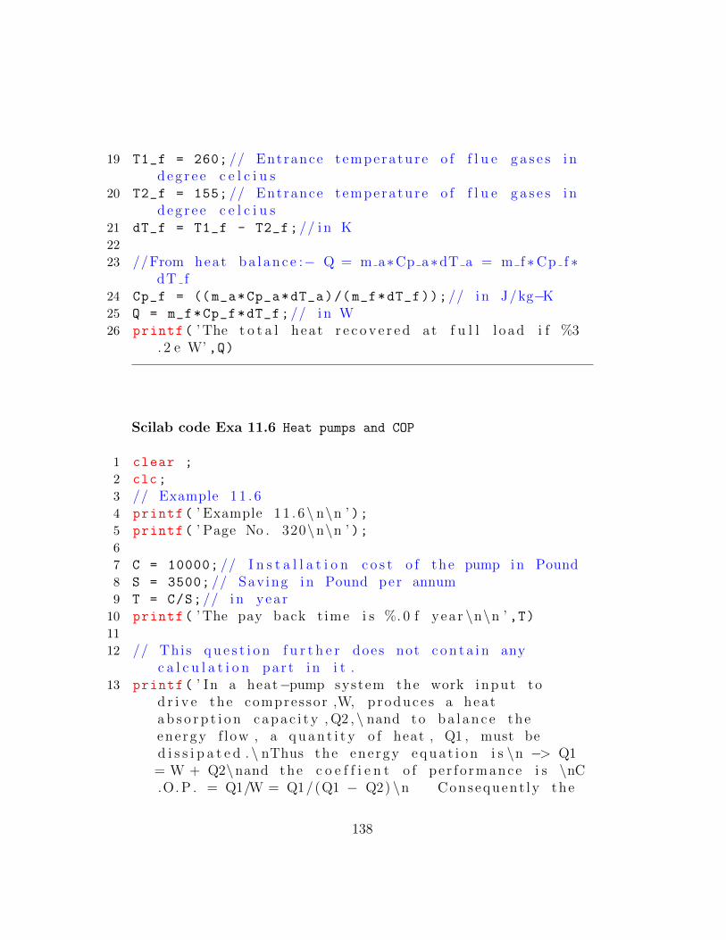
19 T1_f = 260; // Entrance t empera tu r e o f f l u e g a s e s i nd e g r e e c e l c i u s

20 T2_f = 155; // Entrance t empera tu r e o f f l u e g a s e s i nd e g r e e c e l c i u s

21 dT_f = T1_f - T2_f;// i n K22

23 //From heat b a l a n c e :− Q = m a∗Cp a∗dT a = m f ∗Cp f ∗dT f

24 Cp_f = ((m_a*Cp_a*dT_a)/(m_f*dT_f));// i n J/kg−K25 Q = m_f*Cp_f*dT_f;// i n W26 printf( ’ The t o t a l heat r e c o v e r e d at f u l l l o ad i f %3

. 2 e W’ ,Q)

Scilab code Exa 11.6 Heat pumps and COP

1 clear ;

2 clc;


7 C = 10000; // I n s t a l l a t i o n c o s t o f the pump i n Pound8 S = 3500; // Sav ing i n Pound per annum9 T = C/S;// i n yea r

10 printf( ’ The pay back t ime i s %. 0 f yea r \n\n ’ ,T)11

12 // This q u e s t i o n f u r t h e r does not c o n t a i n anyc a l c u l a t i o n pa r t i n i t .

13 printf( ’ In a heat−pump system the work input tod r i v e the compressor ,W, produce s a heata b s o r p t i o n c a p a c i t y , Q2 , \ nand to b a l a n c e theene rgy f low , a q u a n t i t y o f heat , Q1 , must bed i s s i p a t e d . \ nThus the ene rgy e q u a t i o n i s \n −> Q1= W + Q2\nand the c o e f f i e n t o f pe r f o rmance i s \nC.O. P . = Q1/W = Q1/(Q1 − Q2) \n Consequent ly the

138

C.O. P . i s a lways g r e a t e r than u n i t y . \ nThe maximumt h e o r e t i c a l v a l u e o f the C .O. P . i s tha t

p r e d i c t e d by the Carnot i n c h a p t e r 2 , namely : \ n−> (C .O. P . ) max = T1/(T1 − T2) ’ )

Scilab code Exa 11.7 Coefficient of performance

1 clear ;

2 clc;


7 // g i v e n8 T1 = 40; // i n d e g r e e9 T2 = 0; // i n d e g r e e c e l c i u s10 //As from c a r n o t c y c l e , C .O. P = (T1/(T1 − T2) ) ,

where t empera tu re a r e i n d e g r e e c e l c i u s11 C_O_P1 = ((T1 +273) /((T1 +273) - (T2 +273)));

12 printf( ’C .O. P . i s %. 1 f \n ’ ,C_O_P1)13

14 // A seconda ry f l u i d as hot water at 60 deg C i sused

15 T3 = 60; // Temperature o f hot water i n d e g r e ec e l c i u s

16 C_O_P2 = ((T3 +273) /((T3 +273) - (T2 +273)));

17 printf( ’C .O. P . when s e conda ry f l u i d i s used i s %. 1 f\n ’ ,C_O_P2)

Scilab code Exa 11.8 Incineration plant

1 clear ;

2 clc;

139


7 // This q u e s t i o n does not c o n t a i n any c a l c u l a t i o npa r t i n i t .

8 printf( ’No c a l c u l a t i o n i s r e q u i r e d as not i n showni n book ’ )

Scilab code Exa 11.9 Regenerators

1 clear ;

2 clc;


7 // g i v e n8 T1 = 273; // Measured t empera tu r e In d e g r e e c e l c i u s9 P = 1; // Measured p r e s s u r e i n bar

10 T2 = 290; // i n i t i a l t empera tu r e In d e g r e e c e l c i u s11 T3 = 1000; // F i n a l t empera tu r e In d e g r e e c e l c i u s12 T4 = 1150; // E nt e r i ng t empear tu r e In d e g r e e c e l c i u s13 v1 = 7; // i n mˆ3/ s14 v2 = 8; // i n mˆ s15 M = 22.7; // i n kmol /mˆ316 d = 0.1; // Diameter i n m17 A = 0.01; // S u r f a c e a r ea per r e g e n e r a t o r channe l i n

mˆ218 u = 1; // maximum v e l o c i t y i n m/ s19 Cp_1 = 34*10^3; // Heat c a p a c i t y at T4 tempera tu re i n

J/kmol−K20 Cp_2 = 32*10^3; // Heat c a p a c i t y at o u t l e t

t empera tu re i n J/kmol−K21 Cp_m = 30*10^3; // Heat c a p a c i t y at mean tempera tu re

140

i n J/kmol−K22

23 m_c = v1/M;// Mola l a i r f l o w r a t e i n kmol / s24 H_c1 = Cp_m*(T3 - T1);// Enthalpy o f a i r a t 1000K i n

J/mol25 H_c2 = Cp_m*(T2 - T1);// Enthalpy o f a i r a t 290 i n J

/mol26 Q = (m_c*(H_c1 - H_c2))/10^6; // i n 10ˆ6 W27 printf( ’ The heat t r a n s f e r , Q i s %. 1 f ∗10ˆ6 W \n ’ ,Q)28

29 m_F = v2/M;// Mola l f l o w r a t e o f f l u e gas i n kmol / s30 dH = (Q/m_F)*10^6; // en thap ly chnage o f the f l u e gas

i n J/ kmol31 H_F1 = Cp_1*(T4 - T1);// Enthalpy o f the f l u e gas at

1150 K i n J/ kmol32 H_F2 =H_F1 - dH;// Enthalpy at the e x i t t empera tu r e

i n J/ kmol33 T_F2 = (H_F2/Cp_2) + T1;// i n K34 printf( ’ The e x i t t empear tu r e o f the f l u e gas i s %. 0 f

K \n ’ ,T_F2)35 S_R = v2/u;// c r o s s s e c t i o n a l a r ea o f the r e g e n e r a t o r

i n mˆ236 N = S_R/A;

37 printf( ’ The number o f c h a n n e l s r e q u i r e d i s %. 0 f \n ’ ,N)

38 printf( ’ Consequent ly f o r t h i s r e g e n e r a t o r a squa r el a y o u t cou ld be a c h i e v e d with 40 c h a n n e l sa r ranged h o r i z o n t a l l y and 20 c h a n n e l s v e r t i c a l l y .’ )

Scilab code Exa 11.10 Waste heat boilers

1 clear ;

2 clc;

3 // Example 1 1 . 1 0

141

4 printf( ’ Example 1 1 . 1 0\ n\n ’ );5 printf( ’ Page No . 324\n\n ’ );6

7 // g i v e n8 Pr = 100; // Produc t i on i n tonne s per day9 p = 10.2; // p e r c e n t a g e o f s u l p h u r d i o x i d e

10 T1 = 900; // Burner t empera tu r e i n d e g r e e c e l c i u s11 T2 = 425; // Requ i red t empera tu r e i n d e g r e e c e l c i u s12 P = 10; // Dry s a t u r a t e d steam p r e s s u r e i n bar13 T = 120; // Dry s a t u r a t e d steam tempera tu r e i n d e g r e e

c e l c i u s14 //At the g i v e n Temperature =T and P r e s s u r e P , the

r e q u i r e d heat Qr to g e b e r a t e steam from f e e dwater i s c a l c u l a t e d from the steam t a b l e .

15 Qr = 2.27*10^6; // i n J/ kg16

17 Sp_1 = 1.14*10^3; // S p e c i f i c heat o f the i n l e t gasi n J/kmol−K

18 Sp_2 = 1.03*10^3; // S p e c i f i c heat o f the o u t l e t gasi n J/kmol−K

19 pr_rate = 1.2; // p r o d u c t i o n r a t e i n kmol / s20

21 // In the c a l c u l a t i o n part , the book has takenp e r c e n t a g e o f s u l p h u r d i o x i d e p = 1 0 . 6 i n thep l a c e o f p = 1 0 . 2 , so t h e r e e x i s t s a d e v i a t i o n i n

answer22 Q_in = ((Pr*pr_rate)/p) * Sp_1 * T1;// Heat c o n t e n t

o f the i n l e t gas i n J/ s23 Q_out = ((Pr*pr_rate)/p) * Sp_2 * T2;// Heat c o n t e n t

o f the o u t l e t gas i n J/ s24 Qa = Q_in - Q_out;// Heat a v a i l a b l e f o r steam25 S = Qa/Qr;// i n kg / s26 printf( ’ The steam p r o d u c t i o n i s %. 3 f kg / s ’ ,S)//

D e v i a t i o n i n answer i s due to some wrong v a l u es u b s t i t i o n as d i s c u s s e d above

142

Scilab Textbook Companion for Energy Management by W. R. ...

Documents

Transcript of Scilab Textbook Companion for Energy Management by W. R. ...