Scilab Textbook Companion forNon-conventional Energy Sources

by G. D. Rai1

Created byMohammed Touqeer Mohammed Toufique Khan

B.EElectronics Engineering

Anjuman i islam Kalsekar Technical CampusCollege Teacher

NoneCross-Checked byChaya Ravindra

July 31, 2019

1Funded by a grant from the National Mission on Education through ICT,http://spoken-tutorial.org/NMEICT-Intro. This Textbook Companion and Scilabcodes written in it can be downloaded from the ”Textbook Companion Project”section at the website http://scilab.in

Book Description

Title: Non-conventional Energy Sources

Author: G. D. Rai

Publisher: Khanna Publishers

Edition: 1

Year: 2010

ISBN: 8174090738

1

Scilab numbering policy used in this document and the relation to theabove book.

Exa Example (Solved example)

Eqn Equation (Particular equation of the above book)

AP Appendix to Example(Scilab Code that is an Appednix to a particularExample of the above book)

For example, Exa 3.51 means solved example 3.51 of this book. Sec 2.3 meansa scilab code whose theory is explained in Section 2.3 of the book.

2

Contents

List of Scilab Codes 4

2 Solar radiation and its Measurement 5

3 Solar Energy Collectors 9

6 Wind Energy 14

7 Energy from Biomass 16

8 Geothermal Energy 18

9 Energy from the Oceans 22

10 Chemical Energy Sources 24

12 Magneto Hydro Dynamic Power Generation 29

13 Thermo Electric Power 30

14 Thermionic Generation 37

3

List of Scilab Codes

Exa 2.4.1 Local solar time and declination . . . . . . . 5Exa 2.4.2 Angle made by beam radiation . . . . . . . 6Exa 2.7.1 Average value of Solar radiation on a horizon-

tal surface . . . . . . . . . . . . . . . . . . . 7Exa 3.6.1 Solar altitude angle and Incident angle and

Collector efficiency . . . . . . . . . . . . . . 9Exa 3.9.1 Useful gain and exit fluid temperature and

collection efficiency . . . . . . . . . . . . . . 11Exa 6.2.1 Torque and axial thrust . . . . . . . . . . . 14Exa 7.15.1 Volume of biogas digester and power available

from the digester . . . . . . . . . . . . . . . 16Exa 8.5.1 Plant efficiency and Heat rate . . . . . . . . 18Exa 8.5.2 Cycle efficiency and Plant Heat Rate . . . . 20Exa 9.3.5.1 Energy Generated . . . . . . . . . . . . . . 22Exa 9.3.6.1 The Yearly Power Output . . . . . . . . . . 23Exa 10.2.8.1 Reversible Voltage for Hydrogen oxygen fuel

cell . . . . . . . . . . . . . . . . . . . . . . . 24Exa 10.2.8.2 Voltage output and efficiency and heat transfer 24Exa 10.2.8.3 Voltage output and efficiency and heat trans-

ferred . . . . . . . . . . . . . . . . . . . . . 25Exa 10.2.8.4 Gibbs free energy and Entropy change . . . 26Exa 10.2.8.5 Heat transfer rates . . . . . . . . . . . . . . 27Exa 12.6.1 Open circuit voltage and maximum power out-

put . . . . . . . . . . . . . . . . . . . . . . . 29Exa 13.2.1 Peltier heats absorbed and rejected . . . . . 30Exa 13.3.2 Thomson heat transferred . . . . . . . . . . 31Exa 13.4.1 Carnot Efficiency . . . . . . . . . . . . . . . 31

4

Exa 13.4.2 Maximum generator efficiency and Power Out-put . . . . . . . . . . . . . . . . . . . . . . . 32

Exa 13.4.3 Maximum efficiency and Thermocouples inseries and also Heat input and rejected at fullLoad . . . . . . . . . . . . . . . . . . . . . . 35

Exa 14.4.1 Efficiency of the generator and Carnot effi-ciency . . . . . . . . . . . . . . . . . . . . . 37

5

Chapter 2

Solar radiation and itsMeasurement

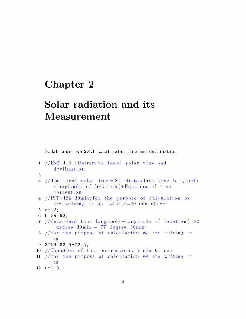
Scilab code Exa 2.4.1 Local solar time and declination

1 //Ex2 . 4 . 1 . ; Detremine l o c a l s o l a r t ime andd e c l i n a t i o n

2

3 //The l o c a l s o l a r t ime=IST−4( s tandard t ime l o n g i t u d e−l o n g i t u d e o f l o c a t i o n )+Equat ion o f t imec o r r e s t i o n

4 // IST=12h 30 min ; f o r the purpose o f c a l c u l a t i o n wea r e w r i t i n g i t as a=12h , b=29 min 60 s e c ;

5 a=12;

6 b=29.60;

7 // ( s tandard t ime l o n g i t u d e−l o n g i t u d e o f l o c a t i o n ) =82d e g r e e 30 min − 77 d e g r e e 30 min ;

8 // f o r the purpose o f c a l c u l a t i o n we a r e w r i t i n g i tas

9 STL3 =82.5 -72.5;

10 // Equat ion o f t ime c o r r e s t i o n : 1 min 01 s e c11 // f o r the purpose o f c a l c u l a t i o n we a r e w r i t i n g i t

as12 c=1.01;

6

13 //The l o c a l s o l a r t ime=IST−4( s tandard t ime l o n g i t u d e−l o n g i t u d e o f l o c a t i o n )+Equat ion o f t imec o r r e s t i o n

14 LST=b-STL3 -c;

15 printf(” The l o c a l s o l a r t ime=%f . %f i n hr . min . s e c ”,a,LST);

16 // D e c l i n a t i o n d e l t a can be o b t a i n by cooper ’ s eqn :d e l t a =23.45∗ s i n ( ( 3 6 0 / 3 6 5 ) ∗(284+n ) )

17 n=170; // ( on June 19)18 // l e t19 a=(360/365) *(284+n);aa=(a*%pi)/180;

20 // t h e r e f o r e21 delta =23.45* sin(aa);

22 printf(”\n d e l t a=%f d e g r e e ”,delta);

Scilab code Exa 2.4.2 Angle made by beam radiation

1 //Ex2 . 4 . 2 . ; C a l c u l a t e a n g l r made by beam r a d i a t i o nwith the normal to a f l a t c o l l e c t o r .

2 gama =0; // s i n c e c o l l e c t o r i s p o i n t i n g due south .3 // For t h i s c a s e we have e q u a t i o n : c o s ( t h e t a t )=co s

( f i e −s ) ∗ co s ( d e l t a ) ∗ co s (w)+s i n ( f i e −s ) ∗ s i n ( d e l t a )4 // with the he lp o f coope r eqn on december 1 ,5 n=335;

6 // l e t7 a=(360/365) *(284+n);aa=(a*%pi)/180;

8 // t h e r e f o r e9 delta =23.45* sin(aa);

10 printf(” d e l t a=%f d e g r e e ”,delta);11 // Hour a n g l e w c o r r e s p o n d i n g to 9 . 0 0 hour=45 Degreew12 w=45; // d e g r e e13 // l e t14 a=cos (((28.58* %pi)/180) -((38.58* %pi)/180))*cos(delta

*%pi *180^ -1)*cos(w*%pi *180^ -1);

15 b=sin(delta*%pi *180^ -1)*sin (((28.58* %pi)/180)

7

-((38.58* %pi)/180));

16 // t h e r e f o r e17 cos_of_theta_t=a+b;

18 theta_t=acosd(cos_of_theta_t);

19 printf(”\n t h e t a t=%f Degree ”,theta_t);

Scilab code Exa 2.7.1 Average value of Solar radiation on a horizontal surface

1 //Ex2 . 7 . 1 . ; Determine the ave rage v a l u e s o f r a d i a t i o non a h o r i z o n t a l s u r f a c e

2

3 // D e c l i n a t i o n d e l t a f o r June 22=23.5 degree , s u n r i c ehour a n g l e ws

4 delta =(23.5* %pi)/180; // u n i t=r a d i a n s5 fie =(10* %pi)/180;; // u n i t=r a d i a n s6 // S u n r i c e hour a n g l e ws=acosd (− tan ( f i e ) ∗ tan ( d e l t a ) )7 ws=acosd(-tan(fie)*tan(delta));

8 printf(” S u n r i c e hour a n g l e ws=%f Degree ”,ws);9 n=172; //=days o f the yea r ( f o r June 22)10 //We have the r e l a t i o n f o r Average i n s o l a t i o n at the

top o f the atmosphere11 //Ho=(24/%pi ) ∗ I s c ∗ [{1+0 .033∗ ( 360∗ n /365) }∗ ( ( c o s ( f i e )

∗ co s ( d e l t a ) ∗ s i n ( ws ) ) +(2∗%pi∗ws /360) ∗ s i n ( f i e ) ∗ s i n (d e l t a ) ) ]

12 Isc =1353; // SI u n i t=W/mˆ213 ISC =1165; //MKS u n i t=k c a l / hr mˆ214 // l e t15 a=24/ %pi;

16 aa =(360*172) /365; aaa=(aa*%pi)/180;

17 b=cos(aaa);bb =0.033*b;bbb=1+bb;

18 c=(10* %pi)/180; c1=cos(c);

19 cc =(23.5* %pi)/180; cc1=cos(cc);

20 ccc =(94.39* %pi)/180; ccc1=sin(ccc);

21 c=c1*cc1*ccc1;

22 d=(2* %pi*ws)/360;

8

23 e=(10* %pi)/180; e1=sin(e);

24 ee =(23.5* %pi)/180; ee1=sin(ee);

25 e=e1*ee1;

26 // t h e r e f o e Ho i n SI u n i t27 Ho=a*Isc*(bbb*(c+(d*e)));

28 printf(”\n SI UNIT−>Ho=%f W/mˆ2 ”,Ho);29 Hac=Ho *(0.3+(0.51*0.55))

30 printf(”\n SI UNIT−>Hac=%f W/mˆ2 day ”,Hac);31 ho=a*ISC*(bbb*(c+(d*e)));

32 printf(”\n MKS UNIT−>Ho=%f k c a l /mˆ2 ”,ho);33 hac=ho *0.58;

34 printf(”\n MKS UNIT−>Hac=%f k c a l /mˆ2 day ”,hac);35

36 //The v a l u e s a r e approx imat e l y same as i n t ex tbook

9

Chapter 3

Solar Energy Collectors

Scilab code Exa 3.6.1 Solar altitude angle and Incident angle and Collector efficiency

1 //Ex3 . 6 . 1 . ; c a l c u l a t e : s o l a r a l t i t u d e ang l r , I n c i d e n tang l e , C o l l e c t o r e f f i c i e n c y

2

3 // S o l a r d e c l i n a t i o n : d e l t a4 n=1

5 delta =23.45* sin ((360/365) *(284+n));

6 printf(” S o l a r d e c l i n a t i o n d e l t a=%f d e g r e e ”,delta);7 fie =22; // d e g r e e8 // s o l a r hour a n g l e ws =0 ,( at mean o f 1 1 : 3 0 and 1 2 : 3 0 )9 ws=0;

10 // S o l a r a l t i t u d e a n g l r a lpha i s g i v e n by11

12 // a lpha=a s i n d ( ( ( co s ( f i e ) ∗ co s ( d e l t a ) ∗ co s ( ws ) ) +( s i n (f i e ) ∗ s i n ( d e l t a ) ) )

13 // l e t14 a=cos ((22* %pi)/180)*cos ((-23*%pi)/180)*cos (0);

15 b=sin ((22* %pi)/180)*sin ((-23*%pi)/180);

16 // t h e r e f o r e17 sin_alpha=a+b;

18 printf(”\n s i n a p l h a=%f”,sin_alpha);19 alpha=asind(sin_alpha);

10

20 printf(”\n ap lha=%f Degree ”,alpha);21 // I n c i d e n t a n g l e22 theta =(180/2) -alpha;

23 printf(”\n I n c i d e n t a n g l e=%f Degree ”,theta);24 //Rb i s g i v e n by25 Rb=((cos (((22* %pi)/180) -(37*%pi)/180)*cos ((-23*%pi)

/180)*cos (0))+(sin (((22* %pi)/180) -(37*%pi)/180)*

sin ((-23*%pi)/180)))/sin_alpha;

26 printf(”\n Rb=%f”,Rb);27 // E f f e c t i v e a b s o r p t a n c e product i s <t . a lpha>=t . a lpha

/ 1−(1−a lpha ) ∗pd28 pd =0.24; // D i f f u s e r e f l e c t a n c e f o r two g l a s s c o v e r s29 // l e t TA=<t . a lpha>30 TA =(0.88*0.90) /(1 -(1 -0.90)*pd);

31 printf(”\n E f f e c t i v e a b s o r p t a n c e product i s <t . a lpha>=%f”,TA);

32 // S o l a r r a d i a t i o n i n t e n s i t y ( c o n s i d e r beam r a d i a t i o non ly )

33 //Hb=0.5 l y /mm = 0 . 5 c a l /cmˆ2 ∗ min34 Hb =((0.5*10^4) /10^3) *60; // u n i t=k c a l /mˆ2 hr35 printf(”\n Hb=%f k c a l /mˆ2 hr ”,Hb);36 Hb=Hb *1.163; // u n i t=W/mˆ2 hr ; [ s i n c e 1 k c a l =

1 . 1 6 3 watt ]37 printf(”\n Hb=%f W/mˆ2 hr ”,Hb);38 //S=Hb∗Rb∗<t . a lpha>39 S=Hb*Rb*TA;

40 printf(”\n S=%f W/mˆ2 hr ”,S);41 s=S/1.163;

42 printf(”\n S=%f k c a l /mˆ2 hr ”,s);43 // U s e f u l ga in44 // qu=FR( S−UL∗ ( Tf i−Ta) )45 qu =0.810*(s -(6.80*(60 -15)))

46 printf(”\n qu=%f k c a l /mˆ2 hr ”,qu);47 //Qu=FR( S−UL∗ ( Tf i−Ta) )48 Qu =0.810*(S -(7.88*(60 -15)))

49 printf(”\n qu=%f W/mˆ2 hr ”,Qu);50 // C o l l e c t i o n E f f i c i e n c y : nc=(qu /(Hb∗Rb) ) ∗1 0 0 ;51 nc =(28.07/(300* Rb))*100;

11

52 printf(”\n C o l l e c t i o n E f f i c i e n c y=%f p e r s e n t ”,nc);53

54

55 // v a l u e s o f ” s i n e a lpha ” i n the t ex tbook i s takenapprox imate to the r e a l v a l u e s

Scilab code Exa 3.9.1 Useful gain and exit fluid temperature and collection efficiency

1 // c a l c u l a t e the u s e f u l ga in , e x i t f l u i d t empera tu r eand c o l l e c t i o n e f f i c i e n c y

2 // O p t i c a l p r o p e r t i e s a r e e s t i m a t e d as3 p=0.85;

4 // (T . a lpha ) =0 .77 ; l e t A=(T. a lpha )5 A=0.77

6 gama =0.94;

7 Do =0.06;

8 L=8; // u n i t=meter , / / L=l e n g t h o f c o n c e n t r a t o r9 W=2; //W=width o f c o n c e n t r a t o r i n meter

10 dco =0.09; // dco=d iamete r o f t r a n s p a a r e n t c o v e r11 Ar= %pi*Do*L;//Ar=area o f the r e c e i v e r p ip e12 A_alpha =(W-dco)*L;// a p e r t u r e a r ea o f the

c o n c e n t r a t i o n13 Cp =0.30; // u n i t=k c a l / kg d e g r e e c a l c i u s14 m=400; // u n i t=kg / hr ,m=f l o w r a t e15 HbRb =600; // u n i t=k c a l / hr mˆ216 Tfi =150; // d e g r e e c a l c i u s17 T_alpha =25; // d e g r e e c a l c i u s18 // Heat t r a n s f e r c o e f f i c i e n t from f l u i d i n s i d e to

su r r ound i ng s ,19 Uo=5.2; // u n i t=k c a l / hr−mˆ220 // Heat t r a n s f e r c o e f f i c i e n t from a b s o r b e r c o v e r

s u r f a c e to su r r ound in g s ,21 UL=6; // u n i t=k c a l / hr−mˆ222 F=(Uo/UL);

23 // Heat removed f a c t o r FR i s

12

24 //FR=((m∗Cp) /( Ar∗UL) ) ∗(1−(%eˆ−((Ar∗UL∗F) /(m∗Cp) ) ) )25 // l e t X=(m∗Cp) /( Ar∗UL) ;Y=(%eˆ−((Ar∗UL∗F) /(m∗Cp) ) )26 X=(m*Cp)/(1.51* UL *0.86);

27 Y=%e^(-1/X);

28 FR=X*0.86*(1 -Y);

29 // Absorbed s o l a r ene rgy i s30 S=HbRb*p*gama*A;

31 printf(” Area o f the r e c e i v e r p ip e Ar= %f =1.51 mˆ2 \n A aplha= %f mˆ2= c o l l e c t i o n e f f i c i e n c y f a c t o r ”,Ar ,A_alpha);

32 printf(”\n v a l u e o f F= %f”,F);33 printf(”\n Heat removed f a c t o r FR=%f \n Absorbed

s o l a r ene rgy i s \n S=%f k c a l /Hr mˆ2 . . . . . ( MKS) ”,FR ,S);

34 // f o r u n i t i n S . I . , 1 k c a l /Hr mˆ2 = 1 . 1 6 2 9 8 W/mˆ235 s= S*1.16298; // i n W/mˆ236 printf(”\n S=%f W/m ˆ 2 . . . . . ( SI ) ”,s);37 // the v a l u e s o f F ,FR w i l l be same i n any un i t , s i n c e

they a r e f a c t o r s ( d i m e n s i o n l e s s )38 // U s e f u l Gain=Qu=A alpha ∗FR∗ ( S−((Ar∗UL) / A alpha ) ∗ (

Tf i−T alpha ) )39 // In MKS u n i t40 Qu=A_alpha*FR*(S -((1.51* UL)/A_alpha)*(Tfi -T_alpha))

41 printf(”\n u s e f u l ga in i n (MKS) Qu=%f k c a l / hr ”,Qu);42 // IN SI u n i t43 qu=A_alpha*FR*(s -((1.51*6.98)/A_alpha)*(Tfi -T_alpha)

)//UL=6.98 W/mˆ2 d e g r e e c e l c i u s44 printf(”\n u s e f u l ga in i n ( SI ) Qu=%f Watt”,qu);45 // the e x i t f l u i d t empera tu re can be o b t a i n e d from46 tci =150; // d e g r e e c e l c i u s47 tco=tci+(Qu/(m*Cp));// from Qu=mCp( tco−t c ) ; where ,

t c o=c o l l e c t o r f l u i d temp . at o u t l e t , t c i=F l u idi n l e t temp .

48 n=(Qu /(16* HbRb))*100; // n c o l l e c t o r=Qu/( A alpha ∗HbRb)∗1 0 0 ;

49 printf(”\n c o l l e c t o r f l u i d temp . at o u t l e t t c o=%fd e g r e e c e l c i u s \n n c o l l e c t o r = %f p e r c e n t ”,tco ,n);

13

50

51 //The v a l u e s / r e s u l t s / answer s i s approx imate i n thet e x t book to the r e a l c a l c u l a t e d v a l u e

14

Chapter 6

Wind Energy

Scilab code Exa 6.2.1 Torque and axial thrust

1 //Ex . 6 . 2 . 1 .2 // For a i r , the v a l u e o f gas c o n s t a n t3 R=0.287 // u n i t=k j / kg K4 //T=15 i n d e g r e e c a l c i u s5 T=15+273; // i n k a l v i n6 RT =0.287*10^3*288;

7 P=1.01325*10^5; // u n i t=Pa ; at 1 atm8 Vi=15; // u n i t=m/ s9 gc=1;

10 D=120; // t u r b i n e d i amete r ; u n i t=m11 N=40/60;

12 // Air d e n s i t y13 p=(P/RT);

14 printf(” Air d e n s i t y p=%f kg /Mˆ3 ”,p);15 // 1 ] Tota l power= P t o t a l=p∗A∗Vi ˆ3/2∗ gc16 // power d e n s i t y =P t o t a l /A=p∗Vi ˆ3/2∗ gc17 power_density =(1/(2* gc))*(p*Vi^3);

18 // 2 ] Maximum power density=Pmax/A=8∗p∗Vi ˆ3/27∗ gc19 Maximum_power_density =(8/(27* gc))*(p*Vi^3);

20 printf(”\n power d e n s i t y =P t o t a l /A= %f W/mˆ2 \nMaximum power d e n s i t y=Pmax/A= %f W/mˆ2 ”,

15

power_density ,Maximum_power_density);

21 // 3 ] Assuming n=35%22 n=0.35;

23 // l e t P/A=x24 x=n*( power_density);

25 printf(”\n P/A=%f W/mˆ2 ”,x);26 // 4 ] Tota l power P= power d e n s i t y ∗ Area27 Total_power_P =724*( %pi /4)*(D^2) // Tota l power P=

power d e n s i t y ∗ ( %pi /4) ∗Dˆ228 printf(”\n Tota l power P=%f watt=%f∗10ˆ−3 kW”,

Total_power_P ,Total_power_P);

29 // 5 ] Torgue at maximum e f f i c i e n c y30 Tmax =(2/(27* gc))*((1.226*D*Vi*Vi*Vi)/N);//Tmax

=(2/(27∗ gc ) ) ∗ ( ( p∗D∗Vi∗Vi∗Vi ) /N) ;31 printf(”\n Torgue at maximum e f f i c i e n c y=%f Newton”,

Tmax)

32 // and maximum a x i a l t h u r s t33 Fxmax =(3.14/(9* gc))*1.226*D^2*Vi^2; //Fxmax=(%pi /(9∗

gc ) ) ∗p∗Dˆ2∗Vi ˆ 2 ;34 printf(”\n maximum a x i a l t h u r s t=%f Newton”,Fxmax);

16

Chapter 7

Energy from Biomass

Scilab code Exa 7.15.1 Volume of biogas digester and power available from the digester

1 //Ex7 . 1 5 . 1 ; c a l c u l a t e volume o f b i o g a s d i g e s t e r andpower a v a i l a b l e from the d i g e s t e r

2 // Mass o f the dry input3 M0=2*5; //M0=2.5 kg / day ∗ 54 pm=50; // u n i t=kg /mˆ35 tr=20; // r e t e n t i o n t ime i n days6 C=0.24; // u n i t=mˆ3 per kg ; B iogas y e i l d .7 n=0.6; // e f f i c i e n c y o f burner8 Hm=28; // u n i t=MJ/mˆ3// combust ion o f methane9 Fm=0.8; // methane p r o p o r t i o n a l

10 // F lu id volume Vf i s =M0/pm11 Vf=M0/pm;

12 printf(” Mass o f the dry input M0=%f kg / day \n F l u idvolume Vf=%f mˆ3 / day ”,M0 ,Vf);

13 // f o r e x p r e s s i o n Vd=Vftr , the d i g e s t e r volume i s14 Vd=Vf*tr;

15 printf(”\n Vd=%f mˆ3 ”,Vd);16 // volume o f b i o g a s i s Vb=C∗M0= b i o g a s y i e l d input ∗

mass o f dry input17 Vb=C*M0;

18 printf(”\n volume o f b i o g a s i s Vb=%f mˆ3 / day ”,Vb);

17

19 //The Power a v a i l a b l e from the d i g e s t e r i s20 E=n*Hm*Fm*Vb;

21 printf(”\n The Power a v a i l a b l e from the d i g e s t e r=%fMj/ day ”,E);

22 E=E*0.2728; // u n i t=kWh/ day23 printf(”=%f kWh/ day ”,E);24 E=E*41.8 // u n i t=W( c o n t i n u o u s therma l )25 printf(”=%f W( c o n t i n u o u s the rma l ) ”,E);

18

Chapter 8

Geothermal Energy

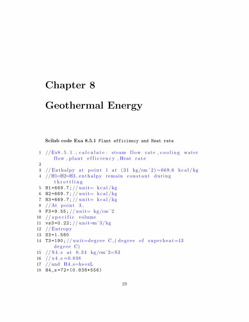
Scilab code Exa 8.5.1 Plant efficiency and Heat rate

1 //Ex8 . 5 . 1 . ; c a l c u l a t e : steam f l o w ra t e , c o o l i n g waterf low , p l a n t e f f i c i e n c y , Heat r a t e

2

3 // Enthalpy at p o i n t 1 at (31 kg /cmˆ2) =669.6 k c a l / kg4 //H1=H2=H3 , en tha lpy remain c o n s t a n t dur ing

t h r o t t l i n g5 H1 =669.7; // u n i t= k c a l / kg6 H2 =669.7; // u n i t= k c a l / kg7 H3 =669.7; // u n i t= k c a l / kg8 //At p o i n t 3 ,9 P3 =9.55; // u n i t= kg /cmˆ210 // s p e c i f i c volume11 vs3 =0.22; // u n i t=mˆ3/ kg12 // Entropy13 S3 =1.580

14 T3=190; // u n i t=d e g r e e C , ( d e g r e e o f s u p e r h e a t =13d e g r e e C)

15 // S 4 s at 0 . 3 4 kg /cmˆ2=S316 // x 4 s =0.83817 // and H4 s=hs+xL18 H4_s =72+(0.838*556)

19

19 printf(” H4 s=%f k c a l / kg ”,H4_s)20 // I s e n t r o p i c t u r b i n e work=H3−H4 s21 ITW=H3 -H4_s;

22 printf(”\n I s e n t r o p i c t u r b i n e work=%f k c a l / kg ”,ITW);23 // Actua l t u r b i n e work24 ATW =0.80* ITW;

25 printf(”\n Actua l t u r b i n e work=%f k c a l / kg ”,ATW);26 H4=669.7 - ATW;

27 printf(”\n H4=%f k c a l / kg ”,H4)28 h5_6 =72; // u n i t= k c a l / kg ; ( I g n o r i n g pump work )29 // s e n s i b l e heat h7=h5=25 k c a l / kg30 h5=25; // u n i t=k c a l / kg31 h7=25; // u n i t=k c a l / kg32 // Turbine steam f l o w33 TSF =(250*0.860*10^6) /(ATW *0.9);

34 printf(”\n Turbine steam f l o w=%f kg / hr ”,TSF);35 // l e t36 m4=TSF;

37 // Turbine volume f l o w38 TVF=(TSF /60)*vs3;

39 printf(”\n Turbine volume f l o w=%f mˆ3/ min”,TVF);40 // c o o l i n g water f l o w m7 : m7( h5 6−h7 )=m4(H4−h5 6 )41 m7=((H4-h5_6)/(h5_6 -h7))*m4;

42 printf(”\n c o o l i n g water f l o w m7=%f kg / hr ”,m7);43 Heat_added=H1 -h5_6;

44 printf(”\n Heat added=%f k c a l / kg ”,Heat_added);45 // p l a n t e f f i c i e n c y =( Actua l Turbine work∗nmg) / Heat

added46 //nmg=combined mechan i ca l and e l e c t r i c a l e f f i c i e n c y

o f tu rb in e−g e n e r a t o r47 nmg =0.90;

48 Plant_efficiency =(ATW*nmg)/Heat_added;

49 plant_efficiency=Plant_efficiency *100;

50 printf(”\n Plant E f f i c i e n c y np lan t=%f p e r s e n t ”,plant_efficiency);

51 // Plant heat r a t e =(860∗Heat added ) / net work52 // net work =105 .36∗0 .9053 Plant_heat_rate =(860/ Plant_efficiency);

20

54 printf(”\n Plant heat r a t e=%f k c a l /kWH”,Plant_heat_rate);

55

56

57 //The v a l u e o f ” t u r b i n e steam f l o w ” i s wrong due toc a l c u l a t i n g mistak i n textbook , due to which thef u r t h e r v a l u e r e l a t e d with i t i s g i v e n wrong

58 //The v a l u e s a r e c o r r e c t e d i n t h i s program

Scilab code Exa 8.5.2 Cycle efficiency and Plant Heat Rate

1 //Ex8 . 5 . 2 . ; c a l c u l a t e : hot water f low , co nde n s e rc o o l i n g water f low , c y c l e e f f i c i e n c y , p l a n t heatr a t e .

2 H1 =669.6; // u n i t=k c a l / kg3 H2 =669.6; // u n i t=k c a l / kg4 // p r e s s u r e at p o i n t 2 , i s 1 0 . 5 kg /cm ˆ 2 ; thus ,5 T2=195; // u n i t=d e g r e e c e l c i u s ; (14 d e g r e e c e l c i u s o f

s u p e r h e a t )6 s2 =1.567;

7 vsup =0.27;

8 x3s =0.832;

9 H3s =535; // u n i t=k c a l / kg10 // I s e n t r o p i c t u r b i n e work11 ITW=H2 -H3s;

12 printf(” I s e n t r o p i c t u r b i n e work=%f k c a l / kg ”,ITW);13 // Actua l t u r b i n e work14 ATW =0.65* ITW;

15 printf(”\n Actua l t u r b i n e work=%f k c a l / kg ”,ATW);16 H3=669.6 - ATW;

17 printf(”\n H3=%f k c a l / kg ”,H3)18 // h 4 −5( i g n o r e bpump work )19 h4 =72.4; // u n i t=k c a l / kg20 // h6 at 27 d e g r e e c21 h6=27; // u n i t=k c a l / kg

21

22 // Turbine steam f l o w or hot water f l o w=power output /a c t u a l t u r b i n e work

23 TSF =(10*10^6*0.86)/ATW;

24 printf(”\n Turbine steam f l o w or hot water f l o w=%fkg / hr ”,TSF);

25 // c o n s i d e r c o o l i n g water f l o w m4 : m3∗ (H3−h4 )=m4( h4−h6 )

26 // or27 m4 =((582.11 -72.4) *0.983*10^5) /(72.4 -27);

28 printf(”\n c o o l i n g water f l o w=%f kg / hr ”,m4);29 Heat_added=H1 -h4

30 printf(”\n Heat added=%f k c a l / kg ”,Heat_added);31 // p l a n t e f f i c i e n c y=Turbine work / Heat added32 Plant_efficiency =(ATW/Heat_added);

33 plant_efficiency=Plant_efficiency *100;

34 printf(”\n Plant E f f i c i e n c y=%f p e r s e n t ”,plant_efficiency);

35 // Plant heat r a t e =860/ Plant E f f i c i e n c y36 Plant_heat_rate =860/ Plant_efficiency;

37 printf(”\n Plant heat r a t e=%f k c a l /kWh”,Plant_heat_rate);

38

39

40 //The v a l u e o f m3=14.03∗10ˆ5 i s g i v e n wrong i n thet e x t book ; the a c t u a l v a l u e i s m3=11.03∗10ˆ5

22

Chapter 9

Energy from the Oceans

Scilab code Exa 9.3.5.1 Energy Generated

1 //Ex9 . 3 . 5 . 1 . ; C a l c u l a t e Energy g e n e r a t e d2 R=12; // u n i t=m; R i s the range3 r=3; // u n i t=m; the head below t u r b i n e s t o p s o p e r a t i n g4 time =(44700/2);

5 A=30*10^6;

6 g=9.80;

7 p=1025;

8 //The t o t a l t h e o r e t i c a l work W=i n t e g r a t e ( ’ 1 ’ , ’w’ , R, r) ;

9 W=(g*p*A*((R^2) -(r^2)))/2;

10 printf(” W=%f ”,W);11 //The ave rage power g e n e r a t e d12 Pav=W/time;// u n i t=watt s13 printf(”\n The ave rage power g e n e r a t e d=%f watt s ”,Pav

);

14 pav=(Pav /1000) *3600; // u n i t=kWh15 printf(”\n The ave rage power g e n e r a t e d=%f kWh”,pav)16 // the ene rgy g e n e r a t e d17 Energy_generated=pav *0.73

18 printf(”\n Energy g e n e r a t e d=%f kWh”,Energy_generated);

23

Scilab code Exa 9.3.6.1 The Yearly Power Output

1 //Ex9 . 3 . 6 . 1 ; c a l c u l a t e power i n h . p . a t any i n s t a n tand the y e a r l y power output

2 A=0.5*10^6; // u n i t=m3 h0=8.5; // u n i t=m4 t=3*3600 // u n i t=s ; s i n c e t=3 hr5 p=1025; // u n i t=kg /mˆ36 h=8; // u n i t=m7 n0 =0.70; // e f f i c i e n c y o f the g e n e r a t o r ; 7 0%8 // volume o f the b a s i n=Ah09 volume_of_the_basin=A*h0;

10 // Average d i s c h a r g e Q=volume / t ime p e r i o d11 Q=(A*h0)/t;

12 printf(” volume o f the b a s i n=%f mˆ3 \n Averaged i s c h a r g e Q=%f mˆ3 / s ”,volume_of_the_basin ,Q);

13 // power at any i n s t a n t14 P=((Q*p*h)/75)*n0;

15 printf(”\n power at any i n s t a n t P=%f h . p . ”,P);16 //The t o t a l ene rgy i n kWh/ t i d a l c y c l e17 E=P*0.736*3;

18 printf(”\n The t o t a l ene rgy i n kWh/ t i d a l c y c l e E=%f”,E);

19 // Tota l number o f t i d a l c y c l e i n a yea r =70520 printf(”\n Tota l number o f t i d a l c y c l e i n a yea r =705

”);21 // T h e r e f o r e Tota l output per annum22 Total_output_per_annum=E*705;

23 printf(”\n Tota l output per annum=%f kWh/ year ”,Total_output_per_annum);

24

25 //The v a l u e o f ” power o f i n s t a n t ” i n a t e x t book i sm i s p r i n t e d .

24

Chapter 10

Chemical Energy Sources

Scilab code Exa 10.2.8.1 Reversible Voltage for Hydrogen oxygen fuel cell

1 // Ex10 . 2 . 8 . 1 ; Find R e v e r s i b l e v o l t a g e f o r hydrogenoxygen f u e l c e l l

2 del_G = -237.3*10^3; // J o u l e s /gm−mole o f H23 // R e v e r s i b l e v o l t a f e E o f a c e l l i s g i v e n by =

del Wrev /nF=−de l G /nF4 // s i n c e 2 e l e c t r o n s a r e t r a n s f e r r e d per m o l e c u l e o f

H2 . thus5 n=2;

6 F=96500; // Faraday ’ s c o n s t a n t7 E=-del_G/(n*F);

8 printf(” R e v e r s i b l e v o l t a g e=%f v o l t s ”,E);

Scilab code Exa 10.2.8.2 Voltage output and efficiency and heat transfer

1 // Ex10 . 2 . 8 . 2 ; c a l c u l a t e v o l t a g e output o f c e l l ,e f f i c i e n c y , e l e c t r i c work output , heat t r a n s f e r tothe s u r r o u n d i n g s

2

25

3 // 1 ] v o l t a g e output o f c e l l4 del_G = -237.3*10^3; // J o u l e s /gm−mole o f H25 n=2;

6 F=96500; // Faraday ’ s c o n s t a n t7 E=-del_G/(n*F);

8 printf(” E=%f v o l t s ”,E);9 // 2 ] E f f i c i e n c y

10 //nmax=del Wmax/−( de l H ) 25 d e g r e e c e l c u i s = −( de l G )T/(− de l H ) 25

11 del_G_at298k = -56690; // u n i t=k c a l / kg mole12 del_H_at298k = -68317; // u n i t=k c a l / kg mole13 nmax=del_G_at298k/del_H_at298k ,

14 printf(”\n nmax=%f”,nmax);15 // 3 ] E l e c t r i c work output per mole16 F=(96500/4.184);

17 del_Wrever =(n*F*E);

18 printf(”\n E l e c t r i c work output per mole=%f k c a l / kgmole ”,del_Wrever);

19 // 4 ] Heat t r a n s f e r to the s u r r o u n d i n g s20 // the heat t r a n s f e r i s Q=T∗ de l−s=de l H at298k−

d e l G a t 2 9 8 k21 Q=del_H_at298k -del_G_at298k;

22 printf(”\n The heat t r a n s f e r i s Q=%f k c a l / kg mole ”,Q);

23 //The n e g a t i v e s i g n i n d i c a t e s tha t the heat i sremoved from the c e l l and t r a n s f e r r e d to thes u r r o u n d i n g

24

25 // v a l u e o f ” E l e c t r i c work output per mole ” i sapprox imate i n the t e x t book to the r e a lc a l c u l a t e d v a l u e

Scilab code Exa 10.2.8.3 Voltage output and efficiency and heat transferred

1 // Ex10 . 2 . 8 . 3 ; The heat t r a n s f e r r e d to the s u r r o u n d i n g

26

2 del_G_at298k = -237191; // u n i t=kJ/ kg mole3 del_H_at298k = -285838; // u n i t=kJ/ kg mole4 ne=2;

5 F=96500; // Faraday ’ s c o n s t a n t6 E=-del_G_at298k /(ne*F);

7 printf(” E=%f v o l t s ”,E);8 nmax=del_G_at298k/del_H_at298k ,

9 printf(”\n nmax=%f”,nmax);10 nmax=nmax *100;

11 printf(”=%f p e r s e n t ”,nmax);12 // E l e c t r i c work output per mole o f the f u l e i s We=−

de l G kJ/ kg mole13 We=del_G_at298k;// kJ/ kg mole14 printf(”\n E l e c t r i c work output per mole o f the f u l e

i s We=%f kJ/ kg mole ”,We);15 // s i n c e t h e r e i s 1 mol os H2O f o r each mole o f f u l e ,

t h e r e i s a l s o a work output o f 237191 kJ/ kg mole16 // Heat t r a n s f e r r e d i s Q=T∗ de l−s=de l H at298k−

d e l G a t 2 9 8 k17 Q=del_H_at298k -del_G_at298k;

18 printf(”\n The heat t r a n s f e r i s Q=%f kJ/ kg mole ”,Q);19 //The n e g a t i v e s i g n i n d i c a t e s tha t the heat i s

removed from the c e l l and t r a n s f e r r e d to thes u r r o u n d i n g

20

21 // v a l u e o f ” E l e c t r i c work output per mole ” i sm i s p r i n t e d i n the t e x t book .

Scilab code Exa 10.2.8.4 Gibbs free energy and Entropy change

1 // Ex10 . 2 . 8 . 4 ; c a l c u l a t e del G , de l S , de l H ;2

3 //We have the r e l a t i o n de l G=−n∗F∗E4 // where , de l G=g i b b s f r e e ene rgy o f the system at 1

atm and tempera tu r e (T)

27

5 n=1; // numbers o f e l e c t o n s t r a n s f e r r e d per m o l e c u l eo f r e a c t a n t

6 E=0.0455; // v o l t s ; e .m. f . o f the c e l l7 F=96500; // Faraday ’ s c o n s t a n t8 // l e t X=dE/dT9 X=0.000338;

10 del_G=-n*F*E;

11 printf(” de l G=%f j o u l e s ”,del_G);12 // d e l S = Entropy change o f the system at

t empera tu re T and p r e s s p=1 atm i n the c a s e13 del_S=n*F*(X);// d e l S=n∗F∗ (dE/dT)14 printf(”\n d e l S=%f j o u l e s / deg . ”,del_S);15 //And ent ropy change i s g i v e n by the r e l a t i o n de l H=

nF [T(dE/dT)−E ]16 T=298;

17 del_H=n*F*((T*X)-E);

18 printf(”\n de l H=%f j o u l e ”,del_H);19

20

21 // v a l u e a r e taken approx imate i n the t e x t book tothe r e a l c a l c u l a t e d v a l u e

Scilab code Exa 10.2.8.5 Heat transfer rates

1 // Ex10 . 2 . 8 . 5 ; heat t r a n s f e r r a t e would be i n v o l v e dunder t h e s e c i r c u m s t a n c e s

2

3 del_G_at25degree_celcius = -195500; // u n i t=c a l /gm mole4 del_H_at25degree_celcius = -212800; // u n i t=c a l /gm mole5 F=(96500/4.184);// s i n c e F=96500 coulombs /gm−mole6 n=8

7 E_at25degree_celcius=-del_G_at25degree_celcius /(n*F)

;// J o u l e s / coulomb8 printf(” E a t 2 5 d e g r e e c e l c i u s=%f v o l t s =1.060 v o l t s ”,

E_at25degree_celcius);

28

9 //Max . e f f i c i e n c y nmax=del Wmax/−( de l H ) at25 d e g r e ec e l c u i s = −( de l G )T/(− de l H ) 25

10 nmax=del_G_at25degree_celcius/

del_H_at25degree_celcius;

11 printf(”\n nmax=%f”,nmax);12 // v o l t a g e e f f i c i e n c y nv=on load v o l t a g e / open c i r c u i t

v o l t a g e=Operat ing v o l t a g e / T h e o r e t i c a l v o l t a g e13 Theoretical_voltage =1.060/0.92;

14 printf(”\n T h e o r e t i c a l v o l t a g e=%f v o l t s ”,Theoretical_voltage);

15 // power deve l oped =100 kW=100∗10ˆ3 W16 power_developed =(100*10^3) *0.86; // u n i t=k c a l / hr ;

s i n c e 1 watt=1 j o u l e / s e c =0.86 k c a l / hr17 printf(”\n power deve l oped=%f k c a l / hr ”,

power_developed);

18 del_G = -195500;

19 // Requ i red f l o w r a t e o f Methane20 R_F_R_O_M =( power_developed *16)/del_G;// kg / hr ;21 // ( methane moles ) =1622 printf(”\n f l o w r a t e o f Methane=%f kg / hr ”,R_F_R_O_M)

;

23 // Heat t r a n s f e r Q=T 8 d e l s=de l H+de l w=del H−de l G24 Q=del_H_at25degree_celcius -del_G_at25degree_celcius;

25 printf(”\n The heat t r a n s f e r i s Q=%f k c a l / kg mole ”,Q);

26

27 //The v a l u e a r e approx imate i n the t e x t book to ther e a l c a l c u l a t e d v a l u e

28 // v a l u e o f ” Requ i red f l o w r a t e o f methane ” i s wrongi n the t e x t book .

29 // v a l u e o f ” Heat t r a n s f e r ” i s wrong i n the t e x t book.

29

Chapter 12

Magneto Hydro DynamicPower Generation

Scilab code Exa 12.6.1 Open circuit voltage and maximum power output

1 // Ex12 . 6 . 1 . ; c a l c u l a t e open c i r c u i t v o l t a g e andmaximum power output

2 B=2; // f l u x d e n s i t y ; u n i t=Wb/mˆ23 u=10^3; // ave rage gas v e l o c i t y ; u n i t=m/ second4 d=0.50; // d i s t a n c e between p l a t e s ; u n i t=m5 E0=B*u*d;//Open c c i r c u i t v o l t a g e6 printf(” Open c c i r c u i t v o l t a g e E0=%f V o l t s ”,E0);7 // Generator r e s i s t a n c e ; Rg=d/ sigma ∗A8 sigma =10; // Gaseous c o n d u c t i v i t y ; u n i t=Mho/m9 A=0.25; // P l a t e Area ; u n i t=mˆ2

10 Rg=d/( sigma*A);

11 printf(”\n Generator r e s i s t a n c e Rg=%f Ohm”,Rg);12 //Maximum power13 Maximum_power =(E0^2) /(4*Rg);

14 printf(”\n Maximum power=%f watt s ”,Maximum_power);

30

Chapter 13

Thermo Electric Power

Scilab code Exa 13.2.1 Peltier heats absorbed and rejected

1 // Ex13 . 2 . 1 . ; P e l t i e r h e a t s absorbed and r e j e c t e d2 // p e l t i e r c o e f f i c i e n t s at t h e s e j u n c t i o n s a r e

ap lha p 1−2=a l p h a s 1 −2∗T3 // Let A=a l p h a s 1 −2 at 373 k=55∗10ˆ−6 v/ d e g r e e k and

B=a l p h a s 1 −2 at 273 k=50∗10ˆ−6 v/ d e g r e e k4 A=(55*10^ -6);

5 B=(50*10^ -6);

6 T1=373; //k7 T2=273; //k8 I=10*10^ -3; // c u r r e n t ; u n i t=Ampere9 alpha_p_1_2_at_373k=A*T1;

10 alpha_p_1_2_at_273k=B*T2;

11 printf(” a l p h a p 1 2 a t 3 7 3 k=%f W/amp \na l p h a p 1 2 a t 2 7 3 k=%f W/amp”,alpha_p_1_2_at_373k=A*T1 ,alpha_p_1_2_at_273k=B*T2);

12 // P e l t i e r h e a t s absorned and r e j e c t e d to be13 q2_peltier=alpha_p_1_2_at_373k*I;

14 q1_peltier=alpha_p_1_2_at_273k*I;

15 printf(”\n q 2 p e l t i e r=%f w \n q 1 p e l t i e r=%f W”,q2_peltier ,q1_peltier);

16 c=q2_peltier -q1_peltier;

31

17 printf(”\n I f no o t h e r heat t r a n s f e r were i nvo l v ed ,the d i f f e r e n c e between t h e s e vaues , ”);

18 printf(”\n %f−%f=%f W, would be s u p p l i e d as e l e c t r i cpower ”,q2_peltier ,q1_peltier ,c);

Scilab code Exa 13.3.2 Thomson heat transferred

1 //Ex . 1 3 . 3 . 2 . ; Find the thomson heat t r a n s f e r r e d2

3

4 // Let D=d a l p h a s 1 /dT ;5 D=5.4*10^ -3; // u n i t=micro V/ d e g r e e kˆ26 T1=273; // u n i t=k7 T2=373; // u n i t=k8 I=10*10^ -3; // u n i t=A9 //Thomson c o e f f i c i e n t sigma , v a r i e s with temp .10 // s i g m a 1 o f T=−T∗D; u n i t=V/ d e g r e e k11 //The thomson heat i s g i v e n by e q u a t i o n12 // qth=I ∗ I n t e g r a t i o n o f s i g m a 1 o f T w. r . t . T13 Integration=integrate( ’T ’ , ’T ’ ,T1 ,T2);14 qth=I*D*Integration;

15 printf(”The THOMSON HEAT=%f micro W”,qth);

Scilab code Exa 13.4.1 Carnot Efficiency

1 // Ex13 . 4 . 1 . ; Determine the e f f i c i e n c y o f thet h e r m o e l e c t r i c g e n e r a t o r . what w i l l be i t s c a r n o te f f i c i e n c y

2

3 TH=600; // d e g r e e k ; / / t empera tu r e o f the hot r e s e r v i o ro f s o u r c e

4 TC=300; // d e g r e e k ; / / t empera tu r e o f the s i n k

32

5 Z=2*(10^ -3);// 1/ d e g r e e k ; / / F igu r e o f mer i t f o r them a t e r i a l

6 M_optimum =(1+((Z/2)*(TH+TC)))^0.5;

7 printf(” M optimum=%f”,M_optimum);8 // E f f i c i e n c y o f the t h e r m o e l e c t r i c g e n e r a t o r i s n

=(((TH−TC) /TH) ∗ ( ( M optimum−1) /( M optimum+(TC/TH) )) ∗1 0 0 ;

9 a=((TH-TC)/TH);

10 b=(M_optimum -1)/( M_optimum +(TC/TH));

11 n=a*b*100;

12 printf(”\n E f f i c i e n c y o f the t h e r m o e l e c t r i cg e n e r a t o r i s n=%f p e r s e n t ”,n);

13 // where as e f f i c i e n c y o f the c a r n o t c y c l e (r e v e r s i b l e ) nc =((TH−TC) /TH) ∗100

14 nc=a*100;

15 printf(”\n E f f i c i e n c y o f the c a r n o t c y c l e (r e v e r s i b l e ) nc=%f p e r s e n t ”,nc);

Scilab code Exa 13.4.2 Maximum generator efficiency and Power Output

1 // Ex13 . 4 . 1 2 . ; C a l c u l a r e maximum g e n e r a t o r e f f i c i e n c yand the e f f i c i e n c y f o r maximum power , power output

2

3 // s e edbeck c o e f f i c i e n t ( a l p h a s ) ; u n i t=v o l t s / d e g r e ec e l c i u s

4 alpha_s1 = -190*10^ -6; //n−type5 alpha_s2 =190*10^ -6; //p−type6 // S p e c i f i c r e s i s t i v i t y ( p ) ; u n i t=Ohm−cm7 p1 =1.45*10^ -3; //n−type8 p2 =1.8*10^ -3; //p−type9 // F igu r e o f mer i t (Z) ; u n i t=d e g r e e kˆ−1

10 Z1=2*10^ -3; //n−type11 Z2 =1.7*10^ -3; //p−type12

13

33

14 // c o n d u c t i v i t y ( n−type ) ,15 k1=( alpha_s1 ^2)/(p1*Z1);

16 // s i m i l a r l y17 k2=( alpha_s2 ^2)/(p2*Z2);

18 printf(” C o n d u c t i v i t y k1=%f W/cm d e g r e e c e l c i u s \nC o n d u c t i v i t y k2=%f W/cm d e g r e e c e l c i u s ”,k1 ,k2);

19 // Z opt =(( a l p h a s 1−a l p h a s 2 ) ˆ2) / [ ( p1∗k1 ) ˆ2+( p2∗k2 )ˆ 2 ] ;

20 // l e t21 a=(alpha_s1 -alpha_s2)

22 b=(p1*k1)

23 c=(p2*k2)

24 A=sqrt(b)

25 B=sqrt(c)

26 C=(A+B);

27 // / t h e r e f o r e28 Z_opt=(a/C)^2;

29 printf(”\n Z opt=%f d e g r e e k”,Z_opt);30 // Thermal conductance31 A1=2.3; //cmˆ232 A2 =1.303; //cmˆ233 l1=1.5; //cm34 l2 =0.653; //cm35 K=((k1*A1)/l1)+((k2*A2)/l2)

36 printf(”\n Thermal conductance K=%f W/ d e g r e e c e l c i u s”,K);

37 //R=R e s i s t a n c e o f the g e n e r a t o r=R1+R238 R=((p1*l1)/A1)+((p2*l2)/A2);

39 printf(”\n R e s i s t a n c e o f the g e n e r a t o r R=%f ohm”,R);40 TH=923; // u n i t=k41 TC=323; // u n i t=k42 M_opt =(1+(( Z_opt /2)*(TH+TC)))^0.5;

43 printf(”\n M opt=%f ohm”,M_opt);44 RL=M_opt*R;

45 printf(”\n RL=%f ohms”,RL);46 //Optimum e f f i c i e n c y n opt =(((TH−TC) /TH) ∗ ( ( M opt−1)

/( M opt+(TC/TH) ) ) ∗1 0 0 ;47 aa=((TH-TC)/TH);

34

48 // t a k i n g M opt =1.4349 b=(1.43 -1) /(1.43+( TC/TH));

50 n_opt=aa*b*100;

51 printf(”\n Optimum e f f i c i e n c y n opt=%f p e r s e n t ”,n_opt);

52 // e f f i c i e n c y f o r max . power output n= (TH−TC) /TH) ∗m/[ ( (1+m) ˆ2/TH) ∗ (KR/ a l p h a s 1 2 ˆ2) +(1+m)−(TH−TC) /2TH) ]

53 // E f f i c i e n c y power output54 //RL=R i . e . m=155 // l e t ab=(1+m) ˆ2/TH; ac=(KR/ a l p h a s 1 2 ˆ2) ; ad=(TH−TC)

/2TH56 m=1;

57 ab=4/TH;

58 ac=1/ Z_opt;

59 ad=aa/2;

60 n_max=[aa/(ab*ac+2-ad)]*100;

61 printf(”\n max . power output n max %f p e r s e n t ”,n_max)

62 // Power output P opt=I ˆ2∗RL=a l p h a s 1 2 ˆ2(TH−TC) ∗RL/(R+RL) ˆ2= a l p h a s 1 2 ˆ2(TH−TC) /(1+ M opt ) ˆ2∗RL

63 // l e t at=a l p h a s 1 2 ˆ2(TH−TC) ; mi=(1+M opt ) ˆ2∗RL64 at=a*a*(TH -TC)*(TH-TC);

65 ml =(1+1.43) *(1+1.43) *2.63*10^ -3

66 P_opt=at/ml;

67 printf(”\n Power output P opt=%f watt s ”,P_opt);68 // f o r max . power P max (RL=R)69 //P max=a l p h a s 1 2 ˆ2(TH−TC) ∗RL/( r+RL) ˆ2= a l p h a s 1 2 ˆ2(

TH−TC)RL∗4RL70 P_max=at /(4*1.84*10^ -3);

71 printf(”\n max . power P max=%f watt s ”,P_max);72

73

74 //Many c a l c u a t i n g mistak a r e t h e r e i n a f o l l o w i n gexample , which i s c o r r e c t e d i n program .

35

Scilab code Exa 13.4.3 Maximum efficiency and Thermocouples in series and also Heat input and rejected at full Load

1 //Ex . 1 3 . 4 . 3 ; maximum e f f i c i e n c y , no . o f the rmocoup l ei n s e r i e s , open ckt v o l t a g e , heat i /p and r e j e c t at

f u l l l o ad .2

3 kA =0.02; // u n i t=watt /cm d e g r e e k e l v i n4 kB =0.03; // u n i t=watt /cm d e g r e e k e l v i n5 pA =0.01; // u n i t=ohm cm6 pB =0.012; // u n i t=ohm cm7 TH =1500; // u n i t=d e g r e e k e l v i n8 TC =1000; // u n i t=d e g r e e k e l v i n9 AA =43.5; // u n i t=cmˆ2

10 AB =48.6; // u n i t=cmˆ211 LA =0.49; // u n i t=cm12 LB =0.49; // u n i t=cm13 I=20*48.6; // Current d e n s i t y i n the e l ement l i m i t e d

to , I =20 amp/cmˆ214 output =100; // u n i t=kW15 // alpha SAB at 1250 d e g r e e k e l v i n =0.0012 v o l t / d e g r e e

k e l v i n=alpha SA−alpha SB16 alpha_SAB =0.0012; // u n i t=v o l t / d e g r e e k e l v i n17 // l e t18 b=(pA*kA);

19 c=(pB*kB);

20 A=sqrt(b);

21 B=sqrt(c);

22 C=(A+B);

23 // f i g u r e o f mer i t24 Z=( alpha_SAB/C)^2;

25 printf(” Z=%f d e g r e e kˆ−1”,Z);26 M=(1+((Z/2)*(TH+TC)))^0.5;

27 printf(”\n M=%f”,M);28 // l e t

36

29 aa=((TH-TC)/TH);

30 bb=(M-1)/(M+(TC/TH));

31 // 1 ] MAx. e f f i c i e n c y o f a t h e r m o e l e c t r i c c o n v e r t e ri s g i v e n by n max =((TH−TC) /TH) ∗ [ (M−1) /(M+(TC/TH) )] ∗ 1 0 0 ;

32 n_max=aa*bb*100;

33 printf(”\n Maximum e f f i c i e n c y n max=%f p e r s e n t ”,n_max);

34 // 2 ] No . o f the rmocoup l e i n s e r i e s35 V=alpha_SAB *(TH -TC);

36 printf(”\n V=%f v o l t ”,V);37 R=((pA*LA)/AA)+((pB*LB)/AB);// s i n c e R=RA+RB=((pA∗LA

) /AA) +((pB∗LB) /AB) ;38 printf(”\n R=%f ohm”,R);39 VL=V-(R*I);

40 printf(”\n VL=%f v o l t ”,VL);41 //NTCS=t o t a l v o l t a g e r e q u i r e d / v o l t a g e r e q u i r e d by

one c o u p l e42 NTCS =115/VL;

43 printf(”\n No . o f the rmocoup l e i n s e r i e s=%f”,NTCS);44 // 3 ] Open c i r c u i t v o l t a g e45 OCV=V*309;

46 printf(”\n Open c i r c u i t v o l t a g e=%f v o l t ”,OCV)47 // 4 ] Heat input and r e j e c t at f u l l l o ad .48 // Heat input at f u l l l o ad .= output / e f f i c e n c y

=100/0.09149 HIFL=output /(n_max /100);

50 printf(”\n Heat input at f u l l l o ad=%f kW”,HIFL)51 // Heat r e j e c t at f u l l l o ad . =Heat input−Work output52 HRFL=HIFL -output;

53 printf(”\n Heat r e j e c t at f u l l l o ad=%f kW”,HRFL)54

55

56

57 //The v a l u e o f ”pB” i s m i s p r i n t e d58 //The v a l u e s a r e taken i n the t e x t book i s

approx imate l y e q u a l to c a l c u l a t e d v a l u e s

37

Chapter 14

Thermionic Generation

Scilab code Exa 14.4.1 Efficiency of the generator and Carnot efficiency

1 //Ex . 1 4 . 4 . 1 . ; C a l c u l a t e the e f f i c i e n c y o f theg e n e r a t o r and a l s o compare with the c a r n o te f f i c i e n c y

2

3 // cathode work f u n t i o n4 flux_c =2.5; // u n i t=v o l t s5 // anode work f u n t i o n6 flux_a =2; // u n i t=v o l t s7 //Temp . o f ca thode8 Tc =2000; // u n i t=d e g r e e k9 //Temp . o f s u r r o u n d i n g

10 Ts =1000; // u n i t=d e g r e e k11 // plasma p o t e n t a i l drop12 flux_p =0.1; // u n i t=v o l t s13 // Net output v o l t a g e14 V=flux_c -flux_a -flux_p

15 printf(” V=%f v o l t ”,V);16 // cha rge o f an e l e c t r o n17 e=1.6*10^ -19; // u n i t=coulomb18 // boltzmann c o n s t a n t19 k=1.38*10^ -23; // u n i t=j o u l e / d e g r e e k e l v i n

38

20 A=1.20*10^6;

21 // one e l e c t r o n v o l t =1.6∗10ˆ−19 j o u l e22 //The net c u r r e n t i n the g e n e r a t o r J=J cathode−

J anode23 // l e t EC=eˆ(− f l u x c /k∗Tc )24 EC=%e ^[ -(1.6*10^ -19* flux_c)/(k*Tc)];

25 J_cathode=A*(Tc*Tc)*EC;// J c a t h o d e=A∗Tcˆ2∗ eˆ(− f l u x c/k∗Tc )

26 printf(”\n J c a t h o d e=%f amp/mˆ2 ”,J_cathode);27 // l e t EA=eˆ(− f l u x c /k∗Ts )28 EA=%e ^[ -(1.6*10^ -19* flux_a)/(k*Ts)];

29 J_anode=A*(Ts^2)*EA;// J c a t h o d e=A∗Ts ˆ2∗ eˆ(− f l u x c /k∗Ts )

30 printf(”\n J anode=%f amp/mˆ2 ”,J_anode);31 //The net c u r r e n t can be taken =Jc , as Ja can be

n e g l e c t e d i n compar i son with Jc32 J=J_cathode;

33 printf(”\n J=%f amp/mˆ2 ”,J);34 //The heat s u p p l i e d to the cathode Qc/Ac=J ( f l u x c

+((2∗k∗Tc ) / e ) )+sames t i on o f s igma ∗ ( Tcˆ4−Ts ˆ4)35 // l e t QA=Qc/Ac ; and36 a=2.5+((2*1.38*10^ -23*2000) /(1.6*10^ -19));

37 b=J*a;

38 c=(0.2*5.67*(10^ -12) *(10^ -4) *((2000^4) -(1000^4)));

39 // t h e r e f o r e40 QA=b+c; // s i n c e : QA=(J ∗ ( 2 . 5+( (2∗ ( 1 . 38∗10ˆ −23 ) ∗2000∗ )

/(1 .6∗10ˆ −19) ) ) ) +(0 .2∗5 .67∗ (10ˆ −12) ∗(10ˆ−4)∗ ( ( 2 0 0 0 ˆ 4 ) −(1000ˆ4) ) )

41 printf(”\n The heat s u p p l i e d to the cathode Qc/Ac=%fwatt /mˆ2 ”,QA);

42 // e f f i c i e n c y o f the g e n e r a t o r43 ng=((J*V)/(7.026*10^6))*100;

44 printf(”\n ng=%f p e r s e n t ”,ng);45 // c a r n o t e f f i c i e n c y t h i s d e v i c e46 T1 =2000;

47 T2 =1000;

48 T=2000;

49 nc=((T1-T2)/T)*100;

39

50 printf(”\n nc=%f p e r s e n t ”,nc);51

52

53 // Value o f ”The heat s u p p l i e d to the cathode Qc/Ac”i s g i v e n wrong

54 // v a l u e o f cha rge e i s taken wrong ; c o r r e c t e d byg i v i n g v a l u e 1.6∗10ˆ−19

55 // v a l u e o f J anode i s d i f f e r from c a l c u l a t e d v a l u e .

40