scientific opinion - CORE
188
SCIENTIFIC OPINION ADOPTED: 27 June 2018 doi: 10.2903/j.efsa.2018.5377 Scientific Opinion on the state of the art of Toxicokinetic/Toxicodynamic (TKTD) effect models for regulatory risk assessment of pesticides for aquatic organisms EFSA Panel on Plant Protection Products and their Residues (PPR), Colin Ockleford, Paulien Adriaanse, Philippe Berny, Theodorus Brock, Sabine Duquesne, Sandro Grilli, Antonio F Hernandez-Jerez, Susanne Hougaard Bennekou, Michael Klein, Thomas Kuhl, Ryszard Laskowski, Kyriaki Machera, Olavi Pelkonen, Silvia Pieper, Robert H Smith, Michael Stemmer, Ingvar Sundh, Aaldrik Tiktak, Christopher J. Topping, Gerrit Wolterink, Nina Cedergreen, Sandrine Charles, Andreas Focks, Melissa Reed, Maria Arena, Alessio Ippolito, Harry Byers and Ivana Teodorovic Abstract Following a request from EFSA, the Panel on Plant Protection Products and their Residues (PPR) developed an opinion on the state of the art of Toxicokinetic/Toxicodynamic (TKTD) models and their use in prospective environmental risk assessment (ERA) for pesticides and aquatic organisms. TKTD models are species- and compound-specific and can be used to predict (sub)lethal effects of pesticides under untested (time-variable) exposure conditions. Three different types of TKTD models are described, viz., (i) the ‘General Unified Threshold models of Survival’ (GUTS), (ii) those based on the Dynamic Energy Budget theory (DEBtox models), and (iii) models for primary producers. All these TKTD models follow the principle that the processes influencing internal exposure of an organism, (TK), are separated from the processes that lead to damage and effects/mortality (TD). GUTS models can be used to predict survival rate under untested exposure conditions. DEBtox models explore the effects on growth and reproduction of toxicants over time, even over the entire life cycle. TKTD model for primary producers and pesticides have been developed for algae, Lemna and Myriophyllum. For all TKTD model calibration, both toxicity data on standard test species and/or additional species can be used. For validation, substance and species-specific data sets from independent refined-exposure experiments are required. Based on the current state of the art (e.g. lack of documented and evaluated examples), the DEBtox modelling approach is currently limited to research applications. However, its great potential for future use in prospective ERA for pesticides is recognised. The GUTS model and the Lemna model are considered ready to be used in risk assessment. © 2018 European Food Safety Authority. EFSA Journal published by John Wiley and Sons Ltd on behalf of European Food Safety Authority. Keywords: Toxicokinetic/Toxicodynamic models, aquatic organisms, prospective risk assessment, time-variable exposure, model calibration, model validation, model evaluation Requestor: EFSA Question number: EFSA-Q-2012-00960 Correspondence: [email protected] EFSA Journal 2018;16(8):5377 www.efsa.europa.eu/efsajournal
-
Upload
khangminh22 -
Category
Documents
-
view
2 -
download
0
Transcript of scientific opinion - CORE

SCIENTIFIC OPINION
ADOPTED: 27 June 2018
doi: 10.2903/j.efsa.2018.5377
Scientific Opinion on the state of the art ofToxicokinetic/Toxicodynamic (TKTD) effect models forregulatory risk assessment of pesticides for aquatic
organisms
EFSA Panel on Plant Protection Products and their Residues (PPR),Colin Ockleford, Paulien Adriaanse, Philippe Berny, Theodorus Brock, Sabine Duquesne,Sandro Grilli, Antonio F Hernandez-Jerez, Susanne Hougaard Bennekou, Michael Klein,
Thomas Kuhl, Ryszard Laskowski, Kyriaki Machera, Olavi Pelkonen, Silvia Pieper,Robert H Smith, Michael Stemmer, Ingvar Sundh, Aaldrik Tiktak, Christopher J. Topping,
Gerrit Wolterink, Nina Cedergreen, Sandrine Charles, Andreas Focks, Melissa Reed,Maria Arena, Alessio Ippolito, Harry Byers and Ivana Teodorovic
Abstract
Following a request from EFSA, the Panel on Plant Protection Products and their Residues (PPR)developed an opinion on the state of the art of Toxicokinetic/Toxicodynamic (TKTD) models and theiruse in prospective environmental risk assessment (ERA) for pesticides and aquatic organisms. TKTDmodels are species- and compound-specific and can be used to predict (sub)lethal effects of pesticidesunder untested (time-variable) exposure conditions. Three different types of TKTD models aredescribed, viz., (i) the ‘General Unified Threshold models of Survival’ (GUTS), (ii) those based on theDynamic Energy Budget theory (DEBtox models), and (iii) models for primary producers. All theseTKTD models follow the principle that the processes influencing internal exposure of an organism,(TK), are separated from the processes that lead to damage and effects/mortality (TD). GUTS modelscan be used to predict survival rate under untested exposure conditions. DEBtox models explore theeffects on growth and reproduction of toxicants over time, even over the entire life cycle. TKTD modelfor primary producers and pesticides have been developed for algae, Lemna and Myriophyllum. For allTKTD model calibration, both toxicity data on standard test species and/or additional species can beused. For validation, substance and species-specific data sets from independent refined-exposureexperiments are required. Based on the current state of the art (e.g. lack of documented andevaluated examples), the DEBtox modelling approach is currently limited to research applications.However, its great potential for future use in prospective ERA for pesticides is recognised. The GUTSmodel and the Lemna model are considered ready to be used in risk assessment.
© 2018 European Food Safety Authority. EFSA Journal published by John Wiley and Sons Ltd on behalfof European Food Safety Authority.
Keywords: Toxicokinetic/Toxicodynamic models, aquatic organisms, prospective risk assessment,time-variable exposure, model calibration, model validation, model evaluation
Requestor: EFSA
Question number: EFSA-Q-2012-00960
Correspondence: [email protected]
EFSA Journal 2018;16(8):5377www.efsa.europa.eu/efsajournal

Panel members: Paulien Adriaanse, Philippe Berny, Theodorus Brock, Sabine Duquesne, Sandro Grilli,Antonio F Hernandez-Jerez, Susanne Hougaard, Michael Klein, Thomas Kuhl, Ryszard Laskowski,Kyriaki Machera, Colin Ockleford, Olavi Pelkonen, Silvia Pieper, Robert Smith, Michael Stemmer, IngvarSundh, Ivana Teodorovic, Aaldrik Tiktak, Chris J Topping and Gerrit Wolterink
Acknowledgements: The Panel on Plant Protection Products and their Residues wishes to thank forthe support provided to this scientific output the member of the Working Group (WG): TheodorusBrock, Nina Cedergreen, Sandrine Charles, Sabine Duquesne, Andreas Focks, Michael Klein, MelissaReed and Ivana Teodorovic and EFSA staff member: Maria Arena, Alessio Ippolito and Harry Byers. Inaddition the PPR Panel wishes to thank Roman Ashauer, Tjalling Jager and Thomas Preuss for theirsupport to the WG as hearing experts.
Suggested citation: EFSA PPR Panel (EFSA Panel on Plant Protection Products and their Residues),Ockleford C, Adriaanse P, Berny P, Brock T, Duquesne S, Grilli S, Hernandez-Jerez AF, Bennekou SH,Klein M, Kuhl T, Laskowski R, Machera K, Pelkonen O, Pieper S, Smith RH, Stemmer M, Sundh I, Tiktak A,Topping CJ, Wolterink G, Cedergreen N, Charles S, Focks A, Reed M, Arena M, Ippolito A, Byers H andTeodorovic I, 2018. Scientific Opinion on the state of the art of Toxicokinetic/Toxicodynamic (TKTD)effect models for regulatory risk assessment of pesticides for aquatic organisms. EFSA Journal 2018;16(8):5377, 188 pp. https://doi.org/10.2903/j.efsa.2018.5377
ISSN: 1831-4732
© 2018 European Food Safety Authority. EFSA Journal published by John Wiley and Sons Ltd on behalfof European Food Safety Authority.
This is an open access article under the terms of the Creative Commons Attribution-NoDerivs License,which permits use and distribution in any medium, provided the original work is properly cited and nomodifications or adaptations are made.
The EFSA Journal is a publication of the European FoodSafety Authority, an agency of the European Union.
TKTD models for aquatic organisms
www.efsa.europa.eu/efsajournal 2 EFSA Journal 2018;16(8):5377

Summary
In 2008, the Panel on Plant Protection Products and their Residues (PPR Panel) was tasked by theEuropean Food Safety Authority (EFSA) with the revision of the Guidance Document on AquaticEcotoxicology under Council Directive 91/414/EEC (SANCO/3268/2001 rev.4 (final), 17 October 2002).1
As a third deliverable of this mandate, the PPR Panel is asked to develop a Scientific Opinion describingthe state of the art of Toxicokinetic/Toxicodynamic (TKTD) models for aquatic organisms andprospective environmental risk assessment (ERA) for pesticides with the main focus on: (i) regulatoryquestions that can be addressed by TKTD modelling, (ii) available TKTD models for aquatic organisms,(iii) model parameters that need to be included and checked in evaluating the acceptability ofregulatory relevant TKTD models, and (iv) selection of the species to be modelled.
Chapter 2 presents the underlying concepts, terminology, application domains and complexitylevels of three different classes of TKTD models intended to be used in risk assessment, viz., (i) the‘General Unified Threshold models of Survival’ (GUTS), (ii) toxicity models derived from the DynamicEnergy Budget theory (DEBtox models), and (iii) models for primary producers. All TKTD models followthe principle that the processes influencing internal exposure of an organism, summarised underToxicokinetics (TK), are separated from the processes that lead to damage and effects/mortality,summarised by the term Toxicodynamics (TD).
The ultimate aim of GUTS is to predict survival of individuals (as influenced by mortality and/orimmobility) under untested time-variable or constant exposure conditions. The GUTS modellingframework connects the external concentration with a so-called damage dynamic, which is in turnconnected to a hazard resulting in simulated mortality/immobility when an internal damage thresholdis exceeded. Within this framework, two reduced versions of GUTS are available: GUTS-RED-SD basedon the assumption of Stochastic Death (SD) and GUTS-RED-IT based on the assumption of IndividualTolerance (IT).
DEBtox modelling is the application of the Dynamic Energy Budget (DEB) theory to deal witheffects of toxic chemicals on life-history traits (sublethal endpoints). DEBtox models incorporate adynamic energy budget part for growth and reproduction endpoints at the individual level. Therefore,DEBtox models consist of two parts, (i) the DEB or ‘physiological’ part that describes the physiologicalenergy flows and (ii) the part that accounts for uptake and effects of chemicals, named ‘TKTD part’.
The third class of TKTD models presented are developed for primary producers. With respect to theanalysis of toxic effects for primary producers, the main endpoint measured is not survival but growth.For that reason, the assessment of toxic effects on algae and vascular plants needs a submodeladdressing growth as a baseline, and a connected TKTD part.
Chapter 3 deals with the problem formulation step that sets the scene for the use of the TKTDmodels within the risk assessment. TKTD models are species and substance specific. TKTD modelsmay either focus on standard test species (Tier-2C1) or also incorporate relevant additional species(Tier-2C2). If risks are triggered in Tier-1 (standard test species approach) and exposure is likely to beshorter than in standard tests, the development of TKTD models for standard test species is the moststraightforward option. If Tier-2A (geometric mean/weight-of-evidence approach) or Tier-2B (speciessensitivity distribution approach) information is also available, the development of TKTD models for awider array of species may be the way forward to refine the risk assessment. Validated TKTD modelsfor these species may be an option to evaluate specific risks, using available field-exposure profiles, bycalculating exposure profile-specific LPx/EPx values (= multiplication factor to an entire specificexposure profile that causes x% Lethality or Effect), informed by an appropriate aquatic exposureassessment. Exposure profile-specific LPx/EPx can be used in the Tier-2C risk assessment by using thesame rules and extrapolation techniques (statistical analysis and assessment factors) as used inexperimental Tier-1 (standard test species approach), Tier-2A (geometric mean/weight-of-evidenceapproach) and Tier-2B (species sensitivity distribution approach).
The GUTS model framework is considered to be an appropriate approach to use in the acute riskassessment scheme for aquatic invertebrates, fish and aquatic stages of amphibians. In the chronicrisk assessment, it is only appropriate to use a validated GUTS model if the critical endpoint ismortality/immobility, which is not often the case. If a sublethal endpoint is the most critical in thechronic lower-tier assessment for aquatic animals, the dynamic energy budget modelling frameworkcombined with a TKTD part (DEBtox) is the appropriate approach to select in the refined riskassessment. TKTD models developed for primary producers may be used in the chronic risk
1 Council Directive 91/414/EEC of 15 July 1991 concerning the placing of plant protection products on the market.
TKTD models for aquatic organisms
www.efsa.europa.eu/efsajournal 3 EFSA Journal 2018;16(8):5377
assessment scheme with a focus on inhibition of growth rate and/or yield. Note that experimental testsand TKTD model assessments for algae and fast-growing macrophytes like Lemna to some extentassess population-level effects, since in the course of the test reproduction occurs.
Chapter 4 deals with the GUTS framework. This framework is considered ready for use in aquaticERA, since a sufficient number of application examples and validation exercises for aquatic species andpesticides are published in the scientific literature, and user-friendly modelling tools are available.Consequently, in this chapter, detailed information is provided on testing, calibration, validation andapplication of the GUTS modelling framework. Documentation of the formal GUTS model, and of theverification of two example implementations of the GUTS model equations in different programminglanguages (R and Mathematica) are presented. In addition, sensitivity analyses of bothimplementations are described, and an introduction is presented for GUTS parameter estimation bothin the Bayesian and frequentist approach. The uncertainty, related to the stochasticity of the survivalprocess in small groups of individuals, is discussed, and the numerical approximation of parameterconfidence/credible limits is described. A checklist for the evaluation of parameter estimation in GUTSmodel applications is given. Descriptions of relevant GUTS modelling output are also given. Approachesto propagate the stochasticity of survival in combination with parameter uncertainty to predictions ofsurvival over time and to LPx/EPx values are presented, allowing the calculation of correspondingconfidence/credible limits. The validation of GUTS models is discussed, including requirements for thevalidation data sets. Qualitative and quantitative model performance criteria are suggested that appearas most suitable for GUTS, and TKTD modelling in general, including the posterior prediction check(PPC), the Normalised Root Mean Square Error (NRMSE) and the survival-probability prediction error(SPPE). Finally, chapter 4 gives an example of the calibration, validation and application of the GUTSframework for risk assessment.
In Appendix A–D, GUTS model implementations in Mathematica and R, the results of theapplication example with the GUT-RED models and supporting information on the GUTS-RED exerciseare provided, respectively. Source codes of the GUTS implementations in Mathematica and R areavailable in Appendix E.
Chapter 5 deals with the documentation, implementation, parameter estimation and output ofDEBtox modelling as illustrated with a case study on lethal and sublethal effects of time-variableexposure to cadmium for Daphnia magna. This case study was selected since sufficiently calibratedand validated DEBtox models for pesticide and aquatic organisms were not yet available in the openliterature, including raw data and programming source code to allow for re-running all calculations.This lack of published examples of DEBtox models for pesticides and aquatic organisms, as well as thefact that no user-friendly DEBtox modelling tools are currently available, results in the conclusion thatthese models are not yet ready for use in aquatic risk assessment for pesticides. Nevertheless, theDEBtox modelling approach is recognised as an important research tool with great potential for futureuse in prospective ERA for pesticides. The DEBtox model described in chapter 5 for cadmium andDaphnia magna illustrates the potential of the DEBtox modelling framework to deal with several kindsof data, namely survival, growth and reproduction data together with bioaccumulation data. It alsoproves the feasibility of estimating all DEBtox parameters from simple toxicity test data under aBayesian framework.
In Appendix A.2.2, a short overview of the DEBtox model implementation in R is given. Therespective R code is available in an archive in Appendix E.
Chapter 6 evaluates the models currently available for primary producers, which all rely on asubmodel for growth, driven by a range of external inputs such as temperature, irradiance, nutrientand carbon availabilities. The effect of the pesticide (TKTD part) on the net growth rate is describedby a dose–response relationship, linking either external (the algae part) or scaled or measured internalconcentrations to the inhibition of the growth rate. All experiments and tests of the models until nowhave been done under fixed growth conditions, as is the case for standard algae, Lemna andMyriophyllum tests. This was done because the focus has been on evaluating the model ability topredict effects under time-variable exposure scenarios using predicted exposure profiles (e.g. FOCUSstep 3 or 4) and Tier-1 toxicity data as a starting point. The growth part of the models, however, allhave the potential to incorporate changes in temperature, irradiance, nutrient and carbon availabilitiesin future applications.
TKTD models to describe effects of time-variable exposures have been developed for two algalspecies and one PSII inhibiting herbicide. The largest drawback for implementing the algae models inpesticide risk assessment is that the flow-through experimental setup used for model calibration/validation to simulate long-term variable exposures of pesticides to fast growing populations of algae
TKTD models for aquatic organisms
www.efsa.europa.eu/efsajournal 4 EFSA Journal 2018;16(8):5377

has not yet been standardised, nor has the robustness of the setup been ring-tested. The currentexperimental setup of refined exposure tests for algae and the algae models is considered animportant research tools but probably not yet mature enough to use for risk-assessment purposes.
Lemna is the most thoroughly tested macrophyte species for which a calibrated and validatedmodel has been documented for a sulfonyl-urea compound. A Lemna TKTD model can be calibratedwith data from the already standardised OECD Lemna test, as long as pesticide concentrations andgrowth are monitored several times during the exposure phase and the test is prolonged with a oneweek recovery period. Growth can be most easily and non-destructively monitored by measuringsurface area or frond number on a daily basis. If properly documented, the published Lemna modelcan be the basis for a compound-specific Lemna model to evaluate the effects of field-exposureprofiles in Tier-2C, particularly if in the Tier-1 assessment Lemna is the only standard test species thattriggers a potential risk. The published Myriophyllum modelling approach is not yet as well developed,calibrated, validated and documented as that for Lemna. Developing a model for Myriophyllum iscomplicated, as this macrophyte also has a root compartment (in the sediment) where the growthconditions (redox potential, pH, nutrient and gas availabilities, sorptive surfaces, etc.), and therefore,bioavailability of pesticides, are very different from the conditions in the shoot compartment (watercolumn). In addition, Myriophyllum grows submerged making inorganic carbon availability in the watercolumn a complicated affair compared to Lemna, for which access to CO2 through the atmosphere isconstant and unlimited. Due to the complexity of the Myriophyllum system and the relative novelty ofthe published modelling approach, the available Myriophyllum model has not yet been very extensivelytested and publicly assessable model codes are not yet available. OECD guidelines for conducting testswith Myriophyllum are available. In order to optimise the use of experimental data from suchstandardised Myriophyllum tests for model calibration, however, it is necessary that the tests areprolonged with a recovery phase in clean water and that growth is monitored over time(non-destructively as shoot numbers and length). Although the published Myriophyllum modellingapproach may be a good basis to further develop TKTD models for rooted submerged macrophytes, itcurrently is considered not yet fit-for-purpose in prospective ERA for pesticides. The currently availableMyriophyllum model needs further documentation, calibration and validation.
Chapter 7 describes how TKTD models submitted in dossiers can be evaluated by regulatoryauthorities. Annex A–C provide checklists for the evaluation of GUTS models, DEBtox models andmodels for primary producers. It expands on the information provided by the EFSA Opinion on GoodModelling Practice in the context of mechanistic effect models for risk assessment (EFSA PPR Panel,2014). The chapter mainly focuses on GUTS models but also provides considerations required forDEBtox and primary producer models. The chapter covers all stages of the modelling cycle and thedocumentation of the model use. For GUTS models the basic model structure is always fixed andconsequently several stages of the modelling cycle have been covered in this Opinion, so they do notneed to be evaluated again for each use. This includes the conceptual model and the formal model.For parameter estimation of each application, all experimental data used to calibrate and validate themodel should be evaluated to ensure they are of sufficient quality. The computer model can beevaluated using a combination of the ring-test data set, a set of default scenarios and testing againstan independent implementation. The regulatory model also needs to be evaluated. The environmentalscenario may be covered by using standard exposure models (FOCUS), leaving the parameterestimation as the key area to evaluate. The evaluation of model analysis (sensitivity and uncertaintyanalysis and validation) is also described. The final stage is the evaluation of the model use thatincludes information about tools available to the evaluators to check the modelling.
For DEBtox models, the evaluation of the DEB (physiological) part of the model is separated fromthe evaluation of the TKTD part of the model. Chapter 7 focusses on the TKTD part and starts with theassumption that the DEB part has been evaluated and accepted before it is used for a regulatory riskassessment.
For primary producer models, as with DEBtox models, the evaluation of the physiological part ofthe model is separated from the evaluation of the TKTD part of the model. For Lemna, this has beencovered in this Opinion. For other primary producers, the evaluation of the physiological part of themodel needs to be completed before use in regulatory risk assessment.
Documentation of any TKTD model application should be done following Annex D.Chapter 8 illustrates the possible use of validated TKTD models as tools in the Tier-2C risk
assessment for plant protection products. The important steps that need to be considered whenconducting an ERA by means of validated TKTD models are described. The description of the approachis followed by an example data set for an organophosphorus insecticide. This case study aims to
TKTD models for aquatic organisms
www.efsa.europa.eu/efsajournal 5 EFSA Journal 2018;16(8):5377

explore how GUTS modelling can be used as a Tier-2C approach in acute ERA in combination with step3 or step 4 FOCUSsw exposure profiles. In addition, this case study aims to compare the outcome ofthe experimental effect assessment tiers (standard test species approach, geometric mean approach,species sensitivity distribution approach, model ecosystem approach) with results of GUTS modelling toput the Tier-2C approach into perspective.
Chapter 9 concludes that, based on the current state of the art (e.g. lack of documented andevaluated examples), the DEBtox modelling approach is currently limited to research applications.However, its great potential for future use in prospective ERA for pesticides is recognised. The GUTSmodel and the Lemna model are considered ready to be used in risk assessment.
Two examples on the evaluation of existing TKTD models (one for GUTS and one for DEBtox) usedin the context of PPP authorisation are reported in Appendices F and G.
Comments received by the Pesticide Steering Network and related replies are reported inAppendix H.
Guide to the reader: the main topic concerns the implementation of modelling techniques forprospective ERA; hence its stays at the interface of different expertise areas. Taking this into account,the document was structured to allow focussing on sections linked to specific expertise.
Chapters 1, 2 and 3 provide a general context: after presenting the scope of the Scientific Opinion,general principles behind TKTD models are described and the scene for the use of the TKTD modelswithin the risk assessment for aquatic organisms is set. Therefore, these chapters are recommendedfor getting a complete picture of this document.
Chapters 4, 5 and 6 focus on the description of specific TKTD models. As such the content of thesechapters contain rather technical concepts and explanations, particularly addressing modellers. Thesechapters may be difficult for readers without modelling experience. Understanding of the technicaldetails included in this part, however, is not critical for the reading and understanding of the followingchapters.
Chapters 7 and 8 illustrate in details how TKTD models can be used in the PPP ERA context,particularly addressing risk assessors. Evaluation criteria for modelling applications are also given inchapter 7. Hence, it is recommended that this part is also carefully considered by modellers providingelaborations for the risk assessment.
Checklists for the evaluation of TKTD models are given in Annex A–C. Model summary for themodel documentation is included in Annex D.
TKTD models for aquatic organisms
www.efsa.europa.eu/efsajournal 6 EFSA Journal 2018;16(8):5377
Table of contents
Abstract................................................................................................................................................. 1Summary............................................................................................................................................... 41. Introduction............................................................................................................................... 101.1. Background and Terms of Reference as provided by the requestor................................................. 101.2. Scope of the opinion and restrictions ........................................................................................... 102. Concepts and examples for TKTD modelling approaches ............................................................... 112.1. Toxicokinetic modelling for uptake and internal dynamics of chemicals ........................................... 122.2. Toxicodynamic models for survival ............................................................................................... 132.3. Toxicodynamic models for effects on growth and reproduction ...................................................... 152.4. Models for algae and aquatic macrophytes ................................................................................... 172.4.1. How are algae and plants different from other higher organisms model? ........................................ 172.4.2. The TKTD concept used on pelagic microalgae ............................................................................. 202.4.3. The TKTD concept used on aquatic macrophytes.......................................................................... 203. Problem definition/formulation..................................................................................................... 243.1. Introduction............................................................................................................................... 243.2. TKTD modelling and species selection.......................................................................................... 263.3. TKTD models and Tier-2 risk assessment for aquatic animals......................................................... 273.3.1. Regulatory context in which the models will be used..................................................................... 273.3.2. Specification of the question(s) that should be answered using the model ...................................... 283.3.3. Specification of necessary model outputs in relation to protection goals ......................................... 293.4. TKTD models and Tier-2 risk assessment for Primary producers..................................................... 293.4.1. Regulatory context in which the model will be used ...................................................................... 293.4.2. Specification of the question(s) that should be answered with the model ....................................... 303.4.3. Specification of necessary model outputs in relation to protection goals ......................................... 303.5. Specification of the domain of applicability of the TKTD model....................................................... 303.5.1. Intraspecies variability ................................................................................................................ 313.5.2. Extrapolation between species..................................................................................................... 313.5.3. Extrapolation across exposure profiles.......................................................................................... 313.5.4. Range of geographical areas covered by the modelling ................................................................. 313.5.5. Type of substance ...................................................................................................................... 324. General Unified Threshold models of Survival (GUTS).................................................................... 324.1. Definition and testing of GUTS .................................................................................................... 324.1.1. Model formalisation .................................................................................................................... 324.1.1.1. Toxicokinetic model and damage dynamics................................................................................... 324.1.1.2. Toxicodynamics and death mechanisms ....................................................................................... 344.1.2. Test results for two model implementations.................................................................................. 354.1.2.1. Model implementation in Mathematica ......................................................................................... 354.1.2.2. Model implementation in R (package ‘morse’)............................................................................... 364.1.2.3. Verification of model implementation ........................................................................................... 364.1.2.4. Model sensitivity analysis ............................................................................................................ 394.1.2.5. Conclusive statement on the formal and computer model.............................................................. 414.1.3. Parameter estimation process...................................................................................................... 414.1.3.1. Introduction............................................................................................................................... 414.1.3.2. Frequentist approach.................................................................................................................. 434.1.3.3. Bayesian approach ..................................................................................................................... 454.1.3.4. Summary on parameter estimation .............................................................................................. 484.1.4. Model predictions ....................................................................................................................... 494.1.4.1. Modelled endpoints .................................................................................................................... 494.1.4.2. Consideration of uncertainty in model predictions ......................................................................... 504.1.4.3. Consideration of uncertainty in model predictions in a frequentist approach.................................... 514.1.4.4. Consideration of uncertainty in model predictions in a Bayesian approach ...................................... 524.1.4.5. Model validation ......................................................................................................................... 524.2. Documentation of GUTS model calibration, validation and application for risk assessment................ 554.2.1. Example data sets ...................................................................................................................... 554.2.1.1. Data sets used for calibration ...................................................................................................... 554.2.1.2. Data sets used for validation ....................................................................................................... 554.2.2. Modelling results ........................................................................................................................ 564.2.2.1. Results of model calibration ........................................................................................................ 564.2.2.2. Results of model validation ......................................................................................................... 60
TKTD models for aquatic organisms
www.efsa.europa.eu/efsajournal 7 EFSA Journal 2018;16(8):5377
4.2.3. Predictions under FOCUS surface water exposure patterns ............................................................ 644.2.3.1. Chemical exposure data.............................................................................................................. 644.2.3.2. Calculation of exposure profile specific concentration–response curves (LPX values)......................... 654.3. Overall summary and conclusions of the GUTS model documentation and application...................... 665. DEBtox models........................................................................................................................... 675.1. Documentation and implementation of the formal model............................................................... 675.1.1. Model formulation ...................................................................................................................... 675.1.1.1. TK models ................................................................................................................................. 685.1.1.2. TD models ................................................................................................................................. 685.1.2. Model implementation in the R software ...................................................................................... 705.1.3. Input data ................................................................................................................................. 705.2. Results of the DEBtox model ....................................................................................................... 715.2.1. Parameter estimates................................................................................................................... 715.2.2. Goodness-of-fit .......................................................................................................................... 735.3. Concluding remarks about the DEBtox application......................................................................... 756. Models for primary producers...................................................................................................... 756.1. The pelagic microalgae model ..................................................................................................... 766.1.1. Documentation, testing and implementation of the formal model................................................... 766.1.1.1. The growth model for algae ........................................................................................................ 766.1.1.2. The TD model for algae .............................................................................................................. 776.1.1.3. Model application ....................................................................................................................... 786.1.1.4. Model implementation ................................................................................................................ 786.1.1.5. Modelling results ........................................................................................................................ 786.1.1.6. Summary and discussion of the application .................................................................................. 796.2. The Lemna model ...................................................................................................................... 806.2.1. Documentation, testing and implementation of the formal model................................................... 806.2.1.1. The growth model...................................................................................................................... 806.2.1.2. The TK model ............................................................................................................................ 826.2.1.3. The TD model ............................................................................................................................ 826.2.1.4. Model application ....................................................................................................................... 826.2.1.5. Model implementation ................................................................................................................ 836.2.1.6. Modelling results ........................................................................................................................ 836.2.1.7. Scientific discussion of the model application................................................................................ 866.2.1.8. Evaluation of the application in risk assessment............................................................................ 876.3. The Myriophyllum model ............................................................................................................. 886.4. Summary, conclusions and recommendations for the algae and plant models ................................. 887. Evaluation of models .................................................................................................................. 897.1. Evaluation of the problem definition............................................................................................. 907.2. Evaluation of the quality of the supporting experimental data........................................................ 907.3. Evaluation of the conceptual model ............................................................................................. 917.4. Evaluation of the formal model.................................................................................................... 917.5. Evaluation of the computer model ............................................................................................... 927.6. Evaluation of the regulatory model .............................................................................................. 927.6.1. Evaluation of the environmental scenarios.................................................................................... 927.6.2. Evaluation of parameter estimation.............................................................................................. 937.7. Evaluation of model analysis ....................................................................................................... 947.7.1. Sensitivity and uncertainty analysis .............................................................................................. 947.7.2. Evaluation of the model by comparison with independent experimental measurements (model
validation).......................................................................................................................... 957.8. Evaluation of model use.............................................................................................................. 988. Use of TKTD models in Tier-2C risk assessment............................................................................ 1068.1. Introduction............................................................................................................................... 1068.2. Steps that need to be considered in Tier-2C ERA based on TKTD models ....................................... 1068.3. Example data set on how to use GUTS in the ERA for Organophosphate A..................................... 1098.3.1. Introduction............................................................................................................................... 1098.3.2. Exposure concentrations in surface waters ................................................................................... 1098.3.3. Laboratory toxicity data for aquatic organisms.............................................................................. 1118.4. Tiered acute effect and risk assessment in line with the EFSA Aquatic Guidance Document ............. 1118.4.1. Tier-1 acute effect and risk assessment ....................................................................................... 1128.4.2. Tier-2A effect and risk assessment .............................................................................................. 1128.4.3. Tier-2B effect and risk assessment............................................................................................... 1138.4.4. Tier-2C acute risk assessment ..................................................................................................... 114
TKTD models for aquatic organisms
www.efsa.europa.eu/efsajournal 8 EFSA Journal 2018;16(8):5377

8.4.5. Tier-3 risk assessment ................................................................................................................ 1208.4.6. Concluding remarks on the use of GUTS models as part of the acute effect and risk assessment for
the example substance Organophosphate A ................................................................................. 1229. Conclusions and recommendations .............................................................................................. 1229.1. Conclusions................................................................................................................................ 1229.2. Recommendations and future perspectives................................................................................... 125References............................................................................................................................................. 127Glossary ................................................................................................................................................ 130Abbreviations ......................................................................................................................................... 134Appendix A – Model implementation details with Mathematica and R ......................................................... 136Appendix B – Additional result from the GUTS application example ............................................................ 141Appendix C – The log-logistic distribution ................................................................................................. 156Appendix D – Supporting information for GUTS model implementation ....................................................... 157Appendix E – Repository of codes............................................................................................................ 162Appendix F – Example of the evaluation of an available GUTS model ......................................................... 163Appendix G – Example of the evaluation of an available DEBtox model....................................................... 169Appendix H – Outcome of the consultation on the Draft Opinion with the Pesticide Steering Network ........... 176Annex A – Checklist for GUTS models ...................................................................................................... 177Annex B – Checklist for DEBtox models .................................................................................................... 180Annex C – Checklist for primary producer models ..................................................................................... 184Annex D – Model Summary template ....................................................................................................... 188
TKTD models for aquatic organisms
www.efsa.europa.eu/efsajournal 9 EFSA Journal 2018;16(8):5377

1. Introduction
1.1. Background and Terms of Reference as provided by the requestor
In 2008 the Panel on Plant Protection Products and their Residues (PPR) was tasked by EFSA withthe revision of the Guidance Document on Aquatic Ecotoxicology under Council Directive 91/414/EEC(SANCO/3268/2001 rev.4 (final), 17 October 2002) (European Commission, 2002). As a thirddeliverable of this mandate, the PPR Panel is asked to develop a Scientific Opinion describing the stateof the art of Toxicokinetic-Toxicodynamic (TKTD) effect models for aquatic organisms with a focus onthe following aspects:
• Regulatory questions that can be addressed by TKTD modelling• Available TKTD models for aquatic organisms• Model parameters that need to be included in relevant TKTD models and that need to be
checked in evaluating the acceptability of effect models• Selection of the species to be modelled.
In 2013, EFSA Panel on Plant Protection Products and their residues published the document“Guidance on tiered risk assessment for plant protection products for aquatic organisms in edge-of-field surface waters” as a first deliverable within the EFSA mandate of the revision of the formerGuidance Document on Aquatic Ecotoxicology. This document (EFSA PPR Panel, 2013) focuses onexperimental approaches within the tiered effect assessment scheme for typical (pelagic) waterorganisms, indicating already how mechanistic effect models could be used within the tiered approach.As a second deliverable the document “Scientific Opinion on the effect assessment for pesticides onsediment organisms in edge-of-field surface water” was published in 2015 (EFSA PPR Panel, 2015).This document focuses on experimental effect assessment procedures for typical sediment-dwellingorganisms and exposure to pesticides via the sediment compartment. Initially, it was emphasized thatthe third deliverable would focus on mechanistic effect models as tools for the prospective effectassessment procedures for aquatic organisms.
Although different types of mechanistic effect models with a focus on different levels of biologicalorganisation are described in the scientific literature (e.g. individual-level models, population-level models,community-level models, landscape/watershed-level models), this Scientific Opinion (SO) predominantlydeals with TKTD models as Tier-2 tools in the aquatic risk assessment for pesticides. These relativelysimple, mechanistic effect models are considered to be in a stage of development that might soon enabletheir appropriate use in the prospective environmental risk assessment for pesticides, particularly topredict potential risks of time-variable exposures on aquatic organisms. This is of relevance since in mostedge-of-field surface waters time-variable exposures are more often the rule than the exception.
A consultation with Member States of the Pesticides Steering Network was held in March 2018.Comments and related replies are reported in Appendix H.
1.2. Scope of the opinion and restrictions
This SO describes the state-of-the-art of TKTD models developed for aquatic organisms andexposure to pesticides in aquatic ecosystems with a focus on prospective environmental riskassessment (ERA) within the context of the regulatory framework underlying the authorisation of plantprotection products in the EU. Within this context, TKTD models developed for specific pesticides andspecific species of water organisms – such as fish, amphibians, invertebrates, algae and vascular plants– may be useful regulatory tools in the linking of exposure to effects in edge-of-field surface waters.
Where appropriate, in this SO the concepts and Tier-1 and Tier-2 experimental approaches alreadydeveloped by EFSA PPR Panel (2013) are considered and aligned with the proposals on the regulatoryuse of TKTD models as tools in Tier-2C ERA. This SO describes the potential use of TKTD models asTier-2C tools of the acute and chronic ERA schemes for pesticides and water organisms in edge-of-fieldsurface waters. In Tier-2, the TKTD models developed for aquatic animals focus on individual-levelresponses to refine the risks of time-variable exposure to pesticides in particular. Although TKTDmodels may play a role in higher-tier ERAs as well, the coupling of TKTD models with population-levelmodels for aquatic invertebrates and vertebrates is not the topic of this SO. In the chronic riskassessment for algae and macrophytes like Lemna, however, a clear distinction between individual-level and population-level effects in Tier-1 and Tier-2 assessments cannot be made. Consequently, inTKTD models for these primary producers, the effects of time-variable exposures on individuals cannot
TKTD models for aquatic organisms
www.efsa.europa.eu/efsajournal 10 EFSA Journal 2018;16(8):5377
fully be separated from population-level effects as influenced by interspecific competition betweenindividuals in experimental test systems, the results of which are used to calibrate and validate TKTDmodels. TKTD models may be used to refine the risk assessment if experimental effect assessmentapproaches in Tier-1 (based on standard test species) and Tier-2 (based on standard and additionaltest species) in combination with an appropriate exposure assessment, trigger potential risks. Thecurrent exposure assessment for active substance approval is based on FOCUS exposure scenarios andmodels (2001, 2006, 2007a,b). At present, the FOCUS exposure assessment framework is underreview to repair deficiencies in the current methodology. One of the main actions foreseen by themandate,2 is that at steps 3 and 4, a series of 20 annual exposure profiles should be delivered for theedge-of-field surface waters of concern instead of one single year exposure profile. It is assumed thatprediction of active substance concentrations in surface waters after pesticide application will befurther performed using the FOCUS surface water (FOCUSsw) methodology until updated or newmethods become available and will replace the existing tools. FOCUSsw is used for approval of activesubstances at EU level. It is also used in some Member States for product authorisation, but alsodifferent exposure assessment procedures may be used. In principle, the TKTD modelling approachesdescribed in this SO can also be used to predict risks to aquatic organisms when linked to exposureprofiles based on Member State specific exposure assessment scenarios and models.
In addition, the recommendations of the ‘Opinion on good modelling practise in the context ofmechanistic effect models for risk assessment’ (EFSA PPR Panel, 2014) are, where appropriate, takenon board and operationalised for TKTD models.
Besides the regulatory use of TKTD model in the context of refined risk assessment for aquaticorganisms, TKTD modelling can also enable exploration of effects of time-variable exposure on specieswith trait assemblages that cannot be (so easily) tested under laboratory conditions, e.g. byextrapolating features from species with fast cycles (features of species usually tested in laboratory) tospecies with lower metabolic rates and longer life cycles that may become exposed more frequently.However, these more fundamental research applications of TKTD models are outside the scope of thisOpinion.
2. Concepts and examples for TKTD modelling approaches
Current acute and chronic lower-tier risk assessments for Plant Protection Products (PPPs) inedge-of-field surface waters (EFSA PPR Panel, 2013) rely on the quantification of treatment-relatedresponses from protocol tests (e.g. OECD) with standard test species or comparable toxicity tests withadditional test species. According to Commission Regulation (EU) No 283/20133 and 284/20134, the L(E)C10, L(E)C20 and L(E)C50 values derived from these tests have to be reported. However, in chronicassessments for aquatic animals no observed effect concentration (NOEC) values may be used if validEC10 values are not reported (predominantly old studies). In a tiered approach, lower-tier assessments(i.e. Tier-1 as described in Section 3) aim to be more conservative than higher-tier assessments. Forexample, a more or less constant exposure is maintained in the standard laboratory test andpre-defined assessment factors (AF) laid down in the uniform principles (Reg 546/20115) are applied inorder to take into account a number of uncertainties, e.g. intra- and interspecies variability,interlaboratory variability and extrapolation from laboratory to field. Toxicity estimates (e.g. LC/ECvalues), however, are time-dependent in that they are usually different for different exposuredurations. In edge-of-field surface waters, time-variable exposure is rather the rule than the exception(as indicated by monitoring data or modelled concentration dynamics of pesticides; see e.g. Brocket al., 2010). Consequently, if a risk is triggered in the conservative Tier-1 approach, a refined riskassessment can be performed by considering realistic time-variable exposure regimes. As outlined inthe Aquatic Guidance Document (EFSA PPR Panel, 2013), this can be addressed experimentally or bymodelling, e.g. by using TKTD modelling approaches.
2 http://registerofquestions.efsa.europa.eu/raw-war/mandateLoader?mandate=M-2016-01243 Commission Regulation (EU) No 283/2013 of 1 March 2013 setting out the data requirements for active substances, inaccordance with Regulation (EC) No 1107/2009 of the European Parliament and of the Council concerning the placing of plantprotection products on the market. OJ L 93, 3.4.2013, p. 1–94.
4 Commission Regulation (EU) No 284/2013 of 1 March 2013 setting out the data requirements for plant protection products, inaccordance with Regulation (EC) No 1107/2009 of the European Parliament and of the Council concerning the placing of plantprotection products on the market. OJ L 93, 3.4.2013, p. 85–152.
5 Commission Regulation (EU) No 546/2011 of 10 June 2011 implementing Regulation (EC) No 1107/2009 of the EuropeanParliament and of the Council as regards uniform principles for evaluation and authorisation of plant protection products. OJ L155, 11.6.2011, p. 127–175.
TKTD models for aquatic organisms
www.efsa.europa.eu/efsajournal 11 EFSA Journal 2018;16(8):5377

TKTD modelling approaches – as outlined in more detail below – provide a modelling approach ofintermediate complexity (Jager, 2017), which ranks between the simple statistical (LC/EC50) models,and fully detailed approaches focusing on the molecular level (Van Straalen, 2003). TKTD models canbe used in aquatic risk assessment to link results of laboratory toxicity data to predicted (time-variable)exposure profiles. These models may also be used to explore the changes of toxicity in time, and toexplore the processes underlying the variations between species and toxicants and how they dependon environmental conditions. Some TKTD models can potentially explain links between life-historytraits, as well as explore effects of toxicants over the entire life cycle (e.g. DEBtox toxicity modelsderived from the Dynamic Energy Budget (DEB) theory). TKTD models for survival can, as has beenrecently shown (e.g. Nyman et al., 2012; Baudrot et al., 2018b; Focks et al., 2018), be parameterisedbased on standard, single-species toxicity tests. These models may still provide relevant information atthe individual level when extrapolating beyond the boundaries of tested conditions in terms ofexposure. The parameters being used in TKTD models remain as species- and compound-specific aspossible and they can usually be interpreted in a physical or a biological way (see Section 2.2 for moredetails). In this way, parameters can be used in a process-based context, aiding the understanding ofthe response of organisms to toxicants (Jager, 2017).
In the following sections, some classes of TKTD models will be explained in more detail concerningtheir terminology, their background and application domains, their relationships to each other, and theintrinsic or explicit complexity levels they account for (Figure 1). After a more detailed explanation of‘Toxicokinetic modelling for uptake and internal dynamics of chemicals’ (Section 2.1), the followingthree sections will be dedicated to: (i) the ‘General Unified Threshold models of Survival’ (GUTS)framework for the analysis of lethal effects (Section 2.2), (ii) toxicity models derived from the DynamicEnergy Budget theory (DEBtox models) (Section 2.3), and (iii) models for primary producers(Section 2.4). An overview about strengths and weaknesses of TKTD models is given in Table 1.
2.1. Toxicokinetic modelling for uptake and internal dynamics ofchemicals
TKTD models follow one general principle: the processes that influence internal exposure ofindividual organisms, summarised under toxicokinetics (TK), are separated from the processes thatlead to their damage and mortality, summarised by the term toxicodynamics (TD) (Figure 1). Ingeneral terms, TK processes correspond to what the organism does to the chemical substance, whilethe TD processes correspond to what the chemical substance does to the organism. More precisely, TKdescribes absorption, distribution, metabolism and elimination of hazardous substances by anorganism. In aquatic systems, the main uptake routes of substances from the water phase include theorganism surface and internal or external gills. Food can also be a relevant uptake route. Transportacross the biological membranes can be passive (e.g. diffusion) or active (e.g. membranetransporters). Inside the organism, TK processes relate to internal partitioning of chemicals between
Figure 1: Schematic presentation of the concepts behind toxicokinetic (TK)/toxicodynamic (TD)models; GUTS stands for the General Unified Threshold model of Survival, while DEBtoxstands for toxicity models derived from the Dynamic Energy Budget (DEB) theory. Thedamage-dynamics concept is explained in Figure 2 and related text
TKTD models for aquatic organisms
www.efsa.europa.eu/efsajournal 12 EFSA Journal 2018;16(8):5377
liquid- and lipid-dominated parts or between different organs of organisms. TK models result inestimates for internal exposure concentrations, which can relate to whole organism scales or to singleorgans. The level of detail of the TK model often depends on the purpose of the study, but also onpracticalities in terms of size of the organism and single organs in question.
Specific aspects of TK, with emphasis on internal compartmentation, were discussed extensively ina recent review (Grech et al., 2017). TK models are categorised into compartment models andphysiologically based TK (PBTK) models. While single organs and blood flow are explicitly considered inPBTK models, one- or multi-compartment models are using a generic simplification of an organism. Foraquatic invertebrates, the one-compartment model is the most often used. One-compartment modelsassume concentration-driven transfer of the chemical from an external compartment into an internalcompartment, where it is homogeneously distributed.
Transformation of molecules within the compartment can play an important role for the link fromTK to the effects, as chemicals are metabolised either into inactive and excretable products(detoxification) or into active or reactive metabolites causing (toxic) effects.
TD processes are related to internal concentrations of a toxicant within individual organisms.Implicitly, biological effects are caused by the toxicant on the molecular scale, where the moleculesinterfere with one or more biochemical pathways. These interactions are lumped into only a fewequations in TKTD models that have to handle the variability of TD processes within species. Theseequations especially have to provide enough degrees of freedom to capture the dynamics of responsesor effects over time; the latter is the most important aspect in the current modelling context since theaim is to understand how toxic effects change over time under time-variable exposure profiles.
2.2. Toxicodynamic models for survival
Historically, TKTD models for survival were developed and applied in a tailor-made way to eachresearch question. Over the years that led to a variety of different TKTD models, in parts redundant orconflicting. This conglomeration of TKTD modelling approaches led to difficulties in the communicationof model applications and results and hampered the assimilation of TKTD models withinecotoxicological research and risk assessment. The publication of Jager et al. (2011), aiming atunifying the existing unrelated approaches and clarifying their underlying assumptions, tremendouslyfacilitated the application of TKTD modelling for survival. In that paper, the General Unified Thresholdmodels of Survival (GUTS) theory was defined and its application developed. The biggest achievementof the developed theory was probably the mathematical unification of almost all existing tailor-madeapproaches under the GUTS umbrella. Recently, an update of the GUTS modelling approach waspublished, which works out more details of the modelling of survival and provides examples and ring-test results; that update also suggests a slightly changed terminology, while the underlying modelassumptions and equations have not been changed (Jager and Ashauer, 2018). In this scientificopinion, the updated terminology suggested by Jager and Ashauer (2018) is used, which refers to‘scaled damage dynamics’ rather than to the previously used concept of ‘dose metrics’.
The ultimate aim of GUTS is to predict survival rate under untested exposure conditions such astime-variable exposures, which are more likely to occur in the environment than the static exposurelevels used in Tier-1 testing. The prediction functionality of GUTS is useful for risk assessment,because in some cases, it may not be possible to test realistic time-variable exposure profiles underlaboratory conditions, e.g. for individuals characterised by a long life cycle. In addition, exposuremodelling can easily create hundreds of potentially environmentally relevant exposure profiles, whichwould require excessive resources if tested in the laboratory (e.g. number of test animals).
All GUTS versions have in common that they connect the external concentration with a so-calleddamage dynamic (see below and Jager and Ashauer (2018) for definition), which is in turn connectedto a hazard resulting in simulated mortality when an internal damage threshold is exceeded (Figure 2).The unification of TKTD models for survival was made possible by creating two categories forassumptions about the death process in the TD part of GUTS: the Stochastic Death (SD) and theIndividual Tolerance (IT) hypotheses that contain all the other published modelling approaches forsurvival.
For models from the SD category, the threshold parameter for lethal effects is fixed and identicalfor all individuals of a group and a so-called killing rate relates the probability of a mortality event inproportion to the scaled damage. Hence, death is modelled as a stochastic (random) process occurringwith increased probability as the scaled damage rises above the threshold.
TKTD models for aquatic organisms
www.efsa.europa.eu/efsajournal 13 EFSA Journal 2018;16(8):5377

For models from the IT category, thresholds for effects are distributed among individuals (sensitivityvaries between individuals of a population) of one group, and once an IT is exceeded, mortality of thisindividual follows immediately, meaning in model terms that the killing rate is set to infinity.
Both models are unified within the ‘combined GUTS’ model, in which a distributed threshold iscombined with a between-individual variable killing rate (Jager et al., 2011; Ashauer et al., 2016; Jagerand Ashauer, 2018). It is assumed that all TK and TD model parameters (see Figure 2) are constantthroughout the exposure profile, i.e. no effects of exposure on TK and TD dynamics are considered inaddition to those already captured from the calibration experiments. Therefore, phenomena likeincrease in sensitivity or tolerance is not taken into account. The possibility of damages being belowthresholds of lethality – inducing faster responses at a next pulse – is accounted for by the use of thescaled damage concept (see Figure 2).
Scaled damage (D in Figure 2) is the internal damage state of an organism after taking the externaltoxicant concentration, the uptake rate, elimination rate and potentially any damage recovery intoaccount. The scaled damage concept translates external exposure into TD processes and finally intomortality. It links the given external concentration dynamics to the time course of the internal hazard.An ‘internal concentration’ (Ci in Figure 2) can only be considered explicitly in the model whenmeasured internal concentrations are available or clear indications in the observed survival over timeare given. The link of external concentrations to the scaled damage via a combined dominant rateconstant kD leads to the ‘reduced GUTS’, which was called ‘scaled internal concentration’ in the olddose metric terminology (Jager et al., 2011). It is most often used when no measurements of internalconcentrations are experimentally available as in the case of standard survival tests (Figure 2).Parameter kD can then be dominated by either elimination or by damage recovery; Chapter 4 gives thecorresponding equations and details about kD estimation.
‘Damage’ is a rather abstract concept here and its level cannot be experimentally measured, butthis concept still allows for further mechanistic considerations. In principle, chemicals that haveentered the organism are expected to cause some damage by interference with biochemical pathways.Organisms will have capacity to repair the damage at a certain rate, but if the damage exceeds acertain threshold the organism will die. The degree to which the dynamics of internal concentrationscan explain the pattern in mortality observed over time can vary. As one possibility, damage repair canbe so fast that disappearance of the chemical from the organism is controlling the scaled damage andso the mortality rate. Fast damage repair in this case does not mean that there are no effects,because as long as there are high levels of scaled damage, instantaneous mortality will occur. If thedamage that is caused by the chemical, however, is repaired so slowly that organisms keep dying also
Figure 2: Overview of state variables in the General Unified Threshold model of Survival (GUTS)framework. The toxicokinetic part of the GUTS theory translates an external concentrationinto an individual damage state dynamics in a more or less (reduced model) detailed way.In the toxicodynamic part of the model, two death mechanisms are distinguished: SD forStochastic Death and IT for Individual Tolerance; see text for more details
TKTD models for aquatic organisms
www.efsa.europa.eu/efsajournal 14 EFSA Journal 2018;16(8):5377
after elimination of the chemical, the dynamics of the internal concentrations can be accounted for inthe model to capture that delay in time. For chemicals which are known to bind irreversibly to theirenzymatic target site, very low or zero depuration or repair rates are supposed to be the case.However, depending on the enzyme turnover of different species, it might also happen that bysynthesis of fresh, ‘clean’ enzymes, depuration or recovery could take place for such irreversiblybinding compounds in case no further internal exposure takes place.
When working with small invertebrates or in some cases with fish, internal concentrations areusually measured on the whole organism level, giving an average concentration across organs andcellular compartments. Hence, measured or modelled internal concentrations might not directly reflectthe concentration at a specific molecular target site, but in the GUTS modelling it is assumed thatmodelled internal concentrations are at least proportional to the concentration at the target sites.
Over-parameterisation of the model could lead to multiple problems, e.g. imprecise and inaccurateparameter estimation. To avoid this, it is recommended to include the internal concentration only ifmeasured internal concentrations are available in a data set. If internal concentrations are not explicitlymodelled (‘scaled internal concentrations’ in the ‘old’ terminology), the rate constant of the scaleddamage (kD) describes the rate-limiting processes of either the chemical elimination/detoxification ofthe organism or the damage repair. When calibrating a GUTS model without considering the internalconcentration as a state variable, it is assumed that survival data over time contain sufficientinformation to allow for calibration of the dominant rate constant, plus parameters for the deathmechanism (SD or IT) which link the scaled damage to effects on survival. The term ‘scaled damage’accounts for the fact that it is in general not possible to determine the absolute ‘damage’-relatedvalues, while it is possible to assume that the scaled damage is proportional to the true (but unknown)damage and has the dimension of the external concentration. Using the scaled damage without explicitinternal concentrations can still give equal or better fits to observed survival data compared with usinginternal concentrations, despite measured internal concentrations being available. This has been shownwhen testing GUTS with observed survival under time-variable, untested exposures (Nyman et al.,2012) and holds especially according to the principle that a simpler model with equal performance ispreferable to a more complex one (parsimony principle).
The choice of the specific GUTS variant is not only a conceptual decision, but has direct implicationsfor the number of parameters and hence for the degrees of freedom for parameter estimation. Despitethe existence of a theoretical framework, modelling TKTD processes with GUTS requires someexperience and thorough thinking about the possible choices and degrees of freedom. The advantageof the GUTS framework is the clear definition of the concepts, of the mathematical equations and ofthe terminology which eases the documentation of any GUTS model application.
Model parameters for GUTS models can be interpreted in a process-based context, despite the factthat they are not defined on a purely mechanistic basis. For example, the uptake rate constant kin hasa process-related interpretation; it quantifies the influx of chemicals into organisms, but in GUTS theuptake rate is not associated with physical processes such as membrane transport and it can accountalso for more than one process. This intermediate complexity of the model is chosen according to thefact that, for many compounds, purely mechanistic parameters are not usually available. Nevertheless,the chosen level of detail enables the determination of GUTS parameters from relatively simple datasets. GUTS parameters are related to dynamic processes such as uptake, elimination, death and/orphysiological recovery. Hence, they can potentially be quantitatively related to biological traits such asbody size, breathing mode or chemical properties such as log Kow or water solubility (Rubach et al.,2011). Understanding these relationships could make TKTD modelling a useful tool for understandingchemical toxicity across species and chemical modes of action. Based on quantitative relationships,extrapolations between species and across chemicals could in theory be possible although this is notapplicable in RA based on the current state of knowledge.
More details about aspects of the GUTS models will be described and discussed in later sections ofthe document, including model calibration (parameter estimation), model testing and validation,deterministic and probabilistic model predictions, the domain of applicability and regulatory questions.
2.3. Toxicodynamic models for effects on growth and reproduction
The Dynamic Energy Budget (DEB) theory was originally proposed by Kooijman who started itsdevelopment in 1979; see for example, Kooijman and Troost, 2007; Kooijman, 2010, where the DEBtheory was used to investigate the toxicity of chemicals on daphnids and several fish species. Sincethen, the DEB theory became widespread and found applications in many fields of environmental
TKTD models for aquatic organisms
www.efsa.europa.eu/efsajournal 15 EFSA Journal 2018;16(8):5377

sciences. The DEB theory is based on the principle that all living organisms consume resources fromthe environment and convert them into energy to fuel their entire life cycle (from egg to death), thusensuring maintenance, development, growth and reproduction. In performing those activities,organisms need to follow the conservation laws for mass and energy. The DEB theory thus proposes acomprehensive set of rules that specifies how organisms acquire their energy and allocate it to thevarious processes. In particular, it is assumed that a fixed fraction (kappa or j) of the mobilised energyis allocated to somatic maintenance and growth, while the rest (1 – kappa) is allocated to maturitymaintenance, maturation and reproduction; this is called the kappa-rule, a core concept within theDEB theory (Figure 3). A conceptual introduction to the DEB theory can be found in Jager (2017),while an extensive and more mathematical description is provided in Kooijman (2010).
When focusing on egg-laying ectotherm animals, a standard DEB model exists (Figure 3), whichassumes that animals do not change their shape when growing (therefore, it does not cover processessuch as metamorphosis), and that animals feed on one food source with a constant composition. The‘Add-my-Pet’6 (AmP) database is a collection of parameters of the standard DEB model, as well as ofits different variants, for more than 1,000 species, including numerous aquatic species. Conceptualoverviews of the DEB theory are given in Jager et al. (2014) and Baas et al. (2018).
From the formulation of the standard DEB model, a simplification for standard laboratory toxicitytests has been derived; it is based on the following assumptions: size is a perfect proxy for maturity;size at puberty remains constant; costs per egg are constant and thus not affected by the reservestatus of the mother; egg costs can only be affected by a direct chemical stress on the overheadcosts; and the reserve is always in steady-state with the food density in the environment. Under thisframework, the kappa (j) rule should not be affected by a toxicant. A reserve-less DEB model (called‘DEBkiss’) has recently been published (Jager et al., 2013; Jager and Ravagnan, 2016), treatingbiomass as a single compartment, thus leading to a simplified version of the standard DEB modelmaking the interpretation of toxicity test data easier. However, the exclusion of the reservecompartment together with the maturation state variable (Figure 3) makes DEBkiss mainly applicableto small invertebrates that feed almost continuously.
DEBtox is the application of the DEB theory to deal with effects of toxic chemicals on life-historytraits. The original DEBtox version was published by Kooijman and Bedaux (1996), but Billoir et al.(2008) and Jager and Zimmer (2012) published updated derivations. Observing effects on life-historytraits due to chemical substances necessarily implies that one or more metabolic processes within anorganism, and consequently also energy acquisition or use by it, are affected by the toxicant. In that
Figure 3: Schematic energy allocation according to the standard DEB model (adapted from Jager,2017): ‘b’ stands for birth and ‘p’ for puberty. The reserve compartment, and consequentlythe maturity one (boxes with dashed borders) may be omitted in a DEBkiss model (reserve-less DEB). Red arrows stand for the five different DEB modes of actions due to toxic stressthat can be described with DEBtox models; see text and references above for moreexplanation on kappa (j)
6 https://www.bio.vu.nl/thb/deb/deblab/add_my_pet/
TKTD models for aquatic organisms
www.efsa.europa.eu/efsajournal 16 EFSA Journal 2018;16(8):5377

sense, energy-budget modelling provides a convenient way of quantitatively assessing effects onsublethal endpoints or life-history traits without the need to go into biological details nor into detailsabout the stressor itself. DEBtox models differ from other TKTD models in their TD part byincorporating a dynamic energy budget part for growth and reproduction endpoints at the individuallevel. Internal chemical exposure has an impact on the energy balance and translates into modifiedDEB rates. On this basis, the DEB part describing the physiological energy flows is considered as thephysiological part of a DEBtox model (as used in later sections of this SO), while the part that accountsfor uptake and effects of chemicals is named the TKTD part.
One of the core assumptions of DEBtox models is the existence of an internal toxicant thresholdbelow which no measurable effect on a specified endpoint can be detected at any time, this is theso-called no-effect-concentration (NEC). The value of the NEC depends on the chemical speciescombination; it can be modified by other stressors (e.g. other chemicals, abiotic factors, etc.) but in aDEBtox framework, the NEC is a time-independent parameter. Although toxicity in experimental testingis related to a certain exposure duration, such time-independent definition of the NEC is of particularinterest in an ERA perspective.
DEB processes can be linked to external exposure via the concept of the scaled damage, which isoften implemented as a basic, ‘linear-with-threshold’ relationship: i.e. the DEB model parameter valueequals its control level until the internal concentration reaches the relevant NEC value, and thenchanges linearly dependent on the internal concentration. Simulated internal concentrations canaccount for constant, but also time-variable external concentrations. DEBtox models are flexibleenough to allow for the description of several modes of action via specific sets of DEBtox equationsdepending on the target process that is affected by the toxicant. Stated simply, in DEBtox, the toxicantcan affect either the acquisition or the use of energy. In more details, typical effect targets are
1) Energy acquisition (assimilation, Figure 3);2) Energy use from reserves (mobilisation);3) Energy spent on growth;4) Energy spent for reproduction; or5) Allocation between somatic maintenance and reproduction.
It should be kept in mind that the definition of ‘mode of action’ in a DEB context (DEBMoA, as statedby Baas et al., 2018) is not the same as the definition of ‘mode of action’ in a general toxicity context. Ina DEB context, the mode of action is mathematically formulated as a change on how the chemical affectsthe physiological processes accounted for in a DEB model. Hence, chemicals with different biochemicalmodes of action as defined by molecular target sites for, e.g. pesticides, may exhibit a similar DEB modeof action when evaluating how the pesticide affects the DEB model parameters.
Even though some tools are already available to perform parameter estimation (e.g. DEBtoxM7 andBYOM8 packages for Matlab, home-made scripts in the R software), DEBtox models in their currentform require advanced statistical skills to be fitted to experimental data. In addition, data sets thatwould be useful to provide best estimate of all DEB model parameters are not standardised yet.Nevertheless, in essence, DEBtox modelling approaches provide a great potential to explore toxicity farbeyond classical dose-effect approaches. A recent paper by Baas et al. (2018) fully explains all thepotentiality of DEB models to assess chemical toxicity on individuals in an ERA perspective.
2.4. Models for algae and aquatic macrophytes
2.4.1. How are algae and plants different from other higher organism model?
Algae and plants are different from other higher organisms in one important aspect: they canphotosynthesise and thereby create their own energy, rather than having to ingest it through food.The rate at which algae and plants photosynthesise depends on a range of environmental factors ofwhich irradiance, inorganic carbon, nutrient availability and temperature are among the mostimportant. This means that the quantification of energy input in a plant system is more challengingthan for an organism where maximum energy uptake basically only depends on its size and foodavailability, and where the nutritional quality of the food is expected to balance the demands of the
7 DEBtoxM is a collection of Matlab scripts and functions to analyse toxicity data in a DEB framework that are provided byT. Jager online: http://www.debtox.info/debtoxm.html
8 Build Your Own Model (BYOM) is a flexible set of Matlab scripts and functions to help building, simulating and fitting its ownDEB models; it is maintained by T. Jager and available online: http://www.debtox.info/byom.html
TKTD models for aquatic organisms
www.efsa.europa.eu/efsajournal 17 EFSA Journal 2018;16(8):5377

organism. Algae and plants need to balance their uptake of inorganic carbon, nitrogen, phosphorousand micronutrients separately to obtain the optimal tissue composition. In addition, plants may havedifferent compartments playing different roles. In rooted aquatic macrophytes, for example, onlyshoots photosynthesise, while roots play an important role in the uptake of nutrients such as nitrogenand phosphorous. Other nutrients, such as potassium, are primarily taken up by the shoot (Barko andSmart, 1981).
Apart from roots and shoots being physiologically different, the environmental medium where theygrow (water vs sediment) also differs immensely in terms of light, inorganic carbon, nutrient andparticularly oxygen availability. This means that availabilities of different chemicals will also differbetween water and sediment. Hence, if toxicity of chemicals towards plants is to be considered viauptake from both water and sediment, plant models need to account for the respective compartments(i.e. leaves/shoots and roots). For the time being, the transport of toxic chemicals between water andsediment in risk assessment is addressed with fate modelling alone. Scientifically sound and functionalinterfaces between fate and exposure models and effect models could help here in the future to unifysuch tightly connected processes. Algae and floating macrophytes get all nutrients and toxicantsthrough the water phase; hence, for these organisms it may suffice to use one-compartment models.
Another important difference between most heterotrophic organisms used for toxicity testing andalgae and plants is that many plants, particularly aquatic macrophytes, are clonal and therefore a largepart of their reproduction is vegetative. Microalgae almost exclusively reproduce by cell division,macroalgae, which are not addressed here, can have more complex life cycles. Allocation to sexualreproduction in aquatic macrophytes might take place depending on species and growth conditions,but allocation to storage organs (e.g. root stocks and vegetative propagules) that can enable the plantto survive winters or dry periods might be equally or even more important in terms of resourceallocation than sexual reproduction. Hence, resource allocation patterns might be more complex inhigher plants than for heterotrophic organisms. For the purpose of macrophyte TKTD modelling,macrophytes are thus considered as ‘one individual’ showing unconstrained (exponential) growth for aconstrained time period or density dependent growth. Choosing density dependent growth actuallymeans using saturation-growth curves to describe the growth of heterotrophic organisms. Sexualreproduction or allocation to storage organs in the macrophyte growth models is not explicitlyconsidered at this stage of plant modelling.
With respect to the analysis of toxic effects, the most obvious difference between primaryproducers (e.g. algae and vascular plants) and animals (e.g. invertebrates, fish and amphibians) is thatfor primary producers the main parameter measured is growth (OECD, 2006, 2011a, 2014a,b).
TKTD models for aquatic organisms
www.efsa.europa.eu/efsajournal 18 EFSA Journal 2018;16(8):5377

Figure 4: Schematic representation of the algae, Lemna spp. and Myriophyllum spp. modelspresented in Weber et al. (2012); Schmitt et al. (2013); Heine et al. (2014, 2015, 2016a).External factors affecting chemical uptake or growth are given in blue, internal chemicalconcentrations in orange and the different rate constants affecting biomass growth of theplants or algae in the respective models are given in green. White squares denote otherfactors included in the model such as the algae media dilution rate specific for the flowthough system used in the algae test and the density-dependent growth incorporated inthe Lemna model. Model endpoints are given in white circles. The output of the growthmodel is relative growth rates (RGR) and the growth rates are affected by the internalconcentrations via a concentration–response relationship defined by the concentrationdecreasing growth by 50% (EC50) and a slope parameter of the curve (Hill slope). Thesetwo parameters are equivalent to the m and b describing the relationship between internalconcentrations or damage and hazard in the IT version of GUTS (see Figure 2)
TKTD models for aquatic organisms
www.efsa.europa.eu/efsajournal 19 EFSA Journal 2018;16(8):5377
While for the analysis of mortality on invertebrates or vertebrates like fish, the survival of theindividual is the normal case (or null model), this does not hold for algae and vascular plants, becausethey do not simply ‘die’ under exposure to a toxic chemical, but their growth dynamics can decrease oreventually completely stop. Certainly, algae and vascular plants can also die after being intoxicated,but this mortality is a process that takes much longer and is much more challenging to detect than formacroinvertebrates or fish. For microalgae, which are typically used for toxicity assessment, populationdensity is usually measured. Hence, mortality of individual cells is difficult to distinguish frombackground mortality and from the reproduction of growing cells. For that reason, the assessment oftoxic effects on algae and vascular plants needs growth models as a baseline or null model.
The next two sections will give an overview of how the TKTD concepts can be used on growthmodels for algae and the aquatic macrophyte species typically used in environmental risk assessment.An overview of the models is given in Figure 4.
2.4.2. The TKTD concept used on pelagic microalgae
The algal species most routinely tested for risk-assessment purposes of plant protection products isthe pelagic microalga Raphidocelis subcapitata (formerly known as Pseudokirchneriella subcapitata orSelenastrum capricornutum). Models have been developed for both static (Copin and Chevre, 2015;Copin et al., 2016) and flow-through growth systems (Weber et al., 2012), with the latter being themost elaborate model. Using flow-through systems is the only way effects of variable exposures can betested on microalgae growth without filtering or centrifuging the algae to separate them from themedium and keeping them in an exponential growth phase over a prolonged time span of days toweeks. As the design of the flow-through system defines the growth conditions of the algae, it istherefore an inherent part of the model. In a flow-through system, new growth medium iscontinuously being added to replace media with algae. In this way, the algae can be kept in a constantgrowth phase with the maximal density being determined by the growth conditions (irradiance,temperature, nutrient and carbon availability) and the flow-through rate of the medium. Using a flow-through system, the model can be used to simulate multiple peak/pulsed exposures such as those,e.g. from the FOCUS exposure profiles in a ‘stream scenario’. This is therefore the only algae modelthat will be evaluated here. Contrary to the macrophyte models, the algae model of Weber et al.(2012) does not contain a TK section, nor does it distinguish between temperature effects onphotosynthesis and respiration. Instead the external chemical concentration affects the relative growthrate of the population directly, as does temperature, nutrient (only phosphorous considered) andirradiance (Weber et al., 2012). The algae model is pictured together with the two macrophyte modelsfor comparison in Figure 4. As the TK part of the model is non-existing, it can be argued whether themodel can be categorised as a true TKTD model.
2.4.3. The TKTD concept used on aquatic macrophytes
Presently, there are two models available integrating macrophyte growth models with the TKTDprinciple: the Lemna model by Schmitt et al. (2013), and the Myriophyllum model by Heine et al.(2014, 2015) which is further extended in Hommen et al. (2016). The two macrophyte species are thestandard test species representing an aquatic (floating) monocot (Lemna spp.) and a dicot(Myriophyllum spp.) which is rooted in the sediment. Having both a monocot and a dicot in the testbattery is important, as some herbicides are selective against one of these plant groups. A rootedspecies will also be useful in addressing the bioavailability and toxicity of sediment-bound pesticides. Inaddition, the two species represent a floating and a submerged rooted phenotype, and species withdifferent life cycles – fast vs. more slowly growing species. In both the Lemna and Myriophyllummodels, internal toxicant concentrations are modelled based on a plant/water partitioning coefficient,corresponding to a bioconcentration factor, and a measure of cuticular permeability that determine theuptake rate. Uptake by roots is not considered at present but can be implemented in the future ifneeded. The internal concentrations are then directly related to growth via a log-logistic concentration-effect model, whereby the per cent inhibition of net photosynthesis is determined. Plant growth is thesum of net photosynthesis and respiration processes, which are to different extents affected by, e.g.temperature and are, therefore, modelled as separate processes.
The main difference between the two models on the TK side is that the Lemna model works withscaled internal concentrations (described in Section 2.2), whereas the Myriophyllum model works withmeasured internal concentrations.
TKTD models for aquatic organisms
www.efsa.europa.eu/efsajournal 20 EFSA Journal 2018;16(8):5377

The largest difference between the two models on the TD side is the growth model. Lemna is thesimplest plant: (1) it is floating, and hence the sediment compartment is not an issue, and making adistinction between roots and fronds can thus be ignored, (2) it gets its inorganic carbon mainly fromCO2 in the air, which is always available compared to forms and availabilities of inorganic carbon inwater and most likely not limiting for photosynthesis, and (3) it mainly reproduces vegetatively, henceallocation to reproduction or storage organs is of little importance. Assuming non-limiting nutrientsupplies, which will typically be the case in edge-of-field surface waters affected by agriculture, thisleaves photosynthetic rates in the model being dependent only on irradiance and temperature. Theinfluence of plant densities on irradiance is not explicitly considered in the current models, butconsidered indirectly through the carrying capacity. Parameters to quantify the impact of irradiance andtemperature on growth can be obtained from laboratory conditions, and environmentally relevant timeseries of these factors can be obtained from most meteorological stations. The Lemna model does notfocus on a single plant, but instead the plant-biomass growth (photosynthesis minus respiration) perarea is modelled. As the plants/fronds, when reaching a certain density, start to shade each other andblock availability to inorganic carbon and nutrients, the growth will decrease, and the biomass willreach a maximum plateau. This density dependence of areal biomass growth has been built into themodel in order to enable modelling of Lemna growth dynamics over a season with time-variableexposure. The growth rate input to the model can be based both on increase in frond number orsurface area over time, later calibrated to a biomass unit, as the surface area specific parameters caneasily and non-destructively be monitored over time. Converting surface area or frond number specificgrowth rates to biomass, however, ignores potential differences in surface to biomass ratios as afunction of growth conditions.
Myriophyllum spp. are more complex plants; hence, the growth model is more complex ascompared to the Lemna model. Myriophyllum is rooted, hence, the growth model needs at least root,stem and shoot compartments, which are explicitly introduced (Heine et al., 2014) and modelled inHeine et al. (2015, 2016a). In an extended Myriophyllum model (Hommen et al., 2016), rhizomes –which are energy storage organs – are also included to be able to model growth and allocationpatterns over longer timescales, e.g. a whole season, which was not possible in the original model byHeine et al. (2014, 2016a). In the original growth model (Heine et al., 2014), photosynthesis takesplace in the leaves and biomass is allocated to leaves, stems and roots in the fixed proportions55:35:10%, which is an average based on literature data (Jiang et al., 2008). Uptake of chemicals cantake place by leaves, stems and roots using the same cuticular permeability constant for all threetissues, but different surface to volume ratios. This in principle allows for modelling uptake from thesediment compartment in addition to uptake from the water compartment, but sediment uptake hasnot been implemented yet in the published Myriophyllum models. Transport between the plant parts isnot well described in the literature. A rate constant value for the xylem transport of chemicals is givenin the supplementary material of Heine et al. (2016a), but no references for the value is given. Phloemtransport is not considered, although it could be quantified proportional to the amount ofphotosynthates allocated from leaves to support stem and root growth. Hence, although a growthmodel with different plant compartments for Myriophyllum has been built, further developments andimprovements are still needed. The use of these models in risk assessment could profit from thedetailed analysis of uptake and transport of organic contaminants in Myriophyllum (Diepens et al.,2014), where uptake and transport processes have been analysed experimentally and also dynamicallymodelled. In addition, general knowledge on water and carbon flows in aquatic plants (Pedersen andSand-Jensen, 1993; Best and Boyd, 1999) combined with knowledge on physicochemical properties ofthe pesticide could be used to enhance predictability of internal pesticide movements in Myriophyllum.
When it comes to inorganic carbon availability, Myriophyllum is also in a very different positioncompared to Lemna. Contrary to the aerial compartment, the availability of inorganic carbon and othergaseous compounds in the water is strongly limited by their solubility in water and by their diffusiontowards the leaves. In addition, the form by which inorganic carbon exists in the water (e.g. CO2 orHCO3) is strongly pH dependent. Water pH is affected by both plant-nutrient uptake andphotosynthetic rates, which vary over the day; hence, pH can easily vary between pH 6 and 10 in apond during a day, and to even more extreme values within dense macrophyte stands. The varyingcarbon availability and its effect on photosynthetic rate is incorporated in the Myriophyllum model,which is why information on both dissolved inorganic carbon (DIC) and pH is required as inputparameters. As Myriophyllum has access to nutrients from the sediment, also in this model non-limitingnutrient supply is assumed.
TKTD models for aquatic organisms
www.efsa.europa.eu/efsajournal 21 EFSA Journal 2018;16(8):5377

As for Lemna, Myriophyllum reproduces vegetatively; but in addition, it also flowers and producesseeds once or twice a year and allocates energy to rhizomes (Best and Boyd, 1999). In the extendedmodel version (Hommen et al., 2016), the rhizomes are included but it is not explicit which principlesdetermine allocation to rhizomes. Allocation of energy to flowers and seeds has not been incorporated(Hommen et al., 2016), as it is very minor (Best and Boyd, 1999). The typical ‘die-off’ after sexualreproduction described in Best and Boyd (1999) is, however, incorporated in Hommen et al. (2016).Contrary to the Lemna model, density dependence of growth, when Myriophyllum reaches closedstands and thereby creates self-shading of lower leaves, is not incorporated. This could be done, asmaximum leaf area indexes for macrophyte populations exist in the literature. In the paper byHommen et al. (2016), a ‘death rate’ has been incorporated in the Myriophyllum model, but it is notexplicit how this is done mathematically and will therefore not be considered further in this opinion.
TKTD models for aquatic organisms
www.efsa.europa.eu/efsajournal 22 EFSA Journal 2018;16(8):5377

Table 1: Introduction to strengths and weaknesses of TKTD models
Strengths Weaknesses
TKTD models(applicable toGUTS, DEBtoxand models forprimaryproducers)
• Make use of all available standard and non-standard toxicity test data• Make the link from the external concentration to the predicted effects over
time• Involve time-independent parameters• Enables extrapolation of effects from a set of tested exposure conditions to
other, also time-variable exposure profiles• Applications with calibration only or also with validation data sets are
available in the literature• Different and variable environmental conditions can potentially be
implemented to increase realism
• Assume homogeneous mixing of toxic chemical within an organism• Assume static biological status of an organism• Usually based on a one-compartment TK part• Without turnkey dedicated tools, the fit of TKTD models requires
some knowledge in statistics
GUTS • Use a standardised simple model formulation with strictly definedterminology
• Can be calibrated on raw data from standard toxicity testing of survival• Allow for scanning large numbers of scenarios• Application and validation data sets are available in the literature• User-friendly tools exist to either calibrate or simulate GUTS models
• Need of measured internal concentrations to apply the full GUTS• Duality of SD and IT death mechanisms
DEBtox • Provide a fully integrated mechanistic model of toxic effects within the DEBtheory framework
• Provide a combined model for effects on growth and reproduction• Allow for different formulations of the TKTD part depending on the mode
of action of the toxicant• Allows for predicting growth and reproduction under constant or time-
variable exposure profiles
• Calibration requires combinations of time series for growth andreproduction. This could be experimentally demanding for growth
• Simultaneous calibration of all parameters may be difficult in somecases
• No user-friendly dedicated tools are available to calibrate DEBtoxmodels
Primaryproducersmodels
• Non-destructive high time-resolution data can be obtained by measuringsurface area for Lemna and shoot (and root) length for Myriophyllum
• Data obtained from microcosm studies can be used to validate modelpredictions
• Uptake of chemicals from the sediment by Myriophyllum can beincorporated
• Standard tests are not adequate for calibration unless extended bya recovery period
• Assumes nutrient in excess (which might be valid for agriculturaluplands).
• Flow-through setups for algae tests are experimentally demandingand not standardised.
• Density dependent growth is missing for Myriophyllum.• No growth validation under natural dissolved inorganic carbon (DIC)
conditions for Myriophyllum is currently available.• No laboratory ? field extrapolation validation data for Myriophyllum
(and more could be used for Lemna) are available.• Root uptake by Myriophyllum is not considered, nor is transport
between compartments explicitly described.
TKTD models for aquatic organisms
www.efsa.europa.eu/efsajournal 23 EFSA Journal 2018;16(8):5377

3. Problem definition/formulation
3.1. Introduction
The EFSA Opinion on good modelling practice in the context of mechanistic effect models for riskassessment (EFSA PPR Panel, 2014) says:
‘The problem formulation sets the scene for the use of the model within the risk assessment. Ittherefore needs to clearly explain how the modelling fits into the risk assessment and how it can beused to address protection goals’ and ‘The problem formulation needs to address the context in whichthe model will be used, to specify the question(s) that should be answered with the model, theoutputs required to answer the question(s), the domain of applicability of the model, including theextent of acceptable extrapolations, and the availability of knowledge’.
The EFSA Aquatic Guidance Document (EFSA PPR Panel, 2013) describes that TKTD models may beused in the Tier-2 effect assessment procedure to expand the risk assessment of PPPs based onlaboratory single-species tests with standard and additional test species (Figure 5).
The different Tier-2 approaches described in the Aquatic Guidance Document (EFSA PPR Panel,2013) are schematically presented in Figure 6. For convenience, the refined exposure approach(experiments and models) for standard test species are indicated as Tier-2C1 and when relevantadditional test species are involved as Tier-2C2.
Figure 5: Schematic presentation of the tiered approach within the acute (left part) and chronic (rightpart) effect assessment for PPPs. For each PPP, both the acute and chronic effects/riskshave to be assessed. The Tier-1 and Tier-2 effect assessments are based on single specieslaboratory toxicity tests, but to better address risks of time-variable exposures the Tier-2assessment may be complemented with toxicokinetic/toxicodynamic (TKTD) models. Tier-3(population and community level experiments and models) and Tier-4 (field studies andlandscape level models) may concern a combination of experimental data and modelling toassess population and/or community level responses (e.g. recovery; indirect effects) atrelevant spatiotemporal scales. All models included in such a tiered approach need to beproperly tested and fulfil required quality criteria. RAC: Regulatory AcceptableConcentration; sw: surface water; ac: acute; ch: chronic; PEC: Predicted EnvironmentalConcentration; twa: time-weighted average
TKTD models for aquatic organisms
www.efsa.europa.eu/efsajournal 24 EFSA Journal 2018;16(8):5377

Single species toxicity tests with aquatic organisms that are used in Tier-1 (Standard test speciesapproach), Tier-2A (geometric mean/weight-of-evidence (WoE) approach) and Tier-2B (speciessensitivity distribution (SSD) approach) assessments, address concentration–response relationshipsbased on standardised exposure conditions as laid down in test protocols. Toxicity estimates (e.g. EC50,EC10 and NOEC values) from these tests need to be expressed in terms of nominal (or initially measured)concentrations if they deviate less than 20% from the nominal (or initially measured) concentrationsduring the test or otherwise in mean concentrations (i.e. geometric mean or time-weighted averageconcentrations) appropriately measured during the test. Consequently, these tests aim to assess theeffects of a more or less constant exposure. In the field, however, time-variable exposure regimes of PPPsin edge-of-field surface waters may be the rule rather than the exception. To assess toxicity estimates ofmore realistic time-variable exposure profiles as predicted in the prospective exposure assessment, bothrefined exposure experiments and TKTD models may be used, either focussing on standard test species(Tier-2C1) or also incorporating relevant additional species (Tier-2C2) (see Figure 6). In the AquaticGuidance Document (EFSA PPR Panel, 2013), it is stated that for proper use in regulatory riskassessment, experimental refined exposure studies should be based on realistic worst-case exposureprofiles informed by height, width and frequency of toxicologically dependent pulses from the relevantpredicted (modelled) field exposure profiles. The realistic worst-case exposure regimes selected for therefined exposure test thus represents those predicted exposure profiles that likely will trigger the highestrisks. This also implies that the results of refined exposure tests are case-specific. The possibleimplementation of another use pattern of the PPP under evaluation (e.g. due to mitigation measures)may result in a change in the relevant exposure profiles to be assessed. The main advantage of TKTDmodels is that they may be used as a regulatory tool to assess multiple exposure profiles.
Figure 6: Schematic presentation of the different Tier-2 approaches in the aquatic effect/riskassessment for PPPs. The different types of arrows indicate different approaches (solid bluelines refer to tests with standardised exposures; broken lines refer to tests with refinedexposures). Further details on the geometric mean and species sensitivity distribution (SSD)approaches can be found in Chapter 8 of the Aquatic Guidance Document, whileinformation on experimental refined exposure tests are given in Chapter 9 of the AquaticGuidance Document (EFSA PPR Panel, 2013). Suggestions how to apply a Weight-of-Evidence (WoE) approach in Tier-2 effect assessment if toxicity data for a limited number ofadditional species are available can be found in Section 8.2.2 of the Scientific Opinion onsediment effect assessment (EFSA PPR Panel, 2015)
TKTD models for aquatic organisms
www.efsa.europa.eu/efsajournal 25 EFSA Journal 2018;16(8):5377

TKTD models used as tools in Tier-2 assessments need to be calibrated. For this, Tier-1, Tier-2Aand/or Tier-2B toxicity data sets as well as dedicated refined exposure tests with the selected speciesof concern can be used. In addition, substance- and species-specific data sets derived fromindependent refined-exposure experiments are required for TKTD model validation (see Figure 6).These validation experiments could be informed by the predicted field-exposure profiles according tothe worst-case intended agricultural use of the substance. However, simulating the worst-caseexposure profile should not be considered a prerequisite for validation purpose. The validationexperiment, however, should include at least two different profiles with at least two pulses each. Foreach pulse, at least three concentrations should be tested leading to low, medium and strong effects(see Sections 7 and 4.1.4.5 for more details). These recommendations are to address phenomenarelated to dynamics between internal and external exposure concentrations and possible repair ofeffects. To address phenomena related to toxicological dependence/independence, the individualdepuration and repair time (DRT95) should be calculated and considered for the timing of the pulses;one of the profiles should show a no-exposure interval shorter than the DRT95, the other profile clearlylarger than the DRT95 (see Section 4.1.4.5 for more details). In case DRT95 values are larger than canbe realised in the duration of validation experiments, or even exceed the lifetime of the consideredspecies, the second tested exposure profile may be defined independently from the DRT95.
In regulatory decision-making, appropriately validated TKTD models may help to reduceexperimental testing when assessing different exposure profiles of the same PPP for the same speciesand to test more exposure profiles than can be experimentally tested in practice. In addition,calibrated TKTD models may be used as a research tool, for example to:
• design refined exposure experiments to validate the model;• evaluate the possible toxicological (in)dependence of different pulses (see Section 9.3 of EFSA
PPR Panel, 2013);• select the most relevant time-frame of the annual exposure profile that should be addressed in
higher-tier effect assessments (e.g. to design the exposure regime in mesocosm tests);• explore reciprocity of effects (see Section 4.5 of EFSA PPR Panel, 2013).
In this Scientific Opinion, the focus is on the use of TKTD models as Tier 2C tools in regulatory riskassessment.
3.2. TKTD modelling and species selection
In developing TKTD models as tools to assess effects of time-variable exposures, an importantquestion is ‘which species to select for modelling’. The criteria for selecting species in TKTD modellingdo not deviate from the criteria in selecting test species for experimental refined exposure tests in thelaboratory.
In the Aquatic Guidance Document (EFSA PPR Panel, 2013), guidance is provided on the derivationof Regulatory Accepted Concentrations (RACs) for edge-of-field surface waters based on refinedexposure laboratory toxicity tests with standard test species (experimental Tier-2C1 in Figure 6).Indeed, current practice is that most laboratory refined exposure tests submitted for active substanceapproval and PPP authorisation were conducted with Tier-1 test species. Although EFSA PPRPanel (2013) does not exclude the use of additional species in RAC derivation by means of laboratoryrefined exposure experiments, less guidance is provided on how to select the additional species totest. It is, however, suggested that refined exposure studies with those additional species that areidentified to trigger risks in Tier-2A and Tier-2B might be used to evaluate the risks of the realisticworst-case exposure profile (in Figure 6 the Tier-2C2 RAC derivation based on experimental studies).
If risks are triggered in Tier-1, the development of TKTD models for Tier-1 test species is moststraightforward since in every dossier for active substance approval and PPP authorisation, acute andchronic toxicity data for Tier-1 species are usually available; these data in raw format, i.e. observationsover time, can directly be used for TKTD model calibration. If only the most sensitive Tier-1 testspecies (surrogate for a certain group of organisms) triggers a potential risk, it may be sufficient tocalibrate and validate a substance-specific TKTD model for the most sensitive Tier-1 species. ValidatedTKTD models for these Tier-1 species can be used to evaluate specific risks of available field-exposureprofiles by calculating exposure-profile specific L(E)Px (= multiplication factor of an entire specificexposure profile that causes x% Mortality/Effect) values. If a potential risk is triggered for more Tier-1species, an option for refinement would be to calibrate and validate substance specific TKTD modelsfor more Tier-1 test species.
TKTD models for aquatic organisms
www.efsa.europa.eu/efsajournal 26 EFSA Journal 2018;16(8):5377

If experimental toxicity data for standard test species and additional test species are available,developing TKTD models for these standard and additional test species may be a way forward as aTier-2C2 approach. This may, e.g. be done when a Tier-2A (geometric mean/WoE approach) or Tier-2B(SSD approach) trigger potential risks. Again, validated TKTD models for these species can be used toevaluate specific risks of available field exposure profiles by calculating exposure profile-specific EPxvalues. Ideally, these additional species should comprise species with lower metabolic rates and slowerrepair mechanisms.
If validated TKTD models for a limited number of species are made available, the exposure-profilespecific risks (Tier-2C2 informed by Tier-2A; see Figure 6) should be estimated with these models byusing rules similar to those used when applying the geometric mean or WoE approaches based onexperimental laboratory-toxicity data. These rules concern the measurement endpoints to select,taxonomic groups that can be combined and the size of the AF to be used (see EFSA PPR Panel, 2013,2015). If validated substance-specific TKTD models are made available for a sufficient number ofrelevant species (Tier-2C2 informed by Tier-2B; see Figure 6), the exposure-profile specific EPx valuesfor the different species can be used to construct an SSD and to derive an exposure-profile specificHP5 (= hazardous profile to 5% of the species tested). This exposure-profile specific HP5 can be usedin the risk assessment following rules similar to those used when applying the SSD approach (seeEFSA PPR Panel, 2013). To ensure that this procedure is not in conflict with the requirement of thetiered approach, in the sense that lower-tiers should be more conservative than higher-tiers, theTier-2C ERAs need to be calibrated with the RACs and associated exposure profiles derived fromthe (surrogate) reference tier for a selected number of substances differing in exposure dynamics andtoxic mode of action (see EFSA PPR Panel, 2010; see also example in Chapter 8); the (surrogate)reference tier may be an adequate Tier-3 approach, i.e. a valid micro/mesocosm experiment or, in thefuture, a validated population or community-level model.
It should always be checked whether the taxonomic groups not addressed in the refined Tier-2Cassessment remain sufficiently protected (iteration with Tier-1 data). Also note that a Tier-2Cassessment will always concern the specific protection goal (SPG) in line with the ecological thresholdoption (ETO) (EFSA PPR Panel, 2013). Only if the linking of TKTD models to population-level modelscan be scientifically supported in regulatory decision-making, then also the SPG in line with theecological recovery option (ERO) might be considered. This scientific opinion, however, focuses on theuse of TKTD models to assess risks that cover lower-tier ETO-RAC values for water and sedimentorganisms in edge-of-field surface waters.
Note that the calibration of Tier-2C with the (surrogate) reference tier, as mentioned above, is animportant issue. Indeed previous calibration exercises performed for aquatic invertebrates exposedexperimentally to insecticides have indicated that in some cases the margin of safety (differencebetween Tier-1/Tier-2 RACs and corresponding Tier-3 RACs) can be small or insufficient, particularly inthe chronic effect assessment (van Wijngaarden et al., 2015; Brock et al., 2016). Although anadvantage of TKTD models is that they can predict potential effects of longer exposure periods thannormally assessed in laboratory single-species tests, the question at stake is whether shifting fromstandard (worst-case) exposure (Tier-2A/B) to refined exposure conditions (Tier-2C), the margin ofsafety remains sufficient. It is thus of high relevance to check the level of protection achieved bycalibrating the Tier-2C approach with results of Tier-3 assessments (see e.g. the example data set inchapter 8).
3.3. TKTD models and Tier-2 risk assessment for aquatic animals
3.3.1. Regulatory context in which the models will be used
TKTD modelling may be used to address (the threshold for) individual-level effects occurring fromtime-variable exposure regimes on aquatic vertebrates and invertebrates. In principle, effects ofconstant exposures can also be addressed by TKTD models, e.g. to estimate a time-independent NEC.The problem formulation for the use of TKTD modelling for predicting (the threshold of) effects shouldinitially identify the area of the risk assessment that is being covered by the modelling and why it isneeded.
The GUTS model framework is developed to address lethal effects and may be an appropriateapproach to use in the acute risk assessment scheme, since lower-tier acute toxicity tests with aquaticanimals are based on the measurement endpoints mortality or immobility. Consequently, if a high riskis triggered for aquatic animals by the acute Tier-1, Tier-2A or Tier-2B effect assessment, the results of
TKTD models for aquatic organisms
www.efsa.europa.eu/efsajournal 27 EFSA Journal 2018;16(8):5377
suitable GUTS models (i.e. appropriately calibrated and validated) can be used. In the chronic riskassessment, however, it is only appropriate to use a validated GUTS model if the critical endpoint ismortality, which is not often the case. In chronic toxicity tests, critical measurement endpoints usuallyconcern sublethal effects like inhibition of reproduction or growth or, in the case of insects, emergence.Consequently, only if the risk is triggered by the chronic Tier-1, Tier-2A or Tier-2B effect assessmentand the critical (lowest) endpoint is mortality (or immobility), the results of suitable GUTS models (i.e.appropriately calibrated and validated) for the surrogate animal species of concern can be used in thechronic risk assessment.
If a sublethal endpoint is the most critical in the chronic lower-tier assessment, the DEB modellingframework is the appropriate TKTD approach to select in the refined risk assessment. Note, however,that DEB modelling is a generic approach that assumes isomorphic growth,9 which may be more validfor aquatic species like fish and worms, but less so for crustaceans and aquatic insects (particularlyduring the final moult when the aquatic stage of the insect becomes a terrestrial stage). DEBtoxmodels focus on body mass (or energy) and length, so if the species does moult then the model mayneed to be adapted to account for moulting of different aquatic larval stages. For insects with both anaquatic and a terrestrial life stage (e.g. Chironomus), emergence might be a problematic sublethalendpoint to address in DEBtox modelling. Modelling of the whole life cycle may not be necessary in thechronic effect assessment, if it is demonstrated that the effect endpoint tested/modelled concerns themost sensitive life stage of the species under evaluation. A recently published DEBtox model for thewhole life cycle of an endoparasitic wasp (Llandres et al., 2015) provides an example of how toapproach ‘non-continuous’ growth. Nevertheless, in order to be used as a tool in prospective ERA forPPPs, it should be demonstrated that the DEBtox model used for a specific (surrogate) species,sufficiently addresses sublethal responses such as delay in hatch or emergence if these endpoints aretriggered in the chronic lower-tier assessment.
3.3.2. Specification of the question(s) that should be answered using the model
Questions that should be answered with the application of TKTD models in risk assessment shouldbe related to the SPG for the group being considered, covered by the EFSA Aquatic guidancedocument (EFSA PPR Panel, 2013) and the sediment opinion (EFSA PPR Panel, 2015). The dimensionsthat need to be considered in defining SPGs for PPPs and aquatic organisms are: (1) the ecologicalentity to protect, (2) the attribute of the selected ecological entity to consider, (3) magnitude of thetolerable effect, (4) temporal scale of the tolerable effect, (5) spatial scale of the tolerable effect, and(6) degree of certainty (EFSA PPR Panel, 2010).
According to EFSA PPR Panel (2010), the degree of certainty should always be high. In the EFSAAquatic Guidance Document (EFSA PPR Panel, 2013), the spatial scale of the risk assessment iscurrently limited to local edge-of-field ponds, ditches and streams as defined by the FOCUS surface-water exposure modelling approach. Within the context of the use of TKTD models in Tier-2, the focusis on the ETO (see Chapter 5 in EFSA PPR Panel, 2013) and not on the ERO. When deriving anETO-RAC, the magnitude of tolerable effects is negligible. As a consequence, the main SPG dimensionsto discuss within the context of TKTD models as Tier-2 tools in aquatic ERA for PPPs are ecologicalentity and attribute.
For aquatic vertebrates in edge-of-field surface waters (e.g. fish and aquatic stages of amphibians),the ecological entity is the individual in acute risk assessments and the population in chronic riskassessments. The attribute to protect concerns lethal effects (mortality) of individuals in the acute riskassessment and effects on population abundance/biomass in the chronic risk assessment (see EFSAPPR Panel, 2013).
For aquatic invertebrates in edge-of-field surface waters, the selected ecological entity is thepopulation and the attribute abundance/biomass (see EFSA PPR Panel, 2013, 2015).
Note that TKTD models can be used to predict lethal and/or sublethal effects on individuals(including individual-level recovery i.e. their repair of damage) of aquatic vertebrates or invertebratesfollowing time-varying exposure, but not to predict population-level effects (including communityinteractions and population recovery). Tier-3 and Tier-4 assessments are needed to addresspopulation- and community-level effects. Nevertheless, results of Tier-1 and Tier-2 approaches areassumed to provide conservative estimates of the ETO-RACsw if applying an appropriate extrapolation
9 Isomorphic growth is growth that occurs at the same rate for all parts of an organism - this means that the organisms shapestays the same even though the organism gets bigger.
TKTD models for aquatic organisms
www.efsa.europa.eu/efsajournal 28 EFSA Journal 2018;16(8):5377

technique (e.g. AFs) calibrated by comparing lower tier assessments with that of the surrogatereference tier (see EFSA PPR Panel, 2010, 2013). In the tiered effect assessment for aquaticinvertebrates, this assumption can be verified by comparing lower-tier RACsw values with ETO-RACsw
values derived from microcosm/mesocosm tests (see e.g. van Wijngaarden et al., 2015). It is usuallynot possible to do this for aquatic vertebrates since microcosm/mesocosm tests that study treatment-related responses of fish and amphibians, and that can be used as surrogate reference tier to calibratethe lower-tier effect assessment for these taxa, are rarely available. Currently, the Tier-2 effectassessment (including the ‘geometric mean/WoE’, ‘SSD’ and ‘refined exposure’ approaches) is thehighest experimental tier used for aquatic vertebrates. The use of TKTD models in the Tier 2 refinedERA for PPP may be of particular importance for vertebrates as it enables a better consideration ofanimal welfare issues, which is an important EU policy.
3.3.3. Specification of necessary model outputs in relation to protection goals
For TKTD modelling of lethal effects of specific exposure profiles (e.g. by means of the GUTSmodelling framework), the outputs from the model are the prediction of: (i) the expected mortality/immobility (0–100%) and (ii) a multiplication factor for the exposure that is necessary to reach acertain level of effect (e.g. 10% or 50%, i.e. LPx/EPx). A more detailed description of LPX/EPX values isgiven in Section 4.1.4.1. This concept of the multiplication factor was originally introduced by Ashaueret al. (2013) as the ‘margin of safety’. Similarly, for predicting sublethal effects (e.g. by means of theDEBtox modelling framework), the relevant model output is the prediction of exposure-profile-specificsublethal effects (e.g. EP10). Within this context, the toxicological (in)dependence of differentexposures (pulses) potentially occurring in edge-of-field surface waters within the lifespan of theindividuals should be considered. The lifespan may be long for, e.g. fish, and short to long forinvertebrates. Toxicological dependence of different pulses is likely to occur if (i) the internalconcentration or the scaled damage is still above (or closely below) the critical threshold level when anindividual experiences another pulse exposure, or (ii) when the repair of the damage caused by theearlier exposure is not yet complete (see the output of the ELINK workshop (Brock et al., 2010)). It isproposed to use the DRT95 (individual-level depuration and repair time for 95% of the effects) as acritical threshold for the design of validation experiments. It is expected that a time-interval < DRT95between two exposure pulses facilitates the demonstration of toxicological dependence, while a timeinterval > DRT95 between pulses enables the demonstration of toxicological independence.
3.4. TKTD models and Tier-2 risk assessment for Primary producers
3.4.1. Regulatory context in which the model will be used
TKTD models developed for primary producers could be used in the chronic risk assessmentscheme with a focus on sublethal effects, since inhibition of growth is not a lethal effect. They can beused to predict (the threshold for) effects of time-variable exposures on growth of primary producersto supplement experimental Tier-1 and Tier-2 assessments. It should be noted that according to EFSAPPR Panel (2013) the lower-tier RACs are derived from estimated concentrations causing 50%inhibition of growth rate (ErC50) for primary producers (r refers to the endpoint growth rate in the EC50
estimate). In cases where proper ErC50 values are not available for primary producers, an alternativeestimated concentration causing 50% inhibition of yield (EyC50) may be used (y refers to the endpointyield in the EC50 estimate). Note that EyC50 values are usually lower than the corresponding ErC50
values. For most macrophytes, the measured endpoints (estimated ErC50 or EyC50) used in effectassessment do concern individual-level effects; however for algae and fast-growing floatingmacrophytes like Lemna, the measured endpoints do not concern individual-level effects, since in thecourse of the test (72–96 h for algae; 7 days for Lemna), many new individuals have developed andeffects on the algal population and Lemna as well as its recovery are ‘entangled’.
The problem formulation for the use of TKTD modelling for effects on primary producers shouldinitially identify the species or group of algae and/or vascular plants to be considered, informed byTier-1 and Tier-2 laboratory toxicity tests. Based on these tests, it may be necessary to selectsubgroups (e.g. the floating macrophyte Lemna spp. may be an order of magnitude more sensitivethan the rooted macrophyte Myriophyllum, and the other way around; the sensitivity of the testedgreen algae may differ more than an order of magnitude compared with the tested diatom or blue-green algae).
TKTD models for aquatic organisms
www.efsa.europa.eu/efsajournal 29 EFSA Journal 2018;16(8):5377
3.4.2. Specification of the question(s) that should be answered with the model
Questions that should be answered with the application of TKTD models in risk assessment shouldbe tied to the SPG for primary producers. According to EFSA PPR Panel (2013), the ecological entity ofconcern is population for both algae and aquatic plants and the related attribute is abundance/biomass/growth. The recommended measurement endpoints for Tier-1 and Tier-2 toxicity tests, usedas the input parameters for TKTD models, concern inhibition of growth rate in terms of shoot length/frond number and biomass for macrophytes and in terms of biomass (cell counts) for algae. Results ofTier-1 and Tier-2 tests are assumed to provide conservative estimates of the ETO-RACsw by applyingan appropriate extrapolation technique (e.g. application of AFs that are calibrated by comparing lower-tier assessments with that based on the surrogate reference tier).
For the ETO, the magnitude of tolerable effects for algae and macrophytes is meant to benegligible in edge-of-field surface waters (duration therefore not relevant). As for aquatic invertebrates,the ERO will not be considered further for primary producers as it is outside the scope of thisdocument.
3.4.3. Specification of necessary model outputs in relation to protection goals
For TKTD modelling, the outputs from the model concern exposure profile-related magnitudes ofgrowth inhibition, preferably of the most sensitive endpoints identified at Tier-1 (either shoot length/frond number, biomass for macrophytes or cell counts (as surrogate for biomass) for algae). SinceEFSA PPR Panel (2013) recommends using ErC50 values in the lower-tier effect assessment, it seemslogical to select also ‘growth rate’ as effect estimate in the TKTD modelling approach. From a biologicaland ecological point of view, the endpoint growth inhibition of biomass seems more fit-for-purpose forTKTD modelling approaches than growth inhibition of shoot length/frond number, since biomass is abetter indicator for the energy stored in plant tissues as a net result of processes like photosynthesisand respiration. Furthermore, the relationship between shoot length/frond number and its biomassmay be quite variable for the same macrophyte depending on, e.g. environmental conditions (e.g. lightconditions). Nevertheless, herbicides that inhibit cell division (e.g. sulfonyl urea herbicides) or stimulateexcessive cell elongation (e.g. auxin-simulating herbicides) total shoot length of macrophytes mayinitially be more critical than biomass. When exposed to herbicides that inhibit cell division, theformation of new shoots may be inhibited but not necessarily the total biomass of shoots, since sugarsand starch may be stored in the older tissues if photosynthesis is not directly inhibited. In the case ofauxin-simulating herbicides, the growth of the plant shoots is stimulated at the cost of its biomass sothat shoots become very long but brittle. Consequently, the use of TKTD models in prospective riskassessment for time-variable exposure of pesticides and aquatic macrophytes in particular, should beevaluated considering the critical endpoint for which the exposure profile-specific inhibition in growthshould be assessed (informed by Tier-1). If in experimental studies the effects of pesticide exposureon growth inhibition of biomass and shoot length/frond number endpoints result in more or less similarErC50 values with confidence intervals that overlap, then it is proposed to select biomass-relatedendpoints in TKTD modelling. If not, the TKTD modelling approach should be used to predict theresponse for the most sensitive relevant endpoint.
3.5. Specification of the domain of applicability of the TKTD model
The domain of applicability is mentioned in the EFSA scientific opinion on Good Modelling Practise(EFSA PPR Panel, 2014) as an important aspect of model application in ERA for PPPs. In thatdocument, it is mentioned that modelling offers the opportunity to go beyond the conditions that havebeen tested in experiments or observed in the field. However, care must be taken when broaderconclusions are drawn from the modelling results, with respect to scales, processes and variables thatare taken into account.
As mentioned already, in order to be used directly in prospective ERA for PPPs, TKTD models needto be calibrated and validated for the PPP and surrogate species of concern. Relevant aspects for thedomain of applicability of the TKTD model outputs in prospective ERA, appear therefore mainly asextrapolation from surrogate to other species (same rules as for experimental data), extrapolationacross different exposure profiles and extrapolation over time. No extrapolation across levels ofbiological organisation (e.g. from individual to population or community level) can be done by the useof TKTD models alone.
TKTD models for aquatic organisms
www.efsa.europa.eu/efsajournal 30 EFSA Journal 2018;16(8):5377

3.5.1. Intraspecies variability
Experimental data sets for calibration and validation of TKTD models may concern a specific lifestage (size class) of individuals of a specific species, particularly in acute laboratory-toxicity tests. It isassumed that if the most sensitive life stage is tested, the calibrated/validated TKTD model most likelywill result in a more conservative prediction than when the experimental data set concerns a lesssensitive life stage. Extrapolation to other life stages (size classes) might be possible for some cases ifthe TKTD processes can be corrected for changes in body size. The phenomenon of extrapolationbetween life stages of the same species is not TKTD specific since it also plays a role in the Tier-1 andTier-2 RAC derivation based on laboratory toxicity data. This uncertainty is addressed in the AF.
3.5.2. Extrapolation between species
Essentially, the calibration and validation of a TKTD model is, at the moment, always fixed for aspecific species, and currently there are no extrapolation methods available that could do species-to-species extrapolation of TKTD model parameters with sufficient quality to allow for the use in ERA ofPPPs. Hence, there is a need for extrapolation of TKTD model predictions from a surrogate species toother species – a normal procedure in lower-tier RAC derivation achieved e.g. by applying anappropriate AF- remains.
Implicitly, the question of the representativeness of one species for one or more other species is ofrelevance here. This, however, does not appear as being specific to TKTD modelling. In this SO, it isassumed that the AFs currently used in Tier-1, Tier-2A and Tier-2B assessments, based on experimentallaboratory toxicity tests, are also fit-for-purpose in Tier-2C assessments using validated TKTD models,since these AF account for extrapolations to other species and from the laboratory to the field.
3.5.3. Extrapolation across exposure profiles
The lifespan of the species to be modelled can be considered for the selection of the worst-casetime window to distinguish between ecologically dependent or independent pulse exposures. Thefollowing stepwise approach might be followed:
1) Use the full length of the predicted exposure profile (currently, 12 months for run-off and 16months for drainage scenarios) in the FOCUSSW calculations as input for the TKTD model.Only if potential high risk is predicted, selecting a (realistic worst-case) time window inaccordance with the life cycle properties of the species of concern may be a refinementoption as described below.
2) Select the worst-case time window within the exposure profile for the species by evaluatingpossible effects by a ‘moving’ time-window equal to the (realistic worst-case) length of itslife cycle (or the duration of its relevant sensitive life stage). Note that algae, multivoltineand bivoltine aquatic invertebrates and aboveground parts of most macrophytes will have alife cycle shorter than the duration of the FOCUS exposure profile. Whether this is also thecase for the sensitive life stages of fish and amphibians and univoltine and semivoltineinvertebrates needs to be carefully evaluated and might result in a request for a prolongedexposure profile.
If the model performs well in predicting the effects of a set of appropriately selected worst-casetime-variable exposure profiles or worst-case time-frames (criteria set in the Section 7) for a specificspecies, it is assumed that for regulatory purposes extrapolation across different exposure profiles canbe done.
3.5.4. Range of geographical areas covered by the modelling
The geographical context is predominantly implemented in the exposure assessment. The Tier-2effect assessment, which may be supplemented with TKTD modelling, focuses on edge-of field scale,and it is generic for the EU. Specific regional ecological scenarios, including regional focal species,become more important in Tier-3 considering exposure conditions at different locations and Tier-4assessments for risks at larger spatial and temporal scales. Extrapolation in space is implicitly donewhen exposure time series of different locations are evaluated by compound and species-specific TKTDmodels. It should be noted that at a landscape scale addressing multiple stressors may become morerelevant. TKTD models may also be used to evaluate time-variable exposures of several pesticides toassess cumulative risks (e.g. Ashauer et al., 2017).
TKTD models for aquatic organisms
www.efsa.europa.eu/efsajournal 31 EFSA Journal 2018;16(8):5377

3.5.5. Type of substance
TKTD models can be developed for any type of PPP but for substances with specific mode of actionsspecial consideration may be required. For example models calibrated on acute tests are a priori notsuitable for insect growth regulators since the test needs to include the critical moulting phase.
In a regulatory context, TKTD models should not be used for extrapolations from one substance toanother with the same MoA. Compound-specific input parameters are needed for regulatory purposes.TKTD models can be applied independently from the MoA, but for their application it has to bechecked whether unexpected mortality is observed under long-term (chronic) exposure. In such cases,toxicity cannot be predicted based on acute testing only; calibration and validation experiments shouldbe available on longer time scales in order to detect such potential delayed effects.
4. General Unified Threshold models of Survival (GUTS)
4.1. Definition and testing of GUTS
This section contains specific information about GUTS itself and its implementation, but not about aspecific application or data set. It contains as separate subsections information about:
• the formal model, that is mathematical (differential) equations and other detailed informationabout the model;
• the model implementation, that is which programming language or environment was used,which settings of key values have been chosen, etc.;
• the verification of the model implementation, that is basic tests to show that the code worksas it should for some selected cases;
• Sensitivity analysis of the model, that is the effects of changes in parameter values on themodel output;
• General information about the way model parameters have been estimated, that is howcalibration routines are performed, which function is used as target for optimisation routine,etc.;
• The definition of model output and how uncertainties in model predictions are handled;• Criteria for the validation of a calibrated model on an external data set.
All the above subsections are exemplified hereafter with implementations of GUTS both in theMathematica and the R programming languages.
4.1.1. Model formalisation
4.1.1.1. Toxicokinetic model and damage dynamics
The simplest GUTS version (e.g. for an aquatic invertebrate like Daphnia magna withoutmeasurements of internal concentrations) assumes a one-compartment model and links externalconcentrations directly to the scaled damage (see Section 2.3 for an introduction to the scaled damageconcept). The choice of this model, called ‘reduced GUTS’ (GUTS-RED) implies that the dominant rateconstant kD (time�1) is determined directly from the raw observed survival data (without internalconcentration measurements). The dynamics of the scaled damage, denoted Dw(t) in this case, isdescribed by the following differential equation
dDw(t)dt
¼ kD � ðCw(t)� Dw(t)). (1)
The scaled damage is given in units of concentration, equal to the units of measurements in theexternal medium Cw (e.g. in mol/L). A more explicit description of the dynamics of internalconcentrations, denoted Ci(t) (e.g. in mol/kg), accounts for the uptake of a chemical in proportion toan external concentration and simultaneous elimination of the chemical in relation to the internalconcentration, as described by
dCi(t)dt
¼ kin � Cw(t)� kout � Ci(t), (2)
where kin (e.g. in L/kg time) and kout (time�1) are the uptake and elimination rate constants.
TKTD models for aquatic organisms
www.efsa.europa.eu/efsajournal 32 EFSA Journal 2018;16(8):5377
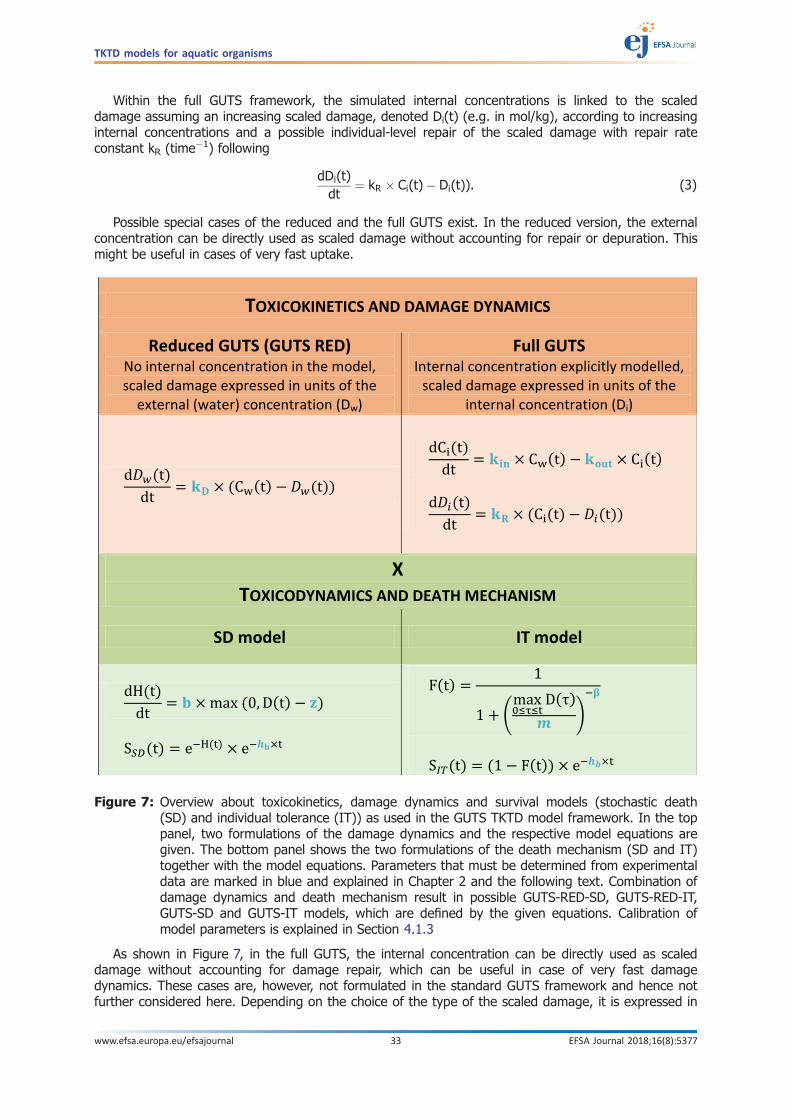
Within the full GUTS framework, the simulated internal concentrations is linked to the scaleddamage assuming an increasing scaled damage, denoted Di(t) (e.g. in mol/kg), according to increasinginternal concentrations and a possible individual-level repair of the scaled damage with repair rateconstant kR (time�1) following
dDi(t)dt
¼ kR � Ci(t)� Di(t)). (3)
Possible special cases of the reduced and the full GUTS exist. In the reduced version, the externalconcentration can be directly used as scaled damage without accounting for repair or depuration. Thismight be useful in cases of very fast uptake.
As shown in Figure 7, in the full GUTS, the internal concentration can be directly used as scaleddamage without accounting for damage repair, which can be useful in case of very fast damagedynamics. These cases are, however, not formulated in the standard GUTS framework and hence notfurther considered here. Depending on the choice of the type of the scaled damage, it is expressed in
Figure 7: Overview about toxicokinetics, damage dynamics and survival models (stochastic death(SD) and individual tolerance (IT)) as used in the GUTS TKTD model framework. In the toppanel, two formulations of the damage dynamics and the respective model equations aregiven. The bottom panel shows the two formulations of the death mechanism (SD and IT)together with the model equations. Parameters that must be determined from experimentaldata are marked in blue and explained in Chapter 2 and the following text. Combination ofdamage dynamics and death mechanism result in possible GUTS-RED-SD, GUTS-RED-IT,GUTS-SD and GUTS-IT models, which are defined by the given equations. Calibration ofmodel parameters is explained in Section 4.1.3
TKTD models for aquatic organisms
www.efsa.europa.eu/efsajournal 33 EFSA Journal 2018;16(8):5377

external or internal concentration units. In consequence, all related parameters, including the killingrate constant b, and the (median) threshold z and m should be given with an index for a specificapplication. In case the scaled damage refers to the external concentration, the index is w, in case itrefers to the internal concentration, it is i. In the general case, where a concrete model has not beenselected, the index can be left out. As this SO uses mainly reduced versions of GUTS, the parameterswill be denoted with index w.
4.1.1.2. Toxicodynamics and death mechanisms
The damage dynamics is connected to an individual hazard state variable, resulting in simulatedmortality when an internal damage threshold is exceeded (Figure 7). Two death mechanisms are usedin this scientific opinion, which are extreme cases of the GUTS theory: the SD and the IT.
For SD models, the threshold parameter for lethal effects is fixed and identical for all individuals of agroup, meaning that the variance of the threshold values is zero, and the killing rate relates theprobability of a mortality event in proportion to the scaled damage. In contrast, in the IT modelsthresholds for effects are distributed among individuals of one group, and once an individual toleranceis exceeded, mortality of this individual follows immediately, meaning in model terms that the killing rateis set to infinity. Both models are unified within the ‘combined GUTS’ model, in which a distributedthreshold is combined with a between-individual variable killing rate (Jager et al., 2011; Ashauer et al.,2016; Jager and Ashauer, 2018). For mathematical reasons, the parameter estimation of a ‘combinedGUTS’ model requires more data than it can be obtained from standard survival testing. With the aim ofmaximising the added value of standard toxicity testing, this SO is considering the reduced GUTSversions only, with the IT and SD models as realisations of the death processes. Combinations of thechoice of the scaled damage and the death mechanism give clearly defined acronyms for the differentvariants of GUTS, e.g. GUTS-RED-SD for the combination of the scaled damage without considerationof internal concentrations and the SD mechanism, or GUTS-IT for the full GUTS model accounting forinternal concentrations in combination with the IT mechanism. Please consult chapter 2 for anintroduction into TKTD modelling, GUTS and the concepts of damage dynamics and death mechanisms.
In the SD model, a hazard rate is calculated following the differential equation
dH(t)dt
¼ b�max(0, D(t)� z), (4)
Table 2: Parameter symbols used for GUTS modelling in this chapter, explanation and units
Symbol Explanation Example Unit
Dw Scaled damage, referenced to external concentration mol/L
Di Scaled damage, referenced to internal concentration mol/kgCw External chemical concentration in the environment mol/L
Ci Internal chemical concentration in an organism mol/LkD Dominant rate constant for the reduced model day�1 (or time�1)
kin Uptake rate constant for chemicals into the body L/kg d�1
kout Elimination rate constant for chemicals from the body day�1
kR Damage repair rate constant day�1
h Cumulative hazard rate day�1
b Killing rate constant [D]/day�1
bi Killing rate constant referenced to internal concentration kg/mol d�1
bw Killing rate constant referenced to external concentration L/mol d�1 (or time�1)z Threshold for effects [D]
zi Threshold for effects referenced to internal concentration mol/kgzw Threshold for effects referenced to external concentration mol/L
hb Background hazard rate day�1
mi Median of the distribution of thresholds, ref. to internal conc. mol/kg
mw Median of the distribution of thresholds, ref. to external conc. mol/L
b Shape parameter for the distribution of thresholds [�]
TKTD models for aquatic organisms
www.efsa.europa.eu/efsajournal 34 EFSA Journal 2018;16(8):5377

which describes hazard increasing in proportion to killing rate constant b, when the scaled damageexceeds the internal threshold concentration z. For the parameter estimation of the SD model, thekilling rate constant b ([D]�1 time�1) and internal threshold concentration z ([D]) must be estimatedfrom the survival data; [D] stands here for the unit of the scaled damage. The parameter values arekept constant during the simulated time, the processes of TK and TD are captured by the ordinarydifferential equations.
In the SD model, the survival probability of an individual to survive until time t is calculated as
SSD(t) ¼ e�HðtÞ � e�hb�t, (5)
where hb (time�1) is the background mortality rate constant.In the IT model, the survival probability of an individual to survive until time t is calculated
following the cumulative log-logistic distribution of the thresholds z in a group of individuals, given bythe function
F(t) ¼ 1
1þ�max0� s� tD(s)
m��b
, (6)
where m is the median of the distribution of z ([D]) and b (�) is the shape parameter of thedistribution.
In the IT model, the survival is related to the maximum scaled damage rather than to the actualscaled damage because death is irreversible, meaning that also under decreasing concentrations, thelevel of mortality in a simulated group of individuals could not become lower again. In the IT model,the survival probability of an individual to survive until time t is then calculated by
SIT(t) ¼ (1� F(t))� e�hb�t. (7)
4.1.2. Test results for two model implementations
The implementation of a model is software-specific. The documentation of the implementationshould contain an overview of the source code files, and the version and necessary packages of theused programming environment. Testing of the implementation (‘implementation verification’) needs tobe performed and documented for any model implementation, while the reasonable behaviour of themodel (‘sensitivity analysis’) has been performed within this opinion for the example implementations(with Mathematica and R) and is not necessarily part of the documentation of a model implementation.The following sections contain a short overview of examples for an implementation of the GUTS TKTDmodel in Mathematica (Section 4.1.2.1) and in R (Section 4.1.2.2), before examples are given for themodel implementation verification (Section 4.1.2.3) and the sensitivity analyses (Section 4.1.2.4).
4.1.2.1. Model implementation in Mathematica
The different GUTS-RED versions have been implemented in Mathematica (Wolfram Research,version 11.0, http://www.wolfram.com/mathematica/). Mathematica is proprietary software forperforming mathematics on a computer. It provides comprehensive methods for computation. TheGUTS implementation in Mathematica uses mainly the functionality to calculate numerical solutions forordinary differential equations (method NDSolve), to find the minimum of a given objective function(NMinimize), to read and write files of various formats (Import/Export) and to operate with lists andmatrices of data. Mathematica is under continuous development; the implementation is steadily testedand verified.
The GUTS Mathematica notebooks contain applications for the single modelling steps, i.e. modelcalibration, model validation, predictions of surviving individuals for the exposure scenarios andprobabilistic model simulations, together with all necessary data import and export functionality (seeAppendix A). The source code of the Mathematica notebooks is not write-protected, that can,however, be achieved if necessary.
Mathematica notebooks come in general in a specific format that contains both the program codeand the output. Providing all notebooks and input files gives the opportunity to look into the sourcecode and to see at the same time the output. A Mathematica installation and license will be necessaryto run the program code and to redo and test calculations.
TKTD models for aquatic organisms
www.efsa.europa.eu/efsajournal 35 EFSA Journal 2018;16(8):5377

The GUTS Mathematica code has not been optimised for providing user-friendly software. Thestructure of the model code enables, however, given a running Mathematica installation, to redo allsteps that have been performed in the scope of the GUTS implementation, by loading and executingthe GUTS-methods notebook, followed by one of the application notebooks. Important for running thecode is that input files are located in the file system as required.
4.1.2.2. Model implementation in R (package ‘morse’)
GUTS-RED versions have also been implemented within the R-package ‘morse’ 3.1.0 (R Core Team,2016; Baudrot et al., 2018a). R is a free software environment for statistical computing and graphics.It compiles and runs on a wide variety of UNIX platforms, Windows and MacOS (https://www.r-project.org/). It can be downloaded from any CRAN mirror (https://cran.r-project.org/mirrors.html).
Package ‘morse’ provides tools for the analysis of survival/reproduction data collected fromstandard toxicity tests. It can be used to explore/visualise experimental data, and to performestimation of LCx/ECx values by fitting concentration–response curves, or estimation of NEC values byfitting GUTS-RED-SD and/or -IT models. The LCx/ECx/NEC as well as model parameters are providedalong with a quantification of their uncertainty. Package ‘morse’ can be downloaded at https://cran.r-project.org/web/packages/morse/index.html; a step-by-step explanation of its use is provided athttps://cran.r-project.org/web/packages/morse/vignettes/tutorial.html, while a more formal descriptionof the underlying estimation procedures is provided at https://cran.r-project.org/web/packages/morse/vignettes/modelling.pdf. The full description of all functions provided by the R-package ‘morse’ can befound at https://cran.r-project.org/web/packages/morse/morse.pdf. The source code of thesefunctions is accessible within R from instruction ‘morse:::function_name’. Moreover, the R-package‘morse’ uses the R-package ‘rjags’ (Plummer, 2013) as an R interface to the JAGS library for Bayesianmodel estimation. Note that package ‘rjags’ does not include a copy of the JAGS library that needs tobe installed separately (http://mcmc-jags.sourceforge.net/).
Note that basic features of the R-package ‘morse’ are also available online within the user-friendlyweb-platform MOSAIC (Charles et al., 2017) which offers a new GUTS module specifically dedicated tothe online fitting of GUTS-RED-SD and GUTS-RED-IT (http://pbil.univ-lyon1.fr/software/mosaic/guts,Baudrot et al., 2018c).
R notebooks are usually provided as readable stand-alone text files directly usable as R scripts (.Rextension). They contain all necessary code lines associated with comments, to run and get outputresults [See Appendix E for the code archive].
4.1.2.3. Verification of model implementation
In order to verify the model code, it would be ideal to show that the code is correctly implemented withrespect to the conceptual and the formal model and that the code is error-free. Model code verification is animportant tool to build trust to model results. A rigorous verification of the complete implementation code,in the sense of a complete check of the computer code would mean an extensive effort and an enormousdocumentation. In order to keep the balance between effort and results, model results have been producedfor a set of scenarios, representing specific classical and extreme cases, and the model outcomes havebeen checked for reasonable results. Results below are given side by side both for Mathematica and Rimplementations in order to illustrate that both independent implementations show the same results.
Classical exposure scenario
The model implementation has first been tested for a classical exposure scenario corresponding toa 4-day period at constant concentration of a theoretical pollutant followed by a 3-day period withoutexposure. For arbitrary parameter values, the survival over time (SOT) has been simulated for both theGUTS-RED-SD and the GUTS-RED-IT models, together with the scaled damage (Figure 8). Asexpected, this latter first increases until day 4, then decreases over the following 3-day period.
Under model GUTS-RED-SD, the SOT first starts with a 100% value until about day 2 when thescaled damage exceeds the threshold zw value (damage curve and dashed line first intersection inFigure 8). Then, the SOT decreases until around day 5 when the scaled damage falls below thethreshold (damage curve and dashed line second intersection in Figure 8). After day 5, the SOTremains constant at about 50%. Under model GUTS-RED-IT, survival starts to decrease from thebeginning of the exposure, but the decrease stops as soon as the exposure concentration falls to zeroat day 4. The final SOT under model GUTS-RED-IT is around 30%. Together, these results corroboratea correct implementation for both GUTS-RED-SD and GUTS-RED-IT models under constant exposure,since both model implementations show the same reasonable behaviour.
TKTD models for aquatic organisms
www.efsa.europa.eu/efsajournal 36 EFSA Journal 2018;16(8):5377

Pulsed scenarios
Another test was performed to check the Mathematica and R implementations of the GUTS-RED-SDand GUTS-RED-IT models for an arbitrary ‘pulsed’ exposure scenario. Such exposure situations, wheresteep increasing concentrations are followed by a period of more or less constant concentrations,which are abruptly falling down to zero concentrations, are challenging for the algorithms being usedto calculate the numerical solutions of the model equations. The test for the same generic modelparameterisation of GUTS-RED-SD and GUTS-RED-IT models as in Figure 8, with multiplication factorsfrom 1 to 50, show technically correct simulation results for the scaled damage and the survival rateover time (Figure 9) (see Section 8). Most importantly, the numerical scheme and precision appears tobe stable, as no indicators for numerical instability under such numerically challenging exposureschemes, i.e. abruptly changing or negative exposure concentrations, are visible. This reinforcesconfidence into the model implementations.
Figure 8: Test of the Mathematica (upper panel) and R (lower panel) implementation of GUTS-RED-SDand GUTS-RED-IT models under 4-days constant exposure. The left panels show the scaleddamage (black) and the external (gray) concentrations together with the internal threshold(dashed line). The middle panels show the survival over time for the GUTS-RED-SD model,parameters: hb = 0, kD = 0.3 (time�1), bw = 0.5 (L mol�1 time�1) and zw = 2.5 ([D]). Theright panels show the survival over time for the GUTS-RED -IT model with parameters:hb = 0, kD = 0.3 (time�1), mw = 2.5 ([D]) and b = 2 (�). Table 2 gives a full list ofparameters with the explanation
TKTD models for aquatic organisms
www.efsa.europa.eu/efsajournal 37 EFSA Journal 2018;16(8):5377

Extreme scenarios
A third and last test was performed to check the robustness of model implementations underextreme cases. Three extreme scenarios were tested as shown in Figure 10:
i) under a zero exposure with no background mortality, the scaled damage is equal to 0 andboth the GUTS-RED-SD and GUTS-RED-IT models predict no mortality, hence survival overtime equals 100%;
ii) on the contrary, when the exposure is short but at very high concentrations (100 arbitraryunits in this example), the scaled damage increases quickly during the period of exposure,then it decreases. Accordingly, the survival over time very quickly decreases from 100% to0% in less than 1 day;
iii) for a scenario with zero exposure but some background mortality, the damage is logicallyequal to 0, as in case (i), but the survival over time slightly decreases according to the valueof parameter hb.
For all the tests, results of both the Mathematica as well as the R implementations of GUTS-REDwere identical and as expected, which further corroborates that the implementations of the GUTSreduced models are correct and stable.
Figure 9: Test of the Mathematica (upper panel) and R (lower panel) implementations of GUTS-RED-SDand GUTS-RED-IT models with increasing multiplication factors for pulsed exposures, withexposure from day 3 to day 5. The external concentration of initially 5 ([D]) has beenmultiplied by factors from 1 to 50 (rainbow colours, first panels from the left). Secondpanels show the scaled damage; third panels show the survival rate over time for modelGUTS-RED-SD and fourth panels for model GUTS-RED-IT. Parameters for model GUTS-RED-SDwere: hb = 0, kD = 0.3 (time�1), bw = 0.5 (L mol�1 time�1) and zw = 2.5 ([D]); parameters formodel GUTS-RED-IT were: hb = 0, kD = 0.3 (time�1), mw = 2.5 ([D]) and b = 2 (�). Table 2gives a full list of parameters with the explanation
TKTD models for aquatic organisms
www.efsa.europa.eu/efsajournal 38 EFSA Journal 2018;16(8):5377

4.1.2.4. Model sensitivity analysis
In addition to the previous numerical tests of the model implementations in Mathematica and R, asensitivity analysis was performed. Sensitivity analyses are a tool to understand how model outputsrespond to changes in parameter values. They allow the modeller to distinguish less influentialparameters (that could be fixed at point values without any major change in model outputs) from themost influential parameters. The most influential parameters should receive most attention whencalibrating the model.
Many methods exist to perform sensitivity analyses (Saltelli et al., 2000; Ciric et al., 2012). Here theone-parameter-at-a-time (OAT) method was used (see Figure 11), which involves varying one parameterat a time, keeping the others fixed at reference values. Excluding parameter hb from our sensitivityanalysis, the toxicokinetic parameter kD was varied as well as bw and zw for the GUTS-RED-SD, and mw
and b for the GUTS-RED-IT model (see Table 2 for the definition of the parameters). For more complexmodels with more parameter values, global sensitivity analyses are recommended in order to quantify thesensitivity of the model for changes in one parameter also in interaction with the other parameters, butfor the GUTS-RED models with three main TKTD parameters, the OAT method is still appropriate (Saltelliet al., 2000). Future sensitivity analysis could, with low effort, further investigate whether there are anyinteractive effects between the main model parameters.
Figure 10: Mathematica (upper panel) and R (lower panel) implementation test under extreme cases:(i) zero exposure and no background mortality (solid lines), (ii) high exposure over days1–4 (100 [D]) (dashed lines) and (iii) zero exposure with a slight background mortality(dotted lines). The left panels show the scaled damage; the middle panels show thesurvival over time under the GUTS-RED-SD model; the right panels show the survivalover time under the GUTS-RED-IT model. Parameter values for the GUTS-RED-SDmodel: kD = 0.5 (time�1), bw = 0.3 (L mol�1 time�1) and zi = 2.5 ([D]); parameter valuesfor the GUTS-RED-IT model: kD = 0.5 (time�1), mi = 2.5 ([D]) and b = 2 (�). Parameterhb was equal to 0 for extreme cases (i) and (ii); hb = 0.05 (time�1) for extreme case (iii).Table 2 gives with the list of parameters and their explanation
TKTD models for aquatic organisms
www.efsa.europa.eu/efsajournal 39 EFSA Journal 2018;16(8):5377
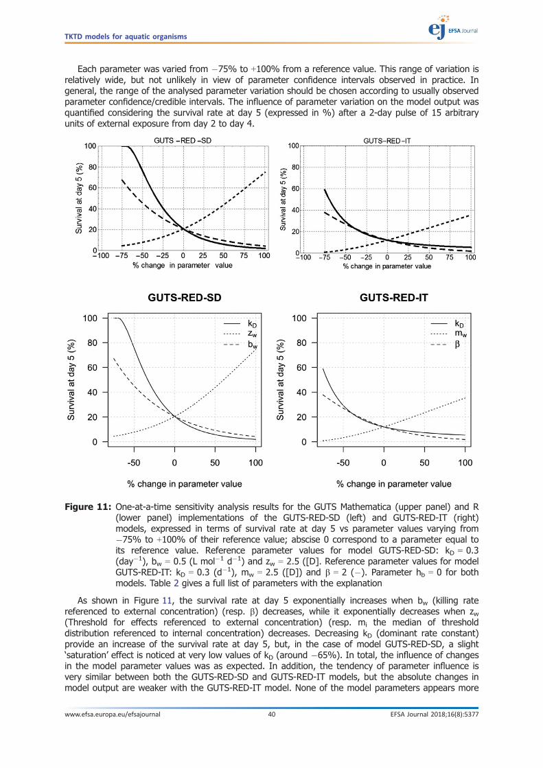
Each parameter was varied from �75% to +100% from a reference value. This range of variation isrelatively wide, but not unlikely in view of parameter confidence intervals observed in practice. Ingeneral, the range of the analysed parameter variation should be chosen according to usually observedparameter confidence/credible intervals. The influence of parameter variation on the model output wasquantified considering the survival rate at day 5 (expressed in %) after a 2-day pulse of 15 arbitraryunits of external exposure from day 2 to day 4.
As shown in Figure 11, the survival rate at day 5 exponentially increases when bw (killing ratereferenced to external concentration) (resp. b) decreases, while it exponentially decreases when zw(Threshold for effects referenced to external concentration) (resp. mi the median of thresholddistribution referenced to internal concentration) decreases. Decreasing kD (dominant rate constant)provide an increase of the survival rate at day 5, but, in the case of model GUTS-RED-SD, a slight‘saturation’ effect is noticed at very low values of kD (around �65%). In total, the influence of changesin the model parameter values was as expected. In addition, the tendency of parameter influence isvery similar between both the GUTS-RED-SD and GUTS-RED-IT models, but the absolute changes inmodel output are weaker with the GUTS-RED-IT model. None of the model parameters appears more
Figure 11: One-at-a-time sensitivity analysis results for the GUTS Mathematica (upper panel) and R(lower panel) implementations of the GUTS-RED-SD (left) and GUTS-RED-IT (right)models, expressed in terms of survival rate at day 5 vs parameter values varying from�75% to +100% of their reference value; abscise 0 correspond to a parameter equal toits reference value. Reference parameter values for model GUTS-RED-SD: kD = 0.3(day�1), bw = 0.5 (L mol�1 d�1) and zw = 2.5 ([D]. Reference parameter values for modelGUTS-RED-IT: kD = 0.3 (d�1), mw = 2.5 ([D]) and b = 2 (�). Parameter hb = 0 for bothmodels. Table 2 gives a full list of parameters with the explanation
TKTD models for aquatic organisms
www.efsa.europa.eu/efsajournal 40 EFSA Journal 2018;16(8):5377

influential than the others; hence, all parameters can be considered to be important and have to becalibrated carefully. In summary, the sensitivity analyses indicate that model output changes in relationto changes in the model parameters in a continuous and reasonable way in the range between �75%and +100% of their respective reference values.
4.1.2.5. Conclusive statement on the formal and computer model
Both implementations, Mathematica and R, finally give exactly the same results when verifying thesource code (Section 4.1.2.3) or analysing the sensitivity of model outputs to changes in parametervalues (Section 4.1.2.4). The results corroborate the correct implementation of the formal model forboth model implementations. Future implementations of GUTS could do the same checks to showcorrect implementation, in addition to the required ring-test performance (see also Section 4.2, andAppendix B.6 and B.7). Moreover, OAT sensitivity analysis of the GUTS-RED models has beenperformed and the results indicate that model parameters have almost equal influence on the modeloutput, hence sensitivity analyses of the GUTS-RED models are not required in future modelapplications.
4.1.3. Parameter estimation process
4.1.3.1. Introduction
Whatever the inference method (frequentist or Bayesian, see Sections 4.1.3.2 and 4.1.3.3), thegoal of model parameter estimation (also named model calibration or parameter optimisation) is to getbest parameter values that give an optimal fit of the modelled survival over time to the observedsurvival over time in the data sets that are used for calibration. According to the inference method, thesteps required to get these optimal values of parameters differ, but in both cases, survival probabilitiesboth for the SD or the IT model are calculated in the same way, with an explicit dependence onparameter vector h, the external concentration over time (Cext(t)), and time (t). For the GUTS-RED-SDand the GUTS-RED-IT models, this is formally
SSD(t) ¼ SSD(h, Cext(t), t) ¼ SSD((bi, zi, kD, hb), Cext(t), t) (8)
and
SIT(t) ¼ SIT(h, Cext(t), t) ¼ SIT((mi, b, kD, hb), Cext(t), t). (9)
Stochasticity of the survival process
Survival is a binary process, i.e. an individual can be either alive or dead. This fact can in smallgroups of individuals lead to stochastic fluctuations of predictions of survival over time, which isimportant to consider when laboratory test results with low numbers of tested individuals are used(e.g. typical acute test setting with 10 or 20 individuals per treatment). In such cases, survival can bemodelled as a binomial process, with the number of surviving individuals being proportional to theconditional binomial distribution
ytþDt �B(ptþDt;yt), (10)
where:ytþDt is the number of survivors in a population at time tþ Dt,yt is the number of individuals being alive at time t, andptþDt is the conditional probability to survive from time t until time t + Dt, given as
ptþDt ¼S (h, Cext (t), t)
S(h, Cext(t+Dt), t+Dt), (11)
where S(h, Cext(t), t) is the deterministic survival rate calculated by the GUTS-RED-SD or the GUTS-RED-IT model for parameter vector h, external concentration time course Cext(t) and time-point t (seeequations 8 and 9).
TKTD models for aquatic organisms
www.efsa.europa.eu/efsajournal 41 EFSA Journal 2018;16(8):5377

Note that the time step is not fixed to 1 here, as the survival rates over time can be evaluated forarbitrary small or large time steps; hence, survival probabilities can be modelled as a random processusing a flexible time step Dt.
For parameter vector h, a chosen external concentration time course Cext(t) and an initial cohortsize Y0, the number of surviving individuals in a group is modelled in an iterative way, starting with Y0individuals at t = 0, by drawing for every new time step t + Dt from a conditional binomial distribution,parameterised by the number of living organisms at time t and the calculated survival rates for times tand t + Dt as given in equations (10) and (11). By performing nSmax repetitions of this procedure,nSmax realisations of the survival probabilities within a cohort of initial size Y0 are obtained, givenparameter vector h and external concentration time course Cext(t). Typically, nSmax will be chosen closeto Y0. From the set of realisations of the stochastic process, statistical descriptors such as medians andpercentiles are calculated. For large numbers of Y0, the stochasticity of model predictions becomesunimportant. The assessment of the stochasticity of the survival process is therefore required when forinstance model predictions are compared with results from laboratory experiments with small numbersof individuals. When predictions of survival are made for environmental systems, it is supposed thatthe cohort size is large enough (Y0 > 100, based on expert knowledge) to ignore the stochasticity ofsurvival.
Likelihood
Although several other methods exist either for the frequentist or the Bayesian methods, themethods here were based on the likelihood of the observed data given a parameter vector h. Thelikelihood is defined as the assumed probability (density) for those observed data given parametervector h
LðYjhÞ ¼ PðYjhÞ: (12)
In survival experiments, the observations at single time-points are binomial (either alive or dead)and dependent on each other (the number of alive individuals at a single time-point depends on theprevious time-point), so that the survival probabilities follow a multinomial distribution (or equivalentlya conditional binomial distribution). Based on the multinomial distribution, Jager et al. (2011) derivedthe log-likelihood function
lnL(Yjh) ¼Xnþ1
i¼1(yi�1 � yi)� ln (Si�1(h;Cext(t), t)� Si(h, Cext(t), (t)), (13)
where yi are experimental observations of survivors at time-points i, and Si are simulated survivalprobabilities at time i, given parameter vector h. For calculation reasons, Sn+1(h, Cext(t), t) = 0 andYnþ1 ¼ 0.
Uncertainty
When using the model, the uncertainty in model parameter estimates comes in addition to thestochasticity of the survival process. Basically, uncertainty in parameter estimates can originate fromdifferent sources, either errors in experimental measurements or from natural biological variability.
Measurement errors and biological variability within the cohort of the individuals is accounted forwithin the process of the model calibration by the calculation of parameter confidence/credibleintervals. While the measurement errors can be minimised by a good experimental quality, variability isintrinsic for biological systems and models are the means to explicitly address such variability. Whenevaluating, e.g. survival in acute toxicity tests by classical dose–response modelling, LC50 values areestimated and reported including uncertainty limits. When using TKTD modelling, uncertainty limits areapproximated and reported for parameters, and the impact of these uncertainties combined with thestochasticity of the survival process are propagated to model predictions. When simulatingenvironmental exposure scenarios, the assumption is that numbers of individuals in environmentalsystems are large enough to marginalise the stochasticity of survival, which results in observabledifferences in predicted survival only for small numbers. Still, for the prediction of environmentalsystems the parameter uncertainty, which captures among others part of the biological variability, hasto be considered (see Section 4.1.4.2). Nevertheless, further sources of the variation of the biologicalresponse in natural systems cannot be estimated from experiments carried out under controlledconditions.
TKTD models for aquatic organisms
www.efsa.europa.eu/efsajournal 42 EFSA Journal 2018;16(8):5377

The next two sections explain the parameter optimisation process for the frequentist(Section 4.1.3.2) and for the Bayesian approach (Section 4.1.3.3), respectively. The Bayesian approachdiffers conceptually from the frequentist one in that it considers that the data are fixed and that theparameters are unknown random variables following a probabilistic distribution. The frequentistapproach considers that the parameters are fixed and known, and that the data are considered to beone realisation of one experiment among many others that could have been performed. It should behighlighted here, that both frequentist and Bayesian approaches result in very similar parametervalues, and that both approaches use approximation methods, often Monte Carlo Markov Chain(MCMC) algorithms to obtain best parameter sets and confidence/credible limits.
4.1.3.2. Frequentist approach
Parameter optimisation and likelihood
In the frequentist approach, parameters are optimised by maximising the log-likelihood function(equation 13). In practice, often the negative of the log-likelihood function is used because typicallyminimisation algorithms are used. Optimal parameter values give the best fit between the model andthe observed data. Optimisation routines yield an optimal parameter vector hopt for which thelog-likelihood function shows the highest values of lnLðYjhoptÞ given the data set Y used. Optimisationresults in practice depend on the starting values of the optimisation routine, so choices of startingvalues need to be documented, in addition to the choice and settings of the used optimisationalgorithm.
For a basic understanding of this step of model calibration, that is parameter fitting via minimisationof the negative log-likelihood, it helps to get a visual impression of what minimisation algorithmsusually do (Figure 12). Parameter optimisation can be interpreted as a way to find the minimum of a‘likelihood-landscape’ in a n + 1-dimensional space (n = 2 in Figure 12, but in general n is equal to thenumber of model parameters).
In the lower panel of Figure 12, the third dimension is in this case the difference between theoptimal and the changed log-likelihood (see equation 14), as introduced in Section 4.1.3.2 and alsocalled log-likelihood ratio and is shown as colour gradient (top) or explicit third dimension (bottom).The log-likelihood ratio gives simply the distance of the log-likelihood value from the optimallog-likelihood value for an arbitrary parameter combination. Intuitively, the yellow point in the centre ofthe diagram represents the optimal parameter value (the minimum of the negative log-likelihoodfunction). During a parameter optimisation routine, red and blue points show parameter combinationsthat were tested with the aim to find the optimal parameter set (yellow point). All red dots representparameter combinations which are within the confidence limits as defined by equation (14), whereasthe blue dots indicate parameter combinations that were tested but which were outside of theconfidence limits. Green dots represent results from the approximation scheme of the parameterconfidence limits.
TKTD models for aquatic organisms
www.efsa.europa.eu/efsajournal 43 EFSA Journal 2018;16(8):5377

Optimisation routines search for a minimum in such likelihood-landscapes (Figure 12) to find theoptimal parameter combination (i.e. the parameter set with the lowest negative log-likelihood value).Parameter confidence interval approximation (indicated by the green points in Figure 12) analyses thelimits of the confidence region in a systematic way. What looks in this example smooth andstraightforward can become very challenging, since not always such clearly defined minimum exists. Forexample, there can be multiple local minima, where the minimisation algorithm can get stuck dependingon starting conditions. Hence, model calibration requires a good implementation of an appropriateoptimisation routine and a comprehensive documentation of relevant aspects of the optimisation.
Examples of methods that can be used for optimisation are random walk algorithms, which searchthe parameter landscape with different choices of acceptance or rejection of tested parameter values.In general, stochastic optimisation algorithms (MCMCs and related methods such as Metropolis, GibbsSampler or Simulated Annealing), or downhill simplex methods such as Nelder–Mead are preferableover deterministic methods (e.g. Levenberg–Marquardt) because of their capability to find globalminima and not to get stuck in non-trivial optimum parameter searches.
Implementations of such algorithms are available and can be used in software such asMathematica, where the Nminimize method gives the opportunity to choose from a variety ofoptimisation algorithms. Also, the OpenModel software (http://openmodel.info/) provides theopportunity of using a MCMC algorithm to find best parameters.
The convergence of optimisation algorithms is checked in the mentioned software implementationsautomatically, the principle is that the optimisation is starting for a number of different startingconditions (so-called ‘chains’), and by the evaluation of differences within and between the differentchains, the convergence of the algorithm is checked, e.g. by the Gelman and Rubin statistical test(Brooks and Gelman, 1998).
Figure 12: Visualisation of the principle of minimising the negative log-likelihood function under afrequentist approach. 2D (top) and 3D (bottom) view on the ‘parameter plane’ that isbuilt by two model parameters
TKTD models for aquatic organisms
www.efsa.europa.eu/efsajournal 44 EFSA Journal 2018;16(8):5377

Numerical approximation of parameter confidence intervals
Unlike in, e.g. linear model fitting, parameter confidence limits in case of GUTS can no longer beestimated in an analytical way. They are not defined by any formula, but instead, need to beapproximated by a numerical procedure. The log-likelihood ratio method is one of the methods thatcan be used to approximate confidence limits for the optimal parameters hopt. Confidence limits for thesingle parameters for a given confidence level a were calculated as those parameter values, for whichthe log-likelihood ratio fulfils the condition
�2½lnLðYjhÞ � lnLðYjhoptÞ� � v2df;1�a; (14)
with v2df;1�a being the value of the chi-square distribution for the confidence level a and the degrees offreedom of the log-likelihood ratio df. For single parameter confidence intervals, the log-likelihood ratiohas df = 1. To find these parameter values, one value in the parameter vector, say parameter hi, is setto successively decreasing values, starting at the maximum-likelihood estimate, i.e. the best parametervalue. All parameter values with exception of parameter i are then again optimised to give a best fit tothe experimental data. The value lnLðYjhÞ of the log-likelihood function corresponding to parametervector h ¼ ðhopt1 ; hopt2 ; . . .; h1; . . .; h
optn Þ is calculated. This procedure is repeated until the constrain on
lnLðYjhÞ is satisfied (equation 14). Likewise, this procedure is repeated for successively increasingparameter values, again starting with the optimal maximum-likelihood estimate. First values ofparameter hi leading to the violation of condition (14) are reported as confidence limits. Furtherreading on the numerical approximation of parameter confidence intervals are reported elsewhere e.g.Jager and Ashauer (2018).
4.1.3.3. Bayesian approach
As mentioned above, the Bayesian approach considers that data are fixed and that the parametersare unknown random variables following a probabilistic distribution. These results in the followingpractical implications: (i) Bayesians want to optimise the probability of parameter vector h given thedata set Y used for calibration, rather than only the likelihood (see below); (ii) the need for Bayesiansto provide reasonable prior information to see the result of an experiment, then updating thisinformation by accounting for the data. Below is a short introduction to Bayesian principles; it isrecommended to readers who would like to learn more about Bayesian data analysis to considerfurther reading; a recommendation is, for example, Gelman (2014).
Basic principles
The keystone of the Bayesian approach is the Bayes formula
PðhjYÞ ¼ pðhÞpðyjhÞP(Y)
; (15)
where Y are the observed data; P(h|Y) is the joint posterior distribution of parameter vector h;P(Y|h) isthe likelihood of the data given the parameters (see equation 12 and 13); P(h) is the joint priordistribution of parameter vector h.
Given that P(Y) is known and fixed, it is often not considered as it does not depend on h and willnot influence the posterior distribution. Hence
PðhjYÞ1PðhÞPðYjhÞ; (16)
with P(h)p(Y|h) the unnormalised posterior density and
P (Y) ¼Z
PðhÞPðYjhÞdh: (17)
The prior distribution P(h) expresses the available parameter information without knowing theobserved data, while the posterior distribution P(h|Y) combines this prior information (which may bemore or less informative depending on what is known about the value of the parameters beforehand)with evidence from the data (expressed through the likelihood) into a posterior density probabilitydistribution for the parameters. The overall expectation is to get a narrower posterior distributioncompared to the prior (illustrated for one parameter in Figure 13, left): the difference between the two
TKTD models for aquatic organisms
www.efsa.europa.eu/efsajournal 45 EFSA Journal 2018;16(8):5377

distributions reflects the information provided by the data. When the prior information is vague(translated into a flat prior distribution), and the data sufficiently informative, the results converge tothose obtained by the frequentist approach (Englehardt and Swartout, 2006).
Directed Acyclic Graph
Under a Bayesian framework, a model is specified by a set of prior distributions on parameters toestimate and a set of hierarchical conditional distributions linking parameters to data, which iscommonly depicted in a Direct Acyclic Graph (DAG). In fact, the DAG represents a series of conditionalindependence assumptions, which allows the full probability model to be factorised into a product ofconditional distributions, and consequently to tackle calculations. Each quantity in the model (data,covariates, parameters and latent variables10 ) corresponds to a node in the DAG, and links betweennodes show direct dependences. The graph is directed, because each link is an arrow; it is acyclicbecause it is not possible to return to a node after leaving it by following the arrows (Lunn et al.,2000). The dependencies can be defined by deterministic (namely, mathematical functions) orstochastic (namely, probability distributions) links. For each node with no incoming arrows, priorinformation (Figure 13, left) should be specified.
Joint posterior distribution
The joint posterior distribution has the dimension of the number of parameters, but it can beplotted in planes of parameter pairs to visualise correlations between parameters. In an example casewith two binormally distributed parameters, the joint posterior distribution can be plotted in the2D-parameter space as illustrated by ellipses on Figure 13 (right); in this example, parameters h1 andh2 appear slightly correlated. From the joint posterior distribution, the marginal posterior distributionsfor each parameter (as illustrated by grey normal distributions on bottom and left sides of Figure 13(right) can be extracted. Then, from the marginal posterior distributions, some statistical summaries onparameter estimates can be extracted, usually the median (illustrated by vertical and horizontal plaingrey lines on Figure 13, right) as well as 2.5% and 97.5% quantiles to serve as 95% credible intervals(illustrated by vertical and horizontal dotted grey lines on Figure 13, right). Another advantage ofhaving the joint posterior distribution is that any posterior distribution of any function of theparameters can be obtained. In particular, when calculating an LCx,t from GUTS (for given choices ofthe x% and of the target-time t), the corresponding formula depends on GUTS parameters. Theuncertainty on these GUTS parameters, which is extracted from the joint posterior distribution, can bepropagated to the LCx,t calculation, on which a posterior probability distribution can then also beobtained (see Section 4.1.4.4 for more details).
10 Variables that are not observed but exist within the model, e.g. scaled damage.
TKTD models for aquatic organisms
www.efsa.europa.eu/efsajournal 46 EFSA Journal 2018;16(8):5377

Parameter uncertainties
One implication of adopting a Bayesian approach is that the uncertainty on a parameter isexpressed as a credible interval (also called a Bayesian confidence interval) instead of an approximateconfidence interval like in the frequentist approach (see Section 4.1.4.3). The 95% credible intervaldelimits a range of values where the parameters should lie with a 95% probability, whereas thecalculation of a confidence interval (usually a 95% confidence interval) is based on hypotheticalrepeated sampling from the model: if samples of the same population size are repeatedly obtained anda 95% confidence interval for each of the samples is got, it is expected that 95% of the confidenceintervals will contain the true value of the parameter. Another difference is that the credibility intervalis conditional to the data used to estimate the parameters, whereas the confidence interval is not.
Numerical computation of the posterior distribution
Based on equation (16), the calculation of the posterior distribution is often tricky. Analyticalsolutions only exist in rare cases. Many numerical methods have been developed to approximatelycompute the posterior distribution in challenging cases, mainly based on simulations by MCMCsampling methods used to generate random numbers from complex joint distributions. MCMCalgorithms are a general method based on drawing values of parameter vector h from approximatedistributions and then correcting those draws to better approximate the target posterior distribution, P(h|Y). The sampling is done sequentially, with the distribution of the sampled draws depending only onthe last value drawn; hence, the draws form a Markov chain. The key to the method’s success,however, is not the Markov property but rather that the approximate distributions are improved ateach step in the simulation, in the sense of converging to the target posterior distribution (Gelmanet al., 2014). With such algorithms, the simulation process must run long enough so that the
Figure 13: Left panel shows Directed Acyclic Graph (DAG) for the model GUTS-RED-SD when theexposure concentration (covariate Cext in double rectangle) is constant over time.Observed survival numbers N are represented in rectangles; ellipses correspond to latentvariables (Dw for the scaled damage and S for the survival rate) and circles to parametersto estimate. Deterministic links are represented by dashed arrows, whereas stochasticlinks are represented by solid arrows. Grey external rectangles stand for replicate (index k),time course (index t) and exposure concentration (index i). Right panel shows theoreticalbinormal joint posterior distribution of parameter vector (h1, h2). Ellipses correspond toisoclines of the joint posterior distribution; grey distributions are marginal posteriordistributions of both parameters; solid horizontal and vertical lines correspond to themedians of these marginal distributions; dashed horizontal and vertical lines correspond tothe 2.5% and 97.5% quantiles of the marginal distributions. See Table 2 with the list ofparameters and their explanation
TKTD models for aquatic organisms
www.efsa.europa.eu/efsajournal 47 EFSA Journal 2018;16(8):5377

distribution of the current draws is close enough to the desired target posterior distribution; hence, theuser himself must choose the number of iterations.
MCMC algorithms use random walk algorithms. Among them, the Metropolis algorithm (and itsgeneralisation, the Metropolis–Hasting algorithm) is an adaptation of a random walk with an acceptance/rejection rule to converge to the specified target distribution (Metropolis et al., 1953; Hastings, 1970).The Gibbs sampler is a special case of the Metropolis–Hastings algorithm applicable when the jointdistribution is not known explicitly, or it is difficult to sample from directly, but the conditional distributionof each parameter is known and is easy (or at least, easier) to sample from (Geman and Geman, 1984).
Several tools are available to automatically perform these computations like: JAGS for Just AnotherGibbs Sampler (Plummer, 2003) as used in some parts of this opinion in combination with theR-package rjags which provides an interface from R to the JAGS library for Bayesian data analysis;STAN, a state-of-the-art platform for statistical modelling and high-performance statistical computation(Carpenter et al., 2017); Winbugs, based on the BUGS (Bayesian inference Using Gibbs Sampling)project (Lunn et al., 2000). Today, the performance of these tools allows a wide use of the Bayesianapproach, even if it is still challenging to deal with ordinary differential equations.
Convergence criteria and goodness-of-fit
When running an MCMC algorithm, it is suggested to run several MCMC chains in parallel (usuallythree). They should all converge to the same target distribution thus providing a sample of the fulljoint posterior distribution. These chains also allow to perform the Gelman and Rubin statistical test(Brooks and Gelman, 1998). For each parameter, the square root of the ratio between the variance ofits posterior marginal distribution and the intrachain variance is calculated; it is expected to be equal to1 if the convergence is reached. In practice, a ratio lower than 1.1 for each parameter is acceptable.Another way of checking the chain convergence is to visualise quantiles of interest of the posteriordistribution (namely, 2.5%, 50% and 97.5% quantiles) over the iterations to ensure that they havestabilised at the end of the running process. Also, the autocorrelation between chain iterations shouldbe checked (further reading in Raftery and Lewis, 1992).
If the model fits well, then the replicated data generated under the fitted model should look likethe observed data. To put it in another way, the observed data should look plausible under theposterior predictive distribution, as a self-consistency check. A basic technique for checking the fit of amodel to observed data is to draw simulated values from the joint posterior predictive distribution ofreplicated data and compare these predicted samples to the observed data. Any systematic differencesbetween the simulations and the observed data indicate potential failings of the model (Gelman,2014). In practice, it is useful to examine graphical comparisons of the observed data with summariesof posterior predictive simulations, what is usually called a posterior predictive check (PPC) plot(Gelman, 2014). In PPC plots, the observed data is plotted against the corresponding estimatedpredictions, along with their 95% credible interval (see Figures 17 and 23 as examples).
Summary of Bayesian approach
In short, the Bayesian approach requires the following steps:
• Choose the prior distributions based on previous results, literature or expert knowledge: P(h);• Define the probabilistic model from the data, that is the random variables whose data would
be one realisation assuming known values of parameters, namely the likelihood: P(Y|h);(equation 1)
• Calculate the joint posterior distribution of the parameters given the data via the Bayesformula: P(h|Y);
• Provide statistical summaries of parameter estimates (namely, appropriate quantiles);• Get any function of the parameter estimates as posterior probability distribution, like for
example LCx,t calculations or predictions of new observations (see Section 4.2.2).
In essence, the Bayesian approach appears intuitive, starting from a prior distribution to derive a posteriorone; this latter may then serve itself as a prior distribution to fit new data. This knowledge accumulation is anadvantage of the Bayesian approach. The consideration of prior knowledge about parameters allows to userelevant information which is often available even before performing a survival experiment.
4.1.3.4. Summary on parameter estimation
The parameter optimisation process is important, because it yields the model parameters anduncertainty limits which are in consequence propagated in the model predictions. Parameter
TKTD models for aquatic organisms
www.efsa.europa.eu/efsajournal 48 EFSA Journal 2018;16(8):5377
optimisation routines are built into different software and can be used without too detailed expertknowledge, but it is advantageous to have some more understanding of the details, because only thisenables a safe use for regulatory risk assessment. This is also the reason why, in this section of thedocument, the technical details behind the parameter optimisation were outlined on a higher level ofdetails than needed to only apply the methods. For the evaluation of parameter estimates in practice,it is convenient that algorithms are implemented in standard software, because that makes sure thatthe algorithms are error-free and the convergence of the algorithm is also automatically tested.
Experience from parameter estimation gives some indication about important aspects for thecalibration of GUTS models:
• Calibration data should span from treatment levels with no effects up to large effects, ideallyincluding full effects (e.g. 0% survival). This is important because parameter estimates canshow reduced accuracy and precision when the experiments do not show a clear andcomprehensively covered dose–response pattern.
• Calibration data sets should report raw observations of mortality or immobility at least for fivetime-points (initial plus four observations over time). The choice of five time-points may beproblematic in standard tests shorter than 4 days. Possible solutions are: (i) increase thenumber of observation in those tests; and (ii) to extend the duration of the test to for instance96 h. If a standard 48-h study is only available, a calibration might still be attempted but thequality of the fit (convergence, uncertainty limits and visual fit) should be carefully checked.
• Attention should be paid in case the influence of time on the exertion of the effects is not fullycaptured in short tests (e.g. onset of effects, delayed effects, accumulated toxicity, etc.) as thisis likely to result in inaccurate predictions in the validation phase.
• Optimisation algorithm needs to be specified including settings (see examples inSections 4.1.4.3 and 4.1.4.4), and also the method that was used for the approximation of theconfidence/credible limits.
• In general, stochastic optimisers (MCMC) are preferable over deterministic methods (e.g.Levenberg–Marquardt) because of their improved capability to find global minima.
• Not only optimal parameter values, but also the log-likelihood value, and approximatedconfidence or credible intervals for all parameters must be given to allow for further checks(see Section 4.2.2.1).
• The ultimate test for the quality of parameter optimisation is given by the comparison betweenthe modelled survival using the optimal parameter set and the observed survival which can bechecked in plots of the survival over time or by the predictive posterior check (PPC) (seeSection 4.2.2.1 for an example).
Most of these points are used also in Section 7.6.2 for the evaluation of the parameter estimationprocess. A checklist for assessing the quality of the parameter estimation process for a GUTSapplication is part of the checklist for GUTS models (Annex A).
Parameter optimisation can be done in one of the frequentist or Bayesian frameworks, which resultfrom different ‘schools of thought’ in statistics. Both methods have advantages and disadvantages, butin practice both can be used, since they result in very similar parameter values, and both approachesdepend on approximation methods such as MCMC to obtain best parameter sets and uncertainty limits.
4.1.4. Model predictions
In this section of model documentation, the specific application of the calibrated model for thecalculation of predicted effects is documented as an example. It defines clearly, which and how riskassessment-relevant endpoints are being calculated. In addition, the basic principle and the technicaldescription of the used approach to propagate parameter uncertainty to model predictions arereported, both for the frequentist and the Bayesian approach.
4.1.4.1. Modelled endpoints
According to the definition of the regulatory questions that should be answered by the applicationof the model, and within the structure of the given regulatory model, the simulation model outputshave to be defined. The basis for these formulations is given in Sections 3.3.2 and 3.4.2. In case therelevant endpoints for the risk assessment are lethal effects (mortality or immobilisation), these can becalculated for time-variable exposure profiles by using a calibrated GUTS model. Before GUTS modelpredictions can be considered relevant for regulatory risk assessment, the GUTS model needs to be
TKTD models for aquatic organisms
www.efsa.europa.eu/efsajournal 49 EFSA Journal 2018;16(8):5377

validated by comparison of model outputs with independent observations of effects. The basic relevantmodel output from GUTS is the predicted mortality/immobility (immobile individuals in acute toxicitytests used for model calibration are considered ecologically dead), which is calculated per exposurepattern. If no specific information about the target time-point of observation is given, mortality/immobility is assessed by default at the end of the analysed exposure profile. For some testedexposure profiles, no mortality/immobility will be observed in the model predictions. Here, anotherrelevant endpoint calculated from the GUTS modelling provides useful information. Exposure profilespecific multiplication factors leading to a certain effect level, e.g. 50%, at the end of the tested profile(lethal profile (LP50) for mortality, effect profile (EP50) for immobility) can be calculated for a givenexposure profile P. The analogy to the LC50 or EC50 of a laboratory test on mortality under staticexposure, which reports the mid-point of the dose–response relationship and the concentration whichis leading to 50% mortality or immobility is intended, but attention is needed because the LCX/ECX areconcentrations, while the LPX/EPX are multiplication factors.
These LPX/EPX values are technically constructed using multiplication factors applied to theconcentration time series of the exposure profile. In such a way, the whole exposure profile can be‘shifted’ and adjusted to exactly the multiplication factor which will result in x% mortality at the end ofexposure profile P. This multiplication factor is then denoted LPX. This approach is illustrated in asimple example (Figure 14).
4.1.4.2. Consideration of uncertainty in model predictions
For any exposure profile P, mortality and LPX/EPX values can be calculated using a calibrated model.This can be done in a deterministic way, i.e. the mortality for a group (or cohort) of individuals of onespecies is predicted in form of the reduction of the deterministic survival rate given the optimalparameter set. In that way, average percentages of mortality/immobility in a cohort are calculated.The EFSA Scientific Opinion on Good Modelling Practice (EFSA PPR Panel, 2014), however, requiresconsideration of model uncertainty when performing predictions from a model (Chapter 9.2 in EFSAPPR Panel, 2014).
In general, EFSA PPR Panel (2014) lists different sources of uncertainty for model predictions suchas the GUTS-based predictions of mortalities and states that uncertainty must be differentiated fromvariability, the former being due to insufficient information within the model, e.g. due to inappropriatecalibration data set, the latter reflecting biological variability which cannot be reduced. One source foruncertainty is the structure of the used modelling approach, which has been discussed in Chapter 2.Additional to the structural uncertainty, uncertainty comes with the exposure time series that are beingused as input for the effect modelling. In the domain of fate modelling, the rationale is to constructrealistic worst-case scenarios by using simulations that show 90th percentile peak concentrations
Figure 14: Example simulations of survival over time (dotted green lines) with the GUTS-RED-SDmodel where parameters are: kD = 0.5 ([time]�1), bw =0.05 (L mol�1 time�1) and zw = 4([D]), for increasing multiplication factors (MF) to an exposure profile P (solid black lines).The dashed red line indicates the 50% survival threshold that is reached for a multiplicationfactor of 6. Hence, in this case, LP50 = 6. Note that the LPX is not necessarily always awhole number. Table 2 gives the list of parameters and their explanation
TKTD models for aquatic organisms
www.efsa.europa.eu/efsajournal 50 EFSA Journal 2018;16(8):5377

(FOCUS, 2001). Without going into detail, the basic assumption is that uncertainty in the exposureestimates is implicitly included by selecting a reasonable worst-case for the PECmax in the time serieswhen, e.g. using FOCUS surface water predictions as input for TKTD modelling.
As stated already in the section about parameter estimation (Section 4.1.3.1), additional sourcesfor uncertainty in the model parameters are measurement errors and biological variability within thecohort of the individuals, which have an impact on the estimated model parameters. Whereas themeasurement errors can be minimised by a good experimental quality, variability is intrinsic forbiological systems and can be explicitly addressed by TKTD models. Using numerical approximations ofthe parameter confidence/credible intervals (see Section 4.1.3.2), the impact of remainingmeasurement errors and the biological variability can be propagated to model predictions.
In the following sections, the computational approach for the propagation of uncertainties in themodel parameters to the model output are introduced for the frequentist and the Bayesianframeworks.
4.1.4.3. Consideration of uncertainty in model predictions in a frequentist approach
1. Step: Construction of joint parameter confidence region
In the first step, joint confidence regions for the model parameters are constructed and acorresponding set of ‘significant’ or likely parameter combinations are defined by
Hconf ¼ fhj � lnLðyjhÞ� � lnLðyjhoptÞ � v2df;1�a
2g; (18)
where the log-likelihood function lnLðyjhÞ has been defined in equation (13), and v2df;1�a is the value ofthe Chi-square distribution for the confidence level a and the degrees of freedom of the log-likelihoodratio df. Critical for this is the correct parameterisation of the chi-square distribution. For the example of athree-parameter model such as the GUTS-RED-SD or GUTS-RED-IT models ignoring the backgroundmortality, the critical value is 7.815 (df = 3, a = 0.05). The degrees of freedom for the log-likelihood ratiothat is being used for the construction of the joint confidence region are defined by the difference in freemodel parameters. In this case, the degree of freedom equals 3 (df = 3), because for optimisation allthree model parameters of the GUTS-RED-SD or GUTS-RED-IT models were free, whereas for theconstruction of the three-dimensional joint confidence region all model parameters were fixed. Incontrast, the degrees of freedom for the construction of a single parameter confidence interval is 1,because for the optimisation also three parameters were free, but only one parameter is fixed for theconstruction of the confidence interval (and two were free); hence for a single parameter confidenceinterval the degree of freedom is one (df = 3–2 = 1). The background mortality rate constant was nottaken into account here, because it was not considered for the uncertainty calculations.
From such joined confidence region, sets of parameters can be constructed either by rejectionsampling from previously stored model parameters that were already used for parameter estimation,or from new random values which are tested for compliance with condition equation (18).
2. Step: Simulations of survival over time in nmax repetitions
In the second step, parameter uncertainty can be propagated to uncertainty in model predictions.For a given exposure profile, a number of nPmax parameter sets from the confidence region Hconf
(equation 19) are drawn, and for every parameter vector, survival over time is simulated.For small cohorts, e.g. typical numbers of fish or invertebrate individuals in a standard toxicity test, the
stochasticity of survival needs to be considered in addition to the uncertainty of the survival. This wouldmean, that for each profile and every parameter set, survival over time is simulated as explicit conditionalbinomial process in nSmax iterations (see Section 4.1.3.1 ‘Stochasticity of the survival process’). The totalnumber of simulations for small numbers of tested individuals amounts to nmax = nPmax 9 nSmax.
For larger cohorts of individuals, as expected for environmental systems, the stochasticity ofsurvival does not need to be considered explicitly, and the total number of simulations is identical tothe simulations using the number of parameter sets from the confidence region (nmax = nPmax).
3. Step: Simulations of survival over time in nmax repetitions
These nmax realisations of the simulated numbers of surviving individuals are statistically described,e.g. the median and e.g. 5th and 95th percentiles of the distribution of the numbers of survivors aredetermined, in this way the uncertainty in the model predictions caused by parameter uncertainty isquantified.
TKTD models for aquatic organisms
www.efsa.europa.eu/efsajournal 51 EFSA Journal 2018;16(8):5377

This technique can also be used for the approximation of exposure profile specific multiplicationfactors (LPX/EPX) values. For this, for each multiplication factor, survival over time is simulated in aprobabilistic way, until the selected lower percentile of the probabilistic predicted survival, e.g. the 5thpercentile, is equal to the intended endpoint, e.g. 50% mortality. The multiplication factor leading tothis is then the lower confidence limit for the LP50, and the procedure is repeated for the upperpercentile, e.g. for the 95th.
4.1.4.4. Consideration of uncertainty in model predictions in a Bayesian approach
In addition to the stochasticity of the survival process (Section 4.1.3.1 ‘Stochasticity of the survivalprocess’), Bayesian uncertainties on parameter estimates are contained within the joint posteriordistribution. The principle to predict a variable of interest (namely, a new observation or a function ofthe parameters) is to consider all parameter sets from the joint posterior distribution and for each ofthem to calculate the variable of interest at any time-point. This provides the posterior distribution ofthe variable of interest at any time-point from which a median (50% quantile) and a 95% credibleinterval (the range from the 2.5% to the 97.5% quantiles) can be extracted. If the variable of interestis the survival rate over time under a given time-variable exposure profile, then the stochasticity of thesurvival process will be considered through equations (10) and (11) for the calculation of the survivalover time. Consequently, the final output looks like a set of curves (one for each parameter set) fromwhich 50% quantiles are extracted leading to a median curve (orange line in Figure 15), as well as2.5% and 97.5% quantiles to serve as a 95% credibility band (grey zone in Figure 15).
4.1.4.5. Model validation
Validation data are needed to test the GUTS model performance for predictions of mortality/immobility under exposure profiles which have not been used for model calibration. The performanceof the model is usually evaluated by comparing relevant model outputs with measurements (oftenreferred to as model validation). For GUTS, relevant outputs are the simulated mortality/immobilityprobability over time and LPx/EPx values. For the model validation, it appears important to differentiatebetween invertebrates and vertebrates, because, for invertebrates, prescriptive criteria for validationdata sets are requested, while for vertebrates the acceptance of already existing data for validationpurpose needs to be critically checked in a case-by-case decision, to balance between requirements forGUTS model validation and the reduction of vertebrate testing.
Figure 15: Basic scheme of the Bayesian prediction principle for a given pulsed exposure profile, ajoint posterior distribution for the GUTS-RED-SD model and a set of observed data
TKTD models for aquatic organisms
www.efsa.europa.eu/efsajournal 52 EFSA Journal 2018;16(8):5377
Validation data check
Validation data sets should be evaluated according to the following questions
• Has the effect data from experiments under time-variable exposure, which the modelpredictions are compared to, been subjected to quality control? Is a description of the dataavailable? (see also list of OECD test guidelines in chapter 7)
• Are effect data from experiments under time-variable exposure provided? Have the minimumrequirements been matched:
� At least two exposure profiles with at least two pulses each, separated by no-exposureintervals of different duration length;
� Mortality or immobility is reported at least for seven time-points11;� The DRT95 (see below) has been calculated, and the duration of the no-exposure
intervals was defined accordingly; one of the profiles shows a no-exposure intervalshorter than the DRT95, the other profile clearly larger than the DRT95; In case DRT95values are larger than it can be realised in validation experiments, or even exceed thelifetime of the considered species, the second tested exposure profile may be definedindependent from the DRT95.� Exposure specific dose–response curves (see Figure 22 for an example) are at leasttested at three concentration levels;
For invertebrates, this is mandatory. For vertebrates, an expert evaluation needs to identify thesuitability of the validation data set on a case-by-case basis.
The duration of the no-exposure time interval should be based on the DRT95, which can becalculated based on the dominant rate constant (kD) when using the GUTS-RED models:
DRT95 ¼ � lnð0:05ÞkD
; (19)
or the elimination and the repair rate constants (kout and kR, respectively) when using the full GUTSmodel:
DRT95 ¼ Max � lnð0:05Þkout
;� lnð0:05ÞkR
� �: (20)
When setting the no-exposure interval shorter than the DRT95, some toxicological dependence canbe expected; when the duration is larger than the DRT95 toxicological independence is more likely.Toxicological dependence or independence is difficult to show ultimately and is hence notrecommended as mandatory criterion.
Special attention is suggested, when the compound of concern is suspected of showing increasedtoxicity over time (e.g. Tennekes and Sanchez-Bayo, 2013). In such cases, specific emphasis should beput on the duration of exposure in the validation experiments, i.e. the duration of the test should belong enough to include the time-to-onset of maximum effects of the relevant pulsed exposure profile.For compounds that show potential latency of effects, the duration of the validation experimentsshould consider the question whether model calibration has been based on survival data from bothacute and chronic exposure tests.
Model performance criteria
The evaluation of the quality of model predictions should be performed considering both qualitativeand quantitative criteria. Qualitatively, it can be checked whether the overall response pattern in thedata is matched by the model output, e.g. whether the time-points of increasing effects in model anddata correspond with each other and whether the behaviour over time is consistent. The visual match(‘visual fit’ in FOCUS Kinetics, 2006) of the model prediction quality gives a basis for the acceptabilityof the model predictions in comparison with the data.
Quantitative performance criteria have to be carefully defined, because many criteria are notsuitable, either because their values cannot be compared with cut-off-criteria (e.g. log-likelihood
11 The choice of seven time-points is based on the fact that observations are usually done at the beginning and the end of apulse, and there are two pulses per treatment and two intermediate time-points of observations between the two pulses. Inaddition, a last time-point at the end of the experiment is considered.
TKTD models for aquatic organisms
www.efsa.europa.eu/efsajournal 53 EFSA Journal 2018;16(8):5377

values) or they are not suitable for the model and question at hand (e.g. R2, chi-squared criterion).Three different quantitative criteria are suggested for the model validation which should be consideredin combination. They are applicable and can be calculated for both frequentist and Bayesianapproaches.
1) The PPC is suggested as first criterion. The PPC concept comes from the Bayesianapproach, and hence can be used naturally here. It is suggested, however, to use theconfidence intervals in a similar way the credible intervals are used and to allow alsofrequentist results to be checked in a PPC-like way. The PPC compares the predicted mediannumbers of survivors associated to their uncertainty limits with the observed numbers ofsurvivors. This can be visualised by plotting the predicted versus the observed values andcounting how frequently the confidence/credible limits intersect with the 1:1 prediction line(see Figure 23 for an example). Based on experience, PPC resulting in less than 50% of theobservations within the uncertainty limits indicate poor model performance.
2) The second criterion suggested is also based on the expectation that predicted andobserved survival numbers matches the 1:1 line in a scatter plot. The criterion is based onthe classical root-mean-square error (RMSE), used to aggregate the magnitudes of theerrors in predictions for various time-points into a single measure of predictive power. Inorder to provide a criterion expressed as a percentage, it is suggested using a normalisedRMSE by the mean of the observations:
NRMSE ¼ RMSE�Y
¼ 1�Y
ffiffiffiffiffiffiffiffiffiffiffiffiffiffiffiffiffiffiffiffiffiffiffiffiffiffiffiffiffiffiffiffiffiffiffiffiffiffiffiffiffiffiffiffiffiffiffiffi1n
Xn
i¼1ðyobs;i � ypred;iÞ2
r; (21)
where �Y ¼ 1nPn
i¼1 yobs;i is the mean of the n observed numbers of survivors yobs,i fori = 1, . . ., n. Numbers ypred,i correspond to the median of the predicted numbers ofsurvivors at each time-point.12
The NRMSE has the advantage to be homogeneous to a coefficient of variation (CV) wherethe RMSE takes the place of the standard deviation. Clear cut-off criteria cannot be givenwithin this SO. Nevertheless, based on experience, it is expected that the NRMSE should notexceed the upper limit of 0.5 (50%).
3) The third criterion is based on the evaluation of the survival probabilities from thebeginning to the end of the validation experiment. When the probability to survive from thebeginning to the end of an experiment is given as the ratio of the number of surviving toinitial individuals ytend/yinit, the difference between the observed and modelled survivalprobabilities, or in other words the survival probability prediction error (SPPE, Focks et al.,2018) is given as
SPPE ¼ yobs;tendyinit
� ymodelled;tend
yinit
� �� 100 ¼ yobs;tend � ymodelled;tend
yinit� 100: (22)
Hence, the SPPE is suggested as indicative of model accuracy considering survival probabilitiesonly at the end of the tested exposure profile. The SPPE indicator is negative (between 0% and�100%) for an underestimation of effects, and positive (between 0% and 100%) for anoverestimation of effects. An SPPE value of 0% means an exact prediction of the observedsurvival probability at the end of the experiment.
The suggested use of 50% as cut-off values for the PPC and the NRMSE is based on experience,meaning the evaluation of the few existing studies available in the literature (Nyman et al., 2012;Ashauer et al., 2016; Focks et al., 2018; Jager and Ashauer, 2018). It is not possible to derive precisethreshold values from mathematical or theoretical considerations, but as said above, 50% deviation inthe NRMSE is according to a CV of 0.5 for the ratio between the RMSE and the mean observedsurvival. This CV value appears not too high, when considering that a factor of two is deemed to beacceptable for the variation of experimentally derived endpoints. Additional confidence for thesuggestion of the 50% is given based on: (a) the 50% can also be on the conservative side of the riskestimate (SPPE value indicates this) and (b) it is recommended to always evaluate both the SD and ITmodel and to use the more conservative, if positively validated.
12 Theoretically it is possible to have the NRMSE as a probability distribution.
TKTD models for aquatic organisms
www.efsa.europa.eu/efsajournal 54 EFSA Journal 2018;16(8):5377

Finally, the suggested acceptability criteria have to be checked based on future applications of theGUTS models and possibly be adapted over time. Only when starting the use of GUTS in regulatoryrisk assessment, the experience basis for the formulation of validation criteria and related cut-offvalues will be possible.
4.2. Documentation of GUTS model calibration, validation andapplication for risk assessment
This section provides an example for a possible application of the GUTS framework with respect tomodel calibration, validation and calculation of endpoints for risk assessment. The example is aboutsurvival of one of the most sensitive aquatic macroinvertebrate species for azole fungicides, Gammaruspulex, with special attention to the impact of time-variable instead of constant exposure topropiconazole. In a practical application for regulatory risk assessment, the selection of the appropriatemodel and species would need more consideration than in the present case (see Chapter 8). As forthis application the focus is more on technical aspects and documentation, the example with G. pulexis considered relevant; the endpoint of interest is survival.
The data set selected for this section is one of the three data sets, data set B1, from the GUTSring-test (Jager and Ashauer, 2018). Hence, the documentation of the model calibration in this sectiongives an example of the documentation according to the ring-test performance that is requested fornew GUTS implementations. The ring-test documentation contains the other results for data sets A, B2and C both for the Mathematica and the R implementations (Appendices B.6 and B.7).
4.2.1. Example data sets
4.2.1.1. Data sets used for calibration
The test data set consists of the raw data from a four-day acute toxicity study taken from thesupporting information of Nyman et al. (2012). Survival of the crustacean G. pulex under exposure tothe azole fungicide propiconazole was observed. Comprehensive documentation can be found in thepublication and the supporting information. The data set appears of a very good quality, with qualitychecks and measurement methods being accurately reported. The acute test consisted of sevenpesticide concentrations between 8.2 and 37.4 nmol/mL (see Table S1–14 in Supporting Information),with two replicate beakers each, each beaker containing ten G. pulex initially. Propiconazoleconcentrations in water were measured and the survival of G. pulex was analysed by prodding andvisual observation of daily movements for 4 days. Responses in survival for the tested concentrationsranged from 0% to 100% effects (i.e. no survival) after 4 days, so the dose–response relationship isfully covered by the set of calibration data. Raw data are provided in Appendix D Table D.1. Therelatively small number of only two replicates is counterbalanced by testing seven treatment levels.The data set was used in a ring test for GUTS models and is considered realistic and sufficient for theparameterisation of GUTS modelling by more than 10 scientists from different backgrounds.
4.2.1.2. Data sets used for validation
The validation data taken as an example comes from the same study as the calibration data(Nyman et al., 2012), but for several variable exposure profiles in a non-standard pulsed toxicityexperiment. The pulsed toxicity experiment lasted 10 days and consisted of three exposure profilesplus a control. Each of the exposure profiles had seven replicate beakers, including one non-solventand one solvent control beaker. All beakers initially contained 10 G. pulex. Under exposure profiles ‘A’and ‘B’, organisms were exposed to two 1-day pulses (at a concentration around the LC30, 28 lmol/L).Between pulses, the organisms had a 2-day (‘A’) or a 6-day (‘B’) period of recovery in uncontaminatedartificial pond water. In the third exposure profile (‘C’), the organisms were constantly exposed to aconcentration about equal to the time-weighted average (TWA) concentration from the pulsedexposure profiles (~ 4.6 lmol/L1). The propiconazole concentration in water was measured and thesurvival was observed on a daily basis. Raw data are provided in Appendix D Tables D.2 and D.3. Thedata set was not produced specifically for this SO, but in the scope of an earlier PhD thesis. The failureof full compliance with the minimum requirements as formulated in this SO (Section 4.1.4.5) does notprohibit its use as a demonstration data set, but the use of the data helped to derive the minimumrequirements instead.
TKTD models for aquatic organisms
www.efsa.europa.eu/efsajournal 55 EFSA Journal 2018;16(8):5377
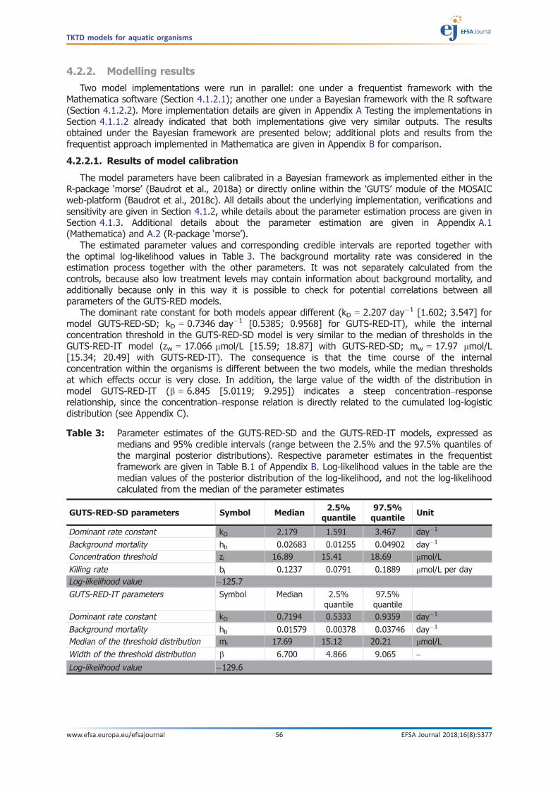
4.2.2. Modelling results
Two model implementations were run in parallel: one under a frequentist framework with theMathematica software (Section 4.1.2.1); another one under a Bayesian framework with the R software(Section 4.1.2.2). More implementation details are given in Appendix A Testing the implementations inSection 4.1.1.2 already indicated that both implementations give very similar outputs. The resultsobtained under the Bayesian framework are presented below; additional plots and results from thefrequentist approach implemented in Mathematica are given in Appendix B for comparison.
4.2.2.1. Results of model calibration
The model parameters have been calibrated in a Bayesian framework as implemented either in theR-package ‘morse’ (Baudrot et al., 2018a) or directly online within the ‘GUTS’ module of the MOSAICweb-platform (Baudrot et al., 2018c). All details about the underlying implementation, verifications andsensitivity are given in Section 4.1.2, while details about the parameter estimation process are given inSection 4.1.3. Additional details about the parameter estimation are given in Appendix A.1(Mathematica) and A.2 (R-package ‘morse’).
The estimated parameter values and corresponding credible intervals are reported together withthe optimal log-likelihood values in Table 3. The background mortality rate was considered in theestimation process together with the other parameters. It was not separately calculated from thecontrols, because also low treatment levels may contain information about background mortality, andadditionally because only in this way it is possible to check for potential correlations between allparameters of the GUTS-RED models.
The dominant rate constant for both models appear different (kD = 2.207 day�1 [1.602; 3.547] formodel GUTS-RED-SD; kD = 0.7346 day�1 [0.5385; 0.9568] for GUTS-RED-IT), while the internalconcentration threshold in the GUTS-RED-SD model is very similar to the median of thresholds in theGUTS-RED-IT model (zw = 17.066 lmol/L [15.59; 18.87] with GUTS-RED-SD; mw = 17.97 lmol/L[15.34; 20.49] with GUTS-RED-IT). The consequence is that the time course of the internalconcentration within the organisms is different between the two models, while the median thresholdsat which effects occur is very close. In addition, the large value of the width of the distribution inmodel GUTS-RED-IT (b = 6.845 [5.0119; 9.295]) indicates a steep concentration–responserelationship, since the concentration–response relation is directly related to the cumulated log-logisticdistribution (see Appendix C).
Table 3: Parameter estimates of the GUTS-RED-SD and the GUTS-RED-IT models, expressed asmedians and 95% credible intervals (range between the 2.5% and the 97.5% quantiles ofthe marginal posterior distributions). Respective parameter estimates in the frequentistframework are given in Table B.1 of Appendix B. Log-likelihood values in the table are themedian values of the posterior distribution of the log-likelihood, and not the log-likelihoodcalculated from the median of the parameter estimates
GUTS-RED-SD parameters Symbol Median2.5%
quantile97.5%quantile
Unit
Dominant rate constant kD 2.179 1.591 3.467 day�1
Background mortality hb 0.02683 0.01255 0.04902 day�1
Concentration threshold zi 16.89 15.41 18.69 lmol/L
Killing rate bi 0.1237 0.0791 0.1889 lmol/L per dayLog-likelihood value �125.7
GUTS-RED-IT parameters Symbol Median 2.5%quantile
97.5%quantile
Dominant rate constant kD 0.7194 0.5333 0.9359 day�1
Background mortality hb 0.01579 0.00378 0.03746 day�1
Median of the threshold distribution mi 17.69 15.12 20.21 lmol/L
Width of the threshold distribution b 6.700 4.866 9.065 –
Log-likelihood value �129.6
TKTD models for aquatic organisms
www.efsa.europa.eu/efsajournal 56 EFSA Journal 2018;16(8):5377

Figure 16 shows the survival over time (expressed as percentage of initial number of livingindividuals) for the calibration data set and corresponding fits as median curves and the 95% credibleband. Both SD and IT models show visually a good fit to the observed survival rate, meaning that theobserved survival rate as indicated by the black dots match well with the model predictions. Additionalgraphical results are provided in Appendix B, Figures B.1, B.2 and B.3).
Figure 16: Survival over time (SOT) view of model calibration based on data from a typical acutetoxicity study, with observations of survival under constant exposure over 4 days: (upperpanel) model GUTS-RED-SD; (lower panel) model GUTS-RED-IT. The survival over time isrepresented as a function of time for each tested concentration (headers of single plots):black dots are the observations (observed numbers of survivors divided by the initialnumber of individuals), black segments show the between-replicate variability, while theorange solid line corresponds to the median curve. The grey band is the 95% credibilityband representing the uncertainty. Survival is shown as rate, meaning that stochasticinfluence on the number of survivors over time is not considered. Respective resultsincluding this stochasticity are shown in Appendix B.1
TKTD models for aquatic organisms
www.efsa.europa.eu/efsajournal 57 EFSA Journal 2018;16(8):5377

Figure 17 illustrates the goodness-of-fit also by plotting the PPC, that is the predicted mediannumbers of survivors (y-coordinates of black dots) as a function of the observed numbers of survivors(x-coordinates of black dots). A good fit will result in black dots lined up along the line y = x. Theestimation process also provides the uncertainty around the predicted median values as an interval(vertical segments), within which 95% of the observations are expected to lie. Visual inspection ofFigure 17 does not yield any systematic bias in the deviations between modelled and observed data.The PPC results in a value 100% of the data are within the uncertainty ranges of the predictions.
Another way of looking at the calibration results is to compile a concentration–response curve at agiven time-point based on the GUTS modelling which also accounts for uncertainties (Figure 18).Under this representation, calibration results can be assessed in the same way as with a classicalconcentration–response relationship (e.g. a log-logistic concentration–response model). Figure 18shows that both GUTS-RED-SD and GUTS-RED-IT models well fit the steep slope of the observedresponse, meaning that the onset of effects at 17.87 lmol/L and the steep slope of the concentration–response that leads to nearly full effects already at the next tested concentration of 24.19 lmol/L arematched. See Appendix B and Figure B.5 for the same results obtained under the Mathematicaimplementation.
An additional view of the GUTS modelling results is given in Figure 19, where LC50 estimates bothfrom classical concentration–response curve fitting at a given target time (among those of theexperimental design) and from the GUTS-RED-SD and GUTS-RED-IT models are shown as function ofthe observation period. Such graphs illustrate the added value of GUTS models which allow estimatingany LCX value at any time period (e.g. between 1 and 4 days as shown in Figure 19). There is a goodaccordance between LC50 estimates from a classical concentration–response curve fitting at the giventarget times, and those obtained from the GUTS-RED modelling. Uncertainties appear in tendencysmaller when using the GUTS instead of classical dose–response modelling, presumably because alldata over time are accounted for in the GUTS estimation process.
(SD) (IT)
Figure 17: Posterior Predictive Check for the GUTS-RED-SD (left panel) and the GUTS-RED-IT (rightpanel) models, calibrated on a typical acute toxicity test. The x-coordinate of black dots isthe observed number of survivors while the y-coordinate is the predicted median numberof survivors. Vertical segments stand for the 95% credible intervals of the predictedvalues. These intervals are represented as green segments if they overlap with the liney = x
TKTD models for aquatic organisms
www.efsa.europa.eu/efsajournal 58 EFSA Journal 2018;16(8):5377

Summarising the model calibration for the example of propiconazole and G. pulex, the data appearappropriate because the concentration–response relation ranges from no up to full effects. The choiceof the reduced GUTS models is appropriate because internal concentrations have not been measuredso that the use of the full model cannot be recommended. The parameters in this example have beenestimated under a Bayesian framework using the MCMC algorithm as implemented either in theR-package ‘morse’ or within the web-platform MOSAIC. Parameter values, credible limits and likelihoodvalues have been reported (Table 3). The results of the model calibration are visualised and tested indifferent ways, including plotting the survival over time, the PPC and concentration–response curves.
Figure 18: Concentration–response view of the GUTS-RED-SD (left panel) and GUTS-RED-IT (rightpanel) model calibration results obtained from data of a typical acute toxicity study withobservations of survival under constant exposure over 4 days. Shown are the observed(black dots) and the modelled survival rates at the end of the 4-day observation period.Please note that the model parameters have been calibrated on the survival probabilitiesover time, and not on the concentration–response data. The solid line corresponds to themedian curve, while the dashed lines delimit the 95% credibility band representing theuncertainty. An analogue plot resulting from GUTS modelling under a frequentistframework is given in Figure B.5 of Appendix B
Figure 19: LC50 estimates from the calibrated GUTS models (GUTS-RED-SD on the left panel, GUTS-RED-IT on the right panel) as represented by the solid lines (median curve) and thedashed lines (95% credibility band for the uncertainty), or from a classical target timeanalysis as represented by black dots (median estimate) and segments (95% credibleintervals)
TKTD models for aquatic organisms
www.efsa.europa.eu/efsajournal 59 EFSA Journal 2018;16(8):5377

4.2.2.2. Results of model validation
Parameter estimates from the calibrated model were used to predict expected survival of G. pulexunder time-variable exposure profiles of propiconazole (exposure profiles ‘A’, ‘B’, ‘C’ and ‘Control’ asshown in Figure 20; concentration values are available in Table D.3 of Appendix D). The validation dataset has been qualitatively checked, quality control aspects are reported in the original publication (Nymanet al., 2012). The design of the experiments fulfils some basic criteria being requested for appropriatevalidation data sets: the observed survival was obtained from experiments under time-variable exposure.Two time-variable exposure profiles with two pulses each have been tested, which were separated by no-exposure intervals of different duration lengths. The length of the no-exposure interval was definedbased on the depuration time and aimed at one exposure profile allowing for individual depuration andrepair (‘B’), the other one (‘A’) not so much, despite the 95% depuration time was determined to about10 h. Two different time-variable exposure profiles haven been tested for one pulse height only, not atthree concentration levels. Despite this, data set does not match all of the minimum requirements forvalidation data, these already published results, which match the calibration data in terms of substanceand species but tested under time-variable exposure, are used.
Visual match
Predicted survival rates are compared with observed survival rates over time under each exposureprofile (Figure 21) or at the end of the exposure period as in a classical concentration–response view(Figure 22). From Figure 21, it appears that the GUTS-RED-SD model is more conservative byunderestimating the observed time course of the survival rate. Both models proved to be sensitiveenough to detect the tendency of the data under both exposure profiles ‘A’ and ‘B’ by predicting aninitial decline during the first pulse followed by a phase of reduced mortality, most probably due tobackground mortality, to continue with another decline after the second pulse (at day 3 in ‘A’ or day 7in ‘B’) for the GUTS-RED-SD model, despite GUTS-RED-IT did not react on the second pulse of profile‘B’. The experiments with exposure profile ‘C’ were performed under constant exposure. They resultedin less mortality than the pulsed profiles with a survival rate between 65% and 95% at day 10. SeeFigure B.6 of Appendix B for the same results obtained under the frequentist implementation. Fromobserved survival rates, the renewal of the untreated medium in profiles ‘A’ at day 7 and ‘B’ at day 3seemed to have affected survival. Apparently, the medium renewal caused stress to the individuals andhence led to increased mortality which could not be captured by model predictions.
Figure 20: Exposure profiles of the validation data set (Nyman et al., 2012, supporting material). ‘A’:two 1-day pulses at concentration (~ LC30 = 28 lmol/L) and 2-days of recovery betweenpulses; ‘B’: two 1-day pulses at concentration (~ LC30 = 28 lmol/L) and 6-days ofrecovery between pulses; ‘C’: constant exposure equal to the time-weighted average(TWA) concentration from the pulsed exposure profiles (~ 4.6 lmol/L)
TKTD models for aquatic organisms
www.efsa.europa.eu/efsajournal 60 EFSA Journal 2018;16(8):5377

Figure 21: GUTS-RED-SD (upper panel) and GUTS-RED-IT (lower panel) model validation results ona typical pulsed experiment data set: the survival rate over time is represented as afunction of time for each exposure profile (headers of single plots): black dots are theobserved survival rates, while the solid line corresponds to the median curve. The dashedlines give the 95% credibility band representing the uncertainty coming from theuncertainty on parameters estimated obtained from the calibration data set
Figure 22: Multiplication factor-response view of the GUTS-RED-SD (upper panel) and GUTS-RED-IT(lower panel) model validation results based on different pulsed or constant exposureprofiles: ‘A’, ‘B’, ‘C’ and ‘Control’ (headers of single plots from left to right). Black dotsdepict the observed survival rate at day 10, while the solid line corresponds to the medianpredicted survival rate at day 10. The dashed lines delineate the 95% credibility bandrepresenting the uncertainty coming from the uncertainty on parameters estimatedobtained from the calibration data set. Corresponding frequentist results are given inFigure B.6 of Appendix B
TKTD models for aquatic organisms
www.efsa.europa.eu/efsajournal 61 EFSA Journal 2018;16(8):5377
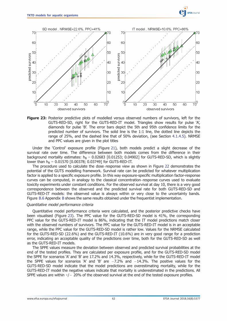
Under the ‘Control’ exposure profile (Figure 21), both models predict a slight decrease of thesurvival rate over time. The difference between both models comes from the difference in theirbackground mortality estimates: hB = 0.02683 [0.01253; 0.04902] for GUTS-RED-SD, which is slightlylower than hB = 0.01570 [0.00378; 0.03749] for GUTS-RED-IT.
The procedure used to calculate the dose–response view as shown in Figure 22 demonstrates thepotential of the GUTS modelling framework. Survival rate can be predicted for whatever multiplicationfactor is applied to a specific exposure profile. In this way exposure-specific multiplication factor-responsecurves can be computed, in analogy to the classical concentration–response curves used to evaluatetoxicity experiments under constant conditions. For the observed survival at day 10, there is a very goodcorrespondence between the observed and the predicted survival rate for both GUTS-RED-SD andGUTS-RED-IT models: the observed value is always within or very close to the uncertainty bands.Figure B.6 Appendix B shows the same results obtained under the frequentist implementation.
Quantitative model performance criteria
Quantitative model performance criteria were calculated, and the posterior predictive checks havebeen visualised (Figure 23). The PPC value for the GUTS-RED-SD model is 41%, the correspondingPPC value for the GUTS-RED-IT model is 86%, indicating that the IT model predictions match closerwith the observed numbers of survivors. The PPC value for the GUTS-RED-IT model is in an acceptablerange, while the PPC value for the GUTS-RED-SD model is rather low. Values for the NRMSE calculatedfor the GUTS-RED-SD (22.6%) and the GUTS-RED-IT (10.6%) are in very good range for a predictionerror, indicating an acceptable quality of the predictions over time, both for the GUTS-RED-SD as wellas the GUTS-RED-IT models.
The SPPE values measure the deviation between observed and predicted survival probabilities at theend of the tested profiles. They are calculated per exposure profile, and for the GUTS-RED-SD modelthe SPPE for scenarios ‘A’ and ‘B’ are 17.2% and 14.3%, respectively, while for the GUTS-RED-IT modelthe SPPE values for scenarios ‘A’ and ‘B’ are �7.2% and �14.3%. The positive values for theGUTS-RED-SD model indicate that the model predictions are overestimating mortality, while for theGUTS-RED-IT model the negative values indicate that mortality is underestimated in the predictions. AllSPPE values are within +/� 20% of the observed survival at the end of the tested exposure profiles.
Figure 23: Posterior predictive plots of modelled versus observed numbers of survivors, left for theGUTS-RED-SD, right for the GUTS-RED-IT model. Triangles show results for pulse ‘A’,diamonds for pulse ‘B’. The error bars depict the 5th and 95th confidence limits for thepredicted number of survivors. The solid line is the 1:1 line, the dotted line depicts therange of 25%, and the dashed line that of 50% deviation, (see Section 4.1.4.5). NRMSEand PPC values are given in the plot titles
TKTD models for aquatic organisms
www.efsa.europa.eu/efsajournal 62 EFSA Journal 2018;16(8):5377
Discussion of the model validation
The three quantitative validation criteria (definition in Section 4.1.4.5) which have been calculatedfor the GUTS models have different emphasis. The PPC takes into account the uncertainty in themodel predictions, while the NRMSE value considers the relation between median predicted andobserved numbers of survivors over time, and the SPPE considers the median observed survivornumber at the end of the experiment.
Overall, the quality of the model predictions appears as acceptable in this case. Quantitatively, theGUTS-RED-IT model gives a better match with this example validation data set, since both NRMSE aswell as SPPE values are smaller. Nevertheless, qualitatively, the GUTS-RED-SD model would be morepreferable for risk assessment, because the GUTS-RED-SD model predictions show values below the1:1 line in Figure 23, hence indicating an over-estimation of mortality and a more conservative riskassessment.
In general, acceptance of a maximum level of 50% deviation between predicted and observednumbers is suggested. This suggestion is based on the consideration that toxicological effects changeon a logarithmic scale rather than on a nominal one (see also Figure 23). In addition, acceptance of50% deviation appears protective when using GUTS predictions in combination with lower-tierassessment factors.
The suggested use of 50% as cut-off values for the PPC and the NRMSE is based on experience,meaning the evaluation of the few existing studies available in the literature (Nyman et al., 2012;Ashauer et al., 2016; Jager and Ashauer, 2018; Focks et al., 2018). It is not possible to derive precisethreshold values from mathematical or theoretical considerations, but as said above, 50% deviation inthe NRMSE is according to a CV of 0.5 for the ratio between the RMSE and the mean observedsurvival. This CV value appears not too high, when considering that a factor of two is deemed to beacceptable for experimentally derived endpoints. Additional confidence for the suggestion of the 50%is given by the fact that (a) the 50% can also be on the conservative side of the risk estimate (whichis seen in the SPPE indicator) and (b) it is recommended to always evaluate both the SD and IT modeland to use the more conservative if positively validated. Finally, suggested acceptability criteria have tobe checked based on future applications of the GUTS models and possibly be adapted over time.Clearer validation criteria and related cut-off values can be better formulated only when experience isgained with the use of GUTS in regulatory risk assessment.
Time course of scaled internal damage
One useful application of the GUTS modelling framework is to check how the simulation of thescaled damage in the GUTS-RED models relate to the dependency of the pulses in both exposureprofiles ‘A’ and ‘B’. As shown in Figure 24, the pulses in exposure profile ‘B’ appear toxicologicallyindependent for both models, because the second peak comes only clearly later than the upperconfidence limit of the DRT95 (see Section 4.1.4.5). For the exposure profile ‘A’, the GUTS-RED-ITmodel indicates toxicological dependence, since the second pulse comes later than the upperconfidence limit of the DRT95, whereas the GUTS-RED-SD model is borderline between toxicologicallydependence and independence.
Such simulations of the scaled damage for different exposure profiles can be of great help indesigning pulsed refined experiments, in order to check if the intended pulses, in terms of height andbetween-pulse period, will be toxicologically independent or not.
TKTD models for aquatic organisms
www.efsa.europa.eu/efsajournal 63 EFSA Journal 2018;16(8):5377

4.2.3. Predictions under FOCUS surface water exposure patterns
4.2.3.1. Chemical exposure data
Chemical exposure data can function as input data for GUTS model predictions. The input canconsist of concentration time series as produced by the FOCUS surface water software or otherexposure assessment tools.
Figure 24: Scaled damage over time for GUTS-RED-SD (top panel) and GUTS-RED-IT (bottom panel)models under time-variable exposure profiles ‘A’ (left panels) or ‘B’ (right panels). The verticaldashed lines correspond to the median DRT95 (see Section 4.1.4.5), calculated based onoptimal parameter values for the dominant rate constant (kD) for the GUTS-RED-SD and theGUTS-RED-IT models and their lower and upper confidence limits (grey band). The medianscaled damage is simulated (solid curve) together with its uncertainty (dashed curves) withthe same equation in both GUTS models. Nevertheless, the median value of the dominantrate constant differs: kD = 2.154 lmol/L per day for model GUTS-RED-SD; kD = 0.732 mol/Lper day for model GUTS-RED-IT
TKTD models for aquatic organisms
www.efsa.europa.eu/efsajournal 64 EFSA Journal 2018;16(8):5377

Predicted exposure profiles in water were produced for 10 scenarios for propiconazole (Figure 25;more details on the FOCUS scenarios are given in Table 4). These exposure time series were used asinput data for the GUTS-SD and GUTS-IT models, without assuming background mortality for any ofthe input scenarios.
4.2.3.2. Calculation of exposure profile specific concentration–response curves (LPX
values)
The FOCUS exposure profiles were used as input data for the calibrated and validated GUTS-RED-SDand GUTS-RED-IT models. Exposure-profile specific LP50 values were calculated by applying increasingmultiplication factors to the profiles until 50% mortality at the end of the simulated exposure patternwas reached (Table 4). LP50 are compared with assessment factors as used for lower-tier RAC values. Itcan nicely be seen from the table entries that, for exposure profiles where the concentration remainsnearly constant (e.g. Figure 25, profiles 1, 3, 6 and 8), the LP50 is identical to the TER.
Figure 25: Concentration over time for 10 FOCUS exposure scenarios, ID numbers are given in theplot titles. More details on the FOCUS scenarios in Table 4
TKTD models for aquatic organisms
www.efsa.europa.eu/efsajournal 65 EFSA Journal 2018;16(8):5377

Nevertheless, in cases where the exposure profile is highly time-variable (i.e. with some peaks andmany phases with lower concentrations in between, e.g. Figure 25, profiles 2, 4, 7, 9 and 10), the LP50values are much higher than the TER. This indicates that, for some tested exposure profiles, the risk ismuch lower than apparent from Tier 1 calculations. It also shows that the GUTS modelling frameworkcan differentiate between different qualities of exposure profiles, unlike the TER calculations. Theevaluation of FOCUS surface water exposure profiles by GUTS modelling confirms that the GUTSmodelling of survival functions exactly as intended: Lower tier risk estimates are kept for moreconstant profiles, whereas the risk for time-variable profiles is refined.
4.3. Overall summary and conclusions of the GUTS modeldocumentation and application
The formal definition for GUTS models is standardised and documented. Examples show how theverification of any new GUTS implementation can be performed using some standard elements: defaultscenarios, pulsed exposure scenarios, and extreme scenarios can be simulated and checked. Sensitivityanalyses of the reduced GUTS models (GUTS-RED) have been performed and are not requested fornew model implementations and applications, because the influence of the model parameters on themodel outcome is known. However, results of sensitivity analyses for new applications of GUTS-REDcan be used to document a correct model implementation, and interactions between modelparameters could be further investigated. For other GUTS models than the reduced, sensitivityanalyses should be included and checked for future applications.
Parameter estimation is a challenging task, but standard implementations of parameter optimisationalgorithms are available in software packages, both under a frequentist and a Bayesian approach. It iscrucial to report not only optimal parameters, but also the optimisation method, settings of theoptimisation routine and of the numerical solver, and parameter confidence limits including informationon how they were derived to allow for potential expert evaluation. Results from model calibration need tobe documented comprehensively. For this purpose, a corresponding checklist is provided in this ScientificOpinion. Relevant model output for risk assessment has been defined as expected mortality/immobility orexposure profile specific multiplication factors (LPx/EPx). The latter factors can be directly compared withrespective assessment factors. Both mortality estimates and LPx/EPx can be calculated includingconfidence limits, which are calculated by propagation of model uncertainty to the model output.
For the validation of calibrated GUTS models, appropriate validation data sets are essential.Differentiating between vertebrates and invertebrates, a set of requirements is given for validationexperiments, among others to test at least two different time-variable exposure profiles. The evaluationof the quality of predictions in comparison with the observed data requires a careful combination ofqualitative and quantitative criteria. Qualitatively, the visual match (‘visual fit’ in FOCUS Kinetics, 2006)between model and data is important to be checked, and quantitatively three criteria are suggested:one that takes into account the uncertainty in the model predictions (PPC), one that measures thematch over time (NRMSE), and one that considers the final match between model and data (SPPE).
GUTS calibration and validation is shown for an example data set, both for a frequentist approachimplemented in Mathematica and a Bayesian approach implemented in R. The results illustrate howcalibration and validation could be performed and documented to allow regulators to evaluate futureapplications, but ideally the validation data would fulfil all minimum criteria. The application of the
Table 4: Analysis of risk estimation using a TER approach and based on GUTS modelling in formof LP50 values (see text for more details). TER based on an LC50 values for G. pulex of19.2 lg/L
Scenario 1 2 3 4 5 6 7 8 9 10
Application Apple Apple Cereals Cereals Cereals Cereals Cereals Cereals Cereals Cereals
FOCUS SWScenario
R1pond
R2stream
D1ditch
D1stream
D3ditch
D4pond
D4stream
D5pond
D5stream
R4stream
PECmax 1.130 2.007 10.564 8.063 9.083 1.668 2.268 1.670 2.401 2.998
TER 17 10 2 2 2 12 8 11 8 6LP50 SDmodel
17 44 3 20 12 12 205 12 195 39
LP50 ITmodel
17 49 3 24 16 12 250 12 237 39
TKTD models for aquatic organisms
www.efsa.europa.eu/efsajournal 66 EFSA Journal 2018;16(8):5377

GUTS model to calculate refined risk estimates for concentration time series from 10 FOCUS surfacewater scenarios delivers very reasonable results, the GUTS modelling allows obviously to differentiatebetween constant exposure situations, where the refined risk is practically identical to the lower-tierestimate, and highly variable exposure over time, where the refined risk is lower as in the lower-tier.
One open issue for the use of GUTS in regulatory risk assessment is a question related to theconstrained possibility to request new validation experiments for vertebrates. It is necessary to buildup an experience base to determine which data sets are suitable for GUTS validation for vertebrates.
Another issue is related to compounds that are suspected of showing increased toxicity over time,e.g. neonicotinoids. Recent research shows that the quality of model predictions for these compoundswas in some cases only acceptable when the GUTS models were calibrated based on chronic testresults (Focks et al., 2018). Further classification of compounds with respect to the potential to showincreased toxicity under long-term exposure would be relevant.
Technically, one of the main questions is whether it is better to allow for user-definedimplementations of GUTS, or to aim for having one standard GUTS implementation, which only needsto be checked once. In this opinion, the decision was to consider user-defined implementations and togive checklists and criteria at hands to allow regulators to evaluate whether a new implementationfulfils the required quality aspects.
Duality of SD and IT models and consequences for practical use in RA
A specific aspect of GUTS modelling is the duality of the SD and IT death mechanisms. As mentionedalready, in theory, these two model variants are extreme cases of one overarching model and can beunified in the combined GUTS, but in practice, most often the two types of reduced GUTS models willbe used. Requirements for the data for model calibration are the same, so usually both reduced modelscan be parameterised. In consequence, decisions are necessary about (a) which of the models isacceptable in the validation, and (b) which of them is used in the regulatory risk assessment.
The application for propiconazole and G. pulex shows a nice example how to handle this duality.Both the GUTS-RED-SD and the GUTS-RED-IT models fulfil validation criteria. Quantitatively, theGUTS-RED-IT model gives a better match with this example validation data set, but qualitatively, theGUTS-RED-SD model would be more preferable for risk assessment, because the GUTS-RED-SD modelpredictions lead in tendency to an over-estimation of mortality and so to a more conservative riskassessment. It is certainly not advisable to always take the more conservative of the IT and SD models,i.e. when one of the two is clearly wrong, either by under- or over-predicting mortality in the validationexperiments, and fulfilment of qualitative and quantitative validation criteria is clearly failed, it shouldnot be used for regulatory risk assessment. When, however, both models appear acceptable in thevalidation, the more conservative is suggested for regulatory use. The same rationale can be applied forthe choice of the death mechanism for coupling of GUTS models with individual-based models in RA.
5. DEBtox models
5.1. Documentation and implementation of the formal model
As already stated in Chapter 2, DEBtox models are rather complex mainly because they offer several waysof accounting for toxicant effect simultaneously on both growth and reproduction processes. Unlike for theGUTS models, this section cannot be comprehensive, because DEBtox model applications are still developedon a more case-by-case basis. However, to exemplify some aspects of the formulation and theimplementation of a DEBtox model, published results by Billoir et al. (2011) are used to illustrate a case studyabout lethal and sublethal effects on daphnids (D. magna) exposed to time-varying cadmium exposureconcentrations within a laboratory aquatic microcosm. It should be highlighted that the example included inthis chapter illustrates the model formulation, implementation, and the results of the calibration phase. Aproper validation with an additional data set was not performed, and therefore could not be included here.
5.1.1. Model formulation
The dynamics of the scaled damage (called ‘scaled internal concentration’ in Billoir et al., 2011)within daphnids is derived from the total cadmium concentrations in water through a toxicokineticmodel. Effects of cadmium on survival, growth and reproduction are then assumed to depend on thisscaled damage. In the following, letter t refers to a general expression of time (in days), while ti refersto the experimental time-point number i which can differ per endpoint (see Figure 27).
TKTD models for aquatic organisms
www.efsa.europa.eu/efsajournal 67 EFSA Journal 2018;16(8):5377

5.1.1.1. TK models
To model the exposure concentration time profile throughout the experiment, an empiricalexponential decay model with a rate b (1/d) is used
Cj(t) ¼ Cð�7Þj expð�b(t+7)), (23)
where Cj(t) is the time-variable exposure cadmium concentration (lg/L) at time t with j = 0,. . .,4 forthe control and the four treatments. Parameters C ð�7Þ
j (j = 0,. . .,4) are fixed at nominal concentrations,0, 10, 20, 40 and 80 lg/L, that is at concentrations initially introduced 7 days before the introductionof the organisms. Consequently, C0(t) = 0, whatever t.
A normal distribution links the exposure model to the measured cadmium concentrations
MCi;j;k �Nðmean = CjðtiÞ; tau ¼ sEÞ for j = 1; :::; 4; (24)
where MCi,j,k are the measured cadmium concentrations (lg/L) at time-point ti, treatment j andreplicate k. Parameter sE is the precision (1/variance) of the measurements ((lg/L)2).
Similarly to GUTS (equation 1), for each treatment, the scaled damage at time t, Dw(t), is linked toCj(t) through a one-compartment model with a dominant rate constant kD (1/d)
dDw(t)dt
¼ kDðCj(t)� Dw(t)), (25)
with the initial condition Dw(0) = 0.
5.1.1.2. TD models
According to the DEBtox modelling approach (Jager, 2017), survival, growth and reproduction arelinked to the scaled damage through ‘linear-with-threshold’ relationships depending on respectiveso-called no-effect-concentrations, i.e. internal concentration thresholds below which no measurableeffect can be detected (see Chapter 2). For the sake of simplicity, in this example, the NEC is assumedto be the same for growth and reproduction.
Survival is modelled with a GUTS-RED-SD model according to (equation 5) with parameter seth = (hb, bw, zw). As shown on Figure 27, the observed number of survivors at time-point ti, treatmentj and replicate k is modelled by variable MSi,j,k through a conditional binomial distribution according to(equation 10) and (equation 11).
D. magna body growth is modelled using the von Bertalanffy growth model (Von Bertalanffy, 1938).Both the growth rate, c (1/d), and the maximum body length, Lm (mm), are assumed to be affectedby the scaled damage
dLj(t)dt
¼ c(1� rGR (t)) (Lm(1� rGR(t)Þ � Lj(t)), (26)
withrGR(t) ¼ minð1,bGRðDw(t)� ZGRÞÞ (27)
and the initial condition Lj(0) = 1,
Figure 26: Observation time-points (in days) of cadmium concentrations (exposure), survival, growthand reproduction of D. magna over the course of the experiment (adapted from Billoiret al., 2011)
TKTD models for aquatic organisms
www.efsa.europa.eu/efsajournal 68 EFSA Journal 2018;16(8):5377
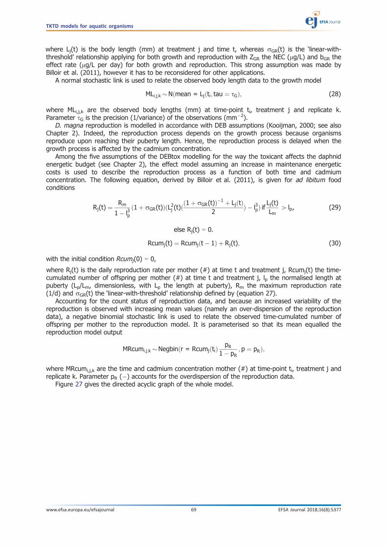
where Lj(t) is the body length (mm) at treatment j and time t, whereas rGR(t) is the ‘linear-with-threshold’ relationship applying for both growth and reproduction with ZGR the NEC (lg/L) and bGR theeffect rate (lg/L per day) for both growth and reproduction. This strong assumption was made byBilloir et al. (2011), however it has to be reconsidered for other applications.
A normal stochastic link is used to relate the observed body length data to the growth model
MLi;j;k �Nðmean = Ljðti; tau ¼ sGÞ; (28)
where MLi,j,k are the observed body lengths (mm) at time-point ti, treatment j and replicate k.Parameter sG is the precision (1/variance) of the observations (mm�2).
D. magna reproduction is modelled in accordance with DEB assumptions (Kooijman, 2000; see alsoChapter 2). Indeed, the reproduction process depends on the growth process because organismsreproduce upon reaching their puberty length. Hence, the reproduction process is delayed when thegrowth process is affected by the cadmium concentration.
Among the five assumptions of the DEBtox modelling for the way the toxicant affects the daphnidenergetic budget (see Chapter 2), the effect model assuming an increase in maintenance energeticcosts is used to describe the reproduction process as a function of both time and cadmiumconcentration. The following equation, derived by Billoir et al. (2011), is given for ad libitum foodconditions
Rj(t) ¼ Rm
1� l3pð1þ rGR(t)ÞðL2j (t)ð
ð1þ rGR(t)Þ�1 þ LjðtÞ2
Þ � l3pÞ ifLj(t)Lm
[ lp, (29)
else Rj(t) = 0.
Rcumj(t) ¼ Rcumjðt� 1Þ þ Rj(t); (30)
with the initial condition Rcumj(0) = 0,
where Rj(t) is the daily reproduction rate per mother (#) at time t and treatment j, Rcumj(t) the time-cumulated number of offspring per mother (#) at time t and treatment j, lp the normalised length atpuberty (Lp/Lm, dimensionless, with Lp the length at puberty), Rm the maximum reproduction rate(1/d) and rGR(t) the ‘linear-with-threshold’ relationship defined by (equation 27).
Accounting for the count status of reproduction data, and because an increased variability of thereproduction is observed with increasing mean values (namely an over-dispersion of the reproductiondata), a negative binomial stochastic link is used to relate the observed time-cumulated number ofoffspring per mother to the reproduction model. It is parameterised so that its mean equalled thereproduction model output
MRcumi;j;k �Negbinðr = RcumjðtiÞ pR1� pR
; p ¼ pRÞ;
where MRcumi,j,k are the time and cadmium concentration mother (#) at time-point ti, treatment j andreplicate k. Parameter pR (�) accounts for the overdispersion of the reproduction data.
Figure 27 gives the directed acyclic graph of the whole model.
TKTD models for aquatic organisms
www.efsa.europa.eu/efsajournal 69 EFSA Journal 2018;16(8):5377

5.1.2. Model implementation in the R software
All endpoints (exposure, survival, growth and reproduction) were fitted simultaneously to estimate all14 model parameters, since all corresponding observed data were linked together as shown in Figure 28.Parameters were estimated within a Bayesian framework via an R code based on JAGS and the R-packagerjags (see Appendix A, Section A.2.2 for additional information). Prior probability distributions are thosereported in Table 5 according to Billoir et al. (2011). Because it is not possible to numerically integratedifferential equations in JAGS, models were implemented in discrete time with one day as time step.
Three independent MCMC chains were run in parallel. After an initial burn-in period of 5,000iterations, the Bayesian algorithm was run 50,000 iterations and the corresponding sample of the jointparameter posterior distribution was recorded. The convergence of the estimation process waschecked with the Gelman and Rubin statistics (Gelman and Rubin, 1992) (see Section 4.1.3.3).
The goodness-of-fit was assessed first by comparing prior and posterior distributions models, thenwith a graphical comparison of observed data and predictions in a way that account for parameteruncertainties and stochasticity of the model. Indeed, predictions are simulated at each MCMC iteration,along which the parameters vary according to their uncertainty, and with the same models than theones considered to fit the observed data.
5.1.3. Input data
As detailed in Billoir et al. (2011), experiments were conducted in laboratory microcosms (2-Lbeakers) filled with artificial sediment and gently aerated synthetic water in which cadmium (Cd) wasintroduced at nominal concentrations 10, 20, 40 and 80 lg/L, hereafter referred to as treatments 1 to4. Four replicates were set up for each treatment. Microcosms were conditioned 7 days in the darkbefore introduction of organisms. Experiments were conducted under constant temperature, pH andlight conditions.
Figure 27: Directed acyclic graph of the DEBtox model used to describe time-variable cadmium effecton survival, growth and reproduction of D. magna. This graph is adapted from by Billoiret al. (2011). Variable q stands for the quantity dH/dt as in equation (4)
TKTD models for aquatic organisms
www.efsa.europa.eu/efsajournal 70 EFSA Journal 2018;16(8):5377

At day 0 (7 days after the introduction of Cd), daphnids were introduced in all microcosms, thenfollowed during 21 days. Numbers of survivors, body length and numbers of offspring were recordedat different time-points (Figure 26). The cadmium water concentration was also regularly measured.
5.2. Results of the DEBtox model
5.2.1. Parameter estimates
According to the Gelman and Rubin convergence diagnostics (Gelman and Rubin, 1992), theconvergence was successfully checked. Posterior distributions of the 14 parameters are shown inFigure 28 with their corresponding priors. Posterior distributions are also summarised by statisticsdirectly extracted from the MCMC samples: 2.5th, 50th (median) and 97.5th percentiles (Table 5).Based on Figure 28 and Table 5, the 14 model parameters were accurately estimated with posteriordistributions narrower than prior ones meaning that the data allowed to reduce the uncertainty.Posterior distributions for parameter Lm (maximum body length) and Rm (maximum reproduction rate)were shifted to higher values than within the priors. This may signify that growth and reproduction ofdaphnids were higher in the experiments conducted by Billoir et al. (2011) than in those on whichpriors were based. Concerning parameters for which priors were large (e.g. b, kD, hb), narrowposteriors means that data were informative enough to provide more reliable parameter estimates.NEC threshold estimates point out that sublethal effects of cadmium were predicted to appear beforelethal effects since zw = 1.78 lg/L [1.19; 2.31] is higher than zGR = 0.15 lg/L [0.0524; 1.02].Parameter estimate kD = 0.897 day�1 [0.785; 1.06] is indicative of a rapid kinetics, inferred from theother related endpoints (survival, growth and reproduction) as no internal concentration data wereavailable in the data set.
TKTD models for aquatic organisms
www.efsa.europa.eu/efsajournal 71 EFSA Journal 2018;16(8):5377

• 1.9 • 1.8 • 1.7 • 1.6
0
2
4
6
8
10
log(b)0.05 0.15 0.25
0
2
4
6
8
10
12
14
τE
• 0.4 • 0.2 0.0 0.2
0
1
2
3
4
5
log(kD)
• 7.5 • 6.5 • 5.5 • 4.5
0.0
0.2
0.4
0.6
0.8
log(hb)• 1.0 0.0 0.5 1.0
0.0
0.5
1.0
1.5
2.0
2.5
log(zw)1 2 3 4
0.0
0.2
0.4
0.6
0.8
log(bw)
4.5 5.0 5.5 6.0
0.0
0.5
1.0
1.5
2.0
2.5
Lm
0.08 0.12 0.16
0
10
20
30
40
γ5 10 15 20 25
0.00
0.05
0.10
0.15
τG
0.4 0.5 0.6 0.7
0
2
4
6
8
10
lp10 15 20
0.00
0.05
0.10
0.15
0.20
0.25
Rm
0.05 0.15 0.25
0
5
10
15
pR
• 3 • 2 • 1 0 1
0.0
0.1
0.2
0.3
0.4
0.5
log(zGR)• 5.0 • 4.0 • 3.0
0.0
0.5
1.0
1.5
2.0
log(bGR)
Figure 28: Posterior distributions of parameters obtained from simultaneous fitting of exposure,survival, growth and reproduction data (solid lines), with the corresponding priordistributions (dashed lines). Adapted from Billoir et al. (2011)
TKTD models for aquatic organisms
www.efsa.europa.eu/efsajournal 72 EFSA Journal 2018;16(8):5377
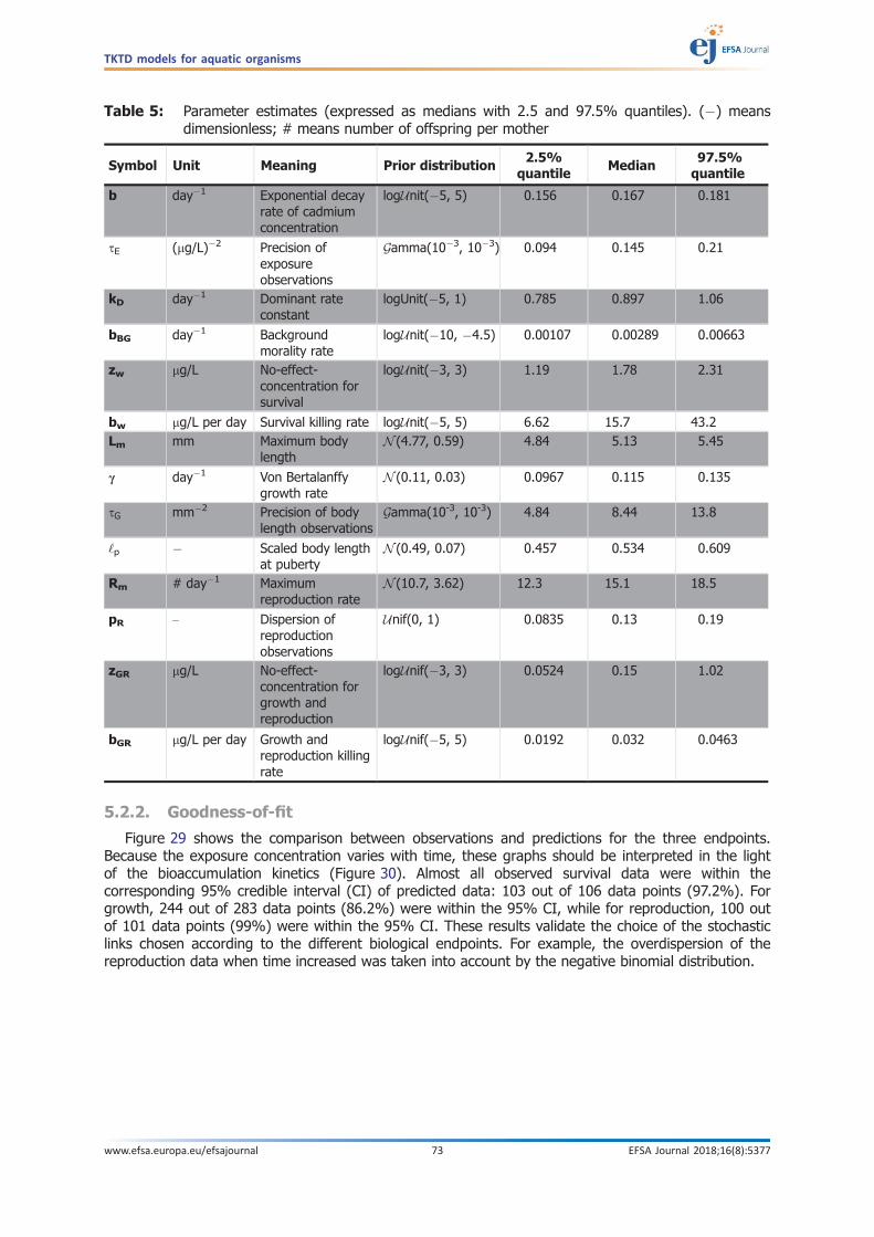
5.2.2. Goodness-of-fit
Figure 29 shows the comparison between observations and predictions for the three endpoints.Because the exposure concentration varies with time, these graphs should be interpreted in the lightof the bioaccumulation kinetics (Figure 30). Almost all observed survival data were within thecorresponding 95% credible interval (CI) of predicted data: 103 out of 106 data points (97.2%). Forgrowth, 244 out of 283 data points (86.2%) were within the 95% CI, while for reproduction, 100 outof 101 data points (99%) were within the 95% CI. These results validate the choice of the stochasticlinks chosen according to the different biological endpoints. For example, the overdispersion of thereproduction data when time increased was taken into account by the negative binomial distribution.
Table 5: Parameter estimates (expressed as medians with 2.5 and 97.5% quantiles). (�) meansdimensionless; # means number of offspring per mother
Symbol Unit Meaning Prior distribution2.5%
quantileMedian
97.5%quantile
b day�1 Exponential decayrate of cadmiumconcentration
logUnit(�5, 5) 0.156 0.167 0.181
sE (lg/L)�2 Precision ofexposureobservations
Gamma(10�3, 10�3) 0.094 0.145 0.21
kD day�1 Dominant rateconstant
logUnit(�5, 1) 0.785 0.897 1.06
bBG day�1 Backgroundmorality rate
logUnit(�10, �4.5) 0.00107 0.00289 0.00663
zw lg/L No-effect-concentration forsurvival
logUnit(�3, 3) 1.19 1.78 2.31
bw lg/L per day Survival killing rate logUnit(�5, 5) 6.62 15.7 43.2Lm mm Maximum body
lengthN (4.77, 0.59) 4.84 5.13 5.45
c day�1 Von Bertalanffygrowth rate
N (0.11, 0.03) 0.0967 0.115 0.135
sG mm�2 Precision of bodylength observations
Gamma(10-3, 10-3) 4.84 8.44 13.8
‘p � Scaled body lengthat puberty
N (0.49, 0.07) 0.457 0.534 0.609
Rm # day�1 Maximumreproduction rate
N (10.7, 3.62) 12.3 15.1 18.5
pR – Dispersion ofreproductionobservations
Unif(0, 1) 0.0835 0.13 0.19
zGR lg/L No-effect-concentration forgrowth andreproduction
logUnif(�3, 3) 0.0524 0.15 1.02
bGR lg/L per day Growth andreproduction killingrate
logUnif(�5, 5) 0.0192 0.032 0.0463
TKTD models for aquatic organisms
www.efsa.europa.eu/efsajournal 73 EFSA Journal 2018;16(8):5377

0
2
4
6
8
10
Time (days)
Num
ber
of s
urvi
ving
D. m
agna
0 2 3 7 10 14 17 20
0
1
2
3
4
5
6
Time (days)
D. m
agna
bod
y le
ngth
(m
m)
02417
0
50
100
150
Time (days)
Cum
ulat
ed n
umbe
r of
offs
prin
g pe
r m
othe
r
0 2 3 7 10 14 17 20
Figure 29: Comparison of observations and predictions for survival (upper panel), growth (middlepanel) and reproduction (lower panel) D. magna data. Observed data (symbols) andcorresponding 95% credible intervals of simulated data (segments) are superimposed tographically assess the goodness-of-fit (Adapted from Billoir et al. (2011))
TKTD models for aquatic organisms
www.efsa.europa.eu/efsajournal 74 EFSA Journal 2018;16(8):5377
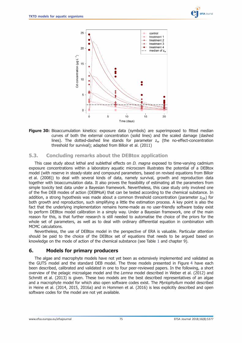
5.3. Concluding remarks about the DEBtox application
This case study about lethal and sublethal effects on D. magna exposed to time-varying cadmiumexposure concentrations within a laboratory aquatic microcosm illustrates the potential of a DEBtoxmodel (with reserve in steady-state and compound parameters, based on revised equations from Billoiret al. (2008)) to deal with several kinds of data, namely survival, growth and reproduction datatogether with bioaccumulation data. It also proves the feasibility of estimating all the parameters fromsimple toxicity test data under a Bayesian framework. Nevertheless, this case study only involved oneof the five DEB modes of action (DEBMoA) that can be tested according to the chemical substance. Inaddition, a strong hypothesis was made about a common threshold concentration (parameter zGR) forboth growth and reproduction, such simplifying a little the estimation process. A key point is also thefact that the underlying implementation remains home-made as no user-friendly software today existto perform DEBtox model calibration in a simply way. Under a Bayesian framework, one of the mainreason for this, is that further research is still needed to automatise the choice of the priors for thewhole set of parameters, as well as to deal with ordinary differential equation in combination withMCMC calculations.
Nevertheless, the use of DEBtox model in the perspective of ERA is valuable. Particular attentionshould be paid to the choice of the DEBtox set of equations that needs to be argued based onknowledge on the mode of action of the chemical substance (see Table 1 and chapter 9).
6. Models for primary producers
The algae and macrophyte models have not yet been as extensively implemented and validated asthe GUTS model and the standard DEB model. The three models presented in Figure 4 have eachbeen described, calibrated and validated in one to four peer-reviewed papers. In the following, a shortoverview of the pelagic microalgae model and the Lemna model described in Weber et al. (2012) andSchmitt et al. (2013) is given. These two models are the best described representatives of an algaeand a macrophyte model for which also open software codes exist. The Myriophyllum model describedin Heine et al. (2014, 2015, 2016a) and in Hommen et al. (2016) is less explicitly described and opensoftware codes for the model are not yet available.
Figure 30: Bioaccumulation kinetics: exposure data (symbols) are superimposed to fitted mediancurves of both the external concentration (solid lines) and the scaled damage (dashedlines). The dotted-dashed line stands for parameter zw (the no-effect-concentrationthreshold for survival); adapted from Billoir et al. (2011)
TKTD models for aquatic organisms
www.efsa.europa.eu/efsajournal 75 EFSA Journal 2018;16(8):5377
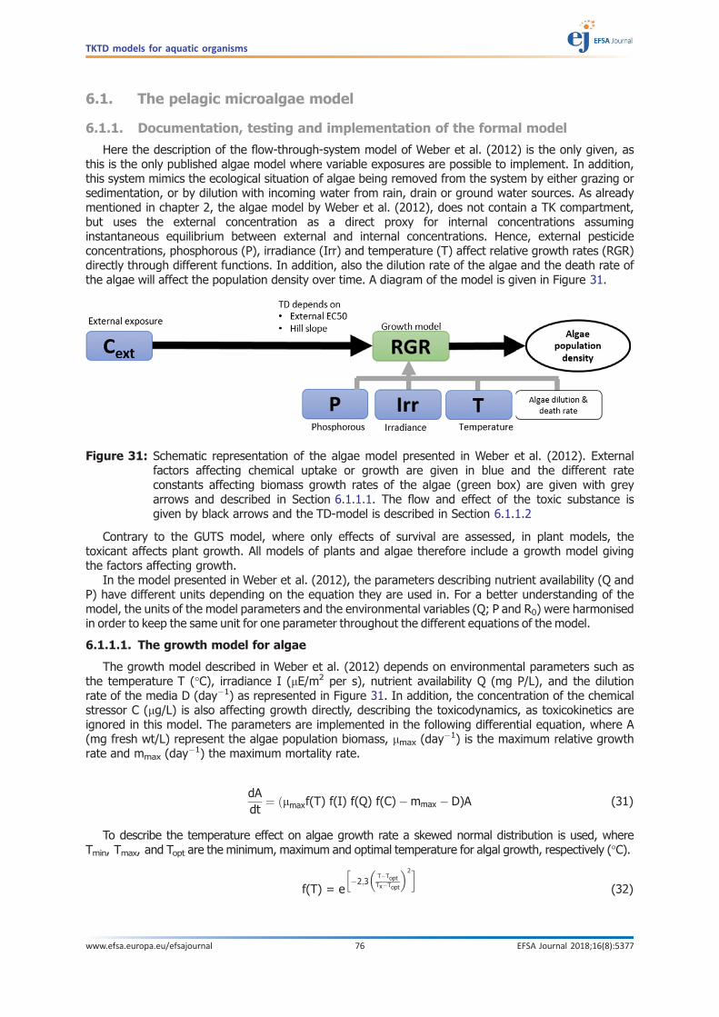
6.1. The pelagic microalgae model
6.1.1. Documentation, testing and implementation of the formal model
Here the description of the flow-through-system model of Weber et al. (2012) is the only given, asthis is the only published algae model where variable exposures are possible to implement. In addition,this system mimics the ecological situation of algae being removed from the system by either grazing orsedimentation, or by dilution with incoming water from rain, drain or ground water sources. As alreadymentioned in chapter 2, the algae model by Weber et al. (2012), does not contain a TK compartment,but uses the external concentration as a direct proxy for internal concentrations assuminginstantaneous equilibrium between external and internal concentrations. Hence, external pesticideconcentrations, phosphorous (P), irradiance (Irr) and temperature (T) affect relative growth rates (RGR)directly through different functions. In addition, also the dilution rate of the algae and the death rate ofthe algae will affect the population density over time. A diagram of the model is given in Figure 31.
Contrary to the GUTS model, where only effects of survival are assessed, in plant models, thetoxicant affects plant growth. All models of plants and algae therefore include a growth model givingthe factors affecting growth.
In the model presented in Weber et al. (2012), the parameters describing nutrient availability (Q andP) have different units depending on the equation they are used in. For a better understanding of themodel, the units of the model parameters and the environmental variables (Q; P and R0) were harmonisedin order to keep the same unit for one parameter throughout the different equations of the model.
6.1.1.1. The growth model for algae
The growth model described in Weber et al. (2012) depends on environmental parameters such asthe temperature T (°C), irradiance I (lE/m2 per s), nutrient availability Q (mg P/L), and the dilutionrate of the media D (day�1) as represented in Figure 31. In addition, the concentration of the chemicalstressor C (lg/L) is also affecting growth directly, describing the toxicodynamics, as toxicokinetics areignored in this model. The parameters are implemented in the following differential equation, where A(mg fresh wt/L) represent the algae population biomass, lmax (day�1) is the maximum relative growthrate and mmax (day
�1) the maximum mortality rate.
dAdt
¼ ðlmaxf(T) f(I) f(Q) f(C)�mmax � D)A (31)
To describe the temperature effect on algae growth rate a skewed normal distribution is used, whereTmin, Tmax, and Topt are the minimum, maximum and optimal temperature for algal growth, respectively (�C).
f(T) = e
h�2;3
�T�ToptTx�Topt
�2i(32)
Figure 31: Schematic representation of the algae model presented in Weber et al. (2012). Externalfactors affecting chemical uptake or growth are given in blue and the different rateconstants affecting biomass growth rates of the algae (green box) are given with greyarrows and described in Section 6.1.1.1. The flow and effect of the toxic substance isgiven by black arrows and the TD-model is described in Section 6.1.1.2
TKTD models for aquatic organisms
www.efsa.europa.eu/efsajournal 76 EFSA Journal 2018;16(8):5377
With Tx ¼ Tmin;T[Topt
Tmax;T�Topt
The effect of irradiance on algal growth rate is given by the following equation describing asaturation curve, where Iopt (lE/m
2 per s is the optimum irradiance for the algal growth rate:
f(I) ¼ IIopt
e
�1� I
Iopt
�(33)
In estimating the effect of nutrient availability to algal growth rate only phosphorous is consideredby Weber et al. (2012) as a limiting nutrient, even though nitrogen and carbon availability can alsolimit growth. In this equation qmin (mg P/mg fresh/wt) is the minimum concentration of P in the cellsto allow any cell division, while Q (mg P/L) is the internal concentration of P.
f(Q) ¼ 1� e(�ln 2( Qqmin:A
�1)) (34)
The internal concentration of P, Q (mg P/L), is given by the following differential equation, wherevmax (mg P/mg fresh wt per day) describes the maximum uptake rate, A, mmax and D is the algalconcentration (mg fresh wt/L), maximal death (day�1) rate and dilution rate (day�1), respectively.
dQdt
¼ vmaxf(Q, P) A � ðmmax þ DÞQ (35)
The uptake of P by the algae is limited by the internal concentration of P in algae represented byf(Q, P) below. In this function qmax and qmin are the maximum and minimum internal concentration forP, respectively, (mg P/L) and ks (mg P/L) is the half-saturated constant for extracellular P.
f(Q, P) ¼ qmax:A � Qðqmax � qminÞA
PkS þ P
(36)
The external concentration of P is as follows with R0 (mg P/L) being the concentration of P enteringthe system.
dPdt
¼ DR0 � DPþ Qmmax � ðvmaxf(Q, P)AÞ (37)
6.1.1.2. The TD model for algae
The algal growth rate is affected by the toxicant as a function of the concentration of the chemicalin the system C (lg/L) and the concentration of the toxicant causing 50% effect EC50 (lg/L), whereb is the slope of the log-logistic function.
f(C) ¼ 1
1þ�
CEC50
��b (38)
The actual concentration of the chemical in the system is equivalent to the concentration of thechemical entering the system Cin (lg/L) while the degradation rate of toxicant in aquatic environmentsk (1 day) and the toxicant eliminated by dilution are taken into account. This relationship is given bythe next differential equation:
dCdt
¼ CinD� kC� DC (39)
TKTD models for aquatic organisms
www.efsa.europa.eu/efsajournal 77 EFSA Journal 2018;16(8):5377

6.1.1.3. Model application
The following section describes the flow-through-system model of Weber et al. (2012), as this isthe only algae model where variable exposures are possible to implement.
Input data
The model was calibrated for two microalgae species: Desmodesmus subspicatus and Raphidocelissubcapitata (formerly known as Pseudokirscheriella subcapitata). The 10 parameters used to describealgal growth capacity and growth dependence on temperature, irradiance and P-availability were archivedthrough the authors own experiments combined with literature reviews on standard toxicity tests and arepresented in Table C in the Supplementary Information of Weber et al. (2012) for both species.Background and further details on model development and the raw data for the calibration is given in thePhD thesis of Weber (2009) (https://publications.rwth-aachen.de/record/211799/). Calibrated parametersfor the susceptibility of the algae to the herbicide isoproturon (PSII inhibitor) were obtained throughstandard chronic tests (OECD, 2011a), performed by the authors, with isoproturon concentration effectson growth rates being described by the Hill equation (equation 38) (Weber et al., 2012).
To validate the calibrated model, an exposure concentration profile was tested in the flow-through-system. The profile was based on a FOCUS D2 drainage scenario with a ditch as water body andautumn application of isoproturon of 1.5 kg a.i./ha. A time-window of 40 days of the most criticalexposure pattern was selected and the exposure profile was modified to make it applicable in the flow-through system (Weber et al., 2012; Supplementary Information, Figure 1), keeping a focus onmaintaining maximal concentration and duration of the peaks. As relatively little effects were seen forthe first pulse in the experiment, pulse exposure concentrations were first doubled for the second peakand finally raised 10-fold for the last peak, compared to the FOCUS predictions, to study recovery froma very high pulse (850 lg/L).
6.1.1.4. Model implementation
The model was implemented in Matlab version 2007b. No optimisation of parameters wasperformed, but model outputs were compared to the results from the flow-through-system employed.Model codes are not published.
6.1.1.5. Modelling results
The results of the model validation are shown as model predictions together with experimental datain Figures 32 and 33 directly copied from Weber et al. (2012).
Figure 32: The results of the model validation for the algae Desmodesmus subspicatus showing theexposure concentrations of isoproturon in black squares (right y-axis), and thecorresponding algal biomass in black triangles (replicate A) and black circles (replicate B)(left y-axis) together with the model prediction and its 95% confidence limits (Weber, 2009)
TKTD models for aquatic organisms
www.efsa.europa.eu/efsajournal 78 EFSA Journal 2018;16(8):5377

6.1.1.6. Summary and discussion of the application
From a visual assessment of the model together with data, the model was able to predict both thelevel of growth inhibition and the rate of recovery of the population well, confirming that toxicity data
A
B
Figure 33: The results of the model validation for the algae Raphidocelis subcapitata (formerly knownas Pseudokirscheriella subcapitata) showing the exposure concentrations of isoproturon inblack squares (right y-axis), and the corresponding algal biomass in black circles (replicateA, Panel A) and black triangles (replicate B, Panel B) (left y-axis) together with the modelprediction and its 95% confidence limits (Weber, 2009)
TKTD models for aquatic organisms
www.efsa.europa.eu/efsajournal 79 EFSA Journal 2018;16(8):5377

from standard toxicity tests can be used to parameterise a dynamic model. The focus of the study wasto predict high and damaging exposures to the algal population; hence, P-availability, temperature andirradiance were kept constant and at close to optimal levels. It is therefore not known how well themodel can also predict herbicide effects under variable growth conditions, possibly reaching extremevalues in terms of P-availability, temperature and irradiance and whether it can be equally wellparameterised for other species.
The uncertainties in terms of effects under more extreme growth conditions, species differences andspecies interactions are, however, the same as for the static tests presently used in risk assessment.
Contrary to the static tests, the dynamic model harbours the potential of implementing effects ofdynamic growth conditions on algal populations. This potential is, however, not yet extensively tested.The largest drawback for implementing the models in pesticide risk assessment is that the flowthrough setup used in the existing example and needed to simulate long term variable exposures ofpesticides to fast growing populations of algae has not yet been standardised, nor has the robustnessof the setup been ring tested. Hence, presently the setup and the models are considered as importantresearch tools but probably not yet mature enough to use for risk assessment purposes.
In principle, dynamic conditions are also recorded in normal static/semi-static tests whenever the testsubstance has a short half-life in water. Such feature, which is normally perceived as a problem by riskassessors, since standard tests aim at maintaining constant conditions, may become an asset if the datacould be used to calibrate and/or validate a TKTD model. Nevertheless, the present model has neverbeen tested under such conditions (i.e. static tests with fast-dissipating substances) and therefore, alsoin this case, its use for the risk assessment cannot be recommended at the present stage.
6.2. The Lemna model
6.2.1. Documentation, testing and implementation of the formal model
The Lemna model is described in Schmitt et al. (2013) and is summarised in Figure 34 below.
The model uses scaled internal concentrations and a one-compartment model, where the flux of pesticidein and out of the plant is governed by cuticular permeability and a plant/water partitioning coefficient,corresponding to the bioconcentration factor. A metabolic rate constant is also applied. Compared to thealgae model, the growth model is extended with dependence on nitrogen availability. Temperature affectsgrowth rates by both affecting photosynthetic rates and respirations rates, but doing so differently. Finally,growth is not exponential, but reaches a carrying capacity, when fronds start to self-shade.
6.2.1.1. The growth model
Schmitt et al. (2013) used a differential equation to describe the growth of a Lemna population in termsof dry biomass BM (g dw/m) where kmax
photo (day) represent the maximum photosynthesis rate, krefresp (day) therespiration rate at reference temperature, fphoto the factor by which the maximum photosynthesis rate isreduced due to suboptimal conditions and fresp the factor by which the maximum respiration rate is reduced.
Figure 34: Schematic representation of the Lemna model presented in Schmitt et al. (2013). Externalfactors affecting chemical uptake or growth are given in blue and the different rateconstants affecting biomass growth of the plants (green) are given with grey arrows. Thegrowth model is described in Section 6.2.1.1. The flow and effect of the toxic substance isgiven by black arrows and the TK-compartment by an orange box. The TK model isdescribed in Section 6.2.1.2 and the TD model in Section 6.2.1.3, respectively
TKTD models for aquatic organisms
www.efsa.europa.eu/efsajournal 80 EFSA Journal 2018;16(8):5377

dBMdt
¼ fphotoðhÞkmaxphotoBM� frespðhÞkrefrespBM (40)
A set of environmental factors, h = {T, I, P, N, D}, affects the photosynthesis and the respirationrate. The environmental factors such as temperature T (°C), light irradiation I (kJ/m2 per day),phosphorous concentration P (mg/L), nitrogen concentration N (mg/L) and population density D (g dwm�2) influence the photosynthesis and respiration factor.
The photosynthetic rate was affected by temperature using an asymmetric bell shape functionincluding an optimum temperature for photosynthesis rate Topt (�C); a minimum temperature forphotosynthesis rate Tmin (�C) and a maximum temperature for photosynthesis rate Tmax (�C),analogous to the equation used in the algae model (equation 32).
fphoto(T) ¼ exp
� lnð10Þ ðT� ToptÞ2
ðTx � ToptÞ2!
(41)
With Tx ¼ Tmin;T\Topt
Tmax;T[Topt
The respiration, however, increases exponentially with temperature as shown in the followingequation; with Q10 (relative change caused by 10°C temperature change which is fixed to the value of 2)being the temperature dependent factor for respiration rate and Tref (�C) the reference temperature forrespiration rate:
fresp(T) ¼ QðT�Tref Þ
1010
. (42)
Relative growth rates, normalised to the maximum rate measured at different temperature conditionshas been observed to increase linearly with irradiance (given as daily energy input) up to a certain level,after which it is constant. The slope of the linear phase is called a, and is given as 1/kJ m�2 day�1,where kJ m�2 day�1 is the amount of energy received per square meter per day. The intercept of thelinear part of the curve is called b, and has a positive value. This is because photosynthesis is calculatedas cross carbon fixation over 24 h as a function of area specific energy input over 24 h, rather than asphotosynthetic rate given in moles of CO2 m-2s�1, as a function of irradiance given as lmol m�2s�1
which are the units most often used for physiological experiments. Using daily averages means that dailyenergy input will never approach zero. The lowest value on the x-axis will therefore be the shortest daywith the lowest energy input allowing Lemna growth. The linear growth increase with increasingirradiation continues until the growth is light saturated at the radiation intensity Isat (kJ m
�2 per day�1)from where the biomass growth stays constant with increasing irradiation.
fphoto(I) ¼ aIþ b; I � Isat1; I\ Isat
(43)
The nutrient dependence is given in the following equation with nitrogen as an example. The sameequation can be used for phosphorus limitation of growth. The equation includes the concentration ofnitrogen [N] (mg/L) and the nitrogen concentration at which half the maximum relative growth rate isreached [N]50 (mg/L).
fphoto ¼ ½N�½N� þ ½N�50
(44)
Lemna growth is also affected by the density. In the model of Schmitt et al. (2013) the relationshipbetween growth rate and density is described by DL (g dw m�2), which is the limit density at whichphotosynthesis and respiration has the same size and net growth therefore is zero.
fphoto(I) ¼DL�DDL
;D�DL
0;D[DL
((45)
TKTD models for aquatic organisms
www.efsa.europa.eu/efsajournal 81 EFSA Journal 2018;16(8):5377
6.2.1.2. The TK model
As all parts of Lemna are in contact with water and due to the simple structure of the plant,Schmitt et al. (2013) used a one-compartment TK model. The following differential equation gives thescaled internal concentration of the substance in the plant Ci (lg/L), in relation to the externalconcentration of the substance Cext (lg/L); where P (dm/day) and A (dm�2) are the plant membranepermeability and available surface area, respectively, while V (L) is the plant compartment volume. Thetwo rates constant used in the equation represent the bioconcentration factor Kp:w and the metabolicdegradation rate kmet (day
�1).
dCi
dt¼ PA
VðCext � Ci
Kp:wÞ � kmetCi (46)
6.2.1.3. The TD model
Schmitt et al. (2013) choose to relate the internal unbound chemical concentration to the effectusing the Hill equation, rather than the calculated internal concentration (equation 46). In theequation, Emax is the maximum effect of the chemical, Cintunb (lg/L) is the chemical concentration in
the water phase of the plant, which is equivalent to ci
kp:w; and EC50int (lg/L) is the internal
concentration causing 50% effect and b is the shape parameter. Schmitt et al. (2013) use a differentparameterisation of the Hill equation than presented in for example equation 36, but it can bere-parameterised as shown in below:
fphoto(E) ¼ 1� EmaxCbintunb
EC50bint þ Cbintunb
¼ 1� Emax
1þ� Cintunb
EC50int
�b ¼ Emax
1þ� Cintunb
EC50int
��b (47)
6.2.1.4. Model application
The Lemna model is well described in Schmitt et al. (2013) and is summarised in Figure 34.
Input data
Five types of data were used to calibrate and validate the model: (1) For calibration of the growthmodel, literature data were used; (2) to validate the growth model, literature data on Lemna biomassin Dutch ditches as a function of irradiance and temperature data were used; (3) to calibrate thetoxicokinetic and dynamic models, standard toxicity test data (OECD, 2006) were used for theherbicide metsulfuron-methyl; (4) to validate the TKTD model, data from a pulse exposure experimentwere used; (5) finally, two FOCUS exposure scenarios for which risk assessment had failed todemonstrate safe use, using the Toxicity Exposure Ratio (TER) approach and a trigger of 10, wereused to predict effects on field populations of Lemna spp. Schmitt et al. (2013).
The literature data used to calibrate the growth model were fitted by the authors to obtain theparameter values using the Optimizer-function in MS EXCEL. The raw data, the criteria for selecting thedata and the fits are shown in the supplementary material of Schmitt et al. (2013). The parametervalues are given in Table 1 of Schmitt et al. (2013) together with the literature references.
The validation data set for the growth model under environmentally realistic, variable growthconditions monitored Lemna biomass in three Dutch ditches over 2 months. The data are published inDriever et al. (2005) and were combined with air temperature and radiation data taken from theEuropean meteorological data base MARS. Mean N and P concentrations from the ditches were usedwithin the two-month timeframe of the experiment. Simulations were run for one year.
The plant/water partitioning coefficient for any pesticide was suggested to be calculated based on arelationship with Kow derived from Crum et al. (1999), and confirmed by other studies for a large range ofchemicals with different Kow values. The cuticular permeability and the Hill parameters for the testedherbicide, metsulfuron-methyl, were obtained using data from a standard 7-day Lemna test (OECD, 2006),followed by a 7 day recovery period, counting frond number every 2–3 days. To validate the TKTD model,data from a pulse-exposure experiment published by DEFRA (2005) and Boxall et al. (2013) was used.
Two FOCUS scenarios were used simulating metsulfuron-exposure resulting from either drainage:The FOCUS scenario D2 ‘Brimstone’ or run-off: FOCUS scenario R3 ‘Bologna’. The scenarios are
TKTD models for aquatic organisms
www.efsa.europa.eu/efsajournal 82 EFSA Journal 2018;16(8):5377
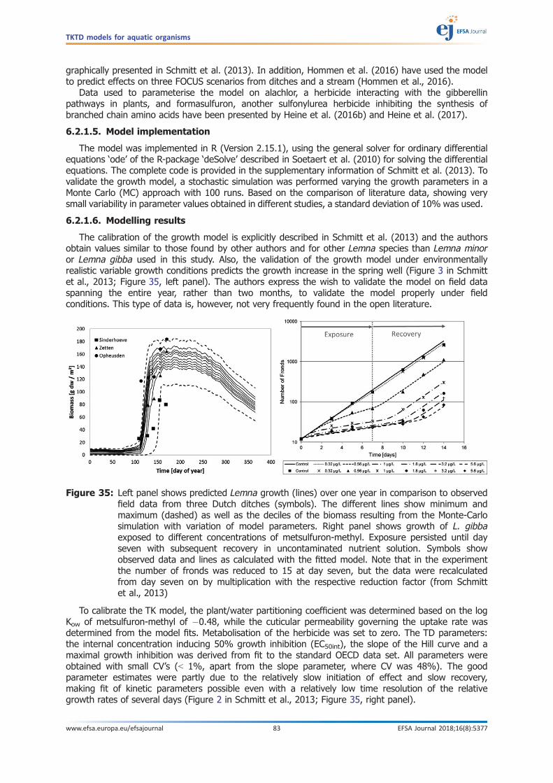
graphically presented in Schmitt et al. (2013). In addition, Hommen et al. (2016) have used the modelto predict effects on three FOCUS scenarios from ditches and a stream (Hommen et al., 2016).
Data used to parameterise the model on alachlor, a herbicide interacting with the gibberellinpathways in plants, and formasulfuron, another sulfonylurea herbicide inhibiting the synthesis ofbranched chain amino acids have been presented by Heine et al. (2016b) and Heine et al. (2017).
6.2.1.5. Model implementation
The model was implemented in R (Version 2.15.1), using the general solver for ordinary differentialequations ‘ode’ of the R-package ‘deSolve’ described in Soetaert et al. (2010) for solving the differentialequations. The complete code is provided in the supplementary information of Schmitt et al. (2013). Tovalidate the growth model, a stochastic simulation was performed varying the growth parameters in aMonte Carlo (MC) approach with 100 runs. Based on the comparison of literature data, showing verysmall variability in parameter values obtained in different studies, a standard deviation of 10% was used.
6.2.1.6. Modelling results
The calibration of the growth model is explicitly described in Schmitt et al. (2013) and the authorsobtain values similar to those found by other authors and for other Lemna species than Lemna minoror Lemna gibba used in this study. Also, the validation of the growth model under environmentallyrealistic variable growth conditions predicts the growth increase in the spring well (Figure 3 in Schmittet al., 2013; Figure 35, left panel). The authors express the wish to validate the model on field dataspanning the entire year, rather than two months, to validate the model properly under fieldconditions. This type of data is, however, not very frequently found in the open literature.
To calibrate the TK model, the plant/water partitioning coefficient was determined based on the logKow of metsulfuron-methyl of �0.48, while the cuticular permeability governing the uptake rate wasdetermined from the model fits. Metabolisation of the herbicide was set to zero. The TD parameters:the internal concentration inducing 50% growth inhibition (EC50int), the slope of the Hill curve and amaximal growth inhibition was derived from fit to the standard OECD data set. All parameters wereobtained with small CV’s (< 1%, apart from the slope parameter, where CV was 48%). The goodparameter estimates were partly due to the relatively slow initiation of effect and slow recovery,making fit of kinetic parameters possible even with a relatively low time resolution of the relativegrowth rates of several days (Figure 2 in Schmitt et al., 2013; Figure 35, right panel).
Figure 35: Left panel shows predicted Lemna growth (lines) over one year in comparison to observedfield data from three Dutch ditches (symbols). The different lines show minimum andmaximum (dashed) as well as the deciles of the biomass resulting from the Monte-Carlosimulation with variation of model parameters. Right panel shows growth of L. gibbaexposed to different concentrations of metsulfuron-methyl. Exposure persisted until dayseven with subsequent recovery in uncontaminated nutrient solution. Symbols showobserved data and lines as calculated with the fitted model. Note that in the experimentthe number of fronds was reduced to 15 at day seven, but the data were recalculatedfrom day seven on by multiplication with the respective reduction factor (from Schmittet al., 2013)
TKTD models for aquatic organisms
www.efsa.europa.eu/efsajournal 83 EFSA Journal 2018;16(8):5377

It is a bit surprising that a maximal inhibition of growth is introduced (being 78%), as one wouldexpect growth inhibition to approach 100% with increasing herbicide concentration. This is most likelydone, because the mode of action of metsulfuron-methyl, inhibition of branched chain amino acidsynthesis, acts really slowly, and in crops can take 4–6 weeks to fully develop. Hence, as growth willalways continue for a time after uptake of the herbicide, growth inhibition measured relative to startbiomass (or frond number) will never be 100% in short experiments.
The TKTD model was validated on constant and pulse exposure scenarios of Lemna grown in thelab over 42 days. The EC50int was recalibrated on the constant exposure data to account for a slightlylower sensitivity of this Lemna clone (parameterised to 0.39 rather than 0.30 lg/L), but all otherparameters were kept from the first calibration data set. The model predictions described data reallywell for the first 3 weeks of the experiment, after which is seemed Lemna became insensitive to theherbicide growing faster than predicted by the model. This tendency was more pronounced at theconstant and long pulse exposure (4-day pulse, 3 days of clean water) compared to the short pulseexposure (2-day pulse, 5 days of clean water), which indicated that continuous exposure leads toselectivity of resistant fronds possibly through upgrading of detoxification capacity (Figure 4 in Schmittet al., 2013; Figure 36).
TKTD models for aquatic organisms
www.efsa.europa.eu/efsajournal 84 EFSA Journal 2018;16(8):5377
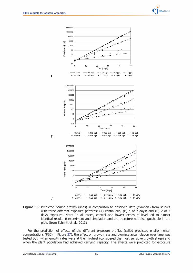
For the prediction of effects of the different exposure profiles (called predicted environmentalconcentrations (PEC) in Figure 37), the effect on growth rate and biomass accumulation over time wastested both when growth rates were at their highest (considered the most sensitive growth stage) andwhen the plant population had achieved carrying capacity. The effects were predicted for exposure
A)
B)
C)
Figure 36: Predicted Lemna growth (lines) in comparison to observed data (symbols) from studieswith three different exposure patterns: (A) continuous; (B) 4 of 7 days; and (C) 2 of 7days exposure. Note: In all cases, control and lowest exposure level led to almostidentical results in experiment and simulation and are therefore not distinguishable in theplots (from Schmitt et al., 2013)
TKTD models for aquatic organisms
www.efsa.europa.eu/efsajournal 85 EFSA Journal 2018;16(8):5377
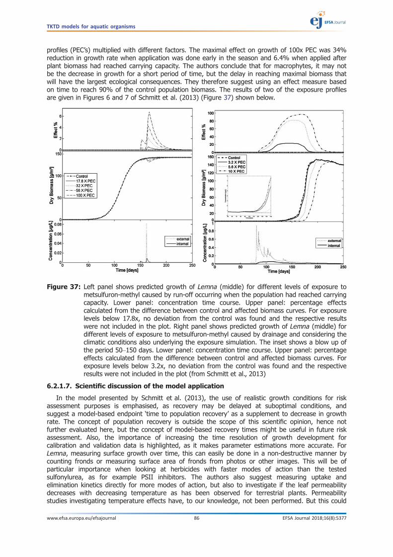
profiles (PEC’s) multiplied with different factors. The maximal effect on growth of 100x PEC was 34%reduction in growth rate when application was done early in the season and 6.4% when applied afterplant biomass had reached carrying capacity. The authors conclude that for macrophytes, it may notbe the decrease in growth for a short period of time, but the delay in reaching maximal biomass thatwill have the largest ecological consequences. They therefore suggest using an effect measure basedon time to reach 90% of the control population biomass. The results of two of the exposure profilesare given in Figures 6 and 7 of Schmitt et al. (2013) (Figure 37) shown below.
6.2.1.7. Scientific discussion of the model application
In the model presented by Schmitt et al. (2013), the use of realistic growth conditions for riskassessment purposes is emphasised, as recovery may be delayed at suboptimal conditions, andsuggest a model-based endpoint ‘time to population recovery’ as a supplement to decrease in growthrate. The concept of population recovery is outside the scope of this scientific opinion, hence notfurther evaluated here, but the concept of model-based recovery times might be useful in future riskassessment. Also, the importance of increasing the time resolution of growth development forcalibration and validation data is highlighted, as it makes parameter estimations more accurate. ForLemna, measuring surface growth over time, this can easily be done in a non-destructive manner bycounting fronds or measuring surface area of fronds from photos or other images. This will be ofparticular importance when looking at herbicides with faster modes of action than the testedsulfonylurea, as for example PSII inhibitors. The authors also suggest measuring uptake andelimination kinetics directly for more modes of action, but also to investigate if the leaf permeabilitydecreases with decreasing temperature as has been observed for terrestrial plants. Permeabilitystudies investigating temperature effects have, to our knowledge, not been performed. But this could
Figure 37: Left panel shows predicted growth of Lemna (middle) for different levels of exposure tometsulfuron-methyl caused by run-off occurring when the population had reached carryingcapacity. Lower panel: concentration time course. Upper panel: percentage effectscalculated from the difference between control and affected biomass curves. For exposurelevels below 17.8x, no deviation from the control was found and the respective resultswere not included in the plot. Right panel shows predicted growth of Lemna (middle) fordifferent levels of exposure to metsulfuron-methyl caused by drainage and considering theclimatic conditions also underlying the exposure simulation. The inset shows a blow up ofthe period 50–150 days. Lower panel: concentration time course. Upper panel: percentageeffects calculated from the difference between control and affected biomass curves. Forexposure levels below 3.2x, no deviation from the control was found and the respectiveresults were not included in the plot (from Schmitt et al., 2013)
TKTD models for aquatic organisms
www.efsa.europa.eu/efsajournal 86 EFSA Journal 2018;16(8):5377

potentially have a large effect on pulse exposures, as short-term pulses may not be taken up veryrapidly at colder temperatures compared to warmer temperatures if permeability is decreased at lowtemperatures. In addition to the issues suggested by the authors, the effect of the pKa of theherbicides combined with the pH of the water may play a role for uptake, as is seen for plant andalgae uptake in general (Fahl et al., 1995; Trapp, 2004; Rendal et al., 2011). It is also known thatfrond size and surface/weight ratios change in Lemna when exposed to herbicides with different modeof action (Cedergreen et al., 2004; Cedergreen and Streibig, 2005). In the model presented by Schmittet al. (2013), these ratios are assumed to be constant. It would, however, be possible to do asensitivity analyses on the effect of variation in the frond/surface/weight ratio based on published datato investigate, if these variations are of significance for the outcome of the model.
6.2.1.8. Evaluation of the application in risk assessment
The Lemna model, its implementation, parameter estimation and validation together with sensitivityanalyses of its robustness to variation in parameters and a discussion of strengths, weaknesses andwishes for future work, is documented in a scientific publication (Schmitt et al., 2013).
Physiological model parameters have been collected from the scientific literature. TKTD modelparameters have been calibrated on data from a modified 14-day OECD toxicity test by non-linearoptimisation and are reported including the parameter variability. Optimisation routine and the methodused for the estimation of the parameter uncertainty limits are not clearly given in the paper or thesupporting information. Variability and sensitivity analyses were made on photosynthetic rate,respiration rate, maximal density and initial biomass. Variability analysis means in this context that theauthors tried to analyse how variable the most relevant model parameters are in literature. Inconclusion of this analysis, the above parameters were varied within 10% CV. In the publication, it wasconcluded that the results of both exposure profiles are relatively robust to variation in the parameters(MC simulation of the parameters given a CV of 10% each). The uncertainty intervals of thepredictions increased 1.5–2-fold adding the variation in the parameters. Given that there is no realempirical basis for the variation of above mentioned parameters given in the paper, the chosenvariation range of 10% appears rather small, especially because the parameters were partially drawnfrom a normal instead of a uniform distribution. Under these circumstances, a 1.5- to 2-fold increase inthe uncertainty intervals appears very high, since this translates to 50%–100% increase in thevariation of the modelled endpoint. For future applications of the Lemna model in risk assessment,optimisation methods need to be described in more detail, and sensitivity analyses should be redone toallow for a comprehensive understanding of the variation in the model parameters.
Nevertheless, in line with the algae model, the Lemna model could potentially be used to predicteffects under variable environmental conditions, as was done for the ditch validation data (Figure 35).The conceptual and the formal model appear suitable for the application of the Lemna model in riskassessment. The model was implemented in R, and the code is available, but not all input files aregiven. A specific implementation of verification was not included in the publication and should beincluded for future applications. The dynamic Lemna model harbours the possibility to predict effectsalso under variable growth conditions, but more validation data is needed to test the robustness ofsuch predictions. None of the long-term predictions of population effects of Lemna exposed to variableFOCUS exposure profiles have been validated by data from long term laboratory or field experiments.If long-term data on Lemna growth exist from for example mesocosm studies, it could be interestingto validate the model against such data sets.
Since the publication of the model in 2013, parameterisation and validation of the model on twoother herbicides with different modes of action, one affecting the gibberellin pathways in plants, andthe other inhibiting branched chain amino acids, have been presented at European SETACconferences, but since the results are not published they cannot be further checked. In addition, anapplication of the Lemna model for an inhibitor of carotenoid synthesis is available.
The model seems to work well for the sulfonyl-urea compound and the validation data as presentedin Schmitt et al., 2013, but the model should be validated on herbicides with other modes of action.
Summarising, the Lemna model appears suitable for use in risk assessment to evaluate effects oftime-variable exposure on Lemna growth. However, the above-mentioned aspects of the model haveto be picked up and improved to make applications acceptable for use in regulatory risk assessment(see Chapter 7 and Annex C).
TKTD models for aquatic organisms
www.efsa.europa.eu/efsajournal 87 EFSA Journal 2018;16(8):5377
6.3. The Myriophyllum model
As discussed in Section 2.4.3 the Myriophyllum model is not as completely described as the Lemnamodel, and source code is, to our knowledge, not publicly available. The model is described in threepapers: The first one builds and parameterises the growth model, and describes how growth varies asa function of irradiance and temperature (Heine et al., 2014). The second paper focusses ondescribing and parameterising the TK-processes for several herbicides, including both sulfonylurea andphoto-system II inhibitors. Also, they determine cuticular permeability for chemicals based on their logKow (Heine et al., 2015). The final paper describes and parameterises the toxicodynamic model usingthe sulfonylurea iofensulfuron (Heine et al., 2016a). The fact that the model is described in threeseparate papers makes it difficult to get an overview of its entity, as is also discussed in Section 2.4.3.Some of the main issues not explicit in the published material on Myriophyllum are:
• How the model deals with density dependent growth.• How toxicants move between compartments, both toxicants taken up by the leaves and
toxicants taken up by the roots.
The Myriophyllum model has only been calibrated and validated on a single substance,iofensulfuron under constant growth conditions. Hence, its more global application to chemicals withother modes of action and to other growth conditions has yet to be seen. More detailed description ofthe model can be found in the PhD thesis of Heine, 2014: https://publications.rwth-aachen.de/record/459446.
A publicly available model implementation in line with that provided for the Lemna model would bea great advantage.
6.4. Summary, conclusions and recommendations for the algae andplant models
The models for the primary producers all rely on a growth model driven by a range of externalinputs such as temperature, irradiance, nutrient and carbon availabilities. The effect of the pesticide onthe net growth rate is described by a log-logistic relationship, linking either external (the algae model)or scaled or measured internal concentrations to growth rate. All experiments and tests of the modelsup till now have been done under fixed growth conditions, as is the case for the standard algae,Lemna and Myriophyllum tests. This is because the focus has been on evaluating the modelavailabilities to predict effects under time-variable exposure scenarios. The growth models do,however, all have the potential to incorporate changes in temperature, irradiance, nutrient and carbonavailabilities in future applications.
For the algae, time-variable exposures were excellently described by the model for two species ofalgae and one PSII inhibiting herbicide. The largest drawback for implementing the models in pesticiderisk assessment is that the flow-through setup used and needed to simulate long-term variableexposures of pesticides to fast growing populations of algae has not yet been standardised, nor hasthe robustness of the setup been ring tested. Hence, for the present, the setup and the models areimportant research tools but probably not yet mature enough to use for risk assessment purposes.
The Lemna model is the most thoroughly tested, calibrated and validated having been verified forfour different herbicides with three modes of action. In addition, it can be calibrated on data from thealready standardised OECD Lemna test, as long as pesticide concentrations and growth is monitoredseveral times during the exposure phase and the test is prolonged with a 1-week recovery period.Growth may be monitored most easily and non-destructively by measuring surface area or frondnumber, either on a daily basis or every 2 days. Calibration to biomass should be done at least at theend of the exposure phase, as some herbicides change surface to weight ratios. Validation data setsshould have different exposure patterns, containing at least one but ideally two pulse exposures andbe tested on a range of concentrations. If the model is properly documented and analysed accordingto the suggestions in Section 6.2.1.8 (See also Annex C), the Lemna model can be an important toolto evaluate the effects of time-variable exposures of pesticides under different growth scenarios.
The Myriophyllum model is not yet as well developed, calibrated, validated and documented as theLemna model. It is more complicated, as Myriophyllum also has a root compartment (in the sediment)where the growth conditions (redox potential, pH, nutrient and gas availabilities, sorptive surfaces etc.)and therefore also bioavailability of pesticides are very different from the conditions in the shootcompartment (water column). In addition, Myriophyllum grows submerged making carbon availability
TKTD models for aquatic organisms
www.efsa.europa.eu/efsajournal 88 EFSA Journal 2018;16(8):5377

in the water column a complicated affair compared to Lemna, where access to carbon through theatmosphere is constant and unlimited. Due to the increased complexity of the system and the relativenovelty of the published model, the Myriophyllum model has not yet been very extensively tested andpublicly assessable model codes are not yet available. Standard guidelines for conducting tests ofMyriophyllum spicatum are available (OECD 2014a,b) As for the Lemna test, the aim is to be able touse data from such standardised tests for calibration with growth being monitored over time (non-destructively as shoot numbers and length), and including a recovery period and length/biomasscalibrations. Validation data set should include at least two pulse exposures. At the present state,however, the model needs further calibration, validation and documentation to be ready to use for riskassessment purposes.
7. Evaluation of models
This section follows Chapter 10 of the EFSA Opinion on good modelling practice in the context ofmechanistic effect models for risk assessment (EFSA PPR Panel, 2014) and expands on the informationprovided that is specific to TKTD models. The chapter focuses on GUTS modelling with additionalparagraphs covering differences for DEBtox and plant models, where appropriate.
The key points that the risk assessor should pay attention to remain the same as in EFSA PPRPanel (2014):
• Is the model based on commonly agreed scientific principles and/or are these principlespublished in the scientific literature?
• Is the general behaviour of the model plausible?• Are all steps of the modelling cycle sufficiently well documented? (see Chapters 4, 5 and 6)• Is the correspondence with available independent observations acceptable?• Is the model fit for regulatory purpose? In other words, can it be used to provide an answer to
the question posed in the problem definition?
Parts of these key questions have been analysed, documented and answered for some of themodels already, particularly for the GUTS models. More details will be given in the following sections.
In the case of DEBtox models, there are two aspects that need to be considered: (1) how well theDEB model describes the energy budget of the species under consideration (physiological part of themodel) and (2) how the effects of the chemical can be modelled through stress functions applied onDEB model parameters (TKTD part of the model).
The DEB part of the model (physiological part of the model) is usually built based on a certainamount of underlying physiological data. There are two options for the evaluation of the data that isunderlying the physiological model:
i) If the species-specific DEB part of the model has been previously documented and validated,then there is no need to check this for each application with a specific toxicant. The species-specific part of the model should be able to describe the relevant endpoints observed in thecontrols of the validation data (e.g. weight/length or reproduction under control conditions).However, in some cases, adaptation of relevant parameters is needed to properly describecontrol data under specific experimental conditions. This is considered necessary for themodel to be fit for purpose (see criteria for evaluating fit of the model, Section 7.7.2).
ii) If the species-specific DEB part of the model has not been documented and validatedpreviously, then this needs to be properly undertaken outside of the evaluation of the TKTDpart (see recommendation in Chapter 9.2).
The first of these two options is likely to be the only option applicable in risk assessment practice,so this is the focus of this SO. For an evaluation of the species-specific DEB part of the model, theEFSA Opinion on good modelling practice in the context of mechanistic effect models for riskassessment (EFSA PPR Panel, 2014) should be used.
Models for primary producers are also divided into the physiological and the TKTD parts, which canbe evaluated separately. For Lemna and some algal species, the physiological part of the model isalready developed and has been evaluated in the SO, but for other aquatic plants and algal speciesfurther work is required before the physiological model and the underlying data are considered to besuitable for use in risk assessment. Similarly to DEB, the species-specific part of the primary producermodel should be able to describe the observed control data of the validation data set. Once again,when necessary, adaptation of the most relevant parameters to specific experimental conditions may
TKTD models for aquatic organisms
www.efsa.europa.eu/efsajournal 89 EFSA Journal 2018;16(8):5377

be needed in order to consider the model fit for purpose (see criteria for evaluating the fit of themodel, Section 7.7.2).
Every model application should be accompanied by a summary according to Annex D.The summary checklist provided in Appendix B of EFSA PPR Panel (2014) has been adapted for
TKTD models and three adapted versions (GUTS, DEBtox and plant models) are provided in Annex A,Annex B and Annex C.
When the evaluator fills in the checklist, justification should be included for all points that are notstraightforward.
In Appendices F and G, the evaluation of two available model examples, one for GUTS and one forDEBtox, is reported for illustration
7.1. Evaluation of the problem definition
The chapter about the problem definition/formulation in this SO (Chapter 3) containscomprehensive information about the regulatory context in which the model is run, the regulatoryquestions that can be addressed with the model and the required model output to answer thesequestions. However, these aspects have to be defined clearly for any model application.
One important aspect that needs to be addressed as part of the problem definition is the selectionof species for the modelling that has been performed (see Section 3.2 for more information aboutselecting species for different tiers of the risk assessment). In line with other higher-tier approaches,the choice of the test species needs to be clearly described and justified, also considering all theavailable valid information. In addition, the problem definition should make clear whether the model isbeing used with a Tier-1 test species, i.e. Tier-2C1 or with one or more relevant species (which mightinclude the Tier-1 species) i.e. Tier-2C2. If the modelling is part of a Tier-2C2 risk assessment, then it isvery likely that TKTD models have been applied for different species, except in the rare situationwhere a large number of species have been tested in the laboratory at Tier-2A/2B, and theseexperiments have shown that only one or a very limited number of species are sensitive to thepesticide (see Chapters 3 and 8).
7.2. Evaluation of the quality of the supporting experimental data
This part of the evaluation checks whether the experimental data which are used for the modelling(both calibration and validation data sets) have been subjected to an acceptable quality control. Thefocus is on data quality, i.e. the laboratory conditions, set-up, chemical analytics and similar. All laboratorystudies used to calibrate or validate the model should be summarised and evaluated considering thespecific guideline that was used. Sometimes the laboratory studies providing the data cannot followstandard guidelines, if for example the design, the experimental conditions and/or the validity criteria ofthe study need to be modified in order to provide more appropriate data for the modelling. In such case,the study should be tailored to the modelling needs but the principles of the most closely related guidelineshould be followed as far as is possible. In such cases, attention should be paid to provide validity criteria,which measure whether the performance of the study is sufficient to provide reasonably reliable data. Itis important that laboratory studies included test concentrations that were high enough to clearlydemonstrate the effects of the toxicant. Additional specific criteria for the suitability of the data sets formodel calibration and validation have been developed earlier (Sections 4.1.3.4 and 4.1.4.5) and areexplained later in more detail (Sections 7.6.2 and 7.7.2, respectively).
Validity criteria and other requirements of OECD guidelines that might be considered when carryingout studies to support TKTD modelling are summarised in Table 6 (given at the end of Chapter 7),together with comments about the relevance of the criteria for data used for this purpose. Where thestudy design is modified in such a way that the validity criteria prescribed in the guideline are nolonger applicable, the performance of the study should be carefully considered (e.g. Did the controlsbehave as expected? Are tested individuals numerous enough to detect effects?).
When the toxicity studies for calibration and validation purposes are evaluated, it is in generalimportant to check that the actual exposure profile in the study matches the intended profile in the test(+/� 20%); if it does not, then measured concentrations are used for the modelling, instead of nominalones. In the case of fast dissipating substances, actual measured exposure profile in the test can be used.
If multiple experiments of reasonable quality are available and suitable for either calibrating orvalidating the TKTD model, cherry-picking of data is not acceptable. In case one relevant data set isexcluded from both calibration and validation, the choice should be appropriately justified.
TKTD models for aquatic organisms
www.efsa.europa.eu/efsajournal 90 EFSA Journal 2018;16(8):5377

In the case of GUTS, it is likely that the supporting data for both calibration and validation of themodel will be laboratory toxicity studies with a range of exposure conditions (including Tier-1 acuteand chronic constant exposure and Tier-2 time-variable exposure) that are evaluated as part of thedata package. As demonstrated in Jager (2014), the use of TKTD models for dose–time–responseanalysis invites a whole new and flexible view on optimal test design. In particular, classical LC50
estimates can be derived with a GUTS-RED-SD model even from experimental set-ups that would havebeen considered as unsuitable for classical Tier-1 regression analyses.
In the case of DEBtox models, the supporting data for the physiological part of the model wereeither already assessed beforehand, or need a separate evaluation than the one outlined in this SO.The only data to be evaluated for DEBtox model applications (once the physiological part of the modelhas been evaluated as acceptable to use in the risk assessment) are hence most likely toxicity studiesfocussing on sublethal effects for a range of exposure conditions, in order to calibrate and to validatethe TKTD part of the model Depending on the DEB model being used, it is pivotal that experimentalfactors like temperature, food conditions, etc. are well documented for all valid data sets.
Models for primary producers are also divided into the physiological and the TKTD part. As withDEBtox models, once the validation of the physiological part of the model has been successfullyachieved, the only additional data to be evaluated are the toxicity studies with a range of exposureconditions, in order to calibrate and validate the TKTD part of the primary producer model. It is veryimportant that experimental conditions influencing growth (i.e. temperature, irradiance, nutrient mediacomposition, handling and thinning, etc.) and growth calculations (frequency and type ofmeasurements, calibration between surface and weight data, etc.) are suitably described anddocumented.
7.3. Evaluation of the conceptual model
For GUTS, the conceptual model is standardised in the sense that the same processes are usedwhatever the toxicant-species combination. When the model is used to address lethal/immobilityeffects in fish or invertebrates, the conceptual model is considered suitable to address the SPGs; so,no further evaluation is required (see Chapters 3.3 and 4). If a GUTS model is being used for anyother reason, then consideration as to whether it is a suitable model to address the question beingasked is required and whether the question is appropriate in the context of risk assessment.
For DEBtox, the conceptual models outlined in Section 2.3 of this SO can be used as basis for thedocumentation of the conceptual model, but the conceptual model for the species under considerationneeds to be explicitly checked (see Chapter 10.2 of EFSA PPR Panel, 2014). Even if the DEB(physiological) part of the model has been previously tested and validated for the species underconsideration, there are different ways the toxicant can impact the life cycle (namely how the toxicantimpacts the energy acquisition or use). The processes impacted by the toxicant should be carefullyconsidered. Based on the available information, all possible processes where the toxicant could havean impact need to be considered (see Figure 3 in Chapter 2). In case environmental factors (e.g.temperature) are explicitly considered, their influence on the physiological part and TKTD processesneeds to be documented in the conceptual model.
For primary producers, the conceptual models outlined in Section 2.4 of this SO can be used as abasis for the documentation of the conceptual model. For Lemna spp. and algae, this SO hasevaluated the conceptual models and they are considered suitable to use without further evaluation,but for Myriophyllum spp. and other aquatic plants, the conceptual model still needs to be checked(see Chapter 10.2 of EFSA PPR Panel, 2014). For all primary producer species, the influence ofenvironmental factors (e.g. light, temperature) on growth and TKTD processes in the conceptualmodel and the linking of those processes in the model need to be documented.
7.4. Evaluation of the formal model
The formal model documents the equations and algorithms that form the basis for the model.For GUTS models, the equations are standardised; so, no further check is necessary. It has to be
documented, however, which GUTS model version is used (full or reduced model).For DEBtox models, a large body of equations has been defined in the scientific literature, but no
standardisation was achieved up to now. In addition, at the moment, internal exposure is linked withtoxicant effects in a tailor-made modus operandi. Hence, a DEBtox model application should documentall equations that are used for the modelling. Evaluation of the formal model would need to be
TKTD models for aquatic organisms
www.efsa.europa.eu/efsajournal 91 EFSA Journal 2018;16(8):5377

achieved on a case-by-case basis by experts, until standardised DEBtox modelling including linksbetween internal exposure and toxic effects becomes available. All variables and parameters should belisted and both the deterministic and stochastic parts of the model should be fully described (seeSection 5.1).
Primary producer models are formulated in a species-specific fashion, considering biological/life-history traits that have an influence on the conceptual and hence also on the formal model, e.g.whether plants are rooted in sediment, or they occur/grow predominantly at the water surface orsubmerged in the water column. For each model application, all equations that are used for themodelling should be documented, and evaluation of the formal model would need to be achieved on acase-by-case basis by experts, until standardised models become available, likely specific for plant/algae species.
7.5. Evaluation of the computer model
For GUTS models, checking the implementation of the computer model should include three lines ofevidence:
1) The proposed implementation should be tested against the ring-test data set (Jager andAshauer, 2018). The performance of the model with the ring-test data sets can be used toconfirm that the computer model is working as it should. It is efficient and safe to test thecomputer code by showing that a given model implementation produces similar outputs(model parameters, confidence limits, model predictions) as previous GUTS implementations.Results of the GUTS implementation in the R package ‘morse’ (Appendix B.6) andMathematica (B.7) are provided as an example;
2) A set of scenarios (default, pulsed and ‘extreme’ cases, see Section 4.1.2.3) should besimulated and checked;
3) An independent implementation of GUTS (e.g. an Excel sheet or a web-based shinyApp –http://lbbe-shiny.univ-lyon1.fr/guts-shinyapp/) should be used by the evaluator to testwhether the output of the evaluated model implementation can be reproduced for someparameter sets.
In addition, the computer code of the model implementation should be made available to allowfurther checks by experts.
A ring-test equivalent to the one available for GUTS models is not available for DEBtox or primaryproducer models yet. Therefore Chapter 10.4 of EFSA PPR Panel (2014) should be used to check thecomputer model code. Such an evaluation includes basically similar steps as described in Section 4.1.2and needs expert assessment.
7.6. Evaluation of the regulatory model
The regulatory model is the combination of the computer model with the environmental scenariosand the model parameters. Figure 5 in EFSA PPR Panel (2014) has been adapted to show the relevantparts of the general regulatory model that apply to TKTD models (Figure 38).
7.6.1. Evaluation of the environmental scenarios
One of the benefits of TKTD modelling is that all the data (simulated time series instead ofmaximum or average concentrations) from the predicted exposure profiles (e.g. from the variousFOCUS scenario) can be used as input for simulations.
For GUTS models using FOCUS scenarios as input, no further definition of the environmentalconditions is needed, since the model parameters will be based on data obtained from experimentsperformed under standard laboratory conditions, and pesticide concentrations will have beengenerated using the relevant FOCUS scenarios, which consider factors such as soil type, rainfall andagronomic practice.
For DEBtox models, a basic environmental scenario has to be defined including temperature andfood conditions. The physiological part of the model has the potential to extrapolate predictions ofgrowth and reproduction to variable environmental conditions, in terms of e.g. temperature and foodavailability. Basically, accounting for variable energy intake is one of the main ideas behind DEBmodelling. The application of the DEB theory for the prediction of toxicological effects, however,requires environmental scenarios to be fixed to the laboratory conditions of the experiments used for
TKTD models for aquatic organisms
www.efsa.europa.eu/efsajournal 92 EFSA Journal 2018;16(8):5377

calibrating the TKTD part of the model. This appears necessary, because it is not possible to assesswhether the extrapolation of toxicity to other environmental conditions would work. In caseappropriate validation data for variable temperature or food conditions is provided, explicitextrapolation to variable environmental conditions and hence the definition of different environmentalscenarios could be possible.
It is considered appropriate to fix abiotic factors of the environmental scenarios to the laboratoryconditions of the experiments used for calibrating the TKTD part of the model, and also to ignoreecological factors such as species interactions. This is because the modelling will be used with theequivalent of Tier-1 or Tier-2 Assessment Factors, which should already cover for the extrapolationfrom laboratory to field conditions.
For primary producer models, a basic environmental scenario has to be defined includingtemperature and/or light conditions, and nutrients availability. The conditions used in the model shouldmirror the conditions in the experiments used for calibration, since this is in line with Tier-2A andTier-2B, where additional species or refined exposure scenarios are tested in laboratory experimentswithout also using realistic light conditions and nutrient levels.
7.6.2. Evaluation of parameter estimation
Parameter estimation requires a suitable data set, the correct application of a parameteroptimisation routine and the comprehensive documentation of methods and results. Supporting datafor TKTD models have to be of sufficient quality (Section 7.2), be relevant for the risk assessment andfulfil a set of basic criteria. One important aspect about the data requirements is to have experimentalobservations of the relevant endpoints (e.g. mortality or reproduction) for a sufficient number of time-points in order to have an appropriate degree of freedom to calibrate the model. The number ofobservations can vary per TKTD model, suggestions are given in the respective checklists (Annex A,Annex B and Annex C). Another important aspect for the calibration data set is that the response inthe observed endpoint should range from no effects up to strong effects, ideally from 0% to 100%.The model can only capture the quantitative relationship between exposure and effects when a cleareffect is visible in the underlying data. Parameter estimates can show reduced accuracy and precisionwhen the experiments do not show a clear and comprehensively covered dose–response pattern. It is
Figure 38: Schematic representation of a TKTD regulatory model (orange boxes). The environmentalscenario feeds into the exposure model in combination with information on pesticideproperties and uses. The exposure model in turn delivers the exposure profile, which isused as input by the TKTD models. Altogether, the regulatory model delivers an output,i.e. the endpoint of the assessment. For DEBtox and primary producers’ models, asindicated by the dotted arrow and the associated box, the recommendation is, for thetime being, to fix the abiotic parameters to the laboratory conditions of the experimentused for calibrating the model. If in the future the relationship between toxicity andenvironmental conditions will be better understood and described, such recommendationcan be revised. The figure represents an adaptation of Figure 5 in EFSA PPR Panel (2014)
TKTD models for aquatic organisms
www.efsa.europa.eu/efsajournal 93 EFSA Journal 2018;16(8):5377

difficult to define a minimum required level of response in the data, but a maximum effect of less than50% in acute assessment for effects on invertebrates and chronic effect on plants, and of less than90% in chronic assessments for effects on aquatic invertebrates and fish, should be well justified. Inaddition, the time course of the experiment used for calibration should be adjusted to capture the fulltoxicity of the pesticide (attention should be paid to time needed for the onset of effects, occurrenceof delayed effects, accumulated toxicity, etc.).
It is possible that more than one suitable data set for calibration of the model does exist, since allavailable reliable data sets (apart from those used for validation) should be used (even non-standardtest data when available and considered reliable). In such a case, parameter optimisation can be doneseparately per data set, resulting in one optimal parameter set per data set. There are at least twostrategies how to continue from there. One option is to predict the validation data set based on eachparameter set and to select the parameter set that shows the best performance (see Section 7.7.2).The other option is to test whether the distributions of the parameter values are significantly different,to merge the corresponding data sets and to re-calibrate the parameters for the merged data set incase they are not.
Some TKTD model parameters may also be taken from the literature. If this is the case, it shouldbe checked whether they are reasonable, and if uncertainty limits are also provided.
Model parameters are always estimated for a specific combination of species and compound (seeChapter 3 for background information). For the evaluation of parameter estimation, also called modelcalibration or fitting, the method used has to be documented in detail, including settings ofoptimisation routines, the numerical solver (including settings) that was used for solving the differentialequations, and the method for the calculation of parameter confidence/credible limits. Knowledgeabout these settings is important to allow experts to further evaluate parameter estimation when thereis uncertainty about the quality of the results. Detailed background information on parameterestimation is given in Section 4.1.3, and example documentations for parameter estimation processand results are given in Section 4.2.2.1 and Appendix A.1 and A.2.
The results of the parameter optimisation process are not limited to the optimal parameterset alone. The optimal parameter values must be given together with confidence or credible intervalsto allow evaluation of their uncertainty. Values of the objective function for calibration (e.g.log-likelihood function) need to be documented with sufficient numerical precision to allow forindependent checks of the optimisation process. For an evaluation of the model calibration, plots ofthe calibrated models in comparison with the calibration data over time should be available and thevisual match should be reasonable. Additional goodness-of-fit criteria can be reported, at least aposterior predictive check should be available and documented (example in Figure 17).
One specific of the parameter estimation for GUTS is how the background mortality rate isconsidered in the optimisation. The standard way is to estimate all parameters simultaneously,including the background mortality in the experiments because control data may contain informationabout TKTD parameters; in addition, it is also possible to check for potential correlations betweenmodel parameters. Alternatively, the background mortality rate constant can be calibrated to theobserved mortality in the controls and be fixed in the calibration of the other GUTS parameters to datafrom the treatments.
All aspects in this section are condensed into corresponding checklists in Annex A (GUTS), Annex B(DEBtox) and Annex C (primary producers).
7.7. Evaluation of model analysis
Model analysis includes sensitivity analysis, uncertainty analysis and evaluation of the model bycomparison of the model output with independent experimental data (model validation).
7.7.1. Sensitivity and uncertainty analysis
Sensitivity analysis quantifies the influence of parameters on the model outputs.For the reduced GUTS models, the influence of the model parameters on the model results is
described in this SO (see Section 4.1.2.4) and does not need to be reported on a case-by-case basis.Results of sensitivity analyses for GUTS can, if contained, demonstrate that the model implementationis done correctly in the process of implementation verification. For other GUTS model versions than thereduced (see Section 4.1.1), sensitivity analyses should be included for future applications.
TKTD models for aquatic organisms
www.efsa.europa.eu/efsajournal 94 EFSA Journal 2018;16(8):5377

Uncertainty analysis aims at identifying how uncertain the model output is, given that theconceptual model is accepted. Uncertainty analysis is used to relate parameter uncertainty as capturedin the parameter confidence/credible intervals to uncertainty in the model output.
Model calibration needs to report estimated parameter values including their uncertainty, i.e. theconfidence/credible limits. It is demonstrated in Section 4.1.4.2 how the information about parameteruncertainty can be used to estimate the uncertainty of predicted model outputs. For example, forGUTS models, calculated exposure profile specific LPx or EPx values can be generated includinguncertainty limits, that explicitly quantify the range of uncertainty in the model output that is causedby experimental variation and biological variability as captured in the model parameter estimates.
For DEBtox models, the sensitivity analysis of the physiological part, i.e. the discussion of thesensitivity of the DEB model parameters, should have already been performed and evaluatedbeforehand. A sensitivity analysis of the parameters for the TKTD part and a related discussion,however, is mandatory in the context of every regulatory risk assessment.
For primary producer models, the sensitivity analysis of the physiological part should already havebeen performed and evaluated beforehand. An example for Lemna is discussed shortly inSection 6.2.1.8, concluding that for future applications of the Lemna model in risk assessment,sensitivity analyses should be redone to allow for a comprehensive understanding of the variation inthe model parameters. The sensitivity analysis of the TKTD part of primary producer models, however,is mandatory in the context of every regulatory risk assessment.
For DEBtox and primary producer models, similar approaches to quantify the uncertainty in modeloutput as outlined in Section 4.1.4.2 are possible. Depending on the number of (relevant) modelparameters, the calculation of confidence/credible intervals for the modelled endpoints may needconsiderable calculation time and effort; therefore, in some cases, simplified ways of uncertaintyassessment may be acceptable, e.g. by reducing the analyses to a subset of the most relevantparameters. This is especially the case for DEBtox models, where it is possible that only parametersdirectly related to the TK and TD processes have to be considered for uncertainty analysis.
7.7.2. Evaluation of the model by comparison with independent experimentalmeasurements (model validation)
Relevant model output
The performance of a model is usually evaluated by comparing relevant model outputs withindependent measurements, a process often referred to as model validation. Relevant outputs in thecontext of model use in risk assessment are certainly those being used for answering the regulatoryquestion, e.g. simulated survival and related LPx/EPx values in case of GUTS survival modelling, andpredictions of reproduction and growth and EPx values for DEBtox and primary producer models.
Evaluation of the experimental data sets
Considering the extrapolation of effects from constant to time-variable exposure patterns, effectdata from the experiments with time-variable exposure appear to be the most meaningful and relevantfor the evaluation of TKTD models. Ideally, laboratory studies which tested different time-variableexposure profiles for the compound, species and endpoint to be modelled, (e.g. invertebrate survivalin case of GUTS, or growth and reproduction data for DEBtox and plant models) should be availablefor calibration For all model types, calibrated models could be used to design validation experiments,which can in turn generate data sets that cover the most important aspects of model validation.
The quality of the experimental data, which are used for comparison of the model, needs to beproperly assessed. To that purpose, the availability of comprehensive documentation is important (seeSection 7.2). Particular attention should be paid on the duration of the experiment, which should beadjusted to capture the full toxicity of the pesticide (time needed for the onset of effects, occurrenceof delayed effects, accumulated toxicity, etc.).
For the evaluation of experimental data set for validation, it is important that the test design shouldbe tailored to the question at hand. Nevertheless, it appears important to differentiate betweeninvertebrates and primary producers on one side, and aquatic vertebrates (e.g. fish) on the other.
For invertebrates and primary producers, new experiments for model validation can be performedas needed, with reasonable time, effort and costs. Ideally, as mentioned before, the validationexperiments are designed on the basis of the calibrated model, in order to address the most criticalaspects.
TKTD models for aquatic organisms
www.efsa.europa.eu/efsajournal 95 EFSA Journal 2018;16(8):5377

For vertebrates like fish, on the other hand, ethical concerns imply that the number of experimentsshould be minimised as much as possible and should only be undertaken when no other methods areavailable (see also Regulation 1107/200913 ). When evaluating the adequacy of validation data for fish,the rationale should be set to ensure as much use of existing data as possible while additional studiesshould only be generated if really essential to produce and validate a suitably reliable model for use inthe risk assessment. Given the relevance of the Tier-2 risk assessment, it is still possible to argue for,and justify, a new fish test under time-variable exposure conditions. Nevertheless, the number oftested scenarios and replicates should be reduced to the minimum needed to gain the necessaryinformation, so may be lower in comparison to invertebrate or primary producers’ testing. A decisionwhether data sets for the validation of TKTD modelling for fish are appropriate and sufficient shouldstill be made on a case-by-case basis, considering the relevance of the tested exposure profiles andthe tested life stages among other aspects. In general, in light of the Regulation requirement aboutthe reduction of vertebrate testing, the use of TKTD modelling for fish with the only scope of reducingor eliminate the use of risk mitigation measures, is discouraged as this would imply further vertebratetesting for the validation.
Criteria for the validation data sets are described in Section 4.1.4.5, but it is noted that whilst thecriteria set out need to be met for non-vertebrates (invertebrates, plants and algae) this is notnecessarily essential for vertebrates.
Accounting for the fact that new experiments for model validation probably have to be performed,a set of standard requirements for validation data sets for invertebrates and primary producers isdeveloped as follows. Two exposure profiles with at least two pulses each, separated by no-exposureintervals of different duration should be tested on their effects. From these tests, the effectobservations are reported for an appropriate number of time-points, for example mortality orimmobility should be reported at least for seven time-points in the validation data set (seeSection 4.1.4.5). The duration between the peaks of the two exposure profiles should be defined inrelation to the individual depuration and repair time (DRT95; see Section 4.1.4.5 and Figure 39), as faras applicable.14 For animals, DRT95 values should be calculated and the duration of the no-exposureintervals defined accordingly: one of the profiles should show a no-exposure interval shorter than theDRT95, the other profile larger than the DRT95. In the case that DRT95 values are larger than it can berealised in validation experiments, or even exceed the lifetime of the considered species, the secondtested exposure profile may be defined independent from the DRT95. For algae, internal concentrationsare considered in fast equilibrium with the external concentrations and hence depend on them. For themacrophytes, the ‘life time’ is defined as the realistic duration of an experiment following standardguidelines. For Lemna spp. the duration is approximately two weeks, with water change and thinningafter one week, while for Myriophyllum spp. the maximal duration will be approximately three weeks.These two different exposure profiles should be tested for at least three concentration levels,corresponding to low, medium, and strong effects in the specific dose–response curves (see Figure 22for an example). Suggested are peak concentrations that lead to exposure profile specific effects of10%, 50% and 90% at the end of the respective experiment.
13 Regulation (EC) No 1107/2009 of the European Parliament and of the Council of 21 October 2009 concerning the placing ofplant protection products on the market and repealing Council Directives 79/117/EEC and 91/414/EEC.
14 For example, for algae, external concentrations are linked directly to effects so that the depurations time would not berelevant.
TKTD models for aquatic organisms
www.efsa.europa.eu/efsajournal 96 EFSA Journal 2018;16(8):5377
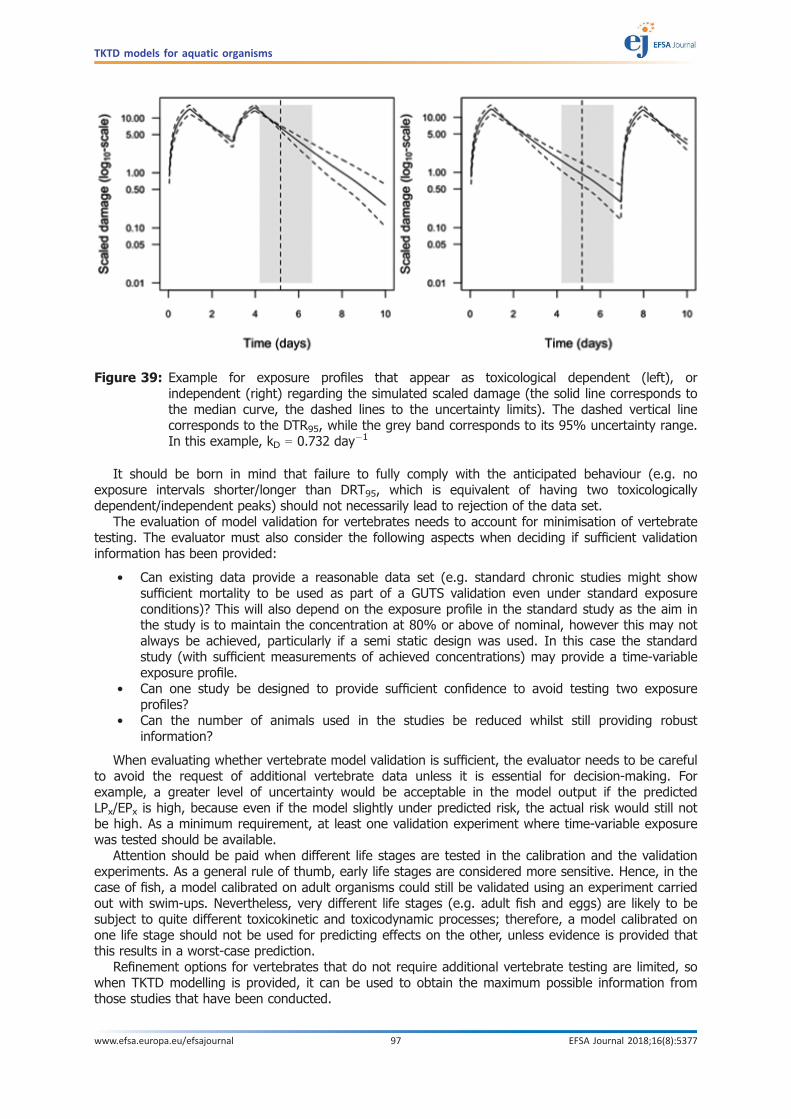
It should be born in mind that failure to fully comply with the anticipated behaviour (e.g. noexposure intervals shorter/longer than DRT95, which is equivalent of having two toxicologicallydependent/independent peaks) should not necessarily lead to rejection of the data set.
The evaluation of model validation for vertebrates needs to account for minimisation of vertebratetesting. The evaluator must also consider the following aspects when deciding if sufficient validationinformation has been provided:
• Can existing data provide a reasonable data set (e.g. standard chronic studies might showsufficient mortality to be used as part of a GUTS validation even under standard exposureconditions)? This will also depend on the exposure profile in the standard study as the aim inthe study is to maintain the concentration at 80% or above of nominal, however this may notalways be achieved, particularly if a semi static design was used. In this case the standardstudy (with sufficient measurements of achieved concentrations) may provide a time-variableexposure profile.
• Can one study be designed to provide sufficient confidence to avoid testing two exposureprofiles?
• Can the number of animals used in the studies be reduced whilst still providing robustinformation?
When evaluating whether vertebrate model validation is sufficient, the evaluator needs to be carefulto avoid the request of additional vertebrate data unless it is essential for decision-making. Forexample, a greater level of uncertainty would be acceptable in the model output if the predictedLPx/EPx is high, because even if the model slightly under predicted risk, the actual risk would still notbe high. As a minimum requirement, at least one validation experiment where time-variable exposurewas tested should be available.
Attention should be paid when different life stages are tested in the calibration and the validationexperiments. As a general rule of thumb, early life stages are considered more sensitive. Hence, in thecase of fish, a model calibrated on adult organisms could still be validated using an experiment carriedout with swim-ups. Nevertheless, very different life stages (e.g. adult fish and eggs) are likely to besubject to quite different toxicokinetic and toxicodynamic processes; therefore, a model calibrated onone life stage should not be used for predicting effects on the other, unless evidence is provided thatthis results in a worst-case prediction.
Refinement options for vertebrates that do not require additional vertebrate testing are limited, sowhen TKTD modelling is provided, it can be used to obtain the maximum possible information fromthose studies that have been conducted.
Figure 39: Example for exposure profiles that appear as toxicological dependent (left), orindependent (right) regarding the simulated scaled damage (the solid line corresponds tothe median curve, the dashed lines to the uncertainty limits). The dashed vertical linecorresponds to the DTR95, while the grey band corresponds to its 95% uncertainty range.In this example, kD = 0.732 day�1
TKTD models for aquatic organisms
www.efsa.europa.eu/efsajournal 97 EFSA Journal 2018;16(8):5377
Matching of the control data
For DEBtox and primary producer models, not only the toxicokinetic and toxicodynamic part, butalso the physiological processes are included. Hence, modelled physiological states can be comparedwith independent control data, to corroborate the adequacy of the model to describe the physiologicalprocesses. Such states could be, e.g. for DEBtox the size at puberty. In some cases, relevant modelparameters might need to be adapted to match the observed control dynamics.
Model performance criteria
Once the suitability and quality of the data set(s) used for model validation were evaluated, criteriafor the model performance need to be defined and applied. For the optimisation of parameters,objective functions are used (e.g. the log-likelihood function), but absolute values of these goodness-of-fit measures depend very often on the specifics of the experiments that were used forparameterisation (number of measurements, number of treatments) and hence cannot be used for acomparison with absolute evaluation criteria.
A combination of qualitative and quantitative criteria is suggested. Qualitatively, it can be checkedwhether the overall response pattern in the data is matched by the model output, e.g. whether the time-points of increasing effects in model and data correspond with each other and whether the behaviourover time is consistent. The visual match (‘visual fit’ in FOCUS Kinetics, 2006) of the model predictionquality gives a basis for the acceptability of the model predictions in comparison with the data.
In addition to the qualitative visual match (‘visual fit’ in FOCUS Kinetics, 2006), three quantitativecriteria are suggested for the evaluation of model validation results: the PPC takes into account theuncertainty in the model predictions, while the NRMSE value considers the relationship betweenmedian predicted and observed numbers of survivors over time, and the SPPE considers the absolutedeviation of the median survivor number at the end of the experiment (see Section 4.1.4.5 for thedefinition of these criteria). These indicators need to be evaluated in concert, and an overall conclusionshould consider that a validation study which shows clear agreement with all three quantitative criteriais for sure acceptable, while it might be tolerated if one indicator is close to the critical limit (e.g. PPCaround 50%), when the other two indicators indicate a good validation quality. As another example, adeviation of the SPPE value could be tolerated if the model predictions overestimate the effects, sincethis would be conservative for the use in risk assessment, as long as the two other criteria indicateacceptable quality.
For the GUTS models, these quantitative performance criteria have to be checked with care,because GUTS models are fitted to deaths-per-time-interval, hence comparing observed and predictedsurvival frequencies is formally not appropriate for testing the model performance (see Chapter 4).However, survival frequencies are more relevant for ERA, and if the fit is good, both comparisons willyield a good performance.
Parameter uncertainty is precisely captured in the parameter confidence/credible limits and ispropagated to modelled outputs. It is also considered when evaluating model predictions using thePPC criterion (see Section 7.6.1).
While the suggested model performance criteria have been tested and documented with GUTS,their adequacy and performance for the other TKTD model types needs to be tested in the future, andpossible adjustments of the model performance criteria may appear suitable. It is, for the time being,suggested to use the same performance criteria as suggested for GUTS (Section 4.1.4.5).
7.8. Evaluation of model use
According to EFSA PPR Panel Opinion on good modelling practice (EFSA PPR Panel 2014), the riskassessor should be able to re-run the modelling using either the parameter values provided oralternative values as a way to both verify the submitted results and check whether the model behavesreasonably. A full access to the model allows the risk assessor to run alternative exposure scenarios incase they consider that the applicant has not provided the required exposure profiles. This requiresthat either the model source code is provided in case the model is run in a standard software (e.g. inR or Mathematica), or alternatively, an executable file or web-based access to the model is provided.
Ideally, standard software should be available, so that applicants and Member State assessors canrun the models, both for calibration and testing scenarios. This would provide a high level ofconfidence in the underlying model application, allowing the evaluation to focus on the specific modelapplication (in the way FOCUS models are used for the exposure).
TKTD models for aquatic organisms
www.efsa.europa.eu/efsajournal 98 EFSA Journal 2018;16(8):5377

In the absence of standard software, it would still be of benefit to both the applicant and theassessor if an implementation of the model can be provided. One key benefit is that, should there beany concerns about the exposure profile(s) used; the assessor would have the opportunity to re-runthe modelling with alternative profiles. Although this is considered to be beneficial, it is not consideredto be essential, noting the difficulty in providing the implementations that can be used by non-TKTDmodelling experts. In case executable implementation of the model is not made available to theassessor, at least the source code should be provided.
For the use of the GUTS model in regulatory risk assessment, levels of background mortality asobserved in the calibration or validation data sets should be noted, but for simulations, backgroundmortality is assumed to be 0, since the only interest is in the toxic effects. For DEBtox and primaryproducer models, the control data for calibration and validation may show different behaviour, whichmakes the adaptation of some model parameters necessary. In such a case, the influence of theadapted model parameter on the relevant model endpoints needs to be evaluated. When suchinfluence is substantial, the parameter set producing the worst-case prediction should be used for riskassessment.
It is acknowledged that standard software suitable for general (non-expert) use is not yet at hand,although for GUTS there are some options available. MOSAIC (MOdeling and StAtistical tools forecotoxicology) developed at the University of Lyon contains a GUTS tool (http://pbil.univ-lyon1.fr/software/mosaic/guts) which can be used for calibration. Moreover, GUTS-ShinyApp (http://lbbe-shiny.univ-lyon1.fr/guts-shinyapp/) can be used to simulate predictions of survival for different exposureprofiles with different TKTD parameter values for both GUTS-RED-SD and GUTS-RED-IT models.
The summary sheet (Annex D) provided by an applicant can be a helpful tool for the evaluators tohighlight the critical information and to guide them through what is likely to be a complex evaluation.So it is highly recommended for applicants to provide such model summary.
For the time being, evaluators would not always be able to re-run all modelling. Therefore, it isvery important that the documentation is clear and can be checked by the evaluator. The modelledexposure scenario(s) must be fully documented. If FOCUS modelling is used for the TKTD riskassessment the following items need to be checked:
• Are the input values used for FOCUS clearly stated?• Which FOCUS Step is used? (It is expected that the results will be from Step 3 or Step 4 – if
Step 4, is it clear what risk mitigation has been used).• Are these the same values that have been used in the Tier-1, Tier-2A or Tier-2B risk
assessment? If not, has the reason for any differences been clearly justified?• Has the modelling used for all tiers been accepted in the Environmental Fate evaluation? If
not, the modelling will usually have to be redone using the accepted inputs.
Overall, the evaluation needs to conclude whether the use of the model is appropriate to answerthe regulatory question identified in the problem formulation section.
TKTD models for aquatic organisms
www.efsa.europa.eu/efsajournal 99 EFSA Journal 2018;16(8):5377
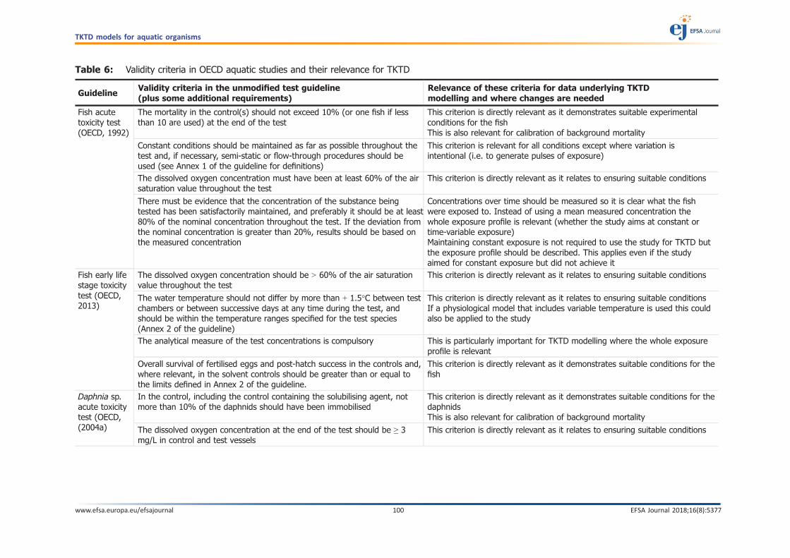
Table 6: Validity criteria in OECD aquatic studies and their relevance for TKTD
GuidelineValidity criteria in the unmodified test guideline(plus some additional requirements)
Relevance of these criteria for data underlying TKTDmodelling and where changes are needed
Fish acutetoxicity test(OECD, 1992)
The mortality in the control(s) should not exceed 10% (or one fish if lessthan 10 are used) at the end of the test
This criterion is directly relevant as it demonstrates suitable experimentalconditions for the fishThis is also relevant for calibration of background mortality
Constant conditions should be maintained as far as possible throughout thetest and, if necessary, semi-static or flow-through procedures should beused (see Annex 1 of the guideline for definitions)
This criterion is relevant for all conditions except where variation isintentional (i.e. to generate pulses of exposure)
The dissolved oxygen concentration must have been at least 60% of the airsaturation value throughout the test
This criterion is directly relevant as it relates to ensuring suitable conditions
There must be evidence that the concentration of the substance beingtested has been satisfactorily maintained, and preferably it should be at least80% of the nominal concentration throughout the test. If the deviation fromthe nominal concentration is greater than 20%, results should be based onthe measured concentration
Concentrations over time should be measured so it is clear what the fishwere exposed to. Instead of using a mean measured concentration thewhole exposure profile is relevant (whether the study aims at constant ortime-variable exposure)Maintaining constant exposure is not required to use the study for TKTD butthe exposure profile should be described. This applies even if the studyaimed for constant exposure but did not achieve it
Fish early lifestage toxicitytest (OECD,2013)
The dissolved oxygen concentration should be > 60% of the air saturationvalue throughout the test
This criterion is directly relevant as it relates to ensuring suitable conditions
The water temperature should not differ by more than + 1.5°C between testchambers or between successive days at any time during the test, andshould be within the temperature ranges specified for the test species(Annex 2 of the guideline)
This criterion is directly relevant as it relates to ensuring suitable conditionsIf a physiological model that includes variable temperature is used this couldalso be applied to the study
The analytical measure of the test concentrations is compulsory This is particularly important for TKTD modelling where the whole exposureprofile is relevant
Overall survival of fertilised eggs and post-hatch success in the controls and,where relevant, in the solvent controls should be greater than or equal tothe limits defined in Annex 2 of the guideline.
This criterion is directly relevant as it demonstrates suitable conditions for thefish
Daphnia sp.acute toxicitytest (OECD,(2004a)
In the control, including the control containing the solubilising agent, notmore than 10% of the daphnids should have been immobilised
This criterion is directly relevant as it demonstrates suitable conditions for thedaphnidsThis is also relevant for calibration of background mortality
The dissolved oxygen concentration at the end of the test should be ≥ 3mg/L in control and test vessels
This criterion is directly relevant as it relates to ensuring suitable conditions
TKTD models for aquatic organisms
www.efsa.europa.eu/efsajournal 100 EFSA Journal 2018;16(8):5377

GuidelineValidity criteria in the unmodified test guideline(plus some additional requirements)
Relevance of these criteria for data underlying TKTDmodelling and where changes are needed
ALSO (not a validity criteria):The concentration of the test substance should be measured, as a minimum,at the highest and lowest test concentration, at the beginning and end ofthe test
It is important that the test concentrations are measured, but the minimumrequirements are likely to be greater for TKTD modelling as information isrequired on the whole exposure profileMaintaining constant exposure is not required to use the study for TKTD butthe exposure profile should be described. This applies even if the studyaimed for constant exposure but did not achieve it
Chironomussp. acuteimmobilisationtest (OECD,2011b)
In the control, including the solvent control if appropriate, not more than15% of the larvae should show immobilisation or other signs of disease orother stress (e.g. abnormal appearance or unusual behaviour, such astrapping at the water surface) at the end of the test
This criterion is directly relevant as it demonstrates suitable conditions for thechironomids
The dissolved oxygen concentration at the end of the test should be≥ 3 mg/L in control and test vessels
This criterion is directly relevant as it relates to ensuring suitable conditions
ALSO (not a validity criteria):The concentration of the test substance should be measured, as a minimum,in the control(s), the highest and lowest test concentration, but preferably inall treatments, at the beginning and end of the test. It is recommended thatresults be based on measured concentrations. However, if evidence isavailable to demonstrate that the concentration of the test substance hasbeen satisfactorily maintained within 20% of the nominal or measuredinitial concentration throughout the test, then the results can be based onnominal or measured initial values.
It is important that the test concentrations are measured, but the minimumrequirements are likely to be greater for TKTD modelling as information isrequired on the whole exposure profileMaintaining constant exposure is not required to use the study for TKTD butthe exposure profile should be described. This applies even if the studyaimed for constant exposure but did not achieve it
Sediment-waterChironomidtoxicity testusing spikedwater (OECD,2004b)
The emergence in the controls must be at least 70% at the end of the test This criterion is directly relevant as it demonstrates suitable conditions for thechironomids
C. riparius and C. yoshimatsui emergence to adults from control vesselsshould occur between 12 and 23 days after their insertion into the vessels;for C. tentans, a period of 20–65 days is necessary
This criterion is directly relevant as it demonstrates suitable conditions for thechironomids
At the end of the test, pH and the dissolved oxygen concentration should bemeasured in each vessel. The oxygen concentration should be at least 60%of the air saturation value (ASV) at the temperature used, and the pH ofoverlying water should be in the 6–9 range in all test vessels
This criterion is directly relevant as it relates to ensuring suitable conditions
The water temperature should not differ by more than 1.0°C. The watertemperature could be controlled in an isothermal room and in that case theroom temperature should be confirmed for appropriate time intervals
This criterion is directly relevant as it relates to ensuring suitable conditionsIf a physiological model that includes variable temperature is used this couldalso be applied to the study
TKTD models for aquatic organisms
www.efsa.europa.eu/efsajournal 101 EFSA Journal 2018;16(8):5377
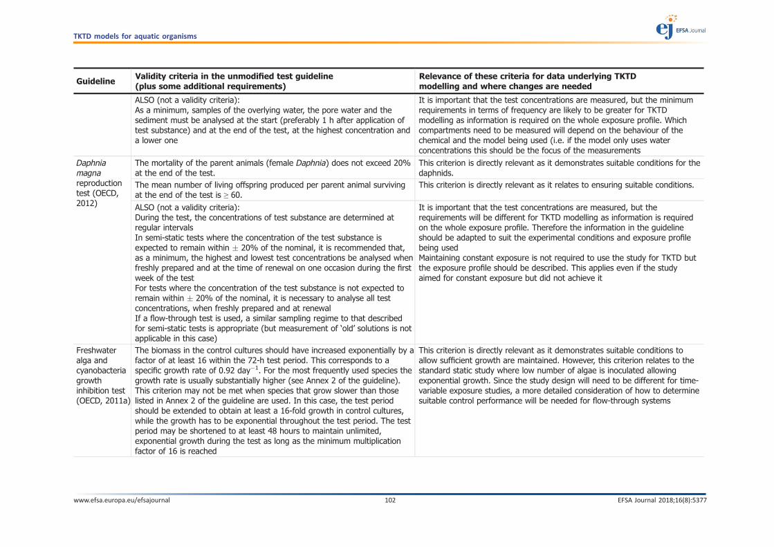
GuidelineValidity criteria in the unmodified test guideline(plus some additional requirements)
Relevance of these criteria for data underlying TKTDmodelling and where changes are needed
ALSO (not a validity criteria):As a minimum, samples of the overlying water, the pore water and thesediment must be analysed at the start (preferably 1 h after application oftest substance) and at the end of the test, at the highest concentration anda lower one
It is important that the test concentrations are measured, but the minimumrequirements in terms of frequency are likely to be greater for TKTDmodelling as information is required on the whole exposure profile. Whichcompartments need to be measured will depend on the behaviour of thechemical and the model being used (i.e. if the model only uses waterconcentrations this should be the focus of the measurements
Daphniamagnareproductiontest (OECD,2012)
The mortality of the parent animals (female Daphnia) does not exceed 20%at the end of the test.
This criterion is directly relevant as it demonstrates suitable conditions for thedaphnids.
The mean number of living offspring produced per parent animal survivingat the end of the test is ≥ 60.
This criterion is directly relevant as it relates to ensuring suitable conditions.
ALSO (not a validity criteria):During the test, the concentrations of test substance are determined atregular intervalsIn semi-static tests where the concentration of the test substance isexpected to remain within 20% of the nominal, it is recommended that,as a minimum, the highest and lowest test concentrations be analysed whenfreshly prepared and at the time of renewal on one occasion during the firstweek of the testFor tests where the concentration of the test substance is not expected toremain within 20% of the nominal, it is necessary to analyse all testconcentrations, when freshly prepared and at renewalIf a flow-through test is used, a similar sampling regime to that describedfor semi-static tests is appropriate (but measurement of ‘old’ solutions is notapplicable in this case)
It is important that the test concentrations are measured, but therequirements will be different for TKTD modelling as information is requiredon the whole exposure profile. Therefore the information in the guidelineshould be adapted to suit the experimental conditions and exposure profilebeing usedMaintaining constant exposure is not required to use the study for TKTD butthe exposure profile should be described. This applies even if the studyaimed for constant exposure but did not achieve it
Freshwateralga andcyanobacteriagrowthinhibition test(OECD, 2011a)
The biomass in the control cultures should have increased exponentially by afactor of at least 16 within the 72-h test period. This corresponds to aspecific growth rate of 0.92 day�1. For the most frequently used species thegrowth rate is usually substantially higher (see Annex 2 of the guideline).This criterion may not be met when species that grow slower than thoselisted in Annex 2 of the guideline are used. In this case, the test periodshould be extended to obtain at least a 16-fold growth in control cultures,while the growth has to be exponential throughout the test period. The testperiod may be shortened to at least 48 hours to maintain unlimited,exponential growth during the test as long as the minimum multiplicationfactor of 16 is reached
This criterion is directly relevant as it demonstrates suitable conditions toallow sufficient growth are maintained. However, this criterion relates to thestandard static study where low number of algae is inoculated allowingexponential growth. Since the study design will need to be different for time-variable exposure studies, a more detailed consideration of how to determinesuitable control performance will be needed for flow-through systems
TKTD models for aquatic organisms
www.efsa.europa.eu/efsajournal 102 EFSA Journal 2018;16(8):5377
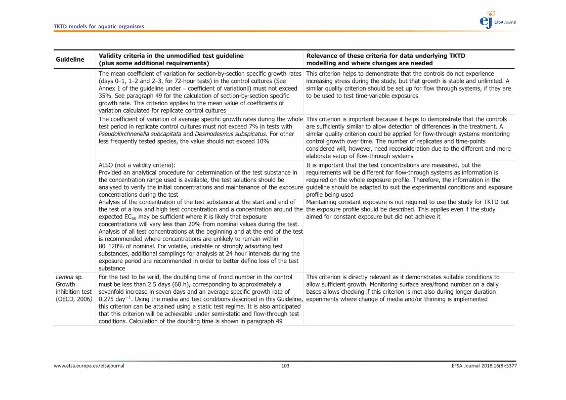
GuidelineValidity criteria in the unmodified test guideline(plus some additional requirements)
Relevance of these criteria for data underlying TKTDmodelling and where changes are needed
The mean coefficient of variation for section-by-section specific growth rates(days 0–1, 1–2 and 2–3, for 72-hour tests) in the control cultures (SeeAnnex 1 of the guideline under – coefficient of variation‖) must not exceed35%. See paragraph 49 for the calculation of section-by-section specificgrowth rate. This criterion applies to the mean value of coefficients ofvariation calculated for replicate control cultures
This criterion helps to demonstrate that the controls do not experienceincreasing stress during the study, but that growth is stable and unlimited. Asimilar quality criterion should be set up for flow through systems, if they areto be used to test time-variable exposures
The coefficient of variation of average specific growth rates during the wholetest period in replicate control cultures must not exceed 7% in tests withPseudokirchneriella subcapitata and Desmodesmus subspicatus. For otherless frequently tested species, the value should not exceed 10%
This criterion is important because it helps to demonstrate that the controlsare sufficiently similar to allow detection of differences in the treatment. Asimilar quality criterion could be applied for flow-through systems monitoringcontrol growth over time. The number of replicates and time-pointsconsidered will, however, need reconsideration due to the different and moreelaborate setup of flow-through systems
ALSO (not a validity criteria):Provided an analytical procedure for determination of the test substance inthe concentration range used is available, the test solutions should beanalysed to verify the initial concentrations and maintenance of the exposureconcentrations during the testAnalysis of the concentration of the test substance at the start and end ofthe test of a low and high test concentration and a concentration around theexpected EC50 may be sufficient where it is likely that exposureconcentrations will vary less than 20% from nominal values during the test.Analysis of all test concentrations at the beginning and at the end of the testis recommended where concentrations are unlikely to remain within80–120% of nominal. For volatile, unstable or strongly adsorbing testsubstances, additional samplings for analysis at 24 hour intervals during theexposure period are recommended in order to better define loss of the testsubstance
It is important that the test concentrations are measured, but therequirements will be different for flow-through systems as information isrequired on the whole exposure profile. Therefore, the information in theguideline should be adapted to suit the experimental conditions and exposureprofile being usedMaintaining constant exposure is not required to use the study for TKTD butthe exposure profile should be described. This applies even if the studyaimed for constant exposure but did not achieve it
Lemna sp.Growthinhibition test(OECD, 2006)
For the test to be valid, the doubling time of frond number in the controlmust be less than 2.5 days (60 h), corresponding to approximately asevenfold increase in seven days and an average specific growth rate of0.275 day�1. Using the media and test conditions described in this Guideline,this criterion can be attained using a static test regime. It is also anticipatedthat this criterion will be achievable under semi-static and flow-through testconditions. Calculation of the doubling time is shown in paragraph 49
This criterion is directly relevant as it demonstrates suitable conditions toallow sufficient growth. Monitoring surface area/frond number on a dailybases allows checking if this criterion is met also during longer durationexperiments where change of media and/or thinning is implemented
TKTD models for aquatic organisms
www.efsa.europa.eu/efsajournal 103 EFSA Journal 2018;16(8):5377
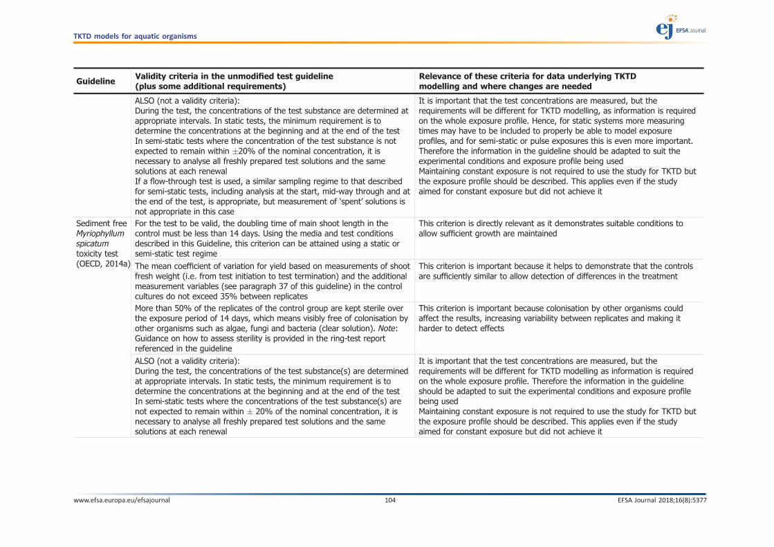
GuidelineValidity criteria in the unmodified test guideline(plus some additional requirements)
Relevance of these criteria for data underlying TKTDmodelling and where changes are needed
ALSO (not a validity criteria):During the test, the concentrations of the test substance are determined atappropriate intervals. In static tests, the minimum requirement is todetermine the concentrations at the beginning and at the end of the testIn semi-static tests where the concentration of the test substance is notexpected to remain within 20% of the nominal concentration, it isnecessary to analyse all freshly prepared test solutions and the samesolutions at each renewalIf a flow-through test is used, a similar sampling regime to that describedfor semi-static tests, including analysis at the start, mid-way through and atthe end of the test, is appropriate, but measurement of ‘spent’ solutions isnot appropriate in this case
It is important that the test concentrations are measured, but therequirements will be different for TKTD modelling, as information is requiredon the whole exposure profile. Hence, for static systems more measuringtimes may have to be included to properly be able to model exposureprofiles, and for semi-static or pulse exposures this is even more important.Therefore the information in the guideline should be adapted to suit theexperimental conditions and exposure profile being usedMaintaining constant exposure is not required to use the study for TKTD butthe exposure profile should be described. This applies even if the studyaimed for constant exposure but did not achieve it
Sediment freeMyriophyllumspicatumtoxicity test(OECD, 2014a)
For the test to be valid, the doubling time of main shoot length in thecontrol must be less than 14 days. Using the media and test conditionsdescribed in this Guideline, this criterion can be attained using a static orsemi-static test regime
This criterion is directly relevant as it demonstrates suitable conditions toallow sufficient growth are maintained
The mean coefficient of variation for yield based on measurements of shootfresh weight (i.e. from test initiation to test termination) and the additionalmeasurement variables (see paragraph 37 of this guideline) in the controlcultures do not exceed 35% between replicates
This criterion is important because it helps to demonstrate that the controlsare sufficiently similar to allow detection of differences in the treatment
More than 50% of the replicates of the control group are kept sterile overthe exposure period of 14 days, which means visibly free of colonisation byother organisms such as algae, fungi and bacteria (clear solution). Note:Guidance on how to assess sterility is provided in the ring-test reportreferenced in the guideline
This criterion is important because colonisation by other organisms couldaffect the results, increasing variability between replicates and making itharder to detect effects
ALSO (not a validity criteria):During the test, the concentrations of the test substance(s) are determinedat appropriate intervals. In static tests, the minimum requirement is todetermine the concentrations at the beginning and at the end of the testIn semi-static tests where the concentrations of the test substance(s) arenot expected to remain within 20% of the nominal concentration, it isnecessary to analyse all freshly prepared test solutions and the samesolutions at each renewal
It is important that the test concentrations are measured, but therequirements will be different for TKTD modelling as information is requiredon the whole exposure profile. Therefore the information in the guidelineshould be adapted to suit the experimental conditions and exposure profilebeing usedMaintaining constant exposure is not required to use the study for TKTD butthe exposure profile should be described. This applies even if the studyaimed for constant exposure but did not achieve it
TKTD models for aquatic organisms
www.efsa.europa.eu/efsajournal 104 EFSA Journal 2018;16(8):5377

GuidelineValidity criteria in the unmodified test guideline(plus some additional requirements)
Relevance of these criteria for data underlying TKTDmodelling and where changes are needed
WatersedimentMyriophyllumspicatumtoxicity test(OECD, 2014b)
For the test results to be valid, the mean total shoot length and mean totalshoot fresh weight in control plants at least double during the exposurephase of the test. In addition, control plants must not show any visualsymptoms of chlorosis and should be visibly free from contamination byother organisms such as algae and/or bacterial films on the plants, at thesurface of the sediment and in the test medium
This criterion is directly relevant as it demonstrates suitable conditions toallow sufficient growth are maintained and because contamination couldaffect the results, increasing variability between replicates and making itharder to detect effects
The mean coefficient of variation for yield based on measurements of shootfresh weight (i.e. from test initiation to test termination) in the controlcultures does not exceed 35% between replicates
This criterion is important because it helps to demonstrate that the controlsare sufficiently similar to allow detection of differences in the treatment
ALSO (not a validity criteria):The correct application of the test chemical should be supported byanalytical measurements of test chemical concentrationsWater samples should be collected for test chemical analysis shortly aftertest initiation (i.e. on the day of application for stable test chemicals or onehour after application for substances that are not stable) and at testtermination for all test concentrationsConcentrations in sediment and sediment pore-water should be determinedat test initiation and test termination, at least in the highest testconcentration, unless the test substances are known to be stable in water(> 80% of nominal). Measurements in sediment and pore-water might notbe necessary if the partitioning of the test chemical between water andsediment has been clearly determined in a water/sediment study undercomparable conditions (e.g. sediment to water ratio, application method,sediment type)See full information about analytical measurements in paragraphs 69–79
It is important that the test concentrations are measured, but therequirements will be different for TKTD modelling as information is requiredon the whole exposure profile. Therefore the information in the guidelineshould be adapted to suit the experimental conditions and exposure profilebeing usedIf a water sediment system is used this is likely to be extremely complicatedfor use in TKTD modelling because the pulses in the water and sediment willnot coincide, so additional consideration of the route of exposure and internaltransportation of chemicals between compartments is requiredMaintaining constant exposure is not required to use the study for TKTD butthe exposure profile should be described. This applies even if the studyaimed for constant exposure but did not achieve it
TKTD models for aquatic organisms
www.efsa.europa.eu/efsajournal 105 EFSA Journal 2018;16(8):5377
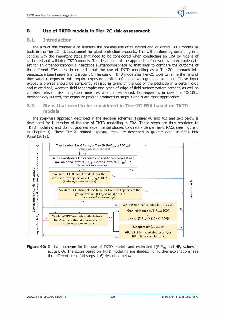
8. Use of TKTD models in Tier-2C risk assessment
8.1. Introduction
The aim of this chapter is to illustrate the possible use of calibrated and validated TKTD models astools in the Tier-2C risk assessment for plant protection products. This will be done by describing in aconcise way the important steps that need to be considered when conducting an ERA by means ofcalibrated and validated TKTD models. The description of the approach is followed by an example dataset for an organophosphorus insecticide (Organophosphate A) that aims to compare the outcome ofthe different ERA tiers, in order to put the use of TKTD modelling as a Tier-2C approach intoperspective (see Figure 6 in Chapter 3). The use of TKTD models as Tier-2C tools to refine the risks oftime-variable exposure will require exposure profiles of an active ingredient as input. These inputexposure profiles should be sufficiently realistic in terms of the use of the pesticide in a certain cropand related soil, weather, field topography and types of edge-of-field surface waters present, as well asconsider relevant risk mitigation measures when implemented. Consequently, in case the FOCUSswmethodology is used, the exposure profiles produced in steps 3 and 4 are most appropriate.
8.2. Steps that need to be considered in Tier-2C ERA based on TKTDmodels
The step-wise approach described in the decision schemes (Figures 40 and 41) and text below isdeveloped for illustration of the use of TKTD modelling in ERA. These steps are thus restricted toTKTD modelling and do not address experimental studies to directly derive Tier-2 RACs (see Figure 6in Chapter 3). These Tier-2C refined exposure tests are described in greater detail in EFSA PPRPanel (2013).
Figure 40: Decision scheme for the use of TKTD models and estimated L(E)P50 and HP5 values inacute ERA. The boxes based on TKTD modelling are shaded. For further explanations, seethe different steps (ad steps 1–6) described below
TKTD models for aquatic organisms
www.efsa.europa.eu/efsajournal 106 EFSA Journal 2018;16(8):5377

Step 1
Identify the taxonomic groups of aquatic organisms potentially at risk in the acute and chronic riskassessment for the substance of concern, informed by the relevant PECs (e.g. FOCUS step 3 or 4) andRACs derived by means of the Tier-1, and if available, the Tier-2A and/or Tier-2B effect assessmentapproaches. Collect the annual exposure profiles for all relevant exposure scenarios and determinewhether a Tier-2C approach using TKTD modelling may be a suitable approach to better describe therisks of time-variable exposures in every situation. However, TKTD modelling is more likely to behelpful to refine the risk if the exposure profiles are characterised by one or more pulse durationsassociated with the PECmax that are smaller than the durations of the toxicity tests that drive the risk.If the PECsw;max is larger but the corresponding PECsw;twa (time-window smaller than the duration ofthe toxicity test that drives the risk) is smaller than the Tier-1 RACsw;ch, this information can be usedas an indication that TKTD modelling may be an appropriate Tier-2C approach. If TKTD modelling isconsidered to be helpful to refine the risks, go to step 2.
Step 2
If, based on laboratory tests, the toxicity of the most sensitive additional test species (for thetaxonomic group identified to be at risk) deviates more than an order of magnitude from any otherTier-1 or additional test species, a risk assessment using a validated TKTD model for that particularlysensitive species (at least one order of magnitude more sensitive) is considered a cost-effective andappropriate approach. If not, in first instance, a Tier-2C1 assessment based on TKTD models for theTier-1 standard test species at risk should be explored.
Step 3 (Tier-2C2 based on TKTD modelling for species that are at least one order of magnitude moresensitive than others)
A validated TKTD model for the particularly sensitive species and the substance of concern is used.Use in first instance the complete annual exposure profiles to calculate LPx and/or EPx values. In theacute risk assessment, the EP50 value for this species (or LP50 value for a fish/amphibian) for eachrelevant annual exposure profile should at least be larger than 100. In the chronic risk assessment, theEP10 (or currently EP50 for primary producers) should at least be larger than 10.
Figure 41: Decision scheme for the use of TKTD models and estimated EP10/EP50 and HP5 values inchronic ERA. The boxes based on TKTD modelling are shaded. For further explanations,see the different steps (ad steps 1–6) described below
TKTD models for aquatic organisms
www.efsa.europa.eu/efsajournal 107 EFSA Journal 2018;16(8):5377

Step 4 (Tier-2C1 based on TKTD models for standard test species)
If only toxicity estimates for Tier-1 standard test species are available, or the lowest toxicityestimate for additional test species (Tier-2A; Tier-2B) of the sensitive taxonomic group does notdeviate more than one order of magnitude from any other test species, a Tier-2C1 assessment isproposed. In this approach, validated TKTD models for the standard (Tier-1) test species of thetaxonomic groups at risk and the substance of concern are used. Use the complete annual exposureprofiles to calculate LPx and/or EPx values, i.e. LP50 for fish and amphibians and/or EP50 values forinvertebrates (considering immobility) in the acute risk assessment, and in the chronic risk assessmentEP10 values for aquatic animals and EP50 values for aquatic algae and vascular plants.
In the acute risk assessment, the exposure profile-specific LP50/EP50 value for all relevant Tier-1species should at least be equal or larger than the acute Tier-1 AF of 100 for risks to be consideredlow. In the chronic risk assessment, the exposure profile-specific EP10 values (all relevant Tier-1animals) and the exposure-profile-specific EP50 values (relevant algae and/or aquatic macrophytes)should at least be equal or larger than the chronic Tier-1 AF of 10 for risks to be considered low. Notethat in a future update of the Aquatic Guidance Document, the effect assessment procedure foraquatic primary producers may be sharpened by using other criteria in lower-tier assessments (i.e. adifferent ErCx and/or a different AF); the exposure-profile-specific EPx values would then be selectedaccordingly.
Step 5 (Tier-2C2 based on TKTD models including standard and additional test species)
For the substance of concern, use validated TKTD models for the Tier-1 and additional test speciesof the sensitive taxonomic group(s) at risk.
If for less than eight aquatic invertebrates and/or primary producers or for less than five fish species,appropriate TKTD models are made available, the calculated LP50/EP50/EP10 values for the differentspecies and relevant annual exposure profiles may be used by adopting the geometric mean approach(currently predominantly in acute risk assessment only) and/or a WoE approach (go to step 5A).
If for at least eight aquatic invertebrates and/or primary producers or for at least five fish species,appropriate TKTD models are made available, the calculated LP50/EP50/EP10 values for the differentspecies and relevant annual exposure profiles may be used by adopting the SSD approach (go to step 5B).
Step 5A (Tier-2C2; geometric mean approach and weight-of-evidence approach
When using the acute Tier-2C2 geometric mean approach, the rules as described in EFSA PPRPanel (2013) should be followed. In this approach, the geometric mean LP50/EP50 values are calculatedfor all relevant taxonomic groups separately (e.g. in insecticide risk assessments for crustaceans andinsects separately, while this may be more taxonomic groups for fungicides). The exposure profile-specific geometric mean LP50/EP50 values for all relevant taxonomic groups should be related to amultiplication factor (margin of safety) greater than or equal to 100 (the Tier-1 AF) for risks to beconsidered acceptable.
In principle, the WoE approach might also be used in the acute risk assessment as an alternative(or validity check) for the geometric mean approach. Then, the lowest EP50 (or LP50 in case of fish)should be equal or larger than e.g. the AF used in the acute Tier-2A WoE approach (see proposal byEFSA PPR Panel, 2015). So, depending on the number of species for which TKTD models are availablefor the substance of concern, the lowest LP50/EP50 for each relevant annual exposure profile should atleast be larger than 10 but may be smaller than 100.
When using the chronic Tier-2C2 WoE approach, the suggestions by EFSA PPR Panel (2015)concerning a reduced AF and the recommendations of EFSA PPR Panel (2013) concerning theendpoints to select, should be considered. In this approach, for each relevant exposure profile thelowest EP10 (or currently EP50 for primary producers) value calculated for the different species isselected. In the chronic risk assessment, the lowest EP10 (or currently EP50 for primary producers) ofeach relevant exposure profile should be equal to or larger than the AF that normally would be used inthe chronic Tier-2A WoE approach. So, depending on the number of species for which TKTD modelsare available for the substance of concern, the lowest EP10 (or currently EP50 for primary producers)should at least be larger than 4 but may be smaller than 10 (see proposal by EFSA PPR Panel, 2015).
In the near future, guidance should be developed on the rationale underlying the reduction of theAF when using the WoE approach in the acute and chronic risk assessment, based on the quantity andquality of the additional toxicity data made available.
TKTD models for aquatic organisms
www.efsa.europa.eu/efsajournal 108 EFSA Journal 2018;16(8):5377

Step 5B (Tier-2C2; SSD approach)
When using the acute Tier-2C2 SSD approach, the rules as described in EFSA PPR Panel (2013)should be followed. In this approach, for each relevant annual exposure profile the LP50/EP50 or EP10calculated for the different species are used to construct exposure profile-specific SSD graphs. The HP5from these SSDs (exposure profile-specific HP5) is the exposure profile derived from the modelledexposure profile that causes a specified effect on 5% of the species tested. For risk assessment, themedian HP5 is selected. In the acute risk assessment for aquatic invertebrates, this median HP5 (basedon acute toxicity data) should at least be equal to or larger than 3–6 (the AF used in the acute Tier-2Beffect assessment), while for aquatic vertebrates this median HP5 should at least be equal or largerthan 9. In the chronic risk assessment (based on chronic toxicity data), the median HP5 should at leastbe greater than or equal to 3 (the AF used in the chronic Tier-2B effect assessment), both for aquaticplants and animals.
Step 6
If risks on the aquatic taxonomic groups of concern cannot be excluded in Tier-2C1 or Tier-2C2assessments when considering the whole annual exposure profile, the substance and species-specificvalidated TKTD models may be used to evaluate the potential risks of a shorter time window withinthe annual exposure profile. Indeed, in the first step, it is considered that the same individual (foranimals) or entity (cell for algae, frond for Lemna, shoot for rooted macrophytes) is present over thewhole year whereas some species have a shorter life expectancy. Therefore, as a second step, it isproposed to use a reduced time-window which should however be larger than the worst-case estimateof the maximum life expectancy of individuals of the test species of concern that drive the risk. Thefull annual exposure profile should be evaluated by a moving time-window approach and selecting thelowest LP50/EP50/EP10 value for use in the risk assessment as described in Tier-2C1 or Tier-2C2. It canbe argued that considering yearly profiles even for short living organisms rather than selecting areduced time-window would be a conservative approach that enables to address potential transfer ofPPP to the next generations. This however may be in conflict with other tiers within the sameassessment scheme, since potential multigeneration effects are not considered in Tier-1, Tier-2A andTier-2B, nor in Tier-3 micro/mesocosm experiments for those species that have a life cycle longer thanthe duration of these semi-field tests (e.g. univoltine and semivoltine taxa).
8.3. Example data set on how to use GUTS in the ERA forOrganophosphate A
8.3.1. Introduction
This example data set is based on realistic ecotoxicological data for an organophosphorusinsecticide selected as benchmark compound to scientifically underpin the tiered aquatic riskassessment procedure. The presented field exposure concentrations are semi-realistic in that they arebased on realistic exposure concentrations for the benchmark compound but adapted by introducingmitigation measures in such a way that they better fit the goal of the case study. This case study aimsto explore how GUTS modelling can be used as a Tier-2C approach in the environmental riskassessment. In addition, this case study aims to compare the outcome of the different effectassessment tiers to put the use of TKTD modelling as a Tier-2C approach into perspective.
8.3.2. Exposure concentrations in surface waters
FOCUS predictions for six relevant exposure scenarios (A–F) for different crops are selected, fourdrift (A, C, D and E) and two run-off scenarios (B and F). In addition, five of these scenarios representstreams (scenarios A, B, C, D and F) and one ditches (scenario E) (see Table 7 and Figure 42).
TKTD models for aquatic organisms
www.efsa.europa.eu/efsajournal 109 EFSA Journal 2018;16(8):5377

The insecticide is applied once a year and a spray drift causes the peak exposure, but in the run-offscenarios the drift exposure peaks are followed by lower run-off exposure peaks. The calculated PECsw;max
values for the scenarios vary from 0.029 to 0.035 lg/L (Table 7). The highest 7-day time-weightedaverage PECs (PECsw;7d-twa) values vary from 0.00019 to 0.00082 lg/L; a 7-d time-window is consideredsuitable in this context dealing with chronic tests on invertebrates. Although the PECsw;max value for ditchscenario E is lower than that for most stream scenarios, its PECsw;7d-twa value is the highest. This can beexplained by the much slower water flow in the ditch D6 scenario than in the stream scenarios. Exposureprofiles for the six scenarios are presented in Figure 42.
Table 7: Characteristics of the exposure scenarios for the example data set of Organophosphate A
Scenario CropFOCUS water bodytype and scenario
PECsw;max
(lg/L)PECsw;7d-twa
(lg/L)
A Legumes Stream D5 0.035 0.00019
B Vines Stream R3 0.034 0.00033C Pome Stream D5 0.031 0.00014
D Maize Stream D5 0.030 0.00035E Maize Ditch D6 0.029 0.00082
F Maize Stream R3 0.029 0.00054
Figure 42: Exposure profiles for scenarios A–F (see Table 10). The Tier-1 RACs are plotted in theprofiles (see Section 8.4.1)
TKTD models for aquatic organisms
www.efsa.europa.eu/efsajournal 110 EFSA Journal 2018;16(8):5377
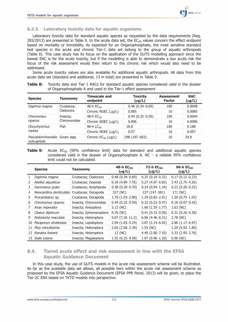
8.3.3. Laboratory toxicity data for aquatic organisms
Laboratory toxicity data for standard aquatic species as requested by the data requirements (Reg.283/2013) are presented in Table 8. In the acute data set, the EC50 values concern the effect endpointbased on mortality or immobility. As expected for an Organophosphate, the most sensitive standardtest species in the acute and chronic Tier-1 data set belong to the group of aquatic arthropods(Table 8). This case study has its focus on the application of the GUTS modelling approach since thelowest RAC is for the acute toxicity, but if the modelling is able to demonstrate a low acute risk thefocus of the risk assessment would then return to the chronic risk which would also need to beaddressed.
Some acute toxicity values are also available for additional aquatic arthropods. All data from thisacute data set (standard and additional, 13 in total) are presented in Table 9.
8.4. Tiered acute effect and risk assessment in line with the EFSAAquatic Guidance Document
In this case study, the use of GUTS models in the acute risk assessment scheme will be illustrated.As far as the available data set allows, all possible tiers within the acute risk assessment scheme asproposed by the EFSA Aquatic Guidance Document (EFSA PPR Panel, 2013) will be given, to place theTier-2C ERA based on TKTD models into perspective.
Table 9: Acute EC50 (95% confidence limit) data for standard and additional aquatic speciesconsidered valid in the dossier of Organophosphate A. NC = a reliable 95% confidencelimit could not be calculated
Species Taxonomy48-h EC50
(lg/L)72-h EC50
(lg/L)96-h EC50
(lg/L)
1 Daphnia magna Crustacea; Cladocera 0.48 (0.34–0.69) 0.25 (0.19–0.32) 0.17 (0.12–0.23)
2 Asellus aquaticus Crustacea; Isopoda 6.16 (4.89–7.76) 5.27 (4.07–6.82) 3.43 (2.75–4.26)3 Gammarus pulex Crustacea; Amphipoda 0.38 (0.20–0.70) 0.24 (0.04–1.34) 0.23 (0.20–0.25)
4 Neocaridina denticulata Crustacea; Decapoda 327 (NC) 237 (147–381) 171 (NC)5 Procambarus sp. Crustacea; Decapoda 1.70 (1.03–2.80) 1.29 (0.82–2.01) 1.20 (0.75–1.93)
6 Chironomus riparius Insecta; Chironomidae 0.44 (0.32–0.59) 0.32 (0.22–0.47) 0.18 (0.07–0.43)7 Anax imperator Insecta; Anisoptera 3.13 (NC) 1.66 (1.55–1.77) 1.63 (NC)
8 Cloeon dipterum Insecta; Ephemeroptera 0.76 (NC) 0.41 (0.33–0.50) 0.31 (0.26–0.38)9 Notonecta maculata Insecta; Heteroptera 9.07 (7.18–11.5) 6.06 (4.46–8.31) 2.78 (NC)
10 Paraponyx stratiotata Insecta; Lepidoptera 2.94 (1.65–5.24) 3.87 (2.14–6.92) 2.86 (1.17–6.97)11 Plea minutissima Insecta; Heteroptera 2.65 (2.06–3.39) 1.55 (NC) 1.29 (0.92–1.80)
12 Ranatra linearis Insecta; Heteroptera 12 (NC) 4.40 (2.80–7.10) 3.33 (2.95–3.76)
13 Sialis lutaria Insecta; Megaloptera 1.55 (0.25–9.58) 1.07 (0.96–1.20) 0.96 (NC)
Table 8: Toxicity data and Tier 1 RACs for standard aquatic species considered valid in the dossierof Organophosphate A and used in the Tier-1 effect assessment
Species TaxonomyTimescale andendpoint
Toxicity(lg/L)
AssessmentFactor
RAC(lg/L)
Daphnia magna Crustacea;Cladocera
48-h EC50 0.48 (0.34–0.69) 100 0.0048
Chronic NOEC (lg/L) 0.085 10 0.0085Chironomusriparius
Insecta;Chironomidae
48-h EC50 0.44 (0.32–0.59) 100 0.0044
Chronic NOEC (lg/L) 0.096 10 0.0096Oncorhynchusmykiss
Fish 96-h LC50 18.8 100 0.188
Chronic NOEC (lg/L) 0.57 10 0.057
Pseudokirchneriellasubcapitata
Green alga Chronic EC50 (lg/L) 298 (197–603) 10 29.8
TKTD models for aquatic organisms
www.efsa.europa.eu/efsajournal 111 EFSA Journal 2018;16(8):5377

8.4.1. Tier-1 acute effect and risk assessment
Tier-1 acute effect assessment
The Tier-1 arthropods (D. magna and Chironomus riparius) are more sensitive than the Tier-1 fishOncorhynchus mykiss (Table 9). By applying an AF of 100 to the lowest toxicity value of 0.44 lg/L (48-h EC50) for Chironomus riparius, the Tier-1 RACsw;ac becomes 0.0044 lg/L.
Tier-1 acute risk assessment
The acute Tier-1 RAC is always compared with PECsw;max values. The outcome of the Tier-1 riskassessment procedure is presented in Table 10. If the PEC:RAC ratio is lower than 1, then theenvironmental risk is considered low. From the results presented in Table 10 it appears that whencomparing the acute Tier-1 RACs with the PECsw;max, potential environmental risks are triggered for allexposure scenarios.
8.4.2. Tier-2A effect and risk assessment
A Tier-2A approach may comprise the geometric mean approach based on experimental data asproposed in the EFSA PPR Panel Aquatic Guidance Document (EFSA PPR Panel, 2013) or a WoEapproach as proposed in the EFSA PPR Panel sediment opinion (EFSA PPR Panel, 2015) when theGeometric mean is not appropriate (e.g. if different endpoints are measured in tests within species ofthe same relevant taxonomic group).
Tier-2A acute effect assessment (Geometric Mean approach)
In total for 13 aquatic arthropods (5 crustaceans and 8 insect taxa) 96-h EC50 values are available(Table 11). Consequently, this data set allows the Tier-2B (SSD) approach (see Section 8.4.3).However, to illustrate the Geometric Mean approach, and to make this case more realistic, the 96-hEC50 values for a lower number of aquatic species are selected in Table 11. The selected additionalspecies are frequently tested in toxicity experiments, since they are abundant in freshwaterecosystems and can be easily kept under laboratory conditions.
Table 10: Tier-1 risk assessment procedure for Organophosphate A. If the PEC:RAC ratio is lowerthan 1, then the environmental risk is considered low
Scenario
Acute risk assessment
PECsw;max
(lg/L)Tier-1 RACsw;ac
(lg/L)PECsw;max:
RACsw;ac ratio
A 0.035 0.0044 7.95
B 0.034 0.0044 7.73C 0.031 0.0044 7.05
D 0.030 0.0044 6.82E 0.029 0.0044 6.59
F 0.029 0.0044 6.59
Table 11: Acute EC50 (95% confidence limit) data for standard and additional aquatic speciesconsidered realistic to explore the Tier-2A effect assessment approach
Species Taxonomy 96-h EC50 (lg/L)(a)
1 Daphnia magna Crustacea; Cladocera 0.17 (0.12–0.23)
2 Asellus aquaticus Crustacea; Isopoda 3.43 (2.75–4.26)3 Gammarus pulex Crustacea; Amphipoda 0.23 (0.20–0.25)
4 Chironomus riparius Insecta; Chironomidae 0.18 (0.07–0.43)5 Cloeon dipterum Insecta; Ephemeroptera 0.31 (0.26–0.38)
6 Plea minutissima Insecta; Heteroptera 1.29 (0.92–1.80)Geometric mean 96-h EC50 for crustaceans 0.51
Geometric mean 96-h EC50 for insects 0.42
(a): Note that for Daphnia magna and Chironomus riparius the 48 h endpoint is normally selected for risk assessment but in thiscase the 96 h endpoints were used.
TKTD models for aquatic organisms
www.efsa.europa.eu/efsajournal 112 EFSA Journal 2018;16(8):5377

The geometric mean 96-h EC50 value for the three crustaceans is 0.51 lg/L. The geometric mean96-h EC50 value for the three insects is 0.42 lg/L. Selecting the lowest value (0.42 lg/L for insects)and applying an AF of 100 results in a Tier-2A RACsw;ac of 0.0042 lg/L.
Tier-2A acute risk assessment (geometric mean approach)
The Tier-2A RAC based on standard and additional laboratory toxicity data is always compared withPECsw;max values. The outcome of the acute Tier-2A risk assessment procedure is presented inTable 12. If the PEC:RAC ratio is lower than 1, then the environmental risk is considered to be low.From the results presented in Table 12, it appears that when comparing the acute Tier-2A RACs withthe PECsw;max, potential environmental risks are triggered for all exposure scenarios.
8.4.3. Tier-2B effect and risk assessment
A Tier-2B approach (SSD approach) is possible for the acute data set since for more than 8different taxa of the sensitive taxonomic group (arthropods) laboratory toxicity data are available.
Tier-2B acute effect assessment (SSD approach)
For the SSD approach, the 96-h EC50 data mentioned in Table 9 are used. The SSD constructedwith the 96-h EC50 values for the 13 different aquatic arthropods is presented in Figure 43.
Several valid approaches can be used to construct SSDs and to calculate HC5 values. As anexample the computer program described by Charles et al. (2017) to calculate HC5 values is selected,since it allows to use censored data and 95% confidence limits of toxicity estimates as input data.Using the approach described in Charles et al. (2017) and a log-normal distribution, the median HC5
value (and 95% confidence interval) on basis of 96-h EC50 values for all aquatic arthropods (n = 13) is:0.079 (0.031–0.370) lg/L. According to EFSA PPR Panel (2013) an AF of 3 to 6 should be applied tothe median HC5. This results in a Tier-2B RACsw;ac of 0.0132–0.0263 lg/L.
Table 12: Tier-2A risk assessment procedure for Organophosphate A. If the PEC:RAC ratio is lowerthan 1, then the environmental risk is considered low
Scenario
Acute risk assessment
PECsw;max
(lg/L)Tier-2A
RACsw;ac (lg/L)PECsw;max:
RACsw;ac ratio
A 0.035 0.0042 8.33
B 0.034 0.0042 8.10C 0.031 0.0042 7.38
D 0.030 0.0042 7.14E 0.029 0.0042 6.90
F 0.029 0.0042 6.90
Figure 43: SSD graph constructed with 96-h EC50 values for 13 different arthropods presented inTable 9
TKTD models for aquatic organisms
www.efsa.europa.eu/efsajournal 113 EFSA Journal 2018;16(8):5377
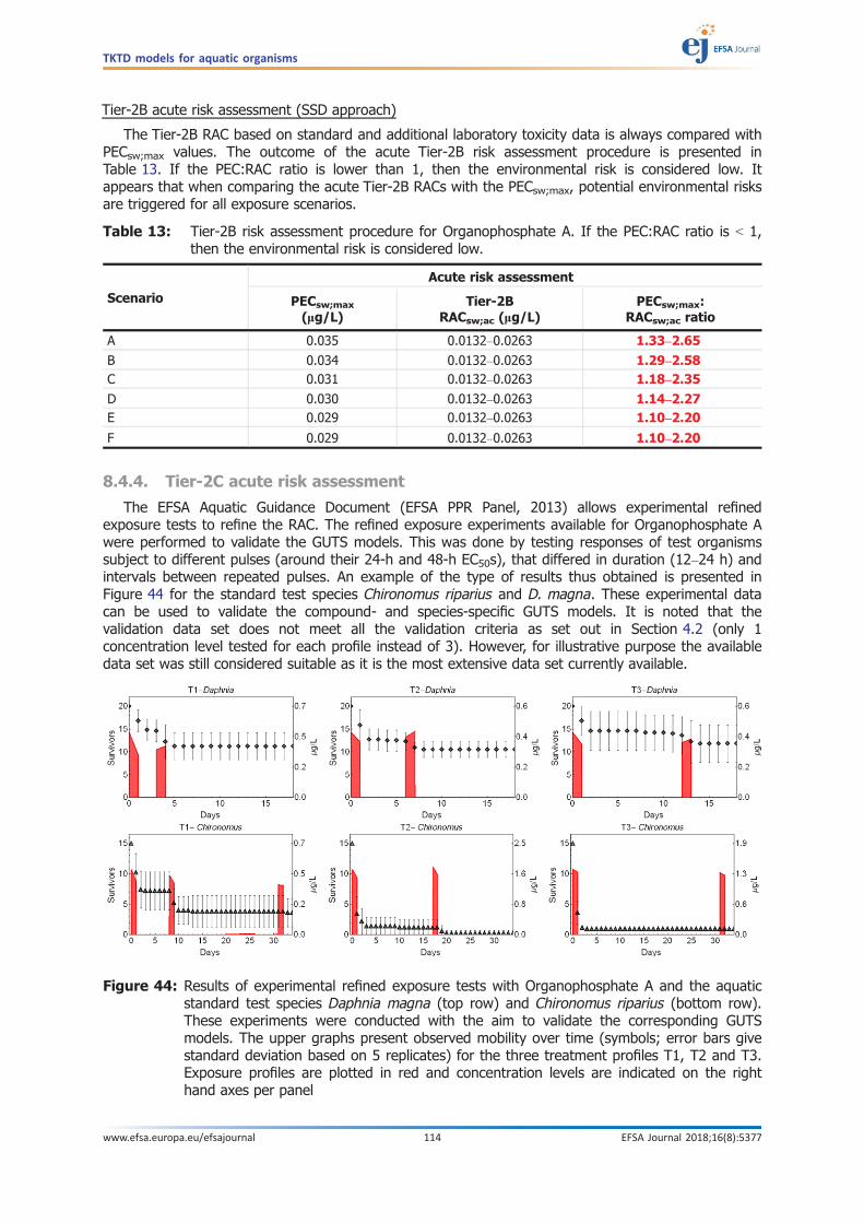
Tier-2B acute risk assessment (SSD approach)
The Tier-2B RAC based on standard and additional laboratory toxicity data is always compared withPECsw;max values. The outcome of the acute Tier-2B risk assessment procedure is presented inTable 13. If the PEC:RAC ratio is lower than 1, then the environmental risk is considered low. Itappears that when comparing the acute Tier-2B RACs with the PECsw;max, potential environmental risksare triggered for all exposure scenarios.
8.4.4. Tier-2C acute risk assessment
The EFSA Aquatic Guidance Document (EFSA PPR Panel, 2013) allows experimental refinedexposure tests to refine the RAC. The refined exposure experiments available for Organophosphate Awere performed to validate the GUTS models. This was done by testing responses of test organismssubject to different pulses (around their 24-h and 48-h EC50s), that differed in duration (12–24 h) andintervals between repeated pulses. An example of the type of results thus obtained is presented inFigure 44 for the standard test species Chironomus riparius and D. magna. These experimental datacan be used to validate the compound- and species-specific GUTS models. It is noted that thevalidation data set does not meet all the validation criteria as set out in Section 4.2 (only 1concentration level tested for each profile instead of 3). However, for illustrative purpose the availabledata set was still considered suitable as it is the most extensive data set currently available.
Table 13: Tier-2B risk assessment procedure for Organophosphate A. If the PEC:RAC ratio is < 1,then the environmental risk is considered low.
Scenario
Acute risk assessment
PECsw;max
(lg/L)Tier-2B
RACsw;ac (lg/L)PECsw;max:
RACsw;ac ratio
A 0.035 0.0132–0.0263 1.33–2.65
B 0.034 0.0132–0.0263 1.29–2.58C 0.031 0.0132–0.0263 1.18–2.35
D 0.030 0.0132–0.0263 1.14–2.27E 0.029 0.0132–0.0263 1.10–2.20
F 0.029 0.0132–0.0263 1.10–2.20
Figure 44: Results of experimental refined exposure tests with Organophosphate A and the aquaticstandard test species Daphnia magna (top row) and Chironomus riparius (bottom row).These experiments were conducted with the aim to validate the corresponding GUTSmodels. The upper graphs present observed mobility over time (symbols; error bars givestandard deviation based on 5 replicates) for the three treatment profiles T1, T2 and T3.Exposure profiles are plotted in red and concentration levels are indicated on the righthand axes per panel
TKTD models for aquatic organisms
www.efsa.europa.eu/efsajournal 114 EFSA Journal 2018;16(8):5377

The available experimental data allowed development of calibrated and validated GUTS models forall aquatic arthropods based on raw data delivering the relevant endpoint (calibration data as thosedelivering effect values reported in Table 9; validation data of the type shown in Figure 44). TheseGUTS models were used to assess the potential environmental risks for annual exposure profiles A–F.
Tier-2C1 acute risk assessment
Since at first, TKTD models for Tier-1 species will be usually used in refined risk assessment (seethe steps described in Section 8.2), the GUTS modelling approach was used to evaluate the potentialrisks of the time-variable exposure profiles on the standard test species D. magna and Chironomusriparius (the acute Tier-2C1 approach). This is done by calculating EP50 values (based on the sumof dead and immobile individuals) for these species. In order not to be in conflict with the Tier-1 effectassessment approach, the EP50 values should at least be equal to or larger than the multiplicationfactor (margin of safety) of 100 (the acute Tier-1 AF). The EP50 values calculated by the GUTS-RED-SDand GUTS-RED-IT models for the standard test species D. magna and C. riparius are presented inTable 14.
When using the GUTS-RED-SD models, it appears that for all scenarios (A–F), risks are triggered(EP50 values for both standard test species should be greater than or equal to 100). The output of theGUTS-RED-IT models indicates that the risk is low in exposure scenario C only.
Tier-2C2 acute risk assessment
A more advanced approach is to calculate EP50 values for standard and additional aquatic taxa forwhich GUTS models are already developed (the acute Tier-2C2 approach). The Tier-2C2 GeometricMean approach normally will be used to assess the risks for the insecticide (Organophosphate A) if forless than eight aquatic arthropods calibrated/validated GUTS models are available. In Tables 15(GUTS-RED-SD model calculations) and 16 (GUTS-RED-IT model calculations), this is explored basedon the species also presented in Table 11.
Table 14: Calculated EP50 values and 95% confidence limits for the Tier-1 aquatic arthropods andexposure profiles A–F by using the GUTS-RED-SD and GUTS-RED-IT model
Exposure scenario
A B C D E F
EP50 values for the different exposure scenarios and GUTS-RED-SD
Daphnia magna 13 (7–61) 5 (2–33) 18 (11–83) 7 (4–35) 3 (2–14) 5 (3–25)Chironomus riparius 93 (75–122) 38 (28–52) 127 (103–163) 51 (40–67) 23 (18–30) 37 (30–48)
EP50 values for the different exposure scenarios and GUTS-RED-ITDaphnia magna 122 (97–145) 39 (32–49) 161 (127–191) 66 (54–78) 28 (23–32) 40 (33–47)
Chironomus riparius 93 (70–111) 33 (26–44) 127 (99–143) 51 (42–60) 22 (17–26) 33 (27–39)
Table 15: Calculated EP50 values and 95% confidence limits for aquatic crustaceans and insectsmentioned in Table 11 and exposure profiles A–F by using the GUTS-RED-SD models toexplore the geometric mean approach
Exposure scenarios
A B C D E F
EP50 values GUTS-RED-SD
1 Daphniamagna
13 (7–61) 5 (2–33) 18 (11–83) 7 (4–35) 3 (2–14) 5 (3–25)
2 Asellusaquaticus
762 (250–1,285) 391 (92–635) 1,035 (340–1,682) 420 (138–682) 181 (58–305) 303 (85–587)
3 Gammaruspulex
37 (6–62) 13 (1–23) 49 (6–85) 20 (2–34) 9 (0.1–15) 13 (1–23)
GeometricmeanCrustacea
71.6 29.4 97.0 38.9 17.0 27.1
TKTD models for aquatic organisms
www.efsa.europa.eu/efsajournal 115 EFSA Journal 2018;16(8):5377
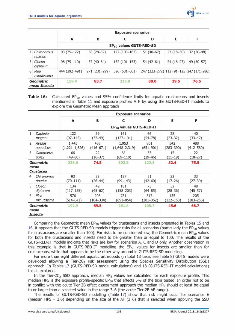
Comparing the Geometric mean EP50 values for crustaceans and insects presented in Tables 15 and16, it appears that the GUTS-RED-SD models trigger risks for all scenarios (particularly the EP50 valuesfor crustaceans are smaller than 100). For risks to be considered low, the Geometric mean EP50 valuesfor both the crustaceans and insects need to be greater than or equal to 100. The results of theGUTS-RED-IT models indicate that risks are low for scenarios A, C and D only. Another observation inthis example is that in GUTS-RED-IT modelling the EP50 values for insects are smaller than forcrustaceans, while that appears to be the other way around in GUTS-RED-SD modelling.
For more than eight different aquatic arthropods (in total 13 taxa; see Table 8) GUTS models weredeveloped allowing a Tier-2C2 risk assessment using the Species Sensitivity Distribution (SSD)approach. In Tables 17 (GUTS-RED-SD model calculations) and 18 (GUTS-RED-IT model calculations)this is explored.
In the Tier-2C2 SSD approach, median HP5 values are calculated for each exposure profile. Thismedian HP5 is the exposure profile-specific EP50 that affects 5% of the taxa tested. In order not to bein conflict with the acute Tier-2B effect assessment approach the median HP5 should at least be equalto or larger than a selected value in the range 3–6 (the acute Tier-2B AF-range).
The results of GUTS-RED-SD modelling (Table 17) show that risk might occur for scenarios E(median HP5 = 3.6) depending on the size of the AF (3–6) that is selected when applying the SSD
Exposure scenarios
A B C D E F
EP50 values GUTS-RED-SD
4 Chironomusriparius
93 (75–122) 38 (28–52) 127 (103–163) 51 (40–67) 23 (18–30) 37 (30–48)
5 Cloeondipterum
98 (75–110) 57 (40–64) 132 (101–153) 54 (42–61) 24 (18–27) 49 (30–57)
6 Pleaminutissima
444 (392–491) 271 (231–299) 596 (531–661) 247 (223–272) 112 (91–125) 247 (171–286)
Geometricmean Insecta
159.4 83.7 215.9 88.0 39.5 76.5
Table 16: Calculated EP50 values and 95% confidence limits for aquatic crustaceans and insectsmentioned in Table 11 and exposure profiles A–F by using the GUTS-RED-IT models toexplore the Geometric Mean approach
Exposure scenarios
A B C D E F
EP50 values GUTS-RED-IT
1 Daphniamagna
122(97–145)
39(32–49)
161(127–191)
66(54–78)
28(23–32)
40(33–47)
2 Asellusaquaticus
1,445(1,221–1,626)
488(416–671)
1,953(1,648–2,319)
801(651–901)
342(283–390)
488(412–580)
3 Gammaruspulex
66(49–80)
22(16–37)
88(69–110)
35(29–46)
15(11–19)
22(18–27)
GeometricmeanCrustacea
226.6 74.8 302.5 122.8 52.4 75.5
4 Chironomusriparius
93(70–111)
33(26–44)
127(99–143)
51(42–60)
22(17–26)
33(27–39)
5 Cloeondipterum
134(117–155)
49(45–62)
181(158–203)
73(64–85)
32(28–36)
48(45–57)
6 Pleaminutissima
576(514–641)
208(184–334)
781(691–854)
317(281–352)
135(122–153)
205(183–256)
GeometricmeanInsecta
192.9 69.5 261.8 105.7 45.6 68.7
TKTD models for aquatic organisms
www.efsa.europa.eu/efsajournal 116 EFSA Journal 2018;16(8):5377

approach. When using the GUTS-RED-IT (Table 18) models the median HP5 values are equal or largerthan 8 (i.e. larger than the upper value of the AF) for all exposure scenarios, suggesting low risks ofthe time-variable exposure regimes evaluated on mortality plus immobility of aquatic arthropods.
In the example data set, the use of the GUTS-RED-SD model results in a more conservative riskassessment than the use of the GUTS-RED-IT model.
TKTD models for aquatic organisms
www.efsa.europa.eu/efsajournal 117 EFSA Journal 2018;16(8):5377
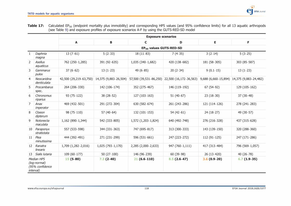
Table 17: Calculated EP50 (endpoint mortality plus immobility) and corresponding HP5 values (and 95% confidence limits) for all 13 aquatic arthropods(see Table 9) and exposure profiles of exposure scenarios A-F by using the GUTS-RED-SD model
Exposure scenarios
A B C D E F
EP50 values GUTS-RED-SD
1 Daphniamagna
13 (7–61) 5 (2–33) 18 (11–83) 7 (4–35) 3 (2–14) 5 (3–25)
2 Asellusaquaticus
762 (250–1,285) 391 (92–635) 1,035 (340–1,682) 420 (138–682) 181 (58–305) 303 (85–587)
3 Gammaruspulex
37 (6–62) 13 (1–23) 49 (6–85) 20 (2–34) 9 (0.1–15) 13 (1–23)
4 Neocaridinadenticulata
42,500 (29,219–63,750) 14,375 (9,883–26,504) 57,500 (39,531–86,250) 22,500 (16,172–36,563) 9,688 (6,660–15,894) 14,375 (9,883–24,482)
5 Procambarusspec.
264 (206–330) 142 (106–174) 352 (275–467) 146 (119–192) 67 (54–92) 129 (105–162)
6 Chironomusriparius
93 (75–122) 38 (28–52) 127 (103–163) 51 (40–67) 23 (18–30) 37 (30–48)
7 Anaximperator
469 (432–501) 291 (272–304) 630 (582–674) 261 (243–286) 121 (114–126) 278 (241–283)
8 Cloeondipterum
98 (75–110) 57 (40–64) 132 (101–153) 54 (42–61) 24 (18–27) 49 (30–57)
9 Notonectamaculata
1,162 (890–1,344) 542 (333–805) 1,572 (1,203–1,824) 640 (492–748) 276 (216–328) 437 (315–628)
10 Paraponyxstratiotata
557 (533–598) 344 (331–363) 747 (695–817) 313 (300–333) 143 (139–150) 320 (288–360)
11 Pleaminutissima
444 (392–491) 271 (231–299) 596 (531–661) 247 (223–272) 112 (91–125) 247 (171–286)
12 Ranatralinearis
1,709 (1,282–2,016) 1,025 (793–1,170) 2,285 (2,000–2,633) 947 (760–1,111) 417 (313–484) 796 (569–1,057)
13 Sialis lutaria 109 (60–177) 50 (27–100) 146 (96–239) 60 (39–98) 26 (13–420) 40 (26–78)
Median HP5(log-normal)(95% confidenceinterval)
15 (5–80) 7.3 (2–40) 21 (6.6–110) 8.5 (2.6–47) 3.6 (0.9–20) 6.7 (1.9–35)
TKTD models for aquatic organisms
www.efsa.europa.eu/efsajournal 118 EFSA Journal 2018;16(8):5377
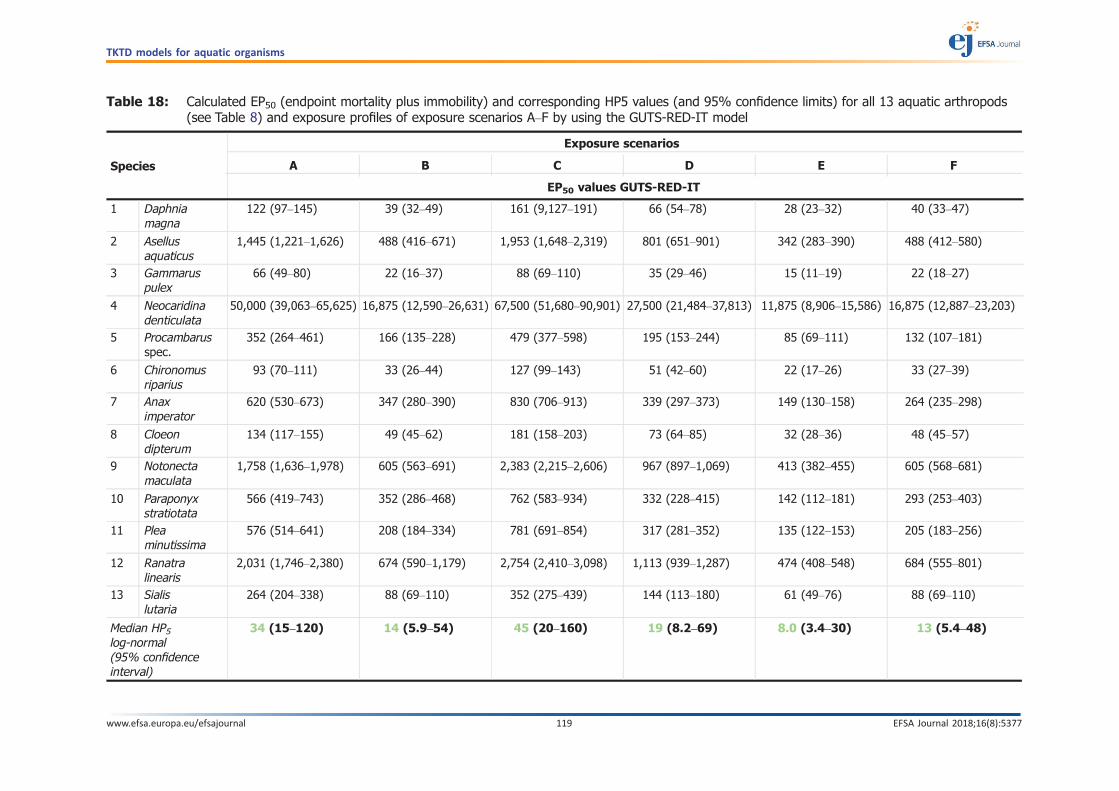
Table 18: Calculated EP50 (endpoint mortality plus immobility) and corresponding HP5 values (and 95% confidence limits) for all 13 aquatic arthropods(see Table 8) and exposure profiles of exposure scenarios A–F by using the GUTS-RED-IT model
Species
Exposure scenarios
A B C D E F
EP50 values GUTS-RED-IT
1 Daphniamagna
122 (97–145) 39 (32–49) 161 (9,127–191) 66 (54–78) 28 (23–32) 40 (33–47)
2 Asellusaquaticus
1,445 (1,221–1,626) 488 (416–671) 1,953 (1,648–2,319) 801 (651–901) 342 (283–390) 488 (412–580)
3 Gammaruspulex
66 (49–80) 22 (16–37) 88 (69–110) 35 (29–46) 15 (11–19) 22 (18–27)
4 Neocaridinadenticulata
50,000 (39,063–65,625) 16,875 (12,590–26,631) 67,500 (51,680–90,901) 27,500 (21,484–37,813) 11,875 (8,906–15,586) 16,875 (12,887–23,203)
5 Procambarusspec.
352 (264–461) 166 (135–228) 479 (377–598) 195 (153–244) 85 (69–111) 132 (107–181)
6 Chironomusriparius
93 (70–111) 33 (26–44) 127 (99–143) 51 (42–60) 22 (17–26) 33 (27–39)
7 Anaximperator
620 (530–673) 347 (280–390) 830 (706–913) 339 (297–373) 149 (130–158) 264 (235–298)
8 Cloeondipterum
134 (117–155) 49 (45–62) 181 (158–203) 73 (64–85) 32 (28–36) 48 (45–57)
9 Notonectamaculata
1,758 (1,636–1,978) 605 (563–691) 2,383 (2,215–2,606) 967 (897–1,069) 413 (382–455) 605 (568–681)
10 Paraponyxstratiotata
566 (419–743) 352 (286–468) 762 (583–934) 332 (228–415) 142 (112–181) 293 (253–403)
11 Pleaminutissima
576 (514–641) 208 (184–334) 781 (691–854) 317 (281–352) 135 (122–153) 205 (183–256)
12 Ranatralinearis
2,031 (1,746–2,380) 674 (590–1,179) 2,754 (2,410–3,098) 1,113 (939–1,287) 474 (408–548) 684 (555–801)
13 Sialislutaria
264 (204–338) 88 (69–110) 352 (275–439) 144 (113–180) 61 (49–76) 88 (69–110)
Median HP5log-normal(95% confidenceinterval)
34 (15–120) 14 (5.9–54) 45 (20–160) 19 (8.2–69) 8.0 (3.4–30) 13 (5.4–48)
TKTD models for aquatic organisms
www.efsa.europa.eu/efsajournal 119 EFSA Journal 2018;16(8):5377

8.4.5. Tier-3 risk assessment
In the dossier, information on a mesocosm study (experimental ponds) conducted withOrganophosphate A is available. In this experimental pond study, the insecticide was applied once andfour exposure concentrations were studied (measured peak concentrations 0.1, 0.9, 6 and 44 lg a.s./L)(Figure 45).
The experimental pond study had a diverse community of aquatic invertebrates and a sufficientnumber of aquatic arthropods were present with a high enough minimum detectable difference (MDD)to consider the study valid. Effect classes (see EFSA PPR Panel, 2013) for the different treatments andmost sensitive endpoints are provided in Table 19.
At the community level (using Principal Response Curves) a NOEC (Effect class 1) of 0.1 lg a.s./Lcould be derived for both the zooplankton and macroinvertebrate community but themacroinvertebrate community showed an overall slower recovery than the zooplankton community. Atthe population-level the most sensitive aquatic arthropod (G. pulex) showed a small treatment-relatedeffect on an isolated sampling in the 0.1 lg a.s./L treatment while all other invertebrate taxa did notshow treatment-related effects. In the 0.9 lg a.s./L treatment the microcrustacean Daphnia galeataand the insects Cloeon diperum and Caenis horaria showed short-term responses on severalconsecutive samplings (Effect class 3A) while G pulex showed a long-term response (Effect class 5B).At the two highest treatment levels, several arthropod populations showed long-term effects.
Assuming that the exposure profile studied in the experimental ponds was realistic-worst case andfollowing EFSA PPR Panel (2013), a Tier-3 ETO-RACsw (ecological threshold option) can be derivedfrom the experimental pond study by applying an AF of 2–3 to the Effect class 2 concentration of 0.1lg a.s./L, resulting in a Tier-3 ETO-RACsw of 0.033–0.05 lg a.s./L. A comparison of the Tier-3RACsw (0.033–0.05 lg/L) with the PECsw;max values as calculated for the different exposure scenariosillustrate that the environmental risks are most likely small to negligible for the exposure scenariosevaluated (see Table 20).
Figure 45: Dynamics of mean concentrations of Organophosphate A in depth-integrated watersamples in experimental ponds treated once with 0.1, 0.9, 6 and 44 lg a.s./L
Table 19: Effect classes (in lg a.s./L) of the most sensitive community- and population-levelendpoints in the experimental pond study that studied the impact of a single applicationof the insecticide Organophosphate A
Treatment-level (measured peak exposure ofOrganophosphate A in lg a.s./L)
0.1 0.9 6 44
Macroinvertebrate community Effect class 1 Effect class 3A Effect class 5B Effect class 5B
Most sensitive arthropod population(Gammarus pulex)
Effect class 2 Effect class 5B Effect class 5B Effect class 5B
TKTD models for aquatic organisms
www.efsa.europa.eu/efsajournal 120 EFSA Journal 2018;16(8):5377

The available experimental pond study can also be used to put the Tier-2C risk assessment basedon GUTS models into perspective of the tiered approach. According to the principles of the tieredapproach, a lower-tier assessment should be more conservative than a higher-tier assessment.Consequently, the Tier-2C risk assessment based on GUTS models should be more conservative than aTier-3 risk assessment (based on semi-field (micro/mesocosm) data). This can be evaluated by usingthe exposure profile with a peak concentration of 0.1 lg/L simulated in the experimental pond study(see Figure 45) as input for the available GUTS models used in the Tier-2C2 SSD approach. For aproper comparison, the exposure profile of the 0.1 lg/L treatment (the Effect class 2 concentration)needs to be divided by a factor of 2 or 3 (corresponding to the range in AFs used to derive a Tier-3ETO-RAC based on an Effect class 2 concentration proposed by EFSA PPR Panel, 2013) to get EP50values that correspond with the Tier-3 RACsw (Table 21).
It appears that the median HP5 values (1.8–2.8) calculated from the SSD of the EP50 valuescorresponding to the liberal ETO-RAC (using and AF of 2 to extrapolate the Effect class 2concentration) and the two types of GUTS models are smaller than 3-6, the range in AF used in theTier-2C2 SSD approach (see Section 8.4.4). Also, when using the GUTS-RED-SD model, the medianHP5 value (2.5) obtained for EP50 values corresponding to the conservative ETO-RAC (using and AFof 3 to extrapolate the Effect class 2 concentration) is smaller than 3-6. Only when using theGUTS-RED-IT model, the median HP5 value (4.4) obtained for EP50 values corresponding to theconservative ETO-RAC (using and AF of 3 to extrapolate the Effect class 2 concentration) is higherthan 3 but smaller than 6.
Overall, it can be concluded that the Tier-2C2 risk assessment approach used in this case studyseems to be worst-case relative to the risk assessment using the Tier-3 RACsw. This is consistent withthe principles of the tiered approach, as mentioned above.
Table 20: Tier-3 risk assessment procedure for Organophosphate A. If the PEC:RAC ratio is < 1,then the environmental risk is considered acceptable
Scenario
Acute risk assessment
PECsw;max
(lg/L)Tier-3 ETO-RACsw
(lg/L)PECsw;max:
ETO-RACsw ratio
A 0.035 0.033–0.05 1.06–0.70
B 0.034 0.033–0.05 1.03–0.68C 0.031 0.033–0.05 0.94–0.62
D 0.030 0.033–0.05 0.91–0.66E 0.029 0.033–0.05 0.88–0.58
F 0.029 0.033–0.05 0.88–0.58
Table 21: Calculated EP50 values (and 95% confidence limits) for aquatic arthropods and theexposure profile corresponding with the ETO-RAC (based on Effect class 2 concentrationof 0.1 lg/L) derived from the experimental pond study by using the GUTS-RED-SD andGUTS-RED-IT models as well as the corresponding HP5 values (and 95% confidencelimits)
EP50 values correspondingto exposure profile
of 0.1 lg/L treatment
EP50 values correspondingto exposure profile of0.1 lg/L treatment
divided by an AF of 2(liberal ETO-RAC option)
EP50 values correspondingto exposure profile of
0.1 lg/L treatment dividedby an AF of 3 (conservative
ETO-RAC option)
Species GUTS-RED-SD GUTS-RED-IT GUTS-RED-SD GUTS-RED-IT GUTS-RED-SD GUTS-RED-IT
Daphniamagna
0.5(0.3–2.9)
3.7(3.0–4.6)
1.0(0.7–5.8)
7.3(6.0–9.3)
1.5(0.9–8.8)
11.0(8.9–13.7)
Asellusaquaticus
36.6(9.9–88.1)
46.4(40.6–63.3)
73.2(19.5–17.4)
92.8(78.3–134)
110(29.2–264)
139(120–209)
Gammaruspulex
1.4(0.2–2.5)
2.1(1.6–4.0)
2.9(0.5–5.3)
4.1(3.3–8.0)
4.3(0.5–7.7)
6.1(5.0–11.8)
Neocaridinadenticulata
1,484(928–3,850)
1,563(1,257–2,832)
2,969(1,856–7,857)
3,125(2,539–5,859)
4,375(3,008–11,758)
4,688(3,516–8,345)
TKTD models for aquatic organisms
www.efsa.europa.eu/efsajournal 121 EFSA Journal 2018;16(8):5377

8.4.6. Concluding remarks on the use of GUTS models as part of the acute effectand risk assessment for the example substance Organophosphate A
The example data set for the substance Organophosphate A and the assessments presented aboveillustrate that our proposals on the use of validated GUTS models in Tier-2C1 (based on standard testspecies) and Tier-C2 assessments are not in conflict with the principle of the tiered approach thatlower-tiers should be more conservative than higher-tiers. It is recommended that similar exercises areconducted with a representative number of substances differing in field exposure dynamics and toxicmode of action.
9. Conclusions and recommendations
In this Scientific Opinion, three different types of TKTD models are described, viz. (i) the GUTS, (ii)DEBtox models and (iii) models for primary producers. All these TKTD models follow the principle thatthe processes influencing internal exposure of an organism, summarised under TK, are separated fromthe processes that lead to damage and effects/mortality, summarised by the term TD. TKTD modelsare substance and species specific.
9.1. Conclusions
The GUTS modelling framework
GUTS models can be used to predict lethal effects under untested (time-variable or constant)exposure conditions. GUTS models can be parameterised using standard single-species toxicity testdata, still providing relevant information at the individual level when extrapolating beyond theboundaries of tested conditions in terms of exposure. Simple model formulation and strictly definedterminology provides the basis for standardisation. Model simplicity allows for scanning large numbers
EP50 values correspondingto exposure profile
of 0.1 lg/L treatment
EP50 values correspondingto exposure profile of0.1 lg/L treatment
divided by an AF of 2(liberal ETO-RAC option)
EP50 values correspondingto exposure profile of
0.1 lg/L treatment dividedby an AF of 3 (conservative
ETO-RAC option)
Species GUTS-RED-SD GUTS-RED-IT GUTS-RED-SD GUTS-RED-IT GUTS-RED-SD GUTS-RED-IT
Procambarusspec.
20.8(11.6–24.6)
17.1(13.4–23.2)
41.5(23.3–52.3)
34.2(28.0–51.3)
61.0(33.6–75.5)
51.3(41.7–76.9)
Chironomusriparius
5.5(3.6–7.9)
3.4(2.7–4.4)
11.0(7.6–15.5)
6.7(5.5–8.4)
16.5(10.3–22.5)
10.1(8.2–13.8)
Anaximperator
39.4(36.3–42.1)
42.4(30.5–48.7)
78.7(70.1–83.7)
84.8(65.0–95.4)
117(107–127)
127(82.8–149)
Cloeondipterum
6.7(3.6–8.6)
5.0(4.6–6.3)
13,4(7.2–17.4)
10.1(9.4–12.6)
20.1(10.8–26.8)
15.3(13.9–19.3)
Notonectamaculata
53.4(32.5–88.9)
58.0(54.4–70.0)
107(65.5–179)
116(109–138)
160(96.1–27.1)
175(163–224)
Paraponyxstratiotata
47.3(47.0–52.0)
48.8(42.7–73.2)
94.6(93.0–104)
97.7(85.6–146)
143(141–153)
146(128–215)
Pleaminutissima
35.4(24.1–41.8)
20.8(17.9–39.9)
70.8(46.7–84.1)
41.5(35.7–77.7)
106(71.3–124)
62.3(54.5–109)
Ranatralinearis
115(86.7–151)
63.5(53.5–115)
231(163–304)
127(111–234)
349(248–447)
190(167–333)
Sialis lutaria 4.8(3.1–10.4)
8.1(6.6–10.6)
9.7(4.3–21.5)
16.2(12.1–20.2)
14.5(6.3–32.2)
24.4(18.3–33.6)
MedianHP5 log-normal(95%confidenceinterval)
0.88(0.26–4.6)
1.4(0.26–4.6)
1.8(0.54–9.9)
2.8(1.2–11)
2.5(0.65–14)
4.4(1.8–17)
TKTD models for aquatic organisms
www.efsa.europa.eu/efsajournal 122 EFSA Journal 2018;16(8):5377

of scenarios without in-depth modelling experience of the user. Parameter estimation requires somestatistical background and computational effort. Nevertheless, in the case of GUTS-RED, the calibrationcan be achieved by using easy- and ready-to-use existing implementations of GUTS. Applicationexamples and validation exercises (including pesticides) are available in the literature.
The DEBtox modelling framework
DEBtox models consider the links between life-history traits such as growth and reproduction andexplore the effects of toxicants over time, even over the entire life cycle under constant or time-variable exposure profiles. DEBtox models can be used to predict both lethal and sublethal effectsunder untested exposure conditions. These models consist of two parts, (i) the DEB or ‘physiological’part that describes the physiological energy flows and (ii) the part that accounts for uptake and effectsof chemicals, named ‘TKTD part’. Model calibration requires combination of time series for growth andreproduction, not typically available from the standard data sets. DEBtox models require quiteadvanced knowledge in modelling and statistics. Although no user-friendly generic tool is currentlyavailable to simply fit a DEBtox model, case-specific implementations exist that can either be used toestimate parameters for a similar case study, or that can be adapted for new case studies.
TKTD modelling framework for primary producers
With respect to the analysis of toxic effects of time-variable exposures on primary producers, themain relevant parameter is growth. A TKTD model for primary producers consists of a part addressinggrowth as a baseline, connected to a TKTD part addressing the toxic effects. Data for modelparameter estimation can be obtained by reporting raw, non-destructive, high-time-resolution data ofstandard tests (including an extended recovery period). For algae models, it is concluded that adrawback for implementing them in pesticide risk assessment is that the flow-through setup used andneeded to simulate long-term variable exposures of pesticides to fast growing populations of algae hasnot yet been standardised, nor has the robustness of the setup been ring tested. Hence, for thepresent, the setup and the models are important research tools but probably not yet mature enoughto use for risk assessment purposes. Use of Lemna and Myriophyllum models require quite advancedknowledge in modelling and statistics, as no generic user-friendly software tool is currently available.Nevertheless, the already existing implementations allow the analysis of newly collected data undersimilar experimental conditions, or they can be adapted to be fit for other purposes.
Use of TKTD models in aquatic risk assessment for pesticides
To assess toxicity estimates for time-variable exposure profiles as predicted by e.g. FOCUSsw steps3 and 4, calibrated and validated TKTD models may be used, either focussing on standard test species(Tier-2C1) or also incorporating relevant additional species (Tier-2C2). A Tier-2C assessment based onTKTD models will always evaluate effects relative to the SPG in accordance with the ETO.
For calibration, Tier-1 (standard test species approach) but also Tier-2A and/or Tier-2B (standardand additional test species) toxicity data sets can be used. For validation, substance and species-specific data sets derived from independent refined-exposure experiments are required. ValidatedTKTD models for these species may be used to evaluate specific risks of available field exposureprofiles by calculating exposure profile-specific specific LPx/EPx values (= multiplication factor to acertain predicted exposure Profile that causes x% Lethality or Effect). These LPx/EPx values can beused in Tier-2C risk assessment using the same rules and extrapolation techniques as used inexperimental Tier-1 (standard test species approach), Tier-2A (geometric mean/WoE approach) andTier-2B (SSD approach). In practice, this means that the estimated LPx/EPx and HP5 values should begreater than or equal to the current AFs used in Tier-1 and Tier-2 approaches as described in theAquatic Guidance Document.
For parameter estimation of TKTD models, it is crucial to report not only optimal parameters withtheir uncertainty limits, but also the optimisation method and the settings of the optimisation and ofthe numerical solver. In validation exercises, the effect predictions by means of a calibrated TKTDmodel need to be reported with their confidence/credible limits, obtained by propagation of theuncertainty associated with model parameters. The evaluation of the quality of the match ofpredictions with the observed data requires a careful combination of qualitative and quantitativecriteria. Qualitatively, the visual match between model predictions and data is required. Quantitatively,three criteria are suggested: one that takes into account the uncertainty in the model predictions(PPC), one that measures the match over time (NRMSE), and one that considers the final matchbetween model prediction and data (SPPE).
TKTD models for aquatic organisms
www.efsa.europa.eu/efsajournal 123 EFSA Journal 2018;16(8):5377

In a prospective ERA, for linking time-variable exposure profiles to validated TKTD models,standard exposure models and scenarios should be selected (e.g. step 3 or 4 FOCUSsw) and their useshould be evaluated as part of the standard risk assessment; if any other exposure models andscenarios are used, these would need to be evaluated separately. The calculated LPX/EPX values forthe relevant exposure profiles should be reported with their confidence/credible limits.
Use of GUTS in aquatic risk assessment for pesticides
The conceptual (basic principles) and formal model (equations) of GUTS is considered to besufficiently evaluated in this Opinion. Other aspects of GUTS model applications are recommended tobe sufficiently documented in order to address the items in the checklist. The GUTS model frameworkis developed to address individual-level lethal effects and may be an appropriate approach to use inthe refined acute risk assessment scheme for aquatic invertebrates, fish and aquatic stages ofamphibians. In the chronic risk assessment scheme, validated GUTS models can be used to predicteffects of long-term exposure on survival of the species of concern. This is only relevant if mortality isthe critical endpoint in the chronic toxicity test. The formal definition for GUTS models is standardisedand documented. Verification of GUTS model implementations can be performed using some standardelements: default scenarios, pulsed exposure scenarios, extreme scenarios. Sensitivity analyses of theGUTS models is not a necessity for new applications (new species-compound combination), becausethe influence of the model parameters on the model outcome has already been analysed. Successfulmodel validation, with observations of survival/mobility which have not been used for modelcalibrations and performed according to the recommendations provided in this SO, are a preconditionfor application in aquatic risk assessment.
The suggested acceptability criteria for the model validation have to be checked based on futureapplications of the GUTS models and possibly be adapted over time. Clearer validation criteria andrelated cut-off values can be better formulated only when experience is gained with the use of GUTSin regulatory risk assessment.
Use of DEBtox in aquatic risk assessment for pesticides
The DEBtox modelling framework, based on the DEB theory, is developed to address individual-level lethal and sublethal chronic effects. It may be an appropriate approach to use in the refinedchronic risk assessment scheme for aquatic invertebrates, fish and aquatic stages of amphibians,particularly when sublethal endpoints are most critical in chronic toxicity tests. The physiological DEBpart of DEBtox models needs to be evaluated separately from the TKTD part and this should be doneahead of submission of DEBtox models for regulatory use (e.g. by a group of experts at EU level). Todate, in the scientific literature sufficiently documented examples of DEBtox modelling for pesticidesand relevant aquatic organisms could not be found. Consequently, at this stage a proper evaluation ofa species and pesticide-specific DEBtox model could not yet be done in this scientific opinion. DEBtoxmodel applications are recommended to be sufficiently documented to address all items in theprovided checklist.
Use of primary producer models in aquatic risk assessment for pesticides
Validated TKTD models developed for primary producers can be used in the chronic risk assessmentscheme with a focus on growth rate and/or yield. TKTD model assessments for algae and fast-growingmacrophytes such as Lemna assess some population-level effects, since in the course of the test manynew individuals (algal cells; Lemna fronds) have developed. The physiological part of TKTD models forprimary producers needs to be evaluated separately from the TKTD part and this should be doneahead of submission of these models for regulatory use (e.g. by a group of experts at EU level). ThisOpinion has completed this stage of the physiological part evaluation for the available Lemna model,but not for the Myriophyllum model. The conceptual and formal model for the Lemna model can beconsidered to be sufficiently evaluated in this Opinion, in contrast to that of Myriophyllum and algae.Primary producers model applications are recommended to be sufficiently documented to address allitems in the provided checklist.
Use of TKTD model output in aquatic risk assessment
In Tier-2C1 acute risk assessment, the exposure profile-specific LP50/EP50 value for all relevantstandard test species should at least be greater than or equal to the acute Tier-1 AF of 100 for risks tobe considered low. In the Tier-2C1 chronic risk assessment, the exposure profile-specific EP10 values(all relevant standard test animals) and the exposure-profile-specific EP50 values (relevant standard
TKTD models for aquatic organisms
www.efsa.europa.eu/efsajournal 124 EFSA Journal 2018;16(8):5377
test algae and/or aquatic macrophytes) should at least be greater than or equal to the chronic Tier-1AF of 10 for risks to be considered low.
If for less than eight aquatic arthropods and/or primary producers or for less than five fish species,appropriate TKTD models are made available, the calculated LP50/EP50/EP10 values for the differentspecies and relevant annual exposure profiles may be used by adopting the geometric mean approach(currently predominantly in acute risk assessment) and/or a WoE approach. When using the acuteTier-2C2 geometric mean approach, the rules as described in EFSA PPR Panel (2013) should befollowed. The exposure profile-specific geometric mean LP50/EP50 values for all relevant taxonomicgroups should be greater than or equal to 100 (the Tier-1 AF) for risks to be considered acceptable.When using the acute Tier-2C2 WoE approach, the lowest LP50/EP50 of the tested species for eachrelevant annual exposure profile should at least be larger than 10 but may be smaller than 100,depending on the number of species for which TKTD models are available for the substance ofconcern. When using the chronic Tier-2C2 WoE approach our proposal is that the lowest EP10 of thetested animal species, or currently the lowest EP50 for primary producers, should at least be largerthan 4 but may be smaller than 10.
If for at least eight aquatic arthropods and/or primary producers or for at least five fish species,appropriate TKTD models are made available, the calculated LP50/EP50/EP10 values for the differentspecies and relevant annual exposure profiles may be used by adopting the SSD approach. In the SSDapproach based on TKTD models, the median HP5, derived from SSDs constructed with relevant LP50or EPx values, is used in the risk assessment. In the acute risk assessment for aquatic invertebrates,this median HP5 should at least be greater than or equal to the AF selected in the range of 3–6 (similarto the range in AF used in SSD approach to derive a RACsw;ac) to demonstrate low risk, while foraquatic vertebrates this median HP5 should at least be greater than or equal to 9. In the chronic riskassessment, the median HP5 should at least be greater than or equal to 3, both for aquatic plants andanimals.
If in Tier-2A or Tier-2B studies, the most sensitive additional test species is an order of magnitudemore sensitive than any other test species, it may be justified to base, in first instance, the refinedTier-2C2 assessment on a TKTD model for this species and the substance of concern. In the acute riskassessment, the EP50 value for this species (or LP50 value for fish/amphibians) for each relevant annualexposure profile should at least be larger than 10. In the chronic risk assessment, it is proposed thatthe EP10 (or currently EP50 for primary producers) should at least be greater than 4.
9.2. Recommendations and future perspectives
Validating TKTD models
The minimum requirements for validation experiments are the testing of two concentration profileswith at least two pulses each to address phenomena related to the modelled internal concentration ordamages states (e.g. dynamics between internal and external exposure concentrations) and repair ofpossible effects. The DRT95 should be calculated and considered for selecting the timing of the pulses;one of the profiles should show a no-exposure interval shorter than the DRT95, the other profile shouldclearly be larger than the DRT95, if feasible within time constraints of laboratory testing.
In order to minimise experimental studies with aquatic vertebrates for animal-welfare reasons, thePanel recommends investigation as to whether the results of chronic Tier-1 vertebrate studies can beused for validation of compound and species specific TKTD models.
GUTS models
The current state of science in the GUTS framework is sufficient to facilitate the use of thesemodels in the aquatic risk assessment for pesticides and to initiate the development of OECDguidelines for their use in ERA.
For compounds that are suspected of showing increased lethal effects over time (incipient toxicitynot reached in the acute tests), it may be necessary also to calibrate the GUTS models withmortality/survival data obtained from prolonged or chronic tests. Further classification of compoundswith respect to the potential to show increased toxicity under long-term exposure would be relevant.
Technically, one of the main questions is whether it is better to allow for user-definedimplementations of GUTS, or to request one specific GUTS implementation, which only needs to bechecked once. In this opinion, the decision was to consider user-defined implementations and to givechecklists and criteria to allow regulators to evaluate whether a new implementation fulfils the requiredquality aspects.
TKTD models for aquatic organisms
www.efsa.europa.eu/efsajournal 125 EFSA Journal 2018;16(8):5377
DEBtox models
The lack of published examples of DEBtox models for pesticides and aquatic organisms, as well asthe fact that no user-friendly DEBtox modelling tools are currently available, result in the conclusionthat these models are not yet ready for use in aquatic risk assessment for pesticides. Nevertheless, theDEBtox modelling approach is recognised as an important research tool with great potential for futureuse in prospective ERA for pesticides.
To facilitate wider use, DEBtox models should be made more accessible to non-advanced modelusers, e.g. by creating user-friendly tools specifically dedicated to the calibration of these models, andby promoting the use of simplified versions when applicable.
Once validated DEBtox models are available, it would be useful to develop an example of itsapplication in risk assessment as done for GUTS.
TKTD models for primary producers
The largest drawback for implementing the published algae models in pesticide risk assessment isthat the flow-through experimental setup used for model calibration/validation to simulate long-termvariable exposures of pesticides to fast growing populations of algae, has not yet been standardised,nor has the robustness of the setup been ring-tested. Hence, presently the experimental setup ofrefined exposure tests for algae and the algae models are considered as important research tools butprobably not yet mature enough to use for risk assessment purposes.
The published Lemna model can be the basis for a compound–specific Lemna model. Such amodel, when properly tested and documented, can be used to evaluate the effects of predictedexposure profiles in Tier-2C, if in the Tier-1 assessment Lemna is the only standard test species thattriggers a potential risk and potential risk to rooted macrophytes can be excluded.
Although the published Myriophyllum modelling approach may be a good basis to further developTKTD models for rooted submerged macrophytes, it is currently considered not yet fit-for-purpose inprospective ERA for pesticides. The currently available Myriophyllum model needs furtherdocumentation, calibration and validation.
Growth models, particularly for Myriophyllum, would benefit from including more natural growthconditions. Also, a more detailed experimental analysis of uptake, transport and elimination processesof organic contaminants in aquatic macrophytes and their incorporation in the dynamic model wouldstrengthen the credibility of the models. A modification of the standard Lemna and Myriophyllum testby including more frequent monitoring of growth and a recovery phase would provide adequate datafor initial fits of plant models.
Once validated models for primary producers are available, it would be useful to develop anexample of their application in risk assessment as done for GUTS.
If the effects of pesticide exposure on growth inhibition of biomass and shoot length/frond numberendpoints result in similar ErC50 values with overlapping confidence intervals, biomass-relatedendpoints are always used in TKTD modelling. If the morphological endpoints prove to be significantlymore sensitive, alternative approaches may need to be developed or the time span of the test mayneed to be extended for the full effect to take place on biomass-related endpoints.
Use of TKTD models in aquatic ERA for pesticides
While evaluation of GUTS models and the Lemna model should be possible by non-modellingexperts using this Opinion, it would be beneficial to set up an expert group to help regulatoryauthorities of Member States to evaluate submissions including these models, at least until moreexperience has been gained.
For a selected number of substances differing in exposure dynamics and toxic mode of action,Tier-2C risk assessments by means of TKTD models need to be compared with the risk assessmentsbased on other tiers to check the consistency of the tiered approach (lower-tiers should be moreconservative than higher-tiers, while respecting the same specific protection goal in all tiers).
In the near future, guidance should be developed on the rationale underlying the reduction of theAF when using the WoE approach in the acute and chronic risk assessment, based on the quantity andquality of the additional toxicity data made available.
It is important to state that the evaluation of TKTD models in the context of this SO focusses onTier-2 refinement, and not on the use of TKTD models in a broader environmental context. Thisimplies that models which have been evaluated positively on their physiological or TKTD parts, would
TKTD models for aquatic organisms
www.efsa.europa.eu/efsajournal 126 EFSA Journal 2018;16(8):5377

need additional testing when they are to be applied in the context of variable environmental conditions(e.g. as Tier-3 tools in combination with population-level modelling).
In support of daily activities of risk assessors, user-friendly tools would need to be made availableas done for GUTS, to allow regulatory authorities to re-run Tier-2C assessments based on DEBtox orprimary producer models. In support of their future development, a privileged collaborative partnershipbetween academia and regulatory authorities could beneficially help to fill in this gap.
ReferencesAshauer R, Thorbek P, Warinton JS, Wheeler JR and Maund S, 2013. A method to predict and understand fish
survival under dynamic chemical stress using standard ecotoxicity data. Environmental Toxicology andChemistry, 32, 954–965.
Ashauer R, Albert C, Augustine S, Cedergreen N, Charles S, Ducrot V, Focks A, Gabsi F, Gergs A, Goussen B, JagerT, Kramer NI, Nyman AM, Poulsen V, Reichenberger S, Schafer RB, Van den Brink PJ, Veltman K, Vogel S,Zimmer EI and Preuss TG, 2016. Modelling survival: exposure pattern, species sensitivity and uncertainty.Scientific Reports, 6, 29178.
Ashauer R, O’Connor I and Esher BI, 2017. Toxic mixtures in time – the sequence makes the poison.Environmental Science and Technology, 51, 3084–3092.
Baas J, Augustine S, Marques GM and Dorne JL, 2018. Dynamic energy budget models in ecological riskassessment: from principles to applications. Science of the Total Environment, 628–629, 249–260.
Barko J and Smart R, 1981. Sediment-based nutrition of submersed macrophyte. Aquatic Botany, 10, 339–352.Baudrot V, Charles S, Delignette-Muller ML, Duchemin W, Kon-Kam-King G, Lopes C, Philippe Ruiz P and Veber P,
2018a. Morse: Modelling Tools for Reproduction and Survival Data in Ecotoxicology. Version 3.1.0. Availableonline: https://CRAN.R-project.org/package=morse.
Baudrot V, Preux S, Ducrot V, Pave A and Charles S, 2018b. New insights to compare and choose TKTD models forsurvival based on an interlaboratory study for Lymnaea stagnalis exposed to Cd. Environmental Science andTechnology, 52, 1582–1590.
Baudrot V, Veber P, Gence G and Charles S, 2018c. Fit GUTS reduced models online: from theory to practice.Integrated Environmental Assessment and Management, https://doi.org/10.1002/ieam.4061
Best EPH and Boyd WA, 1999. A simulation model for growth of the submersed aquatic macrophyte EurasianWatermilfoil (Myriophyllum spictum L.). Aquatic Plant Control Research Program Technical Report No. A-99-3.
Billoir E, Delignette-Muller ML, Pery AR and Charles S, 2008. A Bayesian approach to analyzing ecotoxicologicaldata. Environmental Science and Technology, 42, 8978–8984.
Billoir E, Delhaye H, Clement B, Delignette-Muller ML and Charles S, 2011. Bayesian modelling of daphnidresponses to time-varying cadmium exposure in laboratory aquatic microcosms. Ecotoxicology andEnvironmental Safety, 74, 693–702.
Boxall AB, Fogg LA, Ashauer R, Bowles T, Sinclair CJ, Colyer A and Brain RA, 2013. Effects of repeated pulsed herbicideexposures on the growth of aquatic macrophytes. Environmental Toxicology and Chemistry, 32, 193–200.
Brock TCM, Alix A, Brown CD, Capri E, Gottesb€uren BFF, Heimbach F, Lythgo CM, Schulz R and Streloke M, 2010.Linking Aquatic Exposure and Effects. Risk Assessment of Pesticides (ELINK). CRC Press, Taylor and FrancisGroup, Boca Raton, Florida, USA. 410 pp.
Brock TCM, Bhatta R, Van Wijngaarden RPA and Rico A, 2016. Is the chronic Tier-1 effect assessment approachfor insecticides protective for aquatic ecosystems? Integrated Environmental Assessment and management, 12,747–758.
Brooks SP and Gelman A, 1998. General methods for monitoring convergence of iterative simulations. Journal ofComputational and Graphical Statistics, 7, 434–455.
Carpenter B, Gelman A, Hoffman M, Lee D, Goodrich B and Betancourt M, 2017. Stan: a probabilistic programminglanguage. Journal of Statistical Software, 76, 1–32.
Cedergreen N and Streibig JC, 2005. The toxicity of herbicides to non-target aquatic plants and algae: assessmentof predictive factors and hazard. Pest Management Science, 61, 1152–1160.
Cedergreen N, Spliid NH and Streibig JC, 2004. Species-specific sensitivity of aquatic macrophytes towards twoherbicides. Ecotoxicology and Environmental Safety, 58, 314–323.
Charles S, Veber P and Delignette-Muller ML, 2017. MOSAIC: a web-interface for statistical analyses inecotoxicology. Environmental Science and Pollution Research International, 12, 11295–11302.
Ciric C, Ciffroy P and Charles S, 2012. Use of sensitivity analysis to identify influential and non-influentialparameters within an aquatic ecosystem model. Ecological Modelling, 246, 119–130.
Copin PJ and Chevre N, 2015. Modelling the effects of pulse exposure of several PSII inhibitors on two algae.Chemosphere, 137, 70–77.
Copin PJ, Perronet L and Chevre N, 2016. Modelling the effect of exposing algae to pulses of S-metolachlor: how toinclude a delay to the onset of the effect and in the recovery. Science of the Total Environment, 541, 257–267.
Crum SJ, van Kammen-Polman AM and Leistra M, 1999. Sorption of nine pesticides to three aquatic macrophytes.Archives of Environmental Contamination and Toxicology, 37, 310–316.
TKTD models for aquatic organisms
www.efsa.europa.eu/efsajournal 127 EFSA Journal 2018;16(8):5377

DEFRA, 2005. Final report of the research project “Assessing the ecotoxicological impact to aquatic organismsfrom pulsed exposures to pesticides – PN0946.
Diepens NJ, Arts GHP, Focks A and Koelmans AA, 2014. Uptake, translocation, and elimination in sediment-rootedmacrophytes: a model-supported analysis of whole sediment test data. Environmental Science and Technology,48, 12344–12353.
Driever SM, van Nes EH and Roijackers RMM, 2005. Growth limitation of Lemna minor due to high plant density.Aquatic Botany, 81, 245–251.
EFSA PPR Panel (EFSA Panel on Plant Protection Products and their Residues), 2010. Scientific Opinion on thedevelopment of specific protection goal options for environmental risk assessment of pesticides, in particular inrelation to the revision of the Guidance Documents on Aquatic and Terrestrial ecotoxicology (SANCO/3268/2001and SANCO/10329/2002). EFSA Journal 2010;8(10):1821, 55 pp. https://doi.org/10.2903/j.efsa.2010.1821
EFSA PPR Panel (EFSA Panel on Plant Protection Products and their Residues), 2013. Guidance on tiered riskassessment for plant protection products for aquatic organisms in edge-of-field surface waters. EFSA Journal2013;11(7):3290, 268 pp. https://doi.org/10.2903/j.efsa.2013.3290
EFSA PPR Panel (EFSA Panel on Plant Protection Products and their Residues), 2014. Scientific Opinion on goodmodelling practice in the context of mechanistic effect models for risk assessment of plant protection products.EFSA Journal 2014;12(3):3589, 92 pp. https://doi.org/10.2903/j.efsa.2014.3589
EFSA PPR Panel (EFSA Panel on Plant Protection Products and their Residues), 2015. Scientific Opinion on theeffect assessment for pesticides on sediment organisms in edge-of-field surface water. EFSA Journal 2015;13(7):4176, 145 pp. https://doi.org/10.2903/j.efsa.2015.4176
Englehardt JD and Swartout J, 2006. Predictive Bayesian microbial dose-response assessment based on suggestedself-organization in primary illness response: Cryptosporidium parvum. Risk Analysis, 26, 543–554.
European Commission, 2002. Guidance Document on Aquatic Ecotoxicology Under Council Directive 91/414/EEC.SANCO/3268/2001 rev 4 (final), 17 October 2002.
Fahl GM, Kreft L, Altenburger R, Faust M, Boedeker W and Grimme LH, 1995. pH-dependent sorption,bioconcentration and algal toxicity of sulfunylurea herbicides. Aquatic Ecotoxicology, 31, 175–187.
Focks A, Belgers D, Boerwinkel M-C, Buijse L, Roessink I and Van den Brink P, 2018. Calibration and validation oftoxicokinetic-toxicodynamic models for three neonicotinoids and some aquatic macroinvertebrates.Ecotoxicology, 1–16. https://doi.org/10.1007/s10646-018-1940-6
FOCUS (Forum for the Co-ordination of Pesticide Fate Models and their Use), 2001. FOCUS Surface WaterScenarios in the EU Evaluation Process under 91/414/EEC. Report of the FOCUS Working group on SurfaceWater Scenarios. EC Document Reference SANCO/4802/2001 rev. 2, 245 pp.
FOCUS (Forum for the Co-ordination of Pesticide Fate Models and their Use), 2006. Guidance document onestimating persistence and degradation kinetics from environmental fate studies on pesticides in EUregistration. Report of the FOCUS Working Group on Degradation Kinetics. EC Document Reference SANCO/10058/2005 version 2.0, 434 pp.
FOCUS (Forum for the Co-ordination of Pesticide Fate Models and their Use), 2007a. Landscape and mitigationfactors in aquatic risk assessment. Volume 1. Extended Summary and Recommendations’. Report of the FOCUSWorking Group on Landscape and Mitigation Factors in Ecological Risk Assessment, EC Document ReferenceSANCO/10422/2005 v2.0. 169 pp.
FOCUS (Forum for the Co-ordination of Pesticide Fate Models and their Use), 2007b. Landscape and MitigationFactors In Aquatic Risk Assessment. Volume 2. Detailed Technical Reviews. Report of the FOCUS WorkingGroup on Landscape and Mitigation Factors in Ecological Risk Assessment, EC Document Reference, SANCO/10422/2005 v2.0. 436 pp.
Geiger DL, Call DJ and Brooke LT, 1988. Acute Toxicities of Organic Chemicals to Fathead Minnow (Pimephalespromelas), vol. IV. Center for Lake Superior Environmental Studies, University of Wisconsin-Superior, Superior,WI, USA.
Gelman A, 2014. How Bayesian analysis cracked the red-state, blue-state problem. Statistical Science, 29, 26–35.Gelman S and Rubin D, 1992. Inference from iterative simulation using multiple sequences. Statistical Science, 7,
457–511.Geman S and Geman D, 1984. Stochastic relaxation, gibbs distributions, and the bayesian restoration of images.
IEEE Transactions on Pattern Analysis and Machine Intelligence, 6, 721–741.Grech A, Brochot C, Dorne JL, Quignot N, Bois FY and Beaudouin R, 2017. Toxicokinetic models and related tools
in environmental risk assessment of chemicals. The Science of the Total Environment, 578, 1–15.Hastings W, 1970. Monte Carlo sampling methods using Markov chains and their application. Biometrika, 57, 97–109.Heine S, 2014. Development and specification of a toxicokinetic and toxicodynamic growth model of Myriophyllum
spicatum for use in risk assessment. PhD Thesis, 132 pp. Available online: https://publications.rwth-aachen.de/record/459446
Heine S, Schmitt W, Goerlitz G, Schaeffer A and Preuss TG, 2014. Effects of light and temperature fluctuations onthe growth of Myriophyllum spicatum in toxicity tests. Environmental Science and Pollution Research, 21,9644–9654.
Heine S, Schmitt W, Schaeffer A, Goerlitz G, Buresova H, Arts G and Preuss TG, 2015. Mechanistic modelling oftoxicokinetic processes within Myriophyllum spicatum. Chemosphere, 120, 292–298.
TKTD models for aquatic organisms
www.efsa.europa.eu/efsajournal 128 EFSA Journal 2018;16(8):5377

Heine S, Schild F, Schmitt W, Krebber R, Goerlitz G and Preuss TG, 2016a. A toxicokinetic and toxicodynamicmodeling approach using Myriophyllum spicatum to predict effects caused by short-term exposure to asulfonylurea. Environmental Toxicology and Chemistry, 35, 376–384.
Heine S, Kuhl K, Solga A, Bruns E, Preuss T and Goerlitz G, 2016b. Aquatic macrophyte modelling - increasing therealism of risk assessments. Proceedings of the SETAC Europe, 26th annual meeting. Environmentalcontaminants from land to sea: continuities and interface in environmental toxicology and chemistry, Nantes,France, 395 pp.
Heine S, Bolekhan A, G€orlitz G, Sch€afer D, Bruns E, Solga A and Preuss TG, 2017. Linking time-variable exposureto effects- effect modelling as a tool at different assessment levels. Proceedings of the SETAC Europe, 27thannual meeting. Environmental quality through transdisciplinary collaboration, Brussels, Belgium, 402 pp.
Hommen U, Schmitt W, Heine S, Brock TCM, Duquesme S, Manson P, Meregalli G, Ochoa-Acuna H, van Vliet P andArts G, 2016. How TK-TD and population models for aquatic macrophytes could support the risk 1 assessmentfor plant protection products. Integrated Environmental Assessment and Management, 12, 82–95.
Jager T, 2014. Reconsidering sufficient and optimal test design in acute toxicity testing. Ecotoxicology, 23, 38–44.Jager T, 2017. Making Sense to Chemical Stress. Leanpub, 117 pp. Available online: http://www.debtox.info/book.phpJager T and Ashauer R, 2018. Modelling survival under chemical stress. Lean, 185 pp. Available online: https://
leanpub.com/guts_bookJager T and Ravagnan E, 2016. Modelling growth of Northern krill (Meganyctiphanes norvegica) using an energy-
budget approach. Ecological Modelling, 325, 28–34.Jager T, Albert C, Preuss TG and Ashauer R, 2011. General unified threshold model of survival–a toxicokinetic-
toxicodynamic framework for ecotoxicology. Environmental Science and Technology, 45, 2529–2540.Jager T and Zimmer E, 2012. T. JSimplified dynamic energy budget model for analysing ecotoxicity data. Ecological
Modelling, 225, 74–81.Jager T, Martin BT and Zimmer EI, 2013. DEBkiss or the quest for the simplest generic model of animal life history.
Journal of Theoretical Biology, 328, 9–18.Jager T, Barsi A, Hamda NT, Martin BT, Zimmer EI and Ducrot V, 2014. Dynamic energy budgets in population
ecotoxicology: applications and outlook. Ecological Modelling, 280, 140–147.Jiang JH, Zhou CF, An SQ, Yang HB, Guan BH and Cai Y, 2008. Sediment type, population density and their
combined effect greatly charge the short-time growth of two common submerged macrophytes. EcologicalEngineering, 34, 79–90.
Kooijman SALM, 2000. Dynamic energy and mass budgets in biological systems, 2nd edition. Cambridge UniversityPress, Cambridge, UK. p. 426.
Kooijman SA, 2010. Dynamic Energy Budget Theory for Metabolic Organisation. Cambridge University Press,Cambridge, United Kingdom. 490 pp.
Kooijman SA and Bedaux JJM, 1996. Analysis of toxicity tests on fish growth. Water Research, 30, 1633–1644.Kooijman SA and Troost TA, 2007. Quantitative steps in the evolution of metabolic organisation as specified by the
Dynamic Energy Budget theory. Biological Reviews of the Cambridge Philosophical Society, 82, 113–142.Llandres ALAL, Marques GMGM, Maino JL, Kooijman SALM, Kearney MR and Casas J, 2015. A dynamic energy
budget for the whole life-cycle of holometabolous insects. Ecological Monographs, 85, 353–371.Lunn DJ, Thomas A, Best N and Spiegelhalter D, 2000. WinBUGS – a Bayesian modelling framework: concepts,
structure, and extensibility. Statistics and Computing, 10, 325–337.Metropolis N, Rosenbluth A, Rosenbluth M, Teller A and Teller E, 1953. Equations of state calculations by fast
computing machines. The Journal of Chemical Physics, 21, 1087–1092.Nyman AM, Schirmer K and Ashauer R, 2012. Toxicokinetic-toxicodynamic modelling of survival of Gammarus
pulex in multiple pulse exposures to propiconazole: model assumptions, calibration data requirements andpredictive power. Ecotoxicology, 21, 1828–1840.
OECD (Organisation for Economic Cooperation and Development), 1992. Fish acute toxicity test (No 203). OECDGuidelines for the Testing of Chemicals. OECD, Paris, France.
OECD (Organisation for Economic Cooperation and Development), 2004a. Daphnia sp. acute toxicity test (No202). OECD Guidelines for the Testing of Chemicals. OECD, Paris, France.
OECD (Organisation for Economic Cooperation and Development), 2004b. Sediment-water Chironomid toxicity testusing spiked water (No 2018). OECD Guidelines for the Testing of Chemicals. OECD, Paris, France.
OECD (Organisation for Economic Cooperation and Development), 2006. Lemna sp. Growth Inhibition Test (No221). OECD Guidelines for the Testing of Chemicals. OECD, Paris, France.
OECD (Organisation for Economic Cooperation and Development), 2011a. Freshwater Alga and Cyanobacteria,Growth Inhibition Test (No 201). OECD Guidelines for the Testing of Chemicals. OECD, Paris, France.
OECD (Organisation for Economic Cooperation and Development), 2011b. Chironomus sp. acute immobilisationtest (No 235). OECD Guidelines for the Testing of Chemicals. OECD, Paris, France.
OECD (Organisation for Economic Cooperation and Development), 2012. Daphnia magna reproduction test (No211). OECD Guidelines for the Testing of Chemicals. OECD, Paris, France.
OECD (Organisation for Economic Cooperation and Development), 2013. Fish, Early-life Stage Toxicity Test (No210). OECD Guidelines for the Testing of Chemicals. OECD, Paris, France.
TKTD models for aquatic organisms
www.efsa.europa.eu/efsajournal 129 EFSA Journal 2018;16(8):5377

OECD (Organisation for Economic Cooperation and Development), 2014a. Water-Sediment Myriophyllum spicatumtoxicity test (No 239). OECD Guidelines for the Testing of Chemicals. OECD, Paris, France.
OECD (Organisation for Economic Cooperation and Development), 2014b. Sediment-free Myriophyllum spicatumtoxicity test (No 238). OECD Guidelines for the Testing of Chemicals. OECD, Paris, France.
Pedersen O and Sand-Jensen K, 1993. Water transport in submerged macrophytes. Aquatic Botany, 44, 385–406.Plummer M, 2003. JAGS: A Program for Analysis of Bayesian Graphical Models Using Gibbs Sampling. Proceedings
of the Proceeding of the 3rd International Workshop on distributed statistical computing Vienna.Plummer M, 2013. JAGS Version 3.4.0 user manual. Available online: http://sourceforge.net/projects/mcmc-jags/
files/Manuals/3.x/jags_user_manual.pdf/download.R Core Team, 2016. A Language and Environment for Statistical Computing. R Foundation for Statistical
Computing, Vienna, Austria. Available online: https://www.R-project.org/.Raftery AE and Lewis SM, 1992. How many iterations in the Gibbs Sampler? In: Bernardo JM, Berger JO, Dawid
AP, Smith AFM (eds.). Bayesian Statistics. Oxford University Press, Oxford, United Kingdom. pp. 763–773.Rendal C, Kusk KO and Trapp S, 2011. The effect of pH on the uptake and toxicity of the bivalent weak base
chloroquine tested on Salix viminalis and Daphnia magna. Environmental Toxicology and Chemistry, 30, 354–359.Rubach MN, Ashauer R, Buchwalter DB, De Lange H, Hamer M, Preuss TG, Topke K and Maund SJ, 2011.
Framework for traits-based assessment in ecotoxicology. Integrated Environmental Assessment andManagement, 7, 172–186.
Saltelli A, Chan K and Scott EM, 2000. Sensitivity Analysis. John Wiley & Sons, Chichester.Schmitt WH, Bruns E, Dollinger M and Sowig P, 2013. Mechanistic TK/TD-model simulating the effect of growth
inhibitors on Lemna populations. Ecological Modelling, 255, 1–10.Soetaert K, Petzoldt T and Setzer RW, 2010. Solving differential equations in R. The R Journal, 2, 5–15.Tennekes HA and Sanchez-Bayo F, 2013. The molecular basis of simple relationships between exposure
concentration and toxic effects with time. Toxicology, 309, 39–51.Trapp S, 2004. Plant uptake and transport models for neutral and ionic chemicals. Environmental Science and
Pollution Research International, 11, 33–39.Van Straalen NM, 2003. Ecotoxicology becomes stress ecology. Environmental Science and Technology, 37,
324A–330A.Von Bertalanffy L, 1938. A quantitative theory of organic growth (injuries on growth laws. II). Human Biology, 10,
181–213.Weber D, 2009. Measuring and predicting the effects of time-variable exposure of pesticides on populations of
green algae: combination of flow-through studies and ecological modelling as an innovative tool for refined riskassessments. Available online: https://publications.rwth-aachen.de/record/211799/, 213 pp
Weber D, Sch€affer D, Dorgerloh M, Bruns E, G€orlitz G, Hammel K, Greuss T and Ratte H, 2012. Combination of ahigher-tier flow-through system and population modeling to assess the effects of time-variable exposure ofisoproturon on the green algae Desmodesmus subspictatus and Pseudokirchneriella subcapitata. EnvironmentalToxicology and Chemistry, 31, 899–908.
van Wijngaarden RP, Maltby L and Brock TC, 2015. Acute tier-1 and tier-2 effect assessment approaches in theEFSA Aquatic Guidance Document: are they sufficiently protective for insecticides? Pest Management Science,71, 1059–1067.
Glossary
Bayesian inference An approach to estimate parameter values from data, based on priorknowledge on the parameter. In essence, this approach uses the priorknowledge and the comparison between measured data and model results toget a new probability distribution of the parameter value called posteriordistribution. Often, the parameter value with the highest posterior probabilityis used for further modelling. The posterior distribution also gives a measureof the uncertainty of the parameter value; the wider it is, the less certain isthe value
Compartment models Toxicokinetic models which use a generic idealisation of an organism as one-or multi-compartment. For aquatic invertebrates, the one-compartment modelis the most often used. One-compartment models assume concentration-driven transfer of the chemical from an external compartment into an internalcompartment, where it is homogeneously distributed. For example, thesimplest GUTS (reduced GUTS – GUTS-RED) for invertebrates (e.g. Daphniamagna) assumes one-compartment model and links external concentrationsdirectly to the scaled damage (see also damage and scaled damage concept)
TKTD models for aquatic organisms
www.efsa.europa.eu/efsajournal 130 EFSA Journal 2018;16(8):5377
Conceptual model A hypothesis regarding the structures and important factors that govern thebehaviour of an object or process of interest. This can be an interpretation orworking description of the characteristics and dynamics of a physical system
Confidence interval(see also definitionsof parameterestimation andfrequentist inference)
The range of parameter values that would all be accepted under the assumedstatistical error distribution and the chosen significance level
Credibility interval(see also definitionsof parameterestimation andBayesian inference)
The interval that contains the given parameter value with a certain probability(e.g. 95%). It can be constructed from the posterior distribution in a Bayesianinference
Damage In GUTS theory, damage is a state variable that decouples toxicokinetics fromthe dynamics of the effect (immobility/survival). The internal concentrationleads to damage, which is also repaired at a certain rate. Damage dynamics istherefore the central part of the GUTS model that translates external exposureinto toxicodynamic processes and finally the death mechanism. Note that the‘damage’ is a rather abstract concept and its level cannot be experimentallymeasured
Dynamic EnergyBudget theory(DEB theory)
The DEB theory is based on the fact that all living organisms consumeresources from the environment and convert them into energy (following theconservation laws for mass and energy) to fuel their entire life cycle (from eggto death), thus ensuring maintenance, development, growth and reproduction
DEBtox models The application of the DEB theory to predict the effects of toxic chemicals onlife-history traits or, in ecotoxicological sense – lethal and sublethal endpoints.DEBtox models differ from GUTS models by incorporating a DEB part forgrowth and reproduction endpoints at the individual level. The DEB partdescribing the physiological energy flows is in this Opinion termed as the‘physiological part’ of a DEBtox model, while the part which accounts foruptake and effects of chemicals is named the ‘TKTD part’ of the DEBtox model
Exposure profile-specific LPx/EPx
Multiplication factor to an entire specific exposure profile that causes X%lethality/sublethal effect (see also multiplication factor)
Exposure profile-specific HazardousProfile (HP5)
Hazardous Profile to 5% of the species tested (i.e. Potentially AffectedFraction). If for a sufficient number of relevant species validated substance-specific TKTD models are made available, the exposure profile-specific EPxvalues for the different species can be used to construct an SSD. Theexposure profile-specific HP5 can be used in the risk assessment in the sameway as when applying the SSD approach based on experimental data
Evaluation (of themodel)
The process used to generate information to determine whether a model andits results are of a quality sufficient to serve as the basis for a regulatorydecision. It includes assessment of model parameter estimation, sensitivityanalysis and validation
Formal model (Modelformalisation)
Mathematical equations and other detailed information about the model used
Frequentist inference(also known asclassical inference)
An approach to estimate parameter values from data. The goal is to find thebest parameter value, defined as the one that shows the closest fit betweenmeasurements and the outcome of the simulation or statistical model. Theuncertainty of this value can be described by the confidence interval (orconfidence region). Most often, the error distribution (i.e. the distributiondescribing the random variation in the measurements) is assumed to benormal and independent for the different measurements. Prior knowledge onthe parameter value (e.g. the biologically reasonable range or values fromprevious experiments) is not taken into account during the estimation
TKTD models for aquatic organisms
www.efsa.europa.eu/efsajournal 131 EFSA Journal 2018;16(8):5377

General UnifiedThreshold models ofSurvival theory(GUTS)
Modelling approach used to simulate lethal effects under various exposureconditions. GUTS connects the external concentration with a so-called damagedynamics (see also damage and scaled damage concept) which results insimulated mortality when an internal damage threshold is exceeded. ReducedGUTS (GUTS-RED) is a modelling approach which does not account forinternal concentration of the toxicant; scaled damage is based on the external(water) concentration of the toxicant. In full GUTS, internal concentration ofthe toxicant is explicitly modelled and scaled damage is based on the internalconcentration of the toxicant
GUTS-IT/GUTS-RED-IT
GUTS models (see respective entry) based on Individual Tolerance(IT).Thresholds for effects (immobility/mortality) are distributed amongindividuals as sensitivity varies between individuals of a population so thedeath of the individual occurs once an individual tolerance is exceeded.Combinations of the choice of the scaled damage and the death mechanismgive clearly defined acronyms for the different variants of GUTS, e.g. GUTS-RED-IT for the combination of the scaled damage without consideration ofinternal concentrations and the IT mechanism, or GUTS-IT for the full GUTSmodel accounting for internal concentrations in combination with the ITmechanism
GUTS-SD/GUTS-RED-SD
GUTS models (see respective entry) based on Stochastic Death (SD). Death(mortality) is modelled as a stochastic (random) process occurring withincreased probability as the scaled damage rises above the threshold, which isfixed and identical for all individuals in a group. Combinations of the choice ofthe scaled damage and the death mechanism give clearly defined acronymsfor the different variants of GUTS, e.g. GUTS-RED-SD for the combination ofthe scaled damage without consideration of internal concentrations and theSD mechanism, or GUTS-SD for the full GUTS model accounting for internalconcentrations in combination with the SD mechanism
Implementation of amodel (Modelimplementation)
Definition of a given model code in a software (e.g. R, Mathematica). A modelcan have several implementations. Implementation of a model is done in aparticular software or programming environment. The documentation of theimplementation should contain an overview of the source code files, and theversion and necessary packages of the used programming environment.Testing of the implementation (‘implementation verification’) needs to beperformed and documented for any model implementation
Kappa-rule A core concept of DEB theory (see respective entry). It is assumed that afixed fraction (kappa) of the mobilised energy is allocated to somaticmaintenance and growth, while the rest is allocated to maturity maintenance,maturation and reproduction. Note that in standard DEB framework, thekappa-rule should not be affected by a toxic compound
Multiplication factor (Originally introduced by Ashauer et al. (2013) as the ‘margin of safety’) –Factor applied to an entire specific exposure profiles leading to a certain effectlevel, e.g. 50%, at the end of the tested profile (lethal profile (LP50) formortality, effect profile (EP50) for e.g. immobility). The analogy to the LC50 orEC50 of a laboratory test on mortality/immobility under static exposure isintended, but attention is needed because the LCX/ECX are concentrations,while the LPX/EPX are multiplication factors. By using a specific multiplicationfactors the whole exposure profile can be ‘shifted’ and adjusted to a level thatwill result in x% mortality at the end of exposure profile P. This multiplicationfactor is then denoted LPX. Similarly, multiplication factor relevant modeloutput is the prediction of exposure profile-specific sublethal effects (e.g.multiplication factor to exposure profile causing 10% effect; EP10)
Parameters Terms in the model that are fixed when conducting a model run or simulation(but can be changed in the model development step, as a method forconducting sensitivity analysis or to achieve calibration goals)
TKTD models for aquatic organisms
www.efsa.europa.eu/efsajournal 132 EFSA Journal 2018;16(8):5377

Parameterisationsensu stricto
Parameter definition, the process of defining parameters that are used torepresent the (biological) processes in a model. They determine theinteractions and controls among model mechanisms
Parameterisationsensu lato
A word that modellers use for selecting values for a model’s parameters. Otherequivalent words are parameter estimation or parameter inference (seerespective entries)
Prior distribution (seealso parameterestimation, Bayesianinference)
The formalised knowledge of a parameter value before parameter estimation,e.g. taken from the literature, expert judgement or previous experiments. Forsome parameters, there might be a lot of knowledge available, so that anarrow prior can be constructed (e.g. as a normal distribution with the meanrepresenting the value that was measured most often and the variationrepresenting the spread in the measurements). In other cases nearly nothingmight be known (e.g. for the competitive strength of different species) and avague, flat prior needs to be used that allows for a very wide range ofpotential values
Parameter estimation(model parameterestimation, alsonamed modelcalibration orparameteroptimisation)
The process of adjusting model parameters within physically defensible rangesuntil the resulting predictions give the best possible fit to the observed data.General information about the way model parameters have been estimated,that is how calibration routines are performed, which function is used astarget for optimisation routine, etc. Needs to be performed and documentedfor any model implementation documentation. Inference method could befrequentist or Bayesian (see respective entries)
Physiologically basedtoxicokinetic (PBTK)models
Toxicokinetic models where single organs and blood flow are explicitlyconsidered
Regulatory model The regulatory model is a package consisting of the following components (i)the mechanistic exposure-effects model, (ii) programs for pre- and post-processing, often made available in the form of graphical user interfaces, (iii)model parameters, and (iv) environmental scenarios. By combining thecomputer model with scenarios, the model will address a certain goal and cantherefore be used regulatory purposes
Scaled damageconcept
A general concept that links the external concentration dynamics and the timecourse of the internal hazard. If measured internal concentrations are notavailable (the general case with all standard toxicity test), the dominant rateconstant kD (previously termed ‘scaled internal concentration’) links externalconcentrations to the scaled damage
Sensitivity The degree to which the model outputs are affected by changes in selectedinput parameters
Sensitivity analysis The quantification of the effect of changes in input values or assumptions(including boundaries and model functional form) on the outputs. Byinvestigating the relative sensitivity of model parameters, a user can becomeknowledgeable about the relative importance of parameters in the model
Simulation Development of a solution by incrementing steps through the model domain.Simulations are often used to obtain solutions for models that are too complexto be solved analytically. For most situations, where a differential equation isbeing approximated, the simulation model will use finite time step (or spatialstep) to simulate changes in state variables over time (or space)
Toxicokinetic (TK) All processes that influence the dynamics in internal exposure of an individualto the toxic compound, and include absorption, distribution, metabolism andelimination. Toxicokinetic models are used to estimate internal exposureconcentrations
Toxicodynamics (TD) All processes that lead to the damage and/or mortality of the organismexposed to toxic compounds. Biological effects are caused by the toxiccompounds on the molecular level, where the molecules of the toxiccompound interfere with one or more biochemical pathways. Toxicodynamicpart of TKTD models integrate all those processes into only a few equationsthat capture the dynamics of responses or effects over time
TKTD models for aquatic organisms
www.efsa.europa.eu/efsajournal 133 EFSA Journal 2018;16(8):5377

Toxicological(in)dependence
If the 95% depuration time of maximum of the internal concentration is largerthan the time of the next exposure pulse, the two pulses are assumed to betoxicologically dependent, if the next pulse comes only after the depurationtime, pulses are assumed independent
Uncertainty The term is used to describe the lack of knowledge about models, parameters,constants, data and beliefs. There are many sources of uncertainty, includingthe science underlying a model, uncertainty in model parameters and inputdata, observation error and code uncertainty. Additional studies and collectingmore information allow error that stems from uncertainty to be minimised/reduced (or eliminated). In contrast, variability (see definition) is irreduciblebut can be better characterised or represented with further studies
Uncertainty analysis Investigation of the effects of lack of knowledge or potential errors on themodel (e.g. the uncertainty associated with parameter values). Whencombined with sensitivity analysis (see definition), uncertainty analysis allows amodel user to be more informed about the confidence that can be placed inmodel results
Variable A measured or estimated quantity that describes an object that can beobserved in a system and that is subject to change. Two kinds of variables canbe distinguished. The state variables (e.g. body mass) are the dependentvariables calculated within a model, which are also often the performanceindicators of the models that change over the simulation. The forcing variablecorresponds to input data to the model (e.g. toxicity of the substance). Thisinput data may be defined in the exposure/ecological scenario
Variability Observed differences attributable to true heterogeneity or diversity. Variabilityis the result of natural random processes and is usually not reducible byfurther measurement or study (although it can be better characterised)
Validation (of themodel; modelvalidation)
The process of establishing that the model is a sufficiently accuraterepresentation of the real world to be used as the basis for regulatorydecisions. It assesses how well the model fits relevant data patterns and if themodel provides predicted endpoint/output values with an acceptable errorrange for risk assessment. This last step is performed through the comparisonof model or submodel outputs with independent empirical data or the datathat were not used for parameter estimation (calibration)
Verification (of thecode/modelimplementation)
Examination of the algorithms and numerical technique in the computer codeto ascertain that they truly represent the conceptual model and that there areno inherent numerical problems with obtaining a solution. Refers to basic teststo show that the source code works as it should for selected cases
Abbreviations
a.i. active ingredienta.s. active substanceAF assessment factorDAG Direct Acyclic GraphDEB Dynamic Energy BudgetDEBkiss Reserve-less DEB (Keep It Simple, Stupid)DEBtox TKTD model based on Dynamic Energy Budget theoryDIC dissolved inorganic carbonDRT95 individual-level depuration and repair time for 95% of the effectsECx effective concentration (causing X% effect)EFSA PPR Panel Plant Protection Products and their ResiduesERA Environmental Risk AssessmentERC Ecotoxicologically Relevant exposure ConcentrationERO ecological recovery optionETO ecological threshold optionFOCUS FOrum for the COordination of Pesticide fate models and its USe.GUTS General Unified Threshold models of Survival theoryGUTS-IT GUTS models based on Individual Tolerance
TKTD models for aquatic organisms
www.efsa.europa.eu/efsajournal 134 EFSA Journal 2018;16(8):5377

GUTS-RED-IT reduced GUTS based on Individual ToleranceGUTS-RED reduced GUTSGUTS-RED-SD reduced GUTS based on Stochastic DeathGUTS-SD GUTS models based on Stochastic DeathHP Hazardous ProfileIT Individual ToleranceJAGS Just Another Gibbs SamplerKow octanol/water partition coefficientLCx lethal concentration (causing X% mortality)LP/EPx Exposure Profile causing X% mortality/effectMCMC Monte Carlo Markov ChainMC Monte CarloMF multiplication factorMOA mode of actionNEC no-effect-concentrationNOEC no observed effect concentrationNRMSE Normalised Root Mean Square ErrorOAT One-parameter-At-a-Time methodOECD Organisation for Economic Cooperation and DevelopmentPEC predicted environmental concentrationPPC Posterior Predictive Check plotPPP Plant Protection ProductPPR EFSA Panel on Plant Protection Products and their ResiduesRAC Regulatory Acceptable ConcentrationRAC Regulatory Acceptable ConcentrationRGR relative growth rateSD Stochastic DeathSO Scientific OpinionSOT survival over timeSOT survival over timeSPG specific protection goalSPPE survival-probability prediction errorSSD species sensitivity distributionsw surface waterTER Toxicity Exposure RatioTKTD toxicokinetics/toxicodynamicstwa time-weighted average
TKTD models for aquatic organisms
www.efsa.europa.eu/efsajournal 135 EFSA Journal 2018;16(8):5377
Appendix A – Model implementation details with Mathematica and R
A.1. Information for the Mathematica implementation example
Implementation details for GUTS in Mathematica
Programming
The GUTS TKTD models have been implemented in Mathematica (Wolfram Research, version 11.0).Mathematica is a proprietary software for performing mathematics on a computer. It providescomprehensive methods for computation. The GUTS implementation uses mainly the functionality tocalculate numerical solutions for ordinary differential equations (method NDSolve), to find theminimum of a given objective function (NMinimize), to read and write files of various formats (Import/Export) and to operate with lists and matrices of data. Mathematica is under continuous development,the implementation is steadily tested and verified.
The source code of the GUTS implementation in Mathematica is available, containingimplementations of all necessary program routines. Additional Mathematica notebooks contain exampleapplications for the GUTS Ring test, and the single modelling steps, i.e. model calibration, modelvalidation, predictions of survival rates for the given exposure scenarios including propagation ofuncertainties, together with all necessary data import and export functionality.
Testing and verification of the implementation
The implemented code used in this study has continuously been tested for programming errors andthe used implementation has participated in the GUTS ring test with very good results (Jager andAshauer, 2018). The implemented GUTS-RED-SD model is defined by equations (1), (4) and (5), andthe GUTS-RED-IT model by equations (1), (6) and (7). The Mathematica implementation wasextensively tested, including sensitivity analyses and model code verification (see Section 4.1.2), thecorresponding source code for the tests is available. An archive containing source code can be foundin Appendix E.
Methods for model calibration and parameter estimation
The reduced GUTS models, i.e. the GUTS-RED-SD and GUTS-RED-IT models, were chosen for theexample application to the G. pulex and propiconazole data and calibrated (see Section 4.2.1.1).Optimal parameter values were estimated by using the NMinimize method as available in Mathematica.Optimal parameter values giving the best fit between data and model simulations were identified andare reported in Appendix B – Table B.1. Figure B.5 shows calibrated model in comparison to the dataover time and in a dose–response view.
Settings of the optimisation routine
For the model calibration, the negative of the log-likelihood function was minimised as target forthe minimisation, which is equivalent to the maximisation of the log-likelihood function. The targetfunction was minimised using NMinimize by choosing Simulated Annealing as optimisation algorithm asvariant of the Metropolis algorithm. NMinimize was used with the following settings:{“SimulatedAnnealing”, “PerturbationScale” ? 3, “SearchPoints” ?50}; GeneralOptions ?{PrecisionGoal ? 12, MaxIterations ? 10}.
Parameter confidence intervals
Characterisation of parameter confidence limits by likelihood profiling was done as described inSection 4.1.3.2. Settings for the stepwise optimisation for NMinimize were {“SimulatedAnnealing”,“PerturbationScale” -> 3, “SearchPoints” -> 20}; GeneralOptions:{PrecisionGoal -> 6, MaxIterations ->10}. About 10.000 parameter samples were tested for the model calibration and confidenceapproximation.
Numerical solver
The numerical solver of the ordinary differential equations is important for stability of the numericalsolutions. Exposure time series need to be interpolated and both sudden large shifts of the exposureas well as strongly fluctuating values challenge the numerical stability of the solver. For the testedexposure time series, the NDSolve method of Mathematica was used, with application of the Runge–Kutta solver with adaptive step width. NDSolve provides a collection of different methods, it typically
TKTD models for aquatic organisms
www.efsa.europa.eu/efsajournal 136 EFSA Journal 2018;16(8):5377

solves differential equations by going through several different stages, depending on the type ofequations. For the solutions, the AccuracyGoal option was set to 12, what gives 12 digits absoluteprecision, and the Option Method ? {“StiffnessSwitching”} was used to account for the abruptchanges in concentration levels under pulsed exposure.
Choice of starting values for the optimisation
Since the location of global optimal model parameters in a multi-dimensional parameter space is achallenging task, optimal parameter sets depend to a certain degree on the starting values for theoptimisation procedure. For the application to the G. pulex and propiconazole data sets, randomnumbers between 0 and 5 were used as initially (between 0 and 0.5 for the background mortality).The optimisation was repeated three times, where for the second and third optimisation run randomnumbers between 0 and the ceiling of the optimal value of the optimisation run before were used asstarting values. There were no constraints on the parameter intervals, only they had to be positive(> 0). No further assumptions were made to identify the optimal parameter values.
List of files for the GUTS implementation in Mathematica
The Mathematica implementation of GUTS models consists of the following files:
• GUTS-Methods-v24-07062018.nb: contains the source code which implement the GUTS modelsand all necessary routines, i.e. in detail:
� the implementation of the GUTS-SD and GUTS-IT models;� the implementation of the objective function for parameter optimisation;� the implementation of the parameter optimisation;� the routines for parameter confidence limit approximation;� the routines for uncertainty analysis, i.e. for probabilistic simulations;� the calculation of other goodness-of-fit measures;
• GUTS-Implementation-Check-AF-new.nb: several tests and verification of the modelimplementation functions (see 4.1.2 for the corresponding results).
• GUTS-EFSA-propiconazole-FittingAndFirstSteps.nb: application of the implemented GUTSmodels to the data set B of the GUTS ring test (propiconazole and G. pulex; see Jager andAshauer, 2018). The following steps are done:
� Load data� Parameter optimisation for the GUTS-RED-SD� Parameter optimisation for the GUTS-RED-IT� Confidence limit approximation for the GUTS-RED-SD� Confidence limit approximation for the GUTS-RED-IT� Compile figures of the model calibration over time including uncertainty (Figure B.5)� Calculate LC50 values for constant exposure at different time-points� Create dose–response relationship for the calibration data (Figure B.5)� Predictions of the validation data set� Compile figures of the model validation over time including uncertainty (Figure B.6)� Create and plot dose–response relationship for the validation data (Figure B.6)� Create a PPC plot (Figure 23)
• GUTS-EFSA-propiconazole-exposureAnalysis.nb: calculates LP50 values for the applicationexample in Section 4.2.3 (Predictions under FOCUS surface water exposure patterns)
� reads in parameter information for propiconazole and G. pulex (optimal values andsamples)
� reads in exposure time series� predicts LP50 values (Table 4)
TKTD models for aquatic organisms
www.efsa.europa.eu/efsajournal 137 EFSA Journal 2018;16(8):5377

A.2. Information for the R implementations
A.2.1. GUTS models
Programming
GUTS models (RED versions) are implemented within the R package ‘morse’ 3.1.0 (https://CRAN.R-project.org/package=morse), which provides easy-to-use R functions to explore/visualise experimentaldata and to fit models under a Bayesian framework for getting concentration thresholds (No EffectConcentration) estimates associated to their uncertainty (see chapter 4 for methodological aspects).The source code is available and consists of the file list provided below. Saved R objects (.RDataextension) are also available to exactly reproduce all results (Tables and Figures). This avoids gettingslight differences in the results due to the implemented stochastic processes when running scripts byits own. All the calculation can also be done directly on-line through a web-browser from the web-platform MOSAIC and its specifically dedicated module GUTS: http://pbil.univ-lyon1.fr/software/mosaic/guts.
Testing and verification of the implementation
As detailed in chapter 4, all R functions used to get results from the calibration and the validationdata sets have been extensively tested for their robustness and the relevance of their results. Thisimplementation has also participated in the GUTS ring-test (Jager and Ashauer, 2018). Thecorresponding R code is provided within the file GUTS-implementation-check.R (Appendix E).
Methods for the model calibration
Even if internal concentrations were measured in the Nyman et al., study, the most widely usedversions of GUTS models, namely GUTS-RED-SD and GUTS-RED-IT, were chosen to fit data from thecalibration data set. Parameters were estimated within a Bayesian framework according toSection 4.1.3.3. Three independent MCMC chains were run in parallel. After an initial burn-in period of5,000 iterations, the Bayesian algorithm (from the JAGS software) was run 11,238 iterations and thecorresponding sample of the joint parameter posterior distribution was recorded. The convergence ofthe estimation process was checked with the Gelman and Rubin statistics (see chapter 4,Section 4.1.3.3 for details).
List of files for the GUTS implementation in R
The R implementation of GUTS models consists of the following files:
• GUTS-implementation-check.R: contains the source code to perform testing and verification ofR functions implemented within package ‘morse’ (see chapter 4 for the corresponding results).This file produces the following outputs (.png for Figures):
� test-SD-IT-cst.png: test of the R implementation of GUTS-RED-SD and GUTS-RED-ITmodels under constant exposure;
� test-SD-IT-var.png: test of the R implementation of GUTS-RED-SD and GUTS-RED-ITmodels with increasing multiplication factors for pulsed exposures
� sensi-SD-IT-surv5.png: R one-at-a-time sensitivity analysis of models GUTS-RED-SD andGUTS-RED-IT;
� sensi-SD-IT-extreme.png: R implementation test of GUTS-RED-SD and GUTS-RED-ITmodels under extreme cases.
• GUTS-run-fit.R: contains the source code to fit GUTS GUTS-RED-SD and -IT models on thecalibration data set, to get graphical results for checking the convergence of the Bayesianprocess leading to parameter estimates, and to get plots of the results under various shapesas shown below. This file produces the following outputs (.png for Figures, .txt for text files,.RData for R objets):
� GUTS-calibration-results.txt: parameter estimates of the GUTS GUTS-RED-SD and -ITmodels fitted on the calibration data set;
� plot-fit.cstSD.png: GUTS GUTS-RED-SD model calibration on a typical acute toxicity test:the survival over time is represented as a function of time of each tested concentration;
TKTD models for aquatic organisms
www.efsa.europa.eu/efsajournal 138 EFSA Journal 2018;16(8):5377

� plot-fit.cstIT.png: GUTS GUTS-RED-IT model calibration on a typical acute toxicity test:the survival over time is represented as a function of time of each tested concentration;
� plot-ppc.cstSD.png: Posterior Predictive Check for the GUTS GUTS-RED-SD model,calibrated on a typical acute toxicity test;
� plot-ppc.cstIT.png: Posterior Predictive Check for the GUTS GUTS-RED-IT model,calibrated on a typical acute toxicity test;
� plot-Nsurv-SD.png: GUTS GUTS-RED-SD model calibration on a typical acute toxicity test:the number of survivors over time is represented as a function of time for each testedconcentration;
� plot-Nsurv-IT.png: GUTS GUTS-RED-IT model calibration on a typical acute toxicity test:the number of survivors over time is represented as a function of time for each testedconcentration;
� surv-dose-response.png: GUTS GUTS-RED-SD and -IT model calibration on a typical acutetoxicity test: the survival rate (%) is represented as a function of the concentration at theend of the experiment (day 4);
� Nsurv-dose-response.png: GUTS GUTS-RED-SD and -IT model calibration on a typicalacute toxicity test: the number of survivors is represented as a function of theconcentration at the end of the experiment (day 4);
� LC50-versus-time.png: LC50 estimates from the calibrated GUTS SIC models� quant-Nsurv-SD.txt: quantiles of the simulated numbers of survivors under the GUTS
GUTS-RED-SD model;� quant-Nsurv-IT.txt: quantiles of the simulated numbers of survivors under the GUTS
GUTS-RED-IT model.� fit.cstSD.RData: fit results of model GUTS-RED-SD on calibration data;� fit.cstIT.RData: fit results of model GUTS-RED-IT on calibration data;� Nsurv-SD.Rdata: number of survivors simulated from model GUTS-RED-SD under the
constant exposure scenario of the calibration data set;� surv-SD.Rdata: survival rates simulated from model GUTS-RED-SD under the constant
exposure scenario of the calibration data set;� Nsurv-IT.Rdata: number of survivors simulated from model GUTS-RED-IT under the
constant exposure scenario of the calibration data set;� surv-IT.Rdata: survival rates simulated from model GUTS-RED-IT under the constant
exposure scenario of the calibration data set.
• GUTS-validation.R: contains the source code to perform simulation under the validation dataset, that is under time-variable exposure concentration profiles, and to get also graphicalresults. This file produces the following outputs:
� validation-profiles.png: exposure concentration profiles of the validation data set;� predict-SOT-SD.png: GUTS GUTS-RED-SD model validation on a typical acute toxicity test:
the number of survivors over time is represented as a function of time for each exposurescenario;
� predict-SOT-IT.png: GUTS GUTS-RED-IT model validation on a typical acute toxicity test:the number of survivors over time is represented as a function of time for each exposurescenario;
� predict-MF-SD-SOT.png: GUTS GUTS-RED-SD model validation on a typical acute toxicitytest: the number of survivors at the end of the experiment (day 10) is represented as afunction of a multiplication factor applied to each exposure;
� predict-MF-IT-SOT.png: GUTS GUTS-RED-IT model validation on a typical acute toxicitytest: the number of survivors at the end of the experiment (day 10) is represented as afunction of a multiplication factor applied to each exposure.
A.2.2. DEBtox model
Please refer to Table A.1 below to make easier the connection between parameter symbols in thischapter and their corresponding names within R code files.
The source code of the DEBtox implementation in R is available and consists of the following files:
• DEBtox-data.R: data formatted to be used by rjags;• DEBtox-main.R: the main R code to run the Bayesian process and make predictions;
TKTD models for aquatic organisms
www.efsa.europa.eu/efsajournal 139 EFSA Journal 2018;16(8):5377
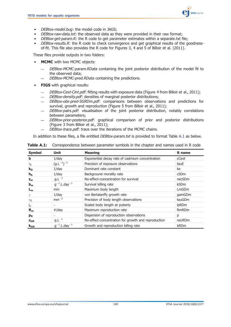
• DEBtox-model.bug: the model code in JAGS;• DEBtox-raw-data.txt: the observed data as they were provided in their raw format;• DEBtox-get-param.R: the R code to get parameter estimates within a separate.txt file;• DEBtox-results.R: the R code to check convergence and get graphical results of the goodness-
of-fit. This file also provides the R code for Figures 3, 4 and 5 of Billoir et al. (2011).
These files provide outputs in two folders:
• MCMC with two MCMC objects:
� DEBtox-MCMC-param.RData containing the joint posterior distribution of the model fit tothe observed data;
� DEBtox-MCMC-pred.RData containing the predictions.
• FIGS with graphical results:
� DEBtox-Cext-Cint.pdf: fitting results with exposure data (Figure 4 from Billoir et al., 2011);� DEBtox-density.pdf: densities of marginal posterior distributions;� DEBtox-obs-pred-SGRDm.pdf: comparisons between observations and predictions for
survival, growth and reproduction (Figure 5 from Billoir et al., 2011);� DEBtox-pairs.pdf: visualisation of the joint posterior distribution, notably correlations
between parameters;� DEBtox-prior-posterior.pdf: graphical comparison of prior and posterior distributions
(Figure 3 from Billoir et al., 2011);� DEBtox-trace.pdf: trace over the iterations of the MCMC chains.
In addition to these files, a file entitled DEBtox-param.txt is provided to format Table A.1 as below.
Table A.1: Correspondence between parameter symbols in the chapter and names used in R code
Symbol Unit Meaning R name
b 1/day Exponential decay rate of cadmium concentration cCext
sE (g.L�1)�2 Precision of exposure observations tauEkD 1/day Dominant rate constant ke
hb 1/day Background morality rate cSDmzw .g.L�1 No-effect-concentration for survival necSDm
bw �g�1.L.day�1 Survival killing rate kSDmLm mm Maximum body length LmGDm
c 1/day von Bertalanffy growth rate gamGDmsG mm�2 Precision of body length observations tauGDm
lp – Scaled body length at puberty lpRDmRm #/day Maximum reproduction rate RmRDm
pR – Dispersion of reproduction observations pzGR �g.L�1 No-effect-concentration for growth and reproduction necRDm
kGR �g�1.L.day�1 Growth and reproduction killing rate kRDm
TKTD models for aquatic organisms
www.efsa.europa.eu/efsajournal 140 EFSA Journal 2018;16(8):5377

Appendix B – Additional result from the GUTS application example
B.1. Fit plots as numbers of survivors
Figure B.1: Fit plot of the GUTS-RED-SD (upper panel) and GUTS-RED-IT (lower panel) modelcalibration results on a typical acute toxicity test: the number of survivors over time isrepresented as a function of time for each tested concentration (headers of single plots):black dots are the observed numbers of survivors, while the orange plain linecorresponds to the predicted median numbers of survivors. The grey band is the 95%credibility band representing the uncertainty
TKTD models for aquatic organisms
www.efsa.europa.eu/efsajournal 141 EFSA Journal 2018;16(8):5377

B.2. Prior-posterior comparison
(SD)
(IT)
Figure B.2: Comparison of priors and posteriors of the GUTS-RED-SD (upper panel) and GUTS-RED-IT (lower panel) model parameters (log10-scale): the dotted distribution corresponds tothe prior and the plain one to the posterior probability distribution of each parameter (x-labels under single plots)
TKTD models for aquatic organisms
www.efsa.europa.eu/efsajournal 142 EFSA Journal 2018;16(8):5377
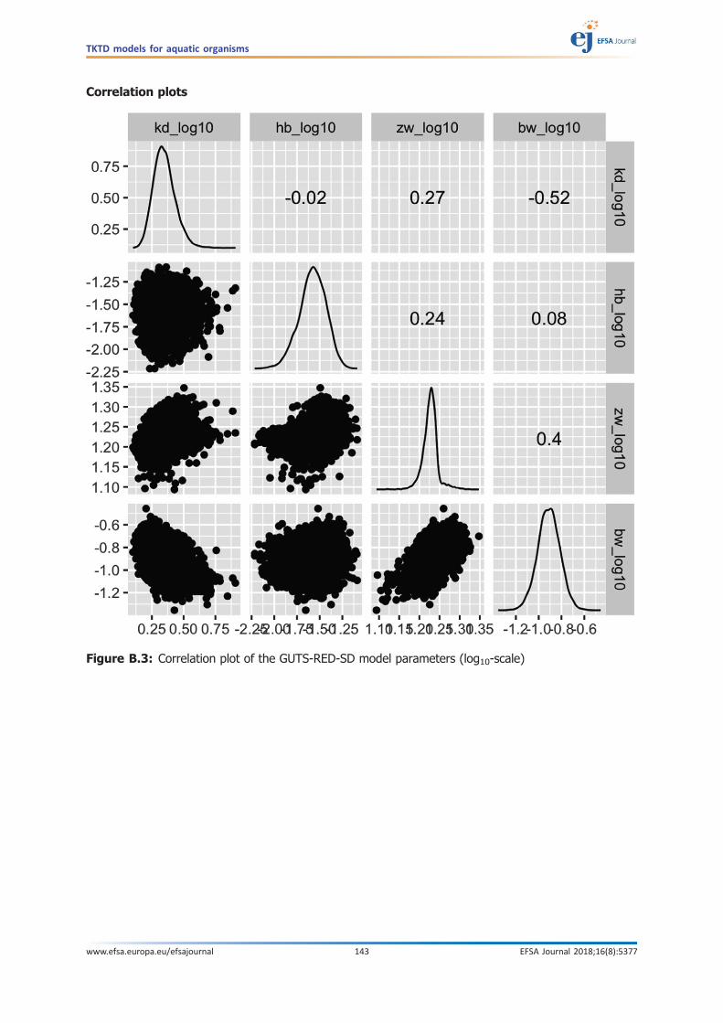
Correlation plots
Figure B.3: Correlation plot of the GUTS-RED-SD model parameters (log10-scale)
TKTD models for aquatic organisms
www.efsa.europa.eu/efsajournal 143 EFSA Journal 2018;16(8):5377
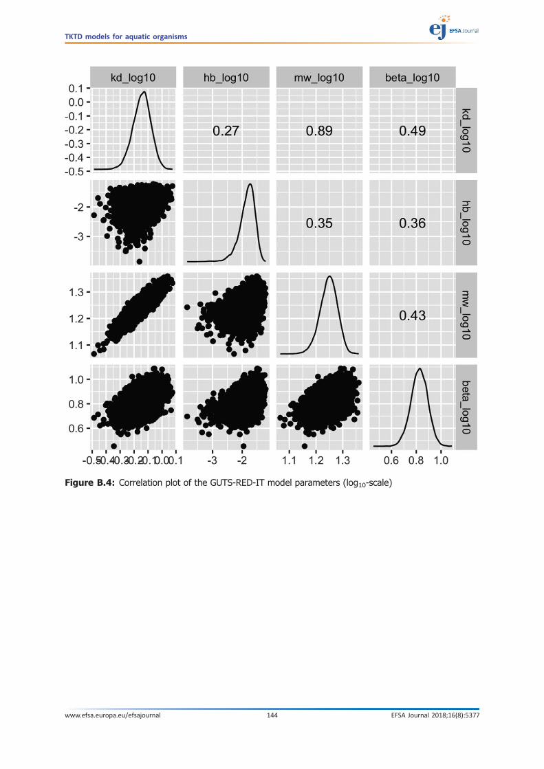
Figure B.4: Correlation plot of the GUTS-RED-IT model parameters (log10-scale)
TKTD models for aquatic organisms
www.efsa.europa.eu/efsajournal 144 EFSA Journal 2018;16(8):5377

B.3. Parameter values as optimised within the frequentist approach
Table B.1: Optimal parameter values (column ‘Value’) as obtained in the frequentist framework(Section 4.1.3.2 and Table 3), and lower (5%) and upper (95%) confidence limits.Values obtained by application of the SimulatedAnnealing optimisation routine (seeAppendix A.1 for more details). The results can be compared with results from theBayesian framework reported in Table 3
Symbol Value 5% CL 95% CL Units
GUTS-SIC-SD
Background hazard rate hb 0.028 0.021 0.031 1/dayDominant rate constant kD 2.154 1.758 2.333 1/day
Killing rate bw 0.132 0.092 0.138 lmol/L per dayThreshold zw 17.067 15.96 18.19 lmol/L
Negative ln likelihood ln L 123.8307592
GUTS-SIC-IT
Background hazard rate hb 0.018 0.005 0.042 1/dayDominant rate constant kD 0.732 0.576 0.909 1/day
Median of threshold distributions mw 17.83 16.25 20.34 lmol L�1
Slope of the distribution b 6.958 5.486 7.845 [�]
Negative ln likelihood ln L 127.7684792
TKTD models for aquatic organisms
www.efsa.europa.eu/efsajournal 145 EFSA Journal 2018;16(8):5377
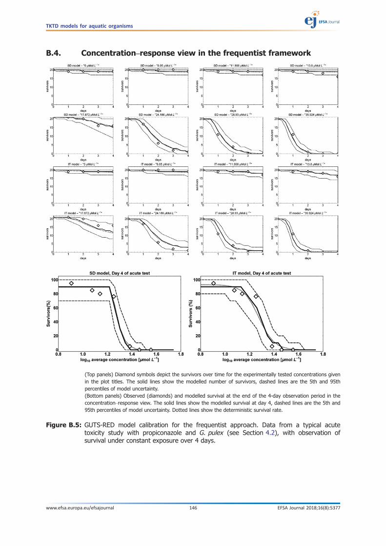
B.4. Concentration–response view in the frequentist framework
(Top panels) Diamond symbols depict the survivors over time for the experimentally tested concentrations givenin the plot titles. The solid lines show the modelled number of survivors, dashed lines are the 5th and 95thpercentiles of model uncertainty.(Bottom panels) Observed (diamonds) and modelled survival at the end of the 4-day observation period in theconcentration–response view. The solid lines show the modelled survival at day 4, dashed lines are the 5th and95th percentiles of model uncertainty. Dotted lines show the deterministic survival rate.
Figure B.5: GUTS-RED model calibration for the frequentist approach. Data from a typical acutetoxicity study with propiconazole and G. pulex (see Section 4.2), with observation ofsurvival under constant exposure over 4 days.
TKTD models for aquatic organisms
www.efsa.europa.eu/efsajournal 146 EFSA Journal 2018;16(8):5377
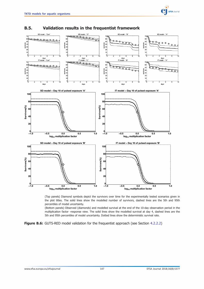
B.5. Validation results in the frequentist framework
(Top panels) Diamond symbols depict the survivors over time for the experimentally tested scenarios given inthe plot titles. The solid lines show the modelled number of survivors, dashed lines are the 5th and 95thpercentiles of model uncertainty.(Bottom panels) Observed (diamonds) and modelled survival at the end of the 10-day observation period in themultiplication factor -response view. The solid lines show the modelled survival at day 4, dashed lines are the5th and 95th percentiles of model uncertainty. Dotted lines show the deterministic survival rate.
Figure B.6: GUTS-RED model validation for the frequentist approach (see Section 4.2.2.2)
TKTD models for aquatic organisms
www.efsa.europa.eu/efsajournal 147 EFSA Journal 2018;16(8):5377

B.6. Documentation of the GUTS ring test results for the Bayesianframework
B.6.1. Preamble
This document quickly summarises parameter estimates and log-likelihood value from the GUTSring-test. Results were obtained with the R-package ‘morse’. R-code lines are given with the first dataset; they can be copied and pasted to repeat the analysis with the other data sets. All results can beidentically reproduced through the MOSAIC web interface available at http://pbil.univ-lyon1.fr/software/mosaic/guts.
Details about the ring-test are available in chapter 7 of the GUTS e-book from Tjalling JAGER andRoman ASHAUER (version 1.0, 2018) downloadable at https://leanpub.com/guts_book.
The parameter names of the GUTS-RED models are the following:
GUTS-RED symbol Morse symbol Meaning
kd Dominant rate constant
mw z (model SD) (Median) thresholdor a (model IT)
bw Killing rateb Slope factor (Fs = 2)
hb Background hazard rate
Calibration exercises with data set A.
Data set A consists of synthetic data, generated with GUTS-RED-SD and GUTS-RED-IT. Below arethe parameter values used to simulate the synthetic data sets A for SD and IT (n.a. means notapplicable).
Symbol True value SD True value IT
kd 0.8 0.8
mw 3 5bw 0.6 n.a.
b n.a. 5.3
hb 0.01 0.02
TKTD models for aquatic organisms
www.efsa.europa.eu/efsajournal 148 EFSA Journal 2018;16(8):5377

B.6.2. Calibration exercises with data set B
Data set B consists of the raw data from a typical four-day acute toxicity study and from anon-standard pulsed toxicity experiment taken from the supporting information of Nyman et al. (2012).
Calibration of GUTS-RED models using only constant exposure data
TKTD models for aquatic organisms
www.efsa.europa.eu/efsajournal 149 EFSA Journal 2018;16(8):5377

Calibration of GUTS-RED models using only time-variable exposure data
B.6.3. Calibration exercises with data set C
Data set C is taken from the fathead minnow toxicity database (Geiger et al., 1988). It represents atypical fish acute toxicity study, from which the raw data are used for calibration.
TKTD models for aquatic organisms
www.efsa.europa.eu/efsajournal 150 EFSA Journal 2018;16(8):5377
B.7. Documentation of the GUTS ring test results for the frequentistframework
B.7.1. Preamble
This section summarises parameter estimates and log-likelihood value from the GUTS ring-testobtained with Mathematica implementation. Example code is given below, which shows a call of theminimisation routine.
Details about the ring-test are available in Chapter 7 of the GUTS e-book from Tjalling Jager andRoman Ashauer (version 1.0, 2018) downloadable at https://leanpub.com/guts_book.
In the following example code lines, the optimisation routine (NMinimize) is called three times, firsttime with Random values between 0 and 5, and the 2nd and 3rd time with adapted starting values.The SimulatedAnnealing method was used, with 50 optimisation queues in parallel. The variable SOT$dataA contains the observed data.
TKTD models for aquatic organisms
www.efsa.europa.eu/efsajournal 151 EFSA Journal 2018;16(8):5377

startSD={foo,RandomReal[5],RandomReal[5],RandomReal[5],RandomReal[0.5]};
startstep=3;
Monitor[
resSD$A1=NMinimize[{
goalFunc$treatments[SOT$dataA,SDmodel,0,p1,p2,p3,kBG,tEnd=6], p1>0&&p2>0&&p3>0&&kBG>0},
{{p1,1/startstep*startSD[[2]],startstep*startSD[[2]]},
{p2,1/startstep*startSD[[3]],startstep*startSD[[3]]},
{p3,1/startstep*startSD[[4]],startstep*startSD[[4]]},
{kBG,1/startstep*startSD[[5]],startstep*startSD[[5]]}},
Method->{"SimulatedAnnealing",
"PerturbationScale"->3,"SearchPoints"->50},
PrecisionGoal->4,
MaxIterations->10],resMon];
Print[ToString[globC]<>" optimisation steps, "<>"optRes 1st loop:"<>ToString[resSD$A1]];
startSD={foo,
RandomReal[Ceiling[p1/.resSD$A1[[2]]]],RandomReal[Ceiling[p2/.resSD$A1[[2]]]],
RandomReal[Ceiling[p3/.resSD$A1[[2]]]],RandomReal[Ceiling[kBG/.resSD$A1[[2]]]]
};
startstep=1.5;
Monitor[
resSD$A1=NMinimize[{
goalFunc$treatments[ SOT$dataA,SDmodel,0,p1,p2,p3,kBG,tEnd=6], p1>0&&p2>0&&p3>0&&kBG>0},
{{p1,1/startstep*startSD[[2]],startstep*startSD[[2]]},
{p2,1/startstep*startSD[[3]],startstep*startSD[[3]]},
{p3,1/startstep*startSD[[4]],startstep*startSD[[4]]},
TKTD models for aquatic organisms
www.efsa.europa.eu/efsajournal 152 EFSA Journal 2018;16(8):5377

{kBG,1/startstep*startSD[[5]],startstep*startSD[[5]]}},
Method->{"SimulatedAnnealing",
"PerturbationScale"->3,"SearchPoints"->50},
PrecisionGoal->4,MaxIterations->10],resMon];
Print[ToString[globC]<>" optimisation steps, "<>" optRes 2nd loop:"<>ToString[resSD$A1]];
startSD={foo,
RandomReal[Ceiling[p1/.resSD$A1[[2]]]],RandomReal[Ceiling[p2/.resSD$A1[[2]]]],
RandomReal[Ceiling[p3/.resSD$A1[[2]]]],RandomReal[Ceiling[kBG/.resSD$A1[[2]]]]
};
startstep=1.2;
Monitor[
resSD$A1=NMinimize[{
goalFunc$treatments[SOT$dataA,SDmodel,0,p1,p2,p3,kBG,tEnd=6],p1>0&&p2>0&&p3>0&&kBG>0},
{{p1,1/startstep*startSD[[2]],startstep*startSD[[2]]},
{p2,1/startstep*startSD[[3]],startstep*startSD[[3]]},
{p3,1/startstep*startSD[[4]],startstep*startSD[[4]]},
{kBG,1/startstep*startSD[[5]],startstep*startSD[[5]]}},
Method->{"SimulatedAnnealing",
"PerturbationScale"->3,"SearchPoints"->50},
PrecisionGoal->8,MaxIterations->10],
resMon];
Print[ToString[globC]<>" optimisation steps, "<>" optRes 3rd loop:"<>ToString[resSD$A1]];
B.7.2. Calibration exercises with data set A
Data set A consists of synthetic data, generated with GUTS-RED-SD and GUTS-RED-IT. Below arethe parameter values used to simulate the synthetic data sets A for SD and IT (n.a. means notapplicable).
Symbol True value SD True value IT
kd 0.8 0.8mw 3 5
bw 0.6 n.a.b n.a. 5.3
hb 0.01 0.02
TKTD models for aquatic organisms
www.efsa.europa.eu/efsajournal 153 EFSA Journal 2018;16(8):5377

GUTS-SIC-SD Symbol Value Lower CI Upper CI Units
Background hazard rate hb 0.008 0.0049 0.0229 1/day
Dominant rate constant kd 0.71 0.52 0.96 1/dayKilling rate bw 0.62 0.49 0.79 L/(lmol*day)
Threshold mw 2.89 2.36 2.96 lmol/L
ln likelihood ln L �96.4464909
GUTS-SIC-IT Symbol Value Lower CI Upper CI Units
Background hazard rate hb 0.0262 0.0102 0.0518 1/dayDominant rate constant kd 0.79 0.66 1.08 1/day
Threshold mw 5.42 4.73 6.41 L/(lmol*day)Slope b 5.19 4.01 5.26 –
ln likelihood ln L �116.021090
B.7.3. Calibration exercises with data set B
Data set B consists of the raw data from a typical 4-day acute toxicity study and from a non-standard pulsed toxicity experiment taken from the supporting information of Nyman et al. (2012).
GUTS-SIC-SD Symbol Value Lower CI Upper CI Units
Background hazard rate hb 0.0276 0.0211 0.0314 1/day
Dominant rate constant kd 2.15 1.76 2.33 1/dayKilling rate bw 0.13 0.09 0.14 L/(lmol*d)
Threshold mw 17.06 15.96 18.19 lmol/L
ln likelihood ln L �123.830759
Parameters of GUTS-SIC-IT Symbol Value Lower CI Upper CI Units
Background hazard rate hb 0.0180 0.0048 0.0416 1/dayDominant rate constant kd 0.73 0.58 0.91 1/day
Threshold mw 17.83 16.25 20.33 L/(lmol*day)Slope b 6.96 5.49 7.85 –
ln likelihood ln L �127.768479
Calibrate GUTS-RED model using only time-variable exposure data
Parameters of GUTS-SIC-SD Symbol Value Lower CI Upper CI Units
Background hazard rate hb 0.0231 0.0176 0.0335 1/day
Dominant rate constant kd 1.81 1.70 6.89 1/dayKilling rate bw 0.33 0.07 0.46 L/(lmol*day)
Threshold mw 20.20 18.60 25.24 lmol/L
ln likelihood ln L �329.031332
Parameters of GUTS-SIC-IT Symbol Value Lower CI Upper CI Units
Background hazard rate hb 0.0221 0.0159 0.0394 1/dayDominant rate constant kd 0.20 0.10 9.47 1/day
Threshold mw 12.15 9.79 19.07 L/(lmol*day)Slope b 1.80 1.35 3.45 –
ln likelihood ln L �333.932485
TKTD models for aquatic organisms
www.efsa.europa.eu/efsajournal 154 EFSA Journal 2018;16(8):5377

B.7.4. Calibration exercises with data set C
Data set C is taken from the fathead minnow toxicity database (Geiger et al., 1988). It represents atypical fish acute toxicity study, from which the raw data are used for calibration.
GUTS-SIC-SD Symbol Value Lower CI Upper CI Units
Background hazard rate hb 0 0 0 1/day
Dominant rate constant kd 51.344 7.549 n.d. 1/dayKilling rate bw 0.083 0.051 0.122 L/(lmol*day)
Threshold mw 6.159 4.836 6.632 lmol/L
ln likelihood ln L �63.2640180
GUTS-SIC-IT Symbol Value Lower CI Upper CI Units
Background hazard rate hb 0 0 0 1/dayDominant rate constant kd 1.26 0.91 1.69 1/day
Threshold mw 9.33 8.62 10.62 L/(lmol*day)Slope b 4.50 3.12 6.25 –
ln likelihood ln L �61.3141725
TKTD models for aquatic organisms
www.efsa.europa.eu/efsajournal 155 EFSA Journal 2018;16(8):5377
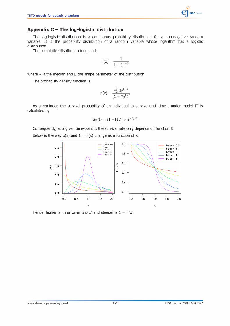
Appendix C – The log-logistic distribution
The log-logistic distribution is a continuous probability distribution for a non-negative randomvariable. It is the probability distribution of a random variable whose logarithm has a logisticdistribution.
The cumulative distribution function is
F(x) ¼ 1
1þ ðxaÞ�b
where a is the median and b the shape parameter of the distribution.
The probability density function is
p(x) ¼ ðbaÞðxaÞb�1
ð1þ ðxaÞbÞ2
As a reminder, the survival probability of an individual to survive until time t under model IT iscalculated by
SIT(t) ¼ ð1� F(t)Þ � e�hb�t
Consequently, at a given time-point t, the survival rate only depends on function F.
Below is the way p(x) and 1 � F(x) change as a function of x.
Hence, higher is �, narrower is p(x) and steeper is 1 � F(x).
TKTD models for aquatic organisms
www.efsa.europa.eu/efsajournal 156 EFSA Journal 2018;16(8):5377
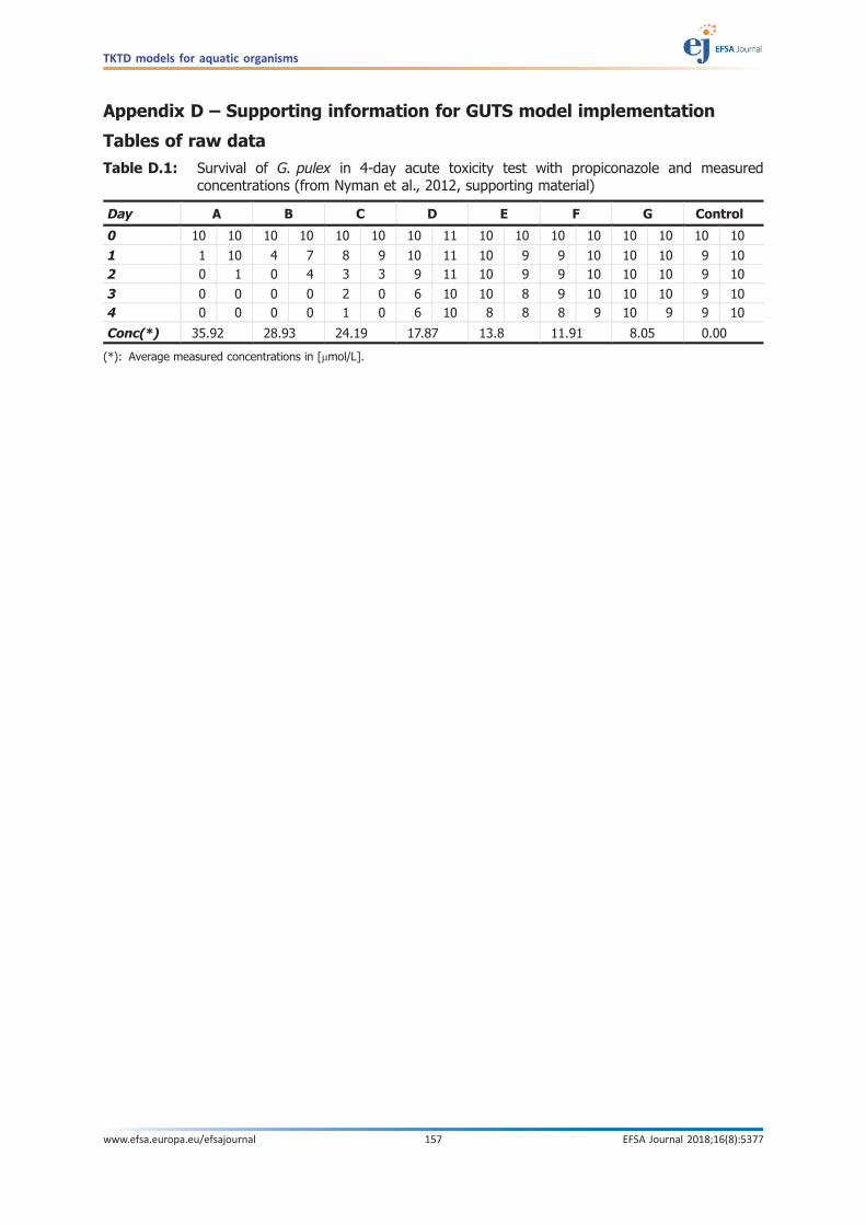
Appendix D – Supporting information for GUTS model implementation
Tables of raw data
Table D.1: Survival of G. pulex in 4-day acute toxicity test with propiconazole and measuredconcentrations (from Nyman et al., 2012, supporting material)
Day A B C D E F G Control
0 10 10 10 10 10 10 10 11 10 10 10 10 10 10 10 10
1 1 10 4 7 8 9 10 11 10 9 9 10 10 10 9 102 0 1 0 4 3 3 9 11 10 9 9 10 10 10 9 10
3 0 0 0 0 2 0 6 10 10 8 9 10 10 10 9 104 0 0 0 0 1 0 6 10 8 8 8 9 10 9 9 10
Conc(*) 35.92 28.93 24.19 17.87 13.8 11.91 8.05 0.00
(*): Average measured concentrations in [lmol/L].
TKTD models for aquatic organisms
www.efsa.europa.eu/efsajournal 157 EFSA Journal 2018;16(8):5377
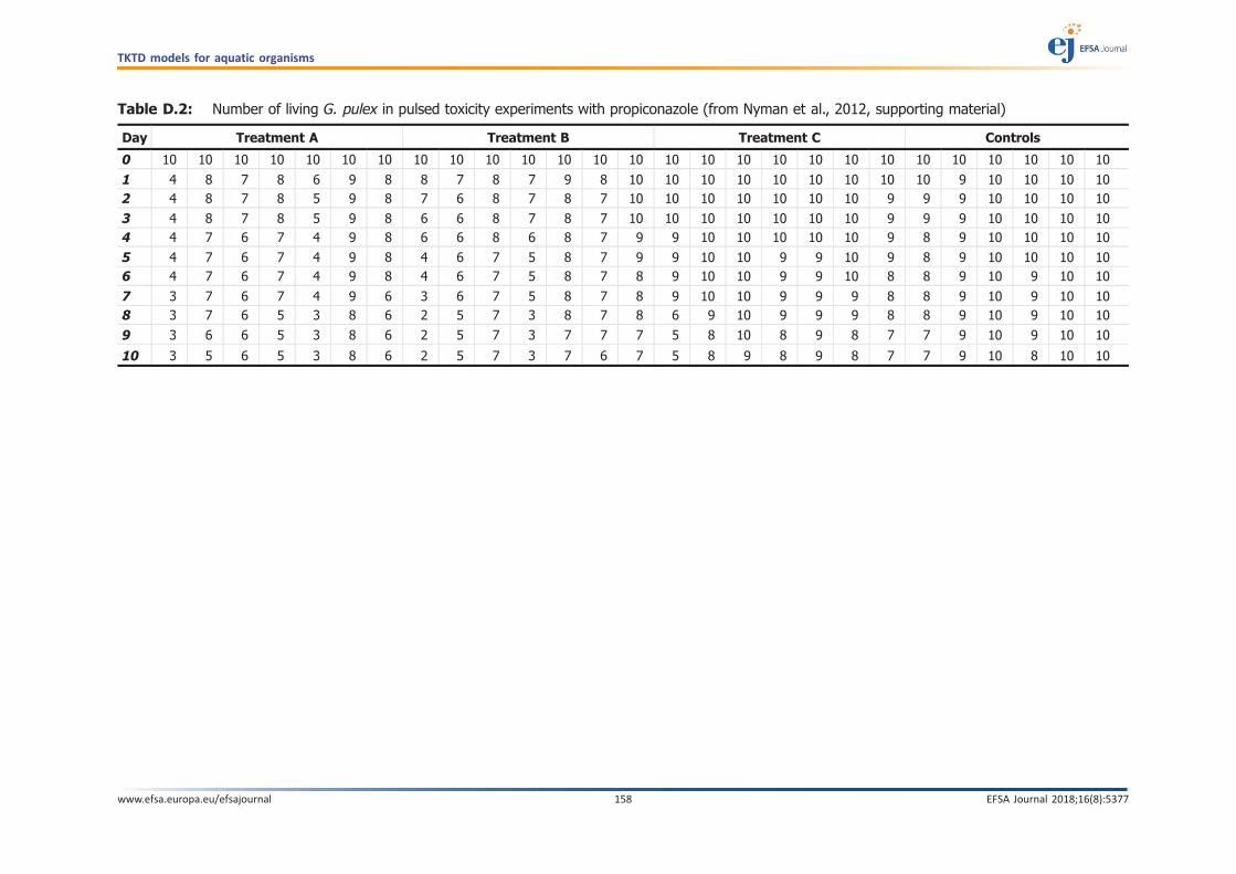
Table D.2: Number of living G. pulex in pulsed toxicity experiments with propiconazole (from Nyman et al., 2012, supporting material)
Day Treatment A Treatment B Treatment C Controls
0 10 10 10 10 10 10 10 10 10 10 10 10 10 10 10 10 10 10 10 10 10 10 10 10 10 10 10
1 4 8 7 8 6 9 8 8 7 8 7 9 8 10 10 10 10 10 10 10 10 10 9 10 10 10 102 4 8 7 8 5 9 8 7 6 8 7 8 7 10 10 10 10 10 10 10 9 9 9 10 10 10 10
3 4 8 7 8 5 9 8 6 6 8 7 8 7 10 10 10 10 10 10 10 9 9 9 10 10 10 104 4 7 6 7 4 9 8 6 6 8 6 8 7 9 9 10 10 10 10 10 9 8 9 10 10 10 10
5 4 7 6 7 4 9 8 4 6 7 5 8 7 9 9 10 10 9 9 10 9 8 9 10 10 10 106 4 7 6 7 4 9 8 4 6 7 5 8 7 8 9 10 10 9 9 10 8 8 9 10 9 10 10
7 3 7 6 7 4 9 6 3 6 7 5 8 7 8 9 10 10 9 9 9 8 8 9 10 9 10 108 3 7 6 5 3 8 6 2 5 7 3 8 7 8 6 9 10 9 9 9 8 8 9 10 9 10 10
9 3 6 6 5 3 8 6 2 5 7 3 7 7 7 5 8 10 8 9 8 7 7 9 10 9 10 10
10 3 5 6 5 3 8 6 2 5 7 3 7 6 7 5 8 9 8 9 8 7 7 9 10 8 10 10
TKTD models for aquatic organisms
www.efsa.europa.eu/efsajournal 158 EFSA Journal 2018;16(8):5377
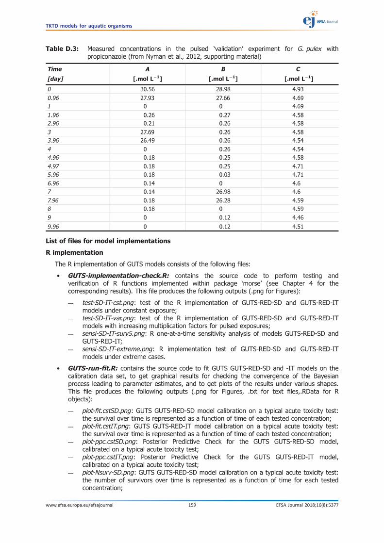
List of files for model implementations
R implementation
The R implementation of GUTS models consists of the following files:
• GUTS-implementation-check.R: contains the source code to perform testing andverification of R functions implemented within package ‘morse’ (see Chapter 4 for thecorresponding results). This file produces the following outputs (.png for Figures):
� test-SD-IT-cst.png: test of the R implementation of GUTS-RED-SD and GUTS-RED-ITmodels under constant exposure;
� test-SD-IT-var.png: test of the R implementation of GUTS-RED-SD and GUTS-RED-ITmodels with increasing multiplication factors for pulsed exposures;
� sensi-SD-IT-surv5.png: R one-at-a-time sensitivity analysis of models GUTS-RED-SD andGUTS-RED-IT;
� sensi-SD-IT-extreme.png: R implementation test of GUTS-RED-SD and GUTS-RED-ITmodels under extreme cases.
• GUTS-run-fit.R: contains the source code to fit GUTS GUTS-RED-SD and -IT models on thecalibration data set, to get graphical results for checking the convergence of the Bayesianprocess leading to parameter estimates, and to get plots of the results under various shapes.This file produces the following outputs (.png for Figures, .txt for text files,.RData for Robjects):
� plot-fit.cstSD.png: GUTS GUTS-RED-SD model calibration on a typical acute toxicity test:the survival over time is represented as a function of time of each tested concentration;
� plot-fit.cstIT.png: GUTS GUTS-RED-IT model calibration on a typical acute toxicity test:the survival over time is represented as a function of time of each tested concentration;
� plot-ppc.cstSD.png: Posterior Predictive Check for the GUTS GUTS-RED-SD model,calibrated on a typical acute toxicity test;
� plot-ppc.cstIT.png: Posterior Predictive Check for the GUTS GUTS-RED-IT model,calibrated on a typical acute toxicity test;
� plot-Nsurv-SD.png: GUTS GUTS-RED-SD model calibration on a typical acute toxicity test:the number of survivors over time is represented as a function of time for each testedconcentration;
Table D.3: Measured concentrations in the pulsed ‘validation’ experiment for G. pulex withpropiconazole (from Nyman et al., 2012, supporting material)
Time A B C
[day] [.mol L�1] [.mol L�1] [.mol L�1]
0 30.56 28.98 4.93
0.96 27.93 27.66 4.691 0 0 4.69
1.96 0.26 0.27 4.582.96 0.21 0.26 4.58
3 27.69 0.26 4.583.96 26.49 0.26 4.54
4 0 0.26 4.544.96 0.18 0.25 4.58
4.97 0.18 0.25 4.715.96 0.18 0.03 4.71
6.96 0.14 0 4.67 0.14 26.98 4.6
7.96 0.18 26.28 4.598 0.18 0 4.59
9 0 0.12 4.46
9.96 0 0.12 4.51
TKTD models for aquatic organisms
www.efsa.europa.eu/efsajournal 159 EFSA Journal 2018;16(8):5377

� plot-sot-SD.png: GUTS GUTS-RED-SD model calibration on a typical acute toxicity test:the survival rate over time is given as a function of time for each tested concentration;
� plot-Nsurv-IT.png: GUTS GUTS-RED-IT model calibration on a typical acute toxicity test:the number of survivors over time is represented as a function of time for each testedconcentration;
� plot-sot-IT.png: GUTS GUTS-RED-IT model calibration on a typical acute toxicity test: thesurvival rate over time is given as a function of time for each tested concentration;
� surv-dose-response.png: GUTS GUTS-RED-SD and -IT model calibration on a typical acutetoxicity test: the survival rate (%) is represented as a function of the concentration at theend of the experiment (day 4);
� Nsurv-dose-response.png: GUTS GUTS-RED-SD and -IT model calibration on a typicalacute toxicity test: the number of survivors is represented as a function of theconcentration at the end of the experiment (day 4);
� LC50-versus-time.png: LC50 estimates from the calibrated GUTS SIC models;� GUTS-calibration-results.txt: parameter estimates of the GUTS GUTS-RED-SD and -IT
models fitted on the calibration data set;� quant-Nsurv-SD.txt: quantiles of the simulated numbers of survivors under the GUTS
GUTS-RED-SD model;� quant-surv-SD.txt: quantiles of the simulated survival rate over time under the GUTS
GUTS-RED-SD model;� quant-Nsurv-IT.txt: quantiles of the simulated numbers of survivors under the GUTS
GUTS-RED-IT model;� quant-surv-IT.txt: quantiles of the simulated survival rate over time under the GUTS
GUTS-RED-IT model;� fit.cstSD.RData: fit results of model GUTS-RED-SD on calibration data;� fit.cstIT.RData: fit results of model GUTS-RED-IT on calibration data;� Nsurv-SD.Rdata: number of survivors simulated from model GUTS-RED-SD under the
constant exposure scenario of the calibration data set;� surv-SD.Rdata: survival rates simulated from model GUTS-RED-SD under the constant
exposure scenario of the calibration data set;� Nsurv-IT.Rdata: number of survivors simulated from model GUTS-RED-IT under the
constant exposure scenario of the calibration data set;� surv-IT.Rdata: survival rates simulated from model GUTS-RED-IT under the constant
exposure scenario of the calibration data set.
• GUTS-validation.R: contains the source code to perform simulation under the validation dataset, that is under time-variable exposure concentration profiles, and to get also graphicalresults. This file produces the following outputs:
� validation-profiles.png: exposure concentration profiles of the validation data set;� predict-SOT-SD.png: GUTS GUTS-RED-SD model validation on a typical acute toxicity test:
the number of survivors over time is represented as a function of time for each exposurescenario;
� predict-MF-SD-SOT.png: GUTS GUTS-RED-SD model validation on a typical acute toxicitytest: the number of survivors at the end of the experiment (day 10) is represented as afunction of a multiplication factor applied to each exposure;
� predict-SOT-IT.png: GUTS GUTS-RED-IT model validation on a typical acute toxicity test:the number of survivors over time is represented as a function of time for each exposurescenario;
� predict-MF-IT-SOT.png: GUTS GUTS-RED-IT model validation on a typical acute toxicitytest: the number of survivors at the end of the experiment (day 10) is represented as afunction of a multiplication factor applied to each exposure;
� internal-conc.png: simulation of the scaled internal concentration under exposure profiles‘A’ and ‘B’ for both kD median estimates of model GUTS-SD and GUTS-IT.
• GUTS-fit-addons.R: contains the source code to get additional fitting results of the GUTS-SDand the GUTS-IT models on the calibration data set. This file produces the following outputs:
� prior-posterior-SD.png: comparison between priors and posteriors of the GUTS-SD modelparameters;
TKTD models for aquatic organisms
www.efsa.europa.eu/efsajournal 160 EFSA Journal 2018;16(8):5377

� prior-posterior-IT.png: comparison between priors and posteriors of the GUTS-IT modelparameters;
� correlation-SD.png: correlation plot of GUTS-SD mode parameters;� correlation-IT.png: correlation plot of GUTS-IT mode parameters.
TKTD models for aquatic organisms
www.efsa.europa.eu/efsajournal 161 EFSA Journal 2018;16(8):5377

Appendix E – Repository of codes
Appendix E can be found in the online version of this output (‘supporting information’ section).
TKTD models for aquatic organisms
www.efsa.europa.eu/efsajournal 162 EFSA Journal 2018;16(8):5377

Appendix F – Example of the evaluation of an available GUTS model
In the context of the approval of the active substance Benzovindiflupyr, a TKTD model wassubmitted to predict survival of the two most sensitive species of fish under more realistic exposure(time-variable) to the fungicide. The GUTS model was used. The documentation of the model isavailable in the RAR of benzovindiflupyr (https://www.efsa.europa.eu/it/efsajournal/pub/4043).Additional information is also provided in the paper by Ashauer et al. (2013).
ASPECT OF THE MODEL TO BE EVALUATED BY THE RISK ASSESSOR – GUTS modelapplication for lethal effectsPlease note that when a Yes/No answer is not possibleor not applicable, the box is highlighted in yellow
Yes No
1. Evaluation of the problem definitionThe problem definition needs to explain how the modelling fits into the risk assessment and how it can be usedto address the specific protection goals. For GUTS, questions to be answered are likely to be those that are setout in Section 3. Nevertheless, the problem definition should make clear the following points:(a) Is the regulatory context for the model application documented? X
(b) Is the question that has to be answered by the model clearly formulated? X(c) Is the model output suitable to answer the formulated questions? X
(d) Was the choice of the test species clearly described and justified, also considering all theavailable valid information (including literature)?
X
(e) Is the species to be modelled specified? – Is it clear whether the model is being usedwith a Tier-1 test species i.e. Tier-2C1 or with one or more relevant species (which mightinclude the Tier-1 species), i.e. Tier-2C2?
X
2. Evaluation of the quality of the supporting experimental dataIn this part of the evaluation, it is checked whether the experimental data with which the model is compared(both calibration and validation data sets) have been subjected to quality control. The focus is on the dataquality, i.e. the laboratory conditions, set-up, chemical analytics and similar. Additional specific criteria for thesuitability of the data sets for model calibration and validation are evaluated later in more detail (Sections 7 and9 of this checklist).(a) Has the quality of the data used been considered and documented? (see list of OECD test
guidelines in Section 7, Table 6)X
(b) Have all available data been used (either for calibration or for validation)? If not, is therea justification why some information has not been used?
X
(c) Is it checked whether the actual exposure profile in the study matches the intendedprofile in the test (+/� 20%); if not, are then measured concentrations used for themodelling, instead of nominal ones?
X
3. Evaluation of the conceptual modelProviding GUTS models are being used to address mortality/immobility effects in fish or invertebrates, theconceptual model will be suitable to address the specific protection goals; so, no further evaluation is required(see Sections 2.1, 2.2 and 4.1).
4. Evaluation of the formal modelThe formal model contains the equations and algorithms to be used in the model. For GUTS models, theequations are standardised, so that no further check is necessary (see Section 4.1.1). It has to be documented,however, which GUTS model version is used (full or reduced model).
5. Evaluation of the computer modelThe formal model is converted into a model that can run on a computer (the computer model). For GUTSmodels, the computer model can be tested by showing the model performance for the GUTS ring-test data andperforming some further checks (see Section 7.5).(a) Is the used implementation of GUTS tested against the ring-test data set (see
Section 4.2)?X
(b) Were GUTS parameters estimated for the ring-test data and compared to the referencevalues, including confidence or credible intervals (Appendix B.6 and B.7)?
X
(c) Is a set of default scenarios (e.g. standard scenarios, extreme cases, see Section 4.1.2)simulated and checked?
X
(d) Are all data and parameters provided to allow an independent implementation of GUTS tobe run?
X
TKTD models for aquatic organisms
www.efsa.europa.eu/efsajournal 163 EFSA Journal 2018;16(8):5377
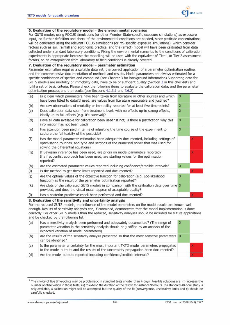
6. Evaluation of the regulatory model – the environmental scenariosFor GUTS models using FOCUS simulations (or other Member State-specific exposure simulations) as exposureinput, no further definition and check of the environmental conditions are needed, since pesticide concentrationswill be generated using the relevant FOCUS simulations (or MS-specific exposure simulations), which considerfactors such as soil, rainfall and agronomic practice, and the (effect) model will have been calibrated from datacollected under standard laboratory conditions. Fixing the environmental scenarios to the conditions of calibrationexperiments is appropriate because the modelling will be used with the equivalent of Tier-1 or Tier-2 assessmentfactors, so an extrapolation from laboratory to field conditions is already covered.
7. Evaluation of the regulatory model – parameter estimationParameter estimation requires a suitable data set, the correct application of a parameter optimisation routine,and the comprehensive documentation of methods and results. Model parameters are always estimated for aspecific combination of species and compound (see Chapter 3 for background information).Supporting data forGUTS models are mortality or immobility data, have to be of sufficient quality (Section 2 in this checklist) andfulfil a set of basic criteria. Please check the following items to evaluate the calibration data, and the parameteroptimisation process and the results (see Sections 4.1.3.1 and 7.6.2):
(a) Is it clear which parameters have been taken from literature or other sources and whichhave been fitted to data?If used, are values from literature reasonable and justified?
X
(b) Are raw observations of mortality or immobility reported for at least five time-points? X(c) Does calibration data span from treatment levels with no effects up to strong effects,
ideally up to full effects (e.g. 0% survival)?X
(d) Have all data available for calibration been used? If not, is there a justification why thisinformation has not been used?
X
(e) Has attention been paid in terms of adjusting the time course of the experiment tocapture the full toxicity of the pesticide?
X
(f) Has the model parameter estimation been adequately documented, including settings ofoptimisation routines, and type and settings of the numerical solver that was used forsolving the differential equations?
X
(g) If Bayesian inference has been used, are priors on model parameters reported?If a frequentist approach has been used, are starting values for the optimisationreported?
X
(h) Are the estimated parameter values reported including confidence/credible intervals? X(i) Is the method to get these limits reported and documented? X
(j) Are the optimal values of the objective function for calibration (e.g. Log-likelihoodfunction) as the result of the parameter optimisation reported?
X
(k) Are plots of the calibrated GUTS models in comparison with the calibration data over timeprovided, and does the visual match appear of acceptable quality?
X
(l) Has a posterior predictive check been performed and documented? X
8. Evaluation of the sensitivity and uncertainty analysisFor the reduced GUTS models, the influence of the model parameters on the model results are known wellenough. Results of sensitivity analyses can, if contained, demonstrate that the model implementation is donecorrectly. For other GUTS models than the reduced, sensitivity analyses should be included for future applicationsand be checked by the following list.
(a) Has a sensitivity analysis been performed and adequately documented? (The range ofparameter variation in the sensitivity analysis should be justified by an analysis of theexpected variation of model parameters)
X
(b) Are the results of the sensitivity analysis presented so that the most sensitive parameterscan be identified?
X
(c) Is the parameter uncertainty for the most important TKTD model parameters propagatedto the model outputs and the results of the uncertainty propagation been documented?
X
(d) Are the model outputs reported including confidence/credible intervals? X
15 The choice of five time-points may be problematic in standard tests shorter than 4 days. Possible solutions are: (i) increase thenumber of observation in those tests; (ii) to extend the duration of the test to for instance 96 hours. If a standard 48-hour study isonly available, a calibration might still be attempted but the quality of the fit (convergence, uncertainty limits and c) should becarefully checked.
TKTD models for aquatic organisms
www.efsa.europa.eu/efsajournal 164 EFSA Journal 2018;16(8):5377

9. Evaluation of the model by comparison with independent measurements (model validation)Validation data are used to test the model performance for predictions of mortality/immobility under exposureprofiles which have not been used for model calibration. The performance of the model is usually evaluated bycomparing relevant model outputs with measurements (often referred to as model validation). For GUTS,relevant outputs are the simulated mortality/immobility probability or LPX/EPX values. The following checklist ismandatory only for invertebrates; for vertebrates, a case-by-case basis check needs to be done (see alsoSections 7.7.2 and 4.1.4.5)(a) Are effect data available from experiments under time-variable exposure? X
(b) Is mortality or immobility reported at least for 7 time-points in the validation data set? X(c) Are two exposure profiles tested with at least two pulses each, separated by no-exposure
intervals of different duration length?X
(d) Is the individual depuration and repair time (DRT95) calculated, and is the duration of theno-exposure intervals defined accordingly?[Ideally one of the profiles should show a no-exposure interval shorter than the DRT95, the other profile clearly larger than the DRT95]
X
(e) Is each profile tested at least at 3 concentration levels, in order to obtain low, mediumand high effects at the end of the respective experiment?
X
(f) Has attention been paid to the duration of the experiments considering the time courseof development in toxicity of the specific pesticide?
X
(g) Does the visual match (‘visual fit’ in FOCUS Kinetics (2006)) of the model predictionquality indicate acceptability of the model predictions in comparison with the validationdata?
X
(h) Do the reported quantitative model performance criteria (e.g. PPC, NRMSE, SPPE)indicate a sufficient model performance?
X
(i) Has the performance of the model been reported in an objective and reproducible way? X
10. Evaluation of model useWhen using a TKTD model for regulatory purposes, the inputs of species- and compound specific modelparameters and of exposure profile data are required to run the model under new conditions. In this stage, it isimportant that the model is well documented and that it is clear how the model works. Please check thefollowing items:(a) Is the use of the model sufficiently documented? X
(b) Is an executable implementation of the model made available to the reviewer, or Is atleast the source code provided?
X
(c) Has a summary sheet been provided by the applicant? The summary sheet shouldprovide quick access to the comprehensive documentation with sections corresponding tothe ones of this checklist.
X
(d) Does the exposure profile used with the TKTD model come from the same source as thePEC used with the Tier-1 effects data? For example if FOCUS Step 3 maximum valueswere used at Tier-1, are the exposure profiles used Tier-2C from the same FOCUS Step 3modelling? If the exposure profile comes from any other source (e.g. different scenarios,different inputs, different model) has this been checked?
X
(e) Further points to be checked by evaluatorsUse an independent implementation of GUTS to test whether the output of the evaluatedmodel implementation can be reproduced for some parameter sets.The MOSAIC_GUTSweb-platform (http://pbil.univ-lyon1.fr/software/mosaic/guts) can be used to test themodel calibrationThe GUTS Shiny App (http://lbbe-shiny.univ-lyon1.fr/guts-shinyapp/) totest model predictions under a specific constant or time-variable exposure profile giventhe set of model parameters can be used.
Explanation of the evaluation
1. Evaluation of the problem definition
It was clear from the model documentation, that the study was conducted as a higher-tierapproach for risk refinement, addressing lethal effects, as part of a weight-of-evidence approach,hence it is concluded that the regulatory context for the model application is not well enoughdocumented. A clear question (objective) to be answered by the model was formulated: ‘The objectiveof this study was the prediction of acute toxicity towards fish under fluctuating and pulsed exposurepatterns’. The model output was not recognised as suitable to answer the formulated questions,
TKTD models for aquatic organisms
www.efsa.europa.eu/efsajournal 165 EFSA Journal 2018;16(8):5377

because the current definition recommends using the multiplication factor leading to 50% mortality(LP50) in the context of acute risk assessment together with a lower-tier assessment factor. In general,there is a specific issue with the selected tolerated effect level of 10% (as used for the multiplicationfactor analysis), which is not in accordance with the SPG for vertebrates in the AGD. When the giveneffect level would have been used together with a lower-tier safety factor it would have beentolerable, but that was not the case for the study: ‘The safety margins ranged from a factor of 26 to500. Thus, the concentrations in the original FOCUS-SW exposure profiles are a factor 26–500 belowlevels for the onset of mortality in the analysed combinations of fish species and application patterns’.The modelled species have been presented and consist of five standard fish species for acute toxicitytests. Models have been parameterised for all five fish species, but predictions of survival under time-variable exposure profiles were carried out for the two most sensitive fish species (Cyprinus carpio &Pimephales promelas). The choice of the test species is considered to be clearly described andjustified. In principle, it would have been possible to calculate LP50 values for 5 fish species and byusing the SSD approach to calculate the corresponding HP5 values. These HP5 values should be largerthan the AF of 9 as proposed for acute fish SSDs in the Aquatic Guidance Document. In the currentexample, however, validation results were presented for only one species.
The question ‘is it clear whether the model is being used with a Tier-1 test species i.e. Tier-2C1 orwith one or more relevant species (which might include the Tier-1 species) i.e. Tier-2C2’ is difficult tobe answered, because this example was produced before this Opinion was written, so the concept ofTier-2C1 and Tier-2C2 had not been developed. The two most sensitive species were modelled, but thisisn’t strictly in line with the proposals for Tier-2C1 (only standard species) or Tier-2C2 (all availablespecies unless there is a clear difference in sensitivity).
2. Evaluation of the quality of the supporting experimental data
Standard laboratory studies were provided on several fish and were evaluated in the DAR forbenzovindiflupyr. The table below lists the studies provided and whether they were considered suitablefor use in the risk assessment (which includes suitable quality to use for the TKTD modelling, but doesnot address whether the study type/design is useful for the TKTD mode) when evaluated by the RMS.
Species Study Is it of suitable quality?
Rainbow trout Acute, OECD 203 YesCarp Acute, OECD 203 Yes
Fathead minnow Acute, OECD 203 YesSheepshead minnow Acute, OECD 203 Yes
Bluegill sunfish Acute, OECD 203 Yes
Fathead minnow ELS, OECD 210 Yes
The most sensitive species tested (acute tests) was the carp (Cyprinus carpio), followed by thefathead minnow (Pimephales promelas). The difference in sensitivity of all five species tested in acutetests was within an order of magnitude (LC50s 3.5–27 lg a.s./L). It is concluded that the quality of thedata used has been considered and documented.
The acute toxicity studies for the two species modelled were used for the model calibration. Thechronic toxicity study was used for model validation. It is concluded that all available data had beenused (although it is noted that no validation data set was available for the carp).
The acute toxicity study on carp was conducted under flow through conditions and measuredconcentrations were between 86% and 110% of nominal. The endpoint was calculated on the basis ofmean measured concentrations. The acute toxicity study on fathead minnow was conducted underflow through conditions and measured concentrations were between 86% and 94% of nominal. Theendpoint was calculated on the basis of mean measured concentrations. The ELS toxicity study onfathead minnow was conducted under flow through conditions for 32 days and measuredconcentrations were between 88% and 120% of nominal. The endpoint was calculated on the basis ofmean measured concentrations. It is concluded that the actual exposure profile in the study matchesthe intended profile in the test (+/�20%) (section B.9.2.1 (acute toxicity studies) and B.9.2.3 (chronictoxicity studies) of the DAR for benzovindiflupyr).
TKTD models for aquatic organisms
www.efsa.europa.eu/efsajournal 166 EFSA Journal 2018;16(8):5377

3. Evaluation of the conceptual model
The GUTS models were used to address mortality/immobility effects in fish, and the standard GUTSframework was applied, hence the conceptual model is considered to be suitable to address thespecific protection goals.
4. Evaluation of the formal model
The GUTS standard model equations using the reduced versions of the SD and IT model have beenused, so no further check of the formal model is necessary.
5. Evaluation of the computer model
The study was performed using a GUTS implementation in ModelMaker. It had been submittedbefore the ring test data were provided, hence it was impossible to test the model performanceagainst the GUTS ring-test data or to compare parameters to the reference values from the GUTS ringtest. No additional testes, for example with standard or extreme scenarios have been provided toshow the correct implementation of the model. A one-at-a-time sensitivity analysis was performed anddocumented (P. 161 of DAR). All parameters values are given in the model documentation, butdetailed information about the exposure profiles is missing in the model documentation.
6. Evaluation of the regulatory model – the environmental scenarios
Since the applied GUTS models used FOCUS surface water simulations as exposure input, nofurther definition and check of the environmental conditions are needed.
7. Evaluation of the regulatory model – parameter estimation
Some aspects of the parameter estimation have been evaluated positively. For model calibration,GUTS model parameters have been fitted to data and raw observations of mortality or immobility forfive time-points (including initial abundance). The calibration data shows strong effects in the highesttreatment levels, and all data available for calibration can be considered to be used. Parameter valueshave been estimated and calibrated including confidence intervals, and optimal values of the objectivefunction for calibration (log-likelihood) as the result of the parameter optimisation were reported(Table 1 in Ashauer et al., 2013). Plots of the calibrated GUTS models in comparison with thecalibration data over time are provided, and the visual match appear of good quality (pp. 149–151 inthe DAR). The question whether attention has been paid in terms of adjusting the time course of theexperiment to capture the full toxicity of the pesticide is answered with ‘Yes’, because the ELS wasperformed under chronic exposure (28 days) and used for validation. Hence, delayed effects wouldhave been detected in the validation experiments.
Some aspects of the model parameter estimation have been evaluated negatively, including thefollowing aspects. The model parameter estimation has not been adequately documented, sincesettings of optimisation routines and type and settings of the numerical solver that were used forsolving the differential equations are not documented. Also, starting values for the optimisation are notreported. The method to obtain parameter confidence limits is not adequately reported anddocumented, since it is a simple reference to a publication. A posterior predictive check has not beenperformed and documented.
8. Evaluation of the sensitivity and uncertainty analysis
The reduced GUTS models have been used, hence influence of the model parameters on the modelresults are considered to be known well enough. Despite this, a one-at-a-time sensitivity analysis wasperformed and documented and it demonstrates that the model implementation is done correctly.
An analysis of uncertainty in the model output was not performed in a technical sense, since theuncertainty in the parameter has not been propagated to the model output.
It is acknowledged, that the study had been performed before the respective computationalapproach was developed, and that a comprehensive discussion of the role of uncertainty for the modeloutput was included in the model documentation (p. 161/162 of the DAR).
TKTD models for aquatic organisms
www.efsa.europa.eu/efsajournal 167 EFSA Journal 2018;16(8):5377

9. Evaluation of the model by comparison with independent measurements (modelvalidation)
The data used for validation is an Early Life Stage test with fathead minnow according to OECD 210under constant exposure. More than 3 treatment levels have been tested, and the number of time-points of reported mortality is larger than 7.
The use of early life stage test data can be considered to deliver conservative results, since ingeneral larvae tend to be more sensitive than the adult fish, and fish early life stage tests tend to bemore sensitive due to size and the prolonged exposure duration. Uncertainty about a positive answerto the abovementioned key question is added by considerations, whether fish fry is really a moresensitive indicator as compared to adult fish in this specific case. For the adult fathead minnow, anexposure to 4.4 lg/L led to about 40% mortality after 4 days. For the fry, exposure to a similar levelof 4 lg/L did not indicate any effect on survival at day 4, also not on day 5, but only at day 6 roughly40% mortality was observed.
The key question for the evaluation of the validity of the validation study is whether thecombination of calibration and validation data allows for a conclusion about the confidence in themodel performance for time-variable exposure profiles. The scientific opinion suggests evaluatingthe validation data set for vertebrates on a case-by-case basis in order to make use of the availabledata and to limit as much as possible additional vertebrate testing. It is, however, also recommendedto have at least one new fish test under time-variable exposure conditions.
In conclusion, in this specific example many of the validation aspects cannot be evaluated positive.Most significantly, the validation data have not been obtained from time-variable exposure. In addition,assuming that the data used for validation had been considered sufficient, this would only beapplicable to fathead minnow since no further validation data for any other species were tested. Hencemodel predictions for carp and other species would have not been considered relevant for regulatoryrisk assessment.
10. Evaluation of model use
While overall the modelling is well described there are aspects that have not been well described,therefore it is concluded that the use of the model is not sufficiently well documented. The question‘Does the exposure profile used with the TKTD model come from the same source as the PEC usedwith the Tier-1 effects data?’ has been answered with ‘no’ because insufficient information has beenprovided to identify what exposure was used. Output from FOCUS modelling was used but it is unclearwhether a) identical inputs were used by the applicant for the standard risk assessment and for theTKTD Tier-2 risk assessment and b) if the submitting was accepted without change or whether theRMS reran the FOCUS modelling. It is necessary to include sufficient information with the TKTD reportto be able to identify the source of the exposure profiles.
11. Conclusion
Overall, the documentation of the GUTS model and its application to predict the survival of fishunder exposure to time-variable profiles of benzovindiflupyr does not comply with the requirements asannounced in this Scientific Opinion. Many aspects of the model documentation were evaluatedpositive, but there were a number of issues. Most critical issues are about the documentation of thecomputer model, the documentation of the parameter estimation method, the analysis of uncertaintyin the model output, and the choice of the data set for model validation. It is of course acknowledged,that the model application was performed long time before the EFSA TKTD SO has been published.
TKTD models for aquatic organisms
www.efsa.europa.eu/efsajournal 168 EFSA Journal 2018;16(8):5377

Appendix G – Example of the evaluation of an available DEBtox model
In the context of the approval of beta-cyfluthrin, a DEBtox model was submitted with the scope ofinvestigating the reasons leading to different results, in terms of survival and growth, obtained theavailable chronic studies (one carried out under constant exposure and another with repeated peakexposure) on rainbow trout. The documentation is available in the RAR of beta-cyfluthrin (inpublication).
ASPECT OF THE MODEL TO BE EVALUATED BY THE RISK ASSESSOR – DEBtox modelapplications for sublethal effectsPlease note that when a Yes/No answer is notpossible or not applicable, the box is highlighted in yellow.
Yes No
0. Evaluation of the physiological DEB partDEBtox models consist of two parts:(iii) the physiological DEB part describing the basic metabolic processes combined with species-specific details;
this part is assumed to have been evaluated and approved beforehand;(iv) the TKTD part, describing the effects of toxicant on life-history traits through changes in the DEB parameters.
This checklist is adapted to the evaluation of the TKTD part of the DEBtox models (see Sections 2.3 and 5), butthe first thing to check is whether the physiological part, meaning the DEB part, was evaluated beforehand forthe chosen species. Without that check, the use of a DEBtox model cannot be suggested, even if the TKTDmodel part is evaluated positively.
(a) Was the evaluation of the physiological DEB part conducted by a regulatory authority or agroup delegated to this at the EU level?
X
(b) If (a) is yes, did the above evaluation of the physiological DEB part conclude that it issuitable for use in risk assessment?
(c) If (a) and (b) are yes, can the physiological DEB part of the model describe thebehaviour of the control data?
1. Evaluation of the problem definitionThe problem definition needs to explain how the modelling fits into the risk assessment and how it can be usedto address the specific protection goals (Chapter 3). Please check if due attention is paid to the following points:
(a) Is the regulatory context for the model application documented? X(b) Is the question that has to be answered with the model clearly formulated? X
(c) Is the model output suitable to answer the formulated questions? X(d) Is the choice of the test species clearly described and justified, also considering all the
available valid information (including literature)?X
(e) Is the species to be modelled specified? – Is it clear whether the model is being usedwith a Tier-1 test species i.e. Tier-2C1 or with one or more relevant species (which mightinclude the Tier-1 species) i.e. Tier-2C2?
X
2. Evaluation of the quality of the supporting experimental dataIn this part of the evaluation, it is checked whether the experimental data with which the model is compared(both calibration and validation data sets) have been subjected to quality control. The focus is on the dataquality, i.e. the laboratory conditions, set-up, chemical analytics and similar. Additional specific criteria for thesuitability of the data sets for model calibration and validation are evaluated later in more detail (Sections 7 and9 of this checklist).
(a) Are all types of data fully described, meaning that factors like temperature, foodconditions, measurements, handling, etc. are documented?
X
(b) Has the quality of the used data been considered and documented? (see the list of OECDtest guidelines in Section 7, Table 6).
X
(c) Have all available data been used (either for calibration or for validation)? If not, is therea justification why some information has not been used?
X
(d) Is it checked whether the actual exposure profile in the study matches the intendedprofile in the test (+/- 20%); if not, are then measured concentrations used for themodelling, instead of nominal ones?
X
3. Evaluation of the conceptual modelThe conceptual model provides a general and qualitative description of the system to be modelled. Thephysiological DEB part should have been evaluated and approved beforehand (see Section 0 of this checklist).Please check the following items for the TKTD part (refer to Section 7.3):(a) Is the reference to the evaluation of the physiological DEB part given? X
TKTD models for aquatic organisms
www.efsa.europa.eu/efsajournal 169 EFSA Journal 2018;16(8):5377

(b) Is the potential mode of action of the toxicant specified (effects on assimilation, growth,maintenance costs, reproductive output and/or survival)?
X
(c) Are the links between the scaled damage or the internal concentration and the DEBparameters logical?
X
(d) In case environmental factors (e.g. temperature) are explicitly considered, is theirinfluence on the physiological and/or TKTD processes documented in the conceptualmodel?
X
(e) Are the modelling endpoints relevant to the specific protection goal? X
4. Evaluation of the formal modelThe formal model contains equations used in the model. The physiological DEB part should have been evaluatedand approved beforehand (see Section 0 of this checklist). Nevertheless, all equations (from either thephysiological or the TKTD part) that include one or more parameters that are impacted by the effects of thetoxicant need to be documented. Please check the following items:(a) Are all mathematical equations relevant for the effect of the toxicant described, including
the equations of the toxicokinetic (TK) part and the equations relating the used scaleddamage or internal concentrations with the DEB parameter(s)?
X
(b) Is there a list or a summary of all variables and parameters including their meaning andunit?
X
(c) Are both the deterministic part (equations describing the mean tendency of the data) andthe stochastic part (the probability law describing the variability around the meantendency) of the model fully described? See Section 5.1 for an example.
X
5. Evaluation of the computer modelThe computer model corresponds to the implementation of the formal model that can run on a computer. Pleasecheck the following items:(a) Is the computer code available, including explaining comments for the most important
functions?X
(b) Is enough information provided to allow non-expert user to re-run the modelindependently (e.g. parameter sets, input data)?
X
(c) Is it demonstrated that the mathematical model is correctly implemented (modelverification), e.g. by checking and documenting the internal consistency of the modelresults based on a set of default or extreme cases (see e.g. Section 4.1.2.3 for anexample with GUTS, ‘reality check’ in chapter 10.4 of EFSA PPR Panel, 2014)?
X
6. Evaluation of the regulatory model – the environmental scenariosThe environmental scenarios determine the environmental context in which the model is run. For the applicationof DEBtox for the prediction of toxicological effects in a regulatory context, the environmental scenario need tobe fixed to the laboratory conditions of the experiments used for calibrating the TKTD part of the model. Pleasecheck the following items:(a) Are all the relevant conditions, recorded in the experiments used for calibrating the TKTD
part of the model, used consistently for the simulations (i.e. for generating EPx) used inthe risk assessment?
7. Evaluation of the regulatory model – parameter estimationParameter estimation requires a suitable data set, the correct application of a parameter optimisation routine,and the comprehensive documentation of methods and results. Model parameters are always estimated for aspecific combination of species and compound (see Section 3 for background information).Supporting data for DEBtox have to be of sufficient quality (Section 2 in this checklist), be relevant to the riskassessment problem and fulfil a set of basic criteria. Typical supporting data for the TKTD part of DEBtox modelsare experimental toxicity data for growth or growth + reproduction, to which mortality or immobility data canalso be added (see Sections 2.3 and 7.2 for background information, Section 5.1.3 for an example). Specificrequirements on the time resolution and temporal scale for the calibration data cannot be given, but in general,the number of time-points has to be sufficient to provide enough degrees of freedom for the model calibration.Please check the following items to evaluate the calibration data, the parameter optimisation process and theresults (see Sections 4.1.3 and 7.6.2):(a) Is it clear which parameters have been taken from literature or other sources and which
have been fitted to data?If used, are values from literature reasonable and justified?X
TKTD models for aquatic organisms
www.efsa.europa.eu/efsajournal 170 EFSA Journal 2018;16(8):5377

(b) Are the calibration data sufficient to provide enough degrees of freedom for the modelcalibration, i.e. are endpoints at least reported at several intermediate time-points?
X
(c) Does calibration data span from treatment levels with no effects up to strong effects,ideally up to full effects (e.g. no growth, no reproduction)?
X
(d) Have all data available for calibration been used? If not, is there a justification why thisinformation has not been used?
X
(e) Has attention been paid in terms of adjusting the time course of the experiment tocapture the full toxicity of the pesticide?
X
(f) Has the model parameter estimation been adequately documented, including settings ofoptimisation routines, and type and settings of the numerical solver that was used forsolving the differential equations?
X
(g) If Bayesian inference has been used, are priors on model parameters reported?If afrequentist approach has been used, are starting values for the optimisation reported?
X
(h) Are the estimated parameter values reported including confidence/credible limits? X(i) Is the method to get these limits reported and documented? X
(j) Are the optimal values of the objective function for calibration (e.g. log-likelihoodfunction) as the result of the parameter optimisation reported?
X
(k) Are plots of the calibrated DEBtox model in comparison with the calibration data overtime provided, and does the visual match appear of acceptable quality?
X
(l) Has a posterior predictive check been performed and documented? X
8. Evaluation of the sensitivity and uncertainty analysisIt is assumed that sensitivity and uncertainty analyses for the physiological DEB model part have been evaluatedand approved beforehand (see Section 0 of this checklist).Sensitivity analysis identifies the influence of theparameters on the model outputs and can hence identify the most influential parameters. Uncertainty analysisaims at identifying how uncertain the model output is regarding the uncertainty in parameter estimates.Pleasecheck the following items for the TKTD part:
(a) Has a sensitivity analysis for the TKTD part been performed and been adequatelydocumented? (The range of parameter variation in the sensitivity analysis should bejustified by an analysis of the expected variation of model parameters.)
X
(b) Are the results of the sensitivity analysis presented so that the most sensitive parameterscan be identified?
X
(c) Is the parameter uncertainty for the most important TKTD model parameters propagatedto the model outputs and the results of the uncertainty propagation been documented?
X
(d) Are the model outputs reported including confidence/credible intervals? X
9. Evaluation of the model by comparison with independent measurements (model validation)The model performance is usually evaluated by comparing relevant model outputs with independentexperimental measurements (i.e. data from other experiments than those used for calibration, often referred toas model validation). These independent measurements (or validation data sets) are used to test the modelperformance in predicting the chosen endpoints under time-variable exposure profiles. For DEBtox models,relevant outputs may be simulated growth and/or reproduction, sometimes together with simulated survival, orEPx values. The following checklist is mandatory only for invertebrates, for vertebrates a case-by-case basischeck needs to be done (see also Sections 7.7.2 and 4.1.4.5):(a) Are effect data available from experiments under time-variable exposure? X
(b) If non-destructive measurement is possible, are sufficient endpoint measurementsprovided in order to cover at least before, during and after each pulse exposure?Arethese time-points enough to allow for evaluation of changes in growth rates differentfrom the control treatment?
X
(c) Are two exposure profiles tested with at least two pulses each, separated by no-exposureintervals of different duration length?
X
(d) Is the individual depuration and repair time (DRT95) calculated based on toxicokineticparameters, and is the duration of the no-exposure intervals defined accordingly?[Ideallyone of the profiles should show a no-exposure interval shorter than the DRT95, the otherprofile clearly larger than the DRT95]
X
16 Time-points usually differ, with classically one measurement per week for growth (even sometimes only one measurement ofgrowth at the end of the experiment) and measurements twice or three times per week for reproduction.
TKTD models for aquatic organisms
www.efsa.europa.eu/efsajournal 171 EFSA Journal 2018;16(8):5377

(e) Is each profile tested at least at 3 concentration levels, in order to obtain low, mediumand high effects at the end of the respective experiment?
X
(f) Has attention been paid to the duration of the experiments considering the time courseof development in toxicity of the specific pesticide?
X
(g) Does the visual match (‘visual fit’ in FOCUS Kinetics, (2006)) of the model predictionquality indicate acceptability of the model predictions in comparison with the validationdata?
X
(h) Do the reported quantitative model performance criteria (e.g. PPC, NRMSE, SPPE)indicate a sufficient model performance?For DEBtox models, the adequacy of thequantitative criteria listed above (set on basis of GUTS models) needs still to be fullytested and may need future adaptation. However, for the time being, this set ofperformance criteria is also suggested for DEBtox models (see Section 7.7.2 ‘Modelperformance criteria’).
X
(i) Has the performance of the model been reported in an objective and reproducible way? X
10. Evaluation of model useWhen using a TKTD model for regulatory purposes, the inputs of species- and compound-specific modelparameters and of exposure profile data are required to run the model under new conditions. In this stage, it isimportant that the model is well documented and that it is clear how the model works. Please check thefollowing items:(a) Is the use of the model sufficiently documented? Is a user manual available? See items
provided in Section 10.7 of the EFSA PPR Panel (2014).X
(b) Is an executable implementation of the model made available to the reviewer, or Is atleast the source code provided?
X
(c) Has a summary sheet been provided by the applicant? The summary sheet shouldprovide quick access to the comprehensive documentation with sections corresponding tothe ones of this checklist.
X
(d) Does the exposure profile used with the TKTD model come from the same source as thePEC used with the Tier-1 effects data? For example, if FOCUS Step 3 maximum valueswere used at Tier-1 are the exposure profiles used Tier-2C from the same FOCUS Step 3modelling? If the exposure profile comes from any other source (e.g. different scenarios,different inputs, different model) has this been checked?
(e) In case parameters of the DEB (physiological) part of the model were changed fromcalibration to validation in order to better describe control data:- Is the difference in theparameters inducing considerable difference in the model predictions?And, if yes:- Are themodel simulations relevant for the risk assessment carried out with the parameter setproducing the more conservative (worst-case) predictions?
Explanation
0. Evaluation of the physiological DEB part
The physiological DEB part of the model has never been reviewed by a regulatory authority or agroup delegated to this at the EU level. Hence, no conclusion can be drawn regarding this part of themodel.
1. Problem definition
The regulatory context of the model application has been defined in the original study report.Reference is made to several EFSA guidance documents, and particularly to the EFSA aquatic guidancedocument (EFSA PPR Panel, 2013), where mechanistic effect models in general and TKTD models inparticular are described as refinement options for pesticide risk assessment.
The author proposes to use the model for investigating the reasons leading to different results (onsurvival and growth) obtained with two ELS experiments with rainbow trout, one carried out underconstant exposure, and another with repeated peak exposure. While the question is clearly formulated,and it is of course of scientific interest, there are doubts that the question as it is can be used todirectly inform the risk assessment for regulatory purposes.
Indeed, the model output consists of predictions of different endpoints (development, growth,reproductive, metabolic) which cannot be directly used in the risk assessment. Furthermore,predictions were carried out only for the exposure profile which was experimentally tested (i.e. for the
TKTD models for aquatic organisms
www.efsa.europa.eu/efsajournal 172 EFSA Journal 2018;16(8):5377

exposure profile from the validation data set). Hence, the output of the model does not provide newendpoint estimations compared to the experimental ones.
The choice of the species is clear (rainbow trout), but it was not really discussed in a riskassessment context. However, considering all the available laboratory experiments for beta-cyfluthrin,rainbow trout was consistently the most sensitive fish species in both the acute and chronic tests.Hence the choice appears reasonable but ideally should be better justified.
Rainbow trout is a Tier-1 test species, but its use for TKTD modelling was not put into a specificassessment tier. However, it should be highlighted that this would have been extremely difficult if notimpossible, as the position of TKTD models in the tiered risk assessment scheme have been specificallyproposed in this SO for the first time.
2. Supporting data
The supporting data consist of two ELS experiments with rainbow trout, one carried out underconstant exposure (used for calibration), and another with repeated peak exposure (used forvalidation). Test conditions are fully described in the specific reports hence full information is availableregarding temperature, water chemistry, food conditions, biological measurements, etc.
The study used for calibration is valid according to the current OECD 210 guideline, with someminor deviations, which was assessed as not critical for the outcome of the study. The dissolvedoxygen concentration stayed within the targeted limits of 6.5–11.9 ppm (three occasions above thatrange). The temperature during the study ranged from 8.3 to 11.9°C (recommended 8.5–11.5). Thestudy used for validation was conducted in accordance with OECD Test Guideline No. 210 withadaptations in order to fulfil the objectives of the experiment (time-variable exposure). Quality criteriaas set out in the respective OECD test guidelines were overall considered fulfilled. Nevertheless, thisinformation was not really accounted for in the phases of the model calibration and validation. It wouldbe desirable that quality criteria are explicitly addressed when developing a model, in order to accountfor relevant deviations which may have had an impact on the biological measurements.
All available data on early life stage of rainbow trout were using for either calibrating or validatingthe model.
For what concerns the calibration data, the actual profile in the study matched the nominalconcentrations reasonably well (mean measured concentrations between 95% and 112% of thenominal). For the validation experiment, on the other hand, measured peak concentrations differed insome cases substantially from the nominal ones. From Figures 2–4, it appears rather clear thatmeasured concentrations in time were used for the estimation of the concentration profiles in theexperiment. Nevertheless, the report does not explicitly address this issue, while a morestraightforward consideration would have been desirable.
3. Conceptual model
As pointed out under Section 0, the physiological DEB part of the model has never been reviewedby a regulatory authority or a group delegated to this at the EU level. Hence, no reference could begiven to a pre-existing evaluation.
In this specific model application, the author specifies that the toxicant acts by impairing thefeeding behaviour, and hence by reducing the food assimilation, and thus lead to growth reduction inthe early life stages, and may lead to a reduction in reproduction in the adult stage. Hence, the modeof action was specified. In addition, the links between the scaled damage and the DEB parametersappear logical. Temperature and food input are reported to be two forcing variables of the model.However, the influence of these parameters in the conceptual model is not clearly described. Theinfluence of temperature on the hatching time is reported by mean of a scatterplot, but it is unclearwhether this and other environmental factors may act in other ways within the conceptual model.
The modelling endpoints are related to lethal and sublethal effects (e.g. development, growth) offish. Hence, they are relevant for the specific protection goals. Reproduction was not considered in themodel, as the focus was on early life stages.
4. Formal model
All mathematical equations relevant for the effect of the toxicant are reported. All variablestogether with the relevant units are described in the text, nevertheless, a list/summary is not availablefor the state variables, but only for the parameters (together with their mean estimate) used in themodel. The stochastic part of the model was not described at all.
TKTD models for aquatic organisms
www.efsa.europa.eu/efsajournal 173 EFSA Journal 2018;16(8):5377

5. Computer model
The computer code is fully available for the MatLab software, although explaining comments arerather limited. Some output graphs are missing or cannot be identically reproduced. All parametervalues are well reported (except that uncertainty limits are missing). Other input data such asbiological observations and analytical measurements from the calibration and the validationexperiments were not available in the modelling report, but could be found in the respectiveexperiment report.
Model verification was performed for the DEB part by means of model simulations for different foodlevel and temperature. The outcome of these simulations confirmed that the computer model correctlyimplemented the influence of the two forcing variables. Model verification for the TKTD part was notperformed. The influence of different exposure scenarios (e.g. default or ‘extreme case’) was notevaluated.
6. Regulatory model: environmental scenario
As no simulation with exposure profiles other than the one tested in the experiment was run, therewas no consideration of particular environmental scenario (i.e. environmental parameters having aninfluence on the model output).
7. Regulatory model: parameter estimation
All parameter related to the DEB part of the model were taken from the literature. On the otherhand, TKTD parameters were fitted to the calibration data set.
The calibration data set consisted of five tested concentrations plus the control, two replicateseach. Survival was measured weekly, and raw data are available from the original study report(although presented in a cumulative way, no distinction between replicates). Hence, for this endpoint,sufficient measurements were available. Weight was only measured at the end of the test (biomassmeasured per chamber, not individual fish) and was presented as mean value of the replicates. While itis acknowledged that obtaining intermediate measurements for biomass might be complex and mightrequire destructive sampling, the available data are not considered ideal for having a fully reliableparameter estimation.
Calibration data span from no effect (no significant growth inhibition, survival comparable tocontrol) up to full effect (100% mortality). As already specified, all data available for this life stagewere used either in the calibration or the validation of the model.
The dossier of beta-cyfluthrin is particularly data rich for what concerns aquatic organisms. Theavailable information does not suggest issues related to delayed effects or particular temporal patternin the manifestation of the effects. Hence, the time course of the experiment seems appropriate.
For the TKTD part of the model, parameter estimation has not been explicitly documented: settingsof optimisation routines, settings of the numerical solver used for solving the differential equations,starting values used for the optimisation, and optimal values of the objective function were all includedin the Matlab code, which was made available. Nevertheless such information is not easily retrievableas it was not explicitly reported in the report.
None of the estimated parameter was reported together with the respective confidence limits.Plots comparing the results of the calibrated DEBtox model and the calibration data over time were
provided for survival. For growth, comparison was only possible at test termination. Overall, the visualmatch appears to be acceptable.
A posterior predictive check was not included in the model documentation.
8. Sensitivity and uncertainty analysis
No sensitivity analysis was available for the TKTD part of the models. Hence, the most influentialparameter could not be identified. Parameter uncertainty was not reported and it was not propagatedto the model output. In fact, no estimation of the uncertainty was presented for the model outputs.
9. Model validation
The model was validated against independent experimental data obtained under time-variableexposure.
In principle, observations on survival were available with a daily resolution. Nevertheless, significantmortality was not observed in the validation experiment at any concentration, hence the comparison
TKTD models for aquatic organisms
www.efsa.europa.eu/efsajournal 174 EFSA Journal 2018;16(8):5377
with model prediction in time is not very informative. Observations on growth were only available atthe end of the experiment, hence no intermediate measurements were available.
Study design requirements included in this Scientific Opinion were not fulfilled (as these have beenformulated afterwards). Nevertheless, one profile with two peaks was tested on three different lifestages of rainbow trout. It is unclear whether the no-exposure interval was shorter than the DRT95.According to the model output for swim-ups (the most sensitive life stage) the two peaks were nottoxicologically independent.
Five different exposure levels had been tested in the validation experiment. Nevertheless, nosignificant effect on either mortality or growth was observed at any of those levels. Ideally, testedlevels should induce low, medium and large effects.
As already specified for the calibration data, the available information does not suggest issuesrelated to delayed effects or particular temporal pattern in the manifestation of the effects for beta-cyfluthrin. Hence, it is considered that the time course of the experiment was appropriate.
The visual match of the model prediction with the experimental measurements was good, but, dueto the lack of any effect, not really informative for assessing the predictive ability of the model. Forgrowth (length and biomass), comparison was only possible for one time-point (experimenttermination). Only control data (mean and standard deviation) were superimposed to the predictedcurves at the end of the pulsed exposure profile.
No quantitative model performance criteria were proposed to check the predictions of the model.Overall, the available data set was not considered appropriate for validating model prediction,
nevertheless, the performance of the model was reported in an objective and reproducible way.
10. Evaluation of model use
Although a proper user manual is not available, the use of the model in this specific case issufficiently documented. There is no executable version of the model available for reproducing theresults. The code was provided in matlab, hence in principle the analysis can be reproduced.Nevertheless, when this code was run during the review of the model, the output plots could not beexactly reproduced.
No summary sheet was provided.It has to be noted that the calibrated model was not used to predict effects related to the
estimated exposure profiles deriving from the representative uses of beta-cyfluthrin (i.e. no simulationwith FOCUS profiles as input).
The scaled functional response f was adapted to match the growth of the control of the differentcohorts in the validation experiment. However no information is given on the way the match has beendone. Hence, there is no way to assess whether the difference in the parameters would inducesignificant difference in the model predictions.
11. Conclusion
Overall, the documentation of the DEBtox model and its application does not comply with therequirements as announced in this Scientific Opinion. Many aspects of the model documentation wereevaluated positive, but there were a number of issues. In particular, no conclusion can be drawn forthe physiological DEB part of the model since that has never been reviewed by a regulatory authorityor a group delegated to this at the EU level. The model output is considered not relevant for riskassessment and the validation data set was not considered appropriate for validating modelpredictions.
TKTD models for aquatic organisms
www.efsa.europa.eu/efsajournal 175 EFSA Journal 2018;16(8):5377

Appendix H – Outcome of the consultation on the Draft Opinion with thePesticide Steering Network
A consultation with the Pesticide Steering Network (mainly Member States representatives) on theDraft Scientific Opinion was held in March 2018. Overall, comments were received by six memberStates. Comments and related replies are available in the online version of this output (‘Supportinginformation’ section).
TKTD models for aquatic organisms
www.efsa.europa.eu/efsajournal 176 EFSA Journal 2018;16(8):5377

Annex A – Checklist for GUTS models
ASPECT OF THE MODEL TO BE EVALUATED BY THE RISK ASSESSOR – GUTS modelapplication for lethal effects
Yes No
1. Evaluation of the problem definitionThe problem definition needs to explain how the modelling fits into the risk assessment and how it can be usedto address the specific protection goals. For GUTS, questions to be answered are likely to be those that are setout in Chapter 3. Nevertheless, the problem definition should make clear the following points:
(a) Is the regulatory context for the model application documented?(b) Is the question that has to be answered by the model clearly formulated?
(c) Is the model output suitable to answer the formulated questions?(d) Was the choice of the test species clearly described and justified, also considering all the
available valid information (including literature)?
(e) Is the species to be modelled specified? – Is it clear whether the model is being usedwith a Tier-1 test species i.e. Tier-2C1 or with one or more relevant species (which mightinclude the Tier-1 species) i.e. Tier-2C2?
2. Evaluation of the quality of the supporting experimental dataIn this part of the evaluation, it is checked whether the experimental data with which the model is compared(both calibration and validation data sets) have been subjected to quality control. The focus is on the dataquality, i.e. the laboratory conditions, set-up, chemical analytics and similar. Additional specific criteria for thesuitability of the data sets for model calibration and validation are evaluated later in more detail (Sections 7 and9 of this checklist).
(a) Has the quality of the data used been considered and documented? (see list of OECD testguidelines in Chapter 7, Table 6)
(b) Have all available data been used (either for calibration or for validation)? If not, is therea justification why some information has not been used?
(c) Is it checked whether the actual exposure profile in the study matches the intendedprofile in the test (+/� 20%); if not, are then measured concentrations used for themodelling, instead of nominal ones?
3. Evaluation of the conceptual modelProviding GUTS models are being used to address mortality/immobility effects in fish or invertebrates, theconceptual model will be suitable to address the specific protection goals; so, no further evaluation is required(see Chapters 2.1, 2.2 and 4.1).
4. Evaluation of the formal modelThe formal model contains the equations and algorithms to be used in the model. For GUTS models, theequations are standardised, so that no further check is necessary (see Chapter 4.1.1). It has to be documented,however, which GUTS model version is used (e.g. full or reduced model).
5. Evaluation of the computer modelThe formal model is converted into a model that can run on a computer (the computer model). For GUTSmodels, the computer model can be tested by showing the model performance for the GUTS ring-test data andperforming some further checks (see Section 7.5).
(a) Is the used implementation of GUTS tested against the ring-test data set (seeSection 4.2)?
(b) Were GUTS parameters estimated for the ring-test data and compared to the referencevalues, including confidence or credible intervals (Appendices B.6 and B.7)?
(c) Is a set of default scenarios (e.g. standard scenarios, extreme cases, see Section 4.1.2)simulated and checked?
(d) Are all data and parameters provided to allow an independent implementation of GUTS tobe run?
6. Evaluation of the regulatory model – the environmental scenariosFor GUTS models using FOCUS simulations (or other Member State-specific exposure simulations) as exposureinput, no further definition and check of the environmental conditions is needed, since pesticide concentrationswill be generated using the relevant FOCUS simulations (or MS-specific exposure simulations), which considerfactors such as soil, rainfall and agronomic practice, and the (effect) model will have been calibrated based ondata collected under standard laboratory conditions. Fixing the environmental scenario to the conditions of thecalibration experiments is considered appropriate because the modelling will be used with the equivalent ofTier-1 or Tier-2 Assessment Factors, so an extrapolation from laboratory to field conditions is already covered.
TKTD models for aquatic organisms
www.efsa.europa.eu/efsajournal 177 EFSA Journal 2018;16(8):5377

7. Evaluation of the regulatory model – parameter estimationParameter estimation requires a suitable data set, the correct application of a parameter optimisation routine,and the comprehensive documentation of methods and results. Model parameters are always estimated for aspecific combination of species and compound (see Chapter 3 for background information). Supporting data forGUTS models are mortality or immobility data, have to be of sufficient quality (Section 2 in this checklist) andfulfil a set of basic criteria. Please check the following items to evaluate the calibration data, and the parameteroptimisation process and the results (see Sections 4.1.3.1 and 7.6.2):
(a) Is it clear which parameters have been taken from literature or other sources and whichhave been fitted to data?If used, are values from literature reasonable and justified?
(b) Are raw observations of mortality or immobility reported for at least five time-points17?
(c) Does calibration data span from treatment levels with no effects up to strong effects,ideally up to full effects (e.g. 0% survival)?
(d) Have all data available for calibration been used? If not, is there a justification?
(e) Has attention been paid in terms of adjusting the time course of the experiment tocapture the full toxicity of the pesticide?
(f) Has the model parameter estimation been adequately documented, including settings ofoptimisation routines, and type and settings of the numerical solver that was used forsolving the differential equations?
(g) If Bayesian inference has been used, are priors on model parameters reported?If a frequentist approach has been used, are starting values for the optimisationreported?
(h) Are the estimated parameter values reported including confidence/credible intervals?
(i) Is the method to get these limits reported and documented?(j) Are the optimal values of the objective function for calibration (e.g. log-likelihood
function) as the result of the parameter optimisation reported?
(k) Are plots of the calibrated GUTS models in comparison with the calibration data over timeprovided, and does the visual match appear of acceptable quality?
(l) Has a posterior predictive check been performed and documented?
8. Evaluation of the sensitivity and uncertainty analysisFor the reduced GUTS models, the influence of the model parameters on the model results are known wellenough. Results of sensitivity analyses can, if contained, demonstrate that the model implementation is donecorrectly. For other GUTS models than the reduced, sensitivity analyses should be included for future applicationsand be checked by the following list.(a) Has a sensitivity analysis been performed and adequately documented18?
(b) Are the results of the sensitivity analysis presented so that the most sensitive parameterscan be identified?
(c) Is the parameter uncertainty for the most important TKTD model parameters propagatedto the model outputs and the results of the uncertainty propagation been documented?
(d) Are the model outputs reported including confidence/credible intervals?
9. Evaluation of the model by comparison with independent measurements (model validation)Validation data are used to test the model performance for predictions of mortality/immobility under exposureprofiles which have not been used for model calibration. The performance of the model is usually evaluated bycomparing relevant model outputs with measurements (often referred to as model validation). For GUTS,relevant outputs are the simulated mortality/immobility probability or LPX/EPX values. The following checklist ismandatory only for invertebrates; for vertebrates, a case-by-case basis check needs to be done (see alsoSections 7.7.2 and 4.1.4.5)
(a) Are effect data available from experiments under time-variable exposure?(b) Is mortality or immobility reported at least for 7 time-points in the validation data set?
(c) Are two exposure profiles tested with at least two pulses each, separated by no-exposureintervals of different duration length?
17 The choice of five time-points may be problematic in standard tests shorter than 4 days. Possible solutions are: (i) increase thenumber of observation in those tests; (ii) to extend the duration of the test to for instance 96 hours. If a standard 48-hour study isonly available, a calibration might still be attempted but the quality of the fit (convergence, uncertainty limits and visual fit) shouldbe carefully checked.
18 The range of parameter variation in the sensitivity analysis should be justified by an analysis of the expected variation of modelparameters.
TKTD models for aquatic organisms
www.efsa.europa.eu/efsajournal 178 EFSA Journal 2018;16(8):5377

(d) Is the individual depuration and repair time (DRT95) calculated, and is the duration of theno-exposure intervals defined accordingly?19
(e) Is each profile tested at least at 3 concentration levels, in order to obtain low, mediumand high effects at the end of the respective experiment?
(f) Has attention been paid to the duration of the experiments considering the time courseof development in toxicity of the specific pesticide?
(g) Does the visual match (‘visual fit’ in FOCUS Kinetics (2006)) of the model predictionquality indicate acceptability of the model predictions in comparison with the validationdata?
(h) Do the reported quantitative model performance criteria (e.g. PPC, NRMSE, SPPE)indicate a sufficient model performance?
(i) Has the performance of the model been reported in an objective and reproducible way?
10. Evaluation of model useWhen using a TKTD model for regulatory purposes, the inputs of species- and compound specific modelparameters and of exposure profile data are required to run the model under new conditions. In this stage, it isimportant that the model is well documented and that it is clear how the model works. Please check thefollowing items:
(a) Is the use of the model sufficiently documented?(b) Is an executable implementation of the model made available to the reviewer, or Is at
least the source code provided?
(c) Has a summary sheet been provided by the applicant? The summary sheet shouldprovide quick access to the comprehensive documentation with sections corresponding tothe ones of this checklist.
(d) Does the exposure profile used with the TKTD model come from the same source as thePEC used with the Tier-1 effects data? For example, if FOCUS Step 3 maximum valueswere used at Tier-1, are the exposure profiles used Tier-2C from the same FOCUS Step 3modelling? If the exposure profile comes from any other source (e.g. different scenarios,different inputs, different model) has this been checked?
(e) Further points to be checked by evaluatorsUse an independent implementation of GUTS to test whether the output of the evaluatedmodel implementation can be reproduced for some parameter sets.The MOSAIC_GUTS web-platform (http://pbil.univ-lyon1.fr/software/mosaic/guts) can beused to test the model calibrationThe GUTS Shiny App (http://lbbe-shiny.univ-lyon1.fr/guts-shinyapp/) to test modelpredictions under a specific constant or time-variable exposure profile given the set ofmodel parameters can be used.
It is recommended that the evaluator justifies the replies that are not straightforward.See also Appendix F – for an example on how to evaluate GUTS models.
19 Ideally one of the profiles should show a no-exposure interval shorter than the DRT95, the other profile clearly larger than theDRT95.
TKTD models for aquatic organisms
www.efsa.europa.eu/efsajournal 179 EFSA Journal 2018;16(8):5377

Annex B – Checklist for DEBtox models
ASPECT OF THE MODEL TO BE EVALUATED BY THE RISK ASSESSOR – DEBtox modelapplications for sublethal effects
Yes No
0. Evaluation of the physiological DEB partDEBtox models consist of two parts:
(i) The physiological DEB part describing the basic metabolic processes combined with species-specific details; this part is assumed to have been evaluated and approved beforehand;
(ii) The TKTD part, describing the effects of toxicant on life-history traits through changes in the DEBmodel parameters.
This checklist is adapted to the evaluation of the TKTD part of the DEBtox models (see Sections 2.3and 5), but the first thing to check is whether the physiological part, meaning the DEB part, wasevaluated beforehand for the chosen species. Without that check, the use of a DEBtox model cannotbe suggested, even if the TKTD model part is evaluated positively.(a) Was the evaluation of the physiological DEB part conducted by a regulatory authority or a
group delegated to this at the EU level?
(b) If (a) is yes, did the above evaluation of the physiological DEB part conclude that it issuitable for use in risk assessment?
(c) If (a) and (b) are yes, can the physiological DEB part of the model describe thebehaviour of the control data?
1. Evaluation of the problem definitionThe problem definition needs to explain how the modelling fits into the risk assessment and how it can be usedto address the specific protection goals (Section 3). Please check if due attention is paid to the following points:(a) Is the regulatory context for the model application documented?
(b) Is the question that has to be answered with the model clearly formulated?(c) Is the model output suitable to answer the formulated questions?
(d) Is the choice of the test species clearly described and justified, also considering all theavailable valid information (including literature)?
(e) Is the species to be modelled specified? – Is it clear whether the model is being usedwith a Tier-1 test species i.e. Tier-2C1 or with one or more relevant species (which mightinclude the Tier-1 species) i.e. Tier-2C2?
2. Evaluation of the quality of the supporting experimental dataIn this part of the evaluation, it is checked whether the experimental data with which the model is compared(both calibration and validation data sets) have been subjected to quality control. The focus is on the dataquality, i.e. the laboratory conditions, set-up, chemical analytics and similar. Additional specific criteria for thesuitability of the data sets for model calibration and validation are evaluated later in more detail (Sections 7 and9 of this checklist).(a) Are all types of data fully described, meaning that factors like temperature, food
conditions, measurements, handling, etc. are documented?
(b) Has the quality of the used data been considered and documented? (see the list of OECDtest guidelines in Section 7, Table 6).
(c) Have all available data been used (either for calibration or for validation)? If not, is therea justification why some information has not been used?
(d) Is it checked whether the actual exposure profile in the study matches the intendedprofile in the test (+/� 20%); if not, are then measured concentrations used for themodelling, instead of nominal ones?
3. Evaluation of the conceptual modelThe conceptual model provides a general and qualitative description of the system to be modelled. Thephysiological DEB part should have been evaluated and approved beforehand (see Section 0 of this checklist).Please check the following items for the TKTD part (refer to Section 7.3):
(a) Is the reference to the evaluation of the physiological DEB part given?(b) Is the potential mode of action of the toxicant specified (effects on assimilation, growth,
maintenance costs, reproductive output and/or survival)?
(c) Are the links between the scaled damage or the internal concentration and the DEBmodel parameters logical?
TKTD models for aquatic organisms
www.efsa.europa.eu/efsajournal 180 EFSA Journal 2018;16(8):5377

(d) In case environmental factors (e.g. temperature) are explicitly considered, is theirinfluence on the physiological and/or TKTD processes documented in the conceptualmodel?
(e) Are the modelling endpoints relevant to the specific protection goal?
4. Evaluation of the formal modelThe formal model contains equations used in the model. The physiological DEB part should have been evaluatedand approved beforehand (see Section 0 of this checklist). Nevertheless, all equations (from either thephysiological or the TKTD part) that include one or more parameters that are impacted by the effects of thetoxicant need to be documented. Please check the following items:
(a) Are all mathematical equations relevant for the effect of the toxicant described, includingthe equations of the toxicokinetic (TK) part and the equations relating the used scaleddamage or internal concentrations with the DEB model parameter(s)?
(b) Is there a list or a summary of all variables and parameters including their meaning andunit?
(c) Are both the deterministic part (equations describing the mean tendency of the data) andthe stochastic part (the probability law describing the variability around the meantendency) of the model fully described? See Section 5.1 for an example.
5. Evaluation of the computer modelThe computer model corresponds to the implementation of the formal model that can run on a computer. Pleasecheck the following items:
(a) Is the computer code available, including explaining comments for the most importantfunctions?
(b) Is enough information provided to allow non-expert user to re-run the modelindependently (e.g. parameter sets, input data)?
(c) Is it demonstrated that the mathematical model is correctly implemented (modelverification), e.g. by checking and documenting the internal consistency of the modelresults based on a set of default or extreme cases (see e.g. Section 4.1.2.3 for anexample with GUTS, ‘reality check’ in chapter 10.4 of EFSA PPR Panel, 2014)?
6. Evaluation of the regulatory model – the environmental scenariosThe environmental scenarios determine the environmental context in which the model is run. For the applicationof DEBtox for the prediction of toxicological effects in a regulatory context, the environmental scenario need tobe fixed to the laboratory conditions of the experiments used for calibrating the TKTD part of the model. Pleasecheck the following items:
(a) Are all the relevant conditions, recorded in the experiments used for calibrating the TKTDpart of the model, used consistently for the simulations (i.e. for generating EPx) used inthe risk assessment?
7. Evaluation of the regulatory model – parameter estimationParameter estimation requires a suitable data set, the correct application of a parameter optimisation routine,and the comprehensive documentation of methods and results. Model parameters are always estimated for aspecific combination of species and compound (see Chapter 3 for background information).Supporting data for DEBtox have to be of sufficient quality (Section 2 in this checklist), be relevant to the riskassessment problem and fulfil a set of basic criteria. Typical supporting data for the TKTD part of DEBtox modelsare experimental toxicity data for growth or growth + reproduction, to which mortality or immobility data canalso be added (see Chapters 2.3 and 7.2 for background information, Section 5.1.3 for an example). Specificrequirements on the time resolution and temporal scale for the calibration data cannot be given, but in general,the number of time-points has to be sufficient to provide enough degrees of freedom for the model calibration.Please check the following items to evaluate the calibration data, the parameter optimisation process and theresults (see Sections 4.1.3 and 7.6.2):
(a) Is it clear which parameters have been taken from literature or other sources and whichhave been fitted to data?If used, are values from literature reasonable and justified?
(b) Are the calibration data sufficient to provide enough degrees of freedom for the modelcalibration, i.e. are endpoints at least reported at several intermediate16 time-points?
(c) Does calibration data span from treatment levels with no effects up to strong effects,ideally up to full effects (e.g. no growth, no reproduction)?
(d) Have all data available for calibration been used? If not, is there a justification why thisinformation has not been used?
TKTD models for aquatic organisms
www.efsa.europa.eu/efsajournal 181 EFSA Journal 2018;16(8):5377
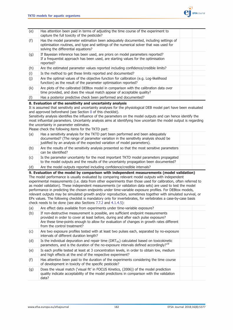
(e) Has attention been paid in terms of adjusting the time course of the experiment tocapture the full toxicity of the pesticide?
(f) Has the model parameter estimation been adequately documented, including settings ofoptimisation routines, and type and settings of the numerical solver that was used forsolving the differential equations?
(g) If Bayesian inference has been used, are priors on model parameters reported?If a frequentist approach has been used, are starting values for the optimisationreported?
(h) Are the estimated parameter values reported including confidence/credible limits?
(i) Is the method to get these limits reported and documented?(j) Are the optimal values of the objective function for calibration (e.g. Log-likelihood
function) as the result of the parameter optimisation reported?
(k) Are plots of the calibrated DEBtox model in comparison with the calibration data overtime provided, and does the visual match appear of acceptable quality?
(l) Has a posterior predictive check been performed and documented?
8. Evaluation of the sensitivity and uncertainty analysisIt is assumed that sensitivity and uncertainty analyses for the physiological DEB model part have been evaluatedand approved beforehand (see Section 0 of this checklist).Sensitivity analysis identifies the influence of the parameters on the model outputs and can hence identify themost influential parameters. Uncertainty analysis aims at identifying how uncertain the model output is regardingthe uncertainty in parameter estimates.Please check the following items for the TKTD part:(a) Has a sensitivity analysis for the TKTD part been performed and been adequately
documented? (The range of parameter variation in the sensitivity analysis should bejustified by an analysis of the expected variation of model parameters).
(b) Are the results of the sensitivity analysis presented so that the most sensitive parameterscan be identified?
(c) Is the parameter uncertainty for the most important TKTD model parameters propagatedto the model outputs and the results of the uncertainty propagation been documented?
(d) Are the model outputs reported including confidence/credible intervals?
9. Evaluation of the model by comparison with independent measurements (model validation)The model performance is usually evaluated by comparing relevant model outputs with independentexperimental measurements (i.e. data from other experiments than those used for calibration, often referred toas model validation). These independent measurements (or validation data sets) are used to test the modelperformance in predicting the chosen endpoints under time-variable exposure profiles. For DEBtox models,relevant outputs may be simulated growth and/or reproduction, sometimes together with simulated survival, orEPx values. The following checklist is mandatory only for invertebrates, for vertebrates a case-by-case basischeck needs to be done (see also Sections 7.7.2 and 4.1.4.5):
(a) Are effect data available from experiments under time-variable exposure?(b) If non-destructive measurement is possible, are sufficient endpoint measurements
provided in order to cover at least before, during and after each pulse exposure?Are these time-points enough to allow for evaluation of changes in growth rates differentfrom the control treatment?
(c) Are two exposure profiles tested with at least two pulses each, separated by no-exposureintervals of different duration length?
(d) Is the individual depuration and repair time (DRT95) calculated based on toxicokineticparameters, and is the duration of the no-exposure intervals defined accordingly?19
(e) Is each profile tested at least at 3 concentration levels, in order to obtain low, mediumand high effects at the end of the respective experiment?
(f) Has attention been paid to the duration of the experiments considering the time courseof development in toxicity of the specific pesticide?
(g) Does the visual match (‘visual fit’ in FOCUS Kinetics, (2006)) of the model predictionquality indicate acceptability of the model predictions in comparison with the validationdata?
TKTD models for aquatic organisms
www.efsa.europa.eu/efsajournal 182 EFSA Journal 2018;16(8):5377

(h) Do the reported quantitative model performance criteria (e.g. PPC, NRMSE, SPPE)indicate a sufficient model performance?For DEBtox models, the adequacy of the quantitative criteria listed above (set on basis ofGUTS models) needs still to be fully tested and may need future adaptation. However, forthe time being, this set of performance criteria is also suggested for DEBtox models (seeSection 7.7.2 ‘Model performance criteria’).
(i) Has the performance of the model been reported in an objective and reproducible way?
10. Evaluation of model useWhen using a TKTD model for regulatory purposes, the inputs of species- and compound specific modelparameters and of exposure profile data are required to run the model under new conditions. In this stage, it isimportant that the model is well documented and that it is clear how the model works. Please check thefollowing items:
(a) Is the use of the model sufficiently documented?Is a user manual available?See items provided in Section 10.7 of the EFSA PPR Panel (2014).
(b) Is an executable implementation of the model made available to the reviewer, or Is atleast the source code provided?
(c) Has a summary sheet been provided by the applicant? The summary sheet shouldprovide quick access to the comprehensive documentation with sections corresponding tothe ones of this checklist.
(d) Does the exposure profile used with the TKTD model come from the same source as thePEC used with the Tier-1 effects data? For example if FOCUS Step 3 maximum valueswere used at Tier-1 are the exposure profiles used Tier-2C from the same FOCUS Step 3modelling? If the exposure profile comes from any other source (e.g. different scenarios,different inputs, different model) has this been checked?
(e) In case parameters of the DEB (physiological) part of the model were changed fromcalibration to validation in order to better describe control data:- Is the difference in the parameters inducing considerable difference in the modelpredictions?And, if yes:- Are the model simulations relevant for the risk assessment carried out with theparameter set producing the more conservative (worst-case) predictions?
It is recommended that the evaluator justifies the replies that are not straightforward.See also Appendix G – for an example on how to evaluate DEBtox models.
TKTD models for aquatic organisms
www.efsa.europa.eu/efsajournal 183 EFSA Journal 2018;16(8):5377
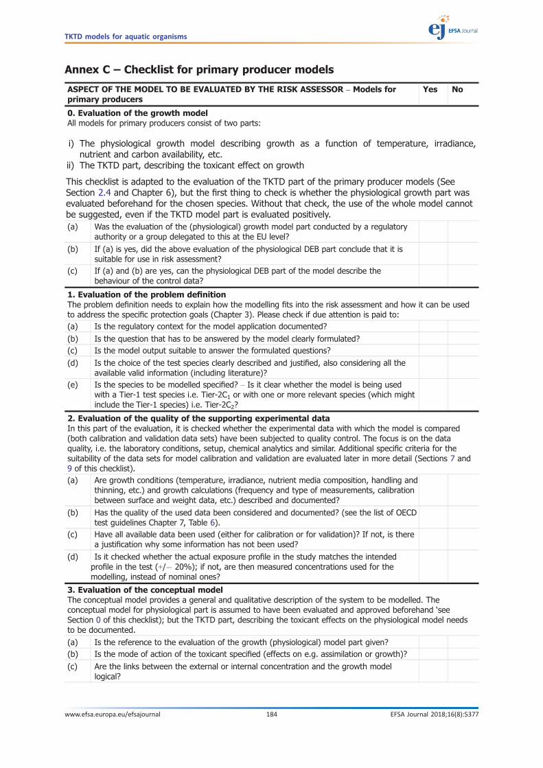
Annex C – Checklist for primary producer models
ASPECT OF THE MODEL TO BE EVALUATED BY THE RISK ASSESSOR – Models forprimary producers
Yes No
0. Evaluation of the growth modelAll models for primary producers consist of two parts:
i) The physiological growth model describing growth as a function of temperature, irradiance,nutrient and carbon availability, etc.
ii) The TKTD part, describing the toxicant effect on growth
This checklist is adapted to the evaluation of the TKTD part of the primary producer models (SeeSection 2.4 and Chapter 6), but the first thing to check is whether the physiological growth part wasevaluated beforehand for the chosen species. Without that check, the use of the whole model cannotbe suggested, even if the TKTD model part is evaluated positively.(a) Was the evaluation of the (physiological) growth model part conducted by a regulatory
authority or a group delegated to this at the EU level?
(b) If (a) is yes, did the above evaluation of the physiological DEB part conclude that it issuitable for use in risk assessment?
(c) If (a) and (b) are yes, can the physiological DEB part of the model describe thebehaviour of the control data?
1. Evaluation of the problem definitionThe problem definition needs to explain how the modelling fits into the risk assessment and how it can be usedto address the specific protection goals (Chapter 3). Please check if due attention is paid to:(a) Is the regulatory context for the model application documented?
(b) Is the question that has to be answered by the model clearly formulated?(c) Is the model output suitable to answer the formulated questions?
(d) Is the choice of the test species clearly described and justified, also considering all theavailable valid information (including literature)?
(e) Is the species to be modelled specified? – Is it clear whether the model is being usedwith a Tier-1 test species i.e. Tier-2C1 or with one or more relevant species (which mightinclude the Tier-1 species) i.e. Tier-2C2?
2. Evaluation of the quality of the supporting experimental dataIn this part of the evaluation, it is checked whether the experimental data with which the model is compared(both calibration and validation data sets) have been subjected to quality control. The focus is on the dataquality, i.e. the laboratory conditions, setup, chemical analytics and similar. Additional specific criteria for thesuitability of the data sets for model calibration and validation are evaluated later in more detail (Sections 7 and9 of this checklist).(a) Are growth conditions (temperature, irradiance, nutrient media composition, handling and
thinning, etc.) and growth calculations (frequency and type of measurements, calibrationbetween surface and weight data, etc.) described and documented?
(b) Has the quality of the used data been considered and documented? (see the list of OECDtest guidelines Chapter 7, Table 6).
(c) Have all available data been used (either for calibration or for validation)? If not, is therea justification why some information has not been used?
(d) Is it checked whether the actual exposure profile in the study matches the intendedprofile in the test (+/� 20%); if not, are then measured concentrations used for themodelling, instead of nominal ones?
3. Evaluation of the conceptual modelThe conceptual model provides a general and qualitative description of the system to be modelled. Theconceptual model for physiological part is assumed to have been evaluated and approved beforehand ‘seeSection 0 of this checklist); but the TKTD part, describing the toxicant effects on the physiological model needsto be documented.
(a) Is the reference to the evaluation of the growth (physiological) model part given?(b) Is the mode of action of the toxicant specified (effects on e.g. assimilation or growth)?
(c) Are the links between the external or internal concentration and the growth modellogical?
TKTD models for aquatic organisms
www.efsa.europa.eu/efsajournal 184 EFSA Journal 2018;16(8):5377

(d) In case environmental factors (e.g. nutrient levels, temperature) are explicitly considered,is their influence on the physiological and/or TKTD processes documented in theconceptual model?
(e) Are the modelling endpoints relevant to the specific protection goal?
4. Evaluation of the formal modelThe formal model contains equations used in the model. For each model application, all equations that are usedfor the modelling should be documented:
(a) Are all mathematical equations described, including the equations of the toxicokinetic(TK) part, and the equations relating the used internal concentration with the growth(physiological) model parameter(s)?
(b) Is there a list or summary of the variables and parameters including their meaning andunit?
(c) Are both the deterministic part (equations describing the mean tendency of the data) andthe stochastic part (the probability law describing the variability around the meantendency) of the model fully described? See Section 5.1 for an example with DEBtox.
5. Evaluation of the computer modelThe computer model corresponds to the implementation of the formalmodel that can run it on a computer. Please check the following items:
(a) Is the computer code available, including explaining comments for the most importantfunctions?
(b) Is enough information provided to allow any user to re-run the model independently (e.g.parameter sets, input data)?
(c) Is it demonstrated that the mathematical model is correctly implemented (modelverification), e.g. by checking and documenting the internal consistency of the modelresults based on a set of default or extreme cases (see e.g. Section 4.1.2.3 for anexample with GUTS, ‘reality check’ in chapter 10.4 of the EFSA PPR Panel (2014))?
6. Evaluation of the regulatory model – the environmental scenariosFor the application of primary producers TKTD models for the prediction of toxicological effects in a regulatorycontext, the environmental scenario need to be fixed to the laboratory conditions of the experiments used forcalibrating the TKTD part of the model. Please check the following items:
(a) Are all the relevant conditions, recorded in the experiments used for calibrating the TKTDpart of the model, used consistently for the simulations (i.e. for generating EPx) used inthe risk assessment?
7. Evaluation of the regulatory model – parameter estimationParameter estimation requires a suitable data set, the correct application of a parameter optimisation routine,and the comprehensive documentation of methods and results (see Chapter 3 for background information).Model parameters are always estimated for a specific combination of species and compound.Supporting data for primary producers have to be of sufficient quality (Section 2 in this checklist), be relevant tothe risk assessment problem and fulfil a set of basic criteria. Typical supporting data for the TKTD part of primaryproducer models are toxicity test data for growth measured either on the basis of frond number, surface area orbiomass over time (see Chapters 2.4 for background information; Chapter 6 for examples). Specific requirementson the time resolution and temporal scale for the calibration data cannot be given, but in general the number oftime-points has to be sufficient to provide enough degrees of freedom for the model calibration.Please check the following items to evaluate the calibration data, the parameter optimisation and the results (seeSections 4.1.3 and 7.6.2):
(a) Is it clear which parameters have been taken from literature or other sources or whichhave been fitted to data?If used, are values from literature reasonable and justified?
(b) Are the calibration data sufficient to provide enough degrees of freedom for the modelcalibration, i.e. are endpoints reported at several20 intermediate time-points?
(c) Does calibration data span from treatment levels with no effects up to strong effects,ideally up to full effects (e.g. no growth)?
(d) Have all data available for calibration been used? If not, is there a justification why thisinformation has not been used?
(e) Has attention been paid in terms of adjusting the time course of the experiment tocapture the full toxicity of the pesticide?
20 Growth should be non-destructively monitored by measuring surface area or frond number on a daily basis or every two days.Biomass should be measured at least at the end of the exposure phase.
TKTD models for aquatic organisms
www.efsa.europa.eu/efsajournal 185 EFSA Journal 2018;16(8):5377

(f) Has the model parameter estimation been adequately documented, including settings ofoptimisation routines, and type and settings of the numerical solver that was used forsolving the differential equations?
(g) If Bayesian inference has been used, are priors on model parameters reported?If a frequentist approach has been used, are starting values for the optimisationreported?
(h) Are the estimated parameter values reported including confidence/credible limits?
(i) Is the method to get these limits reported and documented?(j) Are the optimal values of the objective function for calibration (e.g. Log-likelihood
function) as the result of the parameter optimisation reported?
(k) Are plots of the calibrated TKTD models in comparison with the calibration data over timeprovided, and does the visual match appear of acceptable quality?
(l) Has a posterior predictive check been performed and documented?
8. Evaluation of the sensitivity and uncertainty analysisIt is assumed that sensitivity and uncertainty analyses for the physiological model part have been evaluated andapproved beforehand. Sensitivity analysis identifies the influence parameters have on the model outputs and canhence identify the most relevant model parameters. Uncertainty analysis aims at identifying how uncertain themodel output is regarding the uncertainty in parameter estimates. Please check the following items for the TKTDpart:(a) Has a sensitivity analysis for the TKTD part been performed and been adequately
documented? (The range of parameter variation in the sensitivity analysis should bejustified by an analysis of the expected variation of model parameters).
(b) Are the results of the sensitivity analysis presented so that the most sensitive parameterscan be identified?
(c) Is the parameter uncertainty for the most important TKTD model parameters propagatedto the model outputs and the results of the uncertainty propagation been documented?
(d) Are the model outputs reported including confidence/credible intervals?
9. Evaluation of the model by comparison with independent measurements (model validation)The model performance is usually evaluated by comparing relevant model outputs with experimentalmeasurements (often referred to as model validation). Independent measurements (or validation data sets) areused to test the model performance in predicting the chosen endpoints under time-variable exposure profiles.These data have not been used for the model calibration. For models for primary producers, relevant outputs arebiomass or biomass-proxies such as cell number or chlorophyll content for algae at a specific point in time.Please check the following items:
(a) Are effect data available from experiments under time-variable exposure?(b) Are sufficient endpoint measurements provided in order to cover at least before, during
and after each pulse exposure?Are these time-points enough to allow for evaluation of changes in growth rates differentfrom the control treatment?
(c) Are two exposure profiles tested with at least two pulses each, separated by no-exposureintervals of different duration length?
(d) - point not relevant for algae- Is the individual depuration and repair time (DRT95; see Section 4.1.4.5) calculatedbased on toxicokinetic parameters, and is the duration of the no-exposure intervalsdefined accordingly? [Ideally one of the profiles should show a no-exposure intervalshorter than the DRT95, the other profile clearly larger than the DRT95]
(e) Is each profile tested at least at 3 concentration levels, in order to obtain low, mediumand high effects at the end of the respective experiment?
(f) Has attention been paid to the duration of the experiments considering the time courseof development in toxicity of the specific pesticide?
(g) Does the visual match (‘visual fit’ in FOCUS Kinetics (2006); see Section 4.1.4.5) of themodel prediction quality indicate acceptability of the model predictions in comparison withthe validation data?
TKTD models for aquatic organisms
www.efsa.europa.eu/efsajournal 186 EFSA Journal 2018;16(8):5377
(h) Do the reported quantitative model performance criteria (e.g. PPC, NRMSE, SPPE)indicate a sufficient model performance?For primary producer models, the adequacy of the quantitative criteria listed above (seton basis of GUTS models (see Section 4.1.4.5)) needs still to be fully tested, and mayneed future adaptation. However, for the time being, this set of performance criteria isalso suggested for primary producer models (see Section 7.7.2 ‘Model performancecriteria’).
(i) Has the performance of the model been reported in an objective and reproducible way??
10. Evaluation of model useWhen using a TKTD model for regulatory purposes, the inputs of species- and compound specific modelparameters and of exposure profile data are required to run the model under new conditions. In this stage, it isimportant that the model is well documented and that it is clear how the model works. Please check thefollowing items:
(a) Is the use of the model sufficiently documented?Is a user manual available?See items provided in Section 10.7 of the EFSA PPR Panel (2014).
(b) Is an executable implementation of the model made available to the reviewer, or Is atleast the source code provided?
(c) Has a summary sheet been provided by the applicant? The summary sheet shouldprovide quick access to the comprehensive documentation with sections corresponding tothe ones of this checklist.
(d) Does the exposure profile used with the TKTD model come from the same source as thePEC used with the Tier-1 effects data? For example if FOCUS Step 3 maximum valueswere used at Tier-1, are the exposure profiles used Tier-2C from the same FOCUS Step 3modelling? If the exposure profile comes from any other source (e.g. different scenarios,different inputs, different model) has this been checked?
(e) In case parameters of the growth (physiological) model were changed from calibration tovalidation, in order to better describe control data:- Is the difference in the parametersinducing considerable difference in the model predictions?And, if yes:- Are model simulations relevant for the risk assessment carried out with theparameter set producing the more conservative (worst-case) predictions?
It is recommended that the evaluator justifies the replies that are not straightforward.
TKTD models for aquatic organisms
www.efsa.europa.eu/efsajournal 187 EFSA Journal 2018;16(8):5377

Annex D – Model Summary template
For TKTD model applications, it is strongly suggested to document the study according to therequirements announced in the EFSA TKTD SO. The applicant needs to document in the followingsummary template, that the model-specific checklists (Annex A, B and C of the EFSA TKTD SO) havebeen considered. Clarifications are required on how the aspects listed in the model specific checklistsare reflected in the model documentation. References to the parts of the DAR/RAR or other documentswhere the points are fully explained should be included. This summary should provide sufficient detailto allow the reader to understand the key points about how the modelling was conducted. In addition,it should be suitable to provide the basis for the study summary that RMS will produce for the DAR/RAR. The aim is to ensure the risk assessor that all aspects of the modelling cycle are captured andalso to help the model evaluators to find all the information they need in the model documentation.
AspectReference to section in the modeldocumentation or assessment report
1. Problem definition
2. Supporting data3. Conceptual model1
4. Formal model1
5. Computer model2
6. Regulatory model – the environmental scenario3
7. Regulatory model – parameter estimation
8. Regulatory model – Sensitivity and uncertainty analysis9. Regulatory model – Comparison with measurements
10. Reality/problem – Model use
1: For GUTS models it is sufficient to identify which version of GUTS has been used and to refer to this Scientific Opinion. Thiscan be done since the conceptual and formal models are standardised following Jager and Ashauer (2018).
2: If standard software implementations become available (and have been checked) it will be sufficient to identify whichsoftware and version was used.
3: For GUTS models, if output from FOCUS surface water standard software has been used, it is sufficient to document whichFOCUS model versions and scenarios have been used.
TKTD models for aquatic organisms
www.efsa.europa.eu/efsajournal 188 EFSA Journal 2018;16(8):5377