Scientific Computing with Applications in Tribology - DiVA-Portal
197
January 26, 2022 Scientific Computing with Applications in Tribology -A Course Compendium Andreas Almqvist & Francesc P´ erez R` afols Lule˚ a University of Technology Department of Applied Physics and Mechanical Engineering, Division of Machine Elements
-
Upload
khangminh22 -
Category
Documents
-
view
1 -
download
0
Transcript of Scientific Computing with Applications in Tribology - DiVA-Portal

January 26, 2022
Scientific Computing with Applications in Tribology
-A Course Compendium
Andreas Almqvist & Francesc Perez Rafols
Lulea University of TechnologyDepartment of Applied Physics and Mechanical Engineering,
Division of Machine Elements

Lulea University of Technology, 97187, Lulea, Sweden, 2019

Scientific Computing with Applications in Tribology
- A Course Compendium
Copyright © (2018)
Andreas Almqvist [email protected]
&
Francesc Perez Rafols [email protected]
This document was typeset in LATEX 2ε
.

Abstract
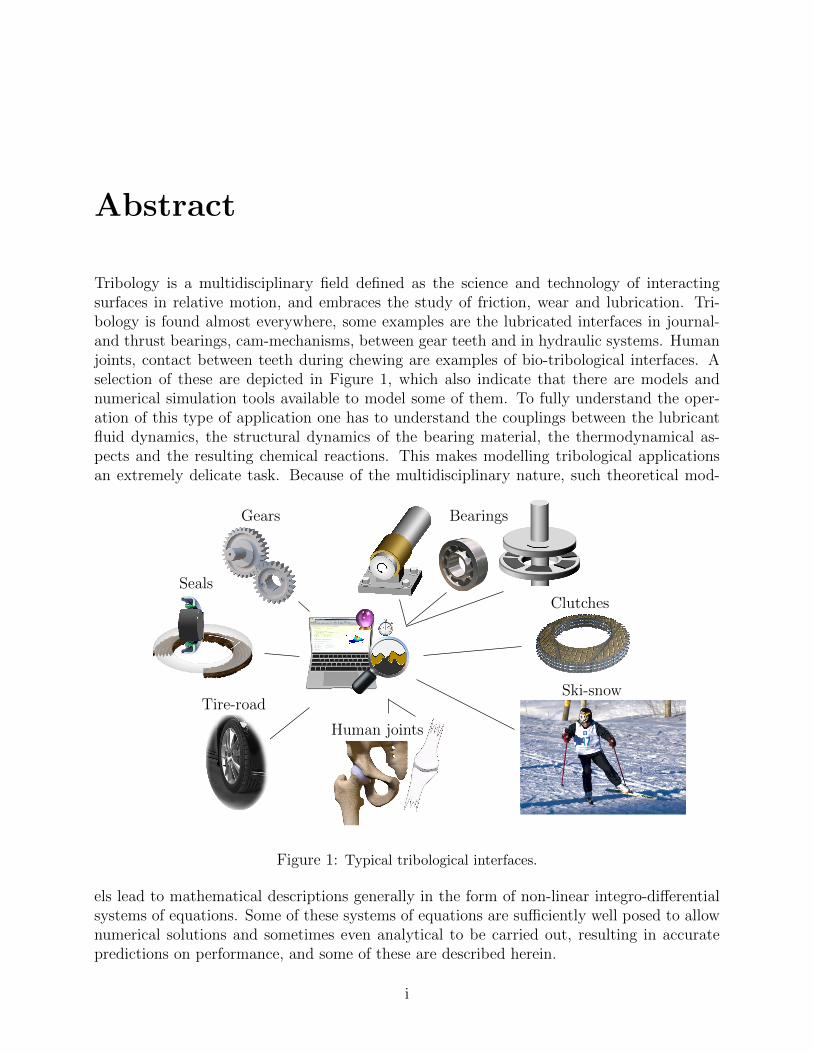
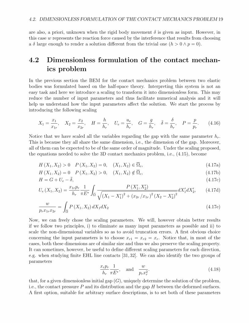
Tribology is a multidisciplinary field defined as the science and technology of interactingsurfaces in relative motion, and embraces the study of friction, wear and lubrication. Tri-bology is found almost everywhere, some examples are the lubricated interfaces in journal-and thrust bearings, cam-mechanisms, between gear teeth and in hydraulic systems. Humanjoints, contact between teeth during chewing are examples of bio-tribological interfaces. Aselection of these are depicted in Figure 1, which also indicate that there are models andnumerical simulation tools available to model some of them. To fully understand the oper-ation of this type of application one has to understand the couplings between the lubricantfluid dynamics, the structural dynamics of the bearing material, the thermodynamical as-pects and the resulting chemical reactions. This makes modelling tribological applicationsan extremely delicate task. Because of the multidisciplinary nature, such theoretical mod-
!🔎
Tire on road
🔮
Seals
Gears Bearings
Clutches
Ski-snow
Human joints
Tire-road
Figure 1: Typical tribological interfaces.
els lead to mathematical descriptions generally in the form of non-linear integro-differentialsystems of equations. Some of these systems of equations are sufficiently well posed to allownumerical solutions and sometimes even analytical to be carried out, resulting in accuratepredictions on performance, and some of these are described herein.
i


Acknowledgment
Although the compilation of this text is the work solely of the authors, the models andassociated solution procedures presented herein, are work by other researchers in the field,joint developments with our co-authors and many knowledgeable colleagues. Our sinceregratitude is extended towards them all.
iii

Contents
1 Introduction 1
2 The Tribological Contact 32.1 The boundary lubrication regime . . . . . . . . . . . . . . . . . . . . . . . . 42.2 The mixed lubrication regime . . . . . . . . . . . . . . . . . . . . . . . . . . 52.3 The full-film lubrication regime . . . . . . . . . . . . . . . . . . . . . . . . . 5
2.3.1 Hydrodynamic lubrication . . . . . . . . . . . . . . . . . . . . . . . . 62.3.2 Elastohydrodynamic lubrication . . . . . . . . . . . . . . . . . . . . . 6
3 Content and Intended Learning Outcomes 93.1 Dry contacts . . . . . . . . . . . . . . . . . . . . . . . . . . . . . . . . . . . . 93.2 Lubricated contacts . . . . . . . . . . . . . . . . . . . . . . . . . . . . . . . . 93.3 Wear . . . . . . . . . . . . . . . . . . . . . . . . . . . . . . . . . . . . . . . . 10
4 The Dry Contact 114.1 Half-space theory and fundamentals of the BEM . . . . . . . . . . . . . . . . 12
4.1.1 The relation between load and deformation . . . . . . . . . . . . . . . 134.1.2 The contact between an elastic body and a rigid flat surface . . . . . 154.1.3 The contact between two elastic bodies . . . . . . . . . . . . . . . . 17
4.2 Dimensionless formulation of the contact mechanics problem . . . . . . . . . 194.3 Examples of analytical solutions . . . . . . . . . . . . . . . . . . . . . . . . . 22
4.3.1 Hertz theory . . . . . . . . . . . . . . . . . . . . . . . . . . . . . . . . 224.3.2 The Westergaard solution . . . . . . . . . . . . . . . . . . . . . . . . 264.3.3 Flattening of bi-sinusoidal surfaces . . . . . . . . . . . . . . . . . . . 29
4.4 Discretisation . . . . . . . . . . . . . . . . . . . . . . . . . . . . . . . . . . . 294.4.1 Discretisation of the domain . . . . . . . . . . . . . . . . . . . . . . . 304.4.2 Discretisation of the gap . . . . . . . . . . . . . . . . . . . . . . . . . 304.4.3 Discretisation of the pressure . . . . . . . . . . . . . . . . . . . . . . 314.4.4 Discretisation of the deformation equation . . . . . . . . . . . . . . . 314.4.5 Discretisation of the load-balance equation . . . . . . . . . . . . . . . 34
4.5 Lemke’s algorithm . . . . . . . . . . . . . . . . . . . . . . . . . . . . . . . . 344.6 Acceleration via FFT . . . . . . . . . . . . . . . . . . . . . . . . . . . . . . . 36
4.6.1 The elastic deformation seen as a convolution . . . . . . . . . . . . . 364.6.2 The DFT-CC method . . . . . . . . . . . . . . . . . . . . . . . . . . 384.6.3 DFT - Discrete Circular Convolution method: Periodic surfaces . . . 40
v

4.6.4 DFT - Discrete Linear Convolution method: Non-periodic surfaces . . 42
4.7 A variational-principle based elastic CM solver . . . . . . . . . . . . . . . . . 43
4.8 Enhanced CM solver including plastic deformation . . . . . . . . . . . . . . . 46
5 The Lubricated Contact 51
5.1 Constitutive relations . . . . . . . . . . . . . . . . . . . . . . . . . . . . . . . 53
5.1.1 Scaling of the Navier-Stokes equations . . . . . . . . . . . . . . . . . 57
5.1.2 Iso-viscous and incompressible fluids . . . . . . . . . . . . . . . . . . 60
5.1.3 Iso-viscous and compressible fluids . . . . . . . . . . . . . . . . . . . 62
5.2 The Reynolds equation . . . . . . . . . . . . . . . . . . . . . . . . . . . . . . 67
5.2.1 Iso-visous and incompressible fluids . . . . . . . . . . . . . . . . . . . 67
5.2.2 Piezo-viscous and compressible fluids . . . . . . . . . . . . . . . . . . 71
5.2.3 Load carrying capacity and friction force . . . . . . . . . . . . . . . . 73
5.2.4 Force balance and rigid body separation . . . . . . . . . . . . . . . . 75
5.3 Solutions to some variants of the 1D Reynolds equation . . . . . . . . . . . . 75
5.3.1 The velocity field . . . . . . . . . . . . . . . . . . . . . . . . . . . . . 82
5.3.2 LCC for the 2D linear slider bearing . . . . . . . . . . . . . . . . . . 85
5.3.3 Friction force for the 2D linear slider bearing . . . . . . . . . . . . . . 85
5.4 Dimensionless formulation . . . . . . . . . . . . . . . . . . . . . . . . . . . . 88
5.4.1 Time dependent Reynolds’ equation and force balance . . . . . . . . 89
5.4.2 Stationary 1D Reynolds’ equation . . . . . . . . . . . . . . . . . . . . 91
5.5 On the unicity of the film thickness . . . . . . . . . . . . . . . . . . . . . . . 93
5.6 On the applicability of the Reynolds equation . . . . . . . . . . . . . . . . . 96
5.7 The finite difference method for Reynolds’ type of PDE:s . . . . . . . . . . . 99
5.7.1 An FDM for the stationary 1D Reynolds equation . . . . . . . . . . . 103
5.7.2 An FDM for the stationary 2D Reynolds equation . . . . . . . . . . . 105
5.8 Modelling mass-conserving hydrodynamic cavitation . . . . . . . . . . . . . . 114
5.8.1 JFO theory . . . . . . . . . . . . . . . . . . . . . . . . . . . . . . . . 115
5.8.2 Elrod’s and Adams’ universal cavitation algorithm . . . . . . . . . . . 116
5.8.3 Vijayaraghavan’s and Keith Jr’s cavitation model . . . . . . . . . . . 117
5.8.4 Arbitrary compressibility switch function based cavitation algorithm 118
5.8.5 The linear complementarity problem formulation . . . . . . . . . . . 119
5.8.6 The FEM and cavitation modelling . . . . . . . . . . . . . . . . . . . 130
5.9 Homogenisation of the Reynolds equation . . . . . . . . . . . . . . . . . . . . 132
5.9.1 Iso-viscous and incompressible flow . . . . . . . . . . . . . . . . . . . 134
5.9.2 Iso-viscous and constant bulk-modulus type of compressible flow . . . 139
5.9.3 Ideal gas flow . . . . . . . . . . . . . . . . . . . . . . . . . . . . . . . 140
5.9.4 Approximative generalisations . . . . . . . . . . . . . . . . . . . . . . 141
5.9.5 Homogenised load carrying capacity, friction and flow . . . . . . . . . 143
5.9.6 Patir and Cheng flow-factors and Homogenised coefficients . . . . . . 147
5.9.7 Homogenised flow factors for mixed lubrication conditions . . . . . . 155
5.10 Modelling mixed lubrication . . . . . . . . . . . . . . . . . . . . . . . . . . . 157

6 Modelling Wear in Lubrication 1596.1 Archard’s model for adhesive wear . . . . . . . . . . . . . . . . . . . . . . . . 1606.2 Archard’s model for abrasive wear . . . . . . . . . . . . . . . . . . . . . . . . 1626.3 A wear model for rough surfaces . . . . . . . . . . . . . . . . . . . . . . . . . 163
A Fourier Techniques 177A.1 The Fourier series . . . . . . . . . . . . . . . . . . . . . . . . . . . . . . . . . 177A.2 The Fourier transform . . . . . . . . . . . . . . . . . . . . . . . . . . . . . . 179A.3 The discrete Fourier transform . . . . . . . . . . . . . . . . . . . . . . . . . . 180A.4 The continuous convolution theorem . . . . . . . . . . . . . . . . . . . . . . 182A.5 Discrete convolutions . . . . . . . . . . . . . . . . . . . . . . . . . . . . . . . 182
A.5.1 The discrete circular convolution . . . . . . . . . . . . . . . . . . . . 182A.5.2 The discrete linear convolution . . . . . . . . . . . . . . . . . . . . . 183


Preface
In this compendium, we have chosen to comprise models and numerical solution procedurefor tribological interfaces. We start by describing the tribological contact and the classicallubrication regimes. Thereafter, fundamentals of half-space theory, which is the foundationfor the contact mechanics models so frequently utilised in tribology, is briefly described.Associated discretisation, suggested numerical solution procedures and how to acceleratethem by using the fast Fourier transformation technique are presented there too.
We also elaborate upon the theoretical foundation for modelling the thin film flow, whichis so characteristic for lubricated contacts. In this part of the compendium, a thoroughderivation of the Reynolds equation from the Navier-Stokes momentum equations and thecontinuity equation for conservation of mass, is presented along with its analytical solutionfor the infinitely wide linear slider bearing. Finite difference schemes for solving the Reynoldsequation are also presented here. The concept of cavitation, homogenisation pf surface rough-ness, the Patir and Cheng method, and how to address mixed lubrication are also elaboratedon.
Modelling and simulation of wear is given a chapter of its own and here we discuss theapplication of Archard’s equation and give a derivation of a model for “polishing” type ofwear.
The compilation of the compendium was conducted by the first author during his tenureas Professor at the Division of Machine Elements, Department of Engineering Sciences andMathematics, Lulea University of Technology and by the second author during his tenure asa postdoctoral researcher at the same division.
Although the compilation of this text is the work solely of the authors, the models andsolution procedure presented herein is joint development of many good colleagues and co-authors. Our sincere gratitude is extended towards them all.
ix


Chapter 1
Introduction
Machines consist of machine elements and their safe and efficient operation relies on care-fully designed interfaces between these elements. The functional design of interfaces coversgeometry, materials, lubrication and surface topography, and an incorrect design may leadto both lowered efficiency and shortened service life. A misalignment due to the geometricaldesign could lead to large stress concentrations that in turn may lead to severe damage whenmounting, a detrimental wear situation, rapid fatigue during operation, etc. Large stressconcentrations also implicitly imply a temperature rise because of the energy dissipation dueto plastic deformations. The choice of mating materials is also of great importance, e.g.electrolytic corrosion may drastically reduce service life. Contact fatigue due to low ductilitywould not only lower the service life but could lead to third body abrasion due to spalling,which in turn could end up lowering the service life of other components. A lubricant servesseveral crucial objectives; when its main objective is to lower friction, the actions of additivesare of concern. If the interface is subjected to excessive wear, the lubricant’s ability to form aseparating film becomes even more crucial. In this case, the bulk properties of the lubricanthave to be carefully chosen. At some scale, regardless of the surface finish, all real surfacesare rough and their topography influences the contact condition.
As implied above, the design parameters are mutually dependent, i.e. they affect theway others influence the operation of the system. For example, a change in geometry couldrequire another choice of materials that may change the objectives of the lubricant and forcethe operation into another lubrication regime.
The influence of the aforementioned design parameters, i.e., geometry, materials, lubri-cation and surface topography on performance has of course been investigated by manyresearchers in the field both experimentally and numerically. However, because of the multi-disciplinary nature of the field and the complexity of the theoretical models associated withtribological problems, the progress in the development of efficient, still user friendly softwarehas not reached as far as in, e.g., computational structural mechanics and computationalfluid dynamics. Moreover, the requirement on the density of the mesh to resolve not onlythe geometrical part of the tribological contact but also the surface topography is difficultto meet. The material herein is meant to provide understanding of established models andnumerical solution procedures that can be used to study behaviour of tribological interfaces.Hopefully, it also inspires and encourages the reader to contribute to further developmentthereof.
1

2 CHAPTER 1. INTRODUCTION

Chapter 2
The Tribological Contact
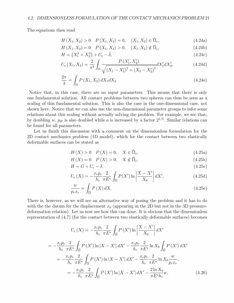
At start-ups, at stops as well as during operation, most machine elements experiences varyingcontact conditions. Take, for example, the (axial) tilted pad thrust bearing illustrated inFig. 2.1. This type of bearing belongs to the class of hydrodynamic fluid film bearings, which
Segment/pad
CollarShaft
Figure 2.1: Schematics of a tilting pad thrust bearing including the shaft connecting e.g. theturbine to the generator in a hydro-power machine.
are designed for fluid film pressure build-up that separate the rotating and stationary surfacesso that contact less rotation while carrying the load on the shaft. In fact, it is the relativemotion of the surfaces, as the lubricant is pulled into the converging geometry between thecollar and the pad, that creates the necessary fluid film pressure.
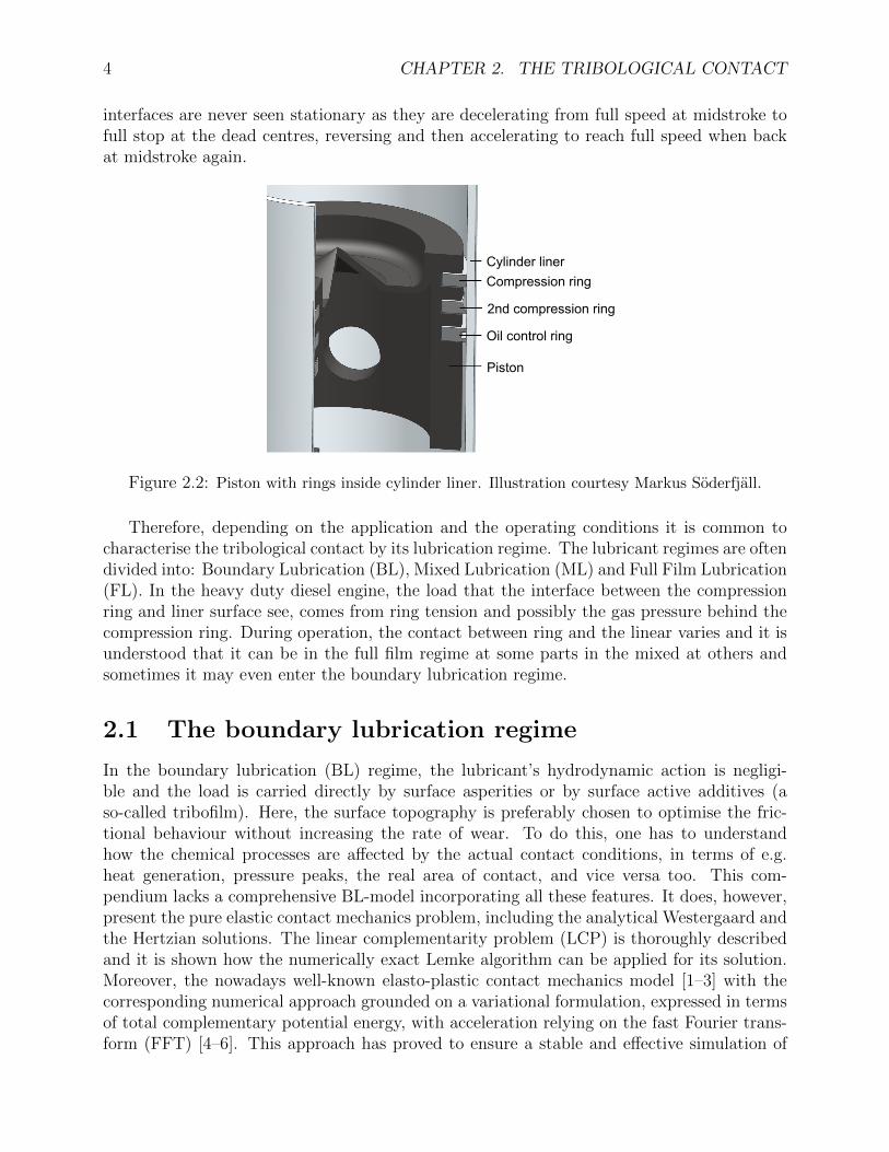
Typically, the collar in a tilting pad thrust bearing is made of steal while the pads havea soft (compliant) facing made of Babbitt (metal alloy) or Teflon® (polytetrafluoroethylene(PTFE)). This means that the littlest direct contact the collar makes with the shaft whilerotating, will cause severe wear on the facing surface and it is of crucial importance to have asystem that separates the surfaces during initiation of start-up and stop. A common solutionis to implement a system that pressurises the supplied lubricant, generating hydrostatic lift.Another example is the piston with its reciprocating motion inside the cylinder of a heavyduty diesel engine, such as the one depicted in Fig. 2.2. In this case, the lubricated ring
3
4 CHAPTER 2. THE TRIBOLOGICAL CONTACT
interfaces are never seen stationary as they are decelerating from full speed at midstroke tofull stop at the dead centres, reversing and then accelerating to reach full speed when backat midstroke again.
Compression ring
2nd compression ring
Cylinder liner
Oil control ring
Piston
Figure 2.2: Piston with rings inside cylinder liner. Illustration courtesy Markus Soderfjall.
Therefore, depending on the application and the operating conditions it is common tocharacterise the tribological contact by its lubrication regime. The lubricant regimes are oftendivided into: Boundary Lubrication (BL), Mixed Lubrication (ML) and Full Film Lubrication(FL). In the heavy duty diesel engine, the load that the interface between the compressionring and liner surface see, comes from ring tension and possibly the gas pressure behind thecompression ring. During operation, the contact between ring and the linear varies and it isunderstood that it can be in the full film regime at some parts in the mixed at others andsometimes it may even enter the boundary lubrication regime.
2.1 The boundary lubrication regime
In the boundary lubrication (BL) regime, the lubricant’s hydrodynamic action is negligi-ble and the load is carried directly by surface asperities or by surface active additives (aso-called tribofilm). Here, the surface topography is preferably chosen to optimise the fric-tional behaviour without increasing the rate of wear. To do this, one has to understandhow the chemical processes are affected by the actual contact conditions, in terms of e.g.heat generation, pressure peaks, the real area of contact, and vice versa too. This com-pendium lacks a comprehensive BL-model incorporating all these features. It does, however,present the pure elastic contact mechanics problem, including the analytical Westergaard andthe Hertzian solutions. The linear complementarity problem (LCP) is thoroughly describedand it is shown how the numerically exact Lemke algorithm can be applied for its solution.Moreover, the nowadays well-known elasto-plastic contact mechanics model [1–3] with thecorresponding numerical approach grounded on a variational formulation, expressed in termsof total complementary potential energy, with acceleration relying on the fast Fourier trans-form (FFT) [4–6]. This approach has proved to ensure a stable and effective simulation of
2.2. THE MIXED LUBRICATION REGIME 5
(rough) contact mechanics and it can help to increase the understanding of how the surfaceroughness influences the elastic deflection, the plastic deformation (and plasticity index), thepressure build up and the real area of contact. An in-depth understanding of this connectionis required to refine the design of interfaces operating under these circumstances.
As the hydrodynamical action of the lubricant increases, the contact mechanical responsebecomes less influential in terms of pressure and real contact area, and a transition from theBL- to the ML- regime may therefore occur.
2.2 The mixed lubrication regime
What characterizes the ML regime is that the load is carried by the lubricant’s hydrodynam-ical action, which may be influenced by the elastic deflection of the surfaces, the tribofilm,directly by surface asperities, or a combination thereof.
This means that the objectives of the surface topography are to support the hydrodynamicaction of the lubricant, aid the elastic deflection in rendering a smoother surface, enablebonding of the surface active additives and optimise friction in the contact spots withoutincreasing wear.
Modelling mixed lubrication has turned out to be a true challenge and the models availableare built upon assumptions simplifying the physics involved in the transition from the BL-and the FL- regime. As indicated above, a contact mechanics model may be used to indicatea possible transition between the BL- and the ML-regimes. Similarly, modelling performedregarding full-film lubrication has lead to numerical approaches that may be used to increasethe understanding of the transition from the FL- to the ML- regimes. One well-knownexample of an ML-model, is the Lulea mixed lubrication model [3], in which partitioningbetween lubricant carried load and load carried by direct contact, is determined by theseparation. More precisely, when the separation becomes smaller than a chosen measureof the surface roughness height, the lubricant load is alleviated with the amount that thecorresponding unlubricated interface would carry at that separation.
2.3 The full-film lubrication regime
When the hydrodynamic action of the lubricant fully separates the surfaces and the loadis no longer carried by the contact between the surfaces, the interface enters the full filmlubrication (FL) regime. In the FL regime, traction may be reduced by carefully chosentopographies. Even though there is no direct contact, the lubricant pressure may lead tostress concentrations high enough to cause fatigue, likely leading to excessive wear in theform of spalling in highly loaded situations.
This regime is commonly sub-divided into hydrodynamic lubrication (HL) and elastohy-drodynamic lubrication (EHL), since the performance is greatly affected by the presence ofelastic deflections, i.e., fluid-structure interaction, at the lubricated interface.

6 CHAPTER 2. THE TRIBOLOGICAL CONTACT
2.3.1 Hydrodynamic lubrication
Slider bearings are typical examples of applications that, under certain conditions, operatein the hydrodynamic lubrication (HL) regime where the elastic deformations of the bearingsurfaces are sufficiently small to be neglected. For example, the tilting pad thrust bearing,as depicted in Fig. 2.1, exhibits a conformal interface between the pad and the collar andis designed to for operation in the hydrodynamic lubrication regime. Note that the angleof inclination of the pads, which is generally only a fraction of a degree, has been greatlyexaggerated in the figure. One problem that arise when modelling conformal interfaces likethis one, comes from the large differences in scales. More precisely, the global scale describingthe geometry, pad - collar interface, is several orders of magnitude larger than the local scaledescribing the surface topography/roughness. This situation can be approached by means ofhomogenisation. This is also a subject discussed herein, see Section 5.9.
2.3.2 Elastohydrodynamic lubrication
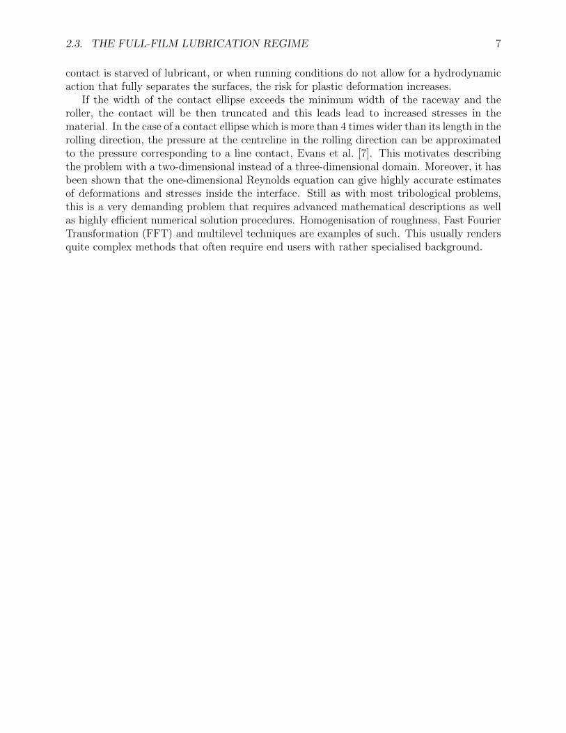
Elastohydrodynamic lubrication is the type of hydrodynamic lubrication where the fluid-structure interaction (FSI), caused by elastic deformations of the contacting surfaces, playsa major role. This situation may occur when lubricating interacting non-conformal bodies.This leads to highly localised (concentrated) contacts, and it is the lubricant’s piezo-viscousresponse combined with elastic flattening of surface roughness features facilitate the separa-tion of the interacting surfaces. An example where EHL is typically found, is at the interfacebetween the roller and the raceway in a typical roller bearing, as shown in Fig. 2.3, are mostcommonly designed to operate in the full-film elastohydrodynamic lubrication regime.
Figure 2.3: Schematics of a typical rolling element bearing-
The apparent contact zone for a rolling bearing is, in general, elliptic in shape. Dependingon the design parameters previously mentioned and the actual running conditions, the shapeof the ellipse will change. In any case, the contact region is small and the concentrated loadimplies a severe surface- as well as sub-surface stress condition that may lead to both elastic-but also plastic deformation. For a bearing in operation, high stresses eventually causes fa-tigue, which in turn can lead to shortened service life due to, for example, spalling. When the
2.3. THE FULL-FILM LUBRICATION REGIME 7
contact is starved of lubricant, or when running conditions do not allow for a hydrodynamicaction that fully separates the surfaces, the risk for plastic deformation increases.
If the width of the contact ellipse exceeds the minimum width of the raceway and theroller, the contact will be then truncated and this leads lead to increased stresses in thematerial. In the case of a contact ellipse which is more than 4 times wider than its length in therolling direction, the pressure at the centreline in the rolling direction can be approximatedto the pressure corresponding to a line contact, Evans et al. [7]. This motivates describingthe problem with a two-dimensional instead of a three-dimensional domain. Moreover, it hasbeen shown that the one-dimensional Reynolds equation can give highly accurate estimatesof deformations and stresses inside the interface. Still as with most tribological problems,this is a very demanding problem that requires advanced mathematical descriptions as wellas highly efficient numerical solution procedures. Homogenisation of roughness, Fast FourierTransformation (FFT) and multilevel techniques are examples of such. This usually rendersquite complex methods that often require end users with rather specialised background.

8 CHAPTER 2. THE TRIBOLOGICAL CONTACT

Chapter 3
Content and Intended LearningOutcomes
The intended learning outcomes are related to modelling and simulation of tribological pro-cesses connected to the following topics Lubricated contacts, Dry contacts and Wear. Thecontent include derivations of models, dimensionless formulation, techniques for discretisa-tion, numerical solution procedures and it discusses verification and validation.
3.1 Dry contacts
In relation to modelling and simulation of the dry contact by means of half-space theory basedcontact mechanics, the usage of the fast Fourier transformation (FFT) technique will be dis-cussed. It will be shown how it can be used applied in order to accelerate the computation ofderivatives and integral equations, and specifically the deflection of linear elastic bodies. Theassociated complementarity problem and the total complementary potential energy problemwill be described, together with two different means of how to numerically solve the contactmechanics model. More precisely, a numerical exact method that finds the solution to thecorresponding linear complementarity problem (LCP) in a finite number of pivoting stepswill be explained [8] The classical variational approach to solve the problem posed as theminimisation of the total complementary potential energy by Kalker [9]. is described herein.The FFT-based solution procedure suggested by Stanley and Kato in [10] is also describedand, in this connection, a simple way of including plastic deformation in accordance with thea quadratic programming approach presented by Tian and Bhushan [1] is given. It should bementioned that this methodology has been described before, namely in the two-part paperby Sahlin et al. [3,11]. In order to verify and validate the results, both the Hertzian contact,for the contact between spherically shaped elastic bodies, and Westergaard’s solution, forharmonic surfaces, are revisited first.
3.2 Lubricated contacts
This part starts with the derivation of the Reynolds equation for the hydrodynamic pressure.The Reynolds equation is a second order Poisson type of differential equation and both the
9

10 CHAPTER 3. CONTENT AND INTENDED LEARNING OUTCOMES
Cartesian and the polar form will be presented here. The derivation involves scaling anddimensional analysis of the Navier-Stokes momentum equations coupled with the continuityequation for mass preservation. The methodology is generic and can be applied in other areasas well. The limitations in the derivation are elaboration upon in the same manner as in thepapers by Almqvist et al. [12–14]. The analytical solution to the one-dimensional Reynoldsequation for an infinitely wide bearing is presented. Then it is shown how it can be used toverify the numerical results obtained with finite difference and finite element based methodsfor realistic bearing geometries.
Hydrodynamic cavitation is found in various lubrication situations, and without includingit in the model the bearing’s load carrying capacity can, in many cases, not be predicted. TheJakobsson, Floberg and Olsson (JFO) boundary conditions [15–18] and the switch-functionbased Elrod and Adams model [19] will be discussed and use as a basis for the derivation ofthe state-of-the-art model. In particular, this model addresses the change of the differentialequation from elliptic in the fully saturated zones to hyperbolic in the cavitated zones. Theextension of the classical switch-function based algorithm, into a clear and concise LCP-formulation [20–24] for incompressible- and the constant bulk modulus type of compressibleflows are also included here.
Homogenisation is presented here as a means for effective treatment of the roughness ofthe interacting surfaces and the derivations herein are inspired from numerous publications.For a compilation of these see e.g. [25, 26]. Finally a mixed lubrication model is presented.However, as mixed lubrication involves direct contact between the surfaces, modelling thedry contact is presented on beforehand.
3.3 Wear
Wear does under some circumstances allow for modelling. Here, Archard’s equation is em-ployed, primarily for the modelling of abrasive wear. Archard’s equation is an initial valueproblem and it is in combination with the contact mechanics model it can be used to pre-dict the material loss in tribological contacts. It is also discussed how the time steppingin subsequent numerical simulation procedure can be adjusted to simulate an adhesive wearprocesses. A lot of what is presented in under this topic originates from the work by Furustig1
et al. [27, 28].
1Previously Andersson and also known as The Wear Doctor (Notningsdoktorn).

Chapter 4
The Dry Contact
In the previous chapter, the lubrication regimes in which the lubricant has more or lessinfluence were described. Let us, however, start by considering the case in which no lubricantis present, i.e., the dry contact. When two bodies are pressed against each other they makecontact and become deformed. The deformation may be both elastic and plastic. Theamount and the relation between the two depend on the type of material, the applied loadand the geometry and micro-scale topography, i.e. roughness, of the contacting surfaces.Engineering surfaces does always exhibit roughness at some scale. Thus, the contact betweentwo components, such as the shaft and the bronze bush in a plain bearing, occurs at firstonly at the peaks of the highest protruding asperities in a complicated pattern. Figure 4.1depicts a series of such contact morphologies, obtained by means of numerical simulations.
Figure 4.1: Contact morphologies, obtained with the enhanced solver including plastic deformationpresented in Section 4.8, when loading the surface with Hurst exponent 0.8 in [29] against a rigidplane. First row depict pure elastic contact, second elastoplastic with hardness value of 4 GPa andthird elastoplastic with hardness value of 1 GPa. The contact load increases from left two right.Red points indicates pure elastic deformation and blue that there is elastoplastic deformation.
11

12 CHAPTER 4. THE DRY CONTACT
Knowing the extent of which the two surfaces are in contact with each other, i.e., how large isthe real area of contact is, as well as how the contact is distributed, i.e. the contact morphol-ogy, is of importance in many machine elements (operating in boundary and mixed lubricationregimes). Indeed, the extent and the contact morphology is related to friction, wear, con-tact resistance, leakage, etc., and under during operation the complex interaction betweenthe surfaces, a liquid or solid lubricant, wear debris and the environment will ultimatelydecide the overall performance. The dry contact is, of course, a considerable simplificationof the complex situations in boundary lubrication. Understanding the dry contact situationis, however, a prerequisite to study the more complex and realistic cases associated withboundary lubrication. Moreover, it represents a first approximation that already providesfor very useful information concerning the functioning of these machine elements. Therefore,this chapter is dedicated to the study of the dry contact.
When studying the contact between two bodies, with rough or smooth surfaces, theboundary element method (BEM) which is developed from a lower-dimensional model, inwhich the contacting bodies are assumed to be half spaces in 3D or half planes in 2D.With this model, we can obtain an approximate solution, in terms of contact pressure anddeformation, to the 3D contact between two bodies by means of solving a 2D problem (andthe 2D contact by means of solving a 1D problem). Contrary to a finite-element basedmethod (FEM), the BEM require only the interface between the boundary surfaces of thecontacting bodies to be meshed. This significantly reduce memory usage, and it improvesthe computational efficiency at the same time. However, to resolve the surfaces’ roughness,a large amount of elements is typically required, i.e. 103 − 106/mm, or even more, to obtainan adequate resolution of the small-scale features. If both roughness and plasticity are takeninto account, this amount of (surface) elements is likely to render lengthy simulations, evenfor the dimension-reduced BEM. This means that, even with today’s available computationalpower, a full 3D, finite-element based contact mechanics simulation (with a carefully adaptedmesh) becomes too demanding and the more approximative BEM is the only viable option.But the simplicity of the BEM is not only a limitation, it facilitates post processing andinterpretation of results.
In the following sections, we will present the half-space theory that the mathematical com-plementarity problem that the BEM is based on, we will describe how to non-dimensionalisethe system of equations and we will give two important examples of analytical solutions.Then we will describe how the model can be discretised, present the Lemke algorithm, thatcan be applied to solve complementarity problems numerically exactly, show how the cal-culation of the elastic deformation can be accelerated by means of Fourier techniques andfinally we will present the variational-principle based, FFT accelerated BEM, which is thecontact-mechanics backbone in the Lulea mixed lubrication model (LMLM) [3,11].
4.1 Half-space theory and fundamentals of the BEM
In this section we will describe the fundamentals of the BEM, which is based on the half-space theory. Let us then start by defining a half space. Consider the infinite 3D Euclideanspace and cut it in half by a plane. Each of the parts will be a half space. Notice that thiswill have one boundary (i.e., the plane) but will be infinite in all other directions. We will

4.1. HALF-SPACE THEORY AND FUNDAMENTALS OF THE BEM 13
x2
x3
x1F
rρ
xr
xr
x3
F
r
ue
Figure 4.2: Illustration of point loading of a half space. Top-left showing the half space in 3Dwith the point load located at (0, 0, 0), bottom-right, visualising the xrx3-plane with the rotationalsymmetric deformation illustrated by the red continuous line. The distance between (0, 0, 0) and(x1, x2, x3) is denoted by ρ and r is the distance between (0, 0, 0) and (x1, x2, 0). The elasticdeflection at (x1, x2, 0) is given by ue.
further assume that this half space is homogeneous and elastic, that the contact is frictionfree and we will not consider the effect of adhesion. It is important to remember to considerweather these assumptions are reasonable in a given problem, before applying the dimensionreduced BEM that will be presented here.
In the subsections below, we present the theoretical backbone for BEM and we startby introducing the relation between a point load and the deformation it causes. Then wegeneralise this theory to enable the study of the contact between a rigid and an elastic bodyand thereafter to the contact between two elastic bodies.
4.1.1 The relation between load and deformation
Let us consider a situation such as the one depicted in Fig. 4.2, in which an half space isloaded with a point load at the origin. Let us further assume that the assumptions of linearelasticity holds and that the contact is frictionless and without adhesion between the surfaces.Under these conditions, we can use the Boussinesq solution for the elastic deformation ueevaluated at the location (x1, x2) caused by a point load F applied at the point (x′1, x
′2) on
the half space, i.e.
ue (x1, x2) =1− ν2
πE
F√(x1 − x′1)2 + (x2 − x′2)2
, (4.1)
where E and ν are the elastic modulus and Poisson’s ratio of the body. From (4.1), it isclear that the deformation is rotational symmetric and inversely proportional to the distancebetween the point (x′1, x
′2), where the point load is applied, and the point (x1, x2), where the
14 CHAPTER 4. THE DRY CONTACT
F1
F2
r1
r2
ue = ue1 + ue2
xr
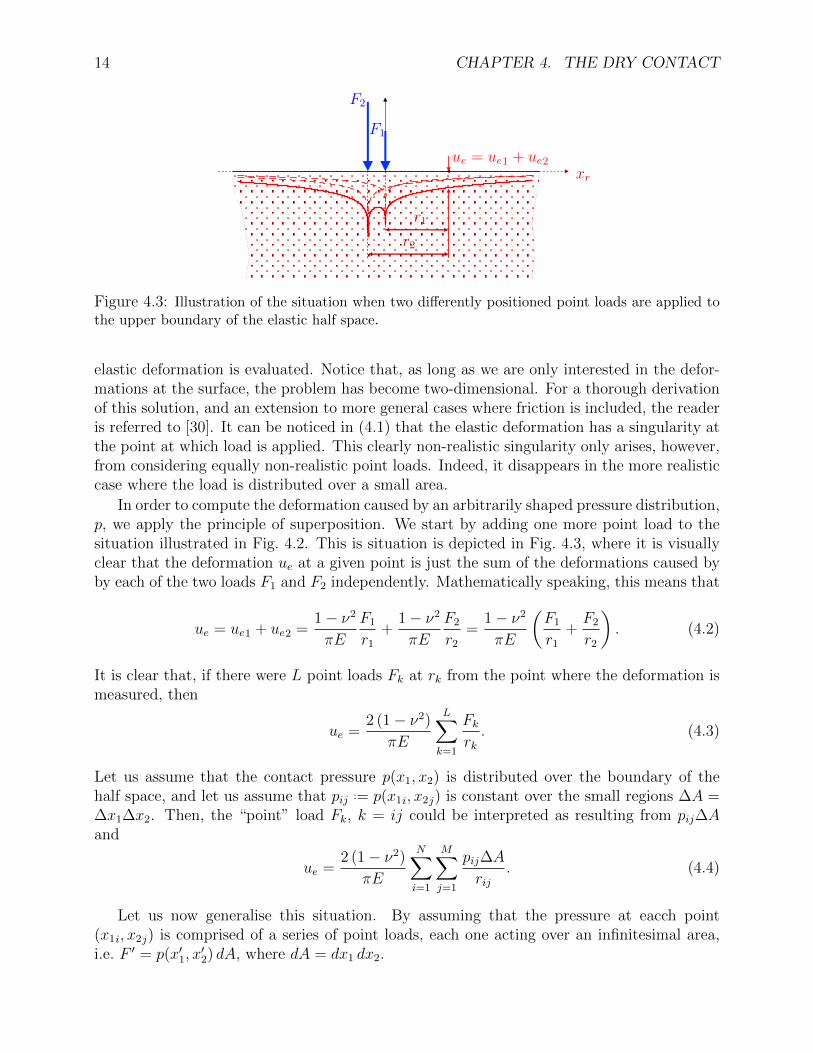
Figure 4.3: Illustration of the situation when two differently positioned point loads are applied tothe upper boundary of the elastic half space.
elastic deformation is evaluated. Notice that, as long as we are only interested in the defor-mations at the surface, the problem has become two-dimensional. For a thorough derivationof this solution, and an extension to more general cases where friction is included, the readeris referred to [30]. It can be noticed in (4.1) that the elastic deformation has a singularity atthe point at which load is applied. This clearly non-realistic singularity only arises, however,from considering equally non-realistic point loads. Indeed, it disappears in the more realisticcase where the load is distributed over a small area.
In order to compute the deformation caused by an arbitrarily shaped pressure distribution,p, we apply the principle of superposition. We start by adding one more point load to thesituation illustrated in Fig. 4.2. This is situation is depicted in Fig. 4.3, where it is visuallyclear that the deformation ue at a given point is just the sum of the deformations caused byby each of the two loads F1 and F2 independently. Mathematically speaking, this means that
ue = ue1 + ue2 =1− ν2
πE
F1
r1
+1− ν2
πE
F2
r2
=1− ν2
πE
(F1
r1
+F2
r2
). (4.2)
It is clear that, if there were L point loads Fk at rk from the point where the deformation ismeasured, then
ue =2 (1− ν2)
πE
L∑k=1
Fkrk. (4.3)
Let us assume that the contact pressure p(x1, x2) is distributed over the boundary of thehalf space, and let us assume that pij ..= p(x1i, x2j) is constant over the small regions ∆A =∆x1∆x2. Then, the “point” load Fk, k = ij could be interpreted as resulting from pij∆Aand
ue =2 (1− ν2)
πE
N∑i=1
M∑j=1
pij∆A
rij. (4.4)
Let us now generalise this situation. By assuming that the pressure at eacch point(x1i, x2j) is comprised of a series of point loads, each one acting over an infinitesimal area,i.e. F ′ = p(x′1, x
′2) dA, where dA = dx1 dx2.
4.1. HALF-SPACE THEORY AND FUNDAMENTALS OF THE BEM 15
The deformation at a point (x1, x2) can now be computed by integrating the contributionfrom all the point loads at points (x′1, x
′2), i.e.,
ue (x1, x2) =1− ν2
πE
∫ ∞−∞
∫ ∞−∞
p (x′1, x′2)√
(x1 − x′1)2 + (x2 − x′2)2dx′1dx
′2. (4.5)
The integrals are evaluated from minus- to plus infinity, but it should be noted that it isonly necessary to consider the domain where the pressure is positive, as long as we neglectadhesion.
Another important case can be accomplished by considering a load distributed along aline on surface of a half space. This exemplifies a situation where it can be assumed thatthe pressure only varies in one direction and that it the contact is long enough in the otherso that the effect of edges can be neglected. In theory, this could be the contact between aninfinitely long cylinder pressed against a rigid body, as long as the radius of the cylinder islarge enough compared to the width of the contact so that the cylinder can be considereda half space. This renders a 1D solution, which is of course very advantageous in terms ofcomputational cost. Indeed, for the 2D contact, the resulting Load-deformation relationshipcan be expressed in 1D and it can be obtained by starting from
ue (x) = −2 (1− ν2)P ′
πEln |x− x′|+ C = −2 (1− ν2)P ′
πEln
∣∣∣∣x− x′x0
∣∣∣∣, (4.6)
where P ′ represents a line load, located at x′, with unit N/m and where C is determined bychoosing a point x0 on the surface as a datum for the displacements, see [30]. We remarkthat also in the case of a line loading the deformation depends solely on the distance betweenthe point x′, where the line load is applied and the location x where it is evaluated. Again,by superposition, i.e. P ′ = p(x′)dx′, this results in
ue (x) = −2 (1− ν2)
πE
∫ ∞−∞
p(x′) ln
∣∣∣∣x− x′x0
∣∣∣∣dx′, (4.7)
for an arbitrarily shaped pressure distribution p(x). Note again, that it is only necessary toconsider the domain where the pressure is positive, as long as we neglect adhesion. For theinterested reader, the relation (4.6) is known as the Flamant solution, and for more detailson the derivation of the 1D pressure-deformation relation we refer to [30].
4.1.2 The contact between an elastic body and a rigid flat surface
In the previous section the pressure was regarded as known. I reality, the pressure that causesthe elastic body to deform is a priori unknown and results from contact between the elasticand the rigid surfaces. The boundary surface an elastic body, considered to be a half space,can describe the geometry of a smooth sphere, a wavy or even a rough surface, as long as theconditions for the Boussinesq or Flamant solutions apply. We will now see more specificallywhat conditions that must apply to for (4.5) to be used to model the deformation that arisewhen a non-flat elastic half space contacts a flat rigid surface. The caveat here is that (4.5)is a model of the deformation resulting from the application of a given pressure distribution

16 CHAPTER 4. THE DRY CONTACT
on a perfectly flat half space. It turns out that, to use (4.5) to model the deformation thatarise between a non-flat elastic body and a rigid flat surface, there are three assumptionsthat must apply to the non-flat elastic body. These are
1. The slopes of the surface features on the elastic body are small enough to be considerednegligible. In practice, this means that the ratio between height and width - of thesurface features with the highest curvature, should at least be O (10−1), but preferablysmaller;
2. The elastic body can be assumed to behave as a half-space. This means that, the (apriori unkown) real contact region must be much smaller than the nominal contactregion, so that the boundaries of the elastic body do not affect the stresses in thevicinity of the contact.
Although, the assumptions that the contact is friction- and adhesion free, is not per se arequirement, the governing equations for the BEM model described in the previous sectionwould need to be modified to incorporate such effects.
In situations were the aforementioned assumptions apply, we can use (4.5) to compute thedeformation of the non-flat elastic body, given the contact pressure distribution. Since thepressure distributions is not known a priory, we need to introduce additional (mathematical)relations to have a well-posed problem. Fortunately, under the considerations at hand, thecontact mechanics problem is a school-book example of a complementarity problem in termsof the two complimentary variables; the pressure and the gap between the contacting bodies.More precisely, i) where there is contact, there is pressure and there is no gap between thecontact bodies ii) where there is no contact pressure, there is a gap between the surfaces. Leth define the (deformed) gap between the two bodies in contact. It can be computed as
h(x) = g(x) + ue(x)− δ, (4.8)
where g(x) ≥ 0 is the initial gap between the bodies (before becoming deformed as the bodiesare brought into contact), ue(x) is the elastic deformation, given by (4.7) in 1D and (4.5) in2D, and δ ≥ 0 is the rigid body movement of the two bodies. Let us also define Ω as thedomain on which g is defined. We also declare that g = |zu − zl|, where zu is the mathematicaldescription of the lower boundary of the upper body and and zl the mathematical descriptionof the upper boundary of the lower body. The area of Ω, i.e. An ..= |A|, is often refereedto as the nominal contact area. In the context of rough surfaces, An is often considered thearea which, from a macroscopic point of view, appears to be in contact. Think of an elasticrectangular block with a non-smooth micro-scale topography, which rests on an infinitelylarge rigid surface. The area of the contacting face of the block would then be consideredas the nominal contact area. The real contact area, here denoted Ar, is often much smaller.Think of being able to look into the contact interface at a magnification sufficiently high toresolve the micro-scale features of the face. This would reveal the real contact morphology,recall Fig. 4.1), showing exactly where the bodies makes contact. Let us denote this subsetof Ω where there is contact by Ωc. Because of complementarity, it is clear that the gapmust be zero and that the pressure is positive within Ωc. Equally, wherever the gap ispositive, i.e. Ω\Ωc, there is no contact and the pressure must be zero. In contact mechanics,

4.1. HALF-SPACE THEORY AND FUNDAMENTALS OF THE BEM 17
these complementarity conditions are known as the Kuhn-Tucker conditions which can besummarised as follows:
h (x) > 0, p (x) = 0, x ∈ Ω\Ωc, (4.9a)
h (x) = 0, p (x) > 0, x ∈ Ωc, (4.9b)
where Ωc represents the contact regions and x = (x1, x2) in the 3D case (2D problem) andx = x1 in the 2D case (1D problem). We note that this effectively means that hp = 0everywhere in Ω, and that an equivalent formulation of (4.9) could be stated as
h(x)p(x) = 0 and h(x) = g(x) + ue(x)− δ, ∀x ∈ Ω. (4.10a)
The complementarity conditions, together with either (4.7) or (4.5) and a specified δ givea unique solution for the contact mechanics problem. It is often more convenient, however, tospecify the applied load, w, as input instead of the rigid body movement δ. Under stationaryconditions, Newton’s first law models the force equilibrium that balances the applied loadand the integrated force from the contact pressure distribution. Because of the half-spaceformulation and the complementarity conditions this load balance equation may be stated as
w =
∫ ∞−∞
p (x) dx =
∫Ω
p (x) dx =
∫Ωc
p (x) dx. (4.11)
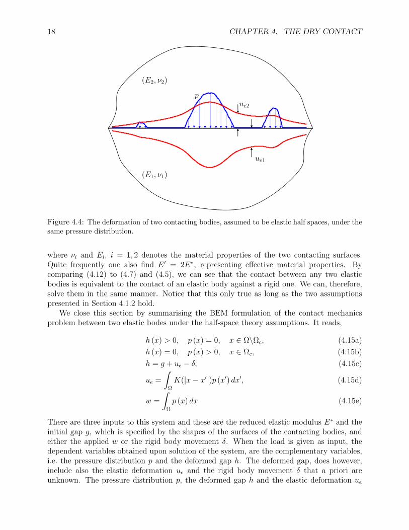
4.1.3 The contact between two elastic bodies
Let us generalise the previous case to the contact of two elastic bodies, both of which canhave a certain shape (e.g. a cylinder or a sphere) and/or have a rough surface. As indicatedin Fig. 4.4, both of them would experience the same contact pressure and the deformationwill, therefore, have the same shape. If the material properties are different the magnitudeof the deformation will, however, not be the equal. The total deformation is clearly thesum of the deformations of the contacting surfaces. Now, the only difference between thedeformation of the individual surfaces, is the material, which will show as a different scalingfactor in front of the integrals in (4.7) and (4.5). By denoting the deformation of the twosurfaces ue1 and ue2 we can, therefore, formulate the total deformation as
ue = ue1 + ue2 =
∫Ω
K(|x− x′|)p (x′) dx′, (4.12)
where
K(|x− x′|) ..=1
πE∗
−2 ln
∣∣∣∣x1 − x′1x0
∣∣∣∣, in 2D,
1√(x1 − x′1)2 + (x2 − x′2)2
, in 3D,
(4.13)
Note that we have replaced the infinite integration limits to an integral over Ω assuming thatno positive pressure acts outside the domain. The parameter E∗, often referred to as thereduced elastic modulus, is the defined as
1
E∗=
1− ν21
E1
+1− ν2
2
E2
, (4.14)
18 CHAPTER 4. THE DRY CONTACT
(E2, ν2)
(E1, ν1)
ue2
ue1
p
Figure 4.4: The deformation of two contacting bodies, assumed to be elastic half spaces, under thesame pressure distribution.
where νi and Ei, i = 1, 2 denotes the material properties of the two contacting surfaces.Quite frequently one also find E ′ = 2E∗, representing effective material properties. Bycomparing (4.12) to (4.7) and (4.5), we can see that the contact between any two elasticbodies is equivalent to the contact of an elastic body against a rigid one. We can, therefore,solve them in the same manner. Notice that this only true as long as the two assumptionspresented in Section 4.1.2 hold.
We close this section by summarising the BEM formulation of the contact mechanicsproblem between two elastic bodes under the half-space theory assumptions. It reads,
h (x) > 0, p (x) = 0, x ∈ Ω\Ωc, (4.15a)
h (x) = 0, p (x) > 0, x ∈ Ωc, (4.15b)
h = g + ue − δ, (4.15c)
ue =
∫Ω
K(|x− x′|)p (x′) dx′, (4.15d)
w =
∫Ω
p (x) dx (4.15e)
There are three inputs to this system and these are the reduced elastic modulus E∗ and theinitial gap g, which is specified by the shapes of the surfaces of the contacting bodies, andeither the applied w or the rigid body movement δ. When the load is given as input, thedependent variables obtained upon solution of the system, are the complementary variables,i.e. the pressure distribution p and the deformed gap h. The deformed gap, does however,include also the elastic deformation ue and the rigid body movement δ that a priori areunknown. The pressure distribution p, the deformed gap h and the elastic deformation ue
4.2. DIMENSIONLESS FORMULATION OF THE CONTACTMECHANICS PROBLEM 19
are also, a priori, unknown when the rigid body movement δ is given as input. However, inthis case w represents the reaction force caused by the interference that results from choosinga δ large enough to render a solution different from the trivial one (h > 0 ∧ p = 0).
4.2 Dimensionless formulation of the contact mechan-
ics problem
In the previous section the BEM for the contact mechanics problem between two elasticbodies was formulated based on the half-space theory. Interpreting this system is not aneasy task and here we introduce a scaling to transform it into dimensionless form. This mayreduce the number of input parameters and thus facilitate numerical analysis and it willhelp us understand how the input parameters affect the solution. We start the process byintroducing the following scaling
X1 =x1
x1r
, X2 =x2
x2r
, H =h
hr, Ue =
uehr, G =
g
hr, δ =
δ
hr, P =
p
pr. (4.16)
Notice that we have scaled all the variables regarding the gap with the same parameter hr.This is because they all share the same dimension, i.e., the dimension of the gap. Moreover,all of them can be expected to be of the same order of magnitude. Under the scaling proposed,the equations needed to solve the 3D contact mechanics problem, i.e., (4.15), become
H (X1, X2) > 0 P (X1, X2) = 0, (X1, X2) ∈ Ωc, (4.17a)
H (X1, X2) = 0 P (X1, X2) > 0, (X1, X2) /∈ Ωc, (4.17b)
H = G+ Ue − δ, (4.17c)
Ue (X1, X2) =x1rprhr
1
πE∗
∫Ω
P (X ′1, X′2)√
(X1 −X ′1)2 + (x2r /x1r )2 (X2 −X ′2)2dX ′1dX
′2, (4.17d)
w
prx1rx2r
=
∫Ω
P (X1, X2) dX1dX2 (4.17e)
Now, we can freely chose the scaling parameters. We will, however obtain better resultsif we follow two principles, i) to eliminate as many input parameters as possible and ii) toscale the non-dimensional variables so as to avoid truncation errors. A first obvious choiceconcerning the input parameters is to choose xr1 = xr2 = xr. Notice that, in most of thecases, both these dimensions are of similar size and thus we also preserve the scaling property.It can sometimes, however, be useful to define different scaling parameters for each direction,e.g. when studying finite EHL line contacts [31, 32]. We can also identify the two groups ofparameters
xrprhr
1
πE∗, and
w
prx2r
. (4.18)
that, for a given dimensionless initial gap (G), uniquely determine the solution of the problem,i.e., the contact pressure P and its distribution and the gap H between the deformed surfaces.A first option, suitable for arbitrary surface descriptions, is to set both of these parameters

20 CHAPTER 4. THE DRY CONTACT
to 1. We note that there are now two groups and three reference parameters, of which twobelong to the dependent variables p and h and the third scales the independent variable x.We can thus choose one reference parameter freely. We can, for example, choose xr = L,where L is the size of the nominal contact area. This leads to
pr =w
L2, and
hrL
=w
L2πE∗, (4.19)
which tells us that the scaling for the pressure is around the mean contact pressure and thatthe ration hr/L is very small, as expected. In this case, the equations read
H (X1, X2) > 0 P (X1, X2) = 0, (X1, X2) ∈ Ωc, (4.20a)
H (X1, X2) = 0 P (X1, X2) > 0, (X1, X2) /∈ Ωc, (4.20b)
H = G+ Ue − δ, (4.20c)
Ue (X1, X2) =
∫Ω
P (X ′1, X′2)√
(X1 −X ′1)2 + (X2 −X ′2)2dX ′1dX
′2, (4.20d)
1 =
∫Ω
P (X1, X2) dX1dX2 (4.20e)
Notice that in the system posed by (4.20), the only input is introduced through the shape ofthe initial gap G. Thus, we have extracted important knowledge even before having solvedthe set of equations. Let us see, for example, what happens when we keep w constant andstretch the surface, which would result in an increase of L. We can see that if we double Lwhile halving E∗, hr remains constant, which indicates that the deformation will also remainconstant. This means that stretching the surface makes its response less stiff. Notice nowthat the topography of a rough surface, can be described as the sum of many sinusoidalwaves, some having long wavelengths and some having shorter ones. We have now seen thatthe former will flatten easily whereas the latter will require a much larger load.
A very common application of the boundary element method (and one of its few analyticalsolutions) is that of the Hertzian contact problem. In two dimensions, this problem is simplythe application of BEM to the contact of smooth spheres. This is reflected in the initial gap,which is
gH =x2
1 + x22
2Rhr, (4.21)
where R is the combined radius of the spheres. In this case, we find another relevant group,namely x2
r/2Rhr. This, of course, motivates choosing another scaling. In particular, thefollowing is often chosen,
x2r
2Rhr=
1
2,
w
prx2r
=2π
3and
xrprhr
1
πE∗=
2
π2. (4.22)
This leads to xr = a, where a is the Hertzian contact radius, hr = a2/R and pr = pH , whichis the Hertzian pressures. These are given as
pH =3w
2πa2, a3 =
3wR
4E∗. (4.23)
4.2. DIMENSIONLESS FORMULATION OF THE CONTACTMECHANICS PROBLEM 21
The equations then read
H (X1, X2) > 0 P (X1, X2) = 0, (X1, X2) ∈ Ωc, (4.24a)
H (X1, X2) = 0 P (X1, X2) > 0, (X1, X2) /∈ Ωc, (4.24b)
H =(X2
1 +X22
)+ Ue − δ, (4.24c)
Ue (X1, X2) =2
π2
∫Ω
P (X ′1, X′2)√
(X1 −X ′1)2 + (X2 −X ′2)2dX ′1dX
′2, (4.24d)
2π
3=
∫Ω
P (X1, X2) dX1dX2 (4.24e)
Notice that, in this case, there are no input parameters. This means that there is onlyone fundamental solution. All contact problems between two spheres can thus be seen as ascaling of this fundamental solution. This is also the case in the one-dimensional case, notshown here. Notice that we can also use the non-dimensional parameter groups to infer somerelations about this scaling without actually solving the problem. For example, we see that,by doubling w, pH is also doubled while a is increased by a factor 21/3. Similar relations canbe found for all parameters.
Let us finish this discussion with a comment on the dimensionless formulation for the2D contact mechanics problem (1D model), which for the contact between two elasticallydeformable surfaces can be stated as
H (X) > 0 P (X) = 0, X ∈ Ωc, (4.25a)
H (X) = 0 P (X) > 0, X /∈ Ωc, (4.25b)
H = G+ Ue − δ, (4.25c)
Ue (X) = −xrprhr
2
πE∗
∫Ω
P (X ′) ln
∣∣∣∣X −X ′X0
∣∣∣∣ dX ′, (4.25d)
w
prxr=
∫Ω
P (X) dX. (4.25e)
There is, however, as we will see an alternative way of posing the problem and it has to dowith the the datum for the displacement x0 (appearing in the 2D but not in the 3D pressure-deformation relation). Let us now see how this can done. It is obvious that the dimensionlessrepresentation of (4.7) (for the contact between two elastically deformable surfaces) becomes
Ue (X) = −xrprhr
2
πE∗
∫Ω
P (X ′) ln
∣∣∣∣X −X ′X0
∣∣∣∣ dX ′= −xrpr
hr
2
πE∗
∫Ω
P (X ′) ln |X −X ′| dX ′ − xrprhr
2
πE∗lnX0
∫Ω
P (X ′) dX ′
= −xrprhr
2
πE∗
∫Ω
P (X ′) ln |X −X ′| dX ′ − xrprhr
2
πE∗lnX0
w
prxr,
= −xrprhr
2
πE∗
∫Ω
P (X ′) ln |X −X ′| dX ′ − 2 lnX0
πE∗hrw, (4.26)
22 CHAPTER 4. THE DRY CONTACT
Let us now define
U ′e (X) ..= −xrprhr
2
πE∗
∫Ω
P (X) ln |X −X ′| dX ′ (4.27)
and
δ′ ..=2 lnX0
πE∗hrw. (4.28)
We can then write (4.26) asUe (X) = U ′e (X)− δ′. (4.29)
Moreover, when introducing the non-dimensional deformation into the non-dimensional gap(4.25c), U ′e can be used to replace Ue and the value of δ′ can be merged with δ, i.e., δ∗ = δ− δ′.Finally, we can pose the 2D contact mechanics problem (4.25) in the following, alternative,way
H (X) > 0 P (X) = 0, X ∈ Ωc, (4.30a)
H (X) = 0 P (X) > 0, X /∈ Ωc, (4.30b)
H = G+ U ′e − δ∗, (4.30c)
U ′e (X) =xrprhr
2
πE∗
∫Ω
P (X ′) ln |X −X ′| dX ′, (4.30d)
w
prxr=
∫Ω
P (X) dX. (4.30e)
Note that, since the model is posed with the applied load w as input, it means that δ∗ is adependent variable which, although related to the interference or rigid body movement, it isno longer equal to it due to the addition of δ′.
4.3 Examples of analytical solutions
In this section, we will give few examples of analytical solution to the contact problem inthe context of the boundary element method. As apparent from the form of the equationsto be solved, finding analytical solutions is no easy task and thus such solutions only existfor a few particular cases. Here we will first consider the famous theory by Hertz and thenconsider surfaces that have the shape of a simple sinusoidal wave, which are a conceptualmodel to understand the behaviour of rough surfaces. Other solutions do exist, usually fortwo-dimensional contact cases. The solutions are, however, quite complex and would notgive the insights that the simpler cases we present here will give us. Therefore we will notconsider them here.
4.3.1 Hertz theory
The theory proposed by Hertz [33] is of the first successfully ones in the field of contactmechanics. We will now see that it is, in fact, a particular case of the more general boundaryelement method. The theory concerns dry non-conformal contacts of elastic bodies, in whichthe contact occurs in a very small area. These include the metal-to-metal contact betweentwo spheres in 3D and two cylinders in 2D, but can, in fact, be applied to other non-conformal
4.3. EXAMPLES OF ANALYTICAL SOLUTIONS 23
w
w
a
A = 1
pH
PH = 1
a) b)
c)
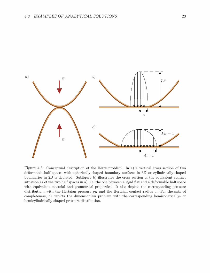
Figure 4.5: Conceptual description of the Hertz problem. In a) a vertical cross section of twodeformable half spaces with spherically-shaped boundary surfaces in 3D or cylindrically-shapedboundaries in 2D is depicted. Subfigure b) illustrates the cross section of the equivalent contactsituation as of the two half spaces in a), i.e. the one between a rigid flat and a deformable half spacewith equivalent material and geometrical properties. It also depicts the corresponding pressuredistribution, with the Hertzian pressure pH and the Hertzian contact radius a. For the sake ofcompleteness, c) depicts the dimensionless problem with the corresponding hemispherically- orhemicylindrically shaped pressure distribution.

24 CHAPTER 4. THE DRY CONTACT
contacts as well. A key assumption for this theory is that the contact region is much smallerthan the extent of the bodies themselves. This is also characteristic for non-conformal metal-to-metal contacts such as the aforementioned ones. Notice, however, that it might not applyfor contacts between compliant materials such as rubber, where large deformations resultsin large contact regions. Another assumption is that the local radius of curvature of thesurfaces at the contact region is small compared to the size of the contact. These twoassumptions are equivalent to the ones presented in Section 4.1.2 and thus allow us to applythe boundary element method to this problem. Moreover, the contact is assumed to befriction and adhesion free, so that only normal compressive pressures are considered and wecan thus use the formulation presented in Section 4.1. With this in mind, let us describe theproblem. A conceptual description, that will be useful during this discussion is depicted inFig. 4.5.
Let us consider the 3D problem with spherically-shaped bodies. Since these are bodiesof revolution it is clear, that the contact region will be circular and we can work with polar-instead of the Cartesian coordinates. The gap between the original undeformed surfaces, g,can be described as
g(x1, x2) =r2
2R, (4.31)
where x1, x2 are the coordinates of the horizontal plane, r2 = x21 + x2
2 and R the equivalentradius of curvature of the two contacting bodies’ boundary surfaces. As depicted in Fig. 4.5a,the problem at hand is to compute the contact when two spherically bodies are pressed againsteach other with a load w. The first thing to notice is that, as discussed in Section 4.1.3, theproblem is equivalent to that of the contact between an elastic sphere and a rigid perfectlyflat surface. The radius of the equivalent sphere, R, i.e. the equivalent radius, can be foundby requiring the gap between the equivalent sphere and the flat surface to be the same asthe gap between the two spheres. Thus it is easily verified that this equivalent radius shouldbe defined as
1
R=
1
R1
+1
R2
. (4.32)
In this case the deformation is known at the contact region r ∈ Ωc and it can be expressedas
ue(r) =a2
R− r2
2R, r ∈ Ωc, (4.33)
where a is the Hertzian contact radius. The reader is referred to [34] for the derivation ofthis expression, which is given there in Equation (3.41a). This equation comes by requiringthat the deformed gap, between the in-contact surfaces, is zero at the contact region. Thekey insight that Hertz had was that the deformation in (4.33) is produced by a pressure ofthe form
p(r) = pH
√1−
(ra
)2
, (4.34)
where pH is the Hertzian pressure, which is also the maximum contact pressure. In order toproduce exactly the deformation in (4.33), the Hertzian pressure must have the value
pH =2E∗a
πR. (4.35)

4.3. EXAMPLES OF ANALYTICAL SOLUTIONS 25
The total load, w, that would result in a given contact radius a can then be found byintegrating (4.34) over the contact area, leading to a value of
w =2
3pHπa
2. (4.36)
Moreover, since the complementarity conditions states that g + ue − δ = 0 in the contactzone, we can compute the corresponding Hertzian rigid body movement δH as
δH = g + ue =r2
2R+a2
R− r2
2R=a2
R. (4.37)
Notice that we here consider the bodies to be originally touching at a single point and δHmeasure how much more they approach due to the applied load. Summing up, we can givethe relation between the different parameters in their typical form, i.e.,
a =
(3wR
4E∗
)1/3
, (4.38a)
pH =
(3w
2πa2
)=
(6wE∗2
π3R2
)1/3
, (4.38b)
δH =a2
R=
(9
16
w2
RE∗2
)1/3
. (4.38c)
Now, recall that we said in Section 4.2 that all Hertzian contact problems collapse to asingle solution when considered in a dimensionless form. Let us see that this is, in fact, thecase. Recall that the gap is scaled by a factor hr = a2/R whereas the other two dimensions arescaled by xr = a, thus r = r/a. Therefore, the non-dimensional gap, between the undeformedbodies, becomes
G(r) =r2
2+ δ, (4.39)
where input parameters are no longer present. Similarly, by scaling the contact pressure withpH , we have
P =√
1− r2, (4.40)
which, again, is free from input parameters. Notice that this equation can be written in theform
P 2 + r2 = 1. (4.41)
This means that the general non-dimensional pressure solution for the Hertzian contactproblem is simply as semi-sphere of unitary radius, such as the one depicted in Fig. 4.5c.
Let us now consider briefly the two-dimensional case representing the contact of infinitelylong bodies such as cylinders. In this case, the contact will be on a line, symmetric withrespect to the centre of the contact. The non-dimensional solution becomes, in this case asemi-circle of unitary radius. This solves the problem completely as any other case can befound via a scaling. Let us therefore solely give a summary of the most common relations in

26 CHAPTER 4. THE DRY CONTACT
this case
a =
(4wR
πE∗
)1/2
, (4.42a)
pH =2w
πa=
(wE∗
πR
)1/2
. (4.42b)
Notice that, in this case, w has the units of force per unit length, (N/m). Notice also that,in this case, the rigid body movement, δH , caused by w cannot be specified. This is becauseof a reference point for the deformation cannot be specified, as reflected by the arbitraryconstant left in (4.6).
Finally, let us give a comment for the three dimensional case in which the solids are notof revolution. Using appropriate axes, the geometry of these bodies can be described as
z =x1
R′+x2
R′′+ δ. (4.43)
Notice that now two radii, R′ and R′′ must be used to describe the surface. In this case thecontact region will form an ellipse instead of a circumference. The solution to this problem,however, is not as simple as the case of bodies of revolution, where the cylindrical symmetrycould be exploited. We will therefore not give the solution and simply refer the interestedreader to, e.g., [30].
4.3.2 The Westergaard solution
Another very important although less well known solution is that given by Westergaard [35]for the 2D contact of surfaces whose profile is characterized by a sinusoidal function. Thissolution was the first to provide a clear insight on the contact of rough surfaces. Withoutrepresenting a realistic surface topography, the sinusoidal wave is the starting point to un-derstand how roughness behaves and the solution will teach us how varying amplitude andfrequency in the roughness will affect the contact behaviour. A representation of the problemand its solution is given in Fig. 4.6. A good description of this problem can also be foundin Johnson’s book [30]. We will follow the latter in this description, instead of the morenuanced but also more cumbersome presentation of Westergaard. Let us set the stage byfirst considering the deformation caused by a sinusoidal pressure, i.e.,
pcos (x) = p∗ cos (2πx/λ) , (4.44)
where p∗ is the amplitude of the pressure wave and λ its wavelength. The deformationcaused by this pressure can be computed using (4.13), although the integration process is byno means trivial. The result is the following:
uecos (x) =λ
πE∗p∗ cos (2πx/λ) (4.45)
Notice that this deformation has the same shape as the original pressure, scaled by a factorλ/ (πE∗). Notice that this scaling factor also reflects what we found in Section 4.2, i.e., that
4.3. EXAMPLES OF ANALYTICAL SOLUTIONS 27
a)
p = 0
b)
p < p∗
c)
p ≥ p∗
λ
a
2∆
2p∗
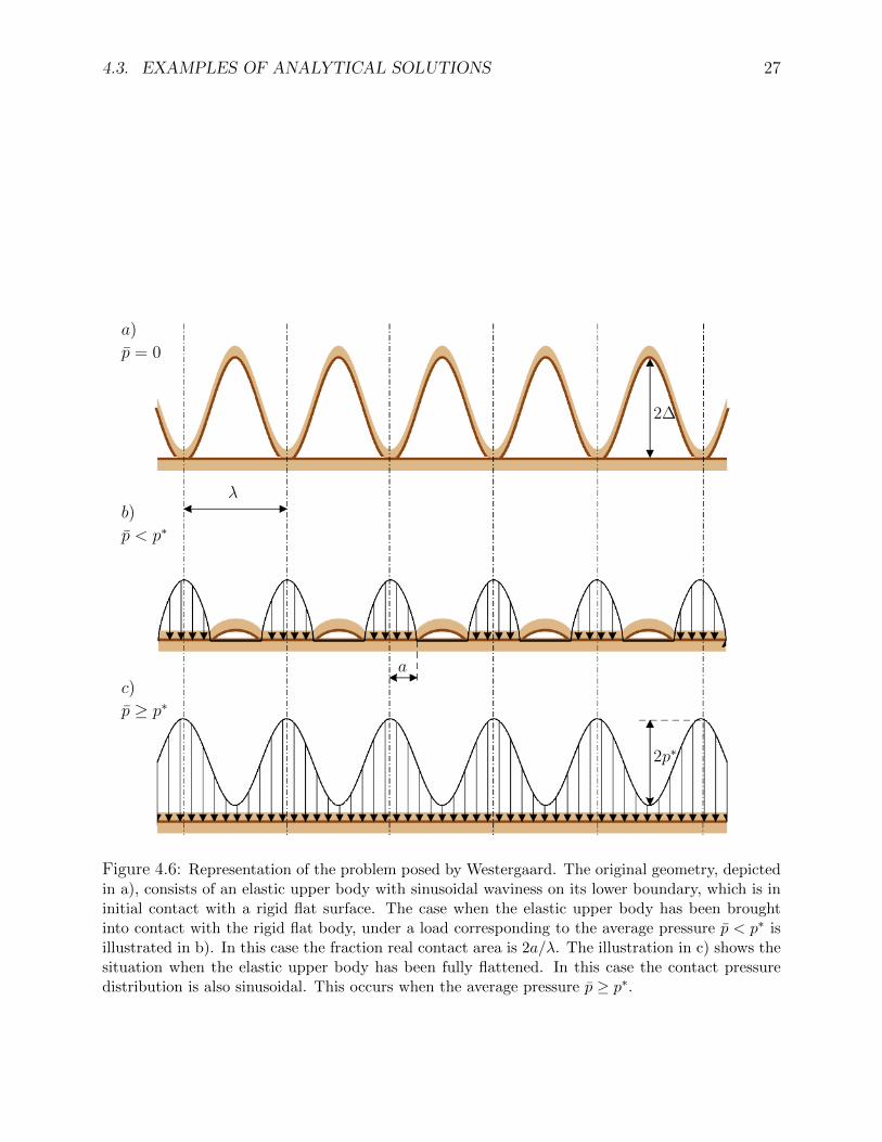
Figure 4.6: Representation of the problem posed by Westergaard. The original geometry, depictedin a), consists of an elastic upper body with sinusoidal waviness on its lower boundary, which is ininitial contact with a rigid flat surface. The case when the elastic upper body has been broughtinto contact with the rigid flat body, under a load corresponding to the average pressure p < p∗ isillustrated in b). In this case the fraction real contact area is 2a/λ. The illustration in c) shows thesituation when the elastic upper body has been fully flattened. In this case the contact pressuredistribution is also sinusoidal. This occurs when the average pressure p ≥ p∗.
28 CHAPTER 4. THE DRY CONTACT
a longer wavelength results in a less stiff surface. We can now use this result to say somethingabout the deformation of a wavy surface. Let us assume that the initial gap between thissurface and a flat one can be written as
gcos (x) = ∆ (1− cos (2πx/λ)) , (4.46)
where ∆ is the amplitude of the wavy surface. By comparing (4.46) with (4.45), we canclearly see that our surface will be flattened completely if p∗ = πE∗∆/λ. Of course, pressuremust be non-negative, implying that the mean pressure must be greater than p∗ for this tomake sense. Therefore, a surface with the gap described in (4.46) will be completely flattenedif pressed by a mean pressure p > p∗. Moreover, the pressure will have the following form
pcos (x) = p+ p∗ cos (2πx/λ) , p∗ =πE∗∆
λ, p > p∗. (4.47)
Obviously, whenever p < p∗, the equation profile in (4.47) will include negative contactpressure, which is not physical. What will happen in reality is that there will be no fullcontact. The solution of the equations for BEM in this case can also be found analytically,albeit the process is even more complicated. The result, provided by Westergaard [35] is thatwhen the surfaces are pressed with a mean pressure p < p∗, the pressure distribution can beexpressed as
pW (x) =2p cos (πx/λ)
sin2 ψa
√sin2 ψa − sin2 ψ, 0 ≤ |x| ≤ a (4.48a)
pW (x) = 0, a ≤ |x| ≤ λ/2 (4.48b)
and the deformation as
ueW (x) =pλ cos (πx/λ)
πE∗ sin2 ψacos 2ψ, 0 ≤ |x| ≤ a (4.49a)
ueW (x) =pλ
πE∗ sin2 ψa
[cos 2ψ + 2 sinψQ− 2 sin2 ψa ln
(sinψ +Q
sinψa
)], a ≤ |x| ≤ λ/2
(4.49b)
where a is the contact width, given by
2a
λ=
2
πsin−1
(p
p∗
)2
. (4.50)
and
Q =
√sin2 ψ − sin2 ψa, ψ =
πx
λand ψa =
πa
λ.
Note that one has to be particularly careful with the sign of Q. A schematic on how thissolution looks like is depicted in Fig. 4.6b.
4.4. DISCRETISATION 29
x1 x2
x3
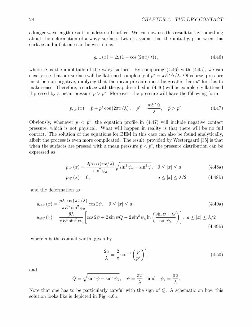
Figure 4.7: A bi-sinusoidal surface, as described by (4.51), facing a flat surface.
4.3.3 Flattening of bi-sinusoidal surfaces
Let us finish with the three dimensional version of the previous one. In this case, we consideran elastic surface described by a bi-sinusoidal function,
z = ∆ sin
(2πx1
λ1
)sin
(2πx2
λ2
)+ δ, (4.51)
facing a flat, rigid surfaces, as depicted in Fig. 4.7. In (4.51), λ1 and λ2 are the wavelengthsin each direction and ∆ is the amplitude. This case is much harder to solve than the previoustwo-dimensional case, and there is no analytical solution for the partial contact situation.Hence, there are only numerical investigations in this case, and the interested reader isreferred to [36] for a detailed analysis of the numerical solution of the partial contact. Weshall here review the solution for the full contact, given by Johnson [34]. Unsurprisingly, thesolution has the same form as for the two-dimensional case. Indeed, if mean pressure p issufficiently large to flat completely the surface, the pressure distribution will be
p = p+ p∗ sin
(2πx1
λ1
)sin
(2πx2
λ2
), p∗ =
√2πE∗
∆√λ2
1 + λ22
. (4.52)
Obviously, this means that p > p∗ is the criteria to know weather the flattening is complete ornot. Notice that p∗ also has the same structure as in the two-dimensional case. This meansthat, also in two dimensions, surfaces with longer wave-lengths will be easier to flatten. Inthis case, however, we need to consider a combination of the wave-lengths in both directions.It is easy to see that if λ1 = λ2, then p∗ is now equal to the one we obtained in the two-dimensional case.
4.4 Discretisation
Except for few very specific cases, such as the examples given in the previous section, thecontact mechanics problem does not permit an analytical solution. Hence, the problem must,in general, be solved numerically and, to this end, it needs to be discretised. We shall do thisin this section, taking one component at a time.
30 CHAPTER 4. THE DRY CONTACT
Before we can discretise the set of equations to be solved numerically, we need to specifythe computational domain Ω which we will solve the set of equations on. Here we considercomputational domains defined as
Ω ..=
[a1, b1] , in 1D,
[a1, b1]× [a2, b2] , in 2D,(4.53)
where we need to remember that the 1D domain is related to the 2D contact problem andthe 2D domain to the 3D contact. Since the apparent contact area is not known a priori, it isnot always an easy task to choose the computational domain. One can, however, always usethe nominal contact area as a starting point and then decrease it to better match the regionrequired to obtain the wanted accuracy of the solution. It is clear, however, that one mustseek a domain such that the pressure is zero at the boundaries (except for periodic domains),as otherwise one can expect the pressure to be non-zero outside the domain. Based on thedefinition of the domain (4.53), we will start to discretise the different parts of the problem,starting by the domain itself. We will then continue with the gap, the pressure distribution,the equation for deformation, (4.12), and the load balance equation, (4.11). For simplicity,we will mainly consider the 1D case, giving the specific formulation for the two-dimensionalcase whenever they are different.
4.4.1 Discretisation of the domain
The domain Ω can be simply discretised by setting
xi = a1 + i∆x1, i = 0, . . . , N1 − 1 in 1D, (4.54a)
(x1i, x2j) = (a1 + i∆x1, a2 + j∆x2) ,i = 0, . . . , N1 − 1j = 0, . . . , N2 − 1
in 2D, (4.54b)
where ∆xi = Li/(Ni − 1), i = 1, 2, where Li is the length of the domain in the xi-directionand Ni is the number of points used to discretise the domain in each direction. Further-more, (a1, a2) defines the South-West corner of the computational domain Ω. Of course, thisdiscretisation, in which ∆xi is constant, is the simplest possible and more complicated onescould also be used. For instance, in [37], they employed a grid that became finer at the edgeof the contact. However, since the contact region is not known a priori, this grid needs toadapt itself as the solution progresses. Therefore, it is much more complex to implement.Moreover, we will see in Section 4.6 that the uniform grid presented in (4.54) allows for usingFFT techniques, to significantly accelerate the calculations.
4.4.2 Discretisation of the gap
In the model, the gap is a continuous function. In reality, we can only acquire surface heightvalues at a set of discrete points xi. If we assume that one of the surfaces is perfectly flat,then this means that we know the gap in the same set of points, i.e. gi ..= g(xi). In thecase with two rough surfaces, we must rely on some sort of interpolation to define heightvalues of both of the surfaces at the same set of discrete points xi. Assuming either the
4.4. DISCRETISATION 31
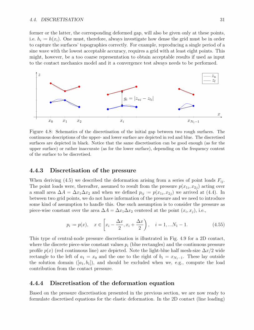
former or the latter, the corresponding deformed gap, will also be given only at these points,i.e. hi ..= h(xi). One must, therefore, always investigate how dense the grid must be in orderto capture the surfaces’ topographies correctly. For example, reproducing a single period of asine wave with the lowest acceptable accuracy, requires a grid with at least eight points. Thismight, however, be a too coarse representation to obtain acceptable results if used as inputto the contact mechanics model and it a convergence test always needs to be performed.
x0 x1 x2 xi xN1−1
gi = |zui − zli|
x
z zuzl
Figure 4.8: Schematics of the discretisation of the initial gap between two rough surfaces. Thecontinuous descriptions of the upper- and lower surface are depicted in red and blue. The discretisedsurfaces are depicted in black. Notice that the same discretisation can be good enough (as for theupper surface) or rather inaccurate (as for the lower surface), depending on the frequency contentof the surface to be discretised.
4.4.3 Discretisation of the pressure
When deriving (4.5) we described the deformation arising from a series of point loads Fij.The point loads were, thereafter, assumed to result from the pressure p(x1i, x2j) acting overa small area ∆A = ∆x1∆x2 and when we defined pij ..= p(x1i, x2j) we arrived at (4.4). Inbetween two grid points, we do not have information of the pressure and we need to introducesome kind of assumption to handle this. One such assumption is to consider the pressure aspiece-wise constant over the area ∆A = ∆x1∆x2 centered at the point (xi, xj), i.e.,
pi ..= p(x), x ∈[xi −
∆x
2, xi +
∆x
2
), i = 1, ...N1 − 1. (4.55)
This type of central-node pressure discretisation is illustrated in Fig. 4.9 for a 2D contact,where the discrete piece-wise constant values pi (blue rectangles) and the continuous pressureprofile p(x) (red continuous line) are depicted. Note the light-blue half mesh-size ∆x/2 widerectangle to the left of a1 = x0 and the one to the right of b1 = xN1−1. These lay outsidethe solution domain ([a1, b1]), and should be excluded when we, e.g., compute the loadcontribution from the contact pressure.
4.4.4 Discretisation of the deformation equation
Based on the pressure discretisation presented in the previous section, we are now ready toformulate discretised equations for the elastic deformation. In the 2D contact (line loading)
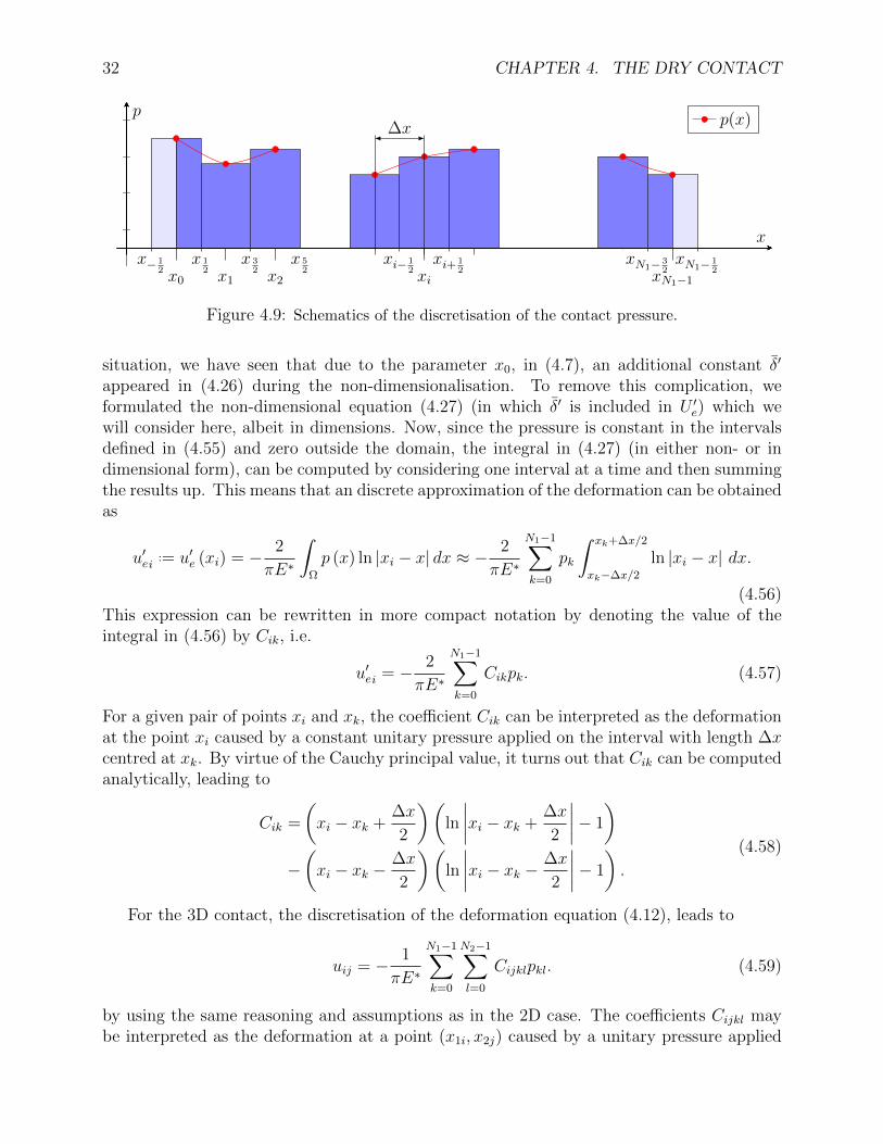
32 CHAPTER 4. THE DRY CONTACT
x
p
x0 x1 x2 xi xN1−1
x− 12
x 12
x 32
x 52
xi− 12
xi+ 12
xN1− 32xN1− 1
2
∆xp(x)
Figure 4.9: Schematics of the discretisation of the contact pressure.
situation, we have seen that due to the parameter x0, in (4.7), an additional constant δ′
appeared in (4.26) during the non-dimensionalisation. To remove this complication, weformulated the non-dimensional equation (4.27) (in which δ′ is included in U ′e) which wewill consider here, albeit in dimensions. Now, since the pressure is constant in the intervalsdefined in (4.55) and zero outside the domain, the integral in (4.27) (in either non- or indimensional form), can be computed by considering one interval at a time and then summingthe results up. This means that an discrete approximation of the deformation can be obtainedas
u′ei..= u′e (xi) = − 2
πE∗
∫Ω
p (x) ln |xi − x| dx ≈ −2
πE∗
N1−1∑k=0
pk
∫ xk+∆x/2
xk−∆x/2
ln |xi − x| dx.
(4.56)This expression can be rewritten in more compact notation by denoting the value of theintegral in (4.56) by Cik, i.e.
u′ei = − 2
πE∗
N1−1∑k=0
Cikpk. (4.57)
For a given pair of points xi and xk, the coefficient Cik can be interpreted as the deformationat the point xi caused by a constant unitary pressure applied on the interval with length ∆xcentred at xk. By virtue of the Cauchy principal value, it turns out that Cik can be computedanalytically, leading to
Cik =
(xi − xk +
∆x
2
)(ln
∣∣∣∣xi − xk +∆x
2
∣∣∣∣− 1
)−(xi − xk −
∆x
2
)(ln
∣∣∣∣xi − xk − ∆x
2
∣∣∣∣− 1
).
(4.58)
For the 3D contact, the discretisation of the deformation equation (4.12), leads to
uij = − 1
πE∗
N1−1∑k=0
N2−1∑l=0
Cijklpkl. (4.59)
by using the same reasoning and assumptions as in the 2D case. The coefficients Cijkl maybe interpreted as the deformation at a point (x1i, x2j) caused by a unitary pressure applied
4.4. DISCRETISATION 33
on a rectangle of size ∆x1 ×∆x2 centred around the point (x1k, x2l). In [38], Love obtaineda closed form expression for Cij00, i.e., the deformation at (x1i, x2j) caused by a unitarypressure applied on a rectangle of size ∆x1×∆x2 centred around the point (x1k, x2l) = (0, 0).The result may be expressed as
πE∗Cij00 = (x2j + ∆x2/2) ln
(x1i + ∆x1/2) +√
(x2j + ∆x2/2)2 + (x1i + ∆x1/2)2
(x1i −∆x1/2) +√
(x2j + ∆x2/2)2 + (x1i −∆x1/2)2
+ (x2j −∆x2/2) ln
(x1i −∆x1/2) +√
(x2j −∆x2/2)2 + (x1i −∆x1/2)2
(x1i + ∆x1/2) +√
(x2j −∆x2/2)2 + (x1i + ∆x1/2)2
+ (x1i + ∆x1/2) ln
(x2j + ∆x2/2) +√
(x1i + ∆x1/2)2 + (x2j + ∆x2/2)2
(x2j −∆x2/2) +√
(x1i + ∆x1/2)2 + (x2j −∆x2/2)2
+ (x1i −∆x1/2) ln
(x2j −∆x2/2) +√
(x1i −∆x1/2)2 + (x2j −∆x2/2)2
(x2j + ∆x2/2) +√
(x1i −∆x1/2)2 + (x2j + ∆x2/2)2
.
(4.60)Notice that Cijkl can be found simply by translation, i.e., by replacing x1i by (x1i − x1k) andx2j by (x2j − x2l)
To conclude this section, let us discuss the shape of the matrix-vector representation of(4.58) (in the case of a 2D contact). We notice that u′ei
..= u′e(xi) depends on the distancebetween the points xi and xk, |xi − xk|, rather than on both xi and xk, individually. Sincewe use a regular grid to discretise our domain, Cik depends on |i− k|, rather than on both iand k, individually. We can thus define a new coefficient K as
Kr = Cik ∀i, k : |i− k| = r. (4.61)
With this coefficient, we can see more clearly the structure of the matrix-vector representationof (4.58). As an example, for the case N = 4 it looks like
u′0u′1u′2u′3
=
K0 K1 K2 K3
K1 K0 K1 K2
K2 K1 K0 K1
K3 K2 K1 K0
p0
p1
p2
p3
. (4.62)
In this way it can be seen that the matrix has a particular symmetry, in which the value onlydepends on the distance from the main diagonal. This type of matrix is called a Toeplitzmatrix. As we shall see in Section 4.6, this type of matrices is closely related to discreteconvolutions. A similar reasoning could be used to describe the symmetries of the matrix forthe two-dimensional case. We will, however, leave out the discussion here, but in Section 4.6we will show how the relation to the convolution can be utilised when applying a fast Fouriertransformation based technique to accelerate the calculation of the summations (or matrixmultiplications) for the discrete elastic deformation.

34 CHAPTER 4. THE DRY CONTACT
4.4.5 Discretisation of the load-balance equation
The last piece to discretise is the load balance equation (4.11). We start from the central-node discretsation of the pressure given in Section 4.4.3. The total load can thus be ap-proximated by simply adding the areas of each rectangle in Fig. 4.9, meaning that we in theone-dimensional case have
w =
∫p (x) dx ≈ ∆x
2
N1−1∑i=0
pi +∆x
2
N1−1∑i=1
pi =∆x
2
N1−1∑i=0
pi + pi+1. (4.63)
The extension to the two-dimensional case is trivial.Notice that, by assuming that the pressure varies linearly between grid points, the ap-
proximation of the integral in (4.11) would be following the trapezoidal rule,
w =
∫p (x) dx ≈
N1−1∑i=0
∆xpi − pi+1
2+ ∆xpi =
∆x
2
N1−1∑i=0
pi + pi+1, (4.64)
which means that the central-node discretisation is as accurate, i.e. of the first order, as thetrapezoidal rule. If the pressure had, instead, been assumed to be constant between thenodes xi, i.e., pi ..= p(x), x ∈ [xi, xi+1) , i = 0, ...N1 − 1., then the approximation of theintegral in (4.11) would be of the zeroth order, viz.
w =
∫p (x) dx ≈ ∆x
N1−1∑i=0
pi. (4.65)
4.5 Solving the CM problem as a complementarity prob-
lem using Lemke’s algorithm
In the previous section, the contact mechanics problem has been posed in a discrete manner.We have, however, not yet discussed how solve it. The solution is not trivial since neither thepressure nor the deformation are known a priory. In this section we thus present a method toobtain the solution. For this, let us write the full discrete problem in the following manner,
h = Kp+ g − δ, (4.66a)
h · p = 0, (4.66b)
h ≥ 0, p ≥ 0. (4.66c)
This problem is not a discrete version of (4.15), since the rigid body movement δ, includedin the equation for the gap between the bodies is taken as input here and in (4.15) the loadw is taken as input. To have a non-zero solution, g− δ must now be negative at some regionsand the resulting pressure will be such that the bodies are deformed to prevent penetrationin reality. With this clarification, it is clear that (4.66) corresponds to (4.15).
The reason for writing (4.66) in this particular manner is that it has the form of a LinearComplementarity Problem. These types of problems are very common and therefore severalalgorithms to solve them are available. We can therefore make use of them to solve our contact
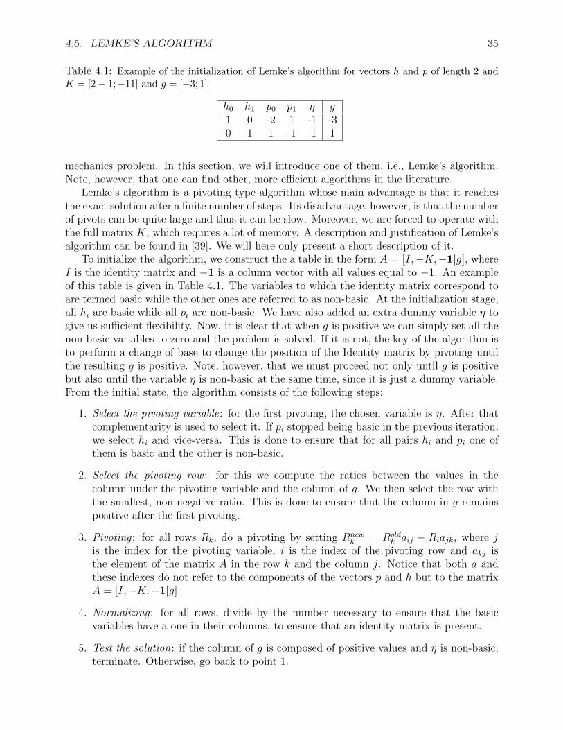
4.5. LEMKE’S ALGORITHM 35
Table 4.1: Example of the initialization of Lemke’s algorithm for vectors h and p of length 2 andK = [2− 1;−11] and g = [−3; 1]
h0 h1 p0 p1 η g1 0 -2 1 -1 -30 1 1 -1 -1 1
mechanics problem. In this section, we will introduce one of them, i.e., Lemke’s algorithm.Note, however, that one can find other, more efficient algorithms in the literature.
Lemke’s algorithm is a pivoting type algorithm whose main advantage is that it reachesthe exact solution after a finite number of steps. Its disadvantage, however, is that the numberof pivots can be quite large and thus it can be slow. Moreover, we are forced to operate withthe full matrix K, which requires a lot of memory. A description and justification of Lemke’salgorithm can be found in [39]. We will here only present a short description of it.
To initialize the algorithm, we construct the a table in the form A = [I,−K,−1|g], whereI is the identity matrix and −1 is a column vector with all values equal to −1. An exampleof this table is given in Table 4.1. The variables to which the identity matrix correspond toare termed basic while the other ones are referred to as non-basic. At the initialization stage,all hi are basic while all pi are non-basic. We have also added an extra dummy variable η togive us sufficient flexibility. Now, it is clear that when g is positive we can simply set all thenon-basic variables to zero and the problem is solved. If it is not, the key of the algorithm isto perform a change of base to change the position of the Identity matrix by pivoting untilthe resulting g is positive. Note, however, that we must proceed not only until g is positivebut also until the variable η is non-basic at the same time, since it is just a dummy variable.From the initial state, the algorithm consists of the following steps:
1. Select the pivoting variable: for the first pivoting, the chosen variable is η. After thatcomplementarity is used to select it. If pi stopped being basic in the previous iteration,we select hi and vice-versa. This is done to ensure that for all pairs hi and pi one ofthem is basic and the other is non-basic.
2. Select the pivoting row : for this we compute the ratios between the values in thecolumn under the pivoting variable and the column of g. We then select the row withthe smallest, non-negative ratio. This is done to ensure that the column in g remainspositive after the first pivoting.
3. Pivoting : for all rows Rk, do a pivoting by setting Rnewk = Rold
k aij − Riajk, where jis the index for the pivoting variable, i is the index of the pivoting row and akj isthe element of the matrix A in the row k and the column j. Notice that both a andthese indexes do not refer to the components of the vectors p and h but to the matrixA = [I,−K,−1|g].
4. Normalizing : for all rows, divide by the number necessary to ensure that the basicvariables have a one in their columns, to ensure that an identity matrix is present.
5. Test the solution: if the column of g is composed of positive values and η is non-basic,terminate. Otherwise, go back to point 1.

36 CHAPTER 4. THE DRY CONTACT
With this algorithm, a solution to (4.66) can be found. Then, the total load can be computedby integrating the pressure following the discretization in Section 4.4.5. Notice that, byshifting the initial gap g up and down, the load can be decreased and increased.
4.6 Acceleration via FFT
When looking at the algorithm presented in Section 4.5 it is clear that the main burdencomes from pivoting in such a large and full matrix. Although one can use other methodswhich might be more efficient in terms of total number of iterations, the burden posed bythe matrix K will still remain. Indeed, computing the deformation using the matrix-vectormultiplication in (4.62) is going to be extremely expensive, as K is of size N2 in one dimensionand N2
1N22 in two-dimensions. Moreover, it is a full matrix, meaning that it has no zeros
that would allow for simplification. It is thus clear that this operation will require a lotof memory and computational power, especially for three-dimensional contacts. Therefore,before introducing a more efficient algorithm, as we will do in Section 4.7, we need to find amanner to compute the deformation in a more efficient way. For this, we can use the fact thatK has a very particular structure, which can be used to significantly lower the requirementsboth in terms of memory and in terms of computational time. In this section, we will recognizethe computation of deformation as a convolution, which will allow us to use the Fast FourierTransform (FFT) to simplify the computations. To set the stage, however, let us begindiscussing the continuous case, i.e., the continuous convolution. After this, we will discussthe discrete convolution, which will be more practical in use. A summary of the differentpaths that we will consider is given in Fig. 4.10. Throughout this chapter, we will consideronly the 1D problem modelling 2D contacts. However, the 2D Fourier transform is obtainedby simply applying the 1D Fourier Transform in each direction. Therefore, everything weconsider here is directly applicable to the 3D contacts as well. A definition of the FourierTransform and some of its properties can be found in the Appendix.
4.6.1 The elastic deformation seen as a convolution
As stated previously, the computation of the deformation can be written as
ue (x) =
∫ ∞−∞
K(x− x′)p(x)dx′. (4.67)
By comparing it to (A.27), this equation can be identified to be the convolution between thekernel K and the pressure p. A common way to interpret a convolution is to note that itbecomes larger the more correlated the two functions are. Indeed, we can see that the moreK and p overlap, i.e., the closer the point x is to a peak of p (x), the larger the deformationis. Having established the deformation as a convolution, we can make use of the ConvolutionTheorem, presented in Section A.4. This states that, since ue is computed as the convolutionof K and p, we can write
F ue = F KF p , (4.68)
where F · indicates the Fourier transform. To make good use of (4.68), we need to find anexpression for F K. Although we could simply try to compute the Fourier transform of
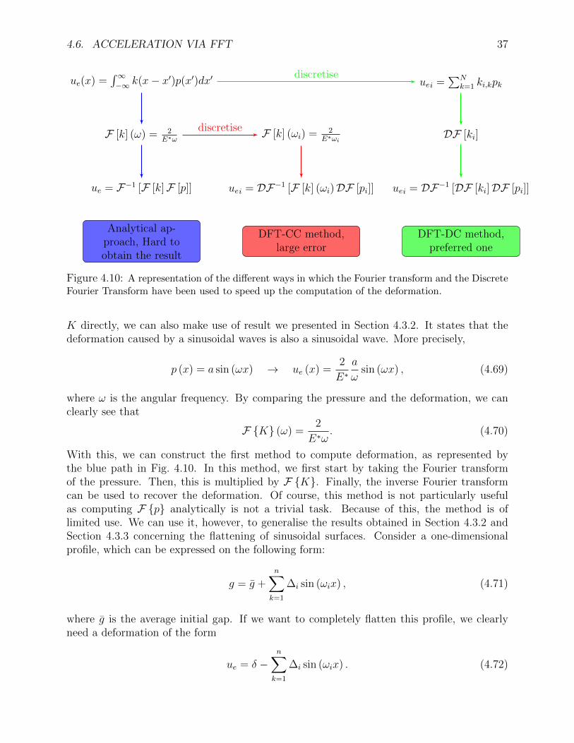
4.6. ACCELERATION VIA FFT 37
ue(x) =∫∞−∞ k(x− x′)p(x′)dx′
F [k] (ω) = 2E∗ω
ue = F−1 [F [k]F [p]]
Analytical ap-proach, Hard toobtain the result
F [k] (ωi) = 2E∗ωi
uei = DF−1 [F [k] (ωi)DF [pi]]
DFT-CC method,large error
discretise
uei =∑N
k=1 ki,kpk
DF [ki]
uei = DF−1 [DF [ki]DF [pi]]
DFT-DC method,preferred one
discretise
Figure 4.10: A representation of the different ways in which the Fourier transform and the DiscreteFourier Transform have been used to speed up the computation of the deformation.
K directly, we can also make use of result we presented in Section 4.3.2. It states that thedeformation caused by a sinusoidal waves is also a sinusoidal wave. More precisely,
p (x) = a sin (ωx) → ue (x) =2
E∗a
ωsin (ωx) , (4.69)
where ω is the angular frequency. By comparing the pressure and the deformation, we canclearly see that
F K (ω) =2
E∗ω. (4.70)
With this, we can construct the first method to compute deformation, as represented bythe blue path in Fig. 4.10. In this method, we first start by taking the Fourier transformof the pressure. Then, this is multiplied by F K. Finally, the inverse Fourier transformcan be used to recover the deformation. Of course, this method is not particularly usefulas computing F p analytically is not a trivial task. Because of this, the method is oflimited use. We can use it, however, to generalise the results obtained in Section 4.3.2 andSection 4.3.3 concerning the flattening of sinusoidal surfaces. Consider a one-dimensionalprofile, which can be expressed on the following form:
g = g +n∑k=1
∆i sin (ωix) , (4.71)
where g is the average initial gap. If we want to completely flatten this profile, we clearlyneed a deformation of the form
ue = δ −n∑k=1
∆i sin (ωix) . (4.72)
38 CHAPTER 4. THE DRY CONTACT
Following (4.68), we can easily see, that the pressure needed for such purpose is
p = p+n∑k=1
2∆i
E∗ωsin (ωix) , (4.73)
which follows from (4.69) and the linearity of the Fourier transform. Moreover, the pressureneeded to completely flatten the profile is that required to ensure that the pressure in (4.73)is always non-negative, i.e.,
p ≥n∑k=1
2∆i
E∗ω. (4.74)
A similar result can be obtained for bi-sinusoidal surfaces.
4.6.2 The DFT-CC method
As we saw, the continuous convolution can facilitate the computation of deformation insome cases. Despite that, it is not always easy to obtain analytically the required Fouriertransforms. A reasonable approach, taken, for example, by [40], is thus to perform themnumerically, which leads to the Discrete Fourier Transform - Continuous Convolution (DFT-CC), depicted in red in Fig. 4.10. In essence, this approach applies the same treatment as wedid to obtain (4.73) to general pressure profiles, which may not fully flatten the surface. Forthis, we start by taking the Discrete Fourier transform of the (discrete) pressure distributionfor which we want to compute the deformation, leading to the following expression for thepressure distribution
pi ..= p(xi) ≈a0
2+
N/2∑n=1
an cos (ωnxi) +
N/2∑n=1
bn sin (ωnxi) , (4.75)
where ωn is a discretisation of the continuous frequency ω, i.e.,
ωn = n∆ω, ∆ω =2π
L, n = 0, ..., N, (4.76)
where L is the length of the domain. The continuous convolution method presented inthe previous section can now be applied to (4.75). Note that this method is equivalent tocomputing the deformation as
ue = DF−1
2
E∗ωnDF p
, (4.77)
where ωn should be interpreted as a series presented in (4.76) and DF · and DF−1 ·stand for the Discrete Fourier Transform and its inverse.
This method is nowadays out of use, since it introduces a larger error in the computationof ue. This error comes from the representation of the pressure in (4.75). Indeed, the methodwill only give accurate results as long as (4.75) is a good approximation to the pressure. Thismeans that the frequency components of p must be well represented in intervals of size ∆ωand that frequencies above ωN/2 are not contributing significantly. We can now ask ourselves
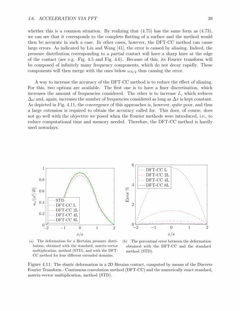
4.6. ACCELERATION VIA FFT 39
whether this is a common situation. By realizing that (4.75) has the same form as (4.73),we can see that it corresponds to the complete flatting of a surface and the method wouldthen be accurate in such a case. In other cases, however, the DFT-CC method can causelarge errors. As indicated by Liu and Wang [41], the error is caused by aliasing. Indeed, thepressure distribution corresponding to a partial contact will have a sharp knee at the edgeof the contact (see e.g. Fig. 4.5 and Fig. 4.6). Because of this, its Fourier transform willbe composed of infinitely many frequency components, which do not decay rapidly. Thesecomponents will then merge with the ones below ωN/2 thus causing the error.
A way to increase the accuracy of the DFT-CC method is to reduce the effect of aliasing.For this, two options are available. The first one is to have a finer discretisation, whichincreases the amount of frequencies considered. The other is to increase L, which reduces∆ω and, again, increases the number of frequencies considered as long as ∆x is kept constant.As depicted in Fig. 4.11, the convergence of this approaches is, however, quite poor, and thusa large extension is required to obtain the accuracy called for. This does, of course, doesnot go well with the objective we posed when the Fourier methods were introduced, i.e., toreduce computational time and memory needed. Therefore, the DFT-CC method is hardlyused nowadays.
−2 −1 0 1 20
0.2
0.4
0.6
0.8
1
x/a
ue/(a
2/R
)
STDDFT-CC LDFT-CC 2LDFT-CC 4LDFT-CC 8L
(a) The deformation for a Hertzian pressure distri-bution, obtained with the standard, matrix-vectormultiplication, method (STD), and with the DFT-CC method for four different extended domains.
−2 −1 0 1 20
2
4
6
x/a
Err
or%
DFT-CC LDFT-CC 2LDFT-CC 4LDFT-CC 8L
(b) The percentual error between the deformationobtained with the DFT-CC and the standardmethod (STD).
Figure 4.11: The elastic deformation in a 2D Herzian contact, computed by means of the DiscreteFourier Transform - Continuous convolution method (DFT-CC) and the numerically exact standard,matrix-vector multiplication, method (STD).

40 CHAPTER 4. THE DRY CONTACT
4.6.3 DFT - Discrete Circular Convolution method: Periodic sur-faces
As we have seen in the previous section, the DFT-CC method is not very accurate. Asdiscussed, aliasing is the responsible for this inaccuracy. Ultimately, the problem can betracked to the mixing between the use of the Discrete Fourier Transform (DFT) to describethe pressure and the Continuous convolution theorem to analyse the deformation causedby this pressure. To avoid this issue, one should therefore consider directly the discreteversion of the problem. The resulting method is known as the DFT-Discrete Convolutionmethod. Remember that the discrete equation for the deformation in 2D, which was derivedin Section 4.4.4, according to (4.57), is
uei..= ue(xi) = − 2
πE∗
N−1∑j=0
Ki,jpj = − 2
πE∗
N−1∑j=0
K|i−j|pj, i = 0, 1, ..., N − 1. (4.78)
Now, this equation is not directly a convolution, although it is fairly close. As described inSection A.5, a circular discrete convolution is defined for periodic functions and has the form
gi = h ∗ f =N−1∑i=0
h〈i−j〉Nfj i = 0, 1, ..., N − 1, (4.79)
where 〈i− j〉N is the N modulus of i − j so that the negative indices are defined throughthe periodicity of the function, i.e. h〈−1〉N = h〈N−1〉N = hN−1, h〈−2〉N = h〈N−2〉N = hN−2, etc.The difference between the operations involved with the circular convolution and the ones inthe elastic deflection is shown in Fig. 4.12.
An important difference is, of course, that the functions in (4.79) are periodic whereasthose in (4.78) are not. The study of the deformation of periodic surfaces is, however, relevantfor the study of roughness. Let us therefore modify (4.78) to account for that. For this, wedefine the deformation as
uei = − 2
πE∗
N−1∑k=0
C〈i−j〉Npj, i = 0, 1, ..., N − 1, (4.80)
where the coefficients C〈i−j〉N are defined as
C =[K0, K1, ..., KN/2−1, KN/2, KN/2−1, .., K1
]. (4.81)
A graphical interpretation of the meaning of this coefficients can be found in Fig. 4.13. Notethat the only thing we have done is to compute the distance allowing for periodicity, which isnicely captured by our repeated and mirrored coefficients in (4.81). For example, the pointN − 1 is actually at a distance 1 from the point 0 and thus the last coefficient in (4.81) isK1. This new deformation equation is in the form of a circular convolution and both thepressure and the kernel K are now considered periodic. Therefore, we can apply the discreteconvolution theorem to write
DF ue = DF KDF p . (4.82)

4.6. ACCELERATION VIA FFT 41
g0
f0 f1 f2 f3
h0 h3 h2 h1
ue0
f0 f1 f2 f3
C0C1 C1 C2 C3 C2
g1
f0 f1 f2 f3
h1 h0 h3 h2
ue1
f0 f1 f2 f3
C1C2 C0 C1 C2 C3
Figure 4.12: Representation of the operations that are performed during convolution, (4.79), (left),and to compute the deformation (4.78) (right). To compute, e.g., g0, one needs to multiply the valuesof f with the values of h below and then add the results. The arrows indicate the change in h or Cto advance one index in g and ue, respectively. Note that two additional nodes have been added toillustrate the calculation of the elastic deformation.
As shown in Section A.5, this relation is exact, i.e., it will give the same solution for ue as(4.80). This means that the only error will come from the discretisation itself, as shown inFig. 4.14 for a slightly different case.
Without having to worry about errors introduced by the model, we can take full advantageof the better performance of this method as compared to the matrix-vector multiplication.Memory-wise we gain a lot since the kernel K is represented only as a vector of size N , insteadof a matrix of size N2 (for the 2D contact). In computational terms, the cost to computethe deformation using the DFT-DC method comes from the DFT. Thankfully, there is analgorithm, called Fast Fourier transform (FFT) which has a complexity N logN . This ismuch quicker than the complexity of the matrix-vector multiplication, which is of order N2.Notice that the complexity must be understood as the rate at which the time increases as afunction of N . The time for the DFT-DC is then proportional to N logN while the one forthe matrix-vector multiplication is N2. This means that for sufficiently large N , the DFT-DCmethod will always by much faster.
Before finishing, let us make it clear that the method as presented here is only valid tocompute the deformation caused by a periodic pressure distribution. Therefore, the surfacesstudied must be periodic as well. One might argue that there is no such thing as a periodicsurface, which is true. However, if we want to study the effect of surface roughness, it is nota bad approximation to assume that the roughness is periodic. This approximation will workfine as long as the wavelength of the roughness is much smaller than the overall contact size.
42 CHAPTER 4. THE DRY CONTACT
This situation is encountered in conformal contacts, which are found in many applications,e.g., journal bearings. Notice that this approximation is also made in the Westergaardsolution, discussed in Section 4.3.2.
4.6.4 DFT - Discrete Linear Convolution method: Non-periodicsurfaces
As we discussed in the previous section, the DFT-DC method is very advantageous in termsof memory and computational time. We therefore want to be able to use it for all contactproblems, including the non-conformal contacts (e.g. the Hertzian contact problem) in whichthe assumption of periodicity cannot be made. As discussed in Section A.5, it is possible totransform linear convolutions of non-periodic functions into circular convolutions of periodicfunctions by extending the domain. The same can be done for (4.78). In order to see howto do it, let us consider the computation of ue0, ue1 and ueN/2−1 in Fig. 4.13. We notice thatthe coefficients of the pressures p0 to pN/2 are correct in our non-periodic computation. Bycorrect we here mean that the index of the coefficient K they are multiplied with, matcheswith |i− k|. It can easily be seen that this holds for all uei with i < N/2. The problem ariseswhen considering pressure points with index larger than N/2. For those points, the distanceis too short. This would not be a problem, however, if all those pressures would be zero. Inthat case, the computation in Fig. 4.13 would be equal to the desired one. Following thisthoughts, one can come up with the following strategy, presented, e.g., in [4],
1. Start with a discrete pressure vector pN and a vector of coefficients KN , both of size N
2. Create a vector of coefficients of size 2N as C2N = [K0, K1, ..., KN−1, 0, KN−1, .., K1]
3. Create another pressure vector p2N , of size 2N , via zero-padding, i.e., p2Ni = pNi for
i = N/2 + 1, ..., N/2 +N and p2Ni = 0 for i ≤ N/2 ∧ i ≥ N/2 +N + 1
4. Compute the deformation ue2N = DF−1
DF
C2N
DF
p2N
.
5. The vector ue2N is now too long, but we only need to keep the initial values, i.e.,
uei = ue2Ni for i = 0, 1, ..., N − 1.
It is easy to see that this zero-padding procedure leads to a convolution which is exactlyequal to (4.62). Therefore, we keep all the benefits of the DFT-DC method, even for non-periodic signals. The price to pay is that the domain needs to be doubled. With thisdoubling, however, we obtain an exact results and thus no further extension of the domainis ever needed. The accuracy of the method is depicted in Fig. 4.14, where the deformationcaused by a Hertzian pressure is computed using the vector-multiplication method as wellas the non-periodic DFT-DC method. Notice that even when an extremely coarse meshis used, both methods coincide. Indeed, the DFT-DC method is numerically exact to thevector-multiplication method and the error only comes from the discretisation itself.
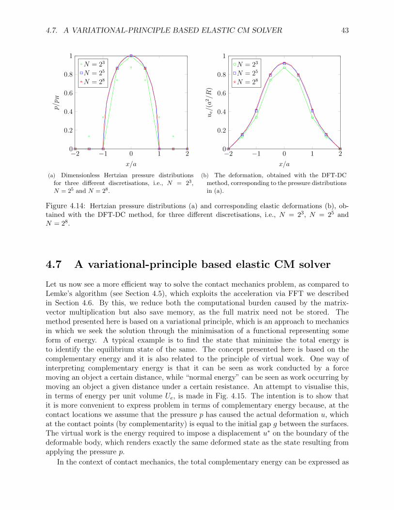
4.7. A VARIATIONAL-PRINCIPLE BASED ELASTIC CM SOLVER 43
−2 −1 0 1 20
0.2
0.4
0.6
0.8
1
x/a
p/p H
N = 23
N = 25
N = 28
(a) Dimensionless Hertzian pressure distributionsfor three different discretisations, i.e., N = 23,N = 25 and N = 28.
−2 −1 0 1 20
0.2
0.4
0.6
0.8
1
x/a
ue/(a
2/R
)
N = 23
N = 25
N = 28
(b) The deformation, obtained with the DFT-DCmethod, corresponding to the pressure distributionsin (a).
Figure 4.14: Hertzian pressure distributions (a) and corresponding elastic deformations (b), ob-tained with the DFT-DC method, for three different discretisations, i.e., N = 23, N = 25 andN = 28.
4.7 A variational-principle based elastic CM solver
Let us now see a more efficient way to solve the contact mechanics problem, as compared toLemke’s algorithm (see Section 4.5), which exploits the acceleration via FFT we describedin Section 4.6. By this, we reduce both the computational burden caused by the matrix-vector multiplication but also save memory, as the full matrix need not be stored. Themethod presented here is based on a variational principle, which is an approach to mechanicsin which we seek the solution through the minimisation of a functional representing someform of energy. A typical example is to find the state that minimise the total energy isto identify the equilibrium state of the same. The concept presented here is based on thecomplementary energy and it is also related to the principle of virtual work. One way ofinterpreting complementary energy is that it can be seen as work conducted by a forcemoving an object a certain distance, while “normal energy” can be seen as work occurring bymoving an object a given distance under a certain resistance. An attempt to visualise this,in terms of energy per unit volume Ue, is made in Fig. 4.15. The intention is to show thatit is more convenient to express problem in terms of complementary energy because, at thecontact locations we assume that the pressure p has caused the actual deformation u, whichat the contact points (by complementarity) is equal to the initial gap g between the surfaces.The virtual work is the energy required to impose a displacement u∗ on the boundary of thedeformable body, which renders exactly the same deformed state as the state resulting fromapplying the pressure p.
In the context of contact mechanics, the total complementary energy can be expressed as

44 CHAPTER 4. THE DRY CONTACT
the different between the internal elastic energy U∗e and the corresponding virtual work U∗v ,i.e.
V ∗ = U∗e − U∗v . (4.83)
The internal elastic energy is given by
U∗e = Ue =1
2
x
Ω
pue dΩ, (4.84)
and the virtual work by
U∗v = Uv = −x
Ω
p(δ − g) dΩ, (4.85)
Thus, the complementary energy can be formulated as
V ∗ =1
2
x
Ω
pue dΩ +x
Ω
p(g − δ) dΩ, (4.86)
see [1]. We note that since
w =x
Ω
p dΩ,
we can write (4.86) as
V ∗ =1
2
x
Ω
pue dΩ +x
Ω
pg dΩ− δw. (4.87)
Dressed in contact mechanics terminology, finding p that minimise the functional V ∗, in thisvariational-principle based method, is equivalent of finding the contact configuration whichminimises the total complementary potential energy. For more details on the variational-based approach, the reader is referred to the work by Kalker, in particular [9].
To find the numerical solution to the contact mechanics problem, we must discretise(4.87). Using the discretisation presented in Section 4.4 and expressing the deformation as afunction of pressure through (4.62), we can write
V ∗ ≈ 1
2pTKp+ pTg − δw, (4.88)
where p and g are vectors, δ the rigid body displacement (mutual approach) and K is thematrix in (4.62). From the discrete formulation of the variational principle it is clear that it isa quadratic problem, which can be solved with various types of readily available algorithms.In the following we will present one of these, which simply consists on following the gradient ofV ∗ towards the minimum, see [10]. In the field of optimisation, this approach is also known asthe gradient decent method, which is the numerical correspondence to the analytical methodof steepest decent. Since δw is independent of p the gradient of V ∗ with respect to p is simply
∇V ∗ = Kp+ g = ue + g. (4.89)
Notice that we do not need to know the value of V ∗ but only its gradient. We do however,need to compute ue, and this can be done through the fast DFT-DC technique presented in

4.7. A VARIATIONAL-PRINCIPLE BASED ELASTIC CM SOLVER 45
Section 4.6.4. A simple algorithm ought to start with a given pressure distribution, e.g., aconstant one, then the deformation can be computed. Thereafter, an initial value for ∇V ∗and used to update pressure according to
pnew = pold + r∇V ∗ = pold + r (ue + g) , (4.90)
until convergence is reached. The relaxation factor r can be defined in different ways, e.g. asin the conjugate gradient method [42] or it may simply be specified as a constant which canbe increased or reduced it the rate of convergence is too high or too slow. Note that, whileupdating the pressure, we have another constraint, i.e., the total load w is also specified,thus we need to take it into account as well. To this end, after every update of the pressureaccording to (4.90), it needs to be modified to comply with the load balance constraint. Thiscan be done by shifting the pressure up or down a certain value α. An overview of thealgorithm resulting from these considerations is given in Fig. 4.16.
Define the gap between the surface: g = |zu − zl|
Initial guess pold = wL1L2
Calc: pnew = pold + r∇V ∗(pold), where ∇V ∗
(pold)
= ue(pold)
+ g
Force balance: find α so that∫
Ωcpnew + α dx = w,
Ωc = x| pnew ≥ 0
Truncate pressure: pnew = pnew + α,pnew ≤ 0→ 0
Check if x ∈ Ωc lie within a plane?|h(x ∈ Ωc)| < ε:
Done!YES
pold ← pnewNO
Figure 4.16: Flow chart of the solution procedure for solving the contact mechanics problem usingthe variational principle.
Let us conclude with a comment on the constraints imposed by the Kuhn-Tucker comple-mentary conditions, (4.15a) and (4.15b). We have not mention them so far in the context ofthis solver. These are, however, implicitly enforced by the minimisation of the complemen-tary energy. Indeed, at its minimum, ∇V ∗ is zero. Note, however, that this means that, forthe points in contact, ue = −g and thus h = 0. We therefore only need to be careful to avoidnegative pressures at each step of the iteration procedure.

46 CHAPTER 4. THE DRY CONTACT
4.8 Enhanced CM solver including plastic deformation
It is clear that introducing plastic deformation in the context of the boundary element methodis not going to be easy. This is because we used very early the linear behaviour of elasticityand the resulting principle of superposition. Remember that we did that to describe thedeformation of a given pressure distribution, given in (4.5), as the sum of the deformationcaused by many point loads, given in (4.1). Plasticity is, however, not linear and thus doesnot allow for such convenient treatment. In this section we will, however, describe a simplemethod to include plastic deformation, which provides for a good first approximation to theeffect of plasticity.
The idea behind the approach presented here, which is the contact-mechanics backbonein the Lulea mixed lubrication model (LMLM) [3, 11], is that when the contact pressureat a given point exceeds a certain value, this point is allowed to flow freely towards thecontact plane without any further increase in the pressure. This maximum allowed valuefor the pressure is defined as the hardness of the (surface-near) material in the softer of thecontacting bodies, H. An approximative estimate of the hardness is given by
H = 2.8σY , (4.91)
where σY is the yield limit of the material [30]. A system defining the contact mechanicsthat includes plastic deformation, via the hardness may, therefore, be formulated as
h (x) > 0, p (x) = 0, x ∈ Ωc, (4.92a)
h (x) = 0, 0 < p (x) ≤ H, x /∈ Ωc, (4.92b)
h = ue + (g − up)− δ, (4.92c)
ue =
∫Ω
K(|x− x′|)p (x′, x′) dx′, (4.92d)
w =
∫Ω
p (x) dx. (4.92e)
In the paper by Tiwari et al. [43] they performed indentation experiments on sandblastedaluminium surfaces to explore the plastic deformation of asperities and modelled the contactmechanics using the aforementioned enhanced CM solver taking into account the plastic flow.It was concluded that the numerical predictions quantitatively describe the plastic deforma-tion that the aluminium surfaces undergo. Moreover, in most cases, the long-wavelengthroughness governs fluid leakage observed in metallic seals, they drew the conclusion that itwould be possible to estimate the leakage using the elastoplastic contact mechanics modeldescribed herein.
The system of equations presented above, can be discretised in the same manner as in theelastic case. Moreover, by introducing two modifications to it, the variational-principle basedmethod, presented in Section 4.7, can be applied also in this case. Firstly, when updatingthe pressure, this must be truncated to ensure 0 ≤ p ≤ H, and secondly, the points wherep = H, i.e. x ∈ Ωp, which experience plastic deformation up will cause ue 6= −(g − δ) andthus ∇V ∗ 6= 0 even if they are in contact. These points must, therefore, excluded from theconvergence criterion |h(x ∈ Ωc)| < ε, with ε specifying the tolerance. The solution procedure

4.8. ENHANCED CM SOLVER INCLUDING PLASTIC DEFORMATION 47
can then be executed in the same manner as in the elastic case. The main difference beingthat the force balance criterion in this case includes the contribution of the yielding points.Indeed, for x ∈ Ωp, the convergence criterion will not be fulfilled. For it to be fulfilled, upat these points must be the solution to (4.92c) when h = 0. This is also how up should becalculated, i.e.
up(x) = g(x) + ue(x)− δ, x ∈ Ωp (4.93)
A flow chart of the solution procedure is depicted in Fig. 4.17.

48 CHAPTER 4. THE DRY CONTACT
ue0
p0 p1 p2 pN2−1 pN
2pN
2+1 pN−2 pN−1
C0 CN−1 CN−2 CN2
+1 CN2
CN2−1 C2 C1
K0 K1 K2KN
2−1 KN
2KN
2−1 K2 K1
ue0
p0 p1 p2 pN2−1 pN
2pN
2+1 pN−2 pN−1
C1 C0 CN−1 CN2
+2 CN2
+1 CN2
C3 C2
K1 K0 K1KN
2−2 KN
2−1 KN
2K3 K2
ue0
p0 p1 p2 pN2−1 pN
2pN
2+1 pN−2 pN−1
C2 C1 C0CN
2+3 CN
2+2 CN
2+1 C4 C3
K2 K1 K0KN
2−3 KN
2−2 KN
2−1 K4 K3
Figure 4.13: Representation of the computation of uei. The calculation procedure is to multiplythe each pressure pj by C〈i−j〉N , which corresponds to the value of Kn on the row below, and thenadd the results together. The arrows indicate the change in C to advance one index i → i + 1 inuei.
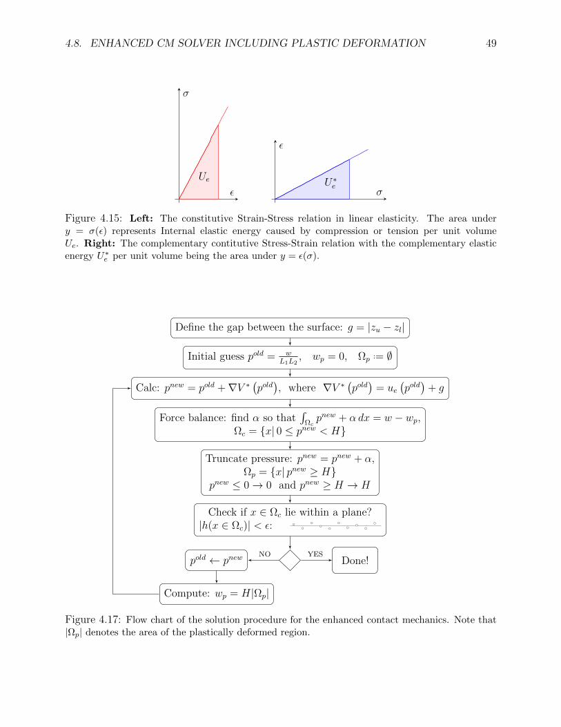
4.8. ENHANCED CM SOLVER INCLUDING PLASTIC DEFORMATION 49
Ue
ε
σ
U∗eσ
ε
Figure 4.15: Left: The constitutive Strain-Stress relation in linear elasticity. The area undery = σ(ε) represents Internal elastic energy caused by compression or tension per unit volumeUe. Right: The complementary contitutive Stress-Strain relation with the complementary elasticenergy U∗e per unit volume being the area under y = ε(σ).
Define the gap between the surface: g = |zu − zl|
Initial guess pold = wL1L2
, wp = 0, Ωp..= ∅
Calc: pnew = pold +∇V ∗(pold), where ∇V ∗
(pold)
= ue(pold)
+ g
Force balance: find α so that∫
Ωcpnew + α dx = w − wp,
Ωc = x| 0 ≤ pnew < H
Truncate pressure: pnew = pnew + α,Ωp = x| pnew ≥ H
pnew ≤ 0→ 0 and pnew ≥ H → H
Check if x ∈ Ωc lie within a plane?|h(x ∈ Ωc)| < ε:
Done!YES
pold ← pnewNO
Compute: wp = H|Ωp|
Figure 4.17: Flow chart of the solution procedure for the enhanced contact mechanics. Note that|Ωp| denotes the area of the plastically deformed region.

50 CHAPTER 4. THE DRY CONTACT
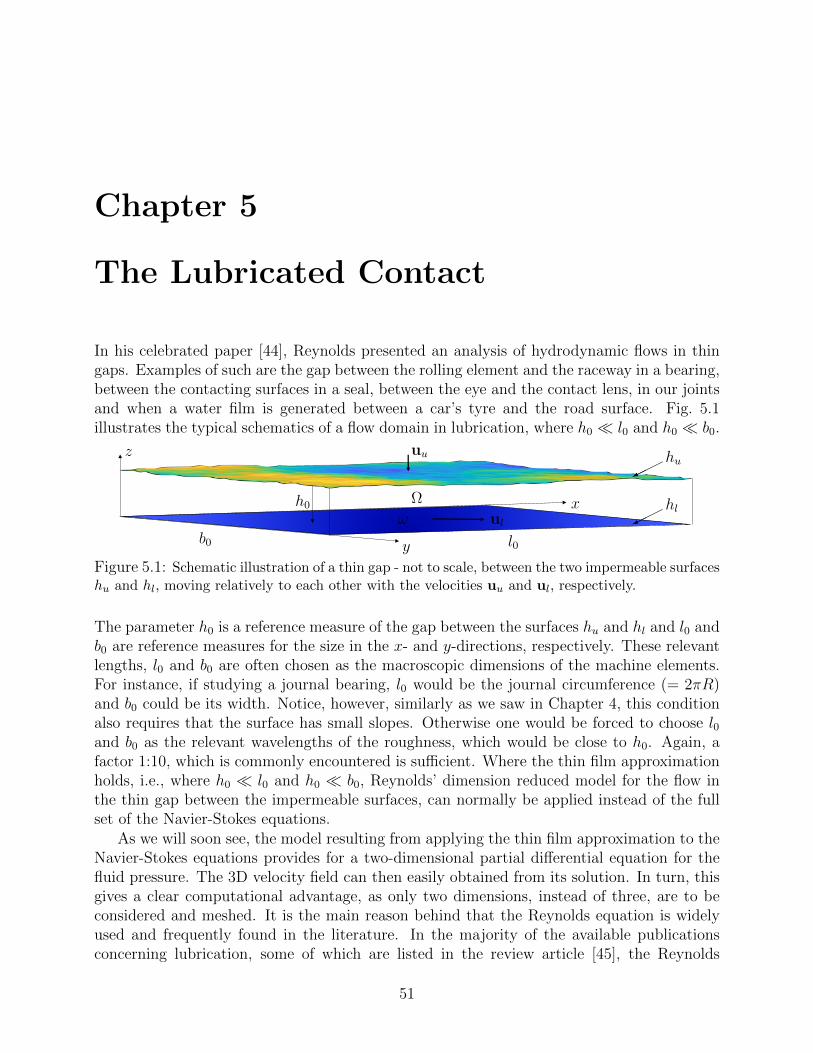
Chapter 5
The Lubricated Contact
In his celebrated paper [44], Reynolds presented an analysis of hydrodynamic flows in thingaps. Examples of such are the gap between the rolling element and the raceway in a bearing,between the contacting surfaces in a seal, between the eye and the contact lens, in our jointsand when a water film is generated between a car’s tyre and the road surface. Fig. 5.1illustrates the typical schematics of a flow domain in lubrication, where h0 l0 and h0 b0.
z
x
y
h0
b0 l0
ul
uu
Ω
ω
hu
hl
Figure 5.1: Schematic illustration of a thin gap - not to scale, between the two impermeable surfaceshu and hl, moving relatively to each other with the velocities uu and ul, respectively.
The parameter h0 is a reference measure of the gap between the surfaces hu and hl and l0 andb0 are reference measures for the size in the x- and y-directions, respectively. These relevantlengths, l0 and b0 are often chosen as the macroscopic dimensions of the machine elements.For instance, if studying a journal bearing, l0 would be the journal circumference (= 2πR)and b0 could be its width. Notice, however, similarly as we saw in Chapter 4, this conditionalso requires that the surface has small slopes. Otherwise one would be forced to choose l0and b0 as the relevant wavelengths of the roughness, which would be close to h0. Again, afactor 1:10, which is commonly encountered is sufficient. Where the thin film approximationholds, i.e., where h0 l0 and h0 b0, Reynolds’ dimension reduced model for the flow inthe thin gap between the impermeable surfaces, can normally be applied instead of the fullset of the Navier-Stokes equations.
As we will soon see, the model resulting from applying the thin film approximation to theNavier-Stokes equations provides for a two-dimensional partial differential equation for thefluid pressure. The 3D velocity field can then easily obtained from its solution. In turn, thisgives a clear computational advantage, as only two dimensions, instead of three, are to beconsidered and meshed. It is the main reason behind that the Reynolds equation is widelyused and frequently found in the literature. In the majority of the available publicationsconcerning lubrication, some of which are listed in the review article [45], the Reynolds
51
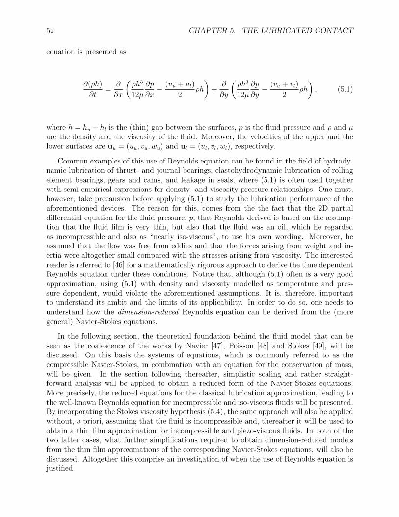
52 CHAPTER 5. THE LUBRICATED CONTACT
equation is presented as
∂(ρh)
∂t=
∂
∂x
(ρh3
12µ
∂p
∂x− (uu + ul)
2ρh
)+
∂
∂y
(ρh3
12µ
∂p
∂y− (vu + vl)
2ρh
), (5.1)
where h = hu − hl is the (thin) gap between the surfaces, p is the fluid pressure and ρ and µare the density and the viscosity of the fluid. Moreover, the velocities of the upper and thelower surfaces are uu = (uu, vu, wu) and ul = (ul, vl, wl), respectively.
Common examples of this use of Reynolds equation can be found in the field of hydrody-namic lubrication of thrust- and journal bearings, elastohydrodynamic lubrication of rollingelement bearings, gears and cams, and leakage in seals, where (5.1) is often used togetherwith semi-empirical expressions for density- and viscosity-pressure relationships. One must,however, take precausion before applying (5.1) to study the lubrication performance of theaforementioned devices. The reason for this, comes from the the fact that the 2D partialdifferential equation for the fluid pressure, p, that Reynolds derived is based on the assump-tion that the fluid film is very thin, but also that the fluid was an oil, which he regardedas incompressible and also as “nearly iso-viscous”, to use his own wording. Moreover, heassumed that the flow was free from eddies and that the forces arising from weight and in-ertia were altogether small compared with the stresses arising from viscosity. The interestedreader is referred to [46] for a mathematically rigorous approach to derive the time dependentReynolds equation under these conditions. Notice that, although (5.1) often is a very goodapproximation, using (5.1) with density and viscosity modelled as temperature and pres-sure dependent, would violate the aforementioned assumptions. It is, therefore, importantto understand its ambit and the limits of its applicability. In order to do so, one needs tounderstand how the dimension-reduced Reynolds equation can be derived from the (moregeneral) Navier-Stokes equations.
In the following section, the theoretical foundation behind the fluid model that can beseen as the coalescence of the works by Navier [47], Poisson [48] and Stokes [49], will bediscussed. On this basis the systems of equations, which is commonly referred to as thecompressible Navier-Stokes, in combination with an equation for the conservation of mass,will be given. In the section following thereafter, simplistic scaling and rather straight-forward analysis will be applied to obtain a reduced form of the Navier-Stokes equations.More precisely, the reduced equations for the classical lubrication approximation, leading tothe well-known Reynolds equation for incompressible and iso-viscous fluids will be presented.By incorporating the Stokes viscosity hypothesis (5.4), the same approach will also be appliedwithout, a priori, assuming that the fluid is incompressible and, thereafter it will be used toobtain a thin film approximation for incompressible and piezo-viscous fluids. In both of thetwo latter cases, what further simplifications required to obtain dimension-reduced modelsfrom the thin film approximations of the corresponding Navier-Stokes equations, will also bediscussed. Altogether this comprise an investigation of when the use of Reynolds equation isjustified.
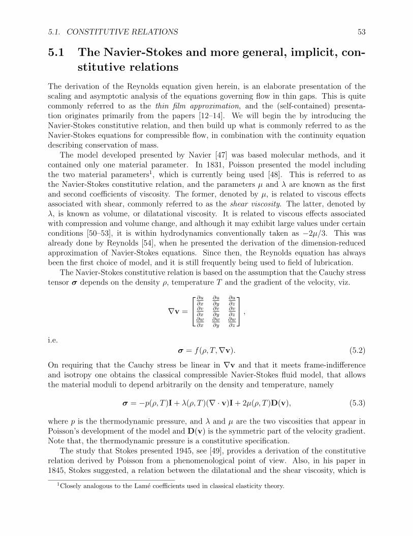
5.1. CONSTITUTIVE RELATIONS 53
5.1 The Navier-Stokes and more general, implicit, con-
stitutive relations
The derivation of the Reynolds equation given herein, is an elaborate presentation of thescaling and asymptotic analysis of the equations governing flow in thin gaps. This is quitecommonly referred to as the thin film approximation, and the (self-contained) presenta-tion originates primarily from the papers [12–14]. We will begin the by introducing theNavier-Stokes constitutive relation, and then build up what is commonly referred to as theNavier-Stokes equations for compressible flow, in combination with the continuity equationdescribing conservation of mass.
The model developed presented by Navier [47] was based molecular methods, and itcontained only one material parameter. In 1831, Poisson presented the model includingthe two material parameters1, which is currently being used [48]. This is referred to asthe Navier-Stokes constitutive relation, and the parameters µ and λ are known as the firstand second coefficients of viscosity. The former, denoted by µ, is related to viscous effectsassociated with shear, commonly referred to as the shear viscosity. The latter, denoted byλ, is known as volume, or dilatational viscosity. It is related to viscous effects associatedwith compression and volume change, and although it may exhibit large values under certainconditions [50–53], it is within hydrodynamics conventionally taken as −2µ/3. This wasalready done by Reynolds [54], when he presented the derivation of the dimension-reducedapproximation of Navier-Stokes equations. Since then, the Reynolds equation has alwaysbeen the first choice of model, and it is still frequently being used to field of lubrication.
The Navier-Stokes constitutive relation is based on the assumption that the Cauchy stresstensor σ depends on the density ρ, temperature T and the gradient of the velocity, viz.
∇v =
∂u∂x
∂u∂y
∂u∂z
∂v∂x
∂v∂y
∂v∂z
∂w∂x
∂w∂y
∂w∂z
,i.e.
σ = f(ρ, T,∇v). (5.2)
On requiring that the Cauchy stress be linear in ∇v and that it meets frame-indifferenceand isotropy one obtains the classical compressible Navier-Stokes fluid model, that allowsthe material moduli to depend arbitrarily on the density and temperature, namely
σ = −p(ρ, T )I + λ(ρ, T )(∇ · v)I + 2µ(ρ, T )D(v), (5.3)
where p is the thermodynamic pressure, and λ and µ are the two viscosities that appear inPoisson’s development of the model and D(v) is the symmetric part of the velocity gradient.Note that, the thermodynamic pressure is a constitutive specification.
The study that Stokes presented 1945, see [49], provides a derivation of the constitutiverelation derived by Poisson from a phenomenological point of view. Also, in his paper in1845, Stokes suggested, a relation between the dilatational and the shear viscosity, which is
1Closely analogous to the Lame coefficients used in classical elasticity theory.
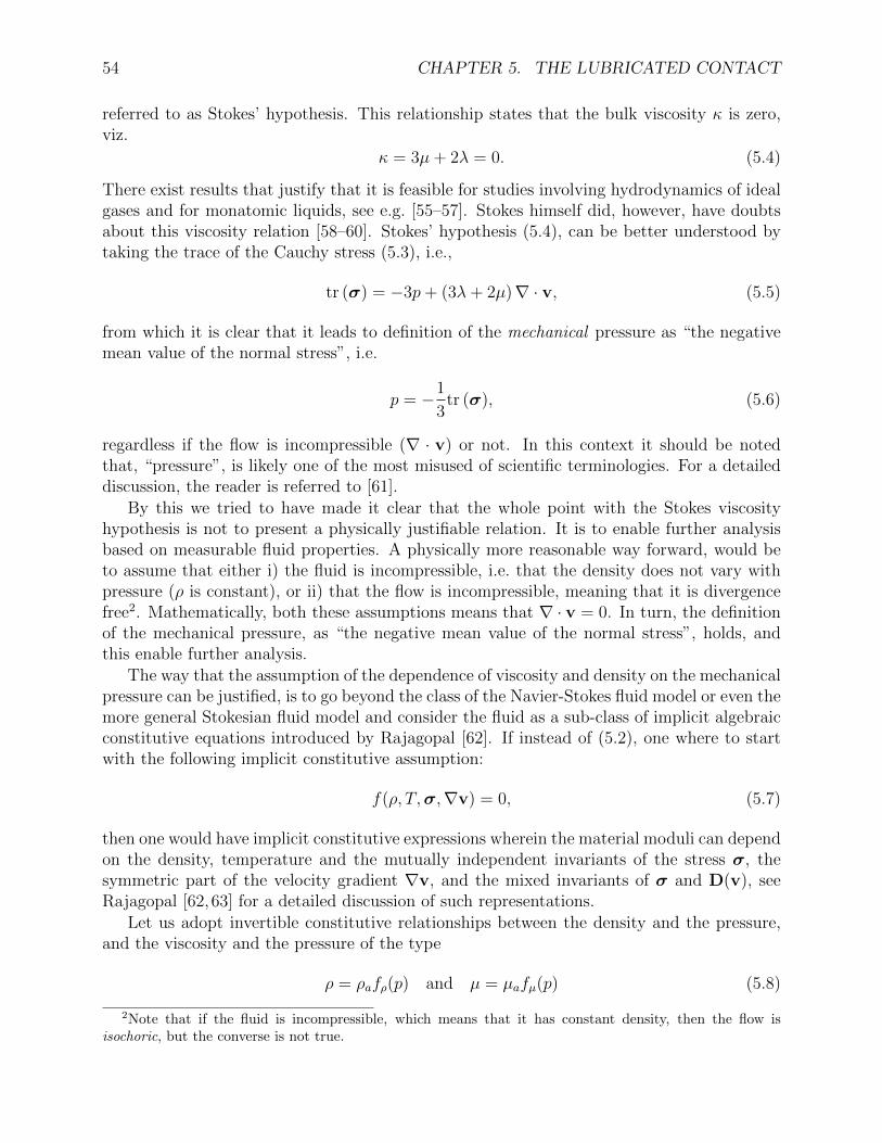
54 CHAPTER 5. THE LUBRICATED CONTACT
referred to as Stokes’ hypothesis. This relationship states that the bulk viscosity κ is zero,viz.
κ = 3µ+ 2λ = 0. (5.4)
There exist results that justify that it is feasible for studies involving hydrodynamics of idealgases and for monatomic liquids, see e.g. [55–57]. Stokes himself did, however, have doubtsabout this viscosity relation [58–60]. Stokes’ hypothesis (5.4), can be better understood bytaking the trace of the Cauchy stress (5.3), i.e.,
tr (σ) = −3p+ (3λ+ 2µ)∇ · v, (5.5)
from which it is clear that it leads to definition of the mechanical pressure as “the negativemean value of the normal stress”, i.e.
p = −1
3tr (σ), (5.6)
regardless if the flow is incompressible (∇ · v) or not. In this context it should be notedthat, “pressure”, is likely one of the most misused of scientific terminologies. For a detaileddiscussion, the reader is referred to [61].
By this we tried to have made it clear that the whole point with the Stokes viscosityhypothesis is not to present a physically justifiable relation. It is to enable further analysisbased on measurable fluid properties. A physically more reasonable way forward, would beto assume that either i) the fluid is incompressible, i.e. that the density does not vary withpressure (ρ is constant), or ii) that the flow is incompressible, meaning that it is divergencefree2. Mathematically, both these assumptions means that ∇ · v = 0. In turn, the definitionof the mechanical pressure, as “the negative mean value of the normal stress”, holds, andthis enable further analysis.
The way that the assumption of the dependence of viscosity and density on the mechanicalpressure can be justified, is to go beyond the class of the Navier-Stokes fluid model or even themore general Stokesian fluid model and consider the fluid as a sub-class of implicit algebraicconstitutive equations introduced by Rajagopal [62]. If instead of (5.2), one where to startwith the following implicit constitutive assumption:
f(ρ, T,σ,∇v) = 0, (5.7)
then one would have implicit constitutive expressions wherein the material moduli can dependon the density, temperature and the mutually independent invariants of the stress σ, thesymmetric part of the velocity gradient ∇v, and the mixed invariants of σ and D(v), seeRajagopal [62,63] for a detailed discussion of such representations.
Let us adopt invertible constitutive relationships between the density and the pressure,and the viscosity and the pressure of the type
ρ = ρafρ(p) and µ = µafµ(p) (5.8)
2Note that if the fluid is incompressible, which means that it has constant density, then the flow isisochoric, but the converse is not true.

5.1. CONSTITUTIVE RELATIONS 55
where p is given by (5.6), as a consequence of Stokes viscosity hypothesis. In this case, it ispossible to deduce an explicit fluid model from the implicit model defined in (5.7), i.e.
σ =− pI− 2
3µ (p) (∇ · v)I + 2µ (p) D(v) = (5.9)
− f−1ρ (ρ/ρa)I−
2
3µafµ(f−1
ρ (ρ/ρa))(∇ · v)I + 2µafµ(f−1ρ (ρ/ρa))D(v).
Note that, it is only within the context of the starting point (5.7) that one can rationallyobtain a model, such as (5.9), wherein the density and the viscosity depends on the mechanicalpressure in an incompressible fluid, thereby giving a proper basis for assumptions of the kindmade by Dowson and Higginson [64] and Barus [65] and their successors.
Let us now consider isothermal flow of an compressible fluid, which, when the Stokesrelation is invoked, can be modelled by the constitutive relation (5.9). Indeed, inserting theconstitutive relation (5.9) into the Cauchy equation (balance of linear momentum), viz.
D (ρv)
Dt= ρg +∇ · σ in Ω, (5.10)
leads to the generalised compressible Navier-Stokes equation
D (ρv)
Dt= ρg −∇p− 2
3∇ · (µ(p)∇ · vI) + 2∇ · (µ(p)D(v)) in Ω, (5.11)
where the density ρ is related to the pressure as in (5.8), ρg accounts for body forces present,µ is the dynamic viscosity,
D
Dt=
∂
∂t+ u
∂
∂x+ v
∂
∂y+ w
∂
∂zand D(v) =
1
2
(∇v + (∇v)T
). (5.12)
Since there are four unknowns in (5.11) it needs to be considered together with theconservation of mass, which for a compressible fluid is given by
∂ (ρv)
∂t+∇ · (ρv) = 0, (5.13)
In component form, the continuity equation and generalised Navier-Stokes equation (5.11)
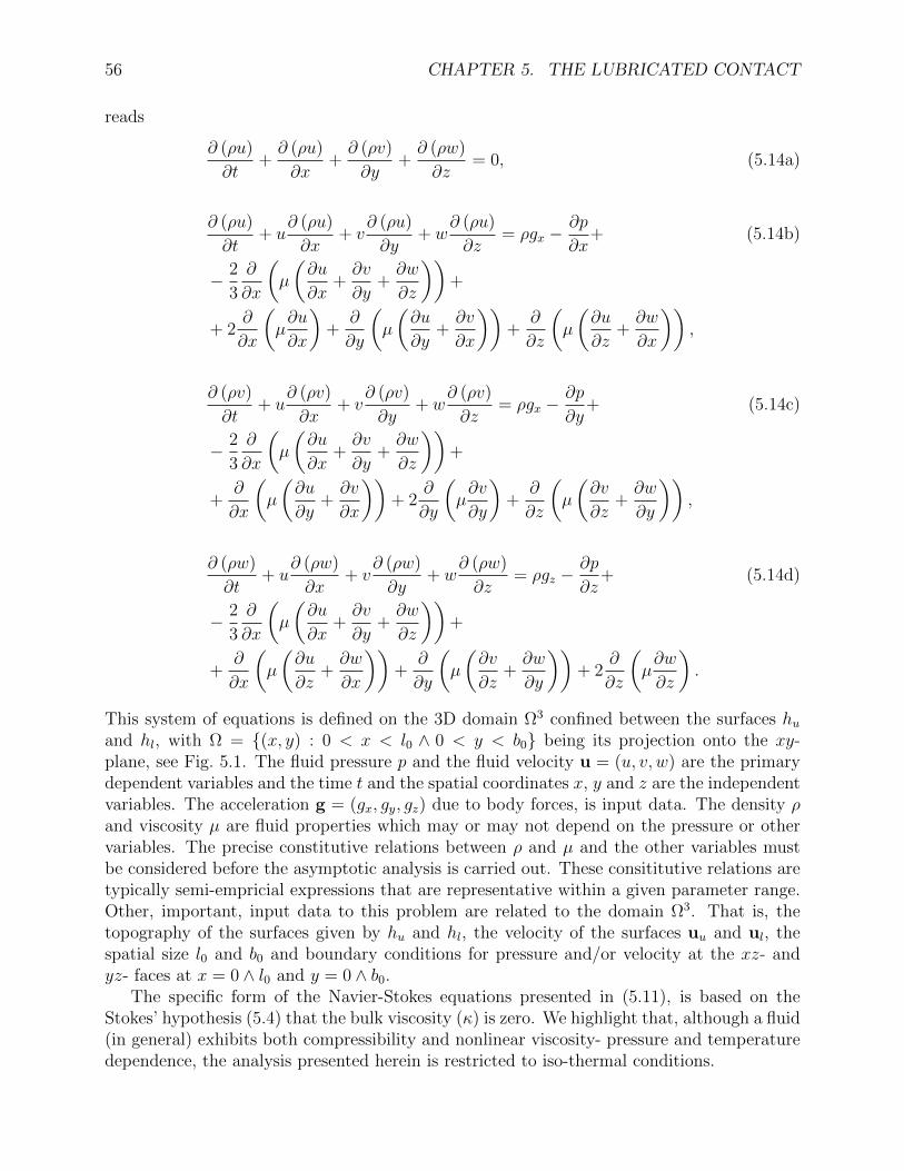
56 CHAPTER 5. THE LUBRICATED CONTACT
reads
∂ (ρu)
∂t+∂ (ρu)
∂x+∂ (ρv)
∂y+∂ (ρw)
∂z= 0, (5.14a)
∂ (ρu)
∂t+ u
∂ (ρu)
∂x+ v
∂ (ρu)
∂y+ w
∂ (ρu)
∂z= ρgx −
∂p
∂x+ (5.14b)
− 2
3
∂
∂x
(µ
(∂u
∂x+∂v
∂y+∂w
∂z
))+
+ 2∂
∂x
(µ∂u
∂x
)+
∂
∂y
(µ
(∂u
∂y+∂v
∂x
))+
∂
∂z
(µ
(∂u
∂z+∂w
∂x
)),
∂ (ρv)
∂t+ u
∂ (ρv)
∂x+ v
∂ (ρv)
∂y+ w
∂ (ρv)
∂z= ρgx −
∂p
∂y+ (5.14c)
− 2
3
∂
∂x
(µ
(∂u
∂x+∂v
∂y+∂w
∂z
))+
+∂
∂x
(µ
(∂u
∂y+∂v
∂x
))+ 2
∂
∂y
(µ∂v
∂y
)+
∂
∂z
(µ
(∂v
∂z+∂w
∂y
)),
∂ (ρw)
∂t+ u
∂ (ρw)
∂x+ v
∂ (ρw)
∂y+ w
∂ (ρw)
∂z= ρgz −
∂p
∂z+ (5.14d)
− 2
3
∂
∂x
(µ
(∂u
∂x+∂v
∂y+∂w
∂z
))+
+∂
∂x
(µ
(∂u
∂z+∂w
∂x
))+
∂
∂y
(µ
(∂v
∂z+∂w
∂y
))+ 2
∂
∂z
(µ∂w
∂z
).
This system of equations is defined on the 3D domain Ω3 confined between the surfaces huand hl, with Ω = (x, y) : 0 < x < l0 ∧ 0 < y < b0 being its projection onto the xy-plane, see Fig. 5.1. The fluid pressure p and the fluid velocity u = (u, v, w) are the primarydependent variables and the time t and the spatial coordinates x, y and z are the independentvariables. The acceleration g = (gx, gy, gz) due to body forces, is input data. The density ρand viscosity µ are fluid properties which may or may not depend on the pressure or othervariables. The precise constitutive relations between ρ and µ and the other variables mustbe considered before the asymptotic analysis is carried out. These consititutive relations aretypically semi-empricial expressions that are representative within a given parameter range.Other, important, input data to this problem are related to the domain Ω3. That is, thetopography of the surfaces given by hu and hl, the velocity of the surfaces uu and ul, thespatial size l0 and b0 and boundary conditions for pressure and/or velocity at the xz- andyz- faces at x = 0 ∧ l0 and y = 0 ∧ b0.
The specific form of the Navier-Stokes equations presented in (5.11), is based on theStokes’ hypothesis (5.4) that the bulk viscosity (κ) is zero. We highlight that, although a fluid(in general) exhibits both compressibility and nonlinear viscosity- pressure and temperaturedependence, the analysis presented herein is restricted to iso-thermal conditions.
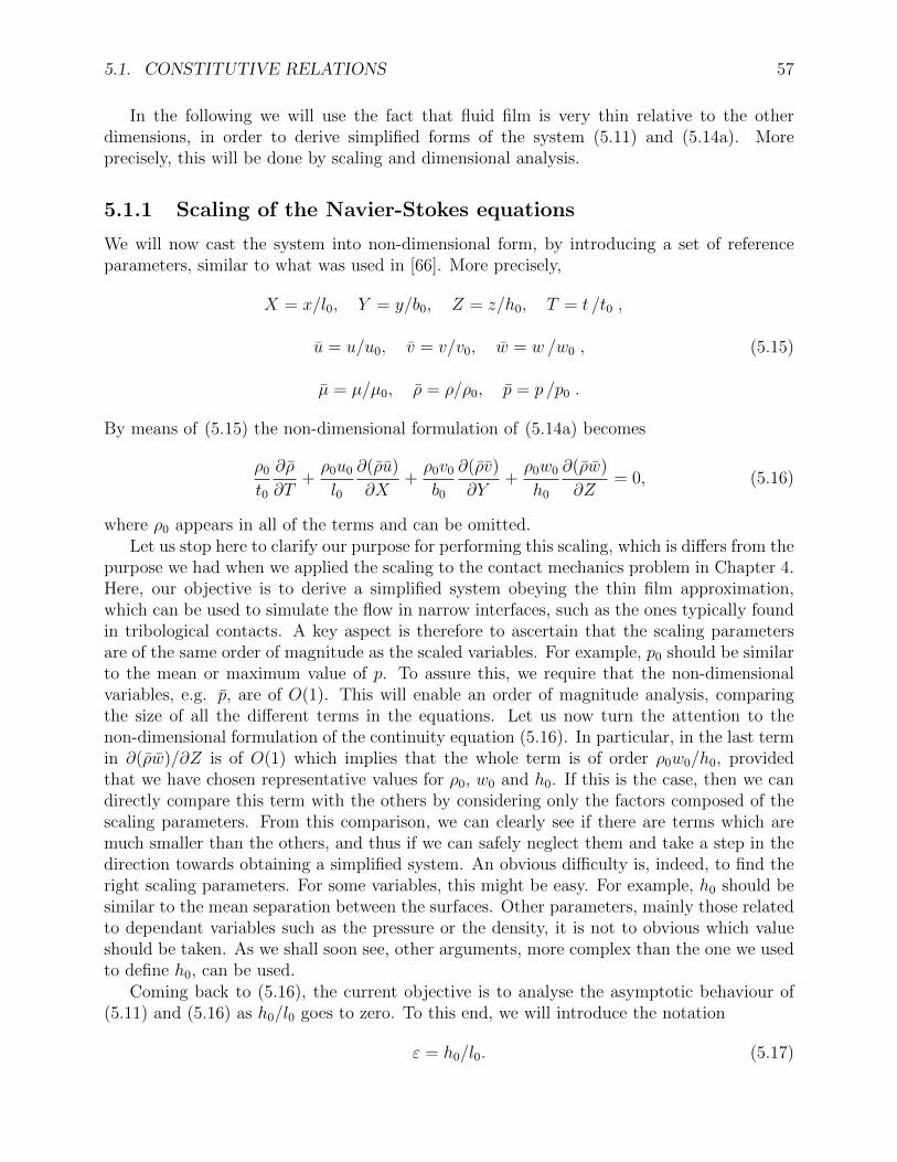
5.1. CONSTITUTIVE RELATIONS 57
In the following we will use the fact that fluid film is very thin relative to the otherdimensions, in order to derive simplified forms of the system (5.11) and (5.14a). Moreprecisely, this will be done by scaling and dimensional analysis.
5.1.1 Scaling of the Navier-Stokes equations
We will now cast the system into non-dimensional form, by introducing a set of referenceparameters, similar to what was used in [66]. More precisely,
X = x/l0, Y = y/b0, Z = z/h0, T = t /t0 ,
u = u/u0, v = v/v0, w = w /w0 ,
µ = µ/µ0, ρ = ρ/ρ0, p = p /p0 .
(5.15)
By means of (5.15) the non-dimensional formulation of (5.14a) becomes
ρ0
t0
∂ρ
∂T+ρ0u0
l0
∂(ρu)
∂X+ρ0v0
b0
∂(ρv)
∂Y+ρ0w0
h0
∂(ρw)
∂Z= 0, (5.16)
where ρ0 appears in all of the terms and can be omitted.Let us stop here to clarify our purpose for performing this scaling, which is differs from the
purpose we had when we applied the scaling to the contact mechanics problem in Chapter 4.Here, our objective is to derive a simplified system obeying the thin film approximation,which can be used to simulate the flow in narrow interfaces, such as the ones typically foundin tribological contacts. A key aspect is therefore to ascertain that the scaling parametersare of the same order of magnitude as the scaled variables. For example, p0 should be similarto the mean or maximum value of p. To assure this, we require that the non-dimensionalvariables, e.g. p, are of O(1). This will enable an order of magnitude analysis, comparingthe size of all the different terms in the equations. Let us now turn the attention to thenon-dimensional formulation of the continuity equation (5.16). In particular, in the last termin ∂(ρw)/∂Z is of O(1) which implies that the whole term is of order ρ0w0/h0, providedthat we have chosen representative values for ρ0, w0 and h0. If this is the case, then we candirectly compare this term with the others by considering only the factors composed of thescaling parameters. From this comparison, we can clearly see if there are terms which aremuch smaller than the others, and thus if we can safely neglect them and take a step in thedirection towards obtaining a simplified system. An obvious difficulty is, indeed, to find theright scaling parameters. For some variables, this might be easy. For example, h0 should besimilar to the mean separation between the surfaces. Other parameters, mainly those relatedto dependant variables such as the pressure or the density, it is not to obvious which valueshould be taken. As we shall soon see, other arguments, more complex than the one we usedto define h0, can be used.
Coming back to (5.16), the current objective is to analyse the asymptotic behaviour of(5.11) and (5.16) as h0/l0 goes to zero. To this end, we will introduce the notation
ε = h0/l0. (5.17)
58 CHAPTER 5. THE LUBRICATED CONTACT
In terms of ε, (5.16) becomes
εl0t0u0
∂ρε∂T
+ ε∂(ρεuε)
∂X+ ε
v0l0b0u0
∂(ρεvε)
∂Y+w0
u0
∂(ρεwε)
∂Z= 0, (5.18)
where the subscript ε indicate dependent variables’ parameterisation in ε. At this point, itis realised that (5.18) have little if any meaning if not at least the three last terms are ofthe same order. In case not, ρεwε would not depend on z, which is unreasonable for mosttypes of flow situations, e.g. for an incompressible fluid confined in a (narrow) converginggap. This is the motivation for the scaling w0 = εu0 and without loss of generality we alsochose
v0 = u0, b0 = l0, t0 = l0 /u0 . (5.19)
In this scaling, the continuity equation (5.18) become
∂ρε∂T
+∂(ρεuε)
∂X+∂(ρεvε)
∂Y+∂(ρεwε)
∂Z= 0, (5.20)
and further we can simplify, (5.14b)-(5.14d) to
ε2ρ0u20
l0ρε
(∂uε∂T
+ uε∂uε∂X
+ vε∂uε∂Y
+ wε∂uε∂Z
)= ε2ρ0ρεgx − ε2p0
l0
∂pε∂X
+
−ε2 2µ0u0
3l20
∂
∂X
(µε
(∂uε∂X
+∂vε∂Y
+∂wε∂Z
))+ ε2 2µ0u0
l20
∂
∂X
(µε∂uε∂X
)+
+ε2µ0u0
l20
∂
∂Y
(µε
(∂uε∂Y
+∂vε∂X
))+µ0u0
l20
∂
∂Z
(µε
(∂uε∂Z
+ ε2∂wε∂X
)),
(5.21)
ε2ρ0u20
l0ρε
(∂vε∂T
+ uε∂vε∂X
+ vε∂vε∂Y
+ wε∂vε∂Z
)= ε2ρ0ρεgy − ε2p0
l0
∂pε∂Y
+
−ε2 2µ0u0
3l20
∂
∂Y
(µε
(∂uε∂X
+∂vε∂Y
+∂wε∂Z
))+ ε2µ0u0
l20
∂
∂X
(µε
(∂uε∂Y
+∂vε∂X
))+
+ε2 2µ0u0
l20
∂
∂Y
(µε∂vε∂Y
)+µ0u0
l20
∂
∂Z
(µε
(∂vε∂Z
+ ε2∂wε∂Y
))(5.22)
and
ε2ρ0u20
l0ρε
(∂wε∂T
+ uε∂wε∂X
+ vε∂wε∂Y
+ wε∂wε∂Z
)= ερ0ρεgz −
p0
l0
∂pε∂Z
+
−2µ0u0
3l20
∂
∂Z
(µε
(∂uε∂X
+∂vε∂Y
+∂wε∂Z
))+µ0u0
l20
∂
∂X
(µε
(∂uε∂Z
+ ε2∂wε∂X
))+
+µ0u0
l20
∂
∂Y
(µε
(∂vε∂Z
+ ε2∂wε∂Y
))+
2µ0u0
l20
∂
∂Z
(µε∂wε∂Z
).
(5.23)

5.1. CONSTITUTIVE RELATIONS 59
Finally, multiplication of (5.21) - (5.23) with
l20µ0u0
leads to
ε2ρ0u0l0µ0
ρε
(∂uε∂T
+ uε∂uε∂X
+ vε∂uε∂Y
+ wε∂uε∂Z
)= ε2 ρ0l
20
µ0u0
ρεgx − ε2 p0l0µ0u0
∂pε∂X
+
−ε2 2
3
∂
∂X
(µε
(∂uε∂X
+∂vε∂Y
+∂wε∂Z
))+
+2ε2 ∂
∂X
(µε∂uε∂X
)+ ε2 ∂
∂Y
(µε
(∂uε∂Y
+∂vε∂X
))+
∂
∂Z
(µε
(∂uε∂Z
+ ε2∂wε∂X
)),
(5.24)
ε2ρ0u0l0µ0
ρε
(∂vε∂T
+ uε∂vε∂X
+ vε∂vε∂Y
+ wε∂vε∂Z
)= ε2 ρ0l
20
µ0u0
ρεgy − ε2 p0l0µ0u0
∂pε∂Y
+
−2
3ε2 ∂
∂X
(µε
(∂uε∂X
+∂vε∂Y
+∂wε∂Z
))+
+ε2 ∂
∂X
(µε
(∂uε∂Y
+∂vε∂X
))+ 2ε2 ∂
∂Y
(µε∂vε∂Y
)+
∂
∂Z
(µε
(∂vε∂Z
+ ε2∂wε∂Y
)),
(5.25)
and
ε2ρ0u0l0µ0
ρε
(∂wε∂T
+ uε∂wε∂X
+ vε∂wε∂Y
+ wε∂wε∂Z
)= ε
ρ0l20
µ0u0
ρεgz −p0l0µ0u0
∂pε∂Z
+
−2
3
∂
∂Z
(µε
(∂uε∂X
+∂vε∂Y
+∂wε∂Z
))+
+∂
∂X
(µε
(∂uε∂Z
+ ε2∂wε∂X
))+
∂
∂Y
(µε
(∂vε∂Z
+ ε2∂wε∂Y
))+ 2
∂
∂Z
(µε∂wε∂Z
).
(5.26)
We note the Reynolds number defined as
R :=ρ0u0l0µ0
, (5.27)
appears in the left hand sides of (5.24)-(5.26).The importance of incorporating a specific constitutive relationship µ(p), before carrying
out the asymptotic analysis, rather than after, was highlighted in [13, 14, 67–69]. A similarconsideration can be made for the case of compressible fluids, see [12], where it was shownthat the asymptotic analysis for a particular choice of constitutive relationships ρ(p) does not
60 CHAPTER 5. THE LUBRICATED CONTACT
necessarily render a dimension-reduced, Reynolds type of equation. In all of the aforemen-tioned articles [12–14, 67–69], it has also been made abundantly clear that it is not possibleto define ρ0 and µ0 prior to knowing the exact formulations of the constitutive relationshipsρ(p) and µ(p), if they depend on the pressure. For example, the derivation of a model fora gas lubricated system, need to incorporate the well-known linear constitutive relation be-tween density and pressure for an ideal gas, i.e., ρ = kp, where k is a constant, before theasymptotic analysis is carried out.
In the following sections, we will incorporate different constitutive density–pressure rela-tions and perform the asymptotic analysis thereafter. We will start with the original casestudied by Reynolds, i.e., considering an incompressible and iso-viscous fluid. Then, we willfollow the analysis in [?] and incorporate a formulation of the density-pressure relationship,that can be used to consider a large class of compressible fluids. The objective here is toclearly show how the precise relation enters the set of scaled equations, and why it is notalways so that the asymptotic analysis renders a dimension-reduced system. We will thenreduced system for two cases where it is possible, i.e., the ideal gas model and fluid for whichdensity increases with pressure following a power law. We will show, in particular, thatdifferent compressibility relations (e.g., the ideal gas model) can render a different reducedsystem as ve goes to zero as compared to the incompressible and iso-viscous case.
5.1.2 Iso-viscous and incompressible fluids
We hereby with incompressible mean that the density is constant, thus the flow is isochoric,and without loss of generality we denote ρ = ρa. Similarly, by iso-viscous we consider theviscosity as being constant and we define µ = µa. In this case, the density and viscosity areno longer dependent variables and we should choose the corresponding reference parametersas ρ0 = ρa and µ0 = µa. This means that ρε = 1 and µε = 1, and that the continuity equation(5.20) reduces to
∂uε∂X
+∂vε∂Y
+∂wε∂Z
= 0. (5.28)
Further, by using (5.28) it follows that (5.24)-(5.26) become
ε2ρau0l0µa
(∂uε∂T
+ uε∂uε∂X
+ vε∂uε∂Y
+ wε∂uε∂Z
)= ε2 ρal
20
µau0
gx − ε2 p0l0µau0
∂pε∂X
+
+2ε2∂2uε∂X2
+ ε2 ∂
∂Y
(∂uε∂Y
+∂vε∂X
)+
∂
∂Z
(∂uε∂Z
+ ε2∂wε∂X
),
(5.29)
ε2ρau0l0µa
(∂vε∂T
+ uε∂vε∂X
+ vε∂vε∂Y
+ wε∂vε∂Z
)= ε2 ρal
20
µau0
gy − ε2 p0l0µau0
∂pε∂Y
+
+ε2 ∂
∂X
(∂uε∂Y
+∂vε∂X
)+ 2ε2∂
2vε∂Y 2
+∂
∂Z
(∂vε∂Z
+ ε2∂wε∂Y
),
(5.30)
and

5.1. CONSTITUTIVE RELATIONS 61
ε2ρau0l0µa
(∂wε∂T
+ uε∂wε∂X
+ vε∂wε∂Y
+ wε∂wε∂Z
)= ε
ρal20
µau0
gz −p0l0µau0
∂pε∂Z
+
+∂
∂X
(∂uε∂Z
+ ε2∂wε∂X
)+
∂
∂Y
(∂vε∂Z
+ ε2∂wε∂Y
)+ 2
∂2wε∂Z2
.
(5.31)
In the following we will investigate different ways of obtaining dimension reduced models forthe flow of this particular type of fluid.
Without considering the physics of the flow that a reduced model would reflect, one couldjust neglect the terms of order ε and higher in (5.29)-(5.31). This leads to the system
∂uε∂X
+∂vε∂Y
+∂wε∂Z
= 0, (5.32a)
0 =∂2uε∂Z2
, (5.32b)
0 =∂2vε∂Z2
, (5.32c)
∂2uε∂X∂Z
+∂2vε∂Y ∂Z
+ 2∂2wε∂Z2
=p0l0µau0
∂pε∂Z
, (5.32d)
which after using (5.28) reads
∂uε∂X
+∂vε∂Y
+∂wε∂Z
= 0, (5.33a)
0 =∂2uε∂Z2
, (5.33b)
0 =∂2vε∂Z2
, (5.33c)
∂2wε∂Z2
=p0l0µau0
∂pε∂Z
. (5.33d)
From (5.33b) and (5.33c) we see that this model implies that uε and vε varies linearly withz, as in the case with moving parallel plates, in other words, plain Couette type of flow.Of course, it is not the case that all thin film flows are Couette flows since this would notcreate any pressure built up and lubrication would not work. To obtain a more general case,we must realize that we do not know a priory the order of magnitude of p0. In order tomodel more general flow situations the pressure have to scale with ε. Let us elaborate onthis by assuming that p0 ∝ εq. If q < −2, then what would remain after neglecting termsof O (ε) and higher, would be ∇p = 0 which implies plain Poiseuille type of flow. This flowis characteristic of static surfaces and would thus also lead to unrealistic results in general.On the other hand, if q > −2, then only the first part of the last terms in (5.29) and (5.30)would remain and that, again, would imply plain Couette type of flow. This motivates the

62 CHAPTER 5. THE LUBRICATED CONTACT
scaling p0 = ε−2µau0 /l0 , which leads to that the system (5.29)-(5.31) is reduced to
∂uε∂X
+∂vε∂Y
+∂wε∂Z
= 0, (5.34a)
∂pε∂X
=∂2uε∂Z2
, (5.34b)
∂pε∂Y
=∂2vε∂Z2
, (5.34c)
∂pε∂Z
= 0, (5.34d)
when terms of order ε and higher are neglected. Note that this is actually the classical setof lubrication equations as obtained by Reynolds in his original derivation. In dimensions, itreads
∂u
∂x+∂v
∂y+∂w
∂z= 0. (5.35a)
∂p
∂x= µa
∂2u
∂z2, (5.35b)
∂p
∂y= µa
∂2v
∂z2, (5.35c)
∂p
∂z= 0. (5.35d)
This system can be integrated to lead to the 2D Reynolds equation, as we will see in Sec-tion 5.2. Note that the fact that p is constant across the film, which is an important ingredientfor the integration, is not an assumption but is obtained in (5.35d) as a result of the asymp-totic analysis.
Remember that one underlying assumption for arriving at (5.35) is that p scales withε−2. Actually, the assumption of incompressibility also played a role as otherwise ρ0 wouldhave depended on ε as well, through the relation between pressure and density. It is alsoimportant to remember that even though the explicit time dependence has disappeared fromthe original set of equations, the dependent variables are still functions of time. For example,the domain may change with time as in the case with moving surfaces.
5.1.3 Iso-viscous and compressible fluids
Let us now consider the case of compressible fluids, under the assumption that Stokes’ hy-pothesis (5.4) holds. As we shall see, in this case, the Navier-Stokes equations do not, ingeneral, permit the application of the same type asymptotic analysis that leads to the system(5.35) and ultimately, see Section 5.2, to Reynolds equation.
In this section we present a reduced form of the system (5.20), (5.24)-(5.26), governingthe flow of compressible and iso-viscous fluids. That is, a class fluids exhibiting differentconstitutive equations for the density-pressure relationship and with constant viscosity. Westart by considering a general density-pressure relationship and then we apply the same typeof asymptotic analysis, that was carried out in Section 5.1.2 for the incompressible and iso-viscous case. To further reduce the model, we need to explicitly specify a constitutive model
5.1. CONSTITUTIVE RELATIONS 63
for the compressibility. By doing so, we will show how to obtain resulting reduced systemsfor the particular case of ideal gas flow, where the density is proportional to pressure, as wellas for another class of models in which the density can be formulated as a power law in termsof pressure.
An arbitrary density-pressure relationship
In Section 5.1.2 we learned that, in order to obtain a reduced system resembling the physicsof a lubricated conjunction in a relevant way, it was necessary to introduce an ε-dependenceof the pressure scaling parameter p0. Note that the Reynolds number R contains scalingparameters for the density ρ and the viscosity µ. In the incompressible and iso-viscouscase, both these are constants and the Reynolds number does not scale with ε. Underthe assumption of compressible flow the density is a dependent variable. In this case, theconstitutive equation will, as we will see, determine the ε-dependence of the density.
The compressibility for a large class of fluids may be described based on a density-pressurerelationship on the form
ρ = ρafρ(p), (5.36)
where fρ(p) is a positive and strictly increasing function and ρa is the density at the ambientpressure pa. In non-dimensional form this relationship can be stated as
ρ =ρaρ0
F (p), (5.37)
where F (p) = fρ(p0p). For instance, an ideal gas satisfies (5.36) with the function
fρ(p) =M
ρaRTp, (5.38)
where M is the molar mass in kg/mol, T is the temperature in K and R = 8.314 J/(mol K)is the universal gas constant. Another example is a fluid obeying the constant bulk-modulustype of compressibility, for which
fρ(p) = e(p−pa)/β, (5.39)
where β is the so-called bulk-modulus of the lubricant. We note that,
∇ρ = ρaf′(p)∇p, ∂ρ
∂t= ρaf
′(p)∂p
∂t
and in non-dimensional form we have
∇ρ =ρaρ0
F ′(p)∇p, ∂ρ
∂T=ρaρ0
F ′(p)∂p
∂T.
Under the assumption that the fluid is iso-viscous and that its density-pressure relationshipis given by (5.36), the dimensionless continuity equation (5.20) reads
F ′(pε)∂pε∂T
+ F (pε)
(∂uε∂X
+∂vε∂Y
+∂wε∂Z
)+ F ′(pε)
(uε∂pε∂X
+ vε∂pε∂Y
+ wε∂pε∂Z
)= 0, (5.40)
64 CHAPTER 5. THE LUBRICATED CONTACT
where F ′(pε) = dF (pε)/dpε. Moreover, the momentum equations, i.e., (5.24)-(5.26) read
ε2ρau0l0µa
F (pε)
(∂uε∂T
+ uε∂uε∂X
+ vε∂uε∂Y
+ wε∂uε∂Z
)= ε2 ρal
20
u0µaF (pε)gx−
ε2 p0l0u0µa
∂pε∂X− ε2 2
3
∂
∂X
(∂uε∂X
+∂vε∂Y
+∂wε∂Z
)+
2ε2∂2uε∂X2
+ ε2 ∂
∂Y
(∂uε∂Y
+∂vε∂X
)+
∂
∂Z
(∂uε∂Z
+ ε2∂wε∂X
),
(5.41)
ε2ρau0l0µa
F (pε)
(∂vε∂T
+ uε∂vε∂X
+ vε∂vε∂Y
+ wε∂vε∂Z
)= ε2 ρal
20
u0µaF (pε)gy−
ε2 p0l0u0µa
∂pε∂Y− 2
3ε2 ∂
∂Y
(∂uε∂X
+∂vε∂Y
+∂wε∂Z
)+
ε2 ∂
∂X
(∂uε∂Y
+∂vε∂X
)+ 2ε2∂
2vε∂Y 2
+∂
∂Z
(∂vε∂Z
+ ε2∂wε∂Y
)(5.42)
and
ε2ρau0l0µa
F (pε)
(∂wε∂T
+ uε∂wε∂X
+ vε∂wε∂Y
+ wε∂wε∂Z
)= ε
ρal0u0µa
F (pε)gz−
p0l0u0µa
∂pε∂Z− 2
3
∂
∂Z
(∂uε∂X
+∂vε∂Y
+∂wε∂Z
)+
∂
∂X
(∂uε∂Z
+ ε2∂wε∂X
)+
∂
∂Y
(∂vε∂Z
+ ε2∂wε∂Y
)+ 2
∂2wε∂Z2
.
(5.43)
By comparing the incompressible and iso-viscous set of equations (5.28)-(5.31) with thecompressible and iso-viscous set of equations (5.40)-(5.43) we clearly see that the asymptoticbehaviour is different, if not f ≡ 1. We further stress that we cannot proceed with theanalysis without assuming a specific form of F (p).
Ideal gas flow
For the flow of an ideal gas, the constitutive density-pressure compressibility relationship isgoverned by the ideal gas law, viz.
ρ =M
RTp, (5.44)
We also recall that from (5.37) this means that
F (pε) =p0
ρa
M
RTpε.

5.1. CONSTITUTIVE RELATIONS 65
Under these assumptions the continuity equation, i.e. (5.40), becomes
∂pε∂T
+ pε
(∂uε∂X
+∂vε∂Y
+∂wε∂Z
)+ uε
∂pε∂X
+ vε∂pε∂Y
+ wε∂pε∂Z
= 0. (5.45)
Moreover, (5.41)-(5.43) becomes
ε2u0l0p0
µ0
M
RTpε
(∂uε∂T
+ uε∂uε∂X
+ vε∂uε∂Y
+ wε∂uε∂Z
)= ε2 l
20p0
µ0u0
M
RTpεgx−
ve2 l0p0
µ0u0
∂pε∂X− ε2 2
3
∂
∂X
(∂uε∂X
+∂vε∂Y
+∂wε∂Z
)+
2ε2∂2uε∂X2
+ ε2 ∂
∂Y
(∂uε∂Y
+∂vε∂X
)+
∂
∂Z
(∂uε∂Z
+ ε2∂wε∂X
),
(5.46)
ε2u0l0p0
µ0
M
RTpε
(∂vε∂T
+ uε∂vε∂X
+ vε∂vε∂Y
+ wε∂vε∂Z
)= ε2 l
20p0
µ0u0
M
RTpεgy−
ε2 l0p0
µ0u0
∂pε∂Y− 2
3ε2 ∂
∂Y
(∂uε∂X
+∂vε∂Y
+∂wε∂Z
)+
ε2 ∂
∂X
(∂uε∂Y
+∂vε∂X
)+ 2ε2∂
2vε∂Y 2
+∂
∂Z
(∂vε∂Z
+ ε2∂wε∂Y
),
(5.47)
and
ε2u0l0p0
µ0
M
RTpε
(∂wε∂T
+ uε∂wε∂X
+ vε∂wε∂Y
+ wε∂wε∂Z
)= ε
l0p0
µ0u0
M
RTpεgz−
l0p0
µ0u0
∂pε∂Z− 2
3
∂
∂Z
(∂uε∂X
+∂vε∂Y
+∂wε∂Z
)+
∂
∂X
(∂uε∂Z
+ ε2∂wε∂X
)+
∂
∂Y
(∂vε∂Z
+ ε2∂wε∂Y
)+ 2
∂2wε∂Z2
.
(5.48)
If we neglect all the terms of order ε and higher, then it will only be possible to capturethe Couette flow situation (with the remaining system), and this does not change if we onlyneglect ε2 and higher. Once again, we arrive at the conclusion that the scaling parameter p0
must be a function of ε, for it to be possible to capture the typical flow situations encounteredin lubrication, with the reduced model.
In view of (5.46)-(5.47) it is realised that, if the pressure is not scaled proportionally toε−2, then the only remaining type of flow the reduced model would be able to capture is againof the Couette type. As before, we use the scaling p0 = ε−2µ0u0 /l0 , which after neglectingterms of order ε2 and higher, reduce (5.46)-(5.48) to
u20
M
RTpε
(∂uε∂T
+ uε∂uε∂X
+ vε∂uε∂Y
+ wε∂uε∂Z
)=
M
RTpεgx −
∂pε∂X
+∂2uε∂Z2
, (5.49)

66 CHAPTER 5. THE LUBRICATED CONTACT
u20
M
RTpε
(∂vε∂T
+ uε∂vε∂X
+ vε∂vε∂Y
+ wε∂vε∂Z
)=
M
RTpεgy −
∂pε∂Y
+∂2vε∂Z2
, (5.50)
and
∂pε∂Z
= 0 (5.51)
As in the analysis in Section 5.1.2, for incompressible and iso-viscous fluids, the z-dependenceof the pressure solution vanishes as ε goes to zero, although the full resulting system is notas simplistic. The most important difference is that the present system is not dimension-reduced. Summing up, we have derived the following lubrication approximation for an idealgas, i.e.,
∂pε∂T
+ uε∂pε∂X
+ vε∂pε∂Y
+ pε
(∂uε∂X
+∂vε∂Y
+∂wε∂Z
)= 0. (5.52a)
u20
M
RTpε
(∂uε∂T
+ uε∂uε∂X
+ vε∂uε∂Y
+ wε∂uε∂Z
)=
M
RTpεgx −
∂pε∂X
+∂2uε∂Z2
, (5.52b)
u20
M
RTpε
(∂vε∂T
+ uε∂vε∂X
+ vε∂vε∂Y
+ wε∂vε∂Z
)=
M
RTpεgy −
∂pε∂Y
+∂2vε∂Z2
, (5.52c)
∂pε∂Z
= 0, (5.52d)
or in dimensions
∂p
∂t+ u
∂p
∂x+ v
∂p
∂y+ p
(∂u
∂x+∂v
∂y+∂w
∂z
)= 0. (5.53a)
M
RTp
(∂u
∂t+ u
∂u
∂x+ v
∂u
∂y+ w
∂u
∂z
)=
M
RTpgx −
∂p
∂x+ µa
∂2u
∂z2, (5.53b)
M
RTp
(∂v
∂t+ u
∂v
∂x+ v
∂v
∂y+ w
∂v
∂z
)=
M
RTpgy −
∂p
∂y+ µa
∂2v
∂z2, (5.53c)
∂p
∂z= 0. (5.53d)
Although, this particular thin film approximation for iso-viscous flow of an ideal gas presenta reduced form of the compressible Navier-Stokes system of equations, further assumptionsand approximations are required in order to obtain a dimension-reduced result, similar tothe thin film approximation (5.35), governing iso-viscous flow of an incompressible fluid.
Power-law type of compressibility
Consider the class of iso-viscous fluids exhibiting power-law type of compressibility, i.e.
ρ = ρa
(p
pa
)1−α/2
, (5.54)

5.2. THE REYNOLDS EQUATION 67
where pa is the pressure for which ρ = ρa. Then, from the general formulation of the density–pressure constitutive relationship (5.36) we have that
fρ(p) =
(p
pa
)1−α/2
, (5.55)
and from the corresponding dimensionless formulation (5.37) we have
F (pε) =
(p0pεpa
)1−α/2
. (5.56)
This means that a modified Reynolds number, which quantifies the effect of inertia, can beexpressed as
Rαε
..= ε2ρau0l0µa
(p0pεpa
)1−α/2
. (5.57)
This shows that the effect of inertia will depend on the pressure and that there are threedifferent types of characteristic behaviour, for α = 0, α > 0 or α < 0. We note that, thecase α = 0 corresponds to the ideal gas type of compressibility which leads to the thin filmapproximation (5.53). Following the same analysis as done above, it can be seen that whenα > 0 it is possible to obtain a dimension reduced system. Indeed, for the system (5.41)-(5.43) to govern a general type of lubrication flow situation, after neglecting terms of orderε and higher, we must have that p0 ∝ ε−2. From (5.57) it is then clear that if p0 ∝ ε−2, thenRαε ∝ εα and as long as α > 0 the terms governing inertia may be neglected for small ε. This
will, therefore, lead to the Reynolds equation (5.1). An α < 0 means that
Rαε
..= ε2ρau0l0µa
(p0pεpa
)1+|α|/2
, (5.58)
which seem to make it impossible to choose p0 such that a meaning full thin film approxima-tion is obtained, and we leave further investigations outside this work.
5.2 The Reynolds equation
In the following sections we will present derivations of Reynolds type of equations, whichrepresent a dimension-reduced form of the Navier-Stokes system of equations (5.11) for certainchoices of constitutive relationships ρ(p) and µ(p). In Section 5.2.1 we will consider the flowof an incompressible and iso-viscous fluid, which leads to classical Reynolds equation, inwhich the pressure p is the dependent variable. In Section 5.2.2, the case of an viscous andcompressible fluid will be considered. In particular, the Reynolds equation in the form as itis commonly found in the literature will be presented, even though it cannot rationally beobtained through dimensional analysis.
5.2.1 Iso-visous and incompressible fluids
The derivation of the classical Reynolds equation for iso-viscous and incompressible fluidstarts from the reduced form of the three-dimensional Navier-Stokes system of equations
68 CHAPTER 5. THE LUBRICATED CONTACT
(5.35), repeated and re-numbered as (5.59), viz.
∂u
∂x+∂v
∂y+∂w
∂z= 0. (5.59a)
∂p
∂x= µa
∂2u
∂z2, (5.59b)
∂p
∂y= µa
∂2v
∂z2, (5.59c)
∂p
∂z= 0, (5.59d)
for the readers convenience. First we note that (5.59d) implies that p does not depend on z,hence we may integrate (5.59b) and (5.59c) twice with respect to z. This leads to
u(x, y, z, t) =1
2µa
∂p
∂xz2 + A11(x, y, t)z + A12(x, y, t), (5.60a)
v(x, y, z, t) =1
2µa
∂p
∂yz2 + A21(x, y, t)z + A22(x, y, t), (5.60b)
where, the functions Aij may be found via boundary conditions on the surfaces. Indeed, letus consider the case when it can be assumed that the fluid stick to the surfaces, i.e. no-slipboundary conditions. This means that the velocity boundary condition at the lower surfaceis
Ul =
u(x, y, hl(x, y, t), t)v(x, y, hl(x, y, t), t)w(x, y, hl(x, y, t), t)
=
ul(x, y, t)vl(x, y, t)∂hl∂t
(x, y, t)
, (5.61)
and at the upper surface it is
Uu =
u(x, y, hu(x, y, t), t)v(x, y, hu(x, y, t), t)w(x, y, hu(x, y, t), t)
=
uu(x, y, t)vu(x, y, t)∂hu∂t
(x, y, t)
, (5.62)
where ul, vl, uu and vu are explicitly given by the problem the model is applied to. Regardingthe boundary conditions for w, these depend indirectly on the changes in the gap geometrydue to the movement ul, vl, uu and vu of the surfaces. However, they may also be relatedto an enforced squeeze motion. One example of where there’s a combination of these twoactions can be found in the piston ring - cylinder liner lubrication situation. More precisely,as the piston moves between the dead centres it gives the ring a unidirectional sinusoidalmotion to the piston ring and w changes mainly due to the geometry change induced by thesliding motion. However as the ring comes to a stop and then changes direction, at one ofthe dead centres in the cylinder, the ring tension and possible also the gas pressure forcesthe ring vertically against the cylinder. In a hydraulic cylinder, the fluid is squeezed betweenthe piston head and the bottom of the cylinder and the boundary condition for w would bean explicit specification of the speed of the pistion would be given as input to the model.
5.2. THE REYNOLDS EQUATION 69
The derivation of the Reynolds equation now proceeds by addressing the boundary con-dition at the lower surface (5.61), which together with (5.60) gives
u(x, y, hl, t) =1
2µa
∂p
∂xh2l + Ahl +B = ul, (5.63a)
v(x, y, hl, t) =1
2µa
∂p
∂yh2l + Chl +D = vl (5.63b)
and for the upper surface we obtain
u(x, y, hu, t) =1
2µa
∂p
∂xh2u + Ahu +B = uu, (5.64a)
v(x, y, hu, t) =1
2µa
∂p
∂yh2u + Chu +D = vu. (5.64b)
It is straight forward to find Aij by solving the system (5.63)-(5.64). Inserting the result into(5.60) gives
u =
[u(x, y, z, t)v(x, y, z, t)
]=
(z − hl)(z − hu)
2µa
∂p
∂x+ (uu − ul)
z − hlhu − hl
+ ul
(z − hl)(z − hu)2µa
∂p
∂y+ (vu − vl)
z − hlhu − hl
+ vl
, (5.65)
Before we proceed with the final step of the derivation we will also derive an expression forthe z-component of the velocity w. This is done by making use of the continuity equation(5.35a), stating that
∂w
∂z= −∂u
∂x− ∂v
∂y. (5.66)
By (5.65), integrating (5.66) once w.r.t. z gives
w = − ∂
∂x
((z − hl)(z − hu)
2µa
∂p
∂x+ (uu − ul)
z − hlhu − hl
)−
∂
∂y
((z − hl)(z − hu)
2µa
∂p
∂y+ (vu − vl)
z − hlhu − hl
)+ C(x, y, t),
(5.67)
where C is a z-independent integration constant, to be determined by the boundary condi-tions for w. If we use the boundary condition for w at the lower surface, which is given by(5.61) we hae
The final step in the derivation is to integrate the continuity equation (5.35a) from z = hlto z = hu, i.e. ∫ hu
hl
(∂u
∂x+∂v
∂y+∂w
∂z
)dz = 0. (5.68)
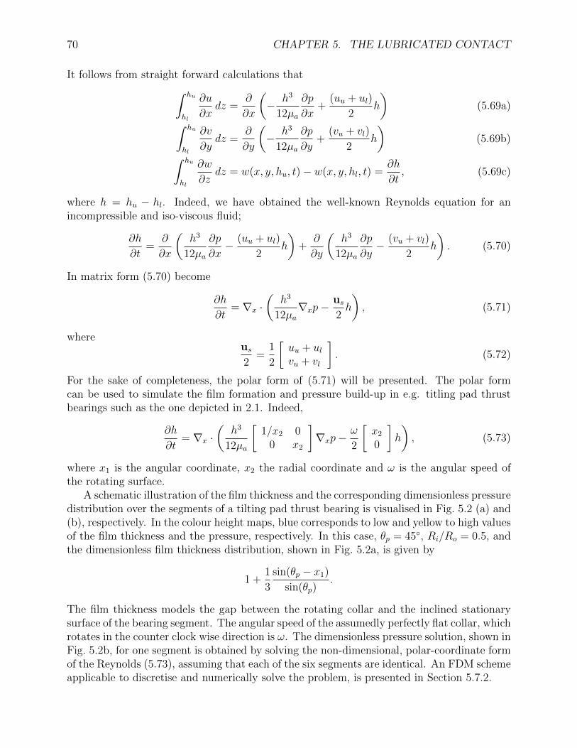
70 CHAPTER 5. THE LUBRICATED CONTACT
It follows from straight forward calculations that∫ hu
hl
∂u
∂xdz =
∂
∂x
(− h3
12µa
∂p
∂x+
(uu + ul)
2h
)(5.69a)∫ hu
hl
∂v
∂ydz =
∂
∂y
(− h3
12µa
∂p
∂y+
(vu + vl)
2h
)(5.69b)∫ hu
hl
∂w
∂zdz = w(x, y, hu, t)− w(x, y, hl, t) =
∂h
∂t, (5.69c)
where h = hu − hl. Indeed, we have obtained the well-known Reynolds equation for anincompressible and iso-viscous fluid;
∂h
∂t=
∂
∂x
(h3
12µa
∂p
∂x− (uu + ul)
2h
)+
∂
∂y
(h3
12µa
∂p
∂y− (vu + vl)
2h
). (5.70)
In matrix form (5.70) become
∂h
∂t= ∇x ·
(h3
12µa∇xp−
us2h
), (5.71)
whereus2
=1
2
[uu + ulvu + vl
]. (5.72)
For the sake of completeness, the polar form of (5.71) will be presented. The polar formcan be used to simulate the film formation and pressure build-up in e.g. titling pad thrustbearings such as the one depicted in 2.1. Indeed,
∂h
∂t= ∇x ·
(h3
12µa
[1/x2 0
0 x2
]∇xp−
ω
2
[x2
0
]h
), (5.73)
where x1 is the angular coordinate, x2 the radial coordinate and ω is the angular speed ofthe rotating surface.
A schematic illustration of the film thickness and the corresponding dimensionless pressuredistribution over the segments of a tilting pad thrust bearing is visualised in Fig. 5.2 (a) and(b), respectively. In the colour height maps, blue corresponds to low and yellow to high valuesof the film thickness and the pressure, respectively. In this case, θp = 45, Ri/Ro = 0.5, andthe dimensionless film thickness distribution, shown in Fig. 5.2a, is given by
1 +1
3
sin(θp − x1)
sin(θp).
The film thickness models the gap between the rotating collar and the inclined stationarysurface of the bearing segment. The angular speed of the assumedly perfectly flat collar, whichrotates in the counter clock wise direction is ω. The dimensionless pressure solution, shown inFig. 5.2b, for one segment is obtained by solving the non-dimensional, polar-coordinate formof the Reynolds (5.73), assuming that each of the six segments are identical. An FDM schemeapplicable to discretise and numerically solve the problem, is presented in Section 5.7.2.
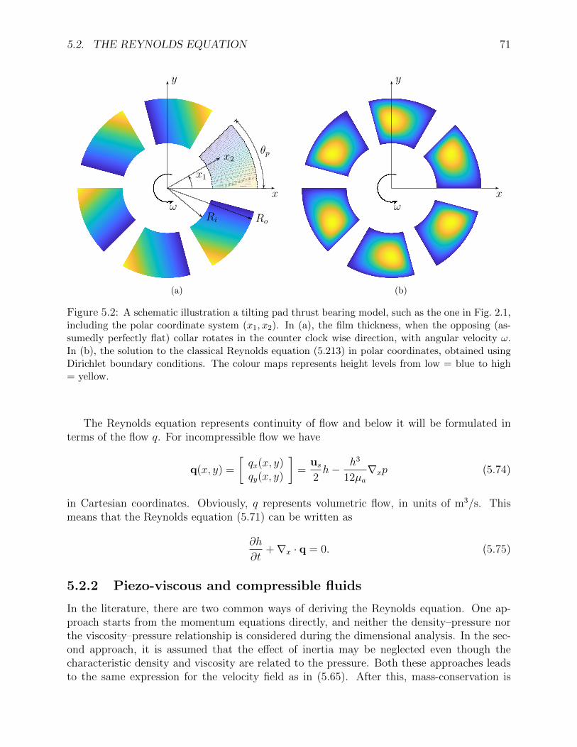
5.2. THE REYNOLDS EQUATION 71
x1
x2
RoRi
ω
θp
x
y
(a)
ωx
y
(b)
Figure 5.2: A schematic illustration a tilting pad thrust bearing model, such as the one in Fig. 2.1,including the polar coordinate system (x1, x2). In (a), the film thickness, when the opposing (as-sumedly perfectly flat) collar rotates in the counter clock wise direction, with angular velocity ω.In (b), the solution to the classical Reynolds equation (5.213) in polar coordinates, obtained usingDirichlet boundary conditions. The colour maps represents height levels from low = blue to high= yellow.
The Reynolds equation represents continuity of flow and below it will be formulated interms of the flow q. For incompressible flow we have
q(x, y) =
[qx(x, y)qy(x, y)
]=
us2h− h3
12µa∇xp (5.74)
in Cartesian coordinates. Obviously, q represents volumetric flow, in units of m3/s. Thismeans that the Reynolds equation (5.71) can be written as
∂h
∂t+∇x · q = 0. (5.75)
5.2.2 Piezo-viscous and compressible fluids
In the literature, there are two common ways of deriving the Reynolds equation. One ap-proach starts from the momentum equations directly, and neither the density–pressure northe viscosity–pressure relationship is considered during the dimensional analysis. In the sec-ond approach, it is assumed that the effect of inertia may be neglected even though thecharacteristic density and viscosity are related to the pressure. Both these approaches leadsto the same expression for the velocity field as in (5.65). After this, mass-conservation is

72 CHAPTER 5. THE LUBRICATED CONTACT
considered. More precisely, the continuity equation (5.14a) is integrated with respect to z(across the fluid film, from hl to hu) viz.
0 =
∫ hu
hl
(∂ρ
∂t+∂(ρu)
∂x+∂(ρv)
∂y+∂(ρw)
∂z
)dz, (5.76)
where it is assumed that density is independent of z, i.e. ρ = ρ(x, y). This leads to a Reynoldsequation including a density, necessarily not being constant. Indeed, in this way, a Reynolds’type of equation (5.1) can be derived, implying that both the density and the viscosity donot need to be constants and thus may depend on the pressure. In matrix form, it can bewritten as
∂ (ρh)
∂t= ∇x ·
(ρh3
12µ∇xp−
us2ρh
). (5.77)
The Cartesian expression for the mass flow q, with units kg/s, is in this case
q(x, y) =
[qx(x, y)qy(x, y)
]=
us2ρ(p)h− ρ(p)h3
12µa∇xp. (5.78)
This means that the Reynolds equation (5.77) can be written as
∂ (ρ(p)h)
∂t+∇x · q = 0. (5.79)
Both the aforementioned approaches builds on the fact that the characteristic density isnot related to the pressure. Strictly speaking, this is inconsistent and, although it is of minorinfluence in many situations, it will have a major impact in some other cases, as will be dis-cussed in Section 5.6. In addition, one finds various derivations where the viscosity-pressurerelation is also disregarded during the asymptotic analysis of the momentum equations, whichalso leads to a similar inconsistency.
Note that in his original derivation [44], Reynolds considers the viscosity to be “nearlyconstant”. He also assumes that “the forces arising from weight and inertia are altogethersmall compared with the stresses arising from viscosity”. Under these assumptions, whichare correct for an incompressible and iso-viscous fluid, all the terms involving the densityin the momentum equations may be omitted as a consequence of that the gap height issmall compared to lateral size of the lubricated conjunction, i.e., h0 l0 and h0 b0 asin Fig. 5.1, and he arrives at (5.70). As we have seen previously, however, not all types ofcompressibility models lead to a reduced system that can be integrated to obtain a dimension-reduced Reynolds type of equation such as (5.77). We have seen, indeed, that this is onlythe case of sub-linear density-pressure relations. In the case of other models, such as the onemodelling an ideal gas, the asymptotic analysis leads to a system that cannot be integratedand additional assumptions needs to be incorporated to obtain a Reynolds type of equation.In Section 5.6, we will present a detailed analysis that shows precisely why this is and alsowhich additional assumptions that are required to obtain a Reynolds equation in the form of(5.77). It will also be shown that, as long as these additional assumptions holds, for instanceif the velocity is not too high, it provides a good approximation to the original compressibleNavier-Stokes system of equations (5.14).

5.2. THE REYNOLDS EQUATION 73
Although we have not discussed it in detail here, a similar caution must be had withpiezo-viscous fluids, i.e., those in which viscosity varies with pressure. Explicit exampleswith pressure-dependent viscosity can be found in [13, 67–69], where they employ Barus’viscosity-pressure relationship (5.108) to elucidate upon the inconsistency in applying theReynolds equation to elastohydrodynamically lubricated applications. In [14], it was shown,for the first time, that it is rationally possible to obtain a dimension-reduced model for allkinds of incompressible fluids, with constitutive viscosity–pressure relations. More precisely,they adopt the general formulation
µ(p) = µar(αp), (5.80)
where r is a strictly positive smooth increasing function such that r(0) = 1, α ≥ 0 is aviscosity-pressure coefficient and µa is the viscosity corresponding to p = 0. The class (5.80)includes most commonly used viscosity-pressure relations, e.g. the Barus viscosity-pressurerelation (5.108), Roelands viscosity-pressure relation [70] and the case with constant viscosity(α = 0).
We conclude this section with a final remark. In the case with stationary surfaces, thenon-linear equation (5.1) was studied in [71], for arbitrary density-pressure relationships (infact piezo-viscosity was also considered). In particular, they obtained a transformation thatmaps (5.1) into a linear equation which can readily be solved numerically. This means thatthe solution to (5.1) can be easily obtained by inverse transformation.
5.2.3 Load carrying capacity and friction force
In the context of Tribology, there are two quantities of relevance that can be obtained fromthe result of Reynolds equation. These are the load the load carrying capacity (LCC) andthe friction force/torque. In this section, expressions for these will be given. The LCC fora bearing is straight-forwardly computed from the fluid pressure distribution (given thatconsideration to hydrodynamic cavitation, to be considered in Section 5.8, has been taken).Given that the pressurised domain is Ω, the load carrying capacity equals normal force Fpsupported by the fluid film and reads
Fp =
∫Ω
p(x) dx. (5.81)
The friction force Ff is a vector valued function computed from the shear stresses τx and τy,which induce resistance against the motion the surface dragging the fluid into the lubricatedconjunction has. For a Newtonian fluid, the constitutive relationship between shear stressand shear strain rate reads [
τxτy
]= µ
∂u
∂z= µ
∂u
∂z∂v
∂z
(5.82)
and the friction force can be obtained by solving the corresponding Reynolds equation for thefluid pressure, then equating the pressure gradient so that the shear stresses can be obtainedthrough (5.82). Indeed
Ff = −∫
Ω
µ∂u
∂z
∣∣∣∣z=hl∨z=hu
dx. (5.83)

74 CHAPTER 5. THE LUBRICATED CONTACT
Let us now make a change of variables z′ = z − hl, and introduce the notation h = hu − hl,which if we considers iso-viscous flow leads to a simplified form of (5.83). That is,
Ff = −∫
Ω
µa∂u
∂z′
∣∣∣∣z′=0∨z′=h
dx =
= −∫
Ω
µa∂
∂z′
z′(z′ − h)
2µa
∂p
∂x+ (uu − ul)
z′
h+ ul
z′(z′ − h)
2µa
∂p
∂y+ (vu − vl)
z′
h+ vl
∣∣∣∣∣∣∣∣∣∣z′=0∨z′=h
dx.
= −∫
Ω
(z′ − h
2
)∂p
∂x+µa(uu − ul)
h(z′ − h
2
)∂p
∂y+µa(vu − vl)
h
∣∣∣∣∣∣∣∣∣∣z′=0∨z′=h
dx. (5.84)
Evaluated at the lower surface (z = 0) we have
Ff (z = 0) = −∫
Ω
−h
2
∂p
∂x+µa(uu − ul)
h
−h2
∂p
∂y+µa(vu − vl)
h
dx (5.85)
and evaluated at the upper surface (z = h) we have
Ff (z = h) = −∫
Ω
h
2
∂p
∂x+µa(uu − ul)
h
h
2
∂p
∂y+µa(vu − vl)
h
dx. (5.86)
For a rotating device the frictional resistance is related to torque Tf . The expression (5.87)is the friction torque in polar coordinates, 0 ≤ ϕ ≤ 2π and Ri ≤ r ≤ Ro, evaluated at thecounter clockwise rotating upper surface, assuming that it has angular velocity ω and thatthe lower surface is stationary,
Tf = −∫
Ω
r
(h(ϕ, r)
2r
∂p
∂ϕ+
µωr
h(ϕ, r)
)rdϕ dr, (5.87)
where r2 = x21 + x2
2 and ϕ = tan−1(x2/x1) is the translation between the angular- and theradial directions in polar coordinates and the principal directions x1 and x2 in Cartesiancoordinates. We note that the velocity vector ul of the lower surface would be 0 and thatthe uu of the upper surface in Cartesian coordinates would be
uu =
[uu
vu
]= rω
[− sinϕ
cosϕ
]. (5.88)

5.3. SOLUTIONS TO SOME VARIANTS OF THE 1D REYNOLDS EQUATION 75
5.2.4 Force balance and rigid body separation
In the real application, it is often the load that is applied fapp on a given system, e.g. abearing. It is therefore convenient to treat is as the input instead of a given rigid bodyseparation, h00. In general, the thin gap between two surfaces can be expressed as
h(x, y) = h00 + h1(x, y), (5.89)
where h1 contains the shape of the surfaces and h00 controls the average separation by shiftingthe shape up and down. In a case where the load is applied, the two surfaces will get closeror further away depending on the magnitude of the load applied. This calls, therefore, for anadditional condition, i.e. a force equilibrium equation balancing the applied load fapp and theload carried by the fluid film fp. Quite generally, this is exactly Newton’s first law, appliedin z-direction, viz.
fapp(t)−∫p(x, y) dx dy = m
d2h0
dt2, (5.90)
where it is understood that fapp is posed as load (N/m) in the 3D case and as load per lengthunit (N/m) in 2D cases. Moreover, m is the systems mass of inertia. The right hand side of(5.90) describes the acceleration of the surfaces towards or away each other. In the stationarycase, this equation reads
fapp −∫p(x, y) dx dy = 0. (5.91)
In this case, there is no explicit appearance of h00. This parameter will, however, influencethe pressure distribution. Therefore (5.91) will still determine the static separation betweenthe surfaces through h00.
5.3 Solutions to some variants of the 1D Reynolds equa-
tion
In few cases, it is possible to obtain an explicit expression for the fluid pressure solution tothe Reynolds equation. Here we will consider such cases, which admits an analytical solutionfor linear- and a parabolic slider bearings. Schematics of the linear- and the parabolic sliderbearings are depicted in Fig. 5.3.

76 CHAPTER 5. THE LUBRICATED CONTACT
h(x) = hL −hL − hT
lx
ul
(a) Linear slider
h(x) = h0 +x2
2R
ul
(b) Parabolic slider
Figure 5.3: Infinitely wide slider bearings.
We will, therefore assume that the bearing is infinitely long in the y-direction (perpendicularto the paper in Fig. 5.3). This means that there are no edges over which side leakage mayoccur and, because of this, there is no dependency on y and the problem can be consideredas two-dimensional. More precisely, a model bearing with a stationary upper surface is andthe lower is moving with the speed ul, i.e., u(x, h) = 0 and u(x, 0) = ul.
The mathematical description of the geometry of the linear slider bearing is given by thefilm thickness function h, which in this case reads
h(x) = hL −hL − hT
lx, (5.92)
where hL and hT are the leading and trailing edge gap heights and l the length of the bearing.We will introduce the inclination parameter k, which is used to describe hL as a scaling ofhT , i.e., hL = (1 + k)hT . In terms of hT and k (5.92) becomes
h(x) = hT
(1 + k − k
lx
), (5.93)
For the parabolic slider the film thickness is given by
h(x) = h0 +x2
2R, (5.94)
The three different cases we will consider are for i) iso-viscous and incompressible fluids,ii) piezo-viscous and incompressible fluids and iii) iso-viscous and constant bulk-moduluscompressible fluids. Note that, case i) is the classical Reynolds equation.
Iso-viscous and incompressible fluid
We will now compute the pressure distribution in the bearing, in the case of an iso-viscousand incompressible fluid. To this end, we adopt the one-dimensional stationary form of the
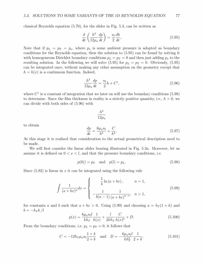
5.3. SOLUTIONS TO SOME VARIANTS OF THE 1D REYNOLDS EQUATION 77
classical Reynolds equation (5.70), for the slider in Fig. 5.3, can be written as
d
dx
(h3
12µa
dp
dx
)=ul2
dh
dx, (5.95)
Note that if pL = pT = pa, where pa is some ambient pressure is adopted as boundaryconditions for the Reynolds equation, then the solution to (5.95) can be found by solving itwith homogeneous Dirichlet boundary conditions pL = pT = 0 and then just adding pa to theresulting solution. In the following we will solve (5.95) for pL = pT = 0. Obviously, (5.95)can be integrated once, without making any other assumption on the geometry except thath = h(x) is a continuous function. Indeed,
h3
12µa
dp
dx=ul2h+ C∗, (5.96)
where C∗ is a constant of integration that we later on will use the boundary conditions (5.98)to determine. Since the film thickness in reality is a strictly positive quantity, i.e., h > 0, wecan divide with both sides of (5.96) with
h3
12µa
to obtaindp
dx=
6µaulh2
+C
h3. (5.97)
At this stage it is realised that consideration to the actual geometrical description need tobe made.
We will first consider the linear slider bearing illustrated in Fig. 5.3a. Moreover, let usassume it is defined on 0 < x < l, and that the pressure boundary conditions, i.e.
p(0)) = pT and p(l) = pL. (5.98)
Since (5.92) is linear in x it can be integrated using the following rule
∫1
(a+ bx)ndx =
1
bln (a+ bx) , n = 1,
− 1
b(n− 1)
1
(a+ bx)n−1 , n > 1,
(5.99)
for constants a and b such that a + bx > 0. Using (5.99) and choosing a = hT (1 + k) andb = −hTk /l
p(x) =6µaull
khT
1
h(x)+
l
2khT
C
h(x)2+D. (5.100)
From the boundary conditions, i.e. pL = pT = 0, it follows that
C = −12hTµaul1 + k
2 + kand D = −6µaull
kh2T
1
2 + k. (5.101)
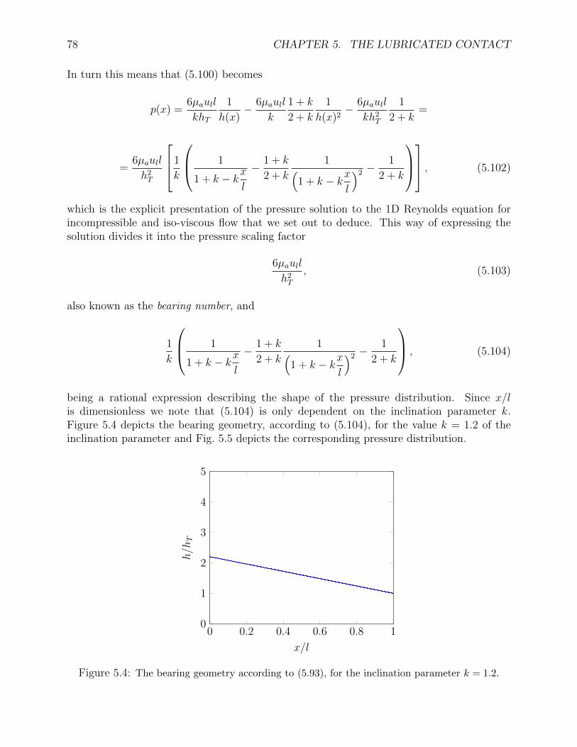
78 CHAPTER 5. THE LUBRICATED CONTACT
In turn this means that (5.100) becomes
p(x) =6µaull
khT
1
h(x)− 6µaull
k
1 + k
2 + k
1
h(x)2− 6µaull
kh2T
1
2 + k=
=6µaull
h2T
1
k
1
1 + k − kxl
− 1 + k
2 + k
1(1 + k − kx
l
)2 −1
2 + k
, (5.102)
which is the explicit presentation of the pressure solution to the 1D Reynolds equation forincompressible and iso-viscous flow that we set out to deduce. This way of expressing thesolution divides it into the pressure scaling factor
6µaull
h2T
, (5.103)
also known as the bearing number, and
1
k
1
1 + k − kxl
− 1 + k
2 + k
1(1 + k − kx
l
)2 −1
2 + k
, (5.104)
being a rational expression describing the shape of the pressure distribution. Since x/lis dimensionless we note that (5.104) is only dependent on the inclination parameter k.Figure 5.4 depicts the bearing geometry, according to (5.104), for the value k = 1.2 of theinclination parameter and Fig. 5.5 depicts the corresponding pressure distribution.
0 0.2 0.4 0.6 0.8 10
1
2
3
4
5
x/l
h/h
T
Figure 5.4: The bearing geometry according to (5.93), for the inclination parameter k = 1.2.
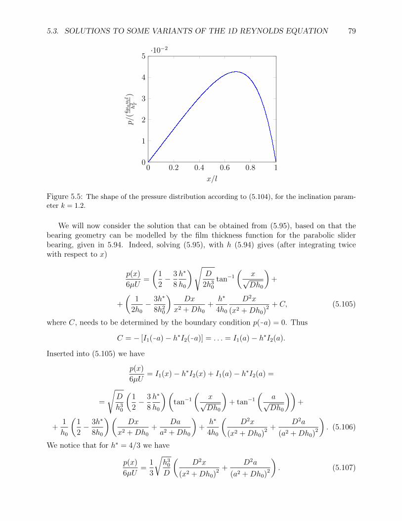
5.3. SOLUTIONS TO SOME VARIANTS OF THE 1D REYNOLDS EQUATION 79
0 0.2 0.4 0.6 0.8 10
1
2
3
4
5·10−2
x/l
p/(6µaull
h2 T
)
Figure 5.5: The shape of the pressure distribution according to (5.104), for the inclination param-eter k = 1.2.
We will now consider the solution that can be obtained from (5.95), based on that thebearing geometry can be modelled by the film thickness function for the parabolic sliderbearing, given in 5.94. Indeed, solving (5.95), with h (5.94) gives (after integrating twicewith respect to x)
p(x)
6µU=
(1
2− 3
8
h∗
h0
)√D
2h30
tan−1
(x√Dh0
)+
+
(1
2h0
− 3h∗
8h20
)Dx
x2 +Dh0
+h∗
4h0
D2x
(x2 +Dh0)2 + C, (5.105)
where C, needs to be determined by the boundary condition p(9a) = 0. Thus
C = − [I1(9a)− h∗I2(9a)] = . . . = I1(a)− h∗I2(a).
Inserted into (5.105) we have
p(x)
6µU= I1(x)− h∗I2(x) + I1(a)− h∗I2(a) =
=
√D
h30
(1
2− 3
8
h∗
h0
)(tan−1
(x√Dh0
)+ tan−1
(a√Dh0
))+
+1
h0
(1
2− 3h∗
8h0
)(Dx
x2 +Dh0
+Da
a2 +Dh0
)+
h∗
4h0
(D2x
(x2 +Dh0)2 +D2a
(a2 +Dh0)2
). (5.106)
We notice that for h∗ = 4/3 we have
p(x)
6µU=
1
3
√h3
0
D
(D2x
(x2 +Dh0)2 +D2a
(a2 +Dh0)2
). (5.107)
80 CHAPTER 5. THE LUBRICATED CONTACT
It is clear that p(0)→ 0, as a→∞ and, moreover we see that P (a)→ 0 as a→∞ and wehave obtained a perfectly anti-symmetrical pressure distribution.
Piezo-viscous and incompressible fluid
If the widely used constitutive relationship between the pressure and the viscosity, known asBarus’ Law3, see e.g. the authoritative articles [76–79] and books [80–83] i.e.
µ(p) = µaeα(p−pa), (5.108)
is adopted to model the piezo-viscosity of the fluid, then the transformation
q(x) = µ(p(x))/µa = eα(p−pa), (5.109)
can be used to linearise the Reynolds type of equation (5.1). Indeed, for the infinitely widelinear slider bearing lubricated with an incompressible fluid obeying Barus’ viscosity-pressurerelationship (5.108) we have
d
dx
(h3
12α
dq
dx
)= −ul
2
dh
dx, 0 ≤ x ≤ l. (5.110)
Note the negative sign in front of the term in the right-hand-side.If we assume that the pressure at the boundaries of the bearing is zero, then the boundary
conditions for (5.110) becomesq(0) = q(l) = 1/µa, (5.111)
and we can as easily as before obtain the closed form expression for q and subsequently alsoobtain the corresponding pressure distribution. Indeed,
q(x) =6αull
h2T
1
k
− 1
1 + k − kxl
+1 + k
2 + k
1(1 + k − kx
l
)2 +1
2 + k
+
1
µa. (5.112)
By inverting (5.109) we finally get the pressure distribution, i.e.
p(x) = pa −1
αln (µaq(x)) (5.113)
It is of crucial importance to notice that the viscosity µ is always positive and, since q = 1/µit must also be positive. It does, however, turn out that the expression for q in (5.112) can
3In the original work [65], Barus studied the rheology of marine glue, and he reported absolute viscosityvalues obtained by applying pressures as high as 200 MPa in order to force charges of marine glue throughsteel tubes. Based on the study, Barus found, that his data was best described by the linear relationshipµ(p) = µ0 (1 + bp). However, he also remarked that the viscosities he measured might be lower than in reality,due to slippage. Therefore, he presented an exponential relation log (µ(p)) = a′ + b′p, i.e. µ(p) = ea
′+b′p,even though it did not agree with his data. Later, successors like Hyde [72], Bridgman [73] and Hersey [74],found, that the data they obtained from high-pressure measurements were in good agreement with (5.108), forvarious liquids over a quite large range of pressures. It is important that scientific findings are appropriatelyreferred to [75] and we are thankful that one of the reviewers pointed out that Barus’ measurements, in hisoriginal work [65], indicated a linear viscosity-pressure relation.
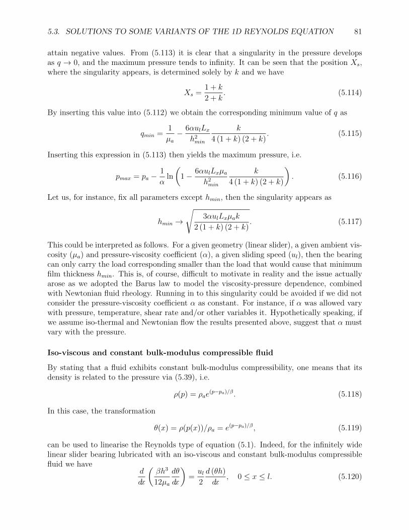
5.3. SOLUTIONS TO SOME VARIANTS OF THE 1D REYNOLDS EQUATION 81
attain negative values. From (5.113) it is clear that a singularity in the pressure developsas q → 0, and the maximum pressure tends to infinity. It can be seen that the position Xs,where the singularity appears, is determined solely by k and we have
Xs =1 + k
2 + k. (5.114)
By inserting this value into (5.112) we obtain the corresponding minimum value of q as
qmin =1
µa− 6αulLx
h2min
k
4 (1 + k) (2 + k). (5.115)
Inserting this expression in (5.113) then yields the maximum pressure, i.e.
pmax = pa −1
αln
(1− 6αulLxµa
h2min
k
4 (1 + k) (2 + k)
). (5.116)
Let us, for instance, fix all parameters except hmin, then the singularity appears as
hmin →√
3αulLxµak
2 (1 + k) (2 + k). (5.117)
This could be interpreted as follows. For a given geometry (linear slider), a given ambient vis-cosity (µa) and pressure-viscosity coefficient (α), a given sliding speed (ul), then the bearingcan only carry the load corresponding smaller than the load that would cause that minimumfilm thickness hmin. This is, of course, difficult to motivate in reality and the issue actuallyarose as we adopted the Barus law to model the viscosity-pressure dependence, combinedwith Newtonian fluid rheology. Running in to this singularity could be avoided if we did notconsider the pressure-viscosity coefficient α as constant. For instance, if α was allowed varywith pressure, temperature, shear rate and/or other variables it. Hypothetically speaking, ifwe assume iso-thermal and Newtonian flow the results presented above, suggest that α mustvary with the pressure.
Iso-viscous and constant bulk-modulus compressible fluid
By stating that a fluid exhibits constant bulk-modulus compressibility, one means that itsdensity is related to the pressure via (5.39), i.e.
ρ(p) = ρae(p−pa)/β. (5.118)
In this case, the transformation
θ(x) = ρ(p(x))/ρa = e(p−pa)/β, (5.119)
can be used to linearise the Reynolds type of equation (5.1). Indeed, for the infinitely widelinear slider bearing lubricated with an iso-viscous and constant bulk-modulus compressiblefluid we have
d
dx
(βh3
12µa
dθ
dx
)=ul2
d (θh)
dx, 0 ≤ x ≤ l. (5.120)

82 CHAPTER 5. THE LUBRICATED CONTACT
Integrating once with respect to x gives
dθ
dx− 6ulµaθ
βh2=
12µaβh3
C, (5.121)
where C is a constant of integration. By the product rule we have
d
dx
(θe
∫ x0
6ulµa
βh2(x′)dx′)
=12µaβh3
Ce∫ x0
6ulµa
βh2(x′)dx′
(5.122)
and integrating one more time with respect to x gives
θ(x) =12µaC
βe−
∫ x0
6ulµa
βh2(x′)dx′∫ x
0
e
6ulµaβ
∫ x′0
1
h2(x′′)dx′′
h3(x′)
dx′ +De−
∫ x0
6ulµa
βh2(x′)dx′. (5.123)
Application of the boundary conditions θ(0) = θ(l) = 1 finally yields an explicit solution to(5.121), i.e.
θ(x) =
(e∫ 10
6ulµa
βh2(x′)dx′ − 1
)∫ x0e
6ulµaβ
∫ x′0
1
h2(x′′)dx′′
h3(x′)
dx′
∫ 1
0e
6ulµaβ
∫ x′0
1
h2(x′′)dx′′
h3(x′)
dx′
+ 1
e−
∫ x0
6ulµa
βh2(x′)dx′. (5.124)
5.3.1 The velocity field
Having an explicit expression for the fluid pressure means that we can obtain an explicit ex-pression for the velocity field from the two-dimensional representations of (5.65) and (5.59a).Adapted to the 2D slider bearing problem at hand, these can be formulated as
u(x, z) =z(z − h(x))
2µa
dp
dx− ul
z
h(x)+ ul, (5.125)
and∂u
∂x+∂w
∂z= 0, (5.126)
where 0 ≤ z ≤ h(x) defines the gap height at position x. To proceed we need explicitexpressions for dp /dx and we will at the same time derive one for d2p /dx2 . To do this westart from (5.102), i.e.,
dp
dx=
d
dx
(6µaull
khT
1
h(x)− 6µaull
k
1 + k
2 + k
1
h(x)2− 6µaull
kh2T
1
2 + k
)=
= 6µaul
(1
h2(x)− 2hT
1 + k
2 + k
1
h(x)3
)=

5.3. SOLUTIONS TO SOME VARIANTS OF THE 1D REYNOLDS EQUATION 83
=6µaulh2T
1(1 + k − kx
l
)2 − 21 + k
2 + k
1(1 + k − kx
l
)3
(5.127)
d2p
dx2=
6µaull
h2T
2
k
1(1 + k − kx
l
)3 −6
k
1 + k
2 + k
1(1 + k − kx
l
)4
(5.128)
By inserting (5.127) into (5.125) we get
u(x, z) = ul
(3z(z − h(x))
h2(x)
(1− 2
1 + k
2 + k
hTh(x)
)− z
h(x)+ 1
), (5.129)
after some algebraic operations. The velocity fields for the 2D slider with inclination param-eters k = 1.2 and 3 are depicted in Fig. 5.6.
0 0.2 0.4 0.6 0.8 10
1
2
3
4
x/l
h/hT
0
1
2
3
4
5
u/ul
(a) k = 1.2.
0 0.2 0.4 0.6 0.8 10
1
2
3
4
x/l
h/hT
0
1
2
3
4
5
u/ul
(b) k = 3.
Figure 5.6: The velocity field u/ul according to (5.129), for two different values of the inclinationparameter k.
A few things to be noted here are i) It is quite clear that the velocity at the lower surface(moving in the x-direction) is ul and that the upper surface is stationary (u(x, h) = 0), ii)There is a vortex at the leading edge side, where fluid is flowing out from the conjunction,i.e. u < 0 there, and iii) the velocity at the trailing edge side exceed ul. All of this is directlycoupled to continuity of flow and for this problem the expression (5.74) for volume flow reads
q(x) = ulh
2− h3
12µa
dp
dx. (5.130)
To obtain w from (5.126), we will first find the partial derivative ∂u/∂x and to do this werestart from (5.129). This means that
∂u
∂x=
∂
∂x
(ul
(3z(z − h(x))
h2(x)
(1− 2
1 + k
2 + k
hTh(x)
)− z
h(x)+ 1
))=

84 CHAPTER 5. THE LUBRICATED CONTACT
= ul∂
∂x
(3z2
h2(x)− 1 + k
2 + k
6z2hTh3(x)
+3z
h(x)+
1 + k
2 + k
6zhTh2(x)
− z
h(x)+ 1
)=
= ulkhTl
(2z
h2(x)− 2
(3z2 − 6zhT
1 + k
2 + k
)1
h3(x)− 18z2 1 + k
2 + k
hTh4(x)
)=
= ulkhTl
1
h2(x)
(2z − 2
(3z2 − 6zhT
1 + k
2 + k
)1
h(x)− 18
1 + k
2 + k
z2hTh2(x)
).
It is now possible to obtain an explicit expression for w, by integrating (5.126) once withrespect to z. That is,
w(x, z) = −ulkhTl
z2
h2(x)
(2− 2
(z − 3hT
1 + k
2 + k
)1
h(x)− 6
1 + k
2 + k
zhTh2(x)
)+ Cw(x).
For impermeable surfaces the boundary conditions w(x, 0) = 0 and w(x, h(x)) = 0 must hold.For the former to hold Cw ≡ 0. Thus
w(x, z) = −ulkhTl
z2
h2(x)
(2− 2
(z − 3hT
1 + k
2 + k
)1
h(x)− 6
1 + k
2 + k
zhTh2(x)
), (5.131)
from which we also see that the boundary condition at the upper surface, i.e. w(x, h(x)) = 0,holds. This vertical velocity component is depicted in Fig. 5.7, for the inclination parametersk = 1.2 and 3.
0 0.2 0.4 0.6 0.8 10
1
2
3
4
x/l
h/hT
−3
−2
−1
0w/ (ulhT /l )
(a) k = 1.2.
0 0.2 0.4 0.6 0.8 10
1
2
3
4
x/l
h/hT
−3
−2
−1
0w/ (ulhT /l )
(b) k = 3.
Figure 5.7: The velocity field w/ (ulhT /l ) according to (5.131), for two different values of theinclination parameter k.
Note here that the velocity w in the z-direction, in dimensions, is significantly smaller (hT/l)than than the velocity u in the x-direction.
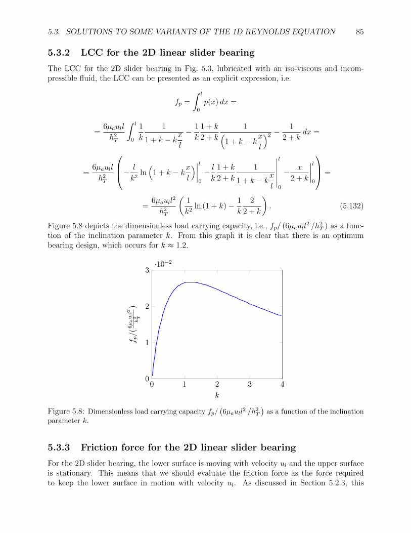
5.3. SOLUTIONS TO SOME VARIANTS OF THE 1D REYNOLDS EQUATION 85
5.3.2 LCC for the 2D linear slider bearing
The LCC for the 2D slider bearing in Fig. 5.3, lubricated with an iso-viscous and incom-pressible fluid, the LCC can be presented as an explicit expression, i.e.
fp =
∫ l
0
p(x) dx =
=6µaull
h2T
∫ l
0
1
k
1
1 + k − kxl
− 1
k
1 + k
2 + k
1(1 + k − kx
l
)2 −1
2 + kdx =
=6µaull
h2T
− l
k2ln(
1 + k − kxl
)∣∣∣∣l0
− lk
1 + k
2 + k
1
1 + k − kxl
∣∣∣∣∣∣l
0
− x
2 + k
∣∣∣∣l0
=
=6µaull
2
h2T
(1
k2ln (1 + k)− 1
k
2
2 + k
). (5.132)
Figure 5.8 depicts the dimensionless load carrying capacity, i.e., fp/ (6µaull2 /h2
T ) as a func-tion of the inclination parameter k. From this graph it is clear that there is an optimumbearing design, which occurs for k ≈ 1.2.
0 1 2 3 40
1
2
3·10−2
k
f p/(
6µaull2
h2 T
)
Figure 5.8: Dimensionless load carrying capacity fp/(6µaull
2/h2T
)as a function of the inclination
parameter k.
5.3.3 Friction force for the 2D linear slider bearing
For the 2D slider bearing, the lower surface is moving with velocity ul and the upper surfaceis stationary. This means that we should evaluate the friction force as the force requiredto keep the lower surface in motion with velocity ul. As discussed in Section 5.2.3, this

86 CHAPTER 5. THE LUBRICATED CONTACT
corresponds to the integral of the shear stresses exerted by fluid on the lower surface (z = 0)and in this particular case (5.85) becomes
ff (0) = −∫ l
0
−h(x)
2
dp
dx− µaulh(x)
dx. (5.133)
Note that the ff is force per length unit, i.e., it has the unit N/m. Inserting the explicitexpression for dp /dx given by (5.127) means that
ff (0) =
=
∫ l
0
hT
(1 + k − kx
l
)2
6µaulh2T
1(1 + k − kx
l
)2 − 21 + k
2 + k
1(1 + k − kx
l
)3
dx+
+µaulhT
∫ l
0
1
1 + k − kxl
dx =
= ff (0)press + ff (0)shear,
where
ff (0)press =3µaulhT
∫ l
0
1(1 + k − kx
l
)dx− 6µaU
hT
1 + k
2 + k
∫ l
0
1(1 + k − kx
l
)2dx (5.134)
and
ff (0)shear =µaulhT
∫ l
0
1
1 + k − kxl
dx. (5.135)
We note here that the first and the third term are of the same type, although the firstoriginates from the pressure driven flow and the third from the shear driven flow. Thepressure driven contribution is often omitted when estimating friction in lubricated contacts,from this expression it is not so clear that this will give a good estimate, although “experience”tells us so.
Proceeding with the derivation of the friction force from (5.134) and (5.135) we get
ff (0)press =µaull
khT
−3 ln(
1 + k − kxl
)∣∣∣l0− 6
1 + k
2 + k
1
1 + k − kxl
∣∣∣∣∣∣l
0
=
=µaull
hT
(3
kln (1 + k)− 6
2 + k
). (5.136)
and
ff (0)shear =µaull
khT
(− ln
(1 + k − kx
l
)∣∣∣l0
)=

5.3. SOLUTIONS TO SOME VARIANTS OF THE 1D REYNOLDS EQUATION 87
=µaull
hT
(1
kln (1 + k)
). (5.137)
Thus,
ff (0) = ff (0)press + ff (0)shear =µaull
hT
(4
kln (1 + k)− 6
2 + k
). (5.138)
In the same manner as we obtained the friction force, we can obtain a closed form expressionfor the resulting force (per unit length) caused by the lubricant shear stresses acting at theupper surface by computing the expression (5.139) below. That is,
ff (h) = −∫ l
0
h(x)
2
dp
dx− µaulh(x)
dx. (5.139)
We again partition the contribution into two parts, one related to the pressure gradient andthe other one related to the shear caused by the moving surface, i.e.,
ff (h) = ff (h)press + ff (h)shear
where
ff (h)press = −3µaulhT
∫ l
0
1(1 + k − kx
l
)dx+6µaulhT
1 + k
2 + k
∫ l
0
1(1 + k − kx
l
)2dx =
=µaull
hT
(3
kln (1 + k) +
6
2 + k
)(5.140)
and
ff (h)shear = +µaulhT
∫ l
0
1
1 + k − kxl
dx.
=µaull
hT
(−1
kln (1 + k)
)(5.141)
Thus
ff (h) =µaull
hT
(2
kln (1 + k) +
6
2 + k
). (5.142)
The inclination is very small and although its x- and z-components would be evaluated as
(ff (h))x =µaull
hT
(2
kln (1 + k) +
6
2 + k
)cos
(khTl
)(5.143)
and
(ff (h))z =µaull
hT
(2
kln (1 + k) +
6
2 + k
)sin
(khTl
), (5.144)
respectively, this is a nearly perfectly horizontal force. Notice that is is in good alignmentwith the thin film approximation. In Fig. 5.9 dimensionless friction force ff/ (µaull /hT )is depicted as a function of the inclination parameter k. In the left side of the figure, theblue line corresponds to the friction force acting on the upper surface, according to (5.142)
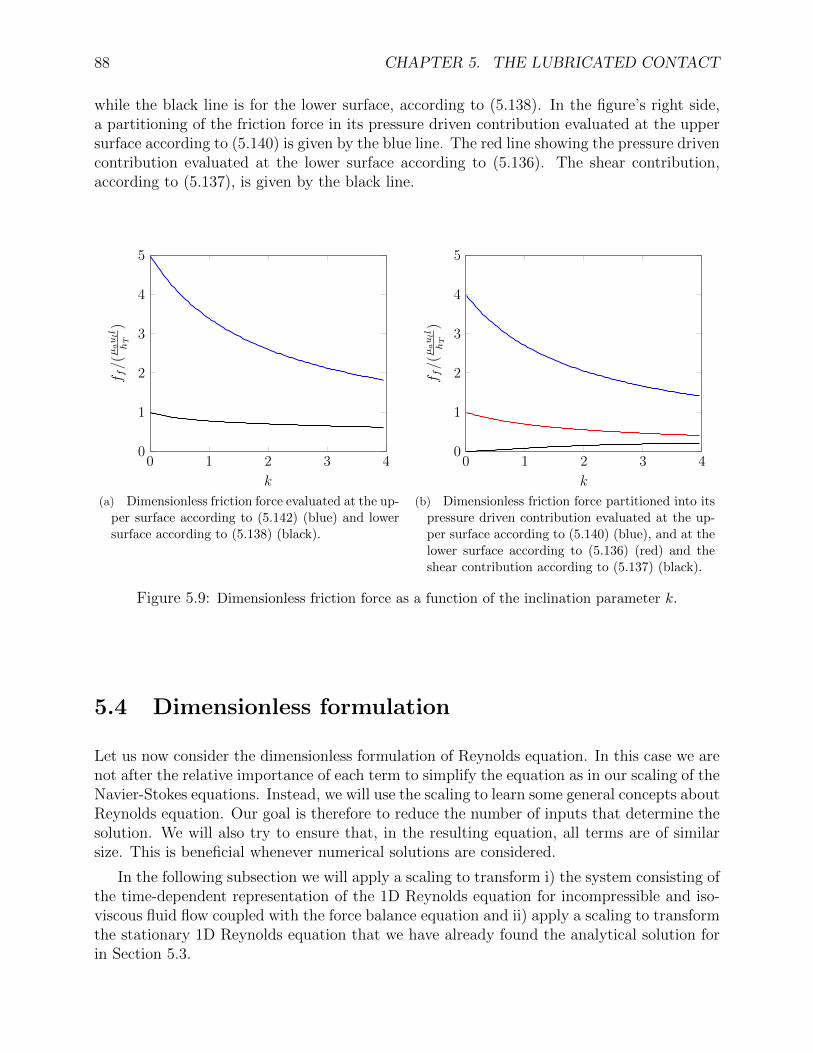
88 CHAPTER 5. THE LUBRICATED CONTACT
while the black line is for the lower surface, according to (5.138). In the figure’s right side,a partitioning of the friction force in its pressure driven contribution evaluated at the uppersurface according to (5.140) is given by the blue line. The red line showing the pressure drivencontribution evaluated at the lower surface according to (5.136). The shear contribution,according to (5.137), is given by the black line.
0 1 2 3 40
1
2
3
4
5
k
f f/(
µaull
hT
)
(a) Dimensionless friction force evaluated at the up-per surface according to (5.142) (blue) and lowersurface according to (5.138) (black).
0 1 2 3 40
1
2
3
4
5
k
f f/(
µaull
hT
)
(b) Dimensionless friction force partitioned into itspressure driven contribution evaluated at the up-per surface according to (5.140) (blue), and at thelower surface according to (5.136) (red) and theshear contribution according to (5.137) (black).
Figure 5.9: Dimensionless friction force as a function of the inclination parameter k.
5.4 Dimensionless formulation
Let us now consider the dimensionless formulation of Reynolds equation. In this case we arenot after the relative importance of each term to simplify the equation as in our scaling of theNavier-Stokes equations. Instead, we will use the scaling to learn some general concepts aboutReynolds equation. Our goal is therefore to reduce the number of inputs that determine thesolution. We will also try to ensure that, in the resulting equation, all terms are of similarsize. This is beneficial whenever numerical solutions are considered.
In the following subsection we will apply a scaling to transform i) the system consisting ofthe time-dependent representation of the 1D Reynolds equation for incompressible and iso-viscous fluid flow coupled with the force balance equation and ii) apply a scaling to transformthe stationary 1D Reynolds equation that we have already found the analytical solution forin Section 5.3.

5.4. DIMENSIONLESS FORMULATION 89
5.4.1 Time dependent Reynolds’ equation and force balance
The system consisting of the time-dependent representation of the 1D Reynolds equationfor incompressible and iso-viscous fluid flow coupled with the force balance equation can beformulated as
∂
∂x
(h3
12µa
∂p
∂x
)=uu + ul
2
∂h
∂x+∂h
∂t, (5.145a)
fapp(t)−∫ l
0
p(x, t) dx = md2h0
dt2. (5.145b)
Next we will transform this system into dimensionless form. This is accomplished by scalingthe independent and dependent variables of the determining system, which in this case arex, t, h and p. We remark that µa, ul, uu, m - being the system’s mass of inertia (unit kg/m),and fapp are input parameters to this problem and thus need not be scaled. The length L ofthe domain Ω is also an input parameter. The film thickness, h, is in this case
h(x, t) = h00(t) + h0(x) + hu(x− uut)− hl(x− ult), (5.146)
where h00 is the rigid body separation and thus a dependent parameter itself (see Section 5.2.4for more details about this).
The most general form of scaling for the problem at hand reads
X = x/xr, T = t/tr, H = h/hr and P = p/pr, (5.147)
where xr, tr, hr and pr are reference parameters, which will be determined in the following.First it is observed that the length of the domain l is given as an input parameter and weshould therefore use this as the reference parameter for x, i.e., xr = l.
By inserting (5.147) into (5.145) we have
h3rprl2
∂
∂X
(H3
12µa
∂P
∂X
)=uu + ul
2
hrl
∂H
∂X+hrtr
∂H
∂T, (5.148a)
fapp(T )− lpr∫ 1
0
P (X,T ) dX = mhrt2r
d2H0
dT 2, (5.148b)
or
∂
∂X
(H3 ∂P
∂X
)=
6 (uu + ul)µal
prh2r
(∂H
∂X+
2l
uu + ul
1
tr
∂H
∂T
), (5.149a)
fapp(T )
lpr−∫ 1
0
P (X,T ) dX =mhrlprt2r
d2H0
dT 2. (5.149b)
Although the reference parameters can be chosen arbitrarily, the preferred choice should bemade to i) minimise the number of input parameters in the resulting dimensionless deter-mining system and ii) to scale the terms so that they will be of similar order of magnitude.The latter is particularly relevant whenever numerical computations are involved. Thus,

90 CHAPTER 5. THE LUBRICATED CONTACT
the procedure is to first identify the dimensionless groups and then find the set of refer-ence parameters that minimise the number of these groups. From (5.149), the followingdimensionless groups are identified
6 (uu + ul)µal
prh2r
, (5.150a)
2l
uu + ul
1
tr, (5.150b)
fapp(T )
lpr, (5.150c)
mhrlprt2r
. (5.150d)
There are four groups and we have four reference parameters. Thus it appears like it ispossible to choose the reference parameters so that the system explicit dependence on inputparameters is totally removed. This is not possible, however, because we have already chosenxr = l in order to remove the inputs from the specification of the domain. Let us now choosethe other reference parameters. Since it is desirable for all terms in each equation to be ofthe same order of magnitude, it is best to choose tr so that,
tr =2l
uu + ul. (5.151)
Expressed in other words, the characteristic time is the time it takes for a feature movingwith the mean speed of the surfaces to travel the length l. This particular choice equalisethe orders of the spatial- and the time derivatives and the system (5.149) becomes
∂
∂X
(H3 ∂P
∂X
)=
6 (uu + ul)µal
prh2r
(∂H
∂X+∂H
∂T
), (5.152a)
fapp(T )
lpr−∫ 1
0
P (X,T ) dX =mhr (uu + ul)
2
4l3pr
d2H0
dT 2. (5.152b)
At this stage we note that there are three groups but only two parameters left and we realisethat it will not be possible to remove the influence of all input parameters in the dimensionlesssystem in the end. No matter if we choose pr as a function of hr or vice versa, as long aswe scale so that all terms in (5.152a) and the left-hand side in (5.152b) will be of the sameorder of magnitude. We thus choose the following set of reference parameters,
xr = l, tr =2l
ul, pr =
fapp(T )
l, hr =
√6 (uu + ul)µal2
fapp(T ), (5.153)
which will reduce (5.148b) to
∂
∂X
(H3 ∂P
∂X
)=∂H
∂X+∂H
∂T, (5.154a)
1−∫ 1
0
P (X,T ) dX = Md2H0
dT 2, (5.154b)
5.4. DIMENSIONLESS FORMULATION 91
where M is a representation of dimensionless mass, defined by
M = m
/(4f
3/2app (T )l
(uu + ul)5/2 (6µa)1/2
). (5.155)
We note that if M 1, i.e., if the mass (per meter) is small enough or the mass referenceparameter in the denominator of (5.155) is large enough, then (5.154) reduces to an inputparameter free system of equations, which after having been solved once, through scaling,gives all possible solutions having the same dimensionless gap H. Note that this is also thecase for systems operating in stationary conditions for which dH0/dT = 0.
5.4.2 Stationary 1D Reynolds’ equation
Let us now have a look at the case we studied in Section 5.3. In this case the system operatesat stationary conditions which means that ∂H/∂T = 0 and ∂2H00/∂t
2 = 0. Therefore,the system (5.154) becomes parameter free. The only parameters relevant for the problemcan thus only come from the definition of H. We will indeed see that only the inclinationparameter k appears in the dimensionless solution. Note that the reference parameter pr isconsistent with using the scaling factor (5.103) as a reference pressure to transform the fluidpressure (5.102) into dimensionless form. More precisely, from (5.153) we obtain
pr =6 (uu + ul)µal
h2r
. (5.156)
However, when we are considering the stationary linear slider problem without applying forcebalance (as in Section 5.3), then hr should be chosen in relation to the input parameter hT ,which is known and will ensure that hr is of order 1. With this choice of reference parameters(5.156) yields
pr =6ulµal
h2T
. (5.157)
Applying this this as a scaling for the pressure,it is clear that the only input parameter thatinfluence the dimensionless pressure distribution P = P (X) is the inclination parameter kand we have i.e.,
P (X) =1
k
(1
1 + k − kX −1 + k
2 + k
1
(1 + k − kX)2 −1
2 + k
). (5.158)
Moreover, the dimensionless expression for the film thickness, described in (5.93), becomes
H(X) = 1 + k − kX. (5.159)
In fact, if the scaling
X = x/l, H = h/hT and P = p
/(6µaull
h2T
), (5.160)
92 CHAPTER 5. THE LUBRICATED CONTACT
is used to transform (5.95) one obtain
d
dX
(H3dP
dX
)=dH
dX, 0 ≤ X ≤ 1, (5.161)
with boundary conditionsP (0) = 0 and P (1) = 0.
Observe that (5.161) has no explicit dependence on the input parameters (l,µa,hT and k).We will now continue to derive dimensionless expression for the velocity u in the x-directionand w in the y-direction. That is, by introducing the scaling U = u/ul as well as definingZ = z/hT we have
U(X,Z) =3Z(Z −H(X))
H2(X)
(1− 2
1 + k
2 + k
1
H(X)
)− Z
H(X)+ 1. (5.162)
In alignment with the scaling that we deduced for the continuity equation in Section 5.1.1,the dimensionless form of W should be defined as W = w/ (ulhT /l ) and thus we have
W (X,Z) = −k Z2
H2(X)
(2− 2
(Z − 3
1 + k
2 + k
)1
H(X)− 6
1 + k
2 + k
Z
H2(X)
). (5.163)
Next, we consider the dimensionless load carrying capacity Fp = fp/fr, with fp defined by(5.132). Note that fp is a priori unknown for this problem and by choosing
fr =6µaull
2
h2T
, (5.164)
we have that
Fp =
∫ 1
0
P (X) dX =1
k2ln (1 + k)− 1
k
2
2 + k. (5.165)
The dimensionless expression for the friction force at the lower- and the upper surface canbe obtained by introducing the reference parameter
ff r =µaull
hT. (5.166)
Then, from (5.138) we have
Ff (0) = Ff (0)press + Ff (0)shear =4
kln (1 + k)− 6
2 + k. (5.167)
For the inclined upper surface the friction force has x- and z-components, although theinclination is very small. The dimensionless friction force acting on this surface and itscomponents can be obtained from the expressions (5.142)-(5.144), i.e.
Ff (h) =
(2
kln (1 + k) +
6
2 + k
), (5.168)
(Ff (h))x =
(2
kln (1 + k) +
6
2 + k
)cos
(khTl
)(5.169)
and
(Ff (h))z =
(2
kln (1 + k) +
6
2 + k
)sin
(khTl
). (5.170)
5.5. ON THE UNICITY OF THE FILM THICKNESS 93
5.5 On the unicity of the film thickness
In the preprint [84], Elgadari and Mohamed show that it is possible to obtain the samepressure solution, to the 1D Reynolds equation (5.161), for infinitely many different choicesof film thickness functions, as long as they are constructed in a specific way. In the following,you will find a self-contained derivation of the same. Indeed, the non-dimensional Reynoldsequation in 1D (5.161) can be written as
d
dX
(H −H3 dP
dX
)= 0. (5.171)
Integrating it once w.r.t. X yields
H −H3 dP
dX= H∗,
where H∗ is an integration constant. Let us now assume that there exist two film thicknessfunctions H1 6= H2, that both gives the same solution P to (5.171). This implies that
H1 −H31
dP
dX= H2 −H3
2
dP
dX,
thus
H1 −H2 −(H3
1 −H32
) dPdX
= 0
or
1−(H2
1 +H1H2 +H22
) dPdX
= 0,
since H31 −H3
2 = (H1 −H2) (H21 +H1H2 +H2
2 ). Now, wherever dP/dX 6= 0, we have
H21 +H1H2 +H2
2 =
(dP
dX
)−1
,
(H2 +
H1
2
)2
− 1
4H2
1 =
(dP
dX
)−1
−H21 ,(
H2 +H1
2
)2
=
(dP
dX
)−1
− 3
4H2
1 . (5.172)
Since we are interested in real solutions only, we must have(dP
dX
)−1
≥ 3
4H2
1 ≥ 0,
or
0 ≤ H21
dP
dX≤ 4
3. (5.173)
When this inequality holds, we can solve (5.172) for H2 to get
H2 = H1
−1
2+
√(H2
1
dP
dX
)−1
− 3
4
. (5.174)
94 CHAPTER 5. THE LUBRICATED CONTACT
Since H2 ≥ 0, it is, however, required that
− 1
2+
√(H2
1
dP
dX
)−1
− 3
4≥ 0,
which means that
0 ≤ H21
dP
dX≤ 1. (5.175)
This impose further restrictions and, therefore, it overrules (5.173). With (5.175) fulfilled,we can conclude that there exists a film thickness function H2, not everywhere equal to H1,that yields the same solution P to (5.171). Moreover, given that H1 yields the solution Pwith dP/dX, then
H2 = H1
−1
2+
√(H2
1
dP
dX
)−1
− 3
4, 0 ≤ H2
1
dP
dX≤ 1,
1, otherwise.
(5.176)
Given the film thickness (5.159), viz.
H1(X) = 1 + k − kX,
from (5.158) we have
H21
dP
dX= 1− 1 + k
2 + k
2
1 + k − kX .
For this specific bearing, the criterion (5.175) can be used to find the part of the solutiondomain where H2 is different from H1, i.e.
X ≤ 1 + k
2 + k.
and from (5.176) we obtain H2 as a different film thickness function describing anothergeometry of a bearing which renders exactly the same pressure distribution, thus momentand force balance. Let us exemplify this by taking k = 1.2, which yields the pressure solutiondepicted in Fig. 5.5, and (approximately) the maximum load carrying according to Fig. 5.8.In Fig. 5.10 the linear slider (5.159) is depicted with the continuous blue line and H2 obtainedfrom (5.176) with the dashed red line.

5.5. ON THE UNICITY OF THE FILM THICKNESS 95
0 0.2 0.4 0.6 0.8 10
10
20
30
40
50
X
H
Figure 5.10: The bearing geometry according to (5.159), for the inclination parameter k = 1.2(continuous blue) and the solution H2 to equation (5.176) (dashed red).
Since H1 and H2 yield the same pressure solution to (5.171) we can combine them both inthe following way
HG = G(X)H1(X) + (1−G(X))H2(X), (5.177)
where
G(X) =
1, D ⊆ [0, 1],
0, elsewhere,(5.178)
and still have the same solution. Notice that the set D may be arbitrarily chosen. Toelucidate on this fact, the film thickness HG based on H1 with k = 4, for three different setsD specified as
D1 = 0 ≤ X ≤ 0.20 , D2 = 0.3 ≤ X ≤ 0.50 , D3 = 0.6 ≤ X ≤ 0.80 , (5.179)
are depicted together with the corresponding pressure solution in Fig. 5.11.

96 CHAPTER 5. THE LUBRICATED CONTACT
00.2 0.4 0.6 0.8 1 D1
D2
D30
1
2
3
4
5
6
X
HG
(a)
0 0.2 0.4 0.6 0.8 10
1
2
3
·10−2
X
P
(b)
Figure 5.11: Three different film thicknesses (a) that gives the same pressure solution (b).
5.6 On the applicability of the Reynolds equation
For incompressible and iso-viscous flow due to motion in the x-direction, the correspond-ing Reynolds equation can be applied to study the flows in narrow gaps operating underconditions such that
Rx :=ρ0u0l0µ0
(h0
l0
)2
1, (5.180)
where Rx is referred to as the modified Reynolds number. We note that, as seen in (5.28) to(5.31), most terms only require that ε2 = (h0/l0)2 to be small but that the terms regardinginertia require Rx to be small. We further note that since it is the square of ε that appears,it is often not required for ε = h0/l0 to be extremely small for Reynolds equation to be avalid approximation. Indeed, ε ≈ 0.1 can, in some cases, be small enough to motivate theuse of Reynolds equation. Note that the directionality, indicated through the subscript x,comes from the problem’s motion and length. Similarly we have modified Reynolds’ numbersin the y- and the z-directions, i.e.
Ry :=ρ0v0b0
µ0
(h0
b0
)2
, (5.181)
and
Rz :=ρ0v0h0
µ0
. (5.182)
Obviously, there are other circumstances that may affect the applicability. For example,hydrodynamic cavitation, that will be thoroughly explained in Section 5.8, may occur invarious lubricated interfaces and it require coupling the Reynolds equation with anotherphysical model that describes it.

5.6. ON THE APPLICABILITY OF THE REYNOLDS EQUATION 97
The applicability of Reynolds equation for the case of compressible fluids is not as clearas in the case of incompressible ones. In this case, it does not only depend on how thin thefilm is but also on the type of compressibility at hand. In the reminder of this section, wewill focus on the case of ideal gases. Recall that we arrived at the reduced system (5.53) forthis type of gases. To investigate the validity of Reynolds equation, numerical simulationspredicting the velocity field and pressure build-up for an infinitely wide linear slider 2D modelbearing, of the same type as the one depicted in Fig. 5.3, was performed. The inclinationparameter k was chosen so that optimal load carry capacity is obtained. For a fluid modelledas an ideal gas k ≈ 5.6, which means that the leading edge gap is ≈ 6.6 times the heightof the trailing edge gap. Recall that, in Section 5.3.2 it was shown that for this type ofbearing lubricated with an incompressible and iso-viscous model fluid, the optimum occursfor k ≈ 1.2, i.e., when the leading edge gap is ≈ 2.2 times height of the trailing edge gap.
Table 5.1 lists the properties of air necessary to analyse the hydrodynamic lubrication ofair flow by means of (5.53).
Table 5.1: Air properties
Parameter Value Unit DescriptionTa 298.15 K Ambient temperaturepa 101325 Pa Ambient pressureρa = ρ(Ta, pa) 1.177 kg/m3 Ambient densityM 29 · 10−3 kg/mol3 Molar massµa = µ(Ta, pa) 18.46 · 10−6 Pas Ambient viscosityR 8.314462175 kg/(mol K) Universal gas constant
Indeed, at room temperature the value of M /(RT ) ≈ 10−5. This means that speeds of a fewhundreds of m/s, are required for the left hand sides of (5.52b) and (5.52c) to be as influentialas the terms in the right hand sides. To see why this is the case, notice in (5.53b) and (5.53c)that the terms on the left hand side are of order (Mu0)/(RT ) whereas those on the right handside are of order 1. This is, of course, only occurring in a small number of applications. Oneexample of a high speed application is a hard disk drive, where the read and write head maybe flying over the disk spinning at 10000 rpm at a 5 cm radius. In this particular case, thespeed is ≈ 50 m/s and (Mu2
0) /(RT ) ≈ 3% meaning that (gx, gy, gz) = (0, 0, g), where g is thegravitation acceleration. This means that (Mgx) /(RT ) = (Mgy) /(RT ) = 0. This impliesthat the compressibility plays a marginal role and that an incompressible solution could serveas a good approximation. There are, however, applications where the relative speed is evenhigher, e.g., high-speed dental drills. According to [85], there are high-speed dental drillswith as large shaft diameter as 3/16” spinning at 500000 rpm, which implies a relative speedof ≈ 125 m/s. Lubricated with air this means that (Mu2
0) /(RT ) ≈ 18%. There are alsoexamples of foil bearing applications and of bearings found in turbo machinery [86] wherethe speed is high enough for the left hand sides of (5.52b) and (5.52c) to be as influential asthe terms in the right hand sides.
In the following we will present the outcome of the numerical analysis of the infinitelywide 2D linear slider model bearing. Figure 5.12a, depicts the velocity in the x-direction
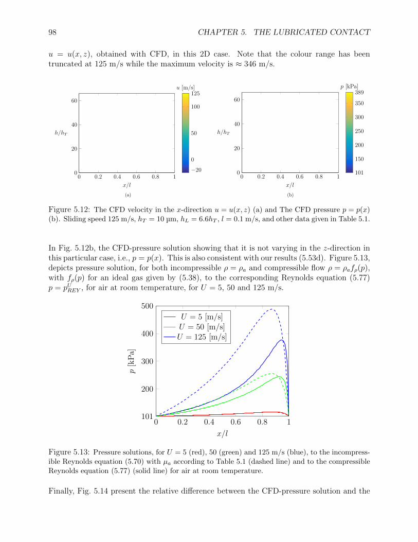
98 CHAPTER 5. THE LUBRICATED CONTACT
u = u(x, z), obtained with CFD, in this 2D case. Note that the colour range has beentruncated at 125 m/s while the maximum velocity is ≈ 346 m/s.
0 0.2 0.4 0.6 0.8 10
20
40
60
x/l
h/hT
−20
0
50
100
125u [m/s]
(a)
0 0.2 0.4 0.6 0.8 10
20
40
60
x/l
h/hT
150
200
250
300
350
101
389p [kPa]
(b)
Figure 5.12: The CFD velocity in the x-direction u = u(x, z) (a) and The CFD pressure p = p(x)(b). Sliding speed 125 m/s, hT = 10 µm, hL = 6.6hT , l = 0.1 m/s, and other data given in Table 5.1.
In Fig. 5.12b, the CFD-pressure solution showing that it is not varying in the z-direction inthis particular case, i.e., p = p(x). This is also consistent with our results (5.53d). Figure 5.13,depicts pressure solution, for both incompressible ρ = ρa and compressible flow ρ = ρafρ(p),with fρ(p) for an ideal gas given by (5.38), to the corresponding Reynolds equation (5.77)p = pUREY , for air at room temperature, for U = 5, 50 and 125 m/s.
0 0.2 0.4 0.6 0.8 1
200
300
400
500
101
x/l
p[k
Pa]
U = 5 [m/s]U = 50 [m/s]U = 125 [m/s]
Figure 5.13: Pressure solutions, for U = 5 (red), 50 (green) and 125 m/s (blue), to the incompress-ible Reynolds equation (5.70) with µa according to Table 5.1 (dashed line) and to the compressibleReynolds equation (5.77) (solid line) for air at room temperature.
Finally, Fig. 5.14 present the relative difference between the CFD-pressure solution and the

5.7. THE FINITE DIFFERENCE METHOD FOR REYNOLDS’ TYPE OF PDE:S 99
solution to (5.77), defined as|pUREY − pUCFD|
max(pUREY ), (5.183)
for each of the three sliding speeds U = 5, 50 and 125 m/s.
0 0.2 0.4 0.6 0.8 10
0.1
0.2
0.3
x/l
|pU REY−pU C
FD|/ m
ax(pU REY
) U = 5 [m/s]U = 50 [m/s]U = 125 [m/s]
Figure 5.14: Relative difference, for U = 5, 50 and 125 m/s, between the CFD-pressure solutionand the solution to the compressible Reynolds equation (5.77) for air at room temperature. Thedifference between the solutions for U = 5 m/s is so small that the black solid line, at the scale ofthe figure, coincides with the x-axis.
From this numerical example it is clear that the classical Reynolds equation predicts thepressure build-up and thus load carrying capacity quite accurately as long as the slidingspeeds are moderate. The difference between the solutions for U = 5 m/s is even so smallthat the black solid line, at the scale of the figure, coincides with the x-axis. But it alsoshows that, if high accuracy is desired in a high velocity case, one is forced to resort to themore consistent (and complex) system (5.53).
5.7 The finite difference method for Reynolds’ type of
PDE:s
In general, solving Reynolds equation analytically is a complicated task. It is possible in somesimple 2D geometries such as the one presented in Section 5.3 but not generally. For 3D cases,one can forget about obtaining an analytical solution altogether. Therefore, numerical toolsare used to solve Reynolds equation in general. In this section we will therefore present onesuch tool. In particular, we will introduce the method of finite differences and apply it toReynolds equation.
The Reynolds equation is a special case of the Poisson second order order differentialequation, i.e.
da∂u
∂t+∇x · (−c∇xu− αu+ γ) + β · ∇u+ au = f, (5.184)

100 CHAPTER 5. THE LUBRICATED CONTACT
where
da = da(t, x), c =
[c11(t, x) c12(t, x)c21(t, x) c22(t, x)
], α =
[α11(t, x)α21(t, x)
],
γ =
[γ11(t, x)γ21(t, x)
], β =
[β11(t, x)β21(t, x)
], a = a(t, x) and f = f(t, x) (5.185)
in 2D and
da∂u
∂t+
∂
∂x
(−c∂u
∂x− αu+ γ
)+ β
∂u
∂x+ au = f, (5.186)
where
da = da(t, x), c = c(t, x), α = α(t, x),
γ = γ(t, x), β = β(t, x), a = a(t, x), and f = f(t, x)(5.187)
in 1D. Note that the we will only consider the situation when c12 = c21. We will start by aderivation of a second order finite difference scheme, with uniform element size ∆x and timestep ∆t, for the 1D case. The spatially discretised finite difference scheme will be realisedby linearisation of the coefficient functions (5.184) to (5.187) at a point xi. In particular, weneed to discretise derivatives of the form
∂u
∂x,
∂
∂x
(c∂u
∂x
)and
∂u
∂t.
The element size is defined by the length l of the domain [a, b] and the number of elements.If we use N + 2 points to discretise this domain (N interior points plus a and b), the elementsize becomes
∆x ..=l
N + 1. (5.188)
Note that N elements are described through N + 1 points. To allow for a compact notationfor the subsequent steps of the derivation we introduce the notation
uki..= u(tk, xi), xi = a+ i∆x. (5.189)
Time is denoted by tk here, but at this time it is not restricted to a particular set of discretetimes. The foundation for the discretisation of the 1D Poisson equation (5.186) is depictedin Fig. 5.15.

5.7. THE FINITE DIFFERENCE METHOD FOR REYNOLDS’ TYPE OF PDE:S 101
a xi−1 xi xi xi+1 b
uki−1
uki
uki+1
, ,
xi− 12xi+ 1
2
x
u
∆x
Figure 5.15: Schematics of a discretised domain in 1D.
In the figure, also the midpoints xi±1/2 are shown. These will be used to derive a secondorder finite difference scheme defined on the interval Ii = [xi−1, xi+1], for the second orderderivative. Based on these definitions it is now possible to define the classical finite differencesfor the first derivative term ∂u/∂x. They are based on the Taylor series expansions at x+∆x,x+ ∆x/2, x−∆x/2 and x−∆x, i.e.,
f(x+ ∆x) = f(x) +∆x
1!f ′(x) +
∆x2
2!f ′′(x) +
∆x3
3!f ′′′(x) +
∆x4
4!f (4)(x) + . . . , (5.190a)
f(x+∆x
2) = f(x) +
∆x
211!f ′(x) +
∆x2
222!f ′′(x) +
∆x3
233!f ′′′(x) +
∆x4
244!f (4)(x) + . . . , (5.190b)
f(x− ∆x
2) = f(x)− ∆x
211!f ′(x) +
∆x2
222!f ′′(x)− ∆x3
233!f ′′′(x) +
∆x4
244!f (4)(x) + . . . , (5.190c)
f(x−∆x) = f(x)− ∆x
1!f ′(x) +
∆x2
2!f ′′(x)− ∆x3
3!f ′′′(x) +
∆x4
4!f (4)(x) + . . . (5.190d)
From (5.190d) get the so called upwind difference scheme directly, i.e.,
∆xf ′(x) = f(x)− f(x−∆x) +O(∆x2
), (5.191)
or
f ′(x) =f(x)− f(x−∆x)
∆x+O (∆x) . (5.192)
Thus, up to first order accuracy the x-derivative of the dependent variable u, at the pointx = xi, can be approximated as
∂u
∂x
∣∣∣∣xi
≈ ui − ui−1
∆x. (5.193)
This is often referred to as an upwind scheme and is particularly suited for hyperbolic equa-tions with initial value or a boundary condition upstream the point itself. By first orderaccuracy, it is meant that the correction terms are of order ∆x1. In practice, this means thatone can expect the error to reduce by a factor 21 upon halving ∆x. In general, an nth orderapproximation will have corrections of order ∆xn and the error will reduce by a factor 2n
102 CHAPTER 5. THE LUBRICATED CONTACT
upon halving ∆x. The difference between (5.190a) and (5.190d) gives the central differencescheme for the first derivative of f , i.e.,
2∆xf ′(x) = f(x+ ∆x)− f(x−∆x) + 2∆x3
3!f ′′′(x) + 2
∆x5
5!f (5)(x) + . . . , (5.194)
which for a function u leads to a finite difference scheme of second order accuracy that reads
∂u
∂x
∣∣∣∣xi
≈ ui+1 − ui−1
2∆x, (5.195)
There are two ways two derive a finite difference scheme for the second order derivative ofa function which is of second order accuracy, the most obvious being to add (5.190a) and(5.190d), i.e.,
∆x2f ′′(x) = f(x+ ∆x) + f(x−∆x)− 2f(x) + 2∆x4
4!f (4)(x) + . . . , (5.196)
which restated as a second order accurate finite difference scheme for the function u reads
∂2u
∂x2
∣∣∣∣xi
≈ ui+1 − 2ui + ui−1
∆x2, (5.197)
For the second term in the 2D and the 1D Poisson equations, (5.184) and (5.186), an approachbased on the points xi±1/2
..= x ± ∆x/2, must be used to obtain a finite difference schemeof second order accuracy. For simplicity we consider the 1D case. Indeed, (5.195) is used toobtain
∂
∂x
(c(t, x)
∂u
∂x
)∣∣∣∣xi
≈
1
∆x
(ci+1/2
∂u
∂x
∣∣∣∣xi+1/2
− ci−1/2∂u
∂x
∣∣∣∣xi−1/2
)≈
=1
∆x
(ci+1/2
ui+1 − ui∆x
− ci−1/2ui − ui−1
∆x
)=
=ci+1/2ui+1 − (ci+1/2 + ci−1/2)ui + ci−1/2ui−1
(∆x)2, (5.198)
which is a second order accurate finite difference scheme for the second term in the Poissonequation. What remains to be deduced, is the values of the function c at the points xi±1/2 =x ± ∆x/2. If an explicit mathematical expression defines c, ci±1/2 can be determined byevaluation directly at the points. Assuming it is not, it can, for example, be determined byaveraging based on its neighbouring values at xi−1, xi and xi+1. The most common methodis, perhaps, to use the arithmetic average, i.e.
ci±1/2 =ci + ci±1
2. (5.199)
Note that in the Reynolds equation, c and γ depend on the film thickness h, which is afunction of x.
5.7. THE FINITE DIFFERENCE METHOD FOR REYNOLDS’ TYPE OF PDE:S 103
The two most typical finite differences of the time derivative are the forward- and back-ward Euler methods. Let us start by formulating (5.184) as
∂u
∂t= F (t, x, u). (5.200)
The forward Euler is an explicit scheme which is obtained by approximating the time deriva-tive with an upwind scheme similar to (5.193), viz.
uk − uk−1
∆t= F (tk, x, u
k−1). (5.201)
This is an initial value problem and starting from the initial value u0 = u(t0, x) the solutionat time tk is given by
uk = uk−1 + ∆tF (tk, x, uk−1). (5.202)
With the backward Euler method the solution uk is obtained by solving
uk+1 − uk∆t
= F (tk+1, x, uk+1). (5.203)
This is an implicit method and it differs from the explicit forward Euler method in that it usesF (tk+1, x, uk+1) instead of F (tk, x, uk). It is seen that the (new) approximation uk+1 appearsin both sides of the equation, and one have to solve an algebraic equation to obtain its value.Thus, the solution procedure must be chosen so that it aligns with the characteristics of theproblem. For a non-stiff problem, fixed-point iteration can be used. More precisely,[
uk+1]0
= uk,[uk+1
]i+1= uk + ∆tF (tk+1, x,
[uk+1
]i). (5.204)
where i is iterated with hope that some specified error measure εi reduces to some specifiedtolerance τε. The error measure is commonly chosen as
εi =|[uk+1
]i+1 −[uk]i |
max(
[uk]i) (5.205)
If it converges, i.e., εi ≤ τε, for lets say i = Nτ then[uk+1
]Nτis used as the approximation
to find uk+2 and so on. The Newton–Raphson (or some kind modification of it) can also beused to solve the algebraic equation. With this we have the tools required to develop finitedifference schemes for all sorts of differential equations, specifically different variants of theReynolds equation.
5.7.1 An FDM for the stationary 1D Reynolds equation
In this section we present a second order finite difference scheme for (5.95), i.e., the linearstationary 1D Reynolds equation, describing incompressible and iso-viscous flow, viz.
d
dx
(h3
12µa
dp
dx
)=ul2
dh
dx, 0 ≤ x ≤ l,

104 CHAPTER 5. THE LUBRICATED CONTACT
with (pressure) boundary conditions
p(0) = pT and p(l) = pL.
By comparing this form of Reynolds equation with (5.186) we can identify coefficients. Indeed
α = 0, c = − h3
12µa, β = 0, γ = −ulh
2, f = 0.
Thus, a second order accurate scheme for (5.95) can be formulated as
ci+1/2pi+1 − (ci+1/2 + ci−1/2)pi + ci−1/2pi−1
(∆x)2=γi+1 − γi−1
2∆x, (5.206)
where ci±1/2 are given by (5.199). The FDM-scheme in (5.206) may be written in a morecompact form as
ewi pi−1 − eci∆xpi + eeipi+1 = Fi, (5.207)
where
ewi =ci−1/2
∆x, eci = −ci+1/2 + ci−1/2
∆x, eei =
ci+1/2
∆xand Fi =
γi+1 − γi−1
2
and p0 = pT and pN+1 = pL. Let us list a few of the equations of the algebraic system thatoften is referred to as the determining system which we will solve. Since i marks the internalnodes only, i = 1 . . . N this system becomes,
i = 1 : ew1 p0 +ec1p1 +ee1p2 = F1,
i = 2 : ew2 p1 +ec2p2 +ee2p3 = F2,
...
ewi pi−1 +ecipi +eeipi+1 = Fi,
...
i = N : ewNpN−1 +ecNpN +eeNpN+1 = FN ,
(5.208)
ori = 1 : ec1p1 +ee1p2 = F1 − ew1 pL,
i = 2 : ew2 p1 +ec2p2 +ee2p3 = F2,
...
ewi pi−1 +ecipi +eeipi+1 = Fi,
...
i = N : ewNpN−1 +ecNpN = FN − eeNpT ,
(5.209)
5.7. THE FINITE DIFFERENCE METHOD FOR REYNOLDS’ TYPE OF PDE:S 105
where the terms including the boundary conditions, which are known, have been moved tothe right-hand side. The determining system is often presented in matrix-vector form, whichin this case reads
ec1 ee1ew2 ec2 ee2
. . .
ewi eci eei. . .
ewN ecN
p1
p2...pi...pN
=
F1 − ew1 pLF2...Fi...
FN − eeNpT
(5.210)
An even more compact notation for this tri-diagonal system reads
Ap = b (5.211)
and its solution
p = A−1b, (5.212)
can be readily obtained with various methods.
5.7.2 An FDM for the stationary 2D Reynolds equation
In this section we address the 3D thin film flow situation and present a second order finitedifference scheme for the stationary form of (5.73), i.e., the linear stationary 2D Reynoldsequation, describing incompressible and iso-viscous flow in polar coordinates, viz.
∇x ·(
h3
12µa
[1/x2 0
0 x2
]∇xp−
ω
2
[x2
0
]h
)= 0, on Ω (5.213)
where Ω is the circle sector defined by Ω = (x1, x2) : 0 < x1 < θp, Ri < x2 < Ro. We willalso discuss the implications of two applicable variants of boundary conditions, i.e. Dirichletin both directions and a combination of Dirichlet- and periodic boundary conditions.
In the 2D case, the grid is enumerated in two directions and when posing the determiningsystem, as we did in the 1D case obtaining (5.209), we first need to decide how we order theelements. In Fig. 5.16

106 CHAPTER 5. THE LUBRICATED CONTACT
i = 0 1 2 i− 1 i i+ 1 N N + 1j = 0
1
2
j − 1
j
j + 1
M
M + 1
∆x1
∆x2
x1
x2
Figure 5.16: Schematics of a discretised domain in 2D. Blue squares marks the boundary nodes,where the solution is known, and the red circles marks the internal nodes, where the solution isunknown.
we find a discretised solution grid, where blue squares marks the boundary nodes, wherethe solution is known and the red circles marks the internal nodes, where the solution isunknown. We also have a so called five-point formula, centred at the node (i, j). We willhere follow use alphabetic order, starting with increasing i and then each N +1 time increasej. If we assume that the value of the pressure is prescribed on the boundaries i = 0 ∧N + 1and j = 0∧M + 1, i.e. Dirichlet boundary conditions, then the solution pij can be formulateas a column vector (here denoted) p, structured as in (5.220), viz.
p =[p11, p21, . . . , pN1 p12, p22, . . . , pN2 · · · p1M , p2M , . . . , pNM
]T.
We remark here thatN andM will determine the positions of the diagonals in the determiningmatrix A and that it in some cases can be wise to change the order. For example, in the casewhen N is significantly larger than M the bandwidth can be reduced by ordering the otherway around. Let us proceed. We will use the formulae in (5.195) and (5.198) with both iand j to obtain an FDM scheme for the 2D stationary Reynolds equation (5.213) with twodifferent variants of boundary conditions. By comparing (5.213) with (5.184) we can identifycoefficients. Indeed
α = 0, c = − h3
12µa
[1/x2 0
0 x2
], β = 0, γ = −ω
2
[x2
0
]h, f = 0.
5.7. THE FINITE DIFFERENCE METHOD FOR REYNOLDS’ TYPE OF PDE:S 107
Therefore, the discrete equation becomes
c11i+1/2,jpi+1,j − (c11
i+1/2,j + c11i−1/2,j)pi,j + c11
i−1/2,jpi−1,j
(∆x)2+
c22i,j+1/2pi,j+1 − (c22
i,j+1/2 + c22i,j−1/2)pi,j + c22
i,j−1/2pi,j−1
(∆y)2=
γ11i+1,j − γ11
i−1,j
2∆x
, (5.214)
where ci±1/2,j and ci,j±1/2 can be obtained from (5.199). In a compacted notation, the five-point FDM scheme (5.214) can be formulated as
esijpi,j−1 + ewijpi−1,j + ecijpij + eeijpi+1,j + enijpi,j+1 = Fij, (5.215)
where
ewij =c11i−1/2,j
(∆x)2, ecij = −
c11i+1/2,j + c11
i−1/2,j
(∆x)2−c22i,j+1/2 + c22
i,j−1/2
(∆y)2, eeij =
c11i+1/2,j
(∆x)2
esij =c22i,j−1/2
(∆y)2, enij =
c22i,j+1/2
(∆y)2,
Fij =γ11i+1,j − γ11
i−1,j
2∆x
We note that if the matrix c would have had non-zero off-diagonal terms, this would haverendered 4 more diagonals, i.e. sub- and super-diagonals to es and en, being multipliers forpi±1,j and pi,j±1. Like we did in the 1D case before, we will now just list the most essentialequations of the algebraic system for the solution pij, commonly referred to as the determiningsystem.
In this case, due to size requirements we will separate it into a left- and a right-hand side

108 CHAPTER 5. THE LUBRICATED CONTACT
part. The left-hand side then reads
es11p1,0 + ew11p0,1 + ec11p1,1 + ee11p2,1 + en11p1,2
es21p2,0 + ew21p1,1 + ec21p2,1 + ee21p3,1 + en21p2,2...
esN1pN,0 + ewN1pN−1,1 + ecN1pN,1 + eeN1pN+1,1 + enN1pN,2
es12p1,1 + ew12p0,2 + ec12p1,2 + ee12p2,2 + en12p1,3
es22p2,1 + ew22p1,2 + ec22p2,2 + ee22p3,2 + en22p2,3...
esN2pN,1 + ewN2pN−1,2 + ecN2pN,2 + eeN2pN+1,2 + enN2pN,3
...
es1Mp1,M−1 + ew1Mp0,M + ec1Mp1,M + ee1MpN+1,M + en1Mp1,M+1
es2Mp2,M−1 + ew2Mp1,M + ec2Mp2,M + ee2MpN+1,M + en2Mp2,M+1...
esNMpN,M−1 + ewNMpN−1,M + ecNMpN,M + eeNMpN+1,M + enNMpN,M+1
(5.216)
and the right-hand side becomes[F11, F21, . . . , FN1 F12, F22, . . . , FN2 · · · F1M , F2M , . . . , FNM
]T. (5.217)
It is now time to address the boundary conditions and we will devote one subsection for eachof the cases.
Dirichlet boundary conditions
For a typical tilting pad bearing, such as the one illustrated in 2.1, each segment is sur-rounded by lubricant supplied at a given pressure pa. If it is assumed that the segmentsbehave identically, the numerical analysis may be focussed on a single element reducing thecomputational burden by a factor equalling the number of pads. This means that the pres-sure distribution on each individual segment assuming Dirichlet boundary conditions is thepressure solution depicted in 5.2.
p(0, x2) = p(θp, x2) = p(x1, Ri) = p(x1, Ro) = pa. (5.218)
Looking at the system above, this means that p0,j = pN+1,j = pi,0 = pi,M+1 = pa fori = 1 . . . N and j = 1 . . .M are known and should be moved to the right-hand side. Thismakes it possible to formulate the determining system in matrix form - in which the subscriptD indicate that Dirichlet boundary conditions are considered, as
ADpD = bD, (5.219)
where AD is an (NM) × (NM) five-diagonal matrix and where pD and bD are (NM) × 1vectors structured in the same way, i.e.[
f11, f21, . . . , fN1 f12, f22, . . . , fN2 · · · f1M , f2M , . . . , fNM]T, (5.220)
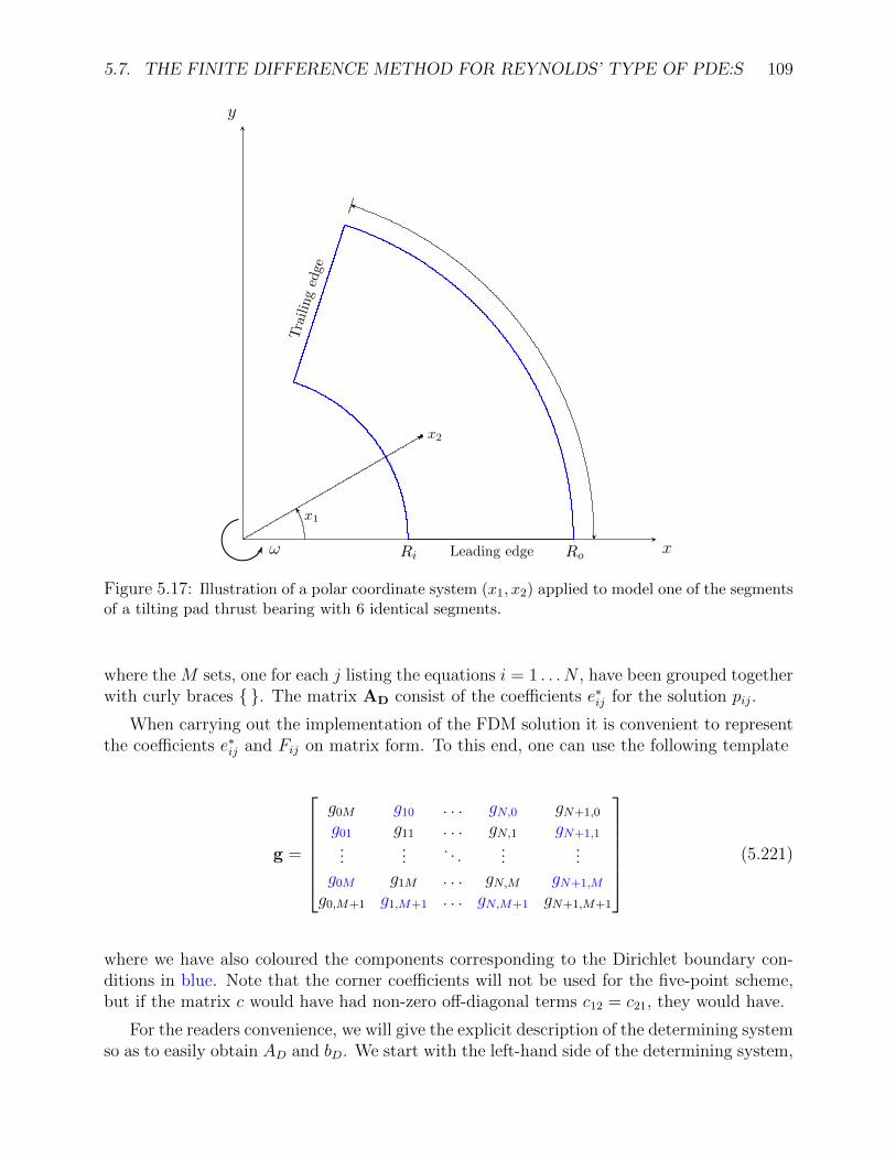
5.7. THE FINITE DIFFERENCE METHOD FOR REYNOLDS’ TYPE OF PDE:S 109
x1
x2
x
y
Ri Leading edge Ro
Tra
ilin
ged
ge
ω
Figure 5.17: Illustration of a polar coordinate system (x1, x2) applied to model one of the segmentsof a tilting pad thrust bearing with 6 identical segments.
where the M sets, one for each j listing the equations i = 1 . . . N , have been grouped togetherwith curly braces . The matrix AD consist of the coefficients e∗ij for the solution pij.
When carrying out the implementation of the FDM solution it is convenient to representthe coefficients e∗ij and Fij on matrix form. To this end, one can use the following template
g =
g0M g10 . . . gN,0 gN+1,0
g01 g11 . . . gN,1 gN+1,1...
.... . .
......
g0M g1M . . . gN,M gN+1,M
g0,M+1 g1,M+1 . . . gN,M+1 gN+1,M+1
(5.221)
where we have also coloured the components corresponding to the Dirichlet boundary con-ditions in blue. Note that the corner coefficients will not be used for the five-point scheme,but if the matrix c would have had non-zero off-diagonal terms c12 = c21, they would have.
For the readers convenience, we will give the explicit description of the determining systemso as to easily obtain AD and bD. We start with the left-hand side of the determining system,
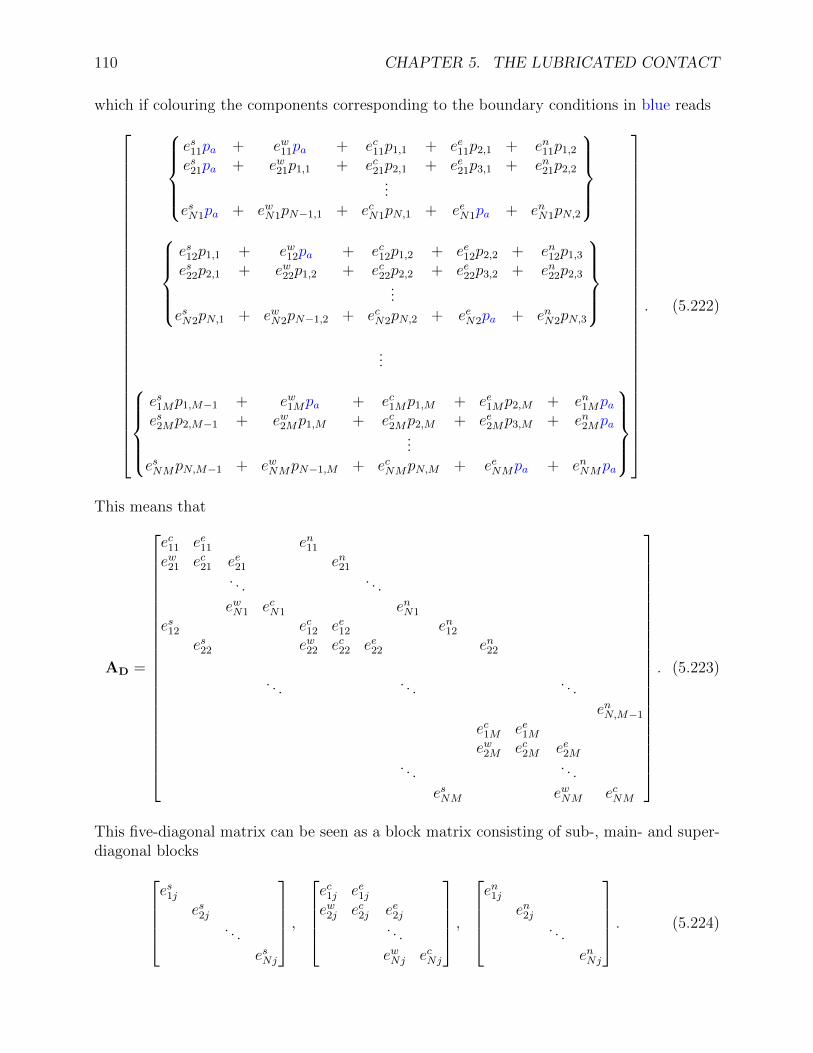
110 CHAPTER 5. THE LUBRICATED CONTACT
which if colouring the components corresponding to the boundary conditions in blue reads
es11pa + ew11pa + ec11p1,1 + ee11p2,1 + en11p1,2
es21pa + ew21p1,1 + ec21p2,1 + ee21p3,1 + en21p2,2...
esN1pa + ewN1pN−1,1 + ecN1pN,1 + eeN1pa + enN1pN,2
es12p1,1 + ew12pa + ec12p1,2 + ee12p2,2 + en12p1,3
es22p2,1 + ew22p1,2 + ec22p2,2 + ee22p3,2 + en22p2,3...
esN2pN,1 + ewN2pN−1,2 + ecN2pN,2 + eeN2pa + enN2pN,3
...
es1Mp1,M−1 + ew1Mpa + ec1Mp1,M + ee1Mp2,M + en1Mpaes2Mp2,M−1 + ew2Mp1,M + ec2Mp2,M + ee2Mp3,M + en2Mpa
...esNMpN,M−1 + ewNMpN−1,M + ecNMpN,M + eeNMpa + enNMpa
. (5.222)
This means that
AD =
ec11 ee11 en11
ew21 ec21 ee21 en21. . . . . .
ewN1 ecN1 enN1
es12 ec12 ee12 en12
es22 ew22 ec22 ee22 en22
. . . . . . . . .
enN,M−1
ec1M ee1Mew2M ec2M ee2M
. . . . . .
esNM ewNM ecNM
. (5.223)
This five-diagonal matrix can be seen as a block matrix consisting of sub-, main- and super-diagonal blocks
es1jes2j
. . .
esNj
,ec1j ee1jew2j ec2j ee2j
. . .
ewNj ecNj
,en1j
en2j. . .
enNj
. (5.224)
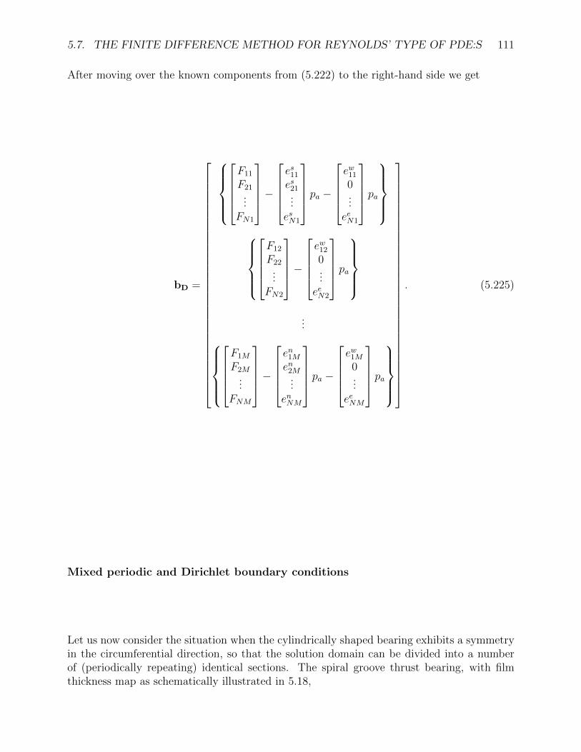
5.7. THE FINITE DIFFERENCE METHOD FOR REYNOLDS’ TYPE OF PDE:S 111
After moving over the known components from (5.222) to the right-hand side we get
bD =
F11
F21...
FN1
−es11
es21...esN1
pa −ew11
0...eeN1
pa
F12
F22...
FN2
−ew12
0...eeN2
pa
...F1M
F2M...
FNM
−en1Men2M
...enNM
pa −ew1M
0...
eeNM
pa
. (5.225)
Mixed periodic and Dirichlet boundary conditions
Let us now consider the situation when the cylindrically shaped bearing exhibits a symmetryin the circumferential direction, so that the solution domain can be divided into a numberof (periodically repeating) identical sections. The spiral groove thrust bearing, with filmthickness map as schematically illustrated in 5.18,

112 CHAPTER 5. THE LUBRICATED CONTACT
ω
x1
x2
θper
x
y
5
3
1h
Figure 5.18: A model of the film thickness of a spiral groove bearing with a θper = 72 period,repeating the same section five times. The colours indicating the (dimensionless) height of theplateau (h = 1), grooves (h = 3) and the central recess area (h = 5).
is a typical example this type of configuration. For this type of application, it is appropriate topose Dirichlet boundary conditions in the radial direction and periodic boundary conditionsin the circumferential direction, i.e.
p(0, x2) = p(θper, x2), p(x1, Ri) = ps, and p(x1, Ro) = pa, (5.226)
where θper angle of periodicity. In discretised notation, the periodic boundary conditionsbecomes p0,j = pN+1,j for j = 0 . . .M + 1. The numerical solution is defined in the ‘periodicwindow’ i = 0 . . . N , and we denote the vector representation as
pper =[p01, p11, . . . , pN,1 p02, p12, . . . , pN,2 · · · p0M , p1M , . . . , pN,M
]T. (5.227)
Note that the periodicity in general means that the solution is the same for any two pointson the same radius, which are separated in the circumferential direction with the angle ofperiodicity θper, i.e., p(x1, x2) = p(x1 +θper, x2). In discretised form this yields pij = pi+N+1,j,and specifically, this means that p−1,j = pN,j, which will be utilised when generating thedetermining matrix for this problem.
The Dirichlet conditions can be expressed as pi,0 = ps and pi,M+1 = pa for i = 1 . . . N ,and as described above these are known and should be moved to the right-hand side.
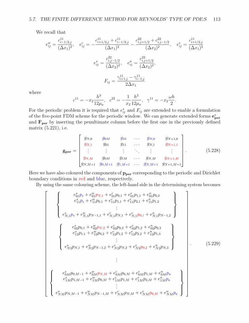
5.7. THE FINITE DIFFERENCE METHOD FOR REYNOLDS’ TYPE OF PDE:S 113
We recall that
ewij =c11i−1/2,j
(∆x1)2, ecij = −
c11i+1/2,j + c11
i−1/2,j
(∆x1)2−c22i,j+1/2 + c22
i,j−1/2
(∆x2)2, eeij =
c11i+1/2,j
(∆x1)2
esij =c22i,j−1/2
(∆x2)2, enij =
c22i,j+1/2
(∆x2)2,
Fij =γ11i+1,j − γ11
i−1,j
2∆x1
where
c11 = −x2h3
12µa, c22 = − 1
x2
h3
12µa, γ11 = −x2
ωh
2.
For the periodic problem it is required that e∗ij and Fij are extended to enable a formulationof the five-point FDM scheme for the periodic window. We can generate extended forms e∗perand Fper by inserting the penultimate column before the first one in the previously definedmatrix (5.221), i.e.
gper =
gN,0 g0M g10 . . . gN,0 gN+1,0
gN,1 g01 g11 . . . gN,1 gN+1,1...
......
. . ....
...gN,M g0M g1M . . . gN,M gN+1,M
gN,M+1 g0,M+1 g1,M+1 . . . gN,M+1 gN+1,M+1
. (5.228)
Here we have also coloured the components of pper corresponding to the periodic and Dirichletboundary conditions in red and blue, respectively.
By using the same colouring scheme, the left-hand side in the determining system becomes
es01ps + ew01pN,1 + ec01p0,1 + ee01p1,1 + en01p0,2
es11ps + ew11p0,1 + ec11p1,1 + ee11p2,1 + en11p1,2...
esN,1ps + ewN,1pN−1,1 + ecN,1pN,1 + eeN,1p0,1 + enN,1pN−1,2
es02p0,1 + ew02pN,2 + ec02p0,2 + ee02p1,2 + en02p0,3
es12p1,1 + ew12p0,2 + ec12p1,2 + ee12p2,2 + en12p1,3...
esN2pN,1 + ewN2pN−1,2 + ecN2pN,2 + eeN2p0,2 + enN2pN,3
...
es0Mp0,M−1 + ew0MpN,M + ec0Mp0,M + ee0Mp1,M + en0Mpaes1Mp1,M−1 + ew1Mp0,M + ec1Mp1,M + ee1Mp2,M + en1Mpa
...esNMpN,M−1 + ewNMpN−1,M + ecNMpN,M + eeNMp0,M + enNMpa
. (5.229)

114 CHAPTER 5. THE LUBRICATED CONTACT
Thus, moving the known components to the right-hand side gives
bper =
F01
F11...
FN1
−es01
es11...esN1
ps
F02
F12...
FN2
...
F0M
F1M...
FNM
−en0Men1M
...enNM
pa
. (5.230)
This makes it possible to write the determining system on the form
Aperpper = bper. (5.231)
We note that the pressure solution consists of (N + 1) ×M unknowns and that, for eachj = 1 . . .M , the column in Aper corresponding to N × j + 1 has the element eeN,j at rowN × j and that the column N × j has the element ew0,j at row N × j + 1. If we express thesub-, main- and super-diagonal blocks, for the determining matrix for this mixed boundarycondition situation, they read
es0j
es1j. . .
esN,j
,ec0j ee0j . . . ew0jew1j ec1j ee1j
.... . .
eeN,j ewN,j ecN,j
,en0j
en1j. . .
enN,j
. (5.232)
5.8 Modelling mass-conserving hydrodynamic cavita-
tion
Hydrodynamic cavitation is found in various lubrication situations. For example, at thedivergent section between the shaft and the bushing in a plain journal bearing, where thefluid film is subjected to a tensile stress situation. The fluid cannot withstand these stressesand thus the fluid film ruptures. In this situation, Reynolds equation will fail to capturethis phenomenon. Instead, it will wrongly predict negative (tensile) pressures. An early

5.8. MODELLING MASS-CONSERVING HYDRODYNAMIC CAVITATION 115
approach to avoid this issue was simply to ignore the negative pressures. This, however, doesnot preserve mass continuity and thus also leads to inaccurate results. The first attempts tomodel mass-conserving hydrodynamic cavitation was presented by three authors Jacobson,Floberg and Olsson [15–18]. They described the so called rupture and reformation boundaryconditions and showed how they could be incorporated in the Reynolds equation leading toa mathematical model of hydrodynamic cavitation.
Elrod and Adams [19] developed a cavitation algorithm using a single equation throughoutthe lubrication region without the need for explicit equations to locate the cavitation bound-aries, and used a switch function to terminate the pressure gradient in the region of cavitation.In [87] Elrod prented a variant of the cavitation algorithm proposed in [19], in which he useda different constitutive relationship between pressure and density. Vijayaraghavan and Keithintroduced a more rigorous derivation and presented their contribution to cavitation mod-elling in [88,89]. As in [19] their algorithm was derived based on the constant bulk modulustype of compressibility. For real lubricants the bulk modulus varies with pressure. The im-portance of using more realistic models for the compressibility was investigated further in thepaper [90] by Sahlin et al. However, treating the bulk modulus as a constant could producegood results in a narrow pressure range. Examples of other work addressing the difficultiesassociated with cavitation modelling are [91–93].
5.8.1 JFO theory
Jakobsson and Floberg [15] developed a mass preserving cavitation theory. They assumed aconstant pressure in the cavitation region, i.e. the pressure gradient is zero. They also deriveda set of conditions to locate the cavitation boundaries. Later, Floberg and Olsson [16–18]extended the theory of cavitation and implemented it in the numerical solution proceduresfor numerous bearing types. The JFO-theory is based on the complementary assumptionthat the fluid is either fully saturated, i.e. θ = 1 and the fluid pressure is larger than thecavitation pressure p > pc, or cavitated, i.e. θ < 1 and the pressure equals the cavitationpressure p = pc. They formulated this mathematically as a boundary condition for thelocation xc of the cavitation inception or rupture, i.e.
p(xc) = pc and∂p
∂n
∣∣∣∣x=xc
(5.233)
and as a condition for preservation of mass flow at the point xr of where the fluid film reforms
h3
12µa
∂p
∂n
∣∣∣∣x=xr
=Vn2
(1− θ)∣∣∣∣x=xr
. (5.234)
Though the JFO-rupture and reformation conditions can be applied to various lubricationproblems, such as the ones for journal bearings, piston ring - cylinder liner conjunctionsand rolling element bearings, it is difficult to handle situations where rupture and cavitationoccurs many times inside the interface, as would be the case with e.g. a textured bearing sur-face. This lead successors to develop “universal” cavitation algorithms, as will be presentedbelow.
116 CHAPTER 5. THE LUBRICATED CONTACT
5.8.2 Elrod’s and Adams’ universal cavitation algorithm
It is not so easy to describe the universal cavitation algorithm developed by Elrod and Adams.One reason is that their work starts in [19], with a paper in which they employ a constantbulk modulus type of constitutive relationship between density and pressure, i.e.,
p = pc + βg(θ) ln θ, (5.235)
where θ is the saturation or the dimensionless density given by
θ(x) =ρ(p(x))
ρc,
and where ρc = ρ(pc) and g(θ) is a so called switch function
g(θ) =
1, p > pc,0, p = pc.
(5.236)
The expression (5.235) comes from
ρ = ρae−(p−pa)/β
with pa = pc. By means of precisely this constitutive relationship between p and θ, Elrodand Adams presented a “universal differential equation” originating from (5.77), which reads
∂ (θh)
∂t= ∇x ·
(βh3
12µag(θ)∇xθ −
us2θh
). (5.237)
Elrod then continues the development in [87] but there another constitutive relationshipbetween density and pressure is adopted, i.e. (5.238). Elrod describes his model like this:“Within the cavitated zone, the liquid everywhere possesses the density, ρc, but the actualmass content is ρcθh per unit area. Here 1− θ, then, is the same as the void fraction. Withinthe complete film, due to variation in pressure, the fluid density also varies. By reason ofslight compression, the film mass content exceeds the content that would exist if the pressurewere pc. In other words, θ = ρ/ρc and the corresponding film pressure is:
p = pc + βg(θ) (θ − 1) , (5.238)
where β =O (109) in SI units for a typical lubricating oil. It is realised, of course, that θ willbe very nearly unity in the full-film zone, but when equation (5.238) constitutes an analyticalconvenience, it will be used.” In a more condensed form this means that the fluid behavesmore or less as incompressible in the full-film zones and that it expands as a homogeneousblend in the cavitated zones.
Based on (5.238), the corresponding Reynolds equation (5.77) would become
∂ (θh)
∂t= ∇x ·
(βθh3
12µa∇x (g(θ)(θ − 1))− us
2θh
). (5.239)
5.8. MODELLING MASS-CONSERVING HYDRODYNAMIC CAVITATION 117
The finite difference scheme presented in [87] implies that it would originate from
∂ (θh)
∂t= ∇x ·
(βh3
12µa∇x (g(θ)(θ − 1))− us
2θh
), (5.240)
which differs from (5.239) as it reflects a flow situation where the fluid behaves like an incom-pressible liquid in the full-film zones and as a homogeneous compressible gas-liquid mixturein the cavitated zones. This is, also, to some extent consistent with Elrod’s description ofhis model, reprinted above. However, they found, and so did successors, that obtaining aconverged numerical solution to this equation can be quite challenging if not even impossiblesometimes.
In the following sections, the inconsistency of the introduction of the constitutive ex-pression in (5.238) and the controversy that Reynolds equation, (5.77), actually reduces to(5.239) when adopting the constitutive relation given by (5.235) will be elaborated upon.
5.8.3 Vijayaraghavan’s and Keith Jr’s cavitation model
As Elrod and Adams did in [19], Vijayaraghavan and Keith Jr. [88,89] also used the constantbulk modulus type of compressibility as a starting point in their derivation of a cavitationmodel. They, however, presented a more rigorous derivation, which finally lead to a cavitationalgorithm similar to the one presented by Elrod in [87]. More precisely, they use the density-pressure relation defined in (5.39) and reach again
∂ (θh)
∂t= ∇x ·
(βh3
12µag(θ)∇xθ −
us2θh
).
Studying this equation they conclude
g(θ)∇x · (θ) = g(θ)∇x · (θ − 1) = ∇x · (g(θ)(θ − 1))− (θ − 1)∇x · (g(θ)) . (5.241)
However, in the full-film zones θ = 1 and in the cavitated ones g(θ) = 0 thus the last termin (5.241) vanishes everywhere except at the point of rupture and we have
g(θ)∇x · (θ) = ∇x · (g(θ)(θ − 1)) (5.242)
so that (5.237) remarkably reduces to (5.240), which is the continuous interpretation of thecavitation algorithm that Elrod proposed in [19]. Moreover, they introduce the concept oftype differencing from transonic flow computations to obtain a finite difference stencil for theshear flow term that effectively considers that the governing equation goes from elliptic tohyperbolic when flow goes from fully flooded to cavitated. That is,
∂(θh)
∂x=
∂
∂x
(θh− (1− g(θ))
∂(θh)
∂x
∆x
2
), (5.243)
where ∆x is the element size in the x-direction. When discretised this leads to the finitedifference scheme
∂(θh)
∂x
∣∣∣∣xi
=(θh)|xi − (θh)|xi−1
∆x+O (∆x) , (5.244)
118 CHAPTER 5. THE LUBRICATED CONTACT
for the shear flow term within the cavitated zone, while it becomes
∂(θh)
∂x
∣∣∣∣xi
=(θh)|xi+1
− (θh)|xi−1
2∆x+O
((∆x)2
), (5.245)
in the full-film zone. In comparison, the scheme presented in [87], yields
∂(θh)
∂x
∣∣∣∣xi
=h|xi − h|xi−1
∆x+O (∆x) , (5.246)
which clearly represents shear flow for an incompressible fluid. The scheme (5.244) is of firstorder, while (5.245) is of second order. In [89], Vijayaraghavan and Keith present the remedyfor this by extending the type differencing scheme to
∂E
∂x=
∂
∂x
(E − (1− g(θ))
(∂2E
∂x2
(∆x)2
2− ∂3E
∂x3
(∆x)3
8
)), (5.247)
where E = θh. This leads to the second order finite difference scheme
∂E
∂x
∣∣∣∣xi
=1
2∆x
(gi+1/2Ei+1 − (2− gi+1/2 − gi−1/2)Ei − (2− gi−1/2)Ei−1
)+
=1
2∆x
((1− gi+1/2)Ei − (2− gi+1/2 − gi−1/2)Ei−1 + (1− gi−1/2)Ei−2
)+
O((∆x)2
). (5.248)
The pressure driven flow can then be discretised with a standard second order accuratefinite difference scheme. This method leads to a much more robust solution than previousapproaches, but the example in Fig. 6 in [88] shows that their implementation of this switch-function based algorithm induce an artificial source term. This is evident due to the factthat the pressure developing over the second parabolic constriction is larger than that of thefirst parabolic constriction. The numerical exact solution to this problem is presented in ??in the Section 5.8.5.
5.8.4 Arbitrary compressibility switch function based cavitationalgorithm
In the paper by Sahlin et al. [90], they adopt the expression (5.36), viz.
ρ = ρafρ(p),
as the constitutive relationship for the fluid compressibility. We recall, from above, that fis a strictly increasing function, f(pa) = 1 and ρa is the density at the ambient pressure pa.This means that
∇ρ = ρaf′(p)∇p, (5.249)
can be inverted to express the pressure gradient as,
∇p =1
f ′(p)∇θ, (5.250)
5.8. MODELLING MASS-CONSERVING HYDRODYNAMIC CAVITATION 119
where θ(x) = ρ(p(x))/ρa. This means that (5.77) including the switch function g(θ) (5.236)can be posed as
∂ (θh)
∂t= ∇x ·
(h3
12f ′(p)µag(θ)∇xθ −
us2θh
). (5.251)
In [90] they analyse the resulting predictions based on both the constant bulk modulus typeof compressibility (5.39) and another kind of density-pressure relationship, the well-knownrelation,
ρ = ρaC1 + C2(p− pa)C1 + p− pa
, (5.252)
deduced by Dowson and Higginson and presented in [64], together with the constants C1 =0.59 GPa and C2 = 1.34 that the found to be best fit to mineral oil density-pressure datathey had access to. Sahlin et al. [90] fitted the constants to another set of mineral oildensity-pressure data for pressures up to 1 GPa, and found a close fit for C1 = 2.22 GPa andC2 = 1.66.
5.8.5 The linear complementarity problem formulation
In 2005, Bayada presented a [94] a continuous complementarity formulation of Elrod’s andAdams’ cavitation algorithm [19]. Later, Giacopini et al. [20] presented the same formula-tion together with the discretised linear complementarity problem formulation of the samecavitation algorithm on the basis that the fluid in the fully flooded regions behaves if asincompressible. Independent of each other Bertocchi et al. [23] and Almqvist et al. [21, 24]developed this further. The work [21] is built upon that the pressure solution given by theReynolds equation (expressed in its most fundamental form):
∇ · q = 0, (5.253)
may well be below pc. It proceeds by stating that in the full film zones, the density can beexpressed as ρ = ρce
(p−pc)/β. In the cavitation zones the density, or the saturation, is anunknown, here denoted by δ, hence
ρ (p) = ρc
e(p−pc)/β , p > pcδ , p = pc
. (5.254)
The unknown saturation function δ satisfies 0 ≤ δ ≤ 1. Since ∇p = 0 in the region wherep = pc we have that
q = ρc
e(p−pc)/βh
2U − e(p−pc)/βh3
12µ∇p , p > pc
δh
2U , p = pc
, (5.255)
which is a nonlinear expression in p. By introducing the following change of variables
u = e(p−pc)/β − 1, u ≥ 0, (5.256)
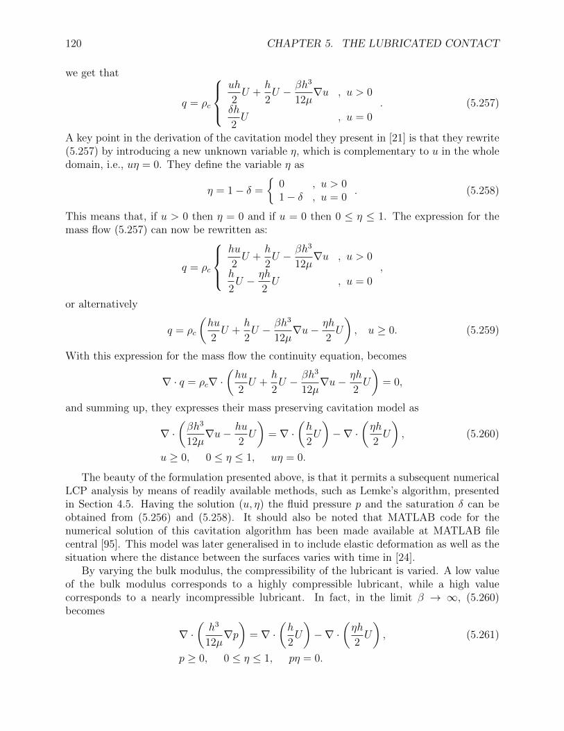
120 CHAPTER 5. THE LUBRICATED CONTACT
we get that
q = ρc
uh
2U +
h
2U − βh3
12µ∇u , u > 0
δh
2U , u = 0
. (5.257)
A key point in the derivation of the cavitation model they present in [21] is that they rewrite(5.257) by introducing a new unknown variable η, which is complementary to u in the wholedomain, i.e., uη = 0. They define the variable η as
η = 1− δ =
0 , u > 01− δ , u = 0
. (5.258)
This means that, if u > 0 then η = 0 and if u = 0 then 0 ≤ η ≤ 1. The expression for themass flow (5.257) can now be rewritten as:
q = ρc
hu
2U +
h
2U − βh3
12µ∇u , u > 0
h
2U − ηh
2U , u = 0
,
or alternatively
q = ρc
(hu
2U +
h
2U − βh3
12µ∇u− ηh
2U
), u ≥ 0. (5.259)
With this expression for the mass flow the continuity equation, becomes
∇ · q = ρc∇ ·(hu
2U +
h
2U − βh3
12µ∇u− ηh
2U
)= 0,
and summing up, they expresses their mass preserving cavitation model as
∇ ·(βh3
12µ∇u− hu
2U
)= ∇ ·
(h
2U
)−∇ ·
(ηh
2U
), (5.260)
u ≥ 0, 0 ≤ η ≤ 1, uη = 0.
The beauty of the formulation presented above, is that it permits a subsequent numericalLCP analysis by means of readily available methods, such as Lemke’s algorithm, presentedin Section 4.5. Having the solution (u, η) the fluid pressure p and the saturation δ can beobtained from (5.256) and (5.258). It should also be noted that MATLAB code for thenumerical solution of this cavitation algorithm has been made available at MATLAB filecentral [95]. This model was later generalised in to include elastic deformation as well as thesituation where the distance between the surfaces varies with time in [24].
By varying the bulk modulus, the compressibility of the lubricant is varied. A low valueof the bulk modulus corresponds to a highly compressible lubricant, while a high valuecorresponds to a nearly incompressible lubricant. In fact, in the limit β → ∞, (5.260)becomes
∇ ·(h3
12µ∇p)
= ∇ ·(h
2U
)−∇ ·
(ηh
2U
), (5.261)
p ≥ 0, 0 ≤ η ≤ 1, pη = 0.
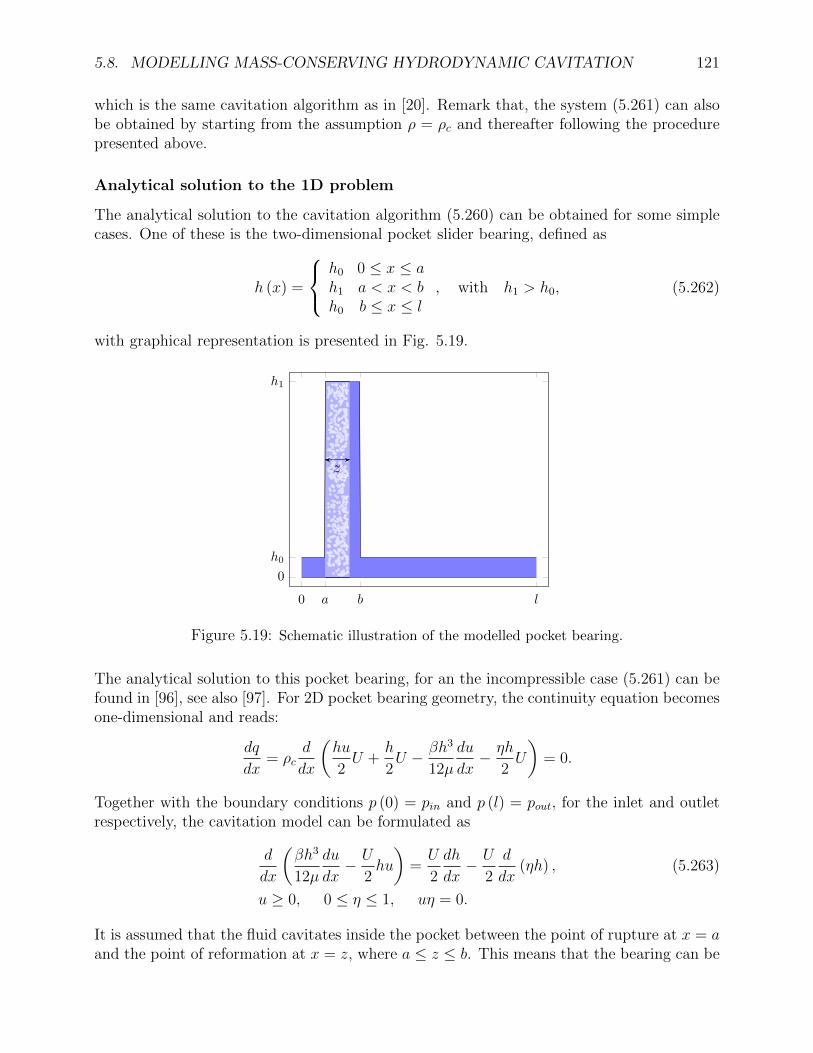
5.8. MODELLING MASS-CONSERVING HYDRODYNAMIC CAVITATION 121
which is the same cavitation algorithm as in [20]. Remark that, the system (5.261) can alsobe obtained by starting from the assumption ρ = ρc and thereafter following the procedurepresented above.
Analytical solution to the 1D problem
The analytical solution to the cavitation algorithm (5.260) can be obtained for some simplecases. One of these is the two-dimensional pocket slider bearing, defined as
h (x) =
h0 0 ≤ x ≤ ah1 a < x < bh0 b ≤ x ≤ l
, with h1 > h0, (5.262)
with graphical representation is presented in Fig. 5.19.
0 a b l
0
h0
h1
z
Figure 5.19: Schematic illustration of the modelled pocket bearing.
The analytical solution to this pocket bearing, for an the incompressible case (5.261) can befound in [96], see also [97]. For 2D pocket bearing geometry, the continuity equation becomesone-dimensional and reads:
dq
dx= ρc
d
dx
(hu
2U +
h
2U − βh3
12µ
du
dx− ηh
2U
)= 0.
Together with the boundary conditions p (0) = pin and p (l) = pout, for the inlet and outletrespectively, the cavitation model can be formulated as
d
dx
(βh3
12µ
du
dx− U
2hu
)=U
2
dh
dx− U
2
d
dx(ηh) , (5.263)
u ≥ 0, 0 ≤ η ≤ 1, uη = 0.
It is assumed that the fluid cavitates inside the pocket between the point of rupture at x = aand the point of reformation at x = z, where a ≤ z ≤ b. This means that the bearing can be
122 CHAPTER 5. THE LUBRICATED CONTACT
subdivided into three liquid phase zones; 0 ≤ x ≤ a and z ≤ x ≤ b and b ≤ x ≤ l and onegas phase zone a ≤ x ≤ z, where u = 0 and 0 ≤ η ≤ 1. In each of the liquid phase zones,η = 0 and u is given by
d
dx
(βh3
12µ
du
dx− U
2hu
)=U
2
dh
dx.
Summing up, for each of the zones the solution explicitly reads
u = C1 + C2 exp
(6µU
βh20
x
), η = 0, 0 ≤ x ≤ a, (5.264)
u = 0, η = C, a ≤ x ≤ z, (5.265)
u = C3 + C4 exp
(6µU
βh21
x
), η = 0, z ≤ x ≤ b, (5.266)
u = C5 + C6 exp
(6µU
βh20
x
), η = 0, b ≤ x ≤ l. (5.267)
The boundary conditions u (0) = e(pin−pc)/β − 1 and u (a) = 0, can be used to determine theconstants C1 and C2, i.e.
C1 = −1− exp ((pin − pc) /β)
1− exp
(−6µUa
βh20
) , (5.268)
C2 = −C1 exp
(−6µUa
βh20
). (5.269)
Knowing the solution u it can be used to equate the mass flow q according to
q =ρcUh0
2
1− 1− exp ((pin − pc) /β)
1− exp
(−6µUa
βh20
) . (5.270)
The mass flow is preserved throughout the whole domain. According to equation (5.259),the mass flow in a < x < z is given by
q =ρcUh0
2(1− C) , (5.271)
and the constant C can be determined. More precisely,
C =1− exp ((pin − pc) /β)
1− exp
(−6µUa
βh20
) ( = −C1) .
The remaining constants Ci, i = 3, . . . , 6 and z, can be found by using the conditions thatboth u and the mass flow are continuous at x = z and x = b and the boundary condition

5.8. MODELLING MASS-CONSERVING HYDRODYNAMIC CAVITATION 123
u (l) = e(pout−pc)/β − 1. Summing up:
C3 =h0
h1
(1− C)− 1, (5.272)
C5 = −C, (5.273)
C6 =exp ((pout − pc) /β)− 1− C5
exp
(6µUl
βh20
) , (5.274)
C4 =
−C3 + C5 + C6 exp
(6µUb
βh20
)exp
(6µUb
βh21
) , (5.275)
and (if it exists) the point of reformation reads
z =βh2
1
6µUln
(−C3
C4
)− a. (5.276)
Note that C3 in (5.272) is the correct value. In [21] it was not correct but an errata with theexpression in (5.272) was published shortly after.
Numerical solution procedures
In the following subsections, we will discuss how to discretise the cavitation model (5.260)such that the discretised problem is on the form of a standard linear complementary problem(LCP). Notice that once written as a LCP, the problem can be solved using various methods.For example Lemke’s algorithm, which was presented in Section 4.5.
Although a two-dimensional formulation is straight forward, a one-dimensional version ispresented here in order not to complicate the notation unnecessarily. Two different typesof differencing schemes are discussed. In the first type, central and upwind differencing iscombined, while the second type is based on central differences only.
Combined central and upwind differencing
Let us recall the one-dimensional form of (5.260):
d
dx
(adu
dx+ bu
)=dF
dx− d
dx(ηF ) , (5.277)
u ≥ 0, 0 ≤ η ≤ 1, uη = 0.
where
a =βh3
12µ, b = −U
2h, F =
U
2h. (5.278)
The problem is discretised again using finite differences by dividing the domain 0 < x < linto a uniform grid with N + 2 points, thus having elements of size ∆x = l/(N + 1). Notethat, by interpreting u as pressure and choosing coefficients as
a =h3
12µ, b = 0, F =
U
2, (5.279)

124 CHAPTER 5. THE LUBRICATED CONTACT
the model obtained corresponds to the one presented in [20], where the lubricant is assumedto be incompressible in the full film regions. The following notation is adopted xi = il/N,where i = 0, . . . , N + 2 and
ui := u (xi) .
The problem at hand is elliptic in the full film domain, where η = 0. A central differencescheme is therefore used to approximate the derivatives in (5.277). Following the schemepresented in Section 5.7 and using the notation
ai±1/2 =ai±1 + ai
2,
and the approximation
du
dx
∣∣∣∣i+1/2
≈ ui+1 − ui∆x
anddu
dx
∣∣∣∣i−1/2
≈ ui − ui−1
∆x,
we obtain
d
dx
(adu
dx+ bu
)≈ai+1/2
du
dx
∣∣∣∣i+1/2
− ai−1/2du
dx
∣∣∣∣i−1/2
∆x+
(bu)i+1 − (bu)i−1
2∆x
≈
(ai+1 + ai
2
)(ui+1 − ui
∆x
)−(ai−1 + ai
2
)(ui − ui−1
∆x
)∆x
+bi+1ui+1 − bi−1ui−1
2∆x
=1
2∆x2[(ai + ai−1)ui−1 − (ai−1 + 2ai + ai+1)ui + (ai + ai+1)ui+1] +
+bi+1ui+1 − bi−1ui−1
2∆x,
for the left hand side. The first term in the right hand side becomes
dF
dx≈ Fi+1 − Fi−1
2∆x.
In the cavitated regions, where u = 0, we observe that the equation is hyperbolic in η andan upwind difference scheme is employed accordingly, i.e.,
d
dx(ηF ) ≈ ηiFi − ηi−1Fi−1
∆x.

5.8. MODELLING MASS-CONSERVING HYDRODYNAMIC CAVITATION 125
Let us introduce the following notation
ewi =ai−1 + ai
2∆x2− bi−1
2∆x,
eci = −ai−1 + 2ai + ai+1
2∆x2,
eei =ai + ai+1
2∆x2+bi+1
2∆x,
zi =Fi+1 − Fi−1
2∆x,
gci = − Fi∆x
,
gwi =Fi−1
∆x.
Using this notation, we define the following matrices and vectors:
A =
ec1 ee1 0 0 0 · · ·ew2 ec2 ee2 0 0 · · ·0 ew3 ec3 ee3 0 · · ·...
.... . . . . . . . .
. . . . . . . . .. . . . . . . . .
ewN−2 ecN−2 eeN−2
0 ewN−1 eeN−1
, (5.280)
f =
z1 − ew1 u0 − gw1 η0
z2
z3
zN−2
zN−1 − eeN−1uN − gcN−1ηN
, (5.281)
where the values of η on the boundaries are computed from the complementarity conditionsu0η0 = 0 and uNηN = 0, and
B =
gc1 0 0 0 0 · · ·gw2 gc2 0 0 0 · · ·0 gw3 gc3 0 0 · · ·...
.... . . . . .
. . . . . .. . . . . .
gwN gcN−2 00 gwN−1 gcN−1
. (5.282)
126 CHAPTER 5. THE LUBRICATED CONTACT
The discretised form of (5.263) can now be written as
Au = f +Bη, ui, ηi ≥ 0, uiηi = 0. (5.283)
Solving this system for u gives
u = q +Mη, ui, ηi ≥ 0, uiηi = 0, (5.284)
where q = A−1f and M = A−1B.The linear complementarity problem (5.284) can readily be solved by employing standard
numerical methods. One which is frequently used is Lemke’s pivoting algorithm, see [39] andSection 4.5. One advantage, is that Lemke’s pivoting algorithm finds the solution in a finitenumber of steps. Hence, the solution obtained is numerically exact. The method chosenfor the present work is a vectorized matlab version of a pivoting algorithm solving linearcomplementarity problems [95].
Note that in the Lemke algorithm it not explicitly stated that ηi ≤ 1. However, byusing the same ideas as in [94], it can be proved that any solution to (5.260), with Dirichletboundary conditions, without the condition η ≤ 1 still satisfies 0 ≤ η ≤ 1. This impliesthat the numerical solution found with the Lemke algorithm automatically satisfies ηi ≤ 1.This agrees with the physical interpretation that the saturation (1− η) must be positive andcannot be larger 1.
Elliptic formulation and central differencing
In the previous subsection, central differences were used above in the full film region andupwind differences in the cavitated regions. However, it is possible to use central differencesthroughout the whole domain by introducing a small perturbation, which makes the problem(5.263) elliptic also in η and not only in u. Indeed,
d
dx
(aduε
dx+ buε
)=dF
dx− d
dx
(εdηε
dx+ ηεF
), (5.285)
uε ≥ 0, 0 ≤ ηε ≤ 1, uεηε = 0.
where ε > 0 is a small parameter. discretised by central differences, in the same manner asdescribed above, this can be written as
Auε = f + (εD +B) ηε, uεi , ηεi ≥ 0, uεiη
εi = 0. (5.286)
In order to get the standard form for linear complementarity problems we can rewrite this as
uε = qε +M εηε, uεi , ηεi ≥ 0, uεiη
εi = 0,
whereqε = A−1f and M ε = A−1 (εD +B) .
For small values of ε, uε and ηε in (5.285) are good approximations of u and η in (5.277).In practice, relatively small means small in comparison to (∆x)2. The idea of adding an

5.8. MODELLING MASS-CONSERVING HYDRODYNAMIC CAVITATION 127
extra term is inspired from regularity theory for partial differential equations, which in thiscontext is known as artificial viscosity, see e.g. [98].
To illustrate the accuracy of the Elliptic formulation and central differencing numericalformulation, we will revisit the double parabolic slider example, originally presented by Vi-jayargahavan and Keith [88], exhibiting an erroneous solution including a numerical source,and compare it with the numerically exact solution LCP-formulation based solution pre-sented by Almqvist et al. [21]. Indeed, the geometry of the slider, the pressure solutionobtained with Combined central and upwind differencing and the pressure solutions obtainedwith the Elliptic formulation and central differencing method are depicted in Fig. 5.20. Thecorresponding input parameters may be found in Table 5.2. Note that, with β = 69 MPa,the supply pressure pin becomes approximately 6.9 kPa.
Table 5.2: Input parameters for the double parabolic slider problem.
l hmax hmin U µ β pc = pout pin7.62 cm 50.8 µm 25.4 µm 4.57 m/s 0.0139 Pa s 69 MPa 0 Pa β ln 1.0001
0 0.2 0.4 0.6 0.8 10
1
2
3
4
5
6
x/l
h[1
0−5
m]
(a) Double parabolic slider geometry.
0 0.2 0.4 0.6 0.8 10
1
2
3
x/l
p[M
Pa]
pε, ε/(∆x)2 = 10
pε, ε/(∆x)2 = 1
pε, ε/(∆x)2 = 0.1p0
(b) Corresponding pressure solution
Figure 5.20: The double parabolic slider example showing pressure solutions pε obtained by meansof the Elliptic formulation and central differencing scheme, for three different values of ε, and thepressure solution p0 obtained by means of the Combined central and upwind differencing scheme.
The LCC was estimated to be approximately 52.8 kN/m and relative difference in terms ofLCC between the solution pε, with ε/(∆x)2 = 0.1 and p0 was calculated to be approximately0.15%.
1D numerical vs. analytical solution
In this example, the numerical simulation procedure described above is verified against theanalytical solution for the pocket bearing problem earlier in this section. The selected set

128 CHAPTER 5. THE LUBRICATED CONTACT
Table 5.3: Input parameters for the pocket bearing problem.
a b l h0 h1 pc U µ pin = pout2 mm 5 mm 20 mm 1 µm 10 µm 0 Pa 1 m/s 0.01 Pa s 100 kPa
of input parameters are presented in Table 5.3. and Fig. 5.21 depicts the correspondinganalytical and the numerical pressure solutions, obtained for β = 5× 10⁸ and N = 512.
0 5 10 15 200
0.1
0.2
0.3
0.4
0.5
x [mm]
p[M
Pa]
AnalyticalNumerical
Figure 5.21: The analytical and the numerical pressure solutions, for the pocket bearing withβ = 5 · 108 and N = 512 and the rest of the input parameters given in Table 5.3.
The relative error, defined as
N∑i=0
∣∣∣panalyticali − pnumerical
i
∣∣∣/ N∑i=0
panalyticali ,
was 6%, 2.5% and 1% (and the computational times were 3 ms, 22 ms and 106 ms on astandard laptop) for N = 128, N = 256 and N = 512 respectively. The numerical deficienciesare concentrated to the point of reformation at x = a+ z ≈ 4.096 mm, and to the back endof the pocket with the discontinuity in h.
It may be worth noticing that even with a minimum film thickness of 1 µm, the maximumpressure is just over 4 times higher than the supply pressure and that the LCC of thebearing is 4.75 kN/m, while the double parabolic slider with a minimum film thickness of1 µm would generate more than 600 times the LCC of the pocket bearing. Moreover, withpc = pin = pout = 0 both the pocket bearing and the double parabolic would generate 0 N/mLCC, according to the cavitation algorithm based on the LCP formulation.
2D numerical solutions with and without cavitation
In Fig. 5.22 depicts dimensionless pressure distributions, for to the inward pumping spiralgroove geometry depicted in Fig. 5.18, with θper = 72. In (a) the solution obtained with
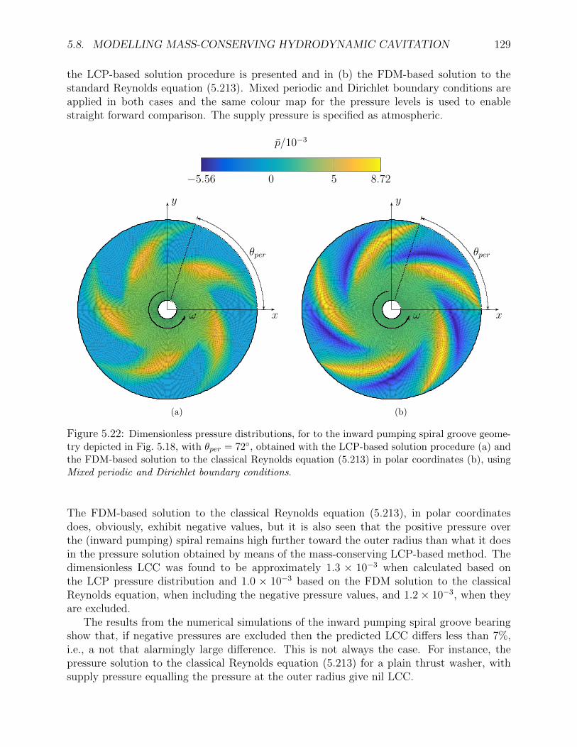
5.8. MODELLING MASS-CONSERVING HYDRODYNAMIC CAVITATION 129
the LCP-based solution procedure is presented and in (b) the FDM-based solution to thestandard Reynolds equation (5.213). Mixed periodic and Dirichlet boundary conditions areapplied in both cases and the same colour map for the pressure levels is used to enablestraight forward comparison. The supply pressure is specified as atmospheric.
−5.56 0 5 8.72
p/10−3
ω
θper
x
y
(a)
ω
θper
x
y
(b)
Figure 5.22: Dimensionless pressure distributions, for to the inward pumping spiral groove geome-try depicted in Fig. 5.18, with θper = 72, obtained with the LCP-based solution procedure (a) andthe FDM-based solution to the classical Reynolds equation (5.213) in polar coordinates (b), usingMixed periodic and Dirichlet boundary conditions.
The FDM-based solution to the classical Reynolds equation (5.213), in polar coordinatesdoes, obviously, exhibit negative values, but it is also seen that the positive pressure overthe (inward pumping) spiral remains high further toward the outer radius than what it doesin the pressure solution obtained by means of the mass-conserving LCP-based method. Thedimensionless LCC was found to be approximately 1.3 × 10⁻³ when calculated based onthe LCP pressure distribution and 1.0 × 10⁻³ based on the FDM solution to the classicalReynolds equation, when including the negative pressure values, and 1.2× 10⁻³, when theyare excluded.
The results from the numerical simulations of the inward pumping spiral groove bearingshow that, if negative pressures are excluded then the predicted LCC differs less than 7%,i.e., a not that alarmingly large difference. This is not always the case. For instance, thepressure solution to the classical Reynolds equation (5.213) for a plain thrust washer, withsupply pressure equalling the pressure at the outer radius give nil LCC.

130 CHAPTER 5. THE LUBRICATED CONTACT
ω
x1
x2
θper
x
y
Figure 5.23: A model of the film thickness of plain thrust washer with a θper = 72 period, repeatingthe same section five times. The yellow patches indicate plateaux, where h = 1, and the blue thegroove, where h = 2.
5.8.6 The FEM and cavitation modelling
It turns out that neither the switch-function nor the LCP-based cavitation models are wellsuited for implementation in an FEM-based framework. It is, however, possible to establishmass-conserving cavitation models in other ways. In the following, a method that assumesthe fluid to be incompressible in its liquid phase, comparable to the model presented in [20],will be described. Soderfjall demonstrated that it is a mass-conserving method in [99], albeitnot conveyed typographically entirely correct. The method was then utilised in numericalinvestigations of texture’s effect in the piston ring - cylinder liner contact operating undermixed lubrication conditions [100]. Even more recently it was used to model inter-asperitycavitation in a two-scale EHL model, based on the Heterogenous Multiscale Method [101].It should be mentioned that these examples were implemented in COMSOL Multiphysicsr.This model assumes that both the lubricant viscosity and density depend on the pressure inthe following way
ρ = ρ0f(p) + αc
1 + αcand µ = µ0
f(p) + αc1 + αc
, (5.287)
where, the dimensionsless auxiliary parameter αc, should be made as small as possible andwhere the function f is specified as
f(p) =
0, p− pc < −βc1− 2
(p− pcβc
)3
− 3
(p− pcβc
)2
, −βc ≤ p− pc ≤ 0
1, p− pc > 0
. (5.288)
The parameter βc is also an auxiliary parameter, with dimensions of pressure, that controlsthe magnitude of the negative pressures. If compared to the LCP solution, which if solved
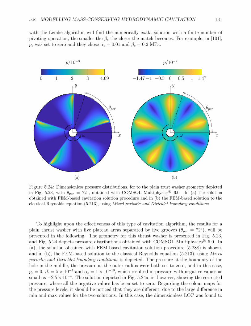
5.8. MODELLING MASS-CONSERVING HYDRODYNAMIC CAVITATION 131
with the Lemke algorithm will find the numerically exakt solution with a finite number ofpivoting operation, the smaller the βc the closer the match becomes. For example, in [101],pc was set to zero and they chose αc = 0.01 and βc = 0.2 MPa.
ω
θper
x
y
0 1 2 3 4.09
p/10−3
(a)
ω
θper
x
y
−1.47−1 −0.5 0 0.5 1 1.47
p/10−2
(b)
Figure 5.24: Dimensionless pressure distributions, for to the plain trust washer geometry depictedin Fig. 5.23, with θper = 72, obtained with COMSOL Multiphysicsr 6.0. In (a) the solutionobtained with FEM-based cavitation solution procedure and in (b) the FEM-based solution to theclassical Reynolds equation (5.213), using Mixed periodic and Dirichlet boundary conditions.
To highlight upon the effectiveness of this type of cavitation algorithm, the results for aplain thrust washer with five plateau areas separated by five grooves (θper = 72), will bepresented in the following. The geometry for this thrust washer is presented in Fig. 5.23,and Fig. 5.24 depicts pressure distributions obtained with COMSOL Multiphysicsr 6.0. In(a), the solution obtained with FEM-based cavitation solution procedure (5.288) is shown,and in (b), the FEM-based solution to the classical Reynolds equation (5.213), using Mixedperiodic and Dirichlet boundary conditions is depicted. The pressure at the boundary of thehole in the middle, the pressure at the outer radius were both set to zero, and in this case,pc = 0, βc = 5× 10⁻⁴ and αc = 1× 10⁻¹⁰, which resulted in pressure with negative values assmall as −2.5× 10⁻⁴. The solution depicted in Fig. 5.24a, is, however, showing the correctedpressure, where all the negative values has been set to zero. Regarding the colour maps forthe pressure levels, it should be noticed that they are different, due to the large difference inmin and max values for the two solutions. In this case, the dimensionless LCC was found to
132 CHAPTER 5. THE LUBRICATED CONTACT
be approximately 3.0×10⁻⁴ for the FEM-based cavitation solution, and 0 for the FEM-basedsolution to the classical Reynolds equation, when including the negative pressure values, and1.4× 10−3, when they are excluded. Here it is clear that a cavitation algorithm is absolutelynecessary for obtaining a reasonably realistic prediction of the pressure and, subsequentlythe LCC, friction torque, mass flow, etc.
5.9 Homogenisation of the Reynolds equation
Up until this point, we have the considered the surfaces’ microscopical topography as perfectlysmooth. Obviously, this is an idealised situation since surfaces always deviates from beingsmooth at some scale. Dependent on various factors the effect of the surface micro structure;surface roughness, may sometimes be small enough to be negligible and sometimes so largethat neglecting it leads to completely wrong conclusions. Figure 5.25 depicts a bearing withthe geometry of a step bearing also including bisinusoidal roughness patterns on both thestationary stepped- and the nominally flat moving surfaces. A direct numerical solutionrequire a mesh fine enough to accurately resolve the roughness. Although, resolving thebisinusoidal roughness pattern in Fig. 5.25 would not require a too dense mesh, it is realisedthat it would be very easy to decrease the wavelength to the point where the computationwould be too memory extensive and/or time consuming to be feasible.
An alternative is to use a two-scale approach. In a two-scale approach the model isconsidered as being composed by two distinct scales. This fact is then used to separatethe problem into two different but interconnected problems, i.e. one for the macro- and onefor the micro scale. Roughly speaking, the solution is obtained by solving the micro-scaleproblem first, then compute the coupling variables, which appear in the macro-scale problemand then obtain the solution. In lubrication, the geometry of the application, should beconsidered as macro-scale features and the surface roughness as micro-scale features. Sincethe macro-scale can be considered is smooth, a coarse discretisation can be used in this scaleavoiding lengthy computation times. To incorporate the effect of roughness, the equationis modified by introducing so-called ‘flow factors’. These are computed by solving a similarflow problem at the local scale. In this scale, the domains are very small and thus can beresolved in the detail required by the roughness. The translation of these loose concepts tomathematical terms is known as homogenisation, which is the topic of this section.
Homogenisation is a type of averaging which has been found applicable for two-scaleproblems with highly varying coefficients. There are many papers reporting the success-ful application of Homogenisation in the field of lubrication, where the fluid flow may begoverned by the Reynolds equation [46, 102–109]. This has lead to highly effective numer-ical tools where the effects caused by the surface roughness are embedded in the derivedhomogenised equations. Moreover, the equations are unambiguously determined and theirnature allow for straight-forward parallelisation. These tools enables studies of rough surfacehydrodynamically lubricated problems such as the one arising in the bearing configurationvisualized in Fig. 2.1. This means that the theoretical model concerns different types of thenon-stationary Reynolds equation in two dimensions.
The key ingredient when homogenising the effect of surface roughness in the Reynoldsequation is the two-scale description of the gap between the surfaces. This is done via

5.9. HOMOGENISATION OF THE REYNOLDS EQUATION 133
a mathematical description of the film thickness that include the surface roughness andappears in the Reynolds equation. More precisely, it is assumed that the film thickness canbe modelled by means of the following auxiliary function
h(x, t, y, τ) = h0(x, t) + hu(y − uuτ)− hl(y − ulτ), (5.289)
where h0, hu and hl are (mathematically) smooth functions, expressed in the independentglobal-scale variables x and t, and the local-scale variables y and τ . We note here that globalscale and local scale are often used, in homogenisation, instead of macro scale and microscale, respectively. In (5.289), the expression uu = [uu, vu]
T defines the velocity of the uppersurface and ul = [ul, vl]
T defines the velocity of the lower surface. Note that the velocitiesmay depend on position, x. The global scale is modelled by the function h0, which describesthe geometry of the problem, and the local scale is modelled via the y- and τ - periodicfunctions hu and hl that describes the surface roughness of the upper and the lower surfaces,respectively. Indeed, the functions hu and hl are assumed to be periodic in their secondargument and the cell of periodicity is denoted by Y for both hu and hl. It is also assumedthat ul, uu, vl and vu are such that h is periodic in τ and the cell of periodicity, in τ , isdenoted by Z. By means of this auxiliary function, a simplified physical description of thegap hε between the surfaces can be achieved. That is
hε(x, t) = h(x, t, x/ε, t/ε), ε > 0. (5.290)
In this expression for the film thickness, which according to (5.289) reads
x1
x2
x3
ul
hl (x− ult)
h0(x, t) + hu (x)
Figure 5.25: A step-shaped bearing including idealised periodic surface roughness at a given timet. The lower surface is moving in the x1-direction with speed ul and the upper surface is stationary.
hε(x, t) = h0(x, t) + hu(x/ε− uut/ε)− hl(x/ε− ult/ε), (5.291)
ε is a (small) parameter which moderates the wavelength of the surface roughness. Asmentioned above (5.290) admits a velocity field that varies with position x (encountered in

134 CHAPTER 5. THE LUBRICATED CONTACT
e.g. a rotating application). Moreover, since hl and hu are functions of x, this also allowsfor different roughness descriptions on different positions. An illustration of a bearing withstep-shaped geometry (global scale) and idealised periodic surface roughness (local scale) ata given time t, is presented in Fig. 5.25. The lower surface is moving in the x1-direction withspeed ul, i.e. ul = [ul, 0]T , and the upper surface is stationary.
In terms of the small wavelength parameter ε, the Reynolds equation for hydrodynamicflow of iso-viscous and compressible fluids (5.77) may be stated as
∂
∂t(hε(x, t)cε(x, t)) = ∇x ·
(h3ε(x, t)Aε(x, t)∇xpε − hε(x, t)Bε(x, t)
), x ∈ Ω (5.292)
where
cε(x, t) = ρ(pε), Aε(x, t) =ρ(pε)
12µa, Bε(x, t) =
us2ρ(pε). (5.293)
and Ω = (x1, x2)|0 < x1 < L1 ∧ 0 < x2 < L2. Due to roughness, hε and the coefficients cε,Aε and Bε are rapidly oscillating functions, which require high spatial and time resolutionfor a mesh independent subsequent numerical analysis.
The main idea in homogenisation is to prove that there exist a solution p0, solving aso-called homogenised equation that does not involve rapidly oscillating coefficient functions,such that
pε → p0, as ε→ 0.
This means that for small values of epsilon - which is the case for realistic surfaces, p0 is agood approximation of pε.
In the subsections below, the homogenisation procedure, referred to as ‘the formal methodof multiple-scale expansion’, will be applied to derive some particular examples of homogenisedReynold’s type of equations that can be solved to obtain the homogenised pressure distri-bution p0. Indeed, the formal method of multiple-scale expansion will be applied to threedifferent variants of the Reynolds equation. More precisely, stationary forms governing iso-viscous flow of incompressible fluids, as well as compressible fluids governed by constant bulkmodulus and ideal gas type of density-pressure relationships, will be presented.
5.9.1 Iso-viscous and incompressible flow
Notice that, the stationary form of the Reynolds equation (5.292) for iso-viscous and incom-pressible flow, in both Cartesian and polar coordinates, admits the following generalisation
∇ ·(h3(x)A(x)∇u(x)
)− λ∇ · (h(x)B(x)) = 0, (5.294)
where u is the dependent variable, h is the film thickness, λ = 6µa, and A and B are knownfunctions of x = (x1, x2). In a Cartesian coordinate formulation, A = I and B = us, whereus = ul + uu, represent the sum of the velocities with which the surfaces of the lower andthe upper body (can be in both directions) moves. In polar coordinates, interpreting x1 asthe angular coordinate x2 as the radial coordinate, for the fluid film formation in a rotatingdevice (with one stator and one rotating collar) - as discussed in [108], they are the matrixand the vector given by
A(x1, x2) =
[1/x2 0
0 x2
], B(x1, x2) = x2ωe1 =
[x2ω
0
], (5.295)

5.9. HOMOGENISATION OF THE REYNOLDS EQUATION 135
where ω is the angular velocity of the rotating surface. The problem with this formulationis it not possible to parametrise the local problems in a effective way, as it leaves the globalcoordinate x2 a parameter to be considered when solving the local problems. This problemand a plausible solution is discussed in [108]. The remedy turns out to be, to considerthe Cartesian formulation (instead for the one in polar coordinates) of the problem and thenadopting the strategy described in [108]. The Cartesian formulation is also a specific exampleof where the flow takes place in both directions. More precisely, when using the Cartesiancoordinate representation of the Reynolds equation (A = I) to model a device in which onesurface is stationary and the other rotates in the counter clockwise direction, then B reads
B(x) = b1(x)e1 + b2(x)e2 = −x2ωe1 + x1ωe2 =
[−x2ωx1ω
]. (5.296)
For the upcoming homogenisation process, we will restrict the analysis to the Cartesiancoordinate formulation and we will consider the following auxiliary equation
∇ ·(h3(x, y)∇u(x, y)
)− λ∇ · (h(x, y)B(x)) = 0, (5.297)
where, again, u is the dependent variable, h is the film thickness, and
B(x) = b1(x)e1 + b2(x)e2 = b1(x)
[10
]+ b2(x)
[01
]..= b1(x) + b2(x), (5.298)
where b1 and b2 are well-defined functions. The variables x = (x1, x2)T and y = (y1, y2)T
refer to the global and local domains, respectively, and it holds that y = x/ε. The size of themicro-scale domain, also referred to as the cell of periodicity, Y , is given by Y = (y1, y2)|0 <y1 < l1 ∧ 0 < y2 < l2.
Now assume that A(x, y) and B(x, y) are periodic in y, and also assume that the followingexpansion holds:
u(x, y) = u0(x, y) + εu1(x, y) + ε2u2(x, y) + ..., (5.299)
where ui are periodic in y. Note that (5.299) is a perturbation series of u(x, y) in termsof ε, which is the so called “small parameter”. Expressed in this terminology, the solutionu(x, y) to the problem including surface roughness is a perturbation of the solution to smoothproblem u0. The perturbation series (5.299) should be interpreted as an approximation tothe solution u, which is given by adding small corrections εiui to u0.
In homogenisation (5.299) constitutes the basis for the formal method of multiple-scaleexpansion, as used in e.g. [102–104,106,108,109], which can be thought of as an engineeringapproach to strict two-scale convergence, see e.g. [105,110]. Now since y = x/ε,
∇ −→ ∇x + ε−1∇y, (5.300)
where ∇x denotes the gradient with respect to the global-scale variables x, and ∇y thegradient with respect to the local-scale variables y. By inserting (5.299) and (5.300) into(5.297) we get(
∇x + ε−1∇y
)·(h3(x, y)
(∇x + ε−1∇y
) (u0 + εu1 + ε2u2 + ...
))−λ(∇x + ε−1∇y
)· (h(x, y)B(x)) = 0.
(5.301)

136 CHAPTER 5. THE LUBRICATED CONTACT
In the following we will consider the asymptotic behaviour of (5.301) as ε goes to zeroand we realise that the reasonable result when expanding (5.301) require that the coefficientsfor ε−2, ε−1 and ε0 are equivalent to zero independently of each other. Indeed, as ε → 0the coefficients of higher orders of ε, i.e., εk with k ≥ 1, will not influence the result and weobtain following set of determining equations
ε−2 : 0 =∇y ·(h3∇yu0
), (5.302a)
ε−1 : 0 =∇y ·(h3 (∇yu1 +∇xu0)− λhB
)+∇x ·
(h3∇yu0
), (5.302b)
ε0 : 0 =∇y ·(h3 (∇yu2 +∇xu1)
)+∇x ·
(h3 (∇yu1 +∇xu0)− λhB
)(5.302c)
where the dependency to x and y has been dropped for the readers convenience.According to a standard result in uniqueness and existence theory for partial differential
equations, see, e.g. [111], we obtain from (5.302a), that u0 = u0(x). By using this fact, thesecond term in the right-hand-side of (5.302b) expands as
∇y ·(h3∇xu0
)= ∇y ·
(h3e1
) ∂u0
∂x1
+∇y ·(h3e2
) ∂u0
∂x2
, (5.303)
which allows us to rewrite (5.302b) as
∇y ·(h3∇yu1
)= ∇y ·
((λhb1 − h3∂u0
∂x1
)e1 +
(λhb2 − h3∂u0
∂x2
)e2
), (5.304)
from which it is realised that the solution (u1) must be on the form
u1 = λb1ψ1 + λb2ψ2 + χ1∂u0
∂x1
+ χ2∂u0
∂x2
(5.305)
where ψi and χi solves the following local problems
0 = ∇y ·(h3∇yψ1
)−∇y · (he1) in Y, (5.306a)
0 = ∇y ·(h3∇yψ2
)−∇y · (he2) in Y, (5.306b)
0 = ∇y ·(h3∇yχ1
)+∇y ·
(h3e1
)in Y, (5.306c)
0 = ∇y ·(h3∇yχ2
)+∇y ·
(h3e2
)in Y, (5.306d)
This type of formulation was used in [108] to study an axial thrust bearing in Cartesiancoordinates. Even though the expression
u1(x, y) = λχ0 + χ1∂u0
∂x1
+ χ2∂u0
∂x2
(5.307)
is the most prevalent and frequently used one, it may not be the most pertinent choice. Thisis made clear in [108] which also present a strong argument for applying (5.305) instead. Thereason being, because it makes it possible to remove the dependence of the global coordinate

5.9. HOMOGENISATION OF THE REYNOLDS EQUATION 137
x2 in the local problems, when the Cartesian coordinate representation of the Reynoldsequation, to model the thin film flow in a rotating device.
Let us now consider (5.302c), together with u0 = u0(x) and u1 defined as in (5.305), inorder to complete the homogenisation process of (5.294). We start by rewriting (5.302c) as
∇x ·(h3∇xu0 + h3∇yu1 − λhB
)= ∇y ·
(h3∇xu1 + h3∇yu2
)(5.308)
and we realise that, due to periodicity
∇x ·(
1
|Y |
∫Y
h3 dy∇xu0 +1
|Y |
∫Y
h3∇yu1 dy −1
|Y |
∫Y
λhB dy
)= 0,
where |Y | = l1l2 defines the area of the local domain. It is clear that the result will notdepend on |Y | and we will continue the derivation for a while without it. Making use of(5.305) we can proceed to get
∇x ·(∫
Y
h3 dy∇xu0 +
∫Y
h3∇y
(λb1ψ1 + λb2ψ2 + χ1
∂u0
∂x1
+ χ2∂u0
∂x2
)dy
)(5.309)
−∇x ·(∫
Y
λhb1e1 + λhb2e2 dy
)= 0,
which can be restated as
∇x ·(∫
Y
h3 dy∇xu0
)+∇x ·
(∫Y
h3∇y
(χ1∂u0
∂x1
+ χ2∂u0
∂x2
)dy
)(5.310)
−∇x ·(λb1
∫Y
(he1 − h3∇yψ1
)dy
)−∇x ·
(λb2
∫Y
(he2 − h3∇yψ2
)dy
)= 0.
Further expanded this reads
∇x ·
1
|Y |
∫Y
h3
1 +∂χ1
∂y1
∂χ2
∂y1
∂χ1
∂y2
1 +∂χ2
∂y2
dy∇xu0
(5.311)
− λ∇x ·
b1
|Y |
∫Y
h− h3∂ψ1
∂y1
−h3∂ψ1
∂y2
dy +b2
|Y |
∫Y
−h3∂ψ2
∂y1
h− h3∂ψ2
∂y2
dy = 0,
where |Y | has been re-introduced for consistency in the reminder of this section. We are nowat the point where it is time to present the homogenised form of (5.294) which we set out toderive, i.e.
∇x ·(h3
0(x)A0(x)∇xu0
)− λ∇x · (h0(x)B0(x)) = 0, (5.312)
where A0 is a 2× 2 matrix and B0 is a 2× 1 vector, i.e.,
A0(x) =
[a0
11(x) a012(x)
a021(x) a0
22(x)
](5.313)
138 CHAPTER 5. THE LUBRICATED CONTACT
and
B0(x) = b01(x) + b0
2(x) =
[b0
11(x)
b012(x)
]+
[b0
21(x)
b022(x)
]. (5.314)
Notice that h30 and h0 has been introduced to the homogenised equation (5.312), in order to
get it on the same form as the equation we started with, i.e. (5.297). The coefficient functionsof A0 reads
a011(x) =
1
h30(x) |Y |
∫Y
h3(x, y)
(1 +
∂χ1
∂y1
)dy, (5.315a)
a012(x) =
1
h30(x) |Y |
∫Y
h3(x, y)∂χ1
∂y2
dy, (5.315b)
a021(x) =
1
h30(x) |Y |
∫Y
h3(x, y)∂χ2
∂y1
dy, (5.315c)
a022(x) =
1
h30(x) |Y |
∫Y
h3(x, y)
(1 +
∂χ2
∂y2
)dy, (5.315d)
and the coefficient functions of B0 reads
b011(x) =
b1(x)
h0(x) |Y |
∫Y
h− h3(x, y)∂ψ1
∂y1
dy, (5.316a)
b012(x) = − b1(x)
h0(x) |Y |
∫Y
h3(x, y)∂ψ1
∂y2
dy, (5.316b)
b021(x) = − b2(x)
h0(x) |Y |
∫Y
h3(x, y)∂ψ2
∂y1
dy, (5.316c)
b022(x) =
b2(x)
h0(x) |Y |
∫Y
h− h3(x, y)∂ψ2
∂y2
dy. (5.316d)
Notice that, in [108], Almqvist considered a rotating device, with the lower surface rotatingwith speed ω in the counter clockwise direction and with the upper stationary. The velocityvector was, therefore, defined as
V l = ω
[x2
−x1
]. (5.317)
The right-hand-side vector B0, corresponding to B0 here, was there defined as
B0(x) =
[x1β11(x) + x2β12(x)
−x1β21(x)− x2β22(x)
], (5.318)
5.9. HOMOGENISATION OF THE REYNOLDS EQUATION 139
with coefficient functions
β11(x) =1
|Y |
∫Y
h3(x, y)∂ψ1
∂y2
dy, (5.319a)
β12(x) =1
|Y |
∫Y
h− h3(x, y)∂ψ1
∂y1
dy, (5.319b)
β21(x) =1
|Y |
∫Y
h− h3(x, y)∂ψ2
∂y2
dy, (5.319c)
β22(x) =1
|Y |
∫Y
h3(x, y)∂ψ2
∂y1
dy. (5.319d)
This means that, the relation between the present coefficient functions b0ij and βij can be
expressed as
b011(x) =
b1(x)
h0(x)β12, b0
12(x) = − b1(x)
h0(x)β22, (5.320)
b021(x) = − b2(x)
h0(x)β11, b0
22(x) =b2(x)
h0(x)β21. (5.321)
We note that, the relations above (in general) can be formulated in vector form as
h0(x)B0(x) =
[b0
11(x) + b021(x)
b012(x) + b0
22(x)
]=
[−b2(x)β11(x) + b1(x)β12(x)
b2(x)β21(x)− b1(x)β22(x)
]= B0(x).
5.9.2 Iso-viscous and constant bulk-modulus type of compressibleflow
Recall that an iso-viscous fluid with constant bulk modulus is characterized by a constantviscosity and a density of the form
ρ = ρaep−pa/β. (5.322)
This particular pressure-density relationship can be seen as transformation that can be usedto transform the, in general, non-linear Reynolds equation for iso-viscous and compressibleflow to a linear form in which density- is the dependent variable. Indeed, the stationary formof the Reynolds equation (5.292), can in this case be written as
∇ ·(h3εβ
12µa∇ρε
)= ∇
(hε
us2ρε
). (5.323)
More generally, (5.323) can be written as
∇ ·(h3ε(x)∇uε(x)
)− γ∇ · (hε(x)Bε(x)uε(x)) = 0, (5.324)
where γ = 6µa/β (and B = us), which permits the following auxiliary form
∇ ·(h3(x, y)∇u(x, y)
)− γ∇ · (h(x, y)B(x, y)u(x, y)) = 0, (5.325)

140 CHAPTER 5. THE LUBRICATED CONTACT
where, again, u is the dependent variable (representing the fluid density), h the film thicknessand B is periodic in y, and on the form (5.298). It is further assumed that the expansion(5.299) holds also in this case. In this terminology (5.325) becomes(
∇x + ε−1∇y
)·(h3(x, y)
(∇x + ε−1∇y
) (u0 + εu1 + ε2u2 + ...
))−γ(∇x + ε−1∇y
)·(h(x, y)B(x, y)
(u0 + εu1 + ε2u2 + ...
))= 0.
(5.326)
Following the procedure introduced in the previous section for incompressible and iso-viscousflow, this leads to the following set of determining equations
ε−2 : 0 =∇y ·(h3∇yu0
), (5.327a)
ε−1 : 0 =∇y ·(h3 (∇yu1 +∇xu0)− γhBu0
)+∇x ·
(h3∇yu0
), (5.327b)
ε0 : 0 =∇y ·(h3 (∇yu2 +∇xu1)− γhBu1
)+ (5.327c)
∇x ·(h3 (∇yu1 +∇xu0)− γhBu0
)Precisely as in the previous case, (5.327a) implies that u0 = u0(x) and we can, therefore,simplify (5.327b) to
∇y ·(h3∇yu1
)= ∇y ·
((γhb1u0 − h3∂u0
∂x1
)e1 +
(γhb2u0 − h3∂u0
∂x2
)e2
). (5.328)
Similar to what was deduced from (5.304) in the case of incompressible flow, (5.328) forconstant bulk modulus type of compressible flow, it is realised that the solution (u1) mustbe on the form
u1 = γb1ψ1u0 + γb2ψ2u0 + χ1∂u0
∂x1
+ χ2∂u0
∂x2
(5.329)
where ψi and χi are the solutions to the same set of local problems (5.306), as in the case ofiso-viscous and incompressible flow. Therefore, by following the same procedure as before,we obtain the homogenised equation
∇x ·(h3
0(x)A0(x)∇xu0
)− γ∇x · (h0(x)B0(x)u0) = 0, (5.330)
and remarkably, the coefficient functions of A0 and B0 are the same as in the case of iso-viscous and incompressible flow, thus given (5.315a)-(5.316d).
5.9.3 Ideal gas flow
An ideal gas is assumed to have a constant viscosity and a density of the form ρ = κp.The Cartesian form of the Reynolds equation for this type of compressible fluid admits thefollowing generalisation
∇ ·(h3(x)u(x)∇u(x)
)− λ∇ · (h(x)B(x)u(x)) = 0, (5.331)

5.9. HOMOGENISATION OF THE REYNOLDS EQUATION 141
where u is the dependent variable, either representing fluid pressure or fluid density. Noticethat this equation is not linear as the two previous cases, for incompressible and for constantbulk-modulus type of compressibility. Anyway, for the subsequent homogenisation processwe now consider the following auxiliary equation
∇ ·(h3(x, y)u(x, y)∇u(x, y)
)− λ∇ · (h(x, y)B(x)u(x, y)) = 0 (5.332)
and that the expansion (5.299) holds. Following the procedure introduced in Section 5.9.1 forincompressible and iso-viscous flow, this leads to the following set of determining equations
ε−2 : 0 =∇y ·(h3u0∇yu0
), (5.333a)
ε−1 : 0 =∇y ·(h3 (u0∇yu1 + u1∇yu0 + u0∇xu0)− λhBu0
)+∇x ·
(h3u0∇yu0
), (5.333b)
ε0 : 0 =∇y ·(h3 (u0∇yu2 + u2∇yu0 + u1∇yu1 + u0∇xu1 + u1∇xu0)− λhBu1
)(5.333c)
+∇x ·(h3 (u0∇yu1 + u1∇yu0 + u0∇xu0)− λhBu0
)Once again, from (5.333a) we have that u0 = u0(x) and since we have u0 > 0 (note thatu0 = 0 would imply a zero density) (5.333b) becomes identical to (5.304) with solution(5.307). Thus we have the same (periodic) local problems (5.306) as for the two previouscases. Finally, from (5.333c) we obtain the homogenised equation for the ideal gas flow case
∇x ·(h3
0(x)A0(x)u0∇xu0
)− λ∇x · (h0(x)B0(x)u0) = 0, (5.334)
We remark that coefficient functions of A0 and B0 are the same as the ones for iso-viscousand incompressible case, as well as the one for the iso-viscous and constant bulk moduluscompressible case, thus given (5.315a)-(5.316d).
5.9.4 Approximative generalisations
If the density’s- and viscosity’s dependence on pressure to be governed by the global scalepressure p0, and if we assume that fluid-structure interaction (FSI) is governed only by p0 wecan achieve a homogenised results describing an approximative generalisation of this morecomplex (non-linear) situation. Moreover, we will assume that the problem is time dependent.Let us, therefore, consider a generalised version of (5.292), i.e.
∂
∂t(hε(x, t, p0(x, t))c(x, t)) =
∇x ·(h3ε(x, t, p0(x, t))A(x, t)∇xpε − hε(x, t, p0(x, t))B(x, t)
), x ∈ Ω
(5.335)
where
c(x, t) = ρ(p0(x, t)), A(x, t) =ρ(p0(x, t))
12µ(p0(x, t)), B(x, t) =
us2ρ(p0(x, t)). (5.336)
142 CHAPTER 5. THE LUBRICATED CONTACT
and Ω = (x1, x2)|0 < x1 < L1 ∧ 0 < x2 < L2. This means that inserting the expansion
p(x, y, t, τ) = p0(x, t) + εp1(x, y, t, τ) + ε2p2(x, y, t, τ) + . . . (5.337)
into (5.335) leads to(∇x + ε−1∇y
)·(ρ(p0)h3(p0)
12µ(p0)
(∇x + ε−1∇y
) (p0 + εp1 + ε2p2 + ...
))
−(∇x + ε−1∇y
)·(h(p0)ρ(p0)
us2
)=
(∂
∂t+ ε−1 ∂
∂τ
)(h(p0)ρ(p0)) ,
(5.338)
where us = [ul + uu, vl + vu]T represents dimensionless velocity. Notice that, since we have
already assumed p0 = p0(x, t), the equation for ε−2 is removed from the system and onlysimplified forms of the equations for ε−1 and ε0 remain, i.e.
ε−1 :∂h
∂τ=∇y ·
(h3
12µ(∇yp1 +∇xp0)− hus
2
)(5.339a)
ε0 :∂h
∂t=∇y ·
(h3
12µ(∇yp2 +∇xp1)
)(5.339b)
+∇x ·(h3
12µ(∇yp1 +∇xp0)− hus
2
),
where, since ρ = ρ(x, t) = ρ(x, t, p0(x, t)), the compressibility is no longer an influencingfactor. This means that the second term in the right-hand-side of (5.339a) expands as
∇y ·(h3
12µ∇xp0
)= ∇y ·
(h3
12µe1
)∂p0
∂x1
+∇y ·(h3
12µe2
)∂p0
∂x2
, (5.340)
which allows us to rewrite (5.339a) as
∇y ·(h3(p0)
12µ(p0)∇yp1
)=∂h(p0)
∂τ+
∇y ·((
ul + uu2
h(p0)− h3(p0)
12µ(p0)
∂p0
∂x1
)e1 +
(vl + vu
2h(p0)− h3(p0)
12µ(p0)
∂p0
∂x2
)e2
),
(5.341)
from which it is realised that if the solution (p1) is presented in this specific form:
p1 = 6µ(p0) (ul + uu)ψ1 + 6µ(p0) (vl + vu)ψ2 + χ1∂p0
∂x1
+ χ2∂p0
∂x2
, (5.342)
then ψi = ψi(x, t, y, τ, p0) and χi = χi(x, t, y, τ, p0) solves the local problems
∂h
∂τ= ∇y ·
(h3∇yψ1
)−∇y · (he1) in Y, (5.343a)
0 = ∇y ·(h3∇yψ2
)−∇y · (he2) in Y, (5.343b)
0 = ∇y ·(h3∇yχ1
)+∇y ·
(h3e1
)in Y, (5.343c)
0 = ∇y ·(h3∇yχ2
)+∇y ·
(h3e2
)in Y (5.343d)
5.9. HOMOGENISATION OF THE REYNOLDS EQUATION 143
that except for the time- (thus τ -) and p0 dependence are on the same form as (5.306), whichwas deduced for the iso-viscous and incompressible problem (and later for the constant bulk-modulus case and for ideal gases). Note that, if these are solved to generate flow factors, suchas we describe it in 5.9.7, then the local-scale contact mechanics problem (5.395) first haveto be solved for a range of loads, F , to obtain the corresponding set of g00, then for a rangeof global-scale separations, α, and then repeat this for a range of global-scale pressure values,p0, which in turn means that we have to compute viscosity, µ(p0), from a given constitutivepressure-viscosity relationship and global-scale deformation ue(p0) by means of (4.5), or (4.7)for a line contact problem.
5.9.5 Homogenised load carrying capacity, friction and flow
In the subsections of this section we will derive the expressions, including the correspondingcorrection factors. for the homogenised load carrying capacity, friction and flow.
Homogenised load carrying capacity
In alignment with the notation in 5.2.3, the load carrying capacity in terms of pε is given as
Fpε..=
∫Ω
pε(x) dx =
∫Ω
p(x, x/ε) dx. (5.344)
The homogenised load carrying capacity is obtained directly from the formal definition oftwo-scale convergence, i.e.∫
Ω
(1
|Y |
∫Y
f(x, x/ε) dy
)dx −→
∫Ω
(1
|Y |
∫Y
f(x, y) dy
)dx as ε −→ 0, (5.345)
where f(x, y) is periodic in y. Since p(x, y) is periodic in y, the homogenised load carryingcapacity can be expressed as
Fp0..=
∫Ω
p0(x) dx =
∫Ω
(1
|Y |
∫Y
p(x, y) dy
)dx. (5.346)
Hence, by (5.345), we haveFpε −→ Fp0 , as ε −→ 0, (5.347)
which suggests that Fp0 provides a suitable approximation of Fpε for small values of ε.
Homogenised friction
According to (5.85) and (5.86), the hydrodynamic friction Ffε , for a bearing operating underlinearly directed motion, is a vector, which evaluated at the lower surface (z = 0) yields
Ffε(z = 0) = −∫
Ω
[τ εx1(z = 0)
τ εx2(z = 0)
]dx = −
∫Ω
−hε2
∂pε∂x1
+µa(uu − ul)
hε
−hε2
∂pε∂x2
+µa(vu − vl)
hε
dx (5.348)
144 CHAPTER 5. THE LUBRICATED CONTACT
and evaluated at the upper surface (z = hε) yields
Ffε(z = hε) = −∫
Ω
[τ εx1(z = h)
τ εx2(z = h)
]dx = −
∫Ω
hε2
∂pε∂x1
+µa(uu − ul)
hεhε2
∂pε∂x2
+µa(vu − vl)
hε
dx. (5.349)
In order to obtain the homogenised correspondences Ff0(z = 0) and Ff0(z = h0) we willhave to use the formal two-scale convergence definition (5.345) of ∇xpε, which according to(5.299) expands as
∇xpε(x) =(∇x + ε−1∇y
)p(x, x/ε) (5.350)
=(∇x + ε−1∇y
) (p0(x) + ε−1p1(x, xε) + ε−2p2(x, xε) + . . .
)= ∇xp0(x) +∇yp1(x, x/ε) + ε (. . .) .
This means that∫Ω
(1
|Y |
∫Y
∇pε(x) dy
)dx −→
∫Ω
(1
|Y |
∫Y
∇xp0(x) +∇yp1(x, y) dy
)dx (5.351)
and by using (5.305), thereby also assuming iso-viscous and incompressible flow, we have∫Ω
(1
|Y |
∫Y
∇xp0(x) +∇yp1(x, y) dy
)dx
=
∫Ω
(1
|Y |
∫Y
∇xp0(x) +∇y
(λb1ψ1p0 + λb2ψ2p0 + χ1
∂p0
∂x1
+ χ2∂p0
∂x2
)dy
)dx
=
∫Ω
1
|Y |
∫Y
λ∂
∂y1
(b1ψ1 + b2ψ2) +
(1 +
∂χ1
∂y1
)∂p0
∂x1
+∂χ2
∂y1
∂p0
∂x2
λ∂
∂y2
(b1ψ1 + b2ψ2) +∂χ1
∂y2
∂p0
∂x1
+
(1 +
∂χ2
∂y2
)∂p0
∂x2
dy dx. (5.352)
Thus, the x1-component of the homogenised friction force Ff0 can be expressed as
Ff0(z = 0) · e1 = −∫
Ω
τ 0x1
(z = 0) dx (5.353)
= −∫
Ω
(1
|Y |
∫Y
−h2
((1 +
∂χ1
∂y1
)∂p0
∂x1
+∂χ2
∂y1
∂p0
∂x2
)dy
)dx
−∫
Ω
(1
|Y |
∫Y
−6µa (ul + uu) b1h
2
∂ψ1
∂y1
− 6µa (ul + uu) b2h
2
∂ψ2
∂y1
+µa(uu − ul)
hdy
)dx
= −∫
Ω
−c011
h0
2
∂p0
∂x1
− c021
h0
2
∂p0
∂x2
dx
−∫
Ω
−6µa (ul + uu)
h0
(d0
11 + d021
)+µa(uu − ul)
h0
e00dx
5.9. HOMOGENISATION OF THE REYNOLDS EQUATION 145
= −∫
Ω
−c011
h0
2
∂p0
∂x1
− c021
h0
2
∂p0
∂x2
dx
−∫
Ω
+µa(uu − ul)
h0
(e0
1 − 6ul + uuuu − ul
(d0
11 + d021
))dx
Following the same nomenclature, the x2-component of the homogenised friction force Ff0
becomes
Ff0(z = 0) · e2 = −∫
Ω
τ 0x2
(z = 0) dx (5.354)
= −∫
Ω
−c012
h0
2
∂p0
∂x1
− c022
h0
2
∂p0
∂x2
dx
−∫
Ω
+µa(vu − vl)
h0
(e0 − 6
vl + vuvu − vl
(d0
12 + d022
))dx.
Thus,
Ff0(z = 0) = −∫
Ω
[τ 0x1
(z = 0)
τ 0x2
(z = 0)
]dx (5.355)
= −∫
Ω
−h0
2
[c0
11 c012
c021 c0
22
]∂p0
∂x1
∂p0
∂x2
+
µa(uu − ul)
h0
(e0 − 6
ul + uuuu − ul
(d0
11 + d021
))µa(vu − vl)
h0
(e0 − 6
vl + vuvu − vl
(d0
12 + d022
)) dx (5.356)
and
Ff0(z = h0) = −∫
Ω
[τ 0x1
(z = h0)
τ 0x2
(z = h0)
]dx (5.357)
= −∫
Ω
h0
2
[c0
11 c012
c021 c0
22
]∂p0
∂x1
∂p0
∂x2
+
µa(uu − ul)
h0
(e0 − 6
ul + uuuu − ul
(d0
11 + d021
))µa(vu − vl)
h0
(e0 − 6
vl + vuvu − vl
(d0
12 + d022
)) dx (5.358)
where
c011(x) =
2
h0(x) |Y |
∫Y
h
2
(1 +
∂χ1
∂y1
)dy, (5.359a)
c012(x) =
2
h0(x) |Y |
∫Y
h
2
∂χ2
∂y1
dy, (5.359b)
c021(x) =
2
h0(x) |Y |
∫Y
h
2
∂χ1
∂y2
dy, (5.359c)
c022(x) =
2
h0(x) |Y |
∫Y
h
2
(1 +
∂χ2
∂y2
)dy, (5.359d)
146 CHAPTER 5. THE LUBRICATED CONTACT
d011(x) =
b1h0
|Y |
∫Y
h
2
∂ψ1
∂y1
dy, (5.360a)
d012(x) =
b2h0
|Y |
∫Y
h
2
∂ψ2
∂y1
dy, (5.360b)
d021(x) =
b1h0
|Y |
∫Y
h
2
∂ψ1
∂y2
dy, (5.360c)
d022(x) =
b2h0
|Y |
∫Y
h
2
∂ψ2
∂y2
dy, (5.360d)
and
e0(x) =h0(x)
|Y |
∫Y
1
hdy, (5.361a)
For a rotating device the frictional resistance is related to torque Tf . In Section 5.2.3,the expression for the friction torque in polar coordinates, 0 ≤ φ ≤ 2π and Ri ≤ r ≤ Ro,evaluated at the counter clockwise rotating upper surface (z = h), assuming that it hasangular velocity ω and that the lower surface (z = 0) is stationary was presented in (5.87).Indeed,
Tfε = −∫ Ro
Ri
∫ 2π
0
r
(hε(ϕ, r)
2r
∂pε∂ϕ
+µωr
hε(ϕ, r)
)rdϕ dr, (5.362)
where r2 = x21 + x2
2 and ϕ = tan−1(x2/x1) is the translation between the angular- and theradial directions in polar coordinates and the principal directions x1 and x2 in Cartesiancoordinates. In Cartesian coordinates, the corresponding expression becomes
Tfε(z = hε) = −∫
Ω
r(τ εx1(z = hε) cosϕ− τ εx2(z = hε) sinϕ
)dx1dx2, (5.363)
where [τ εx1(z = hε)
τ εx2(z = hε)
]=
hε2
∂pε∂x1
+µax2ω
hεhε2
∂pε∂x2
+µa(−x1)ω
hε
. (5.364)
Thus, in terms of the correction factors (5.359a)-(5.361a), the homogenised friction torqueTf0(z = h0) can be expressed as
Tf0(z = h0) = (5.365)
−∫
Ω
x2
((c0
11
h0
2
∂p0
∂x1
+ c012
h0
2
∂p0
∂x2
+µax2ω
h0
(e0 − 6
(d0
11 + d012
)))cosϕ
−(c0
21
h0
2
∂p0
∂x1
+ c022
h0
2
∂p0
∂x2
+µa(−x1)ω
h0
(e0 − 6
(d0
21 + d022
)))sinϕ
)dx1dx2
= −∫
Ω
x2
((h0
2
[c0
11 c012
c021 c0
22
]∇p+
(µah0
e0I− 6
[d0
11 d012
d021 d0
22
])[x2ω
(−x1)ω
])·[
cosϕ− sinϕ
])dx1dx2.
5.9. HOMOGENISATION OF THE REYNOLDS EQUATION 147
Homogenised flow
Based on the Cartesian representation of the Reynolds equation (5.70), the deterministicvolume flow in the x1-direction over the ‘West’ boundary x1 = 0 ∧ 0 ≤ x2 ≤ L2 reads
QWεx1
= e1 ·∫ L2
0
λhε(0, x2)Bε(0, x2)−(h3ε(0, x2)Aε(0, x2)∇pε
)dx2. (5.366)
By means of (5.351) it can then be shown that the corresponding homogenised volume flowbecomes
QW0x1
= e1 ·∫ L2
0
λh0(0, x2)B0(0, x2)−(h3
0(0, x2)A0(0, x2)∇p0
)dx2. (5.367)
Following the same terminology, the deterministic- and homogenised volume flow in the x1-direction over the ‘East’ boundary x1 = L1 ∧ 0 ≤ x2 ≤ L2 read
QEεx1
= e1 ·∫ L2
0
λhε(L1, x2)Bε(L1, x2)−(h3ε(L1, x2)Aε(L1, x2)∇pε
)dx2, (5.368)
and
QE0x1
= e1 ·∫ L2
0
λh0(L1, x2)B0(L1, x2)−(h3
0(L1, x2)A0(L1, x2)∇p0
)dx2, (5.369)
respectively. In addition, the deterministic- and homogenised volume flow in the x2-directionover the ‘South’ boundary x2 = 0 ∧ 0 ≤ x1 ≤ L1 and the ‘North’ boundary x2 = L2 ∧ 0 ≤x1 ≤ L1 read
QSεx2
= e2 ·∫ L1
0
λhε(x1, 0)Bε(x1, 0)−(h3ε(x1, 0)Aε(x1, 0)∇pε
)dx1, (5.370)
QS0x2
= e2 ·∫ L1
0
λh0(x1, 0)B0(x1, 0)−(h3
0(x1, 0)A0(x1, 0)∇p0
)dx1, (5.371)
QNεx2
= e2 ·∫ L1
0
λhε(x1, L1)Bε(x1, L1)−(h3ε(x1, L1)Aε(x1, L1)∇pε
)dx1, (5.372)
and
QN0x2
= e2 ·∫ L1
0
λh0(x1, L1)B0(x1, L1)−(h3
0(x1, L1)A0(x1, L1)∇p0
)dx1, (5.373)
respectively.
5.9.6 Patir and Cheng flow-factors and Homogenised coefficients
The method proposed by Patir and Cheng in [112, 113] considers a representative part ofthe surface roughness and model the complete surface as its periodic extension. Moreover, itconsiders the same type of approximative generalisation as we went through in Section 5.9.4.
148 CHAPTER 5. THE LUBRICATED CONTACT
In the following, we will present a comparison between the averaging technique proposed byPatir and Cheng and homogenisation technique presented in the previous sections. To notunnecessarily complicate the comparison, we will consider a Cartesian representation of thestationary form of (5.335) and without the conventional FSI, including elastic deflection ofthe interacting surfaces. That is,
∇x ·(ρ(p0)h3
ε(x)
12µ(p0)∇xpε
)= ∇x ·
(us2ρ(p0)hε(x)e1
), x ∈ Ω, (5.374)
where the sliding takes place in the x1-direction only, is adopted as the governing equation.Note that the x1-direction has been chosen so that it is aligned with the direction of motion.
Now, retaining as much as possible of the already introduced notation, the stationaryform of the averaged Reynolds equation presented in [112,113] is restated as
∇ ·(ρ(ppc)h3
0(x)
12µ(ppc)
[φ1(x) 0
0 φ2(x)
]∇ppc
)(5.375)
= ∇ ·(us2ρ(ppc)h0(x)
((1
h0(x) |Y |
∫Y
h(x, y) dy
)+ φ0(x)
)e1
)in Ω,
where the flow factors φi are given by
φ0(x) = − 1
h0(x) |Y |
∫Y
h3(x, y)∂v0
∂y1
dy, (5.376)
φ1(x) =l1
h30(x) |Y |
∫Y
h3(x, y)∂v1
∂y1
dy, (5.377)
and
φ2(x) =l2
h30(x) |Y |
∫Y
h3(x, y)∂v2
∂y2
dy. (5.378)
The Patir and Cheng local problems, i.e. the so-called micro bearing problems, determiningvi read
∇y ·(h3∇yv0
)=
∂h
∂y1
in Y, (5.379a)
v0 (x, 0, y2) = v0 (x, l1, y2) = 0,∂v0
∂y2
∣∣∣∣(x,y1,0)
=∂v0
∂y2
∣∣∣∣(x,y1,l2)
= 0,
∇y ·(h3∇yv1
)= 0 in Y, (5.379b)
v1 (x, 0, y2) = 0, v1 (x, l1, y2) = 1,∂v1
∂y2
∣∣∣∣(x,y1,0)
=∂v1
∂y2
∣∣∣∣(x,y1,l2)
= 0,
∇y ·(h3∇yv2
)= 0 in Y (5.379c)
∂v2
∂y1
∣∣∣∣(x,0,y2)
=∂v2
∂y1
∣∣∣∣(x,l1,y2)
= 0, v2 (x, y1, 0) = 0, v2 (x, y1, l2) = 1.
In [112] and [113] these local solutions vi are interpreted as local pressures.
5.9. HOMOGENISATION OF THE REYNOLDS EQUATION 149
To facilitate a comparison between Patir and Cheng flow factors and homogenised coef-ficients the results presented above are reformulated in the following, see also [114]. Indeed,another way of formulating (5.375) is
∇ ·(ρ(ppc)h3
0(x)
12µ(ppc)Apc(x)∇ppc
)= ∇ ·
(us2ρ(ppc)h0(x)Bpc(x)
), (5.380)
where
Apc(x) =
[apc11(x) apc12(x)
apc12(x) apc22(x)
],
apc11 (x) =l1
h30(x) |Y |
∫Y
h3(x, y)∂v1
∂y1
dy, (5.381a)
apc12 (x) = apc21 (x) = 0, (5.381b)
apc22 (x) =l2
h30(x) |Y |
∫Y
h3(x, y)∂v2
∂y2
dy, (5.381c)
and
Bpc = bpc1 (x) + bpc2 (x) =
[b0
11(x)
b012(x)
]+
[b0
21(x)
b022(x)
], (5.382)
bpc11(x) =1
h0(x) |Y |
∫Y
h(x, y)− h3(x, y)∂v0
∂y1
dy, (5.383a)
bpc12(x) = 0, (5.383b)
bpc21(x) = bpc22(x) = 0, (5.383c)
and where the functions vi solve the local problems defined in (5.379).
An alternative way of presenting the homogenisation results in Section 5.9.1 is obtainedby introducing new dependent variables Ψi;
Ψi (y) =yi + χi (y)
li, i = 1, 2, (5.384)
for which the local problems (5.306c) and (5.306d), for χ1 and χ2 become
∇y ·(h3∇yΨ1
)= 0 in Y, (5.385a)
Ψ1 (x, 0, y2) + 1 = Ψ1 (x, l1, y2) , Ψ1 (x, y1, 0) = Ψ1 (x, y1, l2) ,
∇y ·(h3∇yΨ2
)= 0 in Y, (5.385b)
Ψ2 (x, 0, y2) = Ψ2 (x, l1, y2) , Ψ2 (x, y1, 0) + 1 = Ψ2 (x, y1, l2) .
Hence in terms of the two new dependent variables Ψ1 and Ψ2, the homogenised coefficients
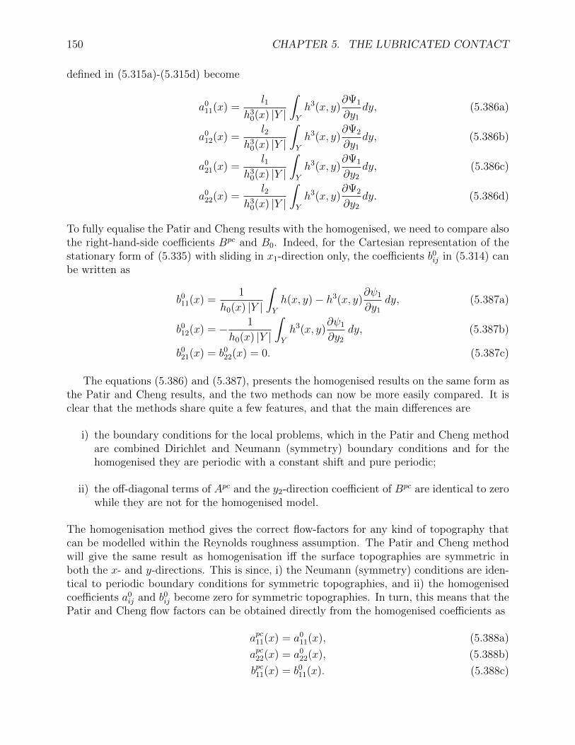
150 CHAPTER 5. THE LUBRICATED CONTACT
defined in (5.315a)-(5.315d) become
a011(x) =
l1h3
0(x) |Y |
∫Y
h3(x, y)∂Ψ1
∂y1
dy, (5.386a)
a012(x) =
l2h3
0(x) |Y |
∫Y
h3(x, y)∂Ψ2
∂y1
dy, (5.386b)
a021(x) =
l1h3
0(x) |Y |
∫Y
h3(x, y)∂Ψ1
∂y2
dy, (5.386c)
a022(x) =
l2h3
0(x) |Y |
∫Y
h3(x, y)∂Ψ2
∂y2
dy. (5.386d)
To fully equalise the Patir and Cheng results with the homogenised, we need to compare alsothe right-hand-side coefficients Bpc and B0. Indeed, for the Cartesian representation of thestationary form of (5.335) with sliding in x1-direction only, the coefficients b0
ij in (5.314) canbe written as
b011(x) =
1
h0(x) |Y |
∫Y
h(x, y)− h3(x, y)∂ψ1
∂y1
dy, (5.387a)
b012(x) = − 1
h0(x) |Y |
∫Y
h3(x, y)∂ψ1
∂y2
dy, (5.387b)
b021(x) = b0
22(x) = 0. (5.387c)
The equations (5.386) and (5.387), presents the homogenised results on the same form asthe Patir and Cheng results, and the two methods can now be more easily compared. It isclear that the methods share quite a few features, and that the main differences are
i) the boundary conditions for the local problems, which in the Patir and Cheng methodare combined Dirichlet and Neumann (symmetry) boundary conditions and for thehomogenised they are periodic with a constant shift and pure periodic;
ii) the off-diagonal terms of Apc and the y2-direction coefficient of Bpc are identical to zerowhile they are not for the homogenised model.
The homogenisation method gives the correct flow-factors for any kind of topography thatcan be modelled within the Reynolds roughness assumption. The Patir and Cheng methodwill give the same result as homogenisation iff the surface topographies are symmetric inboth the x- and y-directions. This is since, i) the Neumann (symmetry) conditions are iden-tical to periodic boundary conditions for symmetric topographies, and ii) the homogenisedcoefficients a0
ij and b0ij become zero for symmetric topographies. In turn, this means that the
Patir and Cheng flow factors can be obtained directly from the homogenised coefficients as
apc11(x) = a011(x), (5.388a)
apc22(x) = a022(x), (5.388b)
bpc11(x) = b011(x). (5.388c)

5.9. HOMOGENISATION OF THE REYNOLDS EQUATION 151
We note that φ1 ≡ apc11(x) and φ2 ≡ apc22(x) and that (5.388c) means that φpc0 (x) can beobtained from b0
11(x) in the following way
φpc0 (x) = b011(x)− 1
h0(x) |Y |
∫Y
h(x, y) dy.
Following the discussion above, the similarities and differences between the Patir andCheng method and homogenisation, are illustrated the figures 5.26-5.31. In Fig. 5.26, theχ1(y) of the local problem in (5.306c) in the homogenisation method, for the bi-sinusoidalsurface defined as
0.1 + 0.5 (1 + sin(2πx) sin(2πy)) , (5.390)
is depicted.
0 0.2 0.4 0.6 0.8 10
0.2
0.4
0.6
0.8
1
x
y
−0.2
0
0.2χ1
Figure 5.26: The solution χ1(y) of the local problem in (5.306c) in the homogenisation method.
Figure 5.27 depicts the solution of the local problem (5.379b) in the Patir and Cheng method,and the solution Ψ1(y) of the local problem in (5.385a) in the homogenisation method, forthe bi-sinusoidal surface defined in (5.390).
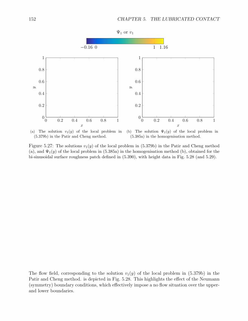
152 CHAPTER 5. THE LUBRICATED CONTACT
−0.16 0 1 1.16
Ψ1 or v1
0 0.2 0.4 0.6 0.8 10
0.2
0.4
0.6
0.8
1
x
y
(a) The solution v1(y) of the local problem in(5.379b) in the Patir and Cheng method.
0 0.2 0.4 0.6 0.8 10
0.2
0.4
0.6
0.8
1
xy
(b) The solution Ψ1(y) of the local problem in(5.385a) in the homogenisation method.
Figure 5.27: The solutions v1(y) of the local problem in (5.379b) in the Patir and Cheng method(a), and Ψ1(y) of the local problem in (5.385a) in the homogenisation method (b), obtained for thebi-sinusoidal surface roughness patch defined in (5.390), with height data in Fig. 5.28 (and 5.29).
The flow field, corresponding to the solution v1(y) of the local problem in (5.379b) in thePatir and Cheng method. is depicted in Fig. 5.28. This highlights the effect of the Neumann(symmetry) boundary conditions, which effectively impose a no flow situation over the upper-and lower boundaries.
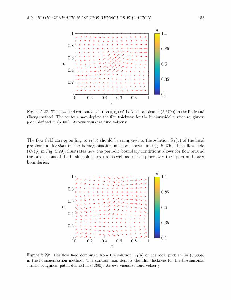
5.9. HOMOGENISATION OF THE REYNOLDS EQUATION 153
0 0.2 0.4 0.6 0.8 10
0.2
0.4
0.6
0.8
1
x
y
0.1
0.35
0.6
0.85
1.1h
Figure 5.28: The flow field computed solution v1(y) of the local problem in (5.379b) in the Patir andCheng method. The contour map depicts the film thickness for the bi-sinusoidal surface roughnesspatch defined in (5.390). Arrows visualize fluid velocity.
The flow field corresponding to v1(y) should be compared to the solution Ψ1(y) of the localproblem in (5.385a) in the homogenisation method, shown in Fig. 5.27b. This flow field(Ψ1(y) in Fig. 5.29), illustrates how the periodic boundary conditions allows for flow aroundthe protrusions of the bi-sinusoidal texture as well as to take place over the upper and lowerboundaries.
0 0.2 0.4 0.6 0.8 10
0.2
0.4
0.6
0.8
1
x
y
0.1
0.35
0.6
0.85
1.1h
Figure 5.29: The flow field computed from the solution Ψ1(y) of the local problem in (5.385a)in the homogenisation method. The contour map depicts the film thickness for the bi-sinusoidalsurface roughness patch defined in (5.390). Arrows visualize fluid velocity.
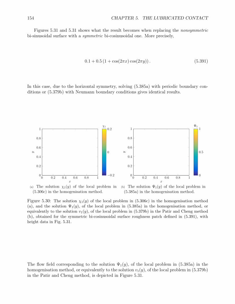
154 CHAPTER 5. THE LUBRICATED CONTACT
Figures 5.31 and 5.31 shows what the result becomes when replacing the nonsymmetricbi-sinusoidal surface with a symmetric bi-cosinusoidal one. More precisely,
0.1 + 0.5 (1 + cos(2πx) cos(2πy)) . (5.391)
In this case, due to the horizontal symmetry, solving (5.385a) with periodic boundary con-ditions or (5.379b) with Neumann boundary conditions gives identical results.
0 0.2 0.4 0.6 0.8 10
0.2
0.4
0.6
0.8
1
x
y
−0.2
0
0.2χ1
(a) The solution χ1(y) of the local problem in(5.306c) in the homogenisation method.
0 0.2 0.4 0.6 0.8 10
0.2
0.4
0.6
0.8
1
x
y
0
0.5
1Ψ1
(b) The solution Ψ1(y) of the local problem in(5.385a) in the homogenisation method.
Figure 5.30: The solution χ1(y) of the local problem in (5.306c) in the homogenisation method(a), and the solution Ψ1(y), of the local problem in (5.385a) in the homogenisation method, orequivalently to the solution v1(y), of the local problem in (5.379b) in the Patir and Cheng method(b), obtained for the symmetric bi-cosinusoidal surface roughness patch defined in (5.391), withheight data in Fig. 5.31.
The flow field corresponding to the solution Ψ1(y), of the local problem in (5.385a) in thehomogenisation method, or equivalently to the solution v1(y), of the local problem in (5.379b)in the Patir and Cheng method, is depicted in Figure 5.31.
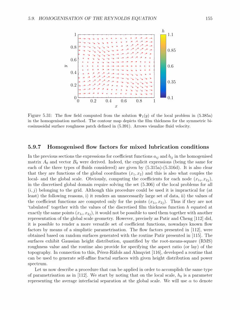
5.9. HOMOGENISATION OF THE REYNOLDS EQUATION 155
0 0.2 0.4 0.6 0.8 10
0.2
0.4
0.6
0.8
1
x
y
0.1
0.35
0.6
0.85
1.1h
Figure 5.31: The flow field computed from the solution Ψ1(y) of the local problem in (5.385a)in the homogenisation method. The contour map depicts the film thickness for the symmetric bi-cosinusoidal surface roughness patch defined in (5.391). Arrows visualize fluid velocity.
5.9.7 Homogenised flow factors for mixed lubrication conditions
In the previous sections the expressions for coefficient functions aij and bij in the homogenisedmatrix A0 and vector B0 were derived. Indeed, the explicit expressions (being the same foreach of the three types of fluids considered) are given by (5.315a)-(5.316d). It is also clearthat they are functions of the global coordinates (x1, x2) and this is also what couples thelocal- and the global scale. Obviously, computing the coefficients for each node (x1i, x2j),in the discretised global domain require solving the set (5.306) of the local problems for all(i, j) belonging to the grid. Although this procedure could be used it is impractical for (atleast) the following reasons, i) it renders an unnecessarily large set of data, ii) the values ofthe coefficient functions are computed only for the points (x1i, x2j). Thus if they are not‘tabulated’ together with the values of the discretised film thickness function h equated atexactly the same points (x1i, x2j), it would not be possible to used them together with anotherrepresentation of the global scale geometry. However, precisely as Patir and Cheng [112] did,it is possible to render a more versatile set of coefficient functions, nowadays known flowfactors by means of a simplistic parametrisation. The flow factors presented in [112], wereobtained based on random surfaces generated with the routine Patir presented in [115]. Thesurfaces exhibit Gaussian height distribution, quantified by the root-means-square (RMS)roughness value and the routine also provide for specifying the aspect ratio (or lay) of thetopography. In connection to this, Perez-Rafols and Almqvist [116], developed a routine thatcan be used to generate self-affine fractal surfaces with given height distribution and powerspectrum.
Let us now describe a procedure that can be applied in order to accomplish the same typeof parametrisation as in [112]. We start by noting that on the local scale, h0 is a parameterrepresenting the average interfacial separation at the global scale. We will use α to denote
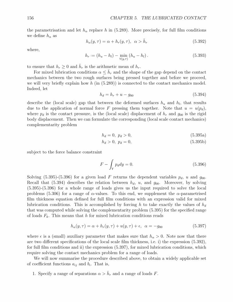
156 CHAPTER 5. THE LUBRICATED CONTACT
the parametrisation and let hα replace h in (5.289). More precisely, for full film conditionswe define hα as
hα(y, τ) = α + hr(y, τ), α > hr (5.392)
where,
hr ..= (hu − hl)− min∀(y,τ)
(hu − hl) . (5.393)
to ensure that hr ≥ 0 and hr is the arithmetic mean of hr.For mixed lubrication conditions α ≤ hr and the shape of the gap depend on the contact
mechanics between the two rough surfaces being pressed together and before we proceed,we will very briefly explain how h (in (5.289)) is connected to the contact mechanics model.Indeed, let
hd = hr + u− g00 (5.394)
describe the (local scale) gap that between the deformed surfaces hu and hl, that resultsdue to the application of normal force F pressing them together. Note that u = u(pd),where pd is the contact pressure, is the (local scale) displacement of hr and g00 is the rigidbody displacement. Then we can formulate the corresponding (local scale contact mechanics)complementarity problem
hd = 0, pd > 0, (5.395a)
hd > 0, pd = 0, (5.395b)
subject to the force balance constraint
F −∫Y
pddy = 0. (5.396)
Solving (5.395)-(5.396) for a given load F returns the dependent variables pd, u and g00.Recall that (5.394) describes the relation between hd, u, and g00. Moreover, by solving(5.395)-(5.396) for a whole range of loads gives us the input required to solve the localproblems (5.306) for a range of α-values. To this end, we supplement the α-parametrisedfilm thickness equation defined for full film conditions with an expression valid for mixedlubrication conditions. This is accomplished by forcing h to take exactly the values of hdthat was computed while solving the complementarity problem (5.395) for the specified rangeof loads Fk. This means that h for mixed lubrication conditions reads
hα(y, τ) = α + hr(y, τ) + u(y, τ) + ε, α = −g00 (5.397)
where ε is a (small) auxiliary parameter that makes sure that hα > 0. Note now that thereare two different specifications of the local scale film thickness, i.e. i) the expression (5.392),for full film conditions and ii) the expression (5.397), for mixed lubrication conditions, whichrequire solving the contact mechanics problem for a range of loads.
We will now summarise the procedure described above, to obtain a widely applicable setof coefficient functions aij and bi. That is,
1. Specify a range of separations α > hr and a range of loads F .

5.10. MODELLING MIXED LUBRICATION 157
2. Solve the complimentarity contact mechanics problem (5.395) for the specified rangeof loads F .
3. Solve the local problems (5.306) for the auxiliary film thickness descriptions (5.392)and (5.397) for the specified α-values (including the values of g00 obtained from thecontact mechanics model).
4. Compute the coefficient functions aij and bi for all the local problems obtained in theprevious steps.
5.10 Modelling mixed lubrication
A mixed lubrication model can be established by by a combination of a model governing thehydrodynamic contribution and a model that accounts for contact mechanics. One of thefirst examples of such a model was presented by Patir and Cheng in [112,113]. They derivedan averaged form of the Reynolds equation, in which the surface roughness was accounted forby means of what we know today as “flow factors”. Then, in order to simulate partial contactthey include the effect of surface roughness by comparing the average interfacial separation
h with the combined variance, σ =√Rq1
2 +Rq22, of any two digitised surface roughness
height descriptions, which full fill the assumptions for Reynolds equation to be valid on thelocal scale. Since the effect of roughness diminishes for large values of h/σ they focus theiranalysis to situations where h/σ < 3 and their work has been formed the starting point fora large number of similar contributions.
The model that Patir and Cheng presented in [112, 113] did not include a contact me-chanics model to account for local deformation of the contacting surfaces. This can e.g. beachieved by incorporating an asperity based contact model, which was also done by Rohdeet al. in [117]. More precisely, they combined the averaged Reynolds equation that Patir andCheng derived, with the model by Greenwood and Tripp [118] and considered cavitation bymeans of the half-Sommerfeld boundary condition. Bolander et al. [119] took this conceptfurther by replacing the half-Sommerfeld condition with cavitation algorithm proposed byElrod and Adams [19].
A mixed lubrication model based on the homogenised Reynolds equation was later pre-sented by Sahlin et al. [3, 11]. Indeed, this model combines half-space theory based contactmechanics of rough surfaces with the homogenised Reynolds equation in which the flow factorshas been obtained in the way described in Section 5.9.7. In addition, to make the method-ology even more versatile one can always generalise by transforming hα into dimensionlessform, i.e.
Hα = hα/href , (5.398)
where href is an appropriate reference parameter. The local problems (5.306c) and (5.306d)are invariant under this transformation, meaning that the solutions χ1 and χ2 will be the samefor any choice of href . The local problem (5.306a) is, however, not invariant and becomes
0 = ∇y ·(Aα∇yχ0
)−∇y · Bα in Y, (5.399)

158 CHAPTER 5. THE LUBRICATED CONTACT
where Aα and Bα indicates that they are transformed and where χ0 = h2refχ0. Moreover the
subscript also indicates that they are parametrised in α. This means that the homogenisedmatrix A0 and vector B0 transforms and their transformed correspondences should be com-puted from
Aα0 =x
Y
[aα11 aα12
aα21 aα22
](ei +∇yχi) dy (5.400a)
Bα0 =
x
Y
Bαe1 + Aα∇yχ0dy (5.400b)
(5.400c)
Before the homogenised solution u0 can be obtained the α-parametrised homogenised matrixAα0 and vector Bα
0 must be mapped onto Ω. This is achieved by interpolating Ah0(x1,x2)0 and
Bh0(x1,x2)0 for each point (x1, x2) in the global scale grid point. Thus
∇x ·(A0(x)∇xu0
)−∇x · B0(x) = 0, (5.401)
where u0 = h2refu0.
This closes the last section of this chapter and the authors thanks the readers for theattention.

Chapter 6
Modelling Wear in Lubrication
In mixed and boundary lubrication, there is contact and relative sliding between the surfaces.Because of this interaction between the surfaces, wear will occur. Wear is often defined asthe loss of material due to sliding, although there is no agreed clear definition and sometimesplastic deformation is included. What is clear, however, is that wear will result in a changeof the topography of the contacting bodies, involving features of contact size down to nano-scale. In turn, this will change the way in which a given machine element operates. It is thusimportant to understand why, when and how wear occurs, as well as to (if possible) be ableto reduce it. Wear is a school-book example of a multiphysics problem involving tribology,material science, chemistry, etc. Some aspects that are of importance are the temperatureincrease, fluid-solid interaction, growth and break down of oxide layers, strain hardening andadhesion [120], which makes it very difficult to isolate the effect of an individual parameter.Because of this multifaceted nature, acquiring the knowledge needed to come up with suitablesolutions require extensive studies on the topic. Moreover, reducing wear involves the capacityof predicting it, which is a very complex task requiring a lot of understanding, a great dealof intuition, and mathematical skills as well. This complexity has often led to a descriptiveand qualitative analysis of wear [120], in which the behaviour of a given experiment will beclassified according to a certain mechanism. Many such mechanisms can also be found in theliterature, and among these the abrasive-, adhesive- and corrosion types of wear are the onesmost frequently encountered. The multifaceted nature of wear and the multitude of physicsinvolved have lead to a variety of different empirical laws, which depend on a multitude ofparameters [121].
The intent with this compendium is not to analyse a lot of different existing types ofwear and the proposed ways to model them. In this chapter, we will instead (only) focus onadhesive- and abrasive wear, both which can modelled by means of Archard’s wear equation.We will start with Section 6.1, where we present a derivation of the form applicable to modeladhesive wear for a single asperity contact, then elaborate on how to generalise it so that itcan be applied to model adhesive wear between two rough surfaces. A similar presentationapplicable to abrasive wear will, thereafter, be presented Section 6.2. In Section 6.3, we closethis chapter by presenting a model for wear of rough surfaces, based on Archard’s equation,jointly with a discussion on its applicability.
159
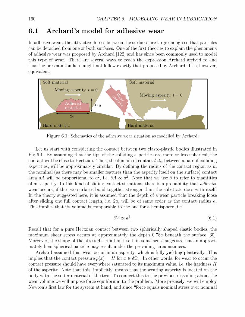
160 CHAPTER 6. MODELLING WEAR IN LUBRICATION
6.1 Archard’s model for adhesive wear
In adhesive wear, the attractive forces between the surfaces are large enough so that particlescan be detached from one or both surfaces. One of the first theories to explain the phenomenaof adhesive wear was proposed by Archard [122] and has since been commonly used to modelthis type of wear. There are several ways to reach the expression Archard arrived to andthus the presentation here might not follow exactly that proposed by Archard. It is, however,equivalent.
“
“Soft material
Moving asperity, t = 0
Adheredmaterial
2a
≈ a
Hard materialW
ear
particle
Soft material
Moving asperity, t = 0
Hard material
Figure 6.1: Schematics of the adhesive wear situation as modelled by Archard.
Let us start with considering the contact between two elasto-plastic bodies illustrated inFig 6.1. By assuming that the tips of the colliding asperities are more or less spherical, thecontact will be close to Hertzian. Thus, the domain of contact δΩc, between a pair of collidingasperities, will be approximately circular. By defining the radius of the contact region as a,the nominal (as there may be smaller features than the asperity itself on the surface) contactarea δA will be proportional to a2, i.e. δA ∝ a2. Note that we use δ to refer to quantitiesof an asperity. In this kind of sliding contact situations, there is a probability that adhesivewear occurs, if the two surfaces bond together stronger than the substrate does with itself.In the theory suggested here, it is assumed that the depth of a wear particle breaking looseafter sliding one full contact length, i.e. 2a, will be of same order as the contact radius a.This implies that its volume is comparable to the one for a hemisphere, i.e.
δV ∝ a3. (6.1)
Recall that for a pure Hertzian contact between two spherically shaped elastic bodies, themaximum shear stress occurs at approximately the depth 0.78a beneath the surface [30].Moreover, the shape of the stress distribution itself, in some sense suggests that an approxi-mately hemispherical particle may result under the prevailing circumstances.
Archard assumed that wear occur in an asperity, which is fully yielding plastically. Thisimplies that the contact pressure p(x) = H for x ∈ δΩc. In other words, for wear to occur thecontact pressure should have everywhere saturated to its maximum value, i.e. the hardness Hof the asperity. Note that this, implicitly, means that the wearing asperity is located on thebody with the softer material of the two. To connect this to the previous reasoning about thewear volume we will impose force equilibrium to the problem. More precisely, we will employNewton’s first law for the system at hand, and since “force equals nominal stress over nominal
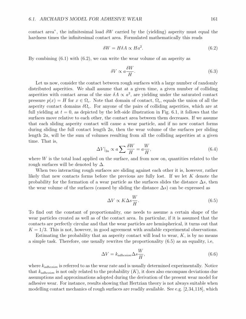
6.1. ARCHARD’S MODEL FOR ADHESIVE WEAR 161
contact area”, the infinitesimal load δW carried by the (yielding) asperity must equal thehardness times the infinitesimal contact area. Formulated mathematically this reads
δW = HδA ∝ Ha2. (6.2)
By combining (6.1) with (6.2), we can write the wear volume of an asperity as
δV ∝ aδW
H. (6.3)
Let us now, consider the contact between rough surfaces with a large number of randomlydistributed asperities. We shall assume that at a given time, a given number of collidingasperities with contact areas of the size δA ∝ a2, are yielding under the saturated contactpressure p(x) = H for x ∈ Ωc. Note that domain of contact, Ωc, equals the union of all theasperity contact domains δΩc. For anyone of the pairs of colliding asperities, which are atfull yielding at t = 0, as depicted by the left-side illustration in Fig. 6.1, it follows that thesurfaces move relative to each other, the contact area between them decreases. If we assumethat each sliding asperity contact will cause a wear particle, and if no new contact formsduring sliding the full contact length 2a, then the wear volume of the surfaces per slidinglength 2a, will be the sum of volumes resulting from all the colliding asperities at a giventime. That is,
∆V |2a ∝ a∑ δW
H= a
W
H, (6.4)
where W is the total load applied on the surface, and from now on, quantities related to therough surfaces will be denoted by ∆.
When two interacting rough surfaces are sliding against each other it is, however, ratherlikely that new contacts forms before the previous are fully lost. If we let K denote theprobability for the formation of a wear particle as the surfaces slides the distance ∆s, thenthe wear volume of the surfaces (caused by sliding the distance ∆s) can be expressed as
∆V ∝ K∆sW
H. (6.5)
To find out the constant of proportionality, one needs to assume a certain shape of thewear particles created as well as of the contact area. In particular, if it is assumed that thecontacts are perfectly circular and that the wear particles are hemispherical, it turns out thatK = 1/3. This is not, however, in good agreement with available experimental observations.
Estimating the probability that an asperity contact will lead to wear, K, is by no meansa simple task. Therefore, one usually rewrites the proportionality (6.5) as an equality, i.e,
∆V = kadhesion∆sW
H, (6.6)
where kadhesion is referred to as the wear rate and is usually determined experimentally. Noticethat kadhesion is not only related to the probability (K), it does also encompass deviations dueassumptions and approximations adopted during the derivation of the present wear model foradhesive wear. For instance, results showing that Hertzian theory is not always suitable whenmodelling contact mechanics of rough surfaces are readily available. See e.g. [2,34,118], which
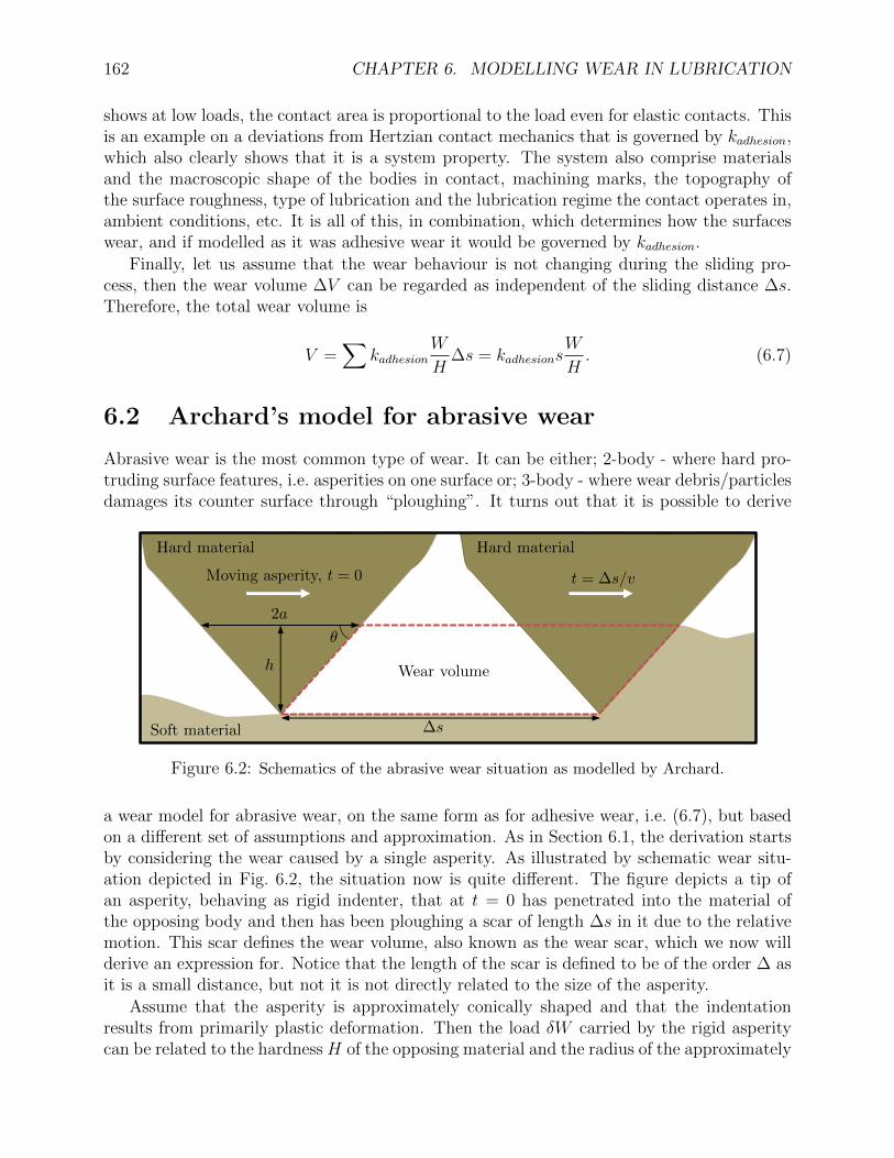
162 CHAPTER 6. MODELLING WEAR IN LUBRICATION
shows at low loads, the contact area is proportional to the load even for elastic contacts. Thisis an example on a deviations from Hertzian contact mechanics that is governed by kadhesion,which also clearly shows that it is a system property. The system also comprise materialsand the macroscopic shape of the bodies in contact, machining marks, the topography ofthe surface roughness, type of lubrication and the lubrication regime the contact operates in,ambient conditions, etc. It is all of this, in combination, which determines how the surfaceswear, and if modelled as it was adhesive wear it would be governed by kadhesion.
Finally, let us assume that the wear behaviour is not changing during the sliding pro-cess, then the wear volume ∆V can be regarded as independent of the sliding distance ∆s.Therefore, the total wear volume is
V =∑
kadhesionW
H∆s = kadhesions
W
H. (6.7)
6.2 Archard’s model for abrasive wear
Abrasive wear is the most common type of wear. It can be either; 2-body - where hard pro-truding surface features, i.e. asperities on one surface or; 3-body - where wear debris/particlesdamages its counter surface through “ploughing”. It turns out that it is possible to derive
Hard material
Moving asperity, t = 0
2a
h
θ
Soft material
Wear volume
∆s
Hard material
t = ∆s/v
Figure 6.2: Schematics of the abrasive wear situation as modelled by Archard.
a wear model for abrasive wear, on the same form as for adhesive wear, i.e. (6.7), but basedon a different set of assumptions and approximation. As in Section 6.1, the derivation startsby considering the wear caused by a single asperity. As illustrated by schematic wear situ-ation depicted in Fig. 6.2, the situation now is quite different. The figure depicts a tip ofan asperity, behaving as rigid indenter, that at t = 0 has penetrated into the material ofthe opposing body and then has been ploughing a scar of length ∆s in it due to the relativemotion. This scar defines the wear volume, also known as the wear scar, which we now willderive an expression for. Notice that the length of the scar is defined to be of the order ∆ asit is a small distance, but not it is not directly related to the size of the asperity.
Assume that the asperity is approximately conically shaped and that the indentationresults from primarily plastic deformation. Then the load δW carried by the rigid asperitycan be related to the hardness H of the opposing material and the radius of the approximately
6.3. A WEAR MODEL FOR ROUGH SURFACES 163
circular cross section. Indeed, precisely as it was done for in the case of adhesive wear in(6.2), the relation comes from imposing force balance, i.e.
δW ∝ Ha2 (6.8)
This implies that the wear volume, defined in the illustration depicted in Fig. 6.2, caused asthe asperity moves the distance ∆s, can be expressed as
δV ∝ a2 tan θ∆s = ∆s tan θδW
H. (6.9)
Let us now consider two rough surfaces, with a large number of randomly distributed as-perities, moving the distance ∆s relative to each other. It is realised that volumes δV (ofthe wear scars caused by the ploughing asperities), is not a deterministic but a stochasticproperty. Thus, the resulting wear volume can be expressed via
∆V =∑
δV ∝ ∆s tan θW
H. (6.10)
The assumptions and approximations employed have, again, resulted in a proportionality.To this end, a wear-rate parameter, this time denoted kabrasive, is introduced to encompasssystem related propertiesd and the wear volume due to the surfaces moving the distance ∆srelative to each other can be expressed as
∆V = kabrasive∆sW
H. (6.11)
Nota bene, as in the case of adhesive wear, the interpretation of kabrasive is far from trivialas it includes the combination of different effects related to roughness, material properties,etc. Therefore, it needs to be obtained by experimental analysis. Again, assuming that thewear behaviour remains the same during sliding we obtain the same type of Archard type ofequation for abrasive wear conditions, as we did for adhesive wear in (6.7). Indeed,
V = kabrasivesW
H. (6.12)
6.3 A wear model for rough surfaces
As touched upon in the beginning of this chapter, there are many causes for wear when twocontacting rough surfaces moves relative to one another, some of which can be modelled andsimulated. Indeed, different types of wear can and should be modelled by different means.Unfortunately, a particular wear model will only lead to accurate prediction for a limitedtype of wear conditions. This is also the case for the model we introduce here, which is alsonot the only one available. Therefore, although it has shown, e.g. by Furustig1 et al. [27,28],that it gives accurate predictions of wear in some situations, one must always ascertain thatthis is the case when applying it to the wear situation at hand. With this said, let us nowdescribe the model.
1Previously Andersson and also known as The Wear Doctor (Notningsdoktorn).
164 CHAPTER 6. MODELLING WEAR IN LUBRICATION
The model is based on Archard’s equation and it utilises the enhanced variational principlebased contact mechanics solver, including plastic deformation that we presented in Chapter 4.In the modelling strategy adopted here, a variant of the Archard equation is derived andapplied locally, i.e. to compute the wear depth for each element (i, j) of the discretisedsolution domain. More precisely, the form of the Archard equation that will be derived here,is described in terms of wear depth caused by the contacting surfaces moving a small distancewhile carrying the load that the element is subjected to.
Let us start this derivation by applying the same type of Archard’s equation, that wederived for adhesive- (6.7) and abrasive wear (6.12) to each element of the solution domain.An element-wise application means that we consider the wear volume ∆V ij, caused by thecontacting surfaces moving a distance ∆s under the load wij, which the element is subjectedto, i.e.
∆V ij = k∆swij, (6.13)
where we have included 1/H into k for simplicity. In this equation, ∆V is the dependentvariable, w may be considered as an independent variable, while k is a direct input and∆s is derived from the inputs v and ∆t. The local load wij is determined by the pressuredistribution obtained by solving the contact mechanics problem presented in Chapter 4, i.e.
wij = pij∆Aij, (6.14)
where ∆Aij = ∆x1∆x2 is the area of the element. Now, since this wear volume correspondsto material loss over rectangular elements, it can be expressed in terms of wear depth ∆hij.Indeed
∆V ij = ∆hij∆Aij, (6.15)
Combining (6.14) and (6.15) with the element-wise applied Archard’s equation,(6.13), wehave derived an equation for the wear depth, viz.
∆hij = k∆spij, (6.16)
Since the plastic deformation is part of the solution to the contact mechanics problem (4.92)it may also be incorporated in the wear model, which then become
∆hij = k∆spij + upij. (6.17)
If the time step ∆t is sufficiently small to consider p as a constant, while the surfaces movesthe distance ∆s relatively to one another, this equation can be applied to numerically simulatethe wear.
An overview of the solution procedure adopted here is depicted in Fig. 6.3, which is alsobriefly described in the following. Starting at time t = 0, the relative position between thetwo surfaces is known. With the surfaces in this position, the pressure distribution and theplastic deformation can be obtained by solving the contact mechanics model in accordancewith the numerical solution procedure presented in Fig. 4.17. Then, (6.17) can be used tocompute the wear depth at each point. By removing ∆hij from the topography of the surfacewith lower hardness, we have obtained a quantitative estimation of the wear process so far.The relative position of the surfaces is shifted a distance ∆s. Time is now ∆t and with the
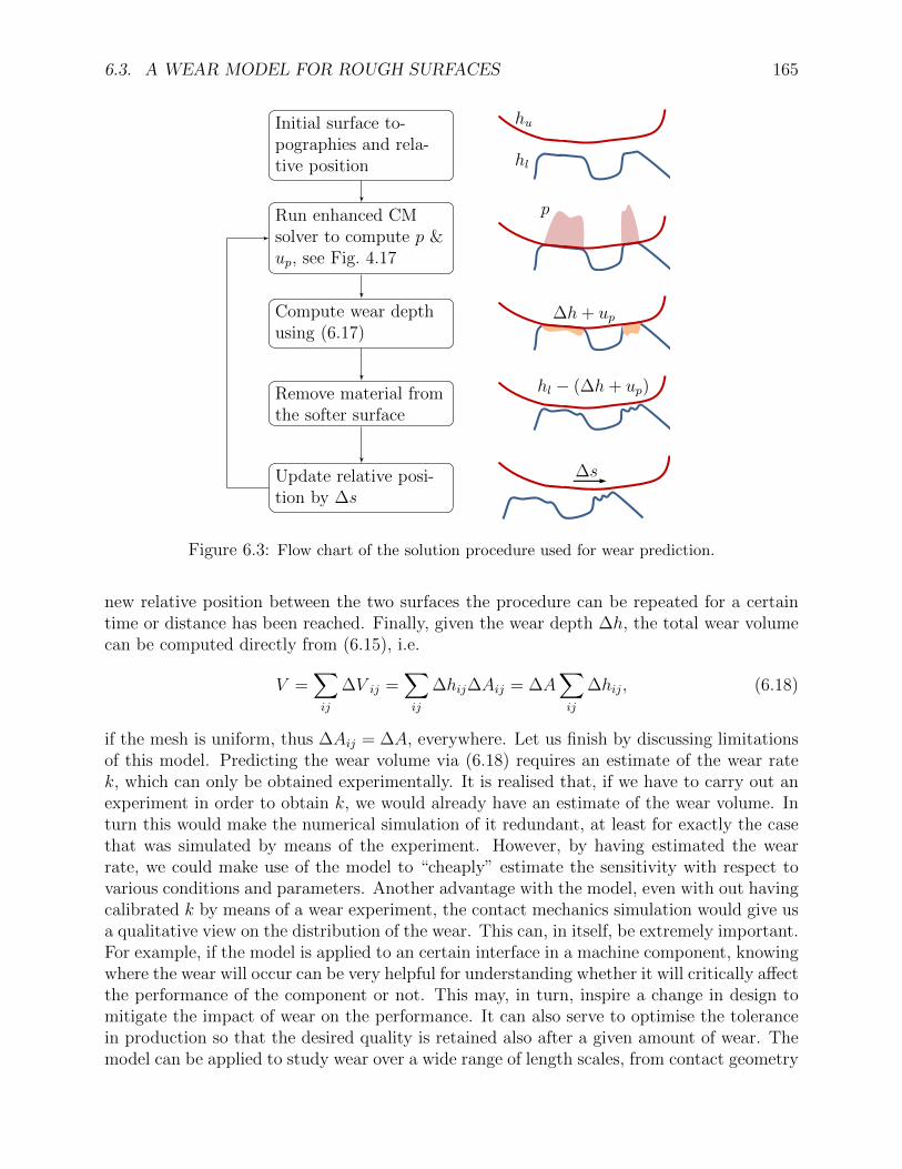
6.3. A WEAR MODEL FOR ROUGH SURFACES 165
hu
hl
Initial surface to-pographies and rela-tive position
pRun enhanced CMsolver to compute p &up, see Fig. 4.17
∆h+ upCompute wear depthusing (6.17)
hl − (∆h+ up)Remove material fromthe softer surface
∆sUpdate relative posi-tion by ∆s
Figure 6.3: Flow chart of the solution procedure used for wear prediction.
new relative position between the two surfaces the procedure can be repeated for a certaintime or distance has been reached. Finally, given the wear depth ∆h, the total wear volumecan be computed directly from (6.15), i.e.
V =∑ij
∆V ij =∑ij
∆hij∆Aij = ∆A∑ij
∆hij, (6.18)
if the mesh is uniform, thus ∆Aij = ∆A, everywhere. Let us finish by discussing limitationsof this model. Predicting the wear volume via (6.18) requires an estimate of the wear ratek, which can only be obtained experimentally. It is realised that, if we have to carry out anexperiment in order to obtain k, we would already have an estimate of the wear volume. Inturn this would make the numerical simulation of it redundant, at least for exactly the casethat was simulated by means of the experiment. However, by having estimated the wearrate, we could make use of the model to “cheaply” estimate the sensitivity with respect tovarious conditions and parameters. Another advantage with the model, even with out havingcalibrated k by means of a wear experiment, the contact mechanics simulation would give usa qualitative view on the distribution of the wear. This can, in itself, be extremely important.For example, if the model is applied to an certain interface in a machine component, knowingwhere the wear will occur can be very helpful for understanding whether it will critically affectthe performance of the component or not. This may, in turn, inspire a change in design tomitigate the impact of wear on the performance. It can also serve to optimise the tolerancein production so that the desired quality is retained also after a given amount of wear. Themodel can be applied to study wear over a wide range of length scales, from contact geometry

166 CHAPTER 6. MODELLING WEAR IN LUBRICATION
down to individual asperities. Thus it may be used to provide insight on the evolution ofwear in a large range of application including seals, bearings, gears, etc.
A second limitation concerns the type of wear that can be modelled. In 6.1, we presenteda derivation of the Archard’s equation for adhesive wear. The derivation lead to the equation(6.7), for the wear volume of a rough surface, including many things in the wear rate param-eter. In particular, it includes the probability for the formation of a wear particle K as thesurfaces slides the distance ∆s. This means that the wear volume should be regarded is inan average sense, suggesting that the model applies well to an interface between two roughsurfaces as the roughness is a random process. When applying the model for rough surfaces,based on (6.17), which we just have described, then the time step needs to be sufficientlysmall for the pressure not to vary notably. This is contradictory, since it cannot be reconciledwith the assumption of a large particle being removed at a time, suggesting a limited capacityof predicting wear under adhesive conditions. In fact, it can easily be seen that in the caseof a rough surfaces sliding against a harder, smoother one, (6.16) will lead, in general, tothe smoothing of the softer surface [27]. Thus, it is clear that the model is more suitablefor modelling wear of“polishing” type, which normally belongs to the category of abrasivewear.
Bibliography
[1] X. Tian and B. Bhushan. A numerical three-dimensional model for the contact of roughsurfaces by variational principle. Journal of Tribology, 118(1):33–42, 1996.
[2] A. Almqvist, F. Sahlin, R. Larsson, and S. Glavatskih. On the dry elasto-plastic contactof nominally flat surfaces. Tribology International, 40(4):574 – 579, 2007.
[3] F. Sahlin, R. Larsson, P. Marklund, P. M. Lugt, and A. Almqvist. A mixed lubrica-tion model incorporating measured surface topography. part 1: theory of flow factors.Proceedings of the Institution of Mechanical Engineers, Part J: Journal of EngineeringTribology, 224(4):335–351, 2010.
[4] S. Liu, Q. Wang, and G. Liu. A versatile method of discrete convolution and FFT(DC-FFT) for contact analyses. Wear, 243(1-2):101 – 11, 2000.
[5] W.-Z. Wang, H. Wang, Y.-C. Liu, Y.-Z. Hu, and D. Zhu. A comparative study of themethods for calculation of surface elastic deformation. Proceedings of the Institutionof Mechanical Engineers, Part J: Journal of Engineering Tribology, 217(2):145 – 154,2003.
[6] Shuangbiao Liu, Diann Hua, W. Wayne Chen, and Q. Jane Wang. Tribological model-ing: Application of fast Fourier transform. Tribology International, 40(8):1284 – 1293,2007.
[7] H. P. Evans, C. D. Elcoate, T. G. Hughes, and R. W. Snidle. Transient elastohydrody-namic analysis of rough surfaces using a novel coupled differential deflection method.Proc Instn Mech Engrs, Part J, 215:319–337, 2001.
[8] P. L. Fackler and M. J. Miranda.
[9] J. J. Kalker. Variational Principles of Contact Elastostatics. IMA J Appl Math,20(2):199–219, 1977.
[10] H. M. Stanley and T. Kato. FFT-based method for rough surface contact. Journal ofTribology, Transactions of the ASME, 119(3):481 – 485, 1997.
[11] F. Sahlin, R. Larsson, P. Marklund, P. M. Lugt, and A. Almqvist. A mixed lubricationmodel incorporating measured surface topography. part 2: roughness treatment, modelvalidation, and simulation. Proceedings of the Institution of Mechanical Engineers, PartJ: Journal of Engineering Tribology, 224(4):353–365, 2010.
167

168 BIBLIOGRAPHY
[12] A. Almqvist, E. Burtseva, F. Perez-Rafols, and P. Wall. New insights on lubrication the-ory for compressible fluids. International Journal of Engineering Science, 145:103170,2019.
[13] A. Almqvist, E. Burtseva, K. Rajagopal, and P. Wall. On lower-dimensional modelsin lubrication, part a: Common misinterpretations and incorrect usage of the reynoldsequation. Proceedings of the Institution of Mechanical Engineers, Part J: Journal ofEngineering Tribology, 235(8):1692–1702, dec 2020.
[14] A. Almqvist, E. Burtseva, K. Rajagopal, and P. Wall. On lower-dimensional modelsin lubrication, part b: Derivation of a reynolds type of equation for incompressiblepiezo-viscous fluids. Proceedings of the Institution of Mechanical Engineers, Part J:Journal of Engineering Tribology, 235(8):1703–1718, dec 2020.
[15] B. Jakobsson and L. Floberg. The Finite Journal Bearing, Considering Vaporization.Technical Report 190, Institute of Machine Elements, Chalmers University of Technol-ogy, Gothenburg, Sweden, 1957.
[16] L. Floberg. The Two-Groove Journal Bearing, considering Cavitation. Technical Report231, Institute of Machine Elements, Chalmers University of Technology, Gothenburg,Sweden, 1960.
[17] L. Floberg. Lubrication of two cylinder surfaces, considering cavitation. Technical Re-port 232, Institute of Machine Elements, Chalmers University of Technology, Gothen-burg, Sweden, 1961.
[18] K.-O. Olsson. Cavitation in dynamically loaded bearings. Technical Report 308, In-stitute of Machine Elements, Chalmers University of Technology, Gothenburg, Sweden,1965.
[19] H. G. Elrod and M. L. Adams. A computer program for cavitation and starvationproblems. In D. Dowson, M. Godet, and C. M. Taylor, editors, Cavitation and relatedphenomena in lubrication, Mechanical Engineering Publications, pages 37–43, London,1975.
[20] M. Giacopini, M. T. Fowell, D. Dini, and A. Strozzi. A mass-conserving complemen-tarity formulation to study lubricant films in the presence of cavitation. Journal ofTribology, 132(4):041702, 2010.
[21] A. Almqvist, J. Fabricius, R. Larsson, and P. Wall. A new approach for studyingcavitation in lubrication. Journal of Tribology, 136(1):011706–1 – 011706–6, 2014.
[22] G. Bayada. From a compressible fluid model to new mass conserving cavitation algo-rithms. Tribology International, 71(0):38 – 49, 2014.
[23] L. Bertocchi, D. Dini, M. Giacopini, M. T. Fowell, and A. Baldini. Fluid film lubri-cation in the presence of cavitation: a mass-conserving two-dimensional formulationfor compressible, piezoviscous and non-Newtonian fluidsbaya. Tribology International,67:61 –71, Nov 2013.
BIBLIOGRAPHY 169
[24] A. Almqvist and P. Wall. Modelling cavitation in (elasto)hydrodynamic lubrication. InPranav H. Darji, editor, Advances in Tribology, chapter 9. IntechOpen, Rijeka, 2016.
[25] A Almqvist. On the Effects of Surface Roughness in Lubrication. PhD thesis,LuleaUniversity of Technology, Department of Applied Physics and Mechanical En-gineering, Division of Machine Elements, Lulea, Sweden, Sep 2006.
[26] A. Almqvist and P. Wall. Homogenization of the reynolds equation. In Q. J. Wangand Y.-W. Chung, editors, Encyclopedia of Tribology, pages 1685–1690. Springer US,Boston, MA, 2013.
[27] J. Andersson and R. Almqvist, A.and Larsson. Numerical simulation of a wear exper-iment. Wear, 271(11-12):2947–2952, 2011.
[28] J. Furustig. Semi-Determinsitic Numerical Simulations of Wear on Various Scales:From Chemo-Mechanical Effects to the Wear of Components in Orbital Type HydraulicMotors. PhD thesis, LuleaUniversity of Technology, Machine Elements, 2014.
[29] A. Almqvist, C. Campana, N. Prodanov, and B. N. J. Persson. Interfacial separationbetween elastic solids with randomly rough surfaces: Comparison between theory andnumerical techniques. Journal of the Mechanics and Physics of Solids, 59(11):2355–2369, 2011.
[30] K. L. Johnson. Contact Mechanics. Cambridge University Press, Cambridge, UK, 1984.
[31] M. Shirzadegan, A. Almqvist, and R. Larsson. Fully coupled ehl model for simulationof finite length line cam-roller follower contacts. Tribology International, 103:584–598,2016.
[32] T. Hultqvist, M. Shirzadegan, A. Vrcek, Y. Baubet, B. Prakash, P. Marklund, andR. Larsson. Elastohydrodynamic lubrication for the finite line contact under transientloading conditions. Tribology International, 127:489–499, 2018.
[33] H. Hertz. Uber die beruhrung fester elastischer korper (on the ccontact of elastic solids).J. Reine und angewandte Mathematik, 92:156–171, 1882.
[34] K.L. Johnson, J.A. Greenwood, and J.G. Higginson. The contact of elastic regular wavysurfaces. International Journal of Mechanical Sciences, 27(6):383–396, 1985. cited By(since 1996) 65.
[35] H. M. Westergaard. Bearing pressure and cracks. ASME Journal of Applied Mechanics,6:49–53, 1939.
[36] V.A. Yastrebov, G. Anciaux, and J.-F. Molinari. The contact of elastic regular wavysurfaces revisited. Tribology Letters, 56(1):171–183, 2014.
[37] C. Putignano, L. Afferrante, G. Carbone, and G. Demelio. A new efficient numericalmethod for contact mechanics of rough surfaces. International Journal of Solids andStructures, 49(2):338–343, January 2012.
170 BIBLIOGRAPHY
[38] A.E.H. Love. Stress produced in a semi-infinite solid by pressure on part of the bound-ary. Philosophical Transactions of the Royal Society of London, 377:54–59, 1929.
[39] R. W. Cottle, J. S. Pang, and R.E. Stone. The Linear Complementarity Problem.Report No. 60, SIAM, Philadelphia, PA., 2009.
[40] Y. Ju and T.N. Farris. Spectral analysis of two-dimensional contact problems. Trans-actions of the ASME. Journal of Tribology, 118(2):320 – 8, 1996.
[41] Shuangbiao Liu and Qian Wang. Studying contact stress fields caused by surfacetractions with a discrete convolution and fast fourier transform algorithm. Transactionsof the ASME, 124:36–45, 2002.
[42] I.A. Polonsky and L.M. Keer. A numerical method for solving rough contact problemsbased on the multi-level multi-summation and conjugate gradient techniques. Wear,231(2):206 – 19, 1999.
[43] A. Tiwari, A. Almqvist, and B. N. J. Persson. Plastic deformation of rough metallicsurfaces. Tribology Letters, 68(4), nov 2020.
[44] O. Reynolds. On the theory of lubrication and its application to Mr. Beauchampstower’s experiments, including an experimental determination of the viscosity of oliveoil. Philosophical Transactions of the Royal Society of London A, 177:157–234, 1886.
[45] A.I. Vakis, V.A. Yastrebov, J. Scheibert, L. Nicola, D. Dini, C. Minfray, A. Almqvist,M. Paggi, S. Lee, G. Limbert, J.F. Molinari, G. Anciaux, R. Aghababaei, S. Echev-erri Restrepo, A. Papangelo, A. Cammarata, P. Nicolini, C. Putignano, G. Carbone,S. Stupkiewicz, J. Lengiewicz, G. Costagliola, F. Bosia, R. Guarino, N.M. Pugno,M.H. Muser, and M. Ciavarella. Modeling and simulation in tribology across scales:An overview. Tribology International, 2018.
[46] J. Fabricius, Y. O. Koroleva, and P. Wall. A rigorous derivation of the time-dependentreynolds equation. Asymptotic Analysis, 84:103–121, 2014.
[47] C. L. M. H. Navier. Sur les lois du mouvement des fluids, en ayant egard a l’adhesiondes molecules. Annalen der Chemie, 19:244–260, 1821.
[48] S. D. Poisson. Memoire sur les e’quations ge’ne’rales de l’equilibre et du mouvementdes corps solides elastiques et des fuides. Journal de l’Ecole Polytechnique, 13(1–174),1831.
[49] G. G. Stokes. On the theories of the internal friction of fluids in motion, and of theequilibrium and motion of elastic solids. Trans. Camb. Phil. Soc., 8:287–305, 1845.
[50] L. N. Liebermann. The Second Viscosity of Liquids. Physical Review, 75(9):1415–1422,May 1949.

BIBLIOGRAPHY 171
[51] Louis Rosenhead. Introduction - The second coefficient of viscosity: a briefreview of fundamentals. Proceedings of the Royal Society of London. Se-ries A. Mathematical and Physical Sciences, 226(1164):1–6, 1954. eprint:https://royalsocietypublishing.org/doi/pdf/10.1098/rspa.1954.0224.
[52] Rick E. Graves and Brian M. Argrow. Bulk Viscosity: Past to Present. Journal ofThermophysics and Heat Transfer, 13(3):337–342, July 1999.
[53] Frederike Jaeger, Omar K. Matar, and Erich A. Muller. Bulk viscosity of molecularfluids. The Journal of Chemical Physics, 148(17):174504, May 2018.
[54] O. Reynolds. On the theory of lubrication and its application to Mr. BeauchampsTower’s experiments, including an experimental determination of the viscosity of oliveoil. Proc. R. Soc. Lond., 40(242-245):191–203, 1886.
[55] Martin Greenspan. Attenuation of Sound in Rarefied Helium. Physical Review,75(1):197–198, January 1949.
[56] Martin Greenspan. Propagation of Sound in Rarefied Helium. The Journal of theAcoustical Society of America, 22(5):568–571, September 1950.
[57] Jordan J. Markham, Robert T. Beyer, and R. B. Lindsay. Absorption of Sound inFluids. Reviews of Modern Physics, 23(4):353–411, October 1951.
[58] G. G. Stokes. On the effect of internal friction of fluids on the motion pendulums.Trans. Cambridge Philos. Soc., 9:8–106, 1851.
[59] K. R. Rajagopal. A new development and interpretation of the Navier–Stokes fluidwhich reveals why the “Stokes assumption” is inapt. Int. J. Non-Linear Mech., 50:141–151, 2013.
[60] G. Buresti. A note on Stokes’ hypothesis. Acta Mech., 226:3555–3559, 2015.
[61] K. R. Rajagopal. Remarks on the notion of “pressure”. Int. J. Non-Linear Mech.,71:165–172, 2015.
[62] K. R. Rajagopal. On implicit constitutive theories. Appl. Math., 48(4):279–319, 2003.
[63] K. R. Rajagopal. On implicit constitutive theories for fluids. J. Fluid Mech., 550:243–249, 2006.
[64] D. Dowson and G. R. Higginson. Elasto-hydrodynamic lubrication: The fundamentalsof roller or gear lubrication. Pergamon Press, Oxford, 1966.
[65] C. Barus. Isotherms, isopiestics and isometrics relative to viscosity. Am. Jour. Sci.,45(266):87–96, 1893.
[66] B. J. Hamrock. Fundamentals of Fluid Film Lubrication. McGraw-Hill, Inc, New York,1994.

172 BIBLIOGRAPHY
[67] K. R. Rajagopal and A. Z. Szeri. On an inconsistency in the derivation of the equationsof elastohydrodynamic lubrication. Proceedings of the Royal Society of London. SeriesA: Mathematical, Physical and Engineering Sciences, 459(2039):2771–2786, 2003.
[68] G. Bayada, B. Cid, G. Garcıa, and C. Vazquez. A new more consistent Reynolds modelfor piezoviscous hydrodynamic lubrication problems in line contact devices. AppliedMathematical Modelling, 37(18-19):8505–8517, 2013.
[69] T. Gustafsson, K. R. Rajagopal, R. Stenberg, and J. Videman. Nonlinear Reynoldsequation for hydrodynamic lubrication. Applied Mathematical Modelling, 39(17):5299– 5309, 2015.
[70] C. J. A. Roelands. Correlational aspects of the viscosity- temperature-pressure relation-ship of lubricating oils. PhD thesis, Delft University of Technology, TU Delft, 1966.
[71] F. Perez-Rafols, P. Wall, and A. Almqvist. On compressible and piezo-viscous flowin thin porous media. Proceedings of the Royal Society of London A: Mathematical,Physical and Engineering Sciences, 474(2209), 2018.
[72] J. H. Hyde. On the viscosities and compressibilities of liquids at high pressures. Pro-ceedings of the Royal Society of London. Series A, Containing Papers of a Mathematicaland Physical Character, 97(684):240–259, may 1920.
[73] P. W. Bridgman. The effect of pressure on the viscosity of forty-three pure liquids.Proceedings of the American Academy of Arts and Sciences, 61(3):57–99, 1926.
[74] M. D. Hersey. A short account of the theory of lubrication. I. Introduction; viscosityand friction. J. Franklin Inst., 219(6):677–702, 1935.
[75] K.R. Rajagopal. On the cavalier attitude towards referencing. International Journalof Engineering Science, 51:338–343, feb 2012.
[76] H. A. Spikes. Sixty years of EHL. Lubrication Science, 18(4):265–291, 2006.
[77] P. M. Lugt and G. E. Morales-Espejel. A review of elasto-hydrodynamic lubricationtheory. Tribol. Trans., 54(3):470–496, 2011.
[78] R. Larsson. EHL governing equations. In Q. J. Wang and Y.-W. Chung, editors,Encyclopedia of Tribology, pages 827–832. Springer US, Boston, MA, 2013.
[79] J. A. Greenwood. Elastohydrodynamic lubrication. Lubricants, 8(5):51, 2020.
[80] D. Dowson and G. R. Higginson. Elasto-Hydrodynamic Lubrication. Pergamon, Oxford,UK, 1977.
[81] B. J. Hamrock, S. R. Schmid, and B. O. Jacobson. Fundamentals of Fluid Film Lubri-cation. Marcel Dekker Inc, New York, 2nd edition, 2004.
[82] C. H. Venner and A. A. Lubrecht. Multilevel Methods in Lubrication. Tribology Series37, 2000.

BIBLIOGRAPHY 173
[83] B. Bhushan. Principles and applications of tribology. Wiley, Chichester, West Sussex,UK, 2013.
[84] Mhammed Elgadari and Hajjam Mohamed. About the Inverse Theory and the Non-Unicity of the Film Thickness: Novel Approach Generating Equivalent Micro-Groovesand Roughness. preprint, In Review, February 2021.
[85] H. G. Elrod and J. T. McCabe. An analysis of the side-leakage effect in high-speed gaslubricated slider and partial arc bearings, 1967.
[86] G. L. Agrawal. Foil air/gas bearing technology – an overview. ASME Digital collectionTurbo Expo: Power for Land, Sea, and Air, page V001T04A006, 1997.
[87] H. G. Elrod. A Cavitation Algorithm. Journal of Tribology, 103:350–354, 1981.
[88] D. Vijayaraghavan and T. G. Keith Jr. Development and evaluation of a cavitationalgorithm. STLE Tribology Transactions, 32(2):225–233, 1989.
[89] D. Vijayaraghavan and T. G. Keith Jr. An efficient, robust, and time accurate numericalscheme applied to a cavitation algorithm. Journal of Tribology, Transactions of theASME, 112(1):44–51, Jan 1990.
[90] F. Sahlin, A. Almqvist, R. Larsson, and S. Glavatskih. A cavitation algorithm forarbitrary lubricant compressibility. Tribology International, 40(8):1294–1300, 2007.
[91] C. M. Woods and D. E. Brewe. The solution of the Elrod algorithm for a dynamicallyloaded journal bearing using multigrid techniques. Journal of Tribology, 111(2):302–308, 04 1989.
[92] M. Boukrouche and G. Bayada. Mathematical model. existence and uniqueness ofcavitation problems in porous journal bearing. Nonlinear Analysis: Theory, Methods& Applications, 20(8):895–920, 1993.
[93] R. F. Ausas, M. Jai, and G. C. Buscaglia. A mass-conserving algorithm for dynamicallubrication problems with cavitation. Journal of Tribology, 131(3):031702, 2009.
[94] G. Bayada, S. Martin, and C. Vazquez. Two-scale homogenization of a hydrodynamicElrod-Adams model. Asymptotic Analysis, 44:75–110, 2005.
[95] A. Almqvist, A. Spencer, and P. Wall. Matlab routines solving a linear complementarityproblem appearing in lubrication with cavitation, 2013.
[96] A. V. Olver, M. T. Fowell, H. A. Spikes, and I. G. Pegg. ’inlet suction’, a load sup-port mechanism in non-convergent, pocketed, hydrodynamic bearings. Proceedingsof the Institution of Mechanical Engineers, Part J: Journal of Engineering Tribology,220(2):105–108, 2006.
[97] M. Fowell, A. V. Olver, A. D. Gosman, H. A. Spikes, and I. Pegg. Entrainment and inletsuction: Two mechanisms of hydrodynamic lubrication in textured bearings. Journalof Tribology, 129(2):336–347, 2007.

174 BIBLIOGRAPHY
[98] L. C. Evans. Partial Differential Equations, volume 19 of Graduate studies in Mathe-matics. American Mathematical Society, Providence, Rhode Island, 2 edition, 2010.
[99] M. Soderfjall, A. Almqvist, and R. Larsson. A model for twin land oil control rings.Tribology International, 95:475 – 482, 2016.
[100] M. Soderfjall, R. Larsson, P. Marklund, and A. Almqvist. Texture-induced effects caus-ing reduction of friction in mixed lubrication for twin land oil control rings. Proceedingsof the Institution of Mechanical Engineers, Part J: Journal of Engineering Tribology,232(2):166–178, 2018.
[101] G. de Boer and A. Almqvist. On the two-scale modelling of elastohydrodynamic lubri-cation in tilted-pad bearings. Lubricants, 6(3), 2018.
[102] G. Bayada and M. Chambat. New models in the theory of the hydrodynamic lubricationof rough surfaces. Journal of Tribology, Transactions of the ASME, 110(3):402 – 407,1988.
[103] G. Bayada, S. Martin, and C. Vazquez. An average flow model of the reynolds roughnessincluding a mass-flow preserving cavitation model. Journal of Tribology, 127(4):793–802, 2005.
[104] A. Almqvist and J. Dasht. The homogenization process of the Reynolds equationdescribing compressible liquid flow. Tribology International, 39(9):994–1002, 2006.
[105] P. Wall. Homogenization of Reynolds equation by two-scale convergence. ChineseAnnals of Mathematics - Series B, 28(3):363–374, 2007.
[106] A. Almqvist, E. K. Essel, L.-E. Persson, and P. Wall. Homogenization of the unsta-tionary incompressible Reynolds equation. Tribology International, 40(9):1344–1350,2007.
[107] D. Lukkassen, A. Meidell, and P. Wall. Homogenization of some variational problemsconnected to the theory of lubrication. International Journal of Engineering Science,47(1):153–162, 2009.
[108] A. Almqvist. Homogenization of the reynolds equation governing hydrodynamic flowin a rotating device. Journal of Tribology, 133(2):021705–1–021705–8, 2011.
[109] A. Almqvist, J. Fabricius, and P. Wall. Homogenization of a reynolds equation describ-ing compressible flow. Journal of Mathematical Analysis and Applications, 390(2):456– 471, 2012.
[110] G Nguetseng, D Lukkassen, and P Wall. Two-scale convergence. International Journalof Pure and Applied Mathematics, 2(1):35–86, 2002.
[111] D. Cioranescu and P. Donato. An introduction to homogenization, volume 17 of OxfordLecture Series in Mathematics and its Applications. Oxford University Press, NewYork, 1999.

BIBLIOGRAPHY 175
[112] N. Patir and H. S. Cheng. An Average Flow Model for Determining Effects of Three-Dimensional Roughness on partial Hydrodynamic Lubrication. Journal of Tribology,Transactions of the ASME, 100:12–17, 1978.
[113] N. Patir and H. S. Cheng. Application of Average Flow Model to Lubrication BetweenRough Sliding Surfaces. Journal of Tribology, Transactions of the ASME, 101:220–230,1979.
[114] A. Almqvist, J. Fabricius, A. Spencer, and P. Wall. Similarities and differences betweenthe flow factor method by patir and cheng and homogenization. Journal of Tribology,133(3):031702, 2011.
[115] N. Patir. A numerical procedure for random generation of rough surfaces. Wear,47(2):263 – 77, 1978.
[116] F. Perez-Rafols and A. Almqvist. Generating randomly rough surfaces with givenheight probability distribution and power spectrum. Tribology International, 131:591 –604, 2019.
[117] S. M. Rodhe, K. W. Whitaker, and G. T. McAllister. A mixed friction model fordynamically loaded contacts with application to piston ring lubrication. In Surfaceroughness effects in hydrodynamic and mixed lubrication. ASME Winter Annual Meet-ing, Chicago, pages 19–50, 1980.
[118] J. A. Greenwood and J. H. Tripp. The contact of two nominally flat rough surfaces.Proceedings of the Institution of Mechanical Engineers, 185(48):625 – 33, 1970.
[119] N. W. Bolander, B. D. Steenwyk, F Sadeghi, and G. R. Gerber. Lubrication regimetransitions at the piston ring-cylinder liner interface. Proceedings of the Institution ofMechanical Engineers, Part J: Journal of Engineering Tribology, 219(1):19–31, 2005.
[120] K. C. Ludema. Friction, wear, lubrication: a textbook in tribology. Boca Raton, Fla.:CRC Press, cop., 1996.
[121] H.C. Meng and K.C. Ludema. Wear models and predictive equations: their form andcontent. Wear, 181-183(PART 2):443–457, 1995.
[122] J. F. Archard. Contact and rubbing of flat surfaces. Journal of Applied Physics,24(8):981–988, August 1953.

176 BIBLIOGRAPHY
Appendix A
Fourier Techniques
In Section 4.6 we saw that the Fourier transform can be used to accelerate the computationsof the elastic deformation caused by a certain pressure distribution. Let us therefore give herea brief reminder of several related concepts such as the Fourier series, the Fourier transformand the Discrete Fourier transform.
A.1 The Fourier series
A Fourier series is a way to represent periodic functions as a summation of infinitely manysinusoidal waves. In particular, if f(x) is periodic with period (0, L], then we can write
f(x) =a0
2+∞∑n=1
an cos (ωnx) + bn sin (ωnx) , ωn =2πn
L. (A.1)
which is valid as long as f(x) is bounded and piecewise differentiable. Let us now see howto compute the coefficients. For this, we shall use the following results∫ L
0
cos
(2πn
L
)cos
(2πm
L
)=L
2δm,n, (A.2a)∫ L
0
sin
(2πn
L
)sin
(2πm
L
)=L
2δm,n, (A.2b)∫ L
0
cos
(2πn
L
)sin
(2πm
L
)= 0, (A.2c)
where δm,n is one if m = n and zero otherwise. These results can be shown by realizing thatthe following relations hold
2 cos
(2πn
L
)cos
(2πm
L
)= cos
(2π(m+ n)
L
)+ cos
(2π(m− n)
L
), (A.3a)
2 sin
(2πn
L
)sin
(2πm
L
)= cos
(2π(n−m)
L
)− cos
(2π(m+ n)
L
), (A.3b)
2 sin
(2πn
L
)cos
(2πm
L
)= sin
(2π(n−m)
L
)− sin
(2π(m+ n)
L
), (A.3c)
177
178 APPENDIX A. FOURIER TECHNIQUES
and that the integral of a sine or cosine along one period is zero. It thus becomes clearthat the integrals become zero unless m = n. We can now use these results to extract thecoefficients from (A.1). To do this, we multiply f(x) by a cosine and integrate, i.e.,∫ L
0
f(x) cos
(2πn
L
)=
∫ L
0
a0
2cos
(2πn
L
)+
∞∑m=1
∫ L
0
an cos
(2πn
L
)cos
(2πm
L
)+∞∑m=1
∫ L
0
bn cos
(2πn
L
)sin
(2πm
L
). (A.4)
From (A.2), we can see that most of this equations are actually zero, leaving∫ L
0
f(x) cos
(2πn
L
)=L
2an. (A.5)
Therefore, the coefficients can be computed as
an =2
L
∫ L
0
f(x) cos
(2πn
L
), (A.6a)
bn =2
L
∫ L
0
f(x) sin
(2πn
L
), (A.6b)
where the bn are obtained in a similar manner, changing only the cosine by the sine function.Note that this equation holds even for a0, which is simply twice the mean of the functionover a period.
An alternative, yet equivalent representation makes use of the complex numbers. Inparticular, we can write
f(x) =∞∑−∞
Aneiωnx, (A.7)
where An is a complex number computed as
An =1
L
∫ L
0
f(x)e−iωnxdx. (A.8)
By exploiting the relationeiθ = cos θ + i sin θ, (A.9)
we can see that
An =1
2
an + ibn n > 0a0 n = 0
an − ibn n < 0. (A.10)
Notice that the 1/2 is related to the introduction of negative values of n in the latter formu-lation. With this representation it is a bit easier to interpret the coefficients. The modulusof An, |An| =
√a2n + b2
n is the amplitude of the sinusoidal function with frequency ωn. Ittherefore tells you how much of that frequency is there in the function f . The phase in An,∠An = tan−1(bn/an) indicates the relative position of the peaks of each frequency. Note thatit is only the relative phase that matters.
A.2. THE FOURIER TRANSFORM 179
A.2 The Fourier transform
Up until now, we have considered periodic functions, in an interval (0, L]. Let us nowconsider how can a similar analysis be applied to non-periodic functions. The result will bethe Fourier transform, which is similar but not equal to the Fourier series representation of aperiodic function. Notice that considering a non-periodic function can be seen as enlargingthe periodicity interval to (−∞,∞). We notice that, by doing so, frequencies ωn are nolonger discrete but become continuous. To see why, notice that
ωn+1 − ωn =2π
L, (A.11)
which tends to zero as L goes to infinity. Clearly, this continuous representation of ω meansthat the summation in (A.1), or (A.7) will become an integral. It should thus be no surprisethat the Fourier transform is
F f (ω) =
∫ ∞−∞
f(x)e−iωxdx, (A.12)
and its inverse is
F−1 f (x) =1
2π
∫ ∞−∞
f(x)eixωdω, (A.13)
Notice that the latter is the equivalent to (A.1) and (A.7) wearas the former is equivalent to(A.6) and (A.8).
The relevance of Fourier transform lays in some of its properties, which make it usefulin many context, including equations including partial differentials and integrals. Withoutgoing into detail, let us comment few of these properties. The first one is linearity, i.e.,
F af + bg = aF f+ bF g , (A.14)
which can be deduced from the linearity properties of integrals. It is also interesting to seewhat does Fourier transform to operations such as derivation and integration. If we definef ′ and F as the derivative and the primitive of f , respectively, we have
F f ′ = iωF f (A.15)
and
F F =1
iωF f . (A.16)
To see why (A.15) holds, one just needs to integrate by parts in the definition of Fouriertransform (A.12), i.e.,
F f ′ =
∫ ∞−∞
f ′(x)e−iωxdx = −∫ ∞−∞
f(x)(−iω)e−iωxdx = iωF f . (A.17)
The correctness of (A.16) then follows from the fact that F ′ = f .

180 APPENDIX A. FOURIER TECHNIQUES
A.3 The discrete Fourier transform
Up until now, we have presented both the Fourier series representation of a function andthe Fourier transform. Both of this, however, operate in a continuous space. In most cases,however, we will be dealing with discrete functions. Let us thus define a discrete function,periodic in the domain (0, L], as
fn ..= f(xn), xn = nL
N, n = 0, 1, ..., N − 1, (A.18)
where N is the number of points used to discretise the domain. In the context of Fourier anal-ysis, the relevant transformation for this discrete function is the Discrete Fourier Transform(DFT). To define it, let us start, again from the Fourier series representation of a periodicfunction. Assume that the discrete function we consider is also periodic, with period (0, L].Then, we can construct a representation of f as the sum of sinusoids as
fn =1
N
N−1∑k=0
Fkei 2πNkn = DF−1 Fk . (A.19)
Now, let us compare this equation with (A.7) to identify the differences. The first clear oneis that the exponent of the exponential part has changed. Notice, however, that the newexponent is simply the discrete version of the previous one, in the sense of (A.18). Theinterpretation of Fk is then equal (up to a constant) to the interpretation of An, i.e., it isclosely related to the amplitude of the sinusoidal waves used to describe f . Another relevantdifference is that the summation is now done only from 0 to N − 1 instead of from −∞ to∞. This is because with N points, we cannot resolve frequencies higher than ωN/2. Notethat (A.19) is known as the Inverse Discrete Fourier Transform (IDFT). the operation usedto compute the coefficients Fk is then the Discrete Fourier Transform (DFT), which has theform
Fk = DF fn =N−1∑n=0
fne−i 2π
Nkn. (A.20)
The derivation of this equation can be done following the same steps as for the coefficientsof the Fourier series.
The Discrete Fourier Transform also has some of the properties we saw for the ContinuousFourier Transform. For example, the DFT is also a linear operation, i.e.,
DF afn + bgn = aDF fn+ bDF gn , (A.21)
which derives from the linearity of the sum operator. In some sense, we can also define thederivative and integration of this discrete functions as
DF f ′n = iωnDF fn , (A.22a)
DF Fn =1
iωnDF fn , (A.22b)
where ωn = 2πLn. Now, of course, the derivative and integration only makes sense in the
context of continuous functions, so what do we mean by f ′n and Fn? Consider first the
A.3. THE DISCRETE FOURIER TRANSFORM 181
continuous function f to be an interpolation passing through the points in fn. To interpolate,the DFT is used, i.e.,
f(x) =1
N
N−1∑k=0
Fkeik2πx, (A.23)
which is the continuous form of (A.18). It is this function which we integrate and derivativeand then sample in order to obtain f ′n and Fn. Note that this interpolation is the best fitone can make in the sense of least square error.
We have started the discussion about the Discrete Fourier Transform considering periodicdiscrete functions. Let us now show that this assumption is, in fact, a requirement. For this,consider the discrete function Fk = DF−1 fn at points k′ = k + aN , where a is an integer.From (A.19) one then has
Fk+aN =N−1∑n=0
fne−i 2π
N(k+aN)n =
N−1∑n=0
fne−i 2π
Nkne−i2πan = Fk, (A.24)
where we have used that for any integer m
ei2πm = 1. (A.25)
In a similar manner, we can see that
fn+aN =N−1∑k=0
Fkei 2πN
(n+aN)k =N−1∑k=0
Fkei 2πNknei2πak = fn. (A.26)
It is thus clear that the DFT only makes sense in the context of periodic functions.
Let us now discuss in more detail the effect of a specific difference between the DiscreteFourier Transform and the Fourier series, i.e., the truncation of the summation. As we haveseen, the DFT of a function is periodic, with period N and thus expanding the summationwill not provide new information. It is clear, however, that this limits the frequencies thatcan be considered. This, of course, comes from the discretisation itself. It is impossible torepresent a sinusoid with less than two points. Therefore, frequencies above N/2L are notecaptured in the discretised function fn and cannot either be represented in its DFT. Notethat, in reality, capturing them with accuracy will put an even more stringent limit. If thesignal contains frequencies larger than this limit, aliasing will occur. This means that thecontribution of larger frequencies will be wrongly attributed to smaller ones. This will, ofcourse distort the representation of the function. From this considerations, and noting thesymmetry in the coefficients, we can see that aliasing can be avoided if the signal has alimited frequency range. If fs is the maximum frequency present, then we will avoid aliasingif ∆x < 1/2fs or N > 2fsL. Equivalently, one can say that aliasing is avoided if the signalhas no frequencies larger than fs > N/2L. In this case the amplitudes that would be wronglyattributed to lower frequencies will all be zero and therefore cause no issue. In an equivalentmanner, the inverse DFT will be free of aliasing if the real signal is zero for x > L/2.
182 APPENDIX A. FOURIER TECHNIQUES
A.4 The continuous convolution theorem
A property of Fourier Transforms, particularly relevant to the contact mechanics problempresented in Chapter 4, is the convolution theorem. Two versions of this exist, concerningcontinuous and discrete convolutions. Let us discus the former in this section and leave thelatter for the next one. Let us then start by defining a continuous convolution. This can bewritten as
g (x) = h ∗ f =
∫ ∞−∞
h (x− x′) f (x′) dx′. (A.27)
There are different interpretations of a convolution, depending on the physical phenomenait represents. A common way to interpret it is that it measures the overlap or correlationbetween h and f when they have been shifted a distance x between each other. Indeed,if h (x− x′) and f (x′) overlap significantly, both have the same sign most of the time andg (x) will be large. Another way to interpret it, closer to the contact mechanics problemconsidered here, is that it is adding all the contributions of f , scaled by a weight dependanton the distance from the points at which f is applied and the one at which we measure. Moresimply, the convolution can be seen as a mathematical tool with certain properties that oneencounters in some physical problem.
Whatever the interpretation, computing the convolution of two functions is not an easytask. A simpler path to the solution, however, can be found through Fourier Transform.Indeed, the Continuous convolution theorem states that
g = h ∗ f ↔ F g = F hF f . (A.28)
To motivate the validity of this relation, one can simply to substitute the definition of Fouriertransform, (A.12), into the right hand side of the second equality in (A.28),
F hF f =
∫ ∞−∞
h(y)e−iωydy
∫ ∞−∞
f(x)e−iωxdx =
∫ ∞−∞
∫ ∞−∞
e−iω(x+y)h(y)f(x)dxdy,
(A.29)which, by introducing the change of variables u = x+ y, becomes∫ ∞
−∞
∫ ∞−∞
e−iωuh(u− x)f(x)dxdu =
∫ ∞−∞
e−iωu[∫ ∞−∞
h(u− x)f(x)dx
]du = F g . (A.30)
A.5 Discrete convolutions
Let us in this section consider the convolution of discrete samples. In this case, two types ofconvolution can be defined, depending on the function at hand.
A.5.1 The discrete circular convolution
Considering first periodic functions, the discrete circular convolution is defined as
gi = h ∗ f =N−1∑j=0
h〈i−j〉Nfj i = 0, 1, ..., N − 1. (A.31)
A.5. DISCRETE CONVOLUTIONS 183
Notice that the index i− j can be negative, but 〈i− j〉N , which is the modulus N of i− j,will reflect periodicity perfectly. Because of this, the discrete circular convolution turns intoa multiplication in the Fourier space. In particular, the discrete convolution theorem statesthat
g = h ∗ f ↔ DF g = DF hDF f . (A.32)
Again, we can motivate the validity of this expression by studying the right-hand side of thesecond equality,
DF hDF f =N−1∑n=0
hne−i 2π
Nkn
N−1∑m=0
fme−i 2π
Nkm =
N−1∑n=0
N−1∑m=0
hnfme−i 2π
Nk(m+n). (A.33)
We can, again, introduce the index change l = m+ n to see that this equals to
N−1∑m=0
N−1+n∑l=n
hl−mfme−i 2π
Nkl =
N−1∑m=0
N−1∑l=0
hl−mfme−i 2π
Nkl =
N−1∑l=0
[N−1∑m=0
hl−mfm
]e−i
2πNkl
= DF g . (A.34)
Notice that we have used the periodicity of h to change the integration limits in the secondstep.
A.5.2 The discrete linear convolution
The linear convolution is another type of discrete convolution in which non-periodic functionsare involved. This linear convolution can be computed even with functions of different size,as it assumes that the functions are zero outside the sampled range. For simplicity, however,let us assume that both f and h have a size N . Then, the linear convolution can be writtenas
gn =N−1∑i=0
hi−nfi, n = 0, 1, ..., 2N − 2 (A.35)
Notice that now the resulting function is actually longer than the original. As this convolutionapplies to non-periodic functions and DFT to periodic functions, the discrete convolutiontheorem cannot be applied directly. A common approach that allows using the discreteconvolution theorem is to replace the original functions for equivalent but periodic ones, insuch a manner that the linear convolution becomes a circular convolution. Notice that, asdiscussed in Section A.3, there will be no aliasing problems as long as the all values are zeroafter L/2. Therefore, we can construct the new functions as
f ′n =
fn, n = 0, 1, ..., N − 10, n = N, ..., 2N − 1
(A.36a)
h′n =
hn, n = 0, 1, ..., N − 10, n = N, ..., 2N − 1
(A.36b)
With this new functions, we can now read the convolution in (A.35) as a circular convolutionand thus
DF g = DF h′DF f ′ . (A.37)