Scholarship at UWindsor - University of Windsor
265
University of Windsor University of Windsor Scholarship at UWindsor Scholarship at UWindsor Electronic Theses and Dissertations Theses, Dissertations, and Major Papers 2005 Design of a research engine for homogeneous charge Design of a research engine for homogeneous charge compression ignition (HCCI) combustion. compression ignition (HCCI) combustion. Philip S. Zoldak University of Windsor Follow this and additional works at: https://scholar.uwindsor.ca/etd Recommended Citation Recommended Citation Zoldak, Philip S., "Design of a research engine for homogeneous charge compression ignition (HCCI) combustion." (2005). Electronic Theses and Dissertations. 1659. https://scholar.uwindsor.ca/etd/1659 This online database contains the full-text of PhD dissertations and Masters’ theses of University of Windsor students from 1954 forward. These documents are made available for personal study and research purposes only, in accordance with the Canadian Copyright Act and the Creative Commons license—CC BY-NC-ND (Attribution, Non-Commercial, No Derivative Works). Under this license, works must always be attributed to the copyright holder (original author), cannot be used for any commercial purposes, and may not be altered. Any other use would require the permission of the copyright holder. Students may inquire about withdrawing their dissertation and/or thesis from this database. For additional inquiries, please contact the repository administrator via email ([email protected]) or by telephone at 519-253-3000ext. 3208.
-
Upload
khangminh22 -
Category
Documents
-
view
3 -
download
0
Transcript of Scholarship at UWindsor - University of Windsor

University of Windsor University of Windsor
Scholarship at UWindsor Scholarship at UWindsor
Electronic Theses and Dissertations Theses, Dissertations, and Major Papers
2005
Design of a research engine for homogeneous charge Design of a research engine for homogeneous charge
compression ignition (HCCI) combustion. compression ignition (HCCI) combustion.
Philip S. Zoldak University of Windsor
Follow this and additional works at: https://scholar.uwindsor.ca/etd
Recommended Citation Recommended Citation Zoldak, Philip S., "Design of a research engine for homogeneous charge compression ignition (HCCI) combustion." (2005). Electronic Theses and Dissertations. 1659. https://scholar.uwindsor.ca/etd/1659
This online database contains the full-text of PhD dissertations and Masters’ theses of University of Windsor students from 1954 forward. These documents are made available for personal study and research purposes only, in accordance with the Canadian Copyright Act and the Creative Commons license—CC BY-NC-ND (Attribution, Non-Commercial, No Derivative Works). Under this license, works must always be attributed to the copyright holder (original author), cannot be used for any commercial purposes, and may not be altered. Any other use would require the permission of the copyright holder. Students may inquire about withdrawing their dissertation and/or thesis from this database. For additional inquiries, please contact the repository administrator via email ([email protected]) or by telephone at 519-253-3000ext. 3208.
Design of a Research Engine for Homogeneous Charge Compression Ignition (HCCI) Combustion.
by
Philip S. Zoldak
A ThesisSubmitted to the Faculty o f Graduate Studies and Research
Through the Department o f Mechanical, Automotive and Materials Engineering in Partial Fulfillment o f the Requirements for
the Degree o f M aster o f Applied Science at the University o f Windsor
Windsor, Ontario, Canada
© 2005 Philip S. Zoldak
Reproduced with permission of the copyright owner. Further reproduction prohibited without permission.

1 * 1Library and Archives Canada
Published Heritage Branch
395 Wellington Street Ottawa ON K1A 0N4 Canada
Bibliotheque et Archives Canada
Direction du Patrimoine de I'edition
395, rue Wellington Ottawa ON K1A 0N4 Canada
Your file Votre reference ISBN: 0-494-09833-3 Our file Notre reference ISBN: 0-494-09833-3
NOTICE:The author has granted a nonexclusive license allowing Library and Archives Canada to reproduce, publish, archive, preserve, conserve, communicate to the public by telecommunication or on the Internet, loan, distribute and sell theses worldwide, for commercial or noncommercial purposes, in microform, paper, electronic and/or any other formats.
AVIS:L'auteur a accorde une licence non exclusive permettant a la Bibliotheque et Archives Canada de reproduire, publier, archiver, sauvegarder, conserver, transmettre au public par telecommunication ou par I'lnternet, preter, distribuer et vendre des theses partout dans le monde, a des fins commerciales ou autres, sur support microforme, papier, electronique et/ou autres formats.
The author retains copyright ownership and moral rights in this thesis. Neither the thesis nor substantial extracts from it may be printed or otherwise reproduced without the author's permission.
L'auteur conserve la propriete du droit d'auteur et des droits moraux qui protege cette these.Ni la these ni des extraits substantiels de celle-ci ne doivent etre imprimes ou autrement reproduits sans son autorisation.
In compliance with the Canadian Privacy Act some supporting forms may have been removed from this thesis.
While these forms may be included in the document page count, their removal does not represent any loss of content from the thesis.
Conformement a la loi canadienne sur la protection de la vie privee, quelques formulaires secondaires ont ete enleves de cette these.
Bien que ces formulaires aient inclus dans la pagination, il n'y aura aucun contenu manquant.
i * i
CanadaReproduced with permission of the copyright owner. Further reproduction prohibited without permission.

( O
ABSTRACT
The design and development of a research engine for Homogeneous Charge Compression Ignition
(HCCI) combustion was performed. The objectives were; to design and build an experimental
apparatus for investigation of parameters affecting control of HCCI bum in engines, to commission
the HCCI bum apparatus, to establish HCCI bum of lean fuel/air mixture, and to enable data
acquisition of in-cylinder pressure measurements.
A simple design methodology was followed. Three different concepts were presented along with the
advantages and disadvantages of each. Concept three was chosen as the best alternative based on
functional objective and cost.
Several parameters were identified to affect control of HCCI bum in the literature review. Systems
were designed to enable variability of these parameters and study of HCCI bum in a variable
compression ratio engine. The criteria and constraints of all the systems of the apparatus were
identified. Detailed design drawings and calculations of each system were performed to enable
component selection. Testing was performed to verify the functional objectives of each system.
Based on methodology, detailed design, fabrication, testing and verification, the project has met all
the objectives. Recommendations for future work were made based on testing.
Reproduced with permission of the copyright owner. Further reproduction prohibited without permission.

Dedicated to my Father and Mother.
iv
Reproduced with permission of the copyright owner. Further reproduction prohibited without permission.

ACKNOWLEDGEMENTS
I would like to thank my supervisor Dr. Andrzej Sobiesiak, for his guidance, encouragement and
allowing me the opportunity to work with one of the finest professors I have ever come to know.
Sincere thanks to Dr. Ming Zheng for his inspiration and to Dr. Leo Oriet, and Dr. Jimi Tjong for
their time and assistance in the development of this thesis.
This project would not have been possible without the personnel of the Technical Support Center in
particular Steve Budinsky and Marc St. Pierre. Their countless hours of expertise and craftsmanship
were greatly appreciated. Additional thanks go to Phil Diett, Pat Sequin, Mohsen Battoei, Chunyi
Xia, and Jeff Defoe for their contributions and assis^nce.
The financial support from Auto21 and equipment donations from Allen-Bradley, Kubota Canada and
Waffle Electric were also much appreciated.
Finally, special thanks to my parents Viktor and Helen, my siblings Tim and Natalia. Thank you for
putting up with my difficult times and for supporting me while I complete one of my dreams.
v
Reproduced with permission of the copyright owner. Further reproduction prohibited without permission.
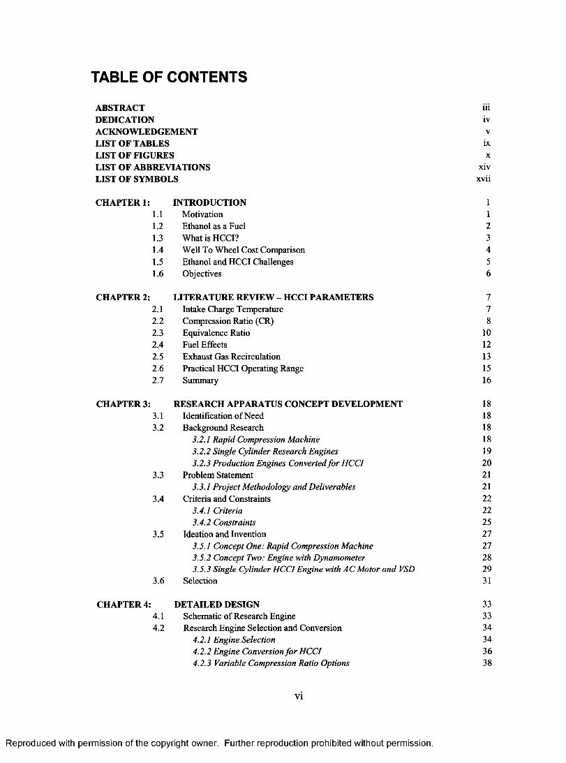
TABLE OF CONTENTS
ABSTRACT iiiDEDICATION ivACKNOWLEDGEMENT vLIST OF TABLES ixLIST OF FIGURES xLIST OF ABBREVIATIONS xivLIST OF SYMBOLS xvii
CHAPTER 1: INTRODUCTION 11.1 Motivation 11.2 Ethanol as a Fuel 21.3 What is HCCI? 31.4 Well To Wheel Cost Comparison 41.5 Ethanol and HCCI Challenges 51.6 Objectives 6
CHAPTER 2: LITERATURE REVIEW - HCCI PARAMETERS 72.1 Intake Charge Temperature 72.2 Compression Ratio (CR) 82.3 Equivalence Ratio 102.4 Fuel Effects 122.5 Exhaust Gas Recirculation 132.6 Practical HCCI Operating Range 152.7 Summary 16
CHAPTER 3: RESEARCH APPARATUS CONCEPT DEVELOPMENT 183.1 Identification of Need 183.2 Background Research 18
3.2.1 Rapid Compression Machine 183.2.2 Single Cylinder Research Engines 193.2.3 Production Engines Converted for HCCI 20
3.3 Problem Statement 213.3.1 Project Methodology and Deliverables 21
3.4 Criteria and Constraints 223.4.1 Criteria 223.4.2 Constraints 25
3.5 Ideation and Invention 273.5.1 Concept One: Rapid Compression Machine 273.5.2 Concept Two: Engine with Dynamometer 283.5.3 Single Cylinder HCCI Engine with AC Motor and VSD 29
3.6 Selection 31
CHAPTER 4: DETAILED DESIGN 334.1 Schematic of Research Engine 334.2 Research Engine Selection and Conversion 34
4.2.1 Engine Selection 344.2.2 Engine Conversion for HCCI 364.2.3 Variable Compression Ratio Options 38
vi
Reproduced with permission of the copyright owner. Further reproduction prohibited without permission.
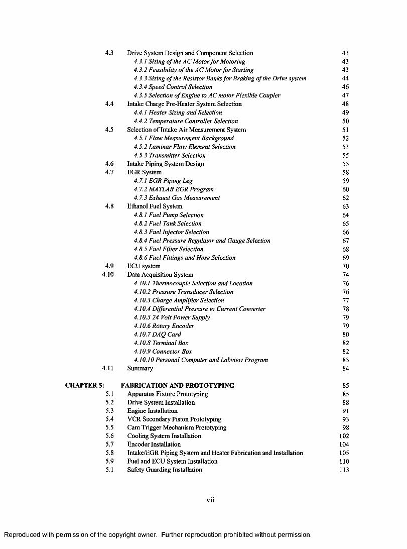
4.3 Drive System Design and Component Selection 414.3.1 Sizing o f the AC Motor fo r Motoring 434.3.2 Feasibility o f the A C Motor for Starting 434.3.3 Sizing o f the Resistor Banks for Braking o f the Drive system 444.3.4 Speed Control Selection 464.3.5 Selection o f Engine to AC motor Flexible Coupler 47
4.4 Intake Charge Pre-Heater System Selection 484.4.1 Heater Sizing and Selection 494.4.2 Temperature Controller Selection 50
4.5 Selection of Intake Air Measurement System 514.5.1 Flow Measurement Background 524.5.2 Laminar Flow Element Selection 534.5.3 Transmitter Selection 55
4.6 Intake Piping System Design 554.7 EGR System 58
4.7. / EGR Piping Leg 594.7.2 MA TLAB EGR Program 604.7.3 Exhaust Gas Measurement 62
4.8 Ethanol Fuel System 634.8.1 Fuel Pump Selection 644.8.2 Fuel Tank Selection 654.8.3 Fuel Injector Selection 664.8.4 Fuel Pressure Regulator and Gauge Selection 674.8.5 Fuel Filter Selection 684.8.6 Fuel Fittings and Hose Selection 69
4.9 ECU system 704.10 Data Acquisition System 74
4.10.1 Thermocouple Selection and Location 764.10.2 Pressure Transducer Selection 764.10.3 Charge Amplifier Selection 774.10.4 Differential Pressure to Current Converter 784.10.5 24 Volt Power Supply 794.10.6 Rotary Encoder 794.10.7DAQ Card 804.10.8 Terminal Box 824.10.9 Connector Box 824.10.10 Personal Computer and Labview Program 83
4.11 Summary 84
CHAPTER 5: FABRICATION AND PROTOTYPING 855.1 Apparatus Fixture Prototyping 855.2 Drive System Installation 885.3 Engine Installation 915.4 VCR Secondary Piston Prototyping 935.5 Cam Trigger Mechanism Prototyping 985.6 Cooling System Installation 1025.7 Encoder Installation 1045.8 Intake/EGR Piping System and Heater Fabrication and Installation 1055.9 Fuel and ECU System Installation 1105.1 Safety Guarding Installation 113
vii
Reproduced with permission of the copyright owner. Further reproduction prohibited without permission.
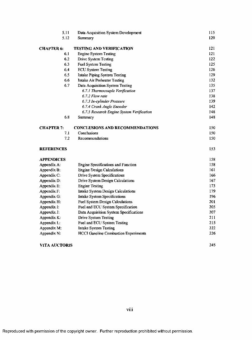
5.11 Data Acquisition System Development 1155.12 Summary 120
CHAPTER 6: TESTING AND VERIFICATION 1216.1 Engine System Testing 1216.2 Drive System Testing 1226.3 Fuel System Testing 1256.4 ECU System Testing 1266.5 Intake Piping System Testing 1296.6 Intake Air Preheater Testing 1326.7 Data Acquisition System Testing 135
6.7.1 Thermocouple Verification 1376.7.2 Flow rate 1386.7.3 In-cylinder Pressure 1396.7.4 Crank Angle Encoder 1426.7.5 Research Engine System Verification 148
6.8 Summary 148
CHAPTER 7: CONCLUSIONS AND RECOMMENDATIONS 1507.1 Conclusions 1507.2 Recommendations 150
REFERENCES 153
APPENDICES 158Appendix A: Engine Specifications and Function 158Appendix B: Engine Design Calculations 161Appendix C: Drive System Specifications 166Appendix D: Drive System Design Calculations 167Appendix E: Engine Testing 173Appendix F: Intake System Design Calculations 179Appendix G: Intake System Specifications 196Appendix H: Fuel System Design Calculations 201Appendix I: Fuel and ECU System Specification 205Appendix J: Data Acquisition System Specifications 207Appendix K: Drive System Testing 211Appendix L: Fuel and ECU System Testing 215Appendix M: Intake System Testing 222Appendix N: HCCI Gasoline Combustion Experiments 226
VITA AUCTORIS 245
viii
Reproduced with permission of the copyright owner. Further reproduction prohibited without permission.
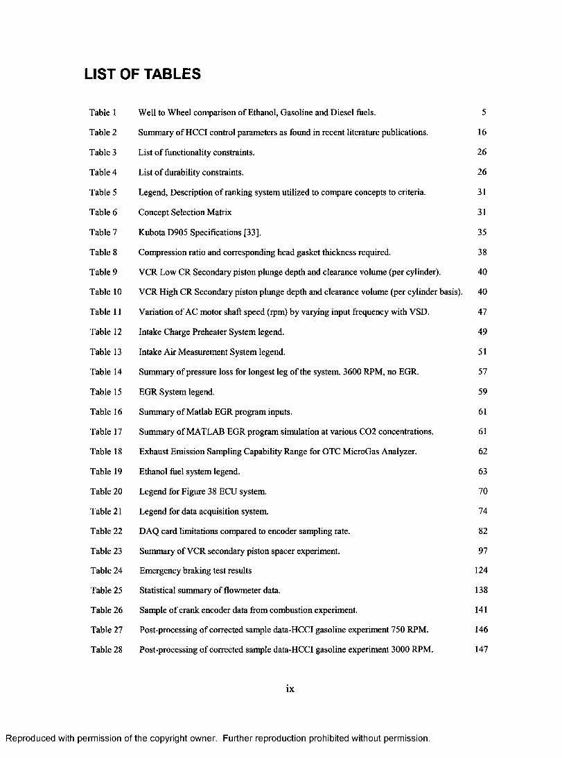
LIST OF TABLES
Table 1 Well to Wheel comparison of Ethanol, Gasoline and Diesel fuels. 5
Table 2 Summary of HCCI control parameters as found in recent literature publications. 16
Table 3 List of functionality constraints. 26
Table 4 List of durability constraints. 26
Table 5 Legend, Description of ranking system utilized to compare concepts to criteria. 31
Table 6 Concept Selection Matrix 31
Table 7 Kubota D905 Specifications [33]. 35
Table 8 Compression ratio and corresponding head gasket thickness required. 38
Table 9 VCR Low CR Secondary piston plunge depth and clearance volume (per cylinder). 40
Table 10 VCR High CR Secondary piston plunge depth and clearance volume (per cylinder basis). 40
Table 11 Variation of AC motor shaft speed (rpm) by varying input frequency with VSD. 47
Table 12 Intake Charge Preheater System legend. 49
Table 13 Intake Air Measurement System legend. 51
Table 14 Summary of pressure loss for longest leg of the system. 3600 RPM, no EGR. 57
Table 15 EGR System legend. 59
Table 16 Summary of Matlab EGR program inputs. 61
Table 17 Summary of MATLAB EGR program simulation at various C02 concentrations. 61
Table 18 Exhaust Emission Sampling Capability Range for OTC MicroGas Analyzer. 62
Table 19 Ethanol fuel system legend. 63
Table 20 Legend for Figure 38 ECU system. 70
Table 21 Legend for data acquisition system. 74
Table 22 DAQ card limitations compared to encoder sampling rate. 82
Table 23 Summary of VCR secondary piston spacer experiment. 97
Table 24 Emergency braking test results 124
Table 25 Statistical summary of flowmeter data. 138
Table 26 Sample of crank encoder data from combustion experiment. 141
Table 27 Post-processing of corrected sample data-HCCI gasoline experiment 750 RPM. 146
Table 28 Post-processing of corrected sample data-HCCI gasoline experiment 3000 RPM. 147
ix
Reproduced with permission of the copyright owner. Further reproduction prohibited without permission.
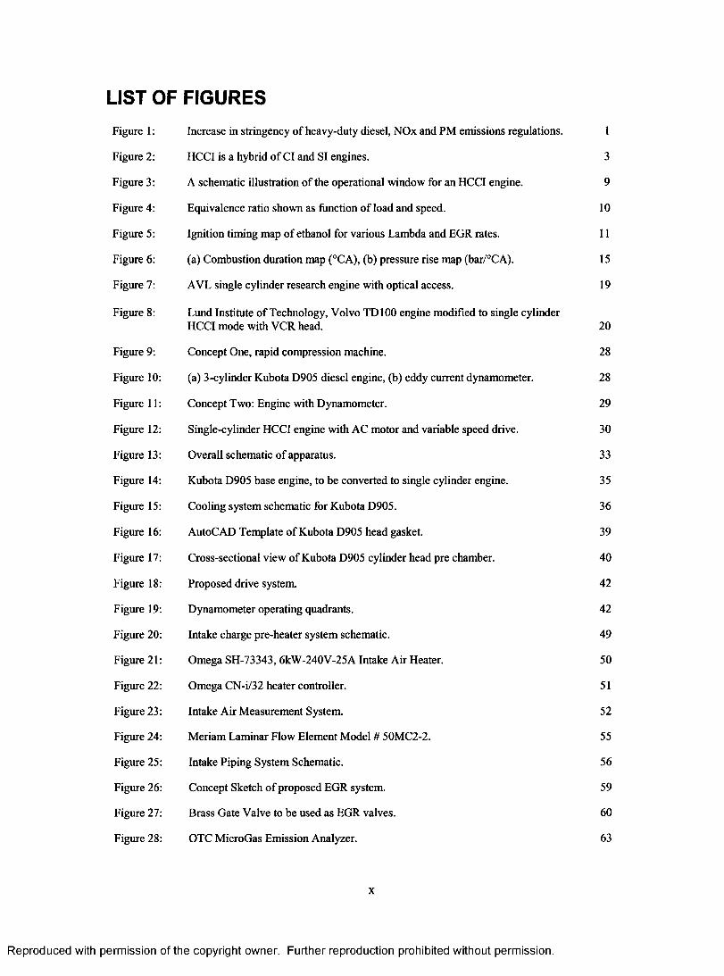
LIST OF FIGURESFigure 1: Increase in stringency of heavy-duty diesel, NOx and PM emissions regulations. 1
Figure 2: HCCI is a hybrid of Cl and SI engines. 3
Figure 3: A schematic illustration of the operational window for an HCCI engine. 9
Figure 4: Equivalence ratio shown as function of load and speed. 10
Figure 5: Ignition timing map of ethanol for various Lambda and EGR rates. 11
Figure 6: (a) Combustion duration map (°CA), (b) pressure rise map (bar/°CA). 15
Figure 7: AVL single cylinder research engine with optical access. 19
Figure 8: Lund Institute of Technology, Volvo TD100 engine modified to single cylinderHCCI mode with VCR head. 20
Figure 9: Concept One, rapid compression machine. 28
Figure 10: (a) 3-cylinder Kubota D905 diesel engine, (b) eddy current dynamometer. 28
Figure 11: Concept Two: Engine with Dynamometer. 29
Figure 12: Single-cylinder HCCI engine with AC motor and variable speed drive. 30
Figure 13: Overall schematic of apparatus. 33
Figure 14: Kubota D905 base engine, to be converted to single cylinder engine. 35
Figure 15: Cooling system schematic for Kubota D905. 36
Figure 16: AutoCAD Template of Kubota D905 head gasket. 39
Figure 17: Cross-sectional view of Kubota D905 cylinder head pre chamber. 40
Figure 18: Proposed drive system. 42
Figure 19: Dynamometer operating quadrants. 42
Figure 20: Intake charge pre-heater system schematic. 49
Figure 21: Omega SH-73343, 6kW-240V-25A Intake Air Heater. 50
Figure 22: Omega CN-i/32 heater controller. 51
Figure 23: Intake Air Measurement System. 52
Figure 24: Meriam Laminar Flow Element Model # 50MC2-2. 55
Figure 25: Intake Piping System Schematic. 56
Figure 26: Concept Sketch of proposed EGR system. 59
Figure 27: Brass Gate Valve to be used as EGR valves. 60
Figure 28: OTC MicroGas Emission Analyzer. 63
x
Reproduced with permission of the copyright owner. Further reproduction prohibited without permission.
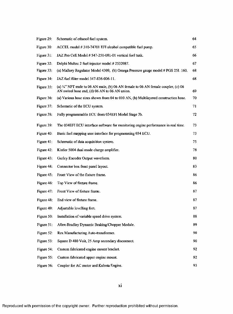
Figure 29: Schematic of ethanol fuel system. 64
Figure 30: ACCEL model # 310-74701 EFI alcohol compatible fuel pump. 65
Figure 31: JAZ Pro Cell Model # 547-250-001-01 vertical fuel tank. 66
Figure 32: Delphi Multec 2 fuel injector model # 2532087. 67
Figure 33: (a) Mallory Regulator Model 4309, (b) Omega Pressure gauge model # PGS 25L 160. 68
Figure 34: JAZ fuel filter model 547-836-006-11. 68
Figure 35: (a) 'A” NPT male to 06 AN male, (b) 06 AN female to 06 AN female coupler, (c) 06AN swivel hose end, (d) 06 AN to 06 AN union. 69
Figure 36: (a) Various hose sizes shown from 04 to 010 AN, (b) Multilayered construction hose. 70
Figure 37: Schematic of the ECU system. 71
Figure 38: Fully programmable ECU from 034EFI Model Stage 3b. 72
Figure 39: The 034EFI ECU interface software for monitoring engine performance in real time. 73
Figure 40: Basic fuel mapping user interface for programming 034 ECU. 73
Figure 41: Schematic of data acquisition system. 7 5
Figure 42: Kistler 5004 dual mode charge amplifier. 78
Figure 43: Gurley Encoder Output waveform. 80
Figure 44: Connector box front panel layout. 83
Figure 45: Front View of the fixture frame. 86
Figure 46: Top View of fixture frame. 86
Figure 47: Front View of fixture frame. 87
Figure 48: End view of fixture frame. 87
Figure 49: Adjustable levelling feet. 87
Figure 50: Installation of variable speed drive system. 88
Figure 51: Allen-Bradley Dynamic Braking/Chopper Module. 89
Figure 52: Rex Manufacturing Auto-transformer. 90
Figure 53: Square D 480 Volt, 25 Amp secondary disconnect. 90
Figure 54: Custom fabricated engine mount bracket. 92
Figure 55: Custom fabricated upper engine mount. 92
Figure 56: Coupler for AC motor and Kubota Engine. 93
xi
Reproduced with permission of the copyright owner. Further reproduction prohibited without permission.
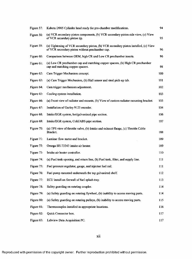
Figure 57: Kubota D905 Cylinder head ready for pre-chamber modifications. 94
Figure 58: (a) VCR secondary piston components, (b) VCR secondary piston side view, (c) Viewof VCR secondary piston tip. 95
Figure 59: (a) Tightening of VCR secondary piston, (b) VCR secondary piston installed, (c) Viewof VCR secondary piston without prechamber cap. 96
Figure 60: Comparison between OEM, high CR and Low CR prechamber inserts. 96
Figure 61: (a) Low CR prechamber cap and matching copper spacers, (b) High CR prechambercap and matching copper spacers. 98
Figure 62: Cam Trigger Mechanism concept. 100
Figure 63: (a) Cam Trigger Mechanism, (b) Hall sensor and steel pick-up tab. 101
Figure 64: Cam trigger mechanism adjustment. 102
Figure 65: Cooling system installation. 103
Figure 66: (a) Front view of radiator and mounts, (b) View of custom radiator mounting bracket. 103
Figure 67: Installation of Gurley 9125 encoder. 104
Figure 68: Intake/EGR system, hot/galvanized pipe section. 106
Figure 69: Intake/EGR system, Cold/ABS pipe section. 107
Figure 70: (a) TPS view of throttle valve, (b) Intake and exhaust flange, (c) Throttle CableBracket. 108
Figure 71: Laminar flow meter and bracket. 109
Figure 72: Omega SH-73343 intake air heater. 109
Figure 73: Intake air heater controller. 110
Figure 74: (a) Fuel tank opening, and return line, (b) Fuel tank, filter, and supply line. 111
Figure 75: Fuel pressure regulator, gauge, and injector fuel rail. 111
Figure 76: Fuel pump mounted underneath the top galvanized shelf. 112
Figure 77: ECU install on firewall of fuel splash tray. 113
Figure 78: Safety guarding on rotating coupler. 114
Figure 79: (a) Safety guarding on rotating flywheel, (b) inability to access moving parts. 114
Figure 80: (a) Safety guarding on rotating pulleys, (b) inability to access moving parts. 115
Figure 81: Thermocouples installed in appropriate locations. 116
Figure 82: Quick Connector box. 117
Figure 83: Labview Data Acquisition PC. 117
Reproduced with permission of the copyright owner. Further reproduction prohibited without permission.
Figure 84: System schematic panel. 118
Figure 85: Configuration panel. 119
Figure 86: Required injector scalar for measured engine speeds. 128
Figure 87: Summary of required injector scalar for all equivalence ratios and engine speeds. 129
Figure 88: Actual flow rate at various engine speeds. 130
Figure 89: Actual volumetric efficiency at various engine speeds. 131
Figure 90: Heater Exit Temperature at various engine speeds. 133
Figure 91: Heat transferred to air at various engine speeds. 134
Figure 92: Real-time unprocessed thermocouple data at 775 RPM. 136
Figure 93: Real-time unprocessed flow meter data at 775 RPM. 137
Figure 94: Real-time unprocessed in-cylinder pressure data for motoring at 775 RPM. 139
Figure 95: Real-time processed encoder signal for motoring at 775 RPM. 140
Pressure versus crank angle degree plot of HCCI gasoline experiment - processed and Figure 96: unprocessed data sample at 750 RPM. 144
Figure 97: P-V diagram (pressure versus volume diagram) of HCCI gasoline experiment,corrected and uncorrected data sample at 750 RPM. 145
Figure 98: Log(P) versus Log(V) plot of Gasoline HCCI. 148
Figure 99: Final HCCI research engine setup. 149
xiii
Reproduced with permission of the copyright owner. Further reproduction prohibited without permission.

LIST OF ABBREVIATIONS
°c degrees Celsius
883ECU ECU calibration programABS plastic plumbing material
AC alternating current
AN type of connector
AVL Powertrain Engineering Company
BDC bottom dead center
BMEP brake mean effective pressure
BNC connector type
C carbon atomCAD computer aided designCDN Canadian Dollarcfm cubic feet per minute
CFR Corporative Fuels Research Company
Cl compression ignition
CLT coolant temperature sensor
CN cetane number
CO carbon monoxideC02 carbon dioxideCPU central processor unitCR compression ratio
CSA Canadian Standards AssociationD905 Kubota Engine ModelDAQ data acquisition
DB15 15-pin connector
DB9 9-pin connector
DC direct currentdyno dynamometerECC Electrical Code of Canada
ECU electronic control unitEFI electronic fuel injection
EGR exhaust gas recirculationEPA US Environmental Protection Agency
g/s grams per secondgal us gallonsGB gigabytes hard drive storage spaceGUI graphic user interfaceH hydrogen atom
Reproduced with permission of the copyright owner. Further reproduction prohibited without permission.

H20 water moleculeHC hydrocarbons
HCCI homogeneous charge compression ignitionHP horse powerHRR heat release rateHz hertz
IDI indirect injectionK degrees kelvin
kPa kilopascals
L/s litres per second
LED low voltage indicator light
LFE laminar flow element meter
MAP manifold absolute pressure sensor
MAT manifold air temperature
MATLAB mathematics programming languageMBT maximum brake torqueN nitrogen atom
N02 nitrogen dioxideNOx oxides of nitrogenNPT national pipe thread
O oxygen atom
02 oxygen molecule
OEM original equipment manufacturer
OTC manufacturer of gas analyzer
PC personal computer
pC picocoloumbs
Phi equivalence ratio
PM particulate matterPV pressure vs. volume diagramPVC poly-vinyl-chlorideRAM temporary PC memory
RCM rapid compression machineRPM revolutions per minuteScalar injector scalar or mulitplierSCRE single cylinder research engine
SI spark ignitionT1 air inlet thermocoupleT2 heater thermocoupleT3 mixture thermocouple
Reproduced with permission of the copyright owner. Further reproduction prohibited without permission.

T4 exhaust thermocoupleT5 EGR thermocoupleT6 coolant thermocoupleTDC top dead centerTDI turbodiesel direct injection
TPS throttle position sensor
UHC unbumed hydrocarbonsUS United States
VCR variable compression ratioVSD variable speed driveVVT variable valve timingkW kilowattW wattMPa megapascals
ft.lbs foot poundskgf.m kilograms force metermm millimetercm centimeter
psi pounds per square inchescfm standard cubic feet per minuteL litrescu.in cubic inches
kg kilograms
lbs poundskJ/kg kilojoules per kilogrambar/°CA bars per degree crank anglem meterin inche
ft footHz cycles per second
J/deg joules per degreeg/HP-hr grams per horsepower hour
hr hour
mA milli-amperes currentV volts
Reproduced with permission of the copyright owner. Further reproduction prohibited without permission.

LIST OF SYMBOLS
%EGR percent by volume EGR gas
°CA crank angle degrees
Cp specific heat, constant pressure
dcam diameter of cam
dcrank diameter of crank
Ap pressure drop
D sp secondary piston diameter
AT change in temperature
dV change in volume
d> equivalence ratiof frequency
Floss heat loss factorFs OS oversize factorF1 service service factor
G amplifier gain
Jt total rotational inertia
X air fuel ratio
Ls piston plunge depth
m amplifier scalar
m g speed ratioNi ’ cam number of teeth of cam
hfcrank number of teeth of crank
nd safety factor
Npoles number of motor poles
nR # of crank revs per power stroke per cylinderP power
P pressure
Pabsorbed power absorbed
Pavg average power absorbed
Pb peak break power
Pg stagnation pressure
Pi net indicated power per cycle
Pincylinder incylinder pressurePif loss of function pressure
pt total pressure
Q charge signal from kistler
p densityR resistance
Reproduced with permission of the copyright owner. Further reproduction prohibited without permission.

Pair density of air
R<lbl total dynamic braking resistanceR H relative humidityT temperature
t time
X torque
tc cycle time
Tcoolant coolant temperatue
^gross gross intermittent torque
Tinlet inlet temperature
^max maximum torque
^net net continuous torque
’'■per maximum permitted torque
"^req required torque
XSup supplied torque
t j total timeU flow velocity
Vc clearance volumeVd DC bus voltageVs swept volumev t total volume
Vtank tank volume
volumetric flowrateVv calculated flowrate
calculated
Nsampling rate per channel
sensor
N required sampling raterequired
N datapar&sdatapoints per degree crank angle
Vv volumetric efficiency
™ amass flowrate of air
(0 rotational speed
COb maximum rotational speed
G>o minimum rotational speedw c,i net indicated work per cycle
Q h t heat transfer rate
r ratio of specific heats
xviii
Reproduced with permission of the copyright owner. Further reproduction prohibited without permission.
1 INTRODUCTION
The purpose of this thesis is to report on the project entitled, “Design of a Research Engine for
Homogeneous Charge Compression Ignition (HCCI) Combustion.” This thesis will present the
motivation for the project, the objectives, methodology, as well as present the details of the
design, fabrication, testing and verification of the apparatus.
1.1 Motivation
For the past three decades, engine research and development has been focusing on new
technologies and methods for combustion that promise to lower vehicle exhaust emissions and
improve fuel economy at part-load conditions.
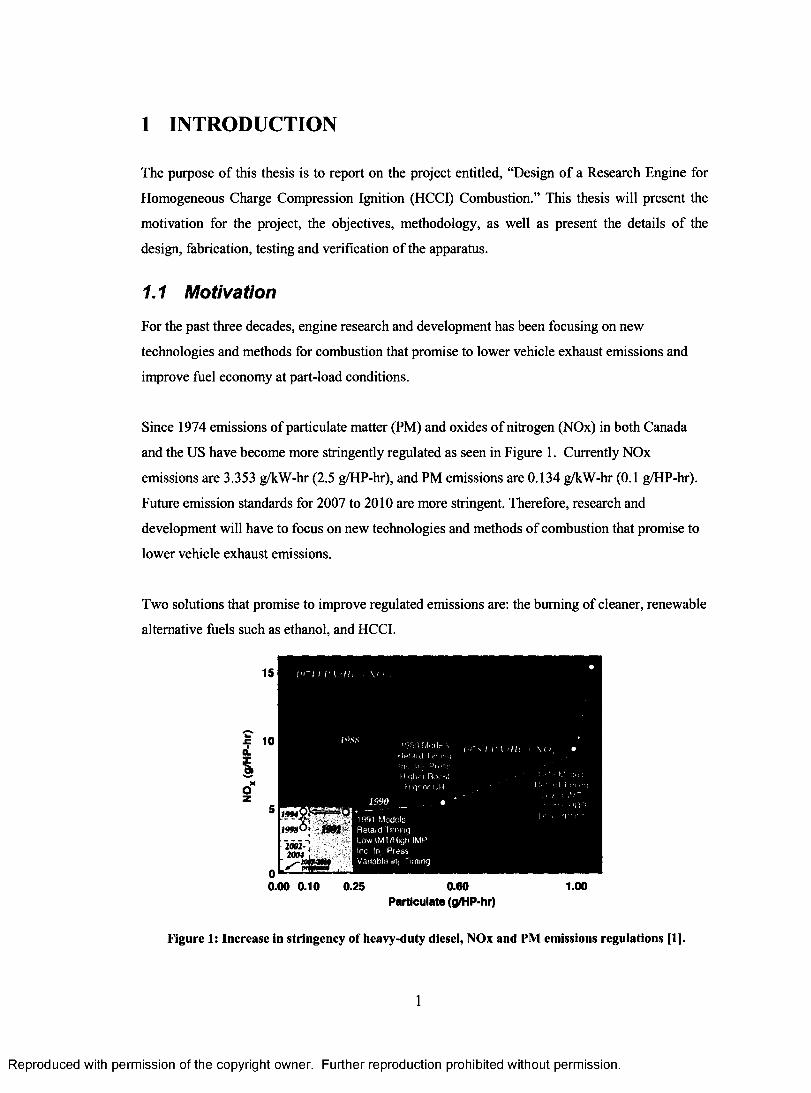
Since 1974 emissions of particulate matter (PM) and oxides of nitrogen (NOx) in both Canada
and the US have become more stringently regulated as seen in Figure 1. Currently NOx
emissions are 3.353 g/kW-hr (2.5 g/HP-hr), and PM emissions are 0.134 g/kW-hr (0.1 g/HP-hr).
Future emission standards for 2007 to 2010 are more stringent. Therefore, research and
development will have to focus on new technologies and methods of combustion that promise to
lower vehicle exhaust emissions.
Two solutions that promise to improve regulated emissions are: the burning of cleaner, renewable
alternative fuels such as ethanol, and HCCI.
15 /*»'/ / r \ • \< * )
U . : r j .
1991 M odels R e ta rd Timing Low iMUHkjM IMP Inc ir>j. Pres-s V ariab le Inj Tim ing
o0.00 0.10 0.25 0.60 1.00
Particulate (g/HP-hr)
Figure 1: Increase in stringency of heavy-duty diesel, NOx and PM emissions regulations [I].
Reproduced with permission of the copyright owner. Further reproduction prohibited without permission.

1.2 Ethanol as a Fuel
Ethanol has been considered as an automotive fuel for many decades. Infact, when Henry Ford
designed the Model T, it was his expectation that ethanol, made from renewable biological
resources would be a major automobile fuel [2]. However, gasoline emerged as the dominant
transportation fuel in the early twentieth century, because of the ease of operation of gasoline
engines with the materials then available for engine construction, and a growing supply of
cheaper petroleum from oil field discoveries.
There are two key reasons why gasoline usage has remained the primary fuel for the past century.
Firstly, the cost per kilometre of travel is lower than other renewable resources. Secondly, large
investments made by both petroleum and auto industries in physical capital, human skills and
technology make the entry of a new cost-competitive industry difficult.
The use of ethanol in internal combustion engines has grown in recent years because it offers
attractive benefits of reduced exhaust emissions and reduced environmental and human health
impact. Due to the finite nature of petroleum reserves, production of ethanol in Canada in the US
has been steadily increasing. Since ethanol is produced from plants that harness the power of the
sun, ethanol is considered to be a renewable fuel.
With internal combustion engines, the pollutants of major concern are NOx, unbumed
hydrocarbons (UHC), carbon monoxide (CO), and PM. Ethanol combustion offers lower NOx
emissions due to its lower flame temperature when compared to petroleum-based fuels. Also the
ethanol molecule contains oxygen which promotes better oxidation of the fuel, and results in
more complete combustion, thus reducing CO and UHC emissions. However, ethanol emissions
are high in formaldehydes.
Formaldehyde has been classified by the EPA as a probable human carcinogen. Formaldehyde in
the atmosphere is directly and indirectly a result of gasoline exhaust emissions. Ethanol
combustion emissions have a higher rate of direct formaldehyde production compared to gasoline
combustion emissions. However, as a result of possible improvements in ethanol-engine and
emission-control technology, formaldehyde emissions can be significantly lowered [69],
2
Reproduced with permission of the copyright owner. Further reproduction prohibited without permission.
Formaldehyde emission is a concern due to the low-temperature combustion nature of ethanol
HCCI. In general, any engine operating or design parameter which would result in increased
temperature of the exhaust or decreased unbumt fuel should encourage formaldehyde oxidation.
Oxidizing catalyst using platinum-rhodium substrates have been used to control formaldehyde
emissions [70].
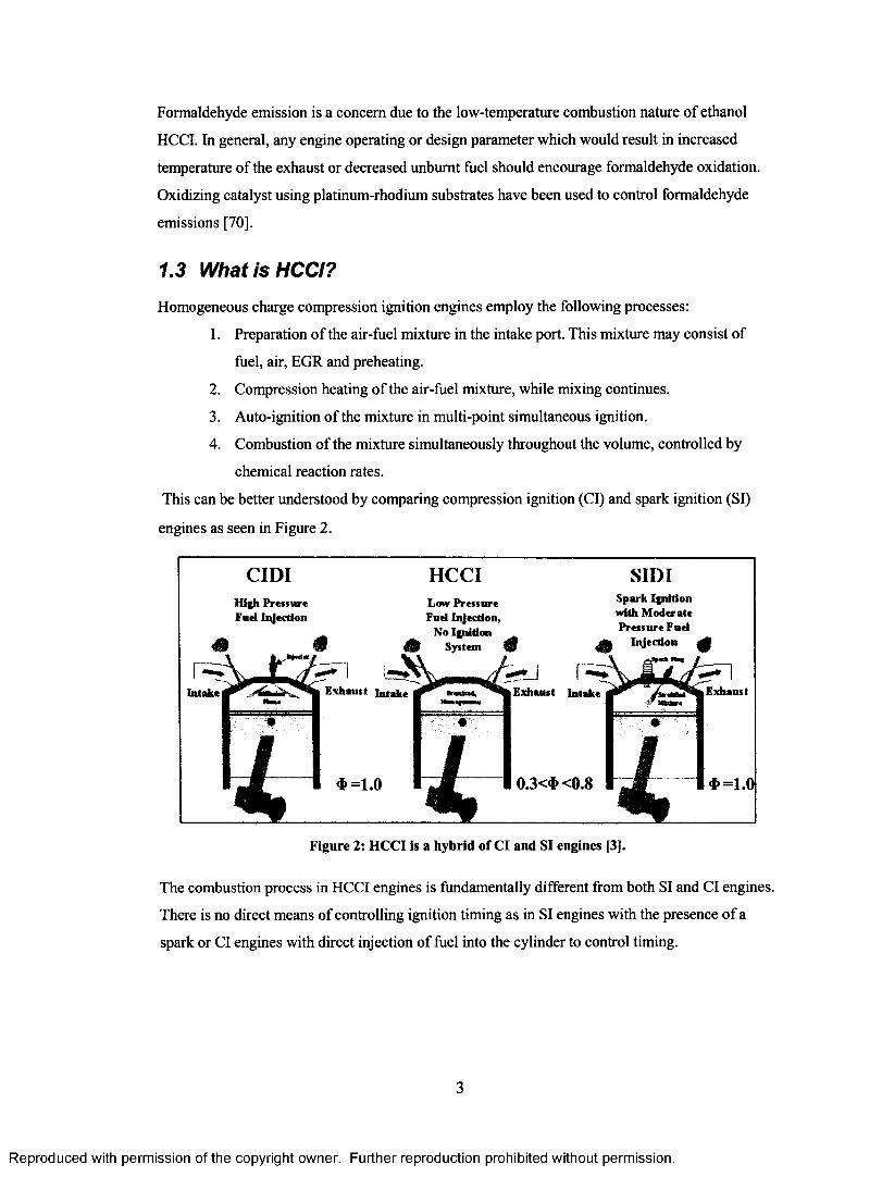
1.3 What is HCCI?
Homogeneous charge compression ignition engines employ the following processes:
1. Preparation of the air-fuel mixture in the intake port. This mixture may consist of
fuel, air, EGR and preheating.
2. Compression heating of the air-fuel mixture, while mixing continues.
3. Auto-ignition of the mixture in multi-point simultaneous ignition.
4. Combustion of the mixture simultaneously throughout the volume, controlled by
chemical reaction rates.
This can be better understood by comparing compression ignition (Cl) and spark ignition (SI)
engines as seen in Figure 2.
CIDIHigh Pressure Fuel Injection
Intake! Exhaust Intake
HCCILow Pressure Fuel Injection,
No Ignition 6 System V
* = 1.0
SIDISpark Ignition with M oderate Pressure Fuel
| Injection ^
Exhaust Intake Exhaust
0.3<* <0.8 * = 1.0
Figure 2: HCCI is a hybrid of Cl and SI engines [3].
The combustion process in HCCI engines is fundamentally different from both SI and Cl engines.
There is no direct means of controlling ignition timing as in SI engines with the presence of a
spark or Cl engines with direct injection of fuel into the cylinder to control timing.
3
Reproduced with permission of the copyright owner. Further reproduction prohibited without permission.

HCCI engines involve compression heating of the air-fuel mixture to its auto-ignition
temperature, which can range anywhere from 700 to 1100K depending on the type of fuel and
mixture strength.
The similarities between Cl engines and HCCI are such: both have high compression ratios (CR)
and both ignite air-fuel mixture by compression heating. Cl engines have CR in the range 16-
23:1. Similarly, HCCI engines have CR in the range 11-25:1 depending on the fuel.
When comparing SI and HCCI engines, both involve the process of homogeneous mixture
preparation in the intake manifold. However, the main difference between SI and HCCI engines
is the lack of spark to initiate ignition, and overall lean equivalence ratios (in the range
0.3>0>0.8.) If we compare SI and HCCI combustion for the same equivalence ratio say 0=1.0,
then HCCI would have a much faster heat release rate compared to SI. However, in reality HCCI
combustion occurs under much leaner conditions that decrease the heat release rate.
Diesel HCCI compression ratios are typically much lower than conventional Cl diesel
combustion. Diesel HCCI CR range is between 11 and 15:1 whereas conventional Cl diesel CR
ranges are between 16 and 23:1. Diesel HCCI has a lower CR range the conventional Cl because
HCCI is an overall lean mixture, and lean mixtures have higher specific heat ratios (closer to 1.4)
than stoichiometric mixtures. Thus, when lean mixtures are compressed the mean temperature
will be higher than conventional mixtures which results in a lower autoignition temperature. The
thermal efficiency is decreased because of the lower CR, however the thermal efficiency
increases due to the lean mixture and the increase in specific heat ratios are closer to 1.4.
Therefore lower compression ratios are employed to expand the operating range of diesel HCCI.
The disadvantage of lower compression ratios is a decrease in thermal efficiency of the engine;
however the advantage is a reduction in frictional losses.
1.4 Well to Wheel Cost Comparison
A well to wheel analysis was performed comparing our research fuel (ethanol) to gasoline and
diesel fuel use. The cost of acquiring ethanol, gasoline and diesel fuels were obtained from the
US Department of Energy website for the current year 2005 [71]. This cost was originally
normalized on a cost per million Btu basis. This was converted to cost per MJ basis and
4
Reproduced with permission of the copyright owner. Further reproduction prohibited without permission.
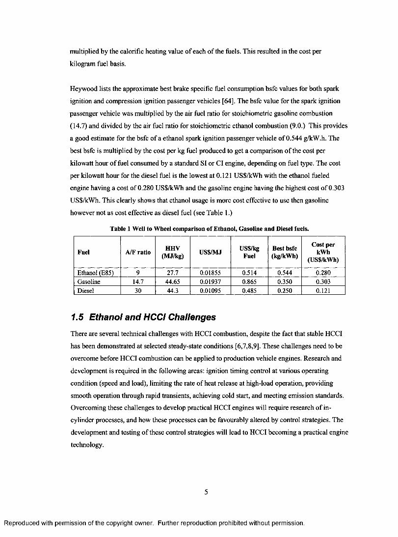
multiplied by the calorific heating value of each of the fuels. This resulted in the cost per
kilogram fuel basis.
Heywood lists the approximate best brake specific fuel consumption bsfc values for both spark
ignition and compression ignition passenger vehicles [64]. The bsfc value for the spark ignition
passenger vehicle was multiplied by the air fuel ratio for stoichiometric gasoline combustion
(14.7) and divided by the air fuel ratio for stoichiometric ethanol combustion (9.0.) This provides
a good estimate for the bsfc of a ethanol spark ignition passenger vehicle of 0.544 g/kW.h. The
best bsfc is multiplied by the cost per kg fuel produced to get a comparison of the cost per
kilowatt hour of fuel consumed by a standard SI or Cl engine, depending on fuel type. The cost
per kilowatt hour for the diesel fuel is the lowest at 0.121 US$/kWh with the ethanol fueled
engine having a cost of 0.280 US$/kWh and the gasoline engine having the highest cost of 0.303
US$/kWh. This clearly shows that ethanol usage is more cost effective to use then gasoline
however not as cost effective as diesel fuel (see Table 1.)
Table 1 Well to Wheel comparison of Ethanol, Gasoline and Diesel fuels.
Fuel A/F ratio HHV(MJ/kg) USS/MJ US$/kg
FuelBest bsfc (kg/kWh)
Cost per kWh
(US$/kWh)
Ethanol (E85) 9 27.7 0.01855 0.514 0.544 0.280Gasoline 14.7 44.65 0.01937 0.865 0.350 0.303Diesel 30 44.3 0.01095 0.485 0.250 0.121
1.5 Ethanol and HCCI Challenges
There are several technical challenges with HCCI combustion, despite the fact that stable HCCI
has been demonstrated at selected steady-state conditions [6,7,8,9]. These challenges need to be
overcome before HCCI combustion can be applied to production vehicle engines. Research and
development is required in the following areas: ignition timing control at various operating
condition (speed and load), limiting the rate of heat release at high-load operation, providing
smooth operation through rapid transients, achieving cold start, and meeting emission standards.
Overcoming these challenges to develop practical HCCI engines will require research of in
cylinder processes, and how these processes can be favourably altered by control strategies. The
development and testing of these control strategies will lead to HCCI becoming a practical engine
technology.
5
Reproduced with permission of the copyright owner. Further reproduction prohibited without permission.

There are some disadvantages with ethanol as an HCCI fuel. Ethanol has difficulties with auto
ignition, which can lead to problems with cold start. This is due to the cooling effect ethanol has
on its surroundings, because of its high latent heat of vaporization (838.3 kJ/kg for ethanol
compared to 306.3 kJ/kg for iso-octane) [4]. Additionally, ethanol has a high octane number
(109) that prevents auto-ignition from occurring readily. Therefore, ethanol HCCI requires the
use of a preheater to promote cold start and improve operating range performance.
HCCI combustion is difficult to control because there is no direct means of control as in SI or Cl
engines. Pressure versus crank angle or engine torque in SI engines is achieved by spark timing,
and in Cl engines it is controlled by fuel injection timing. These means are unavailable for HCCI.
1.6 Objectives
The primary objective of this thesis was to develop an experimental apparatus for investigation of
parameters affecting control of HCCI combustion.
The following is a list of objectives for the thesis:
• To perform a literature review to identify the parameters affecting control of HCCI with
respect to use of ethanol as a fuel.
• To design and fabricate an experimental apparatus for investigation of parameters
affecting control of HCCI by following the design process.
• To commission the HCCI research apparatus by performing initial testing,
troubleshooting, and verification experiments.
• To establish HCCI bum of lean ethanol/air, and obtain in-cylinder pressure measurements
to verify the results.
6
Reproduced with permission of the copyright owner. Further reproduction prohibited without permission.
2 LITERATURE REVIEW - HCCI PARAMETERS
The major challenge for commercialization of HCCI is combustion control in terms of, ignition
timing control, and heat release rate control for a variety of speeds and loads. Several methods
have been proposed for achieving HCCI engine control for operating conditions required for
automotive applications. Control strategies reported in literature have indicated some degree of
success. The following are the main HCCI control parameters:
1. Intake charge temperature.
2. Compression ratio (CR).
3. Equivalence ratio (air/fuel composition).
4. Fuel Effects (primary fuel type, and properties.)
5. Exhaust gas recirculation (EGR).
Selected studies on parameters affecting combustion control will be reviewed in these chapters.
2.1 Intake Charge Temperature
The effects of intake charge temperature have been widely reported. Najt and Foster [6] showed
that HCCI could be achieved using a SI engine under lean fuelling and elevated inlet charge
temperatures (300-500°C). In all cases, intake charge temperature has a strong effect on
combustion for HCCI. The effect of increasing intake charge temperature is to advance auto
ignition timing and decrease combustion duration.
Iida and Igarashi [7] investigated the effect of intake charge temperature on n-butane (C4H10).
The results show that by increasing intake charge temperature from 300K, to 325K, to 355K, the
heat release rates increased from 20J/deg, to 60J/deg, to lOOJ/deg respectively. Also the
combustion duration decreased as expected from 30, to 20 to 10 degrees respectively, for an
increase in intake charge temperature.
Simulation results of ethanol/air HCCI performed by Ng [8] have demonstrated similar findings.
Increasing the intake charge temperature will increase the peak in-cylinder temperature, but it is
dependent on when ignition occurs. If ignition occurs around top dead center (TDC), then most of
the energy will be released during the power stroke. If ignition occurs before TDC, then the effect
o f increased intake charge temperature is minimized, because the combustion reaction is working
7
Reproduced with permission of the copyright owner. Further reproduction prohibited without permission.
against the piston in the compression stroke. Generally speaking, intake charge temperature can
be used to optimize the ignition point, but it must be done correctly to maximize braking torque.
Increased intake charge temperature has also been utilized by Aoyama et al. [9] to extend the lean
bum limit (defined by hydrocarbon emissions and combustion efficiency). In other words, a very
lean mixture can be ignited more easily if intake-charge preheating is utilized.
2.2 Compression Ratio (CR)
HCCI initiates when the charge temperature reaches its auto-ignition temperature. Therefore, the
required inlet charge temperature for MBT combustion timing in HCCI mode is a function of
engine compression ratio. Increasing compression ratio can increase the charge temperature
during the compression stroke and advance the start of auto-ignition.
Hiraya et al. [10] reported for a gasoline HCCI engine, higher compression ratios allowed lower
intake charge temperature, and higher intake density for higher output. Also, higher compression
ratio contributes to higher thermal efficiency. However, HCCI enabled by a higher compression
ratio will encounter problems due to knock at higher loads with lower octane fuels. Variable
compression ratio (VCR) would be a good solution to this problem, since the CR could be
increased for lower loads and lower engine speeds and decreased for higher loads and higher
engines speeds to decrease the onset of combustion.
Systems that achieve combustion timing control through changes in compression ratio can be
divided into two types: Type 1 systems vary combustion chamber geometry, known as variable
compression ratio (VCR), and Type 2 system vary the cylinder volume at inlet valve closing,
variable valve timing (W T ) [11].
A VCR engine has the potential to achieve satisfactory operation in HCCI mode over a wide
range of conditions because the compression ratio can be adjusted as the operating conditions
change. However, operating conditions would change quickly and a fast response control system
for VCR is yet to be established. Christensen et al. [12, 13, 14, 15, 16, 17] have been carefully
investigating compression ratio as an effective means to achieve HCCI combustion control for
several years. The VCR engine used in their studies employs a Type 1 system. A secondary
piston is installed in the cylinder head whose position can be varied to change the compression
ratio [18]. For each test the compression ratio was adjusted to get auto-ignition of the charge
8
Reproduced with permission of the copyright owner. Further reproduction prohibited without permission.
around TDC. The experiments demonstrated the multi-fuel capability of an HCCI engine, and
suggested that adjusting the compression ratio fast and correctly could facilitate control of HCCI
combustion.
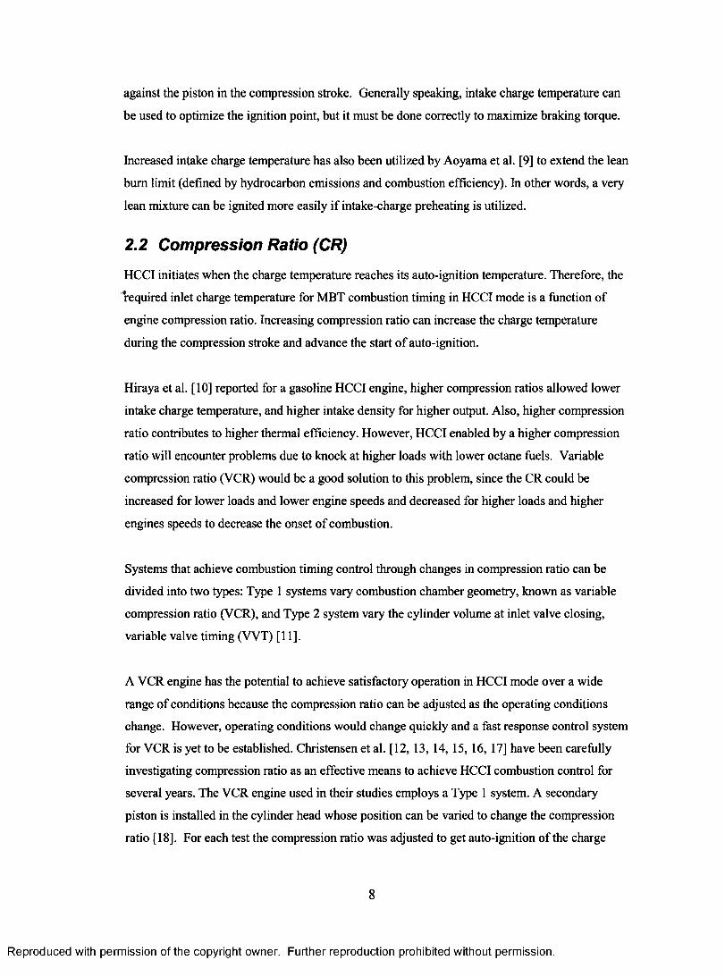
For a given engine system, load will be limited by either saturation of control variables, or by
operational constraints. Operational constraints are represented by limitations of NOx emissions,
peak cylinder pressure, and peak pressure-rise rate. Figure 3 below illustrates these constraints.
The variation of compression ratio can be used to extend the operational range of HCCI shown
below for a given mixture.
A lower CR provides a larger volume for the gas at TDC, which can slow down combustion and
lower the peak pressure, but this provides slower expansion after TDC and increases NOx, CO
and UHC emissions, and requires a higher intake charge temperature. With a fixed geometric
compression ratio, the effective compression ratio can be adjusted by VYT. An engine could be
built with a high geometric compression ratio, and W T could be used to lower the compression
ratio by delaying the closing of the intake valve during the compression stroke. Engines with
W T have the added benefit of retained EGR, which can allow changes in temperature and
exhaust residuals to induce HCCI combustion.
Load
NOx Limit
Peak pressure / peak rate o f pressure limit
VariationLimitHCCI
Window
Combustion timing
Figure 3: A schematic illustration of the operational window for an HCCI engine [18].
9
Reproduced with permission of the copyright owner. Further reproduction prohibited without permission.
2.3 Equivalence Ratio
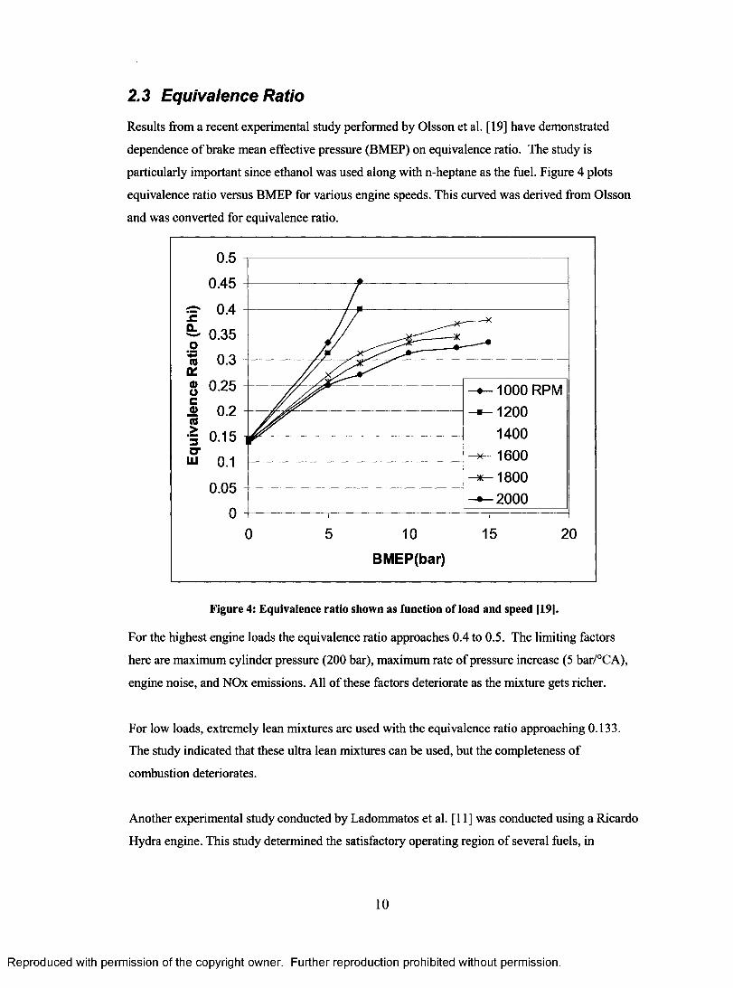
Results from a recent experimental study performed by Olsson et al. [19] have demonstrated
dependence of brake mean effective pressure (BMEP) on equivalence ratio. The study is
particularly important since ethanol was used along with n-heptane as the fuel. Figure 4 plots
equivalence ratio versus BMEP for various engine speeds. This curved was derived from Olsson
and was converted for equivalence ratio.
0.5
0.45
0.4
0.35
0.3
0.25 - -1 0 0 0 RPM - —1200
1400 * -1 6 0 0 * -1 8 0 0 - —2000
0.2
0.15
0.05
BMEP(bar)
Figure 4: Equivalence ratio shown as function of load and speed [19].
For the highest engine loads the equivalence ratio approaches 0.4 to 0.5. The limiting factors
here are maximum cylinder pressure (200 bar), maximum rate of pressure increase (5 bar/°CA),
engine noise, and NOx emissions. All of these factors deteriorate as the mixture gets richer.
For low loads, extremely lean mixtures are used with the equivalence ratio approaching 0.133.
The study indicated that these ultra lean mixtures can be used, but the completeness of
combustion deteriorates.
Another experimental study conducted by Ladommatos et al. [11] was conducted using a Ricardo
Hydra engine. This study determined the satisfactory operating region of several fuels, in
10
Reproduced with permission of the copyright owner. Further reproduction prohibited without permission.
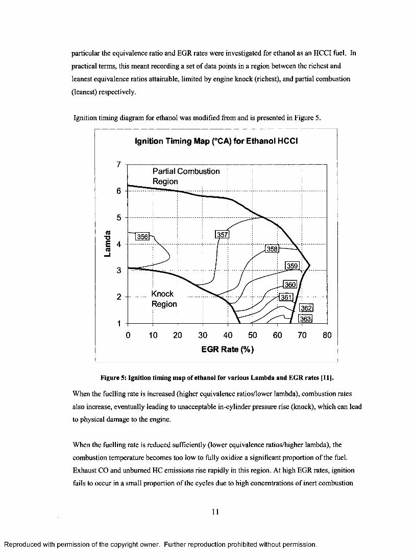
particular the equivalence ratio and EGR rates were investigated for ethanol as an HCCI fuel. In
practical terms, this meant recording a set of data points in a region between the richest and
leanest equivalence ratios attainable, limited by engine knock (richest), and partial combustion
(leanest) respectively.
Ignition timing diagram for ethanol was modified from and is presented in Figure 5.
Ignition Timing Map (°CA) for Ethanol HCCI
7Partial Combustion Region
6
5
3573564 358
3593
360KnockRegion
2 3613623631
10 20 30 40 50 60 70 800
EGR Rate (%)
Figure 5: Ignition timing map of ethanol for various Lambda and EGR rates [11].
When the fuelling rate is increased (higher equivalence ratios/lower lambda), combustion rates
also increase, eventually leading to unacceptable in-cylinder pressure rise (knock), which can lead
to physical damage to the engine.
When the fuelling rate is reduced sufficiently (lower equivalence ratios/higher lambda), the
combustion temperature becomes too low to fully oxidize a significant proportion of the fuel.
Exhaust CO and unbumed HC emissions rise rapidly in this region. At high EGR rates, ignition
fails to occur in a small proportion of the cycles due to high concentrations of inert combustion
11
Reproduced with permission of the copyright owner. Further reproduction prohibited without permission.
products in the mixture. Ethanol has the second largest attainable HCCI region next to methanol
that has the largest HCCI region. The trends for ethanol ignition timing lie between trends
observed for gasoline and methanol. Ethanol ignition timing will show some retardation with
increased EGR rates. For all types of fuels tested ignition timings are relatively independent of
equivalence ratio at low EGR rates. However, as EGR rate is increased beyond 40 %, ignition
timing for gasoline advances under progressively leaner conditions. This is due to the presence of
fewer oxygen molecules at higher EGR rates. Inert EGR gas displaces air that contains oxygen.
However, for alcohols the oxidation process is less sensitive to the presence of EGR because
alcohols already contain a significant portion of oxygen required for combustion.
2.4 Fuel Effects
Fuel selection is perhaps the most important aspect of HCCI engine development. The effect of
fuel volatility and auto-ignition characteristics, are important factors for HCCI engine control.
Epping et al. [20] demonstrated that a fuel must have a high volatility in order to easily form a
homogeneous mixture. Also, fuels with single-stage ignition are less sensitive to changes in
speed and load, and are better suited for HCCI, because they can ease the control requirements.
The auto-ignition temperature of the fuel is also an important consideration for the optimal
selection of an engine compression ratio. With fuel selection for HCCI there is a contradiction.
Selecting a HCCI fuel that is optimal for low loads will limit the range of HCCI operation at high
loads. For example, if one proposes to optimize HCCI engine combustion at low loads, a low
octane fuel is desired, however for high loads this fuel will exhibit extreme knocking, because of
its rapid heat release rate. Additionally, even if one were to employ a dual mode strategy, SI
combustion at high loads and HCCI at low loads, a low octane fuel will not prevent SI knocking
at high loads. Therefore, there is a contradiction in fuelling strategy when it comes to employing
HCCI with a single fuel, and there is no universal fuel that is specific to HCCI operation. The
optimal fuel depends on the combustion control strategies and operating conditions [21].
As discussed by Asmus and Zhao [21], some chemical additives have the ability to inhibit or
promote the heat release process of auto-ignition. Therefore, HCCI auto-ignition can be
controlled by modifying the fuel, in such a way, that it is more chemically reactive or inhibitive
by adding an ignition promoter or inhibitor. For a natural gas fuelled HCCI engine, even a small
presence of N 02 present in the charge may advance auto-ignition of HCCI. The use of varying
N 02 addition by injecting chemical fuel additive can be used as a means of controlling HCCI.
12
Reproduced with permission of the copyright owner. Further reproduction prohibited without permission.
By using two fuels with a large reactivity difference it is possible to extend the operation range
limits of an HCCI engine. Furutani et al. [22] proposed an approach to combine two different
fuels with different octane numbers to enable auto-ignition timing control. The study found that
an optimal combination of these two fuels could be determined for each speed and load condition.
Also, it is necessary for one fuel to have as high an octane number as possible, and for the other
fuel to have as low an octane number as possible. This strategy will enable the widest operating
range possible for HCCI using two fuels. A similar study was conducted by Olsson et al. [19]
using ethanol and n-heptane. It was found that for static engine operation the performance of the
dual fuel system was sufficient, and optimization of MBT timing and low emissions was
attainable for a variety of speeds and loads.
2.5 Exhaust Gas Recirculation
EGR is perhaps the most straightforward way of controlling intake charge temperature, and
consequently combustion timing and duration. The main problem with EGR control is the
response time may be too slow, and difficulties in handling transient conditions.
Control of recycling of burned gases can include both external EGR and internal EGR. External
EGR is the more commonly understood method for recycling exhaust gases. Exhaust gases are
diverted in the exhaust manifold and brought back to the intake manifold to mix with the
incoming air. Internal EGR is more commonly referred to as retained exhaust gas residuals. For
HCCI, the use of W T can be used to re-open the exhaust valve during the intake stroke, thus
allowing exhaust gas residuals to return to the combustion chamber and aid in the combustion
process [21],
Ladomattos et. al [11] stated that EGR systems are attractive for HCCI engine operation because
of three fundamental properties:
1. High temperature residuals aid auto-ignition.
2. Switching from SI to HCCI may be done in one cycle.
3. Degree of residual mixing with fresh charge may be used to control combustion timing
and duration.
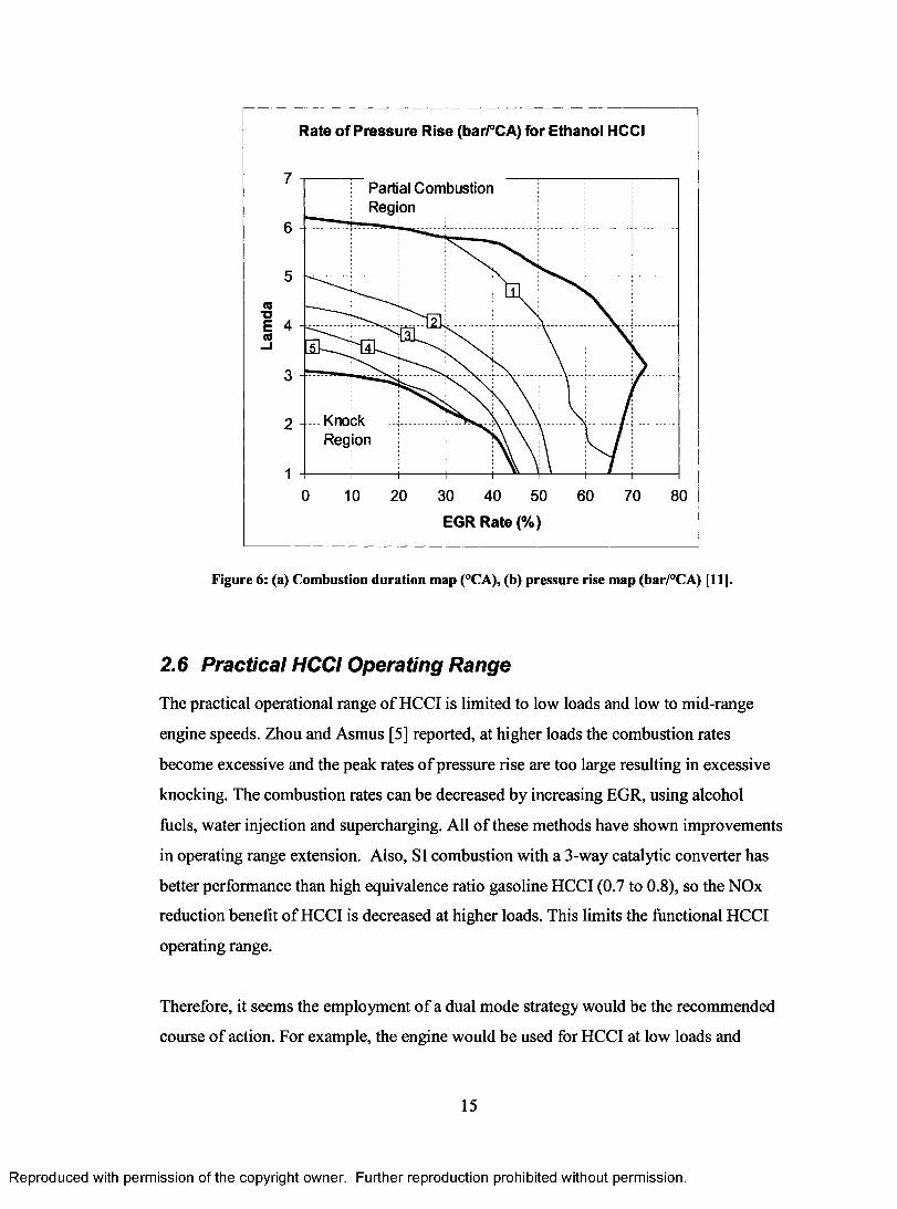
Figure 6a illustrates the combustion durations trends for ethanol, as modified from the same study
as mentioned previously. Unlike ignition trends, combustion duration (or heat release rate) trends
13
Reproduced with permission of the copyright owner. Further reproduction prohibited without permission.
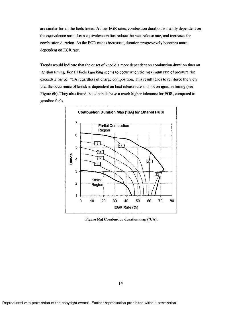
are similar for all the fuels tested. At low EGR rates, combustion duration is mainly dependent on
the equivalence ratio. Lean equivalence ratios reduce the heat release rate, and increases the
combustion duration. As the EGR rate is increased, duration progressively becomes more
dependent on EGR rate.
Trends would indicate that the onset of knock is more dependent on combustion duration than on
ignition timing. For all fuels knocking seems to occur when the maximum rate of pressure rise
exceeds 5 bar per °CA regardless of charge composition. This result tends to reinforce the view
that the occurrence of knock is dependent on heat release rate and not on ignition timing (see
Figure 6b). They also found that alcohols have a much higher tolerance for EGR, compared to
gasoline fuels.
Combustion Duration Map (°CA) for Ethanol HCCI
7Partial Combustion Region
6
5
4
3
KnockRegion2
10 10 20 30 40 50 60 70 80
EGR Rate (%)
Figure 6(a) Combustion duration map (°CA).
14
Reproduced with permission of the copyright owner. Further reproduction prohibited without permission.
Rate of Pressure Rise (bar/°CA) for Ethanol HCCI
7Partial Combustion Region
6
5
4
3
KnockRegion
2
10 10 20 30 40 50 60 70 80
EGR Rate (%)
Figure 6: (a) Combustion duration map (°CA), (b) pressure rise map (bar/°CA) [11].
2.6 Practical HCCI Operating Range
The practical operational range o f HCCI is limited to low loads and low to mid-range
engine speeds. Zhou and Asmus [5] reported, at higher loads the combustion rates
become excessive and the peak rates o f pressure rise are too large resulting in excessive
knocking. The combustion rates can be decreased by increasing EGR, using alcohol
fuels, water injection and supercharging. All o f these methods have shown improvements
in operating range extension. Also, SI combustion with a 3-way catalytic converter has
better performance than high equivalence ratio gasoline HCCI (0.7 to 0.8), so the NOx
reduction benefit o f HCCI is decreased at higher loads. This limits the functional HCCI
operating range.
Therefore, it seems the employment o f a dual mode strategy would be the recommended
course o f action. For example, the engine would be used for HCCI at low loads and
15
Reproduced with permission of the copyright owner. Further reproduction prohibited without permission.

switched to SI combustion at a load point where HCCI shows more challenges in
combustion control and less benefit when compared to SI combustion. The same dual
mode strategy for HCCI can be applied to diesel HCCI engines. For light loads, diesel
HCCI can be employed to eliminate aftertreatment devices where low exhaust gas
temperature make it difficult to reduce NOx and PM emission. For high loads the diesel
engine will be switched to conventional Cl combustion.
2.7 Summary
A summary of the HCCI control parameter trends are listed in Table 2 below. Fuel effects will
not be investigated in this project.
Table 2 Summary of HCCI control parameters as found in recent literature publications.
HCCI Control Parameter Action Resulting Trend (for Ethanol)
Increasing intake charge temperature 1) Advances auto-ignition.
2) Decreases combustion duration.
3) Increases heat release rate (HRR)
4) Extends Lean limit of auto-ignition
5) Temperature range [25-500°C]
Increasing compression ratio 1) Similar as increasing charge temp.
2) Decreases intake charge temperature for auto
ignition.
3) Increases engine knock at high loads.
4) CR range [15 < CR < 25 ] depending on RPM,
load, and Octane #.
5) Increases thermal efficiency.
6) Increases frictional losses.
Varying equivalence ratio (4>) 1) HCCI Range [Lean 0.14< $ <0.5 Rich]
2) Increasing $ increases load (BMEP)
Increases HRR, decreases combustion duration
and lowers efficiency.
3) Decreasing 4> decreases load (BMEP)
Decreases HRR, increases combustion duration,
and increases efficiency.
16
Reproduced with permission of the copyright owner. Further reproduction prohibited without permission.
Fuel Effects 1) Fuel should have high volatility.
2) Optimize low load => low octane fuel
3) Optimize high load =>high octane fuel
4) Additives can control timing
5) Dual fuel strategy to extend range
6) Dual Mode (SI & HCCI) or (Cl &HCCI)
Exhaust gas recirculation (EGR) 1) Decreasing EGR, combustion duration depends
on $ .
2) Increasing EGR, increases combustion duration
and decreases HRR
3) Ethanol has higher tolerance for EGR than
gasoline.
In summary, there are several parameters that affect the control of HCCI bum in an IC engine.
Understanding how these parameters impact the point of auto-ignition, the heat release rate and
combustion duration will enable us to establish design constraints for our ethanol fuelled HCCI
engine. The literature review objective has been performed to identify the parameters affecting
control of HCCI with respect to use of ethanol as a fuel.
Reproduced with permission of the copyright owner. Further reproduction prohibited without permission.
17

3 RESEARCH APPARATUS CONCEPT DEVELOPMENT
3.1 Identification of Need
As presented in Section 2, HCCI combustion is attained by controlling; intake charge
temperature, EGR rate, compression ratio and equivalence ratio. These parameters are varied to
achieve auto-ignition near top-dead-center, control heat release rate and combustion duration.
HCCI combustion is difficult to control due to the absence of direct control methods such as
spark firing or fuel injection to determine ignition timing as in SI or Cl engines. Therefore,
investigation of parameters affecting control of ignition timing, and heat release rate are
significant for the commercialization of this technology. An experimental apparatus for
investigation of all parameters affecting control of HCCI is required to conduct research of this
novel combustion phenomenon.
3.2 Background Research
Background research was performed in the literature review to identify the parameters affecting
control of HCCI engines. However, this section will identify the types of devices that are
currently being used by industry and institutions for investigation of HCCI. Three main
categories of apparatus for experimental investigation of HCCI where identified; a rapid
compression machine, a single-cylinder research engine, and a production engine converted to
run on HCCI.
3.2.1 Rapid Compression Machine
Rapid compression machines (RCM) have been used to study HCCI by several researchers [23,
24]. A rapid compression machine is defined as a device that enables compression of an air fuel
mixture to its auto-ignition temperature. The main use for RCM is to study the effect of fuel
mixtures on auto-ignition. The RCM has been used for many years to investigate the changes in
pressure and ignition properties due to HCCI and other modes of combustion.
The RCM is not a device that can be purchased readily and must be designed and fabricated by
the research institution. As a result they are very costly and the quality of the experimental data is
highly variable and dependent on the specific characteristics of the RCM. Additionally, the
results may not give close correlation to production engine data.
18
Reproduced with permission of the copyright owner. Further reproduction prohibited without permission.
3.2.2 Single Cylinder Research Engines
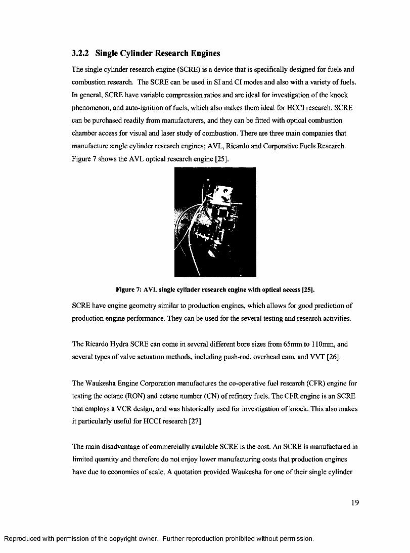
The single cylinder research engine (SCRE) is a device that is specifically designed for fuels and
combustion research. The SCRE can be used in SI and Cl modes and also with a variety of fuels.
In general, SCRE have variable compression ratios and are ideal for investigation of the knock
phenomenon, and auto-ignition of fuels, which also makes them ideal for HCCI research. SCRE
can be purchased readily from manufacturers, and they can be fitted with optical combustion
chamber access for visual and laser study of combustion. There are three main companies that
manufacture single cylinder research engines; AVL, Ricardo and Corporative Fuels Research.
Figure 7 shows the AVL optical research engine [25].
Figure 7: AVL single cylinder research engine with optical access [25].
SCRE have engine geometry similar to production engines, which allows for good prediction of
production engine performance. They can be used for the several testing and research activities.
The Ricardo Hydra SCRE can come in several different bore sizes from 65mm to 110mm, and
several types of valve actuation methods, including push-rod, overhead cam, and W T [26].
The Waukesha Engine Corporation manufactures the co-operative fuel research (CFR) engine for
testing the octane (RON) and cetane number (CN) of refinery fuels. The CFR engine is an SCRE
that employs a VCR design, and was historically used for investigation of knock. This also makes
it particularly useful for HCCI research [27].
The main disadvantage of commercially available SCRE is the cost. An SCRE is manufactured in
limited quantity and therefore do not enjoy lower manufacturing costs that production engines
have due to economies of scale. A quotation provided Waukesha for one of their single cylinder
19
Reproduced with permission of the copyright owner. Further reproduction prohibited without permission.
research engines was for $125,000 US dollars. This cost does not include the data acquisition
system and all other systems that will be required.
3.2.3 Production Engines Converted for HCCI
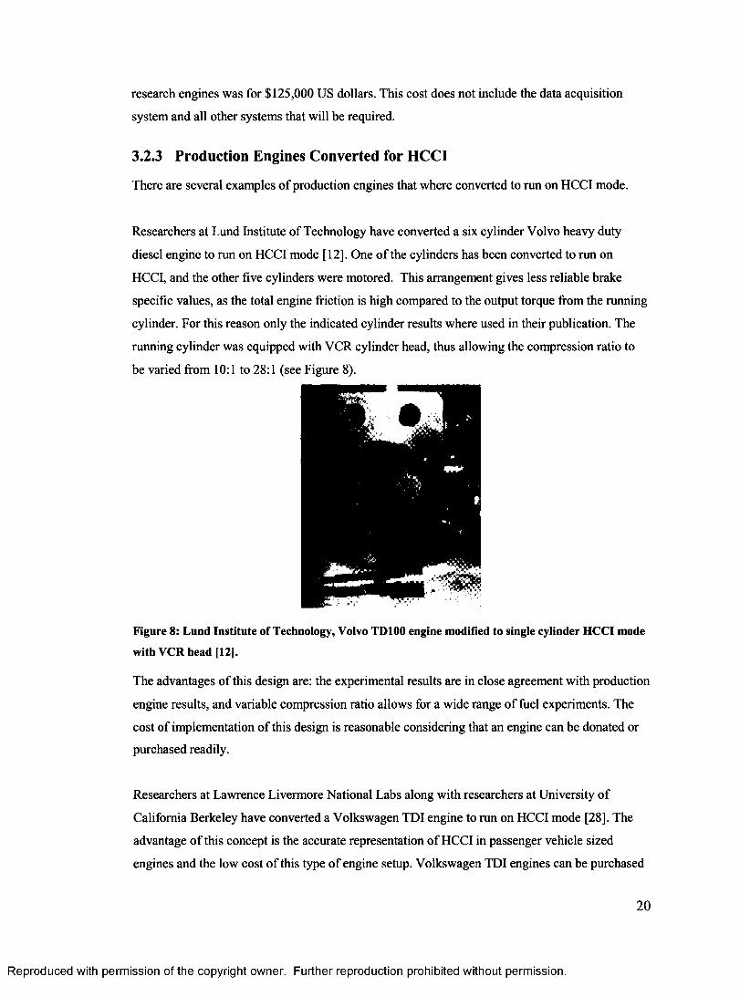
There are several examples of production engines that where converted to run on HCCI mode.
Researchers at Lund Institute of Technology have converted a six cylinder Volvo heavy duty
diesel engine to run on HCCI mode [12]. One of the cylinders has been converted to run on
HCCI, and the other five cylinders were motored. This arrangement gives less reliable brake
specific values, as the total engine friction is high compared to the output torque from the running
cylinder. For this reason only the indicated cylinder results where used in their publication. The
running cylinder was equipped with VCR cylinder head, thus allowing the compression ratio to
be varied from 10:1 to 28:1 (see Figure 8).
Figure 8: Lund Institute of Technology, Volvo TD100 engine modified to single cylinder HCCI mode
with VCR head [12].
The advantages of this design are: the experimental results are in close agreement with production
engine results, and variable compression ratio allows for a wide range of fuel experiments. The
cost of implementation of this design is reasonable considering that an engine can be donated or
purchased readily.
Researchers at Lawrence Livermore National Labs along with researchers at University of
California Berkeley have converted a Volkswagen TDI engine to run on HCCI mode [28], The
advantage of this concept is the accurate representation of HCCI in passenger vehicle sized
engines and the low cost of this type of engine setup. Volkswagen TDI engines can be purchased
20
Reproduced with permission of the copyright owner. Further reproduction prohibited without permission.

for less than $5000 dollars. However, the data acquisition system, and other system will have to
be purchased and would total an estimated $40,000 dollars. The experimental work conducted by
this collaboration was focused on fundamentals of premixed HCCI combustion and on evaluation
of possible techniques for engine operation and control.
In summary, production engines converted to run on HCCI mode are a good option for enabling
HCCI mode for experiments. Several examples of production engines converted to run on HCCI
have been reported in literature.
3.3 Problem Statement
The problem statement is defined as follows:
To design an experimental apparatus that enables investigation o f parameters affecting
combustion control o f a H C C I engine fu e lled with ethanol.
3.3.1 Project Methodology and Deliverables
The methodology employed for this project is as is as follows:
1. Develop a workable design concept that meets all the criteria and constraints.
2. Develop detailed design schematic drawings for all systems of the apparatus.
3. Perform design calculations for each of the systems of the apparatus.
4. Select components based on design calculations and order the necessary components.
5. Fabricate each system of the apparatus.
6. Test each system and implement improvements.
7. Complete verification experiments to ensure functionality of the apparatus.
The necessary outcomes for the apparatus are:
1. To obtain a functional apparatus that is easy to use and will allow future graduate
students the ability to perform HCCI experimental engine research.
2. To have the ability to vary and hold the engine speed with little deviation.
3. To have the ability to acquire in-cylinder pressure measurements, that can be utilized to
study the combustion process.
21
Reproduced with permission of the copyright owner. Further reproduction prohibited without permission.

3.4 Criteria and Constraints
Development of design criteria and constraints are both very important steps of the design
process. This section will review these points with respect to the design process as applied to the
development of our research apparatus.
3.4.1 Criteria
The design criteria for the apparatus are; functionality, durability, manufacturability, cost
effectiveness and safety.
3.4.1.1 Functionality
Functionality is defined as the ability of the apparatus to perform its intended mechanical and/or
electrical design functions. The question one poses to oneself when considering functionality is;
Does this design perform all necessary design functions?
Determining the design functions is the first and most important step when considering
functionality. Based on the literature review, we have identified several functional requirements
to perform HCCI combustion research. However, these requirements are actual system
requirements that are comprised of both mechanical and electrical components.
Firstly, the ability to vary parameters affecting HCCI combustion control will be required. As
mentioned in Chapter 2 these parameters are the following; variable intake air temperature,
variable compression ratio, variable equivalence ratio and variable EGR. Additionally, the ability
to fix engine speed and dissipate excess power produced will be required
Secondly, the ability of the apparatus to perform data acquisition and measurement functions is
also a major criterion. These functions include; high-speed data acquisition for in-cylinder
pressure measurements and crank angle degrees, and the ability to perform and display engine
performance calculations on in-cylinder pressure data. Additionally, low speed data acquisition
and/or measurement will be required for intake air temperature, manifold absolute pressure,
coolant temperature, and fuel pressure.
22
Reproduced with permission of the copyright owner. Further reproduction prohibited without permission.
Lastly, a couple of less tangible functionality items are; the ease at which the apparatus can be
used during experiments, and the versatility of the apparatus for future research projects.
3.4.1.2 Durability
Durability is defined as the resistance of the design to failure. The question one poses to oneself
when considering durability is;
Is this design durable?
Durability can also be defined as the reliability or the robustness of the design. The design of the
apparatus should be optimized for robustness. This is achieved by over-sizing critical systems and
components and selecting components that are readily available to eliminate downtime. Design
with durability in mind will eliminate breakage of costly components and ensure piece-of-mind.
3.4.1.3 Manufacturability
The definition of manufacturability is the ease of which the design can be fabricated. The
question one poses to oneself when considering manufacturability is;
Is this design easy to manufacture?
Often designs that are optimized for ease of fabrication typically use off-the-shelf components,
such as; standard size construction materials such as standard steel tubing for fixture structure or
use of standard fastener sizes. Use of purchased components instead of fabricating all components
will minimize the overall machine shop labour hours and ultimately cost required to fabricate the
apparatus. Additionally, the capabilities of the machine shop must be taken into account when
selecting a design concept as elimination of outsourcing will reduce cost and time.
3.4.1.4 Cost Effectiveness
Cost effectiveness is quite simply the minimization of cost associated with a design concept. The
question one poses to oneself when considering cost effectiveness is;
Will this design be less than or meet budgetary constraints?
23
Reproduced with permission of the copyright owner. Further reproduction prohibited without permission.

There are several design concepts that meet or exceed all other criteria, and are often the ideal
design solution. However the cost of design and fabrication exceeds the allowable budget and this
fact alone eliminates the design from future consideration. Techniques for reducing cost at the
design concept phase are selection of standardized components and selecting the simplest design
that meets all criteria. Often the simplest design concept is the most likely to succeed and meet
budgetary constraints. This involves purchasing components as opposed to fabricating.
3.4.1.5 Safety
The definition of safety is; the state of being certain that adverse effects will not be caused by
some agent under defined conditions. The question one poses to himself when considering safety
is;
Is this design safe fo r use?
It can also be thought of as the degree of safety of the design as a complete system.
Adverse effects that are caused by machine devices are; short-term bodily injury such as, bums,
cuts, contusions, electrocution. The sources of these short-term injuries are; from reciprocating
parts, pinch points, projectile metal debris, heat sources, sharp edges, and electric power wires
and components. Although these are termed short-term bodily injuries since they occur and are
visible instantly, this does not imply that the injuries sustained by these means are for a short
term, but often the injuries are severe and result in long term effects.
Long-term injuries usually are not evident immediately upon exposure. Injuries such as nervous
system damage or other physical injuries that result from exposure to hazardous materials while
operating the device should be avoided when possible. These materials could be a hydrocarbon
fuel such as gasoline and ethanol, exhaust products, or carcinogenic materials such asbestos. Most
safety concerns regarding a design concept can be remedied by conforming to health and safety
regulations.
Care must be taken in the design of the device to prevent, and inform the he operator of the
potential dangers of using ethanol and experiment HCCI combustion. Unpredictable combustion
events and motor run-off must be controlled. Use alcohol fuels such as ethanol of particular
concern, since the flame is not easily detected in daylight, and could lead to serious injuries if
proper precautions are not taken.
24
Reproduced with permission of the copyright owner. Further reproduction prohibited without permission.

3.4.2 Constraints
Now that the criteria have been determined it is important to summarize the constraints on the
apparatus. This section will review constraints on all the criteria mentioned above.
The most significant criterion for our apparatus is functionality. Table 3 lists the constraints on
functionality. This list will be consulted when designing the apparatus along with its various
systems.
The constraint of durability is difficult to quantify, but can be best addressed through common
sense and experience when selecting components, and sizing systems. However there are certain
factors of safety that can give us a degree of durability for critical systems. Table 4 lists the
constraints for durability.
The constraints for manufacturability are mainly subject to the limitation of the capabilities of the
machine shop. Therefore, for each system of the apparatus the technician should be consulted
early in the design process to address concerns and limitations that the machine shop may have.
The main constraint for cost effectiveness is our project budget which is a maximum of $35,000.
To keep costs low it is important to utilize industry contacts, on-campus technical experts, and
off-the-shelf components.
Safety constraints on the apparatus are mostly based on common sense and experience.
There are certain health and safety regulations that the University of Windsor has for laboratories
and research apparatuses, which are governed by the Electrical Code of Canada (ECC), and the
Canadian Safety Association (CSA) Standards. In particular the fuel storage limit on the device
should not exceed 5 liters of flammable liquid [29].
25
Reproduced with permission of the copyright owner. Further reproduction prohibited without permission.
Table 3 List o f functionality constraints.
Functionality Constrained Parameter Constraint Range
HCCI Control Intake Air Temperature Ti„ie,, 0 to 300 °C
Compression Ratio CR, 15 to 25:1
Equivalence Ratio $ , 0.0 to 1.0
Exhaust Gas Recirculation EGR, 0 to 80%
Engine Control Cycle Time, (Engine Speed) 0 to 3600 RPM
Cycle Time Deviation Less than 1% of max.
Power Dissipation Pabsoibed, 0 tO 10 HP
Coolant Temperature Tcoolant, 60 tO 90 °C
Intake Valve Timing Suitable for HCCI
Fuel System Fuel Pressure 2 to 5 bar, Nom. 3.1 bar
Ethanol Compatibility Components must be nonreactive with alcohols and gasoline.
EGR % EGR Measurement Capability required.
Data Acquisition System Labview User Interface Logical layout, easy to use.
Data Acquisition Speed l/lO01 °CA at 2000 RPM
In-Cylinder Pressure Highly sensitive & accurate
Crank Angle Encoder Resolution, >l/10th °CA
Intake Air Thermocouple -10 to 500 °C
Intake Air Pressure sensor 1 to 2.5 bar
Coolant Thermocouple -10 to 200°C
Table 4 List of durability constraints.
Durability Constrained Parameter Constraint RangeFixture Structural Steel Fixture Adequate sizing components
selectedVibration Control Minimize vibration
Engine Combustion Chamber Pressure, 0 to 200 bar
Overall Output Power, <= 25 hp
Subsystem Components Various Of high quality and
durability
26
Reproduced with permission of the copyright owner. Further reproduction prohibited without permission.
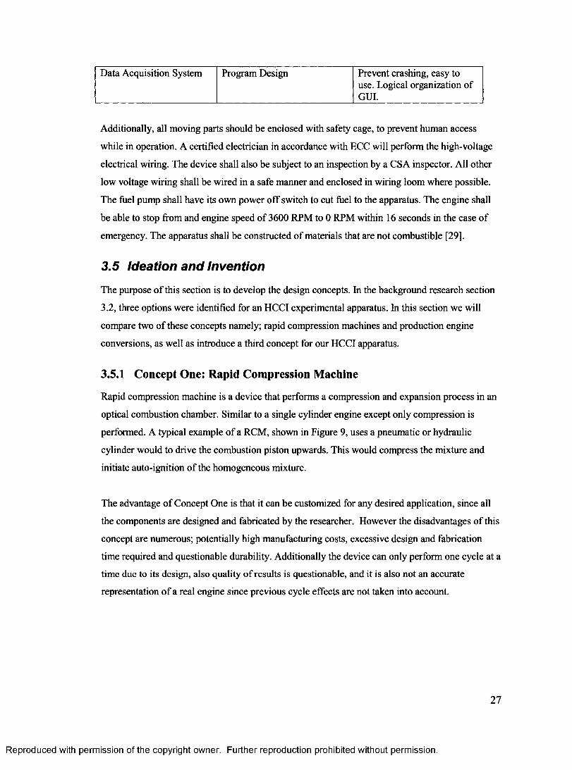
Data Acquisition System Program Design Prevent crashing, easy touse. Logical organization ofGUI.
Additionally, all moving parts should be enclosed with safety cage, to prevent human access
while in operation. A certified electrician in accordance with ECC will perform the high-voltage
electrical wiring. The device shall also be subject to an inspection by a CSA inspector. All other
low voltage wiring shall be wired in a safe manner and enclosed in wiring loom where possible.
The fuel pump shall have its own power off switch to cut fuel to the apparatus. The engine shall
be able to stop from and engine speed of 3600 RPM to 0 RPM within 16 seconds in the case of
emergency. The apparatus shall be constructed of materials that are not combustible [29].
3.5 Ideation and Invention
The purpose of this section is to develop the design concepts. In the background research section
3.2, three options were identified for an HCCI experimental apparatus. In this section we will
compare two of these concepts namely; rapid compression machines and production engine
conversions, as well as introduce a third concept for our HCCI apparatus.
3.5.1 Concept One: Rapid Compression Machine
Rapid compression machine is a device that performs a compression and expansion process in an
optical combustion chamber. Similar to a single cylinder engine except only compression is
performed. A typical example of a RCM, shown in Figure 9, uses a pneumatic or hydraulic
cylinder would to drive the combustion piston upwards. This would compress the mixture and
initiate auto-ignition of the homogeneous mixture.
The advantage of Concept One is that it can be customized for any desired application, since all
the components are designed and fabricated by the researcher. However the disadvantages of this
concept are numerous; potentially high manufacturing costs, excessive design and fabrication
time required and questionable durability. Additionally the device can only perform one cycle at a
time due to its design, also quality of results is questionable, and it is also not an accurate
representation of a real engine since previous cycle effects are not taken into account.
27
Reproduced with permission of the copyright owner. Further reproduction prohibited without permission.
CombustionChamber
Air Cylinder
Figure 9: Concept One, rapid compression machine.
3.5.2 Concept Two: Engine with Dynamometer
The second concept studied was an engine with a dynamometer. This concept consists of a 3-
cylinder Kubota D905 diesel production engine as the base engine (see Figure 10a), and a Land
and Sea #200 eddy current brake as the dynamometer (see Figure 10b).
Figure 10: (a) 3-cylinder Kubota D905 diesel engine, (b) eddy current dynamometer [30].
28
Reproduced with permission of the copyright owner. Further reproduction prohibited without permission.
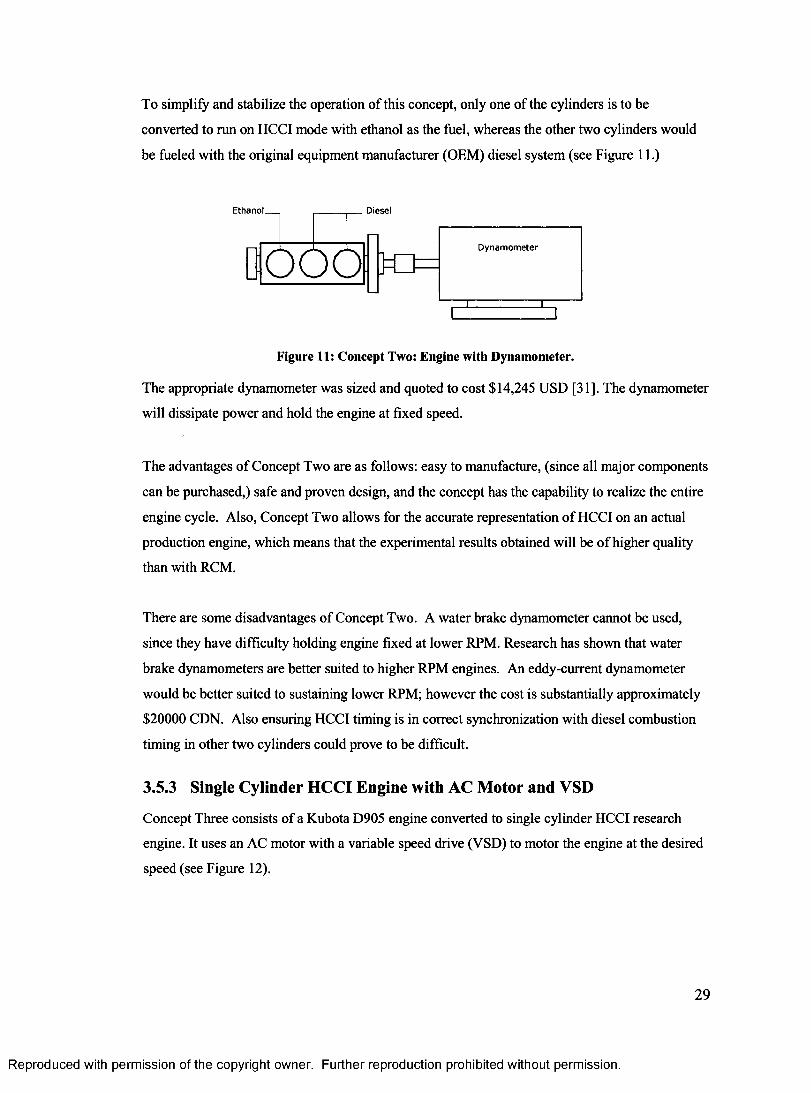
To simplify and stabilize the operation of this concept, only one of the cylinders is to be
converted to run on HCCI mode with ethanol as the fuel, whereas the other two cylinders would
be fueled with the original equipment manufacturer (OEM) diesel system (see Figure 11.)
DieselE thanol___
D ynam om eter
Figure 11: Concept Two: Engine with Dynamometer.
The appropriate dynamometer was sized and quoted to cost $14,245 USD [31]. The dynamometer
will dissipate power and hold the engine at fixed speed.
The advantages of Concept Two are as follows: easy to manufacture, (since all major components
can be purchased,) safe and proven design, and the concept has the capability to realize the entire
engine cycle. Also, Concept Two allows for the accurate representation of HCCI on an actual
production engine, which means that the experimental results obtained will be of higher quality
than with RCM.
There are some disadvantages of Concept Two. A water brake dynamometer cannot be used,
since they have difficulty holding engine fixed at lower RPM. Research has shown that water
brake dynamometers are better suited to higher RPM engines. An eddy-current dynamometer
would be better suited to sustaining lower RPM; however the cost is substantially approximately
$20000 CDN. Also ensuring HCCI timing is in correct synchronization with diesel combustion
timing in other two cylinders could prove to be difficult.
3.5.3 Single Cylinder HCCI Engine with AC Motor and VSD
Concept Three consists of a Kubota D905 engine converted to single cylinder HCCI research
engine. It uses an AC motor with a variable speed drive (VSD) to motor the engine at the desired
speed (see Figure 12).
29
Reproduced with permission of the copyright owner. Further reproduction prohibited without permission.
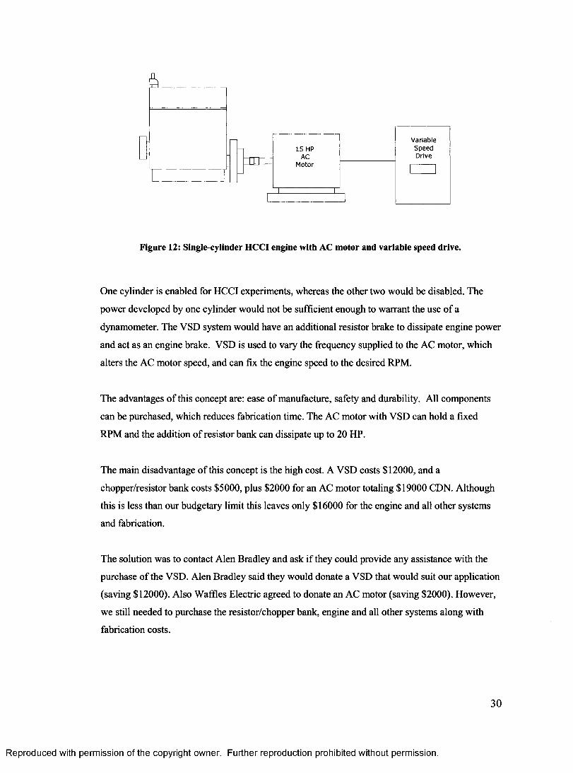
15 HP AC
M otor
V ariableS peedDrive
Figure 12: Single-cylinder HCCI engine with AC motor and variable speed drive.
One cylinder is enabled for HCCI experiments, whereas the other two would be disabled. The
power developed by one cylinder would not be sufficient enough to warrant the use of a
dynamometer. The VSD system would have an additional resistor brake to dissipate engine power
and act as an engine brake. VSD is used to vary the frequency supplied to the AC motor, which
alters the AC motor speed, and can fix the engine speed to the desired RPM.
The advantages of this concept are: ease of manufacture, safety and durability. All components
can be purchased, which reduces fabrication time. The AC motor with VSD can hold a fixed
RPM and the addition of resistor bank can dissipate up to 20 HP.
The main disadvantage of this concept is the high cost. A VSD costs $12000, and a
chopper/resistor bank costs $5000, plus $2000 for an AC motor totaling $19000 CDN. Although
this is less than our budgetary limit this leaves only $16000 for the engine and all other systems
and fabrication.
The solution was to contact Alen Bradley and ask if they could provide any assistance with the
purchase of the VSD. Alen Bradley said they would donate a VSD that would suit our application
(saving $12000). Also Waffles Electric agreed to donate an AC motor (saving $2000). However,
we still needed to purchase the resistor/chopper bank, engine and all other systems along with
fabrication costs.
30
Reproduced with permission of the copyright owner. Further reproduction prohibited without permission.
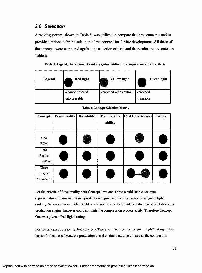
3.6 Selection
A ranking system, shown in Table 5, was utilized to compare the three concepts and to
provide a rationale for the selection of the concept for further development. All three of
the concepts were compared against the selection criteria and the results are presented in
Table 6.
Table 5 Legend, Description of ranking system utilized to compare concepts to criteria.
Legend Red light Yellow light Green light
-cannot proceed
-nto feasable
-proceed with caution -proceed
-feasable
Table 6 Concept Selection Matrix
Concept Functionality Durability M anufactur
ability
Cost Effectiveness Safety
One
RCM • • • • •Two
Enginew/Dyno
Three
Engine AC w/VSD
For the criteria of functionality both Concept Two and Three would enable accurate
representation of combustion in a production engine and therefore received a “green light”
ranking. Whereas Concept One RCM would not be able to provide a realistic representation of a
production engine, however could simulate the compression process easily. Therefore Concept
One was given a “red light” rating.
For the criteria of durability, both Concept Two and Three received a “green light” rating on the
basis of robustness, because a production diesel engine would be utilized as the combustion
31
Reproduced with permission of the copyright owner. Further reproduction prohibited without permission.

apparatus. The Kubota D905E production diesel engine is already designed to handle high
compression ratios (22:1) similar to what would be required for an HCCI engine and therefore
would be a reasonable choice for this application. On the other hand, Concept One will require
design and fabrication of the combustion chamber. This is a difficult endeavour and perhaps out
of scope for a Master’s project. This combustion chamber would have to withstand the pressures
experienced in an HCCI engine close to 150 bar [12]. The design of such a combustion chamber
requires expertise in several different areas. This knowledge is lacking in our research group, and
therefore it would be wise to opt to purchase a proven, existing design, such as a production
diesel engine chosen for Concept Two and Three. Therefore, Concept One is seen as feasible yet
difficult and as such received a “yellow light” ranking.
For the criteria of manufacturability, Concept Two and Three utilize off-the-shelf components
and as such reduce the fabrication time and costs required, whereas Concept One requires
fabrication of all components. Fabrication costs are hard to predict for this type of design, and any
minor setbacks can quickly turn into serious problems with excessively high costs and delays.
Therefore, Concept One was ranked as “red light” because of the high uncertainty of
manufacturing feasibility and expenses.
For the criteria of cost effectiveness, Concept One received a ranking of “yellow light” due to the
uncertain manufacturing costs expected. Concept Two (engine with dyno) was also given a “red
light” because the high cost of an eddy current dynamometer (quoted at $20000). Also Concept
Three (engine with VSD) was originally ranked a “yellow light” because the high cost of the
VSD (quoted at $12000), but because of a generous equipment donation from Alen Bradley and
Waffles Electric, we were able to change the ranking to “green light”.
For the criteria of safety, all designs would employ safety measures to prevent injury to the
operator of the apparatus, and ensure compliance with health and safety regulations. Since these
safety aspects could be designed into each design without much difficulty, all the concepts
received a “green light” ranking. Therefore, on the basis of all the criteria and rankings Concept
Three (engine with AC motor and variable speed drive), was selected as the most feasible design
concept. A detailed design of this concept will be described in Section 4 of this report.
32
Reproduced with permission of the copyright owner. Further reproduction prohibited without permission.
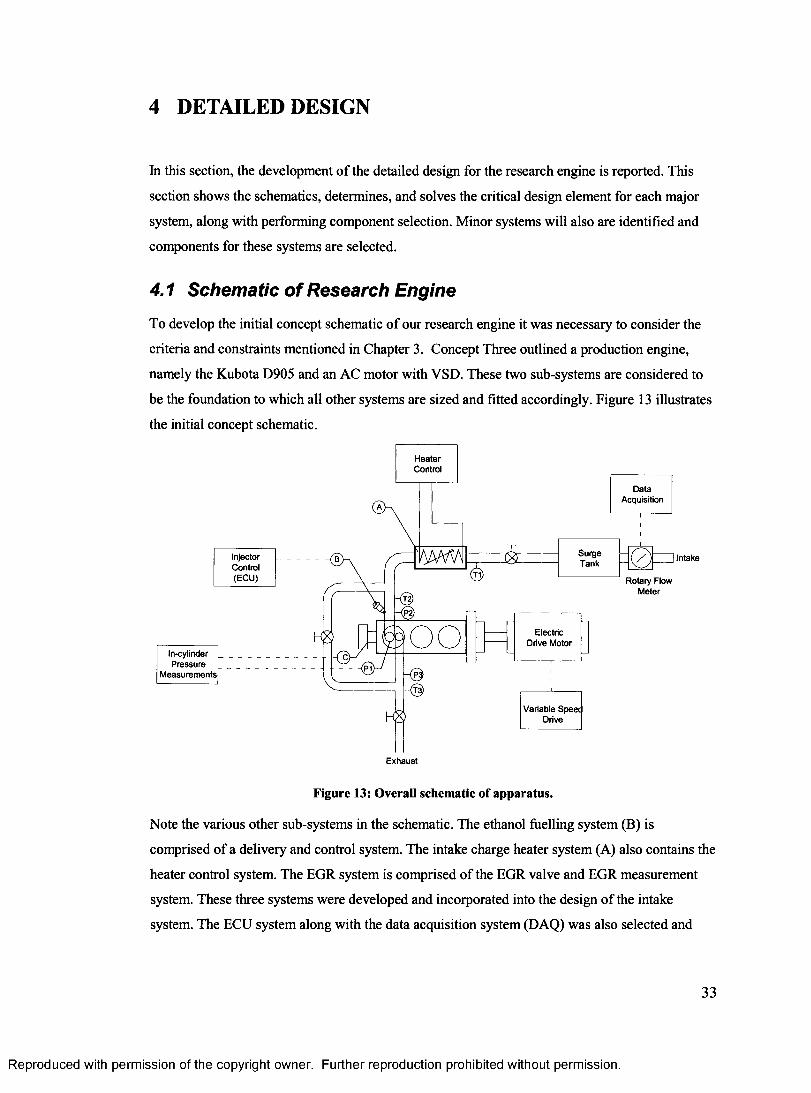
4 DETAILED DESIGN
In this section, the development of the detailed design for the research engine is reported. This
section shows the schematics, determines, and solves the critical design element for each major
system, along with performing component selection. Minor systems will also are identified and
components for these systems are selected.
4.1 Schematic of Research Engine
To develop the initial concept schematic of our research engine it was necessary to consider the
criteria and constraints mentioned in Chapter 3. Concept Three outlined a production engine,
namely the Kubota D905 and an AC motor with VSD. These two sub-systems are considered to
be the foundation to which all other systems are sized and fitted accordingly. Figure 13 illustrates
the initial concept schematic.
HeaterControl
DataAcquisition
SurgeTank
InjectorControl(ECU)
Intake
Rotary Flow Meter
Electric Drive Motor
In-cylinderPressure
M easurements
Variable Speec Drive
Exhaust
Figure 13: Overall schematic of apparatus.
Note the various other sub-systems in the schematic. The ethanol fuelling system (B) is
comprised of a delivery and control system. The intake charge heater system (A) also contains the
heater control system. The EGR system is comprised of the EGR valve and EGR measurement
system. These three systems were developed and incorporated into the design of the intake
system. The ECU system along with the data acquisition system (DAQ) was also selected and
33
Reproduced with permission of the copyright owner. Further reproduction prohibited without permission.
developed. The DAQ system has the capability of providing in-cylinder pressure measurements,
air flow measurements, as well as crank shaft encoder reading and several temperature
thermocouples located at various points of interest.
4.2 Research Engine Selection and Conversion
In this section, the research engine will be selected and design for conversion to an HCCI engine
will be performed.
4.2.1 Engine Selection
The starting point of our design is selecting a suitable base engine. Our objective for the base
engine is to provide a durable, functional, low cost and safe engine for performing HCCI
combustion experiments.
Listed below are the two major design constraints for the research engine:
1. To keep size and cost down, the engine shall have less than 18.6 kW (25 HP) of output
power.
2. Engine shall have a combustion chamber design pressure not exceeding 18 MPa (180 bar).
The selection the base engine has satisfied these constraints. The Kubota D905 is a 3-cylinder
engine that has 18.5 kW (24.8 HP) at 3600 RPM and 5.5 kgf.m (42 ft.lbs) of torque at 2400 RPM
when fuelled with diesel [32], The specifications are summarized in Table 7, while full details are
available in Appendix A. This engine is commonly found in Kubota lawn trackers and was
designed for reliability, durability and fuel efficiency. Since the engine has less than 25 HP in
gross output power the first constraint has been met.
To meet the chamber design pressure constraint we require some assumptions and insight into the
problem. The Kubota D905 has a compression ratio of 22 to 1. The factory specification for a
compression pressure is 3233.6 kPa [33]. The combustion pressure was estimated to be fifty
percent of the compression pressure 1616.8 kPa. Adding 1616.8 to 3233.6 results in a total
pressure ( p t ) 4850.5 kPa on the system. The total pressure is then multiplied by the factor of
safety to get the loss of function pressure ( p lf) or design pressure. See Appendix B.2 for further
detail.
34
Reproduced with permission of the copyright owner. Further reproduction prohibited without permission.
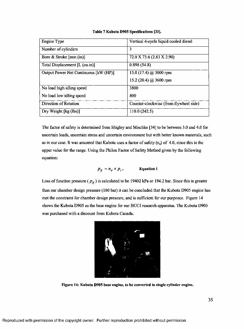
Table 7 Kubota D905 Specifications [33].
Engine Type Vertical 4-cycle liquid cooled diesel
Number of cylinders 3
Bore & Stroke [mm (in)] 72.0X73.6 (2.83X2.90)
Total Displacement [L (cu.in)] 0.898 (54.8)
Output Power Net Continuous [kW (HP)] 13.0 (17.4) @ 3000 rpm
15.2 (20.4) @ 3600 rpm
No load high idling speed 3800
No load low idling speed 800
Direction of Rotation Counter-clockwise (from flywheel side)
Dry Weight [kg (lbs)] 110.0(242.5)
The factor of safety is determined from Shigley and Mischke [34] to be between 3.0 and 4.0 for
uncertain loads, uncertain stress and uncertain environment but with better known materials, such
as in our case. It was assumed that Kubota uses a factor of safety (nd) of 4.0, since this is the
upper value for the range. Using the Philon Factor of Safety Method given by the following
equation:
Pif = nd x Pf> Equation 1
Loss of function pressure ( p ^ ) is calculated to be 19402 kPa or 194.2 bar. Since this is greater
than our chamber design pressure (180 bar) it can be concluded that the Kubota D905 engine has
met the constraint for chamber design pressure, and is sufficient for our purposes. Figure 14
shows the Kubota D905 as the base engine for our HCCI research apparatus. The Kubota D905
was purchased with a discount from Kubota Canada.
Figure 14: Kubota D905 base engine, to be converted to single cylinder engine.
35
Reproduced with permission of the copyright owner. Further reproduction prohibited without permission.
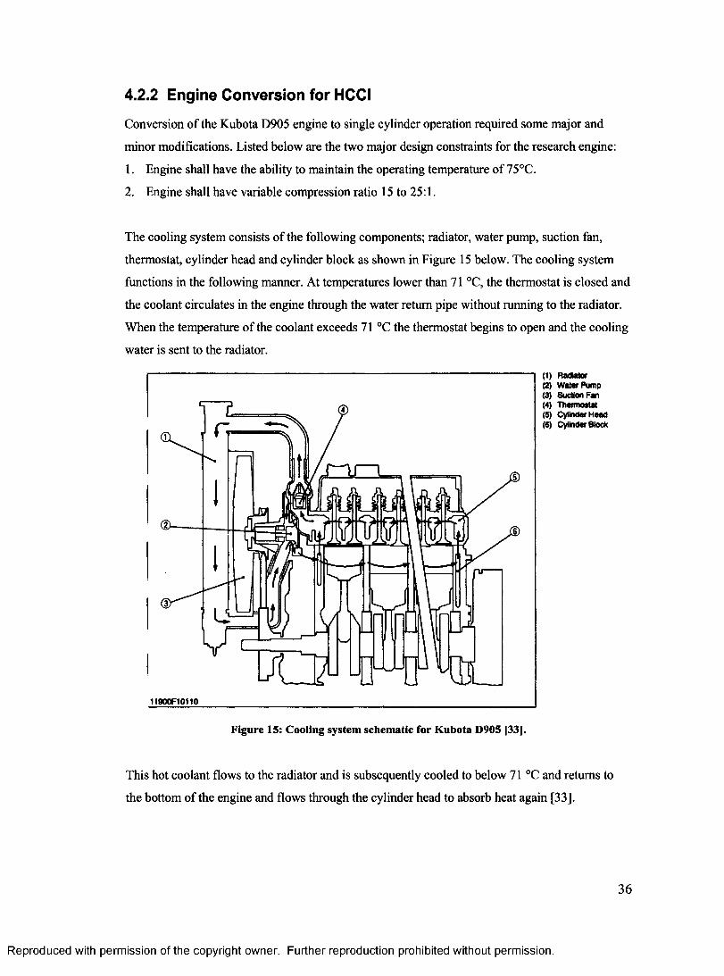
4.2.2 Engine Conversion for HCCI
Conversion of the Kubota D905 engine to single cylinder operation required some major and
minor modifications. Listed below are the two major design constraints for the research engine:
1. Engine shall have the ability to maintain the operating temperature of 75°C.
2. Engine shall have variable compression ratio 15 to 25:1.
The cooling system consists of the following components; radiator, water pump, suction fan,
thermostat, cylinder head and cylinder block as shown in Figure 15 below. The cooling system
functions in the following manner. At temperatures lower than 71 °C, the thermostat is closed and
the coolant circulates in the engine through the water return pipe without running to the radiator.
When the temperature of the coolant exceeds 71 °C the thermostat begins to open and the cooling
water is sent to the radiator.
1I900F10H0
Figure 15: Cooling system schematic for Kubota D905 [33].
(1) Radiator(2) Water Pump(3) Suction Fan(4) Thermostat(5) Cylinder Head(6) Cylinder Block
This hot coolant flows to the radiator and is subsequently cooled to below 71 °C and returns to
the bottom of the engine and flows through the cylinder head to absorb heat again [33].
36
Reproduced with permission of the copyright owner. Further reproduction prohibited without permission.
The cooling system attempts to maintain the engine coolant temperature within a factory
determined design range, for example 71 to 90 °C (Appendix B.3). This meets our design
constraint of having the engine operating temperature at 75 °C.
This temperature range shall be suitable for HCCI operation but is yet to be determined for our
specific setup. However, the proposed design calls for only one cylinder to be enabled as the test
cylinder for combustion, thus our cooling system will most likely have a greater capacity for heat
dissipation then it will require. Furthermore, the cooling system will have some difficulty getting
to the desired operating temperature of 75 °C, since there is less heat being transferred from the
combustion chamber to the cooling system.
The proposed solution required assembly of the cooling system as Kubota had proposed in Figure
15 except the suction fan (3) needed to be removed and mounted at the front of the engine and
replaced with a stand alone floor fan. The purpose of the suction fan was to draw air across the
radiator fins (1) and hence cool the engine. This fan is connected to the water pump flange and
powered by the crankshaft pulley. Therefore, the fan speed or cooling rate is proportional to the
speed of the engine. Removal of the suction fan limits the amount of heat that can be removed
from the cooling system. During testing, if the engine requires additional heat removal, the floor
fan can be turned on to accommodate this.
For our engine heat is only being generated from one cylinder and thus will take longer for the
engine to reach operating temperature of 75 °C. Therefore, an engine block heater shall be
installed in the engine block. Kubota supplied a 1200 W engine block heater that is used in
mainly in cold weather climates. The engine block heater is plugged into a standard 120 V wall
outlet to maintain the engine coolant temperature warm enough to enable faster more reliable cold
starting.
To facilitate ease of use, it is desirable to reach the operating temperature from room temperature
as quickly as possible, or a least estimate the amount of time required to reach operating
temperature. A calculation was performed to estimate the warm up time, assuming the system is
at room temperature of 18°C, and a fixed coolant volume of 4.73 L, and contains a 50/50 mixture
of ethylene glycol and water solution with a specific heat of 3.338 kJ / kg.K [35], The result
indicated that it would take approximately 110 seconds to warm up the coolant engine from room
temperature to operating temperature. See Appendix B.4 for further detail.
37
Reproduced with permission of the copyright owner. Further reproduction prohibited without permission.
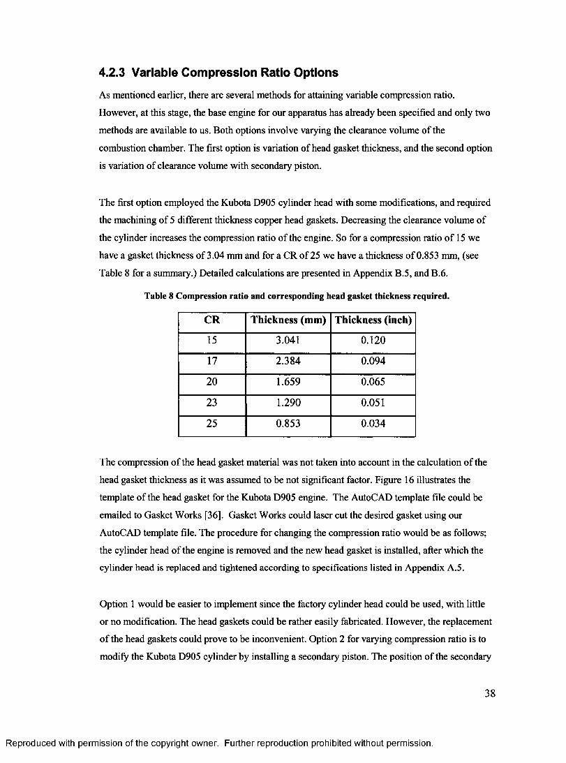
4.2.3 Variable Compression Ratio Options
As mentioned earlier, there are several methods for attaining variable compression ratio.
However, at this stage, the base engine for our apparatus has already been specified and only two
methods are available to us. Both options involve varying the clearance volume of the
combustion chamber. The first option is variation of head gasket thickness, and the second option
is variation of clearance volume with secondary piston.
The first option employed the Kubota D905 cylinder head with some modifications, and required
the machining of 5 different thickness copper head gaskets. Decreasing the clearance volume of
the cylinder increases the compression ratio of the engine. So for a compression ratio of 15 we
have a gasket thickness of 3.04 mm and for a CR of 25 we have a thickness of 0.853 mm, (see
Table 8 for a summary.) Detailed calculations are presented in Appendix B.5, and B.6.
Table 8 Compression ratio and corresponding head gasket thickness required.
C R Thickness (mm) Thickness (inch)
15 3.041 0.120
17 2.384 0.094
20 1.659 0.065
23 1.290 0.051
25 0.853 0.034
The compression of the head gasket material was not taken into account in the calculation of the
head gasket thickness as it was assumed to be not significant factor. Figure 16 illustrates the
template of the head gasket for the Kubota D905 engine. The AutoCAD template file could be
emailed to Gasket Works [36]. Gasket Works could laser cut the desired gasket using our
AutoCAD template file. The procedure for changing the compression ratio would be as follows;
the cylinder head of the engine is removed and the new head gasket is installed, after which the
cylinder head is replaced and tightened according to specifications listed in Appendix A.5.
Option 1 would be easier to implement since the factory cylinder head could be used, with little
or no modification. The head gaskets could be rather easily fabricated. However, the replacement
of the head gaskets could prove to be inconvenient. Option 2 for varying compression ratio is to
modify the Kubota D905 cylinder by installing a secondary piston. The position of the secondary
Reproduced with permission of the copyright owner. Further reproduction prohibited without permission.
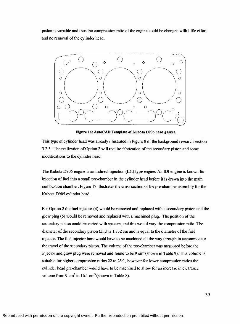
piston is variable and thus the compression ratio of the engine could be changed with little effort
and no removal of the cylinder head.
Figure 16: AutoCAD Template of Kubota D905 head gasket.
This type of cylinder head was already illustrated in Figure 8 of the background research section
3.2.3. The realization of Option 2 will require fabrication of the secondary piston and some
modifications to the cylinder head.
The Kubota D905 engine is an indirect injection (IDI) type engine. An IDI engine is known for
injection of fuel into a small pre-chamber in the cylinder head before it is drawn into the main
combustion chamber. Figure 17 illustrates the cross section of the pre-chamber assembly for the
Kubota D905 cylinder head.
For Option 2 the fuel injector (4) would be removed and replaced with a secondary piston and the
glow plug (5) would be removed and replaced with a machined plug. The position of the
secondary piston could be varied with spacers, and this would vary the compression ratio. The
diameter of the secondary piston (Dsp) is 1.732 cm and is equal to the diameter of the fuel
injector. The fuel injector bore would have to be machined all the way through to accommodate
the travel of the secondary piston. The volume of the pre-chamber was measured before the
injector and glow plug were removed and found to be 9 cm3 (shown in Table 9). This volume is
suitable for higher compression ratios 22 to 25:1, however for lower compression ratios the
cylinder head pre-chamber would have to be machined to allow for an increase in clearance
volume from 9 cm3 to 16.1 cm3 (shown in Table 8).
39
Reproduced with permission of the copyright owner. Further reproduction prohibited without permission.
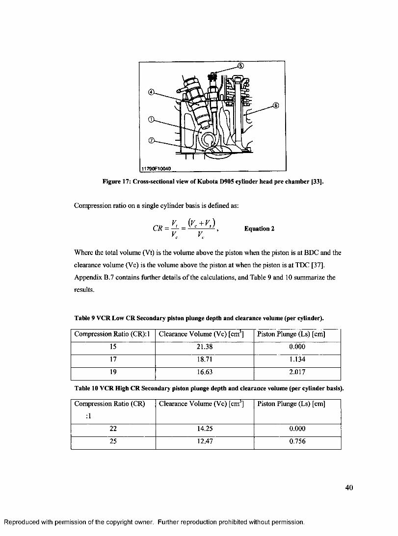
CD-
11790F10040
Figure 17: Cross-sectional view of Kubota D905 cylinder head pre chamber [33].
Compression ratio on a single cylinder basis is defined as:
Equation 2a=H.O^.V V
Where the total volume (Vt) is the volume above the piston when the piston is at BDC and the
clearance volume (Vc) is the volume above the piston at when the piston is at TDC [37],
Appendix B.7 contains further details of the calculations, and Table 9 and 10 summarize the
results.
Table 9 VCR Low CR Secondary piston plunge depth and clearance volume (per cylinder).
Compression Ratio (CR): 1 Clearance Volume (Vc) [cm3] Piston Plunge (Ls) [cm]
15 21.38 0.000
17 18.71 1.134
19 16.63 2.017
Table 10 VCR High CR Secondary piston plunge depth and clearance volume (per cylinder basis).
Compression Ratio (CR)
:1
Clearance Volume (Vc) [cm3] Piston Plunge (Ls) [cm]
22 14.25 0.000
25 12.47 0.756
40
Reproduced with permission of the copyright owner. Further reproduction prohibited without permission.
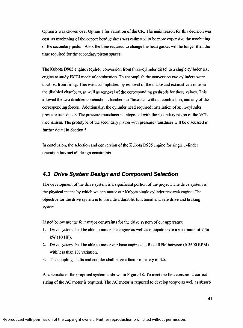
Option 2 was chosen over Option 1 for variation of the CR. The main reason for this decision was
cost, as machining of the copper head gaskets was estimated to be more expensive the machining
of the secondary piston. Also, the time required to change the head gasket will be longer than the
time required for the secondary piston spacer.
The Kubota D905 engine required conversion from three-cylinder diesel to a single cylinder test
engine to study HCCI mode of combustion. To accomplish the conversion two cylinders were
disabled from firing. This was accomplished by removal of the intake and exhaust valves from
the disabled chambers, as well as removal of the corresponding pushrods for these valves. This
allowed the two disabled combustion chambers to “breathe” without combustion, and any of the
corresponding forces. Additionally, the cylinder head required installation of an in-cylinder
pressure transducer. The pressure transducer is integrated with the secondary piston of the VCR
mechanism. The prototype of the secondary piston with pressure transducer will be discussed in
further detail in Section 5.
In conclusion, the selection and conversion of the Kubota D905 engine for single cylinder
operation has met all design constraints.
4.3 Drive System Design and Component Selection
The development of the drive system is a significant portion of the project. The drive system is
the physical means by which we can motor our Kubota single cylinder research engine. The
objective for the drive system is to provide a durable, functional and safe drive and braking
system.
Listed below are the four major constraints for the drive system of our apparatus:
1. Drive system shall be able to motor the engine as well as dissipate up to a maximum of 7.46
kW (10 HP).
2. Drive system shall be able to motor our base engine at a fixed RPM between (0-3600 RPM)
with less than 1% variation.
3. The coupling shafts and coupler shall have a factor of safety of 4.5.
A schematic of the proposed system is shown in Figure 18. To meet the first constraint, correct
sizing of the AC motor is required. The AC motor is required to develop torque as well as absorb
41
Reproduced with permission of the copyright owner. Further reproduction prohibited without permission.
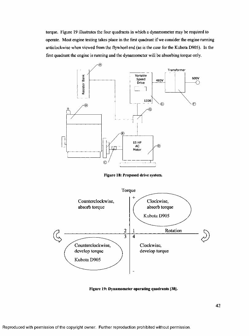
torque. Figure 19 illustrates the four quadrants in which a dynamometer may be required to
operate. Most engine testing takes place in the first quadrant if we consider the engine running
anticlockwise when viewed from the flywheel end (as is the case for the Kubota D905). In the
first quadrant the engine is running and the dynamometer will be absorbing torque only.
Transformer
VariableSpeedDrive
600V480V
1336
15 HP AC
Motor/ - ©
Figure 18: Proposed drive system.
Counterclockwise, absorb torque
Torque
Clockwise, absorb torque
Kubota D905
Rotation
Counterclockwise, develop torque
Clockwise, develop torque
Kubota D905
Figure 19: Dynamometer operating quadrants [38].
42
Reproduced with permission of the copyright owner. Further reproduction prohibited without permission.
For this design, a dynamometer is required that can both absorb torque in the clockwise direction
(quadrant 1) and also develop torque in the counter-clockwise direction (quadrant 3) [38]. A
regular water-brake or hydraulic dynamometer cannot perform both of these functions. AC or DC
machines are the only two choices available when operating in the third or fourth quadrants, as is
the case in our setup.
4.3.1 Sizing of the AC Motor for Motoring
Motoring of an engine is defined as the rotation of the research engine without the occurrence of
combustion. The combustion chamber is sealed and is being prepared for fuel and air mixture.
The Kubota D905 has a maximum gross intermittent torque (Tgr0ss) of 5.5 kgf.m (42 ft-lbs) at
2200 RPM (see Appendix A.l for motor details.) Plint and Martyr [38] suggest that the amount
of motoring torque required (x ^ ) to rotate an engine seldom exceeds 30 percent at steady state
operation and that this motoring torque is directly related to the friction losses of the engine.
Thus, the amount of torque required (xreq) from the electric motor to drive the Kubota engine is
30 percent of 5.5 kgf.m (42 ft-lbs) which equals 1.65 kgf.m (12.6 ft-lbs), (the detailed
calculations are available in Appendix D. 1.) Therefore an electric motor that can supply greater
than 1.65 kgf.m 12.6 ft-lbs of torque will be adequate for motoring of the Kubota D905. Review
of several electric motors indicated that the best alternative for this design is an AC motor. The
main reason was availability of second-hand AC motors, and the relatively small cost and size
when compared to a DC motor.
The subject AC motor is manufactured by Emerson Electric and is a US Motors model H15E1D.
The US Motors model H15E1D can supply a torque (xsup) at 3.07 kgf.m (22.2 ft-lbs), (see
Appendix C.l for AC motor specifications.) Since the supplied torque is greater than the required
torque, the HI5EID would sufficiently meet the functionality constraint for motoring.
4.3.2 Feasibility of the AC Motor for Starting
In order to verify the feasibility of the H15E1D AC motor for starting torque, an approximation
of the required flywheel torque to turn the Kubota engine over needs to be determined. The
existing OEM Kubota starter has more than adequate starting torque (by default) for starting
operation of all three cylinders of the Kubota D905 Engine. A calculation based on the existing
starter performance can be used to determine the torque required on the flywheel. Kubota Canada
supplied the starter performance data for a 1.4 kW Kubota starter. An estimate of performance of
the 1 kW starter was conducted by interpolating specifications for a 1.4 kW Kubota starter (see
43
Reproduced with permission of the copyright owner. Further reproduction prohibited without permission.
Appendix D.3 for detailed calculations). The starting torque required to start the engine is 10.5
kgfm (75.953 ft-lbs,) for three-cylinder operation. Since one cylinder of our engine is under
compression dividing by three to get a rough estimate of starting torque yields 3.50 kgf.m (25.32
ft-lbs), which is the required starting torque for one cylinder.
The maximum amount of motoring torque that the H15E1D AC motor can provide is 3.07 kgf.m
(22.2 ft-lbs). Since, the estimated starting torque of the single-cylinder operation Kubota is 3.50
kgf.m (25.32 ft-lbs) the AC motor cannot provide enough torque on its own for starting. This
could have been grounds for eliminating the HI5EID AC motor for use with our engine, since
the AC motor has insufficient torque for starting (turning over the engine under compression).
However, the H15E1D AC motor has sufficient torque for motoring once it is turned over, and
only needed assistance during starting. The 1 kW Kubota starter motor was utilized to assist the
AC motor in starting the Kubota Engine. This provided the required torque for starting the
Kubota engine. Once the Kubota engine is started (by the starter) and is undergoing motoring by
the AC Motor the starter motor can be disengaged. At this point the single cylinder engine will be
motored (with compression) solely by the AC motor. And the HCCI experiments can commence.
Therefore, with assistance of 1 kW starter motor, the US Motors H15E1D can satisfactorily meet
the design constraints.
4.3.3 Sizing of the Resistor Banks for Braking of the Drive system
The H15E1D AC motor, by itself, cannot act as an engine brake four the single-cylinder Kubota
D905. However with the addition of the chopper module and resistor bank, the excess torque
produced by the Kubota D905 can be absorbed and dissipated by means of a resistor bank. To
dissipate power, a chopper module is installed between the VSD and the AC motor (see Figure
18.) When the research engine begins to develop power this transmits back to the AC motor, and
begins to induce reverse-current in the motor windings. (Basically, the AC electric motor begins
to act as an AC generator, which is harmful to our circuit.) At this point the chopper module will
interrupt the electrical connection from the VSD controller to the resistor bank, where the excess
electrical power can be dissipated. This serves the purpose of braking the research engine as well
as protecting the VSD from back-current induced damage.
44
Reproduced with permission of the copyright owner. Further reproduction prohibited without permission.
The resistor bank is sized by determining both the total resistance value (Rdbi) and the power
absorption capacity (Pavg). The governing dynamics of the system involve dissipation of the
rotational energy at 3600 RPM to a full stop (0 RPM).
The H15E1D AC motor and the Kubota D905 engine are coupled together and have a total
rotational inertia (JT) of 1.852 kg-m2, (see Appendix D.2 for detailed calculations.) A typical
cycle was developed that represents a high load factor on the resistor banks. The engine is
accelerated to its maximum 3600 RPM in 4 seconds, followed by motoring the engine for 30
seconds, and then decelerating from maximum RPM 16 seconds. The total cycle time is 50
seconds.
As mention earlier, the maximum rated speed of the system is 3600 RPM and must be decelerated
to 0 rpm in 16 seconds to meet the design constraint. The necessary values are determined and the
peak braking power (Pb) is calculated using the following equation obtained from Alen Bradley
sizing chart [39]:
j r k k -<■>.)] n3
Where:
JT is the total rotational inertia of the system (1.822 kg-m2).
cob is the maximum speed (3600 RPM).
©o is the minimum speed (0 RPM).
t3-t2 is the deceleration time (16 seconds).
The peak braking power was calculated to be 16.455 kW. The rated power for the AC Motor is 15
HP or 11.19 kW. The peak braking power should be less than 1.5 times the rated power of the
AC motor. This is to prevent current overloads on the system. Note that 1.5 multiplied by 11.10
kW equals 16.785 kW, and our peak braking power is slightly less than this at 16.455 kW. The
average braking power (Pavg) that must be dissipated by the resistor is calculated using:
P =avg3 ^2 )
PX — X K - ® „ )
1-----
1 2
-----1«c>9
1
Equation 4
Note that the average braking power 2.633 kW is less than the peak braking power 16.455 kW.
The maximum braking resistance value (Rdbi) is calculated using the following equation:
45
Reproduced with permission of the copyright owner. Further reproduction prohibited without permission.
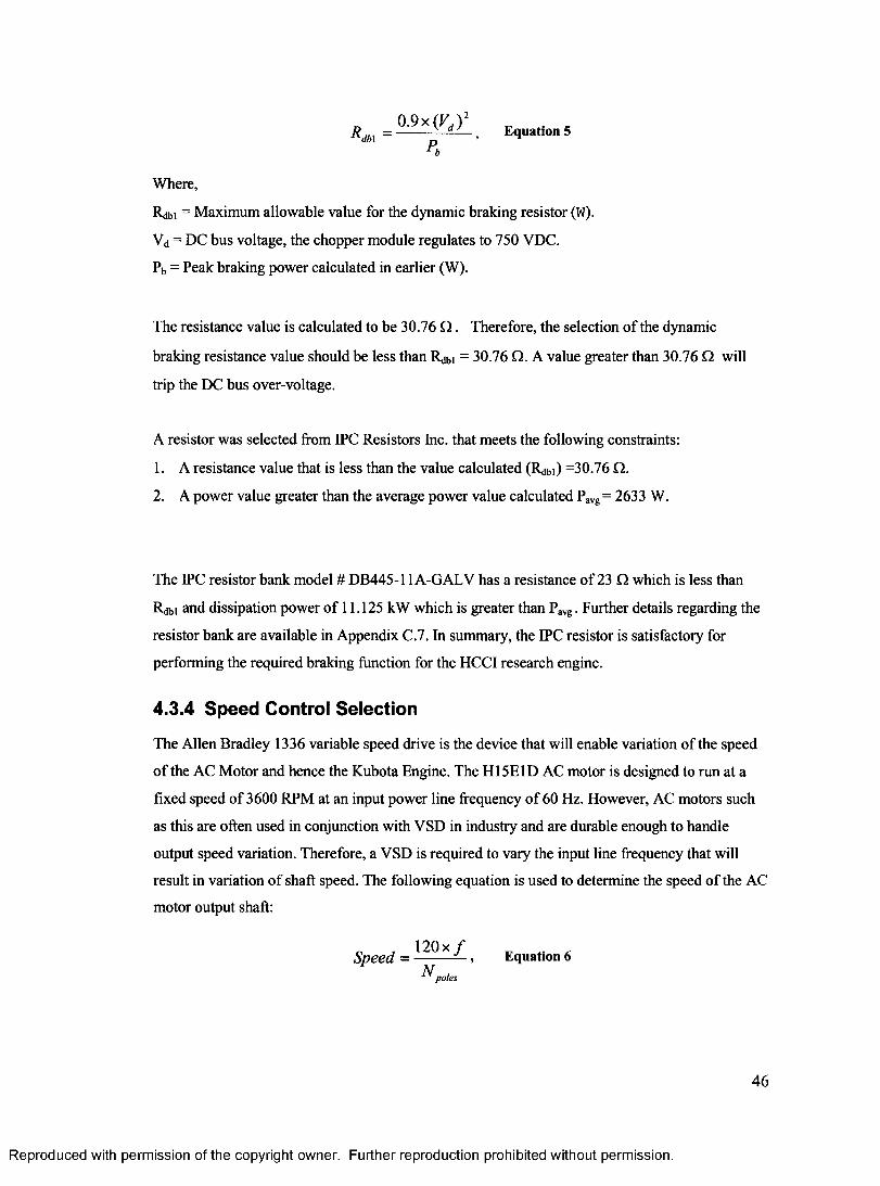
R m = — ~ p V^ • E(luation 5“b
Where,
Rdbi = Maximum allowable value for the dynamic braking resistor (W).
Vd = DC bus voltage, the chopper module regulates to 750 VDC.
Pb = Peak braking power calculated in earlier (W).
The resistance value is calculated to be 30.76 Q . Therefore, the selection of the dynamic
braking resistance value should be less than R^i = 30.76 Q. A value greater than 30.76 Q will
trip the DC bus over-voltage.
A resistor was selected from IPC Resistors Inc. that meets the following constraints:
1. A resistance value that is less than the value calculated (Rdbi) =30.76 Q.
2. A power value greater than the average power value calculated Pavg = 2633 W.
The IPC resistor bank model # DB445-11A-GALV has a resistance of 23 Q which is less than
Rdbi and dissipation power of 11.125 kW which is greater than Pavg. Further details regarding the
resistor bank are available in Appendix C.7. In summary, the IPC resistor is satisfactory for
performing the required braking function for the HCCI research engine.
4.3.4 Speed Control Selection
The Allen Bradley 1336 variable speed drive is the device that will enable variation of the speed
of the AC Motor and hence the Kubota Engine. The H15E1D AC motor is designed to run at a
fixed speed of 3600 RPM at an input power line frequency of 60 Hz. However, AC motors such
as this are often used in conjunction with VSD in industry and are durable enough to handle
output speed variation. Therefore, a VSD is required to vary the input line frequency that will
result in variation of shaft speed. The following equation is used to determine the speed of the AC
motor output shaft:
Speed = , Equation 6N poles
46
Reproduced with permission of the copyright owner. Further reproduction prohibited without permission.
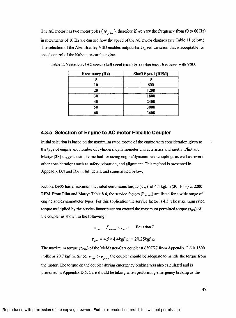
The AC motor has two motor poles ( N potes), therefore if we vary the frequency from (0 to 60 Hz)
in increments of 10 Hz we can see how the speed of the AC motor changes (see Table 11 below.)
The selection of the Alen Bradley VSD enables output shaft speed variation that is acceptable for
speed control of the Kubota research engine.
Table 11 Variation of AC motor shaft speed (rpm) by varying input frequency with VSD.
Frequency (Hz) Shaft Speed (RPM)0 010 60020 120030 180040 240050 300060 3600
4.3.5 Selection of Engine to AC motor Flexible Coupler
Initial selection is based on the maximum rated torque of the engine with consideration given to
the type of engine and number of cylinders, dynamometer characteristics and inertia. Plint and
Martyr [38] suggest a simple method for sizing engine/dynamometer couplings as well as several
other considerations such as safety, vibration, and alignment. This method is presented in
Appendix D.4 and D.6 in full detail, and summarized below.
Kubota D905 has a maximum net rated continuous torque (xnet) of 4.4 kgf.m (30 ft-lbs) at 2200
RPM. From Plint and Martyr Table 8.4, the service factors (Fservice) are listed for a wide range of
engine and dynamometer types. For this application the service factor is 4.5. The maximum rated
torque multiplied by the service factor must not exceed the maximum permitted torque (xper) of
the coupler as shown in the following:
T = F X T .■> Equation7per service net
Tper -- 4.5 x 4.4kgf.m = 20.25kgf.m
The maximum torque (xmax) of the McMaster-Carr coupler # 6507K7 from Appendix C.6 is 1800
in-lbs or 20.7 kgf.m. Since, z ^ > z , the coupler should be adequate to handle the torque from
the motor. The torque on the coupler during emergency braking was also calculated and is
presented in Appendix D.6. Care should be taking when performing emergency braking as the
47
Reproduced with permission of the copyright owner. Further reproduction prohibited without permission.
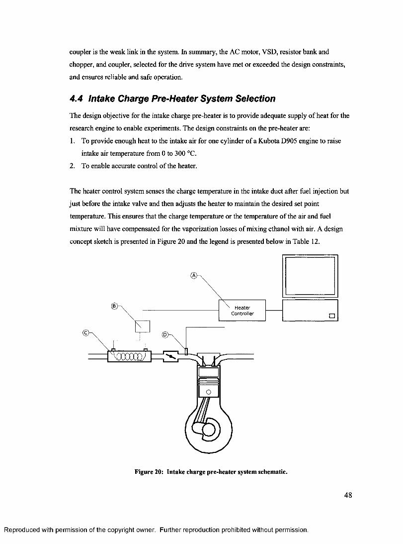
coupler is the weak link in the system. In summary, the AC motor, VSD, resistor bank and
chopper, and coupler, selected for the drive system have met or exceeded the design constraints,
and ensures reliable and safe operation.
4.4 Intake Charge Pre-Heater System Selection
The design objective for the intake charge pre-heater is to provide adequate supply of heat for the
research engine to enable experiments. The design constraints on the pre-heater are:
1. To provide enough heat to the intake air for one cylinder of a Kubota D905 engine to raise
intake air temperature from 0 to 300 °C.
2. To enable accurate control of the heater.
The heater control system senses the charge temperature in the intake duct after fuel injection but
just before the intake valve and then adjusts the heater to maintain the desired set point
temperature. This ensures that the charge temperature or the temperature of the air and fuel
mixture will have compensated for the vaporization losses of mixing ethanol with air. A design
concept sketch is presented in Figure 20 and the legend is presented below in Table 12.
HeaterController
Figure 20: Intake charge pre-heater system schematic.
48
Reproduced with permission of the copyright owner. Further reproduction prohibited without permission.
Table 12 Intake Charge Preheater System legend.
Item DescriptionA Heater ControllerB RelayC HeaterD Thermocouple
The intake charge pre-heater system is comprised of a heater element, a switching relay, a digital
controller, a thermocouple (located close to the intake valve), and capability for data
communications with a personal computer.
4.4.1 Heater Sizing and Selection
The electric heater sizing is based on the air flow rate of one cylinder of a Kubota D905 at 3600
RPM, plus intake heat losses (F,oss) estimated to be 40%. Also the heater was oversized (Fos) by
10% to compensate for any electrical losses not accounted for. The equation below was used to
determine the electric power of the heater in kilowatts (kW):
We = Floss x Fos x p air x V x Cp x A T , Equation 8
Where V is the volumetric flowrate in [m3/s], p air is the average air density, and Cp is the
averaged specific heat of air for the range A T = T2 - T X =300°C . The detailed calculations are
presented in Appendix F.l to F.3.
Based on calculations presented in Appendix F, the electric power requirement ( We ) was
determined to be 5.4 kW. The Omega SH-73343 was selected because it had a power rating of 6
kW and had a lower voltage requirement at 240 V compared to the 480 V model, making it a
safer device to operate.
The Omega SH-73343 (shown in Figure 21) has a cross-flow heating element selected to
minimize flow resistance, as well as an over-temperature circuit for heater element burnout
protection. When operated correctly it has a useful life of 5000 hours. It has a practical flow rate
range of up to 94.4 L/s with internal temperatures up to 700°C. The heating element is nickel-
chrome plated and insulated by ceramic beads on a stainless steel support frame.
4 9
Reproduced with permission of the copyright owner. Further reproduction prohibited without permission.
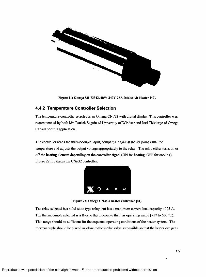
Figure 21: Omega SH-73343,6kW-240V-25A Intake Air Heater [40].
4.4.2 Temperature Controller Selection
The temperature controller selected is an Omega CNi/32 with digital display. This controller was
recommended by both Mr. Patrick Seguin of University of Windsor and Joel Thivierge of Omega
Canada for this application.
The controller reads the thermocouple input, compares it against the set point value for
temperature and adjusts the output voltage appropriately to the relay. The relay either turns on or
off the heating element depending on the controller signal (ON for heating, OFF for cooling).
Figure 22 illustrates the CNi/32 controller.
Figure 22: Omega CN-i/32 heater controller [41].
The relay selected is a solid-state type relay that has a maximum current load capacity of 25 A.
The thermocouple selected is a K-type thermocouple that has operating range (-17 to 650 °C).
This range should be sufficient for the expected operating conditions of the heater system. The
thermocouple should be placed as close to the intake valve as possible so that the heater can get a
50
Reproduced with permission of the copyright owner. Further reproduction prohibited without permission.
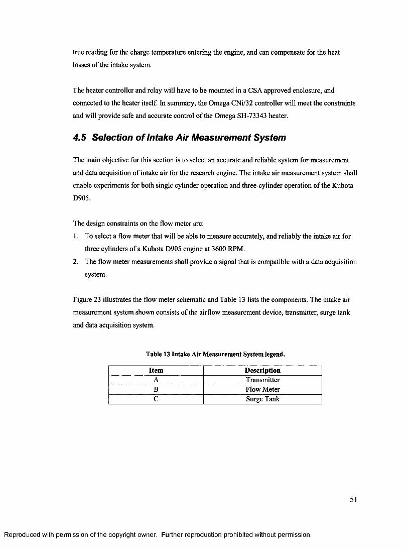
true reading for the charge temperature entering the engine, and can compensate for the heat
losses of the intake system.
The heater controller and relay will have to be mounted in a CSA approved enclosure, and
connected to the heater itself. In summary, the Omega CNi/32 controller will meet the constraints
and will provide safe and accurate control of the Omega SH-73343 heater.
4.5 Selection of Intake Air Measurement System
The main objective for this section is to select an accurate and reliable system for measurement
and data acquisition of intake air for the research engine. The intake air measurement system shall
enable experiments for both single cylinder operation and three-cylinder operation of the Kubota
D905.
The design constraints on the flow meter are:
1. To select a flow meter that will be able to measure accurately, and reliably the intake air for
three cylinders of a Kubota D905 engine at 3600 RPM.
2. The flow meter measurements shall provide a signal that is compatible with a data acquisition
system.
Figure 23 illustrates the flow meter schematic and Table 13 lists the components. The intake air
measurement system shown consists of the airflow measurement device, transmitter, surge tank
and data acquisition system.
Table 13 Intake Air Measurement System legend.
Item DescriptionA TransmitterB Flow MeterC Surge Tank
51
Reproduced with permission of the copyright owner. Further reproduction prohibited without permission.
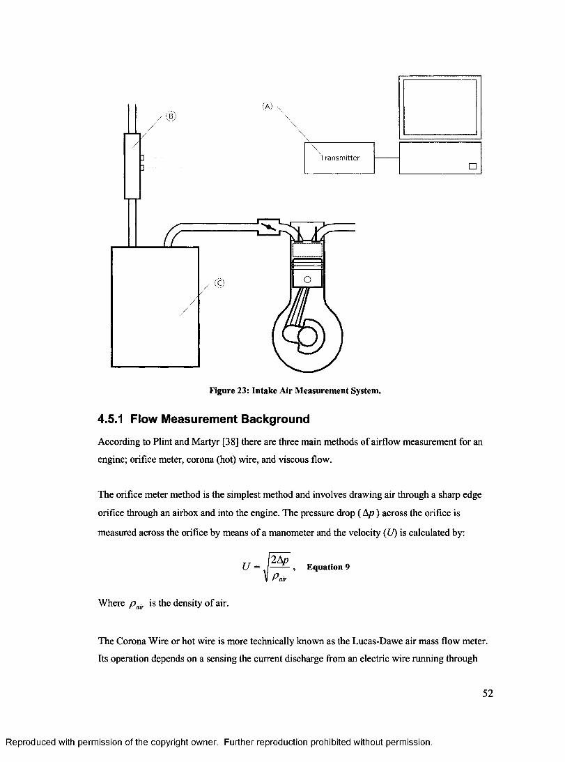
T ra n s m i t te r
Figure 23: Intake Air Measurement System.
4.5.1 Flow Measurement Background
According to Plint and Martyr [38] there are three main methods of airflow measurement for an
engine; orifice meter, corona (hot) wire, and viscous flow.
The orifice meter method is the simplest method and involves drawing air through a sharp edge
orifice through an airbox and into the engine. The pressure drop (A/?) across the orifice is
measured across the orifice by means of a manometer and the velocity (U) is calculated by:
. . 2 ApU = I , Equation 9
Where p air is the density of air.
The Corona Wire or hot wire is more technically known as the Lucas-Dawe air mass flow meter.
Its operation depends on a sensing the current discharge from an electric wire running through
52
Reproduced with permission of the copyright owner. Further reproduction prohibited without permission.
airflow. The discharge from an electrode located on the centerline axis of the duct through which
the air is flowing is measured. An increasing airflow diminishes the passage of ion current from
the corona wire to collector electrodes located on the duct wall. This gives rise to an imbalance of
current flow that is proportional to the airflow rate. This measurement method has the advantage
of a quick response to flow changes, ideal for transient conditions.
The viscous flow air meter is the most widely used alternative to the orifice method for measuring
airflow. The measuring orifice is replaced by an element consisting of a large number of small
passages, generally in triangular form. The flow through these passages is mostly laminar, which
results in the pressure drop being proportional to velocity of flow, rather than to its square. A
viscous flow air meter was selected for this project because of its accuracy, availability and cost
savings compared to orifice flow meter and corona wire.
4.5.2 Laminar Flow Element Selection
The most common industry units for flow rate are cubic feet per minute or (cfm) however L/s are
the appropriate SI units that will be used in this thesis. Often the flow rate value is referenced to
base condition to compensate for temperature and pressure of the gas compared to standard
temperature and pressure (101.3 kPa absolute and 21.1°C) [10]. This is denoted by units of
standard cubic feet per minute or (scfm) or in our case std. L/s. Note the std. L/s equals L/s at
standard temperature and pressure.
The flow rate of air drawn by three cylinders of the Kubota D905 engine was calculated in
Appendix F.4. The same quantities calculated in Appendix F.l, F.2, F.3 are also used in
Appendix F.4 except the flow rate is representative of all three cylinders as opposed to just a
single cylinder. The reason for the over-sizing of the laminar flow element (LFE) is to allow for
future research to be performed on the entire engine, whereas the heater would only be required
for single cylinder operation.
The volumetric flow rate ( Vcalculated ) or air consumption of the engine is calculated by using the
following equations obtained from Heywood [37]:
• Vscalculated = >7v ~ ’ Equation 10
*c
Where:
53
Reproduced with permission of the copyright owner. Further reproduction prohibited without permission.
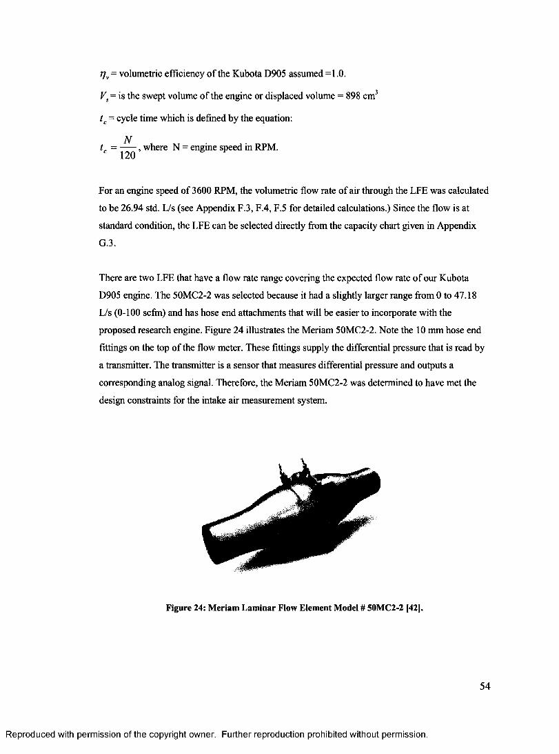
j]v = volumetric efficiency of the Kubota D905 assumed =1.0.
Vs = is the swept volume of the engine or displaced volume = 898 cm3
tc = cycle time which is defined by the equation:
Ntc = , where N = engine speed in RPM.
For an engine speed of 3600 RPM, the volumetric flow rate of air through the LFE was calculated
to be 26.94 std. L/s (see Appendix F.3, F.4, F.5 for detailed calculations.) Since the flow is at
standard condition, the LFE can be selected directly from the capacity chart given in Appendix
G.3.
There are two LFE that have a flow rate range covering the expected flow rate of our Kubota
D905 engine. The 50MC2-2 was selected because it had a slightly larger range from 0 to 47.18
L/s (0-100 scfm) and has hose end attachments that will be easier to incorporate with the
proposed research engine. Figure 24 illustrates the Meriam 50MC2-2. Note the 10 mm hose end
fittings on the top of the flow meter. These fittings supply the differential pressure that is read by
a transmitter. The transmitter is a sensor that measures differential pressure and outputs a
corresponding analog signal. Therefore, the Meriam 50MC2-2 was determined to have met the
design constraints for the intake air measurement system.
Figure 24: Meriam Laminar Flow Element Model # 50MC2-2 [42].
54
Reproduced with permission of the copyright owner. Further reproduction prohibited without permission.
4.5.3 Transmitter Selection
A transmitter was recommended by Paul Derisi of Peocock Inc. to work with the Meriam
50MC2-2 flow meter. The transmitter is manufactured by Honeywell Inc. and is denoted as
Model # STD904. The transmitter senses the differential pressure developed by the LFE, and
produces an analog signal varying from 4 to 20 mA. The 4-20 mA signal can be easily read by a
data acquisition system. See Appendix G.6 for further details or consult the manual available
from Honeywell Inc. [44],
In summary, the Meriam LFE along with the Honeywell transmitter has met the design
constraints and will provide accurate and reliable flow rate measurements for the research engine.
4.6 Intake Piping System Design
The design objective for the intake piping system is to provide an effective means of flowing air
into the engine, exhaust gases out of the engine and providing a means to attain exhaust gas
recirculation (EGR). A schematic of the proposed intake piping system is presented in Figure 25.
The constraints for the intake design include the following:
1. Use of standardized components to reduce cost and manufacturing time.
2. Use of materials that are resistant to high temperatures, and corrosion.
3. Minimize flow resistance by selecting appropriate components.
The intake piping system employs standard galvanized steel piping components (after the heater
element) and plastic ABS piping components (before the heater). These were selected to meet the
constraints for use of standard components, save manufacturing costs, and to improve the safety
of the design.
Galvanized steel piping is also resistant to melting at elevated temperatures. The melting
temperature of steel is dependent on its carbon content. Steel piping components are
manufactured using mild 1040 steel, and then are galvanized to prevent corrosion. According to
Askeland, mild plain-carbon 1040 steel has 40 % carbon content and a corresponding melting
temperature of 723 °C [45]. This is greater than the desired maximum temperature of the heater at
300 °C. Therefore; the galvanized piping should be an adequate material for use with the heater.
(See Appendix F.8 for further details).
55
Reproduced with permission of the copyright owner. Further reproduction prohibited without permission.
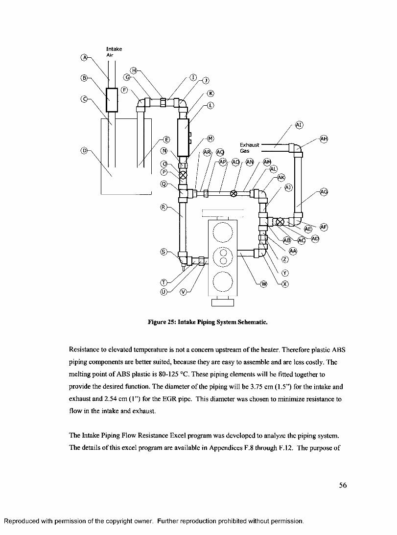
IntakeAir
ExhaustG as
Figure 25: Intake Piping System Schematic.
Resistance to elevated temperature is not a concern upstream of the heater. Therefore plastic ABS
piping components are better suited, because they are easy to assemble and are less costly. The
melting point of ABS plastic is 80-125 °C. These piping elements will be fitted together to
provide the desired function. The diameter of the piping will be 3.75 cm (1.5”) for the intake and
exhaust and 2.54 cm (1”) for the EGR pipe. This diameter was chosen to minimize resistance to
flow in the intake and exhaust.
The Intake Piping Flow Resistance Excel program was developed to analyze the piping system.
The details of this excel program are available in Appendices F.8 through F.12. The purpose of
56
Reproduced with permission of the copyright owner. Further reproduction prohibited without permission.
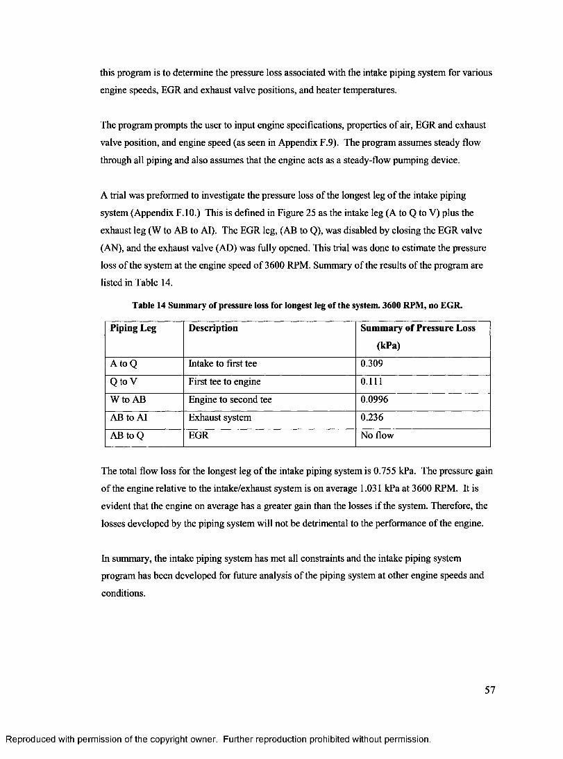
this program is to determine the pressure loss associated with the intake piping system for various
engine speeds, EGR and exhaust valve positions, and heater temperatures.
The program prompts the user to input engine specifications, properties of air, EGR and exhaust
valve position, and engine speed (as seen in Appendix F.9). The program assumes steady flow
through all piping and also assumes that the engine acts as a steady-flow pumping device.
A trial was preformed to investigate the pressure loss of the longest leg of the intake piping
system (Appendix F.10.) This is defined in Figure 25 as the intake leg (A to Q to V) plus the
exhaust leg (W to AB to AI). The EGR leg, (AB to Q), was disabled by closing the EGR valve
(AN), and the exhaust valve (AD) was fully opened. This trial was done to estimate the pressure
loss of the system at the engine speed of 3600 RPM. Summary of the results of the program are
listed in Table 14.
Table 14 Summary of pressure loss for longest leg of the system. 3600 RPM, no EGR.
Piping Leg Description Summary of Pressure Loss
(kPa)
A to Q Intake to first tee 0.309
Q to V First tee to engine 0.111
W toA B Engine to second tee 0.0996
AB to AI Exhaust system 0.236
AB to Q EGR No flow
The total flow loss for the longest leg of the intake piping system is 0.755 kPa. The pressure gain
of the engine relative to the intake/exhaust system is on average 1.031 kPa at 3600 RPM. It is
evident that the engine on average has a greater gain than the losses if the system. Therefore, the
losses developed by the piping system will not be detrimental to the performance of the engine.
In summary, the intake piping system has met all constraints and the intake piping system
program has been developed for future analysis of the piping system at other engine speeds and
conditions.
57
Reproduced with permission of the copyright owner. Further reproduction prohibited without permission.
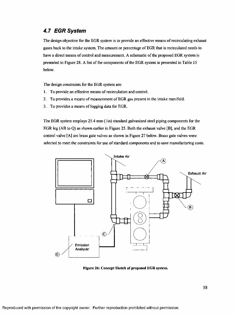
4.7 EGR System
The design objective for the EGR system is to provide an effective means of recirculating exhaust
gases back to the intake system. The amount or percentage of EGR that is recirculated needs to
have a direct means of control and measurement. A schematic of the proposed EGR system is
presented in Figure 28. A list of the components of the EGR system is presented in Table 15
below.
The design constraints for the EGR system are:
1. To provide an effective means of recirculation and control.
2. To provides a means of measurement of EGR gas present in the intake manifold.
3. To provides a means of logging data for EGR.
The EGR system employs 25.4 mm (lin) standard galvanized steel piping components for the
EGR leg (AB to Q) as shown earlier in Figure 25. Both the exhaust valve [B], and the EGR
control valve [A] are brass gate valves as shown in Figure 27 below. Brass gate valves were
selected to meet the constraints for use of standard components and to save manufacturing costs.
In tak e Air
Exhaust Air
EmissionAnalyzer
Figure 26: Concept Sketch of proposed EGR system.
58
Reproduced with permission of the copyright owner. Further reproduction prohibited without permission.
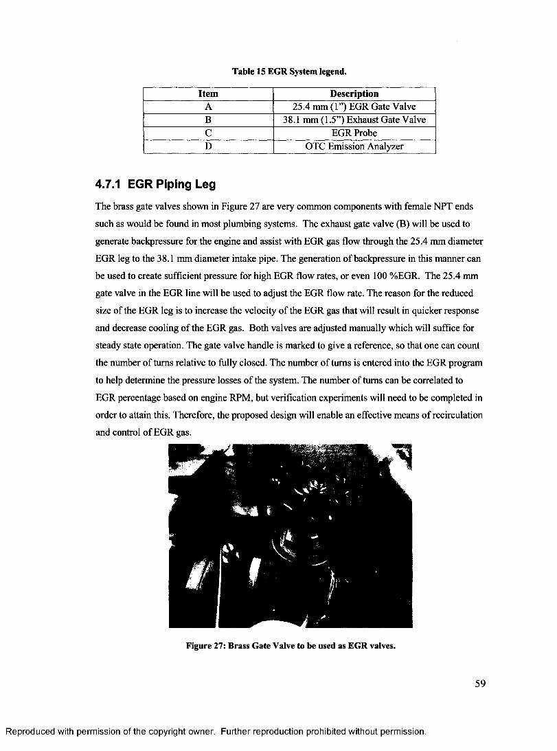
Table 15 EGR System legend.
Item DescriptionA 25.4 mm (1”) EGR Gate ValveB 38.1 mm (1.5”) Exhaust Gate ValveC EGR ProbeD OTC Emission Analyzer
4.7.1 EGR Piping Leg
The brass gate valves shown in Figure 27 are very common components with female NPT ends
such as would be found in most plumbing systems. The exhaust gate valve (B) will be used to
generate backpressure for the engine and assist with EGR gas flow through the 25.4 mm diameter
EGR leg to the 38.1 mm diameter intake pipe. The generation of backpressure in this manner can
be used to create sufficient pressure for high EGR flow rates, or even 100 %EGR. The 25.4 mm
gate valve in the EGR line will be used to adjust the EGR flow rate. The reason for the reduced
size of the EGR leg is to increase the velocity of the EGR gas that will result in quicker response
and decrease cooling of the EGR gas. Both valves are adjusted manually which will suffice for
steady state operation. The gate valve handle is marked to give a reference, so that one can count
the number of turns relative to fully closed. The number of turns is entered into the EGR program
to help determine the pressure losses of the system. The number of turns can be correlated to
EGR percentage based on engine RPM, but verification experiments will need to be completed in
order to attain this. Therefore, the proposed design will enable an effective means of recirculation
and control of EGR gas.
Figure 27: Brass Gate Valve to be used as EGR valves.
59
Reproduced with permission of the copyright owner. Further reproduction prohibited without permission.
4.7.2 MATLAB EGR Program
For determining the EGR mass fraction, a method was developed that require measurement of
C 02 concentration in the intake manifold slightly before the intake valve and then calculating the
EGR percentage in the intake. The gases produced from combustion of hydrocarbons are water
(H20), C 02, CO, NOx, HC and 0 2. These gases can be sampled in the exhaust leg to determine,
and verify the equivalence ratio of the air fuel mixture. Additionally, these gases are brought into
the intake in varying concentration by means of the EGR leg. The EGR gas mixes with the intake
gases to form a reactants mixture.
The Matlab EGR program was developed by Arthur and Defoe [46]. The Matlab EGR program
was utilized for determining EGR mass fraction based on C 02 mass fraction in the intake leg.
Full Details of the Matlab EGR program including: inputs, outputs, and the MATLAB M-file are
listed in Appendices F.13, F.14, and F.15.
The Matlab EGR program inputs are; relative humidity, ambient air pressure, saturation pressure
of water, mass flow rate of intake air, volume fraction of C 02 (from emission analyzer),
composition of fuel (number of atoms of C, H, O, N), composition of additives (number of atoms
of C, H, O, N), mole fraction of fuel and additives, and equivalence ratio. Table 16 below,
summarizes the inputs utilized for the simulation trial of the program.
It is to be noted that this method does not take into account residual combustion gases present in
the combustion chamber of the engine after a combustion event occurs, and would result in a
slight error, but in general the Matlab EGR program should be acceptable for the purposes of this
report.
The output of the Matlab EGR program is mass percentage of EGR (m_EGR_percent) or in other
words, the percentage of mass entering the cylinder that is EGR. A simulation was run of the
program for several different EGR fractions present in the intake and the results are summarized
in Table 17 below. The results of this simulation should be verified with an experiment; however
this step does at least prove functionality of the Matlab EGR program as a method for calculating
percent EGR.
60
Reproduced with permission of the copyright owner. Further reproduction prohibited without permission.
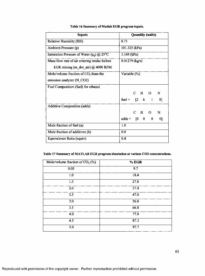
Table 16 Summary of Matlab EGR program inputs.
Inputs Quantity (units)
Relative Humidity (RH) 0.75
Ambient Pressure (p) 101.325 (kPa)
Saturation Pressure of Water (p j @ 25°C 3.169 (kPa)
Mass flow rate of air entering intake before
EGR mixing (m dot air) @ 4000 RPM
0.01279 (kg/s)
Mole/volume fraction of C 02 from the
emission analyzer (N C02)
Variable (%)
Fuel Composition (fuel) for ethanol
C H O N
fuel = [ 2 6 1 0]
Additive Composition (adds)
C H O N
adds = [ 0 0 0 0]
Mole fraction of fuel (a) 1.0
Mole fraction of additives (b) 0.0
Equivalence Ratio (equiv) 0.4
Table 17 Summary of MATLAB EGR program simulation at various C02 concentrations.
Mole/volume fraction of C 02 (%) % EGR
0.05 9.7
1.0 18.4
1.5 27.8
2.0 37.4
2.5 47.0
3.0 56.8
3.5 66.8
4.0 77.0
4.5 87.3
5.0 97.7
Reproduced with permission of the copyright owner. Further reproduction prohibited without permission.
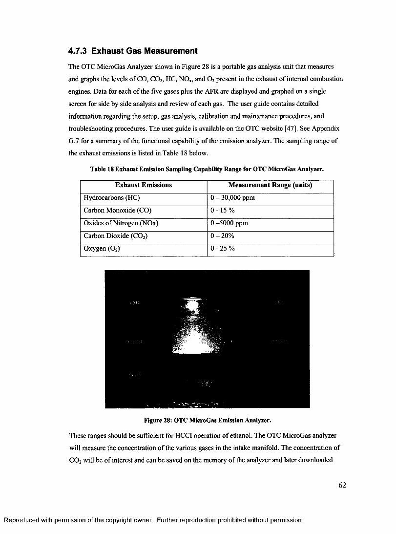
4.7.3 Exhaust Gas Measurement
The OTC MicroGas Analyzer shown in Figure 28 is a portable gas analysis unit that measures
and graphs the levels of CO, C 02, HC, NOx, and 0 2 present in the exhaust of internal combustion
engines. Data for each of the five gases plus the AFR are displayed and graphed on a single
screen for side by side analysis and review of each gas. The user guide contains detailed
information regarding the setup, gas analysis, calibration and maintenance procedures, and
troubleshooting procedures. The user guide is available on the OTC website [47], See Appendix
G.7 for a summary of the functional capability of the emission analyzer. The sampling range of
the exhaust emissions is listed in Table 18 below.
Table 18 Exhaust Emission Sampling Capability Range for OTC MicroGas Analyzer.
Exhaust Emissions Measurement Range (units)
Hydrocarbons (HC) 0 - 30,000 ppm
Carbon Monoxide (CO) 0 -15 %
Oxides of Nitrogen (NOx) 0 -5000 ppm
Carbon Dioxide (C02) 0 -2 0 %
Oxygen (0 2) 0 - 25 %
Figure 28: OTC MicroGas Emission Analyzer.
These ranges should be sufficient for HCCI operation of ethanol. The OTC MicroGas analyzer
will measure the concentration of the various gases in the intake manifold. The concentration of
C 02 will be of interest and can be saved on the memory of the analyzer and later downloaded
62
Reproduced with permission of the copyright owner. Further reproduction prohibited without permission.
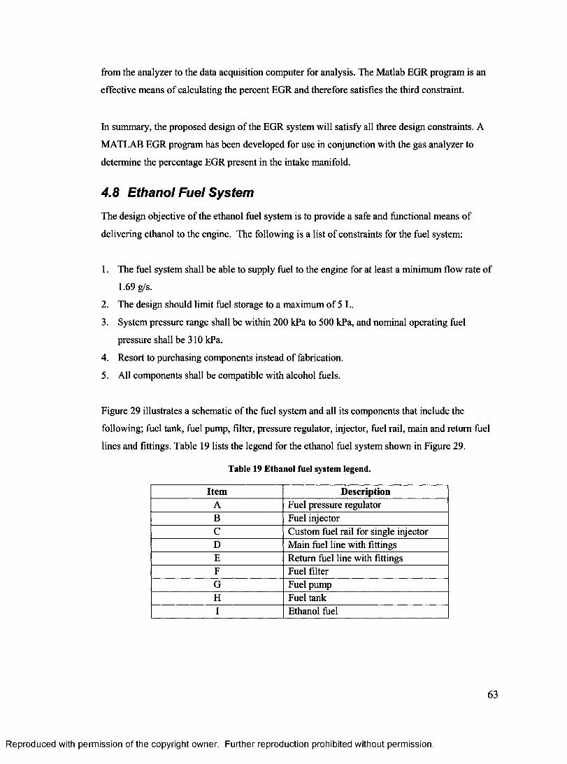
from the analyzer to the data acquisition computer for analysis. The Matlab EGR program is an
effective means of calculating the percent EGR and therefore satisfies the third constraint.
In summary, the proposed design of the EGR system will satisfy all three design constraints. A
MATLAB EGR program has been developed for use in conjunction with the gas analyzer to
determine the percentage EGR present in the intake manifold.
4.8 Ethanol Fuel System
The design objective of the ethanol fuel system is to provide a safe and functional means of
delivering ethanol to the engine. The following is a list of constraints for the fuel system:
1. The fuel system shall be able to supply fuel to the engine for at least a minimum flow rate of
1.69 g/s.
2. The design should limit fuel storage to a maximum of 5 L.
3. System pressure range shall be within 200 kPa to 500 kPa, and nominal operating fuel
pressure shall be 310 kPa.
4. Resort to purchasing components instead of fabrication.
5. All components shall be compatible with alcohol fuels.
Figure 29 illustrates a schematic of the fuel system and all its components that include the
following; fuel tank, fuel pump, filter, pressure regulator, injector, fuel rail, main and return fuel
lines and fittings. Table 19 lists the legend for the ethanol fuel system shown in Figure 29.
Table 19 Ethanol fuel system legend.
Item DescriptionA Fuel pressure regulatorB Fuel injectorC Custom fuel rail for single injectorD Main fuel line with fittingsE Return fuel line with fittingsF Fuel filterG Fuel pumpH Fuel tankI Ethanol fuel
63
Reproduced with permission of the copyright owner. Further reproduction prohibited without permission.
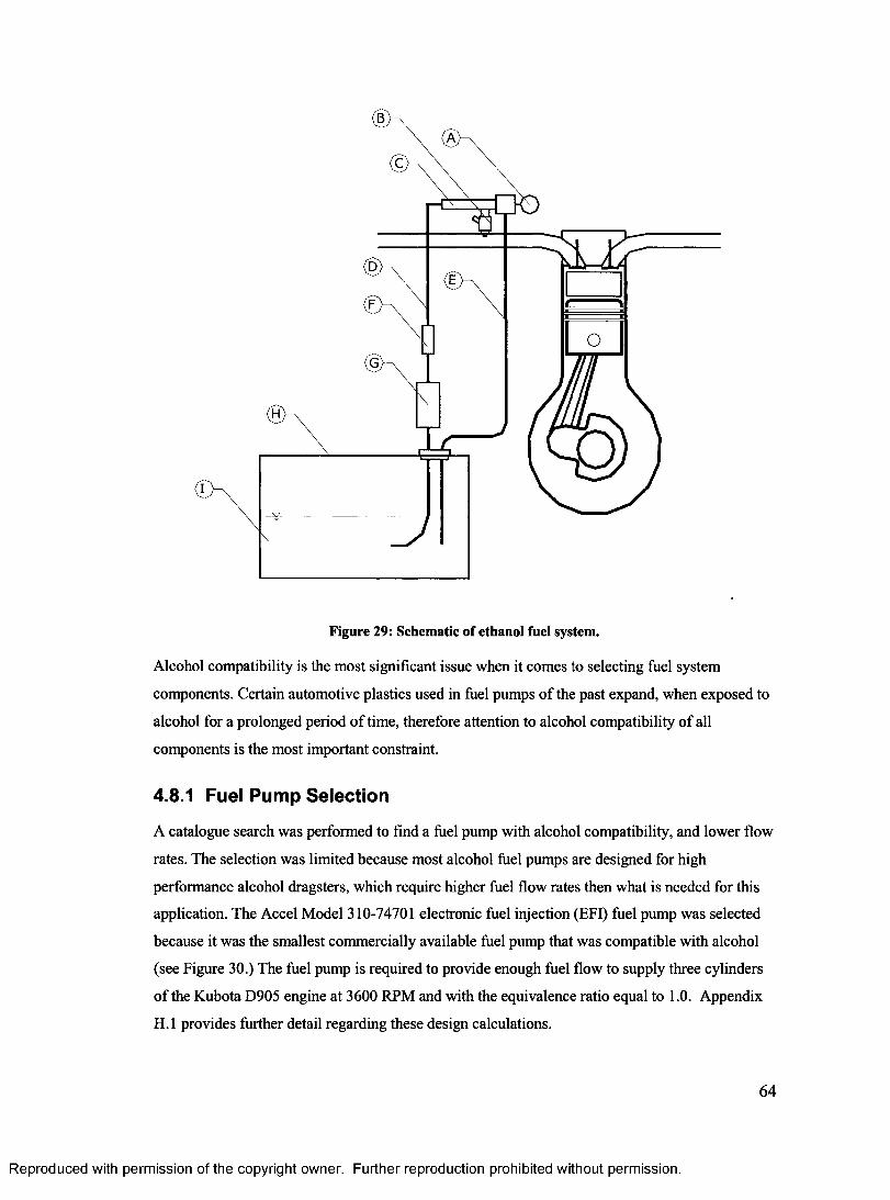
Figure 29: Schematic of ethanol fuel system.
Alcohol compatibility is the most significant issue when it comes to selecting fuel system
components. Certain automotive plastics used in fuel pumps of the past expand, when exposed to
alcohol for a prolonged period of time, therefore attention to alcohol compatibility of all
components is the most important constraint.
4.8.1 Fuel Pump Selection
A catalogue search was performed to find a fuel pump with alcohol compatibility, and lower flow
rates. The selection was limited because most alcohol fuel pumps are designed for high
performance alcohol dragsters, which require higher fuel flow rates then what is needed for this
application. The Accel Model 310-74701 electronic fuel injection (EFI) fuel pump was selected
because it was the smallest commercially available fuel pump that was compatible with alcohol
(see Figure 30.) The fuel pump is required to provide enough fuel flow to supply three cylinders
of the Kubota D905 engine at 3600 RPM and with the equivalence ratio equal to 1.0. Appendix
H.l provides further detail regarding these design calculations.
64
Reproduced with permission of the copyright owner. Further reproduction prohibited without permission.
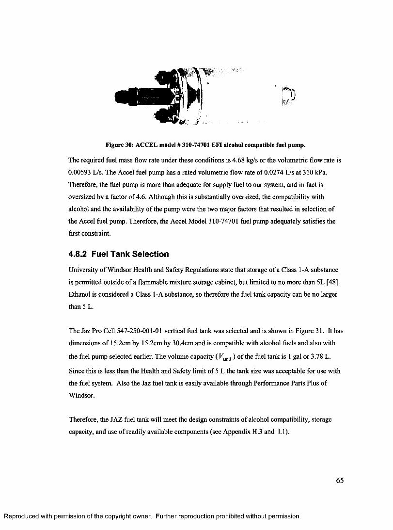
Figure 30: ACCEL model # 310-74701 EFI alcohol compatible fuel pump.
The required fuel mass flow rate under these conditions is 4.68 kg/s or the volumetric flow rate is
0.00593 L/s. The Accel fuel pump has a rated volumetric flow rate of 0.0274 L/s at 310 kPa.
Therefore, the fuel pump is more than adequate for supply fuel to our system, and in fact is
oversized by a factor of 4.6. Although this is substantially oversized, the compatibility with
alcohol and the availability of the pump were the two major factors that resulted in selection of
the Accel fuel pump. Therefore, the Accel Model 310-74701 fuel pump adequately satisfies the
first constraint.
4.8.2 Fuel Tank Selection
University of Windsor Health and Safety Regulations state that storage of a Class 1-A substance
is permitted outside of a flammable mixture storage cabinet, but limited to no more than 5L [48],
Ethanol is considered a Class 1-A substance, so therefore the fuel tank capacity can be no larger
than 5 L.
The Jaz Pro Cell 547-250-001-01 vertical fuel tank was selected and is shown in Figure 31. It has
dimensions of 15.2cm by 15.2cm by 30.4cm and is compatible with alcohol fuels and also with
the fuel pump selected earlier. The volume capacity ( Vtmk) of the fuel tank is 1 gal or 3.78 L.
Since this is less than the Health and Safety limit of 5 L the tank size was acceptable for use with
the fuel system. Also the Jaz fuel tank is easily available through Performance Parts Plus of
Windsor.
Therefore, the JAZ fuel tank will meet the design constraints of alcohol compatibility, storage
capacity, and use of readily available components (see Appendix H.3 and 1.1).
65
Reproduced with permission of the copyright owner. Further reproduction prohibited without permission.
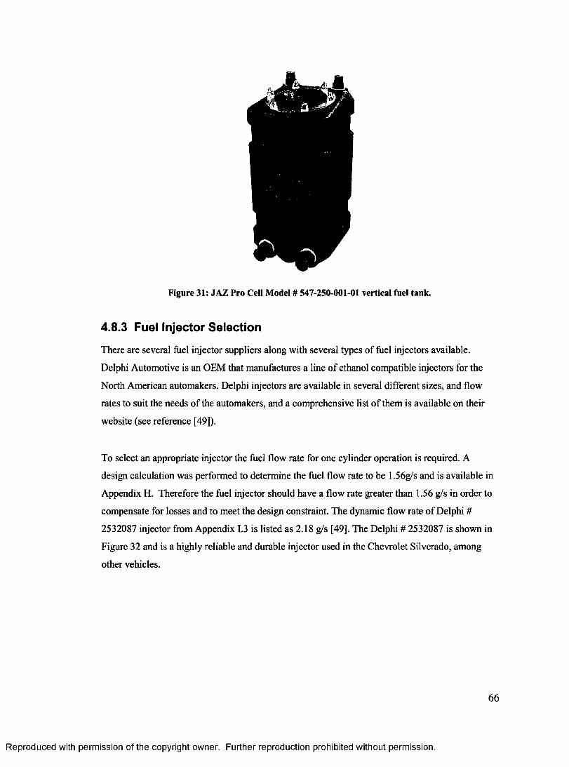
Figure 31: JAZ Pro Cell Model # 547-250-001-01 vertical fuel tank.
4.8.3 Fuel Injector Selection
There are several fuel injector suppliers along with several types of fuel injectors available.
Delphi Automotive is an OEM that manufactures a line of ethanol compatible injectors for the
North American automakers. Delphi injectors are available in several different sizes, and flow
rates to suit the needs of the automakers, and a comprehensive list of them is available on their
website (see reference [49]).
To select an appropriate injector the fuel flow rate for one cylinder operation is required. A
design calculation was performed to determine the fuel flow rate to be 1.56g/s and is available in
Appendix H. Therefore the fuel injector should have a flow rate greater than 1.56 g/s in order to
compensate for losses and to meet the design constraint. The dynamic flow rate of Delphi #
2532087 injector from Appendix 1.3 is listed as 2.18 g/s [49]. The Delphi # 2532087 is shown in
Figure 32 and is a highly reliable and durable injector used in the Chevrolet Silverado, among
other vehicles.
66
Reproduced with permission of the copyright owner. Further reproduction prohibited without permission.
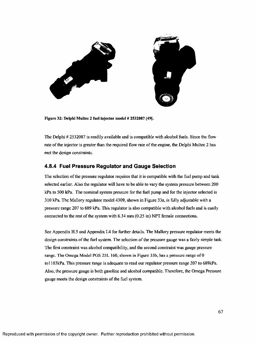
Figure 32: Delphi Multec 2 fuel injector model # 2532087 [49].
The Delphi # 2532087 is readily available and is compatible with alcohol fuels. Since the flow
rate of the injector is greater than the required flow rate of the engine, the Delphi Multec 2 has
met the design constraints.
4.8.4 Fuel Pressure Regulator and Gauge Selection
The selection of the pressure regulator requires that it is compatible with the fuel pump and tank
selected earlier. Also the regulator will have to be able to vary the system pressure between 200
kPa to 500 kPa. The nominal system pressure for the fuel pump and for the injector selected is
310 kPa. The Mallory regulator model 4309, shown in Figure 33a, is fully adjustable with a
pressure range 207 to 689 kPa. This regulator is also compatible with alcohol fuels and is easily
connected to the rest of the system with 6.34 mm (0.25 in) NPT female connections.
See Appendix H.5 and Appendix 1.4 for further details. The Mallory pressure regulator meets the
design constraints of the fuel system. The selection of the pressure gauge was a fairly simple task.
The first constraint was alcohol compatibility, and the second constraint was gauge pressure
range. The Omega Model PGS 25L 160, shown in Figure 33b, has a pressure range of 0
tol 103kPa. This pressure range is adequate to read our regulator pressure range 207 to 689kPa.
Also, the pressure gauge is both gasoline and alcohol compatible. Therefore, the Omega Pressure
gauge meets the design constraints of the fuel system.
67
Reproduced with permission of the copyright owner. Further reproduction prohibited without permission.
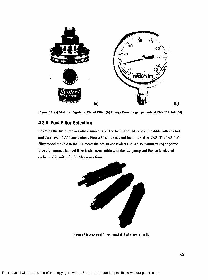
Figure 33: (a) Mallory Regulator Model 4309, (b) Omega Pressure gauge model # PGS 25L 160 (501-
4.8.5 Fuel Filter Selection
Selecting the fuel filter was also a simple task. The fuel filter had to be compatible with alcohol
and also have 06 AN connections. Figure 34 shows several fuel filters from JAZ. The JAZ fuel
filter model # 547-836-006-11 meets the design constraints and is also manufactured anodized
blue aluminum. This fuel filter is also compatible with the fuel pump and fuel tank selected
earlier and is suited for 06 AN connections.
Figure 34: JAZ fuel fdter model 547-836-006-11 [50].
68
Reproduced with permission of the copyright owner. Further reproduction prohibited without permission.
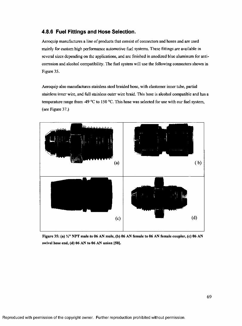
4.8.6 Fuel Fittings and Hose Selection.
Aeroquip manufactures a line of products that consist of connectors and hoses and are used
mainly for custom high performance automotive fuel systems. These fittings are available in
several sizes depending on the applications, and are finished in anodized blue aluminum for anti
corrosion and alcohol compatibility. The fuel system will use the following connectors shown in
Figure 35.
Aeroquip also manufactures stainless steel braided hose, with elastomer inner tube, partial
stainless inner wire, and full stainless outer wire braid. This hose is alcohol compatible and has a
temperature range from -49 °C to 150 °C. This hose was selected for use with our fuel system,
(see Figure 37.)
Figure 35: (a) Vi” NPT male to 06 AN male, (b) 06 AN female to 06 AN female coupler, (c) 06 AN
swivel hose end, (d) 06 AN to 06 AN union [50].
69
Reproduced with permission of the copyright owner. Further reproduction prohibited without permission.
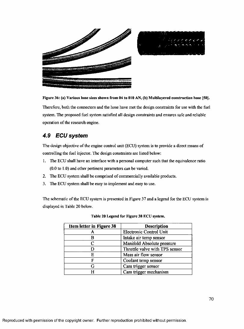
m ilB fc
Figure 36: (a) Various hose sizes shown from 04 to 010 AN, (b) Multilayered construction hose [50].
Therefore, both the connectors and the hose have met the design constraints for use with the fuel
system. The proposed fuel system satisfied all design constraints and ensures safe and reliable
operation of the research engine.
4.9 ECU system
The design objective of the engine control unit (ECU) system is to provide a direct means of
controlling the fuel injector. The design constraints are listed below:
1. The ECU shall have an interface with a personal computer such that the equivalence ratio
(0.0 to 1.0) and other pertinent parameters can be varied.
2. The ECU system shall be comprised of commercially available products.
3. The ECU system shall be easy to implement and easy to use.
The schematic of the ECU system is presented in Figure 37 and a legend for the ECU system is
displayed in Table 20 below.
Table 20 Legend for Figure 38 ECU system.
Item letter in Figure 38 DescriptionA Electronic Control UnitB Intake air temp sensorC Manifold Absolute pressureD Throttle valve with TPS sensorE Mass air flow sensorF Coolant temp sensorG Cam trigger sensorH Cam trigger mechanism
70
Reproduced with permission of the copyright owner. Further reproduction prohibited without permission.
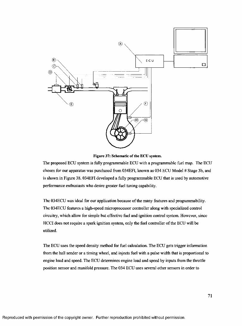
ECU
Figure 37: Schematic of the ECU system.
The proposed ECU system is fully programmable ECU with a programmable fuel map. The ECU
chosen for our apparatus was purchased from 034EFI, known as 034 ECU Model # Stage 3b, and
is shown in Figure 38. 034EFI developed a fully programmable ECU that is used by automotive
performance enthusiasts who desire greater fuel tuning capability.
The 034ECU was ideal for our application because of the many features and programmability.
The 034ECU features a high-speed microprocessor controller along with specialized control
circuitry, which allow for simple but effective fuel and ignition control system. However, since
HCCI does not require a spark ignition system, only the fuel controller of the ECU will be
utilized.
The ECU uses the speed density method for fuel calculation. The ECU gets trigger information
from the hall sender or a timing wheel, and injects fuel with a pulse width that is proportional to
engine load and speed. The ECU determines engine load and speed by inputs from the throttle
position sensor and manifold pressure. The 034 ECU uses several other sensors in order to
71
Reproduced with permission of the copyright owner. Further reproduction prohibited without permission.
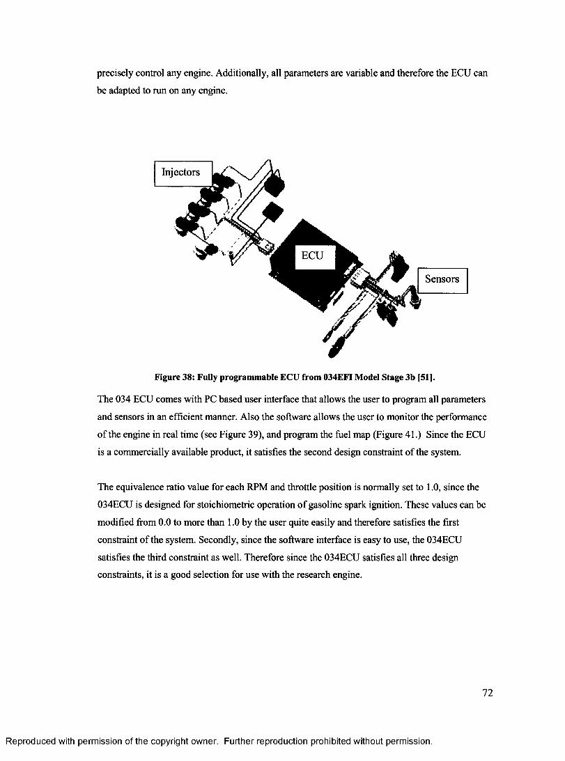
precisely control any engine. Additionally, all parameters are variable and therefore the ECU can
be adapted to run on any engine.
The 034 ECU comes with PC based user interface that allows the user to program all parameters
and sensors in an efficient manner. Also the software allows the user to monitor the performance
of the engine in real time (see Figure 39), and program the fuel map (Figure 41.) Since the ECU
is a commercially available product, it satisfies the second design constraint of the system.
The equivalence ratio value for each RPM and throttle position is normally set to 1.0, since the
034ECU is designed for stoichiometric operation of gasoline spark ignition. These values can be
modified from 0.0 to more than 1.0 by the user quite easily and therefore satisfies the first
constraint of the system. Secondly, since the software interface is easy to use, the 034ECU
satisfies the third constraint as well. Therefore since the 034ECU satisfies all three design
constraints, it is a good selection for use with the research engine.
Inj
Sensors
Figure 38: Fully programmable ECU from 034EFI Model Stage 3b [51].
72
Reproduced with permission of the copyright owner. Further reproduction prohibited without permission.
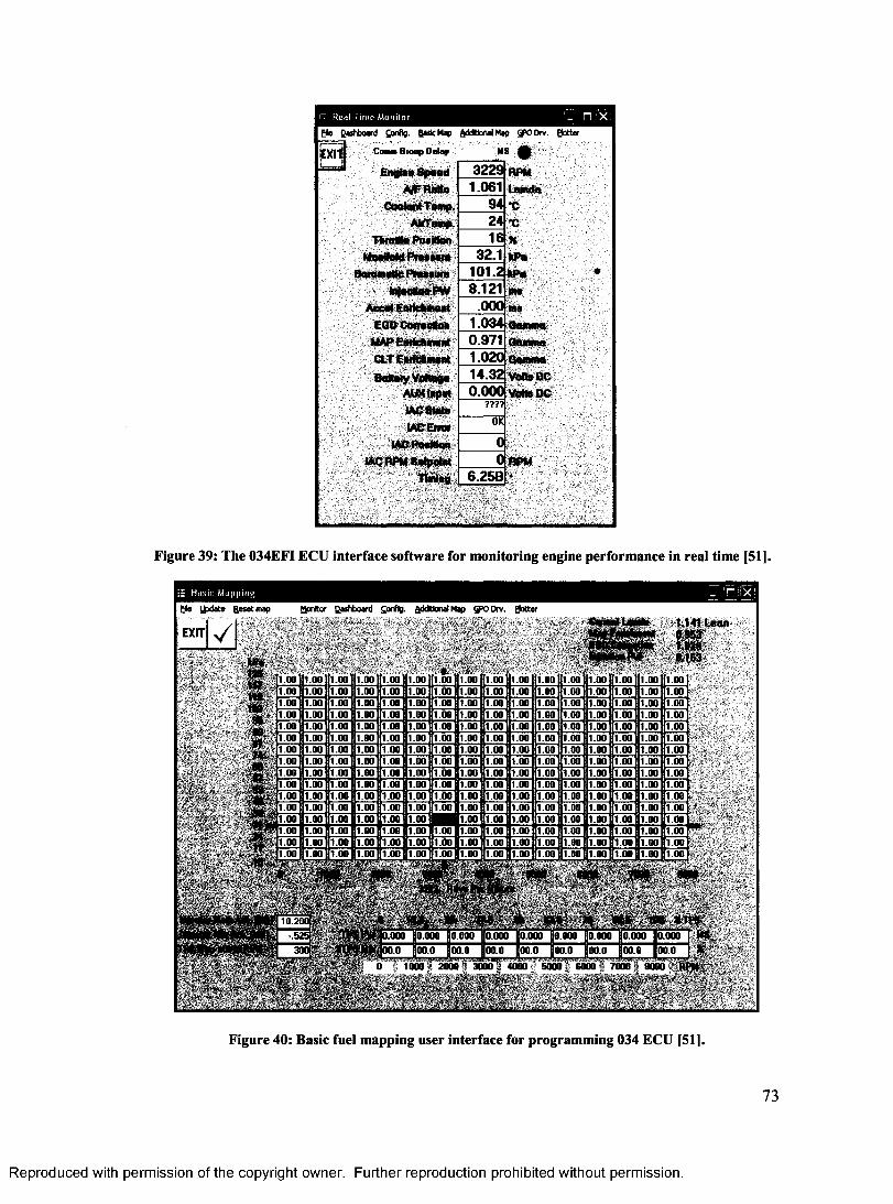
f - K e d l l i m e M o n i t o r
Be dashboard Gorflg. Basic Map ftddbonalMap SPODrv. Blotter
Co m Group Delay MS £
Engine 8peed 3229 RPMA/F Ratio 1.061 Lamda
CoolantTamp. 94 xAitTamp. 24 X
HiwM e PoniBon 16 XManifold Proatura 32.1 kPa
Baromedc Preasura 101.2 kPabtfecttiMPW 8.121 me
Accel Enrichment .000 meEQO CorrecOon 1.034 Qarnmo
MAP Enddtmnnt 0.971 GommoCLT EnriSfcmenl 1.020 Sternum
Battery Voltage AUK Input
14.32 Volte OC0.000 Volte DC
IAC State ????
IAC Error 0K
lACPonMon 0IACRPM Bntpoint 0 RPM
Timing 6.25B
Figure 39: The 034EFI ECU interface software for monitoring engine performance in real time [51].
B a s i c M a p p i n g
l£date Reset map
I. !;□ px1fcjorttor dashboard £prtfig. ftddtional Map 5PO Orv. E^ottor
1.141 Lean 9.953 1.039 9.1 S3
1.00 1.00 1.00 1.00 1.00 1.00 1.00] 1.00 1.00 1.00 1.00 1.00 1.00 1.00 1.00 1.001.00 1.00 1.00 1.00 1.00 1.00 1.00 1.00 100 1.00 1.00 1.00 100 1.00 1.00 1.001.00 1.00 1.00 1.00 1.00 1.00 1.00 1.00 1.00 1.00 1.00 1.00 1.00 1.00 1.00 1.001.00 1.00 1.00 1.00 1.00 1.00 1.00 1.00 1.00 1.00 1.00 1.00 1.00 1.00 1.00 1.001.00 1.00 1.00 1.00 1.00 1.00 1.00 1.00 1.00 1.00 1.00 1.00 1.00 1.00 1.00 1.001.00 1.00 1.00 1.00 1.00 1.00 1.00 1.00 1.00 1.00 1.00 1.00 1.00 1.00 1.00 1.00100 1.00 1.00 1.00 1.00 1.00 1.00 1.00 1.00 1.00 1.00 1.00 1.00 1.00 1.00 i.oo ;100 1.00 1.00 1.00 1.00 1.00 1.00 1.00 1.00 1.00 1.00 1.00 1.00 1.00 1.00 1.001.00 1.00! i.oo! 1.00 1.00 I.OO1[i.oo 1.00 1.00 1.00 1.00 1.00 1.00 1.00 1.00 1.001.00 1.00 1.00 1.00 i.oo Hi.oo [i.oo 1.00 1.00 1.00 1.00 1.00 1.00 koo 1.00 1.001.00 1.00 1.00 1.00 1.00 1.00 [i.oo 1.00 1.00 1.00 1.00 1.00 1.00 1.00 1.00 1.001.00 1.00 1.00 1.00 1.00 1.00 koo 1.00 1.00 1.00 1.00 1.00 1.00 1.00 1.00 1.00i.ool 1.00 1.00 1.00 1.00 i.oo' 1.00 1.00 1.00 1.00 1.00! k o o 11.00I [i.oo 1.001.00 1.00 1.00 1.00 1.00 1.00 [i.oo 1.00 1.00 1.00 koo' 1.00 1.00 1.00 1.00 a1.00 1.00 i.oo11.00 1.00 1.00 1.00 [1.00 1.00 1.00 1.00 koo koo 1.00 1.00 1.001 00 1 00 1 00 100 1 00 [1 00 1 00 1 0011 00 1 00 1 00 1 00 1 00 [l 00 1 00 1 00
0 000 BO 000
■Mh^BMteeMtetetai
1 ■•M
Figure 40: Basic fuel mapping user interface for programming 034 ECU [51].
73
Reproduced with permission of the copyright owner. Further reproduction prohibited without permission.
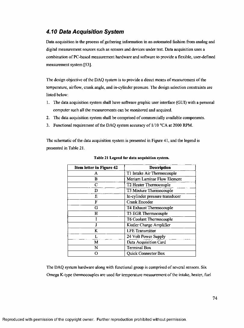
4.10 Data Acquisition System
Data acquisition is the process of gathering information in an automated fashion from analog and
digital measurement sources such as sensors and devices under test. Data acquisition uses a
combination of PC-based measurement hardware and software to provide a flexible, user-defined
measurement system [53].
The design objective of the DAQ system is to provide a direct means of measurement of the
temperature, airflow, crank angle, and in-cylinder pressure. The design selection constraints are
listed below:
1. The data acquisition system shall have software graphic user interface (GUI) with a personal
computer such all the measurements can be monitored and acquired.
2. The data acquisition system shall be comprised of commercially available components.
3. Functional requirement of the DAQ system accuracy of 1/10 °CA at 2000 RPM.
The schematic of the data acquisition system is presented in Figure 41, and the legend is
presented in Table 21.
Table 21 Legend for data acquisition system.
Item letter in Figure 42 DescriptionA T1 Intake Air ThermocoupleB Meriam Laminar Flow ElementC T2 Heater ThermocoupleD T3 Mixture ThermocoupleE In-cylinder pressure transducerF Crank EncoderG T4 Exhaust ThermocoupleH T5 EGR ThermocoupleI T6 Coolant ThermocoupleJ Kistler Charge AmplifierK LFE TransmitterL 24 Volt Power SupplyM Data Acquisition CardN Terminal BoxO Quick Connector Box
The DAQ system hardware along with functional group is comprised of several sensors. Six
Omega K-type thermocouples are used for temperature measurement of the intake, heater, fuel
74
Reproduced with permission of the copyright owner. Further reproduction prohibited without permission.
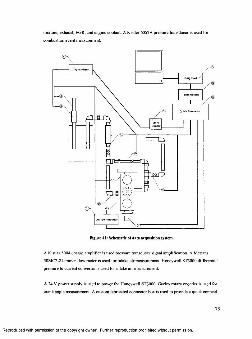
mixture, exhaust, EGR, and engine coolant. A Kistler 6052A pressure transducer is used for
combustion event measurement.
T ransm itter
DAQ Card
Term inal Bo:
Quick C onnects
24 V Supply
Charge Amplifier
Figure 41: Schematic of data acquisition system.
A Kistler 5004 charge amplifier is used pressure transducer signal amplification. A Meriam
50MC2-2 laminar flow meter is used for intake air measurement. Honeywell ST3000 differential
pressure to current converter is used for intake air measurement.
A 24 V power supply is used to power the Honeywell ST3000. Gurley rotary encoder is used for
crank angle measurement. A custom fabricated connector box is used to provide a quick connect
75
Reproduced with permission of the copyright owner. Further reproduction prohibited without permission.
interface for all the sensor connections and a National Instruments SCB-10 terminal box is
housed inside. The connector box is connected via cable to a National Instruments PCI-6071-E
data acquisition card. A 3.0 MHz Dell personal computer is used as the user interface. Further
details of the data acquisition system are available in Appendix J.
A summary of the each device selected as it pertains to the data acquisition system as well as its
intended purpose in controlling the HCCI engine was modified with permission from Defoe [52].
4.10.1 Thermocouple Selection and Location
The thermocouples selected were Omega K-type thermocouple probes with quick disconnect.
These thermocouples are the most popular calibration and are well suited for measuring air and
liquid mixtures in temperature range from -270 to 1372 °C, more than adequate for this
application. The Omega K-Type thermocouples are of high quality and low cost and feature
nylon connectors that are rated for temperatures up to 220 °C. The probes are available in
diameters as small as 0.25 mm (0.010 in) and as large as to 3.0 mm (0.125 in). Therefore, these
thermocouple probes are ideal for this research engine and meet the selection criteria.
The six thermocouples selected are part of the DAQ system and are show in Figure 41.
Thermocouple T1 is located at the beginning of the intake (A) and measures the intake air
temperature. Thermocouple T2 is located just after the charge pre-heater (C) and is used to
determine the temperature increase after the pre-heater. Thermocouple T3 is located at the end of
the intake manifold (D), just before the intake valve and is used to determine the charge
temperature just before the mixture enters the engine. Thermocouple T4 is located in the exhaust
(G), and is used to monitor the temperature of the combustion products exiting the active
cylinder. Thermocouple T5 is in the EGR pipe (H) and is used to determine the temperature of
the gases entering the intake manifold. And lastly thermocouple T6 is set into the cylinder head
at (I), and is used to monitor the coolant temperature.
4.10.2 Pressure Transducer Selection
The in-cylinder pressure transducer is a wall-mounted Kistler 6052A1. According to Kistler it is
the most accurate non-cooled transducer for in-cylinder pressure available on the market. The
Kistler 6052A1 was selected because of its availability, reliability and accuracy.
76
Reproduced with permission of the copyright owner. Further reproduction prohibited without permission.
The sensing element of the transducer is inserted into a hole drilled into the secondary piston
located in the cylinder head and is the pressure sensing tip is exposed to the combustion chamber.
The pressure sensing tip of the transducer face is to be 4mm from the combustion chamber wall.
The element is cooled by heat transfer to the cylinder head water-jacket in order to reduce the
effect of thermal shock.
The pressure transducer outputs a charge (Q) proportional to the gauge pressure (pincyiinder)
according to the following formula:
Q = m ' P incy iinder’ Equation 11
Where m = 19.2 pC/bar [23]. See Appendix J.6 for calibration certificate.
This transducer is designed to operate in the pressure range from 0 to 250 bar suitable for HCCI
chamber pressures. Kistler pressure transducers are known as the industry standard for in-cylinder
pressure measurement, and are widely used by major automakers, research labs, and universities
for accurate data collection. Specifications are available in Appendix J.3 and J.5.
4.10.3 Charge Amplifier Selection
The Kistler 5004 Charge Amplifier is necessary component that accompanies the Kistler 6052A1
pressure transducer. The Kistler Charge Amplifier converts the charge signal output from the
Kistler pressure transducer to a voltage signal that is easily read by the data acquisition (DAQ)
card, (see Figure 42.)
There are two selector knobs that control the settings of the amplifier: one specifies the sensitivity
of the input device in picocoulombs per mechanical unit (pC/bar); the other specifies the output
gain of the amplifier in mechanical units per Volt (bar/Volt). Since the DAQ card can handle
signals only up to 5 Volts, and the expected maximum pressure to be measured is 100 bar, the
required gain (G) setting is determined by the equation:
100 bar barG = ------------= 2 0 ------, Equation 12
5 V V
Charge amplifier specifications are listed in Appendix J.3.
77
Reproduced with permission of the copyright owner. Further reproduction prohibited without permission.
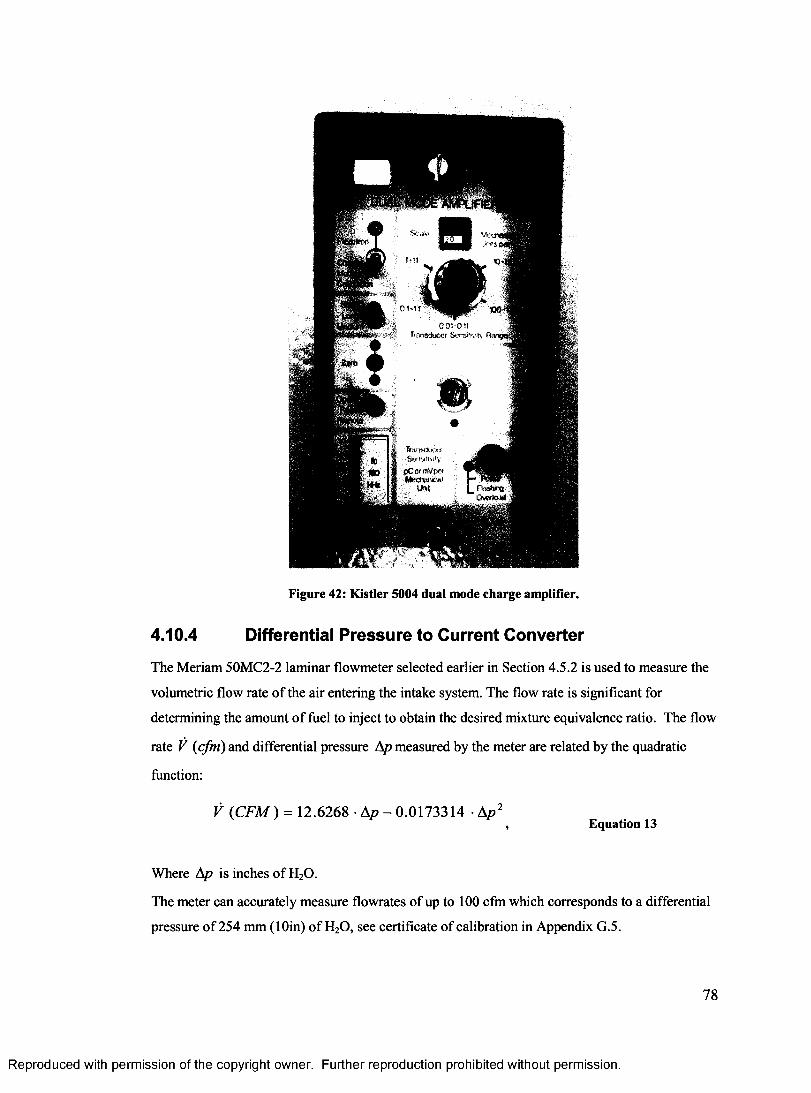
Figure 42: Kistler 5004 dual mode charge amplifier.
4.10.4 Differential Pressure to Current Converter
The Meriam 50MC2-2 laminar flowmeter selected earlier in Section 4.5.2 is used to measure the
volumetric flow rate of the air entering the intake system. The flow rate is significant for
determining the amount of fuel to inject to obtain the desired mixture equivalence ratio. The flow
rate V (cfm) and differential pressure Ap measured by the meter are related by the quadratic
function:
V (C FM ) = 12.6268 • Ap - 0.0173314 ■ A p 2, Equation 13
Where Ap is inches of H20 .
The meter can accurately measure flowrates of up to 100 cfm which corresponds to a differential
pressure of 254 mm (lOin) of H20 , see certificate of calibration in Appendix G.5.
78
Reproduced with permission of the copyright owner. Further reproduction prohibited without permission.
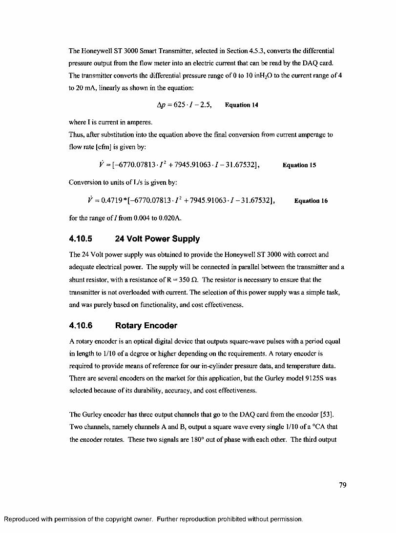
The Honeywell ST 3000 Smart Transmitter, selected in Section 4.5.3, converts the differential
pressure output from the flow meter into an electric current that can be read by the DAQ card.
The transmitter converts the differential pressure range of 0 to 10 inH20 to the current range of 4
to 20 mA, linearly as shown in the equation:
k p = 625 • 7 - 2.5, Equation 14
where I is current in amperes.
Thus, after substitution into the equation above the final conversion from current amperage to
flow rate [cfm] is given by:
V = [-6770.07813 -72 +7945 .91063-7-31 .67532], Equation 15
Conversion to units of L/s is given by:
V = 0 .4719*[-6770.07813-72 +7945 .91063-7-31 .67532], E quation^
for the range of 7 from 0.004 to 0.020A.
4.10.5 24 Volt Power Supply
The 24 Volt power supply was obtained to provide the Honeywell ST 3000 with correct and
adequate electrical power. The supply will be connected in parallel between the transmitter and a
shunt resistor, with a resistance of R = 350 Q. The resistor is necessary to ensure that the
transmitter is not overloaded with current. The selection of this power supply was a simple task,
and was purely based on functionality, and cost effectiveness.
4.10.6 Rotary Encoder
A rotary encoder is an optical digital device that outputs square-wave pulses with a period equal
in length to 1/10 of a degree or higher depending on the requirements. A rotary encoder is
required to provide means of reference for our in-cylinder pressure data, and temperature data.
There are several encoders on the market for this application, but the Gurley model 9125S was
selected because of its durability, accuracy, and cost effectiveness.
The Gurley encoder has three output channels that go to the DAQ card from the encoder [53].
Two channels, namely channels A and B, output a square wave every single 1/10 of a °CA that
the encoder rotates. These two signals are 180° out of phase with each other. The third output
79
Reproduced with permission of the copyright owner. Further reproduction prohibited without permission.
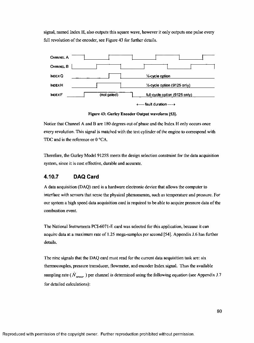
signal, named Index H, also outputs this square wave, however it only outputs one pulse every
full revolution of the encoder, see Figure 43 for further details.
C h a n n e l A
C h a n n e l B
In d e x Q
In d e x H
In d e x F
%-cycle option
Mt-cycle option (9125 only)
(not gated) full-cycle option (9125 only)
fault duration
Figure 43: Gurley Encoder Output waveform [53|.
Notice that Channel A and B are 180 degrees out of phase and the Index H only occurs once
every revolution. This signal is matched with the test cylinder of the engine to correspond with
TDC and is the reference or 0 °CA.
Therefore, the Gurley Model 9125S meets the design selection constraint for the data acquisition
system, since it is cost effective, durable and accurate.
4.10.7 DAQ Card
A data acquisition (DAQ) card is a hardware electronic device that allows the computer to
interface with sensors that sense the physical phenomenon, such as temperature and pressure. For
our system a high speed data acquisition card is required to be able to acquire pressure data of the
combustion event.
The National Instruments PCI-6071-E card was selected for this application, because it can
acquire data at a maximum rate of 1.25 mega-samples per second [54], Appendix J.6 has further
details.
The nine signals that the DAQ card must read for the current data acquisition task are: six
thermocouples, pressure transducer, flowmeter, and encoder Index signal. Thus the available
sampling rate ( N semor ) per channel is determined using the following equation (see Appendix J.7
for detailed calculations):
80
Reproduced with permission of the copyright owner. Further reproduction prohibited without permission.
N sensor= ~ ^ , Equation 17sensors
_ 1.25x10⁹ samples / secsensor _ Q 9
Nsensor = 1 3 8 , samples / s e c ,
Since there is a switching delay between channels, a maximum rate of approximately 90% of this
value so N semor becomes 125,000 samples/sec. Recall that the functional requirement of the
DAQ system is an accuracy of 1/10 °CA at 2000 RPM. The required sampling rate ( N required) for
this is determined from the following equation:
= o, ■ 1V ^ „ „ = 33.3 •3600 = 1 2 0 ,0 0 0 ^ ^ ^ Eq“a"0n “sec
Where N dalapoirits is the number of data points per crank angle degrees.
N datapomXs = 1 0 J * - • 360— = 3600dampomts CAD rof
and CD is the angular engine speed calculated from the following,
lm in - rot(o = 2000 rpm 33.3 — ,
60s s
Thus, the required sampling rate N required is less than the N sensor available sampling rate.
The maximum sampling rate of the DAQ card is 125000 samples per second. The encoder rate is
determined by the angular velocity of the crankshaft for a given engine speed multiplied by the #
of encoder ticks per revolution which is 3600. At 2084 RPM the encoder rate exceeds the
maximum sampling rate of the DAQ card. Therefore, achieving data acquisition at engine speeds
higher than 2000 RPM is not technically possible with the current DAQ card. It should be noted
out that the DAQ card selection was completed by a previous student. Therefore, the National
Instruments PCI-6071-E DAQ has fulfilled the resolution requirement for up to 2000 RPM,
however is not able to provide sampling at a higher engines speeds (see Table 22.)
81
Reproduced with permission of the copyright owner. Further reproduction prohibited without permission.
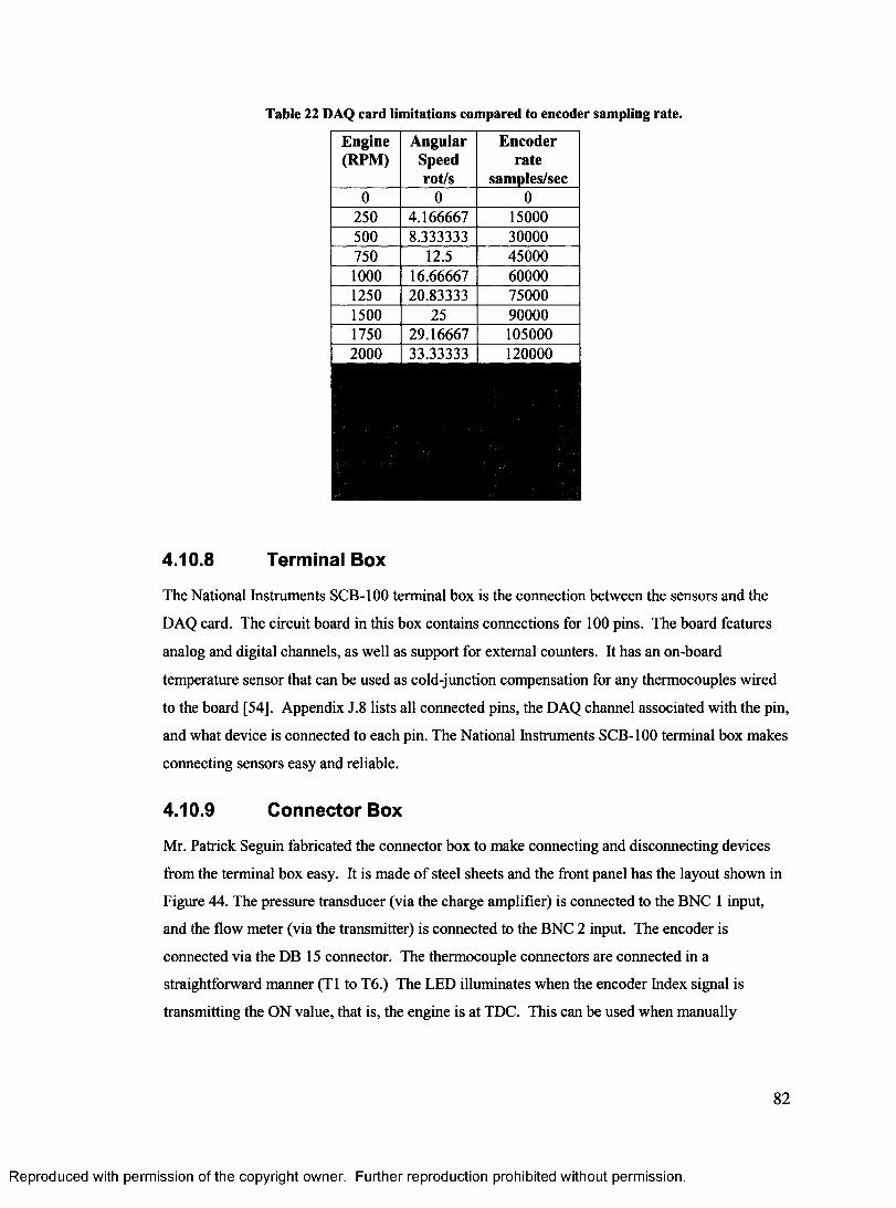
Table 22 DAQ card limitations compared to encoder sampling rate.
Engine(RPM)
AngularSpeedrot/s
Encoderrate
samples/sec0 0 0
250 4.166667 15000500 8.333333 30000750 12.5 450001000 16.66667 600001250 20.83333 750001500 25 900001750 29.16667 1050002000 33.33333 120000
4.10.8 Terminal Box
The National Instruments SCB-100 terminal box is the connection between the sensors and the
DAQ card. The circuit board in this box contains connections for 100 pins. The board features
analog and digital channels, as well as support for external counters. It has an on-board
temperature sensor that can be used as cold-j unction compensation for any thermocouples wired
to the board [54]. Appendix J.8 lists all connected pins, the DAQ channel associated with the pin,
and what device is connected to each pin. The National Instruments SCB-100 terminal box makes
connecting sensors easy and reliable.
4.10.9 Connector Box
Mr. Patrick Seguin fabricated the connector box to make connecting and disconnecting devices
from the terminal box easy. It is made of steel sheets and the front panel has the layout shown in
Figure 44. The pressure transducer (via the charge amplifier) is connected to the BNC 1 input,
and the flow meter (via the transmitter) is connected to the BNC 2 input. The encoder is
connected via the DB 15 connector. The thermocouple connectors are connected in a
straightforward manner (T1 to T6.) The LED illuminates when the encoder Index signal is
transmitting the ON value, that is, the engine is at TDC. This can be used when manually
82
Reproduced with permission of the copyright owner. Further reproduction prohibited without permission.
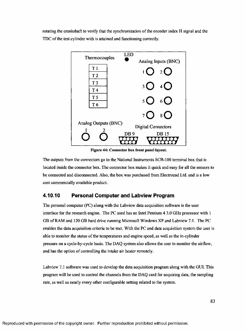
rotating the crankshaft to verify that the synchronization of the encoder index H signal and the
TDC of the test cylinder with is attained and functioning correctly.
ThermocouplesLED® Analog Inputs (BNC)
T 1 -o 3 0T 2T 3 3 0 4 0T 4T 5 60T 6 5 W
?o * 0Analog Outputs (BNC)
Digital Connectors
0 DB 9 DB 15v J W r W v m w /Figure 44: Connector box front panel layout.
The outputs from the connectors go to the National Instruments SCB-100 terminal box that is
located inside the connector box. The connector box makes it quick and easy for all the sensors to
be connected and disconnected. Also, the box was purchased from Electrozad Ltd. and is a low
cost commercially available product.
4.10.10 Personal Computer and Labview Program
The personal computer (PC) along with the Labview data acquisition software is the user
interface for the research engine. The PC used has an Intel Pentium 4 3.0 GHz processor with 1
GB of RAM and 120 GB hard drive running Microsoft Windows XP and Labview 7.1. The PC
enables the data acquisition criteria to be met. With the PC and data acquisition system the user is
able to monitor the status of the temperatures and engine speed, as well as the in-cylinder
pressure on a cycle-by-cycle basis. The DAQ system also allows the user to monitor the airflow,
and has the option of controlling the intake air heater remotely.
Labview 7.1 software was used to develop the data acquisition program along with the GUI. This
program will be used to control the channels from the DAQ card for acquiring data, the sampling
rate, as well as nearly every other configurable setting related to the system.
83
Reproduced with permission of the copyright owner. Further reproduction prohibited without permission.
The components of the DAQ system were selected to meet the constraints of the system. All
components were commercially available, the graphic user interface developed in Labview is
easy to use, and a DAQ card was selected to meet the constraint for sampling rate. For further
details of the Labview program and the user interface consult Defoe [52].
4.11 Summary
In summary, all the systems of the HCCI research engine have met design constraints and should
provide functional, safe and reliable service for the combustion lab.
Reproduced with permission of the copyright owner. Further reproduction prohibited without permission.
84
5 FABRICATION AND PROTOTYPING
The purpose of this section is to detail the fabrication and prototyping phase of the research
engine project. This section discusses fabrication details in chronological order. These details
include the following; prototype development, design methods, fabrications materials and
methods, any difficulties, and final product description.
5.1 Apparatus Fixture Prototyping
The objective of the apparatus fixture is to provide the structural skeleton for which all the other
components of the apparatus can be mounted. The apparatus fixture design must provide a solid
mounting point for the research engine and the AC motor. The design of the fixture must also
provide adequate space for the VSD, resistor bank, transformer, fuel system, cooling system, and
the intake/EGR systems.
The fixture designs were produced using AutoCAD and are presented in Figures 45 and 46. In
both figures the units of measure are in inches to simplify fabrication. The fixture table height of
88.9cm (35 in) was selected to provide easy access to the systems of the research engine that
require the most adjustment (ie; intake and fuel systems.) The width and length were limited by
the 1.52 x 2.133 m (5 x 7 ft) bolster plate. Consideration was also given to frame materials and
sizes. The heaviest components namely the Kubota engine and AC motor are supported by a
rectangular steel frame constructed of 5.04 x 5.04 cm (2 x 2 in) rectangular steel tubing. The
lighter components are supported on 2.54 x 2.54 cm (1 x 1 in) rectangular steel tubing. Welding
and fabrication was performed by Marc St. Pierre according to ASTM standards to ensure
structural rigidity and alignment [56].
Photographs of the final apparatus fixture design are presented in Figures 47,48 and 49.
Adjustable fixture feet were designed to have the ability to accept castors and also to rigidly
mount the fixture to the bolster plate (Figure 49). The castors enable the fixture to be rolled
around the machine shop during the fabrication phase and also made it easier to transport to the
combustion lab. Once the final position was determined the fixture was secured with levelling
fasteners to the bolster plate to provide added stability.
85
Reproduced with permission of the copyright owner. Further reproduction prohibited without permission.
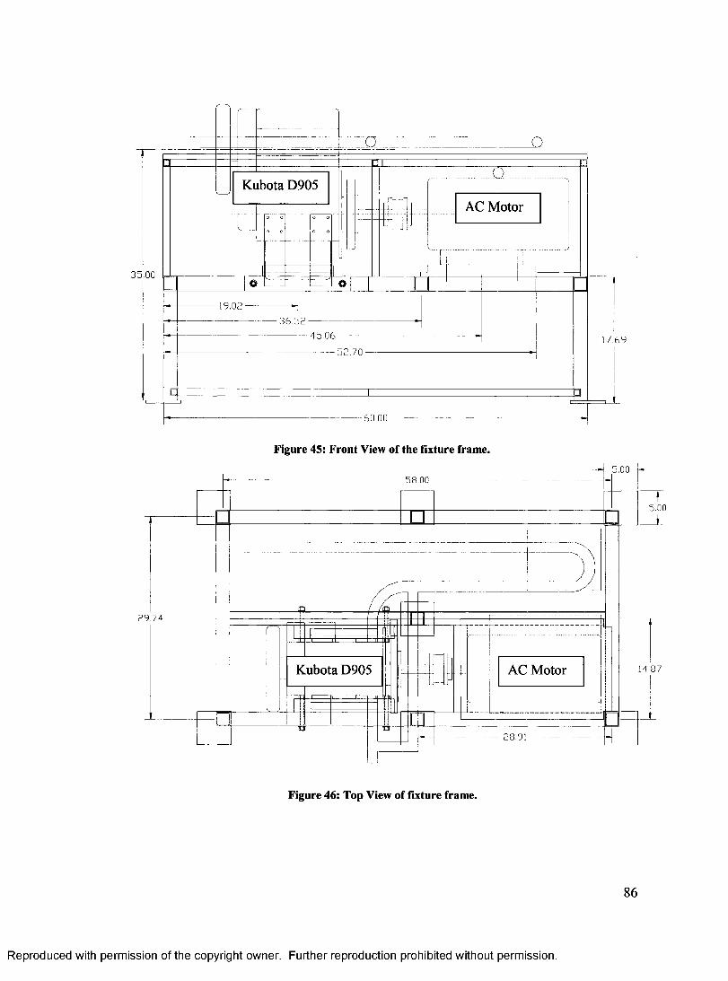
Kubota D905
AC Motor
19 .0 2 -
3 6 .5 245.06 —
- 5 2 . 7 0 - -
60,00
35.00
17,69
Figure 45: Front View of the fixture frame.
5,0058,00
5.00
29.74
Kubota D905 AC Motor 14.87
TT28,91
Figure 46: Top View of fixture frame.
86
Reproduced with permission of the copyright owner. Further reproduction prohibited without permission.
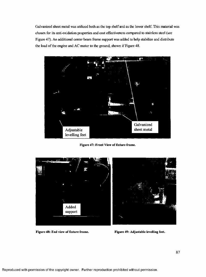
Galvanized sheet metal was utilized both as the top shelf and as the lower shelf. This material was
chosen for its anti-oxidation properties and cost effectiveness compared to stainless steel (see
Figure 47). An additional center beam frame support was added to help stabilize and distribute
the load of the engine and AC motor to the ground, shown if Figure 48.
Galvanized sheet metalAdjustable
levelling feet
Figure 47: Front View of fixture frame.
Addedsupport
Figure 48: End view of fixture frame. Figure 49: Adjustable levelling feet.
87
Reproduced with permission of the copyright owner. Further reproduction prohibited without permission.
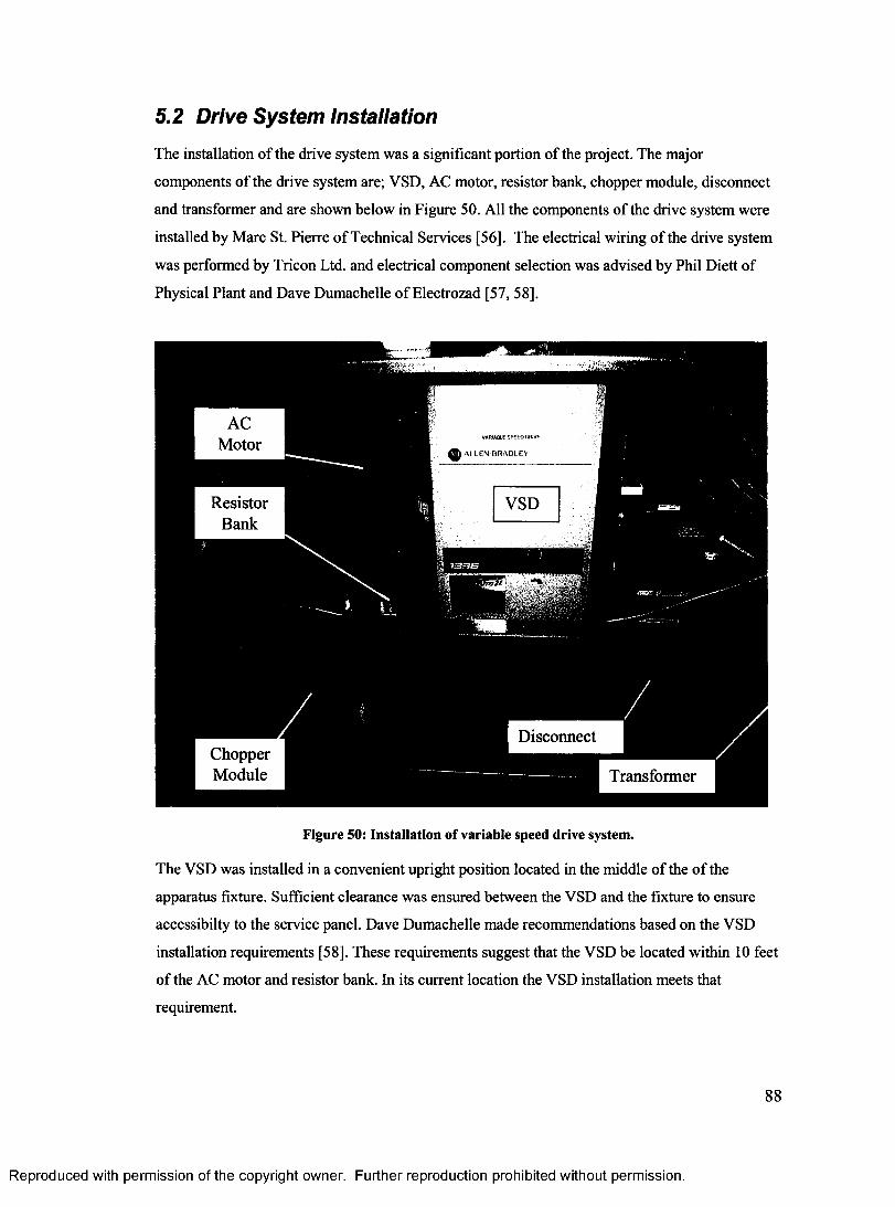
5.2 Drive System Installation
The installation of the drive system was a significant portion of the project. The major
components of the drive system are; VSD, AC motor, resistor bank, chopper module, disconnect
and transformer and are shown below in Figure 50. All the components of the drive system were
installed by Marc St. Pierre of Technical Services [56]. The electrical wiring of the drive system
was performed by Tricon Ltd. and electrical component selection was advised by Phil Diett of
Physical Plant and Dave Dumachelle of Electrozad [57, 58].
MotorA l L t N B R A D L E Y
ResistorBank
Disconnect
Transformer
Figure 50: Installation of variable speed drive system.
The VSD was installed in a convenient upright position located in the middle of the of the
apparatus fixture. Sufficient clearance was ensured between the VSD and the fixture to ensure
accessibilty to the service panel. Dave Dumachelle made recommendations based on the VSD
installation requirements [58]. These requirements suggest that the VSD be located within 10 feet
of the AC motor and resistor bank. In its current location the VSD installation meets that
requirement.
88
Reproduced with permission of the copyright owner. Further reproduction prohibited without permission.
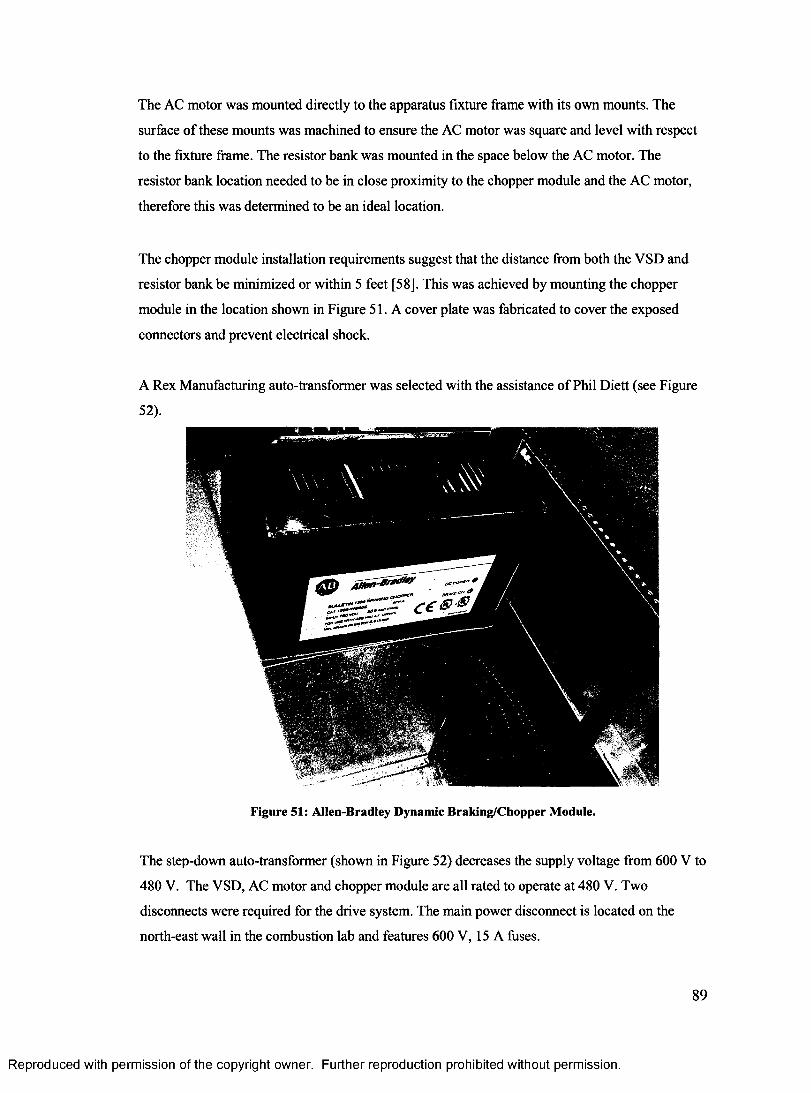
The AC motor was mounted directly to the apparatus fixture frame with its own mounts. The
surface of these mounts was machined to ensure the AC motor was square and level with respect
to the fixture frame. The resistor bank was mounted in the space below the AC motor. The
resistor bank location needed to be in close proximity to the chopper module and the AC motor,
therefore this was determined to be an ideal location.
The chopper module installation requirements suggest that the distance from both the VSD and
resistor bank be minimized or within 5 feet [58]. This was achieved by mounting the chopper
module in the location shown in Figure 51. A cover plate was fabricated to cover the exposed
connectors and prevent electrical shock.
A Rex Manufacturing auto-transformer was selected with the assistance of Phil Diett (see Figure
52).
Figure 51: Allen-Bradley Dynamic Braking/Chopper Module.
The step-down auto-transformer (shown in Figure 52) decreases the supply voltage from 600 V to
480 V. The VSD, AC motor and chopper module are all rated to operate at 480 V. Two
disconnects were required for the drive system. The main power disconnect is located on the
north-east wall in the combustion lab and features 600 V, 15 A fuses.
89
Reproduced with permission of the copyright owner. Further reproduction prohibited without permission.
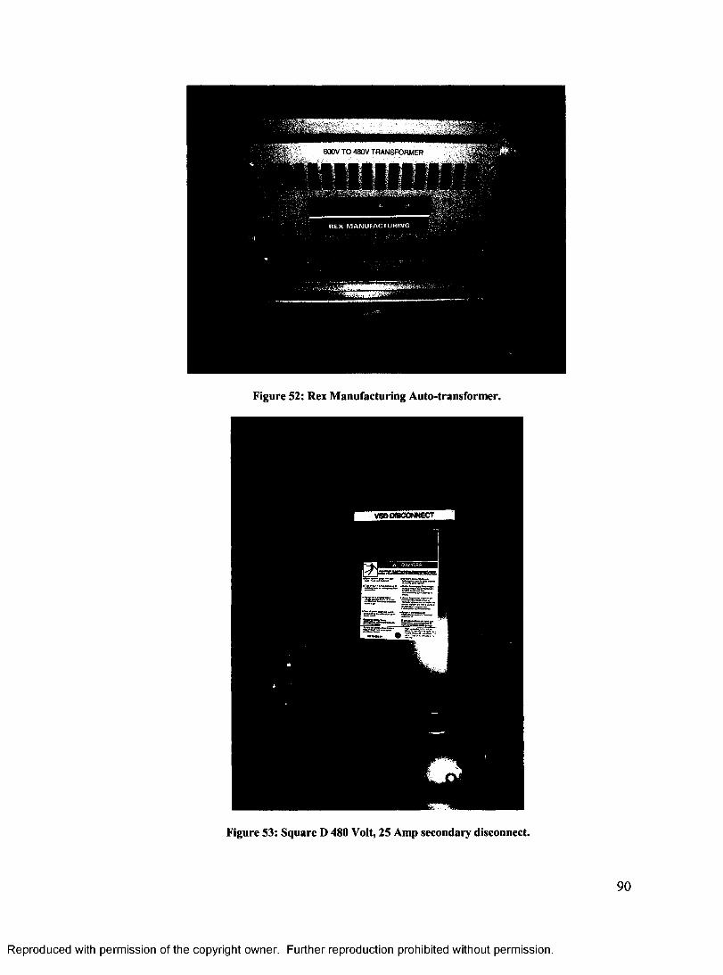
600V TO 480V TRANSFORMER
Figure 52: Rex Manufacturing Auto-transformer.
Figure 53: Square D 480 Volt, 25 Amp secondary disconnect.
90
Reproduced with permission of the copyright owner. Further reproduction prohibited without permission.
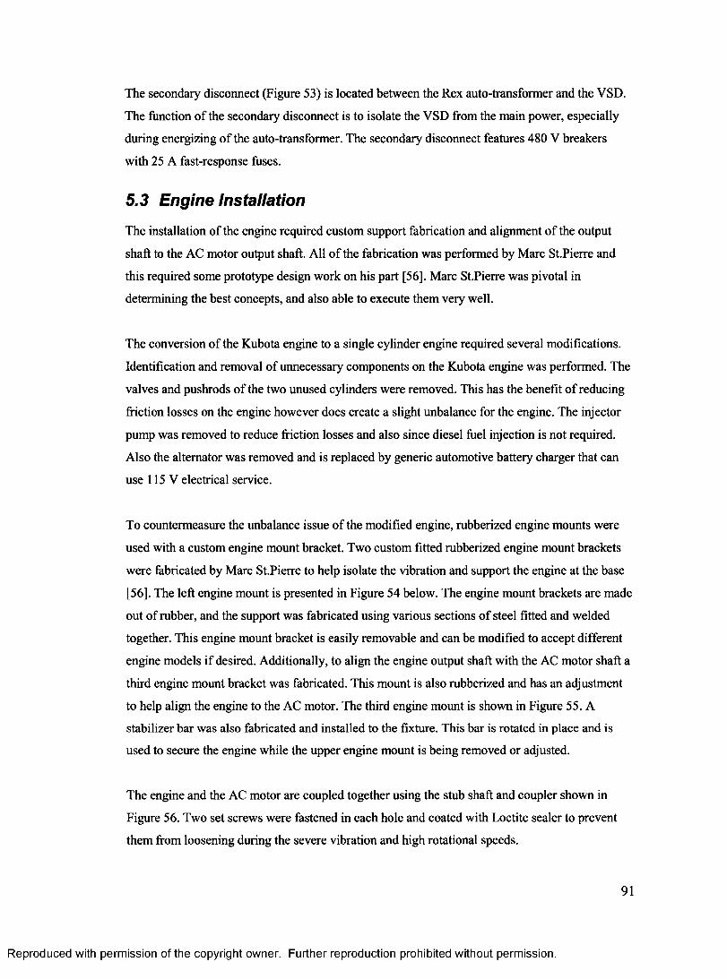
The secondary disconnect (Figure 53) is located between the Rex auto-transformer and the VSD.
The function of the secondary disconnect is to isolate the VSD from the main power, especially
during energizing of the auto-transformer. The secondary disconnect features 480 V breakers
with 25 A fast-response fuses.
5.3 Engine Installation
The installation of the engine required custom support fabrication and alignment of the output
shaft to the AC motor output shaft. All of the fabrication was performed by Marc St.Pierre and
this required some prototype design work on his part [56]. Marc St.Pierre was pivotal in
determining the best concepts, and also able to execute them very well.
The conversion of the Kubota engine to a single cylinder engine required several modifications.
Identification and removal of unnecessary components on the Kubota engine was performed. The
valves and pushrods of the two unused cylinders were removed. This has the benefit of reducing
friction losses on the engine however does create a slight unbalance for the engine. The injector
pump was removed to reduce friction losses and also since diesel fuel injection is not required.
Also the alternator was removed and is replaced by generic automotive battery charger that can
use 115 V electrical service.
To countermeasure the unbalance issue of the modified engine, rubberized engine mounts were
used with a custom engine mount bracket. Two custom fitted rubberized engine mount brackets
were fabricated by Marc St.Pierre to help isolate the vibration and support the engine at the base
[56]. The left engine mount is presented in Figure 54 below. The engine mount brackets are made
out of rubber, and the support was fabricated using various sections of steel fitted and welded
together. This engine mount bracket is easily removable and can be modified to accept different
engine models if desired. Additionally, to align the engine output shaft with the AC motor shaft a
third engine mount bracket was fabricated. This mount is also rubberized and has an adjustment
to help align the engine to the AC motor. The third engine mount is shown in Figure 55. A
stabilizer bar was also fabricated and installed to the fixture. This bar is rotated in place and is
used to secure the engine while the upper engine mount is being removed or adjusted.
The engine and the AC motor are coupled together using the stub shaft and coupler shown in
Figure 56. Two set screws were fastened in each hole and coated with Loctite sealer to prevent
them from loosening during the severe vibration and high rotational speeds.
91
Reproduced with permission of the copyright owner. Further reproduction prohibited without permission.
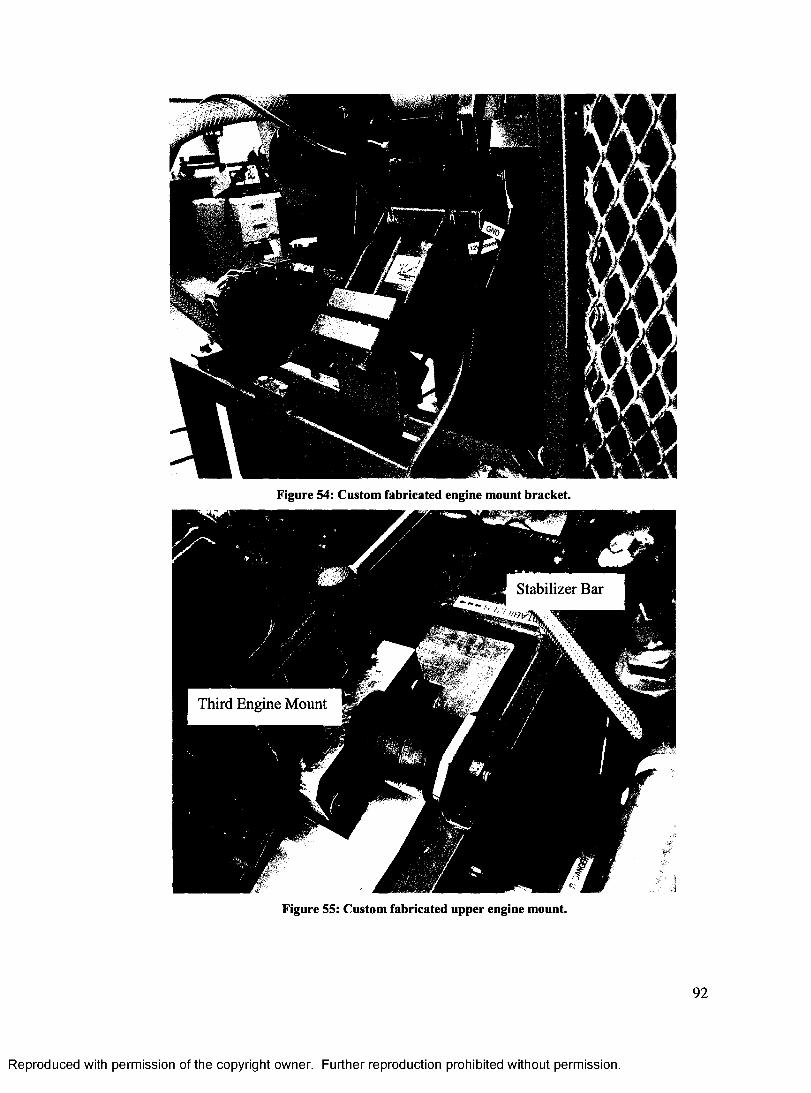
Figure 55: Custom fabricated upper engine mount.
Reproduced with permission of the copyright owner. Further reproduction prohibited without permission.
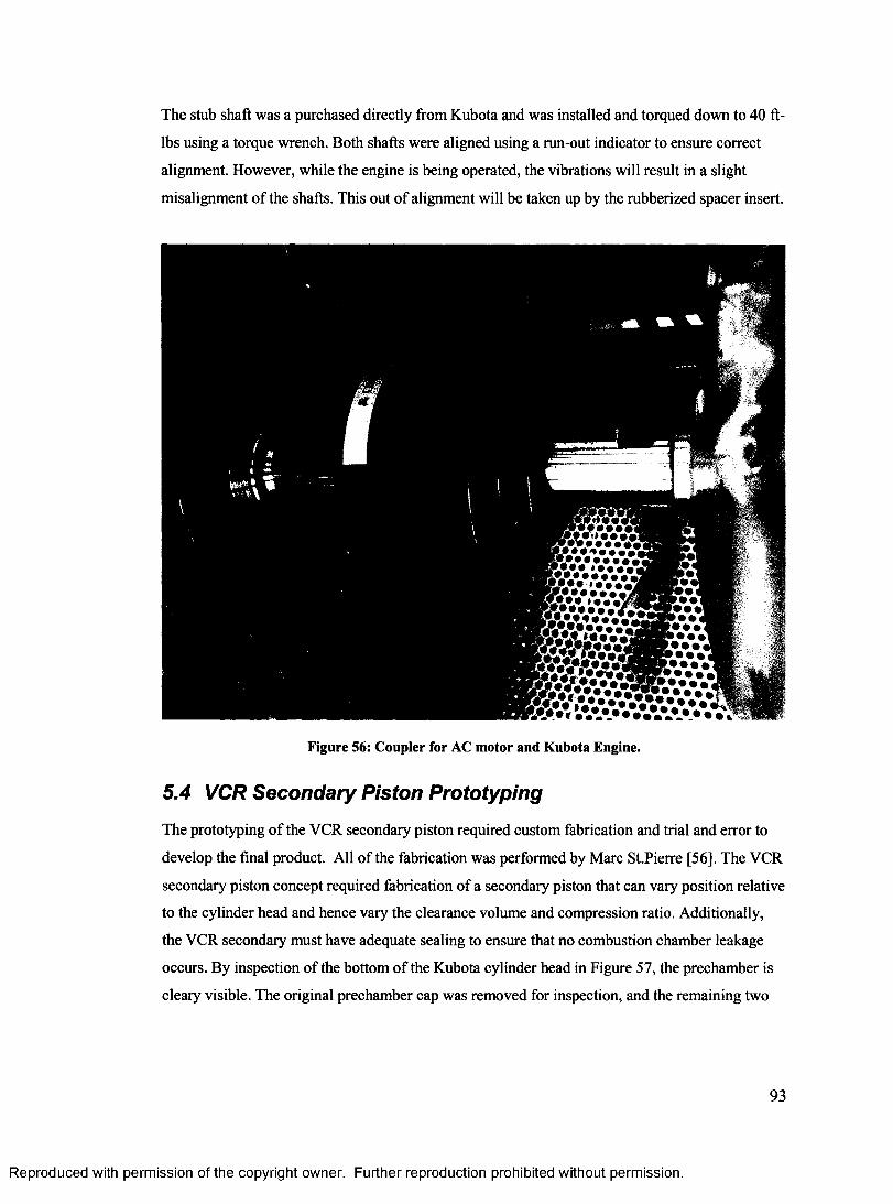
The stub shaft was a purchased directly from Kubota and was installed and torqued down to 40 ft-
lbs using a torque wrench. Both shafts were aligned using a run-out indicator to ensure correct
alignment. However, while the engine is being operated, the vibrations will result in a slight
misalignment of the shafts. This out of alignment will be taken up by the rubberized spacer insert.
E » v « v .v ,v ;iJ& V . • •«R ft.* * * • • • •K v /V .v .y iKraa
Figure 56: Coupler for AC motor and Kubota Engine.
5.4 VCR Secondary Piston Prototyping
The prototyping of the VCR secondary piston required custom fabrication and trial and error to
develop the final product. All of the fabrication was performed by Marc St.Pierre [56]. The VCR
secondary piston concept required fabrication of a secondary piston that can vary position relative
to the cylinder head and hence vary the clearance volume and compression ratio. Additionally,
the VCR secondary must have adequate sealing to ensure that no combustion chamber leakage
occurs. By inspection of the bottom of the Kubota cylinder head in Figure 57, the prechamber is
cleary visible. The original prechamber cap was removed for inspection, and the remaining two
93
Reproduced with permission of the copyright owner. Further reproduction prohibited without permission.
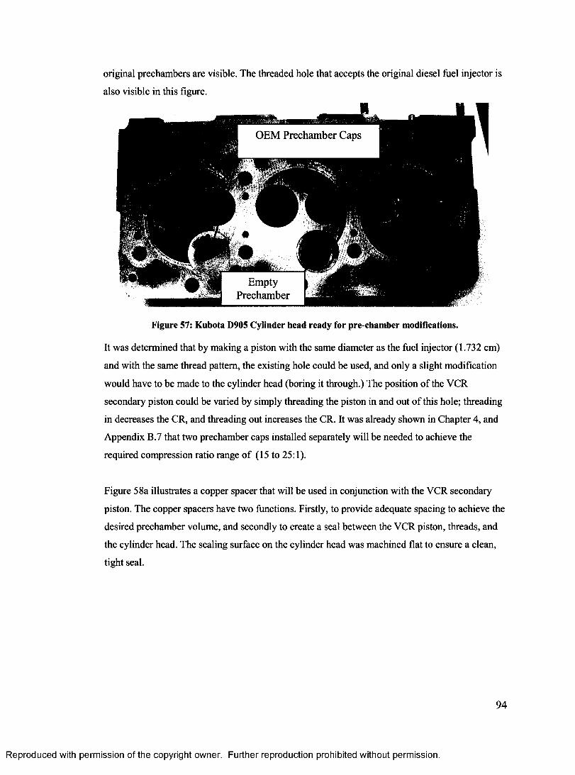
original prechambers are visible. The threaded hole that accepts the original diesel fuel injector is
also visible in this figure.
OEM Prechamber Caps
EmptyPrechamber
Figure 57: Kubota D905 Cylinder head ready for pre-chamber modifications.
It was determined that by making a piston with the same diameter as the fuel injector (1.732 cm)
and with the same thread pattern, the existing hole could be used, and only a slight modification
would have to be made to the cylinder head (boring it through.) The position of the VCR
secondary piston could be varied by simply threading the piston in and out of this hole; threading
in decreases the CR, and threading out increases the CR. It was already shown in Chapter 4, and
Appendix B.7 that two prechamber caps installed separately will be needed to achieve the
required compression ratio range of (15 to 25:1).
Figure 58a illustrates a copper spacer that will be used in conjunction with the VCR secondary
piston. The copper spacers have two functions. Firstly, to provide adequate spacing to achieve the
desired prechamber volume, and secondly to create a seal between the VCR piston, threads, and
the cylinder head. The sealing surface on the cylinder head was machined flat to ensure a clean,
tight seal.
94
Reproduced with permission of the copyright owner. Further reproduction prohibited without permission.
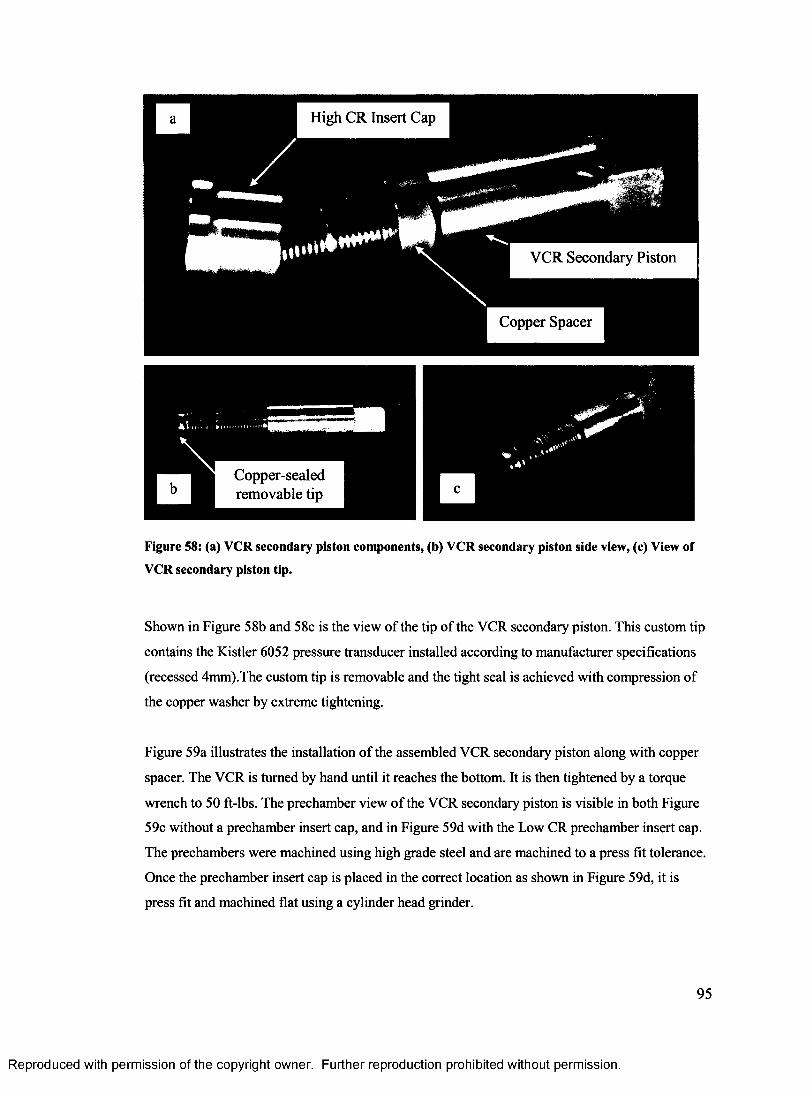
High CR Insert Cap
VCR Secondary Piston
Copper Spacer
Figure 58: (a) VCR secondary piston components, (b) VCR secondary piston side view, (c) View of
VCR secondary piston tip.
Shown in Figure 58b and 58c is the view of the tip of the VCR secondary piston. This custom tip
contains the Kistler 6052 pressure transducer installed according to manufacturer specifications
(recessed 4mm).The custom tip is removable and the tight seal is achieved with compression of
the copper washer by extreme tightening.
Figure 59a illustrates the installation of the assembled VCR secondary piston along with copper
spacer. The VCR is turned by hand until it reaches the bottom. It is then tightened by a torque
wrench to 50 ft-lbs. The prechamber view of the VCR secondary piston is visible in both Figure
59c without a prechamber insert cap, and in Figure 59d with the Low CR prechamber insert cap.
The prechambers were machined using high grade steel and are machined to a press fit tolerance.
Once the prechamber insert cap is placed in the correct location as shown in Figure 59d, it is
press fit and machined flat using a cylinder head grinder.
95
Reproduced with permission of the copyright owner. Further reproduction prohibited without permission.

Figure 59: (a) Tightening of VCR secondary piston, (b) VCR secondary piston installed, (c) View of
VCR secondary piston without prechamber cap, (d) Low CR prechamber cap ready to be press fit.
Figure 60 below illustrates a comparison between the original (OEM), high CR, and low CR
prechamber insert caps.
OEM
Figure 60: Comparison between OEM, high CR and Low CR prechamber inserts.
Although the shape of the combustion chamber appears to be slightly irregular, the desired effect
of varying the CR was achieved and verified by volume measurements.
96
Reproduced with permission of the copyright owner. Further reproduction prohibited without permission.
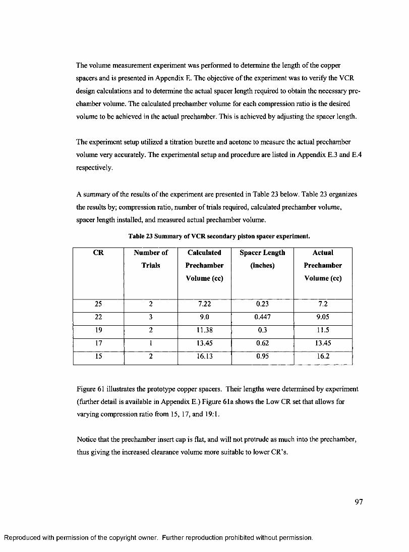
The volume measurement experiment was performed to determine the length of the copper
spacers and is presented in Appendix E. The objective of the experiment was to verify the VCR
design calculations and to determine the actual spacer length required to obtain the necessary pre
chamber volume. The calculated prechamber volume for each compression ratio is the desired
volume to be achieved in the actual prechamber. This is achieved by adjusting the spacer length.
The experiment setup utilized a titration burette and acetone to measure the actual prechamber
volume very accurately. The experimental setup and procedure are listed in Appendix E.3 and E.4
respectively.
A summary of the results of the experiment are presented in Table 23 below. Table 23 organizes
the results by; compression ratio, number of trials required, calculated prechamber volume,
spacer length installed, and measured actual prechamber volume.
Table 23 Summary of VCR secondary piston spacer experiment.
CR Number of
Trials
Calculated
Prechamber
Volume (cc)
Spacer Length
(inches)
Actual
Prechamber
Volume (cc)
25 2 7.22 0.23 7.2
22 3 9.0 0.447 9.05
19 2 11.38 0.3 11.5
17 1 13.45 0.62 13.45
15 2 16.13 0.95 16.2
Figure 61 illustrates the prototype copper spacers. Their lengths were determined by experiment
(further detail is available in Appendix E.) Figure 61a shows the Low CR set that allows for
varying compression ratio from 15, 17, and 19:1.
Notice that the prechamber insert cap is flat, and will not protrude as much into the prechamber,
thus giving the increased clearance volume more suitable to lower CR’s.
97
Reproduced with permission of the copyright owner. Further reproduction prohibited without permission.
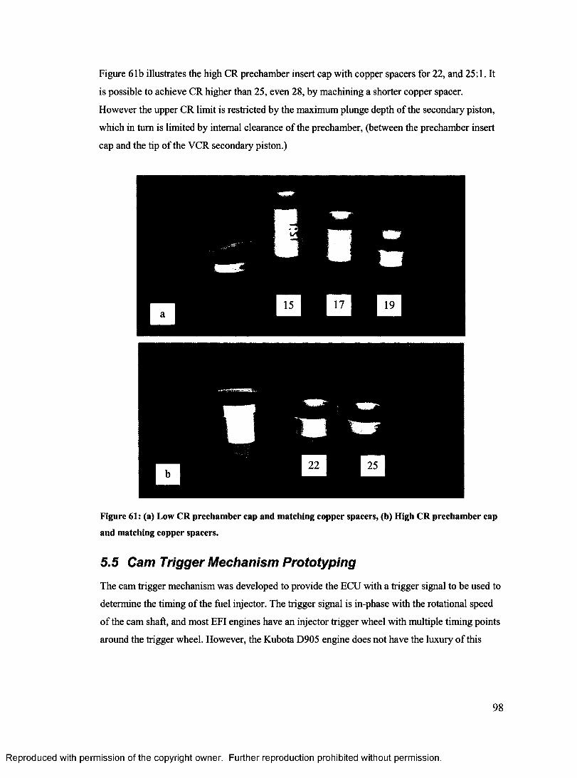
Figure 61b illustrates the high CR prechamber insert cap with copper spacers for 22, and 25:1. It
is possible to achieve CR higher than 25, even 28, by machining a shorter copper spacer.
However the upper CR limit is restricted by the maximum plunge depth of the secondary piston,
which in turn is limited by internal clearance of the prechamber, (between the prechamber insert
cap and the tip of the VCR secondary piston.)
Figure 61: (a) Low CR prechamber cap and matching copper spacers, (b) High CR prechamber cap
and matching copper spacers.
5.5 Cam Trigger Mechanism Prototyping
The cam trigger mechanism was developed to provide the ECU with a trigger signal to be used to
determine the timing of the fuel injector. The trigger signal is in-phase with the rotational speed
of the cam shaft, and most EFI engines have an injector trigger wheel with multiple timing points
around the trigger wheel. However, the Kubota D905 engine does not have the luxury of this
98
Reproduced with permission of the copyright owner. Further reproduction prohibited without permission.
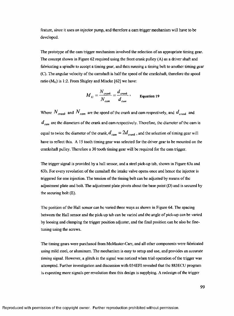
feature, since it uses an injector pump, and therefore a cam trigger mechanism will have to be
developed.
The prototype of the cam trigger mechanism involved the selection of an appropriate timing gear.
The concept shown in Figure 62 required using the front crank pulley (A) as a driver shaft and
fabricating a spindle to accept a timing gear, and then running a timing belt to another timing gear
(C). The angular velocity of the camshaft is half the speed of the crankshaft, therefore the speed
ratio (Mg) is 1:2. From Shigley and Miscke [62] we have:
N dM crank crank
G ~ jlt ~ ’ Equation 19cam cam
Where N crank and Ncam are the speed of the crank and cam respectively, and dcrank and
d cam are the diameters of the crank and cam respectively. Therefore, the diameter of the cam is
equal to twice the diameter of the crank, d cam = 2 d crank, and the selection of timing gear will
have to reflect this. A 15 tooth timing gear was selected for the driver gear to be mounted on the
crankshaft pulley. Therefore a 30 tooth timing gear will be required for the cam trigger.
The trigger signal is provided by a hall sensor, and a steel pick-up tab, shown in Figure 63a and
63b. For every revolution of the camshaft the intake valve opens once and hence the injector is
triggered for one injection. The tension of the timing belt can be adjusted by means of the
adjustment plate and bolt. The adjustment plate pivots about the base point (D) and is secured by
the securing bolt (E).
The position of the Hall sensor can be varied three ways as shown in Figure 64. The spacing
between the Hall sensor and the pick-up tab can be varied and the angle of pick-up can be varied
by loosing and clamping the trigger position adjuster, and the final position can be also be fine-
tuning using the screws.
The timing gears were purchased from McMaster-Carr, and all other components were fabricated
using mild steel, or aluminum. The mechanism is easy to setup and use, and provides an accurate
timing signal. However, a glitch in the signal was noticed when trial operation of the trigger was
attempted. Further investigation and discussion with 034EFI revealed that the 883ECU program
is expecting more signals per revolution then this design is supplying. A redesign of the trigger
99
Reproduced with permission of the copyright owner. Further reproduction prohibited without permission.
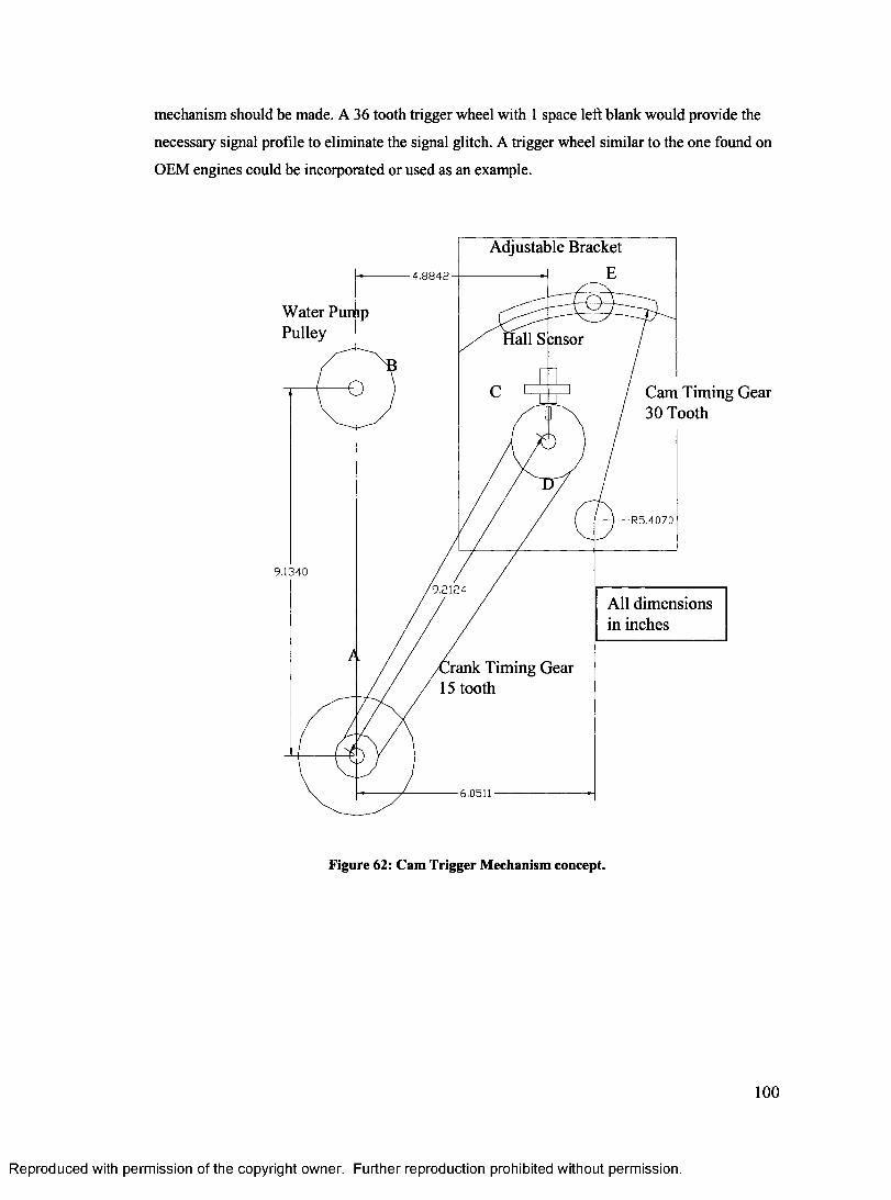
mechanism should be made. A 36 tooth trigger wheel with 1 space left blank would provide the
necessary signal profile to eliminate the signal glitch. A trigger wheel similar to the one found on
OEM engines could be incorporated or used as an example.
Adjustable Bracket
4,8842
Water Pump Pulley all S ;nsor
Cam Timing Gear 30 Tooth
9.13409.2124
Crank Timing Gear 15 tooth
6.0511
All dimensions in inches
Figure 62: Cam Trigger Mechanism concept.
100
Reproduced with permission of the copyright owner. Further reproduction prohibited without permission.
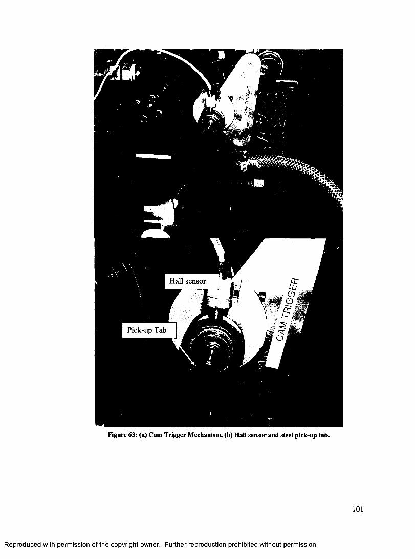
Figure 63: (a) Cam Trigger Mechanism, (b) Hall sensor and steel pick-up tab.
101
Reproduced with permission of the copyright owner. Further reproduction prohibited without permission.
Figure 64: Cam trigger mechanism adjustment.
5.6 Cooling System Installation
The cooling system was a relatively simple system to implement. Section 4.2.2 already discussed
in detail the major components of the cooling system and their functions. Further detail is
presented in Appendix A.5 and A.6. For this section, the installation of the radiator is the major
task that is discussed.
The requirements for the installation of the radiator are as follows:
1. The radiator must be installed in close proximity of the engine, to minimize hose length.
2. The radiator must be easy to install and remove, and the installation should enable easy
access to radiator cap.
Figure 65 is a photo of the completed installation of the radiator. The radiator is located in close
proximity to the engine, and minimizes the hose length. The hose selected is a 2.54 cm (1 in) re
enforced poly-vinyl chloride (PVC) clear hose and makes the coolant level easily visible. Regular
stainless steel hose clamps were used to appropriately secure the hose ends to both the engine and
102
Reproduced with permission of the copyright owner. Further reproduction prohibited without permission.
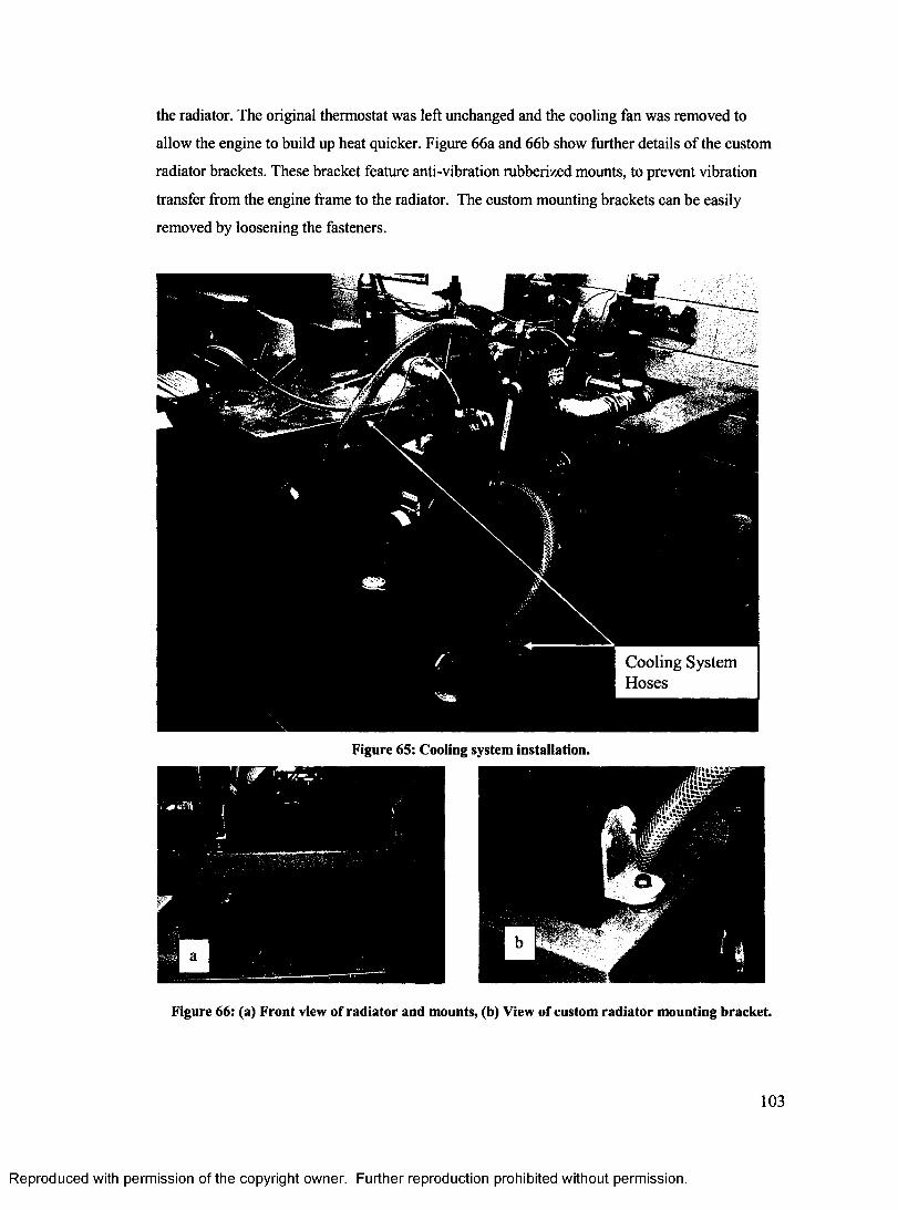
the radiator. The original thermostat was left unchanged and the cooling fan was removed to
allow the engine to build up heat quicker. Figure 66a and 66b show further details of the custom
radiator brackets. These bracket feature anti-vibration rubberized mounts, to prevent vibration
transfer from the engine frame to the radiator. The custom mounting brackets can be easily
removed by loosening the fasteners.
Cooling System Hoses
Figure 65: Cooling system installation.
Figure 66: (a) Front view of radiator and mounts, (b) View of custom radiator mounting bracket.
103
Reproduced with permission of the copyright owner. Further reproduction prohibited without permission.
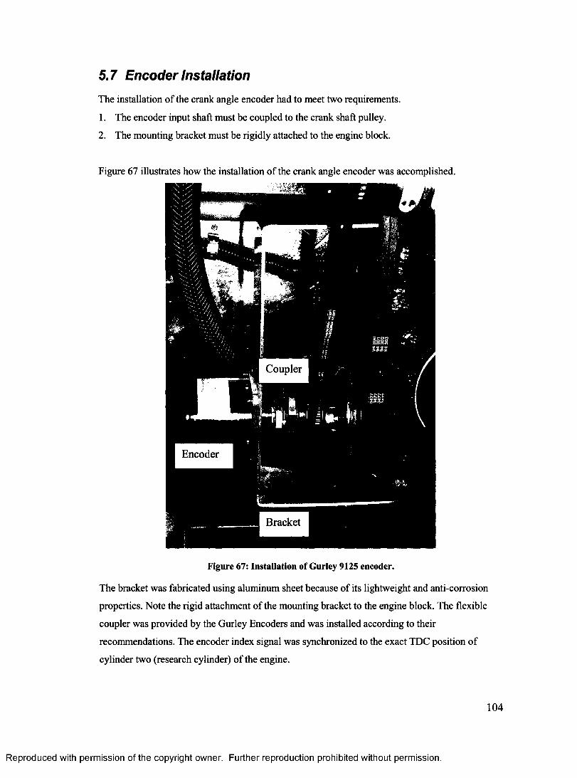
5.7 Encoder Installation
The installation of the crank angle encoder had to meet two requirements.
1. The encoder input shaft must be coupled to the crank shaft pulley.
2. The mounting bracket must be rigidly attached to the engine block.
Figure 67 illustrates how the installation of the crank angle encoder was accomplished.
Coupler
Encoder
Bracket
Figure 67: Installation of Gurley 9125 encoder.
The bracket was fabricated using aluminum sheet because of its lightweight and anti-corrosion
properties. Note the rigid attachment of the mounting bracket to the engine block. The flexible
coupler was provided by the Gurley Encoders and was installed according to their
recommendations. The encoder index signal was synchronized to the exact TDC position of
cylinder two (research cylinder) of the engine.
104
Reproduced with permission of the copyright owner. Further reproduction prohibited without permission.
5.8 Intake/EGR Piping System and Heater Fabrication
The fabrication of the Intake/EGR piping system was completed using off-the-shelf components
as prescribed in Chapter 4. The Intake/EGR piping system is divided into two sections;
hot/galvanized piping section and cold/ABS piping section. These sections are separated by the
intake air heater.
Figure 68 illustrates the hot/galvanized piping section and Figure 69 illustrates the cold/ABS
piping section. Notice the direction of flow indicated by the orange arrows. All the components of
the hot/galvanized piping section were purchased from a local plumbing supplier. They were
measured and cut to the correct length using a cut-off saw. Most of the components were pre
threaded, which made them easy to assemble, however there were a few pipe lengths that needed
to be threaded manually with a 3.81 cm (1.5in) NPT Pipe thread die and threading machine. Prior
to assembly, Teflon tape sealer was applied to the threads to ease assembly and to provide an air
tight seal.
A prototype throttle valve and two prototype flanges were fabricated and are shown in Figure
70a, 70b and 70c. The flange (shown in Figure 70b) was fabricated using a galvanized steel pipe
that was press fit into a flange plate. The flange plate provides a flat surface for a gasket to seal
the intake and exhaust with the cylinder head. The throttle valve shown in Figure 70a was also
fabricated using a galvanized steel pipe. A custom fitted throttle plate was machined and mounted
to a pivot shaft that runs through the pipe and into the aluminum housing. The pivot shaft is
supported by small bearings on either end. A throttle position sensor is mounted on one end of the
housing (Figure 70a) and a throttle cable bracket is mounted on the opposite end (Figure 70c.)
The throttle cable is used to set the position of the throttle valve, and was fabricated using a
simple lawnmower cable.
The cold/ABS piping components were all purchased from a local plumbing supplier. The
assembly of these components was very simple, and only required the use of a hacksaw, and the
ABS adhesive. The piping was cut to length and pre-assembled to test fit, and was glued together
using a special adhesive. Rubber couplers were installed to minimize the transmission of engine
vibration and to ease assembly. The surge tank was developed using a 40 gallon drum. This
reduced cost substantially, and provides enough surge volume to dampen the pressure pulsations
prior to the flow meter.
105
Reproduced with permission of the copyright owner. Further reproduction prohibited without permission.
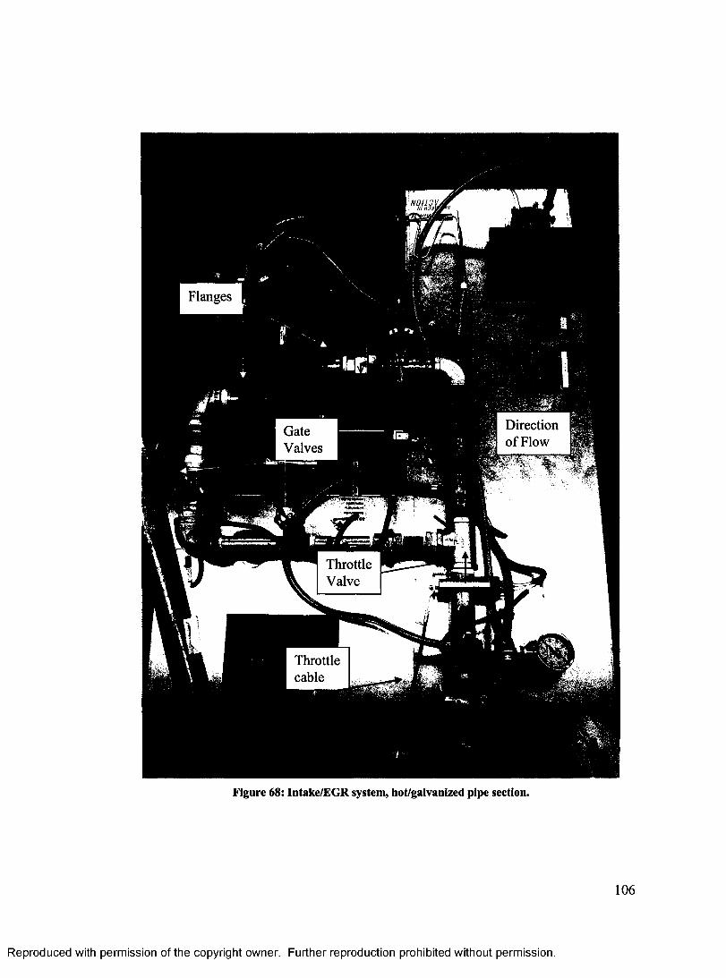
Figure 68: Intake/EGR system, hot/galvanized pipe section.
106
Reproduced with permission of the copyright owner. Further reproduction prohibited without permission.
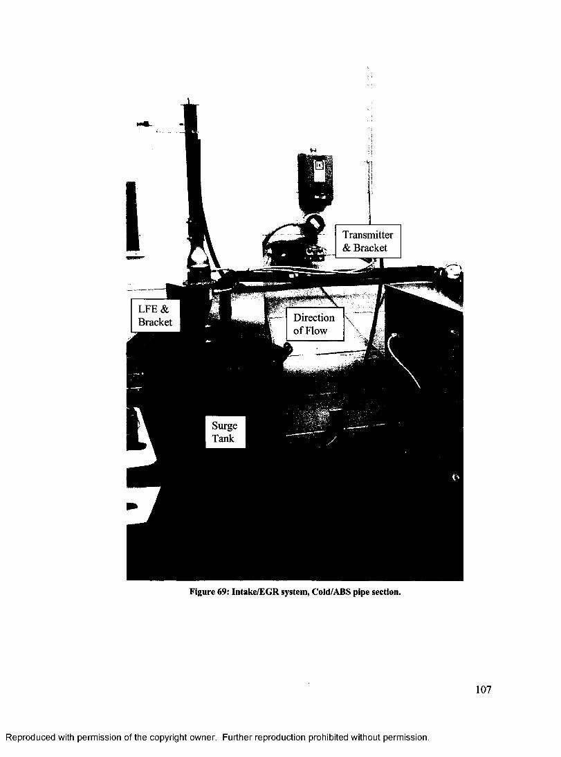
Figure 69: Intake/EGR system, Cold/ABS pipe section.
107
Reproduced with permission of the copyright owner. Further reproduction prohibited without permission.
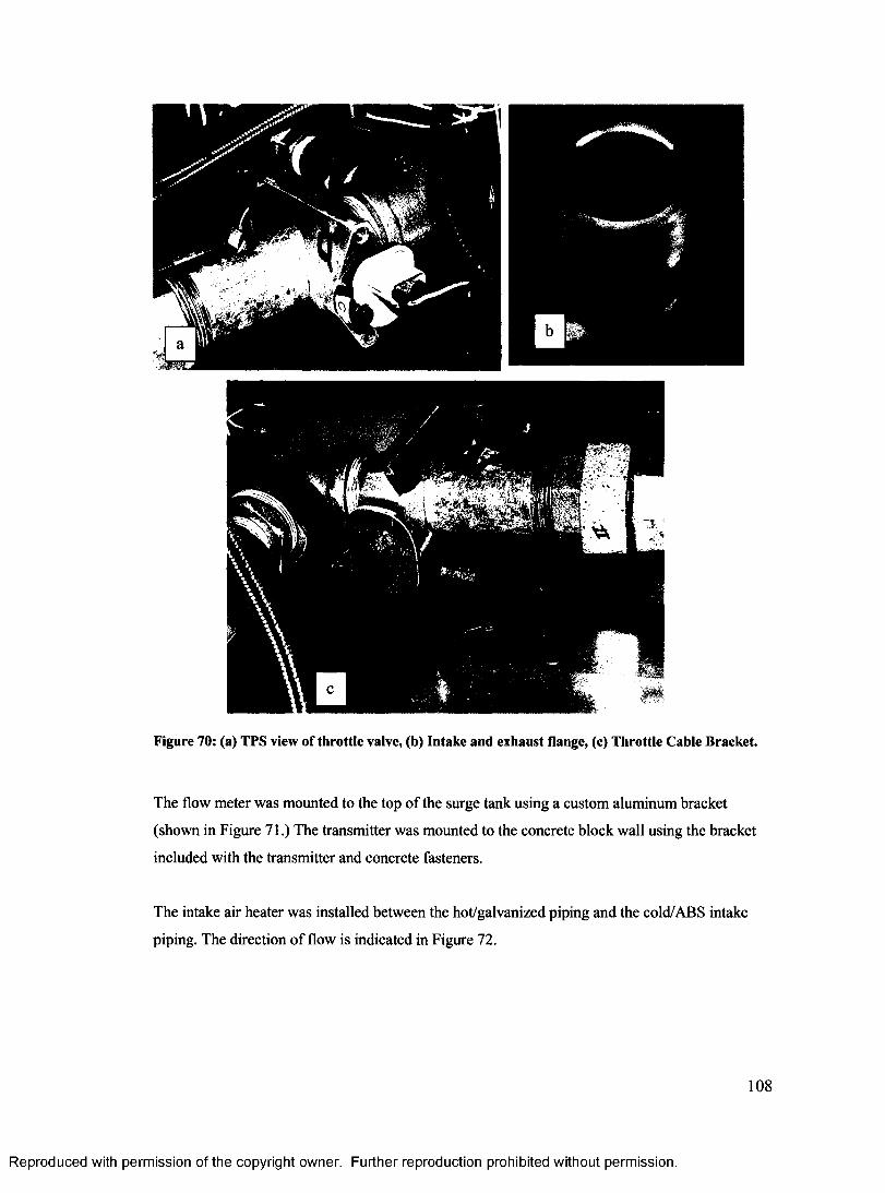
Figure 70: (a) TPS view of throttle valve, (b) Intake and exhaust flange, (c) Throttle Cable Bracket.
The flow meter was mounted to the top of the surge tank using a custom aluminum bracket
(shown in Figure 71.) The transmitter was mounted to the concrete block wall using the bracket
included with the transmitter and concrete fasteners.
The intake air heater was installed between the hot/galvanized piping and the cold/ABS intake
piping. The direction of flow is indicated in Figure 72.
108
Reproduced with permission of the copyright owner. Further reproduction prohibited without permission.
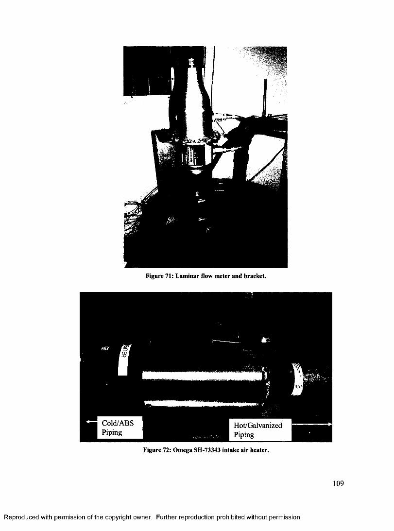
Figure 71: Laminar flow meter and bracket.
Cold/ABSPiping
Hot/GalvanizedPiping
Figure 72: Omega SH-73343 intake air heater.
109
Reproduced with permission of the copyright owner. Further reproduction prohibited without permission.

Figure 73 shows the electrical enclosure that houses the heater controller and wiring. The
enclosure was purchase from Electrozad Ltd and the CNi/32 heater controller from Omega was
installed and setup by Pat Seguin [61].
Figure 73: Intake air heater controller.
5.9 Fuel and ECU System Installation
The installation of the fuel and ECU systems were completed in a timely manner. As mentioned
earlier, all the components of the fuel system are off-the-shelf items, however some fabrication
and fitting was required to install the fuel system.
Firstly, the fuel tank needed to be installed in the top plate; therefore a 10 cm diameter hole was
cut out of the galvanized steel and six bolt holes were drilled for the fuel tank fasteners. The
return line and the fuel cap is shown in Figure 74a and the feed line, fuel tank and fuel filter are
shown in Figure 74b. The fuel lines were difficult to cut to length because the outside stainless
steel sheathing is made from braided wire, and is very difficult to cut a clean edge. A clean
straight edge is necessary to install the hose end fittings, therefore a technique was devised to
overcome this problem. The braided lines were taped in the area to be cut with special packing
tape, and a hacksaw was used to cut the hose. This eliminated the frayed ends, and made it a lot
easier to install. The fuel gauge, pressure regulator and injector fuel rail is shown in Figure 75.
The fuel gauge and regulator were easily assembled and tightened with wrenches, and light anti
seize lubrication. The injector fuel rail was fabricated using off-the-shelf brass fittings that were
machined to accept the injector and create a tight seal.
110
Reproduced with permission of the copyright owner. Further reproduction prohibited without permission.
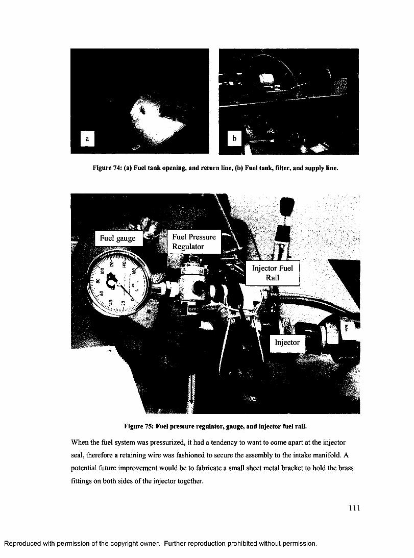
Figure 74: (a) Fuel tank opening, and return line, (b) Fuel tank, filter, and supply line.
* Fuel Pressure & Regulator
Injector Fuel Rail
Injector
Figure 75: Fuel pressure regulator, gauge, and injector fuel rail.
When the fuel system was pressurized, it had a tendency to want to come apart at the injector
seal, therefore a retaining wire was fashioned to secure the assembly to the intake manifold. A
potential future improvement would be to fabricate a small sheet metal bracket to hold the brass
fittings on both sides of the injector together.
I l l
Reproduced with permission of the copyright owner. Further reproduction prohibited without permission.
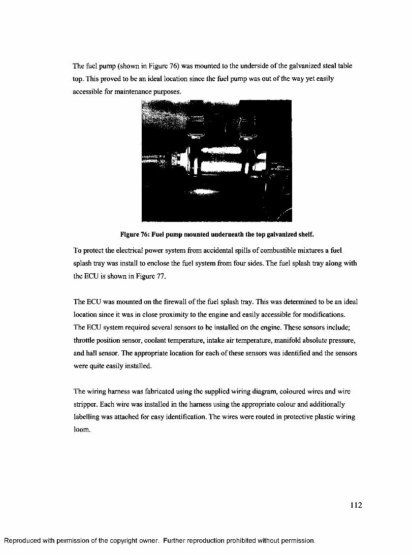
The fuel pump (shown in Figure 76) was mounted to the underside of the galvanized steal table
top. This proved to be an ideal location since the fuel pump was out of the way yet easily
accessible for maintenance purposes.
Figure 76: Fuel pump mounted underneath the top galvanized shelf.
To protect the electrical power system from accidental spills of combustible mixtures a fuel
splash tray was install to enclose the fuel system from four sides. The fuel splash tray along with
the ECU is shown in Figure 77.
The ECU was mounted on the firewall of the fuel splash tray. This was determined to be an ideal
location since it was in close proximity to the engine and easily accessible for modifications.
The ECU system required several sensors to be installed on the engine. These sensors include;
throttle position sensor, coolant temperature, intake air temperature, manifold absolute pressure,
and hall sensor. The appropriate location for each of these sensors was identified and the sensors
were quite easily installed.
The wiring harness was fabricated using the supplied wiring diagram, coloured wires and wire
stripper. Each wire was installed in the harness using the appropriate colour and additionally
labelling was attached for easy identification. The wires were routed in protective plastic wiring
loom.
112
Reproduced with permission of the copyright owner. Further reproduction prohibited without permission.
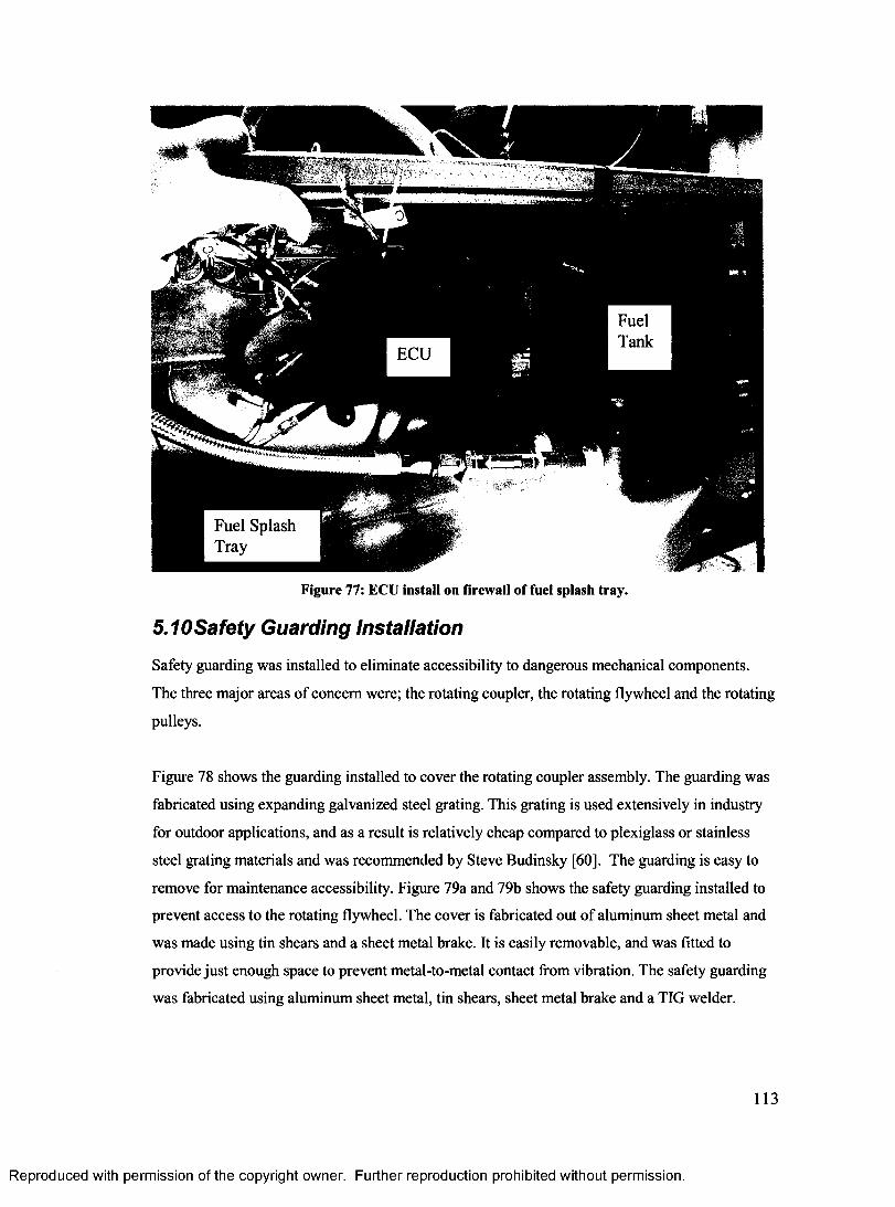
Figure 77: ECU install on firewall of fuel splash tray.
5.10Safety Guarding Installation
Safety guarding was installed to eliminate accessibility to dangerous mechanical components.
The three major areas of concern were; the rotating coupler, the rotating flywheel and the rotating
pulleys.
Figure 78 shows the guarding installed to cover the rotating coupler assembly. The guarding was
fabricated using expanding galvanized steel grating. This grating is used extensively in industry
for outdoor applications, and as a result is relatively cheap compared to plexiglass or stainless
steel grating materials and was recommended by Steve Budinsky [60]. The guarding is easy to
remove for maintenance accessibility. Figure 79a and 79b shows the safety guarding installed to
prevent access to the rotating flywheel. The cover is fabricated out of aluminum sheet metal and
was made using tin shears and a sheet metal brake. It is easily removable, and was fitted to
provide just enough space to prevent metal-to-metal contact from vibration. The safety guarding
was fabricated using aluminum sheet metal, tin shears, sheet metal brake and a TIG welder.
113
Reproduced with permission of the copyright owner. Further reproduction prohibited without permission.
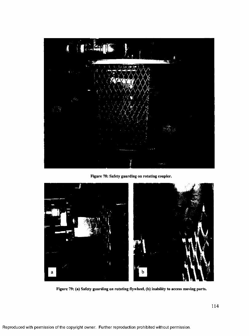
Figure 78: Safety guarding on rotating coupler.
Figure 79: (a) Safety guarding on rotating flywheel, (b) inability to access moving parts.
114
Reproduced with permission of the copyright owner. Further reproduction prohibited without permission.
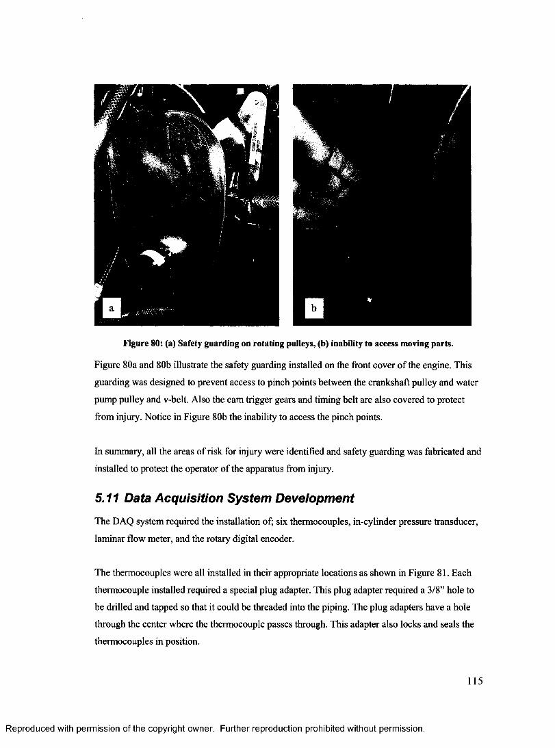
Figure 80: (a) Safety guarding on rotating pulleys, (b) inability to access moving parts.
Figure 80a and 80b illustrate the safety guarding installed on the front cover of the engine. This
guarding was designed to prevent access to pinch points between the crankshaft pulley and water
pump pulley and v-belt. Also the cam trigger gears and timing belt are also covered to protect
from injury. Notice in Figure 80b the inability to access the pinch points.
In summary, all the areas of risk for injury were identified and safety guarding was fabricated and
installed to protect the operator of the apparatus from injury.
5.11 Data Acquisition System Development
The DAQ system required the installation of; six thermocouples, in-cylinder pressure transducer,
laminar flow meter, and the rotary digital encoder.
The thermocouples were all installed in their appropriate locations as shown in Figure 81. Each
thermocouple installed required a special plug adapter. This plug adapter required a 3/8” hole to
be drilled and tapped so that it could be threaded into the piping. The plug adapters have a hole
through the center where the thermocouple passes through. This adapter also locks and seals the
thermocouples in position.
115
Reproduced with permission of the copyright owner. Further reproduction prohibited without permission.
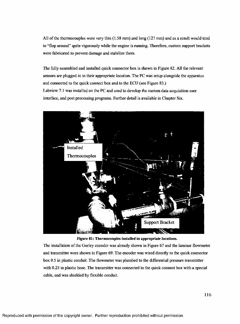
All of the thermocouples were very thin (1.58 mm) and long (127 mm) and as a result would tend
to “flop around” quite vigorously while the engine is running. Therefore, custom support brackets
were fabricated to prevent damage and stabilize them.
The fully assembled and installed quick connector box is shown in Figure 82. All the relevant
sensors are plugged in to their appropriate location. The PC was setup alongside the apparatus
and connected to the quick connect box and to the ECU (see Figure 83.)
Labview 7.1 was installed on the PC and used to develop the custom data acquisition user
interface, and post processing programs. Further detail is available in Chapter Six.
Installed
Thermocouples
Support Bracket
Figure 81: Thermocouples installed in appropriate locations.
The installation of the Gurley encoder was already shown in Figure 67 and the laminar flowmeter
and transmitter were shown in Figure 69. The encoder was wired directly to the quick connector
box 0.5 in plastic conduit. The flowmeter was plumbed to the differential pressure transmitter
with 0.25 in plastic hose. The transmitter was connected to the quick connect box with a special
cable, and was shielded by flexible conduit.
116
Reproduced with permission of the copyright owner. Further reproduction prohibited without permission.
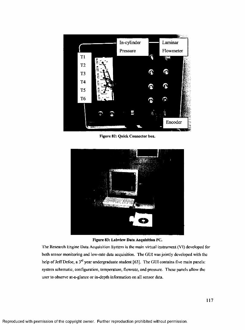
Figure 82: Quick Connector box.
Figure 83: Labview Data Acquisition PC.
The Research Engine Data Acquisition System is the main virtual instrument (VI) developed for
both sensor monitoring and low-rate data acquisition. The GUI was jointly developed with the
help of Jeff Defoe, a 3rd year undergraduate student [63]. The GUI contains five main panels:
system schematic, configuration, temperature, flowrate, and pressure. These panels allow the
user to observe at-a-glance or in-depth information on all sensor data.
117
Reproduced with permission of the copyright owner. Further reproduction prohibited without permission.
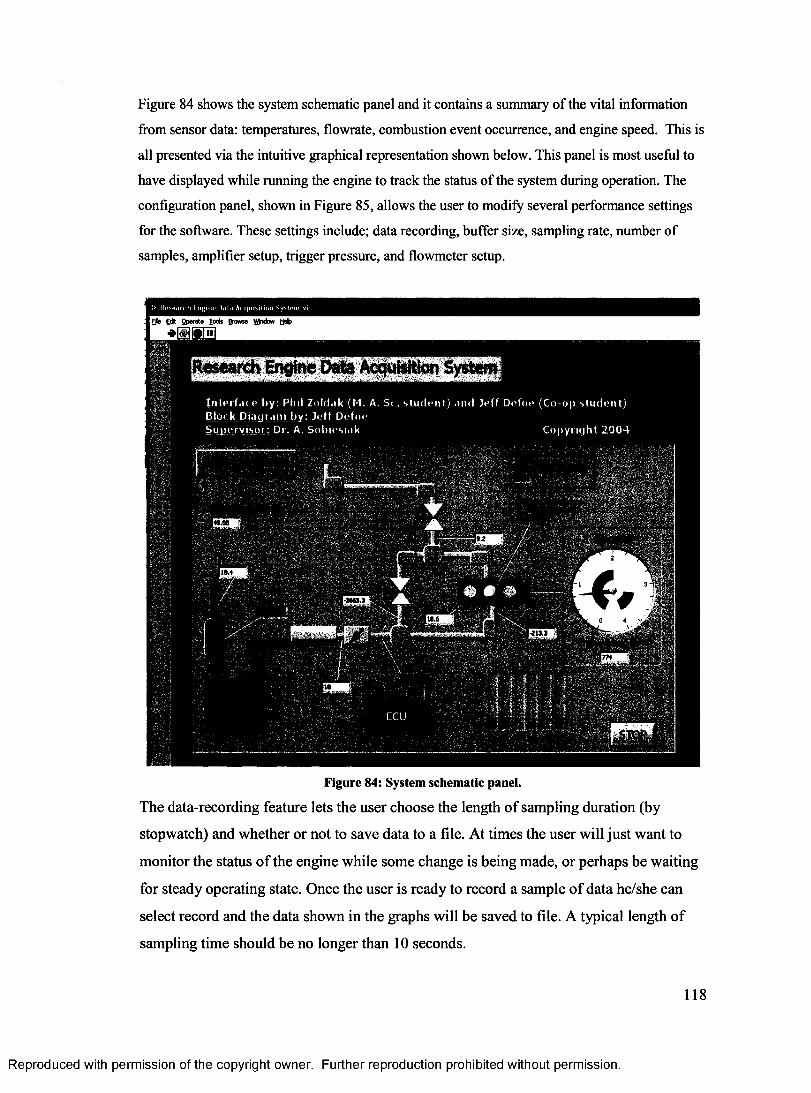
Figure 84 shows the system schematic panel and it contains a summary of the vital information
from sensor data: temperatures, flowrate, combustion event occurrence, and engine speed. This is
all presented via the intuitive graphical representation shown below. This panel is most useful to
have displayed while running the engine to track the status of the system during operation. The
configuration panel, shown in Figure 85, allows the user to modify several performance settings
for the software. These settings include; data recording, buffer size, sampling rate, number of
samples, amplifier setup, trigger pressure, and flowmeter setup.
R e s e a r c h I u g i n e D . i l . ) A c q u i s i t i o n S y s t e m .
Research Engine Data Acquisition System !
I n t i - i f . u *• by : Phil Zold. ik (M. A. S< . s t u d e n t ) <ind J e f f De f oe ( Co - o p s t u d e n t ) Block Di . iur . im by: Je f f De f oeS u j i e i v i s o i : Dr. A. S ob i e s i . i k C o p y r i g h t 2 0 0 4
1-213.3
Figure 84: System schematic panel.
The data-recording feature lets the user choose the length o f sampling duration (by
stopwatch) and whether or not to save data to a file. At times the user will just want to
monitor the status o f the engine while some change is being made, or perhaps be waiting
for steady operating state. Once the user is ready to record a sample o f data he/she can
select record and the data shown in the graphs will be saved to file. A typical length of
sampling time should be no longer than 10 seconds.
118
Reproduced with permission of the copyright owner. Further reproduction prohibited without permission.
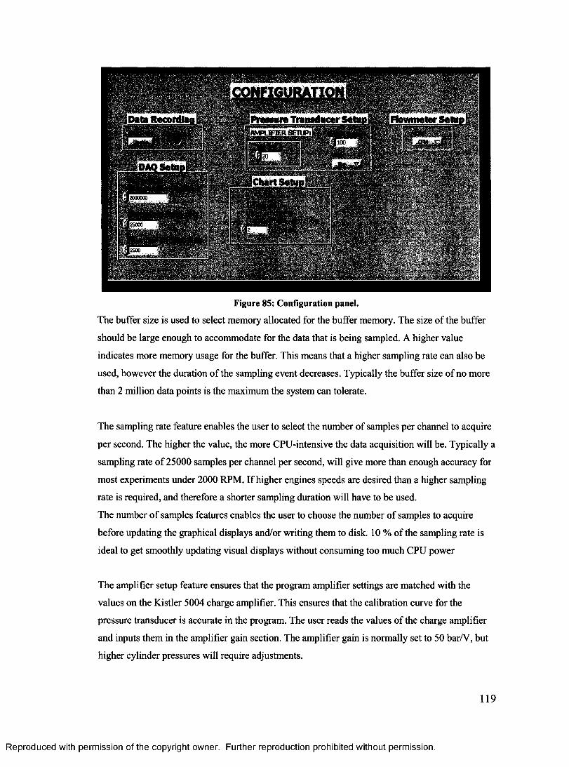
I Flowmeter SeteplBlData Recording h
2000000
Figure 85: Configuration panel.
The buffer size is used to select memory allocated for the buffer memory. The size of the buffer
should be large enough to accommodate for the data that is being sampled. A higher value
indicates more memory usage for the buffer. This means that a higher sampling rate can also be
used, however the duration of the sampling event decreases. Typically the buffer size of no more
than 2 million data points is the maximum the system can tolerate.
The sampling rate feature enables the user to select the number of samples per channel to acquire
per second. The higher the value, the more CPU-intensive the data acquisition will be. Typically a
sampling rate of 25000 samples per channel per second, will give more than enough accuracy for
most experiments under 2000 RPM. If higher engines speeds are desired than a higher sampling
rate is required, and therefore a shorter sampling duration will have to be used.
The number of samples features enables the user to choose the number of samples to acquire
before updating the graphical displays and/or writing them to disk. 10 % of the sampling rate is
ideal to get smoothly updating visual displays without consuming too much CPU power
The amplifier setup feature ensures that the program amplifier settings are matched with the
values on the Kistler 5004 charge amplifier. This ensures that the calibration curve for the
pressure transducer is accurate in the program. The user reads the values of the charge amplifier
and inputs them in the amplifier gain section. The amplifier gain is normally set to 50 bar/V, but
higher cylinder pressures will require adjustments.
119
Reproduced with permission of the copyright owner. Further reproduction prohibited without permission.
The trigger pressure feature enables the user to select the minimum pressure for the combustion
event notification light to come on in the Summary Panel. The GUI also lets the user select the
units for all pressure outputs (bar, psi, and kPa.).
The flowmeter setup feature allows the user to select the units for all flowrate outputs.
The temperature, flowmeter, and in-cylinder pressure panels will be presented in Chapter Six.
5.12 Summary
The fabrication of the research engine along with all of its systems and components was
completed in a timely manner. A prototype VCR secondary piston was developed that enables
variable compression ratio. The fuel system was installed that facilitates accurate fuel metering by
means of an ECU and software. The intake air system, preheater system, and LFE enable accurate
control and measurement of both air flow and temperature. The drive system enables accurate
control of engine speed and provides adequate torque absorption. The frame structure provides a
rigid support structure for the entire apparatus. The safety guarding provides protection from all
rotating objects and prevents the user from accidental injury. The data acquisition system
provides both monitoring, measurement and recording capabilities of important parameters.
Reproduced with permission of the copyright owner. Further reproduction prohibited without permission.
120
6 Testing and Verification
Upon completion of the design and fabrication phase of the project, a series of tests were
performed to validate the functionality of each of the systems of the research engine.
These tests were necessary to ensure that all systems of the apparatus were working correctly.
This section includes the following; testing and verification procedures, results and any
difficulties encountered.
6.1 Engine System Testing
Engine system testing was performed to verify function of the engine prior to combustion
experiments. A leak test was performed on the cylinder head prechamber prior to assembly, and
a compression test was performed on the engine after assembly.
The leak test was performed on the prechamber and fully assembled VCR secondary piston to test
the integrity of the VCR seal. A suction cup was purchased and installed on the suction line of a
vacuum tester. The vacuum tester was used to draw a vacuum on the prechamber. The suction
cup creates a tight seal around the opening of the prechamber from the combustion chamber side
of the cylinder head.
The leak test was performed several times and the procedure and results are presented in
Appendix E.7 through E.10. Initially, the leak test revealed that the VCR assembly had severe
leakage, however it was not apparent what part of the assembly was leaking. The main seal by the
copper spacer and the plug seal were determined to be secure. The leak was isolated and found to
be occurring at the copper washer around the tip of VCR secondary piston. Further tightening and
compression of the copper washer was attained using Teflon tape wrapped around the threads and
the copper washer. The Teflon tape provided a slick surface and enabled the threads to be
tightened further and hence allowing greater deformation of the washer and a tighter seal. As a
result, the prechamber was able to hold the maximum capable vacuum at 90 kPa.
The compression test was performed on the engine once it was fully assembled. A diesel
compression tester was purchased from Snap-On Tools that was well suited for compression
testing up to 6894 kPa (1000 psi). A custom glow plug adapter was fabricated and threaded into
121
Reproduced with permission of the copyright owner. Further reproduction prohibited without permission.
the glow plug hole in the cylinder head. This adapter enabled the compression tester to be
connected to the prechamber (see Appendix E. 11 to E.14 for further details.)
The first compression test resulted in no compression detected in the engine. This was of great
concern as the prechamber had already been verified to hold the maximum vacuum possible. The
cylinder head was removed and inspected, and it was determined there were two possible sources
of compression leakage. The first source was determined to be the lack of flatness of the cylinder
head. A straight edge was used to identify that the cylinder head surface was not perfectly flat.
This would cause an improper seal with the cylinder head gasket and hence substantial leakage.
The second source of leakage was determined to be from the valve seat. The valve seat is located
at the interface between the valve and the cylinder head. Valve seat leakage could cause
substantial leakage since the valves would not close completely and hence the compression
pressure would be completely lost. The cylinder head was sent to Couvillion Automotive
Machine Shop to have the cylinder head ground flat and the valve seats ground and lapped. These
processes ensure the cylinder head is perfectly flat giving a tight and even seal with the head
gasket, and ensured the valves close completely. Also, since the valve seats were ground flat,
some material was removed from the seat and therefore the valve spring tension would be lower
since the spring tension is a function of length, and the length increased from the seat grinding.
Therefore, a shim was fabricated using 0.00254 cm sheet stock and installed under the affected
valve springs. This shim takes up the slack that was removed as a result of the valve grinding, and
restores the spring tension to its originally specification.
The second compression test (CR=22:1) resulted in 2861 kPa (415 psi) compression with the
engine cold, and 3103 kPa (450 psi) compression was measured after the engine was motored for
half an hour and warmed to 40 °C. Therefore, it was verified that the modified Kubota engine
with the VCR secondary piston installed had no leakage and a compression pressure of 3103 kPa.
6.2 Drive System Testing
Drive system testing was performed to verify the function of the VSD prior to combustion
experiments. Motoring tests were performed both with and without the Kubota engine coupled to
the AC motor. Emergency braking tests were also performed to verify the ability of the drive
system to stop during an emergency situation.
122
Reproduced with permission of the copyright owner. Further reproduction prohibited without permission.
The first motoring test was performed without the Kubota engine coupled to the AC motor. This
test involved turning the AC motor without any load, and was performed to verify the
functionality of the AC motor and the VSD. The test was done to ensure that the system was able
to start, stop and run at different speeds. The procedure and results for this test are listed in
Appendix K.3 and K.6. The test proved that the system was able to attain a shaft speed of 530 to
3535 RPM with a corresponding input frequency of 9.0 to 60.0 Hz. The system ran perfectly
without significant evidence of vibration, or any other electrical problem.
The second motoring test was performed with the Kubota engine coupled to the AC motor. This
test was performed to verify the functionality of the drive system while the Kubota engine was
being motored. The test ensured that the system was able to start, brake the engine and run at
different speed. As mentioned previously, the AC motor would require assistance from the starter
motor to overcome the starting torque of the Kubota engine. Therefore, the starter was connected
to 12 volt power and a switch to enable use of the starter. The procedure and results for this test
are listed in Appendix K.4 and K.7.
The results showed that the drive system was unable to start the engine without the assistant of
the starter. However, with the starter engaged shortly, the starting torque of the Kubota engine
was overcome and at that point the drive system would began to rotate the engine under its own
power. The minimum shaft speed of the drive system was determined to be 707 RPM or 12.0 Hz.
Lower speeds were attempted but the vibration of the engine at those speeds was too severe. The
drive system was able to rotate the Kubota engine from 707 to 3004 RPM, with a corresponding
input frequency of 12.0 to 51.0 Hz. Certain shaft speeds induced greater vibrations in the
apparatus than others and this was noted in the observation portion of the results in Appendix
K.7. The system functioned well at all shaft speeds, however in general the noise level became
greater as the shaft speed was increased. The test was stopped at 3004 RPM (51 Hz) due to
excessive noise and vibration of the engine, although the drive system seemed capable of
continuing to maximum speed (3535 RPM.) The vibration was induced by both vertical and yaw
vibrations of the engine on the engine mounts. These two modes would transfer vibrations from
the engine through the engine mounts, and through the intake manifold to the apparatus fixture.
The majority of the noise from vibration seems to be emanating from the following sources;
coupler misalignment due to engine oscillations and sheet metal and exhaust pipe vibrations. The
fabrication and installation of a larger flywheel will help reduce engine oscillations and help
123
Reproduced with permission of the copyright owner. Further reproduction prohibited without permission.
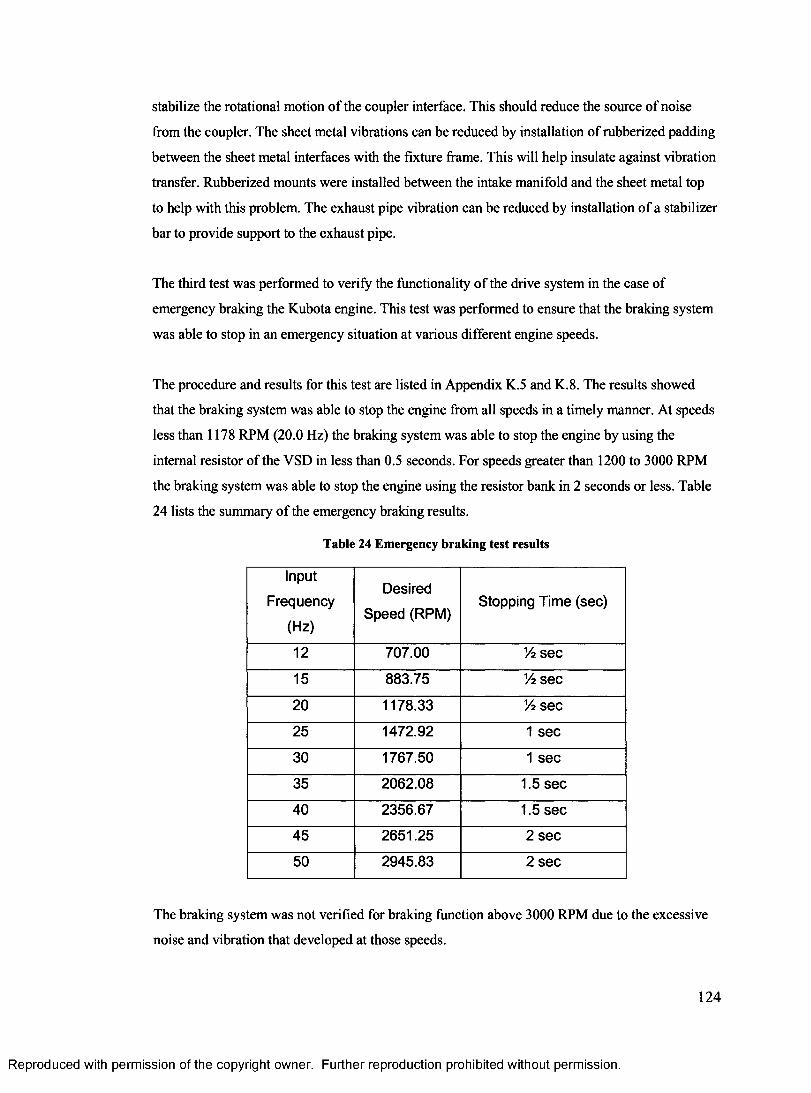
stabilize the rotational motion of the coupler interface. This should reduce the source of noise
from the coupler. The sheet metal vibrations can be reduced by installation of rubberized padding
between the sheet metal interfaces with the fixture frame. This will help insulate against vibration
transfer. Rubberized mounts were installed between the intake manifold and the sheet metal top
to help with this problem. The exhaust pipe vibration can be reduced by installation of a stabilizer
bar to provide support to the exhaust pipe.
The third test was performed to verify the functionality of the drive system in the case of
emergency braking the Kubota engine. This test was performed to ensure that the braking system
was able to stop in an emergency situation at various different engine speeds.
The procedure and results for this test are listed in Appendix K.5 and K.8. The results showed
that the braking system was able to stop the engine from all speeds in a timely manner. At speeds
less than 1178 RPM (20.0 Hz) the braking system was able to stop the engine by using the
internal resistor of the VSD in less than 0.5 seconds. For speeds greater than 1200 to 3000 RPM
the braking system was able to stop the engine using the resistor bank in 2 seconds or less. Table
24 lists the summary of the emergency braking results.
Table 24 Emergency braking test results
Input
Frequency
(Hz)
Desired
Speed (RPM)Stopping Time (sec)
12 707.00 Vz sec
15 883.75 Vz sec
20 1178.33 Vz sec
25 1472.92 1 sec
30 1767.50 1 sec
35 2062.08 1.5 sec
40 2356.67 1.5 sec
45 2651.25 2 sec
50 2945.83 2 sec
The braking system was not verified for braking function above 3000 RPM due to the excessive
noise and vibration that developed at those speeds.
124
Reproduced with permission of the copyright owner. Further reproduction prohibited without permission.
Therefore, it was verified that the drive system was able to motor the Kubota engine, and also the
braking system was able to emergency stop the engine at 3000 RPM in less that 2 seconds.
However, the vibration and noise of the system are significant to hinder the full operation range
of the system therefore effective countermeasures will need to be developed in order to minimize
these concerns.
6.3 Fuel System Testing
Simple functional tests were performed on the fuel system to verify the required function of all
the components of the system.
A visual inspection of the fuel system was performed to ensure all the components were
assembled correctly and no leaks were present. All the fittings were connected properly and
tightened. The fuel pump was connected to the 12 V battery by means of a switch. Two litres of
ethanol fuel was poured in the fuel tank and a visual inspection was performed to ensure no leaks
occurred. The fuel pump was turned on briefly to check operation and then was turned on for 30
seconds to check flow and pressure. Initially, no fuel pressure was registered on the fuel gauge.
The regulator adjustment screw was tightened and adjusted at which point the pressure was
registered to shoot up to over 690 kPa (100 psi). The fuel pressure was adjusted until the gauge
reading was 310 kPa (45 psi), and was locked into place. The gauge was observed to be quite
erratic with the oscillating around 310 kPa +/- 34 kPa . This is most likely due to the turbulence
of the fuel flow moving through the regulator causing the regulator spring to experience
oscillations. This could be improved by using a smaller fuel pump or increasing the line distance
between the fuel pump and the regulator.
The fuel injector was also briefly tested to verify its function. Power (5 V) was supplied to the
injector by means of a power supply and switch. The fuel injector was turned on for a 5 second
interval, and the spray atomization of fuel was observed. The fuel injector had a tendency to
want to separate from the mount fitting due to the pressure. A bracket should be fabricated and
installed to prevent this from happening.
In summary, all the components of the fuel system were observed to function properly but the
injector mount requires fabrication of a bracket to ensure no leaks. A smaller fuel pump would
improve system accuracy, and help reduce turbulence.
125
Reproduced with permission of the copyright owner. Further reproduction prohibited without permission.
6.4 ECU System Testing
The purpose of the ECU is to receive and process sensors outputs that read the current state of the
engine, and output a corresponding injector pulse width based on calculations performed on those
sensors. Therefore, two types of tests were performed on the ECU system to verify operation;
simple functional tests and injector scalar calibration.
Simple functional tests were performed on the ECU system to verify the function of all the
components of the system. The ECU was installed according to the manufacturer’s
recommendations. All the sensors were connected and tested accordingly. The results of the
sensors functional test and procedure are listed in Appendix L.6 and L.7.
The TPS sensor output was found to vary with throttle opening from 1 to 75 %. However, the
TPS sensor maximum reading was at 75 % and corresponded to a fully open throttle valve. This
is not a concern, but needs to be taken into account when programming the ECU. The air
temperature sensor (MAT) functioned correctly for temperature ranges -10 °C to 100 °C. Higher
temperatures, as would be expected with use of the heater, could melt the plastic material of the
MAT sensors. Therefore, it is not recommended to use the MAT for intake temperatures greater
than 100 °C, and the sensor should be removed from the intake when temperatures go beyond this
point. The coolant temperature sensor (CLT) also functioned correctly for temperatures in the
range 0 - 9 0 °C. Subzero temperatures were not tested but it is believed that the sensor would
behave accurately at temperatures lower than -25 °C. The manifold absolute pressure sensor
(MAP) functioned properly as expected. The MAP was able to read manifold pressure accurately
in the range of 95 to 105 kPa. The battery voltage indicator was verified with a voltmeter, and it
was determined that it read the voltage accurately. The hall-effect sensor responded to cam
trigger signal from the cam trigger mechanism. However, there was an glitch with the cam trigger
mechanism. The trigger signal would periodically read a higher engine speed than is actually
occurring. It is believed that this glitch is cause by the overly simplified cam trigger mechanism.
If the cam trigger wheel had 35 teeth and one space, (as in most automotive engines) instead of 1
tooth, this glitch would be eliminated.
Injector scalar calibration was performed to determine the scalar value for the injector at different
equivalence ratios and engine speeds, and also to verify the function of the ECU and all its
components. The procedure and results of the scalar calibration can be found in Appendix L.8
through L.13. Injector calibration experiments were performed for engine speeds of 670, 1000,
126
Reproduced with permission of the copyright owner. Further reproduction prohibited without permission.
1500 and 2000 RPM. The throttle position was set for 65 % for all the injector calibration tests.
For these test the TPS sensor was fixed to establish a baseline. (Increasing TPS percentage will
increase the pulse-width of the injector and deliver more fuel.) Two litres of ethanol were added
to the fuel tank, the weigh scale was zeroed with a plastic bucket, the 883ECU program was
loaded and the ECU was turned on.
The experiment requires the use of the spreadsheet Fuel System Design Calcs2.xls and the
883ECU program. The basic mapping window of the 883ECU is utilized. By trial and error the
injector scalar value was determined and adjusted until the value displayed in the 883ECU
program for pulse width matched the value calculated in the spreadsheet. The scalar value is
entered into the spreadsheet as the initial guess scalar. At this point the engine was motored at the
desired engine speed and the fuel pump and injector were turned on. A stopwatch was used to
ensure the injector operated and sprayed into the plastic container for 4 minutes. Then the injector
and pump were turned off and the plastic bucket was weighed, giving the mass of the fuel in
grams. The mass of fuel was entered into the spreadsheet under initial fuel mass. The program
calculated the ratio between the theoretical mass of fuel and initial mass of fuel, and this ratio was
multiplied by the initial guess scalar to determine the required scalar. The required scalar value
was entered into the basic mapping window and the test was repeated again. The final mass of
fuel was entered into the spreadsheet and compared to the theoretical amount of fuel. The results
for each engine speed are presented in Figure 86.
The lowest engine speed (625 RPM) is the farthest off from the other grouping. This suggests that
for low engines speeds the ECU may be out of range. The next three engines speeds (1000,1500,
and 2000 RPM), are more closely grouped together. This suggests that the ECU functioned more
accurately in this range.
The results also indicate that as the engine speed is decreased the required scalar value also
decreased. This was not expected, since injector scalar varies the pulse width of the injector, and
pulse width should be independent of engine speed. The expected line should have been a linear
line for all engine speeds and should show a linear dependence between equivalence ratio and
scalar value. The equation of this line would be:
Scalar = 25.6950 +.2054.
127
Reproduced with permission of the copyright owner. Further reproduction prohibited without permission.
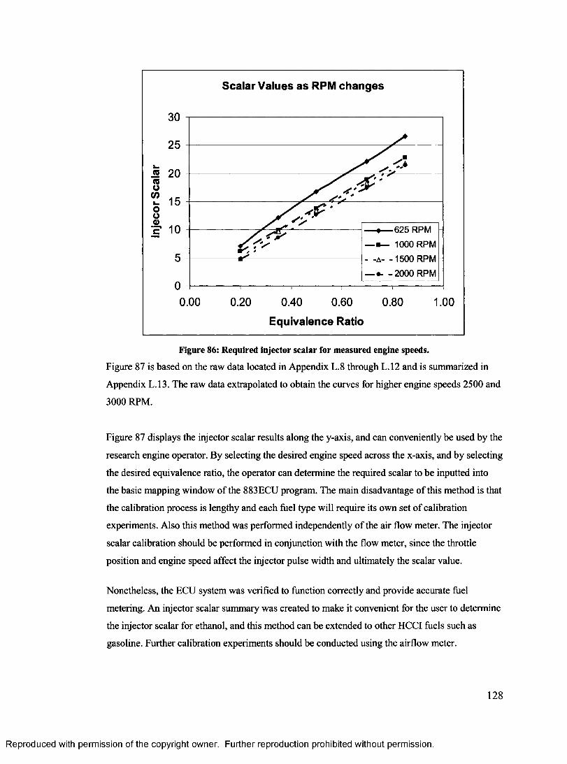
Scalar Values as RPM changes
30
- - a - -1500 RPM — -2000 RPM
625 RPM 1000 RPM
0
0.00 0.20 0.40 0.60 0.80 1.00
Equivalence Ratio
Figure 86: Required injector scalar for measured engine speeds.
Figure 87 is based on the raw data located in Appendix L.8 through L.12 and is summarized in
Appendix L.13. The raw data extrapolated to obtain the curves for higher engine speeds 2500 and
Figure 87 displays the injector scalar results along the y-axis, and can conveniently be used by the
research engine operator. By selecting the desired engine speed across the x-axis, and by selecting
the desired equivalence ratio, the operator can determine the required scalar to be inputted into
the basic mapping window of the 883ECU program. The main disadvantage of this method is that
the calibration process is lengthy and each fuel type will require its own set of calibration
experiments. Also this method was performed independently of the air flow meter. The injector
scalar calibration should be performed in conjunction with the flow meter, since the throttle
position and engine speed affect the injector pulse width and ultimately the scalar value.
Nonetheless, the ECU system was verified to function correctly and provide accurate fuel
metering. An injector scalar summary was created to make it convenient for the user to determine
the injector scalar for ethanol, and this method can be extended to other HCCI fuels such as
gasoline. Further calibration experiments should be conducted using the airflow meter.
3000 RPM.
128
Reproduced with permission of the copyright owner. Further reproduction prohibited without permission.
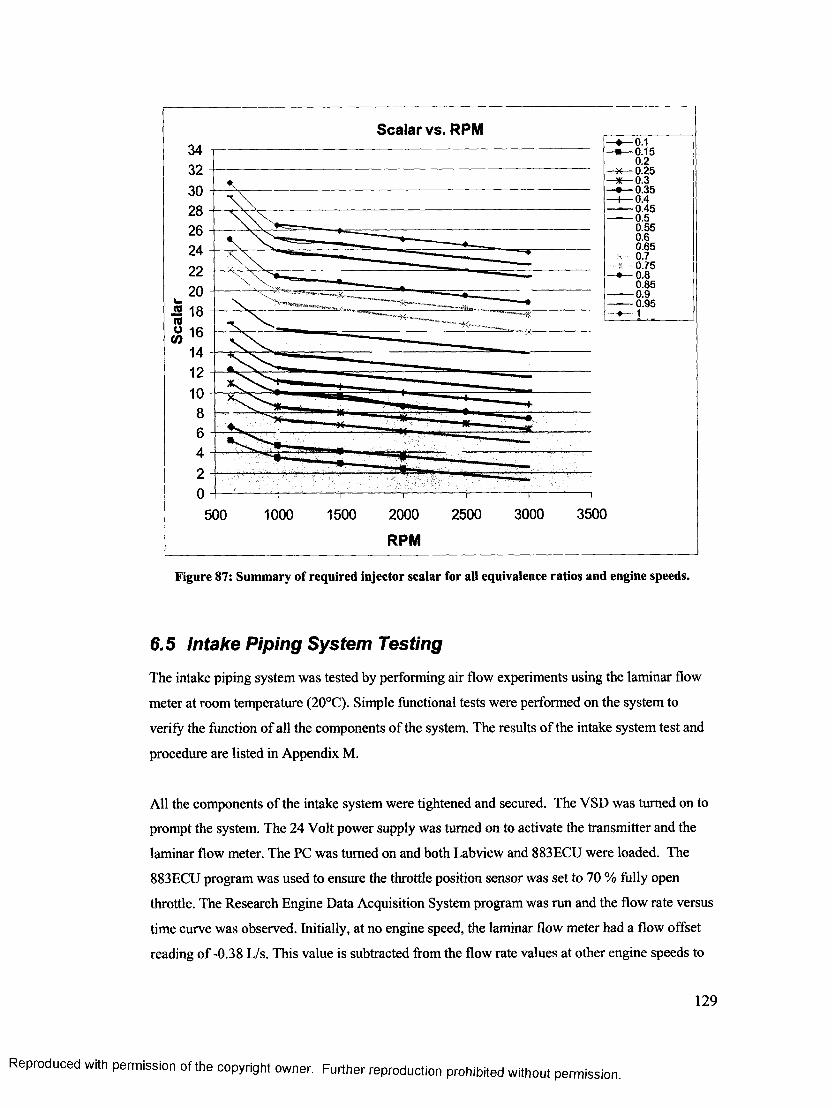
Scalar vs. RPM0.10.150.20.250.30.35
0.45 0.5
0.55 0.6 0.65
: 0.7* 0.75
—• — 0.8 0.85
— 0.9— 0.95
1
350030001500 2000
RPM
2500500 1000
Figure 87: Summary of required injector scalar for all equivalence ratios and engine speeds.
6.5 Intake Piping System Testing
The intake piping system was tested by performing air flow experiments using the laminar flow
meter at room temperature (20°C). Simple functional tests were performed on the system to
verify the function of all the components of the system. The results of the intake system test and
procedure are listed in Appendix M.
All the components of the intake system were tightened and secured. The VSD was turned on to
prompt the system. The 24 Volt power supply was turned on to activate the transmitter and the
laminar flow meter. The PC was turned on and both Labview and 883ECU were loaded. The
883ECU program was used to ensure the throttle position sensor was set to 70 % fully open
throttle. The Research Engine Data Acquisition System program was run and the flow rate versus
time curve was observed. Initially, at no engine speed, the laminar flow meter had a flow offset
reading of -0.38 L/s. This value is subtracted from the flow rate values at other engine speeds to
129
with permission of the copyright owner. Further reproduction prohibited without permission.
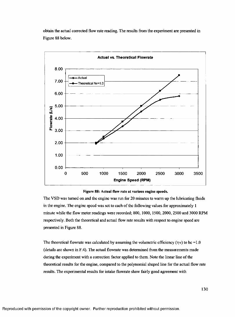
obtain the actual corrected flow rate reading. The results from the experiment are presented in
Figure 88 below.
Actual vs. Theoretical Flowrate
8.00
A ctual7.00
T heoretical Nv=1.0
6.00
5.00
_ 4.00So
3.00
2.00
1.00
0.000 500 1000 1500 2000 2500 3000 3500
Engine Speed (RPM)
Figure 88: Actual flow rate at various engine speeds.
The VSD was turned on and the engine was run for 20 minutes to warm up the lubricating fluids
in the engine. The engine speed was set to each of the following values for approximately 1
minute while the flow meter readings were recorded; 800, 1000,1500, 2000, 2500 and 3000 RPM
respectively. Both the theoretical and actual flow rate results with respect to engine speed are
presented in Figure 88.
The theoretical flowrate was calculated by assuming the volumetric efficiency (pv) to be =1.0
(details are shown in F.4). The actual flowrate was determined from the measurements made
during the experiment with a correction factor applied to them. Note the linear line of the
theoretical results for the engine, compared to the polynomial shaped line for the actual flow rate
results. The experimental results for intake flowrate show fairly good agreement with
130
Reproduced with permission of the copyright owner. Further reproduction prohibited without permission.
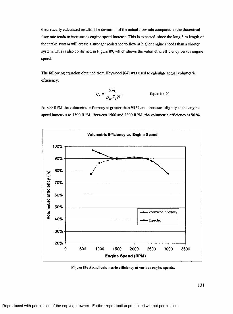
theoretically calculated results. The deviation of the actual flow rate compared to the theoretical
flow rate tends to increase as engine speed increase. This is expected, since the long 3 m length of
the intake system will create a stronger resistance to flow at higher engine speeds than a shorter
system. This is also confirmed in Figure 89, which shows the volumetric efficiency versus engine
speed.
The following equation obtained from Heywood [64] was used to calculate actual volumetric
efficiency.
2mr/v = ------------- , Equation 20
PairVdN
At 800 RPM the volumetric efficiency is greater than 95 % and decreases slightly as the engine
speed increases to 1500 RPM. Between 1500 and 2300 RPM, the volumetric efficiency is 90 %.
Volumetric Efficiency vs. Engine Speed
100%
90%
~ 80%
>g 70%OO§ 60% o
‘C
50%0E3 V olum etric Efficiency
£ 40% -■— E xpected
30%
20%0 500 1000 1500 2000 2500 3000 3500
Engine Speed (RPM)
Figure 89: Actual volumetric efficiency at various engine speeds.
131
Reproduced with permission of the copyright owner. Further reproduction prohibited without permission.
Increasing the engine speed to 2500 RPM the volumetric efficiency decreases until to less than 80
% at 3000 RPM. These volumetric efficiencies are considered to be acceptable based on
Heywood [64]. Improvements can be made by decreasing the intake piping run length, since this
is significantly longer than production OEM length. This will increase the volumetric efficiency
at higher engine speeds.
At 800 and 1000 RPM the actual volumetric efficiencies were higher than expected. The
volumetric efficiencies were expected to be less than 90% at low engine speed. The expected
volumetric efficiency should look more like the expected values shown in Figure 89.
This experiment verifies that the intake piping system and air flow meter functioned correctly.
However, further improvements can be made to improve the volumetric efficiency of the engine.
The air flow meter produced results that were accurate and useful in verifying the functionality of
the intake system.
6.6 Intake Air Preheater Testing
The intake air preheater system was tested by performing air heating experiments. The results of
the intake air preheater system test and procedure are listed in Appendix M.
All the components of the intake system were tightened and secured and the VSD was turned on
to begin motoring. The 240 V disconnect was turned on and the heater controller was connected
and turned on. The PC was turned on and 883ECU was loaded, to ensure the throttle position
sensor was set to fully open (70 %). The intake air temperature sensor was removed to prevent
bum-up. Heater tape was wrapped around the intake manifold to assist in bringing the intake
manifold up to the desired temperature. Insulation was also wrapped around the heater tape to
keep the heat on the intake pipe. Refer to schematic of the intake system in Figure 25 for more
details.
Two batches of experiments were performed. The first experiment utilized the heater tape without
insulation and the second experiment utilized the heater tape with insulation.
For Experiment One, heater tape was installed on the intake system. The heater controller set-
point was set to the desired temperatures of 50 and 100 °C. The controller compared the set-point
value to the thermocouple value located closest to the intake valve. Approximately 20 minutes
Reproduced with permission of the copyright owner. Further reproduction prohibited without permission.
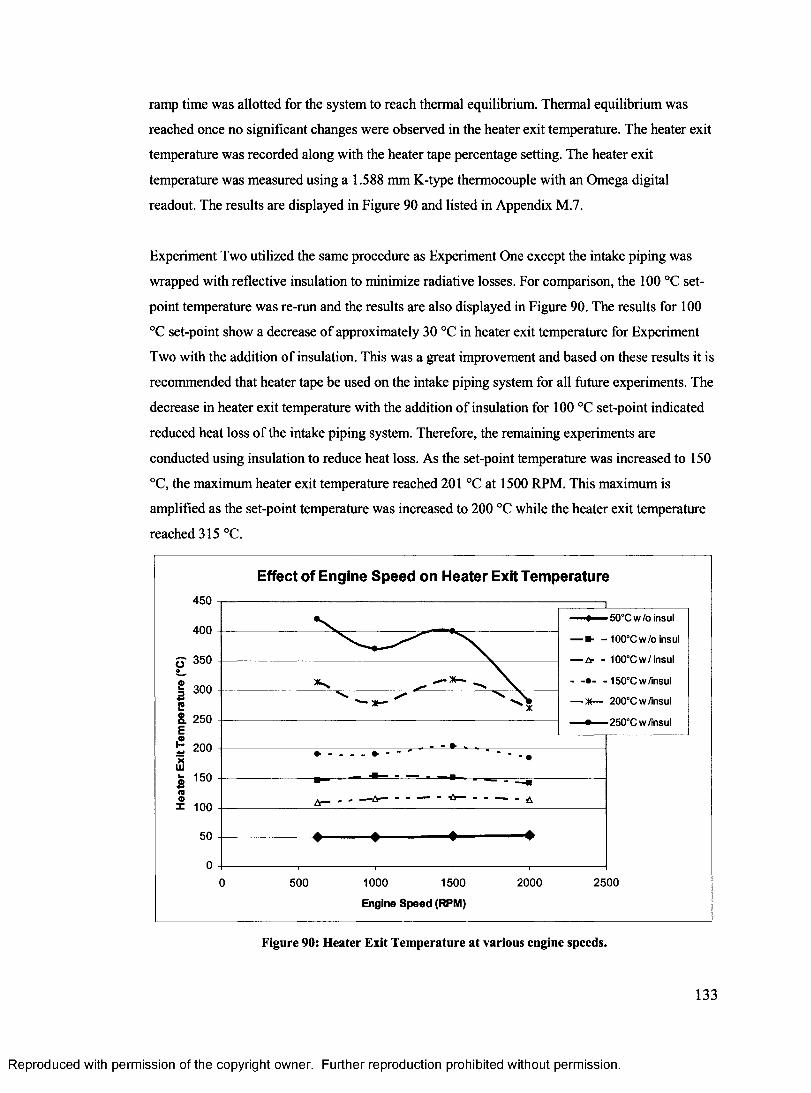
ramp time was allotted for the system to reach thermal equilibrium. Thermal equilibrium was
reached once no significant changes were observed in the heater exit temperature. The heater exit
temperature was recorded along with the heater tape percentage setting. The heater exit
temperature was measured using a 1.588 mm K-type thermocouple with an Omega digital
readout. The results are displayed in Figure 90 and listed in Appendix M.7.
Experiment Two utilized the same procedure as Experiment One except the intake piping was
wrapped with reflective insulation to minimize radiative losses. For comparison, the 100 °C set-
point temperature was re-run and the results are also displayed in Figure 90. The results for 100
°C set-point show a decrease of approximately 30 °C in heater exit temperature for Experiment
Two with the addition of insulation. This was a great improvement and based on these results it is
recommended that heater tape be used on the intake piping system for all future experiments. The
decrease in heater exit temperature with the addition of insulation for 100 °C set-point indicated
reduced heat loss of the intake piping system. Therefore, the remaining experiments are
conducted using insulation to reduce heat loss. As the set-point temperature was increased to 150
°C, the maximum heater exit temperature reached 201 °C at 1500 RPM. This maximum is
amplified as the set-point temperature was increased to 200 °C while the heater exit temperature
reached 315 °C.
Effect of Engine Speed on Heater Exit Temperature
£3P
E£
<g«
4 5 0
5 0°C w /o insul4 0 0
*■ - 100°C w /o insul
350 100°C w /insu l
- 150°Cw /insul300
250 250°Cw /insul
200- •
150
■6—
100
50
01000 1500 2000 250 00 500
Engine Speed (RPM)
Figure 90: Heater Exit Temperature at various engine speeds.
133
Reproduced with permission of the copyright owner. Further reproduction prohibited without permission.
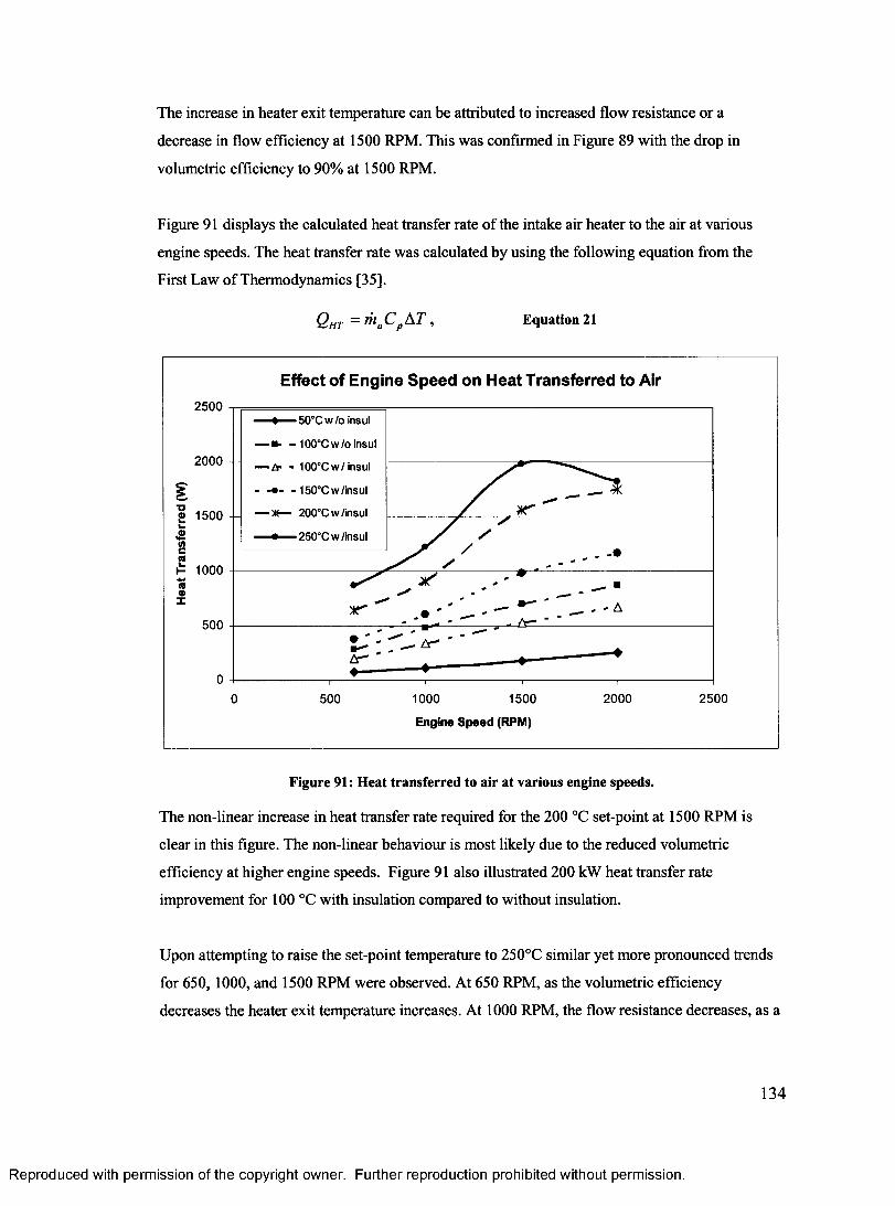
The increase in heater exit temperature can be attributed to increased flow resistance or a
decrease in flow efficiency at 1500 RPM. This was confirmed in Figure 89 with the drop in
volumetric efficiency to 90% at 1500 RPM.
Figure 91 displays the calculated heat transfer rate of the intake air heater to the air at various
engine speeds. The heat transfer rate was calculated by using the following equation from the
First Law of Thermodynamics [35].
Qht = A T , Equation 21
Effect of Engine Speed on Heat Transferred to Air2 5 0 0
50 °C w /o insul
■- - 100°C w /o insul
2000 - - — tr - 100°C w /insu l
- 150°Cw /insul
— 200°C w /insul1 500 - -
1000
500 *-
2 5 0 05 00 1000 1500
Engine Speed (RPM)
2000
Figure 91: Heat transferred to air at various engine speeds.
The non-linear increase in heat transfer rate required for the 200 °C set-point at 1500 RPM is
clear in this figure. The non-linear behaviour is most likely due to the reduced volumetric
efficiency at higher engine speeds. Figure 91 also illustrated 200 kW heat transfer rate
improvement for 100 °C with insulation compared to without insulation.
Upon attempting to raise the set-point temperature to 250°C similar yet more pronounced trends
for 650, 1000, and 1500 RPM were observed. At 650 RPM, as the volumetric efficiency
decreases the heater exit temperature increases. At 1000 RPM, the flow resistance decreases, as a
134
Reproduced with permission of the copyright owner. Further reproduction prohibited without permission.
result the heater exit temperature also decreases to 370°C. Then at 1500 RPM, the flow resistance
increases and corresponds to an increase in exit temperature to 400°C.
This experiment indicated that the intake air preheater did function correctly up until 250 °C set-
point was selected. A replacement heater element will have to be obtained and the experiments
will have to be completed with use of the laminar flow meter to provide more accurate data of air
flow and prevent heater failure.
6.7 Data Acquisition System Testing
The data acquisition system was verified by performing a motoring experiment and acquiring
data using the Labview program. This involved obtaining screen captures of each of the system
panels in the Research Engine Data Acquisition System program. The screen captures were
obtained while the engine was motoring at 750 RPM, with no fuel injected, and hence no
combustion events occurring. The data files were obtained during combustion experiments and
post-processing was performed. Statistical analysis was performed on the data and tabulated. The
screen captures are shown, and the statistical summary is presented in the following sub-sections.
6.7.1 Thermocouple Verification
The thermocouple signals were verified by screen capture of the display screen and by data
acquisition tabulated in Appendix N. The temperature panel display screen (shown in Figure 95)
shows a real-time readout of the data from all six thermocouple channels simultaneously.
The thermocouple wires were routed with insulated conduit to minimize electric field noise from
the AC motor. When the AC motor was not operated, the thermocouples were tested using a
portable omega thermocouple reader. The reader can plug into each thermocouple separately and
provides accurate measurement of the temperature at that location. These values were compared
to the values obtained using the data acquisition system and appeared to be stable and consistent
with expected values.
When the AC motor was started, the field noise from the rotor and stator interfered with the
thermocouple signals significantly. This can be seen in Figure 92.
135
Reproduced with permission of the copyright owner. Further reproduction prohibited without permission.
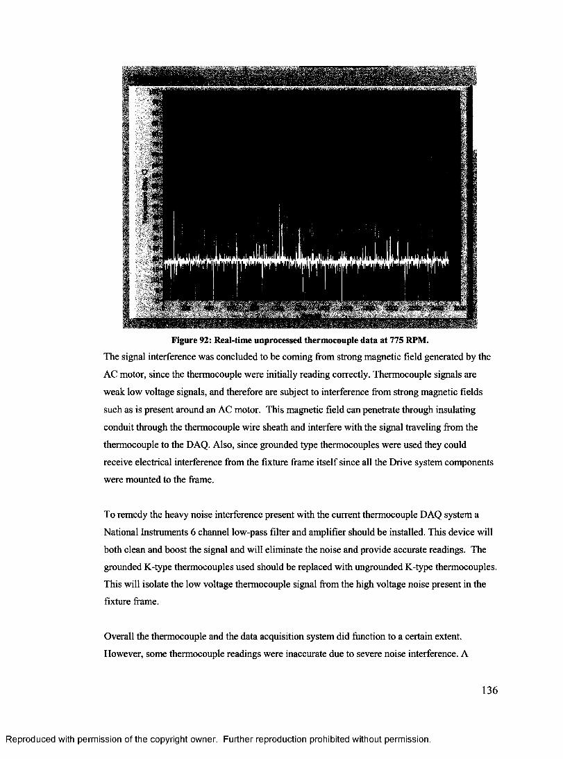
Figure 92: Real-time unprocessed thermocouple data at 775 RPM.
The signal interference was concluded to be coming from strong magnetic field generated by the
AC motor, since the thermocouple were initially reading correctly. Thermocouple signals are
weak low voltage signals, and therefore are subject to interference from strong magnetic fields
such as is present around an AC motor. This magnetic field can penetrate through insulating
conduit through the thermocouple wire sheath and interfere with the signal traveling from the
thermocouple to the DAQ. Also, since grounded type thermocouples were used they could
receive electrical interference from the fixture frame itself since all the Drive system components
were mounted to the frame.
To remedy the heavy noise interference present with the current thermocouple DAQ system a
National Instruments 6 channel low-pass filter and amplifier should be installed. This device will
both clean and boost the signal and will eliminate the noise and provide accurate readings. The
grounded K-type thermocouples used should be replaced with ungrounded K-type thermocouples.
This will isolate the low voltage thermocouple signal from the high voltage noise present in the
fixture frame.
Overall the thermocouple and the data acquisition system did function to a certain extent.
However, some thermocouple readings were inaccurate due to severe noise interference. A
136
Reproduced with permission of the copyright owner. Further reproduction prohibited without permission.
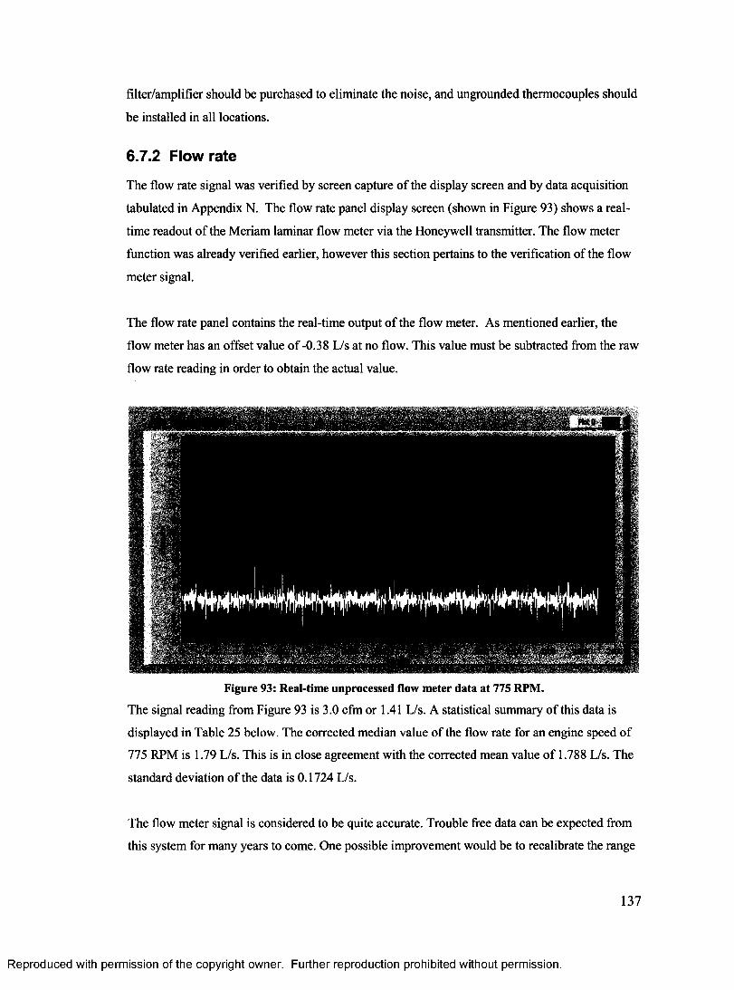
filter/amplifier should be purchased to eliminate the noise, and ungrounded thermocouples should
be installed in all locations.
6.7.2 Flow rate
The flow rate signal was verified by screen capture of the display screen and by data acquisition
tabulated in Appendix N. The flow rate panel display screen (shown in Figure 93) shows a real
time readout of the Meriam laminar flow meter via the Honeywell transmitter. The flow meter
function was already verified earlier, however this section pertains to the verification of the flow
meter signal.
The flow rate panel contains the real-time output of the flow meter. As mentioned earlier, the
flow meter has an offset value of -0.38 L/s at no flow. This value must be subtracted from the raw
flow rate reading in order to obtain the actual value.
Figure 93: Real-time unprocessed flow meter data at 775 RPM.
The signal reading from Figure 93 is 3.0 cfm or 1.41 L/s. A statistical summary of this data is
displayed in Table 25 below. The corrected median value of the flow rate for an engine speed of
775 RPM is 1.79 L/s. This is in close agreement with the corrected mean value of 1.788 L/s. The
standard deviation of the data is 0.1724 L/s.
The flow meter signal is considered to be quite accurate. Trouble free data can be expected from
this system for many years to come. One possible improvement would be to recalibrate the range
137
Reproduced with permission of the copyright owner. Further reproduction prohibited without permission.
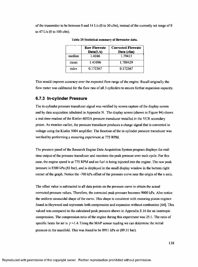
of the transmitter to be between 0 and 14 L/s (0 to 30 cfm), instead of the currently set range of 0
to 47 L/s (0 to 100 cfm).
Table 25 Statistical summary of flowmeter data.
Raw Flowrate Data(L/s)
Corrected Flowrate Data (cfm)
median 1.4166 1.79413
mean 1.41096 1.788429
stdev 0.172367 0.172367
This would improve accuracy over the expected flow range of the engine. Recall originally the
flow meter was calibrated for the flow rate of all 3 cylinders to ensure further expansion capacity.
6.7.3 In-cylinder Pressure
The in-cylinder pressure transducer signal was verified by screen capture of the display screen
and by data acquisition tabulated in Appendix N. The display screen (shown in Figure 94) shows
a real-time readout of the Kistler 6052A pressure transducer installed in the VCR secondary
piston. As mention earlier, the pressure transducer produces a charge signal that is converted to
voltage using the Kistler 5004 amplifier. The function of the in-cylinder pressure transducer was
verified by performing a motoring experiment at 775 RPM.
The pressure panel of the Research Engine Data Acquisition System program displays the real
time output of the pressure transducer and monitors the peak pressure over each cycle. For this
case, the engine speed is at 775 RPM and no fuel is being injected into the engine. The raw peak
pressure is 8300 kPa (83 bar), and is displayed in the small display window in the bottom right
comer of the graph. Notice the -700 kPa offset of the pressure curve near the origin of the x-axis.
The offset value is subtracted to all data points on the pressure curve to obtain the actual
corrected pressure values. Therefore, the corrected peak pressure becomes 9000 kPa. Also notice
the uniform sinusoidal shape of the curve. This shape is consistent with motoring piston engines
found in Heywood and represents both compression and expansion without combustion [64], This
valued was compared to the calculated peak pressure shown in Appendix E.16 for an isentropic
compression. The compression ratio of the engine during this experiment was 25:1. The ratio of
specific heats for air is y =1.4. Using the MAP sensor reading we can determine the initial
pressure in the manifold. This was found to be 8951 kPa or (89.51 bar).
138
Reproduced with permission of the copyright owner. Further reproduction prohibited without permission.
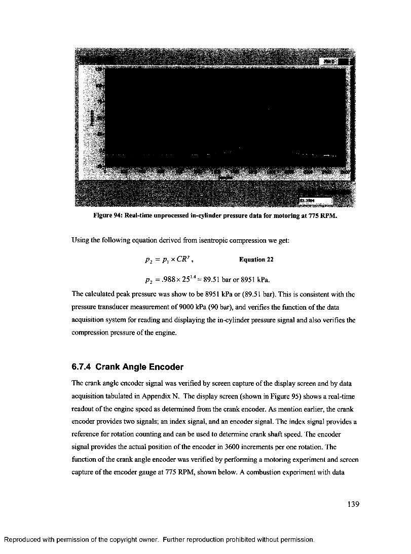
Figure 94: Real-time unprocessed in-cylinder pressure data for motoring at 775 RPM.
Using the following equation derived from isentropic compression we get:
Pi = Pi * C R r , Equation 22
p 2 = .9 8 8 x 2 5 '4 = 89.51 bar or 8951 kPa.
The calculated peak pressure was show to be 8951 kPa or (89.51 bar). This is consistent with the
pressure transducer measurement of 9000 kPa (90 bar), and verifies the function of the data
acquisition system for reading and displaying the in-cylinder pressure signal and also verifies the
compression pressure of the engine.
6.7.4 Crank Angle Encoder
The crank angle encoder signal was verified by screen capture of the display screen and by data
acquisition tabulated in Appendix N. The display screen (shown in Figure 95) shows a real-time
readout of the engine speed as determined from the crank encoder. As mention earlier, the crank
encoder provides two signals; an index signal, and an encoder signal. The index signal provides a
reference for rotation counting and can be used to determine crank shaft speed. The encoder
signal provides the actual position of the encoder in 3600 increments per one rotation. The
function of the crank angle encoder was verified by performing a motoring experiment and screen
capture of the encoder gauge at 775 RPM, shown below. A combustion experiment with data
139
Reproduced with permission of the copyright owner. Further reproduction prohibited without permission.
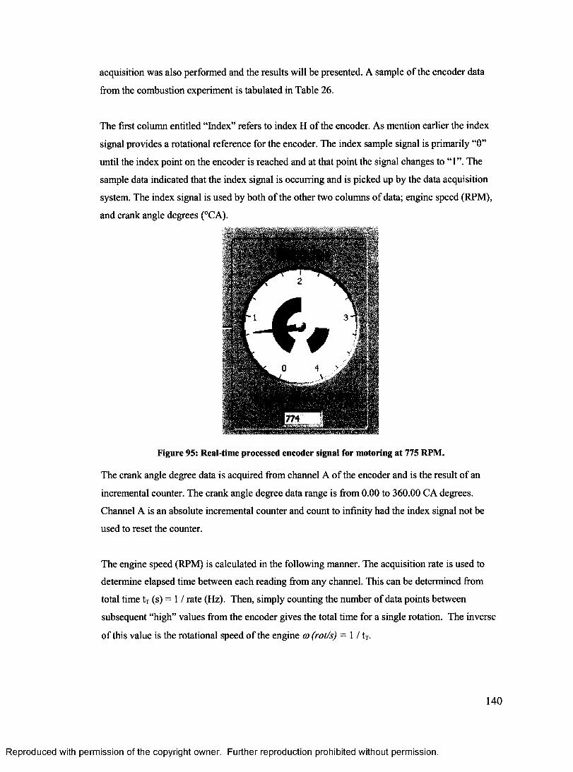
acquisition was also performed and the results will be presented. A sample of the encoder data
from the combustion experiment is tabulated in Table 26.
The first column entitled “Index” refers to index H of the encoder. As mention earlier the index
signal provides a rotational reference for the encoder. The index sample signal is primarily “0”
until the index point on the encoder is reached and at that point the signal changes to “1”. The
sample data indicated that the index signal is occurring and is picked up by the data acquisition
system. The index signal is used by both of the other two columns of data; engine speed (RPM),
and crank angle degrees (°CA).
Figure 95: Real-time processed encoder signal for motoring at 775 RPM.
The crank angle degree data is acquired from channel A of the encoder and is the result of an
incremental counter. The crank angle degree data range is from 0.00 to 360.00 CA degrees.
Channel A is an absolute incremental counter and count to infinity had the index signal not be
used to reset the counter.
The engine speed (RPM) is calculated in the following manner. The acquisition rate is used to
determine elapsed time between each reading from any channel. This can be determined from
total time tT (s) = 1 / rate (Hz). Then, simply counting the number of data points between
subsequent “high” values from the encoder gives the total time for a single rotation. The inverse
of this value is the rotational speed of the engine co (rot/s) = 1 / tT.
140
Reproduced with permission of the copyright owner. Further reproduction prohibited without permission.
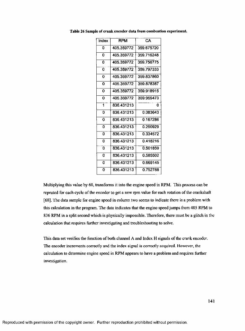
Table 26 Sample of crank encoder data from combustion experiment.
Index RPM CA
0 405.359772 359.675720
0 405.359772 359.716248
0 405.359772 359.756775
0 405.359772 359.797333
0 405.359772 359.837860
0 405.359772 359.878387
0 405.359772 359.918915
0 405.359772 359.959473
1 836.431213 0
0 836.431213 0.083643
0 836.431213 0.167286
0 836.431213 0.250929
0 836.431213 0.334572
0 836.431213 0.418216
0 836.431213 0.501859
0 836.431213 0.585502
0 836.431213 0.669145
0 836.431213 0.752788
Multiplying this value by 60, transforms it into the engine speed in RPM. This process can be
repeated for each cycle of the encoder to get a new rpm value for each rotation of the crankshaft
[68], The data sample for engine speed in column two seems to indicate there is a problem with
this calculation in the program. The data indicates that the engine speed jumps from 405 RPM to
836 RPM in a split second which is physically impossible. Therefore, there must be a glitch in the
calculation that requires further investigating and troubleshooting to solve.
This data set verifies the function of both channel A and Index H signals of the crank encoder.
The encoder increments correctly and the index signal is correctly acquired. However, the
calculation to determine engine speed in RPM appears to have a problem and requires further
investigation.
Reproduced with permission of the copyright owner. Further reproduction prohibited without permission.
6.7.5 Research Engine System Verification
Verification of the research engine as an entire system required conducting HCCI combustion
experiments. One of the main objectives of this project was to obtain in-cylinder pressure
measurements of HCCI bum of lean ethanol/air mixture. This was not possible since intake air
preheater had failed during its verification experiment.
However, HCCI bum of lean gasoline/air mixtures was possible without pre-heating the intake air
because gasoline has a lower octane number and hence lower resistance to auto-ignition, which is
the initiating mechanism to attain HCCI bum.
Therefore, low octane number gasoline was chosen to be the test fuel and HCCI combustion
experiments were performed on the research engine. The results and procedure of the HCCI
combustion experiments are listed in Appendix N.
All the components of the intake system were tightened and secured and the VSD was turned on
to begin motoring. The PC was turned on and 883ECU program and Research Engine Data
Acquisition System programs were loaded. The throttle position sensor was set at 70 % throttle
opening and the engine was motored without fuel for 30 minutes to build up heat in the engine
block. Heater tape was wrapped around the intake manifold to assist in bringing the intake
manifold up to the desired temperature. The intake air heater was replaced with a plastic ABS
straight pipe. Injector scalar calibration experiments were performed for gasoline to obtain the
injector scalar summary for 750 RPM.
Once the engine coolant temperature had reached 30 to 40°C and all safety precautions were
taken, fuel injection of gasoline was started. Initially, fuel was injected to produce lean
equivalence ratios (0.3 to 0.5), but HCCI was not attained because the engine was still to cold and
the fuel mixture far too lean. Fuel was then injected to produce equivalence ratios (0.8 to 0.85)
and auto-ignition and HCCI bum was attained. When auto-ignition began the engine began to
knock severely and the injector had to be shut off to prevent engine damage. This was due to
severe HCCI knock and engine run-off, which was reported in literature to occur with high
equivalence ratios and with gasoline.
A starting strategy was developed that was effective in producing repeatable HCCI initiation. The
strategy was to initially fuel the engine with a richer mixture to attain HCCI combustion and then
142
Reproduced with permission of the copyright owner. Further reproduction prohibited without permission.

lean it out quickly to 0.6 once combustion was attained. As the engine coolant temperature was
increased from 40 to 60 to 70 °C, the equivalence ratio could be leaned out even further to 0.3
and even 0.25. This had the effect of slowing down the combustion and retarding auto-ignition
timing. Increasing equivalence ratio would advance auto-ignition timing and increase the onset of
knocking. Increasing engine speed would cause a halt in HCCI, and equivalence ratio would have
to be increased in order to initiate HCCI combustion again. The onset of knocking occurred
quicker at higher engine speeds.
The drive/braking system was able to both motor the engine before HCCI occurred and provide
braking while HCCI combustion was occurring. Before fuel injection would begin the drive
system would be set to run the engine at 750 RPM, then once HCCI was attained the engine
speed reached closer to 800 to 825 RPM. The drive system prevented the engine from running
away, and provided adequate braking during HCCI combustion experiments. The resistor banks
were not utilized during the experiments since the internal resistor of the VSD seemed to provide
an adequate amount of braking. Experiments will be needed to verify the capability of the resistor
bank braking system.
During HCCI combustion, the engine created strong vibrations, which seemed to be caused by the
imbalance forces present during combustion. The vibrations could be reduced by developing a
larger flywheel to smooth out the imbalance forces. Perhaps an alternative method of running all
three cylinders on HCCI simultaneously or two on diesel and one on HCCI could eliminate the
majority of the vibrations present.
The results of the HCCI gasoline combustion experiments are presented in Appendix N. Post
processing of the data was performed in the following manner. The raw data was surveyed and a
representative sample of HCCI gasoline combustion was determined. Two graphs were
constructed, namely Figure 96 and Figure 97 shown below.
143
Reproduced with permission of the copyright owner. Further reproduction prohibited without permission.
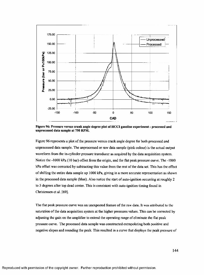
175.00
U nprocessed
P ro c esse d150.00
«■ 125.00 ao? 100.00 a.Laokn.Q
75.00
e 50.003
g£ 25.00
0.00
-25.00-150 -100 -50 0 50 100 150
CAD
Figure 96: Pressure versus crank angle degree plot of HCCI gasoline experiment - processed and unprocessed data sample at 750 RPM.
Figure 96 represents a plot of the pressure versus crank angle degree for both processed and
unprocessed data sample. The unprocessed or raw data sample (pink colour) is the actual output
waveform from the in-cylinder pressure transducer as acquired by the data acquisition system.
Notice the -1000 kPa (10 bar) offset from the origin, and the flat peak pressure curve. The -1000
kPa offset was corrected by subtracting this value from the rest of the data set. This has the effect
of shifting the entire data sample up 1000 kPa, giving in a more accurate representation as shown
in the processed data sample (blue). Also notice the start of auto-ignition occurring at roughly 2
to 5 degrees after top dead center. This is consistent with auto-ignition timing found in
Christensen et al. [69].
The flat peak pressure curve was an unexpected feature of the raw data. It was attributed to the
saturation of the data acquisition system at the higher pressures values. This can be corrected by
adjusting the gain on the amplifier to extend the operating range of eliminate the flat peak
pressure curve. The processed data sample was constructed extrapolating both positive and
negative slopes and rounding the peak. This resulted in a curve that displays the peak pressure of
144
Reproduced with permission of the copyright owner. Further reproduction prohibited without permission.

15500 kPa (155 bar). Although, this peak reconstruction is not 100 % accurate it does give an
adequate representation of the actual shape of the HCCI peak pressure curve.
The pressure volume or PV diagram (shown in Figure 97) was constructed by plotting the change
in pressure against the change in volume. Similar to Figure 96 both unprocessed and processed
data series are presented to illustrate the comparison between the data set. The lower curve
represents compression of the air fuel mixture and the upper curve represents expansion of the
combustion products. The PV diagram is a very useful tool in analyzing in-cylinder combustion
events. Notice the -1000 kPa offset of the unprocessed data compared to the processed data and
the reconstructed peak pressure curve. The area under the curve of the PV diagram represents the
work associated with the compression and expansion of the piston by the gases inside the
cylinder. The work to compress the gases is considered negative work by the gases, and the work
done by the gases to expand the piston is considered positive work. By subtracting the
compression work from the expansion work you obtain the net indicated work for the cycle.
180.00
160.00
140.00
120.00ooZ 100.00 £ t_? 80.00
60.00
40.00
20.00
0.00 0
- 20.00
----- P rocessed
----- U nprocessed
^ — ■' , ll ■ i i
X) .00
Volume (cc)
Figure 97: P-V diagram (pressure versus volume diagram) of HCCI gasoline experiment, corrected and uncorrected data sample at 750 RPM.
145
Reproduced with permission of the copyright owner. Further reproduction prohibited without permission.
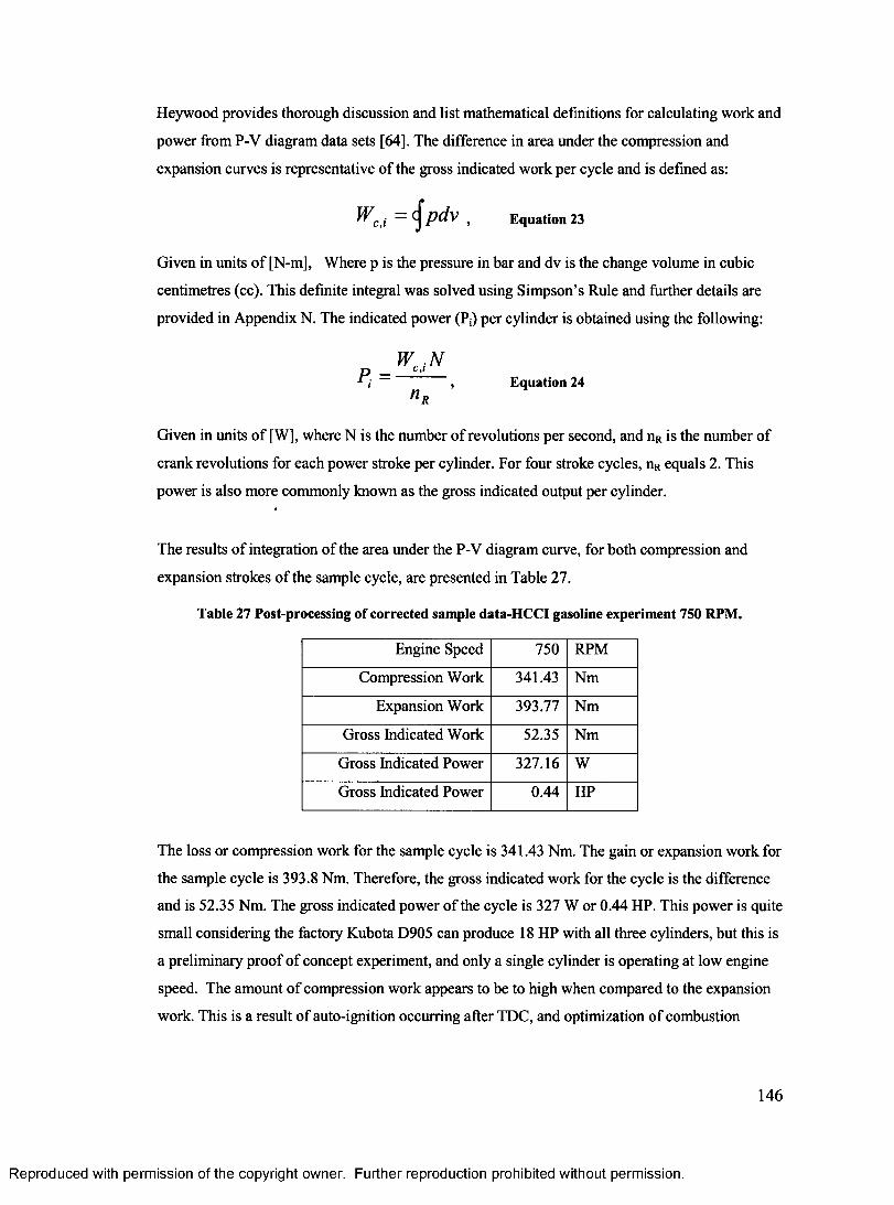
Heywood provides thorough discussion and list mathematical definitions for calculating work and
power from P-V diagram data sets [64]. The difference in area under the compression and
expansion curves is representative of the gross indicated work per cycle and is defined as:
^c,i ~ ^ p d v , Equation 23
Given in units of [N-m], Where p is the pressure in bar and dv is the change volume in cubic
centimetres (cc). This definite integral was solved using Simpson’s Rule and further details are
provided in Appendix N. The indicated power (P;) per cylinder is obtained using the following:
Pi =;N
n .Equation 24
Given in units of [W], where N is the number of revolutions per second, and nR is the number of
crank revolutions for each power stroke per cylinder. For four stroke cycles, nR equals 2. This
power is also more commonly known as the gross indicated output per cylinder.
The results of integration of the area under the P-V diagram curve, for both compression and
expansion strokes of the sample cycle, are presented in Table 27.
Table 27 Post-processing of corrected sample data-HCCI gasoline experiment 750 RPM.
Engine Speed 750 RPM
Compression Work 341.43 Nm
Expansion Work 393.77 Nm
Gross Indicated Work 52.35 Nm
Gross Indicated Power 327.16 W
Gross Indicated Power 0.44 HP
The loss or compression work for the sample cycle is 341.43 Nm. The gain or expansion work for
the sample cycle is 393.8 Nm. Therefore, the gross indicated work for the cycle is the difference
and is 52.35 Nm. The gross indicated power of the cycle is 327 W or 0.44 HP. This power is quite
small considering the factory Kubota D905 can produce 18 HP with all three cylinders, but this is
a preliminary proof of concept experiment, and only a single cylinder is operating at low engine
speed. The amount of compression work appears to be to high when compared to the expansion
work. This is a result of auto-ignition occurring after TDC, and optimization of combustion
146
Reproduced with permission of the copyright owner. Further reproduction prohibited without permission.
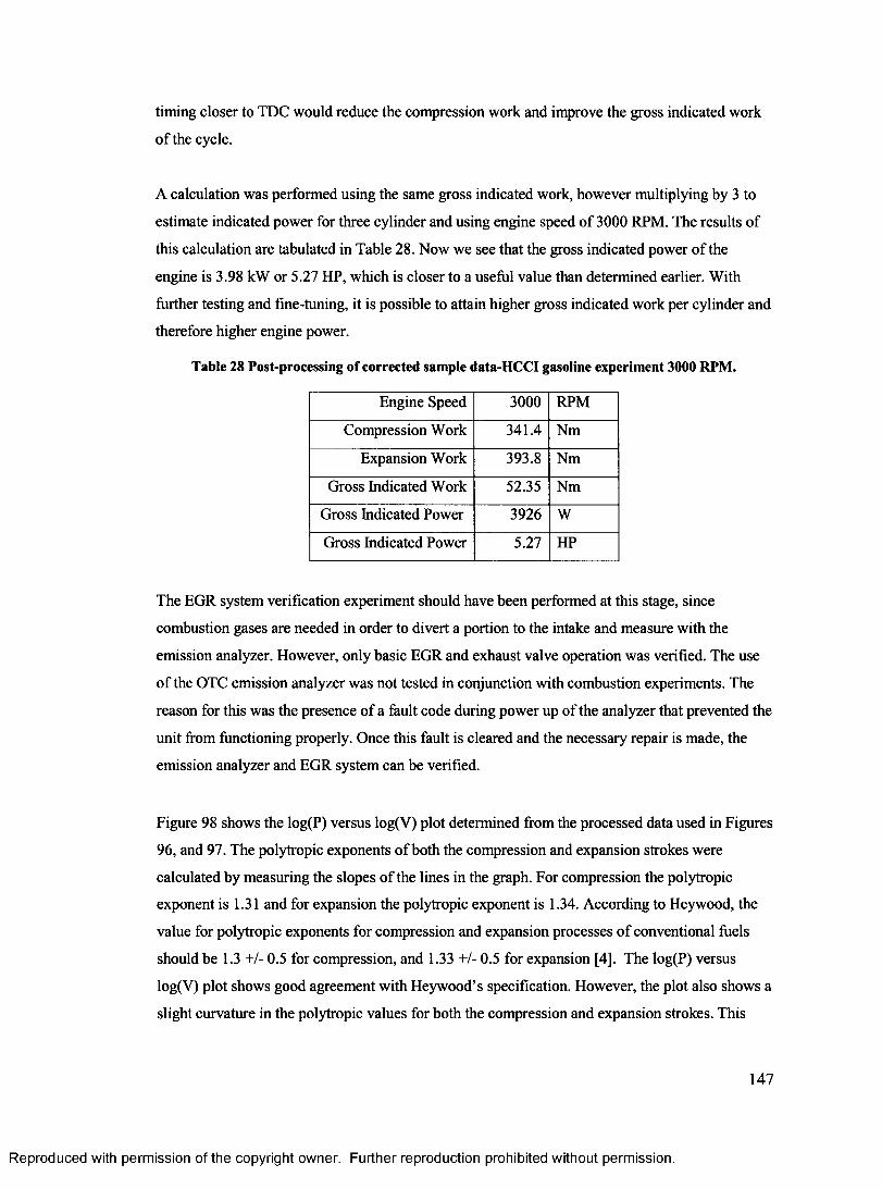
timing closer to TDC would reduce the compression work and improve the gross indicated work
of the cycle.
A calculation was performed using the same gross indicated work, however multiplying by 3 to
estimate indicated power for three cylinder and using engine speed of 3000 RPM. The results of
this calculation are tabulated in Table 28. Now we see that the gross indicated power of the
engine is 3.98 kW or 5.27 HP, which is closer to a useful value than determined earlier. With
further testing and fine-tuning, it is possible to attain higher gross indicated work per cylinder and
therefore higher engine power.
Table 28 Post-processing of corrected sample data-HCCI gasoline experiment 3000 RPM.
Engine Speed 3000 RPM
Compression Work 341.4 Nm
Expansion Work 393.8 Nm
Gross Indicated Work 52.35 Nm
Gross Indicated Power 3926 W
Gross Indicated Power 5.27 HP
The EGR system verification experiment should have been performed at this stage, since
combustion gases are needed in order to divert a portion to the intake and measure with the
emission analyzer. However, only basic EGR and exhaust valve operation was verified. The use
of the OTC emission analyzer was not tested in conjunction with combustion experiments. The
reason for this was the presence of a fault code during power up of the analyzer that prevented the
unit from functioning properly. Once this fault is cleared and the necessary repair is made, the
emission analyzer and EGR system can be verified.
Figure 98 shows the log(P) versus log(V) plot determined from the processed data used in Figures
96, and 97. The polytropic exponents of both the compression and expansion strokes were
calculated by measuring the slopes of the lines in the graph. For compression the polytropic
exponent is 1.31 and for expansion the polytropic exponent is 1.34. According to Heywood, the
value for polytropic exponents for compression and expansion processes of conventional fuels
should be 1.3 +/- 0.5 for compression, and 1.33 +/- 0.5 for expansion [4], The log(P) versus
log(V) plot shows good agreement with Heywood’s specification. However, the plot also shows a
slight curvature in the polytropic values for both the compression and expansion strokes. This
147
Reproduced with permission of the copyright owner. Further reproduction prohibited without permission.
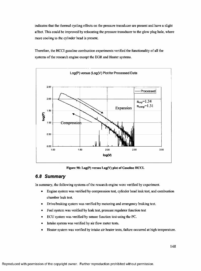
indicates that the thermal cycling effects on the pressure transducer are present and have a slight
affect. This could be improved by relocating the pressure transducer to the glow plug hole, where
more cooling to the cylinder head is present.
Therefore, the HCCI gasoline combustion experiments verified the functionality of all the
systems of the research engine except the EGR and Heater systems.
Log(P) versus (Log(V) Plot for Processed Data
2 .50
Processed
2.00
Expansion1.50
Compression:1.00
0 .50
0.002.50 3.001.00 1.50 2.00
log(V)
Figure 98: Log(P) versus Log(V) plot of Gasoline HCCI.
6.8 Summary
In summary, the following systems of the research engine were verified by experiment.
• Engine system was verified by compression test, cylinder head leak test, and combustion
chamber leak test.
• Drive/braking system was verified by motoring and emergency braking test.
• Fuel system was verified by leak test, pressure regulator function test
• ECU system was verified by sensor function test using the PC.
• Intake system was verified by air flow meter tests.
• Heater system was verified by intake air heater tests, failure occurred at high temperature.
148
Reproduced with permission of the copyright owner. Further reproduction prohibited without permission.
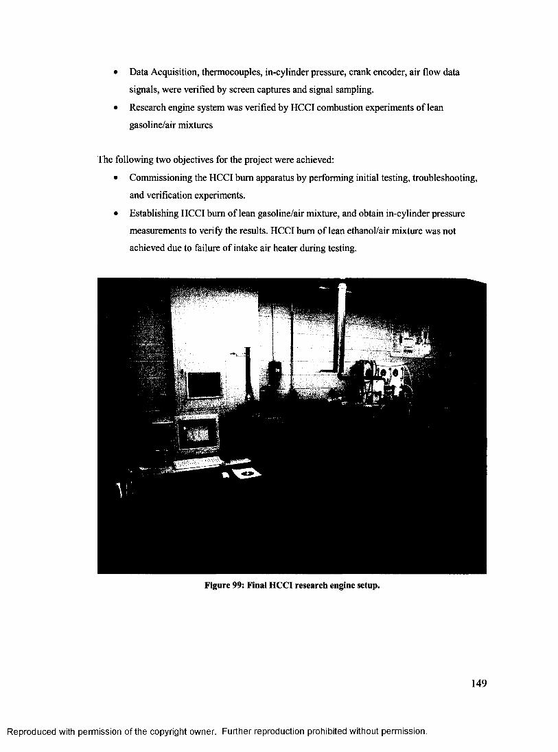
• Data Acquisition, thermocouples, in-cylinder pressure, crank encoder, air flow data
signals, were verified by screen captures and signal sampling.
• Research engine system was verified by HCCI combustion experiments of lean
gasoline/air mixtures
The following two objectives for the project were achieved:
• Commissioning the HCCI bum apparatus by performing initial testing, troubleshooting,
and verification experiments.
• Establishing HCCI bum of lean gasoline/air mixture, and obtain in-cylinder pressure
measurements to verify the results. HCCI bum of lean ethanol/air mixture was not
achieved due to failure of intake air heater during testing.
Figure 99: Final HCCI research engine setup.
149
Reproduced with permission of the copyright owner. Further reproduction prohibited without permission.

7 CONCLUSIONS AND RECOMMENDATIONS
7.1 Conclusions
Overall the design and development of the research engine project was successful in achieving its
criteria and constraints and has met the following objectives;
1. A literature review was performed identify the parameters affecting control of HCCI with
respect to use of ethanol as a fuel.
2. An experimental apparatus was designed, and fabricated for investigation of parameters
affecting control of HCCI.
3. The design process methodology was followed to ensure tasks were completed and
documented correctly.
4. The HCCI research apparatus was commissioned by performing initial testing,
troubleshooting, and verification experiments.
5. HCCI combustion of lean ethanol/air was not achieved due to heater system failure, however
HCCI combustion of lean gasoline/air was achieved and verified by means of in-cylinder
pressure measurements.
7.2 Recommendations
From initial tests, it is recommended that the research engine be utilized as a tool for further
development and understanding of the parameters affecting HCCI combustion properties such as
timing, heat release rate, and combustion duration. Further investigation into HCCI fuels such as
biodiesel would also be beneficial. At present the research engine is able to fulfill its objectives
and provide temperature, air flowrate, engine speed, and in-cylinder pressure measurements. As
with any process or machine, future enhancements will be suggest by new graduate students
These modifications should be considered thoroughly, and investigated to see what impact they
have on the initial objectives of the apparatus. The following recommendations are made with the
intention to provide useful information to guide subsequent students, technicians and researchers
in the appropriate direction.
The fixture frame had significant sources of noise exhibited under testing. These noises can be
reduced by installing anti-vibration padding between any surface contact point of components.
150
Reproduced with permission of the copyright owner. Further reproduction prohibited without permission.

To reduce vibration with the engine, a larger flywheel could be designed and fabricated that will
dampened the angular accelerations. Also, the other two cylinders could be enabled and fuelled
with diesel fuel using the original diesel injector pump or perhaps retrofitting a common rail
system. Therefore the engine could run on all three cylinders and this would most likely reduce
the imbalance of the engine.
The VCR secondary piston could be improved by development of a hydraulic actuated secondary
piston and custom fabricated cylinder head. This concept would allow the compression ratio to be
varied, while the engine is running and would enable advance VCR and HCCI research.
The accuracy of the fuel system could be improved by reducing the size of both the fuel injector
and the fuel pump. The fuel injector should be reduced to 4.5 kg fuel/hour, and a smaller fuel
pump should also be obtained (18.1 kg fuel/hour.) This would enable a higher level of precision
with the fuel metering. Future ECU calibration experiments should be performed using the
laminar flow meter. This will provide a higher level of accuracy.
Further verification experiments will need to be performed on the intake air preheater using the
laminar flow meter while the engine is running. Caution must be taken to ensure air flow through
the heater is not drastically changed, and vibrations are reduced.
For the data acquisition system the thermocouples will have to be replaced with ungrounded
1.5875 mm K-Type. National Instruments thermocouple low-pass filter and amplifier would also
be recommended to eliminate harsh AC motor magnetic field interference. Also, the heater and
equivalence ratio readings must be incorporated into the Research Engine Data Acquisition
System program.
The braking absorption capacity needs to be quantified by means of a combustion experiment
using the resistor banks and the chopper module. A current meter should be installed on the 480
V line between the AC motor and the Chopper in order to determine the current while the engine
is producing torque during HCCI combustion experiments. Current meters can be attained from
Electrozad Ltd in Windsor or any electrical supply store.
The verification of the EGR system needs to be performed by experiment while HCCI
combustion is occurring. The emission analyzer requires clearing of fault codes and then it can be
151
Reproduced with permission of the copyright owner. Further reproduction prohibited without permission.
used to acquire percent volume C02 data. This data can be entered into the MATLAB EGR
program to determine percent EGR. The influence of EGR on HCCI combustion can then be
studied.
A detailed set of HCCI combustion experiments should be performed. They would provide
invaluable information on the effect of parameters affecting HCCI control. These experiments
would be performed at several different engines speeds (750, 1000, 1250, 1500, 1750, 2000,
2250,2500, and 3000 RPM by keeping the engine speed constant and varying one parameter at a
time. The intake charge set-point temperature should be varied from 50, 100, 150, and 200 °C to
study the effect. The EGR rate should be varied from 0 to 80 % to study the effect of EGR. The
equivalence ratio should also be varied from 0.25 to 0.8. The compression ratio should be varied
from 15 to 25:1 to study the effect of VCR. Post-processing should be performed and the effect of
the control parameters on ignition timing, heat release rate and combustion duration would
determined. These experimental results could be compared with results obtained from previous
research and compared with results from previously conducted simulations.
Reproduced with permission of the copyright owner. Further reproduction prohibited without permission.
152
REFERENCES
1. US Environmental Protection Agency - Heavy Trucks, Buses and Engines (n.d), date accessed April 15th, 2004, from “http://www.epa.g0v/0taq/diesel.htm#regs”
2. Canadian Renewal Fuels Association (n.d), date accessed January 15th, 2003, from “http://www.greenfuels.org/ethanol/index.htm.”
3. U.S. Department of Energy, “Homogeneous Charge Compression Ignition (HCCI) Technology-A Report to the U.S. Congress,” April 2001.
4. Cengal, Y., Boles, M., “Thermodynamics, An Engineering Approach, 3rd Edition,” McGraw- Hill, Table A-l, pp. 898, 1998.
5. Norton, R.L., “Design of Machinery, 2nd Edition” Chapter 1, Section 1.5, McGraw-Hill, 2001 .
6. Najt, P.M., and Foster, D.E., “Compression-Ignited Homogeneous Charge Combustion”, SAE Paper 830264, 1983.
7. Iida, N., Igarashi, T., “Auto-Ignition and Combustion of n-Butane and DME/Air Mixtures in a Homogeneous Charge Compression Ignition Engine,” SAE Paper 2000-01-1832, 2000.
8. Ng, C., “The Effect of Fuel/Air Equivalence Raito, Starting Temperature, EGR and Reforming on HCCI Combustion,” University of Toronto-Proposal, 2002.
9. Aoyama, T., Hattori, Y., Mizuta, J., Sato, Y., “An Experimental Study on Premixed-Charge Compression Ignition Gasoline Engine,” SAE Paper 960081,1996.
10. Hiraya K. et al., “A study on gasoline fuelled compression ignition engine ~ a trial of operation region expansion,” SAE Paper 2002-01-0416, 2002.
11. Ladommatos, N., Zhao, H., Oakley, A., “Dilution Effects on the Controlled Auto-Ignition (CAI) Combustion of Hydrocarbon and Alcohol Fuels,” SAE Paper 2001-01-3606, 2001.
12. Christensen, M., et. al, “Supercharged Homogeneous Charge Compression Ignition,” SAE Paper 980787, 1998.
13. Christensen, M. et al., “Homogeneous Charge Compression Ignition (HCCI) using Isooctane, ethanol and natural gas-a comparison with spark ignition operation”, SAE Paper 972874, 1997.
14. Christensen, M. et al., “Influence of mixture quality on homogeneous charge compression ignition,” SAE Paper 982454, 1998.
15. Christensen, M. et al., “Demonstrating the multi-fuel capability of a homogeneous charge compression ignition engine with variable compression ratio,” SAE Paper 1999-01-3679, 1999.
153
Reproduced with permission of the copyright owner. Further reproduction prohibited without permission.
16. Christensen, M. et al., “Homogeneous charge compression ignition with water injection,”SAE Paper 1999-01-0182, 1999.
17. Christensen, M., Johansson, B., “Supercharged homogeneous charge compression ignition (HCCI) with exhaust gas recirculation and pilot fuel,” SAE Paper 2000-01-1835, 2000.
18. Olsson, J., Tunestal, P., Johansson, B., “Compression Ratio Influence on Maximum Load of a Natural Gas Fueled HCCI Engine,” SAE Paper 2002-01-0111, 2002.
19. Olsson, J., Tunestal, P., Haraldsson, G., Johansson, B., “A Turbo Charged Dual Fuel HCCI Engine,” SAE Paper 2001-01-1896, 2001.
20. Epping, K., Aceves, S., Bechtold, R., Dec, J., ‘The potential of HCCI combustion for high efficiency and low emissions,” SAE Paper 2002-01-1923, 2002.
21. Asmus, T., Zhou, F., “Homogeneous Charge Compression Ignition (HCCI) Engines-Key Research and Development Issues,” PT-94 Society of Automotive Engineers, Chp.4, 2003.
22. Furutani, M. et al., “An investigation into the effect of fuel composition on HCCI combustion characteristics,” Proceedings of Comodia ’98. pp. 173-177, 1998.
23. Chemistry Department, University of Ireland, Galway, (n.d), date accessed August, 12th,2003, “http://www.nuigalway.ie/chem/combust.htm.”
24. Nolan, S., Cardiff School of Engineering, date accessed August 10, 2003, “http://www.ucc.ie/research/hmrc/SWERF/conferences/IST/Papers%20and%20Slides/SINE AD~l.pdf.”
25. AVL Ltd. (n.d.), date accessed October 18th, 2003, from “http://tec.avl.com.”
26. Ricardo and Cussons (n.d.), date accessed October 18th, 2003, from “http://www.cussons.co.uk.”
27. Waukesha Engines Corporation (n.d), date accessed October 25th, 2003, from “http://www.waukeshaengine.com/intemet/businessunits/waukesha/pages/applications/produ cts/fueltesting/fl f2. c fm?r=973&numPageID=378.”
28. University of California at Berkeley (n.d), date accessed October 18th, 2003, from “http://www.me.berkeley.edu/cal/HCCI.”
29. Canadian Safety Standards Association (n.d), date accessed October 25, 2003, from “http.7/www.csa.ca/default.asp?language=English.”
30. Land and Sea Inc. (n.d), date accessed June 20,2003, from “http://www.land-and- sea.com/eddy-current-dynamometer/eddy-current-dynamometer.htm.”
31. Quotation #0020959, “200 Eddy Current Absorber 96v - $14,245 US,” Land and Sea Inc, June, 2003.
32. Kubota Canada Ltd, date accessed November 10th, 2003, from “http://www.css- club.net/kubota_catalog/pdf/Super_Five.pdf.”
154
Reproduced with permission of the copyright owner. Further reproduction prohibited without permission.
33. Kubota Corporation (n.a), “Kubota Workshop Manual 9789701642,” May 1996.
34. Shigley J., Mischke C., “Mechanical Engineering Design, 6th Edition,” McGraw-Hill, 2001. pp. 23 -25.
35. Cengal, Boles, “Thermodynamics: An Engineering Approach,” McGraw-Hill, 1998.
36. Gasket Works USA (n.d), date accessed November 25, 2004, from “http://www.headgasket.com/whoweare.html.”
37. Heywood, J.B., “Internal Combustion Engine Fundamentals,” McGraw-Hill, various pages, 1988.
38. Plint, M., Martyr, A., “Engine Testing - Theory and Practice, 2nd Edition,” Society of Automotive Engineers, 1999. pp. 127-135.
39. Rockwell Automation - Drives and Service Support/Resistor Sizing (n.d), date accessed January 20, 2005, from“http://www.ab.com/support/abdrives/peripherals/brakes/rsizing.html.”
40. Omega International (n.d), date accessed December 2004, “http://www.omega.com/pptst/SH_HEATER.html.”
41. Omega International (n.d), date accessed December 2004, “http://www.omega.com/ppt/pptsc.asp?ref=CNI_Series&nav.”
42. Meriam Process Technologies (n.d), date accessed December 20, 2004, from, “http://www.meriam.com/products/default.asp?m=3&d=62&p=14.”
43. Plint, M., Martyr, A., “Engine Testing - Theory and Practice, 2nd Edition,” Society of Automotive Engineers, 1999. pp. 183-219.
44. Installation Guide, “ST3000 Smart Transmitter Release 300 and SFC Smart Field Communicator Model STS103, Installation Guide,” 34-ST-33-39, Honeywell Inc., July,2000.
45. Askeland, D.R., ‘The Science and Engineering of Materials,” Third Edition, Chapman & Hall, London, UK., 1996.
46. Defoe, J.D., Arthur, D.M., “Matlab M-file used to calculate EGR fraction based on fuel and air flow rates, relative humidity and dry C02 molar fraction in intake manifold,” Modified by Defoe, J.D. for use with all fuels and additives, University of Windsor, University of Alberta, 2003,2004.
47. OTC Corporation - MicroGas Analyzer User Guide, date accessed September 10th, 2004, from, “http://www.otctools.com/newcatalog/products/162_man.pdf.”
48. McGinlay, J., “Personal Discussions - Regarding Fuel Storage,” Occupational Health & Safety Department, University of Windsor. (519) 253-3000 ext. 4521, January 2005.
155
Reproduced with permission of the copyright owner. Further reproduction prohibited without permission.
49. Delphi Automotive -Photos and Technical information (n.d), date accessed November 10th, 2004, from “http://go2.delphi.com/default.asp?Language=English.”
50. Jegs Corporation (n.d), date accessed September 8th, 2004, from, “http://www.jegs.com/cgibin/ncommerce3/CategoryDisplay?cgmenbr=361&cgrfhbr=639.”
51. 034EFI Ltd, date accessed May 20th, 2003, from “http://www.034efi.com/034ECUSTGII.html.”
52. Defoe, J. “Data Acquisition System for HCCI Research Engine Design and Implementation,” Work Term Report, University of Windsor, December 2004.
53. Gurley Precision Instruments - Specifications Sheet (n.d), obtained June 20, 2004, “ 9X25 Rotary Incremental Encoder”
54. National Instruments Ltd, date accessed November 20th, 2004, from “http://www.ni.com/dataacquisition/whatis.htm.”
55. Kistler Instruments Inc., “Kistler Calibration Certificate,” Appendix J.5.
56. Personal Conversations, Marc St. Pierre, Technical Services, University of Windsor, December 2002 to January 2005.
57. Personal Conversations, Phil Diett, Physical Plant, University of Windsor, December 2002 to September. 2004.
58. Personal Conversations, Dave Dumachelle, Electrozad Ltd. Windsor, April 2004 -September,2004.
59. Personal Conversations, David Doyscher, Tricon Ltd. Windsor, March 2004-Sept 2004.
60. Personal Conversations, Steve Budinsky, Technical Services, University of Windsor, December 2002 to January 2005.
61. Personal Conversations, Pat Seguin, Faculty of Engineering, University of Windsor, December 2002 to January 2005.
62. Shigley J., Mischke C., “Mechanical Engineering Design, 6th Edition,” McGraw-Hill, 2001. pp. 876,1051.
63. Defoe, J. “Data Acquisition System for HCCI Research Engine Design and Implementation,” Work Term Report, University of Windsor, December 2004.
64. Heywood, J.B., “Internal Combustion Engine Fundamentals,” McGraw-Hill, 1988, pp. 212- 220. 28,47-48, 58, 385.
65. Email Conversations, Arsene Philogene, Omega Service Dept., Omega Newport Montreal, February 2005.
156
Reproduced with permission of the copyright owner. Further reproduction prohibited without permission.
66. Email Conversations, Gary Muzzey, Osram Sylvania., Exeter, New Hampshire, February2005.
67. Defoe, J. “Data Acquisition System for HCCI Research Engine Design and Implementation,” Work Term Report, University of Windsor, December 2004.
68. Christensen, M., Hultqvist, A., Johansson, B., “Demonstrating the Multi-Fuel Capability of a Homogeneous Charge Compression Ignition Engine with Variable Compression Ratio,” Society of Automotive Engineers, 1999-0103679.
69. Kohl, W.L., “Methanol As An Alternative Fuel Choice: An Assessment,” The John Hopkins Foreign Policy Institute, Washington D.C, pp. 236. 1990.
70. Varaprasada, R.R., et al., “Alcohol Fuelling: Effect of Induction Swirl on Aldehyde Emissions,” VII International Symposium on Alcohol Fuels, pp. 438. November 1988.
71. US Department of Energy, date accessed Sept. 2005, “http://www.eia.doe.gov/oiaf/aeo/pdEaeotab 3.pdf.”
Reproduced with permission of the copyright owner. Further reproduction prohibited without permission.
157
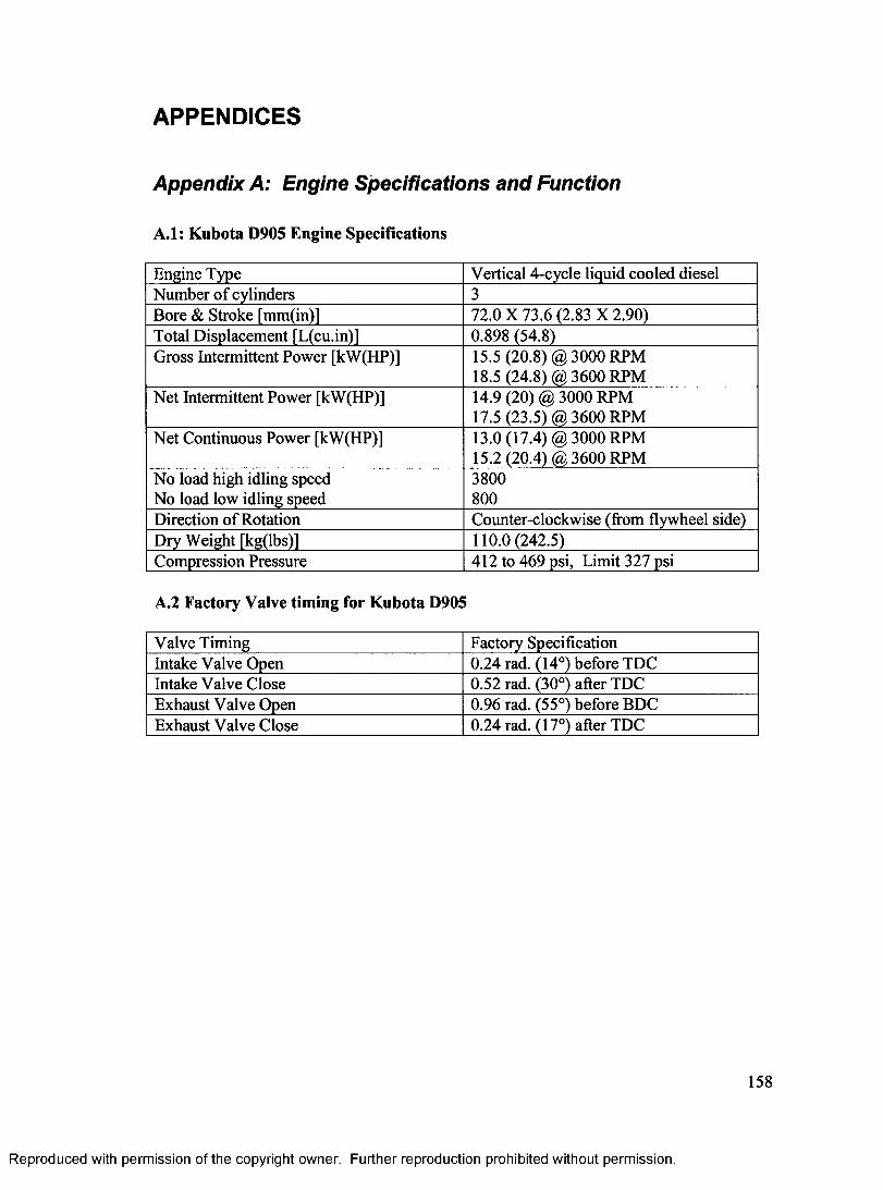
APPENDICES
Appendix A: Engine Specifications and Function
A.1: Kubota D905 Engine Specifications
Engine Type Vertical 4-cycle liquid cooled dieselNumber o f cylinders 3Bore & Stroke [mm(in)] 72.0 X 73.6 (2.83 X 2.90)Total Displacement [L(cu.in)] 0.898 (54.8)Gross Intermittent Power [kW(HP)] 15.5 (20.8) @ 3000 RPM
18.5 (24.8) @ 3600 RPMNet Intermittent Power [kW(HP)] 14.9 (20) @ 3000 RPM
17.5 (23.5) @ 3600 RPMNet Continuous Power [kW(HP)] 13.0 (17.4) @ 3000 RPM
15.2 (20.4) @ 3600 RPMNo load high idling speed 3800No load low idling speed 800Direction of Rotation Counter-clockwise (from flywheel side)Dry Weight [kg(lbs)] 110.0 (242.5)Compression Pressure 412 to 469 psi, Limit 327 psi
A.2 Factory Valve timing for Kubota D905
Valve Timing Factory SpecificationIntake Valve Open 0.24 rad. (14°) before TDCIntake Valve Close 0.52 rad. (30°) after TDCExhaust Valve Open 0.96 rad. (55°) before BDCExhaust Valve Close 0.24 rad. (17°) after TDC
Reproduced with permission of the copyright owner. Further reproduction prohibited without permission.
158
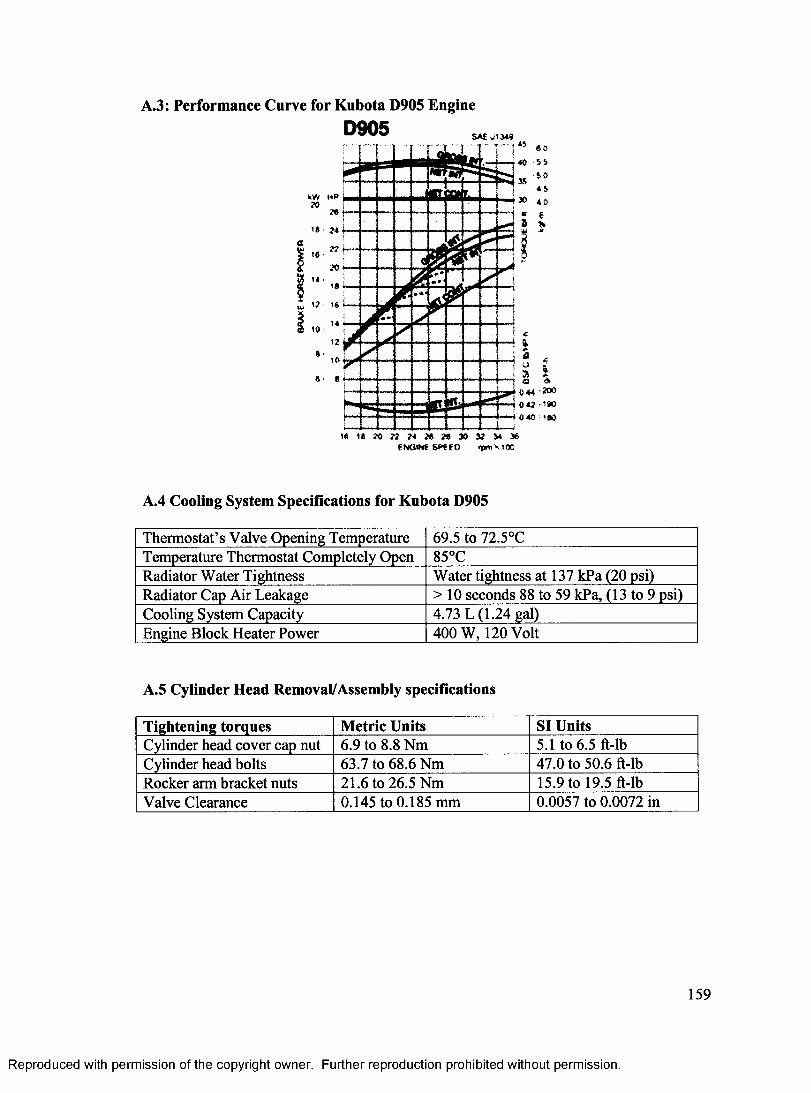
A.3: Performance Curve for Kubota D905 EngineD905
.1349
40 5 *
kW H P
1# 24
1 ? 1 6
0 44 -20004 ? r 1 9 0
0 4 0 160
i« ? 0 » 26 a 30 » J4 36Sf*CED fpmVtOO
A.4 Cooling System Specifications for Kubota D905
Thermostat’s Valve Opening Temperature 69.5 to 72.5°CTemperature Thermostat Completely Open 85°CRadiator Water Tightness Water tightness at 137 kPa (20 psi)Radiator Cap Air Leakage > 10 seconds 88 to 59 kPa, (13 to 9 psi)Cooling System Capacity 4.73 L (1.24 gal)Engine Block Heater Power 400 W, 120 Volt
A.5 Cylinder Head Removal/Assembly specifications
Tightening torques Metric Units SI UnitsCylinder head cover cap nut 6.9 to 8.8 Nm 5.1 to 6.5 ft-lbCylinder head bolts 63.7 to 68.6 Nm 47.0 to 50.6 ft-lbRocker arm bracket nuts 21.6 to 26.5 Nm 15.9 to 19.5 ft-lbValve Clearance 0.145 to 0.185 mm 0.0057 to 0.0072 in
159
Reproduced with permission of the copyright owner. Further reproduction prohibited without permission.
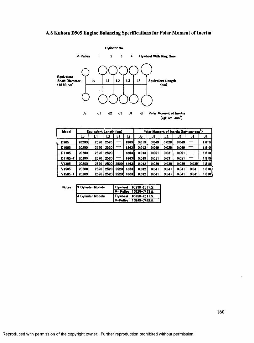
A.6 Kubota D905 Engine Balancing Specifications for Polar Moment of Inertia
Equivalent Shaft Diameter (18.68 cm)
Cylinder No.
V-Pulley I 2 3 4 Flywheel With Ring Gear
o OOOOOLv LI L2 L3 Lf Equivalent Length
(cm)
Jv J1 J2 J3 J4 J f Polar Moment of Inertia(kgf-cm-sec*)
Model Equivalent Length (cm) Polar Moment of Inertia (kgf-cm-sec*)Lv LI L2 L3 Lf Jv J1 J2 J3 J4 Jf
D905 20200 2520 2520 — 1863 0.013 0.049 0.029 0.049 — 1.810D1005 20200 2520 2520 — 1863 0.013 0.049 0.029 0.049 — 1.810D1105 20200 2520 2520 — 1863 0.013 0.051 0.031 0.051 — 1.810D1105-T 20200 2520 2520 — 1863 0.013 0.051 0.031 0.051 — 1.810V1305 20200 2520 2520 2520 1863 0.012 0.039 0.039 0.039 0.039 1.810VI505 20200 2520 2520 2520 1863 0.012 0.041 0.041 0.041 0.041 1.810VI505-T 20200 2520 2520 2520 1863 0.012 0.041 0.041 0.041 0.041 1.810
Notes : 3 Cylinder Models Flywheel 16239-2511AV-PuHey 16229-7428A
4 Cylinder Models Flywheel 16259-2511AV-Pulley 16249-7428A
Reproduced with permission of the copyright owner. Further reproduction prohibited without permission.
160
Appendix B: Engine Design Calculations
B.l Engine Output Power
Design Constraint: Engine Output Power less than 25 hp.P d e s i g n < = 25 hp, (B.l)
Kubota D905 Gross Intermittent Output Power:Pengine = 24.8 hp @ 3600 RPM, (B.2)
Since, Pengine<= Pdesign The design constraint has been met.
B.2 Chamber Pressure
Chamber Design Pressure constraint:Pd<=180 bar
Kubota D906 compression pressure:pc = 469 psi = 3233.6 kPa
Assuming a combustion pressure (pcp) rise of 50%:pcp= 3233.6 x 0.5 = 1616.8 kPa
The total pressure (pt) or the impressed load becomes:Pt = Pcp + Pcpt= 3233.6 + 1616.8= 4850.5 kPa
Based on Shigley and Mischke the assumed that the factor of safety:114 = 4.0
Using the Philon Factor of Safety Method given by the equation:
Pl f = n d X PiSubstitute and solve, pif = 4.0 x 4850.5 kPa = 19402 kPaUnit conversion, 1 bar = 0.00001 kPaEstimated loss of function pressure,
pif=194.02 barSince this is greater than our chamber design pressure (180 bar) it can Kubota D905 satisfy the constraint for chamber design pressure.
B.3 Operating Temperature
Operating temperautre constraint:Td=75°C (B.l 3)
Kubota D905 Thermostat Operating Temperature Range:71°C < Top < 90°C (B.l 4)
Since the desired HCCI operating temperature is within the temperature range of the Kubota thermostat, the thermostat does not need to be changed, and has met the operating range constraint.
B.4 Ramp Time to Reach Operating Temperature
The desired quantity is the ramp time ( Tr) which is defined as an estimate for the elapsed time required for the cooling system to reach operating temperature ( Top) of 75°C.Assumptions: Cooling system is a constant volume liquid,
161
(B.3)
(B.4)
(B.5)
(B.6)(B.7)
(B.8)
(B.9)(B.10) (B.l 1)
(B. 12) be concluded that the
Reproduced with permission of the copyright owner. Further reproduction prohibited without permission.
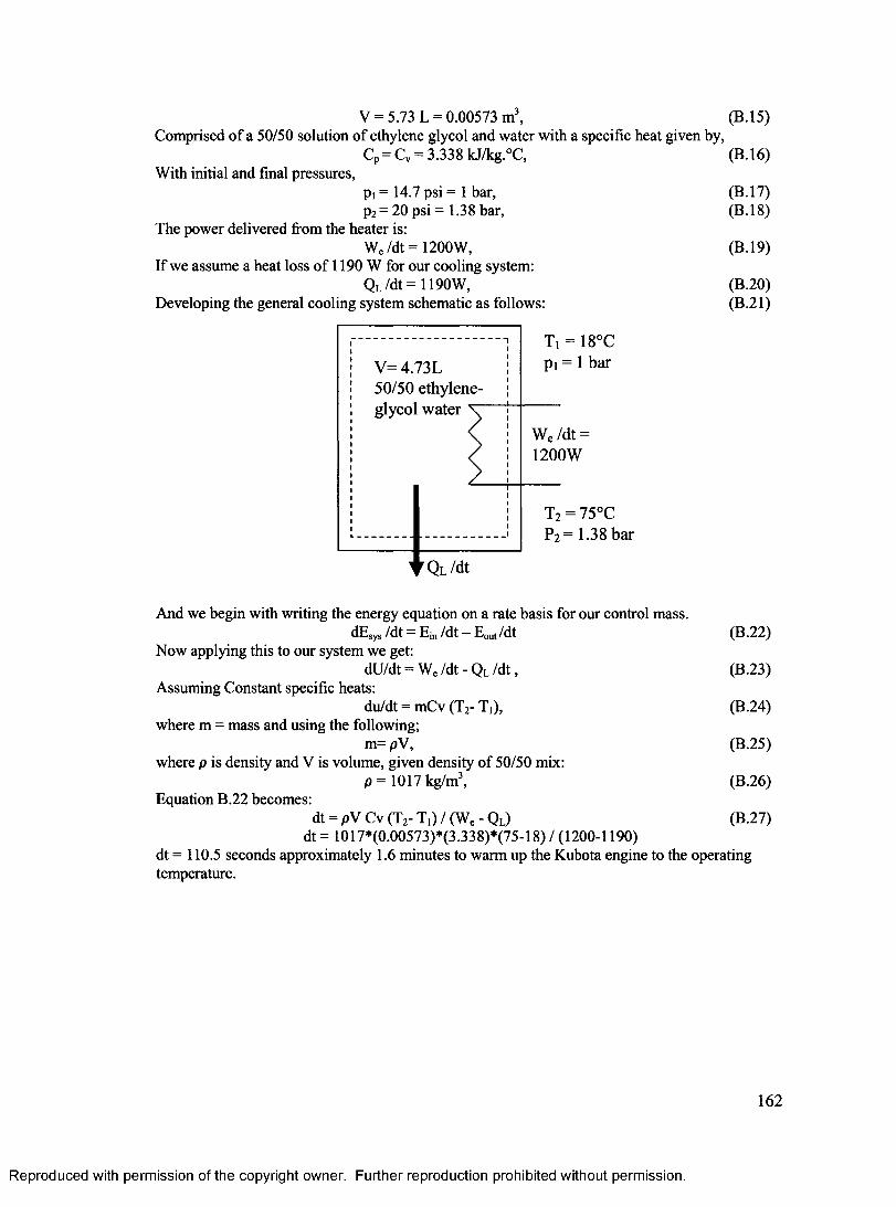
V = 5.73 L = 0.00573 m3, (B.l 5)Comprised of a 50/50 solution of ethylene glycol and water with a specific heat given by,
CP= C V = 3.338 kJ/kg.°C, (B.l 6)With initial and final pressures,
P! = 14.7 psi = 1 bar, (B.l 7)p2 = 20 psi =1.38 bar, (B.l 8)
The power delivered from the heater is:We /dt = 1200W, (B.19)
If we assume a heat loss of 1190 W for our cooling system:Ql /dt = 1190W, (B.20)
Developing the general cooling system schematic as follows: (B.21)
V= 4.73L 50/50 ethylene- glycol water
'Q l /dt
Ti = 18°C pi = 1 bar
We /dt = 1200W
T2 = 75°C P2= 1.38 bar
And we begin with writing the energy equation on a rate basis for our control mass.dEsys /dt = Ej„ /dt - Eout/dt (B.22)
Now applying this to our system we get:dU/dt = We /dt - Ql /d t , (B.23)
Assuming Constant specific heats:du/dt = mCv (T2- T i), (B.24)
where m = mass and using the following;m=pV, (B.25)
where p is density and V is volume, given density of 50/50 mix:p = 1017 kg/m3, (B.26)
Equation B.22 becomes:dt = pV Cv (T2- T,) / (We - Ql) (B.27)
dt = 1017*(0.00573)*(3.338)*(75-18) / (1200-1190) dt = 110.5 seconds approximately 1.6 minutes to warm up the Kubota engine to the operating temperature.
162
Reproduced with permission of the copyright owner. Further reproduction prohibited without permission.

B.5 Variable Compression Ratio Option 1
K u b o ta P 9 0 5 T e c h n ic a l S p e c if ic a tio n s
S troke (m m ) V s (cc) (.898L) total B ore (m m ) CR
73 .6 299 72 22
S w ep t V olum e (cc)P re c h a m b e r S lack
V pc (cc) V olum e (cc)C lea ran ce
V c (cc)
299 9 5 .25 14.25
O p tio n 1
G a s k e t W o rk s USA,V ary c le a ra n c e volum e by o rdering severa l h ttp ://w w w .headgasket.com /w how eare.h tm lg a s k e ts o f varying th ic k n e sse s from G ask e t A vailable M aterial th ick n esses :W orks USA. 0 .022 ,.032 ,.040 ,.0 4 3 ,.0 5 4 ,.0 6 3 ,.0 7 0 ,.0 8 6 , .093, an d .125
in ch es
C om pression R atio C lea ran ce V olum ew/
p rech am b erw/
p rech am b erw/0
pre ch am b erw/0
p re ch am b er
C R V c (c c ) t(m m ) t(inch) t(m m ) t(inch)
8 4 2 .7 6 8 .292 0 .326 10.503 0 .413
9 37 .42 6 .979 0 .275 9 .190 0 .362
10 33.26 5 .958 0 .235 8 .169 0 .322
11 29 .93 5.141 0 .202 7 .352 0 .289
12 27.21 4 .4 7 3 0 .176 6 .684 0 .263
13 24 .94 3 .916 0 .154 6 .127 0.241
14 23 .03 3 .4 4 5 0 .136 5 .6 5 5 0 .223
15 21 .3 8 3.041 0 .120 5.251 0 .207
16 19.96 2.691 0 .106 4.901 0 .193
17 18.71 2 .3 8 4 0 .094 4 .5 9 5 0.181
18 17.61 2 .114 0 .083 4 .3 2 5 0 .170
19 16.63 1.874 0 .074 4 .084 0.161
20 15.75 1 .659 0 .0 6 5 3 .869 0 .152
21 14.97 1 .465 0 .0 5 8 3 .676 0 .145
22 14.25 1.290 0.051 3.501 0 .138
23 13.61 1.131 0 .045 3 .342 0 .132
24 13.01 0 .986 0 .039 3 .196 0 .126
25 12.47 0 .853 0 .0 3 4 3 .063 0.121
B.6 Detailed Calculations for B.5
Given Bore (Dp), Stroke (Ls), Engine displacement (Vd) we can calculate the clearance volume (Vc) for any compression ratio.Determine swept volume Vs for a 3 cylinder engine:
Vs = V d /3 , (B.2 8)Vs = 0.898 L /3 = 0.299 L or 299 cm3 (cc), (B.29)
Then Vc is calculated using the following equation and varying compression ratio CR:Vc
For CR 8:1, VcFor CR 25:1, Vc
163
= (Vs -1) / CR, (B.30)= (299 - 1) / 8 = 42.76 cc, (B.31)= (299 -1) / 25 = 12.47 cc, (B.32)
Reproduced with permission of the copyright owner. Further reproduction prohibited without permission.
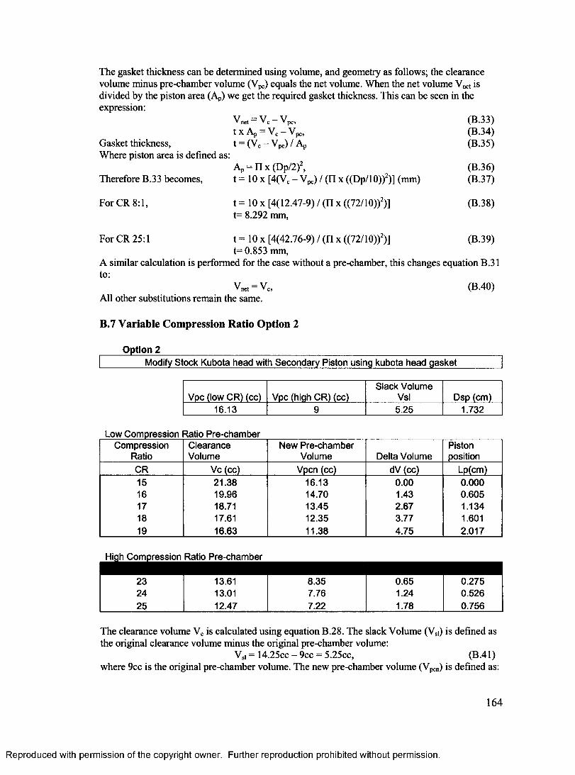
The gasket thickness can be determined using volume, and geometry as follows; the clearance volume minus pre-chamber volume (Vpc) equals the net volume. When the net volume Vnet is divided by the piston area (Ap) we get the required gasket thickness. This can be seen in the expression:
V n et = Vc Vi' nett x A p = V c pC9
Gasket thickness, t = (Vc - Vpc) / ApWhere piston area is defined as:
Ap = n x (Dp/2)2,Therefore B.33 becomes,
For CR 8:1,
For CR 25:1
t = 10 x [ 4 ( V C - V p c ) / ( n x ((Dp/10)) )] (mm)
t = 10 x [4(12.47-9) / (FI x ((72/10))2)] t= 8.292 mm,
(B.33)(B.34)(B.35)
(B.36)(B.37)
(B.38)
(B.39)t = 10 x [4(42.76-9) / ( n x ((72/10))2)] t= 0.853 mm,
A similar calculation is performed for the case without a pre-chamber, this changes equation B.31 to:
Vne, = Vc, (B.40)All other substitutions remain the same.
B.7 Variable Compression Ratio Option 2
Option 2___________________________Modify Stock Kubota head with Secondary Piston using kubota head gasket
Vpc (low CR) (cc) Vpc (high CR) (cc)Slack Volume
Vsl Dsp (cm)16.13 9 5.25 1.732
Low Compression Ratio Pre-chamberCompression
RatioClearanceVolume
New Pre-chamber Volume Delta Volume
Pistonposition
CR Vc (cc) Vpcn (cc) dV (cc) Lp(cm)15 21.38 16.13 0.00 0.00016 19.96 14.70 1.43 0.60517 18.71 13.45 2.67 1.13418 17.61 12.35 3.77 1.60119 16.63 11.38 4.75 2.017
High Compression Ratio Pre-chamber
23 13.61 8.35 0.65 0.27524 13.01 7.76 1.24 0.52625 12.47 7.22 1.78 0.756
The clearance volume Vc is calculated using equation B.28. The slack Volume (Vs)) is defined as the original clearance volume minus the original pre-chamber volume:
Vs, = 14.25cc - 9cc = 5.25cc, (B.41)where 9cc is the original pre-chamber volume. The new pre-chamber volume (Vpcn) is defined as:
164
Reproduced with permission of the copyright owner. Further reproduction prohibited without permission.
V pcn= v c - v sl, (B .4 2 )The delta volume (dV) is defined as the amount of volume that must be removed from the prechamber to attain the desired clearance volume and hence CR:
dV = Vpc-Vpc, (B.43)Where Vpc=16.13cc for low compression ratio range and Vpc=9 cc for high compression ration range. Given the secondary piston diameter (Dsp):
Dsp= 1.732 cm (B.44)The piston plunge depth (Lp) is defined as:
Lp = 4 / ((11 dV)/( Dsp)A2), (B.45)
For 17:1: Lp = 4 / ((11 x 2.67cc)/( 1.732cm)A2), (B.46)Lp = 1.134 cm, (B.47)
For 25:1: Lp = 4 / ((FI x 1.78)/( 1.732cm)A2), (B.48)Lp =0.756 cm, (B.49)
Therefore a method of adjusting and securing and sealing the secondary piston will have to be developed in the prototype fabrication phase.
Reproduced with permission of the copyright owner. Further reproduction prohibited without permission.
165
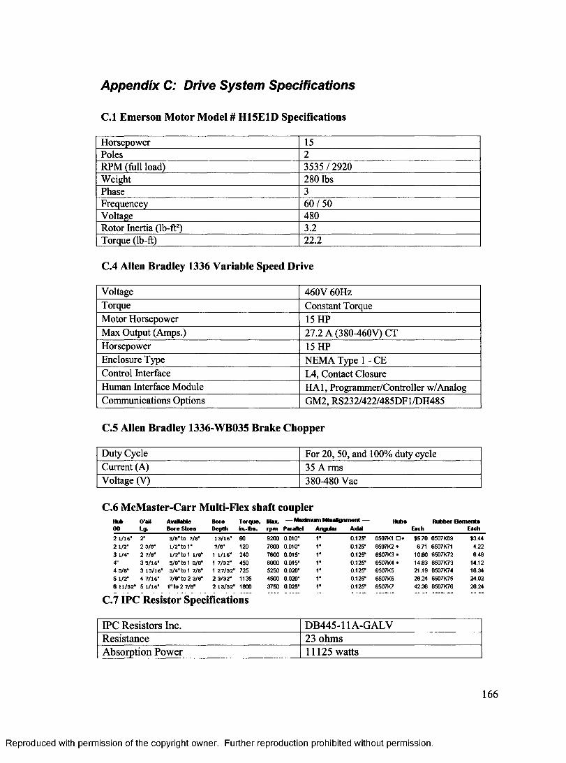
Appendix C: Drive System Specifications
C.l Emerson Motor Model # H15E1D Specifications
Horsepower 15Poles 2RPM (full load) 3535 / 2920Weight 280 lbsPhase 3Frequencey 60 /50Voltage 480Rotor Inertia (lb-ft2) 3.2Torque (lb-ft) 22.2
C.4 Allen Bradley 1336 Variable Speed Drive
Voltage 460V 60HzTorque Constant TorqueMotor Horsepower 15 HPMax Output (Amps.) 27.2 A (380-460V) CTHorsepower 15 HPEnclosure Type NEMA Type 1 - CEControl Interface L4, Contact ClosureHuman Interface Module HA1, Programmer/Controller w/AnalogCommunications Options GM2, RS232/422/485DF1/DH485
C.5 Allen Bradley 1336-WB035 Brake Chopper
Duty Cycle For 20, 50, and 100% duty cycleCurrent (A) 35 ArmsVoltage (V) 380-480 Vac
C.6 McMaster-Carr Multi-Flex shaft couplerHub
0 0O'att
Lg.AvaRaMe
Bore Sizes
Bore
DepthTorque,
in.-H>s.
Max.
rpm
— Maximum MisaHgnmetft —
Parallel Angular Axial
Hubs
Each
Rubber Elements
Each
2 1/16" 2" 3 /8"to 7/8" 13/16" 60 9200 0.010" 0.125" 6507K1 $5.70 65Q7K69 $3.442 1/2" 2 3/8" 1/2" t o r 7/8" 120 7600 0.010" 0.125" 6507K2 • 6.71 6507K71 4.223 1/4" 2 7/e" 1/ 2" to 1 1/ 8" 1 1/16" 240 7600 0.015" 0.125" 6507K3 • 10.60 6507K72 8.484" 3 5/16" 5/8" to 1 3/8" t 7/32" 450 6000 0.015" 1" 0.125" 6S07K4 • 14.83 6507K73 14.124 5/8" 3 15/16" 3/4" to 1 7/8" 1 27/32" 725 5250 0.020" 1" 0.125" 6507K5 21.19 6507K74 18.345 1/2" 4 7/16" 7/8” to 2 3/8" 2 3/32" 1135 4500 0.020" 0.125" 6507K6 28.24 6507K7S 24.026 11/32" 5 1/16" 1" to 2 7/8" 2 13/32" 1800 3750 0.025" 1" 0.125" 6S07K7 42.36 6507K76 28.24
C.7 IPC Resistor Specifications
IPC Resistors Inc. DB445-11A-GALVResistance 23 ohmsAbsorption Power 11125 watts
166
Reproduced with permission of the copyright owner. Further reproduction prohibited without permission.
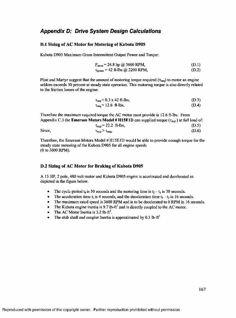
Appendix D: Drive System Design Calculations
D.l Sizing of AC Motor for Motoring of Kubota D905
Kubota D905 Maximum Gross Intermittent Output Power and Torque:
Pgross = 24.8 hp @ 3600 RPM, Voss = 42 ft-lbs @ 2200 RPM,
(D.l)(D.2)
Plint and Martyr suggest that the amount of motoring torque required (xreq) to motor an engine seldom exceeds 30 percent at steady state operation. This motoring torque is also directly related to the friction losses of the engine:
Therefore the maximum required torque the AC motor must provide is 12.6 ft-lbs. From Appendix C.3 the Emerson Motors Model # H15E1D can supplied torque (xsup) at full load of:
Therefore, the Emerson Motors Model # H15E1D would be able to provide enough torque for the steady state motoring of the Kubota D905 for all engine speeds (0 to 3600 RPM).
D.2 Sizing of AC Motor for Braking of Kubota D905
A 15 HP, 2 pole, 480 volt motor and Kubota D905 engine is accelerated and decelerated as depicted in the figure below.
• The cycle period U is 50 seconds and the motoring time is t2 — ti is 30 seconds.• The acceleration time ti is 4 seconds, and the deceleration time t3 - 12 is 16 seconds.• The maximum rated speed is 3600 RPM and is to be decelerated to 0 RPM in 16 seconds.• The Kubota engine inertia is 9.7 lb-ft2 and is directly coupled to the AC motor.• The AC Motor Inertia is 3.2 lb-ft2.• The stub shaft and coupler Inertia is approximated by 0.5 lb-ft2
X req = 0.3 X 42 ft-lbs, xreq= 12.6 ft-lbs,
(D.3)(D.4)
Since,(D.5)(D.6)
167
Reproduced with permission of the copyright owner. Further reproduction prohibited without permission.
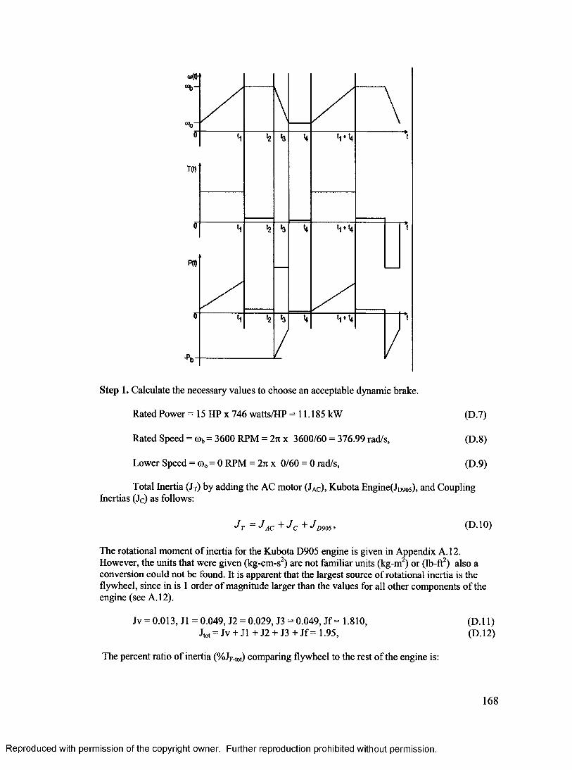
Step 1. Calculate the necessary values to choose an acceptable dynamic brake.
Rated Power = 15 HP x 746 watts/HP =11.185 kW (D-7)
Rated Speed = rob = 3600 RPM = 2 n x 3600/60 = 376.99 rad/s, (D.8)
Lower Speed = to0= 0 RPM = 2% x 0/60 = 0 rad/s, (D.9)
Total Inertia (JT) by adding the AC motor (Jac), Kubota Engine(JD905), and Coupling Inertias (Jc) as follows:
J r ~ J A C + J C "*’ • ^ 0 9 0 5 ’ (D.10)
The rotational moment of inertia for the Kubota D905 engine is given in Appendix A. 12. However, the units that were given (kg-cm-s2) are not familiar units (kg-m2) or (lb-ft2) also a conversion could not be found. It is apparent that the largest source of rotational inertia is the flywheel, since in is 1 order of magnitude larger than the values for all other components of the engine (see A. 12).
Jv = 0.013, J1 =0.049, J2 = 0.029, J3 = 0.049, Jf= 1.810, (D .ll)Jtot = Jv + J l+ J 2 + J3 + Jf= 1.95, (D.12)
The percent ratio of inertia (%JF-tot) comparing flywheel to the rest of the engine is:
168
Reproduced with permission of the copyright owner. Further reproduction prohibited without permission.
%JF -to t
%J
L l
J'O,'1.95
F -to t 1.81%JF-tot= 1-077 ,
(D.13)
(D.14)
(D.15)
Multiplying this by the flywheel inertia 9.01 lb-ft2 given in the schematic in Appendix A. 12 yields:
V-2JD905 =1.077x9.01 = 9.706 lb-ftz,
Now using equation D.10 we can find the total inertia of the system:
J T = J A C ^ C "*■ J D 9 0 5 i
JT = 3.2 + 9.706 + 0.5 = 13.4 lb-ft2,1 lb-ft2 = 0.138255 kg-m2
Therefore the total system inertia is:JT = 13.4 lb-ft2 = 1.852 kg-m2
Step 2. Determine peak braking power (Pb) by using the following equation:
AK(®t -®J]p> =
Pb =
(t3- t 2)1.852 x [376.99 x (376 .99 -0 )]
(16)Pb= 16.455 kW,
Note that this is less than 1.5 times the rated Power for the motor.
Step 3. Calculate Minimum Power Requirements for the Dynamic Braking Resistors.
(D.16)
(D.17) (D.l 8)
(D.l 9)
(D.20)
(D.21)
(D.22)
Determine the average braking power that must be dissipated by the resistor.
P =a vg(^3 ^2 ) P„
X —— X K
1rr-4*4 2 i £ I
p =16 16.455
x ---------------X(3 7 6 .9 9 -0 )
avg 50 2 376.99
< OQ II 633 kW,
(D.23)
(D.24)
(D.25)
Note that the average braking power Pavg = 2.633 kW is less than the peak braking power Pb= l6.455 kW.
169
Reproduced with permission of the copyright owner. Further reproduction prohibited without permission.
Step 4. Calculate the Maximum Dynamic Braking Resistance Value
(D.26)
where,R<tbi = Maximum allowable value for the dynamic braking resistor, (ohms)
Vd = DC bus voltage the chopper module regulates to 750 VDC for 460 Vrms.
Pb = Peak braking power calculated in earlier, (watts)
16455(D.27)
The selection of the dynamic braking resistance value should be less than R^i = 30.76 ohms. If the value is greater the drive can trip the DC bus over-voltage.
Step 5. Selecting a Resistor
Select a resistor bank from the supplier that has:
• A resistance value that is less than the value calculated (Rdbi) =30.76 in ohms.• A power value greater than the average power value calculated Pavg = 2633 W.
The IPC resistor bank model # DB445-11A-GALV has a resistance of 23 ohms which is less than (Rdbi) and dissipation power of 11,125 W which is greater than Pavg. Therefore, this resistor will be adequate to perform the required braking.
D.3 Verifying Starting Torque Requirements
To determine the amount of starting torque required on the flywheel of the Kubota D905 will require calculation based on the starter performance. The performance data available is for a 1.4 kW starter. This information can be scaled down to reflect more accurately the 1 kW starter that is supplied with the Kubota D905.
From Kubota Canada, Xi.4kW= 13.24 Nm, (D.28)Scaled down for lkW starter,
Thus, the amount of starting torque or load on the starter for the D905 engine is 9.45 Nm.
1.413.24 Am
1.4
(D.29)
= 9.457 Nm, (D.30)
From Inspection of Starter, NstarteFrom Inspection of flywheel, Nfiywheei= 98,
(D.31)(D.32)
The gear reduction (Rg) from the starter to flywheel is:
170
Reproduced with permission of the copyright owner. Further reproduction prohibited without permission.
NR = a?r“r... (D.33)8 M
flywheel
R = A =0.0918 (D.34)8 98
Thus, the gear reduction is 0.0918. The flywheel torque required to turn the engine over at 1000 RPM is determined as follows:
Ta = Ii*»L (D.35)1 flywheel D v '
9 457T = = 102.97 Nm (D.36)flywheel 0 0 9 1 8
1 Nm = 0.737562 ft-lbs (D.37)tnyw heei= 75.953 ft-lbs (D.38)
Thus, the amount of torque at the flywheel during starting is 75.95 ft-lbs. This is the amount of torque that our AC motor must provide in order to be able to match the starter performance. However, for this design only 1 cylinder will be enabled and the other 2 cylinders will not have compression, therefore the starting torque will be approximately 1/3 of the actual flywheel torque.
= 75.953 = 25317ft.lbs (D39)flywheel ^
From D.5 the maximum amount of torque that the H15E1D can provide is:
TSUp= 22.2 ft-lbs,Since, sup ^flywheel; (0.40)
Therefore, the H15E1D cannot provide enough torque to overcome the actual flywheel torque. The solution to this is to utilize the lkW starter during starting to assist the AC motor during start-up, and then disengage the starter once the engine is being motored by the AC motor.
D.4 Selection of Coupler Torque Capacity
Initial selection is based on the maximum rated torque of the engine with consideration given to the type of engine and number of cylinder, dynamometer characteristics and inertia.
Kubota D905 has a maximum net rated continuous torque of:Tnet = 30 ft-lbs @ 2200 RPM,
And from Plint and Martyr Table 8.4, the service factor (Fservice) are listed for range of engine and dynamometer types. For this application the service factor is:
Fservice 4.5, (D.41)The maximum rated torque multiplied by the service factor must not exceed the maximum permitted torque (Tper) of the coupler.
T =: p XT > (D'42)per service net
z per = 4.5 x 30 ft.lbs = 135 ft.lbs (D.43)The maximum torque of the McMaster-Carr coupler # 6507K7 from Appendix C.6 is:
xmax= 1800 in-lbs =150 ft-lbs, (D.44)
171
Reproduced with permission of the copyright owner. Further reproduction prohibited without permission.
Since, r > r (D.45)max — per ’
Therefore the coupler should be more than adequate to handle the torque from the motor.
D.S Variable Frequency/Speed Calculations
This AC motor is designed to run at a fixed speed of 3600RPM. A variable speed drive changes the input line frequency (60 hz) to a desired frequency (f) hz. This varies the shaft speed of the AC motor according to the following equation:
Speed = , (D.46)N poles
Varying the desired frequency from (0 to 60 Hz) in increments of 10 Hz we can see how the speed of the AC motor changes in the following table
Frequency (Hz) Shaft Speed (RPM)0 010 60020 120030 180040 240050 300060 3600
D.6 Determining Maximum Torque on Coupler During Emergency Stop
A calculation was needed to determine the maximum Torque on the coupler during an emergency stop. The engine was assumed to be running at 3600 RPM and the deceleration time for the emergency stop was set at 2 seconds.
The inertia of the Kubota Engine is given by equation D.l 6.J D905 = 9-706 _ Ibft2 = 0.409 kg.m2 (D.47)
The Torque applied to the coupler during deceleration can be determined as follows:
' L t c r„ ,= J oM a (D-48)Where a is the angular acceleration of the system and is given by:
a = a = 2nN[rpm] _ 2*3600rpm = {gg ^ (D 49)t 60 x /[s] 60 x 2s
r coupler = J D9 0 5a = 0.409kgm2 x 188.5r a d / s 2
TcouP,er = 77.09Nm = 56.9 ft.lbs The maximum torque of the McMaster-Carr coupler # 6507K7 from Equation D.44.
tm a x = 150 ft-lbs, (D.50)Since, j > r , (D.51)max — coupler ’ '
Therefore the coupler will survive emergency braking of the engine from 3600 RPM.
172
Reproduced with permission of the copyright owner. Further reproduction prohibited without permission.
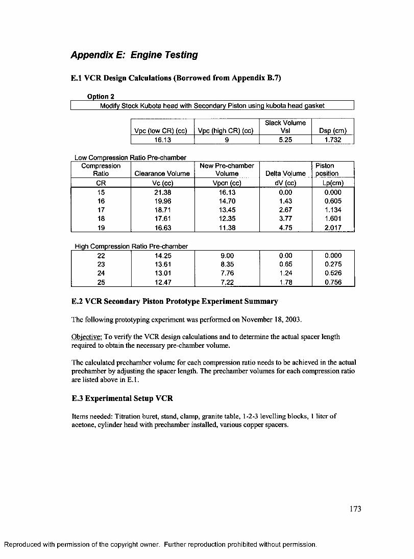
Appendix E: Engine Testing
E.l VCR Design Calculations (Borrowed from Appendix B.7)
Option 2________________________________________________________Modify Stock Kubota head with Secondary Piston using kubota head gasket
Low Compression
Vpc (low CR) (cc) Vpc (high CR) (cc)Slack Volume
Vsl Dsp (cm)16.13 9 5.25 1.732
Ratio Pre-chamberCompression New Pre-chamber Piston
Ratio Clearance Volume Volume Delta Volume positionCR Vc (cc) Vpcn (cc) dV (cc) Lp(cm)15 21.38 16.13 0.00 0.00016 19.96 14.70 1.43 0.60517 18.71 13.45 2.67 1.13418 17.61 12.35 3.77 1.60119 16.63 11.38 4.75 2.017
High Compression Ratio Pre-chamber22 14.25 9.00 0.00 0.00023 13.61 8.35 0.65 0.27524 13.01 7.76 1.24 0.52625 12.47 7.22 1.78 0.756
E.2 VCR Secondary Piston Prototype Experiment Summary
The following prototyping experiment was performed on November 18, 2003.
Objective: To verify the VCR design calculations and to determine the actual spacer length required to obtain the necessary pre-chamber volume.
The calculated prechamber volume for each compression ratio needs to be achieved in the actual prechamber by adjusting the spacer length. The prechamber volumes for each compression ratio are listed above in E. 1.
E.3 Experimental Setup VCR
Items needed: Titration buret, stand, clamp, granite table, 1-2-3 levelling blocks, 1 liter of acetone, cylinder head with prechamber installed, various copper spacers.
173
Reproduced with permission of the copyright owner. Further reproduction prohibited without permission.
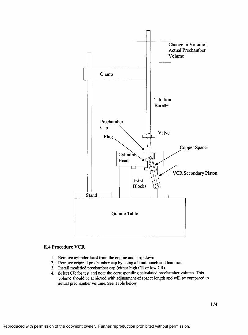
Change in Volume= Actual Prechamber Volume
Clamp
TitrationBurette
Prechamber Cap \
ValvePlug
Copper Spacer
CylindehHead
1 r nVCR Secondary Piston
1-2-3Blocks
Stand
Granite Table
E.4 Procedure VCR
1. Remove cylinder head from the engine and strip down.2. Remove original prechamber cap by using a blunt punch and hammer.3. Install modified prechamber cap (either high CR or low CR).4. Select CR for test and note the corresponding calculated prechamber volume. This
volume should be achieved with adjustment of spacer length and will be compared to actual prechamber volume. See Table below
174
Reproduced with permission of the copyright owner. Further reproduction prohibited without permission.
5. Make an initial guess as to the length of copper spacer and machine to length.6. Install copper spacer on VCR secondary piston and then install in cylinder head.7. Setup the experiment according to experimental setup figure above.8. Fill titration burette with acetone until it reaches the zero mark at the top.9. Open valve of burette and fill prechamber to the top flush with machined surface of
cylinder head.10. Record the value of the change in volume of the titration burette. This is the actual
prechamber volume using the selected copper spacer.11. If actual value matches calculated value then that is the correct spacer length.12. If actual value is greater than calulcated value then shorten spacer length slightly and
repeat from step 5.13. If actual value is less than calculated value then a longer spacer is required. Its best to use
a slightly longer spacer value than expected and machine to the correct length.
Experiment Table
CR Trial Number Calculated Prechamber Volume (cc)
Spacer Length (inches)
Actual Prechamber Volume (cc)
22 1 9.002 9.003 9.00
E.5 Results VCR
For High CR prechamber Cap
CR Trial Number Calculated Prechamber Volume (cc)
Spacer Length (inches)
Actual Prechamber Volume (cc)
22 1 9.00 0.3 7.52 9.00 0.356 8.13 9.00 0.447 9.05
25 1 7.22 0.26 7.62 7.22 0.23 7.2
For Low CR prechamber Cap
CR Trial Number Calculated Prechamber Volume (cc)
Spacer Length (inches)
Actual Prechamber Volume (cc)
15 1 16.13 1.0 16.62 16.13 0.95 16.2
17 1 13.45 0.62 13.4519 1 11.38 0.26 11
2 11.38 0.3 11.5
175
Reproduced with permission of the copyright owner. Further reproduction prohibited without permission.
E.6 Summary of Results VCR
CR Trial Number Calculated Prechamber Volume (cc)
Spacer Length (inches)
Actual Prechamber Volume (cc)
25 2 7.22 0.23 7.222 3 9.0 0.447 9.0519 2 11.38 0.3 11.517 1 13.45 0.62 13.4515 2 16.13 0.95 16.2
E.7 VCR Leak Test
The following verification experiment was performed on June 23, 2004.
Objective: To verify the VCR secondary piston and prechamber design and ensure no leakage occurs.
E.8 Experimental Setup VCR Leak Test
Items needed: vacuum tester, suction cup, cylinder head with prechamber and VCR installed, various copper spacers.
E.9 Procedure VCR Leak Test
Note: Cylinder head must already be removed from engine.
1. Install VCR secondary piston with spacers into the cylinder head and tighten.2. Install plug into glow plug hole and tighten.3. Install modified prechamber into the cylinder head.4. Install suction cup on vacuum tester.5. Place suction cup over prechamber opening.6. Draw vacuum on prechamber.7. Record vacuum pressure observed on indicator of vacuum tester along with observations
using the experimental matrix below.
Experiment Table
Test# Vacuum Drawn (in.Hg.)
Observations
176
Reproduced with permission of the copyright owner. Further reproduction prohibited without permission.
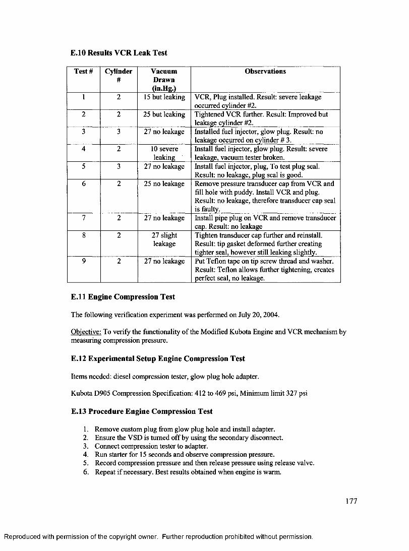
E.10 Results VCR Leak Test
Test# Cylinder#
VacuumDrawn(in.Hg.)
Observations
1 2 15 but leaking VCR, Plug installed. Result: severe leakage occurred cylinder #2.
2 2 25 but leaking Tightened VCR further. Result: Improved but leakage cylinder #2.
3 3 27 no leakage Installed fuel injector, glow plug. Result: no leakage occurred on cylinder # 3.
4 2 10 severe leaking
Install fuel injector, glow plug. Result: severe leakage, vacuum tester broken.
5 3 27 no leakage Install fuel injector, plug, To test plug seal. Result: no leakage, plug seal is good.
6 2 25 no leakage Remove pressure transducer cap from VCR and fill hole with puddy. Install VCR and plug. Result: no leakage, therefore transducer cap seal is faulty.
7 2 27 no leakage Install pipe plug on VCR and remove transducer cap. Result: no leakage
8 2 27 slight leakage
Tighten transducer cap further and reinstall. Result: tip gasket deformed further creating tighter seal, however still leaking slightly.
9 2 27 no leakage Put Teflon tape on tip screw thread and washer. Result: Teflon allows further tightening, creates perfect seal, no leakage.
E .ll Engine Compression Test
The following verification experiment was performed on July 20,2004.
Objective: To verify the functionality of the Modified Kubota Engine and VCR mechanism by measuring compression pressure.
E.12 Experimental Setup Engine Compression Test
Items needed: diesel compression tester, glow plug hole adapter.
Kubota D905 Compression Specification: 412 to 469 psi, Minimum limit 327 psi
E.13 Procedure Engine Compression Test
1. Remove custom plug from glow plug hole and install adapter.2. Ensure the VSD is turned off by using the secondary disconnect.3. Connect compression tester to adapter.4. Run starter for 15 seconds and observe compression pressure.5. Record compression pressure and then release pressure using release valve.6. Repeat if necessary. Best results obtained when engine is warm.
177
Reproduced with permission of the copyright owner. Further reproduction prohibited without permission.
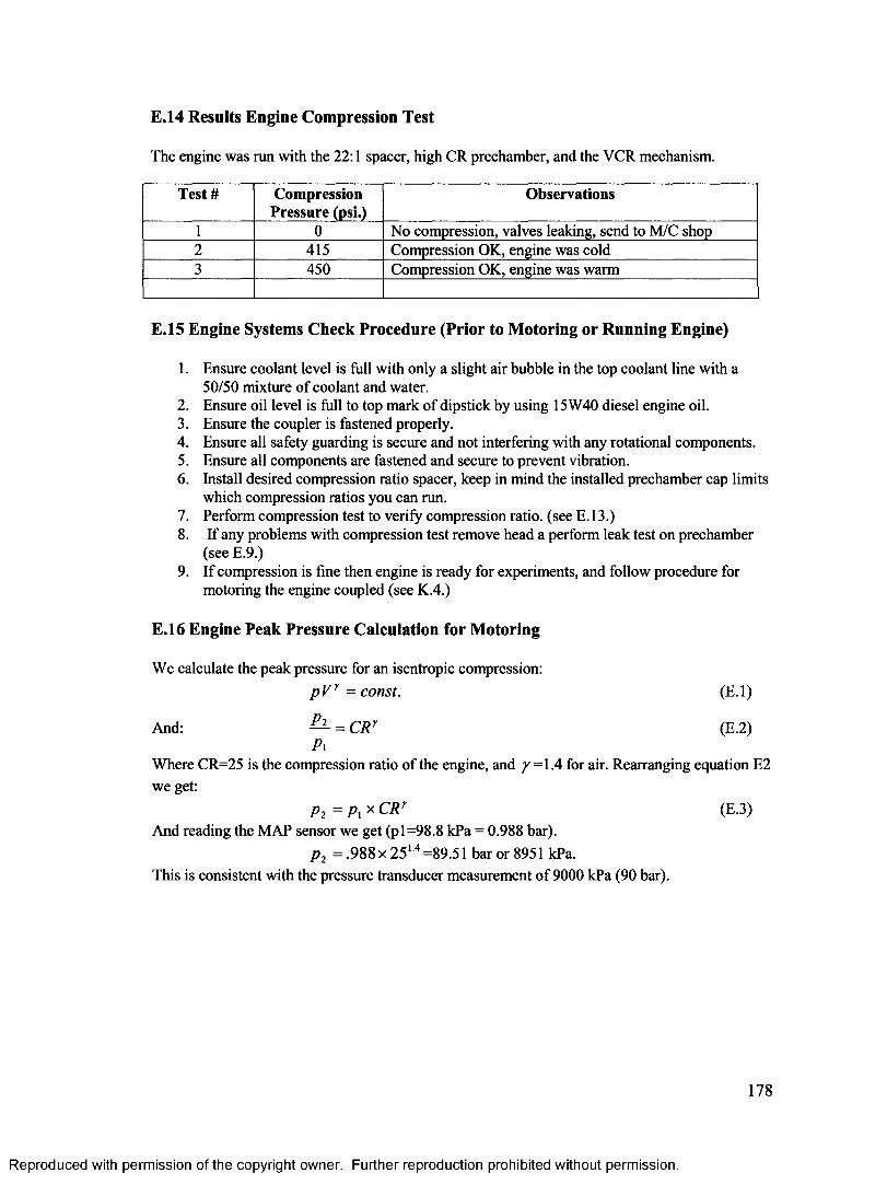
E.14 Results Engine Compression Test
The engine was run with the 22:1 spacer, high CR prechamber, and the VCR mechanism.
Test# Compression Pressure (psi.)
Observations
1 0 No compression, valves leaking, send to M/C shop2 415 Compression OK, engine was cold3 450 Compression OK, engine was warm
E.15 Engine Systems Check Procedure (Prior to Motoring or Running Engine)
1. Ensure coolant level is full with only a slight air bubble in the top coolant line with a 50/50 mixture of coolant and water.
2. Ensure oil level is full to top mark of dipstick by using 15W40 diesel engine oil.3. Ensure the coupler is fastened properly.4. Ensure all safety guarding is secure and not interfering with any rotational components.5. Ensure all components are fastened and secure to prevent vibration.6. Install desired compression ratio spacer, keep in mind the installed prechamber cap limits
which compression ratios you can run.7. Perform compression test to verify compression ratio, (see E.13.)8. If any problems with compression test remove head a perform leak test on prechamber
(see E.9.)9. If compression is fine then engine is ready for experiments, and follow procedure for
motoring the engine coupled (see K.4.)
E.16 Engine Peak Pressure Calculation for Motoring
We calculate the peak pressure for an isentropic compression:p V r = const. (E.l)
And: ^ - = CRr (E.2)P\
Where CR=25 is the compression ratio of the engine, and y =1.4 for air. Rearranging equation E2 we get:
Pi = Pi x C R r (E.3)And reading the MAP sensor we get (pl=98.8 kPa = 0.988 bar).
p 2 = .988 x 2514 =89.51 bar or 8951 kPa.This is consistent with the pressure transducer measurement of 9000 kPa (90 bar).
178
Reproduced with permission of the copyright owner. Further reproduction prohibited without permission.
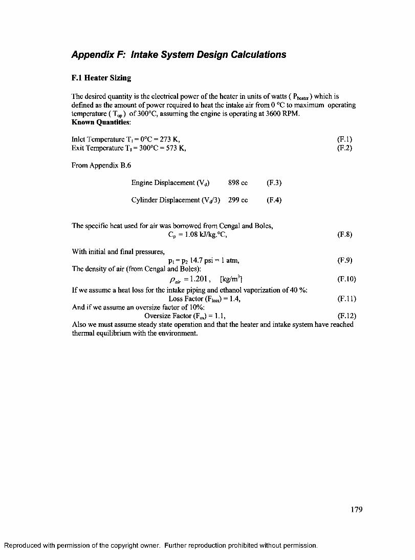
Appendix F: Intake System Design Calculations
F.l Heater Sizing
The desired quantity is the electrical power of the heater in units of watts ( Pheater) which is defined as the amount of power required to heat the intake air from 0 °C to maximum operating temperature ( Top) of 300°C, assuming the engine is operating at 3600 RPM.Known Quantities:
Inlet Temperature Ti = 0°C = 273 K, (F.l)Exit Temperature Ti = 300°C = 573 K, (F.2)
From Appendix B.6
Engine Displacement (Vd) 898 cc (F.3)
Cylinder Displacement (Vd/3) 299 cc (F.4)
The specific heat used for air was borrowed from Cengal and Boles,Cp = 1.08kJ/kg.°C, (F.8)
With initial and final pressures,Pi = p2 14.7 psi = 1 atm, (F.9)
The density of air (from Cengal and Boles):p air= 1.201, [kg/m3] (F.10)
If we assume a heat loss for the intake piping and ethanol vaporization of 40 %:Loss Factor (Fioss) = 1.4, (F. 11)
And if we assume an oversize factor of 10%:Oversize Factor (Fos) =1.1, (F. 12)
Also we must assume steady state operation and that the heater and intake system have reached thermal equilibrium with the environment.
Reproduced with permission of the copyright owner. Further reproduction prohibited without permission.
179
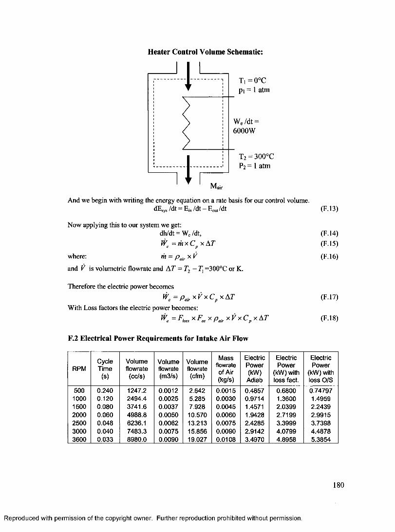
Heater Control Volume Schematic:
T i = 0 ° C
pi = 1 atm
We /dt = 6 0 0 0 W
T 2 = 3 0 0 ° C
P2 = 1 atm
And we begin with writing the energy equation on a rate basis for our control volume.dEsys /dt = Ein /dt - Eout/dt
Now applying this to our system we get:dh/dt = We /dt,We = m x C p x A T
where: m = p air x V
and V is volumetric flowrate and A T = T2 - T X =300°C or K.
Therefore the electric power becomesWe = p airx V x C p x A T
With Loss factors the electric power becomes:
K = F loss X F os X P a ir * V x C p x A T
(F.13)
(F.14)(F.15)
(F.16)
(F.17)
(F.18)
F.2 Electrical Power Requirements for Intake Air Flow
RPMCycleTime
(s)
Volumeflowrate
(cc/s)
Volumeflowrate(m3/s)
Volumeflowrate(cfm)
Mass flowrate of Air (kg/s)
ElectricPower(kW)
Adiab
Electric Power
(kW) with loss fact.
Electric Power
(kW) with loss O/S
500100015002000250030003600
0.2400.1200.0800.0600.0480.0400.033
1247.2 2494.4 3741.6 4988.8 6236.17483.3 8980.0
0.00120.00250.00370.00500.00620.00750.0090
2.6425.2857.92810.57013.21315.85619.027
0.00150.00300.00450.00600.00750.00900.0108
0.4857 0.9714 1.4571 1.9428 2.4285 2.9142 3.4970
0.6800 1.3600 2.0399 2.7199 3.3999 4.0799 4.8958
0.747971.49592.24392.99153.73984.48785.3854
180
Reproduced with permission of the copyright owner. Further reproduction prohibited without permission.
F.3 Detailed Calculations for F.2 For 3600 RPM
Cycle Time (L): tc = , (F. 19)RPM
120t, = -------- = 0.0333 seconds. (F.20)e 3600
Volumetric flowrate ( V ) in units of [cc/s] assuming volumetric efficiency ( Tjv) is 1.0 :
V = rjv — , (F.21)
299ccV = --------------- = 8980 cc/sec. (F.22)
0.0333 secConvert volumetric flowrate ( V ) to units of [m3/s]:
VV = ------------ , (F.23)
10000008980cc/ sec ,
V = ---------------- =0.008980 m /s = 8.98 L/s (F.24)1000000
Convert volumetric flowrate ( V ) to units of [cfm]:V = V x 6 0 x 35 .315 , (F.25)V = 0.00898 x 60 x 35.315 = 19.0275cfm, (F.26)
Mass flowrate ( m ) in units of [kg/s]:m = V x p air> (F.27)
m = 0.00898 x 1.201 = 0.01078 kg/s. (F.28)
Heater Power from without losses (F .l5)We = 0.01078 x 1.08 x 300 = 3.49 kW, (F.29)
Heater Power with Intake LossesWe = 1.4 x 3A 9kW = 4.89 kW, (F.30)
Electric Heater Power with Intake Losses and Oversize FactorWe =1.1 xA.%9kW =5.38 kW, (F.31)
Thus, the Electric Heater Power requirement for a single cylinder Kubota D905 is 5.4 kW, and therefore the heater selected must have a power rating greater than this.
From Appendix G.l we have a list of high quality process air heaters from Omega. The Omega SH-73343 is a 6 kW heater with a voltage of 240 V. Therefore, this air heater will be sufficient for single cylinder operation.
F.4 Calculation of Intake Air Flow Rate
The same quantities used in Appendix F. 1, F.2, F.3 are also used in the following equation except the flow rate is representative of all three cylinders as opposed to just a single cylinder. The reason for over-sizing of the flowmeter is to allow for future research to be performed on the entire engine, whereas the heater would only be required for single cylinder operation.
181
Reproduced with permission of the copyright owner. Further reproduction prohibited without permission.
Multiply volumetric flowrate ( V ) to all three cylinders to units of [L/s]:V - V x 3 , [L/s] (F.32)
From (F.24) for one cylinder the flow rate is 8.98 L/sVcalcula!ed = 8 .9 8 x 3 =26.94 L/s (F.32)
Therefore, the engine will have a maximum calculated flowrate of 26.94 L/s.
All!fhree Cylinders
RPM Cycle Time (s)
Volumetricflowrate(cc/m)
Volumetricflowrate(m3/m)
Volumetric flowrate (Us)
Mass flowrate of Air (kg/s)
500 0.240 224500 0.22 3.74 0.271000 0.120 449000 0.45 7.49 0.541500 0.080 673500 0.67 11.22 0.812000 0.060 898000 0.90 14.96 1.082500 0.048 1122500 1.12 18.7 1.353000 0.040 1347000 1.35 22.45 1.623500 0.034 1571500 1.57 26.18 1.893600 0.033 1616400 1.62 26.94 1.94
F.5 Selection of Laminar Flow Element
scfm = standard cubic feet per minute acfm = actual cubic feet per minute cfm = Cubic feet per minute
Note that scfm = acfm = cfm at 29.92”Hg.Abs and 70°F
The gas flowing is AIR at a flow rate Vcalculated of 26.94 L/s or 57 scfm.The pressure of the flowing AIR is 29.92”Hg.Abs.The temperature of the AIR is 70°F
Since this flow is at standard condition, the LFE can be selected directly from the capacity chart given in Appendix G.3.
There are two LFE that have a flow rate range covering the expected flow rate of our Kubota D905 engine, (see figure below). The 50MC2-2 was selected because it had a slightly larger range from 0-100 scfm and has hose end attachments that will be easier to utilize with the intake for the research engine.
182
Reproduced with permission of the copyright owner. Further reproduction prohibited without permission.
Intake Airflow range
120 Meriam 50MC2-2
100
80
60
40
20
00 1000 30002000 4000
Engine Speed (RPM)
F.6 Calculation of Differential Pressure
The differential pressure Apcalculated of the flow through the LFE is calculated using the following equation:
b p calculated ^calculated (F.25)' LFE
where, k p LFE is the catalog differential pressure rating = 10”H2O, Appendix G.3
VLFE is the catalog flow rate range = 100 scfm, Appendix G.3
Therefore, the calculated differential pressure reading when the engine is at 3600 RPM or flows AIR at a rate of 57 scfm.
8"bp calculated = 51 scfm x = 4.56 inches H20. (F.26)
100 scfm
F.7 Observance of Reynold’s Number for the LFE selected.
To maintain laminar flow with linearity through the LFE consideration must be given to the Reynolds number for the maximum flow condition. Meriam LFE elements will produce linear flow characteristics when the Reynolds number is 150 at 4”H20 differential and 300 at 8”H20 differential. It should be noted that true linearity will not be retained at elevated Reynolds number. However, a calibration made at the operating condition will be fully usable and repeatable.
The maximum allowable Reynolds number to maintain laminar flow at the differential pressure calculated in {F.26) is determined by interpolating between the following:
183
Reproduced with permission of the copyright owner. Further reproduction prohibited without permission.
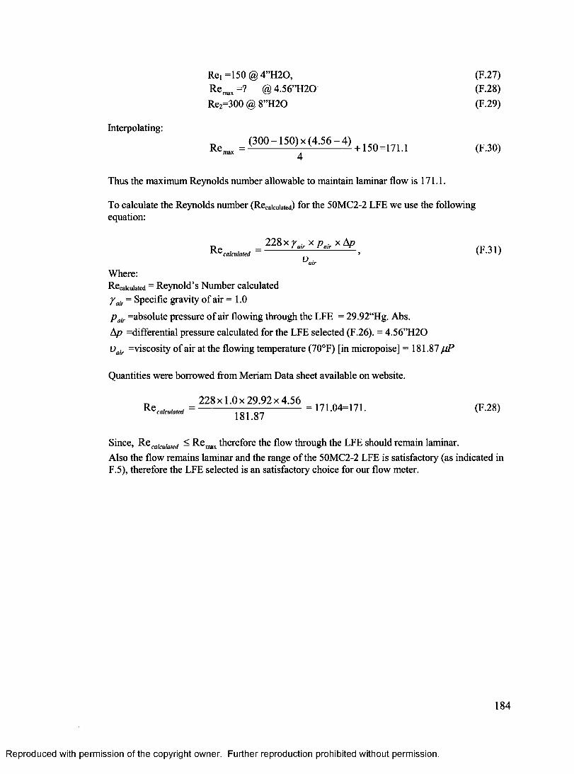
Interpolating:
Re, =150 @ 4”H20, (F.27)R e ^ x =? @ 4.56”H20 (F.28)Re2=300 @ 8”H20 (F.29)
R « „ , (300-150)><(4.56-4)+150^ 711 ^
Thus the maximum Reynolds number allowable to maintain laminar flow is 171.1.
To calculate the Reynolds number (Reca,cuiated) for the 50MC2-2 LFE we use the following equation:
228 x V ■ x P x ApD - _ I air y a i r 4 / p T , \^ c a lc u la t e d ~ »
"airWhere:Recalculated = Reynold’s Number calculated y air = Specific gravity of air =1.0
Pair =absolute pressure of air flowing through the LFE = 29.92“Hg. Abs.Ap =differential pressure calculated for the LFE selected (F.26). = 4.56”H20 °air =viscosity of air at the flowing temperature (70°F) [in micropoise] = 181.87 fiP
Quantities were borrowed from Meriam Data sheet available on website.
228x1 .0x29 .92x4 .56 RQcalculated - IsF sT 171.04-171. (F.28)
Since, Re(,flfcu/ated < R e ^ therefore the flow through the LFE should remain laminar.Also the flow remains laminar and the range of the 50MC2-2 LFE is satisfactory (as indicated inF.5), therefore the LFE selected is an satisfactory choice for our flow meter.
Reproduced with permission of the copyright owner. Further reproduction prohibited without permission.
184
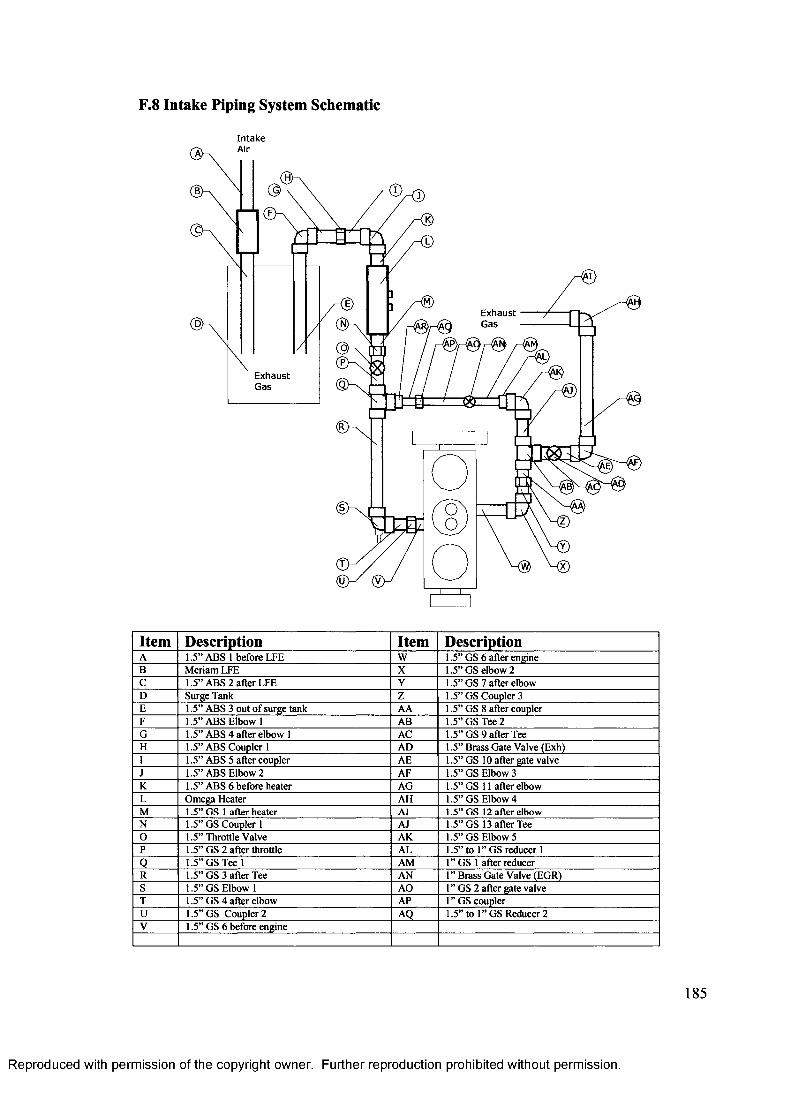
F.8 Intake Piping System Schematic
In ta k eAir
E xhaustG as
E xhaustG as
Item Description Item DescriptionA 1.5” A B S l before LFE w 1.5” G S 6 a fter engineB M eriam LFE X 1.5” G S elbow 2C 1.5” A B S 2 a fter LFE Y 1.5” G S 7 after e lbowD Surge T ank Z 1.5” G S C oupler 3E 1.5” A B S 3 ou t o f surge tank AA 1.5” G S 8 a fter couplerF 1.5” A B S E lbow 1 AB 1.5” G S Tee 2G 1.5” A B S 4 a fter e lbow 1 AC 1.5” G S 9 a fte r TeeH 1.5” A B S C oupler 1 AD 1.5” B rass G ate V alve (E xh)I 1.5” A B S 5 after coupler AE 1.5” G S 10 after gate valveJ 1.5” A B S E lbow 2 AF 1.5” G S E lbow 3K 1.5” A B S 6 b efore heater AG 1.5” G S 11 after elbowL O m ega H eater AH 1.5” G S E lbow 4M 1.5” G S 1 after heater AI 1.5” G S 12 after elbowN 1.5” G S C oupler 1 AJ 1.5” G S 13 afte r TeeO 1.5” T hrottle V alve AK. 1.5” G S E lbow 5P 1.5” G S 2 a fte r throttle A L 1.5” to 1” G S reducer 1
Q 1.5” G S Tee 1 AM 1” G S 1 a fter reducerR 1.5” G S 3 a fte r Tee AN 1” B rass G ate V alve (E G R )S 1.5” G S E lbow 1 AO 1” G S 2 a fter gate valveT 1.5” G S 4 afte r e lbow AP 1” G S couplerU 1.5” G S C oupler 2 AQ 1.5” to 1” G S R educer 2V 1.5” G S 6 b efore engine
Reproduced with permission of the copyright owner. Further reproduction prohibited without permission.
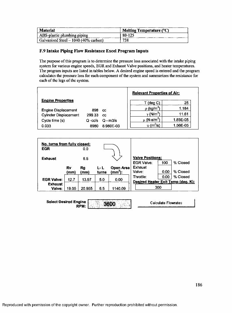
Material Melting Temperature (°C)ABS-plastic plumbing piping 80-125Galvanized Steel - 1040 (40% carbon) 738
F.9 Intake Piping Flow Resistance Excel Program Inputs
The purpose of this program is to determine the pressure loss associated with the intake piping system for various engine speeds, EGR and Exhaust Valve positions, and heater temperatures. The program inputs are listed in tables below. A desired engine speed is entered and the program calculates the pressure loss for each component of the system and summarizes the resistance for each of the legs of the system.
Engine Properties
Engine Displacement Cylinder Displacement Cycle time (s)0.033
898 cc 299.33 cc Q -cc/s Q - m3/s
8980 8.980E-03
Relevant Properties of Air:
T (deg C) 25P (kg/m3) 1.184y (N/m3) 11.61
u (N-s/m2) 1.85E-05u (m2/s) 1.56E-05
No. turns from fully closed: EGR 0.0
Exhaust 6.5
Rv Rg L- L Open Area turns (mm2):
EGR Valve: 12.7 13.97 5.0 0.00Exhaust
Valve: 19.05 20.955 6.5 1140.09
Valve Positions:EGR Valve: 100 % ClosedExhaustValve: 0.00 % ClosedThrottle: 0.00 % ClosedDesired Heater Exit Temp (deq. Kl:
300
Select Desired Engine RPM: 3600 C alculate F low rates
186
Reproduced with permission of the copyright owner. Further reproduction prohibited without permission.
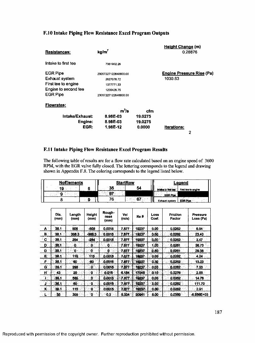
F.10 Intake Piping Flow Resistance Excel Program Outputs
Resistances: kg/m7Height Change (m)
0.28876
Intake to first tee 7381902.26
EGR Pipe Exhaust system First tee to engine Engine to second tee EGR Pipe
23057227122648800.00
2827076.72
1377771.33
1235426.75
23057227122648800.00
Engine Pressure Rise (Pa)1030.63
Flowrates:
Intake/Exhaust:Engine:
EGR:
m3/s8.98E-038.98E-031.98E-12
cfm19.027519.0275 0.0000 Iterations:
F .ll Intake Piping Flow Resistance Excel Program Results
The following table of results are for a flow rate calculated based on an engine speed of 3600 RPM, with the EGR valve fully closed. The lettering corresponds to the legend and drawing shown in Appendix F.8. The coloring corresponds to the legend listed below.
NoElements StartRow LegendIntaka lo (Iret ta e First tee to endne
Dia.(mm)
Length(mm)
Height(mm)
Roughness(mm)
Vel(m/s) Re# Loss
Coef.FrictionFactor
Pressure Loss (Pa)
A 38.1 508 -508 0.0015 7.877 19237 0.00 0.0262 6.94B 38.1 368.3 -368.3 0.0015 7.877 18237 0.50 0.0262 23.40C 38.1 254 t254 0.0015 7.877 18237 0.00 0.0262 3.47D 38.1 0 0 0 7.877 19237 1.00 0.0261 36.73O 38.1 0 0 0 7.877 18237 0.80 0.0261 29.38E. . 38.1 115 115 0.0015 7577 18237 0.00 0.0262 4.24F 38.1 80 60 0.0015 7.877 19237 0.30 0.0262 13.23G 38.1 298 0 0.0015 7*877 19237 0.00 0.0262 7.53H 43 20 0 0.015 6.184 17045 0.10 0.0276 2.551 38.1 585 0 0.0015 7.877 19237 0.00 0.0262 14.78J 38.1 60 0 0.0015 7.877 19237 3.00 0.0262 111.70K 38.1 115 0 0.0015 7.877 18237 000 0.0262 2.91L 35 305 0 0.3 9.334 20941 5.00 0.0389 -6.986E+03
187
Reproduced with permission of the copyright owner. Further reproduction prohibited without permission.
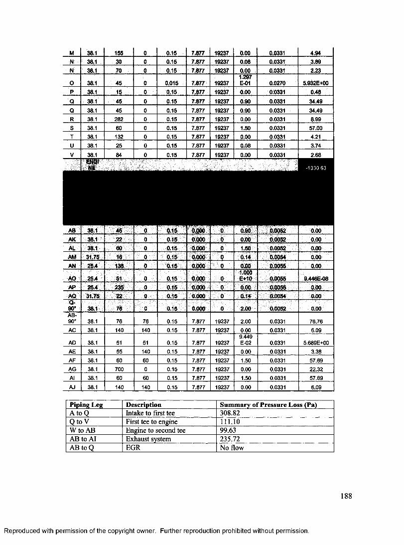
M 38.1 155 0 0.15 7.877 19237 0.00 0.0331 4.94N 38.1 30 0 0.15 7.877 19237 0.08 0.0331 3.89N 38.1 70 0 0.15 7.877 19237 0.00 0.0331 2.23
O 38.1 45 0 0.015 7.877 192371.297E-01 0.0270 5.932E+00
P 38.1 15 0 0.15 7.877 19237 0.00 0.0331 0.48
Q 38.1 45 0 0.15 7.877 19237 0.90 0.0331 34.49Q 38.1 45 0 0.15 7.877 19237 0.90 0.0331 34.49R 38.1 282 0 0.15 7.877 19237 0.00 0.0331 8.99S 38.1 60 0 0.15 7.877 19237 1.50 0.0331 57.00T 38.1 132 0 0.15 7.877 19237 0.00 0.0331 4.21U 38.1 25 0 0.15 7.877 19237 0.08 0.0331 3.74
V 38.1 84 0 0.15 7.877 19237 0.00 0.0331 2.68en3T
AB 38.1 45 0 0.15 0 0.9(1 0.0052 0.00AK 38.1 22 0 0.15 0.000 0 0.00 0.0052 0.00AL 38.1 60 0 0.15 0.000 0 1.50 0.0052 0.00AM 31.75 16 0 0.15 0000 0 0.14 0.0054 0.00AN I 25.4 138 0 0.15 0.000 0 0.00 0.0055 0.00
AO I 25.4 51 0 0.15 0.000 01.000E+10
''0.0055 I 9.446E-08
AP ' 25.4 235 0 0.15 0.000 0 0.00 0.0055 0.00AQ I 31.75 22 0 0.15 0.000 0 0.14 0.0054 , 0.00Q-90* 38.1 76 0 0.15 0.000 0 2.00 0.0052 | 0.00AB- I 90* 38.1 76 76 0.15 7.877 19237 2.00 0.0331 76.76AC 38.1 140 140 0.15 7.877 19237 0.00 0.0331 6.09
AD 38.1 51 51 0.15 7.877 192379.449E-02 0.0331 5.689E+00
AE 38.1 55 140 0.15 7.877 19237 0.00 0.0331 3.38AF 38.1 60 60 0.15 7.877 19237 1.50 0.0331 57.69AG 38.1 700 0 0.15 7.877 19237 0.00 0.0331 22.32Al 38.1 60 60 0.15 7.877 19237 1.50 0.0331 57.69AJ 38.1 140 140 0.15 7.877 19237 0.00 0.0331 6.09
Piping Leg Description Summary of Pressure Loss (Pa)A t o Q Intake to first tee 308.82Q to V First tee to engine 111.10W to AB Engine to second tee 99.63AB to Al Exhaust system 235.72AB to Q EGR No flow
Reproduced with permission of the copyright owner. Further reproduction prohibited without permission.
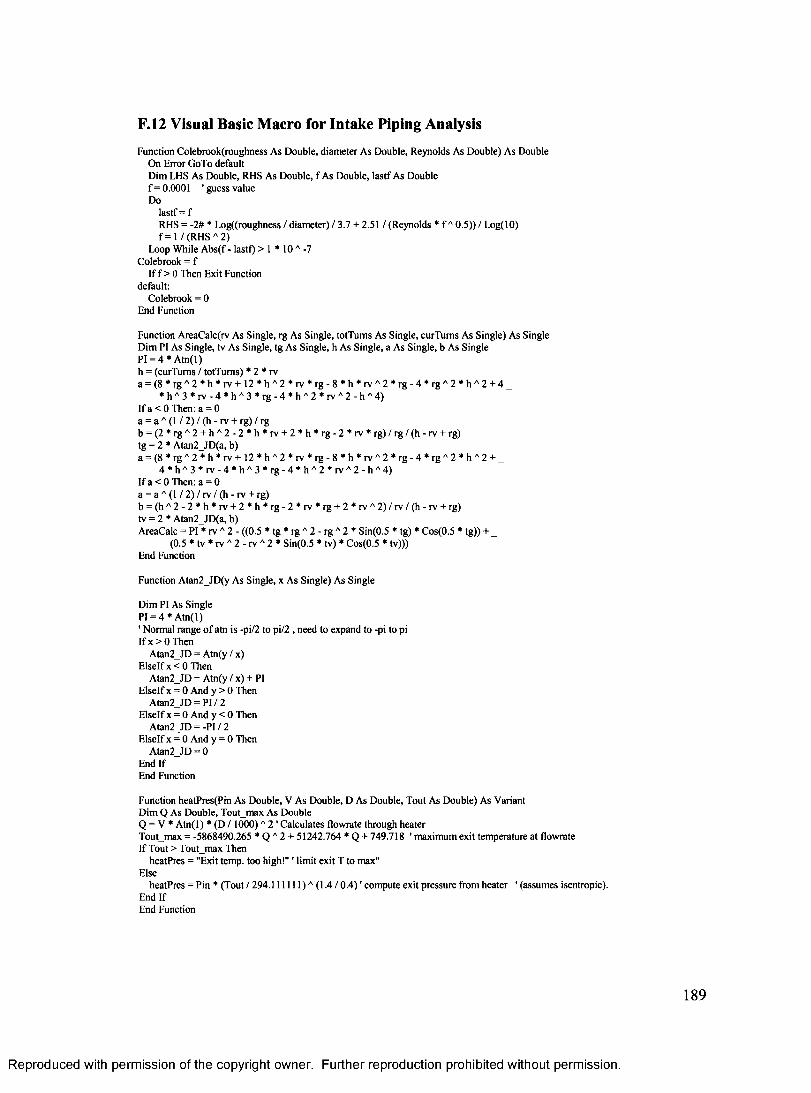
F.12 Visual Basic Macro for Intake Piping AnalysisF unction C olebrook(roughness A s D ouble, d iam eter A s D ouble, R eynolds A s D ouble) A s Double
O n Error G oT o defau ltD im LHS A s D ouble, RH S A s D ouble, f A s D ouble, la s tf As Double f = 0.0001 ' guess value Do
la s t f= fRH S = -2# * Log((roughness / d iam eter) / 3.7 + 2.51 / (R eynolds * f A 0 .5 )) / Log(10) f = l / ( R H S A 2)
Loop W hile A b s(f - lastf) > 1 * 10 A -7 C olebrook = f
I f f > 0 Then E xit Function default:
C olebrook = 0 End Function
Function A reaC alc(rv A s Single, rg A s Single, to tT um s A s Single, cu rT um s A s S ingle) A s S ingle D im PI As Single, tv A s Single, tg A s Single, h A s Single, a A s Single, b As Single PI = 4 * A t n ( l )h = (curT um s / to tT um s) * 2 * rva = ( 8 * r g A 2 * h * r v + 1 2 * h A 2 * r v * r g - 8 * h * r v A 2 * r g - 4 * r g A 2 * h A 2 + 4 _
* h A 3 * r v - 4 * h A 3 * r g - 4 * h A 2 * r v A2 - h A4)If a < 0 Then: a = 0 a = a A (1 / 2 ) / (h - rv + rg) / rgb = ( 2 * r g A 2 + h A2 - 2 * h * r v + 2 * h * r g - 2 * r v , r g ) / r g / ( h - r v + rg) tg = 2 * A tan2_JD (a, b)a = ( 8 * r g A 2 * h * r v + 1 2 * h A 2 * r v * r g - 8 * h * r v A 2 * r g - 4 * r g A 2 * h A2 + _
4 * h A 3 * r v - 4 * h A 3 * r g - 4 * h A 2 * r v A 2 - h A4)I f a < 0 Then: a = 0 a = a A ( l / 2 ) / r v / ( h - r v + rg)b = ( h A 2 - 2 * h * r v + 2 * h * r g - 2 * r v * r g + 2 * r v A 2 ) / r v / ( h - r v + rg) tv = 2 * A tan2_JD (a, b)A reaC alc = PI * rv A 2 - ((0.5 * t g * r g A 2 - r g A 2 * S in(0.5 * tg) * C os(0.5 * tg )) + _
(0.5 * t v * r v A2 - r v A2 * S in(0.5 * tv ) * C os(0.5 * tv)))End Function
Function A tan2_JD (y A s Single, x A s S ingle) A s Single
D im PI As Single PI = 4 * A t n ( l )' N orm al range o f a tn is -pi/2 to pi/2 , need to expand to -pi to pi I f x > 0 Then
A tan2_JD = A tn(y / x)E lse lf x < 0 Then
A tan2_JD = A tn(y / x) + PI E lse lf x = 0 A nd y > 0 TTien
A tan2_JD = PI / 2 E lse lf x = 0 A nd y < 0 Then
A tan2_JD = -PI / 2 E lse lf x = 0 A nd y = 0 Then
A tan2_JD = 0 E nd IfEnd Function
Function heatP res(P in A s D ouble, V As D ouble, D As D ouble, T ou t A s D ouble) As V ariant D im Q As D ouble, Tout_m ax A s Double Q = V * A tn ( l) * (D / 1 0 0 0 ) A 2 ' C alculates flow rate through heaterT out m ax = -5868490.265 * Q A 2 + 51242.764 * Q + 749.718 1 m axim um ex it tem perature a t flow rate I f Tout > Tout_m ax Then
heatPres = "Exit tem p, too h ig h !" ' lim it ex it T to max"Else
heatP res = Pin * (T out / 2 9 4 .1 1 1 1 1 1 )A (1.4 / 0 .4 ) ' com pute exit p ressure from h eater ' (assum es isentropic). End I fE nd Function
Reproduced with permission of the copyright owner. Further reproduction prohibited without permission.
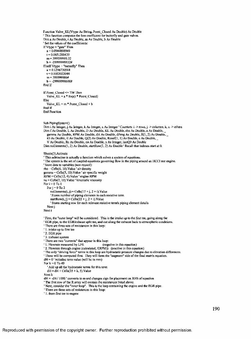
Function V alve_K L (V type A s S tring, P c e n tC lo se d As D ouble) As D ouble ' T his function com putes the loss coeffic ien t for bu tterfly and gate valves. D im a As D ouble, t A s D ouble, m A s D ouble, b As D ouble ' Set the values o f the coefficients:I f V type = "gate” Then
a = 0.0944898949 t = 0.0651200439 m = 399999999.32 b = -2 9 9 99999932#
E lse lf V type = "butterfly" Then a = 0.1296730544 t = 0 .1053022044 m = 399999986# b = -2 9 9 99998600#
End If
If Pcent_C losed <= 75# Then V alve_K L = a * Exp(t * Pcent_C losed)
ElseV a lv e K L = m * P cen t C losed + b
E nd IfEnd Function
Sub PipingSystem ()D im i As Integer, j A s Integer, k A s Integer, x A s In te g e r ' C ounters: i -> row s, j -> colum ns, k, x -> others D im f A s D ouble, L A s D ouble, D A s D ouble, K L As D ouble, rho A s D ouble, a As D ouble, _
gam m a A s D ouble, RPM As D ouble, dH A s D ouble, dPeng As D ouble, R (1 , 2 ) A s D ouble, _ iO As D ouble, il A s D ouble, Q (2) A s D ouble, R coefi(l, 1) A s D ouble, e A s D ouble, _V A s D ouble, R e A s D ouble, nu A s D ouble, y As Integer, lastQO A s Double
D im n o E lem e n ts (l, 2 ) A s D ouble, s ta rtR o w (l, 2 ) A s D o u b le ' Recall that indexes start a t 0.
Sheets(3).A ctivate' This subroutine is actually a function w hich solves a system o f equations.' The system is the set o f coupled equations governing flow in the p ip ing around an H CCI test engine.' S tore data to variables (non-reused): rho = C e lls (4 ,1 0 ) .V a lu e ' a ir density gam m a = C e l ls (5 ,10).V alue ' a ir specific w eight R PM = C e lls (1 2 ,4 ).V a lu e ' engine RPM nu = C e l ls (7 ,10).V a lu e ' k inem atic v iscosity For i = 0 To 1
For j = 0 To 2 noE lem ents(i, j ) = C ells(17 + j , 2 + i). V alue ' Stores num ber o f p ip ing e lem ents in each resistive term startR ow (i, j ) = C ells(22 + j , 2 + i).V alue' Stores starting row for each re levan t resistive term ’s p ip ing elem ent details
N ex tj N ex t i
' F irst, the "outer loop" will be considered . T his is the in take up to the first tee, go ing along the ' E G R p ipe, to the EG R /exhaust sp lit tee, and ou t a long the exhaust b ack to a tm ospheric conditions.' There are three sets o f resistances in th is loop:' 1. intake up to first tee ' 2. E G R pipe ' 3. E xhaust system1 There are tw o "currents" that appear in this loop:' 1. F low rate m easured b y LFE (negative in this equation)' 2. F low rate th rough engine (calculated , f(R PM )) (positive in th is equation)' T he only "driving force" term s in this loop are hydrostatic p ressure changes due to elevation d ifferences.' T hese w ill be com puted first. They w ill form the "augm ent" side o f the final m atrix equation. d H = 0 ' initialise term value (w ill be in m m )For k = 0 To 49
' A dd up all the hydrostatic term s fo r th is term dH = d H + C ells(35 + k, 5). V alue
N e x tkdH = -dH /1 0 0 0 ' converts to m and changes sign for p lacem ent on RH S o f equation ' T he first row o f the R a rray w ill con tain the resistances listed above.1 N ext, consider the " inner loop". This is the loop con tain ing the engine and the EG R pipe.' There are three sets o f resistances in th is loop:' 1. from first tee to engine
Reproduced with permission of the copyright owner. Further reproduction prohibited without permission.
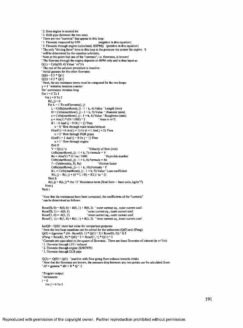
' 2. from engine to second tee ' 3. EG R p ipe (betw een the tw o tees)' There are tw o "currents" that appear in this loop:' 1. F low rate m easured by LFE (negative in th is equation)' 2. F low rate through engine (calculated , ffR PM )) (positive in this equation)' T he on ly "driv ing force" term in this loop is the p ressure rise across the engine. It ' w ill be determ ined b y the equation solutions.' N o te a t th is p o in t that one o f the "currents", i.e. flow rates, is know n 1 ' T he flow rate through the engine depends on RPM only and is thus input as:Q ( l ) = C e lls(1 0 ,4). V a lu e ' m A3/s 1 T he rest o f the so lution procedure is iterative:1 Initial guesses for the o ther flow rates:
Q (0) = 0.5 * Q (1 )Q (2) = 0.5 * Q ( l)1 N ext, the s ix resistance term s m ust be com puted for the tw o loops: y = 1 ' in itialise iteration counter D o 1 com m ence iteration loop For i = 0 To 1
For j = 0 To 2 R ( i , j) = 0For k = 1 To noE lem ents(i, j )
L = C ells(startR ow (i, j ) -1 + k, 4 ).V alue ' Length (m m )D = C ells(startR ow (i, j ) - 1 + k , 3). V alue ' D iam eter (m m ) e = C ells(startR ow (i, j ) -1 + k , 6).V alue ' R oughness (m m ) a = A tn ( l) * (D /1 0 0 0 ) A 2 'A r e a i n m A2If i = 0 A nd (j = 0 O r j = 2) Then
x = 0 1 flow th rough m ain in take/exhaust E lse lf (i = 0 A nd j = 1) O r (i = 1 A nd j = 2 ) Then
x = 2 ' flow th rough E G R pipes E lse lf i = 1 A nd (j = 0 O r j = 1) Then
x = 1 1 flow through engine End IfV = Q (x) / a ' V elocity o f flow (m /s)C ells(startR ow (i, j ) - 1 + k , 7).Form ula = VRe = A bs(V ) * D / n u /1 0 0 0 1 R eynolds num berC ells(startR ow (i, j ) - 1 + k , 8).Form ula = Ref= C olebrook(e, D, R e) ' friction factorC ells(startR ow (i, j ) - 1 + k, 10).Form ula = fK L = C ells(startR ow (i, j ) -1 + k , 9 ).V a lu e ' Loss coeffic ientR(i, j ) = R(i, j ) + ( ( f * L / D ) + K L) / (a A 2)
N e x tkR(i, j ) = R(i, j ) * rho / 2 ' R esistance term (final form — base units, kg/m A7)
N e x tj N ex t i
' N ow that the resistances have been com puted , the coeffic ients o f the "currents"' can be determ ined as follows:
R co e f(0 ,0 ) = R (0 ,0 ) + R ( 0 ,1) + R (0 ,2) ' ou ter cu rren t eq., outer cu rren t coef.R c o e f(0 ,1) = - R ( 0 ,1) ' ou ter curren t eq., inner curren t coef.R co e f( l, 0 ) = -R ( l , 2 ) ' inner curren t eq., ou ter cu rren t coef.R co e f( l, 1) = R ( l , 0 ) + R ( l , 1) + R ( l , 2 ) ' inner curren t eq., inner curren t coef.
lastQO = Q ( 0 ) ' store last value for com parison purposes ' N ow the tw o loop equations can be solved fo r the unknow ns (Q (0) and dPeng):Q (0) = ((gam m a * dH - R c o e f(0 ,1) * Q (1 ) A 2 ) / R co e f(0 ,0 ) ) A 0.5 dPeng = R c o e f ( l ,0 ) * Q ( 0 ) A 2 + R co e f( l, 1) * Q ( l ) A 2' C urrents are equ iva len t to the square o f flow rates. There are three flow rates o f in terest (in m A3/s):' 1. F low rate th rough LFE / exhaust ' 2. F low rate through engine (K N O W N )' 3. Flow rate through E G R pipe
Q (2) = -Q (0) + Q ( l ) ' positive w ith flow going from exhaust tow ards intake ' N ow that the flow rates a re know n, the p ressure d rop betw een any tw o po in ts can be calculated from: ’ dP = gam m a * dH + R * Q A 2
' Program output:' resistances: i = 0
For j = 0 To 2
Reproduced with permission of the copyright owner. Further reproduction prohibited without permission.
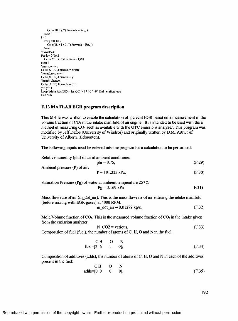
C ells(l 8 + j , 7).Form ula = R (i, j )N e x tj
i = 1 For j = 0 T o 2
C ells(18 + j + 3 , 7).Form ula = R(i, j)N e x tj
' flow rates:For k = 0 To 2
C ells(27 + k , 7).Form ula = Q (k)N ext k' p ressure rise:C ells(22, 10).Form ula = dPeng 1 iteration counter:C ells(30 ,10 ).F o rm ula = y ' he igh t change:C ells(16 ,10 ).F o rm ula = dH y = y + lLoop W hile A bs(Q (0) - lastQO) > 1 * 10 A - 9 ' End iteration loop End Sub
F.13 MATLAB EGR program description
This M-file was written to enable the calculation of percent EGR based on a measurement of the volume fraction of C 02 in the intake manifold of an engine. It is intended to be used with the a method of measuring C 02 such as available with the OTC emissions analyzer. This program was modified by Jeff Defoe (University of Windsor) and originally written by D.M. Arthur of University of Alberta (Edmonton).
The following inputs must be entered into the program for a calculation to be performed:
Relative humidity (phi) of air at ambient conditions:phi = 0.75, (F.29)
Ambient pressure (P) of air:P = 101.325 kPa, (F.30)
Saturation Pressure (Pg) of water at ambient temperature 25 ° C:Pg = 3.169 kPa F.31)
Mass flow rate of air (mdota i r ) . This is the mass flowrate of air entering the intake manifold (before mixing with EGR gases) at 4000 RPM.
m d o t a i r = 0.01279 kg/s, (F.32)
Mole/Volume fraction of C 02. This is the measured volume fraction of C 02 in the intake given from the emission analyzer:
N C 0 2 = various, (F.33)Composition of fuel (fuel), the number of atoms of C, H, O and N in the fuel:
C H O Nfuel=[2 6 1 0]; (F.34)
Composition of additives (adds), the number of atoms of C, H, O and N in each of the additivespresent in the fuel:
C H O Nadds=[0 0 0 0]; (F.35)
192
Reproduced with permission of the copyright owner. Further reproduction prohibited without permission.
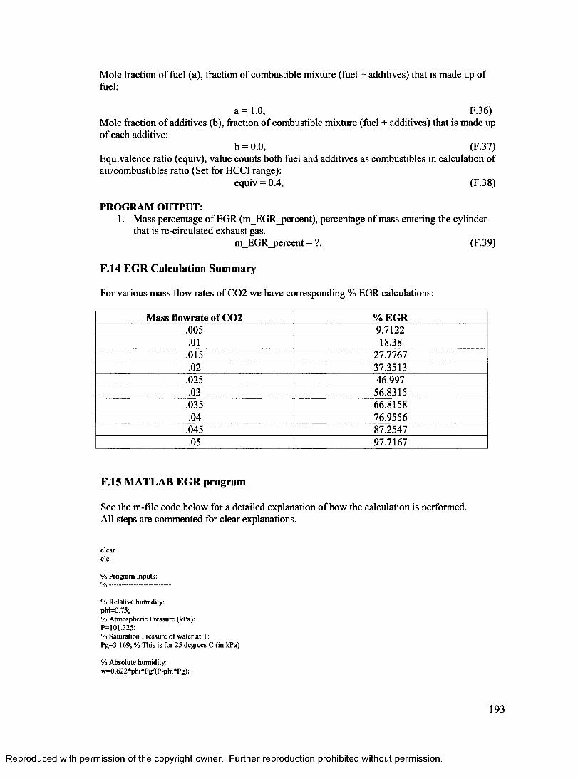
Mole fraction of fuel (a), fraction of combustible mixture (fuel + additives) that is made up of fuel:
a =1.0, F.36)Mole fraction of additives (b), fraction of combustible mixture (fuel + additives) that is made up of each additive:
b = 0.0, (F.37)Equivalence ratio (equiv), value counts both fuel and additives as combustibles in calculation of air/combustibles ratio (Set for HCCI range):
equiv = 0.4, (F.38)
PROGRAM OUTPUT:1. Mass percentage of EGR (m_EGR_percent), percentage of mass entering the cylinder
that is re-circulated exhaust gas.m_EGR_percent = ?, (F.39)
F.14 EGR Calculation Summary
For various mass flow rates of C02 we have corresponding % EGR calculations:
Mass flowrate of C 02 % EGR.005 9.7122.01 18.38.015 27.7767.02 37.3513.025 46.997.03 56.8315.035 66.8158.04 76.9556
.045 87.2547.05 97.7167
F.15 MATLAB EGR program
See the m-file code below for a detailed explanation of how the calculation is performed. All steps are commented for clear explanations.
clearclc
% Program Inputs:% -------------------
% R elative hum idity . phi=0.75;% A tm ospheric Pressure (kPa):P = 101 .325;% Saturation Pressure o f w ater a t T:Pg= 3.169; % This is for 25 degrees C (in kPa)
% A bsolute hum idity: w =0.622*phi*Pg/(P-phi*Pg);
193
Reproduced with permission of the copyright owner. Further reproduction prohibited without permission.
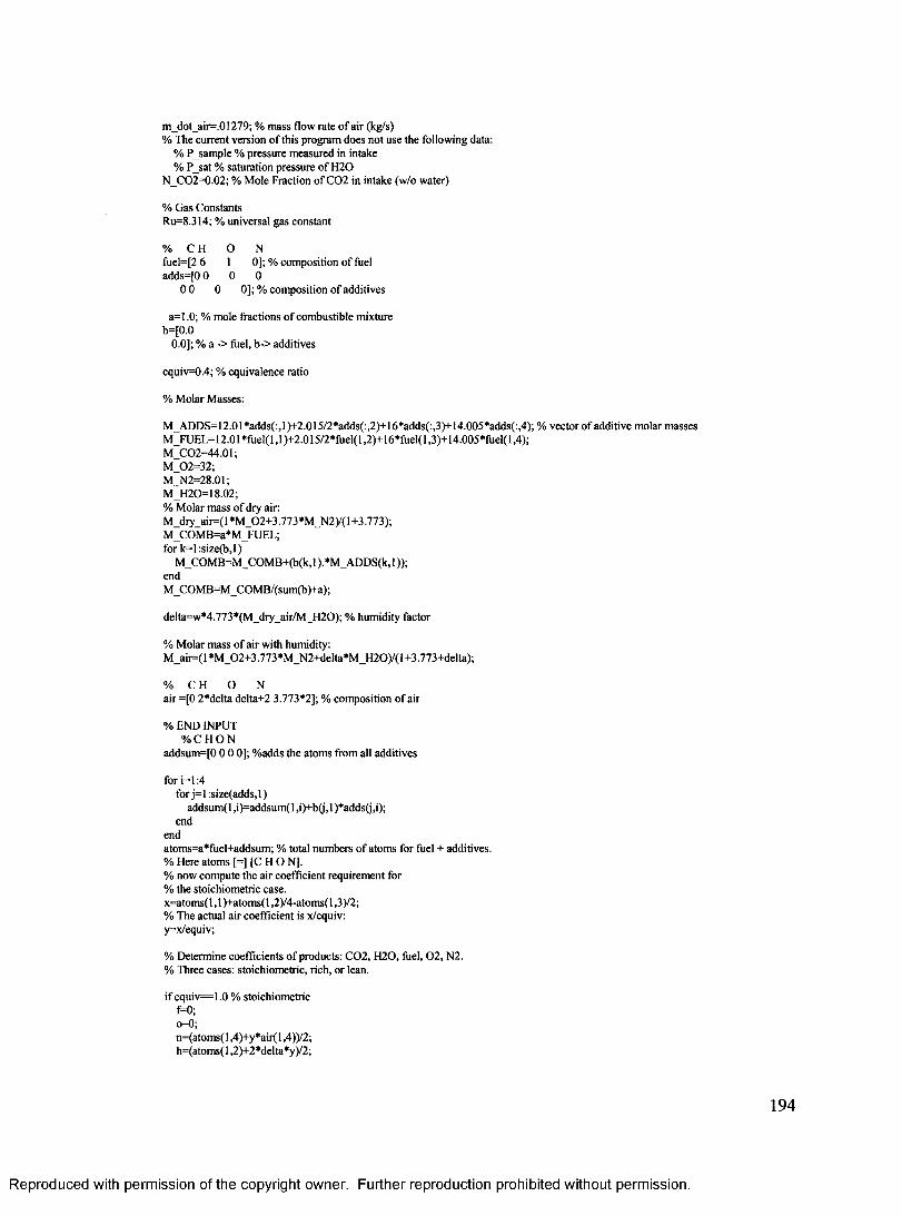
m _dot_air= .01279; % m ass flow rate o f a ir (kg/s)% The cu rren t version o f this p rogram does n o t use the follow ing data:
% P s a m p le % pressure m easured in intake % P sat % saturation p ressure o f H 2 0
N _ C 0 2 = 0 .0 2 ; % M ole Fraction o f C 0 2 in in take (w /o w ater)
% G as C onstantsRu=8.314; % universal gas constant
% C H O Nfuel=[2 6 1 0]; % com position o f fueladds=[0 0 0 0
0 0 0 0]; % com position o f additives
a = l .0 ; % m ole fractions o f com bustib le m ixture b=[0.0
0 .0]; % a -> fuel, b -> additives
equiv=0.4; % equivalence ratio
% M olar M asses:
M _A D D S=12.01 *adds(:,l)+2 .015/2*adds(:,2)+16*adds(:,3)t-14 .005*adds(:,4); % vecto r o f additive m olar m asses M _F U E L = 1 2 .0 1 * fu el(l,l)+ 2 .0 1 5 /2 * fu e l(l,2 )+ 1 6 * fu e l(l,3 )+ 1 4 .0 0 5 * fu e l(l,4 );M _C O 2=44.01;M _0 2 = 3 2 ;M _N 2=28.01;M _H 2O =18.02;% M olar m ass o f dry air:M _dry_air= (l * M _ 0 2 + 3 .773 *M _N 2)/( 1 +3.773);M _CO M B=a*M _FU E L;f o rk = l:s iz e (b ,l)
M _C O M B = M _C O M B + (b(k , 1 ).*M _A D D S(k, 1)); endM _C O M B =M _C O M B /(sum (b)+a);
d e lta= w *4.773*(M _dry_air/M _H 20); % hum idity factor
% M olar m ass o f a ir w ith hum idity:M _air= (l*M _ 0 2 + 3 .7 7 3 * M _ N 2 + d elta* M _ H 2 0 )/(l+ 3 .7 7 3 + d elta );
% C H O Na ir = [0 2*delta delta+2 3.773*2]; % com position o f a ir
% EN D IN PU T % C H O N
addsum =[0 0 0 0]; % adds the a tom s from all additives
fo r i= l :4 fo r j= l:s iz e (a d d s ,l )
addsum ( 1 ,i)=addsum ( 1 ,i)+b(j, 1 )*adds(j ,i); end
endatom s=a*fuel+addsum ; % total num bers o f a tom s for fuel + additives.% H ere a tom s [=] [C H O N].% now com pute the a ir coeffic ient requirem ent for% the sto ichiom etric case.x=atom s( 1,1 )+atom s( 1,2)/4-atom s( 1,3 )/2 ;% The actual a ir coeffic ient is x/equiv: y=x/equiv;
% D eterm ine coeffic ients o f products: C 0 2 , H 2 0 , fuel, 0 2 , N2.% Three cases: sto ichiom etric , rich, o r lean.
i f e q u i v = l .0 % stoichiom etric f=0 ; o=0 ;n=(atom s( 1,4)+y *air( 1,4 ))/2 ; h = (a to m s(l,2) f 2*delta*y)/2;
194
Reproduced with permission of the copyright owner. Further reproduction prohibited without permission.

c = a to m s (l,l) ; e lse if equ iv> l .0 % rich
o=0;% system o f 3 equations in 3 unknow ns to solve % fo r c,f,hM = [2 /a tom s(l,3 ) 1 l/a to m s (l,3 )
0 a to m s(l,2)/2 11 a to m s ( l ,l ) 0 ];
A = [l + (2+delta)*y/atom s( 1,3)(atom s( 1,2)+2 *delta*y)/2 a to m s (l,l ) ] ;
B=M \A ;
c = B ( l ,l ) ;f= B (2 ,l);h= B (3 ,l);n= (atom s(l ,4 )+ y*air(l , 4 ) - f a to m s(l ,4))/2;
e lse if e qu iv< l .0 % leanf=0;c = a to m s (l,l) ;h= (atom s(l ,2>fy*2*delta)/2 ; o=(atom s( 1,1 )t-y *(2+delta )-2 *c-h)/2 ; n=(atom s( 1,4)t-y '*air( 1,4 ))/2 ;
end
% D eterm ine fuel m ass flow rate from equivalence ratio: m _dot_C O M B =m _dot_air*(M _C O M B /M _air)/y ;% M olar flow rates o f com bustib les and air:n_dot_C O M B =m _dot_C O M B /M _C O M B ; % m olar flow ra te o f com bustibles n_dot_aii=m _dot_air/M _air; % m olar flow rate o f a ir (oxid iser)% since m ass is conserved, n_do t*M = const for the m ixture (both before and % afte r com bustion).% C om pute average m olar m ass o f in take (before EG R ) and exhaust:M _IN =(M _C O M B +y*M _air)/(l+y);M _E X = (c*M _C 02+ h*M _H 20+ f*M _C O M B + o*M _02+ n*M _N 2)/(c+ h+ f+ o+ n);% C om pute m olar flow rates o f total in take and total exhaust:n_dot_IN = (m _dot_air+ m _dot_C O M B )/M _IN ;n_dot_E X = (m _dot_air+ m _dot_C O M B )/M _E X ;% M olar flow rates - total exhaust:n_do t_C 02= (c/(c+ h+ n+ f+ o))*n_dot_E X ; % C 0 2 con ten t (depends on com bustibles) n_do t_H 20= (h /(c+ h+ n+ f+ o))*n_dot_E X ; % H 2 0 con ten t from com bustib les and air n_dot_N 2=(n/(c+h+n+ f+o))*n_dot_E X ; % N 2 con ten t from com butib les and air n_dot_C O M B _rich=(f/(c+h+ n+f+ o))*n_dot_E X ;; % rem ain ing fuel i f m ixture is rich n_do t_02_ lean= (o /(c+ h+ n+ f+ o))*n_dot_E X ;; % rem ain ing oxygen i f m ixture is lean
% Solve com bustion equation w ith a given com bustib le com position fo r unknow n "m u"
m u= -N _C 02*(n_do t_ IN )/(N _C 02*n_do t_E X -n_do t_C 02);% m u is the fraction o f the flow diverted from exhaust to EG R
% calculate m olar flow ra te o f C 0 2 , N 2 and H 2 0 , and com bustib les in EGR:n_ d o t_C 02_E G R = m u*n_do t_C 02 ;n_dot_N 2_E G R =m u*n_dot_N 2;n_d o t_ H 2 0 _ E G R = m u * n _ d o t_ H 2 0 ;n_dot_C O M B _E G R =m u*n_dot_C O M B _rich;n_do t_02_E G R = m u*n_do t_02_ lean ;
% m ole fraction o f in take th a t is from E G R (after E G R m ixing):N _E G R = (n_do t_C 02_E G R + n_dot_N 2_E G R + n_dot_H 20_E G R + n_dot_C O M B _E G R + n_dot_02_E G R )/(n_dot_C 02_E G R + n_dotN 2_E G R +n_dot_H 20_E G R + n_dot_C O M B _E G R + n_dot_02_E G R + n_dot_air+ n_dot_C O M B );% M olar m ass o f EGR:M _EG R =M _E X ;% M olar m ass o f in take (after EG R m ixing):M J=(M _IN *n_dot_IN + M _E G R *m u*n_dot_E X )/(n_dot_rN + m u*n_dot_E X );
% m ass fraction o f EG R m _E G R =N _E G R *M _E G R /M _i; m _E G R _percent=m _E G R * 100
% End o f p rogram
195
Reproduced with permission of the copyright owner. Further reproduction prohibited without permission.
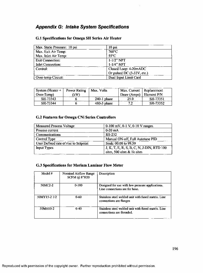
Appendix G: Intake System Specifications
G.l Specifications for Omega SH Series Air Heater
Max. Static Pressure: 10 psi 10 psiMax. Exit Air Temp: 760°CMax. Inlet Air Temp: 55°CExit Connection: 1-1/2” NPTInlet Connection: 1-1/4” NPTControl: Closed Loop: 4-20mADC
Or pulsed DC (3-32V, etc.)Over-temp Circuit: Dual Input Limit Card
System (Heater + Over-Temp)
Power Rating (kW)
Max. Volts Max. Current Draw (Amps)
Replacement Element P/N
SH-73343 6 240-1 phase 25.0 SH-73351SH-73344 6 480-3 phase 7.2 SH-73352
G.2 Features for Omega CNi Series Controllers
Measured Process Voltage 0-100 mV, 0-1 V, 0-10 V ranges.Process current 0-20 mACommunications RS-232Control Type Manual ON-off, Full Autotune PIDUser Defined rate of rise to Setpoint Soak: 00.00 to 99.59Input Types J, K, T, E, R, S, B, C, N, J-DIN, RTD 100
ohm, 500 ohm & lk ohm
G.3 Specifications for Meriam Laminar Flow Meter
Model # Nominal Airflow Range SCFM @ 8”H20
Description
50MC2-2 0-100 Designed for use with low pressure applications. Line connections are for hose.
50MY15-2 1/2 0-60 Stainless steel welded unit with fused matrix. Line connections are flanges
50MH10-2 0-40 Stainless steel welded unit with fused matrix. Line connections are threaded.
196
Reproduced with permission of the copyright owner. Further reproduction prohibited without permission.
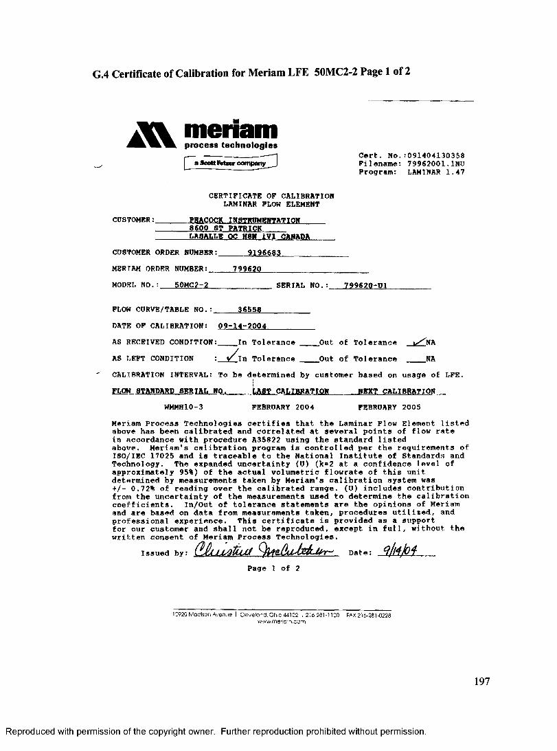
G.4 Certificate of Calibration for Meriam LFE 50MC2-2 Page 1 of 2
A menamp ro cess tech n o lo g ies
" Ia Scott M x c r companyCert. No.:091404130358 Filename: 79962001.1NU Program: LAMINAR 1.47
CUSTOMER:
CERTIFICATE OF CALIBRATION LAMINAR FLOW ELEMENT
PEACOCK INSTRUMENTATION 8600 8T PATRICKLASALLE PC H8N 1V1 CANADA
CUSTOMER ORDER NUMBER:.MERIAM ORDER NUMBER:__MODEL NO.: 50MC2-2
9196683799620
SERIAL NO.: 799620-U1
FLOW CURVE/TABLE NO.:. 36558DATE OF CALIBRATION: 09-14-2004______AS RECEIVED CONDITION:____In ToleranceAS LEFT CONDITION : t/In Tolerance
_Otit of Tolerance Out of Tolerance
CALIBRATION INTERVAL: To be determined by customer based on usage of LFE.]
FLOW STANDARD SERIAL NO._____LAST CALIBRATION_____ NEXT CALIBRATIONWMMH10-3 FEBRUARY 2004 FEBRUARY 2005
Meriam Process Technologies certifies that the Laminar Flow Element listed above has been calibrated and correlated at several points of flow rate in accordance with procedure A35822 using the standard listed above. Meriam's calibration program is controlled per the requirements of ISO/IBC 17025 and is traceable to the National Institute of Standard:* and Technology. The expanded uncertainty (U) (k*2 at a confidence level of approximately 95%) of the actual volumetric flowrate of this unit determined by measurements taken by Meriam's calibration system was +/- 0.72% of reading over the calibrated range. (U) includes contribution from the uncertainty of the measurements used to determine the calibration coefficients. In/Out of tolerance statements are the opinions of Meriam and are based on data from measurements taken, procedures utilised, and professional experience. This certificate is provided as a support for our customer and shall not be reproduced, except in full, without the written consent of Meriam Process Technologies.
Issued by: ClAjLMtLUS Date:Page 1 of 2
1C923 F/odlsor, A v en je I C ievelo-d. Oh o 44102 . 2',6-281-llCO . FAX 2 i6-281 -0228 www.me'ia"vcCT>
197
Reproduced with permission of the copyright owner. Further reproduction prohibited without permission.
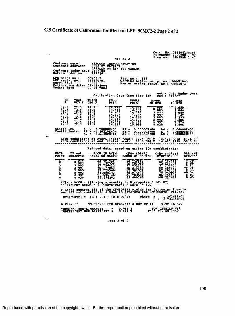
G.5 Certificate of Calibration for Meriam LFE 50MC2-2 Page 2 of 2
Standard Program: LAMINAR 1.47Customer name: Customer address:Customer order no,: Meriam order no.:LFE model no.:LPE serial no.: Curve no.: Calibration date: Todays date:
PEACOCK INSTRUMENTATION8600 ST PATRICK LASALLE QC H8N 9196683 7996201V1 CANADA
50MC2-2799620-U13655809-14-200409-14-2004
Plot no.: 113Working master serial no.: WMMH10-3 Master master serial no.: MMMH10-3
Calibration data from flow lab
52T7-52.451.28 : 148.848.347.8
Tuut DEO F7775“
72! 6 72.672.472.4 72.3
TMASt DEC F74."974.874.8 74.7 74.6 74.4 74.3 74.2
PSuutPSIA14 .416« :ttl14.39714.38714.37714.36414.347
PSMASPSIA'14.379
u - m« : 8 ?13.989
uutmasDPuut In H20
1.056i . mw nl: 991? 8.025
Unit Under Test MasterDpmas In H20
Master LFE Coefficients: A0 = 2.28008E+03Al » -1.20219E+06 A2 = -2,51408E+11A3 = O.OOOOOE+OO A6 =A4 = 0.0Q00QE+0Q A7 =A5 = 0.OOOOOE+OO A8
“ r.OTDl . U it : \ i l6.3057 . 3 7 48.6080.00000E+008 :888881:88
Room conditions at start (inlet read): 72.4 DBG P 14.421 PSIA 53.6 RH Room conditions at end: (inlet read): 72.3 DBG P 14.415 PSIA 50.0 RHReduced data, based on master lfe coefficients:
DATAPOINT DP uut InH20§4C 17035
IT o l3.9975.0055.9926.9378.025
PLOW IN ACPM BASED ON MASTER CFM*_^DATA)
rr. 607518m u m
74.85814286 .53614699.534282
"177540957"i u m n
75.07467086.78353699.808765
CFM* (CURVE) B*DP+C*DP 2
— 1 2 .6 9 0 4 5 8 -
50.18677062.76100175.04097986.755531100.212618181.87)
PERCENTERROR* 4-0739- 8:88 -0.25 -0.33 -0.04 -0.03 0.40
*CPM = ACFM x (Flowing viscosity in Micropoise /** PERCENT ERROR = ( (CURVE-DATA) / DATA) » 100A Least Squares Pit of the CPM(DATA) yields the following formula uut coefficients used to generate the CFM(CURVE) values:and LFE CFM(CURVE)A Flow of
* (B x DP) + (C x DP“2)99.905235 CPM produces a UUT DP of
Where B = 1.26268E+01C = -1.73314E-028.00 In H20
TERMINAL NON-LINEARITY INDEPENDENT NON-LINEARITY 0.9560.144 DETAI FILE NO. 50FOR LS SEE 1:440
Page 2 of 2
198
Reproduced with permission of the copyright owner. Further reproduction prohibited without permission.
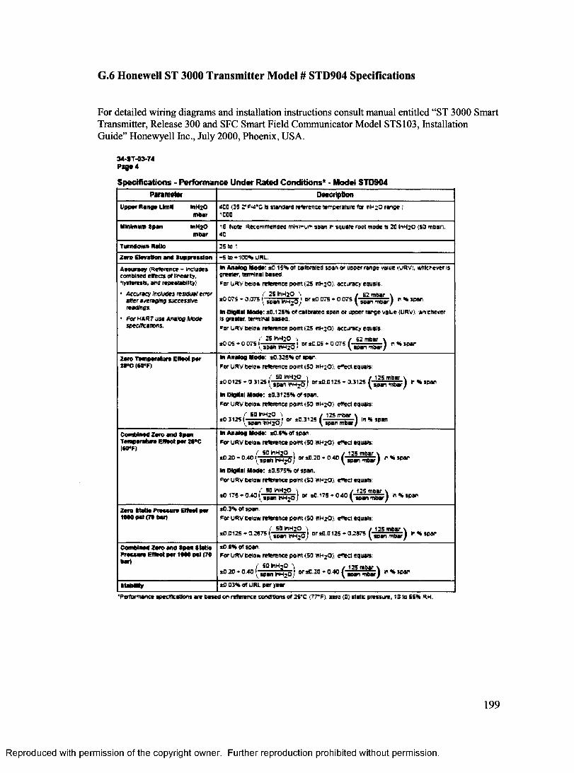
G.6 Honewell ST 3000 Transmitter Model # STD904 Specifications
For detailed wiring diagrams and installation instructions consult manual entitled “ST 3000 Smart Transmitter, Release 300 and SFC Smart Field Communicator Model STS103, Installation Guide” Honewyell Inc., July 2000, Phoenix, USA.
34-ST-03-74 Pag* 4
Specifications - Performance Under Rated Conditions* - Model STD904Parameter Description
Upper Ranee Ltmd InHgO mbar
4CC (39 r ' F ' i ' c b standard reference tem perature for n H j c ra n g e j •ccc
Minimum span m hjO mbar
16 Mote Recom m ended minimum in a n r iq u a re root mode b 2C InH jO (53 mbari. 4C
Turndown Ratio a s to i
Zero Elevation and Suppression -6 t o -1 0 0 % JRL.
Aosunoy R e fe re n c e - Includes com bined effects of I re a r ty , nysteresb , and repeatability:'
■ Accuracy .Irtc'.udei reitouei’ error li f e r a re ra g tap so ccess tre le ad feg s
• fo r HAR7 use Analog Mode specfflciBons.
to Analog Mode: ±0 15% of caiiereled soon o r upper range value (URVl, aftlc rey e r U greater, terminal a a ie c
For URV b e ta* reference p o n t (35 w -2 0 ; accuracy equals
( 25 biH2 0 ■« / £2 m bar \a c 075 - 0.0751, ^ , 0 ,' or lO 075 * 0 075 ^ m r % s p a r
to Dtgdal Mode: ±3.125% <y c iib ra re o sp an or jp o e r range v a k e tURV) veocliever is g rea te r terminal based.F ar URV be tan reference p e n t (25 n h j o ; accuracy eauals
25 lnH2 0 ■, / £ 2 mbar \I. JP M mH^Q i ** --------\m n 'r t o * r f ^
Zero Temperature Effect par I*>C ISO'Fl
to Analog Mode: *0 325% of sp an
For URV b e ip a reference p o r t (53 nHzOX effect equali:
(' 53 P tH 20 / 125 m bar \±0 0 1 2 5 - 0 3125*, or ±0 3125 - 0.3125 ( ^ F % ip a r
to Otgdal Mode: ±3.3125% o r span.f a URV b e ta* reference point (53 rM gOJ effect equals:
f 53 SiHgC *, / 12 5 m bar V ± 0 3 t2 5 I w n H g o j ^ ±E 31IS ( s p a r m b a r )
Combined Zero a n d 8pan Temperature Effect per 2*»C l«*F)
to Analog Mode: *0,6% of sp an
For URV b e to a reference p o r t (50 n H 2 0 J effect equals:
S0tnH 2O 1 / 125 m bar \*0 ZO - 0 4 0 s pan h H jC f " *0-2° * ° 40 ( smt m o a r)
to Dlgdal Mode: ±3.575% or span .
=or URV b etoa reference p o r t (50 nB20>, effect equals:
{ 53 lnH2 0 / 125 m bar \±0 175 - 0 A 0 1 lMn l u. ±C. (75 - 0 40 ( ^ w ) * % s p a r
Zara Statle Fiaeaare EffeeB par 1000 pel (70 bar)
±0.3% of s p a rF or URV b e to a reference p o n t (50 nH2CX effect equab :
( 53 IWH20 / 125 m bar \. 0 0125 - 0 2*75* SMnWj0j nr*0 .312S - 0Z S 75 ( ^ In % s p a r
Combined Zara and tpan itatlo Preaaaia Effect par t*M pal (70 bart
±0 6% o f s p a rFor URV b e to a reference p o n t (50 OHjOX effect equals:
( SB InHgO *, / 1 2 5 m bar \±0 2 0 - 0 .4 0 1 IH ±3.23 ♦ 0 40 ( ^ m % s p a r
Itabaty ±0 03% o f URL p e r yea r
■Performance specifications a re m m on reference conditions or 2S"C (77*fx ze ro (3) ita lic p ressure, 13 to 5SH a n .
199
Reproduced with permission of the copyright owner. Further reproduction prohibited without permission.

G.7 Functional Capability of OTC Emission Analyzer
• Communicates to a PC with OTC software to view live and recorded data in highly detailed graphics.
• Printouts available through PC or OTC printer.• Works on 12 VDC, 110V/60 Hz, 220V/50 Hz power sources.• Software is menu driven and user friendly, icons are available throughout the software.• Can record 20 plus events with record times of 7 minutes per event.• Can be serviced in the field by end user. The NOx cell, 02 cell, and pump are
replaceable.• The MicroGAs analyzer is not designed for use on diesel or two-cycle engines. The
particulate will clog hoses, filters and internal components.• Measurement Ranges
o Hydrocarbons (HC): 0-30000 ppm o Carbon Monoxide (CO): 0-15% o Carbon Dioxide (C02): 0-20% o Oxides of Nitrogen (NOx): 0-5000 ppm o Oxygen (02): 0-25%
Reproduced with permission of the copyright owner. Further reproduction prohibited without permission.
200
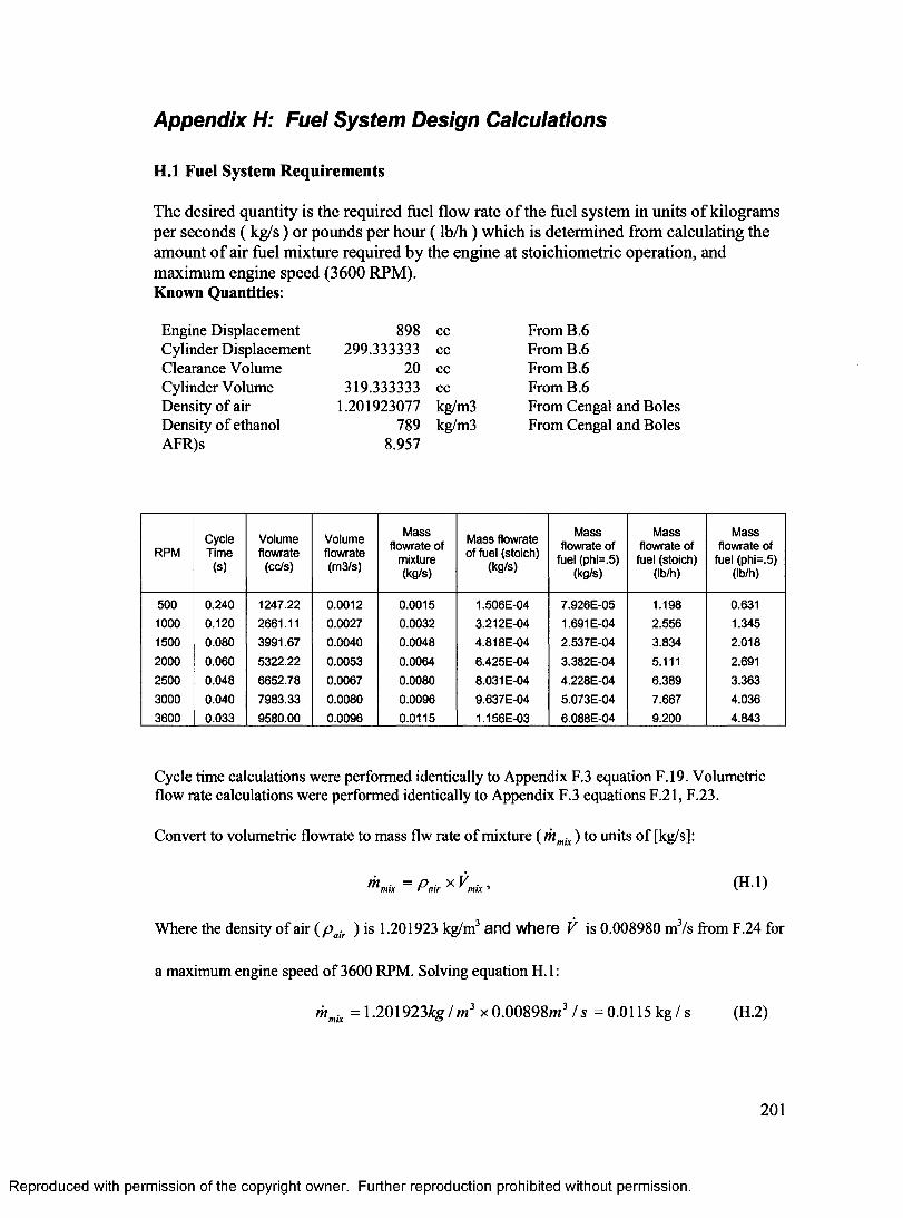
Appendix H: Fuel System Design Calculations
H .l Fuel System Requirements
The desired quantity is the required fuel flow rate o f the fuel system in units o f kilograms per seconds ( kg/s) or pounds per hour ( lb/h) which is determined from calculating the amount o f air fuel mixture required by the engine at stoichiometric operation, and maximum engine speed (3600 RPM).Known Quantities:
Engine Displacement 898 cc From B .6Cylinder Displacement 299.333333 cc From B .6Clearance Volume 20 cc From B .6Cylinder Volume 319.333333 cc From B .6Density of air 1.201923077 kg/m3 From Cengal and BolesDensity of ethanol 789 kg/m3 From Cengal and BolesAFR)s 8.957
RPMC ycleTim e(s)
Volum eflow rate
(cc/s)
Volum eflow rate(m 3/s)
M ass flow rate of
mixture (kg/s)
M ass flow rate of fuel (stoich)
(kg/s)
M ass flow rate of
fuel (phi=.5) (kg/s)
M ass flow rate of
fuel (stoich) (lb/h)
M ass flow rate of
fuel (phi=.5) (lb/h)
500 0 .240 1247.22 0 .0012 0 .0015 1 .506E -04 7 .926E -05 1.198 0.631
1000 0 .120 2661.11 0 .0027 0 .0032 3 .212E -04 1.691 E-04 2 .556 1.345
1500 0 .080 3991 .67 0 .0040 0 .0048 4 .818E -04 2 .537E -04 3 .834 2 .018
2000 0 .060 5322 .22 0.0053 0 .0064 6 .425E -04 3 .382E -04 5.111 2.691
2500 0 .048 6652 .78 0 .0067 0 .0080 8.031 E-04 4 .228E -04 6 .389 3 .363
3000 0 .040 7983 .33 0 .0080 0 .0096 9.637E -04 5 .073E -04 7 .667 4 .036
3600 0 .033 9580 .00 0 .0096 0 .0115 1.156E -03 6 .088E -04 9 .200 4 .843
Cycle time calculations were performed identically to Appendix F.3 equation F.19. Volumetric flow rate calculations were performed identically to Appendix F.3 equations F.21, F.23.
Convert to volumetric flowrate to mass flw rate of mixture (thmix) to units of [kg/s]:
< i X =PairX K u ’ (H 1 )
Where the density of air ( p air ) is 1.201923 kg/m3 and where V is 0.008980 m3/s from F.24 for
a maximum engine speed of 3600 RPM. Solving equation H. 1:
ritmix = 1.201923% /m 3 x 0.00898m3 I s = 0.0115 k g /s (H.2)
201
Reproduced with permission of the copyright owner. Further reproduction prohibited without permission.
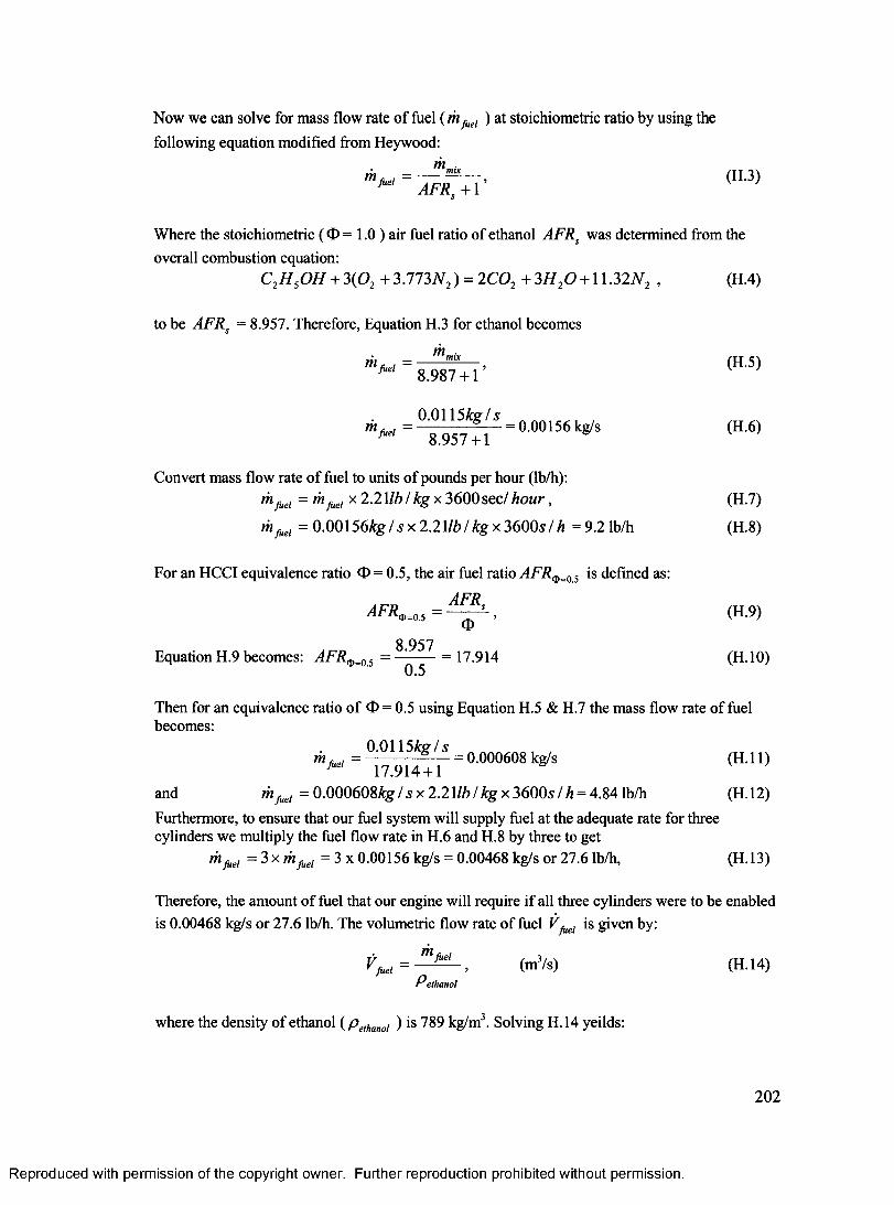
Now we can solve for mass flow rate of fuel ( mfuel ) at stoichiometric ratio by using the following equation modified from Heywood:
h i , , = — , (H.3)** AFRS+ 1 V '
Where the stoichiometric ( ® = 1.0 ) air fuel ratio of ethanol AFRS was determined from theoverall combustion equation:
C2H 50 H + 3 (0 2 + 3.773N2) = 2 C 0 2 + 3H 20 + U .3 2 N 2 , (H.4)
to be AFRS = 8.957. Therefore, Equation H.3 for ethanol becomes
m , , = m,nix , (H.5)^ 8.987 + 1
0 .0115% /sm Ael = --------— — = 0.00156 kg/s (H.6)
M' 8.957 + 1
Convert mass flow rate of fuel to units of pounds per hour (lb/h):m fuel = m fuel x 2.21 lb / % x 3600sec/ h o u r , (H.7)
Wjuei = 0.00156% Is x 2.21/6I k g x 3600s / h =9.2 lb/h (H.8)
For an HCCI equivalence ratio O = 0.5, the air fuel ratio AFR^=0 5 is defined as:
. __ AFR ,AFRo__05= - ^ - , (H.9)
8.957Equation H.9 becomes: AFR^=(> S = =17.914 (H.10)
Then for an equivalence ratio of O = 0.5 using Equation H.5 & H.7 the mass flow rate of fuel becomes:
0 .0115% /sm M = --------— — = 0.000608 kg/s (H.l 1)
^ 17.914 + 1and mfuel = 0 .000608% /s x 2 .21 /6 /% x 3600s lh = 4.84 lb/h (H.12)Furthermore, to ensure that our fuel system will supply fuel at the adequate rate for three cylinders we multiply the fuel flow rate in H .6 and H.8 by three to get
™faei = 3 x fhfaei = 3 x 0.00156 kg/s = 0.00468 kg/s or 27.6 lb/h, (H .l3)
Therefore, the amount of fuel that our engine will require if all three cylinders were to be enabled is 0.00468 kg/s or 27.6 lb/h. The volumetric flow rate of fuel V ju e l is given by:
m ,fuel
* A /V te ,= — ^ - > (m3/s) (H.l 4)
Pethanol
where the density of ethanol ( p ethanoi ) is 789 kg/m3. Solving H. 14 yeilds:
202
Reproduced with permission of the copyright owner. Further reproduction prohibited without permission.
• = 0 .00468% /s = 000005932 m3/s = 0 00593 L/sMl 7 8 9 % //m3
(H.l 5)
Converting volumetric flow rate of fuel to gallons per hour (gal/h) we get:Vjud = Vjuei(m3 / s ) x 264.17(g a l/ m 2)x3 6 0 0 (s / h) (H.16)
V ju = 0.000005932(m3/s )x 2 6 4 .1 7 (g a //m 3)x 3 6 0 0 (s //i) (H.17)
Vfue, =5.64 gal/h (H .l8)
Therefore the fuel flow rate requirement for three cylinder operation of the fuel system is 5.64 gal/h or 0.00593 L/s.
H.2 Fuel Pump Selection:
Accel Model 310-74701 electronic fuel injection (EFI) fuel pump. The Fuel flow rate of the pump
( ^ um/, ) is:
Vpump = 26 gal/hr @ 45 Psi- (H.19)
The factor of oversize ( F0/s ) is determined by:
Fois = TT= -. (H.20)" fu e l
where V fu e l is 5.64 gal/h from equation H .l8 and substituting along with H.19 into H.20 we get:
Fo l s = — = 4.6, (H.21)5.64
Therefore the selection of the Accel Model 310-74701 fuel pump will be more than adequate for the proposed engine, since the factor of oversize is 4.6.
H.3 Fuel Tank Selection:
Fuel volume storage limit ( ) is:
V ^u = U (H-22)
The JAZ 547-250-001-01 Vertical Fuel Tank was selected. It has dimensions of 6” by 6” by 12” and is compatible with the fuel pump selected earlier and alcohol fuels (see Appendix 1.2.)
The volume capacity ( VUnk) of the fuel tank is:=3-7842 L (H.23)
S in C e : K n k ^ *Km i t (H ' 2 4 >
And the JAZ fuel tank is alcohol compatible. Therefore, the JAZ fuel tank will meet the design constraints.
203
Reproduced with permission of the copyright owner. Further reproduction prohibited without permission.
H.4 Fuel Injector Selection
The fuel flow rate for one cylinder was determined earlier (H.8) to be:Wfaei =0-00156k g / s = or 9.2 lb/h,
The dynamic flow rate (m inj ) of the Delphi Multec 2 # 2532087 injector from Appendix 1.3 is:
minj = 17.305 lb/h or 2.1804 g/s, (H.25)
Since: m fue, < minJ (H.26)Therefore, the Delphi Multec 2 injector will meet the design constraints.
H.5 Fuel Regulator and Gauge Selection
The system pressure ( Psys) of the fuel system will be within the following range as determined from the constraints:
Psys = 2 to 5 bar (H.27)
or, Psys = 29 to 72.5 psig, (H.28)
Additionally, the nominal system pressure ( Pnom) for is:
Pnom = 3.1 bar or 45 psig, (H.29)
From Appendix 1.4, the Mallory Regulator Model # 4309 has a regulator pressure range ( Preg ) of:
Preg= 30-100 psi, (H.30)
Since, Preg * Psys (H.31)And the nominal system pressure is within the limits of the pressure regulator:
30psi < Pnom < 100p s i , (H.32)And since, the regulator is both gasoline and alcohol compatible.
Therefore, the Mallory Pressure Regulator meets the design constraints of the fuel system.
From Appendix 1.5, the Omega Model # PGS 25L 160 has a pressure range (Preg) of:
Pgauge = 0-160 psi, (H.30)Since, the pressure regulator range is within the range of the pressure guage.
0 < 30psi < Preg < 100psi < 160psi
Preg
(H.31)
And since, the pressure gauge is both gasoline and alcohol compatible. Therefore, the Omega Pressure gauge meets the design constraints of the fuel system.
204
Reproduced with permission of the copyright owner. Further reproduction prohibited without permission.
Appendix I: Fuel and ECU System Specification
I.l Fuel Pump Specifications
ACCEL Model #310-74710Electronic Fuel Injection (EFI) fuel pump Alcohol compatibilityVolumetric Flow rate Capacity 26 gal/hOperating Pressure 45 psi
1.2 Fuel Tank Specifications
JAZ Model #547-250-001-01Dimensions 6” x 6” x 12”Volume Capacity 1 US gallonVertical design Alcohol compatibility
1.3 Fuel Injector Specifications
Delphi Multec 2 Short Product # FJ10063 or 2532087Operating Pressure 58 psi or (400 kPa)Static Flow Rate 22 lbs/h or (2.76 g/s)Dynamic Flow Rate 17.305 lb/h or (2.1804 g/s)Pulse width / Repetition Rate 2.0 ms / 10.0 msFuel Compatibility Gasoline/alcohol
1.4 Fuel Pressure Regulator
Mallory Racing Regulator Model #4309Fuel compatibility Gasoline/alcoholPressure Range 3 0 -1 0 0 psiType Adjustable, Return style
1.5 Fuel Pressure Gauge
Omega Model # PGS 25L 160Type Stem MountFuel compatibility Gasoline/alcoholPressure Range 0 -1 6 0 psigMaterial 316 stainless steel
1.6 Fuel Filter
JAZ 547-836-006-11Type Inline with -06 AN male endsFuel Compatibility Gasoline/alcoholFinish/Material Blue Anodized aluminiumDimensions 5-l/8”long x 1-1/8” diameter
205
Reproduced with permission of the copyright owner. Further reproduction prohibited without permission.
1.7 Fuel Connectors
Aeroquip Various Model NumbersTypes Swivel Hose ends, AN to NPT, AN union,
AN coupler.Fuel Compatibility Gasoline/alcoholFinish/Material Blue anodized aluminium
1.8 Fuel Hose
Aeroquip Model # 023-FCA0620Type High stress steel braided hoseMaterial Elastomer inner tube, partial stainless inner
wire, and full stainless outer wire braidTemperature Range -49°C to 150°C
1.9 Electronic Control Unit (ECU)
034EFI Stage 3bOperating Temperature -40 to +85°CCurrent Consumption 0.05-16 AmperesInjector Impedance High or low impedance, 12+ ohms recom.Maximum RPM 16000Trigger Modes 5 window hall effect sensorInjection Timing Resolution 1 microsecond to 65.535 millisecondCommunications High Speed RS-232Programming Platform MS Windows98, 2000,Throttle Position Sensor 3 wire universalCoolant Temperature Sensor GM type, 2700 ohm @ 25°CIntake Air Temperature Sensor GM type, 2700 ohm @ 25°CAuxiliary Input 0 - 5 Volt dcManifold Pressure 1 to 2.65 bar provided in enclosureOxygen Sensor 1, 3 or 4 wire universal, for closed loop
206
Reproduced with permission of the copyright owner. Further reproduction prohibited without permission.
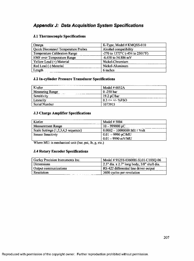
Appendix J: Data Acquisition System Specifications
J.l Thermocouple Specifications
Omega K-Type, Model # KMQSS-010Quick Disconnect Temperature Probes Alcohol compatibilityTemperature Calibration Range -270 to 1372°C (-454 to 2501°F)EMF over Temperature Range -6.458 to 54.886 mVYellow Lead (+) Material Nickel-ChromiumRed Lead (-) Material Nickel-AluminumLength 6 inches
J.2 In-cylinder Pressure Transducer Specifications
Kistler Model # 6052AMeasuring Range 0 -250 barSensitivity 19.2 pC/barLinearity 0.3 <= +/- %FSOSerial Number 1073915
J.3 Charge Amplifier Specifications
Kistler Model # 5004Measurement Range 10 - 999000 pCScale Settings (1,2,3,4,5 sequence) 0.0002 - 10000000 MU / VoltSensor Sensitivty 0.01 -9990 pC/MU
0.01 - 9990 mV/MUWhere MU: is mechanical unit (bar, psi, lb, g, etc.)
J.4 Rotary Encoder Specifications
Gurley Precision Instruments Inc. Model # 9125 S-03600H-5L01 -C18SQ-06Dimensions 2.5" dia. x 2.7" long body; 3/8" shaft dia.Output communications RS-422 differential line driver outputResolution 3600 cycles per revolution
207
Reproduced with permission of the copyright owner. Further reproduction prohibited without permission.
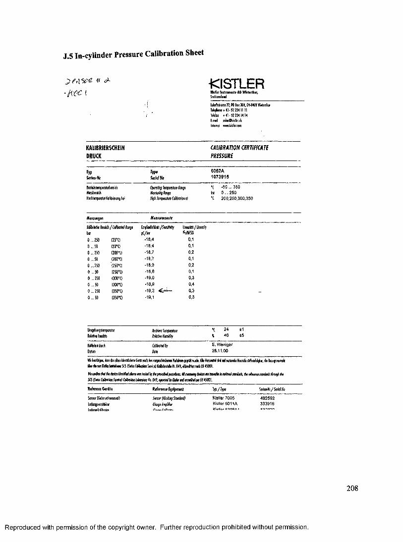
J.5 In-cylinder Pressure Calibration Sheet
•fr-CC-KISTLER
K bflir Tnsirvmeale AG W interthur, Switzerland
Edxhstrosse 22, W Box 304, MOB Winterthur Telephone+ 41- 52 224 1111 Telefax 4 41 - 52 224 14 14 (-moil soleijWt«tler,<h Internet www.kfttlertwn
K A U B R IE R S C H E IND R U C K
C A L IB R A T IO N CERTIFICATE P R E SSU R E
Typ Tyft 6082AS«rien-Nr S trh lN c 1073915
Belriefestemptromibeteich Ofucliaj fenpefo/v/# Sooji ' ( -50 ...350Mesbnekh Mmsjiiiig fmge tar 0 ... 250HKhtefr etofui-Kolibneiung bei Mgh Impaslm CoCbtmm cl °C 200,250,300,350
Mtinmgin Mmuremenh
Uieifei Beteich / (sUhM Smgi EmpfinMta’I /StteMy liimHt/liiemiybof pC/bo s i%fS0
0... 250 (23*0 -18,4 0.10 ...50 (23'C) -18,4 0,10 ...250 (200*0 -18,7 0.20 ... 50 (200*0 -18,7 0,10... 250 (250'Q -18,9 0,2
0 ...50 (250*0 -18,8 0,10 ...250 (300*0 -19,0 0,30 ...50 (300*0 -18,9 0,4
0 ...250 (350*0 -19,2 0,3
0... 50 (350*0 -19,1 0,3
Umjebimistempwolur MUtclImfmlcie
44■*rCM
Kelolbu Fwdile liklin Mfiiy % 46 ±6KoMrtM Calibrated by E. WenigerDotum del) 28.11.00
Wlr best&igea, doss das o6en iiMrietie Getif ooch den vorgesduiebeMt Yafahren gepri# mxde. ABe Messnitlel sind ou( rationale Normafe (Qdyerfolgbw, fa BwugsrormoJe fiber tfievon Kilta betiebene StS (Svrfss (ottwrtkxi Seiviie) KoKbfastifle Wr. 049, ottreitierl iwh EH 45001.
W9wSm^lfa^tilmHM^mtt^bffapftfaMfmt^liM^i^nlM«^ktoaoSonalstonMs,ihtf9ftieKtifonMsAmitith9 SCS (Swiss Cdbotai Swke) CoHtmlkm loimfocf do, 049, opwtdbf CsHtr and ocae&tdper Vi 4SOOJ.
R eferen t G erate Rifermcf Iqtynmi Ty p / T ip # Serieftft/SerWlfoSensor (GebrotxfanotiiiQl)lojuogsversWitorImtiHNKlnliKmlnr
$ww (Wotting Sim fad) Choige AmplifierCt\iunA r
Kistler 7005 Kistler 5011AXi«Har R-lOCrtl
492592333916concio
Reproduced with permission of the copyright owner. Further reproduction prohibited without permission.
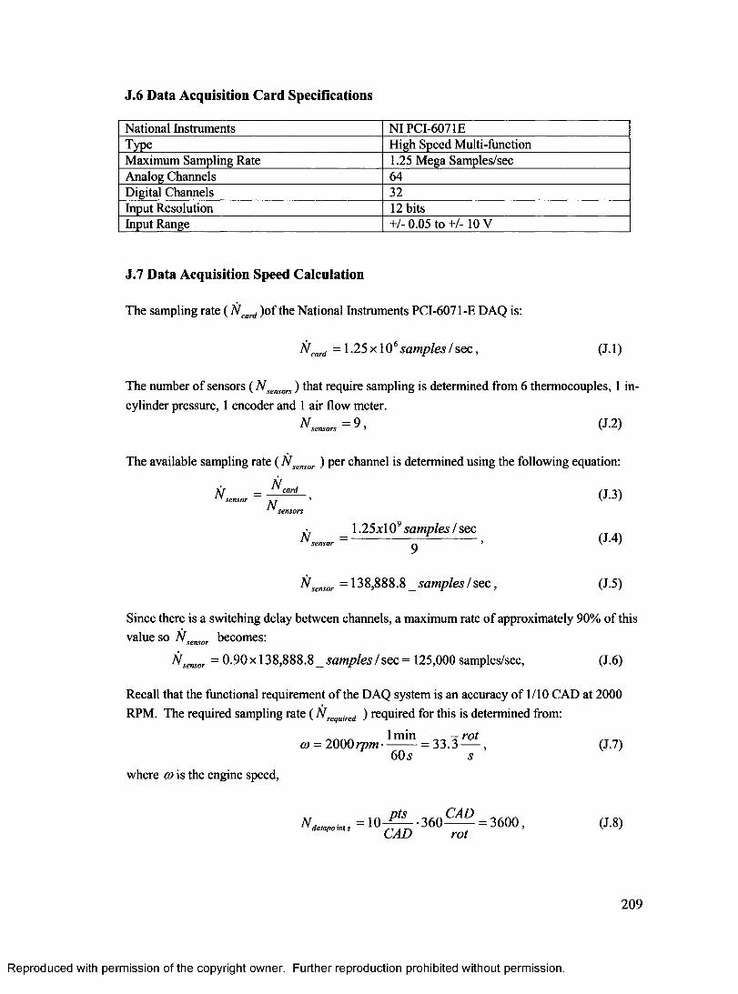
J.6 Data Acquisition Card Specifications
National Instruments NI PCI-607 IEType High Speed Multi-functionMaximum Sampling Rate 1.25 Mega Samples/secAnalog Channels 64Digital Channels 32Input Resolution 12 bitsInput Range +/- 0.05 to +/-10 V
J.7 Data Acquisition Speed Calculation
The sampling rate ( N card )of the National Instruments PCI-6071-E DAQ is:
N card = 1.25 x 10 6 samples / sec , (J. 1)
The number of sensors ( N sensors) that require sampling is determined from 6 thermocouples, 1 incylinder pressure, 1 encoder and 1 air flow meter.
v , „ , „ = 9 , a-2)
The available sampling rate ( N sensor ) per channel is determined using the following equation:
NXT _ ----- ca rd _ , Ji y sensor , 7- >sensor j. j
sensors
1.25x10⁹ samples / secM sen so r = ---------------------- ^ ------------------> ( J - 4 )
N Sensor = 138,888.8 samples / s e c , (J.5)
Since there is a switching delay between channels, a maximum rate of approximately 90% of this value so N sensor becomes:
Nsensor = 0-90 x 138,888.8 _ samples / sec = 125,000 samples/sec, (J.6)
Recall that the functional requirement of the DAQ system is an accuracy of 1/10 CAD at 2000 RPM. The required sampling rate ( N requirei ) required for this is determined from:
a) = 2000 rpm ■ = 33.3 — , (J.7)6O5 s
where co is the engine speed,
= ‘ “ t S t • 360^ r = 3600 - (J-8>CAD rot
209
Reproduced with permission of the copyright owner. Further reproduction prohibited without permission.
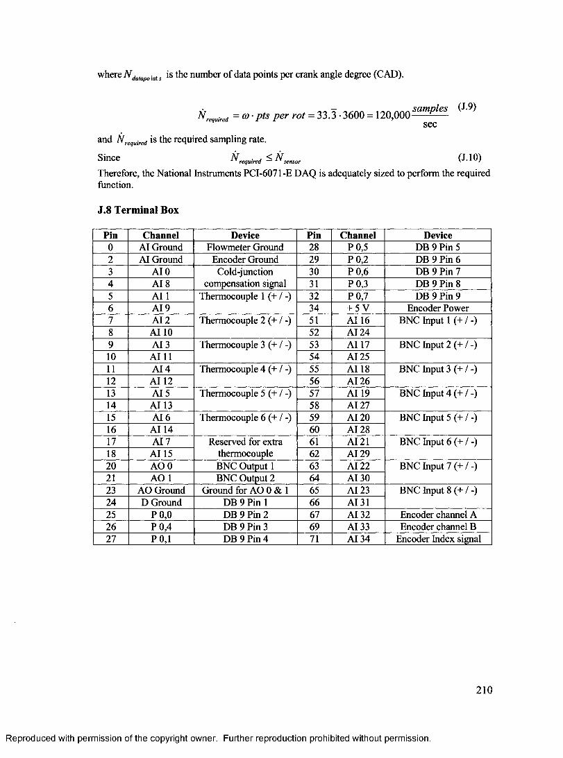
where N datapoints is the number of data points per crank angle degree (CAD).
N required = ® • Pts P ^ rot = 33.3 ■ 3600 = 120,000 samPles ( J ' 9 )
secand N required is the required sampling rate.
S i n C e ^ re q u ir e d ^ ^ s e n s o r ( J 1 0 )
Therefore, the National Instruments PCI-6071-E DAQ is adequately sized to perform the required function.
J.8 Terminal Box
Pin Channel Device Pin Channel Device0 AI Ground Flowmeter Ground 28 P 0,5 DB 9 Pin 52 AI Ground Encoder Ground 29 P 0,2 DB 9 Pin 63 AI 0 Cold-junction
compensation signal30 P 0,6 DB 9 Pin 7
4 AI 8 31 P 0,3 DB 9 Pin 85 AI 1 Thermocouple 1 (+ / -) 32 P 0,7 DB 9 Pin 96 AI 9 34 + 5 V Encoder Power7 AI 2 Thermocouple 2 (+ / -) 51 AI 16 BNC Input 1 (+ /-)8 AI 10 52 AI 249 AI 3 Thermocouple 3 (+ / -) 53 AI 17 BNC Input 2 (+ / -)10 AI 11 54 AI 2511 A I4 Thermocouple 4 (+ / -) 55 AI 18 BNC Input 3 (+ / -)12 AI 12 56 AI 2613 AI 5 Thermocouple 5 (+ / -) 57 AI 19 BNC Input 4 (+ / -)14 AI 13 58 AI 2715 AI 6 Thermocouple 6 (+ / -) 59 AI 20 BNC Input 5 (+ / -)16 AI 14 60 AI 2817 AI 7 Reserved for extra
thermocouple61 AI 21 BNC Input 6 (+ / -)
18 AI 15 62 AI 2920 AO 0 BNC Output 1 63 AI 22 BNC Input 7 (+ / -)21 AO 1 BNC Output 2 64 AI 3023 AO Ground Ground for AO 0 & 1 65 AI 23 BNC Input 8 (+ / -)24 D Ground DB 9 Pin 1 66 AI 3125 P 0,0 DB 9 Pin 2 67 AI 32 Encoder channel A26 P 0,4 DB 9 Pin 3 69 AI 33 Encoder channel B27 P 0,1 DB 9 Pin 4 71 AI 34 Encoder Index signal
210
Reproduced with permission of the copyright owner. Further reproduction prohibited without permission.
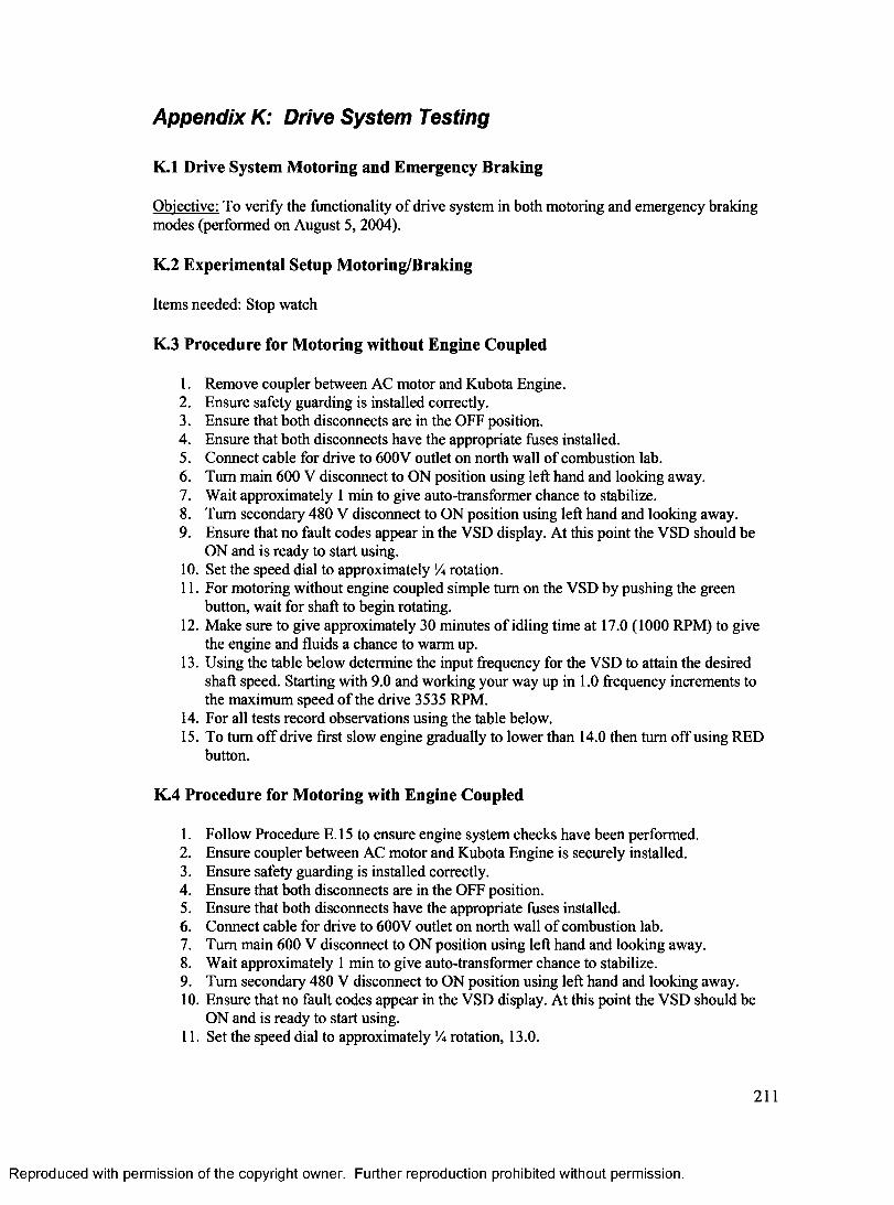
Appendix K: Drive System Testing
K.1 Drive System Motoring and Emergency Braking
Objective: To verify the functionality of drive system in both motoring and emergency braking modes (performed on August 5, 2004).
K.2 Experimental Setup Motoring/Braking
Items needed: Stop watch
K.3 Procedure for Motoring without Engine Coupled
1. Remove coupler between AC motor and Kubota Engine.2. Ensure safety guarding is installed correctly.3. Ensure that both disconnects are in the OFF position.4. Ensure that both disconnects have the appropriate fuses installed.5. Connect cable for drive to 600V outlet on north wall of combustion lab.6 . Turn main 600 V disconnect to ON position using left hand and looking away.7. Wait approximately 1 min to give auto-transformer chance to stabilize.8. Turn secondary 480 V disconnect to ON position using left hand and looking away.9. Ensure that no fault codes appear in the VSD display. At this point the VSD should be
ON and is ready to start using.10. Set the speed dial to approximately XA rotation.11. For motoring without engine coupled simple turn on the VSD by pushing the green
button, wait for shaft to begin rotating.12. Make sure to give approximately 30 minutes of idling time at 17.0 (1000 RPM) to give
the engine and fluids a chance to warm up.13. Using the table below determine the input frequency for the VSD to attain the desired
shaft speed. Starting with 9.0 and working your way up in 1.0 frequency increments to the maximum speed of the drive 3535 RPM.
14. For all tests record observations using the table below.15. To turn off drive first slow engine gradually to lower than 14.0 then turn off using RED
button.
K.4 Procedure for Motoring with Engine Coupled
1. Follow Procedure E. 15 to ensure engine system checks have been performed.2. Ensure coupler between AC motor and Kubota Engine is securely installed.3. Ensure safety guarding is installed correctly.4. Ensure that both disconnects are in the OFF position.5. Ensure that both disconnects have the appropriate fuses installed.6 . Connect cable for drive to 600V outlet on north wall of combustion lab.7. Turn main 600 V disconnect to ON position using left hand and looking away.8. Wait approximately 1 min to give auto-transformer chance to stabilize.9. Turn secondary 480 V disconnect to ON position using left hand and looking away.10. Ensure that no fault codes appear in the VSD display. At this point the VSD should be
ON and is ready to start using.11. Set the speed dial to approximately lA rotation, 13.0.
211
Reproduced with permission of the copyright owner. Further reproduction prohibited without permission.
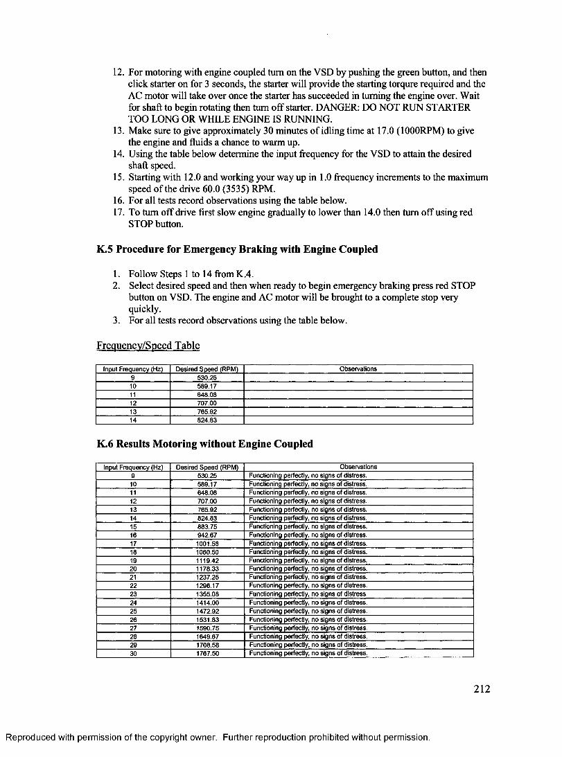
12. For motoring with engine coupled turn on the VSD by pushing the green button, and then click starter on for 3 seconds, the starter will provide the starting torqure required and the AC motor will take over once the starter has succeeded in turning the engine over. Wait for shaft to begin rotating then turn off starter. DANGER: DO NOT RUN STARTER TOO LONG OR WHILE ENGINE IS RUNNING.
13. Make sure to give approximately 30 minutes of idling time at 17.0 (1000RPM) to give the engine and fluids a chance to warm up.
14. Using the table below determine the input frequency for the VSD to attain the desired shaft speed.
15. Starting with 12.0 and working your way up in 1.0 frequency increments to the maximum speed of the drive 60.0 (3535) RPM.
16. For all tests record observations using the table below.17. To turn off drive first slow engine gradually to lower than 14.0 then turn off using red
STOP button.
K.5 Procedure for Emergency Braking with Engine Coupled
1. Follow Steps 1 to 14 from K.4.2. Select desired speed and then when ready to begin emergency braking press red STOP
button on VSD. The engine and AC motor will be brought to a complete stop very quickly.
3. For all tests record observations using the table below.
Frequency/Speed Table
Input Frequency (Hz) Desired Speed (RPM) Observations9 530.2510 589.1711 648.0812 707.0013 765.9214 824.83
K.6 Results Motoring without Engine Coupled
Input Frequency (Hz) Desired Speed (RPM) Observations9 530.25 Functioning perfectly, no signs of distress.10 589.17 Functioning perfectly, no signs of distress.11 648.08 Functioning perfectly, no signs of distress.12 707.00 Functioning perfectly, no signs of distress.13 765.92 Functioning perfectly, no signs of distress.14 824.83 Functioning perfectly, no signs of distress.15 883.75 Functioning perfectly, no signs of distress.16 942.67 Functioning perfectly, no signs of distress.17 1001.58 Functioning perfectly, no signs of distress.18 1060.50 Functioning perfectly, no signs of distress.19 1119.42 Functioning perfectly, no signs of distress.20 1178.33 Functioning perfectly, no signs of distress.21 1237.25 Functioning perfectly, no signs of distress.22 1296.17 Functioning perfectly, no signs of distress.23 1355.08 Functioning perfectly, no signs of distress.24 1414.00 Functioning perfectly, no signs of distress.25 1472.92 Functioning perfectly, no signs of distress.26 1531.83 Functioning perfectly, no signs of distress.27 1590.75 Functioning perfectly, no signs of distress.28 1649.67 Functioning perfectly, no signs of distress.29 1708.58 Functioning perfectly, no signs of distress.30 1767.50 Functioning perfectly, no signs of distress.
212
Reproduced with permission of the copyright owner. Further reproduction prohibited without permission.
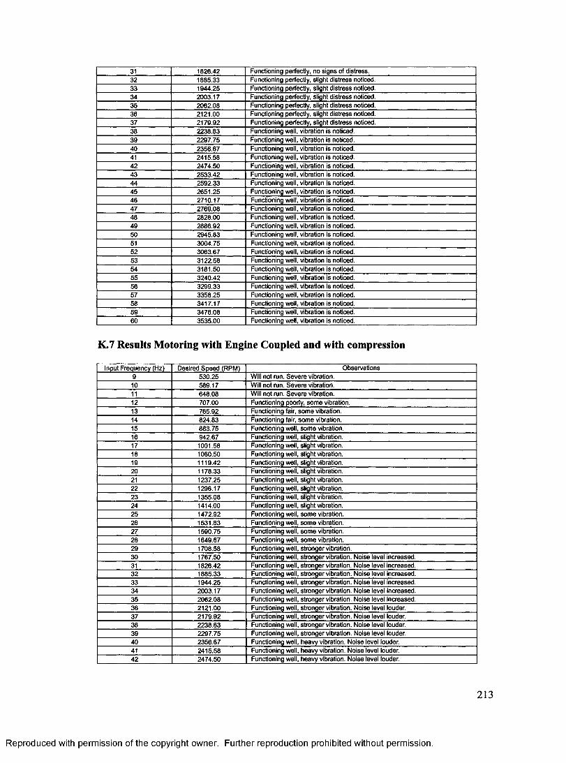
31 1826.42 Functioning perfectly, no signs of distress.32 1885.33 Functioning perfectly, slight distress noticed.33 1944.25 Functioning perfectly, slight distress noticed.34 2003.17 Functioning perfectly, slight distress noticed.35 2062.08 Functioning perfectly, slight distress noticed.36 2121.00 Functioning perfectly, slight distress noticed.37 2179.92 Functioning perfectly, slight distress noticed.38 2238.83 Functioning well, vibration is noticed.39 2297.75 Functioning well, vibration is noticed.40 2356.67 Functioning well, vibration is noticed.41 2415.58 Functioning well, vibration is noticed.42 2474.50 Functioning well, vibration is noticed.43 2533.42 Functioning well, vibration is noticed.44 2592.33 Functioning well, vibration is noticed.45 2651.25 Functioning well, vibration is noticed.46 2710.17 Functioning well, vibration is noticed.47 2769.08 Functioning well, vibration is noticed.48 2828.00 Functioning well, vibration is noticed.49 2886.92 Functioning well, vibration is noticed.50 2945.83 Functioning well, vibration is noticed.51 3004.75 Functioning well, vibration is noticed.52 3063.67 Functioning well, vibration is noticed.53 3122.58 Functioning well, vibration is noticed.54 3181.50 Functioning well, vibration is noticed.55 3240.42 Functioning well, vibration is noticed.56 3299.33 Functioning well, vibration is noticed.57 3358.25 Functioning well, vibration is noticed.58 3417.17 Functioning well, vibration is noticed.59 3476.08 Functioning well, vibration is noticed.60 3535.00 Functioning well, vibration is noticed.
K.7 Results Motoring with Engine Coupled and with compression
Input Frequency (Hz) Desired Speed (RPM) Observations9 530.25 Will not run. Severe vibration.10 589.17 Will not run. Severe vibration.11 648.08 Will not run. Severe vibration.12 707.00 Functioning poorly, some vibration.13 765.92 Functioning fair, some vibration.14 824.83 Functioning fair, some vibration.15 883.75 Functioning well, some vibration.16 942.67 Functioning well, slight vibration.17 1001.58 Functioning well, slight vibration.18 1060.50 Functioning well, slight vibration.19 1119.42 Functioning well, slight vibration.20 1178.33 Functioning well, slight vibration.21 1237.25 Functioning well, slight vibration.22 1296.17 Functioning well, slight vibration.23 1355.08 Functioning well, slight vibration.24 1414.00 Functioning well, slight vibration.25 1472.92 Functioning well, some vibration.26 1531.83 Functioning well, some vibration.27 1590.75 Functioning well, some vibration.28 1649.67 Functioning well, some vibration.29 1708.58 Functioning well, stronger vibration.30 1767.50 Functioning well, stronger vibration. Noise level increased.31 1826.42 Functioning well, stronger vibration. Noise level increased.32 1885.33 Functioning well, stronger vibration. Noise level increased.33 1944.25 Functioning well, stronger vibration. Noise level increased.34 2003.17 Functioning well, stronger vibration. Noise level increased.35 2062.08 Functioning well, stronger vibration. Noise level increased.36 2121.00 Functioning well, stronger vibration. Noise level louder.37 2179.92 Functioning well, stronger vibration. Noise level louder.38 2238.83 Functioning well, stronger vibration. Noise level louder.39 2297.75 Functioning well, stronger vibration. Noise level louder.40 2356.67 Functioning well, heavy vibration. Noise level louder.41 2415.58 Functioning well, heavy vibration. Noise level louder.42 2474.50 Functioning well, heavy vibration. Noise level louder.
213
Reproduced with permission of the copyright owner. Further reproduction prohibited without permission.
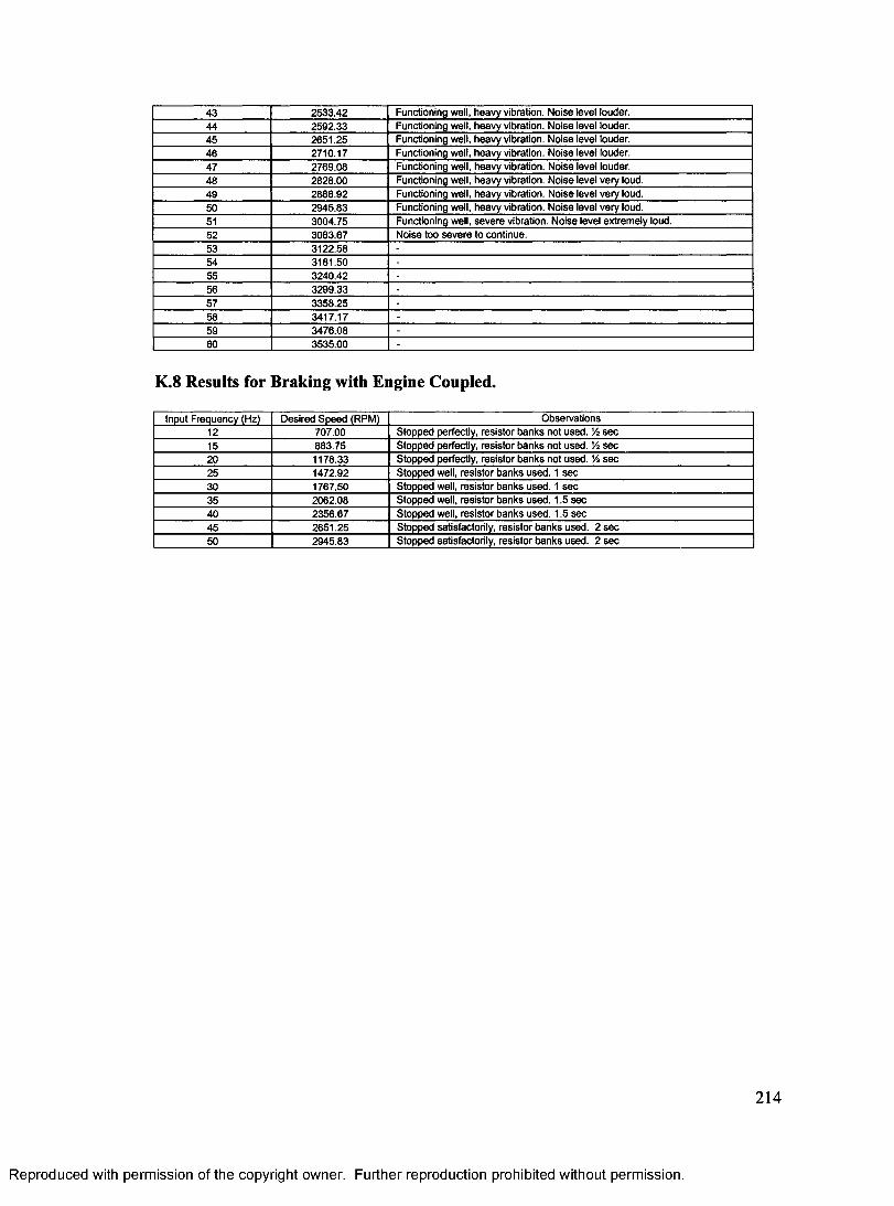
43 2533.42 Functioning well, heavy vibration. Noise level louder.44 2592.33 Functioning well, heavy vibration. Noise level louder.45 2651.25 Functioning well, heavy vibration. Noise level louder.46 2710.17 Functioning well, heavy vibration. Noise level louder.47 2769.08 Functioning well, heavy vibration. Noise level louder.48 2828.00 Functioning well, heavy vibration. Noise level very loud.49 2886.92 Functioning well, heavy vibration. Noise level very loud.50 2945.83 Functioning well, heavy vibration. Noise level very loud.51 3004.75 Functioning well, severe vibration. Noise level extremely loud.52 3063.67 Noise too severe to continue.53 3122.58 -
54 3181.50 -
55 3240.42 -
56 3299.33 -
57 3358.25 -
58 3417.17 -
59 3476.08 -
60 3535.00 -
K.8 Results for Braking with Engine Coupled.
Input Frequency (Hz) Desired Speed (RPM) Observations12 707.00 Stopped perfectly, resistor banks not used. 'A sec15 883.75 Stopped perfectly, resistor banks not used. 'A sec20 1178.33 Stopped perfectly, resistor banks not used. 'A sec25 1472.92 Stopped well, resistor banks used. 1 sec30 1767.50 Stopped well, resistor banks used. 1 sec35 2062.08 Stopped well, resistor banks used. 1.5 sec40 2356.67 Stopped well, resistor banks used. 1.5 sec45 2651.25 Stopped satisfactorily, resistor banks used. 2 sec50 2945.83 Stopped satisfactorily, resistor banks used. 2 sec
Reproduced with permission of the copyright owner. Further reproduction prohibited without permission.
214
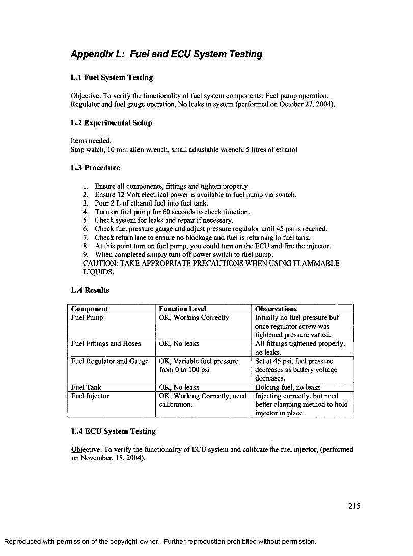
Appendix L: Fuel and ECU System Testing
L.l Fuel System Testing
Objective: To verify the functionality of fuel system components: Fuel pump operation, Regulator and fuel gauge operation, No leaks in system (performed on October 27, 2004).
L.2 Experimental Setup
Items needed:Stop watch, 10 mm alien wrench, small adjustable wrench, 5 litres of ethanol
L.3 Procedure
1. Ensure all components, fittings and tighten properly.2. Ensure 12 Volt electrical power is available to fuel pump via switch.3. Pour 2 L of ethanol fuel into fuel tank.4. Turn on fuel pump for 60 seconds to check function.5. Check system for leaks and repair if necessary.6. Check fuel pressure gauge and adjust pressure regulator until 45 psi is reached.7. Check return line to ensure no blockage and fuel is returning to fuel tank.8 . At this point turn on fuel pump, you could turn on the ECU and fire the injector.9. When completed simply turn off power switch to fuel pump.CAUTION: TAKE APPROPRIATE PRECAUTIONS WHEN USING FLAMMABLE LIQUIDS.
L.4 Results
Component Function Level ObservationsFuel Pump OK, Working Correctly Initially no fuel pressure but
once regulator screw was tightened pressure varied.
Fuel Fittings and Hoses OK, No leaks All fittings tightened properly, no leaks.
Fuel Regulator and Gauge OK, Variable fuel pressure from 0 to 100 psi
Set at 45 psi, fuel pressure decreases as battery voltage decreases.
Fuel Tank OK, No leaks Holding fuel, no leaksFuel Injector OK, Working Correctly, need
calibration.Injecting correctly, but need better clamping method to hold injector in place.
L.4 ECU System Testing
Objective: To verify the functionality of ECU system and calibrate the fuel injector, (performed on November, 18, 2004).
215
Reproduced with permission of the copyright owner. Further reproduction prohibited without permission.
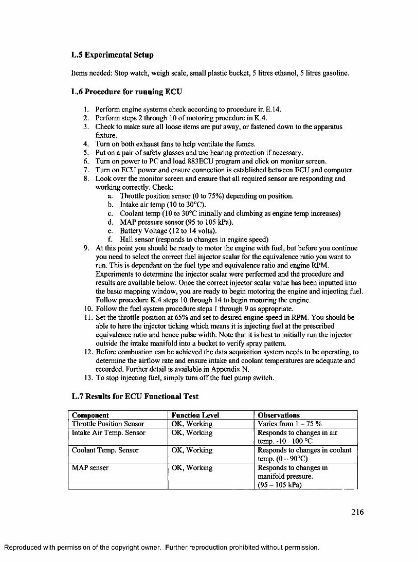
L.5 Experimental Setup
Items needed: Stop watch, weigh scale, small plastic bucket, 5 litres ethanol, 5 litres gasoline.
L.6 Procedure for running ECU
1. Perform engine systems check according to procedure in E. 14.2. Perform steps 2 through 10 of motoring procedure in K.4.3. Check to make sure all loose items are put away, or fastened down to the apparatus
fixture.4. Turn on both exhaust fans to help ventilate the fumes.5. Put on a pair of safety glasses and use hearing protection if necessary.6 . Turn on power to PC and load 883ECU program and click on monitor screen.7. Turn on ECU power and ensure connection is established between ECU and computer.8. Look over the monitor screen and ensure that all required sensor are responding and
working correctly. Check:a. Throttle position sensor (0 to 75%) depending on position.b. Intake air temp (10 to 30°C).c. Coolant temp (10 to 30°C initially and climbing as engine temp increases)d. MAP pressure sensor (95 to 105 kPa).e. Battery Voltage (12 to 14 volts).f. Hall sensor (responds to changes in engine speed)
9. At this point you should be ready to motor the engine with fuel, but before you continue you need to select the correct fuel injector scalar for the equivalence ratio you want to run. This is dependant on the fuel type and equivalence ratio and engine RPM. Experiments to determine the injector scalar were performed and the procedure and results are available below. Once the correct injector scalar value has been inputted into the basic mapping window, you are ready to begin motoring the engine and injecting fuel. Follow procedure K.4 steps 10 through 14 to begin motoring the engine.
10. Follow the fuel system procedure steps 1 through 9 as appropriate.11. Set the throttle position at 65% and set to desired engine speed in RPM. You should be
able to here the injector ticking which means it is injecting fuel at the prescribed equivalence ratio and hence pulse width. Note that it is best to initially run the injector outside the intake manifold into a bucket to verify spray pattern.
12. Before combustion can be achieved the data acquisition system needs to be operating, to determine the airflow rate and ensure intake and coolant temperatures are adequate and recorded. Further detail is available in Appendix N.
13. To stop injecting fuel, simply turn off the fuel pump switch.
L.7 Results for ECU Functional Test
Component Function Level ObservationsThrottle Position Sensor OK, Working Varies from 1 - 75 %Intake Air Temp. Sensor OK, Working Responds to changes in air
temp.-10-100 °CCoolant Temp. Sensor OK, Working Responds to changes in coolant
temp. (0 - 90°C)MAP senser OK, Working Responds to changes in
manifold pressure.(95 - 105 kPa)
216
Reproduced with permission of the copyright owner. Further reproduction prohibited without permission.
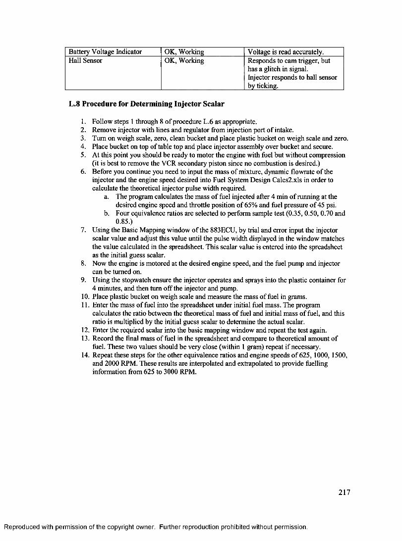
Battery Voltage Indicator OK, Working Voltage is read accurately.Hall Sensor OK, Working Responds to cam trigger, but
has a glitch in signal.Injector responds to hall sensor by ticking.
L.8 Procedure for Determining Injector Scalar
1. Follow steps 1 through 8 of procedure L.6 as appropriate.2. Remove injector with lines and regulator from injection port of intake.3. Turn on weigh scale, zero, clean bucket and place plastic bucket on weigh scale and zero.4. Place bucket on top of table top and place injector assembly over bucket and secure.5. At this point you should be ready to motor the engine with fuel but without compression
(it is best to remove the VCR secondary piston since no combustion is desired.)6 . Before you continue you need to input the mass of mixture, dynamic flowrate of the
injector and the engine speed desired into Fuel System Design Calcs2.xls in order to calculate the theoretical injector pulse width required.
a. The program calculates the mass of fuel injected after 4 min of running at the desired engine speed and throttle position of 65% and fuel pressure of 45 psi.
b. Four equivalence ratios are selected to perform sample test (0.35, 0.50, 0.70 and0.85.)
7. Using the Basic Mapping window of the 883ECU, by trial and error input the injector scalar value and adjust this value until the pulse width displayed in the window matches the value calculated in the spreadsheet. This scalar value is entered into the spreadsheet as the initial guess scalar.
8 . Now the engine is motored at the desired engine speed, and the fuel pump and injector can be turned on.
9. Using the stopwatch ensure the injector operates and sprays into the plastic container for 4 minutes, and then turn off the injector and pump.
10. Place plastic bucket on weigh scale and measure the mass of fuel in grams.11. Enter the mass of fuel into the spreadsheet under initial fuel mass. The program
calculates the ratio between the theoretical mass of fuel and initial mass of fuel, and this ratio is multiplied by the initial guess scalar to determine the actual scalar.
12. Enter the required scalar into the basic mapping window and repeat the test again.13. Record the final mass of fuel in the spreadsheet and compare to theoretical amount of
fuel. These two values should be very close (within 1 gram) repeat if necessary.14. Repeat these steps for the other equivalence ratios and engine speeds of 625, 1000,1500,
and 2000 RPM. These results are interpolated and extrapolated to provide fuelling information from 625 to 3000 RPM.
217
Reproduced with permission of the copyright owner. Further reproduction prohibited without permission.
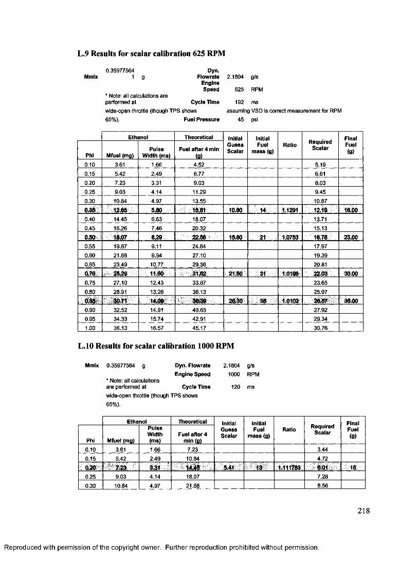
L.9 Results for scalar calibration 625 RPM
0.35977564 D yn.1 9 F lo w ra te 2 .1804 g /s
E n g in eS p e e d 625 RPM
* Note: all calcu la tions a reperfo rm ed a t C y c le T im e 192 m s
w ide-open throttle (though T P S sh o w s a ssu m in g VSD is co rrec t m e a su re m e n t for RPM
65% ). Fuel Pressure 4 5 psi
Ethanol Theoretical InitialGuessScalar
Initial Fuel
mass (g)Ratio Required
ScalarFinalFuel(g)Phi Mfuel (mg)
Pulse Width (ms)
Fuel after 4 min (g)
0.10 3.61 1.66 4 .52 5 .19
0.15 5.42 2 .4 9 6 .77 6.61
0.20 7.23 3.31 9.03 8.03
0.25 9 .03 4 .14 11.29 9 .45
0.30 10.84 4 .97 13.55 10.87
0.35 12.65 5.80 16.81 10.80 14 1.1291 12.19 16.000.40 14.45 O.OJ 18.07 13.71
0 .45 16.26 7.46 20 .32 15.13
0.50 18.07 8.29 22188. 15.60 21 1.0753 18.78 23.000 .55 19.87 9.11 24.84 17.97
0.60 2 1 .68 9.94 27 .10 19.39
0 .65 2 3 .49 10.77 29 .3 6 20.81
0.70 25.29 11.60 31.62 21.80 31 1.0198 22.03 30.000 .75 2 7 .10 12.43 33.87 23 .65
0.80 28.91 13.26 36.13 25 .07
0.85 30.71 14.00 38.39 26.30 38 1.0102 28.87 36.000.90 32 .52 14.91 40 .6 5 27 .92
0.95 34 .33 15.74 42.91 29 .34
1.00 36 .13 16.57 45 .1 7 30 .7 6
L.10 Results for scalar calibration 1000 RPM
M m ix 0 .3 5977564 g D yn. F lo w ra te 2 .1804 g /s
E n g in e S p e e d 1000 RPM* Note: all calcu lationsa re perform ed a t C y c le T im e 120 m s
w ide-open throttle (though T P S sh ow s
65% ).
E th a n o l T h e o re tic a l InitialG u e s sS c a la r
Initial F u e l
m a s s (g)R a tio
R e q u ire dS c a la r
F in a lF u e l(g)
P hi M fuel (m g)
P u ls eW id th(m s)
F u e l a f te r 4 m in (g)
0 .10 3.61 1.66 7.23 3.44
0 .15 5 .42 2 .4 9 10.84 4 .72
0.20 7.23 3.31 14 J8 5.41 13 1.111783 8.01 150 .25 9 .03 4 .14 18.07 7 .28
0 .30 10.84 4 .97 2 1 .6 8 8 .56
218
Reproduced with permission of the copyright owner. Further reproduction prohibited without permission.
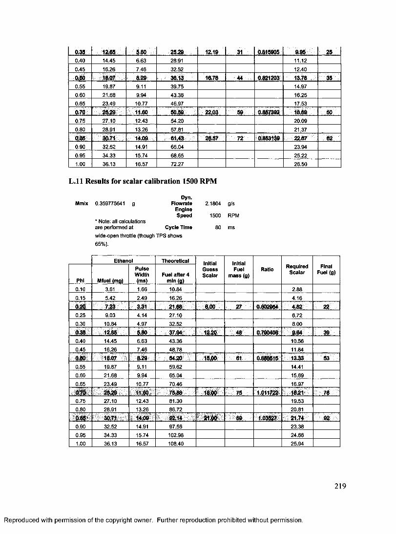
0.35 12.65 5.80 25.29 12.19 31 0.815905 9.95 250 .40 14.45 6.63 28.91 11.12
0 .45 16.26 7 .46 32.52 12.40
0.50 18.07 8.29 36,13 16.78 44 0.821203 13.78 350 .55 19.87 9.11 39 .75 14.97
0.60 21 .6 8 9 .94 4 3 .36 16.25
0.65 23 .4 9 10.77 4 6 .97 17.53
0.70 25.29 11.60 50.59 22.03 59 0.857392 18.69 500.75 27 .1 0 12.43 54 .20 2 0 .09
0.80 28.91 13.26 57.81 21 .37
0.86 30.71 14.09 61.43 26.57 72 0.863139 22.67 620.90 32 .52 14.91 65 .04 23 .94
0.95 34 .33 15.74 68 .65 25 .22
1.00 3 6 .13 16.57 72.27 26 .5 0
L .ll Results for scalar calibration 1500 RPM
0 .359775641 gD yn.
F lo w ra te 2 .1804 g /sE n g in eS p e e d 1500 RPM
* N ote: all calcu lations a re perform ed a t C y c le T im e 80 m s
w ide-open throttle (though T P S sh o w s
65% ).
E th a n o l T h e o re tic a l InitialG u e s sS c a la r
Initial F u e l
m a s s (g)R a tio R e q u ire d
S c a la rF inal
F u e l (g)
P h i M fuel (m g)
P u ls eW id th(m s)
F u e l a f te r 4 m in (g)
0 .10 3.61 1.66 10.84 2 .88
0 .15 5 .42 2 .49 16.26 4 .1 6
0.20 7.23 3.31 21.68 6.00 27 0.802964 4.82 220.25 9 .03 4 .14 2 7 .10 6 .72
0.30 10.84 4 .97 3 2 .52 8 .00
0.35 12.66 5.80 37.94. 12,20 48 0.790408 9.64 390.40 14.45 6 .63 4 3 .3 6 10.56
0.45 16.26 7 .46 48 .7 8 11.84
0.80 18.07 8.29 54.20 15.00 61 0.888615 13.33 530.55 19.87 9.11 59 .62 14.41
0.60 2 1 .68 9 .94 65.04 15.69
0 .65 2 3 .49 10.77 70 .46 16.97
25.29 11.60 75.88 1800 75 1.011722 1821 760 .75 27 .10 12.43 81 .30 19.53
0.80 28.91 13.26 86 .72 20.81
0.8®< 30.71 14.09 92.14 * k f io 89 1.03527 21.74 920 .90 32 .52 14.91 9 7 .56 2 3 .38
0 .95 34 .33 15.74 102.98 2 4 .66
1.00 36.13 16.57 108.40 2 5 .94
Reproduced with permission of the copyright owner. Further reproduction prohibited without permission.
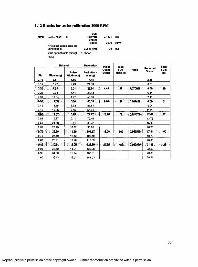
L.12 Results for scalar calibration 2000 RPM
0.359775641 gD yn.
F lo w ra te 2 .1804 g /sE n g in eS p e e d 2000 RPM
* Note: all calcu la tions a re perform ed a t C y c le T im e 60 m s
w ide-open throttle (though T P S sh o w s
65% ).
Ethanol Theoretical InitialGuessScalar
Initial Fuel
m ass (g)Ratio Required
ScalarFinalFuel(9)
Phi Mfuel (mg)Pulse
Width (ms)Fuel after 4
min (g)0.10 3.61 1.66 14.45 2 .35
0.15 5 .42 2 .4 9 2 1 .68 3.61
0.20 7.23 3.31 28.91 4.45 27 1.070806 4.76 290.25 9.03 4 .1 4 36 .13 6 .14
0.30 10.84 4 .97 43 .36 7.41
$38 12,85 ' 580 50.59 9.64 57 0.887476 8.56 510.40 14.45 6 .63 57.81 9.94
0 .45 16.26 7.46 65 .04 11.20
0.50 18.07 8.29 7227 13.78 79 0.914758 12.61 720 .55 19.87 9.11 7 9 .49 13.73
0.60 21 .68 9.94 86 .72 15.00
0.65 23 .49 10.77 93 .95 16.26
0.70 25.29 H .6 0 101.17 18.00 1Q8t 0.963545 17.34 1000.75 27 .10 12.43 108.40 18.79
0.80 28.91 13.26 115.63 20 .0 6
0.80 30.71 14.09 122.85 2t.75 125 0982816 21.38 1230.90 32 .52 14.91 130.08 22 .5 9
0.95 34.33 15.74 137.31 23 .8 6
1.00 36.13 16.57 144.53 25 .1 2
Reproduced with permission of the copyright owner. Further reproduction prohibited without permission.
220
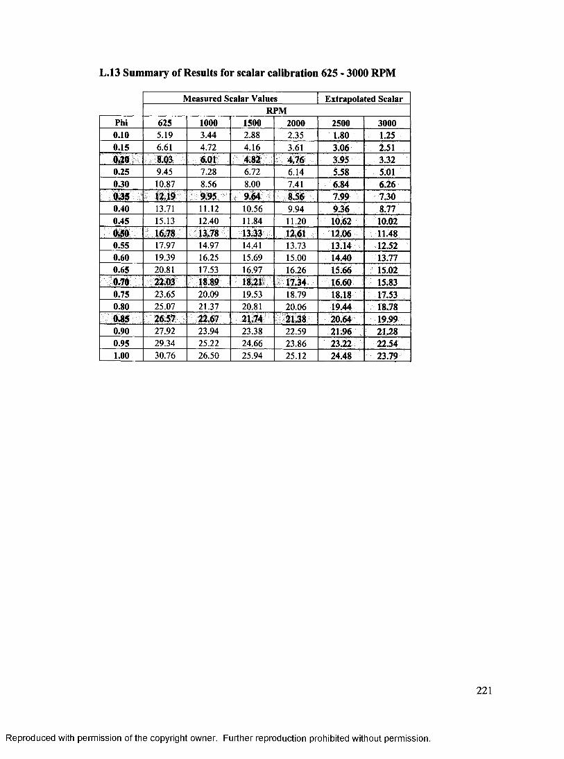
L.13 Summary of Results for scalar calibration 625 - 3000 RPM
Measured Scalar Values Extrapolated ScalarRPM
Phi 625 1000 1500 2000 2500 30000.10 5.19 3.44 2.88 2.35 1.80 1.250.15 6.61 4.72 4.16 3.61 3.06 2.510.20 8.03 6.01 4.82 v. 4 7 6 3.95 3.320.25 9.45 7.28 6.72 6.14 5.58 5.010.30 10.87 8.56 8.00 7.41 6.84 6.260 3 f 12.19 9.95 9.54 8.56 7.99 7.300.40 13.71 11.12 10.56 9.94 9.36 8.770.45 15.13 12.40 11.84 11.20 10.62 10.020.50 16.78 13.78 13.33 12,61 12.06 11.480.55 17.97 14.97 14.41 13.73 13.14 12.520.60 19.39 16.25 15.69 15.00 14.40 13.770.65 20.81 17.53 16.97 16.26 15.66 15.020.70 22.03 18.89 18.21 17.34 16.60 15.830.75 23.65 20.09 19.53 18.79 18.18 17.530.80 25.07 21.37 20.81 20.06 19.44 18.780.85 26.57 22.67 21.74 21.38 20.64 19.990.90 27.92 23.94 23.38 22.59 21.96 21.280.95 29.34 25.22 24.66 23.86 23.22 22.541.00 30.76 26.50 25.94 25.12 24.48 23.79
Reproduced with permission of the copyright owner. Further reproduction prohibited without permission.
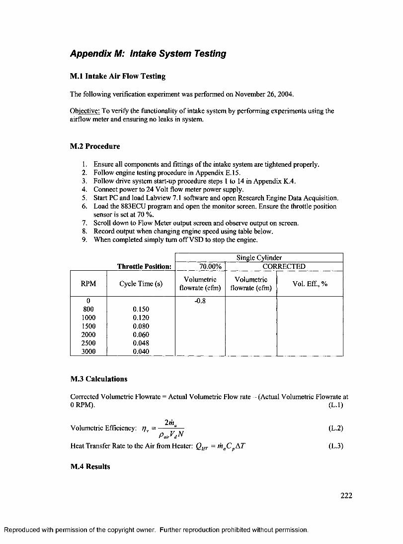
Appendix M: Intake System Testing
M.l Intake Air Flow Testing
The following verification experiment was performed on November 26, 2004.
Objective: To verify the functionality of intake system by performing experiments using the airflow meter and ensuring no leaks in system.
M.2 Procedure
1. Ensure all components and fittings of the intake system are tightened properly.2. Follow engine testing procedure in Appendix E. 15.3. Follow drive system start-up procedure steps 1 to 14 in Appendix K.4.4. Connect power to 24 Volt flow meter power supply.5. Start PC and load Labview 7.1 software and open Research Engine Data Acquisition.6 . Load the 883ECU program and open the monitor screen. Ensure the throttle position
sensor is set at 70 %.7. Scroll down to Flow Meter output screen and observe output on screen.8. Record output when changing engine speed using table below.9. When completed simply turn off VSD to stop the engine.
Throttle Position:Single Cylinder
70.00% CORRECTED
Volumetric VolumetricRPM Cycle Time (s) flowrate (cfm) flowrate (cfm) Vol. Eff., %
0 -0.8800 0.1501000 0.1201500 0.0802000 0.0602500 0.0483000 0.040
M.3 Calculations
Corrected Volumetric Flowrate = Actual Volumetric Flow rate - (Actual Volumetric Flowrate at ORPM). (L.l)
2m„Volumetric Efficiency: r}v = ----------- (L.2)
PoirVdNHeat Transfer Rate to the Air from Heater: QHT = maCpA T (L.3)
M.4 Results
222
Reproduced with permission of the copyright owner. Further reproduction prohibited without permission.
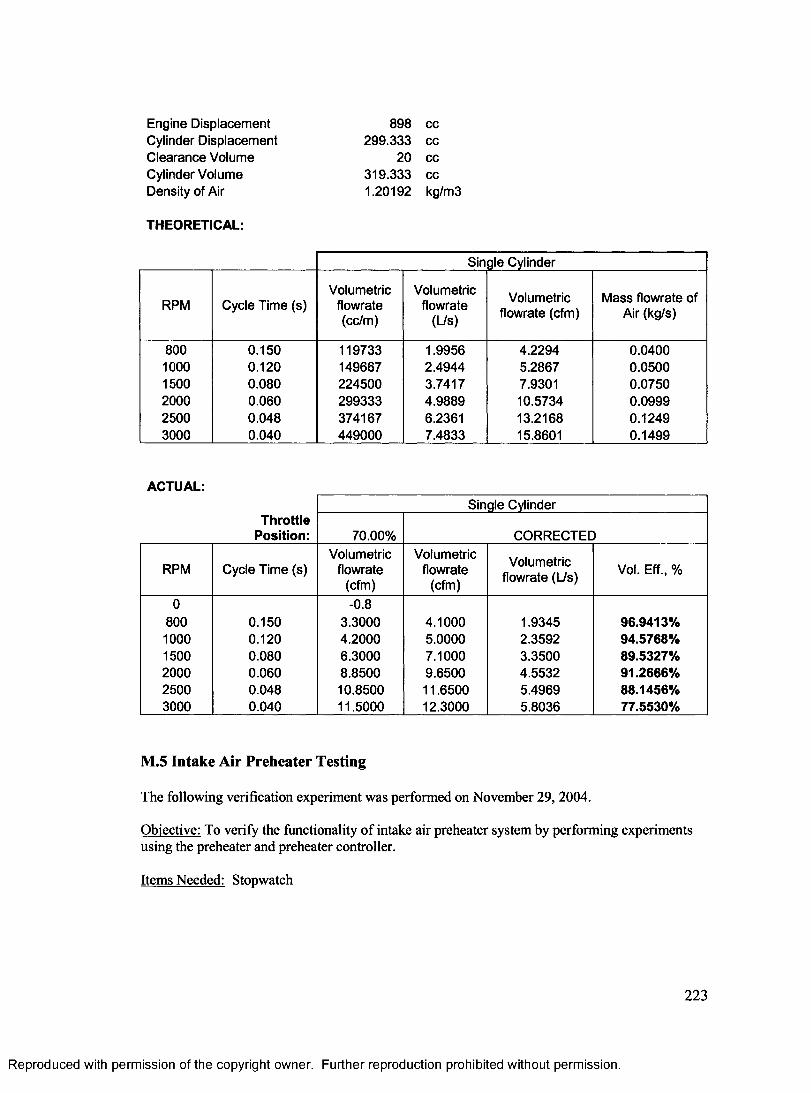
Engine Displacement 898 ccCylinder Displacement 299.333 ccClearance Volume 20 ccCylinder Volume 319.333 ccDensity of Air 1.20192 kg/m3
THEORETICAL:
Single Cylinder
RPM Cycle Time (s)Volumetric
flowrate(cc/m)
Volumetricflowrate
(Us)Volumetric
flowrate (cfm)Mass flowrate of
Air (kg/s)
800 0.150 119733 1.9956 4.2294 0.04001000 0.120 149667 2.4944 5.2867 0.05001500 0.080 224500 3.7417 7.9301 0.07502000 0.060 299333 4.9889 10.5734 0.09992500 0.048 374167 6.2361 13.2168 0.12493000 0.040 449000 7.4833 15.8601 0.1499
ACTUAL:
ThrottlePosition:
Single Cylinder
70.00% CORRECTED
RPM Cycle Time (s)Volumetric
flowrate(cfm)
Volumetricflowrate
(cfm)
Volumetric flowrate (Us) Vol. Eff., %
0 -0.8800 0.150 3.3000 4.1000 1.9345 96.9413%1000 0.120 4.2000 5.0000 2.3592 94.5768%1500 0.080 6.3000 7.1000 3.3500 89.5327%2000 0.060 8.8500 9.6500 4.5532 91.2666%2500 0.048 10.8500 11.6500 5.4969 88.1456%3000 0.040 11.5000 12.3000 5.8036 77.5530%
M.5 Intake Air Preheater Testing
The following verification experiment was performed on November 29, 2004.
Objective: To verify the functionality of intake air preheater system by performing experiments using the preheater and preheater controller.
Items Needed: Stopwatch
223
Reproduced with permission of the copyright owner. Further reproduction prohibited without permission.
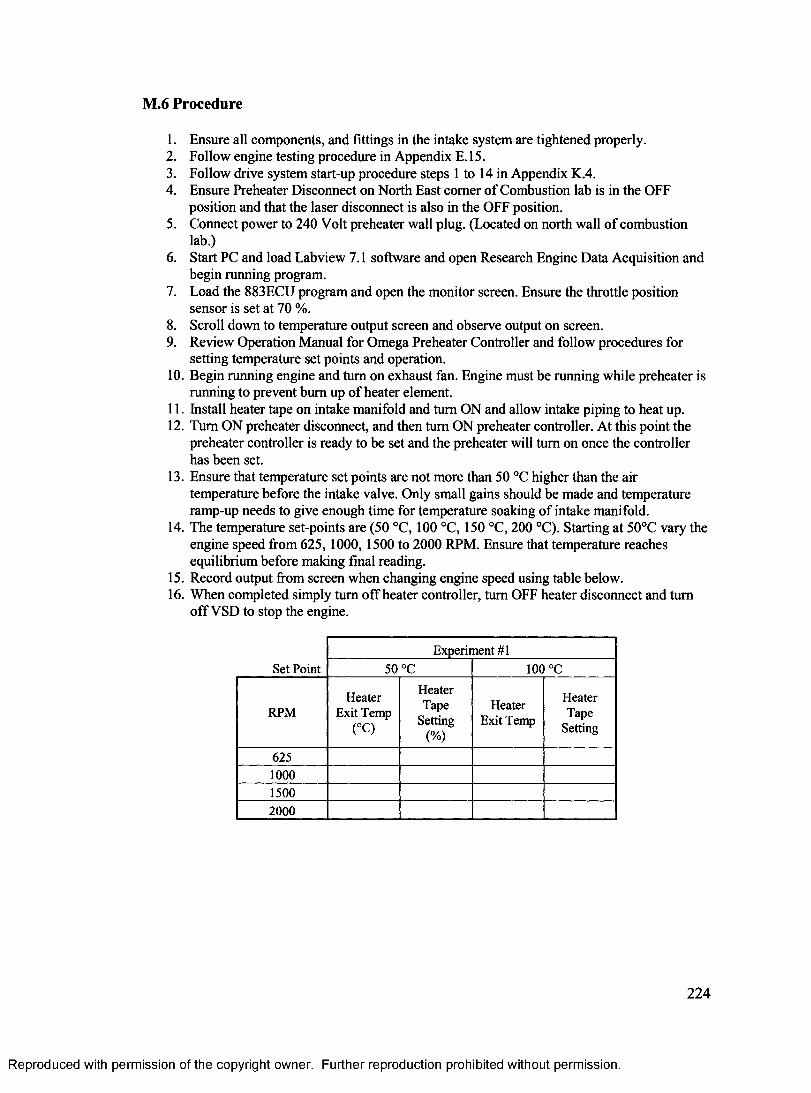
M.6 Procedure
1. Ensure all components, and fittings in the intake system are tightened properly.2. Follow engine testing procedure in Appendix E. 15.3. Follow drive system start-up procedure steps 1 to 14 in Appendix K.4.4. Ensure Preheater Disconnect on North East comer of Combustion lab is in the OFF
position and that the laser disconnect is also in the OFF position.5. Connect power to 240 Volt preheater wall plug. (Located on north wall of combustion
lab.)6. Start PC and load Labview 7.1 software and open Research Engine Data Acquisition and
begin running program.7. Load the 883ECU program and open the monitor screen. Ensure the throttle position
sensor is set at 70 %.8. Scroll down to temperature output screen and observe output on screen.9. Review Operation Manual for Omega Preheater Controller and follow procedures for
setting temperature set points and operation.10. Begin running engine and turn on exhaust fan. Engine must be running while preheater is
running to prevent bum up of heater element.11. Install heater tape on intake manifold and turn ON and allow intake piping to heat up.12. Turn ON preheater disconnect, and then turn ON preheater controller. At this point the
preheater controller is ready to be set and the preheater will turn on once the controller has been set.
13. Ensure that temperature set points are not more than 50 °C higher than the air temperature before the intake valve. Only small gains should be made and temperature ramp-up needs to give enough time for temperature soaking of intake manifold.
14. The temperature set-points are (50 °C, 100 °C, 150 °C, 200 °C). Starting at 50°C vary the engine speed from 625, 1000, 1500 to 2000 RPM. Ensure that temperature reaches equilibrium before making final reading.
15. Record output from screen when changing engine speed using table below.16. When completed simply turn off heater controller, turn OFF heater disconnect and turn
off VSD to stop the engine.
Set PointExperiment #1
50 °C 100 °c
RPMHeater
Exit Temp (°C)
HeaterTape
Setting(%)
Heater Exit Temp
HeaterTape
Setting
625100015002000
224
Reproduced with permission of the copyright owner. Further reproduction prohibited without permission.
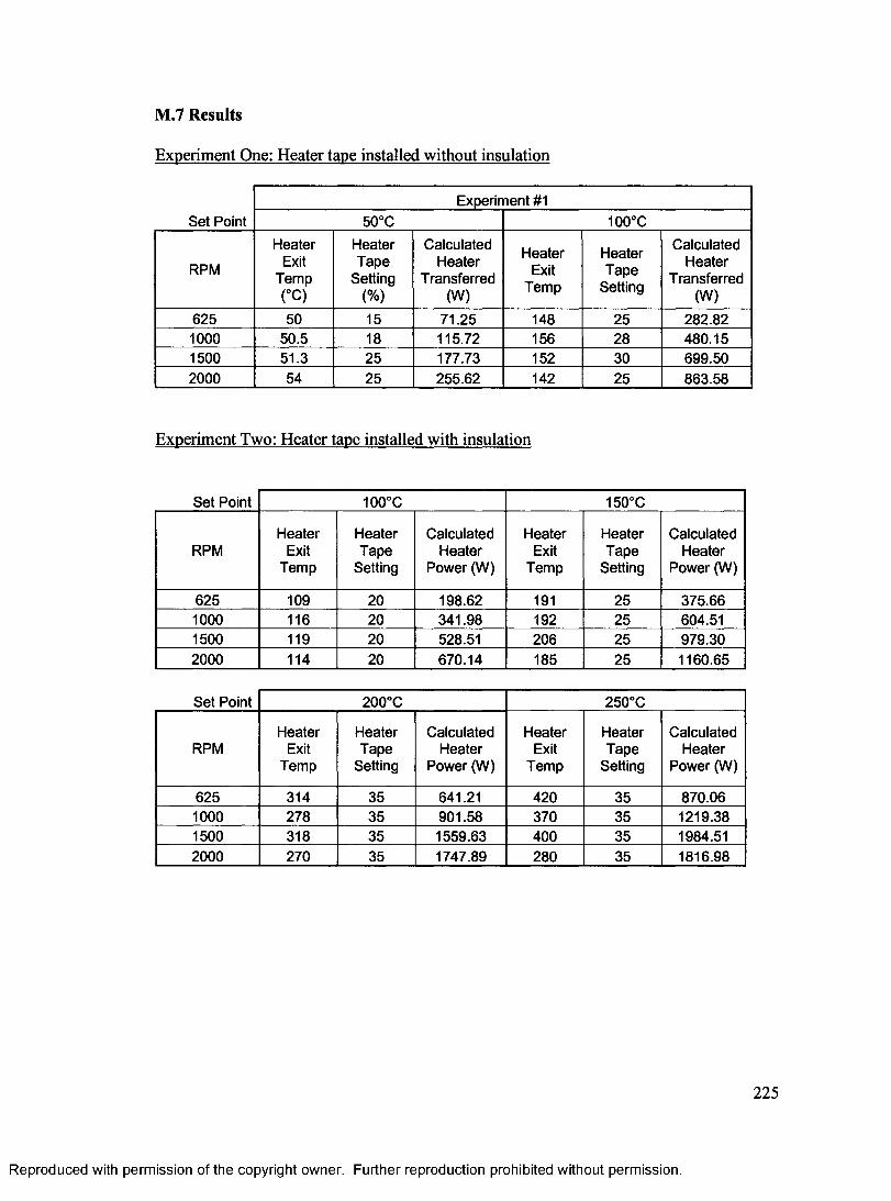
M.7 Results
Experiment One: Heater tape installed without insulation
Set PointExperiment #1
50°C 100°C
RPM
HeaterExit
Temp(°C)
HeaterTape
Setting(%)
CalculatedHeater
Transferred(W)
HeaterExit
Temp
HeaterTape
Setting
CalculatedHeater
Transferred(W)
625 50 15 71.25 148 25 282.821000 50.5 18 115.72 156 28 480.151500 51.3 25 177.73 152 30 699.502000 54 25 255.62 142 25 863.58
Experiment Two: Heater tape installed with insulation
Set Point 100°C 150°C
RPMHeater
ExitTemp
HeaterTape
Setting
Calculated Heater
Power (W)
HeaterExit
Temp
HeaterTape
Setting
Calculated Heater
Power (W)
625 109 20 198.62 191 25 375.661000 116 20 341.98 192 25 604.511500 119 20 528.51 206 25 979.302000 114 20 670.14 185 25 1160.65
Set Point 200°C 250°C
RPMHeater
ExitTemp
HeaterTape
Setting
Calculated Heater
Power (W)
HeaterExit
Temp
HeaterTape
Setting
Calculated Heater
Power (W)
625 314 35 641.21 420 35 870.061000 278 35 901.58 370 35 1219.381500 318 35 1559.63 400 35 1984.512000 270 35 1747.89 280 35 1816.98
Reproduced with permission of the copyright owner. Further reproduction prohibited without permission.
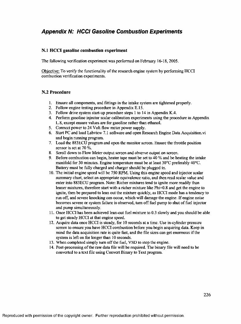
Appendix N: HCCI Gasoline Combustion Experiments
N.l HCCI gasoline combustion experiment
The following verification experiment was performed on February 16-18, 2005.
Objective: To verify the functionality of the research engine system by performing HCCI combustion verification experiments.
N.2 Procedure
1. Ensure all components, and fittings in the intake system are tightened properly.2. Follow engine testing procedure in Appendix E. 15.3. Follow drive system start-up procedure steps 1 to 14 in Appendix K.4.4. Perform gasoline injector scalar calibration experiments using the procedure in Appendix
L.8, except ensure values are for gasoline rather than ethanol.5. Connect power to 24 Volt flow meter power supply.6. Start PC and load Labview 7.1 software and open Research Engine Data Acquisition.vi
and begin running program.7. Load the 883ECU program and open the monitor screen. Ensure the throttle position
sensor is set at 70 %.8. Scroll down to Flow Meter output screen and observe output on screen.9. Before combustion can begin, heater tape must be set to 40 % and be heating the intake
manifold for 30 minutes. Engine temperature must be at least 30°C preferably 40°C. Battery must be fully charged and charger should be plugged in.
10. The initial engine speed will be 750 RPM. Using this engine speed and injector scalar summary chart, select an appropriate equivalence ratio, and then read scalar value and enter into 883ECU program. Note: Richer mixtures tend to ignite more readily than leaner mixtures, therefore start with a richer mixture like Phi=0.8 and get the engine to ignite, then be prepared to lean out the mixture quickly, as HCCI mode has a tendency to run off, and severe knocking can occur, which will damage the engine. If engine noise becomes severe or system failure is observed, turn off fuel pump to shut of fuel injector and pump simultaneously.
11. Once HCCI has been achieved lean-out fuel mixture to 0.3 slowly and you should be able to get steady HCCI at that engine speed.
12. Acquire data once HCCI is steady, for 10 seconds at a time. Use in-cylinder pressure screen to ensure you have HCCI combustion before you begin acquiring data. Keep in mind the data acquisition rate is quite fast, and the file sizes can get enormous if the system is left on for longer than 10 seconds.
13. W hen completed simply turn o ff the fuel, VSD to stop the engine.14. Post-processing of the raw data file will be required. The binary file will need to be
converted to a text file using Convert Binary to Text program.
226
Reproduced with permission of the copyright owner. Further reproduction prohibited without permission.
15. MS Excel is used to import the text data files created using “Convert Binary to Text.VI” into a standard .XLS file.
16. Up to 15 files may be imported at once. Fill in the bordered cells as appropriate and click the IMPORT button.
17. Once the data is imported into Excel, any desired post-processing can be performed easily.
18. Obtain a representative sample of the HCCI combustion event and perform analysis and construct graphs. P-V diagram, P-CAD, and perform calculations to determine indicated power.
w = O i - v 2 ) [ A + 4 ( a + / ?2 ) + / ?2 ]
6 10
Engine Speed Compression
WorkExpansion Work
Indicated Work Indicated Power Indicated Power
3000 RPM
341.43 Nm 393.7736 Nm
52.35 Nm 3925.99 W
5.264838 HP
N.4 Results
UPR Prss (bar) PRC Press (bar) CA CAD Indicated Work volume-3.72 7.80 297.93 -62.07 ffREFI 129.99-8.79 2.70 298.02 -61.98 0.043387 129.77-3.72 7.80 298.10 -61.90 0.043387 129.56-3.72 7.80 298.18 •61.82 0.064481 129.34-3.72 7.80 298.26 -61.74 0.06446 129.13-3.60 7.90 288.35 -61.65 0.064874 128.91-3.42 8.10 298.43 -61.57 0.066114 128.70-3.54 8.00 268.51 -61.49 0.066526 128.49-3.42 8.10 268 60 -61.40 0.066527 128.27-3.60 7.90 298.68 -61.32 0.066113 128.06•3.54 8.00 296.76 -61.24 0.065724 127.84-3.54 8.00 296.84 -61.16 0.066114 127.63-3.05 8.40 298.93 -61.07 0.067766 127.41-3.36 8.10 299.01 -60.96 0.068179 127.20-3.42 8.10 299.09 -60.81 0.06694 126.98-3.42 8.10 299.17 -60.83 0.066939 126.77-3.17 8.30 298.26 -60.74 0.067766 126.56-3.30 8 20 299.34 -60.66 0.06818 126.34-3.23 8.30 299.42 -60.58 0.068179 126.13-3.36 8.10 299.50 -60.50 0.067766 125.91-3.42 8.10 299.59 -60.41 0.066964 125.70-3.78 7.70 299.67 -60.33 0.065287 125.49-3.42 8.10 299.75 -60.25 0.065286 125.27-2.99 8.50 299.83 -60.17 0.068593 125.06-2.81 8.70 298.92 •60.08 0.071071 124.85•2.99 8.50 300.00 -60.00 0.071072 124.63-3.42 8.10 300.08 -59.92 0.068593 124.42-2.93 8.60 300.17 -59.83 0.069005 124.21-2.93 8.60 300.25 -59.75 0.071072 123.99-2.99 6.50 300.33 ■59.67 0.070658 123.78-3.17 8.30 300.41 -59.59 0.069419 123.57-3.05 8.40 300.50 •59.50 0.069031 123.35-2.93 8.60 300.58 -56.42 0.070246 123.14-2.75 8.80 300.66 -59.34 0.071896 122.93-2.99 8.50 300.74 -59.26 0.071485 122.71-2.93 8.60 300.83 -59.17 0.070659 122.50-2.75 8.80 300.91 -58 09 0.071896 122.29•2.93 8.60 300.99 -59.01 0.071896 122.08•2.69 8.60 301.07 -58.93 0.071898 121.86-2.66 8.80 301.16 •58.84 0.072725 12165-2.56 8.90 301.24 -58.76 0.073138 121.44
227
Reproduced with permission of the copyright owner. Further reproduction prohibited without permission.
<b <b
•2.62 8.90 301.32-2.56 8.90 301.40•2.50 9.00 301.49-2.44 9.10 301.57-2.62 8.90 301.65-2.75 8.80 301.74-2.62 8.90 301.82-2.32 9.20 301.90-2.81 8.70 301.98-1.77 9.70 302.07-2.14 9.40 302.15•2.32 9.20 302.23-2.38 9.10 302.31-2.20 9.30 302.40-2.44 9.10 302.48-2.06 9.40 302.56•2.20 9.30 302.64-2.20 9.30 302.73•2.14 9.40 302.81-1.89 9.60 302.89•2.01 9.50 302.98-1.89 9.60 303.06-1.95 9.50 303.14-1.77 9.70 303.22-1.89 9.60 303.31-1.95 9.50 303.39-1.89 9.60 303.47-1.71 9.80 303.55•2.38 9.10 303.64-1.59 9.90 303.72-1.71 9.80 303.80-1.59 6.90 303.88-1.59 9.90 303.97-1.40 10.10 304.05-1.34 10.20 304.13-1.28 10.20 304.21-1.22 10.30 304.30-1.28 10.20 304.38-1.40 10.10 304.46-1.40 10.10 304.55-1.40 10.10 304.63-1.53 10.00 304.71-1.10 10.40 304.79-1.28 10.20 304.88-1.10 10.40 304.96-1.10 10.40 305.04-1.04 10.50 305.12-0.18 11.30 305.21-0.98 10.50 305.29-0.98 10.50 305.37-1.04 10.50 305.45-0.92 10.60 305.54-0.85 10.60 305.62-0.73 10.80 305.70-0.73 10.80 305.79-0.87 10.80 305.87-0.73 10.80 305.95-0.67 10.80 306.03-0.55 11.00 306.12-0.67 10.80 306.20-0.61 10.90 306.28-0.55 11.00 306.36-0.55 11.00 306.45-0.43 11.10 306.53-0.37 11.10 306.61-0.43 11.10 306.69
.43 11.10 306.78
.18 11.30 306.66•2.99 8.50 306.94-0.81 10.90 307.02-0.12 11.40 307.11-0.18 11.30 307.190.24 11.70 307.270.00 11.50 307.360.00 11.50 307.440.12 11.60 307.520.24 11.70 307.600.12 11.60 307.690.06 11.60 307.770.31 11.80 307.850.31 11.80 307.930.37 11.90 308.020.49 12.00 308.100.31 11.80 308.180.49 12.00 306.260.79 12.30 308.350.55 12.00 308.430.73 12.20 308.510.55 12.00 306.600.73 12.20 308.68
-58.66 0.073578 121.23-58.60 0.07355 121.01-5851 0.073965 120.80•58.43 0.07479 120.59-58.35 0.074378 120.38-58.28 0.073138 120.17-56.18 0.073137 119.95-58.10 0.074791 119.74-58.02 0.073964 119.53-57.93 0.076031 119.32-57.85 0.076952 119.11-57.77 0.076857 118.90-57.69 0.075617 118.68-57.60 0.076031 118.47-57.52 0.078031 118.26-57.44 0.076443 118.05♦57.36 0.07727 117.84-57.27 0.076856 117.63-57.19 0.07727 117.42-57.11 0.07851 117.21-57.02 0.078952 117.00•56.94 0.078922 116.79•56.86 0.078923 116.58-56.78 0.079336 116.37•56.69 0.079749 116.16•56.61 0.078923 115.95-56.53 0.078922 115.74-56.45 0.080163 115.53-56.36 0.078097 115.32-56.26 0.078509 115.11•56.20 0.081432 114.90-56.12 0.081402 114.69-56.03 0.081815 114.48-55.95 0.082642 114.27-55.87 0.083882 114.06-55.79 0.084294 113.85-55.70 0.084708 113.64-55.62 0.084707 113.43•55.54 0.083882 113.22-55.45 0.083468 113.01-55.37 0.083499 112.81•55.29 0.083054 112.60-55.21 0.084295 112.39-55.12 0.085121 112.18-55.04 0.08512 111.97•54.96 0.085948 111.76•54.88 0.08636 111.56-54.79 0.09008 111.35-54.71 0.09008 111.14-54.63 0.086773 110.93-54.55 0.086806 110.72-54.46 0.087187 110.52-54.38 0.067601 110.31-54.30 0.088426 110.10-54.21 0.069253 109.90-54.13 0.089252 109.69•54.05 0.089253 109.48-53.97 0.069253 109.27-53.88 0.090079 109.07•53.80 0.09008 106.86-53.72 0.089699 108.65-53.64 0.090492 108.45-53.55 0.090906 108.24-53.47 0.091319 108.04-53.39 0.091732 107.83-53.31 0.091733 107.62-53.22 0.091732 107.42-53.14 0.092559 107.21-53.06 0.081816 107.01-52.98 0.080162 106.80-52.89 0.092179 106.60-52.81 0.093799 106.39-52.73 0.095038 106.16-52.64 0.095864 105.98-52.56 0.095038 105.78-52.48 0.09545 105.57-52.40 0.096278 105.37-52.31 0.096278 105.16-52.23 0.095864 104.96-52.15 0.096691 104.75-52.07 0.097553 104.55-51.98 0.097931 104.34•51.90 0.098756 104.14-51.82 0.098344 103.94-51.74 0.098343 103.73-51.65 0.10041 103.53-51.57 0.10041 103.33-51.49 0.099996 103.12-51.40 0.099997 102.92-51.32 0.099996 102.72
228
Reproduced with permission of the copyright owner. Further reproduction prohibited without permission.
0.73 12.20 306.76 -51.24 0.10086 102.510.24 11.70 308.84 -51.16 0.098757 102.310.79 12.30 308.93 -51.07 0.09917 102.110.85 12.40 309.01 -50.99 0.102062 101.911.22 12.70 309.09 -50.91 0.103716 101.700.73 12.20 309.17 -50.83 0.102868 101.501.22 12.70 309.26 -50.74 0.102889 101.301.10 12.60 309.34 -50.66 0.104542 101.101.77 13.30 309.42 -50.58 0.10702 100.901.16 12.70 309.50 -50.50 0.107435 100.691.28 12.80 309.59 -50.41 0.105407 100.491.22 12.70 309.67 -50.33 0.105369 100.291.34 12.80 309.75 -50.25 0.106367 100.091.26 12.80 309.83 -50.17 0.105782 99.891.40 12.90 309.92 -50.08 0.106194 99.691.46 13.00 310.00 -50.00 0.107021 99.491.59 13.10 310.06 •49.92 0.107848 99.291.65 13.10 310.17 •49.83 0.10826 99.081.59 13.10 310.25 -49.75 0.108261 98.881.65 13.10 310.33 -49.67 0.10826 98.681.77 13.30 310.41 -49.59 0.100087 98.461.89 13.40 310.50 -49.50 0.110367 98.281.89 13.40 310.58 -49.42 0.11074 98.081.71 13.20 310.66 -49.34 0.109913 97.881.83 13.30 310.74 -49.26 0.109501 97.681.83 13.30 310.83 -49.17 0.109914 97.492.01 13.50 310.91 -49.09 0.110739 97.292.01 13.50 310.99 -49.01 0.111567 97.092.01 13.50 311.07 •46.93 0.111565 96.892.20 13.70 311.10 •48.04 0.112393 96.692.08 13.60 311.24 -48.76 0.112806 96.492.32 13.60 311.32 -48.68 0.113201 96.292.20 13.70 311.40 -48.60 0.113631 96.092.38 13.90 311.49 -48.51 0.114046 95.892.38 13.90 311.57 -48.43 0.114871 95.701.95 13.50 311.65 -48.35 0.11322 95.503.23 14.70 311.74 -48.26 0.116525 95.302.50 14.10 311.82 •48.18 0.119003 95.102.75 14.20 311.90 -48.10 0.116938 94.912.01 13.50 311.96 •48.02 0.114458 94.712.62 14.10 312.07 -47.93 0.114046 94.512.93 14.40 312.15 -47.85 0.117800 94.312.62 14.10 312.23 -47.77 0.117765 94.122.93 14.40 312.31 -47.69 0.117763 93.922.87 14.40 312.40 -47.60 0.119004 93.722.99 14.50 312.46 -47.52 0.119418 93 533.17 14.70 312.56 -47.44 0.120656 93.333.23 14.70 312.64 -47.36 0.121484 93.133.30 14.80 312.73 -47.27 0.121895 92.943.17 14.70 312.81 -47.19 0.121897 92.743.23 14.70 312.89 -47.11 0.121484 92.553.72 15.20 312.98 -47.02 0.123595 92.353.54 15.00 313.06 -46.94 0.124788 92.163.48 15.00 313.14 -46.86 0.123963 91.963.36 14.90 31322 -46.78 0 12355 91.773.54 15.00 313.31 -46.69 0.123548 91.573.60 15.10 313.39 -46.01 0.124376 91.383.66 15.20 313.47 -46.53 0.125201 91.164.03 15.50 313.55 •46.45 0.126855 90.993.72 15.20 313.64 -46.36 0.126855 90.793.85 15.30 31372 -46.28 0.126026 90.603.78 15.30 313.80 •46.20 0.126486 90.403.91 15.40 313.88 -46.12 0.126855 90.213.97 15.50 313.97 -46.03 0.12768 90.02421 15.70 314.05 •45.95 0.128922 69.823.66 15.20 314.13 -45.87 0.127682 89.634.09 15.60 314.21 -45.79 0.127207 89.444.21 15.70 314.30 -45.70 0.129335 89.24421 15.70 314.38 -45.62 0.129740 89.054.39 15.90 314.46 -45.54 0.130574 68.864.82 16.30 314.55 •45.45 0.133054 88.074.39 15.90 314.63 -45.37 0.133102 88.474.52 16.00 314.71 -45.29 0.131812 88.284.52 16.00 314.79 -45.21 0.132227 86.094.58 16.10 314.88 -45.12 0.13264 87.904.70 10.20 314.96 -45.04 0.133465 87.714.76 16.30 315.04 -44.96 0.134293 87.514.21 15.70 315.12 -44.68 0.132226 87.324.94 16.40 315.21 -44.79 0.13264 87.134.94 16.40 31529 -44.71 0.135533 86.944.64 10.10 315.37 •44.63 0.134292 86.755.00 10.50 315.45 -44.55 0.134755 86.565.19 16.70 315.54 •44.46 0.137186 86.375.07 16.60 315.62 -44.38 0.137599 86.185.25 16.70 315.70 -44.30 0.137597 85.995.19 10.70 315.79 -44.21 0.138012 85.805.25 18.70 315.87 -44.13 0.13801 85.615.62 17.10 315.95 -44.05 0.139665 85.425.49 17.00 316.03 -43.97 0.140905 85.235.74 17.20 316.12 -43.88 0.141316 85.04
229
Reproduced with permission of the copyright owner. Further reproduction prohibited without permission.
5.68 17.20 316.20 -43.80 0.142144 84.855.55 17.10 316.28 -43.72 0.141782 84.665.74 17.20 316.36 -43.64 0.141729 84.485.86 17.40 316.45 -43.55 0.142971 84.295.86 17.40 316.53 -43.47 0.143797 64.106.16 17.70 316.61 -43.39 0.145035 83.917.08 18.60 316.69 -43.31 0.149995 83.725.98 17.50 316.78 -43 22 0.149167 83 545.86 17.40 316.86 -43.14 0.14421 83.356.04 17.50 316.94 -43.06 0.14421 83.166.29 17.80 317.02 -42.96 0.145661 82.976.35 17.80 317.11 -42.89 0.147156 82.796.29 17.80 317.19 -42.81 0.147103 82.606.47 18.00 317.27 -42.73 0.147929 82.41659 18.10 317.38 •42.64 0.149167 82.236.65 18.20 317.44 •42.56 0.149995 82.046.71 18.20 317.52 -42.48 0.150407 81.856.77 18.30 317.60 -42.40 0.150822 81.677.08 18.60 317.69 -42.31 0.152474 81.487.02 18.50 317.77 -4223 0.153299 81.307.02 18.50 317.85 -42.15 0.152888 81.116.96 16.50 317.93 -42.07 0.152943 80.937.08 18.60 318.02 •41.98 0.153301 80.747.08 18.60 318.10 •41.90 0.153712 80.567.26 18.80 318.18 -41.82 0.154541 80.377.69 19.20 318.26 -41.74 0.157018 80.197.39 18.90 318.35 -41.65 0.157433 80.007.45 18.90 318.43 -41.57 0.156193 79.827.69 19.20 318.51 -41.49 0.157431 79.647.75 19.30 318.60 -41.40 0.159086 79.457.57 19.10 318.68 -41.32 0.158671 79.277.26 16.80 318.78 -41.24 0.156663 79.098.18 19.70 318.84 -41.16 0.159086 78.907.63 19.10 316.93 -41.07 0.160325 78.72824 19.70 319.01 -40.99 0.160324 78.54812 19.60 319.09 -40.91 0.162392 78.368.12 19.60 319.17 •40.83 0.161976 78.178.24 19.70 319.26 -40.74 0.162392 77.998.30 19.80 319.34 -40.66 0.163218 77.818.42 19.90 319.42 -40.58 0.164042 77.638.48 20.00 319.50 •40.50 0.164871 77.458.54 20.00 319.59 -40.41 0.165344 77.278.67 20.20 319.67 -40.33 0.16611 77.088.73 20.20 319.75 -40.25 0.166935 76.908.79 20.30 319.83 -40.17 0.16735 76.729.03 20.50 319.92 -40.08 0.168588 76.549.03 20.50 320.00 -40.00 0.169416 76.389.22 20.70 320.08 •39.92 0.170243 76.189.09 20.60 320.17 •39.83 0.170654 76.009.03 20.50 320.25 -39.75 0.160829 75.829.03 20.50 320.33 -39.67 0.169414 75.649.28 20.80 320.41 -39.59 0.170656 75.469.52 21.00 320.50 -39.50 0.172784 75.299.70 21.20 320.58 -39.42 0.174375 75.119.64 21.10 320.66 -39.34 0.17476Q 74.939.64 21.10 320.74 -39.26 0.174375 74.759.70 21.20 320.83 -39.17 0.174788 74.579.89 21.40 320.91 -39.09 0.176025 74.399.89 21.40 320.99 -39.01 0.176654 74.229.89 21.40 321.07 •38.93 0.176652 74.0410.38 21.90 321.16 •38.84 0.17892 73.8610.31 21.80 321.24 •38.76 0.180573 73.6810.56 22.10 321.32 -36.68 0.181465 73.5110.25 21.80 321.40 -38.60 0.181397 73.3310.44 21.90 321.49 -38.51 0.180573 73.1510.74 22.20 321.57 -38.43 0.162223 72.9810.62 22.10 321.65 -38.35 0.163052 72.8010.74 22.20 321.74 -38.26 0.183052 72.6310.86 22.40 321.82 -36.18 0.184289 72.4511.29 22.80 321.90 -38.10 0.186771 72.2810.99 22.50 321.96 -38.02 0.187182 72.1010.93 22.40 322.07 -37.93 0.185531 71.9311.66 23.20 322.15 -37.85 0.188492 71.7510.86 22.40 322.23 -37.77 0.188424 71.5811.35 22.90 322.31 -37.69 0.167182 71.4011.47 23.00 322.40 -37.60 0.189663 71.2311.54 23.00 322.48 -37.52 0.190077 71.0511.66 23.20 322.56 -37.44 0.190001 70.8811.78 23.30 322.64 -37.36 0.192143 70.7111.84 23.30 322.73 -37.27 0.192554 70.5311.96 23.50 322.81 -37.19 0.193382 70.3612.02 23.50 322.89 -37.11 0.194209 70.1912.33 23.80 322.98 -37.02 0.195519 700212.15 23.60 323.06 -36.94 0.195859 60.8411.78 23.30 323.14 -36.86 0.193795 69.6712.33 23.80 323.22 -36.78 0.194622 69.5012.45 24.00 323.31 -36.69 0.197512 69.3312.57 24.10 323.39 -36.61 0.198754 69.1612.70 24.20 323.47 -36.53 0.199578 689912.63 24.10 323 55 -36.45 0.19958 68.81
230
Reproduced with permission of the copyright owner. Further reproduction prohibited without permission.
1282 24.30 323 64 ■36.36 0.199904 68.641331 24.80 323.72 -36.28 0.202884 68.4713.06 24.60 323.80 -36 20 0.2042 68.3013.18 24.70 323.88 -36.12 0.203713 68.1313.00 24.50 323.97 -36.03 0.203297 67.9613.12 24.60 324.05 -35.95 0.202886 67.7913.00 24.50 324.13 ■35.87 0.202886 67.6213.55 25.00 324.21 ♦35.79 0.204536 67.451373 25.20 324.30 -35.70 0.207431 67.2913.73 25.20 324.38 -35.62 0.206255 67.1213.98 25.50 324.46 -35.54 0.209497 66.951404 25.50 324.55 ■35.45 0.210737 66.7814.16 25.70 324.63 -35.37 0.21164 66.611410 25.60 324.71 -35 29 0.211974 66.4414.40 25.90 324.79 -35.21 0.212803 66.2814.34 25.80 324.88 -35.12 0.21363 66.1114.47 26.00 324.96 •35.04 0.21404 65.9415.08 26.60 325.04 •34.96 0.217348 65.7814.40 25.90 325.12 -34.88 0.216933 65.6114.83 26.30 325.21 -34.79 0.215696 65.4415.08 26.60 325.29 -34.71 0.218588 65 2814.95 26.50 325.37 -34.63 0.219412 65.1115.44 26.90 325.45 -34.55 0.220734 64.9515.20 26.70 325.54 •34.46 0.221481 64.7815.44 26.90 325.62 •34.38 0.221481 64.6115.44 26.90 325.70 ■34.30 0.222304 64.4515.69 27.20 325.79 -34.21 0.223547 64.2915.75 27.20 325.87 -34.13 0.224784 64.1215.75 27.20 325.95 -34.05 0.224786 63.9616.24 27.70 326.03 •33.97 0.226852 63.7916.11 27.60 326.12 •33.88 0.228502 63.6315.93 27.40 326.20 •33.80 0.227265 63.4716.17 27.70 326 28 -33.72 0.227761 63.3016.36 27.90 326.36 -33.64 0.229742 63.1416.42 27.90 326.45 -33.55 0.230571 62.9815.56 27.10 326.53 -33.47 0.227266 62.6116.05 27.60 326.61 -33.39 0.226023 62.6516.91 28.40 326.60 -33.31 0.231306 62.4916.91 28.40 326.78 •33.22 0.2347 62.3317.21 28.70 326.86 -33.14 0.235943 62.1717.15 28.70 326.94 •33.06 0.237183 62.0017.40 28.90 327.02 -32.98 0.238006 61.8417.52 29.00 327.11 -32.69 0.239335 61.6817.46 29.00 327.19 ■32.81 0.239662 61.5217.64 29.10 327.27 -32.73 0 240075 61.3617.52 29.00 327.36 -32.64 0.240072 61.2017.82 29.30 327.44 -32.56 0.240901 61.0418.01 29.50 327.52 -32.48 0.242965 60.8818.13 29.60 327.60 -32.40 0.244207 60.7218.37 29.90 327.66 •32.31 0.24586 60.5616.25 29.70 327.77 -32 23 0.24627 60.4118.74 30 20 327.85 -32.15 0.247513 60.2517.33 28.80 327.93 -32.07 0.243882 60.0918.74 30 20 326.02 -31.98 0.243794 59.9318.86 30.40 328.10 -31.90 0.250402 59.7719.29 30.80 328.16 -31.82 0.252885 59.6219.10 30.60 328.26 -31.74 0.253708 59.4619.17 30.70 328.35 -31.65 0.253298 59.3019.41 30.90 328.43 -31.57 0.254537 59.1419.53 31.00 328.51 -31.49 0.255774 58.9919.53 31.00 328.60 -31.40 0.25619 58.8319.41 30.90 328.68 •31.32 0.255774 58.6719.78 31.30 328.76 -31.24 0.25711 58.5219.96 31.50 326.64 -31.16 0.259496 58.3620.14 31.60 328.93 ■31.07 0.260738 58.2120.69 32.20 329.01 -30.99 0.263625 56.0520.39 31.90 329.09 -30.91 0.264868 57.9020.32 31.80 329.17 •30.83 0.263212 57.7420.57 32.10 329.26 -30.74 0.264041 57.5920.81 32.30 329.34 -30.66 0.266107 57.4421.61 33.10 329.42 -30.58 0.270238 57.2820.94 32.40 329.50 -30.50 0.270653 57.1321.06 32.60 329.59 -30.41 0.268684 56.9821.30 32.80 329.67 -30.33 0.270239 56.8221.18 32.70 329.75 -30 25 0.270649 58.6721.55 33.00 329.83 -30.17 0.271479 56.5221.42 32.90 329.92 -30.08 0.272302 56.3721.97 33.50 330.00 -30.00 0.274371 56.2121.48 33.00 330.08 -29.92 0.274785 56.0622.09 33.60 330.17 -29 63 0.275195 55.9122.46 34.00 330.25 -29.75 0.27933 55.7622 28 33.80 330.33 -29.67 0.280153 55.6122.40 33.90 330.41 -29.59 0.279743 55.4622.71 34.20 330.50 •29.50 0.281498 55.3122.64 34.10 330.58 -29.42 0.282222 55.1622.77 34.30 330.66 •29.34 0.282632 55.0122.95 34.40 330.74 •29.26 0.283875 54.6623.13 34.60 330.83 -29.17 0.285115 54.712325 34.80 330.91 -29.09 0.286764 54.5623.50 35.00 330.99 -29.01 0.288421 54.41
231
Reproduced with permission of the copyright owner. Further reproduction prohibited without permission.
23.56 35.10 331.07 •28.93 0.289657 54.2623.60 35.30 331.16 •26.84 0.2909 54.1123.99 35.50 331.24 •28.78 0.292553 53.9724.05 35.50 331.32 -28.68 0.293486 53.8224.17 35.70 331.40 -28.60 0.294202 53.6724.46 36.00 331.49 -28.51 0.296272 53.5224.35 35.90 331.57 -28.43 0.297094 53.3824.66 36.20 331.65 -28.35 0.297924 53.2324.84 36.30 331.74 -28.26 0.299577 53.0924.96 36.50 331.82 -28.18 0.300813 52.9424.29 35.80 331.90 -28.10 0.298751 52.7925.15 36.60 331.98 -28.02 0.29916 52.6524.90 36.40 332.07 -27.93 0.301643 52.5025.51 37.00 332.15 -27.85 0.303406 52.3625.63 37.10 332.23 -27.77 0.306189 52.2125.86 37.40 332.31 -27.69 0.307838 52.0726.12 37.60 332.40 -27.60 0.309908 51.9226.67 38.20 332.48 -27.52 0.313213 51.7826.31 37.80 332.56 -27.44 0.314036 51.6426.43 37.90 332.64 -27.36 0.3128 51.4926.61 38.10 332.73 -27.27 0.314036 51.3526.73 38.20 332.81 -27.19 0.315279 51.2128.14 39.60 332.89 -27.11 0.321477 51.0726.98 38.50 332.98 -27.02 0.322834 50.9226.73 38.20 333.06 -26.94 0.316928 50.7827 34 38.60 333.14 •26.66 0.318172 50.6427.53 39.00 333.22 -26.78 0321477 50.5027.71 39.20 333.31 -26.69 0.323126 50.3627.71 39.20 333.39 •26.61 0.323957 50 2227.95 39.50 333.47 -26.53 0.325192 50.0827.95 39.50 333.55 •26.45 0.326436 49.9428.14 39.60 333.64 -26.36 0.326849 49.8028.44 39.90 333.72 -2626 0.328498 49.6628.56 40.10 333.60 -26 20 0.330688 49.5228.87 40.40 333.68 -26.12 0332634 49.3825.45 37.00 333.97 -26.03 0.319621 49.2428.87 40.40 334.05 •25.95 0.319825 49.1028.56 40.10 334.13 -2587 0.332634 48.9629.54 41.00 334.21 -25.79 0.335109 48.9329.60 41.10 334.30 -25.70 0.339245 48.6929.66 41.20 334.38 -25.62 0.340068 48.5529.91 41.40 334.46 -25.54 0.341311 48.4130.15 41.70 334.55 -25.45 0.343378 48.2630.33 41.80 334.63 -2537 0.345156 48.1430.21 41.70 334.71 -25.29 0.345026 48.0030.86 42.40 334.79 -25.21 0.34751 47.8730.82 42.30 334.86 -25.12 0.349969 47.7330.21 41.70 334.96 -25.04 0.347092 47.0031.13 42.60 335.04 •24.96 0.348336 47.4631.31 42.80 335.12 -24.88 0.352877 47.3331.92 43.40 335.21 -24.79 0.356167 47.1931.49 43.00 335.29 -24.71 0.357013 47.0628.50 40.00 335.37 -24.63 0.34296 46.9232.10 43.60 335.45 -24.55 0.345569 46.7932.17 43.70 335 54 -24.46 0.360732 46.6632.23 43.70 335.62 •24.38 0.361146 46.5232.23 43.70 335.70 -24.30 0.361141 46.3932.71 44 20 335.79 -24.21 0.363212 46.2633.08 44.60 335.87 -24.13 0.366926 46.1332.96 44.50 335.95 -24.05 0.36817 46.0033.20 44.70 336.03 -23.97 0.368583 45.6633.26 44.80 336.12 -23.88 0.369818 45.7333.51 45.00 336.20 -23.80 0.371063 45.6033.87 45.40 33628 -23.72 0.373677 45.4733.69 45.20 336.36 -23.64 0.374364 45.3434.30 45.80 336.45 -23.55 0.376021 45.2135.16 46.70 336.53 -23.47 0.382219 45.0833.94 45.40 338.81 -23.39 0.380562 44.9534.61 46.10 336.69 -23.31 0.378087 44.8234.42 45.90 336.78 -23.22 0.380149 44.6034.91 46.40 336.66 -23.14 0.381393 44.5635.77 47.30 336.94 -23.06 0.387178 44.4435.40 46.90 337.02 -22.98 0.389239 44.3135.46 47.00 337.11 •22.69 0.388145 44.1835.64 47.10 337.19 -22.81 0.388831 44.0535.95 47.40 337.27 -22.73 0.390483 43.9336.07 47.60 337.36 •22.64 0.392545 43.8036.19 47.70 337.44 -22.56 0.393789 43.673625 47.80 337.52 •22.46 0.394611 436536.56 48.10 337.60 •22.40 0.396268 43.4236.56 48.10 337.69 -22.31 0.397506 43.3036.62 48.10 337.77 -22.23 0.397503 43.1737.66 49.20 337.85 -22.15 0.402053 43.0537.29 48.80 337.93 -22.07 0.405093 42.9237.41 48.90 338.02 -21.96 0.403706 42.8037.11 48.60 338.10 •21.90 0.402875 42.6737.78 49.30 338.18 -21.82 0.404533 425537.72 49.20 338.26 -21.74 0.407007 42.4238.76 50.30 338.35 •21.65 0.411144 42.3038.33 49.80 338.43 -21.57 0.413623 4218
232
Reproduced with permission of the copyright owner. Further reproduction prohibited without permission.
38.70 50.20 338.51 -21.49 0.413205 42.0638.70 50.20 338.60 •21.40 0.414863 41.9338.88 50.40 338.68 -21.32 0.415684 41.8139.06 50.60 338.78 -21 24 0.417494 41.6939.06 50.60 338.84 -21.16 0.416169 41.5739.37 50.90 338.93 -21.07 0.419408 41.4539.61 51.10 339.01 -20.99 0.421469 41.3339.49 51.00 339.09 -20.91 0.421887 41.2140.10 51.60 339.17 -20.83 0.423948 41.0940.28 51.80 339.26 -20.74 0.427256 40.9740.59 52.10 339.34 •20.66 0.429325 40.8540.71 52 20 339.42 •20.58 0.430973 40.7340.65 52.10 339.50 -20.50 0.430678 40.6140.95 52.50 339.59 -20.41 0.432375 40.4941.75 53.20 339.67 -20.33 0.436763 40.3741.38 52.90 339.75 -20.25 0.438411 40.2541.56 53.10 339.83 -20.17 0.438003 40.1441.93 53.40 339.92 •20.08 0.440063 40.0241.93 53.40 340.00 -20.00 0.441308 39.6042.42 53.90 340.08 •10.92 0.443374 39.7936.25 47.80 340.17 •19.83 0.420229 39.6742.54 54.00 340.25 -19.75 0.420648 39.5542.42 53.90 340.33 -19.67 0.445848 39.4442.85 54.30 340.41 -19.59 0.447093 39.3243.27 54.80 340.50 -19.50 0.450976 39.2143.46 55.00 340.58 -19.42 0.453705 39.0943.70 55.20 340.66 -19.34 0.455352 36.9843.68 55.40 340.74 -19.26 0.45701 38.8644.07 55.60 340.83 ♦19.17 0.458663 38.7544.19 55.70 340.91 •19.09 0.459697 38.6444.49 56.00 340.99 •19.01 0.461556 38.5244.80 56.30 341.07 •18.93 0.464029 38.4144.80 56.30 341.16 -18.64 0.465274 38.3045.10 56.60 341.24 -18.76 0.466514 38.1945.35 56.80 341.32 •18.68 0.46875 38.0745.84 57.30 341.40 -16.60 0.471467 37.9644.68 56.20 341.49 •18.51 0.468993 37.6546.02 57.50 341.57 •18.43 0.469814 37.7446.14 57.60 341.65 -18.35 0.475605 37.6346.02 57.50 341.74 -18.26 0.475605 37.5246.69 58.20 341.82 -18.18 0.478078 37.4146.75 58.30 341.90 -18.10 0.48139 37.3047.18 58.70 341.98 -18.02 0.48345 37.1947.24 58.70 342.07 -17.93 0.485109 37.0847.36 58.90 342.15 -17.85 0.486111 36.9747.79 59.30 34223 -17.77 0.488414 36.8647.85 59.40 342.31 -17.69 0.490474 36.7548.03 59.50 342.40 -17.60 0.491307 36.6548.34 59.80 342.48 -17.52 0.49296 36.5448.71 60.20 342.56 -17.44 0.495846 36.4348.28 59.80 342.64 -17.36 0.495852 36.3349.01 60.50 342.73 -17.27 0.497066 36 2246.02 57.50 342.81 -17.19 0.487588 36.1149.44 60.90 342.89 -17.11 0.489241 36.0149.56 61.10 342.98 -17.02 0.504299 35.9049.56 61.10 343.06 -16.94 0.504937 35.8050.11 61.60 343.14 -16.66 0.507009 35.6950.23 61.70 343.22 -16.78 0.509486 35.5950.46 62.00 343.31 -16.69 0.511135 35.4850.60 62,10 343.39 -16.81 0.512794 35.3850.96 62.50 343.47 -16.53 0.514853 35.2851.33 62.80 343.55 -16.45 0.517752 35.1751.45 63.00 343.64 -16.36 0.519818 35.0751.45 63.00 343.72 -16.28 0.520638 34.9752.49 64.00 343.80 -16.20 0.524967 34.865225 63.70 343.88 -16.12 0.527669 34.7652.31 63.80 343.97 -16.03 0.526836 34.6652.80 64.30 344.05 •15.95 0.529322 34.5652.98 64.50 344.13 -15.87 0.532214 34.4653.16 64.70 344.21 -15.79 0.533861 34.3653.34 64.80 344.30 -15.70 0.535107 34.2653.47 65.00 344.38 -15.62 0.53634 34.1653.83 65.30 344.46 -15.54 0.538413 34.0654.14 65.60 344.55 -15.45 0.540892 33.9654.08 65.60 344.63 -15.37 0.542328 33.8654.50 66.00 344.71 -15.29 0.543778 33.7654.69 66.20 344.79 -15.21 0.546264 33.6654 99 66.50 344.88 -15.12 0.54833 33.5655.36 66.90 344.96 -15.04 0.551215 33.4755.48 67.00 345.04 •14.96 0.553288 33.3756.03 67.50 345.12 -14.88 0.555761 33.2755.85 67.30 345.21 -14.79 0.557007 33.1855.79 67.30 345.29 -14.71 0.556181 33.0856.52 68.00 345.37 •14.63 0.559066 32.9856.58 68.10 345.45 -14.55 0.562583 32.8956.82 68.30 345.54 -14.46 0.563618 32.7957.01 68.50 345.62 -14.38 0.565271 32.7057.37 68.90 345.70 -14.30 0.567744 32.9057.62 69.10 345.79 -14.21 0.57023 32.5158.11 69.60 345.87 -14.13 0.573115 32.41
233
Reproduced with permission of the copyright owner. Further reproduction prohibited without permission.
58.04 69.50 345.95 >14.05 0.574775 32 3258.29 69.80 346.03 -1397 0.575602 32 2358.41 69.90 346.12 •1368 0.577247 32.1358.59 70.10 346.20 >13.80 0.578494 32.0459.08 70.60 346.28 -13.72 0.581598 31.9559.20 70.70 346.36 -13.64 0.583859 31.8659.88 71.40 346.45 -13.55 0.587171 31.7760.00 71.50 346.53 -13.47 0.590477 31.6760.06 71.60 346.61 -13.39 0.591296 31.5860.42 71.90 346.69 -13.31 0.592956 31.4960.36 71.90 346.78 •1322 0.594189 31.4060.61 72.10 346.86 -13.14 0.595022 31.3160.85 72.40 346.94 -13.06 0.597088 31.2261.16 72.70 347.02 -1298 0.59956 31.1361.46 73.00 347.11 -12.89 0.602266 31.0561.46 73.00 347.19 -12.81 0.603287 30.9661.95 73.50 347.27 -12.73 0.605353 30.8761.95 73.50 347.36 -12.64 0.607411 30.7862.56 74.10 347.44 -12.56 0.600898 30.6962.68 74.20 347.52 •12.48 0.612763 30.6162.74 74.20 347.60 -12.40 0.613204 30.5263.17 74.70 347.60 -12.31 0.61527 30.4364.09 75.60 347.77 -12.23 0.621047 30.3563.23 74.70 347.85 -12.15 0.621055 30.2663.78 75.30 347.93 -12.07 0.62004 30.1764.51 78.00 348.02 -11.98 0.625187 30.0964.33 75.80 348.10 •11.90 0.627245 30.0064.39 75.90 348.18 •11.82 0.62684 29.9264.94 76.40 348.26 •11.74 0.629311 29.8464.82 76.30 348.35 -11.65 0.630672 29.7565.19 76.70 348.43 -11.57 0.632211 29.6765.25 76.70 348.51 -11.49 0.633856 29.5965.55 77.10 348.60 -11.40 0.635517 29.5065.80 77.30 348.68 -11.32 0.637986 29.4266.22 77.70 348.76 -11.24 0.640708 29.3466.10 77.60 348.64 •11.16 0.641715 29.2666.59 78.10 346.93 -11.07 0.643368 29.1866.71 78.20 349.01 •10.99 0.645839 29.0966.69 78.40 349.09 -10.91 0.647087 29.0167.02 78.50 349.17 -10.83 0.648316 28.9367.20 78.70 349.26 -10.74 0.649566 28.8567.63 79.10 349.34 •10.66 0.652045 28.7767.75 79.20 349.42 •10.56 0.654104 28.6967.87 79.40 349.50 -10.50 0.655351 28.6267.38 78.90 349.59 -10.41 0.654349 28.5487.87 79.40 349.67 -10.33 0.654111 28.4668.54 80.00 349.75 -10.25 0.658649 28.3868.66 80.20 349.83 -10.17 0.661962 28.3068.79 80.30 349.92 -10.08 0.663194 28.2369.21 80.70 350.00 -10.00 0.665268 28.1569.27 80.80 350.08 •9.92 0.667334 28.0769.58 81.10 350.17 -9.63 0.668979 28.0070.01 81.50 350.25 -9.75 0.671879 27,9269.82 81.30 350.33 •9.87 0.672696 27.8470.13 81.60 350.41 •9.59 0.673119 27.7770.56 82.10 350.50 -9.50 0.67667 27.6970.37 81.90 350.58 •9.42 0.677664 27.6270.92 82.40 350.66 -9.34 0.678896 27.5571.11 82.60 350.74 -9.26 0.681797 27.4771.04 82.50 350.83 -9.17 0.68221 27.4071.47 83.00 350.91 •9.09 0.683854 27.3371.72 83.20 350.99 -9.01 0.686755 27.2571.84 83.30 351.07 •8.93 0.687986 27.1872.51 84.00 351.16 -8.84 0.6913 27.1172.33 83.80 351.24 -8.76 0.693366 27.0472.33 63.80 351.32 -6.68 0.692791 26.9772.14 83.60 351.40 -8.60 0.691705 26.8972.45 83.90 351.49 •8.51 0.692127 26.8273.06 84.60 351.57 -8.43 0.69625 26.7573.73 85.20 351.65 -8.35 0.701631 26.6873.18 84.70 351.74 -8 26 0.702044 26.6173.55 85.00 351.82 •8.18 0.701209 26.5573.79 85.30 351.90 -8.10 0.703697 26.4873.91 85.40 351.98 -8.02 0.705341 26.4174.04 85.50 352.07 -7.93 0.706176 26.3474.16 85.70 352.15 -7.85 0.707672 262774.65 86.10 352 23 -7.77 0.709895 26.2074.65 66.10 352.31 -7.69 0.711539 26.1475.38 86.90 352.40 -7.60 0.714853 26.0775.07 86.60 352.48 •7.52 0.716919 26.0075.26 86.80 352.56 -7.44 0.716497 25.9475.68 87.20 352.64 -7.36 0.718985 25.8774.34 85.80 352.73 -7.27 0.714845 25.8175.81 87.30 352.61 -7.19 0.715267 25.7476.05 87.50 352 89 -7.11 0.722291 25.8876.72 88.20 352 98 -7.02 0.726274 25.6176.29 87.80 353.06 -6.94 0.727241 25.5576.54 88.00 353.14 -6.86 0.726423 25.4976.23 87.70 353.22 -6.78 0.72601 25.4276.90 88.40 353.31 -6.69 0.727654 25.36
234
Reproduced with permission of the copyright owner. Further reproduction prohibited without permission.
70.97 88.50 353.39 -8.61 0.730968 25.3077.21 88.70 353.47 -6.53 0.732199 25.2477.50 69.10 353.55 -6.45 0.734687 25.1777.45 89.00 353.64 -6.36 0.735927 25.1177.70 89 20 353.72 -6.28 0.736331 25.0578.00 89.50 353.80 -6.20 0.738674 24.9977.94 89.40 353.88 -6.12 0.739233 24.9377.39 88.90 353.97 -6.03 0.736745 24.8778.37 89.90 354.05 •5.95 0.738819 24.8178.31 69.80 354.13 -5.87 0.742538 24.7578.55 90.10 354.21 -5.79 0.743356 24.6978.80 90.30 354.30 -5.70 0.745431 24.6478.92 90.40 354.38 -5.62 0.746661 24.5879.04 90.50 354.46 -5 54 0.747497 24.5278.98 90.50 354.55 -5.45 0.74791 24.4679.28 90.80 354.63 -5.37 0.749422 24.4179.53 91.00 354.71 -5 29 0.751207 24.3579.71 91.20 354.79 •5.21 0.752869 242979.71 91.20 354.86 -5.12 0.753695 242479.71 91.20 354.96 -5.04 0.753686 24.1880.14 91.00 355.04 -4 96 0.755348 24.1380.32 91.80 355.12 -4.88 0.757018 24.0780.44 91.90 355.21 -4.79 0.759067 24.0280.51 92.00 355.29 -4.71 0.759893 23.9680.57 92.10 355.37 -4.63 0.76071 23.9180.87 92.40 355.45 -4.55 0.762649 23.8581.30 92.80 355.54 •4.46 0.765265 23.8080.99 92.50 355.62 -4.38 0.765878 23.7581.05 92.60 355.70 -4.30 0.764842 23.7081.42 92.90 355.79 -4.21 0.766505 23.6481.48 93.00 355.87 -4.13 0.768148 23.5981.48 93.00 355.95 -4.05 0.768571 23.5481.67 93.20 356.03 -3.97 0.769397 23.4981.54 93.00 358.12 •3.88 0.769388 23.4481.85 93.30 350.20 •3.80 0.76981 23.3981.97 93.50 356 28 -3.72 0.772156 23.3481.60 93.10 356.36 •3.64 0.771041 23.2982.21 93.70 356.45 -3.55 0.771870 23.2482 40 93.90 356.53 -3.47 0.775182 23.1982.70 94.30 356.61 -3.39 0.777652 23.1462.52 94.00 356.69 -3.31 0.778074 23.1082.70 94.20 356.78 -3.22 0.777652 23.0582.62 94.30 356.86 -3.14 0.778901 23.0082 58 94.10 356.94 -3.06 0.778488 22.9683.01 94.50 357.02 •2.98 0.779305 22.9183.13 94.60 357.11 •2.89 0.781664 22.8663.19 94.70 357.19 -2.81 0.782207 22.6283.37 94.90 357.27 -2.73 0.783446 22.7783.37 94.90 357.38 -2.64 0.784263 22.7363.50 95.00 357.44 -2.56 0.784686 22.6863.68 95.20 357.52 •2.46 0.785916 22.6463.80 95.30 357.60 -2.40 0.787165 22.5063.02 95.10 357.69 -2.31 0.786752 22.5583.02 95.10 357.77 -223 0.785916 22.5184.05 95.50 357.85 -2.15 0.787578 22.4683.50 95.10 357.93 -2.07 0.787864 22.4284.05 95.50 358.02 -1.98 0.787578 22.3684.23 95.70 358.10 -1.90 0.790048 22.3484.05 95.50 358.18 -1.82 0.790058 22.3084.53 96.00 358 26 -1.74 0.791288 22 2584.35 95.90 358.35 -1.65 0.70295 22.2184.72 96.20 358.43 -1.57 0.793776 22.1764.72 96.20 358.51 •1.49 0.795006 22.1384.72 96.20 358.60 -1.40 0.795016 22 0984.84 96.30 358.68 -1.32 0.79542 22.0584.72 96.20 358.76 -1.24 0.795718 22.0284 84 96.30 358.84 -1.16 0.795429 21.9684.96 96.50 358.93 -1.07 0.796669 21.9485.08 96.60 359.01 -0.99 0.797899 21.9085.14 96.60 359.09 -0.91 0.798322 21.8685.14 06.60 359.17 -0.83 0.798312 21.8385.39 96.90 359.26 -0.74 0.799561 21.7985.27 96.80 359.34 -0.66 0.800388 21.7585.27 96.80 359.42 -0.58 0.799965 21.7266.30 97.80 359.50 -0.50 0.804107 21.6885.63 97.10 359.59 -0.41 0.805639 21.6585.69 97.20 359.87 -0.33 0.802867 21.6185.57 97.10 359.75 -0.25 0.802857 21.5885.75 97.30 359.83 -0.17 0.80326 21.5485.82 97.30 359.92 -0.08 0.804097 21.5185.62 97.30 0.00 -360.00 -3502 21.4885.88 97.40 0.08 •359.92 0.801599 21.4485.86 97.40 0.10 -359.84 0.802011 21.4185.94 97.40 0.25 -359.75 0.602021 21.3886.30 97.80 0.33 -359.67 0.603658 21.3586.12 97.60 0.41 -359.59 0.804481 21.3286.12 97.60 0.49 •359.51 0.803658 21.2986.43 97.90 0.58 •359.42 0.804893 21.2586.30 97.80 0.66 -359.34 0.805716 21.2280.30 97.80 0.74 -359.26 0.805315 21.19
235
Reproduced with permission of the copyright owner. Further reproduction prohibited without permission.
86.18 97.70 0.82 -359.18 0.604893 21.1686.43 97.90 0.91 -359.09 0.805305 21.1486.55 98.00 0.96 -359.01 0.80654 21.1185.88 97.40 1.07 -358.93 0.804481 21.0886.61 96.10 1.15 -358.85 0.804893 21.0566.55 98.00 1.24 -358.76 0.807373 21.0286.91 98.40 1.32 -356.68 0.608598 20.9986.67 98.20 1.40 •358.60 0.809422 20.9786.73 98.20 1.48 -358.52 0.608598 20.9487.04 98.50 1.56 -358.44 0.809834 20.9187.04 98.50 1.65 -358.35 0.811079 20.8986.67 96.20 1.73 -358.27 0.809834 20.8687.10 68.60 1.81 •358.19 0.810245 20.8487.22 98.70 1.89 •358.11 0.812304 20.8187.59 99.10 1.98 -358.02 0.814362 20.7987.59 96.10 2.06 -357.94 0.816009 20.7687.46 99.00 2.14 -357.86 0.815607 20.7487.65 99.10 222 -357.78 0.815598 20.7287.83 99.30 2.31 -357.69 0.816833 20.6987.95 99.50 2.39 -357.61 0.818479 20.6788.07 99.60 2.47 -357 53 0.819715 20.6588.26 99.80 2.55 -357.45 0.82096 20.6388.20 99.70 2.63 -357.37 0.821361 20.6188.75 100.20 2.72 -357.28 0.823008 20.5988.93 100.40 2.80 -357.20 0.62589 20.5669.84 101.30 2.86 -357.12 0.830419 20.5469.54 101.00 2.96 -357.04 0.832869 20.5289.78 101.30 3.05 -356.95 0.832899 20.5189.84 101.30 3.13 -356.87 0.834124 20.4990.33 101.80 3.21 -356.79 0.836183 20.4790.58 102.10 3.29 •356.71 0.839477 20.4590.64 102.10 3.38 •356.62 0.840712 20.4391.19 102.70 3.46 -356.54 0.843182 20.4191.49 103.00 3.54 •356.46 0.646898 20.4091.86 103.40 3.62 •356.38 0.849769 20.3692.35 103.80 3.71 •356.29 0.853063 20.3692.86 104.50 3.79 •35621 0.857592 20.3592.96 104.50 3.87 -356.13 0.860474 20.3393.38 104.90 3.95 •356.05 0.862131 20.3193.87 105.40 4.03 -355.97 0.665826 20.3094.36 105.90 4.12 •355 68 0.669943 20.2895.76 107.30 4.20 •355.80 0.877766 20.2795.34 106.60 4.28 -355.72 0.881471 20.2696.01 107.50 4.36 -355.64 0.882295 20.2496.62 108.10 4.45 -355.55 0.887647 20.2397.23 108.70 4.53 -355.47 0.892598 20.2287.96 109.50 4.61 -355.39 0.898351 20.2098.14 109.60 4.69 -355.31 0.902057 20.1999.37 110.90 4.78 -355.22 0.907821 20.1699.98 111.50 4.86 -355.14 0.015654 20.17101.56 113.10 4.94 •355.06 0.924701 20.16101.62 113.10 5.02 -354.98 0.931288 20.15102.54 114.00 5.11 -354.89 0.934993 20.14103.03 114.50 5.19 •354.81 0.940757 20.13103.94 115.40 5.27 -354.73 0.946521 20.12104.92 116.40 5.35 -354.85 0.954355 20.11105.65 117.20 5.43 -354.57 0.961755 2010106.57 118.10 5.52 •354.48 0.966754 20.09107.54 119.00 5.60 •354.40 0.978164 20.08106.56 120.10 5.68 -354.32 0.984399 20.07109.44 120.90 5.76 -354.24 0.892221 2007110.53 122.00 5.85 *354.15 1.000044 2006111.63 123.10 5.93 -354.07 1.009113 2005112.49 124.00 6.01 -353.99 1.017335 20.05113.71 125.20 6.09 -353.91 1.025981 2004114.50 126.00 6.18 -353.82 1.034216 2004116.27 127.80 6.26 -353.74 1.044933 20.03116.82 128.30 6.34 -353.66 1.054389 2003118.04 129.50 6.42 -353.58 1.061368 2002118.53 130.00 6.51 -353.49 1.068387 20.02120.06 131.60 6.59 •353.41 1.077033 2002121.09 132.60 6.67 -353 33 1.087738 20.01122.13 133.60 6.75 -353.25 1.095985 20.01122.62 134.10 6.63 -353.17 1.102148 20.01124.08 135.60 6.92 -353.08 1.110382 2000124.76 136.50 7.00 -353.00 1.120263 2000124.94 137.00 7.08 -352.92 1.126027 20.00124.94 137.50 7.16 -352.84 1.130144 20.00124.94 138.00 7.25 -352.75 1.134261 20.00124.94 138.50 7.33 0.00 4876.823 2000124.94 139.00 7.41 0.09 1.195262 2000124.94 139.50 7.49 0.17 1.199569 2000124.94 140.00 7.58 0.26 1.203876 20.00124.94 140.50 7.66 0.34 1.208184 20.00124.94 141.00 7.74 0.43 1.212491 20.01124.94 141.50 7.82 0.52 1.216798 20.01124.94 142.00 7.90 0.60 1.221105 20.01124.94 142.50 7.99 0.69 1.225413 20.01124.94 143.00 8.07 0.78 1.22972 20.02124.94 143.50 6.15 0.86 1234027 20.02
236
Reproduced with permission of the copyright owner. Further reproduction prohibited without permission.
124.94 144.00 623 0.95 1.238334 20.0312494 144.50 8.32 1.03 1 242642 20.03124.94 145.00 8.40 1.12 1.246949 20.0412494 145.50 6.48 1.21 1.251256 20.04124.94 146.00 8.56 1.29 1.255563 20.05124.94 146.50 8.65 1.38 1.259871 20.05124.94 147.00 8.73 1.46 1.264178 20.06124.94 147.50 8.81 1.55 1.266465 20.07124.94 148.00 8.69 1.64 1.272792 20.08124.94 148.50 8.98 1.72 12771 20.08124.94 149.00 9.06 1.61 1.281407 20.09124.94 149.50 9.14 1.90 1.265714 20.10124.94 150.00 9.22 1.98 1.290021 20.11124.94 150.50 9.30 2.07 1.294329 20.12124.94 151.00 9.39 2.15 1.298636 20.13124.94 151.50 9.47 2.24 1.302943 20.14124.94 152.00 9.55 2.33 1.30725 20.15124.94 152.50 9.63 2.41 1.311558 20.17124.94 153.00 9.72 2.50 1.315865 20.16124.94 153.50 9.80 2.56 1.320172 20.19124.94 154.00 9.68 2.67 1.324479 20.20124.94 154.50 9.96 2.76 1.328787 20.22124.94 155.00 10.05 2.84 1.333094 20.23124.94 155.00 10.13 2.93 1.335248 20.24124.94 154.50 10.21 3.02 1.333094 20.26124.94 154.00 10.29 3.10 1.328787 20.27124.94 153.50 10.38 3.19 1.324479 20.29124.94 153.00 10.46 3.27 1.320172 20.31124.94 153.20 10.54 3.36 1.31888 20.32124.94 152.50 10.62 3.45 1.318742 20.34124.94 152.00 10.70 3.53 1.311542 20.36124.94 151.80 10.79 3.62 1.308543 20.37124.94 153.50 10.87 3.70 1.315019 20.39124.94 153.00 10.95 3.79 1.320157 20.41124.94 152.80 11.03 3.88 1.317157 20.43124.94 152.00 11.12 3.96 1.312865 20.45124.94 151.50 11.20 4.05 1.30725 20.47124.94 151.00 11.28 4.13 1.302943 20.49124.94 150.00 11.36 4.22 1.296482 20.51124.94 149.70 11.45 4.31 1.290868 20.53124.94 149.00 11.53 4.39 1 286576 20.55124.94 148.20 11.61 4.48 1.260115 20.57124.94 147.50 11.69 4.57 1.273669 20.59124.94 146.60 11.77 4.65 1.267624 20.62124.94 146.00 11.86 4.74 1.261163 20.64124.94 145.00 11.94 4.82 1.25341 20.66124.94 144.00 12.02 4.91 1.244781 20.69124.94 143.00 12.10 5.00 1.236195 20.71124.94 142.00 12.19 5.06 1.227566 20.74124.94 141.00 12.27 5.17 1 218952 20.76124.94 138.20 12.35 525 1.202584 20.79124.94 136.40 12.43 5.34 1.101365 20.81124.94 138.10 12.52 5.43 1.190941 20.64124.94 137.90 12.60 5.51 1.188815 20.87124.94 137.50 12.68 5.60 1.186217 20.89124.94 137.20 12.76 5.69 1.183202 20.92124.94 137.00 12.65 5.77 1.181048 20.95124.94 136.80 12.93 5.66 1.179325 20.98124.94 136.40 13.01 5.94 1.176741 21.01124.76 136.30 13.09 6.03 1.174587 21.03124.51 136.00 13.17 6.12 1.172864 21.06123.78 135.30 13.26 6.20 1.168557 21.06123.72 135.20 13.34 6.29 1.165111 21.13123.23 134.70 13.42 6.37 1.162527 21.16122.86 134.40 13.50 6.46 1.156081 21.19122.50 134.00 13.59 6.55 1.156066 21.22122.38 133.90 13.67 6.63 1.153912 21.25121.58 133.10 13.75 6.72 1.150036 21.26121.28 132.80 13.83 6.81 1.145298 21.32120.85 132.30 13.92 6.89 1.141852 21.35120.48 132.00 14.00 6.98 1.138406 21.38118.96 130.50 14.08 7.06 1.130653 21.42119.06 130.60 14.16 7.15 1.124623 21.45119.26 130.80 14.25 7.24 1.125915 21.49118.84 130.30 14.33 7.32 1.124623 21.52118.47 130.00 14.41 7.41 1.121177 21.56117.92 129.40 14.49 7.49 1.117301 21.60117.98 129.50 14.57 7.58 1.115147 21.63117.74 129.20 14.66 7.67 1.114286 21.67116.58 128.10 14.74 7.75 1.108255 21.71115.84 127.30 14.82 7.84 1.100072 21.75115.72 127.20 14.90 7.93 1.096195 21.79115.30 126.80 14.99 8.01 1.094041 21.82114.75 126.20 15.07 8.10 1.089734 21.86114.56 126.10 15.15 8.16 1.086719 21.90113.95 125.50 15.23 827 1.083704 21.94113.59 125.10 15.32 8.36 1.079397 21.98113.10 124.60 15.40 8.44 1.07552 22.03112.55 124.00 15.48 8.53 1.070782 22.07112.06 123.60 15.56 8.61 1.066475 22.11
237
Reproduced with permission of the copyright owner. Further reproduction prohibited without permission.
112.00 123.60 15.65 8.70 1.064752 22.15111.33 122.80 15.73 8.79 1.061306 22.19110.84 122.30 15.81 8.87 1.055707 22.24110.47 122.00 15.89 8.66 1.052261 22.28110.05 121.50 15.97 9.05 1.048815 22.32109.56 121.10 18.06 9.13 1.044939 22.37108.89 120.40 16.14 6.22 1.040201 22.41108.06 116.60 1622 9.30 1.03374 22.46107.73 119.20 16.30 9.39 1.028571 22.50107.67 119.20 16.39 6.48 1.026848 22.55107.30 118.60 10.47 9.56 1.025137 22.60106.87 118.40 16.55 9.65 1.021668 22.64106.26 117.80 16.63 9.73 1.017372 22.69105.96 117.50 16.72 982 1.013496 22.74105.47 117.00 16.80 9.61 1.01005 22.79105.10 116.60 16.68 9.99 1.006185 22.83104.68 116.20 16.96 10.08 1.002716 22.88104.06 115.60 17.04 10.17 0.698432 22.93103.64 115.10 17.13 10.25 0.993671 22.96103.52 115.00 17.21 10.34 0.991098 23.03102.97 114.50 17.29 10.42 0.988514 23.08101.81 113.30 17.37 10.51 0.981192 23.13101.26 112.80 17.48 10.60 0.973881 23.18101.44 112.90 17.54 10.68 0.972135 23.24100.95 112.50 17.62 10.77 0.670854 23.29100.71 112.20 17.70 10.85 0.967839 23.34100.10 111.60 17.79 10.94 0.663963 23.3999.67 111.20 17.87 11.03 0.959666 23.4599.00 110.50 17.95 11.11 0.954906 23.5098.75 110.30 18.03 11.20 0.951052 23.5698.27 109.80 18.12 11.28 0.948015 23.6198.02 109.50 18.20 11.37 0.94458 23.6797.47 106.00 18.28 11.46 0.941145 23.7296.96 106.50 18.36 11.54 0.936816 23.7896.68 106.20 18.44 11.63 0.933392 23.8396.13 107.60 18.53 11.72 0.929494 23.8995.76 107.30 18.61 11.60 0.925639 23.9594.67 106.20 16.66 11.86 0.919598 24.0095.03 106.50 18.77 11.97 0.916141 24.0694.67 100.20 18.86 12.06 0.916163 24.1293.93 105.40 18.64 12.15 0.911404 24.1893.57 105.10 19.02 12.23 0.906687 24.2493.08 104.60 19.10 12.32 0.90322 24.3092.90 104.40 19.19 12.40 0.900215 24.3692.22 103.70 19.27 12.49 0.896349 24.4291.61 103.10 19.35 12.58 0.890729 24.4691.25 102.70 19.43 12.66 0.868442 24.5490.64 102.10 16.52 12.75 0.882115 24.6060.58 102.10 19.60 12.84 0.879551 24.6690.15 101.60 19.68 12.62 0.877387 24.7389.60 101.10 19.76 13.01 0.873069 24.7989.26 100.80 19.84 13.09 0.869644 24.8586.81 100.30 19.93 13.18 0.866178 24.9288.38 99.90 20.01 13.27 0.862321 24.9887.95 99.50 20.09 13.35 0.858866 25.0487.59 99.10 20.17 13.44 0.65542 25.1187.04 98.50 2026 13.52 0.851113 25.1788.73 98.20 20.34 13.01 0.647226 252486.24 97.70 20.42 13.70 0.8438 25.3165.88 97.40 20.50 13.78 0.640344 253785.39 96.90 20.56 13.87 0.836899 25.4484.96 96.50 20.67 13.96 0.633022 25.5184.17 95.70 20.75 14.04 0.827844 25.5784.05 95.50 20.83 14.13 0.823556 25.6483.44 94.90 20.91 14.21 0.620091 25.7183.50 95.00 21.00 14.30 0.817956 25.7883.01 94.50 21.08 14.36 0.816224 25.8579.35 90.80 21.16 14.47 0.798133 25.9281.85 93.30 21.24 14.56 0.792965 25.9981.61 93.40 21.33 14.64 0.804154 26.0681.30 92.80 21.41 14.73 0.802019 26.1380.93 92.40 21.49 14.62 0.797703 26.2080.51 92.00 21.57 14.90 0.794257 26.2779.90 91.40 21.66 14.99 0.78995 26.3579.59 91.10 21.74 15.08 0.786073 26 4279.22 90.70 21.82 15.10 0.783056 26.4978.80 90.30 21.90 15.25 0.779612 265678.43 89.90 21.96 15.33 0.776166 26.6478.13 89.60 22.07 15.42 0.773151 26.7177.76 89.30 22.15 15.51 0.770567 26.7977.33 88.80 22 23 15.56 0.767121 26.8676.66 88.20 22.31 15.68 0.762383 26.9477.33 88.80 22.40 15.76 0.762383 27.0170.23 87.70 22.48 15.85 0.76023 27.0975.62 87.10 22.56 15.94 0.752907 27.1675.81 87.30 22 64 16.02 0.751184 27 2474.89 86.40 22.73 16.11 0.748178 27 3274.52 86.00 2281 16.20 0.74257 27 4074.04 85.50 22.89 16.26 0.738676 274773.79 65.30 22.97 10.37 0.735687 27 55
238
Reproduced with permission of the copyright owner. Further reproduction prohibited without permission.
73.43 84.90 23.06 16.45 0.733094 27.6373.00 84.50 23.14 18.54 0.729657 27.7172.57 84.10 23 22 16.63 0.726202 27.7972.33 83 80 23.30 16.71 0.723179 27.8771.59 83.10 23.39 16.80 0.71888 27.9571.41 82.90 23.47 16.88 0.715004 28.0371.04 82.50 23.55 16.97 0.712427 28.1170.68 82.20 23.63 17.06 0.709388 28.1970.25 81.80 23.71 17.14 0.706397 26.2869.95 81.40 23.60 17.23 0.702943 28.3669.70 81.20 23.68 17.32 0.700359 28.4469.09 80.60 23.96 17.40 0.696921 28.5369.03 60.50 24.04 17.49 0.693882 28.6168.48 60.00 24.13 17.57 0.691322 28.6968.24 79.70 24.21 17.66 0.687868 28.7867.69 79.20 24.29 17.75 0.664422 28.8667.50 79.00 24.37 17.83 0.681415 28.9567.20 78.70 24.46 17.92 0.679238 29.0366.59 78.10 24.54 18.00 0.675385 29.1266.22 77.70 24.62 16.09 0.67107 29.2165.73 77.20 24.70 18.18 0.667201 29.2965.80 77.30 24.78 18.26 0.66547 29.3865.25 76.70 24.87 18.35 0.663301 29.4764.68 76.40 24.95 18.44 0.659448 29.5564.51 76.00 25.03 18.52 0.656425 29.6464.33 75.80 25.11 16.61 0.653848 29.7363 96 75.50 25.20 18.69 0.651687 29.8263.48 75.00 25.28 18.78 0.648234 29.9163.29 74.80 25.36 18.87 0.645226 30.0062.81 74.30 25.44 18.95 0.642211 30.0963.35 74.90 25.53 19.04 0.642649 30.1862.07 73.60 25.61 19.12 0.639627 302761.71 73.20 25.69 19.21 0.632297 30.3661.77 73.30 25.77 19.30 0.631012 30.4561.16 72.70 25.86 19.38 0.628858 30.5560.73 72.20 25.94 19.47 0.624128 30.6460.36 71.90 26.02 19.55 0.620675 30.7359.94 71.40 26.10 19.64 0.617222 30.8359.57 71.10 26.18 19.73 0.613783 30.9259.27 70.80 26.27 19.61 0.611206 31.0159.27 70.80 26.35 19.90 0.609907 31.1158.84 70.30 26.43 19.99 0.607753 31.2058.72 70.20 26.51 20.07 0.605162 31.3058.04 69.50 26.60 20.16 0.601723 31.3957.80 69.30 26.68 20.24 0.597653 31.4957.74 69 20 26.76 20.33 0.596554 31.5957.13 68.60 26.84 20.42 0.593539 31.6856.88 68.40 26.93 20.50 0.590086 31.7856.40 67.90 27.01 20.59 0.587078 31.6855.79 67.30 27.09 20.67 0.582347 31.9855.85 67.30 27.17 20.76 0.579756 32.0755 42 66.90 27.26 20.85 0.578026 32.1755.54 67.00 27.34 20.93 0.576741 32.2754.93 66.40 27.42 21.02 0.574587 32.3754.69 66.20 27.50 21.11 0.571148 32.4753.89 65.40 27.58 21.19 0.566834 32.5753.96 65.50 27.67 21.28 0.563812 32.6753.65 65.10 27.75 21.36 0.562527 32.7752.96 64.50 27.83 21.45 0.556226 32.8753.22 64.70 27 91 21.54 0.556497 32.9852.80 64.30 28.00 21.62 0.555635 33.0852.43 63.90 28.08 21.71 0.552183 33.1851.70 63.20 26.16 21.79 0.547451 33.2651.82 63.30 26.24 21.88 0.544873 33.3951.70 63.20 26.33 21.97 0.544867 33.4951.27 62.80 26.41 22.05 0.542713 33.5951.33 62.80 26.49 22.14 0.540984 33.7050.54 62.00 28.57 22.23 0.537545 33.6050.29 61.80 28.66 22.31 0.533244 33.9150.05 61.50 28.74 22.40 0.531084 34.0149.80 61.30 28.82 22.48 0.528936 34.1250.17 61.70 28.90 22.57 0.529779 34.2349.26 60.80 28.98 22.66 0.527638 34.3348.89 60.40 29.07 22.74 0.522045 34.4448.95 60.50 29.15 22.83 0.520747 34.5548.34 59.60 29.23 22.91 0.518168 34.6548.16 59.70 29.31 23.00 0.514704 34.7648.03 59.50 29.40 23.09 0.51343 34.8747.61 59.10 20.48 23.17 0.51084 34.9847.18 58.70 29 56 23.26 0.507394 35.0947.00 58.50 29.64 23.35 0.504816 35.2046.94 58.40 29.73 23.43 0.503506 35.3146.51 58.00 29.81 23.52 0.50137 35.4246.20 57.70 29.89 23.60 0.498349 35.5345.84 57.30 29.97 23.69 0.495334 35.6445.47 57.00 30.05 23.78 0.492324 35.7545.35 56.60 30.14 23.86 0.490154 35.8644.98 56.50 30.22 23.95 0.488017 35.9744.86 56.40 30.30 24.03 0.486289 36.0944.31 55.80 30.38 24.12 0.483279 36.20
239
Reproduced with permission of the copyright owner. Further reproduction prohibited without permission.
44.01 55.50 30.47 24.21 0.479397 36.3144.01 55.50 30.55 2429 0.478094 36.4343.76 55.30 30.63 24.38 0.477249 36.5443.88 55.40 30.71 24.47 0.476813 36.6643.27 54.80 30.80 24.55 0.474664 36.7743.03 54.50 30.88 24.64 0.470771 36.8942.72 54.20 30.96 24.72 0.468204 37.0042.54 54.00 31.04 24.81 0.466044 37.1242.72 54.20 31.13 24.90 0.466044 37.2342.05 53.60 31.21 24.98 0.464327 37.3541.75 53.20 31.29 25.07 0.460004 37.4741.44 52.90 31.37 25.15 0.457005 37.5841.14 52.60 31.45 25.24 0.454415 37.7041.08 52.60 31.54 25.33 0.453123 37.8240.83 52.30 31.62 25.41 0.451836 37.9440.59 52.10 31.70 25.50 0.449666 38.0640.28 51.60 31.78 25.59 0.447528 38.1739.49 51.00 31.87 25.67 0.442785 38.2939.79 51.30 31.95 25.76 0.440637 38.4139.49 51.00 32.03 25.84 0.440632 38.5339.31 50.80 32.11 25.93 0.438468 38.6538.94 50.40 32.20 26.02 0.435899 38.7838.94 50.40 32.28 26.10 0.434171 38.9038.51 50.00 32.36 26.19 0.432453 39.0238.39 49.90 32.44 26.27 0.430294 39.1438.21 49.70 32.53 26.36 0.428997 39.2638.02 49.50 32.61 26.45 0.427279 39.3837.66 49.20 32.69 26 53 0.425126 39.5137.29 48.80 32.77 26.62 0.422115 39.6337.23 48.70 32.85 26.70 0.419957 39.7536.80 48.30 32.94 26.79 0.417798 30.8836.74 48.20 33.02 26.88 0.41565 40.0036.56 48.10 33.10 26.96 0.414788 40.1336.32 47.80 33.16 27.05 0.41307 40.2536.07 47.60 3327 27.14 0.410912 40.3835.95 47.40 33.35 27.22 0.409184 40.5035.83 47.30 33.43 27.31 0.407697 40.6335.46 47.00 33.51 27.39 0.406178 40.7635.16 46.70 33.60 27.48 0.403589 40.8834.91 46.40 33.68 27.57 0.401005 41.0134.73 46.20 33.76 27.65 0.398847 41.1435.22 46.70 33.84 27.74 0.400144 41.2734.36 45.90 33.92 27.82 0.398856 41.3934.12 45.60 34.01 27.91 0.394113 41.5233.94 45.40 34.09 28.00 0.39196 41.6533.75 45.30 34.17 28.08 0.390663 41.7833.51 45.00 34.25 28.17 0.388945 41.9133.26 44.80 34.34 2626 0.368796 42.0432.96 44.50 34.42 28.34 0.384637 42.1732.96 44.50 34.50 26.43 0.383341 42.3032.90 44.40 34.58 28.51 0.382915 42.4332.41 43.90 34.67 28.60 0.38033 42.5632.41 43.90 34.75 28.69 0.378181 42.7032.47 44.00 34.83 28.77 0.378607 42.8331.92 43.40 34.91 28.86 0.376449 42.9631.62 43.10 35.00 28.94 0.372577 43.0931.25 42.80 35.08 29.03 0.369997 43.2331.25 42.80 35.16 29.12 0.368701 43.3630.88 42.40 35.24 29.20 0.366978 43.4931.01 42.50 35.32 29.29 0.365681 43.6330.03 41.50 35.41 29.38 0.361609 43.7630.52 42.00 35.49 29.46 0.35966 43.9030.21 41.70 35.57 29.55 0.360517 44.0329.72 41.20 35.65 29.63 0.357071 44.1729.91 41.40 35.74 29.72 0.355775 44.3029.66 41.20 35.82 29.61 0.355779 44.4428.99 40.50 35.90 29.69 0.351906 44.5829.42 40.90 35.98 29.98 0.35061 44.7132.41 43.90 36.07 30.06 0.365259 44.8528.81 40.30 36.15 30.15 0.362662 44.9928.81 40.30 36 23 3024 0.347164 45.1328.75 40.20 36.31 30.32 0.346738 45.2628.38 39.90 36.40 30.41 0.345011 45.4028.20 39.70 36.48 30.50 0.342861 45.5427.95 39.50 36.56 30.58 0.341126 45.6827.89 39.40 36.64 30.87 0.339846 45.8228.02 39.50 36.72 30.75 0.339842 45.9627.47 39.00 36.81 30.84 0338119 46.1027.28 38.80 36.89 30.93 0.335108 46.2427.28 38.80 36.97 31.01 0.334235 46.3827.04 38.50 37.05 31.10 0.332954 46.5226.73 38.20 37.14 31.18 0.330366 46.6626.49 38.00 37.22 31.27 0.328212 46.8126.61 38.10 37.30 31.36 0.327786 46.9526.31 37.80 37.38 31.44 0.326913 47.0926.55 38.10 37.47 31.53 0.326924 47.2325.94 37.40 37.55 31.62 0.325197 47.3826.00 37.50 37.63 31.70 0.322817 47.5225.70 37.20 37.71 31.79 0.321752 47.6624.96 36.50 37.80 31.87 0.317437 47.81
240
Reproduced with permission of the copyright owner. Further reproduction prohibited without permission.
25.39 36.90 37.88 31.96 0.316156 47.9525.21 36.70 37.96 32 05 0.317014 48.1025.15 36.60 38.04 32.13 0.315718 48.2424.78 36.30 38.12 32 22 0.314006 48.3924.66 36.20 38.21 32 30 0.312272 48.5324.46 36.00 38.29 3239 0.310991 46.6824.17 35.70 38.37 32.48 0.308823 48 8223.80 35.30 38.45 32.56 0.305811 48.9733.02 44.50 38.54 32.65 0.343727 49.1223.86 35.40 38.62 32.74 0.344145 49.2723.74 35.20 38.70 32.82 0.304099 49.4123.38 34.90 38.78 32.91 0.301931 49.5623.38 34.90 38.87 32.99 0.300643 49.7123.13 34.60 36.95 33.08 0.299361 49.8623.32 34.80 39.03 33.17 0.29892 50.0123.38 34.90 39.11 33.25 0.300222 50.1622.77 34.30 39.19 33.34 0.296058 50.3122.64 34.10 39.28 33.42 0.294609 50.4622.58 34.10 39.36 33.51 0.293761 50.6122.28 33.80 39.44 33.60 0.292459 50.7622.09 33.60 39.52 33.68 0.290315 50.9121.91 33.40 39.61 33.77 0 268582 51.0621.91 33.40 39.69 33.85 0.287718 51.2121.79 33.30 39.77 33.94 0.2873 51.3821.67 33.20 39.85 34.03 0.286429 51.5121.30 32.80 39.94 34.11 0.284272 51.6721.24 32.70 40.02 34.20 0.282135 51.8221.24 32.70 40.10 34.29 0.281688 51.9720.94 32.40 40.18 34.37 0.280412 52.1320.75 32.30 40.27 34.46 0.278673 52 2820.32 31.60 40.35 34.54 0.276088 52.4320.81 32.30 40.43 34.63 0.276104 52.5920.39 31.90 40.51 34.72 0.276519 52.7420.20 31.70 40.59 34 80 0.273951 52.9020.08 31.60 40.66 34.89 0.272643 53.0520.02 31.50 40.76 34.97 0.271784 53.2120.75 32.30 40.84 35.06 0.274809 53.3619.78 31.30 40.92 35.15 0.273935 53.5219.96 31.50 41.01 35.23 0.270505 53.6819.59 31.10 41.09 35.32 0.269628 53.8319.29 30.80 41.17 35.41 0.266616 53.9918.74 30.20 41.25 35.49 0.262748 54.1518.92 30.40 41.34 35.58 0.261013 54.3118.80 30.30 41.42 35.66 0.261459 54.4618.74 30.20 41.50 35.75 0.260583 54.6218.55 30.10 41.58 35.84 0.259724 54.7818.68 30.20 41.67 35.92 0.259733 54.9418.55 30.10 41.75 36.01 0.259724 55.1017.88 29.40 41.83 36.08 0.256287 55.2618.37 29.90 41.91 36.18 0.255414 55.4217.94 29.40 41.99 36.27 0.255417 55.5817.88 29.40 42.08 36.35 0.253272 55.7417.52 29.00 42.16 36.44 0.25154 55.9017.58 29.10 42.24 36.53 0.250257 56.0617.46 29.00 42.32 36.61 0.250245 56.2217.33 28.60 42.41 36.70 0.248956 56.3817.15 28.70 42.49 36.78 0.247873 56.5417.40 28.90 42.57 36.87 0.246095 56.7116.97 26.50 42.65 36.96 0247242 56.8716.97 28.50 42.74 37.04 0.24551 57.0316.72 26.20 42.82 37,13 0.244215 57.2016.11 27.60 42.00 37.21 0.24035 57.3616.66 28.20 42.98 37.30 0240342 57.5216.05 27.60 43.06 37.39 0.24035 57.6916.36 27.90 43.15 37.47 0.23905 57.8516.11 27.60 43.23 37.56 0.239047 56.0216.60 28.10 43.31 37.65 0.239919 58.1816.24 27.70 43.39 37.73 0.240342 58.3415.50 27.00 43.48 37.82 0.235612 58.5115.93 27.40 43.56 37.90 0.234312 58.6815.50 27.00 43.64 37.99 0 234309 58.8415.26 26.80 43.72 38.08 0.231738 59.0115.38 26.90 43.61 38.16 0.231294 59.1714.65 26.10 43.69 38.25 0 22829 59.3414.77 26.30 43.97 38.33 0.225697 59.5114.71 26.20 44.05 38.42 0.226125 59.6814.83 26.30 44.14 38.51 0.226139 59.8414.89 26.40 44.22 38.59 0.226987 60.0114.77 26.30 44.30 38.68 0.226997 60.1814.65 26.10 44.36 38.77 0.225697 60.3514.40 25 90 44.46 38.85 0.223972 60.5213.61 25.10 44.55 38.94 0.219677 60.6914.16 25.70 44.63 39.02 0.218803 60.8614.16 25.70 44.71 39.11 0.2214 61.0313.98 25.50 44.79 39.20 0.220526 61.2013.98 25.50 44.88 39.28 0.219667 61.3713.73 25.20 44.96 39.37 0.218383 61.5413.55 25.00 45.04 39.45 0.216219 61.7113.61 25.10 45.12 39.54 0.215801 61.8813.55 25.00 45 21 39.63 0.215788 62.05
241
Reproduced with permission of the copyright owner. Further reproduction prohibited without permission.
13.92 25.40 45 29 39.71 0.217083 62 2213.37 24.90 45.37 39 80 0.21666 62.3913.12 24.60 45.45 3989 0.213204 62.5712.62 24.30 45.54 39.97 0.210632 62.7413.00 24.50 45.62 40.06 0.210169 62.9112.78 24.30 45.70 40.14 0.210191 63.0813.73 25.20 45.78 40.23 0.213214 63.2612.70 24.20 45.66 40.32 0.212776 63.4312.33 23.80 45.95 40.40 0.206753 63.6012.27 23.80 46.03 40.49 0.20502 63.781233 23.80 46.11 40.57 0.205023 63.9512.33 23.80 46.19 40.66 0.20503 64.1312.15 23.60 46.28 40.75 0.204161 64.3012.06 23.60 46.36 40.83 0.203307 64.4812.15 23.60 46.44 40.92 0.203297 64.6512.02 23.50 46.52 41.01 0.202869 64.8311.72 23.20 46.61 41.09 0.201153 65.0111.72 23.20 46.69 41.18 0.199854 65.1811.54 23.00 48.77 41 28 0.19899 65.3610.50 22.00 46.85 41.35 0.193833 65.5311.35 22.90 46.94 41.44 0.193391 65.7111.23 22.70 47.02 41.52 0.196415 65.8911.11 22.60 47.10 41.61 0.195116 66.0711.11 22.60 47.18 41.60 0.194683 66.2411.17 22.70 47.26 41.78 0.195125 66.4210.66 22.40 47.35 41.87 0.194252 66.6010.99 22.50 47.43 41.95 0.1934 66.7810.80 22.30 47.51 42.04 0.192963 66.9610.86 22.40 47.59 42.12 0.19253 67.1410.56 22.10 47.68 42.21 0.191679 67.3210.62 22.10 47.76 42.30 0.190376 67.5010.50 22.00 47.84 42.36 0.189956 67.6610.25 21.80 47.92 42.47 0.188653 67.8610.25 21.80 48.01 42.56 0.187794 68.0410.19 21.70 48.09 42.64 0.18737 68.229.95 21.40 48.17 42.73 0.185638 68.409.83 21.30 4825 42.81 0.183926 68.5810.38 21.90 48.33 42.90 0.186069 68.7611.11 22.60 48.42 42.99 0.19167 68.949.64 21.10 48.50 43.07 0.188231 69.139.70 21.20 48.56 43.16 0.162192 69.319.77 21.30 48.66 43.24 0.183065 69.499.52 21.00 48.75 43.33 0.162192 69.679.64 21.10 48.63 43.42 0.181333 69.869.16 20.70 48.91 43.50 0.160047 70.049.28 20.80 48.99 43.59 0.178749 70.229.16 20.70 49.08 43.68 0.178755 70.419.03 20.50 49.16 43.76 0.177455 70.598.91 20.40 49.24 43.85 0.176164 70.788.97 20.50 49.32 43.93 0.176171 70.968.91 20.40 49.41 44.02 0.176164 71.155.62 17.10 49.49 44.11 0.161526 71.338.73 20.20 49.57 44.19 0.160657 71.528.48 20.00 49.65 44 28 0.173149 71.708.36 19.90 49.73 44.36 0.171863 71.898.48 20.00 49.82 44.45 0.171857 72.078.42 19.90 49.90 44.54 0.171863 72.287.87 19.40 49.96 44.62 0.169273 72.458.06 19.60 50.06 44.71 0.167979 72.638.18 19.70 50.15 44.80 0.169279 72.828.18 19.70 50.23 44.86 0.169704 73.017.93 19.40 50.31 44.97 0.168417 73.198.06 19.60 50.39 45.05 0.167981 73.387.26 18.80 50.48 45.14 0.165395 73.577.81 19.30 50.56 45.23 0.16411 73.767.87 19.40 50.64 45.31 0.166689 73.957.75 19.30 50.72 45.40 0.166694 74.14763 19.10 50.81 45.48 0.165396 74.327.45 18.90 50.69 45.57 0.163672 74.517.32 18.80 50.97 45.66 0.162389 74.707.08 18.60 51.05 45.74 0.181087 74.897.32 18.80 51.13 45.83 0.161095 75.087.08 18.60 51.22 45.92 0.161089 75277.08 18.60 51.30 46.00 0.160226 75.467.14 18.60 51.38 46.09 0.160235 75.857.39 18.90 51.46 46.17 0.161518 75.846.65 18.20 51.55 46.26 0.159603 76.046.84 16.30 51.63 46.35 0.157213 76.236.84 18.30 51.71 46.43 0.157642 76.426.71 18.20 51.79 46.52 0.15722 78.616.71 18.20 51.88 48.60 0.15678 76.806.53 18.00 51.96 48.69 0.155926 76.996.65 18.20 52.04 46.78 0.155919 77.196.29 17.80 52.12 46.86 0.155059 77.386.35 17.80 52.20 46.95 0.153342 77.576.10 17.60 52.29 47.04 0.152473 77.766.29 17.80 52.37 47.12 0.152462 77.966.04 17.50 52.45 47.21 0.152042 78.156.04 17.50 52.53 47 29 0.150752 78.356.04 17.50 52.62 47.38 0.150757 78.54
242
Reproduced with permission of the copyright owner. Further reproduction prohibited without permission.
5.55 17.10 52.70 47.47 0.149027 78.736.04 17.50 52.78 47.55 0.149036 78.935.86 17.40 52.86 47.64 0.15032 79.125.68 17.20 52.95 47.72 0.149029 79.325.86 17.40 53.03 47.81 0.149034 79.516.04 17.50 53.11 47.90 0.150321 79.714.46 16.00 53.19 47.98 0.144296 79.005.37 16.90 53.28 48.07 0.141705 80.105.68 17.20 53.36 48.16 0.146876 80.305.19 16.70 53.44 4824 0.146019 80.465.37 16.90 53 52 48.33 0.144722 80.695.25 16.70 53.60 46.41 0.144727 80.865.25 16.70 53.69 48.50 0.143859 81.06525 16.70 53.77 48.59 0.14386 81.284.82 16.30 53.85 48.67 0.142143 81.485.55 17.10 53.93 48.76 0.14386 81.675.00 18.50 54.02 48.84 0.14472 81.874.64 16.10 54.10 48.93 0.140421 82.074.94 16.40 54.18 49.02 0.139962 82.274.62 16.30 54 26 49.10 0.14085 82.475.07 16.60 54.35 49.19 0.141707 82.664.70 16.20 54.43 49.27 0.141275 82.864.58 16.10 54.51 49.36 0.130129 83.064.76 16.30 54.59 49.45 0.139552 83.264.58 16.10 54.68 49.53 0.139558 83.465.07 16.60 54.76 49.62 0.140845 83.664.33 15.80 54.84 49.71 0.139552 83.664.15 15.70 54 92 49.79 0.135683 84.064.27 15.80 55.00 49.88 0.135675 84.264.39 15.90 55.09 49.96 0.136545 84.464.39 15.90 55.17 50.05 0.136667 84 664.09 15.60 55 25 50.14 0.135677 84 864.15 15.70 55.33 50 22 0.13482 85.064.33 15.80 55.42 50.31 0.135675 85.264.03 15.50 55.50 50.39 0.134822 85.474.03 15.50 55.58 50.48 0.133522 85.673.91 15.40 55.66 50.57 0.133092 85.873.85 15.30 55.75 50.65 0.132236 86.073.30 14.80 55.83 50.74 0.129645 86.273.66 15.20 55.91 50.83 0.129222 86.483.54 15.00 55.99 50.91 0.130076 66.663.54 15.00 56.08 51.00 0.129216 86.883.54 15.00 56.16 51.08 0.129221 87.083.42 14.90 5624 51.17 0.126784 87.293.30 14.80 56.32 51.26 0.12793 87.493.36 14.90 56.40 51.34 0.127922 87.693.36 14.90 56.49 51.43 0.128355 87.903.36 14.90 56.57 51.51 0.128359 88.103.11 14.60 56.65 51.60 0.127062 88.313.05 14.60 56.73 51.69 0.125775 88.512.87 14.40 56.82 51.77 0.124907 88.723.05 14.60 56.90 51.86 0.124906 88.022.87 14.40 56.98 51.95 0.124913 89.122.87 14.40 57.06 52.03 0.124047 89.332.87 14.40 57.15 52.12 0.124052 89.542.99 14.50 57 23 52.20 0.124477 89.742.87 14.40 57 31 • 52.29 0.124478 89.952.75 14.20 57.39 52.38 0.12319 90.152.56 14.10 57.47 52.46 0.121894 90.362.75 14.20 57.56 52.55 0.121898 90.562.38 13.90 57.64 52.63 0.121032 90.77256 14.10 57.72 52.72 0.1206 90.982.50 14.00 57.80 52.81 0.121037 91.162.50 14.00 57.89 52.89 0.120602 91.392.32 13.80 57.97 52 98 0.119744 91.602.14 13.60 58.05 53.07 0.118017 91.812.32 13.80 58.13 53.15 0.118016 92.012.32 13.80 58 22 53.24 0.118883 92.222.14 13.60 58.30 53.32 0.118017 92.434.33 15.80 58.38 53.41 0.126636 92.642.20 13.70 58.46 53.50 0.127062 92 852.20 13.70 56.55 53.56 0.118016 93.052.08 13.60 58.63 53.67 0.117592 93.261.95 13.50 58.71 53.75 0.116724 93.471.77 13.30 58.79 53.84 0.115437 93.662.01 13.50 58.87 53.93 0.115433 93.892.38 13.90 58.96 54.01 0.118016 94.102.14 13.60 59.04 54.10 0.118454 94.311.77 13.30 59.12 54.19 0.115862 94 521.71 13.20 59.20 54.27 0.114145 94.731.65 13.10 59.29 54.36 0.113279 94.041.71 13.20 59.37 54.44 0.113278 95.151.65 13.10 59.45 54.53 0.113285 95.361.46 13.00 59.53 54.62 0.112417 95.571.53 13.00 59.62 54.70 0.111992 95.781.28 12.80 59.70 54.79 0.111124 95.991.53 13.00 59.78 54.87 0.111126 96.201.40 12.90 59.86 54.96 0.11156 96.41128 12.60 59.95 55.05 0.110694 96.621.28 12.80 60.03 55.13 0.110269 96.84
243
Reproduced with permission of the copyright owner. Further reproduction prohibited without permission.
1.10 12.60 60.11 55.22 0.109402 97051.16 12.70 60.19 55.31 0.108972 97 280.98 12.50 60.27 55.39 0.108545 97.471.04 12.50 60.36 55.48 0.107679 97.660.92 12.40 60.44 55.56 0.107254 97 900.92 12.40 60.52 55.65 0.106817 98.111.04 12.50 60.60 55.74 0.107249 98320.79 12.30 60.69 55.82 0.106622 98530.73 1220 60.77 55.91 0.105526 98.750.61 12.10 60.85 55.99 0.104669 98.960.67 12.20 60.93 56.06 0.104664 99.170.61 12.10 61.02 56.17 0.104665 99.390.67 12.20 61.10 56.25 0.104669 99.600.49 12.00 61.16 56.34 0.104234 99810.73 12.20 61.26 56.42 0.104233 100.030.49 12.00 61.34 56.51 0.104238 100240.06 11.60 61.43 56.60 0.10165 100.460.49 12.00 61.51 56.66 0.101653 100.670.31 11.80 61.59 56.77 0.102511 100880.55 12.00 61.67 56.86 0.10251 101 100.49 12.00 61.76 56.94 0.103378 101310.31 11.80 61.84 57.03 0.10251 101530.12 11.60 61.92 57.11 0.100792 101.740.18 11.70 62.00 57.20 0.100358 101960.24 11.70 62.09 57.29 0.100787 102170.12 11.60 62.17 57.37 0.100362 102 39-0.18 11.30 62.25 57.46 0.098634 102.610.00 11.50 62.33 57.54 0.096208 102.820.00 11.50 62.42 57.63 0.099066 103.040.37 11.90 62.50 57.72 0.100787 103 250.00 11.50 62.58 57.80 0.100793 103.47
Reproduced with permission of the copyright owner. Further reproduction prohibited without permission.
244

VITA AUCTORIS
Philip S. Zoldak was bom in 1976 in Kitchener, Ontario. He grew up working along side his father at the family automotive repair business. He graduated from St. David High School in 1996. From there he went on to study at the University of Waterloo where he attained a B.A.Sc. in Mechanical Engineering in 2002. While a student at University of Waterloo he had several coop placements in automotive manufacturing and product development with firms such as Magna, Ford, and Toyota. He is currently working as a Development Engineer with International Truck and Engine Company. He is also a candidate for the Master’s degree in Mechanical Engineering at the University of Windsor and hopes to graduate in Fall 2005.
Reproduced with permission of the copyright owner. Further reproduction prohibited without permission.
245