Scho ol of Mathematics - UoN Repository - University of Nairobi
90
School of Mathematics University of Nairobi ISSN: 2410-1397 Master Project in Mathematics Application of Ordinal Logistic Regression in Analyzing Students’ Performance at Kenya Certicate of Secondary Education Level in Kiambu County. Research Report in Mathematics, Number 10, 2018 Kenneth Benson Muya August 2018 Submied to the School of Mathematics in partial fulfilment for a degree in Master of Science in Social Statistics
-
Upload
khangminh22 -
Category
Documents
-
view
10 -
download
0
Transcript of Scho ol of Mathematics - UoN Repository - University of Nairobi
Scho
olof
Mat
hem
atic
sU
nive
rsit
yof
Nai
robi
ISSN: 2410-1397
Master Project in Mathematics
Application of Ordinal Logistic Regression in AnalyzingStudents’ Performance at Kenya Certi�cate of SecondaryEducation Level in Kiambu County.
Research Report in Mathematics, Number 10, 2018
Kenneth Benson Muya August 2018
Submi�ed to the School of Mathematics in partial fulfilment for a degree in Master of Science in Social Statistics

Master Project in Mathematics University of NairobiAugust 2018
Application of Ordinal Logistic Regression inAnalyzing Students’ Performance at Kenya Certi�cateof Secondary Education Level in Kiambu County.Research Report in Mathematics, Number 10, 2018
Kenneth Benson Muya
School of MathematicsCollege of Biological and Physical sciencesChiromo, o� Riverside Drive30197-00100 Nairobi, Kenya
Master of Science ProjectSubmi�ed to the School of Mathematics in partial fulfilment for a degree in Master of Science in Social Statistics
Prepared for The DirectorGraduate SchoolUniversity of Nairobi
Monitored by School of Mathematics
ii
Abstract
Background: In the Kenyan education system (8-4-4 system), education progresses from
pre-school to primary school to secondary school to tertiary education. Transition from
one stage/ level to another is normally done after evaluation. Examinations are done at
the end of each stage, National examinations are used to evaluate students for transition
from one level to another
Movement from primary level to secondary level is determined by good performance in
the KCPE examination. The transition from secondary level to tertiary level is determined
by good performance in the KCSE examination. These examinations are normally set,
administered and evaluated by the Kenya National Examinations council (KNEC), a body
set aside by the kenyan government for this purpose.
Method: This study aimed at analyzing the overall performance of students at KCSE level
in Kiambu county. The subjects used in the study included Mathematics, English, Swahili,
Biology & Chemistry. The students gender and also the type/category of secondary school
attended by the students were also considered.
Ordinal logistic regression was the method used in analyzing the students performance
in the year 2014 & 2015. Strati�ed random sampling technique was used, Kiambu county
was strati�ed into the 12 di�erent sub-counties then schools were selected randomly from
them, Selection of schools was on the basis of school category.The samples for both the
years comprised of approximately 24% of the entire population of candidates.
Results & Conclusion: After analysis , the �ndings showed that the subjects that con-
tributed the most to the students overall performance in both the years were Swahili &
Biology. Mathematics did not contribute much. Students gender did signi�cantly have an
e�ect on the students overall grade.
Keywords: Ordinal logistic regression, KCSE, National Schools, Extra county schools,
County Schools, Sub County schools.
Dissertations in Mathematics at the University of Nairobi, Kenya.ISSN 2410-1397: Research Report in Mathematics©Kenneth Muya 2018DISTRIBUTOR: School of Mathematics, University of Nairobi, Kenya

iv
Declaration and Approval
I the undersigned declare that this project report is my original work and to the best of
my knowledge, it has not been submitted in support of an award of a degree in any other
university or institution of learning.
Signature Date
KENNETH BENSON MUYA
Reg No. I56/87473/2016
In my capacity as a supervisor of the candidate, I certify that this report has my approval
for submission.
Signature Date
DR. IVIVI JOSEPH MWANIKI
School of Mathematics,
University of Nairobi,
Box 30197, 00100 Nairobi, Kenya.
E-mail: [email protected]


vii
Dedication.
I dedicate this project to my wife Maureen, Son Ian, Daughter Ivy , my Mother Rebecca,
My sisters Edna, Carol and Tracy. I thank them all for their endless support and patience
especially when i had to attend classes late in the evening.
May they all live to love, cherish and appreciate the power of education.
viii
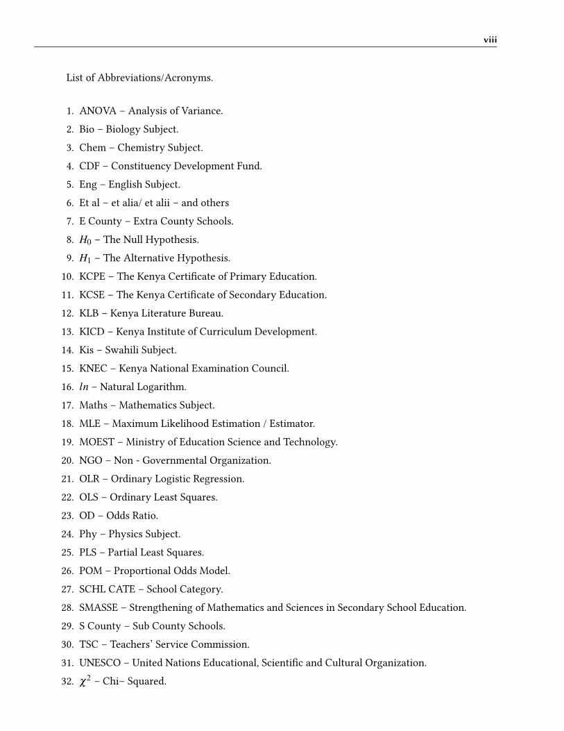
List of Abbreviations/Acronyms.
1. ANOVA – Analysis of Variance.
2. Bio – Biology Subject.
3. Chem – Chemistry Subject.
4. CDF – Constituency Development Fund.
5. Eng – English Subject.
6. Et al – et alia/ et alii – and others
7. E County – Extra County Schools.
8. H0 – The Null Hypothesis.
9. H1 – The Alternative Hypothesis.
10. KCPE – The Kenya Certi�cate of Primary Education.
11. KCSE – The Kenya Certi�cate of Secondary Education.
12. KLB – Kenya Literature Bureau.
13. KICD – Kenya Institute of Curriculum Development.
14. Kis – Swahili Subject.
15. KNEC – Kenya National Examination Council.
16. ln – Natural Logarithm.
17. Maths – Mathematics Subject.
18. MLE – Maximum Likelihood Estimation / Estimator.
19. MOEST – Ministry of Education Science and Technology.
20. NGO – Non - Governmental Organization.
21. OLR – Ordinary Logistic Regression.
22. OLS – Ordinary Least Squares.
23. OD – Odds Ratio.
24. Phy – Physics Subject.
25. PLS – Partial Least Squares.
26. POM – Proportional Odds Model.
27. SCHL CATE – School Category.
28. SMASSE – Strengthening of Mathematics and Sciences in Secondary School Education.
29. S County – Sub County Schools.
30. TSC – Teachers’ Service Commission.
31. UNESCO – United Nations Educational, Scienti�c and Cultural Organization.
32. χ2– Chi– Squared.
ix
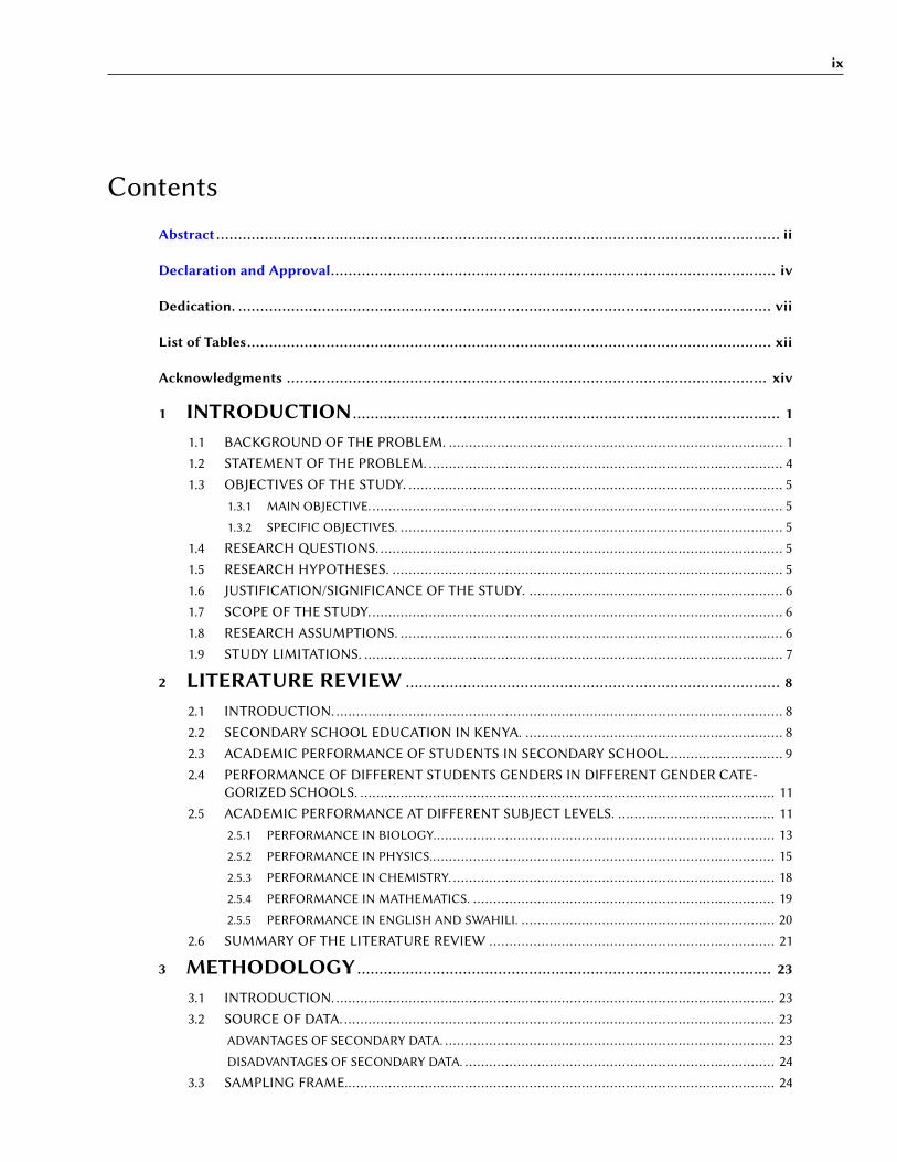
Contents
Abstract ................................................................................................................................ ii
Declaration and Approval..................................................................................................... iv
Dedication. ......................................................................................................................... vii
List of Tables....................................................................................................................... xii
Acknowledgments ............................................................................................................. xiv
1 INTRODUCTION ................................................................................................. 1
1.1 BACKGROUND OF THE PROBLEM. ................................................................................... 11.2 STATEMENT OF THE PROBLEM. ........................................................................................ 41.3 OBJECTIVES OF THE STUDY. ............................................................................................. 5
1.3.1 MAIN OBJECTIVE. ...................................................................................................... 51.3.2 SPECIFIC OBJECTIVES. ............................................................................................... 5
1.4 RESEARCH QUESTIONS. .................................................................................................... 51.5 RESEARCH HYPOTHESES. ................................................................................................. 51.6 JUSTIFICATION/SIGNIFICANCE OF THE STUDY. ............................................................... 61.7 SCOPE OF THE STUDY. ...................................................................................................... 61.8 RESEARCH ASSUMPTIONS. ............................................................................................... 61.9 STUDY LIMITATIONS. ........................................................................................................ 7
2 LITERATURE REVIEW ..................................................................................... 8
2.1 INTRODUCTION. ............................................................................................................... 82.2 SECONDARY SCHOOL EDUCATION IN KENYA. ................................................................ 82.3 ACADEMIC PERFORMANCE OF STUDENTS IN SECONDARY SCHOOL. ............................ 92.4 PERFORMANCE OF DIFFERENT STUDENTS GENDERS IN DIFFERENT GENDER CATE-
GORIZED SCHOOLS. ....................................................................................................... 112.5 ACADEMIC PERFORMANCE AT DIFFERENT SUBJECT LEVELS. ....................................... 11
2.5.1 PERFORMANCE IN BIOLOGY..................................................................................... 132.5.2 PERFORMANCE IN PHYSICS...................................................................................... 152.5.3 PERFORMANCE IN CHEMISTRY. ................................................................................ 182.5.4 PERFORMANCE IN MATHEMATICS. ........................................................................... 192.5.5 PERFORMANCE IN ENGLISH AND SWAHILI. ............................................................... 20
2.6 SUMMARY OF THE LITERATURE REVIEW ....................................................................... 21
3 METHODOLOGY .............................................................................................. 23
3.1 INTRODUCTION. ............................................................................................................. 233.2 SOURCE OF DATA. ........................................................................................................... 23
ADVANTAGES OF SECONDARY DATA. .................................................................................. 23DISADVANTAGES OF SECONDARY DATA. ............................................................................. 24
3.3 SAMPLING FRAME........................................................................................................... 24
x
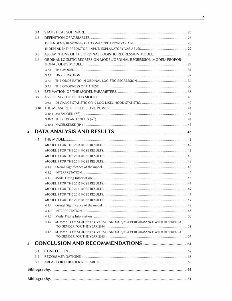
3.4 STATISTICAL SOFTWARE. ................................................................................................ 263.5 DEFINITION OF VARIABLES. ............................................................................................ 26
DEPENDENT/ RESPONSE/ OUTCOME/ CRITERION VARIABLE ................................................. 26INDEPENDENT/ PREDICTOR/ INPUT/ EXPLANATORY VARIABLES............................................ 27
3.6 ASSUMPTIONS OF THE ORDINAL LOGISTIC REGRESSION MODEL. ............................... 283.7 ORDINAL LOGISTIC REGRESSION MODEL/ORDINAL REGRESSION MODEL/ PROPOR-
TIONAL ODDS MODEL. ................................................................................................... 293.7.1 THE MODEL. ........................................................................................................... 313.7.2 LINK FUNCTION. ..................................................................................................... 323.7.3 THE ODDS RATIO IN ORDINAL LOGISTIC REGRESSION................................................ 343.7.4 THE GOODNESS OF FIT TEST..................................................................................... 36
3.8 ESTIMATION OF THE MODEL PARAMETERS. .................................................................. 383.9 ASSESSING THE FITTED MODEL. .................................................................................... 40
3.9.1 DEVIANCE STATISTIC OR -2 LOG-LIKELIHOOD STATISTIC. ........................................... 403.10 THE MEASURE OF PREDICTIVE POWER.......................................................................... 41
3.10.1 Mc FADDEN (R2) ..................................................................................................... 413.10.2 THE COX AND SNELLS (R2) ...................................................................................... 413.10.3 NAGELKERKE (R2) ................................................................................................... 41
4 DATA ANALYSIS AND RESULTS .............................................................. 42
4.1 THE MODEL..................................................................................................................... 42MODEL 1 FOR THE 2014 KCSE RESULTS. ............................................................................... 42MODEL 2 FOR THE 2014 KCSE RESULTS. ............................................................................... 42MODEL 3 FOR THE 2014 KCSE RESULTS. ............................................................................... 42MODEL 4 FOR THE 2014 KCSE RESULTS. ............................................................................... 434.1.1 Overall Significance of the model. ................................................................................ 434.1.2 INTERPRETATION..................................................................................................... 444.1.3 Model Fi�ing Information . ......................................................................................... 46MODEL 1 FOR THE 2015 KCSE RESULTS. ............................................................................... 47MODEL 2 FOR THE 2015 KCSE RESULTS. ............................................................................... 47MODEL 3 FOR THE 2015 KCSE RESULTS. ............................................................................... 47MODEL 4 FOR THE 2015 KCSE RESULTS. ............................................................................... 474.1.4 Overall Significance of the model. ................................................................................ 484.1.5 INTERPRETATION..................................................................................................... 484.1.6 Model Fi�ing Information . ......................................................................................... 504.1.7 SUMMARY OF STUDENTS OVERALL AND SUBJECT PERFORMANCE WITH REFERENCE
TO GENDER FOR THE YEAR 2014............................................................................... 524.1.8 SUMMARY OF STUDENTS OVERALL AND SUBJECT PERFORMANCE WITH REFERENCE
TO GENDER FOR THE YEAR 2015............................................................................... 57
5 CONCLUSION AND RECOMMENDATIONS ...................................... 62
5.1 CONCLUSION ................................................................................................................. 625.2 RECOMMENDATIONS ..................................................................................................... 635.3 AREAS FOR FURTHER RESEARCH ................................................................................... 63
Bibliography....................................................................................................................... 64
Bibliography....................................................................................................................... 64

xi
Appendices ......................................................................................................................... 68
Appendix A: MAP OF KIAMBU COUNTY ............................................................................. A1
Appendix B: R CODES USED ............................................................................................... A2
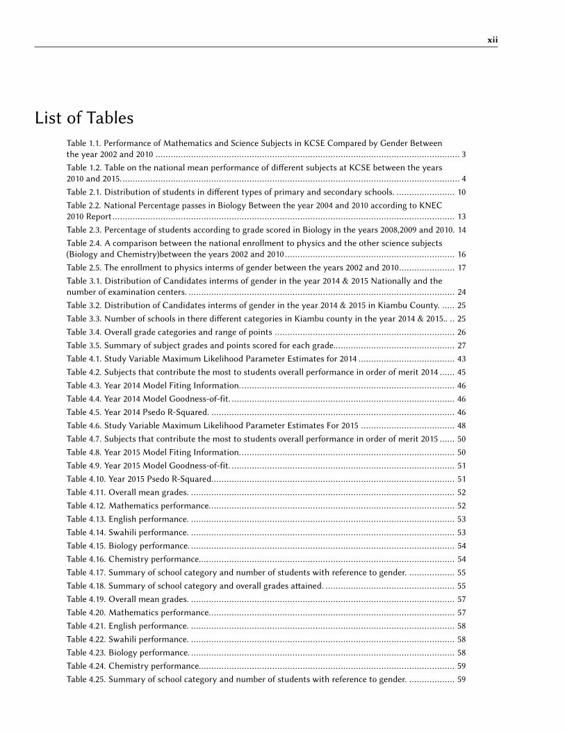
xii
List of TablesTable 1.1. Performance of Mathematics and Science Subjects in KCSE Compared by Gender Betweenthe year 2002 and 2010 ........................................................................................................................ 3Table 1.2. Table on the national mean performance of di�erent subjects at KCSE between the years2010 and 2015. ..................................................................................................................................... 4Table 2.1. Distribution of students in di�erent types of primary and secondary schools. ....................... 10Table 2.2. National Percentage passes in Biology Between the year 2004 and 2010 according to KNEC2010 Report ....................................................................................................................................... 13Table 2.3. Percentage of students according to grade scored in Biology in the years 2008,2009 and 2010. 14Table 2.4. A comparison between the national enrollment to physics and the other science subjects(Biology and Chemistry)between the years 2002 and 2010 ................................................................... 16Table 2.5. The enrollment to physics interms of gender between the years 2002 and 2010...................... 17Table 3.1. Distribution of Candidates interms of gender in the year 2014 & 2015 Nationally and thenumber of examination centers. ......................................................................................................... 24Table 3.2. Distribution of Candidates interms of gender in the year 2014 & 2015 in Kiambu County. ..... 25Table 3.3. Number of schools in there di�erent categories in Kiambu county in the year 2014 & 2015.. .. 25Table 3.4. Overall grade categories and range of points ....................................................................... 26Table 3.5. Summary of subject grades and points scored for each grade................................................ 27Table 4.1. Study Variable Maximum Likelihood Parameter Estimates for 2014 ...................................... 43Table 4.2. Subjects that contribute the most to students overall performance in order of merit 2014 ...... 45Table 4.3. Year 2014 Model Fiting Information. .................................................................................... 46Table 4.4. Year 2014 Model Goodness-of-fit. ........................................................................................ 46Table 4.5. Year 2014 Psedo R-Squared. ................................................................................................ 46Table 4.6. Study Variable Maximum Likelihood Parameter Estimates For 2015 ..................................... 48Table 4.7. Subjects that contribute the most to students overall performance in order of merit 2015 ...... 50Table 4.8. Year 2015 Model Fiting Information. .................................................................................... 50Table 4.9. Year 2015 Model Goodness-of-fit. ........................................................................................ 51Table 4.10. Year 2015 Psedo R-Squared................................................................................................ 51Table 4.11. Overall mean grades. ........................................................................................................ 52Table 4.12. Mathematics performance................................................................................................. 52Table 4.13. English performance. ........................................................................................................ 53Table 4.14. Swahili performance. ........................................................................................................ 53Table 4.15. Biology performance. ........................................................................................................ 54Table 4.16. Chemistry performance..................................................................................................... 54Table 4.17. Summary of school category and number of students with reference to gender. .................. 55Table 4.18. Summary of school category and overall grades a�ained. ................................................... 55Table 4.19. Overall mean grades. ........................................................................................................ 57Table 4.20. Mathematics performance................................................................................................. 57Table 4.21. English performance. ........................................................................................................ 58Table 4.22. Swahili performance. ........................................................................................................ 58Table 4.23. Biology performance. ........................................................................................................ 58Table 4.24. Chemistry performance..................................................................................................... 59Table 4.25. Summary of school category and number of students with reference to gender. .................. 59

xiii
Table 4.26. Summary of school category and overall grades a�ained. ................................................... 60Table 4.27. A comparison between the subjects that contribute the most to students overall perfor-mance interms of odds ratio for both the years 2014 and 2015. ............................................................ 60

xiv
Acknowledgments
I am extremely grateful to the almighty God for the opportunity, energy and wisdom hegave me to pursue the Masters Degree.
I am grateful to the University of Nairobi, School of Mathematics (som). Mainly mysupervisor Dr. Ivivi Joseph Mwaniki for the assistance, continuous advice & guidance,invaluable support and encouragement throughout the entire project. He guided me,corrected me and gave me the freedom to e�ect corrections my own way.
I pass my appreciation to all the University of Nairobi, School of Mathematics (som)lecturers who took me through the whole course work. Prof. Patrick Weke (DirectorSchool of Mathematics), Dr. Nelson Owuor, Dr. George Muhua, Dr. J. Ndiritu, Dr. VincentOeba, Dr. Japheth Awiti, Mrs. Ann Wang’ombe, Dr. Jacob Ong’alo & Dr. Jared Ongaro.
I acknowledge KNEC through the CEO Ms. Mercy Gathigia Karogo, TSC kiambu countyand sub county o�ices for the provision of necessary data for analysis.
I pass my regards to all my classmates (class of 2016-2018) for their tireless support,teamwork and encouragement to carry on to the end of the Masters program.
May God bless you all and your families. . . . .
Kenneth Benson Muya
Nairobi, 2018.

1

1
1 INTRODUCTION
1.1 BACKGROUND OF THE PROBLEM.
Education is one of the most priced and treasured investment in the whole world. Most de-veloped and developing nations normally invest a lot in their education systems.Educationis primarily perceived as a means of solving social problems.
As a means of ensuring that education, moreso basic education is provided, many devel-oping and developed nations for instance as United States of America, Australia and theUnited Kingdom have put in place mechanisms to provide free elementary and secondaryschool education. Developing countries such as Kenya have also come in, through theMOEST to ensure the is provision of subsidized primary and secondary education in orderto achieve the 2030 millennium goals.
Apart from just the provision of free primary and subsidized secondary education;thegovernment has started up initiatives to expand the existing primary and secondaryschools and also building new schools through the various ‘Harambee’ projects and fundsfrom the constituency development funds so as to accommodate the increasing demandfor education.
Education plays a vital role in career development and career shaping.
Students start shaping their careers as early as during elementary studies, that is duringtheir primary education. Thus the provision of education at this early level or stage is veryvital.Students in secondary school are in their exploration phase in life. This is a stagewhere they are likely to be developing their careers (Pa�on and McMahon, 2014).
According to researches done by UNESCO, Many developing and developed Countriesallot a huge percent of their wealth to Education sectors,(UNESCO, 2005) leading to aconsiderable expansion in Educational undertakings world wide.Kenya being a developing country has not been le� behind, Statistics show that Kenyaallocates a huge share of its resources to the sector UNESCO 2005.
Apart from resource allocation, the government has various initiatives that try to makeschooling more e�ective and e�icient to the learners, Such initiatives include the protec-tion of the rights of children for example through the campaigns against female genital
2
mutilation (FGM) and protection against early marriages. The governments working withvarious Non governmental Organizations (NGO,s) Provide sanitary towels to students inneed.Examples of such organizations are Crossroads Global Hand and Mfariji Africa.Thegovernment is also working on the school feeding programs to the needy students.
Since independence in 1963, Education was seen as a means of eradicating poverty.Therefore, the government introduced the 8-4-4 education system, the system has beenproviding a practical oriented curriculum that aims at providing employment opportunitiesfor those who go through it (Eshiwani,1993).
Despite all these provision and support that the education sector is ge�ing. It faces variouschallenges, that is poor overall performance of students at KCSE level.
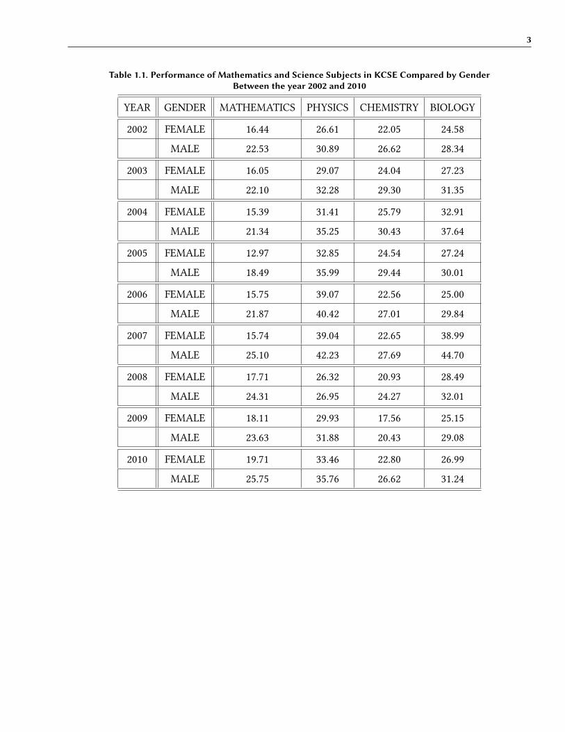
The body that is entrusted with the duty of assessing students at the end of the form4 level that is the Kenya National Examination Council (KNEC), has registered pooroverall performance over the years and more specifically in the mathematics and scienceexaminations. This is shown in the table below (Table 1.2).
3
Table 1.1. Performance of Mathematics and Science Subjects in KCSE Compared by GenderBetween the year 2002 and 2010
YEAR GENDER MATHEMATICS PHYSICS CHEMISTRY BIOLOGY
2002 FEMALE 16.44 26.61 22.05 24.58
MALE 22.53 30.89 26.62 28.34
2003 FEMALE 16.05 29.07 24.04 27.23
MALE 22.10 32.28 29.30 31.35
2004 FEMALE 15.39 31.41 25.79 32.91
MALE 21.34 35.25 30.43 37.64
2005 FEMALE 12.97 32.85 24.54 27.24
MALE 18.49 35.99 29.44 30.01
2006 FEMALE 15.75 39.07 22.56 25.00
MALE 21.87 40.42 27.01 29.84
2007 FEMALE 15.74 39.04 22.65 38.99
MALE 25.10 42.23 27.69 44.70
2008 FEMALE 17.71 26.32 20.93 28.49
MALE 24.31 26.95 24.27 32.01
2009 FEMALE 18.11 29.93 17.56 25.15
MALE 23.63 31.88 20.43 29.08
2010 FEMALE 19.71 33.46 22.80 26.99
MALE 25.75 35.76 26.62 31.24
4
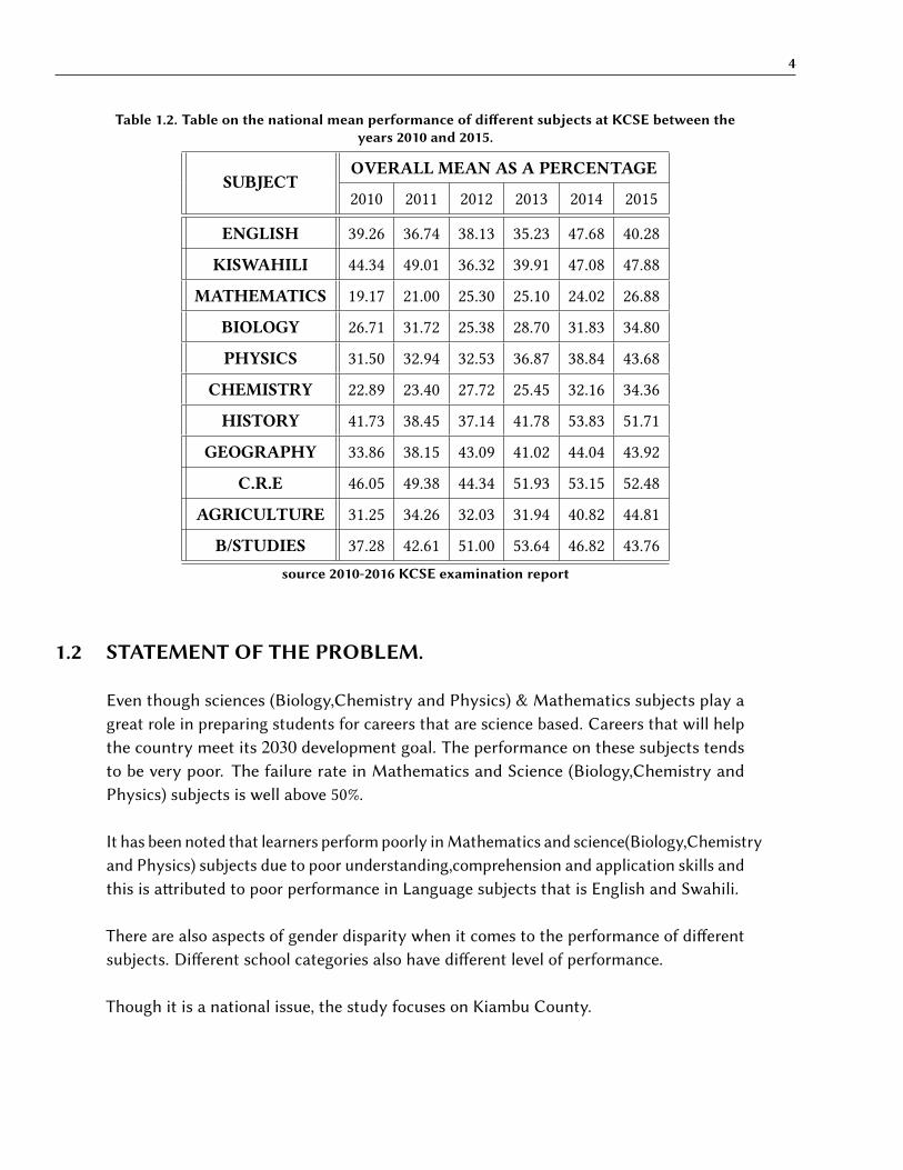
Table 1.2. Table on the national mean performance of di�erent subjects at KCSE between theyears 2010 and 2015.
SUBJECTOVERALL MEAN AS A PERCENTAGE
2010 2011 2012 2013 2014 2015
ENGLISH 39.26 36.74 38.13 35.23 47.68 40.28
KISWAHILI 44.34 49.01 36.32 39.91 47.08 47.88
MATHEMATICS 19.17 21.00 25.30 25.10 24.02 26.88
BIOLOGY 26.71 31.72 25.38 28.70 31.83 34.80
PHYSICS 31.50 32.94 32.53 36.87 38.84 43.68
CHEMISTRY 22.89 23.40 27.72 25.45 32.16 34.36
HISTORY 41.73 38.45 37.14 41.78 53.83 51.71
GEOGRAPHY 33.86 38.15 43.09 41.02 44.04 43.92
C.R.E 46.05 49.38 44.34 51.93 53.15 52.48
AGRICULTURE 31.25 34.26 32.03 31.94 40.82 44.81
B/STUDIES 37.28 42.61 51.00 53.64 46.82 43.76
source 2010-2016 KCSE examination report
1.2 STATEMENT OF THE PROBLEM.
Even though sciences (Biology,Chemistry and Physics) & Mathematics subjects play agreat role in preparing students for careers that are science based. Careers that will helpthe country meet its 2030 development goal. The performance on these subjects tendsto be very poor. The failure rate in Mathematics and Science (Biology,Chemistry andPhysics) subjects is well above 50%.
It has been noted that learners perform poorly in Mathematics and science(Biology,Chemistryand Physics) subjects due to poor understanding,comprehension and application skills andthis is a�ributed to poor performance in Language subjects that is English and Swahili.
There are also aspects of gender disparity when it comes to the performance of di�erentsubjects. Di�erent school categories also have di�erent level of performance.
Though it is a national issue, the study focuses on Kiambu County.
5
1.3 OBJECTIVES OF THE STUDY.
1.3.1 MAIN OBJECTIVE.
Analyzing the performance of students at secondary school level using past KCSE results.
1.3.2 SPECIFIC OBJECTIVES.
(a.) To determine the subject that contributes the most to students overall performanceat KCSE level.
(b.) To establish if there exists a relationship between students gender and overall KCSEperformance.
(c.) To establish if there exists a relationship between the category of school a�ended bya student and the overall KCSE performance.
1.4 RESEARCH QUESTIONS.
(a.) Which subjects contribute the most to the overall performance of students in sec-ondary school at KCSE level?
(b.) Does the gender of students influence their overall performance at KCSE level?
(c.) Is there a relationship between the type/category of school a�ended by a student andthe overall KCSE performance?
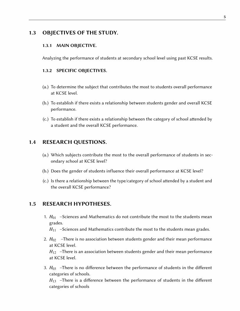
1.5 RESEARCH HYPOTHESES.
1. H01 –Sciences and Mathematics do not contribute the most to the students meangrades.H11 –Sciences and Mathematics contribute the most to the students mean grades.
2. H02 –There is no association between students gender and their mean performanceat KCSE level.H12 –There is an association between students gender and their mean performanceat KCSE level.
3. H03 –There is no di�erence between the performance of students in the di�erentcategories of schools.H13 –There is a di�erence between the performance of students in the di�erentcategories of schools
6
1.6 JUSTIFICATION/SIGNIFICANCE OF THE STUDY.
Despite the fact that many studies have been done to analyze the performance of secondaryschool students at KCSE level,very few studies have been done to analyze the e�ects ofthe performance on individual subjects i.e Mathematics, English, Swahili, Biology, andChemistry on the overall performance of students at KCSE level.The reason for the choice of just 5 subjects to analyze the e�ect of individual subjects onthe overall performance of students at secondary school level is due to the fact that:
(i). English, Kiswahili and Mathematics are compulsory subjects categorized as group 1subjects.
(ii). Chemistry and Biology are compulsory science subjects in most secondary schoolsand they are done by most students.
1.7 SCOPE OF THE STUDY.
This study was carried out using data from past KCSE examinations for selected schoolswithin Kiambu county, the schools are to be categorized as National schools,Countyschools, sub-county schools and district schools.Students are to be further classified interms of gender as either female or male. The selection will also be based on the schoolspopulation in terms of candidates who sat for the national examination (KCSE) in theselected year.
1.8 RESEARCH ASSUMPTIONS.
The following assumptions were considered:
(a). Data analysis was done based on KCSE 2015 results which is a standardized examina-tion which is used to assess learners at the end of there four year secondary educationperiod.
(b). All selected schools have teachers appointed by the Kenyas’ teacher employing bodythat is the Teacher’s service commission (TSC).
(c). All students in the schools under the study have equal study time.
(d). All students in the schools under the study subjected to the same academic syl-labus/curriculum.
(e). Students had similar learning backgrounds in primary schools and any di�erences inlearning, was as a result of classroom experiences in secondary schools.
7
(f). All the schools in the study use the same syllabus books.
(g). Teaching and learning is currently going on in the schools being used in the study.
1.9 STUDY LIMITATIONS.
1. The researcher would have wished to incorporate several counties in the study butdue to logistics, distance, time factor, financial constraints and availability of data. Itwas a challenge.
2. The sample for the research was be picked from Kiambu county only and not fromthe entire country. This implies that the sample may not represent all high schools inKenya.

8
2 LITERATURE REVIEW
2.1 INTRODUCTION.
The chapter contains related reviewed published writings . It focuses on studies done byother researchers, the methods they used and their findings.
2.2 SECONDARY SCHOOL EDUCATION IN KENYA.
Secondary education in Kenya begins immediately a�er primary school. It mainly catersfor learners between the ages of 13 to 19 years. Secondary schools in Kenya are categorizedas National, Extra county, county or sub-county schools for the public schools, we alsohave private schools. These categories are further sub divided according to gender; that ismale only, female only and mixed schools. We also have boarding and day schools Kremer(2009).The public schools are partially sponsored by the government and hence their school feesis subsidized.
National schools receive students from the whole country. County schools admit most oftheir students from within their respective counties. Extra county schools mainly admitstudents within the county of location and neighboring counties. Sub county schoolsadmit most of its students from within their sub counties while day schools admit studentsfrom the immediate neighborhood.
Private schools which are owned by individuals and organizations. They have theirmanagement decide on the mode of admission.
In the recent past, due to the increase in the number of students clearing standard eight(8), that is the highest level of primary education. The secondary schools have been forcedto expand in order to accommodate the increasing number of students joining secondaryschool.
A report by the world bank (2008) observes that out of 7.6 million Kenyans who a�endedprimary school it is only 810,000 or 0.81 million who get admi�ed to secondary schools.The number even reducing further for those who manage to join universities to around10,200.Okenyo,(2010).
9
A study conducted by Asena (2016) on the e�ect of subsidized free day secondary educationin ensuring students are retained in schools. The aim of the study was to determine howfree day secondary education contributes to students being retained in secondary schoolsin Kenya.
Asenas’ objective was to study how availability of finances and teaching resources con-tributes positively to students understanding in school.
Population targeted was made up of 3993 stakeholders in the department of education inBungoma county. Asena sampled 340 respondents.
Data was analyzed by use of descriptive statistics and content analysis.
Asena’s study showed that the number of students in high schools was increasing dras-tically, this is a�ributed to the introduction of subsidized free day secondary educationin the year 2008 by the government. It was aimed at providing basic education to all itscitizens. The result of the subsidized free day secondary education is huge enrollmentand transition rates that have contributed to shortage of teachers & high teacher studentratio. Asena et.al (2016).
2.3 ACADEMIC PERFORMANCE OF STUDENTS IN SECONDARYSCHOOL.
Many studies and researches have been done on the main causes of poor performance(Maiyo, 2009 and Orodho, 2004).
A study done by Cynthia (2014) on factors influencing the academic performance ofstudents in KCSE Examination in Roysambu constituency in Nairobi.The target population was 750 form 4 students and 145 teachers. Stratified samplingtechnique was made use of in the study. study objectives included:
1. Analyzing the influence of availability of learning resources on KCSE performance inRoysambu constituency.
2. To examine the influence of discipline on students performance in KCSE in Roysambuconstituency.
3. To study the influence of home environment on students’ performance.
The research used a descriptive cross-sectional survey design to explore the factors influ-encing students’ performance in KCSE.
10
The research findings indicated that discipline is paramount in the performance of studentsTeaching methods also had a positive influence on the students performance. Schools withadequate teaching and learning resources posted be�er KCSE results than schools withoutadequate teaching and learning resources. Another finding is that home based factorsalso influenced students KCSE performance. These factors included: Parents involvementin learners school activities and the parents level of education (Cynthia 2014).
A research conducted by Samuel (2014) on the determinants of students performance inKCSE using ordinal logistic regression. Samuel’s objectives included the following:
1. To find out the e�ects of private and public primary schooling on a students secondaryschool academic performance.
2. Identify the determinants of students’ performance and achievements based on transi-tion from di�erent categories of schools, that is from private primary school to publicsecondary schools.
The target population was secondary schools in Kiambu county, Samuels’ sample included6 secondary schools in Kiambu county, data used was the KCSE results for the year 2013.
Samuels’ methodology entailed exploratory and confirmatory analysis, he used ordinallogistic regression. The determinants of students performance at KCSE included the ageof the learners, type of primary school a�ended (public or private), students gender andthe KCPE marks a�ained.
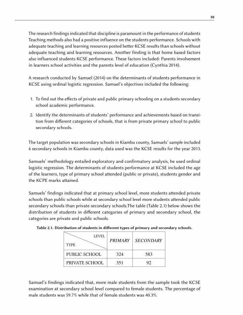
Samuels’ findings indicated that at primary school level, more students a�ended privateschools than public schools while at secondary school level more students a�ended publicsecondary schools than private secondary schools.The table (Table 2.1) below shows thedistribution of students in di�erent categories of primary and secondary school, thecategories are private and public schools.
Table 2.1. Distribution of students in di�erent types of primary and secondary schools.aaaaaaaaaaa
TYPE
LEVEL
PRIMARY SECONDARY
PUBLIC SCHOOL 324 583
PRIVATE SCHOOL 351 92
Samuel’s findings indicated that, more male students from the sample took the KCSEexamination at secondary school level compared to female students. The percentage ofmale students was 59.7% while that of female students was 40.3%.
11
Samuel’s findings further showed that the overall best performance was from students inNational schools. There was also less movement from public primary schools to privatesecondary schools as compared to the movement from private primary schools to publicsecondary schools as indicated in table 2.1 above.
The study indicated that there were more female than male enrollment to private schools.The enrollment was 58.7% and 41.3% respectively. This being an indication that genderparity has not yet been achieved in school enrollment.
Students who a�ended public secondary schools achieved be�er results compared tothose who a�ended private secondary schools. The study indicated that the significantfactors in determining a students performance at KCSE were the KCPE marks obtainedby the same students, the gender of the students and the category of secondary schoola�ended by the students.
The primary school type & students age were not significant to the performance at KCSElevel. Despite this fact an increase in age beyond 20 years had a negative e�ect onKCSE performance. A transition from private primary school to public secondary schoolsignificantly influenced students performance.
2.4 PERFORMANCE OF DIFFERENT STUDENTS GENDERS INDIFFERENT GENDER CATEGORIZED SCHOOLS.
Several studies have been done to analyze the performance of students at secondaryschool level. among the studies done is one by Elvis K M (2015) who analysed the KCSEperformance in Nakuru using Generalized estimating equations. His study showed thatboys in boys schools scored be�er than boys in mixed gender schools. Girls in girls schoolsscored be�er than girls in mixed gender schools. In the mixed schools boys did be�er thangirls.
The study showed that the grades of students in single gender schools that is Boys onlyand girls only schools were be�er than the grades of students in mixed schools.
A study conducted by Lydia (2013) on the factors that determine girls’ scores in science,mathematics & technology subjects in public secondary schools. The research objectivewas to determine female students grades in science, mathematics & technology subjectsin public secondary schools.
Lydia, used an ex-facto survey research design, Descriptive and Inferential statistics werederived. The research findings indicated that the qualification of teachers is a significantdeterminant in the learners performance. The study showed that girls performed poorlyin science subjects compared to the other subjects.
12
2.5 ACADEMIC PERFORMANCE AT DIFFERENT SUBJECT LEVELS.
UNESCO, (2005) and Alidou, (2009), point out clearly that poor achievement from learnersis not due to the students having inherent cognitive problems but rather, inadequatemastery of the language of instruction.
An analysis of past performances by KNEC and the Ministry of Education Science andTechnology (MOEST), show key areas that candidates must prepare in and commonmistakes that they should avoid as they sit for tests and examinations.
A research done by Mwiti (2016) on the grade scores in science subjects. The researchobjectives were:
1. To establish the relationship between achievement in languages, mathematics &sciences.
2. To model the performance in sciences given the grades in english, swahili & mathe-matics.
The data used for the study was KCSE results for the year 2014. The study populationwas 438660 candidates, while the target population was 65,535 candidates who took thethree sciences (biology, chemistry & physics) at KCSE level.
Data analysis was conducted using partial least squares (PLS) regression to establishthe relationship between mathematics, Languages & science subjects and predict theachievement in science subjects given the grades scored in mathematics and languages.
Analysis indicated that there existed a correlation between english, swahili and mathe-matics and that the performance in physics and chemistry is mainly influenced by that ofmathematics. More findings were that gender negatively correlated to the achievement insciences. The type of school a�ended being positively correlated to the science perfor-mance, where by national schools posted the best results followed by extra county schoolsthen the county schools.
13
2.5.1 PERFORMANCE IN BIOLOGY.
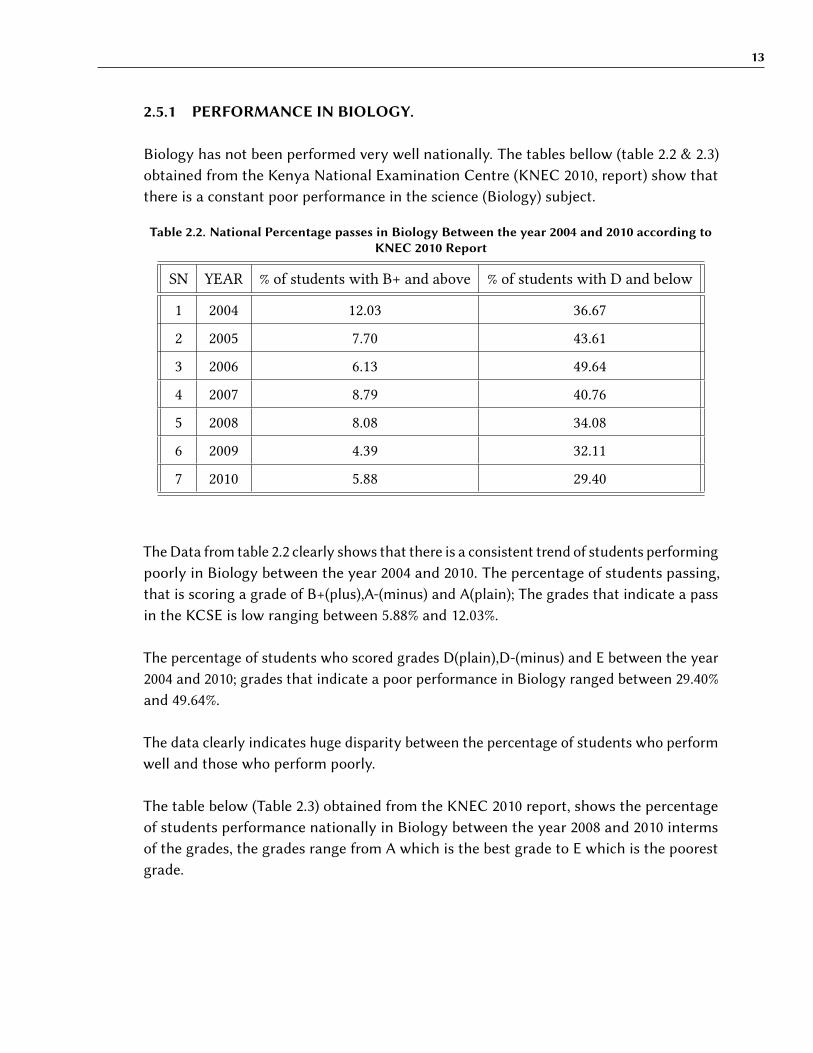
Biology has not been performed very well nationally. The tables bellow (table 2.2 & 2.3)obtained from the Kenya National Examination Centre (KNEC 2010, report) show thatthere is a constant poor performance in the science (Biology) subject.
Table 2.2. National Percentage passes in Biology Between the year 2004 and 2010 according toKNEC 2010 Report
SN YEAR % of students with B+ and above % of students with D and below
1 2004 12.03 36.67
2 2005 7.70 43.61
3 2006 6.13 49.64
4 2007 8.79 40.76
5 2008 8.08 34.08
6 2009 4.39 32.11
7 2010 5.88 29.40
The Data from table 2.2 clearly shows that there is a consistent trend of students performingpoorly in Biology between the year 2004 and 2010. The percentage of students passing,that is scoring a grade of B+(plus),A-(minus) and A(plain); The grades that indicate a passin the KCSE is low ranging between 5.88% and 12.03%.
The percentage of students who scored grades D(plain),D-(minus) and E between the year2004 and 2010; grades that indicate a poor performance in Biology ranged between 29.40%and 49.64%.
The data clearly indicates huge disparity between the percentage of students who performwell and those who perform poorly.
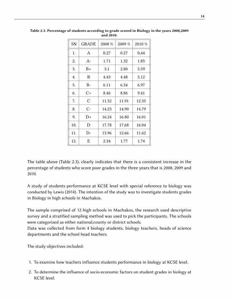
The table below (Table 2.3) obtained from the KNEC 2010 report, shows the percentageof students performance nationally in Biology between the year 2008 and 2010 intermsof the grades, the grades range from A which is the best grade to E which is the poorestgrade.
14
Table 2.3. Percentage of students according to grade scored in Biology in the years 2008,2009and 2010.
SN GRADE 2008 % 2009 % 2010 %
1. A 0.27 0.27 0,44
2. A- 1.71 1.32 1.85
3. B+ 3.1 2.80 3.59
4. B 4.43 4.48 5.12
5. B- 6.11 6.54 6.97
6. C+ 8.46 8.86 9.41
7. C 11.32 11.91 12.35
8. C- 14.23 14.90 14.79
9. D+ 16.24 16.80 16.01
10. D 17.78 17.68 16.04
11. D- 13.96 12.66 11.62
12. E 2.34 1.77 1.74
The table above (Table 2.3), clearly indicates that there is a consistent increase in thepercentage of students who score poor grades in the three years that is 2008, 2009 and2010.
A study of students performance at KCSE level with special reference to biology wasconducted by Lewis (2014). The intention of the study was to investigate students gradesin Biology in high schools in Machakos.
The sample comprised of 12 high schools in Machakos, the research used descriptivesurvey and a stratified sampling method was used to pick the participants. The schoolswere categorized as either national,county or district schools.Data was collected from form 4 biology students, biology teachers, heads of sciencedepartments and the school head teachers.
The study objectives included:
1. To examine how teachers influence students performance in biology at KCSE level.
2. To determine the influence of socio-economic factors on student grades in biology atKCSE level.
15
The study results indicated that the performance of students in biology at secondaryschool level was greatly influenced by syllabus completion, e�ective practical sessions &the teaching methodology.
Another emerging issue was the long distance that had to be traveled by students in dayschools to and from school. These students reached school late and tired thus a�ectingtheir concentration in class which had a ripple e�ect on their performance (Lewis Et al2014).
2.5.2 PERFORMANCE IN PHYSICS.
Physics is an optional science subject. The subject has continually registered low enroll-ment in the the national examination that is KCSE
Data in table 1.2 shows that between the years 2010 and 2015, the performance in physicsnot ignoring the fact that it is still low, has been slightly be�er than that of other sciencessubjects, that is Biology and Chemistry. The national mean grade for physics was 31.5%in the year 2010, 32.94% in 2011, 32.53% in 2012, 36.87% in 2013, 38.84% in 2014 and 43.68%in the year 2015.
In the same year 2015,out of all the students who sat for the physics exam 74,768 scoredgrades D(plain) and below. This number represents a 12% increase from the year 2014.In thesame year (2015) 13,026 students that represents 9% scored grades A(plain) and A-(minus).
The table below (Table 2.4) shows the number of students enrolled to take physics andtheir percentages compared to the number of students and their percentages enrolled totake the other sciences that is Biology and Chemistry.
16
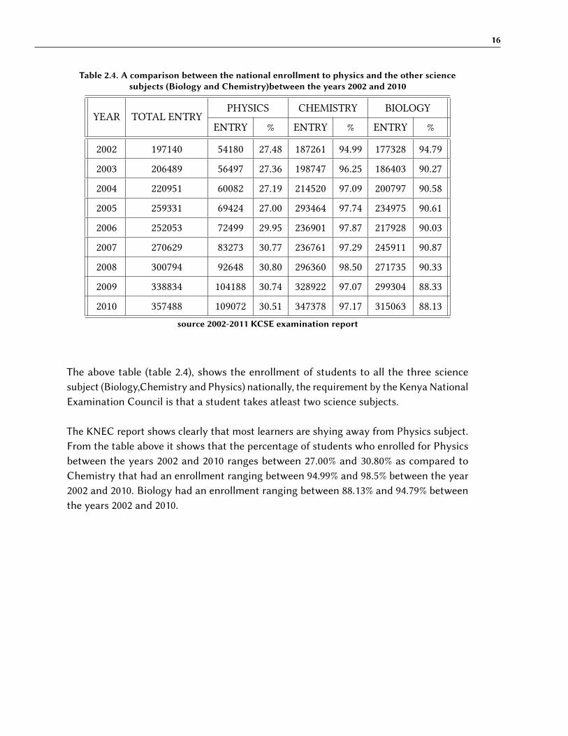
Table 2.4. A comparison between the national enrollment to physics and the other sciencesubjects (Biology and Chemistry)between the years 2002 and 2010
YEAR TOTAL ENTRY
PHYSICS CHEMISTRY BIOLOGY
ENTRY % ENTRY % ENTRY %
2002 197140 54180 27.48 187261 94.99 177328 94.79
2003 206489 56497 27.36 198747 96.25 186403 90.27
2004 220951 60082 27.19 214520 97.09 200797 90.58
2005 259331 69424 27.00 293464 97.74 234975 90.61
2006 252053 72499 29.95 236901 97.87 217928 90.03
2007 270629 83273 30.77 236761 97.29 245911 90.87
2008 300794 92648 30.80 296360 98.50 271735 90.33
2009 338834 104188 30.74 328922 97.07 299304 88.33
2010 357488 109072 30.51 347378 97.17 315063 88.13
source 2002-2011 KCSE examination report
The above table (table 2.4), shows the enrollment of students to all the three sciencesubject (Biology,Chemistry and Physics) nationally, the requirement by the Kenya NationalExamination Council is that a student takes atleast two science subjects.
The KNEC report shows clearly that most learners are shying away from Physics subject.From the table above it shows that the percentage of students who enrolled for Physicsbetween the years 2002 and 2010 ranges between 27.00% and 30.80% as compared toChemistry that had an enrollment ranging between 94.99% and 98.5% between the year2002 and 2010. Biology had an enrollment ranging between 88.13% and 94.79% betweenthe years 2002 and 2010.
17
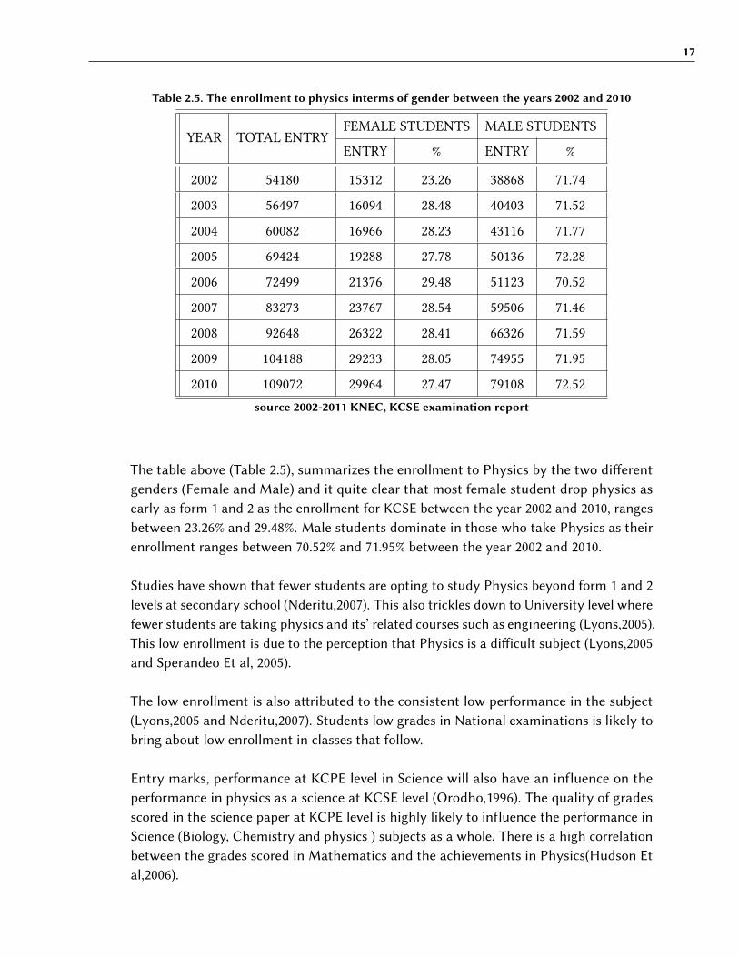
Table 2.5. The enrollment to physics interms of gender between the years 2002 and 2010
YEAR TOTAL ENTRY
FEMALE STUDENTS MALE STUDENTS
ENTRY % ENTRY %
2002 54180 15312 23.26 38868 71.74
2003 56497 16094 28.48 40403 71.52
2004 60082 16966 28.23 43116 71.77
2005 69424 19288 27.78 50136 72.28
2006 72499 21376 29.48 51123 70.52
2007 83273 23767 28.54 59506 71.46
2008 92648 26322 28.41 66326 71.59
2009 104188 29233 28.05 74955 71.95
2010 109072 29964 27.47 79108 72.52
source 2002-2011 KNEC, KCSE examination report
The table above (Table 2.5), summarizes the enrollment to Physics by the two di�erentgenders (Female and Male) and it quite clear that most female student drop physics asearly as form 1 and 2 as the enrollment for KCSE between the year 2002 and 2010, rangesbetween 23.26% and 29.48%. Male students dominate in those who take Physics as theirenrollment ranges between 70.52% and 71.95% between the year 2002 and 2010.
Studies have shown that fewer students are opting to study Physics beyond form 1 and 2levels at secondary school (Nderitu,2007). This also trickles down to University level wherefewer students are taking physics and its’ related courses such as engineering (Lyons,2005).This low enrollment is due to the perception that Physics is a di�icult subject (Lyons,2005and Sperandeo Et al, 2005).
The low enrollment is also a�ributed to the consistent low performance in the subject(Lyons,2005 and Nderitu,2007). Students low grades in National examinations is likely tobring about low enrollment in classes that follow.
Entry marks, performance at KCPE level in Science will also have an influence on theperformance in physics as a science at KCSE level (Orodho,1996). The quality of gradesscored in the science paper at KCPE level is highly likely to influence the performance inScience (Biology, Chemistry and physics ) subjects as a whole. There is a high correlationbetween the grades scored in Mathematics and the achievements in Physics(Hudson Etal,2006).
18
A research conducted Jane by (2011) on the disparities in physics academic achievementsand enrollment to physics at high school level.The study objectives included:
1. To identify the disparities in enrollment of students to physics in secondary schools inwestern Kenya.
2. To identify the disparities in the performance of physics in secondary schools in KCSE.
The sample included secondary schools in western province. The schools were stratifiedinto boys’ boarding , girls’ boarding and co-education (mixed) schools. Data used wasfrom KCSE 2009 results.The results indicated that boys performed be�er than girls in physics also more boys’ thangirls’ take physics as it is an optional subject.
2.5.3 PERFORMANCE IN CHEMISTRY.
Chemistry being another very important science subject that is compulsory in mostsecondary schools and with the highest enrollment in terms of candidature, according totable 2.3 . The enrollment ranges between 94.99% and 98.50% between the year 2002 and2010. Despite this fact; Chemistry is the worst performed subject . According to the datain Table 1.1, the performance of Chemistry ranges between 18.995% and 28.11% betweenthe year 2002 and 2010. The subject also recorded same low mean grades. Just like theother science subjects where male students performed be�er than female students.
Chemistry according to table 1.2 is the poorest performed science subject, in the year 2010chemistry managed a national mean grade of 22.89%, in 2011 it managed 23.40%,27.72%in 2012, 25.45% in 2013, 32.16% in 2014 and finally 34.36% in 2015.
A research done by Muwanga-zake (1998) showed that the performance in sciences moreso chemistry was low due to the following reasons:
1. Teachers misinterpret their own content in the science class.
2. Learners misunderstanding science concepts.
3. There is a barrier between teachers and learners language.
Henerson and Wellington (1998) noted that the greatest barrier to learning Science isLanguage. Some terminologies that are di�erent in chemistry might mean di�erent in ourtraditional languages which is not used as a means of teaching and learning Chemistry. In
19
chemistry smoke, gas and steam are three di�erent things but in the traditional languagelike ‘Kalenjin’ they are referred to with one term ‘aros’.
A research conducted by Amunga J.K et.al (2009) on disproportion / imbalance in theachievement in chemistry & Biology in high school level.The fact finding was conducted in 32 secondary schools in western province.
The study had the following objectives:
1. To identify the disproportion in performance in Chemistry & Biology in KCSE between2005-2009.
2. To explore the factors influencing the distinctive achievements in Chemistry & Biology.
The fact finding mission made use of a descriptive survey design. The data made use ofwas KCSE 2009 results. ANOVA was used to test the di�erences between categories (boys’boarding, girls’ boarding and mixed schools) performance in chemistry and biology.
2.5.4 PERFORMANCE IN MATHEMATICS.
Mathematics is an important area of learning that is aimed at driving the economies andtechnological transformation of societies. Mathematics can be used to describe illustrateand interpret numerical pa�erns of relationship so as to give meaning to various issues inlife (National council of curriculum and assessment,2005).
Data from the KNEC 2002 report as indicated in table 1.1, shows that Mathematicsperformance is even lower than that of the science (Biology, Chemistry and Physics)subjects. The performance ranging between 15.75% and 20.87% between the years 2002and 2010. Female students registered a poorer performance than their Male counter parts.
Despite the fact the performance in Mathematics has been improving over the years, thisperformance is still very low. Data in table 1.2 clearly shows that from the year 2010when mathematics had an overall national mean of 19.17%. this later rose to 21.0% in 2011and 25.30% in 2012. The performance later dropped to 25.10% in 2013 and 24.02% in 2014.Mathematics registered a slight national improvement to 26.88% in 2015.
Statistics have shown that, nearly 90% of candidates who sat for the mathematics exami-nation scored a mean grade of C-(minus) and below. Only 4% of the candidates manageda mean grade of A-(minus) and A (plain).
Analysis done by the Kenya National Examination Council (KNEC), show that despite thee�ort by the government the failure rate in Mathematics is still very high and increasing
20
steadily. For example, in the year 2000, 63.3% of candidates scored grade E, in 2001 thepercentage of students scoring grade E rose to 72.2% and in 2002 it rose to 75% (KNECreport,2002).
A study done in Nigeria by James (2014) showed that the factors that contribute to studentsperformance more so in science and mathematics subjects included:
I. Negative a�itudes towards the subjects.
II. Lack of resources (both teaching and learning)- these resources include well-equippedlaboratories for practicals, Libraries for research and textbooks.
III. Lack of teacher and learner motivation.
IV. Socio-economic back ground.
A study done by Andile & Moses (2006) The study made use of descriptive statistics andnon experimental research. It showed that poor performance in secondary school hasbeen a�ributed to poor teaching methods employed by the teachers, poor motivation ofboth teachers and the learners, incomplete syllabus coverage, over populated class rooms,the use of English as a mode of instruction which is a second and foreign language to thelearners.
A study done by Daniel (2013). The study aimed at establishing if there exists any similar-ities in the grades obtained in mathematics & chemistry between male & female learners.The objective of the study was to analyze how gender a�ects the grades obtained bylearners in Bomet District in Kenya.
A sample of 208 learners was selected. The study showed that there was a disparity inthe grades got in chemistry and mathematics between male and female students wheremale students out did their female counter parts. This implies that there is a relationshipbetween gender and the grades obtained in mathematics and chemistry Daniel (2013).
2.5.5 PERFORMANCE IN ENGLISH AND SWAHILI.
English and Swahili are both compulsory subjects both at Primary and High schoollevel. Performance in English has been be�er than that of sciences and mathematics. Acomparison with Swahili shows that Swahili is performed be�er than English.
According to the data on table 1.2, in 2010, English had a national mean grade of 39.26%while Swahili had a mean of 44.34%. In 2011 English had a mean of 36.74% while Swahilihad a mean of 49.01. In the year 2012, the mean for English improved to 38.12% while
21
that of Swahili dropped to 36.32%. The subsequent year had English drop to 35.23% whileSwahili improved to 39.91%. In the year 2014, Both English and Swahili improved to 47.68%and 47.58% respectively. In the year 2015, the mean of English dropped to 40.29% whileSwahili improved to 47.98%.
English is a second language to most students which is introduced to learners as earlyas pre-school. A lot of emphasis is placed on learning the language as it is the mode ofinstruction used in the learning of all the other subjects both at primary and secondaryschool level.
Claims that poor performance in English language is influenced by the over use of sheng’have been disapproved many organizations, some of such organizations are Uwezo Kenya,Elimu yetu coaltion and also University of Nairobi language department lecturers. UwezoKenya through its director Dr.John Mugo, said the over use of sheng’ would have a�ectedthe performance in Swahili than English.
2.6 SUMMARY OF THE LITERATURE REVIEW
Many researches and studies have been done on the causes of poor performance amonglearners in both secondary and primary school. Most of the them, concentrated on theschool factors, teacher factor and student factors. The main causes of poor performanceincluded the following:
• �ality of teachers / competency and qualification and experience of the teachers.
• Syllabus coverage.
• Location of the school, whether in urban or rural se�ing.
• Type of school: whether, boys, mixed,girls or even boarding or day.
• Category of the school: whether National, County,Extra county, Sub-county or Private.
• Population of students in the school.
• Teacher student ratio.
• Learning resources.
• A�itude of both the teachers and students.Among a few.
Most of the researchers dwelt on the performance in science subjects only not keeping inmind that languages (Swahili and English) also do contribute to the overall performanceof the learners.
22
Some setbacks to most of the studies done include the following:
1. Most of the studies discussed above made use of very small samples that could notgive good inferences for the entire population.
2. Most researches dwelt only on performance in sciences neglecting the performance inother key subjects such as languages.
3. Most of the studies concentrated on the factors a�ecting the performance and notstudied the performance itself.
23
3 METHODOLOGY
3.1 INTRODUCTION.
This chapter will dwell on the data source, the type of data used, definition of variablesto be used in the research, derivation of the model that is the ordinal logistic regression,model assumptions, the sampling frame , sample & sampling technique.
3.2 SOURCE OF DATA.
The data to be used in this research is to be obtained from the Kenya National Examinationscouncil (KNEC) website, some data will be obtained from Kiambu county Education o�iceand the Teachers Service commission (TSC) o�ices in Kiambu county.
The data to be considered is the KCSE results for the year 2014 and 2015 in Kiambu County.
The data being used is secondary data which is preferred to primary data. Secondary datais data that has been collected previously and can be used by other researchers. The aimof using such data is to increase the sample size and it is also fast to work with.
Some of the common sources of secondary data are: libraries, Government departments,Internet searches and Census reports. One benefit of secondary is that it has already beensorted in an electronic format.
ADVANTAGES OF SECONDARY DATA.
(a.) Secondary sources save time, energy and resources as other people have alreadycollected the data.
(b.) Some times this data has to be purchased, but this price is normally less than thecost of collecting similar data from scratch.
(c.) Longitudinal researches enable the researchers to look at trends and changes inphenomenon over time as this data is frequently collected i.e for my study i can lateruse data on KCSE from the years 2016,2017 to build up further on the research.
24
DISADVANTAGES OF SECONDARY DATA.
(a.) It may be strenuous to get data that fits exactly the requirement of the researcher.
(b.) It may be di�icult to verify the accuracy of the information.
(c.) The researcher doesn’t have control of what the data contains. It could have a lot ofirrelevant information to the study being done.
(d.) The data may have not been go�en from a geographical region required for the study,it may also not be from a desired year of study or it may be from a population that isnot needed.
(e.) It may be di�icult for the researcher to tell the process of data collection & howaccurate it was done.
3.3 SAMPLING FRAME.
This is a list of items in a population to be studied. For the case of this study, the samplingframe is the total number of candidates who sat their KCSE in the year 2014 & 2015 countrywide and took the subjects: Mathematics, English, Swahili, Biology and Chemistry whichare compulsory subjects.
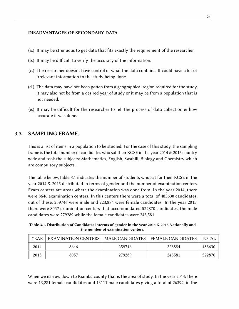
The table below, table 3.1 indicates the number of students who sat for their KCSE in theyear 2014 & 2015 distributed in terms of gender and the number of examination centers.Exam centers are areas where the examination was done from. In the year 2014, therewere 8646 examination centers. In this centers there were a total of 483630 candidates,out of these, 259746 were male and 223,884 were female candidates. In the year 2015,there were 8057 examination centers that accommodated 522870 candidates, the malecandidates were 279289 while the female candidates were 243,581.
Table 3.1. Distribution of Candidates interms of gender in the year 2014 & 2015 Nationally andthe number of examination centers.
YEAR EXAMINATION CENTERS MALE CANDIDATES FEMALE CANDIDATES TOTAL
2014 8646 259746 223884 483630
2015 8057 279289 243581 522870
When we narrow down to Kiambu county that is the area of study. In the year 2014: therewere 13,281 female candidates and 13111 male candidates giving a total of 26392, in the
25
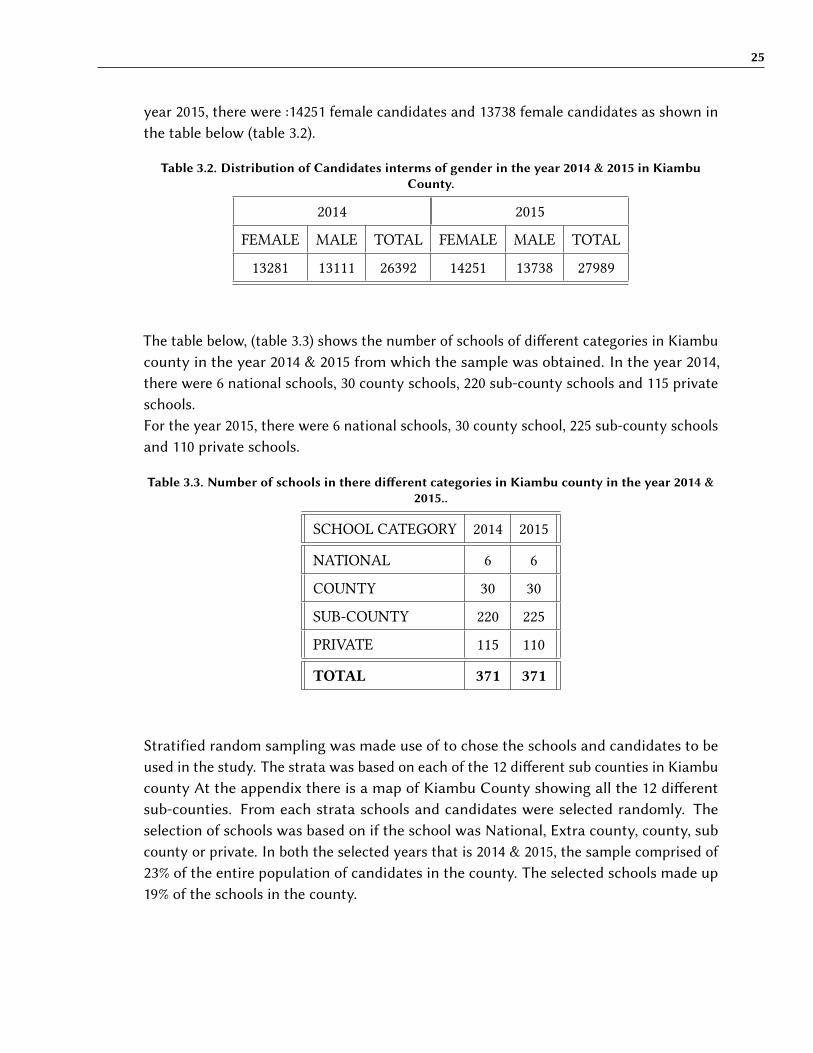
year 2015, there were :14251 female candidates and 13738 female candidates as shown inthe table below (table 3.2).
Table 3.2. Distribution of Candidates interms of gender in the year 2014 & 2015 in KiambuCounty.
2014 2015
FEMALE MALE TOTAL FEMALE MALE TOTAL
13281 13111 26392 14251 13738 27989
The table below, (table 3.3) shows the number of schools of di�erent categories in Kiambucounty in the year 2014 & 2015 from which the sample was obtained. In the year 2014,there were 6 national schools, 30 county schools, 220 sub-county schools and 115 privateschools.For the year 2015, there were 6 national schools, 30 county school, 225 sub-county schoolsand 110 private schools.
Table 3.3. Number of schools in there di�erent categories in Kiambu county in the year 2014 &2015..
SCHOOL CATEGORY 2014 2015
NATIONAL 6 6
COUNTY 30 30
SUB-COUNTY 220 225
PRIVATE 115 110
TOTAL 371 371
Stratified random sampling was made use of to chose the schools and candidates to beused in the study. The strata was based on each of the 12 di�erent sub counties in Kiambucounty At the appendix there is a map of Kiambu County showing all the 12 di�erentsub-counties. From each strata schools and candidates were selected randomly. Theselection of schools was based on if the school was National, Extra county, county, subcounty or private. In both the selected years that is 2014 & 2015, the sample comprised of23% of the entire population of candidates in the county. The selected schools made up19% of the schools in the county.
26
3.4 STATISTICAL SOFTWARE.
The data on KCSE performance comes in Excel.csv format. Excel 2016 program was usedto organize the data, select the data of sampled students & selected schools and convertthe data into numerical form.Rstudio/R version 3.4.0 (2017-04-21) and STATA version 13 were both used in the datacleaning and statistical analysis. The so�ware’s especially R is readily available and free.With R the output is conveniently stored and can be reviewed later and re-run.LATEX.Version Latex2e is the version being used to type this document. The reasonfor using LATEX is scientific. LATEX allows typing of mathematical formula andcomputations, fi�ing of tables, aligning of paragraphs and texts.
3.5 DEFINITION OF VARIABLES.
DEPENDENT/ RESPONSE/ OUTCOME/ CRITERION VARIABLE
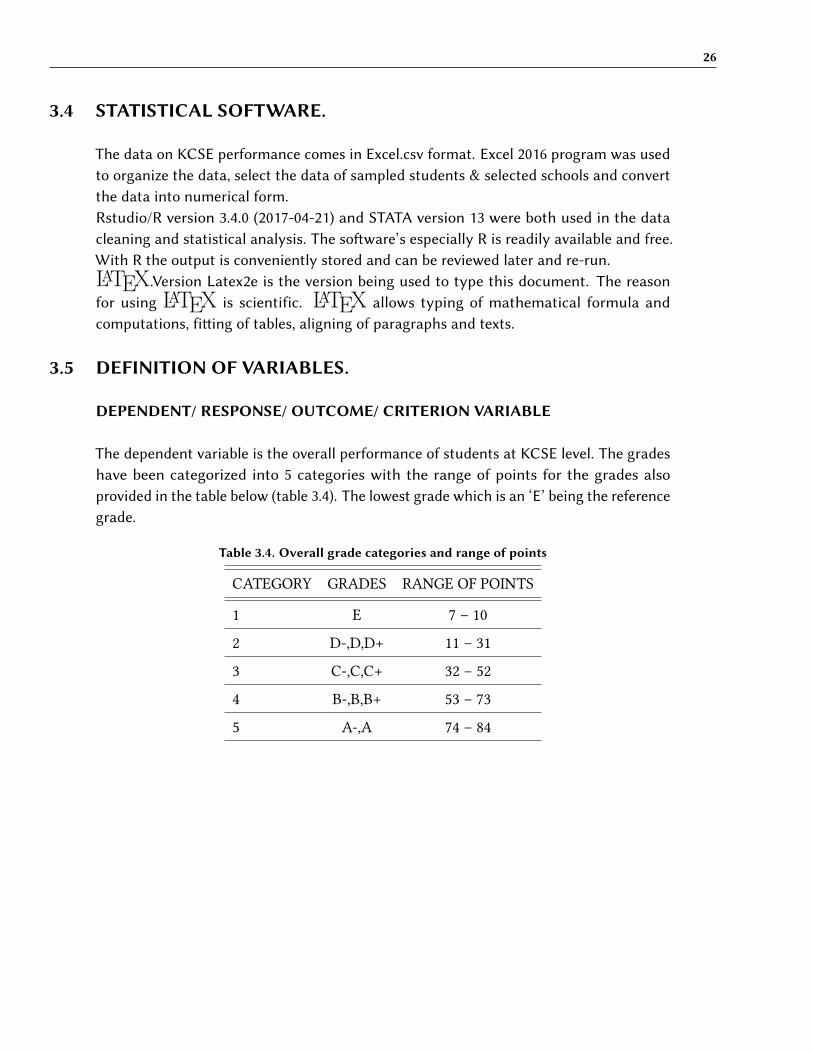
The dependent variable is the overall performance of students at KCSE level. The gradeshave been categorized into 5 categories with the range of points for the grades alsoprovided in the table below (table 3.4). The lowest grade which is an ‘E’ being the referencegrade.
Table 3.4. Overall grade categories and range of points
CATEGORY GRADES RANGE OF POINTS
1 E 7 – 10
2 D-,D,D+ 11 – 31
3 C-,C,C+ 32 – 52
4 B-,B,B+ 53 – 73
5 A-,A 74 – 84
27
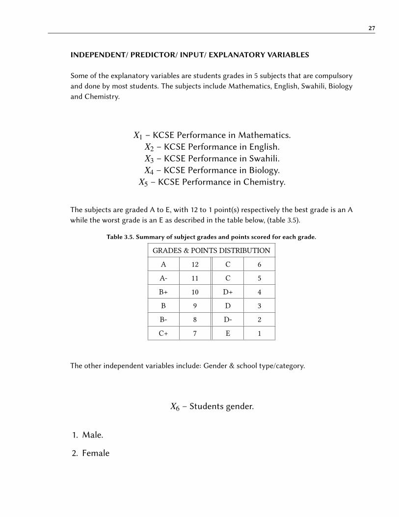
INDEPENDENT/ PREDICTOR/ INPUT/ EXPLANATORY VARIABLES
Some of the explanatory variables are students grades in 5 subjects that are compulsoryand done by most students. The subjects include Mathematics, English, Swahili, Biologyand Chemistry.
X1 – KCSE Performance in Mathematics.X2 – KCSE Performance in English.X3 – KCSE Performance in Swahili.X4 – KCSE Performance in Biology.
X5 – KCSE Performance in Chemistry.
The subjects are graded A to E, with 12 to 1 point(s) respectively the best grade is an Awhile the worst grade is an E as described in the table below, (table 3.5).
Table 3.5. Summary of subject grades and points scored for each grade.
GRADES & POINTS DISTRIBUTION
A 12 C 6
A- 11 C 5
B+ 10 D+ 4
B 9 D 3
B- 8 D- 2
C+ 7 E 1
The other independent variables include: Gender & school type/category.
X6 – Students gender.
1. Male.
2. Female

28
X7 – School type/category.
1. National.
2. Extra County.
3. County.
4. Sub-County.
5. Private.
3.6 ASSUMPTIONS OF THE ORDINAL LOGISTIC REGRESSIONMODEL.
The following assumptions are considered when using the ordinal logistic regression/ theproportional odds model:
1. The outcome variable is to be measured at an ordinal level. The ordinal variable hastwo or several categories that have some natural ordering or ranking.
2. There is one or several input/ explanatory variables that are categorical, Ordinal orContinuous. However, Ordinal input/ explanatory variables must be treated as beingeither categorical or continuous.
3. There isn’t Multicollinearity. Multicollinearity, arises when there are two or severalinput/ explanatory variables that are very much correlated to each other. This eventu-ally develops an issue with figuring out which variable accounts for the interpretationof the outcome/ response variable. Multicollinearity also brings technical issues whenit comes to estimating on ordinal logistic regression.
4. The proportional odds or parallel lines assumption. This means that each Explanatory/input variable has an indistinguishable (similar) e�ect on each aggregate (cumulative)split of the ordinal Response/ output variable (Kleinbaum and Klein, 2010).
Regression coe�icients are the same for all categories.
5. Logistic regression never assumes a linear relationship between the output and inputvariable however a linear relationship is assumed between the logit of the output andinput variables.
29
3.7 ORDINAL LOGISTIC REGRESSION MODEL/ORDINALREGRESSION MODEL/ PROPORTIONAL ODDS MODEL.
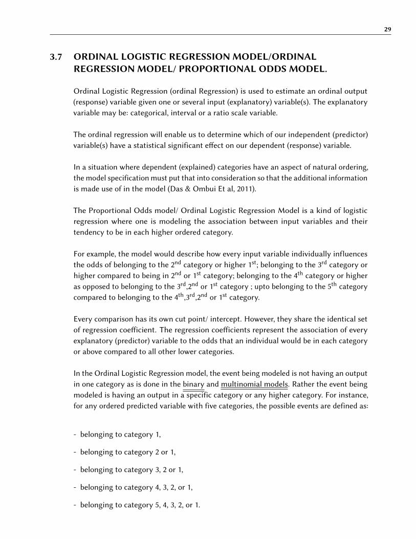
Ordinal Logistic Regression (ordinal Regression) is used to estimate an ordinal output(response) variable given one or several input (explanatory) variable(s). The explanatoryvariable may be: categorical, interval or a ratio scale variable.
The ordinal regression will enable us to determine which of our independent (predictor)variable(s) have a statistical significant e�ect on our dependent (response) variable.
In a situation where dependent (explained) categories have an aspect of natural ordering,the model specification must put that into consideration so that the additional informationis made use of in the model (Das & Ombui Et al, 2011).
The Proportional Odds model/ Ordinal Logistic Regression Model is a kind of logisticregression where one is modeling the association between input variables and theirtendency to be in each higher ordered category.
For example, the model would describe how every input variable individually influencesthe odds of belonging to the 2nd category or higher 1st; belonging to the 3rd category orhigher compared to being in 2nd or 1st category; belonging to the 4th category or higheras opposed to belonging to the 3rd,2nd or 1st category ; upto belonging to the 5th categorycompared to belonging to the 4th,3rd,2nd or 1st category.
Every comparison has its own cut point/ intercept. However, they share the identical setof regression coe�icient. The regression coe�icients represent the association of everyexplanatory (predictor) variable to the odds that an individual would be in each categoryor above compared to all other lower categories.
In the Ordinal Logistic Regression model, the event being modeled is not having an outputin one category as is done in the binary and multinomial models. Rather the event beingmodeled is having an output in a specific category or any higher category. For instance,for any ordered predicted variable with five categories, the possible events are defined as:
- belonging to category 1,
- belonging to category 2 or 1,
- belonging to category 3, 2 or 1,
- belonging to category 4, 3, 2, or 1,
- belonging to category 5, 4, 3, 2, or 1.

30
In the Ordinal Logistic Regression model, Every outcome (response) has its own cut point/intercept but similar regression coe�icients. This implies that, the overall odds of an eventcan di�er, but the e�ect of the regressors on the odds of an event taking place in eachsubsequent category is similar for every category.
31
3.7.1 THE MODEL.
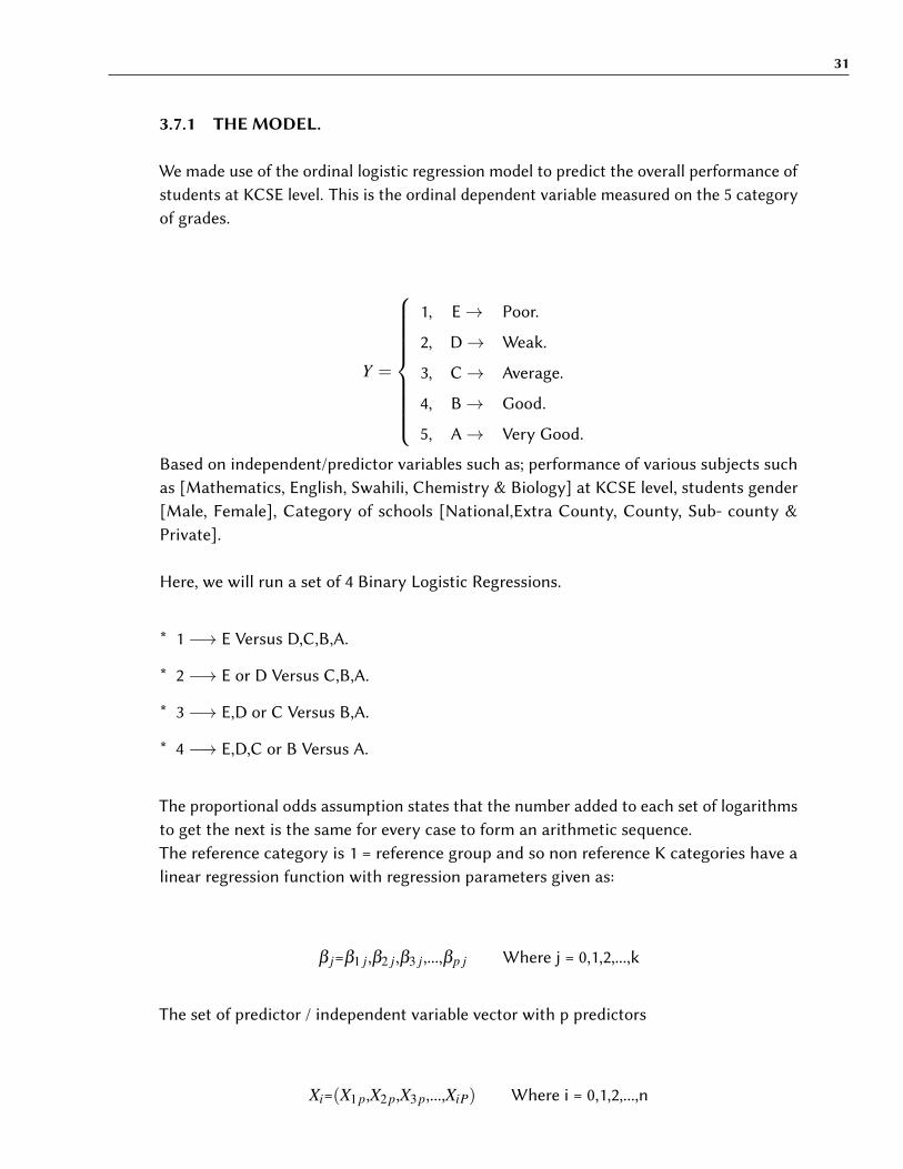
We made use of the ordinal logistic regression model to predict the overall performance ofstudents at KCSE level. This is the ordinal dependent variable measured on the 5 categoryof grades.
Y =
1, E→ Poor.
2, D→ Weak.
3, C→ Average.
4, B→ Good.
5, A→ Very Good.
Based on independent/predictor variables such as; performance of various subjects suchas [Mathematics, English, Swahili, Chemistry & Biology] at KCSE level, students gender[Male, Female], Category of schools [National,Extra County, County, Sub- county &Private].
Here, we will run a set of 4 Binary Logistic Regressions.
* 1 −→ E Versus D,C,B,A.
* 2 −→ E or D Versus C,B,A.
* 3 −→ E,D or C Versus B,A.
* 4 −→ E,D,C or B Versus A.
The proportional odds assumption states that the number added to each set of logarithmsto get the next is the same for every case to form an arithmetic sequence.The reference category is 1 = reference group and so non reference K categories have alinear regression function with regression parameters given as:
β j=β1 j,β2 j,β3 j,...,βp j Where j = 0,1,2,...,k
The set of predictor / independent variable vector with p predictors
Xi=(X1 p,X2 p,X3 p,...,XiP) Where i = 0,1,2,...,n

32
In the Ordinal Logistic Regression the dependent variable is an ordered response categori-cal variable. The independent variable (s) may be categorical, interval or a ratio variable.The response categories have a natural ordering, then the model will be of the form
ln(
P(Y 6 G j)
P(Y > G j)
)= β0 j +β1X1 +β2X2 +β3X3 + ...+βpXp (3.7.1)
NOTE: If there are m predictors in the response variable then there will be m-1 modelswhich have parallel lines as only the intercept is di�erent, for the study we have 5 categoriestherefore we will have 4 models.
3.7.2 LINK FUNCTION.
A link function shows the association between the linear predictor and the mean of thedistribution. It is a transformation of probabilities that allows for estimation of the model.In ordinal logistic regression we use the Logit link function.
The link function is necessary in a categorical response variable as a categorical responsevariable is not continuous, is bounded and is not measured on an interval or ratio scale.The link function is the one that di�erentiates the Logistic regression from the linearregression. It is a function of the mean of the predicted variable Y that is used as theoutput instead of Y itself.
The link function is the inverse of a distribution function. The Logit link function is theinverse of the standard cumulative logistic distribution function.
ln(
π
1−π
)= β0 +β1X1 +β2X2 +β3X3 + ...+βkXk (3.7.2)
The logit function is the natural log of the odds that Y is equal to one of the categories. Thelink function is normally a transformation of the probabilities that allow for approximationof the equation. It’s main purpose is to connect the random component to the le� handside of the equation to the systematic component on the right hand side of the equation.
1. Random Component: This is the probability distribution of the output variable (Y)
2. Systematic Component: It specifies the predictor variables(X1,X2,X3,...,Xk) in the model,moreso their linear combination in creating their linearpredictors. e.g β0+β1X1+β2X2.... in linear regression (Ombui et al,2011).
33
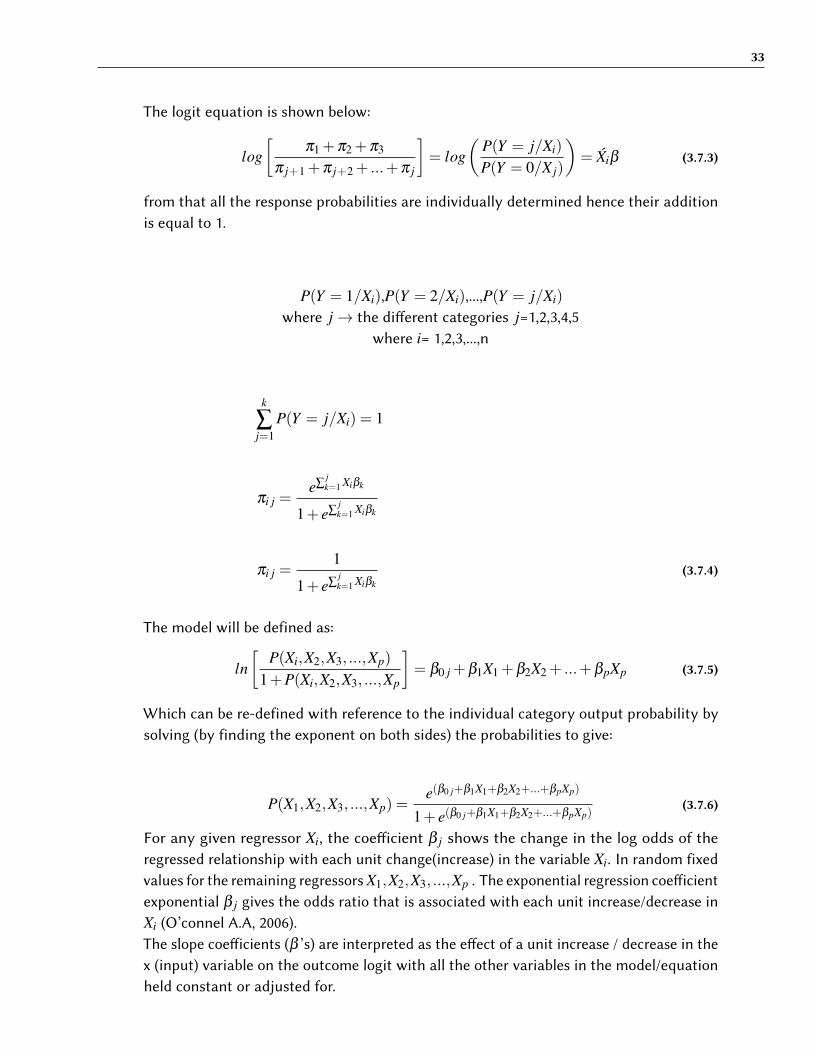
The logit equation is shown below:
log[
π1 +π2 +π3
π j+1 +π j+2 + ...+π j
]= log
(P(Y = j/Xi)
P(Y = 0/X j)
)= X́iβ (3.7.3)
from that all the response probabilities are individually determined hence their additionis equal to 1.
P(Y = 1/Xi),P(Y = 2/Xi),...,P(Y = j/Xi)
where j→ the di�erent categories j=1,2,3,4,5where i= 1,2,3,...,n
k
∑j=1
P(Y = j/Xi) = 1
πi j =e∑
jk=1 Xiβk
1+ e∑jk=1 Xiβk
πi j =1
1+ e∑jk=1 Xiβk
(3.7.4)
The model will be defined as:
ln[
P(Xi,X2,X3, ...,Xp)
1+P(Xi,X2,X3, ...,Xp
]= β0 j +β1X1 +β2X2 + ...+βpXp (3.7.5)
Which can be re-defined with reference to the individual category output probability bysolving (by finding the exponent on both sides) the probabilities to give:
P(X1,X2,X3, ...,Xp) =e(β0 j+β1X1+β2X2+...+βpXp)
1+ e(β0 j+β1X1+β2X2+...+βpXp)(3.7.6)
For any given regressor Xi, the coe�icient β j shows the change in the log odds of theregressed relationship with each unit change(increase) in the variable Xi. In random fixedvalues for the remaining regressors X1,X2,X3, ...,Xp . The exponential regression coe�icientexponential β j gives the odds ratio that is associated with each unit increase/decrease inXi (O’connel A.A, 2006).The slope coe�icients (β ’s) are interpreted as the e�ect of a unit increase / decrease in thex (input) variable on the outcome logit with all the other variables in the model/equationheld constant or adjusted for.
34
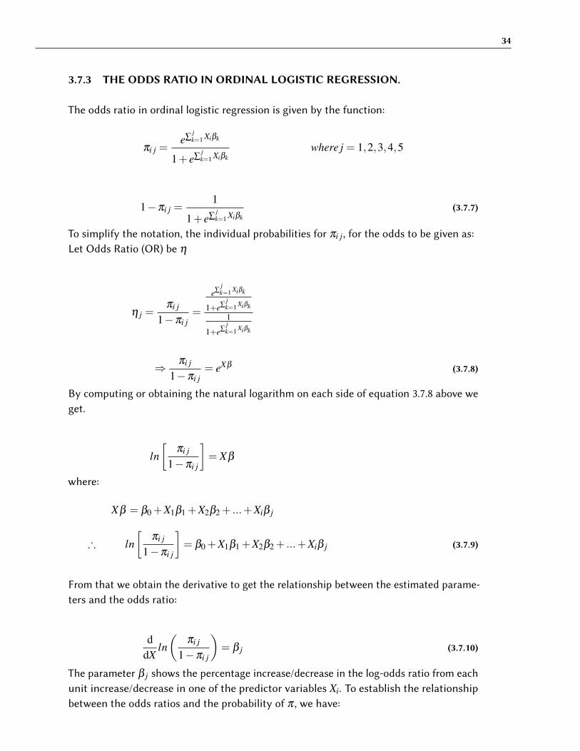
3.7.3 THE ODDS RATIO IN ORDINAL LOGISTIC REGRESSION.
The odds ratio in ordinal logistic regression is given by the function:
πi j =e∑
jk=1 Xiβk
1+ e∑jk=1 Xiβk
where j = 1,2,3,4,5
1−πi j =1
1+ e∑jk=1 Xiβk
(3.7.7)
To simplify the notation, the individual probabilities for πi j, for the odds to be given as:Let Odds Ratio (OR) be η
η j =πi j
1−πi j=
e∑jk=1 Xiβk
1+e∑jk=1 Xiβk
1
1+e∑jk=1 Xiβk
⇒πi j
1−πi j= eXβ (3.7.8)
By computing or obtaining the natural logarithm on each side of equation 3.7.8 above weget.
ln[
πi j
1−πi j
]= Xβ
where:
Xβ = β0 +X1β1 +X2β2 + ...+Xiβ j
∴ ln[
πi j
1−πi j
]= β0 +X1β1 +X2β2 + ...+Xiβ j (3.7.9)
From that we obtain the derivative to get the relationship between the estimated parame-ters and the odds ratio:
ddX
ln(
πi j
1−πi j
)= β j (3.7.10)
The parameter β j shows the percentage increase/decrease in the log-odds ratio from eachunit increase/decrease in one of the predictor variables Xi. To establish the relationshipbetween the odds ratios and the probability of π , we have:
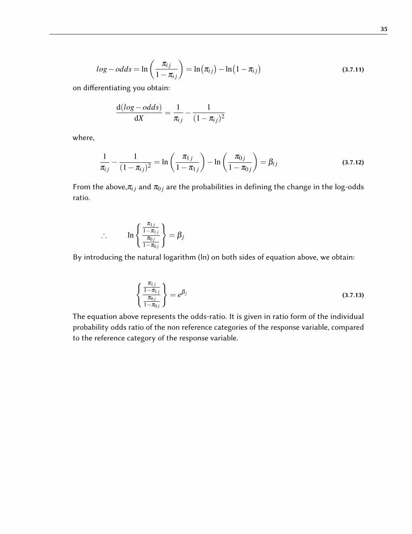
35
log−odds = ln(
πi j
1−πi j
)= ln
(πi j)− ln
(1−πi j
)(3.7.11)
on di�erentiating you obtain:
d(log−odds)dX
=1
πi j− 1
(1−πi j)2
where,
1πi j− 1
(1−πi j)2 = ln(
π1 j
1−π1 j
)− ln
(π0 j
1−π0 j
)= βi j (3.7.12)
From the above,πi j and π0 j are the probabilities in defining the change in the log-oddsratio.
∴ ln
{ π1 j1−π1 j
π0 j1−π0 j
}= β j
By introducing the natural logarithm (ln) on both sides of equation above, we obtain:
{ π1 j1−π1 j
π0 j1−π0 j
}= eβ j (3.7.13)
The equation above represents the odds-ratio. It is given in ratio form of the individualprobability odds ratio of the non reference categories of the response variable, comparedto the reference category of the response variable.
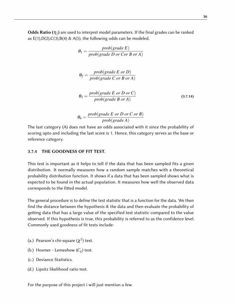
36
Odds Ratio (η j) are used to interpret model parameters. If the final grades can be rankedas E(1),D(2),C(3),B(4) & A(5), the following odds can be modeled.
θ1 =prob(grade E)
prob(grade D or Cor B or A)
θ2 =prob(grade E or D)
prob(grade C or B or A)
θ3 =prob(grade E or D or C)
prob(grade B or A)(3.7.14)
θ4 =prob(grade E or D or C or B)
prob(grade A)The last category (A) does not have an odds associated with it since the probability ofscoring upto and including the last score is 1. Hence, this category serves as the base orreference category.
3.7.4 THE GOODNESS OF FIT TEST.
This test is important as it helps to tell if the data that has been sampled fits a givendistribution. It normally measures how a random sample matches with a theoreticalprobability distribution function. It shows if a data that has been sampled shows what isexpected to be found in the actual population. It measures how well the observed datacorresponds to the fi�ed model.
The general procedure is to define the test statistic that is a function for the data. We thenfind the distance between the hypothesis & the data and then evaluate the probability ofge�ing data that has a large value of the specified test statistic compared to the valueobserved. If this hypothesis is true, this probability is referred to as the confidence level.Commonly used goodness of fit tests include:
(a.) Pearson’s chi-square (χ2) test.
(b.) Hosmer - Lemeshow (Cg) test.
(c.) Deviance Statistics.
(d.) Lipsitz likelihood ratio test.
For the purpose of this project i will just mention a few.

37
3.7.4.1 PEARSONS CHI-SQUARE (χ2) TEST.
This is a goodness of fit test that is used by analysts who desire to tell how well the modelfits the data. It tests/shows the disparity between the reduced model and the full model.It shows how “close" the observed values are to those which are expected in the fi�edmodel. This test is used to tell if the predicted values deviate from the observed valuesin a way that the distribution does not predict. The χ2 test, tests the association of thevariables in the two-way table, where the assumed model of independence is evaluatedagainst the observed data. The general form of the χ2 test is;
χ2 = ∑
(observed− expected)2
expected(3.7.15)
Incase the obtained test statistic is large, this implies that observed and expected valuesare not close and the model is a poor fit to the data.If χ2
calculated > χ2tabulated you reject the null hypothesis (H0) at the given α level of
significance.
However, the test isn’t important if the number of distinct values is approximately equalto the number of observations but is important if you have multiple observations at thesame values of the predictors.
If the p-value for the test is below the chosen significance level, the predicted probabilitieswill deviate from the observed probabilities in a way that the distribution can not predict.Some of the common reasons for this kind of a deviation could be:
. A Link function that is not correct.
. The omission higher-order terms for variance in that model.
. Omission of predictors from the model.
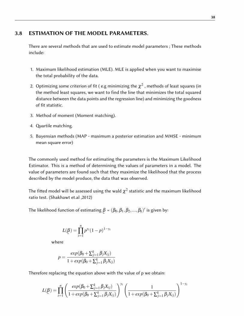
38
3.8 ESTIMATION OF THE MODEL PARAMETERS.
There are several methods that are used to estimate model parameters ; These methodsinclude:
1. Maximum likelihood estimation (MLE). MLE is applied when you want to maximisethe total probability of the data.
2. Optimizing some criterion of fit ( e.g minimizing the χ2 , methods of least squares (inthe method least squares, we want to find the line that minimizes the total squareddistance between the data points and the regression line) and minimizing the goodnessof fit statistic.
3. Method of moment (Moment matching).
4. �artile matching.
5. Bayensian methods (MAP - maximum a posterior estimation and MMSE - minimummean square error)
The commonly used method for estimating the parameters is the Maximum LikelihoodEstimator. This is a method of determining the values of parameters in a model. Thevalue of parameters are found such that they maximize the likelihood that the processdescribed by the model produce, the data that was observed.
The fi�ed model will be assessed using the wald χ2 statistic and the maximum likelihoodratio test. (Shakhawt et.al ,2012)
The likelihood function of estimating˜β = (β0,β1,β2, ...,βk)
′ is given by:
L(˜β ) =
n
∏i=1
pyi(1− p)1−yi
where
p =exp(β0 +∑
kj=1 β jXi j)
1+ exp(β0 +∑kj=1 β jXi j)
Therefore replacing the equation above with the value of p we obtain:
L(˜β ) =
n
∏i=1
(exp(β0 +∑
kj=1 β jXi j)
1+ exp(β0 +∑kj=1 β jXi j)
)yi(
11+ exp(β0 +∑
kj=1 β jXi j)
)1−yi
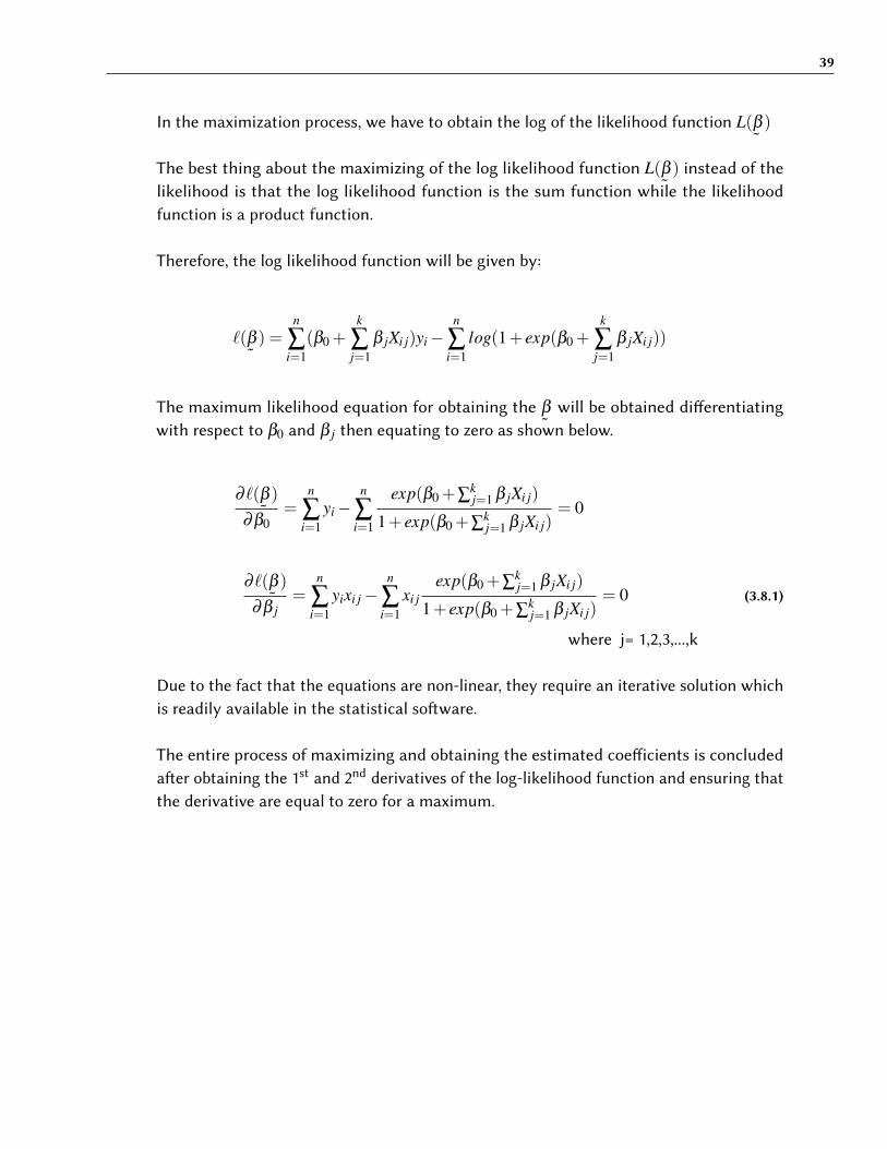
39
In the maximization process, we have to obtain the log of the likelihood function L(˜β )
The best thing about the maximizing of the log likelihood function L(˜β ) instead of the
likelihood is that the log likelihood function is the sum function while the likelihoodfunction is a product function.
Therefore, the log likelihood function will be given by:
`(˜β ) =
n
∑i=1
(β0 +k
∑j=1
β jXi j)yi−n
∑i=1
log(1+ exp(β0 +k
∑j=1
β jXi j))
The maximum likelihood equation for obtaining the˜β will be obtained di�erentiating
with respect to β0 and β j then equating to zero as shown below.
∂`(˜β )
∂β0=
n
∑i=1
yi−n
∑i=1
exp(β0 +∑kj=1 β jXi j)
1+ exp(β0 +∑kj=1 β jXi j)
= 0
∂`(˜β )
∂β j=
n
∑i=1
yixi j−n
∑i=1
xi jexp(β0 +∑
kj=1 β jXi j)
1+ exp(β0 +∑kj=1 β jXi j)
= 0 (3.8.1)
where j= 1,2,3,...,k
Due to the fact that the equations are non-linear, they require an iterative solution whichis readily available in the statistical so�ware.
The entire process of maximizing and obtaining the estimated coe�icients is concludeda�er obtaining the 1st and 2nd derivatives of the log-likelihood function and ensuring thatthe derivative are equal to zero for a maximum.
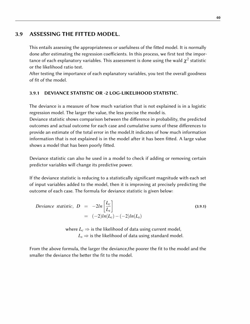
40
3.9 ASSESSING THE FITTED MODEL.
This entails assessing the appropriateness or usefulness of the fi�ed model. It is normallydone a�er estimating the regression coe�icients. In this process, we first test the impor-tance of each explanatory variables. This assessment is done using the wald χ2 statisticor the likelihood ratio test.A�er testing the importance of each explanatory variables, you test the overall goodnessof fit of the model.
3.9.1 DEVIANCE STATISTIC OR -2 LOG-LIKELIHOOD STATISTIC.
The deviance is a measure of how much variation that is not explained is in a logisticregression model. The larger the value, the less precise the model is.Deviance statistic shows comparison between the di�erence in probability, the predictedoutcomes and actual outcome for each case and cumulative sums of these di�erences toprovide an estimate of the total error in the model.It indicates of how much informationinformation that is not explained is in the model a�er it has been fi�ed. A large valueshows a model that has been poorly fi�ed.
Deviance statistic can also he used in a model to check if adding or removing certainpredictor variables will change its predictive power.
If the deviance statistic is reducing to a statistically significant magnitude with each setof input variables added to the model, then it is improving at precisely predicting theoutcome of each case. The formula for deviance statistic is given below:
Deviance statistic, D = −2ln[
Lc
Ls
](3.9.1)
= (−2)ln(Lc)− (−2)ln(Ls)
where Lc⇒ is the likelihood of data using current model,Ls⇒ is the likelihood of data using standard model.
From the above formula, the larger the deviance,the poorer the fit to the model and thesmaller the deviance the be�er the fit to the model.
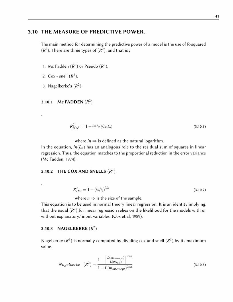
41
3.10 THE MEASURE OF PREDICTIVE POWER.
The main method for determining the predictive power of a model is the use of R-squared(R2). There are three types of (R2), and that is ;
1. Mc Fadden (R2) or Pseudo (R2).
2. Cox - snell (R2).
3. Nagelkerke’s (R2).
3.10.1 Mc FADDEN (R2)
.
R2McF = 1− ln(Lm)/ln(Lo) (3.10.1)
where ln⇒ is defined as the natural logarithm.In the equation, ln(Lo) has an analogous role to the residual sum of squares in linearregression. Thus, the equation matches to the proportional reduction in the error variance(Mc Fadden, 1974).
3.10.2 THE COX AND SNELLS (R2)
.R2
c&s = 1− (lm/l0)2/n (3.10.2)
where n⇒ is the size of the sample.This equation is to be used in normal theory linear regression. It is an identity implying,that the usual (R2) for linear regression relies on the likelihood for the models with orwithout explanatory/ input variables. (Cox et.al, 1989).
3.10.3 NAGELKERKE (R2)
Nagelkerke (R2) is normally computed by dividing cox and snell (R2) by its maximumvalue.
Nagelkerke (R2) =1−[
L(mintercept)L(m f ull)
]2/n
1−L(mintercept)2/n(3.10.3)
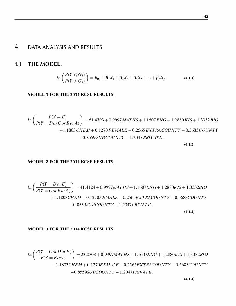
42
4 DATA ANALYSIS AND RESULTS
4.1 THE MODEL.
ln(
P(Y 6 G j)
P(Y > G j)
)= β0 j +β1X1 +β2X2 +β3X3 + ...+βpXp (4.1.1)
MODEL 1 FOR THE 2014 KCSE RESULTS.
ln(
P(Y = E)P(Y = D orC or B or A)
)= 61.4793+0.9997 MAT HS+1.1607 ENG+1.2880 KIS+1.3332 BIO
+1.1803CHEM+0.1270 FEMALE−0.2565 EXT RACOUNTY −0.5683COUNTY
−0.8559 SUBCOUNTY −1.2047 PRIVAT E.(4.1.2)
MODEL 2 FOR THE 2014 KCSE RESULTS.
ln(
P(Y = D or E)P(Y =C or B or A)
)= 41.4124+0.9997MAT HS+1.1607ENG+1.2880KIS+1.3332BIO
+1.1803CHEM+0.1270FEMALE−0.2565EXT RACOUNTY −0.5683COUNTY
−0.8559SUBCOUNTY −1.2047PRIVAT E.(4.1.3)
MODEL 3 FOR THE 2014 KCSE RESULTS.
ln(
P(Y =C or D or E)P(Y = B or A)
)= 23.0308+0.9997MAT HS+1.1607ENG+1.2880KIS+1.3332BIO
+1.1803CHEM+0.1270FEMALE−0.2565EXT RACOUNTY −0.5683COUNTY
−0.8559SUBCOUNTY −1.2047PRIVAT E.(4.1.4)
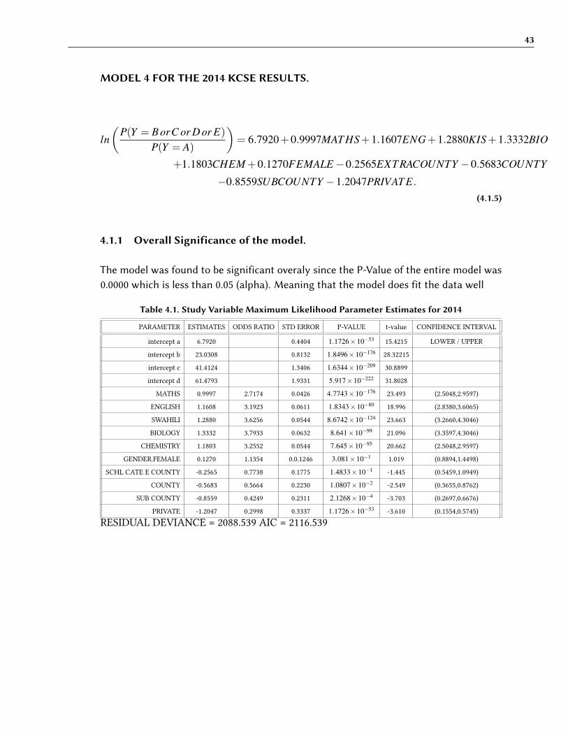
43
MODEL 4 FOR THE 2014 KCSE RESULTS.
ln(
P(Y = B orC or D or E)P(Y = A)
)= 6.7920+0.9997MAT HS+1.1607ENG+1.2880KIS+1.3332BIO
+1.1803CHEM+0.1270FEMALE−0.2565EXT RACOUNTY −0.5683COUNTY
−0.8559SUBCOUNTY −1.2047PRIVAT E.(4.1.5)
4.1.1 Overall Significance of the model.
The model was found to be significant overaly since the P-Value of the entire model was0.0000 which is less than 0.05 (alpha). Meaning that the model does fit the data well
Table 4.1. Study Variable Maximum Likelihood Parameter Estimates for 2014
PARAMETER ESTIMATES ODDS RATIO STD ERROR P-VALUE t-value CONFIDENCE INTERVAL
intercept a 6.7920 0.4404 1.1726×10−5315.4215 LOWER / UPPER
intercept b 23.0308 0.8132 1.8496×10−17628.32215
intercept c 41.4124 1.3406 1.6344×10−20930.8899
intercept d 61.4793 1.9331 5.917×10−22231.8028
MATHS 0.9997 2.7174 0.0426 4.7743×10−17623.493 (2.5048,2.9597)
ENGLISH 1.1608 3.1923 0.0611 1.8343×10−8018.996 (2.8380,3.6065)
SWAHILI 1.2880 3.6256 0.0544 8.6742×10−12423.663 (3.2660,4.3046)
BIOLOGY 1.3332 3.7933 0.0632 8.641×10−9921.096 (3.3597,4.3046)
CHEMISTRY 1.1803 3.2552 0.0544 7.645×10−9520.662 (2.5048,2.9597)
GENDER.FEMALE 0.1270 1.1354 0.0.1246 3.081×10−11.019 (0.8894,1.4498)
SCHL CATE E COUNTY -0.2565 0.7738 0.1775 1.4833×10⁻¹-1.445 (0.5459,1.0949)
COUNTY -0.5683 0.5664 0.2230 1.0807×10⁻²-2.549 (0.3655,0.8762)
SUB COUNTY -0.8559 0.4249 0.2311 2.1268×10⁻⁴-3.703 (0.2697,0.6676)
PRIVATE -1.2047 0.2998 0.3337 1.1726×10−53-3.610 (0.1554,0.5745)
RESIDUAL DEVIANCE = 2088.539 AIC = 2116.539
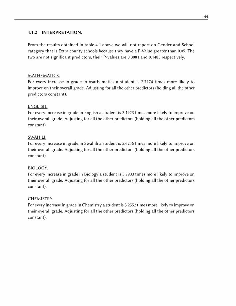
44
4.1.2 INTERPRETATION.
From the results obtained in table 4.1 above we will not report on Gender and Schoolcategory that is Extra county schools because they have a P-Value greater than 0.05. Thetwo are not significant predictors, their P-values are 0.3081 and 0.1483 respectively.
MATHEMATICS.For every increase in grade in Mathematics a student is 2.7174 times more likely toimprove on their overall grade. Adjusting for all the other predictors (holding all the otherpredictors constant).
ENGLISH.For every increase in grade in English a student is 3.1923 times more likely to improve ontheir overall grade. Adjusting for all the other predictors (holding all the other predictorsconstant).
SWAHILI.For every increase in grade in Swahili a student is 3.6256 times more likely to improve ontheir overall grade. Adjusting for all the other predictors (holding all the other predictorsconstant).
BIOLOGY.For every increase in grade in Biology a student is 3.7933 times more likely to improve ontheir overall grade. Adjusting for all the other predictors (holding all the other predictorsconstant).
CHEMISTRY.For every increase in grade in Chemistry a student is 3.2552 times more likely to improve ontheir overall grade. Adjusting for all the other predictors (holding all the other predictorsconstant).
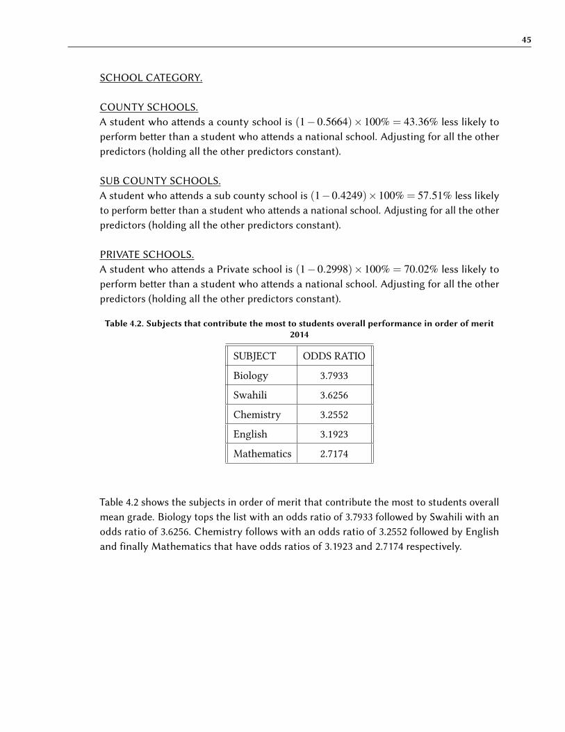
45
SCHOOL CATEGORY.
COUNTY SCHOOLS.A student who a�ends a county school is (1− 0.5664)× 100% = 43.36% less likely toperform be�er than a student who a�ends a national school. Adjusting for all the otherpredictors (holding all the other predictors constant).
SUB COUNTY SCHOOLS.A student who a�ends a sub county school is (1−0.4249)×100% = 57.51% less likelyto perform be�er than a student who a�ends a national school. Adjusting for all the otherpredictors (holding all the other predictors constant).
PRIVATE SCHOOLS.A student who a�ends a Private school is (1− 0.2998)× 100% = 70.02% less likely toperform be�er than a student who a�ends a national school. Adjusting for all the otherpredictors (holding all the other predictors constant).
Table 4.2. Subjects that contribute the most to students overall performance in order of merit2014
SUBJECT ODDS RATIO
Biology 3.7933
Swahili 3.6256
Chemistry 3.2552
English 3.1923
Mathematics 2.7174
Table 4.2 shows the subjects in order of merit that contribute the most to students overallmean grade. Biology tops the list with an odds ratio of 3.7933 followed by Swahili with anodds ratio of 3.6256. Chemistry follows with an odds ratio of 3.2552 followed by Englishand finally Mathematics that have odds ratios of 3.1923 and 2.7174 respectively.
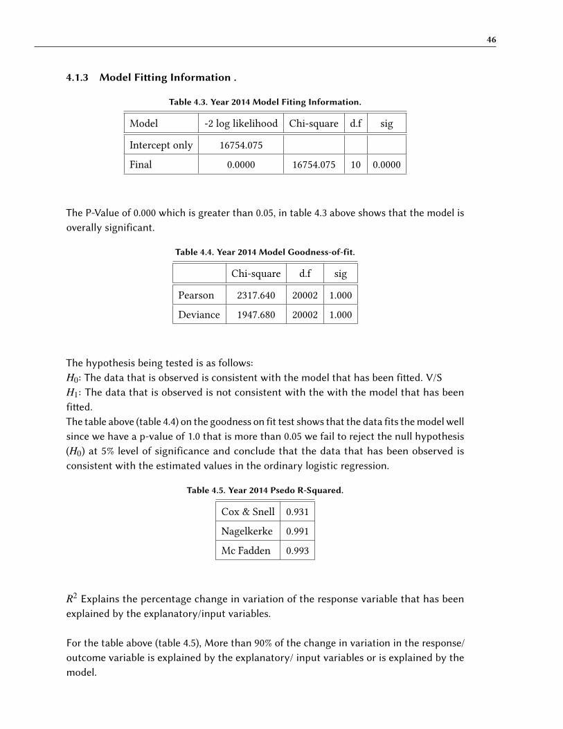
46
4.1.3 Model Fi�ing Information .
Table 4.3. Year 2014 Model Fiting Information.
Model -2 log likelihood Chi-square d.f sig
Intercept only 16754.075
Final 0.0000 16754.075 10 0.0000
The P-Value of 0.000 which is greater than 0.05, in table 4.3 above shows that the model isoverally significant.
Table 4.4. Year 2014 Model Goodness-of-fit.
Chi-square d.f sig
Pearson 2317.640 20002 1.000
Deviance 1947.680 20002 1.000
The hypothesis being tested is as follows:H0: The data that is observed is consistent with the model that has been fi�ed. V/SH1: The data that is observed is not consistent with the with the model that has beenfi�ed.The table above (table 4.4) on the goodness on fit test shows that the data fits the model wellsince we have a p-value of 1.0 that is more than 0.05 we fail to reject the null hypothesis(H0) at 5% level of significance and conclude that the data that has been observed isconsistent with the estimated values in the ordinary logistic regression.
Table 4.5. Year 2014 Psedo R-Squared.
Cox & Snell 0.931
Nagelkerke 0.991
Mc Fadden 0.993
R2 Explains the percentage change in variation of the response variable that has beenexplained by the explanatory/input variables.
For the table above (table 4.5), More than 90% of the change in variation in the response/outcome variable is explained by the explanatory/ input variables or is explained by themodel.
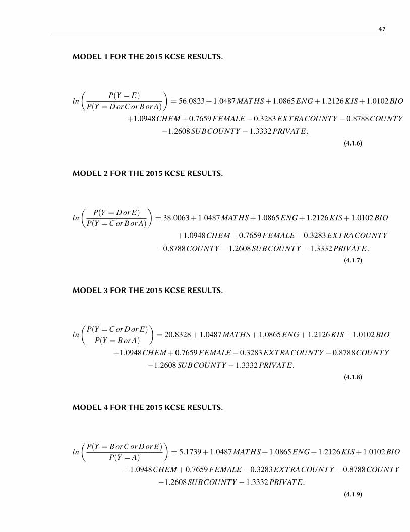
47
MODEL 1 FOR THE 2015 KCSE RESULTS.
ln(
P(Y = E)P(Y = D orC or B or A)
)= 56.0823+1.0487 MAT HS+1.0865 ENG+1.2126 KIS+1.0102 BIO
+1.0948CHEM+0.7659 FEMALE−0.3283 EXT RACOUNTY −0.8788COUNTY
−1.2608 SUBCOUNTY −1.3332 PRIVAT E.(4.1.6)
MODEL 2 FOR THE 2015 KCSE RESULTS.
ln(
P(Y = D or E)P(Y =C or B or A)
)= 38.0063+1.0487 MAT HS+1.0865 ENG+1.2126 KIS+1.0102 BIO
+1.0948CHEM+0.7659 FEMALE−0.3283 EXT RACOUNTY
−0.8788COUNTY −1.2608 SUBCOUNTY −1.3332 PRIVAT E.(4.1.7)
MODEL 3 FOR THE 2015 KCSE RESULTS.
ln(
P(Y =C or D or E)P(Y = B or A)
)= 20.8328+1.0487 MAT HS+1.0865 ENG+1.2126 KIS+1.0102 BIO
+1.0948CHEM+0.7659 FEMALE−0.3283 EXT RACOUNTY −0.8788COUNTY
−1.2608 SUBCOUNTY −1.3332 PRIVAT E.(4.1.8)
MODEL 4 FOR THE 2015 KCSE RESULTS.
ln(
P(Y = B orC or D or E)P(Y = A)
)= 5.1739+1.0487 MAT HS+1.0865 ENG+1.2126 KIS+1.0102 BIO
+1.0948CHEM+0.7659 FEMALE−0.3283 EXT RACOUNTY −0.8788COUNTY
−1.2608 SUBCOUNTY −1.3332 PRIVAT E.(4.1.9)
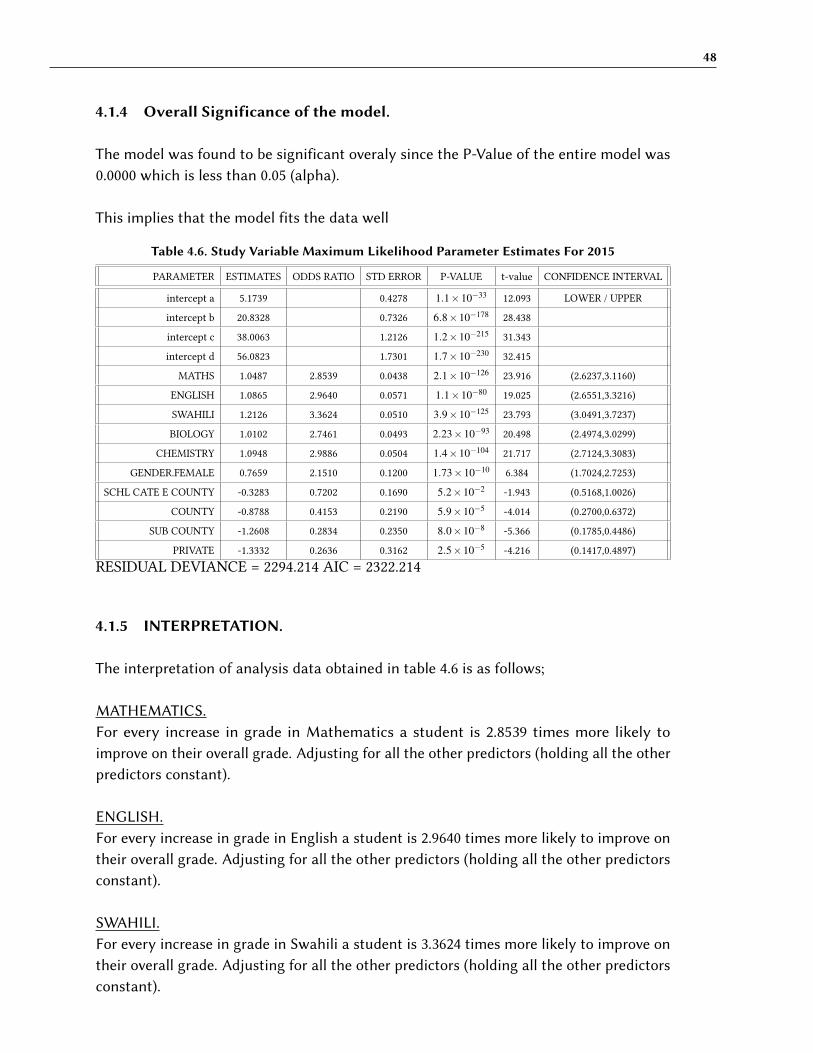
48
4.1.4 Overall Significance of the model.
The model was found to be significant overaly since the P-Value of the entire model was0.0000 which is less than 0.05 (alpha).
This implies that the model fits the data well
Table 4.6. Study Variable Maximum Likelihood Parameter Estimates For 2015
PARAMETER ESTIMATES ODDS RATIO STD ERROR P-VALUE t-value CONFIDENCE INTERVAL
intercept a 5.1739 0.4278 1.1×10−3312.093 LOWER / UPPER
intercept b 20.8328 0.7326 6.8×10−17828.438
intercept c 38.0063 1.2126 1.2×10−21531.343
intercept d 56.0823 1.7301 1.7×10−23032.415
MATHS 1.0487 2.8539 0.0438 2.1×10−12623.916 (2.6237,3.1160)
ENGLISH 1.0865 2.9640 0.0571 1.1×10−8019.025 (2.6551,3.3216)
SWAHILI 1.2126 3.3624 0.0510 3.9×10−12523.793 (3.0491,3.7237)
BIOLOGY 1.0102 2.7461 0.0493 2.23×10−9320.498 (2.4974,3.0299)
CHEMISTRY 1.0948 2.9886 0.0504 1.4×10−10421.717 (2.7124,3.3083)
GENDER.FEMALE 0.7659 2.1510 0.1200 1.73×10−106.384 (1.7024,2.7253)
SCHL CATE E COUNTY -0.3283 0.7202 0.1690 5.2×10⁻²-1.943 (0.5168,1.0026)
COUNTY -0.8788 0.4153 0.2190 5.9×10⁻⁵-4.014 (0.2700,0.6372)
SUB COUNTY -1.2608 0.2834 0.2350 8.0×10⁻⁸-5.366 (0.1785,0.4486)
PRIVATE -1.3332 0.2636 0.3162 2.5×10⁻⁵-4.216 (0.1417,0.4897)
RESIDUAL DEVIANCE = 2294.214 AIC = 2322.214
4.1.5 INTERPRETATION.
The interpretation of analysis data obtained in table 4.6 is as follows;
MATHEMATICS.For every increase in grade in Mathematics a student is 2.8539 times more likely toimprove on their overall grade. Adjusting for all the other predictors (holding all the otherpredictors constant).
ENGLISH.For every increase in grade in English a student is 2.9640 times more likely to improve ontheir overall grade. Adjusting for all the other predictors (holding all the other predictorsconstant).
SWAHILI.For every increase in grade in Swahili a student is 3.3624 times more likely to improve ontheir overall grade. Adjusting for all the other predictors (holding all the other predictorsconstant).
49
BIOLOGY.For every increase in grade in Biology a student is 2.7461 times more likely to improve ontheir overall grade. Adjusting for all the other predictors (holding all the other predictorsconstant).
CHEMISTRY.For every increase in grade in Chemistry a student is 2.9886 times more likely to improve ontheir overall grade. Adjusting for all the other predictors (holding all the other predictorsconstant).
GENDER.Female students are 2.1510 times more likely to perform be�er than their male counterparts. Adjusting for all the other predictors (holding all the other predictors constant).
SCHOOL CATEGORY.We will not report for Extra county schools since it has a P-Value of 0.052 which is slightlyabove the α (0.05) level of significance.
COUNTY SCHOOLS.A student who a�ends a county school is (1− 0.4148)× 100% = 58.47% less likely toperform be�er than a student who a�ends a national school. Adjusting for all the otherpredictors (holding all the other predictors constant).
SUB COUNTY SCHOOLS.A student who a�ends a sub county school is (1−0.2834)×100% = 71.66% less likelyto perform be�er than a student who a�ends a national school. Adjusting for all the otherpredictors (holding all the other predictors constant).
PRIVATE SCHOOLS.A student who a�ends a Private school is (1− 0.2636)× 100% = 73.64% less likely toperform be�er than a student who a�ends a national school. Adjusting for all the otherpredictors (holding all the other predictors constant).
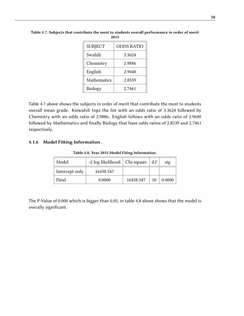
50
Table 4.7. Subjects that contribute the most to students overall performance in order of merit2015
SUBJECT ODDS RATIO
Swahili 3.3624
Chemistry 2.9886
English 2.9640
Mathematics 2.8539
Biology 2.7461
Table 4.7 above shows the subjects in order of merit that contribute the most to studentsoverall mean grade. Kiswahili tops the list with an odds ratio of 3.3624 followed byChemistry with an odds ratio of 2.9886. English follows with an odds ratio of 2.9640followed by Mathematics and finally Biology that have odds ratios of 2.8539 and 2.7461respectively.
4.1.6 Model Fi�ing Information .
Table 4.8. Year 2015 Model Fiting Information.
Model -2 log likelihood Chi-square d.f sig
Intercept only 16438.347
Final 0.0000 16438.347 10 0.0000
The P-Value of 0.000 which is bigger than 0.05, in table 4.8 above shows that the model isoverally significant.

51
Table 4.9. Year 2015 Model Goodness-of-fit.
Chi-square d.f sig
Pearson 2179.649 19670 1.000
Deviance 2103.165 19670 1.000
The hypothesis being tested are as follows:H0: The data that is observed is consistent with the model that has been fi�ed.H1: The data that is observed is not consistent with the with the model that has beenfi�ed.The table above (table 4.9) on the goodness on fit test shows that the data fits the model wellsince we have a p-value of 1.0 that is more than 0.05 we fail to reject the null hypothesis H0
at 5% level of significance and conclude that the data that has been observed is consistentwith the estimated values in the ordinary logistic regression.
Table 4.10. Year 2015 Psedo R-Squared.
Cox & Snell 0.931
Nagelkerke 0.998
Mc Fadden 0.992
R2 Explains the percentage change in variation in the response variable that is explainedby the explanatory/input variables.
For the table above (table 4.10), More than 90% of the change in variation in the re-sponse/outcome variable is explained by the explanatory/input variables or is explainedby the model.
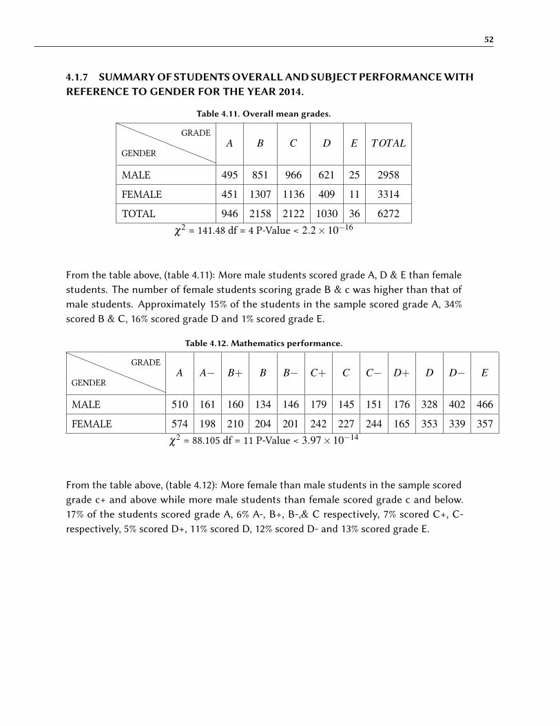
52
4.1.7 SUMMARY OF STUDENTS OVERALL AND SUBJECT PERFORMANCE WITHREFERENCE TO GENDER FOR THE YEAR 2014.
Table 4.11. Overall mean grades.aaaaaaaaaaa
GENDER
GRADE
A B C D E TOTAL
MALE 495 851 966 621 25 2958
FEMALE 451 1307 1136 409 11 3314
TOTAL 946 2158 2122 1030 36 6272
χ2= 141.48 df = 4 P-Value < 2.2×10⁻¹⁶
From the table above, (table 4.11): More male students scored grade A, D & E than femalestudents. The number of female students scoring grade B & c was higher than that ofmale students. Approximately 15% of the students in the sample scored grade A, 34%scored B & C, 16% scored grade D and 1% scored grade E.
Table 4.12. Mathematics performance.aaaaaaaaaaa
GENDER
GRADE
A A− B+ B B− C+ C C− D+ D D− E
MALE 510 161 160 134 146 179 145 151 176 328 402 466
FEMALE 574 198 210 204 201 242 227 244 165 353 339 357χ2
= 88.105 df = 11 P-Value < 3.97×10⁻¹⁴
From the table above, (table 4.12): More female than male students in the sample scoredgrade c+ and above while more male students than female scored grade c and below.17% of the students scored grade A, 6% A-, B+, B-,& C respectively, 7% scored C+, C-respectively, 5% scored D+, 11% scored D, 12% scored D- and 13% scored grade E.
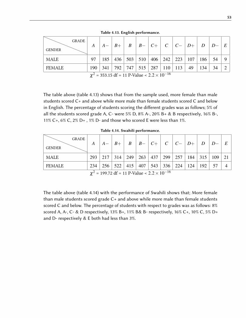
53
Table 4.13. English performance.aaaaaaaaaaa
GENDER
GRADE
A A− B+ B B− C+ C C− D+ D D− E
MALE 97 185 436 503 510 406 242 223 107 186 54 9
FEMALE 190 341 792 747 515 287 110 113 49 134 34 2
χ2= 353.15 df = 11 P-Value < 2.2×10⁻¹⁶
The table above (table 4.13) shows that from the sample used, more female than malestudents scored C+ and above while more male than female students scored C and belowin English. The percentage of students scoring the di�erent grades was as follows; 5% ofall the students scored grade A, C- were 5% D, 8% A-, 20% B+ & B respectively, 16% B-,11% C+, 6% C, 2% D+ , 1% D- and those who scored E were less than 1%.
Table 4.14. Swahili performance.aaaaaaaaaaa
GENDER
GRADE
A A− B+ B B− C+ C C− D+ D D− E
MALE 293 217 314 249 263 437 299 257 184 315 109 21
FEMALE 234 256 522 415 407 543 336 224 124 192 57 4
χ2= 199.72 df = 11 P-Value < 2.2×10⁻¹⁶
The table above (table 4.14) with the performance of Swahili shows that; More femalethan male students scored grade C+ and above while more male than female studentsscored C and below. The percentage of students with respect to grades was as follows: 8%scored A, A-, C- & D respectively, 13% B+, 11% B& B- respectively, 16% C+, 10% C, 5% D+and D- respectively & E both had less than 3%.
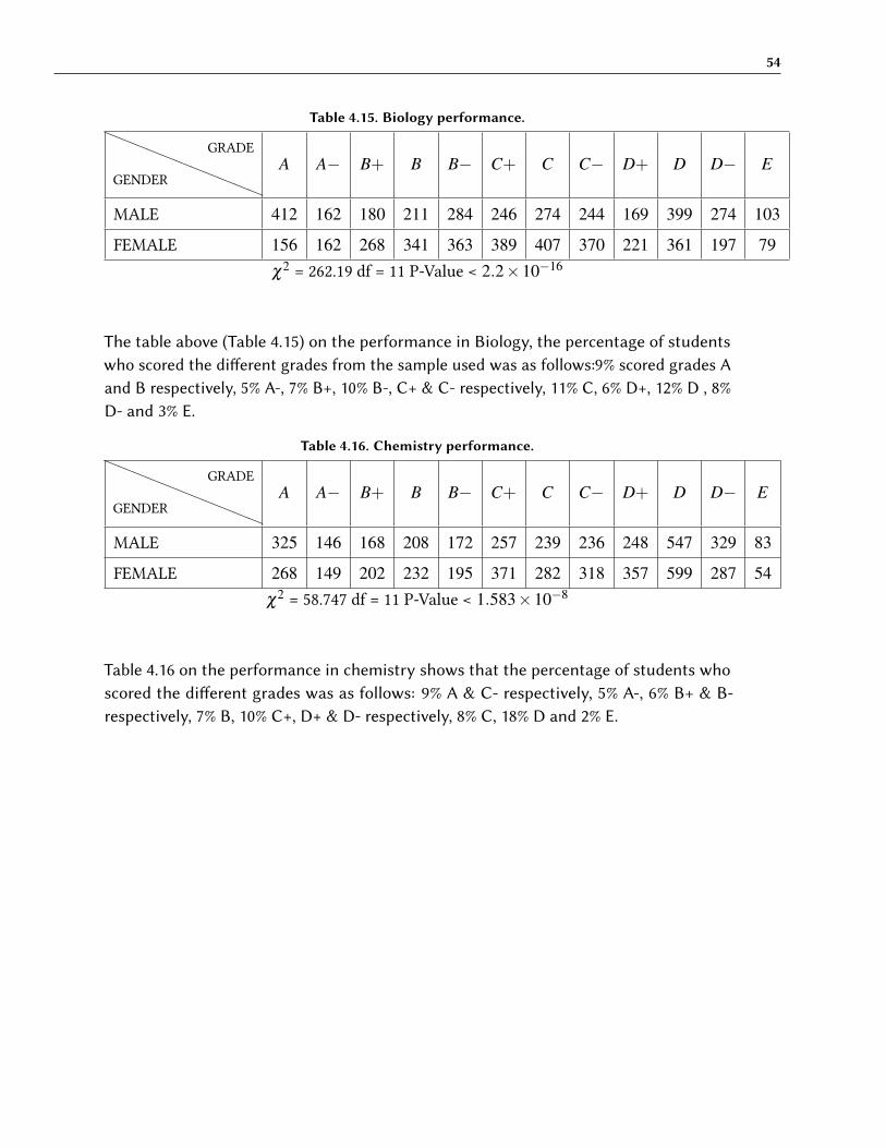
54
Table 4.15. Biology performance.aaaaaaaaaaa
GENDER
GRADE
A A− B+ B B− C+ C C− D+ D D− E
MALE 412 162 180 211 284 246 274 244 169 399 274 103
FEMALE 156 162 268 341 363 389 407 370 221 361 197 79
χ2= 262.19 df = 11 P-Value < 2.2×10⁻¹⁶
The table above (Table 4.15) on the performance in Biology, the percentage of studentswho scored the di�erent grades from the sample used was as follows:9% scored grades Aand B respectively, 5% A-, 7% B+, 10% B-, C+ & C- respectively, 11% C, 6% D+, 12% D , 8%D- and 3% E.
Table 4.16. Chemistry performance.aaaaaaaaaaa
GENDER
GRADE
A A− B+ B B− C+ C C− D+ D D− E
MALE 325 146 168 208 172 257 239 236 248 547 329 83
FEMALE 268 149 202 232 195 371 282 318 357 599 287 54χ2
= 58.747 df = 11 P-Value < 1.583×10⁻⁸
Table 4.16 on the performance in chemistry shows that the percentage of students whoscored the di�erent grades was as follows: 9% A & C- respectively, 5% A-, 6% B+ & B-respectively, 7% B, 10% C+, D+ & D- respectively, 8% C, 18% D and 2% E.
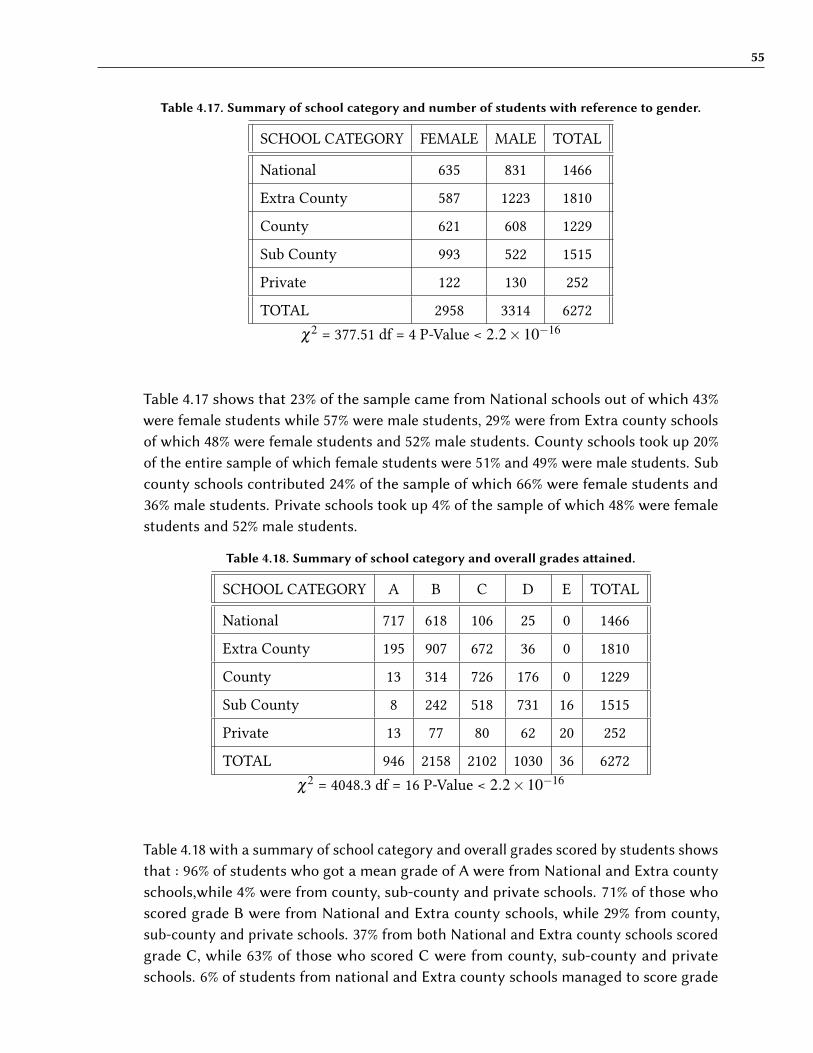
55
Table 4.17. Summary of school category and number of students with reference to gender.
SCHOOL CATEGORY FEMALE MALE TOTAL
National 635 831 1466
Extra County 587 1223 1810
County 621 608 1229
Sub County 993 522 1515
Private 122 130 252
TOTAL 2958 3314 6272
χ2= 377.51 df = 4 P-Value < 2.2×10⁻¹⁶
Table 4.17 shows that 23% of the sample came from National schools out of which 43%were female students while 57% were male students, 29% were from Extra county schoolsof which 48% were female students and 52% male students. County schools took up 20%of the entire sample of which female students were 51% and 49% were male students. Subcounty schools contributed 24% of the sample of which 66% were female students and36% male students. Private schools took up 4% of the sample of which 48% were femalestudents and 52% male students.
Table 4.18. Summary of school category and overall grades a�ained.
SCHOOL CATEGORY A B C D E TOTAL
National 717 618 106 25 0 1466
Extra County 195 907 672 36 0 1810
County 13 314 726 176 0 1229
Sub County 8 242 518 731 16 1515
Private 13 77 80 62 20 252
TOTAL 946 2158 2102 1030 36 6272
χ2= 4048.3 df = 16 P-Value < 2.2×10⁻¹⁶
Table 4.18 with a summary of school category and overall grades scored by students showsthat : 96% of students who got a mean grade of A were from National and Extra countyschools,while 4% were from county, sub-county and private schools. 71% of those whoscored grade B were from National and Extra county schools, while 29% from county,sub-county and private schools. 37% from both National and Extra county schools scoredgrade C, while 63% of those who scored C were from county, sub-county and privateschools. 6% of students from national and Extra county schools managed to score grade

56
D, while 94% were from county, sub-county and private schools. All the students whoscored a mean grade of E were from sub-county and private schools.
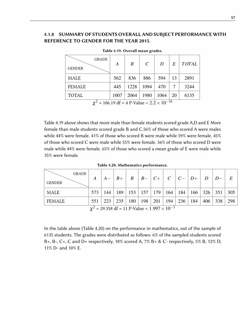
57
4.1.8 SUMMARY OF STUDENTS OVERALL AND SUBJECT PERFORMANCE WITHREFERENCE TO GENDER FOR THE YEAR 2015.
Table 4.19. Overall mean grades.aaaaaaaaaaa
GENDER
GRADE
A B C D E TOTAL
MALE 562 836 886 594 13 2891
FEMALE 445 1228 1094 470 7 3244
TOTAL 1007 2064 1980 1064 20 6135
χ2= 106.19 df = 4 P-Value < 2.2×10⁻¹⁶
Table 4.19 above shows that more male than female students scored grade A,D and E Morefemale than male students scored grade B and C.56% of those who scored A were maleswhile 44% were female. 41% of those who scored B were male while 59% were female. 45%of those who scored C were male while 55% were female. 56% of those who scored D weremale while 44% were female. 65% of those who scored a mean grade of E were male while35% were female.
Table 4.20. Mathematics performance.aaaaaaaaaaa
GENDER
GRADE
A A− B+ B B− C+ C C− D+ D D− E
MALE 573 144 189 153 157 179 164 184 166 326 351 305
FEMALE 551 223 235 180 198 201 194 236 184 406 338 298χ2
= 29.358 df = 11 P-Value < 1.997×10⁻³
In the table above (Table 4.20) on the performance in mathematics, out of the sample of6135 students. The grades were distributed as follows: 6% of the sampled students scoredB+, B-, C+, C and D+ respectively, 18% scored A, 7% B+ & C- respectively, 5% B, 12% D,11% D- and 10% E.
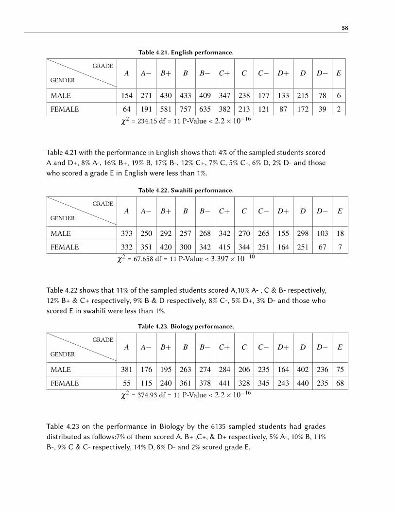
58
Table 4.21. English performance.aaaaaaaaaaa
GENDER
GRADE
A A− B+ B B− C+ C C− D+ D D− E
MALE 154 271 430 433 409 347 238 177 133 215 78 6
FEMALE 64 191 581 757 635 382 213 121 87 172 39 2
χ2= 234.15 df = 11 P-Value < 2.2×10⁻¹⁶
Table 4.21 with the performance in English shows that: 4% of the sampled students scoredA and D+, 8% A-, 16% B+, 19% B, 17% B-, 12% C+, 7% C, 5% C-, 6% D, 2% D- and thosewho scored a grade E in English were less than 1%.
Table 4.22. Swahili performance.aaaaaaaaaaa
GENDER
GRADE
A A− B+ B B− C+ C C− D+ D D− E
MALE 373 250 292 257 268 342 270 265 155 298 103 18
FEMALE 332 351 420 300 342 415 344 251 164 251 67 7χ2
= 67.658 df = 11 P-Value < 3.397×10⁻¹⁰
Table 4.22 shows that 11% of the sampled students scored A,10% A- , C & B- respectively,12% B+ & C+ respectively, 9% B & D respectively, 8% C-, 5% D+, 3% D- and those whoscored E in swahili were less than 1%.
Table 4.23. Biology performance.aaaaaaaaaaa
GENDER
GRADE
A A− B+ B B− C+ C C− D+ D D− E
MALE 381 176 195 263 274 284 206 235 164 402 236 75
FEMALE 55 115 240 361 378 441 328 345 243 440 235 68
χ2= 374.93 df = 11 P-Value < 2.2×10⁻¹⁶
Table 4.23 on the performance in Biology by the 6135 sampled students had gradesdistributed as follows:7% of them scored A, B+ ,C+, & D+ respectively, 5% A-, 10% B, 11%B-, 9% C & C- respectively, 14% D, 8% D- and 2% scored grade E.
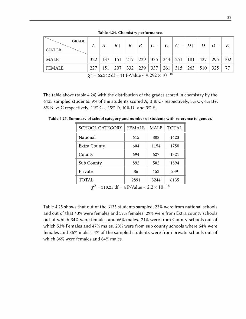
59
Table 4.24. Chemistry performance.aaaaaaaaaaa
GENDER
GRADE
A A− B+ B B− C+ C C− D+ D D− E
MALE 322 137 151 217 229 335 244 251 181 427 295 102
FEMALE 227 151 207 332 239 337 261 315 263 510 325 77χ2
= 65.342 df = 11 P-Value < 9.292×10⁻¹⁰
The table above (table 4.24) with the distribution of the grades scored in chemistry by the6135 sampled students: 9% of the students scored A, B & C- respectively, 5% C-, 6% B+,8% B- & C respectively, 11% C+, 15% D, 10% D- and 3% E.
Table 4.25. Summary of school category and number of students with reference to gender.
SCHOOL CATEGORY FEMALE MALE TOTAL
National 615 808 1423
Extra County 604 1154 1758
County 694 627 1321
Sub County 892 502 1394
Private 86 153 239
TOTAL 2891 3244 6135
χ2= 310.25 df = 4 P-Value < 2.2×10⁻¹⁶
Table 4.25 shows that out of the 6135 students sampled, 23% were from national schoolsand out of that 43% were females and 57% females. 29% were from Extra county schoolsout of which 34% were females and 66% males. 21% were from County schools out ofwhich 53% Females and 47% males. 23% were from sub county schools where 64% werefemales and 36% males. 4% of the sampled students were from private schools out ofwhich 36% were females and 64% males.
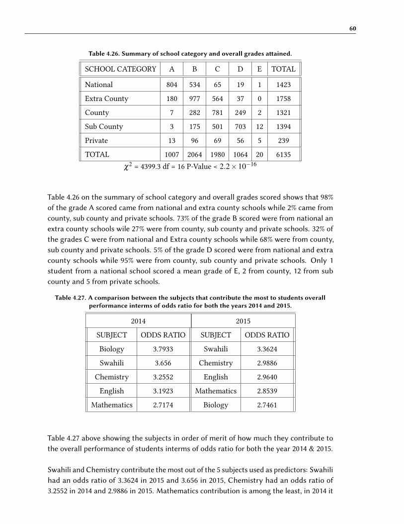
60
Table 4.26. Summary of school category and overall grades a�ained.
SCHOOL CATEGORY A B C D E TOTAL
National 804 534 65 19 1 1423
Extra County 180 977 564 37 0 1758
County 7 282 781 249 2 1321
Sub County 3 175 501 703 12 1394
Private 13 96 69 56 5 239
TOTAL 1007 2064 1980 1064 20 6135
χ2= 4399.3 df = 16 P-Value < 2.2×10⁻¹⁶
Table 4.26 on the summary of school category and overall grades scored shows that 98%of the grade A scored came from national and extra county schools while 2% came fromcounty, sub county and private schools. 73% of the grade B scored were from national anextra county schools wile 27% were from county, sub county and private schools. 32% ofthe grades C were from national and Extra county schools while 68% were from county,sub county and private schools. 5% of the grade D scored were from national and extracounty schools while 95% were from county, sub county and private schools. Only 1student from a national school scored a mean grade of E, 2 from county, 12 from subcounty and 5 from private schools.
Table 4.27. A comparison between the subjects that contribute the most to students overallperformance interms of odds ratio for both the years 2014 and 2015.
2014 2015
SUBJECT ODDS RATIO SUBJECT ODDS RATIO
Biology 3.7933 Swahili 3.3624
Swahili 3.656 Chemistry 2.9886
Chemistry 3.2552 English 2.9640
English 3.1923 Mathematics 2.8539
Mathematics 2.7174 Biology 2.7461
Table 4.27 above showing the subjects in order of merit of how much they contribute tothe overall performance of students interms of odds ratio for both the year 2014 & 2015.
Swahili and Chemistry contribute the most out of the 5 subjects used as predictors: Swahilihad an odds ratio of 3.3624 in 2015 and 3.656 in 2015, Chemistry had an odds ratio of3.2552 in 2014 and 2.9886 in 2015. Mathematics contribution is among the least, in 2014 it

61
had an odds ratio of 2.714 (the least contributing subject) and in 2015 it had an odds ratioof 2.8539 (the second last in order of odds ratio). Biologys’ contribution is not consistent,in 2014 it contributed the most with an odds ratio of 3.7933 and in 2015 it contributed theleast with an odds ratio of 2.7461. The contribution of English subject is average, in 2014it was 4th with an odds ratio of 3.1923 and in 2015 it was 3rd with an odds ratio of 2.9640.
62
5 CONCLUSION AND RECOMMENDATIONS
5.1 CONCLUSION
On the data analyzed for year 2014.Biology seemed to lead with an odds ratio of 3.7933. It contributed the most to the overallperformance of the learners. It was followed by Swahili with an odds ratio of 3.6256, whichwas followed by Chemistry, English, and mathematics, that had odds ratios of 3.2552,3.1923 and 2.7174 respectively.
Students who a�ended National Schools were more likely to perform be�er, followedby those who a�ended Extra County Schools. County schools came third, Sub-countyschools were forth then private schools.
In the year 2014, gender was not significant.
Reject the 1st Null Hypothesis since Biology is a science and the highest contributor (Asindicated by the high odds ratio of 3.7933).
Fail to reject the 2nd Null Hypothesis as there is no correlation between students gender& their performance as was indicated by the P-value of 0.3081 which is greater than α
(0.05).
Reject the 3rd Null Hypothesis as there is a di�erence in the performance of students inthe di�erent categories in schools.
On the data analyzed for the year 2015.Swahili contributed the most to the students’ overall performance with an odds ratio of3.3624. It was followed in that order by Chemistry, English, Mathematics and Biologywith odds ratios of 2.9886, 2.9640, 2.8539 and 2.7461 respectively.
Gender was significant where female students were more likely to perform be�er thantheir male counterparts.
Students from National Schools were most likely to perform be�er than those from ExtraCounty schools, then county schools, sub-county schools and finally students from privateschools.
63
Fail to reject the 1st Null Hypothesis since Swahili contributes the most to the studentsoverall performance (As indicated by the high odds ratio of 3.3624).
Reject the 2nd Null Hypothesis as there is a correlation between students gender & theirperformance as was indicated Female students are are 2 times more likely to performbe�er than male students.
Reject the 3rd Null Hypothesis as there is a di�erence in the performance of students inthe di�erent categories in schools.
5.2 RECOMMENDATIONS
The MOEST should come up with mechanisms of making language subjects such as Swahiliand English more popular among students because they have a significant contributionto students’ overall performance in national exams.
Since the girl child has been empowered more than the boy child, it is time to give thesame empowerment to the boy child because this is likely to significantly improve themale students’ performances.
Upgrading, equipping and allocation of more funds to county, sub-county and privateschools as this may contribute to improved performance among students in these schools.
5.3 AREAS FOR FURTHER RESEARCH
X More research should be done on the reasons as to why the performance of malestudents is deteriorating.
X Research should be done on the reasons/ causes of poor performance among studentsfrom private schools.
X Research should be done on the impact of teacher-student ratio on the overall perfor-mance of students.
X Research should be done on the contribution of optional subjects such as Physics,Humanities, Technical subjects and Foreign languages among others, on the overallperformance of students.
Bibliography
[1] Amunga .J.k,Amadalo M.M & Musera .G. (2009). Disparities in chemistryand biology achievement in secondary schools : Implications of vision 2030.International journal of humanities and social sciences.vol 1 number 18,pp226-236.
[2] Anyango,H.O (2001). Influence of headteachers’ leadership styles on stu-dents KCSE performance in Mombasa District, Unpublished MEd Thesis,Kenya�a University,Nairobi.
[3] Asena M.J,Aggrey M.S,Andrew R. (2016) Factors a�ecting subsidized freeday secondary education in enhancing learners retention in secondaryschool.journal of education and practice.vol 7 number 20.
[4] Cox,D.R and Snell,E.J (1989) Analysis of Binary data.Second edition. Chap-man & Hall.
[5] Cynthia.N.K(2014). Factors influencing Academic performance of studentsin KCSE: A case study of Roysambu constituency, Nairobi Kenya.
[6] Daniel K.K & Beatrice C.J (2014). An assessment on the di�erences in per-formance In mathematics & chemistry between boys & girls in secondaryschools in Bomet District,Kenya. International journal of advanced research(2014),volume 2,issue 2,1348-1355.
[7] Das.s and Rahma,M.R (2011). Application Of Ordinal Logistic RegressionAnalysis in determining risk factors in child malnutrition.
[8] Elvis.K.M,Nelson.O.O (2015). Analysis of KCSE performance in NakuruCounty: A generalized Estimating Equation Approach.Applied mathematics,2015,6,2217-2225
[9] Eshiwani,G.S (1993). Education and Development in Africa . London: TheMaCmillan Press Limited.
[10] Eshiwani,G.S (1993). The education for women in Kenya. Bureau of EducationResearch, Kenya�a University .Nairobi.
[11] Githua,B.N,(2001); Factors A�ecting Teaching and Learning of Mathemat-ics in Kenya Secondary Schools;Unpublished Paper Presented to NakuruDistrict Science and Mathematics Teachers Seminar,Nakuru High School,9th-12th April,2001.
[12] Glassman, D., & Sullivan, P. (2006).Governance, Management, and Account-ability in Secondary Education in Sub-Saharan Africa. Human DevelopmentDepartment, Africa Region (AFTHD), World Bank.
[13] Hosmer,D.W,Jr,S.A Lemeshow and Sturdivant,R.X (2013) Applied LogisticRegression.3rde.d Hoboken,Nj:Wiley.
[14] Hudson,H.T and Ro�oman,R.M (2006). Correlation Between the Perfor-mance in Physics and Prior Mathematics Knowledge. Journal of Research inScience and Technology. Vol. 18 issue number 4.
[15] Hutchings, T.L (1973). Teaching Mathematics at SecondarySchool.Cambridge University Press,London.
[16] Jane K.A,Musasia M.A,Geofrey M.(2011); Disparities in physics Aca-demic achievement and Enrollment in secondary schools in westernprovince;implications for strategy renewals;problems of education in the21st century,vol 31,2011 pp 18-22.
[17] Keith,M. (1996); Introduction to High School Physics 2nd edition.OxfordUniversity Press.
[18] Kleinbaum,D.G and Klein,M.,(2010); Logistic Regression. A self learningtext.Third edition,Springer.
[19] Kenya National Examinations Council (1995); The 1993 and 1994 KCSEMathematics Report.
[20] Kenya National Examinations Council (2000); The KCSE.News le�er Nairobi:KNEC.
[21] Kenya National Examinations Council (2002); The 1989 – 2001 KCSE Mathe-matics Performance Analysis Report;Nairobi:Unpublished.
[22] Kenya National Examinations Council (2004 – 2010); KCSE ExaminationReport: KNEC, Nairobi.
[23] Lewis M.N & Esther N.K(2014); A study of students’ performance in KCSEwith special reference to biology.Journal Of Education Research, paper 17.pp191-201.
[24] Lydia M.M, Joash .M & James M.M(2013); Determinants of girls’ perfor-mance in science, mathematics & technology subjects in public secondaryschools in Kenya International journal of education administration and policystudies, vol.5(3) pp 33-42.h�p://www.academicjournal.org/IJEAPS.
[25] Lyons,T.(2006); The Puzzle of Falling Enrollment in Physics and ChemistryCourses: Pu�ing Some Pieces Together. Research in science education, 36(3),285-311.
[26] Mc Fadden,D. (1973); Conditional logit analysis of qualitative choice be-havior PP 105-142 in P. Zaremka (e.d). Frontiers in economics., Academicpress.
[27] Mwangi,D.T (1983). A Study of the Variation of Teaching Mathematicsat Di�erent Class Levels in Selected schools of Mombasa District. M.EdThesis,Kenya�a University.
[28] Nderitu,M.K (2011); Determinants of Enrollment and Performance in Physicsin Sellected Secondary Schools in Murang’a District.Unpublished M.edThesis.
[29] Ngware,M.W., Ciera,J.,Musyoka,P.K & Oketch,M(2015); �ality of TeachingMathematics and Learning achievement gains : Evidence of Primary Schoolsin Kenya.Educational Studies in Mathematics, 89(1), 111-131DOI 10.1007/510649-015-9594-2.
[30] O’Connel,A.A (2006). Logistic regression models for ordinal response vari-able; �anitative Application in social sciences,Sage publication. Inc
[31] Ombui,G.M & Gichuhi,A.W (2011). Using Ordinal Logistic Regression Model-ing to Evaluate the Sartisfaction of Jomo Kenya�a University of Agriculture& Technology faculty of science students. Journal of Agriculture, Science andTechnology, vol 13(1).
[32] Onyango,J.A (2012). Factors That Influence girls’ Performance in Mathe-matics in Kisumu City Public Secondary Schools’ ,M.Ed Thesis, Kenya�aUniversity,Nairobi ,PP ii.
[33] Orodho,J.A (1996). Factors Determining achievement in Science Subject atSecondary School Level In Kenya.Unpublished PhD dissertation, Kenya�aUniversity.
[34] Orodho,J & Njeru.E. (2003). Education Financing in Kenya: The secondaryschool busary scheme.Institute of Policy Analysis and Research-DiscussionPaper,(35). Rieta Printer. Nairobi.
[35] Orodho,J. & Kombo, W.(2004). Educational Research Methods.Rieta Printer.Nairobi.
[36] Shakhawat.H,Ahmed.S.E and Hatem.A.W (2014) Model selection and pa-rameter estimation of multinomial regression model.Journal of statistical

computation and simulation.84:7, 1412-1426,Doi 10.1080/00949655.2012.746347.
[37] Shikuku,B.N. (2009) E�ect of Syllabus Coverage on Student Performance atKCSE Mathematics: A Case of Kakamega South District,Kenya.lap LambertAcademy Publishing: rehagmbh,DudwilesrstraBe 7266111 Saarbrucken.www.rehagmbh.de.
[38] UNESCO, (2005). Innovation: applying knowledge in development. Paris:United nations Millennium Project task force.

Appendices
68

Appendix A: MAP OF KIAMBU COUNTY
This is the map of Kiambu County showing all the 12 sub counties.
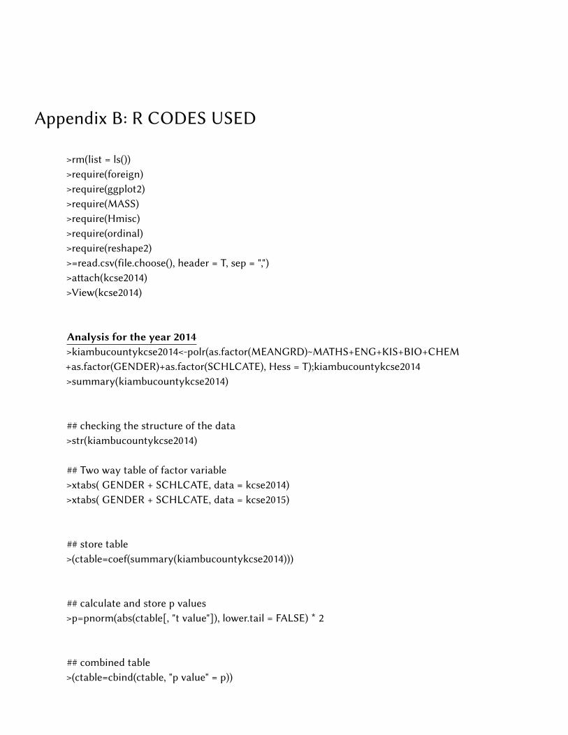
Appendix B: R CODES USED
>rm(list = ls())>require(foreign)>require(ggplot2)>require(MASS)>require(Hmisc)>require(ordinal)>require(reshape2)>=read.csv(file.choose(), header = T, sep = ",")>a�ach(kcse2014)>View(kcse2014)
Analysis for the year 2014>kiambucountykcse2014<-polr(as.factor(MEANGRD)~MATHS+ENG+KIS+BIO+CHEM+as.factor(GENDER)+as.factor(SCHLCATE), Hess = T);kiambucountykcse2014>summary(kiambucountykcse2014)
## checking the structure of the data>str(kiambucountykcse2014)
## Two way table of factor variable>xtabs( GENDER + SCHLCATE, data = kcse2014)>xtabs( GENDER + SCHLCATE, data = kcse2015)
## store table>(ctable=coef(summary(kiambucountykcse2014)))
## calculate and store p values>p=pnorm(abs(ctable[, "t value"]), lower.tail = FALSE) * 2
## combined table>(ctable=cbind(ctable, "p value" = p))
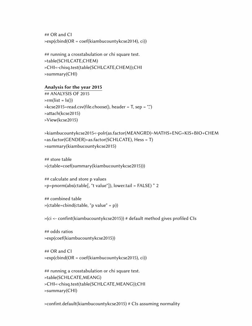
## OR and CI>exp(cbind(OR = coef(kiambucountykcse2014), ci))
## running a crosstabulation or chi square test.>table(SCHLCATE,CHEM)>CHI<-chisq.test(table(SCHLCATE,CHEM));CHI>summary(CHI)
Analysis for the year 2015## ANALYSIS OF 2015>rm(list = ls())>kcse2015=read.csv(file.choose(), header = T, sep = ",")>a�ach(kcse2015)>View(kcse2015)
>kiambucountykcse2015<-polr(as.factor(MEANGRD)~MATHS+ENG+KIS+BIO+CHEM+as.factor(GENDER)+as.factor(SCHLCATE), Hess = T)>summary(kiambucountykcse2015)
## store table>(ctable=coef(summary(kiambucountykcse2015)))
## calculate and store p values>p=pnorm(abs(ctable[, "t value"]), lower.tail = FALSE) * 2
## combined table>(ctable=cbind(ctable, "p value" = p))
>(ci <- confint(kiambucountykcse2015)) # default method gives profiled CIs
## odds ratios>exp(coef(kiambucountykcse2015))
## OR and CI>exp(cbind(OR = coef(kiambucountykcse2015), ci))
## running a crosstabulation or chi square test.>table(SCHLCATE,MEANG)>CHI<-chisq.test(table(SCHLCATE,MEANG));CHI>summary(CHI)
>confint.default(kiambucountykcse2015) # CIs assuming normality
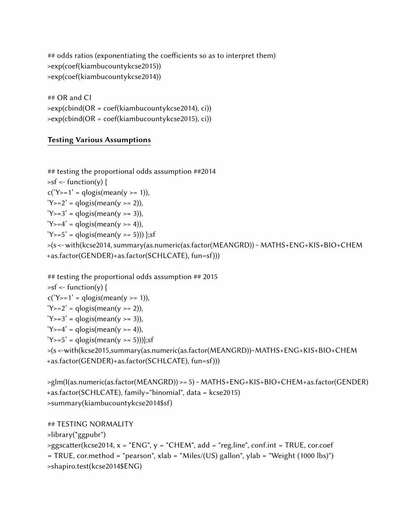
## odds ratios (exponentiating the coe�icients so as to interpret them)>exp(coef(kiambucountykcse2015))>exp(coef(kiambucountykcse2014))
## OR and CI>exp(cbind(OR = coef(kiambucountykcse2014), ci))>exp(cbind(OR = coef(kiambucountykcse2015), ci))
Testing Various Assumptions
## testing the proportional odds assumption ##2014>sf <- function(y) {c(’Y>=1’ = qlogis(mean(y >= 1)),’Y>=2’ = qlogis(mean(y >= 2)),’Y>=3’ = qlogis(mean(y >= 3)),’Y>=4’ = qlogis(mean(y >= 4)),’Y>=5’ = qlogis(mean(y >= 5))) };sf>(s <- with(kcse2014, summary(as.numeric(as.factor(MEANGRD)) ~ MATHS+ENG+KIS+BIO+CHEM+as.factor(GENDER)+as.factor(SCHLCATE), fun=sf)))
## testing the proportional odds assumption ## 2015>sf <- function(y) {c(’Y>=1’ = qlogis(mean(y >= 1)),’Y>=2’ = qlogis(mean(y >= 2)),’Y>=3’ = qlogis(mean(y >= 3)),’Y>=4’ = qlogis(mean(y >= 4)),’Y>=5’ = qlogis(mean(y >= 5)))};sf>(s <-with(kcse2015,summary(as.numeric(as.factor(MEANGRD))~MATHS+ENG+KIS+BIO+CHEM+as.factor(GENDER)+as.factor(SCHLCATE), fun=sf)))
>glm(I(as.numeric(as.factor(MEANGRD)) >= 5) ~ MATHS+ENG+KIS+BIO+CHEM+as.factor(GENDER)+as.factor(SCHLCATE), family="binomial", data = kcse2015)>summary(kiambucountykcse2014$sf)
## TESTING NORMALITY>library("ggpubr")>ggsca�er(kcse2014, x = "ENG", y = "CHEM", add = "reg.line", conf.int = TRUE, cor.coef= TRUE, cor.method = "pearson", xlab = "Miles/(US) gallon", ylab = "Weight (1000 lbs)")>shapiro.test(kcse2014$ENG)

>library("ggpubr")>ggqqplot(kcse2014$SCHLCAT, ylab = "SCHLCAT")
## Goodness of fit testwith(kiambucountykcse2014,pchisq(null.deviance-deviance,df.null-df.residual,lower.tail =F))